CONDENSED MATTER ASTROPHYSICS: A PRESCRIPTION FOR DETERMINING THE SPECIES-SPECIFIC COMPOSITION AND QUANTITY OF INTERSTELLAR DUST USING X-RAYS

arX

iv:0

906.

3720

v1 [

astr

o-ph

.IM

] 1

9 Ju

n 20

09

Condensed Matter Astrophysics

A Prescription for Determining the Species-Specific Composition

and Quantity of Interstellar Dust using X-rays

Julia C. Lee, Jingen Xiang

Harvard University, Department of Astronomy1

Harvard-Smithsonian Center for Astrophysics, 60 Garden Street MS-6, Cambridge, MA

02138

and

Bruce Ravel

National Institute of Standards and Technology

100 Bureau Drive, Gaithersburg, MD 20899

and

Jeffrey Kortright

Lawrence Berkeley National Laboratory, Materials Sciences Division

1 Cyclotron Road MS-2R0100, Berkeley, CA 94720

and

Kathryn Flanagan

Space Telescope Science Institute

3700 San Martin Dr Baltimore MD 21218

Received ; accepted

– 2 –

ABSTRACT

We present a new technique for determining the quantity and composition of

dust in astrophysical environments using < 6 keV X-rays. We argue that high

resolution X-ray spectra as enabled by the Chandra and XMM-Newton gratings

should be considered a powerful and viable new resource for delving into a rela-

tively unexplored regime for directly determining dust properties: composition,

quantity, and distribution. We present initial cross-section measurements of as-

trophysically likely iron-based dust candidates taken at the Lawrence Berkeley

National Laboratory Advanced Light Source synchrotron beamline, as an illus-

trative tool for the formulation of our technique for determining the quantify

and composition of interstellar dust with X-rays. (Cross sections for the materi-

als presented here will be made available for astrophysical modelling in the near

future.) Focused at the 700 eV Fe LIII and LII photoelectric edges, we discuss a

technique for modeling dust properties in the soft X-rays using L-edge data, to

complement K-edge X-ray absorption fine structure analysis techniques discussed

in Lee & Ravel (2005). This is intended to be a techniques paper of interest and

usefulness to both condensed matter experimentalists and astrophysicists. For

the experimentalists, we offer a new prescription for normalizing relatively low

S/N L-edge cross section measurements. For astrophysics interests, we discuss

the use of X-ray absorption spectra for determining dust composition in cold and

ionized astrophysical environments, and a new method for determining species-

specific gas-to-dust ratios. Possible astrophysical applications of interest, includ-

ing relevance to Sagittarius A∗ are offered. Prospects for improving on this work

in future X-ray missions with higher throughput and spectral resolution are also

presented in the context of spectral resolution goals for gratings and calorimeters,

– 3 –

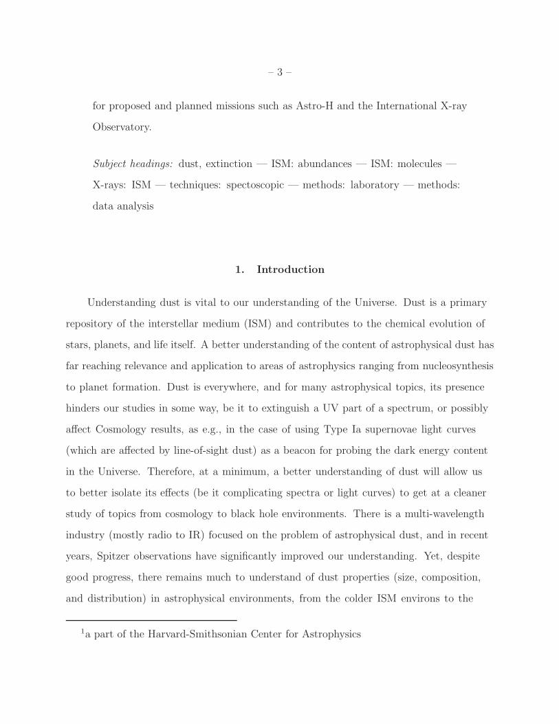
for proposed and planned missions such as Astro-H and the International X-ray

Observatory.

Subject headings: dust, extinction — ISM: abundances — ISM: molecules —

X-rays: ISM — techniques: spectoscopic — methods: laboratory — methods:

data analysis

1. Introduction

Understanding dust is vital to our understanding of the Universe. Dust is a primary

repository of the interstellar medium (ISM) and contributes to the chemical evolution of

stars, planets, and life itself. A better understanding of the content of astrophysical dust has

far reaching relevance and application to areas of astrophysics ranging from nucleosynthesis

to planet formation. Dust is everywhere, and for many astrophysical topics, its presence

hinders our studies in some way, be it to extinguish a UV part of a spectrum, or possibly

affect Cosmology results, as e.g., in the case of using Type Ia supernovae light curves

(which are affected by line-of-sight dust) as a beacon for probing the dark energy content

in the Universe. Therefore, at a minimum, a better understanding of dust will allow us

to better isolate its effects (be it complicating spectra or light curves) to get at a cleaner

study of topics from cosmology to black hole environments. There is a multi-wavelength

industry (mostly radio to IR) focused on the problem of astrophysical dust, and in recent

years, Spitzer observations have significantly improved our understanding. Yet, despite

good progress, there remains much to understand of dust properties (size, composition,

and distribution) in astrophysical environments, from the colder ISM environs to the

1a part of the Harvard-Smithsonian Center for Astrophysics

– 4 –

hotter environments near the disks and envelopes of young stars and compact sources.

Our quest to address outstanding problems, therefore, can greatly benefit from additional

complementary and/or orthogonal techniques.

There are several advantages to studying dust properties in the X-rays, the most

significant of which is that we can directly measure its quantity (relative to gas phase),

and composition. (“Dust” in this papers includes complex molecules). In the UV and

optical, the presence of dust is generally inferred through depletion, rather than directly

measured. Radio spectroscopy is able to probe the presence of certain molecules, and

IR, some subset of ISM compounds (mostly polycyclic aromatic hydrocarbon or PAHs,

graphites, certain silicates, and ice mantle bands). In these bands, spectral features come

from probing the molecule as a whole through rotational or vibrational modes originating

from e.g. the excitation of phonons (rather than electrons). Both gas and (∼< 10µm) dust

are semi-transparent to X-rays, so that the measured absorption in this energy band is

sensitive to all atoms in both gas and solid phase. Therefore, these high energy photons

can be used to facilitate a direct measurement of condensed phase chemistry via a study of

element-specific atomic processes, whereby the excitation of an electron to a higher lying

quantum level, band resonance, or molecular structure will imprint modulations on X-ray

spectra that reflect the individual atoms which make up the molecule or solid. Therefore, in

very much the same way we can look at an absorption or emission line at a given energy to

identify ions, the observed spectral modulations near photoelectric edges, known as X-ray

absorption fine structure (XAFS) provide unique signatures of the condensed matter that

imprinted that signature. For this reason, high resolution X-ray studies, as currently best

enabled by X-ray grating observations (Chandra and XMM), provide a unique and powerful

tool for determining the state and composition of ISM grains.

Lee & Ravel (2005) have already discussed the viability of XAFS analysis and

– 5 –

techniques for K-edge data with particular emphasis on iron in the hard > 7 keV X-rays, in

early anticipation of the launch of the Suzaku calorimeters. (See also Woo 1995, Woo et al.

1997, and Forrey et al. 1998 for early theory discussions relating to XAFS detections in

astrophysical environments.) Due to the unfortunate in-flight failure of the instrument, the

viability of astrophysical XAFS studies will have to focus on the softer < 6 keV regime

with existing instruments, until the Astro-H launch. While a more complicated part of the

spectrum (due to the numerous ions which populate this spectral region), XAFS signatures

in the soft X-rays have been reported in early papers based on Chandra and XMM spectral

studies (Paerels et al. 2001; Lee et al. 2001, 2002; Ueda et al. 2005; Kaastra et al. 2009;

de Vries & Costantini 2009; see also Takei et al. 2002; Schulz et al. 2002; Juett et al.

2004, 2006 for studies focused on the oxygen K edge for abundance determinations.) It

is the detection of these features in X-ray spectra of astrophysical objects which have

motivated us to obtain laboratory measurements of likely ISM grain candidates to facilitate

astrophysical modeling efforts. To date, no modelling of the magnitude we propose here

has been undertaken. The ∼ 0.1 − 8 keV energy coverage combined between the Chandra

and XMM-Newton gratings will allow us to look in more detail at photoelectric edges near

C K, O K, Fe L, Mg K, Si K, Al K, S K, Ca K, and Fe K, and therefore molecules/grains

containing these constituents. We note however that for the K-edges of C, S, Ca and Fe, we

are likely to be limited by signal-to-noise (hereafter, S/N) and/or spectral resolution, but

are nevertheless well situated to study magnesium-, silicate, and aluminum-based grains

using K-edge data, and iron-based grains/molecules can be studied using L-edge spectra

at ∼ 700 eV. Additionally, because X-ray absorption spectra is from some admixture of

gas and dust, each having very different individual spectral signatures, we can separate

their relative contributions through spectral modelling. Our proposed technique for doing

so is discussed in §3, using cross-section measurements of XAFS at Fe L as the illustrative

example for our discussion points.

– 6 –

The intent of this paper is to present dialog focused on the application of condensed

matter X-ray techniques to the soft X-ray absorption study of astrophysical dust properties:

composition and quantity. What knowledge we gain from this work will greatly complement

current IR studies of dust. Ultimately, the questions we would strive to address over

the course of this study include: (1) the mineralogy of dust in different astrophysical

environments, and perhaps (2) something of its nature (e.g. crystalline or amorphous).

Since K-edge analysis has already been discussed by Lee & Ravel (2005), we focus our

attention here on XAFS studies as applied to L-edges, where the spectral modeling of

near-edge absorption modulations (XANES: X-ray absorption near edge structure), rather

than far-edge absorption modulations (EXAFS: Extended X-ray absorption fine structure)

play a primary role. While the emphasis is on the ∼ 700 eV Fe L spectral region, the

techniques presented will be widely applicable to all L-edge studies. Because condensed

matter measurements are discussed in the context of astrophysics studies, we organize this

paper into sections that would be of interest and usefulness to both condensed matter

experimentalists (§2), and astrophysicists (§3, §4), For the experimentalists, §2.2 may be

of particular interest for its discussion of an L-edge cross section normalization technique

that is robust to laboratory synchrotron cross-section measurements with relatively poor

S/N. For astrophysics interests, §3 discusses a new method for determining interstellar

dust quantity and composition, through X-ray studies. This is followed in §4 with a brief

discussion of some possible studies of interest, and thought experiment discussion on this

technique’s ability to separate out fractional contributions of different composition dust in

different regions. Prospects for improving on this work in the context of future missions is

discussed in §5.

– 7 –

2. The samples and laboratory experiment

UV, IR, and planetary studies of meteorites and dust have pointed to interstellar dust

grains condensed from heavier elements such as C, N, O, Mg, Si, and Fe. With respect

to using Chandra High Energy Transmission Grating Spectrometer (HETGS) spectra to

enable detailed studies of absorption structure near photoelectric edges to determine grain

composition, Fe-, Mg-, and Si-based dust would be the most relevant since the L-edge of Fe

and K-edges of Mg and Si are all contained within the ∼ 0.5− 8 keV (∼ 1.5− 25A) HETGS

bandpass, where the effective area is also highest. (The Fe K-edge is also encompassed by

the HETGS, but the S/N there is usually too low to be useful for analysis.) For this paper,

we compare cross section measurements for hematite (α − Fe2O3), iron sulfate (FeSO4),

fayalite (Fe2SiO4), and lepidocrocite (γ − FeOOH). Cross-section measurements at Fe L

and Si K are nearing completion for the most astrophysically-likely iron- and silicon-based

dust, which will be presented in a future paper on XAFS standards for astrophysical use,

while the data presented in this paper is used primarily to illustrate our proposed analysis

techniques and methodology. Planned measurements are also being made for other

interesting edges discussed previously.

The laboratory data presented in this paper were taken at the Lawrence Berkeley

National Laboratory Advanced Light Source beamline 6.3.1. This is a bending magnet

beamline with a Variable Line Spacing Plane Grating Monochromator (VLS-PGM) that

is sensitive to 300-2000 eV energy range and has a resolving power E/∆E = 3000. This

resolution exceeds the E/∆E = 1000 Chandra HETGS resolving power by factor of three.

The 6.3.1 detectors allow for choice between total electron yield, photodiode

(fluorescence), and transmission experiments. The latter would have been the ideal choice,

since transmission measurements would be directly related to what we seek to understand,

namely the transmission of X-rays through interstellar grains of comparable thickness.

– 8 –

However, a nominal thickness estimate for 30% transmission would require film/foil

thicknesses for our candidate samples in the range t ∼ 0.1 − 0.8µm from the transparent to

opaque side of the edge at Fe L, as calculated according to the formalism T = e−µρt. (The

density ρ for the compounds were taken from “The Handbook of Chemistry and Physics”,

and the values for the attenuation length were obtained from the 2CXRO at LBL, and

3NIST.) Preparation of pure-phase samples of that thickness was impractical. As such, we

opted to obtain cross-section measures using both fluorescence and electron yield (§2.1).

2.1. Fluorescence and Electron Yield Experiments

In an X-ray-absorption spectroscopy (XAS) experiment, the incident X-ray photon

promotes a deep-core electron into an unoccupied state above the Fermi energy. For the

iron L edge experiments shown in this paper, that deep core state is a 2p state. As the

incident photon energy is varied using a variable line spacing plane grating monochromator,

the cross section of this absorption process is monitored by measurement of the decay of a

higher-lying electron into the core-hole. The fluorescence of a photon and emission of Auger

and secondary electrons can be monitored in tandem. Because the mean free path of the

electron is limited to a few nanometers or less, the electron yield measurement is mostly

sensitive to the surface of the sample. The fluorescent photon, on the other hand, has a

larger mean-free path, and therefore is a better probe of the bulk of the sample.

The samples measured in this paper were fine powders, either purchased as such or

prepared by grinding in an agate mortar and pestle. A portion of these fine powders were

sprinkled onto conducting carbon tape, another portion was pressed onto a flattened strip

2http://www-cxro.lbl.gov/optical constants/

3http://physics.nist.gov/PhysRefData/FFast/html/form.html

– 9 –

of indium metal. The carbon tape and indium strips were affixed to a glass microscope

slide for mounting onto the sample holder. The fluorescence measurement is made using a

photodiode pointed at the sample. However, since all of our samples were thick compared

to the penetration depth and highly concentrated in iron, the fluorescence data were

significantly attenuated by the self-absorption effect (see e.g. Booth & Bridges 2005). All

data in this paper were measured in electron yield mode.

To measure the electron yield, an alligator clip was clamped onto the glass slide and

electrical contact was made with the otherwise isolated carbon tape and indium strip,

and used to carry the photocurrent into a current-to-voltage amplifier. This experimental

arrangement provided for redundant measurements of each sample. Some samples proved

more amenable to measurement on the carbon tape substrate and others to the indium. For

every sample, each measurement was repeated three times. In each case, the measurement

yielding the highest quality, most reproducible data was selected for presentation. The

three scans for each sample have been calibrated in energy, aligned, and averaged.

Absolute energy calibration was attained by measuring an iron foil and calibrating it

to the tabulated energies of the iron LII and LIII edges (Brennan & Cowen 1992) . We

had no capacity to prepare the surface of our foil, thus we relied upon the fluorescence

measurement. Although the foil measurement is severely attenuated by self-absorption, the

edge position can be reliably extracted. Iron edge scans on other materials were aligned to

the iron foil data using reproducible features in the spectrum of the incident intensity.

2.2. Absorption cross section normalization technique

In an XAS measurement, the absolute scale of the measured cross section is ambiguous.

The size of the measured step at an absorption edge energy depends on a wide variety of

– 10 –

factors, including the concentration of the absorbing atom in the sample, the electronic

gains on the signal chains, and the efficiencies of the detectors. In order to compare

measurements on disparate samples and under differing experimental conditions, it is

standard practice to perform a common normalization of every measured spectrum. In

this work, we choose to perform this normalization by matching the measurements to

tabulated values for bare-atom cross sections, as described in this section. In this way, we

can directly and consistently compare measurements on our samples to one another as well

as to astronomical observations.

The normalization of XAS L edge data is more complicated than for K edge data

due to the close proximity of the LII and LIII edges in the soft X-ray regime. In order

to properly normalize these spectra, we adopt the MBACK normalization technique of

Weng et al. (2005), with modifications. Here, we describe the MBACK technique in brief,

and our modification, which we found to be necessary for data with ∼> 0.2% noise, as typical

of each individual cross section measure. We note that the typical practice has been to

first co-add all individual cross-section measures to increase S/N, before normalization.

However, we wished to be more rigorous in our methodology by first renormalizing the

individually measured cross-sections before combining to create the final used for fitting.

The MBACK technique ensures better normalization for the more complex L-edge cross

sections by calculating a smooth normalizing function over the entire measured data range,

rather than extrapolating from independently pre- and post-edge linear fits as would be

sufficient for the less complex K-edge cross sections. For our data, this normalizing function,

µnorm, is dominated by the Legendre polynomial term (in brackets) of the function:

µnorm(Ei) =

[

m∑

j=0

Cj(Ei − Eedge)j

]

+ A · erfc(Ei − Eem

ξ) (1)

where Eedge is the energy of the onset of the edge-absorption, and m and Cj are respectively

the polynomial order and coefficient. Weng et al. additionally note that a rapidly decreasing

– 11 –

pre-edge shape, due to residual elastic scattering is often seen in fluorescence experiments

using energy discriminating detectors, and therefore include an additional error function

component in the normalization as defined by the non-bracketed term of Eq.1− see Fig. 1 for

the shape of this function as determined from our sample fit to γ-FeO(OH)−lepidocrocite.

Here, Eem and ξ are respectively the centroid energy of the X-ray emission line of the

absorbing element, and its width, with A as a scale factor. We note however that this

function is adopted here solely as an effective way to model similar pre-edge feature shapes

originating from experimental artifacts of uncertain origin. (Residual elastic scattering

effects do not apply to our experiment, which measured total photocurrent.) In any case,

our data do not show a large rapidly decreasing pre-edge slope so this term has negligible

effect on our overall normalization; nevertheless, we include it in our modelling efforts

for completeness, since this would allow for a global prescription for the determination

of µnorm that is independent of experimental technique. – See Fig. 2a for an illustration

of the components which make up the normalizing function for our sample γ−FeO(OH)

compound. In general, the details of the normalization variables would clearly depend on

the composition of the condensed matter.

To determine a best normalization (Fig. 2b), we initially employ the prescribed

minimizing function of Weng et al.:

1

n1

n1∑

i=1

[µbf(Ei)+µnorm(Ei)−sµraw(Ei)]2+

1

n2

N∑

i=N−n2+1

[µbf(Ei)+µnorm(Ei)−sµraw(Ei)]2 (2)

where N represents the total number of data bins, i is the bin index, and n1 and n2 are

respectively the total number of pre-edge and post-edge data bins, such that e.g. N −n2 +1

represents index 1 of the post-edge bin. The variable µbf is the Brennan & Cowen (1992)

tabulated absorption cross-sections representing the bound-free non-resonant absorption

component of Fe. µraw is our measured cross-sections which is scaled by s, and µnorm is the

normalization function of Eq. 1. However, in our fitting efforts, we found the scale factor

– 12 –

s to be very sensitive to noise, often taking on small values for our data which resulted in

badly normalized cross sections. In considering a remedy for this, we tested Eq. 2 based on

simulated cross sections (µbf + µnorm) where we have added controlled levels of Gaussian

distributed noise, as per the prescription (1+f Gnoise) · (µbf +µnorm), where Gnoise is a group

of random numbers following the Gaussian distribution, and modified by the fractional level

f , i.e. f = 0.2% or f = 1%, as in Fig. 3. (The Gaussian distribution function is defined as

φ(x) = e−(x−µ)2/2σ2

/σ√

2π where the expectation value µ = 0 and the standard deviation

σ = 1.) (The µnorm parameters of Eq. 1 are set to C0 = 3.0, C1 = 0.01, C2 = 0.0002, A =

1.0, Eem = 685 eV, ξ = 5.0, Eedge = 707 eV). We then divide the simulated data by the

value of s arbitrarily set to 30, before fitting according to the minimization function of Eq. 2

to see if we can recover the same value. In doing so, we find that the Weng et al. method,

sans modification, is only robust for data with noise at ∼< 0.2%. Accordingly, we modify

Eq. 2 by dividing sµraw(Ei) into the pre-edge and post-edge minimization terms as per:

1

n1

n1∑

i=1

[

µtab(Ei) + µnorm(Ei) − sµraw(Ei)

sµraw(Ei)

]2

+1

n2

N∑

i=N−n2+1

[

µtab(Ei) + µnorm(Ei) − sµraw(Ei)

sµraw(Ei)

]2

(3)

and find that our method (Eq. 3) is robust to data of up to 2% noise. In total, the

normalization procedure will use m + 5 adjustable parameters (m + 1 polynomial

coefficients, two scale factors of s and A as well ξ and Eem) to determine the best

normalization for the measured cross sections.

Of relevance to the cross sections presented in this paper, 18 measurements (9 mounted

on indium substrate and 9 on carbon) of each sample were taken. However, the carbon

substrate measurements were consistently nosier so we exclude those from the final co-added

cross sections. For each individual indium substrate cross section measure (see Fig. 4-top),

the data were normalized using the aforementioned Eqs. 1 and 3 technique based on the

subsequent steps. To compare with our reference spectrum, each measurement is first shifted

– 13 –

by 4.1 eV to correct for the calibration offset of the monochromator. The resultant energy

span of our measurements is then 684.1 eV to 754.1 eV which corresponds to N = 700 total

data bins of 0.1eV widths. As described, Eqs. 1 and 3 were then used to determine the best

normalized description for the combined data set unique to each sample. Since all data

measured spanned the range noted above, the number of pre-edge and post-edge data bins

correspond respectively to n1 = 179 (684.1 eV−702 eV) and n2 = 141 (740 eV−754.1 eV)

for all samples. The edge energy Eedge=707 eV corresponding to the Fe L iii, and a

polynomial of order m = 2 was deemed sufficient, i.e. the goodness of fit showed negligible

improvement for higher polynomial orders. Post-normalization, cross sections of the highest

quality were co-added to create the final cross sections of Fig. 6. For the final cross

sections, no fewer than 9 (indium substrate) data sets were co-added per compound type.

Fig. 6 shows our measured cross sections post-normalization, compared against metallic

(Kortright & Kim 2000), and what we assume for bound-free conintuum absorption by iron

(Brennan & Cowen 1992; Henke et al. 1993). For future fitting efforts to astrophysical data,

we use the structure-less Fe L tabulated values of Brennan & Cowen (1992) to extrapolate

the normalized XAFS data beyond the energy span of our measurements to encompass an

energy range that extends from 0.4 keV−10 keV.

We plan to avail the community of our cross section measurements4 for these and

other compounds, as absolutely calibrated standards for interstellar dust studies, in the

near future. As stated, the data shown here is intended merely as a vehicle to facilitate a

presentation of our new techniques.

4http://www.cfa.harvard.edu/hea/eg/isd.html

– 14 –

3. An X-ray method to determine the quantity and composition of dust in

interstellar space

Our ability to accurately measure the quantity of dust and elemental abundances in

our Galaxy and beyond has far-reaching applications and consequences for a diverse range

of astrophysical topics. Thus far, wavelength-dependent (IR to UV) studies of starlight

attenuation as facilitated by e.g. E(B-V) measurements, and other extinction studies, have

been the primary technique by which we come to measure the amount of dust that is

bound up in interstellar grains. Elemental depletion can be determined by UV absorption

studies comparing the amount expected in gas phase absorption from what is observed,

and IR spectral studies can directly measure certain ISM dust. Here, we present an

X-ray technique for directly determining the (element-specific) quantity and composition of

interstellar gas (§3.1) and dust from within a single observation. What knowledge we gain

from this technique, when combined with the wealth of knowledge from non-X-ray studies

will significantly increase our understanding of ISM dust and its effects on astrophysical

environments.

3.1. Gas Phase ISM Absorption

Like condensed material, atomic transitions to higher quantum levels within an isolated

atom will also give rise to multiplet resonant absorption. To give the example for Fe, these

lines would consist of all possible discrete transitions to all possible configurations of the

3d-shell, since the electronic configuration of Z=26 Fe+0 (or Fe I in the astronomy notation)

is 1s22s22p63s23p64s23d6. Therefore, while the bound-free non-resonant transitions can

be modelled by a simple step function as e.g. that of Brennan & Cowen (1992) for

Fe L, additional discrete resonant features will have to be included to account for the

bound-bound resonant component of absorption.

– 15 –

Fig. 5 shows our calculations for the resonant transition for various Fe ions from

Fe+0 − Fe+4, as evaluated based on the Gu et al. (2006; see also Gu 2005) predictions for

oscillator strengths, radiative decay rates, and autoionization rates for these lines. We note

that because of the electronic structure of Fe, which favors the removal of the s-electrons

prior to d-electrons, the cross sections for Fe+0 ∼ Fe+1 ∼ Fe+2, as evident in the figure.

The relevant cross sections as derived for these atomic transitions are then convolved with

the appropriate instrument resolution (∆E ∼ 0.9 eV at 700 eV Fe L for the Chandra

Medium Energy Grating) to approximate the ion-specific cross section for the bound-bound

transition, σbb. Finally, the cross section for describing the total gas-phase absorption for

the species of interest, σZgas, will be described by the combination of cross-sections from

the bound-bound (µbb−atom) and bound-free (µbf) components. More details on this follow

in §3.2.

For complex astrophysical environments, additional considerations as relates to the

ionization state of the plasma being probed need to be weighed. As such, modelling efforts

need to consider the ionization state of the environment expected for the absorption. For

the three, cold (T < 200K), warm (T ∼ 8000K), and hot (T ∼ 5×105K), phases of the ISM,

the iron ions that contribute most strongly to the L edge region are Fe+0 followed by Fe+1.

At T=8000 K, the peak ion fractions are Fe+0 ∼ 0.67, Fe+1 ∼ 0.33, Fe+2 ∼ 2.8 × 10−3

and Fe+3 ∼ 1.9 × 10−6, assuming the ISM ionizing spectrum defined in Sternberg et al.

(2002). At the much colder temperatures of the cold ISM, only Fe+0 contributes, and at

the much hotter temperatures of the hottest phase of the ISM, it is Fe+25 (at 6.7 keV)

which contributes the bulk ion fraction.

– 16 –

3.2. A prescription for determining species-specific gas-to-dust ratios

As stated in §1, what cross sections we measure in the laboratory of astrophysically-

likely dust candidates (§2) will be applied to X-ray spectra showing structure near

photoelectric edges to determine dust composition, and quantity. We propose the following

prescription to do so.

Ffinal = F0 T = F0 exp [−τLOS(Z′) − τionized−gas − τ(Zgas) − τ(Zdust)] (4)

whereby the absorption contributions from gas (cold and ionized), and dust, can be

separately accounted for by each of the exponential terms. Ffinal and F0 are respectively the

detected and incident flux, and T , represented by the exponential terms is the transmission.

τionized−gas is determined through photoionization modelling to account for any additional

lines arising from the plasma of the source, and should be treated on a source by source

basis. However, in the Fe Liii and L ii edge regions, we note additional line contributions

would have to come from high transition (low oscillator strength) lines of He-like O VII

(O+6) 1s2 −1snp for n ≥ 4, and Fe I-Fe XI (i.e. Fe+0 −Fe+10). Any significant contribution

from oxygen would have to come from very ionized optically thick plasma; for the iron,

moderate temperature plasma would have to be present in large quantities to have any

appreciable effect in this spectral region. Therefore, for many astrophysical situations,

neither ionized oxygen nor iron from the source plasma, is expected to contribute strongly

(if at all) to the Fe L iii and Fe L ii spectral region. Nevertheless, as stated, these can be

modelled out through photoionization studies, the discussion of which is beyond the scope

of this paper. For the total line-of-sight (LOS) (gas+dust) ISM absorption from all heavy

elements, excluding the species of interest,

τLOS(Z′) =∑

Z′

σ′

Z′ NH Asolar (5)

– 17 –

where σZ′ , Asolar, and NH are respectively defined to be the cross section, abundance, and

line-of-sight equivalent Hydrogen column summed over all heavy elements present in the

broad band X-ray spectrum, with the exception of the element we are trying to measure.

One reason for removing the species of interest from the broad-band fitting is because we

are interested in decomposing the gas and dust contribution specific to that species. For

this, we include two additional exponential terms to describe the absorption by the gas and

dust for the species of interest whereby:

τZgas = (σbf + σbb−gas)NHxAZ = σZgasNHxAZ (6)

and

τZdust = (σbf + σbb−dust)NH(1 − x)AZ = σZdustNH(1 − x)AZ (7)

In these equations, σZgas and σZdust refer to the cross section of the gas and dust respectively

for the species of interest. The determination of σZgas was discussed in §3.1. σZdust, and

our efforts to measure this for astrophysically viable dust candidates has been discussed

at length in §2. Given enough S/N, the species-specific abundance AZ can be fitted for,

with the condition that the total abundance should be a combination of both gas and

dust, hence the additional multiplicative factor to AZ of x and (1 − x). Fig. 7 shows these

components as separated out in a fit to the X-ray binary Cygnus X1. − Details about the

dust in Cygnus X1 will be separately discussed in the paper Lee et al. in preparation.

4. Discussion

The Chandra and XMM-Newton archive are rich with high resolution spectra of

X-ray bright binaries and active galactic nuclei (AGN). A cursory look at these spectra

reveal XAFS near many photoelectric edges, and hence dust and/or molecules. Therefore,

there is already a wealth of data for studying astrophysical dust properties in the ISM

– 18 –

and/or the hotter “near binary” environments using the X-ray technique described in this

paper. In combination with X-ray scattering studies which will provide important spatial

information on distribution (see e.g. Xiang et al. 2007 paper which make a first successful

attempt at considering non-uniform dust distributions along the line-of-sight toward the

X-ray dipper 4U 1624−490, and references therein), existing grating observations provide

us with great potential to map out dust distribution along different lines-of-sight, while

determining the species-specific quantity and composition along these same path-lengths to

build upon studies in other wavebands. Given spectra with enough S/N (as true of many of

the existing data), the spectral resolution afforded by the Chandra gratings will allow us to

(1) definitively separate dust from gas phase absorption, and (2) give us good expectations

for being able to directly determine the chemical composition of dust grains containing

oxygen, magnesium, silicon, sulfur, and iron. As such, we expect to be able to make

significant progress over the next few years in our understanding of the sub-micron size

molecules which make up a large fraction of the ISM grains, and/or near-binary/near-AGN

environments. For the latter, this would enable a better understanding of the evolutionary

histories of these black hole and neutron star systems.

For many astrophysical applications, a better understanding of dust properties and its

distribution in interstellar space, carries many advantages. As an example, consider the

supermassive black hole Sagittarius A∗ in our own Galactic center. Current estimates of

the absorption column to Sagittarius A∗ between X-ray and NIR studies differ by a factor

of ∼ 2, which may be attributed to unknowns relating to the metallicity, gas-to-dust ratio,

or the grain size distribution along the line of sight. These uncertainties affect our ability to

accurately use the Fe Kα emission line as a diagnostic of the Sagittarius A∗ hot accretion

flow (see e.g. Xu et al. 2006), and determination of the X-ray spectral slope for observed

flares. Metallicity uncertainties can be greatly improved as we understand the nature of the

absorption towards the Galactic center better. This can be accommodated by the type of

– 19 –

study described in this paper, in large part because the spatial distribution of sources with

spectra of sufficient S/N and spectral resolution necessary for the proposed X-ray study of

dust, encompass much of the region along and around the Galactic plane, and towards the

Galactic center. Ideally, we would additionally conduct case studies of the fainter binaries

in the central parsecs, or at least as many as possible, as close to the Galactic center as

possible (see e.g. Muno et al. 2008 latest X-ray binary catalog based on Chandra ACIS-I

imaging data). Given the relative X-ray faintness of many of these objects however, such

a comprehensive spectral study in the nearest regions of the Galactic Center will have to

await missions with higher throughput, and at least equal spectral resolution.

As stated, studies of many astrophysical systems can be greatly enhanced by a better

understanding of the line-of-sight absorbing material. With the Chandra gratings, we have

entered upon an era where condensed matter theory can be applied to astrophysics studies

of dust. Invariably, interstellar environments present us with additional complications not

of consideration in a controlled laboratory experiment, so we conclude with a thought

problem of relevance to dust studies of interstellar environments.

4.1. A Gedanken problem: can we differentiate dust content in different

locations?

The path-length along the line-of-sight to our illuminating sources, be they X-ray

binaries in our own Galaxy or black hole systems in other galaxies, is complex. Consider,

for example, the simplified scenario of only two components distributed in some manner

along the path. This problem then has two parts, the identification of the chemical

species of those two components and the determination of their distribution along the

path-length. Assuming we can identify the two species, can we distinguish a heterogeneous

arrangement (dust of composition a in location A plus dust of composition b found in

– 20 –

location B), from a homogeneous arrangement (dust of mixed composition AB distributed

along the path) ?

The interpretation of the X-ray spectrum passing along this line-of-sight bears a strong

similarity to the well-established technique of XAS as performed at synchrotron facilities.

The use of XAS to identify chemical species in a chemically heterogeneous sample is

common practice in terrestrial laboratories (Lengke et al. 2006 is but one example among

thousands in the XAS literature.) The common strategy is to interpret the spectrum from

the mixture of species as a linear combination of the spectra from its component species,

i.e.n

∑

i=0

ciαi, where αi represent the different species and ci are their respective fractional

contributions, as per Lengke et al. (2006). The best determined relative percentages for

the linear combination are derived by fits based on minimal χ2, which we recast for our

purposes to bem

∑

j=1

[

∑ni=1 ci αi,j − βj

√

∑ni=1(ci ∆αi,j)2 + (∆βj)2

]2

(8)

where βj and αi,j are the normalized cross sections in the jth bin of respectively the mixture

and pure forms of the individual compounds, ∆βj and ∆αi,j their respective uncertainties,

and n the associated number of compounds and jth bins to sum over; ci has the condition

that

n∑

i=1

ci = 1. With careful sample preparation, the fractional content of the component

species in the spectrum is directly indicative of their fractional content in the physical

sample.

To demonstrate this using iron-bearing species of relevance to the ISM, we performed

the following experiment in the controlled laboratory of the synchrotron facility. We

prepared two samples containing the common terrestrial iron compounds hematite

(α-Fe2O3), ferrosilicate (Fe2SiO4), and lepidocrocite (γ-FeOOH). The first sample contained

equal parts by weight of hematite and ferrosilicate and the second contained equal parts by

weight of all three materials. Samples for measurement by electron yield at beamline 6.3.1

– 21 –

were prepared as described above and the XAS spectra were measured on both mixtures.

The hematite and lepidocrocite were very fine-grained, commercially produced powders.

The ferrosilicate was commercially produced, but was ground by agate mortar and pestle

from a chunk several millimeters across. Consequently, the ferrosilicate component of each

sample was much larger-grained than the other two components.

Because equal parts by weight were mixed in our two samples, we might expect the

measured spectra to be interpreted by equally weighted fractions of the spectra from the

three pure materials. In fact the nature of the interaction between the X-rays and the

morphology of the sample must be considered. Because the ferrosilicate component of each

sample was much larger grained than the other components, its surface-area-to-volume

ratio was considerably smaller. Because the electron yield measurement is surface sensitive,

a much smaller fraction of the iron atoms in the ferrosilicate contributed to the actual

measurement than of the other two components.

The data on the two mixtures along with the results of the linear combination analysis

are shown in Fig. 8. The binary mixture proved to be 16 ± 2% ferrosilicate and 84 ± 2%

hematite. As expected from particle size, the ferrosilicate is under-represented in the

measured spectrum. The trinary mixture was 8 ± 2% ferrosilicate, 51 ± 7% hematite, and

41 ± 7% lepidocrocite. The two components of similar particle size are evenly represented,

while the ferrosilicate is under-represented.

This careful consideration of sample morphology in the synchrotron measurement is

directly relevant to the interpretation of the astrophysical X-ray spectra. The astrophysical

measurement is akin to a transmission measurement at the synchrotron, while the examples

shown in Fig. 8 were measured in electron yield. Still, the correct interpretation of the

XAS spectra requires consideration of the nature of the interaction of the X-rays with the

material through which they pass. A ray interacting with a large particle in the ISM will

– 22 –

be lost to the satellite measurement by virtue of being completely absorbed by the particle.

Consequently, the satellite measurement will be dominated by the small particles in the

ISM as those are the only particles that allow passage of photons for eventual measurement

at the satellite.

Finally, we must address the topic of distinguishing the distribution of the chemical

species along the path-length. By itself, a transmission XAS measurement is incapable

of distinguishing between a layered and a homogenized sample. In transmission, an XAS

measurement on two powders will be the same whether you prepare the powders separately

and stack them in the beam path or mix the powders thoroughly before making the

measurement. Similarly, the X-ray satellite measurement by itself cannot address the

distribution of the species it is able to identify, if co-located at similar redshifts. However,

since an XAFS contribution to a photoelectric edge is scaled according to the optical depth

of that particular species, we can reasonably conclude that the compound that best fits the

astro- spectra is the compound where we are seeing the bulk contributions from, even if

there might be lesser (e.g. 10%) contributions from other compounds along the line-of-sight.

Therefore, in combination with other astrophysical studies using photon wavelengths that

interact differently with the ISM (e.g. IR), the X-ray measurement can serve an important

role in the full determination of the composition of the ISM.

5. XAFS Science: Present and Future

The X-ray energy band has been slow to be exploited for dust studies due largely to

instrumental requirements for both good spectral resolution (R ∼> 1000), and throughput.

Yet, condensed matter astrophysics (i.e. the merging of high energy condensed matter and

astrophysics techniques for X-ray studies of dust), as a new sub-field can be realized in the

present era of Chandra and XMM-Newton . As such, X-rays should be considered a powerful

– 23 –

and viable new resource for delving into a relatively unexplored regime for determining

dust properties: composition, quantity, and distribution. Present day studies with extant

satellites will set the foundation for future studies with larger, more powerful missions such

as the joint ESA-JAXA-NASA International X-ray Observatory (5IXO). Proposed spectral

instruments such as the Critical-Angle Transmission grating (6,7CAT; Flanagan et al.

2007) and Off-Plane Reflection Gratings (Lillie et al. 2007) are designed to provide IXO’s

baseline resolving power of 3000 under 1 keV, and configurations are contemplated which

will boost this to 5000 or more. Similar baseline resolving power are also expected from

the calorimeters for the hard (> 6 keV) spectral region. IXO’s target spectral resolution

R = 3000 in the 0.2-10 keV bandpass, in combination with planned higher throughput (10×

XMM, and 60× Chandra) will allow us in the future to move beyond the realm discussed

in this paper to being able to use XAFS to recreate the crystalline structure of interstellar

grains and determine precise oxidation states. In the interest of providing information for

the planning of future missions, we provide spectral resolution goals that are mapped to

XAFS science hurdles, for gratings and calorimeters (Table 2).

acknowledgements

We acknowledge Eric Gullickson, Pannu Nachimuthu, and Elke Arenholz for beamline

support. We thank Claude Canizares and Alex Dalgarno for advice and conversations, and

Fred Baganoff for discussions relating to Sgr A∗. The Advanced Light Source and JKB

is supported by the Director, Office of Science, Office of Basic Energy Sciences, of the

5http://ixo.gsfc.nasa.gov/

6http://space.mit.edu/home/dph/ixo/

7http://space.mit.edu/home/dph/ixo/comparison.html

– 24 –

U.S. Department of Energy under Contract No. DE-AC02-05CH11231. JCL is grateful to

Chandra grant SAO AR8-9007 and the Harvard Faculty of Arts and Sciences for financial

support.

Table 1. Photoelectric edge energies of measured compounds.

Compoundsa Chargeb EcLIII ∆Ed

LIII EeLII ∆Ef

LII

state eV(A) eV(A) eV(A) eV(A)

FeO(OH)-lepidocrocite Fe3+ 705.7(17.57) -2.7 (+0.07) 718.9(17.25) -2.3 (+0.06)

Fe2O3-hematite Fe3+ 705.7(17.57) -2.7 (+0.07) 718.9(17.25) -2.3 (+0.06)

Fe2SiO4-fayalite Fe2+ 704.3(17.60) -4.1 (+0.10) 717.4(17.28) -3.8 (+0.09)

FeSO4-iron sulfate Fe2+ 704.3(17.60) -4.1 (+0.10) 717.8(17.27) -3.4 (+0.08)

a Laboratory measurements of Cross sections for astrophysically-likely species presented in this paper.

b The charge state reflects the number of electrons removed from iron when the compound is formed. To take Fe2SiO4

(fayalite) as an example: silicon (atomic orbital: 1s22s22p63s23p2), will lose 4 electrons in its outmost shell so that oxygen

(1s22s22p4) can fill its shell. Since there are 4 oxygen atoms however, two additional electrons will be taken from Fe such that

the charge state of the compound is +2.

c The Fe LIII photoelectric edge energy relevant to the different compounds as measured at where the Brennan & Cowen

(1992) cross sections, which we assume for bound-free gas phase iron absorption, peaks at 708.4 eV. See Fig. 6 inset for

illustration.

d The energy difference between compound and gas as measured at the peak of the Brennan & Cowen (1992)

e Same as column c but for the Fe LII photoelectric edge at 721.2 eV assumed for bound-free gas phase absorption.

f Same as column d but for the Fe LII photoelectric edge at 721.2 eV.

– 25 –

Table 2: X-ray Instrument Capabilities and Goals for ISM Grain Physics Studies

Gratings Calorimeter

0.25-6 keV FWHM 6-10 keV FWHM

Chandra Suzaku† SXS prototype‡ IDEAL§

Spectral Resolution⋆ R < 500 R = 1000 R = 923 R ∼ 1500 R

Distinguish gas from dust difficult1 yes2 yes yes

Differentiate dust not possible yes3 ok3 yes3 30004

Discern oxides not possible no no maybe5 5000

⋆ Spectral resolution R = E/∆E = λ/∆λ referenced to 1 keV for the gratings at 6 keV for

the calorimeters.

† The spectral resolution of the calorimeter on board Suzaku which has since failed in-flight.

‡ Reasonable expectation for spectral resolution to be achieved with SXS prototype detectors

(HgCdTe absorbers and implanted silicon thermometers) planned for the Astro-H mission.

4 eV resolution (R = 1500) at 6 keV has been achived in laboratory measurements. –

Astro-H Team (private communication). The IXO calorimeter baseline performance is 2.5

eV.

§ Applies to the 0.25-10 keV range for both grating and calorimeter instrument considera-

tions.

1 Insufficient spectral resolution limits our ability to discern the component of the photo-

electric edge due to dust versus gas.

2 As stated in §1, the soft X-ray band is also complicated by ionized absorption lines im-

printed by the hot plasma environment of the illuminating source (black hole or neutron

star, e.g.) that need to be modeled out in order to isolate the XAFS features.

3 Possible with adequate statistics obtained either from long observation time or large mea-

surement area

4 Different forms of iron (silicates, oxides, metal) and be distinguished, but not oxides cannot

be distinguished from other oxides.

5 Challenging measurement requiring measurement statistics approaching the level of syn-

chrotron experiment

– 26 –

REFERENCES

Booth, C. & Bridges, F. 2005, Physica Scripta, T115, 202

Brennan & Cowen 1992, Rev. Sci. Instru, 63, 850

de Vries, C. P. & Costantini, E. 2009, ArXiv e-prints, 0901.3050

Flanagan, K., et al. 2007, in Society of Photo-Optical Instrumentation Engineers (SPIE)

Conference Series, vol. 6688 of Society of Photo-Optical Instrumentation Engineers

(SPIE) Conference Series

Forrey, R. C., Woo, J. W., & Cho, K. 1998, ApJ, 505, 236

Gu, M. F. 2005, ApJS, 156, 105

Gu, M. F., Holczer, T., Behar, E., & Kahn, S. M. 2006, ApJ, 641, 1227,

arXiv:astro-ph/0512410

Henke, B. L., Gullikson, E. M., & Davis, J. C. 1993, Atomic Data and Nuclear Data Tables,

53, 181

Juett, A. M., Schulz, N. S., & Chakrabarty, D. 2004, ApJ, astro-ph/0312205

Juett, A. M., Schulz, N. S., Chakrabarty, D., & Gorczyca, T. W. 2006, ApJ, 648, 1066,

arXiv:astro-ph/0605674

Kaastra, J. S., de Vries, C. P., Costantini, E., & den Herder, J. W. A. 2009, ArXiv e-prints,

0902.1094

Kortright, J. B. & Kim, S. 2000, Phys. Rev. B, 62, 12216

Lee, J. C., Ogle, P. M., Canizares, C. R., Marshall, H. L., Schulz, N. S., Morales, R., Fabian,

A. C., & Iwasawa, K. 2001, ApJ, 554, L13

– 27 –

Lee, J. C. & Ravel, B. 2005, ApJ, 622, 970, arXiv:astro-ph/0412393

Lee, J. C., Reynolds, C. S., Remillard, R., Schulz, N. S., Blackman, E. G., & Fabian, A. C.

2002, ApJ, 567, 1102

Lee, J. C., Xiang, J., Hines, D., Ravel, B., Kortright, J., & Heinz, S. in preparation

Lengke, M. F., Ravel, B., Fleet, M. E., Wanger, G., Gordon, R. A., & Southam, G. 2006,

Environmental Science Technology, 40, 6304

Lillie, C., Cash, W., Arav, N., Shull, J. M., & Linsky, J. 2007, in Society of Photo-Optical

Instrumentation Engineers (SPIE) Conference Series, vol. 6686 of Society of

Photo-Optical Instrumentation Engineers (SPIE) Conference Series

Muno, M. P., et al. 2008, ArXiv e-prints, 0809.1105

Paerels, F., et al. 2001, ApJ, 546, 338

Schulz, N. S., Cui, W., Canizares, C. R., Marshall, H. L., Lee, J. C., Miller, J. M., & Lewin,

W. H. G. 2002, ApJ, 565, 1141

Sternberg, A., McKee, C. F., & Wolfire, M. G. 2002, ApJS, 143, 419,

arXiv:astro-ph/0207040

Takei, Y., Fujimoto, R., Mitsuda, K., & Onaka, T. 2002, ApJ, 581, 307

Ueda, Y., Mitsuda, K., Murakami, H., & Matsushita, K. 2005, ApJ, 620, 274,

arXiv:astro-ph/0410655

Weng, T.-C., Waldo, G. S., & Penner-Hahn, J. E. 2005, J. Synchrotron Radiation, 12, 506

Woo, J. W. 1995, ApJ, 447, L129+

Woo, J. W., Forrey, R. C., & Cho, K. 1997, ApJ, 477, 235

– 28 –

Xiang, J., Lee, J. C., & Nowak, M. A. 2007, ApJ, 660, 1309

Xu, Y.-D., Narayan, R., Quataert, E., Yuan, F., & Baganoff, F. K. 2006, ApJ, 640, 319,

arXiv:astro-ph/0511590

This manuscript was prepared with the AAS LATEX macros v5.0.

– 29 –

660 680 700 720 740

00.

51

1.5

Energy (eV)

Cro

ss S

ectio

n σ

(10−

18 c

m2 )

Erfc Function

Fig. 1.— The error function as defined in Eq. 1, which accounts for any decreasing function

in the pre-edge slope, due to residual inelastic scattering.

– 30 –10

25

20

Synchrotron Data (sµraw)Normalization (µnorm=µerfc+µpoly, Eq1)Legendre Polynomial (µpoly)Erfc Function (µerfcx20)

Wavelength (10−4 µm)

17.97 17.71 17.46 17.22 16.98 16.75 16.53

(a)

102

520

Synchrotron Data (sµraw)Normalization (µ norm)Continuum Absorption by Fe (µBFx8)µ norm + µ BF

(b)

700 720 7400.1

110

Synchrotron Data (sµraw)Normalization (µ norm)Continuum Absorption by Fe (µBF)Normalized γ−FeO(OH) (sµraw−µnorm)

(c)

Energy (eV)

Cro

ss S

ectio

n σ

(10−

18 c

m2 )

Fig. 2.— An illustration, based on γ-FeO(OH) of the steps involved in the normalization of

Fe L edge synchrotron data as detailed in §2.2, and Eqs. 1 and 3. (a) Our measured cross

section scaled by s (black), plotted with the best determined normalization µnorm (magenta),

as defined in Eq. 1 to be the sum of µpoly (dashed dark blue) and µerfc (dashed-dot light

blue). (b) The pre- and post-edge regions are then normalized against the tabulated cross

sections µCL of Brennan & Cowen (1992) which are shown here as a step function arbitrarily

enhanced to 5× its value (dash-dot green), for illustrative purposes. Shown in orange solid is

the µCL+µback component of the Eq. 3 minimizing function. (c) The normalized γ-FeO(OH)

cross sections (red) representing bound-bound absorption, plotted with the µCL absorption

cross-sections (green-dashed) respresenting bound-free continuum absorption by Fe L; also

plotted is the pre-normalization data of panel-a (black).

– 31 –

10.

20.

52

5 (a) noise = 0.2%

Simulation Data (µBF+µback)Normalization (µnorm, this paper, Eq1)Continuum Absorption by Fe (µBF)

Normalized Data (this paper, Eq1 + Eq3)

Normalized Data (Weng et al 05, Eq1 + Eq2)

10.

20.

52

5 (b) noise = 1%

700 720 740

10.

20.

52

5

Energy (eV)

(c) noise = 2%

Cro

ss S

ectio

n (1

0−18

cm2 )

Fig. 3.— A comparison of the normalization technique for compound γ−FeOOH, based on

Eq. 2 (normalized data based on the method of Weng et al. 2005 shown in blue; arbitrarily

scaled up for illustrative purposes), versus its modification (Eq. 3) as proposed in this paper

(normalized data shown in red) for simulated data (green) with varying levels of Gaussian

distributed noise. The Fe L cross sections of Brennan & Cowen (1992) are shown in black

to illustrate goodness of fit. The normalization function of Eq. 1 is show in magenta.

– 32 –0.

11

10C

ross

Sec

tion

(10−

18cm

2 )

Wavelength (10−4 µm)17.97 17.71 17.46 17.22 16.98 16.75 16.53

Method−−this paper (Eq. 3)

Normalized γ−FeO(OH) (Dataset)Continuum Absorption by Fe (µBF)Normalized γ−FeO(OH) (Average)Deviation

700 720 7400.1

110

Cro

ss S

ectio

n (1

0−18

cm2 )

Energy (eV)

Method−−Weng et al 2005 (Eq. 2)

Normalized γ−FeO(OH) (Dataset)Continuum Absorption by Fe (µBF)Normalized γ−FeO(OH) (Average)Deviation

Fig. 4.— A comparison of the cross section normalization technique proposed in this pa-

per (top; Eq. 3) versus that proposed by Weng et al. 2005 (Eq. 2; bottom) for the sample

compound γ−FeO(OH). In each panel, individual cross section measurements (arbitrarily

scaled higher to facilitate plotting purposes) are shown in multicolors, while directly below,

the combined normalized data according to the respective methods are shown in red. The

blue bracketing this is the standard deviation based on the individual measurements to give

sense of measurement differences as a function of energy. The Brennan & Cowen (1992)

cross sections are shown in black to compare how the normalization techniques differ.

– 33 –0

510

1520

Fe0+

E/∆E = inftyE/∆E = 3000Chandra HETGS

Wavelength (10−4 µm)17.97 17.71 17.46 17.22 16.98 16.75 16.53

05

1015 Fe1+

05

1015

20

Fe2+

010

2030 Fe3+

690 700 710 720 730 740 750

010

2030

40

Fe4+

Energy (eV)

Cro

ss S

ectio

n (x

10−

18 c

m−

2 )

Fig. 5.— The bound-bound resonant transition for various Fe ions from Fe+0 − Fe+4,

as calculated based on the (Gu et al. 2006; Gu 2005) predictions for oscillator strengths,

radiative decay rates, and autoionization rates for these lines. Based on the ISM ionization

spectrum of Sternberg et al. (2002), the most prominent contribution from Fe ions in the

L-edge region would come from neutral Fe+0 (i.e. Fe I), or singly ionized Fe+1 (Fe II). These

lines are convolved with the Chandra HETGS spectral resolution (R ∼ 0.9 eV at FeL; blue),

and the resolution of ALS beamline 6.3.1 used for the XAFS measurements presented in

this paper (red). At present, R ∼ 3000 is also the baseline spectral resolution for the IXO

spectrometers.

– 34 –

700 720 7400.1

110

Energy (eV)

Cro

ss S

ectio

n σ

(10−1

8 cm

2 )

Continuum Absorption by Fe L

Cro

mer

−Lib

erm

an

Wavelength (10−4 µm)17.97 17.71 17.46 17.22 16.98 16.75 16.53

LBNL measurements (metallic Fe)

Fe LIII

Fe LII

Fe metal measured at ALSKortright & Kim 2000

Fayalite (Fe2SiO4)Hematite (Fe2O3)Lepidocrocite γ−FeO(OH)Iron Sulfate (FeSO4)

Molecules/Solids (this paper)

700 705 710 715 720 7250.1

11

0

∆ELIII

∆ELII

Fig. 6.— X-ray absorption near edge structure in the vicinity of the Fe L photoelectric edge,

post normalization, reveal that structure known as XAFS are distinct for different states of

condensed matter. Notice also differences in edge structure between bound-free continuum

absorption (solid black step function) versus metallic (dashed black) and molecular (in color)

states. Note that these are only preliminary measurements which we intend to improve upon

before incorporation into astrophysical databases for common use. The inset illustrates the

∆E values distinguishing condensed matter (red) from gas-phase (black) absorption at the

Fe LIII and LII photoelectric edges energies, for the different compounds which are tabulated

in Table 1.

– 35 –

0.7 0.75

0.5

11.

5

Energy (KeV)

Flux

(ph

s−

1 cm

−2 ke

V−

1 )

High/Soft State

18.79 18.23 17.71 17.22 16.75 16.31 15.90Wavelength (10−4 µm)

FeBF (CM + Gas)

CM + GasAll Gas (cold + ionized)

Cold Gas (Fe0+)

Fig. 7.— The 700 eV Fe L photoelectric edge region as observed in the X-ray binary Cygnus

X-1 reveals how we can decompose the absorption components to determine the quantity and

composition of dust. The best fit (red) shows the combined absorption from all gas (blue)

which includes line-of-sight cold gas (magenta) and XAFS signifying condensed matter (CM).

Here, the ionized gas component contribution comes largely from plasma that is optically

thick to He-like O vii , and therefore the 1s2 − 1snp (for n > 3) O vii resonance lines (blue)

contribute to the absorption region co-located with the Fe Liii and L ii edges. In green

is the absorption component representing the bound-free transition from the Fe ion and

solid/molecule.

– 36 –

0.1

110

Wavelength (10−4 µm)17.97 17.71 17.46 17.22 16.98 16.75 16.53

Cro

ss S

ectio

n (1

0−18

cm

2 )

Fe2SiO4Fe2O3 Mixture16% Fe2SiO4 −0.4 eV84% Fe2O3 −0.4 eV16% Fe2SiO4 + 84% Fe2O3

690 700 710 720 730 740 7500.01

0.1

110

Energy (eV)

Cro

ss S

ectio

n (1

0−18

cm

2 )

Fe2SiO4 Fe2O3 γ−FeO(OH) Mixture 8% Fe2SiO4 −1.0 eV50% Fe2O3 −0.5 eV42% γ−FeO(OH)−0.3 eV 8% Fe2SiO4 + 50% Fe2O3 + 42% γ−FeO(OH)

Fig. 8.— A comparison of the linear combination (red) of the pure compounds against the

mixture (black) for the problem considered in §4.1. In blue and green are the cross sections

of the individual compounds reduced according to their fractional contributions in the linear

combination; small energy shifts are allowed. The best determined relative percentages for

the linear combination are derived by fits based on minimal χ2 according to Eq. 8. This

color coding applies to both the linear combination of the binary (top) and trinary (bottom)

mixtures.