Confidence Sets for Split Points in Decision Treesim2131/ps/split-to-appear.pdfConfidence Sets for Split Points in Decision Trees Moulinath Banerjee∗ University of Michigan Ian

Confidence Sets for Split Points in Decision Trees

Moulinath Banerjee∗

University of Michigan

Ian W. McKeague†

Columbia University

June 8, 2006

Abstract

We investigate the problem of finding confidence sets for split points in decision trees

(CART). Our main results establish the asymptotic distribution of the least squares estimators

and some associated residual sum of squares statistics in a binary decision tree approximation

to a smooth regression curve. Cube-root asymptotics with non-normal limit distributions

are involved. We study various confidence sets for the split point, one calibrated using

the subsampling bootstrap, and others calibrated using plug-in estimates of some nuisance

parameters. The performance of the confidence sets is assessed in a simulation study. A

motivation for developing such confidence sets comes from the problem of phosphorus pollution

in the Everglades. Ecologists have suggested that split points provide a phosphorus threshold

at which biological imbalance occurs, and the lower endpoint of the confidence set may be

interpreted as a level that is protective of the ecosystem. This is illustrated using data from a

Duke University Wetlands Center phosphorus dosing study inthe Everglades.

Key words and phrases:CART, change-point estimation, cube-root asymptotics, empirical

processes, logistic, Poisson, nonparametric regression,split point.

1 Introduction

It has been over twenty years since decision trees (CART) came into widespread use for

obtaining simple predictive rules for the classification ofcomplex data. For each predictor

variableX in a (binary) regression tree analysis, the predicted response splits according

to whetherX ≤ d or X > d, for some split pointd. Although the rationale behind

CART is primarily statistical, the split point can be important in its own right, and in

∗Supported by NSF Grant DMS-0306235.†Supported by NSF Grant DMS-0505201.

1

some applications it represents a parameter of real scientific interest. For example, split

points have been interpreted as thresholds for the presenceof environmental damage in the

development of pollution control standards. In a recent study (Qian, King and Richardson,

2003) of the effects of phosphorus pollution in the Everglades, split points are used in a

novel way to identify threshold levels of phosphorus concentration that are associated with

declines in the abundance of certain species. The present paper introduces and studies

various approaches to finding confidence sets for such split points.

The split point represents the best approximation of a binary decision tree (piecewise

constant function with a single jump) to the regression curve E(Y |X = x), whereY

is the response. Buhlmann and Yu (2002) recently studied the asymptotics of split point

estimation in a homoscedastic nonparametric regression framework, and showed that the

least squares estimatordn of the split pointd converges at a cube-root rate, a result that is

important in the context of analyzing bagging. As we are interested in confidence intervals,

however, we need the exact form of the limiting distribution, and we are not able to use

their result due to an implicit assumption that the “lower” least squares estimatorβl of the

optimal level to the left of the split point converges at√n-rate (similarly for the “upper”

least squares estimatorβu). Indeed, we find thatβl andβu converge atcube-root rate, which

naturally affects the asymptotic distribution ofdn, although not its rate of convergence.

In the present paper we find the joint asymptotic distribution of (dn, βl, βu) and

some related residual sum of squares (RSS) statistics. Homoscedasticity of errors is

not required, although we do require some mild conditions onthe conditional variance

function. In addition, we show that our approach readily applies in the setting of generalized

nonparametric regression, including nonlinear logistic and Poisson regression. Our results

are used to construct various types of confidence intervals for split points. Plug-in estimates

for nuisance parameters in the limiting distribution (which include the derivative of the

regression function at the split point) are needed to implement some of the procedures.

We also study a type of bootstrap confidence interval, which has the attractive feature

that estimation of nuisance parameters is eliminated, albeit at a high computational cost.

Efron’s bootstrap fails fordn (as pointed out by Buhlmann and Yu, 2002, p. 940), but the

subsampling bootstrap of Politis and Romano (1994) still works. We carry out a simulation

study to compare the performance of the various procedures.

We also show that the working model of a piecewise constant function with a single

jump can be naturally extended to allow a smooth parametric curve to the left of the jump

and a smooth parametric curve to the right of the jump. A modelof this type is a two-

phase linear regression (also called break-point regression), as has been found useful, e.g.,

2

in change-point analysis for climate data (Lund and Reeves,2002) and the estimation of

mixed layer depth from oceanic profile data (Thomson and Fine, 2003). Similar models

are used in econometrics, where they are called structural change models and threshold

regression models.

In change-point analysis the aim is to estimate the locations of jump discontinuities in

an otherwise smooth curve. Methods to do this are well developed in the nonparametric

regression literature; see, e.g., Gijbels, Hall and Kneip (1999), Antoniadis and Gijbels

(2002), and Dempfle and Stute (2002). No distinction is made between the working

model that has the jump point and the model that is assumed to generate the data. In

contrast, confidence intervals for split points are model-robust in the sense that they apply

under misspecification of the discontinuous working model by a smooth curve. Split point

analysis can thus be seen as complimentary to change-point analysis: it is more appropriate

in applications (such as the Everglades example mentioned above) in which the regression

function is thought to be smooth, and does not require the a priori existence of a jump

discontinuity. The working model has the jump discontinuity and is simply designed to

condense key information about the underlying curve to a small number of parameters.

Confidence intervals for change-points are highly unstableunder model

misspecification by a smooth curve due to a sharp decrease in estimator rate of

convergence: from close ton under the assumed change-point model, to only a cube-root

rate under a smooth curve (as for split point estimators). This is not surprising because

the split point depends on local features of a smooth regression curve which are harder

to estimate than jumps. Misspecification of a change-point model thus causes confidence

intervals to be misleadingly narrow, and rules out applications in which the existence of an

abrupt change cannot be assumed a priori. In contrast, misspecification of a continuous

(parametric) regression model (e.g., linear regression) causes no change in the√n-rate

of convergence and the model-robust (Huber–White) sandwich estimate of variance is

available. While the statistical literature on change-point analysis and model-robust

estimation is comprehensive, split point estimation fallsin the gap between these two

topics and is in need of further development.

The paper is organized as follows. In Section 2 we develop ourmain results and indicate

how they can be applied in generalized nonparametric regression settings. In Section 3 we

discuss an extension of our procedures to decision trees that incorporate general parametric

working models. Simulation results and an application to Everglades data are presented in

Section 4. Proofs are collected in Section 5.

3

2 Split point estimation in nonparametric regression

We start this section by studying the problem of estimating the split point in a binary

decision tree for nonparametric regression.

Let X,Y denote the (one-dimensional) predictor and response variables, respectively,

and assume thatY has a finite second moment. The nonparametric regression function

f(x) = E(Y |X = x) is to be approximated using a decision tree with a single (terminal)

node, i.e., a piecewise constant function with a single jump. The predictorX is assumed to

have a densitypX , and its distribution function is denotedFX . For convenience, we adopt

the usual representationY = f(X) + ǫ, with the errorǫ = Y − E(Y |X) having zero

conditional mean givenX. The conditional variance ofǫ givenX = x is denotedσ2(x).

Suppose we haven i.i.d. observations(X1, Y1), (X2, Y2), . . . , (Xn, Yn) of (X,Y ).

Consider the working model in whichf is treated as a stump, i.e., a piecewise constant

function with a single jump, having parameters(βl, βu, d), whered is the point at which

the function jumps,βl is the value to the left of the jump andβu is the value to the right of

the jump. Best projected values are then defined by

(β0l , β

0u, d

0) = argminβl,βu,dE [Y − βl 1(X ≤ d) − βu 1(X > d)]2 . (2.1)

Before proceeding, we impose some mild conditions.

Conditions

(A1) There is a unique minimizer(β0l , β

0u, d

0) of the expectation on the right side of (2.1)

with β0l 6= β0

u.

(A2) f(x) is continuous and is continuously differentiable in an openneighborhoodN of

d0. Also,f ′(d0) 6= 0.

(A3) pX(x) does not vanish and is continuously differentiable onN .

(A4) σ2(x) is continuous onN .

(A5) supx∈N E[ǫ2 1|ǫ| > η|X = x] → 0 asη → ∞.

The vector(β0l , β

0u, d

0) then satisfies the normal equations

β0l = E(Y |X ≤ d0), β0

u = E(Y |X > d0), f(d0) =β0

l + β0u

2.

The usual estimates of these quantities are obtained via least squares as

(βl, βu, dn) = argminβl,βu,d

n∑

i=1

[Yi − βl 1(Xi ≤ d) − βu 1(Xi > d)]2 . (2.2)

4

Here and in the sequel, whenever we refer to a minimizer, we mean some choice of

minimizer rather than the set of all minimizers (similarly for maximizers). Our first result

gives the joint asymptotic distribution of these least squares estimators.

Theorem 2.1 If (A1)–(A5) hold, then

n1/3(

βl − β0l , βu − β0

u, dn − d0)

→d (c1, c2, 1) argmaxtQ(t),

where

Q(t) = aW (t) − bt2,

W is a standard two-sided Brownian motion process on the real line,a2 = σ2(d0) pX(d0),

b = b0 −1

8|β0

l − β0u| pX(d0)2

(

1

FX(d0)+

1

1 − FX(d0)

)

> 0,

with b0 = |f ′(d0)| pX(d0)/2, and

c1 =pX(d0)(β0

u − β0l )

2FX(d0), c2 =

pX(d0)(β0u − β0

l )

2(1 − FX(d0)).

In our notation, Buhlmann and Yu’s (2002) Theorem 3.1 states thatn1/3(dn − d0) →d

argmaxtQ0(t) whereQ0(t) = aW (t) − b0t2. The first step in their proof assumes that it

suffices to study the case in which(β0l , β

0u) is known. To justify this, they claim that(βl, βu)

converges at√n-rate to the population projected values(β0

l , β0u), which is faster than the

n1/3-rate of convergence ofdn to d0. However, Theorem 2.1 shows that this is not the case;

all three parameter estimates converge at cube-root rate, and have a non-degenerate joint

asymptotic distribution concentrated on a line through theorigin. Moreover, the limiting

distribution of dn differs from the one stated by Buhlmann and Yu becauseb 6= b0; their

limiting distribution will appear later in connection with(2.8).

Wald-type confidence intervals. It can be shown using Brownian scaling (see, e.g.,

Banerjee and Wellner, 2001) that

Q(t) =d a (a/b)1/3 Q1((b/a)2/3 t), (2.3)

whereQ1(t) = W (t)− t2, so the limit in the above theorem can be expressed more simply

as

(c1, c2, 1) (a/b)2/3 argmaxtQ1(t).

Let pα/2 denote the upperα/2-quantile of the distribution of argmaxtQ1(t) (this is

symmetric about 0), known as Chernoff’s distribution. Accurate values ofpα/2, for selected

5

values ofα, are available in Groeneboom and Wellner (2001), where numerical aspects

of Chernoff’s distribution of are studied. Utilizing the above theorem, this allows us to

construct approximate100(1−α)% confidence limits simultaneously for all the parameters

(β0l , β

0u, d

0) in the working model:

βl ± c1δn, βu ± c2δn, dn ± δn, where δn = n−1/3(a/b)2/3pα/2, (2.4)

given consistent estimatorsc1, c2, a, b of the nuisance parameters. The density and

distribution function ofX at d0 can be estimated without difficulty, since an i.i.d. sample

from the distribution ofX is available. The derivativef ′(d0) and the conditional variance

σ2(d0) are harder to estimate, but many methods to do this are available in the literature,

e.g., local polynomial fitting with data-driven local bandwidth selection (Ruppert, 1997).

These confidence intervals are centered on the point estimate and have the disadvantage

of not adapting to any skewness in the sampling distribution, which might be a problem

in small samples. A more serious problem, however, is that the width of the interval is

proportional toa/b, which blows up ifb is small relative toa. It follows from Theorem

2.1 that in the presence of conditions (A2) – (A5), the uniqueness condition (A1) fails

if b < 0. Moreover,b < 0 if the gradient of the regression function is less than the

jump in the working model multiplied by the density ofX at the split point:|f ′(d0)| <pX(d0)|β0

u − β0l |. This suggests that the Wald-type confidence interval becomes unstable if

the regression function is flat enough at the split point.

Subsampling. Theorem 2.1 also makes it possible to avoid the estimation ofnuisance

parameters by using the subsampling bootstrap, which involves drawing a large number of

subsamples of sizem = mn from the original sample of sizen (without replacement). Then

we can estimate the limiting quantiles ofn1/3(dn − d0) using the empirical distribution of

m1/3 (d∗m− dn); hered∗m is the value of the split point of the best fitting stump based on the

subsample. For consistent estimation of the quantiles, we needm/n→ 0. In the literature,

m is referred to as the block-size, see Politis, Romano and Wolf (1999). The choice ofm

has a strong effect on the precision of the confidence interval, so a data driven choice ofm

is recommended in practice; Delgado, Rodriguez-Poo and Wolf (2001) suggest a bootstrap

based algorithm for this purpose.

Confidence sets based on residual sums of squares.Another strategy is to use

the quadratic loss function as an asymptotic pivot, which can be inverted to provide

a confidence set. Such an approach was originally suggested by Stein (1981) for a

multivariate normal mean and has recently been used by Genovese and Wasserman (2005)

for nonparametric wavelet regression. To motivate the approach in the present setting,

6

consider testing the null hypothesis that the working modelparameters take the values

(βl, βu, d). Under the working model with a constant error variance, thelikelihood-ratio

statistic for testing this null hypothesis is given by

RSS0(βl, βu, d) =

n∑

i=1

(Yi − βl 1(Xi ≤ d) − βu 1(Xi > d))2

−n∑

i=1

(

Yi − βl 1(Xi ≤ dn) − βu 1(Xi > dn))2.

The corresponding profiled RSS statistic for testing the null hypothesis thatd0 = d replaces

βl andβu in RSS0 by their least squares estimates under the null hypothesis,giving

RSS1(d) =n∑

i=1

(

Yi − βdl 1(Xi ≤ d) − βd

u 1(Xi > d))2

−n∑

i=1

(

Yi − βl 1(Xi ≤ dn) − βu 1(Xi > dn))2,

where

(βdl , β

du) = argminβl,βu

n∑

i=1

(Yi − βl 1(Xi ≤ d) − βu 1(Xi > d))2 .

Our next result provides the asymptotic distribution of these residual sums of squares.

Theorem 2.2 If (A1)–(A5) hold, then

n−1/3 RSS0(β0l , β

0u, d

0) →d 2|β0l − β0

u|maxtQ(t),

whereQ is given in Theorem 2.1, andn−1/3 RSS1(d0) has the same limiting distribution.

Using the Brownian scaling (2.3), the above limiting distribution can be expressed more

simply as

2|β0l − β0

u|a(a/b)1/3 maxtQ1(t).

This leads to the following approximate100(1 − α)% confidence set for the split point:

d : RSS1(d) ≤ 2n1/3|βl − βu|a(a/b)1/3 qα, (2.5)

whereqα is the upperα-quantile ofmaxt Q1(t). This confidence set becomes unstable if

b is small relative toa, as with the Wald-type confidence interval. This problem canbe

7

lessened by changing the second term in RSS1 to make use of the information in the null

hypothesis, to obtain

RSS2(d) =n∑

i=1

(

Yi − βdl 1(Xi ≤ d) − βd

u 1(Xi > d))2

−n∑

i=1

(

Yi − βdl 1(Xi ≤ d d

n) − βdu 1(Xi > d d

n))2,

where

d dn = argmind′

n∑

i=1

(

Yi − βdl 1(Xi ≤ d′) − βd

u 1(Xi > d′))2. (2.6)

The following result gives the asymptotic distribution ofRSS2(d0).

Theorem 2.3 If (A1)–(A5) hold, then

n−1/3 RSS2(d0) →d 2|β0

l − β0u|maxtQ0(t),

whereQ0(t) = aW (t) − b0t2, anda, b0 are given in Theorem 2.1.

This leads to the following approximate100(1−α)% confidence set for the split point:

d : RSS2(d) ≤ 2n1/3|βl − βu|a(a/b0)1/3 qα, (2.7)

whereb0 is a consistent estimator ofb0. This confidence set could be unstable ifb0 is small

compared witha, but this is less likely to occur than the instability we described earlier

becauseb0 > b. The proof of Theorem 2.3 also shows thatn1/3(d d0

n − d0) converges in

distribution to argmaxtQ0(t), recovering the limit distribution in Theorem 3.1 of Buhlmann

and Yu (2002), and this provides another pivot-type confidence set for the split point:

d : |d dn − d| ≤ n−1/3(a/b0)

2/3pα/2. (2.8)

Typically, (2.5), (2.7) and (2.8) are not intervals, but their endpoints, or the endpoints of

their largest component, can be used as approximate confidence limits.

Remark 1. The uniqueness condition (A1) may be violated if the regression function is

not monotonic on the support ofX. A simple example in which uniqueness fails is given

by f(x) = x2 andX ∼ Unif[−1, 1], in which case the normal equations for the split

point have two solutions:d0 = ±1/√

2, and the correspondingβ0l andβ0

u are different for

each solution; neither split point has a natural interpretation because the regression function

has no trend. More generally, we would expect lack of unique split points for regression

8

functions that are unimodal on the interior of the support ofX. In a practical situation,

split point analysis (with stumps) should not be used unlessthere is reason to believe that

a trend is present, in which case we expect there to be a uniquesplit point. An increasing

trend, for instance, gives thatE(Y |X ≤ d) < E(Y |X > d) for all d, so a unique split

point will exist provided the normal equationg(d) = 0 has a unique solution, whereg is

the “centered” regression functiong(d) = f(d) − (E(Y |X ≤ d) + E(Y |X > d))/2.

A sufficient condition forg(d) = 0 to have a unique solution is thatg is continuous and

strictly increasing, withg(x0) < 0 andg(x1) > 0 for somex0 < x1 in the support ofX.

Generalized nonparametric regression.Our results apply to split point estimation for

a generalized nonparametric regression model in which the conditional distribution ofY

givenX is assumed to belong to an exponential family. The canonicalparameter of the

exponential family is expressed asθ(X) for an unknown smooth functionθ(·), and we

are interested in estimation of the split point in a decisiontree approximation ofθ(·).Nonparametric estimation ofθ(·) has been studied extensively, see, e.g., Fan and Gijbels

(1996, Section 5.4). Important examples include the binarychoice or nonlinear logistic

regression modelY |X ∼ Ber(f(X)), wheref(x) = eθ(x)/(1 + eθ(x)), and the Poisson

regression modelY |X ∼ Poi(f(X)), wheref(x) = eθ(x).

The conditional density ofY givenX = x is specified as

p(y|x) = expθ(x)y −B(θ(x))h(y),

whereB(·) andh(·) are known functions. Herep(·|x) is a probability density function with

respect to some given Borel measureµ. Here the cumulant functionB is twice continuously

differentiable andB′ is strictly increasing, on the range ofθ(·). It can be shown thatf(x) =

E(Y |X = x) = B′(θ(x)), or equivalentlyθ(x) = ψ(f(x)), whereψ = (B′)−1 is the link

function. For logistic regression,ψ(t) = log(t/(1−t)) is the logit function, and for Poisson

regressionψ(t) = log(t). The link function is known, continuous, and strictly increasing,

so a stump approximation toθ(x) is equivalent to a stump approximation tof(x), and the

split points are identical. Exploiting this equivalence, we define the best projected values

of the stump approximation forθ(·) as(ψ(β0l ), ψ(β0

u), d0), where(β0l , β

0u, d

0) are given in

(2.1).

Our earlier results apply under a reduced set of conditions due to the additional structure

in the exponential family model: we only need (A1), (A2) withθ(·) in place off , and (A3).

It is then easy to check that the original assumption (A2) holds; in particular,f ′(d0) =

B′′(θ(d0))θ′(d0) 6= 0. To check (A4), note thatσ2(x) = Var(Y |X = x) = B′′(θ(x)) is

continuous inx. Finally, to check (A5), letN be a bounded neighborhood ofd0. Note that

9

f(·) andθ(·) are bounded onN . Let θ0 = infx∈N θ(x) andθ1 = supx∈N θ(x). For η

sufficiently large,y : |y− f(x)| > η ⊂ y : |y| > η/2 for all x ∈ N , and consequently

supx∈N

E[ǫ2 1| ǫ |> η | X = x] = supx∈N

∫

|y−f(x)|>η(y − f(x))2p(y|x) dµ(y)

≤ C

∫

|y|>η/2(y2 + 1)(eθ0y + eθ1y)h(y) dµ(y) → 0

asη → ∞, whereC is a constant (not depending onη). The last step follows from the

dominated convergence theorem.

We have focused on confidence sets for the split point, butβ0l andβ0

u may also be

important. For example, in logistic regression where the responseY is an indicator variable,

the relative risk

r = P (Y = 1|X > d0)/P (Y = 1|X ≤ d0) = β0u/β

0l

is useful for comparing the risks before and after the split point. Using Theorem 2.1 and

the delta method, we can obtain the approximate100(1 − α)% confidence limits

exp

(

log(βu/βl) ±(

c2

βu

− c1

βl

)

δn

)

for r, whereδn is defined in (2.4) and it is assumed thatc1/βl 6= c2/βu to ensure thatβu/βl

has a non-degenerate limit distribution. The odds ratio forcomparingP (Y = 1|X ≤ d0)

andP (Y = 1|X > d0) can be treated in a similar fashion.

3 Extending the decision tree approach

We have noted that split point estimation with stumps shouldonly be used if a trend is

present. The split point approach can be adapted to more complex situations, however, by

using a more flexible working model that provides a better approximation to the underlying

regression curve. In this section, we indicate how our main results extend to a broad class

of parametric working models. The proofs are omitted as theyrun along similar lines.

The constantsβl and βu are now replaced by functionsΨl(βl, x) and Ψu(βu, x)

specified in terms of vector parametersβl andβu. These functions are taken to be twice

continuously differentiable with respect toβl ∈ Rm and βu ∈ R

k, respectively, and

continuously differentiable with respect tox. The best projected values of the parameters

in the working model are defined by

(β0l , β

0u, d

0) = argminβl,βu,dE [Y − Ψl(βl,X) 1(X ≤ d) − Ψu(βu,X) 1(X > d)]2 ,

(3.9)

10

and the corresponding normal equations are

E

[

∂

∂βlΨl(β

0l ,X)(Y − Ψl(β

0l ,X)) 1(X ≤ d0)

]

= 0,

E

[

∂

∂βuΨu(β0

u,X) (Y − Ψu(β0u,X))1(X > d0)

]

= 0,

andf(d0) = Ψ(d0), whereΨ(x) = (Ψl(β0l , x)+Ψu(β0

u, x))/2. The least squares estimates

of these quantities are obtained as

(βl, βu, dn) = argminβl,βu,d

n∑

i=1

[Yi − Ψl(βl,Xi) 1(Xi ≤ d) − Ψu(βu,Xi) 1(Xi > d)]2 .

(3.10)

To extend Theorem 2.1, we need to modify conditions (A1) and (A2) as follows:

(A1)′ There is a unique minimizer(β0l , β

0u, d

0) of the expectation on right side of (3.9) with

Ψl(β0l , d

0) 6= Ψu(β0u, d

0).

(A2)′ f(x) is continuously differentiable in an open neighborhoodN of d0. Also,f ′(d0) 6=Ψ′(d0).

In addition, we need the following Lipschitz condition on the working model:

(A6) There exist functionsΨl(x) andΨu(x), bounded on compacts, such that

|Ψl(βl, x)−Ψl(βl, x)| ≤ Ψl(x)|βl−βl| and|Ψu(βu, x)−Ψu(βu, x)| ≤ Ψu(x)|βu−βu|

with Ψl(X),Ψl(β0l ,X), Ψu(X),Ψu(β0

u,X) having finite fourth moments, where| · |is Euclidean distance.

Condition (A6) holds, for example, ifΨl(βl, x) andΨu(βu, x) are polynomials inxwith the

components ofβl andβu serving as coefficients, andX has a finite moment of sufficiently

high order.

Theorem 3.1 If (A1)′, (A2)′ and (A3)–(A6) hold, then

n1/3(

βl − β0l , βu − β0

u, dn − d0)

→d argminhW (h),

whereW is the Gaussian process

W (h) = aW (hm+k+1) + hT V h/2, h ∈ Rm+k+1,

11

V is the (positive definite) Hessian matrix of the function

(βl, βu, d) 7→ E [Y − Ψl(βl,X) 1(X ≤ d) − Ψu(βu,X) 1(X > d)]2

evaluated at(β0l , β

0u, d

0), anda = 2|Ψl(β0l , d

0) − Ψu(β0u, d

0)|(σ2(d0) pX(d0))1/2.

Remark 2. As in the decision tree case, subsampling can now be used to construct

confidence intervals for the parameters of the working model. Although Brownian scaling is

still available (minimizingW (h) by first holdinghm+k+1 fixed), the construction of Wald-

type confidence intervals would be cumbersome, needing estimation of all the nuisance

parameters involved ina andV . The complexity ofV is already evident whenβl andβu

are one-dimensional, in which case direct computation shows thatV is the3 × 3 matrix

with entriesV12 = V21 = 0,

V11 = 2

∫ d0

−∞

(

∂

∂ βlΨl(β

0l , x)

)2

pX(x) dx

+2

∫ d0

−∞

∂2

∂ β2l

Ψl(β0l , x) (Ψl(β

0l , x) − f(x)) pX(x) dx ,

V22 = 2

∫ ∞

d0

(

∂

∂ βuΨu(β0

u, x)

)2

pX(x) dx

+2

∫ ∞

d0

∂2

∂ β2u

Ψu(β0u, x) (Ψu(β0

u, x) − f(x)) pX(x) dx ,

V33 = 2 | (Ψl(β0u, d

0) − Ψl(β0l , d

0)) (f ′(d0) − Ψ′(d0)) | pX(d0) ,

V13 = V31 = (Ψl(β0l , d

0) − Ψu(β0u, d

0))∂

∂βlΨl(β

0l , d

0) pX(d0) ,

V23 = V32 = (Ψl(β0l , d

0) − Ψu(β0u, d

0))∂

∂βuΨu(β0

u, d0) pX(d0) .

Next we show that extending Theorem 2.3 allows us to circumvent this problem. Two

more conditions are needed:

(A7)∫

D (Ψl(β0l , x) − Ψu(β0

u, x)) (f(x) − Ψ(x)) pX(x) dx 6= 0, for D = (−∞, d0] and

D = [d0,∞).

(A8)√n (βd0

l − β0l ) = Op(1) and

√n (βd0

u − β0u) = Op(1), whereβd

l andβdu are defined

in an analogous fashion to Section 2.

Note that (A8) holds automatically in the setting of Section2, using the central limit

theorem and the delta method. In the present setting, sufficient conditions for (A8) can be

12

easily formulated in terms ofΨl, Ψu and the joint distribution of(X,Y ), using the theory of

Z-estimators. If we defineφβl(x, y) = (y − Ψl(βl, x)) (∂ Ψl(βl, x)/∂ βl) 1(x ≤ d0), then

β0l satisfies the normal equationP φβl

= 0, while βd0

l satisfiesPn φβl= 0, wherePn is

the empirical distribution of(Xi, Yi). Sufficient conditions for the asymptotic normality of√n (βd0

l −β0l ) are then given by Lemma 3.3.5 of van der Vaart and Wellner (1996) (see also

Examples 3.3.7 and 3.3.8 in Section 3.3 of their book, which are special cases of Lemma

3.3.5 in the context of finite-dimensional parametric models) in conjunction withβ 7→ P φβ

possessing a non-singular derivative atβ0l . In particular, ifΨl andΨu are polynomials in

x with theβl andβu serving as coefficients, then the displayed condition in Example 3.3.7

is easily verifiable under the assumption thatX has a finite moment of a sufficiently high

order (which is trivially true ifX has compact support).

Defining

RSS2(d) =n∑

i=1

(

Yi − Ψl(βdl ,Xi) 1(Xi ≤ d) − Ψu(βd

u,Xi) 1(Xi > d))2

−n∑

i=1

(

Yi − Ψl(βdl ,Xi) 1(Xi ≤ d d

n) − Ψu(βdu,Xi) 1(Xi > d d

n))2,

where

d dn = argmind′

n∑

i=1

(

Yi − Ψl(βdl ,Xi) 1(Xi ≤ d′) − Ψu(βd

u,Xi) 1(Xi > d′))2,

we obtain the following extension of Theorem 2.3.

Theorem 3.2 If (A1)′, (A2)′, (A3)–(A5), (A7) and (A8) hold, and the random variables

Ψl(X), Ψl(β0l ,X), Ψu(X) andΨu(β0

u,X) are square integrable, then

n−1/3 RSS2(d0) →d 2

∣

∣Ψl(β0l , d

0) − Ψu(β0u, d

0)∣

∣maxtQ0(t),

whereQ0(t) = aW (t) − b0 t2, anda2 = σ2(d0)pX(d0), b0 = |f ′(d0) − Ψ′(d0)|pX(d0).

Application of the above result to construct confidence sets(as in (2.7)) is easier than

using Theorem 3.1, since estimation ofa andb0 requires much less work than estimation

of the matrixV ; the latter is essentially intractable, even for moderatek andm.

4 Numerical examples

In this section we compare the various confidence sets for thesplit point in a binary decision

tree using simulated data. We also develop the Everglades application mentioned in the

Introduction.

13

4.1 Simulation study

We consider a regression model of the formY = f(X) + ǫ, whereX ∼ Unif[0, 1] and

ǫ|X ∼ N(0, σ2(X)). The regression functionf is specified as the sigmoid (or logistic

distribution) function

f(x) = e15(x−0.5)/(1 + e15(x−0.5)).

This increasing S-shaped function rises steeply between0.2 and0.8, but is relatively flat

otherwise. It is easily checked thatd0 = 0.5, β0l = 0.092 andβ0

u = 0.908. We take

σ2(x) = 0.25 to produce an example with homoscedastic error, andσ2(x) = exp(−2.77x)

for an example with heteroscedastic error; these two error variances agree at the split point.

To compute the subsampling confidence interval, a data-driven choice of block-size was

not feasible computationally. Instead, the block size was determined via a pilot simulation.

For a given sample size,1000 independently replicated samples were generated from the

(true) regression model, and for each data set a collection of subsampling based intervals

(of nominal level 95%) was constructed, for block sizes of the formmn = nγ , for γ on a

grid of values between0.33 and0.9. The block size giving the greatest empirical accuracy

(in terms of being closest to 95% coverage based on the replicated samples) was used in

the subsequent simulation study. To provide a fair comparison, we used the true values of

the nuisance parameters to calibrate the Wald- and RSS-typeconfidence sets. For RSS1

and RSS2 we use the endpoints of the longest connected component to specify confidence

limits.

Tables 1 and 2 report the results of simulations based on 1000replicated samples,

with sample sizes ranging from 75 to 2000, and each CI calibrated to have nominal

95% coverage. The subsampling CI tends to be wider than the others, especially at

small sample sizes. The Wald-type CI suffers from severe undercoverage, especially in

the heteroscedastic case and at small sample sizes. The RSS1-type CI is also prone to

undercoverage in the heteroscedastic case. The RSS2-type CI performs well, although there

is a slight undercoverage at high sample sizes (the intervalformed by the endpoints of the

entire confidence set has greater accuracy in that case).

4.2 Application to Everglades data

The “river of grass” known as the Everglades is a majestic wetland covering much of

South Florida. Severe damage to large swaths of this unique ecosystem has been caused

by pollution from agricultural fertilizers and the disruption of water flow (e.g., from the

construction of canals). Efforts to restore the Evergladesstarted in earnest in the early

14

Table 1: Coverage and average confidence interval length,σ2(x) = .25

Subsampling Wald RSS1 RSS2

n Coverage Length Coverage Length Coverage Length Coverage Length

75 0.957 0.326 0.883 0.231 0.942 0.273 0.957 0.345

100 0.970 0.283 0.894 0.210 0.954 0.235 0.956 0.280

200 0.978 0.200 0.926 0.167 0.952 0.174 0.959 0.198

500 0.991 0.136 0.947 0.123 0.947 0.118 0.948 0.128

1000 0.929 0.093 0.944 0.097 0.955 0.091 0.952 0.098

1500 0.936 0.098 0.947 0.085 0.933 0.078 0.921 0.083

2000 0.944 0.090 0.954 0.077 0.935 0.070 0.939 0.074

Table 2: Coverage and average confidence interval length,σ2(x) = exp(−2.77x)

Subsampling Wald RSS1 RSS2

n Coverage Length Coverage Length Coverage Length Coverage Length

75 0.951 0.488 0.863 0.231 0.929 0.270 0.949 0.354

100 0.957 0.315 0.884 0.210 0.923 0.231 0.944 0.283

200 0.977 0.257 0.915 0.167 0.939 0.173 0.949 0.196

500 0.931 0.124 0.926 0.123 0.936 0.117 0.948 0.128

1000 0.917 0.095 0.941 0.097 0.948 0.090 0.945 0.097

1500 0.938 0.083 0.938 0.085 0.928 0.078 0.922 0.083

2000 0.945 0.076 0.930 0.077 0.933 0.070 0.934 0.074

15

1990s. In 1994, the Florida legislature passed the Everglades Forever Act which called for a

threshold level of total phosphorus that would prevent an “imbalance in natural populations

of aquatic flora or fauna.” This threshold may eventually be set at around 10 or 15 parts

per billion (ppb), but it remains undecided despite extensive scientific study and much

political and legal debate; see Qian and Lavine (2003) for a discussion of the statistical

issues involved.

Between 1992 and 1998, the Duke University Wetlands Center (DUWC) carried out

a dosing experiment at two unimpacted sites in the Everglades. This experiment was

designed to find the threshold level of total phosphorus concentration at which biological

imbalance occurs. Changes in the abundance of various phosphorus-sensitive species were

monitored along dosing channels in which a gradient of phosphorus concentration had been

established. Qian, King and Richardson (2003) analyzed data from this experiment using

Bayesian change-point analysis, and also split point estimation with the split point being

interpreted as the threshold level at which biological imbalance occurs. Uncertainty in the

split point was evaluated using Efron’s bootstrap.

We illustrate our approach with one particular species monitored in the DUWC dosing

experiment: the bladderwortUtricularia Purpurea, which is considered a keystone species

for the health of the Everglades ecosystem. Figure 1 shows 340 observations of stem density

plotted against the six month geometric mean of total phosphorus concentration. The

displayed data were collected in August 1995, March 1996, April 1998 and August 1998

(observations taken at unusually low or high water levels, or before the system stabilized in

1995, are excluded). Water levels fluctuate greatly and havea strong influence on species

abundance, so a separate analysis for each data collection period would be preferable, but

not enough data are available for separate analyses and a more sophisticated model would

be needed, so for simplicity we have pooled all the data.

Estimates ofpX , f ′ andσ2 needed fora, b andb0, and the estimate off shown in Figure

1, are found using David Ruppert’s (Matlab) implementationof local polynomial regression

and density estimation with empirical-bias bandwidth selection (Ruppert, 1997). The

estimated regression function shows a fairly steady decrease in stem density with increasing

phosphorus concentration, but there is no abrupt change around the split point estimate of

12.8 ppb, so we expect the CIs to be relatively wide. The 95% Wald-type and RSS1-

type CIs for the split point are 0.7–24.9 and 9.7–37.1 ppb, respectively. The instability

problem mentioned earlier may be causing these CIs to be so wide (herea/b = 722). The

subsampling and RSS2-type CIs are narrower, at 8.5–17.1 and 7.1–26.1 ppb, respectively,

see the vertical lines in Figure 1, but they still leave considerable uncertainty about the true

16

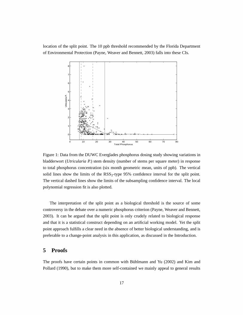
location of the split point. The 10 ppb threshold recommended by the Florida Department

of Environmental Protection (Payne, Weaver and Bennett, 2003) falls into these CIs.

0 10 20 30 40 50 60 70 80

0

1

2

3

4

5

6

7

8

Total Phosphorus

Utri

cula

ria P

.

Figure 1: Data from the DUWC Everglades phosphorus dosing study showing variations in

bladderwort (Utricularia P.) stem density (number of stems per square meter) in response

to total phosphorus concentration (six month geometric mean, units of ppb). The vertical

solid lines show the limits of the RSS2-type 95% confidence interval for the split point.

The vertical dashed lines show the limits of the subsamplingconfidence interval. The local

polynomial regression fit is also plotted.

The interpretation of the split point as a biological threshold is the source of some

controversy in the debate over a numeric phosphorus criterion (Payne, Weaver and Bennett,

2003). It can be argued that the split point is only crudely related to biological response

and that it is a statistical construct depending on an artificial working model. Yet the split

point approach fulfills a clear need in the absence of better biological understanding, and is

preferable to a change-point analysis in this application,as discussed in the Introduction.

5 Proofs

The proofs have certain points in common with Buhlmann and Yu (2002) and Kim and

Pollard (1990), but to make them more self-contained we mainly appeal to general results

17

on empirical processes and M-estimation that are collectedin the book of van der Vaart and

Wellner (1996).

We begin by proving Theorem 2.3, which is closely related to Theorem 3.1 of Buhlmann

and Yu (2002).

Proof of Theorem 2.3.We derive the joint limiting distribution of

(n1/3 (d d0

n − d0), n−1/3 RSS2(d0)),

the marginals of which are involved in calibrating the confidence sets (2.7) and (2.8). To

simplify the notation, we denote(βd0

l , βd0

u , d d0

n ) by (β 0l , β

0u, d

0n). Also, we assume that

β0l > β0

u; the derivation for the other case is analogous. LettingPn denote the empirical

measure of the pairs(Xi, Yi), i = 1, . . . , n, we can write

RSS2(d0) =

n∑

i=1

(Yi − β0l )2 (1(Xi ≤ d0) − 1(Xi ≤ d0

n))

+n∑

i=1

(Yi − β0u)2 (1(Xi > d0) − 1(Xi > d0

n))

= nPn

[(

(Y − β0l )2 − (Y − β0

u)2) (

1(X ≤ d0) − 1(X ≤ d0n))]

= 2 (β0l − β0

u)nPn

[(

Y − β0l + β0

u

2

)

(

1(X ≤ d0n) − 1(X ≤ d0)

)

]

.

Therefore,

n−1/3 RSS2(d0) = 2 (β0

l − β0u)n2/3

Pn

[

(Y − f(d0)) (1 (X ≤ d0n) − 1 (X ≤ d0))

]

,

wheref(d0) = (β0l + β0

u)/2. Let

ξn(d) = n2/3Pn

[

(Y − f(d0)) (1(X ≤ d) − 1(X ≤ d0))]

and letdn be the maximizer of this process. Sinceβ0l − β0

u → β0l − β0

u > 0 almost surely,

it is easy to see thatdn = d0n for n sufficiently large almost surely. Hence, the limiting

distribution ofn−1/3 RSS2(d0) must be the same as that of2 (β0

l −β0u) ξn(dn), which in turn

is the same as that of2 (β0l −β0

u) ξn(dn) (providedξn(dn) has a limit distribution), because

β 0l and β0

u are√n-consistent. Furthermore, the limiting distribution ofn1/3 (d 0

n − d0) is

the same as that ofn1/3 (dn − d0) (provided a limiting distribution exists).

LetQn(t) = ξn(d0 + t n−1/3) andtn = argmaxtQn(t), so thattn = n1/3 (dn − d0). It

now suffices to find the joint limiting distribution of(tn, Qn(tn)). Lemma 5.1 below shows

18

thatQn(t) converges in distribution in the spaceBloc(R) (the space of locally bounded

functions onR equipped with the topology of uniform convergence on compacta) to the

Gaussian processQ0(t) ≡ aW (t) − b0 t2 whose distribution is a tight Borel measure

concentrated onCmax(R) (the separable subspace ofBloc(R) of all continuous functions

onR that diverge to−∞ as the argument runs off to±∞ and that have a unique maximum).

Furthermore, Lemma 5.1 shows that the sequencetn of maximizers ofQn(t) isOp(1).

By Theorem 5.1 below, we conclude that(tn, Qn(tn)) →d (argmaxtQ0(t),maxtQ0(t)).

This completes the proof.

The following theorem provides sufficient conditions for the joint weak convergence of

a sequence of maximizers and the corresponding maxima of a general sequence of processes

in Bloc(R). A referee suggested that an alternative approach would be to useD(R) (the

space of right-continuous functions with left-limits equipped with Lindvall’s extension of

the Skorohod topology), instead ofBloc(R), as in an argmax-continuous mapping theorem

due to Ferger (2004, Theorem 3).

Theorem 5.1 LetQn(t) be a sequence of stochastic processes converging in distribution

in the spaceBloc(Rk) to the processQ(t), whose distribution is a tight Borel measure

concentrated onCmax(Rk). If tn is a sequence of maximizers ofQn(t) such that

tn = Op(1), then

(tn, Qn(tn)) →d (argmaxtQ(t),maxtQ(t)).

Proof. For simplicity, we provide the proof for the case thatk = 1; the same argument

essentially carries over to thek-dimensional case. By invoking Dudley’s representation

theorem (Theorem 2.2 of Kim and Pollard, 1990), for the processesQn, we can construct

a sequence of processesQn and a processQ defined on a common probability space

(Ω, A, P ) with (a) Qn being distributed asQn, (b) Q being distributed asQ and (c)

Qn converging toQ almost surely (with respect toP ) under the topology of uniform

convergence on compact sets. Thus, (i)tn, the maximizer ofQn, has the same distribution

as tn, (ii) t, the maximizer ofQ(t), has the same distribution as argmaxQ(t), and (iii)

Qn(tn) andQ(t) have the same distribution asQn(tn) and maxtQ(t), respectively. So it

suffices to show thattn converges inP ⋆ (outer) probability tot andQn(tn) converges in

P ⋆ (outer) probability toQ(t). The convergence oftn to t in outer probability is shown in

Theorem 2.7 of Kim and Pollard (1990).

To show thatQn(tn) converges in probability toQ(t), we need to show that for fixed

ǫ > 0, δ > 0, we eventually have

P ⋆(

| Qn(tn) − Q(t) |> δ)

< ǫ.

19

Sincetn andt areOp(1), there existsMǫ > 0 such that, with

Acn ≡ tn /∈ [−Mǫ,Mǫ], Bc

n ≡ t /∈ [−Mǫ,Mǫ],

P ⋆(Acn) < ǫ/4 andP ⋆(Bc

n) < ǫ/4, eventually. Furthermore, asQn converges toQ almost

surely and therefore in probability, uniformly on every compact set, with

Ccn ≡ sups∈[−Mǫ,Mǫ] |Qn(s) − Q(s)| > δ ,

we haveP ⋆(Ccn) < ǫ/2, eventually. Hence,P ⋆(Ac

n ∪Bcn ∪Cc

n) < ǫ, so thatP⋆(An ∩Bn ∩Cn) > 1 − ǫ, eventually. But

An ∩Bn ∩ Cn ⊂ | Qn(tn) − Q(t) |≤ δ, (5.11)

and consequently

P⋆(| Qn(tn) − Q(t) |≤ δ) ≥ P⋆(An ∩Bn ∩Cn) > 1 − ǫ

eventually. This implies immediately that

P ⋆(| Qn(tn) − Q(t) |> δ) < ǫ

for all sufficiently largen. It remains to show (5.11). To see this, note that for anyω ∈An ∩Bn ∩ Cn ands ∈ [−Mǫ,Mǫ],

Qn(s) = Q(s) + Qn(s) − Q(s) ≤ Q(t) + |Qn(s) − Q(s)| .

Taking the supremum overs ∈ [−Mǫ,Mǫ] and noting thattn ∈ [−Mǫ,Mǫ] on the set

An ∩Bn ∩ Cn, we have

Qn(tn) ≤ Q(t) + sups∈[−Mǫ,Mǫ] |Qn(s) − Q(s)|,

or equivalently

Qn(tn) − Q(t) ≤ sups∈[−Mǫ,Mǫ] |Qn(s) − Q(s)| .

An analogous derivation (replacingQn everywhere byQ, andtn by t, and vice-versa) yields

Q(t) − Qn(tn) ≤ sups∈[−Mǫ,Mǫ] |Q(s) − Qn(s)|.

Thus

|Qn(tn) − Q(t)| ≤ sups∈[−Mǫ,Mǫ] |Qn(s) − Q(s)| ≤ δ,

which completes the proof.

The following modification of a rate theorem of van der Vaart and Wellner (1996,

Theorem 3.2.5) is needed in the proof of Lemma 5.1. The notation . means that the left

side is bounded by a generic constant times the right side.

20

Theorem 5.2 Let Θ andF be semimetric spaces. LetMn(θ, F ) be stochastic processes

indexed byθ ∈ Θ andF ∈ F . LetM(θ, F ) be a deterministic function, and(θ0, F0) be a

fixed point in the interior ofΘ ×F . Assume that for everyθ in a neighborhood ofθ0,

M(θ, F0) − M(θ0, F0) . −d2(θ, θ0), (5.12)

whered(·, ·) is the semimetric forΘ. Let θn be a point of maximum ofMn(θ, Fn), where

Fn is random. For eachǫ > 0, suppose that the following hold:

(a) There exists a sequenceFn,ǫ, n = 1, 2, . . ., of metric subspaces ofF , each containing

F0 in its interior.

(b) For all sufficiently smallδ > 0 (sayδ < δ0, whereδ0 does not depend onǫ), and for

all sufficiently largen,

E∗ supd(θ, θ0) < δ

F ∈ Fn,ǫ

|(Mn(θ, F ) − M(θ, F0)) − (Mn(θ0, F ) − M(θ0, F0))| ≤ Cǫφn(δ)√

n

(5.13)

for a constantCǫ > 0 and functionsφn (not depending onǫ) such thatδ 7→ φn(δ)/δα

is decreasing inδ for some constantα < 2 not depending onn.

(c) P (Fn /∈ Fn,ǫ) < ǫ for n sufficiently large.

If r2nφn(r−1n ) .

√n for everyn and θn →p θ0, thenrnd(θn, θ0) = Op(1).

Lemma 5.1 The processQn(t) defined in the proof of Theorem 2.3 converges in

distribution in the spaceBloc(R) to the Gaussian processQ0(t) ≡ aW (t) − b0 t2, whose

distribution is a tight Borel measure concentrated onCmax(R). Herea andb0 are defined

in Theorem 2.1. Furthermore, the sequencetn of maximizers ofQn(t) isOp(1) (and

hence converges to argmaxtQ0(t) by Theorem 5.1).

Proof. We apply the general approach outlined on page 288 of van der Vaart and Wellner

(1996). Define

Mn(d) = Pn

[

(Y − f(d0)) (1(X ≤ d) − 1(X ≤ d0))]

,

M(d) = P[

(Y − f(d0)) (1(X ≤ d) − 1(X ≤ d0))]

.

Now, dn = argmaxd∈RMn(d) andd0 = argmaxd∈R

M(d) and, in fact,d0 is the unique

maximizer ofM under the stipulated conditions. The last assertion needs proof, which

21

will be supplied later. We establish the consistency ofdn for d0 and then find the rate of

convergencern of dn; in other words thatrn for which rn (dn − d0) isOp(1). To establish

the consistency ofdn for d0, we apply Corollary 3.2.3 (part (i)) of van der Vaart and Wellner

(1996). We first show that supd∈R| Mn(d) −M(d) |→p 0. We can write

supd∈R| Mn(d) − M(d) | ≤ sup

d∈R

∣

∣(Pn − P ) [(Y − f(d0)) (1(X ≤ d) − 1(X ≤ d0))]∣

∣

+ supd∈R

∣

∣

∣Pn [(f(d0) − f(d0))(1(X ≤ d) − 1(X ≤ d0))]∣

∣

∣ .

The class of functions(Y − f(d0)) (1(X ≤ d) − 1(X ≤ d0)) : d ∈ R is VC with

a square integrable envelope (sinceE(Y 2) < ∞) and consequently Glivenko–Cantelli in

probability. Thus the first term converges to zero in probability. The second term is easily

seen to be bounded by2 | f(d0)−f(d0) |, which converges to zero almost surely. It follows

that supd∈R| Mn(d) − M(d) |= op(1). It remains to show thatM(d0) > supd/∈G M(d)

for every open intervalG that containsd0. Sinced0 is the unique maximizer of the

continuous (in fact, differentiable) functionM(d) and M(d0) = 0, it suffices to show

that limd→−∞ M(d) < 0 and limd→∞ M(d) < 0. This is indeed the case, and will be

demonstrated at the end of the proof. Thus, all conditions ofCorollary 3.2.3 are satisfied,

and hencedn converges in probability tod0.

Next we apply Theorem 5.2 to find the rate of convergencern of dn. Given ǫ > 0,

let Fn,ǫ = [f(d0) − Mǫ/√n, f(d0) + Mǫ/

√n], whereMǫ is chosen in such a way that

√n(f(d0) − f(d0)) ≤ Mǫ, for sufficiently largen, with probability at least1 − ǫ. Since

f(d0) = (β0l + β0

u)/2 is√n-consistent forf(d0), this can indeed be arranged. Then, setting

Fn = f(d0), we haveP (Fn /∈ Fn,ǫ) < ǫ for all sufficiently largen. We letd play the role

of θ, with d0 = θ0, and define

Mn(d, F ) = Pn [(Y − F ) (1(X ≤ d) − 1(X ≤ d0))],

M(d, F ) = P [(Y − F ) (1(X ≤ d) − 1(X ≤ d0))].

Thendn maximizesMn(d, Fn) ≡ Mn(d) andd0 maximizesM(d, F0), whereF0 = f(d0).

Consequently,

M(d, F0) − M(d0, F0) ≡ M(d) − M(d0) ≤ −C(d− d0)2

(for some positive constantC) for all d in a neighborhood ofd0 (sayd ∈ [d0− δ0, d0 + δ0]),

on using the continuity ofM′′(d) in a neighborhood ofd0 and the fact thatM′′(d0) < 0

(which follows from arguments at the end of this proof). Thus(5.12) is satisifed. We will

22

next show that (5.13) is also satisfied in our case, withφn(δ) ≡√δ, for all δ < δ0. Solving

r2n φn(r−1n ) .

√n, yieldsrn = n1/3, and we conclude thatn1/3(dn − d0) = Op(1).

To show (5.13), we need to find functionsφn(δ) such that

E⋆ sup|d−d0|<δ,F∈Fn,ǫ

√n |Mn(d, F ) − M(d, F0)|

is bounded byφn(δ). Writing Gn ≡ √n (Pn − P ), we find that the left side of the above

display is bounded byAn +Bn where,

An = E⋆ sup|d−d0|<δ,F∈Fn,ǫ

∣

∣Gn [(Y − F ) (1(X ≤ d) − 1(X ≤ d0))]∣

∣

and

Bn = E⋆ sup|d−d0|<δ,F∈Fn,ǫ

√n∣

∣P [(F − F0) (1(X ≤ d) − 1(X ≤ d0))]∣

∣ .

First consider the termAn. For sufficiently largen,

An ≤ E⋆ sup|d−d0|<δ,F∈[F0−1,F0+1]

∣

∣Gn [(Y − F ) (1(X ≤ d) − 1(X ≤ d0))]∣

∣ .

Denote byMδ the class of functions(Y −F ) (1(X ≤ d)−1(X ≤ d0)) : |d−d0| ≤ δ, F ∈[F0−1, F0+1]. An envelope function for this class is given byMδ = (|Y |+F0+2) 1 (X ∈[d0 − δ, d0 + δ]). From van der Vaart and Wellner (1996, p. 291), using their notation,

E⋆(

‖Gn‖Mδ

)

. J(1,Mδ) (P M2δ )1/2,

whereMδ is an envelope function forMδ andJ(1,Mδ) is the uniform entropy integral

(considered below). By straightforward computation, there existsδ0 > 0 such that for all

δ < δ0, we haveE(M2δ ) . δ, for a constant not depending onδ (but possibly onδ0). Also,

as will be shown below,J(1,Mδ) is bounded for all sufficiently smallδ. Hence,An .√δ.

Next, note that

Bn = sup|d−d0|<δ,F∈Fn,ǫ

√n∣

∣P [(F − F0) (1(X ≤ d) − 1(X ≤ d0))]∣

∣

≤ Mǫ sup|d−d0|<δ

|FX(d) − FX(d0)| . Mǫδ

using condition (A3) in the last step. HenceAn +Bn .√δ+ δ .

√δ, sinceδ can be taken

less than 1. Thus the choiceφn(δ) =√δ does indeed work.

23

Now we check the boundedness of

J(1,Mδ) = supQ

∫ 1

0

√

1 + log N(η ‖Mδ‖Q,2,Mδ , L2(Q)) d η

for smallδ, as claimed above. Take anyη > 0. Construct a grid of points on[F0−1, F0+1]

such that two successive points on the grid are at distance less thanη apart. This can be done

using fewer than3/η points. Now, take a function inMδ. This looks like(Y −F ) (1(X ≤d) − 1(X ≤ d0)) for someF ∈ [F0 − 1, F0 + 1] and somed with | d − d0 |≤ δ. Find the

closest point toF on this grid; call thisFc. Note that

| (Y − F ) (1(X ≤ d) − 1(X ≤ d0)) − (Y − Fc) (1(X ≤ d) − 1(X ≤ d0)) |≤ η 1[X ∈ [d0 − δ, d0 + δ]] ≤ ηMδ ,

whence

∥

∥(Y − F ) (1(X ≤ d) − 1(X ≤ d0)) − (Y − Fc) (1(X ≤ d) − 1(X ≤ d0))∥

∥

Q,2

is bounded byη‖Mδ‖Q,2. Now for any fixed pointFgrid on the grid, Mδ,Fgrid=

(Y − Fgrid) (1(X ≤ d) − 1(X ≤ d0)) : d ∈ [d0 − δ, d0 + δ] is a VC-class with

VC-dimension bounded by a constant not depending onδ or Fgrid. Also, Mδ is an

envelope forMδ,Fgrid; it follows from bounds on covering numbers for VC-classes that

N(η ‖Mδ‖Q,2,Mδ,Fgrid, L2(Q)) . η−V1 for someV1 > 0 that does not depend onQ,Fgrid

or δ. Since the number of grid points is of order1/η, using the bound on the above display

we have

N(2 η ‖Mδ‖Q,2,Mδ , L2(Q)) . η−(V1+1).

Using this upper bound on the covering number, we obtain a finite upper bound on

J(1,Mδ) for all δ < δ0, via direct computation. This completes the proof thattn =

n1/3 (dn − d0) = Op(1).

Recalling notation from the proof of Theorem 2.3, we can write

Qn(t) = ξn(d0 + t n−1/3) = Rn(t) + rn,1(t) + rn,2(t),

whereRn(t) = n2/3Pn [g(·, d0 + t n−1/3)] with

g((X,Y ), d) =

(

Y − β0l + β0

u

2

)

[

1 (X ≤ d) − 1 (X ≤ d0)]

,

rn,1(t) = n1/6 (f(d0) − f(d0))√n (Pn − P )

[

1 (X ≤ d0 + t n−1/3) − 1 (X ≤ d0)]

24

and

rn,2(t) = n2/3 (f(d0) − f(d0))P(

1 (X ≤ d0 + t n−1/3) − 1 (X ≤ d0))

.

Here, rn,1(t) →p 0 uniformly on every compact set of the form[−K,K] by applying

Donsker’s theorem to the empirical process√

n (Pn − P ) (1(X ≤ d0 + s) − 1(X ≤ d0)) : s ∈ (−∞,∞)

along with n1/6 (f(d0) − f(d0)) = op(1). The term rn,2(t) →p 0

uniformly on every [−K,K] since n1/3 (f(d0) − f(d0)) = op(1) and

n1/3 supt∈[−K,K] P(

1 (X ≤ d0 + t n−1/3) − 1 (X ≤ d0))

= O(1). Hence, the

limiting distribution ofQn(t) will be the same as the limiting distribution ofRn(t). We

show thatRn →d Q0, whereQ0 is the Gaussian process defined in Theorem 2.3. Write

Rn(t) = n2/3 (Pn − P )[

g(·, d0 + t n−1/3)]

+ n2/3 P[

g(·, d0 + t n−1/3)]

= In(t) + Jn(t) .

In terms of the empirical processGn, we haveIn(t) = Gn (fn,t) where

fn,t(x, y) = n1/6 (y − f(d0)) (1 (x ≤ d0 + t n−1/3) − 1 (x ≤ d0)) .

We will use Theorem 2.11.22 from van der Vaart and Wellner (1996) to show that on each

compact set[−K,K], Gn fn,t converges as a process inl∞ [−K,K] to the tight Gaussian

processaW (t), wherea2 = σ2(d0) pX(d0). Also, Jn(t) converges on every[−K,K]

uniformly to the deterministic function−b0 t2, with b0 = |f ′(d0)|pX(d0)/2 > 0. Hence

Qn(t) →d Q0(t) ≡ aW (t) − b0 t2 in Bloc(R), as required.

To complete the proof, we need to show thatIn andJn have the limits claimed above.

As far asIn is concerned, provided we can verify the other conditions ofTheorem 2.11.22,

the covariance kernelH(s, t) of the limit of Gn fn,t is given by the limit ofP (fn,s fn,t) −P fn,s P fn,t asn → ∞. We first computeP (fn,s fn,t). This vanishes ifs and t are of

opposite signs. Fors, t > 0,

P fn,s fn,t = E [n1/3 (Y − f(d0))2 1X ∈ (d0, d0 + (s ∧ t)n−1/3]]

=

∫ d0+(s∧t) n−1/3

d0

n1/3[

E [(f(X) + ǫ− f(d0))2 | X = x]]

pX(x) dx

= n1/3

∫ d0+(s∧t) n−1/3

d0

(

σ2(x) + (f(x) − f(d0))2)

pX(x) dx

→ σ2(d0) pX(d0) (s ∧ t)

≡ a2 (s ∧ t) .

25

Also, it is easy to see thatP fn,s andP fn,t converge to 0. Thus, whens, t > 0,

P (fn,s fn,t) − P fn,s P fn,t → a2 (s ∧ t) ≡ H(s, t) .

Similarly, it can be checked that fors, t < 0, H(s, t) = a2 (−s ∧ −t). ThusH(s, t) is the

covariance kernel of the Gaussian processaW (t).

Next we need to check

supQ

∫ δn

0

√

log N(ǫ ‖Fn‖Q,2,Fn, L2(Q)) d ǫ→ 0 , (5.14)

for everyδn → 0, where

Fn =

n1/6(y − f(d0)) [1(x ≤ d0 + t n−1/3) − 1(x ≤ d0)] : t ∈ [−K,K]

and

Fn(x, y) = n1/6∣

∣y − f(d0)∣

∣ 1(x ∈ [d0 −K n−1/3, d0 +K n−1/3])

is an envelope forFn. From van der Vaart and Wellner (1996, p. 141),

N(ǫ ‖Fn‖Q,2,Fn, L2(Q)) ≤ K V (Fn) (16 e)V (Fn)

(

1

ǫ

)2 (V (Fn)−1)

for a universal constantK and0 < ǫ < 1, whereV (Fn) is the VC-dimension ofFn. Since

V (Fn) is uniformly bounded, we see that the above inequality implies

N(ǫ ‖Fn‖Q,2,Fn, L2(Q)) .

(

1

ǫ

)s

wheres = supn 2(V (Fn) − 1) <∞, so (5.14) follows from

∫ δn

0

√

− log ǫ d ǫ→ 0

asδn → 0. We also need to check the conditions (2.11.21) in van der Vaart and Wellner

(1996):

P ⋆ F 2n = O(1), P ⋆ F 2

n 1Fn > η√n → 0, ∀η > 0 ,

and

sup|s−t|<δn

P (fn,s − fn,t)2 → 0, ∀δn → 0 .

With Fn as defined above, an easy computation shows that

P ⋆ F 2n = K

1

K n−1/3

∫ d0+K n−1/3

d0−K n−1/3

(σ2(x) + (f(x) − f(d0))2) pX(x) dx = O(1) .

26

Denote the set[d0 −K n−1/3, d0 +K n−1/3] by Sn. Then

P ⋆ (F 2n 1Fn > η

√n)

= E [n1/3 | Y − f(d0) |2 1X ∈ Sn 1 | Y − f(d0) | 1X ∈ Sn > η n1/3]≤ E

[

n1/3 | Y − f(d0) |2 1X ∈ Sn 1| ǫ |> η n1/3/2]

≤ E[

2n1/3 (ǫ2 + (f(X) − f(d0))2) 1X ∈ Sn 1| ǫ |> η n1/3/2]

(5.15)

eventually, since for all sufficiently largen

| Y − f(d0) | 1 X ∈ Sn > η n1/3 ⊂ | ǫ |> η n1/3/2 .

Now, the right side of (5.15) can be written asT1 + T2, where

T1 = 2n1/3 E [ǫ2 1 | ǫ |> η n1/3/2 1 X ∈ Sn]

and

T2 = 2n1/3E [(f(X) − f(d0))2 1 X ∈ Sn 1 | ǫ |> η n1/3/2] .

We will show thatT1 = o(1). We have

T1 = 2n1/3

∫ d0+K n−1/3

d0−K n−1/3

E [ǫ2 1 | ǫ |> η n1/3/2 | X = x] pX(x) dx .

By (A5), for anyξ > 0,

supx∈Sn

E [ǫ2 1 | ǫ |> η n1/3/2 | X = x] < ξ

for n sufficiently large. Sincen1/3∫

SnpX(x) dx is eventually bounded by2K pX(d0) it

follows thatT1 is eventually smaller than2 ξKpX(d0). We conclude thatT1 = o(1). Next,

note that (A5) implies thatsupx∈SnE [1 | ǫ |> η n1/3/2 | X = x] → 0 asη → ∞, so

T2 = o(1) by a similar argument as above. Finally,

sup|s−t|<δn

P (fn,s − fn,t)2 → 0

asδn → 0 can be checked via similar computations.

We next deal withJn. For convenience we sketch the uniformity of the convergence of

Jn(t) to the claimed limit on0 ≤ t ≤ K. We have

Jn(t) = n2/3E[

(Y − f(d0)) (1 (X ≤ d0 + t n−1/3) − 1 (X ≤ d0))]

27

= n2/3E[

(f(X) − f(d0)) 1 (X ∈ (d0, d0 + t n−1/3])]

= n2/3

∫ d0+t n−1/3

d0

(f(x) − f(d0)) pX(x) dx

= n1/3

∫ t

0(f(d0 + un−1/3) − f(d0)) pX(d0 + un−1/3) du

=

∫ t

0uf(d0 + un−1/3) − f(d0)

un−1/3pX(d0 + un−1/3) du

→∫ t

0u f ′(d0) pX(d0) du (uniformly on 0 ≤ t ≤ K)

=1

2f ′(d0) pX(d0)t2.

It only remains to verify that (i)d0 is the unique maximizer ofM(d), (ii) M(−∞) <

0,M(∞) < 0 and (iii) f ′(d0) pX(d0) < 0 (so the processaW (t) + (f ′(d0) pX(d0)/2) t2

is indeed inCmax(R)). To show (i), recall that

M(d) = E [g((X,Y ), d)] = E

[(

Y − β0l + β0

u

2

)

(1(X ≤ d) − 1(X ≤ d0))

]

.

Let ξ(d) = E [Y − β0l 1(X ≤ d) − β0

u 1(X > d)]2 . By condition (A1),d0 is the unique

minimizer ofξ(d). Consequently,d0 is also the unique maximizer of the functionξ(d0) −ξ(d). Straightforward algebra shows that

ξ(d0) − ξ(d) = 2 (β0l − β0

u) M(d)

and sinceβ0l −β0

u > 0, it follows thatd0 is also the unique maximizer ofM(d). This shows

(i). Next,

M(d) = E[(

f(X) − f(d0))

(1(X ≤ d) − 1(X ≤ d0))]

=

∫ ∞

−∞

(

f(x) − f(d0)) (

1(x ≤ d) − 1(x ≤ d0))

pX(x) dx

=

∫ d

−∞

(

f(x) − f(d0))

pX(x) dx−∫ d0

−∞

(

f(x) − f(d0))

pX(x) dx,

so that

M(−∞) = limd→−∞

M(d) = −∫ d0

−∞(f(x) − f(d0)) pX(x) dx < 0

if and only if∫ d0

−∞ f(x) pX(x) dx > f(d0)FX (d0) if and only if β0l ≡

∫ d0

−∞ f(x) pX(x) dx/FX (d0) > (β0l + β0

u)/2, and this is indeed the case, sinceβ0l > β0

u.

28

We can prove thatM(∞) < 0 in a similar way, so (ii) holds. Also,M′(d) = (f(d) −f(d0)) pX(d), soM

′(d0) = 0. Finally,

M′′(d) = f ′(d) pX(d) + (f(d) − f(d0))p′X(d),

soM′′(d0) = f ′(d0) pX(d0) ≤ 0, sinced0 is the maximizer. This implies (iii), since by our

assumptionsf ′(d0) pX(d0) 6= 0.

Proof of Theorem 2.1. Let Θ denote the set of all possible values of(βl, βu, d) and θ

denote a generic vector inΘ. Define the criterion functionM(θ) = Pmθ, where

mθ(x, y) = (y − βl)2 1(x ≤ d) + (y − βu)2 1(x > d).

The vectorθ0 ≡ (β0l , β

0u, d

0) minimizesM(θ), while θn ≡ (βl, βu, dn) minimizesMn(θ) =

Pnmθ. Sinceθ0 uniquely minimizesM(θ) under condition (A1), using the twice continuous

differentiability of M atθ0, we have

M(θ) − M(θ0) ≥ C d2(θ, θ0)

in a neighborhood ofθ0 (for someC > 0), whered(·, ·) is the l∞ metric onR3. Thus,

there existsδ0 > 0 sufficiently small, such that for all(βl, βu, d) with | βl − β0l |< δ0,

| βu − β0u |< δ0 and| d− d0 |< δ0, the above display holds.

For all δ < δ0 we will find a bound onE⋆P ‖Gn‖Mδ

, whereMδ ≡ mθ − mθ0:

d(θ, θ0) < δ andGn ≡ √n (Pn − P ). From van der Vaart and Wellner (1996, p. 298),

E⋆P ‖Gn‖Mδ

≤ J(1,Mδ) (P M2δ )1/2 ,

whereMδ is an envelope function for the classMδ. Straightforward algebra shows that

(mθ −mθ0)(X,Y ) = 2 (Y − f(d0)) (β0

u − β0l ) 1(X ≤ d) − 1(X ≤ d0)

+(β0l − βl)(2Y − β0

l − βl) 1(X ≤ d) + (β0u − βu) (2Y − β0

u − βu) 1(X > d).

The class of functions

M1,δ = 2 (Y − f(d0)) (β0u − β0

l ) 1(X ≤ d) − 1(X ≤ d0) : d ∈ [d0 − δ, d0 + δ]

is easily seen to be VC, with VC-dimension bounded by a constant not depending onδ;

furthermore,M1,δ = 2|(Y − f(d0)) (β0u − β0

l )|1(X ∈ [d0 − δ, d0 + δ]) is an envelope

function for this class. It follows that

N (ǫ ‖M1,δ‖P,2,M1,δ , L2(P )) . ǫ−V1 ,

29

for someV1 > 0 that does not depend onδ. Next, consider the class of functions

M2,δ = (β0l −βl)(2Y −β0

l −βl) 1(X ≤ d) : d ∈ [d0− δ, d0 + δ], βl ∈ [β0l − δ, β0

l + δ] .

Fix a grid of pointsβl,c in [β0l − δ, β0

l + δ] such that successive points on this grid are at a

distance less thanǫ apart, whereǫ = ǫ δ/2. The cardinality of this grid is certainly less than

3 δ/ǫ. For a fixedβl,c in this grid, the class of functionsM2,δ,c ≡ (β0l − βl,c)(2Y − β0

l −βl,c) 1(X ≤ d) : d ∈ [d0 − δ, d0 + δ] is certainly VC with VC-dimension bounded by a

constant that does not depend onδ or the pointβl,c. Also, note thatM2,δ ≡ δ (2|Y | + C),

whereC is a sufficiently large constant not depending onδ, is an envelope function for the

classM2,δ, and hence also an envelope function for the restricted class withβl,c held fixed.

It follows that for some universal positive constantV2 > 0 and anyη > 0,

N (η ‖M2,δ‖P,2,M2,δ,c, L2(P )) . η−V2 .

Now, ‖M2,δ‖P,2 = δ‖G‖P,2, whereG = 2|Y | + C. Thus,

N (ǫ ‖G‖P,2,M2,δ,c, L2(P )) .

(

δ

ǫ

)V2

.

Next, consider a functiong(X,Y ) = (β0l − βl)(2Y − β0

l − βl) 1(X ≤ d) in M2,δ. Find a

βl,c that is within ǫ distance ofβl. There are of order(δ/ǫ)V2 balls of radiusǫ ‖G‖P,2 that

cover the classM2,δ,c, so the functiongc(X,Y ) ≡ (β0l − βl,c)(2Y − β0

l − βl,c) 1(X ≤ d)

must be at distance less thanǫ ‖G‖P,2 from the center of one of these balls, sayB. Also,

it is easily checked that‖g − gc‖P,2 < ǫ‖G‖P,2. Henceg must be at distance less than

2 ǫ‖G‖P,2 from the center ofB. It then readily follows that

N (2 ǫ ‖G‖P,2,M2,δ, L2(P )) .

(

δ

ǫ

)V2+1

,

on using the fact that the cardinality of the gridβl,c is of orderδ/ǫ. Substitutingǫ δ/2 for

ǫ in the above display, we get

N (ǫ ‖M2,δ‖P,2,M2,δ, L2(P )) .

(

1

ǫ

)V2+1

.

Finally, with

M3,δ = (β0u−βu)(2Y −β0

u−βu) 1(X > d) : d ∈ [d0−δ, d0 +δ], βu ∈ [β0u−δ, β0

u +δ]

andM3,δ = δ (2|Y | + C ′) for some sufficiently large constantC ′ not depending onδ, we

similarly argue that

N (ǫ ‖M3,δ‖P,2,M3,δ, L2(P )) .

(

1

ǫ

)V3+1

,

30

for some positive constantV3 not depending onδ. The classMδ ⊂ M1,δ+M2,δ+M3,δ ≡Mδ. SetMδ = M1,δ +M2,δ +M3,δ. Now, it is not difficult to see that

N (3 ǫ ‖Mδ‖P,2,Mδ , L2(P )) .

(

1

ǫ

)V1+V2+V3

.

This also holds for any probability measureQ such that0 < EQ(Y 2) < ∞, with the

constant being independent ofQ or δ. SinceMδ ⊂ Mδ, it follows that

N (3 ǫ ‖Mδ‖Q,2,Mδ, L2(Q)) .

(

1

ǫ

)V1+V2+V3

.

Thus, withQ denoting the set of all such measuresQ,

J(1,Mδ) ≡ supQ∈Q

∫ 1

0

√

1 + log N(ǫ ‖Mδ‖Q,2,Mδ, L2(Q)) d ǫ <∞

for all sufficiently smallδ. Next,

P M2δ . P M2

1,δ + P M22,δ + P M2

3,δ . δ + δ2 . δ

since we can assumeδ < 1. ThereforeE⋆P ‖Gn‖Mδ

.√δ, andφn(δ) in Theorem 3.2.5 of

van der Vaart and Wellner (1996) can be taken as√δ. Solvingr2n φn(1/rn) ≤ √

n yields

rn ≤ n1/3, and we conclude that

n1/3(

βl − β0l , βu − β0

u, dn − d0)

= Op(1) .

Having established the rate of convergence, we now determine the asymptotic

distribution. It is easy to see that

n1/3(

βl − β0l , βu − β0

u, dn − d0)

= argminh Vn(h),

where

Vn(h) = n2/3 (Pn − P ) [mθ0+h n−1/3 −mθ0] + n2/3 P [mθ0+h n−1/3 −mθ0

] (5.16)

for h = (h1, h2, h3) ∈ R3. The second term above converges tohT V h/2, uniformly on

every[−K,K]3 (K > 0), whereV is the Hessian of the functionθ 7→ P mθ at the pointθ0,

on using the twice continuous differentiability of the function atθ0 and thatθ0 minimizes

this function. Note thatV is a positive definite matrix. Calculating the Hessian matrix gives

V =

2FX(d0) 0 (β0l − β0

u) pX(d0)

0 2 (1 − FX(d0)) (β0l − β0

u) pX(d0)

(β0l − β0

u) pX(d0) (β0l − β0

u) pX(d0) 2|(β0l − β0

u)f ′(d0) pX(d0)|

.

31

We next deal with distributional convergence of the first term in (5.16), which can be written

as√n(Pn − P ) fn,h, wherefn,h = fn,h,1 + fn,h,2 + fn,h,3 and

fn,h,1(x, y) = n1/6 2 (β0u − β0

l )(y − f(d0)) (1(x ≤ d0 + h3 n−1/3) − 1(x ≤ d0)),

fn,h,2(x, y) = −n−1/6 h1 (2 y − 2β0l − h1 n

−1/3) 1(x ≤ d0 + h3 n−1/3),

fn,h,3(x, y) = −n−1/6 h2 (2 y − 2β0u − h2 n

−1/3) 1(x > d0 + h3 n−1/3).

A natural envelope functionFn for Fn ≡ fn,h : h ∈ [−K,K]3 is given by

Fn(x, y) = 2n1/6 | (β0l − β0

u)(y − f(d0)) | 1x ∈ [d0 −K n−1/3, d0 +K n−1/3]

+K n−1/6 (2 | y − β0l | +1) +K n−1/6 (2 | y − β0

u | +1) .

The limiting distribution of√n(Pn −P ) fn,h is directly obtained by appealing to Theorem

2.11.22 of van der Vaart and Wellner (1996). On each compact set of the form[−K,K]3,

the process√n (Pn−P ) fn,h converges in distribution toaW (h3), wherea = 2 | β0

l −β0u |

(σ2(d0) pX(d0))1/2. This follows on noting that

limn→∞

P fn,s fn,h − Pfn,s Pfn,h = a2 (| s3 | ∧ | h3 |) 1(s3 h3 > 0),

by direct computation and verification of conditions (2.11.21) preceding the statement of

Theorem 2.11.22; we omit the details as they are similar to those in the proof of Lemma

5.1. The verification of the entropy-integral condition, i.e.,

supQ

∫ δn

0

√

log N(ǫ ‖Fn‖Q,2,Fn, L2(Q)) d ǫ→ 0

asδn → 0, usesN(ǫ ‖Fn‖Q,2,Fn, L2(Q)) . ǫ−V for someV > 0 not depending onQ;

the argument is similar to the one we used earlier withJ(1,Mδ).

It follows that the processVn(h) converges in distribution in the spaceBloc(R3) to the

processW (h1, h2, h3) ≡ aW (h3)+hT V h/2. The limiting distribution is concentrated on

Cmin(R3) (defined analogously toCmax(R

3)), which follows on noting that the covariance

kernel of the Gaussian processW has the rescaling property (2.4) of Kim and Pollard

(1990) and thatV is positive definite; furthermore,W (s) − W (h) has non-zero variance

for s 6= h, whence Lemma 2.6 of Kim and Pollard (1990) forces a unique minimizer.

Invoking Theorem 5.1 (to be precise, a version of the theoremwith max replaced by min),

we conclude that

(argminh Vn(h),minh Vn(h)) →d (argminhW (h),minh W (h)). (5.17)

32

But note that

minh W (h) = minh3

aW (h3) + minh1,h2hT V h/2

and we can find argminh1,h2hT V h/2 explicitly. After some routine calculus, we find that

the limiting distribution of the first component in (5.17) can be expressed in the form stated

in the theorem. This completes the proof.

Proof of Theorem 2.2.Inspecting the second component of (5.17), we find

n−1/3 RSS0(β0l , β

0u, d

0) = −minh Vn(h) →d −minh W (h)

and this simplifies to the limit stated in the theorem. To showthat n−1/3 RSS1(d0)

converges to the same limit, it suffices to show that the difference Dn =

n−1/3 RSS0(β0l , β

0u, d

0)−n−1/3 RSS1(d0) is asymptotically negligible. Some algebra gives

thatDn = In + Jn, where

In = n−1/3n∑

i=1

(2Yi − β0l − β0

l ) (β0l − β0

l ) 1(Xi ≤ d0)

and

Jn = n−1/3n∑

i=1

(2Yi − β0u − β0

u) (β0u − β0

u) 1(Xi > d0).

Then

In =√n (β0

l − β0l )n1/6

Pn [(2Y − β0l − β0

l ) 1(X ≤ d0)]

=√n (β0

l − β0l )n1/6 (Pn − P ) [(2Y − β0

l − β0l ) 1(X ≤ d0)]

+√n (β0

l − β0l )n1/6 P [(2Y − β0

l − β0l ) 1(X ≤ d0)]

= In,1 + In,2 .

Since√n (β0

l − β0l ) = Op(1) and

n1/6 (Pn − P ) [(2Y − β0l − β0

l ) 1(X ≤ d0)] = n1/6 (Pn − P ) [(2Y − β0l ) 1(X ≤ d0)]

−β0l n

1/6 (Pn − P ) (1(X ≤ d0))

is clearlyop(1) by the CLT and the consistency ofβ0l , we have thatIn,1 = op(1). To show

In,2 = op(1), it suffices to show thatn1/6 P [(2Y − β0l − β0

l ) 1(X ≤ d0)] → 0. But this

can be written as

n1/6 P [2 (Y − β0l ) 1(X ≤ d0)] + n1/6 P [(β0

l − β0l ) 1(X ≤ d0)] .

33

The first term vanishes, from the normal equations characterizing (β0l , β

0u, d

0), and the

second term isn1/6O(n−1/2) → 0. We have shown thatIn = op(1), andJn = op(1)

can be shown in the same way. This completes the proof.

Acknowledgements. The authors thank Song Qian for comments about the Everglades

application, Michael Woodroofe and Bin Yu for helpful discussion, Marloes Maathuis

for providing the extended rate convergence theorem, and the referees for their detailed

comments.

References

Antoniadis, A. and Gijbels, I. (2002). Detecting abrupt changes by wavelet methods.J.

Nonparametric Statist.14 7–29.

Banerjee, M. and Wellner, J. A. (2001). Likelihood ratio tests for monotone functions.

Ann. Statist.29 1699–1731.

Buhlmann, P. and Yu, B. (2002). Analyzing bagging.Ann. Statist.30 927–961.

Delgado, M. A., Rodriguez-Poo, J. and Wolf, M. (2001). Subsampling inference in cube

root asymptotics with an application to Manski’s maximum score statistic.Econom.

Lett. 73, 241–250.

Dempfle, A. and Stute, W. (2002). Nonparametric estimation of a discontinuity in

regression.Statistica Neerlandica56233–242.

Fan, J. and Gijbels, I. (1996).Local Polynomial Modelling and Its Applications. Chapman

& Hall, London.

Ferger, D. (2004). A continuous mapping theorem for the argmax-functional in the non-

unique case.Statistica Neerlandica58 83–96.

Genovese, C. R. and Wasserman, L. (2005). Confidence sets fornonparametric regression.

Ann. Statist.33 698–729.

Gijbels, I., Hall, P. and Kneip, A. (1999). On the estimationof jump points in smooth

curves.Ann. Inst. Statist. Math.51 231–251.

Groeneboom, P. and Wellner, J. A. (2001). Computing Chernoff’s distribution. Journal of

Computational and Graphical Statistics10388–400.

34

Kim, J. and Pollard, D. (1990). Cube root asymptotics.Ann. Statist.18 191–219.

Lund, R. and Reeves, J. (2002). Detection of undocumented changepoints: a revision of

the two-phase regression model.Journal of Climate15 2547–2554.

Payne, G., Weaver, K. and Bennett, T. (2003). Development ofa numeric phosphorus

criterion for the Everglades protection area.Everglades Consolidated Report, Ch. 5.

www.dep.state.fl.us/water/everglades/docs/ch5 03.pdf

Politis, D. N. , and Romano, J. P. (1994). Large sample confidence regions based on

subsamples under minimal assumptions.Ann. Statist.22 2031–2050.

Politis, D. N., Romano, J. P. and Wolf, M. (1999).Subsampling. Springer, New York.

Qian, S. S., King, R. and Richardson, C. J. (2003). Two statistical methods for the

detection of environmental thresholds.Ecological Modelling16687–97.

Qian, S. S. and Lavine, M. (2003). Setting standards for water quality in the Everglades.

Chance16, No. 3, 10–16.

Ruppert, D. (1997). Empirical-bias bandwidths for local polynomial nonparametric

regression and density estimation,J. Amer. Statist. Assoc.92 1049–1062.

Stein, C. (1981). Estimation of the mean of a multivariate normal distribution.Ann. Statist.

9 1135–1151.

Thomson, R. E. and Fine, I. V. (2003). Estimating mixed layerdepth from oceanic profile

data.J. Atmos. Oceanic Technology20319–329.

van der Vaart, A. and Wellner, J. A. (1996).Weak Convergence and Empirical Processes.

Springer, New York.

35