Conceptual model for improving the link between exposure and effects in the aquatic risk assessment of pesticides

ARTICLE IN PRESS

0147-6513/$ - se

doi:10.1016/j.ec

�CorrespondE-mail addr

Ecotoxicology and Environmental Safety 66 (2007) 291–308

www.elsevier.com/locate/ecoenv

Review

Conceptual model for improving the link between exposure and effectsin the aquatic risk assessment of pesticides

J.J.T.I. Boestena,�, H. Koppb, P.I. Adriaansea, T.C.M. Brocka, V.E. Forbesc

aAlterra, Wageningen University and Research Centre, PO Box 47, 6700 AA Wageningen, The NetherlandsbFederal Office for Consumer Protection and Food Safety, Messeweg 11/12, D-38104 Braunschweig, Germany

cCentre for Integrated Population Ecology, Department of Life Sciences and Chemistry, Roskilde University, PO Box 260, DK-4000 Roskilde, Denmark

Received 10 May 2006; received in revised form 22 August 2006; accepted 15 October 2006

Available online 4 December 2006

Abstract

Assessment of risks to aquatic organisms is important in the registration procedures for pesticides in industrialised countries. This risk

assessment consists of two parts: (i) assessment of effects to these organisms derived from ecotoxicological experiments ( ¼ effect

assessment), and (ii) assessment of concentration levels in relevant environmental compartments resulting from pesticide application

( ¼ exposure assessment). Current procedures lack a clear conceptual basis for the interface between the effect and exposure assessments

which may lead to a low overall scientific quality of the risk assessment. This interface is defined here as the type of concentration that

gives the best correlation to ecotoxicological effects and is called the ecotoxicologically relevant concentration (ERC). Definition of this

ERC allows the design of tiered effect and exposure assessments that can interact flexibly and efficiently. There are two distinctly

different exposure estimates required for pesticide risk assessment: that related to exposure in ecotoxicological experiments and that

related to exposure in the field. The same type of ERC should be used consistently for both types of exposure estimates. Decisions are

made by comparing a regulatory acceptable concentration ( ¼ RAC) level or curve (i.e., endpoint of the effect assessment) with predicted

environmental concentration ( ¼ PEC) levels or curves (endpoint of the exposure assessment). For decision making based on

ecotoxicological experiments with time-variable concentrations a tiered approach is proposed that compares (i) in a first step single RAC

and PEC levels based on conservative assumptions, (ii) in a second step graphically RAC and PEC curves (describing the time courses of

the RAC and PEC), and (iii) in a third step time-weighted average RAC and PEC levels.

r 2006 Elsevier Inc. All rights reserved.

Keywords: Aquatic ecotoxicology; Surface water; Exposure scenarios

Contents

1. Introduction . . . . . . . . . . . . . . . . . . . . . . . . . . . . . . . . . . . . . . . . . . . . . . . . . . . . . . . . . . . . . . . . . . . . . . . . . . . . . . . 292

2. General principles of exposure assessment as part of risk assessment for aquatic organisms . . . . . . . . . . . . . . . . . . . . . . . 293

3. Clear definition of the ecotoxicologically relevant concentration (ERC) . . . . . . . . . . . . . . . . . . . . . . . . . . . . . . . . . . . . . 294

4. Description of the procedure for integrating exposure and effect tiers. . . . . . . . . . . . . . . . . . . . . . . . . . . . . . . . . . . . . . . 295

5. Routes through combined effect and exposure flow charts. . . . . . . . . . . . . . . . . . . . . . . . . . . . . . . . . . . . . . . . . . . . . . . 296

6. Handling time-variable exposure in higher-tier ecotoxicological experiments for aquatic risk assessment . . . . . . . . . . . . . . 296

6.1. Proposal for a stepped approach for handling time-variable exposure . . . . . . . . . . . . . . . . . . . . . . . . . . . . . . . . . . 296

6.2. Application of the proposed stepped approach for time-variable exposure to a case study . . . . . . . . . . . . . . . . . . . . 300

6.3. Consequences for designing the exposure in higher-tier ecotoxicological experiments. . . . . . . . . . . . . . . . . . . . . . . . 303

7. Role of exposure information from ecotoxicological experiments in the exposure assessment for the field . . . . . . . . . . . . . 305

8. Use of the proposed approach in current aquatic risk assessment at EU level . . . . . . . . . . . . . . . . . . . . . . . . . . . . . . . . . 305

e front matter r 2006 Elsevier Inc. All rights reserved.

oenv.2006.10.002

ing author. Fax: +31317 419000.

ess: [email protected] (J.J.T.I. Boesten).

www.elsevier.com/locate/ecoenv

dx.doi.org/10.1016/j.ecoenv.2006.10.002

mailto:[email protected]

ARTICLE IN PRESSJ.J.T.I. Boesten et al. / Ecotoxicology and Environmental Safety 66 (2007) 291–308292

9. Recommendations for future activities to improve the aquatic risk assessment procedure . . . . . . . . . . . . . . . . . . . . . . . . . 306

10. Applicability to risk assessment for soil organisms . . . . . . . . . . . . . . . . . . . . . . . . . . . . . . . . . . . . . . . . . . . . . . . . . . . . 306

11. Conclusions . . . . . . . . . . . . . . . . . . . . . . . . . . . . . . . . . . . . . . . . . . . . . . . . . . . . . . . . . . . . . . . . . . . . . . . . . . . . . . . 307

Acknowledgments . . . . . . . . . . . . . . . . . . . . . . . . . . . . . . . . . . . . . . . . . . . . . . . . . . . . . . . . . . . . . . . . . . . . . . . . . . . 307

References . . . . . . . . . . . . . . . . . . . . . . . . . . . . . . . . . . . . . . . . . . . . . . . . . . . . . . . . . . . . . . . . . . . . . . . . . . . . . . . . 307

1NOEC is ‘no observed effect concentration’.

1. Introduction

Assessment of the risks to aquatic organisms is animportant aspect of pesticide registration procedures inEurope, the USA and other industrialised countries. Thisrisk assessment procedure consists of two parts: (i)assessment of effects to these organisms derived fromecotoxicological experiments (further called ‘effect assess-ment’), and (ii) assessment of concentration levels to whichorganisms will be exposed in the field after pesticideapplication (further called ‘exposure assessment’). Part (i)is the domain of ecotoxicology and part (ii) is the domainof environmental chemistry.

Until 2003, exposure of aquatic organisms to pesticides insurface water in the EU pesticide evaluation procedure wasassessed using a very simple procedure taking into accountonly spray drift as a source of surface water contamination.FOCUS (2001) developed a tiered approach for surfacewater exposure assessment at the EU level. The approach isbased on three steps that also take into account entry ofpesticides into surface water via drainage and runoff (inaddition to spray drift). Steps 1 and 2 are based on verysimple models and scenarios (with a complexity levelcomparable to the procedure used before 2003). However,Step 3 (operational since 2003) is sophisticated; it consists ofexposure assessments for ten scenarios using mechanisticmodels for describing leaching via drainage (MACRO),runoff (PRZM) and behaviour in surface water (TOXS-WA). The ten scenarios represent ‘realistic worst case’exposure in the major agricultural areas across the EU byconsidering the main environmental driving factors (such assoil type, slope and rainfall intensity) for the three entryroutes of the pesticide (spray drift deposition, drainage andrunoff). In addition, FOCUS (2005) developed an extensivelist of modelling refinements and mitigation measures thatled to FOCUS Step 4 scenarios. So in the past years, aquaticexposure assessment at the EU level has become quitesophisticated. In the USA, the aquatic exposure assessmenthas reached a similar high level of sophistication. EPA(2004) has developed the Aquatic Level II Refined RiskAssessment (RRA) model which considers a range ofsurface water scenarios. Pesticide input is derived fromrunoff and erosion simulations with PRZM for a 36-yearperiod. The concentrations in surface water are calculatedwith the VVWMmodel. The resulting 36 annual peak valuesare subsequently used as input to a probabilistic riskassessment procedure.

Also the effect assessment is at a high level ofsophistication. Recently, detailed guidance on aquatic

effect assessment (Campbell et al., 1999) and on riskassessment at EU level (European Commission, 2002a) hasbecome available. The EU guidance document (EuropeanCommission, 2002a) describes the role of the FOCUSStep 1 to Step 3 surface water scenarios. For the lowereffect tiers, this role is straightforward and consistent withthe principles described before: the scenarios deliver theexposure concentrations (peaks or time-weighted averages)that are needed for the effect assessments. However, forhigher-tier studies the EU guidance document offers as acomplementary approach ‘to simulate the fate dynamicsexperimentally in higher-tier studies’ for substances thatshow a higher NOEC1 in static studies (i.e., with adecreasing concentration) than in flow-through studies inwhich the concentration is kept constant (see p. 32 ofguidance document). The document considers this as acomplementary approach to using a time-weighted averageconcentration. Adding sediment to laboratory test systemsto simulate adsorption or degradation or exposing the testsystem to natural light conditions to simulate photolysisare given as examples of this simulation of fate dynamics.Also micro/mesocosm test systems are often designed withthe intention to mimic the time-variable exposure in thefield more realistically. The EU guidance document states:‘In ‘‘fate simulation’’ studies the method used should bejustified on the basis of its relevance to realistic environ-mental conditions.’ No further guidance is provided onhow this justification might be achieved. In regulatorypractice, the notifier usually claims that such studies have amore realistic exposure because a spray drift event issimulated. However, the FOCUS Step 3 scenarios de-scribed above include also exposure from drainage andrunoff and systems with short residence times of waterwhich leads to a wide range of exposure patterns thatcannot possibly all be simulated in one or a few higher-tierecotoxicological experiments (FOCUS, 2001). Moreover,risk managers require usually realistic worst-case exposurepatterns within the risk assessment and it is unlikely thate.g., a single mesocosm experiment available in the dossiershows a realistic worst-case exposure pattern. So the EUguidance document recommends two potentially conflict-ing approaches for exposure assessment in higher effecttiers and gives no guidance as to how the consistencybetween these two approaches should be ensured. Thisshows that the interaction between the assessments ofexposure and of ecotoxicological effects in the higher tiersof risk assessment procedure for aquatic organisms is at a

ARTICLE IN PRESS

Fig. 1. Tiered effect and exposure flow charts for a risk assessment

addressing a protection aim ‘X’ which needs exposure estimates of an

ecotoxicologically relevant concentration (ERC) ‘Y’ as indicated by the

large arrow. The boxes E-1 to E-4 are four effect tiers and the boxes F-1 to

F-4 are four tiers for assessment of exposure in the field (‘F’ from ‘field’).

Downward arrows indicate movement to a higher tier. Horizontal arrows

from the exposure to the effect flow chart indicate delivery of field

exposure estimates for comparison with effect concentrations in the effect

flow chart.

J.J.T.I. Boesten et al. / Ecotoxicology and Environmental Safety 66 (2007) 291–308 293

lower level of sophistication than either assessment ofexposure or assessment of ecotoxicological effects. How-ever, for an adequate risk assessment both aspects need tobe combined in a sound way. Thus there seems to be a needfor improvement of the aquatic risk assessment at the EUlevel by improving the interaction between exposure andecotoxicological effects. The aim of this paper is to providesuch an improvement by (i) defining more explicitly theinterface between the assessment of exposure and of eco-toxicological effects, and (ii) providing adequate proceduresfor linking the exposure in higher-tier ecotoxicologicalexperiments to that expected in surface water in the field.

We restrict ourselves as much as possible to theinteraction between exposure and effects in the riskassessment because a review of assessment procedures ofboth exposure and ecotoxicological effects would divertattention from the interaction issue (see Brock et al., 2006,for a discussion of protection goals for aquatic risks in EUlegislation). Although our discussion refers to the specificapproach used for assessing risks of pesticides undercurrent EU legislation, we believe that the principles weaddress are of much broader relevance with respect toother jurisdictions and other classes of chemicals.

2. General principles of exposure assessment as part of risk

assessment for aquatic organisms

Any ecotoxicological risk assessment has to start withthe question ‘what has to be protected?’ This protectionaim will include usually a spatial component: e.g., protectaquatic and benthic organisms in watercourses neighbour-ing agricultural fields. It may also include a temporalcomponent: e.g., consider only effects to be acceptable thatshow full recovery within a certain time period (see e.g., the‘class-2’ and ‘class-3 effects’ described by EuropeanCommission, 2002a, p. 37). Once the protection aim isclear, a tiered risk assessment procedure can be designed toassess whether the aim will be met after introduction of apesticide on the market. Such a procedure can berepresented as an effect flow chart. The left part of Fig. 1shows an example of an effect flow chart consisting of fourtiers. Each of the effect tiers of this chart needs estimates offield exposure concentrations for decision making. Acrucial step is to define which type of field concentrationis needed as the exposure input to the effect tiers. Thechoice should be based on ecotoxicological considerationsbecause this should be the concentration that gives the bestcorrelation to ecotoxicological effects. This type ofconcentration is defined here as the ‘ecotoxicologicallyrelevant concentration’ (abbreviated to ‘ERC’). Theecotoxicological considerations determining the ERC mayinclude: (i) in which environmental compartment do theorganisms live (e.g., in water and sediment)? (ii) what is themode of action of the pesticide? (iii) what is bioavailablefor the organism? (iv) what is the influence of the exposurepattern (e.g., short peaks or constant concentration overlong periods) on the type and degree of effects? and (v) was

the whole test duration of an ecotoxicological studynecessary to cause the measured effects or would a shorterexposure period have given the same effect? It is of coursenecessary that the ERC is based on information availablein the first tier of the effect assessment (i.e., box E-1 inFig. 1). Otherwise no adequate start of the risk assessmentis possible. Several sources of information are alreadyavailable in this first tier that can be used to define the typeof ERC: data on the mode of action, acute and chronictoxicity to standard test species/taxa, time-to-event infor-mation and identification of the most sensitive lifestages asassessed from chronic standard tests (e.g., by a detailedevaluation of such tests on a time scale of days wherepossible).For instance, for aquatic organisms the ERC could be

e.g., the maximum over time or some time-weightedaverage of the concentration of dissolved pesticide insurface water. For sediment-dwelling organisms that livepredominantly in the top centimetres of sediment, the ERCcould be the maximum over time of the pore waterconcentration in the top 2 cm of the sediment (or as analternative to the pore water concentration the bulksediment concentration). After the ERC has been selected,an exposure flow chart can be designed as shown in theright part of Fig. 1. The large arrow pointing to the right inthe top of Fig. 1 indicates that the effect flow chartdetermines the target for the exposure flow chart illustrat-ing that this exposure flow chart is at a lower hierarchicallevel than the effect flow chart in the risk assessment. Thisis logical because the effect flow chart is more directly


linked to the protection aim whereas the exposure flowchart becomes only meaningful after a relevant type ofERC has been selected.

To keep the example in Fig. 1 simple, it was assumedthat the effect flow chart needs the same type of ERC forall tiers. This is probable if this effect flow chart covers onlyone relevant taxonomic group. If an effect flow chartcovers different relevant taxonomic groups (e.g., inverte-brates, algae, macrophytes), then probably different timescales are to be considered for these different groups whichmay result in the need for different types of ERCs. This canbe solved by designing different exposure flow charts foreach type of ERC.

The concept of an ERC assumes implicitly that aconcentration (i.e., mass per volume) gives the bestcorrelation to an ecotoxicological effect. We use thisconcept because a concentration is the most commonquantity used in the aquatic risk assessment. If anothertype of quantity such as a dosage (e.g., mass of pesticideper area of surface water) or a content (e.g., mass ofpesticide per mass of sediment) would be considered moreappropriate to characterise effects, this quantity can ofcourse also be used as ‘the ERC’ in the system of effect andexposure flow charts of Fig. 1.

The concept of tiered approaches is to start with simpleconservative tiers and to do only more work if necessary(so providing an economic basis both for industry andregulatory agencies). The general principles of such tieredapproaches are: (i) earlier tiers are more conservative thanlater tiers, (ii) later tiers are more realistic than earlier tiers,and (iii) earlier tiers usually require less effort than latertiers. A logical consequence is that jumping to later tiers(without considering all earlier tiers) is acceptable. Anadditional practical aspect is that there has to be somebalance between the efforts and the filtering capacity of atier. For instance, it does not make sense to define a tierthat requires 50% of the efforts of the next higher tier butleads in 95% of the cases to the conclusion that this nexttier is needed.

These general principles of tiered approaches imply thatthere need to be separate flow charts for each type of ERCor for each protection aim because different types ofconcentration may lead to different vulnerable scenarios,and different protection aims may lead to different types ofecotoxicological experiments. For example, exposure as-sessment based on the ERC ‘total content of pesticide inthe top 2 cm of sediment’ will lead to surface water systemscontaining sediments with high organic matter being themost vulnerable scenarios because high organic matterleads to high pesticide contents in sediment. However, theERC ‘concentration of dissolved pesticide in surface water’will lead to sediments with low organic matter giving themost vulnerable scenarios because a low organic mattercontent of the sediment leads to high concentrations insurface water. As a consequence it is probably impossibleto design one sequence of tiers that will assess these twodifferent types of ERC appropriately. These examples

show also that an adequate exposure assessment is onlypossible after the type of ERC has been defined: otherwisethe vulnerability of field exposure estimates used in the riskassessment is undefinable. For types of ERC that differonly from each other with respect to the time aspect (e.g.,peak concentration and 2-day average concentration insurface water), it is probably possible to use one singleexposure flow chart. In general we recommend to firstdevelop separate flow charts for each type of ERC or eachprotection aim and to consider thereafter whether flowcharts can be merged to simplify the procedure as much aspossible.If the type of ERC would be difficult to define for some

reason, it is advised to identify e.g., the two most likelyERCs and to perform the full risk assessment for eachERC hoping that the selected ERC options will lead to thesame conclusion on the acceptability of the risk. If this isnot the case, then a conservative approach would be toaccept the worst result of the two risk assessments.

3. Clear definition of the ecotoxicologically relevant

concentration (ERC)

A clear definition of the ERC is important because itprovides the interface between the effect and exposure flowcharts and thus an interface between two different fields ofscientific expertise (ecotoxicology and environmentalchemistry). Scientists from these two disciplines speak‘different languages’ which may easily lead to confusion.To avoid this confusion, the definition of the ERC has toinclude the following aspects: (i) the definition of thequantity itself, (ii) the definition of the spatial scale of thisquantity, and (iii) the definition of the temporal scale ofthis quantity. Defining the temporal and spatial scales isusually straightforward as shown by earlier examples of theERC (e.g., ‘maximum in time’ and ‘in top 2 cm ofsediment’). The definition of the quantity is morecomplicated. It needs to include (i) the name of thequantity, (ii) the conceptual definition, (iii) the mathema-tical definition, and (iv) the operational definition. Weconsider the quantity with the name ‘concentration ofdissolved pesticide in surface water’ as an example. Itsconceptual definition is ‘mass of dissolved pesticide pervolume of surface water’. Its mathematical definition is

c ¼ c� � sX , (1)

where c is this quantity (mg/L), c* is total concentration ofpesticide in water (mg/L), s is mass of suspended solids pervolume of water (kg/L) and X is mass of pesticide adsorbedper mass of suspended solids (mg/kg). Its operationaldefinition could be: (i) take a certain volume of surfacewater, (ii) filter this sample, (iii) extract the pesticide fromthe filtered water using some suitable extraction procedure(e.g., with acetone), (iv) measure the extracted mass by asuitable analytical method, and (v) divide this mass by thevolume of surface water. In this operational definition it isassumed that filtering the water before extraction removed

ARTICLE IN PRESS

Fig. 2. Schematic representation of activities in any combination of tiers of the effect and exposure flow chart. The dashed-line and dotted-line boxes

indicate the division of the activities over the effect and exposure assessment illustrating that there are two distinctly different exposure assessments (‘A’

and ‘B’) in the risk assessment procedure (activity A being part of exposure tier F that delivers field exposure and activity B being part of the effect tier E).


the suspended solids and did not remove any of thedissolved pesticide due to sorption to the filter material.

4. Description of the procedure for integrating exposure and

effect tiers

We now analyse in more detail how the interactionbetween exposure in the field and in ecotoxicologicalexperiments works. For that purpose, Fig. 2 zooms in onan arbitrary combination of an E-box and an F-box ofFig. 1. The standard procedure in ecotoxicological experi-ments is to use a range of concentration levels to derive aconcentration–response relationship. It is obvious (but alsocrucial) that assessment endpoints within effect tiers suchas the NOEC, the EC502 or the NOEAEC3 have to beexpressed in terms of the same type of ERC as theendpoints of exposure tiers. For instance, if the type ofERC was defined as the concentration in sediment porewater then this has to be used in the risk assessment bothfor evaluating the results of the ecotoxicological experi-ment and for estimating the exposure in the field (therequirement to use the same type of ERC does of coursenot include the spatial aspect of the definition of the type ofERC because many ecotoxicological experiments arecarried out in the laboratory instead of the field). Thisimplies that there are two equally important types ofexposure assessments required for the risk assessmentprocedure. The first assessment (labelled ‘A’ in Fig. 2)involves estimating the exposure (in terms of a certain type

2EC50 is the concentration at which 50% of the test organisms show an

effect.3NOEAEC is No Observed Ecotoxicological Adverse Effect Concen-

tration.

of ERC) that will occur in the field resulting from the use ofthe pesticide in agriculture. This is part of the exposureflow chart in Fig. 1 and often referred to as PEC, i.e.,Predicted Environmental Concentration (we use ‘PEC’because this is the most common term but this does notexclude use of measured field concentrations in higherexposure tiers if these measured concentrations are moreappropriate). The second exposure assessment (labelled ‘B’in Fig. 2) is a characterisation of the exposure (defined interms of the same type of ERC) to which the organismswere exposed in all ecotoxicological experiments (e.g., insimple static or flow-through laboratory experiments or insophisticated outdoor mesocosm experiments). This ex-posure assessment B is part of all tiers in the effect flowchart. Fig. 2 illustrates both exposure assessments and theirinteraction with the ecotoxicological activities. The figurealso implies that fate experts and ecotoxicological expertshave to co-operate closely in exposure assessment B.Within an effect tier, the measured NOEC, EC50 or

NOEAEC may not always be the assessment endpointbecause it may have to be multiplied with a certain safetyfactor (see e.g., TER4 values of 10 and 100 used byEuropean Commission (2002a), and an example of EFSA,2005) or extrapolated with a certain model (e.g., HC55

calculations). We assume here that the assessment endpointof any effect tier can be simply called the ‘regulatoryacceptable concentration (RAC)’ level thus includingalready any safety factors or extrapolation methods that

4TER is toxicity exposure ratio.5HC5 is the concentration at which only 5% of the species show an

effect for the selected endpoint. This value is derived from a Species

Sensitivity Distribution curve (SSD) which may be constructed either with

acute toxicity data (e.g., EC50s) or chronic toxicity data (e.g., NOECs).

ARTICLE IN PRESS

Fig. 3. Diagrams of two different conceptual models of possible routes

through combined effect and exposure flow charts. The boxes E-1 to E-4

are four effect tiers and the boxes F-1 to F-4 are four tiers for assessment

of exposure in the field. Part A shows routes in which each effect tier is at

the same level of sophistication as the exposure tier (called the ‘ladder’

model). Part B shows all possible routes (called the ‘criss-cross’ model).

Downward arrows indicate movement to a higher tier. Arrows from right

to left indicate delivery of field exposure estimates to the indicated effect

tiers.

J.J.T.I. Boesten et al. / Ecotoxicology and Environmental Safety 66 (2007) 291–308296

are considered necessary. Once this RAC level has beendetermined, it has to be compared with the endpoint of anexposure tier (i.e., the field concentration level, called PEClevel) after which it can be decided whether the riskaccording to this tier is acceptable. This activity takes placewithin the box ‘compare and decide’ in Fig. 2. The simplestprocedure is to calculate the quotient of the RAC level andthe PEC level. If the concentration of the pesticide varieswith time in the ecotoxicological experiment, also PEC andRAC curves (describing the time course) may have to becompared instead of PEC and RAC levels. This leads to amore complicated procedure which will be described laterin Fig. 4. Similarly the simplest procedure is to havedeterministic RAC and PEC values (so a single RAC and asingle PEC). However, the effect and exposure flow chartsmay produce probabilistic estimates of RAC and/or PEC(e.g., using RACs derived from SSD curves, usingprobabilistic PEC modelling tools or using field measuredPECs that show considerable variability). In such a case thecomparison between RAC and PEC will result inprobabilistic risk assessment conclusions. E.g., the AquaticLevel II Refined Risk Assessment (RRA) model generates36 annual peak surface water concentrations (EPA, 2004).If a single scenario run from this RRA model is used forestimating the PEC, the outcome of the ‘compare anddecide’-box could be that the risk is acceptable in 33 out of36 years (so in 92% of the years). It is of course alsopossible to combine probabilistic PEC estimates withprobabilistic RAC estimates using statistical techniquesto estimate the probability that the PEC exceeds the RAC.

5. Routes through combined effect and exposure flow charts

The route through combined effect and exposure flowcharts is relevant because it influences the costs of the riskassessment (both in terms of conducting the risk assess-ment by industry and the subsequent review by regulatoryauthorities). One approach could be to link the level ofsophistication in the ecotoxicological domain to that in theexposure domain. Fig. 3A shows an example of thisapproach in which there is a one-to-one link between theeffect and exposure tiers. We will call this the ‘ladder’model. This is very restrictive and rigid. Moreover such astrong link between effect and exposure flow charts seemsundesirable because changes in the exposure flow chart(e.g., incorporation of new emission routes) may thenrequire changes in the effect flow chart. This seems not acost-effective approach in the longer term.

The principles of tiered approaches as described beforeimply that jumping to later tiers is always acceptable. Sothere is no need to restrict the route to the ladder modeland any effect tier should be able to use results from anyexposure tier. This approach is illustrated by Fig. 3B. Wewill call this the ‘criss-cross’ model. In this figure any arrowimplies a route through the flow chart. For instance, thearrow going from F-4 to E-2 implies that the risk assessorarrived in the tier F-4 for exposure and arrived in the tier

E-2 for the effect assessment. In this criss-cross model thechoice of the exposure tier is free and thus will bedetermined in practice by economic principles. Forinstance, if going to tier F-4 is much less expensive thangoing to tier E-4, then industry will first refine the exposureassessment via tier F-4 and compare this with e.g., tier E-1of the effect flow chart (and of course the opposite if theeffect tiers are much less expensive than the exposure tiers).In principle, there is no need for any restrictions, andtherefore we recommend use of this criss-cross model. Itimplies a fully modular approach in which changes ofelements of the exposure flow chart have no consequencesfor the effect flow chart. The criss-cross model is currentlyregulatory practice for aquatic risk assessment for theevaluation at the EU level, where recently exposure for aFOCUS Step 4 has been developed FOCUS (2005),because the first three tiers developed by FOCUS (2001)lead too frequently to the conclusion that risks cannot beexcluded. FOCUS (2005) presented a diagram similar tothe ladder diagram in Fig. 3 (at p. 53 of this report) butadded in the legend that in practice there can be flexibilityas shown in the criss-cross diagram of Fig. 3. So thereseems to be consensus that the criss-cross model is betterthan the ladder model.

6. Handling time-variable exposure in higher-tier

ecotoxicological experiments for aquatic risk assessment

6.1. Proposal for a stepped approach for handling time-

variable exposure

Higher-tier ecotoxicological experiments are the corner-stone of the aquatic risk assessment procedure. One of themost complex factors in the aquatic risk assessment withrespect to the interaction of exposure and effects, is thehandling of time-variable exposure concentrations in such

ARTICLE IN PRESS

Fig. 4. Flow chart for handling the procedure in the box ‘compare and decide’ of the effect tier shown in Fig. 2 in case of a time-variable exposure

concentration in the ecotoxicological experiment. The numbers 1, 2, and 3 indicate the numbers of the three steps. RAC is ‘regulatory acceptable

concentration’, PEC is ‘predicted environmental concentration’, TWA is ‘time-weighted average’.


higher-tier ecotoxicological experiments in relation to time-variable exposure concentrations in the field. Time-variableexposure concentrations are the rule rather than theexception for most pesticides under realistic field condi-tions. Also in sophisticated higher-tier ecotoxicologicalexperiments such as mesocosms usually a pulsed exposureregime (i.e., based on repeated pesticide applications) issimulated. In fact time-variable exposure concentrations incomplex test systems are inevitable in practice (e.g., it isdifficult to keep a concentration of a non-persistentpesticide perfectly constant in a sophisticated outdoormesocosm study). Considering the aspect of the time-variable exposure in the risk assessment is only relevant ifthe pesticide shows effects at lower initial concentrationswhen going from static studies (with single application anda decreasing concentration) to semi-static studies (withrepeated refreshment of pesticide solution) to flow-throughstudies (with constant concentration). Otherwise the effectis obviously determined by the initial/maximum concentra-

tion and changes of the concentration over time do notmatter for the risk assessment.Until now, the standard procedure in most aquatic

higher-tier ecotoxicological experiments (i.e., micro/meso-cosm tests) has been as follows: (i) the study is conductedusing a range of concentration levels (either static or semi-static; see previous paragraph), and (ii) the dynamics of theconcentration in the water are measured for all or selectedconcentration levels. The background for this procedure isthat in the past the design of the exposure regimepredominantly aimed at simulating the contamination byspray drift. EFSA (2005) analysed the time aspect of onespecific higher-tier ecotoxicological experiment in detail.Inspired by this case study, we developed the flow chart inFig. 4 for handling such cases. This flow chart zooms in onthe box ‘compare and decide’ of Fig. 2 for ecotoxicologicalexperiments in which the exposure concentrations varywith time. Fig. 5 illustrates that there are two zoomingprocedures: Fig. 4 zooms in on Fig. 2 while this Fig. 2 itself

ARTICLE IN PRESS

Fig. 5. Schematic representation of the relationships between the flow charts of Figs. 1, 2 and 4 illustrating that the flow chart of Fig. 2 zooms in on a

combined set of an effect tier and an exposure tier of Fig. 1 and that the flow chart of Fig. 4 zooms in on the ‘compare and decide’ box of Fig. 2.


zoomed in on Fig. 1. The flow chart in Fig. 4 consists ofthree steps. For all steps it first has to be decided whichtreatment level (characterised by its initial concentrationlevel) in the experiment corresponds with the effectassessment endpoint derived from the experiment (e.g.,LC50,6 NOEC, NOEAEC). Then this treatment level isconverted to an initial RAC level by applying anappropriate safety factor or an extrapolation model (ifnecessary). Linked to this initial RAC level, the time courseof the concentration in the experiment may be available aswell and we will call this ‘the RAC curve’. This RAC curvemay be needed in the risk assessment because the timecourse of the concentration in the experiment thatdetermines the RAC, is an exposure characteristic thatcannot be ignored in a consistent risk assessment if theobserved effects (or their recovery) are not only influencedby the initial concentration level but also by this timecourse. If the effect assessment endpoint derived from theexperiment is not one of the treatment levels (e.g., in case ofthe LC50 which may be determined by a statisticalinterpolation procedure), then the RAC curve may be

6LC50 is the concentration at which 50% of the organisms tested in an

ecotoxicological experiment are killed.

estimated from the time courses at the two closesttreatment levels.Aquatic higher-tier ecotoxicological experiments (micro/

mesocosms) may run for several months (see e.g., Crum etal., 1998). However, standard chronic toxicity tests in thefirst effect tier last usually much shorter; e.g., 7 days forvascular plants [Lemna test], 21 days for invertebrates[Daphnia test], 28–60 days for fish (European Commission,2002a). It is not consistent in higher effect tiers to use timewindows of the RAC curve that are longer than theexperimental period of the chronic test in the first tierbecause the duration of this test should in principle be longenough to reveal possible effects that may occur during thewhole life cycle of that species. If this assumption isfrequently violated, the first-tier procedures should beadapted and made more conservative. Furthermore there isadditional justification for this restriction to the timewindow of the RAC curve. Micro/mesocosm experimentsare not only designed to assess threshold levels for effectsbut are also performed to study the potential for recoveryof sensitive endpoints at higher exposure concentrations. Inmany micro/mesocosm experiments the ‘post-application’period (i.e., after the last pesticide application to thesystem) is at least 8 weeks and often the exposure

ARTICLE IN PRESSJ.J.T.I. Boesten et al. / Ecotoxicology and Environmental Safety 66 (2007) 291–308 299

concentration has decreased to below the detection limitduring part of this post-application period. So using theRAC curve of the full experimental period would implythat this 8-week period with low concentrations wouldbecome part of the RAC curve as well. This would lead inthe risk assessment to ‘punishment’ of experimenters thatcontinue their ecotoxicological observations for prolongedtimes. Such a punishment seems in principle undesirable inany pesticide risk assessment. However, if higher-tier testswould demonstrate unexpected effects resulting from long-term exposure to lower concentrations outside this ‘first-tier’ RAC time window, then it is advised (i) to analysethese effects critically, (ii) to assess their possible regulatoryconsequences, and (iii) to review the adequateness of thecomplete effect flow chart (which may e.g., lead toidentifying the need for revising the experimental designof tests in the first tier).

So as an endpoint of the effect assessment we consideronly time windows of the RAC curve that are equal to orshorter than the duration of the first-tier chronic test of therelevant taxonomic group. We will call this ‘the relevanttime window of the RAC curve’. This restriction to thetime window applies only to the RAC curve (which is basedon the exposure assessment in box B of Fig. 2) and not tothe effect assessment itself (i.e., the box ‘assess effects inecotox. experiment’ in Fig. 2). For this effect assessment itis of course desirable to consider the full experimentalperiod of the micro/mesocosm experiment for the evalua-tion, e.g., to evaluate latency of effects, indirect effects andrecovery.

The underlying principle for the flow chart in Fig. 4 is asystematic comparison between the time course of theexposure concentration (PEC) in the field (further calledthe ‘PEC curve’) and the relevant time window of the RACcurve. The first step in Fig. 4 is straightforward (andadmittedly conservative). The RAC level is simply basedon the minimum concentration of the RAC curve (withinthe relevant time window) and this is compared with the

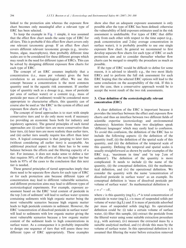
Fig. 6. Different hypothetical PEC curves compared with the same hypothetica

curve (illustrating the procedure of Step 2 of Fig. 4). Solid lines are PEC curves;

identical except for a translation in time); the dotted line segments with the arro

in each graph. Part A is an example demonstrating that RAC time windo

demonstrating that not only the time window starting at the time of the global

local maxima. Part C is an example demonstrating that a low local PEC maximu

risk assessment procedure.

maximum PEC level (for all times considered, so globalmaximum), obtained from a relevant exposure scenario.The second step in Fig. 4 is more sophisticated: here therelevant time window of the RAC curve is graphicallycompared with the PEC curve from a relevant exposurescenario. In the FOCUS Step 3 scenarios, the time of thePEC curve is available on an absolute scale (e.g., runningfrom 1 January 1982 to 1 May 1983 using availablemeteorological time series). The RAC curve is on a relativetime scale e.g., because it may be based on an ecotox-icological experiment in the laboratory. So it is mostappropriate to start with the time scale of the PEC curveand to choose the starting point of the RAC curve freely inthis graphical comparison. The concept of the comparisonis that the PEC curve has to be below the RAC curve for allappropriate starting points of the RAC time windowbecause this guarantees that the risk is acceptable in thisStep 2 of Fig. 4.The definition of ‘all appropriate starting points’ of the

relevant time window of the RAC curve is crucial as isillustrated by a few hypothetical examples in Fig. 6. In thisfigure, all RAC curves are identical (e.g., based on the sameecotoxicological experiment and using the same relevanttime window). Fig. 6A shows an example where the PECcurve has only one maximum. It is then only meaningful toconsider a time window that starts at the time of thismaximum (i.e., time window II) because this is the mostcritical period with respect to the effects. Fig. 6A showsthat the PEC curve is below the RAC curve for this timewindow II. So the conclusion in Fig. 4 is ‘risk acceptable’.It does not matter that the PEC curve is below the RACcurve for other starting points of the time window (such astime window I) because these are irrelevant to the riskassessment procedure. Fig. 6B shows an example where thePEC curve has two maxima (one global and one local) andwhere the RAC time window that starts at the localmaximum of the PEC curve (i.e., window II) leads to ‘risknot acceptable’ in Step 2 of Fig. 4 whereas the RAC time

l RAC curve using different starting points of the time window of this RAC

dashed lines are relevant time windows of RAC curves (all dashed lines are

ws (labelled ‘I’ and ‘II’) indicate the two time windows that are considered

ws have to start when a PEC maximum occurs. Part B is an example

maximum has to be checked but also time windows starting at the time of

m occurring just before the global PEC maximum should be ignored in the


window that starts at the global maximum of the PECcurve (i.e. window I) would have led to ‘risk acceptable’. SoFig. 6B demonstrates that not only the time windowstarting at the time of the global maximum has to bechecked but also time windows that start at the time oflocal maxima. This leads to the following workinghypothesis for the definition of appropriate starting pointsof RAC time windows: all windows starting at the time ofoccurrence of local maxima of the PEC curve. However,Fig. 6C shows that this working hypothesis may be tooconservative. Here a low local maximum of the PEC curveoccurs shortly before the global maximum. According tothe working hypothesis, time window I is appropriate andthe PEC curve exceeds the RAC curve for part of the time.However, it seems unlikely that this would lead to anunacceptable risk. Thus we adopt the following revisedworking hypothesis for appropriate starting points of RACtime windows: starting at the times of all maxima (local orglobal) but excluding time windows such as window I inFig. 6C where the PEC curve remains initially below theRAC curve but later exceeds the tail of this RAC curve dueto a new PEC maximum.

The examples in Fig. 6 show that the definitionof appropriate starting points of the RAC time windowin Step 2 of Fig. 4 is a complicated issue. Considerationof a range of other examples in the future may lead toother subtle refinements of this definition. In principle,this comparison of PEC and RAC curves can be easilyautomated via software in which all necessary refine-ments (based on expert judgement) are included via well-defined procedures (e.g., using output from the TOXSWAmodel which produces daily values of the pesticideconcentration for the FOCUS surface water scenariosor using a time series of measured concentrations in thefield).

The approach in Step 2 of Fig. 4 (illustrated in Fig. 6)implies that the PEC curve always has to be below therelevant time window of the RAC curve for all appropriatestarting points of this time window. So if the PEC curve isabove the RAC curve only for a few days in a time windowof e.g., 21 d, this step cannot conclude an acceptable risk.This may be a serious restriction for such cases. Analternative is to define some time-weighted average(abbreviated to TWA) type of ERC as indicated in Step3 of Fig. 4. Use of TWA concentrations is a normalprocedure in aquatic risk assessment at the EU level(European Commission, 2002a). However, the definition ofthe length of the TWA time window over which averagingis justifiable requires additional ecotoxicological (andpossibly toxicokinetic) a priori knowledge (see Reinert etal., 2002, for a discussion of temporal aspects of effects ofchemicals). If this knowledge is not sufficiently available,one could consider selecting one short TWA time windowand one long TWA window (not exceeding the time frameof the relevant first-tier chronic test as discussed above) andperforming the risk assessment twice, hoping that bothtime windows lead to the same conclusion. If this is not the

case, the conservative choice would be to accept the resultof Step 2.Step 1 offers a very simple (but conservative) approach.

Thus the more sophisticated Steps 2 and 3 are onlynecessary in the borderline cases in which the decline of theconcentration during the higher-tier ecotoxicological ex-periment determines whether the risk is consideredacceptable or not, thus leading the risk assessor to moveto these more complex steps (or to stop, accepting theconclusion that the risk is not acceptable).Once the length of the time window has been selected,

carrying out Step 3 will be relatively easy. The standardoutput of the Step 3 FOCUS scenarios (i.e., surface waterconcentrations calculated by the TOXSWA model; notethat Step 3 of Fig. 4 has no relationship whatsoever to Step3 of the FOCUS scenarios) contains time-weightedaverages for periods of 1, 2, 4, 7, 14, 21, 28, 42, 50 and100 days (Beltman et al., 2006). Calculation of time-weighted averages of RAC curves or of field-measuredPEC curves usually requires little effort as well (e.g., ifcompared to the effort associated with performing andreporting higher-tier ecotoxicological experiments).Until now the discussion of the stepped procedure of

Fig. 4 has been restricted to considerations on the timecourses of the RAC and PEC curves. Ecotoxicologicalconsiderations can of course also restrict the comparisonbetween these curves. E.g., consider an example where theRAC curve of an insecticide was based on an experimentwith juvenile insects because this was considered the mostsensitive part of the life cycle of this insect to this particularinsecticide. Let us further assume that these juvenile insectsoccur in surface water only in spring. In such a case it couldbe justifiable to restrict the time window of the PEC curveto spring. It may also be justifiable e.g., to ignore PECcurves of winter periods if the organisms that have to beprotected do not occur in surface waters in winter. Suchecotoxicological restrictions can be easily applied to thePEC curves before they are fed into the flow chart of Fig. 4.However, ecotoxicologists have to justify and documentany such restrictions appropriately as part of the riskassessment procedure.

6.2. Application of the proposed stepped approach for time-

variable exposure to a case study

We illustrate now the use of the flow chart of Fig. 4 witha case study for the herbicide linuron. The effect tier of thecase study was based on a mesocosm experiment by Crumet al. (1998), Kersting and Van Wijngaarden (1999) andVan Geest et al. (1999). The mesocosm experiment lastedfor about 90 days and linuron was applied three times atmonthly intervals using nominal concentration levels of0.5, 5, 15 and 50 mg/L. Between applications the concen-tration decreased by more than a factor 10 as the result ofdegradation in the water and of flushing of the systemswith clean water. Based on the evaluation of the experi-ment (Kersting and Van Wijngaarden, 1999; Van Geest

ARTICLE IN PRESS

Fig. 7. Linuron concentrations in surface water as a function of time as calculated with the TOXSWA model for three FOCUS Step 3 surface water

scenarios compared with a RAC curve as derived from the mesocosm experiment by Van Geest et al. (1999) using effects of class 1 as a basis. Part A is

scenario D1-ditch, part B is scenario R1-stream and part C is scenario R1-pond (see FOCUS, 2001, for definition of the scenarios). Time 0 is 1 January

1982 for the FOCUS PEC curve in part A and 1 January 1984 for the FOCUS PEC curves in parts B and C. The RAC curves start at arbitrary times. The

arrow indicates the application time of linuron in the TOXSWA simulations. Note that the RAC curve is the same for all three graphs.


et al., 1999), we concluded that their repeated nominaltreatment level of 5 mg/L can be considered as the RACcurve for the risk assessment. At this treatment level noeffects (‘effect class 1’) could be demonstrated onecosystem structure and only transient and slight effects(‘effect class 2’) on oxygen metabolism (Van den Brink etal., 2006). The RAC curve for this treatment level is shownin Figs. 7A–C. For herbicides, the relevant time window isconsidered to be 7 days (length of the standard Lemna test)because linuron is a photosynthesis inhibitor that affectsboth algae and vascular plants. This relevant time windowis assumed to start at the time of the maximumconcentration of the RAC because this maximum isconsidered most relevant for the risk assessment (see thefat line segment in Figs. 7A-C).

The exposure tier of the case study was based oncalculations for three FOCUS surface water scenariosdefined by FOCUS (2001). It was assumed that 1 kg/ha oflinuron was applied to soil in spring just before emergence(i) of spring oilseed rape in the D1-ditch scenario, and

(ii) of potatoes in the R1-stream and R1-pond scenarios.These are realistic applications for linuron. The half-life oflinuron in soil (DT50) at 20 1C and moisture content atfield capacity was assumed to be 89 days; this is the averagevalue of 18 soils as measured by Walker and Thompson(1977). The organic-matter/water adsorption coefficient(KOM) of linuron was assumed to be 414L/kg (based onaverage value of 18 soils; Walker and Thompson, 1977).The Freundlich exponent was assumed to be 0.9 (FOCUS,2001). The half-life of linuron in water was estimated to be10 days at 20 1C based on dissipation rates in waterobserved in the mesocosm experiment Crum et al. (1998).In this experiment, the water was stagnant in the first weekafter each of the three applications. Crum et al. (1998)report dissipation half-lives in this set of three weeksranging from 7 to 12 days at water temperatures rangingfrom 13 to 23 1C. Only 6–7% of the doses was sorbed to thesediment and only about 1% was sorbed to the macro-phytes. So the dissipation in the water was mostly theresult of transformation in the water and a transformation

ARTICLE IN PRESS

Table 1

Characteristics of the D1 and R1 FOCUS Step 3 scenarios (taken from FOCUS, 2001)

Scenario characteristic D1 scenario R1 scenario

Type of scenario Drainage Run-off

Representative field site Lanna (Sweden) Weiherbach (Germany)

Soil Clay with shallow groundwater Light silt with low organic matter content

Mean spring and autumn temperature (1C) o 6.6 6.6–10

Mean annual rainfall (mm) 600–800 600–800

Mean annual recharge (mm) 100–200 100–200

Slope (%) 0–0.5 2–4


half-life of 10 days at 20 1C seems a reasonable estimate.The half-life in sediment was set at 1000 days (i.e., aconservative value because reliable data on the transforma-tion rate in sediment were not found in literature).

Figs. 7A–C show the resulting FOCUS PEC curves ascalculated with the TOXSWA model for the threescenarios. In the D1-scenario linuron enters the surfacewater by leaching through drain pipes (calculated with theMACRO model) and by spray drift. In the MACROcalculations for the FOCUS Step 3 scenarios the pesticideis applied each year over a period of six years before theexposure calculations with the TOXSWA model start (seep. 121 of FOCUS, 2001, for the background). This is ofcourse a worst-case assumption for pesticides that are notapplied every year (such as linuron) but this is part of thepackage of FOCUS Step 3 scenario assumptions (it wouldof course be possible to perform FOCUS Step 4 calcula-tions with more realistic application schemes of linuron butthis is beyond the scope of this example). In the R1-scenarios linuron enters the surface water by runoff(calculated with the PRZM model) and by spray drift.Table 1 gives general characteristics of the D1 and R1scenarios. The D1-ditch scenario in Fig. 7A shows a moreor less gradual increase in the calculated linuron concen-tration between 0 and 100 days from zero to about 9 mg/L.This is the result of leaching through drain pipes of linuronthat was applied in the six years before the start of theTOXSWA calculations. After about 140 days there is asharp peak of about 14 mg/L caused by spray drift . So bothdrain flow and spray drift contributed to the linuronconcentrations shown in Fig. 7A. The R1-stream scenarioin Fig. 7B shows a number of very sharp concentrationpeaks. The first peak is caused by spray drift on the day ofapplication of linuron and the other peaks are caused byrunoff. The peaks are very sharp because the residence timeof the water in this stream is very short due to high waterflow rates. The R1-pond scenario in Fig. 7C shows lowcalculated concentrations with a first low peak resultingfrom spray drift on the day of application and subsequentincreases due to runoff events. The calculated concentra-tions show no sharp peaks such as the ones in Fig. 7Bbecause the residence time of water in the pond is muchlonger than the residence time of water in the stream.

So we have a number of PEC curves and the relevanttime window of the RAC curve and can now perform

‘compare and decide’ as described in Fig. 2. Note that thesources for the PEC curves and the RAC curve arecompletely different (e.g., the RAC curve was determinedlong before the FOCUS Step 3 scenarios became avail-able). This will be the normal situation in current riskassessment procedures because the FOCUS Step 3scenarios have become available only recently. However,this is not a problem for the ‘compare and decide’ activity.We follow the flow chart of Fig. 4. In Step 1 we have tocheck whether the maximum of the PEC curve is alwaysbelow the minimum of the relevant time window of theRAC curve. This is not the case in Figs. 7A and B but it istrue for Fig. 7C. So for the R1-pond scenario we concludethat the risk is acceptable and for the D1-ditch and R1-stream scenario we have to go to Step 2. We now have tocheck whether a time window exists (including all relevantlocal maxima of the PEC curve) in which the PEC curve isalways lower than the relevant time window of the RACcurve. This is clearly not the case in Figs. 7A and B so wego to Step 3 for these scenarios. In Step 3 we have to decidefirstly whether it is possible to decide on a length of a timewindow for averaging the exposure concentration. Weconsider it acceptable to use TWA-concentrations forlinuron because effects of linuron have shown to bereversible (Snel et al., 1998). Fig. 7A shows that averagingthe concentration over a certain time window will not helpfor the D1-scenario because the PEC curve is for the fulllength of the time window of the mesocosm experimentabove the RAC curve. So we will restrict ourselves to theR1-stream scenario for Step 3. Fig. 8 shows the effect of thelength of the time window on the TWA concentrationsbased on the RAC curve and taken from the calculationswith TOXSWA for the R1-stream scenario. The TWAconcentrations from the RAC curve were obtained vianumerical integration of the RAC curve. Fig. 8 shows thatthe TWA PEC curve for the R1-stream scenario decreasessharply. It is about 8 mg/L for a time window that is zero(i.e., simply the maximum value in Fig. 7B). However, for atime window of 1 day, it has decreased to about 4 mg/L andis then already below the TWA RAC curve. So for anytime window exceeding 1 day, the R1-stream scenarioresults in acceptable risk in Step 3.As described above, the RAC curve used in Figs. 7 and 8

was determined using an effect class 1 for ecosystemstructure as a basis which implies that no treatment-related

ARTICLE IN PRESS

Fig. 9. Linuron concentrations in surface water as a function of time as

calculated with the TOXSWA model for the D1-ditch FOCUS Step 3

surface water scenario compared with an effect-class-1 and an effect-class-

3 RAC curve as derived from the mesocosm experiment by Van Geest et

al. (1999). Time 0 is 1 January 1982. The arrow indicates the application

time of linuron in the TOXSWA simulations.

Fig. 8. Maxima of time-weighted average (TWA) linuron concentrations

in surface water calculated for the R1-stream FOCUS scenario as a

function of the length of the time window compared with the TWA

concentration derived from a RAC curve derived from a mesocosm study

by Van Geest et al. (1999) using effects of class 1 as a basis. The scenario

concentrations are output from the TOXSWAmodel and the line from the

RAC curve was obtained by numerical integration of the time course of

concentrations measured by Van Geest et al. (1999).


effects on the abundance of species should occur. For theD1-ditch scenario this led to the conclusion that the riskwas unacceptable using all three steps of Fig. 4 (whichresulted in a case that was not very interesting). Weperform now as an additional example the risk assessmentusing an ‘effect class 3’ as a basis. The EU guidancedocument on aquatic ecotoxicology (European Commis-sion, 2002a) defined this effect class as giving a clearresponse to sensitive endpoints but showing full recovery ofaffected endpoints within 8 weeks post last application(Brock et al., 2000). At the regulatory level, there is noconsensus between EU member states which effect classshould be used, and using effect class 3 is a realisticregulatory option. When evaluating the possible ecologicalrisks of a certain PEC curve (including the recoverypotential), it is not only important to consider the rate ofrecovery (after exposure has dropped below a certaincritical concentration level) but also the period in whichpossible effects can be expected (e.g., the period that thePEC is above the effect-class-1 RAC curve derived from amicro/mesocosm). Based on the evaluation of the meso-cosm experiment by Van Geest et al. (1999), their treatmentlevel of 15 mg/L might be considered as the effect-class-3RAC curve for the risk assessment. We use the graphicalcomparison of PEC and RAC curves (so Step 2 of Fig. 4).Fig. 9 compares the PEC curve with effect-class-1 andeffect-class-3 RAC curves. The effect-class-3 RAC curvehas a maximum of about 14 mg/L based on measuredvalues (Crum et al., 1998). The relevant time window of theRAC curve was selected to start at such a time that themaximum of this curve coincides with that of the PECcurve. We have to check whether the PEC curve is alwaysbelow the effect-class-3 RAC curve for the relevant time

window. Fig. 9 shows that this is indeed the case(admittedly, the maxima of the curves are difficult tocompare in Fig. 9 but the values are 14.0 mg/L for the RACcurve and 13.6 mg/L for the PEC curve). So the effect-class-3 RAC curve does not exclude recovery for this exposurescenario. However, Fig. 9 shows also that the PEC curve isabove the relevant time window of the effect-class-1 RACcurve for more than 100 days. Thus for a period of morethan 100 days possible effects cannot be excluded. It is amatter for the risk manager to decide whether such longperiods of possible effects are considered acceptable. Thisexample shows that the graphical comparison of PEC andRAC curves may provide additional information thatcould be relevant to the risk manager.In general, this case study shows that the approach of

Fig. 4 can be applied quite easily once PEC levels or curvesand the RAC level or curve have become available.

6.3. Consequences for designing the exposure in higher-tier

ecotoxicological experiments

We now consider the consequences of the steppedapproach of Fig. 4 for the exposure designs for higher-tier ecotoxicological experiments. When designing such anexperiment, the RAC level is generally not known a priori.Performing such an experiment implies that lower tiershave already indicated risk. Therefore time course of theexposure concentration is likely to be a critical factor. Weconsider two alternative design approaches. The firstapproach is based on the desire to be able to use theresults of this higher-tier ecotoxicological experiment for asmany exposure scenarios as possible. The logical conse-quence for exposure in the ecotoxicological experiments isthen to keep the concentration as constant as possible (i.e.,as worst case as possible) within the time window that is


relevant for the exposure assessment. This can beillustrated with Fig. 6B: if the RAC curve (dashed line) ismore or less constant over time, the PEC curve will bealways below the RAC curve if the global peak of the PECcurve is below the RAC curve. If the RAC is constant, theapproach in Fig. 4 can be restricted to checking whetherthe exposure peak is below the RAC value (so to Step 1 inFig. 4).

Keeping the concentration as constant as possible hasthe disadvantage that it may lead to a too conservative riskassessment if the decline in all relevant exposure scenariosproceeds rapidly (as e.g., in the R1-stream scenario inFig. 7B). Therefore we consider here also a secondapproach in which first an analysis is made of the timecourse in the relevant exposure scenarios and subsequentlythis time course is simulated as closely as possible in theecotoxicological experiments. However, this type of designhas the disadvantage that the interpretation of theecotoxicological experiment may become cumbersome ifthe range of exposure scenarios that has to be protected,changes after the ecotoxicological experiment has finished(or if, for some reason, the characteristics of the exposurescenario changes). We would like to stress that the designof the experiment in this second approach has to be basedon adequate exposure scenarios and can never be based onthe behaviour of the pesticide in the ecotoxicologicalexperiment itself because (i) the water in such experimentsis usually stagnant, and (ii) the time course of theconcentration in stagnant water is not necessarily a realisticworst case. This can be illustrated with the linuronconcentrations calculated for the D1-ditch scenario asshown in Fig. 9. As described before, it was assumed inthese calculations that the half-life of linuron in water was10 days at 20 1C (based on the observed degradation rate inthe mesocosm experiment; Crum et al., 1998). However,the D1-ditch scenario shows a linuron concentration thatfluctuates within the narrow range of 7–9 mg/L betweenabout 70 and 150 days (ignoring the sharp peakimmediately after the application). The background of thismore or less constant concentration is that the residencetime of water in this ditch is only in the order of days assoon as significant drainage fluxes enter the ditch, and thatthese drainage fluxes are also the main source of pesticideinput into the ditch. So when drain-flow events occur, thereis a quick flow-through of water containing the pesticide.So this exposure scenario shows a more or less constantlinuron concentration over a period of about 80 dayswhereas a stagnant mesocosm experiment at 20 1C wouldhave shown a decline corresponding with a half-life of 10days (assuming that degradation was the only loss processfrom the water phase; other loss processes such as sorptionto the sediment would lead to an even faster decline in themesocosm experiment).

As described in the Introduction, the current technicalguidance document on aquatic ecotoxicology for riskassessment at EU level (European Commission, 2002a)includes the suggestion to simulate the fate dynamics

experimentally in higher-tier ecotoxicological experiments.According to EFSA (2005), risk assessors usually justifythis methodology in the regulatory practice by checkingwhether all exposure-relevant properties of the system usedin the experiment are in the range to be expected forrelevant exposure scenarios and, based on this, assesswhether the exposure was conservative enough. Theserelevant system properties may include (i) organic matterand clay content of the sediment (may influence sorption tosediment), (ii) redox potential in the sediment (mayinfluence the degradation rate in the sediment), (iii) pHof the water (may influence the hydrolysis rate), (iv) lightintensity (may influence photolytic degradation rate inwater), (v) depth of the water layer (may influence thedistribution of the pesticide over water and sediment), etc.(EFSA, 2005). We consider this justification unacceptablebecause it is only qualitative and because it ignores theconcentration curves that are produced by the exposureflow chart (see linuron discussion in preceding paragraph).Instead we recommend the Step-2 approach of Fig. 4 tojustify that the measured course of the concentration withtime in the ecotoxicological experiment is constant enoughfor the exposure scenarios that need to be assessed. ThisStep-2 approach is quantitative, considering the measuredexposure in the ecotoxicological experiment as the onlyyardstick for comparison with exposure in the field. This isjustifiable because this measured exposure is the onlyexposure characteristic that matters for the effect assess-ment conclusion.It should be noted that this criticism of simulating fate

dynamics in higher-tier ecotoxicological experiments isrestricted to the exposure part of the risk assessment. Let usconsider an example where the most relevant aquaticspecies in a certain effect tier is more sensitive to thepesticide if the pH is above 8 (e.g., because of toxicoki-netics). Then it would be justifiable for ecotoxicologicalreasons to require that the pH in the higher-tier ecotox-icological experiment is above 8. Another example is a casewhere the most relevant aquatic species has a preference fora certain pH range. Then it would be justifiable forecotoxicological reasons that the pH in the higher-tierecotoxicological experiment is within the range of the pHvalues of the type of water body to be protected (e.g., asmall stream with a pH below 7 in the case of an insecti-cide for forest application). Another example relates tophototoxic pesticides where the test species are likely to bemore sensitive if exposed to such pesticides under naturallight.A completely different solution for matching the time

course of the concentration in ecotoxicological experimentswith that in the field would be to develop methods andmodels for extrapolating ecotoxicological responses fromone exposure regime to other exposure regimes (Reinertet al., 2002). However, it will need considerable researchefforts to develop methods and models that can begenerally applied as extrapolation tools in the aquaticeffect assessment because they will differ probably between


pesticide groups that have different mode of actions andbetween different types of aquatic organisms. A disadvan-tage of this approach could be that an extrapolationmethod will introduce additional uncertainty in the riskassessment while such a method is mainly needed inborderline cases for decision making. However, anadvantage could be that this approach simplifies the riskassessment procedure because it enables extrapolation ofeffects observed in one higher-tier ecotoxicological experi-ment to a range of different exposure scenarios.

7. Role of exposure information from ecotoxicological

experiments in the exposure assessment for the field

In the practice of aquatic ecotoxicological risk assess-ment there is regular discussion over the role andsignificance that the exposure part of higher-tier ecotox-icological experiments should play in the exposure assess-ment. It goes almost without saying that a higher-tierexposure assessment should take into account all relevantinformation. Usually lower-tier exposure assessments arebased on input parameters for pesticide fate that have beenderived from laboratory experiments. Higher-tier ecotox-icological experiments are often conducted outdoors.Therefore, higher-tier ecotoxicological experiments willoften also deliver higher-tier fate information as a spin-off. However, as described above, there are two distinctlydifferent exposure assessments needed in the risk assess-ment procedure: (A) exposure assessment in the field, and(B) exposure assessment in higher-tier ecotoxicologicalexperiments (see Fig. 2). The fate information derived froma higher-tier ecotoxicological experiment is crucial andunique information for assessment B and, in this context,overrules fate information from any other source. How-ever, for assessment A this is different. The purpose of theexposure flow chart in Fig. 1 is to estimate concentrationsin the field for situations that are vulnerable with respect toexposure. Therefore, within the context of this flow chart,fate information derived from higher-tier ecotoxicologicalexperiments is not to be preferred over fate informationderived from other higher-tier fate experiments: both typesof information are in principle equally important for theexposure assessment in the exposure flow chart. Let us forinstance consider a substance which has a transformationhalf-life in water of 100 days derived from a water-sedimentstudy conducted in the dark. A first exposure tier couldthen be to run FOCUS Step 3 scenarios using this half-lifein water of 100 days. However, if a higher-tier ecotox-icological outdoor experiment would demonstrate atransformation half-life in water of 15 days (caused byphotochemical transformation), the next exposure tiercould be to run these FOCUS Step 3 scenarios with thishalf-life of 15 days. If there were two additional outdoorfate studies showing transformation half-lives in water of20 and 65 days, it would be more appropriate to use theaverage of these three half-lives in runs of the FOCUS Step3 scenarios or to run FOCUS Step 3 scenarios with all

three half-lives to analyse the uncertainty resulting fromthis range in half-lives.

8. Use of the proposed approach in current aquatic risk

assessment at EU level

We now will illustrate how the proposed approach of theinteracting effect and fate flow charts shown in Figs. 1, 2and 4 could be applied within the current aquatic riskassessment procedure at the EU level (European Commis-sion, 2002a). This procedure distinguishes between stan-dard and higher-tier risk assessments (EuropeanCommission, 2002a). The standard assessment consists ofacute and chronic testing and of comparing exposureendpoints to acute and chronic effect endpoints includingsafety factors of 10–100 (European Commission, 2002a).A range of options is described for the higher-tierassessment but no hierarchy of these options is given.Brock et al. (2006) propose a tiered risk assessmentapproach with a clear hierarchy considering both acuteand chronic toxicity. Based on the EU guidance document(European Commission, 2002a) and Brock et al. (2006) wepropose in Fig. 10 a system of effect flow charts that isconsistent with (i) current aquatic risk assessment practice,and (ii) the system of flow charts shown in Figs. 1, 2 and 4.The system of effect flow charts of Fig. 10 branches into (i)short-term risks, and (ii) long-term risks. As indicated,short-term risks are always linked to ERCs at short timescales whereas long-term risks may be linked to ERCs ateither short or long time scales. For instance, an effect on asublethal endpoint like reproduction may have been causedby some short-term peak concentration (latency of effect)or by a long-term exposure. In the example, each of the twoeffect flow charts has four tiers (standard test species,SSDs, population level studies and microcosm/mesocosms)largely in accordance to Brock et al. (2006). The exposureflow charts have also four tiers based on FOCUS (2001,2005). All effect and exposure tiers are given here only forillustrative purposes, and their contents are not furtherdiscussed.Fig. 10 shows a dashed arrow going from the short-term

to the long-term risk assessment. This arrow is necessarybecause a risk manager may consider short-term effects notto be a regulatory problem if long-term effects are absent.This may happen already in the first tiers of the EU riskassessment procedure (European Commission, 2002a). Inthis procedure the first-tier acute trigger concentrationcould be for example the 48-h EC50 Daphnia magna

divided by 100 while the corresponding first-tier chronictrigger concentration would be the 21-d NOEC Daphnia

magna divided by 10 (European Commission, 2002a). So ifthis EC50 is less than 10 times higher than this NOEC(which is not exceptional), then the first-tier acute triggerconcentration is lower than the first-tier chronic triggerconcentration. Another example of this dashed arrow isthat risk managers may accept effect-class-3 concentrationsdue to short-term exposure as demonstrated in micro/

ARTICLE IN PRESS

Fig. 10. Proposed system of effect and exposure flow charts for aquatic risk assessment at EU level. The two solid arrows from the box ‘Protect

biodiversity of aquatic life in EU’ indicate the need to assess always both short-term and long-term risks. The dashed arrow indicates the possibility for the

risk manager to ignore short-term risks if long-term risks are absent.


mesocosm tests (effect class 3 implies clear short-termeffects but recovery within 8 weeks). There is no arrowsimilar to the dashed arrow in the opposite direction in Fig.10: regulatory concerns on long-term risks will be difficultto remove by absence of short-term risks. Note that thisdashed arrow in Fig. 10 is not meant to describe the flow ofinformation for cases where chronic toxicity is estimatedfrom acute toxicity by extrapolation methods: use of suchmethods is simply part of the box ‘standard test species’ ofthe effect flow chart for long-term risks.

Fig. 10 is at a general level and therefore cannotprescribe exactly which type of ERC should be used.However, the branching into short-term and long-termrisks implies the following restrictions to the time scales:(i) for short-term risks the ERC may be a peak concentra-tion or e.g., a time-weighted average over a period of a fewdays; and (ii) for long-term risks the ERC may vary from apeak concentration to a time-weighted average over aperiod not exceeding the duration of the standard chronictest with the most relevant test species as discussed before.

9. Recommendations for future activities to improve the

aquatic risk assessment procedure

1.
For the exposure assessment at the EU level, it isrecommended to check via a number of well-definedexperiments across the EU whether the FOCUS surfacewater scenarios are close enough to reality for realisticworst-case exposure conditions. Until now, these havebeen based only on calculations with sets of complexsimulation models (FOCUS, 2001). It would be un-
fortunate if ecotoxicologists would start new researchlines based on the correctness of these FOCUS scenariosto discover five years later that an important part of thescenarios lack realism. It is recommended to includeecotoxicological expertise in this checking procedure toensure that the experiments are performed at locationsthat are also most appropriate for the risk assessmentfrom an ecological point of view.

2.
To facilitate the exposure assessment of the ecotoxico-logical experiments (activity B in Fig. 2) it would beuseful to review available methods and software for thecalculation of time-weighted averages from measuredtime courses of the concentration and, based on this, toprovide guidance on the most appropriate methods andsoftware.
3.
The temporal scale of the ERC plays an important rolein the proposed approach. Therefore, it is recommendedto perform measurements of effects in ecotoxicologicalexperiments as often as possible (e.g., in daily incre-ments) to gather time-to-event information necessary forthe determination of the appropriate temporal scale ofthe ERC.
10. Applicability to risk assessment for soil organisms

All considerations so far have been restricted to the riskassessment for aquatic organisms. However, the principlesof the interaction between exposure and ecotoxicologicaleffect are exactly the same for aquatic and soil organisms.The flow charts and procedures described in Figs. 1–4 arebased on general principles and do not imply any


assumptions that are specific for aquatic risk assessment.So they apply equally well to risk assessment for soilorganisms. However, the risk assessment for soil organismsis especially relevant for persistent pesticides in soil.Concentrations of persistent pesticides in soil are expectedto fluctuate less than concentrations of pesticides in surfacewater. As a consequence, the handling of time-variableexposure as described in Fig. 4 may be less an issue in riskassessment for soil organisms.

In 2002, the European Commission presented a detailedrisk assessment procedure for soil organisms including atest for earthworms (European Commission, 2002b).Comparatively little attention was paid to exposure in thisguidance. Let us consider as an example the exposureassessment for earthworms. The guidance document states‘PEC values for the various use scenarios are supplied bythe environmental fate section’ (at its p. 29). However, nosuch section can be found in this document. The guidancegiven for earthworms implies that the pore water concen-tration in soil is considered as the yardstick for assessingeffects (also recommended by Van Gestel, 1992). However,nowhere is any guidance given on how to estimate reliablerealistic worst-case exposure concentrations for soil porewater. Instead it is recommended to divide the LC50 by afactor of 2 for compounds whose sorption is correlated toorganic matter. The justification for this is that thestandard soil used in earthworm tests has an organicmatter content of about 10%, whereas the EU guidancedocument considers 5% organic matter more representa-tive for agricultural soils. However, this 5% is nowherejustified and is certainly not justifiable as a realistic worst-case assumption for the EU (see organic carbon map of theEU; Jones et al., 2004). It seems thus not acceptable to usethis 5% in the first (and also final) exposure tier. So itseems that also the interaction between effects andexposure in the risk assessment of soil organisms couldbe improved by using the procedure that we propose.

11. Conclusions

1.
Within the risk assessment for aquatic organisms, theinterface between ecotoxicological effects and exposureshould be based on the type of exposure concentrationthat gives the best correlation to ecotoxicological effects(i.e., the ERC).
2.
Definition of this type of ERC is necessary for aconsistent handling of exposure in pesticide risk assess-ment.
3.
Once this type of ERC has been defined, effect andexposure flow charts for risk assessment can beestablished that are flexible with respect to the route tobe followed through the combined system of effect andexposure flow charts.
4.
Within the risk assessment procedure, there are twoequally important exposure assessments required: (A)exposure in the field, and (B) exposure in ecotoxicolo-gical experiments. Within a certain effect tier, the same
type of ERC should be used consistently for both typesof assessments.

5.
Risk assessment conclusions that are based on higher-tier ecotoxicological experiments in which the ERCvaries with time, should be based on a systematiccomparison between (i) the time course of the ERC inthese experiments, and (ii) the time course of the ERC inrelevant exposure scenarios. In this comparison the timecourse in the experiments should in general be restrictedto a time window with a length that does not exceed theduration of the standard chronic test in the first tier forthe relevant taxonomic group considered.
6.
The issues raised here, though focussing on aquatic riskassessment, are of more general relevance and may e.g.,also improve risk assessment of soil organisms.
7.
Application of the proposed approach is expected tolead to a better communication between ecotoxicologi-cal experts and fate experts within the risk assessment.
Acknowledgments

We thank Steven Crum (Alterra) for providing thelinuron concentrations and Mechteld ter Horst (Alterra)for performing the calculations for the FOCUS surfacewater scenarios.

Funding sources:

�
Dutch Ministry of Agriculture, Nature and FoodQuality for P. Adriaanse, T. Brock and J. Boesten. � Federal Office for Consumer Protection and Food
Safety for H. Kopp.
� Centre for Integrated Population Ecology for V. Forbes.
This paper uses published data (references Kersting &Van Wijngaarden and Van Geest et al.) on the effects oflinuron in a mesocosm study. These were conducted inaccordance with national and institutional guidelines forthe protection of animal welfare (Van Wijngaarden is co-author of both papers and is member of the same researchteam as T. Brock).

References

Beltman, W.H.J., Ter Horst M.M.S., Adriaanse, P.I., De Jong, A., 2006.

Manual of FOCUS_TOXSWA version 2.2.1., Alterra Report 586,

Alterra, Wageningen, The Netherlands, 198 pp., available at /www.

toxswa.pesticidemodels.euS.

Brock, T.C.M., Lahr, J., Van den Brink, P.J., 2000. Ecological risks of

pesticides in freshwater ecosystems. Part 1: Herbicides. Alterra

Rapport 088, Alterra, Wageningen, The Netherlands, 124pp.

Brock, T.C.M., Arts, G.H.P., Maltby, L., Van Den Brink, P.J., 2006.

Aquatic risks of pesticides, ecological protection goals and common

aims in EU legislation. Integr. Environ. Assess. Manage. 2, e20–e46.

Campbell, P.J., Arnold, D.J.S., Brock, T.C.M., Grandy, N.J., Heger, W.,

Heimbach, F., Maund, S.J., Streloke, M., 1999. Guidance Document

on Higher-Tier Aquatic Risk Assessment for Pesticides (HARAP).

SETAC-Europe Publication.

Crum, S.J.H., Aalderink, G.H., Brock, T.C.M., 1998. Fate of the

herbicide linuron in outdoor experimental ditches. Chemosphere 36,

2175–2190.

http://www.toxswa.pesticidemodels.eu

http://www.toxswa.pesticidemodels.eu


EFSA, 2005. Opinion of the scientific panel on plant health, plant

protection products and their residues on a request from EFSA related

to the evaluation of dimoxystrobin. EFSA J. 178, 1–45.

EPA, 2004. OPP’s initiative to revise the ecological assessment process for

pesticides. IV. The aquatic level II refined risk assessment model

(version 2.0). /www.epa.gov/oppefed1/ecoriskS.

European Commission, 2002a. Guidance document on aquatic ecotox-

icology in the context of Directive 91/414/EEC. European Commis-

sion, Health & Consumer Protection Directorate General. EC

Document reference SANCO/3268/2001 rev.4, 62 pp.

European Commission, 2002b. Guidance document on terrestrial ecotox-

icology under council directive 91/414/EEC. European Commission,

Health & Consumer Protection Directorate General. EC Document

reference SANCO/10329/2002 rev.2, 39 pp.

FOCUS, 2001. FOCUS surface water scenarios in the EU evaluation

process under 91/414/EEC. Report of the FOCUS workgroup on

surface water scenarios. EC Document reference SANCO/4802/2001

rev.2, 245 pp, /http://viso.ei.jrc.it/focus/S.

FOCUS, 2005. Landscape and mitigation factors in aquatic risk

assessment. Vol. 1. Extended summary and recommendations. Report

of the FOCUS working group on landscape and mitigation factors in

ecological risk assessment. EC Document reference SANCO/10422/

2005, 133 pp.

Jones, R.J.A., Hiederer, R., Rusco, E., Loveland, P.J., Montanarella, L.,

2004. The map of organic carbon in topsoils in Europe, Version 1.2,

September 2003: explanation of special publication Ispra 2004 No. 72

(S.P.I.04.72). European Soil Bureau Report No. 17, EUR 21209 EN,

26pp. Office for Official Publications of the European Communities,

Luxembourg.

Kersting, K., Van Wijngaarden, R.P.A., 1999. Effects of a pulsed

treatment with the herbicide Afalon (active ingredient linuron) on

macrophyte-dominated mesocosms. I. Responses of ecosystem meta-

bolism. Environ. Toxicol. Chem. 18, 2859–2865.

Reinert, K.H., Giddings, J.M., Judd, L., 2002. Effects analysis of time-

varying or repeated exposures in aquatic ecological risk assessment of

agrochemicals. Environ. Toxicol. Chem. 21, 1977–1992.

Snel, J.F.H., Vos, J.H., Gylstra, R., Brock, T.C.M., 1998. Inhibition of

photosystem II (PSII) electron transport as a convenient endpoint to

assess stress of the herbicide linuron on freshwater plants. Aquat. Ecol.

32, 113–123.

Van Den Brink, P.J., Blake, N., Brock, T.C.M., Maltby, L., 2006.

Predictive value of species sensitivity distributions for effect of herbi-

cides in freshwater ecosystems. Human Ecol. Risk Assess. 12, 645–674.

Van Geest, G.J., Zwaardemaker, N.G., Van Wijngaarden, R.P.A.,

Cuppen, J.G.M., 1999. Effects of a pulsed treatment with the herbicide

Afalon (active ingredient linuron) on macrophyte-dominated meso-

cosms. II. Structural responses. Environ. Toxicol. Chem. 18,

2866–2874.

Van Gestel, C.A.M., 1992. The influence of soil characteristics on the

toxicity of chemicals for earthworms: a review. In: Greig-Smith, P.W.,

Becker, H., Edwards, P.J., Heimbach, F. (Eds.), Ecotoxicology of

Earthworms. Intercept Press, Andover, pp. 44–54.

Walker, A., Thompson, J.A., 1977. The degradation of simazine, linuron

and propyzamide in different soils. Weed Res. 17, 399–405.

http://www.epa.gov/oppefed1/ecorisk

http://viso.ei.jrc.it/focus/

Conceptual model for improving the link between exposure and effects in the aquatic risk assessment of pesticides

Documents