1 Climate Dynamics: Concepts, Scaling and Multiple Equilibria by Gerrit Lohmann Alfred Wegener Institute, Helmholtz Centre for Polar and Marine Research, Bremerhaven, Germany. Department of Physics, University of Bremen, Bremen, Germany. Lecture Notes 2018 version of June 25, 2018

Welcome message from author
This document is posted to help you gain knowledge. Please leave a comment to let me know what you think about it! Share it to your friends and learn new things together.
Transcript
1
Climate Dynamics:
Concepts, Scaling and Multiple Equilibria
by Gerrit Lohmann
Alfred Wegener Institute, Helmholtz Centre for Polar and Marine Research,
Bremerhaven, Germany.
Department of Physics, University of Bremen, Bremen, Germany.
Lecture Notes 2018
version of June 25, 2018
Contents
I First part: Dynamical systems 3
1 Introduction and Preparation 4
1.1 Pendulum . . . . . . . . . . . . . . . . . . . . . . . . . . . . . . . . . . . 10
1.2 Fourier transform . . . . . . . . . . . . . . . . . . . . . . . . . . . . . . . 19
1.3 Covariance and spectrum . . . . . . . . . . . . . . . . . . . . . . . . . . . . 30
1.4 Transport phenomena . . . . . . . . . . . . . . . . . . . . . . . . . . . . . 36
1.5 General form of wave equations . . . . . . . . . . . . . . . . . . . . . . . . 38
2 General concepts 42
2.1 Programming with R . . . . . . . . . . . . . . . . . . . . . . . . . . . . . . 42
2.2 Netcdf and climate data operators . . . . . . . . . . . . . . . . . . . . . . . . 52
2.2.1 The Bash, a popular UNIX-Shell . . . . . . . . . . . . . . . . . . . . 57
2.2.2 Reducing data sets with CDO . . . . . . . . . . . . . . . . . . . . . . 60
2.2.3 A simple model of sea level rise . . . . . . . . . . . . . . . . . . . . 64
2.3 Bifurcations . . . . . . . . . . . . . . . . . . . . . . . . . . . . . . . . . . 72
2.3.1 Linear stability analysis . . . . . . . . . . . . . . . . . . . . . . . . 73
2.3.2 Population Dynamics . . . . . . . . . . . . . . . . . . . . . . . . . . 78
2.3.3 Lorenz system . . . . . . . . . . . . . . . . . . . . . . . . . . . . . 84
2.3.4 Conceptual model of the ocean circulation: Stommel’s box model . . . . 95
2.3.5 Non-normal dynamics of the ocean box model* . . . . . . . . . . . . . 101
2
CONTENTS 3
3 Statistical Mechanics and Fluid Dynamics* 106
3.1 Mesoscopic dynamics . . . . . . . . . . . . . . . . . . . . . . . . . . . . . 107
3.1.1 Liouville equation . . . . . . . . . . . . . . . . . . . . . . . . . . . 107
3.1.2 Master equation . . . . . . . . . . . . . . . . . . . . . . . . . . . . 108
3.1.3 Fokker-Planck dynamics . . . . . . . . . . . . . . . . . . . . . . . . 111
3.2 The Boltzmann Equation . . . . . . . . . . . . . . . . . . . . . . . . . . . . 112
3.3 H-Theorem and approximation of the Boltzmann equation . . . . . . . . . . . . 115
3.4 Application: Lattice Boltzmann Dynamics . . . . . . . . . . . . . . . . . . . 120
3.4.1 Lattice Boltzmann Methods . . . . . . . . . . . . . . . . . . . . . . 120
3.4.2 Simulation set-up of the Rayleigh-Bénard convection . . . . . . . . . . 125
3.4.3 System preparations and running a simulation . . . . . . . . . . . . . . 128
3.5 Projection methods: coarse graining . . . . . . . . . . . . . . . . . . . . . . 134
II Second part: Fluid Dynamics 141
4 Basics of Fluid Dynamics 142
4.1 Material laws . . . . . . . . . . . . . . . . . . . . . . . . . . . . . . . . . 143
4.2 Navier-Stokes equations . . . . . . . . . . . . . . . . . . . . . . . . . . . . 145
4.3 Integral and differential formulation . . . . . . . . . . . . . . . . . . . . . . 148
4.4 Elimination of the pressure term . . . . . . . . . . . . . . . . . . . . . . . . 155
4.5 Non-dimensional parameters: The Reynolds number . . . . . . . . . . . . . . 156
4.6 Characterising flows by dimensionless numbers . . . . . . . . . . . . . . . . . 159
4.7 Dynamic similarity: Application in engineering* . . . . . . . . . . . . . . . . 160
5 Fluid-dynamical Examples 164
5.1 Potential flow . . . . . . . . . . . . . . . . . . . . . . . . . . . . . . . . . 164
5.1.1 Kelvin’s circulation theorem* . . . . . . . . . . . . . . . . . . . . . . 166
5.1.2 Streamlines . . . . . . . . . . . . . . . . . . . . . . . . . . . . . . 167
4 CONTENTS
5.1.3 Bernoulli’s equations* . . . . . . . . . . . . . . . . . . . . . . . . . 168
5.1.4 Bernoulli flow* . . . . . . . . . . . . . . . . . . . . . . . . . . . . 169
5.1.5 Comparison with flow of a real fluid past a cylinder* . . . . . . . . . . 173
5.1.6 Analysis for two-dimensional flow using conformal mapping* . . . . . . 175
5.2 More on fluid flows* . . . . . . . . . . . . . . . . . . . . . . . . . . . . . . 178
5.2.1 Tube flows* . . . . . . . . . . . . . . . . . . . . . . . . . . . . . . 178
5.2.2 Boundary layers* . . . . . . . . . . . . . . . . . . . . . . . . . . . 178
5.2.3 Heat conductance* . . . . . . . . . . . . . . . . . . . . . . . . . . . 179
5.2.4 Turbulence* . . . . . . . . . . . . . . . . . . . . . . . . . . . . . . 180
5.2.5 Couette flow* . . . . . . . . . . . . . . . . . . . . . . . . . . . . . 181
5.3 Convection in the Rayleigh-Bénard system . . . . . . . . . . . . . . . . . . . 184
5.3.1 Geometry and set up . . . . . . . . . . . . . . . . . . . . . . . . . . 184
5.3.2 The usual approach: Elimination of pressure and vorticity dynamics . . . 185
5.3.3 Boundary conditions . . . . . . . . . . . . . . . . . . . . . . . . . . 193
5.3.4 Galerkin approximation: Obtaining the Lorenz system . . . . . . . . . . 194
6 Atmosphere and Ocean Dynamics 196
6.1 Pseudo forces and the Coriolis effect . . . . . . . . . . . . . . . . . . . . . . 196
6.2 Scaling of the dynamical equations . . . . . . . . . . . . . . . . . . . . . . . 199
6.3 The coordinate system . . . . . . . . . . . . . . . . . . . . . . . . . . . . . 201
6.4 Geostrophy . . . . . . . . . . . . . . . . . . . . . . . . . . . . . . . . . . 205
6.5 Conservation of vorticity . . . . . . . . . . . . . . . . . . . . . . . . . . . . 215
6.5.1 Potential vorticity equation (ζ + f)/h . . . . . . . . . . . . . . . . . 217
6.5.2 Taylor-Proudman Theorem . . . . . . . . . . . . . . . . . . . . . . . 226
6.6 Wind-driven ocean circulation . . . . . . . . . . . . . . . . . . . . . . . . . 229
6.6.1 Sverdrup relation . . . . . . . . . . . . . . . . . . . . . . . . . . . . 231
6.6.2 Ekman Pumping . . . . . . . . . . . . . . . . . . . . . . . . . . . . 234
6.6.3 Ekman spiral* . . . . . . . . . . . . . . . . . . . . . . . . . . . . . 240
CONTENTS 5
6.6.4 Western Boundary Currents . . . . . . . . . . . . . . . . . . . . . . . 250
6.7 Thermohaline ocean circulation . . . . . . . . . . . . . . . . . . . . . . . . 257
7 Simple Climate Models 270
7.1 Engery balance model . . . . . . . . . . . . . . . . . . . . . . . . . . . . . 270
7.1.1 Zero-dimensional Model . . . . . . . . . . . . . . . . . . . . . . . . 270
7.1.2 One dimensional atmospheric energy balance model . . . . . . . . . . . 272
7.2 Interhemispheric box model . . . . . . . . . . . . . . . . . . . . . . . . . . 279
7.2.1 Model description . . . . . . . . . . . . . . . . . . . . . . . . . . . 279
7.2.2 Run the model . . . . . . . . . . . . . . . . . . . . . . . . . . . . . 283
7.2.3 Run the box model in Fortran90* . . . . . . . . . . . . . . . . . . . . 288
7.2.4 Model scenarios . . . . . . . . . . . . . . . . . . . . . . . . . . . . 292
7.3 Weather and climate: Stochastic climate model . . . . . . . . . . . . . . . . . 295
7.3.1 Brownian motion . . . . . . . . . . . . . . . . . . . . . . . . . . . . 295
7.3.2 Stochastic climate model . . . . . . . . . . . . . . . . . . . . . . . . 302
8 Waves in the climate system 319
8.1 Shallow water dynamics . . . . . . . . . . . . . . . . . . . . . . . . . . . . 319
8.2 Planetary waves on the computer . . . . . . . . . . . . . . . . . . . . . . . . 324
8.3 Plain waves . . . . . . . . . . . . . . . . . . . . . . . . . . . . . . . . . . 334
8.3.1 Inertial Waves . . . . . . . . . . . . . . . . . . . . . . . . . . . . . 335
8.3.2 Gravity Waves . . . . . . . . . . . . . . . . . . . . . . . . . . . . . 339
8.3.3 Extratropical Rossby Waves . . . . . . . . . . . . . . . . . . . . . . 341
8.4 Kelvin waves . . . . . . . . . . . . . . . . . . . . . . . . . . . . . . . . . 343
8.4.1 Coastal Kelvin waves . . . . . . . . . . . . . . . . . . . . . . . . . . 343
8.4.2 Equatorial Kelvin waves . . . . . . . . . . . . . . . . . . . . . . . . 344
8.5 Equatorial waves: Theory of Matsuno* . . . . . . . . . . . . . . . . . . . . . 346
8.6 Spheroidal Eigenfunctions of the Tidal Equation* . . . . . . . . . . . . . . . . 355
6 CONTENTS
III Third part: Climate 365
9 Paleoclimate 366
9.1 Temperature reconstructions . . . . . . . . . . . . . . . . . . . . . . . . . . 370
9.2 Hydrological cycle and Oxygen isotope ratio cycle . . . . . . . . . . . . . . . 376
9.3 Role of the Ocean in Ice-Age Climate Fluctuations . . . . . . . . . . . . . . . 385
9.4 Abrupt climate change . . . . . . . . . . . . . . . . . . . . . . . . . . . . . 394
9.4.1 Astronomical theory of ice ages . . . . . . . . . . . . . . . . . . . . . 396
9.4.2 Antarctic glaciation . . . . . . . . . . . . . . . . . . . . . . . . . . 399
9.4.3 Mid-Pleistocene revolution . . . . . . . . . . . . . . . . . . . . . . . 400
9.5 Carbon cycle and isotopes in the ocean . . . . . . . . . . . . . . . . . . . . . 403
9.5.1 The water mass tracer δ13C . . . . . . . . . . . . . . . . . . . . . . . 408
9.5.2 Carbon Cycle Model . . . . . . . . . . . . . . . . . . . . . . . . . . 412
9.5.3 Carbon isotope clock . . . . . . . . . . . . . . . . . . . . . . . . . . 416
9.6 Kepler orbit and the Earth-Sun geometry . . . . . . . . . . . . . . . . . . . . 418
9.7 Tides . . . . . . . . . . . . . . . . . . . . . . . . . . . . . . . . . . . . . 431
9.8 The Earth-Sun geometry . . . . . . . . . . . . . . . . . . . . . . . . . . . . 432
9.9 Template model . . . . . . . . . . . . . . . . . . . . . . . . . . . . . . . . 434
10 Dynamics of spatio-temporal pattern 440
10.1 Time domain . . . . . . . . . . . . . . . . . . . . . . . . . . . . . . . . . 441
10.1.1 Poisson process* . . . . . . . . . . . . . . . . . . . . . . . . . . . . 449
10.2 Frequency domain . . . . . . . . . . . . . . . . . . . . . . . . . . . . . . . 449
10.2.1 Discrete Fourier transform* . . . . . . . . . . . . . . . . . . . . . . . 450
10.2.2 Wavelet spectrum* . . . . . . . . . . . . . . . . . . . . . . . . . . . 457
10.2.3 Pseudospectrum* . . . . . . . . . . . . . . . . . . . . . . . . . . . 459
10.2.4 Resonance in an atmospheric circulation model* . . . . . . . . . . . . 463
10.3 Principal Component Analysis . . . . . . . . . . . . . . . . . . . . . . . . . 469
CONTENTS 7
10.3.1 Singular Value Decomposition . . . . . . . . . . . . . . . . . . . . . 470
10.3.2 Empirical orthogonal functions . . . . . . . . . . . . . . . . . . . . . 472
10.4 Pattern of climate variability . . . . . . . . . . . . . . . . . . . . . . . . . . 482
10.4.1 ENSO . . . . . . . . . . . . . . . . . . . . . . . . . . . . . . . . . 484
10.4.2 NAO . . . . . . . . . . . . . . . . . . . . . . . . . . . . . . . . . 490
10.4.3 Atlantic Multidecadal Oscillation . . . . . . . . . . . . . . . . . . . . 490
10.4.4 Reconstructing past climates from high-resolution proxy data . . . . . . 492
10.4.5 Climate variability and bifurcation* . . . . . . . . . . . . . . . . . . . 499
10.4.6 Millennial climate variability* . . . . . . . . . . . . . . . . . . . . . 504
10.4.7 Noise induced transitions* . . . . . . . . . . . . . . . . . . . . . . . 506
11 Future Directions 511
IV Fourth part: Numerical applications and further exercises 515
12 Appendix: Numerical examples 516
12.1 Examples in matlab . . . . . . . . . . . . . . . . . . . . . . . . . . . . . . 516
12.1.1 Covariance . . . . . . . . . . . . . . . . . . . . . . . . . . . . . . . 516
12.1.2 Random walk . . . . . . . . . . . . . . . . . . . . . . . . . . . . . 517
12.1.3 Carbon cycle . . . . . . . . . . . . . . . . . . . . . . . . . . . . . . 518
12.1.4 Earth orbital parameters and insolation . . . . . . . . . . . . . . . . . 521
12.2 The paleoLibrary in R . . . . . . . . . . . . . . . . . . . . . . . . . . . . . 527
12.3 Examples in Python . . . . . . . . . . . . . . . . . . . . . . . . . . . . . . 551
12.3.1 Plotting climate data . . . . . . . . . . . . . . . . . . . . . . . . . . 552
12.3.2 Itation map . . . . . . . . . . . . . . . . . . . . . . . . . . . . . . 555
12.3.3 The Linear Advection Equation . . . . . . . . . . . . . . . . . . . . . 558
13 Appendix: Questions 566
8 CONTENTS
13.1 Test for exam . . . . . . . . . . . . . . . . . . . . . . . . . . . . . . . . . 566
13.2 Other questions . . . . . . . . . . . . . . . . . . . . . . . . . . . . . . . . 592
13.3 Exam 3 . . . . . . . . . . . . . . . . . . . . . . . . . . . . . . . . . . . . 601
List of Figures 616
List of Tables 617
List of exercises 618
Bibliography 618

Part I
First part: Dynamical systems
9
Chapter 1
Introduction and Preparation
General framework: Climate dynamics from a fluid dynamics
and complex systems approach
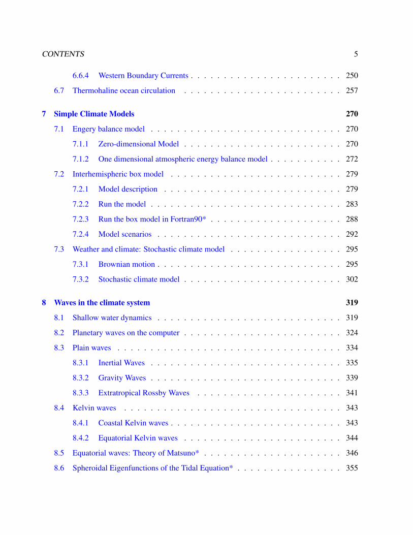
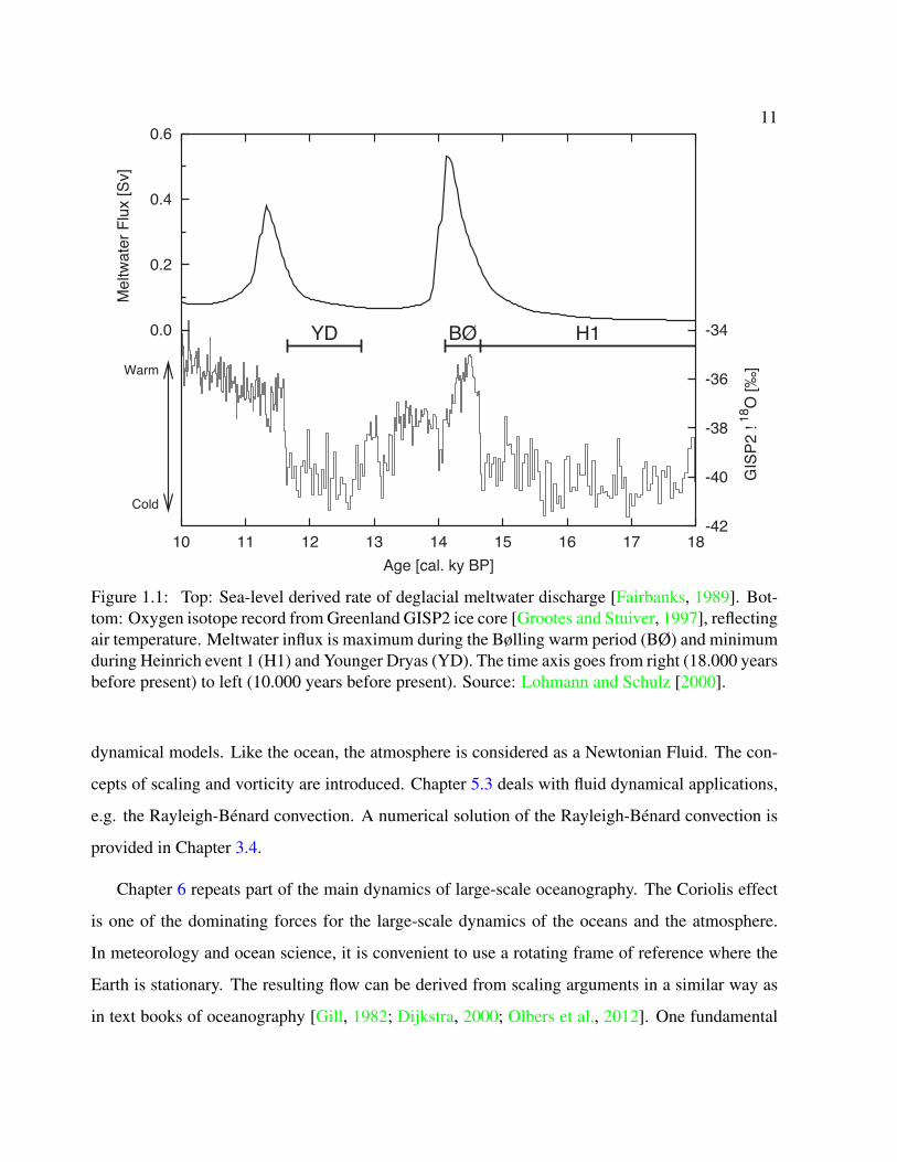
Paleoclimate reconstructions, in particular from ice cores have also shown that climate can change
over relatively short periods such as a few years to decades (Fig. 1.1). Over the last century, hu-
mans have altered the composition of the Earth’s atmosphere and surface to the extent that these
factors measurably affect current climate conditions. The objective of the book is to examine fun-
damental concepts used to understand climate dynamics. Here, we will approach climate dynamics
from a fluid dynamics and complex systems point of view.
In Chapter 2.3 I provide a framework to analyze the stability of dynamical systems. These sys-
tems provide the prototype of nonlinear dynamics, bifurcations, multiple equilibria. A bifurcation
occurs when a parameter change causes the stability of an equilibrium. In his classic studies of
chaotic systems, Lorenz has proposed a deterministic theory of climate change with his concept
of the ’almost-intransitivity’ of the highly non-linear climate systems. In the Lorenz equations
exist the possibility of multiple stable solutions and internal variability, even in the absence of any
variations in external forcing [Lorenz, 1976]. More complex models, e.g. Bryan [1986]; Dijkstra
et al. [2004] also demonstrated this possibility. Chapter 4 deals with the general structure of fluid
10
11
0.0
0.2
0.4
0.6
10 11 12 13 14 15 16 17 18-42
-40
-38
-36
-34
Mel
twat
er F
lux
[Sv]
GIS
P2 !
18O
[‰]
Age [cal. ky BP]
BØ H1YDWarm
Cold
Figure 1.1: Top: Sea-level derived rate of deglacial meltwater discharge [Fairbanks, 1989]. Bot-tom: Oxygen isotope record from Greenland GISP2 ice core [Grootes and Stuiver, 1997], reflectingair temperature. Meltwater influx is maximum during the Bølling warm period (BØ) and minimumduring Heinrich event 1 (H1) and Younger Dryas (YD). The time axis goes from right (18.000 yearsbefore present) to left (10.000 years before present). Source: Lohmann and Schulz [2000].
dynamical models. Like the ocean, the atmosphere is considered as a Newtonian Fluid. The con-
cepts of scaling and vorticity are introduced. Chapter 5.3 deals with fluid dynamical applications,
e.g. the Rayleigh-Bénard convection. A numerical solution of the Rayleigh-Bénard convection is
provided in Chapter 3.4.
Chapter 6 repeats part of the main dynamics of large-scale oceanography. The Coriolis effect
is one of the dominating forces for the large-scale dynamics of the oceans and the atmosphere.
In meteorology and ocean science, it is convenient to use a rotating frame of reference where the
Earth is stationary. The resulting flow can be derived from scaling arguments in a similar way as
in text books of oceanography [Gill, 1982; Dijkstra, 2000; Olbers et al., 2012]. One fundamental
12 CHAPTER 1. INTRODUCTION AND PREPARATION
aspect of ocean dynamics are waves. A short theory is given and numerical examples are pro-
vided. Furthermore, the deep ocean circulation is studied in a conceptual box model. Here, we
introduce an interhemispheric box model of the deep ocean circulation to study the feedbacks in
the climate system. The box model consists of four oceanic and three atmospheric boxes. The
Atlantic deep ocean circulation is simulated by a simple model of meridional overturning. In the
model of [Rooth, 1982] the Atlantic Ocean is described over both hemispheres and consider the
North Atlantic and South Atlantic Ocean, respectively. This model is implemented in Chapter 7.2
and several applications can be performed such as the effect of meltwater on climate (Fig. 1.1).
Such simple systems provide a general idea of the dominant processes in a complex system.
The structure of fluid dynamical models is valid for systems with many degrees of freedom,
many collisions, and for substances which can be described as a continuum. The transition from
the highly complex dynamical equations to a reduced system is an important step since it gives
more credibility to the approach and its results. The transition is also necessary since the active
entangled processes are running on spatial scales from millimetres to thousands of kilometres, and
temporal scales from seconds to millennia. Therefore, the unresolve processes on subgrid scales
have to be described. This is the typical problem in statistical physics: How can we obtain the
macroscopic dynamics from the underlying (and often known microdynamical) theory? Two dif-
ferent solutions are known, one is the so-called Mori-Zwanzig approach [Mori, 1965; Zwanzig,
1960, 1980] which relates the evolution of macroscopic variables to microscopic dynamics. The
basic idea is the evolution of a system through a projection on a subset (macroscopic relevant part),
where a randomness reflects the effects of the unresolved degrees of freedom. A particular exam-
ple is the Brownian motion [Einstein, 1905; Langevin, 1908]. The other solution for the transition
form the micro to macro-scales goes back to Boltzmann [1896]. The Boltzmann equation, also
often known as the Boltzmann transport equation [Boltzmann, 1896; Bhatnagar et al., 1954; Cer-
cignani, 1990] describes the statistical distribution of one particle in a fluid. It is one of the most
important equations of non-equilibrium statistical mechanics, the area of statistical mechanics that
deals with systems far from thermodynamic equilibrium. It is applied, for instance, when there
13
is an applied temperature gradient or electric field. Both, the Mori-Zwanzig and Boltzmann ap-
proaches play also a fundamental role in physics. The microscopic equations show no preferred
time direction, whereas the macroscopic phenomena in the thermodynamics have a time direction
through the enthropy. The underlying procedure is that part of the microscopic information is lost
through coarse graining in space and time. Chapter 3 describes the approach from statistical me-
chanics towards the macroscopic theory. The Boltzmann equation and the Brownian motion are
the approaches to understand the transition from micro to macro scales. For climate, this transition
between the climate and weather scales has been formulated [Hasselmann, 1976; Leith, 1975], and
later re-formulated in a mathematical context [Arnold, 2001; Chorin et al., 1999; Gottwald, 2010].
The effect of the weather on climate is seen by red-noise spectra in the climate system, showing
one of the most fundamental aspects of climate, and serving also as a null hypothesis for climate
variability studies. Chapter 3.4 deals with a fluid dynamical application, a 2D implementation of
the Lattice Boltzmann Method (LBM) with the Bhatnagar-Gross-Krook (BGK) collision operator.
The main structural parts of the program and several hints for the potential users are provided.
While we do include a brief outline of the theory of LBM, detailed explanations are out of the
scope of this book. Fore more details, please consult the references herein. The present code is in-
tended to serve mainly as a showcase/practical introduction to Lattice Boltzmann Methods, hence
advanced features and state-of-the-art algorithm improvements have been intentionally ommitted
in favor of simplicity. One practical example, the Rayleigh-Benard convection [Rayleigh, 1916],
is presented.
The content (first part) is designed for 12 lessons for a master course. The numerical examples
may be helpful for the students who are already familiar with programming (they can improve
the code and follow the main ideas of the code etc.), for those who are not familiar they can use
it more as a black box and as a starting point for more research. Several task do not require
that the complete code is understood, but one can change initial conditions or parameters in the
problems. In the following, I list some exercises and introductionary material which can be used
in the preparation of this course.

14 CHAPTER 1. INTRODUCTION AND PREPARATION
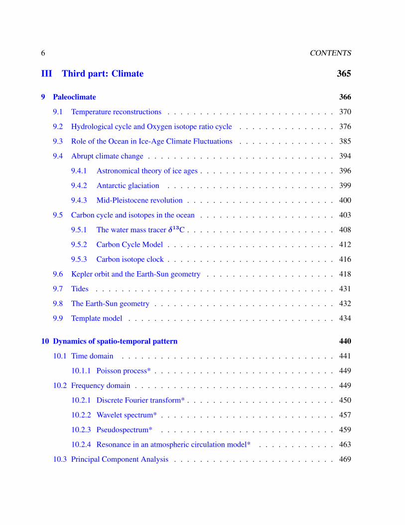
Exercise 1 – Earth’s curvature
1. The highest building on the campus of the University of Bremen is the so-called drop tower
with a hight of h=110 metres (Fig. 13.2 upper panel). How far one can look onto the horizon
under good weather conditions?
Hint: Denote this distance by d. Remember the Earth’s radius a = 6378km and apply
Pythogoras!
2. Why is the rule-of-thumb
d =√
2ha
a good approximation? (For h=10m this means d=11 km.) When h is in m, d in km, the
formula can be written as
d = 3.5
√h
mkm.
3. The town Bremerhaven where the Alfred Wegener Institute is located lies about 60 km north
of Bremen. How big must a tower in Bremen be in order to see the coast in Bremerhaven?
(Fig. 1.2 lower panel).
Exercise 2 – Nabla
Calculate the following operations for the function
f(x, y, z) = x3 + 3x− 4xz + z4 : (1.1)
a)∇f ,
b) calculate the divergence of the result!
c) Calculate the rotation of∇f !

15
Figure 1.2: Upper panel: Drop tower in Bremen. Lower panel: Harbor in Bremerhaven, ca. 60 kmnorth of Bremen.
16 CHAPTER 1. INTRODUCTION AND PREPARATION
1.1 Pendulum
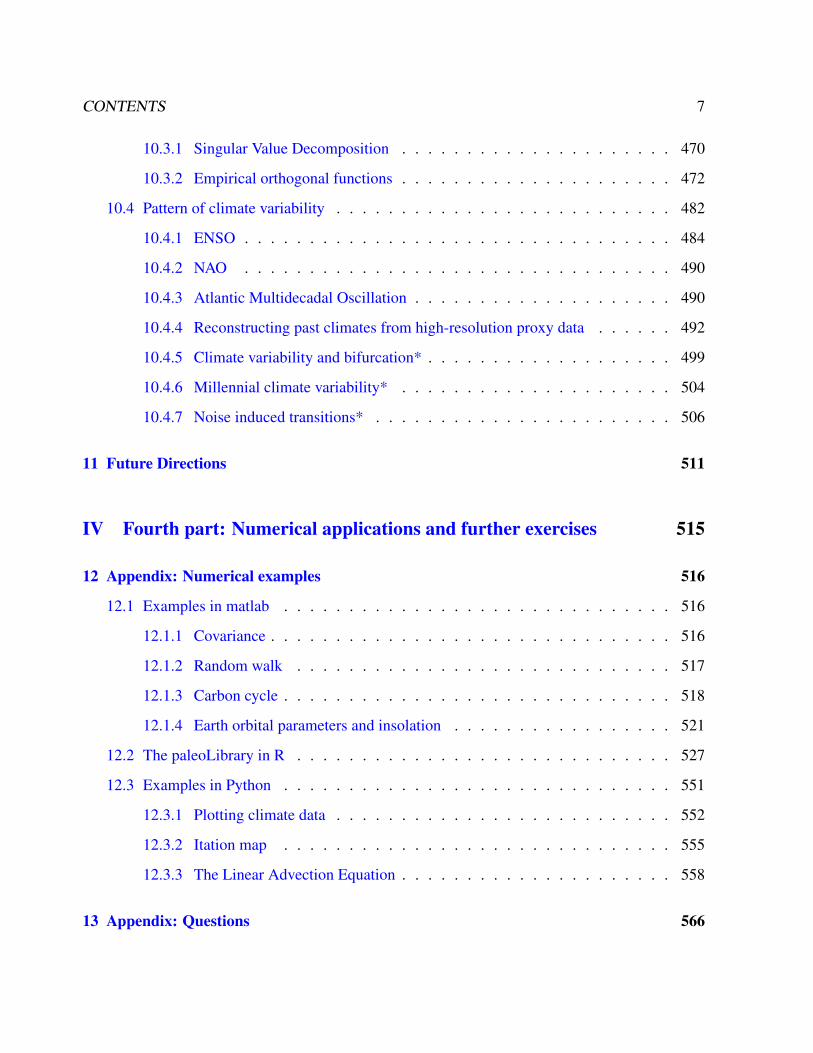
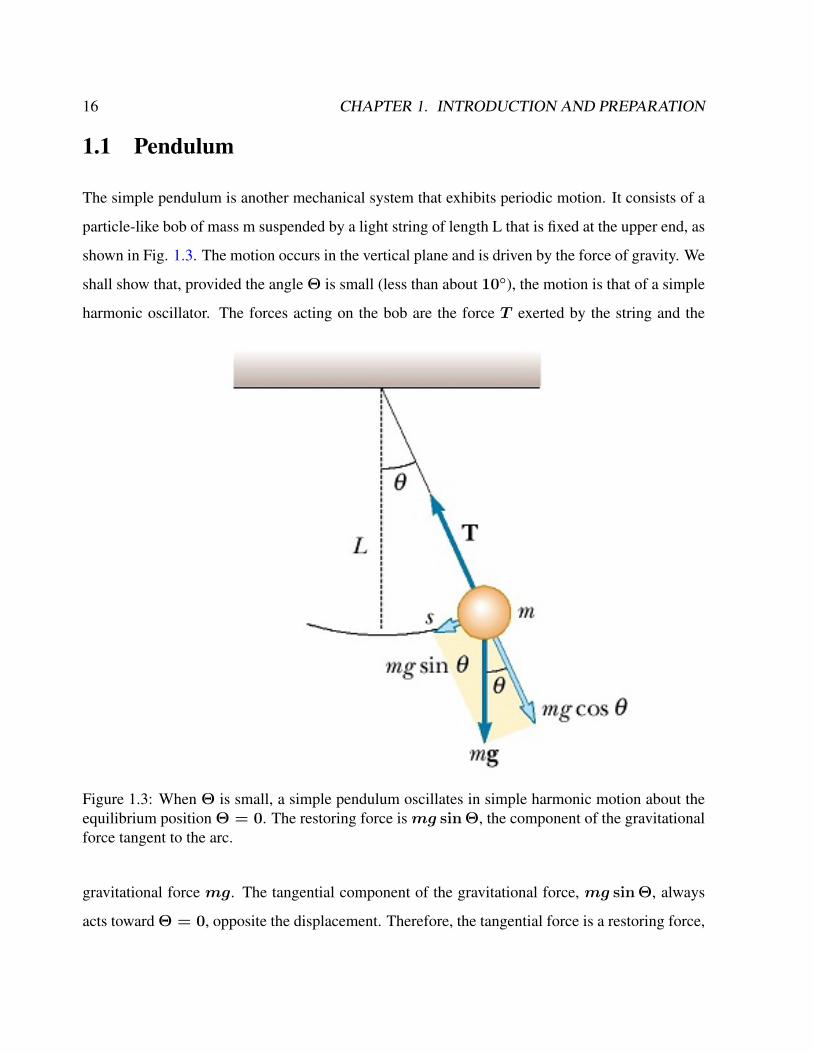
The simple pendulum is another mechanical system that exhibits periodic motion. It consists of a
particle-like bob of mass m suspended by a light string of length L that is fixed at the upper end, as
shown in Fig. 1.3. The motion occurs in the vertical plane and is driven by the force of gravity. We
shall show that, provided the angle Θ is small (less than about 10), the motion is that of a simple
harmonic oscillator. The forces acting on the bob are the force T exerted by the string and the
Figure 1.3: When Θ is small, a simple pendulum oscillates in simple harmonic motion about theequilibrium position Θ = 0. The restoring force ismg sin Θ, the component of the gravitationalforce tangent to the arc.
gravitational force mg. The tangential component of the gravitational force, mg sin Θ, always
acts toward Θ = 0, opposite the displacement. Therefore, the tangential force is a restoring force,
1.1. PENDULUM 17
and we can apply Newton’s second law for motion in the tangential direction:
F = −mg sin Θ = md2s
dt2(1.2)
where s is the bob’s displacement measured along the arc and the minus sign indicates that the tan-
gential force acts toward the equilibrium (vertical) position. Because s = LΘ and L is constant,
this equation reduces to the equation of motion for the simple pendulum.
d2Θ
dt2= −
g
Lsin Θ (1.3)
If we assume that Θ is small, we can use the approximation sin Θ = Θ, thus the equation of
motion for the simple pendulum becomes equation of motion for the simple pendulum
d2Θ
dt2= −
g
LΘ (1.4)
with solution
Θ = Θ0 cos(ωt) (1.5)
where ω =√
gL
is the angular frequency.
The period and frequency of a simple pendulum depend only on the length of the string and
the acceleration due to gravity. Because the period is independent of the mass, we conclude that
all simple pendulums that are of equal length and are at the same location (so that g is constant)
oscillate with the same period. The simple pendulum can be used as a timekeeper because its
period depends only on its length and the local value of g. It is also a convenient device for making
precise measurements of the free-fall acceleration. Such measurements are important because
variations in local values of g can provide information on the location of oil and of other valuable
underground resources.
18 CHAPTER 1. INTRODUCTION AND PREPARATION
Rule of thumb for pendulum length
It is useful to have a Rule of thumb for the period of the motion, the time for a complete oscillation
(outward and return) is
T = 2π
√L
gcan be expressed as L =
g
π2
T 2
4. (1.6)
If SI units are used (i.e. measure in metres and seconds), and assuming the measurement is taking
place on the Earth’s surface, then g ≈ 9.81m/s2, and g/π2 ≈ 1 (0.994 is the approximation to
3 decimal places). Therefore, a relatively reasonable approximation for the length and period are,
L ≈T 2
4,
T ≈ 2√L
(1.7)
where T is the number of seconds between two beats (one beat for each side of the swing), and L
is measured in metres.
Full problem without the approximation
If we consider the full problem without the approximation, the period is modified according to
T = 4
√L
gK(k), k = sin
θ0
2(1.8)
where K is the complete elliptic integral of the first kind defined by
K(k) =
∫ π2
0
1√1− k2 sin2 u
du . (1.9)
1.1. PENDULUM 19
For comparison of the approximation to the full solution, consider the period of a pendulum of
length 1 m on Earth at initial angle 10 degrees is
4
√1 mgK
(sin
10
2
)≈ 2.0102 s. (1.10)
The linear approximation gives
2π
√1 mg≈ 2.0064 s. (1.11)
The difference between the two values, less than 0.2%,is much less than that caused by the varia-
tion of g with geographical location.
Foucault pendulum
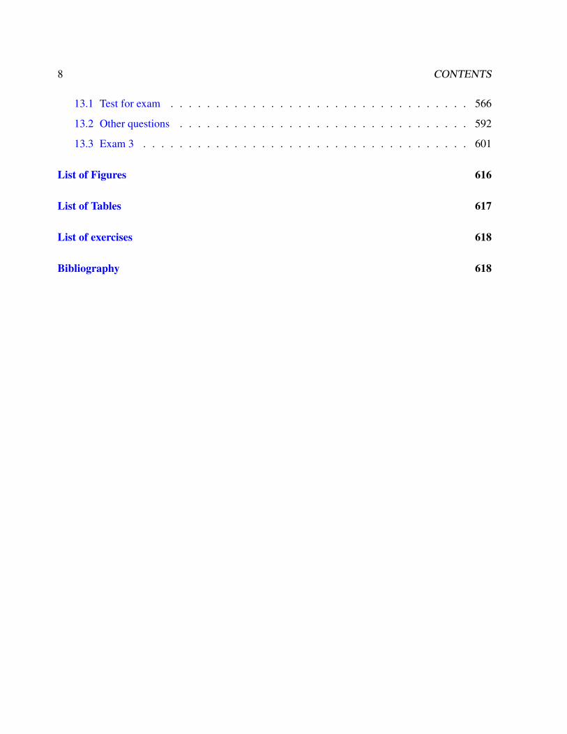
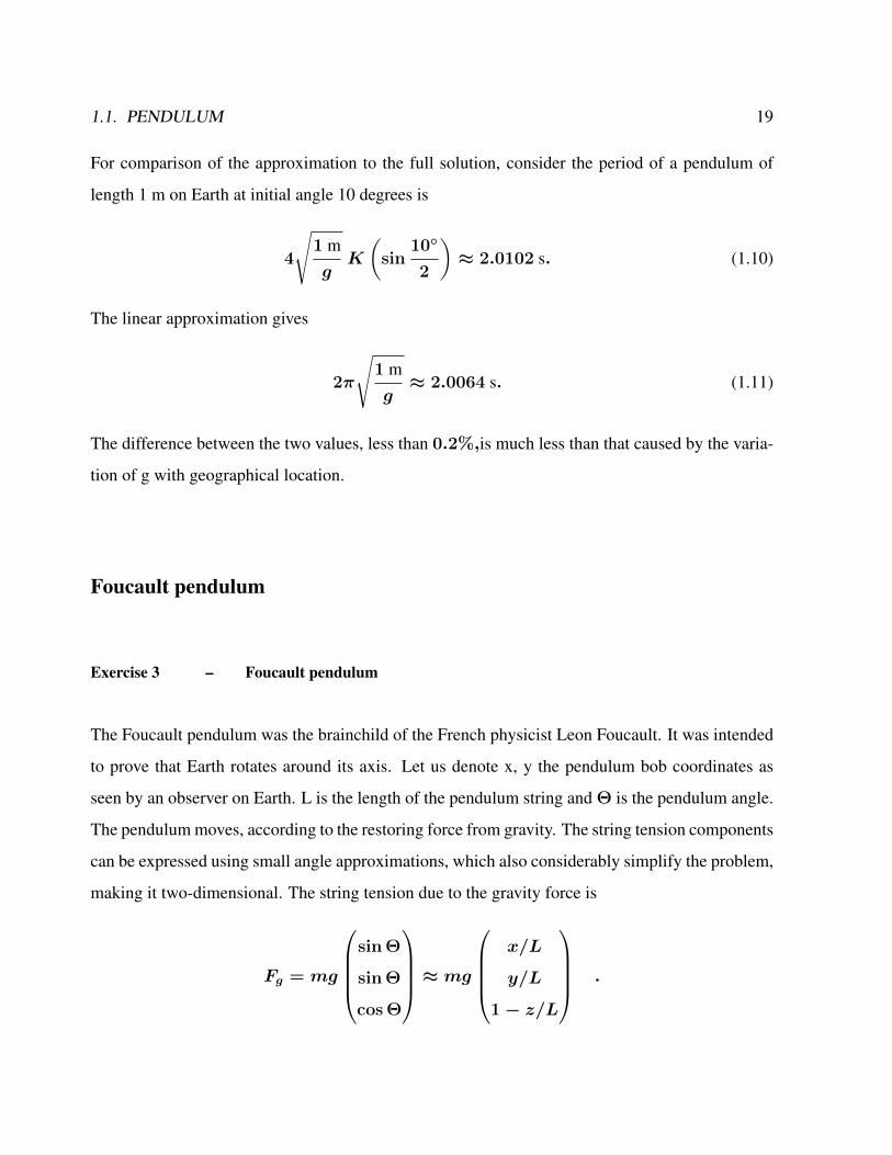
Exercise 3 – Foucault pendulum
The Foucault pendulum was the brainchild of the French physicist Leon Foucault. It was intended
to prove that Earth rotates around its axis. Let us denote x, y the pendulum bob coordinates as
seen by an observer on Earth. L is the length of the pendulum string and Θ is the pendulum angle.
The pendulum moves, according to the restoring force from gravity. The string tension components
can be expressed using small angle approximations, which also considerably simplify the problem,
making it two-dimensional. The string tension due to the gravity force is
Fg = mg
sin Θ
sin Θ
cos Θ
≈ mg
x/L
y/L
1− z/L
.
20 CHAPTER 1. INTRODUCTION AND PREPARATION
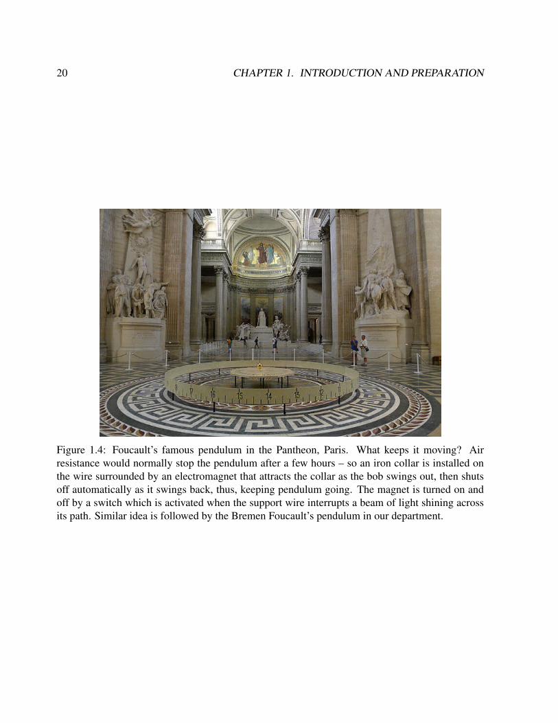
Figure 1.4: Foucault’s famous pendulum in the Pantheon, Paris. What keeps it moving? Airresistance would normally stop the pendulum after a few hours – so an iron collar is installed onthe wire surrounded by an electromagnet that attracts the collar as the bob swings out, then shutsoff automatically as it swings back, thus, keeping pendulum going. The magnet is turned on andoff by a switch which is activated when the support wire interrupts a beam of light shining acrossits path. Similar idea is followed by the Bremen Foucault’s pendulum in our department.
1.1. PENDULUM 21
Then, the horizontal dynamics can be described as
x = fy −g
Lx (1.12)
y = −fx−g
Ly (1.13)
where f = 2Ω sinϕ.
1. Show the analytic solution to the Foucault pendulum problem introducing the complex num-
ber ξ = x+ i · y. Furthermore, call ω =√
gL
is the angular frequency. Then,
ξ + ifξ + ω2ξ = 0 (1.14)
With the ansatz
ξ = H(t) · exp
(−if
2t
)(1.15)
we obtain an equation for H
H +
(ω2 +
f2
4
)H = 0 (1.16)
H(t) = C exp
±it√ω2 +
f2
4
(1.17)
and therefore
ξ = C exp
it−f
2±
√ω2 +
f2
4
≈ C exp
[it
(−f
2± ω
)](1.18)
where C is a complex integration constant. The pendulum swing has a natural frequency
22 CHAPTER 1. INTRODUCTION AND PREPARATION
(also called pulsation) ω =√g/L, which depends on the length of the pendulum string.1
Looking at the last term in (1.23): At either the North Pole or South Pole, the plane of oscil-
lation of a pendulum remains fixed relative to the distant masses of the universe while Earth
rotates underneath it, taking one day to complete a rotation (frequency Ω = 2π/24h). So,
relative to Earth, the plane of oscillation of a pendulum at the North Pole undergoes a full
clockwise rotation during one day, a pendulum at the South Pole rotates counterclockwise.2
When a Foucault pendulum is suspended at the equator, the plane of oscillation remains fixed
relative to Earth. At other latitudes, the plane of oscillation precesses relative to Earth with
a frequency f/2 = Ω sinϕ proportional to the sine of the latitude, where latitudes north
and south of the equator are defined as positive and negative, respectively. For example, a
Foucault pendulum at 30 S, viewed from above by an earthbound observer, rotates coun-
terclockwise 360 in two days.
2. For Foucault’s famous pendulum in Paris: The plane of the pendulum’s swing rotated clock-
wise 11 per hour, making a full circle in 32.7 hours. What is the time period in Bremen,
Germany?
3. Display the solution and compare it with the numerical solution with the following initial
condition:
g = 9.81 # acceleration of gravity (m/s^2)L = 67 # pendulum length (m) for the experiment in Parisinitial_x = L/100 # initial x coordinate (m)initial_y = 0 # initial y coordinate (m)initial_u = 0 # initial x velocity (m/s)initial_v = 0 # initial y velocity (m/s)Omega=2*pi/86400 # Earth’s angular velocity of rotation (rad/s)phi=49/180*pi # 49 deg latitude in (rad) for Paris 1851
1For Foucault’s famous pendulum: he suspended a 28 kg brass-coated lead bob with a 67 meter long wire from thedome of the Pantheon in Paris (about 49N). The natural frequency is
√g/L = 0.381/s related to a time period of
16 s.2for the South Pole, there was indeed an experiment [Baker and Blackburn, 2005].
1.1. PENDULUM 23
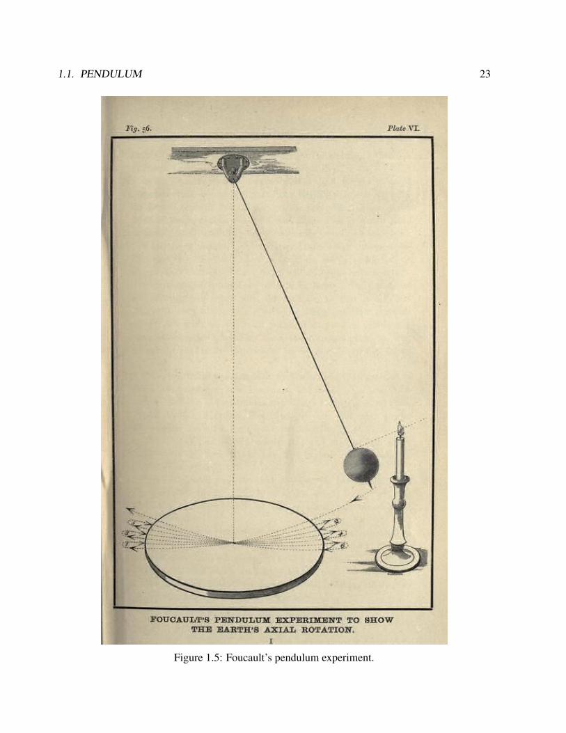
Figure 1.5: Foucault’s pendulum experiment.
24 CHAPTER 1. INTRODUCTION AND PREPARATION
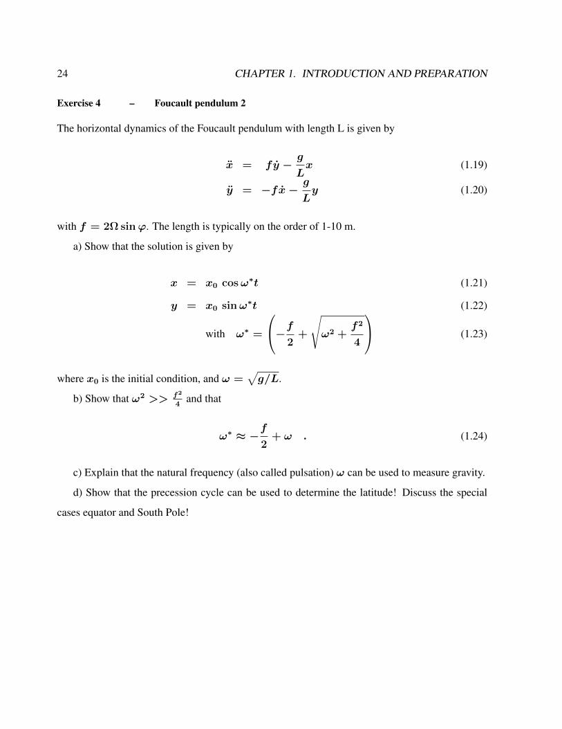
Exercise 4 – Foucault pendulum 2
The horizontal dynamics of the Foucault pendulum with length L is given by
x = fy −g
Lx (1.19)
y = −fx−g
Ly (1.20)
with f = 2Ω sinϕ. The length is typically on the order of 1-10 m.
a) Show that the solution is given by
x = x0 cosω∗t (1.21)
y = x0 sinω∗t (1.22)
with ω∗ =
−f2
+
√ω2 +
f2
4
(1.23)
where x0 is the initial condition, and ω =√g/L.
b) Show that ω2 >> f2
4and that
ω∗ ≈ −f
2+ ω . (1.24)
c) Explain that the natural frequency (also called pulsation) ω can be used to measure gravity.
d) Show that the precession cycle can be used to determine the latitude! Discuss the special
cases equator and South Pole!

1.2. FOURIER TRANSFORM 25
1.2 Fourier transform
The Fourier transform decomposes a function of time (e.g., a signal) into the frequencies that
make it up, similarly to how a musical chord can be expressed as the amplitude (or loudness)
of its constituent notes. The Fourier transform of a function of time itself is a complex-valued
function of frequency, whose absolute value represents the amount of that frequency present in the
original function, and whose complex argument is the phase offset of the basic sinusoid in that
frequency. The Fourier transform is called the frequency domain representation of the original
signal. The term Fourier transform refers to both the frequency domain representation and the
mathematical operation that associates the frequency domain representation to a function of time
(see also https://en.wikipedia.org/?title=Fourier_transform).
The Fourier transformation of x is defined as
x(ω) =
∫R
x(t)eiωt dt (1.25)
and is denoted as a hat in the following.3 And the inverse Fourier transformation of x is defined as
x(t) =1
2π
∫R
x(ω)e−iωt dω (1.26)
or with ω = 2πν :
x(t) =
∫R
xe−i2πνt dν . (1.27)
3Other common notations for the Fourier transform x(ω): x(ω), x(ω), F (ξ), F (x) (ω), (Fx) (ω), F(x), F(ω), F (ω).The sign of the exponential in the Fourier transform is something that we are concerned with for many years. Ofcourse, there are two conventions that have been used with almost equal frequency, but I try to stick to one of them toavoid confusion. Here, we have used the convention of the positive sign in the exponential for the forward transformwhich represents the Fraunhofer diffraction pattern for a real-space object. This is consistent with assuming that aplane wave, going in positive direction in real space is written exp [i(ωt− kx)] rather than a minus sign before thei, so that the phase advances with time.
26 CHAPTER 1. INTRODUCTION AND PREPARATION
Exercise 5 – Fourier transformation
Tasks: Calculate the Fourier transformation of
1. x(t+ a) (time shift).
2. x(t ∗ a) (Scaling in the time domain).
3. ddtx(t) (time derivative).
4. x(t) = exp(−at2) (Gaussian).
5. x(t) = δ(t) where the δ distribution is definedthrough the operator on any function y:
y(t0) =∫Ry(t)δ(t− t0) dt
6. Show that for x(t) = exp(−iat), the Fourier transformation x(ω) = 2πδ(ω−a). Hint:
use the Fourier back transformation (1.25).
7. Calculate the Fourier transformation of a the periodic function x(t) = sin(ω0t). Remem-
ber that sinx = 12i
(eix − e−ix).
8. Prove the Uncertainty principle: the more concentrated x(t) is, the more spread out its
Fourier transform x(ω) must be. In particular, the scaling property of the Fourier transform
may be seen as saying: if we "squeeze" a function in t, its Fourier transform "stretches out"
in ω. It is not possible to arbitrarily concentrate both a function and its Fourier transform.
9. Consider the sine and cosine transforms and show the following. Fourier’s original formula-
tion of the transform did not use complex numbers, but rather sines and cosines. Statisticians
and others still use this form. An absolutely integrable function f for which Fourier inversion
holds good can be expanded in terms of genuine frequencies (avoiding negative frequencies,
which are sometimes considered hard to interpret physically) λ by
f(t) =
∫ ∞0
[a(λ) cos 2πλt+ b(λ) sin 2πλt] dλ. (1.28)
This is called an expansion as a trigonometric integral, or a Fourier integral expansion. The
coefficient functions a and b can be found by using variants of the Fourier cosine transform

1.2. FOURIER TRANSFORM 27
and the Fourier sine transform (the normalisations are, again, not standardised):
a(λ) = 2
∫ ∞−∞
f(t) cos(2πλt)dt (1.29)
b(λ) = 2
∫ ∞−∞
f(t) sin(2πλt)dt. (1.30)
Laplace transform
The Fourier transform is intimately related with the Laplace transform F (s), which is also used
for the solution of differential equations and the analysis of filters (https://en.wikipedia.
org/wiki/Laplace_transform). We introduce the complex variable s = −iω.
Lx(t) = F (s) =
∫ ∞0
e−stx(t)dt (1.31)
It follows (integration by parts for 1.32)
Ld
dtx(t)
= sF (s)− x(0) (1.32)
Lexp(−at) =1
s+ a(1.33)
L− exp(−at) + exp(−bt) =−1
s+ a+
1
s+ b=
a− b(s+ a)
1
(s+ b)(1.34)
The Laplace transform of a sum is the sum of Laplace transforms of each term.
Lf(t) + g(t) = Lf(t)+ Lg(t) (1.35)
The Laplace transform of a multiple of a function is that multiple times the Laplace transformation

28 CHAPTER 1. INTRODUCTION AND PREPARATION
Function Time domain Laplace s-domainf(t) = L−1F (s) F (s) = Lf(t)
unit impulse δ(t) 1delayed impulse δ(t− τ ) e−τs
unit step u(t) 1s
delayed unit step u(t− τ ) 1se−τs
exponential decay e−αt · u(t) 1s+α
sine sin(ωt) · u(t) ωs2+ω2
cosine cos(ωt) · u(t) ss2+ω2
decaying sine wave e−αt sin(ωt) · u(t) ω(s+α)2+ω2
decaying cosine wave e−αt cos(ωt) · u(t) s+α(s+α)2+ω2
natural logarithm ln(t) · u(t) −1s
[ln(s) + γ]
Convolution (f ∗ g)(t) =∫ t
0f(τ )g(t− τ ) dτ F (s) ·G(s)
Table 1.1: Laplace transformation (https://en.wikipedia.org/wiki/Laplace_transform.
of that function.
Laf(t) = aLf(t) (1.36)
Using this linearity, and various trigonometric, hyperbolic, and complex number (etc.) properties
and/or identities, some Laplace transforms can be obtained from others quicker than by using the
definition directly.
Exercise 6 – Laplace transformation of mixed layer model
Solve the Imagine that the temperature of the ocean mixed layer is governed by
dT
dt= −λT +Q(t) , (1.37)
where λ is the typical damping rate of a temperature anomaly andQ(t) a forcing.
1.2. FOURIER TRANSFORM 29
1. Use the Laplace transformation to show
F (s) =Q(s) + T (0)
s+ λ. (1.38)
whereQ(s) = LQ(t)
2. Consider the special case Q(t) = exp(iω0t), then Q(s) = 1s−iω0
. The forcing and
the temperature is of course a real number, by representing is as a complex number we can
simultaneously keep track of both phase components. Show
F (s) =T (0) +Q(s)
s+ λ=T (0)
s+ λ+
1
(s+ λ)
1
(s− iω0)(1.39)
and via the Laplace back-transformation and (13.42, 13.47) that
T (t) = exp(−λt)T (0) +[exp(iω0t)− exp(−λt)]
λ+ iω0
. (1.40)
3. Calculate the real and complex part of (13.46).
4. Show: At low frequencies, the output is equal to the input. At high frequencies it rolls off as
1/ω (it is a low-pass filter) and is out of phase by 90.
Let x(t) be the input to a general linear time-invariant system, and y(t) be the output, and
the Laplace transform of x(t) and y(t) be X(s) and Y (s). Then, the output is related to the
input by convolution with respect to the impulse response h(t) by
y(t) =
∫ ∞0
h(t′)x(t− t′)dt (1.41)
Because of the convolution, the transfer function H(s) is equal to the to the ratio of the Laplace
30 CHAPTER 1. INTRODUCTION AND PREPARATION
transforms of the input and output
H(s) =Y (s)
X(s). (1.42)
The impulse response of a linear transformation is the image of Dirac’s delta function under the
transformation, analogous to the fundamental solution of a partial differential operator. The general
feature of the transfer function is that is the ratio of two polynomials. Since the polynomials
can be constructed from knowledge of the roots, the location of the poles and zeros completetly
characterizes the response of the system. The system is globally stable if all poles lie in the left
half-plane with Re(poles) < 0. For example Lexp(−at) = 1s+a
, i.e. the system is stable if
Re(a) < 0. Poles off the real axes are associated with oscillations. Summarizing, the convolution
that gives the output of the system can be transformed to a multiplication in the transform domain,
given signals for which the transforms exist
y(t) = (h ∗ x)(t)def=
∫ ∞−∞
h(t− τ )x(τ ) d τdef= L−1H(s)X(s). (1.43)
Transfer functions are commonly used in the analysis of systems such as single-input single-
output filters, typically within the fields of signal processing, communication theory, and control
theory. The term is often used exclusively to refer to linear, time-invariant systems. The descrip-
tions below are given in terms of a complex variable, s = σ−iω,which bears a brief explanation.
In many applications, it is sufficient to define σ = 0, which reduces the Laplace transforms with
complex arguments to Fourier transforms with real argument ω. The applications where this is
common are ones where there is interest only in the steady-state response.4 The stability of linear
systems will be discussed further in section 10.2.3.
4In discrete-time systems, the relation between an input signal x(t) and output y(t) is dealt with using the z-transform, and then the transfer function is similarly written as H(z) = Y (z)
X(z)and this is often referred to as the
pulse-transfer function.
1.2. FOURIER TRANSFORM 31
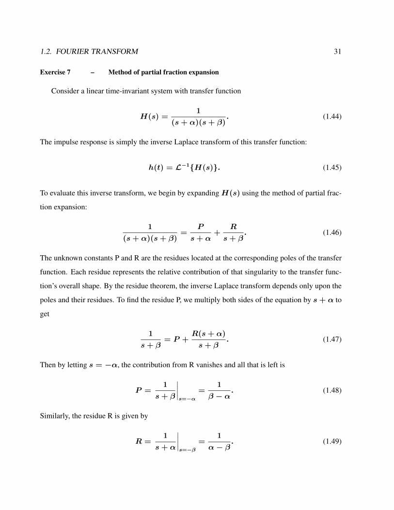
Exercise 7 – Method of partial fraction expansion
Consider a linear time-invariant system with transfer function
H(s) =1
(s+ α)(s+ β). (1.44)
The impulse response is simply the inverse Laplace transform of this transfer function:
h(t) = L−1H(s). (1.45)
To evaluate this inverse transform, we begin by expandingH(s) using the method of partial frac-
tion expansion:
1
(s+ α)(s+ β)=
P
s+ α+
R
s+ β. (1.46)
The unknown constants P and R are the residues located at the corresponding poles of the transfer
function. Each residue represents the relative contribution of that singularity to the transfer func-
tion’s overall shape. By the residue theorem, the inverse Laplace transform depends only upon the
poles and their residues. To find the residue P, we multiply both sides of the equation by s+ α to
get
1
s+ β= P +
R(s+ α)
s+ β. (1.47)
Then by letting s = −α, the contribution from R vanishes and all that is left is
P =1
s+ β
∣∣∣∣s=−α
=1
β − α. (1.48)
Similarly, the residue R is given by
R =1
s+ α
∣∣∣∣s=−β
=1
α− β. (1.49)
32 CHAPTER 1. INTRODUCTION AND PREPARATION
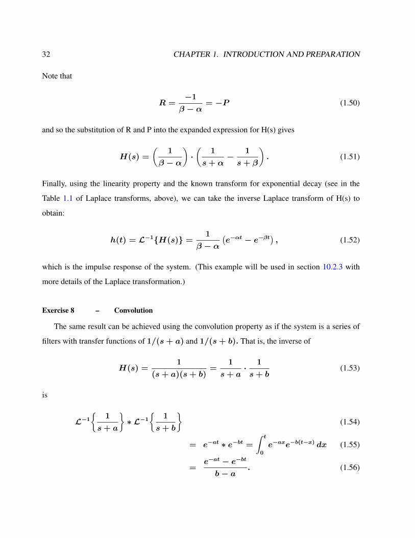
Note that
R =−1
β − α= −P (1.50)
and so the substitution of R and P into the expanded expression for H(s) gives
H(s) =
(1
β − α
)·(
1
s+ α−
1
s+ β
). (1.51)
Finally, using the linearity property and the known transform for exponential decay (see in the
Table 1.1 of Laplace transforms, above), we can take the inverse Laplace transform of H(s) to
obtain:
h(t) = L−1H(s) =1
β − α(e−αt − e−βt
), (1.52)
which is the impulse response of the system. (This example will be used in section 10.2.3 with
more details of the Laplace transformation.)
Exercise 8 – Convolution
The same result can be achieved using the convolution property as if the system is a series of
filters with transfer functions of 1/(s+ a) and 1/(s+ b). That is, the inverse of
H(s) =1
(s+ a)(s+ b)=
1
s+ a·
1
s+ b(1.53)
is
L−1
1
s+ a
∗ L−1
1
s+ b
(1.54)
= e−at ∗ e−bt =
∫ t
0
e−axe−b(t−x) dx (1.55)
=e−at − e−bt
b− a. (1.56)
1.2. FOURIER TRANSFORM 33
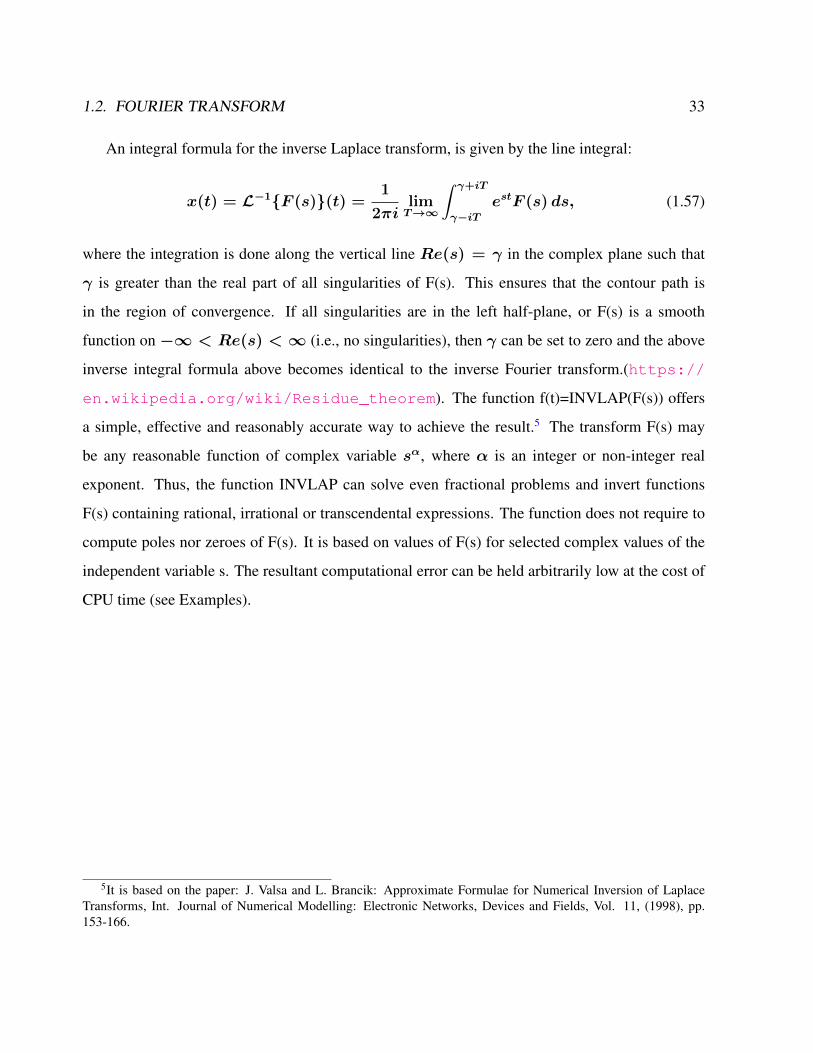
An integral formula for the inverse Laplace transform, is given by the line integral:
x(t) = L−1F (s)(t) =1
2πilimT→∞
∫ γ+iT
γ−iTestF (s) ds, (1.57)
where the integration is done along the vertical line Re(s) = γ in the complex plane such that
γ is greater than the real part of all singularities of F(s). This ensures that the contour path is
in the region of convergence. If all singularities are in the left half-plane, or F(s) is a smooth
function on−∞ < Re(s) < ∞ (i.e., no singularities), then γ can be set to zero and the above
inverse integral formula above becomes identical to the inverse Fourier transform.(https://
en.wikipedia.org/wiki/Residue_theorem). The function f(t)=INVLAP(F(s)) offers
a simple, effective and reasonably accurate way to achieve the result.5 The transform F(s) may
be any reasonable function of complex variable sα, where α is an integer or non-integer real
exponent. Thus, the function INVLAP can solve even fractional problems and invert functions
F(s) containing rational, irrational or transcendental expressions. The function does not require to
compute poles nor zeroes of F(s). It is based on values of F(s) for selected complex values of the
independent variable s. The resultant computational error can be held arbitrarily low at the cost of
CPU time (see Examples).
5It is based on the paper: J. Valsa and L. Brancik: Approximate Formulae for Numerical Inversion of LaplaceTransforms, Int. Journal of Numerical Modelling: Electronic Networks, Devices and Fields, Vol. 11, (1998), pp.153-166.
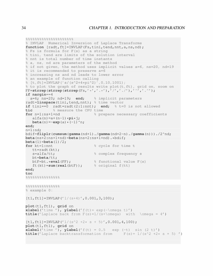
34 CHAPTER 1. INTRODUCTION AND PREPARATION
%%%%%%%%%%%%%%%%%%%%%% INVLAP Numerical Inversion of Laplace Transformsfunction [radt,ft]=INVLAP(Fs,tini,tend,nnt,a,ns,nd);% Fs is formula for F(s) as a string% tini, tend are limits of the solution interval% nnt is total number of time instants% a, ns, nd are parameters of the method% if not given, the method uses implicit values a=6, ns=20, nd=19% it is recommended to preserve a=6% increasing ns and nd leads to lower error% an example of function calling% [t,ft]=INVLAP(’s/(s^2+4*pi^2)’,0,10,1001);% to plot the graph of results write plot(t,ft), grid on, zoom onFF=strrep(strrep(strrep(Fs,’*’,’.*’),’/’,’./’),’^’,’.^’);if nargin==4
a=6; ns=20; nd=19; end; % implicit parametersradt=linspace(tini,tend,nnt); % time vectorif tini==0 radt=radt(2:1:nnt); end; % t=0 is not allowedtic % measure the CPU timefor n=1:ns+1+nd % prepare necessary coefficients
alfa(n)=a+(n-1)*pi*j;beta(n)=-exp(a)*(-1)^n;
end;n=1:nd;bdif=fliplr(cumsum(gamma(nd+1)./gamma(nd+2-n)./gamma(n)))./2^nd;beta(ns+2:ns+1+nd)=beta(ns+2:ns+1+nd).*bdif;beta(1)=beta(1)/2;for kt=1:nnt % cycle for time t
tt=radt(kt);s=alfa/tt; % complex frequency sbt=beta/tt;btF=bt.*eval(FF); % functional value F(s)ft(kt)=sum(real(btF)); % original f(tt)
end;toc%%%%%%%%%%%%%%%
%%%%%%%%%%%%%%%% example 0:
[t1,ft1]=INVLAP(’1/(s+4)’,0.001,3,100);
plot(t1,ft1), grid onxlabel(’time ’), ylabel(’f(t)= exp(-\omega t)’)title(’Laplace back from F(s)=1/(s+\omega) with \omega = 4’)
[t1,ft1]=INVLAP(’1/(s^2 +2* s + 5)’,0.001,4,100);plot(t1,ft1), grid onxlabel(’time ’), ylabel(’f(t) = 0.5 exp (-t) sin (2 t)’)title(’Laplace backtransformation from F(s)= 1/(s^2 +2* s + 5) ’)
1.2. FOURIER TRANSFORM 35
[t1,ft1]=INVLAP(’(3 * s^2 +7 *s +10)/(4*s + s *(s + 1)^2)’,0.001,4,100);plot(t1,ft1), grid onxlabel(’time ’), ylabel(’f(t) = 2+exp(-t) *cos(2t)+exp(-t)+sin(2t)’)title(’Laplace back from F(s)= (3 * s^2 +7 *s +10)/(4*s + s *(s + 1)^2) ’)
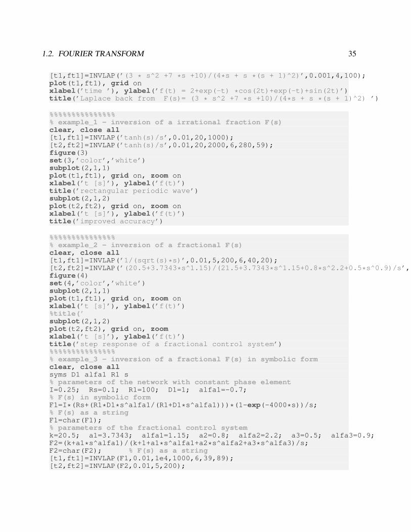
%%%%%%%%%%%%%%%% example_1 - inversion of a irrational fraction F(s)clear, close all[t1,ft1]=INVLAP(’tanh(s)/s’,0.01,20,1000);[t2,ft2]=INVLAP(’tanh(s)/s’,0.01,20,2000,6,280,59);figure(3)set(3,’color’,’white’)subplot(2,1,1)plot(t1,ft1), grid on, zoom onxlabel(’t [s]’), ylabel(’f(t)’)title(’rectangular periodic wave’)subplot(2,1,2)plot(t2,ft2), grid on, zoom onxlabel(’t [s]’), ylabel(’f(t)’)title(’improved accuracy’)
%%%%%%%%%%%%%%%% example_2 - inversion of a fractional F(s)clear, close all[t1,ft1]=INVLAP(’1/(sqrt(s)*s)’,0.01,5,200,6,40,20);[t2,ft2]=INVLAP(’(20.5+3.7343*s^1.15)/(21.5+3.7343*s^1.15+0.8*s^2.2+0.5*s^0.9)/s’,0.01,5,200);figure(4)set(4,’color’,’white’)subplot(2,1,1)plot(t1,ft1), grid on, zoom onxlabel(’t [s]’), ylabel(’f(t)’)%title(’subplot(2,1,2)plot(t2,ft2), grid on, zoomxlabel(’t [s]’), ylabel(’f(t)’)title(’step response of a fractional control system’)%%%%%%%%%%%%%%%% example_3 - inversion of a fractional F(s) in symbolic formclear, close allsyms D1 alfa1 R1 s% parameters of the network with constant phase elementI=0.25; Rs=0.1; R1=100; D1=1; alfa1=-0.7;% F(s) in symbolic formF1=I*(Rs+(R1*D1*s^alfa1/(R1+D1*s^alfa1)))*(1-exp(-4000*s))/s;% F(s) as a stringF1=char(F1);% parameters of the fractional control systemk=20.5; a1=3.7343; alfa1=1.15; a2=0.8; alfa2=2.2; a3=0.5; alfa3=0.9;F2=(k+a1*s^alfa1)/(k+1+a1*s^alfa1+a2*s^alfa2+a3*s^alfa3)/s;F2=char(F2); % F(s) as a string[t1,ft1]=INVLAP(F1,0.01,1e4,1000,6,39,89);[t2,ft2]=INVLAP(F2,0.01,5,200);
36 CHAPTER 1. INTRODUCTION AND PREPARATION
figure(4)set(4,’color’,’white’)subplot(2,1,1)plot(t1,ft1), grid on, zoom onxlabel(’t [s]’), ylabel(’f(t)’)title(’response to the input current impulse’)subplot(2,1,2)plot(t2,ft2), grid on, zoomxlabel(’t [s]’), ylabel(’f(t)’)title(’step response of a fractional control system’)
1.3 Covariance and spectrum
A stationary process exhibits an autocovariance function of the form
Cov(τ ) = 〈(x(t+ τ )− 〈x〉)(x(t)− 〈x〉)〉 (1.58)
where 〈. . . 〉 denotes the statistical ensemble mean.6 Normalized to the variance (i.e. the autoco-
variance function at τ = 0) one gets the autocorrelation function C(τ ) :
C(τ ) = Cov(τ )/Cov(0) . (1.59)
Many stochastic processes in nature exhibit short-range correlations, which decay exponentially:
C(τ ) ∼ exp(−τ/τ0), for τ →∞ (1.60)
These processes exhibit a typical time scale τ0. For a white noise process ξ (as defined in 7.55),
the autocorrelation function C(τ ) is given by
C(τ ) = δ(τ ) . (1.61)
6For the covariance, one can have two processes Cov(τ ) = 〈(x(t+ τ )− 〈x〉)(y(t)− 〈y〉)〉.
1.3. COVARIANCE AND SPECTRUM 37
Spectrum of the stochastic process
The Fourier transformation of the random variable x is
x(ω) =
∫R
x(t)eiωt dt = limT→∞
∫ T/2
−T/2x(t)eiωt dt (1.62)
and is also a ramdom variable, but its power spectral density S(ω) is not:
S(ω) :=⟨xx+
⟩=⟨|x(ω)|2
⟩. (1.63)
Using the ergodic hypothesis, the ensemble average S(ω) = 〈 xx+ 〉 can be expressed as the
time average
limT→∞
1
T
∫ T/2
−T/2dt xx+ (1.64)
and therefore the spectrum can be expressed as
S(ω) = limT→∞
1
T
∫ T/2
−T/2eiωtx(t)dt
∫ T/2
−T/2e−iωt
′x(t′)dt′ . (1.65)
The "total" integrated spectral density equals the variance of the series. Thus the spectral density
within a particular interval of frequencies can be viewed as the amount of the variance explained
by those frequencies. Mathematically, the spectral density is defined for both negative and positive
frequencies. However, due to symmetry of the function S(ω) is quite often displayed for positive
values only.
Let us calculate the inverse Fourier transformation of S(ω) and calculate the relation to the
autocovariance function Cov(τ ) of the stationary process x(t):
38 CHAPTER 1. INTRODUCTION AND PREPARATION
1
2π
∫R
S(ω) e−iωτdω
= limT→∞
1
T
∫R
dωe−iωτ
2π
∫ T/2
−T/2eiωtx(t)dt
∫ T/2
−T/2e−iωt
′x(t′)dt′
= limT→∞
1
T
∫ T/2
−T/2
∫ T/2
−T/2
(1
2π
∫R
eiω(t−t′−τ)dω
)x(t)x(t′)dtdt′
= limT→∞
1
T
∫ T/2
−T/2
∫ T/2
−T/2δ(t− t′ − τ )x(t)x(t′)dtdt′ (1.66)
= limT→∞
1
T
∫ T/2
−T/2x(t)x(t− τ )dt (1.67)
= 〈x(t)x(t− τ )〉 = Cov(τ ) (1.68)
The transformation (1.66) comes from the Fourier transform of the δ−function:
∫R
e−iωtδ(t)dt = 1 −→ δ(t) =1
2π
∫R
eiωtdω (1.69)
As the frequency domain counterpart of the autocovariance function of a stationary process, one
can calculate the spectrum as
S(ω) = Cov(τ ) , (1.70)
where the hat denotes again the Fourier transformation. This is the Wiener-Chinchin theorem,
relating the sprectrum of a random process to its autocorrelation function (Fig. 10.1).
1.3. COVARIANCE AND SPECTRUM 39
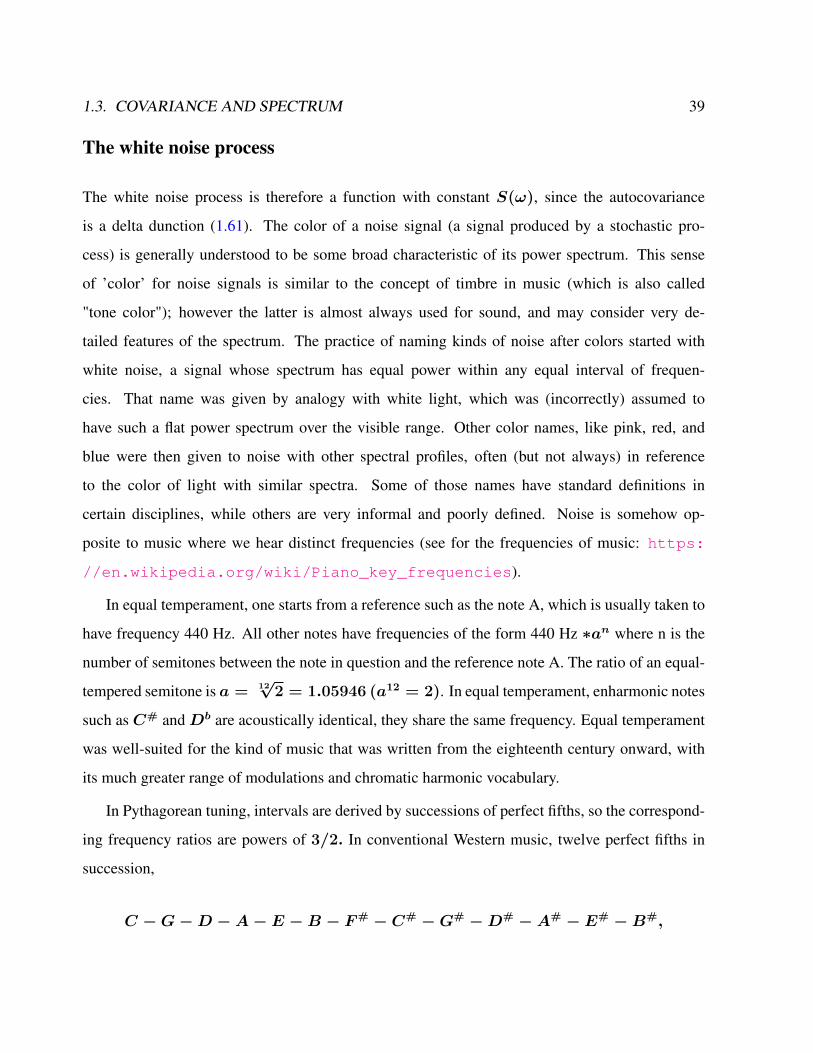
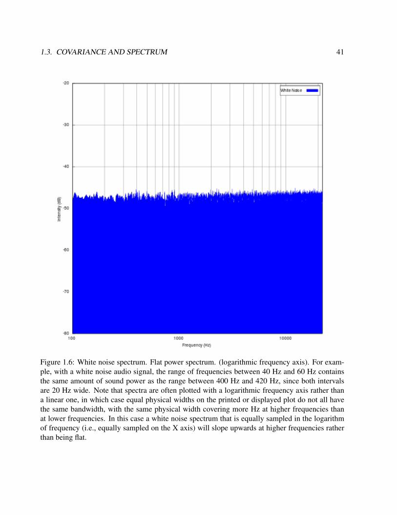
The white noise process
The white noise process is therefore a function with constant S(ω), since the autocovariance
is a delta dunction (1.61). The color of a noise signal (a signal produced by a stochastic pro-
cess) is generally understood to be some broad characteristic of its power spectrum. This sense
of ’color’ for noise signals is similar to the concept of timbre in music (which is also called
"tone color"); however the latter is almost always used for sound, and may consider very de-
tailed features of the spectrum. The practice of naming kinds of noise after colors started with
white noise, a signal whose spectrum has equal power within any equal interval of frequen-
cies. That name was given by analogy with white light, which was (incorrectly) assumed to
have such a flat power spectrum over the visible range. Other color names, like pink, red, and
blue were then given to noise with other spectral profiles, often (but not always) in reference
to the color of light with similar spectra. Some of those names have standard definitions in
certain disciplines, while others are very informal and poorly defined. Noise is somehow op-
posite to music where we hear distinct frequencies (see for the frequencies of music: https:
//en.wikipedia.org/wiki/Piano_key_frequencies).
In equal temperament, one starts from a reference such as the note A, which is usually taken to
have frequency 440 Hz. All other notes have frequencies of the form 440 Hz ∗an where n is the
number of semitones between the note in question and the reference note A. The ratio of an equal-
tempered semitone is a = 12√
2 = 1.05946 (a12 = 2). In equal temperament, enharmonic notes
such as C# andDb are acoustically identical, they share the same frequency. Equal temperament
was well-suited for the kind of music that was written from the eighteenth century onward, with
its much greater range of modulations and chromatic harmonic vocabulary.
In Pythagorean tuning, intervals are derived by successions of perfect fifths, so the correspond-
ing frequency ratios are powers of 3/2. In conventional Western music, twelve perfect fifths in
succession,
C −G−D −A− E −B − F# − C# −G# −D# −A# − E# −B#,
40 CHAPTER 1. INTRODUCTION AND PREPARATION
are supposed to equal seven octaves (C = B#). However, since (3/2)12 does not equal 27, twelve
Pythagorean perfect fifths give an interval slightly larger than seven octaves. The difference is a
small interval known as the Pythagorean comma, which corresponds to a ratio of (3/2)12 to 27 ≈
1.013643. The system of equal temperament gradually became adopted because it removed the
limitations on keys for modulation. The discrepancies between just and equaltempered intervals
are small and easily accepted by most listeners.
1.3. COVARIANCE AND SPECTRUM 41
Figure 1.6: White noise spectrum. Flat power spectrum. (logarithmic frequency axis). For exam-ple, with a white noise audio signal, the range of frequencies between 40 Hz and 60 Hz containsthe same amount of sound power as the range between 400 Hz and 420 Hz, since both intervalsare 20 Hz wide. Note that spectra are often plotted with a logarithmic frequency axis rather thana linear one, in which case equal physical widths on the printed or displayed plot do not all havethe same bandwidth, with the same physical width covering more Hz at higher frequencies thanat lower frequencies. In this case a white noise spectrum that is equally sampled in the logarithmof frequency (i.e., equally sampled on the X axis) will slope upwards at higher frequencies ratherthan being flat.
42 CHAPTER 1. INTRODUCTION AND PREPARATION
1.4 Transport phenomena
As preparation of the course, you may repeat several mathematical formulations. It is important
to notice that the fluid dynamical equations are generally formulated as a transport phenomenon.
An important relation is: if X is a quantity of a volume element which travels from position ~r to
~r + d~r in a time dt, the total differential dX is then given by:
dX =∂X
∂xdx+
∂X
∂ydy +
∂X
∂zdz +
∂X
∂tdt
⇒dX
dt=
∂X
∂xvx +
∂X
∂yvy +
∂X
∂zvz +
∂X
∂t(1.71)
This results in general to:dX
dt=∂X
∂t+ (~v · ∇)X .
From this follows that also holds:
d
dt
∫∫∫Xd3V =
∂
∂t
∫∫∫Xd3V +
∫∫©X(~v · ~n )d2A (1.72)
where the volume V is surrounded by surfaceA. Some properties of the∇ operator are:
div(φ~v ) = φdiv~v +∇φ · ~v rot(φ~v ) = φrot~v + (∇φ)× ~v rot∇φ = ~0
div(~u× ~v ) = ~v · (rot~u )− ~u · (rot~v ) rot rot~v = ∇ div~v −∇2~v div rotv = 0
div∇φ = ∇2φ ∇2~v ≡ (∇2v1,∇2v2,∇2v3)

1.4. TRANSPORT PHENOMENA 43
Here, ~v is an arbitrary vector field andφ an arbitrary scalar field. Some important integral theorems
are:Gauss:
∫∫© (~v · ~n )d2A =
∫∫∫(div~v )d3V
Stokes for a scalar field:∮
(φ · ~et)ds =
∫∫(~n×∇φ)d2A
Stokes for a vector field:∮
(~v · ~et)ds =
∫∫(rot~v · ~n )d2A
This results in:∫∫© (rot~v · ~n )d2A = 0
Ostrogradsky:∫∫© (~n× ~v )d2A =
∫∫∫(rot~v )d3A∫∫
© (φ~n )d2A =
∫∫∫(∇φ)d3V
Here, the orientable surface∫ ∫d2A is limited by the Jordan curve
∮ds.
Exercise 9 – Self test
1. Given
f(x, y, z, t) = x2 + y2 + z2 sin(ωt).
What are the partial derivatives with respect to the variables x and t?
2. What is the definition of ∇, Laplace, divergence, total (substantial) derivative, total differ-
ential for a function f(x, y, z, t)?
3. Calculate the rotation of∇f .
4. Given the function g(x) = ax2−3x4 +2x sin(αx), please provide the Taylor expansion
of g around x = 0 up to the 3rd order in x !
5. In the atmosphere, ocean, ice system, we are dealing with forces. Please list some relevant
real and apparent forces.
6. What is the differential equation describing radioactive decay? Please provide also the solu-
tion with initial condition x(t = 0) = x0. How is the half-life time defined?

44 CHAPTER 1. INTRODUCTION AND PREPARATION
7. The potential temperature of a parcel of fluid at pressure p is the temperature that the parcel
would acquire if adiabatically brought to a standard reference pressure p0, usually 100 kPa.
The potential temperature of air is often given by
Θ = T (p0/p)R/cp
where T is the current absolute temperature of the parcel, R is the gas constant of air, and cp
is the specific heat capacity at a constant pressure. κ = R/cp = 2/7 for an ideal diatomic
gas. For a constant lapse rate dTdz
= γ = const., why does the potential temperature Θ
increase with height? Hint: Atmospheric pressure decreases with height.
1.5 General form of wave equations
The general form of the wave equation is:
1
c2
∂2q
∂t2=∂2q
∂x2+∂2q
∂y2+∂2q
∂z2(1.73)
where q is the disturbance and c the propagation velocity. In general holds: c = νλ. By definition
holds: kλ = 2π and ω = 2πν. Therefore,
c = νλ = 2πν/k = ω/k . (1.74)
In principle, there are two types of waves:
1. Longitudinal waves: for these holds ~k ‖ ~c ‖ ~q. In a longitudinal wave the particle displace-
ment is parallel to the direction of wave propagation. The animation (http://www.acs.
psu.edu/drussell/Demos/waves/wavemotion.html) shows a one-dimensional
longitudinal plane wave propagating down a tube. The particles do not move down the tube
with the wave; they simply oscillate back and forth about their individual equilibrium po-
1.5. GENERAL FORM OF WAVE EQUATIONS 45
sitions. Pick a single particle and watch its motion. The wave is seen as the motion of the
compressed region (ie, it is a pressure wave), which moves from left to right. The second
animation shows the difference between the oscillatory motion of individual particles and
the propagation of the wave through the medium. The animation also identifies the regions
of compression and rarefaction.
2. Transversal waves: for these holds ~k ‖ ~c ⊥ ~q. In a transverse wave the particle displace-
ment is perpendicular to the direction of wave propagation. The animation (http://www.
acs.psu.edu/drussell/Demos/waves/wavemotion.html) below shows a one-
dimensional transverse plane wave propagating from left to right. The particles do not move
along with the wave; they simply oscillate up and down about their individual equilibrium
positions as the wave passes by. Pick a single particle and watch its motion. The S waves
(Secondary waves) in an earthquake are examples of Transverse waves. S waves propagate
with a velocity slower than P waves, arriving several seconds later.
3. Water waves: Water waves are an example of waves that involve a combination of both lon-
gitudinal and transverse motions. As a wave travels through the waver, the particles travel
in clockwise circles. The radius of the circles decreases as the depth into the water in-
creases. The animation (http://www.acs.psu.edu/drussell/Demos/waves/
wavemotion.html) below shows a water wave travelling from left to right in a region
where the depth of the water is greater than the wavelength of the waves. I have identified
two particles in yellow to show that each particle indeed travels in a clockwise circle as the
wave passes.
The phase velocity is given by
cph = ω/k . (1.75)
46 CHAPTER 1. INTRODUCTION AND PREPARATION
The group velocity is given by:
cg =dω
dk= cph + k
dcph
dk(1.76)
If cph does not depend on ω holds: cph = cg. In a dispersive medium it is possible that cg > cph
or cg < cph. If one wants to transfer information with a wave, e.g. by modulation of an electro-
magnetic wave, the information travels with the velocity at with a change in the electromagnetic
field propagates. This velocity is often almost equal to the group velocity.
For some media, the propagation velocity follows from:
• Pressure waves in a liquid or gas: c =√κ/%, where κ is the modulus of compression.
• For pressure waves in a gas also holds: c =√γp/% =
√γRT/M .
Plane waves
The equation for a harmonic traveling plane wave is
q(~x, t) = q cos(~k · ~x± ωt+ ϕ
).
When the situation is spherical or cylindrical symmetric, the the homogeneous wave equation can
be solved. When the situation is spherical symmetric, the homogeneous wave equation is given
by:1
c2
∂2(rq)
∂t2−∂2(rq)
∂r2= 0
with general solution:
q(r, t) = C1
f(r − ct)r
+ C2
g(r + ct)
r
When the situation has a cylindrical symmetry, the homogeneous wave equation becomes:
1
c2
∂2q
∂t2−
1
r
∂
∂r
(r∂q
∂r
)= 0
1.5. GENERAL FORM OF WAVE EQUATIONS 47
This is a Bessel equation, with solutions which can be written as Hankel functions. For sufficient
large values of r these are approximated by:
q(r, t) =q√r
cos(k(r ± vt))
If an observer is moving w.r.t. the wave with a velocity cobs, she/he will observe a change in
frequency: the Doppler effect. This is given by:ν
ν0
=cf − cobs
cf
.
The general solution in one dimension
Starting point is the equation:
∂2q(x, t)
∂t2=
N∑m=0
(bm
∂m
∂xm
)q(x, t)
where bm ∈ IR. Substituting q(x, t) = Aei(kx−ωt) gives two solutions ωj = ωj(k) as
dispersion relations. The general solution is given by:
q(x, t) =
∞∫−∞
(a(k)ei(kx−ω1(k)t) + b(k)ei(kx−ω2(k)t)
)dk
Because in general the frequencies ωj are non-linear in k there is dispersion and the solution
cannot be written any more as a sum of functions depending only on x ± ct: the wave front
transforms.
Chapter 2
General concepts
2.1 Programming with R
Install R
The latest version of R for Linux, OS X and Windows is freely available on the CRAN webpage:
http://cran.r-project.org (Fig. 2.1). Download and install the R version for your operating system
(for many linux distributions R is also available in the package management system).Furthermore,
look at the web page for R studio http://www.rstudio.com/, R studio is a free and open source user
interface for R. One particular package is Shiny. This makes it super simple for R users like you to
turn analyses into interactive web applications that anyone can use.
Examples to start
Please see the web page for some information how to get R running:
http://www.r-project.org/
http://www.awi.de/en/go/paleo/methods/r/
48

2.1. PROGRAMMING WITH R 49
Figure 2.1: R is available for download from the CRAN webpage: http://cran.r-project.org.
Using R for Introductory Statistics:
http://cran.r-project.org/doc/contrib/Verzani-SimpleR.pdf
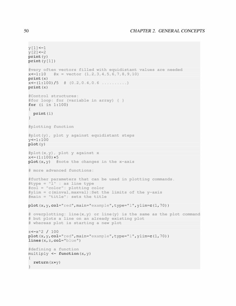
############# this letter is used for comments
#?function shows the help for a function?sin
#There is no definition needed for simple (scalar) variables#but instead of =, <- is used#just assign name<-valuea<-1
#Print the number on the screen:a #prints only on the consoleprint(a) #prints always
#simple algebraic calculationsa<-2*3a<-a/2print(a) # and print again
#some vector / array functions#vectors / arrays normally need to be defined that R can distinguish it#from a scalar.
y<-vector() #Produces an empty vector...
#the size of vectors in R is dynamic... I can now assign y[1]...#Assign elements of the vector [i], Vectors index are starting with 1
50 CHAPTER 2. GENERAL CONCEPTS
y[1]<-1y[2]<-2print(y)print(y[1])
#very often vectors filled with equidistant values are neededx<-1:10 #x = vector (1,2,3,4,5,6,7,8,9,10)print(x)x<-(1:100)/5 # (0.2,0.4,0.6 ..........)print(x)
#Control structures:#for loop: for (variable in array) for (i in 1:100)
print(i)
#plotting function
#plot(y), plot y against equidistant stepsy<-1:100plot(y)
#plot(x,y), plot y against xx<-(1:100)*5plot(x,y) #note the changes in the x-axis
# more advanced functions:
#further parameters that can be used in plotting commands.#type = "l" : as line type#col = "color": plotting color#ylim = c(minval,maxval):Set the limits of the y-axis#main = "title": sets the title
plot(x,y,col="red",main="example",type="l",ylim=c(1,70))
# overplotting: line(x,y) or line(y) is the same as the plot command# but plots a line on an already existing plot# whereas plot is starting a new plot
z<-x^2 / 100plot(x,y,col="red",main="example",type="l",ylim=c(1,70))lines(x,z,col="blue")
#defining a functionmultiply <- function(x,y)
return(x*y)

2.1. PROGRAMMING WITH R 51
print(multiply(3,4))
Reading and writing data
#Data Input from File, place file in dir. getwd()#Store a table from a text file in an R-variable DD<-read.table("test.txt",header=T)
# What read.table does is try to read data# from the file named as the first argument.# If header is specified as T (True),# the first line will be read as the column names# to which the values are assigned. Header defaults to F (False).# The function write.table() performs the opposite transformation.
#reading and writing datax<-(1:100)*5y<-x^2write.table(y,file="xytdata.dat") # writing
#dev.print(pdf, MyPlot.pdf)
1. Load a R file into the R workspace
2. Save the file using another name
3. Keep the original version when modifying the file
4. Execute the whole file (CTRL-A to mark everything, CTRL-R to run it)
5. All functions are then in the memory
Exercise 10 – Simple start of R
1. Download and install the R-Software. http://cran.r-project.org → Download CRAN →
search a city near you Choose your system (Windows / Mac / Linux) Follow the instruc-
tions.
52 CHAPTER 2. GENERAL CONCEPTS
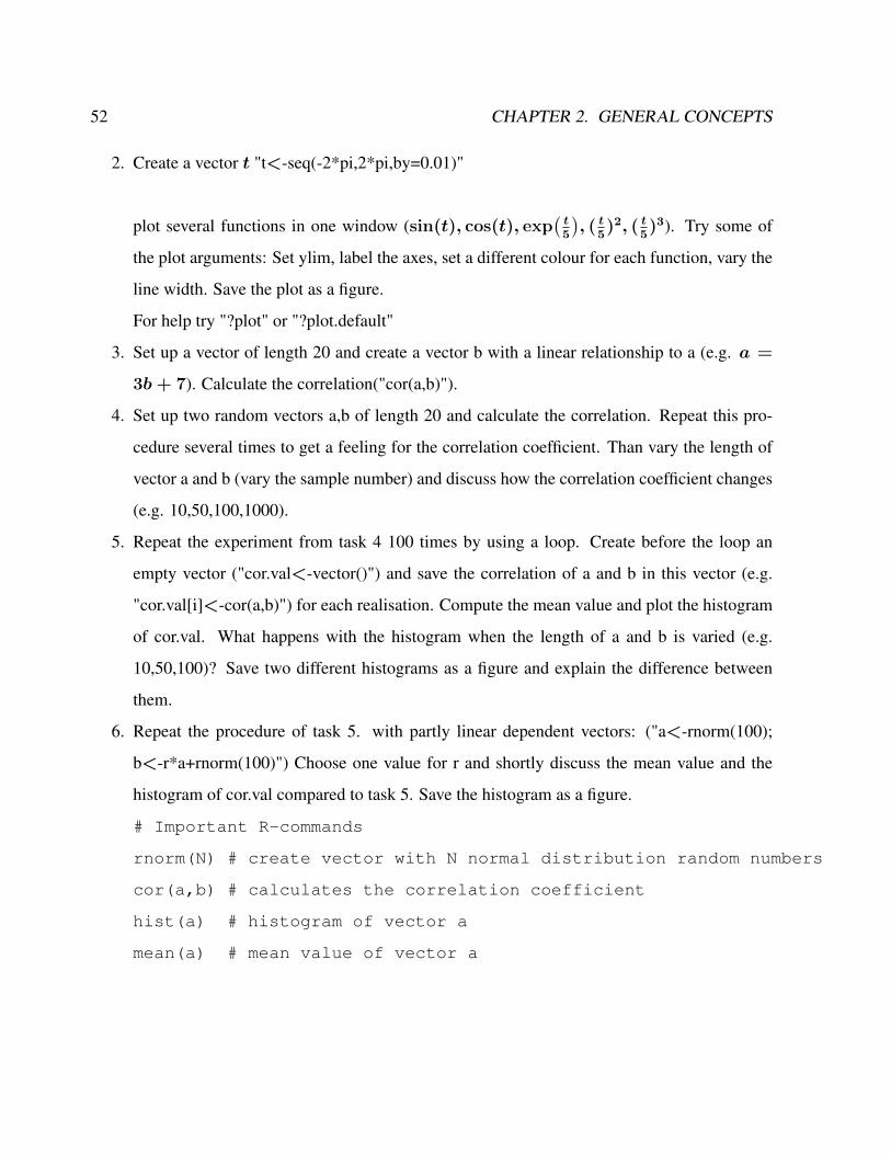
2. Create a vector t "t<-seq(-2*pi,2*pi,by=0.01)"
plot several functions in one window (sin(t), cos(t), exp(t5
), ( t
5)2, ( t
5)3). Try some of
the plot arguments: Set ylim, label the axes, set a different colour for each function, vary the
line width. Save the plot as a figure.
For help try "?plot" or "?plot.default"
3. Set up a vector of length 20 and create a vector b with a linear relationship to a (e.g. a =
3b+ 7). Calculate the correlation("cor(a,b)").
4. Set up two random vectors a,b of length 20 and calculate the correlation. Repeat this pro-
cedure several times to get a feeling for the correlation coefficient. Than vary the length of
vector a and b (vary the sample number) and discuss how the correlation coefficient changes
(e.g. 10,50,100,1000).
5. Repeat the experiment from task 4 100 times by using a loop. Create before the loop an
empty vector ("cor.val<-vector()") and save the correlation of a and b in this vector (e.g.
"cor.val[i]<-cor(a,b)") for each realisation. Compute the mean value and plot the histogram
of cor.val. What happens with the histogram when the length of a and b is varied (e.g.
10,50,100)? Save two different histograms as a figure and explain the difference between
them.
6. Repeat the procedure of task 5. with partly linear dependent vectors: ("a<-rnorm(100);
b<-r*a+rnorm(100)") Choose one value for r and shortly discuss the mean value and the
histogram of cor.val compared to task 5. Save the histogram as a figure.
# Important R-commands
rnorm(N) # create vector with N normal distribution random numbers
cor(a,b) # calculates the correlation coefficient
hist(a) # histogram of vector a
mean(a) # mean value of vector a

2.1. PROGRAMMING WITH R 53
# Helpful introductions to R can be found in e.g.
link to Rintro.pdf
link to http://cran.r-project.org/doc/manuals/R-intro.pdf
Exercise 11 – Logistic equation
As see in Fig. 2.10, the Lorenz system can exhibit chaotic behavior after a series of bifurca-
tions. This concept is known as the Feigenbaum cascade Feigenbaum [1980]. In this scenario the
solution undergoes a series of period-doublings, until the bifurcation parameter reaches a critical
value where the system has an accumulation point of period-doublings. Feigenbaum also found the
convergence behavior of the bifurcation points to the critical value. When the bifurcation parameter
passes this point, chaos appears. A simple system which has such a behavior is the logistic equa-
tion.. It is worth to analyze a one dimensional logistic equation (also known as Malthus-Verhulst
model), which was originally proposed to describe the evolution of a biological population. Let
x denote the number (or density) of individuals of a certain population. This number will change
due to growth, death, and competition. In the simplest version, birth and death rates are assumed
proportional to n,, but accounting for limited resources and competition it is modified by (1−x):
d
dtx(t) = a(1− x) x (2.1)
In climate, the logistic equation is also important for Lorenz’s error growth model [Lorenz, 1982]:
where x(t) is the algebraic forecast error at time t and a is the linear growth rate. Here, will
analyze a discrete version of the logistic equation.
1. Write a function which solves the logistic difference-equation xn+1 = rxn(1 − xn) and
returns the vector xn. Use an initial value x0 ∈ [0, 1], and a parameter-value r ∈ [1, 4].
2. Investigate the sensitivity of the solution on the parameter r (especially using r ∈ [3, 4]).
3. Now, investigate the solution dependence on r systematically: write a function which saves
the local extrema of a vector (fixed points) and returns them in a vector.
4. For each value of r, iterate the logistic difference equation 500 times, discard the first 200
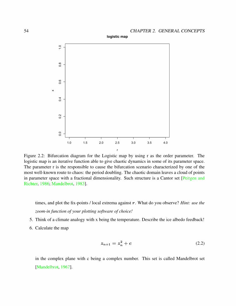
54 CHAPTER 2. GENERAL CONCEPTS
1.0 1.5 2.0 2.5 3.0 3.5 4.0
0.0
0.2
0.4
0.6
0.8
1.0
logistic map
r
x
Figure 2.2: Bifurcation diagram for the Logistic map by using r as the order parameter. Thelogistic map is an iterative function able to give chaotic dynamics in some of its parameter space.The parameter r is the responsible to cause the bifurcation scenario characterized by one of themost well-known route to chaos: the period doubling. The chaotic domain leaves a cloud of pointsin parameter space with a fractional dimensionality. Such structure is a Cantor set [Peitgen andRichter, 1986; Mandelbrot, 1983].
times, and plot the fix-points / local extrema against r. What do you observe? Hint: use the
zoom-in function of your plotting software of choice!
5. Think of a climate analogy with x being the temperature. Describe the ice albedo feedback!
6. Calculate the map
zn+1 = z2n + c (2.2)
in the complex plane with c being a complex number. This set is called Mandelbrot set
[Mandelbrot, 1967].
2.1. PROGRAMMING WITH R 55
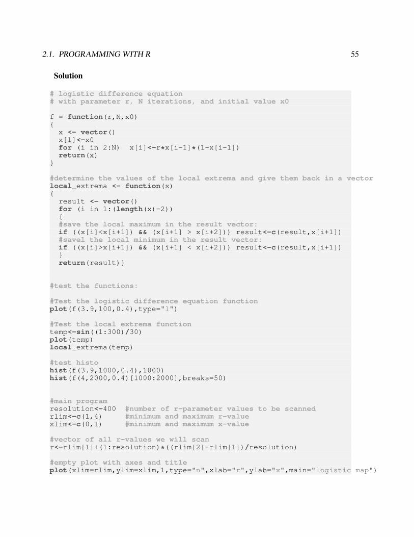
Solution
# logistic difference equation# with parameter r, N iterations, and initial value x0
f = function(r,N,x0)
x <- vector()x[1]<-x0for (i in 2:N) x[i]<-r*x[i-1]*(1-x[i-1])return(x)
#determine the values of the local extrema and give them back in a vectorlocal_extrema <- function(x)
result <- vector()for (i in 1:(length(x)-2))#save the local maximum in the result vector:if ((x[i]<x[i+1]) && (x[i+1] > x[i+2])) result<-c(result,x[i+1])#savel the local minimum in the result vector:if ((x[i]>x[i+1]) && (x[i+1] < x[i+2])) result<-c(result,x[i+1])return(result)
#test the functions:
#Test the logistic difference equation functionplot(f(3.9,100,0.4),type="l")
#Test the local extrema functiontemp<-sin((1:300)/30)plot(temp)local_extrema(temp)
#test histohist(f(3.9,1000,0.4),1000)hist(f(4,2000,0.4)[1000:2000],breaks=50)
#main programresolution<-400 #number of r-parameter values to be scannedrlim<-c(1,4) #minimum and maximum r-valuexlim<-c(0,1) #minimum and maximum x-value
#vector of all r-values we will scanr<-rlim[1]+(1:resolution)*((rlim[2]-rlim[1])/resolution)
#empty plot with axes and titleplot(xlim=rlim,ylim=xlim,1,type="n",xlab="r",ylab="x",main="logistic map")
56 CHAPTER 2. GENERAL CONCEPTS
for (i in 1:resolution)
temp<-f(r[i],300,0.5)[200:300]save<-local_extrema(temp)points(rep(r[i],length(save)),save,pch=".")
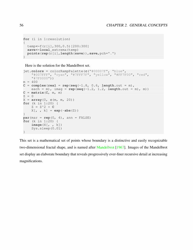
Here is the solution for the Mandelbrot set.jet.colors = colorRampPalette(c("#00007F", "blue",
"#007FFF", "cyan", "#7FFF7F", "yellow", "#FF7F00", "red","#7F0000"))
m = 400C = complex(real = rep(seq(-1.8, 0.6, length.out = m),
each = m), imag = rep(seq(-1.2, 1.2, length.out = m), m))C = matrix(C, m, m)Z = 0X = array(0, c(m, m, 20))for (k in 1:20)
Z = Z^2 + CX[, , k] = exp(-abs(Z))
par(mar = rep(0, 4), ann = FALSE)for (k in 1:20)
image(X[, , k])Sys.sleep(0.01)
This set is a mathematical set of points whose boundary is a distinctive and easily recognizable
two-dimensional fractal shape, and is named after Mandelbrot [1967]. Images of the Mandelbrot
set display an elaborate boundary that reveals progressively ever-finer recursive detail at increasing
magnifications.
2.1. PROGRAMMING WITH R 57
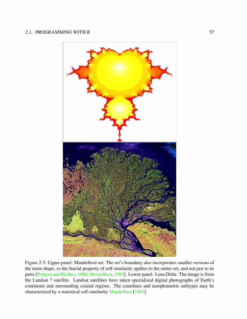
Figure 2.3: Upper panel: Mandelbrot set. The set’s boundary also incorporates smaller versions ofthe main shape, so the fractal property of self-similarity applies to the entire set, and not just to itsparts [Peitgen and Richter, 1986; Mandelbrot, 1983]. Lower panel: Lena Delta. The image is fromthe Landsat 7 satellite. Landsat satellites have taken specialized digital photographs of Earth’scontinents and surrounding coastal regions. The coastlines and morphometric subtypes may becharacterized by a statistical self-similarity Mandelbrot [1967].
58 CHAPTER 2. GENERAL CONCEPTS
Exercise 12 – Short programming questions
Write down the output for the following R-commands:
a) 0:10
b) a<-c(0,5,3,4); mean(a)
c) max(a)-min(a)
d) paste("The mean value of a is",mean(a),"for sure",sep="_")
e) a*2+c(1,1,1,0)
f) my.fun<-function(n)return(n*n+1)
my.fun(10)-my.fun(1)
2.2 Netcdf and climate data operators
NetCDF (Network Common Data Form) is a set of software libraries and self-describing, machine-
independent data formats that support the creation, access, and sharing of array-oriented scientific
data. The project homepage is hosted by the Unidata program at the University Corporation for
Atmospheric Research (UCAR). They are also the chief source of netCDF software, standards
development, updates etc. The format is an open standard.
The software libraries supplied by UCAR provide read-write access to netCDF files, encoding
and decoding the necessary arrays and metadata. The core library is written in C, and provides
an API for C, C++ and Fortran applications. An independent implementation, also developed
and maintained by Unidata, is written in 100% Java, which extends the core data model and adds
additional functionality. Interfaces to netCDF based on the C library are also available in other
languages including R (ncdf and ncvar packages), Perl, Python, Ruby, Matlab, IDL, and Octave.
A wide range of application software has been written which makes use of netCDF files. These
range from command line utilities to graphical visualization packages.
• A commonly used set of Unix command line utilities for netCDF files is the NetCDF Op-
erators (NCO) suite, which provide a range of commands for manipulation and analysis of
2.2. NETCDF AND CLIMATE DATA OPERATORS 59
netCDF files including basic record concatenating, slicing and averaging.
• NcBrowse is a generic netCDF file viewer that includes Java graphics, animations and 3D
visualizations for a wide range of netCDF file conventions.
• ncview is a visual browser for netCDF format files. Typically you would use ncview to get
a quick and easy, push-button look at your netCDF files. You can view simple movies of
the data, view along various dimensions, take a look at the actual data values, change color
maps, invert the data, etc.
• Panoply is a netCDF file viewer developed at the NASA Goddard Institute for Space Studies
which focuses on presentation of geo-gridded data. It is written in Java and thus platform
independent. Although its feature set overlaps with ncBrowse and ncview, Panoply is dis-
tinguished by offering a wide variety of map projections and ability to work with different
scale color tables.
• The NCAR Command Language is used to analyze and visualize data in netCDF files
(among other formats).
• PyNIO is a Python programming language module that allows read and/or write access to a
variety of data formats, including netCDF.
• Ferret is an interactive computer visualization and analysis environment designed to meet
the needs of oceanographers and meteorologists analyzing large and complex gridded data
sets. Ferret offers a Mathematica-like approach to analysis; new variables may be defined
interactively as mathematical expressions involving data set variables. Calculations may be
applied over arbitrarily shaped regions. Fully documented graphics are produced with a
single command.
• nCDF-Browser is a visual nCDF browser, written in the IDL programming language. Vari-
ables, attributes, and dimensions can be immediately downloaded to the IDL command line
60 CHAPTER 2. GENERAL CONCEPTS
for further processing. All the Coyote Library files necessary to run nCDF-Browser are
available in the zip file.
• ArcGIS version 9.2 supports netCDF files. The Multidimension Tools toolbox can be used to
create raster layers, feature layers, and table views from netCDF data in ArcMap, or convert
feature, raster, and table data to netCDF.
• Origin 8 imports netCDF files as matrix books where each book can hold a 4D array. Users
can select a subset of the imported data to make surface, controur or image plots.
• The Geospatial Data Abstraction Library provides support for read and write access to
netCDF data.
Exercise netcdf
In this exercise we will learn to know various helpful tools and techniques that are used in the
analysis and processing of climate data. First, we will learn to know the NetCDF file format in
a few short practical demonstrations. Second, some data analysis will be performed on available
gridded climate data. In a third step we will transfer our knowledge to shell-programming, in that
we combine a number of common command-line tools in order to solve a simple scientific problem.
To this end, a Linux-shell, in combination with common shell-programs, is necessary. Since not
every attendee of this course has such a computing environment available, the shell-program will
be demonstrated by the tutor.
Topics that this exercise considers are:
• Network Common Data Form (NetCDF): general information on the topic and how to use
NetCDF files
• Climate Data Operators (CDO): several examples of data reduction, analysis and transfor-
mation of NetCDF files, including operator piping

2.2. NETCDF AND CLIMATE DATA OPERATORS 61
• Bourne-again shell (Bash): definition of variables, if-then-else construct, checking for the
existence of a specific file, for-counter-loops, integer-arithmetic, pipes, initializing of shell
variables with program output, generation of strings via variable concatenation; these programming-
methods are illustrated at the example of a simple scientific model of sea-level rise
• Stream EDitor (SED): removing spaces from a string
• basic calculator (bc): simple floating-point arithmetic
In the following some information regarding tools and methods of this exercise is collected in
the form of a very general overview. This information collection is intended as a supplement to
the lecture. Few further information sources are listed in the subsection “Further Reading”. This
list is obviously far from being complete, there is a vast amount of freely-accessible information
available on-line.
A very precise definition on the characteristic and purpose of NetCDF is given in the NetCDF
FAQ, “What is netCDF?” (for a link, see section “Further Reading”):
“NetCDF (network Common Data Form) is a set of interfaces for array-oriented
data access and a freely distributed collection of data access libraries for C, Fortran,
C++, Java, and other languages. The netCDF libraries support a machine-independent
format for representing scientific data. Together, the interfaces, libraries, and format
support the creation, access, and sharing of scientific data.”
NetCDF is a data-container that has been established as a widely used file-standard in science
and engineering. It has been developed for storing array-oriented values in compact and inter-
changeable files. The most important characteristics of NetCDF files can as well be found in the
NetCDF FAQ, “What is netCDF?”. An excerpt, that highlights the advantages of NetCDF with
respect to this exercise, is listed here:
• Self-Describing. A NetCDF file includes a description of the data that it contains.
62 CHAPTER 2. GENERAL CONCEPTS
• Portable. A NetCDF file can be accessed by computers that apply different formats of storing
integers, characters, and floating-point numbers.
• Scalable. A small subset of a large dataset may be accessed efficiently.
• Appendable. Data may be appended to a properly structured NetCDF file without copying
the dataset or redefining its structure.
These characteristics make NetCDF a perfect choice for storing any kind of array-oriented data.
The data form that we will work with in this exercise is as well array-oriented - therefore, we will
use NetCDF as data container for both input and output of computations.
Since NetCDF is a binary format (in contrast to ASCII-text, which can be examined and edited
by means of any common text editor), reading, writing and changing of NetCDF files necessitates
the use of dedicated software. Fortunately, such software is freely available and can easily be
installed on any UNIX system. The following tools are of particular importance:
• ncview (lightweight but mighty explorer for NetCDF files)
• ncbrowse (a Java-based alternative to ncview for Windows)
• Panoply (a flexible Java-based generator of geographic maps of NetCDF data)
• ncdump (tool for “dumping” the contents of a NetCDF file to human-readable ASCII-text;
the complete description and structure of the NetCDF file is preserved)
• ncgen (complementary to ncdump, generates a binary NetCDF file from a NetCDF ASCII-
dump)
• ncks (mighty toolbox for modification of NetCDF files)
• cdo (mighty toolbox for analysis and modification of NetCDF files, strong focus on clima-
tological data)
2.2. NETCDF AND CLIMATE DATA OPERATORS 63
2.2.1 The Bash, a popular UNIX-Shell
Shells with their scripting ability are probably the most powerful tool of UNIX-systems, which
make UNIX-computers the choice for tackling complex scientific problems that involve the anal-
ysis and processing of large amounts of data. Particularly the bash-shell is a famous tool for sci-
entists and commonly used during the daily work routine. Yet, giving a comprehensive overview
on the use and ability of the bash clearly exceeds the scope of this course. Please refer to a bash-
scripting guide referenced below if you would like to gain further insights into the topic and gain
abilities in shell-scripting - and note: “... the only way to really learn scripting is to write scripts”
(Advanced Bash-Scripting Guide).
Further Reading
The following resources provide an introduction to tools and methods considered in this exercise:
• NetCDF: The NetCDF FAQ
(www.unidata.ucar.edu/software/netcdf/docs/faq.html)
The NetCDF Fact Sheet
(http://www.unidata.ucar.edu/publications/factsheets/current/netcdf_
factsheet.pdf)
• CDO: The CDO User’s Guide
(https://code.zmaw.de/projects/cdo/embedded/1.6.3/cdo.html)
The CDO Reference Card
(http://www.iac.ethz.ch/edu/courses/master/modules/radiation_and_
climate_change/download/cdo_refcard.pdf)
• Bash: Bash Guide for Beginners
(http://www.tldp.org/LDP/Bash-Beginners-Guide/html/)
Advanced Bash-Scripting Guide
(http://www.tldp.org/LDP/abs/html/)

64 CHAPTER 2. GENERAL CONCEPTS
Practical exercises for UNIX, cdo, netcdf
For those of you who consider to work in a scientific field with a strong focus on programming
or the analysis of large amounts of data: Consider to gain experience with a UNIX-environment,
e.g. Ubuntu. In many scientific fields, definitely in climate sciences, UNIX-like operating-systems
are the computing environments of choice. Many tools that are necessary for efficiently working
in such scientific fields are not natively available on Windows-systems; even if ports are available,
they may still suffer from limitations or incompatibilities. It definitely makes sense for you to
setup an own partition on your laptop with a Linux-system, and to learn how to use and program
the available software tools. For every free UNIX-environment (e.g. Ubuntu) and the included
software tools, a vast amount of detailed, yet free, documentation, addressing both novices and
experts, can be found on-line.
Visualizing the content of a NetCDF file
Among the provided data files you find a gridded global distribution of sea-ice concentration (vari-
able seaice) and surface temperature (variable tsurf) retrieved from a simulation with a compre-
hensive climate model (file INIOM_PD_3901-4000_tsurf_seaice.nc). NetCDF is a binary data
format that cannot be directly visualized with a simple text editor, special software exists for this
purpose. Windows-users please use the program ncbrowse, linux-users may alternatively use the
native Linux-tool ncview.
Please open the NetCDF file and visually inspect the content of variable tsurf. Try to generate
an animation of the time evolution of tsurf and answer the following questions:
• What obvious time-dependent pattern is visible?
• How can this pattern be explained, considering that you see the time evolution of a global
climatological field?
2.2. NETCDF AND CLIMATE DATA OPERATORS 65
Creating a PDF that visualizes a regional selection of the content of a NetCDF file
Now please visualize a global distribution of seaice also found in the provided NetCDF file INIOM_PD_3901-
4000_tsurf_seaice.nc. The software to be used for this task is panoply. Create two plots of Arctic
sea-ice distribution, from 45N to the North Pole, for March and September of model year 3911,
18:00:00. Apply a meaningful colorbar and export the figure to PDF. Answer the following ques-
tions:
• Where do you identify the southernmost extent of sea-ice in boreal winter?
• Where is the sea-ice retreat in summer, by visual inspection, most prominent?
Hint: You can create a map centered on the North Pole by applying a stereographic projection.
Identifying the spatial resolution and physical unit of a NetCDF data set
By use of the tool ncdump it is possible to generate a human-readable description of a NetCDF
file, that may also include the full data record. Sometimes you are only interested in the header
information, and do not want the data record to be extracted (extracting the data record to ASCII
can lead to HUGE dumps). If you have ncdump available, extract only the NetCDF data header
of file INIOM_PD_3901-4000_tsurf_seaice.nc. This can be done in a Linux shell-terminal via
entering the following command:
ncdump -h INIOM_PD_3901-4000_tsurf_seaice.nc > headerdump.nc#the parameter ’-h’ forces ncdump to omit the extensive data record#the character ’>’ is an output-redirection command, that makes sure that# the output produced by ncdump is written to a file (here: headerdump.nc)# rather then to the computer screen
Open the resulting file, or alternatively the file INIOM_PD_39010131_tsurf_seaice.nc.dump
that has been provided to you, in an arbitrary text-viewer or -editor, analyze the file content, and
answer the following questions:
66 CHAPTER 2. GENERAL CONCEPTS
• What is the horizontal data resolution in units of degrees? Hint: Calculate the meridional
(latitudinal) and zonal (longitudinal) resolution of the data set from the number of longi-
tudes and latitudes. Assume that grid cells are equally spaced, and the data set has a global
coverage.
• What is the physical unit of variable tsurf?
• If you analyze the header dump of the file INIOM_PD_3901-4000_tsurf_seaice.nc: What is
the time resolution of the data? Assume that the complete data set covers a time span of 100
calendar years.
2.2.2 Reducing data sets with CDO
While NetCDF defines a file format (and supporting programs and routines) that can store clima-
tological data in a practical way, the CDO are a collection of operators that allow analysis and
modification of gridded binary climatological data. In climate sciences, the CDO have become a
very common software tool due to the vast number of available operators and their flexibility:
• more than 400 designated operators are available
• operator-piping allows the application of complex methods on climatological data in a com-
pact way
• the CDO are command-line programs; in combination with shell-scripts they can be auto-
mated, and enhanced complexity of data processing and analysis may be achieved
CDO operator piping in combination with shell-programming can be demonstrated shortly in
the following very short bash-script, where two input files are interpolated to a common resolution,
the resulting fields are added, and the sum is time-averaged, the result being stored in a new file.
Shell-programming allows for the diagnostic output of additional information to the screen, here
the spatial-average of the field resulting from the CDO-operator-chain. You may find this code in
file fldmean.sh that is among the distributed files.
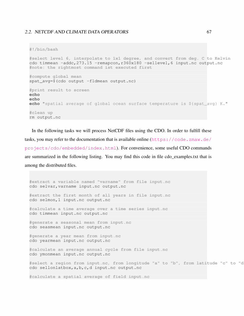
2.2. NETCDF AND CLIMATE DATA OPERATORS 67
#!/bin/bash
#select level 6, interpolate to 1x1 degree, and convert from deg. C to Kelvincdo timmean -addc,273.15 -remapcon,r360x180 -sellevel,6 input.nc output.nc#note: the rightmost command ist executed first
#compute global meanspat_avg=$(cdo output -fldmean output.nc)
#print result to screenechoechoecho "spatial average of global ocean surface temperature is $spat_avg K."
#clean uprm output.nc
In the following tasks we will process NetCDF files using the CDO. In order to fulfill these
tasks, you may refer to the documentation that is available online (https://code.zmaw.de/
projects/cdo/embedded/index.html). For convenience, some useful CDO commands
are summarized in the following listing. You may find this code in file cdo_examples.txt that is
among the distributed files.
#extract a variable named "varname" from file input.nccdo selvar,varname input.nc output.nc
#extract the first month of all years in file input.nccdo selmon,1 input.nc output.nc
#calculate a time average over a time series input.nccdo timmean input.nc output.nc
#generate a seasonal mean from input.nccdo seasmean input.nc output.nc
#generate a year mean from input.nccdo yearmean input.nc output.nc
#calculate an average annual cycle from file input.nccdo ymonmean input.nc output.nc
#select a region from input.nc, from longitude "a" to "b", from latitude "c" to "d"cdo sellonlatbox,a,b,c,d input.nc output.nc
#calculate a spatial average of field input.nc

68 CHAPTER 2. GENERAL CONCEPTS
cdo fldmean input.nc output.nc
#write the output of a CDO operator "a" to the screen (omits file output.nc)cdo output -a input.nc
#calculate the difference between two NetCDF files input1.nc and input2.nccdo sub input1.nc input2.nc output.nc
#multiply two fields input1.nc and input2.nccdo mul input1.nc input2.nc output.nc
#add a constant "a" to field input.nccdo addc,a input.nc output.nc
#select only regions of input2.nc, for which mask input1.nc is true (i.e. 1)#represents an if-then programming constructcdo ifthen input1.nc input2.nc output.nc
#use input2.nc, where mask input1.nc is true - otherwise use input3.nc#represents an if-then-else programming constructcdo ifthenelse input1.nc input2.nc input3.nc output.nc
#reduce a data range (a,b) in input.nc to the constant value "c"cdo setrtoc,a,b,c input.nc output.nc
#replace a data range (a,b) in input.nc by the missing value ("NaN")cdo setrtomiss,a,b input.nc output.nc
#calculate the trend of a time series in input.nc;#the trend is defined by offset "a" and slope "b" of the regression line;#"a" is stored in a.nc, "b" is stored in b.nccdo trend input.nc a.nc b.nc
#calculate the horizontal area covered by each grid cell of input.nccdo gridarea input.nc output.nc
Reducing NetCDF data sets
The file INIOM_PD_3901-4000_tsurf_seaice.nc contains two time series of climatological fields.
Reduce the NetCDF file by performing the following tasks using the CDO:
• Task 1: Split the data set in two separate data sets, one for variable tsurf, one for variable
seaice.
• Task 2: Calculate a time average over the full time period available in each of the separate
data sets created in Task 1.
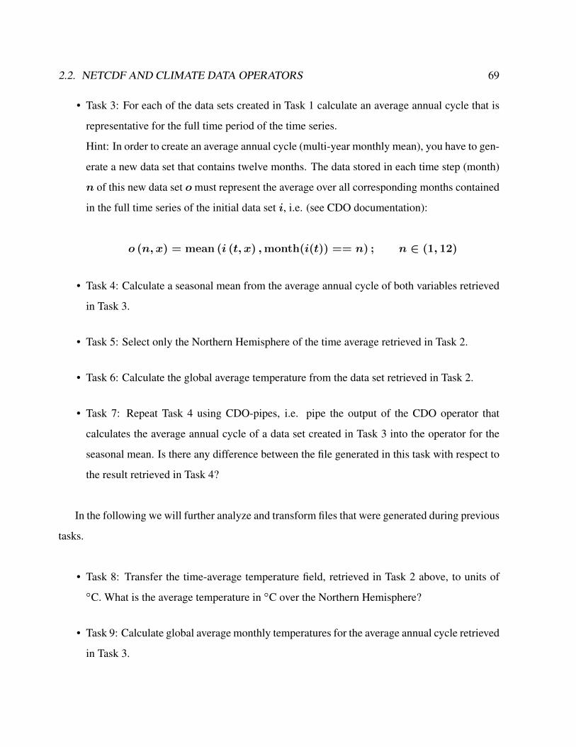
2.2. NETCDF AND CLIMATE DATA OPERATORS 69
• Task 3: For each of the data sets created in Task 1 calculate an average annual cycle that is
representative for the full time period of the time series.
Hint: In order to create an average annual cycle (multi-year monthly mean), you have to gen-
erate a new data set that contains twelve months. The data stored in each time step (month)
n of this new data set omust represent the average over all corresponding months contained
in the full time series of the initial data set i, i.e. (see CDO documentation):
o (n, x) = mean (i (t, x) ,month(i(t)) == n) ; n ∈ (1, 12)
• Task 4: Calculate a seasonal mean from the average annual cycle of both variables retrieved
in Task 3.
• Task 5: Select only the Northern Hemisphere of the time average retrieved in Task 2.
• Task 6: Calculate the global average temperature from the data set retrieved in Task 2.
• Task 7: Repeat Task 4 using CDO-pipes, i.e. pipe the output of the CDO operator that
calculates the average annual cycle of a data set created in Task 3 into the operator for the
seasonal mean. Is there any difference between the file generated in this task with respect to
the result retrieved in Task 4?
In the following we will further analyze and transform files that were generated during previous
tasks.
• Task 8: Transfer the time-average temperature field, retrieved in Task 2 above, to units ofC. What is the average temperature in C over the Northern Hemisphere?
• Task 9: Calculate global average monthly temperatures for the average annual cycle retrieved
in Task 3.
70 CHAPTER 2. GENERAL CONCEPTS
• Task 10: What is the global- and time-averaged temperature over land and ocean? As input
you may use the file generated in Task 2. You need to supply to CDO a mask that defines
distributions of land and ocean; use variable SLM of file T31GR30_jan_surf.nc.
• Task 11: What is the global average trend in the temperature time series created in Task 1?
• Task 12: Calculate the monthly average sea-ice cover in units of km2 in the Northern Hemi-
sphere. Use the average annual cycle of the sea-ice field generated in Task 3.
2.2.3 A simple model of sea level rise
In this task we will learn how shell-programming can help in solving scientific problems. We will,
based on simple assumptions, write a shell-script that generates a NetCDF data set of a rising sea
level, attributed to a loss of land ice, and produces a data set that illustrates the resulting continental
flooding. This shell-script can be considered as a very simplified model of continental flooding due
to sea-level rise. The only necessary input for this model is a global data set of surface elevation.
The world’s water is unevenly distributed among four major climate subsystems and three
different states of matter. Respective climate subsystems are the atmosphere (water vapor and
droplets, ice crystals), the ocean (liquid water and frozen, solid water), and the land surface (liq-
uid and solid water). The subsystem of the Earth composed of frozen water is commonly re-
ferred to as the Cryosphere. It includes permafrost, lake and river ice, sea ice, snow, glaciers,
ice caps and ice sheets. Within the Cryosphere, ice sheets are the largest storage of frozen wa-
ter. At present, there are two major ice-sheets, the Greenland Ice-Sheet (GIS) and the Antarctic
Ice-Sheet (AIS), containing water volumes of 7.3 m and 56.6 m sea level equivalent, respec-
tively (see Table 4.1 of the contribution of Working Group 1 to the Fourth Assessment Report by
the IPCC, page 342 of http://www.ipcc.ch/pdf/assessment-report/ar4/wg1/
ar4-wg1-chapter4.pdf). This means that, assumed both the GIS and the AIS melted com-
pletely, the global average sea level would rise by 63.9 m, leading to a flooding of large parts of
coastal regions, where 44% of humankind live.
2.2. NETCDF AND CLIMATE DATA OPERATORS 71
The relative volume distribution of water between the different physical states of matter (solid,
liquid, evaporated) depends on the average surface temperature of the Earth. There have been geo-
logic time scales that were much warmer than present, where virtually no ice sheets were available
(see e.g. Fig. 2 of Zachos et al., 2001, http://science.sciencemag.org/content/
292/5517/686.full). Anthropogenic emissions of, particularly, carbon dioxide, are expected
to increase the average surface temperature on Earth via a modification of the global radiative en-
ergy balance, since carbon dioxide in the atmosphere contributes to the so-called greenhouse ef-
fect (see the publication by Arrhenius, 1896, available at http://www.rsc.org/images/
Arrhenius1896_tcm18-173546.pdf). Due to global warming, the volume of water stored
in ice sheets will become smaller, and ultimately increase the volume of the global oceans, thus
causing sea level to rise.
Outline of the exercise Here, we develop a simple model of sea level rise which illustrates
regions of the earth that are flooded if the GIS and AIS melt. Our work employs command line
tools that are freely available and should be present on the computer of any scientist that performs
numerical modelling or substantial scientific data processing. If you run a linux system, these tools
should either already be available, or should be installted with a minimum amount of work.
As it is the case for any scientific model, which is per definition only an idealization of a natural
system, our methodology is based on several simplifications. First of all, it is assumed that the melt
process of available ice sheets is linear and occurs over a time period of 1000 y. Furthermore, we
do not apply a physical flow model that simulates water inflow from the coast, since such a model
can hardly be designed and formulated within the framework of this exercise. Instead, we will
calculate water height over land via subtracting the rising sea level from the global elevation field.
Negative values indicate the presence of water over land.
Our work depends on the availability of a gridded land elevation data set and a land-sea-mask
that separates the land surface into regions that belong to land and ocean. These data sets are also
the only input files that are necessary for our analysis. The files are taken from a set of boundary

72 CHAPTER 2. GENERAL CONCEPTS
conditions for numerical models of the circulation of the atmosphere. These have been derived
from global elevation data sets, that are commonly generated using modern satellite-based radar
interferometry, e.g. by the satellite system ICESat (icesat.gsfc.nasa.gov/icesat/).
For use in climate modelling, this data has been interpolated to the resolution of the climate model.
The orography in a climate model itself is therefore also a model - a model of the land surface
elevation, whose accuracy depends on the quality of the measurement and on the grid resolution
to which it is interpolated to. Higher resolution of the model grid means better agreement of the
gridded orography with the original high-resolution orography data set. The data set used here
originates from the boundary conditions of the Atmosphere General Circulation Model ECHAM5
at T63-resolution, which corresponds to a horizontal resolution of 1.9 by 1.9. Close to the
equator, this corresponds to roughly 200 km by 200 km per grid cell.
#!/bin/bash
#some definitions that control the scriptn_time_steps=1000 #number of time steps over which sea level risestime_unit=’1year’ #resolution of the time axistime_reference=’2000-01-01,00:00:00’ #reference time (first date) of the time axissea_level_start=0 #sea level ramp starts with elevation of 0 msea_level_end=75 #sea level ramp ends with elevation of 75 m
#definition of input filesorography_file=’data/orography.nc’lsm_file=’data/land_sea_mask.nc’
#definition of output filessea_level_output_file="sea_level_time_series.nc"flooding_file=’flooding_due_to_ice_melt.nc’
#clean up from (potential) previous runs of this scriptif [ -e $sea_level_output_file ]then
rm $sea_level_output_filefiif [ -e $flooding_file ]then
rm $flooding_filefi
#find minimum and maximum values of orography (necessary for file processing)min_val=$(cdo output -fldmin $orography_file | sed ’s/ //g’)max_val=$(cdo output -fldmax $orography_file | sed ’s/ //g’)

2.2. NETCDF AND CLIMATE DATA OPERATORS 73
#subtract / add small value from / to min_val and max_val in order to increase the#data range#(cdo setrtomiss, used below, does not include limits of the processed data range,#but we need to include these)min_val=$(echo "scale=3; $min_val-1" | bc)max_val=$(echo "scale=3; $max_val-1" | bc)
#generate a NetCDF file that contains n_time_steps, all values NaN;#this file will be used to generate a time-dependent sea level data set;#our approach, taking an existing NetCDF file and modifying it, saves#lots of tedious work in setting up a new NetCDF file from scratch,#which involves definition of dimensions, variables, and the definition of#links between thesefor ((i=0; i<$n_time_steps; i+=1))do
#generate n_time_steps copies of orography,#add a time axis, and replace all values by NaNecho "creating file timestep_$i.nc ..."cdo setrtomiss,$min_val,$max_val \
-settaxis,$time_reference,$time_unit \$orography_file timestep_$i.nc 2>/dev/null
done
#merge the above generated files to one NetCDF filecdo mergetime timestep_?.nc timestep_??.nc timestep_???.nc timeseries.nc
#set a proper time axis for the whole time seriescdo settaxis,$time_reference,$time_unit timeseries.nc timeseries_timeaxis.nc
#clean up temporary filesrm timestep_*.nc timeseries.nc
#run a loop that generates a linear sea level ramp, starting a sea_level_start#and ending at sea_level_endcurrent_sea_level=$sea_level_startfor ((i=0; i<$n_time_steps; i+=1))do
#redefine current_sea_level depending on the value of icurrent_sea_level=$(echo "scale=3; $sea_level_start+$sea_level_end*$i/($n_time_steps-1)" | bc)
#generate a three digit string of i containing a leading zero (for file names)if [ $i -le 9 ]thencounter_str="00$i"
elseif [ $i -le 99 ]then
counter_str="0$i"else
counter_str="$i"fi
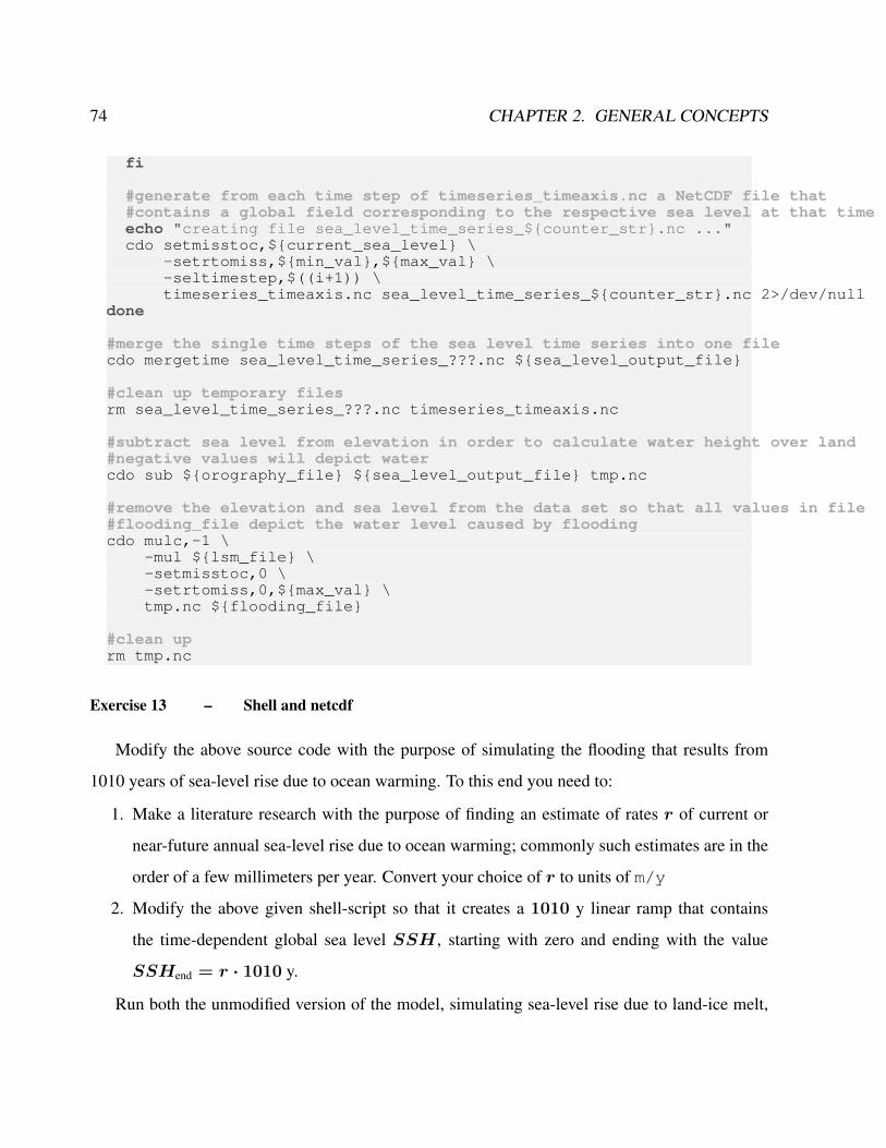
74 CHAPTER 2. GENERAL CONCEPTS
fi
#generate from each time step of timeseries_timeaxis.nc a NetCDF file that#contains a global field corresponding to the respective sea level at that timeecho "creating file sea_level_time_series_$counter_str.nc ..."cdo setmisstoc,$current_sea_level \
-setrtomiss,$min_val,$max_val \-seltimestep,$((i+1)) \timeseries_timeaxis.nc sea_level_time_series_$counter_str.nc 2>/dev/null
done
#merge the single time steps of the sea level time series into one filecdo mergetime sea_level_time_series_???.nc $sea_level_output_file
#clean up temporary filesrm sea_level_time_series_???.nc timeseries_timeaxis.nc
#subtract sea level from elevation in order to calculate water height over land#negative values will depict watercdo sub $orography_file $sea_level_output_file tmp.nc
#remove the elevation and sea level from the data set so that all values in file#flooding_file depict the water level caused by floodingcdo mulc,-1 \
-mul $lsm_file \-setmisstoc,0 \-setrtomiss,0,$max_val \tmp.nc $flooding_file
#clean uprm tmp.nc
Exercise 13 – Shell and netcdf
Modify the above source code with the purpose of simulating the flooding that results from
1010 years of sea-level rise due to ocean warming. To this end you need to:
1. Make a literature research with the purpose of finding an estimate of rates r of current or
near-future annual sea-level rise due to ocean warming; commonly such estimates are in the
order of a few millimeters per year. Convert your choice of r to units of m/y
2. Modify the above given shell-script so that it creates a 1010 y linear ramp that contains
the time-dependent global sea level SSH , starting with zero and ending with the value
SSHend = r · 1010 y.
Run both the unmodified version of the model, simulating sea-level rise due to land-ice melt,
2.2. NETCDF AND CLIMATE DATA OPERATORS 75
and the modified version of the model, simulating sea-level rise due to ocean warming.
Note: in order to execute a bash script “script.sh”, open a Linux shell-session, navigate to the
folder where the script is located, and execute the command “./script.sh”. You might have to
activate executable rights for this script by executing “chmod u+x script.sh” in advance.
Analyze and discuss your results:
1. Make a time-dependent analysis of the flooding that is predicted by this simple model of sea
level rise; you could, for example, generate plots of the flooding over land for two or three
interesting time steps that you select from the 1010 y time series.
2. Make a similar analysis for the sea level rise that is simulated by the unchanged original
shell-script, which considers melting of land-ice.
3. Compare the results of both analyses and discuss differences. Where are regions located,
where people should not live anymore in the future?
4. Make a critical analysis of the flooding simulated by this very simple model.
For the last point, these are questions that you might consider:
1. What are weak points of the simulation? Consider in your discussion the term “volume
conservation”, the stationarity of the applied sea level rise, and the spatial resolution of the
orographic data. How would you expect the simulated flooding to look like if the spatial
resolution of orography was higher?
2. The model, in its current version, has at least one dramatic flaw. Where is the simulated
flooding, that should only be attributed to water inflow from the ocean, obviously wrong?
What is the reason for the erroneous result?
3. Could you imagine what additional physical processes a corrected version of the model
would need to contain in order to avoid the identified problem? Give a short description of
your ideas, maybe illustrate them with some sketches.
Exercise 14 – Evaluate possible zones of wine production and climatic conditions
For wine production there exists some empirical laws:
76 CHAPTER 2. GENERAL CONCEPTS
Northern Hemisphere: degree of latitude 40 – 50
Southern Hemisphere: degree of latitude 30 – 40
The climatic demands are:
1. Vegetation period 180 – 250 days (days with daily mean> 5 C)
2. Mean temperature 9 C– 21 C
3. White wines optimal annual mean temperature 9.5–11.5 C
4. Red Wines optimal annual mean temperature 10.5–13 C
5. Sunshine hours per year: 1500–2000 h
6. Precipitation 480 mm–700 mm
Task: Please calculate the possible zones of red wine production using 4 and 6 using tempera-
ture and precipitation constraints. The resulting figure should be similar to Fig. 2.4. Here are the
links for getting the CRU surface temperature:
http://climexp.knmi.nl//CRUData/cru_ts3.23.1901.2014.tmp.dat_1.nc
and precipitation data:
http://climexp.knmi.nl//CRUData/cru_ts3.23.1901.2014.pre.dat_1.nc
Choose two different reference periods: 1901-1920 and 1991-2010
Calculate furthermore the zones for future scenarios (RCP4.5 and RCP8) for the years 2081-
2100. Data are accessible here:
http://cmip-pcmdi.llnl.gov/cmip5/data_getting_started.html.
For this, choose one particular model and compare the zones with a reference period using the
same model (e.g., 1960-1980). Some people could speculate that the alcohol belts (Fig. 2.5) may
be shifting under global warming. Can this be substantiated by your results?
Hint: use the cdo commands from the lecture!

2.2. NETCDF AND CLIMATE DATA OPERATORS 77
Figure 2.4: Zones of todays wine production.
Figure 2.5: Alcohol belts in Europe.
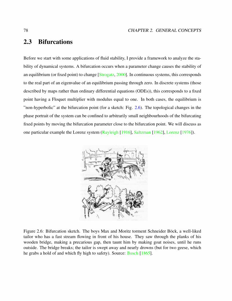
78 CHAPTER 2. GENERAL CONCEPTS
2.3 Bifurcations
Before we start with some applications of fluid stability, I provide a framework to analyze the sta-
bility of dynamical systems. A bifurcation occurs when a parameter change causes the stability of
an equilibrium (or fixed point) to change [Strogatz, 2000]. In continuous systems, this corresponds
to the real part of an eigenvalue of an equilibrium passing through zero. In discrete systems (those
described by maps rather than ordinary differential equations (ODEs)), this corresponds to a fixed
point having a Floquet multiplier with modulus equal to one. In both cases, the equilibrium is
”non-hyperbolic” at the bifurcation point (for a sketch: Fig. 2.6). The topological changes in the
phase portrait of the system can be confined to arbitrarily small neighbourhoods of the bifurcating
fixed points by moving the bifurcation parameter close to the bifurcation point. We will discuss as
one particular example the Lorenz system (Rayleigh [1916], Saltzman [1962], Lorenz [1976]).
Figure 2.6: Bifurcation sketch. The boys Max and Moritz torment Schneider Böck, a well-likedtailor who has a fast stream flowing in front of his house. They saw through the planks of hiswooden bridge, making a precarious gap, then taunt him by making goat noises, until he runsoutside. The bridge breaks; the tailor is swept away and nearly drowns (but for two geese, whichhe grabs a hold of and which fly high to safety). Source: Busch [1865].
2.3. BIFURCATIONS 79
2.3.1 Linear stability analysis
Consider the continuous dynamical system described by the ODE
x = f(x, λ) f : Rn × R→ Rn. (2.3)
A bifurcation occurs at (x0, λ0) if the Jacobian matrix dfx0,λ0 has an Eigenvalue with zero real
part. If the eigenvalue is equal to zero, the bifurcation is a steady state bifurcation, but if the
eigenvalue is non-zero but purely imaginary, this is a Hopf bifurcation.
For discrete dynamical systems, consider the system
xn+1 = f(xn, λ) . (2.4)
Then a local bifurcation occurs at (x0, λ0) if the matrix dfx0,λ0 has an eigenvalue with modulus
equal to one. If the eigenvalue is equal to one, the bifurcation is either a saddle-node (often called
fold bifurcation in maps), transcritical or pitchfork bifurcation. If the eigenvalue is equal to−1, it
is a period-doubling (or flip) bifurcation, and otherwise, it is a Hopf bifurcation.
Examples of bifurcations include [Strogatz, 2000]:
• A transcritical bifurcation is one in which a fixed point exists for all values of a parameter
and is never destroyed. However, such a fixed point interchanges its stability with another
fixed point as the parameter is varied. The normal form of a transcritical bifurcation is
dx
dt= rx− x2. (2.5)
This equation is similar to logistic equation but in this case we allow r and x to be positive or
negative. The two fixed points are at x = 0 and x = r. When the parameter r is negative,
the fixed point at x = 0 is stable and the fixed point x = r is unstable. But for r > 0,
the point at x = 0 is unstable and the point at x = r is stable. So the bifurcation occurs at
r = 0.
80 CHAPTER 2. GENERAL CONCEPTS
• A ”’saddle-node bifurcation”’ is a bifurcation in which two fixed points collide and anni-
hilate each other. If the phase space is one-dimensional, one of the equilibrium points is
unstable (the saddle), while the other is stable (the node). The normal form of a saddle-node
bifurcation is:
dx
dt= r + x2 (2.6)
Here x is the state variable and r is the bifurcation parameter. If r < 0 there are two
equilibrium points, a stable equilibrium point at −√−r and an unstable one at +
√−r.
At r = 0 (the bifurcation point) there is exactly one equilibrium point. At this point the
fixed point is no longer hyperbolic. In this case the fixed point is called a saddle-node fixed
point. If r > 0 there are no equilibrium points. Saddle-node bifurcations may be associated
with hysteresis loops. The term ’saddle-node bifurcation’ is most often used in reference to
continuous dynamical systems. In discrete dynamical systems, the same bifurcation is often
instead called a ”’fold bifurcation”’.
• A Hopf is a bifurcation in which a fixed point of a dynamical system loses stability as a pair
of complex conjugate eigenvalues of the linearization around the fixed point cross the imag-
inary axis of the complex plane. In a bifurcation, a small-amplitude limit cycle branching
from the fixed point. The normal form of a Hopf bifurcation is:
dz
dt= z((λ+ i) + b|z|2), (2.7)
where z, b are both complex and λ is a parameter. Write b = α + iβ. The number ’α is
called the first Lyapunov coefficient. If α is negative then there is a stable limit cycle for
λ > 0 :
z(t) = reiωt (2.8)

2.3. BIFURCATIONS 81
where
r =√−λ/α and ω = 1 + βr2. (2.9)
The bifurcation is then called ”’supercritical.”’ If α is positive then there is an unstable limit
cycle for λ < 0. The bifurcation is called ”’subcritical.”’
• Pitchfork bifurcations occur generically in systems with symmetry. Pitchfork bifurcations,
like Hopf bifurcations have two types - supercritical or subcritical. The normal form of the
supercritical pitchfork bifurcation is
dx
dt= rx− x3. (2.10)
For negative values of r, there is one stable equilibrium at x = 0. For r > 0 there is an
unstable equilibrium at x = 0, and two stable equilibria at x = ±√r. The normal form
for the subcritical case is dx
dt= rx+ x3. (2.11)
In this case, for r < 0 the equilibrium at x = 0 is stable, and there are two unstable
equilbria at x = ±√−r. For r > 0 the equilibrium at x = 0 is unstable.
For computational methods to obtain bifurcations: [Doedel et al., 1997; Kuznetsov, 1998].
Exercise 15 – Graphical method for bifurcations
We introduce a graphical method to obtain stability or instability. Consider the ”’saddle-node
bifurcation”’, one of the equilibrium points is unstable (the saddle), while the other is stable (the
node). In Fig. 2.7, we can plot dxdt
= f(x) dependent on x (left panel) for
dx
dt= b+ x2 (2.12)
with b < 0 in this particular case (For b > 0 we would have no equilibrium, and we have no
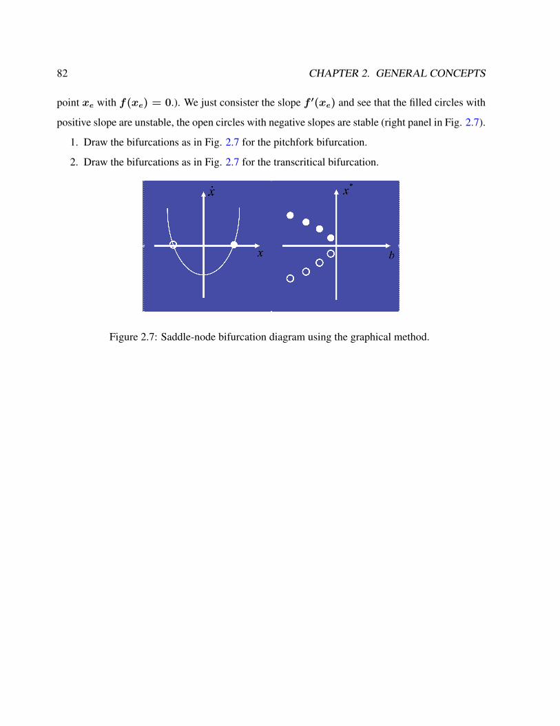
82 CHAPTER 2. GENERAL CONCEPTS
point xe with f(xe) = 0.). We just consister the slope f ′(xe) and see that the filled circles with
positive slope are unstable, the open circles with negative slopes are stable (right panel in Fig. 2.7).
1. Draw the bifurcations as in Fig. 2.7 for the pitchfork bifurcation.
2. Draw the bifurcations as in Fig. 2.7 for the transcritical bifurcation.
Figure 2.7: Saddle-node bifurcation diagram using the graphical method.
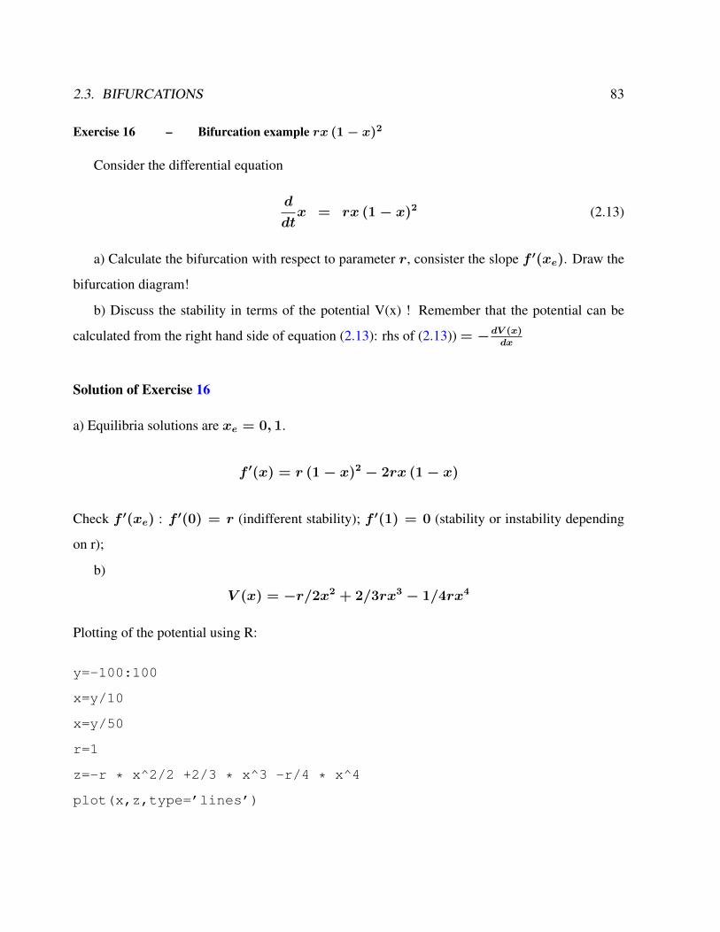
2.3. BIFURCATIONS 83
Exercise 16 – Bifurcation example rx (1− x)2
Consider the differential equation
d
dtx = rx (1− x)2 (2.13)
a) Calculate the bifurcation with respect to parameter r, consister the slope f ′(xe). Draw the
bifurcation diagram!
b) Discuss the stability in terms of the potential V(x) ! Remember that the potential can be
calculated from the right hand side of equation (2.13): rhs of (2.13)) = −dV (x)
dx
Solution of Exercise 16
a) Equilibria solutions are xe = 0, 1.
f ′(x) = r (1− x)2 − 2rx (1− x)
Check f ′(xe) : f ′(0) = r (indifferent stability); f ′(1) = 0 (stability or instability depending
on r);
b)
V (x) = −r/2x2 + 2/3rx3 − 1/4rx4
Plotting of the potential using R:
y=-100:100
x=y/10
x=y/50
r=1
z=-r * x^2/2 +2/3 * x^3 -r/4 * x^4
plot(x,z,type=’lines’)
84 CHAPTER 2. GENERAL CONCEPTS
2.3.2 Population Dynamics
Exercise 17 – Population Dynamics
Consider population dynamics with population x > 0 and reproduction (birth-death) r:
d
dtx = r(x)x (2.14)
1. Solve the differential equation for r = r0 = const.! What happens for t → ∞ when
r0 > 0 or r0 < 0 ?
2. Solve the differential equation for r = r0(1 − x)! (limited growth)! What happens for
t→∞?
3. Consider the case r = r0(1− x/K) withK > 0 ! Give a physical interpretation forK!
Solution of Population Dynamics
Solve for r(x) = r0 using separation of variables:
dx
dt=r0x∫
dx
x=
∫r0dt
ln(x) =r0t+A′
=⇒ x =Aer0t with A = eA′
with limt→∞
x =
∞ , r0 > 0
0 , r0 < 0
2.3. BIFURCATIONS 85
Solve for r(x) = r0(1− x) using separation of variables:
dx
dt=r0(1− x)x
dx
x(1− x)=r0dt∫ (
1
x+
1
1− x
)dx =
∫r0dt
ln(x)− ln(1− x) =r0t+A′
=⇒ x =Aer0t
1 +Aer0twith A = eA
′
and the limiting cases limt→∞
x =
1 , r0 > 0
0 , r0 < 0
Consider r(x) = r0
(1− x
K
)with K > 0. Analogous procedure results then in a similar
solution with an additional scaling factorK which provides an upper limit for any population.
dx
dt=r0(1−
x
K)x
...
=⇒ x =KAer0t
1 +Aer0t
with limt→∞
x =
K , r0 > 0
0 , r0 < 0
Exercise 18 – Difference equations
Consider the discretised form of (2.14) with r = r0(1− x). Using the Euler scheme
d
dtx ≈
xn+1 − xn∆t
. (2.15)
86 CHAPTER 2. GENERAL CONCEPTS
1. Write down the iteration xn+1 as a function of xn for the case 1a!
2. What is the solution of xn+1 as a function of x0? Consider the stability for the cases r > 0,
0 > ∆t r > −1, −1 > ∆t r > −2, −2 > ∆t r . Do you have a graphical
interpretation of the oscillation/decay?
3. Write down the iteration xn+1 as a function of xn for the case 1b!
Exercise 19 – Bifurcation of the logistic equation
1. Consider the system (2.14) r = r0(1 − x). Calculate the bifurcation with respect to
parameter r!
Draw the bifurcation diagram!
2. as in 1., but for
d
dtx = r0 + x2 (2.16)
3. as in 1., but for
d
dtx = x
√(r0 + x)2 (2.17)
Solution of Bifurcation of the logistic equation
Given the logistic equation
f(x) ≡dx
dt= r0x(1− x)
=⇒ f ′(x) =r0 − 2r0x
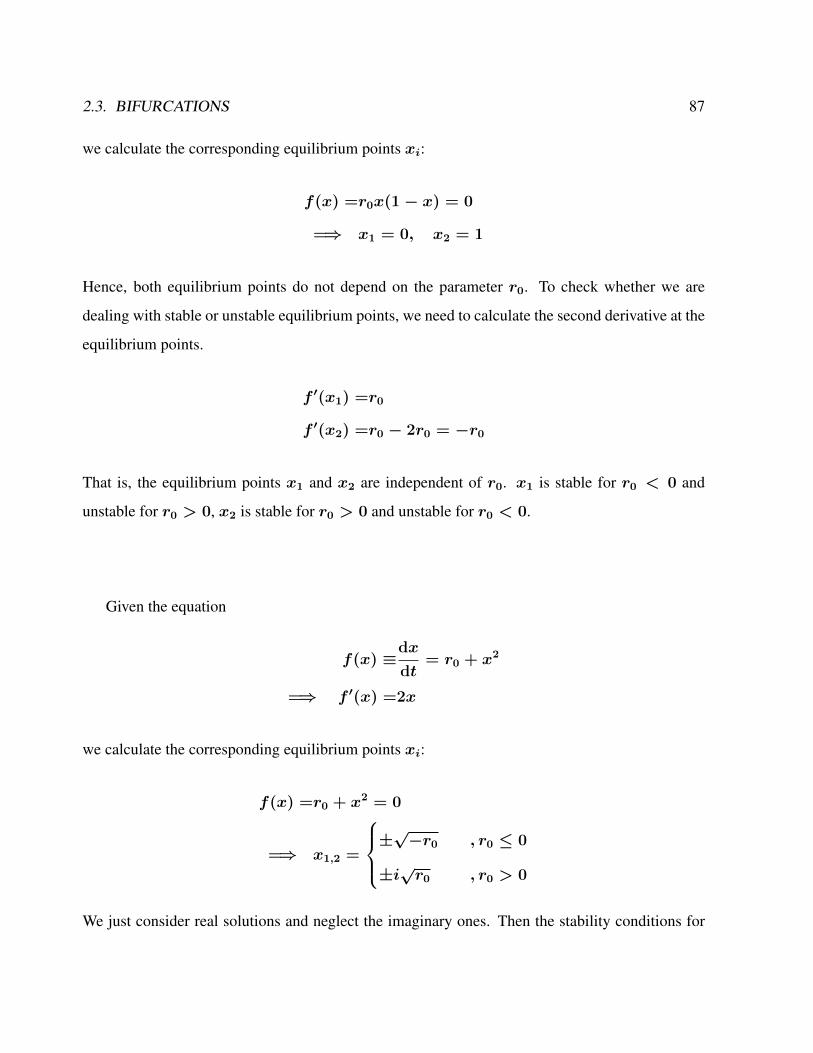
2.3. BIFURCATIONS 87
we calculate the corresponding equilibrium points xi:
f(x) =r0x(1− x) = 0
=⇒ x1 = 0, x2 = 1
Hence, both equilibrium points do not depend on the parameter r0. To check whether we are
dealing with stable or unstable equilibrium points, we need to calculate the second derivative at the
equilibrium points.
f ′(x1) =r0
f ′(x2) =r0 − 2r0 = −r0
That is, the equilibrium points x1 and x2 are independent of r0. x1 is stable for r0 < 0 and
unstable for r0 > 0, x2 is stable for r0 > 0 and unstable for r0 < 0.
Given the equation
f(x) ≡dx
dt= r0 + x2
=⇒ f ′(x) =2x
we calculate the corresponding equilibrium points xi:
f(x) =r0 + x2 = 0
=⇒ x1,2 =
±√−r0 , r0 ≤ 0
±i√r0 , r0 > 0
We just consider real solutions and neglect the imaginary ones. Then the stability conditions for
88 CHAPTER 2. GENERAL CONCEPTS
the equilibrium points are given by
f ′(x1) =2√−r0
< 0 stable
≥ 0 unstable
f ′(x2) =− 2√−r0
< 0 stable
≥ 0 unstable
From the condition r0 ≤ 0 follows that x1 is always unstable and x2 is always stable. For the
special case r0 = 0 there is just one equilibrium point x1 = 0 which is unstable as well.
Given the equation
f(x) ≡dx
dt= x
√(r0 + x)2 =
x(r0 + x) , x ≥ −r0
−x(r0 + x) , x < −r0
=⇒ f ′(x) =
r0 + 2x , x > −r0
−r0 − 2x , x < −r0
not defined , x = −r0
we calculate the corresponding equilibrium points xi:
f(x) =x√
(r0 + x)2 = 0
=⇒ x1 = 0, x2 = −r0
Since for x2 = −r0 the derivative f ′(x) does not exist, we need to treat both cases of a small
deviation δ > 0 from the equilibrium point x2 to each side separately. The stability conditions

2.3. BIFURCATIONS 89
then yield:
f ′(x1) =
r0 , x1 = 0 > −r0 ⇒ r0 > 0 ⇒ unstable
−r0 , x1 = 0 < −r0 ⇒ r0 < 0 ⇒ unstable
f ′(x2 + δ) = −r0 + δ ⇒
stable , r0 > 0
unstable , r0 < 0
f ′(x2 − δ) = r0 − δ ⇒
unstable , r0 > 0
stable , r0 < 0
Exercise 20 – Bifurcation of the logistic map
1. Write a function which solves the logistic difference equation xn+1 = axn(1 − xn) and
returns the vector x(n). Use an initial value x0 ∈ [0, 1], and a parameter value a ∈ [1, 4]
2. Investigate the sensitivity of solution on the parameter a (especially using a ∈ [3, 4])
3. Now investigate the solutions dependent on r systematically: write a function which saves
the local extrema of a vector (fixed points) and returns them in a vector.
4. For each value of a, iterate the logistic difference equation 500 times, discard the first 200
times, and plot the fix-points/local extrema against a. What do you see? Zoom into the plot!
Solution: Bifurcation of the logistic map
#logistic difference equation,#with parameter a, N iterations, and initial value x0f = function(r,N,x0)
x <- vector()x[1]<-x0for (i in 2:N) x[i]<-a*x[i-1]*(1-x[i-1])
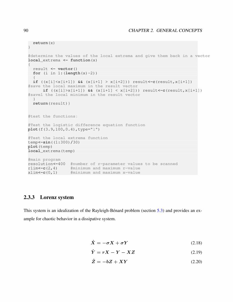
90 CHAPTER 2. GENERAL CONCEPTS
return(x)
#determine the values of the local extrema and give them back in a vectorlocal_extrema <- function(x)
result <- vector()for (i in 1:(length(x)-2))if ((x[i]<x[i+1]) && (x[i+1] > x[i+2])) result<-c(result,x[i+1])
#save the local maximum in the result vectorif ((x[i]>x[i+1]) && (x[i+1] < x[i+2])) result<-c(result,x[i+1])
#savel the local minimum in the result vectorreturn(result)
#test the functions:
#Test the logistic difference equation functionplot(f(3.9,100,0.4),type="l")
#Test the local extrema functiontemp<-sin((1:300)/30)plot(temp)local_extrema(temp)
#main programresolution<-400 #number of r-parameter values to be scannedrlim<-c(2,4) #minimum and maximum r-valuexlim<-c(0,1) #minimum and maximum x-value
2.3.3 Lorenz system
This system is an idealization of the Rayleigh-Bénard problem (section 5.3) and provides an ex-
ample for chaotic behavior in a dissipative system.
X = −σX + σY (2.18)
Y = rX − Y −XZ (2.19)
Z = −bZ +XY (2.20)
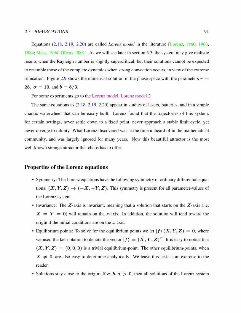
2.3. BIFURCATIONS 91
Equations (2.18, 2.19, 2.20) are called Lorenz model in the literature [Lorenz, 1960, 1963,
1984; Maas, 1994; Olbers, 2001]. As we will see later in section 5.3, the system may give realistic
results when the Rayleigh number is slightly supercritical, but their solutions cannot be expected
to resemble those of the complete dynamics when strong convection occurs, in view of the extreme
truncation. Figure 2.9 shows the numerical solution in the phase-space with the parameters r =
28, σ = 10, and b = 8/3.
For some experiments go to the Lorenz model, Lorenz model 2
The same equations as (2.18, 2.19, 2.20) appear in studies of lasers, batteries, and in a simple
chaotic waterwheel that can be easily built. Lorenz found that the trajectories of this system,
for certain settings, never settle down to a fixed point, never approach a stable limit cycle, yet
never diverge to infinity. What Lorenz discovered was at the time unheard of in the mathematical
community, and was largely ignored for many years. Now this beautiful attractor is the most
well-known strange attractor that chaos has to offer.
Properties of the Lorenz equations
• Symmetry: The Lorenz equations have the following symmetry of ordinary differential equa-
tions: (X,Y, Z) → (−X,−Y, Z). This symmetry is present for all parameter-values of
the Lorenz system.
• Invariance: The Z-axis is invariant, meaning that a solution that starts on the Z-axis (i.e.
X = Y = 0) will remain on the z-axis. In addition, the solution will tend toward the
origin if the initial conditions are on the z-axis.
• Equilibrium points: To solve for the equilibrium points we let |f〉 (X,Y, Z) = 0, where
we used the ket-notation to denote the vector |f〉 = (X, Y , Z)T . It is easy to notice that
(X,Y, Z) = (0, 0, 0) is a trivial equilibrium-point. The other equilibrium-points, when
X 6= 0, are also easy to determine analytically. We leave this task as an exercise to the
reader.
• Solutions stay close to the origin: If σ, b, a > 0, then all solutions of the Lorenz system
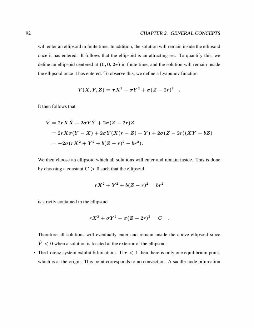
92 CHAPTER 2. GENERAL CONCEPTS
will enter an ellipsoid in finite time. In addition, the solution will remain inside the ellipsoid
once it has entered. It follows that the ellipsoid is an attracting set. To quantify this, we
define an ellipsoid centered at (0, 0, 2r) in finite time, and the solution will remain inside
the ellipsoid once it has entered. To observe this, we define a Lyapunov function
V (X,Y, Z) = τX2 + σY 2 + σ(Z − 2r)2 .
It then follows that
V = 2rXX + 2σY Y + 2σ(Z − 2r)Z
= 2rXσ(Y −X) + 2σY (X(r − Z)− Y ) + 2σ(Z − 2r)(XY − bZ)
= −2σ(rX2 + Y 2 + b(Z − r)2 − br2).
We then choose an ellipsoid which all solutions will enter and remain inside. This is done
by choosing a constant C > 0 such that the ellipsoid
rX2 + Y 2 + b(Z − r)2 = br2
is strictly contained in the ellipsoid
rX2 + σY 2 + σ(Z − 2r)2 = C .
Therefore all solutions will eventually enter and remain inside the above ellipsoid since
V < 0 when a solution is located at the exterior of the ellipsoid.
• The Lorenz system exhibit bifurcations. If r < 1 then there is only one equilibrium point,
which is at the origin. This point corresponds to no convection. A saddle-node bifurcation
2.3. BIFURCATIONS 93
occurs at r = 1, and for r > 1 two additional critical points appear at
(±√b(r − 1),±
√b(r − 1), r − 1
). (2.21)
These correspond to steady convection. This pair of equilibrium points is stable only if
r < rc = σσ + b+ 3
σ − b− 1(≈ 24.74) , (2.22)
which can hold only for positive rif σ > b+1.At the critical value, both equilibrium points
lose stability through a (inverse) Hopf bifurcation. One normally assumes that the parameters
σ, r, and b are positive. Lorenz used the values σ = 10, b = 8/3 and r = 28. At such
large r the three mode approximation for the Rayleigh-Bénard system describing thermal
convection has of course ceased to be physically realistic, but mathematically the model
now starts to show its most fascinating properties, because the aperiodic strange attractor
behavior becomes dominant for r > rc. The system exhibits chaotic behavior1 for these
values (Fig. 2.9) and the state variables that can be represented in phase space2. Repeating,
X is proportional to the circulatory fluid velocity, Y characterizes the temperature difference
between ascending and descending fluid elements, and Z is proportional to the distortion
of the vertical temperature profile from its equilibrium (which is linear with height). The
Lorenz system has either stable or unstable fixed points, a globally attracting periodic or
nonperiodic solutions, bistability and hysteresis, and a variety of cascading bifurcations (see
Fig. 2.10).
1Lorenz’s conclusions about weather forescasting stated: "When our results concerning the instability of non-periodic flow are applied to the atmosphere, which is ostensibly nonperiodic, they indicate that prediction of thesufficiently distant future is impossible by any method, unless the present conditions are known exactly. In view of theinevitable inaccuracy and incompleteness of weather observations, precise very-long-range forecasting would seem tobe non-existent".
2The set of chaotic solutions make up the Lorenz attractor with a Hausdorff dimension which is estimated to be2.06 ± 0.01 and the correlation dimension estimated to be 2.05 ± 0.01. For other values of r, the system displaysknotted periodic orbits. For example, with r = 99.96 it becomes a ”T”(3,2) torus knot (Grassberger and Procaccia[1983]).
94 CHAPTER 2. GENERAL CONCEPTS
Exercise 21 – Bifurcation Lorenz and map
1. Following Fig. 2.10, show the bifurcation diagram for the intervals 45 < σ < 55 and
8.0 < σ < 9.5. Notice, that except for their different scales the pictures are much like
mirror images of each other.
2. Show that in both cases the scenarios coincide in many aspects (though not completely) with
the bifurcation scheme of the antisymmetric cubic map
xn+1 = (1− c)xn + cx3n ,−1 ≤ x ≤ 1, (2.23)
in the ranges 3.2 ≤ c ≤ 3.4 and 0.25 ≤ x ≤ 0.8.
3. Show that the reason for the good correspondence seems to be that (2.23) is the simplest
polynomial 1-dim map that shares with the Lorenz model a reflection symmetry.

2.3. BIFURCATIONS 95
-2 -1 0 1 2
-10
-8-6
-4-2
0
x
z
-2 -1 0 1 2
02
46
810
x
z
Figure 2.8: Potential V (x) = −r/2x2 + 2/3rx3 − 1/4rx4 for r = 1 (upper panel) andr = −1 (lower panel).
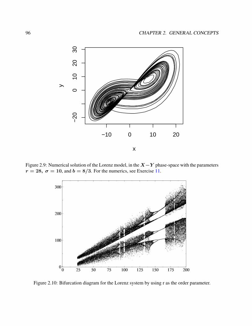
96 CHAPTER 2. GENERAL CONCEPTS
−10 0 10 20
−20
010
2030
LORENZ ATTRACTOR
x
y
Figure 2.9: Numerical solution of the Lorenz model, in theX−Y phase-space with the parametersr = 28, σ = 10, and b = 8/3. For the numerics, see Exercise 11.
Figure 2.10: Bifurcation diagram for the Lorenz system by using r as the order parameter.
2.3. BIFURCATIONS 97
Exercise 22 – Lorenz equations
Consider the Lorenz equations (which were derived from the Rayleigh-Bernard system)
x = σ(y − x) (2.24)
y = rx− xz − y (2.25)
z = xy − bz (2.26)
with σ, r, b > 0. σ is the Prandtl number. Furthermore, Rayleigh number Ra ∼ ∆T , critical
Rayleigh numberRc, and r = Ra/Rc.
1. Evaluate the equilibrium points.
2. Determine the stability of the (0, 0, 0)−equilibrium through linearization! Control param-
eter is r.
3. Show the symmetry: The Lorenz equation has the following symmetry (x, y, z)→ (−x,−y, z)
independent on the parameters σ, r, b.
4. Show the invariance: The z-axis is invariant, meaning that a solution that starts on the z-axis
(i.e. x = y = 0) will remain on the z-axis. In addition the solution will tend toward the
origin if the initial condition are on the z-axis.
5. Lorenz system has bounded solutions: Show that all solutions of the Lorenz equation will
enter an ellipsoid centered at (0, 0, 2r) in finite time, and the solution will remain inside the
ellipsoid once it has entered. To observe this, define a Lyapunov function
V (x, y, z) = rx2 + σy2 + σ(z − 2r)2 (2.27)
Exercise 23 – Lorenz Problem
1. Write the numerical solution for the Lorenz system.
2. Use an initial value x0 ∈ [0, 1], and a parameter value r ∈ [0, 1]
3. Investigate the sensitivity of the solution on the parameter r (especially using r = 13, 14
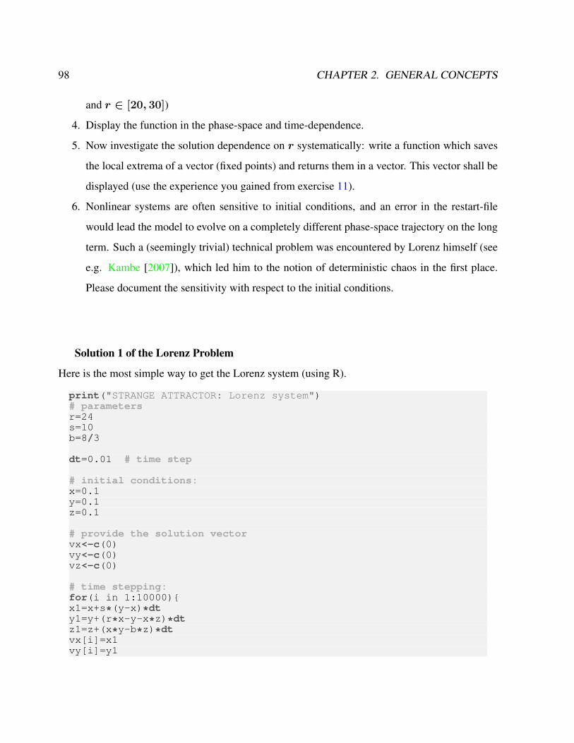
98 CHAPTER 2. GENERAL CONCEPTS
and r ∈ [20, 30])
4. Display the function in the phase-space and time-dependence.
5. Now investigate the solution dependence on r systematically: write a function which saves
the local extrema of a vector (fixed points) and returns them in a vector. This vector shall be
displayed (use the experience you gained from exercise 11).
6. Nonlinear systems are often sensitive to initial conditions, and an error in the restart-file
would lead the model to evolve on a completely different phase-space trajectory on the long
term. Such a (seemingly trivial) technical problem was encountered by Lorenz himself (see
e.g. Kambe [2007]), which led him to the notion of deterministic chaos in the first place.
Please document the sensitivity with respect to the initial conditions.
Solution 1 of the Lorenz Problem
Here is the most simple way to get the Lorenz system (using R).
print("STRANGE ATTRACTOR: Lorenz system")# parametersr=24s=10b=8/3
dt=0.01 # time step
# initial conditions:x=0.1y=0.1z=0.1
# provide the solution vectorvx<-c(0)vy<-c(0)vz<-c(0)
# time stepping:for(i in 1:10000)x1=x+s*(y-x)*dty1=y+(r*x-y-x*z)*dtz1=z+(x*y-b*z)*dtvx[i]=x1vy[i]=y1
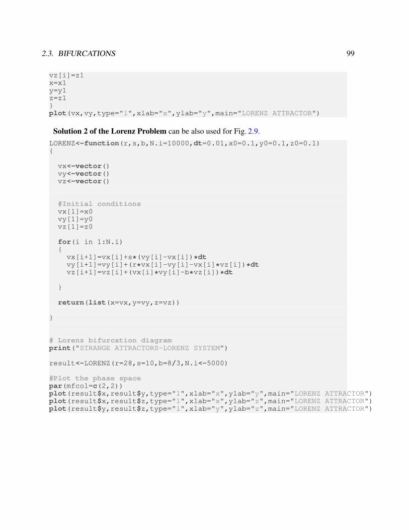
2.3. BIFURCATIONS 99
vz[i]=z1x=x1y=y1z=z1plot(vx,vy,type="l",xlab="x",ylab="y",main="LORENZ ATTRACTOR")
Solution 2 of the Lorenz Problem can be also used for Fig. 2.9.LORENZ<-function(r,s,b,N.i=10000,dt=0.01,x0=0.1,y0=0.1,z0=0.1)
vx<-vector()vy<-vector()vz<-vector()
#Initial conditionsvx[1]=x0vy[1]=y0vz[1]=z0
for(i in 1:N.i)vx[i+1]=vx[i]+s*(vy[i]-vx[i])*dtvy[i+1]=vy[i]+(r*vx[i]-vy[i]-vx[i]*vz[i])*dtvz[i+1]=vz[i]+(vx[i]*vy[i]-b*vz[i])*dt
return(list(x=vx,y=vy,z=vz))
# Lorenz bifurcation diagramprint("STRANGE ATTRACTORS-LORENZ SYSTEM")
result<-LORENZ(r=28,s=10,b=8/3,N.i<-5000)
#Plot the phase spacepar(mfcol=c(2,2))plot(result$x,result$y,type="l",xlab="x",ylab="y",main="LORENZ ATTRACTOR")plot(result$x,result$z,type="l",xlab="x",ylab="z",main="LORENZ ATTRACTOR")plot(result$y,result$z,type="l",xlab="y",ylab="z",main="LORENZ ATTRACTOR")
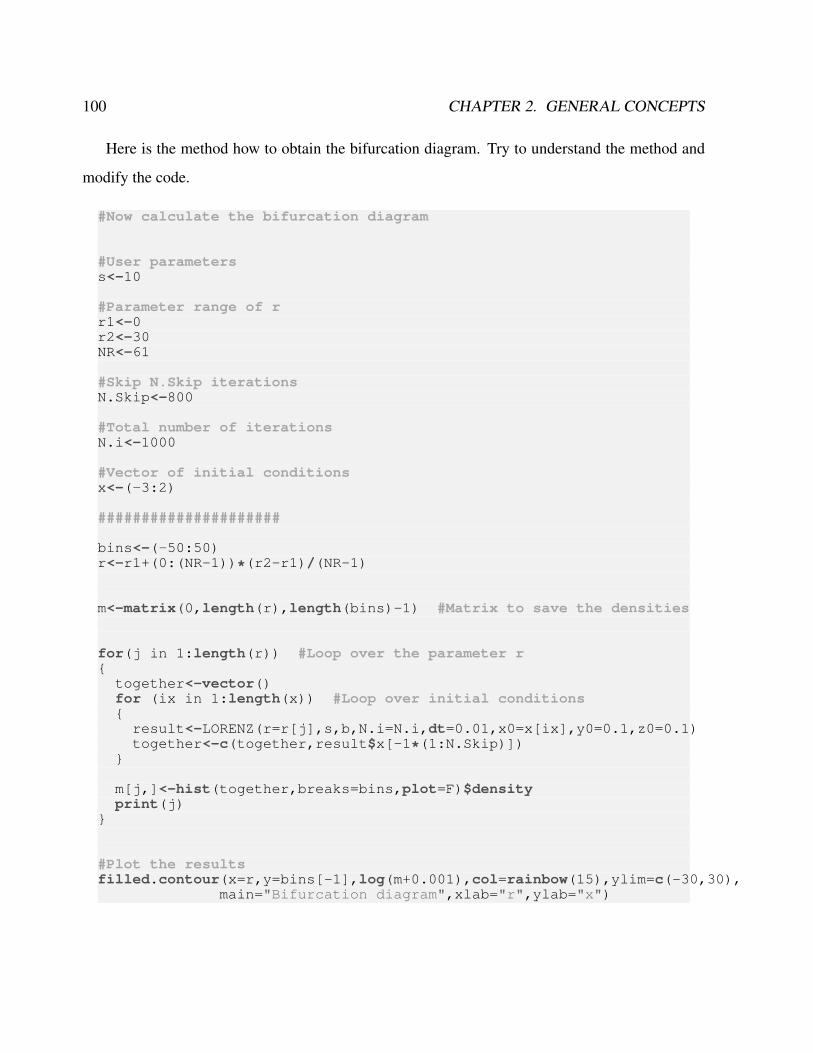
100 CHAPTER 2. GENERAL CONCEPTS
Here is the method how to obtain the bifurcation diagram. Try to understand the method and
modify the code.
#Now calculate the bifurcation diagram
#User parameterss<-10
#Parameter range of rr1<-0r2<-30NR<-61
#Skip N.Skip iterationsN.Skip<-800
#Total number of iterationsN.i<-1000
#Vector of initial conditionsx<-(-3:2)
#####################
bins<-(-50:50)r<-r1+(0:(NR-1))*(r2-r1)/(NR-1)
m<-matrix(0,length(r),length(bins)-1) #Matrix to save the densities
for(j in 1:length(r)) #Loop over the parameter r
together<-vector()for (ix in 1:length(x)) #Loop over initial conditionsresult<-LORENZ(r=r[j],s,b,N.i=N.i,dt=0.01,x0=x[ix],y0=0.1,z0=0.1)together<-c(together,result$x[-1*(1:N.Skip)])
m[j,]<-hist(together,breaks=bins,plot=F)$densityprint(j)
#Plot the resultsfilled.contour(x=r,y=bins[-1],log(m+0.001),col=rainbow(15),ylim=c(-30,30),
main="Bifurcation diagram",xlab="r",ylab="x")
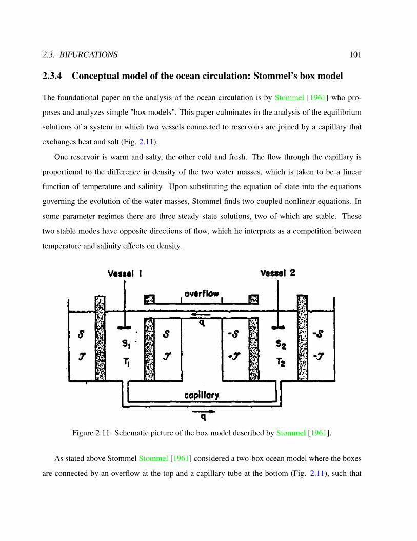
2.3. BIFURCATIONS 101
2.3.4 Conceptual model of the ocean circulation: Stommel’s box model
The foundational paper on the analysis of the ocean circulation is by Stommel [1961] who pro-
poses and analyzes simple "box models". This paper culminates in the analysis of the equilibrium
solutions of a system in which two vessels connected to reservoirs are joined by a capillary that
exchanges heat and salt (Fig. 2.11).
One reservoir is warm and salty, the other cold and fresh. The flow through the capillary is
proportional to the difference in density of the two water masses, which is taken to be a linear
function of temperature and salinity. Upon substituting the equation of state into the equations
governing the evolution of the water masses, Stommel finds two coupled nonlinear equations. In
some parameter regimes there are three steady state solutions, two of which are stable. These
two stable modes have opposite directions of flow, which he interprets as a competition between
temperature and salinity effects on density.
Figure 2.11: Schematic picture of the box model described by Stommel [1961].
As stated above Stommel Stommel [1961] considered a two-box ocean model where the boxes
are connected by an overflow at the top and a capillary tube at the bottom (Fig. 2.11), such that
102 CHAPTER 2. GENERAL CONCEPTS
the capillary flow is directed from the high density vessel to the low density vessel following with
a rate Φ. The common assumption of these box models is that the oceanic overturning rate Φ can
be expressed by the meridional density difference:
Φ = −c (α∆T − β∆S) , (2.28)
where α and β are the thermal and haline expansion coefficients, c is a tunable parameter, and ∆
denotes the meridional difference operator applied to the variables temperature T and salinity S,
respectively. ∆T = T1−T2 with T1, T2 are the high-latitude and the tropical boxes in Fig. 2.11.
The equations for temperature T and salinity S are the heat and salt budgets using an upstream
scheme for the advective transport and fluxes with the atmosphere:
d
dtT1 =
Φ
VT2 −
F oa1
ρ0cph(2.29)
d
dtS1 =
Φ
VS2 −
S0
h(P − E)1 , (2.30)
d
dtT2 =
Φ
VT1 −
F oa2
ρ0cph(2.31)
d
dtS2 =
Φ
VS1 −
S0
h(P − E)2 , (2.32)
where V is the volume of the box with depth h , and (P − E) denotes the freshwater flux (pre-
cipitation minus evaporation plus runoff). Foa is the heat flux at the ocean-atmosphere interface,
S0 is a reference salinity, and ρ0cp denotes the heat capacity of the ocean. Subtraction leads to
d
dt∆T = −
Φ
V∆T − ∆
F oa
ρ0cph(2.33)
d
dt∆S = −
Φ
V∆S −
S0
h∆(P − E) . (2.34)
The heat flux F oa at the ocean-atmosphere interface can be replaced by a restoring term to the
respective atmospheric temperatures, and to a first order approximation the temperatures are fixed.
2.3. BIFURCATIONS 103
We now make an approximation of (2.33, 2.34) and assume that ∆T, c, and∆(P − E) are fixed
parameters. The dynamics is then given by
d
dt∆S =
c
V(α∆T − β∆S) ∆S −
S0
h∆(P − E) . (2.35)
The steady state solution of (2.35) for ∆S can be obtained as
0 =c
V(α∆T − β∆Seq) ∆Seq −
S0
h∆(P − E) , (2.36)
which leads to a quadratic equation for
∆Seq =α∆T
β
(1
2±
√1
4−βS0V∆(P − E)
ch(α∆T )2
). (2.37)
It can be shown (exercise 24) that the negative root leads to an unstable solution. Furthermore
ch(α∆T )2 > 4βS0V∆(P − E) (2.38)
which means there exists a critical ∆(P − E)crit above which the flow has no solution:
∆(P − E)crit = ch(α∆T )2
4βS0V. (2.39)
What will hapen if ∆(P − E) > ∆(P − E)crit ? Stommel [1961] modified equation (6.158)
to Φ = −c |α∆T − β∆S| (2.40)
Then the steady-state solutions are classified according to the sign of q = α∆T − β∆S. When
q > 0, the circulation is driven by the thermal contrast. When q < 0, the haline contrast is
dominant in driving the current.

104 CHAPTER 2. GENERAL CONCEPTS
Exercise 24 – Bifurcation of Stommel’s model
Consider Fig. 2.11 where the ocean surface water is heated at the equatorial region and flows
toward high latitudes. At the pole the water is cooled and sinks, upwelling is at the equator.
1. Starting from (2.35), calculate the linear stability of the equilibrium solution (2.37).
2. Investigate the sensitivity of the stability with respect to (P − E)crit and the other param-
eters in the model.
Solution for Bifurcation of Stommel’s model
We rewrite (2.35) into
V
c
d
dtβ∆S = (α∆T − β∆S) β∆S −
βS0 V
ch∆(P − E) . (2.41)
Denoting x = β∆S, a = α∆T, b =βS0 V
ch∆(P − E), and a non-dimentional time
td = tc
V, we have
d
dtdx = (a− x) · x− b (2.42)
The equilibrium solutions are
x1,2 =a
2±
√a2
4− b (2.43)
Therefore, (2.42) can be rewritten as
d
dtdx = f(x) = −(x− x1) · (x− x2) (2.44)
The derivative is
f ′(x) = −(x− x1)− (x− x2) (2.45)
2.3. BIFURCATIONS 105
and
f ′(x1) = −(x1 − x2) = −2
√a2
4− b < 0 stable (2.46)
f ′(x2) = −(x2 − x1) = +2
√a2
4− b > 0 unstable (2.47)
Furthermore,
b <a2
4which means that (2.48)
∆(P − E) < ∆(P − E)crit = ch(α∆T )2
4βS0V. (2.49)
Reversed mode of the model: What happens if ∆(P − E) > ∆(P − E)crit ?
Then the direction of the circulation is anti-clockwise and the current is driven predominantly by
haline contrast with higher density at low latitudes. The equation has to modified according to
(2.40) and the equilibrium solutions are
x3,4 =a
2±
√a2
4+ b (2.50)
This solution has the requirement that a2
4+ b > 0. Let us now look on the linear stability of x3,4
d
dtdx = f(x) = (x− x3) · (x− x4) (2.51)
The derivative is
f ′(x) = (x− x3) + (x− x4) (2.52)

106 CHAPTER 2. GENERAL CONCEPTS
and
f ′(x3) = (x3 − x4) = +2
√a2
4+ b > 0 unstable (2.53)
f ′(x4) = (x4 − x3) = −2
√a2
4+ b < 0 stable (2.54)
This means tha tthere exists two stable equilibria (Fig. 2.12) for
−a2
4< b = 2
βS0 V
ch(P − E) <
a2
4=
(α∆T )2
4. (2.55)
b
xeq
b=a2/4b=-a2/4
xeq=a
xeq=0
xeq=a/2
x1
x4
x2
x3
Figure 2.12: Schematic bifurcation of the Stommel box model. Dashed solutions are unstable, thesolid red and blue lines represent the stable solutions, x1 and x4, respectively.
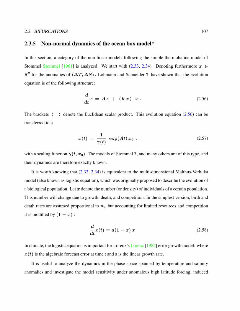
2.3. BIFURCATIONS 107
2.3.5 Non-normal dynamics of the ocean box model*
In this section, a category of the non-linear models following the simple thermohaline model of
Stommel Stommel [1961] is analyzed. We start with (2.33, 2.34). Denoting furthermore x ∈
R2 for the anomalies of (∆T,∆S) , Lohmann and Schneider ? have shown that the evolution
equation is of the following structure:
d
dtx = Ax + 〈 b|x 〉 x . (2.56)
The brackets 〈 | 〉 denote the Euclidean scalar product. This evolution equation (2.56) can be
transferred to a
x(t) =1
γ(t)exp(At)x0 , (2.57)
with a scaling function γ(t, x0). The models of Stommel ?, and many others are of this type, and
their dynamics are therefore exactly known.
It is worth knowing that (2.33, 2.34) is equivalent to the multi-dimensional Malthus-Verhulst
model (also known as logistic equation), which was originally proposed to describe the evolution of
a biological population. Let x denote the number (or density) of individuals of a certain population.
This number will change due to growth, death, and competition. In the simplest version, birth and
death rates are assumed proportional to n,, but accounting for limited resources and competition
it is modified by (1− x) :
d
dtx(t) = a(1− x) x (2.58)
In climate, the logistic equation is important for Lorenz’s Lorenz [1982] error growth model: where
x(t) is the algebraic forecast error at time t and a is the linear growth rate.
It is useful to analyze the dynamics in the phase space spanned by temperature and salinity
anomalies and investigate the model sensitivity under anomalous high latitude forcing, induced
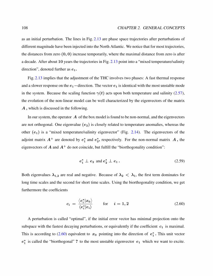
108 CHAPTER 2. GENERAL CONCEPTS
as an initial perturbation. The lines in Fig. 2.13 are phase space trajectories after perturbations of
different magnitude have been injected into the North Atlantic. We notice that for most trajectories,
the distances from zero (0, 0) increase temporarily, where the maximal distance from zero is after
a decade. After about 10 years the trajectories in Fig. 2.13 point into a “mixed temperature/salinity
direction”, denoted further as e1.
Fig. 2.13 implies that the adjustment of the THC involves two phases: A fast thermal response
and a slower response on the e1−direction. The vector e1 is identical with the most unstable mode
in the system. Because the scaling function γ(t) acts upon both temperature and salinity (2.57),
the evolution of the non-linear model can be well characterized by the eigenvectors of the matrix
A , which is discussed in the following.
In our system, the operator A of the box model is found to be non-normal, and the eigenvectors
are not orthogonal. One eigenvalue (e2) is closely related to temperature anomalies, whereas the
other (e1) is a “mixed temperature/salinity eigenvector” (Fig. 2.14). The eigenvectors of the
adjoint matrix A+ are denoted by e∗1 and e∗2, respectively. For the non-normal matrix A , the
eigenvectors ofA andA+ do not coincide, but fulfill the “biorthogonality condition”:
e∗1 ⊥ e2 and e∗2 ⊥ e1 . (2.59)
Both eigenvalues λ1,2 are real and negative. Because of λ2 < λ1, the first term dominates for
long time scales and the second for short time scales. Using the biorthogonality condition, we get
furthermore the coefficients
ci =
⟨e∗i |x0
⟩〈e∗i |ei〉
for i = 1, 2 (2.60)
A perturbation is called “optimal”, if the initial error vector has minimal projection onto the
subspace with the fastest decaying perturbations, or equivalently if the coefficient c1 is maximal.
This is according to (2.60) equivalent to x0 pointing into the direction of e∗1 . This unit vector
e∗1 is called the “biorthogonal” ? to the most unstable eigenvector e1 which we want to excite.
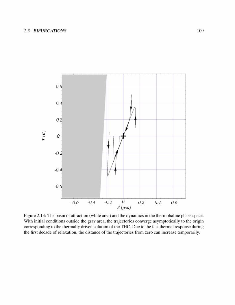
2.3. BIFURCATIONS 109
Figure 2.13: The basin of attraction (white area) and the dynamics in the thermohaline phase space.With initial conditions outside the gray area, the trajectories converge asymptotically to the origincorresponding to the thermally driven solution of the THC. Due to the fast thermal response duringthe first decade of relaxation, the distance of the trajectories from zero can increase temporarily.
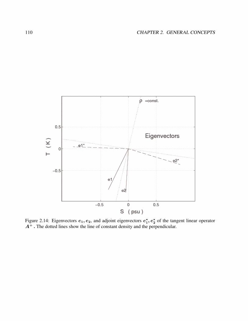
110 CHAPTER 2. GENERAL CONCEPTS
Figure 2.14: Eigenvectors e1, e2, and adjoint eigenvectors e∗1, e∗2 of the tangent linear operator
A+ . The dotted lines show the line of constant density and the perpendicular.
2.3. BIFURCATIONS 111
In order to make a geometrical picture for the mathematical considerations, assume that the tail
of the vector x0 is placed on the e1−line and its tip on the e2−line. This vector is stretched
maximally because the tail decays to zero quickly, whereas the tip is hardly unchanged due to the
larger eigenvalue λ1 . The most unstable mode e1 and its biorthogonal e∗1 differ greatly from
each other, and the perturbation that optimally excites the mode bears little resemblance to the
mode itself.
It is remarkable that the optimal initial perturbation vector e∗1 does not coincide with a pertur-
bation in sea surface density at high latitudes, which would reside on the dotted line perpendicular
to ρ = const. in Fig. 2.14. Even when using a space spanned by (αT, βS) instead of (T, S) ,
to take into account the different values for the thermal and haline expansion coefficients, vector
e∗1 is much more dominated by the scaled salinity anomalies than the temperature anomalies of
the high latitudinal box.
Numerical simulations by Manabe and Stouffer Manabe and Stouffer [1993] showed, for the
North Atlantic, that between two and four times the preindustrial CO2 concentration, a threshold
value is passed and the thermohaline circulation ceases completely. One other example of early
Holocene rapid climate change is the ’8200 yr BP’ cooling event recorded in the North Atlantic
region possibly induced by freshwater. One possible explanation for this dramatic regional cooling
is a shutdown in the formation of deep water in the northern North Atlantic due to freshwater input
caused by catastrophic drainage of Laurentide lakes Barber et al. [1999]; Lohmann [2003]. The
theoretic considerations and these numerical experiments suggest that the formation of deep water
in the North Atlantic is highly sensitive to the freshwater forcing.

Chapter 3
Statistical Mechanics and Fluid Dynamics*
There are two ways of changing the descrition of the dynamics: from the micro to the macro
scales. This is a common problem since we are not able to describe the systems on all temporal
and spatial scales. One straitforward approach is coarse graining where the underlying dynamics
is projected onto the macroscopic dynamics (section 3.5), the other is the statistical physics theory
of non-equilibrium statistical mechanics (section 3.2).
A general question within the micro-macro dynamic is that of integration between the two
different levels. Two distinctly different levels emerge with different rules governing each, but
they then need to be reconciled in some way to create an overall functioning system. Physical,
chemical, biological, economic, social and cultural systems all exhibit this micro-macro dynamic
and how the system comes to reconcile it forms a primary determinate in its identity and overall
structure. This multi-dimensional nature to a system that results in the micro-macro dynamic is a
product of synthesis and emergence. In many instances when we put elements together they do
not simply remain discrete separate entities but they interact, co-evolve and they differentiate their
states and function with respect to each other to become an interdependent whole, which comes
to have properties and features that none of its parts possess. A whole new level of organization
emerges that is different from the parts. This is made manifest in ecosystems; as they have co-
evolved over millennia the parts are intricately interdependent forming a whole system that has
112
3.1. MESOSCOPIC DYNAMICS 113
features and dynamics independent from any of its parts and thus a two-tier system and a resulting
emergent micro-macro dynamic. The whole ecosystem goes through processes of change - such
as ecological succession - that are not associated with any of the parts but condition what creatures
can viably exist within that macro regime.
We start from the point of view of kinetic theory of fluids where a gas is composed of a set of
interacting particles Boltzmann [1896]. We are then interested in the probability of finding a fluid
particle at a certain point in space and with a certain velocity. The moments of this probablility are
related to our macroscopic fluid-dynamical quantities like density or velocity.
3.1 Mesoscopic dynamics
3.1.1 Liouville equation
In the deterministic framework, the dynamics is characterized by
d
dtx(t) = f(x(t)) , (3.1)
and in the special case of classical mechanics can be descibed by a set of differential equations
known as the Hamilton equations for that system. Hamiltonians can be used to describe such
simple systems as a bouncing ball, a pendulum or an oscillating spring in which energy changes
from kinetic to potential and back again over time. Hamiltonians can also be employed to model
the energy of other more complex dynamic systems such as planetary orbits in celestial mechanics
and also in quantum mechanics. The Hamilton equations are generally written as follows:
p = −∂H∂q
(3.2)
q =∂H∂p
(3.3)
114 CHAPTER 3. STATISTICAL MECHANICS AND FLUID DYNAMICS*
In the above equations, the dot denotes the ordinary derivative with respect to time of the functions
p = p(t) (called generalized momenta) and q = q(t) (called generalized coordinates), taking
values in some vector space, andH = H(p, q, t) is the so-called Hamiltonian, or (scalar valued)
Hamiltonian function. The associated probability distribution for the generalized dynamics (3.1)
is given in the phase space
p(x, t) = δ(x− x(t)) (3.4)
yielding the Liouville equation
∂tp = −d
dx(t)[δ(x− x(t))]
d
dtx(t) = −
∂p
∂xf(x) . (3.5)
The Liouville equation is often used in the framework of the Hamiltonian dynamics (3.3). Since
the phase space velocity (pi, qi) has zero divergence, and probability is conserved. Its substantial
derivative can be shown to be zero and so
∂
∂tρ = − ρ,H. (3.6)
using the Poisson bracket
f, g =N∑i=1
[∂f
∂qi
∂g
∂pi−∂f
∂pi
∂g
∂qi
]. (3.7)
3.1.2 Master equation
The master equation is a phenomenological set of first-order differential equations describing the
time evolution of the probability of a system to occupy each one of a discrete set of states:
dPk
dt=∑`
Tk`P`, (3.8)
3.1. MESOSCOPIC DYNAMICS 115
where Pk is the probability for the system to be in the state k, while the matrix T`k is filled with a
grid of transition-rate constants. In probability theory, this identifies the evolution as a continuous-
time Markov process, with the integrated master equation obeying a Chapman-Kolmogorov equa-
tion. Note that
∑`
T`k = 0 (3.9)
(i.e. probability is conserved), so the equation may also be written as
dPk
dt=∑`
(Tk`P` − T`kPk). (3.10)
allowing us to omit the term ` = k from the summation. Thus, in the latter form of the master
equation there is no need to define the diagonal elements of T.
The master equation exhibits detailed balance if each of the terms of the summation disappears
separately at equilibrium, i.e. if, for all states k and l having equilibrium probabilities pik and π`
Tk`π` = T`kπk (3.11)
Many physical problems in classical, quantum mechanics and problems in other sciences, can be
reduced to the form of a master equation, thereby performing a great simplification of the problem.
In the continous case, the Chapman-Kolmogorov equation has similarities with the Master equa-
tion. The Chapman-Kolmogorov equation is an identity relating the joint probability distributions
of different sets of coordinates on a stochastic process. Suppose that xi is an indexed collection
of random variables, that is, a stochastic process. Let
pi1,...,in(x1, . . . , xn) (3.12)
be the joint probability density function of the values of the random variables x1 to xn. Then, the
116 CHAPTER 3. STATISTICAL MECHANICS AND FLUID DYNAMICS*
Chapman-Kolmogorov equation is
pi1,...,in−1(x1, . . . , xn−1) =
∫ ∞−∞
pi1,...,in(x1, . . . , xn) dxn (3.13)
i.e. a straightforward marginalization over the nuisance variable.
When the stochastic process under consideration is Markovian, the Chapman-Kolmogorov
equation is equivalent to an identity on transition densities. In the Markov chain setting, one
assumes that i1 < . . . < in. Then, because of the Markov property,
pi1,...,in(x1, . . . , xn) = pi1(x1)pi2;i1(x2 | x1) · · · pin;in−1(xn | xn−1), (3.14)
where the conditional probability pi;j(xi | xj) is the transition probability between the times
i > j. So, the Chapman-Kolmogorov equation takes the form
pi3;i1(x3 | x1) =
∫ ∞−∞
pi3;i2(x3 | x2)pi2;i1(x2 | f1) dx2. (3.15)
When the probability distribution on the state space of a Markov chain is discrete and the Markov
chain is homogeneous, the Chapman-Kolmogorov equations can be expressed in terms of (possibly
infinite-dimensional) matrix multiplication, thus:
P (t+ s) = P (t)P (s) (3.16)
where P(t) is the transition matrix, i.e., if Xt is the state of the process at time t, then for any two
points i and j in the state space, we have
Pij(t) = P (Xt = j | X0 = i). (3.17)
Example for the Chapman-Kolmogorov and Master equations in climate dynamics are related
to transitions between different states.
3.1. MESOSCOPIC DYNAMICS 117
3.1.3 Fokker-Planck dynamics
In the stochastic context, we make a Taylor expansion up to order two in dx = x(t+dt)−x(t)
from the Master equation:
dp = p(x, t+ dt)− p(x, t)
= < δ(x− x(t+ dt)) > − < δ(x− x(t)) >
= − <d
dx(t)[δ(x− x(t))] dx > +
1
2<
d2
dx2[δ(x− x(t))] dx2 >
= −∂p
∂x< dx > +
1
2
∂2
∂x2p < dx2 >
= −∂p
∂xf(x)dt+
1
2
∂2
∂x2p g2dt (3.18)
The probability density p(x, t) for the variable x(t) in (7.53) obeys therefore the Fokker-Planck
equation
∂tp = −∂
∂x[f(x)p] +
∂
∂x
[g(x)
∂
∂xg(x)p
]. (3.19)
Its stationary probability density of (7.53) is given by
pst(x) = ℵ exp
(−2
∫ x
x0
f(y)− g(y)g′(y)
g(y)2dy
). (3.20)
where ℵ is a normalization constant. g′(y) stands for the derivative of g with respect to its argu-
ment. The extrema xm of the steady state density obey the equation
f(xm)− g(xm)g′(xm) = 0 (3.21)
for g(xm)ne0. Here is the crux of the noise-induced transition phenomenon: one notes that this
equation is not the same as the equation f(xm) = 0 that determines the steady states of the system
in the absence of multiplicative noise. As a result, the most probable states of the noisy system
118 CHAPTER 3. STATISTICAL MECHANICS AND FLUID DYNAMICS*
need not to coincide with the deterministic stationary states. More importantly, new solutions
may appear or existing solutions may be destabilized by the noise. These are the changes in the
asymptotic behavior of the system caused by the presence of the noise, e.g. ?.
3.2 The Boltzmann Equation
One of the most significant theoretical breakthroughs in statistical physics was due to Ludwig
Boltzmann (Boltzmann [1896], Boltzmann [1995] for a recent reprint of his famous lectures on
kinetic theory), who pioneered non-equilibrium statistical mechanics. Boltzmann postulated that a
gas was composed of a set of interacting particles, whose dynamics could be (at least in principle)
modelled by classical dynamics. Due to the very large number of particles in such a system, a
statistical approach was adopted, based on simplified physics composed of particle streaming in
space and billiard-like inter-particle collisions (which are assumed elastic). Instrumental to the
theory is the single-particle distribution function (hereafter SPDF), f(~x, ~e, t) which represents
the probability density of having a particle at the point (~x, ~e) in the phase space. Hence, the
quantity
f(~x, ~e, t)d~xd~e (3.22)
represents the probability of finding a particle inside an infinitesimal space cubelet centered around
~x, and inside an infinitesimal momentum-space cubelet around ~e at any given time t. In the
presence of a body-force ~F , the SPDF will evolve according to
f(~x+ d~x, ~e+ d~e, t+ dt)d~xd~e = f(~x, ~e, t)d~xd~e , (3.23)
where d~x = ~edt and d~e = ~Fdt/m. If we also include the effect of the collisions, and denote
by Γ+d~xd~edt the probability for a particle to start from outside the d~x×d~e domain and to enter
this phase-space region during the infinitesimal time dt and by Γ−d~xd~edt the probability for a
particle to start from the d~x×d~e domain and leave this phase-space region during the infinitesimal

3.2. THE BOLTZMANN EQUATION 119
time dt, the evolution of the SPDF becomes
f(~x+ d~x, ~e+ d~e, t+ dt)d~xd~e = f(~x, ~e, t)d~xd~e+ (Γ+ − Γ−) d~xd~edt (3.24)
Expanding the LHS into a Taylor series around the phase-space point (~x, ~u, t), we obtain:
f(~x+d~x, ~e+d~e, t+dt)d~xd~e = f(~x, ~e, t)d~xd~e+
(∂f
∂t
)dt+(∇~xf)·d~x+(∇~ef)·d~e+. . .
(3.25)
Inserting Eq. (3.25) into Eq. (3.24) and cancelling terms, we easily obtain Boltzmann’s Equation:
∂f
∂t+ ~e · ∇~xf + ~F/m · ∇~ef = Γ+ − Γ− (3.26)
where∇~x is the gradient operator in physical space and∇~e the same in momentum space.1
For the sake of clarity, we have not written the collision operator explicitly yet. The important
point is that the separation of the dynamics into collisions and streaming is already apparent from
Eq. (3.26). The collision operator, which is in itself a complex integro-differential expression,
reads
Γ+ − Γ− ≡∫d~e1
∫dΩ σ(Ω) |~e− ~e1|
[f(~e′)f(~e′1)− f(~e)f(~e1)
](3.27)
where σ is the differential cross-section in the case of the 2-particle collisions (which is a func-
tion of the solid angle Ω only), unprimed velocities are incoming (before collision) and primed
1The collisionless Boltzmann equation is often mistakenly called the Liouville equation (the Liouville Equationis an N-particle equation being N the number of microscopic particles). The Boltzmann equation is a mesoscopicdynamics with degrees of freedom<< N .
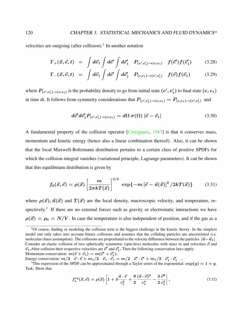
120 CHAPTER 3. STATISTICAL MECHANICS AND FLUID DYNAMICS*
velocities are outgoing (after collision).2 In another notation
Γ+(~x, ~e, t) =
∫d~e1
∫d~e′
∫d~e′1 P(e′,e′1)→(e,e1) f(~e′)f(~e′1) (3.28)
Γ−(~x, ~e, t) =
∫d~e1
∫d~e′
∫d~e′1 P(e,e1)→(e′,e′1) f(~e)f(~e1) (3.29)
whereP(e′,e′1)→(e,e1) is the probability density to go from initial state (e′, e′1) to final state (e, e1)
in time dt. It follows from symmetry considerations that P(e′,e′1)→(e,e1) = P(e,e1)→(e′,e′1) and
d~e′d~e′1P(e′,e′1)→(e,e1) = dΩ σ(Ω) |~e− ~e1| (3.30)
A fundamental property of the collision operator [Cercignani, 1987] is that it conserves mass,
momentum and kinetic energy (hence also a linear combination thereof). Also, it can be shown
that the local Maxwell-Boltzmann distribution pertains to a certain class of positive SPDFs for
which the collision integral vanishes (variational principle, Lagrange parameters). It can be shown
that this equilibrium distribution is given by
f0(~x, ~e) = ρ(~x)
[m
2πkT (~x)
]3/2
exp−m [~e− ~u(~x)]2 /2kT (~x) (3.31)
where ρ(~x), ~u(~x) and T (~x) are the local density, macroscopic velocity, and temperature, re-
spectively.3 If there are no external forces such as gravity or electrostatic interactions we have
ρ(~x) = ρ0 = N/V . In case the temperature is also independent of position, and if the gas as a
2Of course, finding or modeling the collision term is the biggest challenge in the kinetic theory. In the simplestmodel one only takes into account binary collisions and assumes that the colliding particles are uncorrelated (i.e.molecular chaos assumption). The collisions are proportianal to the velocity difference between the particles |~u−~u1| .Consider an elastic collision of two spherically symmetric (spin-less) molecules with mass m and velocities ~e and~e1.After collision their respective velocities are ~e′ and ~e′1. Then the following conservation laws apply:Momentum conservation: m(~e+ ~e1) = m(~e′ + ~e′1).Energy conservation: m/2 ~e · ~e+m1/2 ~e1 · ~e1 = m/2 ~e′ · ~e′ +m1/2 ~e′1 · ~e′1 .
3This experssion of the SPDF can be approximated through a Taylor series of the exponential: exp(y) = 1 + y.Task: Show that
feqa (~x, ~e) = ρ(~x)
[1 + 3
~u · ~ec2s
+9
2
(~u · ~e)2
c4s−
3
2
~e2
c2s
], (3.32)
3.3. H-THEOREM AND APPROXIMATION OF THE BOLTZMANN EQUATION 121
whole is not moving (~u = 0), then f(~x, ~e) = ρ0f0(~e), with
f0(~e) =
[m
2πkT
]3/2
e−m~e2/2kT ,
This implies that, if this distribution is attained, we also have a state where incoming SPDFs ex-
actly balance the outgoing ones, maintaining a local dynamic equilibrium. This observation is of
paramount importance for our method, which uses the (discretized) Maxwell-Boltzmann distribu-
tion as the equilibrium distribution functions.
3.3 H-Theorem and approximation of the Boltzmann equation
The other important feature of this equation is that the integral
H =
∫ ∫d~xd~e f(~x, ~e, t) ln f(~x, ~e, t) (3.34)
can only decrease. This can be seen by using the following:
dH
dt=
∫d~e1
∫dΩ σ(Ω) |~e− ~e1|
[f(~e′)f(~e′1)− f(~e)f(~e1)
][1 + ln f(~e1)] (3.35)
and the same term for
dH
dt=
∫d~e1
∫dΩ σ(Ω) |~e− ~e1|
[f(~e′)f(~e′1)− f(~e)f(~e1)
] [1 + ln f(~e′1)
](3.36)
with the speed of sound cs and
1
c2s=
1
γ
m
kT(3.33)
and γ the adiabatic factor.
122 CHAPTER 3. STATISTICAL MECHANICS AND FLUID DYNAMICS*
The term is also invariant with respect to the notation (’), i.e.
dH
dt=
∫d~e1
∫dΩ σ(Ω) |~e− ~e1|
[f(~e)f(~e1)− f(~e′)f(~e′1)
] [1 + ln f(~e′1)
](3.37)
and
dH
dt=
∫d~e1
∫dΩ σ(Ω) |~e− ~e1|
[f(~e)f(~e1)− f(~e′)f(~e′1)
] [1 + ln f(~e′2)
](3.38)
Use furthermore
η′ = f(~e′)f(~e′1) and η = f(~e)f(~e1) (3.39)
E = (η′ − η) [ln η − ln η′] (3.40)
and recognize that E is negative. ddtH is equal zero for
f(~e′)f(~e′1) = f(~e)f(~e1) . (3.41)
For a system of N statistically independent particles, H is related to the thermodynamic entropy S
through:
Sdef= −NkH (3.42)
Therefore, according to the H-theorem, S can only increase.4 The same functionH is also used as
”information function”:
I = −∑i
fi ln fi =< − ln f > . (3.43)
where the fi can be interpreted as probablity and not only as a measure of the breadth of the spread
of states available to a single particle in a gas of like particles, where fi represented the relative
4Please see the link to the Lyapunov function for the Lorenz system in Chapter 5.3.
3.3. H-THEOREM AND APPROXIMATION OF THE BOLTZMANN EQUATION 123
frequency distribution of each possible state. When all the probabilities fi are equal, I is maximal,
and we have minimal information about the system. When our information is maximal (i.e., one fi
is equal to one and the rest to zero, such that we know what state the system is in), the function is
minimal. This information function is also called ”reduced entropic function” in thermodynamics
[Shannon, 1948]. Gibbs proposed a general formula for statistical-mechanical entropy, no longer
requiring identical and non-interacting particles, but instead based on the probability distribution
pi for the complete microstate i of the total system:
S = −k∑i
pi ln pi (3.44)
dS
dt= −k
∑i
(dpi
dtln pi +
dpi
dt
)= −k
∑i
dpi
dtln pi (3.45)
because∑idpidt
= ddt
∑i pi = d
dt(1) = 0. Now, formulate a master equation [van Kampen,
1981] for the average rate of jumps5 from state α to β, and from state β to α:
dpα
dt=
∑β
ναβ(pβ − pα) (3.46)
dpβ
dt=
∑α
ναβ(pα − pβ) (3.47)
where the reversibility of the dynamics ensures that the same transition constant ναβ appears in
both expressions. So
dS
dt=
1
2k∑α,β
ναβ(ln pβ − ln pα)(pβ − pα). (3.48)
5The master equation is quite often written as: d~Pdt
= A ~P ,where ~P is a column vector (where element i representsstate i), and A is the matrix of connections. The way connections among states are made determines the dimensionof the problem. When the connections are time-independent rate constants, the master equation represents a kineticscheme and the process is Markovian (any jumping time probability density function for state i is an exponential, witha rate equal to the value of the connection). When the connections depend on the actual time (i.e. matrix A dependson the time, A→ A(t)), and the process is not stationary. For an application in meteorogy, e.g. Egger [2001].
124 CHAPTER 3. STATISTICAL MECHANICS AND FLUID DYNAMICS*
But the two brackets will have the same sign (the same argument as in equation 3.40), so each
contribution to dS/dt cannot be negative and therefore, dSdt≥ 0 for an isolated system. Due to
the complex expression for the collision operator, it became clear that approximations were desir-
able. It was also proven (see Cercignani [1990]) that such approximations were also reasonable,
since the details of the two-body interaction are not likely to influence significantly experimentally-
measured quantities. Hence, approximate collision operators were proposed, all of which had to
1 conserve local mass, momentum and energy and 2 develop a collisional contribution in Boltz-
mann’s equation (3.26) which tends to a local Maxwellian distribution. It was soon realized that a
model developed at the middle of last century Bhatnagar et al. [1954] (also known as Bhatnagar-
Gross-Krook; hereafter BGK) satisfied both of these conditions. Chapman and Enskog developed a
general procedure for the approximate solution of Boltzmann’s equation. For certain simple model
systems such as hard spheres their method produces predictions for (or its moments) which may
be tested in computer simulations. Another more modern approach to the numerical solution of the
transport equation is the “Lattice Boltzmann” method in which the continuous variables and are
restricted to a set of discrete values; the time change of these values is then described by a modified
transport equation which lends itself to fast computation. The moments of the distribution function
represent macroscopic variables density and velocity fields:
ρ(~x, t) = m
∫d~ef(~x, ~e, t) (3.49)
ρ(~x, t)~u(~x, t) = m
∫d~e~ef(~x, ~e, t) (3.50)
Note that the molecular velocities ~e is different from the macroscopic veleocity field ~u(~x, t). The
basic idea was that each collision changes the SPDF by an amount which is proportional to the
departure from the local Maxwellian distribution:
Γ+ − Γ− = −f(~x, ~e, t)− f0(~x, ~e)
τ(3.51)
3.3. H-THEOREM AND APPROXIMATION OF THE BOLTZMANN EQUATION 125
with relaxation constant τ . In dimensionless units, τ is replaced by the dimensionless Knudsen
number Kn = l/L with l is the mean-free-path. It is the small parameter in the kinetics - fluid
dynamics transition. If the Kn >> 1 then the continuum assumption of fluid mechanics is no
longer a good approximation and kinetic equations must be used.

126 CHAPTER 3. STATISTICAL MECHANICS AND FLUID DYNAMICS*
3.4 Application: Lattice Boltzmann Dynamics
3.4.1 Lattice Boltzmann Methods
LBMs recently proved to be viable alternatives to traditional computational fluid dynamics (CFD).
The latter adopts a strategy consisting of: writing the macroscopic flow equations; discretizing
the macroscopic equations using finite differences, finite volumes or finite elements; solving the
discretized equations on a computer. In contrast, LBM takes a different route towards the same
results. The LBM approach is composed of formulating a mesoscopic model for the evolution of
the PDF such that the desired macroscopic flow equations are obtained. The end result of both
approaches are similar. However, the algorithms differ due to the different perspective on the
physics of the flow. There are in principle an infinite set of possible mesoscopic models. However,
we focus on the most common ones, which consist of a streaming and a collision process. These
LBMs use a simplified collision operator Bhatnagar et al. [1954], hence they are also referred to as
LBM-BGK models.
There are several possible choices for the underlying lattice. These are usually classified in
the literature using the DαQβ-notation, where α is an integer number denoting the space di-
mensionality and β is another integer indicating the number of discrete velocities (including the
particle at rest) within the momentum discretization. Some restrictions have to be fulfilled (espe-
cially Galilean and rotational invariance)6 to ensure that a particular discretization can simulate the
Navier-Stokes equations. Among the lattices in common use there are the D2Q9 and D3Q19-
models (see for example discussion in He and Luo [1997]). Our focus here is the 2D case, hence
we have chosen the D2Q9 momentum discretization. The discrete velocity directions for the
D2Q9 lattice are shown in Fig 3.1. The macroscopic variables are defined as functions of the
6A lattice with reduced symmetry can be (and has been) used, see d’Humieres et al. [2001], where a D3Q13-lattice is used. However, this approach also departs from the classical BGK-LBM dynamics.

3.4. APPLICATION: LATTICE BOLTZMANN DYNAMICS 127
0
D2Q9
latticeunit (lu)
84
1
526
3
7
Figure 3.1: Discrete lattice velocities for theD2Q9 model.
particle distribution functions (hereafter DFs) according to:
ρ =
β−1∑a=0
fa (macroscopic fluid density) (3.52)
and ~u =1
ρ
β−1∑a=0
fa~ea (macroscopic velocity). (3.53)
The DFs at each lattice point are updated using the equation:
fa(~x+ ~eaδt, t+ δt) = fa(~x, t)︸ ︷︷ ︸Streaming
−[fa(~x, t)− feqa (~x, t)]
τ︸ ︷︷ ︸Collision
, (3.54)
where a ∈ [0, β−1] is an index spanning the (discretized) momentum space and τ is a relaxation
parameter, which is related to the fluid viscosity. The streaming step, where the DFs are translated
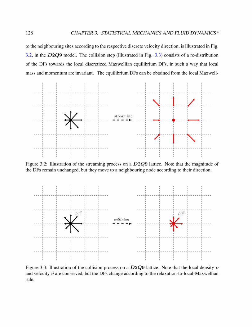
128 CHAPTER 3. STATISTICAL MECHANICS AND FLUID DYNAMICS*
to the neighbouring sites according to the respective discrete velocity direction, is illustrated in Fig.
3.2, in the D2Q9 model. The collision step (illustrated in Fig. 3.3) consists of a re-distribution
of the DFs towards the local discretized Maxwellian equilibrium DFs, in such a way that local
mass and momentum are invariant. The equilibrium DFs can be obtained from the local Maxwell-
streaming
Figure 3.2: Illustration of the streaming process on a D2Q9 lattice. Note that the magnitude ofthe DFs remain unchanged, but they move to a neighbouring node according to their direction.
ρ,~v
collision
ρ,~v
Figure 3.3: Illustration of the collision process on a D2Q9 lattice. Note that the local density ρand velocity ~v are conserved, but the DFs change according to the relaxation-to-local-Maxwellianrule.
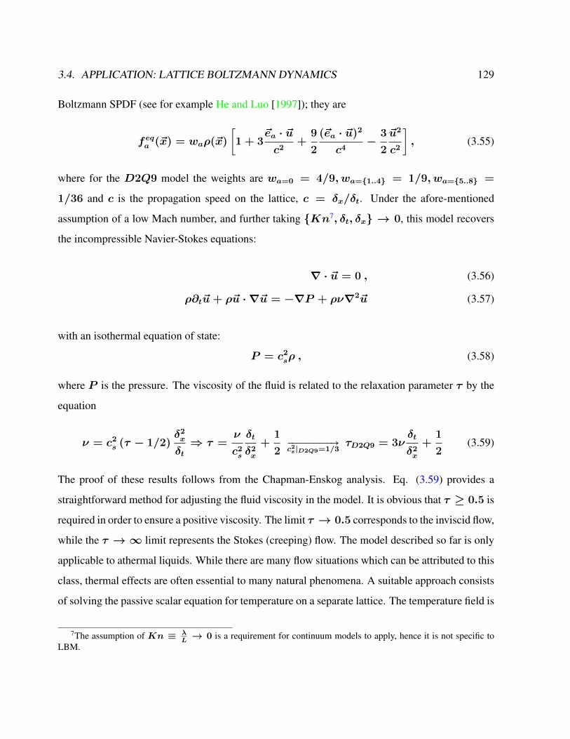
3.4. APPLICATION: LATTICE BOLTZMANN DYNAMICS 129
Boltzmann SPDF (see for example He and Luo [1997]); they are
feqa (~x) = waρ(~x)
[1 + 3
~ea · ~uc2
+9
2
(~ea · ~u)2
c4−
3
2
~u2
c2
], (3.55)
where for the D2Q9 model the weights are wa=0 = 4/9, wa=1..4 = 1/9, wa=5..8 =
1/36 and c is the propagation speed on the lattice, c = δx/δt. Under the afore-mentioned
assumption of a low Mach number, and further taking Kn7, δt, δx → 0, this model recovers
the incompressible Navier-Stokes equations:
∇ · ~u = 0 , (3.56)
ρ∂t~u+ ρ~u · ∇~u = −∇P + ρν∇2~u (3.57)
with an isothermal equation of state:
P = c2sρ , (3.58)
where P is the pressure. The viscosity of the fluid is related to the relaxation parameter τ by the
equation
ν = c2s (τ − 1/2)
δ2x
δt⇒ τ =
ν
c2s
δt
δ2x
+1
2−−−−−−−−−→c2s |D2Q9=1/3
τD2Q9 = 3νδt
δ2x
+1
2(3.59)
The proof of these results follows from the Chapman-Enskog analysis. Eq. (3.59) provides a
straightforward method for adjusting the fluid viscosity in the model. It is obvious that τ ≥ 0.5 is
required in order to ensure a positive viscosity. The limit τ → 0.5 corresponds to the inviscid flow,
while the τ →∞ limit represents the Stokes (creeping) flow. The model described so far is only
applicable to athermal liquids. While there are many flow situations which can be attributed to this
class, thermal effects are often essential to many natural phenomena. A suitable approach consists
of solving the passive scalar equation for temperature on a separate lattice. The temperature field is
7The assumption of Kn ≡ λL→ 0 is a requirement for continuum models to apply, hence it is not specific to
LBM.
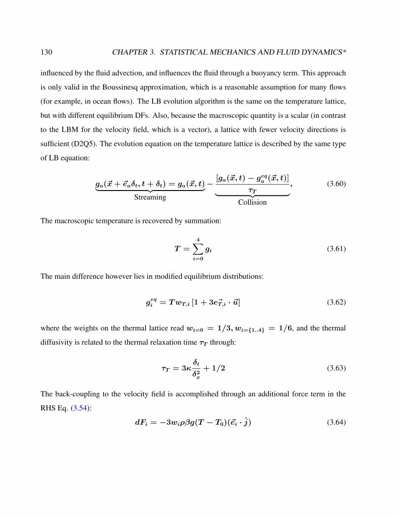
130 CHAPTER 3. STATISTICAL MECHANICS AND FLUID DYNAMICS*
influenced by the fluid advection, and influences the fluid through a buoyancy term. This approach
is only valid in the Boussinesq approximation, which is a reasonable assumption for many flows
(for example, in ocean flows). The LB evolution algorithm is the same on the temperature lattice,
but with different equilibrium DFs. Also, because the macroscopic quantity is a scalar (in contrast
to the LBM for the velocity field, which is a vector), a lattice with fewer velocity directions is
sufficient (D2Q5). The evolution equation on the temperature lattice is described by the same type
of LB equation:
ga(~x+ ~eaδt, t+ δt) = ga(~x, t)︸ ︷︷ ︸Streaming
−[ga(~x, t)− geqa (~x, t)]
τT︸ ︷︷ ︸Collision
, (3.60)
The macroscopic temperature is recovered by summation:
T =4∑i=0
gi (3.61)
The main difference however lies in modified equilibrium distributions:
geqi = TwT,i [1 + 3 ~eT,i · ~u] (3.62)
where the weights on the thermal lattice read wi=0 = 1/3, wi=1..4 = 1/6, and the thermal
diffusivity is related to the thermal relaxation time τT through:
τT = 3κδt
δ2x
+ 1/2 (3.63)
The back-coupling to the velocity field is accomplished through an additional force term in the
RHS Eq. (3.54):
dFi = −3wiρβg(T − T0)(~ei · j) (3.64)

3.4. APPLICATION: LATTICE BOLTZMANN DYNAMICS 131
3.4.2 Simulation set-up of the Rayleigh-Bénard convection
An important part of any numerical simulation is relating the simulation input parameters and
output results to the exact flow we intend to model. The key concept during these procedures is
dynamic similarity, which tells us that two flows with different physical parameters are effectively
equivalent as long as several dimensionless numbers are the same. This idea is of special impor-
tance in experimental and numerical fluid dynamics (e.g., sections 4.5, 8.5). Similarily, in CFD,
the fluid solver usually works in a different lengthscale than the original, physical system that is
to be simulated. We can distinguish 3 different frames of reference in a simulation, described be-
low. The dimensionless system may seem like an unnecessary complication in the beginning, but
it reflects the fact that flows are often given in the literature in this form.
1. Physical system: is the actual system that we intend to simulate. Here, we measure things
in the usual meters, seconds and kilograms. A problem with this system is that it is very
dependent on the units, which are not important to the mathematics behind the PDEs gov-
erning the flow. However, any practical application of fluid mechanics has to start from this
system and return to it when results are to be reported.
2. Dimensionless system: by choosing typical length- and time-scales for our flows, we can
non-dimensionalize the equations, which then become more amenable to numerical simula-
tion. Note that, sometimes, it is necessary to choose also a typical mass and/or temperature,
depending on the form we take for the macroscopic equations.
3. Discrete system: is the coordinate system in which our numerical simulation lives. The
input parameters for our simulation propagate from the physical system, through the non-
dimensional system until here. Due to reasons of numerical stability, several restrictions are
in place at this level, as will be discussed during the practical examples below.
The application we are looking at is the two-dimensional convection driven by a temperature
gradient (Rayleigh-Bénard convection). The geometry consists of a rectangular channel, with
periodic BCs at the sides and no-slip and constant temperature BCs on the top and bottom walls
(section 5.3). Now we can non-dimensionalize the equations by choosing some typical values

132 CHAPTER 3. STATISTICAL MECHANICS AND FLUID DYNAMICS*
for lengthscale L and timescale T of the system. As a reference length L, we take the distance
between the two walls. We also need a value for scaling our temperature. Since we are imposing a
specific temperature difference throughout our fluid domain, the temperature values will be within
this range everywhere, and it makes sense to scale temperature by this value (∆T ). The presence
of the gravitational constant in the equations provides us a natural timeframe. The first guess would
be to take g = L/T 2, but we can make a better choice which also allows us to cancel-out the
thermal expansion coefficient in the dimensionless system, namely:
g =L
α(∆T )T 2⇒ T =
√L
gα(∆T )(3.65)
The physical quantities can then be written in terms of the dimensionless ones as p = ρ0L2
T 2pd
and for temperature T = Td(∆T ) + T0. Plugging-in these expressions into the eqs. in section
5.3 we eventually obtain:
∇d · ~ud = 0 (3.66)
∂td ~ud + ( ~ud · ∇d) ~ud = −∇dpd +
√Pr
Ra∇2d ~ud + Tdj (3.67)
∂tdTd +∇d · ( ~udTd) =
√1
RaPr∇2dTd (3.68)
WhereRa and Pr are the characteristic Rayleigh and Prandtl numbers of the system, defined as
Pr ≡ν
κ(3.69)
Ra ≡gα(∆T )L3
νκ= Pr ·
gα(∆T )L3
ν2(3.70)
eq.3.65−−−−→ ν =T
L2ν =
√Pr
Ra; κ =
√1
RaPr(3.71)

3.4. APPLICATION: LATTICE BOLTZMANN DYNAMICS 133
The temperature BCs become in the dimensionless system:
Td,hot = 1
Td,cold = 0
Discretization of the dimensionless system Let us denote by N the number of gridpoints we
use to discretize and by Niter the number of time iterations which will resolve our unit timescale
Td. We then have the following discrete space- and time-step in the dimensionless system:
δx =1
N − 2; δt =
1
Niter − 1(3.72)
Note that for computing the space-step we need to subtract 1 because p points always delimitate p − 1
segments, and (2 × 0.5) = 1 due to the interpretation of the horizontal walls half-way between 1st and
2nd (respectively half-way between N − 1th and N th) lattice rows. For time-steps, we obviously do not
have the second issue, thus we only subtract 1.
In a sense, we repeat the procedure we applied to non-dimensionalize the original equations,
except that we use δx and δt instead of the previous L and T . There is no need to rewrite the
equations, since we are interested at this stage only on the parameters that we need to provide
to our simulation to get the desired flow. We can easily write expressions for the most relevant
quantities in the discrete (LB) system:
~ulb =δt
δx~ud; glb =
δ2t
δxgd;
νlb =δt
δ2x
νd =δt
δ2x
√Pr
Ra; κlb =
δt
δ2x
κd =δt
δ2x
√1
RaPr; (3.73)
In order to ensure that the compressibility effects do not become significant, a general rule is to
keep δt ∼ δ2x. Let us denote by β the proportionality factor (i.e. δt = βδ2
x). The choice of
β is not very obvious. If it is chosen too big, the timesteps get too large and the accuracy of the
simulation decreases. However, if β is too small, the simulation takes a long time. This means
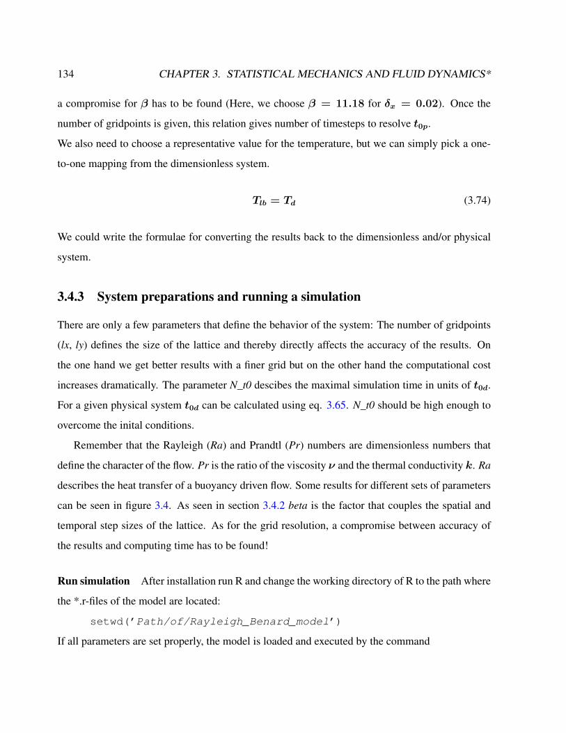
134 CHAPTER 3. STATISTICAL MECHANICS AND FLUID DYNAMICS*
a compromise for β has to be found (Here, we choose β = 11.18 for δx = 0.02). Once the
number of gridpoints is given, this relation gives number of timesteps to resolve t0p.
We also need to choose a representative value for the temperature, but we can simply pick a one-
to-one mapping from the dimensionless system.
Tlb = Td (3.74)
We could write the formulae for converting the results back to the dimensionless and/or physical
system.
3.4.3 System preparations and running a simulation
There are only a few parameters that define the behavior of the system: The number of gridpoints
(lx, ly) defines the size of the lattice and thereby directly affects the accuracy of the results. On
the one hand we get better results with a finer grid but on the other hand the computational cost
increases dramatically. The parameter N_t0 descibes the maximal simulation time in units of t0d.
For a given physical system t0d can be calculated using eq. 3.65. N_t0 should be high enough to
overcome the inital conditions.
Remember that the Rayleigh (Ra) and Prandtl (Pr) numbers are dimensionless numbers that
define the character of the flow. Pr is the ratio of the viscosity ν and the thermal conductivity k. Ra
describes the heat transfer of a buoyancy driven flow. Some results for different sets of parameters
can be seen in figure 3.4. As seen in section 3.4.2 beta is the factor that couples the spatial and
temporal step sizes of the lattice. As for the grid resolution, a compromise between accuracy of
the results and computing time has to be found!
Run simulation After installation run R and change the working directory of R to the path where
the *.r-files of the model are located:
setwd(’Path/of/Rayleigh_Benard_model’)
If all parameters are set properly, the model is loaded and executed by the command
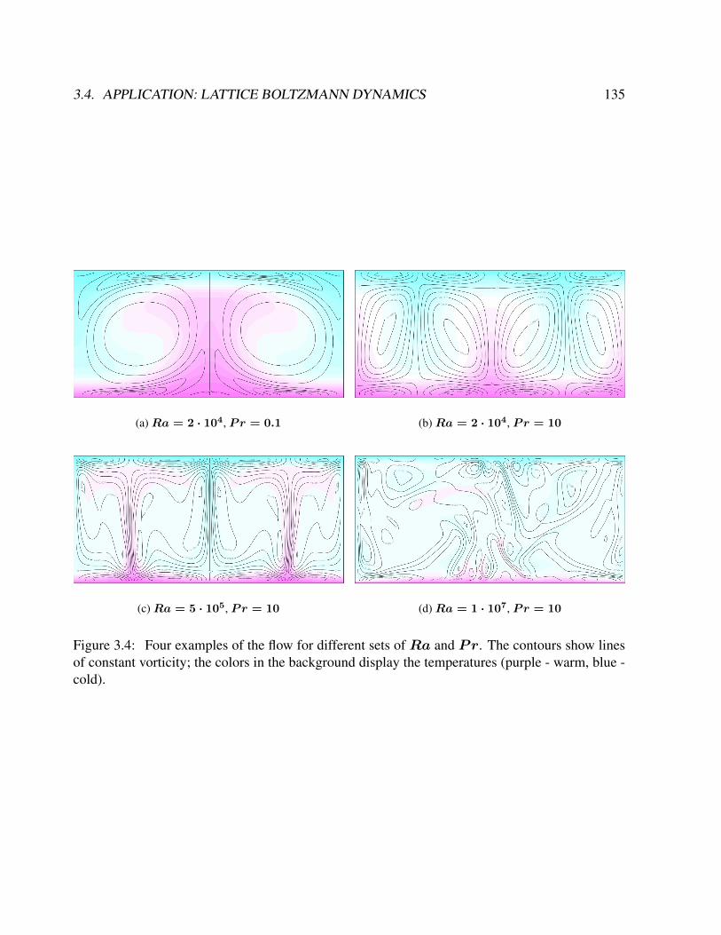
3.4. APPLICATION: LATTICE BOLTZMANN DYNAMICS 135
(a)Ra = 2 · 104, Pr = 0.1 (b)Ra = 2 · 104, Pr = 10
(c)Ra = 5 · 105, Pr = 10 (d)Ra = 1 · 107, Pr = 10
Figure 3.4: Four examples of the flow for different sets of Ra and Pr. The contours show linesof constant vorticity; the colors in the background display the temperatures (purple - warm, blue -cold).
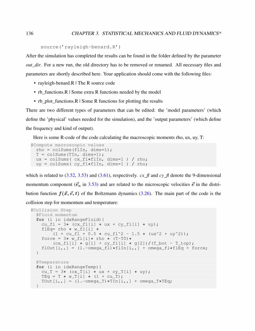
136 CHAPTER 3. STATISTICAL MECHANICS AND FLUID DYNAMICS*
source(’rayleigh-benard.R’)
After the simulation has completed the results can be found in the folder defined by the parameter
out_dir. For a new run, the old directory has to be removed or renamed. All necessary files and
parameters are shortly described here. Your application should come with the following files:
• rayleigh-benard.R | The R source code
• rb_functions.R | Some extra R functions needed by the model
• rb_plot_functions.R | Some R functions for plotting the results
There are two different types of parameters that can be edited: the ’model parameters’ (which
define the ’physical’ values needed for the simulation), and the ’output parameters’ (which define
the frequency and kind of output).
Here is some R-code of the code calculating the macroscopic moments rho, ux, uy, T:#Compute macroscopic values
rho = colSums(flIn, dims=1);T = colSums(TIn, dims=1);ux = colSums( cx_fl*flIn, dims=1 ) / rho;uy = colSums( cy_fl*flIn, dims=1 ) / rho;
which is related to (3.52, 3.53) and (3.61), respectively. cx_fl and cy_fl denote the 9-dimensional
momentum component (~ea in 3.53) and are related to the microscopic velocities ~e in the distri-
bution function f(~x, ~e, t) of the Boltzmann dynamics (3.26). The main part of the code is the
collision step for momentum and temperature:#Collision Step
#Fluid momentumfor (i in idxRangeFluid)cu_fl = 3* (cx_fl[i] * ux + cy_fl[i] * uy);flEq= rho * w_fl[i] *
(1 + cu_fl + 0.5 * cu_fl^2 - 1.5 * (ux^2 + uy^2));force = 3* w_fl[i]* rho * (T-T0)*
(cx_fl[i] * g[1] + cy_fl[i] * g[2])/(T_bot - T_top);flOut[i,,] = (1.-omega_fl)*flIn[i,,] + omega_fl*flEq + force;
#Temperaturefor (i in idxRangeTemp)cu_T = 3* (cx_T[i] * ux + cy_T[i] * uy);TEq = T * w_T[i] * (1 + cu_T);TOut[i,,] = (1.-omega_T)*TIn[i,,] + omega_T*TEq;
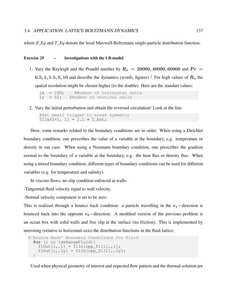
3.4. APPLICATION: LATTICE BOLTZMANN DYNAMICS 137
where fl_Eq and T_Eq denote the local Maxwell-Boltzmann single-particle distribution function.
Exercise 25 – Investigations with the LB-model
1. Vary the Rayleigh and the Prandtl number by Ra = 20000, 40000, 60000 and Pr =
0.5, 1, 1.5, 5, 10 and describe the dynamics (words, figures) ! For high values of Ra the
spatial resolution might be chosen higher (to the double). Here are the standart values:
lx = 100; #Number of horizontal cellsly = 52; #Number of vertical cells
2. Vary the initial perturbation and obtain the reversed circulation! Look at the line
#Set small trigger to break symmetryT[lx/2+1, 1] = 1.1 * T_bot;
Here, some remarks related to the boundary conditions are in order. When using a Dirichlet
boundary condition, one prescribes the value of a variable at the boundary, e.g. temperature or
density in our case. When using a Neumann boundary condition, one prescribes the gradient
normal to the boundary of a variable at the boundary, e.g. the heat flux or density flux. When
using a mixed boundary condition, different types of boundary conditions can be used for different
variables (e.g. for temperature and salinity).
In viscous flows, no-slip condition enforced at walls:
-Tangential fluid velocity equal to wall velocity.
-Normal velocity component is set to be zero.
This is realized through a bounce back condition: a particle travelling in the e1−direction is
bounced back into the opposite e5−direction. A modified version of the previous problem is
an ocean box with solid walls and free slip at the surface (no friction). This is implemented by
mirroring (relative to horizontal-axis) the distribution functions in the fluid-lattice:
#"Bounce Back" Boundary Conditions for Fluidfor (i in idxRangeFluid)flOut[i,,1] = flIn[opp_fl[i],,1];flOut[i,,ly] = flIn[opp_fl[i],,ly];
Used when physical geometry of interest and expected flow pattern and the thermal solution are
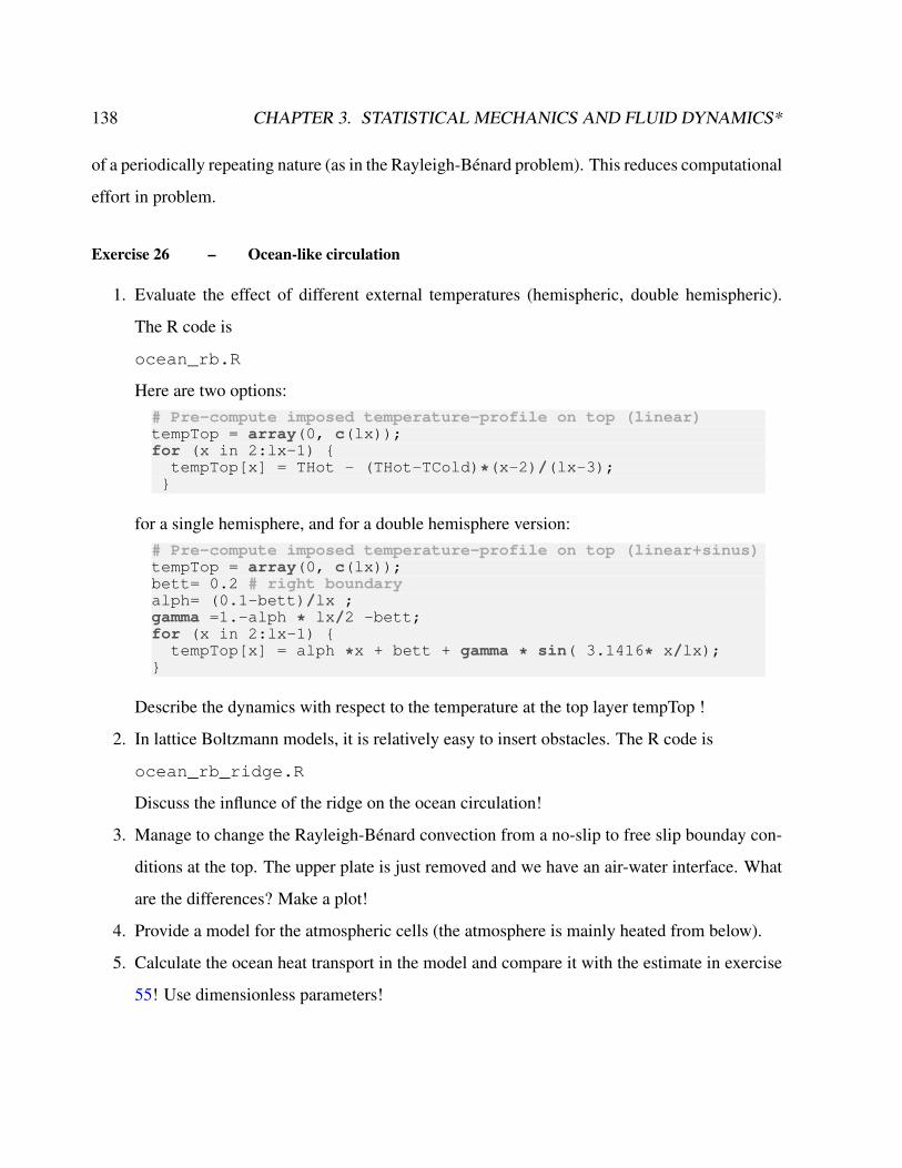
138 CHAPTER 3. STATISTICAL MECHANICS AND FLUID DYNAMICS*
of a periodically repeating nature (as in the Rayleigh-Bénard problem). This reduces computational
effort in problem.
Exercise 26 – Ocean-like circulation
1. Evaluate the effect of different external temperatures (hemispheric, double hemispheric).
The R code is
ocean_rb.R
Here are two options:# Pre-compute imposed temperature-profile on top (linear)tempTop = array(0, c(lx));for (x in 2:lx-1)
tempTop[x] = THot - (THot-TCold)*(x-2)/(lx-3);
for a single hemisphere, and for a double hemisphere version:# Pre-compute imposed temperature-profile on top (linear+sinus)tempTop = array(0, c(lx));bett= 0.2 # right boundaryalph= (0.1-bett)/lx ;gamma =1.-alph * lx/2 -bett;for (x in 2:lx-1)
tempTop[x] = alph *x + bett + gamma * sin( 3.1416* x/lx);
Describe the dynamics with respect to the temperature at the top layer tempTop !
2. In lattice Boltzmann models, it is relatively easy to insert obstacles. The R code is
ocean_rb_ridge.R
Discuss the influnce of the ridge on the ocean circulation!
3. Manage to change the Rayleigh-Bénard convection from a no-slip to free slip bounday con-
ditions at the top. The upper plate is just removed and we have an air-water interface. What
are the differences? Make a plot!
4. Provide a model for the atmospheric cells (the atmosphere is mainly heated from below).
5. Calculate the ocean heat transport in the model and compare it with the estimate in exercise
55! Use dimensionless parameters!
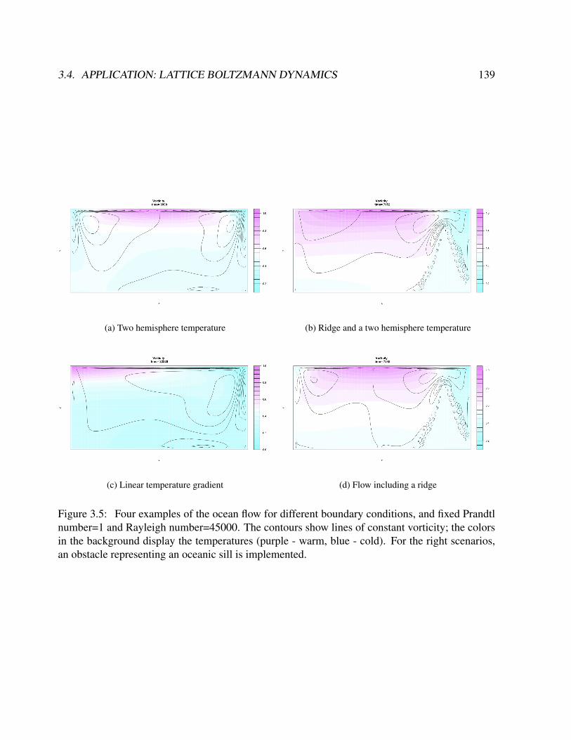
3.4. APPLICATION: LATTICE BOLTZMANN DYNAMICS 139
(a) Two hemisphere temperature (b) Ridge and a two hemisphere temperature
(c) Linear temperature gradient (d) Flow including a ridge
Figure 3.5: Four examples of the ocean flow for different boundary conditions, and fixed Prandtlnumber=1 and Rayleigh number=45000. The contours show lines of constant vorticity; the colorsin the background display the temperatures (purple - warm, blue - cold). For the right scenarios,an obstacle representing an oceanic sill is implemented.
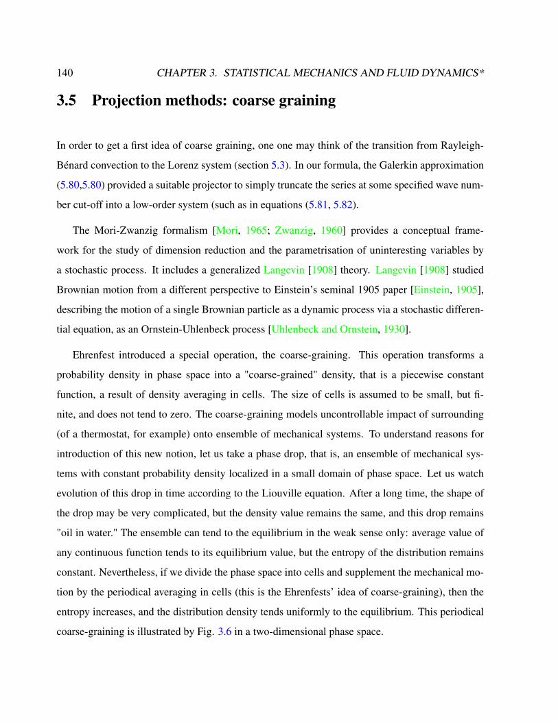
140 CHAPTER 3. STATISTICAL MECHANICS AND FLUID DYNAMICS*
3.5 Projection methods: coarse graining
In order to get a first idea of coarse graining, one one may think of the transition from Rayleigh-
Bénard convection to the Lorenz system (section 5.3). In our formula, the Galerkin approximation
(5.80,5.80) provided a suitable projector to simply truncate the series at some specified wave num-
ber cut-off into a low-order system (such as in equations (5.81, 5.82).
The Mori-Zwanzig formalism [Mori, 1965; Zwanzig, 1960] provides a conceptual frame-
work for the study of dimension reduction and the parametrisation of uninteresting variables by
a stochastic process. It includes a generalized Langevin [1908] theory. Langevin [1908] studied
Brownian motion from a different perspective to Einstein’s seminal 1905 paper [Einstein, 1905],
describing the motion of a single Brownian particle as a dynamic process via a stochastic differen-
tial equation, as an Ornstein-Uhlenbeck process [Uhlenbeck and Ornstein, 1930].
Ehrenfest introduced a special operation, the coarse-graining. This operation transforms a
probability density in phase space into a "coarse-grained" density, that is a piecewise constant
function, a result of density averaging in cells. The size of cells is assumed to be small, but fi-
nite, and does not tend to zero. The coarse-graining models uncontrollable impact of surrounding
(of a thermostat, for example) onto ensemble of mechanical systems. To understand reasons for
introduction of this new notion, let us take a phase drop, that is, an ensemble of mechanical sys-
tems with constant probability density localized in a small domain of phase space. Let us watch
evolution of this drop in time according to the Liouville equation. After a long time, the shape of
the drop may be very complicated, but the density value remains the same, and this drop remains
"oil in water." The ensemble can tend to the equilibrium in the weak sense only: average value of
any continuous function tends to its equilibrium value, but the entropy of the distribution remains
constant. Nevertheless, if we divide the phase space into cells and supplement the mechanical mo-
tion by the periodical averaging in cells (this is the Ehrenfests’ idea of coarse-graining), then the
entropy increases, and the distribution density tends uniformly to the equilibrium. This periodical
coarse-graining is illustrated by Fig. 3.6 in a two-dimensional phase space.
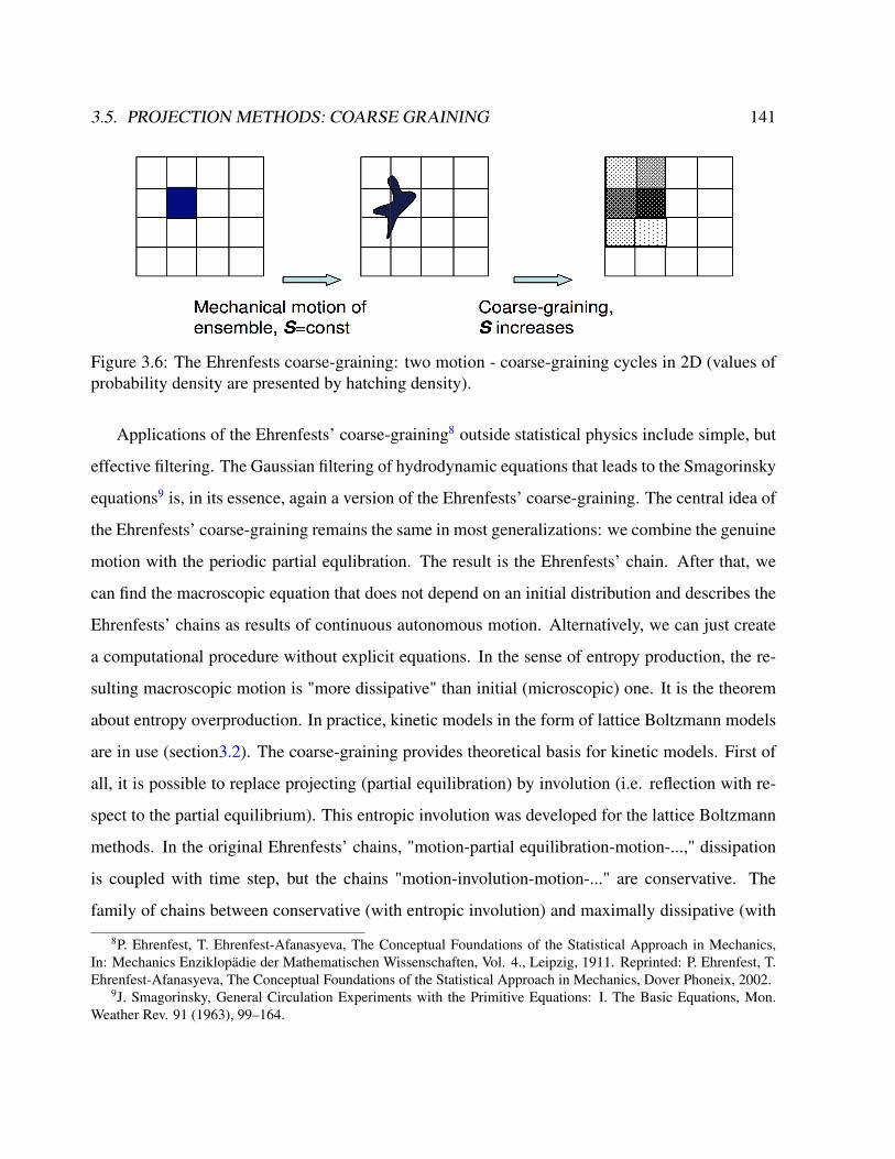
3.5. PROJECTION METHODS: COARSE GRAINING 141
Figure 3.6: The Ehrenfests coarse-graining: two motion - coarse-graining cycles in 2D (values ofprobability density are presented by hatching density).
Applications of the Ehrenfests’ coarse-graining8 outside statistical physics include simple, but
effective filtering. The Gaussian filtering of hydrodynamic equations that leads to the Smagorinsky
equations9 is, in its essence, again a version of the Ehrenfests’ coarse-graining. The central idea of
the Ehrenfests’ coarse-graining remains the same in most generalizations: we combine the genuine
motion with the periodic partial equlibration. The result is the Ehrenfests’ chain. After that, we
can find the macroscopic equation that does not depend on an initial distribution and describes the
Ehrenfests’ chains as results of continuous autonomous motion. Alternatively, we can just create
a computational procedure without explicit equations. In the sense of entropy production, the re-
sulting macroscopic motion is "more dissipative" than initial (microscopic) one. It is the theorem
about entropy overproduction. In practice, kinetic models in the form of lattice Boltzmann models
are in use (section3.2). The coarse-graining provides theoretical basis for kinetic models. First of
all, it is possible to replace projecting (partial equilibration) by involution (i.e. reflection with re-
spect to the partial equilibrium). This entropic involution was developed for the lattice Boltzmann
methods. In the original Ehrenfests’ chains, "motion-partial equilibration-motion-...," dissipation
is coupled with time step, but the chains "motion-involution-motion-..." are conservative. The
family of chains between conservative (with entropic involution) and maximally dissipative (with
8P. Ehrenfest, T. Ehrenfest-Afanasyeva, The Conceptual Foundations of the Statistical Approach in Mechanics,In: Mechanics Enziklopädie der Mathematischen Wissenschaften, Vol. 4., Leipzig, 1911. Reprinted: P. Ehrenfest, T.Ehrenfest-Afanasyeva, The Conceptual Foundations of the Statistical Approach in Mechanics, Dover Phoneix, 2002.
9J. Smagorinsky, General Circulation Experiments with the Primitive Equations: I. The Basic Equations, Mon.Weather Rev. 91 (1963), 99–164.
142 CHAPTER 3. STATISTICAL MECHANICS AND FLUID DYNAMICS*
projection) ones give us a possibility to model hydrodynamic systems with various dissipation
(viscosity) coefficients that are decoupled with time steps.
Of particular interest is the work of Mori [Mori, 1965] and Zwanzig [Zwanzig, 1960] which re-
lates the evolution of macroscopic variables to microscopic dynamics. The standard Mori-Zwanzig
theory has been given a nonlinear generalization by Zwanzig [Zwanzig, 1980], and is furthermore
not limited to Hamiltonian dynamics [Chorin et al., 1999; Gottwald, 2010]. This approach of
modelling fast small-scale processes by a stochastic process is intuitive: provided the fast pro-
cesses decorrelate rapidly enough, the slow variables experience the sum of uncorrelated events
of the fast dynamics, which according to the (weak) central limit theorem corresponds to approxi-
mate Gaussian noise. A method whereby many fast degrees of freedom are replaced by a stochastic
process is called stochastic model reduction.
Consider the very simple coupled linear system10
x = L11x+ L12y the "climate" equation (3.75)
y = L21x+ L22y the "whether" equation. (3.76)
Suppose we are only interested in the dynamics of x, and have only some climatic knowledge of
the initial conditions of the variables y, that is the mean and variance. The whether differential
equation (3.76) can be solved by the ansatz
y(t) = eL22ty(0) · C(t) (3.77)
Inserting this, we can then solve the inhomogenous problem to obtain
y(t) = eL22ty(0) +
∫ t
0
eL22(t−s)L21x(s)ds,
10We follow the notation of [Hasselmann, 1976; Chorin et al., 1999; Gottwald, 2010].
3.5. PROJECTION METHODS: COARSE GRAINING 143
which we may use to express the dynamics of the climate variable as
x = L11x+ L12
∫ t
0
eL22(t−s)L21x(s)ds+ L12eL22ty(0). (3.78)
This is of the form of a generalised Langevin equation, where the first term is Markovian (no
dependence on the history of the process), the second is a memory term, and the last can be
interpreted as a noise term, provided that the initial conditions y(0) are randomly distributed. A
similar reduction of the dynamics can be described by fast and slow variables applying the center
manifold theory [Arnold, 1995] or slaving principle [Haken, 1996].
For the more general non-linear case, the instantaneous state of the Earth System, compris-
ing the components ‘atmosphere-ocean-cryosphere-land’, can be expressed by a set of variables
z = (z1, z2, ...), representing the density, velocity, temperature, etc. of the various media. The
evolution of this system will be given by a series of prognostic equations of the form
z = f(z), (3.79)
with initial condition z(0) = z0 and z ∈ Rd, suppose we are not interested in the full solu-
tion z(t), but rather only in a few n ≤ d observables Φ(z) = (Φ1(z),Φ2(z), ...,Φn(z)).
This includes the case Φ(z) = (z1, ..., zn), when the state space is decomposed as z =
(x, y) into ’interesting’ variables, x = (z1, ..., zn) ∈ Rn, and ’uninteresting’ variables, y =
(zn+1, ..., zd) ∈ Rd−n. In the Earth System, a separation may be into a fast ‘weather subsystem’
(y) and a slow ‘climate subsystem’ (x) with different order of magnitude in the correlation times
(or, the response/relaxation times) for the slow variable is much larger than that of the fast variable,
i.e.
τy τx. (3.80)
Now let us ask the following question: what are the effective dynamics of the interesting observ-
ables for an ensemble of initial conditions z(0), where Φ(z(0)) is known and the uninteresting
subspace is equipped with a known distribution?

144 CHAPTER 3. STATISTICAL MECHANICS AND FLUID DYNAMICS*
Rather than investigating the dynamical system (3.79) directly, one may choose to look at
how observables V (z(t)) evolve in time. Applying the chain rule, one can naturally define the
generator
L = f(z) · ∇,
and writed
dtV (z(t)) = LV (z(t)).
Note that L is the adjoint operator of the Liouville operator L∗ with L∗ρ = −∇ · (f(z)ρ)
controlling the evolution of densities of ensembles propagated according to (3.79). We seek for the
solution v(z, t) of∂v
∂t= Lv with v(z, 0) = φ(z), (3.81)
where z is an independent variable and denotes initial conditions. The solution of (3.81) can be
formally written as
v(z, t) = eLtφ(z), (3.82)
To filter out the dynamics of the interesting variables we require a projection operator P that
maps functions of z to functions of Φ(z). If the manifold consists for example of a product of
submanifolds of relevant and irrelevant variables, one can take a conditional expectation
(Pv)(x) =
∫Rd−n v(z)ρ(x, y)dy∫
Rd−n ρ(x, y)dy(3.83)
where ρ(x, y) denotes the joint probability function of the initial conditions for the full system
(3.79). It is easy to show that this a projection (P2 = P). In the context of PDEs one may
use Galerkin approximations, a perfectly valid projector would be to simply truncate the Galerkin
series at some specified high wave number cut-off. We also define the orthogonal projector Q
that projects onto y, with Q = 1− P. Now, the derivation of the Mori-Zwanzig equation is
a two-linear: given the Cauchy problem (3.81) and its formal solution (3.82) we write, using
3.5. PROJECTION METHODS: COARSE GRAINING 145
P + Q = 1,∂v
∂t(z, t) = LeLtΦ(z) = eLtPLΦ(z) + eLtQLΦ(z)
which, upon using the Duhamel-Dyson formula [Evans and Morriss, 2008] for operators A and B,
yields
et(A+B) = etA +
∫ t
0
e(t−s)(A+B)BesAds.
By differentiation, this becomes the celebrated Mori-Zwanzig equation [Mori et al., 1974; Zwanzig,
1960]
∂v
∂t(z, t) = eLtPLΦ(z) +
∫ t
0
e(t−s)LPLesQLQLΦ(z)ds+ etQLQLΦ(z). (3.84)
Note that the Mori-Zwanzig equation (3.84) is not an approximation but is exact and constitutes an
equivalent formulation of the full problem (3.79). The Mori-Zwanzig equation (3.84) is in the form
of a generalised Langevin equation. The first term on the right-hand side is Markovian, the second
term is a memory term, and the last term lives in the uninteresting orthogonal subspace and can be
called noise. Ideally one would like to approximate the noise term by white noise. Heuristically
this should be possible in the case of time-scale separation or of weak coupling. The advantage of
looking at this limit is however that the noise autocorrelation function and memory kernel can now
be written as simple correlation and response functions of the unresolved dynamics. The reader is
referred to [Chorin and Hald, 2006; Chorin et al., 2000; Zwanzig, 2001; Evans and Morriss, 2008;
Givon et al., 2004; Lucarini et al., 2014] for more details.
The projection method includes the procedure to parameterize the turbulent energy dissipation
in turbulent flows, where the larger eddies extract energy from the mean flow and ultimately trans-
fer some of it to the smaller eddies which, in turn, pass the energy to even smaller eddies, and so
on up to the smallest scales, where the eddies convert the kinetic energy into internal energy of
the fluid. At this scales (also known as Kolmogorov scale), the viscous friction dominates the flow
[Frisch, 1996].
The theory of scientific reduction is important for different theories: the microscopic informa-
146 CHAPTER 3. STATISTICAL MECHANICS AND FLUID DYNAMICS*
tion in the brain with enormous amount of possible solutions is reduced to macroscopic actions
and human behaviour. This implies that the actions are not deterministic, but stochastic in the
sense of the standard Mori-Zwanzig theory or Brownian motion. Without being a specialist, this
seems to be important for neuroscience and for the philosophy of science in general. The activity
of neurons in the brain can be modelled statistically (e.g., https://en.wikipedia.org/
wiki/Ising_model).
Part II
Second part: Fluid Dynamics
147
Chapter 4
Basics of Fluid Dynamics
Our starting point is a mathematical model for the system of interest. In physics a model typically
describes the state variables, plus fundamental laws and equations of state. These variables evolve
in space and time. For the ocean circulation, we proceed as follows:
• State variables: Velocity (in each of three directions), pressure, temperature, salinity, density
• Fundamental laws: Conservation of momentum, conservation of mass, conservation of tem-
perature and salinity
• Equations of state: Relationship of density to temperature, salinity and pressure, and perhaps
also a model for the formation of sea-ice
The state variables for the ocean model are expressed as a continuum in space and time, and the
fundamental laws as partial differential equations1. Even at this stage, though, simplifications may
be made. For example, it is common to treat seawater as incompressible. Furthermore, equations
of state are often specified by empirical relationships or laboratory experiments.
In the following, the general structure of ocean circulation, atmospheric energy balance as well
as ice sheet models are described. The dynamics of flow are based on the Navier-Stokes equations.
The derivation of the Navier-Stokes equations begins with an application of Newton’s second law:
conservation of momentum (often alongside mass and energy conservation) being written for an
1If the atmosphere is becoming too thin in the upper levels, a more molecular, statistical description is appropiate(section 3)
148
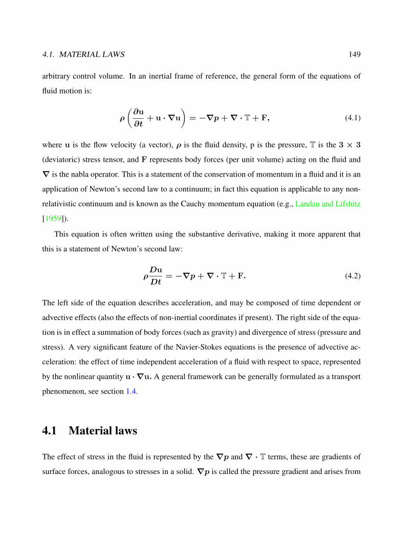
4.1. MATERIAL LAWS 149
arbitrary control volume. In an inertial frame of reference, the general form of the equations of
fluid motion is:
ρ
(∂u
∂t+ u · ∇u
)= −∇p+∇ · T + F, (4.1)
where u is the flow velocity (a vector), ρ is the fluid density, p is the pressure, T is the 3 × 3
(deviatoric) stress tensor, and F represents body forces (per unit volume) acting on the fluid and
∇ is the nabla operator. This is a statement of the conservation of momentum in a fluid and it is an
application of Newton’s second law to a continuum; in fact this equation is applicable to any non-
relativistic continuum and is known as the Cauchy momentum equation (e.g., Landau and Lifshitz
[1959]).
This equation is often written using the substantive derivative, making it more apparent that
this is a statement of Newton’s second law:
ρDu
Dt= −∇p+∇ · T + F. (4.2)
The left side of the equation describes acceleration, and may be composed of time dependent or
advective effects (also the effects of non-inertial coordinates if present). The right side of the equa-
tion is in effect a summation of body forces (such as gravity) and divergence of stress (pressure and
stress). A very significant feature of the Navier-Stokes equations is the presence of advective ac-
celeration: the effect of time independent acceleration of a fluid with respect to space, represented
by the nonlinear quantity u · ∇u. A general framework can be generally formulated as a transport
phenomenon, see section 1.4.
4.1 Material laws
The effect of stress in the fluid is represented by the∇p and∇ · T terms, these are gradients of
surface forces, analogous to stresses in a solid. ∇p is called the pressure gradient and arises from
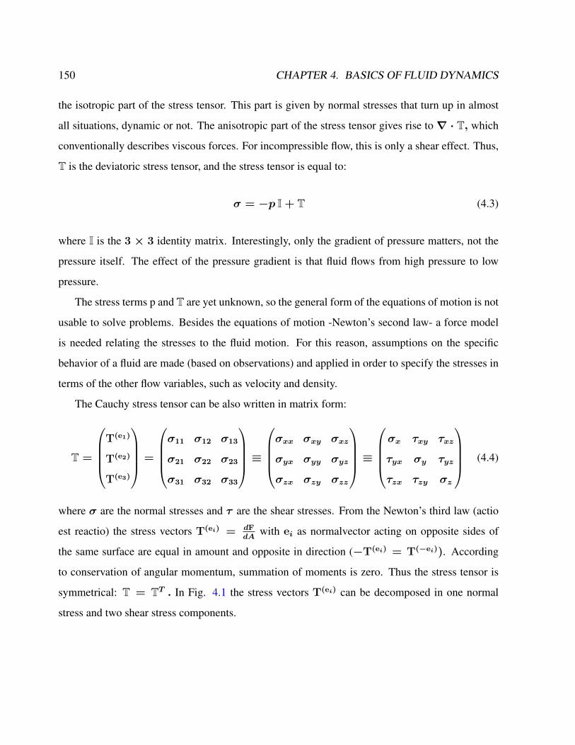
150 CHAPTER 4. BASICS OF FLUID DYNAMICS
the isotropic part of the stress tensor. This part is given by normal stresses that turn up in almost
all situations, dynamic or not. The anisotropic part of the stress tensor gives rise to∇ · T, which
conventionally describes viscous forces. For incompressible flow, this is only a shear effect. Thus,
T is the deviatoric stress tensor, and the stress tensor is equal to:
σ = −p I + T (4.3)
where I is the 3 × 3 identity matrix. Interestingly, only the gradient of pressure matters, not the
pressure itself. The effect of the pressure gradient is that fluid flows from high pressure to low
pressure.
The stress terms p and T are yet unknown, so the general form of the equations of motion is not
usable to solve problems. Besides the equations of motion -Newton’s second law- a force model
is needed relating the stresses to the fluid motion. For this reason, assumptions on the specific
behavior of a fluid are made (based on observations) and applied in order to specify the stresses in
terms of the other flow variables, such as velocity and density.
The Cauchy stress tensor can be also written in matrix form:
T =
T(e1)
T(e2)
T(e3)
=
σ11 σ12 σ13
σ21 σ22 σ23
σ31 σ32 σ33
≡σxx σxy σxz
σyx σyy σyz
σzx σzy σzz
≡σx τxy τxz
τyx σy τyz
τzx τzy σz
(4.4)
where σ are the normal stresses and τ are the shear stresses. From the Newton’s third law (actio
est reactio) the stress vectors T(ei) = dFdA
with ei as normalvector acting on opposite sides of
the same surface are equal in amount and opposite in direction (−T(ei) = T(−ei)). According
to conservation of angular momentum, summation of moments is zero. Thus the stress tensor is
symmetrical: T = TT . In Fig. 4.1 the stress vectors T(ei) can be decomposed in one normal
stress and two shear stress components.
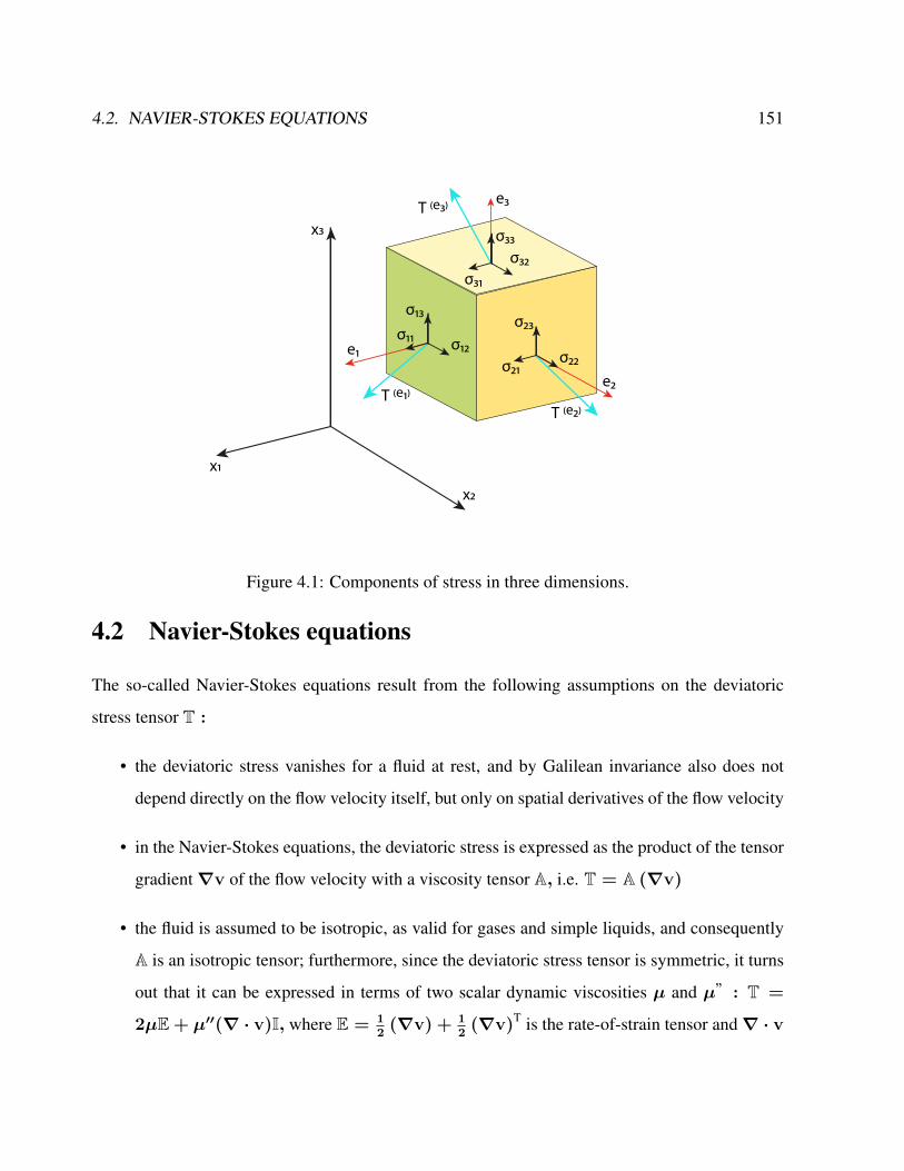
4.2. NAVIER-STOKES EQUATIONS 151
x3
x1
x2
e1
e2
e3
T (e1)T (e2)
T (e3)
σ13
σ11σ12
σ23
σ21 σ22
σ33
σ31σ32
Figure 4.1: Components of stress in three dimensions.
4.2 Navier-Stokes equations
The so-called Navier-Stokes equations result from the following assumptions on the deviatoric
stress tensor T :
• the deviatoric stress vanishes for a fluid at rest, and by Galilean invariance also does not
depend directly on the flow velocity itself, but only on spatial derivatives of the flow velocity
• in the Navier-Stokes equations, the deviatoric stress is expressed as the product of the tensor
gradient∇v of the flow velocity with a viscosity tensor A, i.e. T = A (∇v)
• the fluid is assumed to be isotropic, as valid for gases and simple liquids, and consequently
A is an isotropic tensor; furthermore, since the deviatoric stress tensor is symmetric, it turns
out that it can be expressed in terms of two scalar dynamic viscosities µ and µ” : T =
2µE + µ′′(∇ · v)I, where E = 12
(∇v) + 12
(∇v)T is the rate-of-strain tensor and∇ · v
152 CHAPTER 4. BASICS OF FLUID DYNAMICS
is the rate of expansion of the flow
• the deviatoric stress tensor has zero trace, so for a three-dimensional flow 2µ+ 3µ” = 0
As a result, in the Navier-Stokes equations the deviatoric stress tensor has the following form:
T = 2µ(E− 1
3(∇ · u)I
), (4.5)
with the quantity between brackets the non-isotropic part of the rate-of-strain tensor E. The dynamic
viscosity µ does not need to be constant - in general it depends on conditions like temperature and
pressure, and in turbulence modelling the concept of eddy viscosity is used to approximate the
average deviatoric stress.
The Navier-Stokes equations are strictly a statement of the conservation of momentum. In order
to fully describe fluid flow, more information is needed (how much depends on the assumptions
made), this may include boundary data (no-slip, capillary surface, etc), the conservation of mass,
the conservation of energy, and/or an equation of state. Regardless of the flow assumptions, a
statement of the conservation of mass is generally necessary. This is achieved through the mass
continuity equation, given in its most general form as:
∂ρ
∂t+∇ · (ρu) = 0 (4.6)
or, using the substantive derivative:
Dρ
Dt+ ρ(∇ · u) = 0. (4.7)
A simplification of the resulting flow equations is obtained when considering an incompressible
flow of a Newtonian fluid. The assumption of incompressibility rules out the possibility of sound
or shock waves to occur; so this simplification is invalid if these phenomena are important. The
incompressible flow assumption typically holds well even when dealing with a "compressible"
fluid -such as air at room temperature- at low Mach numbers (even when flowing up to about Mach
4.2. NAVIER-STOKES EQUATIONS 153
0.3).2 Taking this into account and assuming constant viscosity, the Navier-Stokes equations will
read, in vector form:
ρ
(∂u
∂t+ u · ∇u
)= −∇p+ µ∇2u + F. (4.8)
The vector field F represents "other" (body force) forces. Typically this is only gravity, but may
include other fields (such as electromagnetic). In a non-inertial coordinate system, other "forces"
such as that associated with rotating coordinates may be inserted3. Often, these forces may be
represented as the gradient of some scalar quantity. Gravity in the z direction, for example, is the
gradient of−ρgz. Since pressure shows up only as a gradient, this implies that solving a problem
without any such body force can be mended to include the body force by modifying pressure. The
shear stress term∇T becomes the useful quantityµ∇2u when the fluid is assumed incompressible
and Newtonian, where µ is the dynamic viscosity.
It’s well worth observing the meaning of each term (compare to the Cauchy momentum equa-
tion):
Inertia (per volume)︷ ︸︸ ︷ρ( ∂u
∂t︸︷︷︸Unsteady
acceleration
+ u · ∇u︸ ︷︷ ︸Advective
acceleration
)=
Divergence of stress︷ ︸︸ ︷−∇p︸ ︷︷ ︸Pressuregradient
+µ∇2u︸ ︷︷ ︸Viscosity
+ F︸︷︷︸Otherbodyforces
. (4.9)
Note that only the advection terms are nonlinear for incompressible Newtonian flow. This acceler-
ation is an acceleration caused by a (possibly steady) change in velocity over position, for example
the speeding up of fluid entering a converging nozzle. Though individual fluid particles are being
accelerated and thus are under unsteady motion, the flow field (a velocity distribution) will not
2The density and pressure fields can be expressed as a perturbation from a hydrostatically balanced state arounda reference density ρr(z) (e.g. a horizontal mean of density in the area of interest) and associated pressure pr(z)which are linked through dpr/dz = −gρr and pr(z = 0) = 0. Sound waves are filtered by realizing that thetime rate of change of density due to diabatic effects and compressibility is much smaller than that due to change ofvolume.
3We will see later that the Coriolis force will be one of the main contributions in the rotating Earth system (section6.1)
154 CHAPTER 4. BASICS OF FLUID DYNAMICS
necessarily be time dependent.
Another important observation is that the viscosity is represented by the vector Laplacian of
the velocity field. This implies that Newtonian viscosity is diffusion of momentum, this works
in much the same way as the diffusion of heat seen in the heat equation (which also involves the
Laplacian).
If temperature effects are also neglected, the only "other" equation (apart from initial/boundary
conditions) needed is the mass continuity equation. Under the incompressible assumption, density
is a constant and it follows that the equation will simplify to:
∇ · u = 0 . (4.10)
This is more specifically a statement of the conservation of volume (see divergence). These equa-
tions are commonly used in 3 coordinates systems: Cartesian, cylindrical, and spherical. While
the Cartesian equations seem to follow directly from the vector equation above, the vector form
of the Navier-Stokes equation involves some tensor calculus which means that writing it in other
coordinate systems is not as simple as doing so for scalar equations (such as the heat equation).
4.3 Integral and differential formulation
On a volume work two types of forces:
1. The force ~F on each volume element. For gravity holds: ~F = %~g.
2. Surface forces working only on the margins: ~t. For these holds: ~t = ~n σ, where σ is the
stress tensor.
σ can be split in a part p I representing the normal tensions and a part T representing the shear
stresses: σ = T + p I, where I is the unit tensor or identity matrix. When viscous aspects can be
4.3. INTEGRAL AND DIFFERENTIAL FORMULATION 155
ignored holds:
div σ = −∇p . (4.11)
When the flow velocity is ~v at position ~r holds on position ~r + d~r:
~v(~r + d~r ) = ~v(~r )︸ ︷︷ ︸translation
+ d~r · (∇~v )︸ ︷︷ ︸rotation, deformation, dilatation
The quantity L:= ∇~v can be split in a symmetric part D and an antisymmetric part W. L = D + W
with
Dij :=1
2
(∂vi
∂xj+∂vj
∂xi
), Wij :=
1
2
(∂vi
∂xj−∂vj
∂xi
)When the rotation or vorticity ~ω = rot~v is introduced holds: Wij = 1
2εijkωk. ~ω represents the
local rotation velocity: ~dr · W = 12ω × ~dr.
For a Newtonian liquid holds: T = 2ηD. Here, η is the dynamical viscosity. This is related to
the shear stress τ by:
τij = η∂vi
∂xj
For compressible media can be stated: T = (η′div~v )I + 2ηD. From equating the thermody-
namical and mechanical pressure it follows: 3η′ + 2η = 0. If the viscosity is constant holds:
div(2D) = ∇2~v + grad div~v.
The conservation laws for mass, momentum and energy for continuous media can be written
in both integral and differential form. They are:
Integral notation:
1. Conservation of mass:∂
∂t
∫∫∫%d3V +
∫∫© %(~v · ~n )d2A = 0
2. Conservation of momentum:∂
∂t
∫∫∫%~vd3V +
∫∫© %~v(~v · ~n )d2A =
∫∫∫f0d
3V +∫∫© ~n · Td2A
156 CHAPTER 4. BASICS OF FLUID DYNAMICS
3. Conservation of energy:∂
∂t
∫∫∫(1
2v2 + e)%d3V +
∫∫© (1
2v2 + e)%(~v · ~n )d2A =
−∫∫© (~q · ~n )d2A+
∫∫∫(~v · ~f0)d3V +
∫∫© (~v · ~n T)d2A
Differential notation:
1. Conservation of mass:∂%
∂t+ div · (%~v ) = 0
2. Conservation of momentum: %∂~v
∂t+ (%~v · ∇)~v = ~f0 + divT = ~f0 − gradp+ divT
′
3. Conservation of energy: %Tds
dt= %
de
dt−p
%
d%
dt= −div~q + T : D
Here, e is the internal energy per unit of mass E/m and s is the entropy per unit of mass
S/m. ~q = −κ~∇T is the heat flow. Further holds:
p = −∂E
∂V= −
∂e
∂1/%, T =
∂E
∂S=∂e
∂s
so
CV =
(∂e
∂T
)V
and Cp =
(∂h
∂T
)p
with h = H/m the enthalpy per unit of mass.
From this one can derive the Navier-Stokes equations for an incompressible, viscous and heat-
conducting medium:
div~v = 0
%∂~v
∂t+ %(~v · ∇)~v = %~g − gradp+ η∇2~v
%C∂T
∂t+ %C(~v · ∇)T = κ∇2T + 2ηD : D
withC the thermal heat capacity. The force ~F on an object within a flow, when viscous effects are
limited to the boundary layer, can be obtained using the momentum law. If a surface A surrounds
4.3. INTEGRAL AND DIFFERENTIAL FORMULATION 157
the object outside the boundary layer holds:
~F = −∫∫© [p~n+ %~v(~v · ~n )]d2A
Exercise 27 – Questions about advection
1. A ship is steaming northward at a rate of 10 km/h. The surface pressure increases toward the
northwest at a rate of 5 Pa/km. What is the pressure tendency recorded at a nearby island
station if the pressure aboard the ship decreases at a rate of 100Pa/3h?
2. The temperature at a point 50 km north of a station is 3C cooler than at the station. If the
wind is blowing from the northeast at 20m/s and the air is being heated by radiation at a rate
of 1C/h, what is the local temperature change at the station?
3. The following data were received from 50 km to the east, north, west and south of a station,
respectively: 90 degree, 10m/s; 120 degree,4m/s; 90degree,8m/s; 60 degree, 4m/s. Given
are the angle and absolute value of the wind speed. Calculate the approximate horizontal
divergence at the station.
4. Let the x = (x1, x2, x3) coordinates be inertial. What are the necessary and sufficient
conditions that the coordinates yi = Aijxj + vj(x, t)t be inertial for constant matrix
A = (Aij) ?
5. How can the movement of fluid particel be descibed in accordance with Newton’s first law?
Which forces can create accelerations or decelerations? Please use the definition of specific
forces, that is, the force per unit mass: f = F/m.
6. The potential temperature in the atmosphere is defined as
Θ = T (p0/p)R/cp (4.12)
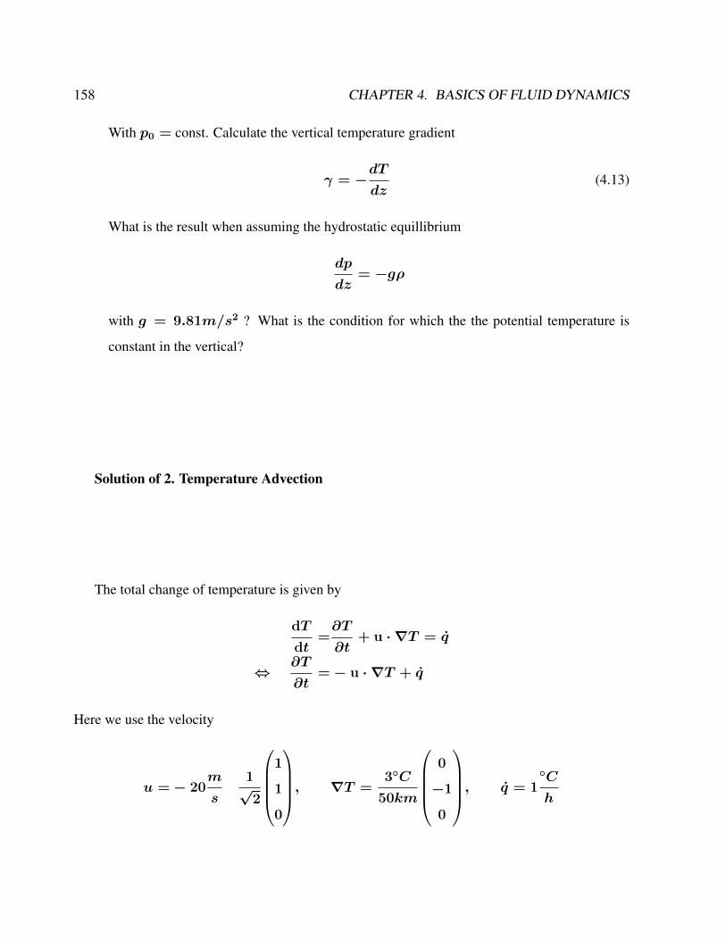
158 CHAPTER 4. BASICS OF FLUID DYNAMICS
With p0 = const. Calculate the vertical temperature gradient
γ = −dT
dz(4.13)
What is the result when assuming the hydrostatic equillibrium
dp
dz= −gρ
with g = 9.81m/s2 ? What is the condition for which the the potential temperature is
constant in the vertical?
Solution of 2. Temperature Advection
The total change of temperature is given by
dT
dt=∂T
∂t+ u · ∇T = q
⇔∂T
∂t=− u · ∇T + q
Here we use the velocity
u =− 20m
s
1√
2
1
1
0
, ∇T =3C
50km
0
−1
0
, q = 1C
h
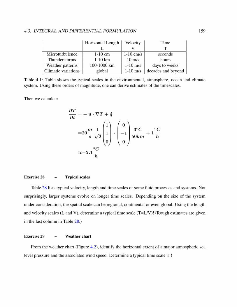
4.3. INTEGRAL AND DIFFERENTIAL FORMULATION 159
Horizontal Length Velocity TimeL V T
Microturbulence 1-10 cm 1-10 cm/s secondsThunderstorms 1-10 km 10 m/s hours
Weather patterns 100-1000 km 1-10 m/s days to weeksClimatic variations global 1-10 m/s decades and beyond
Table 4.1: Table shows the typical scales in the environmental, atmosphere, ocean and climatesystem. Using these orders of magnitude, one can derive estimates of the timescales.
Then we calculate
∂T
∂t=− u · ∇T + q
=20m
s
1√
2
1
1
0
·
0
−1
0
3C
50km+ 1
C
h
≈−2.1C
h
Exercise 28 – Typical scales
Table 28 lists typical velocity, length and time scales of some fluid processes and systems. Not
surprisingly, larger systems evolve on longer time scales. Depending on the size of the system
under consideration, the spatial scale can be regional, continental or even global. Using the length
and velocity scales (L and V), determine a typical time scale (T=L/V)! (Rough estimates are given
in the last column in Table 28.)
Exercise 29 – Weather chart
From the weather chart (Figure 4.2), identify the horizontal extent of a major atmospheric sea
level pressure and the associated wind speed. Determine a typical time scale T !
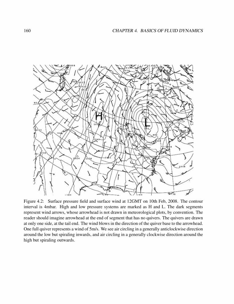
160 CHAPTER 4. BASICS OF FLUID DYNAMICS
Figure 4.2: Surface pressure field and surface wind at 12GMT on 10th Feb, 2008. The contourinterval is 4mbar. High and low pressure systems are marked as H and L. The dark segmentsrepresent wind arrows, whose arrowhead is not drawn in meteorological plots, by convention. Thereader should imagine arrowhead at the end of segment that has no quivers. The quivers are drawnat only one side, at the tail end. The wind blows in the direction of the quiver base to the arrowhead.One full quiver represents a wind of 5m/s. We see air circling in a generally anticlockwise directionaround the low but spiraling inwards, and air circling in a generally clockwise direction around thehigh but spiraling outwards.
4.4. ELIMINATION OF THE PRESSURE TERM 161
4.4 Elimination of the pressure term
Taking the curl of the Navier-Stokes equation results in the elimination of pressure. This is espe-
cially easy to see if 2D Cartesian flow is assumed (w = 0 and no dependence of anything on z),
where the equations reduce to:
ρ
(∂u
∂t+ u
∂u
∂x+ v
∂u
∂y
)= −
∂p
∂x+ µ
(∂2u
∂x2+∂2u
∂y2
)(4.14)
ρ
(∂v
∂t+ u
∂v
∂x+ v
∂v
∂y
)= −
∂p
∂y+ µ
(∂2v
∂x2+∂2v
∂y2
). (4.15)
Differentiating the first with respect to y, the second with respect to x and subtracting the resulting
equations will eliminate pressure and any potential force. Defining the stream function ψ through
u =∂ψ
∂y; v = −
∂ψ
∂x(4.16)
results in mass continuity being unconditionally satisfied (given the stream function is continu-
ous), and then incompressible Newtonian 2D momentum and mass conservation degrade into one
equation:
∂
∂t
(∇2ψ
)+∂ψ
∂y
∂
∂x
(∇2ψ
)−∂ψ
∂x
∂
∂y
(∇2ψ
)= ν∇4ψ (4.17)
or using the total derivative
Dt
(∇2ψ
)= ν∇4ψ (4.18)
where ∇4 is the (2D) biharmonic operator and ν is the kinematic viscosity ν = µρ. This sin-
gle equation together with appropriate boundary conditions describes 2D fluid flow, taking only
kinematic viscosity as a parameter. Note that the equation for creeping flow results when the left
162 CHAPTER 4. BASICS OF FLUID DYNAMICS
side is assumed zero. In axisymmetric flow another stream function formulation, called the Stokes
stream function, can be used to describe the velocity components of an incompressible flow with
one scalar function. The concept of taking the curl of the flow will become very important in
ocean dynamics (section 6.5). The term ζ = ∇2ψ is called relative vorticity, its dynamics can be
described as
Dtζ = ν∇2ζ . (4.19)
4.5 Non-dimensional parameters: The Reynolds number
For the case of an incompressible flow in the Navier-Stokes equations, assuming the temperature
effects are negligible and external forces are neglected, they consist of conservation of mass
∇ · u = 0 (4.20)
and conservation of momentum (4.8).
∂tu + (u · ∇)u = −1
ρ0
∇p+ ν∇2u (4.21)
where u is the velocity vector and p is the pressure, ν denotes the kinematic viscosity. The equa-
tions can be made dimensionless by a length-scale L, determined by the geometry of the flow, and
by a characteristic velocity U. For inter-comparison of analytical solutions, numerical results, and
of experimental measurements, it is useful to report the results in a dimensionless system. This is
justified by the important concept of dynamic similarity (Buckingham [1914]). The main goal for
using this system is to replace physical or numerical parameters with some dimensionless numbers,
which completely determine the dynamical behavior of the system4. The procedure for converting
4It is this fact that allows engineers to make solid predictions of how a large-scale system would perform based ona miniature model. The dimensionless quantities can often be kept constant when the size of the system is changedby using a fluid with a different viscosity during the tests. The miniature and the "real" flows are then equivalent.The Buckingham π theorem is a key theorem in dimensional analysis. It is a formalization of Rayleigh’s method of

4.5. NON-DIMENSIONAL PARAMETERS: THE REYNOLDS NUMBER 163
to this system first implies, first of all, the selection of some representative values for the physical
quantities involved in the original equations (in the physical system). For our current problem,
we need to provide representative values for velocity (U), time (T ), distances (L). From these,
we can derive scaling parameters for the time-derivatives and spatial-gradients also. Using these
values, the values in the dimensionless-system (written with subscript d) can be defined:
u = U · ud (4.22)
t = T · td (4.23)
x = L · xd (4.24)
with U = L/T . From these scalings, we can also derive
∂t =∂
∂t=
1
T·∂
∂td(4.25)
∂x =∂
∂x=
1
L·∂
∂xd(4.26)
Note furthermore the units of [ρ0] = kg/m3, [p] = kg/(ms2), and [p]/[ρ0] = m2/s2.
Therefore the pressure gradient term in (4.8) has the scaling U2/L. Furthermore, devide the
equation (4.8) by U2/L and the scalings vanish completely in front of the terms except for the
∇2dud-term! This procedure yields therefore for (4.20,4.21):
∇d · ud = 0 (4.27)
dimensional analysis. Loosely, the theorem states that if there is a physically meaningful equation involving a certainnumber n of physical variables, then the original equation can be rewritten in terms of a set of p = n−k dimensionlessparameters constructed from the original variables where k is the number of physical dimensions involved. For thesystem (4.20,4.21), n = 4 for velocity, density, pressure, ν; k = 3 for mass, length and time; p = 4− 3 = 1 onedimensionless parameter, the Reynolds number.
164 CHAPTER 4. BASICS OF FLUID DYNAMICS
and conservation of momentum
∂
∂tdud + (ud · ∇d)ud = −∇dpd +
1
Re∇2dud (4.28)
The dimensionless parameter Re = UL/ν is the Reynolds number and the only parameter left!
For large Reynolds numbers, the flow is turbulent. In most practical flows Re is rather large
(104 − 108), large enough for the flow to be turbulent. A large Reynolds number allows the flow
to develop steep gradients locally. The typical length-scale corresponding to these steep gradients
can become so small that viscousity is not negligible. So the dissipation takes place at small
scales. In this way different lengthscales are present in a turbulent flow, which range from L to the
Kolmogorov length scale. This length scale is the typical length of the smallest eddy present in a
turbulent flow. In the climate system, this dissipation by turbulence is modeled via eddy terms.
In the literature, the term "equations have been made dimensionless", means that this procedure
is applied and the subscripts d are dropped.
Remark: For inter-comparison of analytical solutions, numerical results, and of experimental
measurements, it is useful to report the results in a dimensionless system. The main goal for using
this system is to replace physical or numerical parameters with some dimensionless numbers,
which completely determine the dynamical behavior of the system.
Exercise 30 – Repeat: Concept of dynamic similarity
1. Show: The equations (4.20,4.21) can be made dimensionless by a length-scale L, determined
by the geometry of the flow, and by a characteristic velocity U.
2. What is the charateristic number? Discuss that it is Convective Inertial ForceShear Force . When the number is
large, it shows that the flow is dominated by convective inertial effects. When the number is
small, it shows that the flow is dominated by shear effects.
3. Please start from the potential vorticity dynamics (4.19) instead of (4.20,4.21). Derive the
non-dimensionalized potential vorticity dynamics.
Remark: Later we will include the Coriolis effect (exercise 39).
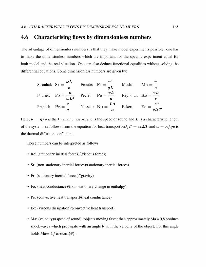
4.6. CHARACTERISING FLOWS BY DIMENSIONLESS NUMBERS 165
4.6 Characterising flows by dimensionless numbers
The advantage of dimensionless numbers is that they make model experiments possible: one has
to make the dimensionless numbers which are important for the specific experiment equal for
both model and the real situation. One can also deduce functional equalities without solving the
differential equations. Some dimensionless numbers are given by:
Strouhal: Sr =ωL
vFroude: Fr =
v2
gLMach: Ma =
v
c
Fourier: Fo =a
ωL2Péclet: Pe =
vL
aReynolds: Re =
vL
ν
Prandtl: Pr =ν
aNusselt: Nu =
Lα
κEckert: Ec =
v2
c∆T
Here, ν = η/% is the kinematic viscosity, c is the speed of sound and L is a characteristic length
of the system. α follows from the equation for heat transport κ∂yT = α∆T and a = κ/%c is
the thermal diffusion coefficient.
These numbers can be interpreted as follows:
• Re: (stationary inertial forces)/(viscous forces)
• Sr: (non-stationary inertial forces)/(stationary inertial forces)
• Fr: (stationary inertial forces)/(gravity)
• Fo: (heat conductance)/(non-stationary change in enthalpy)
• Pe: (convective heat transport)/(heat conductance)
• Ec: (viscous dissipation)/(convective heat transport)
• Ma: (velocity)/(speed of sound): objects moving faster than approximately Ma = 0,8 produce
shockwaves which propagate with an angle θ with the velocity of the object. For this angle
holds Ma= 1/ arctan(θ).

166 CHAPTER 4. BASICS OF FLUID DYNAMICS
• Pr and Nu are related to specific materials.
Now, the dimensionless Navier-Stokes equation becomes, with xd = x/L, ~vd = ~v/V , ∇d =
L∇d,∇2d = L2∇2 and td = tω:
Sr∂~vd
∂td+ (~vd · ∇d)~vd = −∇dpd +
~g
Fr+∇2d~vd
Re(4.29)
4.7 Dynamic similarity: Application in engineering*
Engineering models are used to study complex fluid dynamics problems where calculations and
computer simulations are not reliable. Models are usually smaller than the final design, but not
always. Scale models allow testing of a design prior to building, and in many cases are a critical
step in the development process. Construction of a scale model, however, must be accompanied
by an analysis to determine what conditions it is tested under. While the geometry may be simply
scaled, other parameters, such as pressure, temperature or the velocity and type of fluid may need
to be altered. Similitude is achieved when testing conditions are created such that the test results
are applicable to the real design. The following criteria are required:
1. Geometric similarity: The model is the same shape as the application, usually scaled.
2. Kinematic similarity: Fluid flow of both the model and real application must undergo similar
time rates of change motions. (fluid streamlines are similar)
3. Dynamic similarity: Ratios of all forces acting on corresponding fluid particles and boundary
surfaces in the two systems are constant.
Dimensional analysis is used to express the system with as few independent variables and as
many dimensionless parameters as possible. The values of the dimensionless parameters are held
to be the same for both the scale model and application. The design of marine vessels remains
more of an art than a science in large part because dynamic similitude is especially difficult to
attain for a vessel that is partially submerged: a ship is affected by wind forces in the air above it,
by hydrodynamic forces within the water under it, and especially by wave motions at the interface
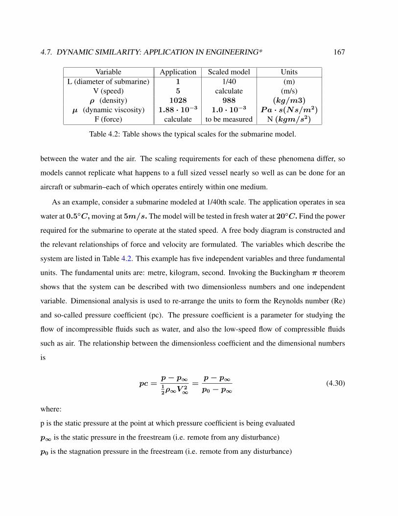
4.7. DYNAMIC SIMILARITY: APPLICATION IN ENGINEERING* 167
Variable Application Scaled model UnitsL (diameter of submarine) 1 1/40 (m)
V (speed) 5 calculate (m/s)ρ (density) 1028 988 (kg/m3)
µ (dynamic viscosity) 1.88 · 10−3 1.0 · 10−3 Pa · s(Ns/m2)F (force) calculate to be measured N (kgm/s2)
Table 4.2: Table shows the typical scales for the submarine model.
between the water and the air. The scaling requirements for each of these phenomena differ, so
models cannot replicate what happens to a full sized vessel nearly so well as can be done for an
aircraft or submarin–each of which operates entirely within one medium.
As an example, consider a submarine modeled at 1/40th scale. The application operates in sea
water at 0.5C,moving at 5m/s. The model will be tested in fresh water at 20C. Find the power
required for the submarine to operate at the stated speed. A free body diagram is constructed and
the relevant relationships of force and velocity are formulated. The variables which describe the
system are listed in Table 4.2. This example has five independent variables and three fundamental
units. The fundamental units are: metre, kilogram, second. Invoking the Buckingham π theorem
shows that the system can be described with two dimensionless numbers and one independent
variable. Dimensional analysis is used to re-arrange the units to form the Reynolds number (Re)
and so-called pressure coefficient (pc). The pressure coefficient is a parameter for studying the
flow of incompressible fluids such as water, and also the low-speed flow of compressible fluids
such as air. The relationship between the dimensionless coefficient and the dimensional numbers
is
pc =p− p∞12ρ∞V 2
∞=
p− p∞p0 − p∞
(4.30)
where:
p is the static pressure at the point at which pressure coefficient is being evaluated
p∞ is the static pressure in the freestream (i.e. remote from any disturbance)
p0 is the stagnation pressure in the freestream (i.e. remote from any disturbance)
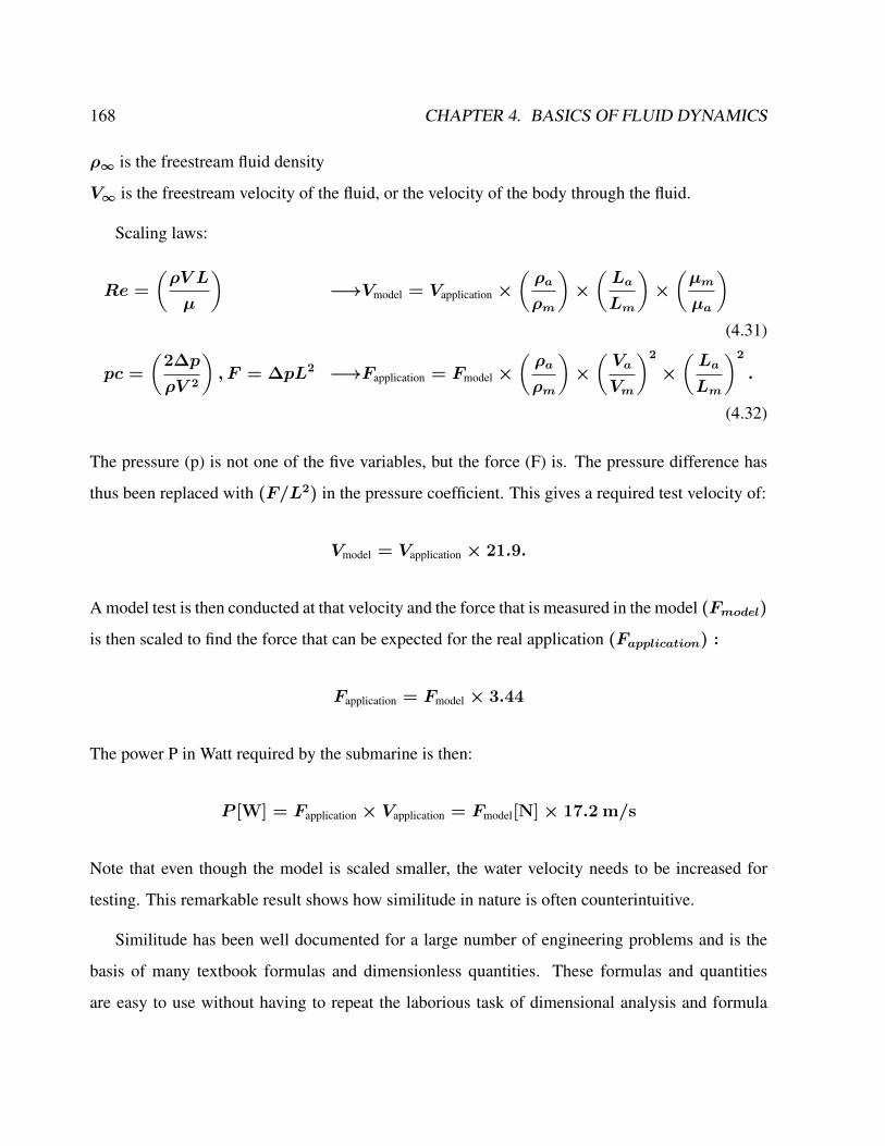
168 CHAPTER 4. BASICS OF FLUID DYNAMICS
ρ∞ is the freestream fluid density
V∞ is the freestream velocity of the fluid, or the velocity of the body through the fluid.
Scaling laws:
Re =
(ρV L
µ
)−→Vmodel = Vapplication ×
(ρa
ρm
)×(La
Lm
)×(µm
µa
)(4.31)
pc =
(2∆p
ρV 2
), F = ∆pL2 −→Fapplication = Fmodel ×
(ρa
ρm
)×(Va
Vm
)2
×(La
Lm
)2
.
(4.32)
The pressure (p) is not one of the five variables, but the force (F) is. The pressure difference has
thus been replaced with (F/L2) in the pressure coefficient. This gives a required test velocity of:
Vmodel = Vapplication × 21.9.
A model test is then conducted at that velocity and the force that is measured in the model (Fmodel)
is then scaled to find the force that can be expected for the real application (Fapplication) :
Fapplication = Fmodel × 3.44
The power P in Watt required by the submarine is then:
P [W] = Fapplication × Vapplication = Fmodel[N]× 17.2 m/s
Note that even though the model is scaled smaller, the water velocity needs to be increased for
testing. This remarkable result shows how similitude in nature is often counterintuitive.
Similitude has been well documented for a large number of engineering problems and is the
basis of many textbook formulas and dimensionless quantities. These formulas and quantities
are easy to use without having to repeat the laborious task of dimensional analysis and formula
4.7. DYNAMIC SIMILARITY: APPLICATION IN ENGINEERING* 169
derivation. Similitude can be used to predict the performance of a new design based on data from
an existing, similar design. In this case, the model is the existing design. Another use of similitude
and models is in validation of computer simulations with the ultimate goal of eliminating the need
for physical models altogether. Another application of similitude is to replace the operating fluid
with a different test fluid. Wind tunnels, for example, have trouble with air liquefying in certain
conditions so helium is sometimes used. Other applications may operate in dangerous or expensive
fluids so the testing is carried out in a more convenient substitute.

Chapter 5
Fluid-dynamical Examples
5.1 Potential flow
In fluid dynamics, potential flow describes the velocity field as the gradient of a scalar function:
the velocity potential. As a result, a potential flow is characterized by an irrotational velocity field,
which is a valid approximation for several applications. The irrotationality of a potential flow is
due to the curl of a gradient always being equal to zero. In the case of an incompressible flow
the velocity potential satisfies Laplace’s equation. However, potential flows also have been used to
describe compressible flows. The potential flow approach occurs in the modeling of both stationary
as well as nonstationary flows.
A potential flow is described by means of a velocity potential, being a function of space and
time. The flow velocity v is a vector field equal to the gradient of the velocity potential φ
v = ∇φ. (5.1)
From vector calculus it is known, that the curl of a gradient is equal to zero:
∇×∇φ = 0, (5.2)
170
5.1. POTENTIAL FLOW 171
and consequently the vorticity, the curl of the velocity field v, is zero:
∇× v = 0. (5.3)
This implies that a potential flow is an irrotational flow. This has direct consequences for the
applicability of potential flow. In flow regions where vorticity is known to be important, such as
wakes and boundary layers, potential flow theory is not able to provide reasonable predictions of
the flow. Fortunately, there are often large regions of a flow where the assumption of irrotationality
is valid, which is why potential flow is used for various applications.1
In case of an incompressible flow2 the velocity v has zero divergence:
∇ · v = 0, (5.4)
with the dot denoting the inner product. As a result, the velocity potential satisfies Laplace’s
equation
∇2φ = 0 . (5.5)
In this case the flow can be determined completely from its kinematics: the assumptions of ir-
rotationality and zero divergence of the flow. Dynamics only have to be applied afterwards, if
one is interested in computing pressures: for instance for flow around airfoils through the use of
Bernoulli’s principle. In two dimensions, potential flow reduces to a very simple system that is
analyzed using complex analysis (section 5.1.6).
1For instance in: flow around aircraft, groundwater flow, acoustics and water waves.2for instance of a liquid, or a gas at low Mach numbers; but not for sound waves
172 CHAPTER 5. FLUID-DYNAMICAL EXAMPLES
5.1.1 Kelvin’s circulation theorem*
In fluid mechanics, Kelvin’s circulation theorem states In a barotropic ideal fluid with conservative
body forces, the circulation around a closed curve (which encloses the same fluid elements) moving
with the fluid remains constant with time.
DΓ
Dt= 0 (5.6)
where the circulation Γ is the circulation around a material contour
Γ =
∮(~v · ~et)ds (5.7)
The circulation is the line integral of the tangential component of velocity taken about a closed
curve in the flow field. The integral is taken in a counterclockwise direction about the contour C
and ds is a differential length along the contour. No singularities can lie directly on the contour.
The origin (center) of the potential vortex is considered as a singularity point in the flow since the
velocity goes to infinity at this point. If the contour encircles the potential vortex origin, the circu-
lation will be non-zero. If the contour does not encircle any singularities, however, the circulation
will be zero. Stated more simply this theorem says that if one observes a closed contour at one
instant, and follows the contour over time (by following the motion of all of its fluid elements), the
circulation over the two locations of this contour are equal. This theorem does not hold in cases
with viscous stresses, nonconservative body forces (for example Coriolis force) or non-barotropic
pressure-density relations.
In the case of a potential flow, the vorticity is zero (5.3), Kelvin’s theorem can be derived using
Γ =
∫∫(∇× ~v ) · ~n d2A = 0 (5.8)
5.1. POTENTIAL FLOW 173
Exercise 31 – Circulation theorem
Show (5.6) using that the governing equation for an inviscid fluid with a conservative body
force isDu
Dt= −
1
ρ∇p+∇Φ
where Φ is the potential for the body force.
Hint: Potential flow, Kelvin’s theorem
5.1.2 Streamlines
For a 2-dimensional flow a flow functionψ(x, y) can be defined: u = ∂ψ/∂y, v = −∂ψ/∂x.
With ΨAB the amount of liquid flowing through a curve s between the points A and B:
ΨAB =
B∫A
(~v · ~n )ds =
B∫A
(udy − vdx) (5.9)
=
B∫A
dψ = ψ(B)− ψ(A) . (5.10)
The lines of constant φ = 0 are called potential lines of the flow.
dφ =∂φ
∂xdx+
∂φ
∂ydy = udx+ vdy (5.11)
Since dφ = 0 along a potential line, we have
dy
dx= −
u
v(5.12)
Recall that streamlines are lines everywhere tangent to the velocity,
dy
dx=u
v(5.13)
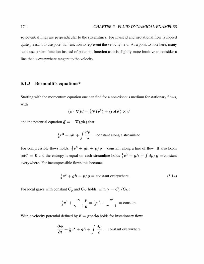
174 CHAPTER 5. FLUID-DYNAMICAL EXAMPLES
so potential lines are perpendicular to the streamlines. For inviscid and irrotational flow is indeed
quite pleasant to use potential function to represent the velocity field. As a point to note here, many
texts use stream function instead of potential function as it is slightly more intuitive to consider a
line that is everywhere tangent to the velocity.
5.1.3 Bernoulli’s equations*
Starting with the momentum equation one can find for a non-viscous medium for stationary flows,
with
(~v · ∇)~v = 12∇(v2) + (rot~v )× ~v
and the potential equation ~g = −∇(gh) that:
12v2 + gh+
∫dp
%= constant along a streamline
For compressible flows holds: 12v2 + gh + p/% =constant along a line of flow. If also holds
rot~v = 0 and the entropy is equal on each streamline holds 12v2 + gh +
∫dp/% =constant
everywhere. For incompressible flows this becomes:
12v2 + gh+ p/% = constant everywhere. (5.14)
For ideal gases with constant Cp and CV holds, with γ = Cp/CV :
12v2 +
γ
γ − 1
p
%= 1
2v2 +
c2
γ − 1= constant
With a velocity potential defined by ~v = gradφ holds for instationary flows:
∂φ
∂t+ 1
2v2 + gh+
∫dp
%= constant everywhere
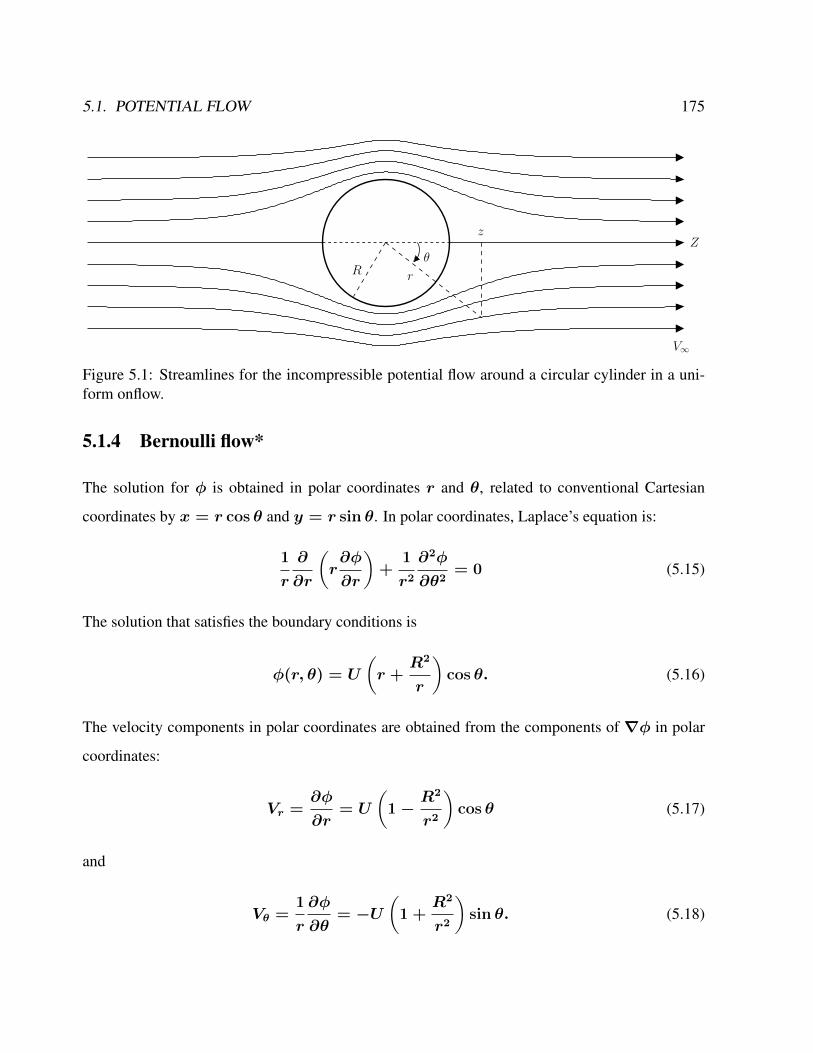
5.1. POTENTIAL FLOW 175
R r
θ
V∞
zZ
Figure 5.1: Streamlines for the incompressible potential flow around a circular cylinder in a uni-form onflow.
5.1.4 Bernoulli flow*
The solution for φ is obtained in polar coordinates r and θ, related to conventional Cartesian
coordinates by x = r cos θ and y = r sin θ. In polar coordinates, Laplace’s equation is:
1
r
∂
∂r
(r∂φ
∂r
)+
1
r2
∂2φ
∂θ2= 0 (5.15)
The solution that satisfies the boundary conditions is
φ(r, θ) = U
(r +
R2
r
)cos θ. (5.16)
The velocity components in polar coordinates are obtained from the components of ∇φ in polar
coordinates:
Vr =∂φ
∂r= U
(1−
R2
r2
)cos θ (5.17)
and
Vθ =1
r
∂φ
∂θ= −U
(1 +
R2
r2
)sin θ. (5.18)
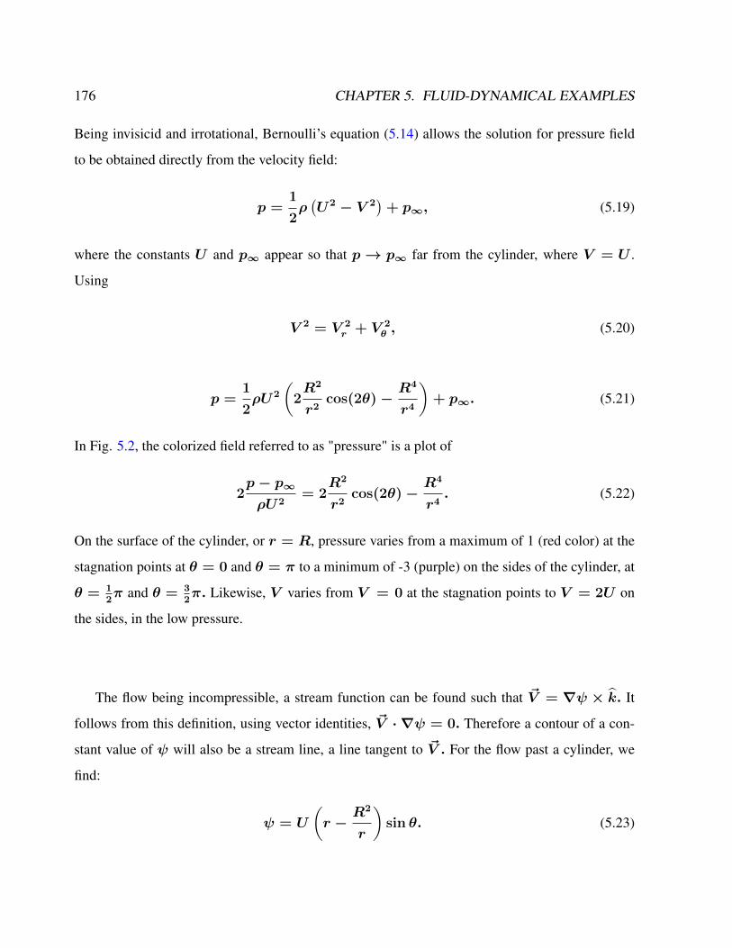
176 CHAPTER 5. FLUID-DYNAMICAL EXAMPLES
Being invisicid and irrotational, Bernoulli’s equation (5.14) allows the solution for pressure field
to be obtained directly from the velocity field:
p =1
2ρ(U2 − V 2
)+ p∞, (5.19)
where the constants U and p∞ appear so that p→ p∞ far from the cylinder, where V = U .
Using
V 2 = V 2r + V 2
θ , (5.20)
p =1
2ρU2
(2R2
r2cos(2θ)−
R4
r4
)+ p∞. (5.21)
In Fig. 5.2, the colorized field referred to as "pressure" is a plot of
2p− p∞ρU2
= 2R2
r2cos(2θ)−
R4
r4. (5.22)
On the surface of the cylinder, or r = R, pressure varies from a maximum of 1 (red color) at the
stagnation points at θ = 0 and θ = π to a minimum of -3 (purple) on the sides of the cylinder, at
θ = 12π and θ = 3
2π. Likewise, V varies from V = 0 at the stagnation points to V = 2U on
the sides, in the low pressure.
The flow being incompressible, a stream function can be found such that ~V = ∇ψ × k. It
follows from this definition, using vector identities, ~V · ∇ψ = 0. Therefore a contour of a con-
stant value of ψ will also be a stream line, a line tangent to ~V . For the flow past a cylinder, we
find:
ψ = U
(r −
R2
r
)sin θ. (5.23)
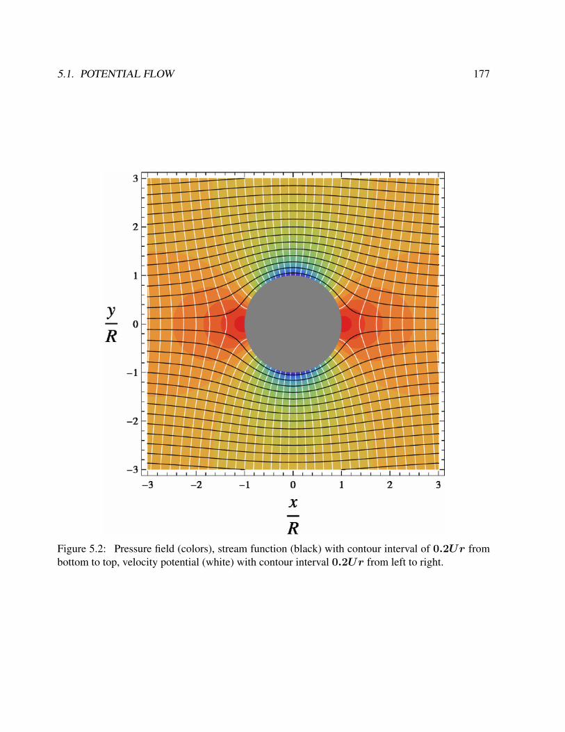
5.1. POTENTIAL FLOW 177
Figure 5.2: Pressure field (colors), stream function (black) with contour interval of 0.2Ur frombottom to top, velocity potential (white) with contour interval 0.2Ur from left to right.
178 CHAPTER 5. FLUID-DYNAMICAL EXAMPLES
Physical interpretation
Laplace’s equation is linear, and is one of the most elementary partial differential equations. The
dynamic pressure at the upstream stagnation point has value of ρU2/2, a value needed to deceler-
ate the free stream flow of speed U. This same value appears at the downstream stagnation point,
this high pressure is again need to decelerate the flow to zero speed. This symmetry arises only
because the flow is completely frictionless. The low pressure on sides on the cylinder is needed to
provide the centripetal acceleration of the flow:
∂p
∂r=ρV 2
L, (5.24)
where L is the radius of curvature of the flow. But L ≈ R, and V ≈ U. The integral of the
equation for centripetal acceleration, which will over a distance ∆r ≈ R will thus yield
p− p∞ ≈ −ρU2. (5.25)
The exact solution has, for the lowest pressure,
p− p∞ = −3
2ρU2. (5.26)
The low pressure, which must be present to provide the centripetal acceleration, will also increase
the flow speed as the fluid travels from higher to lower values of pressure. Thus we find the
maximum speed in the flow, V = 2U, in the low pressure on the sides of the cylinder. A value of
V > U is consistent with conservation of the volume of fluid. With the cylinder blocking some
of the flow, V must be greater than U somewhere in the plane through the center of the cylinder
and transverse to the flow.
5.1. POTENTIAL FLOW 179
5.1.5 Comparison with flow of a real fluid past a cylinder*
This symmetry of this ideal solution has the peculiar property of having zero net drag on the
cylinder, a property known as d’Alembert’s paradox. Unlike an ideal inviscid fluid, a viscous
flow past a cylinder, no matter how small the viscosity, will acquire vorticity in a thin boundary
layer adjacent to the cylinder. Boundary layer separation can occur, and a trailing wake will occur
behind the cylinder. The pressure will be lower on the wake side of the cylinder, than on the
upstream side, resulting in a drag force in the downstream direction. A particular aspect are the
Von Karman Vortices.
Fig. 5.3 features a ubiquitous occurrence in the motion of fluids–a vortex street, which is a
linear chain of spiral eddies called von Karman vortices. Von Karman vortices are named after
Theodore von Karman, who first described the phenomenon in the atmosphere. von Karman vor-
tices form nearly everywhere that fluid flow is disturbed by an object and form at all scales of
fluid motion. The "object" that is disturbing the fluid flow is an island or group of islands. As a
prevailing wind encounters the island, the disturbance in the flow propagates downstream of the
island in the form of a double row of vortices which alternate their direction of rotation.
As a fluid particle flows toward the leading edge of a cylinder, the pressure on the particle
rises from the free stream pressure to the stagnation pressure. The high fluid pressure near the
leading edge impels flow about the cylinder as boundary layers develop about both sides. The high
pressure is not sufficient to force the flow about the back of the cylinder at high Reynolds numbers.
Near the widest section of the cylinder, the boundary layers separate from each side of the cylinder
surface and form two shear layers that trail aft in the flow and bound the wake. Since the innermost
portion of the shear layers, which is in contact with the cylinder, moves much more slowly than
the outermost portion of the shear layers, which is in contact with the free flow, the shear layers
roll into the near wake, where they fold on each other and coalesce into discrete swirling vortices.
A regular pattern of vortices, called a vortex street, trails aft in the wake.
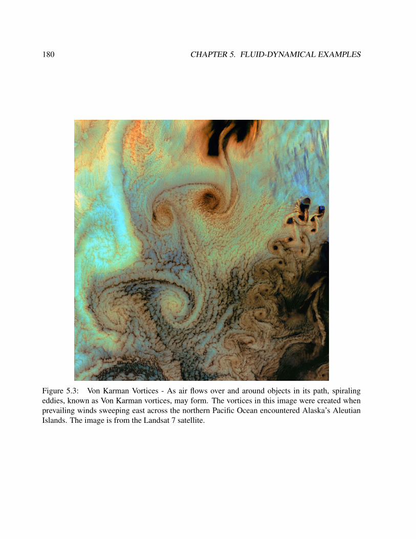
180 CHAPTER 5. FLUID-DYNAMICAL EXAMPLES
Figure 5.3: Von Karman Vortices - As air flows over and around objects in its path, spiralingeddies, known as Von Karman vortices, may form. The vortices in this image were created whenprevailing winds sweeping east across the northern Pacific Ocean encountered Alaska’s AleutianIslands. The image is from the Landsat 7 satellite.

5.1. POTENTIAL FLOW 181
5.1.6 Analysis for two-dimensional flow using conformal mapping*
Potential flow does not include all the characteristics of flows that are encountered in the real world.
Potential flow theory cannot be applied for viscous internal flows. Richard Feynman considered
potential flow to be so unphysical that the only fluid to obey the assumptions was "dry water"
(quoting John von Neumann). More precisely, potential flow cannot account for the behaviour of
flows that include a boundary layer. Nevertheless, understanding potential flow is important in
many branches of fluid mechanics. In particular, simple potential flows (called elementary flows)
such as the free vortex and the point source possess ready analytical solutions. These solutions can
be superposed to create more complex flows satisfying a variety of boundary conditions. These
flows correspond closely to real-life flows over the whole of fluid mechanics; in addition, many
valuable insights arise when considering the deviation (often slight) between an observed flow and
the corresponding potential flow. Potential flow finds many applications in fields such as aircraft
design. For instance, in computational fluid dynamics, one technique is to couple a potential
flow solution outside the boundary layer to a solution of the boundary layer equations inside the
boundary layer.
Potential flow in two dimensions is simple to analyze using conformal mapping, by the use of
transformations of the complex plane. The basic idea is to use a holomorphic (also called analytic)
or meromorphic function f, which maps the physical domain (x,y) to the transformed domain
(φ, ψ). While x, y, φ, ψ are all real valued, it is convenient to define the complex quantities
z = x + iy and w = φ + iψ. Now, if we write the mapping f as f(x + iy) = φ + iψ
or f(z) = w. Then, because f is a holomorphic function, it has to satisfy the Cauchy-Riemann
equations
∂ϕ
∂x=∂ψ
∂y,
∂ϕ
∂y= −
∂ψ
∂x. (5.27)
The velocity components (u,v), in the (x,y) directions respectively, can be obtained directly from f
182 CHAPTER 5. FLUID-DYNAMICAL EXAMPLES
by differentiating with respect to z. That is
df
dz= u− iv (5.28)
So the velocity field (u,v) is specified by
u =∂ϕ
∂x=∂ψ
∂y, v =
∂ϕ
∂y= −
∂ψ
∂x. (5.29)
Both ϕ and ψ then satisfy Laplace’s equation:
∆ϕ =∂2ϕ
∂x2+∂2ϕ
∂y2= 0 and ∆ψ =
∂2ψ
∂x2+∂2ψ
∂y2= 0. (5.30)
So ϕ can be identified as the velocity potential and ψ is called the stream function. Lines of
constant ψ are known as streamlines and lines of constant ϕ are known as equipotential lines.
Streamlines and equipotential lines are orthogonal to each other, since
∇φ · ∇ψ =∂φ
∂x
∂ψ
∂x+∂φ
∂y
∂ψ
∂y=∂ψ
∂y
∂ψ
∂x−∂ψ
∂x
∂ψ
∂y= 0. (5.31)
Thus the flow occurs along the lines of constant ψ and at right angles to the lines of constant ϕ. It
is interesting to note that ∆ψ = 0 is also satisfied, this relation being equivalent to∇× v = 0.
Exercise 32 – Conformal mapping
We note that the complex velocity potential must be an analytic function respecting the bound-
ary conditions, and once we have it, we can easily obtain the flow field. Let us see how we can use
this fact to solve some basic fluid mechanics problems. In case the following power-law conformal
map is applied, from z = x+ iy to w = φ+ iψ :
w = Azn, (5.32)

5.1. POTENTIAL FLOW 183
then, writing z in polar coordinates as z = x+ iy = reiΘ, we have
ϕ = Arn cos(nθ) and ψ = Arn sin(nθ). (5.33)
Study the cases n = 1/2, 2/3, 3/2, 2, 3 and draw the streamlines and equipotential!
Hint: web site for conformal mapping
Solution n = 1: uniform flow
Uniform flow: v = V If w = Az, that is, a power law with n = 1, the streamlines (i.e. lines of
constant ψ) are a system of straight lines parallel to the x-axis. This is easiest to see by writing in
terms of real and imaginary components: f(x+ iy) = Uz = Ux+ iUy thus givingφ = Ux
and ψ = Uy. This flow may be interpreted as uniform flow parallel to the x-axis.
Think on the problem of flow around a corner. What is a consistent flow pattern past a corner
according to the ideal fluid conditions? f(z) = Uz2 Why ? One uses analytic functions to map
a fluids problem (or more generally a Laplace equation problem) from a given domain to a domain
on which the problem is solved.
Another problem where we know the solution from the last section: Flow around a cylinder
with f(z) = U(z + 1/z).
One of the more important potential flow results obtained using conformal mapping begins
with the known solution for the flow past a circular cylinder (with circulation) and maps the circle
into an airfoil shape using waht is called the Joukowski mapping.
184 CHAPTER 5. FLUID-DYNAMICAL EXAMPLES
5.2 More on fluid flows*
5.2.1 Tube flows*
For tube flows holds: they are laminar if Re< 2300 with dimension of length the diameter of the
tube, and turbulent if Re is larger. For an incompressible laminar flow through a straight, circular
tube holds for the velocity profile:
v(r) = −1
4η
dp
dx(R2 − r2)
For the volume flow holds: ΦV =
R∫0
v(r)2πrdr = −π
8η
dp
dxR4
The entrance length Le is given by:
1. 500 < ReD < 2300: Le/2R = 0.056ReD
2. Re > 2300: Le/2R ≈ 50
For gas transport at low pressures (Knudsen-gas) holds: ΦV =4R3α
√π
3
dp
dx
For flows at a small Re holds: ∇p = η∇2~v and div~v = 0. For the total force on a sphere
with radius R in a flow then holds: F = 6πηRv. For large Re holds for the force on a surface
A: F = 12CWA%v
2.
5.2.2 Boundary layers*
If for the thickness of the boundary layer holds: δ L holds: δ ≈ L/√
Re. With v∞ the
velocity of the main flow it follows for the velocity vy ⊥ the surface: vyL ≈ δv∞. Blasius’
equation for the boundary layer is, with vy/v∞ = f(y/δ): 2f ′′′ + ff ′′ = 0 with boundary
conditions f(0) = f ′(0) = 0, f ′(∞) = 1. From this follows: CW = 0.664 Re−1/2x .
The momentum theorem of Von Karman for the boundary layer is:d
dx(ϑv2)+δ∗v
dv
dx=τ0
%
5.2. MORE ON FLUID FLOWS* 185
where the displacement thickness δ∗v and the momentum thickness ϑv2 are given by:
ϑv2 =
∞∫0
(v − vx)vxdy , δ∗v =
∞∫0
(v − vx)dy and τ0 = −η∂vx
∂y
∣∣∣∣y=0
The boundary layer is released from the surface if(∂vx
∂y
)y=0
= 0. This is equivalent with
dp
dx=
12ηv∞
δ2.
If the thickness of the temperature boundary layer δT L holds: 1. If Pr ≤ 1: δ/δT ≈√
Pr.
2. If Pr 1: δ/δT ≈ 3√
Pr.
5.2.3 Heat conductance*
For non-stationairy heat conductance in one dimension without flow holds:
∂T
∂t=
κ
%c
∂2T
∂x2+ Φ
where Φ is a source term. If Φ = 0 the solutions for harmonic oscillations at x = 0 are:
T − T∞Tmax − T∞
= exp
(−x
D
)cos
(ωt−
x
D
)
with D =√
2κ/ω%c. At x = πD the temperature variation is in anti-phase with the surface.
The one-dimensional solution at Φ = 0 is
T (x, t) =1
2√πat
exp
(−x2
4at
)
This is mathematical equivalent to the diffusion problem:
∂n
∂t= D∇2n+ P −A

186 CHAPTER 5. FLUID-DYNAMICAL EXAMPLES
where P is the production of andA the discharge of particles. The flow density J = −D∇n.
5.2.4 Turbulence*
The time scale of turbulent velocity variations τt is of the order of: τt = τ√
Re/Ma2 with
τ the molecular time scale. For the velocity of the particles holds: v(t) = 〈v〉 + v′(t) with
〈v′(t)〉 = 0. The Navier-Stokes equation now becomes:
∂ 〈~v 〉∂t
+ (〈~v 〉 · ∇) 〈~v 〉 = −∇〈p〉%
+ ν∇2 〈~v 〉+divSR
%
where SRij = −% 〈vivj〉 is the turbulent stress tensor. Boussinesq’s assumption is: τij =
−%⟨v′iv′j
⟩. It is stated that, analogous to Newtonian media: SR = 2%νt 〈D〉. Near a boundary
holds: νt = 0, far away of a boundary holds: νt ≈ νRe.
For a (semi) two-dimensional flow holds:
dω
dt=∂ω
∂t+ J(ω, ψ) = ν∇2ω (5.34)
With J(ω, ψ) the Jacobian. So if ν = 0, ω is conserved. Further, the kinetic energy/mA
and the enstrofy V are conserved: with ~v = ∇× (~kψ)
E ∼ (∇ψ)2 ∼∞∫
0
E(k, t)dk = constant , V ∼ (∇2ψ)2 ∼∞∫
0
k2E(k, t)dk = constant
From this follows that in a two-dimensional flow the energy flux goes towards large values of k:
larger structures become larger at the expanse of smaller ones. In three-dimensional flows the
situation is just the opposite.
5.2. MORE ON FLUID FLOWS* 187
5.2.5 Couette flow*
Couette flow refers to the laminar flow of a viscous fluid in the space between two parallel plates,
one of which is moving relative to the other. The flow is driven by virtue of viscous drag force
acting on the fluid and the applied pressure gradient parallel to the plates. This type of flow is
named in honor of Maurice Marie Alfred Couette, a Professor of Physics at the French university
of Angers in the late 19th century. Couette flow is frequently used in undergraduate physics and
engineering courses to illustrate shear-driven fluid motion. The simplest conceptual configuration
finds two infinite, parallel plates separated by a distance h. One plate, say the top one, translates
with a constant velocity u0 in its own plane. Neglecting pressure gradients, the Navier-Stokes
equations simplify to
d2u
dy2= 0, (5.35)
where y is a spatial coordinate normal to the plates and u (y) is the velocity distribution. This equa-
tion reflects the assumption that the flow is uni-directional. That is, only one of the three velocity
components (u,v,w) is non-trivial. If y originates at the lower plate, the boundary conditions are
u(0) = 0 and u(h) = u0. The exact solution
u(y) = u0
y
h(5.36)
can be found by integrating twice and solving for the constants using the boundary conditions.
A notable aspect of this model is that shear stress is constant throughout the flow domain. In
particular, the first derivative of the velocity, u0/h, is constant. (This is implied by the straight-
line profile in the figure.) According to Newton’s Law of Viscosity (Newtonian fluid), the shear
stress is the product of this expression and the (constant) fluid viscosity.
A more general Couette flow situation arises when a pressure gradient is imposed in a direction
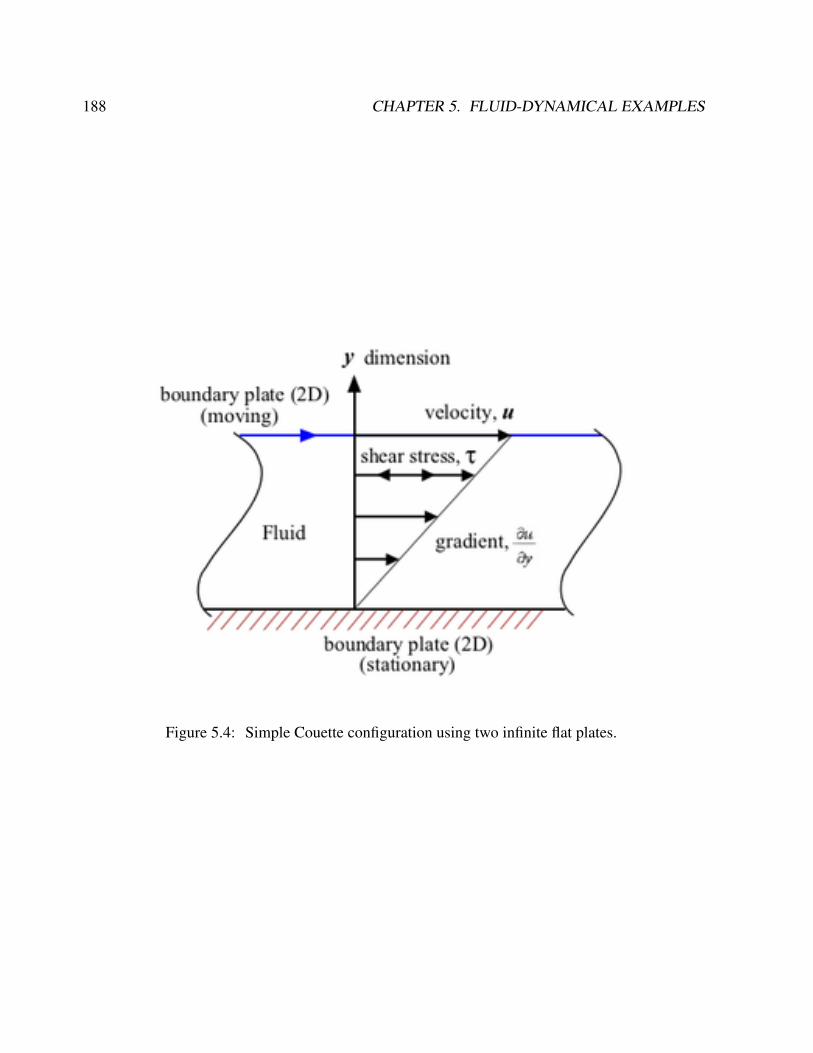
188 CHAPTER 5. FLUID-DYNAMICAL EXAMPLES
Figure 5.4: Simple Couette configuration using two infinite flat plates.
5.2. MORE ON FLUID FLOWS* 189
parallel to the plates. The Navier-Stokes equations, in this case, simplify to
d2u
dy2=
1
µ
dp
dx, (5.37)
where dp/dx is the pressure gradient parallel to the plates and µ is fluid viscosity. Integrating the
above equation twice and applying the boundary conditions (same as in the case of Couette flow
without pressure gradient) to yield the following exact solution
u(y) = u0
y
h+
1
2µ
(dp
dx
) (y2 − hy
). (5.38)
The shape of the above velocity profile depends on the dimensionless parameter
P = −h2
2µu0
(dp
dx
). (5.39)
The pressure gradient can be positive (adverse pressure gradient) or negative (favorable pressure
gradient). It may be noted that in the limiting case of stationary plates, the flow is referred to
as plane Poiseuille flow with a symmetric (with reference to the horizontal mid-plane) parabolic
velocity profile.
In fluid dynamics, the Taylor-Couette flow consists of a viscous fluid confined in the gap be-
tween two rotating cylinders. For low angular velocities, measured by the Reynolds number Re,
the flow is steady and purely azimuthal. This basic state is known as circular Couette flow, after
Maurice Marie Alfred Couette who used this experimental device as a means to measure viscos-
ity. Sir Geoffrey Ingram Taylor investigated the stability of the Couette flow in a ground-breaking
paper which has been a cornerstone in the development of hydrodynamic stability theory.
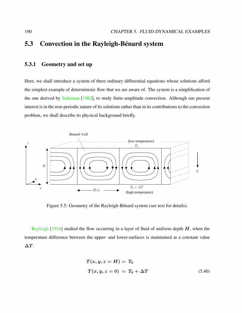
190 CHAPTER 5. FLUID-DYNAMICAL EXAMPLES
5.3 Convection in the Rayleigh-Bénard system
5.3.1 Geometry and set up
Here, we shall introduce a system of three ordinary differential equations whose solutions afford
the simplest example of deterministic flow that we are aware of. The system is a simplification of
the one derived by Saltzman [1962], to study finite-amplitude convection. Although our present
interest is in the non-periodic nature of its solutions rather than in its contributions to the convection
problem, we shall describe its physical background briefly.
Benard−Cell
(high temperature)
(low temperature)
H/a
H
T0 +∆Tx
y
zT0
g
Figure 5.5: Geometry of the Rayleigh-Bénard system (see text for details).
Rayleigh [1916] studied the flow occurring in a layer of fluid of uniform depth H , when the
temperature difference between the upper- and lower-surfaces is maintained at a constant value
∆T .
T (x, y, z = H) = T0
T (x, y, z = 0) = T0 + ∆T (5.40)
5.3. CONVECTION IN THE RAYLEIGH-BÉNARD SYSTEM 191
The Boussinesq approximation is used, which results in a buoyancy force term which couples the
thermal and fluid velocity fields. Therefore
ρ ≈ ρ0 = const. (5.41)
except in the buoyancy term, where:
% = %0(1− α(T − T0)) with α > 0 . (5.42)
ρ0 is the fluid density in the reference state. This assumption reflects a common feature of geo-
physical flows, where the density fluctuations caused by temperature variations are small, yet they
are the ones driving the overall flow. We have the following relations. Furthermore, we assume
that the density depends linearly on temperature T .
For some experiments go to the trailer 1, trailer 2, trailer in German, KIT trailer: Rayleigh
Benard Thermal Convection 3D Simulation.
This system possesses a steady-state solution in which there is no motion, and the temperature
varies linearly with depth:
u = w = 0
Teq = T0 +
(1−
z
H
)∆T (5.43)
When this solution becomes unstable, convection should develop.

192 CHAPTER 5. FLUID-DYNAMICAL EXAMPLES
5.3.2 The usual approach: Elimination of pressure and vorticity dynamics
In the case where all motions are parallel to the x− z-plane, and no variations in the direction of
the y-axis occur, the governing equations may be written (see Saltzman [1962]) as:
Dtu = −1
ρ0
∂xp+ ν∇2u (5.44)
Dtw = −1
ρ0
∂zp+ ν∇2w + g(1− α(T − T0)) (5.45)
DtT = κ∇2T (5.46)
∂xu+ ∂zw = 0 (5.47)
wherew and u are the vertical and horizontal components of the velocity,Dtu = ∂tu+u∂xu+
w∂zu, Dtw = ∂tw + u∂xw + w∂zw, and DtT = ∂tT + u∂xT + w∂zT respectively.
Furthermore, ν = η/ρ0, κ = λ/(ρ0Cv) the momentum diffusivity (kinematic viscosity) and
thermal diffusivity, respectively.
Now, compare the procedure with the elimination of the pressure term in section 4.4 where we
derive the vorticity equationDt (∇2ψ) = ν∇4ψ. Here, it is useful to define the stream function
Ψ for the two-dimensional motion, i.e.
∂Ψ
∂x= w (5.48)
∂Ψ
∂z= −u . (5.49)
We take the
∂
∂x(5.45)−
∂
∂z(5.44) =
∂
∂xDtw −
∂
∂zDtu = Dt
∂w
∂x−Dt
∂u
∂z(5.50)
= = Dt
∂2Ψ
∂x2−Dt
∂2Ψ
∂z2= Dt∇2Ψ . (5.51)
5.3. CONVECTION IN THE RAYLEIGH-BÉNARD SYSTEM 193
Note thatDt∇2Ψ does not contain u,w anymore:
Dt
(∇2Ψ
)= ∂t∇2Ψ−
∂Ψ
∂z
∂∇2Ψ
∂x+∂Ψ
∂x
∂∇2Ψ
∂z.
Furthermore, we introduce the function Θ as the departure of temperature from that occurring in
the state of no convection (5.43):
T = Teq + Θ (5.52)
In the temperature term in ∂∂x
(5.45) on the right hand side:
∂
∂xg(1− α(Teq + Θ− T0)) = −gα
∂
∂xΘ
The left hand side of (5.46) reads
DtT = DtTeq +DtΘ = w ·−∆T
H+DtΘ = −
∆T
H
∂Ψ
∂x+DtΘ
Then, the dynamics can be formulated as
Dt
(∇2Ψ
)= ν∇4Ψ− gα
∂Θ
∂x(5.53)
DtΘ =∆T
H
∂Ψ
∂x+ κ∇2Θ . (5.54)
Non-dimensionalization of the problem yields equations including the dimensionless Prandtl
number3 σ and the Rayleigh numberRa which are the control parameters of the problem. One can
3The Prandtl number is a dimensionless number; the ratio of momentum diffusivity (kinematic viscosity) to thermaldiffusivity. It is named after the German physicist Ludwig Prandtl. Note that whereas the Reynolds number andGrashof number are subscripted with a length scale variable, the Prandtl number contains no such length scale in itsdefinition and is dependent only on the fluid and the fluid state. As such, the Prandtl number is often found in propertytables alongside other properties such as viscosity and thermal conductivity. Typical values for are:1) Low - thermal diffusivity dominant: 13.4 and 7.2 for seawater at 0 and 20 Celsius respectively.2) High - momentum diffusivity dominant: For mercury, heat conduction is very effective compared to convection:thermal diffusivity is dominant. For engine oil, convection is very effective in transferring energy from an area,
194 CHAPTER 5. FLUID-DYNAMICAL EXAMPLES
take the layer thickness H as the length of unit, the time T = H2/κ of vertical diffusion of heat
as the unit of time, and the temperature difference ∆T as the unit of temperature. See exercise 33
for the non-dimensionalization procedure.
compared to pure conduction: momentum diffusivity is dominant.In heat transfer problems, the Prandtl number controls the relative thickness of the momentum and thermal boundarylayers. When σ is small, it means that the heat diffuses very quickly compared to the velocity (momentum). Thismeans that for liquid metals the thickness of the thermal boundary layer is much bigger than the velocity boundarylayer. The Rayleigh number is named after Lord Rayleigh and is defined as the product of the Grashof number, whichdescribes the relationship between buoyancy and viscosity within a fluid, and the Prandtl number, which describes therelationship between momentum diffusivity and thermal diffusivity. Hence the Rayleigh number itself may also beviewed as the ratio of buoyancy and viscosity forces times the ratio of momentum and thermal diffusivities.
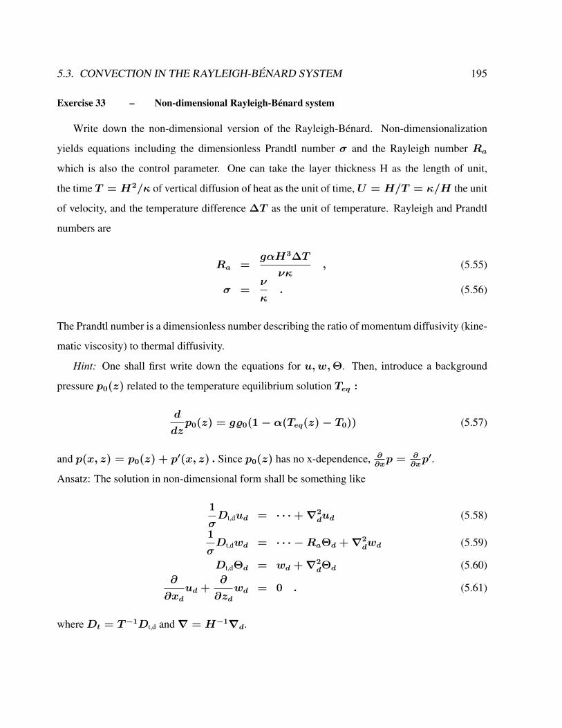
5.3. CONVECTION IN THE RAYLEIGH-BÉNARD SYSTEM 195
Exercise 33 – Non-dimensional Rayleigh-Bénard system
Write down the non-dimensional version of the Rayleigh-Bénard. Non-dimensionalization
yields equations including the dimensionless Prandtl number σ and the Rayleigh number Ra
which is also the control parameter. One can take the layer thickness H as the length of unit,
the time T = H2/κ of vertical diffusion of heat as the unit of time,U = H/T = κ/H the unit
of velocity, and the temperature difference ∆T as the unit of temperature. Rayleigh and Prandtl
numbers are
Ra =gαH3∆T
νκ, (5.55)
σ =ν
κ. (5.56)
The Prandtl number is a dimensionless number describing the ratio of momentum diffusivity (kine-
matic viscosity) to thermal diffusivity.
Hint: One shall first write down the equations for u,w,Θ. Then, introduce a background
pressure p0(z) related to the temperature equilibrium solution Teq :
d
dzp0(z) = g%0(1− α(Teq(z)− T0)) (5.57)
and p(x, z) = p0(z) + p′(x, z) . Since p0(z) has no x-dependence, ∂∂xp = ∂
∂xp′.
Ansatz: The solution in non-dimensional form shall be something like
1
σDt,dud = · · ·+∇2
dud (5.58)
1
σDt,dwd = · · · −RaΘd +∇2
dwd (5.59)
Dt,dΘd = wd +∇2dΘd (5.60)
∂
∂xdud +
∂
∂zdwd = 0 . (5.61)
whereDt = T−1Dt,d and∇ = H−1∇d.

196 CHAPTER 5. FLUID-DYNAMICAL EXAMPLES
Solution 1 of exercise 33
• Write the characteristic scales of the RB system
length: H → x = Hxd (5.62a)
time: T =H2
κ→ t =
H2
κtd (5.62b)
velocity: U =H
T=κ
H→ u =
κ
Hud (5.62c)
pressure: P = ρ0
H2
T 2= ρ0
κ2
H2→ p = ρ0
κ2
H2pd (5.62d)
temperature: ∆T → T = ∆T Td (5.62e)
Furthermore the following definitions for the Rayleigh (Ra) and Prandtl (σ) numbers are
given:
Ra =gαH3∆T
νκ(5.63)
and
σ =ν
κ. (5.64)
• Modifications of temperature and pressure terms
We introduce the temperature difference from the equilibrium solution:
θ = T − Teq → T = θ + Teq, (5.65)
where Teq is given as:
Teq = T0 + (1−z
H)∆T. (5.66)
Later we will need the following terms:
∂zTeq = −∆T
H(5.67)
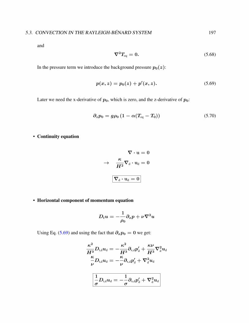
5.3. CONVECTION IN THE RAYLEIGH-BÉNARD SYSTEM 197
and
∇2Teq = 0. (5.68)
In the pressure term we introduce the background pressure p0(z):
p(x, z) = p0(z) + p′(x, z). (5.69)
Later we need the x-derivative of p0, which is zero, and the z-derivative of p0:
∂zp0 = gρ0 (1− α(Teq − T0)) (5.70)
• Continuity equation
∇ · u = 0
→κ
H2∇d · ud = 0
∇d · ud = 0
• Horizontal component of momentum equation
Dtu = −1
ρ0
∂xp+ ν∇2u
Using Eq. (5.69) and using the fact that ∂xp0 = 0 we get:
κ2
H3Dt,dud = −
κ2
H3∂x,dp
′d +
κν
H3∇2
dud
κ
νDt,dud = −
κ
ν∂x,dp
′d +∇2
dud
1
σDt,dud = −
1
σ∂x,dp
′d +∇2
dud
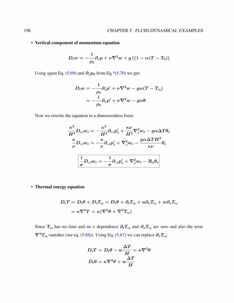
198 CHAPTER 5. FLUID-DYNAMICAL EXAMPLES
• Vertical component of momentum equation
Dtw = −1
ρ0
∂zp+ ν∇2w + g ((1− α(T − T0))
Using again Eq. (5.69) and ∂zp0 from Eq.*(5.70) we get:
Dtw = −1
ρ0
∂zp′ + ν∇2w − gα(T − Teq)
= −1
ρ0
∂xp′ + ν∇2w − gαθ
Now we rewrite the equation in a dimensionless form:
κ2
H3Dt,dwd = −
κ2
H3∂z,dp
′d +
κν
H3∇2
dwd − gα∆Tθd
κ
νDt,dwd = −
κ
ν∂z,dp
′d +∇2
dwd −gα∆TH3
κνθd
1
σDt,dwd = −
1
σ∂z,dp
′d +∇2
dwd −Raθd
• Thermal energy equation
DtT = Dtθ +DtTeq = Dtθ + ∂tTeq + u∂xTeq + w∂zTeq
= κ∇2T = κ(∇2θ +∇2Teq)
Since Teq has no time and no x dependence ∂tTeq and ∂xTeq are zero and also the term
∇2Teq vanishes (see eq. (5.68)). Using Eq. (5.67) we can replace ∂zTeq:
DtT = Dtθ − w∆T
H= κ∇2θ
Dtθ = κ∇2θ + w∆T
H
5.3. CONVECTION IN THE RAYLEIGH-BÉNARD SYSTEM 199
By introducing the dimensionless variables (Eq. (5.62)) we get:
κ∆T
H2Dt,dθd =
κ∆T
H2∇2
dθd +κ∆T
H2wd
Dt,dθd = ∇2dθd + wd
Solution 2 of exercise 33
A shorter solution is to use the (5.53, 5.54) system.
1
T
1
L2
L2
TDt,d
(∇2dΨd
)= ν
1
L4
L2
T∇4dΨd − gα
∆T
L
∂Θd
∂xd(5.71)
∆T
TDt,dΘd =
∆T
H
L2
TL
∂Ψd
∂xd+ κ
∆T
L2∇2dΘd . (5.72)
This yields (remember L = H)
Dt,d(∇2dΨd
)= ν
T
H2∇4dΨd − gα
T 2∆T
H
∂Θd
∂xd(5.73)
Dt,dΘd =∂Ψd
∂xd+ κ
T
H2∇2dΘd . (5.74)
Inserting T = H2/κ, gives
Dt,d(∇2dΨd
)=ν
κ∇4dΨd − gα
H3∆T
κ2
∂Θd
∂xd(5.75)
Dt,dΘd =∂Ψd
∂xd+∇2
dΘd . (5.76)
Finally, inserting the RayleighRa = gαH3∆Tνκ
and Prandtl σ = νκ
numbers:
Dt,d(∇2dΨd
)= σ∇4
dΨd −Raσ∂Θd
∂xd
200 CHAPTER 5. FLUID-DYNAMICAL EXAMPLES
5.3.3 Boundary conditions
We shall now discuss the boundary conditions: Θ = 0 at z = 0,H . As further boundary
condition, the normal component could be set to zero straightaway and we have vnormal = w =
0 at z = 0,H .
In many applications, one may assume no-slip boundary condition as the appropriate condi-
tions for velocity components at the wall. In general, while the tangential component is set to the
velocity of the wall:
vtangential = vwall . (5.77)
The fluid velocity at all fluid-solid boundaries is equal to that of the solid boundary. Conceptually,
one can think of the outermost molecules of fluid as stuck to the surfaces past which it flows.
Because the solution is prescribed at given locations, this is an example of a Dirichlet boundary
condition. Particles close to a surface do not move along with a flow when adhesion is stronger
than cohesion. At the fluid-solid interface, the force of attraction between the fluid particles and
solid particles (adhesive forces) is greater than that between the fluid particles (cohesive forces).
This force imbalance brings down the fluid velocity to zero. In our case: since the wall is not
moving u = 0 at z = 0,H .
Another boundary condition is called free boundary condition. All the normal velocities
normal to the wall should be zero, and furthermore the gradient of velocity parallel to wall should
be zero:
∂
∂zvtangential = 0 (5.78)
Here, we assume a free surface both the upper- and the lower-boundaries because then the problem
is most analytically tractable.4 In our case this means no tangential stress is for ∂u∂z
= ∂2ψ∂z2
= 0
One can show that in which case Ψ and∇2Ψ vanish at both boundaries. The basis functions can
4In practical applications, the boundaries are not free and there is friction.
5.3. CONVECTION IN THE RAYLEIGH-BÉNARD SYSTEM 201
be chosen as sinus and cosinus as orthogonal set of base functions. In chapter 3.4, the dynamics
is solved numerically using the Lattice Boltzmann approach. Other techniques and experimental
approaches are summarized in Tritton [1988].
5.3.4 Galerkin approximation: Obtaining the Lorenz system
Saltzman [1962] derived a set of ordinary differential equations by expanding Ψ and Θ in double
Fourier series in x and z, with functions of t alone for coefficients, and substituting these series
into (5.53) and (5.54) A complete Galerkin approximation
Ψ(x, z, t) =∞∑k=1
∞∑l=1
Ψk,l(t) sin
(kπa
Hx
)× sin
(lπ
Hz
)(5.79)
Θ(x, z, t) =∞∑k=1
∞∑l=1
Θk,l(t) cos
(kπa
Hx
)× sin
(lπ
Hz
)(5.80)
yields an infinite set of ordinary differential equations for the time coefficients. He arranged the
right-hand sides of the resulting equations in double Fourier-series form, by replacing products of
trigonometric functions of x (or z) by sums of trigonometric functions, and then equated coef-
ficients of similar functions of x and z. He then reduced the resulting infinite system to a finite
system by omitting reference to all but a specified finite set of functions of t. He then obtained
time-dependent solutions by numerical integration. In certain cases all, except three of the depen-
dent variables, eventually tended to zero, and these three variables underwent irregular, apparently
non-periodic fluctuations. These same solutions would have been obtained if the series had been
at the start truncated to include a total of three terms. Accordingly, in this study we shall let
a
1 + a2κ Ψ = X
√2 sin
(πa
Hx
)sin
(π
Hz
)(5.81)
πRa
Rc
1
∆TΘ = Y
√2 cos
(πa
Hx
)sin
(π
Hz
)− Z sin
(2π
Hz
)(5.82)
whereX(t), Y (t), and Z(t) are functions of time alone.
202 CHAPTER 5. FLUID-DYNAMICAL EXAMPLES
It is found that fields of motion of this form would develop if the Rayleigh number
Ra =gαH3∆T
νκ, (5.83)
exceeds a critical value
Rc = π4a−2(1 + a2)3 . (5.84)
The minimum value of Rc, namely 27π4/4 = 657.51, occurs when a2 = 1/2. In fluid
mechanics, the Rayleigh number for a fluid is a dimensionless number associated with the relation
of buoyancy and viscosity in a flow. When the Rayleigh number is below the critical value for that
fluid, heat transfer is primarily in the form of conduction; when it exceeds the critical value, heat
transfer is primarily in the form of convection.
When the above truncation (5.81,5.82) is substituted into the dynamics, we obtain the equations
X = −σX + σY (5.85)
Y = rX − Y −XZ (5.86)
Z = −bZ +XY (5.87)
Here a dot denotes a derivative with respect to the dimensionless time td = π2H−2(1 + a2)κt,
while σ = νκ−1 is the Prandtl number, r = Ra/Rc, and b = 4(1 + a2)−1.
Except for multiplicative constants, our variablesX,Y, Z are the same as Saltzman’s variables
A, D, and G. These equations are the convection equations whose solutions we shall study. In
these equationsX is proportional to the intensity of the convective motion, whileY is proportional
to the temperature difference between the ascending and descending currents, identical signs of
X and Y denoting that warm fluid is rising and cold fluid is descending. The variable Z is
proportional to the distortion of the vertical temperature-profile from linearity, a positive value
indicating that the strongest gradients occur near the boundaries.

Chapter 6
Atmosphere and Ocean Dynamics
Here, we shortly introduce the basic concepts of oceanography: the fundamental equations and
approximations. Basically, we deal with the dynamical equations on a rotating sphere. Several
approximations can be done since the scales of the components in the dynamical equations differ
in the orders of magnitude. A more detailled description can be found in text books [Von Arx,
1962; Gill, 1982; Holton, 2004; Pickard and Emery, 1990; Stewart, 2005; Dijkstra, 2000; Olbers
et al., 2012].
6.1 Pseudo forces and the Coriolis effect
A pseudo force on an object arises when the frame of reference used to describe the object’s
motion is accelerating compared to a non-accelerating frame. It acts on all masses whose motion
is described using a non-inertial frame of reference, such as a rotating reference frame. The inertial
frame is the Sun and not the Earth.1 Assuming Newton’s second law in the form F = ma, pseudo
1Galilean invariance or Galilean relativity states that the laws of motion are the same in all inertial frames. GalileoGalilei first described this principle in 1632 in his Dialogue Concerning the Two Chief World Systems using theexample of a ship travelling at constant velocity, without rocking, on a smooth sea; any observer doing experimentsbelow the deck would not be able to tell whether the ship was moving or stationary. Galilean relativity can be shownas follows. Consider two inertial frames S and S’ . A physical event in S will have position coordinates r = (x, y, z)and time t; similarly for S’ . By the second axiom above, one can synchronize the clock in the two frames and assumet = t′. Suppose S’ is in relative uniform motion to S with velocity v. Consider a point object whose position is
203

204 CHAPTER 6. ATMOSPHERE AND OCEAN DYNAMICS
forces are always proportional to the mass m. The surface of the Earth is a rotating reference
frame. To solve classical mechanics problems exactly in an Earth-bound reference frame, three
pseudo forces must be introduced, the Coriolis force, the centrifugal force (described below) and
the Euler force. The Euler force is typically ignored because the variations in the angular velocity
of the rotating Earth surface are usually insignificant. Both of the other pseudo forces are weak
compared to most typical forces in everyday life, but they can be detected under careful conditions.
For example, Foucault was able to show the Coriolis force that results from the Earth’s rotation
using the Foucault pendulum (see Exercise 3). If the Earth were to rotate a thousand times faster
(making each day only ≈ 86 seconds long), people could easily get the impression that such
fictitious forces are pulling on them, as on a spinning carousel.
In the rotating framework, we have the Coriolis and centrifugal forces which stem from the
rotating framework. We derive from the simple relation for the time derivative in the inertial
system (i) to the Earth system (e)
(dtA)i = (dtA)e + Ω×A (6.1)
where the× symbol represents the cross product operator. For the case A = r, it follows for the
velocity
vi = ve + Ω× r (6.2)
and the relation for the acceleration (caseA = vi)
ai = (dtvi)e + Ω× vi (6.3)
= dtve + Ω× ve + Ω× (ve + Ω× r) = ae + 2Ω× ve + Ω× Ω× r
given by r′(t) = r(t) in S. We see that r′(t) = r(t) − vt. and acceleration is identical in the two framesa′(t) = d2
dt2r′(t) = d2
dt2r(t) = a(t). A side remark: All approximations of the dynamical equations shall be
Galilean invariant. In numerical examples, the lack of invariance for unresolved solutions is because the truncationerror is not Galilean invariant. While advanced methods reduce the truncation error, none of them eliminate it entirely,and therefore formally solutions will still violate Galilean invariance at the level of the truncation error.
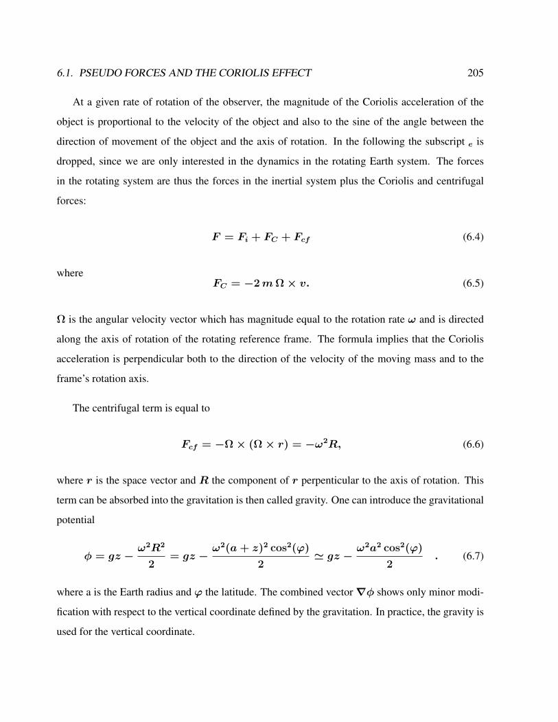
6.1. PSEUDO FORCES AND THE CORIOLIS EFFECT 205
At a given rate of rotation of the observer, the magnitude of the Coriolis acceleration of the
object is proportional to the velocity of the object and also to the sine of the angle between the
direction of movement of the object and the axis of rotation. In the following the subscript e is
dropped, since we are only interested in the dynamics in the rotating Earth system. The forces
in the rotating system are thus the forces in the inertial system plus the Coriolis and centrifugal
forces:
F = Fi + FC + Fcf (6.4)
whereFC = −2mΩ× v. (6.5)
Ω is the angular velocity vector which has magnitude equal to the rotation rate ω and is directed
along the axis of rotation of the rotating reference frame. The formula implies that the Coriolis
acceleration is perpendicular both to the direction of the velocity of the moving mass and to the
frame’s rotation axis.
The centrifugal term is equal to
Fcf = −Ω× (Ω× r) = −ω2R, (6.6)
where r is the space vector and R the component of r perpenticular to the axis of rotation. This
term can be absorbed into the gravitation is then called gravity. One can introduce the gravitational
potential
φ = gz −ω2R2
2= gz −
ω2(a+ z)2 cos2(ϕ)
2' gz −
ω2a2 cos2(ϕ)
2. (6.7)
where a is the Earth radius and ϕ the latitude. The combined vector∇φ shows only minor modi-
fication with respect to the vertical coordinate defined by the gravitation. In practice, the gravity is
used for the vertical coordinate.
206 CHAPTER 6. ATMOSPHERE AND OCEAN DYNAMICS
6.2 Scaling of the dynamical equations
As we will see now, the Coriolis effect is one of the dominating forces for the large-scale dynamics
of the oceans and the atmosphere. It is convenient to work in the rotating frame of reference of the
Earth. The equation can be scaled by a length-scale L, determined by the geometry of the flow,
and by a characteristic velocity U. Starting from (4.9), we can estimate the relative contributions
in units ofm/s2 in the horizontal momentum equations:
∂v
∂t︸︷︷︸U/T∼10−8
+ v · ∇v︸ ︷︷ ︸U2/L∼10−8
= −1
ρ∇p︸ ︷︷ ︸
δP/(ρL)∼10−5
+ 2Ω× v︸ ︷︷ ︸f0U∼10−5
+ fric︸ ︷︷ ︸νU/H2∼10−13
(6.8)
where fric denotes the contributions of friction due to eddy stress divergence (usually ∼ ν∇2v).
Typical values are given in Table 6.2. The values have been taken for the ocean. You may repeat
the estimate for the atmosphere using Table 6.2.
It is useful to think about the orders of magnitude: Because of the continuity equationU/L ∼
W/H and since the horizonatal scales are orders of magnitude larger than the vertical ones, the
vertical velocity is very small relative to the horizontal. For small scale motion (like small-scale
ocean convection or cumuls clouds) the horizontal length scale is of the same order as the vertical
one and therefore the vertical motion is in the same order of magnitude as the horizontal motion.
The timescales are related to T ∼ L/U ∼ H/W .
It is already useful to think about the relative importance of the different terms in the momen-
tum balance (6.8). The Rossby number Ro is the ratio of inertial (the left hand side) to Coriolis
(second term on the right hand side) terms
Ro =(U2/L)
(fU)=
U
fL. (6.9)
It is used in the oceans and atmosphere, where it characterizes the importance of Coriolis acceler-
ations arising from planetary rotation. It is also known as the Kibel number. Ro is small when the
flow is in a so-called geostrophic balance. This will be the subject in the next paragraphs.
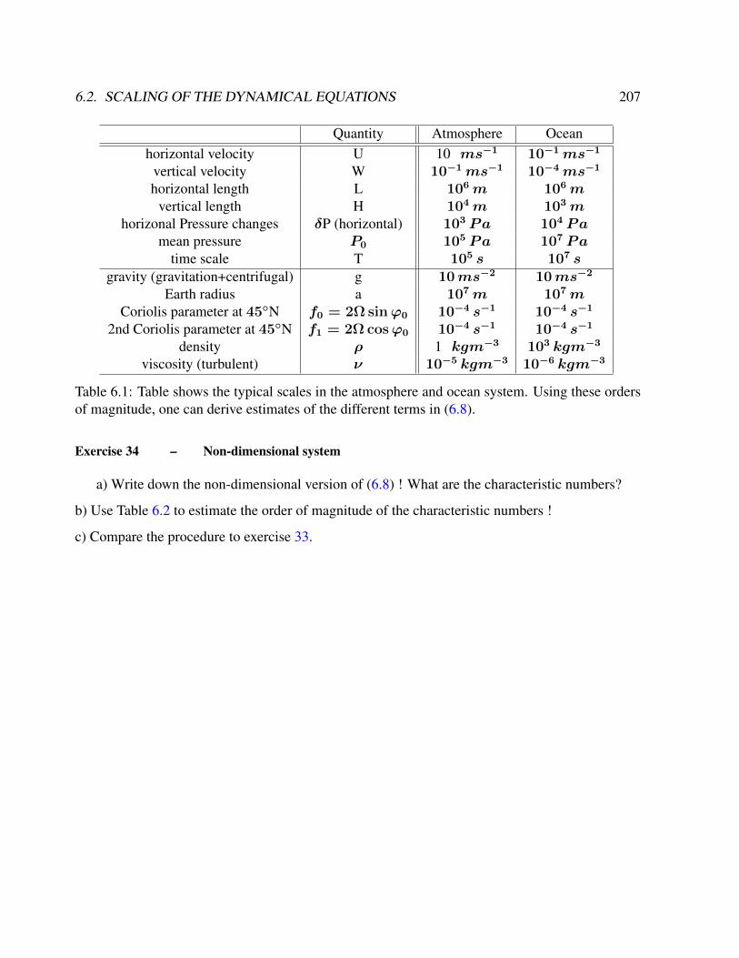
6.2. SCALING OF THE DYNAMICAL EQUATIONS 207
Quantity Atmosphere Oceanhorizontal velocity U 10 ms−1 10−1ms−1
vertical velocity W 10−1ms−1 10−4ms−1
horizontal length L 106m 106mvertical length H 104m 103m
horizonal Pressure changes δP (horizontal) 103 Pa 104 Pamean pressure P0 105 Pa 107 Pa
time scale T 105 s 107 sgravity (gravitation+centrifugal) g 10ms−2 10ms−2
Earth radius a 107m 107mCoriolis parameter at 45N f0 = 2Ω sinϕ0 10−4 s−1 10−4 s−1
2nd Coriolis parameter at 45N f1 = 2Ω cosϕ0 10−4 s−1 10−4 s−1
density ρ 1 kgm−3 103 kgm−3
viscosity (turbulent) ν 10−5 kgm−3 10−6 kgm−3
Table 6.1: Table shows the typical scales in the atmosphere and ocean system. Using these ordersof magnitude, one can derive estimates of the different terms in (6.8).
Exercise 34 – Non-dimensional system
a) Write down the non-dimensional version of (6.8) ! What are the characteristic numbers?
b) Use Table 6.2 to estimate the order of magnitude of the characteristic numbers !
c) Compare the procedure to exercise 33.
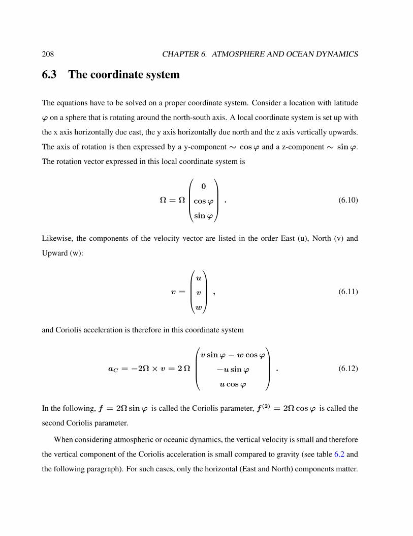
208 CHAPTER 6. ATMOSPHERE AND OCEAN DYNAMICS
6.3 The coordinate system
The equations have to be solved on a proper coordinate system. Consider a location with latitude
ϕ on a sphere that is rotating around the north-south axis. A local coordinate system is set up with
the x axis horizontally due east, the y axis horizontally due north and the z axis vertically upwards.
The axis of rotation is then expressed by a y-component ∼ cosϕ and a z-component ∼ sinϕ.
The rotation vector expressed in this local coordinate system is
Ω = Ω
0
cosϕ
sinϕ
. (6.10)
Likewise, the components of the velocity vector are listed in the order East (u), North (v) and
Upward (w):
v =
u
v
w
, (6.11)
and Coriolis acceleration is therefore in this coordinate system
aC = −2Ω× v = 2 Ω
v sinϕ− w cosϕ
−u sinϕ
u cosϕ
. (6.12)
In the following, f = 2Ω sinϕ is called the Coriolis parameter, f (2) = 2Ω cosϕ is called the
second Coriolis parameter.
When considering atmospheric or oceanic dynamics, the vertical velocity is small and therefore
the vertical component of the Coriolis acceleration is small compared to gravity (see table 6.2 and
the following paragraph). For such cases, only the horizontal (East and North) components matter.
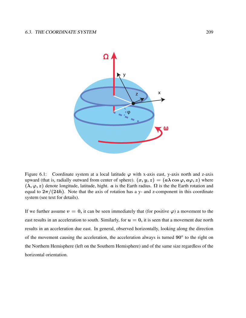
6.3. THE COORDINATE SYSTEM 209
ω
y
z x
Ω
φ
Figure 6.1: Coordinate system at a local latitude ϕ with x-axis east, y-axis north and z-axisupward (that is, radially outward from center of sphere). (x, y, z) = (aλ cosϕ, aϕ, z) where(λ, ϕ, z) denote longitude, latitude, hight. a is the Earth radius. Ω is the the Earth rotation andequal to 2π/(24h). Note that the axis of rotation has a y- and z-component in this coordinatesystem (see text for details).
If we further assume v = 0, it can be seen immediately that (for positive ϕ) a movement to the
east results in an acceleration to south. Similarly, for u = 0, it is seen that a movement due north
results in an acceleration due east. In general, observed horizontally, looking along the direction
of the movement causing the acceleration, the acceleration always is turned 90 to the right on
the Northern Hemisphere (left on the Southern Hemisphere) and of the same size regardless of the
horizontal orientation.
210 CHAPTER 6. ATMOSPHERE AND OCEAN DYNAMICS
Exercise 35 – Double Vector Product
Examine the double vector product Ω× (Ω× r) with vectors Ω = (0, 0, ω), r = (x, y, z).
Solution
Ω× (Ω× r) =
0
0
ω
×
0
0
ω
×x
y
z
=
0
0
ω
×−ωy
ωx
0
=
−ω2y
−ω2x
0
= −‖Ω‖2R
with R = (x, y, 0)T and ‖Ω‖2 = ω2 .
Exercise 36 – Some Questions Dynamics
1. Consider the heat diffusion-advection equation
∂T
∂t= k
∂2T
∂x2+ u
∂T
∂x
and determine the time evolution with initial conditions
a) T (x, 0) = exp(−x2/a) with a = constant.
b) T (x, 0) = T0 for x ≥ 0 and T (x, 0) = 0 elsewhere.
Discuss the special cases k = 0 (no diffusion) and u = 0 (no advection).
6.3. THE COORDINATE SYSTEM 211
2. A tornado rotates with constant angular velocity ω. Show that the surface pressure at the
center of the tornado is given by:
p = p0 exp(−ω2r0
2/(2RT ))
where p0 is the surface pressure at the distance r0 from the center and T is the temperature
(assumed constant). [Hint: What are the dominant forces? Pressure gradient and centrifugal
force.]
If temperature is 288K, pressure at 100m from the center is 102 kPa, and wind speed at
100m from the center is 100m/s, what is the central pressure?
3. Suppose a 1kg parcel of dry air is rising at a constant vertical velocity. If the parcel is being
heated by radiation at a rate of 10−1W/kg, what must the speed of rise be in order to
maintain the parcel at a constant temperature. [Hint: Energy equation.]
4. Show that for an atmosphere with an adiabatic lapse rate (i.e. constant potential temperature),
the geopotential Z(z) := Φ(z)/g0 is given by
Z = HΘ[1− (p/p0)a]
where p0 is the pressure at Z = 0 and HΘ = cpΘ/g0 is the total geopotential in the
atmosphere. a = R/cp.
Exercise 37 – Some questions
1. Please write down the equation of state for the ocean and atmosphere!
2. What is the hydrostatic approximation in the momentum equations?
3. Please clarify: On the Northern Hemisphere, particles tend to go to the right or left relative
to the direction of motion due to the Coriolis force?

212 CHAPTER 6. ATMOSPHERE AND OCEAN DYNAMICS
6.4 Geostrophy
The momentum equations (6.8) can be also written in the coordinate system (Fig. 6.1) above as
∂u
∂t+ v · ∇u−
uv tanϕ
a−uw
a= −
1
ρ
∂p
∂x+ fv − f (2)w + ν∇2u (6.13)
∂v
∂t+ v · ∇v −
u2 tanϕ
a−vw
a= −
1
ρ
∂p
∂y− fu + ν∇2v (6.14)
complemented by the dynamics for the vertical component w :
∂w
∂t︸︷︷︸W/T∼10−11
+ v · ∇w︸ ︷︷ ︸UW/L∼10−11
−u2 + v2
a︸ ︷︷ ︸U2/a∼10−9
= −1
ρ
∂p
∂z︸ ︷︷ ︸P0/(ρH)∼10
+ g︸︷︷︸∼10
+ f (2)u︸ ︷︷ ︸∼10−5
+ ν∂2zw︸ ︷︷ ︸
νW/H2∼10−16
(6.15)
As boundary conditions, equations (6.13, 6.14) are complemented by the horizontal wind stresses
∂zτxz and ∂zτyz at the ocean surface, respectively.
∂u
∂t+ v · ∇u+ . . . = −
1
ρ
∂p
∂x+ fv − f (2)w + ν∇2u+
1
ρ∂zτxz (6.16)
∂v
∂t+ v · ∇v + . . . = −
1
ρ
∂p
∂y− fu + ν∇2v +
1
ρ∂zτyz (6.17)
It should be noted that due to sperical coordinates (see Fig. 6.1), one has metric terms, e.g. on the
left hand sides of (6.13,6.14,6.15): −uv tanϕa− uw
a, u
2 tanϕa− vw
a, and u2+v2
a, respectively. In
the geostropic approximation, one can drop these terms.2
A small Rossby number signifies a system which is strongly affected by Coriolis forces, and
a large Rossby number signifies a system in which inertial forces dominate. For example, in
tornadoes, the Rossby number is large (≈ 103), in atmospheric low-pressure systems it is low
(≈ 0.1 − 1), but depending on the phenomena can range over several orders of magnitude (≈
10−2 − 102).3 Using the values in table 6.2, Ro in oceanic systems is of the order of 10−3.
2Task: Calculate the order of magnitude of the metric terms in (6.13,6.14) by using table 6.2.3As a result, in tornadoes the Coriolis force is negligible, and balance is between pressure and centrifugal forces
(called cyclostrophic balance). This balance also occurs at the outer eyewall of a tropical cyclone.
6.4. GEOSTROPHY 213
When the Rossby number is large (either because f is small, such as in the tropics and at lower
latitudes; or because L is small, that is, for small-scale motions such as flow in a bathtub; or for
large speeds), the effects of planetary rotation are unimportant and can be neglected. Repeating:
When the Rossby number is small, then the effects of planetary rotation are large and the net
acceleration is comparably small allowing the use of the so-called geostrophic approximation: The
force balance is largely between the pressure gradient force acting towards the low-pressure area
and the Coriolis force acting away from the center of the low pressure in equation (6.8). By scaling
arguments, one can derive the geostrophic horizontal flow components (ug, vg) as:
ug = −1
fρ
∂p
∂y(6.18)
vg =1
fρ
∂p
∂x(6.19)
The validity of this approximation depends on the local Rossby number. It is invalid at the equator,
because f = 2Ω sinϕ is equal to zero there, and therefore generally not used in the tropics.
Equations (6.18,6.19) show that large-scale motions in the atmosphere and ocean tend to occur
perpendicular to the pressure gradient, instead of flowing down the gradient. This circulation is
called geostrophic flow. On a non-rotating planet, fluid would flow along the straightest possible
line, quickly eliminating pressure gradients.4
4Task: Think how the geostrophy can be derived in the inertial system with a fixed reference frame, e.g. the Sun.The final result shall be independent on the reference system used!
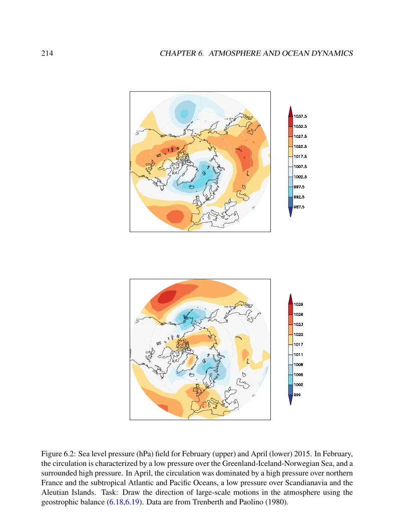
214 CHAPTER 6. ATMOSPHERE AND OCEAN DYNAMICS
Figure 6.2: Sea level pressure (hPa) field for February (upper) and April (lower) 2015. In February,the circulation is characterized by a low pressure over the Greenland-Iceland-Norwegian Sea, and asurrounded high pressure. In April, the circulation was dominated by a high pressure over northernFrance and the subtropical Atlantic and Pacific Oceans, a low pressure over Scandianavia and theAleutian Islands. Task: Draw the direction of large-scale motions in the atmosphere using thegeostrophic balance (6.18,6.19). Data are from Trenberth and Paolino (1980).
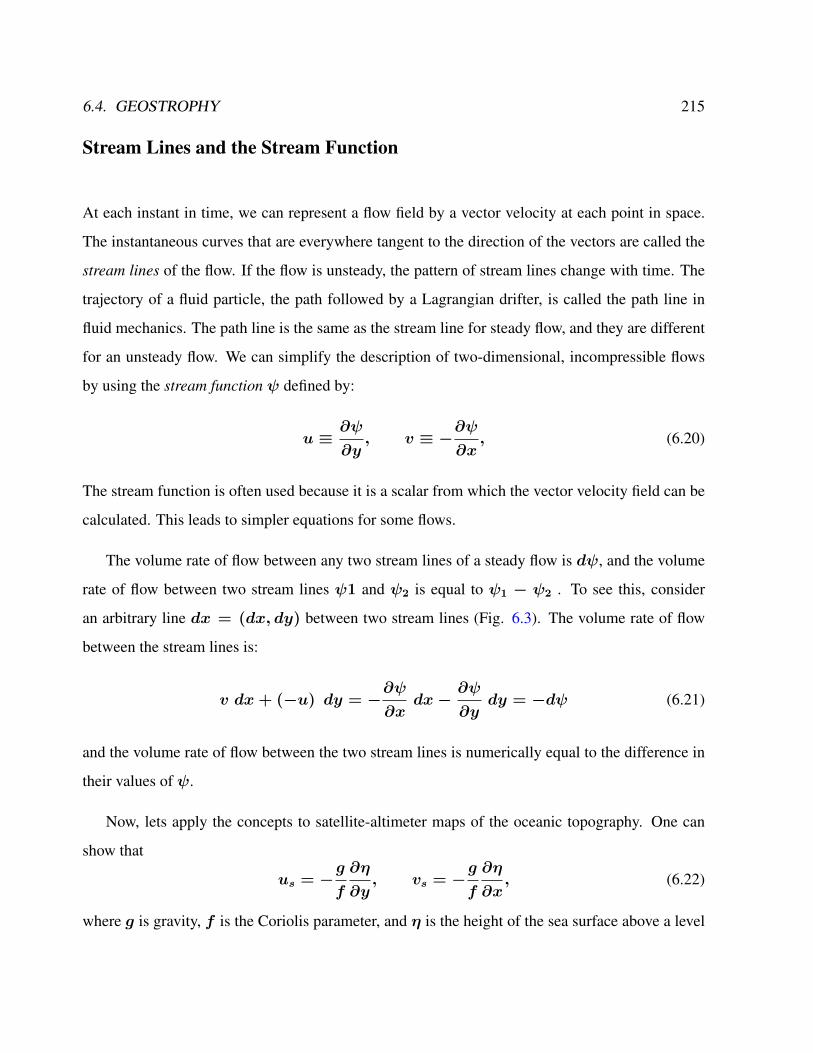
6.4. GEOSTROPHY 215
Stream Lines and the Stream Function
At each instant in time, we can represent a flow field by a vector velocity at each point in space.
The instantaneous curves that are everywhere tangent to the direction of the vectors are called the
stream lines of the flow. If the flow is unsteady, the pattern of stream lines change with time. The
trajectory of a fluid particle, the path followed by a Lagrangian drifter, is called the path line in
fluid mechanics. The path line is the same as the stream line for steady flow, and they are different
for an unsteady flow. We can simplify the description of two-dimensional, incompressible flows
by using the stream function ψ defined by:
u ≡∂ψ
∂y, v ≡ −
∂ψ
∂x, (6.20)
The stream function is often used because it is a scalar from which the vector velocity field can be
calculated. This leads to simpler equations for some flows.
The volume rate of flow between any two stream lines of a steady flow is dψ, and the volume
rate of flow between two stream lines ψ1 and ψ2 is equal to ψ1 − ψ2 . To see this, consider
an arbitrary line dx = (dx, dy) between two stream lines (Fig. 6.3). The volume rate of flow
between the stream lines is:
v dx+ (−u) dy = −∂ψ
∂xdx−
∂ψ
∂ydy = −dψ (6.21)
and the volume rate of flow between the two stream lines is numerically equal to the difference in
their values of ψ.
Now, lets apply the concepts to satellite-altimeter maps of the oceanic topography. One can
show that
us = −g
f
∂η
∂y, vs = −
g
f
∂η
∂x, (6.22)
where g is gravity, f is the Coriolis parameter, and η is the height of the sea surface above a level

216 CHAPTER 6. ATMOSPHERE AND OCEAN DYNAMICS
Figure 6.3: Volume transport between stream lines in a two-dimensional, steady flow. After Kundu(1990: 68).
surface. Comparing 6.22 with 6.20 it is clear that
ψ = −g
fη (6.23)
and the sea surface is a stream function scaled by g/f . The lines of constant height are stream
lines, and flow is along the lines. The surface geostrophic transport is proportional to the difference
in height, independent of the distance between the stream lines. The transport is relative to transport
at the 1000 decibars surface, which is roughly one kilometer deep.
In addition to the stream function, oceanographers use the mass-transport stream function Ψ
defined by:
Mx ≡∂Ψ
∂y, My ≡ −
∂Ψ
∂x(6.24)

6.4. GEOSTROPHY 217
Figure 6.4: Schematic picture of the Hadley Cell and the jet streams.
218 CHAPTER 6. ATMOSPHERE AND OCEAN DYNAMICS
Exercise 38 – Angular momentum and Hadley Cell
Consider a zonally symmetric circulation (i.e., one with no longitudinal variations) in the atmo-
sphere. In the inviscid upper troposphere one expects such a flow to conserve absolute angular
momentum, i.e., DA
Dt= 0,
where A is the absolute angular momentum per unit mass (parallel to the Earth’s rotation axis)
A = r (u+ Ωr) = Ωa2 cos2 ϕ+ ua cosϕ .
Ω is the Earth rotation rate, u the eastward wind component, r = a cosϕ is the distance from
the rotation axis, a the Earth’s radius, and ϕ latitude.
1. Show, for inviscid zonally symmetric flow, that the relation DADt
= 0 is consistent with
the zonal component of the equation of motion (using our standard notation, with Fx the
x-component of the friction force per unit mass)
Du
Dt− fv = −
1
ρ
∂p
∂x+ Fx
in (x, y, z) coordinates, where y = aϕ.
2. Use angular momentum conservation to describe how the existence of the Hadley circulation
explains the existence of both the subtropical jet in the upper troposphere.
Hint: In the upper troposphere, the flow leaves the rising branch of the Hadley cell at the
equator (cf. Fig. 6.4) with angular momentum density A0 = Ωa2, if we assume that
the flow rises from the ground there with no relative motion. The zonal flow can then be
described as u = Ωa sin2 ϕ/ cosϕ . Show that the zonal flow will be greatest at the edge
of the cell, where ϕ is greatest, thus producing the subtropical jet.
Note that Ωa2 = 2π86400 s
· (6.371 · 106m)2 = 3 · 109m2s−1.
3. Describe the near-surface trade winds by recognizing that this low-level flow is under the
6.4. GEOSTROPHY 219
influence of surface friction and A will therefore be progressively reduced. Show that
ulow < Ωasin2 ϕ
cosϕ
and some ϕ that ulow becomes negative (eastward winds).
4. If the Hadley circulation is symmetric about the equator, and its edge is at 20 latitude, de-
termine the strength of the subtropical jet.
(The observed zonal winds are weaker than the value. In reality, non-axisymmetric atmo-
spheric eddies act to reduce angular momentum in the outflow, and hence reduce the strength
of the jets.)
5. Consider the tropical Hadley circulation in northern winter. The circulation rises at 10S,
moves northward across the equator in the upper troposphere, and sinks at 20N . Assuming
that the circulation, outside the near-surface boundary layer, is zonally symmetric (indepen-
dent of x) and inviscid (and thus conserves absolute angular momentum about the Earth’s
rotation axis), and that it leaves the boundary layer at 10S with zonal velocity u = 0, calcu-
late the zonal wind in the upper troposphere and provide the numbers for the equator, 10N ,
and 20N .
Solution of Exercise 38
1. For inviscid axisymmetric flow, conservation of angular momentum implies
Dt(Ωa2 cos2 ϕ+ ua cosϕ) = 0

220 CHAPTER 6. ATMOSPHERE AND OCEAN DYNAMICS
Remember that y = aϕ, dx = a cosϕdλ. Here, we reformulate the planetary term:
Dt(Ωa2 cos2 ϕ) = v∂y(Ωa
2 cos2 ϕ) (6.25)
= Ωav∂ϕ(cos2 ϕ) (6.26)
= −2Ωav sinϕ cosϕ (6.27)
= −fv · a cosϕ (6.28)
SimilarDt(ua cosϕ) = a cosϕDtu+ u · v ∂ϕ cosϕ (6.29)
where in the coordinate system
Dtu = (∂t + u∂x + v∂y)u +uv
atanϕ (6.30)
(the last term is a metric term). Therefore and under the assumption ∂xp = 0:
Dtu− fv = 0 (6.31)
2. Use angular momentum conservation to describe how the existence of the Hadley circulation
explains the existence of both the subtropical jet in the upper troposphere. In the upper
troposphere, the flow leaves the rising branch of the Hadley cell at the equator (cf. Fig. 6.4)
with angular momentum density A0 = Ωa2, if we assume that the flow rises from the
ground there with no relative motion. We have
A = Ωa2 cos2 ϕ+ ua cosϕ = A0 = Ωa2
and therefore the zonal flow can then be described as
u = Ωa sin2 ϕ/ cosϕ .
6.4. GEOSTROPHY 221
The zonal flow will be greatest at the edge of the cell, where ϕ is greatest, thus producing
the subtropical jet.
3. If the return flow, in the lower troposphere, were inviscid and thus also conserved angular
momentum with Alow = A0, then at a given latitude the low level flow would be the same
as that aloft, since in u is a function of ϕ only. However, in reality this low-level flow is
under the influence of surface friction and A will therefore be progressively reduced. Thus,
Alow = Ωa2 cos2 ϕ+ ulowa cosϕ < A0 = Ωa2
Thus ulow < Ωasin2 ϕ
cosϕ
and some ϕ0 north of the equator that ulow becomes negative (eastward winds), and so the
low level flow will be equatorward and eastward there. (Note that Ωa2 = 2π86400 s
· (6.371 ·
106m)2 = 3 · 109m2s−1.)
4. Assume the Hadley circulation is symmetric about the equator, and its edge is at 20 latitude,
determine the strength of the subtropical jet by
u(20) = Ωa sin2(20)/ cos(20) = 57.6ms−1
The observed zonal winds are weaker than the value. In reality, non-axisymmetric atmo-
spheric eddies act to reduce angular momentum in the outflow, and hence reduce the strength
of the jets.
5. Consider the angular momentum A = Ωa2 cos2 ϕ + ua cosϕ = A0 = Ωa2 with
A0 = Ωa2 cos2(10S) = 2.952 · 109m2s−1.
Therefore u =A0 − Ωa2 cos2 ϕ
a cosϕ
At ϕ = 0, u = −13.9ms−1, at ϕ = 10, u = 0ms−1, at ϕ = 20, u =
42.8ms−1.
222 CHAPTER 6. ATMOSPHERE AND OCEAN DYNAMICS
6.5 Conservation of vorticity
In simple words, vorticity is the rotation of the fluid. The rate of rotation can be defined in various
ways. Consider a bowl of water sitting on a table in a laboratory. The water may be spinning in
the bowl. In addition to the spinning of the water, the bowl and the laboratory are rotating because
they are on a rotating earth. The two processes are separate and lead to two types of vorticity.
Everything on earth, including the ocean, the atmosphere, and bowls of water, rotates with the
earth. This rotation is the planetary vorticity f . It is twice the local rate of rotation of earth:
f ≡ 2 Ω sinϕ
(1
s
)= 2 sinϕ
(cycles
day
)(6.32)
Planetary vorticity is also called the Coriolis parameter. It is greatest at the poles where it is twice
the rotation rate of earth. Note that the vorticity vanishes at the equator and that the vorticity in the
Southern Hemisphere is negative because ϕ is negative.
The ocean and atmosphere do not rotate at exactly the same rate as the Earth. They have some
rotation relative to Earth due to currents and winds. Relative vorticity ζ is the vorticity due to
currents in the ocean.5 Mathematically it is:
ζ ≡∂v
∂x−∂u
∂y(6.33)
where we have assumed that the flow is two-dimensional.
For a rigid body rotating at rate Ω, ζ = 2 Ω. Of course, the flow does not need to rotate
as a rigid body to have relative vorticity. Vorticity can also result from shear. For example, at a
north/south western boundary in the ocean, u = 0, v = v (x) and ζ = ∂v (x) /∂x.
ζ is usually much smaller than f . To make an estimate for ζ : It is greatest at the edge of fast
currents such as the Gulf Stream. To obtain some understanding of the size of ζ, consider the edge
5ζ is the vertical component of the threedimensional vorticity vector ω, and it is sometimes written ωz . ζ ispositive for counter-clockwise rotation viewed from above. This is the same sense as Earth’s rotation in the NorthernHemisphere. One could use ωz for relative vorticity, but ω is also commonly used to mean frequency in radians persecond.

6.5. CONSERVATION OF VORTICITY 223
of the Gulf Stream off Cape Hatteras where the velocity decreases by 1ms−1 in 100km at the
boundary. The curl of the current is approximately
ζ =∂v
∂x=
1ms−1
100 km= 0.14
cycles
day= 1
cycle
week= 1.62 · 10−6
1
s. (6.34)
Hence even this large relative vorticity is still almost seven times smaller than f (compare 6.32).
A more typical value of relative vorticity, such as the vorticity of eddies, is a cycle per month. The
sum of the planetary and relative vorticity is called absolute vorticity:
Absolute Vorticity ≡ (ζ + f) (6.35)
We can obtain an equation for absolute vorticity in the ocean by manipulating the equations of
motion for frictionless flow. We begin with:
Du
Dt− f v = −
1
ρ
∂p
∂x(6.36)
Dv
Dt+ f u = −
1
ρ
∂p
∂y(6.37)
If we expand the substantial derivative, and if we subtract ∂/∂y of (6.36) from ∂/∂x of (6.37) to
eliminate the pressure terms, we obtain
D
Dt(∂xv − ∂yu) + (∂xu∂xv + ∂xv∂yv)− (∂yu∂xu+ ∂yv∂yu)
+ f (∂xu+ ∂yv) + v ∂yf = 0 (6.38)
Using DDtf = v ∂yf :
D
Dtζ + ∂xv (∂xu+ ∂yv)− ∂yu (∂xu+ ∂yv)
+ f (∂xu+ ∂yv) +D
Dtf = 0 (6.39)
224 CHAPTER 6. ATMOSPHERE AND OCEAN DYNAMICS
this yieldsD
Dt(ζ + f) + (ζ + f)
(∂u
∂x+∂v
∂y
)= 0 . (6.40)
Exercise 39 – Non-dimensional system of the vorticity dynamics
a) For cnstant depth, derive the the non-dimensional version of the vorticity equation
D
Dt(ζ + f) = ν∇2ζ .
Hint: Repeat exercise 30. b) What are the characteristic numbers?
c) Estimate the order of magnitude of the characteristic numbers for the atmosphere and ocean !
You can use Table 6.2 and other references.
6.5.1 Potential vorticity equation (ζ + f)/h
The rotation rate of a column of fluid changes as the column is expanded or contracted. This
changes the vorticity through changes in ζ. To see how this happens, consider barotropic, geostrophic
flow in an ocean with depth h (x, y, t), where h is the distance from the sea surface to the bottom.
That is, we allow the surface to have topography (Fig. 6.5). Integrating the continuity equation
from the bottom to the top of the ocean gives:
(∂u
∂x+∂v
∂y
)∫ b+h
b
dz + w|b+hb = 0 (6.41)
where b is the topography of the bottom, and h is the depth of the water. Notice that ∂u/∂x
and ∂v/∂y are independent of z because they are barotropic, and the terms can be taken outside
the integral. The boundary conditions require that flow at the surface and the bottom be along the
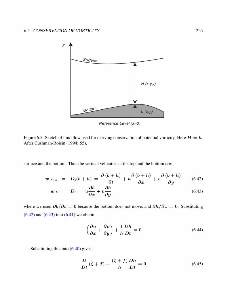
6.5. CONSERVATION OF VORTICITY 225
Figure 6.5: Sketch of fluid flow used for deriving conservation of potential vorticity. HereH = h.After Cushman-Roisin (1994: 55).
surface and the bottom. Thus the vertical velocities at the top and the bottom are:
w|b+h = Dt(b+ h) =∂ (b+ h)
∂t+ u
∂ (b+ h)
∂x+ v
∂ (b+ h)
∂y(6.42)
w|b = Db = u∂b
∂x+ v
∂b
∂y(6.43)
where we used ∂b/∂t = 0 because the bottom does not move, and ∂h/∂z = 0. Substituting
(6.42) and (6.43) into (6.41) we obtain
(∂u
∂x+∂v
∂y
)+
1
h
Dh
Dt= 0 (6.44)
Substituting this into (6.40) gives:
D
Dt(ζ + f)−
(ζ + f)
h
Dh
Dt= 0 (6.45)
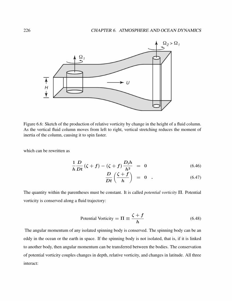
226 CHAPTER 6. ATMOSPHERE AND OCEAN DYNAMICS
Figure 6.6: Sketch of the production of relative vorticity by change in the height of a fluid column.As the vertical fluid column moves from left to right, vertical stretching reduces the moment ofinertia of the column, causing it to spin faster.
which can be rewritten as
1
h
D
Dt(ζ + f)− (ζ + f)
Dth
h2= 0 (6.46)
D
Dt
(ζ + f
h
)= 0 . (6.47)
The quantity within the parentheses must be constant. It is called potential vorticity Π. Potential
vorticity is conserved along a fluid trajectory:
Potential Vorticity = Π ≡ζ + f
h(6.48)
The angular momentum of any isolated spinning body is conserved. The spinning body can be an
eddy in the ocean or the earth in space. If the spinning body is not isolated, that is, if it is linked
to another body, then angular momentum can be transferred between the bodies. The conservation
of potential vorticity couples changes in depth, relative vorticity, and changes in latitude. All three
interact:
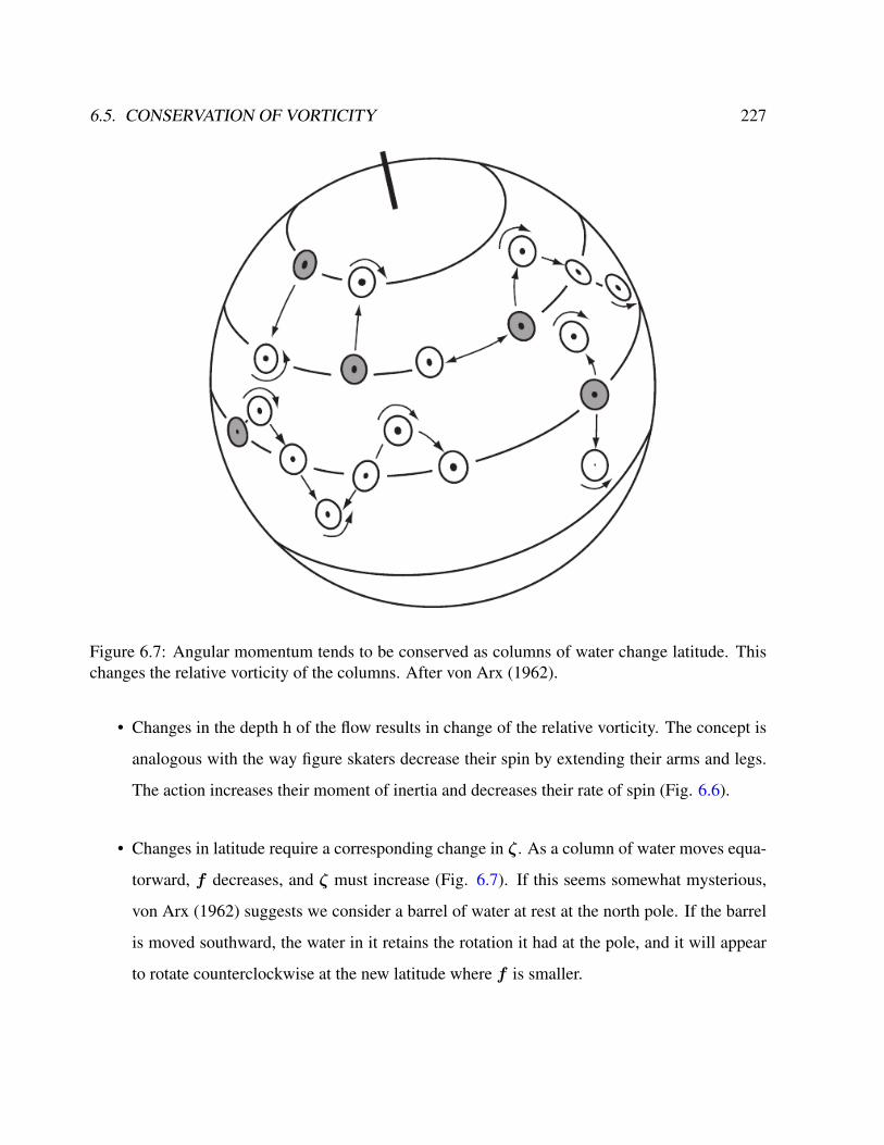
6.5. CONSERVATION OF VORTICITY 227
Figure 6.7: Angular momentum tends to be conserved as columns of water change latitude. Thischanges the relative vorticity of the columns. After von Arx (1962).
• Changes in the depth h of the flow results in change of the relative vorticity. The concept is
analogous with the way figure skaters decrease their spin by extending their arms and legs.
The action increases their moment of inertia and decreases their rate of spin (Fig. 6.6).
• Changes in latitude require a corresponding change in ζ. As a column of water moves equa-
torward, f decreases, and ζ must increase (Fig. 6.7). If this seems somewhat mysterious,
von Arx (1962) suggests we consider a barrel of water at rest at the north pole. If the barrel
is moved southward, the water in it retains the rotation it had at the pole, and it will appear
to rotate counterclockwise at the new latitude where f is smaller.
228 CHAPTER 6. ATMOSPHERE AND OCEAN DYNAMICS
Potential vorticity conservation (ζ + f)/h: Implications
The concept of conservation of potential vorticity has far reaching consequences, and its applica-
tion to fluid flow in the ocean gives a deeper understanding of ocean currents.
Flow Tends to be Zonal
In the ocean f tends to be much larger than ζ and thus f/h = constant. This requires that the flow
in an ocean of constant depth be zonal. Of course, depth is not constant, but in general, currents
tend to be east-west rather than north-south. Wind makes small changes in ζ, leading to a small
meridional component of the flow (see Fig. 6.7).
Topographic Steering
Barotropic flows are diverted by sea floor features. Consider what happens when a flow that extends
from the surface to the bottom encounters a sub-sea ridge (Fig. 6.8). As the depth decreases, ζ+f
must also decrease, which requires that f decrease, and the flow is turned toward the equator. This
is called topographic steering. If the change in depth is sufficiently large, no change in latitude will
be sufficient to conserve potential vorticity, and the flow will be unable to cross the ridge. This is
called topographic blocking.
Streamfunction f/h
In the ocean, f tends to be much larger than ζ and
D
Dt
(f
h
)= 0 (6.49)

6.5. CONSERVATION OF VORTICITY 229
Figure 6.8: Barotropic flow over a sub-sea ridge is turned equatorward to conserve potential vor-ticity. After Dietrich et al. (1980: 333).
implies f/h = constant along the flow. In this case, we have a streamfunction Ψ and pressure p
that are functions of f/h:
Ψ = Ψ(f/h) ; p = p(f/h). (6.50)
This requires that the flow in an ocean of constant depth be zonal. Of course, depth is not constant,
but in general, currents tend to be east-west rather than north-south. Wind makes small changes
in ζ, leading to a small meridional component of the flow (see figure 6.7). The geostrophic con-
tours f/h turn out to be an interesting combination of latitude circles and bottom topographic
contours. Over small horizontal distances6 and at high latitude topography, h tends to dominate (as
in the example in Fig.6.10), but over longer distances or in the tropics, the latitude-variation of f
dominates.
6Then DDt
(fh
)= 0 can be transformed into D
Dth = 0.
230 CHAPTER 6. ATMOSPHERE AND OCEAN DYNAMICS
Exercise 40 – Differential operators
Deriving the vorticity equation
D
Dt
(ζ + f
h
)= 0 ,
we need to evaluate the terms ∂y DDtu and ∂x DDtv. Write down the explicit terms!
Exercise 41 – Potential vorticity in the atmosphere
An air column at 53N with ζ = 0 initially streches from the surface to a fixed tropopause at
10 km height. If the air column moves until it is over a mountain barrier 2.5 km hight at 30N,
what is its absolute vorticity and relative vorticity as it passes the mountain top?
Assume: sin 53 = 0.8; sin 30 = 0.5. The angular velocity of the Earth Ω = 2π/(1day).
Exercise 42 – f/h contours
Geostrophic contours using available topography data. Barotropic flows are diverted by sea
floor features. Consider what happens when a flow that extends from the surface to the bottom
encounters a sub-sea ridge.
1. Show the f/h contours for the North Atlantic Ocean! See Fig. 6.9.
2. Show it for low latitudes regions: region around 20S to 20N in the Atlantic and Pacific
Ocean. One problem is that the geostrophic contours bump into continents, so that ocean
currents running along them have a serious difficulty there. Actually all such f/h contours
head toward the Equator as they run up into shallow water (as h→ 0 f → 0 also, hence
ϕ → 0). This shows that we need more terms in the vorticity dynamics to describe the
ocean circulation.
3. The examination of tidal rhythmites and theories about the Earth-Moon dynamics suggest
that the length of day 900 million years ago was 18 h instead of 24h. How are the results of
the vorticity dynamics are affected?
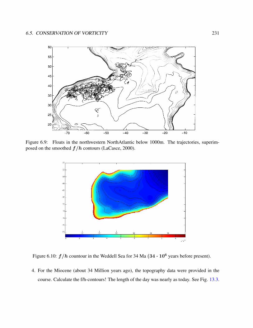
6.5. CONSERVATION OF VORTICITY 231
Figure 6.9: Floats in the northwestern NorthAtlantic below 1000m. The trajectories, superim-posed on the smoothed f/h contours (LaCasce, 2000).
Figure 6.10: f/h countour in the Weddell Sea for 34 Ma (34 · 106 years before present).
4. For the Miocene (about 34 Million years ago), the topography data were provided in the
course. Calculate the f/h-contours! The length of the day was nearly as today. See Fig. 13.3.
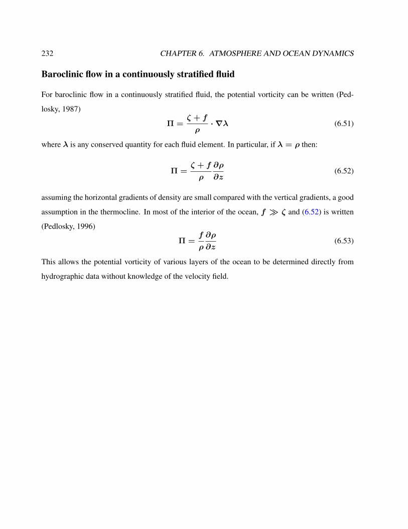
232 CHAPTER 6. ATMOSPHERE AND OCEAN DYNAMICS
Baroclinic flow in a continuously stratified fluid
For baroclinic flow in a continuously stratified fluid, the potential vorticity can be written (Ped-
losky, 1987)
Π =ζ + f
ρ· ∇λ (6.51)
where λ is any conserved quantity for each fluid element. In particular, if λ = ρ then:
Π =ζ + f
ρ
∂ρ
∂z(6.52)
assuming the horizontal gradients of density are small compared with the vertical gradients, a good
assumption in the thermocline. In most of the interior of the ocean, f ζ and (6.52) is written
(Pedlosky, 1996)
Π =f
ρ
∂ρ
∂z(6.53)
This allows the potential vorticity of various layers of the ocean to be determined directly from
hydrographic data without knowledge of the velocity field.
6.5. CONSERVATION OF VORTICITY 233
6.5.2 Taylor-Proudman Theorem
The influence of vorticity due to Earth’s rotation is most striking for geostrophic flow of a fluid
with constant density ρ0 on a plane with constant rotation f = f0 . The components of the
geostrophic and hydrostatic pressure equations are:
−f v = −1
ρ0
∂p
∂x(6.54)
f u = −1
ρ0
∂p
∂y(6.55)
g = −1
ρ0
∂p
∂z(6.56)
and the continuity equation is:
0 =∂u
∂x+∂v
∂y+∂w
∂z(6.57)
Taking the z derivative of (6.54) and using (6.56) gives:
−f0
∂v
∂z= −
1
ρ0
∂
∂z
(∂p
∂x
)=
∂
∂x
(−
1
ρ0
∂p
∂z
)=∂g
∂x= 0 (6.58)
Therefore for f0 6= 0∂v
∂z= 0
Similarly, for the u-component of velocity (6.55). Thus, the vertical derivative of the horizontal
velocity field must be zero.∂u
∂z=∂v
∂z= 0 (6.59)
The flow is two-dimensional and does not vary in the vertical direction. This is the Taylor-
Proudman Theorem, which applies to slowly varying flows in a homogeneous, rotating, inviscid
fluid. The theorem places strong constraints on the flow7. The physical origin of this strangely
7Taylor (1921): If therefore any small motion be communicated to a rotating fluid the resulting motion of the fluidmust be one in which any two particles originally in a line parallel to the axis of rotation must remain so, except for

234 CHAPTER 6. ATMOSPHERE AND OCEAN DYNAMICS
constrained flow is in the stiffness endowed to the fluid by rapid rotation of the Earth, which has a
peculiarly strong sense along the axis of rotation. Taylor’s laboratory experiments showed how ho-
mogeneous fluid tends to move in vertical columns. Dye in the water forms curtains, and viewing
the dye from above shows fine twists and whirls that are vertically coherent.
Hence, rotation greatly stiffens the flow! Geostrophic flow cannot go over a seamount, it
must go around it. Taylor [1917] explicitly derived (6.59) and (6.61) below. Proudman [1916]
independently derived the same theorem but not as explicitly.
Laboratory experiments showing the formation of a Taylor column, go to 2:50, other material:
vorticity and circulation, boundary layers, good introduction, Taylor column
Vertical velocity in the the Taylor-Proudman theorem
Further consequences of the theorem can be obtained by eliminating the pressure terms from (6.54,
6.55) to obtain:
∂u
∂x+∂v
∂y= −
∂
∂x
(1
f0ρ0
∂p
∂y
)+
∂
∂y
(1
f0ρ0
∂p
∂x
)=
1
f0ρ0
(−∂2p
∂x∂y+
∂2p
∂x∂y
)= 0 (6.60)
Because the fluid is incompressible, the continuity equation (6.57) requires
∂w
∂z= 0 (6.61)
Furthermore, because w = 0 at the sea surface and at the sea floor, if the bottom is level, there
can be no vertical velocity on an f -plane.
possible small oscillations about that position.

6.5. CONSERVATION OF VORTICITY 235
Geostrophic flow: Vertical velocity leads to north-south currents
If the Taylor-Proudman theorem in (6.61) is true, the flow cannot expand or contract in the vertical
direction, and it is indeed as rigid as a steel bar. Since we observe gradients of vertical movements,
one of the constraints used in deriving (6.61) must be violated, i.e. our assumption that f = f0
can not be a good approximation.
Going back to (6.40):
D
Dt(ζ + f) + (ζ + f)
(∂u
∂x+∂v
∂y
)= 0 . (6.62)
we obtain
β v + f
(∂u
∂x+∂v
∂y
)= 0 . (6.63)
Using the continuity equation, we obtain
f∂wg
∂z= β v (6.64)
where we have used the subscript g to emphasize that (6.64) applies to the ocean’s interior,
geostrophic flow. Thus the variation of Coriolis force with latitude allows vertical velocity gradi-
ents in the geostrophic interior of the ocean, and the vertical velocity leads to north-south currents.
236 CHAPTER 6. ATMOSPHERE AND OCEAN DYNAMICS
6.6 Wind-driven ocean circulation
What drives the ocean currents? At first, we might answer, the winds drive the circulation. But if
we think more carefully about the question, we might not be so sure. We might notice, for example,
that strong currents, such as the North Equatorial Countercurrents in the Atlantic and Pacific Ocean
go upwind. Spanish navigators in the 16th century noticed strong northward currents along the
Florida coast that seemed to be unrelated to the wind. How can this happen? And, why are strong
currents found offshore of east coasts but not offshore of west coasts?8
Friction is essential for the transfer of momentum in a fluid. Friction transfers momentum from
the atmosphere to the ocean through the thin, frictional, Ekman layer at the sea surface. Friction
transfers momentum from the ocean to the solid earth through the Ekman layer at the sea floor.
Friction along the sides of subsea mountains leads to pressure differences on either side of the
mountain which causes another kind of drag called form drag. This is the same drag that causes
wind force on cars moving at high speed. In the vast interior of the ocean, however, the flow is
frictionless, and vorticity is conserved. Such a flow is said to be conservative. Here, we apply the
vorticity dynamics for the ocean and include the wind stress term in (6.16, 6.17):
Dtu− fv = −1
ρ
∂p
∂x+
1
ρ∂zτxz (6.65)
Dtv + fu = −1
ρ
∂p
∂y+
1
ρ∂zτyz (6.66)
in order to get the modified vorticity balance (6.45):
D
Dt(ζ + f)−
(ζ + f)
h
D
Dth =
1
ρcurlz ∂zτ =
1
ρ
(∂
∂x∂zτyz −
∂
∂y∂zτxz
).(6.67)
8Answers to the questions can be found in a series of three remarkable papers published from 1947 to 1951. In thefirst, Harald Sverdrup (1947) showed that the circulation in the upper kilometer or so of the ocean is directly related tothe curl of the wind stress. Henry Stommel (1948) showed that the circulation in oceanic gyres is asymmetric becausethe Coriolis force varies with latitude. Finally, Walter Munk (1950) added eddy viscosity and calculated the circulationof the upper layers of the Pacific. Together the three oceanographers laid the foundations for a modern theory of oceancirculation.

6.6. WIND-DRIVEN OCEAN CIRCULATION 237
Quantity Oceanhorizontal velocity U 1.6 · 10−2ms−1
horizontal length L 106mvertical length D 103m
wind stress τ0 1.5 · 10−1 PaCoriolis parameter at 45N f0 = 2Ω sinϕ0 10−4 s−1
density ρ0 103 kgm−3
viscosity (turbulent) AH 102 − 104m2s−1
Reynolds number Re 1.6− 160wind stress strength number α 1 · 103
Table 6.2: Table shows the typical scales in the ocean system for exercise 43.
The formulation ’wind stress curl’ stands for the z-component of
∇×
τx
τy
0
= curl
τx
τy
0
.
Exercise 43 – Non-dimensional vorticity dynamics including wind stress
a) Derive the the non-dimensional version of the vorticity equation (6.67) assuming that h is not
varying and include friction! We can vertically integrate (6.67) over depth∫ 0
−D dz :
D
Dt(ζ + f) = AH∇2ζ +
1
ρD
(∂
∂xτy −
∂
∂yτx
). (6.68)
Include the Reynolds number Re = UL/AH , Rossby number Ro = U/(f0L), and the wind
stress strength number α = τ0L/(ρ0DU2). Compare to exercises 30, 39.
b) Estimate the order of magnitude of the characteristic numbers for the ocean ! You can use Table
6.6.
238 CHAPTER 6. ATMOSPHERE AND OCEAN DYNAMICS
Solution of Non-dimensional vorticity dynamics including wind stress
Starting from (6.68),
1
T
D
Dtd
(1
Tζd + f0fd
)= AH
1
L2T∇2dζd +
τ0
ρ0DL
(∂
∂xdτy,d −
∂
∂ydτx,d
)(6.69)
D
Dtd
(1
Tζd + f0fd
)= AH
1
L2∇2dζd +
τ0T
ρ0DL
(∂
∂xdτy,d −
∂
∂ydτx,d
).(6.70)
Multiplying with T and using T = L/U , we obtain
D
Dtd
(ζd +
f0L
Ufd
)=
AH
UL∇2dζd +
τ0L
ρ0DU2
(∂
∂xdτy,d −
∂
∂ydτx,d
)(6.71)
and finally
D
Dtd
(ζd +
1
Rofd
)=
1
Re∇2dζd + α
(∂
∂xdτy,d −
∂
∂ydτx,d
)(6.72)
6.6.1 Sverdrup relation
Suppose for simplicity that h is constant, so the only ’topography’ is that of the spherical shape
of the ocean. This produces a simple version of the vorticity balance in the ocean circulation, the
Sverdrup relation. For most regions, the right hand side in (6.67) or the left hand side in (6.72) is
dominated by the term v∂yf = vβ.
vβ =1
ρ
(∂
∂x∂zτyz −
∂
∂y∂zτxz
). (6.73)
Integrating over z, we receive
β
∫ 0
h
dz v = βV =1
ρcurlz τ (z = 0) =
1
ρ
(∂τyz
∂x−∂τxz
∂y
). (6.74)
6.6. WIND-DRIVEN OCEAN CIRCULATION 239
Mass transport and Stream Lines of Sverdrup’s Theory*
While Sverdrup was analyzing observations of equatorial currents, he derived the relation by the
the wind stress to mass transport within the upper ocean. It is assumed that the flow is stationary,
that lateral friction and molecular viscosity are small, that non-linear terms such as u∂u/∂x are
small. With these assumptions, the horizontal components of the momentum equation are:
∂p
∂x= f ρ v +
∂τxz
∂z(6.75)
∂p
∂y= −f ρ u+
∂τyz
∂z(6.76)
Sverdrup integrated these equations from the surface to a depth −D equal to or greater than the
depth at which the horizontal pressure gradient becomes zero. We can define
∂P
∂x=
∫ 0
−D
∂p
∂xdz,
∂P
∂y=
∫ 0
−D
∂p
∂ydz, (6.77)
Mx, My are the mass transports in the wind-driven layer extending down to an assumed depth of
no motion:
Mx ≡∫ 0
−Dρ u (z) dz, My ≡
∫ 0
−Dρ v (z) dz . (6.78)
The horizontal boundary condition at the sea surface is the wind stress, and the boundary at depth
−D is zero stress because the currents go to zero:
τxz (0) = τx τxz (−D) = 0 (6.79)
τyz (0) = τy τyz (−D) = 0 . (6.80)
Using these definitions and boundary conditions, (6.75, 6.76) becomes:
∂P
∂x= f My + τx (6.81)
∂P
∂y= −f Mx + τy . (6.82)
240 CHAPTER 6. ATMOSPHERE AND OCEAN DYNAMICS
In a similar way, Sverdrup integrated the continuity equation over the same vertical depth, assum-
ing the vertical velocity at the surface and at depth−D are zero, to obtain:
∂Mx
∂x+∂My
∂y= 0 (6.83)
Differentiating (6.81) with respect to y and (6.82) with respect to x, subtracting, and using (6.83)
gives:β My =
∂τy
∂x−∂τx
∂y= curlz (τ ) (6.84)
where β ≡∂f
∂y=
2Ω cosϕ
R(6.85)
with R as earth’s radius and ϕ as latitude. Over much of the open ocean, the wind is zonal and
∂τy/∂x is sufficiently small thatMy ≈ −
1
β
∂τx
∂y(6.86)
Substituting (6.86) into (6.83), and (6.85) we obtain
∂Mx
∂x= −
1
2 Ω cosϕ
(∂τx
∂ytanϕ+
∂2τx
∂y2R
)(6.87)
Sverdrup integrated this equation from a north-south eastern boundary at x = 0, assuming no flow
into the boundary. This requiresMx = 0 at x = 0. Then
Mx = −1
2 Ω cosϕ
([∫ x
0
∂τx
∂ydx′]
tanϕ+
[∫ x
0
∂2τx
∂y2dx′]R
)(6.88)
= −1
2 Ω cosϕ
(tanϕ
∂
∂y
[∫ x
0
τxdx′]
+R∂2
∂y2
[∫ x
0
τxdx′])
. (6.89)
If τx can be approximated by its zonal mean, then
Mx = −∆x
2 Ω cosϕ
[tanϕ
∂ 〈τx〉∂y
+R∂2 〈τx〉∂y2
](6.90)
where ∆x is the distance from the eastern boundary of the ocean basin, and brackets indicate zonal
averages of the wind stress.
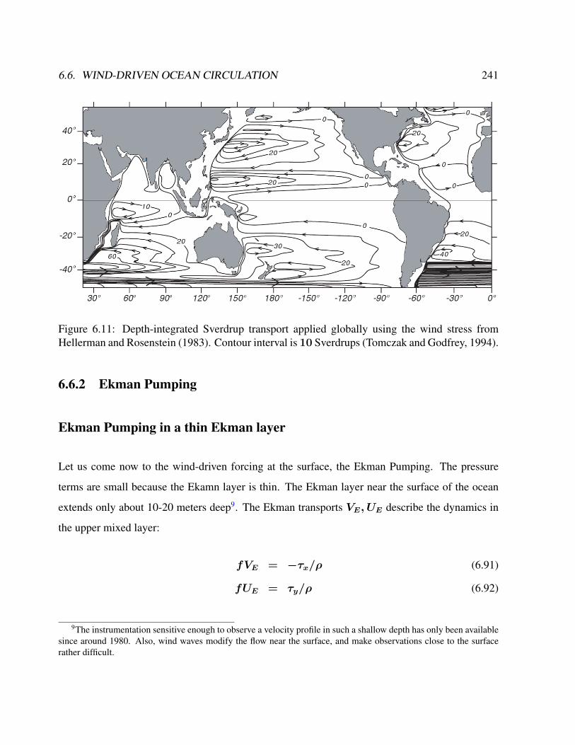
6.6. WIND-DRIVEN OCEAN CIRCULATION 241
Figure 6.11: Depth-integrated Sverdrup transport applied globally using the wind stress fromHellerman and Rosenstein (1983). Contour interval is 10 Sverdrups (Tomczak and Godfrey, 1994).
6.6.2 Ekman Pumping
Ekman Pumping in a thin Ekman layer
Let us come now to the wind-driven forcing at the surface, the Ekman Pumping. The pressure
terms are small because the Ekamn layer is thin. The Ekman layer near the surface of the ocean
extends only about 10-20 meters deep9. The Ekman transports VE, UE describe the dynamics in
the upper mixed layer:
fVE = −τx/ρ (6.91)
fUE = τy/ρ (6.92)
9The instrumentation sensitive enough to observe a velocity profile in such a shallow depth has only been availablesince around 1980. Also, wind waves modify the flow near the surface, and make observations close to the surfacerather difficult.
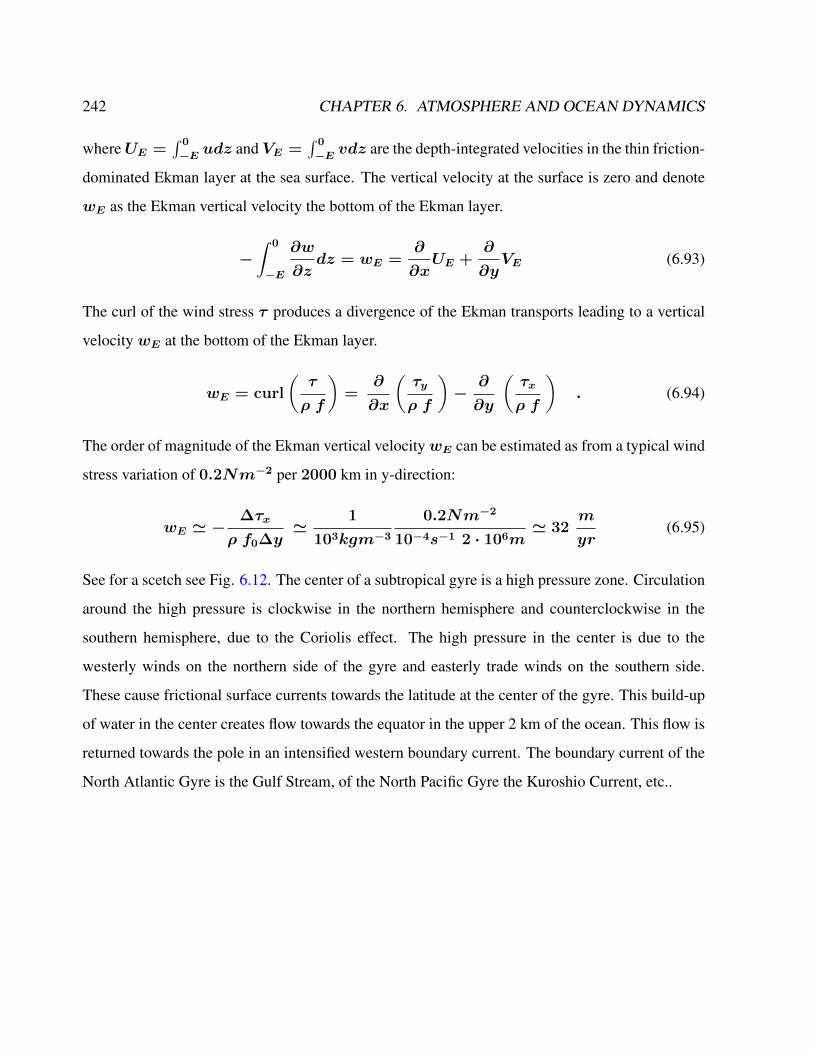
242 CHAPTER 6. ATMOSPHERE AND OCEAN DYNAMICS
whereUE =∫ 0
−E udz andVE =∫ 0
−E vdz are the depth-integrated velocities in the thin friction-
dominated Ekman layer at the sea surface. The vertical velocity at the surface is zero and denote
wE as the Ekman vertical velocity the bottom of the Ekman layer.
−∫ 0
−E
∂w
∂zdz = wE =
∂
∂xUE +
∂
∂yVE (6.93)
The curl of the wind stress τ produces a divergence of the Ekman transports leading to a vertical
velocity wE at the bottom of the Ekman layer.
wE = curl
(τ
ρ f
)=
∂
∂x
(τy
ρ f
)−
∂
∂y
(τx
ρ f
). (6.94)
The order of magnitude of the Ekman vertical velocitywE can be estimated as from a typical wind
stress variation of 0.2Nm−2 per 2000 km in y-direction:
wE ' −∆τx
ρ f0∆y'
1
103kgm−3
0.2Nm−2
10−4s−1 2 · 106m' 32
m
yr(6.95)
See for a scetch see Fig. 6.12. The center of a subtropical gyre is a high pressure zone. Circulation
around the high pressure is clockwise in the northern hemisphere and counterclockwise in the
southern hemisphere, due to the Coriolis effect. The high pressure in the center is due to the
westerly winds on the northern side of the gyre and easterly trade winds on the southern side.
These cause frictional surface currents towards the latitude at the center of the gyre. This build-up
of water in the center creates flow towards the equator in the upper 2 km of the ocean. This flow is
returned towards the pole in an intensified western boundary current. The boundary current of the
North Atlantic Gyre is the Gulf Stream, of the North Pacific Gyre the Kuroshio Current, etc..

6.6. WIND-DRIVEN OCEAN CIRCULATION 243
Figure 6.12: Ekman pumping that produces a downward velocity at the base of the Ekman layerforces the fluid in the interior of the ocean to move southward. Winds at the sea surface driveEkman transports to the right of the wind in this northern hemisphere example. The convergingEkman transports driven by the trades and westerlies drive a downward geostrophic flow just belowthe Ekman layer.
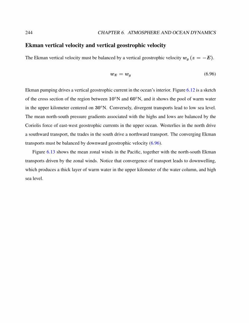
244 CHAPTER 6. ATMOSPHERE AND OCEAN DYNAMICS
Ekman vertical velocity and vertical geostrophic velocity
The Ekman vertical velocity must be balanced by a vertical geostrophic velocity wg (z = −E).
wE = wg (6.96)
Ekman pumping drives a vertical geostrophic current in the ocean’s interior. Figure 6.12 is a sketch
of the cross section of the region between 10N and 60N, and it shows the pool of warm water
in the upper kilometer centered on 30N. Conversely, divergent transports lead to low sea level.
The mean north-south pressure gradients associated with the highs and lows are balanced by the
Coriolis force of east-west geostrophic currents in the upper ocean. Westerlies in the north drive
a southward transport, the trades in the south drive a northward transport. The converging Ekman
transports must be balanced by downward geostrophic velocity (6.96).
Figure 6.13 shows the mean zonal winds in the Pacific, together with the north-south Ekman
transports driven by the zonal winds. Notice that convergence of transport leads to downwelling,
which produces a thick layer of warm water in the upper kilometer of the water column, and high
sea level.
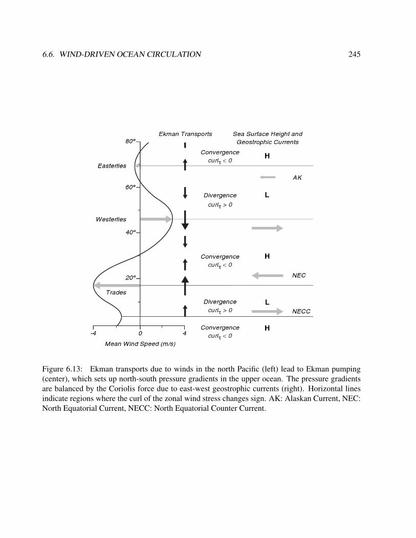
6.6. WIND-DRIVEN OCEAN CIRCULATION 245
Figure 6.13: Ekman transports due to winds in the north Pacific (left) lead to Ekman pumping(center), which sets up north-south pressure gradients in the upper ocean. The pressure gradientsare balanced by the Coriolis force due to east-west geostrophic currents (right). Horizontal linesindicate regions where the curl of the zonal wind stress changes sign. AK: Alaskan Current, NEC:North Equatorial Current, NECC: North Equatorial Counter Current.

246 CHAPTER 6. ATMOSPHERE AND OCEAN DYNAMICS
Exercise 44 – Ekman transports and pumping
The Ekman transports VE, UE describe the dynamics in the upper mixed layer:
fVE = −τx/ρ0 (6.97)
fUE = τy/ρ0 (6.98)
Derive the Ekman pumping wE velocity at the bottom of the mixed layer
wE = curl(τ
fρ0
)=
∂
∂x
(τy
ρ0f
)−
∂
∂y
(τx
ρ0f
). (6.99)
Exercise 45 – Sverdrup relation, Ekman transports and pumping
The windstress vector τ is taken zonal. Assume τx = −τ0 cosπy/B for an ocean basin
0 < x < L, 0 < y < B. The wind driven meridional ocean velocity is given by the Sverdrup
relation
βV = curl(τ/ρ0) = −∂
∂yτx/ρ0 . (6.100)
1. at what latitudes y are |V | and |VE| maximum? Calculate their magnitudes. Take con-
stant f = 10−4 s−1 and β = 1.8 · 10−11 m−1s−1 and B = 5000 km, τ0/ρ0 =
10−4 m2s−2.
2. Calculate the maximum of wE for constant f (value see above). Is this measurable?
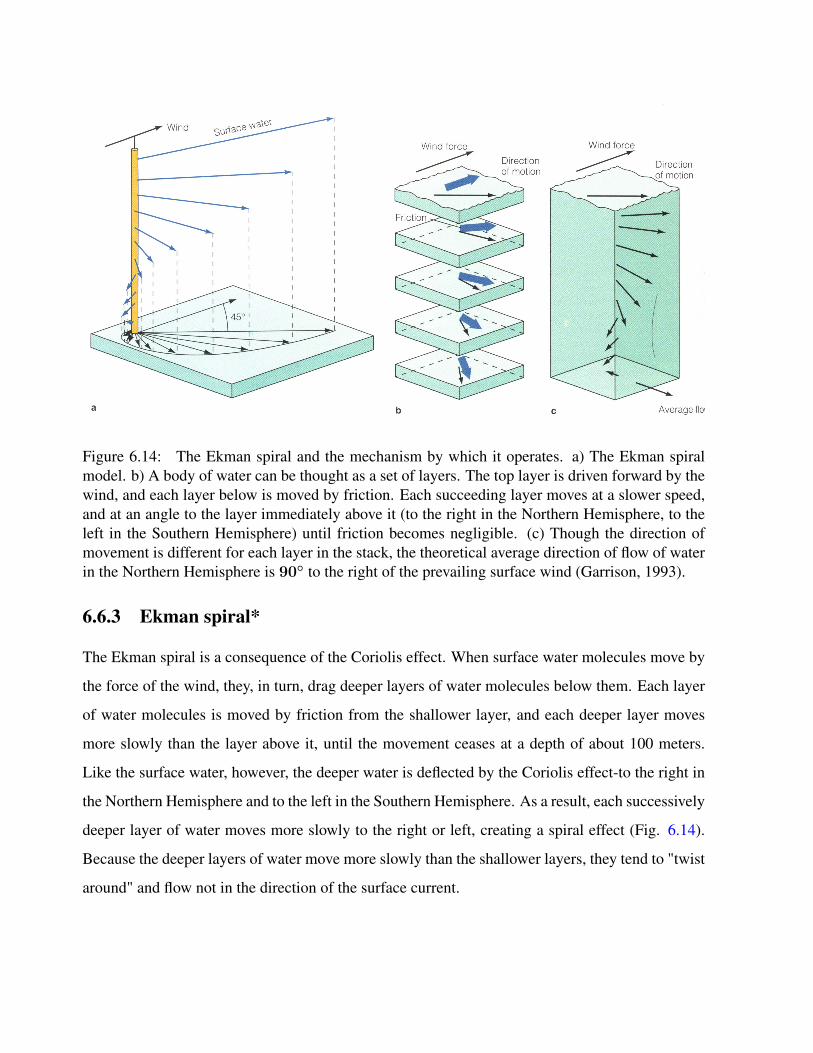
6.6. WIND-DRIVEN OCEAN CIRCULATION 247
Figure 6.14: The Ekman spiral and the mechanism by which it operates. a) The Ekman spiralmodel. b) A body of water can be thought as a set of layers. The top layer is driven forward by thewind, and each layer below is moved by friction. Each succeeding layer moves at a slower speed,and at an angle to the layer immediately above it (to the right in the Northern Hemisphere, to theleft in the Southern Hemisphere) until friction becomes negligible. (c) Though the direction ofmovement is different for each layer in the stack, the theoretical average direction of flow of waterin the Northern Hemisphere is 90 to the right of the prevailing surface wind (Garrison, 1993).
6.6.3 Ekman spiral*
The Ekman spiral is a consequence of the Coriolis effect. When surface water molecules move by
the force of the wind, they, in turn, drag deeper layers of water molecules below them. Each layer
of water molecules is moved by friction from the shallower layer, and each deeper layer moves
more slowly than the layer above it, until the movement ceases at a depth of about 100 meters.
Like the surface water, however, the deeper water is deflected by the Coriolis effect-to the right in
the Northern Hemisphere and to the left in the Southern Hemisphere. As a result, each successively
deeper layer of water moves more slowly to the right or left, creating a spiral effect (Fig. 6.14).
Because the deeper layers of water move more slowly than the shallower layers, they tend to "twist
around" and flow not in the direction of the surface current.
248 CHAPTER 6. ATMOSPHERE AND OCEAN DYNAMICS
Ekman developed the theory of the Ekman layer after Fridtjof Nansen observed that ice drifts
at an angle of 20− 40 to the right of the prevailing wind direction while on an Arctic expedition
aboard the Fram. Nansen asked his colleague, Vilhelm Bjerknes to set one of his students upon
study of the problem. Bjerknes tapped Ekman, who presented his results in 1902 as his doctoral
thesis.
The mathematical formulation of the Ekman layer can be found by assuming a neutrally strat-
ified fluid, with horizontal momentum in balance between the forces of pressure gradient, Coriolis
and turbulent drag.
−fv = −1
ρo
∂
∂xp + ν
∂2u
∂z2, (6.101)
fu = −1
ρo
∂
∂yp + ν
∂2v
∂z2, (6.102)
where ν is the diffusive eddy viscosity, which can be derived using mixing length theory. There
are many regions where an Ekman layer is theoretically plausible; they include the bottom of the
atmosphere, near the surface of the earth and ocean, the bottom of the ocean, near the sea floor and
at the top of the ocean, near the air-water interface. Different boundary conditions are appropriate
for each of these different situations. We will consider boundary conditions of the Ekman layer in
the upper ocean:
at z = 0 : ν∂u
∂z= τx and ν
∂v
∂z= τ y, (6.103)
where τx and τ y are the components of the surface stress, τ, of the wind field or ice layer at the
top of the ocean and ug and vg are the geostrophic flows as z → ∞ : u → ug, v → vg. In
the other situations, other boundary conditions, such as the no-slip condition, may be appropriate
instead.
6.6. WIND-DRIVEN OCEAN CIRCULATION 249
The dynamics (6.101, 6.102) can be reformulated as
−fv = −fvg + ν∂2u
∂z2, (6.104)
fu = fug + ν∂2v
∂z2, (6.105)
Now multiply (6.104) with i and subtract it from (6.105):
ifv − ifvg + iν∂2u
∂z2+ fu− fug − ν
∂2v
∂z2= 0 (6.106)
Denoting ξ = u+ iv, we get
fξ − fξg + iν∂2ξ
∂z2= 0 (6.107)
We rewite this as
∂2ξ
∂z2−(if
ν
)ξ = −
(if
ν
)ξg (6.108)
We solve the inhomogenous equation (6.108) in two steps:
1. find a particular solution of the inhomogenous equation:
assume that ξ is independent on z
−(if
ν
)ξ = −
(if
ν
)ξg (6.109)
with the solution ξ = ξg
2. find a complementary function, a general solution of the homogenous part of (6.108):
∂2ξh
∂z2−(if
ν
)ξh = 0 (6.110)
ξh = C exp(λz) with λ2 =if
ν(6.111)
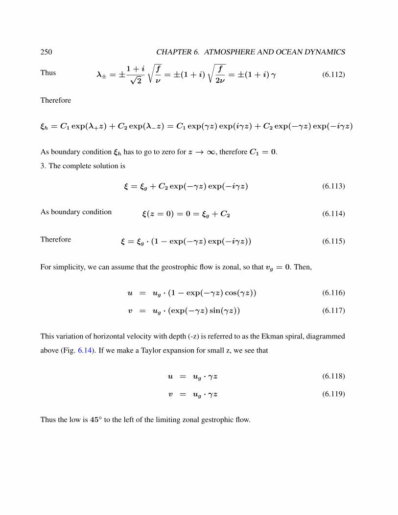
250 CHAPTER 6. ATMOSPHERE AND OCEAN DYNAMICS
Thus λ± = ±1 + i√
2
√f
ν= ±(1 + i)
√f
2ν= ±(1 + i) γ (6.112)
Therefore
ξh = C1 exp(λ+z) + C2 exp(λ−z) = C1 exp(γz) exp(iγz) + C2 exp(−γz) exp(−iγz)
As boundary condition ξh has to go to zero for z →∞, therefore C1 = 0.
3. The complete solution is
ξ = ξg + C2 exp(−γz) exp(−iγz) (6.113)
As boundary condition ξ(z = 0) = 0 = ξg + C2 (6.114)
Therefore ξ = ξg · (1− exp(−γz) exp(−iγz)) (6.115)
For simplicity, we can assume that the geostrophic flow is zonal, so that vg = 0. Then,
u = ug · (1− exp(−γz) cos(γz)) (6.116)
v = ug · (exp(−γz) sin(γz)) (6.117)
This variation of horizontal velocity with depth (-z) is referred to as the Ekman spiral, diagrammed
above (Fig. 6.14). If we make a Taylor expansion for small z, we see that
u = ug · γz (6.118)
v = ug · γz (6.119)
Thus the low is 45 to the left of the limiting zonal gestrophic flow.
6.6. WIND-DRIVEN OCEAN CIRCULATION 251
By applying the continuity equation we can have the vertical velocity as following
w =1
fρo
[(∂τ y
∂x−∂τx
∂y
) (1− e−γz cos (γz)
)−(∂τx
∂x+∂τ y
∂y
)e−γz sin (γz)
]
Note that when vertically integrated the volume transport associated with the Ekman spiral is to
the right of the wind direction in the Northern Hemisphere.
There is much difficulty associated with observing the Ekman layer for two main reasons: the
theory is too simplistic as it assumes a constant eddy viscosity, which Ekman himself anticipated,
recognizing that is obvious that ν cannot generally be regarded as a constant when the density of
water is not uniform within the region considered and because it is difficult to design instruments
with great enough sensitivity to observe the velocity profile in the ocean.
Because the real ocean does not match the idealized conditions of the Ekman spiral, wind-
induced water movements often differ appreciably from theoretical predictions. In shallow water,
for example, the water depth is insufficient for the full spiral to develop so that the angle between
the horizontal wind direction and surface-water movements can be as little as 15 degrees. As waters
deepen, the angle increases and approaches 45 degrees. The stable pycnocline inhibits the transfer
of kinetic energy to deeper waters, helping to contain wind-driven currents to the mixed layer; that
is, the pycnocline acts as a permeable boundary for Ekman transport and surface currents.
252 CHAPTER 6. ATMOSPHERE AND OCEAN DYNAMICS
Exercise 46 – Ekman layer in the atmosphere
Consider a geostrophic flow (ug, vg)
−fvg = −1
ρ0
∂p
∂x(6.120)
fug = −1
ρ0
∂p
∂y. (6.121)
The boundary-layer equations are then
−f(v − vg) = ν∂2u
∂z2(6.122)
f(u− ug) = ν∂2v
∂z2. (6.123)
The boundary conditions are specified to be at the surface
ρ0ν∂u
∂z= τx (6.124)
ρ0ν∂v
∂z= τ y (6.125)
and for z → −∞ : u = ug, v = vg .
1. Calculate the flow (u,v) as the departure from the interior flow (ug, vg)!
2. Calculate the net wind-driven horizontal transport through integration
V =
∫ 0
−∞dz(v − vg) and U =
∫ 0
−∞dz(u− ug) . (6.126)
What is the direction of U and V in terms of the surface wind stress τ ?
3. For the case f = f0 of constant Coriolis parameter, determine the divergence of the flow
∫ 0
−∞dz
(∂u
∂x+∂v
∂y
)(6.127)
which is identical to the vertical velocity across the Ekman layer (since w(0)=0).
6.6. WIND-DRIVEN OCEAN CIRCULATION 253
Exercise 47 – Ekamn spiral in the ocean
Consider the solution (6.116,6.117) for the wind-driven Ekman layer at the surface of the
ocean in the Northern Hemisphere. The geostrophic velocity is zero in this example. Show that
(6.116,6.117) is a solution of (6.101, 6.102) !
Tea leaf paradox*
The tea leaf paradox describes a phenomenon where tea leaves in a cup of tea migrate to the center
and bottom of the cup after being stirred rather than being forced to the edges of the cup, as would
be expected in a spiral centrifuge.10 Stirring the liquid makes it spin around the cup. Because
of inertia, the pressure is higher along the rim than in the middle. However, near the bottom and
outer edges the liquid is slowed by the friction against the cup. There the outward force cannot
overcome the pressure gradient, so these pressure differences become more important for the water
flow. This is called a boundary layer or more specifically an Ekman layer.
In a teacup, where the rotation is slower at the bottom, the pressure gradient takes over and cre-
ates an inward flow along the bottom. Higher up, the liquid flows outward instead. This secondary
flow travels inward along the bottom bringing the leaves to the center, then up, out and down near
the rim. The leaves are too heavy to lift upwards, so they stay in the middle. Combined with the
primary rotational flow, the leaves will spiral inward along the bottom.
Besides tea leaves stirred in a cup, other classroom demonstrations can show the secondary
circulation that arises due to the presence of friction. We discuss a simple laboratory experiment
below, which demonstrates these ideas in a more controlled setting and can be readily applied to
both atmospheric low and high pressure systems. All one needs is a rotating turntable, a cylindrical
container (a large transparent beaker or a cylindrical insert inside a square container works fine),
and some potassium permanganate crystals. When rotated at a constant rate, all the water comes
10The formation of secondary flows in an annular channel was theoretically treated by Boussinesq in 1868.Themigration of near-bottom particles in river-bend flows was experimentally investigated by A.Ya.Milovich in 1913.The solution first came from Albert Einstein in a 1926 paper where he used it to explain the erosion of river banks(Baer’s law) [?].
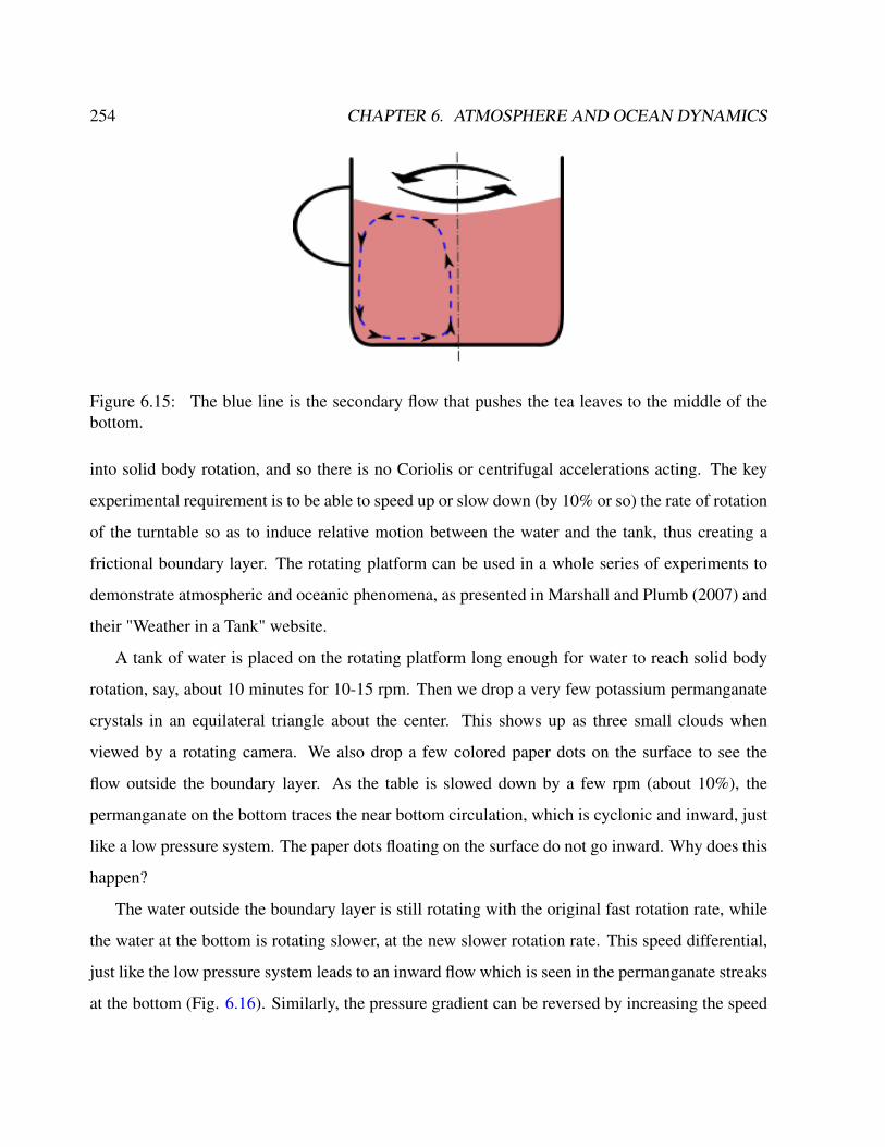
254 CHAPTER 6. ATMOSPHERE AND OCEAN DYNAMICS
Figure 6.15: The blue line is the secondary flow that pushes the tea leaves to the middle of thebottom.
into solid body rotation, and so there is no Coriolis or centrifugal accelerations acting. The key
experimental requirement is to be able to speed up or slow down (by 10% or so) the rate of rotation
of the turntable so as to induce relative motion between the water and the tank, thus creating a
frictional boundary layer. The rotating platform can be used in a whole series of experiments to
demonstrate atmospheric and oceanic phenomena, as presented in Marshall and Plumb (2007) and
their "Weather in a Tank" website.
A tank of water is placed on the rotating platform long enough for water to reach solid body
rotation, say, about 10 minutes for 10-15 rpm. Then we drop a very few potassium permanganate
crystals in an equilateral triangle about the center. This shows up as three small clouds when
viewed by a rotating camera. We also drop a few colored paper dots on the surface to see the
flow outside the boundary layer. As the table is slowed down by a few rpm (about 10%), the
permanganate on the bottom traces the near bottom circulation, which is cyclonic and inward, just
like a low pressure system. The paper dots floating on the surface do not go inward. Why does this
happen?
The water outside the boundary layer is still rotating with the original fast rotation rate, while
the water at the bottom is rotating slower, at the new slower rotation rate. This speed differential,
just like the low pressure system leads to an inward flow which is seen in the permanganate streaks
at the bottom (Fig. 6.16). Similarly, the pressure gradient can be reversed by increasing the speed
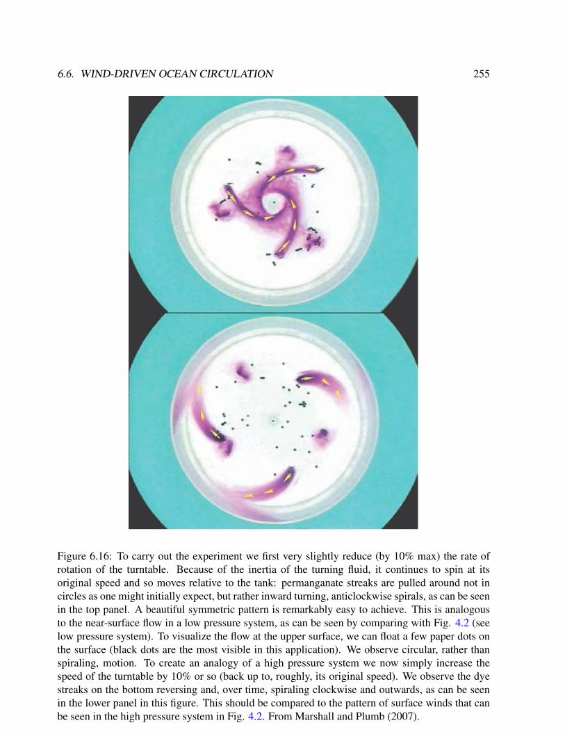
6.6. WIND-DRIVEN OCEAN CIRCULATION 255
Figure 6.16: To carry out the experiment we first very slightly reduce (by 10% max) the rate ofrotation of the turntable. Because of the inertia of the turning fluid, it continues to spin at itsoriginal speed and so moves relative to the tank: permanganate streaks are pulled around not incircles as one might initially expect, but rather inward turning, anticlockwise spirals, as can be seenin the top panel. A beautiful symmetric pattern is remarkably easy to achieve. This is analogousto the near-surface flow in a low pressure system, as can be seen by comparing with Fig. 4.2 (seelow pressure system). To visualize the flow at the upper surface, we can float a few paper dots onthe surface (black dots are the most visible in this application). We observe circular, rather thanspiraling, motion. To create an analogy of a high pressure system we now simply increase thespeed of the turntable by 10% or so (back up to, roughly, its original speed). We observe the dyestreaks on the bottom reversing and, over time, spiraling clockwise and outwards, as can be seenin the lower panel in this figure. This should be compared to the pattern of surface winds that canbe seen in the high pressure system in Fig. 4.2. From Marshall and Plumb (2007).
256 CHAPTER 6. ATMOSPHERE AND OCEAN DYNAMICS
by a few rpm to the original speed, and it leads to permanganate streaks that show an outward anti-
cyclonic flow, analogous to the surface boundary layer of a High pressure system. This secondary
flow in the boundary layer has important implications for movement in the vertical direction. The
inward flow associated with a low pressure system leads to rising air near the center of the Low.
As this air rises, it expands (pressure always decreases going upward in the atmosphere) and cools.
Since the saturation of the air is very strongly dependent on the temperature, as the air cools, it
may get saturated, and the water vapor may condense out to form clouds! This is why the Low
pressure systems are the ones associated with stormy weather and precipitation. Conversely, high
pressure systems are associated with outward motion in the boundary layer, and hence subsidence.
As the air descends, it gets compressed due to the pressure increase, warms, and becomes less and
less saturated. Thus the High pressure systems are fair weather systems.
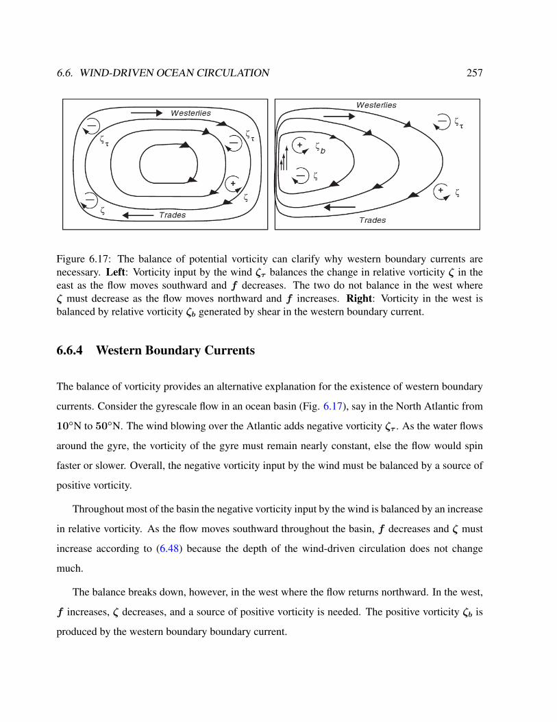
6.6. WIND-DRIVEN OCEAN CIRCULATION 257
Figure 6.17: The balance of potential vorticity can clarify why western boundary currents arenecessary. Left: Vorticity input by the wind ζτ balances the change in relative vorticity ζ in theeast as the flow moves southward and f decreases. The two do not balance in the west whereζ must decrease as the flow moves northward and f increases. Right: Vorticity in the west isbalanced by relative vorticity ζb generated by shear in the western boundary current.
6.6.4 Western Boundary Currents
The balance of vorticity provides an alternative explanation for the existence of western boundary
currents. Consider the gyrescale flow in an ocean basin (Fig. 6.17), say in the North Atlantic from
10N to 50N. The wind blowing over the Atlantic adds negative vorticity ζτ . As the water flows
around the gyre, the vorticity of the gyre must remain nearly constant, else the flow would spin
faster or slower. Overall, the negative vorticity input by the wind must be balanced by a source of
positive vorticity.
Throughout most of the basin the negative vorticity input by the wind is balanced by an increase
in relative vorticity. As the flow moves southward throughout the basin, f decreases and ζ must
increase according to (6.48) because the depth of the wind-driven circulation does not change
much.
The balance breaks down, however, in the west where the flow returns northward. In the west,
f increases, ζ decreases, and a source of positive vorticity is needed. The positive vorticity ζb is
produced by the western boundary boundary current.
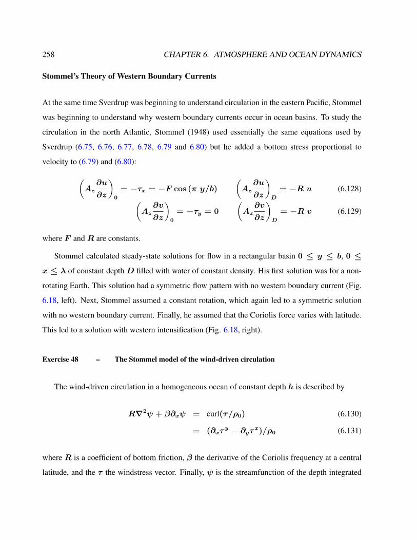
258 CHAPTER 6. ATMOSPHERE AND OCEAN DYNAMICS
Stommel’s Theory of Western Boundary Currents
At the same time Sverdrup was beginning to understand circulation in the eastern Pacific, Stommel
was beginning to understand why western boundary currents occur in ocean basins. To study the
circulation in the north Atlantic, Stommel (1948) used essentially the same equations used by
Sverdrup (6.75, 6.76, 6.77, 6.78, 6.79 and 6.80) but he added a bottom stress proportional to
velocity to (6.79) and (6.80):
(Az
∂u
∂z
)0
= −τx = −F cos (π y/b)
(Az
∂u
∂z
)D
= −R u (6.128)(Az
∂v
∂z
)0
= −τy = 0
(Az
∂v
∂z
)D
= −R v (6.129)
where F andR are constants.
Stommel calculated steady-state solutions for flow in a rectangular basin 0 ≤ y ≤ b, 0 ≤
x ≤ λ of constant depth D filled with water of constant density. His first solution was for a non-
rotating Earth. This solution had a symmetric flow pattern with no western boundary current (Fig.
6.18, left). Next, Stommel assumed a constant rotation, which again led to a symmetric solution
with no western boundary current. Finally, he assumed that the Coriolis force varies with latitude.
This led to a solution with western intensification (Fig. 6.18, right).
Exercise 48 – The Stommel model of the wind-driven circulation
The wind-driven circulation in a homogeneous ocean of constant depth h is described by
R∇2ψ + β∂xψ = curl(τ/ρ0) (6.130)
= (∂xτy − ∂yτx)/ρ0 (6.131)
where R is a coefficient of bottom friction, β the derivative of the Coriolis frequency at a central
latitude, and the τ the windstress vector. Finally, ψ is the streamfunction of the depth integrated
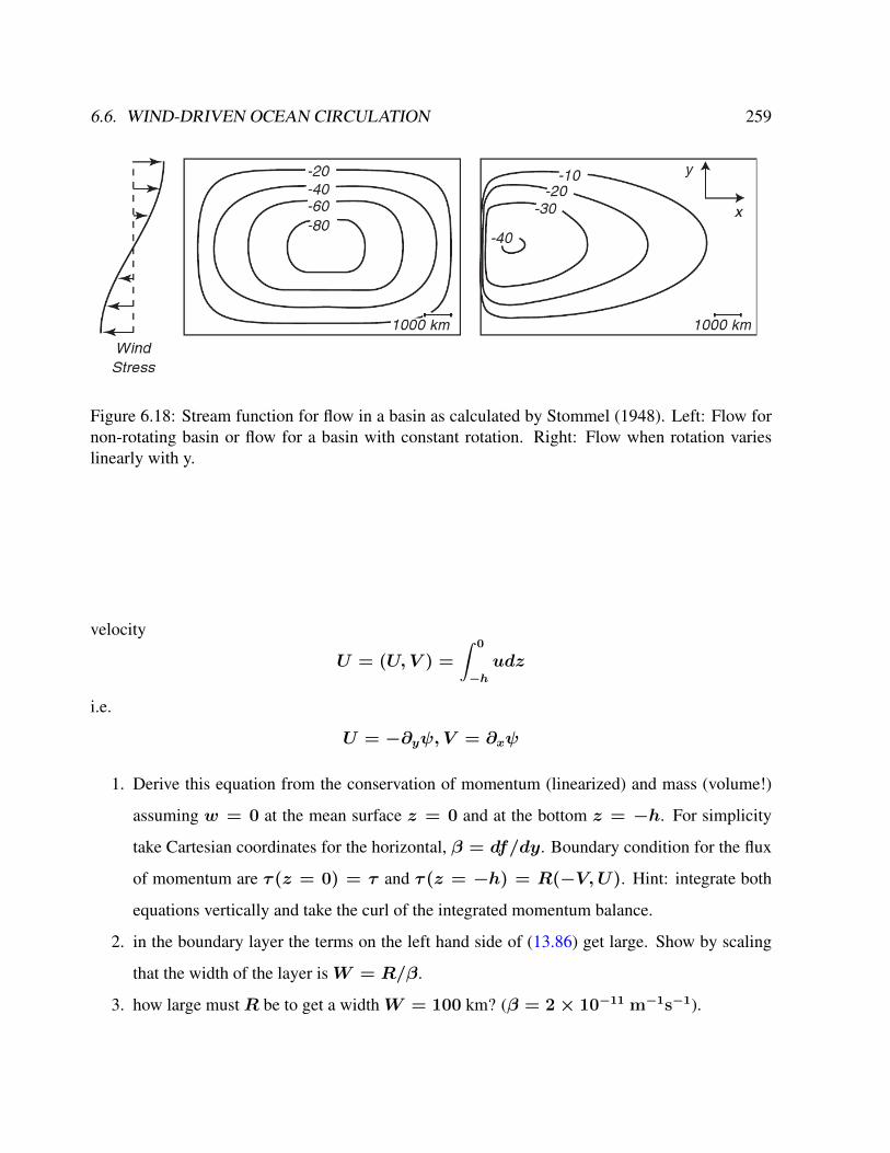
6.6. WIND-DRIVEN OCEAN CIRCULATION 259
Figure 6.18: Stream function for flow in a basin as calculated by Stommel (1948). Left: Flow fornon-rotating basin or flow for a basin with constant rotation. Right: Flow when rotation varieslinearly with y.
velocity
U = (U, V ) =
∫ 0
−hudz
i.e.
U = −∂yψ, V = ∂xψ
1. Derive this equation from the conservation of momentum (linearized) and mass (volume!)
assuming w = 0 at the mean surface z = 0 and at the bottom z = −h. For simplicity
take Cartesian coordinates for the horizontal, β = df/dy. Boundary condition for the flux
of momentum are τ (z = 0) = τ and τ (z = −h) = R(−V,U). Hint: integrate both
equations vertically and take the curl of the integrated momentum balance.
2. in the boundary layer the terms on the left hand side of (13.86) get large. Show by scaling
that the width of the layer isW = R/β.
3. how large mustR be to get a widthW = 100 km? (β = 2× 10⁻¹¹ m−1s−1).
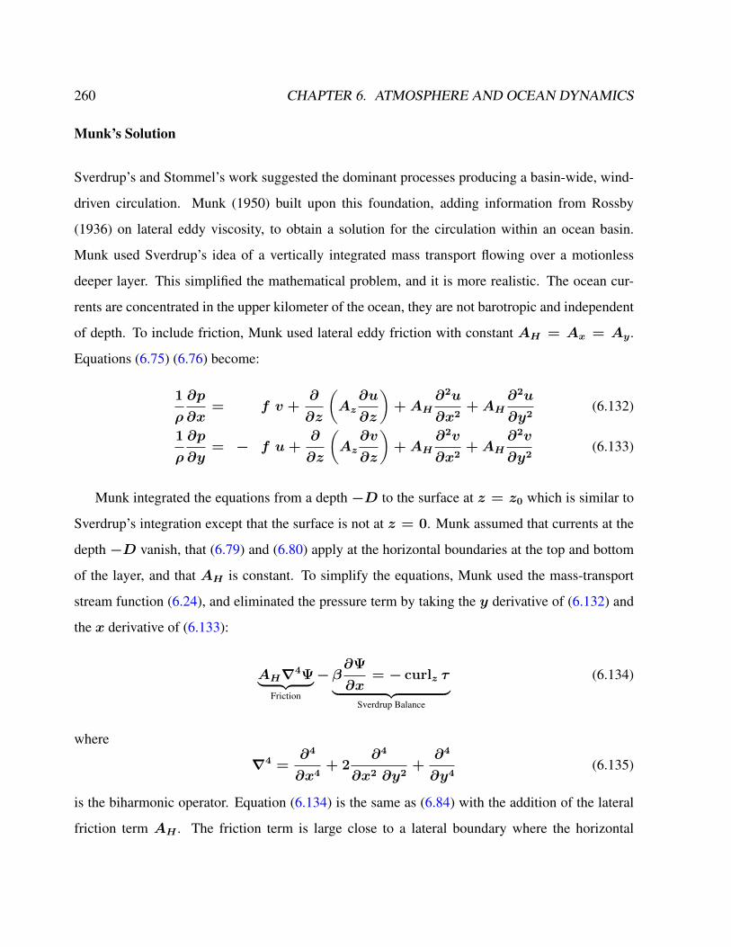
260 CHAPTER 6. ATMOSPHERE AND OCEAN DYNAMICS
Munk’s Solution
Sverdrup’s and Stommel’s work suggested the dominant processes producing a basin-wide, wind-
driven circulation. Munk (1950) built upon this foundation, adding information from Rossby
(1936) on lateral eddy viscosity, to obtain a solution for the circulation within an ocean basin.
Munk used Sverdrup’s idea of a vertically integrated mass transport flowing over a motionless
deeper layer. This simplified the mathematical problem, and it is more realistic. The ocean cur-
rents are concentrated in the upper kilometer of the ocean, they are not barotropic and independent
of depth. To include friction, Munk used lateral eddy friction with constant AH = Ax = Ay.
Equations (6.75) (6.76) become:
1
ρ
∂p
∂x= f v +
∂
∂z
(Az
∂u
∂z
)+AH
∂2u
∂x2+AH
∂2u
∂y2(6.132)
1
ρ
∂p
∂y= − f u+
∂
∂z
(Az
∂v
∂z
)+AH
∂2v
∂x2+AH
∂2v
∂y2(6.133)
Munk integrated the equations from a depth −D to the surface at z = z0 which is similar to
Sverdrup’s integration except that the surface is not at z = 0. Munk assumed that currents at the
depth −D vanish, that (6.79) and (6.80) apply at the horizontal boundaries at the top and bottom
of the layer, and that AH is constant. To simplify the equations, Munk used the mass-transport
stream function (6.24), and eliminated the pressure term by taking the y derivative of (6.132) and
the x derivative of (6.133):
AH∇4Ψ︸ ︷︷ ︸Friction
−β∂Ψ
∂x= − curlz τ︸ ︷︷ ︸
Sverdrup Balance
(6.134)
where
∇4 =∂4
∂x4+ 2
∂4
∂x2 ∂y2+
∂4
∂y4(6.135)
is the biharmonic operator. Equation (6.134) is the same as (6.84) with the addition of the lateral
friction term AH . The friction term is large close to a lateral boundary where the horizontal
6.6. WIND-DRIVEN OCEAN CIRCULATION 261
derivatives of the velocity field are large, and it is small in the interior of the ocean basin. Thus in
the interior, the balance of forces is the same as that in Sverdrup’s solution.
Equation (6.134) is a fourth-order partial differential equation, and four boundary conditions
are needed. Munk assumed the flow at a boundary is parallel to a boundary and that there is no slip
at the boundary:
Ψboundary = 0,
(∂Ψ
∂n
)boundary
= 0 (6.136)
where n is normal to the boundary. Munk then solved (6.134) with (6.136) assuming the flow was
in a rectangular basin extending from x = 0 to x = r, and from y = −s to y = +s. He further
assumed that the wind stress was zonal and in the form:
τ = a cosny + b sinny + c (6.137)
n = j π/s, j = 1, 2, ... (6.138)
Munk’s solution (figure 6.19) shows the dominant features of the gyre-scale circulation in an
ocean basin. It has a circulation similar to Sverdrup’s in the eastern parts of the ocean basin
and a strong western boundary current in the west. Using AH = 5 · 103m2
sgives a boundary
current roughly 225km wide with a shape similar to the flow observed in the Gulf Stream and the
Kuroshio.
The transport in western boundary currents is independent ofAH , and it depends only on (6.84)
integrated across the width of the ocean basin. Hence, it depends on the width of the ocean, the curl
of the wind stress, and β. Using the best available estimates of the wind stress, Munk calculated
that the Gulf Stream should have a transport of 36Sv and that the Kuroshio should have a transport
of 39Sv. The values are about one half of the measured values of the flow available to Munk. This
is very good agreement considering the wind stress was not well known.11
11Recent recalculations show good agreement except for the region offshore of Cape Hatteras where there is a strongrecirculation. Munk’s solution was based on wind stress averaged over 5 squares. This underestimated the curl ofthe stress. Leetmaa and Bunker (1978) used modern drag coefficient and 2 × 5 averages of stress to obtain 32Svtransport in the Gulf Stream, a value very close to that calculated by Munk.
262 CHAPTER 6. ATMOSPHERE AND OCEAN DYNAMICS
Figure 6.19: Left: Mean annual wind stress τx (y) over the Pacific and the curl of the wind stress.φb are the northern and southern boundaries of the gyres, where My = 0 and curl τ = 0.φ0 is the center of the gyre. Upper Right: The mass transport stream function for a rectangularbasin calculated by Munk (1950) using observed wind stress for the Pacific. Contour intervalis 10 Sverdrups. The total transport between the coast and any point x, y is ψ (x, y). Thetransport in the relatively narrow northern section is greatly exaggerated. Lower Right: North-South component of the mass transport. After Munk (1950).
6.6. WIND-DRIVEN OCEAN CIRCULATION 263
Summarizing important concepts of vorticity
• Vorticity strongly constrains ocean dynamics
• Vorticity due to earth’s rotation is much greater than other sources of vorticity
• Taylor and Proudman showed that vertical velocity is impossible in a uniformly rotating
flow. Hence Ekman pumping requires that planetary vorticity varies with latitude.
• The curl of the wind stress adds relative vorticity to central gyres of each ocean basin. For
steady state circulation in the gyre, the ocean must lose vorticity in western boundary cur-
rents.
• Positive wind stress curl leads to divergent flow in the Ekman layer. The ocean’s interior
geostrophic circulation adjusts through a northward mass transport.
Exercise 49 – Cyclostrophic wind
When the flow is sufficiently near the equator so that f is small or when the Corolis force is
negligible compared to the centripedal acceleration, the gradient wind equation becomes
vk × v
R= −
1
ρ∇zp (6.139)
where k is the unit vector in z direction, v is the velocity vector, v ist the meridional velocity, R
Earth radius,∇z horizontal nabla operator.
1. Derive this equation!
2. What is the associated gradient wind equation including the Coriolis force?
3. What is the Rossby number?

264 CHAPTER 6. ATMOSPHERE AND OCEAN DYNAMICS
6.7 Thermohaline ocean circulation
Water, that is dense enough to sink from the surface to the bottom, is formed when cold air blows
across the ocean at high latitudes in winter in the northern North Atlantic (e.g. in the Labrador Sea
and between Norway and Greenland) and near Antarctica. The wind cools and evaporates water.
If the wind is cold enough, sea ice forms, further increasing the salinity of the water because sea
ice is fresher than sea water and salty water remains in the water when ice is formed. Bottom water
is produced only in these regions, and the deep ocean is affected by these deep water formation
processes. In other regions, cold, dense water is formed, but it is not quite salty enough to sink
to the bottom. At mid and low latitudes, the density, even in winter, is sufficiently low that the
water cannot sink more than a few hundred meters into the ocean. The only exception are some
seas, such as the Mediterranean Sea, where evaporation is so great that the salinity of the water
is sufficiently great for the water to sink to intermediate depths in the seas. If these seas are
can exchange water with the open ocean, the waters formed in winter in the seas spreads out to
intermediate depths in the ocean. Detailed measurements of the Atlantic current structure were
made by an expedition of the research vessel Meteor from 1925-1927. On the basis of these data,
Wüst [1935] characterized water masses necessary to describe the Atlantic currents and tracer
distribution (Fig. 6.23). Broecker proposed a circulation model based on findings of the Meteor
and other expeditions. In his model, large-scale oceanic circulation is represented by the transport
system of a conveyor belt (Fig. 6.21) [Broecker and Peng, 1982].
The oceans carry about one third to one half the heat out of the tropics needed to maintain
earth’s temperature. Heat carried by the Gulf Stream and the North Atlantic drift warms the North
Atlantic, keeping it ice free in winter, and it helps warm Europe. Norway, at 60N is far warmer
than southern Greenland or northern Labrador at the same latitude. Palm trees grow on the west
coast of Ireland, but not in Newfoundland which is further south. The oceanic component of the
heat-transport system is also called the Global Conveyor Belt. The basic idea is that the Gulf
Stream carries heat to the North Atlantic realm. There the surface water releases heat and water to
the atmosphere. Some of the ocean water becomes sufficiently cold, salty, and dense that it sinks

6.7. THERMOHALINE OCEAN CIRCULATION 265
Figure 6.20: The surface (red, orange, yellow) and deep (violet, blue, green) currents in the NorthAtlantic. The North Atlantic Current brings warm water northward where it cools. Some sinksand returns southward as a cold, deep, western-boundary current. Some returns southward at thesurface. From Woods Hole Oceanographic Institution.
to the bottom in the Norwegian and Greenland Seas. It then flows southward in very cold, bottom
currents along western boundaries as a western boundary current. Some of the water remains at
the surface and returns to the south in cool surface currents such as the Labrador Current and the
Portugal Current (see Fig. 6.20).
The deep bottom water from the North Atlantic is mixed upward in other regions and ocean,
and eventually it makes its way back to the Gulf Stream and the North Atlantic. Thus most of
the water that sinks in the North Atlantic must be replaced by water from the far South Atlantic.
As this surface water moves northward across the equator and eventually into the Gulf Stream, it
carries heat out of the south Atlantic. So much heat is pulled northward by the formation of north-
Atlantic bottom water in winter that heat transport in the Atlantic is entirely northward, even in the

266 CHAPTER 6. ATMOSPHERE AND OCEAN DYNAMICS
southern hemisphere. Much of the solar heat absorbed by the tropical Atlantic is shipped north to
warm Europe and the Northern Hemisphere. Imagine then what might happen if the supply of heat
is shut off. We will get back to that topic in the next section, applying the box model.
We can make a crude estimate of the importance of the conveyor-belt circulation from a simple
calculation. The Gulf Stream carries 40 Sv of 18C water northward. Of this, 15 Sv return
southward in the deep western boundary current at a temperature of 2C. The flow carried by
the conveyor belt must therefore lose 1 Petawatts (1 Petawatt = 1015 Watt = 1 PW) in the North
Atlantic north of 24N. Although the calculation is very crude, it is remarkably close to the value
of 1.2± 0.2 PW estimated by Rintoul and Wunsch (1991). Calculation: Exercise 55.
The production of bottom water is influenced by the salinity of surface waters in the North
Atlantic. It is also influenced by the rate of upwelling due to mixing in other oceanic areas. First,
let’s look at the influence of salinity. Saltier surface waters form denser water in winter than less
salty water. At first you may think that temperature is also important, but at high latitudes water
in all ocean basins gets cold enough to freeze, so all ocean produce -2C water at the surface. Of
this, only the most salty will sink, and the saltiest water is in the Atlantic and under the ice on the
continental shelves around Antarctica.
The the conveyor is driven by deepwater formation in the northern North Atlantic, making it the
engine of conveyor belt circulation. The conveyor belt metaphor necessarily simplifies the ocean
system, it is of course not a full description of the deep ocean circulation, it contains different
aspects of it [Brüning and Lohmann, 1999]. Broecker’s [Broecker, 1987; Broecker et al., 1991]
concept provides a successful approach for global ocean circulation, although several features can
be wrong like the missing Antarctic bottom water, the upwelling areas etc.. However, the global
conveyor belt metaphor inspired new ideas of halting or reversing the ocean circulation and put it
into a global climate context [Bryan, 1986]. This was helpful for the interpretation of Greenland ice
core records (Fig. 9.9) indicating different climate states with different ocean modes of operation
(like on and off states of a mechanical maschine). From the analogy, it was possible to a) identify
the relevance of North Atlantic deep water production and b) realize the possibility of multiple
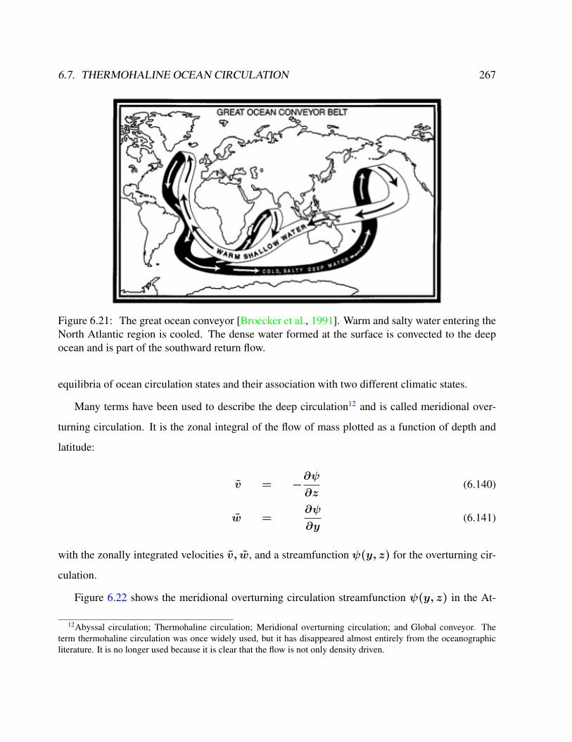
6.7. THERMOHALINE OCEAN CIRCULATION 267
Figure 6.21: The great ocean conveyor [Broecker et al., 1991]. Warm and salty water entering theNorth Atlantic region is cooled. The dense water formed at the surface is convected to the deepocean and is part of the southward return flow.
equilibria of ocean circulation states and their association with two different climatic states.
Many terms have been used to describe the deep circulation12 and is called meridional over-
turning circulation. It is the zonal integral of the flow of mass plotted as a function of depth and
latitude:
v = −∂ψ
∂z(6.140)
w =∂ψ
∂y(6.141)
with the zonally integrated velocities v, w, and a streamfunction ψ(y, z) for the overturning cir-
culation.
Figure 6.22 shows the meridional overturning circulation streamfunction ψ(y, z) in the At-
12Abyssal circulation; Thermohaline circulation; Meridional overturning circulation; and Global conveyor. Theterm thermohaline circulation was once widely used, but it has disappeared almost entirely from the oceanographicliterature. It is no longer used because it is clear that the flow is not only density driven.

268 CHAPTER 6. ATMOSPHERE AND OCEAN DYNAMICS
Figure 6.22: Modelled meridional overturning streamfunction in Sv (1 Sv ≡ 106 m3s−1) in theAtlantic Ocean. Grey areas represent zonally integrated smoothed bathymetry.
lantic. The streamfunction is calculated as a cumulative sum of zonally integrated mass transports
of the ocean at each latitude from surface to the particular depth. The zonally intregrated mass
transport at a certain latitude derives from the zonally averaged meridional velocity component
times the height of the ocean layer and the width of the ocean. Water flows along the stream
lines. For instance, increasing positive values of MOC from surface to about 1,000m depth at mid
latitudes of the Northern Hemisphere denote northward flowing water. With increasing depth the
values of the MOC streamfunction decrease until a minimum at about 4,000m depth is reached.
These waters move southward instead. In the Atlantic two major, a shallower and a deeper over-
turning cell exist according to figure 6.22. One cell shows positive values, thus, clockwise volume
transport and stretches from almost the surface to about 2,500 - 3,000m depth. The other expands
from about 3,000m depth to the bottom of the ocean at latitudes south of 40N. The shallower cell
denotes the modelled equivalent of North Atlantic Deep Water (NADW) while Antarctic Bottom
6.7. THERMOHALINE OCEAN CIRCULATION 269
Water (AABW), transporting Southern Ocean water into the Atlantic, is simulated by the deeper
cell. An overturning maximum of 18.7 Sv (1 Sv≡ 106 m3s−1) is found at 40- 50N and 1,000m
depth and an export into the Southern Ocean across 30S of 14.9 Sv. This results in an overturning
ratio of 0.79, so only little recirculation occurs. A closer look at Figure 6.22 reveals that NADW
is predominantly formed north of 60N with about 10 Sv. The inflow of AABW into the Atlantic
is much weaker than the outflow of NADW. At 30S a value of less than 1 Sv is calculated by the
model while the maximum counter-clockwise overturning of the bottom water cell reaches 4.7 Sv
at 25N.
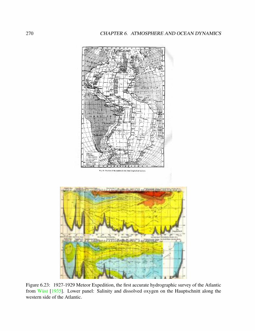
270 CHAPTER 6. ATMOSPHERE AND OCEAN DYNAMICS
Figure 6.23: 1927-1929 Meteor Expedition, the first accurate hydrographic survey of the Atlanticfrom Wüst [1935]. Lower panel: Salinity and dissolved oxygen on the Hauptschnitt along thewestern side of the Atlantic.
6.7. THERMOHALINE OCEAN CIRCULATION 271
Exercise 50 – Ocean thermohaline circulation
Consider a geostrophic flow (u, v)
−fv = −1
ρ0
∂p
∂x(6.142)
fu = −1
ρ0
∂p
∂y. (6.143)
Use the hydrostatic approximation
∂p
∂z= −gρ (6.144)
and equation (13.110) in order to derive the meridional overturning stream function Φ(y, z) as a
fuction of density ρ at the basin boundaries! Φ is defined via
Φ(y, z) =
∫ z
0
∂Φ
∂zdz (6.145)
∂Φ
∂z=
∫ xw
xe
v(x, y, z) dx (zonally integrated transport), (6.146)
where xe and xw are the eastward and westward boundaries in the ocean basin (think e.g. of the
Atlantic Ocean). Units of Φ arem3s−1. At the surface Φ(y, 0) = 0.
Solution of Exercise 50: Ocean thermohaline circulation
∂Φ
∂z=
∫ xw
xe
v(x, y, z) dx (6.147)
=1
ρ0f
∫ xw
xe
∂p
∂xdx =
1
ρ0f(p(xw, y, z)− p(xe, y, z)) (6.148)
= −g
ρ0f
∫ z
0
(ρ(xw, y, z′)− ρ(xe, y, z
′))dz′ (6.149)
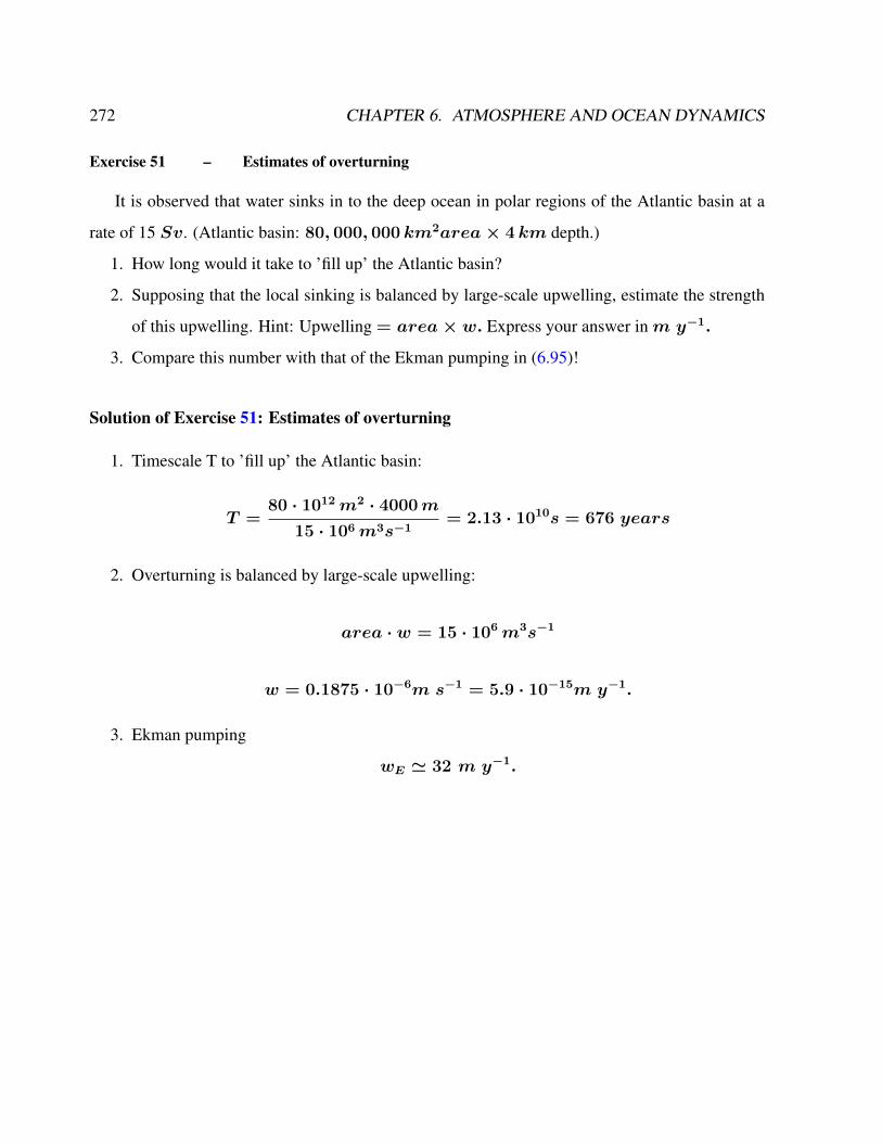
272 CHAPTER 6. ATMOSPHERE AND OCEAN DYNAMICS
Exercise 51 – Estimates of overturning
It is observed that water sinks in to the deep ocean in polar regions of the Atlantic basin at a
rate of 15 Sv. (Atlantic basin: 80, 000, 000 km2area× 4 km depth.)
1. How long would it take to ’fill up’ the Atlantic basin?
2. Supposing that the local sinking is balanced by large-scale upwelling, estimate the strength
of this upwelling. Hint: Upwelling = area× w. Express your answer inm y−1.
3. Compare this number with that of the Ekman pumping in (6.95)!
Solution of Exercise 51: Estimates of overturning
1. Timescale T to ’fill up’ the Atlantic basin:
T =80 · 1012m2 · 4000m
15 · 106m3s−1= 2.13 · 1010s = 676 years
2. Overturning is balanced by large-scale upwelling:
area · w = 15 · 106m3s−1
w = 0.1875 · 10−6m s−1 = 5.9 · 10−15m y−1.
3. Ekman pumping
wE ' 32 m y−1.
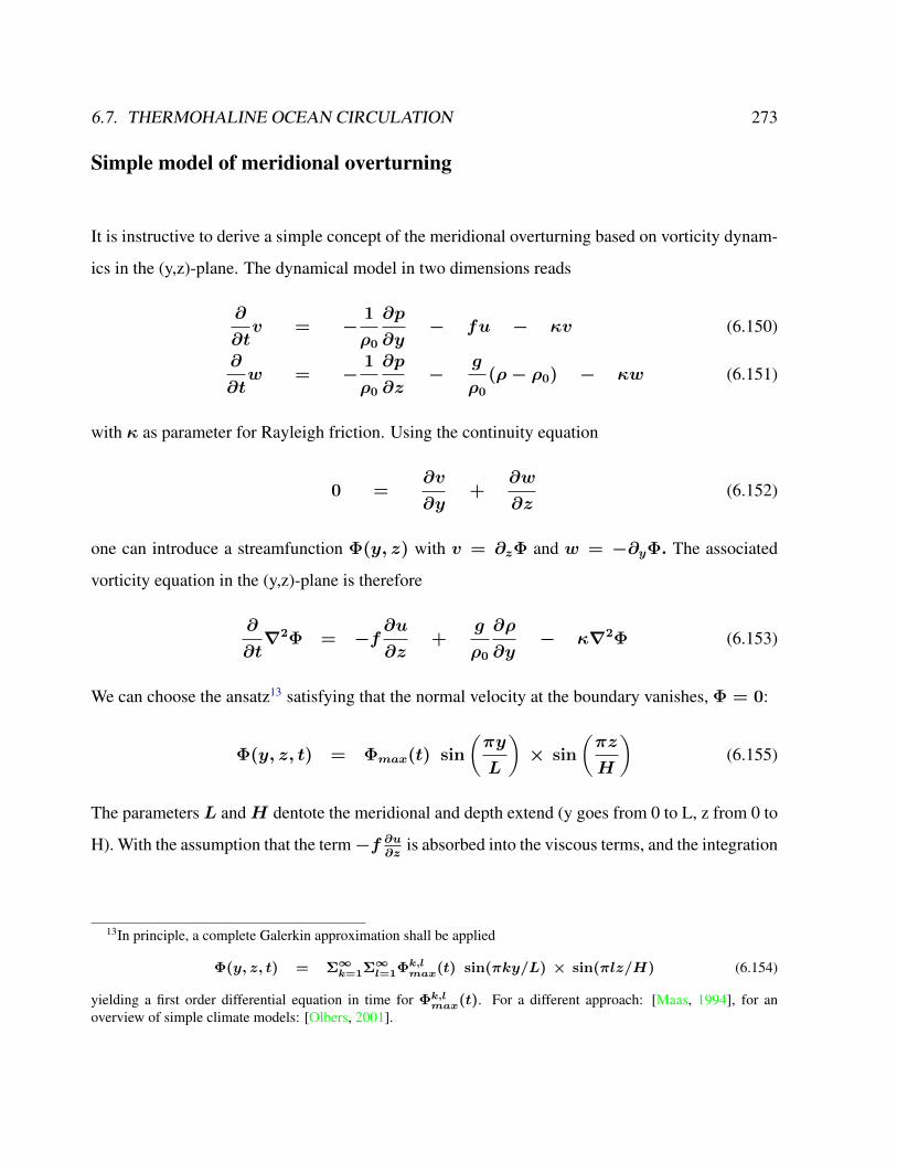
6.7. THERMOHALINE OCEAN CIRCULATION 273
Simple model of meridional overturning
It is instructive to derive a simple concept of the meridional overturning based on vorticity dynam-
ics in the (y,z)-plane. The dynamical model in two dimensions reads
∂
∂tv = −
1
ρ0
∂p
∂y− fu − κv (6.150)
∂
∂tw = −
1
ρ0
∂p
∂z−
g
ρ0
(ρ− ρ0) − κw (6.151)
with κ as parameter for Rayleigh friction. Using the continuity equation
0 =∂v
∂y+
∂w
∂z(6.152)
one can introduce a streamfunction Φ(y, z) with v = ∂zΦ and w = −∂yΦ. The associated
vorticity equation in the (y,z)-plane is therefore
∂
∂t∇2Φ = −f
∂u
∂z+
g
ρ0
∂ρ
∂y− κ∇2Φ (6.153)
We can choose the ansatz13 satisfying that the normal velocity at the boundary vanishes, Φ = 0:
Φ(y, z, t) = Φmax(t) sin
(πy
L
)× sin
(πz
H
)(6.155)
The parameters L andH dentote the meridional and depth extend (y goes from 0 to L, z from 0 to
H). With the assumption that the term−f ∂u∂z
is absorbed into the viscous terms, and the integration
13In principle, a complete Galerkin approximation shall be applied
Φ(y, z, t) = Σ∞k=1Σ∞l=1Φk,lmax(t) sin(πky/L) × sin(πlz/H) (6.154)
yielding a first order differential equation in time for Φk,lmax(t). For a different approach: [Maas, 1994], for anoverview of simple climate models: [Olbers, 2001].
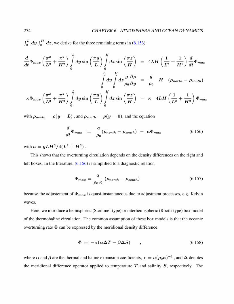
274 CHAPTER 6. ATMOSPHERE AND OCEAN DYNAMICS∫ L0dy∫H
0dz, we derive for the three remaining terms in (6.153):
d
dtΦmax
(π2
L2+π2
H2
) L∫0
dy sin
(πy
L
) H∫0
dz sin
(πz
H
)= 4LH
(1
L2+
1
H2
)d
dtΦmax
L∫0
dy
H∫0
dzg
ρ0
∂ρ
∂y=
g
ρ0
H (ρnorth − ρsouth)
κΦmax
(π2
L2+π2
H2
) L∫0
dy sin
(πy
L
) H∫0
dz sin
(πz
H
)= κ 4LH
(1
L2+
1
H2
)Φmax
with ρnorth = ρ(y = L) , and ρsouth = ρ(y = 0), and the equation
d
dtΦmax =
a
ρ0
(ρnorth − ρsouth) − κΦmax (6.156)
with a = gLH2/4(L2 +H2) .
This shows that the overturning circulation depends on the density differences on the right and
left boxes. In the literature, (6.156) is simplified to a diagnostic relation
Φmax =a
ρ0 κ(ρnorth − ρsouth) (6.157)
because the adjustement of Φmax is quasi-instantaneous due to adjustment processes, e.g. Kelvin
waves.
Here, we introduce a hemispheric (Stommel-type) or interhemispheric (Rooth-type) box model
of the thermohaline circulation. The common assumption of these box models is that the oceanic
overturning rate Φ can be expressed by the meridional density difference:
Φ = −c (α∆T − β∆S) , (6.158)
whereα and β are the thermal and haline expansion coefficients, c = a(ρ0κ)−1 , and ∆ denotes
the meridional difference operator applied to temperature T and salinity S, respectively. The
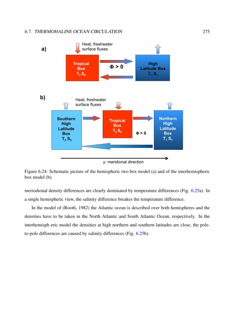
6.7. THERMOHALINE OCEAN CIRCULATION 275
Tropical Box T2 S2
Northern High
Latitude Box T1 S1
Southern High
Latitude Box
T3 S3
Φ > 0
Heat, freshwater surface fluxes
y: meridional direction
b)
Heat, freshwater surface fluxes
Tropical Box T2 S2
High Latitude Box
T1 S1
Φ > 0
a)
Figure 6.24: Schematic picture of the hemispheric two box model (a) and of the interhemisphericbox model (b).
meriodional density differences are clearly dominated by temperature differences (Fig. 6.25a). In
a single hemispheric view, the salinity difference breakes the temperature difference.
In the model of (Rooth, 1982) the Atlantic ocean is described over both hemispheres and the
densities have to be taken in the North Atlantic and South Atlantic Ocean, respectively. In the
interhemisph eric model the densities at high northern and southern latitudes are close, the pole-
to-pole differences are caused by salinity differences (Fig. 6.25b).
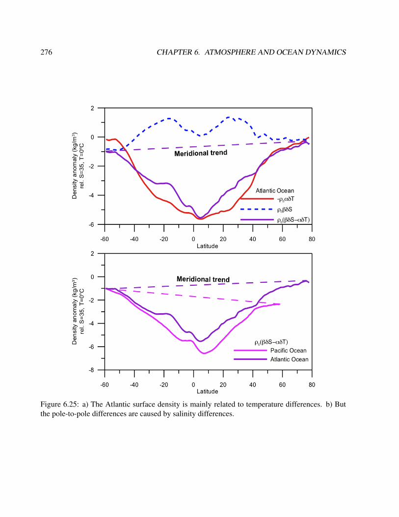
276 CHAPTER 6. ATMOSPHERE AND OCEAN DYNAMICS
Figure 6.25: a) The Atlantic surface density is mainly related to temperature differences. b) Butthe pole-to-pole differences are caused by salinity differences.

Chapter 7
Simple Climate Models
7.1 Engery balance model
7.1.1 Zero-dimensional Model
Energy balance models (EBM) are highly simplified systems of the climate system. A zero-
dimensional model of the radiative equilibrium of the Earth is
(1− α)SπR2 = 4πR2εσT 4 (7.1)
where the left hand side represents the incoming energy from the Sun the right hand side repre-
sents the outgoing energy from the Earth, calculated from the Stefan-Boltzmann law assuming
a constant radiative temperature, T, that is to be found, and S is the solar constant - the incom-
ing solar radiation per unit area– about 1367Wm−2, α is the Earth’s average albedo, mea-
sured to be 0.3. R is Earth’s radius = 6.371 × 10⁶ m, σ is the Stefan-Boltzmann constant =
5.67× 10⁻⁸JK−4m−2s−1, and ε is the effective emissivity of earth (about 0.612).
The geometrical constant πR2 can be factored out, giving
(1− α)S = 4εσT 4 (7.2)
277
278 CHAPTER 7. SIMPLE CLIMATE MODELS
Solving for the temperature,
T =4
√(1− α)S
4εσ(7.3)
This yields an average earth temperature of 288 K. This is because the above equation represents
the effective radiative temperature of the Earth (including the clouds and atmosphere). The use of
effective emissivity and albedo account for the greenhouse effect.
The average emissivity of the earth is readily estimated from available data. The emissivities
of terrestrial surfaces are all in the range of 0.96 to 0.99 (except for some small desert areas which
may be as low as 0.7). Clouds, however, which cover about half of the earth’s surface, have an
average emissivity of about 0.5 (which must be reduced by the fourth power of the ratio of cloud
absolute temperature to average earth absolute temperature) and an average cloud temperature of
about 258 K. Taking all this properly into account results in an effective earth emissivity of about
0.64 (earth average temperature 285 K). This simple model readily determines the effect of changes
in solar output or change of earth albedo or effective earth emissivity on average earth temperature.
It says nothing, however about what might cause these things to change. Zero-dimensional models
do not address the temperature distribution on the earth or the factors that move energy about the
earth. A logical next step is to introduce a latitude-dependent model.
Exercise 52 – Energy balance
The EMB (7.1) determines the effect on average earth temperature of changes in solar constant
or change of albedo or effective earth emissivity. Show: The percent change of the average amount
of each parameter, considered independently, to cause a one degree Kelvin change in steady-state
average earth temperature is Solar constant 1.4%, Albedo 3.3%, Effective emissivity 1.4% using
(7.3).
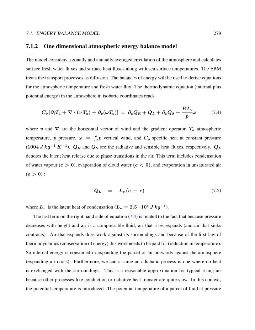
7.1. ENGERY BALANCE MODEL 279
7.1.2 One dimensional atmospheric energy balance model
The model considers a zonally and annually averaged circulation of the atmosphere and calculates
surface fresh water fluxes and surface heat fluxes along with sea surface temperatures. The EBM
treats the transport processes as diffusion. The balances of energy will be used to derive equations
for the atmospheric temperature and fresh water flux. The thermodynamic equation (internal plus
potential energy) in the atmosphere in isobaric coordinates reads
Cp [∂tTa +∇ · (v Ta) + ∂p(ωTa)] = ∂pQR +QL + ∂pQS +RTa
pω (7.4)
where v and ∇ are the horizontal vector of wind and the gradient operator, Ta atmospheric
temperature, p pressure, ω = ddtp vertical wind, and Cp specific heat at constant pressure
(1004 J kg−1K−1). QR and QS are the radiative and sensible heat fluxes, respectively. QL
denotes the latent heat release due to phase transitions in the air. This term includes condensation
of water vapour (c > 0), evaporation of cloud water (c < 0), and evaporation in unsaturated air
(e > 0) :
QL = Lv (c − e) (7.5)
where Lv is the latent heat of condensation (Lv = 2.5 · 106 J kg−1).
The last term on the right hand side of equation (7.4) is related to the fact that because pressure
decreases with height and air is a compressible fluid, air that rises expands (and air that sinks
contracts). Air that expands does work against its surroundings and because of the first law of
thermodynamics (conservation of energy) this work needs to be paid for (reduction in temperature).
So internal energy is consumed in expanding the parcel of air outwards against the atmosphere
(expanding air cools). Furthermore, we can assume an adiabatic process is one where no heat
is exchanged with the surroundings. This is a reasonable approximation for typical rising air
because other processes like conduction or radiative heat transfer are quite slow. In this context,
the potential temperature is introduced. The potential temperature of a parcel of fluid at pressure

280 CHAPTER 7. SIMPLE CLIMATE MODELS
P is the temperature that the parcel would acquire if adiabatically brought to a standard reference
pressure P0, usually 1000 millibars. The potential temperature is denoted θ and, for air, is often
given by
θ = T
(P0
P
)R/cp, (7.6)
where T is the current absolute temperature (in K) of the parcel, R is the gas constant of air, and
cp is the specific heat capacity at a constant pressure. R/cp = 0.286 for air (meteorology).
Potential temperature is a more dynamically important quantity than the actual temperature. This
is because it is not affected by the physical lifting or sinking associated with flow over obstacles
or large-scale atmospheric turbulence. A parcel of air moving over a small mountain will expand
and cool as it ascends the slope, then compress and warm as it descends on the other side- but the
potential temperature will not change in the absence of heating, cooling, evaporation, or conden-
sation (processes that exclude these effects are referred to as dry adiabatic). Since parcels with
the same potential temperature can be exchanged without work or heating being required, lines of
constant potential temperature are natural flow pathways.1
Additionally to (7.4), the budget equations for the mass mixing ratio of water vapour qv and
cloud water qw are used:
∂tqv + ∇ · ( v qv) + ∂p(ω qv) = e − c + E (7.7)
∂tqw + ∇ · ( v qw) + ∂p(ω qw) = c − ℘ (7.8)
where ℘ denotes the formation of precipitation and E denotes the evaporation from the ground
(ocean and land).
1The equation comes from the enthalpy form of the first law of thermodynamics can be written as: dh = T ds+v dp, where dh denotes the enthalpy change, T the temperature, ds the change in entropy, v the specific volume, andp the pressure. For adiabatic processes, the change in entropy is zero: dh = v dp. For approximately ideal gases,such as the dry air in the Earth’s atmosphere, the equation of state, pv = RT can be substituted by dpv = R/vdTdpp
=cpRdTT, where the dh = cpdT was used and both terms were divided by the product pv. Integrating yields
7.6.
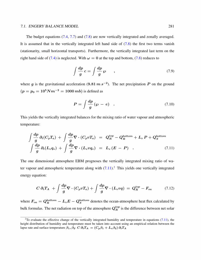
7.1. ENGERY BALANCE MODEL 281
The budget equations (7.4, 7.7) and (7.8) are now vertically integrated and zonally averaged.
It is assumed that in the vertically integrated left hand side of (7.8) the first two terms vanish
(stationarity, small horizontal transports). Furthermore, the vertically integrated last term on the
right hand side of (7.4) is neglected. With ω = 0 at the top and bottom, (7.8) reduces to
∫dp
gc =
∫dp
g℘ , (7.9)
where g is the gravitational acceleration (9.81ms−2). The net precipitation P on the ground
(p = p0 = 105Nm−2 = 1000mb) is defined as
P =
∫dp
g(℘ − e) . (7.10)
This yields the vertically integrated balances for the mixing ratio of water vapour and atmospheric
temperature:
∫dp
g∂t(CpTa) +
∫dp
g∇ · (CpvTa) = Qtop
R −QbottomR + Lv P +Qbottom
S∫dp
g∂t(Lvqv) +
∫dp
g∇ · (Lvvqv) = Lv (E − P ) . (7.11)
The one dimensional atmosphere EBM prognoses the vertically integrated mixing ratio of wa-
ter vapour and atmospheric temperature along with (7.11).2 This yields one vertically integrated
energy equation:
C ∂tTA +
∫dp
g∇ · (CpvTa) +
∫dp
g∇ · (Lvvq) = Qtop
R − Foa (7.12)
where Foa = QbottomR − LvE −Qbottom
S denotes the ocean-atmosphere heat flux calculated by
bulk formulas. The net radiation on top of the atmosphereQtopR is the difference between net solar
2To evaluate the effective change of the vertically integrated humidity and temperature in equations (7.11), theheight distribution of humidity and temperature must be taken into account using an empirical relation between thelapse rate and surface temperature β1, β2: C ∂tTA = (Cpβ1 + Lvβ2) ∂tTA
282 CHAPTER 7. SIMPLE CLIMATE MODELS
radiation and net outgoing longwave radiation QtopLW . In a further approximation, the longwave
radiationQtopLW is described by a linear law:
QtopLW = A+B TA with (7.13)
A = 213.2 W m−2 and B = 2.2 W m−2K−1 .
For QS , one needs a climate-dependent formulation of the planetary albedo α, which is parame-
terized in terms of the surface air temperature:
α(TA) = 0.42 − 0.20 · tanh [0.052 (TA − 276.15)] . (7.14)
This parameterization incorporates high albedos of snow and ice in terms of the surface tempera-
ture (TA in Kelvin). With equation (7.12) the surface temperature TA is calculated prognostically,
while the fresh water flux for the ocean surface is given by the right hand side of equation (7.11)
by evaluating the left hand side of the water vapour budget.
Meridional Transports
The transport parameterizations are based on diffusion. The mechanism of heat and moisture trans-
port in middle and high latitudes by baroclinic instability is the most important mechanism in the
atmospheric energy balance model. Consider an atmospheric condition with isotherms coincident
with latitude circles. A cold anomaly, which could be thought of as a cold air outbreak from the
North American continent, results in a changed surface heat flux from the ocean. In the region of
strong temperature gradient, cyclones (low pressure) and anticyclones (high pressure on the north-
ern hemisphere) are formed. These traveling weather systems move north-eastward defining the
major storm track. The scale over which this process is important is about 1000 km.
This process is the main source of meridional heat transport in middle and high latitudes. The
balances of heat and moisture (7.11) are averaged over a length scale of synoptic scale disturbances
of O(1000) km and a time scale longer than the life time of such disturbances (e.g. two weeks).
The variables can be splitted into a large-scale, long-term quantities (Ta, qv, v) and the deviations
7.1. ENGERY BALANCE MODEL 283
(T ′a, q′v, v′). The moments v′T ′a and v′q′v are connected mainly with transient processes in the
atmosphere. The transients act as diffusion in a statistical sense bringing warm and moist air
poleward due to individual high and low pressure contributions.
The eddy fluxes, in a statistically steady state of the atmosphere, scale as:
v′T ′a ∼(∂Ta
∂y
)(7.15)
where T ′, v′ are the perturbation of potential temperature and meridional velocity. The vertical in-
tegrated sensible eddy heat transport can be calculated in terms of the surface temperature gradient
TA ∫dp
gv′T ′a = − Ks
(∂ TA
∂y
). (7.16)
whereKs is tuned to reproduce the current climate.
The latent eddy heat transport is parameterized as
v′q′v = rh(p)∂ qs
∂Ta(Ta, p) v′T ′a , (7.17)
where rh is the relative humidity and qs the saturation water vapour. The relative humidity is
prescribed. For the latent heat transport (7.17), the relative humidity and ∂ qs∂T
strongly decrease
with height. Therefore, the surface values for the latent heat transport is a good choice in the
vertical integrated model:
∫dp
gv′q′v = −Kl rh(p0)
∂ qs
∂TA(TA, p0)
(∂ TA
∂y
). (7.18)
As for the sensible heat transport, the coefficientKl can be tuned that (7.18) reproduces the latent
eddy heat transports of current climate. The eddy activity is greatly enhanced over the ocean
surfaces as opposed to over land surfaces. In the Northern Hemisphere, two major storm tracks
284 CHAPTER 7. SIMPLE CLIMATE MODELS
exists extending northeast across the Atlantic and Pacific oceans from the east coast of the major
continents. It is along these tracks that the majority of eddy heat and vorticity transport takes place.
In the Southern Hemisphere the transport is relatively homogeneous in the zonal direction.3 In the
boxmodel in section 7.2, we assume that the atmospheric heat transport across the box boundaries
are completely by transient eddies.
Exercise 53 – Analytical EBM
Starting from (7.12), we are interested in the vertically integrated energy equation where we
include the atmosphere and ocean in one temperature T and describe the heat transport (sensible,
latent and ocean) as diffusion:
Cp ∂tT + k ∂2yT = (1− α)Qtop
S − (A+B T ) (7.19)
If α is chosen as parameter, we can easily solve (7.19) with the ansatz with a global component
and a latitude component
T (y, t) = T0(t) + T1(t) · cos(by) (7.20)
QtopS = Q0 +Q1 · cos(by) (7.21)
with y = aϕ and b = 2/a.
Task: Solve the Energy balance model (7.19) for constant α.
3The heat transport by stationary baroclinic waves is larger in winter on the northern hemisphere when the land-seacontrast is most pronounced. Green ? argued that stationary eddies are more transient phenomena which repeat-edly occur at the same location. This happens due to fixed topographic effects providing perturbations upon whichbaroclinic waves can grow. These phenomena relating to stationary eddies are ultimately driven by the large scalebaroclinicity of the atmosphere. Therefore, standing eddies could be parameterized as transient eddies.
7.1. ENGERY BALANCE MODEL 285
Solution
Hint: For constant α, one can separate the dynamics for T0 and T1:
CpdtT0 = (1− α)Q0 − (A+BT0) (7.22)
CpdtT1 = (kb2 +B)T1 + (1− α)Q1 (7.23)
because∫ 90
−90cos(2ϕ) dϕ = 0
The solution of an inhomogenous linear differential equation is the solution of the homogenous
differential equation plus a particular solution of the inhomogenous case. y′ + uy = v, then the
solution of the homogenous system is yh = C exp(−ut), and a particular solution yp = v/u
independent on t, and therefore y = yh + yp as the solution. Note that a particular solution yp
can be also found through variation of constant C(t).
Exercise 54 – Analytical EBM: Ice-albedo feedback
Based in exercise 53, one can introduce a climate-dependent formulation of the planetary
albedo α on the global temperature:
α(T ) = α0 − α1 · T0 (7.24)
Tasks:
a) Solve the Energy balance model (7.19) for the case α(T0) as in (7.24).
b) Show that the stability of the solution depends onB − α1Q0 !
c) explain the ice-albedo effect through this solution!

286 CHAPTER 7. SIMPLE CLIMATE MODELS
7.2 Interhemispheric box model
7.2.1 Model description
Here we introduce an interhemispheric box model of the deep ocean circulation to study the feed-
backs in the climate system. Like in the model of Rooth [1982] the Atlantic Ocean is described
over both hemispheres. The box model consists of four oceanic and three atmospheric boxes,
as indicated in Fig. 13.6. The ocean boxes represent the Atlantic Ocean from 80N to 60S.
The indices of the temperatures T, the salinities S, the surface heat fluxes H, the atmospheric heat
fluxes F, the radiation terms R as well as later on the volumes bear on the different boxes (N for
the northern, M for the tropical, D for the deep and S for the southern box).
The discrete boxes are utterly homogeneous, which implies that the temperatures and the salin-
ities everywhere within one box are alike. The climate model is based on mass and energy consid-
erations. Emphasis is placed on the overturning flow Φ of the ocean circulation.
Figure 7.1: Schematic illustration of the Climate-Box-Model
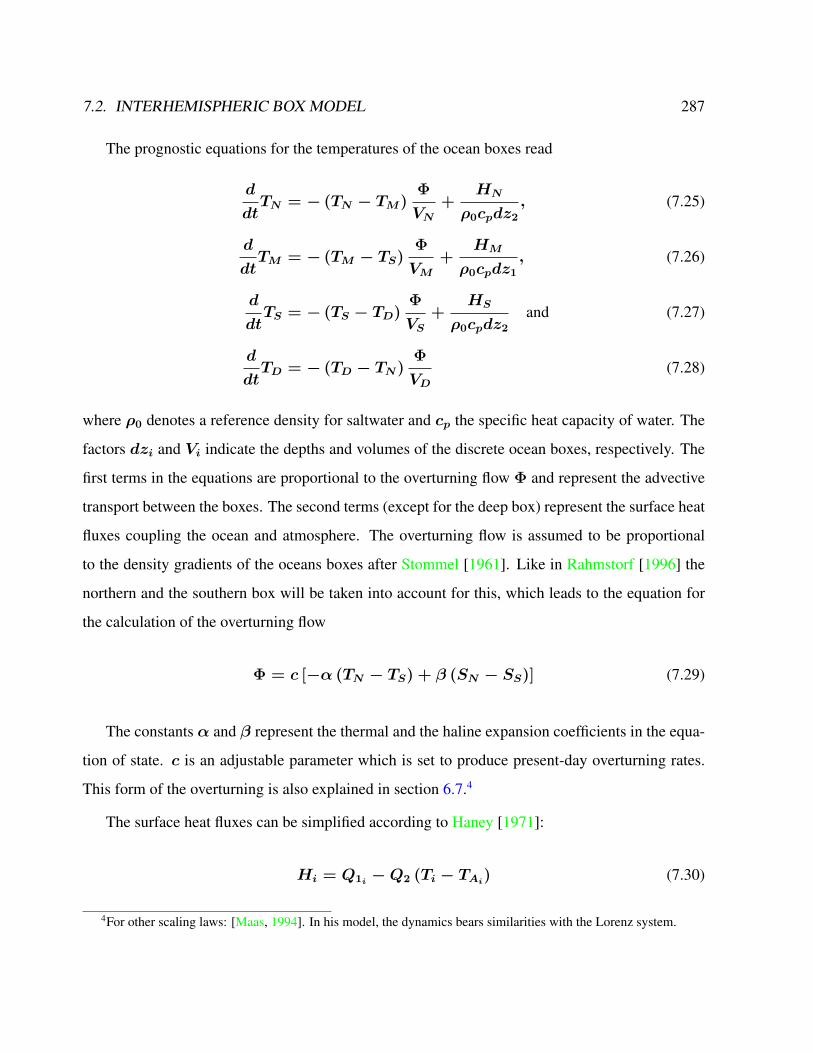
7.2. INTERHEMISPHERIC BOX MODEL 287
The prognostic equations for the temperatures of the ocean boxes read
d
dtTN = − (TN − TM)
Φ
VN+
HN
ρ0cpdz2
, (7.25)
d
dtTM = − (TM − TS)
Φ
VM+
HM
ρ0cpdz1
, (7.26)
d
dtTS = − (TS − TD)
Φ
VS+
HS
ρ0cpdz2
and (7.27)
d
dtTD = − (TD − TN)
Φ
VD(7.28)
where ρ0 denotes a reference density for saltwater and cp the specific heat capacity of water. The
factors dzi and Vi indicate the depths and volumes of the discrete ocean boxes, respectively. The
first terms in the equations are proportional to the overturning flow Φ and represent the advective
transport between the boxes. The second terms (except for the deep box) represent the surface heat
fluxes coupling the ocean and atmosphere. The overturning flow is assumed to be proportional
to the density gradients of the oceans boxes after Stommel [1961]. Like in Rahmstorf [1996] the
northern and the southern box will be taken into account for this, which leads to the equation for
the calculation of the overturning flow
Φ = c [−α (TN − TS) + β (SN − SS)] (7.29)
The constants α and β represent the thermal and the haline expansion coefficients in the equa-
tion of state. c is an adjustable parameter which is set to produce present-day overturning rates.
This form of the overturning is also explained in section 6.7.4
The surface heat fluxes can be simplified according to Haney [1971]:
Hi = Q1i −Q2 (Ti − TAi) (7.30)
4For other scaling laws: [Maas, 1994]. In his model, the dynamics bears similarities with the Lorenz system.

288 CHAPTER 7. SIMPLE CLIMATE MODELS
Analogue to (13.52) to (7.28) the prognostic differential equations for the salinities consist
out of two components. One of those is again the advective part, caused by the interconnection
between the boxes and the other one is the influence of the freshwater fluxes between the ocean
and the atmosphere. The latter is again only for the boxes near the surface, thus the equations are
d
dtSN = − (SN − SM)
Φ
VN− Sref
(P − E)N
dzN, (7.31)
d
dtSM = − (SM − SS)
Φ
VM+ Sref
(P − E)M
dzM, (7.32)
d
dtSS = − (SS − SD)
Φ
VS− Sref
(P − E)S
dzS, (7.33)
d
dtSD = − (SD − SN)
Φ
VD. (7.34)
The reference salinity Sref is a characteristic average value for the entire Atlantic Ocean, and the
freshwater fluxes are denoted as precipitation minus evaporation (P-E). These freshwater fluxes are
calculated by the divergence of the latent heat transport in the atmosphere and are assumed to be
proportional to the meridional moisture gradient explained below.
The atmospheric energy-balance-model (EBM) calculates the heat fluxes between the ocean
and atmosphere, as well as horizontal latent and sensible heat transports as diffusion following
Chen et al. [1995]. The EBM contains sensible and latent heat transports, radiation Ri, as well as
the surface heat fluxes Hi between the atmosphere and the ocean. The atmospheric temperatures
TAi follow the prognostic equations
c2
d
dtTAN =
∂ (FsN + FlN )
∂y+RN −HN , (7.35)
c2
d
dtTAM =
∂ (FsS + FlS)
∂y+RM −HM , (7.36)
c2
d
dtTAS =
∂ (FsS + FlS)
∂y+RS −HS. (7.37)
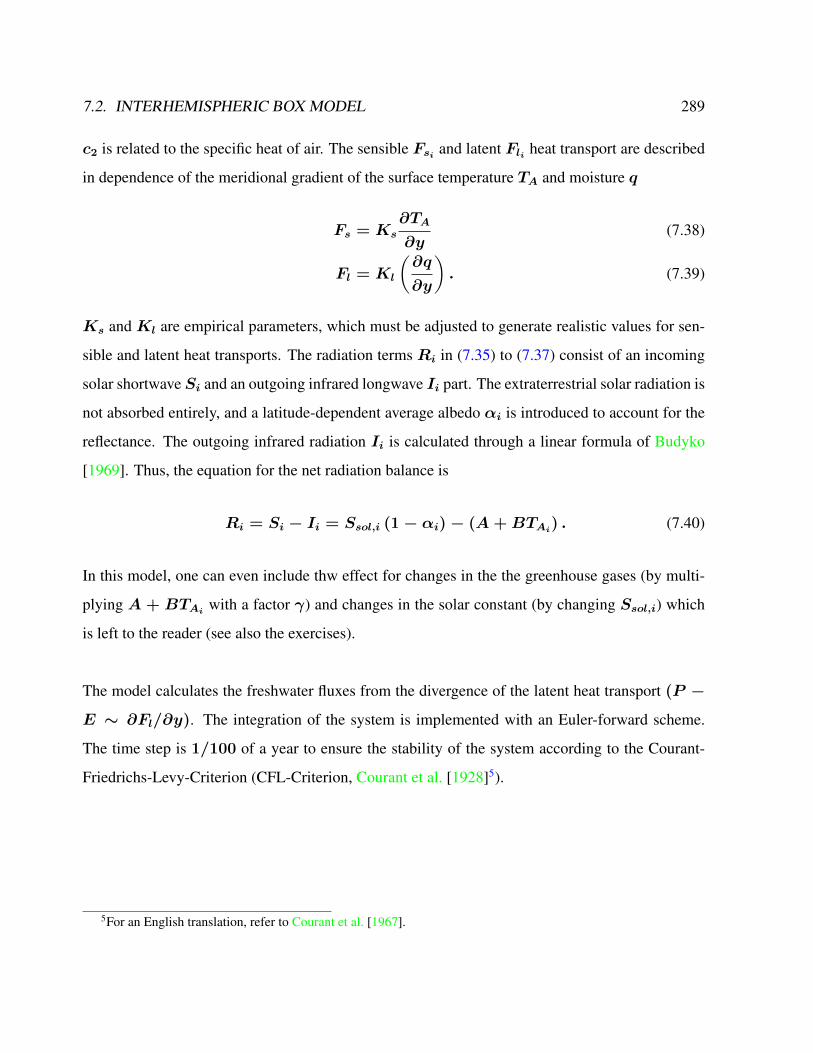
7.2. INTERHEMISPHERIC BOX MODEL 289
c2 is related to the specific heat of air. The sensible Fsi and latent Fli heat transport are described
in dependence of the meridional gradient of the surface temperature TA and moisture q
Fs = Ks
∂TA
∂y(7.38)
Fl = Kl
(∂q
∂y
). (7.39)
Ks and Kl are empirical parameters, which must be adjusted to generate realistic values for sen-
sible and latent heat transports. The radiation terms Ri in (7.35) to (7.37) consist of an incoming
solar shortwaveSi and an outgoing infrared longwave Ii part. The extraterrestrial solar radiation is
not absorbed entirely, and a latitude-dependent average albedo αi is introduced to account for the
reflectance. The outgoing infrared radiation Ii is calculated through a linear formula of Budyko
[1969]. Thus, the equation for the net radiation balance is
Ri = Si − Ii = Ssol,i (1− αi)− (A+BTAi) . (7.40)
In this model, one can even include thw effect for changes in the the greenhouse gases (by multi-
plying A + BTAi with a factor γ) and changes in the solar constant (by changing Ssol,i) which
is left to the reader (see also the exercises).
The model calculates the freshwater fluxes from the divergence of the latent heat transport (P −
E ∼ ∂Fl/∂y). The integration of the system is implemented with an Euler-forward scheme.
The time step is 1/100 of a year to ensure the stability of the system according to the Courant-
Friedrichs-Levy-Criterion (CFL-Criterion, Courant et al. [1928]5).
5For an English translation, refer to Courant et al. [1967].
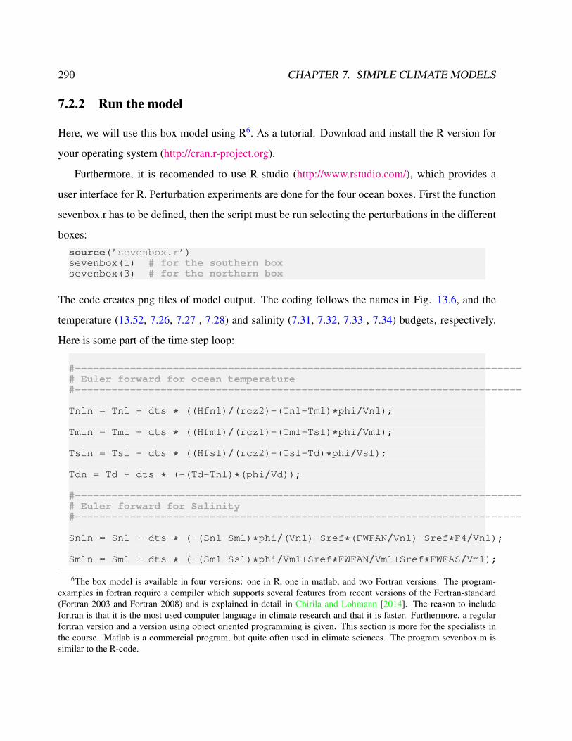
290 CHAPTER 7. SIMPLE CLIMATE MODELS
7.2.2 Run the model
Here, we will use this box model using R6. As a tutorial: Download and install the R version for
your operating system (http://cran.r-project.org).
Furthermore, it is recomended to use R studio (http://www.rstudio.com/), which provides a
user interface for R. Perturbation experiments are done for the four ocean boxes. First the function
sevenbox.r has to be defined, then the script must be run selecting the perturbations in the different
boxes:
source(’sevenbox.r’)sevenbox(1) # for the southern boxsevenbox(3) # for the northern box
The code creates png files of model output. The coding follows the names in Fig. 13.6, and the
temperature (13.52, 7.26, 7.27 , 7.28) and salinity (7.31, 7.32, 7.33 , 7.34) budgets, respectively.
Here is some part of the time step loop:
#-------------------------------------------------------------------------# Euler forward for ocean temperature#-------------------------------------------------------------------------
Tnln = Tnl + dts * ((Hfnl)/(rcz2)-(Tnl-Tml)*phi/Vnl);
Tmln = Tml + dts * ((Hfml)/(rcz1)-(Tml-Tsl)*phi/Vml);
Tsln = Tsl + dts * ((Hfsl)/(rcz2)-(Tsl-Td)*phi/Vsl);
Tdn = Td + dts * (-(Td-Tnl)*(phi/Vd));
#-------------------------------------------------------------------------# Euler forward for Salinity#-------------------------------------------------------------------------
Snln = Snl + dts * (-(Snl-Sml)*phi/(Vnl)-Sref*(FWFAN/Vnl)-Sref*F4/Vnl);
Smln = Sml + dts * (-(Sml-Ssl)*phi/Vml+Sref*FWFAN/Vml+Sref*FWFAS/Vml);
6The box model is available in four versions: one in R, one in matlab, and two Fortran versions. The program-examples in fortran require a compiler which supports several features from recent versions of the Fortran-standard(Fortran 2003 and Fortran 2008) and is explained in detail in Chirila and Lohmann [2014]. The reason to includefortran is that it is the most used computer language in climate research and that it is faster. Furthermore, a regularfortran version and a version using object oriented programming is given. This section is more for the specialists inthe course. Matlab is a commercial program, but quite often used in climate sciences. The program sevenbox.m issimilar to the R-code.
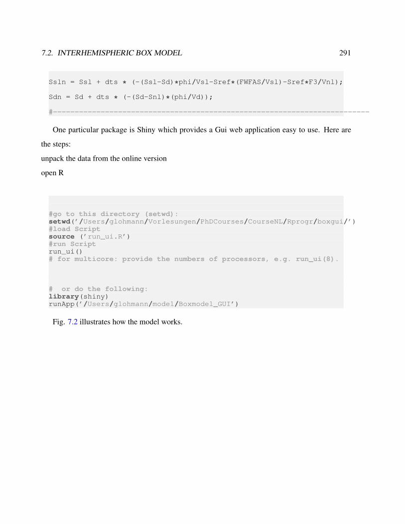
7.2. INTERHEMISPHERIC BOX MODEL 291
Ssln = Ssl + dts * (-(Ssl-Sd)*phi/Vsl-Sref*(FWFAS/Vsl)-Sref*F3/Vnl);
Sdn = Sd + dts * (-(Sd-Snl)*(phi/Vd));
#-------------------------------------------------------------------------
One particular package is Shiny which provides a Gui web application easy to use. Here are
the steps:
unpack the data from the online version
open R
#go to this directory (setwd):setwd(’/Users/glohmann/Vorlesungen/PhDCourses/CourseNL/Rprogr/boxgui/’)#load Scriptsource (’run_ui.R’)#run Scriptrun_ui()# for multicore: provide the numbers of processors, e.g. run_ui(8).
# or do the following:library(shiny)runApp(’/Users/glohmann/model/Boxmodel_GUI’)
Fig. 7.2 illustrates how the model works.
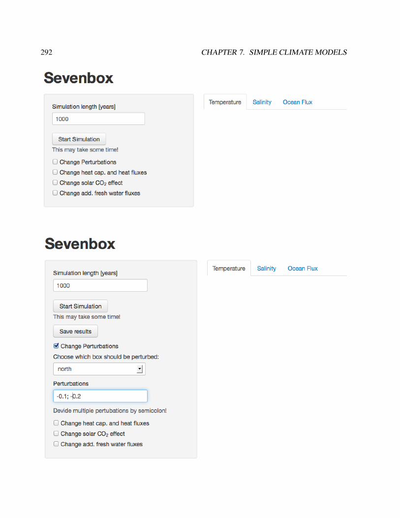
292 CHAPTER 7. SIMPLE CLIMATE MODELS
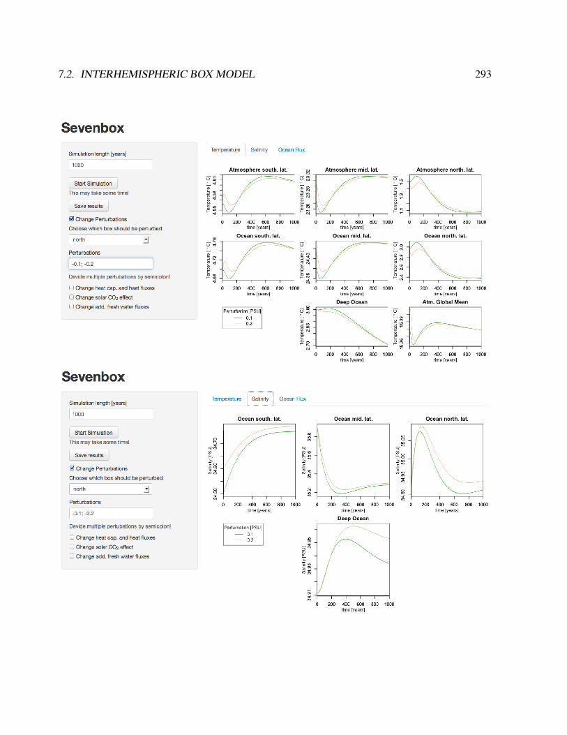
7.2. INTERHEMISPHERIC BOX MODEL 293

294 CHAPTER 7. SIMPLE CLIMATE MODELS
Figure 7.2: Output of the climate box model illustrating the procedure.
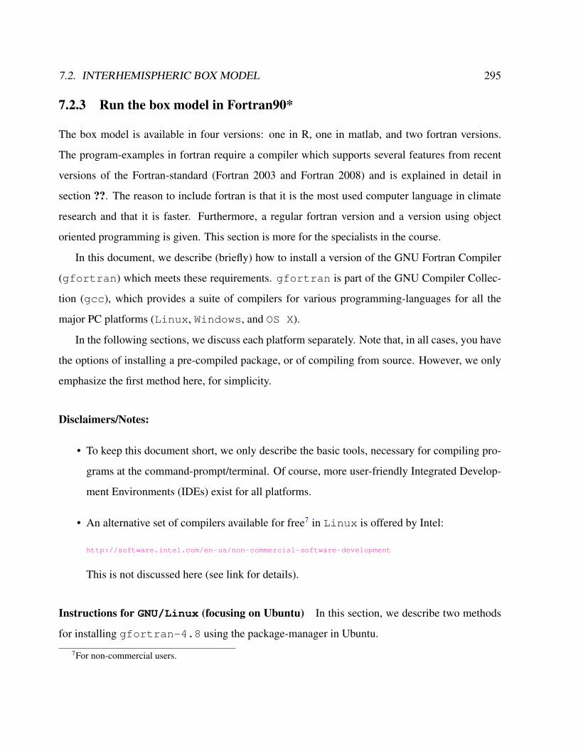
7.2. INTERHEMISPHERIC BOX MODEL 295
7.2.3 Run the box model in Fortran90*
The box model is available in four versions: one in R, one in matlab, and two fortran versions.
The program-examples in fortran require a compiler which supports several features from recent
versions of the Fortran-standard (Fortran 2003 and Fortran 2008) and is explained in detail in
section ??. The reason to include fortran is that it is the most used computer language in climate
research and that it is faster. Furthermore, a regular fortran version and a version using object
oriented programming is given. This section is more for the specialists in the course.
In this document, we describe (briefly) how to install a version of the GNU Fortran Compiler
(gfortran) which meets these requirements. gfortran is part of the GNU Compiler Collec-
tion (gcc), which provides a suite of compilers for various programming-languages for all the
major PC platforms (Linux, Windows, and OS X).
In the following sections, we discuss each platform separately. Note that, in all cases, you have
the options of installing a pre-compiled package, or of compiling from source. However, we only
emphasize the first method here, for simplicity.
Disclaimers/Notes:
• To keep this document short, we only describe the basic tools, necessary for compiling pro-
grams at the command-prompt/terminal. Of course, more user-friendly Integrated Develop-
ment Environments (IDEs) exist for all platforms.
• An alternative set of compilers available for free7 in Linux is offered by Intel:
http://software.intel.com/en-us/non-commercial-software-development
This is not discussed here (see link for details).
Instructions for GNU/Linux (focusing on Ubuntu) In this section, we describe two methods
for installing gfortran-4.8 using the package-manager in Ubuntu.
7For non-commercial users.

296 CHAPTER 7. SIMPLE CLIMATE MODELS
Ubuntu 12.04 (Precise) Because gcc-4.8 was released quite recently (March 22, 2013), most
distributions did not yet have this package in the default-repositories at the time of this writing
(June 25, 2018). However, Ubuntu Precise (12.04) users can add a repository for this, as in:
sudo add-apt-repository ppa:ubuntu-toolchain-r/test
sudo apt-get update
sudo apt-get install gfortran-4.8
Note that, when using this method, the compiler to be invoked will be named gfortran-4.8.
Ubuntu (other releases) Users of other Ubuntu releases can add the latest release of GCC as
follows:
sudo apt-get install gcc-snapshot
# can add the two lines below to ~/.bashrc,
# to automatize the compiler-selection
export PATH=$PATH:/usr/lib/gcc-snapshot/bin/
export LD_LIBRARY_PATH=$LD_LIBRARY_PATH:/usr/lib/gcc-snapshot/lib/
An overview of the gcc/gfortran versions available for each distribution is also available
here: http://gcc.gnu.org/wiki/GFortranDistros.
Instructions for MS Windows The easiest way to get GCC on Windows is to use the packages
provided at the website www.equation.com:
1. go to www.equation.com, then (in the menu on the left) navigate to “Programming
Tools”→ “Fortran, C, C++”
2. scroll to the section “DOWNLOAD: OFFICIAL RELEASES”
3. download a “Self-Extracting File” (either the 32bit or the 64bit version, depending on your
version of Windows)
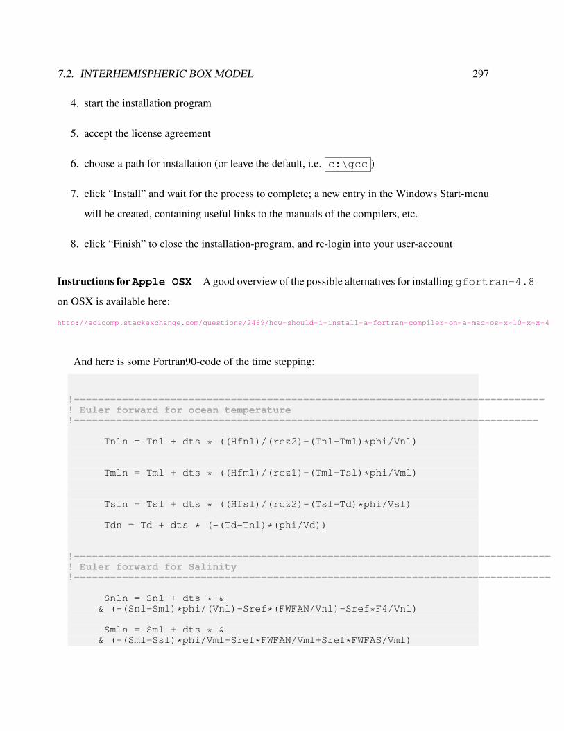
7.2. INTERHEMISPHERIC BOX MODEL 297
4. start the installation program
5. accept the license agreement
6. choose a path for installation (or leave the default, i.e. c:\gcc )
7. click “Install” and wait for the process to complete; a new entry in the Windows Start-menu
will be created, containing useful links to the manuals of the compilers, etc.
8. click “Finish” to close the installation-program, and re-login into your user-account
Instructions for Apple OSX A good overview of the possible alternatives for installing gfortran-4.8
on OSX is available here:
http://scicomp.stackexchange.com/questions/2469/how-should-i-install-a-fortran-compiler-on-a-mac-os-x-10-x-x-4
And here is some Fortran90-code of the time stepping:
!------------------------------------------------------------------------------! Euler forward for ocean temperature!-----------------------------------------------------------------------------
Tnln = Tnl + dts * ((Hfnl)/(rcz2)-(Tnl-Tml)*phi/Vnl)
Tmln = Tml + dts * ((Hfml)/(rcz1)-(Tml-Tsl)*phi/Vml)
Tsln = Tsl + dts * ((Hfsl)/(rcz2)-(Tsl-Td)*phi/Vsl)
Tdn = Td + dts * (-(Td-Tnl)*(phi/Vd))
!-------------------------------------------------------------------------------! Euler forward for Salinity!-------------------------------------------------------------------------------
Snln = Snl + dts * && (-(Snl-Sml)*phi/(Vnl)-Sref*(FWFAN/Vnl)-Sref*F4/Vnl)
Smln = Sml + dts * && (-(Sml-Ssl)*phi/Vml+Sref*FWFAN/Vml+Sref*FWFAS/Vml)
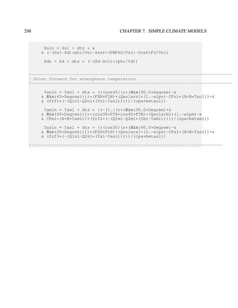
298 CHAPTER 7. SIMPLE CLIMATE MODELS
Ssln = Ssl + dts * && (-(Ssl-Sd)*phi/Vsl-Sref*(FWFAS/Vsl)-Sref*F3/Vnl)
Sdn = Sd + dts * (-(Sd-Snl)*(phi/Vd))
!-------------------------------------------------------------------------------! Euler forward for atmosphere temperature!-------------------------------------------------------------------------------
Tanln = Tanl + dts * (((cos45/(r*(Sin(90.0*Degree)-&& Sin(45*Degree))))*(FSN+FLN)+(Qsolarnl*(1.-alpn)-CFnl*(A+B*Tanl))+&& (frf1*(-(Q1nl-Q2nl*(Tnl-Tanl)))))/(cpa*betanl))
Tamln = Taml + dts * ((-(1./(r*(Sin(30.0*Degree)+&& Sin(45*Degree))))*(cos30*FTS+cos45*FTN)+(Qsolarml*(1.-alpm)-&& CFml*(A+B*Taml))+(frf2*(-(Q1ml-Q2ml*(Tml-Taml)))))/(cpa*betaml))
Tasln = Tasl + dts * (((cos30/(r*(Sin(90.0*Degree)-&& Sin(30*Degree))))*(FSS+FLS)+(Qsolarsl*(1.-alps)-CFsl*(A+B*Tasl))+&& (frf3*(-(Q1sl-Q2sl*(Tsl-Tasl)))))/(cpa*betasl))
!---------------------------------------------------------------------------

7.2. INTERHEMISPHERIC BOX MODEL 299
7.2.4 Model scenarios
Paleoclimatic evidence suggests (e.g. Dansgaard et al. [1993]) that some past climate shifts were
associated with changes in North Atlantic Deep Water (NADW) formation. Deep water formation
in the Greenland-Iceland-Norwegian Sea and in Labrador Sea drive the large-scale ocean circu-
lation imposing strong northward heat transport. This makes the northern North Atlantic about
4 K warmer than corresponding latitudes in the Pacific and is responsible for the mild climate of
Western Europe. Variations in NADW circulation therefore have the potential to cause significant
climate change in the North Atlantic region.
Numerical simulations by Manabe and Stouffer [1993] showed, for the North Atlantic, that be-
tween two and four times the preindustrial CO2 concentration, a threshold value is passed and the
thermohaline circulation ceases completely. One other example of early Holocene rapid climate
change is the ’8200 yr BP’ cooling event recorded in the North Atlantic region possibly induced
by freshwater. One possible explanation for this dramatic regional cooling is a shutdown in the
formation of deep water in the northern North Atlantic due to freshwater input caused by catas-
trophic drainage of Laurentide lakes (e.g., Barber et al. [1999]; Lohmann [2003]). After the end
of the last glacial, freshwater entered into the Atlantic Ocean (Fig. 9.9) and may have affected the
ocean circulation.
Exercise 55 – Investigations with the box-model
1. In the regions of deep water formation in the North Atlantic, relatively small amounts of
fresh water added to the surface can stabilize the water column to the extent that convection
can be prevented from occurring. Such interruption decreases the poleward oceanic mass
transport Φ. Furthermore, this perturbation of the meridional transport can be amplified
by positive feedbacks: a weaker northward salt transport brings less dense water to high
latitudes, which further reduces the high-latitude density. Discuss the case where the initial
conditions in salinity at different latitudes is changed. Show this scenario in the box model!
2. Comment on the scenario of climate change as shown in the cinema movie The Day After
Tomorrow: link to the website or go to the trailer.
300 CHAPTER 7. SIMPLE CLIMATE MODELS
3. Which feedbacks are acting for global warming? You can change the long wave radiation.
A doubling of pCO2 is equivalent to an additional forcing of 4 Wm−2. For this you
have to modify the net radiation balance (7.40) through reduction in the outgoing longwave
radiation (parameter γ). Additional radiative forcing may come from increased tracer gas
concentrations in the atmosphere. Please evaluate the hydrological cycle and atmospheric
heat transports! What is the change in the overturning rate?
4. Change the ocean heat capacity by a factor of 10 and describe the change in the response to
warming induced by 90
5. The initial values of the model represent averages for present-day climate conditions. De-
termine the effect of the parameter c in the numerical example (representing a different long
wave radiation) Can you derive a glacial climate? The glacial climate was 3 K colder in the
tropics.
6. Calculate the ocean heat transport in the model and compare it with the following estimate!
H =
∫ top
bottom
ρ0vTdz (7.41)
= −cp∫ top
bottom
∂Φ
∂zTdz (7.42)
= cp
∫ top
bottom
Φ∂T
∂zdz (7.43)
= cp
∫ T (top)
T (bottom)
ΦdT (7.44)
where Φ = ρ0ΦMOC with ΦMOC being the volume transport. Therefore, the heat transport
can be estimated in terms of the mass transport in temperature layers:
H = cp (T (top)− T (bottom))︸ ︷︷ ︸15K
Φmax︸ ︷︷ ︸20·109kg/s
(7.45)
which is about 1.2 PW (PW = 1015W ).
7.2. INTERHEMISPHERIC BOX MODEL 301
7. Question for specialists: The coupled model shall be used to investigate the sensitivity of the
system with respect to stochastic weather perturbations reflecting unresolved effects of the
atmospheric transports modeled as white noise. How will the atmospheric noise influence
the stability of the system?
Exercise 56 – Interhemispheric Box model on the web
Repeat the exercise 55 using the R-Shiny App on https://paleosrv2.awi.de/. The
username is student and the Password is EbJir5ow !

302 CHAPTER 7. SIMPLE CLIMATE MODELS
7.3 Weather and climate: Stochastic climate model
The daily observed maximum and minimum temperatures is often compared to the "normal" tem-
peratures based upon the 30-year average. Climate averages provide a context for something like
"this winter will be wetter (or drier, or colder, or warmer, etc.) than normal. It has been said
"Climate is what you expect. Weather is what you get."
What is the difference between weather and climate? This can be also answered by an ex-
ample/a methaphor in the football league. Predicting the outcome of the next game is difficult
(weather), but predicting who will end up as German champion is unfortunately relatively easy
(climate). In this section, I will give a general approach to the mean and fluctuations in the climate
system. Indeed, the Brownian motion approach is a helpful analogue for weather and climate.
7.3.1 Brownian motion
The Roman Lucretius’s scientific poem On the Nature of Things (ca. 60 BC) has a remarkable
description of Brownian motion of dust particles8. Jan Ingenhousz had described the irregular
motion of coal dust particles on the surface of alcohol in 1785. Nevertheless Brownian motion
is traditionally regarded as discovered by the botanist Robert Brown in 1827. It is believed that
Brown was studying pollen particles floating in water under the microscope. He then observed
minute particles within the vacuoles of the pollen grains executing a jittery motion. By repeating
the experiment with particles of dust, he was able to rule out that the motion was due to pollen
particles being ’alive’, although the origin of the motion was yet to be explained.
See the film: https://en.wikipedia.org/wiki/Brownian_motion#/media/
8He uses this as a proof of the existence of atoms: "Observe what happens when sunbeams are admitted into abuilding and shed light on its shadowy places. You will see a multitude of tiny particles mingling in a multitude ofways... their dancing is an actual indication of underlying movements of matter that are hidden from our sight... Itoriginates with the atoms which move of themselves [i.e. spontaneously]. Then those small compound bodies that areleast removed from the impetus of the atoms are set in motion by the impact of their invisible blows and in turn cannonagainst slightly larger bodies. So the movement mounts up from the atoms and gradually emerges to the level of oursenses, so that those bodies are in motion that we see in sunbeams, moved by blows that remain invisible." Althoughthe mingling motion of dust particles is caused largely by air currents, the glittering, tumbling motion of small dustparticles is, indeed, caused chiefly by true Brownian dynamics.
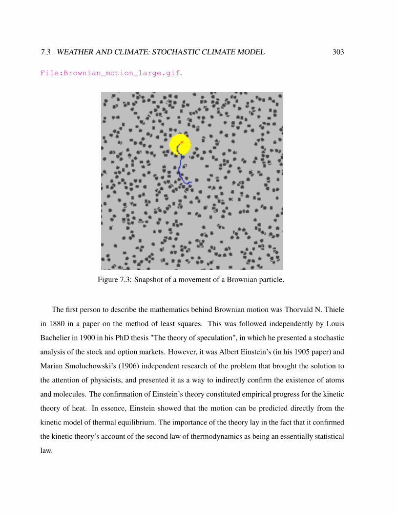
7.3. WEATHER AND CLIMATE: STOCHASTIC CLIMATE MODEL 303
File:Brownian_motion_large.gif.
Figure 7.3: Snapshot of a movement of a Brownian particle.
The first person to describe the mathematics behind Brownian motion was Thorvald N. Thiele
in 1880 in a paper on the method of least squares. This was followed independently by Louis
Bachelier in 1900 in his PhD thesis "The theory of speculation", in which he presented a stochastic
analysis of the stock and option markets. However, it was Albert Einstein’s (in his 1905 paper) and
Marian Smoluchowski’s (1906) independent research of the problem that brought the solution to
the attention of physicists, and presented it as a way to indirectly confirm the existence of atoms
and molecules. The confirmation of Einstein’s theory constituted empirical progress for the kinetic
theory of heat. In essence, Einstein showed that the motion can be predicted directly from the
kinetic model of thermal equilibrium. The importance of the theory lay in the fact that it confirmed
the kinetic theory’s account of the second law of thermodynamics as being an essentially statistical
law.

304 CHAPTER 7. SIMPLE CLIMATE MODELS
Brownian motion: Statistical description
Einstein’s argument was to determine how far a Brownian particle travels in a given time interval.
Classical mechanics is unable to determine this distance because of the enormous number of bom-
bardments a Brownian particle will undergo, roughly of the order of 1021 collisions per second.
Thus Einstein was led to consider the collective motion of Brownian particles.
Figure 7.4: The characteristic bell-shaped curves of the diffusion of Brownian particles. Thedistribution begins as a Dirac delta function, indicating that all the particles are located at theorigin at time t=0, and for increasing times they become flatter and flatter until the distributionbecomes uniform in the asymptotic time limit.
He regarded the increment of particle positions in unrestricted one dimensional x− domain
as a random variable (∆ or x, under coordinate transformation so that the origin lies at the initial
position of the particle) with some probability density function φ(∆). Further, assuming conser-
vation of particle number, he expanded the density (number of particles per unit volume) change
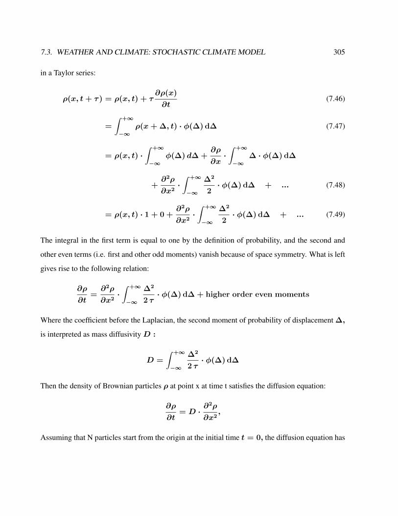
7.3. WEATHER AND CLIMATE: STOCHASTIC CLIMATE MODEL 305
in a Taylor series:
ρ(x, t+ τ ) = ρ(x, t) + τ∂ρ(x)
∂t(7.46)
=
∫ +∞
−∞ρ(x+ ∆, t) · φ(∆) d∆ (7.47)
= ρ(x, t) ·∫ +∞
−∞φ(∆) d∆ +
∂ρ
∂x·∫ +∞
−∞∆ · φ(∆) d∆
+∂2ρ
∂x2·∫ +∞
−∞
∆2
2· φ(∆) d∆ + ... (7.48)
= ρ(x, t) · 1 + 0 +∂2ρ
∂x2·∫ +∞
−∞
∆2
2· φ(∆) d∆ + ... (7.49)
The integral in the first term is equal to one by the definition of probability, and the second and
other even terms (i.e. first and other odd moments) vanish because of space symmetry. What is left
gives rise to the following relation:
∂ρ
∂t=∂2ρ
∂x2·∫ +∞
−∞
∆2
2 τ· φ(∆) d∆ + higher order even moments
Where the coefficient before the Laplacian, the second moment of probability of displacement ∆,
is interpreted as mass diffusivityD :
D =
∫ +∞
−∞
∆2
2 τ· φ(∆) d∆
Then the density of Brownian particles ρ at point x at time t satisfies the diffusion equation:
∂ρ
∂t= D ·
∂2ρ
∂x2,
Assuming that N particles start from the origin at the initial time t = 0, the diffusion equation has

306 CHAPTER 7. SIMPLE CLIMATE MODELS
the solution
ρ(x, t) =N
√4πDt
e−x2
4Dt .
This expression allowed Einstein to calculate the moments directly. The first moment is seen to
vanish, meaning that the Brownian particle is equally likely to move to the left as it is to move to
the right. The second moment is, however, non-vanishing, being given by
x2 = 2D t.
This expresses the mean squared displacement in terms of the time elapsed and the diffusivity.
From this expression Einstein argued that the displacement of a Brownian particle is not propor-
tional to the elapsed time, but rather to its square root. His argument is based on a conceptual
switch from the "ensemble" of Brownian particles to the "single" Brownian particle: we can speak
of the relative number of particles at a single instant just as well as of the time it takes a Brownian
particle to reach a given point.
This can be formalized as follows. The Wiener process is a continuous-time stochastic process
with stationary independent increments. The Wiener processWt is characterized by three facts:
• W0 = 0
• Wt is almost surely continuous
• Wt has independent increments with normal distribution Wt − Wt0 ∼ N(0, t − t0).
N(µ, σ2) denotes the normal distribution with expected value µ and variance σ2. The
condition that it has independent increments means that if then and are independent random
variables.
The Wiener process can be constructed as the scaling limit of a random walk, or other discrete-time
stochastic processes with stationary independent increments. It can be denoted as
var(Wt) = dW 2t = 2σ2t (7.50)
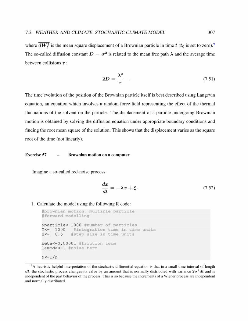
7.3. WEATHER AND CLIMATE: STOCHASTIC CLIMATE MODEL 307
where dW 2t is the mean square displacement of a Brownian particle in time t (t0 is set to zero).9
The so-called diffusion constant D = σ2 is related to the mean free path λ and the average time
between collisions τ :
2D =λ2
τ. (7.51)
The time evolution of the position of the Brownian particle itself is best described using Langevin
equation, an equation which involves a random force field representing the effect of the thermal
fluctuations of the solvent on the particle. The displacement of a particle undergoing Brownian
motion is obtained by solving the diffusion equation under appropriate boundary conditions and
finding the root mean square of the solution. This shows that the displacement varies as the square
root of the time (not linearly).
Exercise 57 – Brownian motion on a computer
Imagine a so-called red-noise process
dx
dt= −λx+ ξ . (7.52)
1. Calculate the model using the following R code:#brownian motion, multiple particle#forward modelling
Nparticle<-1000 #number of particlesT<- 1000 #integration time in time unitsh<- 0.5 #step size in time units
beta<-0.00001 #friction termlambda<-1 #noise term
N<-T/h
9A heuristic helpful interpretation of the stochastic differential equation is that in a small time interval of lengthdt, the stochastic process changes its value by an amount that is normally distributed with variance 2σ2dt and isindependent of the past behavior of the process. This is so because the increments of a Wiener process are independentand normally distributed.
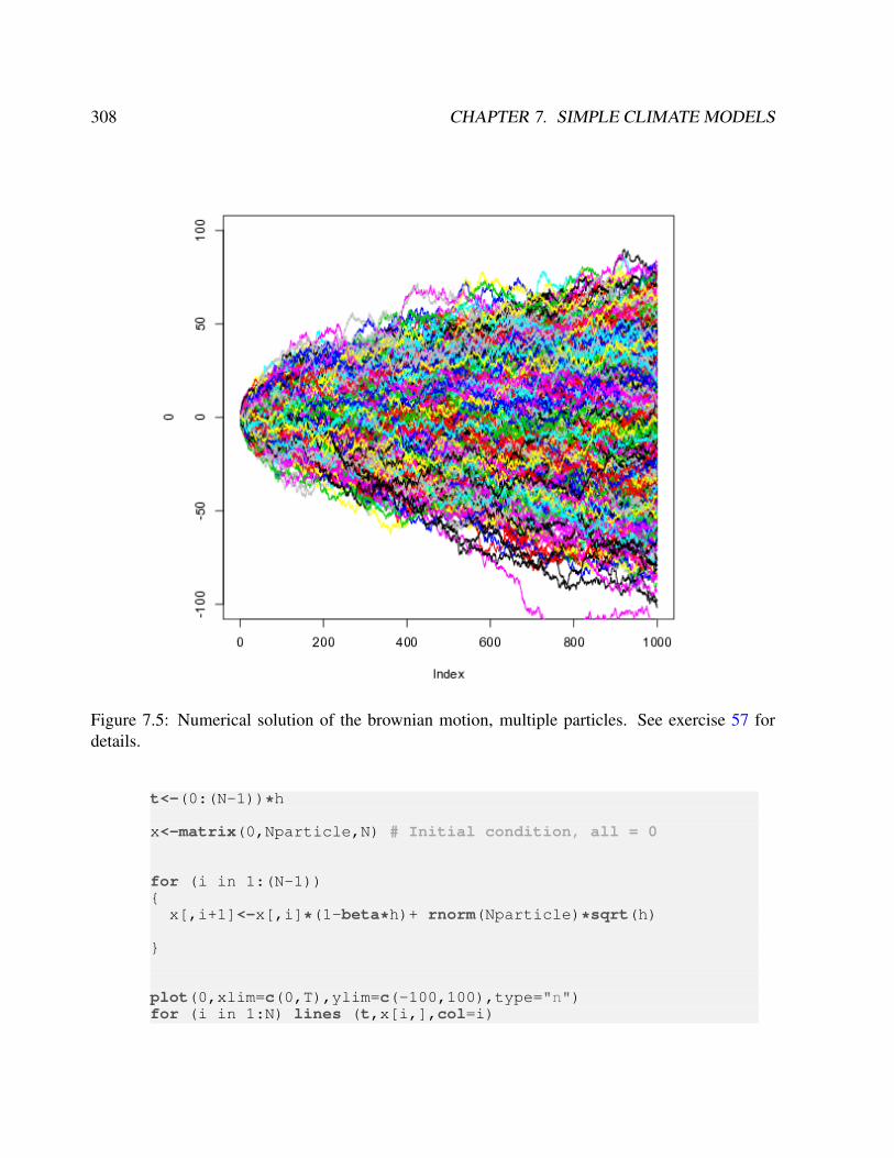
308 CHAPTER 7. SIMPLE CLIMATE MODELS
Figure 7.5: Numerical solution of the brownian motion, multiple particles. See exercise 57 fordetails.
t<-(0:(N-1))*h
x<-matrix(0,Nparticle,N) # Initial condition, all = 0
for (i in 1:(N-1))
x[,i+1]<-x[,i]*(1-beta*h)+ rnorm(Nparticle)*sqrt(h)
plot(0,xlim=c(0,T),ylim=c(-100,100),type="n")for (i in 1:N) lines (t,x[i,],col=i)
7.3. WEATHER AND CLIMATE: STOCHASTIC CLIMATE MODEL 309
#analyse the densitiesh<-matrix(0,N,40)
for (i in 1:(N-1)) h[i,]<-hist(x[,i],breaks=c((-20:20)*10),freq=FALSE,ylim=c(0,0.04))$counts
filled.contour(t,(-19:20)*10-5,h,color.palette=rainbow,xlab="time",ylab="space")
2. Show that the displacement varies as the square root of the time (not linearly).
7.3.2 Stochastic climate model
In a stochastic framework of climate theory one may use an appropriate stochastic differential
equation (Langevin equation)
d
dtx(t) = f(x) + g(x)ξ, (7.53)
where ξ = ddtW (t) is a stationary stochastic process and the functions f, g : Rn → Rn describe
the climate dynamics. The properties of the random force are described through its distribution
and its correlation properties at different times. The process ξ is assumed to have a Gaussian
distribution of zero average,
< ξ(t) >= 0 (7.54)
and to be δ-correlated in time,
< ξ(t)ξ(t+ τ ) >= δ(τ ) (7.55)
where δ is the delta function defined by
∫R
f(x) δ(x− x0) dx = f(x0) . (7.56)
310 CHAPTER 7. SIMPLE CLIMATE MODELS
The brackets indicate an average over realizations of the random force.10 For a Gaussian pro-
cess only the average and second moment need to be specified since all higher moments can be
expressed in terms of the first two. Note that the dependence of the correlation function on the
time difference τ assumes that ξ is a stationary process. ξ is called a white-noise process (for the
colors of noise: https://en.wikipedia.org/wiki/Colors_of_noise). In general,
the stochastic processes can be also described by the probablity distributions (3.19) which will be
considered later.
Additionally, there might be an external forcing F (x, t) which is generally time-, variable-,
and space-dependent. In his theoretical approach, Hasselmann [1976] formulated a linear stochas-
tic climate model
d
dtx(t) = Ax+ σξ + F (t) , (7.57)
with system matrixA ∈ Rn×n, constant noise term σ, and stochastic process ξ.Many features of
the climate system can be well described by (7.57), which is analogous to the Ornstein-Uhlenbeck
process in statistical physics [Uhlenbeck and Ornstein, 1930]. Notice that σξ represents a station-
ary random process. The relationship derived above is identical to that describing the diffusion of
a fluid particle in a turbulent fluid. In a time-scale separated system, during one slow-time unit the
fast uninteresting variables y perform many ’uncorrelated’ events (provided that the fast dynamics
are sufficiently chaotic). The contribution of the uncorrelated events to the dynamics of the slow
interesting variables x is as a sum of independent random variables. By the weak central limit theo-
rem this can be expressed by a normally distributed variable. Note, in the absence of any feedback
effectsAx, the climate variations would continue to grow indefinitely as the Wiener process.
10Formally: ξ(t) is a random variable, i.e. ξ(t)(α) with different realizations due to random variable α. Theexpectation < ξ(t) > is thus the mean over all α :< ξ(t)(α) >α. Using the ergodic hypothesis, the ensembleaverage 〈〉 can be expressed as the time average limT→∞
1T
∫ T/2−T/2 dt of the function. Almost all points in any
subset of the phase space eventually revisit the set. (https://en.wikipedia.org/wiki/Ergodic_theory
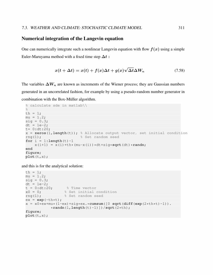
7.3. WEATHER AND CLIMATE: STOCHASTIC CLIMATE MODEL 311
Numerical integration of the Langevin equation
One can numerically integrate such a nonlinear Langevin equation with flow f(x) using a simple
Euler-Maruyama method with a fixed time step ∆t :
x(t+ ∆t) = x(t) + f(x)∆t+ g(x)√
∆t∆Wn (7.58)
The variables ∆Wn are known as increments of the Wiener process; they are Gaussian numbers
generated in an uncorrelated fashion, for example by using a pseudo-random number generator in
combination with the Box-Müller algorithm.% calculate sde in matlab\\%th = 1;mu = 1.2;sig = 0.3;dt = 1e-2;t= 0:dt:20;x = zeros(1,length(t)); % Allocate output vector, set initial conditionrng(1); % Set random seedfor i = 1:length(t)-1
x(i+1) = x(i)+th*(mu-x(i))*dt+sig*sqrt(dt)*randn;endfigure;plot(t,x);
and this is for the analytical solution:th = 1;mu = 1.2;sig = 0.3;dt = 1e-2;t = 0:dt:20; % Time vectorx0 = 0; % Set initial conditionrng(1); % Set random seedex = exp(-th*t);x = x0*ex+mu*(1-ex)+sig*ex.*cumsum([0 sqrt(diff(exp(2*th*t)-1)).
*randn(1,length(t)-1)])/sqrt(2*th);figure;plot(t,x);
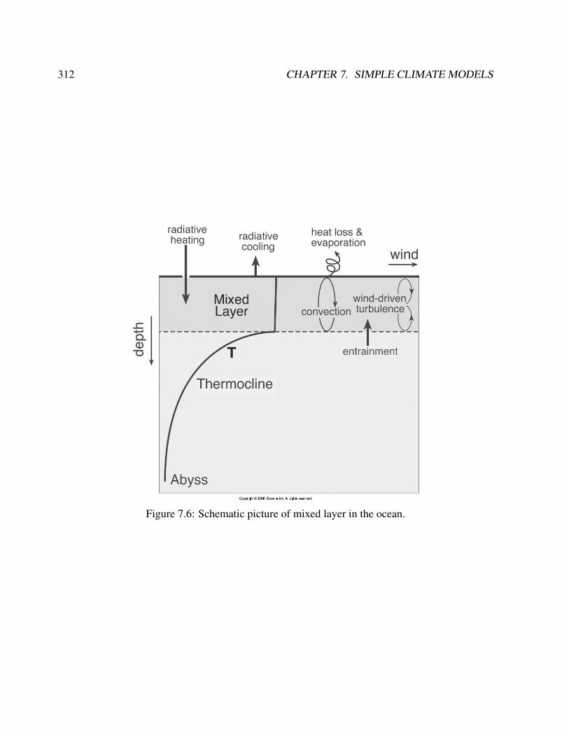
312 CHAPTER 7. SIMPLE CLIMATE MODELS
Figure 7.6: Schematic picture of mixed layer in the ocean.
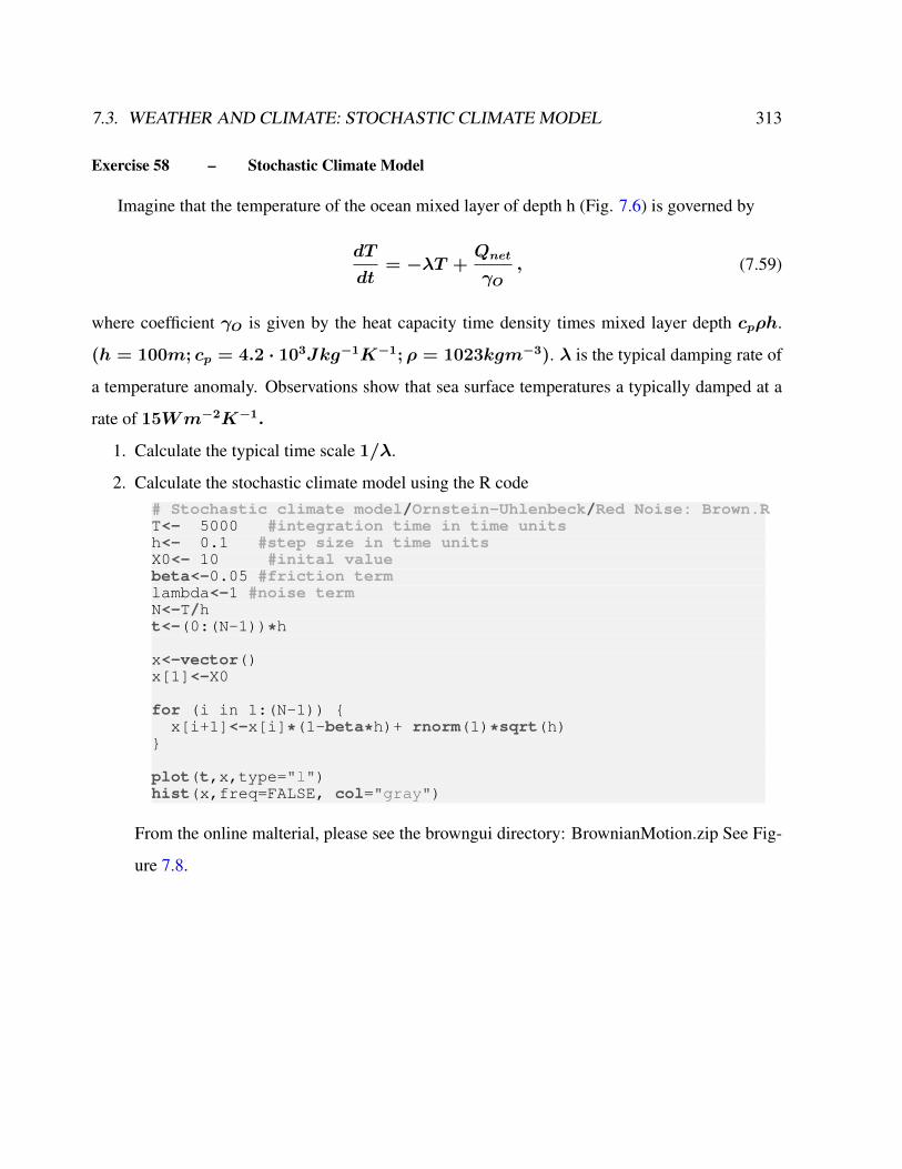
7.3. WEATHER AND CLIMATE: STOCHASTIC CLIMATE MODEL 313
Exercise 58 – Stochastic Climate Model
Imagine that the temperature of the ocean mixed layer of depth h (Fig. 7.6) is governed by
dT
dt= −λT +
Qnet
γO, (7.59)
where coefficient γO is given by the heat capacity time density times mixed layer depth cpρh.
(h = 100m; cp = 4.2 · 103Jkg−1K−1; ρ = 1023kgm−3). λ is the typical damping rate of
a temperature anomaly. Observations show that sea surface temperatures a typically damped at a
rate of 15Wm−2K−1.
1. Calculate the typical time scale 1/λ.
2. Calculate the stochastic climate model using the R code# Stochastic climate model/Ornstein-Uhlenbeck/Red Noise: Brown.RT<- 5000 #integration time in time unitsh<- 0.1 #step size in time unitsX0<- 10 #inital valuebeta<-0.05 #friction termlambda<-1 #noise termN<-T/ht<-(0:(N-1))*h
x<-vector()x[1]<-X0
for (i in 1:(N-1)) x[i+1]<-x[i]*(1-beta*h)+ rnorm(1)*sqrt(h)
plot(t,x,type="l")hist(x,freq=FALSE, col="gray")
From the online malterial, please see the browngui directory: BrownianMotion.zip See Fig-
ure 7.8.
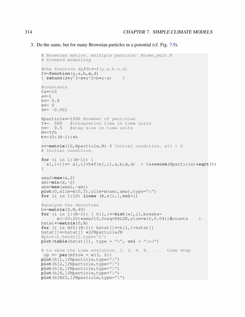
314 CHAPTER 7. SIMPLE CLIMATE MODELS
3. Do the same, but for many Brownian particles in a potential (cf. Fig. 7.9).
# Brownian motion, multiple particle: Brown_mult.R# forward modelling
#the function dy/dt<-f(y,a,b,c,d)f<-function(y,a,b,c,d) return(d*y^3+c*y^2+b*y-a)
#constantsCa<-10a<-1b<- 0.8c<- 0d<- -0.001
Nparticle<-1000 #number of particlesT<- 500 #integration time in time unitsh<- 0.5 #step size in time unitsN<-T/ht<-(0:(N-1))*h
x<-matrix(10,Nparticle,N) # Initial condition, all = 0# Initial condition,
for (i in 1:(N-1)) x[,i+1]<- x[,i]+h*f(x[,i],a,b,c,d) + Ca*rnorm(Nparticle)*sqrt(h)
ama2=max(x,2)ami=min(x,-2)ama=max(ama2,-ami)plot(0,xlim=c(0,T),ylim=c(ami,ama),type="n")for (i in 1:10) lines (t,x[i,],col=i)
#analyse the densitiesh<-matrix(0,N,40)for (i in 1:(N-1)) h[i,]<-hist(x[,i],breaks=
c(-20:20)*ama/10,freq=FALSE,ylim=c(0,0.04))$counts hstat<-matrix(0,N)for (i in N/2:(N-1)) hstat[]<-h[i,]+hstat[]hstat[]<-hstat[] *2/Nparticle/N#plot(t,hstat[],type="l")plot(table(hstat[]), type = "h", col = "red")
# to show the time evolution, 1, 2, 4, 8, .... time stepop <- par(mfrow = c(3, 2))plot(h[1,]/Nparticle,type="l")plot(h[2,]/Nparticle,type="l")plot(h[4,]/Nparticle,type="l")plot(h[8,]/Nparticle,type="l")plot(h[N/2,]/Nparticle,type="l")
7.3. WEATHER AND CLIMATE: STOCHASTIC CLIMATE MODEL 315
plot(h[N-1,]+h[N-2,]/Nparticle/2,type="l")
filled.contour(t,(-19:20)*ama/10-ama/20,h,color.palette=rainbow,xlab="time",ylab="space")
4. Calculate the stationary density from the numerical example analytically using∫f(y)dy.
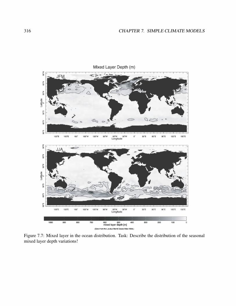
316 CHAPTER 7. SIMPLE CLIMATE MODELS
Figure 7.7: Mixed layer in the ocean distribution. Task: Describe the distribution of the seasonalmixed layer depth variations!
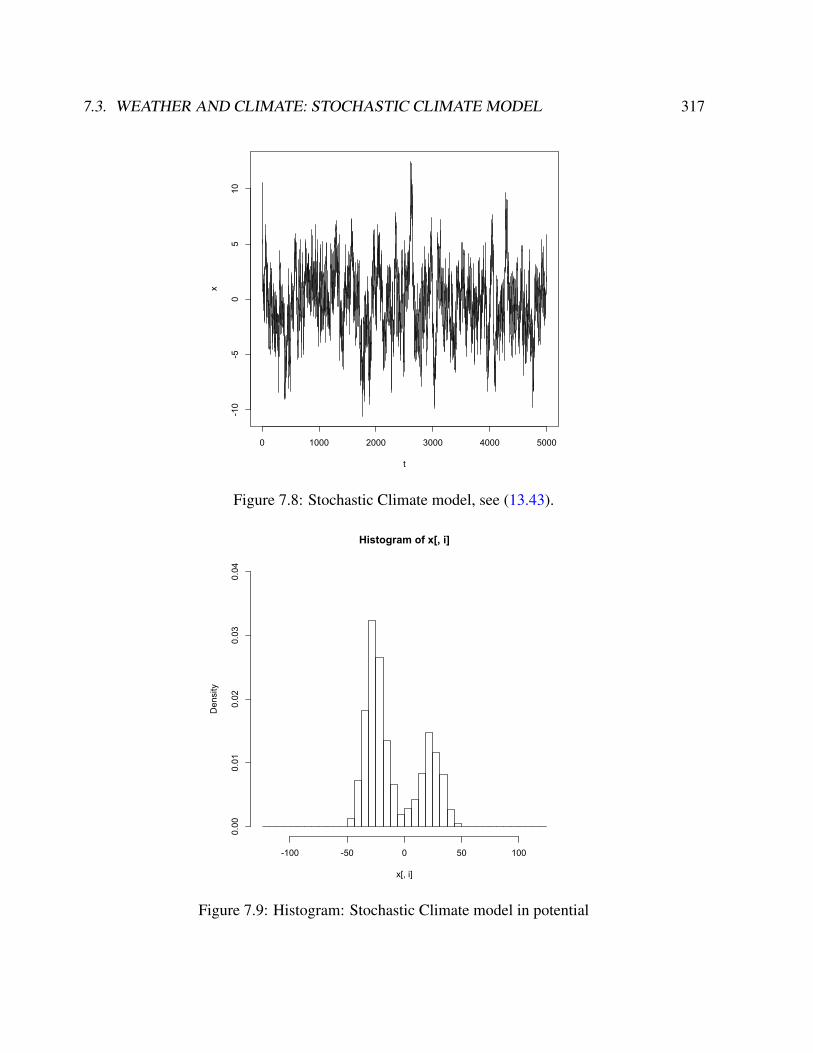
7.3. WEATHER AND CLIMATE: STOCHASTIC CLIMATE MODEL 317
0 1000 2000 3000 4000 5000
-10
-50
510
t
x
Figure 7.8: Stochastic Climate model, see (13.43).
Histogram of x[, i]
x[, i]
Density
-100 -50 0 50 100
0.00
0.01
0.02
0.03
0.04
Figure 7.9: Histogram: Stochastic Climate model in potential
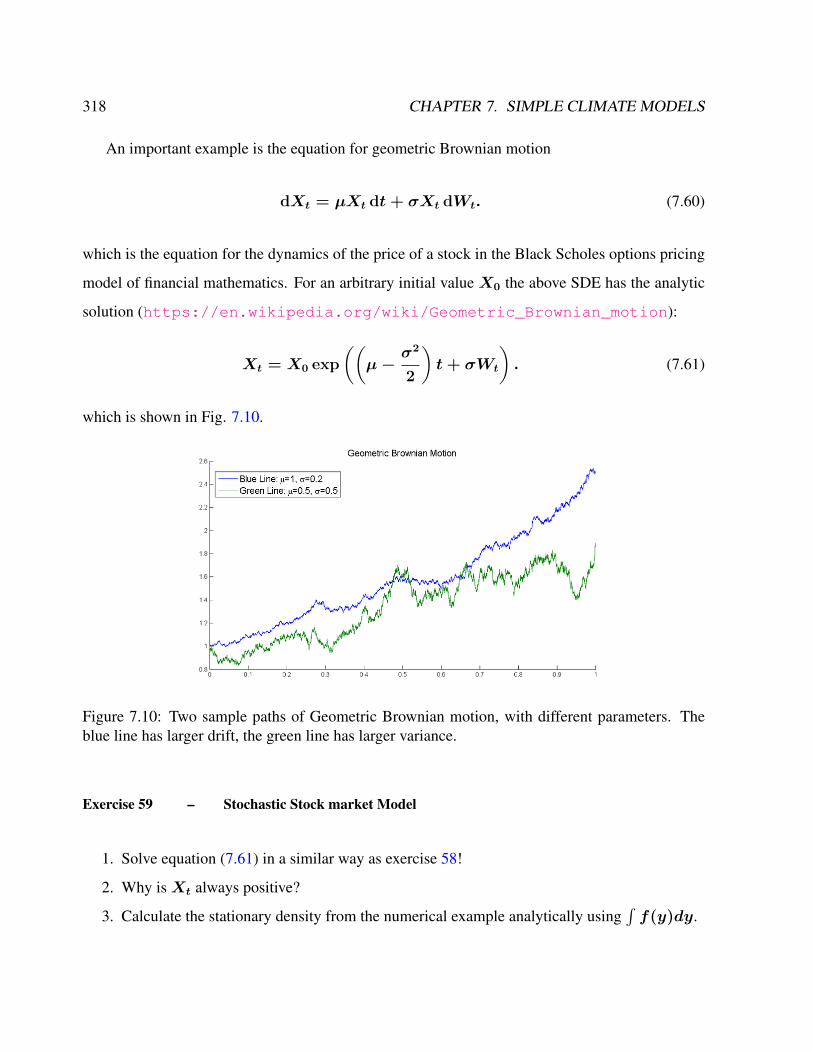
318 CHAPTER 7. SIMPLE CLIMATE MODELS
An important example is the equation for geometric Brownian motion
dXt = µXt dt+ σXt dWt. (7.60)
which is the equation for the dynamics of the price of a stock in the Black Scholes options pricing
model of financial mathematics. For an arbitrary initial value X0 the above SDE has the analytic
solution (https://en.wikipedia.org/wiki/Geometric_Brownian_motion):
Xt = X0 exp
((µ−
σ2
2
)t+ σWt
). (7.61)
which is shown in Fig. 7.10.
Figure 7.10: Two sample paths of Geometric Brownian motion, with different parameters. Theblue line has larger drift, the green line has larger variance.
Exercise 59 – Stochastic Stock market Model
1. Solve equation (7.61) in a similar way as exercise 58!
2. Why isXt always positive?
3. Calculate the stationary density from the numerical example analytically using∫f(y)dy.

7.3. WEATHER AND CLIMATE: STOCHASTIC CLIMATE MODEL 319
Exercise 60 – Spectrum of Stochastic Climate Model
Imagine that the temperature of the ocean mixed layer of depth h is governed by
dT
dt= −λT +
Qnet
γO, (7.62)
where coefficient γO is given by the heat capacity cpρh, and λ is the typical damping rate of a
temperature anomaly. The air-sea fluxes due to weather systems are represented by a white-noise
process Qnet = Qωeiωt where Qω is the amplitude of the random forcing at frequency ω and
Q∗ is the complex conjugate. Remember that Qnet can be described through its distribution and
its correlation properties: a Gaussian distribution of zero average< Qnet >= 0 and δ-correlated
in time < Qnet(t)Qnet(t + τ ) >= δ(τ ) The brackets indicate an average over realizations of
the random force. The spectrum of a process x is defined as
S(ω) := 〈xx∗〉 = Covx(τ ) =
∫R
exp(iωτ )Covx(τ )dτ (7.63)
1. Calculate SQ(ω) and describe whyQnet is called a white noise process.
2. Solve Eq. 7.62 for the temperature response T = Tωeiωt and hence show that:
Tω =Qω
γO (λ+ iω)(7.64)
3. Show that it has a spectral density TωT ∗ω is given by:
T T ∗ =QQ∗
γ2O (λ2 + ω2)
(7.65)
and the spectrum
S(ω) =< T T ∗ >=1
γ2O (λ2 + ω2)
. (7.66)
The brackets < · · · > denote the ensemble mean. Make a sketch of the spectrum using a
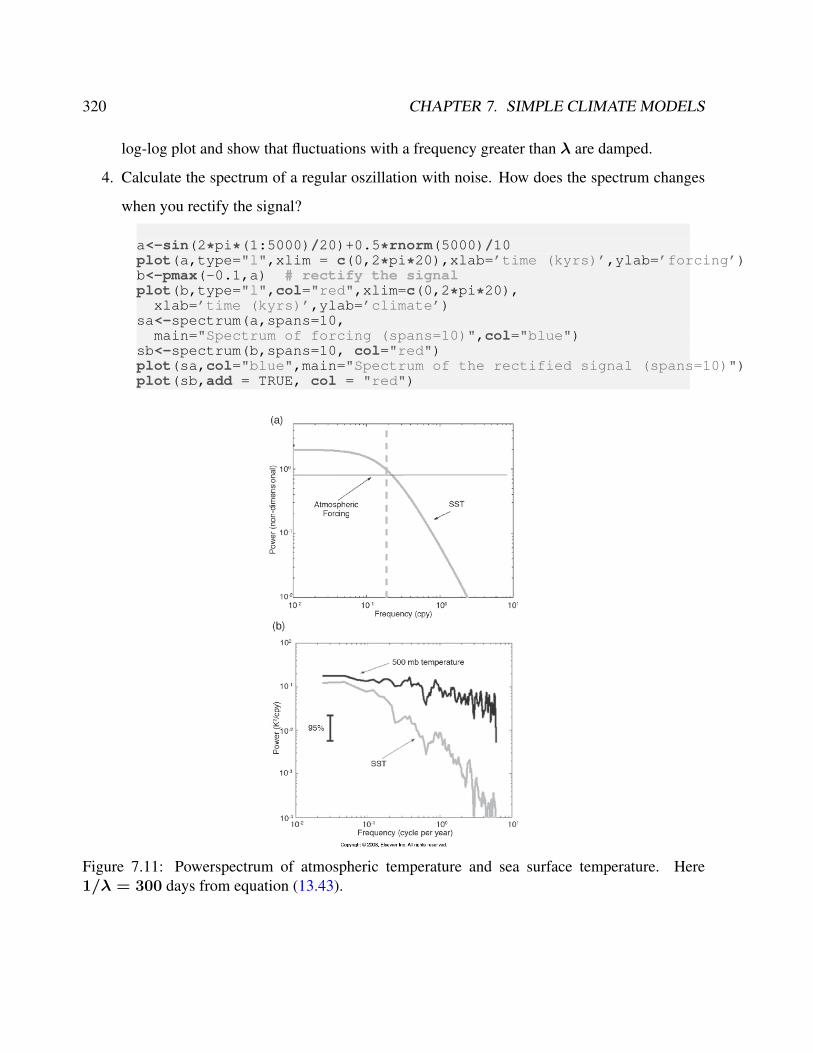
320 CHAPTER 7. SIMPLE CLIMATE MODELS
log-log plot and show that fluctuations with a frequency greater than λ are damped.
4. Calculate the spectrum of a regular oszillation with noise. How does the spectrum changes
when you rectify the signal?
a<-sin(2*pi*(1:5000)/20)+0.5*rnorm(5000)/10plot(a,type="l",xlim = c(0,2*pi*20),xlab=’time (kyrs)’,ylab=’forcing’)b<-pmax(-0.1,a) # rectify the signalplot(b,type="l",col="red",xlim=c(0,2*pi*20),
xlab=’time (kyrs)’,ylab=’climate’)sa<-spectrum(a,spans=10,
main="Spectrum of forcing (spans=10)",col="blue")sb<-spectrum(b,spans=10, col="red")plot(sa,col="blue",main="Spectrum of the rectified signal (spans=10)")plot(sb,add = TRUE, col = "red")
Figure 7.11: Powerspectrum of atmospheric temperature and sea surface temperature. Here1/λ = 300 days from equation (13.43).
7.3. WEATHER AND CLIMATE: STOCHASTIC CLIMATE MODEL 321
Exercise 61 – Climate sensitivity and variability in the Stochastic Climate Model
As in exercise 60, imagine that the temperature of the ocean mixed layer of depth h is governed
bydT
dt= −λT +Qnet + f(t) , (7.67)
where the air-sea fluxes due to weather systems are represented by a white-noise process with
zero average < Qnet >= 0 and δ-correlated in time < Qnet(t)Qnet(t + τ ) >= δ(τ ). The
function f(t) is a time dependent deterministic forcing. Assume furthermore that f(t) = c ·u(t)
with u(t) as unit step or the so-called Heaviside step function and solve (13.48). What is the
relationship of the dissipation (through λ ) and the fluctuations (through the spectrum S(ω)) ?
Solution
SinceQ(t) is a stochastic process, it has to be solved for the moments. Because< Qnet >=
0,< T (t) > can be solved using the Laplace transform:
< T (t) > = L−1F (s)(t) = L−1
< T (0) >
s+ λ+c
s·
1
s+ λ
(7.68)
= T (0) · exp(−λt) +c
λ(1− exp(−λt)) (7.69)
because we have< T (0) >= T (0). As equilibrium response, we have
∆T = limt→∞
< T (t) >=c
λ. (7.70)
The fluctuation can be characterized by the spectrum (exercise 60)
S(ω) =< T T ∗ >=1
λ2 + ω2. (7.71)
and therefore, the spectrum and the equilibrium response are closely coupled (fluctuation-dissipation
theorem).
322 CHAPTER 7. SIMPLE CLIMATE MODELS
For some energy considerations, it is usefull to re-write equation (13.48) as
CdT
dt= −λCT + fC , (7.72)
withC = cpρdz as the heat capacity of the ocean. For a depth of 200 m of water distributed over
the globe,C = 4.2·103Wskg−1K−1×1000 kgm−3×200m = 8.4·108Wsm−2K−1 .
The temperature evolution is
T (t) = T (0) · exp(−λc/C t) +fC
λC(1− exp(−λC/C t)) (7.73)
The left hand side of (7.72) represents the heat uptake by the ocean, which plays a central role in
the transient response of the system to a perturbation (7.73).
Typical changes in fC are 4Wm−2 for doubling of CO2, λC = 1 − 2Wm−2K−1. The
typical time scale for a mixed layer ocean isC/λC = 13−26 years . Please note that the climate
system is simplified by a slab ocean with homogenous temperature and heat capacity. This is an
approximation as the heat capacity should vary in time as the perturbation penetrates to deeper
oceanic levels.
The equilibrium temperature change ∆T is
∆T =∆fC
λC=c
λ(7.74)
with values of ∆T = 2 − 4 K. The term CS = 1λC
is called climate sensitivity to a radiative
forcing ∆fC :
∆T = CS · ∆fC . (7.75)
In the literature, the concept of climate sensitivity is quite often used as the equilibrium temperature
increase for a forcing ∆fC related to doubling of CO2.

7.3. WEATHER AND CLIMATE: STOCHASTIC CLIMATE MODEL 323
Exercise 62 – Stochastic differential equation
Tasks:
1. Simulate the velocity evolution of one particle which is determined by the following stochas-
tic dv/dt = −b ∗ v + k ∗ dW (t)/dt
2. What happens if you change the timestep?
3. Simulate the ensemble of multiple particles, plot the time evolution of the v-Distribution
4. Test the ergodic theorem: time average = ensemble average
Solution#brownian motion, one particle
T<- 5000 #integration time in time unitsh<- 0.1 #step size in time unitsX0<- 10 #inital value
beta<-0.05 #friction termlambda<-1 #noise term
N<-T/ht<-(0:(N-1))*h
x<-vector()x[1]<-X0
for (i in 1:(N-1))
x[i+1]<-x[i]*(1-beta*h)+ rnorm(1)*sqrt(h)
plot(t,x,type="l")# dev.print(postscript, file="random.ps")#hist(x)#hist(x,freq=FALSE, col="gray")
Solution brownian motion, multiple particle#brownian motion, multiple particle#forward modelling
#the function dy/dt<-f(y,a,b,c,d)# double well potential
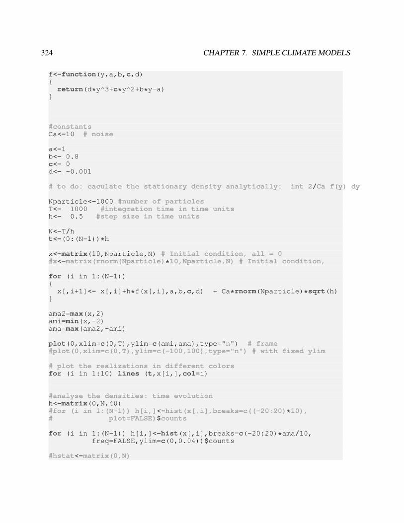
324 CHAPTER 7. SIMPLE CLIMATE MODELS
f<-function(y,a,b,c,d)
return(d*y^3+c*y^2+b*y-a)
#constantsCa<-10 # noise
a<-1b<- 0.8c<- 0d<- -0.001
# to do: caculate the stationary density analytically: int 2/Ca f(y) dy
Nparticle<-1000 #number of particlesT<- 1000 #integration time in time unitsh<- 0.5 #step size in time units
N<-T/ht<-(0:(N-1))*h
x<-matrix(10,Nparticle,N) # Initial condition, all = 0#x<-matrix(rnorm(Nparticle)*10,Nparticle,N) # Initial condition,
for (i in 1:(N-1))
x[,i+1]<- x[,i]+h*f(x[,i],a,b,c,d) + Ca*rnorm(Nparticle)*sqrt(h)
ama2=max(x,2)ami=min(x,-2)ama=max(ama2,-ami)
plot(0,xlim=c(0,T),ylim=c(ami,ama),type="n") # frame#plot(0,xlim=c(0,T),ylim=c(-100,100),type="n") # with fixed ylim
# plot the realizations in different colorsfor (i in 1:10) lines (t,x[i,],col=i)
#analyse the densities: time evolutionh<-matrix(0,N,40)#for (i in 1:(N-1)) h[i,]<-hist(x[,i],breaks=c((-20:20)*10),# plot=FALSE)$counts
for (i in 1:(N-1)) h[i,]<-hist(x[,i],breaks=c(-20:20)*ama/10,freq=FALSE,ylim=c(0,0.04))$counts
#hstat<-matrix(0,N)
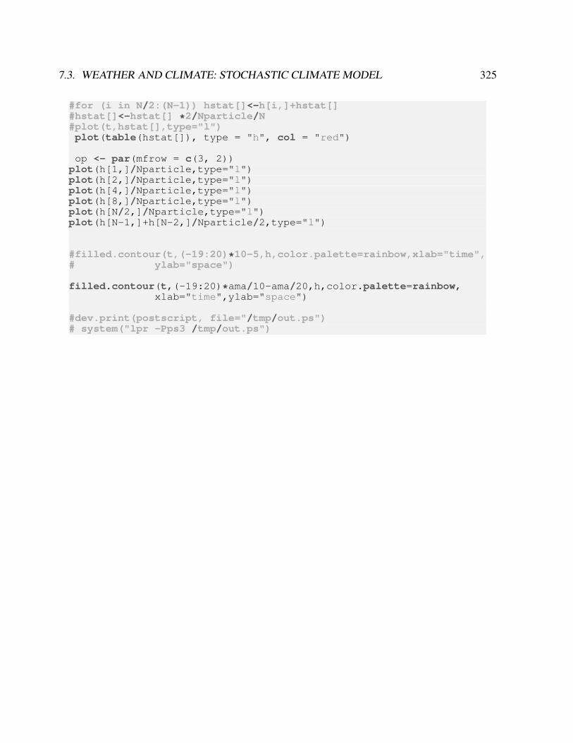
7.3. WEATHER AND CLIMATE: STOCHASTIC CLIMATE MODEL 325
#for (i in N/2:(N-1)) hstat[]<-h[i,]+hstat[]#hstat[]<-hstat[] *2/Nparticle/N#plot(t,hstat[],type="l")plot(table(hstat[]), type = "h", col = "red")
op <- par(mfrow = c(3, 2))plot(h[1,]/Nparticle,type="l")plot(h[2,]/Nparticle,type="l")plot(h[4,]/Nparticle,type="l")plot(h[8,]/Nparticle,type="l")plot(h[N/2,]/Nparticle,type="l")plot(h[N-1,]+h[N-2,]/Nparticle/2,type="l")
#filled.contour(t,(-19:20)*10-5,h,color.palette=rainbow,xlab="time",# ylab="space")
filled.contour(t,(-19:20)*ama/10-ama/20,h,color.palette=rainbow,xlab="time",ylab="space")
#dev.print(postscript, file="/tmp/out.ps")# system("lpr -Pps3 /tmp/out.ps")
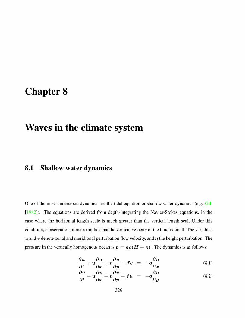
Chapter 8
Waves in the climate system
8.1 Shallow water dynamics
One of the most understood dynamics are the tidal equation or shallow water dynamics (e.g. Gill
[1982]). The equations are derived from depth-integrating the Navier-Stokes equations, in the
case where the horizontal length scale is much greater than the vertical length scale.Under this
condition, conservation of mass implies that the vertical velocity of the fluid is small. The variables
u and v denote zonal and meridional perturbation flow velocity, and η the height perturbation. The
pressure in the vertically homogenous ocean is p = gρ(H + η) . The dynamics is as follows:
∂u
∂t+ u
∂u
∂x+ v
∂u
∂y− fv = −g
∂η
∂x(8.1)
∂v
∂t+ u
∂v
∂x+ v
∂v
∂y+ fu = −g
∂η
∂y(8.2)
326
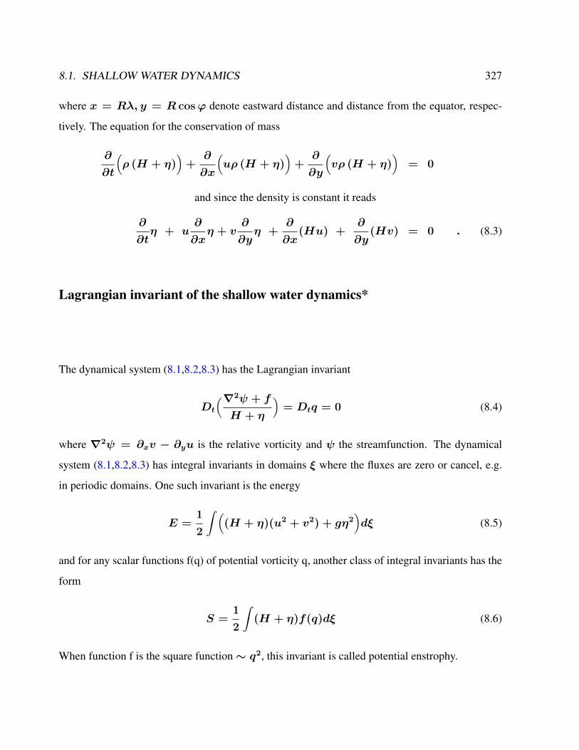
8.1. SHALLOW WATER DYNAMICS 327
where x = Rλ, y = R cosϕ denote eastward distance and distance from the equator, respec-
tively. The equation for the conservation of mass
∂
∂t
(ρ (H + η)
)+
∂
∂x
(uρ (H + η)
)+
∂
∂y
(vρ (H + η)
)= 0
and since the density is constant it reads
∂
∂tη + u
∂
∂xη + v
∂
∂yη +
∂
∂x(Hu) +
∂
∂y(Hv) = 0 . (8.3)
Lagrangian invariant of the shallow water dynamics*
The dynamical system (8.1,8.2,8.3) has the Lagrangian invariant
Dt
(∇2ψ + f
H + η
)= Dtq = 0 (8.4)
where ∇2ψ = ∂xv − ∂yu is the relative vorticity and ψ the streamfunction. The dynamical
system (8.1,8.2,8.3) has integral invariants in domains ξ where the fluxes are zero or cancel, e.g.
in periodic domains. One such invariant is the energy
E =1
2
∫ ((H + η)(u2 + v2) + gη2
)dξ (8.5)
and for any scalar functions f(q) of potential vorticity q, another class of integral invariants has the
form
S =1
2
∫(H + η)f(q)dξ (8.6)
When function f is the square function∼ q2, this invariant is called potential enstrophy.
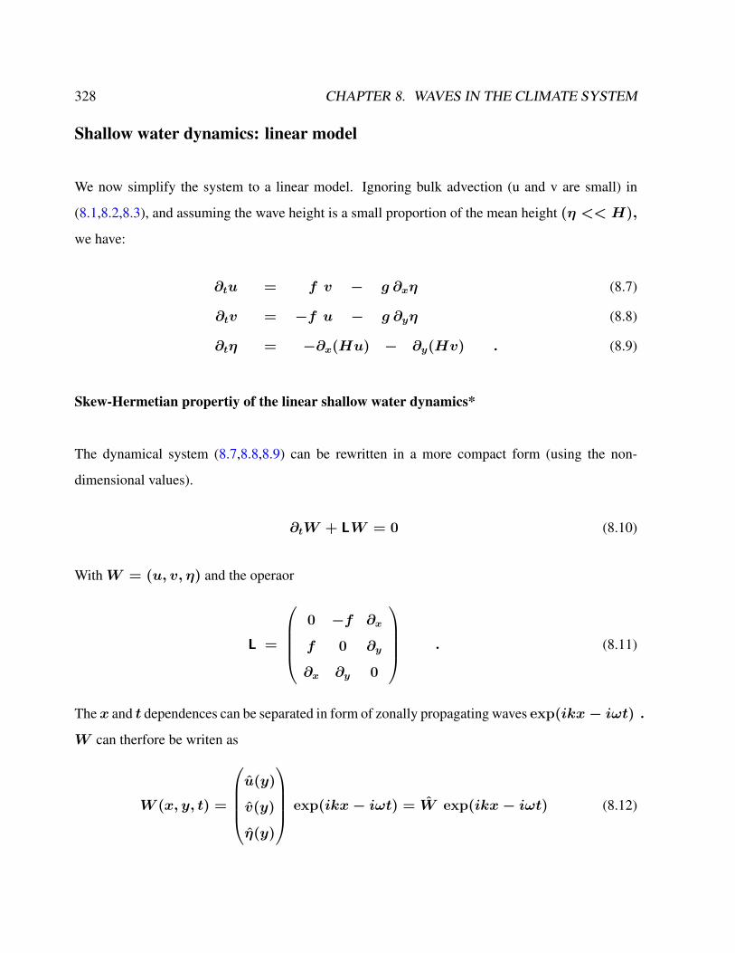
328 CHAPTER 8. WAVES IN THE CLIMATE SYSTEM
Shallow water dynamics: linear model
We now simplify the system to a linear model. Ignoring bulk advection (u and v are small) in
(8.1,8.2,8.3), and assuming the wave height is a small proportion of the mean height (η << H),
we have:
∂tu = f v − g ∂xη (8.7)
∂tv = −f u − g ∂yη (8.8)
∂tη = −∂x(Hu) − ∂y(Hv) . (8.9)
Skew-Hermetian propertiy of the linear shallow water dynamics*
The dynamical system (8.7,8.8,8.9) can be rewritten in a more compact form (using the non-
dimensional values).
∂tW + LW = 0 (8.10)
WithW = (u, v, η) and the operaor
L =
0 −f ∂x
f 0 ∂y
∂x ∂y 0
. (8.11)
Thex and t dependences can be separated in form of zonally propagating waves exp(ikx− iωt) .
W can therfore be writen as
W (x, y, t) =
u(y)
v(y)
η(y)
exp(ikx− iωt) = W exp(ikx− iωt) (8.12)

8.1. SHALLOW WATER DYNAMICS 329
This leads to an eigenvalue problem
−iωW (k, y) + LW (k, y) = 0 (8.13)
where
L =
0 −f ik
f 0 ∂y
ik ∂y 0
. (8.14)
The adjoint of L with respect to the inner product is the operator L+
(transpose and conjugate):
L+
=
0 f −ik
−f 0 ∂y
−ik ∂y 0
. (8.15)
The operator L is skew-Hermetian, as the adjoint of L is L+
= −L (8.15). For two arbitrary
vector functionsW1,W2 one can define a scalar product:
(LW1,W2) =
∫ ∞−∞
LW1 ·W ∗2 dy = (W1,−LW2) = (W1, L
+W2) (8.16)
with the symbol ∗ being the conjugate.
The skew-Hermetian property dictates that the eigenvalues of L are purely imaginary, so that
we have a mathematical basis for looking for wave-like solutions. In addition, the eigenfunctions
form a complete orthogonal set for the functions W satisfying (W,W ) < ∞ . This is because
L is normal:
LL+
= L+L . (8.17)

330 CHAPTER 8. WAVES IN THE CLIMATE SYSTEM
Furthermore, L in (8.14) belongs to the unitary group U(3), forming a compact connected Lie
group and has the special property det(L) = 0.
These considerations provide the mathematical framework for wave studies. Analytical work
is presented in section 8.5 in the case of equatorial wave dynamics. The dynamical system
(8.7,8.8,8.9) contains already the zoo of waves. Here, we give a short description. In the exer-
cises, these waves are numerically solved.
Exercise 63 – Energy conservation
Show that the dynamical system (8.1,8.2,8.3) has integral invariants in domains ξ where the
fluxes are zero or cancel, e.g. in periodic domains. One such invariant is the energy
E =1
2
∫ ((H + η)(u2 + v2) + gη2
)dξ (8.18)
and for any scalar functions f(q) of potential vorticity q, another class of integral invariants has the
form
S =1
2
∫(H + η)f(q)dξ (8.19)
8.2. PLANETARY WAVES ON THE COMPUTER 331
8.2 Planetary waves on the computer
Rossby (or planetary) waves are giant meanders in high-altitude winds that are a major influence
on weather. They are easy to observe as (usually 4-6) large-scale meanders of the jet stream. When
these loops become very pronounced, they detach the masses of cold, or warm, air that become
cyclones and anticyclones and are responsible for day-to-day weather patterns at mid-latitudes.
Their emergence is due to shear in rotating fluids, so that the Coriolis force changes along the
sheared coordinate.1 In planetary atmospheres, they are due to the variation in the Coriolis effect
with latitude. The waves were first identified in the Earth’s atmosphere by Rossby [1939]. The
terms "barotropic" and "baroclinic" Rossby waves are used to distinguish their vertical structure.
Barotropic Rossby waves do not vary in the vertical, and have the fastest propagation speeds.
The baroclinic wave modes are slower, with speeds of only a few centimetres per second or less
(atmosphere).
Oceanic Rossby waves are thought to communicate climatic changes due to variability in forc-
ing, due to both the wind and buoyancy. Both barotropic and baroclinic waves cause variations
of the sea surface height, although the length of the waves made them difficult to detect until the
advent of satellite altimetry [Chelton and Schlax, 1996]. Baroclinic waves also generate signifi-
cant displacements of the oceanic thermocline, often of tens of meters. Satellite observations have
revealed the stately progression of Rossby waves across all the ocean basins, particularly at low-
and mid-latitudes. These waves can take months or even years to cross a basin like the Pacific.
The first order equations of motion into an appropriate wave equation is cumbersome, namely
because the two-dimensional geometry of the spherical surface is non-Euclidean (the Coriolis ef-
fect depends on the latitude). It can be shown [Müller et al., 1994; Müller and O’Brien, 1995;
1The dynamics in an inertial reference frame, e.g. with a coordinate system fixed at the Sun, would not havea Coriolis force, but would certainly observe Rossby wave propagation. In the inertial system, the near-equatorialmotion is seen to be faster than off the equator. Zero vorticity in the rotating Earth’s coordinate system correspondsto a basic flow with non-zero vorticity flow (zonal velocity U = RΩ cosϕ ) (ϕ: latitude) in the inertial referenceframe [Müller and Maier-Reimer, 2000]. Linearizing the dynamics in the non-rotating system around the basic stateU yields exactly Matsuno’s wave equations taking the partial substantial derivative with advection U. Therefore, theeffect of Earth’s rotation is formally equivalent to a shear flow system. The mean flow energy is supplied by the Earth’srotation.
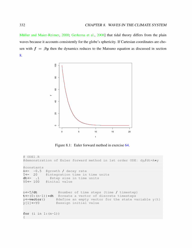
332 CHAPTER 8. WAVES IN THE CLIMATE SYSTEM
Müller and Maier-Reimer, 2000; Gerkema et al., 2008] that tidal theory differs from the plain
waves because it accounts consistently for the globe’s sphericity. If Cartesian coordinates are cho-
sen with f = βy then the dynamics reduces to the Matsuno equation as discussed in section
8.
0 5 10 15 20
020
4060
80100
t
y
Figure 8.1: Euler forward method in exercise 64.
# ODE1.R#demonstration of Euler forward method in 1st order ODE: dy/dt=A*y
#constantsA<- -0.5 #growth / decay rateT<- 20 #integration time in time unitsdt<- .1 #step size in time unitsY0<- 100 #inital value
n<-T/dt #number of time steps (time / timestep)t<-(0:(n-1))*dt #create a vector of discrete timestepsy<-vector() #define an empty vector for the state variable y(t)y[1]<-Y0 #assign initial value
for (i in 1:(n-1))
8.2. PLANETARY WAVES ON THE COMPUTER 333
y[i+1]<-y[i]+dt*A*y[i]
plot(t,y,type="l") #plot the result against time
#additionaly plot the analytical solution in redlines(t,Y0*exp(A*t),col="red")
Exercise 64 – Euler numerical scheme
Demonstration of the Euler forward scheme on the first order ODE: dy/dt=A*y
• Describe one physical process which can be described with this ODE
• Write the analytic solution for this ODE
• Write the ODE as finite differences
• Open the program ODE1.R and try roughly to understand the code (where is the integration?)
• Run the code and compare the numerical results with the analytic ones.
Exercise 65 – Numerical solution of 1D Diffusion
• What is the differential equation for the 1D Diffusion
• Open DiffusionEulerForward.R
• Identify / extract the finite difference scheme which is used approximate the 2nd derivative
• Run the program and play with the parameters#Diffusion_EulerForward.R# 1D diffusion equation, explicit scheme
#ConstantsL.X<-50 #width of latticeL.T<-5 #length of timedx <- 1 #space stepdt <- 0.1 #time stepD<-1 #Diffusion coefficent
N.x<-L.X/dx + 2 #number of space boxes + 2 boundary boxesN.t<-L.T/dt #number of time boxes
u<-matrix(0,N.t,N.x) #grid#temporary vector which stores the state of of one timestep:u.temp<-rep(0,N.x)
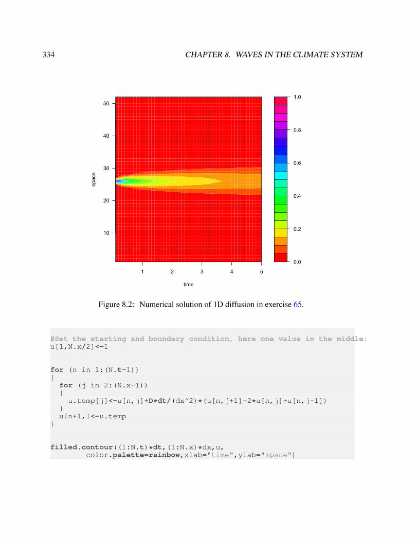
334 CHAPTER 8. WAVES IN THE CLIMATE SYSTEM
0.0
0.2
0.4
0.6
0.8
1.0
1 2 3 4 5
10
20
30
40
50
time
space
Figure 8.2: Numerical solution of 1D diffusion in exercise 65.
#Set the starting and boundary condition, here one value in the middle:u[1,N.x/2]<-1
for (n in 1:(N.t-1))
for (j in 2:(N.x-1))u.temp[j]<-u[n,j]+D*dt/(dx^2)*(u[n,j+1]-2*u[n,j]+u[n,j-1])
u[n+1,]<-u.temp
filled.contour((1:N.t)*dt,(1:N.x)*dx,u,color.palette=rainbow,xlab="time",ylab="space")
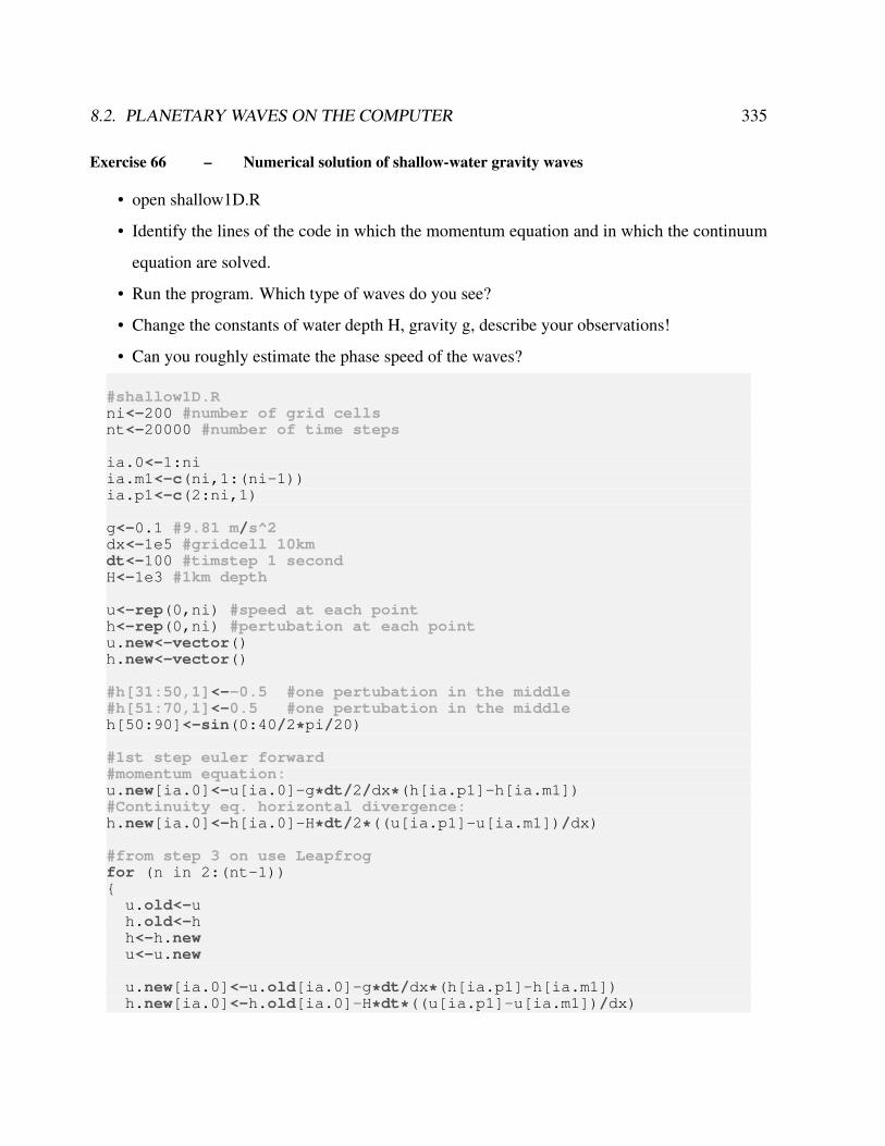
8.2. PLANETARY WAVES ON THE COMPUTER 335
Exercise 66 – Numerical solution of shallow-water gravity waves
• open shallow1D.R
• Identify the lines of the code in which the momentum equation and in which the continuum
equation are solved.
• Run the program. Which type of waves do you see?
• Change the constants of water depth H, gravity g, describe your observations!
• Can you roughly estimate the phase speed of the waves?
#shallow1D.Rni<-200 #number of grid cellsnt<-20000 #number of time steps
ia.0<-1:niia.m1<-c(ni,1:(ni-1))ia.p1<-c(2:ni,1)
g<-0.1 #9.81 m/s^2dx<-1e5 #gridcell 10kmdt<-100 #timstep 1 secondH<-1e3 #1km depth
u<-rep(0,ni) #speed at each pointh<-rep(0,ni) #pertubation at each pointu.new<-vector()h.new<-vector()
#h[31:50,1]<--0.5 #one pertubation in the middle#h[51:70,1]<-0.5 #one pertubation in the middleh[50:90]<-sin(0:40/2*pi/20)
#1st step euler forward#momentum equation:u.new[ia.0]<-u[ia.0]-g*dt/2/dx*(h[ia.p1]-h[ia.m1])#Continuity eq. horizontal divergence:h.new[ia.0]<-h[ia.0]-H*dt/2*((u[ia.p1]-u[ia.m1])/dx)
#from step 3 on use Leapfrogfor (n in 2:(nt-1))
u.old<-uh.old<-hh<-h.newu<-u.new
u.new[ia.0]<-u.old[ia.0]-g*dt/dx*(h[ia.p1]-h[ia.m1])h.new[ia.0]<-h.old[ia.0]-H*dt*((u[ia.p1]-u[ia.m1])/dx)
336 CHAPTER 8. WAVES IN THE CLIMATE SYSTEM
# modulo operator, smoothing every 10 time stepsif ((n%%10)==0) u.new[ia.0]<-(u.new[ia.0]+u[ia.0])/2
h.new[ia.0]<-(h.new[ia.0]+h[ia.0])/2
# modulo operator: plottingif ((n%%101)==0)par(ask = TRUE) # to make a breakplot(h,type="l",lwd=2,ylim=c(-1,1))
############
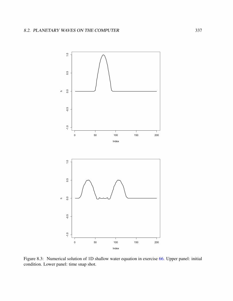
8.2. PLANETARY WAVES ON THE COMPUTER 337
0 50 100 150 200
-1.0
-0.5
0.0
0.5
1.0
Index
h
0 50 100 150 200
-1.0
-0.5
0.0
0.5
1.0
Index
h
Figure 8.3: Numerical solution of 1D shallow water equation in exercise 66. Upper panel: initialcondition. Lower panel: time snap shot.
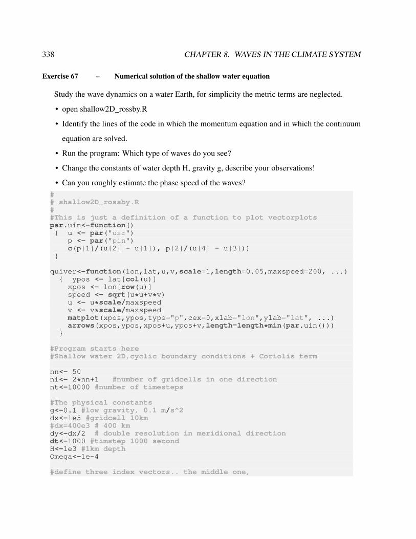
338 CHAPTER 8. WAVES IN THE CLIMATE SYSTEM
Exercise 67 – Numerical solution of the shallow water equation
Study the wave dynamics on a water Earth, for simplicity the metric terms are neglected.
• open shallow2D_rossby.R
• Identify the lines of the code in which the momentum equation and in which the continuum
equation are solved.
• Run the program: Which type of waves do you see?
• Change the constants of water depth H, gravity g, describe your observations!
• Can you roughly estimate the phase speed of the waves?## shallow2D_rossby.R##This is just a definition of a function to plot vectorplotspar.uin<-function() u <- par("usr")
p <- par("pin")c(p[1]/(u[2] - u[1]), p[2]/(u[4] - u[3]))
quiver<-function(lon,lat,u,v,scale=1,length=0.05,maxspeed=200, ...) ypos <- lat[col(u)]xpos <- lon[row(u)]speed <- sqrt(u*u+v*v)u <- u*scale/maxspeedv <- v*scale/maxspeedmatplot(xpos,ypos,type="p",cex=0,xlab="lon",ylab="lat", ...)arrows(xpos,ypos,xpos+u,ypos+v,length=length*min(par.uin()))
#Program starts here#Shallow water 2D,cyclic boundary conditions + Coriolis term
nn<- 50ni<- 2*nn+1 #number of gridcells in one directionnt<-10000 #number of timesteps
#The physical constantsg<-0.1 #low gravity, 0.1 m/s^2dx<-1e5 #gridcell 10km#dx=400e3 # 400 kmdy<-dx/2 # double resolution in meridional directiondt<-1000 #timstep 1000 secondH<-1e3 #1km depthOmega<-1e-4
#define three index vectors.. the middle one,
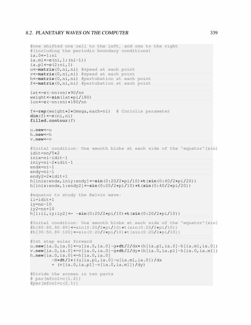
8.2. PLANETARY WAVES ON THE COMPUTER 339
#one shifted one cell to the left, and one to the right#(including the periodic boundary conditions)ia.0<-1:niia.m1<-c(ni,1:(ni-1))ia.p1<-c(2:ni,1)u<-matrix(0,ni,ni) #speed at each pointv<-matrix(0,ni,ni) #speed at each pointh<-matrix(0,ni,ni) #pertubation at each pointf<-matrix(0,ni,ni) #pertubation at each point
lat<-c(-nn:nn)*90/nnweight<-sin(lat*pi/180)lon<-c(-nn:nn)*180/nn
f<-rep(weight*2*Omega,each=ni) # Coriolis parameterdim(f)<-c(ni,ni)filled.contour(f)
u.new<-uh.new<-hv.new<-v
#Inital condition: One smooth blobs at each side of the "equator"(sin)idit=nn/5*2inix=ni-idit-1iniy=ni-2*idit-1endx=ni-1endy=ni-1endy2=2*idit+1h[inix:endx,iniy:endy]<-sin(0:20/2*pi/10)*t(sin(0:40/2*pi/20))h[inix:endx,1:endy2]<-sin(0:20/2*pi/10)*t(sin(0:40/2*pi/20))
#equator to study the Kelvin wave:ii=idit+1iy=nn-10iy2=nn+10h[1:ii,iy:iy2]<- -sin(0:20/2*pi/10)*t(sin(0:20/2*pi/10))
#Inital condition: One smooth blobs at each side of the "equator"(sin)#h[60:80,60:80]<-sin(0:20/2*pi/10)*t(sin(0:20/2*pi/10))#h[30:50,80:100]<-sin(0:20/2*pi/10)*t(sin(0:20/2*pi/10))
#1st step euler forwardu.new[ia.0,ia.0]<-u[ia.0,ia.0]-g*dt/2/dx*(h[ia.p1,ia.0]-h[ia.m1,ia.0])v.new[ia.0,ia.0]<-v[ia.0,ia.0]-g*dt/2/dy*(h[ia.0,ia.p1]-h[ia.0,ia.m1])h.new[ia.0,ia.0]<-h[ia.0,ia.0]
-H*dt/2*((u[ia.p1,ia.0]-u[ia.m1,ia.0])/dx+ (v[ia.0,ia.p1]-v[ia.0,ia.m1])/dy)
#Divide the screen in two parts# par(mfcol=c(1,2))#par(mfcol=c(2,1))
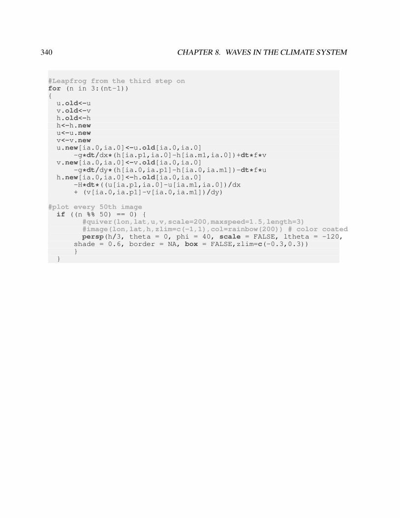
340 CHAPTER 8. WAVES IN THE CLIMATE SYSTEM
#Leapfrog from the third step onfor (n in 3:(nt-1))
u.old<-uv.old<-vh.old<-hh<-h.newu<-u.newv<-v.newu.new[ia.0,ia.0]<-u.old[ia.0,ia.0]
-g*dt/dx*(h[ia.p1,ia.0]-h[ia.m1,ia.0])+dt*f*vv.new[ia.0,ia.0]<-v.old[ia.0,ia.0]
-g*dt/dy*(h[ia.0,ia.p1]-h[ia.0,ia.m1])-dt*f*uh.new[ia.0,ia.0]<-h.old[ia.0,ia.0]
-H*dt*((u[ia.p1,ia.0]-u[ia.m1,ia.0])/dx+ (v[ia.0,ia.p1]-v[ia.0,ia.m1])/dy)
#plot every 50th imageif ((n %% 50) == 0)
#quiver(lon,lat,u,v,scale=200,maxspeed=1.5,length=3)#image(lon,lat,h,zlim=c(-1,1),col=rainbow(200)) # color coatedpersp(h/3, theta = 0, phi = 40, scale = FALSE, ltheta = -120,
shade = 0.6, border = NA, box = FALSE,zlim=c(-0.3,0.3))
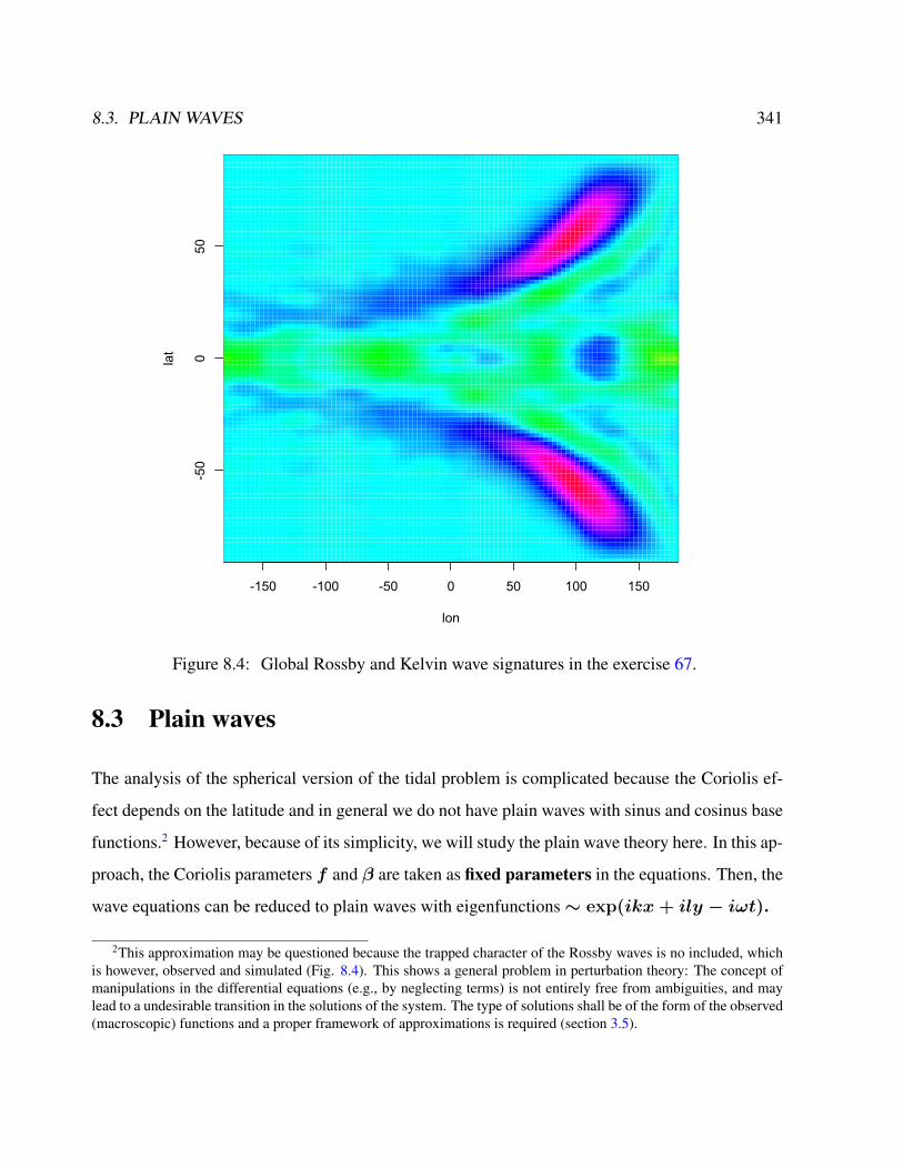
8.3. PLAIN WAVES 341
-150 -100 -50 0 50 100 150
-50
050
lon
lat
Figure 8.4: Global Rossby and Kelvin wave signatures in the exercise 67.
8.3 Plain waves
The analysis of the spherical version of the tidal problem is complicated because the Coriolis ef-
fect depends on the latitude and in general we do not have plain waves with sinus and cosinus base
functions.2 However, because of its simplicity, we will study the plain wave theory here. In this ap-
proach, the Coriolis parameters f and β are taken as fixed parameters in the equations. Then, the
wave equations can be reduced to plain waves with eigenfunctions∼ exp(ikx+ ily − iωt).
2This approximation may be questioned because the trapped character of the Rossby waves is no included, whichis however, observed and simulated (Fig. 8.4). This shows a general problem in perturbation theory: The concept ofmanipulations in the differential equations (e.g., by neglecting terms) is not entirely free from ambiguities, and maylead to a undesirable transition in the solutions of the system. The type of solutions shall be of the form of the observed(macroscopic) functions and a proper framework of approximations is required (section 3.5).
342 CHAPTER 8. WAVES IN THE CLIMATE SYSTEM
8.3.1 Inertial Waves
From the equations (8.7,8.8,8.9), we drop the term ∂xη, ∂yη, and f = f0 = const. (no pressure
gradients and constant f). Then, air or water mass moving with speed v subject only to the Coriolis
force travels in a circular trajectory called an ’inertial circle’. Since the force is directed at right
angles to the motion of the particle, it will move with a constant speed, and perform a complete
circle with frequency f. The magnitude of the Coriolis force also determines the radius of this
circle:
R = v/f . (8.20)
On the Earth, a typical mid-latitude value for f is 10−4s−1; hence for a typical atmospheric speed
of 10 m/s the radius is 100 km, with a period of about 14 hours. In the ocean, where a typical speed
is closer to 10 cm/s, the radius of an inertial circle is 1 km. These inertial circles are clockwise
in the Northern Hemisphere (where trajectories are bent to the right) and anti-clockwise in the
Southern Hemisphere. If the rotating system is a parabolic turntable, then f is constant and the
trajectories are exact circles. On a rotating planet, f varies with latitude and the paths of particles
do not form exact circles. Since the parameter f varies as the sine of the latitude, the radius of the
oscillations associated with a given speed are smallest at the poles and increase toward the equator
(Fig. 8.5).
∂u
∂t− f0v = 0 (8.21)
∂v
∂t+ f0u = 0 (8.22)
yields
∂2u
∂t2= −f2
0u . (8.23)
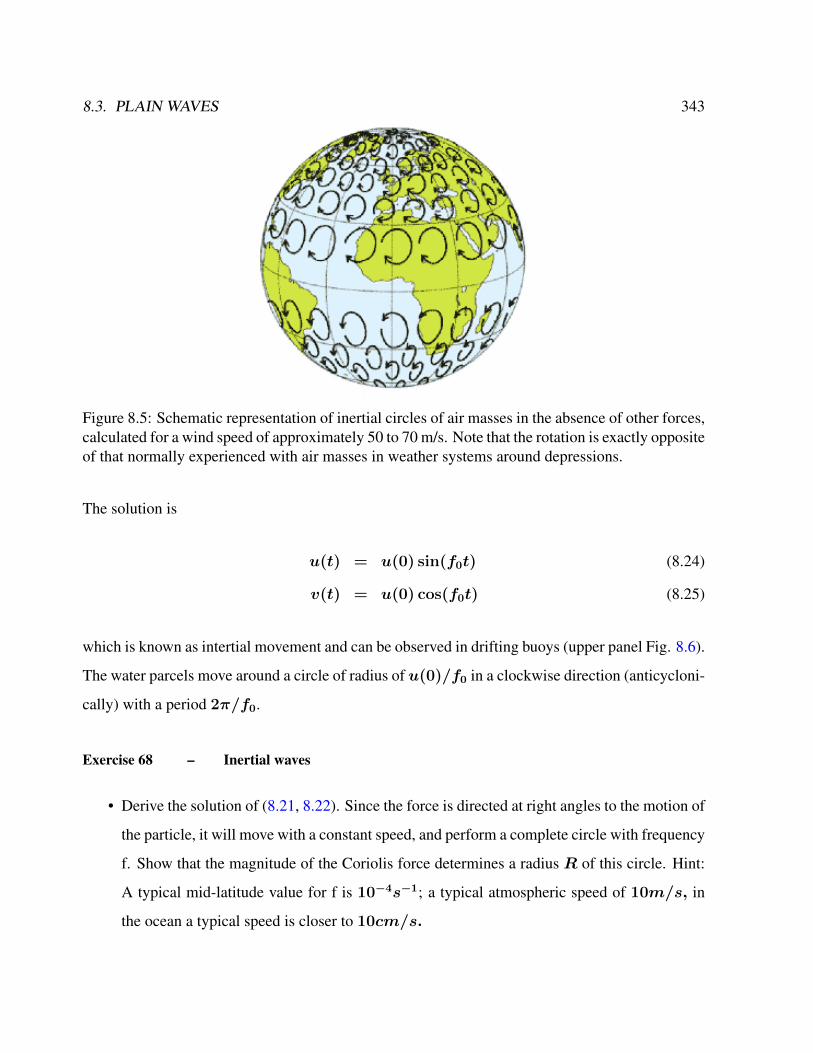
8.3. PLAIN WAVES 343
Figure 8.5: Schematic representation of inertial circles of air masses in the absence of other forces,calculated for a wind speed of approximately 50 to 70 m/s. Note that the rotation is exactly oppositeof that normally experienced with air masses in weather systems around depressions.
The solution is
u(t) = u(0) sin(f0t) (8.24)
v(t) = u(0) cos(f0t) (8.25)
which is known as intertial movement and can be observed in drifting buoys (upper panel Fig. 8.6).
The water parcels move around a circle of radius of u(0)/f0 in a clockwise direction (anticycloni-
cally) with a period 2π/f0.
Exercise 68 – Inertial waves
• Derive the solution of (8.21, 8.22). Since the force is directed at right angles to the motion of
the particle, it will move with a constant speed, and perform a complete circle with frequency
f. Show that the magnitude of the Coriolis force determines a radius R of this circle. Hint:
A typical mid-latitude value for f is 10−4s−1; a typical atmospheric speed of 10m/s, in
the ocean a typical speed is closer to 10cm/s.
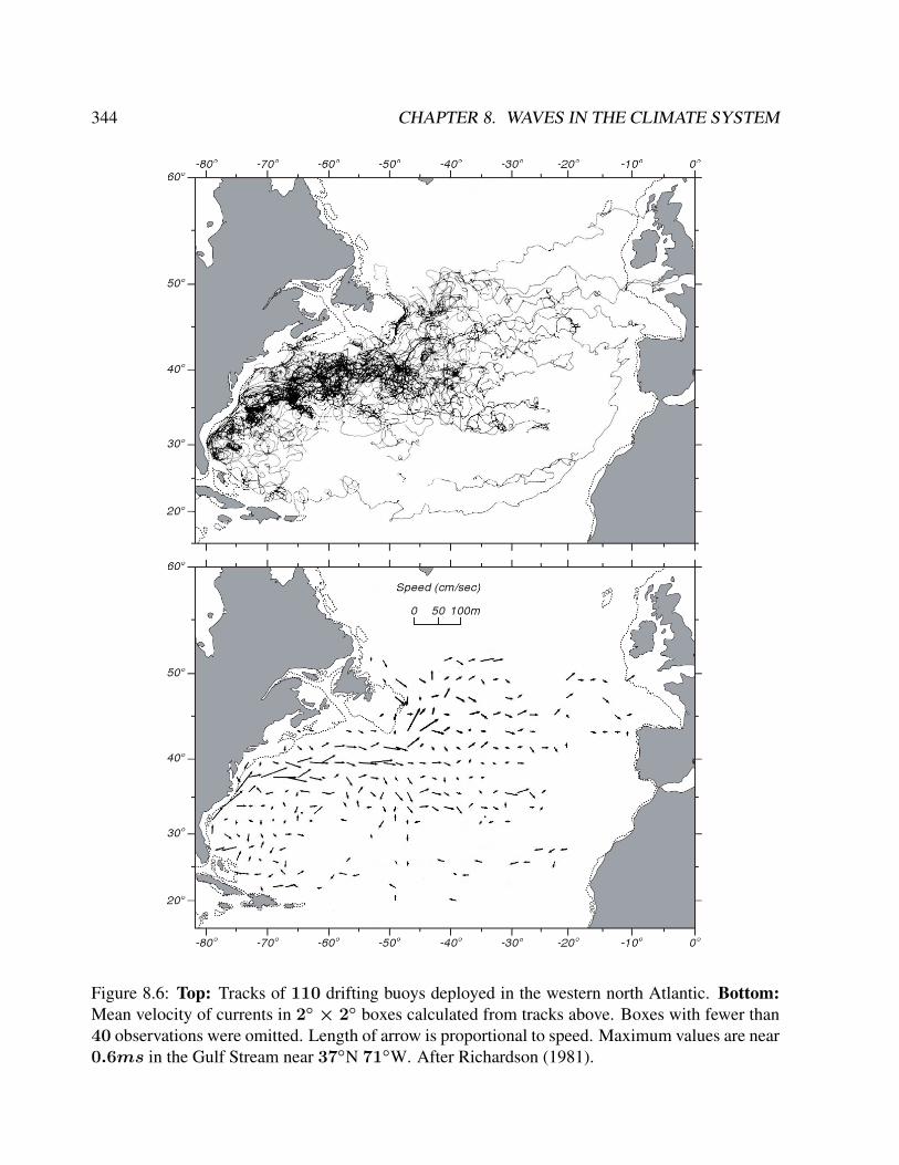
344 CHAPTER 8. WAVES IN THE CLIMATE SYSTEM
Figure 8.6: Top: Tracks of 110 drifting buoys deployed in the western north Atlantic. Bottom:Mean velocity of currents in 2 × 2 boxes calculated from tracks above. Boxes with fewer than40 observations were omitted. Length of arrow is proportional to speed. Maximum values are near0.6ms in the Gulf Stream near 37N 71W. After Richardson (1981).
8.3. PLAIN WAVES 345
• Provide the solution for the coordinates x(t), y(t).
• Show that the dynamics in the inertial coordinate system reduces to
uin(t) = 0 (8.26)
vin(t) = u(0) cos Ωt (8.27)
The trajectory in the inertial frame is a straight line. The length of the line is twice the
diameter of the inertial circle and the frequency of the oscillation is one-half that observed
in the rotating frame.

346 CHAPTER 8. WAVES IN THE CLIMATE SYSTEM
8.3.2 Gravity Waves
Shallow-water gravity waves are defined through their dynamics without the effect of the Earth’s
rotation, i.e. f = 0:
∂2η
∂t2= gH
(∂2
∂x2+
∂2
∂y2
)η (8.28)
With the ansatz
η = exp(ikx+ ily − iωt) (8.29)
ω is given by
ω(k, l) = ±√gH (k2 + l2), (8.30)
where k and l are the zonal and meridional wavenumbers. Since there is no preferred direction in
the (x,y) coordinate, we simply drop the y-dependence and introduce the phase speed
c = ω/k = ±√gH . (8.31)
In the limit β → 0 i.e. f = f0 = const., the dynamics consists of gravity waves with
ω2 = f20 + (ck)2 (8.32)
Output from a shallow water equation model of water in a bathtub. The water experiences five
splashes which generate surface gravity waves that propagate away from the splash locations and
reflect off the bathtub walls. (https://en.wikipedia.org/wiki/Shallow_water_
equations#/media/File:Shallow_water_waves.gif)
8.3. PLAIN WAVES 347
Exercise 69 – Baroclinic shallow-water gravity waves
In case we have a layed ocean, we consider the so-called baroclinic dynamics with the modified
gravity g′ = ρ1−ρ2ρ1
using the densities ρ1,2. Task: Derive the baroclinic dynamics using the
shallow water equations for 2 different layers and subtract the equations from each other!
Exercise 70 – Shallow-water waves
We consider tidal equation on the β−plane. This fluid dynamical system is described as
∂tu = f v − g ∂xη (8.33)
∂tv = −f u − g ∂yη (8.34)
∂tη = −∂x(Hu) − ∂y(Hv) . (8.35)
The variables u and v denote zonal and meridional perturbation flow velocity, and η the height
perturbation.
• Derive the dispersion relationships ω(k) for the cases:
a) In the limit β → 0, i.e. f → f0
b) c→∞.
c) For infinite Rossby radius a =√c/(2β).
d) When filtering out gravity waves by eliminating the time derivative in (8.35), (u, v) in
(8.33, 8.34) can be taken as plane waves proportional to exp(ikx+ ily), where l denotes
the meridional wave number. Derive the dispersion relationships ω(k) for the so-called
non-divergent Rossby waves.
• Provide typical values of ω(k) for M,N=1,2,3 and the atmosphere and ocean.
348 CHAPTER 8. WAVES IN THE CLIMATE SYSTEM
8.3.3 Extratropical Rossby Waves
From the equations (8.7,8.8,8.9), we drop the term ∂tη and introduce the stream function ψ
through
u =∂ψ
∂y; v = −
∂ψ
∂x(8.36)
such that (8.9) is fulfilled. Taking ∂∂y
of (8.7) and subtract ∂∂x
of (8.8) elimintates the η term as in
section 4.4:
∂
∂t
(∂2
∂x2+
∂2
∂y2
)ψ = −β
∂ψ
∂x(8.37)
With the ansatz
ψ = exp(ikx+ ily − iωt) (8.38)
and assumption that β is just a parameter, ω is given by
ω(k, l) = −βk
k2 + l2, (8.39)
where k and l are the zonal and meridional wavenumbers. Again, β is used as a parameter (also
called Rossby parameter) and is not expressed in terms of y:
β =df
dy=
1
R
d
dϕ(2Ω sinϕ) =
2Ω cosϕ
R(8.40)
where ϕ is the latitude, Ω is the angular speed of the Earth’s rotation, and R is the mean radius of
the Earth. The wave speed c = ω/k = −β (k2 + l2)−1. The feature that the phase speed is
faster at low latitudes can be also seen in Fig. 8.4 using the full dynamics.
More information about Rossby waves: https://youtu.be/6UCiRIc0nK0
Rossby waves and extreme weather: https://youtu.be/MzW5Isbv2A0
8.3. PLAIN WAVES 349
Exercise 71 – Rossby waves
Consider the vorticity equation
D
Dt[(ζ + f)/h] = 0 (8.41)
with h =const., u and v are the velocity components.
1. Assume a mean flow with constant zonal velocity U
u = U = const > 0 (8.42)
and a varying north-south component
v = v(x, t) (8.43)
which gives the total motion a wave-like form around a reference latitude where the wave
is trapped. Derive the associated vorticity equation and linearize the vorticity equation by
dropping all non-linear terms!
2. With the ansatz
v(x, t) = A cos[(kx− ωt)] (8.44)
determine the disperion relation ω(k), group velocity ∂ω∂k
, and the phase velocity c = ω/k.
3. Derive the wavelength L = 2π/k of the stationary wave given by c = 0.
4. A typical wavelength is 6000 km, a typical U is 15 m/s. Does the wave propagate from east
to west or opposite?
350 CHAPTER 8. WAVES IN THE CLIMATE SYSTEM
8.4 Kelvin waves
8.4.1 Coastal Kelvin waves
A Kelvin wave is a wave in the ocean or atmosphere that balances the Coriolis force against a
topographic boundary such as a coastline. If one assumes that the Coriolis coefficient f is constant
along the right boundary conditions, u = 0, and the zonal wind speed is set equal to zero, then
the equations become the following:
∂η
∂t= −H
∂v
∂y(8.45)
∂v
∂t= −g
∂η
∂y(8.46)
and therefore
∂2η
∂t2= gH
∂2
∂y2η (8.47)
The solution to these equations yields the following phase speed: c2 = gH and ω = ±cl, which
is the same speed as for shallow-water gravity waves without the effect of Earth’s rotation. We see
that η and v have also an x-dependence
η(x, y, t) = η(x) exp(ily − iωt) (8.48)
v(x, y, t) = v(x) exp(ily − iωt) . (8.49)
Using (8.46), we obtain
−iω v(x) = −gil η(x) and therefore v(x) =g
ωl η(x) = ±
g
cη(x) (8.50)
From the u-momentum equation∂η
∂x=f
gv (8.51)
8.4. KELVIN WAVES 351
we obtain therefore∂η
∂x= ±
f
cη (8.52)
where only the minus sign provides a useful solution (not blowing up). The solution has an expon-
tial decay of η(x) = exp(−x/Lr) on the scale of the Rossby radius Lr = c/f . The wave has
a trapped character along the boundary. It is important to note that for an observer traveling with
the wave, the coastal boundary (maximum amplitude) is always to the right in the Northern Hemi-
sphere and to the left in the Southern Hemisphere, i.e. these waves move equatorward/southward
on a western boundary and poleward/northward on an eastern boundary. Thus, the waves move
cyclonically around an ocean basin.
On the black board: A Coastal Kelvin Wave moving northward along the coast is deflected to
the right, but the coast prevents the wave from turning right and instead causes water to pile up on
the coast. The pile of water creates a pressure gradient directed offshore and a geostrophic current
directed northward.
On the northern hemisphere: The Kelvin wave always travels with the wall on its right side
(anti-clockwise). The wave amplitude decreases exponentially away from the wall. The wave is
trapped along the wall by rotation. Rotation does not affect the particle motion and wave propaga-
tion; only traps the wave to the coastline.
8.4.2 Equatorial Kelvin waves
Analogous we have Equatorial Kelvin waves: assume v = 0, then the equations become the
following:
∂η
∂t= −H
∂u
∂y(8.53)
∂u
∂t= −g
∂η
∂y(8.54)
352 CHAPTER 8. WAVES IN THE CLIMATE SYSTEM
and therefore again
∂2η
∂t2= gH
∂2
∂y2η (8.55)
The solution to these equations yields the phase speed: c2 = gH and ω = ck, which is the same
speed as for shallow-water gravity waves without the effect of Earth’s rotation. We see that η and
u have also an x-dependence
η(x, y, t) = η(y) exp(ikx− iωt) (8.56)
u(x, y, t) = u(y) exp(ikx− iωt) . (8.57)
Using (8.54), we obtain
−iω u(y) = −gik η(y) and therefore u(y) =g
ωk η(y) =
g
cη(y) (8.58)
From the v-momentum equation∂η
∂y=βy
gu (8.59)
we obtain therefore∂η
∂y= −
βy
cη . (8.60)
The solution is η(x) = exp(−βy2/c) with the scale of the Rossby radius Lr =√c/β. The
wave has a trapped character along the equator.
A feature of a Kelvin wave is that it is non-dispersive, i.e., the phase speed of the wave crests is
equal to the group speed of the wave energy for all frequencies. This means that it retains its shape
in the alongshore direction over time. In the ocean these waves propagate along coastal boundaries
(and hence become trapped in the vicinity of the coast itself) on a scale of about 30 km.
Equatorial Kelvin waves are a special type of Kelvin wave that balances the Coriolis Force in
8.5. EQUATORIAL WAVES: THEORY OF MATSUNO* 353
the northern hemisphere against its southern hemisphere counterpart. This wave always propagates
eastward and only exists on the equator. Equatorial Kelvin Waves propagating in the thermocline
have wave speeds slow enough to give a Rossby Radius of Deformation that is on the order of 250
km and thus they appear to be trapped close to the equator.
8.5 Equatorial waves: Theory of Matsuno*
We consider the equations (8.7,8.8,8.9) on the equatorial β−plane. In the equatorial region, the
fluid dynamical system is described as
∂tu = βy v − g ∂xη (8.61)
∂tv = −βy u − g ∂yη (8.62)
∂tη = −∂x(Hu) − ∂y(Hv) . (8.63)
We non-dimensionalize the system through the parameters listed in Table 8.1. In the non-
dimensional form (and dropping the stars in Table 8.1), the system reads then
∂tu = y v − ∂xη (8.64)
∂tv = −y u − ∂yη (8.65)
∂tη = −∂xu − ∂yv . (8.66)
Introducing the new variables
q = η + u (8.67)
r = η − u (8.68)
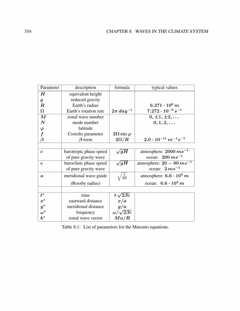
354 CHAPTER 8. WAVES IN THE CLIMATE SYSTEM
Parameter description formula typical valuesH equivalent heightg reduced gravityR Earth’s radius 6.371 · 106mΩ Earth’s rotation rate 2π day−1 7.272 · 10−5 s−1
M zonal wave number 0,±1,±2, . . .N mode number 0, 1, 2, . . .ϕ latitudef Coriolis parameter 2Ω sinϕβ β-term 2Ω/R 2.0 · 10−11m−1s−1
c barotropic phase speed√gH atmosphere: 2000ms−1
of pure gravity wave ocean: 200ms−1
c baroclinic phase speed√gH atmosphere: 20− 80ms−1
of pure gravity wave ocean: 2ms−1
a meridional wave guide√
c2β
atmosphere: 6.6 · 105m
(Rossby radius) ocean: 6.6 · 104m
t∗ time t√
2βcx∗ eastward distance x/ay∗ meridional distance y/aω∗ frequency ω/
√2βc
k∗ zonal wave vector Ma/R
Table 8.1: List of parameters for the Matsuno equations.
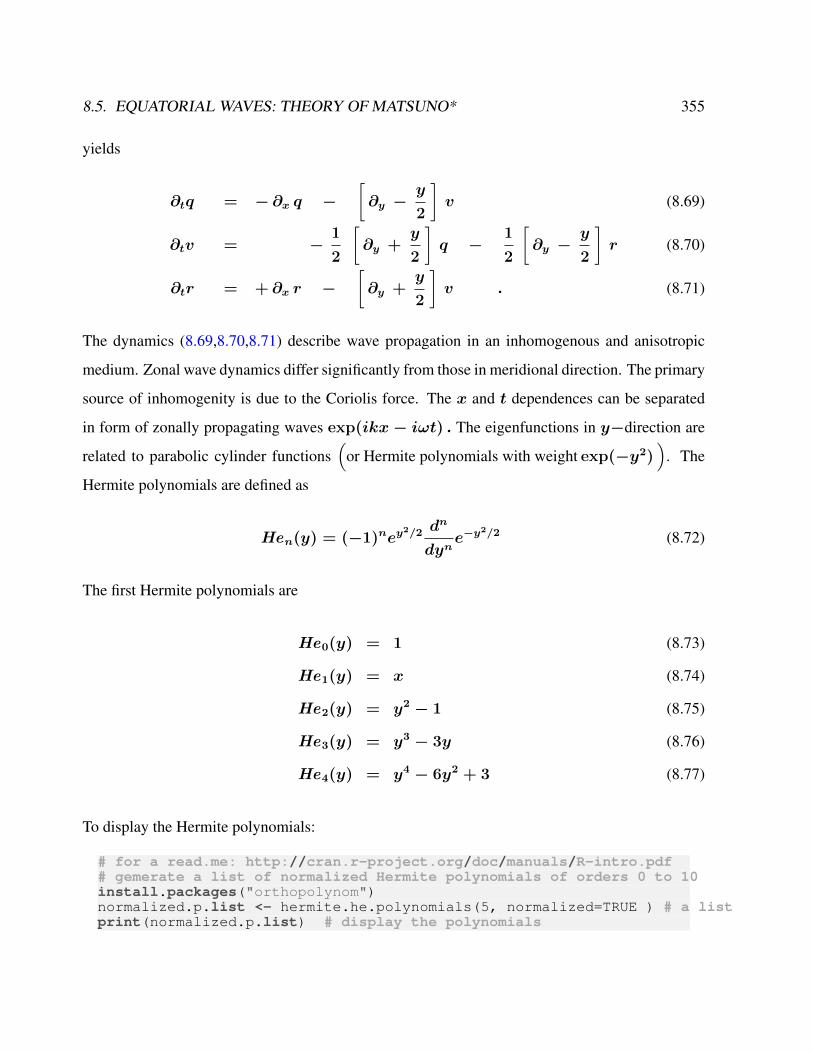
8.5. EQUATORIAL WAVES: THEORY OF MATSUNO* 355
yields
∂tq = − ∂x q −[∂y −
y
2
]v (8.69)
∂tv = −1
2
[∂y +
y
2
]q −
1
2
[∂y −
y
2
]r (8.70)
∂tr = + ∂x r −[∂y +
y
2
]v . (8.71)
The dynamics (8.69,8.70,8.71) describe wave propagation in an inhomogenous and anisotropic
medium. Zonal wave dynamics differ significantly from those in meridional direction. The primary
source of inhomogenity is due to the Coriolis force. The x and t dependences can be separated
in form of zonally propagating waves exp(ikx− iωt) . The eigenfunctions in y−direction are
related to parabolic cylinder functions(
or Hermite polynomials with weight exp(−y2))
. The
Hermite polynomials are defined as
Hen(y) = (−1)ney2/2
dn
dyne−y
2/2 (8.72)
The first Hermite polynomials are
He0(y) = 1 (8.73)
He1(y) = x (8.74)
He2(y) = y2 − 1 (8.75)
He3(y) = y3 − 3y (8.76)
He4(y) = y4 − 6y2 + 3 (8.77)
To display the Hermite polynomials:
# for a read.me: http://cran.r-project.org/doc/manuals/R-intro.pdf# gemerate a list of normalized Hermite polynomials of orders 0 to 10install.packages("orthopolynom")normalized.p.list <- hermite.he.polynomials(5, normalized=TRUE ) # a listprint(normalized.p.list) # display the polynomials
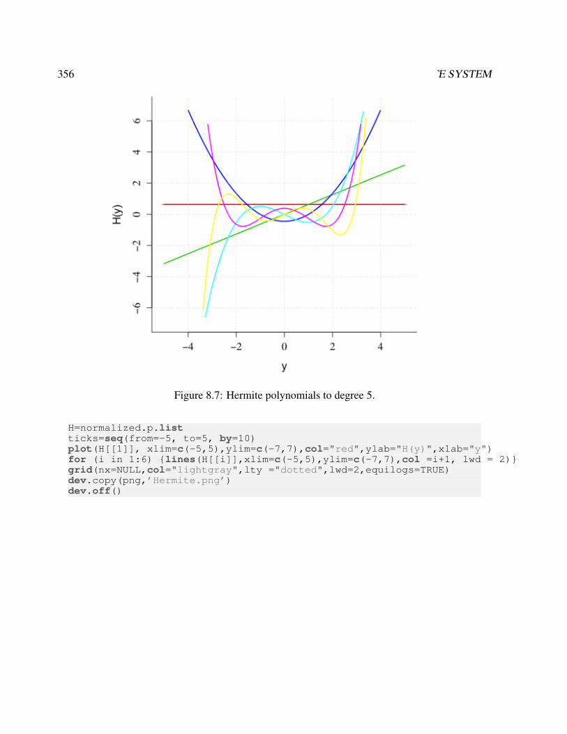
356 CHAPTER 8. WAVES IN THE CLIMATE SYSTEM
Figure 8.7: Hermite polynomials to degree 5.
H=normalized.p.listticks=seq(from=-5, to=5, by=10)plot(H[[1]], xlim=c(-5,5),ylim=c(-7,7),col="red",ylab="H(y)",xlab="y")for (i in 1:6) lines(H[[i]],xlim=c(-5,5),ylim=c(-7,7),col =i+1, lwd = 2)grid(nx=NULL,col="lightgray",lty ="dotted",lwd=2,equilogs=TRUE)dev.copy(png,’Hermite.png’)dev.off()

8.5. EQUATORIAL WAVES: THEORY OF MATSUNO* 357
They satisfy following recursion relationship:
[∂y +
y
2
]DN = N DN−1 ;
[∂y −
y
2
]DN = −DN+1 . (8.78)
The operators [∂y ± y2] annihilate or excite one quantum of mode index number N and are
called lowering and raising ladder operators in quantum mechanics. A basic feature of DN ∼
exp(−y2) is that significant wave amplitudes are trapped in a wave guide centered at the latitude
ϕ0, similar to the equator-centered Yoshida guide [Gill, 1982].
The Fourier modes ξN(t) := (qN−1, vN , rN+1) correspond to order N > 0 and wave
vector k. The prognostic equations for the Fourier modes are first order in time
d
dtξN = AN(k) ξN . (8.79)
and are described by 3× 3 matricesAN(k)
AN(k) =
−ik 1 0
−N/2 0 1/2
0 −(N + 1) ik
. (8.80)
MatrixAN(k) describes the dynamics of one Rossby and two gravity waves with eigenfrequencies
ω (eigenvalue ofA = iω) satisfying
ω3 − ω(
2N + 1
2+ k2
)−k
2= 0 . (8.81)
The sum of the eigenfrequencies in (8.81) is zero due to trace (AN) = 0 and
3∑l=1
ωl = limT→∞
1
T
∫ T
0
dt trace (AN) = 0 . (8.82)

358 CHAPTER 8. WAVES IN THE CLIMATE SYSTEM
ForN = 0, the system matrixA0 is specified to be
A0(k) =
ik 0 0
0 0 1/2
0 −1 ik
. (8.83)
The different signs of the ·11−elements in (8.80) and (8.83) originate from the requirement that the
corresponding eigenmode qN=0 in (8.83) is integrable [Gill, 1982]. This mode with v = r = 0
is called equatorial Kelvin wave which propagates eastward without dispersion:
ω = k . (8.84)
The dynamics of the Kelvin wave is decoupled from the Yanai wave dynamics described by the
second and third eigenvectors of matrix (8.83). The Yanai wave, also known as mixed planetary-
gravity wave in the literature [Gill, 1982], has a quadratic relation
ω2 − kω − 1/2 = 0 . (8.85)
Dispersion curves for the Rossby/gravity (8.81), Kelvin (8.84), and Yanai (8.85) waves are shown
in Fig. 8.8 as a function on zonal wave vector k = Ma/R and mode number N. The figure
depicts eastward propagating Kelvin and westward propagating Rossby modes. Gravity waves can
propagate east- and westward. The Yanai wave behaves as a gravity wave for k ≥ 0 and as a
Rossby wave for k < 0 . Note that (8.81) is invariant under ω → −ω, k → −k , which is a
consequence of (8.82). Dispersion diagrams like Fig. 8.8 can be found in standard text books of
geophysical fluid dynamics showing the upper [Gill, 1982] or right [Holton, 2004] part of Fig. 8.8,
respectively.
The equatorial zone essentially acts as a waveguide, causing disturbances to be trapped in the
vicinity of the equator. For the first baroclinic mode in the ocean, a typical phase speed would
be about 2.8m/s, causing an equatorial Kelvin wave to take 2 months to cross the Pacific Ocean
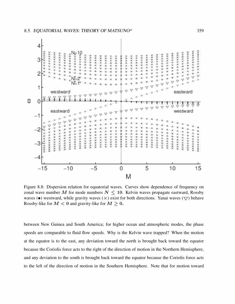
8.5. EQUATORIAL WAVES: THEORY OF MATSUNO* 359
Figure 8.8: Dispersion relation for equatorial waves. Curves show dependence of frequency onzonal wave number M for mode numbers N ≤ 10. Kelvin waves propagate eastward, Rossbywaves (•) westward, while gravity waves (×) exist for both directions. Yanai waves (5) behaveRossby-like forM < 0 and gravity-like forM ≥ 0.
between New Guinea and South America; for higher ocean and atmospheric modes, the phase
speeds are comparable to fluid flow speeds. Why is the Kelvin wave trapped? When the motion
at the equator is to the east, any deviation toward the north is brought back toward the equator
because the Coriolis force acts to the right of the direction of motion in the Northern Hemisphere,
and any deviation to the south is brought back toward the equator because the Coriolis force acts
to the left of the direction of motion in the Southern Hemisphere. Note that for motion toward
360 CHAPTER 8. WAVES IN THE CLIMATE SYSTEM
the west, the Coriolis force would not restore a northward or southward deviation back toward the
equator; thus, equatorial Kelvin waves are only possible for eastward motion (as noted above).
Both atmospheric and oceanic equatorial Kelvin waves play an important role in the dynamics of
El Niño-Southern Oscillation, by transmitting changes in conditions in the Western Pacific to the
Eastern Pacific [Gill, 1982]. This can be also studied in exercise 67.
It is instructive to look for approximations in tidal theory. One can simplify the solution of the
Matsuno theory, or simplify the equations (8.7,8.8,8.9) which will be done in section 8.3.
When filtering out gravity waves by eliminating the time derivative in (8.63), (u, v) in (8.61,
8.62) is equivalent to c→∞. The evolution equation reduces to
∂t(∂yu− ∂xv) = βu (8.86)
with plane waves proportional to exp(ikx+ ily). Then, non-divergent Rossby waves with ω =
−βk/(k2 + l2) are retained only. The trapped character of the waves vanishes with infinite
Rossby radius a =√c/(2β), a measure of the wave guide geography.
Exercise 72 – Shallow-water dynamics: eigenfunctions
• Show that the eigenfunctions in y−direction, which are are related to parabolic cylin-
der functions(
or Hermite polynomials with weight exp(−y2))
, satisfy following recur-
sion relationship:
[∂y +
y
2
]DN = N DN−1 ;
[∂y −
y
2
]DN = −DN+1 . (8.87)
The operators [∂y ± y2] annihilate or excite one quantum of mode index numberN and are
called lowering and raising ladder operators in quantum mechanics.
DN(y) =1
π
∫ π
0
sin(NΘ− y sin Θ))
8.5. EQUATORIAL WAVES: THEORY OF MATSUNO* 361
• Show that the functions are orthogonal, i.e.
∫ ∞−∞
dyDN(y)DM(y) = δNM N !√
2π
• The dynamics in an inertial reference frame, e.g. with a coordinate system fixed at the Sun,
would not have a Coriolis force (and thus f = 0), but would certainly observe Rossby wave
propagation. How can this be reconciled?
(Hint: In the inertial system, the near-equatorial motion is seen to be faster than off the
equator. Zero vorticity in the rotating Earth’s coordinate system corresponds to a basic flow
U = RΩ cosϕ with non-zero vorticity flow.)
Exercise 73 – Shallow-water dynamics: A different approach
We may seek travelling-wave solutions of the form
u, v, η
=u(y), v(y), η(y)
ei(kx−ωt) (8.88)
Please check the following arguments.
• Subsitituting this exponential form into the three equations (8.61,8.62,8.63), and eliminating
u, and η leaves us with an eigenvalue equation for v(y)
−∂2v
∂y2+
(β2
c2
)v =
(ω2
c2− k2 −
βk
ω
)v. (8.89)
• Recognizing this as the Schrödinger equation of a quantum harmonic oscillator of frequency
β/c, we know that we must have
(ω2
c2− k2 −
βk
ω
)=β
c(2n+ 1), n ≥ 0 (8.90)
for the solutions to tend to zero away from the equator. For each integer n, this last equation
provides a dispersion relation linking the wavenumber k to the angular frequency ω.
362 CHAPTER 8. WAVES IN THE CLIMATE SYSTEM
• In the special special case n = 0 the dispersion equation reduces to
(ω + ck)(ω2 − ckω − cβ) = 0, (8.91)
but the root ω = −ck has to be discarded because we had to divide by this factor in elimi-
nating u, η.
• The remaining pair of roots correspond to the Yanai or mixed Rossby-gravity mode whose
group velocity is always to the east and interpolates between two types of n > 0 modes:
the higher frequency Poincare gravity waves whose group velocity can be to the east or to
the west, and the low-frequency equatorial Rossby waves whose dispersion relation can be
approximated as
ω =−βk
k2 + β(2n+ 1)/c. (8.92)
8.6 Spheroidal Eigenfunctions of the Tidal Equation*
Laplace’s tidal equations, governing the small amplitude dynamics of a shallow fluid on a rotating
sphere, are the fundamental linear problems of large-scale geophysical fluid dynamics. Originally
formulated by Laplace, its general solution and, in particular, its full dispersion relation are still
not known. The current understanding of the problem rests essentially on the equatorial β-plane
approximation [Matsuno, 1966] and extensive numerical studies [Longuet-Higgins, 1968]. In this
framework the system has been found to exhibit Rossby waves, Yanai waves, and gravity waves,
including the Kelvin wave. In spite of its elegance and fundamental significance for the terrestrial
climate problem, the β-plane concept is not entirely free from ambiguities. Although the Matsuno
wave equation appears to be a well-posed problem, its dispersion relation admits an unphysical,
westward propagating "Kelvin" mode. This has to be ruled out a posteriori [Matsuno, 1966].
Furthermore, the β-plane concept does not yield a physically meaningful nonrotating limit. And
8.6. SPHEROIDAL EIGENFUNCTIONS OF THE TIDAL EQUATION* 363
finally, the Matsuno equation is invariant under meridional translations. Yanai waves should thus
be observed at all latitudes and every latitude defines the center of a waveguide. Such properties
are not physically realizable. On the other hand, the analysis of the spherical version of the tidal
problem is complicated. First, the manipulation of the first order equations of motion into an
appropriate wave equation is cumbersome, namely because the two-dimensional (2D) geometry
of the spherical surface is non-Euclidean. Second, as shown below, the basic wave operator in
the various forms of the tidal problem is the spheroidal wave equation. For this equation, infinity
is an irregular singular point precluding the establishment of recurrence relations similar to those
for functions of the hypergeometric type [Flammer, 1957]. The transformation of differential
operations in physical space into some simpler algebra in wave number space is thus impossible.
Geometrical difficulties are largely simplified by a systematic application of tensor analysis in
2D Riemann space. Here, index notation will be used with indices m, n,... running from 1 to 2
and a semicolon denoting covariant differentiation. For details of the notation and the form of
the geometrical tensors in spherical, geophysical coordinates see [Townsend et al., 1992]. The
linearized equations of motion of a shallow fluid on a rotating sphere are shown in [Townsend
et al., 1992] to assume the form
∂tr + jn;n = 0,
∂tjn + εmnfjm + c2∂nr = 0,
where jn = Rvn is the effective momentum density, R the constant equilibrium mass per unit
area, and f = 2Ω sinϕ using the latitude dependent Coriolis parameter. For the potential vortic-
ity z, defined by
Rz = εmnvn;m−fr/R,
the linearized equations of motion imply the relation
R∂tz + fnvn = 0,
364 CHAPTER 8. WAVES IN THE CLIMATE SYSTEM
where fn is the contravariant gradient of the Coriolis parameter. Furthermore, the gradient of the
divergence of a vector on the spherical surface is given by
ja;an = gab(jn;ab−εnaεrsjr;sb−Gambnjm),
where gab is the metric and Gambn the Riemannian [Townsend et al., 1992]. Using this identity
and the potential vorticity equation it is fairly straightforward to derive the system
R2[(∂2t + f2 − c2∆)∂t + c2εabfa∂b
]∂tz = −c2(∆f)∂2
t r, (8.93a)[(∂2t + f2 − c2∆)∂t + c2εabfb∂a
]r = −2R2f∂tz, (8.93b)
from the equations of motion, where ∆ denotes the 2D Laplacian in spherical coordinates. If
Cartesian coordinates (x, y) are chosen with f = βy, i.e., in particular ∆f = 0, the first of these
equations reduces to the Matsuno equation. To obtain (8.93a) in the spherical case, eliminate r
from the equations of motion
(∂2t + f2 − c2∆)∂tjn + c2εna
[∂a(fbj
b) + fajb;b]
= 0, (8.94)
with
∆jn = gabjn;ab−a−2jn,
where a denotes the Earth’s radius. Using
fn∆jn = ∆(fnjn)− (∆f)jn;n
.
scalar multiplication of (8.94) with the contravariant gradient of the Coriolis parameter yields
(8.93a). Equation (8.94) as well as the coupled nature of the system (8.93) demonstrate that the
8.6. SPHEROIDAL EIGENFUNCTIONS OF THE TIDAL EQUATION* 365
tidal equation is inherently a 20 vector wave equation. In order to evaluate the eigenfunctions of
this system, the dependent variables are assumed to be proportional to
e−i(ωt−MλF (y),
where λ is longitude, y = sinϕ, and M the zonal wave number. Substituting this into (8.93), the
system becomes
(P −m)V = −2αyD, (8.95a)
(P +m)D = 2αyV, (8.95b)
HereD = r/R = ivn;n /ω and V = aRz/c = −iαvϕ × cosϕ/cv, while
P = a2∆− α2y2 + ν2
is the prolate spheroidal wave operator with Lamb parameter u = 2aΩ/c, ν = aω/c, andm =
αM/ν. In the form (8.95) the tidal problem emerges as a system of coupled spheroidal wave
equations. In special cases, exact analytical solutions can be readily obtained without considering
the complete fourth order system. Elimination of j1 between the continuity equation and the one-
component of the momentum budget yields
αD = −(µ+ y2)−1[(1− y2)∂y −my
]V,
with µ = (M2 − ν2)/ν2, while elimination of ji between the one-component and the two-
component of the momentum budget leads to
αV = −(n2 − y2)−1[(1− y2)∂y +my
]D,
366 CHAPTER 8. WAVES IN THE CLIMATE SYSTEM
with n = ν/α. Inserting these expressions into the right hand side (rhs) of (8.95) results in
(P +m)V = 2(µ+ y2)−1[y(1− y2)∂y +mµ
]V, (8.96a)
(P −m)D = −2(n2 − y2)−1[y(1− y2)∂y +mn2
]D. (8.96b)
Equation (8.96a) is the spherical generalization of the Matsuno equation, while (8.96b) is the
form of the tidal equation studied by Longuet-Higgins. In view of the general solution, (8.96) may
not be the most convenient form as it exhibits far less symmetry than the coupled system (8.95)
suggests. It nevertheless lends itself readily to the evaluation of two special cases. For standing
waves (M = 0) the spherical Matsuno equation (8.96a) is exactly solved by
V = (1− y2)1/2(AS1L +BS−1
L ),
with constants A and B and prolate spheroidal wave functionsS±1L (y;α2) of order±1 and degree
L ≥ 1. The corwhere responding divergence becomes
D ∼ ∂y(1− y2)1/2(AS1L +BS−1
L ). (8.97)
A closed expression for the eigenvalues of the spheroidal wave equation does not exist and
approximations depend strongly on the value of the Lamb parameter. On Earth, the value of the
Lamb parameter ranges from α ≈ 1 for the atmospheric Lamb wave, over α ≈ 5 for barotropic
gravity waves in the ocean to α ≈ 300 for the first baroclinic mode in the ocean. For α2
1 , spheroidal wave functions are approximated by expansions in terms of associated Legendre
polynominals, and the dispersion relation for standing waves becomes toO(α0) [Flammer, 1957]
[Abramowitz and Stegun, 1965].
8.6. SPHEROIDAL EIGENFUNCTIONS OF THE TIDAL EQUATION* 367
ν2 = Λ2 + α2(2Λ2 − 3)/(4Λ2 − 3) (8.98a)
with Λ2 = L(L + 1). In the nonrotating limit, this reduces to the familiar ν2 = L(L +
1). For α2 1, the prolate spheroidal wave function SKL is appropriately approximated by
parabolic cylinder functions of nonnegative, integer order, and the corresponding eigenvalue to
O(α0) becomes [Flammer, 1957] [Abramowitz and Stegun, 1965]
ε(L,K,α) = αq +K2 − 1 + p,
with q = 2N + 1, p = (3− q2)/8, andN = L− |K| . In the present case of standing waves
(ε = ν2,K2 = 1) this yields the dispersion relation toO(α0)
ν2 = α(2N2 + 1) + p, (8.98b)
where the mode numberN2 = L− 1 measures the number of zeros of j2 in the open interval
y ∈ (−1, 1). With the inclusion of higher orders in α and 1/α, respectively, the dispersion
relation (8.98) and the corresponding expansion of the spheroidal wave function permit the con-
struction of Fig. 1 and Fig. 7 of [Longuet-Higgins, 1968] to an arbitrary degree of accuracy from
[Abramowitz and Stegun, 1965] . The asymptotic expansion of (8.96a) provides an estimate of
the domain of validity of the β-plane approximation in physical and wave number space. For low
frequencies ν2 M2, the first order Taylor expansion of the denominator on the rhs of (8.96a)
is justified and yields
(α2∆− δy2 + ν2 −m)V = O,
with δ = α2 − 2m/µ, . For large a in the low-frequency domain under consideration α2
2m/µ, so that δ ≈ α2. Assuming V = (1−y2)|M |/2F , where the absolute value of M ensures
368 CHAPTER 8. WAVES IN THE CLIMATE SYSTEM
the regularity of V at the poles for negative M, and transforming to x = y√α
[(α− x2)∂2
x − 2(|M |+ 1)x∂x − αx2 + α(2N2 + 1)]F ≈ 0
yields for α x2, i.e., in the vicinity of the equator y2 1
(∂2x − x
2 + 2N2 + 1− x+ 2N2 + 1)F ≈ O
the familiar β-plane version of the Matsuno equation with dispersion relation
ν3 −[α(2N2 + 1) +M2
]ν − αM = 0,
with N2 = L− |M |. The β-plane approximation thus emerges asymptotically from the full
tidal equation as an equatorial (y2 1), baroclinic (α2 1) low-frequency approximation.
While the original frequency restriction ν2 M2 admits Rossby waves only, the additional re-
striction to low latitudes also allows for low-frequency gravity waves in this approximation. The
equatorial nature of these asymptotics is obviously not compatible with a "midlatitude β-plane,"
while the large u condition rules out a nonrotating limit. The β-plane approximation essentially
neglects the coupling of Eqs. (8.95a) and (8.95b). In the full tidal vector equation it is this cou-
pling that excludes the "wrong Kelvin wave" a priori. A second special, but exact solution can be
obtained for inertial waves. At the inertial frequency ν = α, (8.96b) has the exact solution
D = (1− y2)1/2(ASM−1L +BS1−M
L ), (8.99)
with L ≥ 0 and 1− L ≤M ≤ L+ 1. The dispertion relation in this case
[ε = α2 −M, K2 = (M − 1)2
]can again be read from [Abramowitz and Stegun, 1965] . For small α one finds toO(α2)
8.6. SPHEROIDAL EIGENFUNCTIONS OF THE TIDAL EQUATION* 369
α2 = Λ2 +M + α2[2Λ2 − 2M(M − 2)− 3
]/(4Λ2 − 3) (8.100a)
admitting onlyL = 0 andM = 0 in the nonrotationg case, while the dispersion relation for large
α becomesO(α2)
α2 = α(2N0 + 1) +M2 −M + p (8.100b)
where N0 = L − |M − 1| measures the number of seros of the mass perturbation r in the
open interval y ∈ (−1, 1). At M = 0, the relation (8.100) coincides obviously with (8.98) at
ν = α, where N0(M = 0, ν = α = N2(M = 0, ν = α), while in general the number of
zeros of the mass perturbation r will differ from the number of zeros of j2. The divergence (8.99)
at M=0 agrees with (8.97) at ν = α, since for spheroidal wave functions [Flammer, 1957] :
ME/W =1
2±√α2 − αq + p+
1
4,
with
|MW | = ME − 1 < ME. (8.101)
The same inequality is found from (8.100a). In contrast to the β-plane approximation, modes
in this frequency domain are labeled by Np, and the phase speed of eastward propagating gravity
waves is smaller than the westward speed at the same frequency and mode number. At high
frequencies ν2 α2, the approximation of (8.96b) by
(α2∆− δy2 + ν2 +m)D ≈ 0,
with δ = α2 − 2M/n3, is uncritical. For large α and positive M not too large δ ≈ α2, and the
370 CHAPTER 8. WAVES IN THE CLIMATE SYSTEM
expansion of this equation similar to the Matsuno equation yields the
approximate dispersion relation
ν3 −[α(2N0 + 1) +M2
]ν + αM = 0,
withN0 = L− |M |. The eastward propagating "Rossby" solutions of this dispersion have to be
discarded, as they do not satisfy the defining inequality. On the other hand, the gravity solutions
including the Kelvin wave satisfy this inequality. As a consequence of the positive sign of the
last term, westward phase speeds are larger than eastward speeds. This is in agreement with the
exact solution (8.100). The wave number space of the tidal equation is thus separated at the inertial
frequency ν = α into a lowfrequency domain, where modes are governed by N2 and a high-
frequency domain with gravity modes controlled by N0. This is the mode number that survives
the transition to the nonrotating case. For Ω = 0, D is proportional to the associated Legendre
polynominalPML withN0 = L−|M | zeros in the open interval y ∈ (−1, 1), and the dispersion
relation ν2 = L(L+ 1) can alternatively be written
ν2(M) = N0(N0 + 1) + (2N0 + 1) |M |+M2 = ν2(−M)
. As indicated by the inequality (8.101), rotation leads primarily to the loss of this synunetry for
gravity modes. At lower frequencies, additional Rossby modes emerge in rotating systems, which
can no longer be accormnodated by Np. Hence, the mode number Np governs that domain of wave
number space, where rotation merely modifies modes already existing in the nonrotating case. The
transition between mode numbers is only possible due to the vector character of the tidal equa-
tion. On Earth, this highfrequency domain of wave number space is occupied by Lamb waves
and barotropic gravity waves, which are of minor significance on larger scales. The atmosphere
of Venus, on the other hand, is characterized by much lower values of the Lamb parameter, and
gravity waves with ν ≥ α gain greater relevance for large-scale aspects of the circulation. The
concept of covariant differentiation renders the derivation of wave equations from the equations

8.6. SPHEROIDAL EIGENFUNCTIONS OF THE TIDAL EQUATION* 371
of motion fairly straightforward. The prolate spheroidal wave operator assumes a central role in
these vector wave equations. For the first time since Laplace’s formulation of the problem, exact
analytical solutions are presented in the special cases of standing waves and inertial waves. These
solutions confirm corresponding numerical calculations, while the asymptotics of the spheroidal
wave equation for equatorial, baroclinic, low-frequency waves yield indeed the β-plane approxi-
mation. Furthermore, the results demonstrate a fundamental separation of the wave number space
of the tidal equation at the inertial frequency. At higher frequencies, the mode numberN0 controls
the dispersion of gravity waves, which experience rotation effects merely as a loss of syrrunetry
with respect toM = 0. For a corotating observer westward
propagating gravity waves at these frequencies are faster and longer than their eastward coun-
terparts. At low frequencies the dispersion of additional Rossby modes is incorporated by transition
to the mode numberN2. This transition is primarily possible due to the vector character of the tidal
problem. It can be expected that in the framework of the complete analytical theory of the tidal
equation the angular momentum of eigensolutions, measured by the degree L, will be essential for
this separation of the wave number space.

Part III
Third part: Climate
372
Chapter 9
Paleoclimate
For present climate state we are able to directly measure all involved quantities. From measure-
ments we can draw conclusions about physical, chemical and biological relationships between the
variables. Our understanding about the involved processes is far from complete, but nevertheless
we derive equations that describe and predict the observed phenomena.
One the other hand, the knowledge about the climate of the past relies on the use of indi-
rect methods. Palaeotemperatures and -precipitation have to be derived from materials that had
been exposed to the environment which in turn had an impact on this material. Then it had to be
conserved and locked from any further alteration. Finally, the material has to be examined and
the alterations have to be understood and interpreted as anomalies of temperature or precipitation.
Therefore, assumptions have to be made that are independent of the type of the climate archive, the
materials involved and the methods used to extract the information from the archive. For example,
we assume that correlations between measured quantities and climate variables do not change in
time. These measured quantities are called proxies if they convey indirect information about past
climates.
Past climates left their imprints in a large variety of archives. Depending on the type of the
archive, knowledge about the processes during the formation of the archive is useful and often
essential for the interpretation. Some of the most influential climate archives are:
373
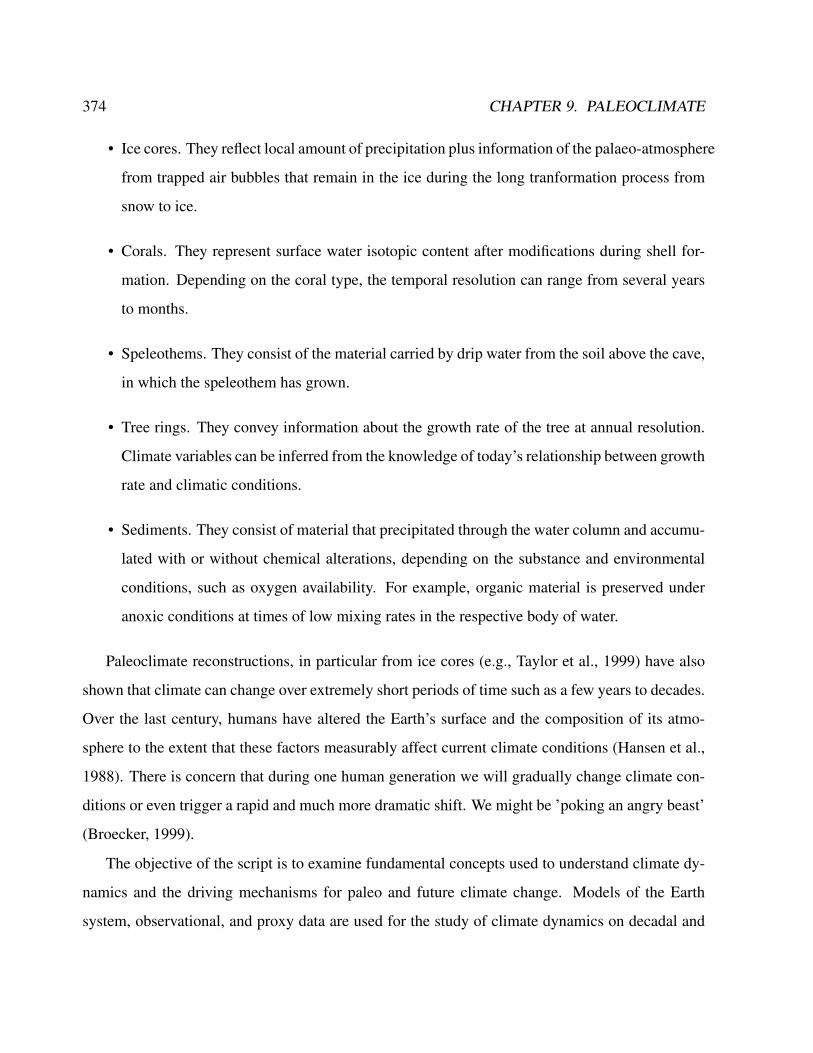
374 CHAPTER 9. PALEOCLIMATE
• Ice cores. They reflect local amount of precipitation plus information of the palaeo-atmosphere
from trapped air bubbles that remain in the ice during the long tranformation process from
snow to ice.
• Corals. They represent surface water isotopic content after modifications during shell for-
mation. Depending on the coral type, the temporal resolution can range from several years
to months.
• Speleothems. They consist of the material carried by drip water from the soil above the cave,
in which the speleothem has grown.
• Tree rings. They convey information about the growth rate of the tree at annual resolution.
Climate variables can be inferred from the knowledge of today’s relationship between growth
rate and climatic conditions.
• Sediments. They consist of material that precipitated through the water column and accumu-
lated with or without chemical alterations, depending on the substance and environmental
conditions, such as oxygen availability. For example, organic material is preserved under
anoxic conditions at times of low mixing rates in the respective body of water.
Paleoclimate reconstructions, in particular from ice cores (e.g., Taylor et al., 1999) have also
shown that climate can change over extremely short periods of time such as a few years to decades.
Over the last century, humans have altered the Earth’s surface and the composition of its atmo-
sphere to the extent that these factors measurably affect current climate conditions (Hansen et al.,
1988). There is concern that during one human generation we will gradually change climate con-
ditions or even trigger a rapid and much more dramatic shift. We might be ’poking an angry beast’
(Broecker, 1999).
The objective of the script is to examine fundamental concepts used to understand climate dy-
namics and the driving mechanisms for paleo and future climate change. Models of the Earth
system, observational, and proxy data are used for the study of climate dynamics on decadal and
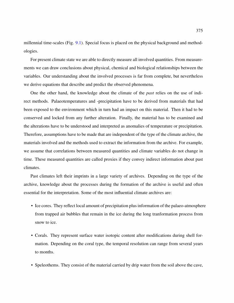
375
millennial time-scales (Fig. 9.1). Special focus is placed on the physical background and method-
ologies.
For present climate state we are able to directly measure all involved quantities. From measure-
ments we can draw conclusions about physical, chemical and biological relationships between the
variables. Our understanding about the involved processes is far from complete, but nevertheless
we derive equations that describe and predict the observed phenomena.
One the other hand, the knowledge about the climate of the past relies on the use of indi-
rect methods. Palaeotemperatures and -precipitation have to be derived from materials that had
been exposed to the environment which in turn had an impact on this material. Then it had to be
conserved and locked from any further alteration. Finally, the material has to be examined and
the alterations have to be understood and interpreted as anomalies of temperature or precipitation.
Therefore, assumptions have to be made that are independent of the type of the climate archive, the
materials involved and the methods used to extract the information from the archive. For example,
we assume that correlations between measured quantities and climate variables do not change in
time. These measured quantities are called proxies if they convey indirect information about past
climates.
Past climates left their imprints in a large variety of archives. Depending on the type of the
archive, knowledge about the processes during the formation of the archive is useful and often
essential for the interpretation. Some of the most influential climate archives are:
• Ice cores. They reflect local amount of precipitation plus information of the palaeo-atmosphere
from trapped air bubbles that remain in the ice during the long tranformation process from
snow to ice.
• Corals. They represent surface water isotopic content after modifications during shell for-
mation. Depending on the coral type, the temporal resolution can range from several years
to months.
• Speleothems. They consist of the material carried by drip water from the soil above the cave,

376 CHAPTER 9. PALEOCLIMATE
Figure 9.1: Schematic view on the climate system. Global climate is a result of the complexinteractions between the atmosphere, cryosphere (ice), hydrosphere (oceans), lithosphere (land),and biosphere (life), fueled by the non-uniform spatial distribution of incoming solar radiation(e.g. Peixoto and Oort, 1992). We know from climate reconstructions using recorders such as icecores, ocean and lake sediment cores, tree rings, corals, cave deposits, and ground water that theEarth’s climate has seen major changes over its history. An analysis of the temperature variationspatched together from all these data reveals that climate change occurs in cycles with characteristicperiods, for example 200 million, 100 thousand, or 4-7 years. For some of these cycles, particularmechanisms can be identified, for example forcing by changes in the Earth’s orbital parametersor internal oscillations of the coupled ocean-atmosphere system. However, major uncertaintiesremain in our understanding of the interplay of the components of the climate system.
9.1. TEMPERATURE RECONSTRUCTIONS 377
in which the speleothem has grown.
• Tree rings. They convey information about the growth rate of the tree at annual resolution.
Climate variables can be inferred from the knowledge of today’s relationship between growth
rate and climatic conditions.
• Sediments. They consist of material that precipitated through the water column and accumu-
lated with or without chemical alterations, depending on the substance and environmental
conditions, such as oxygen availability. For example, organic material is preserved under
anoxic conditions at times of low mixing rates in the respective body of water.
9.1 Temperature reconstructions
Alkenones are highly resistant organic compounds (ketones) produced by phytoplankton of the
class Prymnesiophyceae. The exact function of the alkenones remains under debate. Coccol-
ithophoroids, for instance Emiliania huxleyi, respond to changes in water temperature by altering
the production of long-chain unsaturated alkenones in the structure of their cell. At higher tempera-
tures, more of the di-unsaturated molecules are produced than tri-unsaturated (Prahl and Wakeham,
1987). The molecules are resistant to diagenesis, and can be recovered from sediments up to 110
million years old. The ambient water temperature in which the organisms dwelt can be estimated
from ratio of their unsaturated alkenones (C37-C39) that are preserved in marine sediments. The
Unsaturation Index of di- versus tri-unsaturated C37 alkenone is calculated according to the fol-
lowing relationship (Brassell et al., 1986):
UK′37 = C37 : 2/(C37 : 2 + C37 : 3) (9.1)
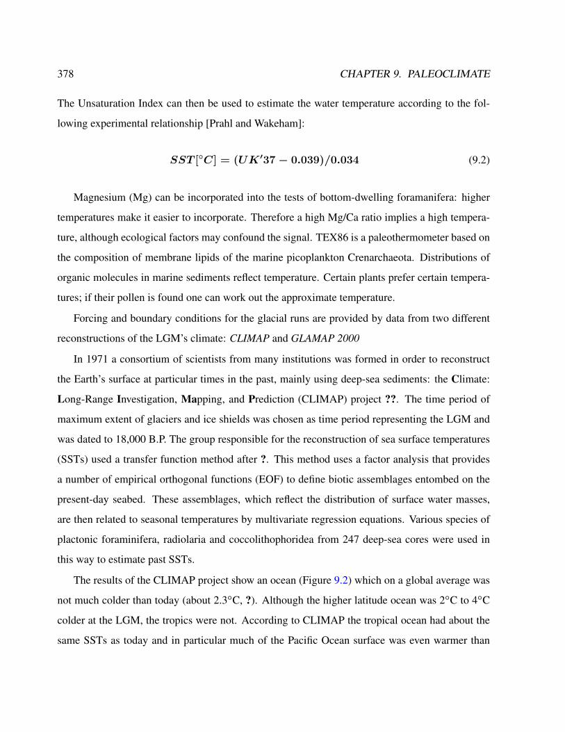
378 CHAPTER 9. PALEOCLIMATE
The Unsaturation Index can then be used to estimate the water temperature according to the fol-
lowing experimental relationship [Prahl and Wakeham]:
SST [C] = (UK′37− 0.039)/0.034 (9.2)
Magnesium (Mg) can be incorporated into the tests of bottom-dwelling foramanifera: higher
temperatures make it easier to incorporate. Therefore a high Mg/Ca ratio implies a high tempera-
ture, although ecological factors may confound the signal. TEX86 is a paleothermometer based on
the composition of membrane lipids of the marine picoplankton Crenarchaeota. Distributions of
organic molecules in marine sediments reflect temperature. Certain plants prefer certain tempera-
tures; if their pollen is found one can work out the approximate temperature.
Forcing and boundary conditions for the glacial runs are provided by data from two different
reconstructions of the LGM’s climate: CLIMAP and GLAMAP 2000
In 1971 a consortium of scientists from many institutions was formed in order to reconstruct
the Earth’s surface at particular times in the past, mainly using deep-sea sediments: the Climate:
Long-Range Investigation, Mapping, and Prediction (CLIMAP) project ??. The time period of
maximum extent of glaciers and ice shields was chosen as time period representing the LGM and
was dated to 18,000 B.P. The group responsible for the reconstruction of sea surface temperatures
(SSTs) used a transfer function method after ?. This method uses a factor analysis that provides
a number of empirical orthogonal functions (EOF) to define biotic assemblages entombed on the
present-day seabed. These assemblages, which reflect the distribution of surface water masses,
are then related to seasonal temperatures by multivariate regression equations. Various species of
plactonic foraminifera, radiolaria and coccolithophoridea from 247 deep-sea cores were used in
this way to estimate past SSTs.
The results of the CLIMAP project show an ocean (Figure 9.2) which on a global average was
not much colder than today (about 2.3C, ?). Although the higher latitude ocean was 2C to 4C
colder at the LGM, the tropics were not. According to CLIMAP the tropical ocean had about the
same SSTs as today and in particular much of the Pacific Ocean surface was even warmer than
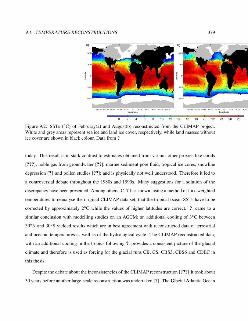
9.1. TEMPERATURE RECONSTRUCTIONS 379
Figure 9.2: SSTs (C) of February(a) and August(b) reconstructed from the CLIMAP project.White and grey areas represent sea ice and land ice cover, respectively, while land masses withoutice cover are shown in black colour. Data from ?
today. This result is in stark contrast to estimates obtained from various other proxies like corals
[???], noble gas from groundwater [??], marine sediment pore fluid, tropical ice cores, snowline
depression [?] and pollen studies [??]; and is physically not well understood. Therefore it led to
a controversial debate throughout the 1980s and 1990s. Many suggestions for a solution of the
discrepancy have been presented. Among others, C. ? has shown, using a method of flux-weighted
temperatures to reanalyse the original CLIMAP data set, that the tropical ocean SSTs have to be
corrected by approximately 2C while the values of higher latitudes are correct. ? came to a
similar conclusion with modelling studies on an AGCM: an additional cooling of 3C between
30N and 30S yielded results which are in best agreement with reconstructed data of terrestrial
and oceanic temperatures as well as of the hydrological cycle. The CLIMAP reconstructed data,
with an additional cooling in the tropics following ?, provides a consistent picture of the glacial
climate and therefore is used as forcing for the glacial runs CB, CS, CBS3, CBS6 and CDEC in
this thesis.
Despite the debate about the inconsistencies of the CLIMAP reconstruction [???] it took about
30 years before another large-scale reconstruction was undertaken [?]. The Glacial Atlantic Ocean

380 CHAPTER 9. PALEOCLIMATE
Figure 9.3: Input data set of the GLAMAP 2000 project. The symbols represent the positionswhere deep-sea core data was taken. Triangles: ?. Diamonds: ?. Boxes: ?(Aug), ?(Feb). Circles:?(Atlantic), ?(Mediterranean). Blue lines: Ice edges after ?, ?, ?. From ?.
Mapping project (GLAMAP 2000) combined data from deep-sea sediment cores throughout the
Atlantic Ocean to obtain a better and revised picture of the conditions during the Last Glacial
Maximum. First of all the time period representing the LGM had to be chosen. Two major defi-
nitions for the LGM exist: The Last benthic oxygen Isotope Maximum (LIM), which assumably
corresponds to the maximum volume of global ice sheets and the insolation minimum at 65 for
summer. The former is dated to the time period between 21,500 and 18,000 years B.P. and the
latter to 21,000 ± 2,000 years B.P. The project members agreed on an overlapping time period,
covering both definitions: 22,000 - 19,000 years B.P. [?]. Furthermore compared to CLIMAP a
larger number of sediment cores was available (Figure 9.3) which were calibrated in a standard-
ised way using the World Ocean Atlas (WOA 94). The extent of sea-ice cover during summer
and winter for the Southern Hemisphere was estimated by ?, using diatom abundances. The same
was performed for the Northern Atlantic through foraminiferic assemblages [?] and dinoflagellate
cyst assemblages [?]. Moreover as compared to CLIMAP, the GLAMAP project used various new
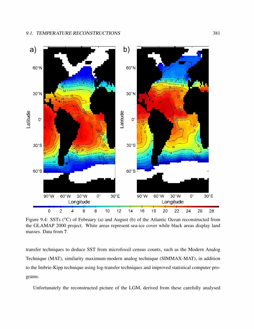
9.1. TEMPERATURE RECONSTRUCTIONS 381
Figure 9.4: SSTs (C) of February (a) and August (b) of the Atlantic Ocean reconstructed fromthe GLAMAP 2000 project. White areas represent sea-ice cover while black areas display landmasses. Data from ?.
transfer techniques to deduce SST from microfossil census counts, such as the Modern Analog
Technique (MAT), similarity maximum-modern analog technique (SIMMAX-MAT), in addition
to the Imbrie-Kipp technique using log-transfer techniques and improved statistical computer pro-
grams.
Unfortunately the reconstructed picture of the LGM, derived from these carefully analysed

382 CHAPTER 9. PALEOCLIMATE
Figure 9.5: Comparison of the SSTs (February (a) and August (b)) in C between GLAMAP 2000and CLIMAP reconstructed data (GLAMAP minus CLIMAP). Black and white areas representland masses and ice cover, respectively. Sea ice is shown where both data sets contain sea ice. TheSST of water underneath the sea-ice cover is set to -1.8C.
sediment cores, is confined to the Atlantic Ocean. Hence, ? transformed the reconstructed SST,
using variogram analysis and kriging for interpolation into a 1x 1grid and embedded it into the
CLIMAP SST reconstruction of the other oceans in order to obtain a global gridded data set (Figure
9.4).
Upon comparing the newly gridded SST and the CLIMAP reconstruction (Figure 9.5) the most

9.2. HYDROLOGICAL CYCLE AND OXYGEN ISOTOPE RATIO CYCLE 383
prominent features are the different sea-ice margins, particularly in the northern Atlantic. The
northernmost sea-ice margin reconstructed by the CLIMAP project is located at about 45N in
February and 60N in August. On the other hand, GLAMAP 2000 locates the sea-ice margin to
up to about 60N in February and 80N in August. Nevertheless the open ocean in front of the
CLIMAP ice edge tends to be colder in the GLAMAP data set. Therefore the latter shows a weaker
meridional temperature gradient in the mid latitudes of the northern Atlantic.
Except for the waters off the North African coast, the Atlantic Ocean of the GLAMAP recon-
struction turns out to be generally colder in the low latitudes. This is most pronounced near the
equator. These colder values are well supported by many studies focusing on the reconstruction of
land temperatures in the tropics and subtropics.
The idea of ice-free Nordic Seas is not only proven by faunal assemblages, but as well by
temperature reconstructions from alkenone concentrations [?]. While the band of higher SST in the
northern mid-latitude Atlantic is well supported by deep-sea cores taken from different institutions,
the high temperatures at approximately 40- 50S and 30- 40W are considered as an artefact,
due to the lack of sediment cores from this area [?]. ? also challenge the reliability of the very low
temperatures off the Argentine coast, since a single sediment core is responsible for this local drop
of SST.
9.2 Hydrological cycle and Oxygen isotope ratio cycle
The hydrological cycle describes the transport of water in all three phases on the global scale.
Summing up all water volume contributions, about 14 × 1017 m3 water are on the Earth and
are stored in different components of the climate system. Most of the water (more than 97%) is
in the salty oceans, and about 2% is stored in the glaciers. The remainder is unevenly divided
between the reservoirs of groundwater, lakes and rivers, the atmosphere, and soil [Baumgartner
and Reichel, 1975; Peixoto and Oort, 1992]. The atmosphere is a central subsystem in the global
climate system, because it has the highest mobility and it connects the other subsystems.
384 CHAPTER 9. PALEOCLIMATE
Dansgaard et al. [1993] used stable isotope measurements from the full length of the 250 kyr
(thousands of years) Greenland ice core record (Greenland Ice Sheet Project) to examine climate
stability during glacial periods. They found that apart from the most recent 10,000 years, instability
dominated the North Atlantic climate over the last 230 kyr. Other paleoclimate proxies point out
an extreme rapidity in the changes of aridity, dust, and chemical composition, as recorded by
Greenland ice cores [Mayewski et al., 1993], or by marine sediment cores [Lehman and Keigwin,
1992], implying that events at the end of the last glaciation could have been responses to a threshold
in the North Atlantic climate system.
One possible mechanism for such a threshold is associated with the hydrological cycle [Birch-
field, 1989; Broecker et al., 1990; Zaucker et al., 1994; Rahmstorf, 1995]. Besides the exchange
of energy and momentum between atmosphere and ocean, the freshwater flux is one of the main
driving forces for the oceanic thermohaline circulation (THC). While air-sea heat fluxes damp sea
surface temperature anomalies quite effectively, there is no direct feedback in the atmosphere for
removing sea surface salinity anomalies, because precipitation and evaporation are not dependent
on ocean salinity. Numerical experiments suggest that the THC is very sensitive to the atmospheric
freshwater forcing [Manabe and Stouffer, 1995; Rahmstorf, 1996; Weaver et al., 1998].
Warren [1983] suggested that the low surface salinities in the Pacific are due to an excess of
precipitation over evaporation and that this can be the reason for the absence of deep water forma-
tion there. Because the salinity characteristic is affected by the interbasin transport of water vapor
it is therefore conceivable that the hydrological cycle is responsible for the difference between the
thermohaline circulation in the North Atlantic and Pacific Oceans. It has been argued [Birchfield,
1989; Broecker et al., 1990; Zaucker et al., 1994] that the interbasin water vapor transport pro-
vides for multiple equilibria of the climate system. A recent sensitivity study [Weaver et al., 1998]
confirms this idea: By changing the Atlantic catchment of a few rivers, the Weaver et al. [1998]
model is able to enhance or to slow down the Atlantic thermohaline circulation.
The hydrological cycle and its associated distribution of moisture is furthermore of interest
because of its important influence on the terrestrial climate, distribution of vegetation and deserts,
9.2. HYDROLOGICAL CYCLE AND OXYGEN ISOTOPE RATIO CYCLE 385
and the growth of ice sheets. These geographical features are documented by the proxy data
available, as for example lake levels and vegetation types [Crowley and North, 1991; Farrera et
al., 1999]. Further links of the water vapor transport with climate are due to the ice sheets and the
water’s isotopic compositions [Werner et al., 2000].
Oxygen isotope ratio cycles are cyclical variations in the ratio of the mass of oxygen with an
atomic weight of 18 to the mass of oxygen with an atomic weight of 16 present in some substance,
such as polar ice or calcite in ocean core samples. The ratio is linked to water temperature of
ancient oceans, which in turn reflects ancient climates. Cycles in the ratio mirror climate changes
in geologic history.
Oxygen (chemical symbol O) has three naturally occurring isotopes: 16O, 17O, and 18O, where
the 16, 17 and 18 refer to the atomic weights. The most abundant is 16O, with a small percentage
of 18O and an even smaller percentage of 17O. Oxygen isotope analysis considers only the ratio of18O to 16O present in a sample. The calculated ratio of the masses of each present in the sample
is then compared to a standard, which can yield information about the temperature at which the
sample was formed.
18O is two neutrons heavier than 16O and causes the water molecule in which it occurs to be
heavier by that amount. The addition of more energy is required to vaporize H182 O than H16
2 O,
and H182 O liberates more energy when it condenses. In addition, H16
2 O tends to diffuse more
rapidly. BecauseH162 O requires less energy to vaporize, and is more likely to diffuse to the liquid
surface, the first water vapor formed during evaporation of liquid water is enriched in H162 O,
and the residual liquid is enriched in H182 O. When water vapor condenses into liquid, H18
2 O
preferentially enters the liquid, whileH162 O is concentrated in the remaining vapor. As an air mass
moves from a warm region to a cold region, water vapor condenses and is removed as precipitation.
The precipitation removes H182 O, leaving progressively more H16
2 O−rich water vapor. This
distillation process causes precipitation to have lower 18O/16O as the temperature decreases.
Additional factors can affect the efficiency of the distillation, such as the direct precipitation of ice
crystals, rather than liquid water, at low temperatures.
386 CHAPTER 9. PALEOCLIMATE
The 18O/16O ratio provides a record of ancient temperature. Precipitation and therefore
glacial ice contain water with a low 18O content. Since large amounts of 16O water are being
stored as glacial ice, the 18O content of oceanic water is high. Water up to 5 degrees warmer than
today represents an interglacial, when the 18O content is lower. A plot of ancient water temper-
ature over time indicates that climate has varied cyclically, with large cycles and harmonics, or
smaller cycles, superimposed on the large ones. This technique has been especially valuable for
identifying glacial maxima and minima in the Pleistocene.
Limestone is deposited from the calcite shells of microorganisms. Calcite, or calcium carbon-
ate, chemical formulaCaCO3, is formed from water,H2O, and carbon dioxide,CO2, dissolved
in the water. The carbon dioxide provides two of the oxygen atoms in the calcite. The calcium
must rob the third from the water. The isotope ratio in the calcite is therefore the same, after com-
pensation, as the ratio in the water from which the microorganisms of a given layer extracted the
material of the shell. The microorganism most frequently referenced is foraminifera (Fig. 9.6).
There are two stable isotopes of hydrogen (1H, protium, and 2H, deuterium) and three stable
isotopes of oxygen (16O, 17O, and 18O). Further, there are three out of nine isotopically different
water isotopes 1 that are available in measurable quantities: H162 O, H18
2 O, and 1H2H16O.
High values in the ratio of 18O to 16O reflect usually mean low temperatures in foram tests or
ice cores. Confounded by ice volume - more ice means higher δ18O values. Ocean water is mostly18O with small amounts of HD16O and 16O.
Table 9.1 shows the relative quantities of the isotopes. 17O appears equally in this table because
H172 O is involved in the same physical processes as H18
2 O. Only its abundance and fractionation
rate is less useful for palaeoclimate research. However, it is used for research topics involving
very long time scales. The ratio of 17O/18O in a given substance does change on geological time
scales and can be used to distinguish the origins of meteorites and materials on different planets
[e.g.][]Clayton:03.
1The term water isotope is often used in the scientific community. It is not correct, since water is obviously not anelement. In this study, this expression is used as an abbreviation for water molecule containing a heavy stable isotopeof oxygen or hydrogen.
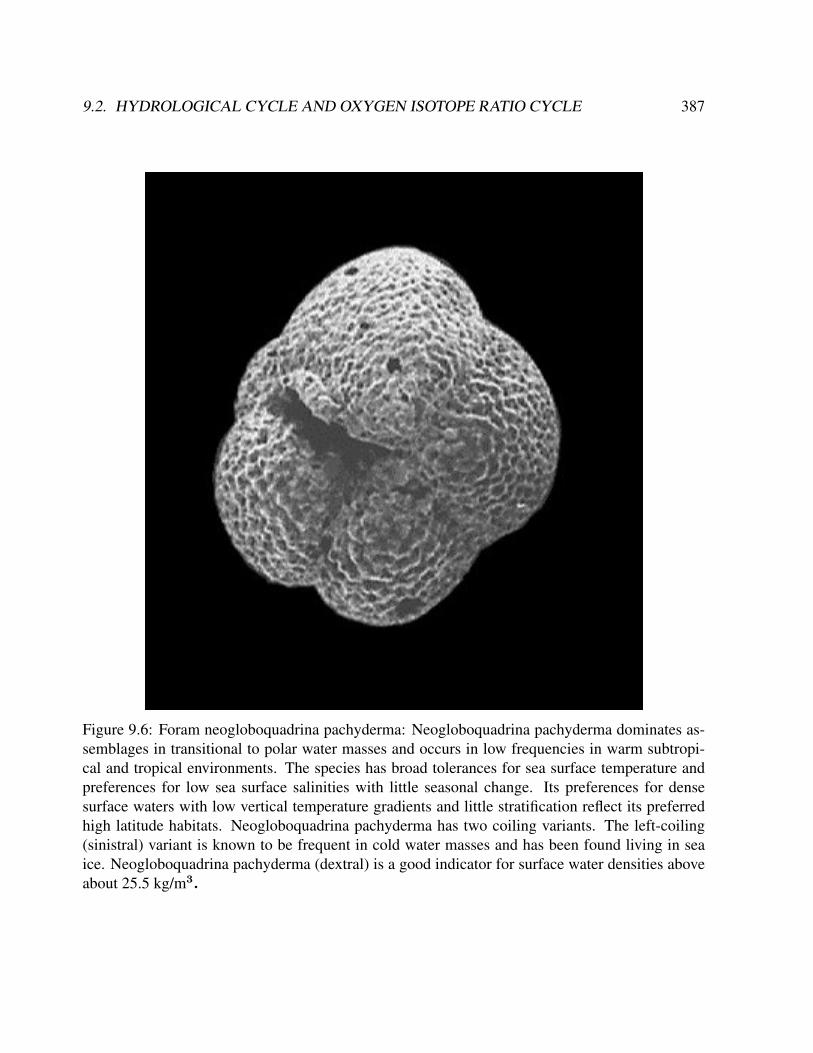
9.2. HYDROLOGICAL CYCLE AND OXYGEN ISOTOPE RATIO CYCLE 387
Figure 9.6: Foram neogloboquadrina pachyderma: Neogloboquadrina pachyderma dominates as-semblages in transitional to polar water masses and occurs in low frequencies in warm subtropi-cal and tropical environments. The species has broad tolerances for sea surface temperature andpreferences for low sea surface salinities with little seasonal change. Its preferences for densesurface waters with low vertical temperature gradients and little stratification reflect its preferredhigh latitude habitats. Neogloboquadrina pachyderma has two coiling variants. The left-coiling(sinistral) variant is known to be frequent in cold water masses and has been found living in seaice. Neogloboquadrina pachyderma (dextral) is a good indicator for surface water densities aboveabout 25.5 kg/m3.

388 CHAPTER 9. PALEOCLIMATE
Hydrogen Oxygen1H 2H 16O 17O 18O
99.985 0.015 99.759 0.037 0.204
Table 9.1: Natural abundance in h of stable hydrogen and oxygen isotopes used in climate re-search.
In Standard Mean Ocean Water (SMOW) the ratio of D to H is 155.8 · 10−6 and 18O to 16O
is 2005 · 10−6. The difference from VSMOW is expressed as
δ18O =
((18O/16O)
(18O/16O)SMOW
− 1
)· 1000%0 (9.3)
and a similar formula for δD. Fractionation occurs during changes between condensed and vapour
phases: the vapour pressure of heavier isotopes is lower, so vapour contains relatively more of the
lighter isotopes and when the vapour condenses the precipitation preferentially contains heavier
isotopes. The major influence on δ18O is the difference between ocean temperatures where the
moisture evaporated and the place where the final precipitation occurred; since ocean temperatures
are relatively stable the δ18O value mostly reflects the temperature where precipitation occurs.
Taking into account that the precipitation forms above the inversion layer, we are left with a linear
relation:
δ18O = aT + b (9.4)
which is empirically calibrated from measurements of temperature and δ18O as a = 0.67/ppm/C
for Greenland and 0.76/ppm/C for East Antarctica. The calibration was initially done on the
basis of spatial variations in temperature and it was assumed that this corresponded to temporal
variations (Jouzel and Merlivat, 1984). More recently, borehole thermometry has shown that for
glacial-interglacial variations, a = 0.33/ppm/C (Cuffey et al., 1995), implying that glacial-
interglacial temperature changes were twice as large as previously believed.
9.2. HYDROLOGICAL CYCLE AND OXYGEN ISOTOPE RATIO CYCLE 389
The empirical relationships between the observed isotopic composition of meteoric water and
environmental parameters were summarized by ?. Relations between surface-air temperature, dis-
tance from the coast, height above sea level and amount of precipitation to the measured isotopic
composition were termed ’effects’ (temperature, continental, altitude and amount effect, respec-
tively). These effects can be considered as a measure of rain-out of a given air mass on its way to
the preipiation region. ? used a Rayleigh model to explain the linear relationship between the iso-
topic composition of precipitation and the annual mean surface temperature. Under the simplifying
assumption that this air mass is isolated and constantly cooled, the Rayleigh approach describes
the observed gradient of 0.58 h/C at higher latitudes, if the annual mean surface temperature
<15C. In the tropics, the annual temperature variation generally is low. On the other hand there
are large variations in the rainfall intensity. Therefore, the isotopic composition is mainly influ-
enced by the amount effect. Increased precipitation leads to isotopically more depleted rainfall and
the δ18O/temperature relationship is not valid. However, the effects mentioned above do not occur
isolated or separated from each other. Any change in the environment in which water undergoes
phase changes will have an effect on the fractionation.
The Rayleigh model approach has been refined to include kinetic fractionation during evap-
oration and formation of ice, the simultaneous existence of vapour, liquid and ice in clouds, and
partial re-evaporation of precipitation from land surfaces [?]. Mixing of air masses from different
origin cannot be described by Rayleigh models. The implementation of isotope physics in general
circulation models has therefore been the next step in simulation of the global hydrological cycle.
The isotope signature of evaporating vapour depends on sea surface temperature, relative hu-
midity and the delta-value of atmospheric vapour [?]. The latter is an independent quantity, allow-
ing for example a degree of freedom in the interpretation of the deuterium excess.
The ratios of the heavy isotopic water H182 O/H16
2 O and HDO/H162 O usually are expressed in
parts per thousand deviation relative to the standard V-SMOW (Vienna standard mean ocean wa-
390 CHAPTER 9. PALEOCLIMATE
ter). The delta notations δ18O and δD are defined as
δsample =
(Rsample
Rstandard
− 1
)∗ 1000 (9.5)
whereRsample is the measured isotope ratio andRstandard is the V-SMOW value for the respec-
tive isotope.
The water isotopes are transported in parallel to atmospheric water. The advection and diffusion
routines therefore ensure constant ratios of H182 O/H16
2 O and HDO/H162 O, respectively. The isotopic
composition is then expressed in terms of VSMOW, the Vienna standard mean ocean water. For18O we use the formula
δ18O = [(18O/16O)sample/(18O/16O)V SMOW − 1]. (9.6)
δD is calculated correspondingly for HD16O. The first fractionation process occurs during evapo-
ration at the ocean surface. The evaporative flux of isotopes is calculated using
Ex = ρCv|~vh|(1− k)(xvap − xsat) (9.7)
where ρ is the density of air, Cv the drag coefficient depending on the stability of the atmospheric
boundary layer, |~vh| the horizontal wind speed, xvap the water isotope mixing ratio in the first
model layer, and xsat = α(Tsurf)−1βRocqsat, with α the temperature-dependent equilibrium
fractionation factor, β an enrichment factor for the oceanic surface due to evaporation, Roc the
oceanic mass relation corresponding to RSMOW , and qsat is the saturation mixing ratio. Non-
equilibrium effects (kinetic diffusion from the thin sub-layer above the ocean surface to the atmo-
sphere) are taken into account with the factor 1− k [see ?]. Dividing Ex by the evaporative flux
of H162 O E = ρCv|~vh|(qvap − qsat) results in the isotopic composition of the evaporative flux
δEx + 1 = (1− k)/(1− h)[α(Tsurf)−1(δxoc + 1)− (δxvap + 1)h] (9.8)
9.2. HYDROLOGICAL CYCLE AND OXYGEN ISOTOPE RATIO CYCLE 391
with δxoc = β(Roc/RSMOW ) − 1, the relative humidity h, and the atmospheric delta-value
δxvap.
Condensation to liquid or ice phase is treated as an equilibrium process (Rl,i = αRvap).
A kinetic process becomes important at low temperatures, namely the diffusion of isotopes
through the oversaturated zone around forming ice crystals. This is considered in the model with
an effective fractionation coefficient
αeff = αeqαkin (9.9)
with αkin = S/(αeqRD(S − 1) + 1). RD is the ratio of the diffusivities of H162 O and the
isotopic water, and S = 1 + 0.003T (T in C) the oversaturation function [see ?].
Re-evaporation of raindrops in the undersaturated air below cloud base occurs in an equilibrium
and non-equilibrium process: The kinetic fractionation is formulated similar to equation (2), using
undersaturation described by heff , the mean relative humidity of the air below cloud base in the
grid box. The fraction of droplets that reach isotopic equilibrium depends on the droplet size. In
the implementation of numerical models, the heavy isotopic water exactly follows the hydrological
routines, except where fractionation during phase changes is altering the ratios H182 O/H16
2 O in the
vapour, liquid and solid phase, respectively. The fractionation coefficients α for 18O are
lnαl = 1137/T 2 − 0.4156/T + 0.00206, and (9.10)
lnαi = 11.839/T − 0.28224, (9.11)
where αl and αi are the fractionation factors for transitions from liquid to vapour phase and from
solid to vapour phase, respectively. This modelling approach allows to examine climate variables,
such as P and T independently from the isotopic water composition. The results presented here
are therefore physically consistent and do not rely on any further concepts or models.
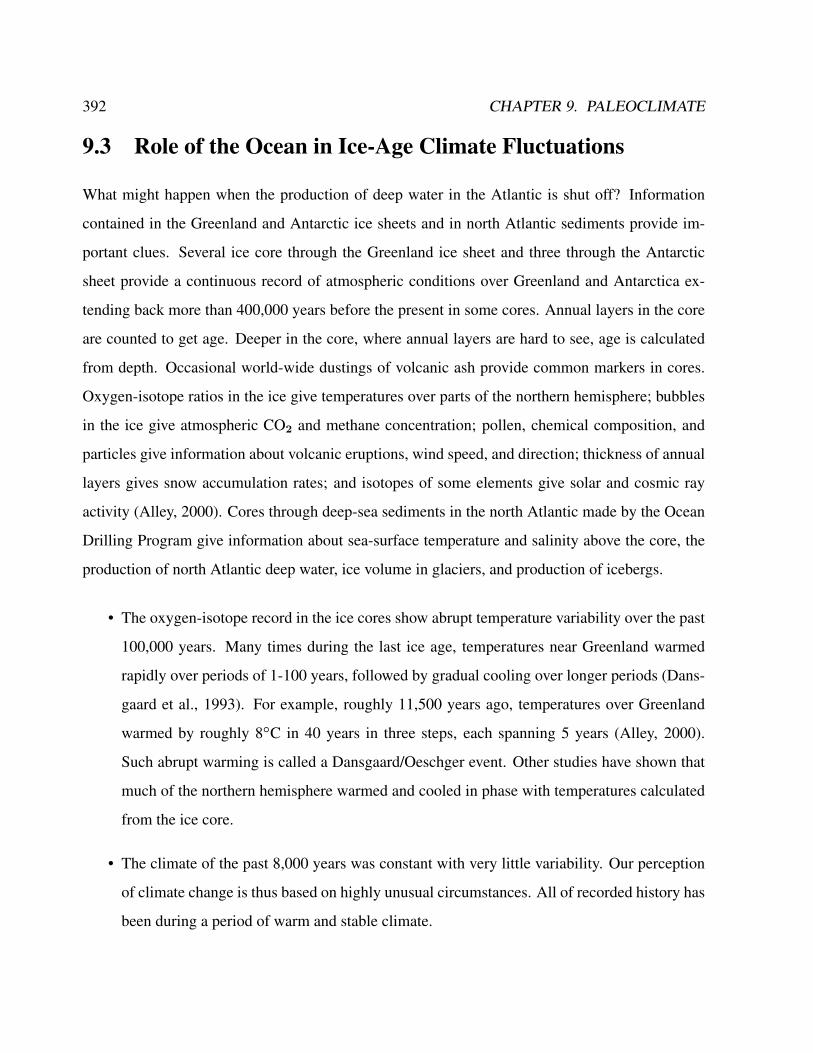
392 CHAPTER 9. PALEOCLIMATE
9.3 Role of the Ocean in Ice-Age Climate Fluctuations
What might happen when the production of deep water in the Atlantic is shut off? Information
contained in the Greenland and Antarctic ice sheets and in north Atlantic sediments provide im-
portant clues. Several ice core through the Greenland ice sheet and three through the Antarctic
sheet provide a continuous record of atmospheric conditions over Greenland and Antarctica ex-
tending back more than 400,000 years before the present in some cores. Annual layers in the core
are counted to get age. Deeper in the core, where annual layers are hard to see, age is calculated
from depth. Occasional world-wide dustings of volcanic ash provide common markers in cores.
Oxygen-isotope ratios in the ice give temperatures over parts of the northern hemisphere; bubbles
in the ice give atmospheric CO2 and methane concentration; pollen, chemical composition, and
particles give information about volcanic eruptions, wind speed, and direction; thickness of annual
layers gives snow accumulation rates; and isotopes of some elements give solar and cosmic ray
activity (Alley, 2000). Cores through deep-sea sediments in the north Atlantic made by the Ocean
Drilling Program give information about sea-surface temperature and salinity above the core, the
production of north Atlantic deep water, ice volume in glaciers, and production of icebergs.
• The oxygen-isotope record in the ice cores show abrupt temperature variability over the past
100,000 years. Many times during the last ice age, temperatures near Greenland warmed
rapidly over periods of 1-100 years, followed by gradual cooling over longer periods (Dans-
gaard et al., 1993). For example, roughly 11,500 years ago, temperatures over Greenland
warmed by roughly 8C in 40 years in three steps, each spanning 5 years (Alley, 2000).
Such abrupt warming is called a Dansgaard/Oeschger event. Other studies have shown that
much of the northern hemisphere warmed and cooled in phase with temperatures calculated
from the ice core.
• The climate of the past 8,000 years was constant with very little variability. Our perception
of climate change is thus based on highly unusual circumstances. All of recorded history has
been during a period of warm and stable climate.
9.3. ROLE OF THE OCEAN IN ICE-AGE CLIMATE FLUCTUATIONS 393
• Hartmut Heinrich and colleagues (Bond et al., 1992), studying the sediments in the north
Atlantic noticed periods when coarse material was deposited on the bottom in mid-ocean.
Only icebergs can carry such material out to sea, and the find indicated times when large
numbers of icebergs were released into the north Atlantic. These are now called Heinrich
events.
• The correlation of Greenland temperature with iceberg production is related to the merid-
ional overturning circulation. When icebergs melted, the surge of fresh water increased the
stability of the water column shutting off the production of North Atlantic Deep Water. The
shut-off of deep-water formation greatly reduced the transport of warm water in the north
Atlantic, producing very cold northern hemisphere climate (Figure 13.2). The melting of
the ice pushed the polar front, the boundary between cold and warm water in the north At-
lantic further south than its present position. The location of the front, and the time it was at
different positions can be determined from analysis of bottom sediments.
• When the meridional overturning circulation shuts down, heat normally carried from the
south Atlantic to the north Atlantic becomes available to warm the southern hemisphere.
This explains the Antarctic warming.
• The switching on and off of the meridional overturning circulation has large hysteresis (Fig-
ure 13.3). The circulation has two stable states. The first is the present circulation. In the
second, deep water is produced mostly near Antarctica, and upwelling occurs in the far north
Pacific (as it does today) and in the far north Atlantic. Once the circulation is shut off, the
system switches to the second stable state. The return to normal salinity does not cause the
circulation to turn on. Surface waters must become saltier than average for the first state to
return (Rahmstorf, 1995)
• Heinrich events seem to precede the largest Dansgaard/Oeschger events (Stocker and Mar-
chal, 2000). Here’s what seems to happen. The Heinrich event shuts off the Atlantic deep
circulation which leads to a very cold North Atlantic. This is followed about 1000 years later
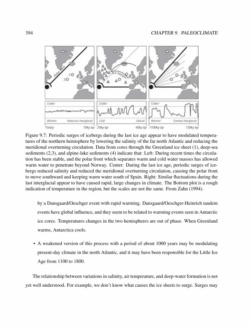
394 CHAPTER 9. PALEOCLIMATE
Figure 9.7: Periodic surges of icebergs during the last ice age appear to have modulated tempera-tures of the northern hemisphere by lowering the salinity of the far north Atlantic and reducing themeridional overturning circulation. Data from cores through the Greenland ice sheet (1), deep-seasediments (2,3), and alpine-lake sediments (4) indicate that: Left: During recent times the circula-tion has been stable, and the polar front which separates warm and cold water masses has allowedwarm water to penetrate beyond Norway. Center: During the last ice age, periodic surges of ice-bergs reduced salinity and reduced the meridional overturning circulation, causing the polar frontto move southward and keeping warm water south of Spain. Right: Similar fluctuations during thelast interglacial appear to have caused rapid, large changes in climate. The Bottom plot is a roughindication of temperature in the region, but the scales are not the same. From Zahn (1994).
by a Dansgaard/Oeschger event with rapid warming. Dansgaard/Oeschger-Heinrich tandem
events have global influence, and they seem to be related to warming events seen in Antarctic
ice cores. Temperatures changes in the two hemispheres are out of phase. When Greenland
warms, Antarctica cools.
• A weakened version of this process with a period of about 1000 years may be modulating
present-day climate in the north Atlantic, and it may have been responsible for the Little Ice
Age from 1100 to 1800.
The relationship between variations in salinity, air temperature, and deep-water formation is not
yet well understood. For example, we don’t know what causes the ice sheets to surge. Surges may
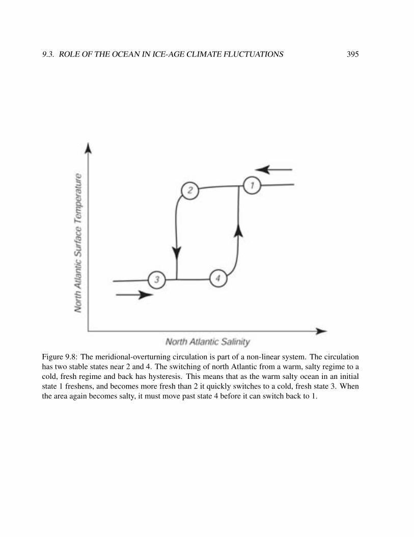
9.3. ROLE OF THE OCEAN IN ICE-AGE CLIMATE FLUCTUATIONS 395
Figure 9.8: The meridional-overturning circulation is part of a non-linear system. The circulationhas two stable states near 2 and 4. The switching of north Atlantic from a warm, salty regime to acold, fresh regime and back has hysteresis. This means that as the warm salty ocean in an initialstate 1 freshens, and becomes more fresh than 2 it quickly switches to a cold, fresh state 3. Whenthe area again becomes salty, it must move past state 4 before it can switch back to 1.
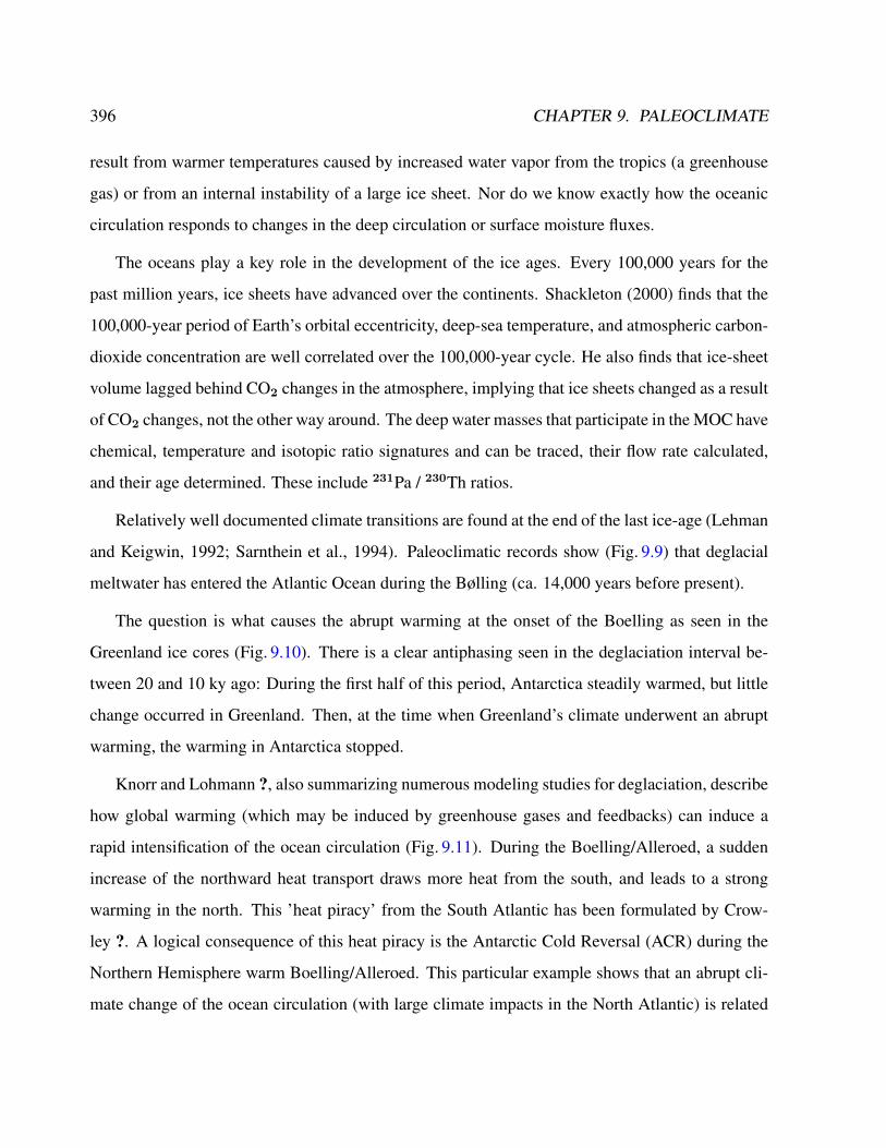
396 CHAPTER 9. PALEOCLIMATE
result from warmer temperatures caused by increased water vapor from the tropics (a greenhouse
gas) or from an internal instability of a large ice sheet. Nor do we know exactly how the oceanic
circulation responds to changes in the deep circulation or surface moisture fluxes.
The oceans play a key role in the development of the ice ages. Every 100,000 years for the
past million years, ice sheets have advanced over the continents. Shackleton (2000) finds that the
100,000-year period of Earth’s orbital eccentricity, deep-sea temperature, and atmospheric carbon-
dioxide concentration are well correlated over the 100,000-year cycle. He also finds that ice-sheet
volume lagged behind CO2 changes in the atmosphere, implying that ice sheets changed as a result
of CO2 changes, not the other way around. The deep water masses that participate in the MOC have
chemical, temperature and isotopic ratio signatures and can be traced, their flow rate calculated,
and their age determined. These include 231Pa / 230Th ratios.
Relatively well documented climate transitions are found at the end of the last ice-age (Lehman
and Keigwin, 1992; Sarnthein et al., 1994). Paleoclimatic records show (Fig. 9.9) that deglacial
meltwater has entered the Atlantic Ocean during the Bølling (ca. 14,000 years before present).
The question is what causes the abrupt warming at the onset of the Boelling as seen in the
Greenland ice cores (Fig. 9.10). There is a clear antiphasing seen in the deglaciation interval be-
tween 20 and 10 ky ago: During the first half of this period, Antarctica steadily warmed, but little
change occurred in Greenland. Then, at the time when Greenland’s climate underwent an abrupt
warming, the warming in Antarctica stopped.
Knorr and Lohmann ?, also summarizing numerous modeling studies for deglaciation, describe
how global warming (which may be induced by greenhouse gases and feedbacks) can induce a
rapid intensification of the ocean circulation (Fig. 9.11). During the Boelling/Alleroed, a sudden
increase of the northward heat transport draws more heat from the south, and leads to a strong
warming in the north. This ’heat piracy’ from the South Atlantic has been formulated by Crow-
ley ?. A logical consequence of this heat piracy is the Antarctic Cold Reversal (ACR) during the
Northern Hemisphere warm Boelling/Alleroed. This particular example shows that an abrupt cli-
mate change of the ocean circulation (with large climate impacts in the North Atlantic) is related
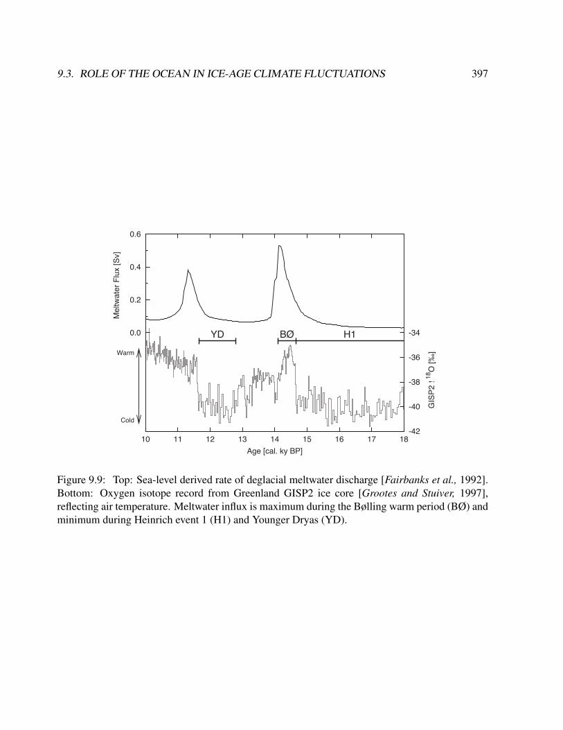
9.3. ROLE OF THE OCEAN IN ICE-AGE CLIMATE FLUCTUATIONS 397
0.0
0.2
0.4
0.6
10 11 12 13 14 15 16 17 18-42
-40
-38
-36
-34
Mel
twat
er F
lux
[Sv]
GIS
P2 !
18O
[‰]
Age [cal. ky BP]
BØ H1YDWarm
Cold
Figure 9.9: Top: Sea-level derived rate of deglacial meltwater discharge [Fairbanks et al., 1992].Bottom: Oxygen isotope record from Greenland GISP2 ice core [Grootes and Stuiver, 1997],reflecting air temperature. Meltwater influx is maximum during the Bølling warm period (BØ) andminimum during Heinrich event 1 (H1) and Younger Dryas (YD).
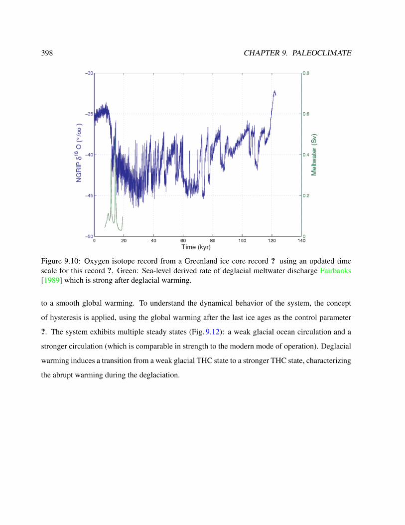
398 CHAPTER 9. PALEOCLIMATE
Figure 9.10: Oxygen isotope record from a Greenland ice core record ? using an updated timescale for this record ?. Green: Sea-level derived rate of deglacial meltwater discharge Fairbanks[1989] which is strong after deglacial warming.
to a smooth global warming. To understand the dynamical behavior of the system, the concept
of hysteresis is applied, using the global warming after the last ice ages as the control parameter
?. The system exhibits multiple steady states (Fig. 9.12): a weak glacial ocean circulation and a
stronger circulation (which is comparable in strength to the modern mode of operation). Deglacial
warming induces a transition from a weak glacial THC state to a stronger THC state, characterizing
the abrupt warming during the deglaciation.
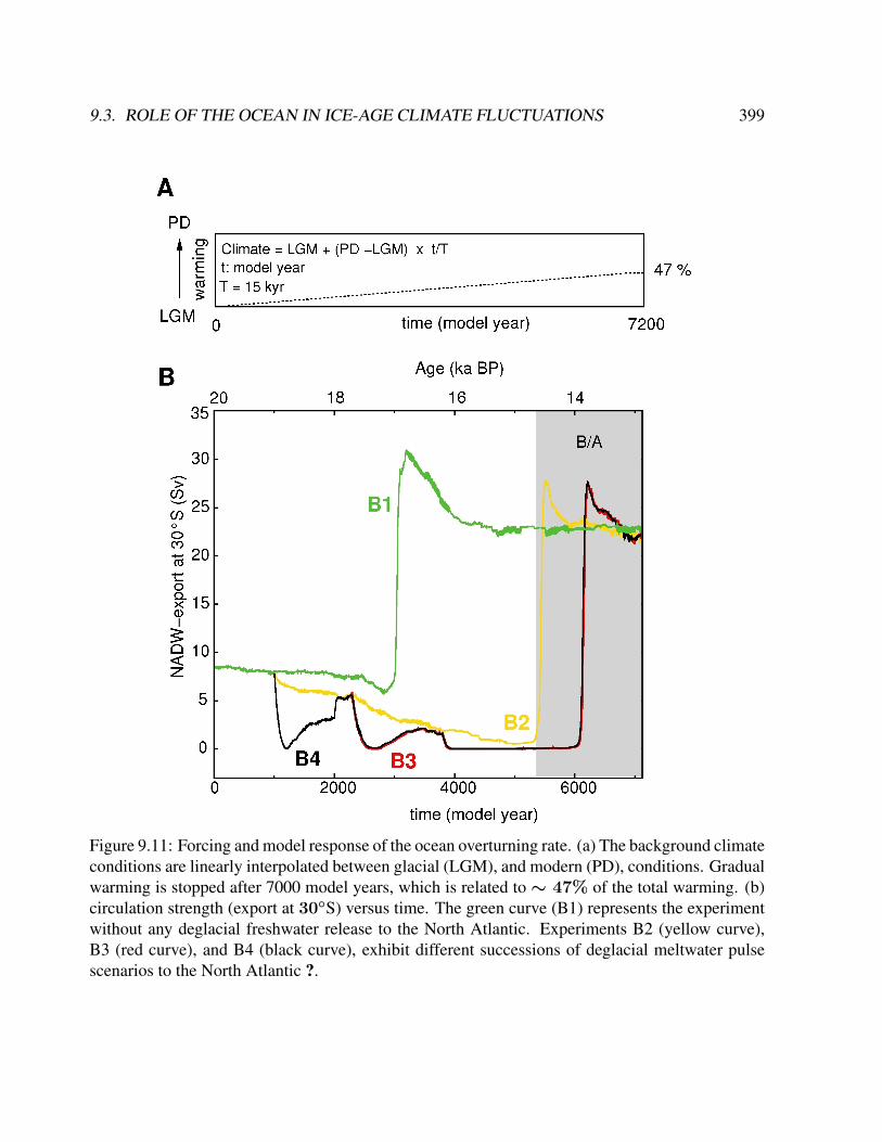
9.3. ROLE OF THE OCEAN IN ICE-AGE CLIMATE FLUCTUATIONS 399
Figure 9.11: Forcing and model response of the ocean overturning rate. (a) The background climateconditions are linearly interpolated between glacial (LGM), and modern (PD), conditions. Gradualwarming is stopped after 7000 model years, which is related to ∼ 47% of the total warming. (b)circulation strength (export at 30S) versus time. The green curve (B1) represents the experimentwithout any deglacial freshwater release to the North Atlantic. Experiments B2 (yellow curve),B3 (red curve), and B4 (black curve), exhibit different successions of deglacial meltwater pulsescenarios to the North Atlantic ?.
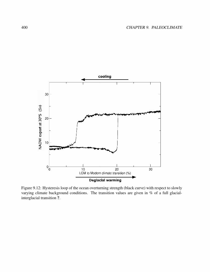
400 CHAPTER 9. PALEOCLIMATE
Figure 9.12: Hysteresis loop of the ocean overturning strength (black curve) with respect to slowlyvarying climate background conditions. The transition values are given in % of a full glacial-interglacial transition ?.

9.4. ABRUPT CLIMATE CHANGE 401
9.4 Abrupt climate change
The occurrence of abrupt changes in the climate system at various time scales has attracted a great
deal of interest for its theoretical and practical significance ?; ?; ?. To some extent, a definition
of what constitutes an abrupt climatic change depends on the sampling interval of the data being
examined ?. For the instrumental period covering approximately the last 100 years of annually
or seasonally sampled data, an abrupt change in a particular climate variable will be taken to
mean a statistically highly significant difference between adjacent 10-year sample means. In the
paleoclimate context (i.e. on long time scales), an abrupt climate change can be in the order of
decades to thousands of years. Since the climate dynamics can be often projected onto a limited
number of modes or patterns of climate variability (e.g., ?; ?), the definition of abrupt climate
change is also related to spatio-temporal patterns.
The concept of abrupt climate change is therefore applied for different time scales. For exam-
ple, changes in climatic regimes were described associated with surface temperature, precipitation,
atmospheric circulation in North America during the 1920s and 1960s ?; ?. Sometimes, the term
’climate jump’ is used instead of ’abrupt climate change’, e.g. ?. Flohn ? expanded the con-
cept of abrupt climate change to include both singular events and catastrophes such as the extreme
El Niño of 1982/1983, as well as discontinuities in paleoclimate indices taken from ice cores and
other proxy data. In the instrumental record covering the last 150 years, there is a well-documented
abrupt shift of sea surface temperature and atmospheric circulation features in the Northern Hemi-
sphere in the mid-1970s, e.g. ?; ?; ?. Some of the best-known and best-studied widespread abrupt
climate changes started and ended during the last deglaciation, most pronounced at high latitudes.
In his classic studies of chaotic systems, Lorenz has proposed a deterministic theory of climate
change with his concept of the ’almost-intransitivity’ of the highly non-linear climate systems. In
this set of equations, exists the possibility of multiple stable solutions to the governing equations,
even in the absence of any variations in external forcing Lorenz [1976]. More complex models,
e.g. Bryan [1986]; Dijkstra et al. [2004] also demonstrated this possibility. On the other hand,
variations in external forcing, such as the changes of incoming solar radiation, volcanic activity,
402 CHAPTER 9. PALEOCLIMATE
deglacial meltwater, and increases of greenhouse gas concentration have also been proposed to
account for abrupt changes in addition to climate intransitivity ?; ?; ?; ?, ?. A particular climate
change is linked to the widespread continental glaciation of Antarctica during the Cenozoic (65
Ma to present) at about 34 Ma, e.g. ?. It should be noted that many facets of regional climate
change are abrupt changes although the global means are rather smoothly changing.
Besides abrupt climate change as described in the time domain, we can find abrupt shifts in the
frequency domain. A prominent example for an abrupt climate change in the frequency domain
is the mid-Pleistocene transition or revolution (MPR), which is the last major ’event’ in a secular
trend towards more intensive global glaciation that characterizes the last few tens of millions of
years. The MPR is the term used to describe the transition between 41 ky (ky=103 years) and 100
ky glacial-interglacial cycles which occurred about one million years ago (see a recent review in
?). Evidence of this is provided by high-resolution oxygen isotope data from deep sea cores, e.g.
?; ?.
Another example is the possibility of greenhouse gas-driven warming leading to a change in
El Niño events. Modeling studies indicate that a strong enhancement of El Niño conditions in the
future is not inconceivable ?. Such a shift would have enormous consequences for both the bio-
sphere and humans. The apparent phase shift during the 1970s seems unique over this time period,
and may thus represent a real climate shift although the available time series is probably too short
to unequivocally prove that the shift is significant ?. The inability to resolve questions of this kind
from short instrumental time series provides one of the strongest arguments for extending the in-
strumental record of climate variability with well-dated, temporally finely resolved and rigorously
calibrated proxy data.
The period of regular instrumental records of global climate is relatively short (100-200 years).
Even so, this record shows many climatic fluctuations, some abrupt or sudden, as well as slow
drifts in climate. Climatic changes become apparent on many temporal and spatial scales. Most
abrupt climate changes are regional in their spatial extent. However, regional changes can have
remote impacts due to atmospheric and oceanic teleconnections. Some of these shifts may be
9.4. ABRUPT CLIMATE CHANGE 403
termed abrupt or sudden in that they represent relatively rapid changes in otherwise comparatively
stable conditions, but they can also be found superimposed on other much slower climatic changes.
The definition of ’abrupt’ or ’rapid’ climate changes is therefore necessarily subjective, since
it depends to a large extent on the sample interval used in a particular study and on the pattern of
longer-term variation within which the sudden shift is embedded. It is therefore useful to avoid a
too general approach, but instead to focus on different types of rapid transitions as they are detected
and modeled for different time periods. Although distinctions between types are somewhat arbi-
trary, together they cover a wide range of shifts in dominant climate modes on time scales ranging
from the Cenozoic (the last 65 millions of years) to the recent and future climate.
In the frequency domain, abrupt climate shifts are due to changes in the dominant oscillations
(as in the case of the MPR), or due to a shift in the phase between different climate signals. As an
example, the phase between the Indian Monsoon and ENSO exhibits significant shifts for the past
100 years ?.
9.4.1 Astronomical theory of ice ages
Over the past half million years, marine, polar ice core and terrestrial records all highlight the
sudden and dramatic nature of glacial terminations, and the shifts in global climate that occurred
as the world passed from dominantly glacial to interglacial conditions, e.g. ?; ?. These climate
transitions, although probably of relatively minor relevance to the prediction of potential future
rapid climate change, do provide the most compelling evidence available in the historical record
for the role of greenhouse gas, oceanic and biospheric feedbacks as non-linear amplifiers in the
climate system. It is such evidence for the dramatic effect of non-linear feedbacks that relatively
minor changes in climatic forcing may lead to abrupt climate response.
A salient feature of glacial-interglacial climate change is furthermore its asymmetry (Fig. 9.13).
Warmings are rapid, usually followed by slower descent into colder climate. Given the symmetry
of orbital forcings F (t), the cause of rapid warming at glacial ’terminations’ must lie in a climate
feedback ?; ?. Clearly, the asymmetric feedback is due to the albedo (reflectance) of ice and snow
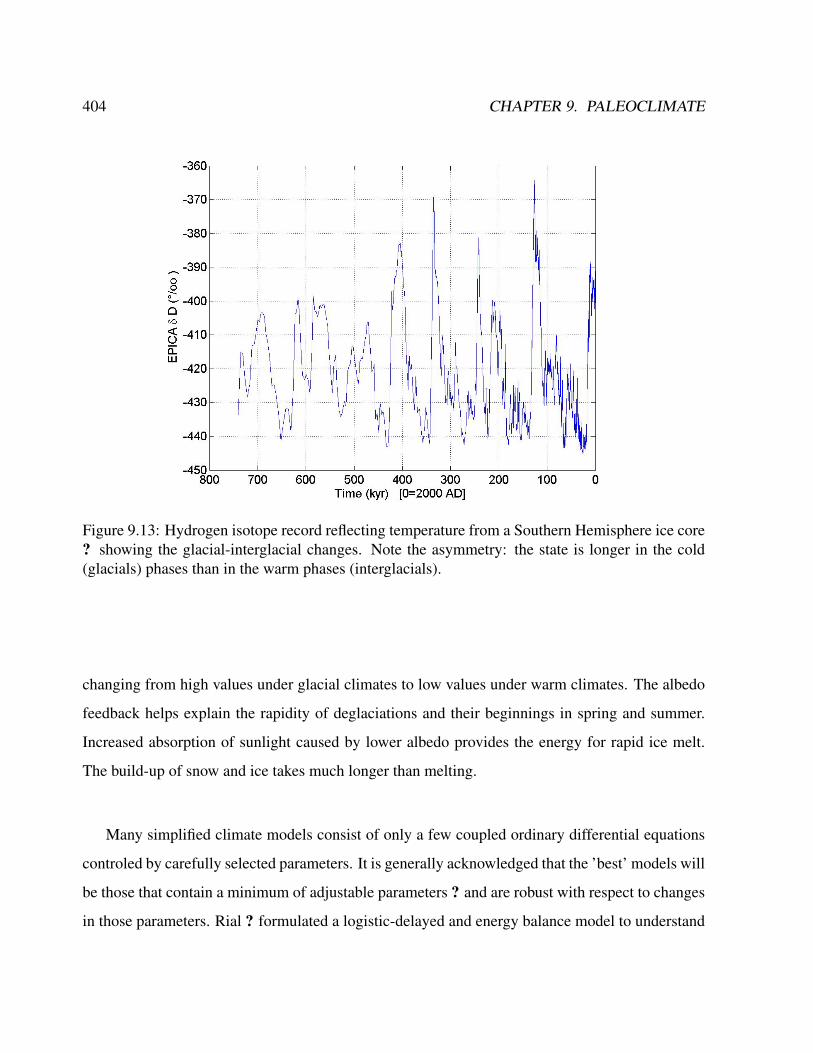
404 CHAPTER 9. PALEOCLIMATE
Figure 9.13: Hydrogen isotope record reflecting temperature from a Southern Hemisphere ice core? showing the glacial-interglacial changes. Note the asymmetry: the state is longer in the cold(glacials) phases than in the warm phases (interglacials).
changing from high values under glacial climates to low values under warm climates. The albedo
feedback helps explain the rapidity of deglaciations and their beginnings in spring and summer.
Increased absorption of sunlight caused by lower albedo provides the energy for rapid ice melt.
The build-up of snow and ice takes much longer than melting.
Many simplified climate models consist of only a few coupled ordinary differential equations
controled by carefully selected parameters. It is generally acknowledged that the ’best’ models will
be those that contain a minimum of adjustable parameters ? and are robust with respect to changes
in those parameters. Rial ? formulated a logistic-delayed and energy balance model to understand
9.4. ABRUPT CLIMATE CHANGE 405
the saw-tooth shape in the paleoclimate record: A fast warming-slow cooling is described by
d
dtx(t) = R
(1−
x(t− τ )
K(t)
)x(t− τ ) (9.12)
Cd
dtT (t) = Q (1− α(x)) − (A+BT ) (9.13)
with x(t) for the normalized ice extent, τ time delay, K(t) = 1 + e(t)T (t) carrying capac-
ity, 1/R response time of the ice sheet, T (t) global mean temperature, α(x) planetary albedo,
external parameter e(t), and Rτ bifurcation parameter. A,B,C,Q are constants for the energy
balance of the climate. The equation is calibrated so that for x(t) = 1 the albedo α(x) = 0.3
and T (t) = 15C.With (9.13), saw-toothed waveforms and frequency modulation can be under-
stood ?. The delayed equation yields damped oscillations of x(t) about the carrying capacity for
small τ. If τ becomes long compared to the natural response time of the system, the oscillations
will become strong, and will grow in amplitude, period and duration. As in the logistic equation
for growth, here the product Rτ is a bifurcation parameter, which when crossing the threshold
value π/2 makes the solutions undergo a Hopf bifurcation and settle to a stable limit cycle with
fundamental period∼ 4τ ?.
The astronomical theory of ice ages –also called Milankovitch ? theory– gained the status
of a paradigm for explaining the multi-millennial variability. A key element of this theory is
that summer insolation at high latitudes of the northern hemisphere determines glacial-interglacial
transitions connected with the waxing and waning of large continental ice sheets, e.g. ?; ?, the
dominant signal in the climate record for the last million years. Climate conditions of glacials
and interglacials are very different. During the Last Glacial Maximum, about 20,000 years before
present, surface temperature in the north Atlantic realm was 10-20C lower than today ?. A recent
study of Huybers and Wunsch ? has shown that the most simple system for the phase of ice volume
x(t) is given by
x(t+ 1) = x(t) + σξ (9.14)
406 CHAPTER 9. PALEOCLIMATE
with ξ a Gaussian white noise process, but with mean µ = 1, and σ = 2. ξ represents the unpre-
dictable background weather and climate variability spanning all time scales out to the glacial/in-
terglacial. This highly simplified model posits 1-ky steps in ice volume x(t). The non-zero mean
biases the Earth toward glaciation. Once x(t) reaches a threshold, a termination is triggered, and
ice-volume is linearly reset to zero over 10 ky. The following threshold condition for a termination
makes it more likely for a termination of ice volume to occur when obliquity Θ(t) is large:
x(t) ≥ T0 − aΘ(t) . (9.15)
Θ(t) has a frequency of about 41 ky, and is furthermore normalized to zero mean with unit vari-
ance. The other parameters are: amplitude a = 15, T0 = 105. Furthermore, the initial ice
volume at 700 ky before present is set to x(t = −700) = 30. Equation (9.14) resembles
an order-one autoregressive process, similar to (7.57), plus the threshold condition (9.15). Mod-
els like (9.14, 9.15) are not theories of climate change, but rather attempts at efficient kinematic
descriptions of the data, and that different mechanisms can be consistent with the limited observa-
tional records. In the next section, the process of deglaciation is modeled in a three-dimensional
model including the spatial dimension.
9.4.2 Antarctic glaciation
During the Cenozoic (65 million years ago (Ma) to present), there was the widespread glaciation
of the Antarctic continent at about 34 Ma, e.g. ?. Antarctic glaciation is the first part of a climate
change from relatively warm and certainly ice-free conditions to massive ice sheets in both, the
southern and northern hemispheres ?. Opening of circum-Antarctic seaways is one of the fac-
tors that have been ascribed as a cause for Antarctic climate change so far ?; ?. Besides gateway
openings, the atmospheric carbon dioxide concentration is another important factor affecting the
evolution of the Cenozoic climate ?; ?. As a third component in the long-term evolution of Antarc-
tic glaciation, land topography is able to insert certain thresholds for abrupt ice sheet build-up.
9.4. ABRUPT CLIMATE CHANGE 407
Whereas tectonics, land topography, and long-term Cenozoic CO2-decrease act as precondition-
ing for Antarctic land ice formation, the cyclicities of the Earth’s orbital configuration are super-
imposed on shorter time scales and may have served as the ultimate trigger and pacemaker for
ice-sheet growth at the Eocene-Oligocene boundary around 34 Ma ?.
DeConto and Pollard ? varied Southern Ocean heat transport to mimic gateway opening instead
of an explicit simulation of ocean dynamics. They found a predominating role of pCO2 in the onset
of glaciation instead of a dominating tectonic role for ’thermal isolation’.
9.4.3 Mid-Pleistocene revolution
Glaciation in the Northern Hemisphere lagged behind, with the earliest recorded glaciation any-
where in the Northern Hemisphere occurring between 10 and 6 Ma and continuing through to the
major increases in global ice volume around 2-3 Ma ?. A recent compilation of 57 globally dis-
tributed records ? is shown in Fig. 9.14. Let us focus now on the mid-Pleistocene transition or
revolution (MPR), describing the transition from 41 ky to 100 ky glacial-interglacial cycles.
Milankovitch ? initially suggested that the critical factor was total summer insolation at about
65N, because for an ice sheet to grow some additional ice must survive each successive summer.
In contrast, the Southern Hemisphere is limited in its response because the expansion of ice sheets
is curtailed by the Southern Ocean around Antarctica. The conventional view of glaciation is thus
that low summer insolation in the temperate North Hemisphere allows ice to survive summer and
thus starts to build up on the northern continents. If so, how then do we account for the MPR?
Despite the pronounced change in Earth system response evidenced in paleoclimatic records, the
frequency and amplitude characteristics of the orbital parameters which force long-term global
climate change, e.g., eccentricity (∼100 ky), obliquity (∼ 41 ky) and precession (∼ 21 and
∼ 19 ky), do not vary during the MPR ?. This suggests that the cause of change in response at the
MPR is internal rather than external to the global climate system.
The result of a wavelet spectral analysis (Fig. 9.15) suggests several abrupt climate changes in
the frequency domain (shown as schematic arrows in the figure). These abrupt climate shifts repre-

408 CHAPTER 9. PALEOCLIMATE
Figure 9.14: A compilation of 57 globally distributed records by Lisiecki and Raymo ?: The δ18Orecord reflects mainly the climate variables temperature and ice volume.
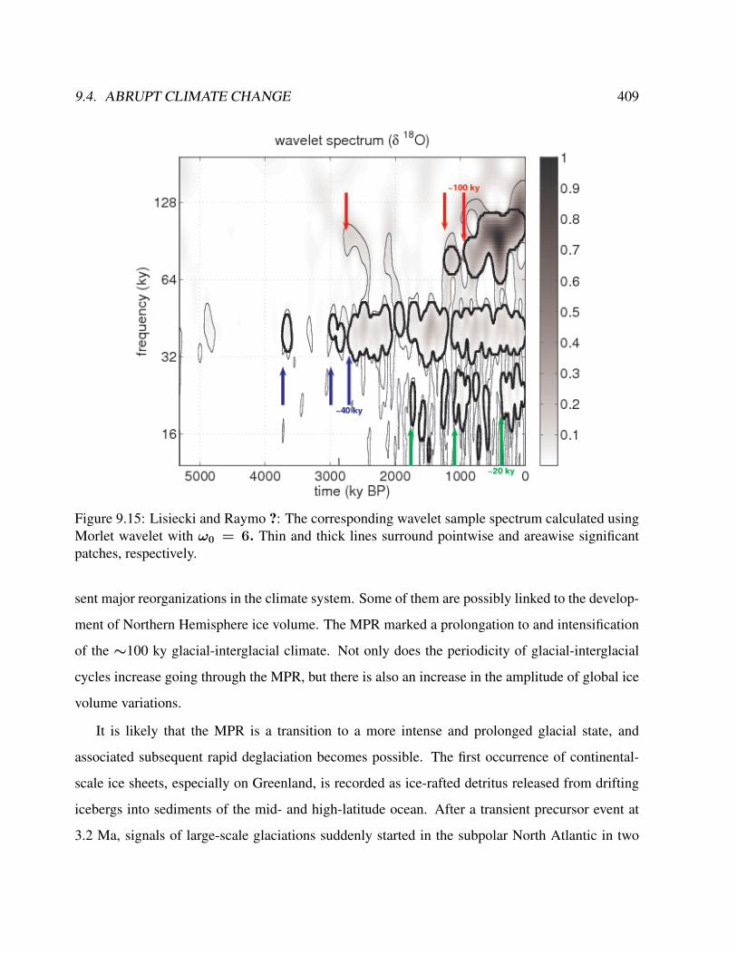
9.4. ABRUPT CLIMATE CHANGE 409
Figure 9.15: Lisiecki and Raymo ?: The corresponding wavelet sample spectrum calculated usingMorlet wavelet with ω0 = 6. Thin and thick lines surround pointwise and areawise significantpatches, respectively.
sent major reorganizations in the climate system. Some of them are possibly linked to the develop-
ment of Northern Hemisphere ice volume. The MPR marked a prolongation to and intensification
of the ∼100 ky glacial-interglacial climate. Not only does the periodicity of glacial-interglacial
cycles increase going through the MPR, but there is also an increase in the amplitude of global ice
volume variations.
It is likely that the MPR is a transition to a more intense and prolonged glacial state, and
associated subsequent rapid deglaciation becomes possible. The first occurrence of continental-
scale ice sheets, especially on Greenland, is recorded as ice-rafted detritus released from drifting
icebergs into sediments of the mid- and high-latitude ocean. After a transient precursor event at
3.2 Ma, signals of large-scale glaciations suddenly started in the subpolar North Atlantic in two
410 CHAPTER 9. PALEOCLIMATE
steps, at 2.9 and 2.7 Ma, e.g. ?.
The ice volume increase may in part be attributed to the prolonging of glacial periods and thus
of ice accumulation. The amplitude of ice volume variation is also accentuated by the extreme
warmth of many interglacial periods. Thus, a colder climate with larger ice sheets should have the
possibility of a greater sudden warming ?. The MPR therefore marks a dramatic sharpening of
the contrast between warm and cold periods. Note however, that the amount of energy at 40 ka
period is hardly changed in the time after 1 Ma, and notably, one sees the addition of energy at
longer periods, without any significant reduction in obliquity-band energy. After about 1 Ma, large
glacial-interglacial changes begin to occur on an approximately 100 ka time scale (but not period-
ically) superimposed upon the variability which continues largely unchanged ?. Why did 100 ka
glacial-interglacials also become possible in addition to the ice volume variability? Lowering of
global CO2 below some critical threshold, or changes in continental configuration, or atmospheric
circulation patterns, or all together, are among the conceivable possibilities, e.g. ?.
9.5 Carbon cycle and isotopes in the ocean
Two aspects of the deep circulation are especially important for understanding Earth’s climate and
its possible response to increased carbon dioxide CO2 in the atmosphere:
• The ability of cold water to absorb CO2 from the atmosphere, and
• the ability of deep currents to modulate the heat transported from the tropics to high latitudes.
The oceans are the primary reservoir of readily available CO2 , an important greenhouse gas.
The oceans contain 40,000 GtC of dissolved, particulate, and living forms of carbon. The land
contains 2,200 GtC, and the atmosphere contains only 750 GtC. Thus the oceans hold 50 times
more carbon than the air. Furthermore, the amount of new carbon put into the atmosphere since
the industrial revolution, 150 GtC, is less than the amount of carbon cycled through the marine
ecosystem in five years. (1 GtC = 1 gigaton of carbon = 1012 kilograms of carbon.) Carbonate
9.5. δ13C DISTRIBUTION 411
rocks such as limestone, the shells of marine animals, and coral are other, much larger, reservoirs.
But this carbon is locked up. It cannot be easily exchanged with carbon in other reservoirs. More
CO2 dissolves in cold water than in warm water. Just imagine shaking and opening a hot can of
tea. The CO2 from a hot can will spew out far faster than from a cold can. Thus the cold deep
water in the ocean is the major reservoir of dissolved CO2 in the ocean.
New CO2 is released into the atmosphere when fossil fuels and trees are burned. Very quickly,
48% of the CO2 released into the atmosphere dissolves in the cold waters of the ocean, much of
which ends up deep in the ocean. Forecasts of future climate change depend strongly on how
much CO2 is stored in the ocean and for how long. If little is stored, or if it is stored and later
released into the atmosphere, the concentration in the atmosphere will change, modulating Earth’s
long-wave radiation balance. How much and how long CO2 is stored in the ocean depends on the
deep circulation and the net flux of carbon deposited on the seafloor. The amount that dissolves
depends on the temperature of the deep water, the storage time in the deep ocean depends on the
rate at which deep water is replenished, and the deposition depends on whether the dead plants and
animals that drop to the sea floor are oxidized. Increased ventilation of deep layers, and warming
of the deep layers could release large quantities of the gas to the atmosphere. The storage of carbon
in the ocean also depends on the dynamics of marine ecosystems, upwelling, and the amount of
dead plants and animals stored in sediments.
In contrast to investigations of present-day climate systems, an investigation of past climate
lacks the possibility of measuring chemical, physical or biological properties directly. Therefore
proxies are needed. In paleoceanography, elements and their isotopes incorporated in marine mi-
croorganisms (e.g. cadmium, strontium, oxygen) serve well for drawing a picture of the climate
conditions of different time periods [?]. The ratio of the carbon isotope 13C to 12C in benthic
foraminifers contains information about the amount of nutrients which were available to the phy-
toplankton upon uptake of the carbon. Furthermore the distribution of 13C in an ocean reveals the
basic ocean circulation and the net flow of water masses in that ocean. In this section I will intro-
duce δ13C as an important proxy for the paleo ocean and describe mechanisms for its distribution
412 CHAPTER 9. PALEOCLIMATE
pattern in the ocean.
Carbon consists of two stable isotopes: 12C and 13C. The former is used as the reference mass
for the atomic weight scale and has a natural abundance of 98.89% while the latter has a natural
abundance of 1.11%. Chemical behaviour of an element is determined by its electronic structure.
Differences in chemical or physical properties of isotopes of the same element are smaller than be-
tween different elements and arise from variations in the atomic mass. During chemical processes
one isotope is preferred to another. This is called fractionation. Such a fractionation occurs during
equilibrium exchange reactions, for instance. For the air-sea exchange of CO2 through the surface
ocean interface an equilibrium is attained between atmospheric carbon dioxide and dissolved bi-
carbonate. Due to the more inert chemical behaviour of the “heavier” isotope the ocean is enriched
in 13C by about 8h compared to the atmosphere [??]. This effect is temperature dependent with
-0.1h per K [?]. Thus, in equilibrium colder waters are enriched in 13C compared to warmer wa-
ters. Though, the time required by the ocean to reach isotopical equilibrium with the atmosphere
is much longer than an average residence time of carbon in the surface water of the ocean [??]. As
a result, 13C isotopes of dissolved inorganic carbon (DIC) in ocean surface waters generally never
reach isotopic equilibrium with CO2 of the atmosphere. Hence, different SSTs and residence times
on the surface lead to regional variations of 13C in surface DIC.
In geochemistry it is common to express the isotopic composition in terms of “delta” values.
δA :=
(RA
RSt
− 1
)· 103 (9.16)
In this equation RARSt
denotes the ratio of the number of isotopes of a substance to a standard value.
A second process alters the chemical and isotopical composition of the ocean surface water: the
uptake of carbon by phytoplankton used for photosynthesis. This represents a kinetic fractionation
process and is primarily caused by differences in reaction rates of isotopic molecules. Photosyn-
thesis consists of two subprocesses: The uptake and intracellular diffusion of CO2 as well as the
biosynthesis of cellular components. The synthesised organic material has isotopic compositions
of -20h to -30h [?]. In the same time as CO2, nutrients are taken up as well. In cases where
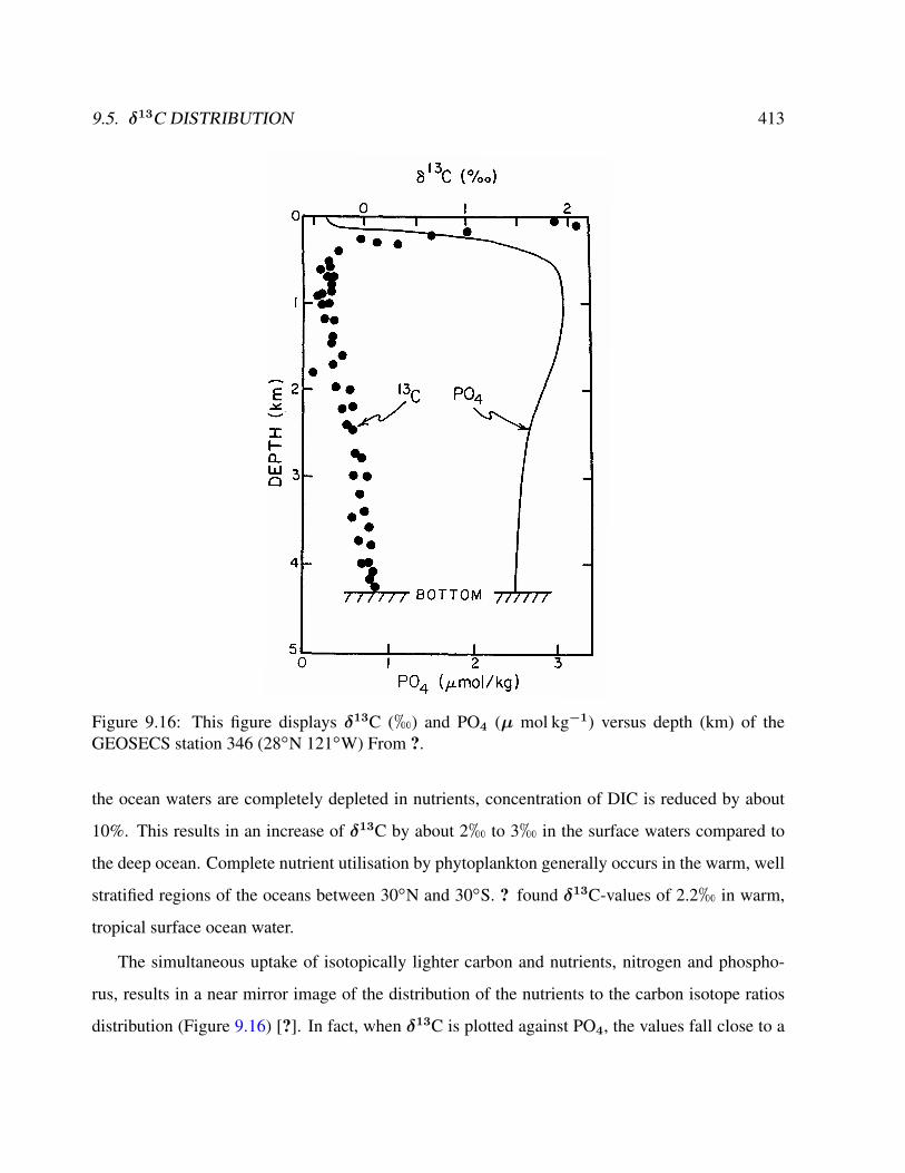
9.5. δ13C DISTRIBUTION 413
Figure 9.16: This figure displays δ13C (h) and PO4 (µ mol kg−1) versus depth (km) of theGEOSECS station 346 (28N 121W) From ?.
the ocean waters are completely depleted in nutrients, concentration of DIC is reduced by about
10%. This results in an increase of δ13C by about 2h to 3h in the surface waters compared to
the deep ocean. Complete nutrient utilisation by phytoplankton generally occurs in the warm, well
stratified regions of the oceans between 30N and 30S. ? found δ13C-values of 2.2h in warm,
tropical surface ocean water.
The simultaneous uptake of isotopically lighter carbon and nutrients, nitrogen and phospho-
rus, results in a near mirror image of the distribution of the nutrients to the carbon isotope ratios
distribution (Figure 9.16) [?]. In fact, when δ13C is plotted against PO4, the values fall close to a
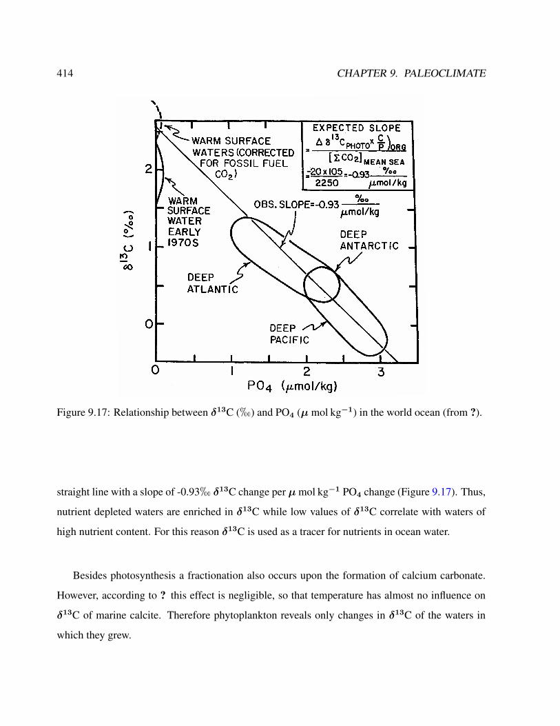
414 CHAPTER 9. PALEOCLIMATE
Figure 9.17: Relationship between δ13C (h) and PO4 (µ mol kg−1) in the world ocean (from ?).
straight line with a slope of -0.93h δ13C change per µmol kg−1 PO4 change (Figure 9.17). Thus,
nutrient depleted waters are enriched in δ13C while low values of δ13C correlate with waters of
high nutrient content. For this reason δ13C is used as a tracer for nutrients in ocean water.
Besides photosynthesis a fractionation also occurs upon the formation of calcium carbonate.
However, according to ? this effect is negligible, so that temperature has almost no influence on
δ13C of marine calcite. Therefore phytoplankton reveals only changes in δ13C of the waters in
which they grew.
9.5. δ13C DISTRIBUTION 415
9.5.1 The water mass tracer δ13C
After leaving the euphotic zone (e.g. formation of NADW in the North Atlantic) δ13C of the ocean
water is only influenced by 2 different processes: Remineralisation of particulate organic matter
(POM) and mixing with other water masses. δ13C of deep water generally decreases when it is
moved from the position of its most recent ventilation, due to in situ oxidation of POM settling
from the surface. POM, detrital remains of plankton of the euphotic zone, sinks down and, depend-
ing on its residence time in the water column, becomes degraded to a different degree. During the
process, labile, 13C-enriched amino acids and sugars are degraded first while the isotopically light
lipids are left behind [??]. Thus, the “biological pump” creates a vertical gradient in the ocean
with high δ13C values close to the surface and nutrient-rich, 13C-depleted deep waters. Generally,
below the main thermocline of the oceans, the δ13C distribution in deep waters is decoupled from
that in surface waters. Only in regions of deep water formation the distribution is homogenous
from the surface to the bottom of the ocean, due to convection [?]. In summary, the longer deep
waters do not have contact to the surface of the ocean the more the isotopic signal δ13C decreases.
The distribution of δ13C in the present-day ocean displays the general distribution of water
masses in the oceans. The net flow directions between ocean basins are represented by gradients
of δ13C. The first truly global measurements of δ13C of dissolved inorganic carbon in the ocean
were performed by the Geochemical Ocean Sections Study (GEOSECS) project [???]. Its results
have drawn an interesting picture of the 13C distribution in the ocean: Following the “conveyor
belt” of the global ocean circulation and starting from the formation of NADW in the North At-
lantic, δ13C decreases continuously. The isotopic signal globally covers a range of 3h. North
Atlantic Deep Water is formed at about 1h - 1.5h and becomes gradually lower in δ13C as it
travels southward and mixes with water from the Southern Ocean, which has an average δ13C
value of 0.3h [?]. Mixing of NADW and AABW occurs at bathymetric gradients of δ13C at
clearly defined water mass boundaries [?]. Furthermore the confluence of 13C-enriched NADW
water with 13C-depleted water of the deep Pacific in the Southern Ocean can clearly be identified
by measurements, before forming AABW. There upwelling of waters from the deep circumpolar
416 CHAPTER 9. PALEOCLIMATE
current occurs which cools rapidly when it reaches the surface, due to heat exchange with sea ice
and atmosphere. Formation of sea ice then leads to higher salinities which increases downwelling
and thus, formation of AABW [?]. The residence time of these waters at the surface is short, so
that neither CO2 exchange with the atmosphere nor phytoplankton utilisation occurs [?]. How-
ever, mixing is strong and the whole southern ocean deep water mass below 1,500m has fairly
homogenous δ13C values south of the polar front [??]. Pacific bottom waters are farthest from the
NADW source region on the “conveyor belt” of the global ocean circulation and therefore contain
globally the lowest δ13C values of 0.2h to -0.2h due to continuous oxidation of 13C poor organic
material.
Consequently, the global composition of δ13C in ocean water or within an ocean basin, does
not represent a conservative tracer for water masses if there is a high productivity rate of organic
matter at the surface or long residence time of the deep water. The deep Pacific is an example of
that. About 0.4h lower δ13C values are measured than expected for a conservative tracer [?]. This
discrepancy represents the so-called “age effect”. The anomaly for δ13C between North Atlantic
Deep Water and Pacific Deep Water is about 1.2h where mixing accounts for a difference of about
0.8h and 0.4h which derives from the “age effect”. A similar situation exists in the Eastern
Atlantic. In the western basin of the South Atlantic the main body of the AABW flows northward
at depth greater than 4,000m. It is driven eastward once it crosses the equator by Coriolis force,
but the Mid-Atlantic Ridge presents a physical barrier to bottom water circulation at low and high
latitudes in the Atlantic, almost isolating the deep East Atlantic from the thermohaline circulation.
Here as well a longer residence time yields in an “age effect”, resulting in a drop of δ13C by about
0.2h [?]. On the other hand, production rates and degradation rates of POM in the present-day
West Atlantic are small, so that δ13C can be trusted as a conservative tracer [?].
Principally δ13C does not serve as a tracer for present-day ocean circulation, but for the re-
construction of past condition in the ocean. Carbon isotopic composition of benthic foraminifers
has proven to be a reliable source of information to measure changes in deep water circulation and
intensity. In particular, the species C. wuellerstorfi became the scientific base of deep water carbon
9.5. δ13C DISTRIBUTION 417
chemistry [?]. Due to global changes in the distribution of carbon between the ocean and transient
reservoirs in past climates, the δ13C values incorporated in benthic foraminifers are significantly
different to today. Because the mixing time for the ocean is of a timescale of 1,000 years, all
foraminifers of present-day measurements are affected in the same way. So only the mean δ13C
is changed [?]. Furthermore reconstructions of the deep water and bottom water circulation using
δ13C generally are in good agreement with the results of other non-conservative tracer. Hence,
nowadays δ13C is widely used to describe paleo productivity and deep ocean circulation of the
late Quaternary climate cycles [?].
Figure 9.18 displays the distribution of δ13C in the Atlantic. The vertical cross-section follows
the cruise track of the Geochemical Ocean Sections Study (GEOSECS) project.
North of 60N, δ13C shows a small vertical gradient with values of 1.5h at the surface to
about 1h in the deep North Atlantic. Although δ13C is not entirely homogeneous in this region,
as found by ?, it can be clearly identified as the source region of NADW.
At depths about 1,500 - 3,000m in the Atlantic between 60N and 30S, the meridional gradient
of δ13C is small compared to other depths, indicating a strong southward movement of NADW
waters [?]. Nonetheless δ13C of water below 1,500m depth decreases towards the south, reaching
a minimum of -0.5h at depths between 1,000 - 2,500m at 60S. This might be the inflow of deep
Pacific water into the Southern Ocean [?], although its values are by 0.3h too low compared to
measured values [?]. The vertical gradient between surface waters and waters at intermediate depth
at 60S exceeds 1.5h in the top 1,500m. This points to the fact that these waters are much less
mixed than those in the North Atlantic at 60N. Therefore AABW formation is weak compared to
NADW formation [?]. δ13C values of less than 0.5 h are found below 3,000m depth in the area
between 30S and the equator and as far as 40N below 3,500m. This points to an intrusion of
Southern Ocean water into the Atlantic at depth below 3,000m.
Maximal values of δ13C of about 2.1h are found in surface waters of the tropics and subtrop-
ics, although values at the equator are slightly lower. This is in good agreement with data obtained
by the GEOSECS project [??].
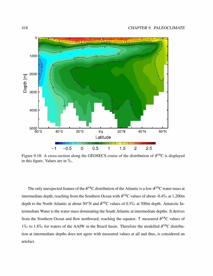
418 CHAPTER 9. PALEOCLIMATE
Figure 9.18: A cross-section along the GEOSECS cruise of the distribution of δ13C is displayedin this figure. Values are in h.
The only unexpected feature of the δ13C distribution of the Atlantic is a low-δ13C water mass at
intermediate depth, reaching from the Southern Ocean with δ13C values of about -0.4h at 1,200m
depth to the North Atlantic at about 50N and δ13C values of 0.5h at 500m depth. Antarctic In-
termediate Water is the water mass dominating the South Atlantic at intermediate depths. It derives
from the Southern Ocean and flow northward, reaching the equator. ? measured δ13C values of
1h to 1.8h for waters of the AAIW in the Brazil basin. Therefore the modelled δ13C distribu-
tion at intermediate depths does not agree with measured values at all and thus, is considered an
artefact.
9.5. δ13C DISTRIBUTION 419
9.5.2 Carbon Cycle Model
In order to model distributions of the carbon isotopes 12C and 13C in the ocean, a global marine
carbon cycle model is needed. The Hamburg Ocean Carbon Cycle Model (HAMOCC, originally
developed by ?) in its refined version HAMOCC 2s [?] is employed for that purpose. The model
simulates the inorganic carbon cycle, partly the organic carbon cycle as well as the silicate cycle.
It consists of three reservoirs: atmosphere, water column and lithosphere. The simple atmo-
sphere model implemented in HAMOCC serves the purpose of exchanging carbon dioxide and
oxygen with the surface ocean, and the meridional transport of CO2. Inter-hemispheric mixing has
a timescale of about one year while the atmosphere is considered to be zonally well mixed.
Prognostic tracer variables in the water column are alkalinity (ALK), dissolved inorganic car-
bon (DIC, equivalent to total CO2), phosphate, oxygen, dissolved organic carbon (DOC) and silicic
acid. Those of the simulated porewater in the bioturbated sediment are identical to those in the wa-
ter column, except for DOC, while in the sediment the tracer variables are calcium carbonate, opal,
organic carbon and clay.
Weathering fluxes are prescribed and matter enters the ocean globally. The cycle is closed
by accumulation in the sediment. Therein the output rate from the water column asymptotically
matches the input rate of terrigeneous matter. However, the spartial distribution of the sedimented
matter can differ significantly from the input field. Therefore inventories of the model are variable,
but stabilise in a steady-state.
The internal redistribution of tracers within the ocean is based on velocity fields and thermo-
haline fields of the Hamburg Large-Scale Geostrophic Ocean General Circulation Model (LSG
OGCM, see above). Hence, they are not computed explicitly in HAMOCC. Convection adjust-
ment and sea-ice cover are provided by LSG as well. For that reason the grid, the spartial and
temporal resolution of the carbon cycle model as well as the advection scheme and topography are
chosen identical to the OGCM.
The carbon cycle basic structure is according to ? while the sediment simulation bases on
?. The so-called “biological pump” is modelled in three components: The “soft tissue pump” or
420 CHAPTER 9. PALEOCLIMATE
organic carbon pump caused by formation of organic material and depletion of carbon and nutrients
in surface waters, the calcium carbonate counterpump as well as biogenic silica (opal) pump.
These three species of biogenic particles, particulate organic carbon (POC), calcium carbonate and
biogenic silica, are produced in the euphotic zone. In the model the euphotic zone is represented
by the uppermost ocean layer (0 - 50m). Silicic acid and phosphate are chosen as the biolimiting
nutrients upon production. Biological export production of POC and opal is assumed to follow the
Michaelis-Menten nutrient uptake kinetics [?]:
POC
PPOC =vPOCmax ·
[PO3−
4
]2 ·Red(C : P )
KPOCs +
[PO3−
4
] (9.17)
where PPOC denotes the POC export production (mol l−1 a−1), vPOCmax the maximum uptake rate
of phosphate (a−1), KPOCs the half saturation constant for POC production (mol l−1),
[PO3−
4
]the concentration of phosphate in the euphotic zone (mol l−1) andRed(C : P ) the Redfield ratio
C:P [?].
Opal
Popal =vopalmax · [Si(OH)4]2
Kopals + [Si(OH)4]
(9.18)
wherePopal describes the opal export production (mol l−1 a−1), vopalmax the maximum uptake rate of
silicic acid (a−1),Kopals the half saturation constant for opal production (mol l−1) and [Si(OH)4]
the concentration of silicic acid in the euphotic zone (mol l−1). The uptake rate of silicic acid is
assumed to be faster than that of phosphate.
The export production of CaCO3 is linked to the local production ratio Popal/PPOC . As long
as the ratio does not exceed a threshold value Sopal, CaCO3 is produced according to the following
equation
PCaCO3 = PPOC ·R ·(
1−Popal/PPOC
Sopal
)(9.19)
9.5. δ13C DISTRIBUTION 421
where R marks the maximum possible rain ratio C(CaCO3):C(POC).
Fractionation of the carbon isotopes 12C and 13C upon organic matter production is also im-
plemented in the model. A constant fractionation factor of -20h for present day and -18h for the
LGM [?] is assumed.
When particulate organic matter (POM) leaves the euphotic zone, remineralisation takes place
during the settling process. This is parameterised by an exponential redistribution profile in which
both sinking velocity and redissolution rate are implicitly included:
F (z) = P (z0) · e(z−z0)/dp (9.20)
In this equation F (z) denotes the particle flux at depth z, P (z0) the export production, z0 =
50m the depth of the euphotic zone and dp marks the depth where flux is 1/e of export produc-
tion. For the remineralisation, oxygen is utilised. If oxygen concentration drops below a certain
threshold, no remineralisation takes place.
POM which leaves the deepest layer of the water column reaches the uppermost bioturbated
sediment layer. These two layers also exchange concentration via pore water, which is modelled
in HAMOCC. All matter deposited on the sediment, which is not redissolved, is accumulated.
Beside organic carbon cycle and silicate cycle, the inorganic carbon cycle is implemented in
the model [?]. For the computation of the CO2 partial pressure, which is equivalent to the free
carbon dioxide in water H2CO3, the following reactions have to be considered:
H2CO3 HCO−3 +H+ (9.21)
HCO−3 CO2−3 +H+ (9.22)
H2O +B(OH)3 B(OH)−4 +H+ (9.23)
H2O OH− +H+ (9.24)
422 CHAPTER 9. PALEOCLIMATE
With the help of the total dissolved inorganic carbon (DIC), total boron (BT ) and total alkalinity
(ALK)
[DIC] = [H2CO3] + [HCO−3 ] + [CO2−3 ] (9.25)
[BT ] = [B(OH)3] + [B(OH)−4 ] (9.26)
[ALK] = [HCO−3 ] + 2 · [CO2−3 ] + [B(OH)−4 ] + [OH−]− [H+] (9.27)
all other reaction partners can be calculated.
All dissolved and suspended water column tracers are transported with the ocean velocity field
using the tracer transport equation
∂c
∂t= −div(~v · c)− q (9.28)
where c is the tracer concentration, t time, ~v the velocity vector and q the sinks and sources. Local
sinks are the marine biota as described above as well as the gas exchange with the atmosphere. The
net flux of carbon isotopes 12C and 13C (F12 and F13) through the air-sea interface is proportional
to the difference between the atmosphere and ocean partial pressure of CO2 [?]:
F 12 = Fas − Fsa = λ(Pa − Ps) (9.29)
F 13 = αasFasR13a − αsaFsaR
13s (9.30)
where λ = 0.06molm−2 ppm−1 a−1 denotes the bulk coefficient, Pa and Ps the partial
pressure of CO2 in the atmosphere and the ocean and R13a and R13
s the 13C/12C ratio of the
atmosphere and the ocean, respectively. The isotopic fractionation through the air-sea interface is
determined by the fractionation factors
αas = [−0.373/(Ts + 273.15) + 1.00019]αk (9.31)
αsa = [1.02389− 9.483/(Ts + 273.15)]αk (9.32)
9.5. δ13C DISTRIBUTION 423
where Ts is the SST in C and αk = 0.9995 is the kinetic fractionation factor [?].
9.5.3 Carbon isotope clock
Scientists have different tools to date samples, ranging from layer counting in trees and some
ice cores, to the analysis of radiogenic isotopes the decay of which forms a clock marking long
intervals of time. Denote C(t) the concentration of the radiogenic isotopes 14C at time t, the
dynamics is as follows:
d
dtC(t) = −λC + P (9.33)
withP as the cosmic production rate and decay constantλ = 1/(5730 years).Assume a constant
production rate. Measuring the concentration at time t with respect to t0, one can calculate the time
difference
t− t0 = −1/λ ln
( 14C(t)14C(t0)
)(9.34)
Knowing the time between different samples (through (9.34)), and the magnitude of change ob-
served in the proxy, the rate of change can be calculated. Uncertainties in the proxies, and uncer-
tainties in the dating, are the main reasons that abrupt climate change is one of the more difficult
topics in the field of paleoclimatology.
Exercise 74 – Age of a water mass
Carbon-14 ages (10 points)
The number of decays per time is proportional to the current number of radioactive atoms. This
is expressed by the following differential equation, where N is the number of radioactive atoms and
424 CHAPTER 9. PALEOCLIMATE
λ is a positive number called the decay constant:
dN
dt= −λN (9.35)
1λ
is the radiocarbon mean- or average-life = 8033 years (Libby value)
a) Calculate the radiocarbon half-life based on Libby’s value of 1λ
! The correct half-life is
5, 730± 40 years.
b) Plants take up atmospheric carbon dioxide by photosynthesis, and are ingested by animals, so
every living thing is constantly exchanging carbon-14 with its environment as long as it lives. Once
it dies, however, this exchange stops, and the amount of carbon-14 gradually decreases through
radioactive beta decay. Calculate a raw radiocarbon date from N and an initial condition ofN0 for
radioactive atoms at t = 0 ! Why is it difficult to report C-14 ages greater than 60,000 years?
c) Typical values for δ14C are−50%o in the mixed layer ocean with depth 50m and−150%o
in deep water (layer depth 4 km). What are the 14C ages of surface and deep water?
d) Measurements of air-sea exchange fluxes suggest that the residence time of CO2 in the
mixed layer is about 5 years. Do you have an explanation for the difference?
9.6. KEPLER ORBIT AND THE EARTH-SUN GEOMETRY 425
9.6 Kepler orbit and the Earth-Sun geometry
In celestial mechanics, a Kepler orbit (or Keplerian orbit) describes the motion of an orbiting
body as an ellipse, parabola, or hyperbola, which forms a two-dimensional orbital plane in three-
dimensional space. The movement of the Earth and Moon around the Sun is fundamental for the
annual cycle, tides as well on ice ages. n 1601, Johannes Kepler acquired the extensive, meticulous
observations of the planets made by Tycho Brahe. Kepler would spend the next five years trying
to fit the observations of the planet Mars to various curves. In 1609, Kepler published the first two
of his three laws of planetary motion. The first law states: "The orbit of every planet is an ellipse
with the sun at a focus."
More generally, the path of an object undergoing Keplerian motion may also follow a parabola
or a hyperbola, which, along with ellipses, belong to a group of curves known as conic sections.
Mathematically, the distance between a central body and an orbiting body can be expressed as:
r(ϕ) =a(1− ε2)
1 + ε cos(ϕ)(9.36)
where
• r is the distance
• a is the semi-major axis, which defines the size of the orbit
• ε is the eccentricity, which defines the shape of the orbit
• ϕ is the true anomaly, which is the angle between the current position of the orbiting object
and the location in the orbit at which it is closest to the central body (called the periapsis)
Newton’s law of gravitation states: Every point mass attracts every other point mass by a force
pointing along the line intersecting both points. The force is proportional to the product of the two
masses and inversely proportional to the square of the distance between the point masses:
F = Gm1m2
r2(9.37)
426 CHAPTER 9. PALEOCLIMATE
where:
• F is the magnitude of the gravitational force between the two point masses
• G is the gravitational constant
• m1 is the mass of the first point mass
• m2 is the mass of the second point mass
• r is the distance between the two point masses
From the laws of motion and the law of universal gravitation, Newton was able to derive Kepler’s
laws, demonstrating consistency between observation and theory. The laws of Kepler and Newton
formed the basis of modern celestial mechanics until Albert Einstein introduced the concepts of
special and general relativity in the early 20th century. For most applications, Keplerian motion
approximates the motions of planets and satellites to relatively high degrees of accuracy and is
used extensively in astronomy and astrodynamics.
To solve for the motion of an object in a two body system, two simplifying assumptions can be
made:
1. The bodies are spherically symmetric and can be treated as point masses.
2. There are no external or internal forces acting upon the bodies other than their mutual gravita-
tion.
The shapes of large celestial bodies are close to spheres. By symmetry, the net gravitational
force attracting a mass point towards a homogeneous sphere must be directed towards its centre.
The shell theorem (also proven by Isaac Newton) states that the magnitude of this force is the same
as if all mass was concentrated in the middle of the sphere, even if the density of the sphere varies
with depth (as it does for most celestial bodies). From this immediately follows that the attraction
between two homogeneous spheres is as if both had its mass concentrated to its center.
Smaller objects, like asteroids or spacecraft often have a shape strongly deviating from a sphere.
But the gravitational forces produced by these irregularities are generally small compared to the

9.6. KEPLER ORBIT AND THE EARTH-SUN GEOMETRY 427
gravity of the central body. The difference between an irregular shape and a perfect sphere also
diminishes with distances, and most orbital distances are very large when compared with the di-
ameter of a small orbiting body. Thus for some applications, shape irregularity can be neglected
without significant impact on accuracy.
Planets rotate at varying rates and thus may take a slightly oblate shape because of the cen-
trifugal force. With such an oblate shape, the gravitational attraction will deviate somewhat from
that of a homogeneous sphere. This phenomenon is quite noticeable for artificial Earth satellites,
especially those in low orbits. At larger distances the effect of this oblateness becomes negligible.
Planetary motions in the Solar System can be computed with sufficient precision if they are treated
as point masses.
Two point mass objects with massesm andM and position vectors r1 and r2 relative to some
inertial reference frame experience gravitational forces:
m1r1 =−GmM
r2r (9.38)
m2r2 =GmM
r2r (9.39)
where r is the relative position vector of mass 1 with respect to mass 2, expressed as:
r = r1 − r2 (9.40)
and r is the unit vector in that direction and r is the length of that vector. Dividing by their respective
masses and subtracting (9.39) from (9.38) yields the equation of motion for the acceleration of the
first object with respect to the second:
r = −µ
r2r (9.41)
428 CHAPTER 9. PALEOCLIMATE
where µ is the gravitational parameter and is equal to
µ = G(m+M) (9.42)
In many applications, a third simplifying assumption can be made:
3. When compared to the central body, the mass of the orbiting body is insignificant. Mathe-
matically,M >> m, so µ = G(m+M) ≈ GM.
This assumption is not necessary to solve the simplified two body problem, but it simplifies
calculations, particularly with Earth-orbiting satellites and planets orbiting the Sun. Even Jupiter’s
mass is less than the Sun’s by a factor of 1047, which would constitute an error of 0.096% in the
value of µ. Notable exceptions include the Earth-moon system (mass ratio of 81.3), the Pluto-
Charon system (mass ratio of 8.9) and binary star systems.
The differential equation for the two body case can be completely solved mathematically and
the resulting orbit which follows Kepler’s laws of planetary motion is called a "Kepler orbit".
Using the energy conservation per mass
E =x2
2+ V (x) (9.43)
one can derive an equation for the velocity x:
x =√
2(E − V (x)) → t =
∫ x
dx′1√
2(E − V (x′))(9.44)
For our case for the planetary motion, we have for the gravitational force per mass
FG
m= −dV (r)/dr and V (r) = −GM/r (9.45)
leading to
E =1
2
(r2 + r2ϕ2
)+ V (r) . (9.46)
9.6. KEPLER ORBIT AND THE EARTH-SUN GEOMETRY 429
Because the force has no ϕ−dependence, we have conservation of angular momentum l per mass:
d
dtl =
d
dt(r× r) = (r× r + r× r) = r× r = r× f(r)r = 0 (9.47)
with the gravitational function f(r) = −GMr3
. The conservation of angular momentum is a
special feature for all central body forces with F ∼ r and
l = r2ϕ . (9.48)
Since the cross product of the position vector and its velocity stays constant, they must lie in the
same plane, orthogonal to l. This implies the vector function is a plane curve.
The energy equation (9.46) can be rewritten as
E =1
2
(r2 +
l2
r2
)+ V (r) =
1
2r2 +
(l2
2r2−GM
r
)=
1
2r2 + Veff(r) (9.49)
with an effective potentialVeff(r) depending only upon radial position, consisting of the attractive
Newtonian gravitational potential energy and the repulsive "centrifugal" potential energy. The
effective potential is shown in Fig. 9.19. For E ≥ 0, one has unbounded solutions (parabola or
hyperbola), forE < 0 bounded (ellipse or circle). One can show that the solutions of the problem
are conic section that has one focus at the origin.
Formal solution
The solution of the problem uses the energy equation (9.49)
r =√
2E + 2GM/r − l2/r2 . (9.50)
We calculate
d
dt(GM/r) = −GM
r
r2= −
√2E + 2GM/r − l2/r2
r2(9.51)
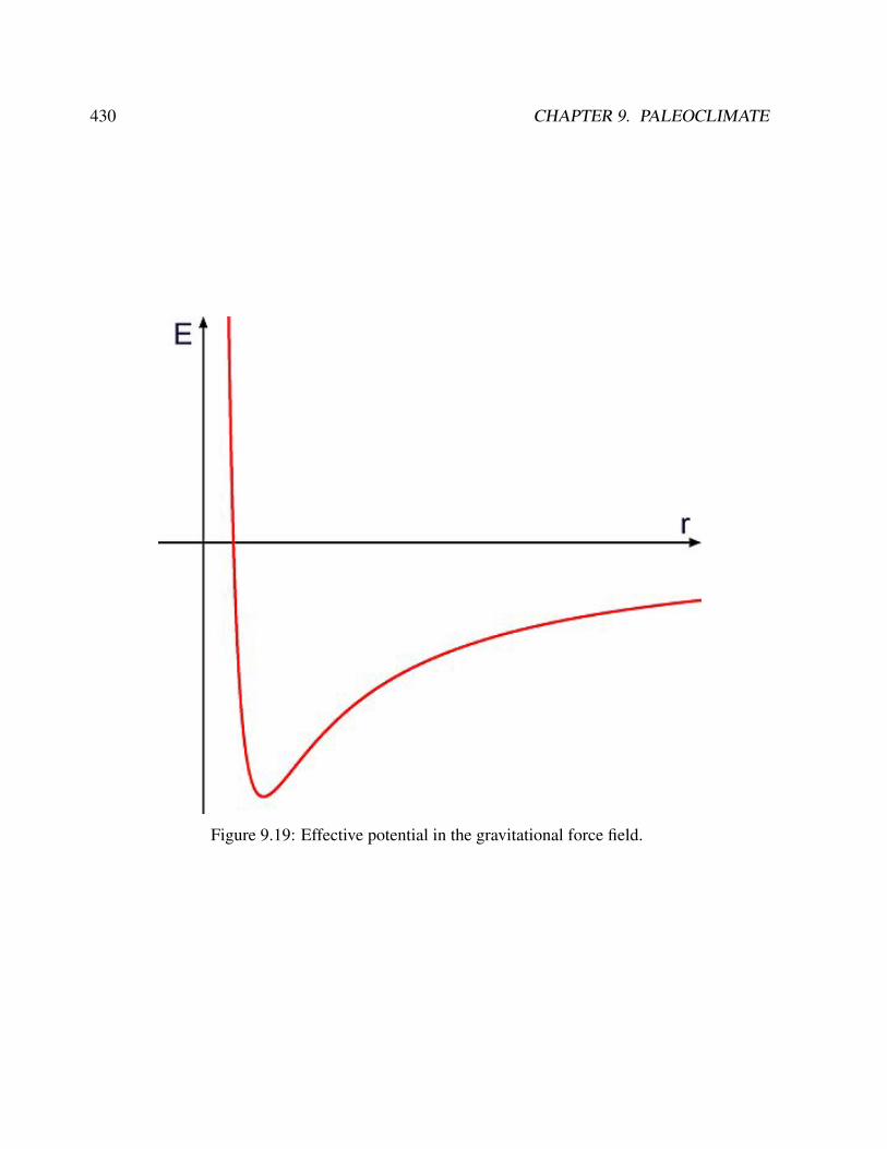
430 CHAPTER 9. PALEOCLIMATE
Figure 9.19: Effective potential in the gravitational force field.
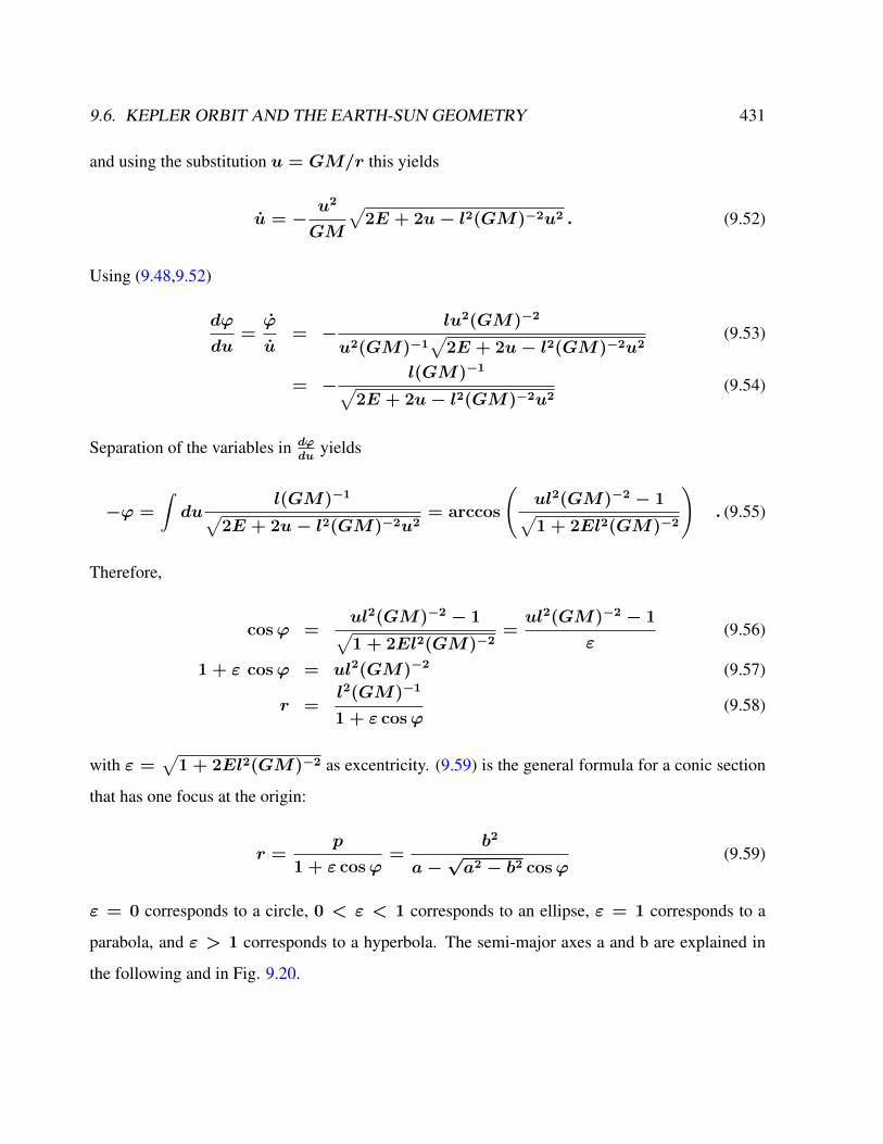
9.6. KEPLER ORBIT AND THE EARTH-SUN GEOMETRY 431
and using the substitution u = GM/r this yields
u = −u2
GM
√2E + 2u− l2(GM)−2u2 . (9.52)
Using (9.48,9.52)
dϕ
du=ϕ
u= −
lu2(GM)−2
u2(GM)−1√
2E + 2u− l2(GM)−2u2(9.53)
= −l(GM)−1√
2E + 2u− l2(GM)−2u2(9.54)
Separation of the variables in dϕdu
yields
−ϕ =
∫du
l(GM)−1√2E + 2u− l2(GM)−2u2
= arccos
(ul2(GM)−2 − 1√1 + 2El2(GM)−2
). (9.55)
Therefore,
cosϕ =ul2(GM)−2 − 1√1 + 2El2(GM)−2
=ul2(GM)−2 − 1
ε(9.56)
1 + ε cosϕ = ul2(GM)−2 (9.57)
r =l2(GM)−1
1 + ε cosϕ(9.58)
with ε =√
1 + 2El2(GM)−2 as excentricity. (9.59) is the general formula for a conic section
that has one focus at the origin:
r =p
1 + ε cosϕ=
b2
a−√a2 − b2 cosϕ
(9.59)
ε = 0 corresponds to a circle, 0 < ε < 1 corresponds to an ellipse, ε = 1 corresponds to a
parabola, and ε > 1 corresponds to a hyperbola. The semi-major axes a and b are explained in
the following and in Fig. 9.20.

432 CHAPTER 9. PALEOCLIMATE
The orbits of all planets are to high accuracy Kepler orbits around the Sun. The small devia-
tions are due to the much weaker gravitational attractions between the planets, and in the case of
Mercury, due to general relativity. The orbits of the artificial satellites around the Earth are, with a
fair approximation, Kepler orbits with small perturbations due to the gravitational attraction of the
sun, the moon and the oblateness of the Earth. In high accuracy applications for which the equa-
tion of motion must be integrated numerically with all gravitational and non-gravitational forces
(such as solar radiation pressure and atmospheric drag) being taken into account, the Kepler orbit
concepts are of paramount importance and heavily used.
Let us look at Keppler’s first law and the geometry of the ellipse. At ϕ = 0, perihelion,
the distance is minimum
rmin =p
1 + ε. (9.60)
At ϕ = 90 and at ϕ = 270, the distance is equal to the semi-latus rectum. At ϕ = 180,
aphelion, the distance is maximum
rmax =p
1− ε. (9.61)
The semi-major axis a is the arithmetic mean between rmax and rmin :
rmax − a = a− rmin (9.62)
a =p
1− ε2. (9.63)
The semi-minor axis b is the geometric mean between rmax and rmin :
rmax
b=
b
rmin
(9.64)
b =p
√1− ε2
. (9.65)

9.6. KEPLER ORBIT AND THE EARTH-SUN GEOMETRY 433
The semi-latus rectum p is the harmonic mean between rmax and rmin :
1
rmin
−1
p=
1
p−
1
rmax
(9.66)
pa = rmaxrmin = b2 . (9.67)
The eccentricity ε is the coefficient of variation between rmax and rmin :
ε =rmax − rmin
rmax + rmin
. (9.68)
The area of the ellipse is
A = πab . (9.69)
The special case of a circle is ε = 0, resulting in r = p = rmax = rmin = a = b and
A = πr2.
Let us look at Keppler’s second law and the mathematical derivation. In a small time dt
the planet sweeps out a small triangle (or, more precisely, a sector) having base line r and height
rdϕ and area dA = 12· r · rdϕ and so the constant areal velocity is dA
dt= 1
2r2 dϕ
dt. The planet
moves faster when it is closer to the Sun. Since the area enclosed by the elliptical orbit is πab,
the period P satisfies
P · 12r2dϕ
dt= πab (9.70)
and the mean motion of the planet around the Sun n = 2π/P satisfies
r2dϕ = abndt. (9.71)

434 CHAPTER 9. PALEOCLIMATE
Figure 9.20: Three different types of conic sections. Focal-points corresponding to all conic sec-tions are placed at the origin.
9.6. KEPLER ORBIT AND THE EARTH-SUN GEOMETRY 435
Keppler’s third law reads as:
T 2
r3=
4π2
GM(9.72)
where T is the orbital period of the orbiting body. In the full formulation under Newton’s laws of
motion, M should be replaced byM+m,where m is the mass of the orbiting body. Consequently,
the proportionality constant is not truly the same for each planet. Nevertheless, given that m is so
small relative to M for planets in our solar system, the approximation is good in the original setting.
Kepler’s laws refine the model of Copernicus, which assumed circular orbits. If the eccentricity
of a planetary orbit is zero, then Kepler’s laws state:
• The planetary orbit is a circle with the Sun at the center
• The speed of the planet in the orbit is constant
• The square of the sidereal period is proportionate to the cube of the distance from the Sun.
Actually, the eccentricities of the orbits of the six planets known to Copernicus and Kepler are
quite small, so the rules above give excellent approximations of planetary motion, but Kepler’s
laws fit observations even better.
Kepler’s corrections to the Copernican model are not at all obvious:
• The planetary orbit is not a circle, but an ellipse
• The Sun is not at the center but at a focal point
• Neither the linear speed nor the angular speed of the planet in the orbit is constant, but the
area speed is constant.
• The square of the sidereal period is proportionate to the cube of the mean between the max-
imum and minimum distances from the Sun.

436 CHAPTER 9. PALEOCLIMATE
The nonzero eccentricity of the orbit of the earth makes the time from the March equinox to the
September equinox, around 186 days, unequal to the time from the September equinox to the
March equinox, around 179 days. A diameter would cut the orbit into equal parts, but the plane
through the Sun parallel to the equator of the Earth cuts the orbit into two parts with areas in a 186
to 179 ratio, so the eccentricity of the orbit of the Earth is approximately
ε ≈π
4
186− 179
186 + 179≈ 0.015, (9.73)
which is close to the correct value (0.016710219). The calculation is correct when the perihelion,
the date that the Earth is closest to the Sun, is on a solstice. The current perihelion, near January
4, is fairly close to the solstice on December 21 or 22.
Earth’s orbit about the sun is nearly circular at a mean distance of 1.5 × 10⁸ km. The ec-
centricity of the orbit is small, 0.0168. Thus earth is 3.4% further from the Sun at aphelion than
at perihelion, the time of closest approach to the sun. Perihelion occurs nowadays every year in
January, and the exact time changes by about 20 minutes per year. In 1995, it occurred on 3 Jan-
uary. Earth’s axis of rotation is inclined 23.45 to the plane of earth’s orbit around the sun (Fig.
9.21). The orientation is such that the sun is directly overhead at the Equator on the vernal and
autumnal equinoxes, which occur on or about 21 March and 21 September each year. The latitudes
of 23.45 North and South are the Tropics of Cancer and Capricorn respectively. The tropics
lie equatorward of these latitudes. As a result of the eccentricity of earth’s orbit, maximum solar
insolation averaged over the surface of the earth occurs in early January each year. As a result
of the inclination of earth’s axis of rotation, the maximum insolation at any location outside the
tropics occurs around 21 June in the northern hemisphere, and around 21 December in the southern
hemisphere.
Exercises: satellites as cellestrial objects
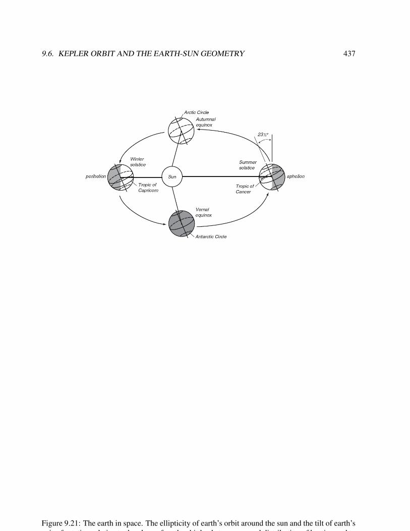
9.6. KEPLER ORBIT AND THE EARTH-SUN GEOMETRY 437
Figure 9.21: The earth in space. The ellipticity of earth’s orbit around the sun and the tilt of earth’saxis of rotation relative to the plane of earth orbit leads to an unequal distribution of heating and tothe seasons. Earth is closest to the sun at perihelion.
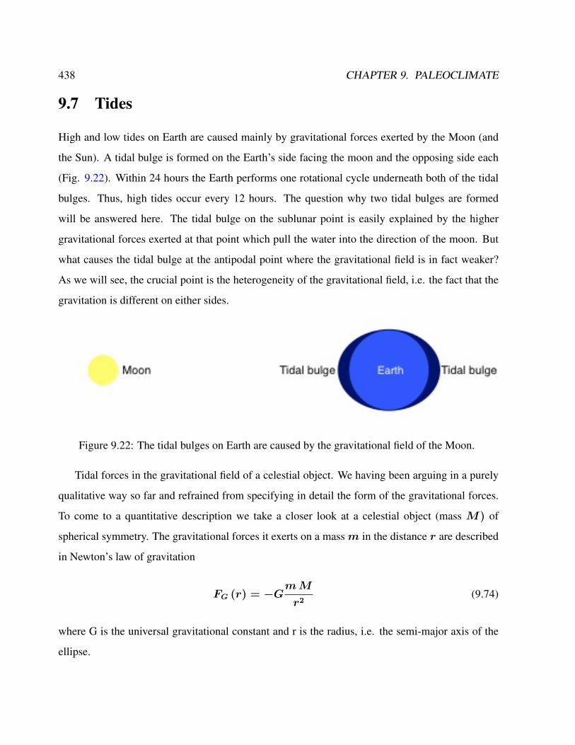
438 CHAPTER 9. PALEOCLIMATE
9.7 Tides
High and low tides on Earth are caused mainly by gravitational forces exerted by the Moon (and
the Sun). A tidal bulge is formed on the Earth’s side facing the moon and the opposing side each
(Fig. 9.22). Within 24 hours the Earth performs one rotational cycle underneath both of the tidal
bulges. Thus, high tides occur every 12 hours. The question why two tidal bulges are formed
will be answered here. The tidal bulge on the sublunar point is easily explained by the higher
gravitational forces exerted at that point which pull the water into the direction of the moon. But
what causes the tidal bulge at the antipodal point where the gravitational field is in fact weaker?
As we will see, the crucial point is the heterogeneity of the gravitational field, i.e. the fact that the
gravitation is different on either sides.
Figure 9.22: The tidal bulges on Earth are caused by the gravitational field of the Moon.
Tidal forces in the gravitational field of a celestial object. We having been arguing in a purely
qualitative way so far and refrained from specifying in detail the form of the gravitational forces.
To come to a quantitative description we take a closer look at a celestial object (mass M) of
spherical symmetry. The gravitational forces it exerts on a massm in the distance r are described
in Newton’s law of gravitation
FG (r) = −GmM
r2(9.74)
where G is the universal gravitational constant and r is the radius, i.e. the semi-major axis of the
ellipse.
9.8. THE EARTH-SUN GEOMETRY 439
The gravitational field is heterogeneous, its strength depending on the distance. Tidal forces
will occur. The Earth is in the gravitational field of the Moon and Sun. The distance between the
sea surface and the centre of gravity is ∆r. The tidal force now is the difference of the gravitational
forces between the sea surface and the centre of gravity:
Ftidal (r) = FG(rs + ∆r)− FG(rs) (9.75)
= −GmM
(1
(rs + ∆r)2−
1
r2s
)(9.76)
We presume ∆r << rs for a good approximation. Thus, having factored out r2s in the denomi-
nator, we can use the approximation
Ftidal (r) = −GmM
r2s
(1
(1 + ∆r/rs)2− 1
)(9.77)
≈ −GmM
r2s
(1− 2∆r/rs − 1) (9.78)
= 2GmM
r3s
∆r (9.79)
Its dependence on distance is typical for tidal force that diminishes by the third power of distance
(and thus much stronger than the gravitational force). This explains why the Sun’s tidal forces
act more weakly on Earth than those of the moon despite the Sun’s gravitational force being 178
times larger. The tidal forces that act on a physical object in the gravitation field of a celestial body
diminish by 1/r3 and are proportional to the size ∆r of the object.
9.8 The Earth-Sun geometry
Earth’s orbit about the sun is nearly circular at a mean distance of 1.5× 10⁸ km. The eccentricity
of the orbit is small, 0.0168. Thus earth is 3.4% further from the Sun at aphelion than at perihelion,
the time of closest approach to the sun. Perihelion occurs every year in January, and the exact time
changes by about 20 minutes per year. In 1995, it occurred on 3 January. Earth’s axis of rotation is
440 CHAPTER 9. PALEOCLIMATE
inclined 23.45 to the plane of earth’s orbit around the sun (Fig. 9.21). The orientation is such that
the sun is directly overhead at the Equator on the vernal and autumnal equinoxes, which occur on
or about 21 March and 21 September each year. The latitudes of 23.45 North and South are the
Tropics of Cancer and Capricorn respectively. The tropics lie equatorward of these latitudes. As
a result of the eccentricity of earth’s orbit, maximum solar insolation averaged over the surface of
the earth occurs in early January each year. As a result of the inclination of earth’s axis of rotation,
the maximum insolation at any location outside the tropics occurs around 21 June in the northern
hemisphere, and around 21 December in the southern hemisphere.
On glacial-interglacial time scales, the geometry of the Earth-Sun system provides a pacing of
climate change. Earth’s climate is constantly undergoing changes due to temporal changes in the
orbital parameters eccentricity e, precession e sin ω and obliquity ε.
Eccentricity descibes the deviation of Earth’s orbit from a circular shape (in this case, eccen-
tricity equals zero). The precession of Earth’s orbit around the Sun results in a variation of the
distance between Earth and Sun at a given time in the year. The precession parameter is e sin ω
with ω measured from the vernal equinox. Currently, ω is 102 which means that the boreal
winter solistice occurs close to perhelion. Therefore, the northern hemisphere receives more than
average energy in winter and less in summer.
Obliquity is the tilt of Earth’s rotational axis relative to a perpendicular drawn to the plane of
the ecliptic. It varies with an average period of 41 ka. Currently, Earth’s tilt is 23.44. This value
lies in the middle of a 2.4 range between 22.1 and 24.5. At times of high ε-values the summer
insolation is inceased and the winter insolation is decreased in both hemispheres. Therfore, the
seasonality of incoming solar radiation is increased everywhere.
The eccentricity e is the only orbital parameter that changes the total average annual amount of
incoming solar radiation. The other parameters modify the seasonal and hemispheric distribution
of incoming solar radiation. Berger (1978( provided expressions for e sin ω, e and ε in a form
9.9. TEMPLATE MODEL 441
suitable for the astronomical theory of palaeoclimates:
e sin ω =∑i
Pi sin(αit+ ηi) (9.80)
ε = ε∗ +∑i
Ai cos(γit+ ζi) (9.81)
e = e∗ +∑i
Ei cos(λit+ Φi) (9.82)
Milankovitch theory (1941) gained the status of a paradigm for explaining the Pleistocene ice-
ages. A key element of this theory is that summer insolation at high latitudes of the northern
hemisphere determines glacial-interglacial transitions connected with the waxing and waning of
large continental ice sheets (e.g. Imbrie and Imbrie, 1980). In the last two million years, the
glacial-interglacial cycles provide the dominant signal in the climate record. Climate conditions of
glacials and interglacials are very different. During the Last Glacial Maximum, about 20,000 years
before present, surface temperature in the north Atlantic realm was 10-20 degree lower than today
(CLIMAP, 1976).
Although there are indications for Milankovitsch’s astronomical theory (Hays et al., 1976),
the driving mechanism of the northern hemisphere is under debate. Recent radiometric datings
of past sea-level, which is intimately linked to continental ice mass, indicate that the penultimate
deglaciation is in phase with an insolation maximum at high latitudes of the southern hemisphere
(Henderson and Slowey, 2000). Moreover, paleoclimatic proxy data reveal that the Southern Ocean
warmed before the northern hemisphere during deglaciations (e.g. Imbrie et al., 1992; 1993).
9.9 Template model
basedrive="/Users/tlaepple/data/"path<-paste(basedrive,"paleoLibrary/src/",sep="")source(paste(path,"header.R",sep=""))setwd(paste(basedrive,"SmallHypothesis/",sep=""))
#Library for insolation->climate->proxy calculations
442 CHAPTER 9. PALEOCLIMATE
#Read climatology of SST and SATsat.clim<-read_ncep.clim.day("sat.clim.day.nc",varname="air")
analyse.transferfunction<-function(lat1,lon1,dataset,bPlot=T,b3plot=T,main=NULL)
a.matrix<-matrix(NA,365,365)
#Insolationinsol<-daily_insolation(0,lat1,1:365)$Fswins.1<-insolins.2<-insol^2ins.3<-insol^3
#daily temperature dataa<-selspace(dataset,lat1=lat1,lon1=lon1)
basis<-rep(a,2)
for (iopt in 1:365) a.matrix[,iopt]<-basis[iopt:(iopt+364)] #Jahre werden verschoben gespeichert
t<-lm(a.matrix~ins.1+ins.2+ins.3) #Das Polynom wird gefittetrmse<-colMeans(t$residuals^2)
#ul, il und index.neg wurde verwendet um eine positive Steigung zu erreichen,# dies brachte in Afrika auchdie richtige Monsoonantwort mit sich !
ul<-max(insol)*t$coefficients[2,]+max(insol)^2*t$coefficients[3,]+max(insol)^3*t$coefficients[4,]ll<-min(insol)*t$coefficients[2,]+min(insol)^2*t$coefficients[3,]+min(insol)^3*t$coefficients[4,]
index.neg<-((ul-ll)<=0)rmse[index.neg]<-1e6bestfit.index<-which.min(rmse)
coeff<-t$coefficients[,bestfit.index]
t.lin<-lm(a.matrix[,bestfit.index]~ins.1)coeff.lin<-t.lin$coeff
############# Plotting routineif (is.null(main)) main=paste(lon1,"E / ",lat1,"N",sep="")if (bPlot)
at<-basisat<-filter(at,rep(1/20,20),circular=T)at.scale<-scale(at)insol.scale<-scale(rep(insol,2))
at.sc<-attr(at.scale,"scaled:scale")at.offset<-attr(at.scale,"scaled:center")
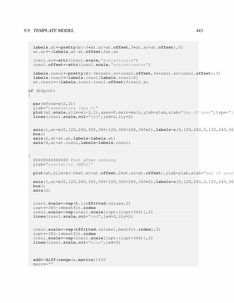
9.9. TEMPLATE MODEL 443
labels.at<-pretty(c(-3*at.sc+at.offset,3*at.sc+at.offset),5)at.at<-(labels.at-at.offset)/at.sc
insol.sc<-attr(insol.scale,"scaled:scale")insol.offset<-attr(insol.scale,"scaled:center")
labels.insol<-pretty(c(-3*insol.sc+insol.offset,3*insol.sc+insol.offset),5)labels.insol<-labels.insol[labels.insol>0]at.insol<-(labels.insol-insol.offset)/insol.sc
if (b3plot)
par(mfrow=c(2,2))ylab="temperature (deg C)"plot(at.scale,ylim=c(-2,2),axes=F,main=main,ylab=ylab,xlab="day of year",type="l",lwd=2)lines(insol.scale,col="red",lwd=2,lty=2)
axis(1,at=c(0,120,240,365,365+120,365+240,365*2),labels=c(0,120,240,0,120,240,365))box()axis(2,at=at.at,labels=labels.at)axis(4,at=at.insol,labels=labels.insol)
############## Plot after cuttingylab="insolation (W/m2)"
plot(at,ylim=c(-2*at.sc+at.offset,2*at.sc+at.offset),ylab=ylab,xlab="day of year",type="l",lwd=2,axes=F)
axis(1,at=c(0,120,240,365,365+120,365+240,365*2),labels=c(0,120,240,0,120,240,365))box()axis(2)
insol.scale<-rep(t.lin$fitted.values,2)iopt<-365-1*bestfit.indexinsol.scale<-rep(insol.scale[iopt:(iopt+364)],2)lines(insol.scale,col="red",lwd=2,lty=2)
insol.scale<-rep(t$fitted.values[,bestfit.index],2)iopt<-365-1*bestfit.indexinsol.scale<-rep(insol.scale[iopt:(iopt+364)],2)lines(insol.scale,col="blue",lwd=2)
add<-diff(range(a.matrix))/10main<-""
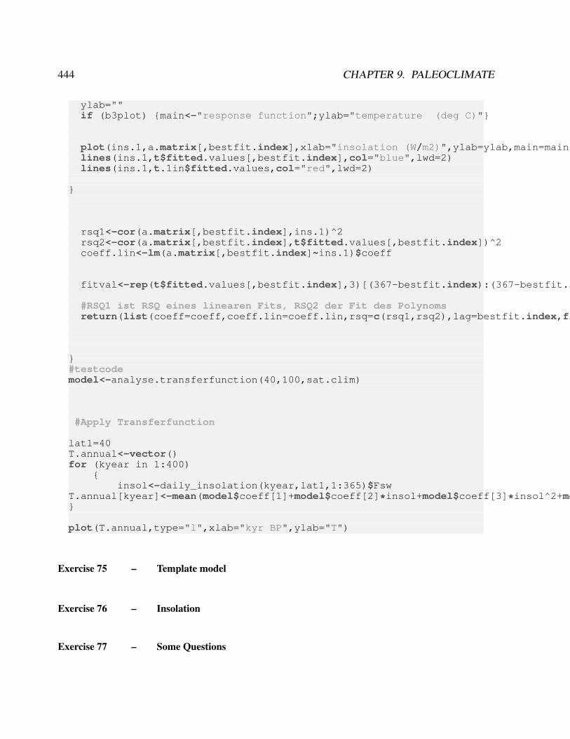
444 CHAPTER 9. PALEOCLIMATE
ylab=""if (b3plot) main<-"response function";ylab="temperature (deg C)"
plot(ins.1,a.matrix[,bestfit.index],xlab="insolation (W/m2)",ylab=ylab,main=main,ylim=range(a.matrix[,bestfit.index])+c(-add,add))lines(ins.1,t$fitted.values[,bestfit.index],col="blue",lwd=2)lines(ins.1,t.lin$fitted.values,col="red",lwd=2)
rsq1<-cor(a.matrix[,bestfit.index],ins.1)^2rsq2<-cor(a.matrix[,bestfit.index],t$fitted.values[,bestfit.index])^2coeff.lin<-lm(a.matrix[,bestfit.index]~ins.1)$coeff
fitval<-rep(t$fitted.values[,bestfit.index],3)[(367-bestfit.index):(367-bestfit.index+364)]
#RSQ1 ist RSQ eines linearen Fits, RSQ2 der Fit des Polynomsreturn(list(coeff=coeff,coeff.lin=coeff.lin,rsq=c(rsq1,rsq2),lag=bestfit.index,fitted=fitval))
#testcodemodel<-analyse.transferfunction(40,100,sat.clim)
#Apply Transferfunction
lat1=40T.annual<-vector()for (kyear in 1:400)
insol<-daily_insolation(kyear,lat1,1:365)$Fsw
T.annual[kyear]<-mean(model$coeff[1]+model$coeff[2]*insol+model$coeff[3]*insol^2+model$coeff[4]*insol^3)
plot(T.annual,type="l",xlab="kyr BP",ylab="T")
Exercise 75 – Template model
Exercise 76 – Insolation
Exercise 77 – Some Questions
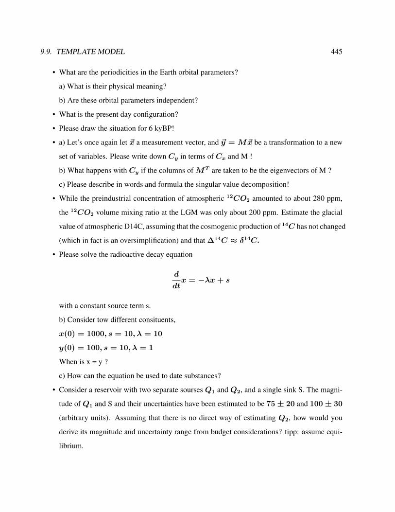
9.9. TEMPLATE MODEL 445
• What are the periodicities in the Earth orbital parameters?
a) What is their physical meaning?
b) Are these orbital parameters independent?
• What is the present day configuration?
• Please draw the situation for 6 kyBP!
• a) Let’s once again let ~x a measurement vector, and ~y = M~x be a transformation to a new
set of variables. Please write down Cy in terms of Cx and M !
b) What happens with Cy if the columns ofMT are taken to be the eigenvectors of M ?
c) Please describe in words and formula the singular value decomposition!
• While the preindustrial concentration of atmospheric 12CO2 amounted to about 280 ppm,
the 12CO2 volume mixing ratio at the LGM was only about 200 ppm. Estimate the glacial
value of atmospheric D14C, assuming that the cosmogenic production of 14C has not changed
(which in fact is an oversimplification) and that ∆14C ≈ δ14C.
• Please solve the radioactive decay equation
d
dtx = −λx+ s
with a constant source term s.
b) Consider tow different consituents,
x(0) = 1000, s = 10, λ = 10
y(0) = 100, s = 10, λ = 1
When is x = y ?
c) How can the equation be used to date substances?
• Consider a reservoir with two separate sourses Q1 and Q2, and a single sink S. The magni-
tude of Q1 and S and their uncertainties have been estimated to be 75± 20 and 100± 30
(arbitrary units). Assuming that there is no direct way of estimating Q2, how would you
derive its magnitude and uncertainty range from budget considerations? tipp: assume equi-
librium.
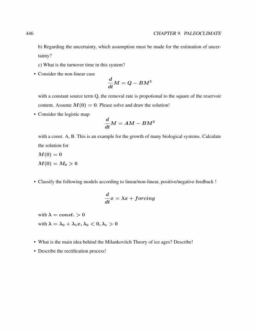
446 CHAPTER 9. PALEOCLIMATE
b) Regarding the uncertainty, which assumption must be made for the estimation of uncer-
tainty?
c) What is the turnover time in this system?
• Consider the non-linear cased
dtM = Q−BM2
with a constant source term Q, the removal rate is propotional to the square of the reservoir
content. AssumeM(0) = 0. Please solve and draw the solution!
• Consider the logistic map:d
dtM = AM −BM2
with a const. A, B. This is an example for the growth of many biological systems. Calculate
the solution for
M(0) = 0
M(0) = M0 > 0
• Classify the following models according to linear/non-linear, positive/negative feedback !
d
dtx = λx+ forcing
with λ = const. > 0
with λ = λ0 + λ1x, λ0 < 0, λ1 > 0
• What is the main idea behind the Milankovitch Theory of ice ages? Describe!
• Describe the rectification process!

Chapter 10
Dynamics of spatio-temporal pattern
A major challenge is to understand the dynamics of past periods in which rapid climate changes
have occurred and interactions between solid Earth and ocean that may drive climate change. The
dependence on background climate, driving mechanisms and feedbacks will provide a suitable
framework to study conditions which are expected to develop in the future. Since Earth System
Models have to simplify the system and rely on parameterizations of unresolved processes using
present data, paleoclimate records provide a unique tool to validate models for conditions which
are different from our present one. Suitable data-model analyses provide therefore a proper basis
to estimate and possibly reduce uncertainties of future climate change projections.
The current and future climate is subject to significant change due to the increasing human
influence on the climate system. Polar regions are especially affected and contain key drivers for
this change. The extent and the rate of this change are controversial, however. It is therefore
necessary to improve the understanding of natural climate variability and trends by searching for
their causes at all time scales. Furthermore, the model scenarios in conjunction with the long-
term data can be used to examine mechanisms for the statistics of regional climate extremes under
different boundary conditions.
447
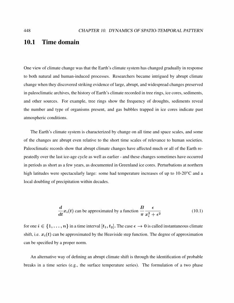
448 CHAPTER 10. DYNAMICS OF SPATIO-TEMPORAL PATTERN
10.1 Time domain
One view of climate change was that the Earth’s climate system has changed gradually in response
to both natural and human-induced processes. Researchers became intrigued by abrupt climate
change when they discovered striking evidence of large, abrupt, and widespread changes preserved
in paleoclimatic archives, the history of Earth’s climate recorded in tree rings, ice cores, sediments,
and other sources. For example, tree rings show the frequency of droughts, sediments reveal
the number and type of organisms present, and gas bubbles trapped in ice cores indicate past
atmospheric conditions.
The Earth’s climate system is characterized by change on all time and space scales, and some
of the changes are abrupt even relative to the short time scales of relevance to human societies.
Paleoclimatic records show that abrupt climate changes have affected much or all of the Earth re-
peatedly over the last ice-age cycle as well as earlier - and these changes sometimes have occurred
in periods as short as a few years, as documented in Greenland ice cores. Perturbations at northern
high latitudes were spectacularly large: some had temperature increases of up to 10-20C and a
local doubling of precipitation within decades.
d
dtxi(t) can be approximated by a function
B
π
ε
x2i + ε2
(10.1)
for one i ∈ 1, . . . , n in a time interval [t1, t2]. The case ε→ 0 is called instantaneous climate
shift, i.e. xi(t) can be approximated by the Heaviside step function. The degree of approximation
can be specified by a proper norm.
An alternative way of defining an abrupt climate shift is through the identification of probable
breaks in a time series (e.g., the surface temperature series). The formulation of a two phase
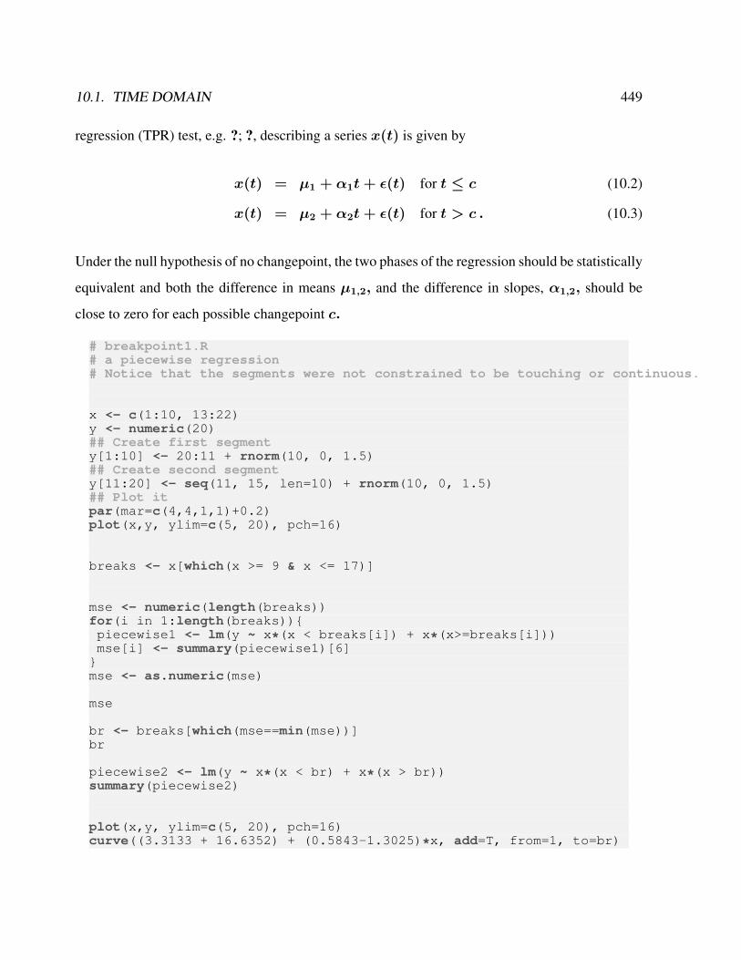
10.1. TIME DOMAIN 449
regression (TPR) test, e.g. ?; ?, describing a series x(t) is given by
x(t) = µ1 + α1t+ ε(t) for t ≤ c (10.2)
x(t) = µ2 + α2t+ ε(t) for t > c . (10.3)
Under the null hypothesis of no changepoint, the two phases of the regression should be statistically
equivalent and both the difference in means µ1,2, and the difference in slopes, α1,2, should be
close to zero for each possible changepoint c.
# breakpoint1.R# a piecewise regression# Notice that the segments were not constrained to be touching or continuous.
x <- c(1:10, 13:22)y <- numeric(20)## Create first segmenty[1:10] <- 20:11 + rnorm(10, 0, 1.5)## Create second segmenty[11:20] <- seq(11, 15, len=10) + rnorm(10, 0, 1.5)## Plot itpar(mar=c(4,4,1,1)+0.2)plot(x,y, ylim=c(5, 20), pch=16)
breaks <- x[which(x >= 9 & x <= 17)]
mse <- numeric(length(breaks))for(i in 1:length(breaks))piecewise1 <- lm(y ~ x*(x < breaks[i]) + x*(x>=breaks[i]))mse[i] <- summary(piecewise1)[6]mse <- as.numeric(mse)
mse
br <- breaks[which(mse==min(mse))]br
piecewise2 <- lm(y ~ x*(x < br) + x*(x > br))summary(piecewise2)
plot(x,y, ylim=c(5, 20), pch=16)curve((3.3133 + 16.6352) + (0.5843-1.3025)*x, add=T, from=1, to=br)

450 CHAPTER 10. DYNAMICS OF SPATIO-TEMPORAL PATTERN
curve((3.3133 - 0.9116) + 0.5843*x, add=T, from=br, to=max(x))abline(v=br, lty=3)
#################
# http://www.r-bloggers.com/r-for-ecologists-putting-together-a-piecewise-regression/
x <- c(1:10, 13:22)y <- numeric(20)## Create first segmenty[1:10] <- 20:11 + rnorm(10, 0, 1.5)## Create second segmenty[11:20] <- seq(11, 15, len=10) + rnorm(10, 0, 1.5)## Plot itpar(mar=c(4,4,1,1)+0.2)plot(x,y, ylim=c(5, 20), pch=16)
breaks <- x[which(x >= 9 & x <= 17)]
mse <- numeric(length(breaks))for(i in 1:length(breaks))piecewise1 <- lm(y ~ x*(x < breaks[i]) + x*(x>=breaks[i]))mse[i] <- summary(piecewise1)[6]mse <- as.numeric(mse)
mse
br <- breaks[which(mse==min(mse))]br
piecewise2 <- lm(y ~ x*(x < br) + x*(x > br))summary(piecewise2)
plot(x,y, ylim=c(5, 20), pch=16)curve((3.3133 + 16.6352) + (0.5843-1.3025)*x, add=T, from=1, to=br)curve((3.3133 - 0.9116) + 0.5843*x, add=T, from=br, to=max(x))abline(v=br, lty=3)
# Notice that the segments were not constrained to be touching or continuous. This is inherent in the algorithm that we used.
#Implementation of Rampfit#Ramp (x1,y1 - x2,y2) + two horizontal pieces with a fix length#Parameters: Search area for x1 and x2, length of horizontal piece
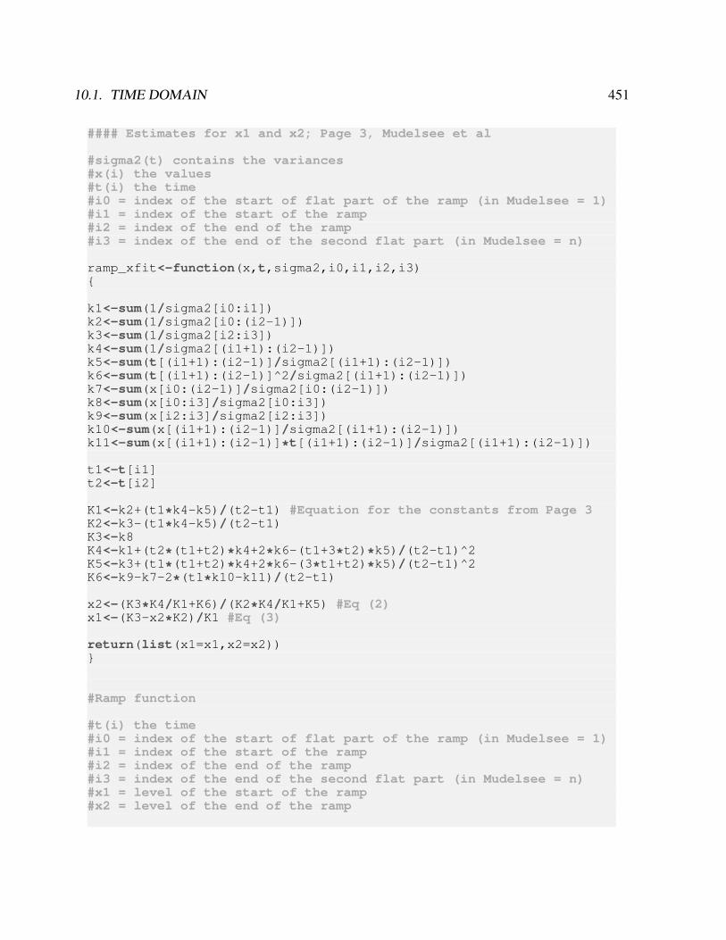
10.1. TIME DOMAIN 451
#### Estimates for x1 and x2; Page 3, Mudelsee et al
#sigma2(t) contains the variances#x(i) the values#t(i) the time#i0 = index of the start of flat part of the ramp (in Mudelsee = 1)#i1 = index of the start of the ramp#i2 = index of the end of the ramp#i3 = index of the end of the second flat part (in Mudelsee = n)
ramp_xfit<-function(x,t,sigma2,i0,i1,i2,i3)
k1<-sum(1/sigma2[i0:i1])k2<-sum(1/sigma2[i0:(i2-1)])k3<-sum(1/sigma2[i2:i3])k4<-sum(1/sigma2[(i1+1):(i2-1)])k5<-sum(t[(i1+1):(i2-1)]/sigma2[(i1+1):(i2-1)])k6<-sum(t[(i1+1):(i2-1)]^2/sigma2[(i1+1):(i2-1)])k7<-sum(x[i0:(i2-1)]/sigma2[i0:(i2-1)])k8<-sum(x[i0:i3]/sigma2[i0:i3])k9<-sum(x[i2:i3]/sigma2[i2:i3])k10<-sum(x[(i1+1):(i2-1)]/sigma2[(i1+1):(i2-1)])k11<-sum(x[(i1+1):(i2-1)]*t[(i1+1):(i2-1)]/sigma2[(i1+1):(i2-1)])
t1<-t[i1]t2<-t[i2]
K1<-k2+(t1*k4-k5)/(t2-t1) #Equation for the constants from Page 3K2<-k3-(t1*k4-k5)/(t2-t1)K3<-k8K4<-k1+(t2*(t1+t2)*k4+2*k6-(t1+3*t2)*k5)/(t2-t1)^2K5<-k3+(t1*(t1+t2)*k4+2*k6-(3*t1+t2)*k5)/(t2-t1)^2K6<-k9-k7-2*(t1*k10-k11)/(t2-t1)
x2<-(K3*K4/K1+K6)/(K2*K4/K1+K5) #Eq (2)x1<-(K3-x2*K2)/K1 #Eq (3)
return(list(x1=x1,x2=x2))
#Ramp function
#t(i) the time#i0 = index of the start of flat part of the ramp (in Mudelsee = 1)#i1 = index of the start of the ramp#i2 = index of the end of the ramp#i3 = index of the end of the second flat part (in Mudelsee = n)#x1 = level of the start of the ramp#x2 = level of the end of the ramp
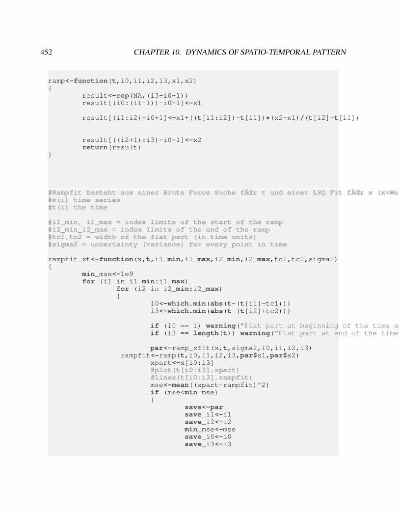
452 CHAPTER 10. DYNAMICS OF SPATIO-TEMPORAL PATTERN
ramp<-function(t,i0,i1,i2,i3,x1,x2)
result<-rep(NA,(i3-i0+1))result[(i0:(i1-1))-i0+1]<-x1
result[(i1:i2)-i0+1]<-x1+((t[i1:i2])-t[i1])*(x2-x1)/(t[i2]-t[i1])
result[((i2+1):i3)-i0+1]<-x2return(result)
#Rampfit besteht aus einer Brute Force Suche fÃŒr t und einer LSQ Fit fÃŒr x (x=Werte)#x(i) time series#t(i) the time
#i1_min, i1_max = index limits of the start of the ramp#i2_min_i2_max = index limits of the end of the ramp#tc1,tc2 = width of the flat part (in time units)#sigma2 = uncertainty (variance) for every point in time
rampfit_xt<-function(x,t,i1_min,i1_max,i2_min,i2_max,tc1,tc2,sigma2)
min_mse<-1e9for (i1 in i1_min:i1_max)
for (i2 in i2_min:i2_max)
i0<-which.min(abs(t-(t[i1]-tc1)))i3<-which.min(abs(t-(t[i2]+tc2)))
if (i0 == 1) warning("Flat part at beginning of the time series")if (i3 == length(t)) warning("Flat part at end of the time series")
par<-ramp_xfit(x,t,sigma2,i0,i1,i2,i3)rampfit<-ramp(t,i0,i1,i2,i3,par$x1,par$x2)
xpart<-x[i0:i3]#plot(t[i0:i3],xpart)#lines(t[i0:i3],rampfit)mse<-mean((xpart-rampfit)^2)if (mse<min_mse)
save<-parsave_i1<-i1save_i2<-i2min_mse<-msesave_i0<-i0save_i3<-i3
10.1. TIME DOMAIN 453
return(list(i1=save_i1,i2=save_i2,x1=save$x1,x2=save$x2,mse=min_mse,i0=save_i0,i3=save_i3))
x<-xClean+rnorm(length(x))*5result<-rampfit_xt(x,t=seq(x),i1_min,i1_max,i2_min,i2_max,flatwidth=5,sigma2=rep(1,length(x)))
rampfit.val<-function(x,t,param,bPlot=F)
rampfit<-ramp(t,param$i0,param$i1,param$i2,param$i3,param$x1,param$x2)xpart<-x[param$i0:param$i3]
if (bPlot) plot(t,x);lines(t[param$i0:param$i3],rampfit,lwd=2,col="red")
return(list(residuals=xpart-rampfit,ramp=rampfit))
x<-datat<-seq(data)sigma2<-rep(1,length(data))
#Test ramp_xfit(x,t,sigma2,10,31,44,60) #Geschwindigkeit ca. 4000/Sekunde
plot(ramp(0,10,20,30,5,30))
###
rampfit<-function(x,t=seq(x),i1_min,i1_max,i2_min,i2_max,tc1,tc2,sigma2=rep(1,length(x)),N.R=10)
bresult<-list()bresult$i1<-vector()bresult$i2<-vector()bresult$x1<-vector()bresult$x2<-vector()bresult$mse<-vector()
bestfit<-rampfit_xt(x,t,i1_min,i1_max,i2_min,i2_max,tc1,tc2,sigma2)
bestfit.val<-rampfit.val(x,t,bestfit,bPlot=T)a1<-acf(bestfit.val$residuals,plot=F)$acf[2]nblock<-lopt(a1,length(bestfit.val$residuals))
454 CHAPTER 10. DYNAMICS OF SPATIO-TEMPORAL PATTERN
plot(x)for (i in 1:N.R)
x_sur<-xplot(x)
x_sur[bestfit$i0:bestfit$i3]<-bestfit.val$ramp+blocksample(bestfit.val$residuals,blocklength=nblock) #Surrogates auf alle darauf geben, nicht nur Rampe!
lines(x_sur)
#bzw... fit auf allen durchfÃŒhrenfit.sur<-rampfit_xt(x_sur,t,i1_min,i1_max,i2_min,i2_max,tc1,tc2,sigma2=sigma2)bresult$i0[i]<-fit.sur$i0bresult$i3[i]<-fit.sur$i3bresult$i1[i]<-fit.sur$i1bresult$i2[i]<-fit.sur$i2bresult$x1[i]<-fit.sur$x1bresult$x2[i]<-fit.sur$x2bresult$mse[i]<-fit.sur$mse
return(list(bestfit=bestfit,bootstrap=bresult))
###blocksample<-function(data,blocklength=10)
nblock<-ceiling(length(data)/blocklength)starts<-floor(runif(nblock,min=1,max=length(data)-blocklength+1))index<-rep(1:blocklength,nblock) + rep(starts,each=blocklength)return(data[index[1:length(data)]])
lopt<-function(a1,n) if (a1<0) a1=0return(max(1,ceiling((6^(0.5)*a1/(1-a1)^2)^(2/3)*n^(1/3))))
## Test code for the rampt<-seq(from=1,to=100,by=1)testramp1<-ramp(t,1,30,60,100,1,10)sigma2<-rep(1,length(t))
ramp_xfit(testramp1,t,sigma2,1,30,60,100) #OK
#Testcase: non equidistantindex_ne<-cumsum(round(runif(50,min=1,max=5))) #some random sorted indicestestramp_ne<-testramp1[index_ne]
10.1. TIME DOMAIN 455
index<-!is.na(testramp_ne) #Remove the missing values in x and timetestramp_ne<-testramp_ne[index]t_ne<-t[index_ne][index]
sigma_ne<-rep(1,length(t_ne)) #No weighting
i0<-1 #Position of the rampi1<-which(testramp_ne>1)[1]-1i2<-which(testramp_ne==10)[1]i3<-length(t_ne) #
ramp_xfit(testramp_ne,t_ne,sigma_ne,i0,i1,i2,i3) #OK
res<-rampfit_xt(testramp_ne,t_ne,i1_min=1,i1_max=12,i2_min=13,i2_max=19,tc1=10,tc2=10,sigma_ne)
t1<-rampfit.val(testramp_ne,t_ne,res,bPlot=TRUE)
testramp_noise<-testramp_ne+rnorm(length(testramp_ne))temp<-rampfit(testramp_noise,t_ne,i1_min,i1_max,i2_min,i2_max,tc1,tc2,sigma2=rep(1,length(t)),N.R=100)
plot(t_ne,testramp_noise)abline(v=t_ne[c(temp$bestfit$i1,temp$bestfit$i2)])
for (i in 1:10)
sr<-ramp(t_ne,temp$bootstrap$i0[i],temp$bootstrap$i1[i],temp$bootstrap$i2[i],temp$bootstrap$i3[i],temp$bootstrap$x1[i],temp$bootstrap$x2[i])lines(t_ne[temp$bootstrap$i0[i]:temp$bootstrap$i3[i]],sr,col=i)
quantile(temp$bootstrap$x1,c(0.025,0.975))quantile(temp$bootstrap$x2,c(0.025,0.975))
quantile(temp$bootstrap$i1,c(0.025,0.975))quantile(temp$bootstrap$i2,c(0.025,0.975))
### Step1: Visual choice of start and endpoints### Choice of width
## Result: Ramp + uncertainties
index<-!is.na(dO18b)
x<-dO18b[index]*-1t<-time.huybers[index]
456 CHAPTER 10. DYNAMICS OF SPATIO-TEMPORAL PATTERN
plot(t,x,type="l")ival<-identify(t,x,n=4)
res<-rampfit(x,t,ival[1],ival[2],ival[3],ival[4],2,2,sigma2=rep(1,length(t)),N.R=10)
abline(v=res$bootstrap$i1,col="red")abline(v=res$bootstrap$i2,col="blue")
abline(h=res$bootstrap$x1,col="red")abline(h=res$bootstrap$x2,col="blue")
10.1.1 Poisson process*
In probability theory, a Poisson process is a stochastic process that counts the number of events and
the time points at which these events occur in a given time interval. The time between each pair of
consecutive events has an exponential distribution with parameter λ and each of these inter-arrival
times is assumed to be independent of other inter-arrival times. The process is named after the
Poisson distribution introduced by French mathematician Siméon Denis Poisson. It describes
the time of events in radioactive decay, telephone calls at a call center, document requests on a web
server, and many other punctual phenomena where events occur independently from each other.
The Poisson process is a continuous-time stochastic process; the sum of a Bernoulli process
can be thought of as its discrete-time counterpart. A Poisson process is a pure-birth process, the
simplest example of a birth-death process. It is also a point process on the real half-line.
Link: https://en.wikipedia.org/?title=Poisson_process
10.2 Frequency domain
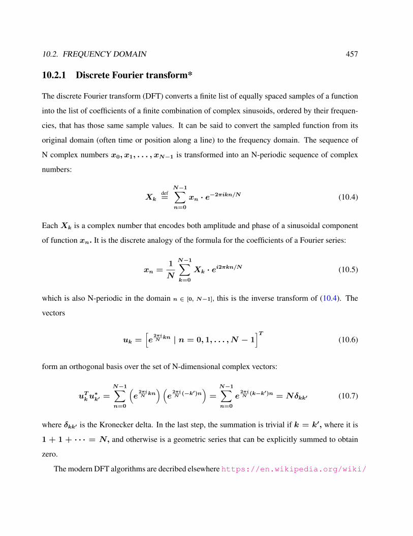
10.2. FREQUENCY DOMAIN 457
10.2.1 Discrete Fourier transform*
The discrete Fourier transform (DFT) converts a finite list of equally spaced samples of a function
into the list of coefficients of a finite combination of complex sinusoids, ordered by their frequen-
cies, that has those same sample values. It can be said to convert the sampled function from its
original domain (often time or position along a line) to the frequency domain. The sequence of
N complex numbers x0, x1, . . . , xN−1 is transformed into an N-periodic sequence of complex
numbers:
Xkdef=
N−1∑n=0
xn · e−2πikn/N (10.4)
Each Xk is a complex number that encodes both amplitude and phase of a sinusoidal component
of function xn. It is the discrete analogy of the formula for the coefficients of a Fourier series:
xn =1
N
N−1∑k=0
Xk · ei2πkn/N (10.5)
which is also N-periodic in the domain n ∈ [0, N−1], this is the inverse transform of (10.4). The
vectors
uk =[e
2πiNkn | n = 0, 1, . . . , N − 1
]T(10.6)
form an orthogonal basis over the set of N-dimensional complex vectors:
uTku∗k′ =
N−1∑n=0
(e
2πiNkn) (e
2πiN
(−k′)n)
=
N−1∑n=0
e2πiN
(k−k′)n = Nδkk′ (10.7)
where δkk′ is the Kronecker delta. In the last step, the summation is trivial if k = k′, where it is
1 + 1 + · · · = N, and otherwise is a geometric series that can be explicitly summed to obtain
zero.
The modern DFT algorithms are decribed elsewhere https://en.wikipedia.org/wiki/
458 CHAPTER 10. DYNAMICS OF SPATIO-TEMPORAL PATTERN
Fast_Fourier_transform where the main idea goes back to Gauss (1866).
We previously saw a periodogram, a function/graph that displays information about the peri-
odic components of a time series. Any time series can be expressed as a sum of cosine and sine
waves oscillating at the fundamental (harmonic) frequencies = j/n, with j = 1, 2, . . . , n/2.
The periodogram gives information about the relative strengths of the various frequencies for ex-
plaining the variation in the time series. The periodogram is a sample estimate of a population
function, i.e. the spectral density S(ω), which is the frequency domain characterization of a pop-
ulation stationary time series. The estimate through the periodogram is rough, in part, because we
only use the discrete fundamental harmonic frequencies for the periodogram whereas the spectral
density is defined over a continuum of frequencies.
The usual method for smoothing a periodogram, it is merely a centered moving average proce-
dure with a few possible modifications. For a time series, the Daniell kernel with parameterm is a
centered moving average which creates a smoothed value at time t by averaging all values between
times t−m and t+m(inclusive). For example, the smoothing formula for a Daniell kernel with
m = 2 is
xt =xt−2 + xt−1 + xt + xt+1 + xt+2
5(10.8)
The Fourier transform is used for the spectral analysis of time-series. The subject of statistical
signal processing does not, however, usually apply the Fourier transformation to the signal itself.
Even if a real signal is indeed transient, it has been found in practice advisable to model a signal
by a function (or, alternatively, a stochastic process) which is stationary in the sense that its char-
acteristic properties are constant over all time. The Fourier transform of such a function does not
exist in the usual sense, and it has been found more useful for the analysis of signals to instead take
the Fourier transform of its auto-correlation function.
In R, the weighting coefficients for a Daniell kernel with m = 2 can be generated with the
command kernel("daniell", 2). The result is
coef[-2] = 0.2

10.2. FREQUENCY DOMAIN 459
coef[-1] = 0.2coef[ 0] = 0.2coef[ 1] = 0.2coef[ 2] = 0.2
The subscripts for coef [ ] refer to the time difference from the center of the average at time t. Thus
the smoothing formula in this instance is xt = 0.2xt−2+0.2xt−1+0.2xt+0.2xt+1+0.2xt+2,
which is the same as the formula given above. The modified Daniell kernel is such that the two
endpoints in the averaging receive half the weight that the interior points do. For a modified Daniell
kernel withm = 2, the smoothing is
xt =xt−2 + 2xt−1 + 2xt + 2xt+1 + xt+2
8(10.9)
= 0.125xt−2 + 0.25xt−1 + 0.25xt + 0.25xt+1 + 0.125xt+2 (10.10)
In R, the command kernel("modified.daniell", 2) will list the weighting coefficients just used. Ei-
ther the Daniell kernel or the modified Daniell kernel can be convoluted (repeated) so that the
smoothing is applied again to the smoothed values. This produces a more extensive smoothing by
averaging over a wider time interval. For instance, to repeat a Daniell kernel with m = 2 on the
smoothed values that resulted from a Daniell kernel withm = 2, the formula would be
˜xt =xt−2 + xt−1 + xt + xt+1 + xt+2
5
This is the average of the smoothed values within two time periods of time t, in either direction.
In R, the command kernel("daniell",c(2,2)) will supply the coefficients that would be applied
to as weights in averaging the original data values for a convoluted Daniell kernel with m = 2 in
both smoothings. The result is> kernel ("daniell",c(2,2))coef[-4] = 0.04coef[-3] = 0.08coef[-2] = 0.12coef[-1] = 0.16coef[ 0] = 0.20coef[ 1] = 0.16coef[ 2] = 0.12
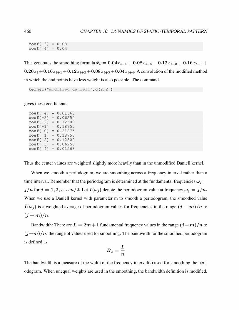
460 CHAPTER 10. DYNAMICS OF SPATIO-TEMPORAL PATTERN
coef[ 3] = 0.08coef[ 4] = 0.04
This generates the smoothing formula xt = 0.04xt−4 + 0.08xt−3 + 0.12xt−2 + 0.16xt−1 +
0.20xt+0.16xt+1 +0.12xt+2 +0.08xt+3 +0.04xt+4.A convolution of the modified method
in which the end points have less weight is also possible. The command
kernel("modified.daniell",c(2,2))
gives these coefficients:
coef[-4] = 0.01563coef[-3] = 0.06250coef[-2] = 0.12500coef[-1] = 0.18750coef[ 0] = 0.21875coef[ 1] = 0.18750coef[ 2] = 0.12500coef[ 3] = 0.06250coef[ 4] = 0.01563
Thus the center values are weighted slightly more heavily than in the unmodified Daniell kernel.
When we smooth a periodogram, we are smoothing across a frequency interval rather than a
time interval. Remember that the periodogram is determined at the fundamental frequencies ωj =
j/n for j = 1, 2, . . . , n/2. Let I(ωj) denote the periodogram value at frequency ωj = j/n.
When we use a Daniell kernel with parameter m to smooth a periodogram, the smoothed value
I(ωj) is a weighted average of periodogram values for frequencies in the range (j −m)/n to
(j +m)/n.
Bandwidth: There areL = 2m+1 fundamental frequency values in the range (j−m)/n to
(j+m)/n, the range of values used for smoothing. The bandwidth for the smoothed periodogram
is defined as
Bω =L
n
The bandwidth is a measure of the width of the frequency interval(s) used for smoothing the peri-
odogram. When unequal weights are used in the smoothing, the bandwidth definition is modified.
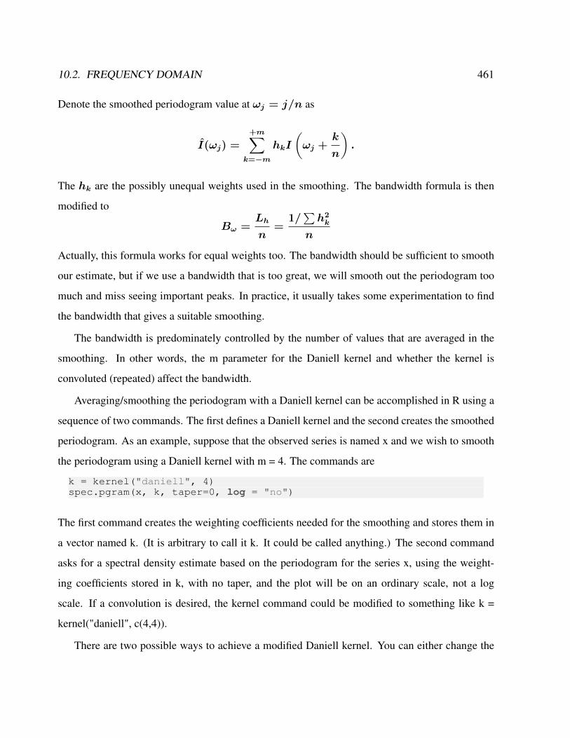
10.2. FREQUENCY DOMAIN 461
Denote the smoothed periodogram value at ωj = j/n as
I(ωj) =
+m∑k=−m
hkI
(ωj +
k
n
).
The hk are the possibly unequal weights used in the smoothing. The bandwidth formula is then
modified to
Bω =Lh
n=
1/∑h2k
n
Actually, this formula works for equal weights too. The bandwidth should be sufficient to smooth
our estimate, but if we use a bandwidth that is too great, we will smooth out the periodogram too
much and miss seeing important peaks. In practice, it usually takes some experimentation to find
the bandwidth that gives a suitable smoothing.
The bandwidth is predominately controlled by the number of values that are averaged in the
smoothing. In other words, the m parameter for the Daniell kernel and whether the kernel is
convoluted (repeated) affect the bandwidth.
Averaging/smoothing the periodogram with a Daniell kernel can be accomplished in R using a
sequence of two commands. The first defines a Daniell kernel and the second creates the smoothed
periodogram. As an example, suppose that the observed series is named x and we wish to smooth
the periodogram using a Daniell kernel with m = 4. The commands are
k = kernel("daniell", 4)spec.pgram(x, k, taper=0, log = "no")
The first command creates the weighting coefficients needed for the smoothing and stores them in
a vector named k. (It is arbitrary to call it k. It could be called anything.) The second command
asks for a spectral density estimate based on the periodogram for the series x, using the weight-
ing coefficients stored in k, with no taper, and the plot will be on an ordinary scale, not a log
scale. If a convolution is desired, the kernel command could be modified to something like k =
kernel("daniell", c(4,4)).
There are two possible ways to achieve a modified Daniell kernel. You can either change the
462 CHAPTER 10. DYNAMICS OF SPATIO-TEMPORAL PATTERN
kernel command to refer to the "modified.daniell" rather than "daniell" or you can skip using the
kernel command and use a spans parameter in the spec.pgram command.1
The spans parameter gives the length (= 2m+ 1) of the desired modified Daniell kernel. For
instance, a modified Daniell kernel with m = 4 has length L = 2m + 1 = 9 so the we could
use the commandspec.pgram(x, spans=9, taper = 0, log="no")
Two passes of a modified Daniell kernel with m = 4 on each pass can be done usingspec.pgram(x, spans=c(9,9), taper = 0, log="no")
To learn where the two dominant peaks are located, assign a name to the spec.pgram output
and then you can list it. For instance,specvalues = spec.pgram(x, k, taper=0, log="no")specvalues
One can put vertical dotted lines onto the (estimated) spectral density plot at the approximate
locations of the peak densities.abline(v=1/44, lty="dotted")
A series should be de-trended prior to a spectral analysis. A trend will cause such a dominant
spectral density at a low frequency that other peaks would not be seen. By default, the R command
spec.pgram performs a de-trending using a linear trend model. That is, the spectral density is
estimated using the residuals from a regression done where the y-variable = observed data and the
x-variable = t. If a different type of trend is present, a quadratic for instance, then a polynomial
regression could be used to de-trend the data before the estimated spectral density is explored.
Note, however, that the R command spec.ar, however does not perform a de-trending by default.
Exercise 78 – Calculate a spectrum
1The smoothing method of spectral density estimation is called a nonparametric method because it does not use anyparametric model for the underlying time series process. An alternative method is a parametric method which entailsfinding the best fitting AR model for the series and then plotting the spectral density of that model. This method issupported by a theorem which says that the spectral density of any time series process can be approximated by thespectral density of an AR model (of some order, possibly a high one). In R, parametric estimation of the spectraldensity is easily done with the command/function spec.ar

10.2. FREQUENCY DOMAIN 463
Tasks: Using R https://stat.ethz.ch/R-manual/R-devel/library/stats/
html/spectrum.html:
1. Create a vector containing a sinus signal and plot the spectrum on the right top corner you
see a cross which shows the bandwith (horizontal bar) and 95% confidence interval (vertical
bar)
2. Vary the averaging and look how the shape (width) of the peak varies
3. Now add noise to the data and repeat 1 and 2. You will see that when you increase the
smoothing you get a smaller variance and a larger bandwith. The information content is
limited and you have to make your choice.
464 CHAPTER 10. DYNAMICS OF SPATIO-TEMPORAL PATTERN
Solution#Spectrum, bandwith and variance
a<-sin(2*pi*(1:5000)*1/10)+0.5*rnorm(5000)/10#a<-sin((1:1000)/10)plot(a,type="l")
spectrum(a)spectrum(a, method = "ar")spectrum(a,spans=10,main="spans=10")spectrum(a,spans=30,main="spans=30")spectrum(a,spans=100,main="spans=100")spectrum(a,spans = c(5,7), log = "dB", ci = 0.8)dev.print(postscript, file="spectrumtest.ps")
With the R-command??spectrum
you get help a description of the function. It says that the as arguments is has a univariate or mul-
tivariate time series x. The spectrum here is defined with scaling 1/frequency(x). A confidence
interval will be plotted by plot.spec: this is asymmetric, and the width of the centre mark indicates
the equivalent bandwidth.
Another important method is the cross-spectrum analysis where you can have two processes x
and y.#Coherence spectrum - cross-spectrum analysislibrary(clim.pact)coherence(x,y,dt=1,M=NULL,plot=TRUE)# or for the spectrum if both processes are the samecoherence(a,a,dt=1,M=NULL,plot=TRUE)
10.2.2 Wavelet spectrum*
Many geophysical processes are furthermore often non-stationary. In this regard, the optimal
method is continuous wavelet analysis as it intrinsically adjusts the time resolution to the ana-
lyzed scale, e.g. ?; ?. Wavelet analysis is based on the convolution of f(t) with a set of functions
gab(t) derived from the translations and dilations (and rotations in higher dimensions) of a mother
10.2. FREQUENCY DOMAIN 465
wavelet g(t), where
gab =1√ag
(t− ba
)(10.11)
a > 0 and b are real. Any set of functions gab(t) constructed from (10.11) and meeting the
conditions outlined below are called wavelets. The convolution of f(t) with the set of wavelets is
the wavelet transform (WT)
Tg(b, a) =1√a
∫g
(t− ba
)f(t) dt (10.12)
This is known as the continuous wavelet transform since "a" and "b" may be varied continuously.
Translation parameter "b" corresponds to position or time if the data is spatial or temporal, es-
pectively. Dilation parameter "a" then corresponds to scale length or temporal period. Equation
(10.12) expands a one-dimensional time series into the two-dimensional parameter space (b, a)
and yields a local measure of the relative amplitude of activity at scale a at time b. This is in
contrast to the Fourier transform that yields an average amplitude over the entire dataset. Note,
we have avoided the use of the words "wavelength" or "frequency" in our description of the WT.
Though wavelets have a definite scale, they need not to bear any resemblance to Fourier modes(
sines and cosines). However, a correspondence between wavelength and scale a sometimes can
be achieved. In contrast to the standard Fourier analysis and the incentive for the development of
wavelet analysis, the WT produces "instantaneous" coefficients and therefore can yield information
on the evolution of nonstationary processes.
A major question concerns the significance testing of wavelet spectra. Torrence and Compo ?
formulated pointwise significance tests against reasonable background spectra. However, Maraun
and Kurths ? pointed out a serious deficiency of pointwise significance testing: Given a realiza-
tion of white noise, large patches of spurious significance are detected, making it - without further
insight - impossible to judge which features of an estimated wavelet spectrum differ from back-
ground noise and which are just artefacts of multiple testing. Under these conditions, a reliable
466 CHAPTER 10. DYNAMICS OF SPATIO-TEMPORAL PATTERN
corroboration of a given hypothesis is impossible. This demonstrates the necessity to study the
significance testing of continuous wavelet spectra in terms of sensitivity and specificity. Given the
set of all patches with pointwise significant values, areawise significant patches are defined as the
subset of additionally areawise significant wavelet spectral coefficients given as the union of all
critical areas that completely lie inside the patches of pointwise significant values. Whereas the
specificity of the areawise test appears to be - almost independently of the signal to noise ratio
- close to one, that of the pointwise test decreases for high background noise, as more and more
spurious patches appear ?.
10.2.3 Pseudospectrum*
Another spectral method characterizing the abruptness and resonance of the linear system (7.57)
is the pseudospectrum. As we will see later in the context of atmosphere and ocean instabilities,
an eigenvalue analysis is inappropriate in describing the dynamics of the system (??). One of the
most prominent of these problems is equations of the form
d
dtx(t) = Ax+ forcing , (10.13)
A perturbation in a system with a negative feedback mechanism will be reduced whereas in a
system with positive feedback mechanisms, the perturbation will grow. In the one dimensional
case, A can be rewritten as −λ. The real part of λ determines then the stability of the system
and is called feedback factor. We have discussed this dynamics in the context of the mixed layer
model (??). Let us start with a simple model: We have a two-dimensional system with matrix A,
eigenvectors and eigenvalues are simply calculated:
a = [-1 20; 0 -5 ][v,l]=eig(a)vlv1=v(:,1)v2=v(:,2)v1’*v2
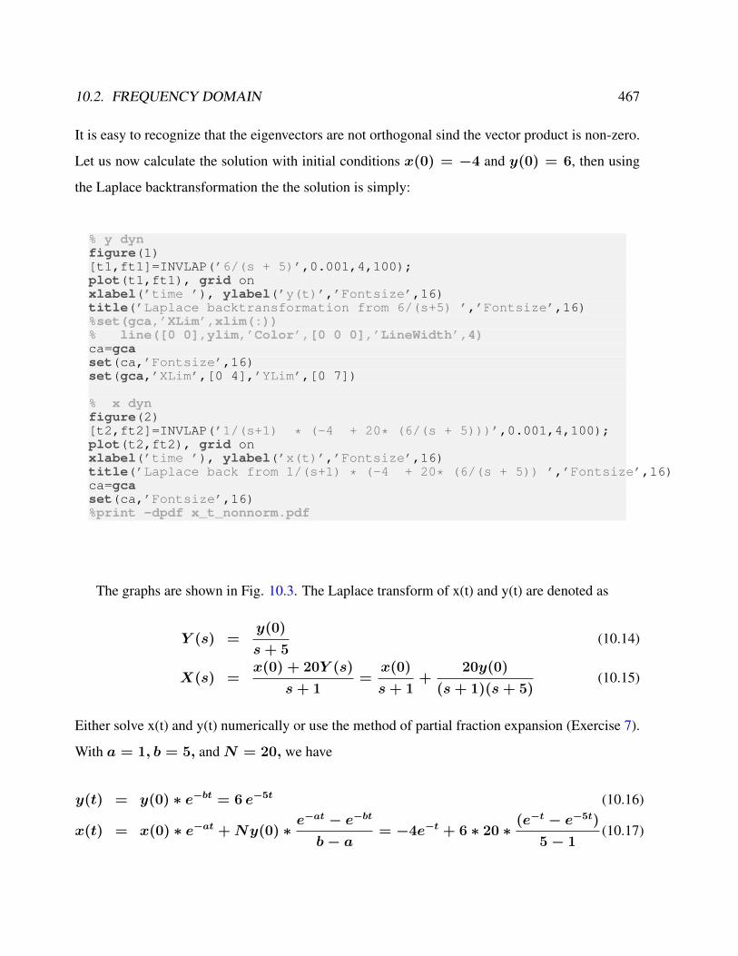
10.2. FREQUENCY DOMAIN 467
It is easy to recognize that the eigenvectors are not orthogonal sind the vector product is non-zero.
Let us now calculate the solution with initial conditions x(0) = −4 and y(0) = 6, then using
the Laplace backtransformation the the solution is simply:
% y dynfigure(1)[t1,ft1]=INVLAP(’6/(s + 5)’,0.001,4,100);plot(t1,ft1), grid onxlabel(’time ’), ylabel(’y(t)’,’Fontsize’,16)title(’Laplace backtransformation from 6/(s+5) ’,’Fontsize’,16)%set(gca,’XLim’,xlim(:))% line([0 0],ylim,’Color’,[0 0 0],’LineWidth’,4)ca=gcaset(ca,’Fontsize’,16)set(gca,’XLim’,[0 4],’YLim’,[0 7])
% x dynfigure(2)[t2,ft2]=INVLAP(’1/(s+1) * (-4 + 20* (6/(s + 5)))’,0.001,4,100);plot(t2,ft2), grid onxlabel(’time ’), ylabel(’x(t)’,’Fontsize’,16)title(’Laplace back from 1/(s+1) * (-4 + 20* (6/(s + 5)) ’,’Fontsize’,16)ca=gcaset(ca,’Fontsize’,16)%print -dpdf x_t_nonnorm.pdf
The graphs are shown in Fig. 10.3. The Laplace transform of x(t) and y(t) are denoted as
Y (s) =y(0)
s+ 5(10.14)
X(s) =x(0) + 20Y (s)
s+ 1=x(0)
s+ 1+
20y(0)
(s+ 1)(s+ 5)(10.15)
Either solve x(t) and y(t) numerically or use the method of partial fraction expansion (Exercise 7).
With a = 1, b = 5, andN = 20, we have
y(t) = y(0) ∗ e−bt = 6 e−5t (10.16)
x(t) = x(0) ∗ e−at +Ny(0) ∗e−at − e−bt
b− a= −4e−t + 6 ∗ 20 ∗
(e−t − e−5t)
5− 1(10.17)

468 CHAPTER 10. DYNAMICS OF SPATIO-TEMPORAL PATTERN
It is interesting to write an approximation of x(t) for small t:
x(t) ≈ x(0) ∗ (1− at) +Ny(0) ∗(1− at)− (1− bt)
b− a(10.18)
= x(0) + t(−ax(0) +Ny(0)) (10.19)
A linear increase in t with−ax(0) +Ny(0) = (−1) ∗ (−4) + 20 ∗ 6 = 124 is nicely seen
in Fig. 10.3. It strongly depends on N, the higher N (the more non-normal the matrix A is), the
stronger can be the transient growth. The example shows furthermore, that the transfer function
with a multiplication in the denominator Ny(0)
(s−a)(s−b) provides the source of the transient growth.
In the one-dimensional case for x(t) = exp(at) we have the the inverse Laplace transform
exp(at) = L−1F (s)(t) =1
2πilimT→∞
∫ γ+iT
γ−iTest
1
s− ads, (10.20)
and and the entire range of t is controlled t by the resolvent | 1s−a |.Using the Fourier transformation,
(10.13) with forcing F(t) is tranformed to
(iωI −A)x = F (10.21)
x = (iωI −A)−1F (10.22)
where I is the identity. The so-called resolvent operator of matrix A is R(ω) = (iωI − A)−1
The behavior of the norms || exp(At)|| over the entire range of t is controlled t by the resolvent
norm ||R(ω)||. If A is a normal operator
A A+ = A+ A , (10.23)
where + denotes the adjoint-complex operator, then
||R(ω)|| = 1/dist(iω, σ(A)) (10.24)
10.2. FREQUENCY DOMAIN 469
is completely determined by the spectrum σ(A) alone. The operator dist denotes the shortest
distance of ω to the eigenvalues, the spectrum σ(A). This explains the success of eigenvalue
analysis. In contrast to this, for non-normal operators the behavior of ||R(ω)|| may deviate from
that dramatically and hence in this context pseudospectral analysis is just the right tool ?; ?. More
about the dynamics can be learned by examining the pseudospectrum of A in the complex plane.
Inspection of many geophysical systems shows that most of the systems fail the normality condi-
tion (10.23). The ε−pseudospectrum of operatorA is defined by two equivalent formulations:
Λε(A) = z ∈ C : ||(zI −A)−1|| ≥ ε−1
= z ∈ C : [ smallest singular value of (zI −A)] ≤ ε . (10.25)
This set of values z in the complex plane are defined by contourlines of the resolvent (zI −
A)−1. The resolvent determines the system’s response to a forcing as supplied by external forcing
F (x, t), stochastic forcing g(x)ξ, or initial/boundary conditions. The pseudospectrum reflects
the robustness of the spectrum and provides information about instability and resonance. One
theorem is derived from Laplace transformation stating that transient growth is related to how far
the ε−pseudospectrum extends into the right half plane:
|| exp(At) || ≥1
εsup
z∈Λε(A)
Real(z) . (10.26)
In terms of climate theory, the pseudospectrum indicates resonant amplification. Maximal amplifi-
cation is at the poles of (zI−A)−1, characterized by the eigenfrequencies. In a system satisfying
(10.23), the system’s response is characterized solely by the proximity to the eigenfrequencies. In
the non-normal case, the pseudospectrum shows large resonant amplification for frequencies which
are not eigenfrequencies. This transient growth mechanism is important for both initial value and
forced problems.

470 CHAPTER 10. DYNAMICS OF SPATIO-TEMPORAL PATTERN
10.2.4 Resonance in an atmospheric circulation model*
An atmospheric general circulation model PUMA ? is applied to the problem. The model is based
on the multi-level spectral model described by Hoskins and Simmons ?. For our experiments we
chose five vertical levels and a T21 horizontal resolution. PUMA belongs to the class of models of
intermediate complexity ?; it has been used to understand principle feedbacks ?, and dynamics on
long time scales ?. For simplicity, the equations are scaled here such that they are dimensionless.
The model is linearized about a zonally symmetric mean state providing for a realistic storm track
at mid-latitudes ?. In a simplified version of the model and calculating the linear model A with
n = 214, one can derive the pseudospectrum. Fig. 10.4 indicates resonances besides the poles
(the eigenvalues) indicated by crosses. The Im(z)−axis shows the frequencies, theRe(z)−axis
the damping/amplification of the modes. Important modes for the climate system are those with
−0.5 < Im(z) < 0.5 representing planetary Rossby waves. The basic feature is that transient
growth of initially small perturbations can occur even if all the eigenmodes decay exponentially.
Mathematically, an arbitrary matrixA can be decomposed as a sum
A = D +N (10.27)
where A is diagonalizable, and N is nilpotent (there exists an integer q ∈ N with Nq = 0),
and D commutes with N (i.e. DN = NA). This fact follows from the Jordan-Chevalley
decomposition theorem. This means that we can compute the exponential of (A t) by reducing to
the cases:
exp(At) = exp( (D +N) t) = exp(Dt) exp(Nt) (10.28)
where the exponential of Nt can be computed directly from the series expansion, as the series
terminates after a finite number of terms. Basically, the number q ∈ N is related to the transient
growth of the system (q = 1 means no transient growth).
The resonant structures are due to the mode interaction: It is not possible to change one variable
10.2. FREQUENCY DOMAIN 471
without the others, because they are not orthogonal. Interestingly, one can also compute the A+
model, showing the optimal perturbation of a mode ei through its biorthogonal vector (2.60).
The analysis indicates that non-normality of the system is a fundamental feature of the atmo-
spheric dynamics. This has consequences for the error growth dynamics, and instability of the
system, e.g. ?; ?. Similar features are obtained in shear flow systems ?; ? and other hydrody-
namic applications. This transient growth mechanism is important for both initial value and forced
problems of the climate system ?.
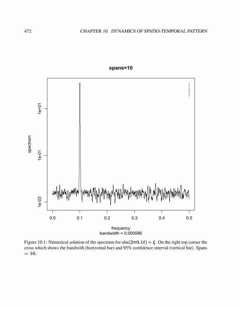
472 CHAPTER 10. DYNAMICS OF SPATIO-TEMPORAL PATTERN
0.0 0.1 0.2 0.3 0.4 0.5
1e-03
1e-01
1e+01
frequency
spectrum
spans=10
bandwidth = 0.000586
Figure 10.1: Numerical solution of the spectrum for sin(2π0.1t) + ξ. On the right top corner thecross which shows the bandwith (horizontal bar) and 95% confidence interval (vertical bar). Spans= 10.
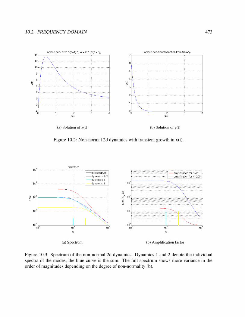
10.2. FREQUENCY DOMAIN 473
(a) Solution of x(t) (b) Solution of y(t)
Figure 10.2: Non-normal 2d dynamics with transient growth in x(t).
(a) Spectrum (b) Amplification factor
Figure 10.3: Spectrum of the non-normal 2d dynamics. Dynamics 1 and 2 denote the individualspectra of the modes, the blue curve is the sum. The full spectrum shows more variance in theorder of magnitudes depending on the degree of non-normality (b).
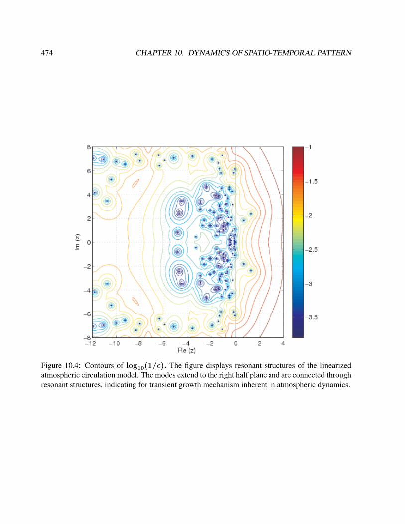
474 CHAPTER 10. DYNAMICS OF SPATIO-TEMPORAL PATTERN
Figure 10.4: Contours of log10(1/ε). The figure displays resonant structures of the linearizedatmospheric circulation model. The modes extend to the right half plane and are connected throughresonant structures, indicating for transient growth mechanism inherent in atmospheric dynamics.
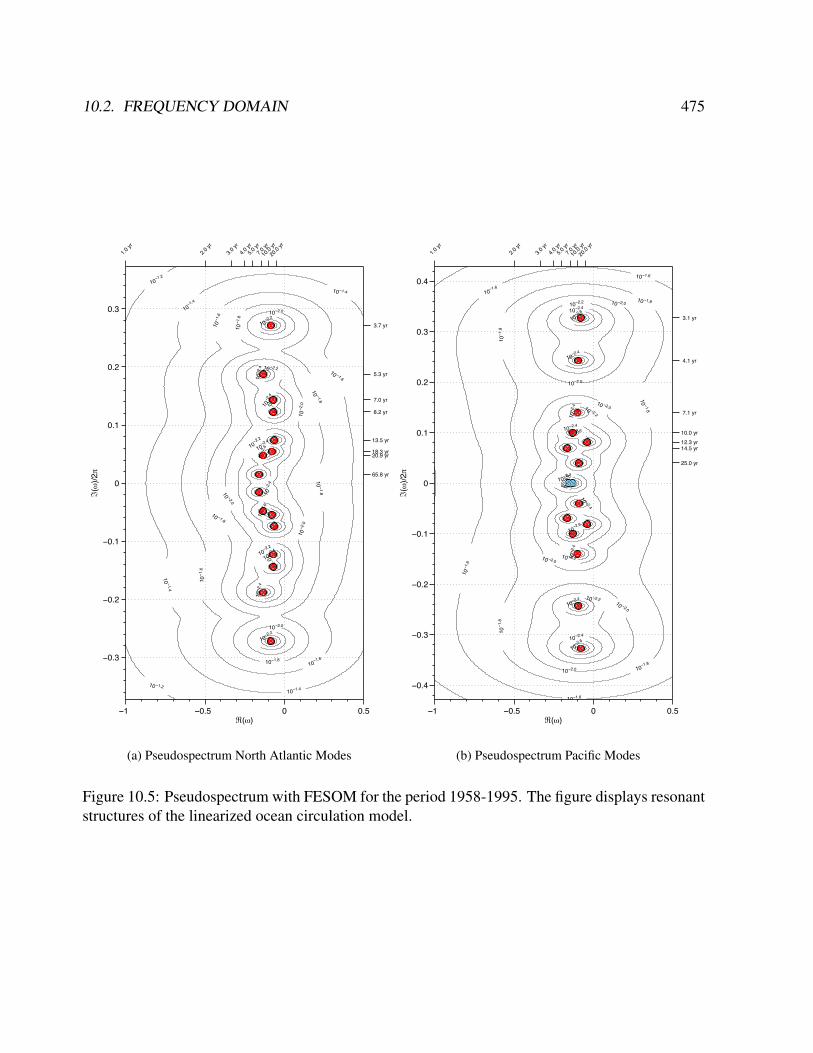
10.2. FREQUENCY DOMAIN 475
−1 −0.5 0 0.5
−0.3
−0.2
−0.1
0
0.1
0.2
0.3
10 −2.6
10 −2.6
10−2
.610
−2.6
10−2
.4
10−2.4
10−2
.4
10−2.4
10−2
.410
−2.4
10−2.2
10−2.2
10−2.2
10−2.2
10−2.2
10−2
.0
10 −2.0
10−2
.0
10−2.0
10−2.0
10 −1.8
10−1
.8
10 −1.8
10−1.8
10 −1.8
10 −1.6
10−1
.6
10−1
.6
10−1.6
10 −1.4
10−1.4
10 −1.4
10−1.4
10−1.2
10 −1.2
½(t)
¼(t
)/2/ 65.8 yr
20.9 yr18.3 yr
13.5 yr
8.2 yr
7.0 yr
5.3 yr
3.7 yr
1.0 y
r
2.0 y
r
3.0 y
r
4.0 y
r
5.0 y
r
7.0 y
r
10.0
yr
20.0
yr
(a) Pseudospectrum North Atlantic Modes
−1 −0.5 0 0.5
−0.4
−0.3
−0.2
−0.1
0
0.1
0.2
0.3
0.4
10−3
.0
10−2.6
10−2.6
10−2.6
10−2.6
10−2
.6
10−2.4
10−2.4
10−2.4
10 −2.4
10−2.4
10−2.4
10−2
.410
−2.4
10−2.4
10−2.2
10 −2.2
10 −2.2
10 −2.2
10−2.0
10−2.0
10 −2.0
10−2.0
10 −2.0
10 −2.0
10 −1.8
10−1
.810
−1.8
10−1.8
10 −1.8
10−1.6
10−1.6
10−1
.6
10−1.6
½(t)
¼(t
)/2/
25.0 yr
14.5 yr12.3 yr10.0 yr
7.1 yr
4.1 yr
3.1 yr
1.0 y
r
2.0 y
r
3.0 y
r
4.0 y
r
5.0 y
r
7.0 y
r
10.0
yr
20.0
yr
(b) Pseudospectrum Pacific Modes
Figure 10.5: Pseudospectrum with FESOM for the period 1958-1995. The figure displays resonantstructures of the linearized ocean circulation model.

476 CHAPTER 10. DYNAMICS OF SPATIO-TEMPORAL PATTERN
10.3 Principal Component Analysis
Principal component analysis (PCA) is a statistical procedure that uses an orthogonal transforma-
tion to convert a set of observations of possibly correlated variables into a set of values of linearly
uncorrelated variables called principal components. The number of principal components is less
than or equal to the number of original variables. This transformation is defined in such a way that
the first principal component has the largest possible variance.
One of the most ubiquitous uses of eigenanalysis in data analysis is the construction of EOFs,
the topic of this section. EOFs are a transform of the data; the original set of numbers is trans-
formed into a different set with some desirable properties. In this sense the EOF transform is
similar to other transforms such as the Fourier or Laplace transforms. In all these cases, we project
the original data onto a set of orthogonal functions, thus replacing the original data with the set
of projection coefficients on the basis vectors. However, the choice of the specific basis set varies
from case to case.
In the Fourier case, for example, the choice is a set of sines and cosines of various frequen-
cies. This is motivated by the desire to identify the principal modes of oscillation of the system.
Thus if the signal projects strongly on sine waves of 2 frequencies, we will say that the signal is
approximately the linear combination of these 2 frequencies. We will then attribute the remainder
to other processes that are more weakly represented in the signal (the signal has low projection on
them), and are thus assumed unimportant for the signal. Another important property for a basis is
orthogonality (like sines or various frequencies); we would like to account for a certain component
of the signal only once. An alternative to the sine/cosine set is a set of orthogonal polynomials,
such as those named after Legendre.
The representation of the signal in terms of the projection coefficients on a basis set is often very
useful at separating cleanly various scales. For example, if our data is the sea surface temperature
of a given ocean basin, we can think of the projection on the lowest frequency wave (the one which
has one crest and one trough within the spatial extent of the domain) as representing the ocean’s
‘large-scale’, while that on wavelengths of order 10-100 km as ‘eddies’. In EOF analysis we also

10.3. PRINCIPAL COMPONENT ANALYSIS 477
project the original data on a set of orthogonal basis vectors. However, the choice of the basis
is different. Here, the first EOF is chosen to be the pattern, without the constraint of a particular
analytic form, on which the data project most strongly. In other words, the leading EOF (sometime
called the ‘gravest’, or ‘leading’, mode) is the pattern most frequently realized. The second mode
is the one most commonly realized under the constraint of orthogonality to the first one, the third
is the most frequently realized pattern that is orthogonal to both higher modes, and so on. Hence
the term ‘empirical’; we still have an orthogonal basis, like the Fourier or Legendre bases, but
whose members are not chosen based on analytic considerations, but based on maximization of the
projection of the data on them.
10.3.1 Singular Value Decomposition
In linear algebra, the singular value decomposition (SVD) is a factorization of a real or complex
matrix. It is the generalization of the eigendecomposition of a positive semidefinite normal matrix
(for example, a symmetric matrix with positive eigenvalues) to any m × n matrix. It has many
useful applications in signal processing and statistics. Suppose M is a m × n matrix whose
entries are real or complex numbers. Then there exists a factorization, called a singular value
decomposition of M, of the form
M = UΣV∗ (10.29)
whereU is am×m unitary matrix, Σ is am×n diagonal matrix with non-negative real numbers
on the diagonal, and V ∗ is a n×n unitary matrix. The diagonal entries σi of Σ are known as the
singular values of M. A common convention is to list the singular values in descending order. In
this case, the diagonal matrix Σ is uniquely determined by M (though not the matrices U and V).
The columns of U and V are orthonormal bases. Since U and V∗ are unitary, the columns of
each of them form a set of orthonormal vectors, which can be regarded as basis vectors. In short,
the columns of U,U∗, V, and V ∗ are orthonormal bases.
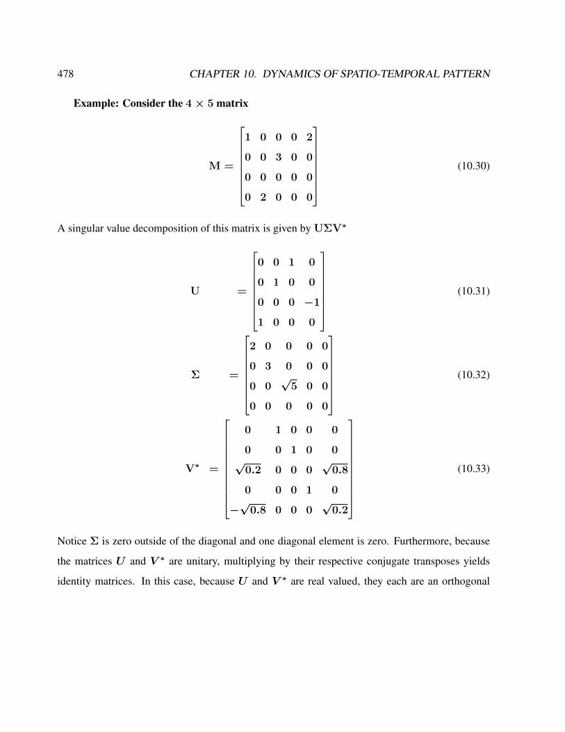
478 CHAPTER 10. DYNAMICS OF SPATIO-TEMPORAL PATTERN
Example: Consider the 4× 5 matrix
M =
1 0 0 0 2
0 0 3 0 0
0 0 0 0 0
0 2 0 0 0
(10.30)
A singular value decomposition of this matrix is given by UΣV∗
U =
0 0 1 0
0 1 0 0
0 0 0 −1
1 0 0 0
(10.31)
Σ =
2 0 0 0 0
0 3 0 0 0
0 0√
5 0 0
0 0 0 0 0
(10.32)
V∗ =
0 1 0 0 0
0 0 1 0 0√
0.2 0 0 0√
0.8
0 0 0 1 0
−√
0.8 0 0 0√
0.2
(10.33)
Notice Σ is zero outside of the diagonal and one diagonal element is zero. Furthermore, because
the matrices U and V ∗ are unitary, multiplying by their respective conjugate transposes yields
identity matrices. In this case, because U and V ∗ are real valued, they each are an orthogonal
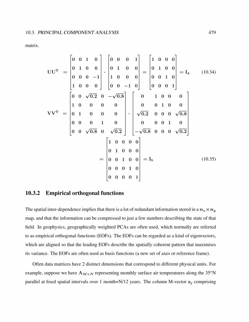
10.3. PRINCIPAL COMPONENT ANALYSIS 479
matrix.
UUT =
0 0 1 0
0 1 0 0
0 0 0 −1
1 0 0 0
·
0 0 0 1
0 1 0 0
1 0 0 0
0 0 −1 0
=
1 0 0 0
0 1 0 0
0 0 1 0
0 0 0 1
= I4 (10.34)
VVT =
0 0√
0.2 0 −√
0.8
1 0 0 0 0
0 1 0 0 0
0 0 0 1 0
0 0√
0.8 0√
0.2
·
0 1 0 0 0
0 0 1 0 0√
0.2 0 0 0√
0.8
0 0 0 1 0
−√
0.8 0 0 0√
0.2
=
1 0 0 0 0
0 1 0 0 0
0 0 1 0 0
0 0 0 1 0
0 0 0 0 1
= I5 (10.35)
10.3.2 Empirical orthogonal functions
The spatial inter-dependence implies that there is a lot of redundant information stored in anx×nymap, and that the information can be compressed to just a few numbers describing the state of that
field. In geophysics, geographically weighted PCAs are often used, which normally are referred
to as empirical orthogonal functions (EOFs). The EOFs can be regarded as a kind of eigenvectors,
which are aligned so that the leading EOFs describe the spatially coherent pattern that maximises
its variance. The EOFs are often used as basis functions (a new set of axes or reference frame).
Often data matrices have 2 distinct dimensions that correspond to different physical units. For
example, suppose we have AM×N representing monthly surface air temperatures along the 35N
parallel at fixed spatial intervals over 1 month=N/12 years. The column M-vector aj comprising
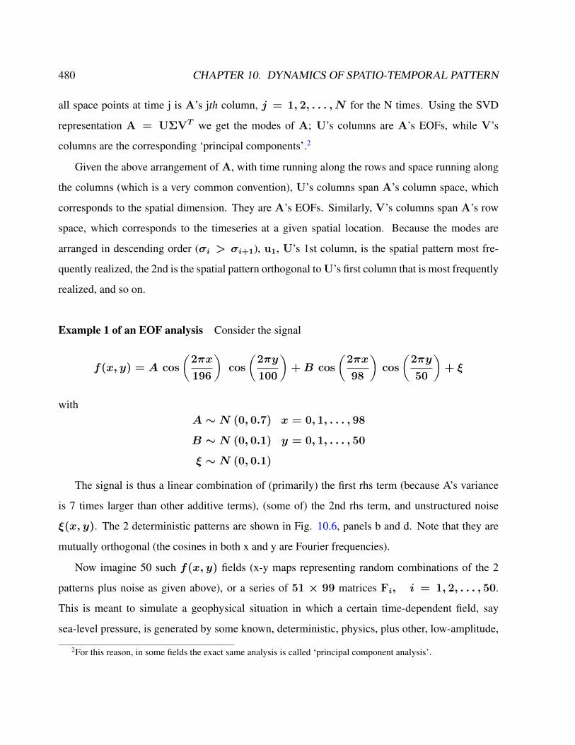
480 CHAPTER 10. DYNAMICS OF SPATIO-TEMPORAL PATTERN
all space points at time j is A’s jth column, j = 1, 2, . . . , N for the N times. Using the SVD
representation A = UΣVT we get the modes of A; U’s columns are A’s EOFs, while V’s
columns are the corresponding ‘principal components’.2
Given the above arrangement of A, with time running along the rows and space running along
the columns (which is a very common convention), U’s columns span A’s column space, which
corresponds to the spatial dimension. They are A’s EOFs. Similarly, V’s columns span A’s row
space, which corresponds to the timeseries at a given spatial location. Because the modes are
arranged in descending order (σi > σi+1), u1, U’s 1st column, is the spatial pattern most fre-
quently realized, the 2nd is the spatial pattern orthogonal to U’s first column that is most frequently
realized, and so on.
Example 1 of an EOF analysis Consider the signal
f(x, y) = A cos
(2πx
196
)cos
(2πy
100
)+B cos
(2πx
98
)cos
(2πy
50
)+ ξ
withA ∼ N (0, 0.7) x = 0, 1, . . . , 98
B ∼ N (0, 0.1) y = 0, 1, . . . , 50
ξ ∼ N (0, 0.1)
The signal is thus a linear combination of (primarily) the first rhs term (because A’s variance
is 7 times larger than other additive terms), (some of) the 2nd rhs term, and unstructured noise
ξ(x, y). The 2 deterministic patterns are shown in Fig. 10.6, panels b and d. Note that they are
mutually orthogonal (the cosines in both x and y are Fourier frequencies).
Now imagine 50 such f(x, y) fields (x-y maps representing random combinations of the 2
patterns plus noise as given above), or a series of 51 × 99 matrices Fi, i = 1, 2, . . . , 50.
This is meant to simulate a geophysical situation in which a certain time-dependent field, say
sea-level pressure, is generated by some known, deterministic, physics, plus other, low-amplitude,
2For this reason, in some fields the exact same analysis is called ‘principal component analysis’.
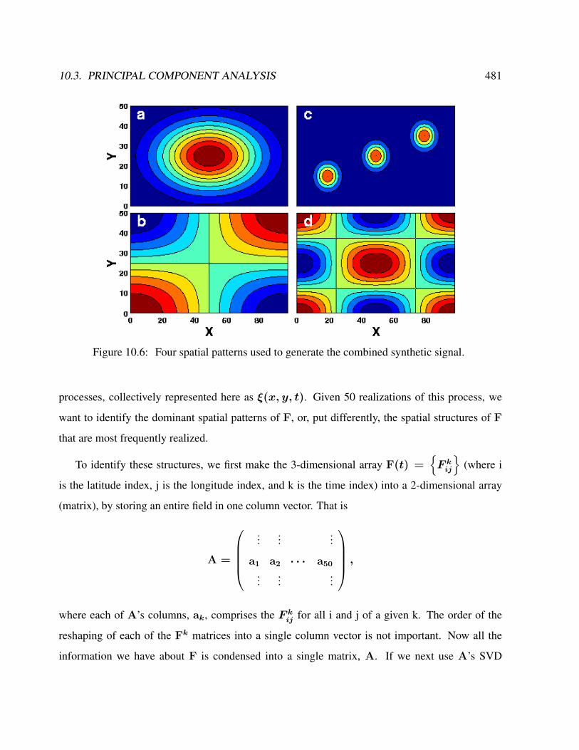
10.3. PRINCIPAL COMPONENT ANALYSIS 481
Figure 10.6: Four spatial patterns used to generate the combined synthetic signal.
processes, collectively represented here as ξ(x, y, t). Given 50 realizations of this process, we
want to identify the dominant spatial patterns of F, or, put differently, the spatial structures of F
that are most frequently realized.
To identify these structures, we first make the 3-dimensional array F(t) =F kij
(where i
is the latitude index, j is the longitude index, and k is the time index) into a 2-dimensional array
(matrix), by storing an entire field in one column vector. That is
A =
...
......
a1 a2 · · · a50
......
...
,
where each of A’s columns, ak, comprises the F kij for all i and j of a given k. The order of the
reshaping of each of the Fk matrices into a single column vector is not important. Now all the
information we have about F is condensed into a single matrix, A. If we next use A’s SVD
482 CHAPTER 10. DYNAMICS OF SPATIO-TEMPORAL PATTERN
representation, A = UΣVT , and reshape U’s columns in a manner exactly opposite to the one
we employed while forming A from F, we get F’s EOFs.
To demonstrate the method in action, let’s use the 50 fields of the above f(x, y, t), generated
from the patterns shown in Fig. 10.6 b and d. Fig. 10.7 a, b and c show the 3 leading EOFs of the
cosine signal. Note how both generating patterns are well reproduced by the method (the leading
2 patterns), despite the noise and the random blending of the the signals by the amplitudes A and
B. Note also the sign reversal, which is completely immaterial - the singular values (and hence the
EOFs and Principal Components) are all known to within a sign, as they are the square root of the
eigenvalues of AAT and ATA. Clearly, the 3rd pattern is structureless noise.
A possible critique of the previous example is that we made the method’s job particularly (and
artificially) easy by using 2 mutually orthogonal generating patterns. This can be fair - if the
method is designed to turn arbitrary signals into an orthogonal decomposition of those signals, the
real test of the method is with non-orthogonal signals.
Fig. 10.7 d-f show that the method functions well even when the input signal is not artificially
orthogonal. The 2 leading modes are nicely reproduced with good fidelity (compared with the gen-
erating patterns). The 3rd, while clearly structured (unlike the case with the 2 orthogonal cosines),
is a combination of the generating patterns, not an individual pattern. This is the consequence of
the non-orthogonality of the exponential generating patterns. Since they are not orthogonal either
to each other or to the cosines, they project on them, resulting in the blend shown in Fig. 10.7 f.
It is always extremely important to examine the fraction of the total variance the various modes
account for. For the 2 synthetic cases above, this is shown in Fig. 10.8. (Note that only the leading
9 are shown, of of the 50 total. The rest are very near zero in both cases.) The cosine signals are
very similar in both (modes 1 and 2). Higher modes differ. In the cosine only, where the only
reminder is noise, it is roughly equally distributed over the entire spectrum. Conversely, in the
case of the added exponentials, the remainder has 2 structured modes (the 2 exponential terms, and
indeed the singular values 3 and 4 are distinct from zero. The rest, just like in the pure cosine case,
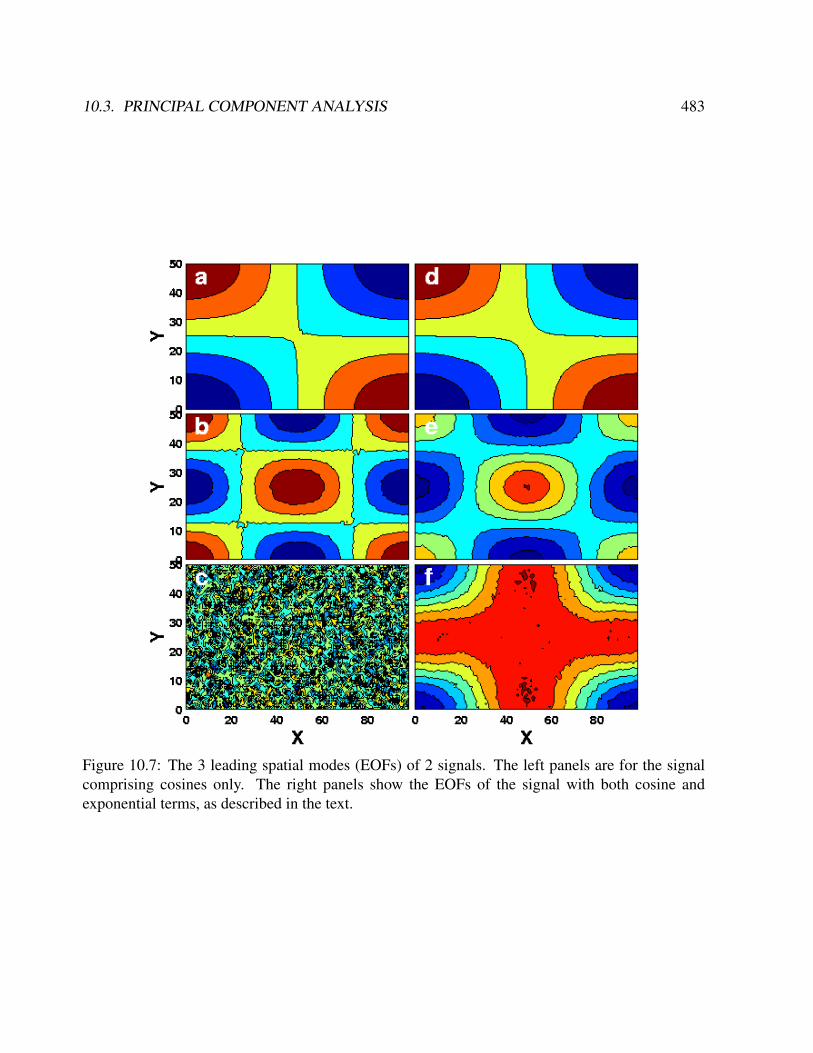
10.3. PRINCIPAL COMPONENT ANALYSIS 483
Figure 10.7: The 3 leading spatial modes (EOFs) of 2 signals. The left panels are for the signalcomprising cosines only. The right panels show the EOFs of the signal with both cosine andexponential terms, as described in the text.
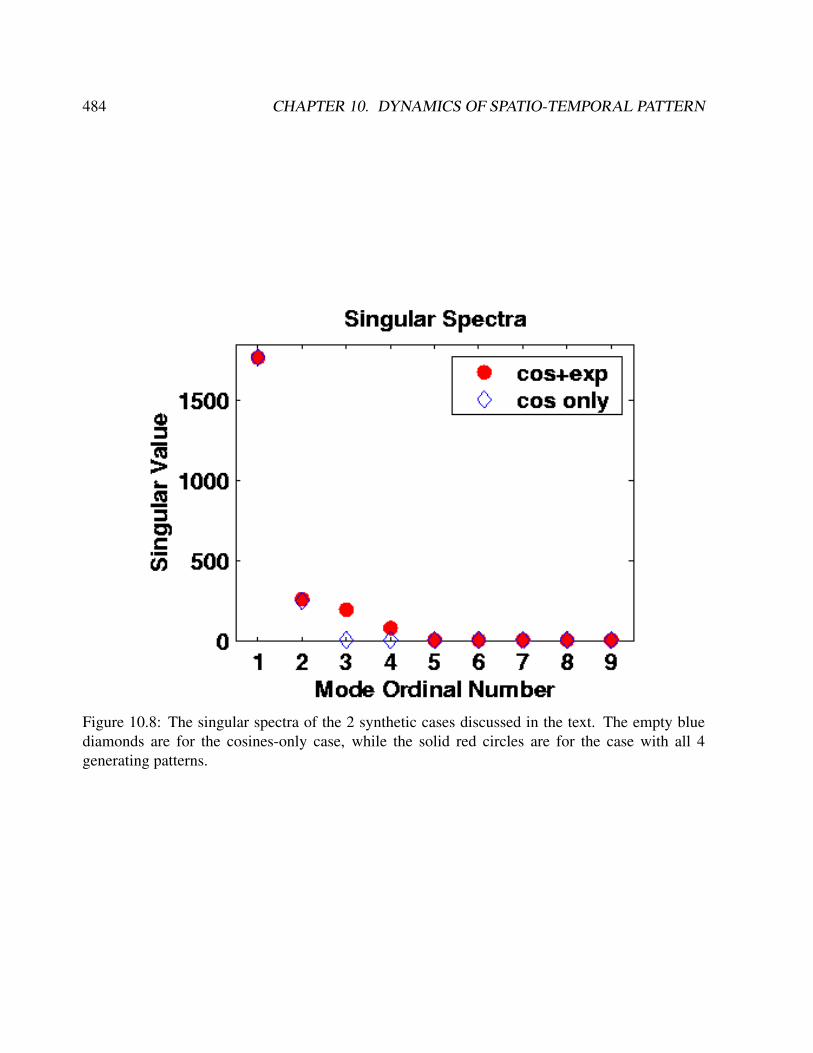
484 CHAPTER 10. DYNAMICS OF SPATIO-TEMPORAL PATTERN
Figure 10.8: The singular spectra of the 2 synthetic cases discussed in the text. The empty bluediamonds are for the cosines-only case, while the solid red circles are for the case with all 4generating patterns.
10.3. PRINCIPAL COMPONENT ANALYSIS 485
are statistically indistinguishable from zero.3
3Note that the decrease in amplitude with mode number (the falloff of the singular spectrum) is a property of theanalysis, and does not always contain useful information. There is a substantial body of literature about the issue ofthe appropriate cutoff of the singular spectrum, beyond which, it is assumed, there is little or no useful information.The most commonly used cutoff rule in geophysics is the so-called ‘Rule N’, which basically retains only thosemodes whose amplitudes stand out above the population of singular spectra extracted from a large number of syntheticmatrices of the same dimensions as the one being tested. We will not treat this issue here.
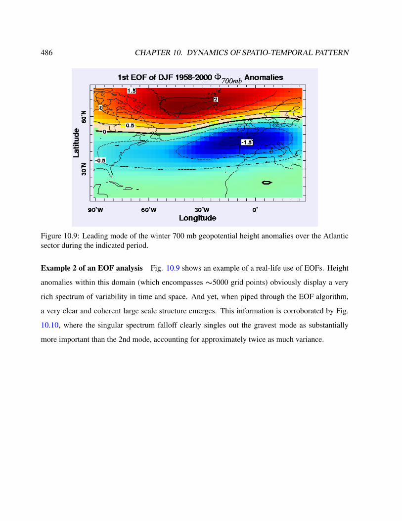
486 CHAPTER 10. DYNAMICS OF SPATIO-TEMPORAL PATTERN
Figure 10.9: Leading mode of the winter 700 mb geopotential height anomalies over the Atlanticsector during the indicated period.
Example 2 of an EOF analysis Fig. 10.9 shows an example of a real-life use of EOFs. Height
anomalies within this domain (which encompasses ∼5000 grid points) obviously display a very
rich spectrum of variability in time and space. And yet, when piped through the EOF algorithm,
a very clear and coherent large scale structure emerges. This information is corroborated by Fig.
10.10, where the singular spectrum falloff clearly singles out the gravest mode as substantially
more important than the 2nd mode, accounting for approximately twice as much variance.
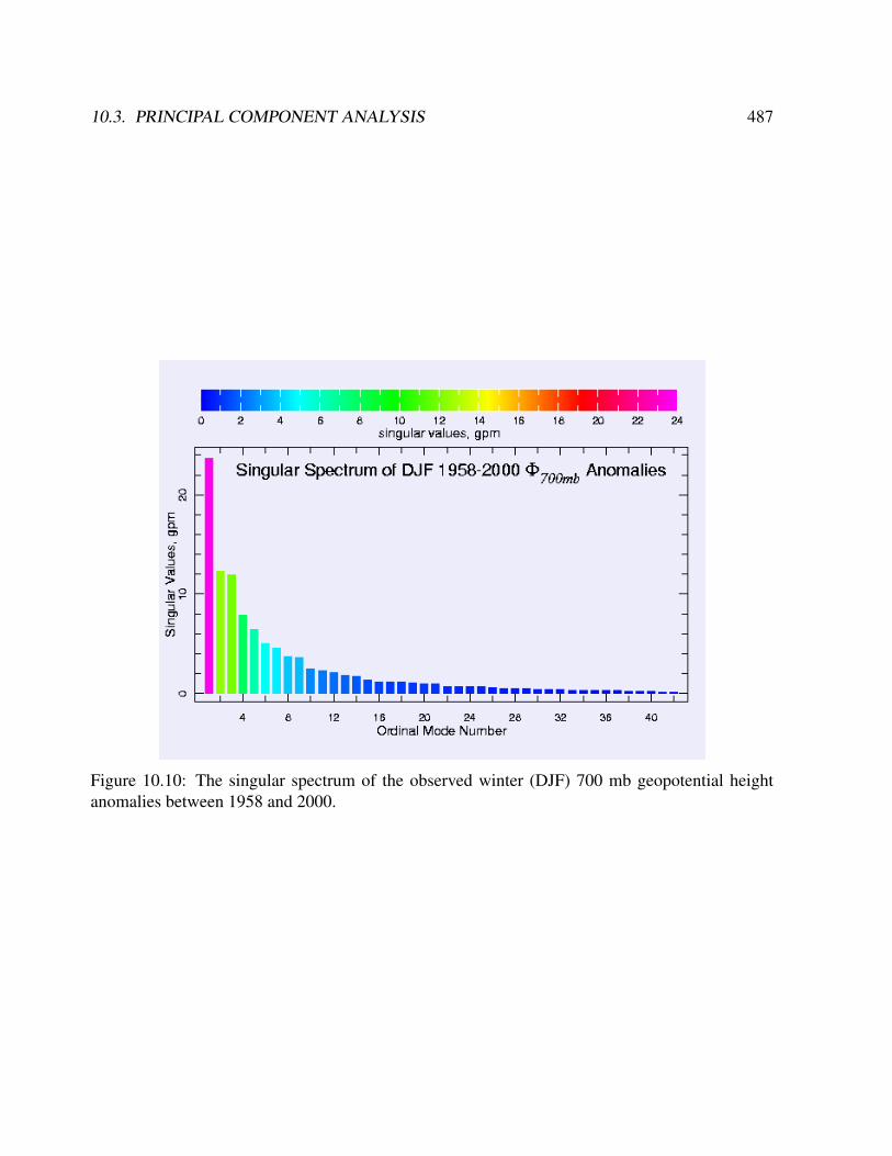
10.3. PRINCIPAL COMPONENT ANALYSIS 487
Figure 10.10: The singular spectrum of the observed winter (DJF) 700 mb geopotential heightanomalies between 1958 and 2000.

488 CHAPTER 10. DYNAMICS OF SPATIO-TEMPORAL PATTERN
Figure 10.11: how to calculate EOFs.
Example 3 of an EOF analysis The third example shows two different ways oh how to calculate
EOFs of time series.
Based on pca:#EOF’s and PCs from the pcarm(list=ls()) #clean the environmenta=read.table("ser1.txt") #read ser 1b=read.table("ser2.txt") #read ser2x=a[,1]y=b[,1]xa=x-mean(x) #anomalies xya=y-mean(y) #anomalies ymdat=cbind(xa,ya)aa=prcomp(mdat)eof1=aa$rotation[1,] #eof1eof2=aa$rotation[2,] #eof2pc=predict(aa)pc1=pc[,1] #pc1pc2=pc[,2] #pc2
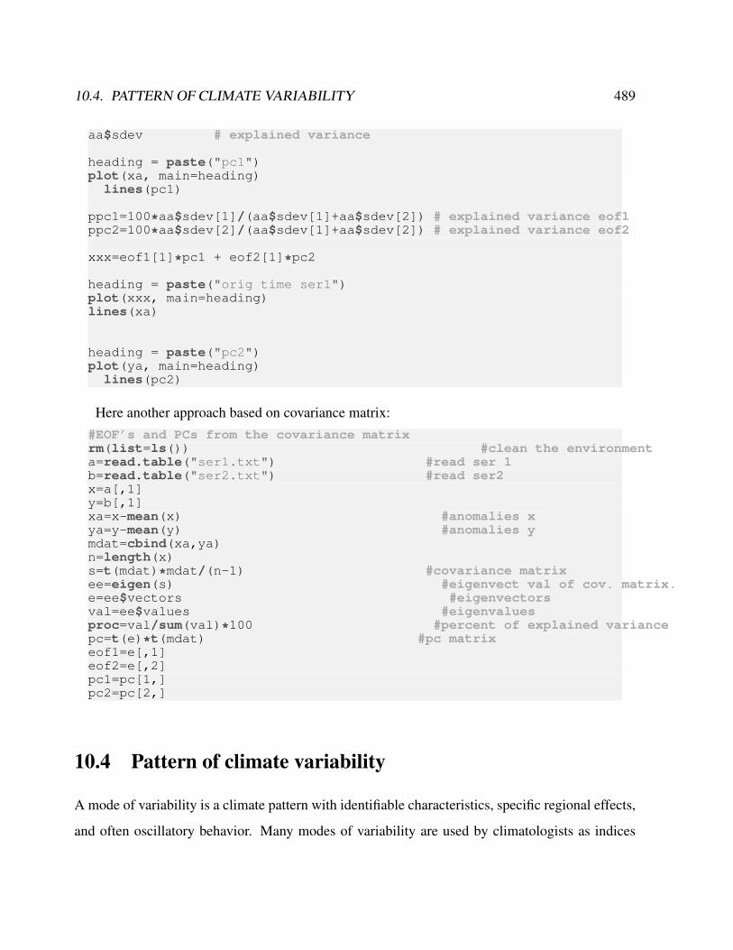
10.4. PATTERN OF CLIMATE VARIABILITY 489
aa$sdev # explained variance
heading = paste("pc1")plot(xa, main=heading)
lines(pc1)
ppc1=100*aa$sdev[1]/(aa$sdev[1]+aa$sdev[2]) # explained variance eof1ppc2=100*aa$sdev[2]/(aa$sdev[1]+aa$sdev[2]) # explained variance eof2
xxx=eof1[1]*pc1 + eof2[1]*pc2
heading = paste("orig time ser1")plot(xxx, main=heading)lines(xa)
heading = paste("pc2")plot(ya, main=heading)
lines(pc2)
Here another approach based on covariance matrix:#EOF’s and PCs from the covariance matrixrm(list=ls()) #clean the environmenta=read.table("ser1.txt") #read ser 1b=read.table("ser2.txt") #read ser2x=a[,1]y=b[,1]xa=x-mean(x) #anomalies xya=y-mean(y) #anomalies ymdat=cbind(xa,ya)n=length(x)s=t(mdat)*mdat/(n-1) #covariance matrixee=eigen(s) #eigenvect val of cov. matrix.e=ee$vectors #eigenvectorsval=ee$values #eigenvaluesproc=val/sum(val)*100 #percent of explained variancepc=t(e)*t(mdat) #pc matrixeof1=e[,1]eof2=e[,2]pc1=pc[1,]pc2=pc[2,]
10.4 Pattern of climate variability
A mode of variability is a climate pattern with identifiable characteristics, specific regional effects,
and often oscillatory behavior. Many modes of variability are used by climatologists as indices

490 CHAPTER 10. DYNAMICS OF SPATIO-TEMPORAL PATTERN
to represent the general climatic state of a region affected by a given climate pattern. Measured
via an empirical orthogonal function analysis, the mode of variability with the greatest effect on
climates worldwide is the seasonal cycle, followed by El Nino-Southern Oscillation, followed by
the Atlantic Multidecadal Oscillation.
Other well-known modes of variability include:
• The Antarctic oscillation (AAO)
• The Arctic oscillation (AO)
• The Atlantic multidecadal oscillation (AMO)
• The Indian Ocean Dipole
• The Madden-Julian oscillation (MJO)
• The North Atlantic oscillation (NAO)
• The Pacific decadal oscillation (PDO)
• The Pacific-North American teleconnection pattern (PNA)
• The Quasi-biennial oscillation (QBO)
Links: https://en.wikipedia.org/wiki/Climate_pattern
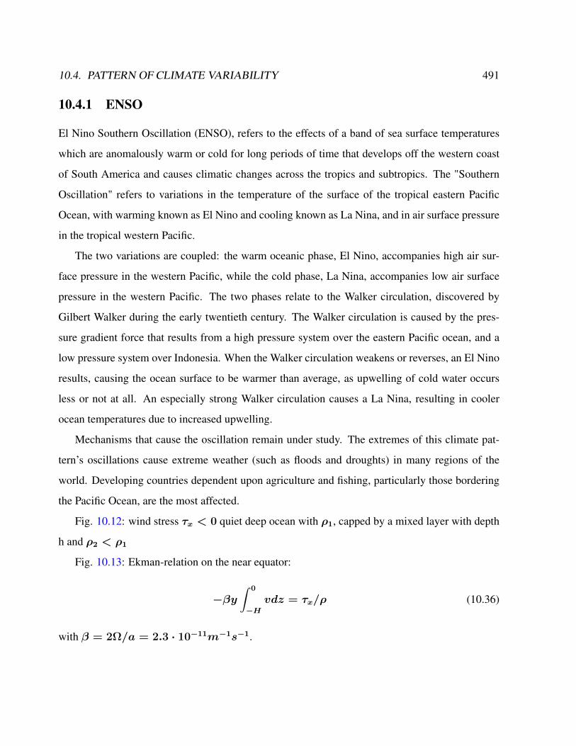
10.4. PATTERN OF CLIMATE VARIABILITY 491
10.4.1 ENSO
El Nino Southern Oscillation (ENSO), refers to the effects of a band of sea surface temperatures
which are anomalously warm or cold for long periods of time that develops off the western coast
of South America and causes climatic changes across the tropics and subtropics. The "Southern
Oscillation" refers to variations in the temperature of the surface of the tropical eastern Pacific
Ocean, with warming known as El Nino and cooling known as La Nina, and in air surface pressure
in the tropical western Pacific.
The two variations are coupled: the warm oceanic phase, El Nino, accompanies high air sur-
face pressure in the western Pacific, while the cold phase, La Nina, accompanies low air surface
pressure in the western Pacific. The two phases relate to the Walker circulation, discovered by
Gilbert Walker during the early twentieth century. The Walker circulation is caused by the pres-
sure gradient force that results from a high pressure system over the eastern Pacific ocean, and a
low pressure system over Indonesia. When the Walker circulation weakens or reverses, an El Nino
results, causing the ocean surface to be warmer than average, as upwelling of cold water occurs
less or not at all. An especially strong Walker circulation causes a La Nina, resulting in cooler
ocean temperatures due to increased upwelling.
Mechanisms that cause the oscillation remain under study. The extremes of this climate pat-
tern’s oscillations cause extreme weather (such as floods and droughts) in many regions of the
world. Developing countries dependent upon agriculture and fishing, particularly those bordering
the Pacific Ocean, are the most affected.
Fig. 10.12: wind stress τx < 0 quiet deep ocean with ρ1, capped by a mixed layer with depth
h and ρ2 < ρ1
Fig. 10.13: Ekman-relation on the near equator:
−βy∫ 0
−Hvdz = τx/ρ (10.36)
with β = 2Ω/a = 2.3 · 10−11m−1s−1.
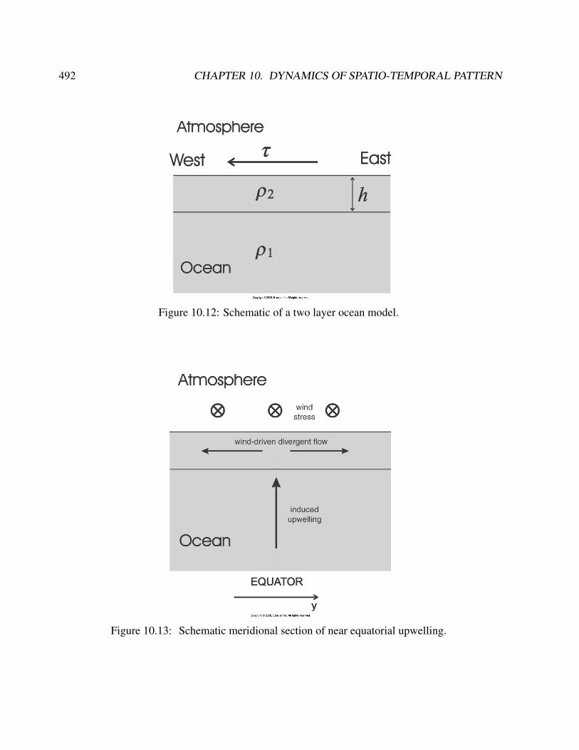
492 CHAPTER 10. DYNAMICS OF SPATIO-TEMPORAL PATTERN
Figure 10.12: Schematic of a two layer ocean model.
Figure 10.13: Schematic meridional section of near equatorial upwelling.
10.4. PATTERN OF CLIMATE VARIABILITY 493
Links: https://www.youtube.com/watch?feature=player_embedded&v=huweohIh_
Bw
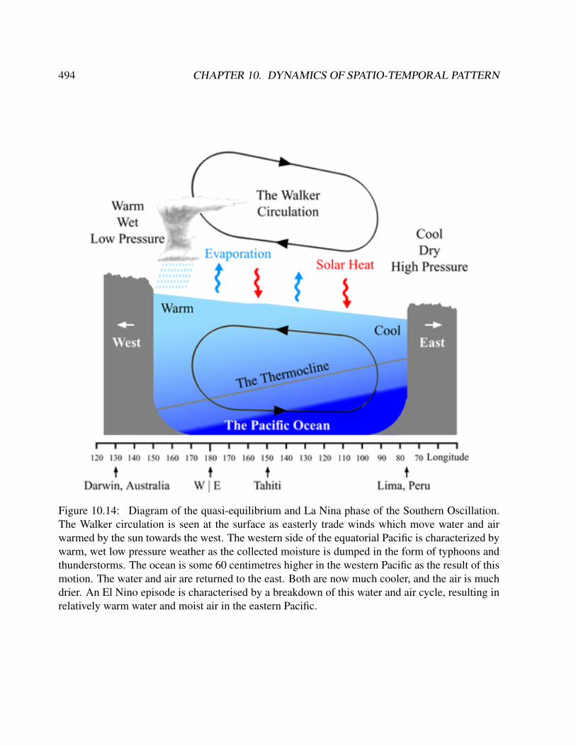
494 CHAPTER 10. DYNAMICS OF SPATIO-TEMPORAL PATTERN
Figure 10.14: Diagram of the quasi-equilibrium and La Nina phase of the Southern Oscillation.The Walker circulation is seen at the surface as easterly trade winds which move water and airwarmed by the sun towards the west. The western side of the equatorial Pacific is characterized bywarm, wet low pressure weather as the collected moisture is dumped in the form of typhoons andthunderstorms. The ocean is some 60 centimetres higher in the western Pacific as the result of thismotion. The water and air are returned to the east. Both are now much cooler, and the air is muchdrier. An El Nino episode is characterised by a breakdown of this water and air cycle, resulting inrelatively warm water and moist air in the eastern Pacific.
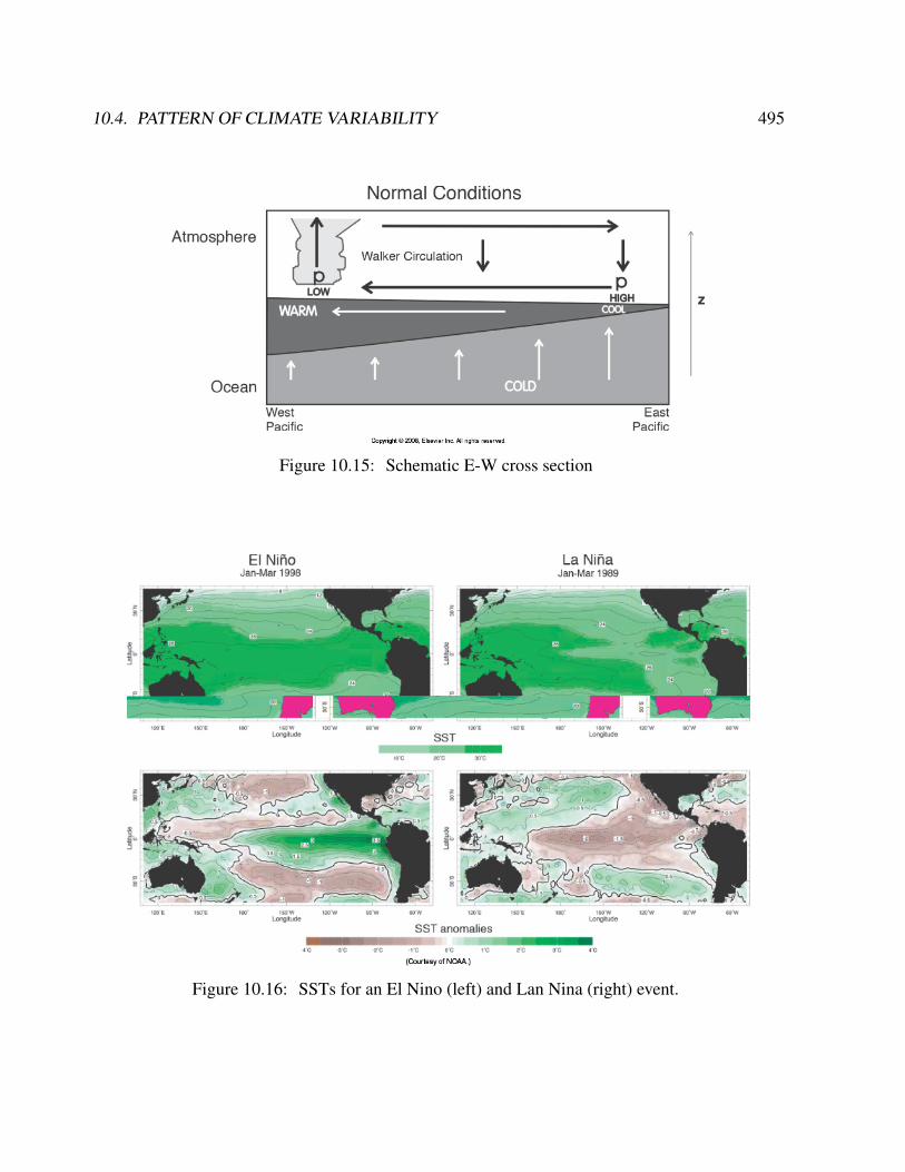
10.4. PATTERN OF CLIMATE VARIABILITY 495
Figure 10.15: Schematic E-W cross section
Figure 10.16: SSTs for an El Nino (left) and Lan Nina (right) event.
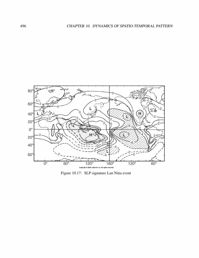
496 CHAPTER 10. DYNAMICS OF SPATIO-TEMPORAL PATTERN
Figure 10.17: SLP signature Lan Nina event
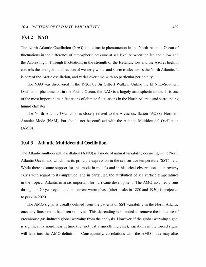
10.4. PATTERN OF CLIMATE VARIABILITY 497
10.4.2 NAO
The North Atlantic Oscillation (NAO) is a climatic phenomenon in the North Atlantic Ocean of
fluctuations in the difference of atmospheric pressure at sea level between the Icelandic low and
the Azores high. Through fluctuations in the strength of the Icelandic low and the Azores high, it
controls the strength and direction of westerly winds and storm tracks across the North Atlantic. It
is part of the Arctic oscillation, and varies over time with no particular periodicity.
The NAO was discovered in the 1920s by Sir Gilbert Walker. Unlike the El Nino-Southern
Oscillation phenomenon in the Pacific Ocean, the NAO is a largely atmospheric mode. It is one
of the most important manifestations of climate fluctuations in the North Atlantic and surrounding
humid climates.
The North Atlantic Oscillation is closely related to the Arctic oscillation (AO) or Northern
Annular Mode (NAM), but should not be confused with the Atlantic Multidecadal Oscillation
(AMO).
10.4.3 Atlantic Multidecadal Oscillation
The Atlantic multidecadal oscillation (AMO) is a mode of natural variability occurring in the North
Atlantic Ocean and which has its principle expression in the sea surface temperature (SST) field.
While there is some support for this mode in models and in historical observations, controversy
exists with regard to its amplitude, and in particular, the attribution of sea surface temperatures
in the tropical Atlantic in areas important for hurricane development. The AMO assumedly runs
through an 70-year cycle, and its current warm phase (after peaks in 1880 and 1950) is projected
to peak in 2020.
The AMO signal is usually defined from the patterns of SST variability in the North Atlantic
once any linear trend has been removed. This detrending is intended to remove the influence of
greenhouse gas-induced global warming from the analysis. However, if the global warming signal
is significantly non-linear in time (i.e. not just a smooth increase), variations in the forced signal
will leak into the AMO definition. Consequently, correlations with the AMO index may alias

498 CHAPTER 10. DYNAMICS OF SPATIO-TEMPORAL PATTERN
Figure 10.18: NAO plus and minus
effects of global warming. In 2008, new models revealed that global warming should reduce the
frequency of hurricanes overall, while intensity might increase in some areas. Because reliable
records of hurricane strength and frequency only extend back to approximately 1970, researchers
have faced difficulty in developing reliable models.
In models, AMO-like variability is associated with small changes in the North Atlantic branch
of the Thermohaline Circulation, however historical oceanic observations are not sufficient to as-
sociate the derived AMO index to present day circulation anomalies.
The AMO index is correlated to air temperatures and rainfall over much of the Northern Hemi-
sphere, in particular, North America and Europe such as North Eastern Brazilian and African Sahel
rainfall and North American and European summer climate. It is also associated with changes in

10.4. PATTERN OF CLIMATE VARIABILITY 499
Figure 10.19: NAO
the frequency of North American droughts and is reflected in the frequency of severe Atlantic
hurricanes. It alternately obscures and exaggerates the global increase in temperatures due to
human-induced global warming.
Recent research suggests that the AMO is related to the past occurrence of major droughts in
the Midwest and the Southwest. When the AMO is in its warm phase, these droughts tend to be
more frequent or prolonged. Vice-versa for negative AMO (cool phase). Two of the most severe
droughts of the 20th century occurred during the positive AMO between 1925 and 1965: The Dust
Bowl of the 1930s and the 1950s drought. Florida and the Pacific Northwest tend to be the opposite
warm AMO, more rainfall.
Climate models suggest that a warm phase of the AMO strengthens the summer rainfall over
India and Sahel and the North Atlantic tropical cyclone activity.[3] Paleoclimatologic studies have
confirmed this pattern increased rainfall in AMO warmphase, decreased in cold phase for the Sahel
over the past 3,000 years.
10.4.4 Reconstructing past climates from high-resolution proxy data
It is difficult to forecast the long term climatic changes on the basis of the instrument records be-
cause of their short time series. Accordingly, how to apply the geological and phenological records
to reconstruct paleo-environmental changes is very important for studying the global changes.
Deep-sea sediments, ice cores, lake sediments, and corals have been widely used in the recent
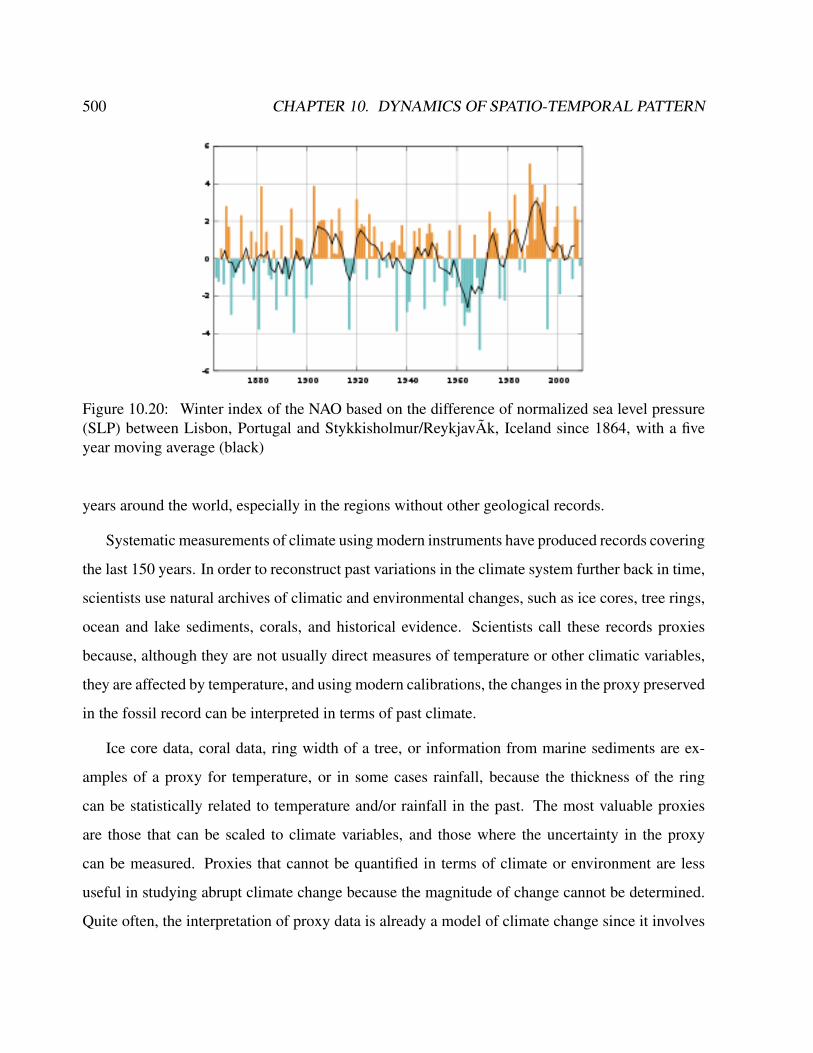
500 CHAPTER 10. DYNAMICS OF SPATIO-TEMPORAL PATTERN
Figure 10.20: Winter index of the NAO based on the difference of normalized sea level pressure(SLP) between Lisbon, Portugal and Stykkisholmur/ReykjavÃk, Iceland since 1864, with a fiveyear moving average (black)
years around the world, especially in the regions without other geological records.
Systematic measurements of climate using modern instruments have produced records covering
the last 150 years. In order to reconstruct past variations in the climate system further back in time,
scientists use natural archives of climatic and environmental changes, such as ice cores, tree rings,
ocean and lake sediments, corals, and historical evidence. Scientists call these records proxies
because, although they are not usually direct measures of temperature or other climatic variables,
they are affected by temperature, and using modern calibrations, the changes in the proxy preserved
in the fossil record can be interpreted in terms of past climate.
Ice core data, coral data, ring width of a tree, or information from marine sediments are ex-
amples of a proxy for temperature, or in some cases rainfall, because the thickness of the ring
can be statistically related to temperature and/or rainfall in the past. The most valuable proxies
are those that can be scaled to climate variables, and those where the uncertainty in the proxy
can be measured. Proxies that cannot be quantified in terms of climate or environment are less
useful in studying abrupt climate change because the magnitude of change cannot be determined.
Quite often, the interpretation of proxy data is already a model of climate change since it involves
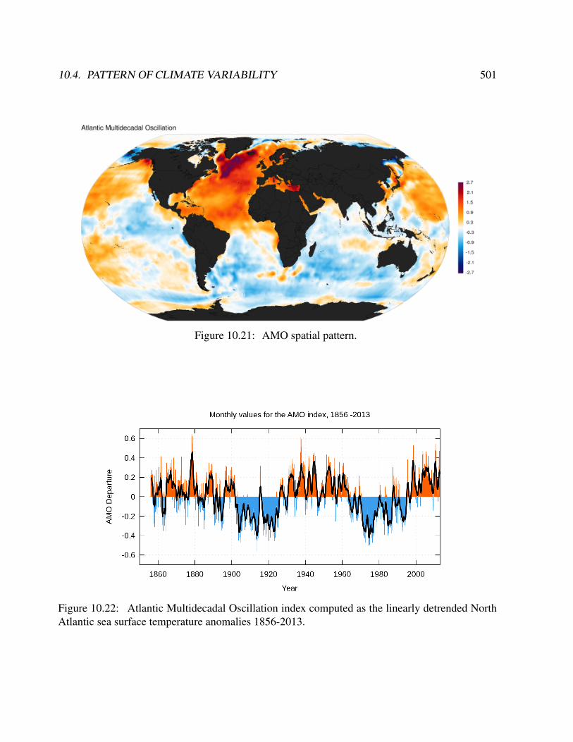
10.4. PATTERN OF CLIMATE VARIABILITY 501
Figure 10.21: AMO spatial pattern.
Figure 10.22: Atlantic Multidecadal Oscillation index computed as the linearly detrended NorthAtlantic sea surface temperature anomalies 1856-2013.
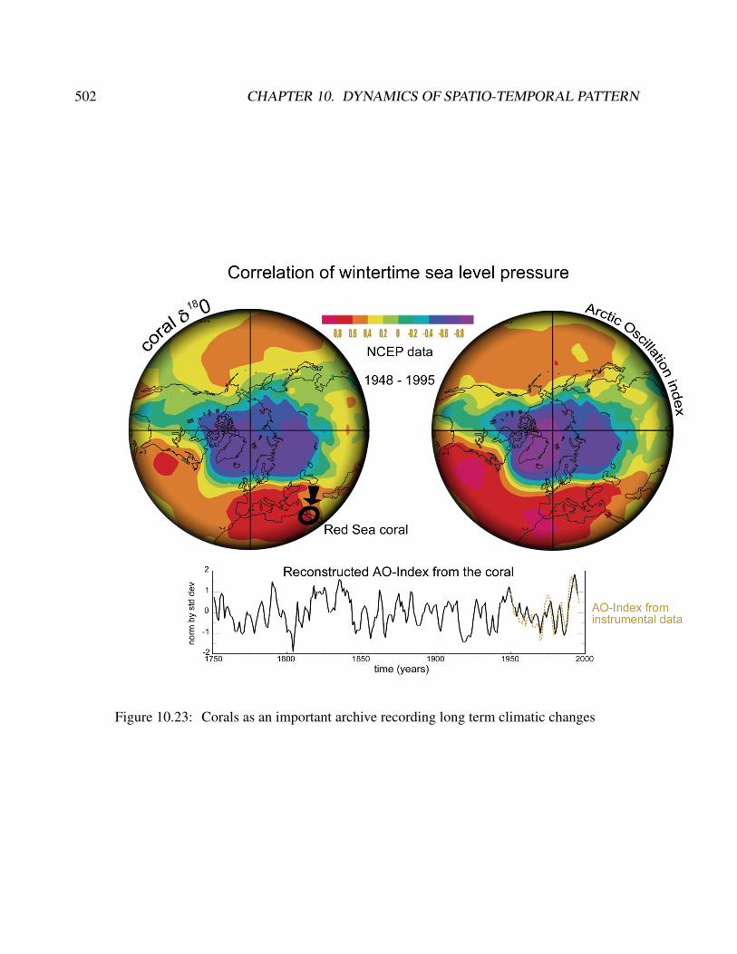
502 CHAPTER 10. DYNAMICS OF SPATIO-TEMPORAL PATTERN
Figure 10.23: Corals as an important archive recording long term climatic changes
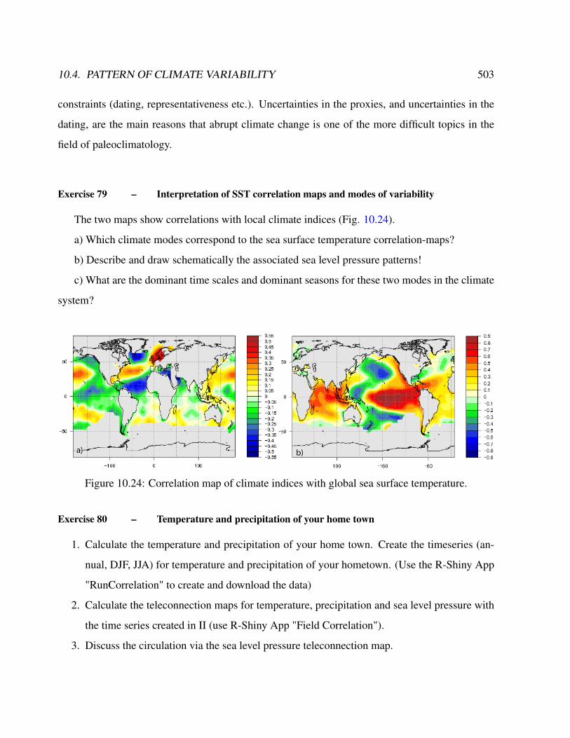
10.4. PATTERN OF CLIMATE VARIABILITY 503
constraints (dating, representativeness etc.). Uncertainties in the proxies, and uncertainties in the
dating, are the main reasons that abrupt climate change is one of the more difficult topics in the
field of paleoclimatology.
Exercise 79 – Interpretation of SST correlation maps and modes of variability
The two maps show correlations with local climate indices (Fig. 10.24).
a) Which climate modes correspond to the sea surface temperature correlation-maps?
b) Describe and draw schematically the associated sea level pressure patterns!
c) What are the dominant time scales and dominant seasons for these two modes in the climate
system?
Figure 10.24: Correlation map of climate indices with global sea surface temperature.
Exercise 80 – Temperature and precipitation of your home town
1. Calculate the temperature and precipitation of your home town. Create the timeseries (an-
nual, DJF, JJA) for temperature and precipitation of your hometown. (Use the R-Shiny App
"RunCorrelation" to create and download the data)
2. Calculate the teleconnection maps for temperature, precipitation and sea level pressure with
the time series created in II (use R-Shiny App "Field Correlation").
3. Discuss the circulation via the sea level pressure teleconnection map.
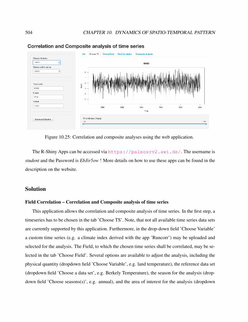
504 CHAPTER 10. DYNAMICS OF SPATIO-TEMPORAL PATTERN
Figure 10.25: Correlation and composite analyses using the web application.
The R-Shiny Apps can be accessed via https://paleosrv2.awi.de/. The username is
student and the Password is EbJir5ow ! More details on how to use these apps can be found in the
description on the website.
Solution
Field Correlation – Correlation and Composite analysis of time series
This application allows the correlation and composite analysis of time series. In the first step, a
timeseries has to be chosen in the tab ’Choose TS’. Note, that not all available time series data sets
are currently supported by this application. Furthermore, in the drop-down field ’Choose Variable’
a custom time series (e.g. a climate index derived with the app ’Runcorr’) may be uploaded and
selected for the analysis. The Field, to which the chosen time series shall be correlated, may be se-
lected in the tab ’Choose Field’. Several options are available to adjust the analysis, including the
physical quantity (dropdown field ’Choose Variable’, e.g. land temperature), the reference data set
(dropdown field ’Choose a data set’, e.g. Berkely Temperature), the season for the analysis (drop-
down field ’Choose seasons(s)’, e.g. annual), and the area of interest for the analysis (dropdown
10.4. PATTERN OF CLIMATE VARIABILITY 505
field ’Select Area’, e.g. Europe). After all options have been set as wished, it can be selected what
kind of metrics for the analysis to use (dropdown field ’Show’, e.g. a plot or a histogram). After
the application has finished some computations, a graphical representation of the chosen metric
will be shown. If ’Plot’ has been chosen, a geographical map will appear that presents the chosen
field.
In the tab ’Field Correlation’ the correlation of the two selected timeseries (refer to tab ’Choose
TS’ and ’Choose Field’) can be computed. A respective plot is shown, potentially with significance
testing.
In the tab ’Composite Analysis’ a composite analysis of the two selected timeseries (refer to
tab ’Choose TS’ and ’Choose Field’) can be computed. A respective plot is shown.
Note: if you get an error message that is similar to ’no time series or field chosen’, just re-
activate the tabs ’Choose TS’ und ’Choose Field’ once more before you select either one of the
tabs ’Field Correlation’ or ’Composite Analysis’. Furthermore, this application has not yet been
extensively used, so bugs may occur from time to time.
Run Correlation and generation of climate indices – Running correlation of a timeseries
and generation of climate indices (e.g. for use in the Field Correlation app)
This application allows the computation of running correlation of time series. Such time series
may be uploaded via the tab ’Upload TS’. Alternatively, the time series may be extracted from
already present historical climate data in the application’s database (tab ’Create Index’). Such
indices may be also downloaded and used in other applications, e.g. in the app "Field Correlation".
The generation of a climate index from the application’s climate data inventory for use within the
Runcorr application, or for alternative download and later use in other apps, is in the following
shortly illustrated.
Click on the tab ’Create Index’ and select the desired climate variable (e.g. ’Land Tempera-
ture’) from your preferred data set (e.g. ’Berkeley Temperature’). As soon as you select a season, a
plot of the data will appear, and options for changing the appearance of the plot will become avail-
able. Furthermore, you can choose the spatial domain for the climate index. The options ’Area’

506 CHAPTER 10. DYNAMICS OF SPATIO-TEMPORAL PATTERN
(creating an index via averaging over a specific latitude and longitude range) and ’Single Point’
(for creating an index at a specific location) are available. After carefully selecting the options for
the climate index, click on the button ’Create Index’ in order to create a derived data set. Below
the spatial representation of the climate data that was already present before, a second plot will
appear that provides an illustration of the just created climate index. Now it is possible to either
keep this index for further use in the Runncorr app (button ’Save Index’, note down the attributed
name to access the index in other tabs of the Runcorr app), or to download a text file that contains
the time series for use in other apps (button ’Download Index’).
Computation of the running correlation between two time series that are either a part of the
data base of the app, but that can also include a custom index as created via the procedure illus-
trated above, may be performed in the tab ’Choose TS’. Further adjustments of the analysis (e.g.
detrending and scaling) as well as custom modification of the plot appearance is available in the
tab ’Running Correlation’. There, it is also possible to download a plot of the running correlation
of the two selected time series.
10.4.5 Climate variability and bifurcation*
The internal free variations within the climate system are associated with both positive and negative
feedback interactions between the atmosphere, oceans, cryosphere and biosphere. These feedbacks
lead to instabilities or oscillations of the system on all time scales, and can either operate indepen-
dently or reinforce external forcings. Investigations of the properties of systems which are far
from equilibrium show that they have a number of unusual properties. In particular, as the distance
from equilibrium increases, they can develop complex oscillations with both chaotic and periodic
characteristics. They also may show bifurcation points where the system may switch between var-
ious regimes. Under non-equilibrium conditions, local events have repercussions throughout the
whole system. These long-range correlations are at first small, but increase with distance from
equilibrium, and may become essential at bifurcation points.
When applying (??), different concepts of climate change are in the literature. Quite often, the
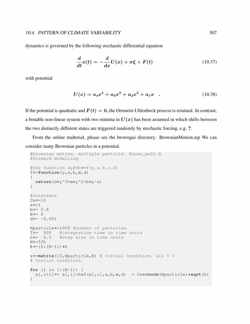
10.4. PATTERN OF CLIMATE VARIABILITY 507
dynamics is governed by the following stochastic differential equation
d
dtx(t) = −
d
dxU(x) + σξ + F (t) (10.37)
with potential
U(x) = a4x4 + a3x
3 + a2x2 + a1x . (10.38)
If the potential is quadratic andF (t) = 0, the Ornstein-Uhlenbeck process is retained. In contrast,
a bistable non-linear system with two minima in U(x) has been assumed in which shifts between
the two distinctly different states are triggered randomly by stochastic forcing, e.g. ?.
From the online malterial, please see the browngui directory: BrownianMotion.zip We can
consider many Brownian particles in a potential.
#brownian motion, multiple particle: Brown_mult.R#forward modelling
#the function dy/dt<-f(y,a,b,c,d)f<-function(y,a,b,c,d)
return(d*y^3+c*y^2+b*y-a)
#constantsCa<-10a<-1b<- 0.8c<- 0d<- -0.001
Nparticle<-1000 #number of particlesT<- 500 #integration time in time unitsh<- 0.5 #step size in time unitsN<-T/ht<-(0:(N-1))*h
x<-matrix(10,Nparticle,N) # Initial condition, all = 0# Initial condition,
for (i in 1:(N-1)) x[,i+1]<- x[,i]+h*f(x[,i],a,b,c,d) + Ca*rnorm(Nparticle)*sqrt(h)
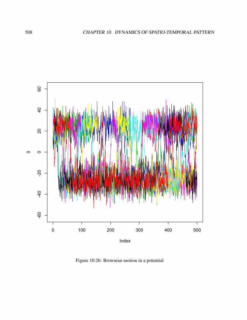
508 CHAPTER 10. DYNAMICS OF SPATIO-TEMPORAL PATTERN
0 100 200 300 400 500
-60
-40
-20
020
4060
Index
0
Figure 10.26: Brownian motion in a potential
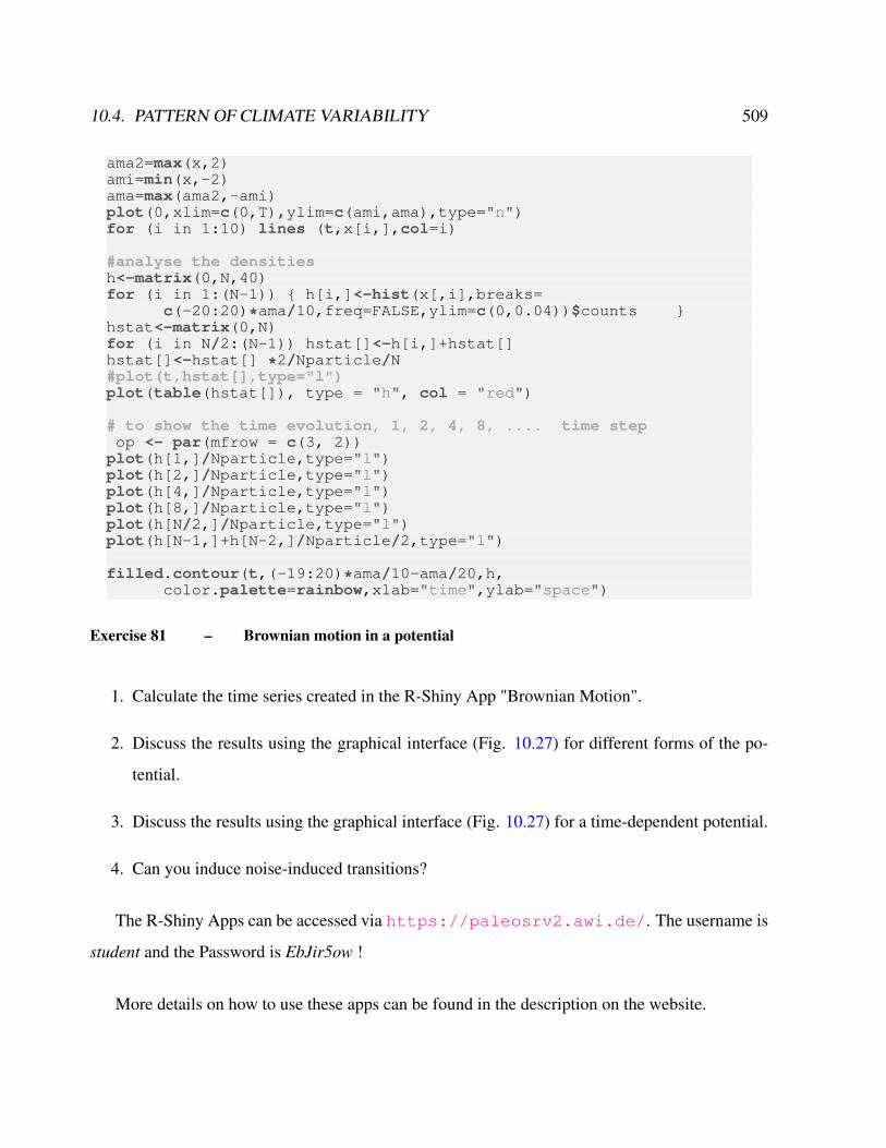
10.4. PATTERN OF CLIMATE VARIABILITY 509
ama2=max(x,2)ami=min(x,-2)ama=max(ama2,-ami)plot(0,xlim=c(0,T),ylim=c(ami,ama),type="n")for (i in 1:10) lines (t,x[i,],col=i)
#analyse the densitiesh<-matrix(0,N,40)for (i in 1:(N-1)) h[i,]<-hist(x[,i],breaks=
c(-20:20)*ama/10,freq=FALSE,ylim=c(0,0.04))$counts hstat<-matrix(0,N)for (i in N/2:(N-1)) hstat[]<-h[i,]+hstat[]hstat[]<-hstat[] *2/Nparticle/N#plot(t,hstat[],type="l")plot(table(hstat[]), type = "h", col = "red")
# to show the time evolution, 1, 2, 4, 8, .... time stepop <- par(mfrow = c(3, 2))plot(h[1,]/Nparticle,type="l")plot(h[2,]/Nparticle,type="l")plot(h[4,]/Nparticle,type="l")plot(h[8,]/Nparticle,type="l")plot(h[N/2,]/Nparticle,type="l")plot(h[N-1,]+h[N-2,]/Nparticle/2,type="l")
filled.contour(t,(-19:20)*ama/10-ama/20,h,color.palette=rainbow,xlab="time",ylab="space")
Exercise 81 – Brownian motion in a potential
1. Calculate the time series created in the R-Shiny App "Brownian Motion".
2. Discuss the results using the graphical interface (Fig. 10.27) for different forms of the po-
tential.
3. Discuss the results using the graphical interface (Fig. 10.27) for a time-dependent potential.
4. Can you induce noise-induced transitions?
The R-Shiny Apps can be accessed via https://paleosrv2.awi.de/. The username is
student and the Password is EbJir5ow !
More details on how to use these apps can be found in the description on the website.
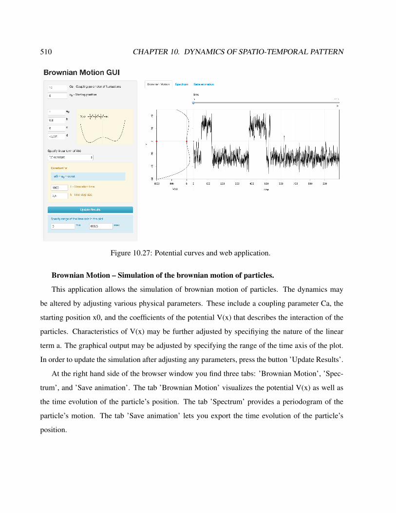
510 CHAPTER 10. DYNAMICS OF SPATIO-TEMPORAL PATTERN
Figure 10.27: Potential curves and web application.
Brownian Motion – Simulation of the brownian motion of particles.
This application allows the simulation of brownian motion of particles. The dynamics may
be altered by adjusting various physical parameters. These include a coupling parameter Ca, the
starting position x0, and the coefficients of the potential V(x) that describes the interaction of the
particles. Characteristics of V(x) may be further adjusted by specifiying the nature of the linear
term a. The graphical output may be adjusted by specifying the range of the time axis of the plot.
In order to update the simulation after adjusting any parameters, press the button ’Update Results’.
At the right hand side of the browser window you find three tabs: ’Brownian Motion’, ’Spec-
trum’, and ’Save animation’. The tab ’Brownian Motion’ visualizes the potential V(x) as well as
the time evolution of the particle’s position. The tab ’Spectrum’ provides a periodogram of the
particle’s motion. The tab ’Save animation’ lets you export the time evolution of the particle’s
position.
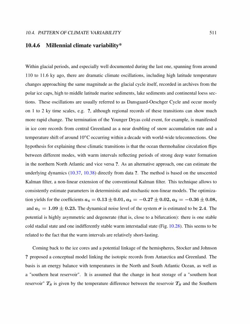
10.4. PATTERN OF CLIMATE VARIABILITY 511
10.4.6 Millennial climate variability*
Within glacial periods, and especially well documented during the last one, spanning from around
110 to 11.6 ky ago, there are dramatic climate oscillations, including high latitude temperature
changes approaching the same magnitude as the glacial cycle itself, recorded in archives from the
polar ice caps, high to middle latitude marine sediments, lake sediments and continental loess sec-
tions. These oscillations are usually referred to as Dansgaard-Oeschger Cycle and occur mostly
on 1 to 2 ky time scales, e.g. ?, although regional records of these transitions can show much
more rapid change. The termination of the Younger Dryas cold event, for example, is manifested
in ice core records from central Greenland as a near doubling of snow accumulation rate and a
temperature shift of around 10C occurring within a decade with world-wide teleconnections. One
hypothesis for explaining these climatic transitions is that the ocean thermohaline circulation flips
between different modes, with warm intervals reflecting periods of strong deep water formation
in the northern North Atlantic and vice versa ?. As an alternative approach, one can estimate the
underlying dynamics (10.37, 10.38) directly from data ?. The method is based on the unscented
Kalman filter, a non-linear extension of the conventional Kalman filter. This technique allows to
consistently estimate parameters in deterministic and stochastic non-linear models. The optimiza-
tion yields for the coefficients a4 = 0.13± 0.01, a3 = −0.27± 0.02, a2 = −0.36± 0.08,
and a1 = 1.09 ± 0.23. The dynamical noise level of the system σ is estimated to be 2.4. The
potential is highly asymmetric and degenerate (that is, close to a bifurcation): there is one stable
cold stadial state and one indifferently stable warm interstadial state (Fig. 10.28). This seems to be
related to the fact that the warm intervals are relatively short-lasting.
Coming back to the ice cores and a potential linkage of the hemispheres, Stocker and Johnson
? proposed a conceptual model linking the isotopic records from Antarctica and Greenland. The
basis is an energy balance with temperatures in the North and South Atlantic Ocean, as well as
a "southern heat reservoir". It is assumed that the change in heat storage of a "southern heat
reservoir" TS is given by the temperature difference between the reservoir TS and the Southern
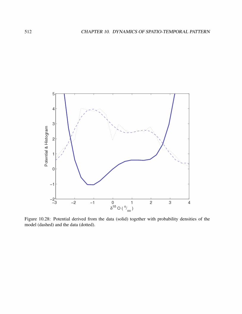
512 CHAPTER 10. DYNAMICS OF SPATIO-TEMPORAL PATTERN
Figure 10.28: Potential derived from the data (solid) together with probability densities of themodel (dashed) and the data (dotted).
10.4. PATTERN OF CLIMATE VARIABILITY 513
Ocean temperature T , with a characteristic time scale τ :
d
dtTS(t) =
1
τ[T − TS] (10.39)
TN denotes the time-dependent temperature anomaly of the North Atlantic. The Southern Ocean
temperature T is assumed to be −TN according to the bipolar seesaw (North Atlantic cold↔
South Atlantic warm). Using Laplace transform, one can solve for TS
TS = −1
τ
∫ t
0
TN(t− t′) exp(−t′/τ )dt′ + TS(0) exp(−t/τ ) (10.40)
The reservoir temperature is therefore a convolution of the northern temperature using the time
scale τ ranging from 100 to 4000 years. Equation (10.40) demonstrates that TS and TN will have
entirely different time characteristics. Abrupt changes in the north appear damped and integrated in
time in the southern reservoir. A sudden reduction in the thermohaline circulation causes a cooling
in the North Atlantic and a warming in the South, a situation similar to the Younger Dryas period
?, see also Fig. 9.10.
10.4.7 Noise induced transitions*
More specifically, one considers one-variable bistable dynamical systems subjected simultaneously
to noise and to a weak periodic forcing:
dx
dt= −
∂U
∂x+ F (t) + εh(x) cos(ω0t+ φ) (10.41)
Here x is the state variable (e.g., the global temperature or the global ice volume in the context of
the Quaternary glaciations); U is the "potential" driving the internal dynamics, taken to possess two
minima x+ and x− associated to the two stable states, separated by a maximum corresponding to
an intermediate unstable state x0;F (t) is a "random force" accounting for internal variability or
environmental noise and modeled classically as a Gaussian white noise of zero mean and strength
514 CHAPTER 10. DYNAMICS OF SPATIO-TEMPORAL PATTERN
equal to q2; and ε, ω0 and φ are, respectively, the amplitude, frequency and phase of the periodic
forcing. Actually, the forcing contribution can be cast in a form similar to the first term in the right
hand side of (10.41) by introducing a generalized time-dependent potential
W (x, t) = U(x)− εg(x) cos(ω0t+ φ) (10.42)
with dg(x)/dx = h(x).
According to the theory of stochastic processes the stochastic differential equation for the ran-
dom process x(t) in (10.41) is equivalent to a Fokker-Planck equation for the probability distribu-
tion function P(x,t) of values of x. In the absence of periodic forcing this latter equation defines a
particular type of Markov process known as diffusion process: The variable x realizes, for most of
the time, small scale excursions around x+ or x−, which are interrupted every now and then by
noise-driven abrupt transitions from x+ to x− or vice versa across the unstable state x0, which
constitutes a barrier of some sort. The kinetics of these transitions are determined by two quanti-
ties: The noise strength q2 and the potential barrier ∆U±, defined by
∆U± = U(x0)− U(x±) (10.43)
In the limit where q2 is much smaller than ∆U± the mean value of the transition time is given by
the celebrated Kramers formula
τ−1± = r± =
1
2π(−U ′′(x0)U ′′(x±))
1/2exp
(−
∆U±
q2/2
)(10.44)
where the double prime designates the second derivative. The transitions themselves occur in an
incoherent fashion, as their dispersion around the above mean value is comparable to the mean
itself.
When the periodic forcing is switched on U is replaced by the generalized potential W. The
corresponding barrier ∆W± is now modulated in time leading periodically to situations where
10.4. PATTERN OF CLIMATE VARIABILITY 515
states x± are found at the bottom of wells that are, successively, less shallow and more shallow
than those in the forcing-free system. One is thus led to expect that the transitions will be facilitated
during a part of this cycle, provided the periodicity of the forcing matches somehow the Kramers
time τ . As it turns out this intuitive idea is fully justified in the asymptotic limit of small q2 in
which the Fokker-Planck equation can be reduced, using an adiabatic approximation, to a closed
equation for the probability p± to be in the attraction basin of state x+ or x− :
dp+(t)
dt= r−(t) p−(t)− r+(t) p+(t) (10.45)
with p+ + p− = 1 and r± given by an expression in which U is replaced by the generalized
potential W. This equation can be solved straightforwardly. In most of the quantitative studies
of stochastic resonance the result is further expanded to the first non-trivial order in the forcing
amplitude ε.A popular minimal model capturing the essence of the results is to set h(x) = 1 (and
hence g(x) = x) and to consider a symmetric quartic potentialU(x) = −λx2/2+x4/4(λ >
0), corresponding to x± = ±λ1/2 and x0 = 0. This leads to the following expression for the
periodic component δp(t) of the response,
δp(t) = A cos(ω0t+ φ+ ψ) (10.46)
Here the amplitude A and phase shift ψ are given by
A = ελ
q2
r(q2)
(r2(q2) + ω20/4)1/2
ψ = − arctan
(ω0
2r
)(10.47)
where r(q2) = r+ = r− = (√
2π)−1λ exp(−λ2/(2q2)) for the symmetric potential
model. The essential point is now that
• the transitions across the barrier have been synchronized to follow, in the mean, the period-
icity of the external forcing;
• the response is negligible unless the period of the forcing comes close to the (noise intensity-
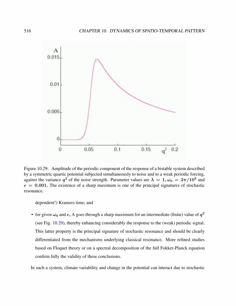
516 CHAPTER 10. DYNAMICS OF SPATIO-TEMPORAL PATTERN
Figure 10.29: Amplitude of the periodic component of the response of a bistable system describedby a symmetric quartic potential subjected simultaneously to noise and to a weak periodic forcing,against the variance q2 of the noise strength. Parameter values are λ = 1, ω0 = 2π/105 andε = 0.001. The existence of a sharp maximum is one of the principal signatures of stochasticresonance.
dependent!) Kramers time; and
• for given ω0 and ε, A goes through a sharp maximum for an intermediate (finite) value of q2
(see Fig. 10.29), thereby enhancing considerably the response to the (weak) periodic signal.
This latter property is the principal signature of stochastic resonance and should be clearly
differentiated from the mechanisms underlying classical resonance. More refined studies
based on Floquet theory or on a spectral decomposition of the full Fokker-Planck equation
confirm fully the validity of these conclusions.
In such a system, climate variability and change in the potential can interact due to stochastic
10.4. PATTERN OF CLIMATE VARIABILITY 517
resonance ?; ?. Stochastic resonance occurs when the signal-to-noise ratio of a non-linear device
is maximized for a moderate value of noise intensity σ. It often occurs in bistable and excitable
systems with sub-threshold inputs. For lower noise intensities, the signal does not cause the device
to cross threshold, so little signal is passed through it. For large noise intensities, the output is
dominated by the noise, also leading to a low signal-to-noise ratio. For moderate intensities, the
noise allows the signal to reach threshold, but the noise intensity is not so large as to swamp it.
Strictly speaking, stochastic resonance occurs in bistable systems, when a small periodic force
F (t) (which is external) is applied together with a large wide-band stochastic force σξ (which is
internal). The system response is driven by the combination of the two forces that compete/co-
operate to make the system switch between the two stable states. The degree of order is related
to the amount of periodic function that it shows in the system response. When the periodic force
is chosen small enough in order not to make the system response switch, the presence of a non-
negligible noise is required for it to happen. When the noise is small very few switches occur,
mainly at random with no significant periodicity in the system response. When the noise is very
strong a large number of switches occur for each period of the periodic force and the system re-
sponse does not show remarkable periodicity. Quite surprisingly, between these two conditions,
there exists an optimal value of the noise that cooperatively concurs with the periodic forcing in
order to make almost exactly one switch per period (a maximum in the signal-to-noise ratio).
Furthermore, non-linear oscillators have been proposed where the timing of the deterministic
external forcing is crucial for generating oscillations ?; Lorenz [1976]; ?. Some aspects of non-
equilibrium systems can be found in the climatic system. On the climatological scale, it exhibits
abrupt jumps in the long-term rate of temperature change, which are often associated with changes
in circulation patterns.

Chapter 11
Future Directions
Until now, details of abrupt climate change are not well known to be able to accurately predict it.
With better information, the society could take more confident action to reduce the potential impact
of abrupt changes on agriculture, water resources, and the built environment, among other impacts.
A better understanding of sea-ice and glacier stability, land-surface processes, and atmospheric
and oceanic circulation patterns is needed. Moreover, to effectively use any additional knowledge
of these and other physical processes behind abrupt climate change, more sophisticated ways of
assessing their interactions must be developed, including:
Better models. At present, the models used to assess climate and its impacts cannot simulate
the size, speed, and extent of past abrupt changes, let alone predict future abrupt changes. Efforts
are needed to improve how the mechanisms driving abrupt climate change are represented in these
models and to more rigorously test models against the climate record.
More theory. There are concepts to find the underlying dynamical system, to derive a theory
from a high-order to low-order description similar to what is done in statistical physics (Mori-
Zwanzig approach ?; ?, Master equation), or in stochastic differential equations. A systematic
reduction of the complex system into fewer degrees of freedom shall bring a deeper level of un-
derstanding about the underlying physics. A systematic approach was suggested by Saltzman ?.
Spectral and pseudo-spectral concepts have not been used too much in climate theory. There is
518

519
a variety of phenomenological stochastic models in which non-linearity and fluctuations coexist,
and in which this coexistence leads to interesting phenomena.
Earth System Modeling and Analysis Modeling is necessary to produce a useful understand-
ing of abrupt climate processes. Model analyses help to focus research on possible causes of abrupt
climate change, such as human activities; on key areas where climatic thresholds might be crossed;
and on fundamental uncertainties in climate-system dynamics. Improved understanding of abrupt
climatic changes that occurred in the past and that are possible in the future can be gained through
climate models. A comprehensive modeling strategy designed to address abrupt climate change
includes vigorous use of a hierarchy of models, from theory and conceptual models through mod-
els of intermediate complexity, to high-resolution models of components of the climate system,
to fully coupled earth-system models. The simpler models are well-suited for use in developing
new hypotheses for abrupt climate change. Model-data comparisons are needed to assess the qual-
ity of model predictions. It is important to note that the multiple long integrations of enhanced,
fully coupled Earth system models required for this research are not possible with the computer
resources available today, and thus, these resources are currently enhanced.
One particularly convincing example showing that the feedbacks in the climate system are im-
portant is the drying of the Sahara about 5000 years before present which is triggered by variations
in the Earth’s orbit around the sun. Numerous modeling studies, e.g. ?, suggest that the abruptness
of the onset and termination of the early to mid-Holocene humid period across much of Africa
north of the equator depends on the presence of non-linear feedbacks associated with both ocean
circulation and changes in surface hydrology and vegetation, e.g. ?. Without including these feed-
backs alongside gradual insolation forcing, it is impossible for existing models to come even close
to simulating the rapidity or the magnitude of climatic change associated with the extension of
wetlands and plant cover in the Sahara/Sahel region prior to the onset of extreme dryness around
5000 years before present.
Paleoclimatic data. More climate information from the distant past would go a long way
toward strengthening our understanding of abrupt climate changes and models of past climate. In

520 CHAPTER 11. FUTURE DIRECTIONS
particular, an enhanced effort is needed to expand the geographic coverage, temporal resolution,
and variety of paleoclimatic data. Although the present climate has no direct analogon to the
past ?, the dynamical interpretation of data will improve the understanding of thresholds and non-
linearities in the Earth system.
Systematic measurements of climate using modern instruments have produced records covering
the last 150 years. In order to reconstruct past variations in the climate system further back in time,
scientists use natural archives of climatic and environmental changes, such as ice cores, tree rings,
ocean and lake sediments, corals, and historical evidence. Scientists call these records proxies
because, although they are not usually direct measures of temperature or other climatic variables,
they are affected by temperature, and using modern calibrations, the changes in the proxy preserved
in the fossil record can be interpreted in terms of past climate.
Ice core data, coral data, ring width of a tree, or information from marine sediments are ex-
amples of a proxy for temperature, or in some cases rainfall, because the thickness of the ring
can be statistically related to temperature and/or rainfall in the past. The most valuable proxies
are those that can be scaled to climate variables, and those where the uncertainty in the proxy
can be measured. Proxies that cannot be quantified in terms of climate or environment are less
useful in studying abrupt climate change because the magnitude of change cannot be determined.
Quite often, the interpretation of proxy data is already a model of climate change since it involves
constraints (dating, representativeness etc.). Uncertainties in the proxies, and uncertainties in the
dating, are the main reasons that abrupt climate change is one of the more difficult topics in the
field of paleoclimatology.
Appropriate statistical tools. Because most statistical calculations at present are based on
the assumption that climate is not changing but is stationary, they have limited value for non-
stationary (changing) climates and for climate-related variables that are often highly skewed by
rapid changes over time such as for abrupt-change regimes. Available statistical tools themselves
need to be adapted or replaced with new approaches altogether to better reflect the properties of
abrupt climate change.

521
Synthesis. Physical, ecological, and human systems are complex, non-linear, dynamic and im-
perfectly understood. Present climate change is producing conditions outside the range of recent
historical experience and observation, and it is unclear how the systems will interact with and react
to further climate changes. Hence, it is crucial to be able to better understand and recognize abrupt
climate changes quickly. This capability will involve improved monitoring of parameters that de-
scribe climatic, ecological, and economic systems. Some of the desired data are not uniquely
associated with abrupt climate change and, indeed, have broad applications. Other data take on
particular importance because they concern properties or regions implicated in postulated mecha-
nisms of abrupt climate change. Research to increase our understanding of abrupt climate change
should be designed specifically within the context of the various mechanisms thought to be in-
volved. Focus is required to provide data for process studies from key regions where triggers of
abrupt climate change are likely to occur, and to obtain reliable time series of climate indicators
that play crucial roles in the postulated mechanisms. Observations could enable early warning of
the onset of abrupt climate change. New observational techniques and data-model comparisons
will also be required.

Part IV
Fourth part: Numerical applications and
further exercises
522
Chapter 12
Appendix: Numerical examples
12.1 Examples in matlab
How to plot in matlab:% graphlab.m% sin(x)/x example%x = -10.5:.2:10.5;plot(x,sin(x)./x)set(gca,’FontName’,’Times-Roman’,’FontSize’,16);print -deps graphlab.eps
12.1.1 Covariance
% calculate Covariance in matlab\\%% pca.m%clear alleps = 1e-10;npts = 100000;x(:,1) = randn(npts,1);x(:,2) = randn(npts,1);x(:,3) = x(:,1)+x(:,2);Cx = cov(x);fprintf(’covariance of x:\n’)fprintf(’ %f %f %f\n’,Cx)[M,Ex] = eig(Cx);
523

524 CHAPTER 12. APPENDIX: NUMERICAL EXAMPLES
fprintf(’eigenvalues of covariance of x:\n’)fprintf(’ %f %f %f\n’,Ex)M = M’;index = (diag(Ex) > eps);M = M(index,:);y = (M*x’)’;Cy = cov(y);fprintf(’measured covariance of y:\n’)fprintf(’ %f %f\n’,cov(y))
12.1.2 Random walk
Running stochwalk.m will open a window showing the results of 10 random walks. Every time
you run the script the output will be different, but a typical run will produce something like this.npts = 1000;nplot = 10;seed = 1;for i = 1:nplot
xplot = [];x = 0;for j=1:npts
seed = rem(8121 * seed + 28411, 134456);if (seed > (134456/2))
x = x + 1;else
x = x - 1;end
xplot = [xplot x];end
plot(xplot,’g’)hold onend
t = 1:(npts/10):npts;error = sqrt(t)*1.5;errorbar(t,zeros(size(t)),error,error,’.’)xlabel(’t’)ylabel(’x’)axis([0 npts -2*sqrt(npts) 2*sqrt(npts)])hold offprint -deps plot.eps
Two dimensional random walk
npts = 10000;seed = 1;xplot = [];yplot = [];

12.1. EXAMPLES IN MATLAB 525
Figure 12.1: Numerical solution of the brownian motion.
x = 0;y = 0;for i = 1:npts
x = x + (rand-0.5);xplot = [xplot x];y = y + (rand-0.5);yplot = [yplot y];end
plot(xplot,yplot)axis([min(min(xplot),min(yplot)) max(max(xplot),max(yplot)) ...
min(min(xplot),min(yplot)) max(max(xplot),max(yplot))])%axis(’off’)hold onplot(0,0,’+’,’LineWidth’,5)print -djpeg twoDrandom.jpg
12.1.3 Carbon cycle
Zeebe, R. E. and D. A. Wolf-Gladrow, \COz in Seawater:
Equilibrium, Kinetics, Isotopes, Elsevier Oceanography Series, 65, pp. 346,
526 CHAPTER 12. APPENDIX: NUMERICAL EXAMPLES
Amsterdam, 2001. Reprinted in 2003, 2005.
ReadMe file for csys3.m
This file contains instructions on how to run the MATLAB file with the user-interface (recommended) and without (for expert users only). For either mode to work, both the csys3.m and equic.m files must be in the same folder (or directory).
The file csys.m contains numerical routines to calculate carbonate system parameters
from any two given quantities.
The file equic.m contains equations to calculate the various
equilibrium constants used in csys.m.
Table of Contents:
---------------------------------------------------------------------
I) INTERFACE MODE
1) Inputting a Small Set of Values
‘i) Default Values
2) Inputting a Large Set of Values
i) Location of Input Data File
ii) Input File Format
iii) Order of Input Data
iv) Default values
v) Output File Format
vi) Order of Output File Data
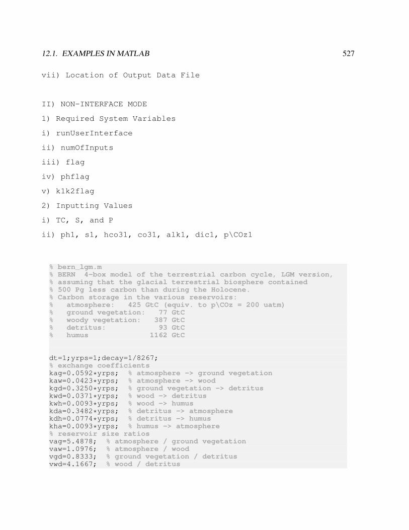
12.1. EXAMPLES IN MATLAB 527
vii) Location of Output Data File
II) NON-INTERFACE MODE
1) Required System Variables
i) runUserInterface
ii) numOfInputs
iii) flag
iv) phflag
v) k1k2flag
2) Inputting Values
i) TC, S, and P
ii) ph1, s1, hco31, co31, alk1, dic1, p\COz1
% bern_lgm.m% BERN 4-box model of the terrestrial carbon cycle, LGM version,% assuming that the glacial terrestrial biosphere contained% 500 Pg less carbon than during the Holocene.% Carbon storage in the various reservoirs:% atmosphere: 425 GtC (equiv. to p\COz = 200 uatm)% ground vegetation: 77 GtC% woody vegetation: 387 GtC% detritus: 93 GtC% humus 1162 GtC
dt=1;yrps=1;decay=1/8267;% exchange coefficientskag=0.0592*yrps; % atmosphere -> ground vegetationkaw=0.0423*yrps; % atmosphere -> woodkgd=0.3250*yrps; % ground vegetation -> detrituskwd=0.0371*yrps; % wood -> detrituskwh=0.0093*yrps; % wood -> humuskda=0.3482*yrps; % detritus -> atmospherekdh=0.0774*yrps; % detritus -> humuskha=0.0093*yrps; % humus -> atmosphere% reservoir size ratiosvag=5.4878; % atmosphere / ground vegetationvaw=1.0976; % atmosphere / woodvgd=0.8333; % ground vegetation / detritusvwd=4.1667; % wood / detritus
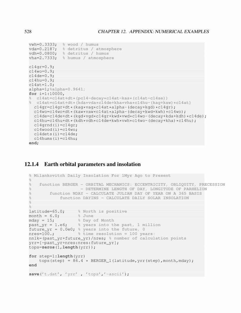
528 CHAPTER 12. APPENDIX: NUMERICAL EXAMPLES
vwh=0.3333; % wood / humusvda=0.2187; % detritus / atmospherevdh=0.0800; % detritus / humusvha=2.7333; % humus / atmosphere
c14gr=0.9;c14wo=0.9;c14de=0.9;c14hu=0.9;c14at=1.0;alpha=1;%alpha=0.9641;for i=1:10000,% c14at=c14at+dt*(pc14-decay*c14at-kas*(c14at-c14se))% c14at=c14at+dt*(kda*vda*c14de+kha*vha*c14hu-(kag+kaw)*c14at)
c14gr=c14gr+dt*(kag*vag*c14at*alpha-(decay+kgd)*c14gr);c14wo=c14wo+dt*(kaw*vaw*c14at*alpha-(decay+kwd+kwh)*c14wo);c14de=c14de+dt*(kgd*vgd*c14gr+kwd*vwd*c14wo-(decay+kda+kdh)*c14de);c14hu=c14hu+dt*(kdh*vdh*c14de+kwh*vwh*c14wo-(decay+kha)*c14hu);c14grnd(i)=c14gr;c14wood(i)=c14wo;c14dets(i)=c14de;c14hums(i)=c14hu;
end;
12.1.4 Earth orbital parameters and insolation
% Milankovitch Daily Insolation For 1Myr Ago to Present%% function BERGER - ORBITAL MECHANICS: ECCENTRICITY, OBLIQUITY, PRECESSION% - DETERMINE LENGTH OF DAY, LONGITUDE OF PARHELION% function NDAY - CALCULATE JULIAN DAY OF YEAR ON A 365 BASIS% function DAYINS - CALCULATE DAILY SOLAR INSOLATION%%latitude=65.0; % North is positivemonth = 6.0; % Junemday = 15; % Day of Monthpast_yr = 1.e6; % years into the past, 1 millionfuture_yr = 0.0e0; % years into the future, 0nres=100.; % time resolution = 100 years:nnlk=(past_yr+future_yr)/nres; % number of calculation pointsyrr=[-past_yr+nres:nres:future_yr];tops=zeros(1,length(yrr));
for step=1:length(yrr)tops(step) = 86.4 * BERGER_1(latitude,yrr(step),month,mday);
end
save(’t.dat’, ’yrr’ , ’tops’,’-ascii’);

12.1. EXAMPLES IN MATLAB 529
%%%%%%%%%%%%function BERGER = my_BERGER(PHI,T,MA,JA)%% PROGRAM ORIGINALLY DEVELOPED BY A. BERGER (1978)%% DECRIPTION OF PROGRAM :% A.BERGER : A SIMPLE ALGORITHM TO COMPUTE LONG TERM VARIATIONS OF% DAILY OR MONTHLY INSOLATION% INSTITUT D’ASTRONOMIQUE ET DE GEOPHYSIQUE% UNIVERSITE CATHOLIQUE DE LOUVIAN% CONTRIBUTION NO. 18 (1978)% %% INPUT :% PHI - LATITUDE IN DEGREES% NORTHERN HEMISPH. : POSITIVE VALUES% SOUTHERN HEMISPH. : NEGATIVE VALUES% T - TIME IN YEARS, NEGATIVE FOR THE PAST% (REFERENCE YEAR : 1950 A.D.)% MA - MONTH IN SPECIFIED YEAR% JA - DAY IN SPECIFIED MONTH% %% OUTPUT :% FUNCTION ’BERGER’ GIVES DAILY INSOLATION IN KJ M(-2) DAY(-1)%% EXAMPLE : BERGER(45.,0.,7,15) = 40304.05 KJ M(-2) DAY(-1)%% ORBITAL PARAMETERS:% ADDITIONAL OUTPUT OF ORBITAL PARAMETERS IS POSSIBLE, SEE WRITE-% STATEMENTS MARKED BY ’CPPP’%%% CONSTANTS%PIR = pi/180.0;PIRR = PIR/3600.0;STEP = 360.0/365.25;TEST = 0.0001;%% 1.EARTH ORBITAL ELEMENTS : ECCENTRICITY ECC TABLE 1% *************************** PRECESSIONAL PARAMETER PRE% OBLIQUITY XOB TABLE 2% GENERAL PRECESSION PRG% LONGITUDE PERIHELION PERH TABLE 3%% AMPLITUDE A MEAN RATE B PHASE C% THEY ARE IMMEDIATELY CONVERTED IN RADIANS%%% ECCENTRICITY
530 CHAPTER 12. APPENDIX: NUMERICAL EXAMPLES
%NEF=19;AE = ones(19,1);BE=ones(19,1);CE=ones(19,1);
AE(1:5) = [0.01860798 0.01627522 -0.01300660 0.00988829 -0.00336700];AE(6:10) = [0.00333077 -0.00235400 0.00140015 0.00100700 0.00085700];AE(11:15) = [0.00064990 0.00059900 0.00037800 -0.00033700 0.00027600];AE(16:19) = [0.00018200 -0.00017400 -0.00012400 0.00001250];
BE(1:5) = [ 4.2072050 7.3460910 17.8572630 17.2205460 16.8467330];BE(6:10) = [ 5.1990790 18.2310760 26.2167580 6.3591690 16.2100160];BE(11:15) = [ 3.0651810 16.5838290 18.4939800 6.1909530 18.8677930];BE(16:19) = [17.4255670 6.1860010 18.4174410 0.6678630];BE = BE.*PIRR;
CE(1:5) = [ 28.620089 193.788772 308.307024 320.199637 279.376984];CE(6:10) = [ 87.195000 349.129677 128.443387 154.143880 291.269597];CE(11:15) = [114.860583 332.092251 296.414411 145.769910 337.237063];CE(16:19) = [152.092288 126.839891 210.667199 72.108838];CE = CE.*PIR;%% OBLIQUITY%XOD=23.320556;NOB=18;AOB=ones(18,1);BOB=ones(18,1);COB=ones(18,1);
AOB(1:5) = [-2462.2214466 -857.3232075 -629.3231835 -414.2804924 -311.7632587];AOB(6:10) = [ 308.9408604 -162.5533601 -116.1077911 101.1189923 -67.6856209];AOB(11:15) = [ 24.9079067 22.5811241 -21.1648355 -15.654987615.3936813];AOB(16:18) = [ 14.6660938 -11.7273029 10.2742696];
BOB(1:5) = [31.609974 32.620504 24.172203 31.983787 44.828336];BOB(6:10) = [30.973257 43.668246 32.246691 30.599444 42.681324];BOB(11:15) = [43.836462 47.439436 63.219948 64.230478 1.010530];BOB(16:18) = [ 7.437771 55.782177 0.373813];BOB = BOB.*PIRR;
COB(1:5) = [251.9025 280.8325 128.3057 292.7252 15.3747];COB(6:10) = [263.7951 308.4258 240.0099 222.9725 268.7809];COB(11:15) = [316.7998 319.6024 143.8050 172.7351 28.9300];COB(16:18) = [123.5968 20.2082 40.8226];COB = COB.*PIR;%% GENERAL PRECESSION IN LONGITUDE%XOP=3.392506;

12.1. EXAMPLES IN MATLAB 531
PRM=50.439273;NOP=9;AOP=ones(9,1);BOP=ones(9,1);COP=ones(9,1);
AOP(1:5) = [7391.0225890 2555.1526947 2022.7629188 -1973.6517951 1240.2321818];AOP(6:9) = [ 953.8679112 -931.7537108 872.3795383 606.3544732];
BOP(1:5) = [ 31.609974 32.620504 24.172203 0.636717 31.983787];BOP(6:9) = [ 3.138886 30.973257 44.828336 0.991874];BOP = BOP.*PIRR;
COP(1:5) = [251.9025 280.8325 128.3057 348.1074 292.7252];COP(6:9) = [165.1686 263.7951 15.3747 58.5749];COP = COP.*PIR;%% 3.NUMERICAL VALUE FOR ECC PRE XOB%% T IS NEGATIVE FOR THE PAST T IS IN YEARS%%
ARG = BE .* T + CE;XES = sum(AE .* sin(ARG));XEC = sum(AE .* cos(ARG));ECC = sqrt(XES2 + XEC2);TRA = abs(XEC);
%if(TRA <= 1.0E-08 | XEC == 0.0)
if(XES<0.0)RP = 1.5 * pi;
elseif(XES == 0.0)RP = 0.0;
elseRP = pi/2.0;
endelse
RP=atan(XES/XEC);if (XEC<0.0)
RP = RP + pi;elseif(XEC == 0.0)
if(XES<0.0)RP = 1.5 * PI;
elseif(XES==0.0)RP = 0.0;
elseRP = pi/2.0;
endelse
if(XES<0.0)RP = RP + 2.0 * pi;
532 CHAPTER 12. APPENDIX: NUMERICAL EXAMPLES
endend
endPERH = RP/PIR;
PRG = PRM*T + sum(AOP .* sin(BOP .* T + COP));PRG = PRG/3600.0 + XOP;PERH = PERH + PRG;if(PERH<0.0)
PERH = PERH + 360.0;elseif(PERH>=360.0)
PERH = PERH - 360.0;end
%PRE=ECC * sin(PERH * PIR);%XOB = XOD + sum(AOB ./ 3600.0 .* cos(BOB .* T + COB));%% 4.DAILY INSOLATION%%% DAILY INSOLATION IN KJ M(-2) DAY(-1)% IF SS IN W M(-2)% AND TAU = 24*60*60 SEC / 1000%SS=1353.0;TAU=86.4;SF=TAU * SS / pi;SO=sin(XOB * PIR);XL=PERH + 180.0;%% 4.2 CALENDAR DATE MA-JA%--------------------% ND NUMBER OF THIS DAY IN A YEAR OF 365 DAYS% XLAM = MEAN LONG. SUN FOR TRUE LONG. = 0% DLAMM = MEAN LONG. SUN FOR MA-JA%ND=NDAY(MA,JA); % NDAY user defined MatLab functionXLLP=XL * PIR;XEE=ECC2;XSE=sqrt(1.0 - XEE);XLAM=(ECC/2.0 + ECC * XEE/8.0) * (1.0 + XSE) * sin(XLLP)...
-XEE/4.0 * (0.5 + XSE) * sin(2.0 * XLLP)...+ ECC * XEE/8.0 * (1.0/3.0 + XSE) * sin(3.0 * XLLP);
XLAM=2.0 * XLAM/PIR;DLAMM=XLAM + ( ND - 80) * STEP;ANM=DLAMM - XL;RANM=ANM * PIR;XEE=XEE.*ECC;RANV=RANM + (2.0 * ECC - XEE / 4.0) * sin(RANM)...
+ 5.0/4.0 * ECC2 * sin(2.0 * RANM) + 13.0/12.0 * XEE * sin(3.0 * RANM);
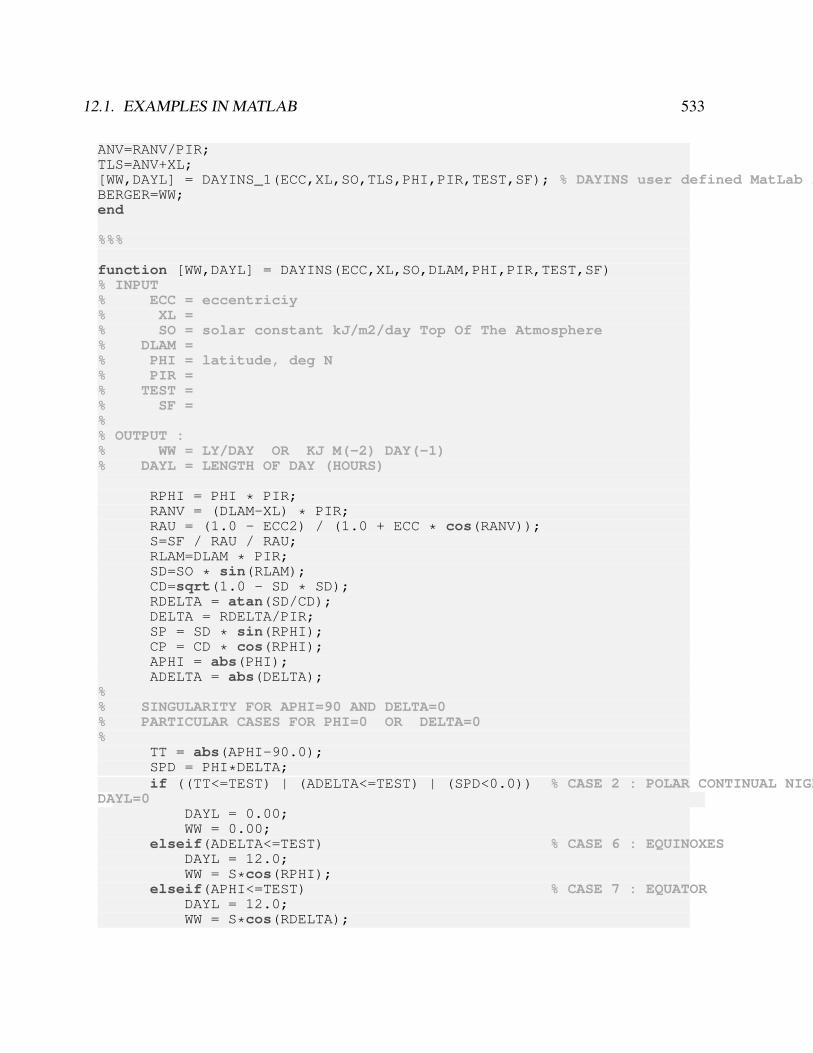
12.1. EXAMPLES IN MATLAB 533
ANV=RANV/PIR;TLS=ANV+XL;[WW,DAYL] = DAYINS_1(ECC,XL,SO,TLS,PHI,PIR,TEST,SF); % DAYINS user defined MatLab functionBERGER=WW;end
%%%
function [WW,DAYL] = DAYINS(ECC,XL,SO,DLAM,PHI,PIR,TEST,SF)% INPUT% ECC = eccentriciy% XL =% SO = solar constant kJ/m2/day Top Of The Atmosphere% DLAM =% PHI = latitude, deg N% PIR =% TEST =% SF =%% OUTPUT :% WW = LY/DAY OR KJ M(-2) DAY(-1)% DAYL = LENGTH OF DAY (HOURS)
RPHI = PHI * PIR;RANV = (DLAM-XL) * PIR;RAU = (1.0 - ECC2) / (1.0 + ECC * cos(RANV));S=SF / RAU / RAU;RLAM=DLAM * PIR;SD=SO * sin(RLAM);CD=sqrt(1.0 - SD * SD);RDELTA = atan(SD/CD);DELTA = RDELTA/PIR;SP = SD * sin(RPHI);CP = CD * cos(RPHI);APHI = abs(PHI);ADELTA = abs(DELTA);
%% SINGULARITY FOR APHI=90 AND DELTA=0% PARTICULAR CASES FOR PHI=0 OR DELTA=0%
TT = abs(APHI-90.0);SPD = PHI*DELTA;if ((TT<=TEST) | (ADELTA<=TEST) | (SPD<0.0)) % CASE 2 : POLAR CONTINUAL NIGHT OR W=0
DAYL=0DAYL = 0.00;WW = 0.00;
elseif(ADELTA<=TEST) % CASE 6 : EQUINOXESDAYL = 12.0;WW = S*cos(RPHI);
elseif(APHI<=TEST) % CASE 7 : EQUATORDAYL = 12.0;WW = S*cos(RDELTA);
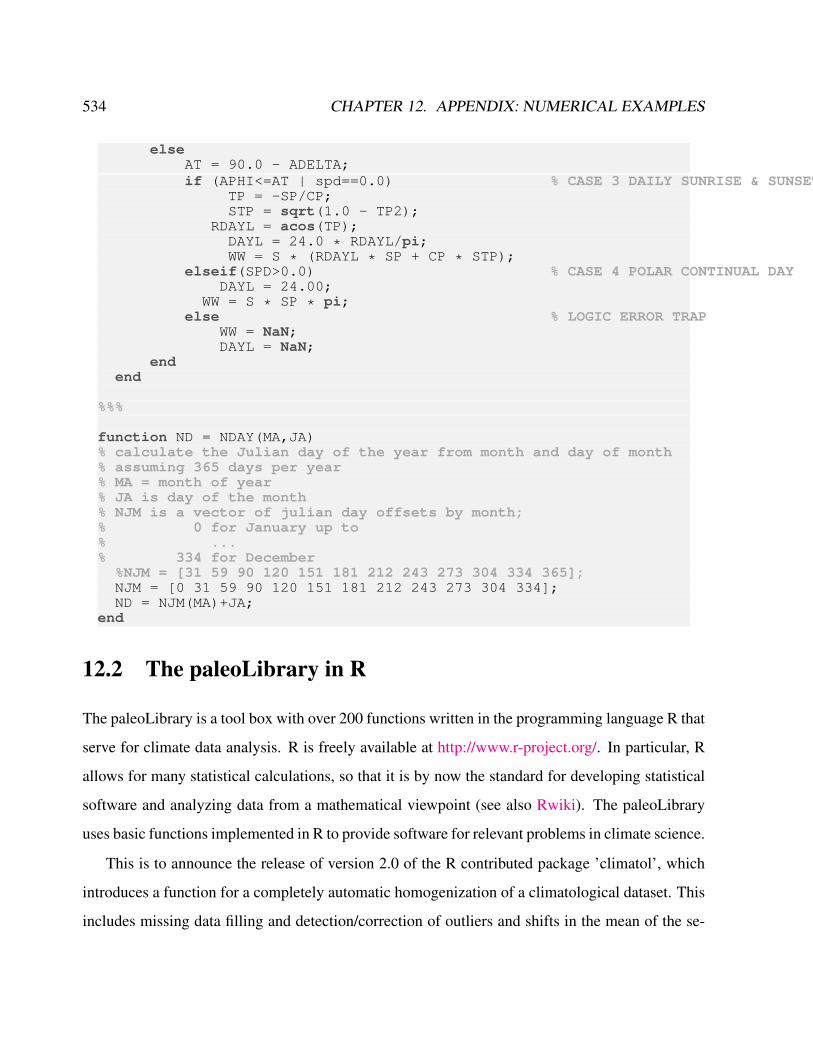
534 CHAPTER 12. APPENDIX: NUMERICAL EXAMPLES
elseAT = 90.0 - ADELTA;if (APHI<=AT | spd==0.0) % CASE 3 DAILY SUNRISE & SUNSET
TP = -SP/CP;STP = sqrt(1.0 - TP2);
RDAYL = acos(TP);DAYL = 24.0 * RDAYL/pi;WW = S * (RDAYL * SP + CP * STP);
elseif(SPD>0.0) % CASE 4 POLAR CONTINUAL DAYDAYL = 24.00;
WW = S * SP * pi;else % LOGIC ERROR TRAP
WW = NaN;DAYL = NaN;
endend
%%%
function ND = NDAY(MA,JA)% calculate the Julian day of the year from month and day of month% assuming 365 days per year% MA = month of year% JA is day of the month% NJM is a vector of julian day offsets by month;% 0 for January up to% ...% 334 for December
%NJM = [31 59 90 120 151 181 212 243 273 304 334 365];NJM = [0 31 59 90 120 151 181 212 243 273 304 334];ND = NJM(MA)+JA;
end
12.2 The paleoLibrary in R
The paleoLibrary is a tool box with over 200 functions written in the programming language R that
serve for climate data analysis. R is freely available at http://www.r-project.org/. In particular, R
allows for many statistical calculations, so that it is by now the standard for developing statistical
software and analyzing data from a mathematical viewpoint (see also Rwiki). The paleoLibrary
uses basic functions implemented in R to provide software for relevant problems in climate science.
This is to announce the release of version 2.0 of the R contributed package ’climatol’, which
introduces a function for a completely automatic homogenization of a climatological dataset. This
includes missing data filling and detection/correction of outliers and shifts in the mean of the se-
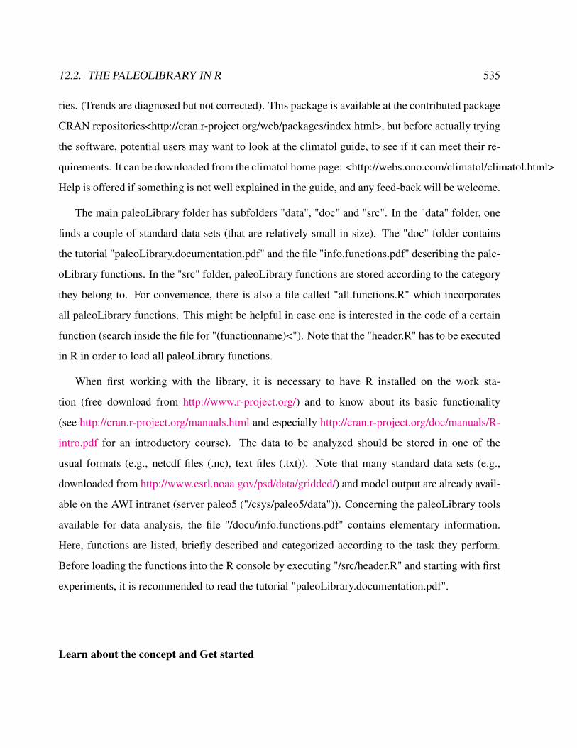
12.2. THE PALEOLIBRARY IN R 535
ries. (Trends are diagnosed but not corrected). This package is available at the contributed package
CRAN repositories<http://cran.r-project.org/web/packages/index.html>, but before actually trying
the software, potential users may want to look at the climatol guide, to see if it can meet their re-
quirements. It can be downloaded from the climatol home page: <http://webs.ono.com/climatol/climatol.html>
Help is offered if something is not well explained in the guide, and any feed-back will be welcome.
The main paleoLibrary folder has subfolders "data", "doc" and "src". In the "data" folder, one
finds a couple of standard data sets (that are relatively small in size). The "doc" folder contains
the tutorial "paleoLibrary.documentation.pdf" and the file "info.functions.pdf" describing the pale-
oLibrary functions. In the "src" folder, paleoLibrary functions are stored according to the category
they belong to. For convenience, there is also a file called "all.functions.R" which incorporates
all paleoLibrary functions. This might be helpful in case one is interested in the code of a certain
function (search inside the file for "(functionname)<"). Note that the "header.R" has to be executed
in R in order to load all paleoLibrary functions.
When first working with the library, it is necessary to have R installed on the work sta-
tion (free download from http://www.r-project.org/) and to know about its basic functionality
(see http://cran.r-project.org/manuals.html and especially http://cran.r-project.org/doc/manuals/R-
intro.pdf for an introductory course). The data to be analyzed should be stored in one of the
usual formats (e.g., netcdf files (.nc), text files (.txt)). Note that many standard data sets (e.g.,
downloaded from http://www.esrl.noaa.gov/psd/data/gridded/) and model output are already avail-
able on the AWI intranet (server paleo5 ("/csys/paleo5/data")). Concerning the paleoLibrary tools
available for data analysis, the file "/docu/info.functions.pdf" contains elementary information.
Here, functions are listed, briefly described and categorized according to the task they perform.
Before loading the functions into the R console by executing "/src/header.R" and starting with first
experiments, it is recommended to read the tutorial "paleoLibrary.documentation.pdf".
Learn about the concept and Get started

536 CHAPTER 12. APPENDIX: NUMERICAL EXAMPLES
Data and metadata In the paleoLibrary, the data are always encapsulated together with their
metadata as position, time, name, etc. Additionally, the history of the data processing is saved,
such that one can easily keep track of the changes made / experiments carried through.
Object orientation The object orientation of R is used to make the work more intuitive. For
instance, if you execute plot(data) with data being a time series, you will create a time series
plot; if data is a 2D field (≡ matrix) instead, you will get a map.
After having installed R etc (see readme file), you need to load the paleoLibrary functions into
R. If path is the directory the paleoLibrary files are stored in (e.g., path="C:/Dokumente
und Einstellungen/Micha/Eigene Dateien/uni/hiwi awi 2011/paleoLibrary/src/"),
this can be done by typing
source(paste(path,"header.R",sep=""))
into the opened R console. It may occur that you get an error message like
Error in library(...) : there is no package called ’...’
in which case you have to install the missing package(s) by hand. For Windows users, this is
straightforward:
• click ’Packages’
• click ’Install Package(s)’
• select a CRAN mirror
• download the package of interest (see Figure 12.2)
If no more error messages pop up when loading the functions via
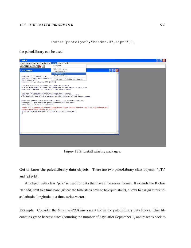
12.2. THE PALEOLIBRARY IN R 537
source(paste(path,"header.R",sep="")),
the paleoLibrary can be used.
Figure 12.2: Install missing packages.
Get to know the paleoLibrary data objects There are two paleoLibrary class objects: "pTs"
and "pField".
An object with class "pTs" is used for data that have time series format. It extends the R class
"ts" and, next to a time base (where the time steps have to be equidistant), allows to assign attributes
as latitude, longitude to a time series vector.
Example Consider the burgundy2004.harvest.txt file in the paleoLibrary data folder. This file
contains grape harvest dates (counting the number of days after September 1) and reaches back to
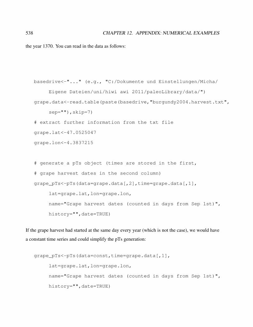
538 CHAPTER 12. APPENDIX: NUMERICAL EXAMPLES
the year 1370. You can read in the data as follows:
basedrive<-"..." (e.g., "C:/Dokumente und Einstellungen/Micha/
Eigene Dateien/uni/hiwi awi 2011/paleoLibrary/data/")
grape.data<-read.table(paste(basedrive,"burgundy2004.harvest.txt",
sep=""),skip=7)
# extract further information from the txt file
grape.lat<-47.0525047
grape.lon<-4.3837215
# generate a pTs object (times are stored in the first,
# grape harvest dates in the second column)
grape_pTs<-pTs(data=grape.data[,2],time=grape.data[,1],
lat=grape.lat,lon=grape.lon,
name="Grape harvest dates (counted in days from Sep 1st)",
history="",date=TRUE)
If the grape harvest had started at the same day every year (which is not the case), we would have
a constant time series and could simplify the pTs generation:
grape_pTs<-pTs(data=const,time=grape.data[,1],
lat=grape.lat,lon=grape.lon,
name="Grape harvest dates (counted in days from Sep 1st)",
history="",date=TRUE)
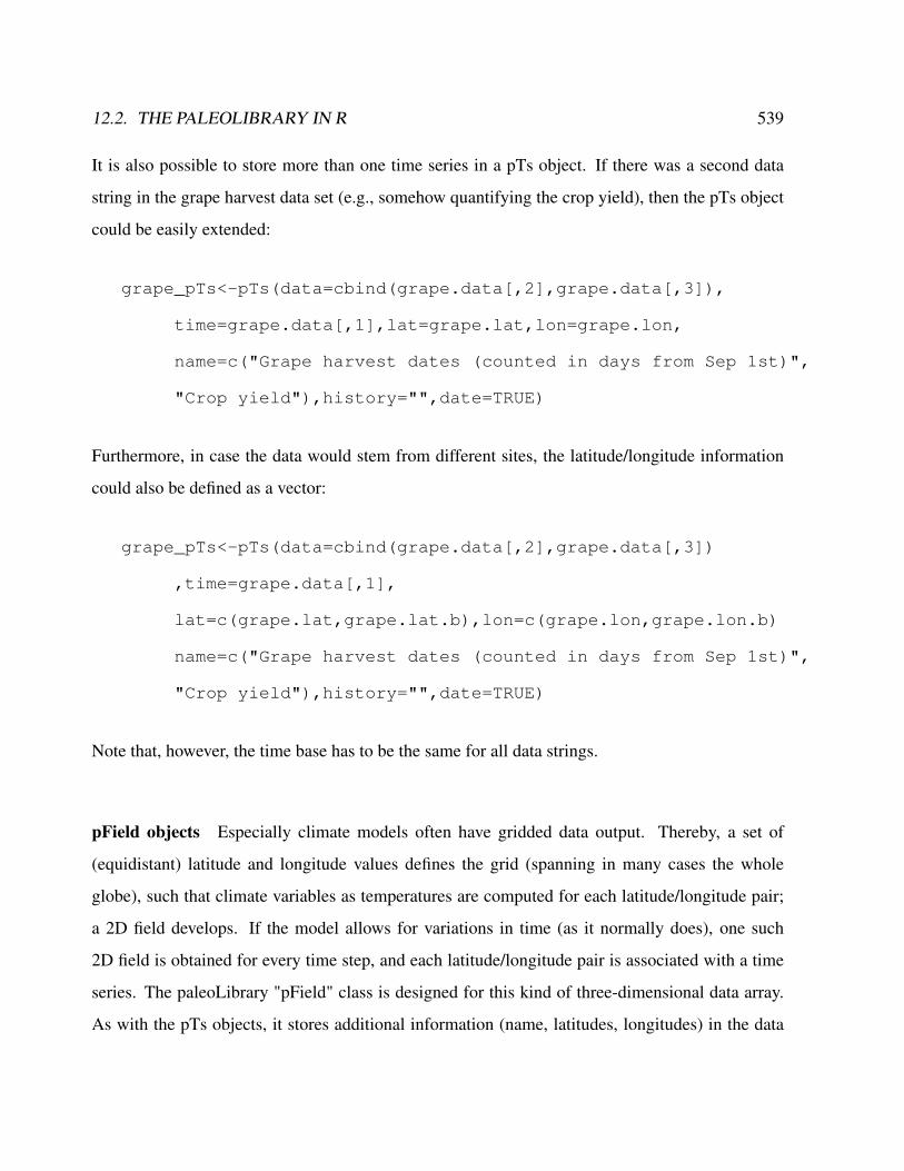
12.2. THE PALEOLIBRARY IN R 539
It is also possible to store more than one time series in a pTs object. If there was a second data
string in the grape harvest data set (e.g., somehow quantifying the crop yield), then the pTs object
could be easily extended:
grape_pTs<-pTs(data=cbind(grape.data[,2],grape.data[,3]),
time=grape.data[,1],lat=grape.lat,lon=grape.lon,
name=c("Grape harvest dates (counted in days from Sep 1st)",
"Crop yield"),history="",date=TRUE)
Furthermore, in case the data would stem from different sites, the latitude/longitude information
could also be defined as a vector:
grape_pTs<-pTs(data=cbind(grape.data[,2],grape.data[,3])
,time=grape.data[,1],
lat=c(grape.lat,grape.lat.b),lon=c(grape.lon,grape.lon.b)
name=c("Grape harvest dates (counted in days from Sep 1st)",
"Crop yield"),history="",date=TRUE)
Note that, however, the time base has to be the same for all data strings.
pField objects Especially climate models often have gridded data output. Thereby, a set of
(equidistant) latitude and longitude values defines the grid (spanning in many cases the whole
globe), such that climate variables as temperatures are computed for each latitude/longitude pair;
a 2D field develops. If the model allows for variations in time (as it normally does), one such
2D field is obtained for every time step, and each latitude/longitude pair is associated with a time
series. The paleoLibrary "pField" class is designed for this kind of three-dimensional data array.
As with the pTs objects, it stores additional information (name, latitudes, longitudes) in the data
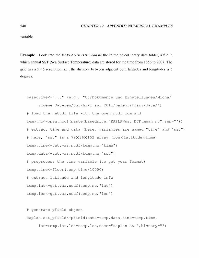
540 CHAPTER 12. APPENDIX: NUMERICAL EXAMPLES
variable.
Example Look into the KAPLANsst.DJF.mean.nc file in the paleoLibrary data folder, a file in
which annual SST (Sea Surface Temperature) data are stored for the time from 1856 to 2007. The
grid has a 5×5 resolution, i.e., the distance between adjacent both latitudes and longitudes is 5
degrees.
basedrive<-"..." (e.g., "C:/Dokumente und Einstellungen/Micha/
Eigene Dateien/uni/hiwi awi 2011/paleoLibrary/data/")
# load the netcdf file with the open.ncdf command
temp.nc<-open.ncdf(paste(basedrive,"KAPLANsst.DJF.mean.nc",sep=""))
# extract time and data (here, variables are named "time" and "sst")
# here, "sst" is a 72×36×152 array (lon×latitude×time)
temp.time<-get.var.ncdf(temp.nc,"time")
temp.data<-get.var.ncdf(temp.nc,"sst")
# preprocess the time variable (to get year format)
temp.time<-floor(temp.time/10000)
# extract latitude and longitude info
temp.lat<-get.var.ncdf(temp.nc,"lat")
temp.lon<-get.var.ncdf(temp.nc,"lon")
# generate pField object
kaplan.sst_pField<-pField(data=temp.data,time=temp.time,
lat=temp.lat,lon=temp.lon,name="Kaplan SST",history="")

12.2. THE PALEOLIBRARY IN R 541
The loading scheme has to be individually adjusted for each ncdf file, as different authors also have
different preferences regarding, for instance, time format and variable naming. For this purpose,
there is a universal reading tool in the paleoLibrary that copes with the various input styles (see the
function read_data in the load.datasets.R file), requiring only the path to the ncdf file and the
variable name(s) if known. More specifically, the load.datasets.R file also provides import tools
for some standard data sets.
Extract information from paleoLibrary objects Functions is_pTs and is_pField allow
for testing objects with regard to the pTs and pField class, respectively. With a pTs or pField object
at hand (let’s name it pL.object), one can easily retrieve the additional attributes (latitude,
longitude, name, history):
# latitude scalar/vector
getlat(pL.object)
# longitude scalar/vector
getlon(pL.object)
# name(s) of the pTs/pField object
getname(pL.object)
# history of the pTs/pField object
gethistory(pL.object)
It is also possible to print out a summary via summary(pL.object), stating the object’s details.
Concerning subsetting, the [ ] operator works as follows for pTs objects:
• pts[i] = pTs object at time(s) i (considering only one series in the multivariate case)
• pts[,j] = pTs object: jth time series (multivariate case)

542 CHAPTER 12. APPENDIX: NUMERICAL EXAMPLES
• pts[i,j] = pTs object at time(s) i and jth time series
and likewise for pField objects:
• pfield[i] = scalar/vector: with n time steps, pfield[1:n] is the first grid point’s time
series, pfield[(n+1):2n] the second grid point’s time series, . . .
• pfield[i,] = pField object: pfield at time(s) i (2D if i is a scalar)
• pfield[,j] = pTs object: time series at jth grid point (see Figure 12.3)
• pfield[i,j] = scalar/vector/matrix: pfield at time(s) i, grid point(s) j
Figure 12.3: 2D field grid points: the ordering starts at the bottom left and ends at the top right.
Zoom into paleoLibrary data objects Often, the spatial and / or temporal extent of a data set
exceeds one’s actual needs. In this case, functions selspace (for pField objects) and window
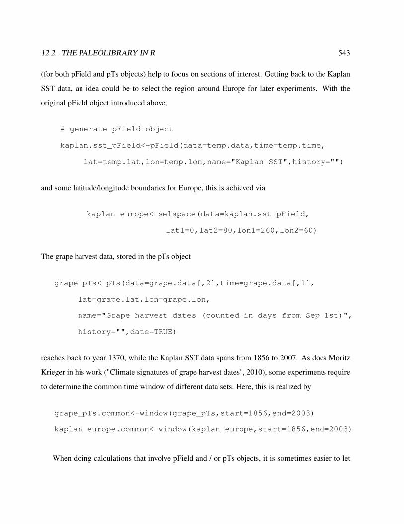
12.2. THE PALEOLIBRARY IN R 543
(for both pField and pTs objects) help to focus on sections of interest. Getting back to the Kaplan
SST data, an idea could be to select the region around Europe for later experiments. With the
original pField object introduced above,
# generate pField object
kaplan.sst_pField<-pField(data=temp.data,time=temp.time,
lat=temp.lat,lon=temp.lon,name="Kaplan SST",history="")
and some latitude/longitude boundaries for Europe, this is achieved via
kaplan_europe<-selspace(data=kaplan.sst_pField,
lat1=0,lat2=80,lon1=260,lon2=60)
The grape harvest data, stored in the pTs object
grape_pTs<-pTs(data=grape.data[,2],time=grape.data[,1],
lat=grape.lat,lon=grape.lon,
name="Grape harvest dates (counted in days from Sep 1st)",
history="",date=TRUE)
reaches back to year 1370, while the Kaplan SST data spans from 1856 to 2007. As does Moritz
Krieger in his work ("Climate signatures of grape harvest dates", 2010), some experiments require
to determine the common time window of different data sets. Here, this is realized by
grape_pTs.common<-window(grape_pTs,start=1856,end=2003)
kaplan_europe.common<-window(kaplan_europe,start=1856,end=2003)
When doing calculations that involve pField and / or pTs objects, it is sometimes easier to let

544 CHAPTER 12. APPENDIX: NUMERICAL EXAMPLES
the data come along in standard R arrays / vectors. Two commands are helpful in this regard:
c(pL.object)
outputs the data as a vector (also for pField objects, for which the output structure is as described
in the first item of the [ ] enumeration (see previous subsection)), whereas
unclass(pL.object)
returns a matrix (with respect to pField objects, each column being associated with a certain grid
point).
Process paleoLibrary data objects All regular operators (+,-,∗,∇·) work with pField and pTs
objects. For instance, scalar multiplication can be done by scalar*pL.object (affecting each
element of the pField/pTs object pL.object). Elementwise operations (more generally indicated
by the ’·’ symbol) between two pTs/pField objects of the same length are performed as for regular
R objects:
pL.object1 · pL.object2.
More complex tools exist in particular for pField objects. To start with, some input function FUN
can be applied to a 3D field either by fixing the time steps
• applyspace: e.g., in order to compute the field average for each time step with FUN=mean;
the output then is a pTs object, yielding one mean value per time step
or by fixing the grid points
• applytime: e.g., in order to get internal time series correlations associated with the grid
points (using FUN=cor); the output then is a 2D field with one correlation coefficient per
grid point
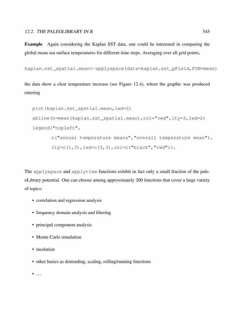
12.2. THE PALEOLIBRARY IN R 545
Example Again considering the Kaplan SST data, one could be interested in comparing the
global mean sea surface temperatures for different time steps. Averaging over all grid points,
kaplan.sst_spatial.mean<-applyspace(data=kaplan.sst_pField,FUN=mean)
the data show a clear temperature increase (see Figure 12.4), where the graphic was produced
entering
plot(kaplan.sst_spatial.mean,lwd=2)
abline(h=mean(kaplan.sst_spatial.mean),col="red",lty=3,lwd=2)
legend("topleft",
c("annual temperature means","overall temperature mean"),
lty=c(1,3),lwd=c(3,3),col=c("black","red")).
The applyspace and applytime functions exhibit in fact only a small fraction of the pale-
oLibrary potential. One can choose among approximately 200 functions that cover a large variety
of topics:
• correlation and regression analysis
• frequency domain analysis and filtering
• principal component analysis
• Monte Carlo simulation
• insolation
• other basics as detrending, scaling, rolling/running functions
• . . .
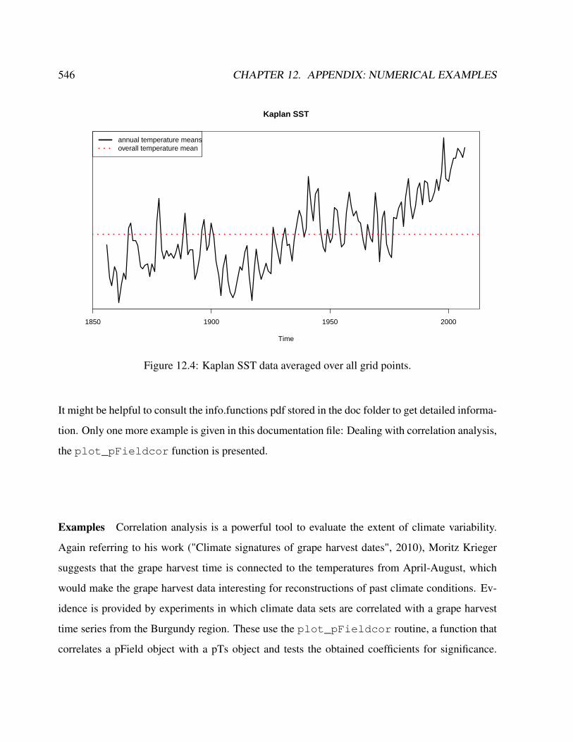
546 CHAPTER 12. APPENDIX: NUMERICAL EXAMPLES
Kaplan SST
Time
1850 1900 1950 2000
annual temperature meansoverall temperature mean
Figure 12.4: Kaplan SST data averaged over all grid points.
It might be helpful to consult the info.functions pdf stored in the doc folder to get detailed informa-
tion. Only one more example is given in this documentation file: Dealing with correlation analysis,
the plot_pFieldcor function is presented.
Examples Correlation analysis is a powerful tool to evaluate the extent of climate variability.
Again referring to his work ("Climate signatures of grape harvest dates", 2010), Moritz Krieger
suggests that the grape harvest time is connected to the temperatures from April-August, which
would make the grape harvest data interesting for reconstructions of past climate conditions. Ev-
idence is provided by experiments in which climate data sets are correlated with a grape harvest
time series from the Burgundy region. These use the plot_pFieldcor routine, a function that
correlates a pField object with a pTs object and tests the obtained coefficients for significance.
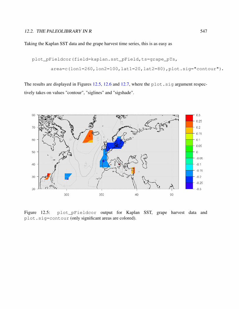
12.2. THE PALEOLIBRARY IN R 547
Taking the Kaplan SST data and the grape harvest time series, this is as easy as
plot_pFieldcor(field=kaplan.sst_pField,ts=grape_pTs,
area=c(lon1=260,lon2=100,lat1=20,lat2=80),plot.sig="contour").
The results are displayed in Figures 12.5, 12.6 and 12.7, where the plot.sig argument respec-
tively takes on values "contour", "siglines" and "sigshade".
Figure 12.5: plot_pFieldcor output for Kaplan SST, grape harvest data andplot.sig=contour (only significant areas are colored).

548 CHAPTER 12. APPENDIX: NUMERICAL EXAMPLES
Figure 12.6: plot_pFieldcor output for Kaplan SST, grape harvest data andplot.sig=siglines (all correlations are colored, significant areas are hatched).
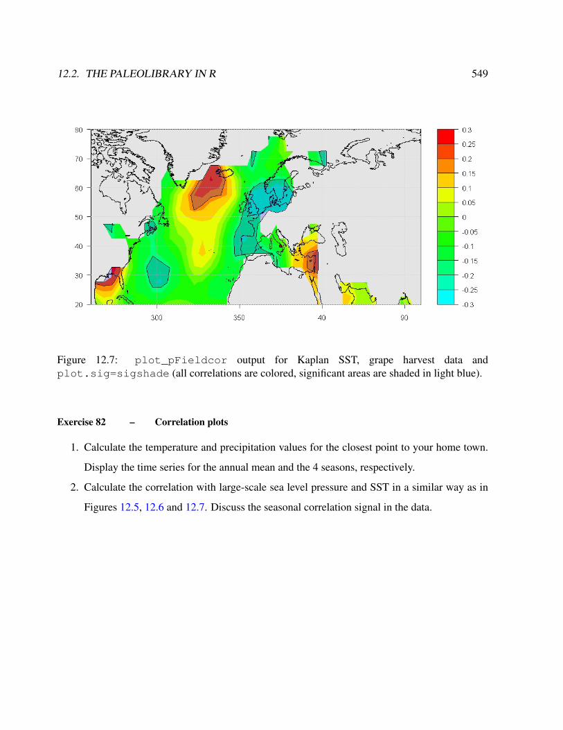
12.2. THE PALEOLIBRARY IN R 549
Figure 12.7: plot_pFieldcor output for Kaplan SST, grape harvest data andplot.sig=sigshade (all correlations are colored, significant areas are shaded in light blue).
Exercise 82 – Correlation plots
1. Calculate the temperature and precipitation values for the closest point to your home town.
Display the time series for the annual mean and the 4 seasons, respectively.
2. Calculate the correlation with large-scale sea level pressure and SST in a similar way as in
Figures 12.5, 12.6 and 12.7. Discuss the seasonal correlation signal in the data.

550 CHAPTER 12. APPENDIX: NUMERICAL EXAMPLES
Plot paleoLibrary data objects As has been shown in one of the previous examples, plotting
is particularly straightforward for pTs objects. The plot arguments are the same as for regular R
time series ("ts" objects; see R help for plot.ts). Also, additional lines and points can be inserted
into a graphics device after a pTs plot has been created. This is different from a pField plot, which
uses the R function filled.contour (to get an overview of the graphic parameters, look up the R help
or the description of filled.contour.own / plotmap.pField in the info.functions pdf).
Here, additional input can be passed on through the FUN argument.
Example One might want to plot the Kaplan SST field at time 1875 and highlight, for some
reason, the capital of Australia, Canberra. It is a good start to put in a point at Canberra using its
geographical coordinates:
canberra<-c(lon=149.12,lat=-35.27)
plot(kaplan.sst_pField[20,],FUN=points(x=canberra[1],
y=canberra[2],pch=21,bg="green",cex=2))

12.2. THE PALEOLIBRARY IN R 551
Then again, this mark is not striking enough. It thus seems appropriate to label the point, leading to
two input functions (R functions text and points). These are passed on to the field plot by entering
canberra.function<-function()
canberra<-c(lon=149.12,lat=-35.27)
points(x=canberra[1],y=canberra[2],pch=21,bg="green",cex=2)
text(x=canberra[1],y=canberra[2],labels="Canberra, Austr.",
col="white",cex=1.5,pos=4)
plot(kaplan.sst_pField[20,],FUN=canberra.function())
For a visualization, see Figures 12.8 and 12.9.
Figure 12.8: Kaplan SST data (year 1875) with the capital of Australia highlighted (green point).
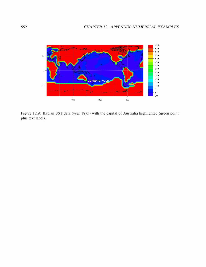
552 CHAPTER 12. APPENDIX: NUMERICAL EXAMPLES
Figure 12.9: Kaplan SST data (year 1875) with the capital of Australia highlighted (green pointplus text label).
12.2. THE PALEOLIBRARY IN R 553
Exercise 83 – Correlation and Monte Carlo experiments
Tasks:
1. Just learn the correlation command: Create two vectors of equal length which have a linear
relation, plot A against B
2. Use R to calculate the correlation between the two.
3. Get a feeling for the interpretation of the size of a correlation: Add noise to B using the
rnorm function, plot the two, add more and more noise
4. How the correlation and the p-value in cor.test are changing? The R2 = coeffient of deter-
mination should be the same as the ratio of the variance of the signal B to the variance of A.
Check this!
5. Sampling variability/correlation which appears by chance: Now create two vectors which
are only containing noise; Calculate the correlation between the two.
6. Vary the number of your samples (length of your vectors), investigate how the correlations
are changing. Now you can see why statistical tests are needed.
7. Monte Carlo experiment to investigate significance in correlations: Repeat the experiments
very often (in a loop, this is called Monte Carlo experiment). Each time save the correlation
between the two random vectors. Plot the histogram of this distribution.
8. You can now see how likely it is to get specific correlation value just by chance. This
probability is strongly dependent on your sample size/degrees of freedom. Now determine
the size of correlation which is needed if you want to have a probability of less/equal 5% to
get the correlation by chance. Use the quantile command.
9. If you create two datasets which have this "limit" correlation you got by the Monte- Carlo
experiment and the same degrees of freedom, cor.test should give you p = 0.05 (here this
is calculated with a t-distribution).
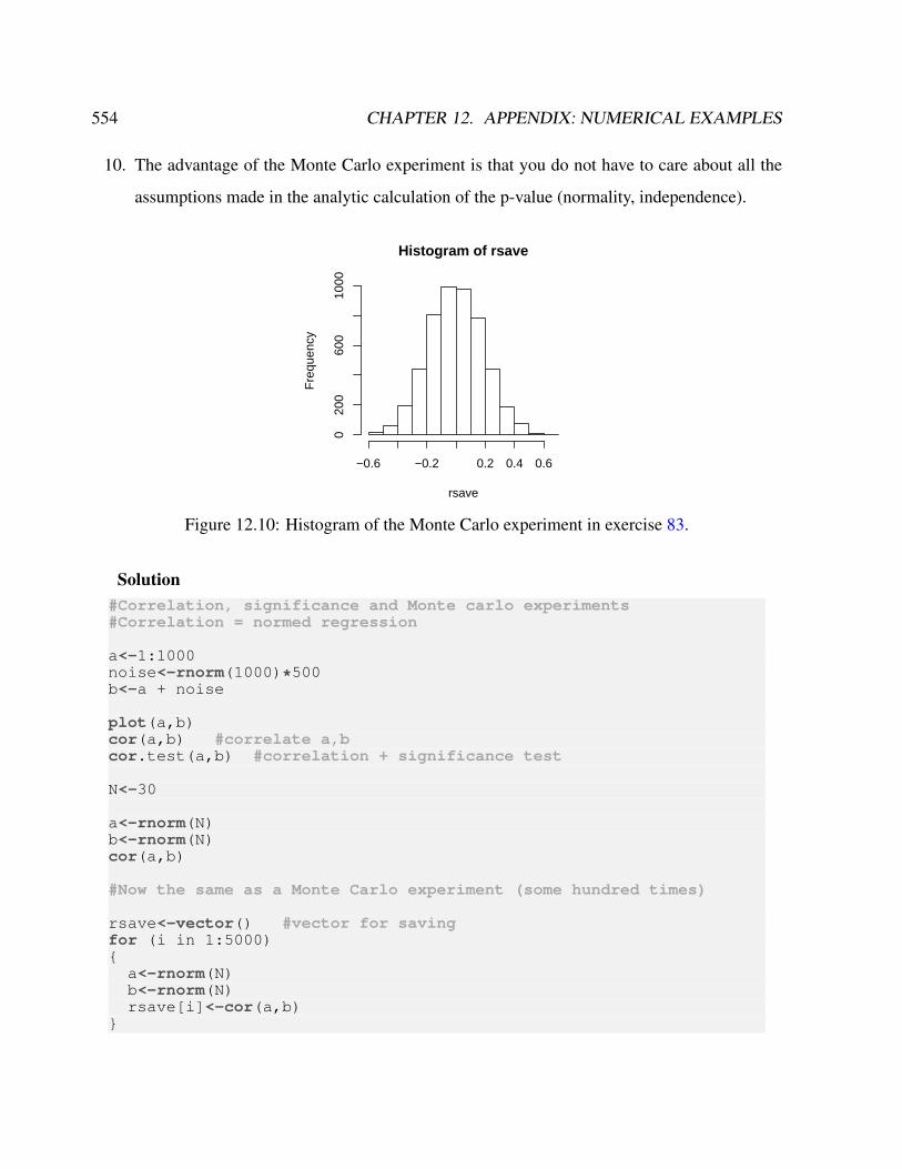
554 CHAPTER 12. APPENDIX: NUMERICAL EXAMPLES
10. The advantage of the Monte Carlo experiment is that you do not have to care about all the
assumptions made in the analytic calculation of the p-value (normality, independence).
Histogram of rsave
rsave
Fre
quen
cy
−0.6 −0.2 0.2 0.4 0.6
020
060
010
00
Figure 12.10: Histogram of the Monte Carlo experiment in exercise 83.
Solution#Correlation, significance and Monte carlo experiments#Correlation = normed regression
a<-1:1000noise<-rnorm(1000)*500b<-a + noise
plot(a,b)cor(a,b) #correlate a,bcor.test(a,b) #correlation + significance test
N<-30
a<-rnorm(N)b<-rnorm(N)cor(a,b)
#Now the same as a Monte Carlo experiment (some hundred times)
rsave<-vector() #vector for savingfor (i in 1:5000)
a<-rnorm(N)b<-rnorm(N)rsave[i]<-cor(a,b)
12.2. THE PALEOLIBRARY IN R 555
hist(rsave)
#abs is used to get the p-values for a two-sided testquantile(abs(rsave),probs=0.95)#dev.print(postscript, file="histogr.ps")
Exercise 84 – Correlation and statistical testing
Two independent time series covering the time from 1850 to 1970 with negligible autocorrela-
tion are given. They are correlated with ρ = −0.2.
a) Describe a statistical test to obtain whether the correlation is significant with p=0.01 or not.
b) How is such a test called?
c) How can this test be realised in R? Write down the programming code. It should also plot a
histogram and the quantiles.
Exercise 85 – Statistical significance
Fig. 12.11 shows the histogram of a statistical test with random time series. The thin red
(green) lines show the p=0.05 (p=0.01) quantiles. Three pairs of time series with the same length
has been correlated and yield the following correlation values:
a) ρ = −0.32, b) ρ = 0.14 and c) ρ = 0.24. Which of the correlation values are statistical
significant with p=0.01 and p=0.05?
Exercise 86 – Palaeolibrary
With the palaeolibrary, climate data can be easily analysed. Describe what the following com-
mands are doing and explain the meaning of the arguments.
a) plot.final(field=sst.field,ts=nao.index,zlim=c(-0.6,0.6),
plot_sig="siglines",area=c(lat1=30,lat2=75,lon1=340,lon2=60),
point=c(lat=46,lon=10))
b) test1<-selspace(field.sst,lat1=30,lat2=45, lon1=20,lon2=60)
test2<-applyspace(test1,mean)
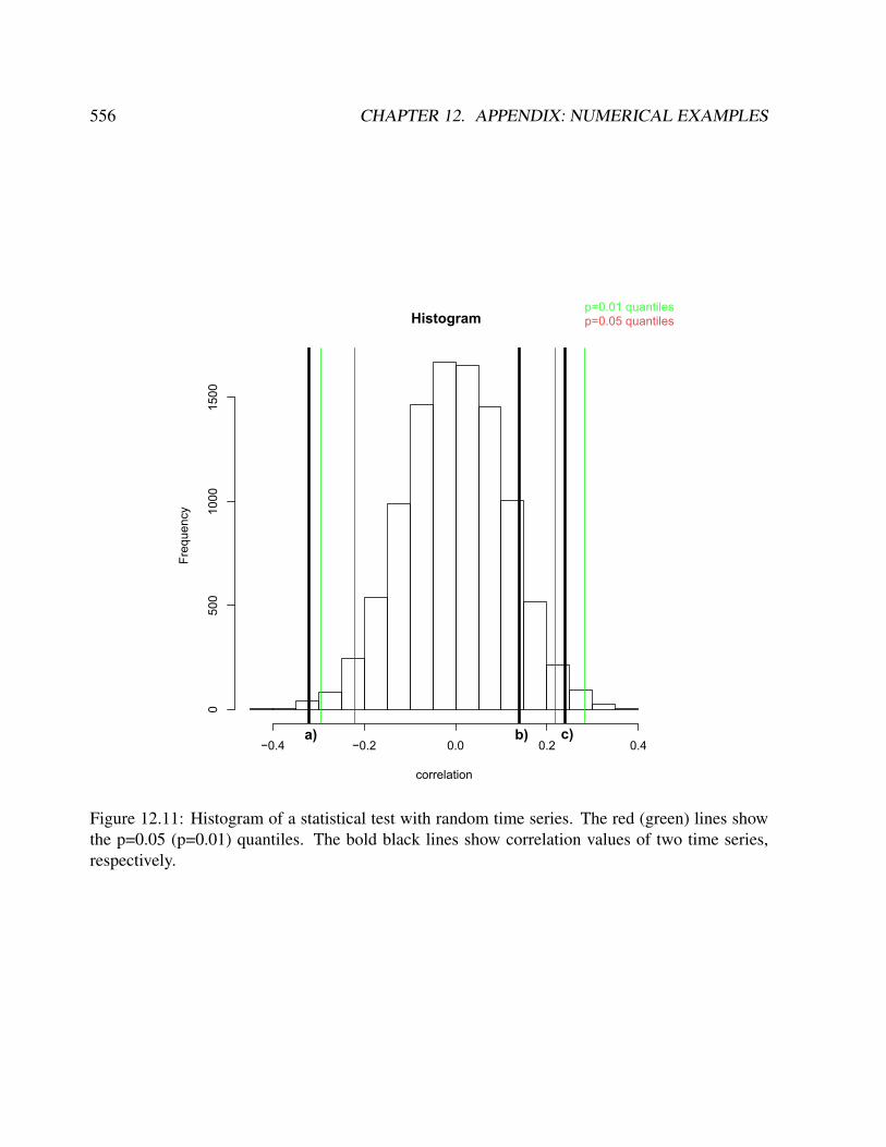
556 CHAPTER 12. APPENDIX: NUMERICAL EXAMPLES
Histogram
correlation
Freq
uenc
y
a) b) c)
p=0.05 quantilesp=0.01 quantiles
−0.4 −0.2 0.0 0.2 0.4
050
010
0015
00
Figure 12.11: Histogram of a statistical test with random time series. The red (green) lines showthe p=0.05 (p=0.01) quantiles. The bold black lines show correlation values of two time series,respectively.

12.2. THE PALEOLIBRARY IN R 557
c) plot(roll.2(test2,nao.index,width=30,by=2,FUN=cor.pTs)
558 CHAPTER 12. APPENDIX: NUMERICAL EXAMPLES
12.3 Examples in Python
This document describes some examples in the programming language python. According to
wikipedia and the development website:
Python is a general-purpose, high-level programming language whose design phi-
losophy emphasizes code readability. Python’s syntax allows programmers to express
concepts in fewer lines of code than would be possible in languages such as C, and the
language provides constructs intended to enable clear programs on both a small and
large scale.
Python supports multiple programming paradigms, including object-oriented, im-
perative and functional programming styles. It features a dynamic type system and
automatic memory management and has a large and comprehensive standard library.
Like other dynamic languages, Python is often used as a scripting language, but is
also used in a wide range of non-scripting contexts. Using third-party tools, Python
code can be packaged into standalone executable programs. Python interpreters are
available for many operating systems.
A couple of thing should be noted. First and foremost, python relies on whitespace to organize
the language syntax. for, if, while, and function definitions via def all need to be properly
indented, either with tabs or spaces. This is a bit irritating if you are coming from a background of
C or Matlab, where loops can easily be enclosed in braces or parentheses. Once you get used to it,
though, proper use of whitespace makes for cleaner and legible code, without having to hunt and
find where a certain block begins and ends.
Secondly, python is object orientated. This means that anything that is defined (or declared)
by the user gets a set of attributes depending on what sort of object/instance it is. These can
be accessed with a . behind the object’s name. Although a computer scientist would probably
furiously disagree with this, I’ll use object and instance interchangeably.1
1Strictly speaking, an object is location within the computer memory with a specific value referred to be an identi-fier. Objects are instances of classes

12.3. EXAMPLES IN PYTHON 559
12.3.1 Plotting climate data
The code that comes with this document, cosmos_plot.py, is designed to plot 2 types of run-
of-the-mill model outputs that you’re bound to encounter sooner or later. First, we will plot a scalar
variable from the ocean: the global salinity field for the surface layer. The function we’ll use to do
this is below.
def plot_scalar(fin):fin = netcdf.netcdf_file(fin, ’r’)global varsvars = fin.variablesvar = fin.variables[’SAO’].data.squeeze()lon = filepath.variables[’lon’].data.squeeze()lat = filepath.variables[’lat’].data.squeeze()var, lon = shiftgrid(180.,var, lon, start=False)lons, lats = np.meshgrid(lon, lat)map = Basemap(projection=’robin’,lon_0=0,resolution=’c’)x, y = map(lons, lats)map.drawmapboundary(fill_color=’0.6’)map.drawcoastlines(linewidth=0.75)cs = map.contourf(x,y,var, cmap = matplotlib.cm.jet, levels=np.arange(20,40,1), extend = ’both’)cbar = map.colorbar(cs, location=’right’,pad="5%", format=’%.2f’, extend = ’both’)
Let’s go through this line by line and figure out what is happening. The first line should be fairly
obvious, we define a function plot_scalar() which takes a single argument, fin. Notice that
since fin is not assigned a default value, calling the function without any arguments would lead
to an error.
Next, we reassign fin by calling the module netcdf which contains the function netcdf_file.
Here, the fin we provided is read by the function with the option ’r’. fin is now no longer a
string but a netcdf_file object.
If we are running python interactively, it would be useful to see which variables are in the file
we read even after the function has completed. Therefore, the variable vars is defined to be global,
making it available to the user outside of the function environment.
Now we want to grab the variable we want to plot out of the dataset. Let’s give it a sensible
name, like var. It’s taken from the netcdf object fin, it’s data is extracted, and the squeeze
command removes any dimensions which have a size of one. This is necessary for plotting, since

560 CHAPTER 12. APPENDIX: NUMERICAL EXAMPLES
plotting in more than 2 dimensions gets a bit tricky. We similarly get the corresponding latitudes
and longitutdes.
Line 8 might not make sense right away. The model gives us outputs on 0 to 360 degrees, so
once around the entire planet. The map projection we will use later needs this to be -180 to 180
instead, otherwise half the plot will have missing values. The rearranged data in var and lon are
overwritten with new values.
Next we set make an evenly spaced grid of the longitudes and latitudes with the meshgrid
function, which is contained in the numpy module (usually abbreviated to np when it’s imported).
The map is set up with the Basemap command, which allows for various projections. We will use
robin, centering the map at the Prime Meridian, and take a pretty coarse resolution, since this will
already be finer than anything the model gives us.
The Basemap instance, now called map, can take the longitudes and latitudes and figure out
how far they are in distances from the map origin, which will be needed for plotting, so we do this
and assign the distances to x and y
A couple of cosmetic things follow. The ocean data has missing values, there’s no such
thing as a surface layer salinity in the Rockies! We’ll get a nice grey color to fill these in us-
ing drawmapboundary. Coastlines are always nice, so we’ll add those two. That’ll give a feel
for where the model coastlines are compared to the real ones.
Finally we can plot. This command is a bit more complicated, so part by part: The map.contourf
calls a filled contourplot command to be drawn by the map instance. It takes the variables x, y, and
var. x and y are lon and lat computed automatically by the map to be in distances var is the
variable we read at the beginning, salt cmap tells contourf which type of colormap to use for the
filled contour. We’ll use jet, it’s a nice span from blue to red over yellow and green levels tells
contourf how many contours to draw and shade the np.arange command within levels gives the
smallest, largest, and interval spacing extend is a 4 type switch with values of none, max, min,
and both. It allows data that is outside the range allowed in levels to appear in the maximum (or
minimum) color
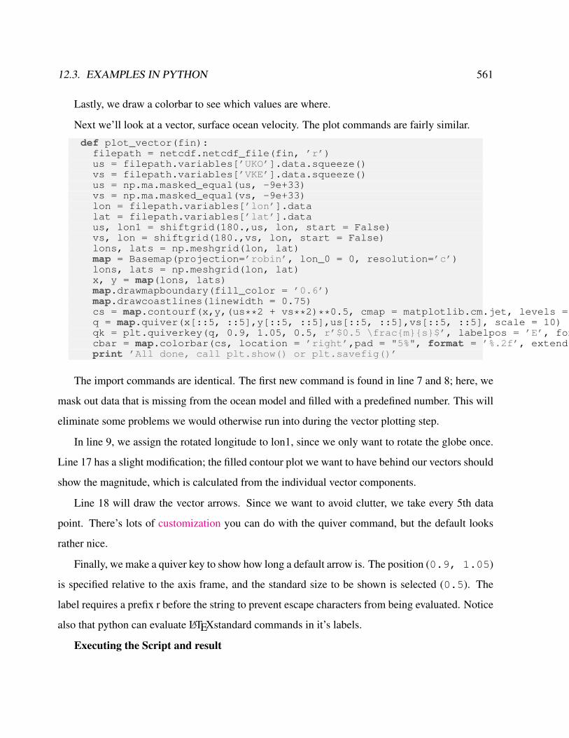
12.3. EXAMPLES IN PYTHON 561
Lastly, we draw a colorbar to see which values are where.
Next we’ll look at a vector, surface ocean velocity. The plot commands are fairly similar.
def plot_vector(fin):filepath = netcdf.netcdf_file(fin, ’r’)us = filepath.variables[’UKO’].data.squeeze()vs = filepath.variables[’VKE’].data.squeeze()us = np.ma.masked_equal(us, -9e+33)vs = np.ma.masked_equal(vs, -9e+33)lon = filepath.variables[’lon’].datalat = filepath.variables[’lat’].dataus, lon1 = shiftgrid(180.,us, lon, start = False)vs, lon = shiftgrid(180.,vs, lon, start = False)lons, lats = np.meshgrid(lon, lat)map = Basemap(projection=’robin’, lon_0 = 0, resolution=’c’)lons, lats = np.meshgrid(lon, lat)x, y = map(lons, lats)map.drawmapboundary(fill_color = ’0.6’)map.drawcoastlines(linewidth = 0.75)cs = map.contourf(x,y,(us**2 + vs**2)**0.5, cmap = matplotlib.cm.jet, levels = np.arange(0,0.5,0.01), extend = ’max’)q = map.quiver(x[::5, ::5],y[::5, ::5],us[::5, ::5],vs[::5, ::5], scale = 10)qk = plt.quiverkey(q, 0.9, 1.05, 0.5, r’$0.5 \fracms$’, labelpos = ’E’, fontproperties = ’weight’: ’bold’)cbar = map.colorbar(cs, location = ’right’,pad = "5%", format = ’%.2f’, extend = ’max’)print ’All done, call plt.show() or plt.savefig()’
The import commands are identical. The first new command is found in line 7 and 8; here, we
mask out data that is missing from the ocean model and filled with a predefined number. This will
eliminate some problems we would otherwise run into during the vector plotting step.
In line 9, we assign the rotated longitude to lon1, since we only want to rotate the globe once.
Line 17 has a slight modification; the filled contour plot we want to have behind our vectors should
show the magnitude, which is calculated from the individual vector components.
Line 18 will draw the vector arrows. Since we want to avoid clutter, we take every 5th data
point. There’s lots of customization you can do with the quiver command, but the default looks
rather nice.
Finally, we make a quiver key to show how long a default arrow is. The position (0.9, 1.05)
is specified relative to the axis frame, and the standard size to be shown is selected (0.5). The
label requires a prefix r before the string to prevent escape characters from being evaluated. Notice
also that python can evaluate LATEXstandard commands in it’s labels.
Executing the Script and result
562 CHAPTER 12. APPENDIX: NUMERICAL EXAMPLES
There are a couple of ways of executing the script, depending on how much you want to learn
about python. The functions themselves can be given to an interpret "as is" in the following man-
ner:$ python>>> execfile(’cosmos_plots.py’)
The functions will now be available to call, just remember to give the filename argument fin as a
string in single quotes.
Alternatively, you could use the ipython interpreter (i for interactive, not to be confused with
numerous apple products). This has several advantages, namely that is much more interactive and
has a build in help. Any object followed by a ? will yield a quick help, and a double ?? will show
the source code of the function. Start this one with:$ ipython -i cosmos_plots.py
The -i flag allows the session to be interactive after the script is executed. ipython also has a
very good traceback system for coding errors.
Finally you could enter the function codes line by line to see how the program evolves, either
as a function using def or as is. ipython offers the ability to see optional keyword arguments I
didn’t discuss. If you like the quality and look-and-feel of the plots produced with this script and
want to use python for additional graphing work, I’d recommend this to get a bit of practice. That
being said, if you find yourself making the same sorts of graphs over and over, it’s generally a
good idea to pack the bulk of the coding into a function with some manipulatable options to set
things like colors, font sizes, etc. This will save lots of work and looking through rather repetitive
codes. The plots that are produced by the program are shown below (Figs. 12.12, 12.13), barring
any implementation or porting errors.
12.3.2 Itation map
Calculate the map
zn+1 = z2n + c (12.1)

12.3. EXAMPLES IN PYTHON 563
20.00
22.00
24.00
26.00
28.00
30.00
32.00
34.00
36.00
38.00
Figure 12.12: Plot of ocean surface salinity using the python script.
Figure 12.13: As in Fig. 12.12, but for ocean surface horizonal velocity.
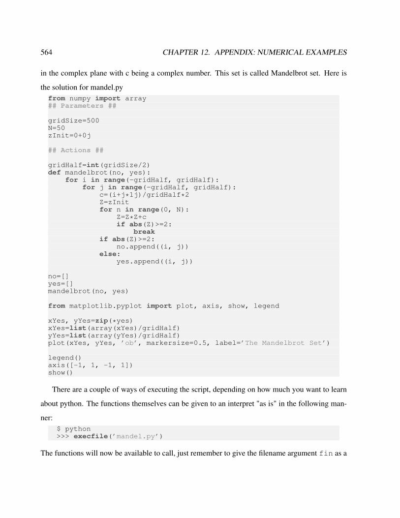
564 CHAPTER 12. APPENDIX: NUMERICAL EXAMPLES
in the complex plane with c being a complex number. This set is called Mandelbrot set. Here is
the solution for mandel.pyfrom numpy import array## Parameters ##
gridSize=500N=50zInit=0+0j
## Actions ##
gridHalf=int(gridSize/2)def mandelbrot(no, yes):
for i in range(-gridHalf, gridHalf):for j in range(-gridHalf, gridHalf):
c=(i+j*1j)/gridHalf*2Z=zInitfor n in range(0, N):
Z=Z*Z+cif abs(Z)>=2:
breakif abs(Z)>=2:
no.append((i, j))else:
yes.append((i, j))
no=[]yes=[]mandelbrot(no, yes)
from matplotlib.pyplot import plot, axis, show, legend
xYes, yYes=zip(*yes)xYes=list(array(xYes)/gridHalf)yYes=list(array(yYes)/gridHalf)plot(xYes, yYes, ’ob’, markersize=0.5, label=’The Mandelbrot Set’)
legend()axis([-1, 1, -1, 1])show()
There are a couple of ways of executing the script, depending on how much you want to learn
about python. The functions themselves can be given to an interpret "as is" in the following man-
ner:$ python>>> execfile(’mandel.py’)
The functions will now be available to call, just remember to give the filename argument fin as a

12.3. EXAMPLES IN PYTHON 565
string in single quotes.
Alternatively, you could use the ipython interpreter (i for interactive, not to be confused with
numerous apple products). This has several advantages, namely that is much more interactive and
has a build in help. Any object followed by a ? will yield a quick help, and a double ?? will show
the source code of the function. Start this one with:
$ ipython -i mandel.py
The -i flag allows the session to be interactive after the script is executed. ipython also has a
very good traceback system for coding errors.
Finally you could enter the function codes line by line to see how the program evolves, either
as a function using def or as is. ipython offers the ability to see optional keyword arguments.2
12.3.3 The Linear Advection Equation
The linear advection equation is simply:
at + uax = 0 (12.2)
where a(x, t) is some scalar quantity and u is the velocity at which it is advected (u > 0
advects to the right). The solution to Eq. 12.2 is to simply take the initial data, a(x, t = 0), and
displace it to the right at a speed u. The shape of the initial data is preserved in the advection.
Many hyperbolic systems of PDEs, e.g. the equations of hydrodynamics, can be written in a form
that looks like a system of (nonlinear) advection equations, so the advection equation provides
important insight into the methods used for these systems.
Exercise 87 – Linear advection analytic solution
2If you like the quality and look-and-feel of the plots produced with this script and want to use python for additionalgraphing work, it is recommend to do this to get a bit of practice. That being said, if you find yourself making thesame sorts of graphs over and over, it’s generally a good idea to pack the bulk of the coding into a function with somemanipulatable options to set things like colors, font sizes, etc. This will save lots of work and looking through ratherrepetitive codes.
566 CHAPTER 12. APPENDIX: NUMERICAL EXAMPLES
Show that a(x−ut) is a solution to Eq. 12.2 for any choice of a. This means that the solution
is constant along the lines x = ut (the curves along which the solution is constant are called the
characteristics).
First-order advection in 1-d and finite-differences
To get a flavor of the methods for advection, we will use a simple finite-difference discretization—
here, the domain is divided into a sequence of points where we store the solution. We will solve
Eq. 12.2 numerically by discretizing the solution at these points. The index i denotes the point’s lo-
cation, and ai denotes the discrete value of a(x) in zone i. The data in each zone can be initialized
as ai = a(xi). Figure 12.14 shows the grid.
We also need to discretize in time. We denote the time-level of the solution with a superscript,
so ani = a(xi, tn). For a fixed ∆t, time level n corresponds to a time of t = n∆t.
A simple first-order accurate discretization is:
an+1i − ani
∆t= −u
ani − ani−1
∆x(12.3)
This is an explicit method, since the new solution, an+1i , depends only on information at the old
time level, n.
Finally, we also need to specify a boundary condition for this. Our choice of spatial derivative
is one-sided—it uses information from the zone to the left of the zone we are updating. This is
because information is flowing from left to right in this problem (u > 0). This choice of the
derivative is called upwinding—this choice of derivative results in a stable method. Notice that if
we use Eq. 12.3 to update the data in the first zone inside the boundary, we need data to the left
of this zone—outside of the domain. This means that we need a single ghost point to implement
the boundary conditions for our method. The presence of the ghost points allow us to use the same
update equation (e.g. Eq. 12.3) for all zones in the domain.
The last piece of information needed to update the solution is the timestep, ∆t. It can be shown
that for the solution to be stable, the timestep must be less than the time it takes information to
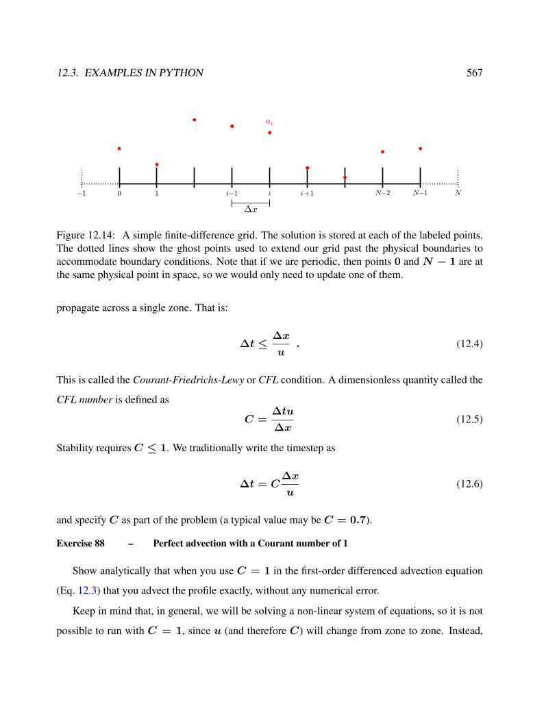
12.3. EXAMPLES IN PYTHON 567
−1 0 1 i−1 i i+1 N−2 N−1 N
ai
∆x
Figure 12.14: A simple finite-difference grid. The solution is stored at each of the labeled points.The dotted lines show the ghost points used to extend our grid past the physical boundaries toaccommodate boundary conditions. Note that if we are periodic, then points 0 and N − 1 are atthe same physical point in space, so we would only need to update one of them.
propagate across a single zone. That is:
∆t ≤∆x
u. (12.4)
This is called the Courant-Friedrichs-Lewy or CFL condition. A dimensionless quantity called the
CFL number is defined as
C =∆tu
∆x(12.5)
Stability requires C ≤ 1. We traditionally write the timestep as
∆t = C∆x
u(12.6)
and specify C as part of the problem (a typical value may be C = 0.7).
Exercise 88 – Perfect advection with a Courant number of 1
Show analytically that when you use C = 1 in the first-order differenced advection equation
(Eq. 12.3) that you advect the profile exactly, without any numerical error.
Keep in mind that, in general, we will be solving a non-linear system of equations, so it is not
possible to run with C = 1, since u (and therefore C) will change from zone to zone. Instead,
568 CHAPTER 12. APPENDIX: NUMERICAL EXAMPLES
one looks at the most restrictive timestep over all the zones and uses that for the entire system.
Exercise 89 – A 1-d finite-difference solver for linear advection
Write a code to solve the 1-d linear advection equation using the discretization of Eq. 12.3 on
the domain [0, 1] with u = 1 and periodic boundary conditions. For initial conditions, try both a
Gaussian profile and a top-hat:
a =
0 if x < 1/3
1 if 1/3 ≤ x < 2/3
0 if 2/3 ≤ x
(12.7)
Note: For a general treatment of boundary conditions, you would initialize the ghost points to their
corresponding periodic data and apply the difference equations to zones 0, . . . , N − 1. However,
for periodic BCs on this grid, points 0 andN − 1 are identical, so you could do the update in this
special case on points 1, . . . , N − 1 without the need for ghost points and then set a0 = aN−1
after the update.
Run you program for one or more periods (one period is T = 1/u) with several different CFL
numbers and notice that there is substantial numerical dissipation (see Figure 12.15).
Exercise 90 – FTCS and stability
You may think that using a centered-difference for the spatial derivative, ux ∼ (ui+1 −
ui−1)/(2∆x) would be more accurate. This method is called FTCS (forward-time, centered-
space). Try this. You will find that the solution is unconditionally unstable.
The classic method for understanding stability is to consider the growth of a single Fourier
mode in our discetization. That is, substitute in ani = Anejiθ, where j =√−1, and θ represents
a phase. A method is stable if |An+1/An| ≤ 1. Performing this with FTCS shows that no value
of C can make the method stable. Doing the same analysis for Eq. 12.3 would show that the
upwind method is stable for 0 ≤ C ≤ 1. (Note that this stability analysis only works for linear
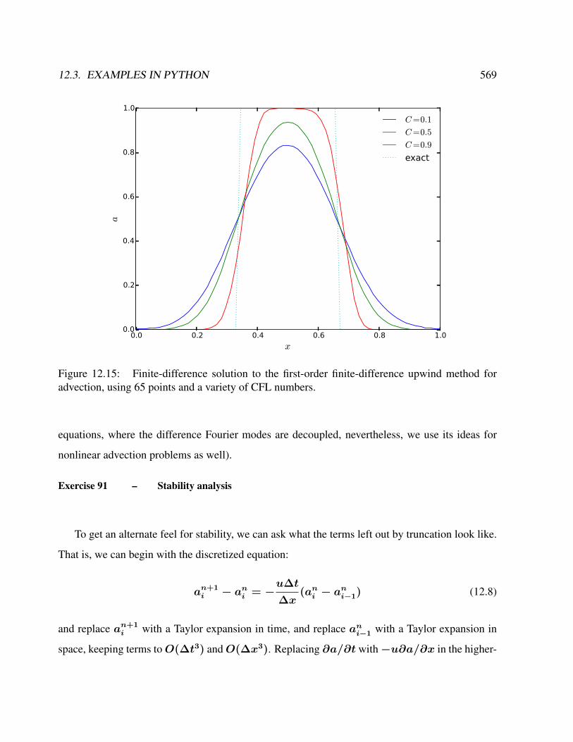
12.3. EXAMPLES IN PYTHON 569
0.0 0.2 0.4 0.6 0.8 1.0
x
0.0
0.2
0.4
0.6
0.8
1.0a
C=0.1
C=0.5
C=0.9
exact
Figure 12.15: Finite-difference solution to the first-order finite-difference upwind method foradvection, using 65 points and a variety of CFL numbers.
equations, where the difference Fourier modes are decoupled, nevertheless, we use its ideas for
nonlinear advection problems as well).
Exercise 91 – Stability analysis
To get an alternate feel for stability, we can ask what the terms left out by truncation look like.
That is, we can begin with the discretized equation:
an+1i − ani = −
u∆t
∆x(ani − a
ni−1) (12.8)
and replace an+1i with a Taylor expansion in time, and replace ani−1 with a Taylor expansion in
space, keeping terms toO(∆t3) andO(∆x3). Replacing ∂a/∂t with−u∂a/∂x in the higher-
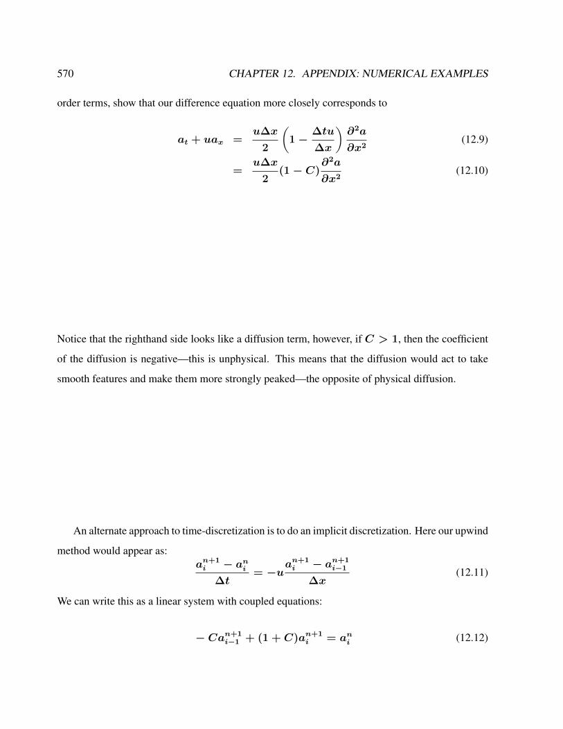
570 CHAPTER 12. APPENDIX: NUMERICAL EXAMPLES
order terms, show that our difference equation more closely corresponds to
at + uax =u∆x
2
(1−
∆tu
∆x
)∂2a
∂x2(12.9)
=u∆x
2(1− C)
∂2a
∂x2(12.10)
Notice that the righthand side looks like a diffusion term, however, if C > 1, then the coefficient
of the diffusion is negative—this is unphysical. This means that the diffusion would act to take
smooth features and make them more strongly peaked—the opposite of physical diffusion.
An alternate approach to time-discretization is to do an implicit discretization. Here our upwind
method would appear as:an+1i − ani
∆t= −u
an+1i − an+1
i−1
∆x(12.11)
We can write this as a linear system with coupled equations:
− Can+1i−1 + (1 + C)an+1
i = ani (12.12)

12.3. EXAMPLES IN PYTHON 571
In matrix form, solving for the points 1, . . . , N − 1, this is:
1 + C −C
−C 1 + C
−C 1 + C
−C 1 + C
. . . . . .
−C 1 + C
−C 1 + C
un+11
un+12
un+13
un+14
...
un+1N−2
un+1N−1
=
un1
un2
un3
un4
...
unN−2
unN−1
(12.13)
This requires a matrix solve—this makes implicit methods generally more expensive than explicit
methods. However, stability analysis would show that this implicit discretization is stable for any
choice of C. (But one must not confuse stability with accuracy—the most accurate solutions with
this method will still have a smallC). Also note that the form of the matrix will change depending
on the choice of boundary conditions. Figure 12.16 shows the result of solving this implicit system.
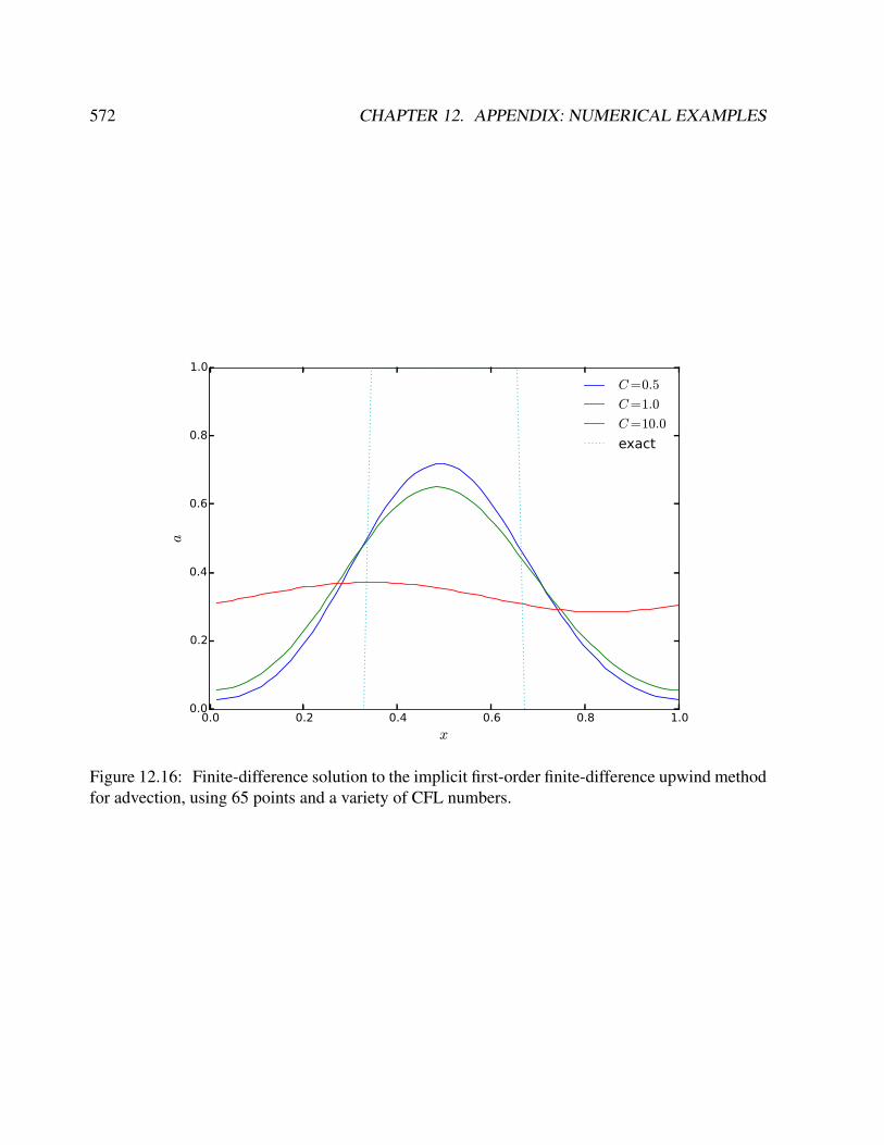
572 CHAPTER 12. APPENDIX: NUMERICAL EXAMPLES
0.0 0.2 0.4 0.6 0.8 1.0
x
0.0
0.2
0.4
0.6
0.8
1.0
a
C=0.5
C=1.0
C=10.0
exact
Figure 12.16: Finite-difference solution to the implicit first-order finite-difference upwind methodfor advection, using 65 points and a variety of CFL numbers.
Chapter 13
Appendix: Questions
13.1 Test for exam
1. Several questions about the course (40 points, for each Q 2 points).
Q1: Please clarify: On the Northern Hemisphere, particles tend to go to the right or left
relative to the direction of motion due to the Coriolis force?
Q2: The Coriolis parameter f is defined as
a) f = Ω cosϕ
b) f = 2Ω cosϕ
c) f = 2Ω sinϕ
d) f = βy
Q3: Please write down the equation of state for the ocean and atmosphere! (for the ocean:
linearized version)
Q4: What are the two dominant terms in the horizontal momentum balance for the large-
scale dynamics at mid-latitudes?
Q5: What is the hydrostatic approximation in the momentum equations?
573
574 CHAPTER 13. APPENDIX: QUESTIONS
Q6: a) What is the Fourier and Laplace transform of a function x(t) ?
b) What is the Fourier transform of the δ(t)-function?
Q7: Name three different dimensionless parameters which characterize the flow.
Q8: a) Please write down the Euler forward numerical scheme for ddtx = f(x) !
b) Consider also the special case f(x) = rx− x2!
Q9: Please write down the barotropic potential vorticity equation for large-scale motion!
Q10: Please write down the dispersion relation for Rossby and gravity waves!
Q11: What is the necessary condition for stability in a linear system
d
dtx = Ax
with real vector x and n× n matrixA?
... and for the analogous non-linear case ddtx = f(x)?
Q12: a) What is the definition of auto-correlation and auto-covariance?
b) How is the Fourier transformation of the auto-covariance called?
Q13: Explain the stochastic climate model.
Q14: Draw a schematic figure of the Atlantic Ocean meridional overturning!
Q15: Explain the Taylor-Proudman Theorem! (remember f = f0, barotropic circulation)
Q16: What is the dispersion relation for Kelvin waves? Make a sketch of the coastally
trapped Kelvin wave on the Northern Hemisphere ocean basin.
13.1. TEST FOR EXAM 575
Q17: Explain the difference between dispersive and non-dispersive waves! You could use
the ω(k) formula for Rossby and Kelvin waves.
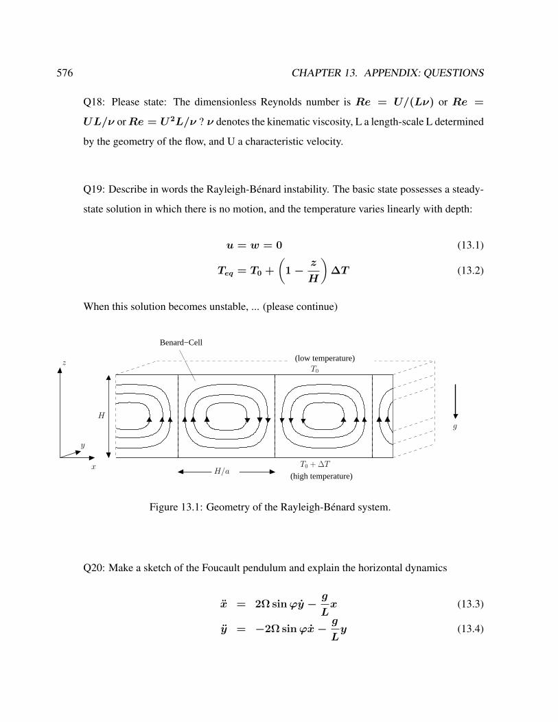
576 CHAPTER 13. APPENDIX: QUESTIONS
Q18: Please state: The dimensionless Reynolds number is Re = U/(Lν) or Re =
UL/ν orRe = U2L/ν ? ν denotes the kinematic viscosity, L a length-scale L determined
by the geometry of the flow, and U a characteristic velocity.
Q19: Describe in words the Rayleigh-Bénard instability. The basic state possesses a steady-
state solution in which there is no motion, and the temperature varies linearly with depth:
u = w = 0 (13.1)
Teq = T0 +
(1−
z
H
)∆T (13.2)
When this solution becomes unstable, ... (please continue)
Benard−Cell
(high temperature)
(low temperature)
H/a
H
T0 +∆Tx
y
zT0
g
Figure 13.1: Geometry of the Rayleigh-Bénard system.
Q20: Make a sketch of the Foucault pendulum and explain the horizontal dynamics
x = 2Ω sinϕy −g
Lx (13.3)
y = −2Ω sinϕx−g
Ly (13.4)

13.1. TEST FOR EXAM 577
2. Earth’s curvature (6 points)
I. The highest building on the campus of the University of Bremen is the so-called drop
tower with a height of h=110 metres (Fig. 13.2 upper panel). How far one can look
onto the horizon under good weather conditions?
Hint: Denote this distance by d. Remember the Earth’s radius R = 6378km and
apply Pythagoras.
II. Show that the rule-of-thumb d =√
2hR is a good approximation? (For h=10m this
means d=11 km.) Notice: When h is in m, d in km, the formula can be written as
d = 3.5√
hm km.
III. The town Bremerhaven which is at the North Sea is about 60 km north of Bremen.
How big must a tower in Bremen be in order to see the coast in Bremerhaven? (Fig.
13.2 lower panel).
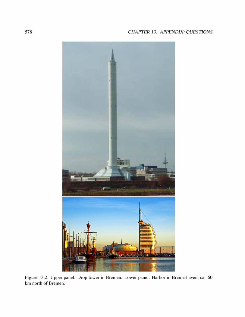
578 CHAPTER 13. APPENDIX: QUESTIONS
Figure 13.2: Upper panel: Drop tower in Bremen. Lower panel: Harbor in Bremerhaven, ca. 60km north of Bremen.
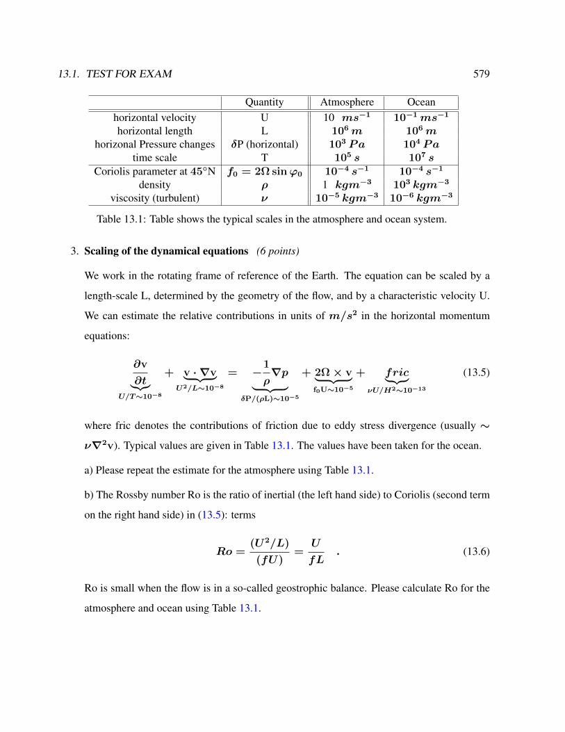
13.1. TEST FOR EXAM 579
Quantity Atmosphere Oceanhorizontal velocity U 10 ms−1 10−1ms−1
horizontal length L 106m 106mhorizonal Pressure changes δP (horizontal) 103 Pa 104 Pa
time scale T 105 s 107 sCoriolis parameter at 45N f0 = 2Ω sinϕ0 10−4 s−1 10−4 s−1
density ρ 1 kgm−3 103 kgm−3
viscosity (turbulent) ν 10−5 kgm−3 10−6 kgm−3
Table 13.1: Table shows the typical scales in the atmosphere and ocean system.
3. Scaling of the dynamical equations (6 points)
We work in the rotating frame of reference of the Earth. The equation can be scaled by a
length-scale L, determined by the geometry of the flow, and by a characteristic velocity U.
We can estimate the relative contributions in units of m/s2 in the horizontal momentum
equations:
∂v
∂t︸︷︷︸U/T∼10−8
+ v · ∇v︸ ︷︷ ︸U2/L∼10−8
= −1
ρ∇p︸ ︷︷ ︸
δP/(ρL)∼10−5
+ 2Ω× v︸ ︷︷ ︸f0U∼10−5
+ fric︸ ︷︷ ︸νU/H2∼10−13
(13.5)
where fric denotes the contributions of friction due to eddy stress divergence (usually ∼
ν∇2v). Typical values are given in Table 13.1. The values have been taken for the ocean.
a) Please repeat the estimate for the atmosphere using Table 13.1.
b) The Rossby number Ro is the ratio of inertial (the left hand side) to Coriolis (second term
on the right hand side) in (13.5): terms
Ro =(U2/L)
(fU)=
U
fL. (13.6)
Ro is small when the flow is in a so-called geostrophic balance. Please calculate Ro for the
atmosphere and ocean using Table 13.1.
580 CHAPTER 13. APPENDIX: QUESTIONS
4. Concept of dynamic similarity (8 points)
For the case of an incompressible flow, assuming the temperature effects are negligible and
external forces are neglected, the Navier-Stokes equations consist of conservation of mass
∇ · u = 0 (13.7)
and conservation of momentum
∂tu + (u · ∇)u = −1
ρ0
∇p+ ν∇2u (13.8)
where u is the velocity vector and p is the pressure, ν denotes the kinematic viscosity.
a) Show: The equations (13.7,13.8) can be made dimensionless by a length-scale L, de-
termined by the geometry of the flow, and by a characteristic velocity U. For example:
u = U · ud.
Note: the units of [ρ0] = kg/m3, [p] = kg/(ms2), and [p]/[ρ0] = m2/s2. Therefore
the pressure gradient term in (4.21) has the scaling U2/L.
b) Show: The scalings vanish completely in front of the terms except for the ∇2ud-term!
The dimensionless parameter is the Reynolds number and the only parameter left!
Remark: For large Reynolds numbers, the flow is turbulent. In most practical flows Re is
rather large (104 − 108), large enough for the flow to be turbulent.
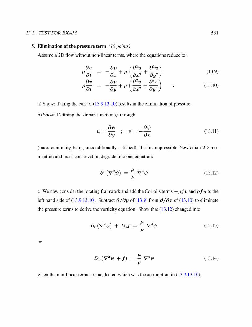
13.1. TEST FOR EXAM 581
5. Elimination of the pressure term (10 points)
Assume a 2D flow without non-linear terms, where the equations reduce to:
ρ∂u
∂t= −
∂p
∂x+ µ
(∂2u
∂x2+∂2u
∂y2
)(13.9)
ρ∂v
∂t= −
∂p
∂y+ µ
(∂2v
∂x2+∂2v
∂y2
). (13.10)
a) Show: Taking the curl of (13.9,13.10) results in the elimination of pressure.
b) Show: Defining the stream function ψ through
u =∂ψ
∂y; v = −
∂ψ
∂x(13.11)
(mass continuity being unconditionally satisfied), the incompressible Newtonian 2D mo-
mentum and mass conservation degrade into one equation:
∂t(∇2ψ
)=µ
ρ∇4ψ (13.12)
c) We now consider the rotating framwork and add the Coriolis terms−ρfv and ρfu to the
left hand side of (13.9,13.10). Subtract ∂/∂y of (13.9) from ∂/∂x of (13.10) to eliminate
the pressure terms to derive the vorticity equation! Show that (13.12) changed into
∂t(∇2ψ
)+ Dtf =
µ
ρ∇4ψ (13.13)
or
Dt
(∇2ψ + f
)=µ
ρ∇4ψ (13.14)
when the non-linear terms are neglected which was the assumption in (13.9,13.10).

582 CHAPTER 13. APPENDIX: QUESTIONS
Figure 13.3: f/h countours in the Weddell Sea for 34 · 106 years before present.
6. f/h contours (6 points)
For the Oligocene (about 34 Million years ago), the topography was reconstructed. The
f/h-contours are shown in Fig. 13.3. The length of the day was nearly as today.
a) Draw the barotropic streamlines in this figure?
b) How would the circulation look like if the Earth would rotate faster?
c) What will happen if we include a clockwise wind circulation on top of the Weddell Sea?
Please specify: Horizontal variations in this wind stress will cause vertical Ekman pumping
which presses down or Ekman suction which pulls up the water below the Ekman layer? Use
equation (13.17) !
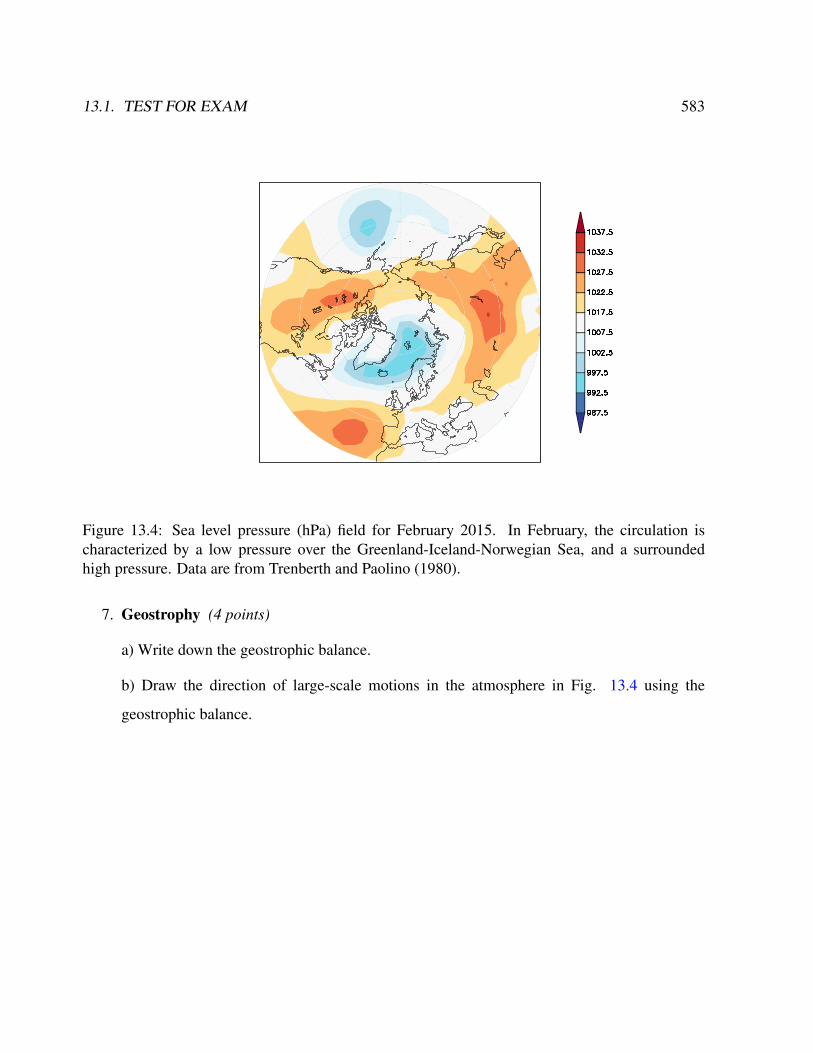
13.1. TEST FOR EXAM 583
Figure 13.4: Sea level pressure (hPa) field for February 2015. In February, the circulation ischaracterized by a low pressure over the Greenland-Iceland-Norwegian Sea, and a surroundedhigh pressure. Data are from Trenberth and Paolino (1980).
7. Geostrophy (4 points)
a) Write down the geostrophic balance.
b) Draw the direction of large-scale motions in the atmosphere in Fig. 13.4 using the
geostrophic balance.
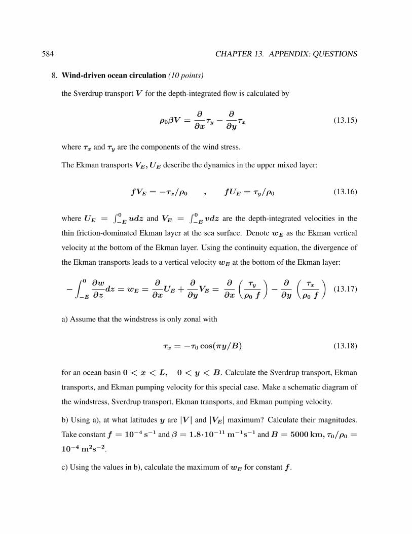
584 CHAPTER 13. APPENDIX: QUESTIONS
8. Wind-driven ocean circulation (10 points)
the Sverdrup transport V for the depth-integrated flow is calculated by
ρ0βV =∂
∂xτy −
∂
∂yτx (13.15)
where τx and τy are the components of the wind stress.
The Ekman transports VE, UE describe the dynamics in the upper mixed layer:
fVE = −τx/ρ0 , fUE = τy/ρ0 (13.16)
where UE =∫ 0
−E udz and VE =∫ 0
−E vdz are the depth-integrated velocities in the
thin friction-dominated Ekman layer at the sea surface. Denote wE as the Ekman vertical
velocity at the bottom of the Ekman layer. Using the continuity equation, the divergence of
the Ekman transports leads to a vertical velocity wE at the bottom of the Ekman layer:
−∫ 0
−E
∂w
∂zdz = wE =
∂
∂xUE +
∂
∂yVE =
∂
∂x
(τy
ρ0 f
)−
∂
∂y
(τx
ρ0 f
).(13.17)
a) Assume that the windstress is only zonal with
τx = −τ0 cos(πy/B) (13.18)
for an ocean basin 0 < x < L, 0 < y < B. Calculate the Sverdrup transport, Ekman
transports, and Ekman pumping velocity for this special case. Make a schematic diagram of
the windstress, Sverdrup transport, Ekman transports, and Ekman pumping velocity.
b) Using a), at what latitudes y are |V | and |VE| maximum? Calculate their magnitudes.
Take constant f = 10−4 s−1 and β = 1.8·10−11 m−1s−1 andB = 5000 km, τ0/ρ0 =
10−4 m2s−2.
c) Using the values in b), calculate the maximum of wE for constant f .
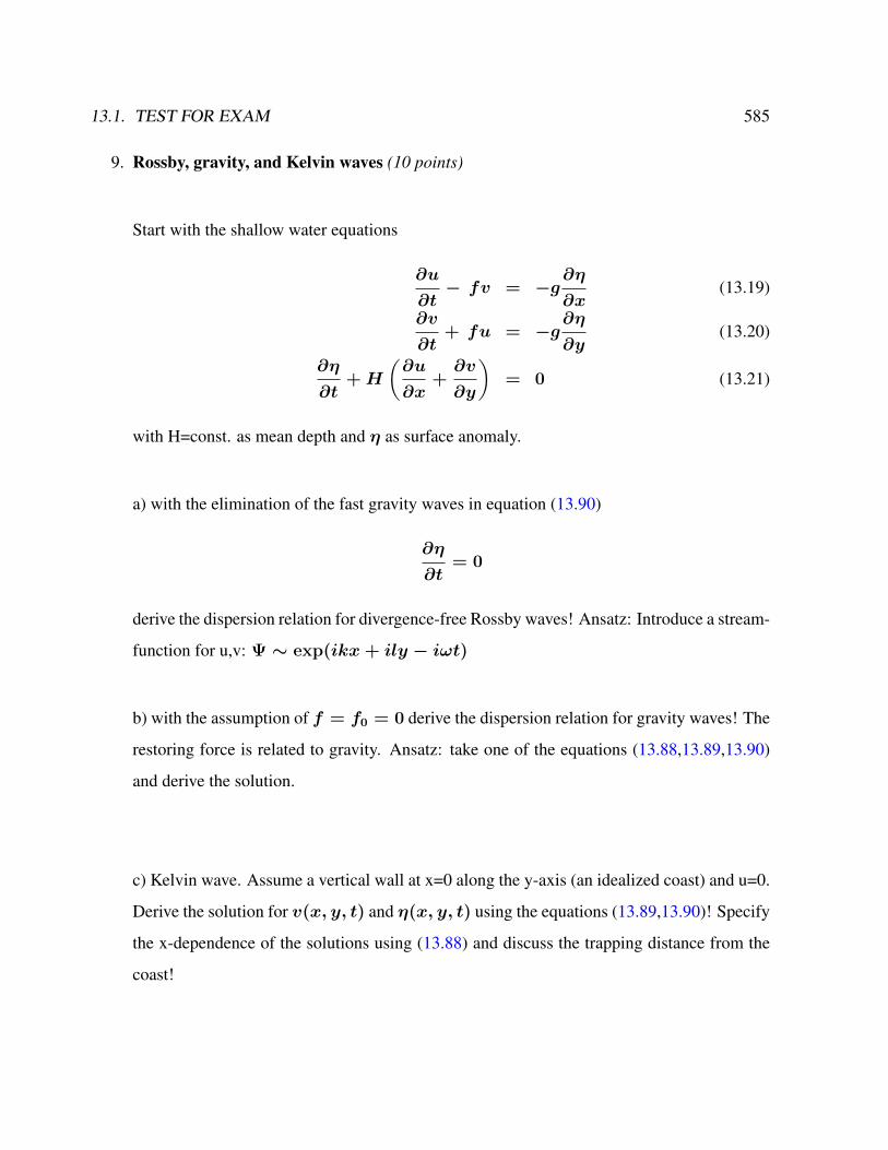
13.1. TEST FOR EXAM 585
9. Rossby, gravity, and Kelvin waves (10 points)
Start with the shallow water equations
∂u
∂t− fv = −g
∂η
∂x(13.19)
∂v
∂t+ fu = −g
∂η
∂y(13.20)
∂η
∂t+H
(∂u
∂x+∂v
∂y
)= 0 (13.21)
with H=const. as mean depth and η as surface anomaly.
a) with the elimination of the fast gravity waves in equation (13.90)
∂η
∂t= 0
derive the dispersion relation for divergence-free Rossby waves! Ansatz: Introduce a stream-
function for u,v: Ψ ∼ exp(ikx+ ily − iωt)
b) with the assumption of f = f0 = 0 derive the dispersion relation for gravity waves! The
restoring force is related to gravity. Ansatz: take one of the equations (13.88,13.89,13.90)
and derive the solution.
c) Kelvin wave. Assume a vertical wall at x=0 along the y-axis (an idealized coast) and u=0.
Derive the solution for v(x, y, t) and η(x, y, t) using the equations (13.89,13.90)! Specify
the x-dependence of the solutions using (13.88) and discuss the trapping distance from the
coast!
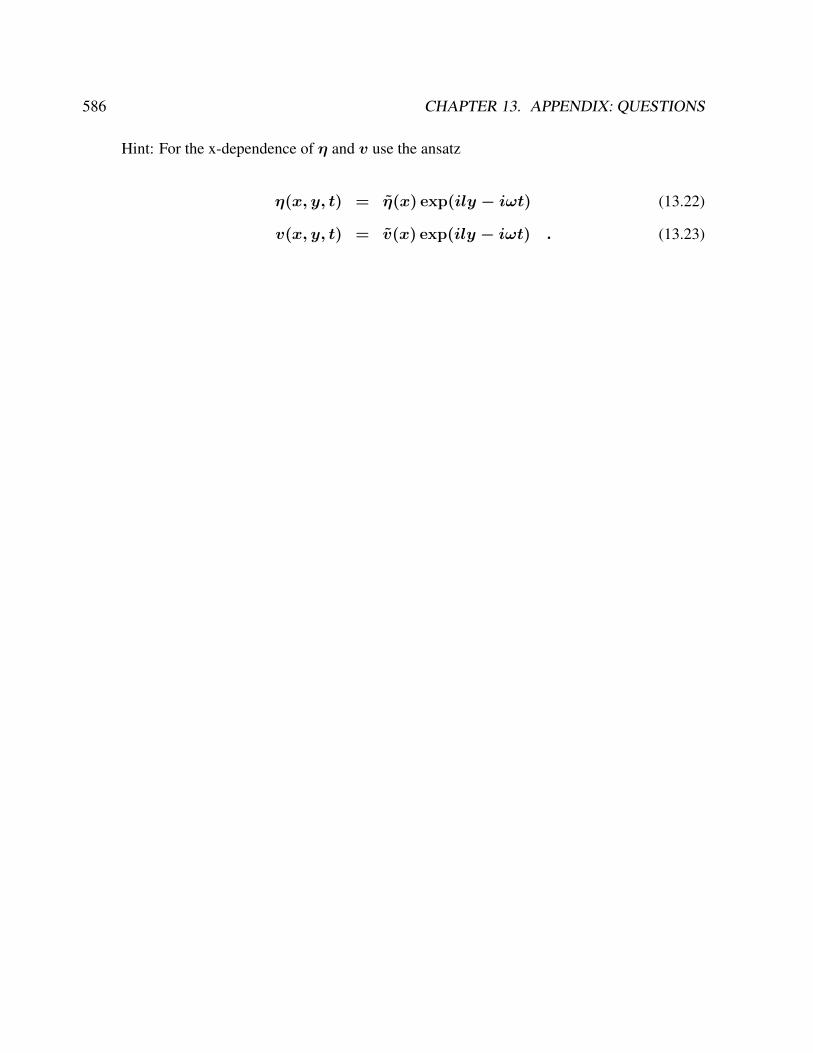
586 CHAPTER 13. APPENDIX: QUESTIONS
Hint: For the x-dependence of η and v use the ansatz
η(x, y, t) = η(x) exp(ily − iωt) (13.22)
v(x, y, t) = v(x) exp(ily − iωt) . (13.23)
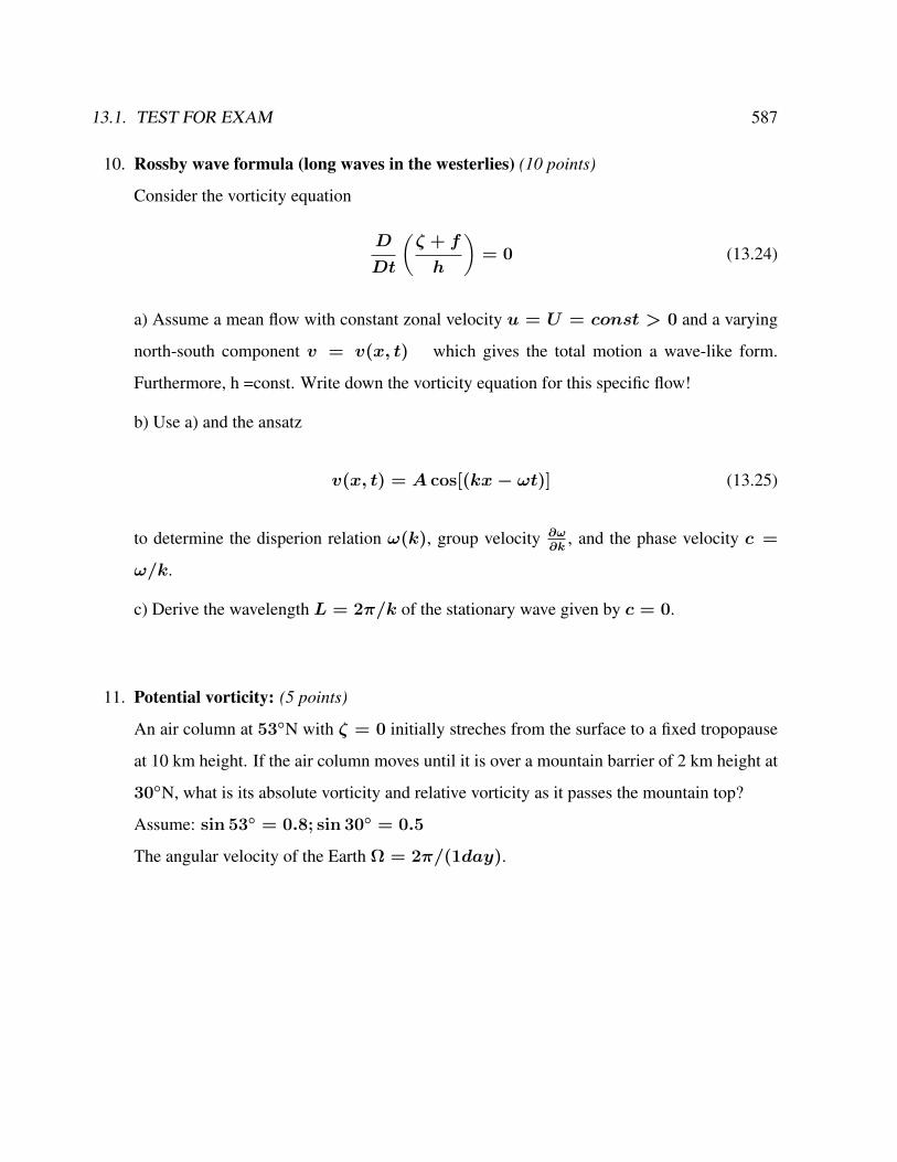
13.1. TEST FOR EXAM 587
10. Rossby wave formula (long waves in the westerlies) (10 points)
Consider the vorticity equation
D
Dt
(ζ + f
h
)= 0 (13.24)
a) Assume a mean flow with constant zonal velocity u = U = const > 0 and a varying
north-south component v = v(x, t) which gives the total motion a wave-like form.
Furthermore, h =const. Write down the vorticity equation for this specific flow!
b) Use a) and the ansatz
v(x, t) = A cos[(kx− ωt)] (13.25)
to determine the disperion relation ω(k), group velocity ∂ω∂k
, and the phase velocity c =
ω/k.
c) Derive the wavelength L = 2π/k of the stationary wave given by c = 0.
11. Potential vorticity: (5 points)
An air column at 53N with ζ = 0 initially streches from the surface to a fixed tropopause
at 10 km height. If the air column moves until it is over a mountain barrier of 2 km height at
30N, what is its absolute vorticity and relative vorticity as it passes the mountain top?
Assume: sin 53 = 0.8; sin 30 = 0.5
The angular velocity of the Earth Ω = 2π/(1day).
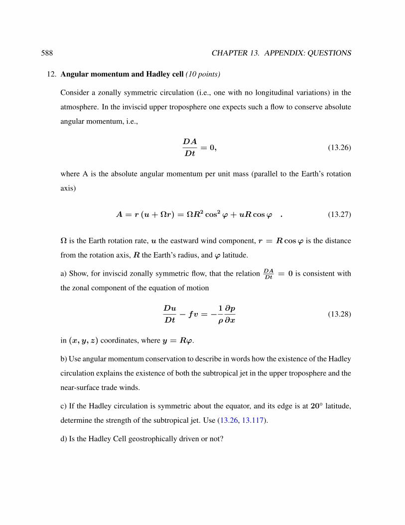
588 CHAPTER 13. APPENDIX: QUESTIONS
12. Angular momentum and Hadley cell (10 points)
Consider a zonally symmetric circulation (i.e., one with no longitudinal variations) in the
atmosphere. In the inviscid upper troposphere one expects such a flow to conserve absolute
angular momentum, i.e.,
DA
Dt= 0, (13.26)
where A is the absolute angular momentum per unit mass (parallel to the Earth’s rotation
axis)
A = r (u+ Ωr) = ΩR2 cos2 ϕ+ uR cosϕ . (13.27)
Ω is the Earth rotation rate, u the eastward wind component, r = R cosϕ is the distance
from the rotation axis,R the Earth’s radius, and ϕ latitude.
a) Show, for inviscid zonally symmetric flow, that the relation DADt
= 0 is consistent with
the zonal component of the equation of motion
Du
Dt− fv = −
1
ρ
∂p
∂x(13.28)
in (x, y, z) coordinates, where y = Rϕ.
b) Use angular momentum conservation to describe in words how the existence of the Hadley
circulation explains the existence of both the subtropical jet in the upper troposphere and the
near-surface trade winds.
c) If the Hadley circulation is symmetric about the equator, and its edge is at 20 latitude,
determine the strength of the subtropical jet. Use (13.26, 13.117).
d) Is the Hadley Cell geostrophically driven or not?

13.1. TEST FOR EXAM 589
13. Analytical EBM (5 points)
The temperature is described as T (y) and the heat transport (sensible, latent and ocean) is
modelled as diffusion:
Cp ∂tT + k ∂2yT = (1− α)Qtop
S − (A+B T ) (13.29)
a) Show the solution if the planetary albedo α is chosen as a constant parameter. Hint: Use
the ansatz with a global component and a latitude component
T (y, t) = T0(t) + T1(t) · cos(ay) (13.30)
QtopS = Q0 +Q1 · cos(ay) (13.31)
with y = Rϕ and a = 2/R.
b) Determine the solution with the assumption of planetary albedo α deprending on the
global temperature:
α(T ) = α0 + α1 · T0 (13.32)
Hint: Separate the dynamics for T0 and T1 and use
∫ 90
−90cos(2ϕ) dϕ = 0 (13.33)
590 CHAPTER 13. APPENDIX: QUESTIONS
14. Bifurcation: (6 points)
Consider the differential equation
d
dtx = rx (1− x)2 (13.34)
a) Calculate the bifurcation with respect to the parameter r and draw the bifurcation diagram!
b) Discuss the stability in terms of the potential V(x) ! (remember that the potential can be
calculated from the right hand side of equation (13.34): -V’ = rhs of (13.34))
c) Discuss the stability in terms of the graphical method!
d) Which types of bifurcations do you know?
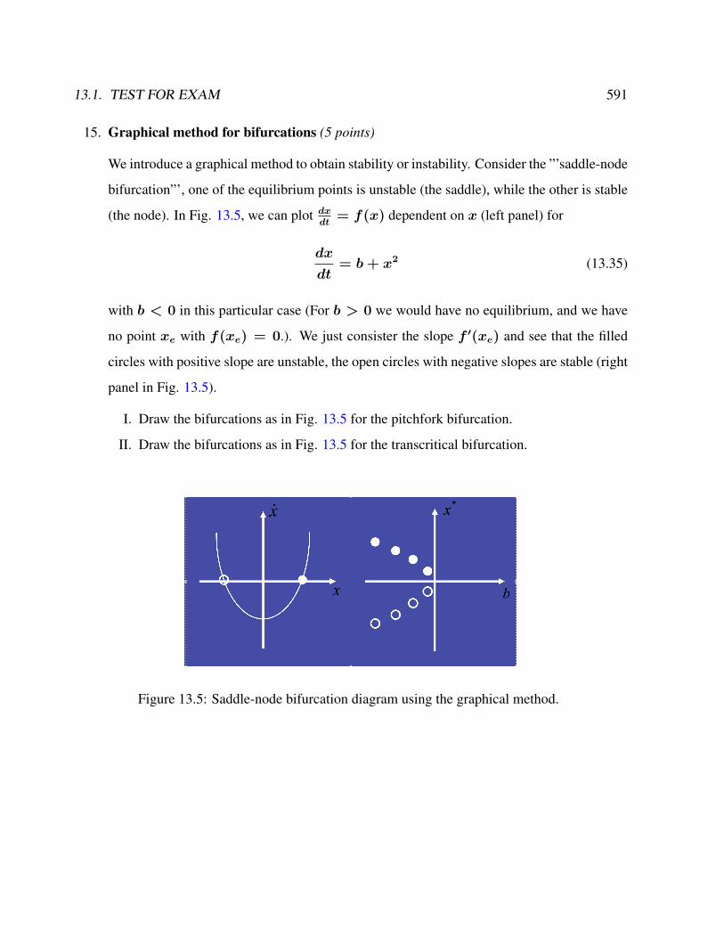
13.1. TEST FOR EXAM 591
15. Graphical method for bifurcations (5 points)
We introduce a graphical method to obtain stability or instability. Consider the ”’saddle-node
bifurcation”’, one of the equilibrium points is unstable (the saddle), while the other is stable
(the node). In Fig. 13.5, we can plot dxdt
= f(x) dependent on x (left panel) for
dx
dt= b+ x2 (13.35)
with b < 0 in this particular case (For b > 0 we would have no equilibrium, and we have
no point xe with f(xe) = 0.). We just consister the slope f ′(xe) and see that the filled
circles with positive slope are unstable, the open circles with negative slopes are stable (right
panel in Fig. 13.5).
I. Draw the bifurcations as in Fig. 13.5 for the pitchfork bifurcation.
II. Draw the bifurcations as in Fig. 13.5 for the transcritical bifurcation.
Figure 13.5: Saddle-node bifurcation diagram using the graphical method.
592 CHAPTER 13. APPENDIX: QUESTIONS
16. Stochastic climate model (8 points)
Imagine that the temperature of the ocean mixed layer of depth h is governed by
dT
dt= −λT +
Qnet
γO, (13.36)
where coefficient γO is given by the heat capacity cpρh, and λ is the typical damping rate
of a temperature anomaly. The air-sea fluxes due to weather systems are represented by a
white-noise process Qnet = Qωeiωt where Qω is the amplitude of the random forcing at
frequency ω. Q∗ is the complex conjugate.
a) Solve Eq. 13.104 for the temperature response T = Tωeiωt and hence show that:
Tω =Qω
γO (λ+ iω)(13.37)
b) Show that it has a spectral density Tω T ∗ω is given by:
T T ∗ =Q Q∗
γ2O (λ2 + ω2)
(13.38)
and the spectrum
S(ω) =< T T ∗ >=1
γ2O (λ2 + ω2)
. (13.39)
The brackets < · · · > denote the ensemble mean. Make a sketch of the spectrum using a
log-log plot and show that fluctuations with a frequency greater than λ are damped.
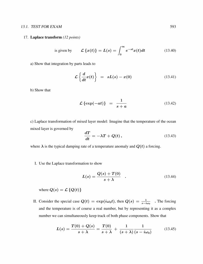
13.1. TEST FOR EXAM 593
17. Laplace transform (12 points)
is given by Lx(t) = L(s) =
∫ ∞0
e−stx(t)dt (13.40)
a) Show that integration by parts leads to
Ld
dtx(t)
= sL(s)− x(0) (13.41)
b) Show that
Lexp(−at) =1
s+ a(13.42)
c) Laplace transformation of mixed layer model: Imagine that the temperature of the ocean
mixed layer is governed bydT
dt= −λT +Q(t) , (13.43)
where λ is the typical damping rate of a temperature anomaly andQ(t) a forcing.
I. Use the Laplace transformation to show
L(s) =Q(s) + T (0)
s+ λ. (13.44)
whereQ(s) = LQ(t)
II. Consider the special case Q(t) = exp(iω0t), then Q(s) = 1s−iω0
. The forcing
and the temperature is of course a real number, but by representing it as a complex
number we can simultaneously keep track of both phase components. Show that
L(s) =T (0) +Q(s)
s+ λ=T (0)
s+ λ+
1
(s+ λ)
1
(s− iω0)(13.45)
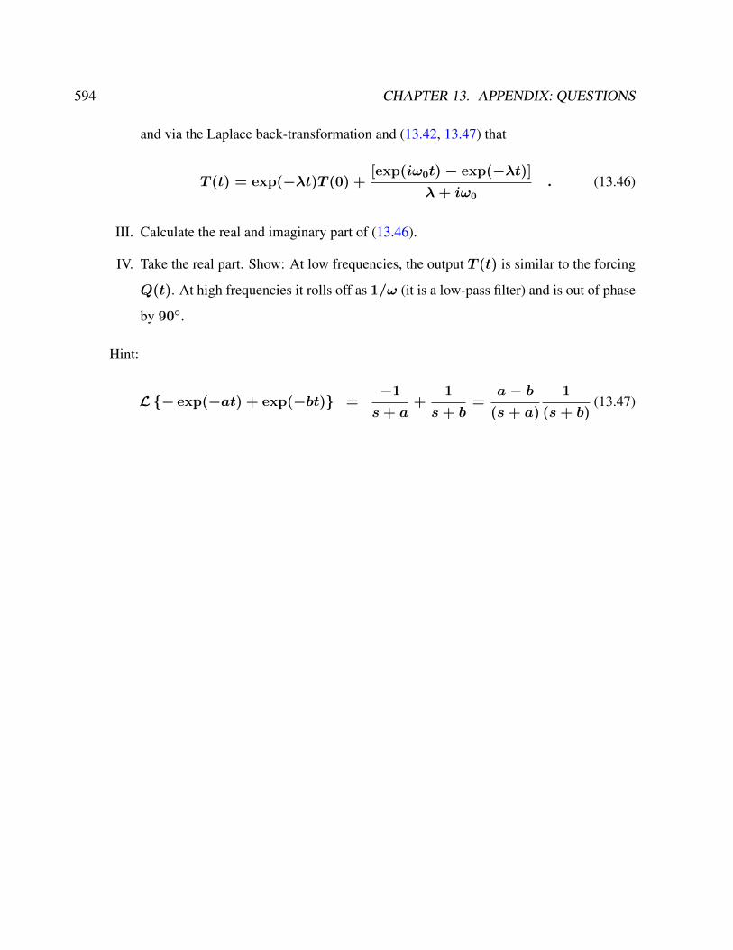
594 CHAPTER 13. APPENDIX: QUESTIONS
and via the Laplace back-transformation and (13.42, 13.47) that
T (t) = exp(−λt)T (0) +[exp(iω0t)− exp(−λt)]
λ+ iω0
. (13.46)
III. Calculate the real and imaginary part of (13.46).
IV. Take the real part. Show: At low frequencies, the output T (t) is similar to the forcing
Q(t). At high frequencies it rolls off as 1/ω (it is a low-pass filter) and is out of phase
by 90.
Hint:
L− exp(−at) + exp(−bt) =−1
s+ a+
1
s+ b=
a− b(s+ a)
1
(s+ b)(13.47)

13.1. TEST FOR EXAM 595
18. Climate sensitivity and variability in the Stochastic Climate Model (8 points)
Imagine that the temperature of the ocean mixed layer of depth h is governed by
dT
dt= −λT +Qnet + f(t) , (13.48)
where the air-sea fluxes due to weather systems are represented by a white-noise process
with zero average < Qnet >= 0 and δ-correlated in time < Qnet(t)Qnet(t + τ ) >=
δ(τ ). The function f(t) is a time dependent deterministic forcing. Assume furthermore
that f(t) = c · u(t) with u(t) as unit step or the so-called Heaviside step function.
a) Show via Laplace transform that
< T (t) > = L−1L(s)(t) = L−1
< T (0) >
s+ λ+c
s·
1
s+ λ
(13.49)
= T (0) · exp(−λt) +c
λ(1− exp(−λt)) (13.50)
b) Show that the equilibrium response is
∆T = limt→∞
< T (t) >=c
λ. (13.51)
c) Calculate the spectrum of (13.48) for f(t) = 0 ! What is the relationship of the dissipa-
tion (through λ ) and the fluctuations (through the spectrum S(ω)) ?
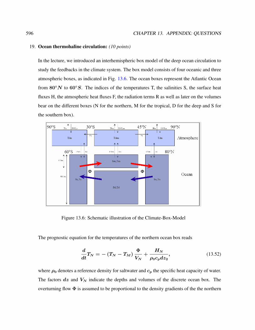
596 CHAPTER 13. APPENDIX: QUESTIONS
19. Ocean thermohaline circulation: (10 points)
In the lecture, we introduced an interhemispheric box model of the deep ocean circulation to
study the feedbacks in the climate system. The box model consists of four oceanic and three
atmospheric boxes, as indicated in Fig. 13.6. The ocean boxes represent the Atlantic Ocean
from 80N to 60S. The indices of the temperatures T, the salinities S, the surface heat
fluxes H, the atmospheric heat fluxes F, the radiation terms R as well as later on the volumes
bear on the different boxes (N for the northern, M for the tropical, D for the deep and S for
the southern box).
Figure 13.6: Schematic illustration of the Climate-Box-Model
The prognostic equation for the temperatures of the northern ocean box reads
d
dtTN = − (TN − TM)
Φ
VN+
HN
ρ0cpdz2
, (13.52)
where ρ0 denotes a reference density for saltwater and cp the specific heat capacity of water.
The factors dz and VN indicate the depths and volumes of the discrete ocean box. The
overturning flow Φ is assumed to be proportional to the density gradients of the the northern
13.1. TEST FOR EXAM 597
and the southern box:
Φ = c [−α (TN − TS) + β (SN − SS)] (13.53)
a) Explain the terms in equation (13.52).
b) Write down the associated equations for salinities! (only for SN ).
c) Explain in words what will happen if the high-latitude salinity SN is reduced (e.g., due to
melting of Greenland).
20. Short programming questions. (6 points)
Write down the output for the following R-commands:
a) 0:10
b) a<-c(0,5,3,4); mean(a)
c) max(a)-min(a)
d) paste("The mean value of a is",mean(a),"for sure",sep="_")
e) a*2+c(1,1,1,0)
f) my.fun<-function(n)return(n*n+1)
my.fun(10)-my.fun(1)
21. Interpretation of SST correlation maps and modes of variability (5 points)
The two maps show correlations with local climate indices (Fig. 13.8).
a) Which climate modes correspond to the sea surface temperature correlation-maps?
b) Describe and draw schematically the associated sea level pressure patterns!
c) What are the dominant time scales and dominant seasons for these two modes in the
climate system?
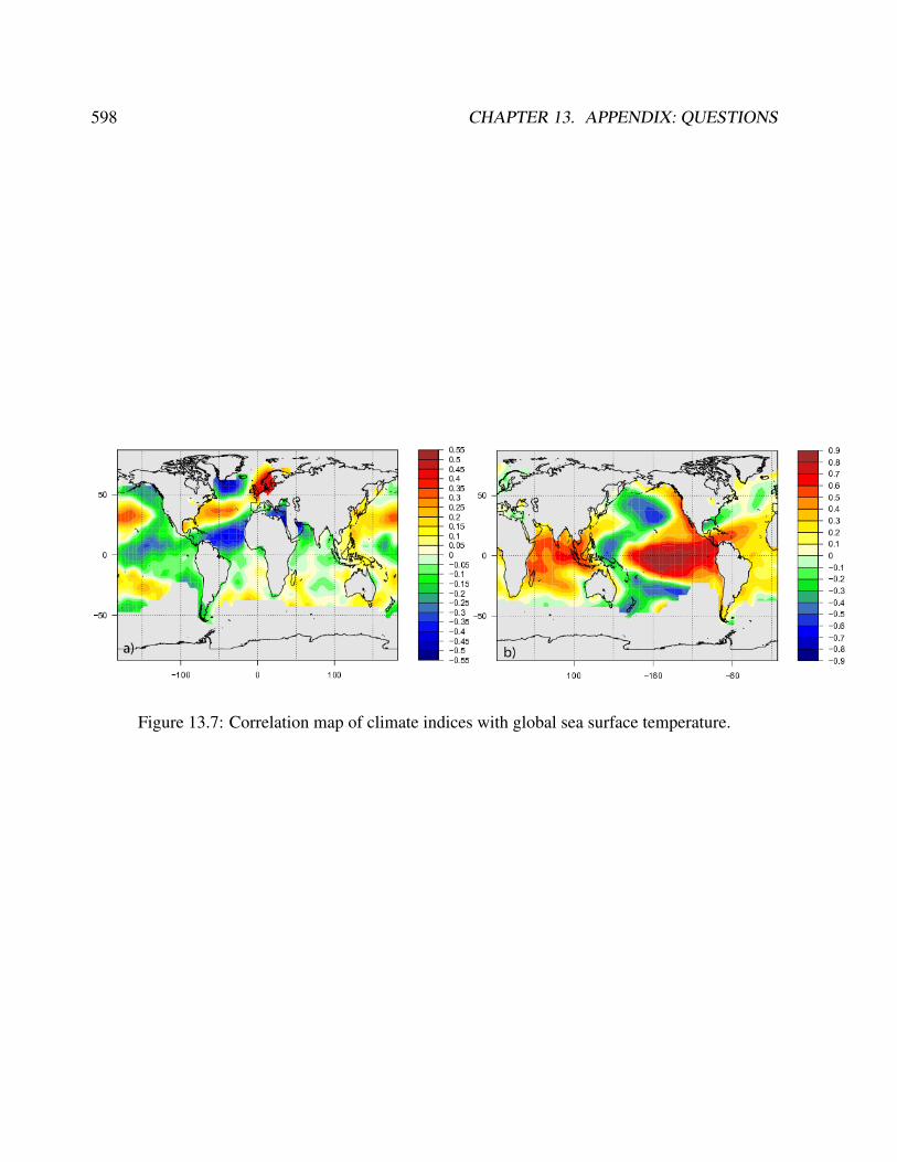
598 CHAPTER 13. APPENDIX: QUESTIONS
Figure 13.7: Correlation map of climate indices with global sea surface temperature.
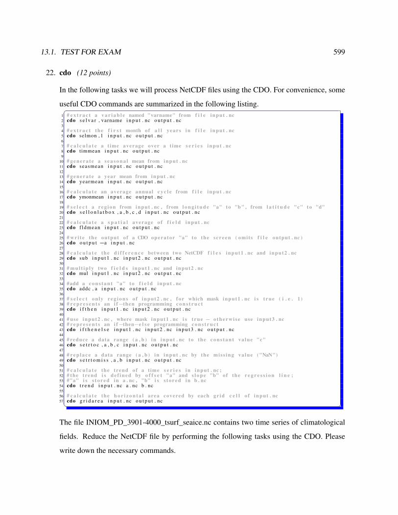
13.1. TEST FOR EXAM 599
22. cdo (12 points)
In the following tasks we will process NetCDF files using the CDO. For convenience, some
useful CDO commands are summarized in the following listing.1 # e x t r a c t a v a r i a b l e named "varname" from f i l e input . nc2 cdo s e l v a r , varname i n p u t . nc o u t p u t . nc34 # e x t r a c t the f i r s t month of a l l years in f i l e input . nc5 cdo selmon , 1 i n p u t . nc o u t p u t . nc67 # c a l c u l a t e a t ime average over a time s e r i e s input . nc8 cdo t immean i n p u t . nc o u t p u t . nc9
10 # g e n e r a t e a s e a s o n a l mean from input . nc11 cdo seasmean i n p u t . nc o u t p u t . nc1213 # g e n e r a t e a year mean from input . nc14 cdo yearmean i n p u t . nc o u t p u t . nc1516 # c a l c u l a t e an average annual c y c l e from f i l e input . nc17 cdo ymonmean i n p u t . nc o u t p u t . nc1819 # s e l e c t a reg io n from input . nc , from l o n g i t u d e "a" to "b" , from l a t i t u d e "c" to "d"20 cdo s e l l o n l a t b o x , a , b , c , d i n p u t . nc o u t p u t . nc2122 # c a l c u l a t e a s p a t i a l average of f i e l d input . nc23 cdo f ldmean i n p u t . nc o u t p u t . nc2425 # w r i t e the output o f a CDO operator "a" to the s cr ee n ( omits f i l e output . nc )26 cdo o u t p u t −a i n p u t . nc2728 # c a l c u l a t e the d i f f e r e n c e between two NetCDF f i l e s input1 . nc and input2 . nc29 cdo sub i n p u t 1 . nc i n p u t 2 . nc o u t p u t . nc3031 # m u l t i p l y two f i e l d s input1 . nc and input2 . nc32 cdo mul i n p u t 1 . nc i n p u t 2 . nc o u t p u t . nc3334 #add a c o n s t a n t "a" to f i e l d input . nc35 cdo addc , a i n p u t . nc o u t p u t . nc3637 # s e l e c t only r e g i o n s o f input2 . nc , f o r which mask input1 . nc i s t rue ( i . e . 1 )38 # r e p r e s e n t s an i f−then programming c o n s t r u c t39 cdo i f t h e n i n p u t 1 . nc i n p u t 2 . nc o u t p u t . nc4041 # use input2 . nc , where mask input1 . nc i s t rue − o t h e r w i s e use input3 . nc42 # r e p r e s e n t s an i f−then−e l s e programming c o n s t r u c t43 cdo i f t h e n e l s e i n p u t 1 . nc i n p u t 2 . nc i n p u t 3 . nc o u t p u t . nc4445 # reduce a data range ( a , b ) in input . nc to the c o n s t a n t va lue "c"46 cdo s e t r t o c , a , b , c i n p u t . nc o u t p u t . nc4748 # r e p l a c e a data range ( a , b ) in input . nc by the miss ing va lue ("NaN")49 cdo s e t r t o m i s s , a , b i n p u t . nc o u t p u t . nc5051 # c a l c u l a t e the trend of a t ime s e r i e s in input . nc ;52 # the trend i s d e f i n e d by o f f s e t "a" and s l o p e "b" of the r e g r e s s i o n l i n e ;53 #"a" i s s t o r e d in a . nc , "b" i s s t o r e d in b . nc54 cdo t r e n d i n p u t . nc a . nc b . nc5556 # c a l c u l a t e the h o r i z o n t a l area covered by each gr id c e l l o f input . nc57 cdo g r i d a r e a i n p u t . nc o u t p u t . nc The file INIOM_PD_3901-4000_tsurf_seaice.nc contains two time series of climatological
fields. Reduce the NetCDF file by performing the following tasks using the CDO. Please
write down the necessary commands.
600 CHAPTER 13. APPENDIX: QUESTIONS
• Task 1: Split the data set in two separate data sets, one for variable tsurf, one for
variable seaice.
• Task 2: Calculate a time average over the full time period available in each of the
separate data sets created in Task 1.
• Task 3: For each of the data sets created in Task 1 calculate an average annual cycle
that is representative for the full time period of the time series.
Hint: In order to create an average annual cycle (multi-year monthly mean), you have
to generate a new data set that contains twelve months. The data stored in each time
step (month) n of this new data set omust represent the average over all corresponding
months contained in the full time series of the initial data set i, i.e. (see CDO docu-
mentation):
o (n, x) = mean (i (t, x) ,month(i(t)) == n) ; n ∈ (1, 12)
• Task 4: Calculate a seasonal mean from the average annual cycle of both variables
retrieved in Task 3.
• Task 5: Select only the Northern Hemisphere of the time average retrieved in Task 2.
• Task 6: Calculate the global average temperature from the data set retrieved in Task 2.
13.2 Other questions
1. Ocean thermohaline circulation: Consider a geostrophic flow (u, v)
−fv = −1
ρ0
∂p
∂x(13.54)
fu = −1
ρ0
∂p
∂y(13.55)
with pressure p(x, y, z, t).

13.2. OTHER QUESTIONS 601
a) Use the hydrostatic approximation ∂p∂z
and equation (13.110) in order to derive the meridional
overturning stream function Φ(y, z). Φ is defined via
Φ(y, z) =
∫ z
0
∂Φ
∂zdz (13.56)
∂Φ
∂z=
∫ xw
xe
v(x, y, z) dx (zonally integrated transport), (13.57)
where xe and xw are the eastward and westward boundaries in the ocean basin (think e.g. of the
Atlantic Ocean). Units of Φ arem3s−1. At the surface Φ(y, 0) = 0.
b) Another definition of Φ(y, z) is via
−∂Φ
∂y=
∫ xw
xe
w dx (13.58)
with vertical velocity w. Why is the definition of a streamfunction useful? What is the physical
law and equation behind that?
c) Consider now a water planet with flat bottom (unlike the Earth). Provide the meridional over-
turning stream function Φ(y, z) in this ocean! Is there a meridional transport due to geostrophy
in the atmosphere?
2. Ekman layer: Consider a geostrophic flow (u, v)
−fv = −1
ρ0
∂p
∂x(13.59)
fu = −1
ρ0
∂p
∂y(13.60)
602 CHAPTER 13. APPENDIX: QUESTIONS
with pressure p(x, y, t). The boundary-layer equations are then
−f(v − v) = ν∂2u
∂z2(13.61)
f(u− u) = ν∂2v
∂z2. (13.62)
The boundary conditions are specified to be at the surface
ρ0ν∂u
∂z= τx (13.63)
ρ0ν∂v
∂z= τ y (13.64)
and for z → −∞ : u = u, v = v .
a) Calculate the flow (u,v) as the departure from the interior flow (u, v)!
b) Calculate the net wind-driven horizontal transport through integration
V =
∫ 0
−∞dz(v − v) (13.65)
U =
∫ 0
−∞dz(u− u) . (13.66)
What is the direction of U and V in terms of the surface wind stress τ ?
c) For the case f = f0 of constant Coriolis parameter, determine the divergence of the flow
∫ 0
−∞dz(
∂u
∂x+∂v
∂y) (13.67)
which is identical to the vertical velocity across the Ekman layer (since w(0)=0).
3. Energy
13.2. OTHER QUESTIONS 603
Start with the shallow water equations
∂u
∂t− fv = −g
∂η
∂x(13.68)
∂v
∂t+ fu = −g
∂η
∂y(13.69)
∂η
∂t+H
(∂u∂x
+∂v
∂y
)= 0 (13.70)
with H=const. as mean depth and η as surface anomaly.
a) Show that the total energy throughout the shallow water column satisfies
∂(PE +KE)
∂t+∇ · F = 0, (13.71)
where
KE =1
2ρH(u2 + v2), PE =
1
2ρgη2, and vector F = ρgH (uη, vη). (13.72)
b) Determine the dispersion relation for plane wave solutions to this problem of the form
(u0, v0, η0) exp i(kx+ ly − ωt) (13.73)
and express u0, v0 in terms of η0.
c) Let
exp i(kx+ ly − ωt) = eiΨ (13.74)
and let an overbar denote the average of the quantity over a full phase of the wave, i.e., over the
interval 0 ≤ Ψ ≤ 2π. Show that
KE
PE=ω2 + f2
ω2 − f2. (13.75)
604 CHAPTER 13. APPENDIX: QUESTIONS
Under what circumstances is there an equipartion of energy KE = PE?
30 points
4. Barotropic wave:
A jet stream of speed 50m/s meanders with 6000 km wavelength and 1500 km amplitude, centred
at 45N. Compute the path (the meridional displacement) of the barotropic wave and find the
phase speed. The path can be approximated:
y = A cos[2π(x− ct)/λ] (13.76)
2Ω/Rearth = 2.29 · 10−11m/s (13.77)
c0 = −β(λ
2π)2 (13.78)
Write:
β =?
c =?
y(x) =?.
30 points
5) Ice Dynamics:
a) The forces, acting on a block of ice are given in terms of stresses. What are the two stress
components and how is the stress tensor defined.
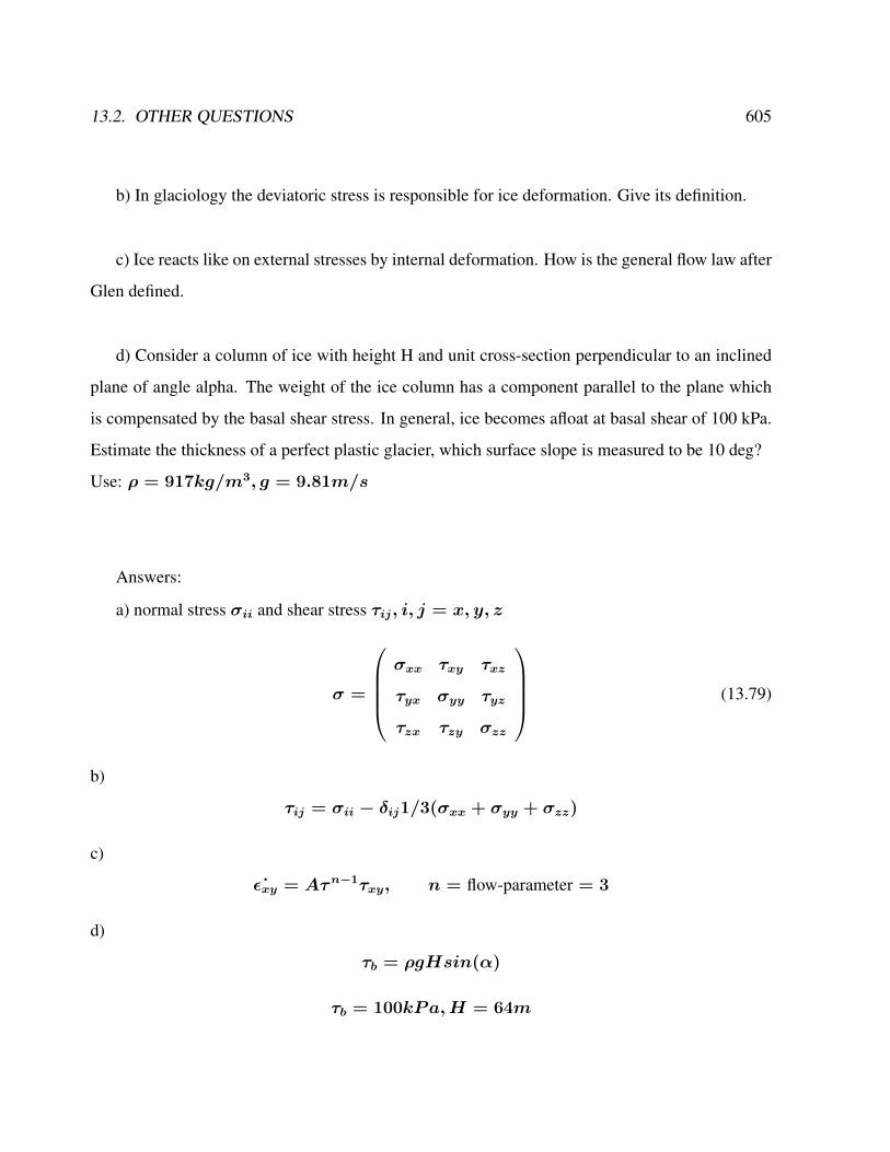
13.2. OTHER QUESTIONS 605
b) In glaciology the deviatoric stress is responsible for ice deformation. Give its definition.
c) Ice reacts like on external stresses by internal deformation. How is the general flow law after
Glen defined.
d) Consider a column of ice with height H and unit cross-section perpendicular to an inclined
plane of angle alpha. The weight of the ice column has a component parallel to the plane which
is compensated by the basal shear stress. In general, ice becomes afloat at basal shear of 100 kPa.
Estimate the thickness of a perfect plastic glacier, which surface slope is measured to be 10 deg?
Use: ρ = 917kg/m3, g = 9.81m/s
Answers:
a) normal stress σii and shear stress τij, i, j = x, y, z
σ =
σxx τxy τxz
τyx σyy τyz
τzx τzy σzz
(13.79)
b)
τij = σii − δij1/3(σxx + σyy + σzz)
c)
˙εxy = Aτn−1τxy, n = flow-parameter = 3
d)
τb = ρgHsin(α)
τb = 100kPa,H = 64m
606 CHAPTER 13. APPENDIX: QUESTIONS
30 points
6) Ocean thermohaline circulation: a) Consider a geostrophic flow (u, v)
−fv = −1
ρ0
∂p
∂x(13.80)
fu = −1
ρ0
∂p
∂y(13.81)
with pressure p(x, y, z, t).
Use the hydrostatic approximation
∂p
∂z= −gρ (13.82)
and equation (13.110) in order to derive the meridional overturning stream function Φ(y, z) as a
fuction of density ρ at the basin boundaries! Φ is defined via
Φ(y, z) =
∫ z
0
∂Φ
∂zdz (13.83)
∂Φ
∂z=
∫ xw
xe
v(x, y, z) dx (zonally integrated transport), (13.84)
where xe and xw are the eastward and westward boundaries in the ocean basin (think e.g. of the
Atlantic Ocean). Units of Φ arem3s−1. At the surface Φ(y, 0) = 0.
b) Draw a figure of the Atlantic overturning!
10 points
7) Methods:
13.2. OTHER QUESTIONS 607
a) Consider the differential equation
d
dtx = ax − εx2 (13.85)
Explain the asymptotic method in case of ε << 0. Expand x variables in a power series.
b) Provide an example from atmosphere-ocean dynamics!
10 points
8) Cells:
What are the names of the 3 meridional cells in the atmosphere? Draw a picture!
How is the equatorial cell driven? Are these cells geostrophically driven or not?
10 points
20 points
9) The Stommel model: of the wind-driven circulation in a homogeneous ocean of constant depth
h is described by
R∇2ψ + β∂xψ = curl(τ0/ρ0) (13.86)
= ∂xτy0 /ρ0 − ∂yτx0 /ρ0 (13.87)
where R is a coefficient of bottom friction, β the derivative of the Coriolis frequency at a central
latitude, and the τ0 the windstress vector. Finally, ψ is the streamfunction of the depth integrated
velocity
U = (U, V ) =
∫ 0
−hudz
i.e.
U = −∂yψ, V = ∂xψ

608 CHAPTER 13. APPENDIX: QUESTIONS
a) Derive this equation from the conservation of momentum (linearized) and mass (volume!)
assuming w = 0 at the mean surface z = 0 and at the bottom z = −h. For simplicity
take Cartesian coordinates for the horizontal, β = df/dy. Boundary condition for the flux of
momentum are τ (z = 0) = τ0 and τ (z = −h) = R(−V,U).
b) in the boundary layer the terms on the left hand side of (13.86) get large. Show by scaling
that the width of the layer isW = R/β.
c) how large mustR be to get a widthW = 100 km? (β = 2× 10⁻¹¹ m−1s−1).
d) can you imagine a planet form or rotation conditions where the other circulations are possible
for the Stommel gyre?
20 points
13.3. EXAM 3 609
13.3 Exam 3
Instructions before you start: The perfect score for this exam is 100 points, although the sum of the
problems is 140. Therefore, you can choose among the problems to solve. 50 points are necessary
for the course.
You are allowed to use a calculator & pen and only the paper we provide. Collaboration or use of
alternative sources of information is not allowed. Good luck!
1. Several questions about the course (32 points, for each Q 2 points).
Q1: The Coriolis parameter f is defined as
a) f = Ω cosϕ
b) f = 2Ω cosϕ
c) f = 2Ω sinϕ
d) f = βy
Q2: Please clarify: On the Northern Hemisphere, particles tend to go to the right or left
relative to the direction of motion due to the Coriolis force?
Q3: Please write down the equation of state for the ocean and atmosphere!
Q4: What are the dominant terms in the momentum balance for the large-scale dynamics at
mid-latitudes?
Q5: What is the hydrostatic approximation in the momentum equations?
610 CHAPTER 13. APPENDIX: QUESTIONS
Q6: Which are the characteristics of baroclinic and barotropic atmosphere (baroclinic vs.
barotropic)?
Q7: Name the at least five monsoon systems and enumerate the time scales of the monsoon
variability .
Q8: Please write down the Euler forward numerical scheme for ddtx = f(x) !
Consider also the special case f(x) = rx− x2!
Q9: Please write down the barotropic potential vorticity equation for large-scale motion!
Q10: Please write down the dispersion relation for Rossby and gravity waves!
Q11: What is the necessary condition for stability in a linear system
d
dtx = Ax
with real vector x andN ×N matrix A?
... and for the analogous non-linear case ddtx = f(x)?
Q12: What is the definition of correlation and covariance?
How is the Fourier transformation of the covariance called?
Q13: Explain the δ notation for stable oxygen isotopes! Provide an example of an stable and

13.3. EXAM 3 611
an unstable isotope in nature! Why are they important?
Q14: Draw a schematic figure of the Atlantic Ocean meridional overturning!
Q15: What are the names of the 3 meridional cells in the atmosphere? Draw a picture with
the direction! How is the equatorial cell driven? Are these cells geostrophically driven or
not?
Q16: Explain dispersive and non-dispersive waves!
612 CHAPTER 13. APPENDIX: QUESTIONS
2. Rossby, gravity, and Kelvin waves (12 points)
Start with the shallow water equations
∂u
∂t− fv = −g
∂η
∂x(13.88)
∂v
∂t+ fu = −g
∂η
∂y(13.89)
∂η
∂t+H
(∂u∂x
+∂v
∂y
)= 0 (13.90)
with H=const. as mean depth and η as surface anomaly.
a) with the elimination of the fast gravity waves in equation (13.90)
∂η
∂t= 0
derive the dispersion relation for divergence-free Rossby waves! Ansatz: Introduce a stream-
function for u,v:
Ψ ∼ exp(ikx+ ily − iωt)
b) with the assumption of f = f0 = 0 derive the dispersion relation for gravity waves! The
restoring force is related to gravity. Ansatz: take one of the equations (13.88,13.89,13.90)
and derive the solution.
c) Kelvin wave. Assume a vertical wall at x=0 along the y-axis (an idealized coast) and u=0.
Derive the solution for v(x, y, t) and η(x, y, t) using the equations (13.89,13.90)! Specify
the x-dependence of the solutions using (13.88) and discuss the trapping distance from the
coast!
13.3. EXAM 3 613
3. Rossby wave formula (long waves in the westerlies) (11 points)
Consider the vorticity equation
D
Dt[(ζ + f)/h] = 0 (13.91)
with h =const., u and v are the velocity components.
a) Assume a mean flow with constant zonal velocity U
u = U = const > 0 (13.92)
and a varying north-south component
v = v(x, t) (13.93)
which gives the total motion a wave-like form. Derive the vorticity equation!
b) With the ansatz
v(x, t) = A cos[(kx− ωt)] (13.94)
determine the disperion relation ω(k), group velocity ∂ω∂k
, and the phase velocity c = ω/k.
c) Derive the wavelength L = 2π/k of the stationary wave given by c = 0.
4. Wind-driven ocean circulation (8 points)
When the windstress is only zonal, the Sverdrup transport is
ρ0βV = curl τ = −∂
∂yτx (13.95)
614 CHAPTER 13. APPENDIX: QUESTIONS
and Ekman transports and Ekman pumping velocity are
ρ0fVE = −τx (13.96)
ρ0wE = curl τ = −∂
∂yτx. (13.97)
Assume furthermore
τx = −τ0 cos(πy/B) (13.98)
for an ocean basin 0 < x < L, 0 < y < B.
a) at what latitudes y are |V | and |VE| maximum? Calculate their magnitudes. Take con-
stant f = 10−4 s−1 and β = 1.8 · 10−11 m−1s−1 and B = 5000 km, τ0/ρ0 =
10−4 m2s−2.
b) calculate the maximum of wE for constant f (value see above).
5. Potential vorticity: (6 points)
An air column at 53N with ζ = 0 initially streches from the surface to a fixed tropopause
at 10 km height. If the air column moves until it is over a mountain barrier 2.5 km hight at
30N, what is its absolute vorticity and relative vorticity as it passes the mountain top?
Assume: sin 53 = 0.8; sin 30 = 0.5
The angular velocity of the Earth Ω = 2π/(1day).
6. Bifurcation: (6 points)
Consider the differential equation
d
dtx = rx (1− x) (13.99)
13.3. EXAM 3 615
Similar dynamics can be derived from the logistic growth or Stommel’s box model of the
ocean circulation (see lecture).
a) Calculate the bifurcation with respect to the parameter r and draw the bifurcation diagram!
b) Is this bifurcation a transcritical or Hopf bifurcation?
c) which types of bifurcations do you know?
7. Lorenz equations (12 points)
Consider the Lorenz equations (which were derived from the Rayleigh-Bernard system)
x = σ(y − x) (13.100)
y = rx− xz − y (13.101)
z = xy − bz (13.102)
with σ, r, b > 0. σ is the Prandtl number. Rayleigh number Ra ∼ ∆T , critical Rayleigh
numberRc, and r = Ra/Rc.
a) Evaluate the equilibrium points and determine their stability through linearization!
b) Show the symmetry: The Lorenz equation has the following symmetry (x, y, z) →
(−x,−y, z) independent on the parameters σ, r, b.
c) Lorenz system has bounded solutions: Show that all solutions of the Lorenz equation will
enter an ellipsoid centered at (0, 0, 2r) in finite time, and the solution will remain inside the
ellipsoid once it has entered. To observe this, define a Lyapunov function
V (x, y, z) = rx2 + σy2 + σ(z − 2r)2 (13.103)
616 CHAPTER 13. APPENDIX: QUESTIONS
8. Stochastic climate model (9 points)
Imagine that the temperature of the ocean mixed layer of depth h is governed by
dT
dt= −λT +
Qnet
γO, (13.104)
where coefficient γO is given by the heat capacity cpρh, and λ is the typical damping rate
of a temperature anomaly. The air-sea fluxes due to weather systems are represented by a
white-noise process Qnet = Qωeiωt where Qω is the amplitude of the random forcing at
frequency ω. Q∗ is the complex conjugate.
a) What is a white-noise process? Remember that
∫R
exp(iωt)δ(t− 0)dt = 1 (13.105)
and use the Fourier transformation.
b) Solve Eq. 13.104 for the temperature response T = Tωeiωt and hence show that:
Tω =Qω
γO (λ+ iω)(13.106)
c) Show that it has a spectral density TωT ∗ω is given by:
T T ∗ =QQ∗
γ2O (λ2 + ω2)
(13.107)
and the spectrum
S(ω) =< T T ∗ >=1
γ2O (λ2 + ω2)
. (13.108)
The brackets < · · · > denote the ensemble mean. Make a sketch of the spectrum using a

13.3. EXAM 3 617
log-log plot and show that fluctuations with a frequency greater than λ are damped.
618 CHAPTER 13. APPENDIX: QUESTIONS
9. Carbon-14 ages (10 points)
The number of decays per time is proportional to the current number of radioactive atoms.
This is expressed by the following differential equation, where N is the number of radioactive
atoms and λ is a positive number called the decay constant:
dN
dt= −λN (13.109)
1λ
is the radiocarbon mean- or average-life = 8033 years (Libby value)
a) Calculate the radiocarbon half-life based on Libby’s value of 1λ
! The correct half-life is
5, 730± 40 years.
b) Plants take up atmospheric carbon dioxide by photosynthesis, and are ingested by animals,
so every living thing is constantly exchanging carbon-14 with its environment as long as it
lives. Once it dies, however, this exchange stops, and the amount of carbon-14 gradually
decreases through radioactive beta decay. Calculate a raw radiocarbon date from N and an
initial condition of N0 for radioactive atoms at t = 0 ! Why is it difficult to report C-14
ages greater than 60,000 years?
c) Typical values for δ14C are −50%o in the mixed layer ocean with depth 50m and
−150%o in deep water (layer depth 4 km). What are the 14C ages of surface and deep
water?
10. Short programming questions. (6 points)
Write down the output for the following R-commands:
a) 0:10
b) a<-c(0,5,3,4); mean(a)
13.3. EXAM 3 619
c) max(a)-min(a)
d) paste("The mean value of a is",mean(a),"for sure",sep="_")
e) a*2+c(1,1,1,0)
f) my.fun<-function(n)return(n*n+1)
my.fun(10)-my.fun(1)
620 CHAPTER 13. APPENDIX: QUESTIONS
11. Ocean thermohaline circulation: (10 points)
a) Consider a geostrophic flow (u, v)
−fv = −1
ρ0
∂p
∂x(13.110)
fu = −1
ρ0
∂p
∂y(13.111)
with pressure p(x, y, z, t).
Use the hydrostatic approximation
∂p
∂z= −gρ (13.112)
and equation (13.110) in order to derive the meridional overturning stream function Φ(y, z)
as a fuction of density ρ at the basin boundaries! Φ is defined via
Φ(y, z) =
∫ z
0
∂Φ
∂zdz (13.113)
∂Φ
∂z=
∫ xw
xe
v(x, y, z) dx (zonally integrated transport), (13.114)
where xe and xw are the eastward and westward boundaries in the ocean basin (think e.g.
of the Atlantic Ocean). Units of Φ arem3s−1. At the surface Φ(y, 0) = 0.
b) Draw a figure of the Atlantic overturning!
12. Nabla(4 points)
Calculate the following operations for the function
f(x, y, z) = x3 + 3x− 4xz + z4 : (13.115)
13.3. EXAM 3 621
∇f , calculate the divergence of the result!
Calculate the rotation of∇f !
13. Angular momentum and Hadley cell (8 points)
Consider a zonally symmetric circulation (i.e., one with no longitudinal variations) in the
atmosphere. In the inviscid upper troposphere one expects such a flow to conserve absolute
angular momentum, i.e.,
DA
Dt= 0, (13.116)
where A is the absolute angular momentum per unit mass (parallel to the Earth’s rotation
axis)
A = r (u+ Ωr) = ΩR2 cos2 ϕ+ uR cosϕ . (13.117)
Ω is the Earth rotation rate, u the eastward wind component, r = R cosϕ is the distance
from the rotation axis,R the Earth’s radius, and ϕ latitude.
a) Show, for inviscid zonally symmetric flow, that the relation DADt
= 0 is consistent with
the zonal component of the equation of motion
Du
Dt− fv = −
1
ρ
∂p
∂x(13.118)
in (x, y, z) coordinates, where y = Rϕ.
b) Use angular momentum conservation to describe in words how the existence of the Hadley
circulation explains the existence of both the subtropical jet in the upper troposphere and the
near-surface trade winds.
c) If the Hadley circulation is symmetric about the equator, and its edge is at 20 latitude,
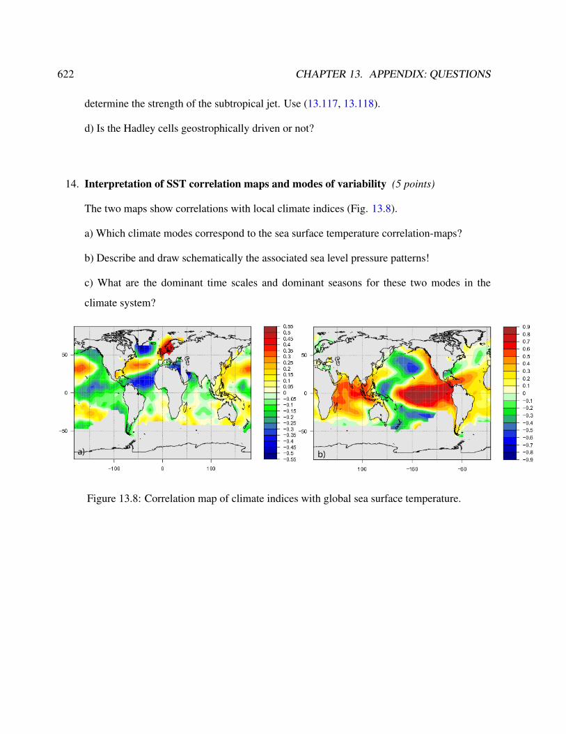
622 CHAPTER 13. APPENDIX: QUESTIONS
determine the strength of the subtropical jet. Use (13.117, 13.118).
d) Is the Hadley cells geostrophically driven or not?
14. Interpretation of SST correlation maps and modes of variability (5 points)
The two maps show correlations with local climate indices (Fig. 13.8).
a) Which climate modes correspond to the sea surface temperature correlation-maps?
b) Describe and draw schematically the associated sea level pressure patterns!
c) What are the dominant time scales and dominant seasons for these two modes in the
climate system?
Figure 13.8: Correlation map of climate indices with global sea surface temperature.

13.3. EXAM 3 623
Acknowledgements
The script benefited from Master or PhD work of Matthias Prange, Nils Kaiser, Gregor Knorr
related to the climate box model, as well of Dragos Chirila and Sebastian Hinck for several com-
ments and the implementation of the Lattice Boltzmann Model. Thomas Laepple, Sebastian Hinck,
Christopher Danek, Christian Stepanek and Paul Gierz helped with some R, python and shell pro-
gramming, and Stefanie Klebe with editing.
List of Figures
1.1 Sea-level derived rate of deglacial meltwater discharge . . . . . . . . . . . . . 5
1.2 Drop tower in Bremen. . . . . . . . . . . . . . . . . . . . . . . . . . . . . . 9
1.3 Pendulum. . . . . . . . . . . . . . . . . . . . . . . . . . . . . . . . . . . . 10
1.4 Foucault pendulum in Paris . . . . . . . . . . . . . . . . . . . . . . . . . . . 14
1.5 Foucault pendulum principle . . . . . . . . . . . . . . . . . . . . . . . . . . 17
1.6 White noise spectrum. . . . . . . . . . . . . . . . . . . . . . . . . . . . . . 35
2.1 R download . . . . . . . . . . . . . . . . . . . . . . . . . . . . . . . . . . 43
2.2 Logistic map bifurcation . . . . . . . . . . . . . . . . . . . . . . . . . . . . 48
2.3 Mandelbrot set and Lena Delta . . . . . . . . . . . . . . . . . . . . . . . . . 51
2.4 Zones of todays wine production. . . . . . . . . . . . . . . . . . . . . . . . . 71
2.5 Alcohol belts in Europe. . . . . . . . . . . . . . . . . . . . . . . . . . . . . 71
2.6 Bifurcation sketch . . . . . . . . . . . . . . . . . . . . . . . . . . . . . . . 72
2.7 Saddle-node bifurcation . . . . . . . . . . . . . . . . . . . . . . . . . . . . 76
2.8 Potential r . . . . . . . . . . . . . . . . . . . . . . . . . . . . . . . . . . . 89
2.9 Lorenz model . . . . . . . . . . . . . . . . . . . . . . . . . . . . . . . . . 90
2.10 Lorenz bifurcation diagram . . . . . . . . . . . . . . . . . . . . . . . . . . . 90
2.11 Schematic picture of the Stommel’s box model . . . . . . . . . . . . . . . . . 95
2.12 Bifurcation of the Stommel box model . . . . . . . . . . . . . . . . . . . . . 100
2.13 Basin of attraction . . . . . . . . . . . . . . . . . . . . . . . . . . . . . . . 103
624
LIST OF FIGURES 625
2.14 Eigenvectors and adjoint eigenvectors . . . . . . . . . . . . . . . . . . . . . 104
3.1 Discrete lattice velocities for theD2Q9 model. . . . . . . . . . . . . . . . . . 121
3.2 Illustration of the streaming process on aD2Q9 lattice. . . . . . . . . . . . . . 122
3.3 Illustration of the collision process on aD2Q9 lattice. . . . . . . . . . . . . . 122
3.4 Four examples of the flow for different sets ofRa and Pr. . . . . . . . . . . . 129
3.5 Ocean flow for different boundary conditions . . . . . . . . . . . . . . . . . . 133
3.6 Ehrenfests coarse-graining . . . . . . . . . . . . . . . . . . . . . . . . . . . 135
4.1 Components of stress in three dimensions . . . . . . . . . . . . . . . . . . . . 145
4.2 Surface pressure field and surface wind, scales . . . . . . . . . . . . . . . . . 154
5.1 Potential flow around a circular cylinder . . . . . . . . . . . . . . . . . . . . 169
5.2 Potential flow around a circular cylinder: solution . . . . . . . . . . . . . . . . 171
5.3 Von Karman Vortices . . . . . . . . . . . . . . . . . . . . . . . . . . . . . 174
5.4 Simple Couette configuration . . . . . . . . . . . . . . . . . . . . . . . . . . 182
5.5 Rayleigh-Benard system . . . . . . . . . . . . . . . . . . . . . . . . . . . . 184
6.1 Coordinate system at latitude ϕ . . . . . . . . . . . . . . . . . . . . . . . . . 202
6.2 Sea level pressure . . . . . . . . . . . . . . . . . . . . . . . . . . . . . . . 207
6.3 Volume transport between stream lines . . . . . . . . . . . . . . . . . . . . . 209
6.4 Hadely Cell . . . . . . . . . . . . . . . . . . . . . . . . . . . . . . . . . . 210
6.5 conservation of potential vorticity . . . . . . . . . . . . . . . . . . . . . . . 218
6.6 production of relative vorticity . . . . . . . . . . . . . . . . . . . . . . . . . 219
6.7 Angular momentum tends to be conserved . . . . . . . . . . . . . . . . . . . 220
6.8 Barotropic flow over a sub-sea ridge . . . . . . . . . . . . . . . . . . . . . . 222
6.9 Floats in the northwestern NorthAtlantic below 1000m. . . . . . . . . . . . . . 224
6.10 f/h countour in the Weddell Sea . . . . . . . . . . . . . . . . . . . . . . . . 224
6.11 Depth-integrated Sverdrup transport . . . . . . . . . . . . . . . . . . . . . . 234
626 LIST OF FIGURES
6.12 Ekman pumping . . . . . . . . . . . . . . . . . . . . . . . . . . . . . . . . 236
6.13 Geostrophic currents running upwind. . . . . . . . . . . . . . . . . . . . . . 238
6.14 The Ekman spiral and the mechanism by which it operates . . . . . . . . . . . . 240
6.15 Tea leaf Paradox . . . . . . . . . . . . . . . . . . . . . . . . . . . . . . . . 247
6.16 Experiment with a turntable . . . . . . . . . . . . . . . . . . . . . . . . . . 248
6.17 western boundary currents . . . . . . . . . . . . . . . . . . . . . . . . . . . 250
6.18 Stream function for flow in a basin as calculated by Stommel . . . . . . . . . . 252
6.19 The mass transport stream function for a rectangular basin . . . . . . . . . . . . 255
6.20 The North Atlantic Current . . . . . . . . . . . . . . . . . . . . . . . . . . 258
6.21 Ocean Conveyor Belt . . . . . . . . . . . . . . . . . . . . . . . . . . . . . 260
6.22 Atlantic meridional overturning streamfunction . . . . . . . . . . . . . . . . . 261
6.23 Meteor Expedition Wuest . . . . . . . . . . . . . . . . . . . . . . . . . . . 263
6.24 Schematic picture of the box modela . . . . . . . . . . . . . . . . . . . . . . 268
6.25 Atlantic surface density . . . . . . . . . . . . . . . . . . . . . . . . . . . . 269
7.1 Schematic illustration of the Climate-Box-Model . . . . . . . . . . . . . . . . 279
7.2 Output of the climate box model illustrating the procedure. . . . . . . . . . . . 287
7.3 Brownian particle . . . . . . . . . . . . . . . . . . . . . . . . . . . . . . . 296
7.4 diffusion of Brownian particles . . . . . . . . . . . . . . . . . . . . . . . . . 297
7.5 Numerical solution of the brownian motion, multiple particles . . . . . . . . . . 301
7.6 Schematic picture of mixed layer in the ocean . . . . . . . . . . . . . . . . . . 305
7.7 Mixed layer in the ocean distribution . . . . . . . . . . . . . . . . . . . . . . 309
7.8 Stochastic Climate model . . . . . . . . . . . . . . . . . . . . . . . . . . . 310
7.9 Stochastic Climate model in potential . . . . . . . . . . . . . . . . . . . . . . 310
7.10 Geometric Brownian motion . . . . . . . . . . . . . . . . . . . . . . . . . . 311
7.11 Spectrum of atmospheric temperature and sea surface temperature. . . . . . . . . 313
8.1 Euler forward method . . . . . . . . . . . . . . . . . . . . . . . . . . . . . 325
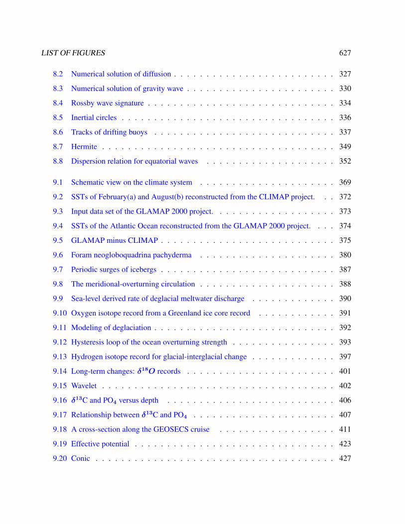
LIST OF FIGURES 627
8.2 Numerical solution of diffusion . . . . . . . . . . . . . . . . . . . . . . . . . 327
8.3 Numerical solution of gravity wave . . . . . . . . . . . . . . . . . . . . . . . 330
8.4 Rossby wave signature . . . . . . . . . . . . . . . . . . . . . . . . . . . . . 334
8.5 Inertial circles . . . . . . . . . . . . . . . . . . . . . . . . . . . . . . . . . 336
8.6 Tracks of drifting buoys . . . . . . . . . . . . . . . . . . . . . . . . . . . . 337
8.7 Hermite . . . . . . . . . . . . . . . . . . . . . . . . . . . . . . . . . . . . 349
8.8 Dispersion relation for equatorial waves . . . . . . . . . . . . . . . . . . . . 352
9.1 Schematic view on the climate system . . . . . . . . . . . . . . . . . . . . . 369
9.2 SSTs of February(a) and August(b) reconstructed from the CLIMAP project. . . 372
9.3 Input data set of the GLAMAP 2000 project. . . . . . . . . . . . . . . . . . . 373
9.4 SSTs of the Atlantic Ocean reconstructed from the GLAMAP 2000 project. . . . 374
9.5 GLAMAP minus CLIMAP . . . . . . . . . . . . . . . . . . . . . . . . . . . 375
9.6 Foram neogloboquadrina pachyderma . . . . . . . . . . . . . . . . . . . . . 380
9.7 Periodic surges of icebergs . . . . . . . . . . . . . . . . . . . . . . . . . . . 387
9.8 The meridional-overturning circulation . . . . . . . . . . . . . . . . . . . . . 388
9.9 Sea-level derived rate of deglacial meltwater discharge . . . . . . . . . . . . . 390
9.10 Oxygen isotope record from a Greenland ice core record . . . . . . . . . . . . 391
9.11 Modeling of deglaciation . . . . . . . . . . . . . . . . . . . . . . . . . . . . 392
9.12 Hysteresis loop of the ocean overturning strength . . . . . . . . . . . . . . . . 393
9.13 Hydrogen isotope record for glacial-interglacial change . . . . . . . . . . . . . 397
9.14 Long-term changes: δ18O records . . . . . . . . . . . . . . . . . . . . . . . 401
9.15 Wavelet . . . . . . . . . . . . . . . . . . . . . . . . . . . . . . . . . . . . 402
9.16 δ13C and PO4 versus depth . . . . . . . . . . . . . . . . . . . . . . . . . . 406
9.17 Relationship between δ13C and PO4 . . . . . . . . . . . . . . . . . . . . . . 407
9.18 A cross-section along the GEOSECS cruise . . . . . . . . . . . . . . . . . . 411
9.19 Effective potential . . . . . . . . . . . . . . . . . . . . . . . . . . . . . . . 423
9.20 Conic . . . . . . . . . . . . . . . . . . . . . . . . . . . . . . . . . . . . . 427

628 LIST OF FIGURES
9.21 Earth’s orbit . . . . . . . . . . . . . . . . . . . . . . . . . . . . . . . . . . 430
9.22 Tides . . . . . . . . . . . . . . . . . . . . . . . . . . . . . . . . . . . . . 431
10.1 Spectrum: Numerical solution . . . . . . . . . . . . . . . . . . . . . . . . . 465
10.2 Non-normal 2d dynamics . . . . . . . . . . . . . . . . . . . . . . . . . . . . 466
10.3 Non-normal 2d dynamics: Spectrum . . . . . . . . . . . . . . . . . . . . . . 466
10.4 Linearized atmospheric dynamics . . . . . . . . . . . . . . . . . . . . . . . . 467
10.5 Pseudospectrum with FESOM . . . . . . . . . . . . . . . . . . . . . . . . . 468
10.6 Four spatial patterns for synthetic signal. . . . . . . . . . . . . . . . . . . . . 474
10.7 The 3 leading spatial modes . . . . . . . . . . . . . . . . . . . . . . . . . . 476
10.8 The singular spectra of the 2 synthetic cases . . . . . . . . . . . . . . . . . . . 477
10.9 Leading mode of the winter 700 mb geopotential . . . . . . . . . . . . . . . . 479
10.10Singular spectrum of DJF 700 mb geopotential . . . . . . . . . . . . . . . . . 480
10.11how to calculate EOFs . . . . . . . . . . . . . . . . . . . . . . . . . . . . . 481
10.12Schematic of a two layer ocean model. . . . . . . . . . . . . . . . . . . . . . 485
10.13Schematic meridional section of near equatorial upwelling . . . . . . . . . . . . 485
10.14Diagram of the quasi-equilibrium and La Nina phase of the Southern Oscillation. 487
10.15Schematic E-W cross section . . . . . . . . . . . . . . . . . . . . . . . . . . 488
10.16SSTs for an El Nino and Lan Nina event . . . . . . . . . . . . . . . . . . . . 488
10.17SLP signature Lan Nina event . . . . . . . . . . . . . . . . . . . . . . . . . 489
10.18NAO . . . . . . . . . . . . . . . . . . . . . . . . . . . . . . . . . . . . . 491
10.19NAO . . . . . . . . . . . . . . . . . . . . . . . . . . . . . . . . . . . . . 492
10.20NAO index . . . . . . . . . . . . . . . . . . . . . . . . . . . . . . . . . . 493
10.21AMO spatial pattern. . . . . . . . . . . . . . . . . . . . . . . . . . . . . . . 494
10.22AMO index. . . . . . . . . . . . . . . . . . . . . . . . . . . . . . . . . . . 494
10.23Corals and teleconnections . . . . . . . . . . . . . . . . . . . . . . . . . . . 495
10.24Correlation map of climate indices with global sea surface temperature. . . . . . 496
10.25Correlation and composite analyses using the web application . . . . . . . . . . 497
LIST OF FIGURES 629
10.26Brownian motion in a potential . . . . . . . . . . . . . . . . . . . . . . . . . 501
10.27Potential curves and web application . . . . . . . . . . . . . . . . . . . . . . 503
10.28Bifurcation: Potential curves . . . . . . . . . . . . . . . . . . . . . . . . . . 505
10.29Stochastic resonance . . . . . . . . . . . . . . . . . . . . . . . . . . . . . . 509
12.1 Numerical solution of the brownian motion. . . . . . . . . . . . . . . . . . . . 518
12.2 Install missing packages. . . . . . . . . . . . . . . . . . . . . . . . . . . . . 530
12.3 2D field grid points . . . . . . . . . . . . . . . . . . . . . . . . . . . . . . 535
12.4 Kaplan SST data averaged over all grid points. . . . . . . . . . . . . . . . . . 539
12.5 plot_pFieldcor . . . . . . . . . . . . . . . . . . . . . . . . . . . . . . 540
12.6 plot_pFieldcor . . . . . . . . . . . . . . . . . . . . . . . . . . . . . . 541
12.7 plot_pFieldcor . . . . . . . . . . . . . . . . . . . . . . . . . . . . . . 542
12.8 Kaplan SST with point . . . . . . . . . . . . . . . . . . . . . . . . . . . . . 544
12.9 Kaplan SST with text . . . . . . . . . . . . . . . . . . . . . . . . . . . . . 545
12.10Histogram of the Monte Carlo experiment . . . . . . . . . . . . . . . . . . . 547
12.11Histogram of a statistical test with random time series. . . . . . . . . . . . . . 549
12.12Plot of ocean surface salinity using the python script. . . . . . . . . . . . . . . 556
12.13As in Fig. 12.12, but for ocean surface horizonal velocity. . . . . . . . . . . . . 556
12.14A simple finite-difference grid . . . . . . . . . . . . . . . . . . . . . . . . . 560
12.15First-order finite-difference solution to linear advection . . . . . . . . . . . . . 562
12.16First-order implicit finite-difference solution to linear advection . . . . . . . . . 565
13.1 Rayleigh-Benard system . . . . . . . . . . . . . . . . . . . . . . . . . . . . 569
13.2 Drop tower in Bremen. . . . . . . . . . . . . . . . . . . . . . . . . . . . . . 571
13.3 f/h countours in the Weddell Sea . . . . . . . . . . . . . . . . . . . . . . . 575
13.4 Sea level pressure . . . . . . . . . . . . . . . . . . . . . . . . . . . . . . . 576
13.5 bifgrapht . . . . . . . . . . . . . . . . . . . . . . . . . . . . . . . . . . . 583
13.6 Schematic illustration of the Climate-Box-Model . . . . . . . . . . . . . . . . 588
630 LIST OF FIGURES
13.7 Correlation map of climate indices with global sea surface temperature. . . . . . 590
13.8 Correlation map of climate indices with global sea surface temperature. . . . . . 614
List of Tables
1.1 Laplace transformation . . . . . . . . . . . . . . . . . . . . . . . . . . . . . 22
4.1 Typical scales in the environmental, atmosphere, ocean and climate system. . . . 153
4.2 Table shows the typical scales for the submarine model. . . . . . . . . . . . . . 161
6.1 Scales in the atmosphere and ocean system . . . . . . . . . . . . . . . . . . . 200
6.2 Scales in the ocean system . . . . . . . . . . . . . . . . . . . . . . . . . . . 230
8.1 List of parameters for the Matsuno equations. . . . . . . . . . . . . . . . . . 347
9.1 Abundance of stable hydrogen and oxygen isotopes . . . . . . . . . . . . . . . 381
13.1 Scales in the atmosphere and ocean system . . . . . . . . . . . . . . . . . . . 572
631
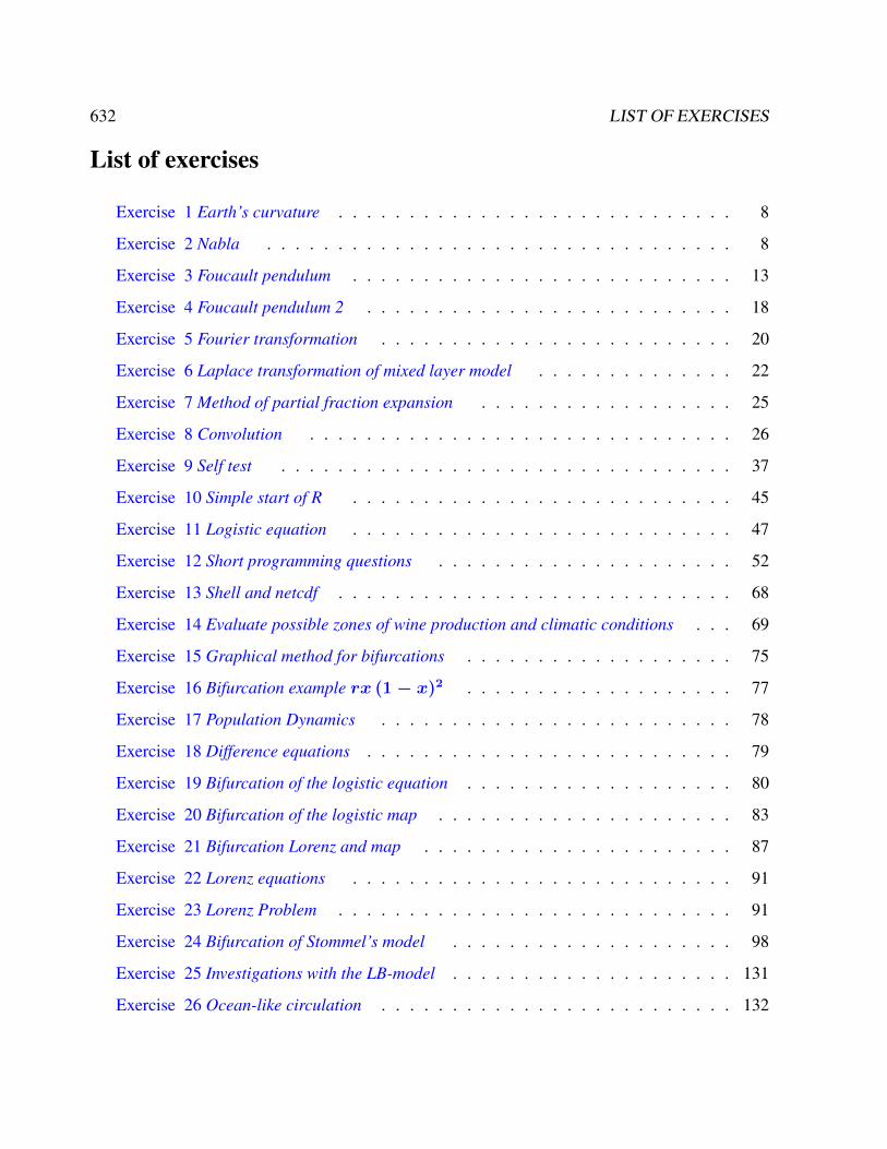
632 LIST OF EXERCISES
List of exercises
Exercise 1 Earth’s curvature . . . . . . . . . . . . . . . . . . . . . . . . . . . . 8
Exercise 2 Nabla . . . . . . . . . . . . . . . . . . . . . . . . . . . . . . . . . 8
Exercise 3 Foucault pendulum . . . . . . . . . . . . . . . . . . . . . . . . . . . 13
Exercise 4 Foucault pendulum 2 . . . . . . . . . . . . . . . . . . . . . . . . . . 18
Exercise 5 Fourier transformation . . . . . . . . . . . . . . . . . . . . . . . . . 20
Exercise 6 Laplace transformation of mixed layer model . . . . . . . . . . . . . . 22
Exercise 7 Method of partial fraction expansion . . . . . . . . . . . . . . . . . . 25
Exercise 8 Convolution . . . . . . . . . . . . . . . . . . . . . . . . . . . . . . 26
Exercise 9 Self test . . . . . . . . . . . . . . . . . . . . . . . . . . . . . . . . 37
Exercise 10 Simple start of R . . . . . . . . . . . . . . . . . . . . . . . . . . . 45
Exercise 11 Logistic equation . . . . . . . . . . . . . . . . . . . . . . . . . . . 47
Exercise 12 Short programming questions . . . . . . . . . . . . . . . . . . . . . 52
Exercise 13 Shell and netcdf . . . . . . . . . . . . . . . . . . . . . . . . . . . . 68
Exercise 14 Evaluate possible zones of wine production and climatic conditions . . . 69
Exercise 15 Graphical method for bifurcations . . . . . . . . . . . . . . . . . . . 75
Exercise 16 Bifurcation example rx (1− x)2 . . . . . . . . . . . . . . . . . . . 77
Exercise 17 Population Dynamics . . . . . . . . . . . . . . . . . . . . . . . . . 78
Exercise 18 Difference equations . . . . . . . . . . . . . . . . . . . . . . . . . . 79
Exercise 19 Bifurcation of the logistic equation . . . . . . . . . . . . . . . . . . . 80
Exercise 20 Bifurcation of the logistic map . . . . . . . . . . . . . . . . . . . . . 83
Exercise 21 Bifurcation Lorenz and map . . . . . . . . . . . . . . . . . . . . . . 87
Exercise 22 Lorenz equations . . . . . . . . . . . . . . . . . . . . . . . . . . . 91
Exercise 23 Lorenz Problem . . . . . . . . . . . . . . . . . . . . . . . . . . . . 91
Exercise 24 Bifurcation of Stommel’s model . . . . . . . . . . . . . . . . . . . . 98
Exercise 25 Investigations with the LB-model . . . . . . . . . . . . . . . . . . . . 131
Exercise 26 Ocean-like circulation . . . . . . . . . . . . . . . . . . . . . . . . . 132
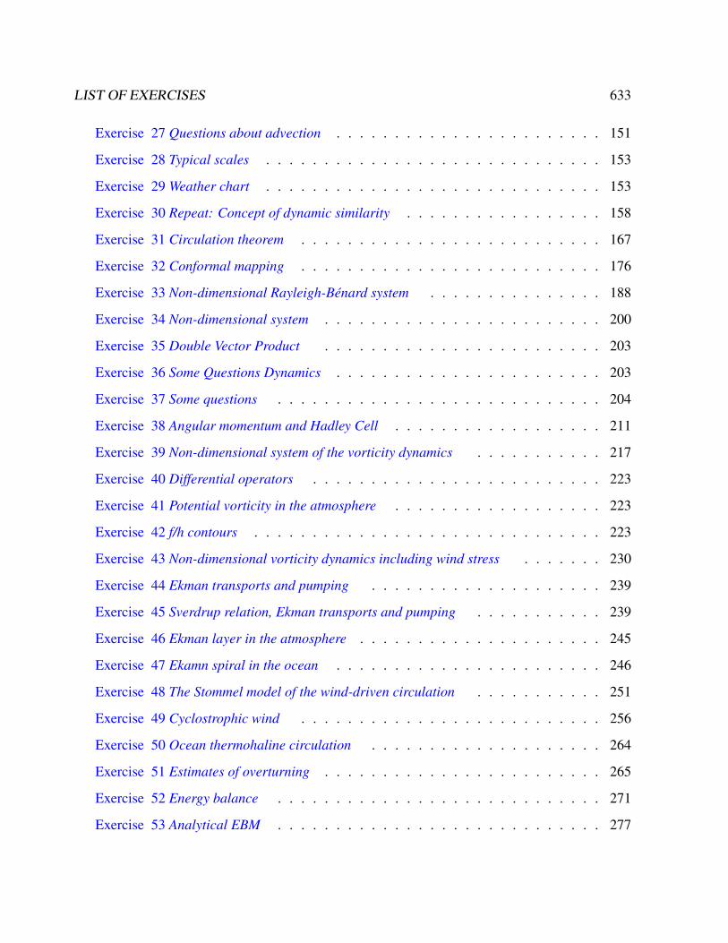
LIST OF EXERCISES 633
Exercise 27 Questions about advection . . . . . . . . . . . . . . . . . . . . . . . 151
Exercise 28 Typical scales . . . . . . . . . . . . . . . . . . . . . . . . . . . . . 153
Exercise 29 Weather chart . . . . . . . . . . . . . . . . . . . . . . . . . . . . . 153
Exercise 30 Repeat: Concept of dynamic similarity . . . . . . . . . . . . . . . . . 158
Exercise 31 Circulation theorem . . . . . . . . . . . . . . . . . . . . . . . . . . 167
Exercise 32 Conformal mapping . . . . . . . . . . . . . . . . . . . . . . . . . . 176
Exercise 33 Non-dimensional Rayleigh-Bénard system . . . . . . . . . . . . . . . 188
Exercise 34 Non-dimensional system . . . . . . . . . . . . . . . . . . . . . . . . 200
Exercise 35 Double Vector Product . . . . . . . . . . . . . . . . . . . . . . . . 203
Exercise 36 Some Questions Dynamics . . . . . . . . . . . . . . . . . . . . . . . 203
Exercise 37 Some questions . . . . . . . . . . . . . . . . . . . . . . . . . . . . 204
Exercise 38 Angular momentum and Hadley Cell . . . . . . . . . . . . . . . . . . 211
Exercise 39 Non-dimensional system of the vorticity dynamics . . . . . . . . . . . 217
Exercise 40 Differential operators . . . . . . . . . . . . . . . . . . . . . . . . . 223
Exercise 41 Potential vorticity in the atmosphere . . . . . . . . . . . . . . . . . . 223
Exercise 42 f/h contours . . . . . . . . . . . . . . . . . . . . . . . . . . . . . . 223
Exercise 43 Non-dimensional vorticity dynamics including wind stress . . . . . . . 230
Exercise 44 Ekman transports and pumping . . . . . . . . . . . . . . . . . . . . 239
Exercise 45 Sverdrup relation, Ekman transports and pumping . . . . . . . . . . . 239
Exercise 46 Ekman layer in the atmosphere . . . . . . . . . . . . . . . . . . . . . 245
Exercise 47 Ekamn spiral in the ocean . . . . . . . . . . . . . . . . . . . . . . . 246
Exercise 48 The Stommel model of the wind-driven circulation . . . . . . . . . . . 251
Exercise 49 Cyclostrophic wind . . . . . . . . . . . . . . . . . . . . . . . . . . 256
Exercise 50 Ocean thermohaline circulation . . . . . . . . . . . . . . . . . . . . 264
Exercise 51 Estimates of overturning . . . . . . . . . . . . . . . . . . . . . . . . 265
Exercise 52 Energy balance . . . . . . . . . . . . . . . . . . . . . . . . . . . . 271
Exercise 53 Analytical EBM . . . . . . . . . . . . . . . . . . . . . . . . . . . . 277
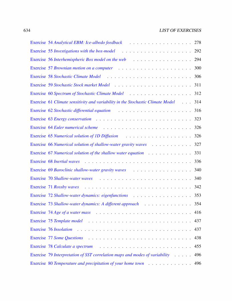
634 LIST OF EXERCISES
Exercise 54 Analytical EBM: Ice-albedo feedback . . . . . . . . . . . . . . . . . 278
Exercise 55 Investigations with the box-model . . . . . . . . . . . . . . . . . . . 292
Exercise 56 Interhemispheric Box model on the web . . . . . . . . . . . . . . . . 294
Exercise 57 Brownian motion on a computer . . . . . . . . . . . . . . . . . . . . 300
Exercise 58 Stochastic Climate Model . . . . . . . . . . . . . . . . . . . . . . . 306
Exercise 59 Stochastic Stock market Model . . . . . . . . . . . . . . . . . . . . . 311
Exercise 60 Spectrum of Stochastic Climate Model . . . . . . . . . . . . . . . . . 312
Exercise 61 Climate sensitivity and variability in the Stochastic Climate Model . . . 314
Exercise 62 Stochastic differential equation . . . . . . . . . . . . . . . . . . . . 316
Exercise 63 Energy conservation . . . . . . . . . . . . . . . . . . . . . . . . . . 323
Exercise 64 Euler numerical scheme . . . . . . . . . . . . . . . . . . . . . . . . 326
Exercise 65 Numerical solution of 1D Diffusion . . . . . . . . . . . . . . . . . . 326
Exercise 66 Numerical solution of shallow-water gravity waves . . . . . . . . . . . 327
Exercise 67 Numerical solution of the shallow water equation . . . . . . . . . . . . 331
Exercise 68 Inertial waves . . . . . . . . . . . . . . . . . . . . . . . . . . . . . 336
Exercise 69 Baroclinic shallow-water gravity waves . . . . . . . . . . . . . . . . 340
Exercise 70 Shallow-water waves . . . . . . . . . . . . . . . . . . . . . . . . . 340
Exercise 71 Rossby waves . . . . . . . . . . . . . . . . . . . . . . . . . . . . . 342
Exercise 72 Shallow-water dynamics: eigenfunctions . . . . . . . . . . . . . . . . 353
Exercise 73 Shallow-water dynamics: A different approach . . . . . . . . . . . . . 354
Exercise 74 Age of a water mass . . . . . . . . . . . . . . . . . . . . . . . . . . 416
Exercise 75 Template model . . . . . . . . . . . . . . . . . . . . . . . . . . . . 437
Exercise 76 Insolation . . . . . . . . . . . . . . . . . . . . . . . . . . . . . . . 437
Exercise 77 Some Questions . . . . . . . . . . . . . . . . . . . . . . . . . . . . 438
Exercise 78 Calculate a spectrum . . . . . . . . . . . . . . . . . . . . . . . . . 455
Exercise 79 Interpretation of SST correlation maps and modes of variability . . . . . 496
Exercise 80 Temperature and precipitation of your home town . . . . . . . . . . . . 496
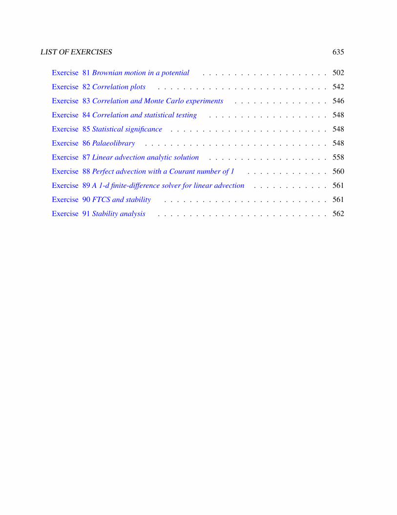
LIST OF EXERCISES 635
Exercise 81 Brownian motion in a potential . . . . . . . . . . . . . . . . . . . . 502
Exercise 82 Correlation plots . . . . . . . . . . . . . . . . . . . . . . . . . . . 542
Exercise 83 Correlation and Monte Carlo experiments . . . . . . . . . . . . . . . 546
Exercise 84 Correlation and statistical testing . . . . . . . . . . . . . . . . . . . 548
Exercise 85 Statistical significance . . . . . . . . . . . . . . . . . . . . . . . . . 548
Exercise 86 Palaeolibrary . . . . . . . . . . . . . . . . . . . . . . . . . . . . . 548
Exercise 87 Linear advection analytic solution . . . . . . . . . . . . . . . . . . . 558
Exercise 88 Perfect advection with a Courant number of 1 . . . . . . . . . . . . . 560
Exercise 89 A 1-d finite-difference solver for linear advection . . . . . . . . . . . . 561
Exercise 90 FTCS and stability . . . . . . . . . . . . . . . . . . . . . . . . . . 561
Exercise 91 Stability analysis . . . . . . . . . . . . . . . . . . . . . . . . . . . 562

Bibliography
Abramowitz, M. and Stegun, I. A. (1965). Handbook of mathematical functions with formulas,
graph, and mathematical tables. Applied Mathematics Series, 55:1046.
Arnold, L. (1995). Random dynamical systems. Springer.
Arnold, L. (2001). Hasselmann’s program revisited: The analysis of stochasticity in deterministic
climate models, volume 49. Birkhäuser, Boston.
Baker, G. L. and Blackburn, J. A. (2005). The pendulum: a case study in physics, volume 8.
Oxford University Press Oxford.
Barber, D., Dyke, A., Hillaire-Marcel, C., Jennings, J., Andrews, J., Kerwin, M., Bilodeau, G.,
McNeely, R., Southon, J., Morehead, M., and Gagnonk, J.-M. (1999). Forcing of the cold event
of 8,200 years ago by catastrophic drainage of laurentide lakes. Nature, 400(6742):344–348.
Bhatnagar, P., Gross, E. P., and Krook, M. K. (1954). A model for collision process in gases. i.
small amplitude processes in charged and neutral one-component system. Phys. Rev, 94:511.
Boltzmann, L. (1896). Vorlesungen über Gastheorie : 2 Volumes (in German). Leipzig 1895/98
UB: O 5262-6.
Boltzmann, L. (1995). Lectures on Gas Theory. Dover Publ. New York. ISBN 978-0486684550.
Broecker, S. and Peng, T.-H. (1982). Tracers in the Sea. Columbia University.
636
BIBLIOGRAPHY 637
Broecker, W. S. (1987). The biggest chill. Natural History, 97(2):74–82.
Broecker, W. S. et al. (1991). The great ocean conveyor. Oceanography, 4(2):79–89.
Brüning, R. and Lohmann, G. (1999). Charles s. peirce on creative metaphor: a case study on the
conveyor belt metaphor in oceanography. Foundations of science, 4(4):389–403.
Bryan, F. (1986). High latitude salinity effects and inter-hemispheric thermohaline circulations.
Nature, 323(3):301–304.
Buckingham, E. (1914). On physically similar systems; illustrations of the use of dimensional
equations. Physical Review, 4(4):345–376.
Budyko, M. I. (1969). The effect of solar radiation variations on the climate of earth. Tellus,
21:611–619.
Busch, W. (1865). Max und Moritz (in German); Max and Maurice, a Juvenile History in Seven
Tricks . Braun und Schneider, München.
Cercignani, C. (1987). The Boltzmann equation and its applications. Springer New York. ISBN
978-0387966373.
Cercignani, C. (1990). Mathematical methods in kinetic theory. Plenum, 2 edition. ISBN 978-
0306434600.
Chelton, D. B. and Schlax, M. G. (1996). Global Observations of Oceanic Rossby Waves. Science,
272:234–238.
Chen, D., Gerdes, R., and Lohmann, G. (1995). A 1-d atmospheric energy balance model devel-
oped for ocean modelling. Theoretical and Applied Climatology, 51:25–38.
Chirila, D. and Lohmann, G. (2014). Introduction to Modern Fortran for Earth System Sciences.
SpringerBriefs in Earth System Sciences. Springer. ISBN 978-3642370083 (to appear).
638 BIBLIOGRAPHY
Chorin, A. J. and Hald, O. H. (2006). Stochastic tools in mathematics and science. surveys and
tutorials in the applied mathematical sciences, vol. 1.
Chorin, A. J., Kast, A. P., and Kupferman, R. (1999). Unresolved computation and optimal pre-
dictions. Communications on pure and applied mathematics, 52(10):1231–1254.
Chorin, A. J., Kupferman, R., and Levy, D. (2000). Optimal prediction for hamiltonian partial
differential equations. Journal of Computational Physics, 162(1):267–297.
Courant, R., Friedrichs, K., and Lewy, H. (1928). Über die partiellen Differenzengleichungen der
mathematischen Physik. Mathematische Annalen, 100:32–74.
Courant, R., Friedrichs, K., and Lewy, H. (1967). On the partial difference equations of mathemat-
ical physics. IBM J. Res. Dev., 11(2):215–234.
Dansgaard, W., Johnsen, S., Clausen, H., Dahl-Jensen, D., Gundestrup, N., Hammer, C.,
C.S. Hvidberg, J. S., Sveinbjoernsdottir, A., Jouzel, J., and Bond, G. (1993). Evidence for
general instability of past climate from a 250-kyr ice-core record. Nature, 364:218–220.
d’Humieres, D., Bouzidi, M., and Lallemand, P. (2001). Thirteen-velocity three-dimensional lat-
tice boltzmann model. PRE, 63(6, Part 2).
Dijkstra, H., Raa, L. T., and Weijer, W. (2004). A systematic approach to determine thresholds of
the ocean’s thermohaline circulation. Tellus A, 56 (4):362.
Dijkstra, H. A. (2000). Nonlinear Physical Oceanography: A Dynamical systems approach to the
large scale ocean circulation and El Nino. Kluwer Academic Publishers.
Doedel, E. J., Champneys, A. R., Fairgrieve, T. F., Kuznetsov, Y. A., Sandstede, B., and Wang,
X. (1997). Continuation and bifurcation software for ordinary differential equations (with hom-
cont). Available by anonymous ftp from ftp cs concordia ca, directory pub/doedel/auto.
BIBLIOGRAPHY 639
Egger, J. (2001). Master equations for climatic parameter sets. Climate Dynamics, 18(1-2):169–
177.
Einstein, A. (1905). Investigations on the theory of the brownian movement. Ann. der Physik,
17:549–560.
Evans, D. J. and Morriss, G. (2008). Statistical mechanics of nonequilibrium liquids. Cambridge
University Press.
Fairbanks, R. G. (1989). A 17, 000-year glacio-eustatic sea level record: influence of glacial
melting rates on the younger dryas event and deep-ocean circulation. Nature, 342(6250):637–
642.
Feigenbaum, M. J. (1980). The transition to aperiodic behaviour in turbulent systems. Commun.
Math. Phys., 77.
Flammer, C. (1957). Spheroidal wave functions. Stanford University Press.
Frisch, U. (1996). Turbulence: the legacy of A.N. Kolmogorov. Cambridge University Press. ISBN
0-521-45103-5.
Gerkema, T., Zimmerman, J., Maas, L., and Van Haren, H. (2008). Geophysical and astrophysical
fluid dynamics beyond the traditional approximation. Reviews of Geophysics, 46(2).
Gill, A. E. (1982). Atmosphere-ocean dynamics, volume 30. Academic Press. International
Geophysics Series.
Givon, D., Kupferman, R., and Stuart, A. (2004). Extracting macroscopic dynamics: model prob-
lems and algorithms. Nonlinearity, 17(6):R55.
Gottwald, G. (2010). On recent trends in climate dynamics. AMS Gazette, 37(5).
Grassberger, P. and Procaccia, I. (1983). Measuring the strangeness of strange attractors. Physica
D: Nonlinear Phenomena, 9(2):189–208.
640 BIBLIOGRAPHY
Grootes, P. and Stuiver, M. (1997). Oxygen 18/16 variability in Greenland snow and ice with 103
to 105-year time resolution. Journal of Geophysical Research, 102:26,455–26,470.
Haken, H. (1996). Slaving principle revisited. Physica D: Nonlinear Phenomena, 97(1):95–103.
Haney, R. L. (1971). Surface thermal boundary conditions for ocean circulation models. Journal
of Physical Oceanography, 1:241–248.
Hasselmann, K. (1976). Stochastic climate models. Part I. Theory. Tellus, 6:473–485.
He, X. and Luo, L. S. (1997). Theory of the lattice Boltzmann method: From the Boltzmann
equation to the lattice Boltzmann equation. Phys. Rev. E, 56(6):6811–6817.
Holton, J. R. (2004). An Introduction to Dynamic Meteorology. Elsevier Academic Press, Burling-
ton, MA.
Kambe, T. (2007). Elementary Fluid Mechanics. World Scientific Publishing.
Kuznetsov, Y. A. (1998). Elements of applied bifurcation theory, volume 112. Springer, New York.
Landau, L. D. and Lifshitz, E. M. (1959). Fluid Mechanics, volume 6 of Course of Theoretical
Physics. Pergamon Press, Oxford.
Langevin, P. (1908). On the theory of brownian motion. Comptes Rendues, 146:530–533.
Leith, C. (1975). Climate response and fluctuation dissipation. Journal of the Atmospheric Sci-
ences, 32(10):2022–2026.
Lohmann, G. (2003). Atmospheric and oceanic freshwater transport during weak atlantic over-
turning circulation. Tellus A, 55(5):438–449.
Lohmann, G. and Schulz, M. (2000). Reconciling bølling warmth with peak deglacial meltwater
discharge. Paleoceanography, 15(5):537–540.

BIBLIOGRAPHY 641
Longuet-Higgins, M. S. (1968). The eigenfunctions of laplace’s tidal equations over a sphere.
Philosophical Transactions for the Royal Society of London. Series A, Mathematical and Phys-
ical Sciences, pages 511–607.
Lorenz, E. (1982). Atmospheric predictability experiments with a large numerical model. Tellus
A, 34:505–513.
Lorenz, E. N. (1960). Maximum simplification of the dynamic equations. Tellus, 12(3):243–254.
Lorenz, E. N. (1963). Deterministic nonperiodic flow. Journal of the atmospheric sciences,
20(2):130–141.
Lorenz, E. N. (1976). Nondeterministic theories of climatic change. Quaternary Research,
6(4):495–506.
Lorenz, E. N. (1984). Irregularity: a fundamental property of the atmosphere*. Tellus A, 36(2):98–
110.
Lucarini, V., Blender, R., Herbert, C., Pascale, S., Ragone, F., and Wouters, J. (2014). Mathemati-
cal and physical ideas for climate science. Rev. Gephys.
Maas, L. R. (1994). A simple model for the three-dimensional, thermally and wind-driven ocean
circulation. Tellus A, 46(5):671–680.
Manabe, S. and Stouffer, R. (1993). Century-scale effects of increased atmospheric CO2 on the
ocean atmosphere system. Nature, 364:215–218.
Mandelbrot, B. B. (1967). How long is the coast of britain: Statistical self-similarity and fractal
dimension. Science, 155:636–638.
Mandelbrot, B. B. (1983). The fractal geometry of nature. Macmillan.
Matsuno, T. (1966). Quasi-geostrophic motions in the equatorial area. J. Meteor. Soc. Japan,
44(1):25–43.
642 BIBLIOGRAPHY
Mori, H. (1965). Transport, collective motion, and brownian motion. Progress of Theoretical
Physics, 33(3):423–455.
Mori, H., Fujisaka, H., and Shigematsu, H. (1974). A new expansion of the master equation.
Progress of Theoretical Physics, 51(1):109–122.
Müller and Maier-Reimer (2000). Trapped rossby waves. Phys. Rev. E, 61:1468 – 1485.
Müller, D., Kelly, B., and O’brien, J. (1994). Spheroidal eigenfunctions of the tidal equation.
Physical review letters, 73(11):1557.
Müller, D. and O’Brien, J. (1995). Shallow water waves on the rotating sphere. Physical Review
E, 51(5):4418.
Olbers, D. (2001). A gallery of simple models from climate physics. In: Stochastic Climate
Models, Progress in Probability (Eds.: P. Imkeller and J. von Storch), 49:3–63.
Olbers, D., Willebrand, J., and Eden, C. (2012). Ocean Dynamics. Springer.
Peitgen, H.-O. and Richter, P. (1986). The Beauty of Fractals. Heidelberg: Springer-Verlag.
Pickard, G. L. and Emery, W. J. (1990). Descriptive physical oceanography. Pergamon Press
Oxford.
Proudman, J. (1916). On the motion of solids in a liquid possessing vorticity. Proc. R. Soc. Lond.
A, 92:408–424.
Rahmstorf, S. (1996). On the freshwater forcing and transport of the Atlantic thermohaline circu-
lation. Climate Dynamics, 12:799–811.
Rayleigh, L. (1916). On convection currents in a horizontal layber of fluid, when the higher
temperature is on the under side. Phil. Mag., 6:529–546.
Rooth, C. (1982). Hydrology and ocean circulation. Progress in Oceanography, 11:131–149.
BIBLIOGRAPHY 643
Rossby, C.-G. (1939). "relation between variations in the intensity of the zonal circulation of the
atmosphere and the displacements of the semi-permanent centers of action". Journal of Marine
Research, 2 (1):38–55.
Saltzman, B. (1962). Finite amplitude free convection as an initial value problem – i. Journal of
the Atmoshpheric Sciences, 19:329–341.
Shannon, C. E. (1948). A Mathematical Theory of Communication. Bell System Technical Journal,
27 (3):379–423.
Stewart, R. H. (2005). Introduction to physical oceanography.
Stommel, H. (1961). Thermohaline convection with two stable regimes of flow. Tellus, 13:224–
230.
Strogatz, S. (2000). Non-linear Dynamics and Chaos: With applications to Physics, Biology,
Chemistry and Engineering. Perseus Books.
Taylor, G. (1917). Motion of solids in fluids when the flow is not irrotational. Proc. R. Soc. Lond.
A, 93:92–113.
Townsend, S., Lenosky, T., Muller, D., Nichols, C., and Elser, V. (1992). Negatively curved
graphitic sheet model of amorphous carbon. Physical Review Letters, 69(6):921–924.
Tritton, D. J. (1988). Physical Fluid Dynamics. Oxford University Press, Science Publication.
ISBN 978-0-19-854493-7.
Uhlenbeck, G. E. and Ornstein, L. S. (1930). On the theory of the brownian motion. Physical
review, 36(5):823.
van Kampen, N. G. (1981). Stochastic processes in physics and chemistry. North Holland. IISBN
978-0-444-52965-7.
Von Arx, W. S. (1962). An introduction to physical oceanography. Addison-Wesley.
644 BIBLIOGRAPHY
Wüst, G. (1935). Schichtung und Zirkulation des Atlantischen Ozeans. Das Bodenwasser und die
Stratosphäre. Wiss. Ergebn. Dtsch. Atlant. Exped. ’Meteor’ 1925-1927, 6(1):1–288.
Zwanzig, R. (1960). Ensemble method in the theory of irreversibility. The Journal of Chemical
Physics, 33:1338.
Zwanzig, R. (1980). Problems in nonlinear transport theory. In Systems far from equilibrium,
pages 198–225. Springer.
Zwanzig, R. (2001). Nonequilibrium statistical mechanics. Oxford University Press, USA.
Related Documents