Concepts in quantum state tomography and classical ...

Concepts in quantum statetomography and classicalimplementation with intenselight: a tutorialERMES TONINELLI,1,† BIENVENU NDAGANO,2,† ADAM VALLÉS,2

BERENEICE SEPHTON,2 ISAAC NAPE,2 ANTONIO AMBROSIO,3

FEDERICO CAPASSO,4 MILES J. PADGETT,1 AND ANDREW FORBES2,*

1SUPA, School of Physics and Astronomy, University of Glasgow, Glasgow G12 8QQ, UK2School of Physics, University of the Witwatersrand, Private Bag 3, Johannesburg 2050, South Africa3Center for Nanoscale Systems, Harvard University, Cambridge, Massachusetts 02138, USA4Harvard John A. Paulson School of Engineering and Applied Sciences, Harvard University, Cambridge,Massachusetts 02138, USA*Corresponding author: [email protected]

Received August 31, 2018; revised November 30, 2018; accepted December 3, 2018;published March 7, 2019 (Doc. ID 344254)

A tomographic measurement is a ubiquitous tool for estimating the properties of quan-tum states, and its application is known as quantum state tomography (QST). The pro-cess involves manipulating single photons in a sequence of projective measurements,often to construct a density matrix from which other information can be inferred,and is as laborious as it is complex. Here we unravel the steps of a QST and outlinehow it may be demonstrated in a fast and simple manner with intense (classical) light.We use scalar beams in a time reversal approach to simulate the outcome of a QST andexploit non-separability in classical vector beams as a means to treat the latter as a “clas-sically entangled” state for illustrating QSTs directly. We provide a complete do-it-your-self resource for the practical implementation of this approach, complete with tutorialvideo, which we hope will facilitate the introduction of this core quantum tool into teach-ing and research laboratories alike. Our work highlights the value of using intenseclassical light as a means to study quantum systems and in the process provides a tutorialon the fundamentals of QSTs. © 2019 Optical Society of America

https://doi.org/10.1364/AOP.11.000067

1. Introduction. . . . . . . . . . . . . . . . . . . . . . . . . . . . . . . . . . . . . . . . . . . . 691.1. Basic Concept. . . . . . . . . . . . . . . . . . . . . . . . . . . . . . . . . . . . . . . 691.2. Brief Historical Review . . . . . . . . . . . . . . . . . . . . . . . . . . . . . . . . 701.3. Outline of the Tutorial . . . . . . . . . . . . . . . . . . . . . . . . . . . . . . . . . 71

2. QST of Two-Level States . . . . . . . . . . . . . . . . . . . . . . . . . . . . . . . . . . 722.1. Polarization Qubit . . . . . . . . . . . . . . . . . . . . . . . . . . . . . . . . . . . . 72

Tutorial Vol. 11, No. 1 / March 2019 / Advances in Optics and Photonics 67

https://orcid.org/0000-0002-8063-6185

https://orcid.org/0000-0002-8063-6185

https://orcid.org/0000-0002-8063-6185

https://orcid.org/0000-0002-5200-4914

https://orcid.org/0000-0002-5200-4914

https://orcid.org/0000-0002-5200-4914

https://orcid.org/0000-0002-8519-3862

https://orcid.org/0000-0002-8519-3862

https://orcid.org/0000-0002-8519-3862

https://orcid.org/0000-0003-2552-5586

https://orcid.org/0000-0003-2552-5586

https://orcid.org/0000-0003-2552-5586

mailto:[email protected]




https://doi.org/10.1364/AOP.11.000067

https://crossmark.crossref.org/dialog/?doi=10.1364/AOP.11.000067&domain=pdf&date_stamp=2019-03-08

2.2. Spatial Mode Qubit . . . . . . . . . . . . . . . . . . . . . . . . . . . . . . . . . . . 782.3. Biphoton Qubits . . . . . . . . . . . . . . . . . . . . . . . . . . . . . . . . . . . . . 832.4. Extracting Information from QST Measurements . . . . . . . . . . . . . . . 91

3. Simulating QST Measurements with Scalar Light . . . . . . . . . . . . . . . . . . 934. QSTS with Classically Entangled Light . . . . . . . . . . . . . . . . . . . . . . . . . 96

4.1. What is Entanglement? . . . . . . . . . . . . . . . . . . . . . . . . . . . . . . . . . 984.2. Non-Separability, Vector Beams, and Classical Entanglement . . . . . . . 984.3. Controlled Classical Entanglement by Spin–Orbit Coupling . . . . . . . 1004.4. Exploiting the Mathematical Similarity . . . . . . . . . . . . . . . . . . . . . 1044.5. Measurement in a Classical QST . . . . . . . . . . . . . . . . . . . . . . . . . 1064.6. Bell Measurement with Classical Light . . . . . . . . . . . . . . . . . . . . . 1094.7. Experimental Demonstration . . . . . . . . . . . . . . . . . . . . . . . . . . . . 110

5. DIY Laboratory Implementation . . . . . . . . . . . . . . . . . . . . . . . . . . . . . 1185.1. 3D-Printed Roto-Flip Stages . . . . . . . . . . . . . . . . . . . . . . . . . . . . 1185.2. Video Demonstration of the Automated State-Tomography System in

Action . . . . . . . . . . . . . . . . . . . . . . . . . . . . . . . . . . . . . . . . . . . 1206. Conclusion and Outlook . . . . . . . . . . . . . . . . . . . . . . . . . . . . . . . . . . 121Funding . . . . . . . . . . . . . . . . . . . . . . . . . . . . . . . . . . . . . . . . . . . . . . . 121Acknowledgment . . . . . . . . . . . . . . . . . . . . . . . . . . . . . . . . . . . . . . . . . 121References . . . . . . . . . . . . . . . . . . . . . . . . . . . . . . . . . . . . . . . . . . . . . 121

68 Vol. 11, No. 1 / March 2019 / Advances in Optics and Photonics Tutorial

Concepts in quantum statetomography and classicalimplementation with intenselight: a tutorialERMES TONINELLI, BIENVENU NDAGANO, ADAM VALLÉS, BERENEICE

SEPHTON, ISAAC NAPE, ANTONIO AMBROSIO, FEDERICO CAPASSO,MILES J. PADGETT, AND ANDREW FORBES

1. INTRODUCTION

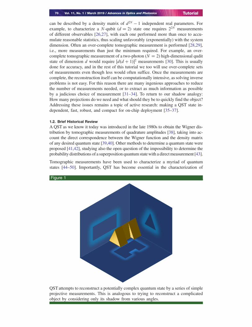
1.1. Basic ConceptOne of the challenges in quantum optics is to unravel an unknown state [1–3], with thedifficulty arising primarily from the measurement problem in quantum mechanics[4,5]. First, a measurement destroys the information of the state, or at the very leastperturbs it [6], negating the possibility of performing multiple measurements on thesame state [7]. Neither is it possible to clone the state one wishes to study: this impliesthat measurements cannot be performed on exact copies of a state [8]. Moreover, astate is generally unknown—it could be pure or mixed, high dimensional or low di-mensional—and so the choice of basis and measurement sequence is not trivial[9–12]. Consequently, we can infer only a little information at a time by probinga particular aspect of a quantum state [13]. In other words, only one question canbe asked (by performing a measurement) from which we get one piece of information(the measurement’s outcome). The standard approach for collecting information abouta quantum state is to perform multiple tomographic measurements, so-called projec-tive measurements, in what is known as a quantum state tomography (QST) [seeRefs. [1,14] for good reviews]. A QST is very similar to the well-known computedtomography or “CT” scans in medicine: once many projective measurements aremade, each probing a particular aspect of the possible state, the complete quantumstate is built up through a tomographic process. In essence, each unknown quantumstate is “sliced” and completely characterized through a series of projective measure-ments in different bases, retrieving the information of a new dimension for each mea-surement [15]. It is akin to building up an image of a complex object by making onlysimple projections of its shadow, as illustrated in Fig. 1. In this picture, the unknownshape of an object (i.e., the unknown state) can be worked out by the informationcontained in the measured shadows (i.e., the results of projection measurements).In the quantum case, the outcome is the complete set of observables whose proba-bilistically weighted outcome fully describes the quantum state [16]. This then be-comes an inverse problem: knowing the outcome of every question (the outcomesof our measurements), can we work out what the “object” is? In the quantum worldthis often translates into determining a density matrix for the quantum state fromwhich all other required information can be inferred [15,17,18].

QSTs (plural because they come in various guises) are time consuming and complex:the number of measurements does not scale well with the dimension of the quantumstate [19,20], noise affects the outcome [21–24], and one must assume that identicalstates are produced at the source, e.g., identical copies of photons from a spontaneousparametric downconversion (SPDC) process [25]. Consider systems with N photons,each in d dimensional states. The total dimension of the system is then D � dN and


can be described by a density matrix of d2N − 1 independent real parameters. Forexample, to characterize a N -qubit (d � 2) state one requires 22N measurementsof different observables [26,27], with each one performed more than once to accu-mulate reasonable statistics, thus scaling unfavorably (exponentially) with the systemdimension. Often an over-complete tomographic measurement is performed [28,29],i.e., more measurements than just the minimum required. For example, an over-complete tomographic measurement of a two-photon (N � 2) high-dimensional quditstate of dimension d would require �d�d � 1��2 measurements [30]. This is usuallydone for accuracy, and in the rest of this tutorial we too will use over-complete setsof measurements even though less would often suffice. Once the measurements arecomplete, the reconstruction itself can be computationally intensive, as solving inverseproblems is not easy. For this reason there are many ingenious approaches to reducethe number of measurements needed, or to extract as much information as possibleby a judicious choice of measurement [31–34]. To return to our shadow analogy:How many projections do we need and what should they be to quickly find the object?Addressing these issues remains a topic of active research: making a QST state in-dependent, fast, robust, and compact for on-chip deployment [35–37].

1.2. Brief Historical ReviewAQST as we know it today was introduced in the late 1980s to obtain the Wigner dis-tribution by tomographic measurements of quadrature amplitudes [38], taking into ac-count the direct correspondence between the Wigner function and the density matrixof any desired quantum state [39,40]. Other methods to determine a quantum state wereproposed [41,42], studying also the open question of the impossibility to determine theprobability distributions of a superposition quantum statewith a directmeasurement [43].

Tomographic measurements have been used to characterize a myriad of quantumstates [44–50]. Importantly, QST has become essential in the characterization of

Figure 1

QST attempts to reconstruct a potentially complex quantum state by a series of simpleprojective measurements. This is analogous to trying to reconstruct a complicatedobject by considering only its shadow from various angles.


entanglement sources, e.g., entanglement sources using photons [51–57], atoms[58,59], and even with molecular vibrational modes [60]. However, the polarizationof a photon is the most common known degree of freedom used to encode a quantumstate. This is due to the great variety and availability of high-efficiency polarizationcontrol elements. Consequently, many experimental milestones in quantum opticshave been accomplished by using the polarization degree of freedom [61–64].

Although QSTs have been performed on many quantum systems, in this tutorial wewill consider photonic quantum states, exploiting the spatial mode and polarizationdegrees of freedom in light. QSTs have been performed extensively on the latter (see,for example, Refs. [53,56,65,66]), while other degrees of freedom are becoming moreprevalent these days, e.g., entangled spatial modes [67–72] for improved communi-cation security [73–76] and high-dimensional entanglement [77–80]. Although high-dimensional quantum state generation is increasingly relevant, the characterization ofsuch systems is extremely complex due to the exponential increase of projections withdimension. Nevertheless, QSTs have been successfully demonstrated on high-dimen-sional spatial mode entanglement by using various projection approaches [81–83].

There are also advantages when mixing two degrees of freedom in the same photon,also known as hybrid states [84–86]. One pertinent example that we will consider inmore detail in this tutorial is that of hybrid polarization and orbital angular momentum(OAM) degrees of freedom [87]; they are relevant as natural modes of optical fibers[88] and free space [89]. The generation of such states can be achieved by using holo-grams [90], but also in a more straightforward way by using spin–orbit conversiondevices based on liquid crystals [91], or even based on metamaterial technology[92,93]. On the other hand, instead of the most general case of generating entangle-ment between two photons, we can study entanglement between two degrees of free-dom in a single photon [94,95], paving the way for the use of quantum measurementtools to characterize states generated with intense laser beams [96–98].

1.3. Outline of the TutorialIn this tutorial, we will not only outline the core ideas of a QST, but will also showhow they may be performed in a fast and easy manner with intense classical light.Classical laser light does not suffer from the aforementioned quantum measurementwoes: one can make as many measurements as one likes simultaneously on the sameintense light field. The use of classical light in quantum studies is not new [99–101],while today there is a growing realization that non-separability, the quintessentialproperty of quantum entanglement, is not unique to quantum mechanics[102–106]. As such, many classical systems exhibit properties usually associated withquantum entangled states [107–109], also referred as nonquantum entanglement[110,111], or non-separable states [112,113]. However, even though a particularclassical system can simulate most of the features of entanglement, it fails to simulatequantum nonlocality [114]. In relation to QSTs, classical light has been exploited asan alignment and predictive tool using the so-called backprojection with single pho-tons [115–121], following the time reversal analogy given by Klyshko [122].

We exploit these similarities between some classical and quantum states to develop auseful laboratory tool for teaching and demonstrating QSTs. First we outline the gen-eral principles of quantum tomographic measurements, explaining in tutorial fashionhow to translate theory into experiment, how to perform the measurements, and howto extract the required information. Next, we explain how to use the time reversalconcept to mimic the quantum system using backprojected scalar light. This allowsone to perform the measurement as if there were entangled photons. To actually usethe quantum toolbox directly, we make use of non-separable classical light, exploiting


the fact that non-separability is the hallmark of quantum entangled systems. We usevector vortex beams as our non-separable states of light, depicted on a high-orderPoincaré sphere [123–125], and perform a QST with standard optical components.This allows us to create any state from fully separable to fully non-separable, andtreat it as a controlled source of entanglement, albeit entirely classical and with intenselaser light. As a consequence, however, the possibility of studying the quantum non-locality is discarded. We show that we can easily reconstruct any quantum state byautomating the optical elements that perform each particular projection. We demon-strate all the measurements typically performed in a quantum laboratory, such as theBell inequality measurements, but here with intense laser beams. We provide the com-plete toolkit, from the software to the three-dimensional (3D) designs (see Ref. [126]),for others to duplicate as a versatile teaching tool that can be 3D printed and automatedwith all the designs and software used to obtain the results shown in this tutorial, aswell as a video (see Visualization 1 [126]) demonstrating the process in action. Wehope that this tutorial and associated resource will inspire the teaching of quantummechanics from an experimental perspective, a component sorely lacking in manyquantum courses, and be of value in realizing educational and research objec-tives alike.

2. QST OF TWO-LEVEL STATES

2.1. Polarization QubitThe quantum bit (qubit) is the fundamental unit of quantum information. Unlike aclassical bit that assumes one of two distinct states, 0 or 1, the quantum bit is aweighted superposition of two orthogonal states of a given degree of freedom, forexample,

jψi � αj0i � βj1i, (1)

with probability amplitudes α and β so that jαj2 � jβj2 � 1. Spin states are the mostcommon example of qubits currently explored to realize quantum computation andcommunication. For photons, these spin states can correspond to left- and right-cir-cular polarization states [127]. In general, one can express the state of a polarizationqubit as

jψi � cos�θ∕2�jRi � exp�iφ� sin�θ∕2�jLi, (2)

where jRi and jLi represent the right- and left-circular polarization states, respectively.The parameter φ ∈ �0, 2π� is related to the phase difference between the polarizationstates, while θ defines the weighting factor. In the special cases of θ � 0 and θ � π,the qubit state jψi corresponds to the polarization eigenstates jRi and jLi, respectively.By manipulating both θ and φ, one can produce arbitrary polarization states. For ex-ample, for θ � π∕2, one can prepare any linear polarization state as depicted graphi-cally in Table 1.

The definition of the qubit state in Eq. (2) has an intuitive representation as a point on asphere, commonly referred to as the Poincaré sphere. Historically the Poincaré sphereis the name used when describing classical polarization states, while the Bloch sphereis used when the polarization is regarded as a quantum state. Nevertheless, they de-scribe the same two-dimensional space. First let us look at the effect of tuning theprobability amplitudes, by varying θ. Normalization of the quantum state requires

Table 1. Linear Polarization States Produced for θ � π∕2

Phase φ 0 π∕2 π 3π∕2

Qubit state jψi. ↔ ⤡ ↕ ⤢


https://doi.org/10.6084/m9.figshare.7035497

conservation of probability; that is, the probability of finding the qubit jψi in any of itseigenstates must be 1 (the qubit must be in some state after all). Mathematically, this isexpressed as

jhψ jψij2 � jcos2�θ∕2�j2 � sin2�θ∕2� � 1: (3)

By visual examination, one notices that Eq. (3) describes a circle of radius 1, where θparameterizes the position on the circle, as shown in Fig. 2(a). Let us refer to this as theamplitude circle.

The phase term exp�iφ� is an oscillatory function, whose variable φ can be bounded inthe interval �0, 2π�. By plotting this oscillatory function on the complex plane, onerealizes that the angle φ maps to an angular position on a unit circle. Varying φchanges the relative phase between the basis states, resulting in a rotation of the qubitstate on a unit circle, as shown in Fig. 2(b) for linearly polarized states (θ � π∕2). Wewill refer to this circle as the phase circle.

The Poincaré sphere brings the description of amplitude and phase variation into asingle picture. Place a point on the amplitude circle by fixing θ, rotate it aroundthe phase circle by an angle φ, and one has the recipe for locating a position onthe surface of the Poincaré sphere. Thus, an arbitrary qubit state parameterized bya unique set of coordinates (θ, φ) can be mapped to a point on the unit sphere, asshown in Fig. 2(c). In the Poincaré sphere representation, the qubit state lives onthe surface of a sphere, and motion on the sphere transforms one qubit state into an-other. To be useful in a quantum application, it is necessary to be able to manipulateand characterize the qubit state. This requires locating the qubit on the sphere andmoving it to a different position. Given that the geometry is spherical, we simply needa reference point on the sphere and a set of rotation transformations about the origin.In three dimensions, one needs a set of rotations about the x, y, or z axis, as shown inFig. 3. Given that the initial state is known, the final state can be uniquely determinedby evaluating the influence of the various rotations: this is the objective of a quantumstate tomographic measurement (QSTM). But before we delve into the inner workingsof a QST, we first need an additional description of qubit states: the density matrix.

Figure 2

(a) (b) (c)

Intuitive description of the Poincaré sphere. (a) Control over the amplitude parameterθ allows one to continuously change the position of the qubit (indicated by the arrow)on the unit circle, resulting in a change of the relative amplitudes of left- and right-circular polarizations. (b) Control over the phase parameter φ allows one to contin-uously change the position of the qubit (indicated by the arrow) on a different unitcircle, this time resulting in a rotation of the polarization state. This is demonstratedfor θ � π∕2 in Eq. (2). (c) Simultaneous control of phase and amplitude results in adescription of the general qubit in Eq. (2) on a unit sphere where the poles are thepolarization states.


The density matrix description of quantum states is more general than the state vectordescription of Eq. (2). This is because density matrices allow one to describe the actualoutcome of measurements, and pertinently, for both pure and mixed states. Imaginewe have an ensemble of K independent single photons, each prepared in the qubit statejψni with n � f1, 2,…,Kg. If all the photons are identical, that is, they are prepared inthe same state jψni � jψi, then every photon can be described using a single statevector jψi as in Eq. (2). The state of every photon is said to be pure. Conversely,if some (or all) of the K photons are prepared in different states, the result is a stat-istical mixture of pure states. A photon randomly chosen in the mixture can be foundto be in a given pure state jψni with a certain probability. However, because all thephotons are independent and uncorrelated, there exists no phase relation between theirstates. Consequently, the formalism in Eq. (2) cannot appropriately describe such amixture. A density matrix is a useful tool to overcome this hurdle.

Assume that the state of a single photon in the aforementioned ensemble can bedescribed by a 2 × 2 matrix, ρ, called the density matrix. In general, ρ can be decom-posed in terms of its eigenvectors and eigenvalues:

ρmixed �Xm

cmjψmihψmj: (4)

In this description each cm is real, positive, and corresponds to the probability of meas-uring a photon prepared in the eigenstate jψmi. Conservation of probabilities requiresthat

Pmcm � 1. By construction, density matrices must be Hermitian; that is, ρ† � ρ,

where superscript †, called “dagger,” refers to the complex conjugation and transposeoperation. This can be easily verified as �jaihbj�† � jbihaj.The density matrix in Eq. (4) describes a statistical mixture of pure qubit statesjψmihψmj. Hence, we refer to ρ as a mixed state density matrix. In the special casewhere all photons are identically prepared (pure state), there exists only one eigenstatewith unit eigenvalue. The pure state density matrix then reads ρpure � jψihψ j. For thepure state in Eq. (2), the density matrix is expressed as follows:

ρ � jψihψ j � cos2�θ∕2�jRihRj � sin2�θ∕2�jLihLj� cos�θ∕2� sin�θ∕2� exp�−iφ�jRihLj� cos�θ∕2� sin�θ∕2� exp�iφ�jLihRj: (5)

One can now provide a matrix representation of ρ by assigning coordinate vectorsto the basis states. For example, assume the following representation of the

Figure 3

(a) (b) (c)

Elementary rotations on the surface of the Poincaré sphere. The qubit state, indicatedby the position vector colored orange, can be rotated on the surface of the sphere aboutthe (a) x axis, (b) y axis, and (c) z axis.


polarization states: jRi ≡ �1 0�T and jLi ≡ �0 1�T where the superscript T refers to ma-trix transpose. The density matrix thus assumes the following matrix representation:

ρ �

cos2�θ∕2� cos�θ∕2� sin�θ∕2� exp�−iφ�cos�θ∕2� sin�θ∕2� exp�iφ� sin2�θ∕2�

!: (6)

For density matrices, the conservation of probability in Eq. (3) is expressed as tr�ρ� � 1,where tr�ρ� �P

iρii is the trace. For the density matrix in our example this becomes

tr�ρ� � cos2�θ∕2� � sin2�θ∕2� � 1: (7)

This is a physical requirement for any density matrix. However, one can concludewhether it corresponds to a pure or a mixed state by computing the purity:

tr�ρ2� � tr

�Xm

Xn

cmcnjψmihψmjjψnihψnj�

�Xm

Xn

cmcnjhψmjψnij2: (8)

It follows that jhψmjψnij2 ≤ 1; this is because the probability of measuring a state jψmigiven that we prepared jψni is in general less than 1, except when jψmi � jψni, inwhich case the overlap is 1. We can then bound Eq. (8) by

0 ≤Xm

Xn

cmcnjhψmjψnij2 ≤Xm

cmXn

cn � 1, (9)

where we have used the fact thatP

mcm � 1. One then arrives at the followingcriterion for purity:�

tr�ρ2� � 1 for cm � cn � 1 ⇒ ρ is pure

0 ≤ tr�ρ2� < 1 for cm, cn < 1 ⇒ ρ is mixed:(10)

The objective of a QST is to reconstruct the density matrix of an arbitrary state using anappropriate set of measurements, regardless of whether the state is pure or mixed[9,30,53,128]. It is this broad applicability that makes QSTs such a powerful tool inquantum information and communication. The procedure behind a QST for two-dimen-sional quantum states consists of locating the qubit state on the Poincaré sphere; that is,as mentioned before, characterizing the rotation angles about the x, y, and z axes. Giventhat the motion of our qubit state is restricted to rotations on the Poincaré sphere, thedensity matrix can thus be expressed in terms of rotation operators about the x, y, and zaxes. In two dimensions, these rotation operators are the Pauli matrices, σi, plus theidentity

σ1 ��0 1

1 0

�; σ2 �

�0 −ii 0

�; σ3 �

�1 0

0 −1�; I �

�1 0

0 1

�:

The Pauli matrices are traceless operators (tr�σi� � 0) that obey the following tracerelations:

tr�σiσj� � 2δi,j, for i, j � 1, 2 or 3: (11)

This is an expression of the completeness relation between the matrices. Unlike theother Pauli matrices, the identity operator is not traceless, but obeys the trace relations


I � σ0 ��1 0

0 1

�; tr�σ0σ0� � 2; tr�σ0σi� � tr�σiσ0� � tr�σj� � 0:

That the σi matrices form a complete set means that one can express the density matrix ρas a linear combination of our σi matrices,

ρ � 1

2

X3n�0

ρnσn, (12)

where ρn are the expectation values of the matrices σn and are obtained from

tr�ρσn� �1

2tr

�X3m�0

ρmσmσn

�� 1

2

X3m�0

ρm tr�σmσn� �X3m�0

ρmδm,n � ρn: (13)

Therefore, provided one can obtain the expectation values, ρn, it is then trivial toreconstruct the density matrix of the system. However, one first needs to clarify themeasurement procedure that leads to the computation of ρn. To do so, it is useful toexpress the matrices σn in terms of eigenvalues and eigenvectors that, as we will show,correspond to physical states that can be measured directly.

The matrices σn each have two eigenvectors, jλ0ni and jλ1ni, with eigenvalues α0n and α1nand thus can be expressed as

σn � α0njλ0nihλ0nj � α1njλ1nihλ1nj: (14)

Based on this decomposition, we can express the expectation values in Eq. (13) as

ρn � tr�ρσn� � α0nhλ0njρjλ0ni � α1nhλ1njρjλ1ni: (15)

The matrices jλnihλnj are called projectors; these are Hermitian and positive operatorsthat form a complete orthonormal set [129]. This is a rather dense description, so let usgo through each property one by one.

(1) Hermiticity: Projectors are self-adjoint operators, i.e., they are equal to theirown conjugate transpose, and have real expectation values. This is a fundamentalrequirement for projectors to be physical observables.

(2) Positivity: Positive operators have expectation values greater or equal to 0. This isa natural requirement for projectors given that their expectation values correspondto probabilities.

(3) Completeness:P

mjλmn ihλmn j � σ0. This is a requirement for conservation ofprobability

(4) Orthonormality: jλmn ihλmn jjλlnihλlnj � jλmn ihλlnjδl,m. This is not a physical require-ment but implies that the eigenstates of two projectors within a complete set haveno overlap.

From their definition, one can easily compute the eigenvalues of the matrices σn andshow that they are�1, as shown in Table 2. Interestingly, the eigenvectors correspondto the polarization states on the surface of the Poincaré sphere, previously shown inFig. 2. We now have the recipe to compute the expectation values of the σn matrices interms of direct measurement that can be performed on the quantum state, and it is asfollows:

ρ0 � tr�ρσ0� � hRjρjRi � hLjρjLi, (16)


ρ1 � tr�ρσ1� � hH jρjHi − hV jρjV i, (17)

ρ2 � tr�ρσ2� � hDjρjDi − hAjρjAi, (18)

ρ3 � tr�ρσ3� � hRjρjRi − hLjρjLi: (19)

Observe, however, that the measurements required to compute ρ0 are the same as thatof ρ3. In fact, tr�ρσ0� is an expression of the conservation of probability. Given thatprojectors of a given Pauli matrix form a complete set, the conservation of probabilityis independent of the measurement basis. Thus, one can deduce that ρ0 can be obtainedin a similar manner from the projective measurements of ρ1 and ρ2. Thus, the over-complete tomographic measurement of a single qubit requires a total of six projectivemeasurements: d�d � 1� as mentioned in the introduction, for d � 2. To illustrate thereconstruction, we will consider two examples: a pure and a mixed qubit states.

• Pure state. Let us consider the state jψi expressed in the polarization basis as

jψi �ffiffiffi3

p

2jRi � 1

2exp

�−i π

3

�jLi, (20)

so that the density matrix ρ � jψihψ j reads

ρ �

0B@ 3

4

ffiffi3

p4

exp�i π3

�ffiffi3

p4

exp�−i π3� 1

4

1CA: (21)

We then perform the tomographic measurement of the state by performing thenecessary projections, as shown in Table 3.

Next we compute the expectation values ρn,

ρ0 � 1; ρ1 �ffiffiffi3

p

4; ρ2 � − 3

4; ρ3 �

1

2,

Table 2. Eigenvectors and Eigenvalues of the Identity and Pauli Matrices in thePolarization Basis

Matrices σn α0n jλ0ni α1n jλ1ni

σ0 1 jRi ≡�1

0

1 jLi ≡

�0

1

σ1 −1 jV i ≡ 1ffiffi

2p�

1

−1

1 jHi ≡ 1ffiffi2

p�1

1

σ2 −1 jAi ≡ −iffiffi

2p�

1

−i

1 jDi ≡ −iffiffi2

p�1

i

σ3 1 jRi ≡

�1

0

−1 jLi ≡

�0

1

Table 3. Tomographic Measurements of a Pure State

hRjρjRi hLjρjLi hH jρjHi hV jρjV i hDjρjDi hAjρjAi3/4 1/4 4�

ffiffi3

p8

4− ffiffi3

p8

1/8 7/8


and reconstruct the density matrix:

ρ � 1

2

�1 0

0 1

��

ffiffiffi3

p

8

�0 1

1 0

�− 3

8

�0 −ii 0

�� 1

4

�1 0

0 −1�

�

34

ffiffi3

p �3i8ffiffi

3p −3i

814

!�

34

ffiffi3

p4

exp�i π3

�ffiffi3

p4

exp�−i π

3

�14

!:

• Mixed state. Now we consider the case of a mixed state ρ expressed in the polari-zation basis as follows:

ρ � 1

3jRihRj � 2

3jLihLj �

�13

0

0 23

�: (22)

Similarly, we perform a tomographic measurement of the state obtaining the pro-jections shown in Table 4.

We then compute the expectation values ρn,

ρ0 � 1; ρ1 � 0; ρ2 � 0; ρ3 � − 1

3,

and reconstruct the density matrix:

ρ � 1

2

�1 0

0 1

�− 1

6

�1 0

0 −1�

��

13

0

0 23

�:

A graphical representation of the density matrix in terms of real and imaginary parts ispresented in Figs. 4(a) and 4(b) for the pure state jψi �

ffiffi3

p2jRi � 1

2exp�−i π

3�jLi and

the mixed state ρ � 13jRihRj � 2

3jLihLj, respectively.

A useful way to visualize these measurements is to see that they are made up of pro-jections into two orthogonal bases, say jLi and jRi, and into four mutually unbiasedbases (MUBs): jHi, jV i, jAi, and jDi. The MUBs can be constructed from superpo-sitions of the two orthogonal bases, i.e., the horizontal MUB, jHi, can be written as asuperposition of jLi and jRi. Although obvious for polarization, we show themgraphically in Fig. 5 as we will build up this figure throughout the tutorial withexamples beyond polarization. The mutually unbiased states have the property thatthe overlap with one of the orthogonal states always yields an outcome with a prob-ability of 1∕d, where d is the dimension of the Hilbert space. For polarization d � 2,so this is 1/2.

2.2. Spatial Mode QubitWhile in the above we have presented the qubit QST in terms of polarization, oneshould note that the choice of degree of freedom is arbitrary. An alternative and topicaldegree of freedom is the spatial mode of the photon [130]. The term spatial moderefers to transverse solutions of the wave equation in the paraxial limit; that is, whenthe variation in transverse momentum is negligible in comparison to its longitudinalcounterpart. In this regime, a family of solutions arise: Hermite–Gaussian, Laguerre–Gaussian, and Bessel–Gaussian modes, just to name a few. Some of these modes carry

Table 4. Tomographic Measurements of a Mixed State

hRjρjRi hLjρjLi hH jρjHi hV jρjV i hDjρjDi hAjρjAi1/3 2/3 1/2 1/2 1/2 1/2


discrete units of a fundamental quantum number: the OAM. Conserved at the singlephoton level [67], the OAM degree of freedom is particularly attractive in classical andquantum information, communication, and computation [131–135]. Unlike polariza-tion, the state space of OAM modes is infinitely large, allowing more information tobe encoded in photons [75,76,79,136–139].

Recall the polarization qubit state in Eq. (2). An analogous description can be pro-vided in terms of spatial modes that carry OAM [140]:

jψi � cos�θ∕2�jl1i � exp�iφ� sin�θ∕2�jl2i, (23)

where the ket jli refers to a paraxial field that carries lℏ units of OAM. Such a fieldcan be expressed in cylindrical coordinates �r,ϕ, z� [141]:

jli ≡ A�r, z� exp�ilϕ�, (24)

where A�r, z� is an amplitude term that varies transversally and longitudinally. Theintensity and phase of some OAM modes of the Laguerre–Gaussian type are shown

Figure 5

Graphical representation of orthogonal and mutually unbiased states used in the QSTprojections. Here only the polarization matters, shown overlaid on a Gaussian mode.

Figure 4

(a)

(b)

Graphical representation of the density matrix in terms of its real and imaginary com-ponents for the (a) pure state and (b) mixed state examples as given in the main bodytext.


in Fig. 6. The azimuthal phase creates a twisted wavefront with a central discontinuitywhere the phase is undefined, resulting in an intensity null.

Observe that the field of the OAM mode is separable in both amplitude andazimuthal phase, arg�exp�ilϕ�]; that is, the amplitude and azimuthal phase can

Figure 6

(a)

(b)

(a) Intensities and (b) phase maps of OAM modes carrying, from left to right,l � −3, − 2,…, �2, and �3 units of OAM.

Figure 7

(a)

(c)

(b)

(d)

(a) Representation of polarization states on the Poincaré sphere. The poles representthe eigenstates of the basis, from which all other states are constructed. An arbitrarypolarization state thus maps to a point on the surface of the Poincaré sphere. (b) Thenormalized outcomes of projective measurements onto the eigenstates of the Paulimatrices, for given horizontally polarized state. (c) Equivalently, one can constructa similar sphere, a Bloch sphere, where the poles correspond to OAM eigenstates.Here, the eigenstates of the Pauli matrices correspond to spatial modes. (d) Fromprojective measurement onto these spatial modes, one performs the quantum-statetomographic measurement of an OAM state �jli � j−li�∕ ffiffiffi

2p

with l � −1.


be factorized. The orthogonality of OAM modes at a given z plane (say z � z0) maybe expressed by

hl1jl2i �Z

∞

0

dr rA�r, z0�Z

2π

0

dϕ exp�i�l2 − l1�ϕ� � δl1,l22π

Z∞

0

dr rA�r, z0�:

(25)

Similar to polarization, OAM qubits can be represented on the surface of a sphere,the OAM Bloch sphere [140], as shown in Fig. 7. Here the poles are the OAM states,while the equator represents the Hermite–Gaussian modes, as detailed in Fig. 8, forl1 � −l2 � 1. Observe that the superposition of two oppositely charged OAMstates leads to azimuthal fringes, which then rotate with the intermodal phase φ.This is similar to the rotation of the linear polarization states in Fig. 2.

A QST of an OAM qubit follows the same procedure as that outlined previously. Thedensity matrix is expanded in terms of Pauli matrices and the identity. The eigenvec-tors now take on a different meaning: rather than polarization states, they now cor-respond to OAM modes and their superpositions, as shown in Fig. 9. Means toperform projective measurements on these spatial modes have been extensively re-ported for quantum [19,142] and classical light [143–147]. Progress in liquid crystaltechnology and digital micro mirror devices has made it possible to generate and de-tect arbitrary spatial modes using digital holograms (see Ref. [130] and Ref. [148] for

Figure 8

(a) (b)

(c)

Bloch sphere description of an OAM qubit in Eq. (23) with l1 � −l2 � 1. Controlover the amplitude parameter θ and phase parameter φ, as shown in (a) and (b), re-spectively, leads to (c) a description of the general OAM qubit on a unit sphere wherethe poles are the pure OAM states.


a comprehensive review and tutorial, respectively). This has opened avenues for anall-digital realization of QSTwith spatial modes. The core idea is to consider the pat-tern creation step but in reverse. If a particular hologram were to convert a Gaussianmode into a desired pattern, then in reverse the same hologram will convert the patterninto a Gaussian. As Gaussians are the only modes that couple into single-mode fiber(SMF), we have the means of a “pattern sensitive” detector, as illustrated in Fig. 10.An example of projective measurements, together with the reconstructed densitymatrix of pure OAM qubit state jψi � �j1i � j−1i� ffiffiffi

2p

, is shown in Fig. 11.

Note again that we can see the link between orthogonal and MUB projections, thistime into jli and j−li states, plus the four MUBs made up of superpositions ofthese: jli � exp�iθ�j−li for θ � �0, π∕2, π, 3π∕2�, as shown graphically inFig. 12. Because such MUBs require amplitude modulation to implement, one oftenapproximates them in the projective measurement as arg�jli � exp�iθ�j−li�,producing a binary phase pattern rather than an amplitude function. This is whyall the Pauli matrices in Fig. 9 are phase-only patterns. In general the OAM examplecan be replaced with arbitrary modes by substituting jli → jM 1i and j−li → jM 2ieverywhere in the above analysis.

Figure 9

Eigenvectors and eigenvalues of the identity and Pauli matrices in the OAM basis.

Figure 10

Detection of a spatial mode requires a “pattern sensitive” detector. This is achieved byexploiting the reciprocity of light, passing the incoming beam backward through thehologram that would detect it.


2.3. Biphoton QubitsTransitioning from single particles to multi-particle systems allows for the existence ofcorrelations, one of the most remarkable being non-local entanglement [149].Mathematically, the states of entangled systems are non-separable, i.e., the statesin an entangled system do not factorize into product states. Physically this means that,through non-local correlations, the unknown state of one particle can be uniquelydetermined through measurements on its entangled partner(s). Entanglement is a valu-able resource in quantum information and quantum computation, and as such requirescertification. While there exists various means to characterize entanglement, a stan-dard and widely used approach is to first reconstruct the density matrix of the stateunder study and then determine whether it is entangled or not. The tool of choice forthis task is a QST, first performed on OAM modes with physical holograms [67] andlater with digital holograms [142].

Here we look at a two-qubit system (N � 2 and d � 2) and go through the methodbehind a two-particle QST. As discussed before, the choice of degree of freedom is

Figure 12

Graphical representation of the orthogonal and MUBs used in the QST projections for(a) polarization and (b) OAM modes. In the case of the latter, the polarization is nolonger important and so is shown as horizontal everywhere. The patterns are shown asintensity functions, while the actual projections are often done with phase-only ap-proximations to these.

Figure 11

(b)

(a)

(a) Graphical representation of the outcomes of the projective measurements of a QSTon the state jψi � �j1i � j − 1i�∕ ffiffiffi

2p

, shown in the inset. (b) Based on these tomo-graphic measurements, one reconstructs the density matrix of the state.


arbitrary and as such we will choose the OAM degree of freedom to illustrate thetomographic measurements. We will work in a generic OAM subspace with eigen-states j−li and jli (the same substitution rules apply as mentioned earlier should thereader wish to adapt the basis to another mode type)

We start by describing a general two-particle system with a density matrix ρ as

ρ �Xm

cmjψmihψmj, (26)

where the pure states jψmi are now two particle qubit states, described by

jψmi �Xi, j

αijmjiiA ⊗ jjiB: (27)

The states jii and jji are eigenstates of the systems A and B, respectively, with as-sociated complex coefficients αijm that define the mth state jψmi. The symbol ⊗ is atensor product operation that, in essence, is a way to multiply two state spaces ofdimensions d1 and d2, respectively, to form a new larger state space with dimensiond1 × d2. In the case of a two-qubit state, the joint system is four dimensional. It isworth spending some time describing the computation of the tensor productoperation.

Given two matrices S and T (we will assume without loss of generality that these aresquare matrices), the tensor product S ⊗ T produces a new matrix M computed by

M � S ⊗ T �

0B@

S1,1 × T S1,N × T

..

. . .. ..

.

SN ,1 × T SN ,N × T

1CA: (28)

Using this procedure we can deduce the basis vectors for the two-qubit states of in-terest, jψmi, by considering all the tensor product combinations jii ⊗ jji. In the spatialmode basis of interest here, these are the OAM eigenstates j � li. We then obtain thebasis states for the joint system as follows:

jli ⊗ jli ��1

0

�⊗�1

0

��

0BBB@

1

�1

0

�

0

�1

0

�1CCCA �

0BBB@

1

0

0

0

1CCCA, (29)

jli ⊗ j−li ��1

0

�⊗�0

1

��

0BBB@

1

�0

1

�

0

�0

1

�1CCCA �

0BBB@

0

1

0

0

1CCCA, (30)

j−li ⊗ jli ��0

1

�⊗�1

0

��

0BBB@

0

�1

0

�

1

�1

0

�1CCCA �

0BBB@

0

0

1

0

1CCCA, (31)


j−li ⊗ j−li ��0

1

�⊗�0

1

��

0BBB@

0

�0

1

�

1

�0

1

�1CCCA �

0BBB@

0

0

0

1

1CCCA: (32)

Now that we have an understanding of the tensor product operation, the state-tomog-raphy measurement of the two-qubit state can be intuitively understood. The state of eachqubit can be characterized with the set of rotation matrices (Pauli matrices) plus the iden-tity matrix. The joint state, therefore, follows a tensor product construction as follows:

ρ ��1

2

X3m�0

ρmσm

�A

⊗�1

2

X3n�0

ρnσn

�B

� 1

4

X3m, n�0

ρmnσm ⊗ σn: (33)

The above construction naturally leads to the description of the qubit pair on the surfaceof a higher order Bloch sphere, as shown in Fig. 13. From Eq. (33), the state of the qubitpair is defined by a set of single-qubit rotations, together with single-qubit identity op-erators. Similar to the case of a single qubit, these rotations occur on the surface of asphere, a higher order Bloch sphere. In this description, the states on the sphere follow thesame tensor product construction as that in Eq. (27), as shown in Fig. 13. In the case ofOAM states, the poles correspond to the tensor product of single-qubit OAM states.While there are many tensor product combinations of single-photon qubit states, thereis only one rule for constructing the higher order Bloch sphere: each single qubit musthave orthogonal states on the poles of the sphere. For example, one cannot constructa higher order Bloch sphere with the states jlij−li and jlijli on the poles. This isbecause any two-qubit pair formed as a linear superposition of these two-qubit statesfactorizes with respect to each subsystem. This simply means that one can write thetwo-qubit state as jψi � �·�A ⊗ �·�B. This can be shown as follows:

Figure 13

Description of qubit pairs on the higher order Bloch sphere. States on the surface of thehigher order Bloch sphere are constructed from the tensor product of qubit states fromtwo Bloch spheres, each describing a subsystem (photon). The entire space is fourdimensional, shown here as two-dimensional subspaces for visualization purposes.


jψi � cos�θ∕2�jliAj−liB � exp�iφ� sin�θ∕2�jliAjliB, (34)

⇒ jψi � jliA ⊗ �cos�θ∕2�j−li � exp�iφ� sin�θ∕2�jli�B: (35)

Observe that the two-qubit state is parameterized by θ and φ, and can be entirely char-acterized by a single qubit rotation on subsystem B alone. We thus say that the twosubsystems factorize, or equivalently, that they are separable. The notion of separabilitywill be treated in more detail a little later.

Note that an arbitrary state on the surface of the higher order Bloch sphere cannot bedescribed by a single qubit rotation on one subsystem alone. In other words, the higherorder Bloch sphere describes a set of both separable and non-separable states. In thecase of two-qubit states, this non-separability is what we traditionally refer to as“quantum entanglement.” In general, arbitrary states on the higher order Bloch spheresin Fig. 13 are represented as

jψi � cos�θ∕2�jl1ijl2i � exp�iφ� sin�θ∕2�j−l1ij−l2i ≠ �·�A ⊗ �·�B: (36)

Fortunately, the separability of the state does not affect the reconstruction procedurethrough QST. In what follows, we will outline the steps to perform a two-qubit QSTfor an arbitrary state represented by the density matrix, ρ.

Once again, the task of a QST is to realize direct measurements to compute the expect-ation values ρmn. We follow the same tensor product construction of the expectationvalue to express ρmn in terms of eigenvalues and eigenvectors of the basis operators forthe joint system; these are σm ⊗ σn and can be expressed as follows:

σm ⊗ σn � �α0mjλ0mihλ0mj � α1mjλ1mihλ1mj� ⊗ �α0njλ0nihλ0nj � α1njλ1nihλ1nj�: (37)

By expanding the expression above, the measurements required in a QST can bedirectly read as

σm ⊗ σn � α0mα0njλ0mihλ0mj ⊗ jλ0nihλ0nj � α1mα

1njλ1mihλ1mj ⊗ jλ1nihλ1nj

� α1mα0njλ1mihλ1mj ⊗ jλ0nihλ0nj � α0mα

1njλ0mihλ0mj ⊗ jλ1nihλ1nj: (38)

The projectors jλmihλmj have been discussed in the previous section and we haveshown that they can be realized through direct measurement on the quantum state.In the case of two qubits, the tensor product jλmihλmj ⊗ jλnihλnj means that one mustperform joint projective measurements on both photons. Practically, this implies thatthe projective measurements must be done in coincidence. This can be done usingsingle photon detectors and a counting module. The expectation values ρmn then takethe following form:

ρmn � α0mα0nhλ0mλ0njρjλ0mλ0ni � α1mα

1nhλ1mλ1njρjλ1mλ1ni

� α1mα0nhλ1mλ0njρjλ1mλ0ni � α0mα

1nhλ0mλ1njρjλ0mλ1ni: (39)

In the above, we have used a compact notation for the projective measurement, wherejλ0mλ0ni ≡ jλ0mi ⊗ jλ0ni. Note the order of the eigenstate in both the bra and ket in theexpression of the expectation value: the first state refers a measurement on particle A,while the second state refers to a measurement on particle B. For example, the expect-ation value hλ0mλ1njρjλ0mλ1ni is obtained by projecting photons A and B on the state jλ0miand jλ1ni, respectively, and measuring in coincidence. The eigenvalues αm and eigen-vectors jλmi are known from the single-qubit QST; we can thus write the expressionof the expectation values ρmn in terms of direct projective measurements. With four


measurements per expectation value, one would in principle perform a total of 64measurements. However, upon close examination of the expectation values, one real-izes that a total of only 36 measurements is necessary. This is because some of theexpectation values share a common set of measurements. Recall from single-qubitQST that the projectors of the identity matrix are the same as that of any singlePauli matrix. Therefore, by measuring the expectation value ρmn for m, n > 0, onecan compute ρ00, ρm0, and ρ0n. This is what reduces the number of necessary projec-tive measurements from 64 to 36, the value given in the introduction for a biphotonsystem as �d�d � 1��2, which for d � 2 yields 36.

Experimental implementation is, however, not without its own set of challenges.Engineering quantum states is a probabilistic process. A standard method of generat-ing two-photon states that are correlated is through spontaneous parametric down con-version (SPDC), where a nonlinear crystal is pumped with photons from a laser, asshown in Fig. 14(a). An entangled pair is produced with a certain probability depend-ing on the type of nonlinear crystal used. This results in fluctuations in photon numbermeasured by the single-photon detectors, resulting in experimental errors that affectthe reconstruction of the quantum state. Statistical techniques can be employed tomitigate these errors, one being the maximum likelihood estimation [142]. The prin-ciples of the method are as follows:

Figure 14

Quantum-state tomographic measurement of a two-photon state. (a) An experimentalsetup to generate entangled two-photon states through spontaneous parametric down-conversion in a nonlinear crystal (NLC). The downconverted photons travel to twoOAM analyzers, and their quantum states are measured in coincidence. (b) Shows atwo-qubit QST where the projected state of each photon in the entangled pair is in-dicated by its phase map. The color of each box represents the normalized coincidencecounts for a given set of projection on the two-photon state. Using the tomographicdata, the density matrix is computed, and its real and imaginary components areshown in (c) and (d). The sum of the measurements enclosed by the red squaresdefines the expectation value of the identity (probability conservation).


1. Perform the tomographic measurements on the quantum state.

2. Guess a physical density matrix for the state (Hermitian with unit trace and non-negative eigenvalues)

3. Computationally perform a tomographic measurement of the state based on theguessed density matrix.

4. Compute the difference between the guessed and experimental tomographic mea-

surements: χ2 ��P

36i�1

Ciexp−Ci

guessffiffiffiffiffiffiffiffiffiffiffiCiexp�1

p2, where the subscript i refers to the ith tomo-

graphic projections. The experimental tomographic measurements are labeledCi

exp, while those simulated based on the guessed density matrix are labeled Ciguess.

5. Update the guessed density matrix such that it minimizes the χ2 difference.

This procedure ensures that the reconstructed density matrices meet the criteria re-quired to be physical; i.e., the density matrix is Hermitian with non-negative eigen-values. An example of a tomographic measurement of the state of OAM entangledphoton pairs is shown in Fig. 14(b). Using the maximum likelihood estimation, onereconstructs the real and imaginary components of the density matrix shown inFigs. 14(c) and 14(d), respectively.

But how to actually perform the QST? A summary of the measurement settings for abiphoton QST and the estimation of a Bell parameter (to be discussed later) is shownin Fig. 15. For QST, a total of 36 projective measurements are required (highlighted

Figure 15

Concept diagram illustrating the measurements required on two photons, A and B, toperform an over-complete QST (highlighted in yellow) and a Bell violation measure-ment (highlighted in gray) for polarization and spatial mode correlations. The valuesshow the expected outcomes for a biphoton maximally entangled state. By followingthe rows/columns through from one end to the other, one finds the equivalent mea-surement in the alternative basis, i.e., from polarization to spatial mode and vice versa.Measurements on hybrid states can be deduced by selecting a row of one degree offreedom and a column of another, i.e., photon A from the polarization and photon Bfrom the OAM space. The spatial modes are shown with their phases as insets, thelatter actually used in the measurement process.


yellow). The rows and columns in Fig. 15 are labeled with the eigenstates of the de-gree of freedom onto which the projections are performed; these can, for example, bethe polarization or OAM of two entangled photons, or a hybrid polarization–OAMcombination (one photon from each degree of freedom). Similarly, the highlightedgray areas show the required measurements for which the Bell parameter is maxi-mized. These are the optimum measurements used to show possible violation ofthe Clauser–Horne–Shimony–Holt (CHSH) inequality (see later). To translate thisto spatial modes, say OAM, one follows the same approach as one would with polari-zation but with polarization measurements replaced by spatial mode measurements, asillustrated in Fig. 15 (for jlj � �1), with the relation to an actual experiment shown inFig. 16 (for jlj � �3). As with polarization, 36 measurements are needed, consistingof holograms that depict the two orthogonal modes as well as the four mutually un-biased modes (superpositions of the orthogonal modes), for photon A and B, dis-played on holograms A and B. A QST on OAM modes is shown in Fig. 17, withvarying degrees of entanglement. It is also possible to mix two degrees of freedom,to form so-called hybrid entangled states [94,104,150,151]. An example of a maxi-mally entangled hybrid state in polarization and spatial (OAM) modes may be ex-pressed as

jψi � 1ffiffiffi2

p�jliAjRiB � j−liAjLiB

�, (40)

where we have labeled the states as photon A and photon B. The above state can bedescribed as a point on the surface of a new sphere, the high-order Poincaré sphere

Figure 16

Each entangled photon in the pair is directed to a SLM that displays a hologram. Thehologram is programmed with appropriate phase patterns to detect spatial modes. In thisexample, the holograms are shown for OAM modes of jlj � �3 as well as the super-positions thereof, all six required for over-complete tomographic reconstruction.Running through six holograms on each SLM produces the 36 measurements required.


(HOPS) [123–125]. The sphere is constructed from the tensor product of the eigen-states of the individual subsystems, as shown in Fig. 18.

We can express the density matrix of this system analogously to before as

ρ ��1

2

X3m�0

ρmσm

�orbit⊗�1

2

X3n�0

ρnσn

�spin� 1

4

X3m, n�0

ρmnσorbitm ⊗ σspinn , (41)

Figure 17

Examples of QST measurements and the resulting density matrices for hybrid (left)and OAM (middle and right) biphoton states, with varying degrees of entanglement.

Figure 18

Description of hybrid states on the HOPS. States on the surface of the HOPS areconstructed from the tensor product of OAM states from the Bloch sphere and polari-zation states from the Poincaré sphere. The entire space is four dimensional but illus-trated here by spheres representing the subspaces. The equator represents maximallyentangled states, whereas the poles represent non-entangled states.


where σorbitm and σspinm refer to the Pauli and identity matrices, whose eigenstates cor-respond to OAM and polarization states, respectively. To see how to perform the QSTwe return to Fig. 15; we see that we should select projections from each degree offreedom: spatial mode projections on photon A and polarization measurements onphoton B, to return the required data in the yellow block, following the same proce-dures outlined for biphoton qubits in a single degree of freedom. An example of such ameasurement is shown in Fig. 19 for both maximally entangled and non-entangledhybrid states.

It is worth noting that the principles of QSTs presented here can be extended tohigher dimensions. Beyond the qubit, one requires a generalization of the Paulimatrices to higher dimensions: these are the Gell–Mann matrices. However, thephysical interpretations are not as straightforward as with the Pauli matricesand require more acrobatics. A recipe to construct these matrices is presentedin Ref. [30] and has been used to perform state tomography of higher dimensionalstates [19]. In this tutorial we wish to demonstrate how to perform a QST withclassical light, and, as we shall see, it is convenient to do so directly with twodegrees of freedom, restricting us to qubit states.

2.4. Extracting Information from QST MeasurementsThere are many ways to characterize the purity and quality of quantum states once thedensity matrix has been reconstructed from a QST. Here we introduce some of thewidely known measures, namely, the fidelity, linear entropy, and concurrence [149].Importantly, one can analogously apply these measures to classically entangled statesto test for non-separability between internal degrees of freedom of photons[112,152,153].

First we introduce the fidelity that quantifies the equivalence or similarity between thereconstructed and target density matrices. It can be expressed as [154]

F � Tr

� ffiffiffiffiffiffiffiffiffiffiffiffiffiffiffiffiffiffiffiffiffiffiffiffiffiffiffiρ1

pρ2

ffiffiffiffiffiρ1

pq �2

, (42)

where ρ1 is the density matrix representing a target state and ρ2 is the predicted(or reconstructed) density matrix. If the matrices are identical, then F � 1; conversely,if they have no similarity, then F � 0. Also note that this definition is generalizedfor both pure and mixed density matrices. For a target state that is pure, sayρ1 � jψ1ihψ1j, Eq. (42) can be easily expressed as

Figure 19

(a) (b)

(a) Density matrix representation for a maximally entangled biphoton hybrid state andsimilarly in (b) for a hybrid state that is not entangled.


F � Tr�ρ1ρ2� � hψ1jρ2jψ1i, (43)

reducing to a simple inner product between the two states. This then asks the question:is what I measured (ρ2) the same as ρ1? Often the comparison is made to maximallyentangled states so that the fidelity answers the question: is my state maximallyentangled?

To illustrate how the fidelity is computed, suppose we have the density matrix shownin Fig. 19(a), which in matrix notation reads

ρ1 �1

2

0BB@

0 0 0 0

0 1 1 0

0 1 1 0

0 0 0 0

1CCA, (44)

while Fig. 19(b) corresponds to the matrix

ρ2 �

0BB@

0 0 0 0

0 1 0 0

0 0 0 0

0 0 0 0

1CCA: (45)

By applying Eq. (42) we obtain F�ρ1, ρ2� � 0.5. Equivalently, the result can be in-terpreted as ρ1 and ρ2 having a 50% overlap. We will use this measure as figure ofmerit for determining the overlap between density matrices.

Next we present the linear entropy. For any given density matrix, ρ, the linear entropyis expressed as

SL � �1 − Tr�ρ2��: (46)

We see that SL � 0 for the density matrices ρ1,2 in Eqs. (44) and (45) since they satisfyTr�ρ2� � Tr�ρ� � 1. This is generally true for pure states (entangled or separable).However, mixed states are not idempotent, i.e., ρ2 ≠ ρ and 0 < Tr�ρ2� < 1. For acompletely mixed state, that is, a sum of equally weighted pure state density matrices,the purity attains a minimum bound of 1∕d, where d is the dimension of the densitymatrix. Consequently, the linear entropy can be as large as �d − 1�∕d for a maximallymixed density matrix. Moreover, SL → 1 as d → ∞ for maximally mixed states.

Next, we present a measure for the degree of entanglement, namely, the concurrence,C. It can be expressed as [155]

C�ρ� � max

�0,

ffiffiffiffiffiλ1

p −Xi�2

ffiffiffiffiλi

p , (47)

where ρ is the density matrix of the system being studied (mixed or pure); λi are theeigenvalues of the operator R � ffiffiffi

ρp ffiffiffi

ρp

in descending order, with ρ � ΘρΘ where denotes complex conjugation. The operator Θ represents an anti-unitary operator sat-isfying hψ jΘjϕi=hϕjΘ−1jψi for any states jϕi and jψi [149]. The concurrence cantake values from 0 to 1; with no entanglement corresponding to a value of 0, whilean increasing degree of entanglement reaches values up to 1.

As an example, we compute the concurrence of the density matrices from Eqs. (44)and (45) We use the following anti-unitary operator for a two-qubit state given by


Θ � σ2 ⊗ σ2 �

0BB@

0 0 0 −10 0 1 0

0 1 0 0

−1 0 0 0

1CCA, (48)

where σ2 is the spin–flip Pauli matrix with Θ satisfying Θ−1 � Θ†. Accordingly, wecompute ρ

ρ1 �1

2

0BB@

0 0 0 0

0 1 1 0

0 1 1 0

0 0 0 0

1CCA, ρ2 �

0BB@

0 0 0 0

0 0 0 0

0 0 1 0

0 0 0 0

1CCA, (49)

for matrices ρ1,2 in Eqs. (44) and (45) [see Figs. 19(a) and 19(b) for illustrations],respectively. Note that ρ1 � ρ1 but ρ2 ≠ ρ2. The R matrix can thus be computed as

R1 �1

2

0BB@

0 0 0 0

0 1 1 0

0 1 1 0

0 0 0 0

1CCA, R2 �

0BB@

0 0 0 0

0 0 0 0

0 0 0 0

0 0 0 0

1CCA, (50)

each with eigenvalues {1,0,0,0} and {0,0,0,0} respectively. Subsequently the concur-rence is computed from Eq. (47) for both states, yielding C�ρ1� � 1 and C�ρ2� � 0.Therefore, the density matrix ρ1 corresponds is a maximally entangled state while ρ2corresponds to a separable state, as expected. Thus the concurrence suffices as figureof merit for the measure of the amount of entanglement in a quantum system.Furthermore, the concurrence can be simplified to C�ρ� �

ffiffiffiffiffiffiffiffiffiffiffiffiffiffiffiffiffiffiffiffiffiffiffiffiffiffiffi2�1 − Tr�ρ2B��

p, where

ρB is the reduced state in the case of pure states.

3. SIMULATING QST MEASUREMENTS WITH SCALAR LIGHT

The aforementioned examples of a QST were all performed on suitably entangledquantum states from a SPDC source. To understand how entanglement arises inthe SPDC process, Klyshko put forward the idea of “time reversal” [122]. To seethe implication of this rather abstract notion, consider the illustrations in Fig. 20.In the top panel we have the traditional quantum experiment: a noncollinear, degen-erate SPDC process produces two photons (our biphotons), one in arm A and one inarm B. Each of the two entangled photons travels in a particular direction, here arms Aand B, until they are measured by some projection on the spatial light modulator(SLM), collected at the single-mode fiber (SMF), and resulting in a particular coinci-dence rate with the outcome of a similar process in arm B. Because of the phase-matching condition of our SPDC crystal, the ejection angles of the biphotons atthe crystal are equal and opposite, forming a ring-like structure of SPDC light.For our entanglement studies, we collect photons from diametrically opposite sidesof the ring with suitably sized and placed apertures. Klyshko argued that to understandthis process one could imagine one of the photons, say that in arm A, traveling back-ward in time, interacting with the crystal, and resulting in a new photon traveling inarm B. In this scheme the crystal is treated as a mirror. This works because mirrorsreflect light at an angle equal to the angle of incidence, mimicking the SPDC phase-matching condition for momentum. To realize this concept in the laboratory, onemerely needs to replace the detector in one arm, say arm A, with a source of pho-tons—a laser at the same wavelength as the biphotons. The bright laser beam will passbackward through arm A, reflect off the crystal surface (if flat and normal, otherwise apop-up mirror), and then continue in arm B as if it were photon B through to the


detector. Rather than two measurements on spatially separated photons (A and B),here we prepare the intense light in arm A to be in some state, and then detectthe state in arm B.

This tool is often exploited for alignment of quantum experiments, but recently hasbeen demonstrated as a versatile tool for actually predicting the outcome of quantumexperiments, including full QSTs. It has been used to understand QSTs usingspatial modes [118,156], to mimic pumping shaping of SPDC sources [121,157],to study losses in high-dimensional quantum key distribution systems [74], and to

Figure 20

Top: conventional quantum experiment with biphotons using an SPDC source andprojections using SLMs to explore spatial mode entanglement. Here two photonsare produced at the crystal and travel in equal but opposite directions due to the crystalphase-matching condition. Middle: the detector in arm A is replaced with a source ofbright light. The light travels backward through the system, bouncing off the crystaland passing through arm B to the detector. Because the angle of incidence equals theangle of reflection, the light in arm B has the correct properties to mimic the SPDCphoton in this arm. Bottom: this concept can be further extended to simulate differentSPDC processes by replacing the mirror by a third SLM, i.e., to simulate the mode ofthe pump beam.


understand ghost imaging [117,119,158–162]. This approach is sometimes called“back-projection” [118].

To see why the QST is accurately mimicked, consider the example of OAM shownschematically in Fig. 21. The biphotons are created from a SPDC process that is ex-cited with an l � 0 pump, so that lA � lB � 0. Here, if lA � 1 is the measurementin arm A, then a coincidence occurs only if the hologram in arm B is given bylB � −1. Now consider the classical light equivalent. The laser beam from sourceA passes through the same hologram A but backward, so that after the hologramthe OAM state of the light is given by lA � −1. After reflection from the mirrorthe helicity inverts, so the light is now lA � 1 and traveling toward hologram B.This light now encounters the detection in arm B, programmed as lB � −1.Modulating an incoming OAM of lA � 1 with a hologram of lB � −1 results inzero OAM since the helicity is removed. Since the SMF couples in light of l � 0

(Gaussian beams with no OAM), the result is detection of the light. If the hologramin arm Awas changed to lA � 10, then at the SMF the helicity of the beam would bel � 9, which would result in no “click.” One can run this thought experiment for allprojections required for a QSTand find that in all cases the classical experiment imple-ments the process as it would be seen in the quantum case. In Fig. 22(a) we showresults for OAM correlations performed on quantum states and on bright classicallight, respectively, with full QSTs for the hybrid state shown in Fig. 22(b). It is clearthat this is a very powerful tool to study QSTs with all the advantages of intense light,e.g., strong signals for fast and accurate QSTs. Further examples of higher dimensionsand ghost imaging are shown in Figs. 23 and 24.

Figure 21

In the usual SPDC process the OAMmodes in arms A and B have opposite sign due toconservation of OAM (assuming a Gaussian pump mode). In the classical experimentwith one detector replaced by a laser, the extra reflection off the mirror suffices to flipthe sign of the OAM that travels to arm B, thus mimicking the physics correctly for aQST.


4. QSTS WITH CLASSICALLY ENTANGLED LIGHT

The hallmark of the biphoton quantum states that we have written in the earlier sec-tions is their non-separability. This gives rise to the concept of entanglement: that ameasurement on one photon affects the outcome of a measurement on the other. Nowwe will show that non-separability is not unique to quantum mechanics, and that this

Figure 23

Example of actual classical signals at the detector (left) together with the resulting fullQST on the classical beam (middle) and the corresponding quantum case (right). Theagreement is excellent. Here the QST was performed on a d � 3 Hilbert space.

Figure 22

OAM spiral bandwidth shown for (a) the SPDC experiment with single photons (left)and the classical backprojection experiment (right). In (b) we show the outcome of afull QST (with differing degrees of freedom), again with quantum on the left andclassical on the right.


fact can be exploited to perform “quantum” measurements on purely classical light,observing all the salient features as if the state under study were really quantum. Thisfacilitates a pedagogical approach to teaching QSTs with easy implementation forexperimental demonstration.

Previously, we have used the density matrix approach to describe a quantum system ofone and two qubits. However, this description is not in itself quantum; it is simply amathematical tool to arrive at a physical description of reality. As such, it should alsobe applicable to non-quantum states. How does a single-qubit description vary fromthat of a classical state? The answer is not much, since photons are elementary ex-citation of the electromagnetic field. More interesting is the case of two entangledphotons: can this be described classically?

Through “spooky action at a distance,” the states of two systems can be coupled in anon-separable manner, such that they cannot be described independently from eachother, regardless of how far apart they are located. One way to test the “quantumness”of correlations arising from entanglement is through the CHSH inequality, and this hassuccessfully been demonstrated experimentally [163]. However, how does the natureof the entangled parties come into the description of entanglement? We have describedentanglement correlation as existing between two distinct systems that can be physi-cally separated. What is the physical reason behind such a requirement? Can non-quantum systems exhibit entanglement correlations? These questions have becometopical recently [105,106,108,109,164,165]. In this section we will present our view

Figure 24

The backprojection approach can also be used to demonstrate other quantum experi-ments, for example, ghost imaging. Here we illustrated examples of ghost imagingwith position and momentum correlations using SPDC photons as well as a classicallyequivalent backprojection experiment. Copyright 2014 from “Experimental demon-stration of Klyshko’s advanced-wave picture using a coincidence-count based, cam-era-enabled imaging system,” Aspden et al. [119]. Reproduced by permission ofTaylor and Francis Group, LLC, a division of Informapic.


on the issue and, more practically, show how to exploit so-called classical entangle-ment for research and teaching purposes.

4.1. What is Entanglement?The quintessential property of entanglement is non-separability, the notion that twosystems cannot be described independently from each other, or put another way, that ameasurement on one system is strongly (i.e., beyond classical correlations) linked tothe outcome of the measurement of the other. Mathematically we say that the jointstate does not factorize; that is, given two systems A and B, the joint density matrix ρABcannot be expressed as the tensor product of the individual density matrices ρA and ρB.Thus any state that is not separable is said to be entangled. Note at this point that wehave not specified anything about the nature of the systems A and B (whether they areclassical or quantum). Yet, we have logically arrived at a condition for separability andentanglement. So where does the “quantumness” of entanglement originate? The rea-son is none other than context. We believe the issue lies in understanding what isentangled.

Suppose you were to deliver pairs of identically prepared entangled photons to twoexperimentalists, Alice and Bob, who are both tasked to test for violation of the CHSHinequality. In our picture, Alice and Bob cannot agree on what to measure: Alicewishes to perform her measurement in the polarization basis, while Bob prefers todo it in the spatial degree of freedom basis. They both proceed and return their resultsto a third party, Eve, as one of two possibilities: “entangled” or “not entangled.” Evecan draw the following conclusions:

(1) Both or none of the outcomes handed by Alice and Bob show the violation of theCHSH inequality. In this case, both experimentalists agree and Eve can logicallyconfirm or rebuke the presence of entanglement.

(2) Either one of the outcomes handed by Alice or Bob show the violation of theCHSH inequality. In this case, Eve is in a difficult position: by not knowingwhether Alice and Bob performed an entanglement test using the same basis(i.e., whether their measurement was made using different degrees of freedom),she is faced with ambiguous and potentially conflicting results, and thus cannotestablish the presence (or absence) of entanglement.

Therefore, it is imperative that one specifies the degree of freedom in which the pho-tons are entangled. This brings us back to the question of what it is that is entangled:are the photons entangled? Or are the states of the photons entangled? Based on ourimagined experiment involving Bob, Alice and Eve, it is clear that it is the latter: thestates are entangled and the objects that happen to carry those states are not! This is animportant distinction because it brings us to a current topical issue, that of classicalentanglement: can a classical state of light be entangled? We can now reformulate thequestion in terms of our criterion for separability, namely, “Is it possible to construct aclassical state of light that is non-separable?” If the answer to that question is yes, thenthe classical state can be said to be entangled in the non-separable degree(s) of free-dom, which in the case of vector modes would be polarization and OAM, as discussedin the next section.

4.2. Non-Separability, Vector Beams, and Classical EntanglementOptical fields may be scalar or vector, with the latter now topical classical states oflight [166,167]. For a thorough and up-to-date discussion of vector beams, the readeris directed to the review article by Rosales-Guzmán et al. [168], and all referencestherein. The vector nature of these beams stems from the fact that they possess


spatially varying polarization in the transverse plane, i.e., inhomogeneous polarizationstates of light. This coupling of space to polarization can be expressed as a non-sepa-rable superposition of spatial mode and polarization. To see what this means, considerthe example vector beams shown in Fig. 25(b). If one of them, say the first on the left(radially polarized light), were passed through a polarizer, the intensity pattern ob-served by a detector (for example a camera) would change, shown in Fig. 25(c).We understand this as filtering out only particular polarization directions from thefield. Put into the language of quantum mechanics: a measurement on one systemaffects the outcome of a measurement on the other. In other words, the measurementon the spatial mode (as observed by the camera) was affected by the prior choice of ameasurement on the polarization (as performed by the polarizer). In contrast, this de-scription does not apply to scalar beams, which are completely separable (i.e., thespatial properties are not affected by a change in polarization). For instance, insertinga polarizer in the path of a scalar beam will cause the intensity detected by the camerato globally increase or decrease according to the angle of the polarizer, but the spatialpattern of light as detected by the camera will not be affected. We therefore say that thespatial and polarization states of scalar modes are completely separable, as one doesnot affect the other.

Figure 25

(a) Illustrative experiment able to reveal the separability and non-separability of vectorand scalar modes, consisting of a light source, a vector/scalar beam generator, anadjustable polarizer, and a spatially resolved camera detector. (b) Intensity and polari-zation map of a few vector beams. The non-separability of the space and polarizationdegrees of freedom is reflected in the space variant (inhomogeneous) polarization.(c) The non-separability of the two degrees of freedom manifests itself if one passesthe beam through an adjustable polarizer and measures the resulting spatial mode on acamera as the polarizer is rotated, as represented here for two vector beams.


The vector beams shown in Fig. 25(b) can be conveniently expressed using a notationborrowed from quantum mechanics as follows:

jψi � cos�θ∕2�jliAjRiB � exp�iφ� sin�θ∕2�j−liAjLiB: (51)

Note that this expression of a vector beam is reminiscent of that in Eq. (36), which weused to describe an arbitrary state on the surface of the higher order Bloch sphere. Oneof the conclusions we drew was that such a state is non-separable, and we can now callit an entangled state. In Eq. (40) we saw that the non-separability of a hybrid entangledstate was expressed across two photons, A and B. Here we have only one intense beamof light that is non-separable in two degrees of freedom: A and B. Once again wehighlight that entanglement is the presence of a strong correlation between states.Thus we can conclude that a vector beam also carries a form of entanglement inits two degrees of freedom, albeit local. We call this “classical entanglement.”

Entanglement between the quantum states of two particles exhibits non-locality: itpersists even when the particles are space-like separated; that is, the particles are suf-ficiently far apart that in the event of a joint measurement, a field would need to propa-gate faster than light from one detector to the other to influence the measurementoutcome. It is because of this non-locality that entanglement cannot be classifiedas exchange of information between the correlated particles; measuring the OAMof one photon in the OAM entangled pair does not result in a signal traveling tothe other photon that tells it to assume a particular state. Such non-locality doesnot exist in the classically entangled fields we are describing here.

The degrees of freedom of the vector beam are defined locally and thus cannot exhibitnon-local correlations. So can one still maintain that vector beams are entangledstates? Yes, because the definition of entanglement was linked to the separabilityof the state and made no mention of non-locality. The issue of non-locality arose onlywhen we added additional constraints to the description of the system: we specifiedthe nature of the carriers of the entangled state. It is only when the entangled states aregiven properties of particles that the issue of non-locality emerges. When consideringan inherently local system there is naturally no chance of non-local correlations. Thisbeing said, correlations do still exist in both systems. It is thus useful to make a dis-tinction between these two “flavors” of entanglement: i.e., quantum and classical en-tanglement. More specifically, since non-local correlations are inherently quantum,we can logically refer to the entanglement of quantum particles as quantum entangle-ment and that of local classical systems, such as vector beams, as classical entan-glement.

4.3. Controlled Classical Entanglement by Spin–Orbit CouplingHow should we produce such controlled “classically entangled” vector beams? Thetask is to do so in a manner that is tunable, moving freely around the HOPS, fromseparable modes on the poles to non-separable modes on the equator. Further, we wishto do so with intense light fields. It is possible to do so by employing the tools ofstructured light in general [134], for example, with dynamic phase using SLMs[169], directly from custom lasers [170], and by the use of spin–orbit coupling[171–173]. Devices called spin-to-orbital angular momentum converters (SOCs) al-low to convert a Gaussian beam into a helical beam with an OAM related to the spinstate of the input light, as illustrated in Fig. 26(a). This is possible in optically inho-mogeneous and anisotropic media, such as oriented liquid crystals [91,174,175–178].

A completely different approach consists in using metasurfaces [179–181]. Thegeneral idea of metasurfaces is to have a nanostructured interface to shape the light


wavefront at will [182,183], being able to implement not only SOCs but also lenses,axicons, and even ultrathin gratings [184,185]. For mid-IR light, metallic nanostruc-tures can be used [186]. However, metals are too lossy in the visible, where they mustbe replaced by dielectric materials. A possible design approach for a dielectric meta-surface in the visible is based on nanoposts made of a dielectric material [187] that hashigh refractive index and low losses in the visible. Later in this tutorial we will dem-onstrate how to perform a QSTwith intense laser light in the visible. With this in mind,our material of choice is titanium dioxide (TiO2) with a refractive index of ∼2.4 atgreen wavelengths (λ � 532 nm) and negligible losses in the whole visible range[180]. When the dimensions of such dielectric nanoposts are smaller than the lightwavelength, each post behaves like a truncated waveguide with most of the light justpassing through, with negligible reflection at the interfaces. For a fixed height of the

Figure 26

(a) Representation of a SOC based on a dielectric metasurface for visible light. Thisdevice converts a left-circularly polarized light Gaussian beam into a right-circularlypolarized helical beam with OAM m � 2. (b) Design of a rectangular-section dielec-tric nanopost (nanofin). If the material is TiO2, and the height of the post (H) is600 nm, in order to achieve structural birefringence value of π at 532 nm incidentwavelength, the width (W) and the length (L) must be, respectively, 90 and250 nm. (c) SEM micrograph of a TiO2 metasurface SOC that produces helical beamsof OAM�1. (d) Beam profile generated by the device in (c). (e) and (f) Interference ofthe helical beam in (d) with a reference beam. The spiral interference handednessdepends on the sign of the helical beam OAM.


post, the width and length can be then adjusted to impose a certain phase delay duringthe propagation. Let us call this propagation phase (Ψ). In the case that the transversesection of the nanopost is not cylindrically symmetric (width and length are different),as shown in Fig. 26(b), also a phase delay (ΔΦ) can be accumulated between the fieldcomponents along the axes of the post. If this is the case, the nanopost behaves like awaveplate with an effective birefringence (ΔΦ), called form or structural birefrin-gence. The effect of a nanopost oriented by the angle α to the propagating lightcan be described by the Jones formalism as

R�−α��eiψ 0

0 ei�ψ�ΔΦ�

�R�α�: (52)

If circularly polarized light, left or right, passes through each of such elements and thestructural birefringence is fixed at a value ΔΦ � π, the output fields become

Ein ��1

i

�→ Eout � eiψe−i2α

�1

−i�, (53)

Ein ��1

−i�→ Eout � eiψei2α

�1

i

�: (54)

The output light is then still circularly polarized but with opposite handedness withrespect to the input field. Moreover, the output beam has accumulated an overall phasethat depends not only by the propagation phase (Ψ) but also by the orientation of theelement (�2α). If we now place on a surface all equal nanoposts but differently ori-ented [Fig. 26(c)], the wavelets emerging from each nanopost are dephased only bymeans of the orientations 2α. This phase term is a particular manifestation of thePancharatman–Berry (PB) phase or geometric phase (see Ref. [188] for a popularreview). Note that here, α ≡ α�x, y�, i.e., it is a spatially variant function accordingto the desired phase change. For example, to generate a helical beam with OAMjmj, the azimuthal phase gradient mϕ must be imposed:

2α�ϕ� � mϕ: (55)

This results in a metasurface made of identical nanoposts, each with an orientationgiven by the equation above. Figure 26(c) shows a scanning electron microscope(SEM) image of a device that converts right- and left-circularly polarized light intoleft- and right-circularly polarized light and angular momentum �1 and −1, respec-tively. Such a metasurface-based device has several advantages with respect to theequivalent liquid crystal devices in terms of reproducibility, degradation, and accuracyin encoding the azimuthal phase profile as well as the complexity of the possible de-signs. These devices are fabricated by means of electron beam lithography followedby atomic layer deposition (see Ref. [180] for further details on the fabricationprocess)

The metasurface approach also allows more exotic conversions with a single device.In fact, the propagation phase can also be made a of the azimuthal coordinateΨ ≡Ψ�ϕ�. With the metasurface design there is then an extra “knob” to adjust to makemore complex transformations. For example, a device can be produced to convert twocircularly polarized Gaussian beams into helical beams of opposite spin momentumand arbitrary values of OAM. For instance, Fig. 27(a) shows the SEM micrograph ofpart of a device that converts left-circularly polarized light into a right-circularly po-larized helical beam with OAM 3, while it converts right-circularly polarized light into


a left-circularly polarized helical beam with OAM 6. In this case, since both the PBphase and the propagation phase have to change in the transverse plane, the nanopostsare not just differently oriented, but they also have different widths and lengths. Suchdevice allows then transforming the spin base into an arbitrary subspace of the totalangular momentum J [93]. For this reason, these recently demonstrated devices arecalled J -plates. An example of a transformation allowed by a J -plate designed forcircularly polarized input states is generated when such device is illuminated withlinearly polarized light. In this case in the spin base, the input beam polarization state

Figure 27

(a) SEM image of a J -plate. This dielectric metasurface device is made of different anddifferently oriented nanoposts with the same height. This allows to control both thepropagation phase and the geometrical phase to map the spin base into an arbitrarysubspace of the OAM. For instance, as represented on the HOPS, left-circularly po-larized light is converted into right-circularly polarized light with OAM �3, whileright-circularly polarized light is converted into left-circularly polarized beam withOAM of �6, shown in (b) and (c). When the input polarization state is not a purestate, both helical beams are generated. These two beams are in orthogonal polariza-tion states and do not interfere. However, when they are both projected into the samepolarization state by means of a polarizer, they produce complex interference pictures.(d) The interference picture obtained from incident horizontal polarization state.(e) The same as (d) when the incident light is vertically polarized.


has complex weights that depend on the orientation of the polarization direction[Eq. (2)]. The output beam is then a complex superposition of two helical beams withdifferent OAM, as shown in Figs. 27(d) and 27(e).

The design of a J -plate can be further generalized to accept any pair of orthogonalpolarization states as input states, not necessarily the spin base. A J -plate can be de-signed to work, for instance, with input linear polarization states as well as with twoorthogonal elliptical polarization states. However, to obtain such general mapping,making both the PB phase and the propagation phase function of the nano-elementposition on the surface is not enough. Such degree of conversion needs to also even-tually change the birefringence of each nano-element [93]. Such condition in factmeans that the wavelets from each of the nano-elements are potentially in differentpolarization states. Considering that each nanopost has subwavelength transverse di-mensions, i.e., millions of them are illuminated by the incident beam simultaneously, aJ -plate allows to generate complex polarization patterns in the output beam, i.e., com-plex vector beams.

The result of such devices is the ability to access arbitrary HOPS of a more generalform. First, having shown the ability to create arbitrary intense beams with variable“entanglement,” we need to complete the tool-kit with the classically equivalent de-tection of such beams.

4.4. Exploiting the Mathematical SimilarityGiven the mathematical similarities between quantum entangled states and vectorbeams, there has been interest in using classical states of light to model local quantumentanglement dynamics [104,189,190,191]. This requires some commonality betweenthe quantum and classical systems in the way they are analyzed to make a fair com-parison. In the previous section we have identified a QST as the tool of choice forquantum state reconstruction. Fortunately, the procedure behind a QST of a biphotonstate can be directly applied to vector beams [152,153,192,193] following the sameapproach as for the hybrid entangled states. This is because of the mathematical equiv-alence of the two functions. The only adaptation is in terms of the projective mea-surements required: now in series on one classical beam rather than on two photons.So let us go through the procedure of the tomographic measurement of the state of avector beam. Recall the expression of a vector beam:

jψi � cos�θ∕2�jlijRi � exp�iφ� sin�θ∕2�j−lijLi: (56)

We have shown previously that the above state can be described as a point on thesurface of a sphere. We have demonstrated that the sphere is constructed from thetensor product of the eigenstates of the individual subsystems. Here, the two systemscorrespond to degrees of freedom of a classical beam; these are hybrid states of OAMand polarization. Previously we expressed the density matrix of a two-photon hybridstate as

ρ ��1

2

X3m�0

ρmσm

�orbit⊗�1

2

X3n�0

ρnσn

�spin� 1

4

X3m, n�0

ρmn σorbitm ⊗ σspinn , (57)

and now we see that this must work for our vector beam, too, except that we have twodegrees of freedom rather than two photons. Similar to the biphoton case, one canplace the vector beam on the surface of one of two distinct spheres, known asHOPS [123,125,194]. The states on the poles are separable eigenstates of OAMand polarization and can be of the form


jS1i � jlijRi,jS2i � jlijLi,jS3i � j−lijRi,jS4i � j−lijLi,

spanning a four-dimensional space. The states on the equator are of particular interest,as they correspond to maximally entangled vector beams, otherwise known as thecylindrical vector vortex beams, of which four common examples are the fiber modes:

jTMi � 1ffiffiffi2

p �jlijRi � j−lijLi�,

jTEi � −iffiffiffi2

p �jlijRi − j−lijLi�,

jHEoi �1ffiffiffi2

p �jlijLi � j−lijRi�,

jHEei �i ffiffiffi2

p �jlijLi − j−lijRi�:These spatial modes have been used in various applications, such as quantum met-rology and communication [89,103,104,138,195–200].

The projective measurements necessary for a QST of the classical vector beam arethe same as those of the biphoton case, with the exception that one set of eigenstatescorresponds to polarization and the other to the spatial mode, as depicted inFigs. 28(a) and 28(b). This is the same approach as was explained earlier with

Figure 28

(a) (b)

(c) (d)

Graphical representation of the tomographic projections onto both eigenstates of theOAM and polarization Pauli matrices for (a) a maximally non-separable vector modeand (b) a left-circularly polarized OAM mode with l � 1 (scalar mode). (c) and(d) show the reconstructed density matrices for the classical vector and scalar modesin (a) and (b), respectively.


the aid of Fig. 15. Rather than two photons, A and B, we replace “photons” with“degrees of freedom.” Then the measurement of the hybrid quantum state and theclassically entangled vector beam are identical. Let us return to the usual entangle-ment case, say biphotons entangled in OAM: we have one degree of freedom andtwo photons. The QST is then based on projections in one degree of freedom on eachof the two photons, following Fig. 15. In the classically entangled case we have twomeasurements on one intense beam of light. In the former, the measurements are ingeneral non-local, while in the latter they are local. The measurements again followthe rules of Fig. 15.

Consider the outcome of this process, shown in Fig. 28(a). The set of measurementsfrom the eigenvalues of the identity operator σ0 ⊗ σ0 are shown to be enclosed by oneof the red squares; this is a consequence of the completeness of projectors that ensureconservation of probabilities. From these measurements, one computes the densitymatrix, whose real part is shown in Fig. 28(c).

In the context of QST, the joint measurements hλmi λnj jΩjλmi λnj i on the subsystemsA and B translate into joint measurement of spatial modes shown on the OAMBloch sphere and polarization states shown on the Poincaré sphere. These mea-surements are graphically depicted in Fig. 28(a) for a vector mode withl1 � −l2 � 1, α � 1∕2, and φ � 0 in Eq. (51). Similarly, Fig. 28(b) showsgraphically the outcomes of the 36 measurements for a scalar beam withl2 � −1, α � 0, and φ � 0. One then computes the expectation values Ωmn

and obtains the density matrices shown in Figs. 28(c) and 28(d). Note thatthe reconstructed density matrices in Figs. 28(c) and 28(d) using intense laserbeams are identical to those corresponding to the two-photon hybrid quantumstates shown earlier in Fig. 19. It is owing to this resemblance to quantum en-tanglement that vector beams are coined nonquantum entangled states. With re-gards to a QST, nonquantum entangled states provide useful insights in themeasurement procedure for the expectation values of the density matrix withouthaving to work with single photons.

4.5. Measurement in a Classical QSTAQST requires the experimentalist to perform a series of tomographic measurements.We have shown in the quantum cases of single and bi-qubit states that these measure-ments can be realized using polarization optics or holographic filters. When transfer-ring the principles of QST from the quantum to the classical world and applying themto vector modes, we have shown that the tomographic measurements now requiredprojections on both space and polarization degrees of freedom [94,201]. It thus isinteresting to examine how these are practically performed in the laboratory.Let us start with polarization projections.

Recall that measurements of the Pauli matrices σi in the polarization basis requireprojections on various states on the Poincaré sphere. Naturally, one might askwhat optical elements are required to perform such projections. Taking advantageof linear optics, one can turn the question around and ask: how can one generatean arbitrary state on the Poincaré sphere? This is because a linear transformationM that takes jAi to jBi through MjAi � jBi necessarily takes jBi back to jAiby simply reversing the process. Mathematically, this implies that such amap is unitary and can therefore be reversed by applying the adjoint transforma-tion M†:

M†jBi � M†MjAi � jAi, (58)


given that unitarity implies M†M � 1. Thus, if we know how to linearly mapstate jAi to jBi (preparation), reversing the transformation takes us from jBi tojAi: detection. Here is how this is used in the case of polarization.

First we need a state on the Poincaré sphere. This will be our reference state. Let ustake it to be the horizontally polarized state jHi. Motion on the Poincaré sphere can beachieved through a series of rotations, as shown in Fig. 2. This is achieved using twopolarizations optics: a quarter-wave plate (Rλ∕4) and a half-wave plate (Rλ∕2).Assuming a 0 angle along the horizontal direction, the matrix representations of thesetwo optics are

Rλ∕4�ξ� � exp�−iπ∕4��cos2�ξ� � i sin2�ξ� �1 − i� sin�2ξ�∕2�1 − i� sin�2ξ�∕2 i cos2�ξ� � sin2�ξ�

�, (59)

Rλ∕2�ξ� � exp�−iπ∕2��cos�2ξ� sin�2ξ�sin�2ξ� − cos�2ξ�

�: (60)

By using the two waveplates in tandem, one can generate arbitrary states on thePoincaré sphere, some of which are shown in Table 5. Thus, one can produce arbitrarystates on the surface of the Poincaré sphere using a polarizer to fix the reference (in ourexample, horizontally polarized light), and a combination of a quarter- and half-waveplates. Given that the generation setup is known from Table 5, namely, polarizer–quar-ter-wave plate–half-wave plate, the setup for the detection is deduced to simply be thereverse: half-wave plate–quarter-wave plate–polarizer.

We use a similar approach to perform projections on the spatial degree of freedom,extensively studied using liquid crystal based spin–orbit converters [202–205]. Tomanipulate the spatial degree of freedom in our case, we make use of spin–orbit cou-pling with a geometric phase element in the form of our metasurface, as discussedearlier [93]. As the name implies, the state produced has coupled spatial and polari-zation degrees of freedom, coupling that also depends on the initial polarization state.First, we need to decouple the two degrees of freedom; that means we need to gen-erate/detect spatial modes independently of their polarization. Given that spin–orbitcoupling changes the polarization state, we can fix a reference before and after thegeometric phase element. Just as in the previous demonstration with polarization, thiscan be achieved by using a polarizer.

Next, we select our spatial mode by accounting for the transformation of our geomet-ric phase element, for example: jlijRi → jl − 2mijLi and jlijLi → jl� 2mijRi,where m is the topological charge of the plate. Assume that we start with an arbitrarilypolarized Gaussian beam (l � 0). The selection of spatial mode is as described in thefollowing four steps.

1. Use the polarizer to set your desired reference (our choice in the example ishorizontal):

aj0ijRi � bj0ijLi !polariserj0ijRi � j0ijLi � j0ijHi: (61)

Table 5. Transformation of an Input Horizontally Polarized State on the Surface of thePoincaré Sphere Using Wave Plates

Rλ∕4 ξ1 � −π∕4 ξ1 � −π∕4 ξ1 � 0 ξ1 � 0 ξ1 � π∕4 ξ1 � π∕4

Rλ∕2 ξ2 � 0 ξ2 � 0 ξ2 � 0 ξ2 � π∕4 ξ2 � π∕8 ξ2 � −π∕8State jRi jLi jHi jV i jDi jAi


2. Introduce spin–orbit coupling with the J -plate (or equivalent element):

j0ijRi � j0ijLi !J -platej − 2mijLi � j2mijRi: (62)

3. Use polarization rotators to control the coupled space–polarization basis states:

j−2miRλ∕2�ξ2�Rλ∕4�ξ1�jLi � j2miRλ∕2�ξ2�Rλ∕4�ξ1�jRi: (63)

Examples of vector modes produced for different orientations of the half- andquarter-wave plates are shown in Table 6.

4. Select a particular state with a linear polarizer at the reference orientation (we usehorizontal). In our case, the states selected after the polarizer are as shown inTable 7.

Exploiting the linearity of our wave plates and the fact that the reference states(horizontally polarized) at both ends of the transformations remain unchanged, thedetection procedure is exactly as highlighted above, but in reverse. Note that inthe above, we have purposely omitted normalization constants to avoid clutteringthe description.

In the case of the tomographic measurement of a state of classically non-separablelight, projections on the space and polarization degrees of freedom are performedin tandem using the optics described above. The reverse operations applied to performthe tomographic projections can be expressed as an inner product measurement be-tween an input state ψ�r� and a post-selected scalar projection with spatial pattern u�r�and polarization si. After passing through the various optics, the resulting field is givenby the product ψ�r� · u�r�s†i . By Fourier transforming the output and probing thebeam on the optical axis (that is, setting the spatial frequency to 0), one can expresseach tomographic projection as an inner product measurement between the incident

Table 6. Spin-Orbit States Produced through Polarization Control

Rλ∕2 Rλ∕4 State Produced

ξ2 � 0 ξ1 � π∕4 j−2mijHi � j2mijV iξ2 � 0 ξ1 � −π∕4 j−2mijV i � j2mijHiξ2 � 0 ξ1 � 0 j−2mijLi � j2mijRiξ2 � π∕4 ξ1 � 0 j−2mijLi−j2mijRiξ2 � π∕8 ξ1 � −π∕4 j−2mijDi−ij2mijAiξ2 � −π∕8 ξ1 � −π∕4 j−2mijDi � ij2mijAi

Table 7. Post-Selected Horizontally Polarized State

State before Polarizer State after Polarizer

j−2mijHi�j2mijV i j−2mij−2mijV i�j2mijHi j2mij−2mijLi�j2mijRi j−2mi�j2mij−2mijLi−j2mijRi j−2mi−j2mij−2mijDi−ij2mijAi j−2mi−ij2mij−2mijDi�ij2mijAi j−2mi�ij2mi


beam and the post-selected state (see Refs. [130,143,148,206] for an overview of thisapproach): ��

Zdr ψ�r� · u�r�s†i

��2 � jhu, sijψij2: (64)

4.6. Bell Measurement with Classical LightOne test of “quantumness” is a violation of a Bell’s inequality [207], in optics theadapted CHSH inequality [163], devised to test for local hidden variables that wouldunderpin the seemingly counterintuitive predictions of quantum mechanics. One ofthe main assertions of quantum mechanics is that correlations between two entangledparticles persist, irrespective of the physical separation between the particles. Thisstatement is rather profound as it rules out entanglement as an interaction, but ratherembraces Einstein’s description of “spooky action at a distance.” It is to rule out (orconfirm) a theory based on local hidden variables that the Bell parameter, S, places abound on local realism. In the case of two-qubit entanglement, S is defined as

S � E�θ1, θ2� − E�θ1, θ 02� � E�θ 0

1, θ2� � E�θ 01, θ

02�, (65)

where θi and θ 0i are different angle projections and admits an upper bound jSj ≤ 2 for

any classical hidden variable theory. However, quantum entangled states are allowedto violate this bound, with maximally entangled states reaching a maximum value ofjSj � 2

ffiffiffi2

pin two dimensions.

The adapted CHSH inequality was originally devised for quantum states entangled inpolarization, considering a source emitting pairs of entangled photon in opposite di-rections. To perform the measurement, photon A is passed through a rotating polarizerwith transmission axis at θ1, while photon B is passed through a similar polarizer withtransmission axis at θ2. The photon correlation functions E�θ1, θ2� are given by

E�θ1, θ2� �I�θ1, θ2� � I�θ⊥1 , θ⊥2 � − I�θ⊥1 , θ2� − I�θ1, θ⊥2 �I�θ1, θ2� � I�θ⊥1 , θ⊥2 � � I�θ⊥1 , θ2� � I�θ1, θ⊥2 �

, (66)

where θ⊥i � θi � π∕2, and I�θ1, θ2� is the probability of measuring the two photons incoincidence, when polarizers A and B have their transmission axes at θ1 and θ2, re-spectively. The violation is indicative of how entangled the state is, as dictated by thenon-separability of the degrees of freedom in which the entanglement is expressed. InFig. 29 we show the result of such a measurement on biphotons entangled in OAM.

An analogous measurement can be performed on the non-separable vector beams.Here, I�θ1, θ2� does not represent a probability of coincidence measurements, butrather intensity measurements on the classical beam. Recall the analogy betweenthe Poincaré and Bloch spheres. A vector beam is a hybrid state of polarizationand OAM. By mapping polarization states on the Poincaré sphere to OAM stateson the Bloch sphere, one deduces the classical analogy of I�θ1, θ2�; namely, it isthe joint probability of projecting the vector mode onto a linear polarization stateon the equator of the Poincaré sphere, jθ1i, parameterized as follows: jθ1i ��jRi � exp�−2iθ1�jLi�∕

ffiffiffi2

p. The angle θ2 can be viewed as describing a state jθ2i

on the equator of the Bloch sphere, such that jθ2i � �jli � exp�2iθ2�j − li�∕ffiffiffi2

p.

For an arbitrary vector vortex mode described by Eq. (56), one then obtains

I�θ1, θ2� � jhθ1, θ2jΨij2 �1� sin θ cos�2θ1 − 2θ2 � ϕ�

4: (67)


From Eqs. (65) and (66), one can show that the Bell parameter reaches a maximumvalues of 2

ffiffiffi2

pfor θ1 � 0, θ2 � π∕8 and θ0i � θi � π∕4. Theoretical simulations of

I�θ1, θ2� for our “classically entangled” vector beams are shown in Fig. 30. Thisworks because we are measuring the non-separability of the state, which is not anintrinsically quantum property.

What we have shown in this and the previous sections is that there is no differencebetween the classical non-separable state and a quantum entangled state insofar as aQST or Bell violation is concerned, so long as we replace the concept of two photonswith two degrees of freedom. This means that all biphoton qubit QSTs can be dem-onstrated pedagogically with vector beams, the core message of this tutorial. We willnow demonstrate how to actually do this in the laboratory in the next section.

4.7. Experimental DemonstrationIn this section we wish to set up an experiment and perform the required measure-ments to demonstrate the theory we have covered so far. Importantly, we wish to do iton purely classical light. We wish to proceed as if we had two photons entangled insome degree of freedom, but rather than a quantum experiment we will perform thetests with a much simpler classical experiment. Both quantum-state tomographic mea-surements and the CHSH Bell-like inequality measurements can be achieved with theexperimental configuration detailed in Fig. 31, dividing the process into two coreparts: the generation of the non-separable classical states and projection of these statesinto the proper bases for QST and for violation of a Bell-type inequality. We wish tocompute the density matrix, degree of entanglement, fidelity, and the S parameter.Further, we wish to control the mode at the generation step to illustrate that theentanglement can be varied very easily, as well as changed from one subspace toanother with simple optics. Here we will use the term entanglement, whereas it should

Figure 29

Bell measurement with spatially separated photon pairs generated from a spontaneousparametric downconversion source. Local measurements were performed using spatialanalyzers that project each photon onto superposition states defined on the equator ofthe Bloch sphere. The projections were mapped onto the states �jli � exp�−2iθ1�j −li�∕ ffiffiffi

2p

and �jli � exp�2iθ2�j−li�∕ffiffiffi2

p. Subsequently, the signals of the projected

photons were measured in coincidence with an amplitude proportional to I�θ1, θ2�.The high visibility of the amplitude variation is indicative of non-local interactionsbetween the spatially separated photons [208].


now be understood that we are referring to non-separability of the vector state, a localentanglement, as a proxy for what one would see with true quantum entanglementbetween two photons.

In the generation step we need to prepare vector beams of the form given by Eq. (51).Wewill control the parameters to control the degree of non-separability, moving freelyaround the HOPS. Moreover, we will switch from one HOPS to another by use ofgeometric phase optics, as explained earlier. The essential task is that the outcomeis some desired state on a HOPS that can then be analyzed.

In our example setup we used a green laser (λ � 532 nm, Verdi G5, Coherent) thatwas directed to the setup through the fiber and collimated with a collimation package(F220 HPC-532, Thorlabs), yielding a Gaussian beam (l � 0) of radius 1.05 mm. Ademagnification of the beam radius is needed to keep the beam within the dimensionsof the geometric optic, J 1. The new beam radius of 175 μm was obtained with a tele-scope formed by lenses L1 (f � 300 mm) and L2 (f � 300 mm). The output was thenvertically polarized with P0. Waveplates HWP0 and QWP0 allowed manipulation ofthe polarization state incident on J 1, generating the desired state on the HOPS.

The HOPS states were generated by using a nano-structured dielectric spin-to-orbitalangular momentum converter of radius 250 μm and designed for green light. Thisoptical device, J 1, correlates the OAM of the vortex beam with the polarization ofthe incoming light, being able to flip the sign of the OAM charge contribution byilluminating the device with a particular circular polarization state (see section onspin–orbit coupling). The devices used in our tests performed the transformations

j0ijRi ⇒ j−1ijLi,j0ijLi ⇒ j�1ijRi: (68)

That is to say, the handedness of the incoming circularly polarized light inducesa handedness on the topological charge l in the vortex beam at the output. For example,incident with a superposition of circular polarization states results in the generation of

Figure 30

Simulation of Bell measurements on an input vector vortex beam. The angles θ1 andθ2 parameterize the states used to compute the projection. These are polarizationand OAM superposition states on the equator of the Poincaré and Bloch spheres,�jRi � exp�−2iθ1�jLi�∕

ffiffiffi2

pand �jli � exp�2iθ2�j−li�∕

ffiffiffi2

p.


vector modes as given by Eq. (56) with θ � π2and ϕ � 0. The degree of non-separabil-

ity may consequently be made to vary from purely scalar to maximally non-separable. Itfollows that generation of the HOPS states may be accomplished simply by manipu-lating the circular polarization weightings of the beam being directed through the geo-metric phase plate. For example, in the experiment, the laser beam polarization was setto horizontal, using P0, allowing full control of the polarization being passed to thephase plate by manipulation of waveplates before J 1, as shown in the generationstep of Fig. 31(a). Accordingly, for the generation of a scalar state, QWP0 placed at45° resulted in circularly polarized Gaussian input, which was then converted to a singleOAM beam with opposite circular polarization. In the case of generating a classicallyentangled state, adjusting the angle of the HWP0 (with QWP0 removed) allowedone to tailor the phase difference between the circular polarization superposition com-prising the linear states chosen. This circular-polarization superposition thus resultsin the generation of an OAM superposition once passed through J 1.

For state projection, we performed a QST and Bell measurement as described earlier.The 36 configurations of the optics required for an over-complete tomographicmeasurement of the state are listed in Fig. 32. The capital letters R, L, H, V, D, andA refer to right-circular, left-circular, horizontal, vertical, diagonal, and anti-diagonal

Figure 31

Experimental setup scheme: (a) state generation and (b) automated state projection.LS, laser source (532 nm fiber-coupled light from Verdi G5, Coherent); Li, Fourierlenses; P0,1&2, polarizers; HWP0,1&2, half-waveplates; QWP0,1&2, quarter-waveplates;CCD, Chameleon3 CCD camera (Point Grey, FLIR). The waveplates HWP1&2

and QWP1&2 are mounted on roto-flip mounts. The lenses L1 (f � 300 mm) andL2 (f � 50 mm) demagnify the laser beam to match the size of J 1, L3&4

(f � 300 mm) relay the plane of J 1 onto J 2, L5 (f � 150 mm) Fourier transformsthe J 2 plane to spatially project into the Gaussian mode (l � 0) or, replacing itby L6&7 (f � 75 mm), the plane of J 2 is relayed onto the CCD for alignment pur-poses. Polarizers P1&2 are polarizing beam splitters, providing extra output from portorthogonal to the optical axis for convenience during alignment.


polarizations, respectively. In our experimental realization, the polarization states andOAM states shown in Fig. 32 are related to the angular positions of optical compo-nents QWP1, QWP1 and HWP2, QWP2, as shown in Fig. 33.

In our experiment we used 3D printed and home-automated optics to make the entireexperiment inexpensive and DIY (see the section to follow for the resources on how todo this). First, the combination of waveplatesQWP1 andHWP1 (both automated), andthe polarizer P1 is used to project only the polarization degree of freedom from theinput state without affecting the OAM. Accordingly, one is able to select each polari-zation state shown alongside the rows in Fig. 28(b) just by clicking a button. Forexample, consider the first row of Fig. 28(b), which corresponds to the first rowof Fig. 32. Here the selection of jRi is achieved by placing these waveplates atthe angles specified by R1. jRi is then converted to horizontal polarization, resultingin the jRi component of the generated beam being isolated by P1 and carrying theunaffected OAM information through.

Projection of the chosen polarization state onto the OAM states illustrated alongsidethe columns of Fig. 28(b) was then obtained through the use of a second geometricphase optic, J 2. As the incoming polarization controls the OAM states generated[see Eq. (68)], reversing the process can result in a projective measurement.

Figure 32

Thirty-six angular arrangements of the polarization optics. The subscript-1 and sub-script-2 terms indicate the polarization states and the OAM states created with the firstand second pairs of QWPs and HWPs, respectively.

Figure 33

In our experimental realization, the indicated angular positions in radians of QWP1,QWP1 and QWP2, HWP2 allow to generate the desired polarization states. Thesubscript-1 and subscript-2 terms indicate the polarization states and the OAM statescreated with the first and second pairs of QWPs and HWPs, respectively.


Specifically, by transforming the polarization state after P1 with the automated rota-tion of HWP2 and QWP2, the OAM mode experienced by the polarization state tra-versing the second geometric phase optic may also be altered as governed by theselection rules in Eq. (68). With only J 2, however, the mode experienced is vectoralin nature and, thus, by placing P2 afterward, the correct projective OAM modesuperposition may be construed as seen by the spatial modes in the HOPS.Capturing the outcome with the CCD camera in the Fourier plane after L5

(f � 150 mm) and measuring the on-axis intensity then allows the weighting for eachprojection to be measured according to the rotational angles listed in Fig. 32.

For example, if we consider a scalar mode at the input of our automated state pro-jection section, such as jl � −1ijLi, we will have a horizontally polarized statejl � −1ijHi, with the OAM contribution still intact after P1, independently ofthe chosen polarization projection. This state is transformed by HWP2 and QWP2with the angles at the configurations described as V 2, converting it into vertical polari-zation 1ffiffi

2p jl � −1ifjRi − jLig. It is then trivial to see that, by directing jV i through J 2

and P2, the OAM information carried by the initial jRi subsequently experiencesOAM transformation (jl � −1i → jl � 0i), following the selection rules ofEq. (68), retaining only the Gaussian mode contribution after spatially filtering theresulting intensity profile at the Fourier plane.

Alignment of the system was simplified by imaging J 1 onto J 2. Replacement of L5

with L6 and L7 allowed the geometric phase optics to be further imaged onto the CCDsuch that the positions may be adjusted to achieve a centered superposition of thesingularities. Figures 34–37 show the experimental data of example QST measure-ments and the resulting density matrices when choosing various input states onthe HOPS. In the QST data, each row corresponds to a particular polarization

Figure 34

Quantum-state tomography measurements (a) theory and (b) experiment, with result-ing density matrices in (c) and (d), respectively, for a scalar mode of the formjψi0 � jl � 1ijRi.


Figure 35

Quantum-state tomography measurements (a) theory and (b) experiment, with result-ing density matrices in (c) and (d), respectively, for a horizontally polarized mode ofthe form jψi0 � �jl � 1i � jl � −1i�jHi.

Figure 36

Quantum-state tomography (a) theory and (b) experiment, with resulting densitymatrices in (c) and (d), respectively, for a vector mode of the formjψi0 � 1ffiffi

2p �jl � 1ijRi � jl � −1ijLi�.


projection, and each column to the OAM degree of freedom projection. For example,the results shown in Figs. 34 and 35 are the reconstructed graphical representations oftomographic projections for a separable scalar mode [Eq. (69)], while the resultsshown in Figs. 36 and 37 are the reconstructed graphical representation of the tomo-graphic projections for a maximally non-separable vector mode [Eq. (70)], both inagreement with the theoretical simulation. The states are given below:

jψiscalar � jl � −1ijLi, (69)

jψivector �1ffiffiffi2

p �jl � 1ijRi � jl � −1ijLi�: (70)

The CHSH inequality measurement for our hybrid input state requires selecting twopolarization projections, θ1 and θ01 of Eq. (65), and two OAM projections, θ2 and θ02,also considering all their orthogonal angle combinations as detailed in Eq. (66). Thefirst degree of freedom that is projected is the spin, and it is performed by fixingQWP1and rotating HWP1, selecting the proper polarization angle, i.e., θ1 of Eq. (66). Then,the OAM degree of freedom is projected, but, in this case, also by using polarizationcontrol elements (fixingQWP2 and rotatingHWP2), and decoding its spatial degree offreedom with J 2. In this case, the OAM state is correlated with the previouslyselected polarization state, being able to project it after the second polarizer (P2),by measuring also the Gaussian mode (l � 0) intensity with a CCD camera inthe Fourier plane.

The relation between the projection angles (θ) from Eq. (65) is not arbitrary, and mustalways fulfill the following condition:

θ ≡ θ2 − θ1 � θ02 � θ01 � −θ2 − θ01, (71)

Figure 37

Quantum-state tomography (a) theory and (b) experiment, with resulting densitymatrices in (c) and (d), respectively, for a vector mode jψi0 � 1ffiffi

2p �jl � 1ijRi�

ijl � −1ijLi�.


giving a maximum value of S � 2ffiffiffi2

pwhen choosing θ � 22.5° and having a max-

imally non-separable state, but the angle θ at which to find the maximum of S in-creases if the degree of non-separability of the input state decreases [150]. Theangles usually chosen to violate the CHSH inequality are θ1 � 0°, θ01 � −45°,θ2 � 22.5°, and θ02 � 67.5°. The high number of projections when considering theorthogonal angles makes the measurement tedious to perform. We show all the curvescontaining all the necessary values to extract the S parameter value.

As can be seen in Fig. 38, the results of the projection curves used to extract the Sparameter of Eq. (65) mimic closely the simulated curves. The normalized intensity isplotted as a function of OAM projection θ2, having different angles of spin projectionsθ1 under consideration. Experimentally, we performed a full -tomographic measure-ment for two vector modes input states (i.e., “classically entangled”), as shown inFigs. 38(a) and 38(b), and two scalar modes (i.e., “non-entangled”) input states,as shown in Figs. 38(c) and 38(d). As expected, for the two classically entangled stateswe computed S � 2.60� 0.08 and S � 2.57� 0.09, violating the CHSH inequalityby more than 7 and 6 standard deviations, respectively. In the case of the two non-entangled input scalar modes, we computed S � 1.42 and S � 0.10, respectively,leaving the CHSH inequality unscathed.

In the case of classical light, the experimental error associated to the measured inten-sity values is not subject to shot noise, as the system operates with a very large numberof photons. One would therefore expect a very small standard deviation in the esti-mated Bell parameters. This was indeed the case in our implementation. However, theS parameter reported above is shown to beat the CHSH inequality by only 7 standarddeviations. The reason for this is that we decided to relate the experimental error to the

Figure 38

Experimental Bell measurement curves for (a), (b) two “classically entangled” vectormodes, and (c), (d) two “non-entangled” scalar modes. The solid lines represent theexpected theoretical values, whereas the scattered data points represent the experimen-tally measured values.


ability of the roto-flip stages to repeatedly reproduce the full set of angular positionsrequired for a Bell measurement. Consequently, instead of computing the errors basedon multiple frames acquired for each angular position of the polarization optics, weallowed instead for only one frame to be acquired at each angular position, repeatingthe whole procedure for a number of times. This is why the error associated to ourestimation of the S parameter is still appreciable, as it now depends on the combinedability of the four roto-flip stages to reproducibly position themselves over multipleruns of the experiment, instead of depending on the small readout noise of the a CCDdetector operating with a bright light source and hence at an optimal dynamic range (inthe case of our 10 bit CCD camera, the read noise was ≈5 counts, for a full dynamicrange of 4096 counts)

The conclusion from these results is that it is possible to perform a QSTand associatedmeasurements as if one was operating on a biphoton quantum state. The mathematicalformalism means that the process requires no amendments, while physically the re-sults are likewise equivalent: we are measuring the non-separability of the state. Thisallows the user to perform all tests on intense light beams, a useful approach both forteaching and for research, e.g., initial tests prior to experimenting on single photons.

Perhaps a comment on the limitations of the approach is necessary. While our classicalapproach accurately mimics the quantum world, it does not replace it. There are manyquantum processes for which classical light is not suitable. For example, while themeasurement process and probabilities of a quantum key distribution experimentcan be simulated (say with the backprojection approach as shown earlier), it is clearlynot possible to guarantee the security without true quantum entanglement or true sin-gle photons. There are many such examples and it is not necessary to dwell on themall; suffice it to say that what we offer here is an additional resource when performingquantum experiments rather than a replacement for existing quantum approaches.

In the experimental realization outlined in this section we have used home-built 3Dprinted optical components to allow for easy implementation. As the final part of thetutorial, we now provide the resources for this to be implemented by others.

5. DIY LABORATORY IMPLEMENTATION

State-tomography experiments can be a tedious experimental task, involving thepainstaking collection of several measurements in order to reconstruct the densitymatrix of an input state. It may be possible to choose a suitable set of states to con-veniently automate these experiments, for instance by using a digital SLM to displaycomputer-generated holograms of an OAM basis. However, SLMs may not be avail-able or may not be suited to the experiment at hand. The alternative is to revert topolarization optics and the meticulous tuning of the angular positions of half-wave-plates and quarter-waveplates. In this case, the mere process of manually adjustingeach component for each iteration of the experiment becomes an uncomfortable hin-drance, which, unless plenty of time is at hand, either prevents the busy experimen-talist from obtaining the best set of data, or it makes it hard to appreciate and enjoy thephysics, which ends up being diluted over hours and hours of repetitive procedure.

In this section we describe how to produce with a 3D printer inexpensive electro-mechanical roto-flip stages that allow automation of the angular positioning of polari-zation optics, and to fully automate the state projection measurements required toreconstruct the density matrix of an unknown input state.

5.1. 3D-Printed Roto-Flip StagesAn obvious advantage of automating an experiment is the resulting speed and reli-ability of the results, as well as the ability to perform a larger number of incremental


fine adjustments. To fully automate our polarization-based state-projection measure-ment, four motorized roto-flip stages were designed, 3D printed, and linked to anautomated data-acquisition program written in LabVIEW (available for download,together with the Arduino code and data processing LabVIEW code (Code 1, Ref.[126]; Code 2, Ref. [126]; and Code 3, Ref. [126]), as well as the 3D schematicsat Ref. [126]). As the name suggests, each roto-flip stage can both rotate an opticalcomponent along the transverse plane, and also act as a flip mount, pivoting 90° awayfrom the beam path. The rotary motion was achieved with a combination of 3D-printed spur gears with a 4∶1 gear ratio and a stepper motor, obtaining a maximumangular resolution of 0.17°. The pivoting motion was achieved by using a servo. Thecombination of four motorized roto-flip stages allowed to quickly automate the posi-tioning of two HWPs and two QWPs over 36 angular configurations, performing a fullstate reconstruction in approximately 2 min, as shown in the video demonstration ofour automated tomography system in action, accessible from Ref. [126].

Excellent angular resolution as well as a sturdy and compact design were the mainmechanical requirements for the rapid-prototyped angular stages. These requirementscan be easily fulfilled by plastic 3D-printed parts and cheap electronics components[209–213]. We used an Ultimaker 2+ 3D printer, loaded with polylactic acid (PLA)filament to print the motion components. The 3D models were designed withAutodesk Inventor. Each stage employed an Arduino Nano microcontroller, to actuate

Figure 39

Detailed description of the 3D-printed roto-flip stage. (a) Front and back views;(b) 3D-printed parts assembly. The numbers in the figure indicate the following:(1) roto-flip stage support board; (2) parallax standard servo; (3) servo connectionboard; (4) 28BYJ-48 stepper motor; (5) back-support board for stepper with ball-bear-ing slot; (6) small spur gear with 26 teeth; (7) ball bearing (17 mm inside diameter,26 mm outside diameter, 5 mm race width); (8) big spur gear with 104 teeth and ball-bearing slot; (9) clip for SM1 optical components. The various 3D printed parts areassembled by both pressure fitting and by using commonM4 screws and nuts. (4), (5),(6), (7), and (8) can be pressure fitted. The screw holes in (1) and (5) were threadedwith a tapping tool to complete the assembly.





the driver (ULN200xx chip) of the stepper motor (28BYJ-48) and operate the servo(Parallax Standard Servo), as well as handling communication with the LabVIEWautomation program via the serial port. A detailed representation of the motorizedroto-flip mounts is shown in Fig. 39, and the electronics component description isin Fig. 40.

5.2. Video Demonstration of the Automated State-Tomography System in ActionA video demonstration of our automated tomography system in action is provided.Both the projected states, as acquired by the CCD camera, and the angular positionsof each roto-flip stage are highlighted, as schematically represented by a few extractedframes in Fig. 41. In the video, the system can be seen iterating over the 36 angularpositions of the polarization optics (two pairs of quarter- and half-waveplates), whichare required to identify an unknown input state. We hope that this video demonstrationmay facilitate the assimilation of the concepts covered in this tutorial and help thereader appreciate what, from a practical point of view, the tomographic measurementof a state involves.

Figure 40

Electronics schematic diagram. The numbers in the figure indicate the following:(1) 28BYJ-48 stepper motor; (2) 1 A, 12 V power supply socket; (3) ULN200xx chipstepper-driver board; (4) Arduino Nano microcontroller; (5) parallax standard servo.

Figure 41

Video demonstration of the automated state-tomography system. (a)–(c) Three angu-lar arrangements of the polarization optics as performed during a tomographic mea-surement are shown. In the video (see Visualization 1 [126]), we show our automatedtomography system in action: both the projected states, as acquired by the CCD cam-era, and the extracted intensities are displayed, as the system iterates through the 36programmed angular positions of the polarization optics.



6. CONCLUSION AND OUTLOOK

In this tutorial we have outlined the basic concepts of a quantum state tomography, anessential tool in any quantum laboratory for inferring information on quantum states.We have outlined the ideas using polarization and spatial modes of light as bases, aswell as hybrid states of the two. Importantly, we have emphasized that a QST may besimulated with bright classical light in two ways: first, using scalar light in a back-projection approach, in which one detector in the quantum setup is replaced with anintensity laser beam. This allows the entire QST to be mimicked very accurately.Second, we have shown that a QST may be performed without any procedural adjust-ments with vector beams—classically entangled bright laser beams. In this approach,all the essential features of a QST may be demonstrated, which we believe will be aninvaluable tool in teaching experimental quantum science without the complexity ofhandling single photons. We have 3D printed the core components and automatedthem with home-built systems, and provide all the necessary detail (designs and code)for this to be repeated by others. We hope that this will inspire the introduction ofexperimental tomographic measurements in undergraduate quantum courses, whilethe core of the tutorial will be useful to researchers.

FUNDING

Engineering and Physical Sciences Research Council (EPSRC) (EP/L016753/1);Claude Leon Foundation.

ACKNOWLEDGMENT

E. T. thanks Dr. Graham Gibson for useful discussions about rapid prototyping and forlogistical support.

†These authors contributed equally to this work.

REFERENCES

1. A. I. Lvovsky and M. G. Raymer, “Continuous-variable optical quantum-statetomography,” Rev. Mod. Phys. 81, 299–332 (2009).

2. M. Paris and J. Řeháček, eds., Quantum State Estimation, Vol. 649 of LectureNotes in Physics (Springer, 2004).

3. G. M. D’Ariano, M. G. Paris, and M. F. Sacchi, “Quantum tomography,” Adv.Imaging Electron Phys. 128, 206–309 (2003).

4. D. F. James, P. G. Kwiat, W. J. Munro, and A. G. White, “On the measurement ofqubits,” in Asymptotic Theory of Quantum Statistical Inference: Selected Papers(World Scientific, 2005), pp. 509–538.

5. M. Schlosshauer, “Decoherence, the measurement problem, and interpretationsof quantum mechanics,” Rev. Mod. Phys. 76, 1267–1305 (2005).

6. S. Luo, “Using measurement-induced disturbance to characterize correlations asclassical or quantum,” Phys. Rev. A 77, 022301 (2008).

7. G. M. D’Ariano and H. Yuen, “Impossibility of measuring the wave function of asingle quantum system,” Phys. Rev. Lett. 76, 2832–2835 (1996).

8. W. K. Wootters and W. H. Zurek, “A single quantum cannot be cloned,” Nature299, 802–803 (1982).

9. A. G. White, D. F. James, P. H. Eberhard, and P. G. Kwiat, “Nonmaximallyentangled states: production, characterization, and utilization,” Phys. Rev.Lett. 83, 3103–3107 (1999).

10. N. Brunner, S. Pironio, A. Acin, N. Gisin, A. A. Méthot, and V. Scarani, “Testingthe dimension of Hilbert spaces,” Phys. Rev. Lett. 100, 210503 (2008).


https://doi.org/10.1103/RevModPhys.81.299


https://doi.org/10.1103/PhysRevA.77.022301

https://doi.org/10.1103/PhysRevLett.76.2832

https://doi.org/10.1038/299802a0

https://doi.org/10.1038/299802a0




11. M. Hendrych, R. Gallego, M. Mičuda, N. Brunner, A. Acín, and J. P. Torres,“Experimental estimation of the dimension of classical and quantum systems,”Nat. Phys. 8, 588–591 (2012).

12. J. Ahrens, P. Badziag, A. Cabello, and M. Bourennane, “Experimental device-independent tests of classical and quantum dimensions,” Nat. Phys. 8, 592–595(2012).

13. L. M. Johansen, “Quantum theory of successive projective measurements,” Phys.Rev. A 76, 012119 (2007).

14. J. B. Altepeter, E. R. Jeffrey, and P. G. Kwiat, “Photonic state tomography,” Adv.At. Mol. Opt. Phys. 52, 105–159 (2005).

15. L. P. Hughston, R. Jozsa, and W. K. Wootters, “A complete classificationof quantum ensembles having a given density matrix,” Phys. Lett. A 183,14–18 (1993).

16. U. Fano, “Description of states in quantum mechanics by density matrix andoperator techniques,” Rev. Mod. Phys. 29, 74–93 (1957).

17. K. Banaszek, G. D’ariano, M. Paris, and M. Sacchi, “Maximum-likelihoodestimation of the density matrix,” Phys. Rev. A 61, 010304 (1999).

18. S. R. White, “Density matrix formulation for quantum renormalization groups,”Phys. Rev. Lett. 69, 2863–2866 (1992).

19. M. Agnew, J. Leach, M. McLaren, F. S. Roux, and R. W. Boyd, “Tomography ofthe quantum state of photons entangled in high dimensions,” Phys. Rev. A 84,062101 (2011).

20. K. Banaszek, M. Cramer, and D. Gross, “Focus on quantum tomography,” NewJ. Phys. 15, 125020 (2013).

21. C. H. Bennett, G. Brassard, S. Popescu, B. Schumacher, J. A. Smolin, and W. K.Wootters, “Purification of noisy entanglement and faithful teleportation via noisychannels,” Phys. Rev. Lett. 76, 722–725 (1996).

22. E. Knill, R. Laflamme, and L. Viola, “Theory of quantum error correction forgeneral noise,” Phys. Rev. Lett. 84, 2525–2528 (2000).

23. P. Samuelsson and M. Büttiker, “Quantum state tomography with quantum shotnoise,” Phys. Rev. B 73, 041305 (2006).

24. T. Monz, P. Schindler, J. T. Barreiro, M. Chwalla, D. Nigg, W. A. Coish, M.Harlander, W. Hänsel, M. Hennrich, and R. Blatt, “14-qubit entanglement: cre-ation and coherence,” Phys. Rev. Lett. 106, 130506 (2011).

25. P. G. Kwiat, K. Mattle, H. Weinfurter, A. Zeilinger, A. V. Sergienko, and Y. Shih,“New high-intensity source of polarization-entangled photon pairs,” Phys. Rev.Lett. 75, 4337–4341 (1995).

26. J. Lawrence, C. Brukner, and A. Zeilinger, “Mutually unbiased binary observ-able sets on n qubits,” Phys. Rev. A 65, 032320 (2002).

27. M. Żukowski and C. Brukner, “Bell’s theorem for general n-qubit states,” Phys.Rev. Lett. 88, 210401 (2002).

28. M. D. de Burgh, N. K. Langford, A. C. Doherty, and A. Gilchrist, “Choiceof measurement sets in qubit tomography,” Phys. Rev. A 78, 052122(2008).

29. H. Zhu, “Quantum state estimation with informationally overcomplete measure-ments,” Phys. Rev. A 90, 012115 (2014).

30. R. T. Thew, K. Nemoto, A. G. White, and W. J. Munro, “Qudit quantum-statetomography,” Phys. Rev. A 66, 012303 (2002).

31. D. J. Lum, S. H. Knarr, and J. C. Howell, “Fast Hadamard transforms forcompressive sensing of joint systems: measurement of a 3.2 million-dimensionalbi-photon probability distribution,” Opt. Express 23, 27636–27649 (2015).

32. S. S. Straupe, “Adaptive quantum tomography,” JETP Lett. 104, 510–522(2016).


https://doi.org/10.1038/nphys2334





https://doi.org/10.1016/S1049-250X(05)52003-2

https://doi.org/10.1016/S1049-250X(05)52003-2

https://doi.org/10.1016/0375-9601(93)90880-9

https://doi.org/10.1016/0375-9601(93)90880-9






https://doi.org/10.1088/1367-2630/15/12/125020

https://doi.org/10.1088/1367-2630/15/12/125020



https://doi.org/10.1103/PhysRevB.73.041305











https://doi.org/10.1364/OE.23.027636

https://doi.org/10.1134/S0021364016190024

https://doi.org/10.1134/S0021364016190024

33. H. Sosa-Martinez, N. Lysne, C. Baldwin, A. Kalev, I. Deutsch, and P. Jessen,“Experimental study of optimal measurements for quantum state tomography,”Phys. Rev. Lett. 119, 150401 (2017).

34. J. Bavaresco, N. H. Valencia, C. Klöckl, M. Pivoluska, P. Erker, N. Friis, M.Malik, and M. Huber, “Measurements in two bases are sufficient for certifyinghigh-dimensional entanglement,” Nat. Phys. 14, 1032–1037 (2018).

35. J. G. Titchener, M. Gräfe, R. Heilmann, A. S. Solntsev, A. Szameit, and A. A.Sukhorukov, “Scalable on-chip quantum state tomography,” npj Quantum Inf. 4,19 (2018).

36. K. Wang, J. G. Titchener, S. S. Kruk, L. Xu, H.-P. Chung, M. Parry, I. I.Kravchenko, Y.-H. Chen, A. S. Solntsev, Y. S. Kivshar, D. N. Neshev, andA. A. Sukhorukov, “Quantum metasurface for multi-photon interference andstate reconstruction,” Science 361, 1104–1108 (2018).

37. L. Banchi, W. S. Kolthammer, and M. Kim, “Multiphoton tomography with lin-ear optics and photon counting,” arXiv:1806.02436 (2018).

38. K. Vogel and H. Risken, “Determination of quasiprobability distributions interms of probability distributions for the rotated quadrature phase,” Phys.Rev. A 40, 2847–2849 (1989).

39. E. Wigner, “On the quantum correction for thermodynamic equilibrium,” Phys.Rev. 40, 749–759 (1932).

40. M. Hillery, R. F. O’Connell, M. O. Scully, and E. P. Wigner, “Distribution func-tions in physics: fundamentals,” Phys. Rep. 106, 121–167 (1984).

41. W. Band and J. L. Park, “The empirical determination of quantum states,” Found.Phys. 1, 133–144 (1970).

42. A. Royer, “Measurement of quantum states and the Wigner function,” Found.Phys. 19, 3–32 (1989).

43. G. Birkhoff and J. Von Neumann, “The logic of quantum mechanics,” Ann.Math. 37, 823–843 (1936).

44. F. Mallet, M. Castellanos-Beltran, H. Ku, S. Glancy, E. Knill, K. Irwin, G.Hilton, L. Vale, and K. Lehnert, “Quantum state tomography of an itinerantsqueezed microwave field,” Phys. Rev. Lett. 106, 220502 (2011).

45. M. Crispino, G. Di Giuseppe, F. De Martini, P. Mataloni, and H. Kanatsoulis,“Towards a Fock-states tomographic reconstruction,” Fortschr. Phys. 48, 589–598 (2000).

46. A. Lvovsky and M. Raymer, “Continuous-variable quantum-state tomography ofoptical fields and photons,” in Quantum Information with Continuous Variablesof Atoms and Light (World Scientific, 2007), pp. 409–433.

47. D. Gross, Y.-K. Liu, S. T. Flammia, S. Becker, and J. Eisert, “Quantum statetomography via compressed sensing,” Phys. Rev. Lett. 105, 150401 (2010).

48. M. Ghalaii, M. Afsary, S. Alipour, and A. Rezakhani, “Quantum imaging as anancilla-assisted process tomography,” Phys. Rev. A 94, 042102 (2016).

49. K. J. Resch, P. Walther, and A. Zeilinger, “Full characterization of a three-photonGreenberger-Horne-Zeilinger state using quantum state tomography,” Phys. Rev.Lett. 94, 070402 (2005).

50. V. Man’ko and O. Man’ko, “Spin state tomography,” J. Exp. Theor. Phys. 85,430–434 (1997).

51. K. Sanaka, K. Kawahara, and T. Kuga, “New high-efficiency source of photonpairs for engineering quantum entanglement,” Phys. Rev. Lett. 86, 5620–5623(2001).

52. W. J. Munro, D. F. James, A. G. White, and P. G. Kwiat, “Maximizing the en-tanglement of two mixed qubits,” Phys. Rev. A 64, 030302 (2001).

53. D. F. V. James, P. G. Kwiat, W. J. Munro, and A. G. White, “Measurement ofqubits,” Phys. Rev. A 64, 052312 (2001).



https://doi.org/10.1038/s41567-018-0203-z

https://doi.org/10.1038/s41534-018-0063-5

https://doi.org/10.1038/s41534-018-0063-5

https://doi.org/10.1126/science.aat8196



https://doi.org/10.1103/PhysRev.40.749


https://doi.org/10.1016/0370-1573(84)90160-1

https://doi.org/10.1007/BF00708723

https://doi.org/10.1007/BF00708723

https://doi.org/10.1007/BF00737764

https://doi.org/10.1007/BF00737764

https://doi.org/10.2307/1968621

https://doi.org/10.2307/1968621


https://doi.org/10.1002/(ISSN)1521-3978

https://doi.org/10.1002/(ISSN)1521-3978





https://doi.org/10.1134/1.558326

https://doi.org/10.1134/1.558326





54. Y. Nambu, K. Usami, Y. Tsuda, K. Matsumoto, and K. Nakamura, “Generationof polarization-entangled photon pairs in a cascade of two type-I crystalspumped by femtosecond pulses,” Phys. Rev. A 66, 033816 (2002).

55. I. Marcikic, H. De Riedmatten, W. Tittel, H. Zbinden, and N. Gisin, “Long-distance teleportation of qubits at telecommunication wavelengths,” Nature421, 509–513 (2003).

56. J. L. O’Brien, G. J. Pryde, A. G. White, T. C. Ralph, and D. Branning,“Demonstration of an all-optical quantum controlled-NOT gate,” Nature 426,264–267 (2003).

57. T. Yamamoto, M. Koashi, Ş. K. Özdemir, and N. Imoto, “Experimental extrac-tion of an entangled photon pair from two identically decohered pairs,” Nature421, 343–346 (2003).

58. H. Häffner, W. Hänsel, C. Roos, J. Benhelm, M. Chwalla, T. Körber, U.Rapol, M. Riebe, P. Schmidt, C. Becher, O. Gühne, W. Dür, and R. Blatt,“Scalable multiparticle entanglement of trapped ions,” Nature 438, 643–646(2005).

59. D. Leibfried, E. Knill, S. Seidelin, J. Britton, R. B. Blakestad, J. Chiaverini, D. B.Hume, W. M. Itano, J. D. Jost, C. Langer, R. Ozeri, R. Reichle, and D. J.Wineland, “Creation of a six-atom ‘Schrödinger cat’ state,” Nature 438,639–642 (2005).

60. T. Dunn, I. Walmsley, and S. Mukamel, “Experimental determination of thequantum-mechanical state of a molecular vibrational mode using fluorescencetomography,” Phys. Rev. Lett. 74, 884–887 (1995).

61. A. Aspect, P. Grangier, and G. Roger, “Experimental tests of realistic local the-ories via Bell’s theorem,” Phys. Rev. Lett. 47, 460–463 (1981).

62. A. Aspect, J. Dalibard, and G. Roger, “Experimental test of Bell’s inequalitiesusing time-varying analyzers,” Phys. Rev. Lett. 49, 1804–1807 (1982).

63. D. Bouwmeester, J.-W. Pan, K. Mattle, M. Eibl, H. Weinfurter, and A. Zeilinger,“Experimental quantum teleportation,” Nature 390, 575–579 (1997).

64. P. G. Kwiat, E. Waks, A. G. White, I. Appelbaum, and P. H. Eberhard,“Ultrabright source of polarization-entangled photons,” Phys. Rev. A 60,R773–R776 (1999).

65. A. Chefles, “12 quantum states: discrimination and classical information trans-mission. A review of experimental progress,” in Quantum State Estimation(Springer, 2004), pp. 467–511.

66. Ö. Bayraktar, M. Swillo, C. Canalias, and G. Björk, “Quantum-polarization statetomography,” Phys. Rev. A 94, 020105 (2016).

67. A. Mair, A. Vaziri, G. Weihs, and A. Zeilinger, “Entanglement of the orbitalangular momentum states of photons,” Nature 412, 313–316 (2001).

68. M. McLaren, M. Agnew, J. Leach, F. S. Roux, M. J. Padgett, R. W. Boyd, and A.Forbes, “Entangled Bessel-Gaussian beams,” Opt. Express 20, 23589–23597(2012).

69. M. Krenn, R. Fickler, M. Huber, R. Lapkiewicz, W. Plick, S. Ramelow, and A.Zeilinger, “Entangled singularity patterns of photons in Ince-Gauss modes,”Phys. Rev. A 87, 012326 (2013).

70. E. Karimi, R. Boyd, P. De La Hoz, H. De Guise, J. Řeháček, Z. Hradil, A. Aiello,G. Leuchs, and L. L. Sánchez-Soto, “Radial quantum number of Laguerre-Gaussmodes,” Phys. Rev. A 89, 063813 (2014).

71. V. Salakhutdinov, E. Eliel, and W. Löffler, “Full-field quantum correlations ofspatially entangled photons,” Phys. Rev. Lett. 108, 173604 (2012).

72. Y. Zhang, S. Prabhakar, C. Rosales-Guzmán, F. S. Roux, E. Karimi, and A.Forbes, “Hong-Ou-Mandel interference of entangled Hermite-Gauss modes,”Phys. Rev. A 94, 033855 (2016).



https://doi.org/10.1038/nature01376













https://doi.org/10.1038/37539

https://doi.org/10.1103/PhysRevA.60.R773



https://doi.org/10.1038/35085529

https://doi.org/10.1364/OE.20.023589

https://doi.org/10.1364/OE.20.023589





73. S. Gröblacher, T. Jennewein, A. Vaziri, G. Weihs, and A. Zeilinger,“Experimental quantum cryptography with qutrits,” New J. Phys. 8, 75 (2006).

74. M. Mafu, A. Dudley, S. Goyal, D. Giovannini, M. McLaren, M. J. Padgett, T.Konrad, F. Petruccione, N. Lütkenhaus, and A. Forbes, “Higher-dimensionalorbital-angular-momentum-based quantum key distribution with mutually un-biased bases,” Phys. Rev. A 88, 032305 (2013).

75. M. Mirhosseini, O. S. Magaña-Loaiza, M. N. O’Sullivan, B. Rodenburg, M.Malik, M. P. J. Lavery, M. J. Padgett, D. J. Gauthier, and R. W. Boyd,“High-dimensional quantum cryptography with twisted light,” New J. Phys.17, 033033 (2015).

76. S. Walborn, D. Lemelle, M. Almeida, and P. S. Ribeiro, “Quantum key distri-bution with higher-order alphabets using spatially encoded qudits,” Phys. Rev.Lett. 96, 090501 (2006).

77. D. Collins, N. Gisin, N. Linden, S. Massar, and S. Popescu, “Bell inequalities forarbitrarily high-dimensional systems,” Phys. Rev. Lett. 88, 040404 (2002).

78. A. C. Dada, J. Leach, G. S. Buller, M. J. Padgett, and E. Andersson,“Experimental high-dimensional two-photon entanglement and violations ofgeneralized Bell inequalities,” Nat. Phys. 7, 677–680 (2011).

79. Y. Zhang, F. S. Roux, T. Konrad, M. Agnew, J. Leach, and A. Forbes,“Engineering two-photon high-dimensional states through quantum interfer-ence,” Sci. Adv. 2, e1501165 (2016).

80. Y. Zhang, M. Agnew, T. Roger, F. S. Roux, T. Konrad, D. Faccio, J. Leach, andA. Forbes, “Simultaneous entanglement swapping of multiple orbital angularmomentum states of light,” Nat. Commun. 8, 632 (2017).

81. D. Giovannini, J. Romero, J. Leach, A. Dudley, A. Forbes, and M. J. Padgett,“Characterization of high-dimensional entangled systems via mutually unbiasedmeasurements,” Phys. Rev. Lett. 110, 143601 (2013).

82. M. Cramer, M. B. Plenio, S. T. Flammia, R. Somma, D. Gross, S. D. Bartlett, O.Landon-Cardinal, D. Poulin, and Y.-K. Liu, “Efficient quantum state tomogra-phy,” Nat. Commun. 1, 149 (2010).

83. N. Bent, H. Qassim, A. Tahir, D. Sych, G. Leuchs, L. Sánchez-Soto, E. Karimi,and R. Boyd, “Experimental realization of quantum tomography of photonicqudits via symmetric informationally complete positive operator-valued mea-sures,” Phys. Rev. X 5, 041006 (2015).

84. M. Żukowski and A. Zeilinger, “Test of the Bell inequality based on phase andlinear momentum as well as spin,” Phys. Lett. A 155, 69–72 (1991).

85. X.-S. Ma, A. Qarry, J. Kofler, T. Jennewein, and A. Zeilinger, “Experimentalviolation of a Bell inequality with two different degrees of freedom of entangledparticle pairs,” Phys. Rev. A 79, 042101 (2009).

86. L. Neves, G. Lima, A. Delgado, and C. Saavedra, “Hybrid photonic entangle-ment: realization, characterization, and applications,” Phys. Rev. A 80, 042322(2009).

87. E. Karimi, J. Leach, S. Slussarenko, B. Piccirillo, L. Marrucci, L. Chen, W. She,S. Franke-Arnold, M. J. Padgett, and E. Santamato, “Spin-orbit hybrid entangle-ment of photons and quantum contextuality,” Phys. Rev. A 82, 022115 (2010).

88. D. Richardson, J. Fini, and L. Nelson, “Space-division multiplexing in opticalfibres,” Nat. Photonics 7, 354–362 (2013).

89. G. Milione, M. P. J. Lavery, H. Huang, Y. Ren, G. Xie, T. A. Nguyen, E. Karimi,L. Marrucci, D. A. Nolan, R. R. Alfano, and A. E. Willner, “4 × 20 Gbit/s modedivision multiplexing over free space using vector modes and a q-plate mode (de)multiplexer,” Opt. Lett. 40, 1980–1983 (2015).

90. C. Rosales-Guzmán, N. Bhebhe, and A. Forbes, “Simultaneous generation ofmultiple vector beams on a single SLM,” Opt. Express 25, 25697–25706 (2017).


https://doi.org/10.1088/1367-2630/8/5/075


https://doi.org/10.1088/1367-2630/17/3/033033

https://doi.org/10.1088/1367-2630/17/3/033033





https://doi.org/10.1126/sciadv.1501165

https://doi.org/10.1038/s41467-017-00706-1


https://doi.org/10.1038/ncomms1147

https://doi.org/10.1103/PhysRevX.5.041006

https://doi.org/10.1016/0375-9601(91)90566-Q





https://doi.org/10.1038/nphoton.2013.94

https://doi.org/10.1364/OL.40.001980

https://doi.org/10.1364/OE.25.025697

91. L. Marrucci, C. Manzo, and D. Paparo, “Optical spin-to-orbital angular momen-tum conversion in inhomogeneous anisotropic media,” Phys. Rev. Lett. 96,163905 (2006).

92. R. C. Devlin, A. Ambrosio, D. Wintz, S. L. Oscurato, A. Y. Zhu, M.Khorasaninejad, J. Oh, P. Maddalena, and F. Capasso, “Spin-to-orbital angularmomentum conversion in dielectric metasurfaces,” Opt. Express 25, 377–393(2017).

93. R. C. Devlin, A. Ambrosio, N. A. Rubin, J. B. Mueller, and F. Capasso,“Arbitrary spin-to-orbital angular momentum conversion of light,” Science358, 896–901 (2017).

94. E. Nagali, F. Sciarrino, F. De Martini, L. Marrucci, B. Piccirillo, E. Karimi, andE. Santamato, “Quantum information transfer from spin to orbital angularmomentum of photons,” Phys. Rev. Lett. 103, 013601 (2009).

95. B. Gadway, E. Galvez, and F. De Zela, “Bell-inequality violations with singlephotons entangled in momentum and polarization,” J. Phys. B 42, 015503(2009).

96. K. H. Kagalwala, G. Di Giuseppe, A. F. Abouraddy, and B. E. Saleh, “Bell’smeasure in classical optical coherence,” Nat. Photonics 7, 72–78 (2013).

97. B. Ndagano, R. Brüning, M. McLaren, M. Duparré, and A. Forbes, “Fiber propa-gation of vector modes,” Opt. Express 23, 17330–17336 (2015).

98. E. Otte, I. Nape, C. Rosales-Guzmán, A. Vallés, C. Denz, and A. Forbes,“Recovery of local entanglement in self-healing vector vortex Bessel beams,”arXiv:1805.08179 (2018).

99. M. Raymer, M. Beck, and D. McAlister, “Complex wave-field reconstructionusing phase-space tomography,” Phys. Rev. Lett. 72, 1137–1140 (1994).

100. D. McAlister, M. Beck, L. Clarke, A. Mayer, and M. Raymer, “Optical phaseretrieval by phase-space tomography and fractional-order Fourier transforms,”Opt. Lett. 20, 1181–1183 (1995).

101. A. Luis, “Coherence, polarization, and entanglement for classical light fields,”Opt. Commun. 282, 3665–3670 (2009).

102. C. Borges, M. Hor-Meyll, J. Huguenin, and A. Khoury, “Bell-like inequality forthe spin-orbit separability of a laser beam,” Phys. Rev. A 82, 033833 (2010).

103. G. Milione, T. A. Nguyen, J. Leach, D. A. Nolan, and R. R. Alfano, “Using thenonseparability of vector beams to encode information for optical communica-tion,” Opt. Lett. 40, 4887–4890 (2015).

104. B. Ndagano, B. Perez-Garcia, F. S. Roux, M. McLaren, C. Rosales-Guzman, Y.Zhang, O. Mouane, R. I. Hernandez-Aranda, T. Konrad, and A. Forbes,“Characterizing quantum channels with non-separable states of classical light,”Nat. Phys. 13, 397–402 (2017).

105. X.-F. Qian, B. Little, J. C. Howell, and J. Eberly, “Shifting the quantum-classicalboundary: theory and experiment for statistically classical optical fields,” Optica2, 611–615 (2015).

106. X.-F. Qian, A. N. Vamivakas, and J. H. Eberly, “Emerging connections: classicaland quantum optics,” Opt. Photon. News 28(10), 34–41 (2017).

107. X.-F. Qian and J. Eberly, “Entanglement and classical polarization states,” Opt.Lett. 36, 4110–4112 (2011).

108. P. Ghose and A. Mukherjee, “Entanglement in classical optics,” Rev. Theor. Sci.2, 274–288 (2014).

109. F. Töppel, A. Aiello, C. Marquardt, E. Giacobino, and G. Leuchs, “Classicalentanglement in polarization metrology,” New J. Phys. 16, 073019 (2014).

110. B. N. Simon, S. Simon, F. Gori, M. Santarsiero, R. Borghi, N. Mukunda, andR. Simon, “Nonquantum entanglement resolves a basic issue in polarizationoptics,” Phys. Rev. Lett. 104, 023901 (2010).




https://doi.org/10.1364/OE.25.000377

https://doi.org/10.1364/OE.25.000377

https://doi.org/10.1126/science.aao5392

https://doi.org/10.1126/science.aao5392


https://doi.org/10.1088/0953-4075/42/1/015503

https://doi.org/10.1088/0953-4075/42/1/015503


https://doi.org/10.1364/OE.23.017330


https://doi.org/10.1364/OL.20.001181

https://doi.org/10.1016/j.optcom.2009.06.024


https://doi.org/10.1364/OL.40.004887


https://doi.org/10.1364/OPTICA.2.000611


https://doi.org/10.1364/OPN.28.10.000034

https://doi.org/10.1364/OL.36.004110

https://doi.org/10.1364/OL.36.004110

https://doi.org/10.1166/rits.2014.1024

https://doi.org/10.1166/rits.2014.1024

https://doi.org/10.1088/1367-2630/16/7/073019


111. C. Samlan and N. K. Viswanathan, “Generation of vector beams using a double-wedge depolarizer: non-quantum entanglement,” Opt. Lasers Eng. 82, 135–140(2016).

112. K. Subramanian and N. K. Viswanathan, “Measuring correlations in non-separable vector beams using projective measurements,” Opt. Commun. 399,45–51 (2017).

113. A. Aiello, F. Töppel, C. Marquardt, E. Giacobino, and G. Leuchs, “Quantum-likenonseparable structures in optical beams,” New J. Phys. 17, 043024 (2015).

114. R. J. Spreeuw, “Classical wave-optics analogy of quantum-information process-ing,” Phys. Rev. A 63, 062302 (2001).

115. T. Pittman, Y. Shih, D. Strekalov, and A. Sergienko, “Optical imaging by meansof two-photon quantum entanglement,” Phys. Rev. A 52, R3429 (1995).

116. D. Strekalov, A. Sergienko, D. Klyshko, and Y. Shih, “Observation of two-photon ‘ghost’ interference and diffraction,” Phys. Rev. Lett. 74, 3600–3603(1995).

117. T. Pittman, D. Strekalov, D. Klyshko, M. Rubin, A. Sergienko, and Y. Shih,“Two-photon geometric optics,” Phys. Rev. A 53, 2804–2815 (1996).

118. M. McLaren, J. Romero, M. J. Padgett, F. S. Roux, and A. Forbes, “Two-photonoptics of Bessel-Gaussian modes,” Phys. Rev. A 88, 033818 (2013).

119. R. S. Aspden, D. S. Tasca, A. Forbes, R. W. Boyd, and M. J. Padgett,“Experimental demonstration of Klyshko’s advanced-wave picture using acoincidence-count based, camera-enabled imaging system,” J. Mod. Opt. 61,547–551 (2014).

120. S. Oemrawsingh, J. de Jong, X. Ma, A. Aiello, E. Eliel, and J. Woerdman, “High-dimensional mode analyzers for spatial quantum entanglement,” Phys. Rev. A73, 032339 (2006).

121. Y. Zhang, M. McLaren, F. S. Roux, and A. Forbes, “Simulating quantum stateengineering in spontaneous parametric down-conversion using classical light,”Opt. Express 22, 17039–17049 (2014).

122. D. Klyshko, “A simple method of preparing pure states of an optical field, ofimplementing the Einstein–Podolsky–Rosen experiment, and of demonstratingthe complementarity principle,” Sov. Phys. Usp. 31, 74–85 (1988).

123. G. Milione, H. I. Sztul, D. A. Nolan, and R. R. Alfano, “Higher-order Poincarésphere, Stokes parameters, and the angular momentum of light,” Phys. Rev. Lett.107, 053601 (2011).

124. A. Holleczek, A. Aiello, C. Gabriel, C. Marquardt, and G. Leuchs, “Classical andquantum properties of cylindrically polarized states of light,” Opt. Express 19,9714–9736 (2011).

125. G. Milione, S. Evans, D. A. Nolan, and R. R. Alfano, “Higher orderPancharatnam-Berry phase and the angular momentum of light,” Phys. Rev.Lett. 108, 190401 (2012).

126. Supplemental material to this publication including the video of the systemin action, 3D-designs of the roto-flip stages, the Arduino firmware, and theLabVIEW programs, can be found at the following links: https://doi.org/10.6084/m9.figshare.7035506, https://doi.org/10.6084/m9.figshare.7035509,and https://doi.org/10.6084/m9.figshare.7035518.

127. R. A. Beth, “Mechanical detection and measurement of the angular momentumof light,” Phys. Rev. 50, 115–125 (1936).

128. R. Schmied, “Quantum state tomography of a single qubit: comparison of meth-ods,” J. Mod. Opt. 63, 1744–1758 (2016).

129. S. Barnett, Quantum Information (Oxford University, 2009), Vol. 16.130. A. Forbes, A. Dudley, and M. McLaren, “Creation and detection of optical

modes with spatial light modulators,” Adv. Opt. Photon. 8, 200–227 (2016).


https://doi.org/10.1016/j.optlaseng.2016.02.016

https://doi.org/10.1016/j.optlaseng.2016.02.016



https://doi.org/10.1088/1367-2630/17/4/043024







https://doi.org/10.1080/09500340.2014.899645

https://doi.org/10.1080/09500340.2014.899645



https://doi.org/10.1364/OE.22.017039

https://doi.org/10.1070/PU1988v031n01ABEH002537



https://doi.org/10.1364/OE.19.009714

https://doi.org/10.1364/OE.19.009714











https://doi.org/10.1080/09500340.2016.1142018

https://doi.org/10.1364/AOP.8.000200

131. S. Franke-Arnold, L. Allen, and M. Padgett, “Advances in optical angularmomentum,” Laser Photon. Rev. 2, 299–313 (2008).

132. A. M. Yao and M. J. Padgett, “Orbital angular momentum: origins, behavior andapplications,” Adv. Opt. Photon. 3, 161–204 (2011).

133. A. E. Willner, H. Huang, Y. Yan, Y. Ren, N. Ahmed, G. Xie, C. Bao, L. Li, Y.Cao, Z. Zhao, J. Wang, M. P. J. Lavery, M. Tur, S. Ramachandran, A. F. Molisch,N. Ashrafi, and S. Ashrafi, “Optical communications using orbital angularmomentum beams,” Adv. Opt. Photon. 7, 66–106 (2015).

134. H. Rubinsztein-Dunlop, A. Forbes, M. V. Berry, M. R. Dennis, D. L. Andrews,M. Mansuripur, C. Denz, C. Alpmann, P. Banzer, T. Bauer, E. Karimi, L.Marrucci, M. Padgett, M. Ritsch-Marte, N. M. Litchinitser, N. P. Bigelow, C.Rosales-Guzmán, A. Belmonte, J. P. Torres, T. W. Neely, M. Baker, R.Gordon, A. B. Stilgoe, J. Romero, A. G. White, R. Fickler, A. E. Willner, G.Xie, B. McMorran, and A. M. Weiner, “Roadmap on structured light,” J.Opt. 19, 013001 (2017).

135. A. E. Willner, Y. Ren, G. Xie, Y. Yan, L. Li, Z. Zhao, J. Wang, M. Tur, A. F.Molisch, and S. Ashrafi, “Recent advances in high-capacity free-space opticaland radio-frequency communications using orbital angular momentum multi-plexing,” Philos. Trans. R. Soc. London Ser. A 375, 20150439 (2017).

136. M. Krenn, M. Malik, M. Erhard, and A. Zeilinger, “Orbital angular momentumof photons and the entanglement of Laguerre-Gaussian modes,” Philos. Trans. R.Soc. London Ser. A 375, 20150442 (2017).

137. M. Erhard, R. Fickler, M. Krenn, and A. Zeilinger, “Twisted photons: new quan-tum perspectives in high dimensions,” Light Sci. Appl. 7, 17146 (2018).

138. A. Sit, F. Bouchard, R. Fickler, J. Gagnon-Bischoff, H. Larocque, K. Heshami,D. Elser, C. Peuntinger, K. Gunthner, B. Heim, C. Marquardt, G. Leuchs, R. W.Boyd, and E. Karimi, “High-dimensional intracity quantum cryptography withstructured photons,” Optica 4, 1006–1010 (2017).

139. F. Bouchard, R. Fickler, R. W. Boyd, and E. Karimi, “High-dimensional quantumcloning and applications to quantum hacking,” Sci. Adv. 3, e1601915 (2017).

140. M. J. Padgett and J. Courtial, “Poincaré-sphere equivalent for light beams con-taining orbital angular momentum,” Opt. Lett. 24, 430–432 (1999).

141. L. Allen, M. W. Beijersbergen, R. Spreeuw, and J. Woerdman, “Orbital angularmomentum of light and the transformation of Laguerre-Gaussian laser modes,”Phys. Rev. A 45, 8185–8189 (1992).

142. B. Jack, J. Leach, H. Ritsch, S. M. Barnett, M. J. Padgett, and S. Franke-Arnold,“Precise quantum tomography of photon pairs with entangled orbital angularmomentum,” New J. Phys. 11, 103024 (2009).

143. D. Flamm, D. Naidoo, C. Schulze, A. Forbes, and M. Duparré, “Mode analysiswith a spatial light modulator as a correlation filter,” Opt. Lett. 37, 2478–2480(2012).

144. D. Flamm, C. Schulze, D. Naidoo, S. Schroter, A. Forbes, and M. Duparre, “All-digital holographic tool for mode excitation and analysis in optical fibers,”J. Lightwave Technol. 31, 1023–1032 (2013).

145. C. Schulze, S. Ngcobo, M. Duparré, and A. Forbes, “Modal decomposition with-out a priori scale information,” Opt. Express 20, 27866–27873 (2012).

146. C. Schulze, A. Dudley, D. Flamm, M. Duparré, and A. Forbes, “Measurement ofthe orbital angular momentum density of light by modal decomposition,” New J.Phys. 15, 073025 (2013).

147. A. Dudley, Y. Li, T. Mhlanga, M. Escuti, and A. Forbes, “Generating andmeasuring nondiffracting vector Bessel beams,”Opt. Lett. 38, 3429–3432 (2013).

148. C. Rosales-Guzmán and A. Forbes, How to Shape Light with Spatial LightModulators (SPIE, 2017).


https://doi.org/10.1002/lpor.v2:4

https://doi.org/10.1364/AOP.3.000161

https://doi.org/10.1364/AOP.7.000066

https://doi.org/10.1088/2040-8978/19/1/013001

https://doi.org/10.1088/2040-8978/19/1/013001

https://doi.org/10.1098/rsta.2015.0439



https://doi.org/10.1038/lsa.2017.146


https://doi.org/10.1126/sciadv.1601915

https://doi.org/10.1364/OL.24.000430


https://doi.org/10.1088/1367-2630/11/10/103024

https://doi.org/10.1364/OL.37.002478

https://doi.org/10.1364/OL.37.002478

https://doi.org/10.1109/JLT.2013.2240258

https://doi.org/10.1364/OE.20.027866

https://doi.org/10.1088/1367-2630/15/7/073025

https://doi.org/10.1088/1367-2630/15/7/073025

https://doi.org/10.1364/OL.38.003429

149. R. Horodecki, P. Horodecki, M. Horodecki, and K. Horodecki, “Quantumentanglement,” Rev. Mod. Phys. 81, 865–942 (2009).

150. A. Vallés, V. D’Ambrosio, M. Hendrych, M. Mičuda, L. Marrucci, F. Sciarrino,and J. P. Torres, “Generation of tunable entanglement and violation of a Bell-likeinequality between different degrees of freedom of a single photon,” Phys. Rev.A 90, 052326 (2014).

151. I. Nape, B. Ndagano, and A. Forbes, “Erasing the orbital angular momentuminformation of a photon,” Phys. Rev. A 95, 053859 (2017).

152. M. McLaren, T. Konrad, and A. Forbes, “Measuring the nonseparability of vec-tor vortex beams,” Phys. Rev. A 92, 023833 (2015).

153. B. Ndagano, H. Sroor, M. McLaren, C. Rosales-Guzmán, and A. Forbes, “Beamquality measure for vector beams,” Opt. Lett. 41, 3407–3410 (2016).

154. R. Jozsa, “Fidelity for mixed quantum states,” J. Mod. Opt. 41, 2315–2323(1994).

155. S. Hill and W. K. Wootters, “Entanglement of a pair of quantum bits,” Phys. Rev.Lett. 78, 5022–5025 (1997).

156. M. McLaren, T. Mhlanga, M. J. Padgett, F. S. Roux, and A. Forbes, “Self-healingof quantum entanglement after an obstruction,” Nat. Commun. 5, 3248(2014).

157. M. Arruda, W. Soares, S. Walborn, D. Tasca, A. Kanaan, R. M. de Araújo, and P.Ribeiro, “Klyshko’s advanced-wave picture in stimulated parametric down-conversion with a spatially structured pump beam,” Phys. Rev. A 98, 023850(2018).

158. A. I. Lvovsky and T. Aichele, “Conditionally prepared photon and quantum im-aging,” Proc. SPIE 5551, 1–7 (2004).

159. R. Meyers, K. S. Deacon, and Y. Shih, “Ghost-imaging experiment by measuringreflected photons,” Phys. Rev. A 77, 041801 (2008).

160. M. McLaren and A. Forbes, “Digital spiral-slit for bi-photon imaging,” J. Opt.19, 044006 (2017).

161. A. F. Abouraddy, P. R. Stone, A. V. Sergienko, B. E. Saleh, and M. C. Teich,“Entangled-photon imaging of a pure phase object,” Phys. Rev. Lett. 93, 213903(2004).

162. P.-A. Moreau, E. Toninelli, T. Gregory, and M. J. Padgett, “Ghost imaging usingoptical correlations,” Laser Photon. Rev. 12, 1700143 (2018).

163. J. F. Clauser, M. A. Horne, A. Shimony, and R. A. Holt, “Proposed experimentto test local hidden-variable theories,” Phys. Rev. Lett. 23, 880–884(1969).

164. E. Karimi and R. W. Boyd, “Classical entanglement?” Science 350, 1172–1173(2015).

165. L. J. Pereira, A. Z. Khoury, and K. Dechoum, “Quantum and classical separabil-ity of spin-orbit laser modes,” Phys. Rev. A 90, 053842 (2014).

166. Q. Zhan, “Cylindrical vector beams: from mathematical concepts to applica-tions,” Adv. Opt. Photon. 1, 1–57 (2009).

167. B. Ndagano, I. Nape, M. A. Cox, C. Rosales-Guzman, and A. Forbes, “Creationand detection of vector vortex modes for classical and quantum communication,”J. Lightwave Technol. 36, 292–301 (2018).

168. C. Rosales-Guzmán, B. Ndagano, and A. Forbes, “A review of complex vectorlight fields and their applications,” J. Opt. 20, 123001 (2018).

169. C. Maurer, A. Jesacher, S. Fürhapter, S. Bernet, and M. Ritsch-Marte, “Tailoringof arbitrary optical vector beams,” New J. Phys. 9, 78 (2007).

170. D. Naidoo, F. S. Roux, A. Dudley, I. Litvin, B. Piccirillo, L. Marrucci, and A.Forbes, “Controlled generation of higher-order Poincaré sphere beams from alaser,” Nat. Photonics 10, 327–332 (2016).







https://doi.org/10.1364/OL.41.003407

https://doi.org/10.1080/09500349414552171

https://doi.org/10.1080/09500349414552171







https://doi.org/10.1117/12.561885


https://doi.org/10.1088/2040-8986/aa5e6b

https://doi.org/10.1088/2040-8986/aa5e6b



https://doi.org/10.1002/lpor.v12.1



https://doi.org/10.1126/science.aad7174

https://doi.org/10.1126/science.aad7174


https://doi.org/10.1364/AOP.1.000001

https://doi.org/10.1109/JLT.2017.2766760

https://doi.org/10.1088/2040-8986/aaeb7d

https://doi.org/10.1088/1367-2630/9/3/078


171. Z. Bomzon, G. Biener, V. Kleiner, and E. Hasman, “Radially and azimuthallypolarized beams generated by space-variant dielectric subwavelength gratings,”Opt. Lett. 27, 285–287 (2002).

172. K. Y. Bliokh, F. J. Rodrguez-Fortuño, F. Nori, and A. V. Zayats, “Spin-orbitinteractions of light,” Nat. Photonics 9, 796–808 (2015).

173. F. Cardano and L. Marrucci, “Spin-orbit photonics,” Nat. Photonics 9, 776–778(2015).

174. F. Cardano, E. Karimi, S. Slussarenko, L. Marrucci, C. de Lisio, and E.Santamato, “Polarization pattern of vector vortex beams generated by q-plateswith different topological charges,” Appl. Opt. 51, C1–C6 (2012).

175. M. G. Nassiri and E. Brasselet, “Multispectral management of the photon orbitalangular momentum,” Phys. Rev. Lett. 121, 213901 (2018).

176. E. Brasselet, “Tunable high-resolution macroscopic self-engineered geometricphase optical elements,” Phys. Rev. Lett. 121, 033901 (2018).

177. M. Rafayelyan and E. Brasselet, “Spin-to-orbital angular momentum mapping ofpolychromatic light,” Phys. Rev. Lett. 120, 213903 (2018).

178. E. Brasselet, N. Murazawa, H. Misawa, and S. Juodkazis, “Optical vortices fromliquid crystal droplets,” Phys. Rev. Lett. 103, 103903 (2009).

179. N. Shitrit, I. Yulevich, E. Maguid, D. Ozeri, D. Veksler, V. Kleiner, and E.Hasman, “Spin-optical metamaterial route to spin-controlled photonics,”Science 340, 724–726 (2013).

180. R. C. Devlin, M. Khorasaninejad, W. T. Chen, J. Oh, and F. Capasso,“Broadband high-efficiency dielectric metasurfaces for the visible spectrum,”Proc. Natl. Acad. Sci. USA 113, 10473–10478 (2016).

181. A. Ambrosio, “Structuring visible light with dielectric metasurfaces,” J. Opt. 20,113002 (2018).

182. E. Hasman, G. Biener, A. Niv, and V. Kleiner, “Space-variant polarizationmanipulation,” Prog. Opt. 47, 215–289 (2005).

183. N. F. Yu and F. Capasso, “Flat optics with designer metasurfaces,” Nat. Mater.13, 139–150 (2014).

184. F. Aieta, P. Genevet, M. A. Kats, N. Yu, R. Blanchard, Z. Gaburro, and F.Capasso, “Aberration-free ultrathin flat lenses and axicons at telecom wave-lengths based on plasmonic metasurfaces,” Nano Lett. 12, 4932–4936(2012).

185. D. Lin, P. Fan, E. Hasman, and M. L. Brongersma, “Dielectric gradient metasur-face optical elements,” Science 345, 298–302 (2014).

186. N. F. Yu, P. Genevet, M. A. Kats, F. Aieta, J. P. Tetienne, F. Capasso, and Z.Gaburro, “Light propagation with phase discontinuities: generalized laws of re-flection and refraction,” Science 334, 333–337 (2011).

187. A. Arbabi, Y. Horie, M. Bagheri, and A. Faraon, “Dielectric metasurfaces forcomplete control of phase and polarization with subwavelength spatial resolutionand high transmission,” Nat. Nanotechnol. 10, 937–943 (2015).

188. M. J. Escuti, J. Kim, and M. W. Kudenov, “Controlling light with geometric-phase holograms,” Opt. Photon. News 27(2), 22–29 (2016).

189. Y. Bromberg, Y. Lahini, R. Morandotti, and Y. Silberberg, “Quantum andclassical correlations in waveguide lattices,” Phys. Rev. Lett. 102, 253904(2009).

190. R. Keil, A. Szameit, F. Dreisow, M. Heinrich, S. Nolte, and A. Tünnermann,“Photon correlations in two-dimensional waveguide arrays and their classicalestimate,” Phys. Rev. A 81, 023834 (2010).

191. R. Keil, F. Dreisow, M. Heinrich, A. Tünnermann, S. Nolte, and A. Szameit,“Classical characterization of biphoton correlation in waveguide lattices,”Phys. Rev. A 83, 013808 (2011).


https://doi.org/10.1364/OL.27.000285




https://doi.org/10.1364/AO.51.0000C1





https://doi.org/10.1126/science.1234892

https://doi.org/10.1073/pnas.1611740113

https://doi.org/10.1088/2040-8986/aae3d0

https://doi.org/10.1088/2040-8986/aae3d0

https://doi.org/10.1016/S0079-6638(05)47004-3

https://doi.org/10.1038/nmat3839

https://doi.org/10.1038/nmat3839

https://doi.org/10.1021/nl302516v

https://doi.org/10.1021/nl302516v



https://doi.org/10.1038/nnano.2015.186

https://doi.org/10.1364/OPN.27.2.000022





192. H. Sroor, N. Lisa, D. Naidoo, I. Litvin, and A. Forbes, “Purity of vector vortexbeams through a birefringent amplifier,” Phys. Rev. Appl. 9, 044010(2018).

193. P. Li, S. Zhang, and X. Zhang, “Classically high-dimensional correlation: sim-ulation of high-dimensional entanglement,” Opt. Express 26, 31413–31429(2018).

194. X. Yi, Y. Liu, X. Ling, X. Zhou, Y. Ke, H. Luo, S. Wen, and D. Fan, “Hybrid-order Poincaré sphere,” Phys. Rev. A 91, 023801 (2015).

195. B. Ndagano, I. Nape, B. Perez-Garcia, S. Scholes, R. I. Hernandez-Aranda, T.Konrad, M. P. J. Lavery, and A. Forbes, “A deterministic detector for vectorvortex states,” Sci. Rep. 7, 13882 (2017).

196. G. Milione, A. Dudley, T. A. Nguyen, O. Chakraborty, E. Karimi, A. Forbes, andR. R. Alfano, “Measuring the self-healing of the spatially inhomogeneous statesof polarization of vector Bessel beams,” J. Opt. 17, 035617 (2015).

197. G. Vallone, V. D’Ambrosio, A. Sponselli, S. Slussarenko, L. Marrucci, F.Sciarrino, and P. Villoresi, “Free-space quantum key distribution by rotation-invariant twisted photons,” Phys. Rev. Lett. 113, 060503 (2014).

198. R. Fickler, R. Lapkiewicz, S. Ramelow, and A. Zeilinger, “Quantum entangle-ment of complex photon polarization patterns in vector beams,” Phys. Rev. A 89,060301 (2014).

199. S. Berg-Johansen, F. Töppel, B. Stiller, P. Banzer, M. Ornigotti, E. Giacobino, G.Leuchs, A. Aiello, and C. Marquardt, “Classically entangled optical beams forhigh-speed kinematic sensing,” Optica 2, 864–868 (2015).

200. P. Li, B. Wang, and X. Zhang, “High-dimensional encoding based on classicalnonseparability,” Opt. Express 24, 15143–15159 (2016).

201. L. Marrucci, E. Karimi, S. Slussarenko, B. Piccirillo, E. Santamato, E.Nagali, and F. Sciarrino, “Spin-to-orbital conversion of the angular momentumof light and its classical and quantum applications,” J. Opt. 13, 064001(2011).

202. E. Nagali, F. Sciarrino, F. De Martini, B. Piccirillo, E. Karimi, L. Marrucci, andE. Santamato, “Polarization control of single photon quantum orbital angularmomentum states,” Opt. Express 17, 18745–18759 (2009).

203. E. Nagali, L. Sansoni, L. Marrucci, E. Santamato, and F. Sciarrino,“Experimental generation and characterization of single-photon hybrid ququartsbased on polarization and orbital angular momentum encoding,” Phys. Rev. A81, 052317 (2010).

204. V. D’Ambrosio, E. Nagali, S. P. Walborn, L. Aolita, S. Slussarenko, L. Marrucci,and F. Sciarrino, “Complete experimental toolbox for alignment-free quantumcommunication,” Nat. Commun. 3, 961 (2012).

205. G. Vallone, V. D’Ambrosio, A. Sponselli, S. Slussarenko, L. Marrucci, F.Sciarrino, and P. Villoresi, “Free-space quantum key distribution by rotation-invariant twisted photons,” Phys. Rev. Lett. 113, 060503 (2014).

206. A. Forbes, Laser Beam Propagation: Generation and Propagation ofCustomized Light (CRC Press, 2014).

207. J. S. Bell, “On the problem of hidden variables in quantum mechanics,” Rev.Mod. Phys. 38, 447–452 (1966).

208. J. Leach, B. Jack, J. Romero, M. Ritsch-Marte, R. Boyd, A. Jha,S. Barnett, S. Franke-Arnold, and M. Padgett, “Violation of a Bell inequalityin two-dimensional orbital angular momentum state-spaces,” Opt. Express17, 8287–8293 (2009).

209. M. Delmans and J. Haseloff, “μCube: a framework for 3D printable optome-chanics,” J. Open Hardware 2, 2 (2018).


https://doi.org/10.1103/PhysRevApplied.9.044010

https://doi.org/10.1103/PhysRevApplied.9.044010

https://doi.org/10.1364/OE.26.031413

https://doi.org/10.1364/OE.26.031413


https://doi.org/10.1038/s41598-017-12739-z

https://doi.org/10.1088/2040-8978/17/3/035617





https://doi.org/10.1364/OE.24.015143

https://doi.org/10.1088/2040-8978/13/6/064001

https://doi.org/10.1088/2040-8978/13/6/064001

https://doi.org/10.1364/OE.17.018745







https://doi.org/10.1364/OE.17.008287

https://doi.org/10.1364/OE.17.008287

https://doi.org/10.5334/joh.8

210. L. J. Salazar-Serrano, J. P. Torres, and A. Valencia, “A 3D printed toolbox foropto-mechanical components,” PloS One 12, e0169832 (2017).

211. J. P. Sharkey, D. C. W. Foo, A. Kabla, J. J. Baumberg, and R. W. Bowman, “Aone-piece 3D printed flexure translation stage for open-source microscopy,” Rev.Sci. Instrum. 87, 025104 (2016).

212. A. P. Zwicker, J. Bloom, R. Albertson, and S. Gershman, “The suitabilityof 3D printed plastic parts for laboratory use,” Am. J. Phys. 83, 281–285(2015).

213. M. A. Hossain, J. Canning, K. Cook, and A. Jamalipour, “Smartphone laserbeam spatial profiler,” Opt. Lett. 40, 5156–5159 (2015).

Ermes Toninelli enjoys doing research in the Optics Group at theUniversity of Glasgow, which he joined in 2014 for his Ph.D. stud-ies, and continuing since October 2018 as a postdoctoral re-searcher. His current research interests are in single-photonimaging and sensing, orbital angular momentum (acoustic and op-tical), and the development of novel imaging and sensing tech-niques, both in the classical and quantum regimes.

Bienvenu Ndagano completed his Ph.D. at the University of theWitwatersrand, where he worked on applications of classical andquantum entanglement to quantum communication with structuredphotons. His research has produced 13 peer-reviewed journal ar-ticles and 8 conference proceedings. Bienvenu holds a M.Sc. andB.Sc. in Physics from the University of the Witwatersrand and co-led the organizing committee for OSA-IONS hosted in SouthAfrica in October 2018. Bienvenu has now moved to the

University of Glasgow as a postdoctoral researcher in the Extreme Light group.

Adam Vallés obtained his B.Sc. in telecom engineering by thePolytechnic University of Catalonia. He then changed course, con-ducting his master research in photonics, and his Ph.D. based onstudying the relation between entanglement, Bell’s inequalitiesand coherence, at the Institute of Photonic Sciences (ICFO). Hehas been awarded with a postdoctoral fellowship by the ClaudeLeon Foundation to work in the structured light group from theUniversity of the Witwatersrand. His research at Wits has been

focused on high-dimensional quantum communication and quantum imaging.

Bereneice Sephton recieved her B.Sc. (Hons.) in physics fromNelson Mandela Metropolitan University in 2016 and M.Sc. fromthe University of Witwatersrand (Wits) in 2018, where she inves-tigated the realization of Quantum Walks with classical light. Sheis now pursuing a doctorate in quantum imaging, looking to ex-plore the extremes of current techniques.


https://doi.org/10.1371/journal.pone.0169832

https://doi.org/10.1063/1.4941068

https://doi.org/10.1063/1.4941068

https://doi.org/10.1119/1.4900746

https://doi.org/10.1119/1.4900746

https://doi.org/10.1364/OL.40.005156

Isaac Mphele Nape graduated from the University of Pretoria andis currently a Ph.D. student at the Wits Structured LightLaboratory in the School of Physics based at the University ofthe Witwatersrand (South Africa). His research interests includetailoring light’s transverse spatial structure for applications in highdimensional quantum information and communication.

Antonio Ambrosio received his Master’s Degree in CondensedMatter Physics from the University of Napoli “Federico II”,Italy. In 2006, he received his Ph.D. degree in Applied Physicsfrom the University of Pisa, Italy. From 2006–2013 he worked atConsiglio Nazionale delle Ricerche (CNR), the Italian ResearchCouncil, focusing on developing high-resolution optical micros-copy techniques and investigating the light-driven surface structur-ing of azobenzene-containing polymer films. In April 2013,

Dr. Ambrosio started collaborating with Prof. Federico Capasso’s group atHarvard University as a Visiting Research Scholar of the John A. Paulson Schoolof engineering and Applied Sciences. At Harvard, Dr. Ambrosio built a nano-imagingspectroscopical facility that allows optical imaging with 50 nm resolution in a broadwavelength range (from 450 nm to 1.7 um), for instance, the steering of surface plas-mon polaritons in one- and two-dimensional metamaterials. At Harvard, Dr. Ambrosioalso started working on dielectric metasurfaces, which allow controlling light in itsamplitude, phase, and polarization in ways that are not reproducible with standardoptical components. Since July 2016, Dr. Ambrosio has been the Principal Scientistat the Center for Nanoscale Systems at Harvard University, where he has establishedthe Optical Nano-imaging Lab that he is leading in research activity about thedevelopment of new optical near-field imaging and spectroscopy techniques for2D materials, polymers, and nanostructured surfaces.

Federico Capasso is the Robert Wallace Professor of AppliedPhysics at Harvard University, which he joined in 2003 after27 years at Bell Labs, where he rose from postdoc to VP ofPhysical Research. He pioneered bandgap engineering of semi-conductors, including the invention of the quantum cascade laser,and the field of flat optics with metasurfaces. He carried out highprecision measurements of the Casimir force with MEMS and thefirst measurement of the repulsive Casimir-Lifshitz force. His

awards include the Fermi Prize of the Italian Physical Society, the Balzan prizefor Applied Photonics, the King Faisal Prize for Science, the IEEE Edison Medal,the APS Arthur Schawlow Prize, the OSA Wood prize, the SPIE Gold Medal, theRumford Prize of the American Academy of Arts and Sciences, the FranklinInstitute Wetherill Medal, and the Materials Research Society Medal. He is a memberof the National Academy of Sciences, the National Academy of Engineering, and theAmerican Academy of Arts and Sciences.


Miles Padgett holds the Kelvin Chair of Natural Philosophy at theUniversity of Glasgow. He is fascinated by light both classical andquantum—specifically light's momentum. In 2001 he was electedto Fellowship of the Royal Society of Edinburgh and in 2014 theRoyal Society, the UK's National Academy. In 2009, with LesAllen, he won the IoP Young Medal, in 2014 the RSE KelvinMedal, in 2015 the Science of Light Prize from the EPS, andin 2017 the Max Born Award of the OSA.

Andrew Forbes received his Ph.D. (1998) from the University ofNatal (South Africa) and subsequently spent several years as anapplied laser physicist, including in a private laser company atwhich he was Technical Director and later as Chief Researcherand Research Group Leader of the Mathematical Optics groupat the CSIR. Andrew is presently a Distinguished Professor withinthe School of Physics at the U. Witwatersrand (South Africa),where he has established a new laboratory for Structured Light.

Andrew is active in promoting photonics in Africa, a founding member of thePhotonics Initiative of South Africa, a Fellow of both SPIE and the OSA, and anelected member of the Academy of Science of South Africa. He spends his time hav-ing fun with the taxpayers’ money, exploring structured light in lasers, quantum op-tics, and classical optics.


Concepts in quantum state tomography and classical ...

Documents