Concept of Privacy protection in Data Mining

Data mining techniques are used in business and research and are becoming more and more popular with time. Confidentiality issues in data mining. A key problem that arises in any en masse collection of data is that of confidentiality. The need for privacy is sometimes due to law (e.g., for medical databases) or can be motivated by business interests. However, there are situations where the sharing of data can lead to mutual gain. A key utility of large databases today is research, whether it be scientific, or economic and market oriented. Thus, for example, the medical field has much to gain by pooling data for research, as can even competing businesses with mutual interests. Despite the potential gain, this is often not possible due to the confidentiality issues which arise. We address this question and show that highly efficient solutions are possible. Our scenario is the following: Let P1 and P2 be parties owning (large) private databases D1 and D2. The parties wish to apply a data-mining algorithm to the joint database D1[D2 without revealing any unnecessary information about their individual databases. That is, the only information learned by P1 about D2 is that which can be learned from the output of the data mining algorithm, and vice versa. We do not assume any “trusted” third party who computes the joint output. Very large databases and efficient secure computation. We have described a model which is exactly that of multi-party computation. Therefore, there exists a secure protocol for any probabilistic polynomial-time functionality [10, 17]. However, as we discuss in Section 1.1, these generic solutions are very inefficient, especially when large inputs and complex algorithms are involved. Thus, in the case of private data mining, more efficient solutions are required. It is clear that any reasonable solution must have the individual parties do the majority of the computation independently. Our solution is based on this guiding principle and in fact, the number of bits communicated is dependent on the number of transactions by a logarithmic factor only. We remark that a necessary condition for obtaining such a private protocol is the existence of a (non-private) distributed protocol with low communication complexity. Semi-honest adversaries. In any multi-party computation setting, a malicious adversary can always alter its input. In the data-mining setting, this fact can be very damaging since the adversary can define its input to be the empty database. Then, the output obtained is the result of the algorithm on the other party’s database alone. Although this attack cannot be prevented, we would like to prevent a malicious party from executing any other attack. However, for this initial work we assume that the adversary is semi-honest (also known as passive). That is, it correctly follows the protocol specification, yet attempts to learn additional information by analyzing the transcript of messages received during the execution. We remark that although the semi-honest adversarial model is far weaker than the malicious model (where a party may arbitrarily deviate from the protocol specification), it is often a realistic one. This is because deviating from a specified program which may be buried in a complex application is a non-trivial task. Semi-honest adversarial behavior also models a scenario in which both parties that participate in the protocol are honest. However, following the protocol execution, an adversary may obtain a transcript of the protocol execution by breaking into one of the parties’ machines.

Vikram Singh et al, Int. J. Comp. Tech. Appl., Vol 2 (4), 955-980

IJCTA | JULY-AUGUST 2011 Available [email protected]

956

ISSN:2229-6093

1.1 Related Work Secure two party computations were first investigated by Yao [17], and was later generalized to multi-party computation in [10, 1, 4]. These works all use a similar methodology: the functionality f to be computed is first represented as a combinatorial circuit, and then the parties run a short protocol for every gate in the circuit. While this approach is appealing in its generality and simplicity, the protocols it generates depend on the size of the circuit. This size depends on the size of the input (which might be huge as in a data mining application), and on the complexity of expressing f as a circuit (for example, a naïve multiplication circuit is quadratic in the size of its inputs). We stress that secure two-party computation of small circuits with small inputs may be practical using the [17] protocol. Due to the inefficiency of generic protocols, some research has focused on finding efficient protocols for specific (interesting) problems of secure computation. See [2, 5, 7, 13] for |just a few examples. In this paper, we continue this direction of research for the specific problem of distributed ID3. 1.2 Organization In the next section we describe the problem of classification and a widely used solution to it, the ID3 algorithm for decision tree learning. Then, the definition of security is presented in Section 3 followed by a description of the cryptographic tools used in Section 4. Section 5 contains the protocol for private distributed ID3 and in Section 6 we describe the main subprotocol that privately computes random shares of f(v1, v2) (def/ =) (v1 + v2) ln(v1 + v2). Finally, in Section 7

we discuss practical considerations and the efficiency of our protocol.

2. Classification by Decision Tree Learning This section briefly describes the machine learning and data mining problem of classification and ID3, a well-known algorithm for it. The presentation here is rather simplistic and very brief and we refer the reader to Mitchell [12] for an in-depth treatment of the subject. The ID3 algorithm for generating decision trees was first introduced by Quinlan in [15] and has since become a very popular learning tool. 2.1 The Classification Problem The aim of a classification problem is to classify transactions into one of a discrete set of possible categories. The input is a structured database comprised of attribute-value pairs. Each row of the database is a transaction and each column is an attribute taking on different values. One of the attributes in the database is designated as the class attribute, the set of possible values for this attribute being the classes. We wish to predict the class of a transaction by viewing only the non-class attributes. This can then be used to predict the class of new transactions for which the class is unknown. For example, a bank may wish to conduct credit risk analysis in an attempt to identify non-profitable customers before giving a loan.



957

ISSN:2229-6093

The bank then defines “Profitable-customer” (obtaining values “yes” or “no”) to be the class attribute. Other database attributes may include: Home-Owner, Income, Years of-Credit, Other-Delinquent-Accounts and other relevant information. The bank is interested in learning rules such as:

If (Other-Delinquent-Accounts = 0) and (Income > 30k or Years-of-Credit > 3) Then Profitable-customer = YES [accept credit-card application]

A collection of such rules covering all possible transactions can then be used to classify a new customer as potentially profitable or not. The classification may also be accompanied with a probability of error. Not all classification techniques output a set of meaningful rules, we have brought just one example here. Another example application is to attempt to predict whether a woman is at high risk for an Emergency Caesarean Section, based on data gathered during the pregnancy. There are many useful examples and it is not hard to see why this type of learning or mining task has become so popular. The success of an algorithm on a given data set is measured by the percentage of new transactions correctly classified. Although this is an important data mining (and machine learning) issue, we do not go into it here. 2.2 Decision Trees and the ID3 Algorithm A decision tree is a rooted tree containing nodes and edges. Each internal node is a test node and corresponds to an attribute- the edges leaving a node correspond to the possible values taken on by that attribute. For example, the attribute “Home-Owner” would have two edges leaving it, one for “Yes” and one for “No”. Finally, the leaves of the tree contain the expected class value for transactions matching the path from the root to that leaf. Given a decision tree, one can predict the class of a new transaction t as follows. Let the attribute of a given node v (initially the root) be A, where A obtains possible values a1,…., am. Then, as described, the m edges leaving v are labeled a1,…., am respectively. If the value of A in t equals ai, we simply go to the son pointed to by ai. We then continue recursively until we reach a leaf. The class found in the leaf is then assigned to the transaction. We use the following notation:

• R: the set of attributes • C: the class attribute • T: the set of transactions

The ID3 algorithm assumes that each attribute is categorical, that is containing discrete data only, in contrast to continuous data such as age, height etc. The principle of the ID3 algorithm is as follows. The tree is constructed top-down in a recursive fashion. At the root, each attribute is tested to determine how well it alone classifies the transactions.



958

ISSN:2229-6093

The “best” attribute (to be discussed below) is then chosen and the remaining transactions are partitioned by it. ID3 is then recursively called on each partition (which is a smaller database containing only the appropriate transactions and without the splitting attribute). See following Figure for a description of the ID3 algorithm

What remains is to explain how the best predicting attribute is chosen. This is the central principle of ID3 and is based on information theory. The entropy of the class attribute clearly expresses the difficulty of prediction. We know the class of a set of transactions when the class entropy for them equals zero. The idea is therefore to check which attribute reduces the information of the class-attribute to the greatest degree. This results in a greedy algorithm which searches for a small decision tree consistent with the database. The bias favoring short descriptions of a hypothesis is based on Occam’s razor. As a result of this, decision trees are usually relatively small, even for large databases. The exact test for determining the best attribute is defined as follows. Let c1,……, cl be the class attribute values and let T(ci) denote the set of transactions with class ci. Then the information needed to identify the class of a transaction in T is the entropy, given by:

Let T be a set of transactions, C the class attribute and A some non-class attribute. We wish to quantify the information needed to identify the class of a transaction in T given that the value of A has been obtained. Let A obtain values a1,……, am and let T(a|) be the transactions obtaining value a| for A. Then, the conditional information of T given A, equals:



959

ISSN:2229-6093

Now, for each attribute A the information-gain is defined by,

Gain (A) def = HC(T) ¡ HC(T|A) The attribute A which has the maximum gain (or equivalently minimum HC (T|A)) over all attributes in R is then chosen. Extensions of ID3- Since its inception there have been many extensions to the original algorithm, the most well-known being C4.5. We now briefly describe some of these extensions. One of the immediate shortcomings of ID3 is that it only works on discrete data, whereas most databases contain continuous data. A number of methods enable the incorporation of continuous-value attributes, even as the class attribute. Other extensions include handling missing attribute values, alternative measures for selecting attributes and reducing the problems of over fitting by pruning. 2.3 The ID3δ Approximation The ID3 algorithm chooses the “best” predicting attribute by comparing entropies that are given as real numbers. If at a given point, two entropies are very close together, and then the two (different) trees resulting from choosing one attribute or the other are expected to have almost the same predicting capability. Formally stated, let ± be some small value. Then, for a pair of attributes A1 and A2, we say that A1 and A2 have δ-close information gains if

This definition gives rise to an approximation of ID3 as follows. Let A be the attribute for which HC(T|A) is minimum (over all attributes). Then, let Aδ equal the set of all attributes A0, for which A and A0 have δ-close information gains. Now, denote by ID3δ the set of all possible trees which are generated by running the ID3 algorithm with the following modification to Step 3(a). Let A be the best predicting attribute for the remaining subset of transactions. Then, the algorithm can choose any attribute from Aδ as the best predicting attribute (instead of A itself). Thus, any tree taken from ID3δ approximates ID3 in that the difference in information gain at any given node is at most δ. We actually present a protocol for the secure computation of a specific algorithm ID3δ 2 ID3δ, in which the choice of A’ from Aδ is implicit by an approximation that is used instead of the log function. The value of δ influences the efficiency, but only by a logarithmic factor.



960

ISSN:2229-6093

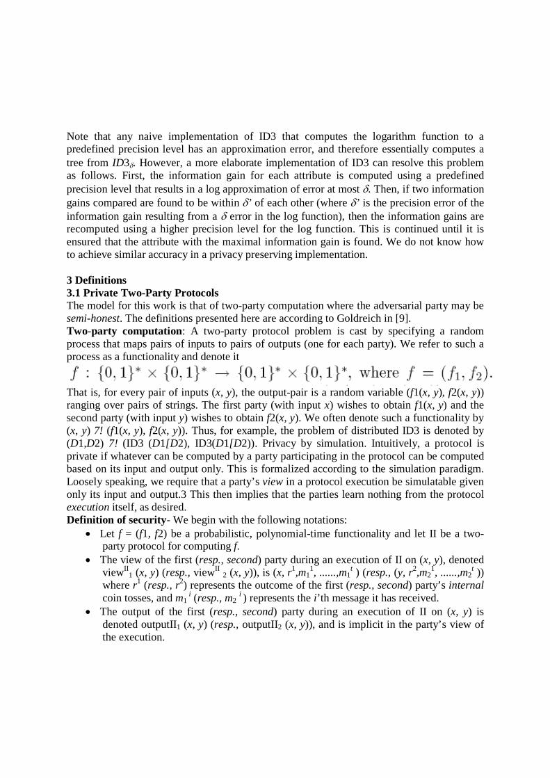
Note that any naive implementation of ID3 that computes the logarithm function to a predefined precision level has an approximation error, and therefore essentially computes a tree from ID3δ. However, a more elaborate implementation of ID3 can resolve this problem as follows. First, the information gain for each attribute is computed using a predefined precision level that results in a log approximation of error at most δ. Then, if two information gains compared are found to be within δ’ of each other (where δ’ is the precision error of the information gain resulting from a δ error in the log function), then the information gains are recomputed using a higher precision level for the log function. This is continued until it is ensured that the attribute with the maximal information gain is found. We do not know how to achieve similar accuracy in a privacy preserving implementation. 3 Definitions 3.1 Private Two-Party Protocols The model for this work is that of two-party computation where the adversarial party may be semi-honest. The definitions presented here are according to Goldreich in [9]. Two-party computation: A two-party protocol problem is cast by specifying a random process that maps pairs of inputs to pairs of outputs (one for each party). We refer to such a process as a functionality and denote it

That is, for every pair of inputs (x, y), the output-pair is a random variable (f1(x, y), f2(x, y)) ranging over pairs of strings. The first party (with input x) wishes to obtain f1(x, y) and the second party (with input y) wishes to obtain f2(x, y). We often denote such a functionality by (x, y) 7! (f1(x, y), f2(x, y)). Thus, for example, the problem of distributed ID3 is denoted by (D1,D2) 7! (ID3 (D1[D2), ID3(D1[D2)). Privacy by simulation. Intuitively, a protocol is private if whatever can be computed by a party participating in the protocol can be computed based on its input and output only. This is formalized according to the simulation paradigm. Loosely speaking, we require that a party’s view in a protocol execution be simulatable given only its input and output.3 This then implies that the parties learn nothing from the protocol execution itself, as desired. Definition of security- We begin with the following notations:

• Let f = (f1, f2) be a probabilistic, polynomial-time functionality and let II be a two-party protocol for computing f.

• The view of the first (resp., second) party during an execution of II on (x, y), denoted viewII

1 (x, y) (resp., viewII 2 (x, y)), is (x, r1,m11, ......,m1

t ) (resp., (y, r2,m21, ......,m2

t )) where r1 (resp., r2) represents the outcome of the first (resp., second) party’s internal coin tosses, and m1

i (resp., m2 i ) represents the i’th message it has received. • The output of the first (resp., second) party during an execution of II on (x, y) is

denoted outputII1 (x, y) (resp., outputII2 (x, y)), and is implicit in the party’s view of the execution.



961

ISSN:2229-6093

Definition 1: (privacy w.r.t. semi-honest behavior): For a functionality f, we say that II privately computes f if there exist probabilistic polynomial time algorithms, denoted S1 and S2, such that

Equations (1) and (2) state that the view of a party can be simulated by a probabilistic polynomial-time algorithm given access to the party’s input and output only. We emphasize that the adversary here is semi honest and therefore the view is exactly according to the protocol definition. We note that it is not enough for the simulator S1 to generate a string indistinguishable from viewII 1 (x, y). Rather, the joint distribution of the simulator’s output and f2(x, y) must be indistinguishable from (viewII 1 (x, y), outputII 2 (x, y)). This is necessary for probabilistic functionalities, see [3, 9] for a full discussion. Private data mining: We now discuss issues specific to the case of two-party computation where the inputs x and y are databases. Denote the two parties P1 and P2 and their respective private databases D1 and D2. First, we assume that D1 and D2 have the same structure and that the attribute names are public. This is essential for carrying out any joint computation in this setting. There is a somewhat delicate issue when it comes to the names of the possible values for each attribute. On the one hand, universal names must clearly be agreed upon in order to compute any joint function. On the other hand, even the existence of a certain attribute value in a database can be sensitive information. This problem can be solved by a pre-processing phase in which random value names are assigned to the values such that they are consistent in both databases. Doing this efficiently is in itself a non-trivial problem. However, in our work we assume that the attribute-value names are also public (as would be after the above-described random mapping stage). Next, as we have discussed, each party should receive the output of some data mining algorithm on the union of their databases, D1 U D2. We note that in actuality we consider a merging of the two databases so that if the same transaction appears in both databases, then it appears twice in the merged database. Finally, we assume that an upper-bound on the size of |D1 U D2| is known and public. 3.2 Composition of Private Protocols In this section, we briefly discuss the composition of private protocols. The theorem and its corollary brought here are used a number of times throughout the paper. The protocol for privately computing ID3δ is composed of many invocations of smaller private computations. In particular, we reduce the problem to that of privately computing smaller sub problems and show how to compose them together in order to obtain a complete ID3δ solution. Although intuitively clear, this composition requires formal justification. We present a brief, informal discussion and refer the reader to Goldreich [9] for a complete, formal treatment. Informally, consider oracle-aided protocols, where the queries are supplied by both parties.



962

ISSN:2229-6093

The oracle answer may be different for each party depending on its definition, and may also be probabilistic. An oracle-aided protocol is said to privately reduce g to f if it privately computes g when using the oracle functionality f. The security of our solution relies heavily on the following intuitive theorem. Theorem 2 (composition theorem for the semi-honest model, two parties): Suppose that g is privately reducible to f and that there exists a protocol for privately computing f. Then, the protocol defined by replacing each oracle-call to f by a protocol that privately computes f, is a protocol for privately computing g. Since the adversary considered here is semi-honest, this theorem is easily obtained by plugging in the simulator for the private computation of the oracle functionality. Furthermore, it is easily generalized to the case where a number of oracle-functionalities f1, f2, ...... are used in privately computing g. Many of the protocols presented in this paper involve the sequential invocation of two private subprotocols, where the parties’ outputs of the first sub protocol are random shares which are then input into the second sub protocol. The following corollary to Theorem 2 states that such a composed protocol is private. Corollary 3 Let IIg and IIh be two protocols that privately compute probabilistic polynomial-time functionalities g and h respectively. Furthermore, let g be such that the parties’ outputs, when viewed independently of each other, are uniformly distributed (in some finite field). Then, the protocol II comprised of first rennin IIg and then using the output of IIg as input intoIIh, is a private protocol for computing the functionality f(x, y) = h(g1(x, y), g2(x, y)), where g = (g1, g2). Proof: By Theorem 2 it is enough to show that the oracle-aided protocol is private. However, this is immediate because, apart from the final output, the parties’ views consist only of uniformly distributed shares that can be generated by the required simulators. 3.3 Private Computation of Approximations and of ID3δ Our work takes ID3δ as the starting point and privacy is guaranteed relative to the approximated algorithm, rather than to ID3 itself. That is, we present a private protocol for computing ID3δ. This means that P1’s view can be simulated given D1 and ID3δ(D1 U D2) only (and likewise for P2’s view). However, this does not mean that ID3δ(D1 U D2) reveals the “same” (or less) information as ID3(D1 U D2) does (in particular, given D1 and ID3(D1 U D2) it may not be possible to compute ID3δ(D1 U D2)). In fact, it is clear that although the computation of ID3δ is private, the resulting tree may be different from the tree output by the exact ID3 algorithm itself (intuitively though, no “more” information is revealed). The problem of secure distributed computation of approximations was introduced by Feigenbaum et. al. [8]. Their motivation was a scenario in which the computation of an approximation to a function f might be considerably more efficient than the computation of f itself. According to their definition, a protocol constitutes a private approximation of f if the approximation reveals no more about the inputs than f itself does. Thus, our protocol is not a private approximation of ID3, but rather a private protocol for computing ID3.



963

ISSN:2229-6093

4. Cryptographic Tools Oblivious transfer: The notion of 1-out-2 oblivious transfer (OT2

1 ) was suggested by Even, Goldreich and Lempel [6] as a generalization of Rabin’s “oblivious transfer” [16]. This protocol involves two parties, the sender and the receiver. The sender’s input is a pair (x0, x1) and the receiver’s input is a bit σε{0,1}. The protocol is such that the receiver learns xσ (and nothing else) and the sender learns nothing. In other words, the oblivious transfer functionality is denoted by ((x0, x1), σ) 7! (¸, xσ). In the case of semi-honest adversaries, there exist simple and efficient protocols for oblivious transfer [6, 9]. Oblivious polynomial evaluation: The problem of “oblivious polynomial evaluation” was first considered in [13]. As with oblivious transfer, this problem involves a sender and a receiver. The sender’s input is a polynomial Q of degree k over some finite field F and the receiver’s input is an element z ε F (the degree k of Q is public). The protocol is such that the receiver obtains Q(z) without learning anything else about the polynomial Q, and the sender learns nothing. That is, the problem considered is the private computation of the following functionality: (Q, z) →(¸,Q(z)). An efficient solution to this problem was presented in [13]. The overhead of that protocol is O(k) exponentiations (using the method suggested in [14] for doing a 1-out-of-N oblivious transfer with O(1) exponentiations). (Note that the protocol suggested there maintains privacy in the face of a malicious adversary, while our scenario only requires a simpler protocol that provides security against semi-honest adversaries. Such a protocol can be designed based on any homomorphism encryption scheme, with an overhead of O(k) computation and O(k|F|) communication.) Yao’s two-party protocol: In [17], Yao presented a constant-round protocol for privately computing any probabilistic polynomial-time functionality (where the adversary may be semi-honest). Denote Party 1 and Party 2’s respective inputs by x and y and let f be the functionality that they wish to compute (for simplicity, assume that both parties wish to receive the same value f(x, y)). Loosely speaking, Yao’s protocol works by having one of the parties (say Party 1) first generate an “encrypted” or “garbled” circuit computing f(x, .) and send it to Party 2. The circuit is such that it reveals nothing in its encrypted form and therefore Party 2 learns nothing from this stage. However, Party 2 can obtain the output f(x, y) by “decrypting” the circuit. In order to ensure that nothing is learned beyond the output itself, this decryption must be “partial” and must reveal f(x, y) only. Without going into details here, this is accomplished by Party 2 obtaining a series of keys corresponding to its input y such that given these keys and the circuit, the output value f(x, y) (and only this value) may be obtained. Of course, Party 2 must obtain these keys from Party 1 without revealing anything about y and this can be done by running |y| instances of a private 1-out-of-2 Oblivious Transfer protocol. See Appendix B for a more detailed description of Yao’s protocol. The overhead of the protocol involves: (1) Party 1 sending Party 2 tables of size linear in the size of the circuit (each node is assigned a table of keys for the decryption process), (2) Party 1 and Party 2 engaging in an oblivious transfer protocol for every input wire of the circuit, and (3) Party 2 computing a pseudo-random function a constant number of times for every gate (this is the cost incurred in decrypting the circuit).



964

ISSN:2229-6093

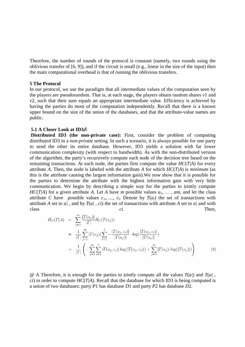
Therefore, the number of rounds of the protocol is constant (namely, two rounds using the oblivious transfer of [6, 9]), and if the circuit is small (e.g., linear in the size of the input) then the main computational overhead is that of running the oblivious transfers. 5 The Protocol In our protocol, we use the paradigm that all intermediate values of the computation seen by the players are pseudorandom. That is, at each stage, the players obtain random shares v1 and v2, such that their sum equals an appropriate intermediate value. Efficiency is achieved by having the parties do most of the computation independently. Recall that there is a known upper bound on the size of the union of the databases, and that the attribute-value names are public. 5.1 A Closer Look at ID3δ: Distributed ID3 (the non-private case): First, consider the problem of computing distributed ID3 in a non-private setting. In such a scenario, it is always possible for one party to send the other its entire database. However, ID3 yields a solution with far lower communication complexity (with respect to bandwidth). As with the non-distributed version of the algorithm, the party’s recursively compute each node of the decision tree based on the remaining transactions. At each node, the parties first compute the value HC(T|A) for every attribute A. Then, the node is labeled with the attribute A for which HC(T|A) is minimum (as this is the attribute causing the largest information gain).We now show that it is possible for the parties to determine the attribute with the highest information gain with very little communication. We begin by describing a simple way for the parties to |ointly compute HC(T|A) for a given attribute A. Let A have m possible values a1, … , am, and let the class attribute C have possible values c1,….., cl. Denote by T(a|) the set of transactions with attribute A set to a| , and by T(a| , ci) the set of transactions with attribute A set to a| and with class ci. Then,

@ A Therefore, it is enough for the parties to |ointly compute all the values T(a|) and T(a| , ci) in order to compute HC(T|A). Recall that the database for which ID3 is being computed is a union of two databases: party P1 has database D1 and party P2 has database D2.



965

ISSN:2229-6093

The number of transactions for which attribute A has value a| can therefore be written as |T(a|)| = |T1(a|)| + |T2(a|)|, where Tb(a|) equals the set of transactions with attribute A set to a| in database Db. Therefore, Eq. (3) is easily computed by party P1 sending P2 all of the values |T1(a|)| and |T1(a| , ci)| from its database. Party P2 then sums these together with the values |T2(a|)| and |T2(a| , ci)| from its database and completes the computation. The communication complexity required here is only logarithmic in the number of transactions and linear in the number of attributes and attribute-values/class pairs. Specifically, the number of bits sent for each attribute is at most O(m . `l . log |T|) (where the log |T| factor is due to the number of bits required to represent the values |T(a|)| and |T(a| , ci)|). This is repeated for each attribute and thus O(|R|ml. log |T|) bits are sent overall for each node of the decision tree output by ID3. Private distributed ID3. Our aim is to privately compute ID3 such that the communication complexity is close to that of the non-private protocol described above. A key observation enabling us to achieve this is that each node of the tree can be computed separately, with the output made public, before continuing to the next node. In general, private protocols have the property that intermediate values remain hidden. However, in this specific case, some of these intermediate values (specifically, the assignments of attributes to nodes) are actually part of the output and may therefore be revealed. We stress that although the name of the attribute with the highest information gain is revealed, nothing is learned of the actual HC(T|A) values themselves. Once the attribute of a given node has been found, both parties can separately partition their remaining transactions accordingly for the coming recursive calls. We therefore conclude that private distributed ID3 can be reduced to privately finding the attribute with the highest information gain. (We note that this is slightly simplified as the other steps of ID3 must also be carefully dealt with. However, the main issues arise within this step.) As we have mentioned, our aim is to privately find the attribute A for which HC(T|A) is minimum. We do this by computing random shares of HC(T|A) for every z, neither party learns anything of these intermediate values, yet given shares of all these values, it is easy to privately find the attribute with the smallest HC(T|A). Now, notice that the algorithm needs only to find the name of the attribute A which minimizes HC(T|A), the actual value is irrelevant. Therefore, in Eq. (3), the coefficient 1=|T| can be ignored (it is the same for every attribute). Furthermore, natural logarithms can be used instead of logarithms to base 2. As in the non-private case the values |T1(a|)| and |T1(a| , ci)| can be computed by party P1 independently, and the same holds for P2. Therefore the value HC(T|A) can be written as a sum of expressions of the form (v1 + v2) . ln(v1 + v2) where v1 is known to P1 and v2 is known to P2 (e.g., v1 = |T1(a|)|, v2 = |T2(a|)|). The main task is therefore to privately compute x ln x using a protocol that receives private inputs x1 and x2 such that x1 + x2 = x and outputs random shares of an approximation of x ln x. In Section 6 a protocol for this task is presented. In the remainder of this section, we show how the private x ln x protocol can be used in order to privately compute ID3δ.



966

ISSN:2229-6093

5.2 Finding the Attribute with Maximum Gain Given the above described protocol for privately computing shares of x ln x, the attribute with the maximum information gain can be determined. This is done in two stages: first, the parties obtain shares of HC(T|A) .||T|. ln 2 for all attributes A and second, the shares are input into a small circuit which outputs the appropriate attribute. In this section we refer to a field F which is defined so that |F| > HC(T|A) . |T| . ln 2. Stage 1 (computing shares): For every attribute A, every attribute-value a| 2 A and every class ci 2 C, parties P1 and P2 use the private x ln x protocol in order to obtain random shares wA,1(a| ), wA,2(a| ), wA,1(a| , ci) and wA,2(a| , ci) 2R F such that

wA,1(aj) + wA,2(aj)≡|T(aj)|.In(|T(aj)|) mod |F|

wA,1(aj,ci)+wA,2(aj,ci) ≡|T(aj,ci)|.In(|T(aj,ci)|) mod |F|

where the quality of the approximation can be determined by the parties. Specifically, the approximation factor is set so that the resulting approximation to HC(T|A) ensures that the output tree is from ID3±. The choice of the approximation level required is discussed in detail in Section 6.4. Now, define ˆH C(T|A) def = HC(T|A) . |T| . ln 2. Then, ˆH C(T|A) = ¡

Therefore, given the above shares, P1 (and likewise P2) can compute its own share in ˆHC(T||A) as follows:

It follows that SA,1 +SA,2 ≅ ˆHC(T|A) mod |F| and we therefore have that for every attribute A, parties P1 and P2 obtain (approximate) shares of ˆHC(T|A) (with this last step involving local computation only). Stage 2 (finding the attribute): It remains to find the attribute minimizing ˆHC(T|A) (and therefore HC(T|A)).



967

ISSN:2229-6093

This is done using Yao’s protocol for two-party computation [17]. The functionality to be computed is defined as follows:

• Input: The party’s input consists of their respective shares SA,1 and SA,2 for every attribute A.

• Output: The name of the attribute A for which SA,1 + SA,2 mod |F| is minimum (recall that SA,1 + SA,2 ≅ ˆHC(|A) mod |F|).

The above functionality can be computed by a small circuit. First notice that since ˆHC(T|A) < |F|, it holds that either SA,1 + SA,2 ≅ ˆHC(T|A) or SA,1 + SA,2 ≅ ˆHC(T|A) + |F|. Therefore, the modular addition can be computed by first summing SA,1 and SA,2 and then subtracting |F| if the sum of the shares is larger than |F| ¡ 1, or leaving it otherwise. The circuit computes this value for every attribute and then outputs the attribute name with the minimum value. This circuit has 2|R| inputs of size log |F| and its size is O(|R| log |F|). Note that |R| log |F| is a small number and thus this circuit evaluation is efficient. Privacy: The above protocol for finding the attribute with the smallest HC(T|A) involves invoking two private sub protocols. The parties’ outputs of the first sub protocol are random shares which are then input into the second sub protocol. Therefore, the privacy of the protocol is obtained directly from Corollary 3. (We note that Stage 1 actually contains the parallel composition of many private x ln x protocols. However, in the semi-honest case, parallel composition holds. Therefore, we can view Stage 1 as a single private protocol for computing many x ln x values simultaneously.) Efficiency: Note the efficiency achieved by the above protocol. Each party has to compute the same set of values |T(a| , ci)| as it computes in the non-private distributed version of ID3. For each of these values it engages in the x ln x protocol. (We stress that the number of values here does not depend on the number of transactions, but rather on the number of different possible values for each attribute, which is usually smaller by orders of magnitude.) The party then locally sums the results of these protocols together and runs Yao’s protocol on a circuit whose size is only linear in the number of attributes. Privacy-Preserving Protocol for ID3: Step 1: If R is empty, return a leaf-node with the class value assigned to the most transactions in T. Since the set of attributes is known to both parties, they both publicly know if R is empty. If yes, the parties run Yao’s protocol for the following functionality: Parties 1 and 2 input (|T1(c1)|, …, |T1(c`)|) and (|T2(c1)|, … , |T2(c`)|) respectively. The output is the class index i for which |T1(ci)| + |T2(ci)| is largest. The size of the circuit computing the above functionality is linear in ` and log |T|. Step 2: If T consists of transactions which all have the same value c for the class attribute, return a leaf-node with the value c. In order to compute this step privately, we must determine whether both parties remain with the same single class or not. We define a fixed symbol ? Symbolizing the fact that a party has more than one remaining class.



968

ISSN:2229-6093

A party’s input to this step is then ?, or ci if it is its one remaining class. All that remains to do is check equality of the two inputs. The value causing the equality can then be publicly announced as ci (halting the tree on this path) or ? (to continue growing the tree from the current point). For efficient secure protocols for checking equality, see [7, 13] or simply run Yao’s protocol with a circuit for testing equality. Step 3: (a) Determine the attribute that best classifies the transactions in T, let it be A. For every value a| of every attribute A, and for every value ci of the class attribute C, the parties run the x ln x protocol of Section 6 for |T(a|)| and |T(a| , ci)|. They then continue as described in Section 5.2 by computing independent additions, and inputting the results into Yao’s protocol for a small circuit computing the attribute with the highest information gain. This attribute is public knowledge as it becomes part of the output. (b,c) Recursively call ID3δ for the remaining attributes on the transaction sets T(a1), … , T(am) (where a1, … , am are the values of attribute A). The result of 3(a) and the attribute values of A are public and therefore both parties can individually partition the database and prepare their input for the recursive calls. 5.3 The Private ID3δ Protocol In the previous subsection we showed how each node can be privately computed. The complete protocol for privately computing ID3δ can be seen in previous section. The steps of the protocol correspond to those in the original algorithm. Although each individual step of the complete protocol is private, we must show that the composition is also private. Recall that the composition theorem (Theorem 2) only states that if the oracle-aided protocol is private, then so too is the protocol for which we use private protocols instead of oracles. Here we prove that the oracle-aided ID3δ protocol is indeed private. The central issue in the proof involves showing that despite the fact that the control flow depends on the input (and is not predetermined), a simulator can exactly predict the control flow of the protocol from the output. This is non-trivial and in fact, as we remark below, were we to switch Steps (1) and (2) in the protocol (as the algorithm is in fact presented in [12]) the protocol would no longer be private. Formally, of course, we show how the simulator generates a party’s view based solely on the input and output. Theorem 4 The protocol for computing ID3δ is private: Proof: In this proof the simulator is described in generic terms as it is identical for P1 and P2. Furthermore, we skip details which are obvious. Recall that the simulator is given the output decision tree. We need to show that a party’s view can be correctly simulated based solely on its input and output. Recall that the computation of the tree is recursive beginning at the root. For each node, a “splitting” class is chosen (due to it having the highest information gain) developing the tree to the next level. Any implementation defines the order of developing the tree and this order is the one followed by the Simulator as well. According to this specified order, at any given step the computation is based on finding the highest information gain for a known node (for the proof we ignore optimizations which find the gain for more than one node in parallel, although this is easily dealt with). We now describe the simulator for each node. We differentiate between two cases: (1) a given node is a leaf node and (2) a given node is not a leaf.



969

ISSN:2229-6093

1. The current node in the computation is a leaf-node: The simulator checks, by looking at the input, if the set of attributes R at this point is empty or not. If it is not empty (this can be deduced from the tree and the attribute-list which is public), then the computation proceeds to Step (2). In this case, the simulator writes that the oracle-answer from the equality call in Step (2) is equal (or else it would not be a leaf). On the other hand, if the list of attributes is empty, the computation is executed in Step (1) and the simulator writes the output of the majority evaluation to be the class appearing in the leaf. 2. The current node in the computation is not a leaf-node: In this case Step (1) is skipped and the oracle-answer of Step (2) must be not-equal, this is therefore what the simulator writes. The computation then proceeds to Step (3) which involves many invocations of the x ln x protocol, returning values uniformly distributed in F. Therefore, the simulator simply chooses the correct number of random values (based on the public list of attribute names, values and class values) and writes them. The next step of the algorithm is a local computation (not included in the view) and a private protocol for finding the best attribute. The simulator simply looks to see which attribute is written in the tree at this node and writes the attribute name as the oracle-answer for this functionality query. We have therefore shown that for each party there exists a simulator that given the party’s input and the output decision tree, generates a string that is computationally indistinguishable from the party’s view in a real execution. (In fact, in the oracle-aided protocol, the view generated by the simulator is identically distributed to that of a real execution.) This completes the proof. Remark: It is interesting to note that if Steps (1) and (2) of the protocol are switched (as the algorithm is in fact presented in [12]), then it is no longer private. This is due to the equality evaluation in Step (2), which may leak information about the other party’s input. Consider the case of a computation in which at a certain point the list of attributes is empty and P1 has only one class c left in its remaining transactions. The output of the tree at this point is a leaf with a class, assume that the class is c. From the output it is impossible for P1 to know if P2’s transactions also have only one remaining class or if the result is because the majority of the transactions of both databases together have the class c. The majority circuit of Step (1) covers both cases and therefore does not reveal this information. However, if P1 and P2 first execute the equality evaluation, this information is revealed. Extending the ID3δ protocol: we discussed the problem of decision trees which may be very large. As we mentioned, one strategy employed to prevent this problem is to halt in the case that no attributes have information gain above some predetermined threshold. Such an extension can be included by modifying Step 2 of the private ID3δ protocol as follows. In the new Step 2, the parties privately check whether or not there exists an attribute with information gain above the threshold.



970

ISSN:2229-6093

If there is no such attribute, then the output is defined to be the class assigned to the most transactions in T. (Notice that this replaces Step 2 because in the case that all the transactions have the same class, the information gain for every attribute equals zero.) As in Step 3, most of the work involves computing shares of HC(T|A). These shares (along with shares of HC(T)) are then input into a circuit that outputs the desired functionality. Of course, in order to improve efficiency, Steps 2 and 3 should then be combined together. 5.4 Complexity The complexity (measuring both communication and computational complexity) for each node is as follows (recall that R denotes the set of attributes and T the set of transactions):

• The x ln x protocol is repeated m(l + 1) times for each attribute where m and ` are the number of attribute and class values respectively (see Eq. (3)). For all |R| attributes we thus have O(m . l. |R|) invocations of the x ln x protocol. The complexity of the x ln x protocol can be found in Section 6.3. In short, the computational overhead of the x ln x protocol is dominated by O(log |T|) oblivious transfers and the bandwidth is O(k . log |T| . |S|) bits, where k is a parameter depending logarithmically on ± that determines the accuracy of the x ln x approximation and |S| is the length of the key for a pseudorandom function (say 128 bits).

• As we have mentioned, the size of the circuit computing the attribute with the minimum conditional entropy is O(|R| log |F|) where |F| = O(|T|).5 The bandwidth involved in sending the garbled circuit of Yao’s protocol is thus O(|R| log |T| . |S|) where |S| is the length of the key for a pseudorandom function. (This factor is explained in the paragraph titled “overhead” in Appendix B.) The computational complexity of the above circuit evaluation involves |R| log |F| = O(|R| log |T|) oblivious transfers (one for each bit of the circuit input) and O(|R| log |T|) pseudorandom function evaluations.

• The number of rounds needed for each node is constant (the x ln x protocol also requires only a constant number of rounds, see Section 6). The overhead of the x ln x invocations far outweighs the circuit evaluation that completes the computation. We thus consider only these invocations in the overall complexity. The analysis is completed by multiplying the above complexity by the number of nodes in the resulting decision tree (expected to be quite small).6 We note that by computing nodes on the same level of the tree in parallel, the number of rounds of communication can be reduced to the order of the depth of the tree (which is bounded by |R| but is expected to be far smaller). Comparison to non-private distributed ID3. We conclude by comparing the communication complexity to that of the non-private distributed ID3 protocol (see Section 5.1). In the non-private case, the bandwidth for each node is exactly |R|m` log |T| bits. On the other hand, in order to achieve a private protocol, an additional multiplicative factor of k .|S| is incurred (plus the constants incurred by the x ln x and Yao protocols). Thus, the communication complexity of the private protocol is reasonably close to that of its non-private counterpart.



971

ISSN:2229-6093

6. A Private Protocol for Approximating x ln x This section describes an efficient protocol for privately computing an approximation of the x ln x function, as defined in this Figure.

The protocol for approximating x ln x involves two distinct stages. In the first stage, random shares of ln x are computed. This is the main challenge of this section and conceptually involves the following two steps: 1. Yao’s protocol is used to obtain a very rough approximation to ln x. Loosely speaking, the outputs from this step are (random shares) of the values n and " such that x = 2n(1+ε) and -1/2< ε < 1/2. Thus, n ln 2 is a rough estimate on ln x and ln(1+ε) is the “remainder”. (As we will see, the circuit required for computing such a function is very small.) 2. The value " output from the previous step is used to privately compute the Taylor series for ln(1+ε) in order to refine the approximation. This computation involves a private polynomial evaluation of an integer polynomial. Next, we provide a simple and efficient protocol for private, distributed multiplication. Thus, given random shares of x and of ln x, we are able to efficiently obtain random shares of x ln x. 6.1 Computing Shares of ln x We now show how to compute random shares u1 and u2 such that u1 + u2 ≅ ln x (assume for now that x > 1). The starting point for the solution is the Taylor series of the natural logarithm, namely:

It is easy to verify that the error for a partial evaluation of the series is as follows:



972

ISSN:2229-6093

Thus, the error shrinks exponentially as k grows (see Section 6.4 for an analysis of the cumulative effect of this error in computing ID3δ). Given an input x, let 2n be the power of 2 which is closest to x (in the ID3± application, note that n < log |T|). Therefore, x = 2n(1 + ε)

where -1/2< ε< 1/2.Consequently,

Our aim is to compute this Taylor series to the k’th place. Let N be a predetermined (public) upper bound on the value of n (N > n always). In order to do this, we first use Yao’s protocol to privately evaluate a small circuit that receives as input v1 and v2 such that v1+v2 = x (the value of N is hardwired into the circuit), and outputs random shares of the following values:

• 2N . n ln 2 (for computing the first element in the series of ln x) • ε. 2N (for computing the remainder of the series)

This circuit is easily constructed: notice that ε . 2n = x - 2n, where n can be determined by looking at the two most significant bits of x, and ε. 2N is obtained simply by shifting the result by N - n bits to the left. The possible values of 2Nn ln 2 are hardwired into the circuit. (Actually, the values here are also approximations. However, they may be made arbitrarily close to the true values and we therefore ignore this factor from here on.) Therefore, following this step the parties have shares α1, β1 and α2, β2 such that,

and the shares αi and βi are uniformly distributed in the finite field F (unless otherwise specified, all arithmetic is in this field). The above is correct for the case of x ¸ 1. However, if x = 0, then x cannot be written as 2n(1+ε) for -1/2 < ε < 1/2. Therefore, the circuit is modified to simply output shares of zero for both values in the case of x = 0 (i.e., α1 + α2 = 0 and β1 + β2 = 0). The second step of the protocol involves computing shares of the Taylor series approximation. In fact, it computes shares of

(where lcm(2, ......, k) is the lowest common multiple of f2, … , kg, and we multiply by it to ensure that there are no fractions). In order to do this P1 defines the following polynomial:



973

ISSN:2229-6093

Where z1 ∈ R F is randomly chosen. It is easy to see that

Therefore after a single private polynomial evaluation of the k-degree polynomial Q(.), parties P1 and P2 obtain random shares z1 and z2 to the approximation in Eq. (5). Namely P1 defines u1 = z1 + lcm(2, ... , k)β1 and likewise P2. We conclude that

This equation is accurate up to an approximation error which depends on k, and the shares are random as required. Since N and k are known to both parties, the additional multiplicative factor of 2N.lcm (2,…, k) is public and can be removed at the end (if desired). Notice that all the values in the computation are integers (except for 2Nn ln 2 which is given as the closest integer). The size of the field F: It is necessary that the field be chosen large enough so that the initial inputs in each evaluation and the final output be between 0 and |F| ¡ 1. Notice that all computation is based on ε2N. This value is raised to powers up to k and multiplied by lcm(2,… , k). Therefore a field of size 2Nk+2k is large enough, and requires Nk + 2k bits for representation. (This calculation is based on bounding lcm(2,… , k) by ek < 22k.) We now summarize the ln x protocol (recall that N is a public upper bound on log |T|): Protocol 1 (Protocol ln x)

• Input: P1 and P2 have respective inputs v1 and v2 such that v1 + v2 = x. Denote x = 2n(1 + ") for n and " as described above.

• The protocol: 1. P1 and P2, upon input v1 and v2 respectively, run Yao’s protocol for a circuit that outputs the following: (1) Random shares α1 and α2 such that α1 + α2 = ε2N mod|F|, and (2) Random shares β1,β2 such that β1 + β2 = 2N . n ln 2 mod|F|. 2. P1 chooses z1 2R F and defines the following polynomial



974

ISSN:2229-6093

3. P1 and P2 then execute a private polynomial evaluation with P1 inputting Q(.) and P2 inputting α2, in which P2 obtains z2 = Q(α2). 4. P1 and P2 define u1 = lcm(2,… , k)β1 + z1 and u2 = lcm(2, … , k)β2 + z2, respectively. We have that u1 + u2 ε lcm(2,… , k) . 2N . ln x. We now prove that the ln x protocol is correct and secure. We prove correctness by showing that the field and intermediate values are such that the output shares uniquely define the result. On the other hand, privacy is derived directly from Corollary 3. Before beginning the proof, we introduce notation for measuring the accuracy of the approximation. That is, we say that ˜x is a ∇-approximation of x if |x - ˜x| ∇. Proposition 5 Protocol 1 constitutes a private protocol for computing random shares of a c/ 2k(k+1) - approximation of c . ln x in F, where c = lcm(2,… , k) . 2N. Proof: We begin by showing that the protocol correctly computes shares of an approximation of c ln x. In order to do this, we must show that the computation over F results in a correct result over the reals. We first note that all the intermediate values are integers. In particular, ε2n equals x-2n and is therefore an integer as is ε2N (since N > n). Furthermore, every division by i (2 < i<· k) is counteracted by a multiplication by lcm(2,… , k). The only exception is 2Nn ln 2. However, this is taken care of by having the original circuit output the closest integer to 2Nn ln 2. Secondly, the field F is defined to be large enough so that all intermediate values (i.e. the sum of shares) and the final output (as a real number times lcm(2, … , k) . 2N) are between 0 and |F| - 1. Therefore the two shares uniquely identify the result, which equals the sum (over the integers) of the two random shares if it is less than |F| - 1, or the sum minus |F| otherwise. Finally, we show that the accuracy of the approximation is as desired. As we have mentioned in Eq. (4), the ln(1 + ε) error is bounded by |ε|k+1/ k+1, 1/ 1-|ε| . Since -1/ 2 < ε<ε 1/ 2 , we have that this error rate is maximum at |ε| = 1/ 2 . We therefore have that |e ln(1 + ε) ε ln(1 + ε)| < 1 2k(k+1) , where e ln(1 + ε) denotes the approximation of the ln x protocol. Now, c ln x = cn ln 2 + c ln(1 + ε ) and therefore by adding cn ln 2 to both c ln(1+") and c e ln(1+ε) we have that this has no effect on the error. (We note that we actually add an approximation of cn ln 2 to c eln(1+ε) in the protocol. Nevertheless, the error of this approximation can be made to be much smaller than c 2k(k+1) . This is because the approximation of 2Nn ln 2 is hardwired into the circuit as the closest integer, and thus by increasing N the error can be made as small as desired.) Therefore, the total error of c elnx is c 2k(k+1) , which means that the effective error of the approximation of ln x is only 1/ 2k(k+1) . Privacy: The fact that the ln x protocol is private is derived directly from Corollary 3. Recall that this lemma states that a protocol composed of two private protocols, where the first one outputs random shares only, is private. The ln x protocol is constructed in exactly this way and thus the privacy follows from the lemma.



975

ISSN:2229-6093

6.2 Computing Shares of x ln x We begin by describing a multiplication protocol that on private inputs a1 and a2 outputs random shares b1 and b2 (in some finite field F) such that b1 + b2 = a1 . a2. The protocol is very simple and is based on a single private evaluation of a linear polynomial. Protocol 2 (Protocol Mult(a1, a2)) 1. P1 chooses a random value b1 ∈ F and defines the linear polynomial Q(z) = a1z - b1. 2. P1 and P2 engage in a private evaluation of Q, in which P2 obtains b2 = Q(a2) = a1 . a2 - b1. 3. The respective outputs of P1 and P2 are defined as b1 and b2, giving us that b1 + b2 = a1 . a2. The correctness of the protocol (i.e., that b1 and b2 are uniformly distributed in F and sum up to a1 .a2) is immediate from the definition of Q. Furthermore, the privacy follows from the privacy of the polynomial evaluation. We thus have the following proposition: Proposition 6 Protocol 2 constitutes a private protocol for computing Mult as defined above. We are now ready to present the complete x ln x protocol (recall that P1 and P2’s respective inputs are v1 and v2 where v1 + v2 = x): Protocol 3 (Protocol x ln x) 1. P1 and P2 run Protocol 1 for privately computing shares of ln x and obtain random shares u1 and u2 such that u1 + u2 ε ln x. 2. P1 and P2 use two invocations of Protocol 2 in order to obtain shares of u1 . v2 and u2 . v1. 3. P1 (resp., P2) then defines his output w1 (resp., w2) to be the sum of the two Mult shares and u1 .v1 (resp., u2 . v2). 4. We have that w1 + w2 = u1v1 + u1v2 + u2v1 + u2v2 = (u1 + u2)(v1 + v2) ε x ln x as required. Applying Corollary 3 we obtain the following theorem: Theorem 7 Protocol 3 is a private protocol for computing random shares of x ln x. 6.3 Complexity The ln x Protocol (Protocol 1): 1. Step 1 of the protocol (computing random shares α1, α2, β1 and β2) involves running Yao’s protocol on a circuit that is linear in the size of v1 and v2 (these values are of size at most log |T|). The bandwidth involved in sending the garbled circuit in Yao’s protocol is O(log |F||S|) = O(k log |T|.|S|) communication bits where |S| is the length of the key for a pseudorandom function. The computational complexity is dominated by the oblivious transfers that are required for every bit of the circuit input. Since the size of the circuit input is at most 2 log |T|, this upper bounds the number of oblivious transfers required. 2. Steps 2 and 3 of the protocol (computing the Taylor series) involve the private evaluation of a polynomial of degree k over the field F. This private evaluation can be computed using O(k) exponentiations and O(k) messages of total length O(k|E|) where |E| is the length of an element in the group in which the oblivious transfers and exponentiations are implemented.



976

ISSN:2229-6093

The overall computation overhead of the protocol is thus O(maxflog |T|, kg) exponentiations. Since |T| is usually large (e.g. log |T| = 20), and on the other hand k can be set to small values (e.g. k = 12,see below), the computational overhead can be defined as O(log |T|) oblivious transfers. The main communication overhead is incurred by Step 1, and is O(k log |T| . |S|) bits. The Mult Protocol (Protocol 2): This protocol involves a single oblivious evaluation of a linear polynomial by the players. The x ln x Protocol (Protocol 3): This step involves one invocation of Protocol 1, and two invocations of Protocol 2. Its overhead is therefore dominated by Protocol 1. We conclude that the overall computational complexity is O(log |T|) oblivious transfers and that the bandwidth is O(k log |T| . |S|) bits. 6.4 Choosing the Parameter k for the Approximation Recall that the parameter k defines the accuracy of the Taylor approximation of the “ln” function. Given δ, we analyze the value of k needed in order to ensure that the defined δ-approximation is correctly estimated. From here on we denote an approximation of a value z by ez. The approximation definition of ID3δ requires that if an attribute A0 is chosen for any given node, then |HC(T|A0)-HC(T|A)| · δ, where A denotes the attribute with the maximum information gain. In order to ensure that only attributes that are δ-close to A are chosen, it is sufficient to have that for all pairs of attributes A and A0

This is enough because the attribute A’ chosen by our specific protocol is that which has the smallest HC(T|A’). If Eq. (6) holds, then we are guaranteed that HC(T|A’) -HC(T|A) · δ as required (because otherwise we would have that HC(T|A’) > HC(T|A) and then A’ would not have been chosen). Eq. (6) is fulfilled if the approximation is such that for every attribute A, This is enough because the attribute A’ chosen by our specific protocol is that which has the smallest

HC(T|A’). If Eq. (6) holds, then we are guaranteed that HC(T|A’) -HC(T|A) · δ as required (because otherwise we would have that HC(T|A’) > HC(T|A) and then A’ would not have

been chosen). Eq. (6) is fulfilled if the approximation is such that for every attribute A,

We now bound the difference on each | ln x-ln x| in order that the above condition is fulfilled. By replacing log x by 1 ln 2 | ln x-ln x| in Eq. (3) computing HC(T|A) (see Section 5.1), we obtain a bound on the error of HC(T|A) - HC(T|A).



977

ISSN:2229-6093

A straightforward algebraic manipulation gives us that if 1 ln 2 | ln x-ln x| < δ then the error is less than δ 2 as required.7 By Proposition 5, we have that the ln x error is bounded by 1/ 2k(k+1) (the multiplicative factor of c is common to all attributes and can therefore be ignored). Therefore, given δ, we set 1/ 2kk+1 < δ 4 . ln 2 or k + log(k + 1) > log h 4 δ ln 2 i (for δ = 0:0001, it is enough to take k > 1/2). Notice that the value of k is not dependent on the input database. 7. Practical Considerations and Protocol Efficiency A detailed analysis of the complexity of the x ln x protocol can be found in Section 6.3 and the overall ID3δ complexity is analyzed in Section 5.4. In this section we demonstrate the efficiency of our protocol with a concrete analysis based on example parameters for an input database. Furthermore, a comparison of the efficiency of our protocol to that of generic solutions is presented. A Concrete Example: Assume that there are a million transactions (namely |T| = 220), |R| = 15 attributes, each attribute has m = 10 possible values, the class attribute has ` = 4 values, and k = 10 suffices to have the desired accuracy. Say that the depth of the tree is d = 7, and that the length of a key for the pseudorandom function is |S| = 80 bits. As is described in Section 5.4 there are at most m. x . |R| = 600 invocations of the x ln x protocol for each node and these dominate the overall complexity. (In fact, a node of depth d0 in the tree requires only m . x . (|R| ¡ d0) invocations.)

• Bandwidth: Each invocation has a communication overhead of O(k . log |T| . |S|) bits, where the constant in the “O” notation is fairly small. We conclude that the communication overhead of evaluating for each node can be transmitted in a matter of seconds using a fast communication network (e.g. a T1 line with 1.5Mbps bandwidth, or a T3 line with 35Mbps).

• Computation: The computation overhead for each x ln x protocol is O(log |T|) oblivious transfers (and thus exponentiations). In our example log |T| = 20, and each node requires several hundred evaluations of the x ln x protocol.

We can therefore assume that each node requires several tens of thousands of oblivious transfers (and therefore exponentiations). Assuming that a modern PC can compute 50 exponentiations per second, we conclude that the computation per node can be completed in a matter of minutes. The protocol can further benefit from the computation/ communication tradeoff for oblivious transfer suggested in [14], which can reduce the number of exponentiations by a factor of c at the price of increasing the communication by a factor of 2c. Since the latency incurred by the computation overhead is much greater than that incurred by the communication overhead it may make sense to use this tradeoff to balance the two.



978

ISSN:2229-6093

A Comparison to Generic Solutions: Consider a generic solution for the entire ID3δ task using Yao’s two party protocol. Such a solution would require a total of |R| . |T| . dlogme oblivious transfers (one for every input bit). For the above example parameters, we have a total 60, 000, 000 overall oblivious transfers. Furthermore, as the number of transactions |T| grows, the gap between the complexity of the generic protocol and the complexity of our protocol grows rapidly, since the overhead of our protocol is only logarithmic in |T|. The size of the circuit sent in the generic protocol is also at least O(|R| . |T| . |S|) (a very optimistic estimate) which is once again much larger than in our protocol. Consider now a semi-generic solution for which the protocol is exactly as described in Figure 2 However, a generic (circuit-based) solution is used for the x ln x protocol instead of the protocol of Section 6. This generic protocol should compute the Taylor series, namely k multiplications in F, with a communication overhead of O(k log2 |F||S|) = O(k3 log2 |T||S|) (circuit multiplication is quadratic in the length of the inputs). This is larger by a factor of k2 log |T| than the communication overhead of our protocol. On the other hand, the number of oblivious transfers would remain much the same in both cases, and this overhead dominates the computation overhead of both protocols.

References [1] M. Ben-Or, S. Goldwasser and A. Wigderson, Completeness theorems for non cryptographic fault tolerant distributed computation, Proceedings of the 20th Annual Symposium on the Theory of Computing (STOC), ACM, 1988, pp. 1–9. [2] D. Boneh and M. Franklin, Efficient generation of shared RSA keys, Advances in Cryptology - CRYPTO ’97. Lecture Notes in Computer Science, Vol. 1233, Springer-Verlag, 1997, pp. 425–439. [3] R. Canetti, Security and Composition of Multi-party Cryptographic Protocols, Journal of Cryptology, Vol. 13, No. 1, 2000, pp. 143–202. [4] D. Chaum, C. Crepeau and I. Damgard, Multiparty unconditionally secure protocols, Proceedings of the 20th Annual Symposium on the Theory of Computing (STOC), ACM, 1988, pp. 11–19. [5] B. Chor, O. Goldreich, E. Kushilevitz and M. Sudan, Private Information Retrieval, Proceedings 36th Symposium on Foundations of Computer Science (FOCS), IEEE, 1995, pp. 41–50. [6] S. Even, O. Goldreich and A. Lempel, A Randomized Protocol for Signing Contracts, Communications of the ACM, vol. 28, 1985, pp. 637–647. [7] R. Fagin, M. Naor and P. Winkler, Comparing Information Without Leaking It, ommunications of the ACM, vol. 39, 1996, pp. 77–85.



979

ISSN:2229-6093

[8] J. Feigenbaum, Y. Ishai, T. Malkin, K. Nissim, M. Strauss, and R. Wright, Secure Multiparty Computation of Approximations, 28th International Colloquium on Automata, Languages and Programming (ICALP), 2001, pp. 927–938. [9] O. Goldreich, Secure Multi-Party Computation. Manuscript, 1998. (Available at http://www.wisdom.weizmann.ac.il/»oded/pp.html) [10] O. Goldreich, S. Micali and A. Wigderson, How to Play any Mental Game - A Completeness Theorem for Protocols with Honest Majority., Proceedings of the 19th Annual Symposium on the Theory of Computing (STOC), ACM, 1987, pp. 218–229. [11] Y. Lindell and B. Pinkas, Privacy Preserving Data Mining, Advances in Cryptology - CRYPTO ’00.Lecture Notes in Computer Science, Vol. 1880, Springer-Verlag, 2000, pp. 36–53. Earlier version of this paper. [12] T. Mitchell, Machine Learning. McGraw Hill, 1997. [13] M. Naor and B. Pinkas, Oblivious Transfer and Polynomial Evaluation, Proceedings of the 31th Annual Symposium on the Theory of Computing (STOC), ACM, 1999, pp. 245–254. [14] M. Naor and B. Pinkas, Efficient Oblivious Transfer Protocols, Proceedings of 12th SIAM Symposium on Discrete Algorithms (SODA), January 7-9 2001, Washington DC, pp. 448–457. [15] J. Ross Quinlan, Induction of Decision Trees, Machine Learning 1(1), 1986, pp. 81–106. [16] M. O. Rabin, How to exchange secrets by oblivious transfer, Technical Memo TR-81, Aiken Computation Laboratory, 1981. [17] A. C. Yao, How to generate and exchange secrets, Proceedings 27th Symposium on Foundations of Computer Science (FOCS), IEEE, 1986, pp. 162–167.



980

ISSN:2229-6093

Concept of Privacy protection in Data Mining

Documents