CONCEPT MAP

CONCEPT MAP General Properties of Colloids

Colloidal systems contain insoluble particles (dispersed phase) ranging in size from 1 to 1000 nm

dispersed in a continuous phase (dispersion medium).

• Large interfacial areas associated with the solid-liquid interface make surface chemistry important in

colloidal systems.

• Colloidal systems are thermodynamically unstable, but they can be kinetically stabilized by steric

(polymeric) or electrostatic forces.

• Coagulation leads to the irreversible formation of large aggregates of colloidal particles, which

separate out of solution under the influence of gravity.

Formation of Colloidal Particles

• Because colloids are thermodynamically unstable, they must be prepared by condensation (exceeding

an equilibrium solubility limit) or comminution (mechanical grinding) methods.

• To produce monodisperse particles, nucleation and growth steps must be separately controlled (Figure

4.2).

Charged Interfaces

• Virtually all vapor-liquid-solid interfaces acquire charge by dissociation or adsorption of ionic

constituents.

• Because electrostatic forces are long-ranged, charged interfaces play an important role in many

interfacial processes.

• The properties of a charged interface are described by the Gouy-Chapman theory, which relates

surface charge density, σo, and surface potential, Φo, (eq. 4.3.19). The theory also shows that the

potential in an electrolyte solution decays exponentially with distance from the surface (eq. 4.3.12,

Figure 4.7) with a decay constant given by the Debye length, 1/κ.

• The Debye length (eq. 4.3.13) contains the valence and concentration of ions, the dielectric constant

and temperature of the electrolyte solution. It constitutes a key parameter defining the interaction

between charged particles and ions in solutions.

• Near a charged surface, counterions (of opposite charge to the surface) concentrate while co-ions (of

the same charge) are repelled. The Gouy-Chapman theory permits us to calculate how ionic

concentrations vary with distance in solution (Figure 4.8).

• When two charged surfaces approach, the electrostatic potential energy, VR, increases exponentially

with distance. The magnitude of the energy is determined by Φo and κ.

4-I

The DLVO Theory

• DLVO theory gives the total potential energy between two charged surfaces, VT(h) (eq. 4.5.2), by

adding together expressions for their attraction, VA (eq. 4.1.1), and electrostatic repulsion, VR (eq.

4.4.9) (Figure 4.12).

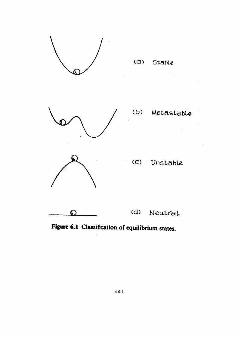
• Key features of V(h) are the values of the maxima and minima, which give the changes in potential

energy associated with coagulation, V pr.min the barrier to coagulation, Vmax, in Figure 4.1.

Colloidal Stability

• When Vmax = 0, coagulation becomes rapid.

• We obtain expressions relating the critical electrolyte concentration for coagulation (CCC) and Φo

(eqs. 4.5.8 and 4.5.9).

• When Φo » kT, the CCC is proportional to 1/z6 (the valence of the counterion) and independent of Φo

(eq. 4.5.8).

• When Φo < kT, the CCC becomes proportional to Φo4 / z2 and the stability of the system becomes

extremely sensitive to Φo (eq. 4.5.9).

Kinetics of Coagulation

• When Vmax = 0, coagulation becomes a diffusion-controlled process.

• Dimer formation is a second-order rate process with kr = 4kT/3η. It is independent of (spherical)

particle size (eq. 4.5.14).

• The time of coagulation, τ (eq. 4.5.17), is the time required for the concentration of dispersed

particles, [P0] to decrease by half. It takes seconds to minutes.

• With a coagulation barrier, Vmax ＞ 0, the coagulation rate constant, ks, is slower, ks = kr/W, where

W, the stability ratio, varies as exp (Vmax/kT) (eq. 4.5.19).

Surface Chemistry in Colloidal Systems

• The Stern model adapts the Gouy-Chapman model to account for ionic size and specific adsorption at

charged surfaces, but introduces a number of parameters that are difficult to evaluate.

• Colloidal stability correlates with the zeta potential, ζ, the surface potential measured in

electrophoretic measurements. In most practical colloidal systems, ζ is the only experimentally

accessible parameter characterizing the potential in the double layer.

• Surface chemistry identifies three specific ionic effects that modify particle—electrolyte interaction:

1. Potential-determining ions that directly affect Φo ; minute changes in their concentration can have a

pronounced effect on coagulation processes.

2. Indifferent electrolytes that change the electrostatic screening through their effect on the Debye

length, 1/κ.

3. Charge-reversing ions that adsorb so strongly they reverse the potential on the colloidal particle.

•Heterocoagulation of dissimilar particles is more complex than that of identical particles because H121

can be attractive or repulsive and the usual assumptions involved in calculating VR do not apply.

4-II

4-III

4-IV

4-V

4 Colloids Colloidal systems contain one phase A dispersed in a

second phase B. Substance A is called the dispersed

phase, and substance B the dispersion medium. Table

4.1 illustrates the generality of this definition and

shows that all possible combinations of insoluble gas,

liquid, and solid phases form colloidal dispersions.

TABLE 4.1 Types of Colloidal Systems with Some Common Examples

Dispersion

medium

Dispersed

particle

Technical name

Examples in nature

Examples in technology

Gas

Liquid

Aerosol

Mist; fog

Hairspray; smog

Gas

Solid

Aerosol

Volcanic smoke; dust

Pharmaceutical

inhalants

Liquid

Gas

Foam

Foam on polluted rivers

Fire-extinguisher foam; porous

plastics

Liquid

Liquid

Emulsion

Milk; biological membranes

Drug delivery emulsions;

mayonnaise; adhesives

Liquid

Solid

Colloidal sol or

dispersion

River water; muddy silt; clay

Printing-ink; paint; toothpaste

Solid

Gas

Solid foam

Pumice; loofah

Styrofoam; zeolites

Solid

Liquid

Solid emulsion

Opal; pearl; oil-bearing rocks

High impact plastics;

bituminous road paving

Solid

Solid

Solid dispersion

Wood;bone

Composites; pigmented plastics

This chapter concentrates on interfacial systems involving solids dispersed in liquids, liquid-solid

colloids.

4-1

Classification of Colloidal Systems:

Lyophobic (liquid-hating) colloids: Two-phase systems

1. Colloidal dispersions (colloids composed of insoluble or

immiscible components)

Lyophilic (liquid-loving) colloids:

1. True solutions of macromolecular material (solute molecules are

much larger than those of the solvent)

2. Association or self-assembled colloids (micelles, vesicles, and

membranes)

4-1-1

Liquid-solid colloidal systems play an important role in many

interfacial industrial processes and products. For example:

1. Processing of clay—water dispersions produces ceramics

ranging from delicate china figurines to toilet bowls and masonry

bricks.

2. Applying modern colloidal technology to silica and other oxide

sols yields tough, fracture-resistant ceramics that find application

in high-temperature automobile engines, rocket nose cones, and as

longer-lasting medical prostheses.

3. Drilling muds used in oil exploration are complex colloidal

materials that are indispensable as lubricants and rheology control

agents.

4. Virtually all coating systems employ colloidal materials, and

most industrial products are coated either for protection or

decoration. Paints are colloidal suspensions containing titanium

dioxide and latex particles.

5. Paper making involves producing a meshwork from colloidal

fibers in which clay particles are used as filler to improve print

quality and produce a pleasing surface texture.

6. Inks used in ordinary ballpoint pens, xerography, and high-

speed printing presses are colloidal liquids or pastes.

7. Scouring powders, toothpaste, and other heavy cleaning

agents contain colloidal material such as pumice.

4-2

4-2-1

Control of colloidal systems is also a central issue in

dealing with a host of environmental problems associated with

our heavy use of technology. For example:

1.Smog consists of colloidal size particles generated by atmospheric

photochemical reactions involving petroleum as well as natural

products.

2 Controlling the fines and other colloidal debris associated with

processing at wood pulping plants, mineral flotation sites, coal grinding

processing units, and asbestos plants requires application of colloidal

chemical techniques.

3 Some of the key steps in the purification of water and the treatment

of sewage also depend on the adsorptive capacity of colloidal materials.

Friend and foe (亦敵亦友)

4-3

What size particles exhibit colloidal behavior? Dispersed

particles must be larger than 1 nm in at least one dimension. Colloidal systems

containing particles smaller than this become indistinguishable from true

solutions. The upper limit for the solid particles is generally set at a radius of

1000 nm (1μm), where Brownian motion keeps the solid particles in solution,

known as a sol. Particles larger than this settle out under the influence of gravity

although entities of larger size are encountered in some emulsions, mineral

separations, and ceramic powders.

A simple geometric calculation illustrates an important aspect of

r = 1 cm, A = 4πr2 = 12.6 cm2 colloidal systems. If we take a sphere with a radius of 1 cm and break it up into

1021 spheres, each with a radius of 1 nm, the total surface area equals 1.26 x 108

cm2! As we have seen, surfaces are generally areas of high free energy, and since

colloidal systems possess intrinsically large interfacial areas, interfacial forces

and surface chemistry must play an important role in their behavior. This is

indeed the case, and our major concern in this chapter will be to develop an

understanding of the methods used to control interfacial interactions between

solid particles held in electrolyte solutions.

4-4

4-4-1

4.1 Colloidal Systems Are

Thermodynamically Unstable, but Can Be

Kinetically Stabilized by Steric or

Electrostatic Repulsive Forces

First, it is important to remember that the attractive forces between particles in

colloidal systems operate as long-range forces. As we demonstrated in Chapter

2.6, the potential energy of attraction, Vatt for two flat parallel particles in a

liquid medium varies with separation distance h as 1/h2

(4.1.1)

and as 1/h for two spherical particles of radius R

(4.1.2)

where H121 is the Hamaker constant for two particles (phase 1) in a liquid medium

(phase 2).

Colloidal particles continually move around in solution as a result of

Brownian motion. When two particles approach one another, attractive

interactions draw them together until they come into contact, a process known

as coagulation. As a result, the particles settle into the deep potential energy

well, known as the primary minimum, Vpr min, in Figure 4.la, defined by the

combination of Vatt and VCR, where VCR is the hard sphere core repulsion (CR)

between molecules located at the surface of the particles, as defined in eq. 2.5.2.

If the magnitude of Vpr min is » kT, coagulation is irreversible.

Figure 4.la also plots the interaction forces F between particles. By

defining F = -dV/dh, a negative force represents an attractive interaction and a

positive force a repulsive interaction.

The initial coagulation event between two particles leads to the

formation of a doublet; the doublet in turn combines with other particles to

form large agglomerates. When agglomerates become large enough, they

settle out of solution under the influence of gravity. In this way, the process of

coagulation converts the sol, which was a homogeneous phase containing

dispersed particles, into a two-phase system consisting of a solid mass at the

bottom of a container and a liquid phase above it.

Later in this chapter, we will show that a typical colloidal system

coagulates in seconds to minutes. For example, titanium dioxide colloidal

particles are used in paints to give them high hiding power, as we will discuss

in more detail in Section 4.7.1. If these TiO2 particles were allowed to interact

only via the normal attractive and repulsive forces, the shelf life of the paint

would be so short that it would never make it out of the paint factory in a usable

form. Clearly steps must be taken to prevent coagulation, that is, to stabilize

the sol, to make it useful in a paint.

For this reason, optimization of colloidal systems focuses in large part

on the introduction of long-range repulsive forces to prevent

coagulation.

4-5

4-5-1

4-5-2

4-5-3

Figure 4.1 The total interaction energy VT is plotted versus distance of separation h for two spheres of equal size. (a) VT is

obtained by adding together contributions from the van der Waals attractive interactions, Vatt and the core

repulsive interactions, VCR, arising from electron overlap of molecules on the surface of the spherical particles.

Particles are tightly bound in the primary minimum Vpr min (b) VT is obtained by adding a second repulsive

interaction, Vrep, associated with electrostatic or steric effects in solution. When Vmax is higher than 2kT, particles

may be held apart at the secondary minimum Vsec min (R.J.Hunter, Foundations of Colloid Science, Oxford Univer-

sity Press, Oxford, 1989, p. 419. By permission of Oxford University Press.)

4-6

4-6-1

These additional repulsive forces have two major origins. The

first leads to steric stabilization. It occurs when particle surfaces are covered

with polymer molecules. If the polymer molecules extend sufficiently far out

into solution, the distance of closest approach for two particles exceeds the

distance where attractive interactions dominate. Because the configuration of

polymer chains plays a decisive role in steric stabilization, we will postpone

discussion of this topic until we review the inter-facial properties of polymers

in more detail in Section 6.5.3.

The second repulsive force leads to electrostatic stabilization. It occurs

when the colloidal particles acquire a surface charge and are stabilized in an

electrolyte solution. We shall show that this potential energy of repulsion

between parallel plates or spheres, Vrep, has the functional form

Vrep = f[ σo,exp (-c1/2h)] (4.1.3)

where σo represents the surface charge density (charge per unit area) on the

particle, c is the electrolyte (salt) concentration in the solution, and h the

distance of separation.

We can write the total interaction potential between two particles as the

sum of the attractive (att), repulsive (rep), and core repulsive (CR) potentials

VT=Vatt + Vrep + VCR (4.1.4)

Figure 4.1b shows how Vatt which has a power-law dependence on h, and Vrep ,

which varies exponentially with distance, add to give VT. VCR has such short

range that it has little impact on the shape of the curve except in the immediate

vicinity of the primary minimum. In later discussion, the contribution of VCR is

often neglected altogether. On the other hand, the effect of electrostatic

repulsion, Vrep . is most important. It produces a repulsive maximum, Vmax, in

the total potential energy curve. Manipulation of this repulsive barrier is our

primary concern. If Vmax » kT, then it serves as a barrier to prevent the particles

from moving together into the primary minimum.

We can summarize these concepts in three principles:

• Colloidal particles in a sol are thermodynamically unstable.

•Coagulation is usually irreversible because Vpr min » kT.

•Colloidal particles are kineticallv stabilized when Vmax» kT.

In the next sections, we describe how colloidal systems are

prepared, develop an understanding of charged interfaces that

permits us to derive eq. 4.1.3 and understand how colloidal

systems can be stabilized, and obtain equations describing the

coagulation process and show under what conditions coagulation

becomes rapid.

4-7

4.2 Colloids Can Be Prepared in Two

Ways

4.2.1 Preparation of Colloids by Precipitation-Nucleation

and Growth Determine the Size, Shape, and Polydispersity

of Colloids

Because colloidal dispersions are thermodynamically unstable, they must be

prepared under nonequilibrium conditions. Two basic strategies for preparing

them are condensation (precipitation)—the formation and growth of a new

phase by exceeding an equilibrium condition such as the solubility limit—or

comminution—the breaking of large particles into successively smaller ones.

Methods for forming colloidal particles by condensation include

chemical reaction, condensation from the vapor, and dissolution and

reprecipitation. We now consider several examples of these techniques.

Condensation processes can form new colloidal phases of a variety of

materials. For example, reduction of the gold chloride complex by hydrogen

peroxide

Au(Cl4)- + H2O2 → Au (sol)

forms colloidal gold. Adding hydroxide to aluminum ions

Al3+ + OH- → Al(OH)3(sol)

leads to the formation of the aluminum hydroxide colloid. The chemical

reaction

KI + AgNO3 → Ag(sol) + K+ , I- , NO3- , Ag+ → AgI (sol)

can be driven to form a silver iodide sol by exceeding the solubility limit of AgI

(see Sections 4.6.3.1 and 8.4.2.3). To prepare a stable colloid, we must remove

the excess ions by dialysis.

All these reaction processes involve simultaneous nucleation and

growth; so they produce colloidal particles that have a wide range of particle

sizes. For example, when we simply mix solutions of AgNO3 and KI, we create

small regions in which the concentration of Ag+ and I- ions exceeds the

solubility product. This condition initiates the nucleation process, and growth

follows. As mixing continues, nucleation followed by growth begins in other

regions of the solution. The sequence of nucleation events accompanied by

continuous growth results in a wide distribution of particle sizes (polydisperse).

While such colloids have many uses, colloids in which all the particles have

the same size (monodisperse) are desirable in a number of applications.

The key to forming monodisperse colloids is to separate and

control the nucleation and growth processes. As we saw in Section 3.4,

nucleation occurs at concentrations or vapor pressures that exceed the

equilibrium value by a considerable amount. For example, in dust-free

conditions water vapor condenses at a pressure that is four times die

equilibrium value. By analogy, we can also force precipitation of colloidal

material to begin at a concentration of reactants that exceeds the solubility

product by a considerable amount.

4-8

4-9

Figure 4.2 Producing monodisperse colloidal

particles requires control and

separation of nucleation and

growth processes. The number of

particles is set by increasing the

concentration of reactants above

the nucleation concentration for a

brief period. Particle growth is

controlled by maintaining the

reactant concentration below the

nucleation concentration but

above the equilibrium

concentration for a period of time

sufficient to obtain the desired

particle size. (D. F. Evans and H.

Wen-nerstrom, The Colloidal

Domain: Where Physics,

Chemistry, Biology, and

Technology Meet, VCH

Publishers, New York, 1994, p.

370. Reprinted with permission

by VCH Publishers © 1994.)

Figure 4.2 illustrates the strategy used to produce monodisperse colloids.

Two important concentrations are involved; the nucleation concentration, above

which nucleation and growth begin, and the saturation concentration, or

solubility limit, below which growth stops. The idea is to adjust the temperature

or composition so that the initial concentration exceeds the nucleation

concentration. Nucleation occurs in a single short burst that causes the

concentration of reactants to change and fall below the nucleation threshold.

Control over subsequent growth can be achieved by maintaining the reaction

concentration at a level below the nucleation threshold but above the solubility

limit. The number of nuclei formed in the initial stage determines the number of

particles; the length of the growth period determines their size.

Formation of monodisperse gold sols illustrates how sometimes we can

completely separate the nucleation and growth steps. In the nucleation step,

small gold particles are formed by reacting the gold chloride complex with red

phosphorus

Au(Cl)4- + P(red) → Au (nuclei)

The growth step involves adding a mild reducing agent, such as formamide,

along with more Au(Cl)4--, under conditions that do not permit new nuclei to

form:

Au (nuclei) + Au(Cl)4- + H2CO → Au(sol)

Matijevic and his co-workers have prepared a number of monodisperse metal

oxide or metal hydroxide colloids using a controlled hydrolysis technique. Their

approach consists of heating the transition metal complex with anions, such as

chloride, sulfate, or phosphate ions, to accelerate the rate of deprotonation of

coordinated water. Manipulating parameters, such as the rate of heating,

concentration and purity of reactants, growth temperature, and time, controls the

nucleation burst and the extent of growth. It is also possible to alter the shape of

the colloidal particles from their common spherical shape to cubic or "needle-

like" acicular shapes. Figure 4.3 shows electron micrographs of several of

Matijevic's colloids.

Organic polymer colloidal particles can be prepared by emulsion

polymerization. For example, the process of preparing monodisperse latex

spheres starts with an emulsion of a monomer, such as styrene, that is stabilized

by a surfactant, such as sodium dodecyi sulfate (SDS). The concentration of

SDS is adjusted so that the emulsion contains micelles that enclose some of the

"solubilized" monomer (see Section 5.4). Then a water-soluble polymerization

initiator, such a potassium persulfate, is added. Statistically, polymerization

begins in the micelles rather than in the emulsion droplets. This step provides

controlled nucleation. As the polymerization process depletes the number of

monomers contained in the micelles, more monomers diffuse into them from

the emulsion. This step provides controlled

4-10

Figure 4.3 Examples of monodisperse colloids

prepared by Matijevic using the con-

trolled hydrolysis technique: (a) zinc

sulfide spherulites (diam. ~ 0.5 μm)

and (b) cadmium carbonate cubelets

(edge ~1.0μm. Small variations in

experimental nucleation and growth

conditions lead to very different par-

ticle morphologies. (Photographs

courtesy of Prof. Egon Matijevic,

Clarkson University, Potsdam, New

York.)

(a)

(b)

4-10-1

growth. Thus the number of activated micelles determines the number of

particles, while the amount of monomer present in the system determines their

size. This process is widely used in the manufacture of monodisperse latex

spheres for various applications.

Latexes differ from inorganic colloidal particles in one important way.

where coalesence leads to the formation of a continuous protective latex film.

At a characteristic temperature for each type of latex, the polymer transforms

from a solid to a glasslike material. Above this glass transition temperature Tg,

coagulated latex particles can coalesce and fuse together upon drying. As we

shall see in Section 4.7.1, this property plays an essential role in paints, where

coalescence leads to the formation of a continuous protective latex film.

4.2.2 Colloids Also Can Be Prepared by

Comminution

The comminution method for preparing colloidal particles requires a

mechanical process for breaking down bulk material into colloidal dimensions.

For example, materials like the titanium dioxide used in paints are broken

down by being tumbled together with ceramic or hardened metal balls in a

comminution mill.

Unfortunately comminution can reduce size only to a limited degree

because small particles tend to agglomerate during the grinding process and

resist redispersion in subsequent processing steps. For this reason,

condensation methods, which are more easily controlled and versatile, are

much more widely used as the starting point for colloid preparation.

4.2.3 The Surfaces of Colloidal Particles Are Charged through

Mechanisms Involving Surface Disassociation or Adsorption of

Ionic Species

A major aspect of the electrostatic stabilization of colloids is concerned with

manipulating the charge on the surface of colloidal particles. First we need to

understand the origins of surface charge. A surface or an interface placed in a

solution can become charged by two mechanisms: (1) surface ionization, in

which ions dissociate from the particle surface and diffuse into the adjoining

phase; or (2) preferential adsorption, in which one ionic species adsorbs onto

the particle surface.

Surface Ionization. An example of surface ionization occurs when a

clay is mixed with water. Clays are a major constituent of soil. Originally they

solidified as crystalline silicates and were subsequently broken down to

colloidal size by geological forces. In their crystalline form they are made up

of stacked unit layers (Figure 4.4) containing silicon tetrahedrally coordinated

with oxygen, and aluminum octahedrally coordinated with oxygen and

hydroxide. In most clays, the tetrahedral and octrahedral sheets join together

to form two- or three-layered sheets. Because the forces between sheets are

much weaker than within them, clay minerals easily break up into platelets.

In many clays, atom substitution occurs in the tetrahedral layers, where

trivalent Al replaces tetravalent Si, or in the octahedral layers, where divalent

Mg replaces trivalent Al. If an atom

4-11

Figure 4.4 Clay particles consist of stacks of identical units held together by van der Waals forces. The units contain (a) two or

(b) three layers composed of silicon and aluminum bonded to oxygen or hydroxide. Charged clay particles result

from impurity substitution. The montmorillonite clay particle shown in (b) has the composition

(Si8)(Al3.33Mg0.67)(O20)(OH)4Na0.67. One aluminum ion in every six has been replaced by a magnesium ion, and for

charge compensation one sodium ion has been added at the surface of the stack, (b) Reproduces one and one-half

unit cells of the basic crystal structure to demonstrate charge balance with substitution. (H. van Olphen, An In-

troduction to Clay Colloid Chemistry: For Clay Technologists, Geologists, and Soil Scientists, © 1963, John Wiley

& Sons, pp. 64-65. Reprinted by permission of John Wiley & Sons, Inc.)

4-12

of lower valence (Mg2+) replaces one of higher valence (Al3+) without any

other structural change, the layer acquires a net negative charge that must be

neutralized by the incorporation of positive cations (such as Na+ or K+) into

the structure. These cations cannot be accommodated within the layer and

instead are located on a plane between the sheets as illustrated in Figure 4.4b.

There they are ionically bonded to the layer. When the sheets are split apart,

the positive charges are exposed, and when placed in water, the sodium (or

potassium) ions readily dissolve, leaving the surface of the particle negatively

charged.

The surface charge density, σo, can be estimated as follows. Figure

4.4b shows a montmorillonite clay structure that has a unit cell formula of

(Si8)(Al3.33Mg0.67)(O20)(OH)4Nao.67. From x-ray measurements, we know that

the surface area per unit cell is 5.15 x 8.9 Å2. Since two surfaces share the

Na0.67, the surface cation density is Na0..33 per unit cell, and the surface charge

density is 0.33e/5.15 x 8.9 Å2 , orσo = 0.12 C/m2 (coulomb per meter squared).

Preferential Adsorption. We can illustrate preferential adsorption, the

second mechanism whereby a particle surface becomes charged, by the

following experiment. If we form air bubbles (small enough so that we can

ignore gravitational forces) in an aqueous NaCl solution, place two electrodes

into the solution, and apply a potential, we find that the bubbles move toward

the positive electrode. This observation establishes the fact that chloride ions

preferentially adsorb over sodium ions at the air-water interface. If we replace

NaCl by a long-chain cationic surfactant, such as dodecylammonium chloride

(C12H25NH3Cl), and repeat the experiment, we find that the air bubbles are now

positively charged and move toward the negative electrode. Thus, by selecting

our electrolyte and varying its concentration, we can control the sign and

magnitude of charges adsorbed at the air-water interface. Similar preferential

adsorption of charged species from solution leads to charged surfaces in solid-

liquid systems, as will be discussed in more detail in Section 4.6.3.

In many manufacturing processes, we purposely add materials that

selectively adsorb onto interfaces to charge them, and then use these charged

interfaces to control the process. Unfortunately, the accumulation of charged

surface-active impurities sometimes creates unwanted charged interfaces

resulting in the formation of new, sometimes troublesome, phases or

microstruc-tures. Many environmental problems arise from this adsorbed

charge accumulation.

4-13

4-14

4.3 Charged Interfaces Play a Decisive Role in Many Interfacial Processes

Charged interfaces are ubiquitous in interfacial systems and often play critical

roles in industrial and biological processes. In colloidal systems, we are

concerned with the interactions between two charged particle surfaces that

stabilize the colloid. In other interfacial systems, single charged interfaces are

important. For example, living cells control the flow of material and information

between their external environment and their interior by manipulating charge

flow across their membranes. Many of the solid-state devices described in

Chapters 10 and 11 operate by controlling charge at solid-solid interfaces. Thus

the equations to be developed in the next section have a broader range of

application than the stabilization of colloids. We will redevelop similar equa-

tions again for solids in Chapter 9.

4.3.1 The Gouy-Chapman Theory Describes How a Charged

Surface and an Adjacent Electrolyte Solution Interact

In this section we focus on electrostatic interactions at solid-liquid interfaces.

We start with the interaction between the charged particle surface and the ions

in the solution surrounding it. If the initial solvent is pure water, then the ions in

solution are hydroxyl ions plus those ions that have been dissolved from the

particle surface. For example, when the clay particles in Figure 4.4b are

immersed in water, they become negatively charged and the water contains

positive sodium ions removed from the clay particle surface; in this instance the

negatively charged clay particles repel each other. More often we are interested

in the behavior of systems where a salt has been added to the water deliberately

to form an electrolyte solution. The behavior of charged particles then depends

critically on how much salt is added to the electrolyte solution. For low salt

concentrations the clay remains dispersed and workable, but above a certain

critical concentration it suddenly becomes an agglomerated mass. We are

interested in the origins of this sudden transition. To achieve this we must

analyze the charge distribution surrounding a charged surface immersed in an

electrolyte, the approach that constitutes the Gouy-Chapman theory.

We derive the Gouy—Chapman equations using the model depicted in

Figure 4.5. It involves a planar charged surface characterized by the surface

charge density σ o and surface potential Φ 0. The adjacent solution is an

electrolyte characterized by the bulk concentration Cio, of ions, charge ze,

Figure 4.5

Model used in deriving the Gouy-Chapman equations that describe the interaction

between a planar charged surface and an adjacent electrolyte solution. The surface

extends infinitely in the x and y directions and is characterized by a charge density σ0

and surface potential Φ0. The solution contains positive and negative ions of valency

zi and concentration C0i which are treated as point charges. (D. F. Evans and H.

Wennerstrom, The Colloidal Domain: Where Physics, Chemistry, Biology, and

Technology Meet, VCH Publishers, New York, 1994, p. 112. Reprinted with

permission by VCH Publishers © 1994.)

4-15

where z is equal to the valence multiplied by the sign of the ion, and dielectric

permittivity εrε0.1 We assume that the ions can be approximated as point

charges. Ions in the electrolyte solution bearing a charge opposite to that on the

particle surface are known as counterions, while those bearing the same charge

are known as co-ions.

Our goals are to determine: (1) how the electrical potential and

distribution of ions in the electrolyte solution varies with distance z from the

charged interface; and (2) the relationship between σo andΦ0. Armed with

these relationships we will then be able to analyze how interparticle repulsion

or attraction depends on electrolyte type, concentration, and temperature.

(1) Eqs. (4.3.6), (4.3.12); 4-18

Figs. 4.7, 4.8; 4-20, 4-21 Eqs. (4.4.9), (4.4.10); 4-29

(2) Eqs. (4.3.19), (4.3.20); 4-22

4.3.1.1 The Poisson-Boltzmann Equation Is Used to Derive an

Expression for the Distribution of Charged Ions in the Electrolyte

and the Associated Electrical Potential

In Section 2.3.1, our discussion of ion-ion charge interactions was restricted to

only a few fixed charges, and under those conditions Coulomb's law was

applicable. However, in the present situation, in which many charges are free

to move throughout the volume of the electrolyte in response to electrical fields

and also are under the influence of thermal motion, we need to use a more

general expression obtained by combining two fundamental equations, the

Poisson equation and the Boltzmann equation, to describe the interaction.

The Poisson equation provides a relation between the electrical

potential Ф and charge density in vacuum

(4.3.1)

where 2 stands for the operator 2/ x2 + 2/ y2 + 2/ z2, and ρ

is the charge density obtained by summing all charges. (Equation 4.3.1 is

written in SI units, and its left-hand side must be multiplied by 1/4Π to convert

it to cgs units. In other texts it is important to ascertain which units are being

used in the electrostatic equations.)

Attempts to use eq. 4.3.1 to describe an electrolyte solution require

simultaneous evaluation of all charge interactions (ion-ion, ion-dipole, dipole-

dipole, etc.) and result in an intractable problem. We can circumvent this

difficulty and write the Poisson equation in a more convenient form by

applying the following arguments. Ion—ion interactions are stronger and

longer-ranged than all other types of charged interactions. As a result, ion-ion

interactions typically play a dominant role in electrolyte solulions.

1Note that in this notationε0 is the dielectric pemittivity of vacuum, εr is the relative

permittivity of the solution between the charged particles, and soεrε0 is the dielectric

permittivity of the electrolyie solution, εr is also known as the dielectric constant. In

most electrolytes the solvent is water, for whichεr〜 78.

4-16

This fact suggests that we write the interaction between free charges explicitly

while averaging over the solvent degree of freedom, thus eliminating the

explicit consideration of ion— dipole and dipole-dipole interactions. We will

not give the detail of this averaging process, but simply note that it transforms

the Poisson equation in a deceptively simple way to

(4.3.2)

where we account for the effect of the solvent through its dielectric

constant εr.

The charge density per unit volume ρat any location in the

solution(Figure 4.5) is expressed as

(4.3.3)

where zi is the valence of the ion multiplied by ±1 according to its sign. and ci*

represents the local concentration of ions of type i, measured as the number of

i ions per unit volume. (We use an asterisk to differentiate between number

concentration c* measured in ions per cubic meter and molar concentration c

measured in moles per liter. Thus c* = 1000 NAv c ions/m3.)

The solution's charge density ρ cannot be associated with a set of

fixed charges because ions in solution are free to move in response to

electrical fields. In addition, we must consider the interplay between

electrostatic interactions that favor an ordered and localized ion

arrangement, and entropic factors that strive to generate a random

distribution of ions.

As we noted in Section 2.2.4 and 2.7, the Boltzmann distribution

expresses the compromise between molecular order and disorder. For

ions in solution the electrostatic energy of an ion of valence zi at a point

where the potential is Φis represented by zieΦ. So the Boltzmann

equation is

(4.3.4)

In this equation, ci 0* equals the concentration of ion species when Φ= 0, which

we usually take as equal to the bulk ion concentration. Near positively charged

surfacesΦis positive, and near negatively charged surfaces Φis negative.

Combining eqs. 4.3.2, 4.3.3, and 4.3.4 gives the Poisson-

Boltzmann equation. Since we are interested in the potential variation

Φ(z) in the direction z away from a charged flat surface, we write

(4.3.5)

which expresses 2Φfrom eq. 4.3.2 in terms of the direction z normal to the

surface in Figure 4.5.

4-17

At this juncture we can either solve eq. 4.3.5 completely or make

simplifying assumptions that lead to solutions that are straightforward but

approximate and therefore of more limited utility. In this text we do both. We

derive the complete solution in Appendix 4A and summarize the results in eqs.

4.3.6 and 4.3.7. We derive the simpler solution starting at eqs. 4.3.8.

From the complete solution the change in potential with distance is

given by

(4.3.6)

where the quantity I/κ is the Debye screening length, to be defined later,

and Γ0 contains the surface potential Φ0 in the form

(4.3.7)

WhenΦ0 = 0, thenΓ0 = 0; and whenΦ0 becomes large, Γ0 →1. To obtain

this solution to the Poisson—Boltzmann equation requires that the valencies

of the counterions (cations) and co-ions (anions) be equal, that is, the

electrolyte be symmetrical, such as Na+Cl-. Consequently, we write these

equations in terms of z = ︱zi︱.

For the approximate solution we limit our interest to the situations in

which zeΦ« kT. We can then expand the exponential in eq. 4.3.5 and neglect

high-order terms to give

(4.3.8)

The electroneutrality condition means that the sum of positive and negative

ion charges is zero

(4.3.9)

leading to the cancellation of the first term displayed in eq. 4.3.8 and leaving

(4.3.10)

It is convenient to identify the cluster of constants in eq. 4.3.10 by the

symbol . Then eq. 4.3.10 becomes

(4.3.11)

Using the boundary conditions Φ→Φ0 as z →0 andΦ→ 0 as z →∞, we

can solve eq. 4.3.11 to give

(4.3.12)

4-18

This result should be compared with the more complex complete solution of eq.

4.3.6. Equation 4.3.12 states that the electrostatic potential drops away

exponentially with distance from a charged surface in an electrolyte at a rate

determined byκ.

The quantity 1/κ has the dimension of length and is defined as the Debye

screening length

when cio is the concentration of counterions in the electrolyte measured in

moles/liter denoted by the unit M.

For water at 25° C (εr = 78.54) containing a symmetrical monovalent salt

such as Na+ Cl-, zi = ±1,

With cio = 0.01M, /κ= 3.043 nm, a dimension comparable to the size of a

colloidal particle. In an aqueous solution,/κ varies only

e = 2.71828……

e－1 = 1/e = 0.3678796… ~ 0.37 = 37%

4-19

Figure 4.6 Decay in the potential in the double layer as a function of distance from a charged surface according to the limiting form of the Gouy—Chapman equation (4.3.12). (a) Curves are drawn for a 1:1 electrolyte of different concentration. (b) Curves are drawn for different 0.001 M symmetrical electrolytes. (P. C. Hiemenz, Principles of Colloid and Surface Chem-istry, 2nd ed., Marcel Dek-ker, New York, 1986, p. 695.)

Eq. (4.3.13)：

4-19-1

1000e2NAVΣ zi2Cio

[ ] κ -1 = 1/2

Σ zi2Cio = 12．Cio+(-1)2．Cio = 2Cio

for 1：1 electrolyte

(NaCl → Na+ + Cl -)

εr εo kT

κ -1 =

(1000)(1.602×10-19)2(6.02×1023)(2Cio)

1/2 (8.854×10-12)(78.54)(1.381×10-23)(300) [ ]

=

(Cio)1/2

3.043×10-10 m ── Eq. (4.3.14)

or =

0.304 nm

√M

── p.4-V

slowly with temperature because εrεokT is almost constant over a broad

temperature range.

Equation 4.3.12 demonstrates that the potential in the solution decays

exponentially with distance from the particle, and the decay rate is set by the

Debye length. In fact, when z = /κ, has dropped to o/exp(l). Figures 4.6a,

4.6b, 4.7a, and 4.7b illustrate the effect of concentration (c io) and valence (z)

of the ions in the electrolyte on (z) as a function of z. As eq. 4.3.13 shows,

the higher the salt concentration and the higher the valence of the salt ions the

more rapidly the electrical potential decays away from the surface of the

particle.

We can gain further insight into the properties of the electrolyte in the

vicinity of a charged surface by calculating how the concentration of both the

counterions and the co-ions varies as a function of distance z from the surface.

Assuming o is constant, we first calculate for different values of z and then

use the Boltzmann equation 4.3.4 to calculate the concentration of positive and

negative ions at those (z) values. Figure 4.8 plots ci versus z for a negatively

charged surface. Figures 4.7 and 4.8 have been constructed using eqs. 4.3.6

and 4.3.7, although we can readily interpret the figures using the simple

equations. In the plot the concentration of positively charged counterions

increases from the bulk value cio as we move toward the negatively charged

surface. At the same time, the concentration of co-ions decreases below the

bulk value. These results accord with our intuition that counterions concentrate

at a charged surface, while co-ions are repelled. As the electrolyte

concentration increases, the departures from cio move closer to the surface, in

accordance with eq.

4-20

Figure 4.7 Change in the potential as a function of distance (eq. 4.3.6) for two different electrolyte concentrations. (a) At constant surface po-

tential, o, addition of elec-trolyte increases σo and thus the slope β is greater than α. (b) At constant surface charge density, σo, the slopes a and β are identical (eq. 4.3.17); the addition of electrolyte decreases the

surface potential o (since

κ increases, o decreases

from eq. 4.3.19). (H. van Olphen, An Introduction to Clay Colloid Chemisty: For Clay Technologists, Ge-ologists, and Soil Scientists, © 1963. John Wiley & Sons, p. 34. Reprinted by permission of John Wiley & Sons, Inc.)

Figure 4.8 Charge distribution in the Gouy-

Chapman double layer at (a)

constant potential and (b) constant

charge density for two different

concentrations of added

electrolyte. D and D' correspond

to the distances where the local

concentrations of cations (c+ as

given by line AD and A'D', and an

ions (c- as given by CD and C' D',

begin to depart from the bulk

concentrations. The algebraic sum

of the curves ACD and A'D'C' are

proportional to the net charge in

the solution and thus equal the

charge density on the surface. For

constant σo, ACD = A'C'D'. while

for constanto, A'C'D' > ACD. (H.

van Olphen, An Introduction to

Clay Colloid Chemistly: For Clay

Tech-nologistSf Geologists, and

Soil Scientists, © 1963, John

Wiley & Sons, pp.32-33.

Reprinted by permission of John

Wiley & Sons, Inc.)

4.3.12. Figures 4.6, 4.7, and 4.8 illustrate how the potential and concentration of

charged ions vary with distance into the electrolyte. These results achieve the first

goal we set for ourselves in Section 4.3.1: to determine how the electrical

potential and distribution of ions in the electrolyte solution varies with distance z

from the charged interface.

4.3.1.2 The Poisson-Boltzmann Equation Also Leads to the Relationship

between Surface Charge Density and Potential at the Charged Surface

We can obtain a relationship between surface charge density σo and the surface

potential by realizing that in order to achieve electroneutrality, the charge per

unit area on the surface must be equal and opposite to the charge contained in a

volume element of solution of unit cross-sectional area extending from the

surface to infinity. Stated as an equation, this equivalence becomes

By combining eq. 4.3.15 with the Poisson equation 4.3.2, we obtain

which is readily integrated to yield

4-21

because d/dz equals zero at infinity. Equation 4.3.17 tells us that the surface charge density is

proportional to the potential gradient in the vicinity of the surface; that is, -d/dz as z→ 0. This

important general result is one we use repeatedly.

Using the approximate solution for (z), eq. 4.3.12, we can evaluate (d/dz) o in the limit

as z → 0 and find

Substituting eq. 4.3.18 into eq. 4.3.17 gives

which shows that the simple solution to the Poisson-Boltzmann equation predicts a linear

relationship between surface charge density and surface potential.

The complete solution for the relationship between the surface charge density and the

surface potential obtained in Appendix 4A gives

The results in eqs. 4.3.19 and 4.3.20 achieve the second goal set in Section 4.3.1: to determine the

relationship between σo and o. We now have the Gouy—Chapman expressions for the

dependence of electrical potential (eqs. 4.3.6 and 4.3.12) and the distribution of ions away from

the charged surface as well as for the relationship between surface charge and surface potential

(eqs. 4.3.19 and 4.3.20). Appendix 4B gives some examples of calculations involving these

formulae.

Now we can consider two limiting cases of these general relationships, either o = constant

or σo constant. Figures 4.6 and 4.7a show how changes with distance from the charged surface

at three different electrolyte concentrations calculated on the assumption that o remains constant.

Since the surface charge density σo is proportional to the limiting slope, -do /dz, from eq. 4.3.17,

then, from Figure 4.7a, surface charge density must increase with added salt at constant surface

potential. At constant surface charge density, Figure 4.7b, the surface potential decreases as the

concentration of salt increases.

Figure 4.8 shows how the concentration of ions varies as a function of distance at either

constant surface potential or constant surface charge density. While the plots for constant o

(Figure 4.8a) and constant σo (Figure 4.8b) look similar, careful inspection proves they contain

important differences. For electroneutrality, the net space charge concentration, depicted by the

difference between the areas DAB (the cation excess) and DCB (the anion depletion), must be

equal and opposite to the charge on the flat surface. With σo = constant, the difference between the

areas

4-22

DAB and DCB must remain constant, irrespective of the concentration of ions

in the electrolyte. With o = constant, the difference in the areas, and

consequently in σo, must increase as the concentration increases in accordance

with eq. 4.3.19 with substitution for κ from eq. 4.3.13.

4.3.2 The Electrical Double Layer Is Equivalent to a Capacitor—

with One Electrode at the Particle Surface and the Other in the

Electrolyte at a Distance Equal to the Debye Length

Now we are in a position to gain a feeling for the significance of the Debye

length, /κ. We start by examining the expression for the capacitance C per

unit area A of a parallel plate capacitor. We assume the capacitor to have a

separation d between the plates and to be filled with a medium of dielectric

constant εr as illustrated in Figure 4.9a. The capacitance per unit area then

equals εrεo /d. The capacitance per unit area is also the charge stored per unit

area of the plates, σo, divided by the potential difference between them, o, so

that

Comparison with eq. 4.3.19 (σo /o =εrεo /κ-1) reveals that

4-23

Figure 4.9 (a) Parallel plate capacitor

showing the variation of

potential with distance be-

tween two charged plates,

separation d, bearing equal but

opposite charges ±σo.

(b) Schematic of a double

layer as a capacitor in which

one plate is the charged

particle surface and the

second plate corresponds to an

imaginary surface placed at a

distance κ that carries all

of the double layer charge.

Thus we can model the electrical interaction between the charged surface and the adjacent solution as if it

were the capacitor shown in Figure 4.9b. One of the capacitor plates represents the surface of the charged

particle, while the second plate represents an imaginary surface located at a distance /κ away from it. The

net space charge resulting from the counterions and the co-ions behaves electrostatically as if all these ions

were located on the imaginary surface. This picture gives rise to the notion of the electrical “double layer. ”

But in no way should it be construed to mean that the ions physically lie on the imaginary plane of the double

layer.

Often the more rapid decay of electrical potential in the solution with increased salt concentration and

the corresponding decrease in Debye length is described as a more effective screening or shielding of the

charged surface by the electrolyte. With the addition of more salt, the concentration of charge on die surface

increases, κ increases, and the double layer narrows, so that the imaginary plate moves closer to the charged

surface.

According to eq. 4.3.12, when the distance from the surface equals /κ, the potential decreases to

= o /exp (l) or by a factor of 2.7 (37%). Viewed in this way the Debye length provides us with a convenient

linear scale with which to assess the importance of electrostatic interactions in solutions. The Debye length

correctly reflects the combined contribution of valence, concentration, and dielectric constant to the

interaction of charges in solution. In the same way that we examine interaction energies by the ratio U/kT,

we can assess the extent of electrostatic interactions by the ratio of distance to Debye length.

We conclude this section by considering the valence of the salt ions, a property that plays a decisive

role in colloidal systems. If we have a solution containing equal bulk concentrations of monovalent and

divalent counterions—for example, two solutions, one cio* (Na+), the other cio* (Ca2+)—what will be the

relative concentration of those ions in the double layer region of a negatively charged surface? If we specify

a potential, such as = 154 mV, for which e/kT = 6, we can use the Boltzmann equation 4.3.4 to calculate

the ratio of the concentration of the two ions in the double layer region

With a trivalent ion, such as lanthium, ci*(La3+)/ ci* (Na+) ≈ 1.6 x 105. Thus we see that multivalent ions

preferentially concentrate near charged surfaces and are very effective at screening the charged surface, a

fact we can also ascertain simply by calculating the Debye length.

Several important industrial processes exploit this congregation of multivalent ions at charged

interfaces. For example, the water softeners we use in our homes contain negatively charged polymer resin

beads. Softening water involves exchanging the Na+ initially loaded onto the resin with dissolved divalent

ions

4-24

like Ca2+, which make water hard. The Ca2+ ions are preferentially concentrated

in the vicinity of the polymer resin beads. When the resin becomes saturated

with Ca2+ ions, then we have to recharge it by passing a concentrated solution

of NaCl over the resin and forcing the equilibrium between Ca2+ and Na+ in the

opposite direction. The first commercial water softening processes used clay

particles like those described in Section 4.2.3 as ion exchangers. Other

processes that exploit this property of charged interfaces are discussed in

Section 4.7.

4-25

Figure 4.10 Overlap of two double layers

between a pair of charged

surfaces separated by a distance

h. The total potential—obtained

by adding the potentials from

each of the double layers—

displays a minimum at the

midplane between the two

surfaces. (P. C. Hiemenz,

Principles of Colloid and Surface

Chemistry, 2nd ed., Marcel

Dekker, New York, 1986, p.

704.)

4.4 The Repulsive Potential Energy of

Interaction, V rep, between Two Identical

Charged Surfaces in an Electrolyte

Increases Exponentially as the Surfaces

Move Together

4.4.1 Repulsive Forces Originate Due to Electrostatic

Interaction

In this section we move on to analyze the potential energy of interaction

between two charged particles immersed in an electrolyte so that we

can determine the value of V rep in eq. 4.1.3. Figure 4.10 shows the configuration

used to model the interaction. We assume that the particles are very large,

parallel plates (so we can ignore edge effects) and that they are immersed in a

bath containing solution with bulk concentration cio. Associated with each plate

is a potential that decays exponentially with distance. We also assume the plates

have identical and fixed surface potentials o.

When the plates are separated by a large distance h, such that h > 1/κ the electrostatic

interaction between them is negligible. When the plates are brought together, electrostatic interactions

between them become appreciable at separations of order 1/κ. At this point, the electrical double

layers overlap, and because both surfaces carry the same charge, they repel one another. We want to

estimate the magnitude of this repulsive interaction as a function of the separation of the particles h.

To accomplish this goal, we consider the hydrodynamic stability of the electrolyte solution. For

a liquid to be in equilibrium, the net force on any volume element of it must be zero, otherwise there

will be flow from one volume element to another. That means the sum of the forces acting on a unit

volume element in the equation of motion (the right-hand term in eq. 3A.6) must be zero.

If we focus our attention on the forces operating on volume elements in the region between the

two plates, we find the electrical field emanating from the charged surfaces exerts an electrostatic

force on the ions in solution. According to eq. 2.2.2, the electrical force exerted on an isolated charge

by an electric field E is Fel= (zie)E. The corresponding expression for the force per unit volume element

exerted on a volume element of the electrolyte in the z direction between the plates is Fel,z = (d /dz),

where is the net charge per unit volume.

4.4.2 Repulsive Forces Also Originate Due to Osmotic Pressure

A second force present in the electrolyte between the plates has an origin that may be less obvious.

Due to the double layer, the concentration of ions in the vicinity of the plates is larger in that region

than it is out in the bulk solution. Differences in concentration give rise to osmotic pressure. Because

osmotic pressure plays such an important role in understanding repulsive forces here and in

subsequent chapters, we will pause to review its origin and magnitude.

According to Raoult's law, when we add a nonvolatile solute to a solvent, we lower the solvent's

vapor pressure by an amount ΔPI = PO XI ,where PO equals the vapor pressure of the pure solvent and

XI is the mole fraction of the solute. (We assume ideal behavior in this discussion.) If we place two

beakers containing solutions with different amounts of solute in a desiccator, as indicated in Figure

4.1la, Raoult's law says solvent will evaporate from the more dilute solution (I) and condense in the

more concentrated solution (II) until both solutions have identical composition.

We can carry out the same experiment with a rigid membrane dial is permeable to solvent, but not

to solute, using the apparatus shown in Figure 4.lib. If we place the two solutions in chambers on

either side of the semipermeable membrane, solvent will flow from I to II. The solution in chamber II

will rise up the capillary tube, generating a difference in hydrostatic pressure ΔP = (density) x gh

between the two solutions. At a value of ΔP (= ΔPI - ΔPII)determined by the difference in concentration

of solutes in I and II, the flow of solvent stops. Viewed in another way, we could

4-26

prevent solvent flow across the membrane at the beginning of the experiment

by placing a small piston in the capillary and using it to exert a pressure

difference of ΔP across the membrane. The difference in pressure is the osmotic

pressure between the two solutions.

For an ideal dilute solution, we can define osmotic pressure

by

Osmotic pressure (like other colligative properties) depends on the number of

solute particles per unit volume. When we add a salt, such as NaCl, we generate

two particles of solute per molecule of salt, so eq. 4.4.1 becomes ∏osm = 2kTcio*

Now we are in a position to explain how variations in osmotic pressure

in die solution between the plates give rise to a repulsive force. The central

point to bear in mind is that counter-ions are constrained to remain between the

charged plates by their electrostatic interactions with the charged surfaces, and

furthermore they are constrained to maintain a concentration gradient in the

vicinity of the plates. The expression for the force per unit volume element

exerted on a volume element of the electrolyte in the z direction due to the

osmotic force in the z direction is

Fosm,z = d∏ osm,z /dz.

4-27

Figure 4.11 Two experiments illustrat-ing osmotic pressure ∏osm. (a) At the start of the first experiment, two beakers containing solutions made up of solute (mole fraction XII > XI) are placed inside a thermostatted, evacuated chamber. Solvent evapo-rates from I and condenses in II until at equilibrium, PI=PoXI=PoXII=PII, where Po represents the vapor pressure of the solvent and PI and PII are the partial pressures of solu-tion I and II. (b) At the be-ginning of the second experiment, solvent is placed in compartment I and solution in compart-ment II. A rigid, semipermeable membrane, which admits only solvent, separates the two compartments. As solvent flows , through the membrane, the solution rises in the capil-lary tube until the pressure head equals the osmotic pressure.

4.4.3 The Total Repulsive Force between Two Charged Particles in an

Electrolyte Is the Sum of the Electrostatic and the Osmotic Force

The total repulsive force on a volume element of the electrolyte is

By examining Figure 4.10, we see that at the midpoint (h/2) between the two particles d /dz = 0; so

the value of Fel.h/2 = 0, and the only force acting on a volume element at that position is the osmotic

force, Fosm,h/2. By arguments of continuity tills same force must act on every volume element in the

region between the plates. Thus the total hydrostatic force of repulsion Frep per unit surface area of

the plate (obtained by integrating Fosm.z dz) equals the difference in osmotic pressure between the

electrolyte at the midway point and the bulk solution.

We can use the Boltzmann equation 4.3.4 to relate the local concentrations of ions, ci*h/2, to the

potential at the midplane, h/2,by

Substituting this value into eq. 4.4.3 gives

where we have used z ≡│ z 1│and ± in the exponential to make a clear distinction between the cation

and anion contribution. Equation 4.4.4 is valid only for symmetrical electrolytes, such as NaCl, z i =

±1, or MgS04, zi = ±2. not asymmetric ones like MgCl2.

Before we proceed further, it is useful to remind ourselves of our goal. We want to obtain an

expression for repulsive interaction energy between two particles as a function of their separation, Vrep

(h), where

Equation 4.4.4 is not yet in a suitable form for integration because F rep is written in terms of an

unknown quantity, h/2. We can relate h/2 to o using the Gouy-Chapman theory with appropriate

boundary conditions. Inserting the complete solution for (eq. 4.3.6) leads to a differential equation

so complex that it requires numerical integration. Instead we consider a simpler case where

4-28

h/2 is large, that is, where zeh/2 << kT. We can then expand eq. 4.4.4 as a

power series to obtain

that still contains the unknown quantity h/2. We now note that h/2 between

two particles is just twice the potential (z) at z = h/2 from each of the

individual surfaces. By expanding the terms involving in the Gouy-Chapman

equation 4.3.6, we obtain (z) at h/2 for each of the individual surfaces and

get

Substituting eq. 4.4.7 into eq. 4.4.6 gives

This result shows that the repulsive force per unit area between two flat

charged surfaces immersed in an electrolyte increases exponentially as the

distance between them decreases. The separation at which the repulsion starts

to become significant equals the Debye length.

Now we can integrate eq. 4.4.8 to yield

for the repulsive potential energy per unit area between two flat charged

particles separated by a distance h in an electrolyte solution.

Using the Derjaguin approximation described in Section 2.6.2, we can

obtain the value of Vrep,s for two spherical particles of radius R separated by a

distance h.

In this instance, Vrep is the repulsive potential energy per pair of identical

spheres.

Equations 4.49 and 4.4.10 are the detailed expressions for the potential

energy of repulsion, Vrep, between two particles as a function of their separation,

a term introduced in eq. 4.1.3. Note in particular that the sensitivity of Vrep to

electrolyte concentration is represented (through κ) by the exponential term;

the higher the concentration of counterions, the shorter the range of the

repulsive interaction. As the concentration increases, the charged particles

come closer together. Thus, while the addition of salt is needed to stabilize a

colloidal system, too much salt allows the particles to come so close together

that they coagulate.

4-29

4.5 Electrostatic Stabilization of Colloidal

Dispersions—Combining Vatt and Vrep Leads

to the DLVO Equation

In the 1940s Derjaguin and Landau in Russia and Verway and Overbeek in the

Netherlands independently published a theory relating colloidal stability to the

balance of long-range attractive and double-layer repulsive forces. The theory

they proposed is known as the DLVO theory, from the initial letters of their

names. They suggested that the total interaction energy VT between two

particles as a function of their separation h is the simple sum of the attractive

and repulsive components

For parallel plates or flat particles, using eqs. 4.1.1 and 4.4.9

and for two spherical particles of radius R, using eqs. 4.1.2 and 4.4.10

These equations do not include the core repulsive terms for electron cloud

overlap, VCR the 1/R12 term of eqs. 2.5.2 and 4.1.4, because it is so short ranged,

and in general are not reliable for h << κ-1.

Figure 4.12 shows VT(h) curves for parallel plates at two values of the

Debye length, κ-1. Vatt dominates over Vrep when h

4-30

Figure 4.12 Total interaction energy VT

obtained by summing the van der

Waals attractive energy Vatt with either

of two repulsion energies, Vrep

(I) or Vrep(II). Curve VT (I) corresponds

to a situation where there is a repulsive

(positive) potential, which stabilizes the

colloid if Vmax ＞＞kT. Curve VT (II)

corresponds to a situation in which the

potential is just zero at the maximum.

The absence of a repulsive interaction

permits rapid coagulation. (D. J. Shaw,

Introduction to Colloid and Surface

Chemistry, 3rd ed., Buttenvorth-

Heinemann, London, 1980, p. 192.)

is either very large or very small. For intermediate separations, the double layer

gives rise to a potential energy barrier if the surfaces are sufficiently charged

(high o) or if the electrolyte concentration is so low (large Debye length) that

it does not screen too much.

Three characteristic features of the total potential energy VT (h) curves

shown in Figure 4.1 are extremely important in determining the behavior of a

colloidal system. They are the primary minimum, Vpr min, the potential energy

barrier, Vmax, and the secondary minimum, Vsec min.

1. The total change in potential energy when particles coagulate is Vpr min. It

is often so large that coagulation is an irreversible process.

2. The rate at which particles coagulate is determined by Vmax (a topic to

be pursued in the next section):

a. When Vmax ＞＞ kT, particles are kinetically stabilized;

b. When Vmax =0, coagulation becomes a rapid diffusion-

controlled process.

3. Vsec min is important only when it has a depth > 5kT and when Vmax is so

large that the particles do not pass over it into the primary minimum.

These conditions are met only with relatively large spheres, but when

they occur, the particles move together until their average separation

equals hsec min. This process is called flocculation, and it is reversible

because stirring easily separates the particles again.

4.5.1 We Can Use the DLVO Theory to Determine the

Conditions under Which Coagulation Becomes Rapid '

When the surface potential o is sufficiently reduced or when the salt

concentration, represented by κ, is sufficiently increased, we reach a special

case in which the barrier to coagulation vanishes and

as illustrated in Figure 4.12, curve VT(II). In this situation, coagulation occurs

rapidly, and a previously stable sol separates into liquid and coagulated solid

particles.

We can understand the features leading to this situation by noting that

the maximum in the potential energy curve corresponds to dVT/dh = 0; that is

For parallel plates, we differentiate eq. 4.5.2 to obtain

and because Vatt = -Vrep at the maximun

4-31

Inserting the values for hmax for plates and spheres from eq. 4.5.7 into eqs. 4.5.2 and 4.5.3,

respectively, and writing out the explicit dependence of κ on c, eq. 4.3.13, we obtain an expression

for the concentration of salt that lowers VT to zero and thus leads to rapid coagulation. This is the

critical coagulation concentration (CCC), sometimes also known as the critical flocculation

concentration (CFC). It is given by

Equation 4.5.8 contains three key variables: T, z, and Γo. The important conclusions with respect

to the first two variables are that coagulation can be stimulated by lowering the temperature and

by increasing the valence of the counterions in the electrolyte. Equation 4.5.8 predicts that the

CCC 1/z6 (when Γo ≈ 1), a result observed quantitatively around 1900 that became known as the

Schulze-Hardy rule. One of the great achievements of the DLVO theory was to provide a simple

theoretical derivation for this rule.

Table 4.2a compares the ratios of the critical coagulation concentrations for counterions

with various valencies to the theoretical predictions of the Schulze-Hardy rule. (Note that because

the counterions are concentrated in the double layer, their valence, rather than the valence of the

co-ions, is important in applying eq. 4.5.8.) The agreement is satisfactory for the low-valence

counterions, but we observe significant deviations for tri-and tetravalent counterions. This

discrepancy arises because the higher-valence multivalent ions, such as trivalent La3+, associate

with anions like chlorine to form divalent complexes, such as (LaCl)2+, thereby reducing the

concentration of the high-valence species.

With respect to the third variable Γo, we now consider how eq. 4.5.8 depends on the surface

potential o. At high surface potentials, o is high and Γo approaches a value of unity (see Section

4.3.1); so the CCC becomes independent of potential and depends on 1/z6. At low surface

potentials, we can expand the exponentials in eq. 4.3.7 to obtain Γo = zeo/4kT. Substituting this

result in eq. 4.5.8 gives

We have reduced the dependency on the counterion valence to 1/z2, but at the same time

introducted an extreme sensitivity to potential o4. Figure 4.13 plots CCC as a function of o

and shows a transition from a z6 dependence (in the "vertical" portions of the curves) to a z-2

dependence (in the "horizontal" portions of the curves) as the potential decreases.

Table 4.2b also contains a specific example of an important phenomenon involving the

effect of counterions. For the Fe2O3, colloid system, the CCC for the hydroxide ion is considerably

4-32

TABLE 4.2 Critical Coagulation Concentrations (CCCs) for Counterions of Different Valence (z) in Negatively and

Positively Charged Sols

(a) Comparison of CCCs for Three Negatively Charged Sols (As2S3, Au, and AgI) Containing Counterions of

Different Valence with Theoretical Predictions of Eq. 4.5.8

Counter-

ion valency

(z)

As2S3 CCC

(milli-

moles per liter)

Ratio

CCC

CCCz=1

Au CCC

(milli-

moles per liter)

Ratio

CCC

CCC z=1

Agl CCC

(milli-

moles per liter)

Ratio

CCC

CCC z=1

Theoretical

value of ratio

(=z-6)

+1

55.0

1.0

24.0

1.0

142.0

1.0

1.0

+2

0.69

0.013

0.38

0.016

2.43

0.017

0.0156

+3

0.091

0.0017

0.006

0.0003

0.068

0.0005

0.00137

+4

0.090

0.0017

0.0009

0.00004

0.013

0.001

0.00024

P. C. Hiemenz, Principles of Colloid and Surface Chemistry, 2nd ed.. Marcel Dekker. New York, 1986, p.718.

(b) Comparison of CCCs for Negatively and Positively Charged Sols Containing Counterions of Different Valence with

Theoretical Predictions of Eq. 4.5.8

Negatively Charged As2S3 Sol

Counterion

valency

(ᵶ)

Electrolyte CCC (millimoles

per liter)

Ratio

CCC

CCC z=1

Theoretical

value of ratio

(=z-6)

Zeta

potential at

CCC(mV)

+1

K-C1

40.0

1.0

1.0

44

+2

Ba-Cl2

1.0

0.025

0.0156

26

+3

A1-Cl3

0.15

0.00375

0.00137

25

+4

Th-(NO3)4

0.20

0.005

0.00024

27

+4

Th-(NO3)4

0.28

0.007

0.00024

26

Positively Charged Fe2O3

Counterion

valency (ᵶ) Electrolyte

CCC (millimoles

per liter)

Ratio CCC

CCC z=1

Theoretical

value of ratio

(=z-6)

Zeta

potential at

CCC(mV)

-1

K-C1

100.0

1.0

1.0

33.7

-1

Na-OH

7.5

—

—

31.5

-2

Ca-SO4

6.6

0.066

0.0156

32.5

-2

K2-CrO4

6.5

0.065

0.0156

32.5

-3

K3-Fe(CN)6

0.65

0.0065

0.00137

30.2

D. F. Evans and H. Wennerstrom. The Colloidal Domain: Where Physics. Chemistry, Biology, and Technology Meet, VCH Publishers, New York. 1994, p. 349. Reprinted with permission VCH Publishers © 1994.

lower than that of other monovalent anions, for example Cl-. This phenomenon

results from a specific interaction of hydroxide ions with the colloids containing

iron or aluminum. Hydroxide ions adsorb on the colloidal particles to change

the surface potential o. They are potential-determining ions—as we will see

in Section 4.6.3.1—and this interaction lowers the CCC.

4-33

where kr is the second-order rate constant for rapid coagulation (the subscript r

stands for rapid).

We can evaluate kr by considering a system of uniform spherical

particles of radius R undergoing Brownian motion. We assume that the spheres

interact only upon contact and adhere to form a doublet. This assumption is

equivalent to replacing the potential energy curve VT(II) in Figure 4.12 by a

square-well potential with an interaction distance equal to 2R, as shown in

Figure 4.14. Although this assumption ignores interactions that occur at a

distance greater than 2R, it provides a simple analytical model from which to

develop more realistic models.

The relation between the rate of coagulation and particle diffusion

assuming the square-well interaction was developed by Von Smoluchowski in

1917. He assumed that particles diffuse toward each other at a rate given by

Fick's first law

4-34

Figure 4.13 Critical coagulation con-

centrations CCC as a function of

particle surface potential o.

Solid lines calculated from eq.

4.5.8 using H121 = 10-19 J, εr =

78.5, and T = 298 K with a

counterion valency of z = 1, 2,

and 3. The region above and to

the left of each of the curves

corresponds to the presence of a

repulsive barrier to coagulation

and is predicted to be a stable sol;

the region to the right is predicted

to coagulate. (D. J. Shaw,

Introduction to Colloid and

Surface Chemistry, 3rd ed.,

Butterworth-Heinemann,

London,1980,p.198.)

4.5.2 We Can Also Use the DLVO Theory to Determine the Rate

at Which Colloidal Particles Coagulate

4.5.2.1 Rapid Coagulation of Colloidal Particles Is Limited Only by the

Viscosity of the Solution

Having established in the previous section an understanding of the conditions

for rapid coagulation, we must now ask how fast it actually occurs—the

kinetics of coagulation. Contrary to the static image presented in our figures, it

is important to emphasize that colloidal particles in a sol are in a continuous

state of movement and agitation due to their thermal energy. They can

approach each other with sufficient energy to overcome the energy barrier and

bond together irreversibly. Coagulation involves a bimolecular association

between two colloidal particles, p, to form a dimer, or P + P —> P2. The

decrease in the concentration of colloidal particles [P] with time is

and obtained an expression for kr.

kr = 8RD

(Appendix 4C gives the derivation.) The relationship between the diffusion

coefficient D, the particle size, and the solvent viscosityη for uniform spheres

with a radius R, is given by the Stokes expression (eq. 3.8.36)

When substituted into eq. 4.5.12, this expression yields

Thus the rate of rapid coagulation of identical spherical particles at a given

temperature depends only on the viscosity of the solution. It is independent of

particle size because the increased probability that small particles will collide

due to their increased mobility offsets the increased probability of large particles

colliding due to their size. In water at 20°C, the diffusion-controlled binary

association rate constant, kr equals 0.54 x 10-17 m3 particle-1 s-1 or 3.25 x 109 M-

1 s-1

During rapid coagulation, the association process does not stop with two

particles coagulating, but continues to three, four, or more particles, until

macroscopic particles precipitate. We derive an expression that describes the

concentration of particles as a function of time in Appendix 4D. The relation

shows that the concentration of particles Pm, with different degrees of

association m, where m = 2 for two coagulated particles, m = 3 for three, and

so forth, is given by the general relation

4-35

Figure 4.14 Square-well potential ap-

proximation. This approximation

replaces the DLVO relation

[corresponding to curve VT(II) in

Figure 4.12] to permit calculation

of coagulation rate under diffu-

sion-controlled conditions. (D. F.

Evans and H. Wen-nerstrom, The

Colloidal Domain: Where

Physics, Chemistry, Biology, and

Technology Meet, VCH

Publishers, New York, 1994, p.

339. Reprinted with permission

by VCH Publishers, © 1994.)

Particle Separation h

DLVO Potential

(4.5.12)

and the total concentration of all particles is

For water and a starting concentration of 1010 particles per cubic centimeter,

equals about 20 s.

Figure 4.15 shows the change in the total number of particles with time

as well as the distribution of single particles, two particles, and so on during a

rapid coagulation process.

4.5.2.2 Slow Coagulation Is Limited by the Height of the Energy

Barrier

When the potential energy curve exhibits a barrier appreciably larger than kT,

Vmax on curve VT(I) in Figure 4.12, the rate of coagulation can slow down by

orders of magnitude compared to the rate calculated by eq. 4.5.14. We can

derive a rate expression for the initial stages of slow coagulation using a

generalized form of Fick's first law that includes a term involving diffusion in

the presence of an external barrier, given in Appendix 4E.

4-36

Figure 4.15

Change in the total fractional

number of particles,

[Pm/[Po (eq. 4.5.16) with time

(upper curve). Curves plot the

concentration of monomers,

[P1/[Po, di-mers, [P2/[Po, and

tri-mers, [P3/[Po as a function of

the reduced time, t/ (eq. 4.5.15);

equals the half-time of

coagulation (eq. 4.5.17). (J. Th.

G. Overbeek, in Colloid Science,

Vol. I, H. R. Kruyt, ed., Elsevier,

Amsterdam, 1952, p. 282.)

4-37

Figure 4.16

Measured values of die log of the

stability ratio W versus log of the

electrolyte concentration c for

AgI sols of five different particle

sizes (represented by different

symbols on each curve). High

values for log W correspond to

very slow coagulation and low

values to very rapid coagulation.

Note in the transition regions

represented by these curves that a

change of electrolyte concentra-

tion by a factor of ten affects W

by l08.The counterion valency z

decreases from 3 to 2 to 1 for the

three curves going from left to

right. Note the pronounced

dependence of W on counterion

valency z. (H. Reerink and J. Th.

G. Overbeek, Discussions of the

Faraday Society 18,74 (1954).)

We can relate the slow rate constant ks in the presence of a barrier to the

rapid rate constant kr in the absence of a barrier by

where W is the stability ratio. When W is high, ks is low, and the sol is extremely

stable for a long period of time. W is expressed in terms of the maximum height

of the potential barrier, Vmax by

where p = [(d2V/dh2)max/2kT1/2 and hmax represents the separation of the particles

at which V(h) = Vmax

Figure 4.16 illustrates the important points concerning coagulation

kinetics in electrostatically stabilized colloidal systems. The switch from slow to

rapid coagulation is sensitive to both the concentration and the valence of the

counterion. Theoretical analysis predicts a linear relationship between log W and

log c in the slow coagulation region, as shown in Figure 4.16. In the region where

the transition from slow to rapid coagulation is taking place, proceeding down

the curves from left to right, the slope is such that increasing the electrolyte

concentration by a factor of 10 decreases W by ≈108 and therefore increases the

coagulation rate by ≈108. As can also be seen in the figure, the concentration at

which the slow to rapid transition is complete increases by approximately four

orders of magnitude as the valence of the counterion decreases from 3 to 2 to 1,

so that a high-valence counterion is much more effective at initiating coagulation.

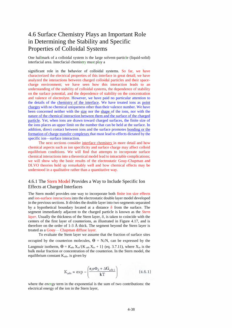
4.6 Surface Chemistry Plays an Important Role

in Determining the Stability and Specific

Properties of Colloidal Systems

One hallmark of a colloidal system is the large solvent-particle (liquid-solid)

interfacial area. Intecfacial chemistry must play a

significant role in the behavior of colloidal systems. So far, we have

characterized the electrical properties of this interface in great detail; we have

analyzed the interactions between charged colloidal particles and their space-

charge environment; we have seen how this interaction leads to an

understanding of the stability of colloidal systems, the dependence of stability

on the surface potential, and the dependence of stability on the concentration

and valence of electrolyte. However, we have paid no particular attention to

the details of the chemistry of the interface. We have treated ions as point

charges with no chemical uniqueness other than their valence number. We have

been concerned neither with the size nor the shape of the ions, nor with the

nature of the chemical interaction between them and the surface of the charged

particle. Yet, when ions are drawn toward charged surfaces, the finite size of

the ions places an upper limit on the number that can be held at the surface. In

addition, direct contact between ions and the surface promotes bonding or the

formation of charge transfer complexes that must lead to effects dictated by the

specific ion—surface interaction.

The next sections consider interface chemistry in more detail and how

chemical aspects such as ion specificity and surface charge may affect colloid

equilibrium conditions. We will find that attempts to incorporate surface

chemical interactions into a theoretical model lead to intractable complications;

we will show why the basic results of the electrostatic Gouy-Chapman and

DLVO theories hold up remarkably well and how chemical effects may be

understood in a qualitative rather than a quantitative way.

4.6.1 The Stern Model Provides a Way to Include Specific Ion

Effects at Charged Interfaces

The Stern model provides one way to incorporate both finite ion size effects

and ion-surface interactions into the electrostatic double layer model developed

in the previous sections. It divides the double layer into two segments separated

by a hypothetical boundary located at a distance from the surface. The

segment immediately adjacent to the charged particle is known as the Stern

layer. Usually the thickness of the Stern layer, , is taken to coincide with the

centers of the first layer of counterions, as illustrated in Figure 4.17, and is

therefore on the order of 1-3 Å thick. The segment beyond the Stern layer is

treated as a Gouy— Chapman diffuse layer.

To evaluate the Stem layer we assume that the fraction of surface sites

occupied by the counterion molecules, Ɵ = Ni/N, can be expressed by the

Langmuir isotherm, Ɵ = Kads Xio/{K ads Xio + 1} (eq. 3.7.11), where Xio is the

bulk molar fraction or concentration of the counterion. In the Stern model, the

equilibrium constant Kads. is given by

where the energy term in the exponential is the sum of two contributions: the

electrical energy of the ion in the Stern layer,

4-38

Figure 4.17 Schematic illustrating the Stern

model that accounts for

counterion size at the surface of

a particle. The Stern layer

extends a distance δ from the

surface. The Gouy-Chapman

diffuse layer starts at δ and

extends beyond the Debye

length (1/κ). The zeta potential,

measured electro-phoretically, is

the potential at the shear surface

between the particle and the

solution. (D. J. Shaw,

Introduction to Colloid and

Surface Chemistry, 3rd ed.,

Butter worth-Heinemann,

London, 1980, p. 156.)

zie and the specific chemical energy associated with the adsorption of ion i

on the particle surface, ΔGads.i.

We can also express Ɵ in terms of the charge densities associated with

the adsorbed ions in the Stern layer, σ, and the -surface charge density on the

particle, σo,

Nis equals the total number of adsorption sites for ion i on the surface, and the

quantity zieNis represents the charge density of the Stern layer if all the sites are

occupied.

4-39

Bibliography

D. J. Shaw, Introduction to Colloid and Surface Chemistry,4th ed.,London:

Butterworth & Co. Ltd., 1992.

D. F. Evans and H. WennerstrÖ m, The Colloidal Domain,2nd ed., New York:

VCH Publishers. Inc., 1999

D. H. Everett, Basic Principles of Colloid Science, London: Royal Society of

Chemistry, 1980.

P. C. Hiemenz, Principles of Colloid and Surface Chemsiry,3rd ed., New

York: Marcel Dekker, Inc., 1997.

R. J. Hunter, Foundations of Colloid Science, New York: Oxford University

Press, 1987.

H. van Olphen, An Introduction to Clay Colloid Chemistry, New York:

Interscience, John Wiley & Sons, Inc., 1963.

Exercises

4.1 The potential at a fixed distance from a charged particle increases _ ;

decreases _ ; or remains the same _ ; as salt is added to a sol.

4.2 The potential at a fixed distance from a charged particle increases _ ;

decreases _ ; or remains the same _ ; as the valence of the ions in

solution increases.

4.3 The charge density on the surface of a colloidal particle increases _ ;

decreases _ ; or remains the same __; as salt is added to a sol.

4.4 Calculate the Debye screening length at 20°C for potassium chloride

solutions containing 0.1 and 1.0 g of KCl per liter, respectively.

4.5 Clay particles with a surface charge of 0.12 C/m2 are immersed in the two

electrolytes in Exercise 4.4. What is the potential in millivolts at

distances of 30 and 100 Å from the particles in each solution?

4.6 Describe the origins of the forces that keep a colloid dispersed by (a)

electrostatic stabilization, and (b) steric (polymer) stabilization.

4.7 Consider two identically charged spherical colloidal particles with a

surface potential of 25 mV dispersed in an aqueous medium. The

effective Hamaker constant is 7 x 10-20 J. Determine the separation ho

for which the interaction potential goes through zero close to the primary

minimum. Assume ƶeo ≈ kT and ho << κ-1.

4.8 The sedimentation rate of a colloidal suspension increases _ ;

decreases _ ; or remains the same _ ; as salt is added.

4.9 What can you say about the sols, A and B, from the following information

concerning the relative molar critical coagulation concentrations

(CCCs)?

4-40

Suggest a mechanism for this behavior.

4.10 Draw curves that depict the potential energy of interaction V(h) between

two colloidal particles as a function of their separation h for the

following conditions (express relevant energies in units of kT): (a) a

stabilized sol that experiences slow coagulation; and (b) a sol that

experiences rapid coagulation. (c) How do you convert a sol from

condition (a) to condition (b)?

4.11 The coagulation rate of a sol

increases _ ; decreases _ ; or remains the same _ ;

as the size of the spherical particles increases.

4.12 Tuorila [Kolloid Chem. Beiheft 22,191 (1926)] measured the rapid

coagulation of a gold sol, radius 51 nm, and obtained the following

values:

Determine the association rate constant and compare with the

theoretical value for a diffusion-controlled reaction.

4.13 Calculate the expected value of the stability ratio W for two spheres of

radius 100 nm in a 2 x 10-3 M aqueous KC1 solution at T = 300 K and

with surface potential 35 mV and Hamaker constant 5 x 10-20 J.

4.14 What is the zeta potential for a sol? How is it measured? What is the

significance of zero zeta potential?

4.15 Increasing the concentration of I－ ions in a silver iodide sol above 2.5 x

10-12 M causes the surface potential on the silver iodide particles to

increase _ ; decrease _ ; or remain the same _ .

4.16 What are the key constituents of a good outdoor paint?

4-41