Comunication

28'1I ,.;

Estimation of a Wideband Fading

HF Channel using

Modified Adaptive Filters /

A Thesis Presented to

The Faculty of the College of Engineering and Technology

Ohio University

In Partial Fulfillment

of the Requirements for the Degree

Master of Science

by

Christopher Alan ~~a1ho

June, 1993

for Lynne and Sarah

Acknowledgements

I wish to thank Dr. Jeff Dill for his guidance and patience through out my

graduate study. Without his support, this thesis would not have been possible.

I would also like to thank my thesis committee and the rest of the Faculty of

the Department of Electrical and Computer Engineering for their help along the way.

A special thanks to Dr. Joseph Smallcomb who had to know the truth.

1

ii

Table of Contents

Acknowledgements

Table of Contents . . . . . . . . . . . . . . . . . . . . . . . . . . ii

List of Figures . . . . . . . . . . . . . . . . . . . . . . . . . . . . . . . . . . . . . . . .. IV

List of Tables V

Chapter 1: Introduction . . . . . . . . . . . . . . . . . . . . . . . . . . . . . . . . . .. 11.1. Purpose. . . . . . . . . . . . . . . . . . . . . . . . . . . . . . . . . . . . .. 11.2. Outline of Thesis . . . . . . . . . . . . . . . . . . . . . . . . . . . . . . .. 11.3. High Frequency Channel 21.4. Time Averaging. . . . . . . . . . . . . . . . . . . . . . . . . . . . . . . .. 51.5. Rake Correlator . . . . . . . . . . . . . . . . . . . . . . . . . . . . . . . .. 61.6. Channel Tap Model 6

Chapter 2: Introduction to Adaptive Filters 82.1. Linear Prediction and Wiener Filter Theory . . . . . . . . . . . . . . .. 82.2. Linear Prediction and AR Processes 122.3. The Method of Steepest Descent . . . . . . . . . . . . . . . . . . . . . .. 132.4. Levinson-Durbin Algorithm and the Lattice Structure . . . . . . . . .. 20

Chapter 3: Adaptive Algorithms . . . . . . . . . . . . . . . . . . . . . . . . . . . . .. 273.1. Introduction 273.2. Computational Complexity 303.3. Finite Precision Effects 303.4. Performance Considerations 32

Chapter 4: Algorithms. . . . . . . . . . . . . . . . . . . . . . . . . . . . . . . . . . .. 344.1. Normalized Least-Mean Square 344.2. Gradient Adaptive Lattice. . . . . . . . . . . . . . . . . . . . . . . . . .. 374.3. Prediction-to-Estimation . . . . . . . . . . . . . . . . . . . . . . . . . . .. 39

Chapter 5: Computer Simulations/Results/Conclusions .... . . . . . . . . . .. 445.1. Computer System . . . . . . . . . . . . . . . . . . . . . . . . . . . . . . .. 445.2. Chi Conversion Factor. . . . . . . . . . . . . . . . . . . . . . . . . . . .. 445.3. Computer Simulations . . . . . . . . . . . . . . . . . . . . . . . . . . . .. 46

5.3.1. General Channel Conditions . . . . . . . . . . . . . . . . . . .. 475.3.2. Tracking Ability. . . . . . . . . . . . . . . . . . . . . . . . . .. 525.3.3: Modification vs. Extended Order. . . . . . . . . . . . . . . .. 545.3.4: Comparison of Lattice Orders 56

5.4 Conclusions and Recommendations 57

111

References . . . . . . . . . . . .. 59

Appendix . . . . . . . . . . . . . . . . . . . . . . . . . . . . . . . . . . . . . . . . . . .. 61A: BOSS Block Diagrams. . . . . . . . . . . . . . . . . . . . . . . . . . . . .. 61

iv

List of Figures

Figure 2.1: Transversal Filter. . . . . . . . . . . . . . . . . . . . . . . . . . . . . .. 14Figure 2.2: Lattice Filter . . . . . . . . . . . . . . . . . . . . . . . . . . . . . . . . .. 26Figure 5.1: Key 5.3.1 / 5.3.2 . . . . . . . . . . . . . . . . . . . . . . . . . . . . . .. 48Figure 5.2: Doppler Shift 1Hz / SNR 0.5 . . . . . . . . . . . . . . . . . . . . . . .. 48Figure 5.3: Doppler Shift 1Hz / SNR 1.0 . . . . . . . . . . . . . . . . . . . . . . .. 48Figure 5.4: Doppler Shift 1Hz / SNR 2.0 . . . . . . . . . . . . . . . . . . . . . . .. 49Figure 5.5: Doppler Spread 1Hz / SNR 0.5 .. . . . . . . . . . . . . . . . . . . .. 49Figure 5.6: Doppler Spread 1Hz / SNR 1.0 . . . . . . . . . . . . . . . . . . . . .. 49Figure 5.7: Doppler Spread 1Hz / SNR 2.0 . . . . . . . . . . . . . . . . . . . . .. 50Figure 5.8: Doppler Shift 10Hz / SNR 0.5 . . . . . . . . . . . . . . . . . . . . . .. 50Figure 5.9: Doppler Shift 10Hz / SNR 1.0 . . . . . . . . . . . . . . . . . . . . . .. 50Figure 5.10: Doppler Shift 10Hz / SNR 2.0 . . . . . . . . . . . . . . . . . . . . .. 51Figure 5.11: Doppler Spread 10Hz / SNR 0.5 . . . . . . . . . . . . . . . . . . . .. 51Figure 5.12: Doppler Spread 10Hz / SNR 1.0 . . . . . . . . . . . . . . . . . . . .. 51Figure 5.13: Doppler Spread 10Hz / SNR 2.0 ~ . .. 52Figure 5.14: Chirped Tone and Estimate . . . . . . . . . . . . . . . . . . . . . . .. 53Figure 5.15: Slow Chirp 53Figure 5.16: Fast Chirp . . . . . . . . . . . . . . . . . . . . . . . . . . . . . . . . . .. 53Figure 5.17: Key 5.3.3 . . . . . . . . . . . . . . . . . . . . . . . . . . . . . . . . . .. 54Figure 5.18: Doppler Shift 1Hz I SNR 1.0 . . . . . . . . . . . . . . . . . . . . . .. 54Figure 5.19: Doppler Spread 1Hz I SNR 1.0 _.................... 55Figure 5.20: Doppler Shift 10Hz I SNR 1.0 . . . . . . . . . . . . . . . . . . . . .. 55Figure 5.21: Doppler Spread 10Hz / SNR 1.0 . . . . . . . . . . . . . . . . . . . .. 55Figure 5.22: Doppler Shift 10Hz I SNR 1.0 . . . . . . . . . . . . . . . . . . . . .. 56Figure 5.23: Doppler Spread 10Hz I SNR 1.0 . . . . . . . . . . . . . . . . . . . .. 56

v

List of Tables

Table 3.1 Adaptive Algorithms 28Table 3.2 Computational Complexity 31Table 4.1 Prediction to Estimation Cost . . . . . . . . . . . . . . . . . . . . . . .. 43Table 5.1 Simulation Parameters 47

1

Chapter 1: Introduction

1.1. Purpose

The purpose of this thesis is to explore adaptive filtering techniques to replace

the time averaging (TA) operation of the communication system described in

(Smallcomb, 1992). The communication system is a High Frequency (HF) spread

spectrum system that transmits a reference signal in conjunction with a pulse-position

modulated data symbol. The purpose of the reference signal is to provide a current

estimate of the impulse response of the channel. This knowledge of the channel

impulse response is then used to remove channel distortion from the data signal prior

to a symbol decision.

At the channel estimator, it will be shown that the adaptive filtering problem is

one of tracking a non-stationary signal of interest buried in white noise. Problems of

this type are ideal for adaptive filters and many similar examples may be found in the

literature.

1.2. Outline of Thesis

This thesis is outlined as follows. The remainder of Chapter 1 is devoted to

background material on HF channels and the TA operation. Topics discussed include

fading and frequency diversity. A brief description of the Rake filter is also included.

Chapter 2 formulates the adaptive filtering problem in a linear prediction

configuration. The Normal or Wiener-Hopf Equations are derived and theoretical

2

performance bounds established. Two optimum filter algorithms are also derived.

These algorithms provide the basis for the eventual adaptive filter implemented.

Chapter 3 introduces some of the common adaptive filtering algorithms that have been

considered for this application. A discussion of practical algorithm characteristics is

also presented. Based on the material in Chapter 3, it is possible to narrow the field

of possible algorithms. Chapter 4 contains derivations of the algorithms considered for

this application. Also included in Chapter 4 is the modification to the adaptive filters

which allows the current observation to be included in the estimation of the channel

impulse response. Chapter 5 includes simulation results and final recommendations.

Appendix A contains the BOSS modules and all computer programs used in the

simulations.

1.3. High Frequency Channel

High Frequency (HF) communication takes place in the 3-30 MHz frequency

band. One attractive feature of the HF channel is the ability to communicate over long

distances. HF waves propagate along two different channels. The first is the ground

wave channel. These signals tend to attenuate rapidly due to rough terrain and/or the

curvature of the earth. The useful communication range of the ground wave is limited

to about 50 miles. The HF skywave propagates toward space and is refracted back to

earth by ionized layers in the ionosphere. It is the skywave that makes long distance

communication possible.

The ionosphere is comprised of a number of horizontal ionized layers. The

3

layers are labeled D, E and F for historic reasons. Under certain conditions, the F

layer may divide into two sublayers, Fl and F2. The D layer acts mainly as an

absorber of HF energy while the refraction takes place in the E and F layers.

The main source of ionization is solar electromagnetic radiation that covers the

ultra-violet and X-ray bands of the spectrum. The ionization rate depends on altitude,

intensity of the solar radiation, the ionization efficiency of the atmospheric gases and

the solar zenith angle. The maximum ionization rate occurs when the sun is directly

overhead. The creation of ions is balanced by ionization losses due to recombination

of electrons with positively charged ions or neutral atoms or molecules. The HF

channel is non-stationary due to the changing ionization rate and the shifting altitudes

of the layers.

The time varying nature of the HF channel results in fluctuations in received

signal strength. This is known as fading. One major cause of fading is the

simultaneous arrival of two or more signals, propagating over different skywave

paths, with time variant phases that add constructively or destructively. A common

fading rate is 10-15 fades per minute with a depth of less than 10 dB.

The communication system in this application employs spread-spectrum as a

frequency diversity technique to reduce the effects of fading. With frequency

diversity, the transmitted signal is spread over a wide band which reduces the

probability of different signal components fading at the same time.

The refraction of a signal by the ionosphere causes that signal to be spread

over time. The duration of the spread is known as the multipath spread T . AverageIn

4

values range from 1-2 milliseconds, but may reach 5-10 milliseconds for disturbed

conditions. The coherence bandwidth of the channel is defined by (Proakis, 1989) as

1w::::­C T

m

(1.1)

This is the minimum separation in frequency at which two signal components are

affected differently by the channel. To achieve frequency diversity, the channel should

be frequency selective. This requires that the signal bandwidth W, be much greaters

than W ·c

A frequency selective channel may be modeled as a tapped delay line where

the unit of delay is 1/ Ws

. The number of taps L, is given by

(1.2)

Each channel tap may be independently modeled as a zero-mean complex-valued

Gaussian random process. The envelope of each tap Ih(n,t) I, has a Rayleigh

distribution. This is commonly know as a Rayleigh fading channel.

It is assumed that the scattering of the multipath is uncorrelated, therefore the

channel taps may also be considered mutually independent random processes (Proakis

1989). Based on this assumption, a bank of adaptive filters will be implemented, one

for each channel tap. The final number of adaptive filters implemented will depend on

the tail-clipping operation described in (Smallcomb, 1992).

5

1.4. Time Averaging

The current method of noise reduction on the channel taps is time averaging

(TA). This is a simple recursive algorithm using a first order IIR filter that sums

weighted combination of the present and past observations attempting to reduce the

additive white noise.

The TA estimate is given by

h(n) = «y(n) + (l-«)h(n-l) (1.3)

where h(n) is the current estimate, y(n) is the current observation and « is a positive

real scalar between 0 and 1. The performance of the TA derived in (Smallcomb,

1992) is described by the noise reduction factor X

(1.4)2-«

(X

X ---

X may also be defined as the ratio of the estimation noise power over the input noise

power. This performance measure assumes rather strict channel conditions: 1) there is

no fading, and 2) the channel tap is time invariant.

There are two shortcomings of the TA module that have spurred the search for

adaptive filters. First, u is not an adaptive parameter. This means that the TA

module has no tracking ability, ie in non-stationary conditions, performance is

degraded. To avoid unstable behavior, «, must be set for the worst case. This limits

its performance for other channel conditions.

The second problem with the TA module is that « is a real scalar. This limits

6

its ability to track complex phase information.

1.5. Rake Correlator

The purpose of the Rake correlator is to recombine the signal components that

were intentionally spread over the multipath channel by the transmitter. The Rake

correlator is a tapped delay line that aligns the phase of each multipath component and

coherently combines them. For optimum Rake performance, its tap weights must be

the same as the channel tap weights (Proakis, 1989).

1.6. Channel Tap Model

To account for the wide variety of channel conditions we will use two channel

tap models. The first model is a complex tone. The second model is a complex

Gaussian auto-regressive (AR) process.

The rising and falling of the ionospheric layers creates a Doppler shift in the

transmitted signal. This shift range from 0.1-1.5 Hz for normal or quiet conditions

and 0.1-10 Hz during disturbed conditions (Maslin 1987). The first model is simply a

complex tone with frequency equal to that of the Doppler shift. The non-stationary

property of the channel will be modeled by a chirped, or frequency swept, complex

tone.

The second model simulates the Doppler spread of the channel during

disturbed conditions. Channel disturbances may occur as the result of sun spots or

other solar activity. The second model, discussed in (Hariharan and Clark, 1990), is

two independent sources of white Gaussian noise passed through identical fifth order

Bessel filters. The filter output is then combined to form the real and imaginary

channel tap. This is the Rayleigh fading channel discussed earlier. The bandwidth of

the Bessel filters corresponds the Doppler spread of the channel. The Doppler spread

effect may range from 0.1 Hz for a mild disturbance to 15 Hz. in an extremely

disturbed channel.

7

8

Chapter 2: Introduction to Adaptive Filters

2.1. Linear Prediction and Wiener Filter Theory

Having demonstrated that the multipath channel may be treated as a collection

of independent taps, it will now shown how adaptive filter techniques may be applied

to estimate each channel tap. In the following discussion, only one tap is considered.

The discrete time period is referred to as the super-symbol period, (Smallcomb 1992).

Consider the received signal from one of the channel multipaths:

yen) = hen) + v(n) (2.1)

where hen) is the multipath impulse response and v(n) is zero mean white Gaussian

noise. The linear prediction problem is to predict the current value of hen) based on a

linear combination of the previous M samples of y(n): y(n-l), y(n-2), ... , y(n-M).

M

yen) = E wty(n-i);=1

Wiener filter theory may be used ttl optimize the prediction. Let e(n) be the

prediction error:

e(n) = yen) - j(n)

The error may also be written in vector form,

(2.2)

(2.3)

e(n) = yen) - wHy(n-l)

where

and

yen-I) = [Y(n-l),y(n-2), ...,y(n-M)]T

Superscript H denotes Hermitian or conjugate transpose.

Let the filter optimization criteria be the minimum mean square error J(w).

.l(w) = E[e(n)e(n)*]

Substituting (2.4) into (2.7) and expanding yields:

J(w) = E{y(n)y(n)*} - E{wHy(n-l)y(n)*}

- E{Y(n)y(n-l)Hw} + E{wHy(n-l)y(n)Hw}

9

(2.4)

(2.5)

(2.6)

(2.7)

(2.8)

(2.9)

Assuming that the filter weights, w, are constant, they may be moved outside the

expectation operator,

J(w) = E{y(n)y(n)*} - w"E{Y(n-l)y(n)*}

- E{Y(n)y(n-l)H)w + wH E{y(n-l)y(n-l)~w

J(w) may now be analyzed on a term by term basis. Assuming yen) to be zero

mean, the first expectation is simply the variance of y(n).

E{y(n)y(nr} = a~

The second term is denoted as the cross-correlation vector p,

E{y(n-l)y(n)*} =p

in expanded form,

[r( -l),r( -2), ,r(_M)]T

P = [r(1)*,r(2)., ,r(m)*f

10

(2.10)

(2.11)

(2.12)

where r(i) is the autocorrelation 'function for lag i. The third expectation term is

simply the Hermitian transpose of the second term.

pH = E{y(n)y(n-l)H}

The fourth term is the (M x M) autocorrelation matrix denoted by R

R = E{Y(n-l)y(n-l)H}

Of,

(2.13)

-(2.14)

R =

r(O)

,*(1)

r*(M-l)

r(1)

r(0)

r(M-l)

r(O)

(2.15)

Note that if y(n) is a wide-sense stationary process, p and R are constants.

Making the substitutions (2.10), (2.11), (2.13) and (2.14) into (2.9), we have

11

(2.16)

From (2.16) it can be seen that J(w) is a second order function of the filter weight

vector w. The dependence of J(w) on w may be viewed as a bowl shaped surface

with a unique minimum (Haykin, 1991), (Alexander, 1986). At the bottom or

minimum of the "error-performance surface" the weight vector, w, attains the

optimum value wII

To determine the optimum weight vector w,,' the mean-square error J(w) is

differentiated with respect to w and the result set equal to zero.

dJ(w) = V(J) = 0d(w)

(2.17)

where del is the gradient vector. Differentiating (2.16) term by term and combining

the results yields the normal or Wiener-Hopf equations.

Rw" = P

solving (2.18) for w :II

(2.18)

(2.19)

It can be shown (Haykin, 1991), (Alexander, 1986) that when the weight

vector w, is at the optimum value w,,' the estimation error, e(n) , is orthogonal to the

input vector y(n-l).

E{y(k) e(k) *} = 0

12

(2.20)

To find the minimum mean-square error, (2.19) is substituted into (2.14):

J 2 H H H Rmin = 0y - pit'. - W. P + W. W •

using (2.19), (2.21) reduces to:

2 HJmin = 0y -p W.

(2.21)

(2.22)

Wiener filter theory provides a solution for the optimal filter coefficients, but

note that for large values of M, matrix inversion may be impractical. In the remaining

sections of the chapter, we will introduce two recursive algorithms for solving the

Weiner-Hopf equations. The recursive algorithms, while requiring explicit knowledge

of the signal statistics, are the basis for the practical adaptive algorithms.

2.2. Linear Prediction and AR Processes

Having derived the optimal prediction error filter and shown that the signal of

interest is an AR process, it is helpful to examine the relationship between the two.

Linear Prediction and autoregressive modeling are complementary operations.

The prediction error filter is an all-zero finite-impulse response filter. The AR model

is an all-pole infinite impulse response filter. When the prediction error filter is

optimized, the zeros of its transfer function are located at exactly the same position of

the poles in the transfer function of the AR model. The relationship between the two

sets of parameters from (Haykin, 1991) is given by:

aM•i = -Wo•i i = 1,2, ...,M

a~ = E{le(n)12}

The ability to predict a signal is based on correlation between adjacent

13

(2.23)

samples. This implies that by increasing the filter order, correlation between adjacent

samples of the error signal is reduced. Theoretically, if the filter order is high

enough, adjacent samples of the error signal are uncorrelated. This is known as the

whitening property of prediction error filters.

2.3. The Method of Steepest Descent

The method of steepest descent is one of a family of iterative optimization

methods that provides a method of searching a multidimensional performance surface.

The particular surface of interest is the mean-square error (MSE) surface. A thorough

discussion of the properties of the MSE surface may be found in (Alexander 1986).

The method of steepest descent is based on a transversal filter structure, (Fig. 2.1).

Recall the prediction error given by (2.4),

e(n) = yen) - wHy(n-l) (2.24)

If we no longer assume that the weight vector is constant, then the mean-

square error become a function of the time index n.

J(n) = a~ - wH(n)p - pw(n) + wHRw(n) (2.25)

14

/\yen)

-1 z' z'Z............... t------r---~ ---------

yen)

Figure 2.1: Transversal Filter

The method of steepest descent proceeds as follows:

1. Start with an initial guess of the optimum weight vector w . UsuallyII

this is the null vector O.

2. Based on the value of the weight vector, compute the gradient

vector.

3. Add a correction term to the current value of the weight vector

based on the opposite direction of the weight vector.

4. Return to step two and repeat the procedure.

The method of steepest descent "steps" down the MSE surface until it reaches the

15

bottom or minimum point.

The recursive equation for the method of steepest descent is:

1wen +1) = wen) + - J.L [ - V(J(n»]

2(2.26)

Where V(J(n)) , is the gradient of the MSE surface, J.L is a positive, real-valued scalar

known as the step size, and the 1/2 factor is simply for convenience. The gradient is

given by,

V(J(n» = -2p + 2Rw(n)

Substituting (2.27) into (2.26) yields:

w(n+ 1) = wen) + 1l[P - Rw(n)]

(2.27)

(2.28)

Two important issues to consider in the analysis of an adaptive algorithm are

its stability and transient behavior. (In this case stability refers to convergence of the

algorithm to the desired solution.) For the method of steepest descent, both stability

and the transient behavior are dependent on the step size I!' and the autocorrelation

matrix R.

In examination of the stability of the method of steepest descent, it is common

to define a weight error vector,

c(n) = wen) - w"

where w is the Wiener weight vector, from equation (2.19). Using (2.28) and"

(2.29),

(2.29)

c(n+1) = (1 - ~R)c(n)

Equation (2.30) represents a series of coupled difference equations. Analysis is

simplified by decoupling the equations using a similarity transform of the

16

(2.30)

autocorrelation matrix R. Using linear algebra techniques, R may be written as

R = QAQ" (2.31)

where Q is a unitary matrix whose columns are the eigenvectors associated with the

eigenvalues of R. A is a diagonal matrix whose elements are the eigenvalues of R.

Al 0 ... 0

o A2

0 ... 0. A =

oo 0 ... AM

Substituting (2.31) into (2.30),

c(n+l) = (I - JJQAQ")c(n)

(2.32)

(2.33)

premultiplying by Q" and using the property of unitary matrices, Q" = o". (2.33)

reduces to

Q"c(n+l) = (I -J-LA)Q"c(n)

We may now define a vector of uncoupled weight difference equations,

(2.34)

v(n) =~c(n)= ~[w(n) - wJ

assuming that w(O) = 0, then

v(O) = _QHW tJ

(2.34) may be rewritten as

v(n+ 1) = (I - JJ,A)v(n)

The kth uncoupled difference weight or natural mode is given by

17

(2.35)

(2.36)

(2.37)

(2.38)

(2.38) is a first order difference equation which may be expressed in terms of vi(O)

by

(2.39)

One of the properties of R is that it is positive definite. This means that all its

eigenvalues are real and positive. Therefore (2.38) represents a geometric series. Of

particular interest is the behavior of the kth natural mode as n approaches infinity.

Convergence of the natural modes to 0 implies

limw(n) = wtJ

For vlen) to decay to 0,

(2.40)

(2.41)

18

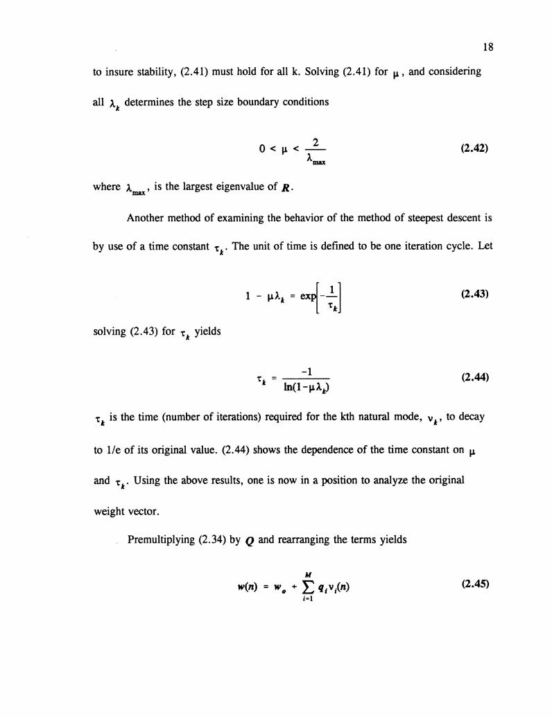
to insure stability, (2.41) must hold for all k. Solving (2.41) for J.L' and considering

all At determines the step size boundary conditions

2O<J.L<--

Amax

where A ,is the largest eigenvalue of R.max

(2.42)

Another method of examining the behavior of the method of steepest descent is

by use of a time constant -rk ' The unit of time is defined to be one iteration cycle. Let

solving (2.43) for tk

yields

t 1 = ----

(2.43)

(2.44)

-rk is the time (number of iterations) required for the kth natural mode, vk' to decay

to lIe of its original value. (2.44) shows the dependence of the time constant on J.L

and tk

• Using the above results, one is now in a position to analyze the original

weight vector.

Premultiplying (2.34) by Q and rearranging the terms yields

M

w(n) = -, + E qjv;(n);=1

(2.45)

19

where qk' are the columns of Q. The transient behavior of the kth tap is

M

wk(n) = Wok + E qkiv;(l-J.LAi)ni=1

Examination of (2.46) reveals that each tap converges as a weighted sum of

(2.46)

exponentials. At this point, one may introduce an overall time constant ,; , which isa

defined as the time required for the left side of (2.46) to decay to lIe of its initial

value. Analysis is simplified by considering only the upper and lower bounds. From

(Haykin 1992), the time constant bounds are

-IIn(1 - ~ Amax>

Equation (2.47) demonstrates the dependence of the weight convergence on the

(2.47)

eigenvalue spread of the autocorrelation matrix R. When R is ill-conditioned the

convergence time is limited by the smallest eigenvalues.

The final property of the method of steepest descent we will deal with is the

transient behavior of the mean-squared error, J(n). The MSE at any time n is given

by (Haykin 1992) as

M

J(n) =Jmin + E Ai Iv;(n) 12

i=1

Substituting (2.38) into (2.48) yields

(2.48)

M

J(n) =Jmin + LAi(l - I!Ai)2nlvi(O)12i=l

When J1 is given by (2.42),

limJ(n) = Jminn"OO

20

(2.49)

(2.50)

The learning curve of the algorithm is a sum of decaying exponentials. The time

constant for the kth natural mode is

-1

(2.51) shows the dependance of the convergence rate on the step-size J.L.

(2.51)

The method of steepest descent requires explicit knowledge of the second

order signal statistics. This makes it of little practical value. The method of steepest

descent, however, forms the basis for the Stochastic Gradient algorithms (most

notably the LMS). These algorithms may be analyzed using the above techniques.

# 2.4. Levinson-Durbin Algorithm and the Lattice Structure

In this section, the Levinson-Durbin algorithm is derived. The Levinson-

Durbin algorithm is an order recursive solution of the Wiener-Hopf equations. The

method behind the algorithm is to derive the rnth order predictor given that the

predictor of order (m-l) is known. Once the general formula has been derived, given

simple initial conditions, any order predictor may be found. The Levinson-Durbin

algorithm also forms the basis for the lattice filter structure, (Figure 2.2), which will

21

introduced in this section.

The general solution for the mth order predictor, in terms of the (m-l)st order

predictor is given by

(2.52)

where k"" is a constant known as the reflection coefficient, and d"'_1 is an unknown

vector. The mth order autocorrelation matrix may be written as

.[R -.jR = .-1 P.-l

• -rP".-l r(O)

(2.53)

where the overbar denotes reverse ordering. Using (2.52) and (2.53), the mth order

Wiener-Hopf equations become

[~.-1 ;:-1] * [ [W__t ] + [d__1] 1= ~.-llP~-1 r(o) 0 1". lr(m)

We now wish to solve (2.54) for k ,and d . The first equation is", .-1

R w + R d + p-. k = P.-1 .-1 .-1 .-1 .-1 lit .-1

however,

and the solution for d"'_1 is given by

(2.54)

(2.55)

(2.56)

d = k p-l -.".-1 - m ....... -lP".-1

From (Alexander, 1986)

and (2.57) reduces to

The scalar equation from (2.54) is

-r -TP".-1 W.-1 + P.-ld._t + r(O)k", = r(m)

Substituting (2.59) into (2.60) and solving for k results in",

22

(2.57)

(2.58)

(2.59)

(2.60)

(2.61)

For a zero-mean random process, 7(0) =0 2 , therefore the denominator of (2.61) is

the mean-squared error for the (m-1)st order predictor, J . (2.61) may be expressed",-1

as

(2.62)

The recursive equation for the mean-squared error J , from (Haykin 1992), is",

23

For a zeroth order predictor, Jo = r(O).

(2.63)

Before deriving the lattice structure, it is useful to introduce the concept of

backward linear prediction. As the name suggests, the idea is to predict an

observation, y(n-M) , based on a linear combination of "future" samples. The

equation for backward prediction is

M

bM = y(n-M) - L gty(n-i+l)i=1

(2.64)

where bM

, is the backward prediction error. A derivation similar to the one in Section

2.1 may be followed to obtain the Wiener-Hopf equations for backward prediction.

The interested reader is referred to (Haykin, 1992).

The relationship between the backward prediction weights, g and the forward

prediction weights, w is given by (Haykin, 1992),II

The backward weights are simply the forward weights in reverse order and

conjugated.

To further simplify the lattice structure, a new vector will be defined

(2.65)

24

Durbin algorithm, the mth order forward predictor may be expressed as

(2.67)

Similarly, the update recursion for the mth order backward predictor is given by

The data input vector may be written as,

r , ..(n)] [y(n)]' ..+I(n) = !y<n-M) = , ..(n-l)

The forward prediction error is defined as,

Using (2.67) and (2.69),

[H ] r' ..(n) ] _".-1 0 L. - fm-1(n)

l.Y(n-M)

and

*[ -T] [ y(n)] *k",O tJ.._1 , ..(n-l) = k",b",_t<n-l)

(2.68)

(2.69)

(2.70)

(2.71)

(2.72)

The combined results of (2.71) and (2.72) yields one of the two key lattice recursive

equations,

fm(n) = f m- 1(n) + k;bm_1(n-l)

The other one, obtained in the same manner is

25

(2.73)

(2.75)

bm(n) = bm_1(n-l) + k,j",(n) (2.74)

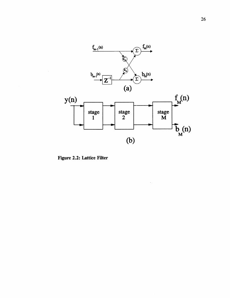
Equations (2.73) and (2.74) make up one stage of a lattice filter, Fig. 2.2 (a). The

zeroth order lattice predictor is

fo(n) = bo(n) = y(n)

The Mth order lattice predictor is shown in Fig. 2.2 (b).

The lattice filter structure has several interesting properties: 1) the various

stages of the lattice are decoupled such that the backward prediction errors produced

by each stage are orthogonal. 2) The lattice filter is modular. Stages may be added or

removed without affecting previous calculations. 3) The lattice stages are identical

which lends itself to VLSI implementation.

(a)

26

y(n)

stage1

stage2

stageM

Figure 2.2: Lattice Filter

(b)

~----' b (n)M

27

Chapter 3: Adaptive Algorithms

3.1. Introduction

In Chapter 2, two optimal filter algorithms were discussed, the Method of

Steepest descent, and the Levinson-Durbin algorithm. Also introduced were two

adaptive filter structures, the transversal or direct filter and the lattice filter. The

algorithms presented in Chapter 2 have little practical value for this particular

application due to the fact that they require knowledge of the second order signal

statistics. In this chapter, some common adaptive filter algorithms which overcome

this limitation are introduced. The algorithm properties of computational complexity

and stability are examined. These properties, along with other performance issues will

aid in selection of one or two algorithms suitable for this application. Note that since

this application operates in "real time", block filtering techniques will not be

considered .

Adaptive filter algorithms are normally divided into categories according to

some cost function .". The two categories of algorithms considered for this

application are the Stochastic Gradient algorithms and the Least-Squares algorithms.

Table 3.1 shows the division of adaptive algorithms by cost function and structure.

28

Stochastic Gradient Least Squares

LatticeI

LatticeTransversal Transversal

LMS GAL FTF LSL

NLMS RLS LSL w/errorfeedback

Table 3.1 Adaptive Algorithms

The Stochastic Gradient algorithms are based on the Method of Steepest

Descent. (section 2.2). The cost function of these algorithms is the mean-squared

error, " = E{le(n) 11} . Unlike the method of steepest descent which uses the

instantaneous gradient of the performance surface, stochastic gradient algorithms

estimate the gradient using the current data vector. The gradient estimate is given by:

V(J(n)) = -2y(n-l)y*(n) + 2y(n-l)yH(n-l)w(n)

The best known of the Stochastic Gradient algorithms is the Least Mean Square

(3.1)

(LMS) algorithm. The LMS algorithm was derived by Widrow and Hopf in 1960.

The simplicity of the LMS algorithm has led to its wide-spread use. The LMS has

also become a benchmark for comparison with more complex algorithms.

Other Stochastic Gradient algorithms considered in this study are the

Normalized LMS (NLMS), and the Gradient Adaptive Lattice (GAL). The NLMS

algorithm was derived in 1967 by Nagumo and Noda, and independently by Albert

29

and Gardner. The NLMS is similar to the LMS algorithm but it incorporates a time-

varying step-size. The Gradient Lattice derived by Griffths in 1977, incorporates the

desirable numerical properties of the lattice filter with the computational simplicity of

the LMS algorithm.

The Least Squares algorithms, as the name suggests are based on the method

of Least Squares. The method of least squares is attributed to Gauss and the

estimation of asteroid orbits (Alexander 1986). Specifically, consider the method of

exponentially weighted least squares. The cost function for these algorithms is

II

'P = L An-i le(,) 12;=0

Because these algorithms do not attempt to minimize a statistical error, they are also

known as exact least squares algorithms. Least squares algorithms all yield the same

solution to a filtering problem. They differ only in form and complexity.

The conventional Recursive Least Squares (RLS) filter, requires a matrix

inversion and is O(M2) where M is the filter order. Several fast RLS algorithms have

been developed which reduce the computational complexity to O(M).

The Fast Transversal Filter (FTF), developed by Carayannis et al in 1983 and

independently by Cioffi and Kalith in 1984, is a combination of four transversal filters

working in parallel to produce the least squares solution.

The least squares lattice (LSL) is generally attributed to Morf. There are

several versions of the LSL, and the interested reader may refer to (Haykin 1992) or

(Friedlander 1982) for details.

30

3.2. Computational Complexity

The first property of adaptive algorithms considered is computational

complexity. Simply, this is the number of arithmetic operations that the algorithm

requires. Usually this is expressed in terms of the filter order M. The computational

complexity of an algorithm directly affects the cost of implementation. The cost

comes in terms of added storage requirements and delay.

As noted above, the conventional RLS algorithm is O(M2) . The fast RLS and

the Stochastic Gradient algorithms are all O(M) in complexity. One important point in

considering complexity is that for this application, a large number of parallel filters

will be implemented. This means that any increase in complexity will be magnified in

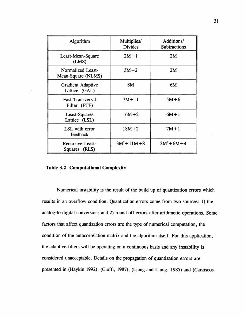
the final system. Table 3.2 lists the various algorithms and their computational

complexities. (All operations are complex.)

3.3. Finite Precision Effects

When an adaptive algorithm is implemented using finite precision arithmetic,

there are two effects that need to be considered: numerical stability and accuracy. An

adaptive algorithm is stable if the use of finite precision arithmetic results in bounded

deviations from the infinite precision form of the algorithm (Haykin 1992). Accuracy

refers to the magnitude of those deviations. An important note is that stability is a

function of the algorithm and not the number of bits used. Accuracy on the other hand

is a function of the number of bits.

31

Algorithm Multiplies/ Additions/Divides Subtractions

Least-Mean-Square 2M+l 2M(LMS)

Normalized Least- 3M+2 2MMean-Square (NLMS)

Gradient Adaptive 8M 6MLattice (GAL)

Fast Transversal 7M+l1 5M+6Filter (FTF)

Least-Squares 16M+2 6M+lLattice (LSL)

LSL with error 18M+2 7M+lfeedback

Recursive Least- 3M2+11M+8 2M2+6M+4

Squares (RLS)

Table 3.2 Computational Complexity

Numerical instability is the result of the build up of quantization errors which

results in an overflow condition. Quantization errors come from two sources: 1) the

analog-to-digital conversion; and 2) round-off errors after arithmetic operations. Some

factors that affect quantization errors are the type of numerical computation, the

condition of the autocorrelation matrix and the algorithm itself. For this application,

the adaptive filters will be operating on a continuous basis and any instability is

considered unacceptable. Details on the propagation of quantization errors are

presented in (Haykin 1992), (Cioffi, 1987), (Ljung and Ljung, 1985) and (Caraiscos

32

and Liu, 1984). The important stability and accuracy results from these and other

references are summarized below.

The LMS algorithm is susceptible to quantization errors. It may be stabilized

by a technique known as leakage or by the addition of a white noise source to the

weight input vector y(n-l). In our application, the channel noise fulfills this role.

The NLMS algorithm may be stabilized using the same methods (Weiss and Mitra,

1979).

The FTF and RLS algorithms are widely known to be numerically unstable.

Two methods discussed to compensate for FTF instability are periodic reinitialization,

and the use of rescue devices (Haykin 1992). The rescue device incorporates

monitoring of a specific variable in the FTF algorithm, and starting a "backup" filter

when this variable becomes negative.

Finally, we consider the-lattice filters GAL and LSL. The lattice structure is

widely regarded to have better numerical- properties than the transversal structure. The

lattice is less sensitive to quantization errors. The use of error feedback to update the

reflection coefficients also improves the accuracy of the algorithm. Details on the

accuracy of adaptive filters is given in (Haykin 1992) and (proakis 1989).(Ljung and

Ljung, 1985) show that the LSL filter is exponentially stable with regard to round-off

errors and other numerical disturbances.

3.4. Performance Considerations

Based upon the discussion of sections 3.2 and 3.3 it is now possible to

33

eliminate some algorithms from consideration. Due to instability, the FTF and

conventional RLS may be ruled out. At this point, the LMS algorithm may also be

discarded. The LMS uses the same step-size bounds as the method of steepest

descent, Eq. (2.43). Lack of knowledge of the channel statistics make selection of an

appropriate step-size impossible. Before eliminating any more algorithms, some

performance issues must be considered.

The two performance issues we will consider are convergence rate and

tracking ability. The convergence time of an adaptive algorithm is the time required

for some performance measure to drop below a specified level (Cioffi, 1986). The

tracking ability of an algorithm refers to how well it follows statistical variations in

the input signal. The tracking. ability of an algorithm is related to the algorithm

parameters. Proper selection of the algorithm parameter is a balance between the

conflicting requirements of minimizing excess MSE when the channel is stationary,

and minimizing MSE due to the changing signal statistics. (Excess MSE is a result of

estimating the signal statistics)

Recall for this application, there is a low SNR and a slowly time varying

channel signal. Two studies that are of particular interest are (Cioffi, 1986) and

(Bershad and Macchi, 1990). The first by Cioffi provides guidelines as to when the

RLS algorithms result in superior performance over the LMS. The second reference

deals with the ability of the LMS and RLS to track a chirped sinusoid in white noise.

The results of these studies indicate that for our application, the RLS algorithms offer

no significant performance advantage.

34

Chapter 4: Algorithms

4.1. Normalized Least-Mean Square

The first algorithm considered for this application is the NLMS. The NLMS

retains the computational simplicity of the LMS, but its time-varying step-size makes

it more practical for non-stationary filtering environments.

The derivation of the NLMS follows the one presented in (Haykin, 1992). A

similar derivation may be found in (Nagumo and Noda, 1967).

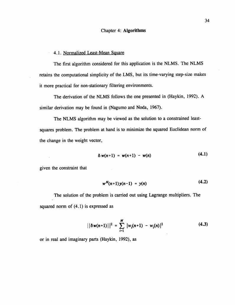
The NLMS algorithm may be viewed as the solution to a constrained least-

squares problem. The problem at hand is to minimize the squared Euclidean norm of

the change in the weight vector,

aw(n+l) = w(n+l) - w(n)

given the constraint that

wH(n+ l)y(n-l) = y(n)

(4.1)

(4.2)

The solution of the problem is carried out using Lagrange multipliers. The

squared norm of (4.1) is expressed as

M

II~w(n+l)112 =E Iwi(n+l ) - wi(n) 12i=1

or in real and imaginary parts (Haykin, 1992), as

(4.3)

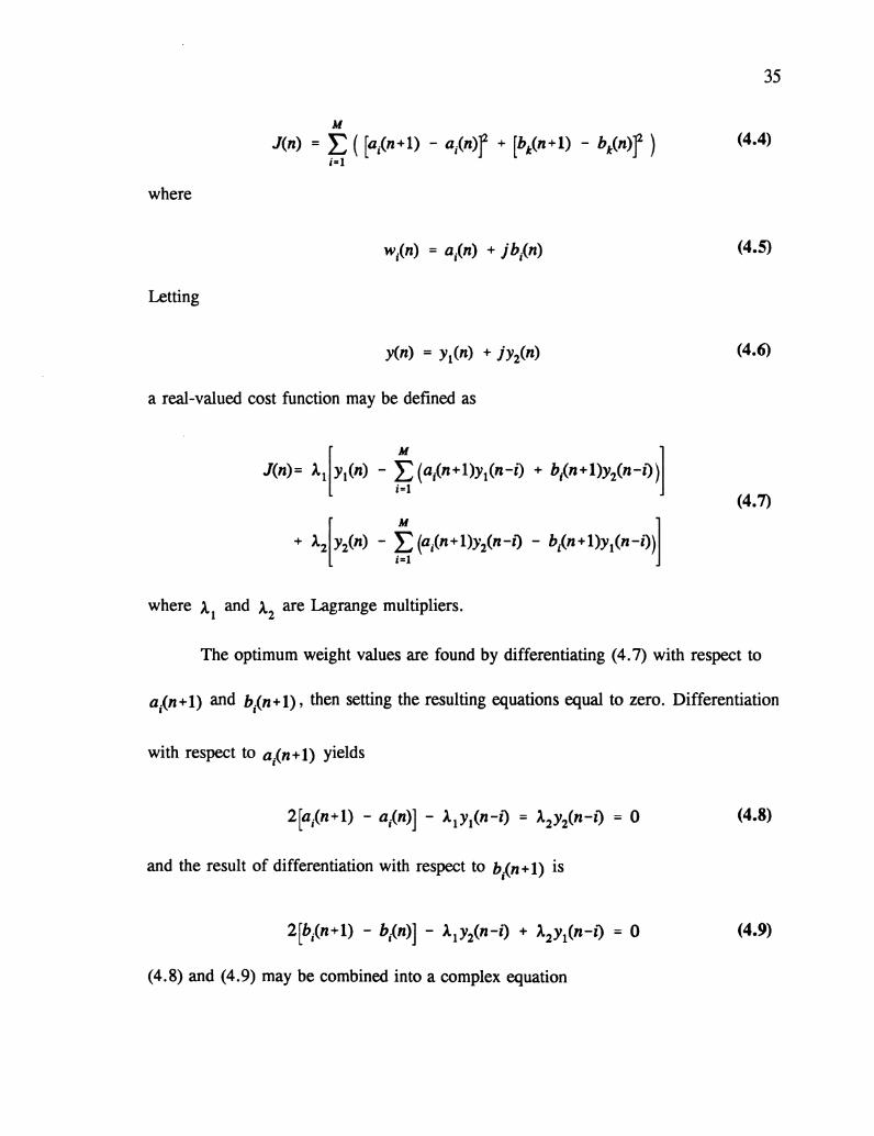
35

M

J(n) = E( [a,(n+l) - a,(n)j + [b,t(n+l) - b,t(n)j) (4.4);=1

where

(4.5)

Letting

a real-valued cost function may be defined as

J(n)= A1[Yt(n) - !t(aj(n+l )Yt(n- i) + bt(n+l)Y2(n-O)]

+ A2k2(n) - it (aj(n+ 1)Y2(n-l) - bj(n+ l)Yt(n-i»)]

where Al and A2

are Lagrange multipliers.

(4.6)

(4.7)

The optimum weight values are found by differentiating (4.7) with respect to

ai(n+1) and bi(n+1), then setting the resulting equations equal to zero. Differentiation

with respect to a;(n+1) yields

(4.8)

and the result of differentiation with respect to b;(n+l) is

(4.9)

(4.8) and (4.9) may be combined into a complex equation

i=1,2,...,M

36

(4.10)

where A=Al +jA2

is a complex Lagrange multiplier. The solution of (4.10) for the

unknown A*, using the constraint equation, is

Using the definition of the prediction error, (4.11) may be reduced to

A* = __2_- e*(n)Ily(n-l) 11

2

Substituting (4.12) into (4.10) yields

5w(n+l) = 1 y(n-l)e*(n)Ily(n-l) 11

2

(4.12)

(4.13)

Control over the change in the tap weight vector is obtained by introducing a

real positive scalar J.L. The final form of the NLMS weight recursions is

w(n +1) = w(n) + JJ. y(n -1) e*(n)Ily(n-l) 11

2

The bounds on ~ for mean-square convergence are

(4.14)

(4.15)

Selection of J.L' involves the performance trade-off between convergence and tracking

ability vs. steady state MSE.

An analysis of NLMS convergence is beyond the scope of this thesis, the

reader is referred to (Bershad, 1986) or (Slock, 1990) for further details. The main

result of interest is in the comparison of excess MSE between the NLMS and the

LMS. From (Bershad, 1986), the increase in misadjustment for the NLMS is

(1-2/M)-1. For a fifth order filter, this is an increase of about 66%. In this

application p. will be rather large due to convergence and tracking considerations.

This also increases the excess MSE and may result is unsatisfactory NLMS

performance.

4.2. Gradient Adaptive Lattice

The second adaptive filter considered for this application is the Gradient

Adaptive Lattice (GAL). The GAL has performance abilities similar to those of the

least-squares lattice but at a much lower computational cost. The GAL has one and

two reflection coefficient versions. By the two coefficient version we mean that the

reflection coefficients for a single stage are not identical. Again, to reduce

computational cost, only the one coefficient form is considered. The two coefficient

form may be found in (Friedlander, 1982) or (Haykin, 1992).

The specific GAL algorithm used in this thesis is found in (Proakis, 1989),

and therefore that derivation is presented here.

Recall the two equations that define a lattice stage

37

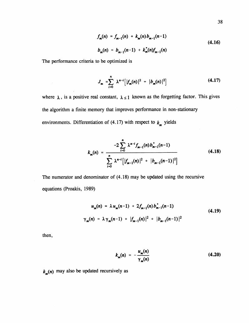
38

f".(n) =f",-t(n) + k".(n)b"'_l(n-l)(4.16)

The performance criteria to be optimized is

11

Jm =I: 1"-i[lfm(n) 12 + Ibm(n)12]

i=O

(4.17)

where "', is a positive real constant, '" s 1 known as the forgetting factor. This gives

the algorithm a finite memory that improves performance in non-stationary

environments. Differentiation of (4.17) with respect to k yields",

(4.18)

II

-2 L AlI-if"'_l(n)b~_l(n-l)i=O

n

L 1,,-i[lfm_t(n) 12 + Ibm_t(n-l) 12]i=O

k".(n) = -----------

The numerator and denominator, of (4.18) may be updated using the recursive

equations (Proakis, 1989)

u",(n) = AU".(n-l) + 2f,"_1(n)b~_1(n-l)(4.19)

then,

k (n) = _ "m(n)". y".(n)

(4.20)

k".(n) may also be updated recursively as

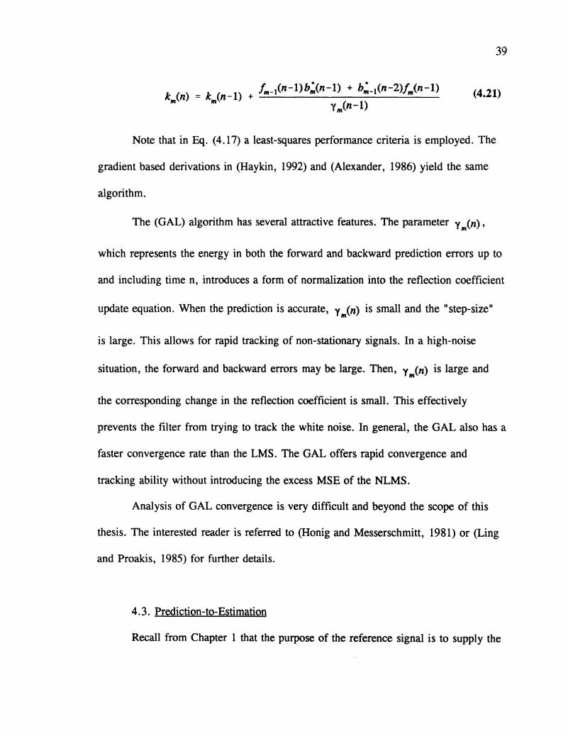
39

(4.21)

Note that in Eq. (4.17) a least-squares performance criteria is employed. The

gradient based derivations in (Haykin, 1992) and (Alexander, 1986) yield the same

algorithm.

The (GAL) algorithm has several attractive features. The parameter Y",(n) ,

which represents the energy in both the forward and backward prediction errors up to

and including time n, introduces a form of normalization into the reflection coefficient

update equation. When the prediction is accurate, Y",(n) is small and the "step-size"

is large. This allows for rapid tracking of non-stationary signals. In a high-noise

situation, the forward and backward errors may be large. Then, y",(n) is large and

the corresponding change in the reflection coefficient is small. This effectively

prevents the filter from trying to track the white noise. In general, the GAL also has a

faster convergence rate than the LMS. The GAL offers rapid convergence and

tracking ability without introducing the excess MSE of the NLMS.

Analysis of GAL convergence is very difficult and beyond the scope of this

thesis. The interested reader is referred to (Honig and Messerschmitt, 1981) or (Ling

and Proakis, 1985) for further details.

4.3. Prediction-to-Estimation

Recall from Chapter 1 that the purpose of the reference signal is to supply the

40

channel tap weights for use in the Rake Correlator. To increase performance of the

Rake correlator, the current tap observation should be used in forming the estimate

(as opposed to simply increasing the filter order). This will insure a minimum

probability of bit error corresponding to the Instantaneous Reference case described in

(Smallcomb, 1992). Recall that the linear prediction of the tap is composed of the

previous M observations.

In a manner similar to the time averager, the tap estimate will be formed based

on a weighted combination of the current observation and the current prediction.

h = «y(n) + (l-u)y(n)

The current observation y(n) is given by:

yen) = hen) + v1(n)

where h(n) is the channel signal and vt(n) is the channel noise. The current

prediction, y(n) , may be defined as:

yen) = hen) + v2(n)

(4.22)

(4.23)

(4.24)

where v2(n)

is the prediction noise. u is a scalar, 0< a < 1. Substitution of (4.23) and

(4.24) into (4.22) yields:

h(n) = h(n) + «v.(n) + (l-«)v2(n)

From (4.25) the estimation noise v3(n)

is defined as:

(4.25)

41

(4.26)

The power in the estimation noise is

(4.27)

since it can be shown that

(4.28)

The parameter « is now calculated in order to minimize the estimation noise

power. Differentiating (4.27) with respect to « and setting the result to 0 yields

ex =--------

Dividing both sides by 2 and solving for « results in

E{ Iv1(n) 12}

E{lvt(n) 11} + E{lv2(n) 1

2}

An estimate of the power of vt(n) may be made at the front end of the

(4.29)

(4.30)

receiver based on a small signal power assumption. However, v2(n)

is not directly

available. To estimate of the power in v2(n)

it is necessary examine the adaptive filter

error signal e(n). The prediction error signal is defined by

e(n) = y(n) - y(n)

Using (4.23) and (4.24), (4.32) reduces to

(4.31)

42

(4.32)

The power in e(n) , using (4.28), is

Substitution of (4.33) into (4.30) provides the final result for u

(4.33)

ex =E{ le(n) 12} - E{ Ivt(n) 12}

E{le(n) 12}

(4.34)

Having derived the equation for u, it is now possible to examine its behavior.

the limits 0 s (X s 1 are met. The behavior of « in a variety of situations is also of

interest. First, consider the noise only case. Adaptive filters are unable to track white

noise, therefore, j(n) =0 and E{le(n) 12} =E{lv1(n) 1

2} . This makes «=0 and the tap

estimate is h(n) =y(n). Next consider the worst possible channel signal. Assume the

channel signal is a white random process. Without the modification, the channel tap

estimate would be approximately zero and system performance would be severely

degraded. With the modification, it is easily shown that

(4.35)

and the estimate is h(n) = ex y(n). This will be sufficient to insure system

43

performance equal to that of the instantaneous reference case described in (Smallcomb

1992). The optimum performance of this system occurs when E{lv2(n)

12} :Jmjn' in

this situation,

«opt =

and the estimation noise is given by

Jmin (4.36)

(4.37)

Equation (4.36) shows that the minimum estimation noise is a function of the input

noise level and the adaptive filter order.

The cost of implementing the modification is outlined in Table 4.1

Step Multiplies/Divides Adds/Subtracts

Recursive Power 3 2Estimate

Compute alpha 1 1

Form estimate 2 2

Table 4.1 Prediction to Estimation Cost

The total cost of the modification is 9 multiplies/divides and 7 adds/subtracts. This is

approximately equal to the computational cost of one gradient lattice stage. By using

the prediction to estimation modification, it is hoped to realize the benefits of using

the current channel observation at a rather small increase in computational cost.

44

Chapter 5: Computer Simulations/Results/Conclusions

5.1. Computer System

The final step in selecting an adaptive filter for this application is a variety of

computer simulations to measure filter performance for a variety of channel

conditions. These simulations were performed using the Block Oriented System

Simulation (BOSS) software package produced by Comdisco Inc. The BOSS software

operated on a Sun Sparc2 Workstation.

The BOSS library contains a large number of modules that perform various

signal processing tasks. The BOSS interactive environment allows the user to create

the desired system in block diagram form. Each of these modules represents a

FORTRAN subroutine, and BOSS creates the simulation program by linking the

subroutines together according to the block diagram connections. The BOSS block

diagrams for the filter used in this thesis are located in the appendix. Although BOSS

performs a time domain simulation of the system, for convenience, the results of the

simulations were plotted using the MatLab software package.

5.2. Chi Conversion Factor

Recall from Chapter 1, the performance measure of the TA filter was

measured in terms of noise reduction, while the performance of the adaptive filters is

measured in MSE. In order to make a fair comparison between the TA and the

adaptive filters, a new conversion factor is introduced.

45

Define a new channel tap estimate as,

(,' = ~h (5.1)

where p is a real scalar. Following the derivation of X in (Smallcomb, 1992) it is

straightforward to show that the amount of noise reduction is unaffected by

introducing p. It is also obvious that the MSE performance criteria is affected by use

the new estimate. To find the appropriate conversion factor, define the MSE to be

J(n) = E{ Ih(n) - ph(n) 12}

Let the estimate be given by

where v2(n)

is zero mean white gaussian noise. Substituting (5.3) into (5.2) and

expanding yields

(5.2)

(5.3)

(5.4)

Differentiating (5.4) with respect to ~, setting the result to zero and solving for p

yields

(5.5)

Dividing the numerator and denominator of (5.5) by l/v (n) and using the definition. . 1

of X given in Eq. (1.4), (5.5) may be written as

~ = SNR;X + SNRi

where SNR., is the receiver input signal-to-noise ratio.I

46

(5.6)

Equation (5.6) shows that the performance gain of a filter and the MSE are

related by a constant. This constant is dependent upon the input SNR and performance

gain. Multiplying the TA estimate by fl prior to computing the MSE provides and

equal basis for filter comparison.

5.3. Computer Simulations

A series of BOSS computer simulations were performed to measure various

aspects of filter performance. The performance criteria for all simulations was the

MSE, E{lh(n) -h(n) 12} . The key simulation parameters are listed in Table 5.1 The

sampling frequency was chosen to be the system transmission frequency. The NLMS

order was chosen to match the order of the Bessel filters in the channel model. The

order of the GAL filter was selected to equal the computational cost of the NLMS.

The TA constant was set at 0.5 to cover the wide range of channel inputs. The

normalized step size, 1.1. was set to balance the needs of rapid convergence and steady

state error performance. The forgetting factor, A was set for a slowly time varying

channel input.

47

Parameter Setting

Sampling Frequency 62.5 Hz

GAL order 2

NLMS order 5

TA a 0.5

Bessel Filter Bandwidth Doppler Spread

Complex Tone Frequency Doppler Shift

Normalized Step Size 0.2

Forgetting Factor 0.99

Table 5.1 Simulation Parameters

5.3.1. General Channel Conditions

The first set of simulations compares the TA filter with modified versions of

the GAL and NLMS filters. The channel input was selected as either a complex tone

(Doppler shift) or a complex AR process (Doppler spread). The simulations were

performed for various combinations of channel input and signal-to-noise ratio (SNR).

The key to this set of simulations is shown in Figure 5.1. The optimum case was

calculated for a second order filter using Eq. (4.36).

Ideal

(J~ -----------------

NLMS

TA

Figure 5.1: Key 5.3.1 I 5.3.2

48

···························i·····························i·····························t····························t····························t················ .: : : : :

......·····················r····························r·······················:····r····························r····························r························'.'

········fr;,~~:~;:rN,..·-· ...::::.::::J-···..r···'::::::· ···· ·..·..'i:.:·..·· ···..·..·..,:::::j:::::.::::::::::::.::::::::::.:f:::::::::::::::::::::::::::..

\~ ,··················1·····························1····· y + + .: : : : :..........................., ···i·····························~···················· -:- __ -:- .: : : : :

···························i·····························i·····························i···················· + + .~ ~ i ~ ~

0

-1

-2

-.:5

~-4-

~-s

-e5

-7

-80 ~OO 1000 1 SOO 2000 2S00 ~OOO

Figure 5.2: Doppler Shift·1Hz I SNR 0.5

0

-1

-2

-.3

~-4-

~-~

-45

-7

-80 ~OO 1000 ,eoo 2000 2~OO 3000

Figure 5.3: Doppler Shift 1Hz I SNR 1.0

49

-2r--------~------~------__------..,......--------------....,

.: ::::::::::::::::::::::::::::j:::::::::::::::::::::::::::::j:::::::::::::::::::::::::::::r:::::::::::::::::::::::::::r::::::::::::::::::::::::::r:::::::::::::::::::::::::~-!5 ···························1·····························j·····························l·····························t····························t·············· -

- es 1" ···1"····························r····························1····························1················· -

- 7 r-···························i·····························i·····························t····························t····························t··············· -

- e l········;..···············i· ··:.:.:.:.:.:.:.:.:.::.:;:::~.:.:·~·t:.::.::.:::.::;:~·:.::.:.:.::.:.:.::G::.::.::.::.::::.::.::::.::.::~.::=.=.::::.::.:::.::.:.::).:.:.:.:::.::=.::=.::::. :.:.::. :.--9 -~s",~"f :::::: j ···j-······················::···f:::::::::::::::::::::::::f::::::::::::::::::::::::::'

.:50002:50020001:5001000~oo

- 1 0 ~ 060-- 060-- """"-- ""-- ~ ~

o

Figure 5.4: Doppler Shift 1Hz I SNR 2.0

o i ~ 1 i i~ . . . . .-, t···························i·..······················· ; ; ·········t····························t··············· -

1\. . . . . .~. . . , . .

=: ~~~~~~a~~~~:~;j~~~~~~~::::~~~I~~~~~~~~:::~:~]~~~~:::~~:~~~::~::I • • • •

- ~ 1--···························1·····························j·····························t····························t····························t··············· -

- es ···········~···············t························· · · · 1· · · · · · · · · · · · · · · · · · · · · · · · · · · · · !· · · · · · · · · · · · · · · · · · · · · · · · · · · · ·t · · · · · · · · · · · · · · · · · · · · · · · · · · · · t · · · · · · · · · · · -

- 7 1' 1' 1' ······r····························r·················· -

.:50002eoo20001eoo1000~oo-e'-----------------------------.......------~------ .....o

Figure 5.5: Doppler Spread 1Hz I SNR 0.5

Or--------~------~------__------~------ __--------,- 1 ~···························i·····························j·····························t····························t····························t··············· -

- 2 1-···························1·····························1·····························1·····························t····························t·············· -

~ ;~ t~;~~~~I~:~;~;J~:::;::::~:::;;t::::..:.:::::::::::]::_~::.:::::::.:.::.:~..--..;

-." _ j l l ,i. l -1 ~ ; ~ ;

.:50002:50020001:5001000~OO-Bo~----- .L-------.L-------.L------_..&....._-----...L-_----_....J

Figure 5.6: Doppler Spread 1Hz I SNR 1.0

50

-2r---------.--------,...---------..--------,...----------....--------,. . . . .

-.3 ~···························t····························t····························r······················ · · · · · · r · · · · · · · · · · · · · · · · · · · · · · · · · · · · r · · · · · · · · · · · · · · · · · -

- 4 1' 1' 1' ······r····························r·················· -

-~ ···························1·····························i·····························!"···················· : ~ -

- C!S ••••••••••••••••••••••••••• ~••••••••••••••••••••••••••••• ~•••••••••••••••••••••••••••••~ ••••••••••••••••••••••••••••~ ••••••••••••••••••••••••••••~ ••••••••••••••••••••••••••• -r. : : : : :

.: ~~~~1~=~~~~:~~~~t~~~~~~::::~~~:1~~~~~~::~~::::::~:1~~~ ~~::~~::: :~~:- 9 :·~w::·············l·····························j·····························j·····························t····························t·························..-

':'00025002000.,eoo1000~oo

-., 0 '----------"--------'----------'--------'---------...--------'o

Figure 5.7: Doppler Spread 1Hz I SNR 2.0

2r-------........-------~------_._------- __------_.....----------,.

, >-••·························1·····························r···························t····························t··..························t····················· -o 1' ··r····························r····························T····························T·················· -

-., ~ ~ .;. -:- .;. --2 t~~::::==..j === j.~~ + =+ ---+.~ ~.=, . . . . .-3 ~,~~..:~J:~~=::.:.~:j.,~::::~:~~~~~~::::+:::::::::::~::::,,::~::;t::;:::::::::::::::::::::;;'t"''''''''··'m''......'''~-4~_~.....=..;;;.... __-+-__~....;......;..~~~:::.J=:.:.:::.:::.:;;;;.:::=.:::.a.....-...a.I-.:::.:a::a.a.I ..- -+ -i

- ~ ~ j ·····l·····························j·····························t·..·························t·············· -

.30002~0020001~001000~oo-e'----------"--------'----------'--------&..-------~-------~o

Figure 5.8: Doppler Shift 10Hz I SNR 0.5

Or--------""""'!"'"-------.-.--------_._-------..--------_.....-------.,- 1 ···························t····························t·····,,······················1·····························r ····························r ··············· -

=: ~5?~==r= : == I =r:::::::::::::::::~::::::~~::::~~- 4 , •..•••......•..••..•••..•..1- j 1- ········t····························t················ -

=: :~~~~;~~~~~~~~~4~~~:~~~-~::::t:~:=:::::::~=::=~=t~:::: :::: : : ::=::=;l;; ;; ; ; ; ; ; ; ; ; ; ; ; ; ; ; ; ; ; ~ ; ; ; ;~- 7 ~ ~ ····~···.·.···· ··· ···· ·.t..· + + -

~ ~ ~ i ~

~ooo2eoo20001eoo1000~OO-eO'--------.&..-------'--------~-------"--------........-------~

Figure 5.9: Doppler Shift 10Hz I SNR 1.0

51

- 2 r----- --------.------~-----_r_-----..,------___,

.: ~~·::···===r=~~:==~:~=t==··t····===····t===-e ·························..1..···························1·····························1······················ j -r -

- 6 1···························1·····························1·····························1·····························t····························t·············· -

- 7 ~~ j j y y y -

-15 ~~tt~~~~~:i:~··········~~~~:····+······················+ ~~~~ + -- 9 '""'···························t························· · · · ~ · · · · · · · · · · · · · · · · · · · · · · · · · · · · · i· · · · · · · · · · · · · · · · · · · · · · · · · · · · · t · · · · · · · · · · · · · · · · · · · · · · · · · · · · t · · · · · · · · · · · · · · · -

30002~0020001~001000~OO- 1 0 '--------------~------"--------------~-------"o

Figure 5.10: Doppler Shift 10Hz / SNR 2.0

2r--------------.-------------..,__------.---------,. . . . .

1 ~························· ..1·························· 1' ···················t····························t····························t···························-

o '""' !" !" ~ ]" ]" ]" -

- 1 '""'·····~~;.~;-:;;;c:.:.:..:;::;.::r:;::;:::~:::.::;:;:::::::::~::::::::::::.:::::.::::::.::::::~:::::::::::::::::::;::;;:;::+::::::::::::::::::::::::':::r::::::::::::::::::::::::::::

- 2 _.:r: ~ ~ ·~··············~.;.;c~b····.::.::··:::===-;~.;;J.;.;:.:.:.::.::.::.::.::.;;=~;.~::.c;;::.&-s·s-ii·~=:·:-:.-:;

.:50002!50020001!500'tOCO~OO-t5 ~--------'_._---~----------""------~-----..........----~

o

Figure 5.11: Doppler Spread 10Hz / SNR 0.5

:::::::::::::::::::::::::::r::::::::::::::::::::::::::T:::::::::::::::::::::::::l:::::::::::::::::::::::::::r:::::::::::::::::::::::::T:::::::::::::::::::::::::

·····;~;;;.;·:;:;:;::t~~~=~===~~::~=$:::.:.:.~~¥:;:~:·~·::::::-=·

0

-1

-2

-:5

~-4

~-!5

-t5

-7

-s0 ~OO 1000 1eoo 2000 2!500 3000

Figure 5.12: Doppler Spread 10Hz I SNR 1.0

52

.30002~0020001~001000~oo

-8 ILI..-- ....&....- ~ __L_ ____a._ _____

o

Figure 5.13: Doppler Spread 10Hz I SNR 2.0

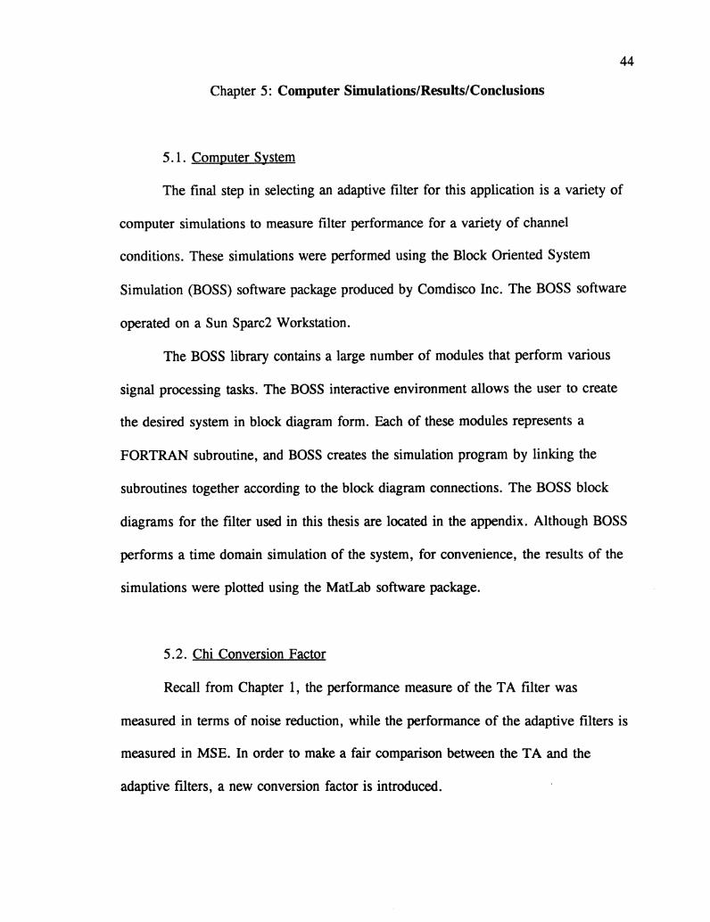
5.3.2. Tracking Ability

In this set of simulations, the channel was modeled by a chirped complex tone.

Two chirp rates were simulated. The "fast" chirp frequency was 0.625 Hz. This

corresponds to one complete chirp cycle every 100 samples. This is roughly the

memory of the GAL. The "slow" chirp frequency was selected as 0.0625 Hz. The

SNR in both simulations was 1.0. Figure 5.14 shows the chirp and the modified GAL

estimate.

53

1 .~ r--------,.----...,...----__-----,.-----,-----__-----,------..------,------,

12001 1 eo11 eo114011201100

\:1

r1015010fSO10....01020

o

-1

o.~

-0.5

,- 1 .~ ~------"----.......----~------"----.......---~~-----I----.......-----"'------'1000

Figure 5.14: Chirped Tone and Estimate

0

-1

-2

-.:5

~-4-

~-5

-fS

-7

................._ ~ _ ~ _~ _ + + .

i~~+~~~~:E:::~::3::::::~:::::::::::::::::r::::~~::::::::r:::::~=:::::·..~\: :~~=::=: ..~.:--::::::::.::: j::~::''':::::::::::::::::::: ;:::::: + + .···························r····························1·····························1'····························r····························r················· .

30002~0020001~001000~oo

-8 "-- ---tl....- ....... ---tlo..- ....... ---'

o

Figure 5.15: Slow Chirp

0

-1

-2

-.3

~ -4-

~-e

-fS

-7

-_ ~ ~ -:- - _ + _ _ ~._ _ _._ .. . . . ., + + + ···f····························f····················· .J : : : : :

\~:;.~~~~:::.::.::.;.:::~.:::=·:.:=:.:.::.::.:.::.::.::~· ..··..····::::::::::::F··.....·::·====··..i......:.:~.:=::=::.:··:::···;·::;::~~::~:::C················:·::=:r::::::~~::::::::::: ..:.:.r-:::::::::::~::::::::::::I:::::::::::::~:=::::::~:r::::::::::::::::::::::~:::

...."oJ .

. ·····r···························1..···························t·······················..··t····························t·········· .••••••••••••••••••••••••••• .& , ••••••••••••••••••••••••••••• , ••••••••••••••••••••••••••••• .;. •••••••••••••••••••••••••••• .;. ••••••••••••••••••••••••• _-

j j 1 l 1

30002~002000,~OO1000~OO-8O--------......---------'''--------~-------L-------.....L-------..J

Figure 5.16: Fast Chirp

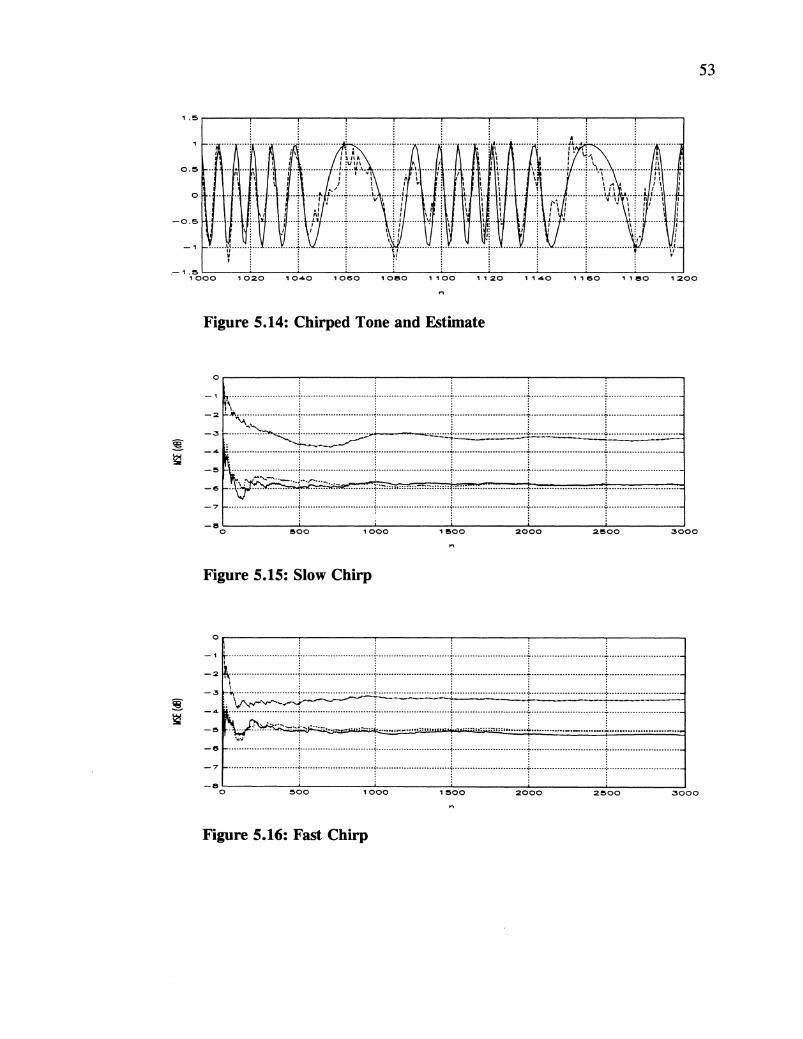
5.3.3: Modification vs. Extended Order

Recall that the purpose of modifying the adaptive filters is to improve Rake

correlator performance by including the current channel tap observation. The

simulations performed in this section compare a modified 2nd order GAL and an

unmodified 3rd order GAL. Refer to Figure 5.17 for the key.

Modified2nd Order

Unmodified3rd Order

Figure 5.17: Key 5.3.3

O~---__---_----...-------..----_---_

54

.: :::::::::::::::::::::::::::j:::::::::::::::::::::::::::::j::::::::::::::::::::::::::::r:::::::::::::::::::::::::T:::::::::::::::::::::::::::r:::::::::::::::::::::::::-.:5 ···························i·····························i·····························i···················· ~ : ., : : : : :

-... ~ l. 1. 1 1 1 .

=: ~~~~I:~~~~~~~f~~=~=~==~===~I~~~===~~~~~~~==!==~========~-7 j j ····.·.· ··.·1·.·.·..···········.········.·t····························t························ .-8~ ...t..- ~ ---L.. ---L ~ ---I

o ~oo 1000 1~00 2000 2~00 3000

Figure 5.18: Doppler Shift 1Hz I SNR 1.0

55

.30002.eoo20001eoo1000~oo

. . . . .···························r····························r····························T····························T····························T·················· .

,··························1·····························1·····························+····························f····························t················ ., : : : : :, : : : : :.+ -1••••••••••••••••••••••••••••• -I••••••••••••••••••••••••••••• ~••••••••••••••••••••••••••••• -:-•••••••••••••••••••••••••••••:••••••••••••••••••••••••••••" : : : : :

··::~~;(:~b~;~:~~~::~t~~~:::::=]~~~~~~~~~~~L~~~~~~~~=~~~L~~~=~~~~~~~···························1·························· j r·················· ········1·· ............................1" ··r····························1"····························f····························f·················· .

0

-1

-2

-~

~ -4

~-e

-e

-7

-80

Figure 5.19: Doppler Spread 1Hz I SNR 1.0

0.___----_....._-----.....-------....-------,..---------.-------,-1 ···························1·····························l·····························t····························t····························t················ .

- 2 \ ···························1·····························1·····························t····························t····························t················ ., : : : : :

-3 ~ ~ .; -:. -:. ~ ., : : : : :

- 4 \ j j·····························t····························t····························t··················· .

.: ··::~~~=:~~~~~~~==F=======t=========j~~:::::::::::L~:::~::::::~-7 j" ··1·····························j·····························t·························..·t················· .

30002eoo2000,eoo1000eoo-s '--- ---L. ..L.- ---&- -L- ~ ---I

o

Figure 5.20: Doppler Shift 10Hz I SNR 1.0

or---------r------~---- -----......_-----.___----....,

-4

-e

-e

-7

.30002eoo20001eoo1000~oo

-8 '--- ~ ..L._ ---&- &.._._ ---'

o

Figure 5.21: Doppler Spread 10Hz I SNR 1.0

56

5.3.4: Comparison of Lattice Orders

The final simulation set is a comparison of different lattice orders. Modified

versions of first through fifth order GAL filters were tested. Two situations were

considered: 1) a non-disturbed channel and 2) a disturbed channel. The results are

shown in Figure 5.22 and Figure 5.23 respectively.

30002!50020001!5001000~oo

::::::::::::::::::::::::::l:::::::::::::::::::::::::::r::::::::::::::::::::::::::r:::::::::::::::::::::::::r:::::::::::::::::::::::::r:::::::::::::::::::::::::...........................! ···j·····························i·····························t····························t··············· .

··························1·····························r····························r····························r····························!················· .

0

-1

-2

-.:5Ci5'"~ -4~E

-~

-6

-7

-e0

Figure 5.22: Doppler Shift 10Hz I SNR 1.0

Or------~---__-------..----~----....--------,

-4

-eo ~OO 1000 1!500 2000 .:5000

Figure 5.23: Doppler Spread 10Hz I SNR 1.0

57

In Fig. 5.22, the results show that the higher the lattice order, the better the

estimate. In Fig. 5.23, there is no significant difference between the different filters.

These simulations give a brief glimpse of the performance vs. computational

complexity trade off. Does the increased performance of the higher order filters for

non-disturbed channel conditions justify the increased cost of implementation?

5.4 Conclusions and Recommendations

A review of the simulation results demonstrates the viability of adaptive filters

for this application. In all channel conditions tested, the adaptive filters performed as

well as if not better then the TA filter currently used in the system. The simulations

of Doppler Shift and the Chirped Tone demonstrate the TA's inability to track

complex phase information.

Of the two adaptive filters tested, the 2nd order Gradient Adaptive Lattice

outperformed the 5th order Normalized Least Mean Square in almost all situations.

The NLMS performance is degraded in high noise environments due to the increased

steady state MSE discussed in Section 4.1, while the modified GAL enjoyed almost

ideal- performance.

The simulations also validated the use of the Prediction-to-Estimation

modification. The performance for the modified 2nd order filter offered a slight

improvement over the 3rd order GAL predictor at a computational cost comparable to

the extra lattice stage.

Based on the results presented in this thesis, a Gradient Adaptive Lattice filter

with the Prediction-to Estimation modification is recommended for this application.

The GAL provides the best compromise between performance and the constraints of

computational complexity and numerical stability. Although a 2nd order GAL was

used for the simulations presented here, a final decision on filter order should be a

result of more extensive system simulations based on actual channel data.

58

59

References

Alexander, S. T. (1986). Adaptive Signal Processing: Theory and Applications,Springer-Verlag, New York.

Bershad, N. and O. Macchi (1990). "Comparison of LMS and RLS Algorithms forthe Prediction of a drifting line," Signal Processing V: Theories and Applications,Elsevier Science Publishers B.V.

Bershad, N. J. (1986). "Analysis of the Normalized LMS algorithm with GaussianInputs," IEEE Trans. Acoust. Speech, Signal Process., vol ASSP-34, pp. 793-806.

Bitmead, R. R. and B. D. O. Anderson (1980). "Performance of Adaptive EstimationAlgorithms in Dependent Enviroments," IEEE Trans. Automatic Control, vol. AC-25,pp. 788-793.

Caraiscos, C and B, Liu (1984). "A Roundoff Error Analysis of the LMS AdaptiveAlgorithm," IEEE Trans. Acoust. Speech, Signal Process., vol ASSP-32, pp. 34-41..

Cioffi, J. M. (1987). "Limited-Precision Effects in Adaptive Filtering," IEEE Trans.Circuits Syst., vol. CAS-34, pp. 821-833.

Cioffi, J. M. (1986). "When do I use an RLS Adaptive Filter," Proceedings, 19thAsilomar Conference on Circuits, Syst., and Computers, Pacific Grove, Ca., pp. 636-639. .

Friedlander, B. (1982). "Lattice Filters for Adaptive Signal Processing" Proc. IEEE,vol. 70, pp. 829-867.

Hariharan, S. and A. P. Clark (1990). "HF Channel Estimation Using a FastTransversal Filter Algorithm," IEEE Trans. Acoust. Speech, Signal Process., volASSP-38, pp. 1353-1362.

Haykin, S. (1991). Adaptive Filter Theory 2nd eel. Prentice-Hall, Englewood Cliffs.

Honig, M. L. and D. G. Messerschmitt (1981). "Convergence Properties of andAdaptive Digital Lattice Filter," IEEE Trans. Acoust. Speech Signal Process., volASSP-29, pp. 642-653.

Ling, F. and J. G. Proakis (1985). "Adaptive Lattice Decision-Feedback Equalizers­Their performance and Application to Time-Variant Multipath Channels," IEEETrans. Commun., vol COM-33, pp. 348-356.

60

Ljung, S. and L. Ljung (1985). "Error Propagation of Recursive Least-SquaresAdaptation Algorithms," Automatica, vol. 21, pp. 157-167.

Makoul, J. (1975). "Linear Prediction: a tutorial review," Proc. IEEE, vol. 63, pp.561-580.

Maslin, N. (1987). HF Communications A Systems Approach, Plenum, New York.

Nagumo, J. I. and A. Noda (1967). "A Learning Method for System Identification,"IEEE Trans. Automatic Control, vol. AC-12, pp. 282-287.

Proakis, J. G. (1989). Digital Communications, 2nd 00. McGraw-Hill, New York.

Slock, D. T. M. (1990). "On the Convergence Behavior of the LMS and NLMSAlgorithms," Signal Processing ~. Theories and Applications, Elsevier SciencePublishers B.V.

Sma1lcomb, J. M. (1992). "Spread Spectrum Communication over a Fading MultipathHF channel using Transform Domain Signal Processing and a Transmitted ReferenceSignal" Ph.D. dissertation, Ohio University, Athens Ohio.

Weiss, A. and D. Mitra (1979) "Digital Adaptive Filters: Conditions forConvergence, Effects of Noise and Errors Arising from the Implementation," IEEETrans. on Info. Theory, vol. IT-25, pp. 637-652.

Widrow, B., J. McCool and M. Ball (1975). "The Complex LMS Algorithm," Proc.IEEE, vol. 63, pp. 719-720.

61

Appendix

A: BOSS Block Diagrams

N ~!JJ.

LJ.J ~o 0

t: ~CHI')

<-I

00~

KMN

[>-------~

(>

VMN

C>~-_----I

t>

<l CONST nnGEN ~

[>UNITII] DELAY t> t>

62

63

MODIFIED NLMS

[>T--------------r------

COMPUTE STEP

nnDIVIDER~ZERO[>PROTECT

6

[>

64

[>.

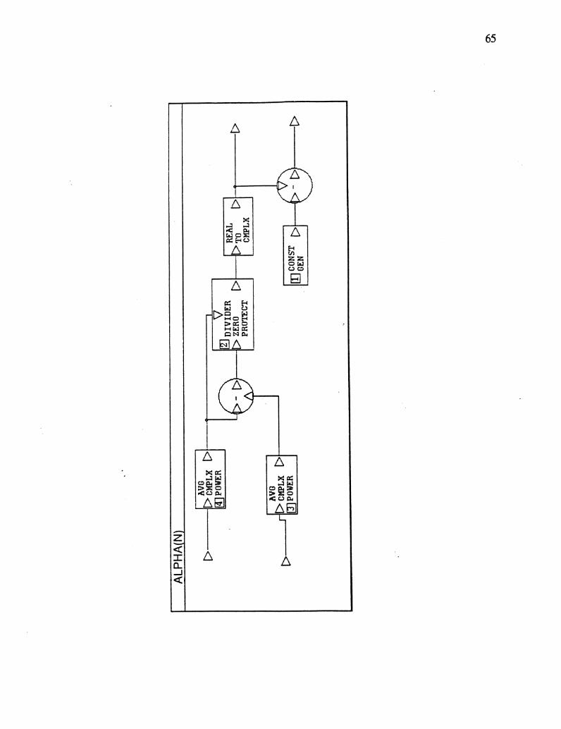
z«:co,-J«

65