COMSOL Multiphysics ® V ERSION 4.0a USER’S GUIDE

Welcome message from author
This document is posted to help you gain knowledge. Please leave a comment to let me know what you think about it! Share it to your friends and learn new things together.
Transcript

COMSOLMultiphysics ®
V E R S I O N 4 . 0 a
USER’S GUIDE

BeneluxCOMSOL BVRöntgenlaan 192719 DX ZoetermeerThe NetherlandsPhone: +31 (0) 79 363 4230 Fax: +31 (0) 79 361 [email protected]
DenmarkCOMSOL A/SDiplomvej 376 2800 Kgs. LyngbyPhone: +45 88 70 82 00Fax: +45 88 70 80 [email protected]
FinlandCOMSOL OYArabiankatu 12 FIN-00560 HelsinkiPhone: +358 9 2510 400Fax: +358 9 2510 [email protected]
FranceCOMSOL FranceWTC, 5 pl. Robert SchumanF-38000 GrenoblePhone: +33 (0)4 76 46 49 01Fax: +33 (0)4 76 46 07 [email protected]
GermanyCOMSOL Multiphysics GmbHBerliner Str. 4D-37073 GöttingenPhone: +49-551-99721-0Fax: [email protected]
IndiaCOMSOL Multiphysics Pvt. Ltd.Esquire CentreC-Block, 3rd FloorNo. 9, M. G. RoadBangalore 560001KarnatakaPhone: +91-80-4092-3859Fax: [email protected]
ItalyCOMSOL S.r.l.Via Vittorio Emanuele II, 2225122 BresciaPhone: +39-030-3793800Fax: [email protected]
NorwayCOMSOL ASSøndre gate 7NO-7485 TrondheimPhone: +47 73 84 24 00Fax: +47 73 84 24 [email protected]
SwedenCOMSOL ABTegnérgatan 23SE-111 40 StockholmPhone: +46 8 412 95 00Fax: +46 8 412 95 [email protected]
SwitzerlandCOMSOL Multiphysics GmbHTechnoparkstrasse 1CH-8005 ZürichPhone: +41 (0)44 445 2140Fax: +41 (0)44 445 [email protected]
United KingdomCOMSOL Ltd.UH Innovation CentreCollege LaneHatfieldHertfordshire AL10 9ABPhone: +44-(0)-1707 636020Fax: +44-(0)-1707 [email protected]
United StatesCOMSOL, Inc.1 New England Executive ParkSuite 350Burlington, MA 01803Phone: +1-781-273-3322Fax: +1-781-273-6603
COMSOL, Inc.10850 Wilshire BoulevardSuite 800Los Angeles, CA 90024Phone: +1-310-441-4800Fax: +1-310-441-0868
COMSOL, Inc.744 Cowper StreetPalo Alto, CA 94301Phone: +1-650-324-9935Fax: +1-650-324-9936
For a complete list of international representatives, visit www.comsol.com/contact
Company home pagewww.comsol.com
COMSOL user forumswww.comsol.com/support/forums
COMSOL Multiphysics User’s Guide COPYRIGHT 1998–2010 COMSOL AB.
Protected by U.S. Patents 7,519,518; 7,596,474; and 7,623,991. Patents pending.
The software described in this document is furnished under a license agreement. The software may be used or copied only under the terms of the license agreement. No part of this manual may be photocopied or reproduced in any form without prior written consent from COMSOL AB.
COMSOL and COMSOL Multiphysics are registered trademarks of COMSOL AB. LiveLink and COMSOL Desktop are trademarks of COMSOL AB..
Other product or brand names are trademarks or registered trademarks of their respective holders.
Version: June 2010 COMSOL 4.0aPart number: CM020002

C O N T E N T S
C h a p t e r 1 : I n t r o d u c t i o n
The Documentation Set 28
Where Do I Access the Documentation and Model Library? . . . . . . 29
Typographical Conventions . . . . . . . . . . . . . . . . . . . 30
About COMSOL Multiphysics 32
The COMSOL Modules 35
The AC/DC Module . . . . . . . . . . . . . . . . . . . . . 35
The Acoustics Module . . . . . . . . . . . . . . . . . . . . . 36
Batteries and Fuel Cells Module . . . . . . . . . . . . . . . . . 37
CFD Module . . . . . . . . . . . . . . . . . . . . . . . . 38
Chemical Reaction Engineering Module . . . . . . . . . . . . . . 38
The Earth Science Module . . . . . . . . . . . . . . . . . . . 40
The Heat Transfer Module . . . . . . . . . . . . . . . . . . . 41
The MEMS Module . . . . . . . . . . . . . . . . . . . . . . 42
Plasma Module. . . . . . . . . . . . . . . . . . . . . . . . 42
The RF Module . . . . . . . . . . . . . . . . . . . . . . . 44
The Structural Mechanics Module . . . . . . . . . . . . . . . . 45
CAD Import and LiveLink Connections 46
LiveLink for MATLAB 47
Internet Resources 48
COMSOL Web Sites . . . . . . . . . . . . . . . . . . . . . 48
COMSOL Community . . . . . . . . . . . . . . . . . . . . . 48
C O N T E N T S | 3
4 | C O N T E N T S
C h a p t e r 2 : T h e C O M S O L M o d e l i n g E n v i r o n m e n t
The COMSOL Desktop Environment 50
Changing the COMSOL Desktop Layout . . . . . . . . . . . . . . 51
Moving Between Windows and Sections on the COMSOL Desktop . . . 52
Changing the COMSOL Desktop Language . . . . . . . . . . . . . 52
The Model Wizard . . . . . . . . . . . . . . . . . . . . . . 53
Basic Steps to Build a Model . . . . . . . . . . . . . . . . . . 55
The Model Builder Window . . . . . . . . . . . . . . . . . . 56
The Settings Window . . . . . . . . . . . . . . . . . . . . . 60
The Graphics Window . . . . . . . . . . . . . . . . . . . . 61
The Messages Window . . . . . . . . . . . . . . . . . . . . 61
The Progress Window. . . . . . . . . . . . . . . . . . . . . 61
The Results Window . . . . . . . . . . . . . . . . . . . . . 61
The Help Window . . . . . . . . . . . . . . . . . . . . . . 62
The Model Library Window . . . . . . . . . . . . . . . . . . 63
The Material Browser Window . . . . . . . . . . . . . . . . . 64
Summary of Keyboard Shortcuts . . . . . . . . . . . . . . . . . 64
C h a p t e r 3 : G l o b a l a n d L o c a l D e f i n i t i o n s
About Global and Local Definitions 68
Global Definitions . . . . . . . . . . . . . . . . . . . . . . 68
Local Definitions . . . . . . . . . . . . . . . . . . . . . . . 68
Building Expressions . . . . . . . . . . . . . . . . . . . . . 69
Operators, Functions, and Variables Reference 70
Unary and Binary Operators . . . . . . . . . . . . . . . . . . 70
Special Operators . . . . . . . . . . . . . . . . . . . . . . 71
Mathematical Functions . . . . . . . . . . . . . . . . . . . . 78
Physical Constants . . . . . . . . . . . . . . . . . . . . . . 80
Global Parameters 82
Defining, Saving, or Importing Global Parameters. . . . . . . . . . . 82
Loading Parameters from a Text File . . . . . . . . . . . . . . . 83
Variables 84
About Global and Local Variables . . . . . . . . . . . . . . . . 84
About Predefined Physics Interface Variables . . . . . . . . . . . . 85
Variable Naming Convention and Scope . . . . . . . . . . . . . . 85
Variable Classification and Geometric Scope . . . . . . . . . . . . 86
Specifying Varying Coefficients and Material Properties . . . . . . . . 87
Variables for Time, Frequency, and Eigenvalues . . . . . . . . . . . 88
Geometric Variables . . . . . . . . . . . . . . . . . . . . . 89
Shape Function Variables . . . . . . . . . . . . . . . . . . . . 93
Entering Ranges and Vector-Valued Expressions . . . . . . . . . . . 97
Adding Global Variables to the Model Builder . . . . . . . . . . . . 99
Adding Local Variables to Individual Models . . . . . . . . . . . . . 99
Assigning Geometric Scope to a Variable . . . . . . . . . . . . . . 99
Adding Variable Definitions . . . . . . . . . . . . . . . . . . . 99
Editing Variable Definitions . . . . . . . . . . . . . . . . . . 100
Saving Variable Definitions to a Text File . . . . . . . . . . . . . 100
Loading Variable Definitions from a Text File . . . . . . . . . . . 100
Summary of Common Predefined Variables . . . . . . . . . . . . 101
Global and Local Functions 102
Defining an Analytic Function . . . . . . . . . . . . . . . . . 104
Defining an External Function . . . . . . . . . . . . . . . . . 106
Defining a Gaussian Pulse Function . . . . . . . . . . . . . . . 107
Defining an Interpolation Function . . . . . . . . . . . . . . . 107
About MATLAB Functions . . . . . . . . . . . . . . . . . . 111
Defining a Piecewise Function . . . . . . . . . . . . . . . . . 111
Defining a Ramp Function . . . . . . . . . . . . . . . . . . 114
Defining a Random Function . . . . . . . . . . . . . . . . . 114
Defining a Rectangle Function . . . . . . . . . . . . . . . . . 115
Defining a Step Function . . . . . . . . . . . . . . . . . . . 115
Defining a Triangle Function . . . . . . . . . . . . . . . . . . 116
Defining a Waveform Function. . . . . . . . . . . . . . . . . 116
Model Couplings 118
About Coupling Operators . . . . . . . . . . . . . . . . . . 118
About Extrusion Model Coupling and Operators. . . . . . . . . . 120
Defining Extrusion Model Coupling . . . . . . . . . . . . . . . 124
About Projection Model Couplings and Operators . . . . . . . . . 131
C O N T E N T S | 5
6 | C O N T E N T S
Defining Projection Model Couplings . . . . . . . . . . . . . . 133
About Scalar Model Couplings and Operators . . . . . . . . . . . 137
Defining Scalar Model Couplings . . . . . . . . . . . . . . . . 139
Coordinate Systems 142
About Boundary Coordinate Systems . . . . . . . . . . . . . . 143
Defining a Boundary Coordinate System . . . . . . . . . . . . . 144
About Base Vector Systems . . . . . . . . . . . . . . . . . . 145
Defining a Base Vector Coordinate System . . . . . . . . . . . . 146
About Cylindrical Coordinate Systems . . . . . . . . . . . . . 146
Defining a Cylindrical Coordinate System . . . . . . . . . . . . 147
About Mapped Coordinate Systems. . . . . . . . . . . . . . . 147
Defining a Mapped Coordinate System . . . . . . . . . . . . . 148
About Rotated Coordinate Systems . . . . . . . . . . . . . . 148
Defining a Rotated Coordinate System . . . . . . . . . . . . . 149
Identity and Contact Pairs 151
Defining an Identity Pair . . . . . . . . . . . . . . . . . . . 151
Defining a Contact Pair . . . . . . . . . . . . . . . . . . . 152
Probes 155
Defining a Domain, Boundary, or Edge Probe . . . . . . . . . . . 155
Defining a Domain Point Probe . . . . . . . . . . . . . . . . 156
Defining a Boundary Point Probe . . . . . . . . . . . . . . . . 157
Defining a Global Variable Probe . . . . . . . . . . . . . . . . 158
C h a p t e r 4 : V i s u a l i z a t i o n a n d S e l e c t i o n To o l s
Working with 3D Geometry 160
About Geometric Entities . . . . . . . . . . . . . . . . . . 161
About Selecting Geometric Entities . . . . . . . . . . . . . . . 162
Pasting a Selection From File . . . . . . . . . . . . . . . . . 164
Using the Selection List Window . . . . . . . . . . . . . . . . 165
Selecting and Deselecting Geometric Entities . . . . . . . . . . . 167
Zooming In and Out in the Graphics Window . . . . . . . . . . . 172
Changing Views in the Graphics Window . . . . . . . . . . . . 172

Moving Around and Rotating 3D Geometry in the Graphics Window . . 173
Lighting, Transparency, and Wireframe Rendering . . . . . . . . . 174
Hiding and Showing Geometric Entities . . . . . . . . . . . . . 175
User-Defined Selections 177
Creating a User-Defined Selection Node . . . . . . . . . . . . . 177
User-Defined Views 180
Creating Views . . . . . . . . . . . . . . . . . . . . . . 180
Adding a 2D User-Defined View . . . . . . . . . . . . . . . . 180
Adding a 3D User-Defined View . . . . . . . . . . . . . . . . 181
Hiding Geometry Objects in a User-Defined View . . . . . . . . . 184
Hiding Geometric Entities in a User-Defined View . . . . . . . . . 185
Screenshots 186
Capturing a Screenshot . . . . . . . . . . . . . . . . . . . 186
C h a p t e r 5 : G e o m e t r y M o d e l i n g a n d C A D To o l s
Creating a Geometry for Successful Analysis 188
The COMSOL Multiphysics Geometry and CAD Environment 190
Overview of Geometry Modeling Concepts . . . . . . . . . . . 190
Geometry Toolbar . . . . . . . . . . . . . . . . . . . . . 191
About Selecting the Cartesian or Cylindrical Coordinate System. . . . 192
Creating Composite Geometry Objects . . . . . . . . . . . . . 193
Adding Affine Transformations to Geometry Objects . . . . . . . . 194
Creating an Array of Identical Geometry Objects . . . . . . . . . 196
Copying and Pasting Geometry Objects . . . . . . . . . . . . . 196
Converting Geometry Objects . . . . . . . . . . . . . . . . 197
Splitting Geometry Objects . . . . . . . . . . . . . . . . . . 198
Deleting Objects and Entities . . . . . . . . . . . . . . . . . 198
C O N T E N T S | 7

8 | C O N T E N T S
Creating a 1D Geometry Model 200
Creating a 2D Geometry Model 201
Creating a 3D Geometry Model 209
Creating 3D Geometries Using the Model Builder . . . . . . . . . 209
C h a p t e r 6 : M a t e r i a l s
Materials Overview 224
Predefined Material Databases Included with COMSOL Modules. . . . 224
About Using Materials in COMSOL . . . . . . . . . . . . . . . 226
About the Material Browser Window and Page . . . . . . . . . . 227
About the Material Page . . . . . . . . . . . . . . . . . . . 228
About the Property Group Page . . . . . . . . . . . . . . . . 230
Adding Predefined Materials 232
Working on the Material Browser . . . . . . . . . . . . . . . 232
Working on the Material Page . . . . . . . . . . . . . . . . . 233
Working on the Property Group Page . . . . . . . . . . . . . . 236
Adding a User-Defined Property Group . . . . . . . . . . . . . 237
User-Defined Materials and Libraries 238
Adding User defined Materials . . . . . . . . . . . . . . . . . 238
Adding an External Material Library . . . . . . . . . . . . . . . 238
Creating a User defined Materials Database . . . . . . . . . . . . 239
Adding a User defined Material Database to the Material Browser . . . 239
Creating a User defined Material Database . . . . . . . . . . . . 240
Material Properties Reference 241
About the Output Materials Properties . . . . . . . . . . . . . 241
Model Input Properties . . . . . . . . . . . . . . . . . . . 245
Predefined Built-In Materials for all COMSOL Modules . . . . . . . 245
Material Property Groups Descriptions . . . . . . . . . . . . . 247
Other Predefined Materials in COMSOL Modules . . . . . . . . . 249

Using Functions 250
Adding a Function to the Material . . . . . . . . . . . . . . . 250
Example of Defining an Analytic Function. . . . . . . . . . . . . 250
C h a p t e r 7 : B u i l d i n g a C O M S O L M o d e l
The Model Wizard and Model Builder 254
The Model Nodes in the Model Builder . . . . . . . . . . . . . 254
Adding Nodes to the Model Builder . . . . . . . . . . . . . . 255
Model Administration 257
Saving Models in Different Formats and Creating a Model Image . . . . 257
Editing Node Properties, Names, and Identifiers . . . . . . . . . . 259
The Model Library . . . . . . . . . . . . . . . . . . . . . 261
Updating Model Libraries Using Model Library Update . . . . . . . 262
Editing Model Preferences Settings . . . . . . . . . . . . . . . 263
Checking and Controlling Products and Licenses Used . . . . . . . 264
Viewing Node Names, Identifiers, Types, Tags, and Equations . . . . . 265
Show More Options on the Context Menu: Equation Based Features . . 267
Show More Options: Consistent and Inconsistent Stabilization . . . . 269
Show More Options: Advanced Settings and Discretization . . . . . . 270
The Physics Interface Feature Nodes 273
Specifying Physics Settings . . . . . . . . . . . . . . . . . . 273
Physics Interface Context Menu Layout . . . . . . . . . . . . . 274
Physics Interface Exclusive and Contributing Feature Node Types . . . 274
Physics Interface Default Feature Nodes . . . . . . . . . . . . . 276
Physics Interface Node Status . . . . . . . . . . . . . . . . . 276
Physics Interface Boundary Types. . . . . . . . . . . . . . . . 277
Continuity on Interior Boundaries . . . . . . . . . . . . . . . 278
Physics Interface Axial Symmetry Feature Node . . . . . . . . . . 279
Physics Interface Common Settings for all the Main Nodes . . . . . . 279
Physics Interface Equation View Node . . . . . . . . . . . . . . 280
Specifying Model Equation Settings 283
Specifying Initial Values. . . . . . . . . . . . . . . . . . . . 283
C O N T E N T S | 9

10 | C O N T E N T S
Modeling Anisotropic Materials . . . . . . . . . . . . . . . . 284
Periodic Boundary Conditions 285
Using Periodic Boundary Conditions . . . . . . . . . . . . . . 285
Periodic Boundary Condition Example. . . . . . . . . . . . . . 285
Computing Accurate Fluxes 288
Flux Computation Example . . . . . . . . . . . . . . . . . . 289
Using Units 291
Unit Systems in COMSOL Multiphysics . . . . . . . . . . . . . 291
Selecting a Unit System . . . . . . . . . . . . . . . . . . . 292
Using Standard Unit Prefixes and Syntax . . . . . . . . . . . . . 293
SI Base, Derived, and Other Units . . . . . . . . . . . . . . . 295
Special British Engineering Units . . . . . . . . . . . . . . . . 300
Special CGSA Units . . . . . . . . . . . . . . . . . . . . . 301
Special EMU Units . . . . . . . . . . . . . . . . . . . . . 301
Special ESU Units. . . . . . . . . . . . . . . . . . . . . . 302
Special FPS Units . . . . . . . . . . . . . . . . . . . . . . 303
Special IPS Units . . . . . . . . . . . . . . . . . . . . . . 303
Special MPa Units. . . . . . . . . . . . . . . . . . . . . . 304
Special Gravitational IPS Units . . . . . . . . . . . . . . . . . 304
Switching Unit System . . . . . . . . . . . . . . . . . . . . 304
About Temperature Units . . . . . . . . . . . . . . . . . . 305
About Editing Geometry Length and Angular Units . . . . . . . . . 306
Indication of Unexpected or Unknown Unit . . . . . . . . . . . 307
C h a p t e r 8 : O v e r v i e w o f t h e P h y s i c s I n t e r f a c e s
The COMSOL Multiphysics Physics Interfaces 310
Introduction . . . . . . . . . . . . . . . . . . . . . . . 310
Physics Interfaces Groups in the Model Wizard . . . . . . . . . . 311
Physics Interfaces in COMSOL Multiphysics . . . . . . . . . . . . 312
Selecting a Physics Interface . . . . . . . . . . . . . . . . . . 313

Modeling Guidelines 315
Using Symmetries . . . . . . . . . . . . . . . . . . . . . 315
Effective Memory Management . . . . . . . . . . . . . . . . 315
Selecting an Element Type . . . . . . . . . . . . . . . . . . 317
Analyzing Model Convergence and Accuracy . . . . . . . . . . . 317
Achieving Convergence When Solving Nonlinear Equations. . . . . . 318
Avoiding Strong Transients . . . . . . . . . . . . . . . . . . 318
Physics-Related Checks and Guidelines . . . . . . . . . . . . . 319
C h a p t e r 9 : E l e c t r o m a g n e t i c s
The Electrostatics Interface 323
Charge Conservation . . . . . . . . . . . . . . . . . . . . 324
Space Charge Density . . . . . . . . . . . . . . . . . . . . 325
Initial Values. . . . . . . . . . . . . . . . . . . . . . . . 325
Boundary Conditions . . . . . . . . . . . . . . . . . . . . 326
Ground . . . . . . . . . . . . . . . . . . . . . . . . . 326
Electric Potential . . . . . . . . . . . . . . . . . . . . . . 327
Surface Charge Density . . . . . . . . . . . . . . . . . . . 328
Displacement Field . . . . . . . . . . . . . . . . . . . . . 328
Periodic Condition . . . . . . . . . . . . . . . . . . . . . 329
Zero Charge . . . . . . . . . . . . . . . . . . . . . . . 329
Thin Low Permittivity Gap . . . . . . . . . . . . . . . . . . 329
Continuity (Pair Feature) . . . . . . . . . . . . . . . . . . . 330
Line Charge . . . . . . . . . . . . . . . . . . . . . . . . 330
Point Charge . . . . . . . . . . . . . . . . . . . . . . . 331
The Electric Currents Interface 332
Current Conservation . . . . . . . . . . . . . . . . . . . . 333
External Current Density. . . . . . . . . . . . . . . . . . . 335
Current Source . . . . . . . . . . . . . . . . . . . . . . 335
Force Calculation. . . . . . . . . . . . . . . . . . . . . . 335
Infinite Elements . . . . . . . . . . . . . . . . . . . . . . 336
Initial Values. . . . . . . . . . . . . . . . . . . . . . . . 336
Boundary Conditions . . . . . . . . . . . . . . . . . . . . 337
Boundary Current Source . . . . . . . . . . . . . . . . . . 337
C O N T E N T S | 11

12 | C O N T E N T S
Ground . . . . . . . . . . . . . . . . . . . . . . . . . 338
Electric Potential . . . . . . . . . . . . . . . . . . . . . . 338
Normal Current Density . . . . . . . . . . . . . . . . . . . 339
Distributed Impedance. . . . . . . . . . . . . . . . . . . . 340
Electric Insulation . . . . . . . . . . . . . . . . . . . . . 340
Periodic Condition . . . . . . . . . . . . . . . . . . . . . 341
Contact Resistance . . . . . . . . . . . . . . . . . . . . . 341
Continuity (Pair Feature) . . . . . . . . . . . . . . . . . . . 342
Sector Symmetry (Pair Feature) . . . . . . . . . . . . . . . . 342
Electric Shielding . . . . . . . . . . . . . . . . . . . . . . 342
Line Current Source . . . . . . . . . . . . . . . . . . . . 343
Point Current Source . . . . . . . . . . . . . . . . . . . . 344
External Surface Charge Accumulation . . . . . . . . . . . . . 344
Dielectric Shielding . . . . . . . . . . . . . . . . . . . . . 344
Terminal . . . . . . . . . . . . . . . . . . . . . . . . . 345
Floating Potential . . . . . . . . . . . . . . . . . . . . . . 346
Distributed Capacitance . . . . . . . . . . . . . . . . . . . 346
The Magnetic Fields Interface 347
Ampère’s Law . . . . . . . . . . . . . . . . . . . . . . . 348
External Current Density. . . . . . . . . . . . . . . . . . . 350
Velocity (Lorentz Term) . . . . . . . . . . . . . . . . . . . 350
Initial Values. . . . . . . . . . . . . . . . . . . . . . . . 350
Boundary Conditions . . . . . . . . . . . . . . . . . . . . 351
Magnetic Insulation . . . . . . . . . . . . . . . . . . . . . 352
Magnetic Field . . . . . . . . . . . . . . . . . . . . . . . 353
Surface Current . . . . . . . . . . . . . . . . . . . . . . 353
Magnetic Potential . . . . . . . . . . . . . . . . . . . . . 353
Perfect Magnetic Conductor . . . . . . . . . . . . . . . . . 354
Thin Low Permeability Gap . . . . . . . . . . . . . . . . . . 354
Continuity (Pair Feature) . . . . . . . . . . . . . . . . . . . 355
Edge Current . . . . . . . . . . . . . . . . . . . . . . . 355
Line Current (Out of Plane). . . . . . . . . . . . . . . . . . 356
Fundamentals of Electromagnetics 357
Maxwell’s Equations . . . . . . . . . . . . . . . . . . . . . 357
Constitutive Relationships . . . . . . . . . . . . . . . . . . 358
Potentials. . . . . . . . . . . . . . . . . . . . . . . . . 359

Material Properties . . . . . . . . . . . . . . . . . . . . . 360
Boundary and Interface Conditions . . . . . . . . . . . . . . . 361
Electromagnetic Forces . . . . . . . . . . . . . . . . . . . 362
Electrostatic Fields 363
Charge Relaxation Theory . . . . . . . . . . . . . . . . . . 363
Theory for the Electrostatics Interface 366
Theory for the Electric Currents Interface 367
Magnetostatic and Quasistatic Fields 368
Maxwell’s Equations . . . . . . . . . . . . . . . . . . . . . 368
Magnetic and Electric Potentials . . . . . . . . . . . . . . . . 368
Gauge Transformations . . . . . . . . . . . . . . . . . . . 369
Selecting a Particular Gauge. . . . . . . . . . . . . . . . . . 369
The Gauge and the Equation of Continuity for Dynamic Fields. . . . . 370
Time-Harmonic Magnetic Fields . . . . . . . . . . . . . . . . 370
Theory for the Magnetic Fields Interface 371
C h a p t e r 1 0 : A c o u s t i c s
The Pressure Acoustics Interface 374
Pressure Acoustics Model . . . . . . . . . . . . . . . . . . 375
Monopole Source . . . . . . . . . . . . . . . . . . . . . 375
Dipole Source . . . . . . . . . . . . . . . . . . . . . . . 376
Initial Values. . . . . . . . . . . . . . . . . . . . . . . . 376
Pressure Acoustics Boundary Conditions. . . . . . . . . . . . . 376
Sound Hard Boundary (Wall) . . . . . . . . . . . . . . . . . 377
Normal Acceleration . . . . . . . . . . . . . . . . . . . . 378
Sound Soft Boundary . . . . . . . . . . . . . . . . . . . . 378
Pressure . . . . . . . . . . . . . . . . . . . . . . . . . 379
Impedance . . . . . . . . . . . . . . . . . . . . . . . . 379
Plane, Spherical, and Cylindrical Radiation Boundary Conditions . . . . 380
Plane Wave Radiation . . . . . . . . . . . . . . . . . . . . 381
C O N T E N T S | 13

14 | C O N T E N T S
Spherical Wave Radiation. . . . . . . . . . . . . . . . . . . 382
Cylindrical Wave Radiation . . . . . . . . . . . . . . . . . . 382
Incident Pressure Field. . . . . . . . . . . . . . . . . . . . 382
Periodic Condition . . . . . . . . . . . . . . . . . . . . . 383
Interior Sound Hard Boundary (Wall) . . . . . . . . . . . . . . 383
Axial Symmetry . . . . . . . . . . . . . . . . . . . . . . 384
Continuity (Pair Feature) . . . . . . . . . . . . . . . . . . . 384
Sound Soft Boundary (Pair Feature) . . . . . . . . . . . . . . . 384
Pressure (Pair Feature) . . . . . . . . . . . . . . . . . . . 385
Acoustics Theory 386
What is Acoustics? . . . . . . . . . . . . . . . . . . . . . 386
Five Standard Acoustics Problems . . . . . . . . . . . . . . . 386
Mathematical Models for Acoustic Analysis . . . . . . . . . . . . 387
Acoustics Quantities and Their SI Units . . . . . . . . . . . . . 388
Theory for the Pressure Acoustics Interface 389
C h a p t e r 1 1 : T h e C h e m i c a l S p e c i e s T r a n s p o r t I n t e r f a c e s
The Transport of Diluted Species Interface 394
Transport Feature Node . . . . . . . . . . . . . . . . . . . 396
Reactions. . . . . . . . . . . . . . . . . . . . . . . . . 397
Initial Values. . . . . . . . . . . . . . . . . . . . . . . . 397
Boundary Conditions . . . . . . . . . . . . . . . . . . . . 398
Concentration . . . . . . . . . . . . . . . . . . . . . . . 398
Flux . . . . . . . . . . . . . . . . . . . . . . . . . . . 399
Inflow . . . . . . . . . . . . . . . . . . . . . . . . . . 400
No Flux . . . . . . . . . . . . . . . . . . . . . . . . . 400
Outflow . . . . . . . . . . . . . . . . . . . . . . . . . 400
Symmetry . . . . . . . . . . . . . . . . . . . . . . . . 401
Flux Discontinuity . . . . . . . . . . . . . . . . . . . . . 401
Open Boundary . . . . . . . . . . . . . . . . . . . . . . 402
Electrode-Electrolyte Interface Coupling . . . . . . . . . . . . . 402

Theory for the Transport of Diluted Species Interface 403
C h a p t e r 1 2 : T h e F l u i d F l o w I n t e r f a c e
The Single-Phase Flow, Laminar Flow Interface 408
Fluid Properties . . . . . . . . . . . . . . . . . . . . . . 410
Volume Force . . . . . . . . . . . . . . . . . . . . . . . 411
Initial Values. . . . . . . . . . . . . . . . . . . . . . . . 412
Boundary Conditions . . . . . . . . . . . . . . . . . . . . 412
Wall. . . . . . . . . . . . . . . . . . . . . . . . . . . 412
Inlet . . . . . . . . . . . . . . . . . . . . . . . . . . . 414
Outlet . . . . . . . . . . . . . . . . . . . . . . . . . . 417
Symmetry . . . . . . . . . . . . . . . . . . . . . . . . 421
Open Boundary . . . . . . . . . . . . . . . . . . . . . . 421
Boundary Stress . . . . . . . . . . . . . . . . . . . . . . 423
Periodic Flow Condition . . . . . . . . . . . . . . . . . . . 425
Flow Continuity . . . . . . . . . . . . . . . . . . . . . . 425
Pressure Point Constraint . . . . . . . . . . . . . . . . . . 425
Theory for the Single-Phase, Laminar Flow Interface 426
Theory for all the Single-Phase Flow Interfaces . . . . . . . . . . 426
Theory for the Laminar Flow Interface . . . . . . . . . . . . . 427
C h a p t e r 1 3 : H e a t T r a n s f e r I n t e r f a c e s
The Heat Transfer Interface 438
Accessing the Heat Transfer Interfaces via the Model Wizard . . . . . 438
The Heat Transfer Interface . . . . . . . . . . . . . . . . . . 438
Heat Transfer in Solids . . . . . . . . . . . . . . . . . . . . 441
Translational Motion . . . . . . . . . . . . . . . . . . . . 442
Heat Transfer in Fluids . . . . . . . . . . . . . . . . . . . . 443
Heat Source. . . . . . . . . . . . . . . . . . . . . . . . 444
Electromagnetic Heat Source . . . . . . . . . . . . . . . . . 445
Initial Values. . . . . . . . . . . . . . . . . . . . . . . . 445
Boundary Conditions . . . . . . . . . . . . . . . . . . . . 446
C O N T E N T S | 15

16 | C O N T E N T S
Temperature . . . . . . . . . . . . . . . . . . . . . . . 446
Thermal Insulation . . . . . . . . . . . . . . . . . . . . . 447
Outflow . . . . . . . . . . . . . . . . . . . . . . . . . 447
Heat Flux. . . . . . . . . . . . . . . . . . . . . . . . . 447
Surface-to-Ambient Radiation . . . . . . . . . . . . . . . . . 448
Periodic Heat Condition . . . . . . . . . . . . . . . . . . . 448
Heat Continuity . . . . . . . . . . . . . . . . . . . . . . 449
Symmetry . . . . . . . . . . . . . . . . . . . . . . . . 449
Boundary Heat Source. . . . . . . . . . . . . . . . . . . . 449
Point Heat Source . . . . . . . . . . . . . . . . . . . . . 450
Line Heat Source . . . . . . . . . . . . . . . . . . . . . . 450
Pair Thin Thermally Resistive Layer . . . . . . . . . . . . . . . 450
The Joule Heating Interface 452
The Joule Heating Interface . . . . . . . . . . . . . . . . . . 452
Joule Heating Model. . . . . . . . . . . . . . . . . . . . . 454
Electromagnetic Heat Source . . . . . . . . . . . . . . . . . 456
Initial Values. . . . . . . . . . . . . . . . . . . . . . . . 456
Theory for the Heat Transfer Interfaces 457
What is Heat Transfer? . . . . . . . . . . . . . . . . . . . 457
The Heat Equation . . . . . . . . . . . . . . . . . . . . . 457
A Note on Heat Flux . . . . . . . . . . . . . . . . . . . . 459
Boundary Conditions . . . . . . . . . . . . . . . . . . . . 462
Radiative Heat Transfer in Transparent Media . . . . . . . . . . . 462
C h a p t e r 1 4 : T h e S t r u c t u r a l M e c h a n i c s I n t e r f a c e
Solid Mechanics Geometry 466
3D Geometry . . . . . . . . . . . . . . . . . . . . . . . 466
2D Geometry . . . . . . . . . . . . . . . . . . . . . . . 467
Axisymmetric Geometry . . . . . . . . . . . . . . . . . . . 468

The Solid Mechanics Interface 469
Linear Elastic Material Model . . . . . . . . . . . . . . . . . 470
Damping . . . . . . . . . . . . . . . . . . . . . . . . . 472
Change Thickness . . . . . . . . . . . . . . . . . . . . . 473
Initial Values. . . . . . . . . . . . . . . . . . . . . . . . 473
Body, Boundary, Edge, and Point Loads . . . . . . . . . . . . . 473
Body Load . . . . . . . . . . . . . . . . . . . . . . . . 474
Boundary Load . . . . . . . . . . . . . . . . . . . . . . 474
Edge Load . . . . . . . . . . . . . . . . . . . . . . . . 475
Point Load . . . . . . . . . . . . . . . . . . . . . . . . 476
Boundary Conditions . . . . . . . . . . . . . . . . . . . . 476
Free. . . . . . . . . . . . . . . . . . . . . . . . . . . 476
Fixed Constraint . . . . . . . . . . . . . . . . . . . . . . 477
Prescribed Displacement . . . . . . . . . . . . . . . . . . . 477
Roller . . . . . . . . . . . . . . . . . . . . . . . . . . 479
Periodic Condition . . . . . . . . . . . . . . . . . . . . . 479
Destination Selection . . . . . . . . . . . . . . . . . . . . 480
Pairs . . . . . . . . . . . . . . . . . . . . . . . . . . 480
Symmetry . . . . . . . . . . . . . . . . . . . . . . . . 480
Antisymmetry . . . . . . . . . . . . . . . . . . . . . . . 481
Rigid Connector . . . . . . . . . . . . . . . . . . . . . . 481
Theory for the Solid Mechanics Interface 483
Frames and Coordinate Systems . . . . . . . . . . . . . . . . 483
Linear Elastic Material . . . . . . . . . . . . . . . . . . . . 483
Plane Strain and Plane Stress Cases . . . . . . . . . . . . . . . 489
Axial Symmetry . . . . . . . . . . . . . . . . . . . . . . 490
Initial Stress and Strain. . . . . . . . . . . . . . . . . . . . 492
Loads . . . . . . . . . . . . . . . . . . . . . . . . . . 493
Equation Implementation . . . . . . . . . . . . . . . . . . . 494
Setting up Equations for Different Studies . . . . . . . . . . . . 495
Damping Models . . . . . . . . . . . . . . . . . . . . . . 497
C O N T E N T S | 17

18 | C O N T E N T S
C h a p t e r 1 5 : E q u a t i o n - B a s e d M o d e l i n g
The Mathematical Interfaces 502
Overview of the Mathematical Interfaces . . . . . . . . . . . . . 502
PDE Interfaces 504
Starting a Model Using a PDE Interface . . . . . . . . . . . . . 504
Coefficient Form PDE Interface (c) . . . . . . . . . . . . . . . 505
Coefficient Form PDE . . . . . . . . . . . . . . . . . . . . 507
Using the General Form PDE Interface (g) . . . . . . . . . . . . 509
General Form PDE . . . . . . . . . . . . . . . . . . . . . 510
Initial Values. . . . . . . . . . . . . . . . . . . . . . . . 511
Adding Extra Source Terms . . . . . . . . . . . . . . . . . . 512
Boundary Conditions . . . . . . . . . . . . . . . . . . . . 512
Dirichlet Boundary Condition . . . . . . . . . . . . . . . . . 512
Constraint . . . . . . . . . . . . . . . . . . . . . . . . 513
Flux/Source . . . . . . . . . . . . . . . . . . . . . . . . 513
Zero Flux . . . . . . . . . . . . . . . . . . . . . . . . 513
Periodic Condition . . . . . . . . . . . . . . . . . . . . . 514
Destination Selection . . . . . . . . . . . . . . . . . . . . 514
Interpreting Boundary Conditions . . . . . . . . . . . . . . . 515
Multiple Dependent Variables—Equation Systems . . . . . . . . . 516
Solving Time-Dependent Problems . . . . . . . . . . . . . . . 525
Solving Eigenvalue Problems. . . . . . . . . . . . . . . . . . 527
Interpreting PDE Coefficients . . . . . . . . . . . . . . . . . 527
Classical PDEs . . . . . . . . . . . . . . . . . . . . . . . 528
Bidirectional and Unidirectional Constraints . . . . . . . . . . . 529
PDE Interface Variables . . . . . . . . . . . . . . . . . . . 531
PDE Coefficients and Boundary Conditions with Time Derivatives . . . 531
Weak Form Modeling 533
Introduction . . . . . . . . . . . . . . . . . . . . . . . 533
The Weak Form Interfaces . . . . . . . . . . . . . . . . . . 533
Weak Form PDE . . . . . . . . . . . . . . . . . . . . . . 534
The Weak Contribution Feature . . . . . . . . . . . . . . . . 535
Weak Contributions on Mesh Boundaries . . . . . . . . . . . . 536
The Auxiliary Dependent Variable Feature . . . . . . . . . . . . 536

Modeling with PDEs on Boundaries, Edges, and Points . . . . . . . . 537
Specifying PDEs in Weak Form. . . . . . . . . . . . . . . . . 538
Using Weak Constraints 539
Weak Constraint . . . . . . . . . . . . . . . . . . . . . . 540
Pointwise Constraint . . . . . . . . . . . . . . . . . . . . 540
Bidirectional and Unidirectional Constraints . . . . . . . . . . . 541
Constraint Forces for PDEs . . . . . . . . . . . . . . . . . . 543
Limitations of Weak Constraints . . . . . . . . . . . . . . . . 544
Solving ODEs and DAEs 545
Adding ODEs, DAEs, and Other Global Equations . . . . . . . . . 545
The ODEs and DAEs Interface. . . . . . . . . . . . . . . . . 545
Global Equations . . . . . . . . . . . . . . . . . . . . . . 546
Weak Contribution (ODEs and DAEs). . . . . . . . . . . . . . 547
Discretization . . . . . . . . . . . . . . . . . . . . . . . 547
Presenting Results for Global Equations . . . . . . . . . . . . . 547
Solving ODEs . . . . . . . . . . . . . . . . . . . . . . . 547
Solving Algebraic and Transcendental Equations . . . . . . . . . . 548
Adding an ODE to a Boundary . . . . . . . . . . . . . . . . 549
The Wall Distance Interface 550
Distance Equation . . . . . . . . . . . . . . . . . . . . . 550
Initial Values. . . . . . . . . . . . . . . . . . . . . . . . 551
Boundary Conditions . . . . . . . . . . . . . . . . . . . . 551
Wall. . . . . . . . . . . . . . . . . . . . . . . . . . . 552
Theory for the Wall Distance Interface . . . . . . . . . . . . . 552
C h a p t e r 1 6 : S e n s i t i v i t y A n a l y s i s
About Sensitivity Analysis 556
Introduction . . . . . . . . . . . . . . . . . . . . . . . 556
Sensitivity Problem Formulation . . . . . . . . . . . . . . . . 556
Sensitivity Analysis in the General Case . . . . . . . . . . . . . 557
Specification of the Objective Function . . . . . . . . . . . . . 558
Methods for Performing Sensitivity Analysis . . . . . . . . . . . . 559
C O N T E N T S | 19

20 | C O N T E N T S
Issues to Consider Regarding the Sensitivity Variable . . . . . . . . 560
Issues to Consider Regarding the Objective Function . . . . . . . . 561
Adding Sensitivity. . . . . . . . . . . . . . . . . . . . . . 562
The Sensitivity Interface . . . . . . . . . . . . . . . . . . . 563
Integral Objective . . . . . . . . . . . . . . . . . . . . . 563
Probe Objective . . . . . . . . . . . . . . . . . . . . . . 564
Control Variable Field . . . . . . . . . . . . . . . . . . . . 564
Global Objective . . . . . . . . . . . . . . . . . . . . . . 565
Global Control Variables . . . . . . . . . . . . . . . . . . . 565
C h a p t e r 1 7 : O p t i m i z a t i o n
Overview of Optimization 568
Introduction . . . . . . . . . . . . . . . . . . . . . . . 568
Basic Optimization Concepts . . . . . . . . . . . . . . . . . 568
Optimization Problem Formulation . . . . . . . . . . . . . . . 569
Methods for Solving Classical Optimization Problems . . . . . . . . 573
The Optimization Interface 576
Adding Optimization to a Model . . . . . . . . . . . . . . . . 576
About the Optimization Interface . . . . . . . . . . . . . . . 576
Integral Objective . . . . . . . . . . . . . . . . . . . . . 577
Probe Objective . . . . . . . . . . . . . . . . . . . . . . 578
Integral Inequality Constraints . . . . . . . . . . . . . . . . . 578
Pointwise Inequality Constraints . . . . . . . . . . . . . . . . 579
Control Variable Field . . . . . . . . . . . . . . . . . . . . 580
Control Variable Bounds . . . . . . . . . . . . . . . . . . . 581
Global Objective . . . . . . . . . . . . . . . . . . . . . . 581
Global Inequality Constraint . . . . . . . . . . . . . . . . . 582
Global Control Variables . . . . . . . . . . . . . . . . . . . 582
C h a p t e r 1 8 : M e s h i n g
Creating Meshes 584
Mesh Elements. . . . . . . . . . . . . . . . . . . . . . . 584

Meshing Techniques . . . . . . . . . . . . . . . . . . . . . 585
Free Meshing in 2D . . . . . . . . . . . . . . . . . . . . . 588
Mapped Meshing in 2D . . . . . . . . . . . . . . . . . . . 591
Converting Meshes in 2D . . . . . . . . . . . . . . . . . . 591
Creating Boundary Layer Meshes. . . . . . . . . . . . . . . . 592
Free Tetrahedral Meshing in 3D . . . . . . . . . . . . . . . . 593
Creating 3D Swept Meshes . . . . . . . . . . . . . . . . . . 597
C h a p t e r 1 9 : M u l t i p h y s i c s M o d e l i n g
Creating Multiphysics Models 602
Multiphysics Modeling Approaches . . . . . . . . . . . . . . . 602
Using Predefined Multiphysics Interfaces . . . . . . . . . . . . . 602
Heat Transfer—Electromagnetic Heating Interfaces . . . . . . . . . 603
Structural Mechanics . . . . . . . . . . . . . . . . . . . . 605
Acoustics. . . . . . . . . . . . . . . . . . . . . . . . . 606
Fluid Flow . . . . . . . . . . . . . . . . . . . . . . . . 606
Adding Physics Sequentially . . . . . . . . . . . . . . . . . . 607
Building a Multiphysics Model Directly . . . . . . . . . . . . . . 607
Adding Multiphysics Couplings . . . . . . . . . . . . . . . . . 608
Removing Physics Interfaces. . . . . . . . . . . . . . . . . . 608
C h a p t e r 2 0 : D e f o r m e d M e s h e s
Deformed Mesh Fundamentals 610
Arbitrary Lagrangian-Eulerian Formulation (ALE) . . . . . . . . . . 610
Frames. . . . . . . . . . . . . . . . . . . . . . . . . . 611
Mathematical Description of the Mesh Movement . . . . . . . . . 612
Derivatives of Dependent Variables . . . . . . . . . . . . . . . 614
Smoothing Methods. . . . . . . . . . . . . . . . . . . . . 616
Limitations of the ALE Method . . . . . . . . . . . . . . . . 617
The Moving Mesh Interface 618
Moving Mesh . . . . . . . . . . . . . . . . . . . . . . . 618
Free Deformation . . . . . . . . . . . . . . . . . . . . . 619
C O N T E N T S | 21

22 | C O N T E N T S
Prescribed Deformation . . . . . . . . . . . . . . . . . . . 619
Fixed Mesh . . . . . . . . . . . . . . . . . . . . . . . . 620
Prescribed Mesh Displacement . . . . . . . . . . . . . . . . 620
Prescribed Mesh Velocity . . . . . . . . . . . . . . . . . . . 621
The Deformed Geometry Interface 622
Deformed Geometry . . . . . . . . . . . . . . . . . . . . 622
Free Deformation . . . . . . . . . . . . . . . . . . . . . 623
Prescribed Deformation . . . . . . . . . . . . . . . . . . . 623
Fixed Mesh . . . . . . . . . . . . . . . . . . . . . . . . 624
Prescribed Mesh Displacement . . . . . . . . . . . . . . . . 624
Prescribed Mesh Velocity . . . . . . . . . . . . . . . . . . . 625
C h a p t e r 2 1 : S o l v i n g
Solver Studies and Study Types 628
Introduction . . . . . . . . . . . . . . . . . . . . . . . 628
Adding a Study. . . . . . . . . . . . . . . . . . . . . . . 628
Available Study Types . . . . . . . . . . . . . . . . . . . . 629
Adding Study Steps . . . . . . . . . . . . . . . . . . . . . 630
Generating Solver- and Job Configurations . . . . . . . . . . . . 631
Computing a Solution . . . . . . . . . . . . . . . . . . . . 632
Updating the Model . . . . . . . . . . . . . . . . . . . . . 632
Computing the Initial Values . . . . . . . . . . . . . . . . . 632
C h a p t e r 2 2 : R e s u l t s
Processing and Analyzing Results 636
Defining Data Sets 641
Defining an Average or Integral Evaluation for a Data Set . . . . . . 643
Defining a Contour Data Set (2D) . . . . . . . . . . . . . . . 644
Defining a Cut Line Data Set (2D or 3D) . . . . . . . . . . . . . 644
Defining a Cut Plane Data Set (3D) . . . . . . . . . . . . . . . 645
Defining a Cut Point Data Set (1D, 2D, or 3D). . . . . . . . . . . 646

Defining Function 1D, 2D, and 3D Data Sets . . . . . . . . . . . 647
Defining an Isosurface Data Set (3D) . . . . . . . . . . . . . . 647
Defining a Maximum or Minimum Evaluation for a Data Set . . . . . . 648
Defining a Mesh Data Set. . . . . . . . . . . . . . . . . . . 648
Defining a Mirror 2D Data Set . . . . . . . . . . . . . . . . . 649
Defining a Parameterized Curve Data Set (2D or 3D) . . . . . . . . 649
Defining a Parameterized Surface Data Set . . . . . . . . . . . . 650
Defining a Parametric Extrusion Data Set (1D or 2D) . . . . . . . . 650
Defining a Revolution Data Set (1D or 2D) . . . . . . . . . . . . 651
Defining a Solution Data Set . . . . . . . . . . . . . . . . . 652
Plot Groups and Plotting 653
About Color Tables . . . . . . . . . . . . . . . . . . . . . 653
Expressions and Predefined Quantities. . . . . . . . . . . . . . 655
Accurate Derivative Recovery . . . . . . . . . . . . . . . . . 656
Vector Inputs and Parametric Sweep Studies . . . . . . . . . . . 657
Creating 1D, 2D, and 3D Plots 658
Defining a 1D Plot Group and Adding Plots . . . . . . . . . . . . 658
Defining a 2D or 3D Plot Group and Adding Plots . . . . . . . . . 660
Adding Deformations, Color Expressions, and Filters to Plots . . . . . 663
Creating a 2D or 3D Arrow Line Plot . . . . . . . . . . . . . . 667
Creating a 2D or 3D Arrow Surface Plot . . . . . . . . . . . . . 669
Creating a 3D Arrow Volume Plot . . . . . . . . . . . . . . . 671
Creating a 2D or 3D Contour Plot . . . . . . . . . . . . . . . 673
Creating Coordinate System Volume, Surface, and Line Plots . . . . . 675
Creating a 1D Global Plot . . . . . . . . . . . . . . . . . . 676
Creating a 3D Isosurface Plot . . . . . . . . . . . . . . . . . 678
Creating a 1D Line Graph . . . . . . . . . . . . . . . . . . 680
Creating a 2D or 3D Line Plot . . . . . . . . . . . . . . . . . 683
Creating Max/Min Volume, Surface, and Line Plots . . . . . . . . . 686
Creating a 2D or 3D Mesh Plot . . . . . . . . . . . . . . . . 687
Creating a 2D or 3D Particle Tracing Plot . . . . . . . . . . . . 688
Creating a 2D or 3D Particle Tracing with Mass Plot . . . . . . . . 692
Creating a 1D Point Graph . . . . . . . . . . . . . . . . . . 699
Creating Principal Stress Volume or Principal Stress Surface Plots . . . 701
Creating a 2D Scatter Surface or 3D Scatter Volume Plot . . . . . . 702
Creating a 3D Slice Plot . . . . . . . . . . . . . . . . . . . 705
C O N T E N T S | 23

24 | C O N T E N T S
Creating a 2D or 3D Streamline Plot . . . . . . . . . . . . . . 708
Creating a 2D or 3D Surface Plot . . . . . . . . . . . . . . . 714
Creating a 1D Table Plot . . . . . . . . . . . . . . . . . . . 718
Creating a 3D Volume Plot . . . . . . . . . . . . . . . . . . 718
Combining Plots . . . . . . . . . . . . . . . . . . . . . . 721
Creating Cross-Section Plots 725
Plotting and Cross-Section Interactive Toolbar. . . . . . . . . . . 726
1D, 2D, and 3D Cross-Section Point Plots . . . . . . . . . . . . 728
2D Cross-Section Line Plots . . . . . . . . . . . . . . . . . 730
3D Cross-Section Line Plots . . . . . . . . . . . . . . . . . 732
3D Cross-Section Surface Plot. . . . . . . . . . . . . . . . . 735
Defining Derived Values and Tables 738
Defining a Volume, Surface, or Line Integration Derived Value . . . . . 738
Defining a Point Evaluation Derived Value . . . . . . . . . . . . 741
Defining a Global Evaluation Derived Value . . . . . . . . . . . . 742
Adding and Evaluating Tables for a Derived Value. . . . . . . . . . 742
Editing and Organizing Results Tables . . . . . . . . . . . . . . 743
Creating Reports and Exporting Data 745
Defining and Exporting Plot Animations . . . . . . . . . . . . . 745
Exporting Data from Data Sets . . . . . . . . . . . . . . . . 748
Exporting Plot Images (1D, 2D or 3D) . . . . . . . . . . . . . . 750
Exporting Individual Plot Data . . . . . . . . . . . . . . . . . 751
Exporting Players . . . . . . . . . . . . . . . . . . . . . . 752
C h a p t e r 2 3 : R u n n i n g t h e C O M S O L S o f t w a r e
Running COMSOL 756
COMSOL Client/Server . . . . . . . . . . . . . . . . . . . 756
Parallel COMSOL . . . . . . . . . . . . . . . . . . . . . 757
COMSOL API . . . . . . . . . . . . . . . . . . . . . . . 757
COMSOL Batch . . . . . . . . . . . . . . . . . . . . . . 758
LiveLink for MATLAB . . . . . . . . . . . . . . . . . . . . 758

COMSOL Client/Server Architecture 759
Standalone COMSOL . . . . . . . . . . . . . . . . . . . . 759
Running COMSOL as a Client/Server . . . . . . . . . . . . . . 759
Running COMSOL with MATLAB . . . . . . . . . . . . . . . 760
Running COMSOL Client/Server 762
Advantages of Using COMSOL Client/Server . . . . . . . . . . . 762
Running COMSOL Client/Server . . . . . . . . . . . . . . . . 762
Running COMSOL in Parallel 765
Shared-Memory Parallel COMSOL . . . . . . . . . . . . . . . 765
COMSOL and BLAS . . . . . . . . . . . . . . . . . . . . 766
Distributed-Memory Parallel COMSOL . . . . . . . . . . . . . 766
C h a p t e r 2 4 : G l o s s a r y
Glossary of Terms 770
INDEX 791
C O N T E N T S | 25

26 | C O N T E N T S

1
I n t r o d u c t i o n
Welcome to COMSOL Multiphysics®! This User’s Guide details features and techniques that help you throughout all of your COMSOL Multiphysics modeling in version 4.0a using the all-new COMSOL Desktop environment. In this book, for example, we detail procedures to build model geometries in COMSOL Multiphysics, create a mesh for the finite elements, create parameters and variables you can use within a model, add the physics and material properties, and solve and display the results. The explanations, tutorials, and examples show you, step by step, how to tap into many functions and capabilities available in the COMSOL environment.
This introductory section provides an overview of COMSOL Multiphysics and its product family.
27

28 | C H A P T E R
Th e Do cumen t a t i o n S e t
The full documentation set that ships with COMSOL Multiphysics consists of the following titles:
• COMSOL Quick Installation Guide—basic information for installing the COMSOL software and getting started. Included in the DVD package.
• Introduction to COMSOL Multiphysics—information about version 4.0a and how to build models using its all-new desktop environment. Included in the DVD package.
• COMSOL License Agreement—the license agreement. Included in the DVD package.
• COMSOL Installation and Operations Guide—besides covering various installation options, it describes system requirements and how to configure and run the COMSOL software on different platforms, including client/server architectures as well as shared-memory and distributed (cluster) parallel versions.
• COMSOL Multiphysics User’s Guide—the book you are reading, it covers the functionality of COMSOL Multiphysics across its entire range from geometry modeling to postprocessing, including the interfaces for physics and equations. It serves as a tutorial and a reference guide to using COMSOL Multiphysics.
• COMSOL Multiphysics Reference Guide—this book reviews geometry, mesh, solver, and postprocessing features and provides detailed information about the model object and the commands that you can use to access COMSOL Multiphysics functions from within MATLAB. Additionally, it describes some advanced features and settings in COMSOL Multiphysics and provides background material and references. This book is only available electronically in HTML and PDF formats.
In addition, each of the optional modules
• AC/DC Module
• Acoustics Module
• Batteries and Fuel Cells Module
• CFD Module
• Chemical Reaction Engineering Module
• Earth Science Module
• Heat Transfer Module
1 : I N T R O D U C T I O N

• MEMS Module
• Plasma Module
• RF Module
• Structural Mechanics Module
has a User’s Guide.
The documentation for the optional CAD Import Module and LiveLinks to CAD packages is available in separate User’s Guides, and the documentation for the optional Material Library in the Material Library User’s Guide.
There COMSOL LiveLink™ for MATLAB® Interface Guide shows how to access all of COMSOL Multiphysics’ capabilities from the MATLAB programming environment.
Note: The full documentation set is available in electronic formats—PDF and HTML—through the COMSOL help system.
Where Do I Access the Documentation and Model Library?
Note: If you are working directly from a PDF on your computer, the blue underlined links do not work to open a model or documentation referenced in a different user guide. However, if you are using the online help desk in COMSOL Multiphysics, these links work to other modules, model examples, and documentation sets.
The DocumentationThe COMSOL Multiphysics User’s Guide and COMSOL Multiphysics Reference Guide describe all the interfaces included with the basic COMSOL license. These guides also have instructions about how to use COMSOL Multiphysics, and how to access the documentation electronically through the COMSOL Multiphysics help desk.
To locate and search all the documentation, in COMSOL, select Help>Documentation from the main menu and either enter a search term or look under a specific module in the documentation tree.
T H E D O C U M E N T A T I O N S E T | 29

30 | C H A P T E R
The Model LibraryEach model comes with a theoretical background and step-by-step instructions to create the model. The models are available in COMSOL as MPH-files that you can open for further investigation. Use both the step-by-step instructions and the actual models as a template for your own modeling and applications. SI units are used to describe the relevant properties, parameters, and dimensions in most examples, but other unit systems are available.
To open any model in COMSOL, select File>Open Model Library from the main menu, and then search either by name or browse by module name. If you also want to review the documentation explaining how to build a model, select Help>Documentation in COMSOL and again, search by name or browse by module.
If you have feedback or suggestions for additional models for the library (including those developed by you), feel free to contact us at [email protected].
Typographical Conventions
All COMSOL manuals use a set of consistent typographical conventions that should make it easy for you to follow the discussion, realize what you can expect to see on the screen, and know which data you must enter into various data-entry fields. In particular, you should be aware of these conventions:
• A boldface font of the shown size and style indicates that the given word(s) appear exactly that way on the COMSOL Desktop (or, for toolbar buttons, in the corresponding tooltip). For instance, we often refer to the Model Builder window, which is the window that contains the model tree. As another example, the instructions might say to click the Zoom Extents button, and the boldface font indicates that you can expect to see a button with that exact label on the COMSOL Desktop.
• Click text highlighted in blue and underlined to go to other information in the PDF. When you are using the online help desk in COMSOL Multiphysics, these links also work to other modules, model examples, and documentation sets.
• The names of other items on the COMSOL Desktop that do not have direct labels contain a leading uppercase letter. For instance, we often refer to the Main toolbar; this horizontal bar containing many icons appears on top of the user interface. However, nowhere on the screen will you see the term “Main” referring to this toolbar.
1 : I N T R O D U C T I O N

• The symbol > indicates a menu item. For example, Options>Results is equivalent to: From the Options menu, choose Results.
• A Code (monospace) font indicates keyboard entries in the user interface. You might see an instruction such as “Type 1.25 in the Current density edit field.” The monospace font also indicates code. This font also indicates variable names. An italic Code (monospace) font indicates user inputs and parts of names that can vary or be defined by the user.
• An italic font indicates the introduction of important terminology. Expect to find an explanation in the same paragraph or in the Glossary. The names of books in the COMSOL documentation set also appear using an italic font.
T H E D O C U M E N T A T I O N S E T | 31
32 | C H A P T E R
Abou t COMSOL Mu l t i p h y s i c s
COMSOL Multiphysics is a powerful interactive environment for modeling and solving all kinds of scientific and engineering problems. The all-new version 4 provides a powerful integrated desktop environment with a Model Builder where you get full overview of the model and access to all functionality. With this software you can easily extend conventional models for one type of physics into multiphysics models that solve coupled physics phenomena—and do so simultaneously. Accessing this power does not require an in-depth knowledge of mathematics or numerical analysis.
Using the built-in physics interfaces and the advanced support for material properties, it is possible to build models by defining the relevant physical quantities—such as material properties, loads, constraints, sources, and fluxes—rather than by defining the underlying equations. You can always apply these variables, expressions, or numbers directly to solid and fluid domains, boundaries, edges, and points independently of the computational mesh. COMSOL Multiphysics then internally compiles a set of equations representing the entire model.
You access the power of COMSOL Multiphysics as a standalone product through a flexible graphical user interface (GUI) or by script programming in Java or the MATLAB® language (requires the COMSOL LiveLink for MATLAB).
Using these physics interfaces, you can perform various types of studies including:
• Stationary and time-dependent (transient) studies
• Linear and nonlinear studies
• Eigenfrequency, modal, and frequency response studies
When solving the models, COMSOL Multiphysics uses the proven finite element method (FEM). The software runs the finite element analysis together with adaptive meshing (if selected) and error control using a variety of numerical solvers. The studies can make use of multiprocessor systems and cluster computing, and you can run batch jobs and parametric sweeps. A more detailed description of this mathematical and numerical foundation is in the COMSOL Multiphysics Reference Guide.
New in version 4 is the concept of sequences, which means that COMSOL Multiphysics records all steps to create the geometry, mesh, studies and solver settings, and visualization and results presentation. It is therefore easy to parameterize any part of the model; simply change a node in the model tree and re-run the sequences. The program remembers and reapplies all other information and data in the model.
1 : I N T R O D U C T I O N
Partial differential equations (PDEs) form the basis for the laws of science and provide the foundation for modeling a wide range of scientific and engineering phenomena. Therefore you can use COMSOL Multiphysics in many application areas, for example:
• Acoustics
• Bioscience
• Chemical reactions
• Diffusion
• Electromagnetics
• Fluid dynamics
• Fuel cells and electrochemistry
• Geophysics
• Heat transfer
• Microelectromechanical systems (MEMS)
• Microwave engineering
• Optics
• Photonics
• Plasma physics
• Porous media flow
• Quantum mechanics
• Radio-frequency components
• Semiconductor devices
• Structural mechanics
• Transport phenomena
• Wave propagation
Many real-world applications involve simultaneous couplings in a system of PDEs—multiphysics. For instance, the electric resistance of a conductor often varies with temperature, and a model of a conductor carrying current should include resistive-heating effects. Chapter 19, “Multiphysics Modeling,” discusses multiphysics modeling techniques. Many predefined multiphysics interfaces provide easy-to-use entry points for common multiphysics applications.
In its base configuration, COMSOL Multiphysics offers modeling and analysis power for many application areas. For several of the key application areas there are also
A B O U T C O M S O L M U L T I P H Y S I C S | 33

34 | C H A P T E R
optional modules. These application-specific modules use terminology and solution methods specific to the particular discipline, which simplifies creating and analyzing models. The COMSOL 4.0a product family includes these modules, including the all-new Batteries and Fuel Cell Module, CFD Module, and Plasma Module:
• AC/DC Module
• Acoustics Module
• Batteries and Fuel Cells Module
• CFD Module
• Chemical Reaction Engineering Module
• Earth Science Module
• Heat Transfer Module
• MEMS Module
• Plasma Module
• RF Module
• Structural Mechanics Module
The CAD Import Module provides the possibility to import CAD data using the following formats: IGES, SAT (Acis), Parasolid, STEP, SolidWorks, Pro/ENGINEER, and Inventor. An additional add-on provides support for CATIA V5. There are also LiveLinks (bidirectional interfaces) for SolidWorks, Pro/ENGINEER, and Autodesk Inventor.
You can build models of all types in the COMSOL Multiphysics user interface. For additional flexibility, COMSOL also provides LiveLink for MATLAB, a seamless interface to MATLAB. This gives you the freedom to combine multiphysics modeling, simulation, and analysis with other modeling techniques. For instance, it is possible to create a model in COMSOL and then export it to Simulink as part of a control-system design.
We are delighted you have chosen COMSOL Multiphysics for your modeling needs and hope that it exceeds all expectations. Thanks for choosing COMSOL!
1 : I N T R O D U C T I O N

Th e COMSOL Modu l e s
The optional modules
• AC/DC Module
• Acoustics Module
• Batteries and Fuel Cells Module
• CFD (Computational Fluid Dynamics) Module
• Chemical Reaction Engineering Module
• Earth Science Module
• Heat Transfer Module
• MEMS Module
• Plasma Module
• RF Module
• Structural Mechanics Module
are optimized for specific application areas. They offer discipline-standard terminology and physics interfaces, material libraries, specialized solvers, element types, and visualization tools.
The AC/DC Module
The AC/DC Module provides a unique environment for simulation of AC/DC electromagnetics in 2D and 3D. The AC/DC Module is a powerful tool for detailed analysis of coils, capacitors, and electrical machinery. With this module you can run static, quasi-static, transient, and time-harmonic simulations in an easy-to-use graphical user interface.
The available physics interfaces cover the following types of electromagnetics field simulations:
• Electrostatics
• Electric currents in conductive media
• Magnetostatics
• Low-frequency electromagnetics
T H E C O M S O L M O D U L E S | 35
36 | C H A P T E R
Material properties include inhomogeneous and fully anisotropic materials, media with gains or losses, and complex-valued material properties. Infinite elements makes it possible to model unbounded domains. In addition to the standard results and visualization functionality, the AC/DC Module supports direct computation of lumped parameters such as capacitances and inductances as well as electromagnetic forces. With the multiphysics capabilities of COMSOL Multiphysics, you can couple simulations with heat transfer, structural mechanics, fluid flow formulations, and any other physical phenomena.
This module also provides interfaces for modeling electrical circuits and importing ECAD drawings.
The Acoustics Module
The Acoustics Module provides tailored physics interfaces for modeling of acoustics in fluids and solids. The module supports time-harmonic, modal, and transient studies for fluid pressure as well as static, transient, eigenfrequency, and frequency-response analyses for structures. The available physics interfaces include the following functionality:
• Frequency-domain and transient pressure acoustics
• Acoustic-structure interactions
• Aeroacoustics
• Boundary mode Acoustics
• Aeroacoustics with flow
• Compressible potential flow
• Solid mechanics
• Piezoelectricity
For the pressure acoustics applications, you can choose to analyze the scattered wave in addition to the total wave. PMLs (perfectly matched layers) provide accurate simulations of open pipes and other models with unbounded domains. The modeling domain can include dipole sources as well as monopole sources, and it is easy to specify point sources in terms of flow, intensity, or power. The module also includes modeling support for several types of damping. For results evaluation of pressure acoustics models, you can compute the far field.
Typical application areas for the Acoustics Module include:
• Automotive applications such as mufflers and car interiors
1 : I N T R O D U C T I O N

• Modeling of loudspeakers and microphones
• Aeroacoustics
• Underwater acoustics
Using the full multiphysics couplings within the COMSOL Multiphysics environment, you can couple the acoustic waves to, for example, an electromagnetic analysis or a structural analysis for acoustic-structure interaction.
Batteries and Fuel Cells Module
The Batteries and Fuel Cells Module provides customized physics interfaces for modeling of batteries and fuel cells. These physics interfaces provide tools for building detailed models of the configuration of the electrodes and electrolyte in electrochemical cells. They include descriptions of the electrochemical reactions and the transport properties that influence the performance of batteries, fuel cells, and other electrochemical cells.
The physics interfaces are organized in primary, secondary and tertiary current density distributions physics interfaces. These are available for solid nonporous electrodes and for porous electrodes. In addition to these generic physics interfaces, the Batteries and Fuel Cells Module contains a dedicated physics interface for the modeling of Li-ion batteries.
The tailored physics interfaces mentioned above are also complemented with extended functionality in other physics interfaces for chemical species transport, heat transfer, and fluid flow.
The physics interfaces for chemical species transport of neutral species are extended by adding nodes that directly couple to electrochemical reactions defined in the physics interfaces for electrochemical cells. A typical example is the transport and reactions of gaseous species in gas diffusion electrodes and gas channels in fuel cells.
The heat transfer physics interfaces include heat sources that describe ohmic losses in the electrodes and electrolyte and heat sources due to electrochemical reactions in electrochemical cells.
The fluid flow capabilities are extended for laminar flow, where the chemical species transport and the energy balances influence the properties of the flow.
T H E C O M S O L M O D U L E S | 37

38 | C H A P T E R
CFD Module
The CFD Module is an optional package that extends the COMSOL Multiphysics modeling environment with customized user interfaces and functionality optimized for the analysis of all types of fluid flow. Ready-to-use interfaces let you model laminar and turbulent flows in single or multiple phases. Functionality for treating coupled free and porous media flow, stirred vessels, and fluid-structure interaction are also included.
• Laminar and turbulent flow
• Single-phase and multiphase flow
• Isothermal and non-isothermal flow
• Compressible and incompressible flow
• Newtonian and non-Newtonian flow
The ready coupling of heat and mass transport to fluid flow enables modeling of a wide range of industrial applications such as heat exchangers, turbines, separations units, and ventilation systems.
Together with COMSOL Multiphysics, the CFD Module takes flow simulations to a new level, allowing for arbitrary coupling to physics interfaces describing other physical phenomena, such as structural mechanics, electromagnetics, or even user defined transport equations. This allows for effortless modeling of any multiphysics application involving fluid flow.
Chemical Reaction Engineering Module
The Chemical Engineering and Reaction Engineering Modules have merged as of COMSOL 4.0a. The new module is called the Chemical Reaction Engineering Module.
The reaction engineering tools use reaction formulas to create models of reacting systems. In this context, a model means the material (mass), energy (heat), and momentum balances for a system. The Chemical Reaction Engineering Module not only defines these balances, it can also solve the material and energy balances for space-independent models (that is, for models where the composition and temperature in the reacting system vary only in time) and space-dependent models. This makes it possible to create models involving material, energy, and momentum balances in COMSOL Multiphysics directly from a set of reaction formulas.
1 : I N T R O D U C T I O N

Included in these models are the kinetic expressions for the reacting system, which are automatically or manually defined in the Chemical Reaction Engineering Module. You also have access to a variety of ready-made expressions in order to calculate a system’s thermodynamic and transport properties.
The Chemical Reaction Engineering Module presents a powerful way of modeling equipment and processes in chemical engineering. It provides customized physics interfaces and formulations for momentum, mass, and heat transport coupled with chemical reactions for applications such as:
• Reaction engineering and design
• Heterogeneous catalysis
• Separation processes
• Fuel cells and industrial electrolysis
• Process control
COMSOL Multiphysics excels in solving systems of coupled nonlinear PDEs that can include:
• Heat transfer
• Mass transfer through diffusion, convection, and migration
• Fluid dynamics
• Chemical reaction kinetics
• Varying material properties
The multiphysics capabilities of COMSOL Multiphysics can fully couple and simultaneously model fluid flow, mass and heat transport, and chemical reactions.
In fluid dynamics you can model fluid flow through porous media, characterize flow with the incompressible Navier-Stokes equations. It is easy to represent chemical reactions by source or sink terms in mass and heat balances. These terms can be of arbitrary order.
The physics interfaces in this module cover the following areas:
T H E C O M S O L M O D U L E S | 39
40 | C H A P T E R
• Chemical Species Transport
- Reaction engineering
- Transport of diluted species through diffusion, convection, and migration in electric fields
- Transport of concentrated species using one of the following diffusion models: mixture-averaged, Maxwell-Stefan, or Fick’s law
- Nernst-Planck transport equations
• Heat Transfer
- Heat transfer in fluids
- Heat transfer in solids
- Heat transfer in porous media
• Fluid Flow
- Single-phase flow (incompressible Navier-Stokes equations)
- Darcy’s law
- Brinkman equations
- Free and porous media flow
The Earth Science Module
The earth and planets are giant laboratories that involve all manner of physics. The Earth Science Module combines physics interfaces for fundamental processes and links to COMSOL Multiphysics and the other modules for structural mechanics and electromagnetics analyses. New physics represented include heating from radiogenic decay that produces the geotherm, which is the increase in background temperature with depth. You can use the variably saturated flow interfaces to analyze unsaturated zone processes (important to environmentalists) and two-phase flow (of particular interest in the petroleum industry as well as steam-liquid systems). Important in earth sciences, the heat transfer and chemical transport interfaces explicitly account for physics in the liquid, solid, and gas phases.
The physics interfaces in this module cover the following areas:
• Darcy’s law for hydraulic head, pressure head, and pressure. Also part of a multiphysics interface for poroelasticity (requires the Structural Mechanics Module or the MEMS Module).
• Fracture flow
1 : I N T R O D U C T I O N
• Solute transport in saturated and variably saturated porous media
• Richards’ equation including nonlinear material properties using van Genuchten, Brooks and Carey, or user defined parameters.
• Heat transfer by conduction and convection in porous media with one mobile fluid, one immobile fluid, and up to five solids
• Brinkman equations
• Single-phase flow (incompressible Navier-Stokes equations)
The Earth Science Module Model Library contains a number of interesting examples, both single physics and multiphysics. This module combines new and existing physics in a form that earth scientists can readily use.
The Heat Transfer Module
The Heat Transfer Module supports all fundamental mechanisms of heat transfer, including conductive, convective, and radiative heat transfer (both surface-to-surface and surface-to-ambient radiation). Using the physics interfaces in this module along with inherent multiphysics capabilities of COMSOL Multiphysics you can model a temperature field in parallel with other physics—a powerful combination that makes your models even more accurate and representative of the real world.
Available physics interfaces include functionality for:
• General heat transfer, including conduction, convection, and surface-to-surface radiation
• Bioheat equation for heat transfer in biomedical systems
• Heat transfer in porous media
• Heat radiation in participating media
• Highly conductive layer for modeling of heat transfer in thin structures
• Nonisothermal incompressible fluid flow
• Turbulent flow using the k- and k- turbulence models
The Heat Transfer Module Model Library contains models, many with multiphysics couplings, that cover applications in electronics and power systems, process industries, and manufacturing industries. This Model Library also provides tutorial and benchmark models.
T H E C O M S O L M O D U L E S | 41
42 | C H A P T E R
The MEMS Module
One of the most exciting areas of technology to emerge in recent years is MEMS (microelectromechanical systems), where engineers design and build systems with physical dimensions of micrometers. These miniature devices require multiphysics design and simulation tools because virtually all MEMS devices involve combinations of electrical, mechanical, and fluid-flow phenomena.
Available physics interfaces include:
• Solid mechanics for 2D plane stress and plane strain, axisymmetry, and 3D solids.
• Piezoelectric modeling for 2D plane stress and plane strain, axisymmetry, and 3D solids.
• Film damping and lubrication shells
• Electrokinetic flow
• General laminar flow, including Stokes flow and multiphase flow
The MEMS module also includes predefined multiphysics interfaces for thermal-structural, Joule heating with thermal stress or thermoelectromechanical (TEM), acoustic-structural, and fluid-structure interaction.
The MEMS Module Model Library contains a suite of models of MEMS devices such as sensors, actuators, and microfluidics systems. The models demonstrate a variety of multiphysics couplings and techniques for moving boundaries.
This module also provides interfaces for circuit modeling, a SPICE interface, and support for importing ECAD drawings.
Plasma Module
The Plasma Module is based on a series of scientific publications on numerical modeling of non-equilibrium discharges. These papers are referenced throughout the documentation and we encourage you to seek out these references for additional background information.
The Plasma Module can model low temperature, non-equilibrium discharges, such as:
• Inductively coupled plasmas (ICP).
• Capacitively coupled plasmas (CCP).
• Microwave plasmas.
• Light sources.
1 : I N T R O D U C T I O N

• Electrical breakdown.
• Space thrusters.
• DC discharges.
• Dielectric barrier discharges (DBD).
• Reactive gas generators.
The complexity of plasma modeling lies in the fact it combines elements of reaction engineering, statistical physics, fluid mechanics, physical kinetics, heat transfer, mass transfer and electromagnetics. The net result is a true multiphysics problem involving complicated coupling between the different physics. The COMSOL Multiphysics Plasma Module is designed to simplify the process of setting up a self consistent model of a low temperature plasma.
The Plasma Module includes all the necessary tools to model plasma discharges, beginning with a Boltzmann Equation, Two-Term Approximation solver that computes the electron transport properties and source coefficients from a set of electron impact collision cross sections. The Boltzmann Equation, Two-Term Approximation interface allows you to determine many of the interesting characteristics of a discharge by providing input properties such as the electric field and the electron impact reactions which make up the plasma chemistry, without solving a space dependent problem.
For space dependent models, the reactions and species which make up the plasma chemistry are conveniently managed in the model builder. Electron impact reactions can be defined directly in the model builder or by reading in a set of collision cross sections from file. When the fluid velocity and gas temperature are of interest, there are physics interfaces available for Laminar Flow and Heat Transfer. There are several options available when coupling the charged species transport to the electromagnetic fields. Poisson’s equation for the electrostatic potential is always solved. For inductively coupled plasmas where induction currents are responsible for sustaining the plasma, the AC/DC Module is required. For wave heated discharges (microwave plasmas), the RF Module is required.
The Plasma Module also includes a set of predefined multiphysics couplings for the most common types of plasma reactors. This eliminates the need for you to manually implement all the complicated couplings between the different physics.
T H E C O M S O L M O D U L E S | 43

44 | C H A P T E R
The RF Module
The RF Module provides a unique environment for the simulation of electromagnetic waves in 2D and 3D. With this module you can run harmonic, transient, and eigenfrequency simulations in an easy-to-use graphical user interface. For example, use the RF Module to simulate electromagnetic wave propagation in microwave components and photonic devices.
The RF Module is useful for component design in virtually all areas where you find electromagnetic waves, such as:
• Antennas
• Waveguides and cavity resonators in microwave engineering
• Optical fibers
• Photonic waveguides
• Photonic crystals
• Active devices in photonics
The available physics interfaces cover the following types of electromagnetics field simulations:
• In-plane, axisymmetric, and full 3D electromagnetic wave propagation
• Full vector mode analysis in 2D and 3D
Material properties include inhomogeneous and fully anisotropic materials, media with gains or losses, and complex-valued material properties. In addition to the standard postprocessing features, the RF Module supports direct computation of S-parameters and far-field patterns. You can add ports with a wave excitation with specified power level and mode type, and add PMLs (perfectly matched layers) to simulate electromagnetic waves that propagate into an unbounded domain. For time-harmonic simulations, you can use the scattered wave or the total wave. Using the multiphysics capabilities of COMSOL Multiphysics you can couple simulations with heat transfer, structural mechanics, fluid flow formulations, and other physical phenomena.
This module also provides interfaces for circuit modeling, a SPICE interface, and support for importing ECAD drawings.
1 : I N T R O D U C T I O N
The Structural Mechanics Module
The Structural Mechanics Module solves problems in structural mechanics and solid mechanics, adding special element types—beam, truss, shell, and plate elements—for engineering simplifications.
Available physics interfaces include:
• Solid mechanics for 2D plane stress and plane strain, axisymmetry, and 3D solids
• Piezoelectric modeling
• Beams in 2D and 3D, Euler theory
• Truss and cable elements
• Shells and plates
Supporting both linear and nonlinear materials, the module’s study capabilities include static, eigenfrequency, time dependent (transient), frequency response, and parametric studies, as well as contact and friction.
The Structural Mechanics Module version 4.0a provides predefined interfaces for elastoplastic, hyperelastic, and viscoelastic materials. Materials can be isotropic, orthotropic, or fully anisotropic, and you can use local coordinate systems to specify material properties.
T H E C O M S O L M O D U L E S | 45

46 | C H A P T E R
CAD Impo r t and L i v e L i n k Conn e c t i o n s
COMSOL 4.0a includes packages for importing CAD drawings into COMSOL Multiphysics and LiveLinks, which provide bidirectional interfaces to SolidWorks®, Pro/ENGINEER®, and Autodesk Inventor®. The following products are available:
• CAD Import Module, for file import of CAD drawings in Parasolid, SAT (ACIS®), STEP, IGES, SolidWorks, Pro/ENGINEER, and Inventor formats.
• CATIA V5 Import Module, which requires the CAD Import Module, imports CAD drawings in CATIA V5 format.
• COMSOL LiveLink for SolidWorks, which provides a fully-associative bidirectional link to SolidWorks.
• COMSOL LiveLink for Pro/ENGINEER, which provides a fully-associative bidirectional link to Pro/ENGINEER.
• COMSOL LiveLink for Inventor, which provides a fully-associative bidirectional link to Autodesk Inventor.
1 : I N T R O D U C T I O N

L i v e L i n k f o r MAT LAB
The LiveLink for MATLAB gives you access to all modeling functionality in COMSOL and add-ons through MATLAB. The interface in the LiveLink is based on the COMSOL API. The product includes utility functions that lets you produce graphics in MATLAB figure windows, access COMSOL data, and to perform postprocessing.
L I V E L I N K F O R M A T L A B | 47

48 | C H A P T E R
I n t e r n e t R e s ou r c e s
A number of Internet resources provide more information about COMSOL Multiphysics, including licensing and technical information. This section provides information about some of the most useful web links and email addresses.
COMSOL Web Sites
Main corporate web site: http://www.comsol.com/
Worldwide contact information: http://www.comsol.com/contact/
Online technical support main page: http://www.comsol.com/support/
COMSOL Support Knowledge Base, your first stop for troubleshooting assistance, where you can search for answers to any COMSOL questions:http://www.comsol.com/support/knowledgebase/
Product updates: http://www.comsol.com/support/updates/
C O N T A C T I N G C O M S O L B Y E M A I L
For general product information, contact COMSOL at [email protected].
Send your COMSOL technical support questions to [email protected]. You will receive an automatic notification and a case number by email.
COMSOL Community
On the COMSOL web site, you find a user community at http://www.comsol.com/community/. The user community includes a discussion forum, a model exchange, news postings, and a searchable database of papers and presentations.
Note: To receive technical support from COMSOL for the COMSOL products, please contact your local COMSOL representative or send your questions to [email protected].
1 : I N T R O D U C T I O N

2
T h e C O M S O L M o d e l i n g E n v i r o n m e n t
The COMSOL Desktop provides a complete and integrated modeling environment for creating, analyzing, and visualizing multiphysics models. This section provides an overview of the COMSOL modeling environment as controlled by COMSOL Desktop and the tools and windows it provides. An introductory model provides step-by-step instructions that show how to use the COMSOL Desktop for setting up and solving a multiphysics model.
In this section:
• Changing the COMSOL Desktop Layout
• Moving Between Windows and Sections on the COMSOL Desktop
• Changing the COMSOL Desktop Language
• The Model Wizard
• Basic Steps to Build a Model
49

50 | C H A P T E R
Th e COMSOL De s k t o p En v i r o nmen t
This section describes the major components in the COMSOL Multiphysics environment. This is completely controlled by the COMSOL Desktop, which you can personalize to your own modeling needs and preferences. Primarily consisting of the Model Builder and Graphics windows, other dockable windows can be opened, closed, and placed according to the modeling settings you need to access and the GUI configuration you want to work in. You can save these configurations and the last opened configuration is always displayed when you open COMSOL Multiphysics again.
Figure 2-1: The COMSOL Desktop with its major windows in a widescreen layout.
The following sections describe how to configure the COMSOL Desktop layout and language and the main functionality of the major windows, most of which appear in Figure 2-1 above.
Model Builder Settings GraphicsMessages Progress
2 : T H E C O M S O L M O D E L I N G E N V I R O N M E N T

Changing the COMSOL Desktop Layout
To customize the COMSOL Desktop environment, you rearrange the windows by moving, resizing, detaching, or docking each window. Predefined layouts are also available from the Options menu.
For any window, perform the following tasks as required.
M O V I N G O R R E S I Z I N G T H E W I N D O W
• Click-and-drag the window tab (the tab is where the window name, Model Builder for example, displays) to where you want it.
• Right-click the window tab and select Move>View (to move a separate window) Move the mouse to where you want to the view or tab to display and left-click to confirm the move.
• Right-click the window tab and select Move>Tab Group (to move several tabbed windows) from the drop-down list. Move the mouse to where you want to the view or tab to display and left-click to confirm the move.
M A X I M I Z I N G A N D R E S T O R I N G A W I N D O W ’ S O R I G I N A L P O S I T I O N
• Double-click a window tab to maximize the window and then double-click it again to restore it.
D E T A C H I N G A W I N D O W F O R M O V I N G A N D R E S I Z I N G
• Right-click the window tab and select Detach so that you can move it and resize it as a separate window. Select Detach again to dock it on the COMSOL Desktop.
M I N I M I Z I N G O R M A X I M I Z I N G T H E W I N D O W
• Click the Minimize or Maximize button in the top-right corner.
• Right-click the window tab and select Minimize or Maximize from the list.
R E S I Z I N G T H E W I N D O W S
• Hover your mouse over the window borders until a double arrow displays. Click-and-drag the borders between windows until the layout is how you want it.
T H E C O M S O L D E S K T O P E N V I R O N M E N T | 51
52 | C H A P T E R
S E T T I N G T H E L A Y O U T T O W I D E S C R E E N O R R E G U L A R S C R E E N
• Select Options>Desktop Layout>
- Widescreen Layout: suitable for widescreen monitors.
The Model Builder window and the Settings window display side by side.
- Regular Screen Layout: suitable for monitors with a regular screen (4:3).
The Model Builder window displays on top of the Settings window.
R E S E T T I N G T H E D E S K T O P T O D E F A U L T S E T T I N G S
• Select Options>Desktop Layout>Reset Desktop.
The default settings are restored either for a widescreen layout or a regular screen layout depending on your monitor.
Moving Between Windows and Sections on the COMSOL Desktop
You can use the mouse and the options in the previous section to select, move, and resize windows. In addition, the following keyboard shortcuts provide quick ways to navigate between the windows on the COMSOL Desktop and to switch focus from one window to another or between sections in the Settings window:
• Press Ctrl+Tab to switch focus to the next window on the desktop.
• Press Ctrl+Shift+Tab to switch focus to the previous window in the desktop.
• Press Ctrl+Alt+left arrow to switch focus to the Model Builder window.
• Press Ctrl+Alt+right arrow to switch focus to the Settings window.
• Press Ctrl+Alt+up arrow to switch focus to the previous section in the Settings window.
• Press Ctrl+Alt+down arrow to switch focus to the next section in the Settings window.
See also Summary of Keyboard Shortcuts.
Changing the COMSOL Desktop Language
1 Start COMSOL Multiphysics.
2 From the Options menu, select Preferences. For other preference settings, see Editing Model Preferences Settings.
2 : T H E C O M S O L M O D E L I N G E N V I R O N M E N T

3 Select an available language for the graphical user interface (GUI) from the Language list. Options are: Traditional Chinese, Simplified Chinese, English, French, German, Italian, Japanese, Korean, or Spanish.
4 Click OK.
A message displays indicating you must restart COMSOL Multiphysics for the changes to take effect.
5 Click OK, exit and re-open COMSOL to display the GUI in the selected language.
The Model Wizard
Note: Also see The Model Wizard and Model Builder.
When you first open COMSOL Multiphysics or start creating a new model, the GUI displays the Model Builder, Graphics, and Model Wizard windows. The Model Wizard window ( ) contains a series of pages to help you build a model—Select Space
Dimension, Select Physics, and Select Study Type.
T H E S E L E C T S P A C E D I M E N S I O N P A G E
Specify the final geometry dimension on the Select Space Dimension page—3D, 2D axisymmetric, 2D, 1D axisymmetric, 1D, or 0D. 0D is used for physics interfaces modeling spatially homogeneous systems such as chemical reacting systems and electrical circuits. If you want to import a geometry, this is done in the Model Builder, but make sure you choose spatial dimensions that this geometry exists in.
T H E C O M S O L D E S K T O P E N V I R O N M E N T | 53

54 | C H A P T E R
T H E A D D P H Y S I C S P A G E
On the Add Physics page, select one or more multiple physics interfaces to describe the model. Use the Add Selected ( ) or Remove
Selected ( ) buttons to easily add or remove physics interfaces for multiphysics models.
The tree organizes the available interfaces on the basis of application areas such as fluid flow, heat transfer, and structural mechanics. The physics found in the modules your license supports display in the different application areas. In some cases, licensing of a module adds physics interfaces to these application areas as well as attributes to existing physics interfaces, which are enhanced with additional functionality. The Recently Used branch lists the last five physics interfaces used in recent modeling sessions.
When selecting and adding a physics interface to the Selected physics section, you can review and optionally modify any dependent variable names in the Dependent variables section and, for some physics interfaces and PDE interfaces, specify the number of dependent variables. For other physics interfaces you can edit both the name of the field and the field components. Examples of fields with components are the displacement field in structural mechanics and the velocity field in fluid flow.
When you are finished adding the physics, click the Next button ( ) to go to the Select Study Type page.
2 : T H E C O M S O L M O D E L I N G E N V I R O N M E N T

T H E S E L E C T S T U D Y TY P E P A G E
In the Studies tree, you select the type of study you want to perform. The Select Study Type
page is dependent on the set of physics interfaces (and mathematics interfaces) selected to describe the model. Some study types are applicable to the physics described while others are not; but all are in some way available to be chosen. You can select the study type from one or more of the following Studies:
• Preset Studies—The study types preset by a physics interface (or mathematics interface) if only one has been chosen.
• Preset Studies for Selected Physics —The study types preset by all of the selected interfaces.
• Custom Studies—This branch contains study types not preset for all physics interfaces, including study types preset for some studies and other study types:
- Preset Studies for Some Physics—The study types preset by some, but not all, of the selected interfaces.
- Other studies—The study types that are not preset by any of the selected interfaces but exist for other interfaces in COMSOL Multiphysics or any of the modules that your license includes. There is also an empty study type.
Basic Steps to Build a Model
Note: Also see Geometry Modeling and CAD Tools.
1 In the Model Wizard, Select a Space Dimension for the model: 3D, 2D axisymmetric, 2D, 1D axisymmetric, 1D, or 0D. Not all physics interfaces are available for all space dimensions.
2 Click the Next button ( ).
The Add Physics page opens.
3 There are several ways to select one or several physics interfaces to add to the model. There are also mathematics interfaces (for PDEs, ODEs, and DAEs) in the
T H E C O M S O L D E S K T O P E N V I R O N M E N T | 55

56 | C H A P T E R
Mathematics branch. Double-click the physics interface, click the Add Selected ( ) or Remove Selected ( ) buttons, or right-click and select Add Selected. The Selected
physics section lists your choices.
Note: When selecting and adding physics or mathematics interfaces in the Selected
physics section, you can review and optionally modify its dependent variable names in the Dependent variables section. For some interfaces, you also specify the number of dependent variables.
4 Click the Next button ( ).
The Select Study Type page opens.
5 Select a study type from the available options.
6 Click the Next button ( ) (when available), otherwise click the Finish button ( ) to confirm your selections and close the Model Wizard.
After clicking Finish, other nodes, such as Materials and Meshes automatically display in the Model Builder in the default sequence.
Note: You can click the Finish button ( ) anytime, and any operation you selected can be added to, changed, or deleted in the Model Builder.
The Model Builder Window
Note: Also see The Model Wizard and Model Builder.
You control the modeling procedure through the Model Builder window ( ). The Model Builder includes a model tree with all the functionality and operations for building and solving models and displaying the results. These are introduced to your modeling procedure by adding a branch, such as the Geometry branch. Branches can have further nodes that relate to their parent node. A leaf is considered to be the final node in a branching structure (tree) and usually has a number of attributes with their own settings that are characteristic to it. Branches and subbranches can also contain attributes and settings. See Figure 2-1.
2 : T H E C O M S O L M O D E L I N G E N V I R O N M E N T

B R A N C H E S I N T H E M O D E L TR E E
You can proceed through your modeling procedure in the Model Builder by selecting the branches in the order suggested by their default positions, from the top down, or selecting and defining each branch as needed. The main branches include:
•The Global Definitions branch: for global definitions, for example, defining parameters and functions that you can use everywhere. See Global and Local Definitions.
•The Model branches: for defining models. A Model branch includes the associated subbranches of Definitions, for locally defining parts of your model, Geometry, Materials, Physics, and Meshes. A Model branch is furnished with functionality for local Definitions because several models can separately be defined in one multiphysics file,
for example, when treating certain parts of your model in 2D and other parts in 3D, or when setting up a system model with several components.
• The Study branch: where you can set up study steps and solver configurations for solving a model using one or more study types for different analyses.
• The Results branch: for presenting and analyzing results. See Results.
One level below, each Model branch contains the following subbranches:
• Just as the Global Definitions branch collects parameters, variables, and functions accessible at all levels in the Model Builder, the Definitions branch (one per Model) collects the definitions of variables, functions, and other objects whose geometric scope is restricted to a single model. An example of the type of objects you can add under the Definitions branch is the Selection feature, which saves selections of geometric entities (boundaries, for example) that relate to a region or part of the overall geometry for reuse in multiple operations later in the modeling process. See Global and Local Definitions.
• The Geometry branch contains the definition of the model’s geometry. See Creating a Geometry for Successful Analysis.
T H E C O M S O L D E S K T O P E N V I R O N M E N T | 57

58 | C H A P T E R
• Under the Materials branch, you can collect all material properties organized in Materials nodes with a defined geometric scope. Material properties required by any of the physics interfaces show up automatically in the defined material’s Settings window. See Materials.
• Each physics interface you include in a model forms its own subbranch placed below the Materials branch.
• The Mesh branch collects all meshes defined for a model. If there is only a single mesh in a model, its Mesh node appears directly under the corresponding Model node. See Meshing.
S E Q U E N C I N G
COMSOL Multiphysics operates through sequencing. By adding nodes to a model branch in the Model Builder in a certain order, you set up sequences of operations, such as geometry, mesh, solver, and results sequences. The software records a sequence as a macro in the background. A solver sequence, for example, could define your model with one solver and then, using the returned solution, solve it with an alternative solver. If you make changes to a node, the software automatically updates other parts of the sequence that are dependent on this change. For most sequences, you run the sequence by right-clicking the top node for the branch and selecting Build All (geometry and mesh), Compute (studies), or Plot (plot groups), or by pressing F8.
O P E N I N G A C O N T E X T M E N U T O A D D N O D E S
Right-click nodes in the Model
Builder to open the context menu and add additional, and relevant, functionality, operations, or attributes to the model sequence. After selecting an option from the list, a Settings window opens to the right (by default) of the Model
Builder window. In the context menu, a plus sign next to the icon means a node of that type is added to the Model Builder. On Windows, you can also open the context menu using
2 : T H E C O M S O L M O D E L I N G E N V I R O N M E N T

the Menu key or by pressing Shift+F10, on Linux by pressing Shift+F10, and on the Mac by pressing Ctrl+F10 (see Summary of Keyboard Shortcuts for a complete list of keyboard shortcuts).
M O V I N G N O D E S I N T H E M O D E L TR E E
The order of the nodes in a branch affects the evaluation of the sequence. In the following branches it is possible to move nodes up and down to control the evaluation of the sequence:
• The Material nodes in the Materials branch.
• The nodes for physics interfaces (such as material models, boundary conditions, and sources) in the Physics branch, except the default nodes.
• The mesh nodes in the Mesh branch.
• The study step nodes in the Study branch.
To move a node up or down, right-click the node and select Move Up ( ) or Move
Down ( ), or by using the corresponding keyboard shortcuts Ctrl+up arrow or Ctrl+down arrow.
G O I N G TO T H E S O U R C E N O D E
In the Settings window for many nodes you reference other nodes in the model tree such as one of the following:
• A model
• A solution
• A study or study step
• A data set
Nodes where you refer to other nodes include plot groups, data sets, and solver; in such nodes’ Settings windows, click the Go to Source button ( ) to move to the node that the selection in the list next to the button refers to.
T H E C O M S O L D E S K T O P E N V I R O N M E N T | 59

60 | C H A P T E R
The Settings Window
The Settings window ( ) is an interactive environment for defining an operation or model property while the model and changes are displayed in the Graphics window. When you click on any node in the Model Builder, the corresponding Settings window displays a page with the same name.
When an operation or property is updated in the Settings window, its effect on the model is displayed in the Graphics window either instantaneously or by clicking the Build Selected button ( ) or the Plot button ( ) available in some of the Settings window toolbars.
To select the parts of the model to define in a specific Settings window, select the relevant geometric entities either directly in the displayed model in the Graphics window or from the Selection List window.
2 : T H E C O M S O L M O D E L I N G E N V I R O N M E N T

The Graphics Window
The Graphics window ( ) presents a graphical view of the geometry, mesh, and postprocess results of your model.
The Graphics window has useful tools for changing the view and selecting multiple entities. For more information, see Visualization and Selection Tools.
The Messages Window
Note: Also see Meshing and Solving.
The Messages window ( ) contains information useful to you after an operation is performed. This includes:
• The number of mesh elements and degrees of freedom in your model.
• Solution times.
• Error messages. The messages are in chronological order and can be scrolled through.
The Progress Window
Note: Also see Meshing and Solving.
The Progress window ( ) displays the progress of the meshing and model solving process. You can stop the solving process if it is determined that a model’s solving time or likelihood for convergence is not progressing as expected.
The Results Window
The Results window ( ) displays the results from integral and variable evaluations defined in Derived Values features and stored in Tables features. For details on how to use these features, see the section Plot Groups and Plotting in the COMSOL Multiphysics Reference Guide (or see Where Do I Access the Documentation and Model Library?).
T H E C O M S O L D E S K T O P E N V I R O N M E N T | 61
62 | C H A P T E R
The Help Window
The Help window provides access to dynamic help in the COMSOL Desktop and has these pages: Related Topics, Contents, Search, Bookmarks, and Index.
• Related Topics: A brief description of the respective branch, sub-branch, or leaf node that is active in the Model Builder. This is an interactive environment. Click on another node then the Related Topics window to update the contents instantly.
To view more detailed information, including summaries of the different attributes and settings related to the node, click on one or more of the topics found under the See also section. This takes you into COMSOL Multiphysics’ documentation.
Note: Once you enter the COMSOL Multiphysics documentation, the contents of the Help window are no longer updated when you change the active node or window. To return to the Related Topics page, either click the Back button or refresh the Help window as described in the next section.
The More results section, if present, gives a shortcut to the Search page with a search string related to the active Model Tree node or COMSOL Desktop component.
• Contents: A tree-based menu structure of COMSOL Multiphysics’ documentation.
• Search: A search engine for returning text strings, and combinations of same. Typing two text strings in the edit field returns all instances where both strings display in the same document (such as a section or example model in a manual). Quotation marks return a text string that displays exactly as it has been written, that is, with the words in the order given within the quotation marks. The “@” works as a wild-card.
• Bookmarks: A list of saved search criteria.
• Index: A tree-based menu structure of the documentation indexes.
O P E N I N G O R R E F R E S H I N G T H E H E L P W I N D O W
There are up to four different ways to open or refresh the Help window:
• Click the Dynamic Help button ( ) in the active window’s toolbar (not all windows have this toolbar).
• From the main menu, select Help>Dynamic Help.
• Press F1.
2 : T H E C O M S O L M O D E L I N G E N V I R O N M E N T
• Right-click a node in the Model Builder and select Dynamic Help ( (the last item in the menu).
By default, the Help window is added to the right of the Graphics window.
If you select the Strict Help Refresh option on the Help menu, the Help window always updates its contents to shows the relevant context help information when clicking on a window tab or on a model tree node in the Model Builder, regardless of which part of the help system that you display in the Help window.
Note: The first time you access the help system during a modeling session COMSOL Multiphysics loads the help files. This might take a few seconds.
Note: The very first time you open the Help window on your computer, the operating system might issue a firewall security warning. To use Dynamic Help, you need to allow COMSOL Multiphysics access through the firewall.
The Model Library Window
Note: Also see Results for various examples of model plots.
Select File>Open Model Library to open the Model Library ( ) window. Browse and load model files to the COMSOL Desktop. To locate any models using a specific feature, type a suitable keyword in the edit field and click Search.
The Model Library window’s toolbar contain the following buttons:
• Refresh ( ): Click to update the Model Library tree, for example if you have saved a file in a folder under the Model Library root directory since you opened the Model
Library window.
T H E C O M S O L D E S K T O P E N V I R O N M E N T | 63

64 | C H A P T E R
e the plot
material step in
• Set Model Library Root ( ): Clicking this button launches the Model Library Root window where you can enter a new root directory for the Model Library or just inspect its current location.
• Dynamic Help ( ): Select a model in the Model Library tree and click this button to read a brief description of the model in the Help window. To read the full model documentation, including step-by-step modeling instructions, click the link under See also in the Help window.
To read the model documentation in PDF format, select the model in the tree and then click the Model PDF button. Alternatively, right-click the model node and select Model PDF from the context menu.
You can load a model to the COMSOL Desktop from the Model Library in three different ways:
• Double-click the model node in the tree.
• Select the model node, then click the Open button.
• Right-click the model node, then select Open from the context menu.
The Material Browser Window
In the Material Browser window ( ) you can browse the material libraries and load materials into your models. For more information about the Material Browser window and working with materials, see Materials.
Summary of Keyboard Shortcuts
The following table summarizes the available keyboard shortcuts on Windows and Linux and on the Mac:
SHORTCUT (WINDOWS, LINUX)
SHORTCUT (MAC) ACTION
F1 F1 Display dynamic help for the selected node
F2 F2 Rename the selected node, file, or folder
F8 F8 Build the geometry, build the mesh, or updat
Del Del Delete a node
Ctrl+up arrow Command+up arrow Move a physics node (except default nodes), node, mesh node, or study step node up onethe sequence
2 : T H E C O M S O L M O D E L I N G E N V I R O N M E N T

material one step
top
esktop
ettings
gs
n in
Ctrl+down arrow Command+down arrow
Move a physics node (except default nodes),node, mesh node, or study step node down in the sequence
Ctrl+Tab Ctrl+Tab Switch focus to the next window in the desk
Ctrl+Shift+Tab Ctrl+Shift+Tab Switch focus to the previous window in the d
Ctrl+Alt+left arrow Command+Alt+left arrow
Switch focus to the Model Builder window
Ctrl+Alt+right arrow Command+Alt+right arrow
Switch focus to the Settings window
Ctrl+Alt+up arrow Command+Alt+up arrow
Switch focus to the previous section in the Swindow
Ctrl+Alt+down arrow Command+Alt+down arrow
Switch focus to the next section in the Settinwindow
Shift+F10 or (Windows only) Menu key
Ctrl+F10 Open context menu
Ctrl+Space Ctrl+Space Open list of predefined quantities for insertioExpression edit fields for plotting and resultsevaluation.
SHORTCUT (WINDOWS, LINUX)
SHORTCUT (MAC) ACTION
T H E C O M S O L D E S K T O P E N V I R O N M E N T | 65

66 | C H A P T E R
2 : T H E C O M S O L M O D E L I N G E N V I R O N M E N T
3
G l o b a l a n d L o c a l D e f i n i t i o n s
This section describes the global and local (model) definitions features. Depending on the geometric scope, you add the feature nodes described in this section to either the Global Definitions node or under the Definitions node for a particular model. The definitions you can add include:
• About Global and Local Definitions
• Global Parameters
• Operators, Functions, and Variables Reference
• Variables
• Global and Local Functions
• Model Couplings
• Coordinate Systems
• Identity and Contact Pairs
• Probes
Also see Visualization and Selection Tools and Using Units.
67

68 | C H A P T E R
Abou t G l o b a l and Lo c a l De f i n i t i o n s
There are two types of definitions that can be defined in the Model Builder—Global and local Definitions.
Global Definitions
Right-click Global Definitions to add the following:
• Parameters: global, scalar values that you can use to parameterize any part of the model. Global Parameters
• Variables: expression variables that can be used anywhere to simplify the specifications of some properties. Variables
• Functions are predefined function templates for common function types such as step functions, ramps, and random functions. Global and Local Functions
Local Definitions
After adding any Model node to the Model Builder, right-click Definitions to add definitions with a local scope that are applied to that specific model. Add:
• Variables: expression variables used to simplify the specifications of some properties. Variables
• Selection: create a user defined set of geometric entities for reuse throughout the model. See User-Defined Selections.
• View: create a user defined view to visualize the model. See User-Defined Views.
• Contact Pair: specify two selections of boundaries that cannot penetrate each other under deformation. Identity and Contact Pairs
• Identity Pair: specify two selections of boundaries that overlap but belong to different parts of an assembly. Then assign a boundary condition to connect the physics in the two parts in a physics interface. Identity and Contact Pairs
• Functions are predefined function templates for common function types such as step functions, ramps, and random functions. Global and Local Functions
• Model Couplings. The coupling operators are useful for creating integrated quantities and identity mappings, adding nonlocal couplings, and many other applications. Model Couplings
3 : G L O B A L A N D L O C A L D E F I N I T I O N S

• Coordinate Systems. You can create additional coordinate systems of different types for use in some of the physics interfaces. Coordinate Systems
• Probes. To monitor the development of a scalar-valued quantity (real or complex valued number) from a dynamic simulation (time-dependent, frequency, parametric). Probes
Building Expressions
When you define any expression, whether it is global or local, there are many available variables, mathematical functions, physical constants, and operators that you can use to define the expression.
You can also use many common mathematical and logical operators and functions along with constants to specify parameters and variables as well as equation coefficients and material properties.
• Variables
• Physical constants are predefined constants for universal constants such as the universal gas constant and the speed of light in vacuum.
• Operators
• Mathematical functions
A B O U T G L O B A L A N D L O C A L D E F I N I T I O N S | 69

70 | C H A P T E R
Ope r a t o r s , F un c t i o n s , a nd V a r i a b l e s R e f e r e n c e
Many common mathematical and logical operators, functions, and constants can be used to specify parameters, variables, equation coefficients, and material properties. These tables list the unary and binary operators (Table 3-1 and Table 3-2), special operators (Table 3-3), mathematical functions and constants (Table 3-4), and physical constants predefined as variables (Table 3-5) that can be used in COMSOL. Also see Model Couplings for information about coupling operators.
Unary and Binary Operators
TABLE 3-1: UNARY OPERATORS
OPERATOR DESCRIPTION
+ unary plus
- unary minus
! logical not
TABLE 3-2: BINARY OPERATORS
OPERATOR DESCRIPTION
+ plus
- minus
* multiply
/ divide
^ power
== equal
!= not equal
> greater than
>= greater than or equal to
< less than
<= less than or equal to
3 : G L O B A L A N D L O C A L D E F I N I T I O N S

Special Operators
There are special operators available to model and evaluate results. Many physics interfaces use these operators to implement equations and special functionality. See Table 3-3 and the detailed descriptions that follow.
&& logical and
|| logical or
TABLE 3-3: SPECIAL OPERATORS
OPERATOR DESCRIPTION
d(f,x) Differentiation operator. Differentiation of f with respect to x. See The Differentiation Operators for more information.
pd(f,x) Differentiation operator. Differentiation of f with respect to x. No chain rule for dependent variables. See The Differentiation Operators for more information.
test(expr) Test function operator. See The Test Operator for more information.
nojac(expr) No contribution to the Jacobian. See The Nojac Operator for more information.
up(expr) Evaluate expression as defined in adjacent upside. See The Up, Down, and Mean Operators for more information.
down(expr) Evaluate expression as defined in adjacent downside. See The Up, Down, and Mean Operators for more information.
mean(expr) Mean value of expression as evaluated on adjacent boundaries. See The Up, Down, and Mean Operators for more information.
depends(expr) True if expression depends on the solution. See The Depends Operator for more information.
islinear(expr) True if expression is a linear function of the solution. See The Islinear Operator for more information.
if(cond,expr1,expr2) Conditional expression evaluating the second or third argument depending on the value of the condition. See The If Operator for more information.
TABLE 3-2: BINARY OPERATORS
OPERATOR DESCRIPTION
O P E R A T O R S , F U N C T I O N S , A N D V A R I A B L E S R E F E R E N C E | 71

72 | C H A P T E R
T H E D I F F E R E N T I A T I O N O P E R A T O R S
• Use the d operator to differentiate a variable with respect to another variable. For example, d(T,x) means differentiation of T with respect to x.
• Use the d operator in the model settings. If it contains any of the dependent variables, it typically makes the model nonlinear.
with Access any solution. See The With Operator for more information.
at Access the solution at any time. See The At Operator for more information.
ppr Accurate derivative recovery. See The Ppr and Pprint Operators for more information.
pprint Accurate derivative recovery within each domain group. See The Ppr and Pprint Operators for more information.
reacf Accurate integrals of reaction forces and fluxes. See The Reacf Operator for more information.
adj(expr) Evaluate expression using the adjoint sensitivity. See The Adj Operator for more information.
fsens(expr) Evaluate expression using the functional sensitivity. See The Fsens Operator for more information.
sens(expr,i) Evaluate expression using the forward sensitivity for the parameter given by the second argument. See The Sens Operator for more information.
realdot(a,b) Treat complex numbers a and b as real 2-vectors and return their dot product. See The Realdot Operator for more information.
shapeorder(variable) The element order used for discretization of variable. See The Shapeorder Operator for more information.
prev(expr,i) Evaluate expression at the ith previous time step. See The Prev Operator for more information.
bdf(expr,i) Apply backward differentiation formula of order i on expression. See The Bdf Operator for more information.
TABLE 3-3: SPECIAL OPERATORS
OPERATOR DESCRIPTION
3 : G L O B A L A N D L O C A L D E F I N I T I O N S

• You can use the d operator during postprocessing to visualize and compute derivatives. Some space derivatives are also available using predefined variables. For example, uxx, d(ux,x), and d(d(u,x),x) are equivalent.
• The pd operator works in a similar way to the d operator but does not apply the chain rule for dependent variables. The expression d(E,TIME) computes the reference time derivative of the expression E.
Examples of Using the Differentiation OperatorsThe expressions d(u^2,u) and pd(u^2,u) both equal 2*u—d also takes the space and time variables into account and treats their derivatives accordingly. In other words, if u is the dependent variable and x and t are the space coordinate and time, respectively, then d(u+x,x) equals ux+1 (ux is the space derivative of u with respect to x), while pd(u+x,x) equals 1, because u is considered to be independent of anything but itself in the case of pd. Equivalently, d(u,t) equals ut, while pd(u,t) is zero.
T H E TE S T O P E R A T O R
• The test operator is available for modeling using the weak formulation of the equations.
• This operator creates the test function for the variable that it operates on. As an alternative to the operator test(u), you can use u_test, that is, append _test to your dependent variable name. For an expression, testFu,u, the test operator is equivalent to:
,
for all dependent variables ui.
T H E N O J A C O P E R A T O R
• The nojac operator makes sure that any expression that it operates on is excluded from the Jacobian computation. This is useful if a Jacobian contribution is not strictly necessary and the computational requirements for it are high.
• The k- turbulence model is an example where the use of the nojac operator improves performance.
T H E U P , D O W N , A N D M E A N O P E R A T O R S
• COMSOL Multiphysics can evaluate expressions on both sides of a domain. These operators are available only on boundaries.
test ui ui F ui ui test ui
ui F ui ui +
i
O P E R A T O R S , F U N C T I O N S , A N D V A R I A B L E S R E F E R E N C E | 73

74 | C H A P T E R
• For an expression or a variable that is discontinuous across a boundary, the value is different on either side, and COMSOL Multiphysics normally displays the mean values on the boundary.
• Use the up, down, and mean operators to evaluate an expression on the upside or downside of the boundary or the mean value on the boundary. If the upside or downside is outside of the geometry, or if the variables in the expression are not active on that side, the up or down operator returns 0.
For more information about the upside and downside of a boundary, see Tangent and Normal Variables.
T H E D E P E N D S O P E R A T O R
• The depends operator returns 1 if the expression that it operates on depends on the solution; otherwise it returns 0.
• Use this operator to check user defined expressions for dependency on the solution.
T H E I S L I N E A R O P E R A T O R
• The islinear operator returns 1 if the expression that it operates on is a linear function of the solution; otherwise it returns 0.
• Use this operator to check user defined expressions for linearity with respect to the solution. The stationary solver does this automatically to choose between a linear or a nonlinear solver.
T H E I F O P E R A T O R
• The if(cond,expr1,expr2) operator implements a conditional expression.
• The first argument is a condition that COMSOL Multiphysics treats as a Boolean expression. If—at a particular evaluation point—cond is true, then the second argument is evaluated, otherwise the third argument is evaluated. That is, only one branch is evaluated at any evaluation point.
• Use the if operator to avoid illegal operations. For example, if(x==0,1,sin(x)/x) is a valid and continuous expression for all values of x, including x = 0.
T H E W I T H O P E R A T O R
• The with operator can access any solution during results evaluation.
• For time-dependent problems, parametric problems, and eigenvalue problems, this makes it possible to use the solution at (1) any of the time steps, (2) any parameter value, or (3) any eigensolution in an expression used for plotting or data evaluation.
3 : G L O B A L A N D L O C A L D E F I N I T I O N S

• Use the solution number as the first input argument. The second input argument is the expression that you want to evaluate using this solution. For example, with(3,u^2) provides the square of the third eigensolution for an eigenvalue problem.
• For example, use the with operator to verify that two eigensolutions are orthogonal.
T H E A T O P E R A T O R
• The at operator can access a solution to a time-dependent problem at any time. COMSOL Multiphysics provides the solution at that time using interpolation.
• The first input argument is the time. The second input argument is the expression that you want to evaluate using this solution. For example, at(12.5,u) is the solution at 12.5 s.
T H E P P R A N D P P R I N T O P E R A T O R S
• When you apply the ppr operator on an expression, COMSOL uses polynomial-preserving recovery to evaluate all variables in the expression that are discretized using Lagrange shape functions; see Accurate Derivative Recovery.
For example, if e = ux + vy, then ppr(e^2)=(ppr(ux)+ppr(vy))^2.
• The pprint operator similarly applies polynomial-preserving recovery within each group of domains with equal settings. You can use these operators to get an estimate of the discretization error in the gradient.
For example ux-pprint(ux) in a 1D model.
Note: If you apply these operators on expressions that are used when solving the model, COMSOL computes the Jacobian approximately by ignoring the operator. For example, the Jacobian of ux-pprint(ux) is 0.
T H E R E A C F O P E R A T O R
• The reaction force operator (reacf) is available when computing integrals of reaction forces or fluxes.
• Apply the reacf operator on the names of dependent variables when doing a surface integration. For example, in structural mechanics, with dependent variable u and v corresponding to x- and y-displacements, use reacf(u) and reacf(v) to access integrals of the reaction forces in the x- and y-direction, respectively.
O P E R A T O R S , F U N C T I O N S , A N D V A R I A B L E S R E F E R E N C E | 75
76 | C H A P T E R
• You can disable access to the operator by clearing the Reaction forces check box in the Output section in the solver’s Settings window.
• The reaction force operator is not available when using weak constraints.
T H E A D J O P E R A T O R
• When you apply the adjoint sensitivity operator (adj) to an expression, COMSOL uses the adjoint sensitivity solution instead of the primal solution for the evaluation.
• The adjoint sensitivity solution is available for results when the sensitivity solver has been used with the adjoint sensitivity method, and for the dependent variables that have been solved for.
T H E F S E N S O P E R A T O R
• When you apply the functional sensitivity operator (fsens) to an expression, COMSOL uses the functional sensitivity solution for the evaluation.
• The functional sensitivity solution is available for postprocessing when the sensitivity solver has been used with either the adjoint or the forward sensitivity method, and for the sensitivity variables that have been solved for.
T H E S E N S O P E R A T O R
• When you apply the forward sensitivity operator (sens) to an expression, COMSOL uses the forward sensitivity solution instead of the primal solution for the evaluation.
• The forward sensitivity solution is available for postprocessing when the sensitivity solver has been used with the forward sensitivity method, and for the dependent variables that have been solved for.
• For scalar sensitivity variables, you can access the corresponding forward sensitivity solution by giving the sensitivity variable name as the second argument to this operator. For example, with the dependent variable u and the scalar sensitivity parameter q, you access the forward sensitivity solution uq as sens(u,q).
• For a sensitivity parameter that is not scalar, a more elaborate syntax specifying a unique degree of freedom must be used. This is done by giving an integer as the second argument, corresponding to the global degree of freedom number for the requested sensitivity parameter.
T H E R E A L D O T O P E R A T O R
• The expression realdot(a,b) treats complex numbers a and b as if they were real-valued vectors of length 2 and returns their dot product. You can also think of the operator call as a shorthand form of real(a*conj(b)). This expression,
3 : G L O B A L A N D L O C A L D E F I N I T I O N S

however, is not an analytical function of its complex arguments and therefore has no unique partial derivatives with respect to a and b.
• The difference between realdot(a,b) and real(a*conj(b)) is that the partial derivatives of the former with respect to a and b are defined as conjb and conja, respectively, while for the latter expression, the partial derivatives are realconja and reala.
• The difference between the partial derivative definitions is important during sensitivity analysis of frequency-response problems (scalar or vector Helmholtz equations).
• Common objective function quantities like power and energy must be redefined in terms of realdot(a,b) rather than real(a*conj(b)) for the sensitivity solver to compute correct derivatives. This applies also to the absolute value, abs(a), via the definition a2realdota,a.
T H E S H A P E O R D E R O P E R A T O R
• The expression shapeorder(u) gives the element order used for discretization of the variable u.
• The argument u must be a dependent variable (or a partial derivative of a dependent variable).
• It is an error to apply the shapeorder operator to, for example, an expression, a constant, or a space coordinate.
T H E P R E V O P E R A T O R
• When the time discrete solver is used, it stores the solution at a number of previous time steps.
• The expression prev(expr,i) evaluates expr using the solution obtained i time steps before the current time step.
• The operator can be used in equations as well as for results evaluation.
• When used in equations, the prev operator makes it possible to discretize time derivatives. For example, to discretize ut (the time derivative of u) with the formula known as the backward Euler method, use the expression (u-prev(u,1))/timestep. Here, timestep is the size of the time step used to reach the current solution u. The prev operator is also applicable for timestep. For example,
O P E R A T O R S , F U N C T I O N S , A N D V A R I A B L E S R E F E R E N C E | 77
78 | C H A P T E R
prev(timestep,1) is the size of the time step used to reach the solution at the previous time step.
• When using the prev operator, sufficiently many previous time steps must be stored. You can specify the number of previous time steps to store in the time discrete solver (time discrete levels) in the Number of time discrete levels field in the General section of the Time Discrete solver’s Settings window. Evaluating an expression at a previous time step that has not been stored results in an error.
T H E B D F O P E R A T O R
• You can use the bdf operator to approximate time derivatives when the time discrete solver is used.
• The expression bdf(expr,i) results in a discretization of the time derivative of expr using a backward differentiation formula.
• The second argument, i, determines the order of accuracy of the discretization. Currently, first order and second order is available, so allowed values are i = 1 and i = 2. A second-order formula requires access to two previous time steps. Because this is not possible at the initial step, the evaluation at the initial step always uses the first-order formula.
• The bdf operator can be implemented using the prev operator. For example, you can obtain the first-order backward differentiation formula, also known as the backward Euler method, through bdf(u,1) = (u-prev(u,1))/timestep.
Mathematical Functions
Note: The following functions are only available when solving and not when evaluating parameters and variables in the user interface: acosh, acoth, acsch, asech, asinh, atanh, besselj, bessely, besseli, besselk, and erf.
TABLE 3-4: MATHEMATICAL FUNCTIONS
FUNCTION DESCRIPTION SYNTAX EXAMPLE
abs absolute value abs(x)
acos inverse cosine acos(x)
acosh inverse hyperbolic cosine acosh(x)
acot inverse cotangent acot(x)
acoth inverse hyperbolic cotangent acoth(x)
3 : G L O B A L A N D L O C A L D E F I N I T I O N S

acsc inverse cosecant acsc(x)
acsch inverse hyperbolic cosecant acsch(x)
arg phase angle arg(x)
asec inverse secant asec(x)
asech inverse hyperbolic secant asech(x)
asin inverse sine asin(x)
asinh inverse hyperbolic sine asinh(x)
atan inverse tangent atan(x)
atan2 four-quadrant inverse tangent atan2(y,x)
atanh inverse hyperbolic tangent atanh(x)
besselj Bessel function of the first kind besselj(a,x)
bessely Bessel function of the second kind bessely(a,x)
besseli modified Bessel function of the first kind besseli(a,x)
besselk modified Bessel function of the second kind besselk(a,x)
ceil round up to nearest integer ceil(x)
conj complex conjugate conj(x)
cos cosine cos(x)
cosh hyperbolic cosine cosh(x)
cot cotangent cot(x)
coth hyperbolic cotangent coth(x)
csc cosecant csc(x)
csch hyperbolic cosecant csch(x)
eps floating point relative accuracy eps
erf error function erf(x)
exp exponential exp(x)
floor round down to nearest integer floor(x)
gamma gamma function gamma(x)
i, j imaginary unit i
imag imaginary part imag(u)
inf infinity inf
log natural logarithm log(x)
TABLE 3-4: MATHEMATICAL FUNCTIONS
FUNCTION DESCRIPTION SYNTAX EXAMPLE
O P E R A T O R S , F U N C T I O N S , A N D V A R I A B L E S R E F E R E N C E | 79

80 | C H A P T E R
Physical Constants
ReferenceThe NIST Reference on Constants, Units, and Uncertainty,http://physics.nist.gov/constants
Physical constants are fundamental, universal constants that represent physical quantities. COMSOL Multiphysics includes the most widely used physical constants as predefined variables. Also see Variables.
Table 3-5 lists all supported physical constants with their names, symbol (variable name), value, and SI unit. When defined as variables, all variable names get the suffix _const that indicates that they are physical constants. For example, mu0_const is the
log10 common logarithm (base 10) log10(x)
log2 base 2 logarithm log2(x)
max maximum of two arguments max(a,b)
min minimum of two arguments min(a,b)
mod modulo operator mod(a,b)
NaN, nan not-a-number nan
pi pi pi
psi psi function and its derivatives psi(x,k)
range create a range of numbers range(a,step,b)
real real part real(u)
round round to closest integer round(x)
sec secant sec(x)
sech hyperbolic secant sech(x)
sign signum function sign(u)
sin sine sin(x)
sinh hyperbolic sine sinh(x)
sqrt square root sqrt(x)
tan tangent tan(x)
tanh hyperbolic tangent tanh(x)
TABLE 3-4: MATHEMATICAL FUNCTIONS
FUNCTION DESCRIPTION SYNTAX EXAMPLE
3 : G L O B A L A N D L O C A L D E F I N I T I O N S

variable name for the permeability of vacuum. The values are taken from Ref. 1 and include the SI unit.
It is important to be careful using physical constants if the unit system is not in SI units. For example, the default values for the permittivity of vacuum and the permeability of vacuum require that you provide all other quantities in SI units and that you use meter (m) for the geometry length. If you draw the geometry using another length scale, you need to change the numerical values for the physical quantities accordingly. For example, if you draw the geometry using m as the length scale, you must use 0 = 8.854187817·1018 F/m and 0 = 4·1013 H/m.
TABLE 3-5: PHYSICAL CONSTANTS
NAME SYMBOL (VARIABLE)
VALUE
Acceleration of gravity g 9.80665[m/s^2]
Avogadro constant N_A 6.02214179e23[1/mol]
Boltzmann constant k_B 1.3806504e-23[J/K]
Characteristic impedance of vacuum (impedance of free space)
Z0 376.730313461...[ohm] (mu0*c)
Electron mass me 9.10938215e-31[kg]
Elementary charge e 1.602176487e-19[C]
Faraday constant F 96485.3399[C/mol]
Fine-structure constant alpha 7.2973525376e-3
Gravitational constant G 6.67428e-11[m^3/(kg*s^2)]
Molar volume of ideal gas (at 273.15 K and 1 atm)
V_m 22.413996e-3[m^3/mol]
Neutron mass mn 1.674927211e-27[kg]
Permeability of vacuum (magnetic constant)
mu0 4*pi*1e-7[H/m]
Permittivity of vacuum (electric constant) epsilon0 8.854187817e-12[F/m]
Planck’s constant h 6.62606896e-34[J*s]
Planck’s constant over 2 pi hbar 1.054571628e-34[J*s]
Proton mass mp 1.672621637e-27[kg]
Speed of light in vacuum c 299792458[m/s]
Stefan-Boltzmann constant sigma 5.670400e-8[W/(m^2*K^4)]
Universal gas constant R 8.314472[J/(mol*K)]
Wien displacement law constant b 2.8977685e-3[m*K]
O P E R A T O R S , F U N C T I O N S , A N D V A R I A B L E S R E F E R E N C E | 81

82 | C H A P T E R
G l oba l Pa r ame t e r s
Under the Global Definitions node, enter values in the Parameters table to define parameters used throughout the model making it possible to parameterize, for example, a geometric dimension. Parameters are scalar numbers and they are the same for all geometries and domains, they can depend on other parameters, and can contain any mathematical functions.
You can use parameters in the following contexts:
• In dimensions for geometric primitives or other geometry features
• As parameters for the mesh generators
• As parameters to control some aspects of the solution process
• To quickly evaluate a mathematical expression, including unit conversion
• Dimensions in the geometry
• As mesh-size parameters
• In physics settings, expressions, and coupling operators
• In expressions when evaluating results
Defining, Saving, or Importing Global Parameters
1 In the Model Builder, right-click Global Definitions and select Parameters.
The Parameters page opens in the Settings window and a node is added under Global Definitions.
2 Enter parameters manually or import from a text file (see Loading Parameters from a Text File below).
a In the Parameters table or the field under the table, enter a parameter Name.
b In the Expression column or field, enter an expression that defines the parameter value—a scalar number.
The parameter value can be a function of other parameters as well as mathematical constants and functions, and it can use unit syntax.
The Value column displays the value of the parameter in the base SI units.
c In the Description column or field, enter an optional description.
3 : G L O B A L A N D L O C A L D E F I N I T I O N S
3 Add more parameters as required to the rows in the table.
Organize the table with the Move Up ( ), Move Down ( ), or Delete ( ) buttons or right-click the cell and select Move Up, Move Down, or Delete.
4 Optional: You can save the parameters to a text file to reuse in other models. Click the Save to File button ( ) and enter a File Name, including the extension .txt. Click to Save the text file.
The information is saved in tab-separated columns in the same order as displayed on screen.
Loading Parameters from a Text File
1 In the Model Builder, right-click Global Definitions and select Parameters.
The Parameters page opens in the Settings window and a node is added under Global Definitions.
2 Load data from a spreadsheet program or other format by saving the file with a .txt extension. Data must be separated by tabs or colons.
3 In the Settings window, click the Load from File button ( ).
4 Navigate to the text (.txt) file to load and click Open.
The data loads to the table. If there is other data already in the table, it adds it after the last row. Move or edit as required.
G L O B A L P A R A M E T E R S | 83
84 | C H A P T E R
V a r i a b l e s
Using the Variables ( ) node’s Settings window you can create symbolic variables that are defined using an expression. Depending on the type of variable, you can use a variable in a local or global context to simplify model definitions and for convenient access to quantities related to the expression that defines the variable. This section describes the syntax and names for variables that you define or that are predefined in a COMSOL Multiphysics model. Variables can be applied both at the global and local levels.
About Global and Local Variables
You can define global variables or local variables in the same way as parameters and functions. Global variables are applied to all the models in a file, whereas local variables are valid in the entire model (geometry) or for specific domains, boundaries, edges, or points. This provides the flexibility to create variables with different meanings in different parts of the model.
T H E B E N E F I T S O F D E F I N I N G V A R I A B L E S
Defining variables simplifies model specification and results analysis. For example, variables can make a model easier to understand by using short names for complicated expressions. You can also use expressions that contain other variables, which are then computed when solving the model.
Using variables can also improve visualization and results analysis. For example, if you need to view a field variable throughout a model, but it has different names in different domains, you can create unique names for the field variables contained in different domains and then plot the variable to show the entire field in all domains. If you have provided a description for a variable that you use as the expression in a plot, it becomes the default description for the plot.
To specify a coefficient or a material property, you can type a value or an expression directly in the corresponding field. Such expressions can contain:
• Numerical values.
• Units (see Using Units).
• Mathematical and logical functions (see Mathematical Functions).
3 : G L O B A L A N D L O C A L D E F I N I T I O N S

• Space coordinates, time, and the dependent variables in any physics interface in the model as well as their space derivatives and time derivatives.
• Physical constants—predefined universal constants (see Physical Constants).
• Parameters, expression variables, coupling operators, and functions you have defined, including external functions and MATLAB functions (requires the COMSOL LiveLink to MATLAB). See Operators, Functions, and Variables Reference.
• COMSOL Multiphysics functions and operators such as d and mean.
You can use these types of variables, constants, and expressions in all features for the physics interfaces; many types of variables are also available anywhere in the model.
About Predefined Physics Interface Variables
Physics interface variables are predefined variables that the physics interfaces introduce. They are typically functions of the dependent variables. Many of these variables are available as Predefined quantities lists in the settings for plots and other results analysis features.
Physics interface variables are physics-interface specific and consist of physically meaningful combinations of material properties and other variables. These variables are predefined for each physics interface.
To access physics interface variables, use a variable scoping syntax that uses the interface identifier to indicate the physics interface that they belong to.
Variable Naming Convention and Scope
COMSOL Multiphysics uses variable scoping to control the access to variables within a model and variables in other models within the same MPH-file, for example. To access variables, use the following scoping mechanisms:
• To refer to the top level of the model tree, use root.
• To refer to variables in a model branch, use its model identifier, such as mod1.
• To refer to variables in a physics interface, use its interface identifier, such as solid.
• COMSOL evaluates the physics interface variables in the model scope so you need to prepend the interface identifier to access these variables. For example, solid.disp refers to the total displacement in a Solid Mechanics interface with the interface identifier solid.
V A R I A B L E S | 85
86 | C H A P T E R
• The dependent variable (field variable) are unique within a model, and you do not need the interface identifier to access them. For example, you can type just T to access the temperature in a Heat Transfer interface.
• When you refer to a variable you only need to provide the part of the full scope that makes the variable unique. For example, within a Solid Mechanics interface solid in Model 1 mod1, it is sufficient to type solid.disp, but mod1.solid.disp and the full scope root.mod1.solid.disp are also correct. To access the same variable from another model, use mod1.solid.disp or root.mod1.solid.disp. The same mechanism applies to variables defined within a model. To access a global parameter param1, you can use param1 directly or root.param1.
For information about the interface identifiers, see the sections about the physics interfaces in this book and the User’s Guides for the modules.
Variable Classification and Geometric Scope
COMSOL Multiphysics provides a set of variables you can use in expressions when specifying a model and for visualizing and postprocessing the solution. A number of variables are common to all physics interfaces in a model, for example, the space coordinate variables x, y, and z.
Every physics interface also has its own set of variables to represent quantities relevant to the physics or equations that it covers. Characteristics of variables include:
• Parameters and geometric variables are always available.
• The choice of physics interfaces and the dimension of the geometries in the model affect the set of available field variables and special variables.
• Equations can be active in different domains, which also affects the set of available variables. Variables corresponding to certain equation terms are available only in the particular part of the geometry (such as domains, boundaries, or points) where the equation is active.
• Variables defined on boundaries, edges, and points are active if the adjacent domain is active.
Variables are divided into the following general categories:
• Parameters (see Global Parameters) and expression variables (user defined parameters)
• Variables for time, frequency, and eigenvalues. See Variables for Time, Frequency, and Eigenvalues.
3 : G L O B A L A N D L O C A L D E F I N I T I O N S

• Physical constants (predefined universal constants)
• Geometric variables (variables that characterize geometric properties). See Geometric Variables.
• Field variables (dependent variables and variables derived from them). For example, shape function variables (see Shape Function Variables) and physics interface variables (see About Predefined Physics Interface Variables).
• Coupling operators. See Model Couplings.
Specifying Varying Coefficients and Material Properties
When assigning varying material properties, for example, you can enter expressions that use:
• Space and time variables
• Results from other physics interfaces in the model
• Results from the current physics interface
• Interpolation from gridded data that is entered into a table or stored in a file
• Interpolation from measured data
There are three categories of properties described next—space-varying, time-varying, and nonlinear. These are the most common for coefficients and material properties that vary during an analysis.
S P A C E - VA R Y I N G P R O P E R T I E S
• Model properties can vary in space for all study types and solvers (except for applications that do not involve a geometry).
• When defining these properties, use the names of the space variables (independent variables)—normally x, y, and z. The space variables in axisymmetric models are normally called r and z.
• Use space variables in expression variables and coupling operators. For example, you might type the expression K0+0.1*x in a field if thermal conductivity varies with x.
• You need to use space variables when using interpolation commands with gridded and measured data sets.
T I M E - V A R Y I N G P R O P E R T I E S
Model properties can vary in time for time-dependent (transient) analyses. Use the reserved variable name for time, t. See The Time Variable.
V A R I A B L E S | 87

88 | C H A P T E R
N O N L I N E A R P R O P E R T I E S
In a nonlinear model, the model properties depend on the variables for which you solve (the dependent variables). For example, you might enter an expression like K0+0.1*T^2 in a field if thermal conductivity varies quadratically with temperature T.
Variables for Time, Frequency, and Eigenvalues
The following variables are predefined to represent time (t), frequency (freq), and eigenvalue (lambda).
T H E T I M E V A R I A B L E
• For time-dependent problems use the time variable (t) with the unit seconds (s).
• It can be part of any expression in the point, edge, boundary, and domain settings, as well as in postprocessing.
• It is always scalar, even when the solution contains more than one output time.
• For stationary models, the value of t is 0.
• The value of t for results evaluation corresponds to the selection made in the Time list in the Data sections for the visualization and data evaluation nodes in the Results branch in the Model Builder. See Results
T H E F R E Q U E N C Y V A R I A B L E
• The frequency variable (freq) is the global frequency for models in the frequency domain (time-harmonic models and frequency response analysis, for example).
T H E E I G E N V A L U E V A R I A B L E
• When specifying an eigenvalue problem, use the eigenvalue variable (lambda) like any other variable.
• The eigenvalue solver extracts the Jacobian, the damping matrix, and the mass matrix through Taylor expansion of the problem with respect to the eigenvalue variable around a specified eigenvalue linearization point (which is zero by default).
• Other solvers treat the eigenvalue variable as a constant with value zero, unless it is set by an eigenvalue solution used as initial solution.
• After solving an eigenvalue problem, the eigenvalue name is available as a scalar variable for use in postprocessing expressions.
• To choose between different eigenvalues, select one from the Eigenvalue list in the Data sections for the visualization and data evaluation features in the Results section
3 : G L O B A L A N D L O C A L D E F I N I T I O N S
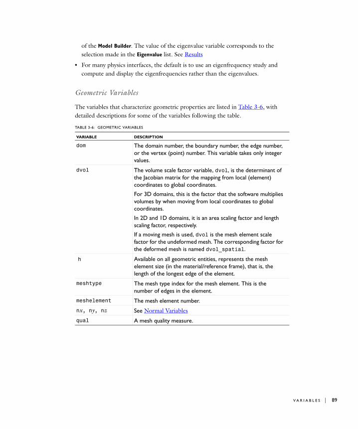
of the Model Builder. The value of the eigenvalue variable corresponds to the selection made in the Eigenvalue list. See Results
• For many physics interfaces, the default is to use an eigenfrequency study and compute and display the eigenfrequencies rather than the eigenvalues.
Geometric Variables
The variables that characterize geometric properties are listed in Table 3-6, with detailed descriptions for some of the variables following the table.
TABLE 3-6: GEOMETRIC VARIABLES
VARIABLE DESCRIPTION
dom The domain number, the boundary number, the edge number, or the vertex (point) number. This variable takes only integer values.
dvol The volume scale factor variable, dvol, is the determinant of the Jacobian matrix for the mapping from local (element) coordinates to global coordinates.
For 3D domains, this is the factor that the software multiplies volumes by when moving from local coordinates to global coordinates.
In 2D and 1D domains, it is an area scaling factor and length scaling factor, respectively.
If a moving mesh is used, dvol is the mesh element scale factor for the undeformed mesh. The corresponding factor for the deformed mesh is named dvol_spatial.
h Available on all geometric entities, represents the mesh element size (in the material/reference frame), that is, the length of the longest edge of the element.
meshtype The mesh type index for the mesh element. This is the number of edges in the element.
meshelement The mesh element number.
nx, ny, nz See Normal Variables
qual A mesh quality measure.
V A R I A B L E S | 89

90 | C H A P T E R
Note: When entering the Space Coordinate, Parameterization, Tangent, and Normal geometric variables, replace the letters highlighted below in italic font with the actual names for the dependent variables (solution components) and independent variables (spatial coordinates) in the model.
For example, replace u with the names of the dependent variables in the model, and replace x, y, and z with the first, second, and third spatial coordinate variable, respectively. xi represents the ith spatial coordinate variable. If the model contains a deformed mesh or the displacements control the spatial frame (in solid mechanics, for example), you can replace the symbols x, y, z with either the spatial coordinates (x, y, z by default) or the material/reference coordinates (X, Y, Z by default).
The variables dvol, h, qual, reldetjac, and reldetjacmin are based on the mesh viewed in the material/reference frame. If you have a moving mesh, the corresponding
reldetjac
reldetjacminThe determinant of the Jacobian matrix for the mapping from local (element) coordinates to global coordinates, normalized to that of a first-order element.
It is the determinant of the Jacobian matrix for the mapping from the straight mesh element to the possibly curved element used when solving.
Use this variable to measure the difference in shape between a curved element and the corresponding straight element.
The variable reldetjacmin is a scalar for each element defined as the minimum value of the reldetjac variable for the corresponding element.
A reldetjacmin value less than zero for an element means that the element is wrapped inside-out; that is, the element is an inverted mesh element.
s, s1, s2 See Parameterization Variables.
tx and ty (2D)t1x, t1y, t1z (3D edges)
2x, t2y, t2z (3D surfaces)
See Tangent Variables.
x, y, zr, z
See Space Coordinate Variables.
TABLE 3-6: GEOMETRIC VARIABLES
VARIABLE DESCRIPTION
3 : G L O B A L A N D L O C A L D E F I N I T I O N S

variables for the mesh viewed in the spatial frame have a suffix _spatial, that is, dvol_spatial, etc. If you use a deformed geometry, the corresponding variables for the original, undeformed mesh have a suffix _mesh.
S P A C E C O O R D I N A T E V A R I A B L E S
• The space coordinate variables (independent variables) x, y, z are available for all domain types.
• For a Cartesian geometry the default names are x, y, z.
• For axisymmetric geometries the space coordinates are normally called r and z.
• You can change the default names of the space coordinates when adding a geometry to a model (see Creating Composite Geometry Objects).
• If a deformed mesh is used, x, y, z can be both the spatial coordinates (x, y, z by default) and the material/reference coordinates (X, Y, Z by default); see Mathematical Description of the Mesh Movement.
• If the model includes a deformed mesh, the variables xTIME, yTIME, zTIME represent the mesh velocity. To access these variables, replace x, y, and z with the names of the spatial coordinates in the model (x, y, and z by default).
P A R A M E T E R I Z A T I O N V A R I A B L E S
The surface-boundary parameterization variables are useful for defining distributed loads and constraints such as a parabolic velocity profile. The available parameterization variables are:
• The curve parameter s (or s1) in 2D. Use a line plot to visualize the range of the parameter, to see if the relationship between x, y (the space coordinates) and s is nonlinear, and to see if the curve parameterization is aligned with the direction of the corresponding boundary. In most cases it runs from 0 to 1 in the direction indicated by the arrows shown on the boundaries in boundary selection mode. You can use s on boundaries when specifying boundary conditions.
• The arc length parameter s1 available on edges in 3D. It is approximately equivalent to the arc length of the edge. Use a line plot to visualize to see the values of s1.
• The surface parameters s1 and s2 in 3D are available on boundaries. In many cases they can be difficult to use because the relationship between x, y, and z (the space coordinates) and s1 and s2 is nonlinear. Often it is more convenient to use expressions with x, y, and z for specifying distributed boundary conditions. To see the values of s1 and s2, plot them using a surface plot.
V A R I A B L E S | 91
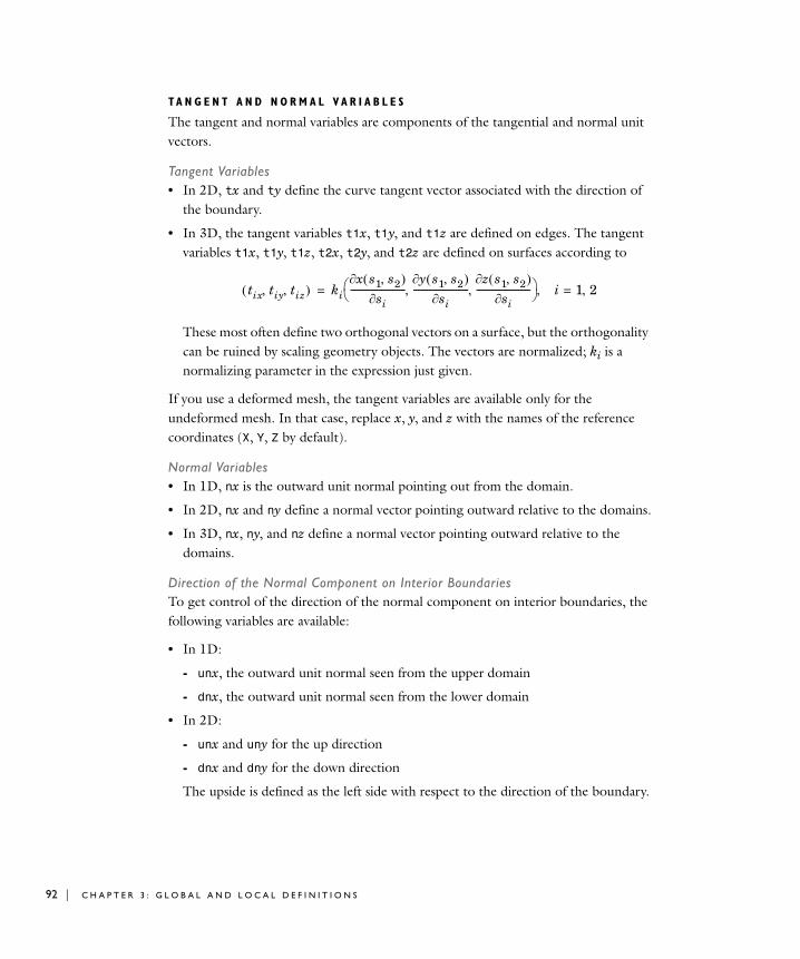
92 | C H A P T E R
TA N G E N T A N D N O R M A L V A R I A B L E S
The tangent and normal variables are components of the tangential and normal unit vectors.
Tangent Variables• In 2D, tx and ty define the curve tangent vector associated with the direction of
the boundary.
• In 3D, the tangent variables t1x, t1y, and t1z are defined on edges. The tangent variables t1x, t1y, t1z, t2x, t2y, and t2z are defined on surfaces according to
These most often define two orthogonal vectors on a surface, but the orthogonality can be ruined by scaling geometry objects. The vectors are normalized; ki is a normalizing parameter in the expression just given.
If you use a deformed mesh, the tangent variables are available only for the undeformed mesh. In that case, replace x, y, and z with the names of the reference coordinates (X, Y, Z by default).
Normal Variables• In 1D, nx is the outward unit normal pointing out from the domain.
• In 2D, nx and ny define a normal vector pointing outward relative to the domains.
• In 3D, nx, ny, and nz define a normal vector pointing outward relative to the domains.
Direction of the Normal Component on Interior BoundariesTo get control of the direction of the normal component on interior boundaries, the following variables are available:
• In 1D:
- unx, the outward unit normal seen from the upper domain
- dnx, the outward unit normal seen from the lower domain
• In 2D:
- unx and uny for the up direction
- dnx and dny for the down direction
The upside is defined as the left side with respect to the direction of the boundary.
tix tiy tiz kix s1 s2
s i-------------------------
y s1 s2 s i
-------------------------z s1 s2
si------------------------
i 1 2==
3 : G L O B A L A N D L O C A L D E F I N I T I O N S

• In 3D:
- unx, uny, and unz for the up direction
- dnx, dny, and dnz for the down direction
To visualize any of these vector variables use arrow plots on surfaces or lines.
If a deformed mesh is used, the normal variables are available both for the deformed configuration and for the undeformed configuration. In the first case, replace x, y, and z with the spatial coordinate names (x, y, and z by default). In the second case, replace x, y, and z with the material/reference coordinate names (X, Y, and Z by default).
Normal Vector Variables Representing Element Surface NormalsA similar set of variables—nxmesh, unxmesh, and dnxmesh, where x is the name of a space coordinate—use the element shape function and are normal to the actual element surfaces rather than to the geometry surfaces.
Shape Function Variables
Shape function variables and boundary-coupled shape variables are related to the shape functions of the finite elements. The shape function variables are related to the degrees of freedom defined by a finite element.
A finite element defines a number of variables, typically a dependent variables and its derivatives. Such variables are called shape functions variables because they are computed directly from shape functions and the degrees of freedom.
When you select a physics interface, you enter names for the dependent variables—these names are used to construct the finite elements. The dependent variable name is the basis for additional variable names that the finite elements generate.
Note: When entering the shape function variables, replace the letters highlighted below in italic font with the actual names for the dependent variables (solution components) and independent variables (spatial coordinates) in the model.
For example, replace u with the names of the dependent variables in the model, and replace x, y, and z with the first, second, and third spatial coordinate variable, respectively. xi represents the ith spatial coordinate variable. If the model contains a deformed mesh or the displacements control the spatial frame (in solid mechanics, for
V A R I A B L E S | 93

94 | C H A P T E R
example), you can replace the symbols x, y, z with either the spatial coordinates (x, y, z by default) or the material/reference coordinates (X, Y, Z by default).
A N E X A M P L E O F L A G R A N G E E L E M E N T V A R I A B L E S
For the Lagrange element, which is the element type used by most physics interfaces, Table 3-7 lists the available variable names, assuming you gave the name u as the argument to the shape function, and that the names x, y, and z are provided for the independent variables.
For example, with a fluid-flow interface, you get the set of variables indicated in Table 3-7 for u, v, w, and p, respectively.
• The variables ux, uy, and uz are the components of the gradient u, that is, the 1st-order spatial derivatives.
• The variables uxx, uxy, uxz, uyx, uyy, uyz, uzx, uzy, and uzz are the 2nd-order space derivative components. They are meaningful only if the degree of the polynomial shape function used in an element is high enough.
TABLE 3-7: LAGRANGE ELEMENT VARIABLE NAMES
ENTITY TYPE\ SPACE DIMENSION
1D 2D 3D
POINT u u
EDGE u, uTx, uTy, uTzBOUNDARY u, uTx, ut, uTxt u, uTx, uTy, ut,
uTxt, uTytu, uTx, uTy, uTz, ut, uTxt, uTyt, uTzt
DOMAIN u, ux, uxx, ut, uxt, uxxt, utt, uxtt, uxxtt,
u, ux, uy, uxx, uxy, uyx, uyy, ut, uxt, uyt, uxxt, uxyt, uyxt, uyyt, utt, uxtt, uytt, uxxtt, uxytt, uyxtt, uyytt
u, ux, uy, uz, uxx, uxy, uxz, uyx, uyy, uyz, uzx, uzy, uzz, ut, uxt, uyt, uzt, uxxt, uxyt, uxzt, uyxt, uyyt, uyzt, uzxt, uzyt, uzzt, utt, uxtt, uytt, uztt, uxxtt, uxytt, uxztt, uyxtt, uyytt, uyztt, uzxtt, uzytt, uzztt,
3 : G L O B A L A N D L O C A L D E F I N I T I O N S
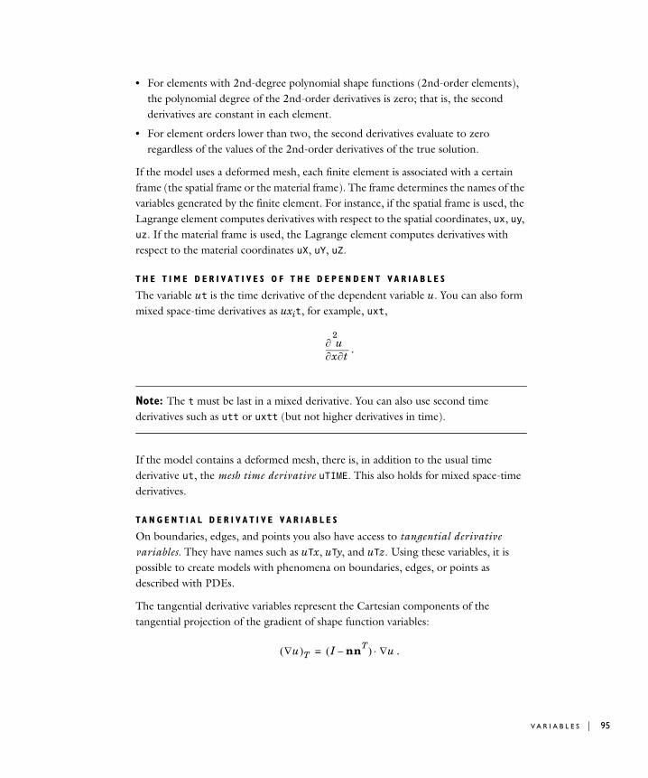
• For elements with 2nd-degree polynomial shape functions (2nd-order elements), the polynomial degree of the 2nd-order derivatives is zero; that is, the second derivatives are constant in each element.
• For element orders lower than two, the second derivatives evaluate to zero regardless of the values of the 2nd-order derivatives of the true solution.
If the model uses a deformed mesh, each finite element is associated with a certain frame (the spatial frame or the material frame). The frame determines the names of the variables generated by the finite element. For instance, if the spatial frame is used, the Lagrange element computes derivatives with respect to the spatial coordinates, ux, uy, uz. If the material frame is used, the Lagrange element computes derivatives with respect to the material coordinates uX, uY, uZ.
T H E T I M E D E R I V A T I V E S O F T H E D E P E N D E N T V A R I A B L E S
The variable ut is the time derivative of the dependent variable u. You can also form mixed space-time derivatives as uxit, for example, uxt,
.
Note: The t must be last in a mixed derivative. You can also use second time derivatives such as utt or uxtt (but not higher derivatives in time).
If the model contains a deformed mesh, there is, in addition to the usual time derivative ut, the mesh time derivative uTIME. This also holds for mixed space-time derivatives.
TA N G E N T I A L D E R I V A T I V E V A R I A B L E S
On boundaries, edges, and points you also have access to tangential derivative variables. They have names such as uTx, uTy, and uTz. Using these variables, it is possible to create models with phenomena on boundaries, edges, or points as described with PDEs.
The tangential derivative variables represent the Cartesian components of the tangential projection of the gradient of shape function variables:
.
xt
2
u
u T I nnT– u=
V A R I A B L E S | 95
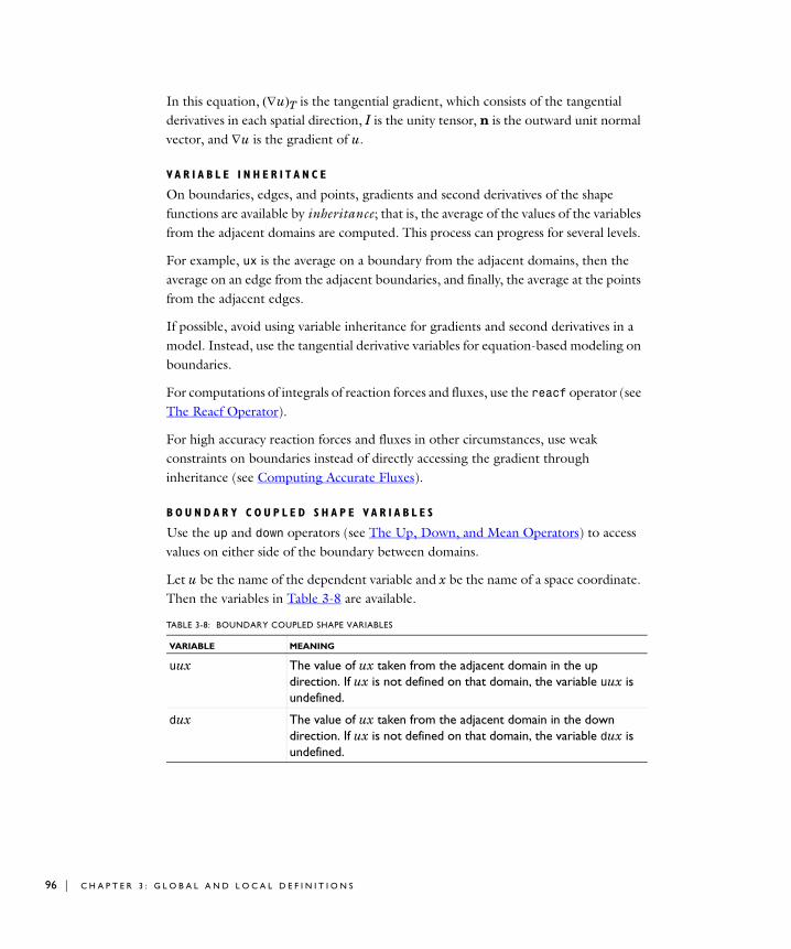
96 | C H A P T E R
In this equation, uT is the tangential gradient, which consists of the tangential derivatives in each spatial direction, I is the unity tensor, n is the outward unit normal vector, and u is the gradient of u.
VA R I A B L E I N H E R I T A N C E
On boundaries, edges, and points, gradients and second derivatives of the shape functions are available by inheritance; that is, the average of the values of the variables from the adjacent domains are computed. This process can progress for several levels.
For example, ux is the average on a boundary from the adjacent domains, then the average on an edge from the adjacent boundaries, and finally, the average at the points from the adjacent edges.
If possible, avoid using variable inheritance for gradients and second derivatives in a model. Instead, use the tangential derivative variables for equation-based modeling on boundaries.
For computations of integrals of reaction forces and fluxes, use the reacf operator (see The Reacf Operator).
For high accuracy reaction forces and fluxes in other circumstances, use weak constraints on boundaries instead of directly accessing the gradient through inheritance (see Computing Accurate Fluxes).
B O U N D A R Y C O U P L E D S H A P E V A R I A B L E S
Use the up and down operators (see The Up, Down, and Mean Operators) to access values on either side of the boundary between domains.
Let u be the name of the dependent variable and x be the name of a space coordinate. Then the variables in Table 3-8 are available.
TABLE 3-8: BOUNDARY COUPLED SHAPE VARIABLES
VARIABLE MEANING
uux The value of ux taken from the adjacent domain in the up direction. If ux is not defined on that domain, the variable uux is undefined.
dux The value of ux taken from the adjacent domain in the down direction. If ux is not defined on that domain, the variable dux is undefined.
3 : G L O B A L A N D L O C A L D E F I N I T I O N S

Entering Ranges and Vector-Valued Expressions
You can enter ranges and vector-valued expressions such as extra grid-line coordinates using the following formats:
• A space-separated or comma-separated list of values: 10, 15, 23, 29.7, 30.
• A delimited space-separated list using curly braces; for example, as an argument to a function: cos({0 pi/4 pi/2}).
• Equally-spaced values using the range function as in range(start value,step_size,end value). For example, range(0,0.2,3) creates the values 0, 0.2, 0.4,..., 2.6, 2.8, 3.0. The step size is 1 if you provide only start and end values and skip the step value. Note that start_value can be either smaller or larger than end_value. In the latter case, the step size must be negative.
Combine these formats in a single expression to create an array of values that contain an arbitrary number of segments with differently spaced values mixed with other freely specified values.
E X A M P L E S U S I N G T H E R A N G E F U N C T I O N
• range( a,(b-a)/(n-1),b)gives a list of n equally-spaced increasing values in the range [a, b] if b >a or decreasing values in the range [b, a] if a >b.
• 10^range(-3,3) gives the exponentially increasing sequence 103, 102, …, 103.
• 1^range(1,10) gives a sequence of length 10 where all elements equal 1. Multiplying the vector 1^range(1,n) by a constant value a gives a vector of n elements all equal to a.
• 0^range(1,5) gives the sequence 0 0 0 0 0.
U S I N G T H E R A N G E D I A L O G B O X T O G E N E R A T E A R R A Y S
A convenient way to generate vectors of values is to use the Range dialog box, which you open by clicking the Range button ( ) next to most of the edit fields that accept vectors of values. In that dialog box, use the Entry method list to select Step to enter a step size or Number of values to specify the number of values in the array. You specify the starting and ending values for an array of values in the Start and Stop edit fields, respectively. In addition you enter the step size in the Step edit field or the number of values in the Number of values edit field, depending on the setting in the Entry method list. By default, the spacing of the values is linear, but you can select a function to apply to all values. To do so, choose one of the available arithmetic and trigonometric functions from the Function to apply to all values list. For example, select exp10 to
V A R I A B L E S | 97

98 | C H A P T E R
create an array of exponentially increasing values. The list includes the following functions:
• The default value None, which means linear spacing using the range function directly with the values that you specify.
• The exponential functions exp10 (base-10 exponential function) and exp (base-e exponential function), which create exponentially-spaced values using the specified range of values as powers of 10 and of the mathematical constant e, respectively.
• The trigonometric functions cos (cosine) and sin (sine), which create sinusoidally varying values.
• The square root function sqrt, which creates a vector with values that are the square roots of the values that you specify.
Click Replace to replace the contents in the edit field with the values that you have specified in the Range dialog box. Click Add to add the range of values to the end of the existing values in the associated edit field. That way you can create more complex ranges.
M O D E L I N G F E A T U R E S T H A T S U P P O R T R A N G E S A N D VE C T O R - V A L U E D
E X P R E S S I O N S
The following modeling features support ranges and vector-valued expressions:
• Extra grid lines in the Axis node’s Settings window.
• Interval coordinates when using the Interval node’s Settings window for 1D geometries.
• The times for output from the time-dependent solver and the list of parameter values in the Settings windows for study step nodes for time-dependent and stationary solvers and for parametric sweeps.
• The contour levels, the streamline start-point coordinates, and the coordinates in arrow plots. Whenever you specify a number of coordinates in Settings windows for plots, COMSOL Multiphysics uses scalar expansion—if one component is the same for all coordinates, you can enter a single number in the corresponding text field. For example, to get 101 linearly spaced coordinates from y = 6 to y = 7 along x = 3, enter it as the single scalar 3 for x and then range(6,0.01,7) for y. Thus, you need not enter 101 similar values for x.
• Element distribution in the meshing settings.
3 : G L O B A L A N D L O C A L D E F I N I T I O N S

Adding Global Variables to the Model Builder
1 Open or create a model file.
2 In the Model Builder, right-click Global Definitions and select Variables.
The Variables page opens in the Settings window and a Variables node is added to the model under Global Definitions.
Adding Local Variables to Individual Models
1 Open or create a model file.
2 In the Model Builder, right-click Definitions and select Variables.
The Variables page opens in the Settings window and a Variables node is added to the model under Model>Definitions.
Assigning Geometric Scope to a Variable
Note: The Global Definitions Variables page does not have a Geometric Scope section.
1 Create a local variable for a model.
2 In the Geometric Scope section, select the scope in the Geometric entity level list. The options are Entire Geometry, Domain, Boundary, Edge (3D only), and Point.
If you select a level other than Entire Geometry, a Selection list for geometric entities of the selected type (boundaries, for example) displays. Also see Selecting and Deselecting Geometric Entities for detailed information.
Adding Variable Definitions
1 Create a global or local Variable.
2 On the Variables page, in the Variables table, click the first cell in the Name column. Enter a variable name.
3 In the Expression column, enter an expression that defines the variable. Expressions can contain space coordinates and solution components that are also available within the same scope.
The Unit column displays the unit of the variable.
4 In the Description column, enter an optional description.
V A R I A B L E S | 99
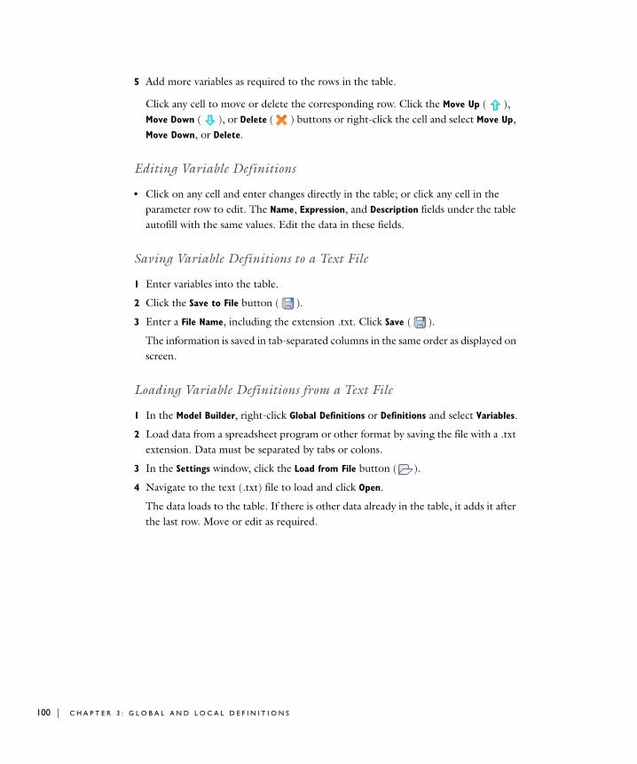
100 | C H A P T E
5 Add more variables as required to the rows in the table.
Click any cell to move or delete the corresponding row. Click the Move Up ( ), Move Down ( ), or Delete ( ) buttons or right-click the cell and select Move Up, Move Down, or Delete.
Editing Variable Definitions
• Click on any cell and enter changes directly in the table; or click any cell in the parameter row to edit. The Name, Expression, and Description fields under the table autofill with the same values. Edit the data in these fields.
Saving Variable Definitions to a Text File
1 Enter variables into the table.
2 Click the Save to File button ( ).
3 Enter a File Name, including the extension .txt. Click Save ( ).
The information is saved in tab-separated columns in the same order as displayed on screen.
Loading Variable Definitions from a Text File
1 In the Model Builder, right-click Global Definitions or Definitions and select Variables.
2 Load data from a spreadsheet program or other format by saving the file with a .txt extension. Data must be separated by tabs or colons.
3 In the Settings window, click the Load from File button ( ).
4 Navigate to the text (.txt) file to load and click Open.
The data loads to the table. If there is other data already in the table, it adds it after the last row. Move or edit as required.
R 3 : G L O B A L A N D L O C A L D E F I N I T I O N S

Summary of Common Predefined Variables
The following table summarizes the most important predefined variables that are generally available in all COSMOL Multiphysics models. Some are only available in certain geometries or in time-dependent models, for example.
TABLE 3-9: COMMON PREDEFINED VARIABLES
TYPE OF VARIABLES VARIABLES
Time t
Frequency freq
Eigenvalues lambda
Position x, y, z, r, X, Y, Z, R
Edge/surface parameters s, s1, s2
Edge/surface normals n, nx, ny, nz, nr
Edge tangents tx, ty, tz, tr
Surface tangents t1x, t1y, t1z, t2x, t2y, t2z
Edge/surface upward normals un, unx, uny, unz
Edge/surface downward normals dn, dnx, dny, dnz
Numerical constants eps, i, j, pi
Mesh information h, dom, meshtype, meshelement, dvol, qual, reldetjac, reldetjacmin
V A R I A B L E S | 101
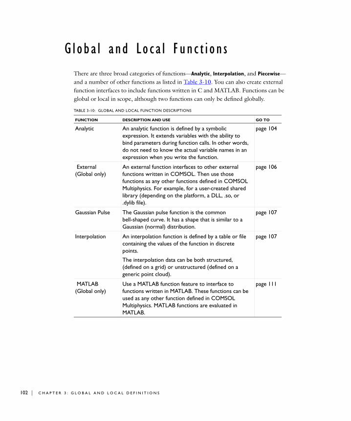
102 | C H A P T E
G l oba l and Lo c a l F un c t i o n s
There are three broad categories of functions—Analytic, Interpolation, and Piecewise—and a number of other functions as listed in Table 3-10. You can also create external function interfaces to include functions written in C and MATLAB. Functions can be global or local in scope, although two functions can only be defined globally.
TABLE 3-10: GLOBAL AND LOCAL FUNCTION DESCRIPTIONS
FUNCTION DESCRIPTION AND USE GO TO
Analytic An analytic function is defined by a symbolic expression. It extends variables with the ability to bind parameters during function calls. In other words, do not need to know the actual variable names in an expression when you write the function.
page 104
External(Global only)
An external function interfaces to other external functions written in COMSOL. Then use those functions as any other functions defined in COMSOL Multiphysics. For example, for a user-created shared library (depending on the platform, a DLL, .so, or .dylib file).
page 106
Gaussian Pulse The Gaussian pulse function is the common bell-shaped curve. It has a shape that is similar to a Gaussian (normal) distribution.
page 107
Interpolation An interpolation function is defined by a table or file containing the values of the function in discrete points.
The interpolation data can be both structured, (defined on a grid) or unstructured (defined on a generic point cloud).
page 107
MATLAB (Global only)
Use a MATLAB function feature to interface to functions written in MATLAB. These functions can be used as any other function defined in COMSOL Multiphysics. MATLAB functions are evaluated in MATLAB.
page 111
R 3 : G L O B A L A N D L O C A L D E F I N I T I O N S
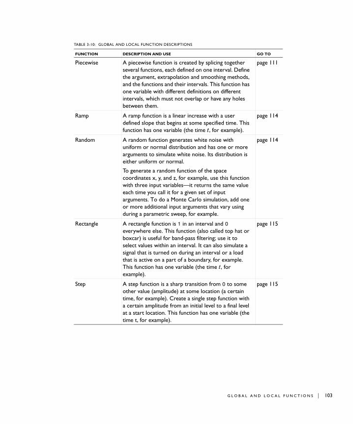
Piecewise A piecewise function is created by splicing together several functions, each defined on one interval. Define the argument, extrapolation and smoothing methods, and the functions and their intervals. This function has one variable with different definitions on different intervals, which must not overlap or have any holes between them.
page 111
Ramp A ramp function is a linear increase with a user defined slope that begins at some specified time. This function has one variable (the time t, for example).
page 114
Random A random function generates white noise with uniform or normal distribution and has one or more arguments to simulate white noise. Its distribution is either uniform or normal.
To generate a random function of the space coordinates x, y, and z, for example, use this function with three input variables—it returns the same value each time you call it for a given set of input arguments. To do a Monte Carlo simulation, add one or more additional input arguments that vary using during a parametric sweep, for example.
page 114
Rectangle A rectangle function is 1 in an interval and 0 everywhere else. This function (also called top hat or boxcar) is useful for band-pass filtering; use it to select values within an interval. It can also simulate a signal that is turned on during an interval or a load that is active on a part of a boundary, for example. This function has one variable (the time t, for example).
page 115
Step A step function is a sharp transition from 0 to some other value (amplitude) at some location (a certain time, for example). Create a single step function with a certain amplitude from an initial level to a final level at a start location. This function has one variable (the time t, for example).
page 115
TABLE 3-10: GLOBAL AND LOCAL FUNCTION DESCRIPTIONS
FUNCTION DESCRIPTION AND USE GO TO
G L O B A L A N D L O C A L F U N C T I O N S | 103
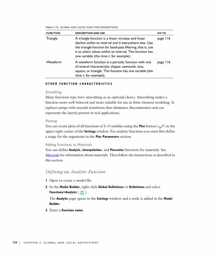
104 | C H A P T E
O T H E R F U N C T I O N C H A R A C T E R I S T I C S
SmoothingMany functions type have smoothing as an optional choice. Smoothing makes a function more well-behaved and more suitable for use in finite element modeling. It replaces jumps with smooth transitions that eliminates discontinuities and can represents the inertia present in real applications.
PlottingYou can create plots of all functions of 1–3 variables using the Plot button ( ) in the upper-right corner of the Settings window. For analytic functions you must first define a range for the arguments in the Plot Parameters section.
Adding Functions to MaterialsYou can define Analytic, Interpolation, and Piecewise functions for materials. See Materials for information about materials. Then follow the instructions as described in this section.
Defining an Analytic Function
1 Open or create a model file.
2 In the Model Builder, right-click Global Definitions or Definitions and select Functions>Analytic ( ).
The Analytic page opens in the Settings window and a node is added in the Model
Builder.
3 Enter a Function name.
Triangle A triangle function is a linear increase and linear decline within an interval and 0 everywhere else. Use the triangle function for band-pass filtering; that is, use it to select values within an interval. This function has one variable (the time t, for example).
page 116
Waveform A waveform function is a periodic function with one of several characteristic shapes: sawtooth, sine, square, or triangle. This function has one variable (the time t, for example).
page 116
TABLE 3-10: GLOBAL AND LOCAL FUNCTION DESCRIPTIONS
FUNCTION DESCRIPTION AND USE GO TO
R 3 : G L O B A L A N D L O C A L D E F I N I T I O N S

4 Under Parameters:
a In the Expression field, enter the mathematical expression that defines the functions, such as a+b*cos(c).
b Enter Arguments to the analytic function as comma-separated entries. For example, a,b,c.
c From the Derivatives list, select Automatic or Manual to enable COMSOL to evaluate the derivatives of all functions. COMSOL Multiphysics must know the derivative of a function if you are using a variable that depends on the solution in a function argument.
- Select Automatic to compute the derivatives symbolically.
- Select Manual to enter the derivatives with respect to one or more of the arguments to the function. For derivatives that you do not define, COMSOL uses 0 as the value of the derivative. In this example, enter 1,cos(c),d(a+b*cos(c),c),0 in the associated edit field.
Notice the use of the d operator (see Special Operators for more information).
5 Under Periodic Extension:
a Select the Make periodic check box to make the function periodic and extend its definition within an interval to the whole real axis.
b Define the interval in the Lower limit and Upper limit fields.
6 Under Advanced, select the May produce complex output for real arguments check box if the defined function works similarly to sqrt; that is, it sometimes returns complex values for a real-valued input.
7 Under Plot parameters, in the Plot Parameters table or the fields under it, enter the Argument name, a Lower limit, and an Upper limit.
Use the Move Up ( ), Move Down ( ), or Delete ( ) buttons to rearrange and delete rows in the table, or right click in any cell and select these options. Click the Plot button ( ) to generate a preview plot of the function and set ranges for all the arguments.
G L O B A L A N D L O C A L F U N C T I O N S | 105

106 | C H A P T E
Defining an External Function
Note: This is only available globally on the Global Definitions node. Also see the COMSOL Multiphysics Reference Guide for details about the interface to the library (or see Where Do I Access the Documentation and Model Library?).
1 Open or create a model file.
2 In the Model Builder, right-click Global Definitions and select Functions>External ( ).
The External page opens in the Settings window and a node is added in the Model
Builder.
3 Under Functions, in the Library field, enter a Library (the complete network path) or Browse to locate a library to import.
4 For each row in the Functions table, enter a Function name (myfun, for example).
5 For each Function in the table, enter a space-separated or comma-separated list of the names of its input Arguments (x y, for example).
Use the Move Up ( ), Move Down ( ), or Delete ( ) buttons and the fields under the table to edit the table contents.
6 Under Derivatives, enter data in this section based on the following.
a In the Derivatives table, each row contains a partial derivative of a function with respect to one of its arguments.
b The entries in the Function column must occur in the function table, and the entries in the Argument column must occur among the arguments listed for that function in the function table.
c The Partial derivative column contains expressions for the partial derivatives. Partial derivatives that are not specified in the table default to 0.
Use the Move Up ( ), Move Down ( ), or Delete ( ) buttons and the fields under the table to edit the table contents.
7 Under Advanced:
a Enter a value in the Initialization data field. The value is sent to the library when it is loaded.
b Select the Thread safe check box to declare that the function is a thread-safe pure function (that is, a function that always returns the same results using the same
R 3 : G L O B A L A N D L O C A L D E F I N I T I O N S

input argument values and that do not have any side effects or output). Selecting this check box can then improve performance.
8 Click the Plot button ( ) to generate a preview plot of the function.
Defining a Gaussian Pulse Function
1 Open or create a model file.
2 In the Model Builder, right-click Global Definitions or Definitions and select Functions>Gaussian Pulse ( ).
The Gaussian Pulse page opens in the Settings window and a node is added in the Model Builder.
3 Enter a Function name.
4 Under Parameters:
a Enter a Location value for the Gaussian pulse mean s0.
b Enter a Standard deviation of the normal distribution.
The Gaussian pulse has the same characteristics as the normal distribution: it is a pulse with a shape that is similar to a normal or Gaussian distribution as a function:
In the equation above, s is the input variable, s0 is the location (mean), and is the standard deviation. This function is a function of one variable (the time t, for example).
5 Click the Plot button ( ) to generate a preview plot of the function.
Defining an Interpolation Function
1 Open or create a model file.
2 In the Model Builder, right-click Global Definitions or Definitions and select Functions>Interpolation ( ).
The Interpolation page opens in the Settings window and a node is added in the Model Builder.
3 Enter a Function name.
y s 1 2---------------e
s s0– 2–
22-----------------------
=
G L O B A L A N D L O C A L F U N C T I O N S | 107

108 | C H A P T E
4 Under Parameters, select Table or File from the Data source list.
- If you select Table, enter a Function name and enter coordinates t and function values ft into the table cells. Use the Move Up ( ), Move Down ( ), or Delete ( ) buttons to rearrange and delete rows in the table.
- If you select File to import function data:
a Enter a Filename (the complete network path) or Browse to locate a file to import.
b From the Data format list select Spreadsheet, Grid, or Sectionwise.
- A spreadsheet file has coordinates and function values; a CSV (comma-separated value) file exported from a spreadsheet program is in this format.
%Coordinates One to three columns containing x, y (optional), and z (optional) %Elements Triangulation where each row contains the row indices of the points in the Coordinates section that make up one element (triangular in 2D, tetrahedral in 3D) %Data (funname) Column of data values for each point
It is possible to include more than one function in the file as long as a %Data header separates them one from the other.
- A grid file
% Grid x grid points separated by spaces y grid points separated by spaces (optional) z grid points separated by spaces (optional) % Data Data values separated by spaces
Each row contains values for different x grid points for fixed values of y and z. The rows first increase the y grid value and then the z grid value. The grid points can also represent another independent variable that the data values depend on. For example, the “grid points” can be temperature values and the data values the thermal conductivity at these temperatures. It is important to use a comment line starting with % to separate the grid points or other interpolation points and the data values that are associated with these coordinates or interpolation points. You
R 3 : G L O B A L A N D L O C A L D E F I N I T I O N S

can use the postwriteinterpfile function to create a file of this format from MATLAB.
It is possible to include more than one function in the file as long as a %Data header separates them one from the other.
- A sectionwise file contains structured mesh and function data; COMSOL can export such files.
%Header (optional) Columns containing x, y (optional), and z (optional) followed by data columns.
You can include function names in the header. In that case, the input columns must be labeled with x, y, and z, respectively, depending on input dimension. For example, a file with the following content creates two 2D functions named myfun1 and myfun2:
% x y myfun1 myfun2 0 0 0.12 0.34 0 1 0.52 1.50 1 0 0.67 0.91
If the file does not include any header to indicate the function dimension, the software assumes that it is identical to the largest geometry dimension present in the model. A file with four columns, for example, is interpreted as one 3D function in a 3D model, two 2D functions in a 2D model, and three 1D functions in a 1D model.
c If you selected Spreadsheet, enter a Number of arguments.
For all file types, enter data into the table. Add a Function name and its Position in
file. The first function in the file has position 1, the following has position 2, and so on. Use the Move Up ( ), Move Down ( ), or Delete ( ) buttons to rearrange and delete rows in the table. Also see the example below.
5 Under Interpolation and Extrapolation:
The interpolation setting controls how the program evaluates the function between the discrete points where it is defined by the table or file, and the behavior of the function outside the domain where it is defined by the table or file.
a Select one of the following methods from the Interpolation list:
- For functions of one variable select Nearest neighbor, Linear, Piecewise cubic, or Cubic spline.
Piecewise-cubic interpolation uses a piecewise-cubic Hermite polynomial with continuous first derivatives. It preserves the shape of the data and respects
G L O B A L A N D L O C A L F U N C T I O N S | 109

110 | C H A P T E
monotonicity. The Cubic-spline method also performs interpolation with a piecewise cubic polynomial. Here, even second derivatives are continuous; however, the method does not necessarily respect monotonicity.
- For functions of more than one variable, select Nearest neighbor or Linear. The other options are not supported.
b Select one of the following methods from the Extrapolation list to specify how to treat arguments outside the grid or mesh of points.
- Constant. Uses the value from the closest point inside the grid (for structured interpolation) or the value from the closest mesh element (for unstructured interpolation). The interpolation function evaluates the polynomial from the closest grid point at the actual point where a value is requested.
- Linear. The function is linear outside the grid with a continuous function value and continuous first derivative at the boundary of the grid. Piecewise cubic or Cubic spline must be selected from the Interpolation list in Step 1.
- Nearest function. Evaluates the polynomial from the closest grid point at the actual point where a value is requested.
- Specific value. Uses a single value, such as zero or NaN (Not a Number), everywhere outside the grid or mesh. Enter the value in the Values outside range edit field.
Note: Unstructured interpolation supports using a constant or a specific value only.
6 Click the Plot button ( ) to generate a preview plot of the function.
E X A M P L E O F I M P O R T I N G A F I L E D A T A S O U R C E I N T O A P A R A M E T E R
T A B L E
You have a file named temp.txt, which contains temperature measurements in nine points in the plane:
10 3 31020 3 30930 3 31410 6 30220 6 30730 6 31110 9 30720 9 30820 9 314
R 3 : G L O B A L A N D L O C A L D E F I N I T I O N S

The data columns contain x-coordinates, y-coordinates, and temperature values, respectively. To use this file as an interpolation function called tempfun, perform the following steps.
1 Select File from the Data source list.
2 Enter a Filename (the complete network path) or Browse to locate a file to import.
3 From the Data format list select Spreadsheet.
4 Enter a Number of arguments. In this example, enter 2.
5 Enter the Function name tempfun.
6 Enter its Position in file as 1. The first function in the file has position 1, the following has position 2, and so on.
The position in file for a function is the column after the space coordinates where it is defined. In this example with two arguments (space coordinates), the third column is Position 1 in the file.
7 If desired, adjust the interpolation and extrapolation settings in the Interpolation and
Extrapolation section.
You can now use the function tempfun with x and y as input arguments in a 2D model to get the interpolated value for the temperature at any position.
About MATLAB Functions
You can use MATLAB functions from COMSOL Multiphysics. This requires the LiveLink for MATLAB product. See the section Defining a MATLAB Function in the LiveLink for MATLAB User’s Guide.
Defining a Piecewise Function
1 Open or create a model file.
2 In the Model Builder, right-click Global Definitions or Definitions and select Functions>Piecewise ( ).
The Piecewise page opens in the Settings window and a node is added in the Model
Builder.
3 Enter a Function name.
G L O B A L A N D L O C A L F U N C T I O N S | 111

112 | C H A P T E
4 Under Parameters:
a Enter a piecewise function name in the Argument field.
b Select one of the following methods from the Extrapolation list to control what happens when the function is evaluated in a point that does not belong to any interval.
- Constant. Uses the function value from the endpoint of the closest interval. Uses the value from the start point of the first and the end point of the last interval on the corresponding sides.
- None. Evaluation fails outside of the intervals where it is defined. Trying to evaluate the function generates an error and evaluates to NaN (Not-a-Number).
- Nearest function. Evaluate the function from the closest interval. The function at the first or last interval (depending of the side) is used to evaluate at the actual point where a value is requested.
- Specific value. Enter a value in the Values outside range field. If selecting the specific-number method you can assign a single value (usually zero or NaN) to all points outside the intervals.
c Select one of the following from the Smoothing list: No smoothing, Continuous
function, Continuous first derivative, or Continuous second derivative.
The functions in contiguous intervals may not evaluate to the same value where the intervals meet. Apply smoothing to make the piecewise function more well-behaved numerically. Functions from neighboring intervals are then blended close to where the intervals meet.
- If you selected Continuous function, Continuous first derivative, or Continuous
second derivative, enter a value in the Relative size of transition zone field. Relative size meaning in relation to the size of the intervals on both sides of the border.
5 Under Parameters, for each cell in the Intervals table:
a Enter Start and End interval limits. The intervals must not overlap, and there cannot be any holes between intervals.
R 3 : G L O B A L A N D L O C A L D E F I N I T I O N S
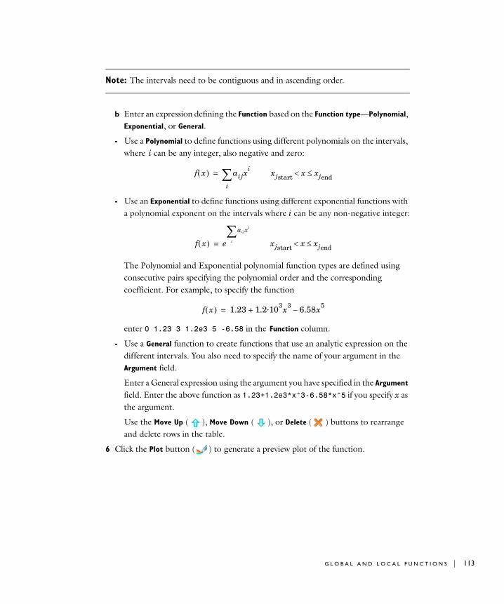
Note: The intervals need to be contiguous and in ascending order.
b Enter an expression defining the Function based on the Function type—Polynomial, Exponential, or General.
- Use a Polynomial to define functions using different polynomials on the intervals, where i can be any integer, also negative and zero:
- Use an Exponential to define functions using different exponential functions with a polynomial exponent on the intervals where i can be any non-negative integer:
The Polynomial and Exponential polynomial function types are defined using consecutive pairs specifying the polynomial order and the corresponding coefficient. For example, to specify the function
enter 0 1.23 3 1.2e3 5 -6.58 in the Function column.
- Use a General function to create functions that use an analytic expression on the different intervals. You also need to specify the name of your argument in the Argument field.
Enter a General expression using the argument you have specified in the Argument field. Enter the above function as 1.23+1.2e3*x^3-6.58*x^5 if you specify x as the argument.
Use the Move Up ( ), Move Down ( ), or Delete ( ) buttons to rearrange and delete rows in the table.
6 Click the Plot button ( ) to generate a preview plot of the function.
f x aij
i xi
= xjstart x xjend
f x e
aij
i
xi
= xjstart x xjend
f x 1.23 1.2·103x3 6.58x5–+=
G L O B A L A N D L O C A L F U N C T I O N S | 113

114 | C H A P T E
Defining a Ramp Function
1 In the Model Builder, right-click Global Definitions or Definitions and select Functions>Ramp ( ).
The Ramp page opens in the Settings window and a node is added in the Model
Builder.
2 Enter a Function name.
3 Under Parameters:
a Enter a Location value s0 for the start of the ramp.The function evaluates to 0 for values less than its start location and increases linearly for values greater than the location.
b Enter a Slope k of the ramp.
c To ensure that the value never exceeds a certain point, select the Cutoff check box and enter a value.
For an input variable s, a start location s0, and a slope k, the ramp function’s value is 0 for s s0 and kss0 for s s0.
4 Click the Plot button ( ) to generate a preview plot of the function.
Defining a Random Function
1 In the Model Builder, right-click Global Definitions or Definitions and select Functions>Random ( ).
The Random page opens in the Settings window and a node is added in the Model
Builder.
2 Enter a Function name.
3 Under Parameters:
a Enter a Number of arguments to the random function.
b Select Uniform or Normal from the Distribution list.
- If you selected Uniform, enter a Mean and Range. The range is the difference between the largest and smallest values that the function can return.
- If you selected Normal, enter a Mean and Standard deviation.
4 Click the Plot button ( ) to generate a preview plot of the function.
R 3 : G L O B A L A N D L O C A L D E F I N I T I O N S

Defining a Rectangle Function
1 In the Model Builder, right-click Global Definitions or Definitions and select Functions>Rectangle ( ).
The Rectangle page opens in the Settings window and a node is added in the Model
Builder.
2 Enter a Function name.
3 Under Limits, enter a Lower limit and Upper limit to specify the interval for the rectangle function. For example, if the input argument is time, enter a start and end time. This function evaluates to 1 for values within an interval. Outside the interval it evaluates to 0.
4 Under Smoothing:
a To turn on the smoothing function select the Size of transition zone check box.
b Enter a value in the Size of transition zone field to control the amount of smoothing. Use smoothing to improve the behavior of the model by avoiding discontinuities that are difficult to handle numerically.
5 Click the Plot button ( ) to generate a preview plot of the function.
Defining a Step Function
1 In the Model Builder, right-click Global Definitions or Definitions and select Functions>Step ( ).
The Step page opens in the Settings window and a node is added in the Model Builder.
2 Enter a Function name.
3 Under Parameters:
a Enter a Location (s0) of the step. The value of the step function is the initial level for input values that are smaller than the location of the step.
b In the From field, enter a start level (Lstart ).
c In the End field, enter a final level (Lend).
For an input variable s, a start location s0, and initial level Lstart and a final level Lend, the step function’s value is Lstart for ss0 and Lend for ss0. The amplitude of the step is LendLstart.
G L O B A L A N D L O C A L F U N C T I O N S | 115

116 | C H A P T E
4 Under Smoothing:
a To turn on the smoothing function select the Size of transition zone check box.
b Enter a value in the Size of transition zone field to control the amount of smoothing. Use smoothing to improve the behavior of the model by avoiding discontinuities that are difficult to handle numerically.
5 Click the Plot button ( ) to generate a preview plot of the function.
Defining a Triangle Function
1 In the Model Builder, right-click Global Definitions or Definitions and select Functions>Triangle ( ).
The Triangle page opens in the Settings window and a node is added in the Model
Builder.
2 Enter a Function name.
3 Under Limits, enter a Lower limit and Upper limit to specify the interval for the triangle function. For example, if the input argument is time, enter a start and end time. In the midpoint of the interval, this function evaluates to 1, and moving toward the interval boundaries it falls off to 0. Outside the interval it evaluates to 0.
4 Under Smoothing:
a To turn on the smoothing function select the Size of transition zone check box.
b Enter a value in the Size of transition zone field to control the amount of smoothing. Use smoothing to improve the behavior of the model by avoiding discontinuities that are difficult to handle numerically.
5 Click the Plot button ( ) to generate a preview plot of the function.
Defining a Waveform Function
1 In the Model Builder, right-click Global Definitions or Definitions and select Functions>Waveform ( ).
The Waveform page opens in the Settings window and a node is added in the Model
Builder.
2 Enter a Function name.
R 3 : G L O B A L A N D L O C A L D E F I N I T I O N S

3 Under Parameters, select a waveform from the Type list: Sawtooth, Sine, Square, or Triangle.
a If you select Sine, enter a Frequency, Phase, and Amplitude value. Smoothing is not available for this waveform.
b For Sawtooth, Square, or Triangle waveforms, the Smoothing check box is selected by default. Enter a value in the Transition zone field.
If required, turn off smoothing by clearing the Smoothing check box.
4 For Sawtooth, Square, or Triangle, enter a Frequency, Phase, and Amplitude value.
5 Click the Plot button ( ) to generate a preview plot of the function.
G L O B A L A N D L O C A L F U N C T I O N S | 117

118 | C H A P T E
Mode l C oup l i n g s
Model couplings establish couplings between different parts of a model or between different models. A model coupling is defined by a coupling operator, taking an expression as its argument. When the operator is evaluated at a point in the destination, the value is computed by evaluating the argument on the source. All coupling types have a source and a destination.
The destination is where the operator can be evaluated. Its value is computed by evaluating the operator's argument at one or several points in the source. Both the source and the destination are purely geometrical objects, but the source is limited to one geometry whereas the destination is usually global. However, with extrusion and projection couplings, the final evaluation fails if the mapping fails, therefore it is the destination that must be well defined. Some operators have a global destination, which means that they are available everywhere.
About Coupling Operators
Coupling operators are useful for modeling coupled problems and are a generalization of ordinary expressions. They are defined by first selecting the source, where the argument of the operator is evaluated, and a destination. You don’t need an evaluation expression to define coupling operators.
Coupling operators can:
• Make the value and the exact Jacobian of an expression available nonlocally (see Nonlocal Couplings and The Sparsity of the Jacobian.
• Take information from a boundary, for example, and make it available on other parts of a model (a domain, for example).
• Be used just for results evaluation and visualization purposes.
• Define nonlocal couplings including mesh transformations, integrals over domains, and projections.
There are three categories of coupling operators:
• Extrusion. These operators connect a source and a destination and take an expression as an argument. When the operator is evaluated at a point in the destination, its value is computed by evaluating the argument at a corresponding point in the source. See About Extrusion Model Coupling and Operators, Defining
R 3 : G L O B A L A N D L O C A L D E F I N I T I O N S

a Boundary Similarity Model Coupling and Defining an Identity Mapping Model Coupling.
• Projection. These coupling operators evaluate a series of line integrals on the source domain, where the line positions depend on the positions of the evaluation points in the destination domain. See About Projection Model Couplings and Operators.
• Scalar. These operators define a scalar value such as an integration, the average over a set of geometric entities, and the maximum or minimum value of an expression. See About Scalar Model Couplings and Operators, Defining an Average Model Coupling, and Defining Maximum and Minimum Model Couplings.
N O N L O C A L C O U P L I N G S A N D T H E S P A R S I T Y O F T H E J A C O B I A N
The Jacobian for problems formulated using the finite element method is usually large but sparse. This is because the solution at each mesh node can depend at most on the degrees of freedom at the neighboring mesh elements. However, by introducing nonlocal model couplings using coupling operators, you create nonlocal dependencies that fill up the rows and columns of the affected source and destination nodes. These additional elements might make the Jacobian matrix only slightly less sparse, with marginal effects on solution speed; it can also make it a great deal less sparse, in which case memory use and CPU time involved in solving the problem increases considerably. For this reason, take particular care when introducing nonlocal couplings.
TABLE 3-11: COUPLING OPERATOR DESCRIPTIONS
COUPLING OPERATOR
DESCRIPTION GO TO
Average Computes the average of an expression over selected geometric entities. It can be evaluated anywhere in any model, and the value does not depend on the evaluation point. It is similar to the Integration operator; the difference being that the integral is divided by the volume, area, arc length, or number of points in the source, depending on the dimension.
page 140
Boundary Similarity
Maps an expression defined on a part of a boundary to another part of a boundary with the same shape. Available in 2D and 3D, it is defined by a similarity mapping from the destination to the source.
page 127
M O D E L C O U P L I N G S | 119
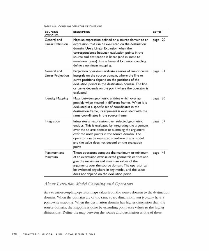
120 | C H A P T E
About Extrusion Model Coupling and Operators
An extrusion coupling operator maps values from the source domain to the destination domain. When the domains are of the same space dimension, you typically have a point-wise mapping. When the destination domain has higher dimension than the source domain, the mapping is done by extruding point-wise values to the higher dimensions. Define the map between the source and destination as one of these
General and Linear Extrusion
Maps an expression defined on a source domain to an expression that can be evaluated on the destination domain. Use a Linear Extrusion when the correspondence between evaluation points in the source and destination is linear (and in some to non-linear cases). Use a General Extrusion coupling define a nonlinear mapping.
page 120
General and Linear Projection
Projection operators evaluate a series of line or curve integrals on the source domain, where the line or curve positions depend on the positions of the evaluation points in the destination domain. The line or curve depends on the point where the operator is evaluated.
page 131
Identity Mapping Maps between geometric entities which overlap, possibly when viewed in different frames. When it is evaluated at a specific set of coordinates in the destination frame, its argument is evaluated with the same coordinates in the source frame.
page 130
Integration Integrates an expression over selected geometric entities. This is evaluated by integrating the argument over the source domain or summing the argument over the node points in the source domain. The operator can be evaluated anywhere in any model, and the value does not depend on the evaluation point.
page 137
Maximum and Minimum
These operators compute the maximum or minimum of an expression over selected geometric entities and give the maximum and minimum values of the arguments over the source domain. The operator can be evaluated anywhere in any model, and the value does not depend on the evaluation point.
page 141
TABLE 3-11: COUPLING OPERATOR DESCRIPTIONS
COUPLING OPERATOR
DESCRIPTION GO TO
R 3 : G L O B A L A N D L O C A L D E F I N I T I O N S
operators: general extrusion, linear extrusion, boundary similarity, or identity mapping.
A B O U T T H E G E N E R A L E X T R U S I O N C O U P L I N G O P E R A T O R
A General Extrusion coupling operator maps an expression defined on a source domain to an expression that can be evaluated on the destination domain. Use this to define a nonlinear mapping of this kind. These operators define a more general extrusion between source and destination than the linear extrusion. Specifically, when the destination has more space dimensions than the source, the operator performs extrusion of values.
A B O U T T H E L I N E A R E X T R U S I O N C O U P L I N G O P E R A T O R
A Linear Extrusion coupling operator maps an expression defined on a source domain to an expression that can be evaluated on the destination domain. Use this to define a linear mapping of this kind. Linear extrusion can be used when the correspondence between evaluation points in the source and destination is linear, and in some non-linear cases. Otherwise, use a general extrusion coupling.
These operators define a linear extrusion that maps between geometric parts of the same dimension. The parts can exist in geometries of different space dimensions. For example, you can couple from edges in 2D to those in 3D; you can also couple 2D domains to 3D faces. In these cases you obviously need geometries of different space dimensions for the source and destination. You define the linear extrusion by specifying points in both the source and destination.
A B O U T T H E B O U N D A R Y S I M I L A R I T Y C O U P L I N G O P E R A T O R
The Boundary Similarity coupling operator is slightly different for 2D and 3D.
In 3D, the destination map is a similarity that maps a destination boundary, onto a set of source boundaries. The mesh is always viewed in the mesh frame.
By default, the algorithm automatically chooses a map when symmetries make several maps possible. To control this choice in 3D, add an Edge Map, One Point Map, or Two
Point Map subfeature.
• Edge Map: Specify that a certain destination edge should be mapped onto a certain source edge. Their relative direction is given by the property direction. The edges must be adjacent to the given boundary.
M O D E L C O U P L I N G S | 121
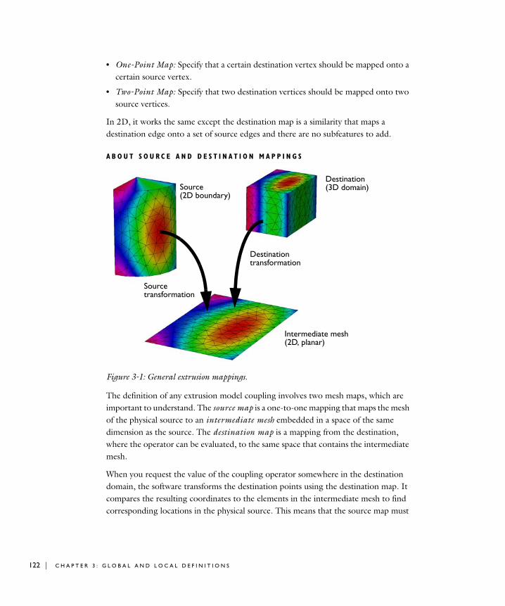
122 | C H A P T E
• One-Point Map: Specify that a certain destination vertex should be mapped onto a certain source vertex.
• Two-Point Map: Specify that two destination vertices should be mapped onto two source vertices.
In 2D, it works the same except the destination map is a similarity that maps a destination edge onto a set of source edges and there are no subfeatures to add.
A B O U T S O U R C E A N D D E S T I N A T I O N M A P P I N G S
Figure 3-1: General extrusion mappings.
The definition of any extrusion model coupling involves two mesh maps, which are important to understand. The source map is a one-to-one mapping that maps the mesh of the physical source to an intermediate mesh embedded in a space of the same dimension as the source. The destination map is a mapping from the destination, where the operator can be evaluated, to the same space that contains the intermediate mesh.
When you request the value of the coupling operator somewhere in the destination domain, the software transforms the destination points using the destination map. It compares the resulting coordinates to the elements in the intermediate mesh to find corresponding locations in the physical source. This means that the source map must
Source Destination
Intermediate mesh
Source
Destinationtransformation
transformation
(2D boundary)(3D domain)
(2D, planar)
R 3 : G L O B A L A N D L O C A L D E F I N I T I O N S

be inverted but not the destination map. The latter can in fact be noninvertible, which is, for example, sometimes the case for a general extrusion.
To avoid the need to solve a nonlinear system of equations for every destination point, the software assumes that the source map is linear on each element of the intermediate mesh. In practice, the map is often trivial and leaves the coordinates unchanged, but it can also rescale, stretch, bend, or reflect the mesh.
E X A M P L E S O F E X T R U S I O N M O D E L C O U P L I N G
Note: All the graphics in these examples use General Extrusion model coupling.
One application of a General Extrusion coupling is to mirror the solution on the x-axis. This can be useful for postprocessing. The source map to enter is x, y, and the destination map is x, -y. This can also be done with Linear Extrusion.
Another General Extrusion example is to extrude the solution in the 1D geometry to a 2D domain along the s-axis. The source map is x, and the destination map is r.
Another example maps values on the lower boundary of a rectangle that extends from x–1 to x1 and from y0 to y1, to the right boundary on the same rectangle. The source map is (x+1)/2 and the destination map is y. This can be done with General or Linear Extrusion, or with Boundary Similarity.
x
y
x
r
s
x
y
M O D E L C O U P L I N G S | 123

124 | C H A P T E
Extrusion Model Coupling—Example 2Consider the case of a single rectangular domain where the source term in Poisson’s equation comes from the inward flux over the right boundary for the corresponding y coordinate.
The figure to the left illustrates the extrusion process. The values of the influx on the boundary become available throughout the domain by extrusion along the y-axis. The source map is y, and the destination map is y.
Defining Extrusion Model Coupling
D E F I N I N G A G E N E R A L E X T R U S I O N M O D E L C O U P L I N G
1 In the Model Builder, right-click Definitions and select Model Couplings>General
Extrusion.
The General Extrusion page opens in the Settings window and a node is added in the Model Builder.
2 Enter an Operator name or use the default.
3 Under Source Selection, from the Geometric entity level list, select Domain, Boundary, Edge (3D only), or Point. Selection from this list turns on the button with the same name on the Graphics window.
4 Select Manual or All (Domains, Boundaries, Edges, or Points) from the Selection list.
- If you select Manual, select geometric entities in the Graphics window.
- Select All to add the applicable geometry to the Selection box.
Use the Add to Selection ( ), Remove from Selection ( ), and Clear Selection
( ) buttons as required on the Settings window. Also see Selecting and Deselecting Geometric Entitiesfor detailed information.
5 Under Destination Map, specify the general extrusion destination map by entering expression in the x-expression, y-expression, and z-expression fields.
This maps each point in the destination to a point in the intermediate mesh, where the argument of the extrusion operator is evaluated. A general extrusion operator can be evaluated at any point where the destination map expressions are defined.
u–n u x2 y on =
u xy on =
x
y
x2
R 3 : G L O B A L A N D L O C A L D E F I N I T I O N S

Note: The number of destination map expressions should be the same as the space dimension of the intermediate mesh. For example, if the intermediate mesh is in two dimensional space, leave the z-expression field empty.
6 Under Source:
a Select a Source frame to use on the source domain. In most cases the Source section default settings can be used.
b Optionally, select the Use source map check box and enter expressions in the x-expression, y-expression, and z-expression fields for the source map from the source to the intermediate mesh. The number of source map expressions should be the same as the number of destination map expressions. With the default source map expressions, the intermediate mesh can be considered identical to the source.
The dimensionality idim of the intermediate space is determined by the number of non-empty source and destination map expressions, which must be the same, and must also satisfy srcedimidimsrcsdim, where srcedim is the dimension of the source selection and srcsdim is the dimension of the source geometry.
7 Under Advanced:
a Select an option from the Mesh search method list to specify what should happen if an evaluation point in the destination is mapped to a point outside the source.
- If Closest point is selected, the closest point in the source selection is used.
- If Use tolerance is selected the result depends on the other field definitions in this section.
b Enter a value in the Extrapolation tolerance field. If the mapped point is within a distance of the extrapolation tolerance times the mesh element size, the point is considered to be in the source. Otherwise, the mapping fails.
c Select the Use NaN when mapping fails check box if you want the operator to evaluate to NaN. Otherwise an error occurs.
D E F I N I N G A L I N E A R E X T R U S I O N M O D E L C O U P L I N G
1 In the Model Builder, right-click Definitions and select Model Couplings>Linear
Extrusion.
The Linear Extrusion page opens in the Settings window and a node is added in the Model Builder.
M O D E L C O U P L I N G S | 125

126 | C H A P T E
2 Enter an Operator name.
3 Under Source Selection, from the Geometric entity level list, select Domain, Boundary, Edge (3D only), or Point. Selection from this list turns on the button with the same name on the Graphics window.
4 Select Manual or All (Domains, Boundaries, Edges, or Points) from the Selection list.
- If you select Manual, select geometric entities in the Graphics window.
- Select All to add the applicable geometry to the Selection box.
Use the Add to Selection ( ), Remove from Selection ( ), and Clear Selection
( ) buttons as required. Also see Selecting and Deselecting Geometric Entities for detailed information.
5 Under Source:
a Select a Source frame to use on the source domain. In most cases the Source section default settings can be used.
b Optionally, select the Use source map check box and enter expressions in the x-expression, y-expression, and z-expression fields for the source map from the source to the intermediate mesh. With the default source map expressions, the intermediate mesh can be considered identical to the source.
6 Under Source Vertices, as required, enter values for Source vertex 1, 2, 3, and 4.
Note: The selection of Source Vertices and Destination Vertices together define the linear mapping from the destination to the source.
- The number of source vertices entered should be the same as the number of destination vertices. This number must be at least one, and not more than 1 + min(srcsdim,dstsdim) where srcsdim and dstsdim are the dimensions of the source and destination geometries.
- If not all source vertices selections are used, the empty selections must be last.
- Click the Activate Selection button ( ) to define the source vertices. Use the Add
to Selection ( ), Remove from Selection ( ), and Clear Selection ( ) buttons as required.
7 Under Destination:
- The mapping from destination to source is defined as the following. First, the destination is orthogonally projected onto the linear space spanned by the
R 3 : G L O B A L A N D L O C A L D E F I N I T I O N S
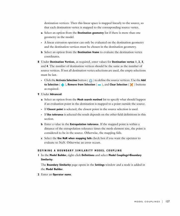
destination vertices. Then this linear space is mapped linearly to the source, so that each destination vertex is mapped to the corresponding source vertex.
a Select an option from the Destination geometry list if there is more than one geometry in the model.
- A linear extrusion operator can only be evaluated on the destination geometry and the destination vertices must be chosen in the destination geometry.
b Select an option from the Destination frame to evaluate the destination vertex coordinates.
8 Under Destination Vertices, as required, enter values for Destination vertex 1, 2, 3, and 4. The number of destination vertices should be the same as the number of source vertices. If not all destination vertex selections are used, the empty selections must be last.
- Click the Activate Selection button ( ) to define the source vertices. Use the Add
to Selection ( ), Remove from Selection ( ), and Clear Selection ( ) buttons as required.
9 Under Advanced:
a Select an option from the Mesh search method list to specify what should happen if an evaluation point in the destination is mapped to a point outside the source.
- If Closest point is selected, the closest point in the source selection is used.
- If Use tolerance is selected the result depends on the other field definitions in this section.
b Enter a value in the Extrapolation tolerance. If the mapped point is within a distance of the extrapolation tolerance times the mesh element size, the point is considered to be in the source. Otherwise, the mapping fails.
c Select the Use NaN when mapping fails check box if you want the operator to evaluate to NaN. Otherwise an error occurs.
D E F I N I N G A B O U N D A R Y S I M I L A R I T Y M O D E L C O U P L I N G
1 In the Model Builder, right-click Definitions and select Model Couplings>Boundary
Similarity.
The Boundary Similarity page opens in the Settings window and a node is added in the Model Builder.
2 Enter an Operator name.
M O D E L C O U P L I N G S | 127

128 | C H A P T E
3 Under Source Boundaries, select Manual or All Boundaries from the Selection list to define the source selection of a boundary similarity operator.
- If you select Manual, select geometric entities in the Graphics window.
- Select All boundaries to add all geometry to the Selection box.
Use the Add to Selection ( ), Remove from Selection ( ), and Clear Selection
( ) buttons as required. Also see Selecting and Deselecting Geometric Entities for detailed information.
4 Under Destination Boundary, enter a single boundary as the destination.
Click the Activate Selection button ( ) to define the source vertices. Use the Add
to Selection ( ), Remove from Selection ( ), and Clear Selection ( ) buttons as required.
5 Under Advanced:
a 2D: Select a relative Direction of the source and destination edges—Automatic, Same, or Opposite orientation. This specifies the relative direction of the source and boundary edges and allows you to specify which one of the two possible similarity mappings between the source and destination edge to use.
3D: Similar 3D direction functionality is provided by the subfeatures One Point
Map, Two-Point Map, and Edge Map to exactly specify the similarity mapping between the source and destination when more than one possibility exists. See Defining One-Point, Two-Point, or Edge Maps (3D).
b Select the Use source map check box to have a nonlinear correspondence between the source and destination. The source map is specified by entering expressions in the x-expression, y-expression, and z-expression fields.
c Select an option from the Mesh search method list to specify what should happen if an evaluation point in the destination is mapped to a point outside the source.
- If Closest point is selected, the closest point in the source selection is used.
- If Use tolerance is selected the result depends on the other field definitions in this section.
d Enter a value in the Extrapolation tolerance field. If the mapped point is within a distance of the extrapolation tolerance times the mesh element size, the point is considered to be in the source. Otherwise, the mapping fails.
e Select the Use NaN when mapping fails check box if you want the operator to evaluate to NaN. Otherwise an error occurs.
R 3 : G L O B A L A N D L O C A L D E F I N I T I O N S
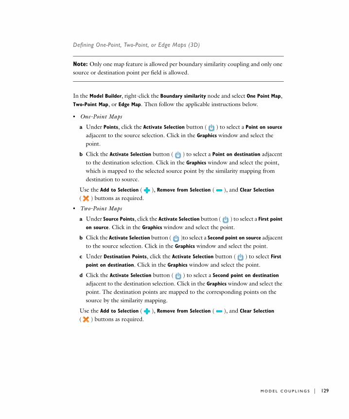
Defining One-Point, Two-Point, or Edge Maps (3D)
Note: Only one map feature is allowed per boundary similarity coupling and only one source or destination point per field is allowed.
In the Model Builder, right-click the Boundary similarity node and select One Point Map, Two-Point Map, or Edge Map. Then follow the applicable instructions below.
• One-Point Maps
a Under Points, click the Activate Selection button ( ) to select a Point on source adjacent to the source selection. Click in the Graphics window and select the point.
b Click the Activate Selection button ( ) to select a Point on destination adjacent to the destination selection. Click in the Graphics window and select the point, which is mapped to the selected source point by the similarity mapping from destination to source.
Use the Add to Selection ( ), Remove from Selection ( ), and Clear Selection
( ) buttons as required.
• Two-Point Maps
a Under Source Points, click the Activate Selection button ( ) to select a First point
on source. Click in the Graphics window and select the point.
b Click the Activate Selection button ( )to select a Second point on source adjacent to the source selection. Click in the Graphics window and select the point.
c Under Destination Points, click the Activate Selection button ( ) to select First point on destination. Click in the Graphics window and select the point.
d Click the Activate Selection button ( ) to select a Second point on destination adjacent to the destination selection. Click in the Graphics window and select the point. The destination points are mapped to the corresponding points on the source by the similarity mapping.
Use the Add to Selection ( ), Remove from Selection ( ), and Clear Selection
( ) buttons as required.
M O D E L C O U P L I N G S | 129

130 | C H A P T E
• Edge Maps
a Under Edges, click the Activate Selection button ( ) to select a Source edge. Click in the Graphics window and select the edge.
b Click the Activate Selection button ( ) to select a Destination edge. Click in the Graphics window and select the edge. The destination edge is mapped to the source edge by the similarity mapping from destination to source.
Use the Add to Selection ( ), Remove from Selection ( ), and Clear Selection
( ) buttons as required.
c Under Advanced, select a relative Direction of the source and destination edges—Automatic, Same, or Opposite orientation. This specifies the relative direction of the source and boundary edges and allows you to specify which one of the two possible similarity mappings between the source and destination edge to use.
D E F I N I N G A N I D E N T I T Y M A P P I N G M O D E L C O U P L I N G
1 In the Model Builder, right-click Definitions and select Model Couplings>Identity
Mapping.
The Identity Mapping page opens in the Settings window and a node is added in the Model Builder.
2 Enter an Operator name.
3 Under Source Selection, from the Geometric entity level list, select Domain, Boundary, Edge (3D only), or Point. Selection from this list turns on the button with the same name on the Graphics window.
4 Select Manual or All (Domains, Boundaries, Edges, or Points) from the Selection list.
- If you select Manual, select geometric entities in the Graphics window.
- Select All to add all applicable geometric entities to the Selection box.
Use the Add to Selection ( ), Remove from Selection ( ), and Clear Selection
( ) buttons as required. Also see Selecting and Deselecting Geometric Entities for detailed information.
5 Under Frames:
a Select a Source frame to use on the source geometric entity. In most cases the default Spatial frame can be used.
b Select a Destination frame to use on the destination geometric entity. In most cases default Spatial frame can be used.
R 3 : G L O B A L A N D L O C A L D E F I N I T I O N S
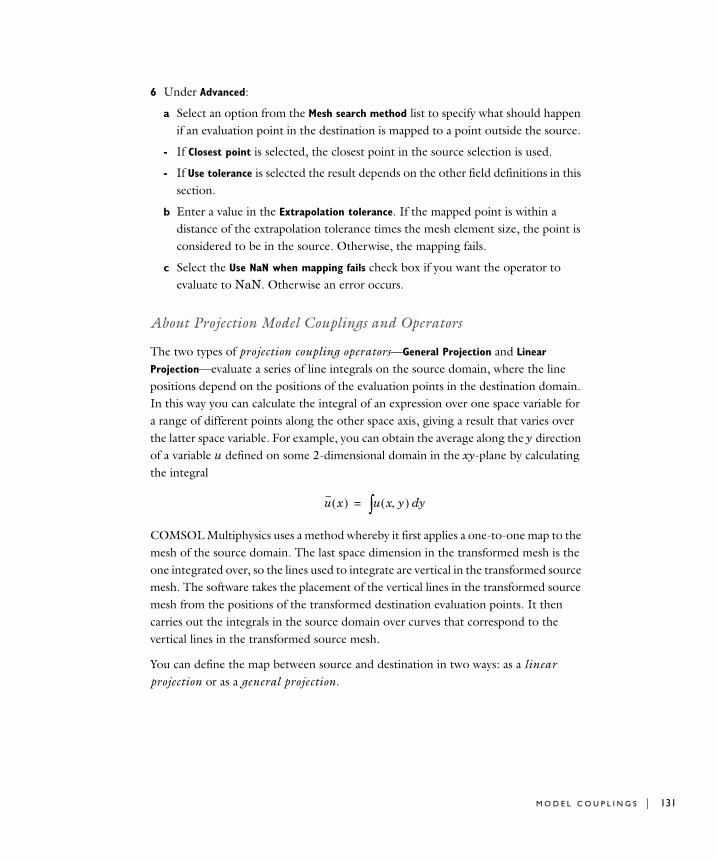
6 Under Advanced:
a Select an option from the Mesh search method list to specify what should happen if an evaluation point in the destination is mapped to a point outside the source.
- If Closest point is selected, the closest point in the source selection is used.
- If Use tolerance is selected the result depends on the other field definitions in this section.
b Enter a value in the Extrapolation tolerance. If the mapped point is within a distance of the extrapolation tolerance times the mesh element size, the point is considered to be in the source. Otherwise, the mapping fails.
c Select the Use NaN when mapping fails check box if you want the operator to evaluate to NaN. Otherwise an error occurs.
About Projection Model Couplings and Operators
The two types of projection coupling operators—General Projection and Linear
Projection—evaluate a series of line integrals on the source domain, where the line positions depend on the positions of the evaluation points in the destination domain. In this way you can calculate the integral of an expression over one space variable for a range of different points along the other space axis, giving a result that varies over the latter space variable. For example, you can obtain the average along the y direction of a variable u defined on some 2-dimensional domain in the xy-plane by calculating the integral
COMSOL Multiphysics uses a method whereby it first applies a one-to-one map to the mesh of the source domain. The last space dimension in the transformed mesh is the one integrated over, so the lines used to integrate are vertical in the transformed source mesh. The software takes the placement of the vertical lines in the transformed source mesh from the positions of the transformed destination evaluation points. It then carries out the integrals in the source domain over curves that correspond to the vertical lines in the transformed source mesh.
You can define the map between source and destination in two ways: as a linear projection or as a general projection.
u x u x y yd=
M O D E L C O U P L I N G S | 131
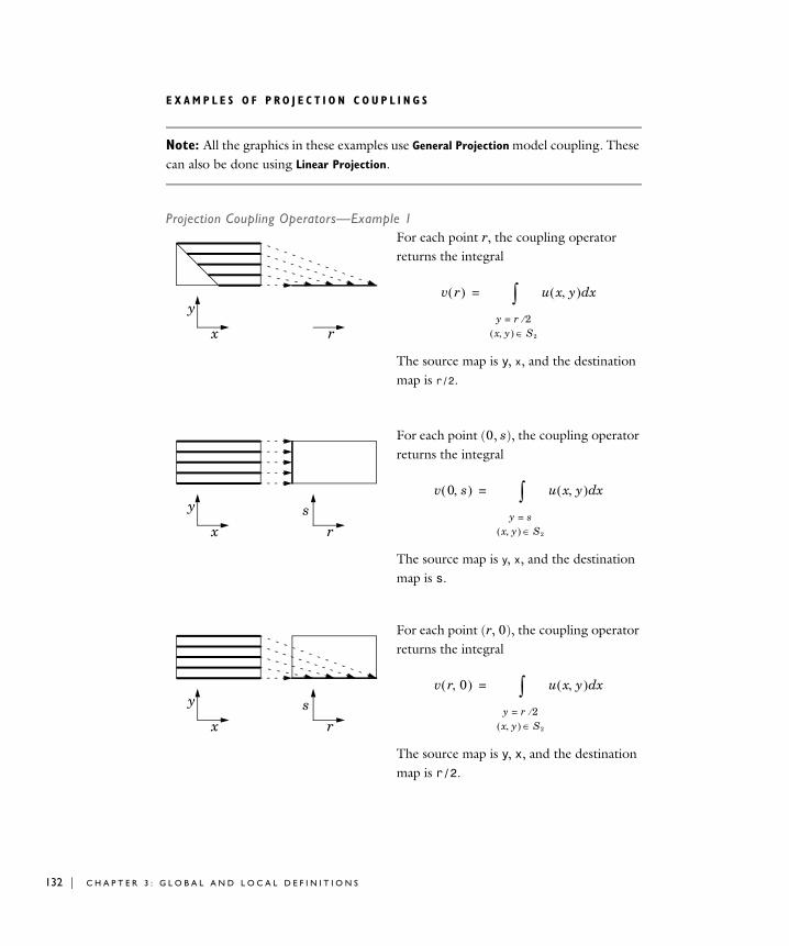
132 | C H A P T E
E X A M P L E S O F P R O J E C T I O N C O U P L I N G S
Note: All the graphics in these examples use General Projection model coupling. These can also be done using Linear Projection.
Projection Coupling Operators—Example 1For each point r, the coupling operator returns the integral
The source map is y, x, and the destination map is r/2.
For each point (0, s), the coupling operator returns the integral
The source map is y, x, and the destination map is s.
For each point (r, 0), the coupling operator returns the integral
The source map is y, x, and the destination map is r/2.
x r
yv r u x y xd
y r 2=
x y S2
=
x
y
rs
v 0 s u x y xd
y s=
x y S2
=
x
y
rs
v r 0 u x y xd
y r 2=
x y S2
=
R 3 : G L O B A L A N D L O C A L D E F I N I T I O N S

Note: The integration can also sweep nonrectangular domains. The integrals include only the source domains; they exclude other domains and the external area.
Projection Coupling Operators—Example 2Consider the case of a single rectangular domain with Poisson’s equation. Integrate the solution squared along lines parallel to the x-axis and make the result available for postprocessing on the left boundary.
The figure illustrates the projection process. Project the integral of the solution squared on the boundary. The source map is y, x and the destination map is y. If the projection operator is called genproj1, the desired result is obtained by evaluating genproj1(u^2).
Defining Projection Model Couplings
D E F I N I N G A G E N E R A L P R O J E C T I O N M O D E L C O U P L I N G
A projection coupling operator evaluates an expression defined on a source domain by integration along lines or curves depending on the evaluation point in the destination domain. Use a General Projection operator to define integration along curves.
Note: It is only possible to use projection model coupling with simplex elements such as triangles and tetrahedra.
About the General Source and Destination Map Vertices The General Projection operator is defined by mapping the source to an abstract intermediate space of dimension srcedim, and the destination to the subspace of dimension srcedim - 1 obtained by setting the last coordinate to 0. Here srcedim is the dimension of the source selection. To every point in the destination, there corresponds a vertical line in the intermediate space, obtained by allowing the last coordinate to vary while the remaining coordinates are given by the destination map. The set of points in the source selection which are mapped onto this line by the source
u– 1 on =
u 0 on =
x
y
x2
M O D E L C O U P L I N G S | 133

134 | C H A P T E
map, is a line or curve, and the projection operator is evaluated by integrating along this line or curve.
1 In the Model Builder, right-click Definitions and select Model
Couplings>General Projection.
The General Projection page opens in the Settings window and a node is added in the Model Builder.
2 Enter an Operator name.
3 Under Source Selection, from the Geometric entity level list, select Domain, Boundary, Edge (3D only), or Point. Selection from this list turns on the button with the same name on the Graphics window.
4 Select Manual or All (Domains, Boundaries, Edges, or Points) from the Selection list.
- If you select Manual, select geometric entities in the Graphics window.
- Select All to add the applicable geometry to the Selection box.
Use the Add to Selection ( ), Remove from Selection ( ), and Clear Selection
( ) buttons as required on the Settings window. Also see Selecting and Deselecting Geometric Entities for detailed information.
5 Under Source Map, specify the general projection source map by entering expressions in the x-expression, y-expression, and z-expression fields.
Note: The dimension of the intermediate space equals the dimension srcedim of the source selection. If the selection has lower dimension than the source geometry, specify only the first srcedim expressions.
You can use expressions containing space coordinates in the source geometry when defining the map. Remember that the map must be approximately linear within each mesh element.
6 Select a Source frame from the list.
R 3 : G L O B A L A N D L O C A L D E F I N I T I O N S

7 Under Destination Map, enter an x-expression and y-expression for each coordinate except the last in the intermediate space.
The destination map has one field less than the source map. When defining the map it is permissible to use expressions containing space coordinates in the destination geometry. The destination mapping can be highly nonlinear or noninvertible.
- If the selection has lower dimension than the source geometry, specify only the first srcedim1 expressions. A general projection operator can be evaluated at any point where its destination map is defined.
- If the source selection has dimension 1, no destination map needs to be specified, and consequently this section is not shown if the source geometry is 1D. In this case, it is probably better to use an Integration coupling.
8 Under Advanced, enter an Integration order of the numerical integration method.
D E F I N I N G A L I N E A R P R O J E C T I O N M O D E L C O U P L I N G
Use a Linear Projection when the argument is to be integrated along a line, and the line depends linearly on the evaluation point.
The linear projection maps between source domains and destination domains of the nearest lower dimension. The domains can exist in geometries of different space dimensions. For example, you can couple from subdomains in 2D to edges in 3D; you can also couple 3D subdomains to 2D subdomains. Define the linear projection by specifying points in both the source and destination domains.
About the Linear Source and Destination Map Vertices The Source Vertices and Destination Vertices together define a linear mapping from the destination to the source. An evaluation point in the destination geometry is first orthogonally projected onto the linear space spanned by the destination vertices (unless they span the entire space). The projected point is then mapped to the source geometry by a linear mapping taking each destination vertex to the corresponding source vertex. Let L be the line through this point which is parallel to a line through the first and the last source vertex.
If the source selection lies in the linear space spanned by the source vertices, the Linear Projection operator is evaluated by integrating along the line L. In general the operator is evaluated by integrating along the line or curve in the source selection which is mapped to L under orthogonal projection onto the linear space spanned by the source vertices.
M O D E L C O U P L I N G S | 135
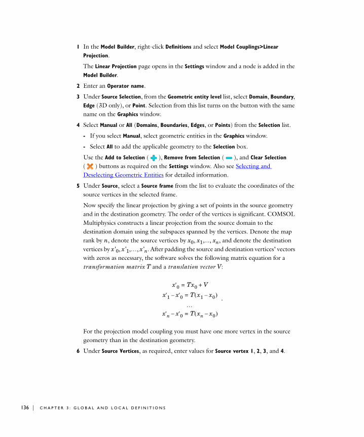
136 | C H A P T E
1 In the Model Builder, right-click Definitions and select Model Couplings>Linear
Projection.
The Linear Projection page opens in the Settings window and a node is added in the Model Builder.
2 Enter an Operator name.
3 Under Source Selection, from the Geometric entity level list, select Domain, Boundary, Edge (3D only), or Point. Selection from this list turns on the button with the same name on the Graphics window.
4 Select Manual or All (Domains, Boundaries, Edges, or Points) from the Selection list.
- If you select Manual, select geometric entities in the Graphics window.
- Select All to add the applicable geometry to the Selection box.
Use the Add to Selection ( ), Remove from Selection ( ), and Clear Selection
( ) buttons as required on the Settings window. Also see Selecting and Deselecting Geometric Entities for detailed information.
5 Under Source, select a Source frame from the list to evaluate the coordinates of the source vertices in the selected frame.
Now specify the linear projection by giving a set of points in the source geometry and in the destination geometry. The order of the vertices is significant. COMSOL Multiphysics constructs a linear projection from the source domain to the destination domain using the subspaces spanned by the vertices. Denote the map rank by n, denote the source vertices by x0, x1,..., xn, and denote the destination vertices by x'0, x'1,…, x'n. After padding the source and destination vertices’ vectors with zeros as necessary, the software solves the following matrix equation for a transformation matrix T and a translation vector V:
.
For the projection model coupling you must have one more vertex in the source geometry than in the destination geometry.
6 Under Source Vertices, as required, enter values for Source vertex 1, 2, 3, and 4.
x'0 Tx0 V+=
x'1 x'0– T x1 x0– =
x'n x'0– T xn x0– =
R 3 : G L O B A L A N D L O C A L D E F I N I T I O N S
Note: The selection of Source Vertices and Destination Vertices together define the linear mapping from the destination to the source.
- Select srcedim + 1 source vertices where srcedim is the dimension of the source selection. Depending on the dimension of the source selection, it may be that some of the last source vertex selections should be left empty.
- If not all source vertices selections are used, the empty selections must be last.
- Click the Activate Selection button ( ) to define the source vertices. Use the Add
to Selection ( ), Remove from Selection ( ), and Clear Selection ( ) buttons as required.
7 Under Destination, select an option from the Destination geometry list if there is more than one geometry in the model.
- A linear projection operator can only be evaluated on the destination geometry and the destination vertices must be chosen in the destination geometry.
- The destination vertex coordinates are evaluated in the selected Destination frame.
8 Under Destination Vertices, as required, enter values for Destination vertex 1, 2, and 3. The number of destination vertices should be one less than the number of source vertices. If not all destination vertex selections are used, the empty selections must be last.
- Select srcedim destination vertices where srcedim is the dimension of the source selection. Depending on the dimension of the source selection, it may be that some of the last destination vertex selections should be left empty.
- Click the Activate Selection button ( ) to define the source vertices. Use the Add
to Selection ( ), Remove from Selection ( ), and Clear Selection ( ) buttons as required.
9 Under Advanced you can enter an Integration order of the numerical integration method.
About Scalar Model Couplings and Operators
A B O U T I N T E G R A T I O N M O D E L C O U P L I N G S A N D O P E R A T O R S
An integration coupling operator is the value of an integral of an expression over a set of geometric entities (domains, for example). Thus, the integration coupling operator is always a scalar quantity. The source of the operator can be an expression at a vertex
M O D E L C O U P L I N G S | 137
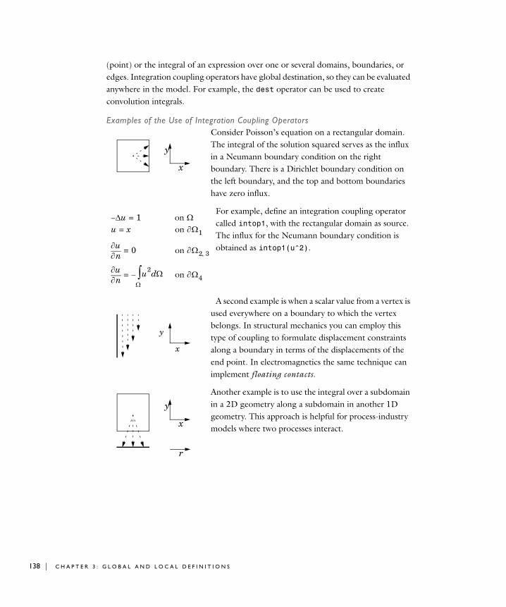
138 | C H A P T E
(point) or the integral of an expression over one or several domains, boundaries, or edges. Integration coupling operators have global destination, so they can be evaluated anywhere in the model. For example, the dest operator can be used to create convolution integrals.
Examples of the Use of Integration Coupling OperatorsConsider Poisson’s equation on a rectangular domain. The integral of the solution squared serves as the influx in a Neumann boundary condition on the right boundary. There is a Dirichlet boundary condition on the left boundary, and the top and bottom boundaries have zero influx.
For example, define an integration coupling operator called intop1, with the rectangular domain as source. The influx for the Neumann boundary condition is obtained as intop1(u^2).
A second example is when a scalar value from a vertex is used everywhere on a boundary to which the vertex belongs. In structural mechanics you can employ this type of coupling to formulate displacement constraints along a boundary in terms of the displacements of the end point. In electromagnetics the same technique can implement floating contacts.
Another example is to use the integral over a subdomain in a 2D geometry along a subdomain in another 1D geometry. This approach is helpful for process-industry models where two processes interact.
x
y
u– 1= on u x= on 1
nu 0= on 2 3
nu u2 d
–= on 4
x
y
x
y
r
R 3 : G L O B A L A N D L O C A L D E F I N I T I O N S
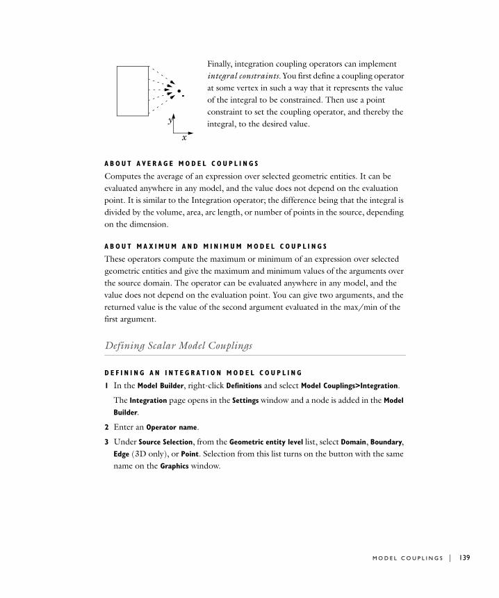
Finally, integration coupling operators can implement integral constraints. You first define a coupling operator at some vertex in such a way that it represents the value of the integral to be constrained. Then use a point constraint to set the coupling operator, and thereby the integral, to the desired value.
A B O U T A V E R A G E M O D E L C O U P L I N G S
Computes the average of an expression over selected geometric entities. It can be evaluated anywhere in any model, and the value does not depend on the evaluation point. It is similar to the Integration operator; the difference being that the integral is divided by the volume, area, arc length, or number of points in the source, depending on the dimension.
A B O U T M A X I M U M A N D M I N I M U M M O D E L C O U P L I N G S
These operators compute the maximum or minimum of an expression over selected geometric entities and give the maximum and minimum values of the arguments over the source domain. The operator can be evaluated anywhere in any model, and the value does not depend on the evaluation point. You can give two arguments, and the returned value is the value of the second argument evaluated in the max/min of the first argument.
Defining Scalar Model Couplings
D E F I N I N G A N I N T E G R A T I O N M O D E L C O U P L I N G
1 In the Model Builder, right-click Definitions and select Model Couplings>Integration.
The Integration page opens in the Settings window and a node is added in the Model
Builder.
2 Enter an Operator name.
3 Under Source Selection, from the Geometric entity level list, select Domain, Boundary, Edge (3D only), or Point. Selection from this list turns on the button with the same name on the Graphics window.
x
y
M O D E L C O U P L I N G S | 139
140 | C H A P T E
4 Select Manual or All (Domains, Boundaries, Edges, or Points) from the Selection list.
- If you select Manual, select geometric entities on the Graphics window. The buttons are already activated.
- Select All to add the applicable geometry to the Selection box.
Use the Add to Selection ( ), Remove from Selection ( ), and Clear Selection
( ) buttons as required on the Settings window. Also see Selecting and Deselecting Geometric Entities for detailed information.
5 Under Advanced, from the Method list select Integration or Summation over nodes. In most cases use integration. Summation over nodes is useful, for example, for computing reaction forces. If Integration is selected, enter a value in the Integration
order field.
6 Under Advanced, when working with multiple frames, select a Frame from the list for the volume element to be used in the integration.
D E F I N I N G A N A V E R A G E M O D E L C O U P L I N G
1 In the Model Builder, right-click Definitions and select Model Couplings>Average.
The Average page opens in the Settings window and a node is added in the Model
Builder.
2 Enter an Operator name.
3 Under Source Selection, from the Geometric entity level list, select Domain, Boundary, Edge (3D only), or Point. Selection from this list turns on the button with the same name on the Graphics window.
4 Select Manual or All (Domains, Boundaries, Edges, or Points) from the Selection list.
- If you select Manual, select geometric entities on the Graphics window. The buttons are already activated.
- Select All to add the applicable geometry to the Selection box.
Use the Add to Selection ( ), Remove from Selection ( ), and Clear Selection
( ) buttons as required on the Settings window. Also see Selecting and Deselecting Geometric Entities for detailed information.
5 Under Advanced:
a Enter an Integration order.
b When working with multiple frames, select a Frame from the list for the volume element to be used in the average.
R 3 : G L O B A L A N D L O C A L D E F I N I T I O N S

D E F I N I N G M A X I M U M A N D M I N I M U M M O D E L C O U P L I N G S
1 In the Model Builder, right-click Definitions and select Model Couplings>Maximum or Minimum.
The Maximum or Minimum page opens in the Settings window and a node is added in the Model Builder.
2 Enter an Operator name.
3 Under Source Selection, from the Geometric entity level list, select Domain, Boundary, Edge (3D only), or Point. Selection from this list turns on the button with the same name on the Graphics window.
4 Select Manual or All (Domains, Boundaries, Edges, or Points) from the Selection list.
- If you select Manual, select geometric entities on the Graphics window. The buttons are already activated.
- Select All to add the applicable geometry to the Selection box.
Use the Add to Selection ( ), Remove from Selection ( ), and Clear Selection
( ) buttons as required on the Settings window. Also see Selecting and Deselecting Geometric Entities for detailed information.
5 Under Advanced, the Point type controls the choice of evaluation points—the result is more accurate with more points but more points also means a slower evaluation.
a From the Point type list, select Node points, Lagrange points, or Integration points to compute the maximum or minimum by evaluating the argument expression at a finite set of points in the source and taking the maximum or minimum of these values.
b If Integration points is selected, enter an Integration order of 1. The default is 4.
c If Lagrange points is selected, enter a Lagrange order. The default is 2.
M O D E L C O U P L I N G S | 141

142 | C H A P T E
Coo r d i n a t e S y s t em s
COMSOL Multiphysics uses a global Cartesian coordinate system by default to specify loads and constraints in all physics interfaces and on all geometric entity levels (points, edges, boundaries, and domains). Also see Space Coordinate Variables.
The Cartesian coordinate system space coordinates default to the following names in 2D and 3D (in 2D axisymmetric geometries, COMSOL Multiphysics uses cylindrical coordinates):
In 3D, an image displays in the lower-left corner of the Graphics window to indicate this coordinate system.
User defined coordinate systems can be used on all geometric entity levels to simplify the modeling process. In some of the physics interfaces, you can use these coordinate systems to define orthotropic and anisotropic material properties that are not aligned with the global Cartesian coordinate system, for example. See Table 3-12.
GEOMETRY DEFAULT NAME OF SPACE COORDINATES
2D x y
3D x y z
Axial symmetry 2D r z
TABLE 3-12: COORDINATE SYSTEM DESCRIPTIONS
COORDINATE SYSTEM
DESCRIPTION GO TO
Boundary System,
2D and 3D. A local base vector system on 2D boundaries (t, n) and on 3D boundaries (t1, t2, n). Use it to apply loads that apply in a normal or tangential direction on a boundary that is not aligned with the global Cartesian coordinate system. This coordinate system is always available.
page 143
Base Vector System
1D, 2D, and 3D. Define this using a set of base vectors to form a coordinate system, which you can declare as orthonormal.
page 145
Cylindrical System
2D and 3D. Use this where rotational symmetry about the axis is required. Not applicable in geometries with 2D axisymmetry.
page 146
R 3 : G L O B A L A N D L O C A L D E F I N I T I O N S

About Boundary Coordinate Systems
Note: For 2D and 3D models, the Boundary System node is automatically added under Definitions.
The boundary coordinate system is available on boundaries in 2D and 3D. Boundary systems are not available in 1D. Use it to apply loads that apply in a normal or tangential direction on a boundary that is not aligned with the global Cartesian coordinate system. Common applications for this coordinate system include specifying pressure or normal displacement on a surface.
To specify the boundary coordinate system, you specify the direction of the normal and a direction that is projected onto the boundary, normalized, and used as the first tangent vector.
The normal direction is in most cases the outward-pointing normal vector. The general definition of the normal (for shells, for example), is the direction of the normal vector n, which you can plot using the variables for its components (typically nx, ny, and nz). See Normal Variables for more information.
2 D B O U N D A R Y C O O R D I N A T E S Y S T E M
• In 2D the local coordinate system is defined by (t1, n, to), representing the tangential and normal direction of the boundary.
Mapped System
1D, 2D and 3D. This can deal with spherical and cylindrical coordinates, and translated and rotated coordinate systems. Use this to create a system that defines a mapping from the frame coordinate system.
page 147
Rotated System
2D and 3D. Use this to define rotation about the out-of-plane direction in 2D and Euler angles in 3D.
page 148
TABLE 3-12: COORDINATE SYSTEM DESCRIPTIONS
COORDINATE SYSTEM
DESCRIPTION GO TO
C O O R D I N A T E S Y S T E M S | 143
144 | C H A P T E
• This coordinate system is always right-oriented. For exterior boundaries the normal is by default directed out from the domain. The user can reverse the normal direction.
• The second tangent direction (to) is the cross product between normal vector (n) and the first tangent direction (t1). This method always gives a right-oriented orthonormal system, unless the tangent direction is parallel to the normal.
3 D B O U N D A R Y C O O R D I N A T E S Y S T E M
• In 3D the local coordinate system is defined by (t1, t2, n), representing two tangential directions and one normal direction. t1 and t2 depend on the parametrization of the geometry.
• This coordinate system is always right-oriented but not always orthogonal. For exterior boundaries the normal is by default directed out from the domain. The user can reverse the normal direction.
• Common applications for this coordinate system include specifying pressure or normal displacement on a surface.
• The second tangent direction (t2) is the cross product between the specified normal vector (n) and the first tangent vector (t1). This method always gives a right-oriented orthonormal system, unless the tangent direction is parallel to the normal.
Defining a Boundary Coordinate System
Note: For 2D and 3D models, a Boundary System node is automatically added under Definitions.
1 In the Model Builder, right-click Definitions and select Coordinate Systems>Boundary
System.
The Boundary System page opens in the Settings window and a node is added in the Model Builder.
2 Enter a Coordinate System Identifier.
3 Under Settings, select a Frame type—Reference configuration, or Deformed
configuration (the default).
4 In the Coordinate names table, the default names are entered—t1, t2, and n (for 3D models) or t1, n, and to (for 2D models). Click the table cells to edit the names.
R 3 : G L O B A L A N D L O C A L D E F I N I T I O N S

Note: t1 and t2 depend on how the geometry was created and are usually perpendicular to each other.
5 To reverse the direction of the normal for the boundary system, select the Reverse
normal direction check box.
6 Select an option from the Create first tangential direction from list: Global Cartesian or Manual.
7 If Global Cartesian is selected, select 1, 2, or 3 (that is, x, y, or z) from the Axis list.
8 If Manual is selected, default values are displayed for the local tangent variables t1x, t1y, and t1z (3D) or t1x and t1y (2D). Enter other values as required to define a tangent direction by specifying directions for a local tangent plane in the x, y, and z fields.
About Base Vector Systems
Define a Base Vector System using a set of base vectors to form a coordinate system, which you can declare as orthonormal.
A vector F in the base of the new base vector system defined by the base vectors u1, u2, and u3 becomes FF1u1F2u2F3u3, and the transformation matrix between bases is
where the last equality holds when the base vector system is orthonormal.
Fx
Fy
Fz
u1 u2 u3
F1
F2
F3
=
F1
F2
F3
u1 u2 u3
1–Fx
Fy
Fz
ui 1=
ui uj ij=
u1 u2 u3
TFx
Fy
Fz
= = =
C O O R D I N A T E S Y S T E M S | 145

146 | C H A P T E
Defining a Base Vector Coordinate System
1 In the Model Builder, right-click Definitions and select Coordinate Systems>Base Vector
System.
The Base Vector System page opens in the Settings window and a node is added in the Model Builder.
2 Enter a Coordinate System Identifier.
3 Under Settings, in the Coordinate names table, the default names are entered—x1, x2, and x3. In planar 2D models, x1 and x2 are typically the in-plane coordinates, and x3 is the out-of-plane coordinate.
4 Under Base vectors, define the base vectors in terms of the global Cartesian coordinates x1, x2, and x3; one base vector on each row (two for 2D and three for 3D).
5 1D and 2D: Select the Plane Index:
- 1D: Select an option from the In-plane index list. The default is 1.
- 2D: Select an option from the Out-of-plane index list. The defaults are 3 for a plane 2D model and 2 for an axisymmetric 2D model.
For example, to map the first vector, x1, to the direction defined by yx in 2D, enter 1 in the fields under x and y on the x1 row.
6 Under Forced simplifications, define properties for the base vector systems to simplify the coordinate transformations.
7 Select the Orthonormal check box to define the system as orthonormal.
About Cylindrical Coordinate Systems
A Cylindrical Coordinate System may be used in 2D and 3D where rotational symmetry about the axis is required. Note that the cylindrical coordinate system is not applicable in geometries with 2D axisymmetry.
The local coordinate system is defined by where r represents the radial distance from the longitudinal axis, is the azimuthal angle and is the distance from origin along the longitudinal axis. In 2D one can only specify the origin, whereas in 3D one may specify the longitudinal axis direction, a, and the radial base vector,
, as well. These direction vectors are automatically normalized.
The definition of the cylindrical coordinates in terms of the global cartesian coordinates are
r a
er 0=
r r x y z =
R 3 : G L O B A L A N D L O C A L D E F I N I T I O N S

Defining a Cylindrical Coordinate System
1 In the Model Builder, right-click Definitions and select Coordinate Systems>Cylindrical
System.
The Cylindrical System page opens in the Settings window and a node is added in the Model Builder.
2 Enter a Coordinate System Identifier.
3 Under Settings, select a Frame type—Mesh, Material, or Spatial. The default is Spatial.
4 In the Coordinate names table, the default Coordinate names are entered—r, phi, and a. In planar 2D models, r and phi are the in-plane coordinates, and a is the out-of-plane coordinate.
5 Enter the Origin of system. The default is an origin coinciding with the one from the global system.
6 For 3D enter the Axis direction. The default axis direction is the z direction in the global system.
7 In 3D enter the Radial base vector direction for azimuthal angle . The default direction is the x direction in the global system.
About Mapped Coordinate Systems
Use a Mapped Coordinate System to create a system that defines a mapping from the frame coordinate system. This method can deal with spherical coordinates, cylindrical coordinates, and translated and rotated coordinate systems.
ra
r r0 a a r r0– + –
a er r r0– er r r0–
---------------------------------------------atan
a r r0–
=
0=
u1
u2
u3
u1 x y z ( )
u2 x y z ( )
u3 x y z ( )
=
C O O R D I N A T E S Y S T E M S | 147

148 | C H A P T E
Defining a Mapped Coordinate System
1 In the Model Builder, right-click Definitions and select Coordinate Systems>Mapped
System.
The Mapped System page opens in the Settings window and a node is added in the Model Builder.
2 Enter a Coordinate System Identifier.
3 Under Settings, select a Frame type—Mesh, Material, or Spatial. The default is Spatial.
4 In the Coordinate names table, the default names are entered—x1, x2, and x3. In planar 2D models, x1 and x2 are typically the in-plane coordinates, and x3 is the out-of-plane coordinate.
5 Under Coordinate mapping, the Coordinate column displays the Coordinate names with the Expression column displaying the associated mapped coordinate.
6 If required, under Forced simplifications, select the Orthonormal check box.
About Rotated Coordinate Systems
Use the Rotated Coordinate System to define rotation about the out-of-plane direction in 2D and Euler angles in 3D.
On the Rotated System page, you define the rotation relative to the global Cartesian coordinate system. In 3D you specify the local coordinate system (xl, yl, zl) using three consecutive Euler angles (rotation angles) , , and . See Figure 3-2.
In 2D you describe the rotated coordinate system by the rotation angle about the out-of-plane vector. In both cases you can define the origin of the coordinate system.
R 3 : G L O B A L A N D L O C A L D E F I N I T I O N S
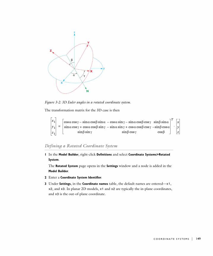
xyz
Figure 3-2: 3D Euler angles in a rotated coordinate system.
The transformation matrix for the 3D case is then
Defining a Rotated Coordinate System
1 In the Model Builder, right-click Definitions and select Coordinate Systems>Rotated
System.
The Rotated System page opens in the Settings window and a node is added in the Model Builder.
2 Enter a Coordinate System Identifier.
3 Under Settings, in the Coordinate names table, the default names are entered—x1, x2, and x3. In planar 2D models, x1 and x2 are typically the in-plane coordinates, and x3 is the out-of-plane coordinate.
x1
y1
z1
coscos sincossin– sincos– coscossin– sinsin cossin sincoscos+ sinsin– coscoscos+ cossin–
sinsin cossin cos
T
=
C O O R D I N A T E S Y S T E M S | 149

150 | C H A P T E
4 Enter a Out of Plane Rotation or Euler Angles:
2D Models:
a Enter the Rotation about out-of-plane axis (in radians).
b Select the coordinate from the Out-of-plane index field. The default index is 3 for planar 2D models and 2 for axisymmetric 2D models.
3D Models: Enter the Euler angles (Z-X-Z) (in radians) in the , , and fields.
5 In the Origin of System field, define the origin of the rotated coordinate system. Define it as a vector with two (for 2D) or three (for 3D) components.
The default is the origin for the global Cartesian coordinate system. Using another origin translates the coordinates in the rotated system by that distance from the global Cartesian origin.
R 3 : G L O B A L A N D L O C A L D E F I N I T I O N S

I d e n t i t y and Con t a c t Pa i r s
Pairs are available for assemblies (that is, geometries created by not forming a union of all geometry objects as the final step), where you need to connect boundaries between parts. There are two types of pairs:
• Identity pairs: these pairs make the fields across two connected boundaries (one from each connecting part) continuous. This is equivalent to the continuity that you get by default on interior boundaries in a geometry created by forming a union. Some physics interfaces provide special boundary conditions for identity pairs.
Use an Identity Pair to specify two selections of boundaries that overlap but belong to different parts of an assembly. Then assign a boundary condition to connect the physics in the two parts in a physics interface. Identity pairs connect overlapping boundaries in different connecting parts of an assembly.
• Contact pairs: these pairs define boundaries where the parts may come into contact but cannot penetrate each other under deformation for modeling of structural contact and multiphysics contact.
Note: Contact modeling requires the Structural Mechanics Module or MEMS Module.
Use a Contact Pair to specify two selections of boundaries that cannot penetrate each other under deformation. The contact pairs defined boundaries for parts that may come into contact (boundaries that cannot penetrate each other under deformation).
Defining an Identity Pair
1 In the Model Builder, right-click Definitions and select Identity Pair ( ).
The Identity Pair page opens in the Settings window and a node is added under Definitions.
2 Enter a Pair name. It is used as a suffix in names of operators and variables defined by the pair.
The operator mapping an expression E on the source side to the destination side is denoted src2dst_pn(E), where pn is the pair name. The variable src2dst_pn (defined on the destination) is 1 where there is a corresponding source point, and 0
I D E N T I T Y A N D C O N T A C T P A I R S | 151

152 | C H A P T E
otherwise. The corresponding operator and variable for use on the source side are denoted dst2src_pn.
3 Under Source Boundaries:
a Click the Activate Selection button ( ) to define the source boundaries.
b Select Manual or All Boundaries for the boundaries on the source side.
If Manual is selected, click in the Graphics window to add boundaries to the Selection section.
Use the Add to Selection ( ), Remove from Selection ( ), and Clear Selection
( ) buttons as required.
4 If required, click the Swap Source and Destination button ( ) to swap the source boundaries and the destination boundaries.
5 Under Destination Boundaries:
a Click the Activate Selection button ( ) to define the source boundaries.
b Select Manual or All Boundaries for the boundaries on the destination side.
These boundaries should overlap the source boundaries. The condition that connects the physics on the destination and source boundaries is specified in the physics interface. For example, it can be a constraint that constrains a dependent variables (temperature, for example) on the destination side to be equal to a dependent variable on the source side.
If Manual is selected, click in the Graphics window to add boundaries to the Selection section.
Use the Add to Selection ( ), Remove from Selection ( ), and Clear Selection
( ) buttons as required.
6 If there are several frames in the model, the Frame section is available. Select the Source frame and the Destination frame. Source and destination points are connected if their coordinates in their respective frames are equal.
7 If required, click the Swap Source and Destination button ( ) to swap the source boundaries and the destination boundaries.
Defining a Contact Pair
1 In the Model Builder, right-click Definitions. Select Contact Pair ( ).
The Contact Pair page opens in the Settings window and a node is added under Definitions.
R 3 : G L O B A L A N D L O C A L D E F I N I T I O N S

2 Enter a Pair name. It is used as a suffix in names of operators and variables defined by the pair.
The operator mapping an expression E on the source side to the destination side is denoted mst2slv_pn(E), where pn is the pair name. Similarly, there is an operator mst2slv_pn_mph that is suited for use in multiphysics coupling.
The variable geomgap_slv_pn is the geometric gap between the source and the destination, seen from the destination side (following the normal of the destination boundary).
The corresponding operators and variables for use on the master side are denoted slv2mst_pn, slv2mst_pn_mph, geomgap_mst_pn.
3 Under Source Boundaries:
a Click the Activate Selection button ( ) to define the source boundaries.
b Select Manual or All Boundaries for the boundaries on the source side.
If Manual is selected, click in the Graphics window to add boundaries to the Selection section.
Use the Add to Selection ( ), Remove from Selection ( ), and Clear Selection
( ) buttons as required.
4 If required, click the Swap Source and Destination button ( ) to swap the source boundaries and the destination boundaries.
5 Under Destination Boundaries:
a Click the Activate Selection button ( ) to define the source boundaries.
b Select Manual or All Boundaries for the boundaries on the destination side.
If you selected Manual, click in the Graphics window to add boundaries to the Selection section.
The contact algorithm constrains the destination boundaries so that they do not penetrate the source boundaries.
6 If required, click the Swap Source and Destination button ( ) to swap the source boundaries and the destination boundaries.
I D E N T I T Y A N D C O N T A C T P A I R S | 153

154 | C H A P T E
7 Under Advanced:
a The Search method defaults to Fast—the algorithm only keeps track of source and destination points that have a distance less than a certain search distance. Select Direct for a slower, but more robust, search.
b Select the Manual control of search distance check box to tune the search distance (SI unit: m). By default, the search distance is taken as 0.01 times the diagonal of the geometry’s bounding box.
c If the Manual control of search distance check box is selected, enter a different value in the Distance field.
R 3 : G L O B A L A N D L O C A L D E F I N I T I O N S
P r ob e s
Probes monitor the development of a scalar-valued quantity (real or complex valued number) from a dynamic simulation (time-dependent, frequency, parametric), by two different techniques; tabulated data and 1D graph plots. It is meaningful to probe while solving, and to probe after the computation is finished.
Plot while solving is a technique used to halt the simulation and launch some predefined plot commands and then continue with the simulation.
Defining a Domain, Boundary, or Edge Probe
1 In the Model Builder, right-click Definitions and select Probes>Domain Probe, Boundary Probe, or Edge Probe (3D).
The Domain, Boundary, or Edge Probe page opens in the Settings window and a node is added in the Model Builder.
2 Under Probe Settings, select an option from the Type list—Average, Maximum, Minimum, or Integral.
3 Enter a Probe name.
4 Under Source Selection, from the Selection list, select Manual or All (Domains, Boundaries, or Edges).
- If Manual is selected, select the domain, boundary or edge in the Graphics window.
- Select All to add the domain, boundary or edge to the Selection box.
Use the Add to Selection ( ), Remove from Selection ( ), and Clear Selection
( ) buttons as required in the Settings window.
For general information about selections, see Using the Selection List Window.
5 Under Expression:
a Click the Replace Expression ( ) or Insert Expression ( ) buttons to select predefined expressions based on the physics of the model. Or enter an Expression.
b Select a Unit.
c Select the Description check box to enter a description of the data set (or edit the default).
P R O B E S | 155
156 | C H A P T E
6 Under Integration Settings:
a From the Method list, select Integration or Summation.
b Enter a value in the Integration order field.
c When working with multiple frames, select a Frame from the list for the volume element to be used in the integration.
Defining a Domain Point Probe
1 In the Model Builder, right-click Definitions and select Probes>Domain Point Probe.
The Domain Point Probe page opens in the Settings window and a node is added in the Model Builder.
2 Under Point Selection select an option from the Line entry method list—Point and
surface normal, Point and direction, Two Points, or None. If None is selected, go to step c.
a If Two Points is selected, from the Point being modified list, select First point or Second point.
b Enter a Depth along line or use the slider to select a value.
c Enter Coordinates. For 2D enter x and y coordinates; for 3D enter x, y, and z coordinates.
d Select the Snap to closest boundary check box to snap the selected points to the grid.
3 If required, define a Point Probe Expression.
Note: A Point Probe Expression node is automatically added under Domain Point Probe. To add more nodes, right-click Domain Point Probe and select Point Probe
Expression.
4 In the Model Builder, under Domain Point Probe, click Point Probe Expression.
The Point Probe Expression page opens in the Settings window.
5 Enter a Probe name.
R 3 : G L O B A L A N D L O C A L D E F I N I T I O N S

6 Under Expression:
a Click the Replace Expression ( ) or Insert Expression ( ) buttons to select predefined expressions based on the physics of the model. Or enter an Expression.
b Select a Unit.
c Select the Description check box to enter a description of the data set (or edit the default).
Defining a Boundary Point Probe
1 In the Model Builder, right-click Definitions and select Probes>Boundary Point Probe.
The Boundary Point Probe page opens in the Settings window and a node is added in the Model Builder.
2 In the Graphics window, click the boundary to add to the Boundary Selection section.
3 Under Point Selection enter the Coordinates. For 2D enter x and y coordinates; for 3D enter x, y, and z coordinates.
4 Define a Point Probe Expression.
Note: A Point Probe Expression node is automatically added under Boundary Point Probe. To add more nodes, right-click Boundary Point Probe and select Point Probe
Expression.
5 In the Model Builder, under Boundary Point Probe, click Point Probe Expression.
The Point Probe Expression page opens in the Settings window.
6 Enter a Probe name.
7 Under Expression:
a Click the Replace Expression ( ) or Insert Expression ( ) buttons to select predefined expressions based on the physics of the model. Or enter an Expression.
b Select a Unit.
c Select the Description check box to enter a description of the data set (or edit the default).
P R O B E S | 157
158 | C H A P T E
Defining a Global Variable Probe
1 In the Model Builder, right-click Definitions and select Probes>Global Variable Probe.
The Global Variable Probe page opens in the Settings window and a node is added in the Model Builder.
2 Enter a Probe name.
3 Under Expression:
a Click the Replace Expression ( ) or Insert Expression ( ) buttons to select predefined expressions based on the physics of the model. Or enter an Expression.
b Select a Unit.
c Select the Description check box to enter a description of the data set (or edit the default).
R 3 : G L O B A L A N D L O C A L D E F I N I T I O N S

4
V i s u a l i z a t i o n a n d S e l e c t i o n T o o l s
COMSOL Multiphysics provides a number of tools to visualize and control how you view models in the Graphics window.
In this section:
• Working with 3D Geometry
• User-Defined Selections
• User-Defined Views
• Screenshots
159

160 | C H A P T E
Work i n g w i t h 3D Geome t r y
COMSOL Multiphysics has many ways to zoom, rotate, and move around the Graphics window in order to adjust the view of a 3D model during its creation and analysis. There are also several ways to select each part of the geometry, the geometric entities, and create reusable Selections and Views.
While building 3D models, it is important to clearly understand what the object looks like and to easily select specific features within the geometry. For example:
• Highlight, select, or hide any part of the geometry using buttons, mouse clicks, keyboard shortcuts, or combinations of actions;
• Create user defined Selections to reuse throughout the model;
• View an object where the edges of a part are represented by solid lines (wireframe rendering);
• Capture a screen-shot of the Graphics window; and
• Control visualization quality with lighting and transparency.
COMSOL Multiphysics also provides many visual tools to help you create a model. For example:
• Different colors, thicker edges (with OpenGL and Software rendering only, not DirectX. See Editing Model Preferences Settings), or larger points to highlight the different geometric entities selected;
• A Selection List window to list all the specific geometric entities in the model and to locate and select complex geometric entities;
• Logical selection of overlapping objects in the Graphics window;
• A variety of Show/Hide and Select buttons in the Graphics toolbar;
• The option to create predefined Views of the geometry. and
• The ability to choose different view combinations of Names, Identifiers, Tags, and Types in the Model Builder (see Building a COMSOL Model).
R 4 : V I S U A L I Z A T I O N A N D S E L E C T I O N TO O L S
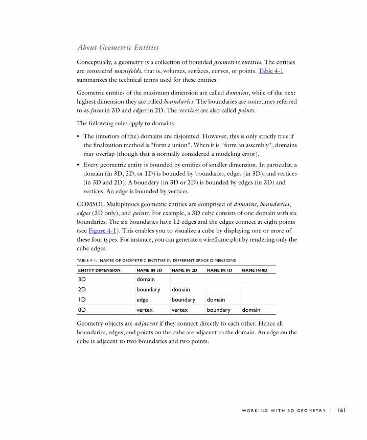
About Geometric Entities
Conceptually, a geometry is a collection of bounded geometric entities. The entities are connected manifolds, that is, volumes, surfaces, curves, or points. Table 4-1 summarizes the technical terms used for these entities.
Geometric entities of the maximum dimension are called domains, while of the next highest dimension they are called boundaries. The boundaries are sometimes referred to as faces in 3D and edges in 2D. The vertices are also called points.
The following rules apply to domains:
• The (interiors of the) domains are disjointed. However, this is only strictly true if the finalization method is "form a union". When it is "form an assembly", domains may overlap (though that is normally considered a modeling error).
• Every geometric entity is bounded by entities of smaller dimension. In particular, a domain (in 3D, 2D, or 1D) is bounded by boundaries, edges (in 3D), and vertices (in 3D and 2D). A boundary (in 3D or 2D) is bounded by edges (in 3D) and vertices. An edge is bounded by vertices.
COMSOL Multiphysics geometric entities are comprised of domains, boundaries, edges (3D only), and points. For example, a 3D cube consists of one domain with six boundaries. The six boundaries have 12 edges and the edges connect at eight points (see Figure 4-1). This enables you to visualize a cube by displaying one or more of these four types. For instance, you can generate a wireframe plot by rendering only the cube edges.
Geometry objects are adjacent if they connect directly to each other. Hence all boundaries, edges, and points on the cube are adjacent to the domain. An edge on the cube is adjacent to two boundaries and two points.
TABLE 4-1: NAMES OF GEOMETRIC ENTITIES IN DIFFERENT SPACE DIMENSIONS
ENTITY DIMENSION NAME IN 3D NAME IN 2D NAME IN 1D NAME IN 0D
3D domain
2D boundary domain
1D edge boundary domain
0D vertex vertex boundary domain
W O R K I N G W I T H 3 D G E O M E T R Y | 161
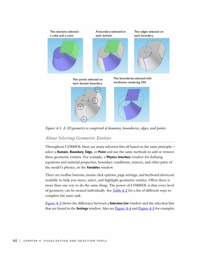
162 | C H A P T E
Figure 4-1: A 3D geometry is comprised of domains, boundaries, edges, and points.
About Selecting Geometric Entities
Throughout COMSOL there are many selection lists all based on the same principle—select a Domain, Boundary, Edge, or Point and use the same methods to add or remove these geometric entities. For example, a Physics Interface window for defining equations and material properties, boundary conditions, sources, and other parts of the model’s physics, or the Variables window.
There are toolbar buttons, mouse click options, page settings, and keyboard shortcuts available to help you move, select, and highlight geometric entities. Often there is more than one way to do the same thing. The power of COMSOL is that every level of geometry can be treated individually. See Table 4-2 for a list of different ways to complete the same task.
Figure 4-2 shows the difference between a Selection List window and the selection lists that are found in the Settings window. Also see Figure 4-4 and Figure 4-5 for examples
Two domains selected - a cube and a cone
A boundary selected on each domain
Two edges selected on each boundary
Two points selected on each domain boundary
Two boundaries selected with wireframe rendering ON
R 4 : V I S U A L I Z A T I O N A N D S E L E C T I O N TO O L S

how to use a combination of the Selection List window and these pages to select geometric entities.
Figure 4-2: Selection List window compared to the Selection list in the Settings window.
V I S U A L I Z A T I O N C U E S T O H E L P W I T H S E L E C T I O N
Geometric Entities Highlighted in Color in the Graphics Window COMSOL Multiphysics highlights geometric entities at different stages of selection. Selected lines also have a thicker line width and selected points are larger. In Figure 4-1, each geometric entity is highlighted in red, blue, green, or with no highlight to indicate its status. It cycles between red (left-click to select the geometric entity), blue (right-click to add it to the selection), green (left-click to show that it is added), and no highlight (right-click to cancel the selection).
Figure 4-3: Selecting geometric levels - highlighted to indicate status.
Selection List window
Selection list
The list of boundaries is the same on both windows
Settings window
The green geometric entity (labeled 1) has been added to the Material selection list.
The red geometric entity (labeled 12) has NOT been added to the Material selection list, but it is highlighted in the Selection List window.
W O R K I N G W I T H 3 D G E O M E T R Y | 163
164 | C H A P T E
Red The geometric entity is highlighted but not added to the model selection list. Left-click once with the mouse. If you right-click it locks all red geometric entities. See Figure 4-3 for an example. Notice how the COMSOL Desktop is rearranged to better view all windows while making a selection.
Blue The geometric entity has been added to the model selection list. The selection is highlighted in blue after you right-click once. See Figure 4-1 for an example.
Green After the geometric entity is added to the selection list, when you click anywhere (directly in the Graphics window, from the Settings page, or in the Selection window) it is highlighted green, which corresponds to the name of the geometric entity in the Selection section in the Settings window. See Figure 4-1 and Figure 4-3 for examples.
No highlight If the geometric entity is not highlighted it means it is not selected.
About Overlapping ObjectsWhen you click on a 3D geometry comprised of several objects, geometric entities of the same type might overlap at the point where you click. Overlapping objects are selected starting with the closest geometric entity and ending with the overlapping entity the furthest away.
For example, if you click on a circle boundary that overlaps with a sphere boundary as well as a square boundary, the first click selects the circle boundary (the point of origin), then the second click selects the next closest boundary on the sphere, and the last click selects the boundary on the square. Then the cycle starts again with the point of origin, the circle boundary.
Pasting a Selection From File
If you have a list of geometric entities (boundaries, for example) in a file or document, you can copy the list and paste that selection into a selection list. This list of numbers could be a step in a COMSOL Multiphysics modeling instruction and can include commas and spaces as separators, ranges such as 10–34, and even words like “and.” When you have selected a list of numbers and copied it using Ctrl+C (from a text file or PDF file, for example), click the Paste Selection button ( ) next to the selection list where you want to add a selection from file. The selection that you paste into the selection list adds to any existing selections.
R 4 : V I S U A L I Z A T I O N A N D S E L E C T I O N TO O L S

Using the Selection List Window
Use the Selection List window to make it easier to choose objects, for example, while working with complex geometries and when you need to easily locate a geometric entity that is not easily viewed. The Selection List is particularly useful when you know the geometric entity number to select; for example, when you are following Model
Library instructions to build a model.
You open this window from the main menu, Options>Selection List, and COMSOL then determines the geometric entities listed based on where in the model you are working.
The Selection List window displays a variety of geometric entities. Click on any item to see it highlighted in the Graphics window and select items as described in Selecting and Deselecting Geometric Entities. For example, use the Selection List in these situations:
• When in the Model Builder under the Geometry node—the geometry objects are displayed in the Selection List, for example, blk1 and cone1.
• When working in windows with Selection or Geometric Scope sections (a Selection window under a Definitions node for example), or anywhere you assign materials, physics, boundary conditions, and other model settings. The Selection List displays the specific Geometric entity level selected (domain, boundary, edge, or point). See Figure 4-4.
• When working in the Geometry node with Chamfer or Fillet features and you want to locate specific points. Specify the selection level by clicking the Select Domains ( ), Select Boundaries ( ), or Select Points ( ) buttons in the Graphics toolbar and add it to the Vertices to fillet or chamfer.
W O R K I N G W I T H 3 D G E O M E T R Y | 165

166 | C H A P T E
Figure 4-4: Using a combination of the Selection List and Selection window to choose boundaries on a 3D model.
Figure 4-5: Using a combination of the Selection List and Selection window to choose fillet points to add to a 2D model.
A N E X A M P L E O F S E L E C T I N G B O U N D A R I E S W I T H T H E S E L E C T I O N L I S T
This example demonstrates the selection of boundaries. When there is the possibility of overlapping geometric entities, it is recommended that you use the Selection List window to ensure the correct part of the geometry is selected.
1 From the main menu, select File>Open Model Library.
2 Navigate to the COMSOL Multiphysics>Structural Mechanics>mast_diagonal_mounting model file. Double-click to open it.
3 In the Graphics toolbar, click the Select Boundaries button ( ).
R 4 : V I S U A L I Z A T I O N A N D S E L E C T I O N TO O L S

4 From the main menu, select Options>Selection List.
The Selection List window lists all the boundaries contained in all the domains.
There are many ways to select the boundaries:
- Click on any boundary contained in the Selection List window.
- Ctrl+click to select more than one boundary from the list at a time. The boundaries are highlighted at the same time in the Graphics window.
- Rotate the geometry as required and click on it to highlight boundary numbers in the Selection List window.
- In the Selection List, shift-click to select contiguous items.
- In the Graphics window, shift-click to add an object to the selection. If objects are overlapping, you may need to click more than twice to select all objects.
Selecting and Deselecting Geometric Entities
Note: The same methods are used when working with 2D geometric entities except there are no edges.
Add and remove 3D geometric entities (domains, boundaries, edges, or points) to selection lists in different ways, including buttons in the Graphics toolbar, using the Selection List window, clicking directly on the geometry, or clicking buttons in the Settings window. In the Graphics window the geometric entities are color highlighted as you make the selections and you can lock items as you select them.
At various stages of selecting geometric entities, it is also useful to lock a selection to prevent it from being removed by accident—for example, if you are making multiple selections among many overlapping objects. When an object is locked (that is to say, added to a selection list) it is highlighted in blue.
If you start by selecting the Geometric entity level>Boundary, and then select All
Boundaries, the Selection list displays all these boundaries. If you make any changes to this list, for example, remove a boundary, the Selection list reverts to Manual. This option is useful, however, for locating and determining which items to add or remove from the selection and is the same as those geometric entities that display in the Selection List window.
W O R K I N G W I T H 3 D G E O M E T R Y | 167

168 | C H A P T E
See Table 4-2 for the many different ways to select geometric entities using toolbar buttons, mouse click options, page settings, and keyboard shortcuts.
TABLE 4-2: DIFFERENT WAYS TO SELECT GEOMETRIC ENTITIES
TASK ACTION
Select any level of geometry:
In the Graphics window, click the geometric entity.
In the Settings window, select from a selection list.
Open the Selection List window and click on entity names.
Select all parts of the geometry:
From the main menu select Edit>Select All or press Ctrl+A. This highlights and selects all entities but does NOT confirm the selection or lock it if the model changes.
To lock a selection, on some pages, the option to select the All (domains, boundaries, edges, or points) check box adds that geometric entity to the list. The selected items are highlighted in the Graphics window and all entities are kept selected even if the geometry changes.
Open the Selection List window, shift+click to select all the entity names.
Deselect all parts of the geometry not added to a selection list:
From the main menu select Edit>Deselect All.
In the Graphics window, click outside of the geometry or press Ctrl+D to deselect all selections whereas locked selections remain intact.
Select adjacent geometric entities (3D):
In the Graphics window, click a geometric entity, for example, an edge. Then click multiple times to cycle through all the edges that are next to an edge. Hold the Ctrl key down while clicking to confirm selection of all the adjacent geometric entities at the same time.
Select, move, and rotate at the same time:
Multiple mouse actions can be done at the same time in 3D. For example, use the mouse to rotate or move the object left and right to locate the geometric entity to add to a selection list, then right-click and left-click to add to the selection or click the Select Box button ( ).
Lock parts of the geometry during selection:
On some Settings windows, click the Select all (domains, boundaries, edges, or points) check box. See Creating a User-Defined Selection Node for an example.
R 4 : V I S U A L I Z A T I O N A N D S E L E C T I O N TO O L S

Add items to a selection list:
For user defined selections this action must be completed on the selection page. See Creating a User-Defined Selection Node for information.
In the Graphics window, left-click (red highlight) then right-click (blue highlight) a geometric entity. Or select one or more geometric entities and click the Add to Selection button ( ) in the Settings window.
In the Selection List window, select the entity names to add, and click the Add to Selection button ( ) in the Settings window.
You can also paste selections from a file. See Pasting a Selection From File for information.
Select multiple parts of the geometry:
In the Graphics window, click the Select Box button ( ) then click and hold the left mouse button to draw a square over the geometry. It is like a “rubberband” selecting all entities enclosed by this operation. Shift-click adds additional geometric entities to the Selection list.
In the Selection List window, select the entity names to add using the Shift or Ctrl keys. Click the Add to Selection button ( ) in the Settings window to add the geometric entity to the Selection list.
2D only: Use an -OR operation with the current selection
In the Graphics window, press Ctrl+click on the geometric entity you want to select. Then click the Select Box button ( ) and click and hold the left mouse button to draw a square over the geometry. Presently selected objects are deselected when inside the Select Box and vice versa.
3D only: Use an -AND operation with the current selection
In the Graphics window, press Ctrl+click on the geometric entity you want to select. Then click the Select Box button ( ) and click and hold the left mouse button to draw a square over the geometry. Only the presently selected objects inside the rubber-band box stay selected. This makes it possible to select a detail from several selected objects.
Select only objects: In the Graphics window, click the Select Objects button ( ). To select more than one at a time, press Ctrl+click or Shift+click.
TABLE 4-2: DIFFERENT WAYS TO SELECT GEOMETRIC ENTITIES
TASK ACTION
W O R K I N G W I T H 3 D G E O M E T R Y | 169

170 | C H A P T E
Select only domains: In the Graphics window, click the Select Domains button ( ). To select more than one at a time, press Ctrl+click or Shift+click.
In the Settings window, select Domain from a Selection list and then click in the Graphics window. Only domains are highlighted.
Select only boundaries: In the Graphics window, click the Select Boundaries button ( ). To select more than one at a time, press Ctrl+click or Shift+click.
In the Settings window, select Boundary from a Selection list and then click in the Graphics window. Only boundaries are highlighted.
Select only edges: In the Graphics window, click the Select Edges button ( ). To select more than one at a time, press Ctrl+click or Shift+click.
In the Settings window, select Edge from a Selection list and then click in the Graphics window. Only edges are highlighted.
Select only points: In the Graphics window, click the Select Points button ( ). To select more than one at a time, press Ctrl+click or Shift+click.
In the Settings window, select Point from a Selection list and then click in the Graphics window. Only points are highlighted.
TABLE 4-2: DIFFERENT WAYS TO SELECT GEOMETRIC ENTITIES
TASK ACTION
R 4 : V I S U A L I Z A T I O N A N D S E L E C T I O N TO O L S

Remove a geometric entity from a selection list:
For user defined selections this action must be completed on the selection page. See Creating a User-Defined Selection Node for information.
In the Graphics window, highlight or select the geometric entity and click the Remove from Selection button ( ) in the Settings window.
In the Graphics window, left-click to highlight and select the geometric entity to remove. Any blue geometric entity turns green. To remove that geometric entity, right-click the mouse button.
In the Selection List window, select the entity names to remove using the Shift or Ctrl keys. Click the Remove from Selection button ( ) in the Settings window to remove the geometric entity from the Selection list.
Clear all items from a selection list:
For user defined selections this action must be completed on the selection page. See Creating a User-Defined Selection Node for information.
Click the Clear Selection button ( ) in the Settings window.
TABLE 4-2: DIFFERENT WAYS TO SELECT GEOMETRIC ENTITIES
TASK ACTION
W O R K I N G W I T H 3 D G E O M E T R Y | 171

172 | C H A P T E
Zooming In and Out in the Graphics Window
Changing Views in the Graphics Window
TASK ACTION
Zoom in and out: Click the Zoom In button ( ) to zoom in.
Click the Zoom Out button ( ) to zoom out.
3D only: Click the middle mouse button and drag it forward and backward to zoom in and out of the object. The zoom is centered where the first click is made in the Graphics window.
Zoom into a general area of the geometry:
Click the Zoom Box button ( ) then click and drag to highlight a section of the geometry to zoom into.
Zoom into a geometric entity:
Click any domain, boundary, edge, or point. Click the Zoom Selected button ( ) to display to the extent of the window. This button is also available in connection with the selection lists for domains, boundaries, edges, and points in 3D models
Zoom out to the view the complete geometry:
Click the Zoom Extents button ( ) to zoom out and fit the complete geometry into the window.
TASK ACTION
Change the view to the xy-, yz-, or zx-plane:
Click the Go to View XY ( ), YZ ( ), or ZX ( ) buttons.
The first click selects the plane view with a positive normal direction. A second click on the same button switches to a negative normal direction.
Change the view to the default:
Click the Go to Default 3D View button ( ).
Display a user defined view: After creating a View under the Definitions node, click the down arrow next to the Go to View button ( ) and select a user defined view from the list.
R 4 : V I S U A L I Z A T I O N A N D S E L E C T I O N TO O L S
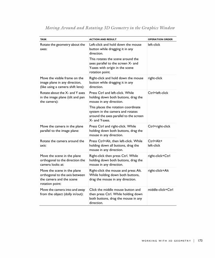
Moving Around and Rotating 3D Geometry in the Graphics Window
TASK ACTION AND RESULT OPERATION ORDER
Rotate the geometry about the axes:
Left-click and hold down the mouse button while dragging it in any direction.
This rotates the scene around the axes parallel to the screen X- and Y-axes with origin in the scene rotation point.
left-click
Move the visible frame on the image plane in any direction, (like using a camera shift lens):
Right-click and hold down the mouse button while dragging it in any direction.
right-click
Rotate about the X- and Y axes in the image plane (tilt and pan the camera):
Press Ctrl and left-click. While holding down both buttons, drag the mouse in any direction.
This places the rotation coordinate system in the camera and rotates around the axes parallel to the screen X- and Y-axes.
Ctrl+left-click
Move the camera in the plane parallel to the image plane:
Press Ctrl and right-click. While holding down both buttons, drag the mouse in any direction.
Ctrl+right-click
Rotate the camera around the axis:
Press Ctrl+Alt, then left-click. While holding down all buttons, drag the mouse in any direction.
Ctrl+Alt+ left-click
Move the scene in the plane orthogonal to the direction the camera looks at:
Right-click then press Ctrl. While holding down both buttons, drag the mouse in any direction.
right-click+Ctrl
Move the scene in the plane orthogonal to the axis between the camera and the scene rotation point:
Right-click the mouse and press Alt. While holding down both buttons, drag the mouse in any direction.
right-click+Alt
Move the camera into and away from the object (dolly in/out):
Click the middle mouse button and then press Ctrl. While holding down both buttons, drag the mouse in any direction.
middle-click+Ctrl
W O R K I N G W I T H 3 D G E O M E T R Y | 173

174 | C H A P T E
Lighting, Transparency, and Wireframe Rendering
Note: The Scene Light feature is available for the 3D View.
Rotate the camera about its axis between the camera and the scene rotation point (roll direction):
Press Alt, then left-click. While holding down both buttons, drag the mouse in any direction.
Alt+left-click
Move the camera along the axis between the camera and the scene rotation point:
Press Alt, then middle-click. While holding down both buttons, drag the mouse in any direction.
Alt+middle-click
TASK ACTION AND RESULT OPERATION ORDER
TASK ACTION
Turn Scene Light ON or OFF:
In the Graphics window, click the Scene Light button ( ). See Figure 4-6.
When creating a View, this action toggles the Scene light check box on the View page.
Turn Transparency ON or OFF:
In the Graphics window, click the Transparency button ( ). See Figure 4-6.
When creating a View, this action toggles the Transparency check box on the View page.
Turn Wireframe Rendering ON or OFF:
In the Graphics window, click the Wireframe Rendering button ( ). See Figure 4-6.
When creating a View, this action toggles the Wireframe Rendering check box on the View page.
Also see Editing Model Preferences Settings to set the level of graphic detail to Wireframe and speed up the rendering of complex models or to improve visual appearance.
R 4 : V I S U A L I Z A T I O N A N D S E L E C T I O N TO O L S
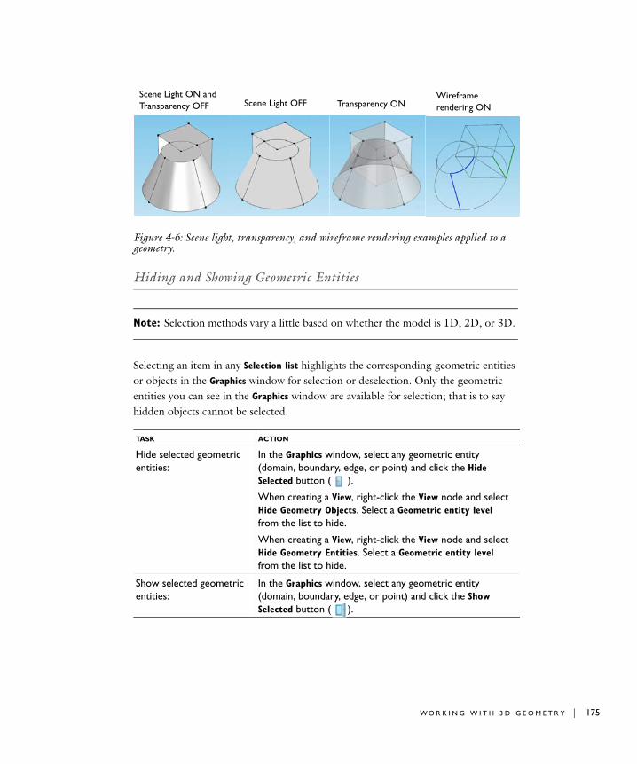
Figure 4-6: Scene light, transparency, and wireframe rendering examples applied to a geometry.
Hiding and Showing Geometric Entities
Note: Selection methods vary a little based on whether the model is 1D, 2D, or 3D.
Selecting an item in any Selection list highlights the corresponding geometric entities or objects in the Graphics window for selection or deselection. Only the geometric entities you can see in the Graphics window are available for selection; that is to say hidden objects cannot be selected.
TASK ACTION
Hide selected geometric entities:
In the Graphics window, select any geometric entity (domain, boundary, edge, or point) and click the Hide Selected button ( ).
When creating a View, right-click the View node and select Hide Geometry Objects. Select a Geometric entity level from the list to hide.
When creating a View, right-click the View node and select Hide Geometry Entities. Select a Geometric entity level from the list to hide.
Show selected geometric entities:
In the Graphics window, select any geometric entity (domain, boundary, edge, or point) and click the Show Selected button ( ).
Transparency ONScene Light OFFScene Light ON and Transparency OFF
Wireframe rendering ON
W O R K I N G W I T H 3 D G E O M E T R Y | 175

176 | C H A P T E
Reset all hidden objects to the default:
In the Graphics window, click the Reset Hiding button ( ) to reset all hidden domains, boundaries, edges, or points to the default.
If working on a user defined View, this removes any Hide Geometry Objects or Entities page added to a View node.
View hidden geometric entities:
In the Graphics window, click the View Hidden Only button ( ) to display only hidden domains, boundaries, edges, or points.
View unhidden geometric entities:
In the Graphics window, click the View Unhidden button ( ) to display any domains, boundaries, edges, or points not hidden.
View all geometric entities:
In the Graphics window, click the View All button ( ) to display all hidden and unhidden domains, boundaries, edges, or points.
TASK ACTION
R 4 : V I S U A L I Z A T I O N A N D S E L E C T I O N TO O L S

U s e r -D e f i n e d S e l e c t i o n s
In the Model Builder, create Selection nodes under model Definitions to represent various parts of the geometry and simplify the process of assigning materials, model equations, boundary conditions, and other model features. Each user defined Selection can be reused during the model design and renamed with descriptive titles—for example, tube, wall, or fluid. Changes to the Selection (for example, by adding or removing a boundary) updates all features in the model that use that particular Selection.
Creating a User-Defined Selection Node
In addition to the following procedure, you can create a Selection node from an existing selection in any Settings window that contains a selection of geometric entities such as boundaries. To do so, click the Create Selection button ( ) in the Settings window that contains the selection.
Use the following steps to create a user defined Selection node:
1 In the Model Builder, right-click any Definitions node under a Model, and choose Selection.
A Selection page opens in the Settings window and a node with the same name is added to the Model Builder.
2 Right-click to Rename the Selection node as required.
3 Under Geometric Scope add geometric entities to the Selection input. See Figure 4-7 and Figure 4-8 for examples and Selecting and Deselecting Geometric Entities for the different ways to select geometric entities.
a Select the All (domains, boundaries, edges, or points) check box to add that geometric entity to the list. The selected items are highlighted in the Graphics window. Selecting this check box locks the entities selected even if the geometry changes.
b Select a Geometric entity level—Domain, Boundary, Edge (3D only), or Point to add or remove from the Selection input list.
U S E R - D E F I N E D S E L E C T I O N S | 177

178 | C H A P T E
Figure 4-7: Adding all 3D edges to a selection.
Figure 4-8: Selecting individual boundaries to remove from a selection list.
Note: For 2D geometries, there are no edges, and the related selection options are not available. For 1D models, there are no edges or points, and the related selection options are not available.
R 4 : V I S U A L I Z A T I O N A N D S E L E C T I O N TO O L S

Note: If a particular selection is used elsewhere in the model, it is not possible to change the output because it can make it invalid by changing the output type, for example, from domains to boundaries.
4 In the Selection output section, define the geometric objects that the selection contains. The options available and defaults depend on your selection in the Geometric entity level list.
- If Domain is the input the default output is the Selected domains.
Select other options as required. Select Adjacent boundaries, Adjacent edges, or Adjacent points to include boundaries, edges, or points next to the selected domains either as Exterior (the default) or Interior boundaries, Interior edges, or Interior points. Click to select or clear the check boxes as needed.
- If Boundary is the input, the default output is the Selected boundaries.
Select other options as required. Select Adjacent edges or Adjacent points to include the edges next to the selected domains either as Exterior (the default) or Interior edges or Interior points. Click to select or clear the check boxes as needed.
- If Edge is the input, the default output is Selected edges.
Select Adjacent points to include the points next to the selected domains either as Exterior (the default) or Interior points. Click to select or clear the check boxes as needed. The Point input is the same as the selection output.
E X A M P L E O F A U S E R D E F I N E D S E L E C T I O N
1 From the main menu, select File>Open Model Library.
2 Navigate to the COMSOL Multiphysics>Structural Mechanics>mast_diagonal_mounting model file. Double-click to open it.
3 Click the Definitions node under Model 1.
Several nodes display in the Model Builder.
4 Click the Fixed face and Force faces nodes to see how each are defined.
5 Click the Face Load node under Solid Mechanics.
The Face Load page opens in the Settings window. Under Boundaries, Force faces is the Selection. Fixed face is also available to be selected from the Selection list.
U S E R - D E F I N E D S E L E C T I O N S | 179

180 | C H A P T E
U s e r -D e f i n e d V i ew s
In the Model Builder, create a user defined View under model Definitions. Each user defined View is accessible in the Graphics window during model creation and analysis, making it easy to switch between views and find the best way to illustrate your model. You can rename the nodes with descriptive titles—for example, transparency with scene light.
Creating Views
Note: For some plots, the View node displays under Results. For example, when 2D axisymmetric revolved plots or 2D cut plane plots for a 3D models are created. For the majority of plots, use the Definitions node to create a View.
Figure 4-9: Selecting a predefined transparency view of the geometry.
Adding a 2D User-Defined View
A D D I N G T H E N O D E T O T H E M O D E L B U I L D E R
1 In the Model Builder, right-click Definitions and select View.
The View page opens in the Settings window and a node with the same name is added to the Model Builder.
R 4 : V I S U A L I Z A T I O N A N D S E L E C T I O N TO O L S

2 On the View page, select the Show geometry labels check box to display the geometric short name in the Graphics window.
3 Select the Lock axis check box to keep the Axis settings from changing when using the mouse.
4 Right-click the View node to add Hide Geometric Entities and Hide Geometry Object
nodes. See Hiding Geometry Objects in a User-Defined View and Hiding Geometric Entities in a User-Defined View
D E F I N I N G T H E V I E W A X I S F O R A 2 D V I E W
1 In the Model Builder, under Definitions>View node, click the Axis node.
The Axis page opens in the Settings window.
2 Under Axis, enter X and Y min and X and Y max values.
3 The Preserve aspect ratio check box is selected by default. Click to clear if required.
4 Under Grid, enter Extra X and Y values.
Select the Manual spacing check box and enter X, Y, and Z spacing values.
Adding a 3D User-Defined View
A D D I N G T H E N O D E T O T H E M O D E L B U I L D E R
1 In the Model Builder, right-click Definitions and select View.
The View page opens in the Settings window and a node with the same name is added to the Model Builder.
2 On the View page, select the Transparency check box to turn the feature on. The Transparency button ( ) is activated in the Graphics window at the same time. Enter a value in the Alpha field or use the slider to select a transparency level.
Watch the changes in the Graphics window at the same time to help choose a transparency level.
3 The Scene light check box is selected by default. Click to clear the check box if required. The Scene Light button ( ) is turned on or off in the Graphics window at the same time.
U S E R - D E F I N E D V I E W S | 181

182 | C H A P T E
Note: The type of Scene Light displayed depends on the other settings made on the View pages. For example, if the Intensity and Color are edited on the Directional Light page, this is what is shown when the Scene Light check box is selected.
4 Select the Wireframe rendering check box to view the edges of the object as solid lines. The Wireframe Rendering button ( ) is turned on or off in the Graphics window at the same time.
5 Select the Show geometry labels check box to display the geometric short name in the Graphics window.
6 Select the Show grid check box to display a numbered grid in the Graphics window.
7 From the Projection list, select Perspective or Orthographic (parallel) as required.
8 Select the Lock camera check box to keep the Camera settings from changing when using the mouse.
9 Right-click the View node to add Directional Light, Point Light, Spotlight, Headlight, Hide Geometric Entities and Hide Geometry Object nodes.
Note: Four Directional Light nodes are automatically added to the Model Builder.
D E F I N I N G T H E C A M E R A PO S I T I O N
1 In the Model Builder, under Definitions click to expand the View node where you want to define the camera position.
2 Click the Camera node.
The Camera page opens in the Settings window.
3 In the Graphics window, left-click and hold the mouse to orient the geometry on the axes. The corresponding coordinates are displayed in the Settings window under the
R 4 : V I S U A L I Z A T I O N A N D S E L E C T I O N TO O L S

Position, Target, and Up Vector sections. Or enter x, y, and z coordinates in each section.
- The Position is the location of the camera and the Target default is 1 unit in front of the camera position. The Up Vector value assigns the orientation of the camera roll direction, usually in the z plane.
4 If Perspective is selected as the 3D view Projection, then under Position, enter a Zoom
angle or use the Zoom buttons on the Graphics toolbar. This angle is half the viewing angle (in degrees) for the shortest side of the 3D canvas.
5 Right-click the mouse and shift the geometry left, right, up, or down as required. This shift operation moves the currently visible frame on the image plane. The corresponding coordinate values that display in the Settings window under View
Offset are relative to the image width and height, respectively. Alternatively, enter x and y coordinates.
6 If Orthographic is selected as the 3D view Projection, then under View Offset, enter an Orthographic scale. This defines the size in scene length of the viewing block along the longest side of the canvas.
D E F I N I N G A V I E W D I R E C T I O N A L L I G H T
1 In the Model Builder, under Definitions click to expand the View node where you want to define the directional light.
2 Click the Directional Light node.
The Directional Light page opens in the Settings window.
3 Under Direction, enter x, y, and z coordinates. This defines where the light comes from (negative to the light direction).
4 Under Settings, enter an Intensity or use the slider to select a value.
5 Select a Color or Custom to select a different option.
6 Select the Show in camera coordinate system check box to make the light rotate together with the camera.
D E F I N I N G A V I E W PO I N T L I G H T
1 In the Model Builder, under Definitions click to expand the View node where you want to define the point light.
2 Right-click the View node and select Point Light.
The Point Light page opens in the Settings window and a node with the same name is added to the Model Builder.
3 Under Position, enter x, y, and z coordinates.
U S E R - D E F I N E D V I E W S | 183
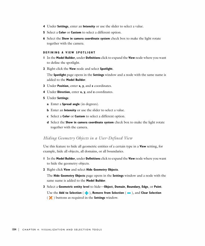
184 | C H A P T E
4 Under Settings, enter an Intensity or use the slider to select a value.
5 Select a Color or Custom to select a different option.
6 Select the Show in camera coordinate system check box to make the light rotate together with the camera.
D E F I N I N G A V I E W S P O T L I G H T
1 In the Model Builder, under Definitions click to expand the View node where you want to define the spotlight.
2 Right-click the View node and select Spotlight.
The Spotlight page opens in the Settings window and a node with the same name is added to the Model Builder.
3 Under Position, enter x, y, and z coordinates.
4 Under Direction, enter x, y, and z coordinates.
5 Under Settings:
a Enter a Spread angle (in degrees).
b Enter an Intensity or use the slider to select a value.
c Select a Color or Custom to select a different option.
d Select the Show in camera coordinate system check box to make the light rotate together with the camera.
Hiding Geometry Objects in a User-Defined View
Use this feature to hide all geometric entities of a certain type in a View setting, for example, hide all objects, all domains, or all boundaries.
1 In the Model Builder, under Definitions click to expand the View node where you want to hide the geometry objects.
2 Right-click View and select Hide Geometry Objects.
The Hide Geometry Objects page opens in the Settings window and a node with the same name is added to the Model Builder.
3 Select a Geometric entity level to hide—Object, Domain, Boundary, Edge, or Point.
Use the Add to Selection ( ), Remove from Selection ( ), and Clear Selection
( ) buttons as required in the Settings window.
R 4 : V I S U A L I Z A T I O N A N D S E L E C T I O N TO O L S
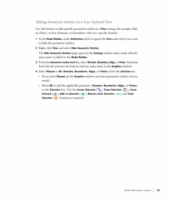
Hiding Geometric Entities in a User-Defined View
Use this feature to hide specific geometric entities in a View setting, for example, hide an object, or four domains, or boundaries only on a specific domain.
1 In the Model Builder, under Definitions click to expand the View node where you want to hide the geometric entities.
2 Right-click View and select Hide Geometric Entities.
The Hide Geometric Entities page opens in the Settings window and a node with the same name is added to the Model Builder.
3 From the Geometric entity level list, select Domain, Boundary, Edge, or Point. Selection from this list activates the button with the same name in the Graphics window.
4 Select Manual or All (Domains, Boundaries, Edges, or Points) from the Selection list.
- If you select Manual, go the Graphics window and select geometric entities of your model.
- Select All to add the applicable geometry (Domains, Boundaries, Edges, or Points) to the Selection box. Use the Create Selection ( ), Paste Selection ( ), Zoom
Selected ( ), Add to Selection ( ), Remove from Selection ( ), and Clear
Selection ( ) buttons as required.
U S E R - D E F I N E D V I E W S | 185

186 | C H A P T E
S c r e e n s h o t s
Capturing a Screenshot
1 In the Graphics window, click the Image Snapshot button ( ).
2 Under Image, select a Unit to define the image size—Pixels, Millimeters, or Inches.
3 Select the Lock aspect ratio check box to maintain the calculation of the width and height (if one or the other is changed).
4 Enter a Width and Height and Resolution.
5 The Antialiasing check box is selected by default. Click to clear if required. Antialiasing determines if jagging in the image is smoothed or not.
6 Under Layout, the Title, Legend, and Axes check boxes are selected by default to display the information on the screenshot. Click Include to edit the selections.
7 Enter a Font size.
8 Select a Background—Current or Color.
9 Click Color to select a custom color.
10 Under File:
a Select a file Format—PNG, BMP, or JPG.
b Enter a file path or click Browse.
R 4 : V I S U A L I Z A T I O N A N D S E L E C T I O N TO O L S

5
G e o m e t r y M o d e l i n g a n d C A D T o o l s
The CAD tools in COMSOL Multiphysics provide many possibilities to create geometries using solid and boundary modeling. This section covers geometry modeling in 1D, 2D, and 3D with examples of solid modeling, boundary modeling, Boolean operators, and other CAD tools in COMSOL Multiphysics. In addition, it shows how to use the tools for exploring geometric properties, such as volumes and surfaces. This section also provides information about using external CAD data.
In this section:
• Creating a Geometry for Successful Analysis
• The COMSOL Multiphysics Geometry and CAD Environment
• Creating a 1D Geometry Model
• Creating a 2D Geometry Model
• Creating a 3D Geometry Model
187

188 | C H A P T E
C r e a t i n g a Geome t r y f o r S u c c e s s f u l Ana l y s i s
Several techniques can ensure that a geometry results in a good mesh and gives reasonable solution times for the finite element analysis. They include the use of symmetry and eliminating small details, gaps, holes, and singularities.
U S I N G S Y M M E T R I E S
Using symmetry is one of the most effective ways to reduce the size of a finite element model.
M A K I N G T H E G E O M E T R Y M A T C H T H E B O U N D A R Y C O N D I T I O N S
In many solutions, the modeling domain is unbounded or too large for successful meshing and analysis. For these cases a suitable boundary condition can replace the exterior of the domain. It is important for the geometry to be large enough to validate these boundary conditions. For outflows in fluid-flow models, for example, the boundary should be perpendicular to the fully developed flow. Inspections and modifications of the solved model might be necessary to verify the validity of the boundary condition.
A VO I D I N G E X C E S S I V E L Y S M A L L D E T A I L S , H O L E S , A N D G A P S
Many geometries, especially those designed using a CAD system without finite element analysis, contain small holes, details, and gaps. These small features can make the domain unbounded and must be removed before analysis. Small details and holes can lead to large meshes and finite element models or even failure during mesh generation. Make sure the snapping feature is activated to avoid small gaps and mismatches between the geometry objects.
The CAD Import Module contains tools for automatic and interactive repair and defeaturing of 3D CAD data.
A VO I D I N G S I N G U L A R I T I E S A N D D E G E N E R A C I E S I N T H E G E O M E T R Y
A singularity in a geometry is a sharp corner or angle that can create problems during meshing and analysis. In reality, a sharp reentrant corner leads to infinite stress values in a stress analysis of a perfectly elastic material. To avoid a singularity, round sharp corners using fillets. The stress value for a sharp corner is finite in the finite element analysis, but refinement of the mesh increases the stresses in the corner without limit.
R 5 : G E O M E T R Y M O D E L I N G A N D C A D TO O L S
A degeneracy in the geometry can occur during solid modeling. For example, fillet areas that taper to a point and the apex of a cone can become degenerate points. These degeneracies might cause problems for the mesh generator and problems during the analysis of the model. A common degeneracy in the geometry occurs when you create a 3D solid (for example, a cylinder) by rotation about an axis that touches the rotation area. In such cases, it is better to create the solid object by extruding a cross section or to use geometric 3D primitives.
A S S O C I A T I V E G E O M E T R Y
Associative geometry is a concept for the automatic updating of applied physical properties, such as boundary conditions and equation coefficients, under geometric transformations. Thus, once you have defined the physical properties of a finite element model and return to the Geometry branch to modify the geometric model, COMSOL Multiphysics updates the physical properties according to the geometry modifications.
The associative geometry functionality utilizes geometry-mapping information between the groups of geometric entities (vertices, edges, boundaries, and domains) in the finalized geometry and the corresponding groups in the geometric model.
This geometry mapping is not always without ambiguities. Thus, COMSOL Multiphysics makes some heuristic decisions when mapping the physical properties between the finalized geometry (the object on which the physical properties are imposed) and the geometric model. In some cases the resulting updated physical properties might not be the ones that you would expect.
C R E A T I N G A G E O M E T R Y F O R S U C C E S S F U L A N A L Y S I S | 189
190 | C H A P T E
Th e COMSOL Mu l t i p h y s i c s Geome t r y and CAD En v i r o nmen t
Overview of Geometry Modeling Concepts
In COMSOL Multiphysics you can use solid modeling or boundary modeling to create objects in 1D, 2D, and 3D. They can be combined in the same geometry (hybrid modeling).
During solid modeling, you form a geometry as a combination of solid objects using Boolean operations like union, intersection, and difference. Objects formed by combining a collection of existing solids using Boolean operations are known as composite solid objects. Boundary modeling is the process of defining a solid in terms of its boundaries, for example using lines to create a solid hexagonal domain in 2D. You can combine such a solid with geometric primitives—common solid modeling shapes like blocks, cones, spheres, rectangles, and circles, which are directly available in COMSOL Multiphysics.
In 3D, you can form 3D solid objects by defining 2D solids in work planes and then extruding and revolving these into 3D solids. It is also possible to embed 2D objects into the 3D geometry.
You can also overlay additional nonsolid objects on top of solid objects to control the distribution of the mesh and to improve postprocessing capabilities. For example, you can add a curve object to a geometry to control the element size in the vicinity of this curve, or add a point to guarantee a mesh vertex in a specific location or to create a time-dependent or parametric-value graph at that location in the geometry.
Once you have created a geometry, the Model Builder gives you an overview of the geometry sequence that creates the objects in a Geometry branch. The settings for the nodes making up the sequence can be changed at any time and the whole sequence is re-run instantaneously.
You can import 2D geometries from DXF files and 3D geometries from STL and VRML files. See Import in the COMSOL Multiphysics Reference Guide for details of how to import these CAD file formats (or see Where Do I Access the Documentation and Model Library?).
R 5 : G E O M E T R Y M O D E L I N G A N D C A D TO O L S

The CAD Import Module provides an interface for the import of CAD files in Parasolid, SAT (ACIS), Inventor, Pro/E, SolidWorks, STEP, and IGES formats. In addition, the CATIAV5 Import Module provides an interface for CATIAV5 files.
The products LiveLink for Inventor, LiveLink for Pro/ENGINEER, and LiveLink for SolidWorks, offer bidirectional links to these respective products. Using these, you can run parametric geometry sweeps driven from the COMSOL environment but operating directly on the geometries in the respective CAD package environments.
Geometry Toolbar
TABLE 5-1: GEOMETRY BUTTONS
BUTTON NAME
Draw Point
Draw Line
Draw Quadratic
Draw Cubic
Draw Square
Draw Square (Center)
Draw Rectangle
Draw Rectangle (Center)
Draw Circle
Draw Circle (Center)
Draw Ellipse
Draw Ellipse (Center)
T H E C O M S O L M U L T I P H Y S I C S G E O M E T R Y A N D C A D E N V I R O N M E N T | 191

192 | C H A P T E
About Selecting the Cartesian or Cylindrical Coordinate System
COMSOL Multiphysics uses a global Cartesian or cylindrical (axisymmetric) coordinate system. You select the geometry dimension and coordinate system when starting a new model in the Model Wizard. Variable names for the spatial coordinates are x, y, and z for Cartesian coordinates and r, , and z for cylindrical coordinates. These coordinate variables (together with the time parameter for time-dependent models) make up the independent variables in COMSOL Multiphysics models. Also see Coordinate Systems for more information.
T H E C O O R D I N A T E S Y S T E M S A N D T H E S P A C E D I M E N S I O N
The labels assigned to the coordinate system variables vary according to the space dimension:
• Models that you open using the space dimensions 1D, 2D, and 3D use the Cartesian coordinate independent variable labels x, y, and z.
Split
Delete
Union
Intersection
Difference
Convert to Solid
Convert to Surface
Convert to Curve
Convert to Point
Measure
TABLE 5-1: GEOMETRY BUTTONS
BUTTON NAME
R 5 : G E O M E T R Y M O D E L I N G A N D C A D TO O L S

• In 2D axisymmetric geometries, the x-axis represents the r label, which is the radial coordinate, while the y-axis represents the z label, the height coordinate.
• In 1D axisymmetric geometries, the default radial coordinate is labelled as r, and represented by the x-axis.
For axisymmetric cases the geometry model must fall in the positive half plane, that is to say r0.
Also see About Cylindrical Coordinate Systems and Defining a Cylindrical Coordinate System for more information.
Selecting the Coordinate System and Space DimensionIn the Model Wizard, select 3D, 2D axisymmetric, 2D, 1D axisymmetric, or 1D from the Select Space Dimension list. You can do this before starting a new model or by right-clicking the root node in the Model Builder and selecting Add Model for creating models with multiple geometries. The Model node’s icon indicates the space dimension:
• for 3D geometries
• for 2D axisymmetric geometries
• for 2D geometries
• for 1D axisymmetric geometries
• for 1D geometries
• for 0D geometries (space-independent models)
Note: Not all physics interfaces are available for all coordinate systems and space dimensions.
Creating Composite Geometry Objects
You can form a composite geometry object by combining objects with Boolean operations: Union, Intersection, Difference, or Compose. Also form complex geometries using Boolean formulas that include multiple objects and operations.
T H E C O M S O L M U L T I P H Y S I C S G E O M E T R Y A N D C A D E N V I R O N M E N T | 193

194 | C H A P T E
1 In the Model Builder, click the Geometry node, select objects in the Graphics window. Then click the Union ( ), Intersection ( ), or Difference ( ) buttons.
- OR -
In the Model Builder, right-click Geometry and select Boolean Operations.
2 Select Union, Intersection, Difference, or Compose.
A Union, Intersection, Difference, or Compose page opens in the Settings window.
3 For Union, Intersection, or Compose, in the Input objects section, add geometry from the Graphics window.
For Difference, click the Activate Selection button ( ) in the Objects to add or Objects to subtract sections. Then add or subtract geometry in the Graphics window.
Use the Add to Selection ( ), Remove from Selection ( ), and Clear Selection
( ) buttons as required in the Settings window.
4 Select the Keep input objects check box to keep the initial objects.
5 Select the Keep interior boundaries check box as required.
6 Edit the Relative repair tolerance default if the geometry has larger defects, or if you need to resolve extremely small details.
During the creation of a composite object, COMSOL automatically repairs the generated geometry object by removing small edges and faces. Edit the default if required. The value is relative to the overall dimensions of the geometry. For example, if the dimensions are in meters, the default repair tolerance of 106 makes the geometry repair heal gaps that are smaller than a micrometer (106 m).
7 For Compose only, enter a Set formula that defines the Boolean operation. Set formulas are only available for solid objects. The symbols +, -, and * represent set union, set difference, and set intersection, respectively. Use these set formulas to form a composite object by combining the selected solid objects according to the set formula. For example, entering (cyl1+sph1)*blk1 first forms the union of the cylinder, cyl1, and the sphere, sph1, and then forms the intersection of that union with the block, blk1.
8 Click the Build Selected button ( ).
Adding Affine Transformations to Geometry Objects
Mirroring, moving, rotating, and scaling are affine transformations applied to geometry objects.
1 Define an object.
R 5 : G E O M E T R Y M O D E L I N G A N D C A D TO O L S

2 In the Model Builder, right-click Geometry and select an option from the Transforms menu:
- Mirror—Specify the reflection axis or reflection plane.
- Move—Specify displacements in all space directions.
- Rotate—Specify the rotation angle with a rotation axis or center of rotation.
- Scale—Specify center of scaling and scaling factors in all space directions.
3 The Mirror, Move, Rotate, or Scale page opens in the Settings window.
4 Under Input, select the Input objects in the Graphics window. The objects display in the Input objects list. Use the Add to Selection ( ), Remove from Selection ( ), and Clear Selection ( ) buttons as required.
5 Select the Keep input objects check box to use the selected geometry objects for further geometric operations.
Mirror1 2D and 3D: Under Point on Line of Reflection, enter a point to be fixed during
reflection by entering x, y, and z coordinates as required based on the model dimensions.
2 2D and 3D: Under Normal vector to Line of Reflection, enter a vector in the direction to reflect by entering x, y, and z coordinates as required based on the model dimensions.
3 ID: Under Point of Reflection, enter the coordinate of the point of reflection in the x field.
Move• Under Displacement, enter the x, y, and z coordinates as required by the model
dimension. To create several copies, enter a comma-separated list of displacements in the fields.
Rotate1 Under Rotation Angle, enter the rotational angle in the Rotation field.
2 2D: Under Center of Rotation, enter x, and y coordinates.
3D: Under Point on Axis of Rotation, enter the x, y, and z coordinates.
3 3D: Under Axis of Rotation, select an Axis type—Cartesian or Spherical.
4 If Cartesian is selected, enter a direction vector in the x, y, and z fields.
If Spherical is selected, enter the angles theta (polar, zenith) and phi (azimuth).
T H E C O M S O L M U L T I P H Y S I C S G E O M E T R Y A N D C A D E N V I R O N M E N T | 195

196 | C H A P T E
Scale1 Under Scale Factor, the Scaling default is Isotropic. Enter a Factor.
If Anisotropic is selected as the Scaling, enter the x, y, and z coordinates as required by the model dimension.
2 Under Center of Scaling, enter the x, y, and z center point coordinates as required by the model dimension.
Creating an Array of Identical Geometry Objects
Create a rectangular or linear array of duplicates of geometry objects.
1 In the Model Builder, right-click Geometry and select Transforms>Array.
The Array page opens in the Settings window.
2 Under Input, select the Input objects to duplicate in the Graphics window. The objects display in the Input objects list. Use the Add to Selection ( ), Remove from
Selection ( ), and Clear Selection ( ) buttons as required.
3 Under Size, the Array type defaults to Rectangular (2D) or Three-dimensional (3D). Enter the number of duplicates in each coordinate direction in the x, y, and z fields.
If Linear is selected as the Array type, enter the number of duplicates in the Size field.
4 Under Displacement, enter the x, y, and z coordinates as required by the model dimension.
Copying and Pasting Geometry Objects
Make a displaced copy of a geometry objects.
1 In the Model Builder, right-click Geometry and select Transforms>Copy.
The Copy page opens in the Settings window.
2 Under Input, select the Input objects to duplicate in the Graphics window. The objects display in the Input objects list. Use the Add to Selection ( ), Remove from
Selection ( ), and Clear Selection ( ) buttons as required.
3 Keep input objects is selected by default. Click to clear the check box if required.
4 Under Displacement, enter the x, y, and z coordinates as required by the model dimension.
R 5 : G E O M E T R Y M O D E L I N G A N D C A D TO O L S
Converting Geometry Objects
Transform one or more geometry objects into a different type of object by converting it, for example, converting from a solid to a curve. The object is then called a composite object, which then becomes a solid, face, curve, or point object depending on the target type chosen.
Converting an object is useful for closed domains in 2D and 3D—create solid domains by converting the surrounding curve object or face object to a solid object. This is necessary to apply physics and material properties to the domain.
Available conversions are:
2 D
• Convert a solid object into a curve or point object.
• Convert a curve object defining at least one closed domain into a solid object.
• Convert a curve object into a point object (2D and 3D).
3 D
• Convert a solid object into a surface, curve, or point object.
• Convert a surface object defining at least one closed domain into a solid object.
• Convert a surface object into a curve, or point object.
• Convert a curve object into a point object (2D and 3D).
1 In the Model Builder, click the Geometry node, select an object in the Graphics window. Then click the Convert to Solid ( ), Convert to Surface (3D) ( ), Convert
to Curve ( ), or Convert to Point ( ) buttons.
- OR -
In the Model Builder, right-click Geometry and select an option from the Conversions
menu—Convert to Solid, Convert to Surface (3D only), Convert to Curve, or Convert
to Point.
The Convert to Solid, Surface, Curve, or Point page opens in the Settings window.
2 Under Input, select the Input objects to convert in the Graphics window. The objects display in the Input objects list. Use the Add to Selection ( ), Remove from Selection
( ), and Clear Selection ( ) buttons as required.
3 Select the Keep input objects check box to use the selected geometry objects for further geometric operations.
T H E C O M S O L M U L T I P H Y S I C S G E O M E T R Y A N D C A D E N V I R O N M E N T | 197

198 | C H A P T E
4 Edit the Relative repair tolerance default if you experience problems with the convert operation. The absolute repair tolerance is the relative repair tolerance times the maximum coordinate of the input objects. Geometric entities that have a distance less than the absolute repair tolerance are merged.
5 Click the Build Selected button ( ).
Splitting Geometry Objects
The split operation splits an object into its entities:
• A solid splits into solids corresponding to its domains.
• A surface object splits into surface objects corresponding to its faces.
• A curve object splits into curve objects corresponding to its edges.
• A point object splits into point objects corresponding to its vertices.
• A general (mixed) object splits into solids (corresponding to the domains), surface objects (corresponding to faces not adjacent to a domain), curve objects (corresponding to edges not adjacent to a face or domain), and point objects (corresponding to vertices not adjacent to an edge, face, or domain).
1 In the Model Builder, click the Geometry node, select objects in the Graphics window. Then click the Split button ( ).
-OR-
In the Model Builder, right-click Geometry and select Split.
The Split page opens in the Settings window.
2 Under Input, select the Input objects to split in the Graphics window. The objects display in the Input objects list. Use the Add to Selection ( ), Remove from Selection
( ), and Clear Selection ( ) buttons as required.
3 Select the Keep input objects check box to use the selected geometry objects for further geometric operations.
4 Click the Build Selected button ( ).
Deleting Objects and Entities
To delete objects or entities, click the Geometry node in the Model Builder, select objects or entities in the Graphics window, and click the Delete button ( ). Alternatively, use a Delete Entities feature according to the following.
R 5 : G E O M E T R Y M O D E L I N G A N D C A D TO O L S
1 In the Model Builder, right-click Geometry and select Delete Entities.
The Delete Entities page opens in the Settings window.
2 Under Input, select a Geometric entity level to delete—Object, Domain, Boundary, Edge, or Point. Select the geometry in the Graphics window. Use the Add to Selection ( ), Remove from Selection ( ), and Clear Selection ( ) buttons as required.
3 Click the Build Selected button ( ).
If you use the Delete button ( ) to delete objects, the software deletes the selected objects that correspond to primitive features by deleting their nodes from the sequence. If you delete objects that do not correspond to primitive features or if you delete geometric entities a Delete Entities node appears in the sequence.
Note: If you want to delete all objects created by a feature, it is better to right-click the feature, and select Delete or Disable.
T H E C O M S O L M U L T I P H Y S I C S G E O M E T R Y A N D C A D E N V I R O N M E N T | 199

200 | C H A P T E
C r e a t i n g a 1D Geome t r y Mode l
1 Double-click the COMSOL icon to launch COMSOL.
The Model Wizard opens.
2 On the Select Space Dimension page, click the 1D button.
3 Click the Finish button ( ).
4 In the Model Builder, right-click Geometry and select Interval.
The Interval page opens in the Settings window.
5 Select a Number of intervals—One or Many. Select Many to get an object consisting of a sequence of connected intervals.
- If Many is selected, in the Points field, enter a comma-separated list of coordinates.
- If One is selected, enter the interval endpoint coordinates in the Left endpoint (default= 0) and Right endpoint (default= 1) fields.
6 Click the Build Selected button ( ).
You can add points to the geometry to divide the domain into two domains.
7 In the Model Builder, right-click Geometry and select Point.
The Point page opens in the Settings window.
8 Under Point, enter the x coordinate.
9 Click the Build All button ( ).
R 5 : G E O M E T R Y M O D E L I N G A N D C A D TO O L S

C r e a t i n g a 2D Geome t r y Mode l
This section describes how to build a 2D cross section of a heat sink and introduces 2D geometry operations in COMSOL. At this time, you do not model the physics that describe the operation of the heat sink.
Assume that you want to estimate the maximum amount of heat dissipated by a heat sink placed around a resistor for high-power applications. The heat sink consists of an extruded aluminum profile as in Figure 5-1. If you neglect the effects at the ends of the elongated heat sink, you can simplify the model and obtain a decent estimate of the heat dissipated by creating a 2D cross section.
Figure 5-1: Example of a 3D heat sink model with cross section.
C R E A T I N G A B A S I C 2 D G E O M E T R Y M O D E L
1 Double-click the COMSOL icon to launch COMSOL.
The Model Wizard opens.
2 On the Select Space Dimension page, click the 2D button.
3 Click the Finish button ( ).
C R E A T I N G P A R A M E T E R S F O R G E O M E T R Y P A R A M E T E R I Z A T I O N
The following steps explain how to create two circles to form the core of the heat sink in Figure 5-1. To investigate different dimensions of the heat sink, parameterize the
C R E A T I N G A 2 D G E O M E T R Y M O D E L | 201

202 | C H A P T E
geometry. Start by defining the radius of the outer arc of the heat sink, the radius of the inner arc, and the thickness and the length of the heat sink flanges.
1 In the Model Builder, right-click Global Definitions and select Parameters.
The Parameters page opens in the Settings window.
2 In the Parameters table, enter these settings:
A D D I N G TW O C I R C L E S W I T H P R E D E F I N E D P A R A M E T E R S
1 In the Model Builder, right-click Geometry 1 and select Circle.
The Circle page opens in the Settings window.
2 Under Size, enter R1 in the Radius field.
3 Click the Build Selected button ( ).
A circle with radius R1 displays in the Graphics window.
4 Right-click Geometry 1 and select Circle.
5 Under Size, enter R2 in the Radius field.
6 Click the Build Selected button ( ).
A circle with radius R2 displays in the Graphics window. Click the Zoom Extents button ( ) to see both circles.
S U B T R A C T I N G T H E S M A L L E R C I R C L E
1 In the Model Builder, right-click Geometry 1 and select Boolean Operations>Difference.
The Difference page opens in the Settings window.
2 Under Difference, click the Activate Selection button ( ) to activate the Objects to
add list for choosing objects.
3 In the Graphics window, select the object c1 (the larger circle) by left- and then right-clicking it.
C1 is highlighted in red, then blue and added to the Objects to add list.
4 Click the Activate Selection button ( )to activate the Objects to subtract list.
NAME EXPRESSION VALUE DESCRIPTION
R1 5e-3[m] 0.0050 m Radius Circle 1
R2 2.5e-3[m] 0.0025 m Radius Circle 2
d 1e-3[m] 0.0010 m Height
L 5e-3[m] 0.0050 m Width
R 5 : G E O M E T R Y M O D E L I N G A N D C A D TO O L S
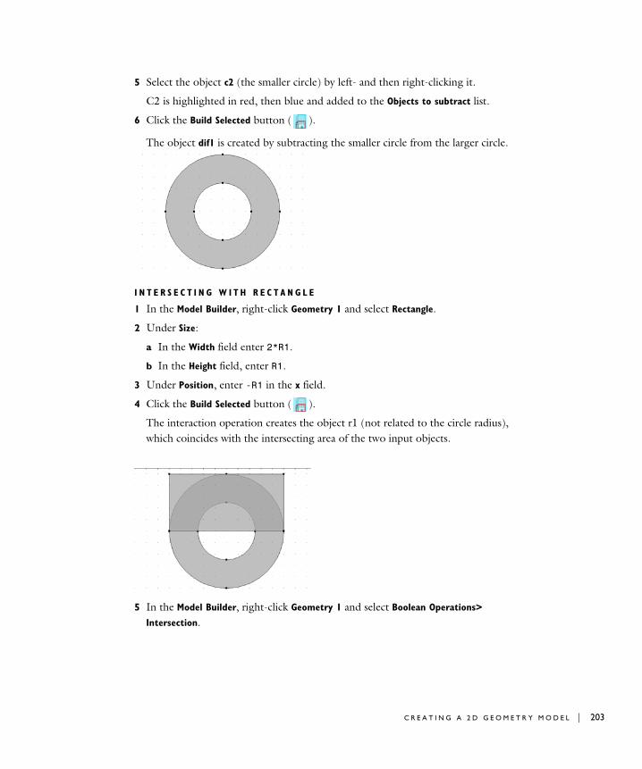
5 Select the object c2 (the smaller circle) by left- and then right-clicking it.
C2 is highlighted in red, then blue and added to the Objects to subtract list.
6 Click the Build Selected button ( ).
The object dif1 is created by subtracting the smaller circle from the larger circle.
I N T E R S E C T I N G W I T H R E C T A N G L E
1 In the Model Builder, right-click Geometry 1 and select Rectangle.
2 Under Size:
a In the Width field enter 2*R1.
b In the Height field, enter R1.
3 Under Position, enter -R1 in the x field.
4 Click the Build Selected button ( ).
The interaction operation creates the object r1 (not related to the circle radius), which coincides with the intersecting area of the two input objects.
5 In the Model Builder, right-click Geometry 1 and select Boolean Operations>
Intersection.
C R E A T I N G A 2 D G E O M E T R Y M O D E L | 203
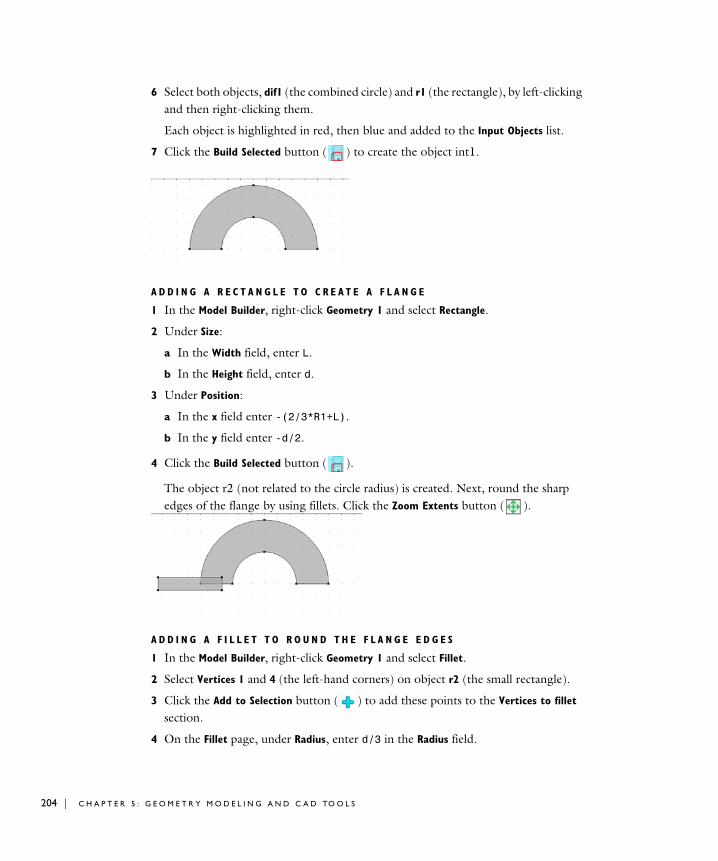
204 | C H A P T E
6 Select both objects, dif1 (the combined circle) and r1 (the rectangle), by left-clicking and then right-clicking them.
Each object is highlighted in red, then blue and added to the Input Objects list.
7 Click the Build Selected button ( ) to create the object int1.
A D D I N G A R E C T A N G L E T O C R E A T E A F L A N G E
1 In the Model Builder, right-click Geometry 1 and select Rectangle.
2 Under Size:
a In the Width field, enter L.
b In the Height field, enter d.
3 Under Position:
a In the x field enter -(2/3*R1+L).
b In the y field enter -d/2.
4 Click the Build Selected button ( ).
The object r2 (not related to the circle radius) is created. Next, round the sharp edges of the flange by using fillets. Click the Zoom Extents button ( ).
A D D I N G A F I L L E T T O R O U N D T H E F L A N G E E D G E S
1 In the Model Builder, right-click Geometry 1 and select Fillet.
2 Select Vertices 1 and 4 (the left-hand corners) on object r2 (the small rectangle).
3 Click the Add to Selection button ( ) to add these points to the Vertices to fillet section.
4 On the Fillet page, under Radius, enter d/3 in the Radius field.
R 5 : G E O M E T R Y M O D E L I N G A N D C A D TO O L S
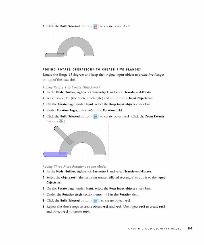
5 Click the Build Selected button ( ) to create object fil1.
A D D I N G R O T A T E O P E R A T I O N S T O C R E A T E F I V E F L A N G E S
Rotate the flange 45 degrees and keep the original input object to create five flanges on top of the heat sink.
Adding Rotate 1 to Create Object Rot11 In the Model Builder, right-click Geometry 1 and select Transforms>Rotate.
2 Select object fil1 (the filleted rectangle) and add it to the Input Objects list.
3 On the Rotate page, under Input, select the Keep input objects check box.
4 Under Rotation Angle, enter -45 in the Rotation field.
5 Click the Build Selected button ( ) to create object rot1. Click the Zoom Extents button ( ).
Adding Three More Rotations to the Model1 In the Model Builder, right-click Geometry 1 and select Transforms>Rotate.
2 Select the object rot1 (the resulting rotated filleted rectangle) to add it to the Input
Objects list.
3 On the Rotate page, under Input, select the Keep input objects check box.
4 Under the Rotation Angle section, enter -45 in the Rotation field.
5 Click the Build Selected button ( ). to create object rot2.
6 Repeat the above steps to create object rot3 and rot4. Use object rot2 to create rot3 and object rot3 to create rot4.
C R E A T I N G A 2 D G E O M E T R Y M O D E L | 205
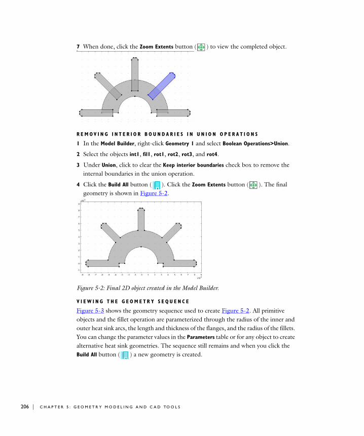
206 | C H A P T E
7 When done, click the Zoom Extents button ( ) to view the completed object.
R E M OV I N G I N T E R I O R B O U N D A R I E S I N U N I O N O P E R A T I O N S
1 In the Model Builder, right-click Geometry 1 and select Boolean Operations>Union.
2 Select the objects int1, fil1, rot1, rot2, rot3, and rot4.
3 Under Union, click to clear the Keep interior boundaries check box to remove the internal boundaries in the union operation.
4 Click the Build All button ( ). Click the Zoom Extents button ( ). The final geometry is shown in Figure 5-2.
Figure 5-2: Final 2D object created in the Model Builder.
V I E W I N G T H E G E O M E T R Y S E Q U E N C E
Figure 5-3 shows the geometry sequence used to create Figure 5-2. All primitive objects and the fillet operation are parameterized through the radius of the inner and outer heat sink arcs, the length and thickness of the flanges, and the radius of the fillets. You can change the parameter values in the Parameters table or for any object to create alternative heat sink geometries. The sequence still remains and when you click the Build All button ( ) a new geometry is created.
R 5 : G E O M E T R Y M O D E L I N G A N D C A D TO O L S

Figure 5-3: an example of a 2D geometry sequence.
R E - R U N N I N G T H E G E O M E T R Y S E Q U E N C E W I T H D I F F E R E N T P A R A M E T E R S
1 In the Model Builder, under Global Definitions, click Parameters.
The Parameters page opens in the Settings window.
2 Under Parameters, enter the following settings in the table. Replace the previous data:.
3 In the Model Builder, click Geometry 1.
NAME EXPRESSION VALUE DESCRIPTION
R1 4e-3[m] 0.0040 m Radius Circle 1
R2 2.5e-3[m] 0.0025 m Radius Circle 2
d 1e-3[m] 0.0010 m Height
L 7e-3[m] 0.0070 m Width
C R E A T I N G A 2 D G E O M E T R Y M O D E L | 207

208 | C H A P T E
4 Click the Build All button ( ). Click the Zoom Extents button ( ) to view the geometry as defined by the new parameters.
R 5 : G E O M E T R Y M O D E L I N G A N D C A D TO O L S
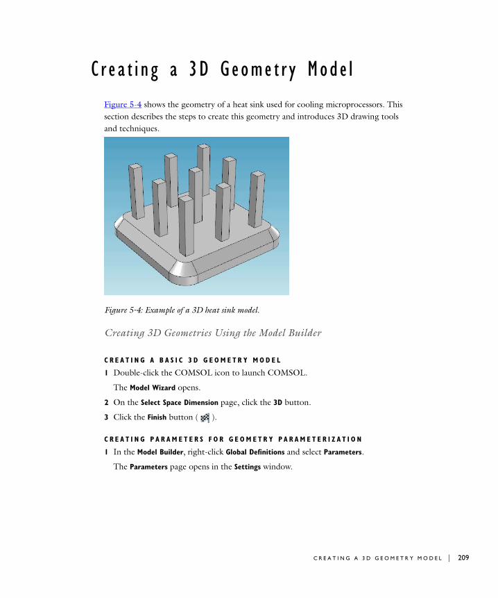
C r e a t i n g a 3D Geome t r y Mode l
Figure 5-4 shows the geometry of a heat sink used for cooling microprocessors. This section describes the steps to create this geometry and introduces 3D drawing tools and techniques.
Figure 5-4: Example of a 3D heat sink model.
Creating 3D Geometries Using the Model Builder
C R E A T I N G A B A S I C 3 D G E O M E T R Y M O D E L
1 Double-click the COMSOL icon to launch COMSOL.
The Model Wizard opens.
2 On the Select Space Dimension page, click the 3D button.
3 Click the Finish button ( ).
C R E A T I N G P A R A M E T E R S F O R G E O M E T R Y P A R A M E T E R I Z A T I O N
1 In the Model Builder, right-click Global Definitions and select Parameters.
The Parameters page opens in the Settings window.
C R E A T I N G A 3 D G E O M E T R Y M O D E L | 209

210 | C H A P T E
2 In the Parameters table, enter these settings:
U S I N G WO R K P L A N E S T O C R E A T E A B É Z I E R P O L Y G O N
Use work planes to create 2D geometries, which you then extrude or revolve to create 3D objects.
Creating a Bézier Polygon1 In the Model Builder, right-click Geometry 1 and select Work Plane.
The Work Plane page opens in the Settings window.
2 Under Work Plane, select xz-plane from the Plane list.
3 Under the Work Plane 1 node, right-click Geometry and select More
Primatives>Bézier Polygon.
4 On the Bézier Polygon page, under Polygon Segments, click Add Linear.
Segment 1 (linear) displays in the Added segments list.
5 Under Control points:
a In row 1, enter -2e-3 in the x field.
b In row 2, enter -4e-3 in the x field.
6 Click Add Linear to add Segment 2 (linear) to the Added segments list. Some of the Control points are automatically filled in with values; the control points from the previous line are already filled in as the starting points for the next line.
7 Under Control points, in row 2, enter 2e-3 in the y field.
8 Click Add Linear to add Segment 3 (linear) to the Added segments list.
a In row 2, enter -2e-3 in the x field.
b In row 2, enter 4e-3 in the y field.
9 Click Add Linear to add Segment 4 (linear) to the Added segments list.
10 Under Control points, in row 2, enter 0 in the y field.
11 Click Close Curve.
NAME EXPRESSION VALUE DESCRIPTION
L1 1.5e-2 0.015 Pillar thickness (in the heat sink)
L2 3e-3 0.0030 Pillar Length (in the heat sink)
R 5 : G E O M E T R Y M O D E L I N G A N D C A D TO O L S

12 Click the Build Selected button ( ) and the Zoom Extents button ( ).
R E VO L V I N G A 2 D O B J E C T T O C R E A T E A 3 D O B J E C T
1 In the Model Builder, right-click Work Plane1 and select Revolve.
The Revolve page opens in the Settings window and the 2D Bézier Polygon displays in the Graphics window.
2 On the Revolve page, under Revolution Angles, enter 90 in the End angle field.
Note: The Revolution Axis corresponds to the position of the y-axis in the work plane’s 2D coordinate system.
3 Under General, select the Keep input objects check box. Work Plane1 is required for the next steps.
4 Click the Build Selected button ( ) and the Zoom Extents button ( ) to view the object rev1.
A D D I N G A N E X T R U S I O N A N D U N I O N
1 In the Model Builder, right-click Work Plane1 and select Extrude.
The Extrude page opens in the Settings window.
2 Under Distances from Work Plane, enter -2e-2 in the Distances row.
C R E A T I N G A 3 D G E O M E T R Y M O D E L | 211

212 | C H A P T E
3 Click the Build Selected button ( ) and the Zoom Extents button ( )to view the object ext1.
4 In the Model Builder, right-click Geometry 1 and select Boolean Operations>Union.
The Union page opens in the Settings window.
5 Select the objects rev1 and ext1 and add them to the Input objects section.
6 On the Union page, under Union, click to clear the Keep interior boundaries check box to remove the interior boundary between the corner section and the edge section of the heat sink.
7 Click the Build Selected button ( ). Objects rev1 and ext1 are combined to create object uni1.
A D D I N G A R O T A T I O N T O T H E 3 D O B J E C T
1 In the Model Builder, right-click Geometry 1 and select Transforms>Rotate.
The Rotate page opens in the Settings window.
2 Select the object uni1 and add it to the Input objects section under Input.
3 Select the Keep input objects check box to leave the input object intact as a rotation of the object is created.
4 Under Rotation Angle, enter -90 in the Rotation field.
5 Under Point on Axis of Rotation:
a In the x field, enter 1e-2.
b In the y field, enter 1e-2.
6 Click the Build Selected button ( ) and the Zoom Extents button ( ) to view the object rot1.
R 5 : G E O M E T R Y M O D E L I N G A N D C A D TO O L S

C R E A T I N G U N I O N 2
1 In the Model Builder, right-click Geometry 1 and select Boolean Operations>Union.
The Union page opens in the Settings window.
2 Select the objects uni1 and rot1 and add them to the Input objects section on the Union page.
3 Under Union, click to clear the Keep interior boundaries check box.
4 Click the Build Selected button ( ) to create object uni2.
A D D I N G A S E C O N D R O T A T I O N
1 In the Model Builder, right-click Geometry1 and select Transforms>Rotate.
The Rotate page opens in the Settings window.
2 Select the object uni2 and add it to the Input objects section under Input.
3 Select the Keep input objects check box.
4 Under Rotation Angle, enter -180 in the Rotation field.
5 Under Point on Axis of Rotation:
a In the x field, enter 1e-2.
b In the y field, enter 1e-2.
C R E A T I N G A 3 D G E O M E T R Y M O D E L | 213
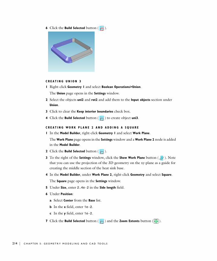
214 | C H A P T E
6 Click the Build Selected button ( ).
C R E A T I N G U N I O N 3
1 Right-click Geometry 1 and select Boolean Operations>Union.
The Union page opens in the Settings window.
2 Select the objects uni2 and rot2 and add them to the Input objects section under Union.
3 Click to clear the Keep interior boundaries check box.
4 Click the Build Selected button ( ) to create object uni3.
C R E A T I N G WO R K P L A N E 2 A N D A D D I N G A S Q U A R E
1 In the Model Builder, right-click Geometry 1 and select Work Plane.
The Work Plane page opens in the Settings window and a Work Plane 2 node is added in the Model Builder.
2 Click the Build Selected button ( ).
3 To the right of the Settings window, click the Show Work Plane button ( ). Note that you can use the projection of the 3D geometry on the xy-plane as a guide for creating the middle section of the heat sink base.
4 In the Model Builder, under Work Plane 2, right-click Geometry and select Square.
The Square page opens in the Settings window.
5 Under Size, enter 2.4e-2 in the Side length field.
6 Under Position:
a Select Center from the Base list.
b In the x field, enter 1e-2.
c In the y field, enter 1e-2.
7 Click the Build Selected button ( ) and the Zoom Extents button ( ).
R 5 : G E O M E T R Y M O D E L I N G A N D C A D TO O L S

TR I M M I N G T H E S Q U A R E T O F I T U S I N G T H E F I L L E T O P E R A T I O N
1 In the Model Builder, under Work Plane 2, right-click Geometry and select Fillet.
The Fillet page opens in the Settings window.
2 Add points 1, 2, 3, and 4 on the object sq1 to the Vertices to fillet section under Points.
3 Under Radius, enter 2e-3 in the Radius field.
4 Click the Build Selected button.( )
C R E A T I N G A 3 D G E O M E T R Y M O D E L | 215
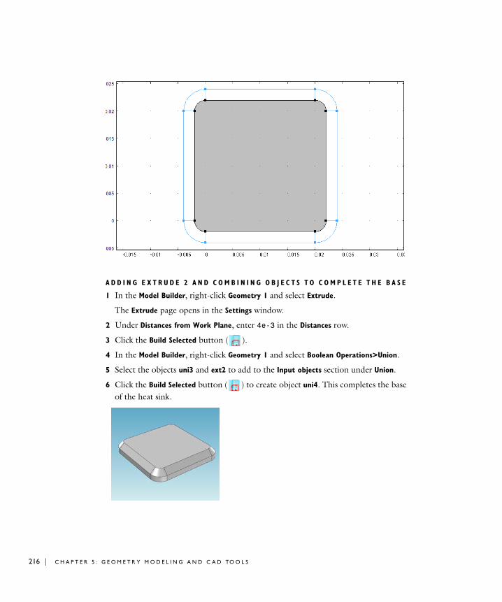
216 | C H A P T E
A D D I N G E X T R U D E 2 A N D C O M B I N I N G O B J E C T S T O C O M P L E T E T H E B A S E
1 In the Model Builder, right-click Geometry 1 and select Extrude.
The Extrude page opens in the Settings window.
2 Under Distances from Work Plane, enter 4e-3 in the Distances row.
3 Click the Build Selected button ( ).
4 In the Model Builder, right-click Geometry 1 and select Boolean Operations>Union.
5 Select the objects uni3 and ext2 to add to the Input objects section under Union.
6 Click the Build Selected button ( ) to create object uni4. This completes the base of the heat sink.
R 5 : G E O M E T R Y M O D E L I N G A N D C A D TO O L S

D R A W I N G T H E U P P E R P A R T O F T H E H E A T S I N K
Creating a Work Plane and a Square1 In the Model Builder, right-click Geometry 1 and select Work Plane.
The Work Plane page opens in the Settings window and a Work Plane 3 node is added in the Model Builder.
2 Under Work Plane, enter 4e-3 in the z-coordinate field.
3 From the 3D projection list, select Entire 3D geometry to visualize the projected edges of the heat sink’s base in the work plane.
4 Click the Build Selected button ( ).
5 To the right of the Settings window, click the Show Work Plane button ( ).
6 In the Model Builder, under Work Plane 3, right-click Geometry and select Square.
The Square page opens in the Settings window
7 Under Size, enter L2 in the Side length field.
8 Click the Build Selected button ( ) to create square sq1 with side length L2.
C R E A T I N G A 3 D G E O M E T R Y M O D E L | 217

218 | C H A P T E
A D D I N G A R R A Y S
1 In the Model Builder, under Work Plane 3, right-click Geometry and select Transforms> Array.
2 Add the object sq1 to the Input objects section under Input.
3 Under Size:
a In the x field, enter 3.
b In the y field, enter 3.
4 Under Displacement:
a In the x field, enter 1e-2-L2/2.
b In the y field, enter 1e-2-L2/2.
5 Click the Build Selected button ( ).
Adding Extrude 3 and Combining Objects (Union)1 In the Model Builder, right-click Geometry 1 and select Extrude.
The Extrude page opens in the Settings window.
2 Under Distances from Work Plane, enter L1 in the Distances row.
3 Click the Build Selected button ( ) and the Zoom Extents button ( ).
R 5 : G E O M E T R Y M O D E L I N G A N D C A D TO O L S

4 Right-click Geometry 1 again and select Boolean Operations>Union.
The Union page opens in the Settings window.
5 Add all the objects to the Input objects list under Union.
6 Click the Build All button ( ) to complete the heat sink geometry.
T H E G E O M E T R Y S E Q U E N C E
Figure 5-5 shows the list of the geometry in the Model Builder used to create Figure 5-4. You can edit any node for each of the drawing operations.
In this case, the upper part of the heat sink is parameterized, through the thickness and height of the heat sink pillars. You can edit the parameter values defined previously to change the heat sink geometry.
C R E A T I N G A 3 D G E O M E T R Y M O D E L | 219
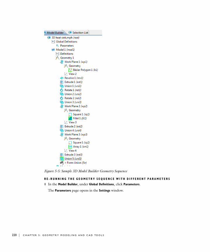
220 | C H A P T E
Figure 5-5: Sample 3D Model Builder Geometry Sequence
R E - R U N N I N G T H E G E O M E T R Y S E Q U E N C E W I T H D I F F E R E N T P A R A M E T E R S
1 In the Model Builder, under Global Definitions, click Parameters.
The Parameters page opens in the Settings window.
R 5 : G E O M E T R Y M O D E L I N G A N D C A D TO O L S
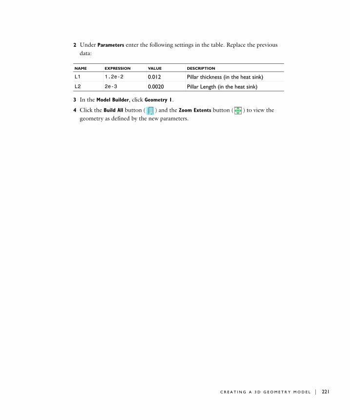
2 Under Parameters enter the following settings in the table. Replace the previous data:
3 In the Model Builder, click Geometry 1.
4 Click the Build All button ( ) and the Zoom Extents button ( ) to view the geometry as defined by the new parameters.
NAME EXPRESSION VALUE DESCRIPTION
L1 1.2e-2 0.012 Pillar thickness (in the heat sink)
L2 2e-3 0.0020 Pillar Length (in the heat sink)
C R E A T I N G A 3 D G E O M E T R Y M O D E L | 221

222 | C H A P T E
R 5 : G E O M E T R Y M O D E L I N G A N D C A D TO O L S
6
M a t e r i a l s
This section describes how to work with materials: adding them to the model, using material databases, and defining material properties.
In this section:
• Materials Overview
• Adding Predefined Materials
• User-Defined Materials and Libraries
• Material Properties Reference
• Using Functions
223

224 | C H A P T E
Ma t e r i a l s O v e r v i ew
Predefined Material Databases Included with COMSOL Modules
All COMSOL modules have predefined material data available to build models. The most extensive material data is contained in the separately purchased Material Library, but all modules contain commonly used or module-specific materials. For example, the Built-In database is available to all users but the MEMS database is included with the Acoustics Module, MEMS Module, and Structural Mechanics Module. You can also create your own materials and material libraries by researching and entering material properties yourself.
You access all the material databases (including the Material Library) from the Material
Browser. These databases are briefly described below.
R E C E N T M A T E R I A L S
From the Recent Materials folder ( ), you can select from a list of recently used materials, with the most recent at the top.
M A T E R I A L L I B R A R Y
An optional add-on database, the Material Library ( ), contains data for over 2500 materials and 20,000 property functions. You can search an online list of available
Material Browser—select predefined materials in all applications.
Material Library—Purchased separately. Select from over 2500 predefined materials.
Built-In database—Available to all users and contains common materials.
Application specific materials databases —Available with specific modules.
User defined material database library.
Recent Materials—Select from materials used recently.
R 6 : M A T E R I A L S

materials in the Material Library from the COMSOL website: http://www.comsol.com/products/material.
B U I L T - I N
Included with COMSOL Multiphysics, the Built-In database ( ) contains common solid materials with electrical, structural, and thermal properties. See Predefined Built-In Materials for all COMSOL Modules for a list.
A C / D C
Included in the AC/DC Module, the AC/DC database ( ) has electric properties for some magnetic and conductive materials.
L I Q U I D S A N D G A S E S
Included in the Acoustics, Chemical Engineering, Earth Science, Heat Transfer, and MEMS Modules, the Liquids and Gases database ( ) includes transport properties and surface tension data for liquid/gas and liquid/liquid interfaces.
M E M S
Included in the Acoustics, MEMS, and Structural Mechanics Modules, the MEMS database ( ) has properties for MEMS materials—metals, semiconductors, insulators, and polymers.
P I E Z O E L E C T R I C
Included in the Acoustics, MEMS, and Structural Mechanics Modules, the Piezoelectric database ( ) has properties for piezoelectric materials.
U S E R - D E F I N E D M A T E R I A L D A T A B A S E S
The User-Defined Library folder ( ) is where you create user defined material databases (libraries). When you create any new database, this also displays in the Material Browser. See Creating a User defined Materials Database.
Note: All material databases (including the Material Library) shipped with COMSOL Multiphysics and the optional modules are read-only.
M A T E R I A L S O V E R V I E W | 225

226 | C H A P T E
About Using Materials in COMSOL
U S I N G T H E M A T E R I A L S I N T H E P H Y S I C S S E T T I N G S
The physics set-up in a model is determined by a combination of settings in the Materials and physics interface pages. When you add the first material to a model, COMSOL automatically assigns that material to the entire geometry. The power of COMSOL is that you can select different geometric entities to have different materials. The following example uses the heat_sink.mph model file contained in the Heat Transfer Module Model Library.
Figure 6-1: Assigning materials to a heat sink model. Air is assigned as the material to the box surrounding the heat sink, and aluminum to the heat sink itself.
If a geometry consists of a heat sink in a container, you can assign Air as the material in the container surrounding the heat sink and Aluminum as the heat sink material itself (see Figure 6-1). The Conjugate Heat Transfer physics interface, selected during model set-up, has a Fluid flow model, defined in the box surrounding the heat sink, and a Heat
Transfer model, defined in both the aluminum heat sink and in the air box. The Heat
Transfer in Solids 1 settings use the material properties associated to the Aluminum
3003-H18 materials node, and the Fluid 1 settings define the flow using the Air material properties. The other nodes under Conjugate Heat Transfer define the initial and boundary conditions.
All physics interface properties automatically use the correct Materials properties when you use the default From material setting. This means that you can use one node to
R 6 : M A T E R I A L S

define the physics across several domains with different materials; COMSOL then uses the material properties from the different materials to define the physics in the domains. If material properties are missing, the Material Contents section on the Materials page displays a stop icon to warn you about the missing properties or values. See About the Material Page.
E V A L U A T I N G A N D P L O T T I N G M A T E R I A L P R O P E R T I E S
{[MR: Add this when Erik D. has checked in support for mat1.rho etc. Notice special case of functions like mat1.def.rho(pA,T)]]
About the Material Browser Window and Page
The Material Browser window ( ) contains a number of databases with a broad collection of physical, elastic, electromagnetic, fluid, piezoelectric, and thermal properties of materials (Figure 6-2). Use the Material Browser to find predefined materials and add them to the Model Builder, or create your own custom material library.
Note: When you are using the Material Browser, the words window and page are interchangeable. For simplicity, the instructions refer only to the Material Browser.
Figure 6-2: Opening the Material Browser page in the Material Browser window.
The Material Browser contains the following sections:
WindowPage
M A T E R I A L S O V E R V I E W | 227

228 | C H A P T E
M A T E R I A L S
Browse all the available material databases or search in the Materials section. Search a specific material by name, UNS number, or DIN number. You can also browse for a specific material by class (for example, in the Material Library) or physics module (for example, MEMS). When you locate the material you want, right-click to Add Material
to Model.
I N F O R M A T I O N
When you are browsing the material databases, in particular the Model Library, some materials include additional information—UNS number, DIN number, and/or Composition.
P R O P E R T I E S
When you are browsing the material databases, this section lists predefined Properties. The table includes the default listings of Property, Expression, and the Property groups to which it belongs.
F U N C T I O N S
When you are browsing the material databases, some materials have predefined Functions listed. The table includes the default listings of Function, Type, Expression, and the Property groups to which it belongs.
I N P U T
When you are browsing the Material Library database, some materials have predefined Input listed. The table includes the default listings of Input, Unit, and Property groups to which it belongs.
About the Material Page
The Material page ( ) summarizes the predefined or user defined material properties. It is where you add material properties specific to the model and assign the geometric entity level where the material is used in the geometry (domain, boundary, edge, or point) and the domains, for example, that consists of this material.
R 6 : M A T E R I A L S

After adding a material, click the material node (for example, Copper) in the Model
Builder. The Material page opens in the Settings window (Figure 6-3).
Figure 6-3: Opening the Material page in the Settings window.
The Material page contains the following sections:
G E O M E T R I C S C O P E
Assign the material to a specific Geometric entity level—Domain, Boundary, Edge (3D only), or Point—on the geometry in the Graphics window (the geometry in the model).
M A T E R I A L P R O P E R T I E S
Add additional material properties to the model if they are not already included in the default settings.
M A T E R I A L C O N T E N T S
View lists of all the default material data. The table lists the Property, Name, Value, Unit, and the Property group. The Property group corresponds to the nodes in the Model
Builder with the same name (see Figure 6-4). If required, edit a default property Value.
The left column provides visual cues about the status of each property.
• A stop sign ( ) indicates that an entry in the Value column is required. It means that the material is used but undefined.
• A warning sign ( ) indicates that the material parameters are undefined and unused. An entry is only required if the material is used.
WindowPageNode
M A T E R I A L S O V E R V I E W | 229

230 | C H A P T E
• A green check mark ( ) indicates that the property has a Value and is currently being used in the physics of the model.
• Properties with no indication in the left column are not currently used by any physics interface in the model.
Figure 6-4: An example of Property Groups on the Material page.
About the Property Group Page
The Property Group page is where you add output and input properties, define local parameters, and enter expressions for a specific property group (Figure 6-5).
The Property Group page is in the Settings window and opens when you click the node (for example, Basic) under the material name in the Model Builder. The Property Group page is associated to other pages relating to the same material.
R 6 : M A T E R I A L S

Figure 6-5: An example of a Basic Property Group page.
O U T P U T P R O P E R T I E S A N D M O D E L I N P U T S
View predefined material properties in the Output properties table. Add additional properties from the Quantities subsection to the Output properties or Model Inputs tables. If required, edit the expressions in the Output properties subsection’s Expression column. The model inputs are physical quantities such as temperature that are used as inputs in the expressions that define the output properties.
L O C A L P A R A M E T E R S
Enter a user defined Parameter and its corresponding Expression and organize the table as required.
About Automatic Adding of Property Groups to a MaterialMaterial property groups are automatically added to the material node in the Model
Builder. You can also add additional predefined property groups or create your own User defined property group. The available properties are grouped together differently according to the physical context. For example, the Copper node in Figure 6-4 contains the following default property groups: Basic, Young’s modulus and Poisson’s ratio, and Linearized resistivity.
Each of the property groups has a Property Group page. When you click a Model Builder node (for example, Basic), the Property Group page displays specific information about that property group. The property groups are summarized in a Material Contents table on the Material page.
M A T E R I A L S O V E R V I E W | 231

232 | C H A P T E
Add i n g P r e d e f i n e d Ma t e r i a l s
Note: The first material added to a model is assigned to entire geometry.
Working on the Material Browser
When you are using the Material Browser, the words window and page are interchangeable. For simplicity, the instructions refer only to the Material Browser.
O P E N I N G T H E M A T E R I A L B R O W S E R
1 Open or create a model file.
2 From the Options menu select Material Browser or right-click the Materials node and select Open Material Browser.
The Material Browser opens by default to the right of the Settings window.
A D D I N G A P R E D E F I N E D M A T E R I A L T O A M O D E L
1 Open the Material Browser.
2 Under Materials, search or browse for materials.
- Enter a Search term to find a specific material by name, UNS number (Material Library materials only), or DIN number (Material Library materials only). If the search is successful, a list of filtered databases containing that material displays under Materials.
Note: To clear the search field and browse, delete the search term and click Search to reload all the databases.
- Click to open each database and browse for a specific material by class (for example, in the Material Library) or physics module (for example, MEMS).
R 6 : M A T E R I A L S

Note: Always review the material properties to confirm they are applicable for the model. For example, Air provides temperature-dependent properties that are valid at pressures around 1 atm.
3 When you locate the material you want, right-click to Add Material to Model.
A node with the material name is added to the Model Builder and the Material page opens.
Working on the Material Page
V I E W I N G A S U M M A R Y O F T H E M A T E R I A L P R O P E R T I E S
1 Add a material and geometry to the model.
2 In the Model Builder, click the material node to open the Material page in the Settings window.
The Material page summarizes all the predefined data and has these sections:
- Geometric Scope: select the object Domain, Boundary, Edge (3D only), or Point to assign material to the geometry domain, boundary, edge or point.
- Material Properties: select and define specific material parameters to add to your model.
- Material Contents: lists all the default material property data. The table contains the Property, Name, Value, Unit, and the Property group. The Property group corresponds to the nodes in the Model Builder with the same name. If required, edit a default property Value.
A S S I G N I N G G E O M E T R I C S C O P E T O A M A T E R I A L
1 Add a material and geometry to the model.
2 On the Material page, from the Geometric entity level list, select Domain, Boundary, Edge (3D only), or Point. Selection from this list activates the button with the same name in the Graphics window.
A D D I N G P R E D E F I N E D M A T E R I A L S | 233

234 | C H A P T E
3 Select Manual or All (Domains, Boundaries, Edges, or Points) from the Selection list.
- If you select Manual, go the Graphics window and select geometric entities of your model.
- Select All to add the applicable geometry (Domains, Boundaries, Edges, or Points) to the Selection box. Click the Add to Selection ( ), Remove from Selection ( ), and Clear Selection ( ) buttons as required.
A D D I N G P R E D E F I N E D M A T E R I A L P R O P E R T I E S
1 Add a material to the model.
2 In the Model Builder, click the material node to open the Material page.
Note: Review the default properties listed in the Material Contents table before adding new material properties.
3 Browse the Material Properties section to locate the property to add to the model. For example, right-click Loss Tangent under Electromagnetic Models and select Add to
Material or click the Add button ( ).
See Figure 6-6. In this example, a Loss Tangent node is added to the Model Builder, and its associated properties are added to the Material Contents table. Any properties requiring Values are highlighted by red stop signs ( ) in the left-hand column.
4 Scroll through the Material Contents table to locate properties with a stop sign ( ) in the column to indicate it is missing data. Enter a Value into the table next to the applicable property. In the example, the Loss tangent and Relative permittivity
R 6 : M A T E R I A L S

properties require data. The left column provides visual cues about the status of each property.
- A stop sign ( ) indicates that an entry in the Value column is required. It means that the material is used but undefined.
- A warning sign ( ) indicates that the material parameters are undefined and unused. An entry is only required if the material is used.
- A green check mark ( ) indicates that the property has a Value and is currently being used in the physics of the model.
- Any entry made on the Material page is also added to the Property Group page under Output properties - Expression column. Click the Property Group node (for example, Loss tangent) to open this page.
Figure 6-6: Adding a material property to a model. Two properties require data.
Note: To delete a property group you have added, right-click the property group node (in the Model Builder) and select Delete. The Basic property group cannot be deleted.
A D D I N G P R E D E F I N E D M A T E R I A L S | 235

236 | C H A P T E
Working on the Property Group Page
A D D I N G O U T P U T P R O P E R T I E S T O P R E D E F I N E D M A T E R I A L S
Note: Output Properties is only accessible from the Basic material properties and with user defined property groups.
1 Add a material to the model.
2 In the Model Builder, click Basic to open the Property Group page. See Figure 6-4.
The Property Group tables are linked to other pages related to the selected material. Use the Move Up ( ), Move Down ( ), and Delete ( ) buttons to organize the tables as required.
3 Under Output Properties and Model Inputs, in the Quantities section:
a Browse the Output Properties list to locate the property to add. See About the Output Materials Properties for a list.
b Right-click the property to Add items to the Output properties table or click the Add button ( ).
c In the Output properties table, edit the Expression column or field.
Use the Move Up ( ), Move Down ( ), and Delete ( ) buttons to organize the table as required.
A D D I N G M O D E L I N P U T S T O P R E D E F I N E D M A T E R I A L S
1 Add a material to the model.
2 In the Model Builder, click the property group node (for example, Basic) to open the Property Group page.
The Property Group page tables display on other pages pertaining to the selected material.
3 Browse the Model Inputs list. Right-click the property to Add items to the Model
inputs table. Or click the Add button ( ). See Model Input Properties for a list.
A D D I N G L O C A L P A R A M E T E R S T O P R E D E F I N E D M A T E R I A L S
1 Add a material to the model.
2 In the Model Builder, click the property group node (for example, Basic) to open the Property Group page.
R 6 : M A T E R I A L S

3 Under Local Parameters, enter Parameters and Expressions as required.
Use the Move Up ( ), Move Down ( ), and Delete ( ) buttons to organize the table as required.
Note: Also see Adding a User-Defined Property Group.
Adding a User-Defined Property Group
1 Open or create a model file and add a material (predefined or user defined) to the model.
2 In the Model Builder, right-click any material node (for example, Copper) and select User defined property group.
A User defined property group node is added to the Model Builder, and a Property
Group page opens in the Settings window.
3 Follow the instructions to define the property group—see Working on the Property Group Page.
A D D I N G P R E D E F I N E D M A T E R I A L S | 237

238 | C H A P T E
U s e r -D e f i n e d Ma t e r i a l s a nd L i b r a r i e s
User defined materials provide the flexibility needed to design your model and experiments using a combination of existing material properties or defining it yourself. You can also create your own materials database (library) to include materials you use often.
Adding User defined Materials
1 Open or create a model file.
2 In the Model Builder, right-click Materials and select Material.
A Material node is added to the Model Builder, and an undefined Material page opens in the Settings window.
3 Follow the instructions as required to define your material:
a Working on the Material Page
b Working on the Property Group Page
c Adding a User-Defined Property Group
d Adding a Function to the Material
R E N A M I N G M O D E L B U I L D E R N O D E S
If required, edit or add comments to the Node Properties.
1 In the Model Builder, right-click any node and select Properties.
2 On the Node Properties page, enter the Name, Author, Version, or Comments about the node. The Tag and Date created fields cannot be changed.
The node’s Name can be edited by right-clicking directly on the node and selecting Rename.
Adding an External Material Library
1 In the Material Browser, under Materials, right-click any database and select Add
Material Library.
The Choose Material Library window opens.
2 Navigate to a material library file and click Save. For example, MatWeb provides a service where you can export technical datasheets from MatWeb’s collection in the
R 6 : M A T E R I A L S

format for a COMSOL material library. For more information about this service, visit www.matweb.com.
Creating a User defined Materials Database
Note: Because there is a separately purchased Materials Library, the user defined “library” is referred to as a database instead.
When you first open the Material Browser, an empty material database (library) is available for you to start creating your own library of materials.
Adding a User defined Material Database to the Material Browser
If this empty database (library) is removed from this list, you can add it back to the Material Browser.
1 Open the Material Browser.
2 Right-click anywhere in the Materials section and select Add Material Library.
3 Navigate to the folder where the empty database is located. This varies based on your installation, but search for the file name def_user_lib.mph.
4 Click Save.
5 Right-click the database to rename it to something meaningful to you.
6 Repeat these steps to add additional user defined material databases. Rename each one as required.
U S E R - D E F I N E D M A T E R I A L S A N D L I B R A R I E S | 239
240 | C H A P T E
R E N A M I N G A U S E R D E F I N E D M A T E R I A L L I B R A R Y
Right click to rename the material database to something meaningful to you.
Creating a User defined Material Database
1 Open the Material Browser.
2 Right-click anywhere in the Materials section and select Add Material Library.
3 Navigate to the folder where the empty database is located. This varies based on your installation, but search for the file name def_user_lib.mph.
4 Click Save.
5 Right-click the database to rename it to something meaningful to you.
You can now add predefined materials or create your own material to add to the user defined database.
A D D I N G A U S E R D E F I N E D M A T E R I A L
1 In the Model Builder, right-click Materials and select Material.
A Material node is added to the Model Builder, and an undefined Material page opens in the Settings window.
2 Follow the instructions as required to define your material:
a Working on the Material Page
b Working on the Property Group Page
c Adding a User-Defined Property Group
d Adding a Function to the Material
3 When you are done, right-click the new material and select Add Material to Library.
A D D I N G A P R E D E F I N E D M A T E R I A L
1 Open the Material Browser and add any predefined material to the Model Builder.
2 Right click the material node and select Add Material to Library.
3 Right-click to Rename Selected material that has been added to your library.
R E M OV I N G A M A T E R I A L F R O M A U S E R D E F I N E D D A T A B A S E
Open the Material Browse. Locate the material to remove. Right-click the material and select Remove Selected.
R 6 : M A T E R I A L S

Ma t e r i a l P r op e r t i e s R e f e r e n c e
You have access to the material properties for the predefined materials in most physics interfaces. Using this information you can either create your own material property group or define a completely new material.
On the Basic>Property Group page, add Output properties from the Quantities subsection. For all Property Group pages, you can add Model inputs.
About the Output Materials Properties
Note: Some of these properties are only applicable to physics interfaces in the add-on modules.
B A S I C M A T E R I A L P R O P E R T I E S
These material properties can be added to models from two pages— Material and Property Group. In both cases the properties belong to the Basic property group.
• When you access this information from the Basic>Property Group page, it is listed under Quantities>Output Properties and Variable is listed in the table.
• When you access this information from the Material page, it is listed under Material
Properties>Basic Properties and Name is listed in the tables.
PROPERTY NAME/VARIABLE UNIT
Characteristic Acoustic Impedance Z Pa*s/m
Bulk Modulus K Pa
Compliance C 1/Pa
Compressibility chif 1/Pa
Piezoelectric Coupling d d C/N
Piezoelectric Coupling e e C/m2
Density rho kg/m3
Elevation D m2/s
Elasticity cE Pa
Electric Conductivity sigma S/m
M A T E R I A L P R O P E R T I E S R E F E R E N C E | 241

242 | C H A P T E
E L E C T R O M A G N E T I C M O D E L S
These material property groups (including all associated properties) can be added to models from the Material page.
Electron Mobility mue m2/(Vs)
Surface Emissivity epsilon rad 1
Heat Capacity at Constant Pressure Cp J/(kgK)
Permeability kappa m2
Isotropic Structural Loss Factor eta s 1
Mean Molar Mass Mn kg/mol
Poisson’s Ratio nu 1
Ratio of Specific Heats gamma 1
Relative Permeability mur 1
Relative Permittivity epsilonr 1
Resistivity res m
Shear Modulus G Pa
Speed of Sound cp m/s
Storage S 1/Pa
Thermal Conductivity k W/(mK)
Coefficient of Thermal Expansion alpha 1/K
Dynamic Viscosity mu (Pa)s
Young’s Modulus E Pa
PROPERTY GROUP AND PROPERTY NAME/VARIABLE UNIT
LINEARIZED RESISTIVITY
Reference resistivity rho0 m
Resistivity temperature coefficient alpha -
Reference temperature Tref K
LOSS TANGENT
Loss tangent delta -
Relative permittivity (real part) epsilonPrim 1
Electric conductivity sigma S/m
DIELECTRIC LOSSES
Relative permittivity (imaginary part) epsilonBis 1
PROPERTY NAME/VARIABLE UNIT
R 6 : M A T E R I A L S

S O L I D M E C H A N I C S
These material property groups (including all associated properties) can be added to models from the Material page.
Relative permittivity (real part) epsilonPrim 1
REFRACTIVE INDEX
Refractive index n 1
Refractive index, imaginary part ki -
MAGNETIC LOSSES
Relative permeability (real part) murPrim -
Relative permeability (imaginary part) murBis -
HB CURVE
Local Parameters normB -
BH CURVE
Local Parameters normH -
PROPERTY GROUP AND PROPERTY NAME/VARIABLE UNIT
PROPERTY GROUP AND PROPERTY NAME/VARIABLE UNIT
LINEAR ELASTIC MATERIAL MODEL
YOUNG’S MODULUS AND POISSON’S RATIO
Young’s Modulus E Pa
Poisson’s Ratio nu 1
LAMÉ CONSTANTS
Lamé Constant lambLame Pa
Lamé Constant muLame Pa
BULK MODULUS AND SHEAR MODULUS
Bulk Modulus K Pa
Shear Modulus G Pa
PRESSURE-WAVE AND SHEAR-WAVE SPEEDS
Pressure-wave Speed cl m/s
Shear-Wave Speed ct m/s
ORTHOTROPIC
Young’s Modulus Evector Pa
Poisson’s Ratio nuvector 1
Shear Modulus Gvector Pa
Loss factor for orthotropic Young’s modulus eta_Evector Pa
M A T E R I A L P R O P E R T I E S R E F E R E N C E | 243

244 | C H A P T E
P I E Z O E L E C T R I C M O D E L S
These material property groups (including all associated properties) can be added to models from the Material page.
Loss factor for orthotropic shear modulus eta_Gvector Pa
ANISOTROPIC
Elasticity matrix D Pa
Loss factor for elasticity matrix D eta_D Pa
ELASTOPLASTIC MATERIAL MODEL
Yield stress level sigmags Pa
Kinematic tangent modulus Ek Pa
Isotropic tangent modulus Et Pa
VISCOELASTIC MATERIAL MODEL
Long-term shear modulus Gv Pa
Bulk modulus K Pa
HYPERELASTIC MATERIAL MODEL
NEO-HOOKEAN
Lamé Constant mu Pa
Lamé Constant lambda Pa
MOONEY-RIVLIN
Model parameters C10 Pa
Model parameters C01 Pa
MURNAGHAN
Murnaghan third-order elastic moduli l Pa
Murnaghan third-order elastic moduli m Pa
Murnaghan third-order elastic moduli n Pa
Lamé Constant lambLame Pa
Lamé Constant muLame Pa
PROPERTY GROUP AND PROPERTY NAME/VARIABLE UNIT
PROPERTY GROUP AND PROPERTY NAME/VARIABLE UNIT
STRESS-CHARGE FORM
Elasticity matrix cE cE Pa
Coupling matrix eES C/m2
Relative permittivity epsilonrS 1
STRAIN-CHARGE FORM
R 6 : M A T E R I A L S
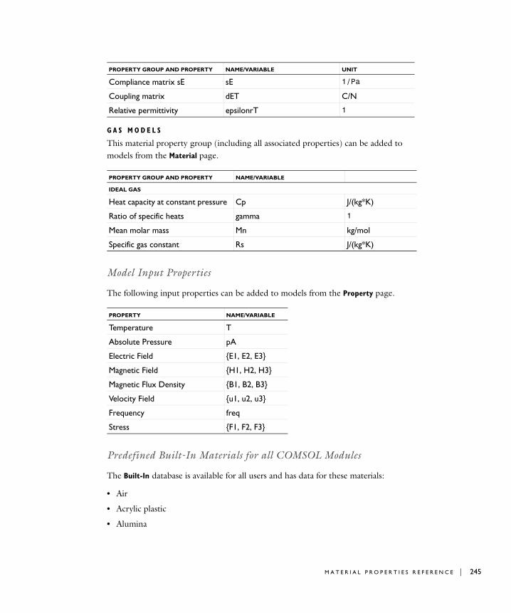
G A S M O D E L S
This material property group (including all associated properties) can be added to models from the Material page.
Model Input Properties
The following input properties can be added to models from the Property page.
Predefined Built-In Materials for all COMSOL Modules
The Built-In database is available for all users and has data for these materials:
• Air
• Acrylic plastic
• Alumina
Compliance matrix sE sE 1/Pa
Coupling matrix dET C/N
Relative permittivity epsilonrT 1
PROPERTY GROUP AND PROPERTY NAME/VARIABLE
IDEAL GAS
Heat capacity at constant pressure Cp J/(kg*K)
Ratio of specific heats gamma 1
Mean molar mass Mn kg/mol
Specific gas constant Rs J/(kg*K)
PROPERTY NAME/VARIABLE
Temperature T
Absolute Pressure pA
Electric Field {E1, E2, E3}
Magnetic Field {H1, H2, H3}
Magnetic Flux Density {B1, B2, B3}
Velocity Field {u1, u2, u3}
Frequency freq
Stress {F1, F2, F3}
PROPERTY GROUP AND PROPERTY NAME/VARIABLE UNIT
M A T E R I A L P R O P E R T I E S R E F E R E N C E | 245

246 | C H A P T E
• Aluminum 3003-H18
• Aluminum 6063-T83
• Aluminum
• American red oak
• Beryllium copper UNS C17200
• Brick
• Cast iron
• Concrete
• Copper
• FR4 (Circuit Board)
• Glass (quartz)
• Granite
• High-strength alloy steel
• Iron
• Magnesium AZ31B
• Mica
• Molybdenum
• Nimonic alloy 90
• Nylon
• Lead Zirconate Titanate (PZT-5H)
• Silica glass
• Silicon
• Polysilicon
• Solder, 60Sn-40Pb
• Steel AISI 4340
• Structural steel
• Titanium beta-21S
• Tungsten
• Water, liquid
R 6 : M A T E R I A L S

Material Property Groups Descriptions
The following material property groups are available for the entire COMSOL Multiphysics product line (some groups are only applicable to physics interfaces in some of the add-on modules):
Basic: Contains over 25 basic material properties for use with all materials. See About the Output Materials Properties for a complete list.
Linearized Resistivity: For electromagnetic models, to define the electric resistivity (and conductivity) as a linear function of temperature.
Loss Tangent: For electromagnetic models, allows you to specify a loss tangent for dielectric losses or take it from the material. Assumes zero conductivity.
Dielectric Losses: For electromagnetic models, allows you to specify the real and imaginary parts of the relative permittivity or take them from the material.
Refractive Index: For electromagnetic models, allows you to specify the real and imaginary parts of the refractive index or take them from the material. Note that this assumes a relative permeability of unity and zero conductivity.
Magnetic Losses: For electromagnetic models, allows you to specify the real and imaginary parts of the relative permeability or take them from the material.
HB Curve: For electromagnetic models, allows you to use a curve that relates magnetic flux density B and the magnetic field H.
BH Curve: For electromagnetic models, allows you to use a curve that relates magnetic flux density B and the magnetic field H.
Young's Modulus and Poisson's Ratio: In solid mechanics models, Young’s Modulus defines the modulus of elasticity and is the spring stiffness in Hooke’s law. Poisson’s Ratio defines the normal strain in the perpendicular direction, generated from a normal strain in the other direction.
Lamé Constants: In solid mechanics models, these are linear elastic material property constants.
Bulk Modulus and Shear Modulus: In solid mechanics models, a linear elastic material property where the bulk modulus is a measure of the solid’s resistance to volume
M A T E R I A L P R O P E R T I E S R E F E R E N C E | 247

248 | C H A P T E
changes. The shear modulus is a measure of the solid’s resistance to shear deformations.
Pressure-Wave and Shear-Wave Speeds: In solid mechanics models, a linear elastic material property where you specify the pressure-wave speed (longitudinal wave speed) and the shear-wave speed (transverse wave speed).
Orthotropic: In solid mechanics models, a linear elastic material property that has different properties in orthogonal directions; its stiffness depends on those properties.
Anisotropic: In solid mechanics models, a linear elastic material property that has different material properties in different directions; the stiffness comes from the symmetric elasticity matrix.
Elastoplastic Material Model: In solid mechanics models, an elastoplastic property group adds these equations: yield stress level, kinematic tangent modulus, and isotropic tangent modulus.
Viscoelastic Material Model: In solid mechanics models, viscoelastic materials are those that exhibit both elastic and viscous behavior when they deform. This property group adds the long-term shear modulus and bulk modulus equations.
Hyperelastic Material Model: In hyperelastic materials the stresses are computed from a strain energy density function. They are often used to model rubber, but also used in acoustoelasticity.
Neo-Hookean: In solid mechanics, a hyperelastic material property with two model parameters. The model is based on modified strain invariants.
Mooney-Rivlin: In solid mechanics, a hyperelastic material property with three model parameters. The model is based on modified strain invariants.
Murnaghan: In solid mechanics, a hyperelastic material property with five model parameters. The model is based on modified strain invariants and is typically used in acoustoelasticity.
Stress-Charge Form: In Piezoelectric models, used to express the constitutive relations using the elasticity matrix, coupling matrix, and relative permittivity equations.
R 6 : M A T E R I A L S

Strain-Charge Form: In Piezoelectric models, used to express the constitutive relations using the compliance matrix, coupling matrix, and relative permittivity equations.
Ideal Gas: In gas models, this property group adds the heat capacity at constant pressure, ratio of specific heats, mean molar mass, and specific gas constant equations.
Other Predefined Materials in COMSOL Modules
• See the AC/DC Module documentation for list of common AC/DC materials.
• See the Acoustics Module or MEMS Module documentation for a list of Liquids and Gases, MEMS, and Piezoelectric materials.
• See the Chemical Reaction Engineering Module, Earth Science Module, or Heat Transfer Module documentation for a list of Liquids and Gases materials.
• See the Structural Mechanics Module documentation for a list of MEMS and Piezoelectric materials.
M A T E R I A L P R O P E R T I E S R E F E R E N C E | 249

250 | C H A P T E
U s i n g Fun c t i o n s
Adding a Function to the Material
Material functions are either automatically added to the Model Builder sequence (usually with materials from the Model Library) or you can add functions based on your own requirements:
1 Add a material to the model.
2 In the Model Builder, right-click a property group node, for example, Basic.
3 Select one of the following from the Functions list:
- Select Analytic to extend properties with the ability to bind parameters during function calls. See Example of Defining an Analytic Function. Also see Analytic.
- Select Interpolation to interpolate from data that can be both structured (defined on a grid) or unstructured (defined on a generic point cloud). See Interpolation.
- Select Piecewise if there is one material property that has different definitions on different intervals.The intervals must not overlap, and there cannot be any holes between intervals. See Piecewise.
Note: Once a function is created, it can be used for any property in the same property group.
Example of Defining an Analytic Function
Assume that you want to define Young’s modulus for a material as a function of pressure and temperature. You can name the function young(p,T) and use the expression 2e10+1e6*p-1e8*T to define the function.
1 Open the Material Browser.
2 Search or browse for a material to add to the model.
a In the Material Library, open the Cast Irons & Mold materials>Cast Irons folder.
b From the list, right-click A297 HI (UNS J94003) to Add Material to Model.
The material is added to the Model Builder with a Basic property group containing Piecewise functions. Observe that Young’s Modulus is not automatically added.
R 6 : M A T E R I A L S
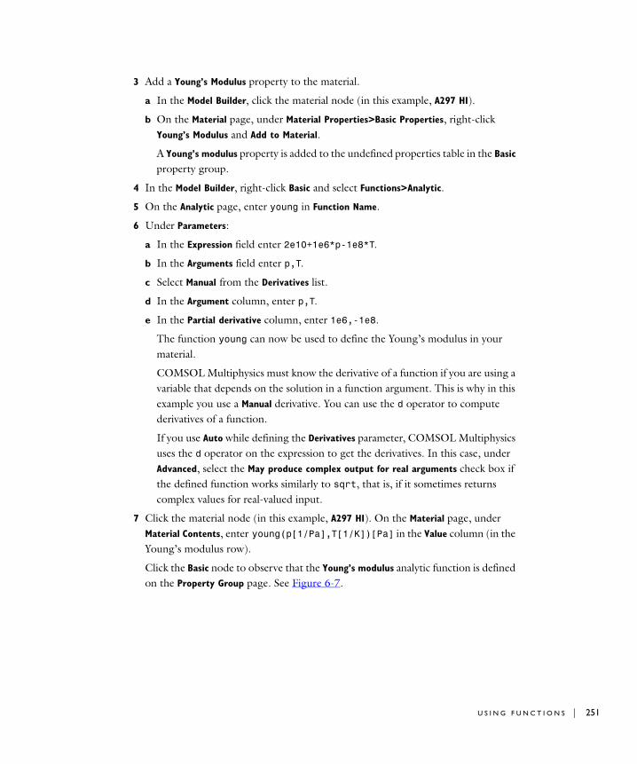
3 Add a Young’s Modulus property to the material.
a In the Model Builder, click the material node (in this example, A297 HI).
b On the Material page, under Material Properties>Basic Properties, right-click Young’s Modulus and Add to Material.
A Young’s modulus property is added to the undefined properties table in the Basic property group.
4 In the Model Builder, right-click Basic and select Functions>Analytic.
5 On the Analytic page, enter young in Function Name.
6 Under Parameters:
a In the Expression field enter 2e10+1e6*p-1e8*T.
b In the Arguments field enter p,T.
c Select Manual from the Derivatives list.
d In the Argument column, enter p,T.
e In the Partial derivative column, enter 1e6,-1e8.
The function young can now be used to define the Young’s modulus in your material.
COMSOL Multiphysics must know the derivative of a function if you are using a variable that depends on the solution in a function argument. This is why in this example you use a Manual derivative. You can use the d operator to compute derivatives of a function.
If you use Auto while defining the Derivatives parameter, COMSOL Multiphysics uses the d operator on the expression to get the derivatives. In this case, under Advanced, select the May produce complex output for real arguments check box if the defined function works similarly to sqrt, that is, if it sometimes returns complex values for real-valued input.
7 Click the material node (in this example, A297 HI). On the Material page, under Material Contents, enter young(p[1/Pa],T[1/K])[Pa] in the Value column (in the Young’s modulus row).
Click the Basic node to observe that the Young’s modulus analytic function is defined on the Property Group page. See Figure 6-7.
U S I N G F U N C T I O N S | 251

252 | C H A P T E
Figure 6-7: Adding a Young’s Modulus property as an Analytic function.
R 6 : M A T E R I A L S

7
B u i l d i n g a C O M S O L M o d e l
This section explains a range of methods and topics used when building models in COMSOL Multiphysics: From working with the Model Wizard and fundamental concepts for the Model Builder to the use of units.
In this section:
• The Model Wizard and Model Builder
• Model Administration
• The Physics Interface Feature Nodes
• Specifying Model Equation Settings
• Periodic Boundary Conditions
• Computing Accurate Fluxes
• Using Units
253
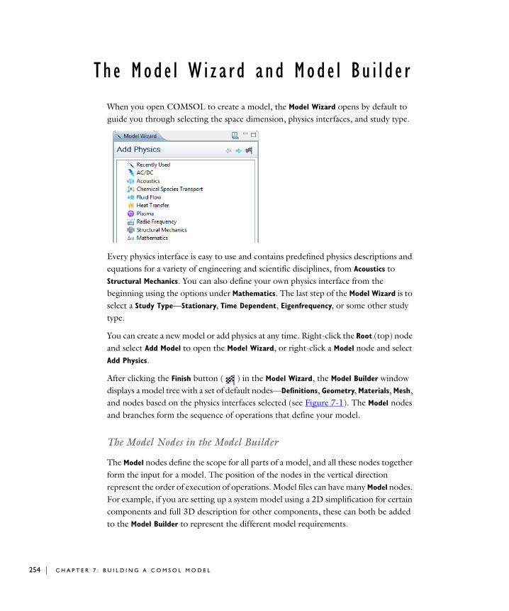
254 | C H A P T E
Th e Mode l W i z a r d and Mode l Bu i l d e r
When you open COMSOL to create a model, the Model Wizard opens by default to guide you through selecting the space dimension, physics interfaces, and study type.
Every physics interface is easy to use and contains predefined physics descriptions and equations for a variety of engineering and scientific disciplines, from Acoustics to Structural Mechanics. You can also define your own physics interface from the beginning using the options under Mathematics. The last step of the Model Wizard is to select a Study Type—Stationary, Time Dependent, Eigenfrequency, or some other study type.
You can create a new model or add physics at any time. Right-click the Root (top) node and select Add Model to open the Model Wizard, or right-click a Model node and select Add Physics.
After clicking the Finish button ( ) in the Model Wizard, the Model Builder window displays a model tree with a set of default nodes—Definitions, Geometry, Materials, Mesh, and nodes based on the physics interfaces selected (see Figure 7-1). The Model nodes and branches form the sequence of operations that define your model.
The Model Nodes in the Model Builder
The Model nodes define the scope for all parts of a model, and all these nodes together form the input for a model. The position of the nodes in the vertical direction represent the order of execution of operations. Model files can have many Model nodes. For example, if you are setting up a system model using a 2D simplification for certain components and full 3D description for other components, these can both be added to the Model Builder to represent the different model requirements.
R 7 : B U I L D I N G A C O M S O L M O D E L

Figure 7-1: An example of the Model Builder default nodes.
These default nodes are normally added under a Model node:
• Definitions: Contains variables, selections, views, pairs, functions, probes, model couplings, and coordinate systems, that are defined locally for the model. See Global and Local Definitions for information about using these local Definitions and Global
Definitions. Use Global Definitions to define Parameters and Variables with a global scope—that is, not specific to one Model node.
• Geometry: Contains the sequence of geometric objects and operations (or imported CAD data) that defines the model geometry. You can also draw your own geometry in the Graphics window.
• Materials: Contains the materials and material properties used as sources for material data in the model. See Materials for detailed information.
• Physics: Any added physics or mathematical interface displays as a node under Model (Heat Transfer in Figure 7-1 for example).
• Meshes: Contain the sequences of mesh operations that defines the computational meshes for the model. When there is only one mesh in the model, its Mesh node appears directly under the Model node.
Adding Nodes to the Model Builder
In the Model Builder, right-click any node to open its context menu. Once a node is highlighted, you can right-click anywhere in the Model Builder to open the context
T H E M O D E L W I Z A R D A N D M O D E L B U I L D E R | 255
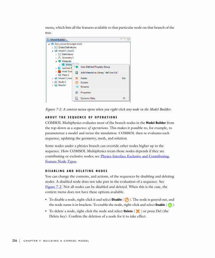
256 | C H A P T E
menu, which lists all the features available to that particular node on that branch of the tree.
Figure 7-2: A context menu opens when you right-click any node in the Model Builder.
A B O U T T H E S E Q U E N C E O F O P E R A T I O N S
COMSOL Multiphysics evaluates most of the branch nodes in the Model Builder from the top-down as a sequence of operations. This makes it possible to, for example, to parameterize a model and rerun the simulation. COMSOL then re-evaluates each sequence, updating the geometry, mesh, and solution.
Some nodes under a physics branch can override other nodes higher up in the sequence. How COMSOL Multiphysics treats those nodes depends if they are contributing or exclusive nodes; see Physics Interface Exclusive and Contributing Feature Node Types.
D I S A B L I N G A N D D E L E T I N G N O D E S
You can change the contents, and actions, of the sequences by disabling and deleting nodes. A disabled node does not take part in the evaluation of a sequence. See Figure 7-2. Not all nodes can be disabled and deleted. When this is the case, the context menu does not have these options available.
• To disable a node, right-click it and select Disable ( ). The node is grayed out, and the node name is in brackets. To enable the node, right-click and select Enable ( ).
• To delete a node, right-click the node and select Delete ( ) or press Del (the Delete key). Confirm the deletion of a node for it to take effect.
R 7 : B U I L D I N G A C O M S O L M O D E L

Mode l Adm i n i s t r a t i o n
A variety of tasks can be done to organize and simplify the model building process. This section includes information about how to:
• Save models in different formats and create a model image associated to the file.
• Edit node properties, names, and identifiers.
• Open the Model Library and change the root folder location.
• Update the model libraries using the Model Library Update service.
• Update preferences including precision level, graphics rendering, the user name, GUI language, and what to display in the Model Builder.
• View a list of licenses and block as required.
Saving Models in Different Formats and Creating a Model Image
A B O U T C O M S O L M O D E L F I L E F O R M A T S
There are three COMSOL Multiphysics model file formats—MPH, Model-M and Model-Java files.
COMSOL MPH FilesThe default standard file with the extension .mph. The file contains both binary and text data. The mesh and solution data are stored as binary data, while all other information is stored as plain text.
You can quickly save and load MPH-files. All the models in the COMSOL Multiphysics Model Library and the model libraries in the add-on modules are MPH-files.
Model M-FilesEditable script file for MATLAB. Contains a sequence of COMSOL Multiphysics commands. Run the Model M-files in MATLAB or open them in COMSOL Multiphysics when you run it with MATLAB. You can edit the file in a text editor to add additional commands.
M O D E L A D M I N I S T R A T I O N | 257

258 | C H A P T E
Note: Running files in the Model M-file format requires the COMSOL LiveLink for MATLAB.
S A V I N G A C O M S O L M U L T I P H Y S I C S M O D E L
If this is the first time saving a model or you want to update the file and keep the current name and format:
1 Click the Save button ( ), press Ctrl+S, or from the File menu, select Save.
2 Navigate to a the location where you want to save the model and enter a File name.
3 Click Save. Also see Changing the Model Library Root Folder to learn how to build your own model library.
If the model has been saved before and you want to save it in a different format or create a copy:
1 From the File menu, select Save As.
2 In the Save as type list, select the file type that you want to use.
3 Navigate to a the location where you want to save the model and enter a File name.
4 Click Save. Also see Changing the Model Library Root Folder to learn how to build your own model library.
S A V I N G A S A M O D E L M - F I L E
1 From the File menu, select Save As Model M-File.
2 Navigate to a the location where you want to save the model and enter a File name.
3 Click Save. Also see Changing the Model Library Root Folder to learn how to build your own model library.
S A V I N G O N A S E R V E R C O M P U T E R
When running a COMSOL Multiphysics server on a remote computer you can save the Model MPH-file to that server.
1 From the File menu, select Connect to Server.
2 Enter your Server and User details and click OK.
3 In the window that opens, enter the full path to the file you want to save. Provide the path in the server computer’s file system. Click Save.
R 7 : B U I L D I N G A C O M S O L M O D E L
S A V I N G A M O D E L I M A G E
To illustrate the model you can save a model image that displays in the Root Node
Properties and when opening a model in the Model Library. To save the current COMSOL Multiphysics plot as a model image, from the File main menu, select Save Model Image. The model image is a copy of the current plot.
R E V E R T I N G T O T H E L A S T S A V E D M O D E L F I L E
1 From the File menu, select Revert to Saved.
2 Select Yes to continue, and No to cancel.
COMSOL opens the last saved version of the file and reinitializes the GUI.
Editing Node Properties, Names, and Identifiers
All nodes, except container nodes, have a common set of node properties, some of which can be changed and some system generated properties that cannot be edited. Also see Viewing Node Names, Identifiers, Types, Tags, and Equations to learn about how some of these properties can be viewed. The Root node has additional information that provides an overview of the complete model file.
E D I T I N G A M O D E L I D E N T I F I E R F O R U S E W I T H V A R I A B L E S
Use a model Identifier to access variables throughout the model. The identifier is part of the full reference to variables (for example, when referring to variables in another model); see Variable Naming Convention and Scope for more information.
Note: To edit the model Name, see Editing Node Properties.
• To edit a model identifier, in the Model Builder, click a Model node. The Model page opens in the Settings window. Edit the default identifiers (mod1, mod2, and so on) as required in the Identifier field. See Figure 7-3 for an example.
R E N A M I N G A N O D E
• To rename a node, in the Model Builder, click a node and select Rename or press F2. Enter a New name and click OK. The Name is both updated in the Model Builder and in the Node Properties section.
M O D E L A D M I N I S T R A T I O N | 259

260 | C H A P T E
E D I T I N G N O D E P R O P E R T I E S
Opening the Properties WindowIn the Model Builder, right-click a node and select Properties from the context menu (see Figure 7-2). The Properties window for that specific node replaces the Settings window.
Node PropertiesThis section contains these fields:
• The Name field defaults to a system name for the node. Edit as required.
• The Tag field has a unique system defined tag for the node, which cannot be changed.
• The Author field contains the name of the author (creator) of the node. In addition to editing the author name manually, you can make a change for all nodes that you add later on by selecting Options>Preferences from the main menu and then select User (see Editing Model Preferences Settings) and edit the username.
• The Date created field contains the node creation date and time. This field cannot be edited.
• The Version and Comments fields are empty by default. Enter version numbers or comments to track model changes or changes to specific node contents.
Used ProductsUnder Used Products, any COMSOL module that is used by that node is listed.
Returning to the Settings WindowWhen you are finished editing the properties, right-click the node again and select Settings to return to the Settings window.
R O O T N O D E P R O P E R T I E S
The Settings window for the root node includes a Node Properties section with additional information about the model file. It also incudes the Used Products section and an additional section, Model Image.
Opening the Root Node Properties WindowTo open the root node’s Settings window with the Node Properties section, click the top Root node in the Model Builder.
The following information displays in the Settings window:
R 7 : B U I L D I N G A C O M S O L M O D E L

Node Properties• The Name field displays the file name as defined by the user. This field cannot be
edited, but if the file name is changed, the new name displays here.
• The Path field displays the full path to the current MPH-file. When a new project is started, the field is empty until the MPH-file is saved for the first time. This field cannot be edited, but if the file path changes, the new path displays here.
• The Program field displays the name and build number for the version of COMSOL Multiphysics used. This field cannot be edited.
• The Author field contains the name of the author (creator) of the model (see above). Click the Reset Author in Model button to reset the author name for all nodes in the model to the name in the Author field for the root node.
• The Tag field has a unique system defined tag for the node. This field cannot be edited.
• The Date created field contains the node creation date and time. This field cannot be edited.
• The Date modified field contains the date and time for the last time when the MPH-file was saved. This field cannot be edited.
• The Modified by field contains the name of the user who most recently saved the MPH-file. Changing the author name in the Author field and then clicking the Reset
Author in Model button also resets the name in the Modified by field.
• The Version and Comments fields are empty by default. Enter version numbers or comments to track model changes or changes to specific file contents.
Used ProductsUnder Used Products, any COMSOL module that is used by the file is listed.
Model ImageUnder Model Image, and only after some results are plotted, an image displays representing the model. See Saving a Model Image for more information.
The Model Library
The Model Library contains sets of models that can be used for a variety of purposes. Each add-on module includes its own model library with models showing how to use the module within its application area. This section explains how to open the Model
Library, search for a model, and how to change the model root directory location.
M O D E L A D M I N I S T R A T I O N | 261

262 | C H A P T E
O P E N I N G A N D S E A R C H I N G T H E M O D E L L I B R A R Y
1 From the File main menu, select Open Model Library.
The Model Library window.
2 Browse the available libraries or enter all or part of the model name and click Search.
Note: COMSOL models are named using an underscore between words, for example, effective_diffusivity. The underscore is required to form a valid filename so it is recommended that, if you are not sure of the full name, you enter only the first word in the Search field.
- If the search is successful, double-click the model file name or the Open button to open the file.
- If the search does not return any results, click the Refresh button ( ) return to the root Model Library folder list.
C H A N G I N G T H E M O D E L L I B R A R Y R O O T F O L D E R
After developing and saving your own models, it may be useful to change the Model
Library root folder. This redirects COMSOL to a different folder where customized models can be stored.
1 From the File menu, choose Open Model Library.
The Model Library window opens.
2 Click the Set Model Library Root button ( ).
3 In the Model Library Root dialog box, navigate to the new root folder location or click Make New Folder.
4 Click OK to save the changes, or Cancel to exit without saving.
Updating Model Libraries Using Model Library Update
The Model Library Update is a service that provides new and updated model for the model libraries. To use the Model Library Update, use the Model Library Update window ( ), which contains new and updated models for the model libraries of the COMSOL products that your license includes:
1 From the Options menu, choose Model Library Update.
R 7 : B U I L D I N G A C O M S O L M O D E L
2 In the Model Library Update window, browse the list of new and updated models that appear with a description and image.
3 Select the models that you want to download by selecting the check box next to the model image.
4 Click the Download button at the bottom of the Model Library Update window.
After downloading new and updated models, click the Refresh button ( ) in the Model Library window to update the lists of models in the model libraries.
Editing Model Preferences Settings
To open the model Preferences settings, select Options>Preferences from the Main menu. The following settings can be edited as required.
G E N E R A L
• Under Precision, edit the Input or Table display precision levels.
• Select a GUI Language—Chinese (Simplified), Chinese (Traditional), English (the default), French, German, Italian, Japanese, Korean, or Spanish. Click OK to exit and re-open COMSOL in order to display the GUI in the selected language.
• Under Help, select the Preload help files check box to preload the help files when launching COMSOL Multiphysics. By preloading the help files the context help opens faster when you use it for the first time.
U S E R
In the User section, edit the Username.
G R A P H I C S
In the Graphics section, under Rendering:
• Select a 3D rendering format—OpenGL (the default), DirectX 9, or Software.
• Select a 2D rendering format—Swing (the default) or SWT.
• Select a Detail—Normal (the default), Wireframe, Coarse, or Fine. This controls the level of graphics rendering detail. Select Wireframe speed up rendering of complex models or to improve visual appearance.
In the Graphics section, under Animation, select a Codec—MJPEG Compressor (the default) or DV Video Encoder.
M O D E L A D M I N I S T R A T I O N | 263

264 | C H A P T E
M O D E L B U I L D E R
• Select the Show equation view check box to always display physics interface Equation
nodes that display the definitions of the underlying equations and variables.
• Select the Show more options check box to always activate the Show More Options setting, which enables some additional options such as some more advances sections in the Settings windows and some additional nonstandard options in the physics interface’s context menus.
Note: These settings also turn on the same items in the Model Builder’s View menu. See Viewing Node Names, Identifiers, Types, Tags, and Equations for information.
R E S U L T S
• The Update plot when selected check box in the Plot area is selected by default. Click to clear the check box if required.
• The Buffer size (rows) in the Table area controls the size of the buffer for storing table data. The default value is 10,000.
When you are done editing, click OK to save the changes, or Cancel to exit without saving.
Checking and Controlling Products and Licenses Used
Open the Licenses window to list or block the products your license includes. Blocking a license may be useful for consultants who want to duplicate a client’s environment while building a model or when collaborating with other users who do not have access to the same set of COMSOL products. You can also use these settings to prevent use of a module when sharing a floating-network license, for example.
1 To view a list of licenses or block the use of a product, from the main menu, select Options>Licenses. The Licenses window opens.
By default the use of all products is active and the check boxes for all products are selected. The licenses currently in use are unavailable (you cannot block the use of products with functionality already in use).
2 Click to clear the check box next to a product to hide or block it from use. Click the Select All button to activate all products. Click the Deselect All button to block all products (except that ones that are already in use).
R 7 : B U I L D I N G A C O M S O L M O D E L

Note: The settings are local for each COMSOL Multiphysics session. The program does not store these settings for future modeling sessions.
3 Click OK to save the changes or Cancel do discard any changes and close the window.
Note: Under Other products is a list of COMSOL products the license does not include. Click the Product Information button to go to the product information pages on the COMSOL website, where you find information about all COMSOL products.
Viewing Node Names, Identifiers, Types, Tags, and Equations
Select the node labels to display in the Model Builder. Names and Identifiers can be changed by the user. The Name of a node can be changed for all levels, but the Identifier can only be changed for the top node. The unique Tag and Type is automatically assigned by the software and cannot be changed.
You can specify the name of a node in its Properties section (see Editing Node Properties, Names, and Identifiers) or by right-clicking on the node and choosing Rename, which opens a window where you can enter a New name. You can also specify the identifier names for nodes that include an identifier.
S E L E C T I N G T H E L A B E L S T O V I E W I N T H E M O D E L B U I L D E R
1 In the Model Builder, click on the top node level where you want to display specific labels. Each node level can display different labels.
2 Click the small down arrow to the left of the Minimize button, the View Menu button, to select from the list: Show Name Only, Show Name and Identifier, Show Name and Tag, Show Type and Identifier, or Show Type and Tag. See Figure 7-3 for examples of the different label types. In addition, you can select Show Equation View and Show More
Options.
The
• Select Show Name Only to only display the name.
• Select Show Name and Identifier to display the name with the identifier in parentheses using an italic font. The identifier appears only where it is defined, that is, for model
M O D E L A D M I N I S T R A T I O N | 265

266 | C H A P T E
nodes, physics interface nodes, mathematical interface nodes, functions, model couplings, and geometry features. This is the default setting.
• Select Show Name and Tag to display each node’s feature name with the predefined tag in curly braces using an italic font.
• Select Show Type and Identifier to display each node’s feature type (predefined name) with the identifier in parentheses using an italic font.
• Select Show Type and Tag to display each node’s feature type (predefined name) with the predefined tag in curly braces using an italic font.
The previous selections are mutually exclusive: only one of them can be active. The following two settings can be activated or turned off individually:
• Select Show Equation View to always display physics interface Equation View nodes. See Physics Interface Equation View Node.
• Select Show More Options to show some advanced sections in the Settings windows and some nonstandard options in the context menus for the physics interfaces. You normally do not need to use these additional options other than in some special cases. The documentation indicates when you need to select Show More Options to access some settings.
Note: These settings also turn on the same feature in the Model Preferences window. See Editing Model Preferences Settings.
R 7 : B U I L D I N G A C O M S O L M O D E L

Figure 7-3: Examples of the available label combinations on the View menu.
Show More Options on the Context Menu: Equation Based Features
In the Model Builder, when you right-click any physics interface node and open the context menu, there are more features available if you select Show More Options from the View menu.
Name—user defined at any level
Identifier—Interface and Model nodes only
Tag—assigned by the software and cannot be changed
Type—assigned by the software and cannot be changed
Equation View—displays when applicable and activated
M O D E L A D M I N I S T R A T I O N | 267

268 | C H A P T E
WE A K C O N T R I B U T I O N
To display this option, select Show More Options from the View menu in the Model
Builder and then select More>Weak Contribution or Global>Weak Contribution from the context menu. See The Weak Contribution Feature for details.
WE A K C O N T R I B U T I O N O N M E S H B O U N D A R I E S
To display this section, select Show More Options from the View menu in the Model
Builder and then select More>Weak Contribution on Mesh Boundaries from the context menu.
This feature is similar to Weak Contribution but is active on mesh boundaries. The settings are the same as for the Weak Contribution. See The Weak Contribution Feature for details.
WE A K C O N S T R A I N T
To display this section, select Show More Options from the View menu in the Model
Builder and then select More>Weak Constraint from the context menu. See Using Weak Constraints for details.
PO I N T W I S E C O N S T R A I N T
To display this section, select Show More Options from the View menu in the Model
Builder and then select More>Pointwise Constraint from the context menu. The settings in this section are similar to those for the weak constraints. See Using Weak Constraints for details.
G L O B A L E Q U A T I O N S
To display this option, select Show More Options from the View menu in the Model
Builder and then select Global>Global Equations from the context menu. See Global Equations for more information.
D I S C R E T I Z A T I O N
To display this section, select Show More Options from the View menu in the Model
Builder and then select Global>Discretization from the context menu. A Discretization
node is added to the Model Builder and you can select the Element order. This can be useful as an alternative discretization in, for example, a multigrid hierarchy.
R 7 : B U I L D I N G A C O M S O L M O D E L

Show More Options: Consistent and Inconsistent Stabilization
Numerical stabilization is available for physics interfaces that model transport such as fluid flow or convective heat transfer, where the fundamental governing equations are less stable than, for example, conduction-dominated models, solid mechanics models, and wave propagation in the frequency domain.
To display this section on a physics interface Settings window, select Show More Options from the View menu in the Model Builder.
Several interfaces have these settings available and below is the common information about these settings. Many interfaces have a couple of differences which are noted in the specific interface documentation.
For more information also see these sections in the COMSOL Multiphysics Reference Guide: Stabilization Techniques and for a general background on stabilization methods, Numerical Stabilization (or see Where Do I Access the Documentation and Model Library?).
C O N S I S T E N T S T A B I L I Z A T I O N
There are two consistent stabilization methods— Streamline diffusion and Crosswind
diffusion. Usually, both check boxes are selected by default and should remain selected for optimal performance. These consistent stabilization methods do not perturb the original transport equation.
The crosswind diffusion method specifies the smallest allowable concentration change across an element. As the concentration gradient appears in the denominator in the equations describing crosswind diffusion, the gradient ensures that unreasonable values do not occur in regions with small to negligible concentration changes.
Crosswind Diffusion and Tuning ParameterOn most interfaces, when the Crosswind diffusion check box is selected, enter a Tuning
parameter Ck. The default is most often 0.5. The Tuning parameter controls the amount of crosswind diffusion introduced. It recommended that it is kept in the order of 1 in order to not introduce excessive amounts of diffusion. The value used must also neither be space nor time dependent.
Crosswind Diffusion and Lower Gradient LimitIn some interfaces, if the Crosswind diffusion check box is selected, the Lower gradient
limit glim (SI unit: K/m) field is available. This variable corresponds to the smallest concentration change across an element considered by the stabilization, and is used to
M O D E L A D M I N I S T R A T I O N | 269

270 | C H A P T E
make sure that the crosswind diffusion expressions are valid also in regions with small to negligible concentration changes.
ResidualFor some interfaces, and for both consistent stabilization methods, select a Residual (or Equation Residual). Approximate residual is the default setting and it means that derivatives of the diffusion tensor components are neglected. This setting is usually accurate enough and is faster to compute. If required, select Full residual instead.
I N C O N S I S T E N T S T A B I L I Z A T I O N
There is usually just one inconsistent stabilization method— Isotropic diffusion. This method is equivalent to adding a term to the diffusion coefficient in order to dampen the effect of oscillations. Use of the inconsistent stabilization method should be minimized if possible because, by using it, you do not solve the original problem.
By default there is no isotropic diffusion selected. If required, select the Isotropic
diffusion check box and enter a Tuning parameter id. The default is 0.25. Increase or decrease this number to increase or decrease the amount of isotropic stabilization, and thus oscillation dampening.
Show More Options: Advanced Settings and Discretization
To display this section on a physics interface Settings window, select Show More Options from the View menu in the Model Builder.
A D V A N C E D S E T T I N G S
Normally these settings do not need to be changed.
Equation FormTypically, the automatic equation form setting is appropriate. The equation formulation then complies with the analysis type. To specify the equation formulation manually select one of the available forms from the Equation form list.
Show All Model InputsSelect the Show all model inputs check box to make all model inputs appear in the Model
Input section of the settings windows for the main model equation features. Such normally hidden model inputs include field variables in predefined multiphysics interfaces and model inputs from user defined property groups.
R 7 : B U I L D I N G A C O M S O L M O D E L

Performance Index Physics interfaces: Heat Transfer in Participating Media and Radiation in Participating Media
There is also a Performance index field where you can select a value between 0 and 1 that modifies the strategy used to define automatic solver settings. With small values, you can expect robust settings for the solver. With large values (up to 1), you can expect to need less memory to solve the model.
Circumferential Wave Number (1D and 2D Axisymmetric Models Only)Physics interfaces: Pressure Acoustics, Boundary Mode Acoustics, Aeroacoustics, Transient Aeroacoustics, Boundary Mode Aeroacoustics.
The circumferential wave number m is an integer-valued number used in axisymmetry and is by default 0. You can change the value in the Circumferential wave number field.
Displacements Control Spatial Frame Physics interfaces: Acoustics-Structure Interaction, Fluid-Structure Interaction, Solid Mechanics, Poroelasticity, Joule Heating and Thermal Expansion, Piezoelectric Devices.
The Displacements control spatial frame check box is selected by default. If required, click to clear the check box.
Convective Term Physics interfaces: Transport of Diluted Species, Nernst-Planck Equations, Solute Transport, Species Transport in Porous Media, Laminar and Turbulent Two-Phase Flow, Level Set, Laminar and Turbulent Two-Phase Flow, Phase Field, Level Set, Phase Field.
Select a Convective term—Non-conservative or Conservative.
Regularization Physics interface: Transport of Concentrated Species
From the Regularization list, select On or Off.
Out-of-plane Wave Number (Acoustics Module Only)The out-of-plane wave number kz is used in 2D and 1D axisymmetry and is by default 0. You can change the value in the Out-of-plane wave number field.
Heat Transfer in Biological Tissue Physics interfaces: Non-Isothermal Flow/Conjugate Heat Transfer, Heat Transfer, Microwave Heating, Thermal Stress.
M O D E L A D M I N I S T R A T I O N | 271

272 | C H A P T E
Select the Heat Transfer in biological tissue check box to enable the Biological Tissue feature. When enabled, Biological Tissue becomes available as a default model.
D I S C R E T I Z A T I O N
Specify the order of the shape functions. The default is to use second-order Lagrange elements (except for the Beam interface and all the Plasma interfaces which use first-order). In some interfaces, also select a Frame type—Material or Spatial.
R 7 : B U I L D I N G A C O M S O L M O D E L

Th e Ph y s i c s I n t e r f a c e F e a t u r e Node s
An important part of building a model is where you add Physics branches. These contain the nodes that define the material properties, equations, loads, initial values, boundary conditions, and other part of the physics that the model describes. This section describes some common behavior for these nodes:
• About exclusive and contributing feature nodes and how they impact operating sequences.
• Physics interface default feature nodes.
• Visual cues about the status of a physics interface node.
• About interior and exterior boundaries and axial symmetry.
• Common Advanced and Discretization settings for all physics interface nodes.
• About variables, shape functions, weak expressions, and constraints included in the Equation node.
Specifying Physics Settings
Each physics interface provide features for specifying all input data for a specific physics in a model:
• Material properties. Also see Materials.
• Boundary and interface conditions
• Equations (for equation-based modeling)
• Initial conditions
In addition, you can specify weak form contributions and element types for additional flexibility.
Specifically, the settings are available on the following parts of the geometry:
• Domains
• Boundaries
• Edges
• Points
• Additional properties that are independent of the geometry
Not all of these options are available for all geometry types and physics interfaces.
T H E P H Y S I C S I N T E R F A C E F E A T U R E N O D E S | 273

274 | C H A P T E
All Settings windows for the specification of the physics and equations accept parameters and variables as input data (see Global and Local Definitions for details).
Physics Interface Context Menu Layout
The context menu opens when you right-click on a physics interface node. This menu is divided into four sections for most physics interfaces: the first section contains domain settings, the second boundary settings, the third edge settings, and the fourth has point settings.
It is important to remember this division as sometimes there are menu items with the same name, but applied to different geometric entities.
Figure 7-4: The physics interface context menu layout.
Physics Interface Exclusive and Contributing Feature Node Types
The nodes for the physics interfaces are in a sequence, which acts like a macro that the software runs in a top-down order. Depending on the selection for each node, a node can totally or partially overlap, or shadow, a node earlier in the sequence. How the
Domain settings
Boundary settings
Edge settings
Point settings
R 7 : B U I L D I N G A C O M S O L M O D E L

software treats these nodes depends on their relationship. There are two different types of nodes: exclusive ( ) and contributing ( ).
Figure 7-5: An example of exclusive and contributing nodes in a physics interface operating sequence. The Flux/Source nodes are contributing: COMSOL Multiphysics adds the contributions from each of them.
Note: The exclusive and contributing nodes maintain the described behavior only in relation to similar types of nodes within the same physics (for example, you can have a temperature constraint and a pressure constraint for the same boundary in the same model).
E X C L U S I V E N O D E S
The use of an exclusive node means that only one can be active for a given selection. That is, if you add another exclusive node (for example, an identical feature) with the same selection, the other exclusive node is overridden and thus has no effect.
Typical exclusive nodes include model equations, initial values, and boundary conditions that are constraints, such as prescribed values for displacements, temperatures, pressures, and so on. Also some boundary conditions that are not constraints but have a definitive meaning are exclusive nodes—for example, electric insulation, thermal insulation, and no-flow conditions. Any icon with green and red arrows: ( ) that display next to a node indicates that it is an exclusive node (on the boundary level). See Figure 7-5 for an example. Depending on the selections for each node, an exclusive node can shadow another node partially. Nodes are exclusive only within their specific physics.
C O N T R I B U T I N G N O D E S
A contributing node means you can have several of these nodes with the same selection—the software adds these together when evaluating the model. Typical contribution nodes are loads, fluxes, and source terms, where you can have more than one of each type that is active on the same domain or boundary, for example.
T H E P H Y S I C S I N T E R F A C E F E A T U R E N O D E S | 275

276 | C H A P T E
COMSOL Multiphysics adds all contributing nodes to the model. Icons with no arrows ( ) displaying next to a node indicate that it is a contributing node (on the boundary level). See Figure 7-5 for an example.
Physics Interface Default Feature Nodes
When you add a physics interface, it automatically adds a main physics interface branch, which typically includes a number of default feature nodes, including but not limited to:
• A model equation or material model node, typically on the domain level. This node defines the domain equations (except optional sources, loads, reactions, and similar contributing domain quantities) and the related material properties or coefficients.
• A boundary condition node. For multiphysics interfaces there is one boundary condition for each physics.
• For axisymmetric models, the symmetry axis has an Axial Symmetry boundary condition (see Physics Interface Axial Symmetry Feature Node).
• An Initial Values node.
The default nodes’ initial selections include all domains or all boundaries (or all instances of another geometric entity level). Their selection is always every instance that has no selection defined by another node on the same geometric entity level that is not contributing to the default node.
For example, for a geometry with four boundaries, the default boundary condition’s initial selection includes all four boundaries. If another exclusive boundary condition for Boundary 3 is added, that boundary becomes overridden (inactive) in the default boundary condition’s selection. If you disable or remove that boundary condition (see Disabling and Deleting Nodes), the default boundary condition becomes active for Boundary 3 again. You cannot change a default node’s selection.
Physics Interface Node Status
The status of a physics interface depends on if it is a default feature node (see Physics Interface Default Feature Nodes), the selection that it applies to, and other nodes in the same branch that can override nodes earlier in the sequence. You can change the order of nodes other than the default feature nodes by moving them up or down.
R 7 : B U I L D I N G A C O M S O L M O D E L
O V E R R I D D E N S E L E C T I O N S
A node can be partially or completely overridden by another node further down in the same branch of the model tree that is of a similar, exclusive type (see Exclusive Nodes). For example, if you specify a temperature boundary condition on boundary 1 and boundary 3, and then add another temperature boundary condition for boundary 3, the first temperature boundary condition is overridden on boundary 3. In the Settings window for the Temperature nodes that define the temperature boundary condition, the Selection list then shows 3 (overridden) to indicate that the temperature boundary condition defined on this selection is overridden for boundary 3 but is still active on boundary 1. Deleting or disabling the other temperature boundary condition on boundary 3 reactivates the original temperature boundary condition, and then shows 3 (without the (overridden) indication).
S E L E C T I O N S T H A T A R E N O T A P P L I C A B L E
For selections that are not applicable for a feature node (interior boundaries for an boundary condition that is only applicable for exterior boundaries, for example), the Selection list then shows (not applicable) next to the entries in the list that are, in this case, interior boundaries.
E N A B L E D / D I S A B L E D N O D E S
By enabling or disabling physics interface nodes, you can activate and inactivate (shadow) other physics interface nodes that appear higher up in the physics inter face branches. See Disabling and Deleting Nodes.
Physics Interface Boundary Types
There are different types of boundaries for the physics interfaces, which all support different types of boundary conditions:
• Exterior boundaries, where most boundary conditions are applicable—see below.
• Interior boundaries, where special interface conditions can be applicable—see below.
• Axial symmetry boundaries, which are artificial boundaries representing the symmetry axis in axisymmetric models. See Physics Interface Axial Symmetry Feature Node.
If a selection for a boundary condition node, for example, contains boundaries of a type that is not applicable or supported, the Selection list has (not applicable) next to those boundary numbers.
T H E P H Y S I C S I N T E R F A C E F E A T U R E N O D E S | 277

278 | C H A P T E
I N T E R I O R A N D E X T E R I O R B O U N D A R I E S
When specifying boundary and interface conditions, COMSOL Multiphysics differentiates between exterior and interior boundaries:
• An exterior boundary is an outer boundary of the modeling domain.
• A interior boundary is a dividing interface between two domains in the modeling domain.
If an equation or physics interface is deactivated in one domain, the interior boundary between the active and inactive domain becomes an exterior boundary for its variables because it then borders on the outside of the active domain for those fields. The boundaries of the inactive domain are then void.
Figure 7-6: Examples of exterior and interior boundaries.
Continuity on Interior Boundaries
Unless you specify a specific boundary condition on interior boundaries (such as a contact resistance condition), COMSOL ensures continuity in the field variables across interior boundaries. For assembly geometries with identity pairs you can select a Continuity node on the Pairs menu in the boundary part of the context menu for most physics interfaces. The Continuity condition is only suitable for pairs where the boundaries match.
The Continuity form includes the following sections:
B O U N D A R I E S
The selection list in this section shows the boundaries for the selected pairs.
P A I R S E L E C T I O N
In this section you select the pairs where you want to impose continuity across the pair boundaries. Select the pairs from the Pairs list (Ctrl-click to deselect).
exteriorinteriorboundary
boundary
R 7 : B U I L D I N G A C O M S O L M O D E L

Physics Interface Axial Symmetry Feature Node
In axisymmetric models, boundaries on the symmetry axis are boundaries where only a condition for the axial symmetry exists. COMSOL Multiphysics adds a default Axial
Symmetry feature node that is active on all boundaries on the symmetry axis. The condition on the symmetry axis is typically a zero Neumann or no-flux condition.
The Axial Symmetry form has this section:
B O U N D A R I E S
The selection list for boundaries is not available because this is a default boundary condition. In the list, boundaries that are not on the symmetry axis have (not
applicable) added after the boundary number.
Physics Interface Common Settings for all the Main Nodes
The Settings windows for the main physics interface nodes (Solid Mechanics, for example) have two sections common to all physics interfaces: Advanced Settings and Discretization. To display these sections, select from the View menu in the Model Builder.
A D V A N C E D S E T T I N G S
The Advanced Settings section does not normally need to be changed, but if you do need to edit it, select Show More Options from the View menu in the Model Builder. In addition to physics-specific settings that are in some physics interfaces, these settings are always included:
• Select an option from the Equation form list to use an equation form that is different from the one that the study type sets up. Automatic is the default, which means that the equation follows the study type (for example, a time-dependent study uses equations that include time-derivatives, when applicable). To override the automatic selection, select an equation form for another study type (Stationary, for example). When the time-dependent solver runs, the solution for the physics where you have changed the equation form does not change with time.
• Select the Show all model inputs check box to make all model inputs appear in the equation model node’s Model Inputs section. Model inputs are fields such as temperature and velocities that act as inputs for material models and model equations. This setting affects model inputs that are not part of the physics interface but that can appear if you define a material so that a material property becomes a function of the temperature, for example. The check box also affects field variables in predefined multiphysics interfaces. In those cases, the model inputs do not appear
T H E P H Y S I C S I N T E R F A C E F E A T U R E N O D E S | 279

280 | C H A P T E
in the equation model node’s Model Inputs section if the Show all model inputs check box is not selected and there is a field that can serve as the model input. If no such field exists, the model input appears in the equation model node’s Model Inputs section with a user defined input setting. When the Show all model inputs check box is not selected, the program automatically connects the model input to an existing field within the physics interface (but not to available fields in other physics interfaces). The Show all model inputs check box does not affect model inputs that are an integral part of a model equation, such as a velocity field for heat transfer in fluids.
D I S C R E T I Z A T I O N
To display this section, select Show More Options from the View menu in the Model
Builder.
The Element order (or, more precisely, the order of the shape function) directly affects the number of degrees of freedom in the solution and the accuracy of the solution. Increasing the order of the elements roughly corresponds to a uniform mesh refinement. Most physics interfaces uses Lagrange elements, which can be of order 1 to 4, with 2 being the default order. You can change the order using the Element order list. The software adapts the order of the numerical integration to the element orders for the physics interfaces in the model. Some physics interfaces use special element types or a reduced element order for some of the field variables.
Physics Interface Equation View Node
The Equation View node ( ) is a subnode to the physics feature nodes. The Equation
View node’s Settings window contains information about the implementation of the physics feature: variables, shape functions, weak-form equation expressions, and constraints. You activate or disable the Equation View nodes by choosing Show Equation
View from the View (down-arrow) menu to the left of the Minimize button at the top of the Model Builder window. See Viewing Node Names, Identifiers, Types, Tags, and Equations.
To update the values in the Equation View node’s Settings window to reflect the latest changes in the physics feature, click the Refresh Equations button ( ) in the Settings window’s toolbar.
R 7 : B U I L D I N G A C O M S O L M O D E L

Note: Editing the predefined expressions for variables, equations, and constraints means that you alter the equations that COMSOL Multiphysics solves or the values of variables.
You can edit the values of variables, weak-form expressions, and constraints in the corresponding tables. This makes it possible to introduce custom changes to the equations and variable definitions.
For a changed definition of a variable or a change to a weak form expression or constraint, a warning icon appears in the leftmost column. To restore only the change in the selected variable, weak-form expression, or constraint, click the Reset Selected
button ( ) under the table in the Variables, Weak Expression, or Constraints section. To reset all changes in the equation view, click the Reset All button ( ) in the Settings window’s toolbar.
The Equation View page contains the following sections:
VA R I A B L E S
This section has a table with the variables that the physics feature defines has these columns:
• Name: the name of the variable.
• Expression: the expression, using COMSOL Multiphysics syntax, that defines the variables.
• Unit: the unit for the variable (in the active unit system)
• Description: a description of the variable.
S H A P E F U N C T I O N S
This section has a table with the dependent variables (field variables) that the physics feature defines and their shape functions. This is primarily applicable to equation model features; for most physics features, the table is empty. The table consists of the following columns:
• Name: the name of the variable.
• Shape function: the type of shape function (element) for the variable (for example, shlag for Lagrange elements)
T H E P H Y S I C S I N T E R F A C E F E A T U R E N O D E S | 281
282 | C H A P T E
• Unit: the unit for the variable (in the active unit system)
• Description: a description of the variable.
WE A K E X P R E S S I O N S
This section has a table with the weak-formulation equation contributions that the physics feature generates. Each equation contribution appears on its own row under Weak expression, but the order is not significant.
Note: The PDE interfaces and the ODEs an DAEs interface do not display any weak expressions. They are either implemented using strong formulations, directly displays the weak formulation, or define equations discretized in the time domain only.
C O N S T R A I N T S
This section has a table with the constraints that the physics feature generates. This is typically the case for boundary conditions of constraint types, such as prescribed displacements, temperature, or velocities. Many other physics features do not generate any constraints, and the table is then empty. The table consists of the following columns:
• Constraint: the expression for the constraint.
• Constraint force: the expression that defines the associated constraint force, which is typically the test function of the constraint.
• Shape function: the type of shape function (element) for the constraint.
R 7 : B U I L D I N G A C O M S O L M O D E L

S p e c i f y i n g Mode l Equa t i o n S e t t i n g s
The model equation settings appear in the main feature for a physics interface and describe the physics on the domains. You can use different values for each domain using settings of the following types:
• Coefficients that define the PDE on the domain. The PDE coefficients are available for the mathematics (equation-based) interfaces.
• Material properties that define the physics in the domain. These properties are available in the physics interfaces.
Specifying Initial Values
An Initial Values node is added by default to each physics interface.
In some types of analyses you must provide initial values:
• As the initial condition for a time-dependent analysis
• As an initial guess for the nonlinear stationary solver
• As a linearization (equilibrium) point when solving a linearized stationary model or when performing an eigenvalue study.
To enter initial values, in the Model Builder, click the Initial Values node under a physics interface node. In the Settings window, enter the Initial Values for all dependent variables (fields) in the physics interface. The default initial values are zero.
For some physics interfaces you can also enter initial values for the first time derivative of the dependent variables. These are used when solving time-dependent problems containing second time derivatives (wave-type applications). Like other default settings, these initial values apply to all domains where you have not specified any other values.
If you want to use different initial values in different domains, right-click the main physics interface node and select Initial Values to create additional nodes as needed.
For more information about using initial conditions, see the section Dependent Variables in the COMSOL Multiphysics Reference Guide (or see Where Do I Access the Documentation and Model Library?).
S P E C I F Y I N G M O D E L E Q U A T I O N S E T T I N G S | 283

284 | C H A P T E
Modeling Anisotropic Materials
The c coefficient in the coefficient form PDE corresponds to physical properties that can be anisotropic such as:
• Diffusion coefficient
• Permittivity
• Thermal conductivity
• Electric conductivity
For an anisotropic material, the c coefficient is a tensor with at most four components in 2D and at most nine components in 3D:
When specify and of the c coefficient components—as well as for certain material properties in some of the other physics interfaces—you can choose from the following types from the list underneath the edit fields:
• Isotropic (the default)—enter only one value.
• Diagonal—enter the diagonal components for an anisotropic material with the main axes aligned with the model’s coordinate system.
• Symmetric—enter a symmetric matrix using the diagonal components and the upper off-diagonal components.
• Anisotropic—enter the full 2-by-2 (2D) or 3-by-3 (3D) matrix for an anisotropic material.
c
c11 c12 c13
c21 c22 c23
c31 c32 c33
=
R 7 : B U I L D I N G A C O M S O L M O D E L

Pe r i o d i c Bounda r y Cond i t i o n s
Using Periodic Boundary Conditions
Use periodic boundary conditions to make the solution equal on two different (but usually equally shaped) boundaries.
To add a periodic boundary condition, in the Model Builder, right-click a physics interface node and select Periodic Condition. The periodic boundary condition typically implements standard periodicity (that is, the value of the solution is the same on the periodic boundaries), but in most cases you can also choose antiperiodicity so that the solutions have opposing signs. For fluid flow interfaces, the Periodic Flow Condition provides a similar periodic boundary condition but without a selection of periodicity.
For some physics interfaces you can choose the direction in which you want a periodic boundary condition. For a description of the standard periodic boundary condition, which most physics interfaces use, see Periodic Condition. See the next section for an example of a periodic boundary condition.
Periodic Boundary Condition Example
This example demonstrates how to implement a simple periodic boundary condition.
M O D E L D E F I N I T I O N
Consider an eigenvalue equation on a rectangle of dimension 1× .
4
3
2
1
u– u= on u x1 y u x4 y = on Boundaries 1 and 4
u x y2 u x y3 = on Boundaries 2 and 3
P E R I O D I C B O U N D A R Y C O N D I T I O N S | 285

286 | C H A P T E
R E S U L T S A N D D I S C U S S I O N
Figure 7-7: The periodic pattern in the solution (6th eigenmode).
The wavelength of the sinusoidal solutions is the rectangle side length divided by a series of integers, each of which corresponds to an eigensolution. The locations of the maxima are random because the model does not constrain the absolute value of the solution anywhere.
M O D E L I N G I N S T R U C T I O N S
Model Wizard1 Start COMSOL Multiphysics.
2 In the Model Wizard, select 2D from the Space dimension list. Click the Next button ( ).
3 From the list of physics interfaces on the Add Physics page, select Mathematics>PDE Interfaces>Coefficient Form PDE (c). Click the Next button ( ).
4 On the Select Study Page, select Preset Studies>Eigenvalue.
5 Click the Finish button ( ).
Geometry Modeling1 Right-click Geometry 1 and select Rectangle ( ).
2 Type sqrt(pi) in the Height edit field.
3 Click the Build All button ( ) in the Settings window toolbar.
R 7 : B U I L D I N G A C O M S O L M O D E L
PDE SettingsThe default coefficient values are correct.
Periodic Boundary Conditions
1 Right-click PDE and select Periodic Condition.
2 Select boundaries 1 and 4 in the Graphics window and click the Add to Selection button ( ).
3 Right-click PDE and select Periodic Condition.
4 Select boundaries 2 and 3in the Graphics window and click the Add to Selection button ( ).
In this case, COMSOL Multiphysics automatically identifies one boundary as the source and the other as the destination.
Mesh Generation1 Right-click Mesh 1 and select Free Triangular ( ).
2 Click the Build All button ( ) in the Settings window toolbar.
Computing the SolutionThe eigenvalue algorithm does not work reliably when the parameter that you specify in the Search for eigenvalues about edit field is equal to an eigenvalue. This particular problem has a zero eigenvalue, so you must change the value of this parameter.
1 Select Study 1>Eigenvalue 1 in the Model Tree.
2 In the Settings window, locate the Study Settings section.
3 Type 10 in the Search for eigenvalues around edit field.
4 Right-click Study 1 and select Solve to compute the solution.
Postprocessing and VisualizationBy default COMSOL Multiphysics plots the first eigenmode, which in this case is a flat solution associated with a zero eigenvalue.
1 Select 2D Plot Group 1 under Results in the Model Tree.
2 In the Settings window, locate the Data section.
3 Look at the solution for different eigenvalues by making a corresponding selection in the Eigenvalue list. Start with the last eigenvalue.
4 Click the Plot button ( ) in the Settings window toolbar to plot each eigenvalue.
P E R I O D I C B O U N D A R Y C O N D I T I O N S | 287

288 | C H A P T E
Compu t i n g A c c u r a t e F l u x e s
COMSOL Multiphysics provides two ways of computing accurate reaction forces and fluxes:
• The first approach involves the reaction force operator (reacf) that makes it possible to compute integrals of reaction forces or fluxes during postprocessing. Use the reaction force operator when computing integrals of reaction forces or fluxes during postprocessing. See The Reacf Operator for details.
• The second, more general approach for computing reaction forces and fluxes is to use weak constrains. Use this approach when you need reaction forces or fluxes in other contexts than computing integrals of reaction forces or fluxes.
Find further information on the use of weak constraints in the section Using Weak Constraints.
When using weak constraints, the Lagrange multipliers are additional dependent variables in physics interfaces using weak constraints. When using the reaction force operator, the reaction force operator of a certain dependent variable corresponds to the Lagrange multiplier of that dependent variable. The Lagrange multipliers correspond to the following quantities in the physics interfaces:
COMSOL Multiphysics computes only the part of the boundary flux captured by the Lagrange multiplier. You might have additional flux coming from boundary sources or nonidentity constraint matrices. This should not happen in the physics interfaces, though.
TABLE 7-1: PHYSICS INTERFACE INTERPRETATION OF LAGRANGE MULTIPLIERS
PHYSICS INTERFACE QUANTITY
Electrostatics Surface charge density
Magnetic Fields Surface current
Electric Currents Current flux
Heat Transfer Heat flux
Transport of Diluted Species Flux
Solid Mechanics Force
Laminar Flow Total force per area
R 7 : B U I L D I N G A C O M S O L M O D E L
Flux Computation Example
Consider computing the flux over the constrained boundary of a rectangle. The PDE of the rectangle is Poisson’s equation, u = 1, with u = 0 on the boundary. This example computes the flux using an expression, a reaction force operator, and a Lagrange multiplier.
M O D E L W I Z A R D
1 On the Select Space Dimension page, click the 2D button. Then click the Next button.
2 In the list of physics interface, open Mathematics>PDE Interfaces and then select Coefficient Form PDE (c). Then click the Next button.
3 From the Studies list, select Preset Studies>Stationary.
4 Click Finish.
G E O M E T R Y M O D E L I N G
Draw a single rectangle of any size.
C O E F F I C I E N T F O R M P D E
The default equation is Poisson’ equation, but the default boundary condition is a zero flux (homogeneous Neumann boundary condition). Instead, add a homogeneous Dirichlet boundary condition: u = 0:
1 In the Model Builder window, right-click PDE (c) node and select Dirichlet Boundary
Condition.
2 In the Dirichlet Boundary Condition node’s Settings window, select All boundaries from the Selection list in the Boundaries section.
C O M P U T I N G T H E S O L U T I O N
In the Model Builder window, right-click Study 1 and choose Compute.
R E S U L T S — F L U X E X P R E S S I O N
1 In the Model Builder window, choose Results>Derived Values>Surface Integration.
2 In the Surface Integration node’s Settings window, type 1 in the Expression edit field.
3 Select Domain 1 and click the Evaluate button ( ) at the top of the Settings window. The rectangle’s area appears in the Results section.
4 Choose Results>Derived Values>Line Integration.
5 In the Line Integration node’s Settings window, type nx*ux+ny*uy in the Expression edit field.
C O M P U T I N G A C C U R A T E F L U X E S | 289

290 | C H A P T E
6 Select all boundaries and click the Evaluate button ( ) at the top of the Settings window. COMSOL Multiphysics computes the flux over the boundaries as the normal component of the gradient of u.
The influx is approximately equal to the integral of the negative source term in Poisson’s equation.
R E S U L T S — R E A C T I O N F O R C E O P E R A T O R
1 In the Line Integration node’s Settings window, type reacf(u) in the Expression edit field.
2 Select all boundaries and click the Evaluate button ( ) at the top of the Settings window. COMSOL Multiphysics computes the flux over the boundaries using the reaction force operator for the solution u. The computed value is much closer to the expected value. To see the value as a double floating-point number with full precision, click the Full Precision button in the Results window’s toolbar.
C O E F F I C I E N T F O R M P D E — L A G R A N G E M U L T I P L I E R
1 Under Physics, select Dirichlet Boundary Condition 1. Clear the Prescribed value of u check box to remove this constraint.
2 Right-click PDE (c) and choose More>Weak Constraint on the boundary level.
3 In the Weak Constraint node’s Settings window, select All boundaries from the Selection list.
4 In the Weak Constraint section, type u in the Constraint expression edit field to constrain u to 0 at the boundary.
5 Expand the Lagrange Multiplier section and replace lm with flux in the Lagrange
multiplier variable edit field.
C O M P U T I N G T H E S O L U T I O N — L A G R A N G E M U L T I P L I E R
Right-click Study 1 and choose Compute.
R E S U L T S — L A G R A N G E M U L T I P L I E R
1 In the Line Integration node’s Settings window, type flux in the Expression edit field.
2 Select all boundaries and click the Evaluate button ( ) at the top of the Settings window. COMSOL Multiphysics computes the flux over the boundaries using the Lagrange multiplies variable. The integral of the flux exactly equals the integral of the finite-element projection of the source term in Poisson’s equation.
R 7 : B U I L D I N G A C O M S O L M O D E L

U s i n g Un i t s
COMSOL Multiphysics supports a number of consistent unit systems, including the SI unit system, which is the default unit system. The user interface displays the unit for the physical quantities entered in the selected unit system, but with the unit syntax (see Using Standard Unit Prefixes and Syntax) you can use any available and applicable unit or SI prefix to define your input quantities. In addition to SI units, many English units and units from the CGS (or cgs) system are also available, regardless of the unit system used in the model. All data in the material databases and Material Library product use SI units with declared units using the unit syntax (see Materials). This makes it possible to use the material data also in models with non-SI unit systems. Regardless of the selected unit system, you can always choose from a list of applicable units for plotting and results evaluation.
Unit Systems in COMSOL Multiphysics
COMSOL Multiphysics supports the following unit systems:
M E T R I C U N I T S Y S T E M S
• SI units, the International System of Units (SI, Système International d’Unités). This is the default unit system (sometimes also called MKS). For a list of SI units in COMSOL Multiphysics, see SI Base, Derived, and Other Units.
• CGSA units. The CGS system uses centimeter, gram, and second as basic units of length, mass, and time, respectively. The remaining basic units are identical to the SI units. The CGS unit system gives nice values for small lengths, masses, forces, pressures, and energies when working on a microscale and with weak electromagnetic forces. The derived units of force, pressure, and energy have well-known and widely used names: dyne, barye, and erg, respectively. CGSA adds ampere as the basic unit for electric current. For a list of the CGSA units, see Special CGSA Units.
• Electromagnetic units (EMU). This system is based on Ampère’s law, which defines the unit of electric current once you select an appropriate value for the constant C. When dealing exclusively with magnetic effects, it is convenient to set C = 1. If CGS units are used for the remaining basic dimensions, the current unit is called an abampere, and the corresponding coherent unit system is called electromagnetic units. Unique names for derived units have been introduced by prefixing the SI name with ab-. For a list of EMU units, see Special EMU Units.
U S I N G U N I T S | 291

292 | C H A P T E
• Electrostatic units (ESU). Based on Coulomb’s law for the force between point charges, ESU uses a unit of charge called the statcoulomb with CGS units for length, mass, and time. From there, the statampere, or franklin, and other derived units of the electrostatic unit system follow. For a list of ESU units, see Special ESU Units.
• MPa units. For stationary structural mechanics, where the density does not appear in the equations, it can be convenient to use a system where the newton and megapascal (hence the name: the MPa system) are naturally derived units of force and pressure. Keeping the SI unit for time, the basic units of length and mass become millimeter and tonne. Except for the force and pressure units, other derived units are nameless. For a list of MPa units, see Special MPa Units.
E N G L I S H U N I T S Y S T E M S
• Foot-pound-second unit system (FPS units). The original foot-pound-second system seems to be the absolute system using the pound as a unit of mass. This version of the FPS system is in agreement with the IEEE standard (the pound is a unit of mass and not of force). The natural derived unit of force is the poundal. For a list of FPS units, see Special FPS Units.
• British engineering units. An alternative to the standard FPS system is the British engineering unit system (also called gravitational foot-pound-second system or foot-slug-second system). Here, the pound force is the natural unit of force, which causes the introduction of the mass unit slug such that a pound force is a slug-foot per second squared. For a list of British engineering units, see Special British Engineering Units.
• Inch-pound-second unit system (IPS units). It is possible to define varieties of the FPS and British engineering systems based on the inch instead of the foot as basic unit of length. This gives rise to two distinct inch-pound-second systems: the absolute IPS system (just called IPS) and the gravitational IPS system. For a list of IPS units, see Special IPS Units.
• Gravitational IPS units. This alternative IPS unit system considers the pound a unit of weight rather than a unit of mass. For a list of Gravitational IPS units, see Special Gravitational IPS Units.
Selecting a Unit System
S E T T I N G T H E U N I T S Y S T E M O N T H E G L O B A L L E V E L
To set the unit system for the entire MPH-file on a global level:
R 7 : B U I L D I N G A C O M S O L M O D E L

1 In the Model Builder, click the root node (the top node in the model tree). The root node’s name is the name of the MPH-file or Untitled.mph before you have saved your work.
2 In the root node’s Settings window, select the unit system from the list in the Unit
System section.
S E T T I N G T H E U N I T S Y S T E M F O R I N D I V I D U A L M O D E L S
By default, all models in the MPH file use the same global unit system, but it is possible to use different unit systems in each model. To do so, follow these steps:
1 In the Model Builder, click the top node for a model branch (Model 1, for example).
2 In the model node’s Settings window, locate the Unit System section.
3 Select the Override global system check box, and then select the unit system from the list of units system that becomes available.
Using Standard Unit Prefixes and Syntax
S T A N D A R D U N I T P R E F I X E S
For SI units you can scale data using the standard prefixes for powers of 10—kilo, mega, milli, or micro, for example. Either the full prefix or the symbol can be used but you must use the same form for the prefix and the unit—that is, [milliampere] and [mA] are valid but not [mampere] or [milliA]). In the Settings windows for plotting and numerical results, the Unit list contains the SI unit for the quantity, including the most common prefixes. The lists also contain applicable non-SI units, which in a few cases also support these prefixes.
Use Table 7-2 as a guide for the format to enter.
TABLE 7-2: SI PREFIXES
FULL PREFIX SYMBOL FACTOR
yotta Y 1024
zetta Z 1021
exa E 1018
peta P 1015
tera T 1012
giga G 109
mega M 106
kilo k 103
U S I N G U N I T S | 293

294 | C H A P T E
S T A N D A R D U N I T S Y N T A X
You can use the unit syntax to specify a quantity with any applicable unit. To do so, append the unit to any constant or variable in a model using a syntax where you enclose the unit in brackets, for example, 200[ft] and 3e6[kg/m^3].
You can use both the name and the symbol for a unit. For example, 2.4[ampere] and 2.4[A] are both valid to indicate an electric current in SI units (see SI Base, Derived, and Other Units). The SI units can also contain standard prefixes. Appending a unit means that you multiply the constant or variable to the left of the unit declaration with this unit. This multiplication takes precedence over other operators so, for example, 1/2[m] evaluates to 0.5 m1 (0.5[1/m]) whereas both (1/2)[m] and 1/2*1[m] evaluate to 50 cm (0.5[m] or 50[cm]). Also, if L is a variable defined as 2[m], L[1/s] evaluates to 2[m/s].
The following examples show how to apply the unit syntax:
• Adding two quantities of the same kind that use different units: 0.5[ft]+33[mm]. COMSOL Multiphysics converts the result to the SI length unit (meters).
• Using multiplication with a unit to get consistent units for two quantities that you want to add, for example, 14[kg]+ht.rho[m^3], which works if ht.rho represents the density for a model.
hekto h 102
deca da 101
deci d 10-1
centi c 10-2
milli m 10-3
micro u 10-6
nano n 10-9
pico p 10-12
femto f 10-15
atto a 10-18
zepto z 10-21
yocto y 10-24
TABLE 7-2: SI PREFIXES
FULL PREFIX SYMBOL FACTOR
R 7 : B U I L D I N G A C O M S O L M O D E L

Note: For unit names with spaces and hyphens, such as British thermal unit and pound-force, you can only use the symbols when declaring units.
It is possible to add constants (without units) to any quantity. COMSOL Multiphysics then assumes that this value has the unit of the SI unit for that quantity. You can also concatenate several units, for example, 3.6[N][m], which is equivalent to 3.6[N*m] and evaluates to 3.6[J].
All data in the material databases and Material Library product use SI units and this unit syntax (see Materials).
D E C L A R I N G U N I T S F O R P A R A M E T E R S A N D E X P R E S S I O N VA R I A B L E S
It is important to be aware of the following:
• If you use parameters or variables in the physics features (see Global and Local Definitions), it is good practice to use the unit syntax to define them. The Settings windows for parameters and variables display the resulting unit, in SI units, of user defined parameters and expressions. It is important to verify that the variables have the expected unit before using them in the physics settings. The unit of parameters and variables are otherwise undefined.
• Using properties with undefined units in a model does not affect the numerical results during the analysis, but undefined units are required in the results and visualization stages—expressions involving such parameters and variables are also unitless.
• To declare the SI unit for electric resistance, ohm, use [ohm]. COMSOL Multiphysics then displays this as [].
• If non-SI units or SI prefixes are used, the conversion to SI units also affects the value (quantity) using a scaling factor (and an offset in the case of temperature units). The Value column in a Parameter node’s Settings window displays the quantity and unit in the base SI unit system so that you can see the result of the unit conversion. For example, if you define a parameter as 3[ft], the result in the Value column is 0.9144 m. See Global and Local Definitions for more information.
SI Base, Derived, and Other Units
The SI units form an internationally accepted system with seven units for base quantities and a large number of derived units. You can use the symbols for these and
U S I N G U N I T S | 295

296 | C H A P T E
other units when declaring units in COMSOL Multiphysics (for example, 10[m/s] for a velocity).
• Table 7-3 lists the SI units for the seven base quantities.
• Table 7-4 lists the SI derived units supported in COMSOL Multiphysics.
• Table 7-5 lists additional units available in COMSOL regardless of the unit system in the model. If more than one name or symbol is available, you can use any of them, except when names contain more than one word or a hyphen. See also the tables with special units for other unit systems than the SI system; special units that are not listed in Table 7-5 are only available when using such a non-SI unit system.
• Table 7-6 lists other SI derived units without special names or symbols
TABLE 7-3: BASE SI UNITS
BASE QUANTITY NAME SYMBOL
length meter, metre* m
mass kilogram kg
time second s
electric current ampere A
temperature kelvin** K
amount of substance mole mol
luminous intensity candela cd
* See About Editing Geometry Length and Angular Units
**See About Temperature Units
TABLE 7-4: SI DERIVED UNITS IN COMSOL MULTIPHYSICS
BASE QUANTITY NAME SYMBOL
absorbed dose gray Gy
capacitance farad F
conductance siemens S
dose equivalent sievert Sv
electric charge coulomb C
electric resistance, impedance, reactance ohm
electric potential difference, voltage volt V
energy, work, heat joule J
force, weight newton N
frequency hertz Hz
R 7 : B U I L D I N G A C O M S O L M O D E L

illuminance lux lx
inductance henry H
luminous flux lumen lm
magnetic flux weber Wb
magnetic flux density, magnetic induction tesla T
plane angle radian rad
power watt W
pressure pascal Pa
radioactivity becquerel Bq
TABLE 7-5: ADDITIONAL UNITS IN COMSOL MULTIPHYSICS
DERIVED QUANTITY NAME SYMBOLS VALUE
acceleration galileo Gal 0.01 m/s2
dipole moment debye D 3.33564095·10-30 C·m
energy British thermal unit*
BTU, Btu 1055.05585 J
energy calorie* cal 4.184 J
energy electronvolt eV 1.6021765314·10-19 J
energy erg erg 10-7 J
force dyne dyn 10-5 N
force poundal pdl 0.138254954376 N
force pound-force lbf 4.4482216152605 N
frequency rpm RPM 1/60 Hz
length angstrom Å 10-10 m
length inch in 0.0254 m
length foot ft 0.3048 m
length mile* mi 1609.344 m
length microinch uin 0.0254·10-6 m
length milliinch mil, thou 0.0254·10-3 m
length nautical mile*, nautimile
nmi 1852 m
length yard yd 0.9144 m
TABLE 7-4: SI DERIVED UNITS IN COMSOL MULTIPHYSICS
BASE QUANTITY NAME SYMBOL
U S I N G U N I T S | 297

298 | C H A P T E
magnetic field strength oersted Oe 103/(4·) A/m
magnetic flux density gauss G 10-4 T
mass atomic mass unit, dalton
u, amu, Da 1.660538782·10-27 kg
mass gram g 0,001 kg
mass pound, pound-mass lb, lbm 0.45359237 kg
mass stone st 6.35029318 kg
mass slug slug approx. 14.5939 kg
mass ton, tonne t 1000 kg
permeability millidarcy* mD 9.869233·10-16 m2
plane angle degree deg /180
pressure atmosphere atm 101325 Pa
pressure bar bar 100000 Pa
pressure barye ba 0.1 Pa
pressure psi psi 6.894757·103 Pa
pressure torr Torr, mmHg 133.322 Pa
speed mph, MPH mph 0.44704 m/s
speed knot* knot 1852 km/h (approx. 0.614 m/s)
temperature Celsius** degC T+273.15
temperature Fahrenheit** degF 5/9·T+459.67
temperature Rankine** R, Ra 5/9·T
time year* a, yr 31556952 s
time day d 86400 s
time hour h 3600 s
time minute min 60 s
volume gallon* gal 0.003785411784 m3
volume imperialgallon impgal 0.00454609 m3
volume liter, litre L, l 0.001 m3
volume pint* pt 0.000473176473 m3
volume quart* qt 0.000946352946 m3
TABLE 7-5: ADDITIONAL UNITS IN COMSOL MULTIPHYSICS
DERIVED QUANTITY NAME SYMBOLS VALUE
R 7 : B U I L D I N G A C O M S O L M O D E L

volume flow rate cubic feet per minute
CFM, cfm 4.719474·10-4 m3/s
* See the additional notes following this table.
** See About Temperature Units
ADDITIONAL NOTES ABOUT Table 7-5UNIT NAME NOTE
British thermal unit
An energy unit defined as the amount of heat required to raise the temperature of one pound (pound-mass) of water by one degree from 60° to 61° Fahrenheit at a constant pressure of one atmosphere. Refer to the British thermal unit using the symbol only (Btu or BTU): for example, 0.28[Btu/(h*in*degF)] for a thermal conductivity.
calorie Small calorie or gram calorie, which equals 4.184 J. A large calorie or kilogram calorie is 1000 calories (4.184 kJ). Use [kcal] for large calories.
millidarcy (mD) Widely used for permeability in petroleum engineering. Typical values for the permeability of porous media are in the range of a few to a few hundred mD. The symbol D represents the debye, a unit for the magnetic dipole moment, and not the darcy unit.
mile The international statute mile, which equals 1609.344 m.
nautimile The nautical mile equals 1852 m.
knot The same as nautical miles per hour.
year A Gregorian year, which equals 365.2425 days.
gallon (gal) This is the U.S. liquid gallon which equals 0.003785411784 m3; the Imperial (UK) gallon (imperialgallon, impgal) is equal to 0.00454609 m3.
pint and quart The U.S. liquid pint and U.S. liquid quart, respectively.
TABLE 7-6: EXAMPLES OF SI DERIVED UNITS WITHOUT SPECIAL NAMES
QUANTITY NAME SYMBOL
acceleration meter per second squared m/s2
amount-of-substance concentration mole per cubic meter mol/m3
area square meter m2
current density ampere per square meter A/m2
heat capacity, specific heat joule per kilogram kelvin J/(kg·K)
magnetic field strength ampere per meter A/m
TABLE 7-5: ADDITIONAL UNITS IN COMSOL MULTIPHYSICS
DERIVED QUANTITY NAME SYMBOLS VALUE
U S I N G U N I T S | 299

300 | C H A P T E
Special British Engineering Units
The base units in the British engineering unit system are identical to the SI units with the following exceptions:
There is one derived unit that differs from the corresponding SI unit:
The British thermal unit is also available as Btu or BTU.
Note: If you specify the British engineering unit system as the base unit system, COMSOL Multiphysics constructs derived units from the applicable SI base units and the units listed in Table 7-7 and Table 7-8. This means, for example, that the unit for voltage displayed in the user interface is lbf·ft/As rather than V (volt). In an edit field that expects a voltage as input, you therefore need to use the unit syntax when entering a numerical value, for example, 10[V].
mass density kilogram per cubic meter kg/m3
permeability henry per meter H/m
speed, velocity meter per second m/s
wave number reciprocal meter m-1
volume cubic meter m3
TABLE 7-7: SPECIAL BASE UNITS IN THE BRITISH ENGINEERING UNIT SYSTEM
BASE QUANTITY NAME SYMBOL
length foot ft
mass slug N/A
temperature Fahrenheit degF
TABLE 7-8: DERIVED BRITISH ENGINEERING UNITS IN COMSOL MULTIPHYSICS
BASE QUANTITY NAME SYMBOL
force pound-force lbf
TABLE 7-6: EXAMPLES OF SI DERIVED UNITS WITHOUT SPECIAL NAMES
QUANTITY NAME SYMBOL
R 7 : B U I L D I N G A C O M S O L M O D E L

Special CGSA Units
The base units in the CGSA unit system are identical to the SI units with the following exceptions:
The CGSA unit system includes the following derived units that differ from the corresponding SI units:
Special EMU Units
The base units in the EMU unit system are identical to the SI units with the following exceptions:
The EMU unit system includes the following derived units that differ from the corresponding SI units:
TABLE 7-9: SPECIAL BASE UNITS IN THE CGSA UNIT SYSTEM
BASE QUANTITY NAME SYMBOL
length centimeter cm
mass gram g
TABLE 7-10: DERIVED CGSA UNITS IN COMSOL MULTIPHYSICS
BASE QUANTITY NAME SYMBOL
acceleration galileo Gal
energy erg N/A
force dyne dyn
pressure barye N/A
speed kyne N/A
TABLE 7-11: SPECIAL BASE UNITS IN THE EMU UNIT SYSTEM
BASE QUANTITY NAME SYMBOL
length centimeter cm
mass gram g
electric current abampere, biot N/A
TABLE 7-12: DERIVED EMU UNITS IN COMSOL MULTIPHYSICS
BASE QUANTITY NAME SYMBOL
acceleration galileo Gal
capacitance abfarad N/A
conductance absiemens N/A
U S I N G U N I T S | 301
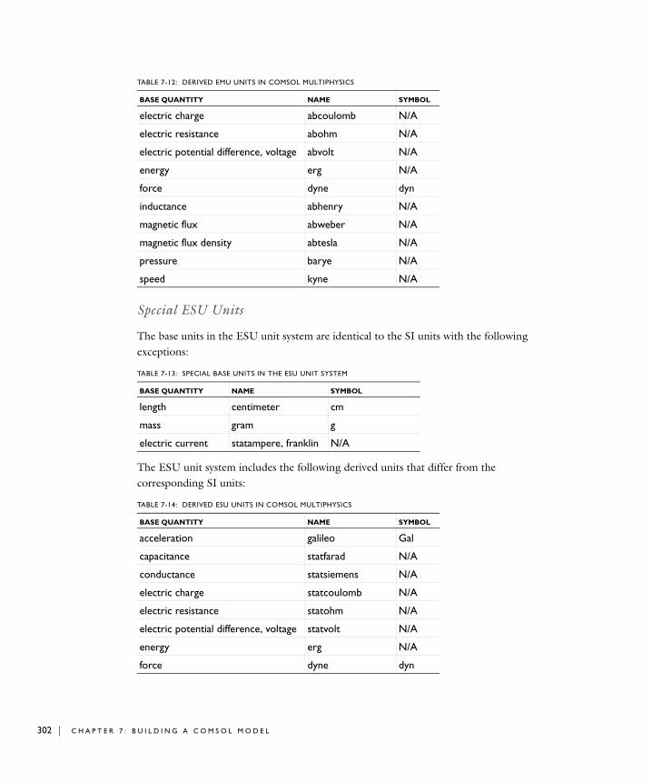
302 | C H A P T E
Special ESU Units
The base units in the ESU unit system are identical to the SI units with the following exceptions:
The ESU unit system includes the following derived units that differ from the corresponding SI units:
electric charge abcoulomb N/A
electric resistance abohm N/A
electric potential difference, voltage abvolt N/A
energy erg N/A
force dyne dyn
inductance abhenry N/A
magnetic flux abweber N/A
magnetic flux density abtesla N/A
pressure barye N/A
speed kyne N/A
TABLE 7-13: SPECIAL BASE UNITS IN THE ESU UNIT SYSTEM
BASE QUANTITY NAME SYMBOL
length centimeter cm
mass gram g
electric current statampere, franklin N/A
TABLE 7-14: DERIVED ESU UNITS IN COMSOL MULTIPHYSICS
BASE QUANTITY NAME SYMBOL
acceleration galileo Gal
capacitance statfarad N/A
conductance statsiemens N/A
electric charge statcoulomb N/A
electric resistance statohm N/A
electric potential difference, voltage statvolt N/A
energy erg N/A
force dyne dyn
TABLE 7-12: DERIVED EMU UNITS IN COMSOL MULTIPHYSICS
BASE QUANTITY NAME SYMBOL
R 7 : B U I L D I N G A C O M S O L M O D E L
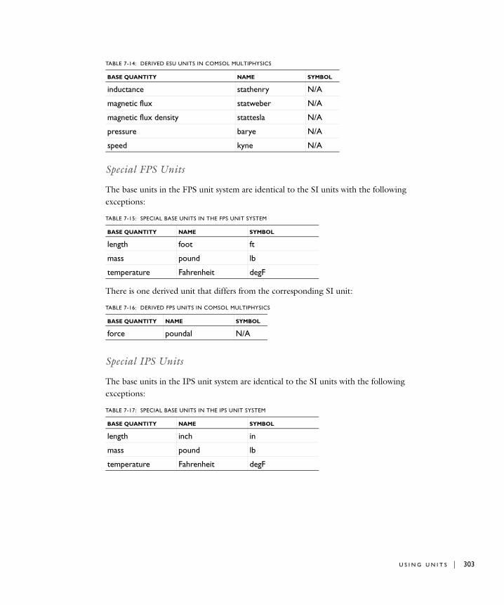
Special FPS Units
The base units in the FPS unit system are identical to the SI units with the following exceptions:
There is one derived unit that differs from the corresponding SI unit:
Special IPS Units
The base units in the IPS unit system are identical to the SI units with the following exceptions:
inductance stathenry N/A
magnetic flux statweber N/A
magnetic flux density stattesla N/A
pressure barye N/A
speed kyne N/A
TABLE 7-15: SPECIAL BASE UNITS IN THE FPS UNIT SYSTEM
BASE QUANTITY NAME SYMBOL
length foot ft
mass pound lb
temperature Fahrenheit degF
TABLE 7-16: DERIVED FPS UNITS IN COMSOL MULTIPHYSICS
BASE QUANTITY NAME SYMBOL
force poundal N/A
TABLE 7-17: SPECIAL BASE UNITS IN THE IPS UNIT SYSTEM
BASE QUANTITY NAME SYMBOL
length inch in
mass pound lb
temperature Fahrenheit degF
TABLE 7-14: DERIVED ESU UNITS IN COMSOL MULTIPHYSICS
BASE QUANTITY NAME SYMBOL
U S I N G U N I T S | 303

304 | C H A P T E
Special MPa Units
The base units in the MPa unit system are identical to the SI units with the following exceptions:
There is one derived unit that differs from the corresponding SI unit:
Special Gravitational IPS Units
The base units in the Gravitational IPS unit system are identical to the SI units with the following exceptions:
The following derived units differ from the corresponding SI units:
Switching Unit System
If you switch the unit system during modeling or use a unit system other than SI, COMSOL Multiphysics does not convert the data in the model. All physical constants and data in the materials libraries are in SI units, but you can use them with any unit system because COMSOL Multiphysics converts these values to the corresponding values in the model’s unit system. Note, however, that you must also declare the units
TABLE 7-18: SPECIAL BASE UNITS IN THE MPA UNIT SYSTEM
BASE QUANTITY NAME SYMBOL
length millimeter mm
mass tonne, ton t
TABLE 7-19: DERIVED MPA UNITS IN COMSOL MULTIPHYSICS
BASE QUANTITY NAME SYMBOL
pressure megapascal MPa
TABLE 7-20: SPECIAL BASE UNITS IN THE GRAVITATIONAL IPS UNIT SYSTEM
BASE QUANTITY NAME SYMBOL
length inch in
mass GIPS_mass N/A
temperature Fahrenheit degF
TABLE 7-21: DERIVED GRAVITATIONAL IPS UNITS IN COMSOL MULTIPHYSICS
BASE QUANTITY NAME SYMBOL
force pound-force lbf
pressure psi psi
R 7 : B U I L D I N G A C O M S O L M O D E L

of other input data for the model using the unit syntax (or convert the numerical values to the new units system). If the length unit changes, you must also convert the geometry dimensions to keep the size of the geometry using another length unit.
About Temperature Units
The relationship between different temperature units involve an offset in addition to the usual scale factor. In many cases, the offset is not important to the physics equations because these equations are concerned only with temperature differences. There are, however, some cases where you must use an absolute or thermodynamic temperature measure. The most common example is the Stefan-Boltzmann law for black-body radiation used in radiation boundary conditions.
The SI unit system uses the kelvin, which is an absolute temperature, as the basic unit of temperature. English unit systems use degree Fahrenheit as the basic unit of temperature, which, because the Fahrenheit scale is not absolute, is fine for most purposes except radiation. For such purposes, the Rankine scale provides the corresponding absolute temperature unit. See Table 7-22 for a list of acceptable unit syntax.
D I F F E R E N T I A L V S . A B S O L U T E TE M P E R A T U R E
If the dimension of an expression that includes a unit is temperature or 1/temperature, COMSOL Multiphysics interprets the dimension as an absolute temperature. If the dimension is something other than temperature but the unit expression includes temperature, the temperature is a differential temperature; that is, COMSOL Multiphysics uses no offset when converting between different temperature units.
The following examples show how the unit conversion works for different expressions that include temperature units:
• 100[degC] is an expression that has temperature as the dimension. COMSOL Multiphysics interprets it as an absolute temperature and evaluates it as 373.15 K.
TABLE 7-22: TEMPERATURE UNITS
SCALE UNIT
Celsius [degC]
Fahrenheit [degF]
Kelvin [K]
Rankine [R] or [Ra]
U S I N G U N I T S | 305

306 | C H A P T E
• 373.15[1/K] is interpreted as an absolute temperature (but no conversion is necessary from kelvin to kelvin).
• 100[degC/K] is dimensionless, and the temperature is therefore a differential temperature; that is, the result is 100 because the conversion uses no offset.
• To make COMSOL Multiphysics interpret 100[degC/K] as an absolute temperature, split the expression using two separate expressions such as 100[degC]*1[1/K], which equals 373.15. This is also what occurs when you use a variable (TC, for example) defined as 100[degC]. TC[1/K] is then also two expressions where both are interpreted as absolute temperature.
About Editing Geometry Length and Angular Units
The default units are meters for length, and degrees for angles. For many applications, an independent length unit for the geometry may be required. For example, if the model describes a MEMS device, the natural length unit might be µm, or the geometry imported from a CAD file might use a unit than meters. It may also be useful to specify the angular unit in radians instead.
Note: The length unit for the geometry does not affect the units that include length in the physics interfaces or any other part of COMSOL Multiphysics.
1 Create or open a model file.
2 In the Model Builder, under a Model node, click the Geometry node.
3 Under Units, select a Length unit from the list.
4 Select an Angular unit—Degrees or Radians.
5 Select the Scale values when changing units check box to automatically scale for dimensions in the existing geometry.
6 Enter a Default relative repair tolerance and select a Geometry representation. For details about the geometry settings, see The Geometry Node and Its Settings of the COMSOL Multiphysics Reference Guide (or see Where Do I Access the Documentation and Model Library?).
R 7 : B U I L D I N G A C O M S O L M O D E L

Indication of Unexpected or Unknown Unit
The unit display appears orange for the properties in the settings for the physics and materials that have an invalid unit or a different unit than expected. A tooltip displays a message at the corresponding edit field. In the case of a valid but unexpected unit, this message contains the deduced and expected units in the current unit system.
U S I N G U N I T S | 307

308 | C H A P T E
R 7 : B U I L D I N G A C O M S O L M O D E L
8
O v e r v i e w o f t h e P h y s i c s I n t e r f a c e s
This section gives an overview of the available physics interfaces as well as some general guidelines for effective modeling.
In this section:
• The COMSOL Multiphysics Physics Interfaces
• Modeling Guidelines
309

310 | C H A P T E
Th e COMSOL Mu l t i p h y s i c s Ph y s i c s I n t e r f a c e s
Introduction
Solving PDEs generally means you must take the time to set up the underlying equations, material properties, and boundary conditions for a given problem. COMSOL Multiphysics, however, relieves you of much of this work. The package provides a number of physics interfaces that consist of predefined templates and user interfaces already set up with equations and variables for specific areas of physics. The physics interfaces consist of a number of features with associated windows on the COMSOL Desktop for the physics in domains and on boundaries, edges, and points along with predefined PDEs. A set of interface-dependent variables makes it easy to visualize and evaluate the important physical quantities using conventional terminology and notation.
Note: Suites of physics interfaces that are optimized for specific disciplines together with specialized model libraries are available in a group of optional products: the AC/DC Module, Acoustics Module, Batteries and Fuel Cells Module, CFD Module, Chemical Reaction Engineering Module, Earth Science Module, Heat Transfer Module, MEMS Module, Plasma Module, RF Module, and Structural Mechanics Module.
A complement to the physics interfaces, special interfaces for equation-based modeling simplify the setup of PDEs for modeling that does not explicitly refer to any particular application field. In addition a number of interfaces supplement the physics interfaces with special functionality such as the Sensitivity and Moving Mesh interfaces.
R 8 : O V E R V I E W O F T H E P H Y S I C S I N T E R F A C E S

Physics Interfaces Groups in the Model Wizard
The Add Physics page in the Model Wizard contains the following main groups of physics interfaces and mathematics interfaces (some appear only if your license includes some of the add-on modules):
• The Recently Used branch ( ) contains the physics interfaces that are most recently used for easy access to the interfaces that you use the most.
• The AC/DC branch ( ) contains physics interface for low-frequency electromagnetics such as Electrostatics and Electric Currents.
• The Acoustics branch ( ) contains physics interfaces for acoustics.
• The Chemical Species Transport branch ( ) contains physics interface for chemical species transport by, for example, convection and diffusion, solving for the species concentrations.
• The Electrochemistry branch ( ) contains physics interfaces for electrochemistry and modeling of electrochemical components such as batteries and fuel cells. This branch is only available if your license includes the Batteries and Fuel Cells Module.
• The Fluid Flow branch ( ) contains physics interfaces for fluid flow such as laminar single-phase flow and, with add-on modules, multiphase flow and turbulent flow.
• The Heat Transfer branch ( ) contains physics interface for heat transfer in solids and fluids and thermal multiphysics applications such as Joule heating.
• The Plasma branch ( ) contains physics interfaces for plasma modeling. This branch is only available if your license includes the Plasma Module.
• The Radio Frequency branch ( ) contains physics interfaces for high-frequency electromagnetic field simulations solving the full Maxwell equations. This branch is only available if your license includes the RF Module.
• The Structural Mechanics branch ( ) contains physics interface for structural mechanics, studying displacements and stresses in solids, for example.
• The Mathematics branch ( ) contains mathematics interfaces for solving PDEs, ODEs, and DAEs, for optimization (requires the Optimization Module) and sensitivity analysis, and for modeling moving meshes and parameterized geometry.
T H E C O M S O L M U L T I P H Y S I C S P H Y S I C S I N T E R F A C E S | 311

312 | C H A P T E
Physics Interfaces in COMSOL Multiphysics
The following table lists the physics interfaces in COMSOL Multiphysics and their availability for 1D, 1D axisymmetric, 2D, 2D axisymmetric, and 3D geometries:
PHYSICS INTERFACE ICON TAG 1D 1D AXI 2D 2D AXI 3D
AC/DC
Electrostatics es
Electric Currents ec
Magnetic Fields mf
Acoustics
Pressure Acoustics acpr
Chemical Species Transport
Transport of Diluted Species chds
Fluid Flow
Single-Phase Flow, Laminar Flow
spf
Heat Transfer
Heat Transfer in Solids ht
Heat Transfer in Fluids ht
Joule Heating jh
Structural Mechanics
Solid Mechanics solid
Mathematics
Coefficient Form PDE c
General Form PDE g
R 8 : O V E R V I E W O F T H E P H Y S I C S I N T E R F A C E S
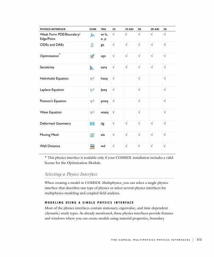
* This physics interface is available only if your COMSOL installation includes a valid license for the Optimization Module.
Selecting a Physics Interface
When creating a model in COMSOL Multiphysics, you can select a single physics interface that describes one type of physics or select several physics interfaces for multiphysics modeling and coupled-field analyses.
M O D E L I N G U S I N G A S I N G L E P H Y S I C S I N T E R F A C E
Most of the physics interfaces contain stationary, eigenvalue, and time-dependent (dynamic) study types. As already mentioned, these physics interfaces provide features and windows where you can create models using material properties, boundary
Weak Form PDE/Boundary/Edge/Point
w/ b, e, p
ODEs and DAEs ge
Optimization* opt
Sensitivity sens
Helmholtz Equation hzeq
Laplace Equation lpeq
Poisson’s Equation poeq
Wave Equation waeq
Deformed Geometry dg
Moving Mesh ale
Wall Distance wd
PHYSICS INTERFACE ICON TAG 1D 1D AXI 2D 2D AXI 3D
T H E C O M S O L M U L T I P H Y S I C S P H Y S I C S I N T E R F A C E S | 313

314 | C H A P T E
conditions, and initial conditions. Each physics interfaces comes with a template that automatically supplies the appropriate underlying PDEs.
If you cannot find a physics interface that matches a given problem, try one of the mathematics interfaces, which allow you to define a custom model in general mathematical terms. Indeed, COMSOL Multiphysics can model virtually any scientific phenomenon or engineering problem that originates from the laws of science.
M U L T I P H Y S I C S M O D E L I N G U S I N G M U L T I P L E I N T E R F A C E S
When modeling real-world systems, you often need to include the interaction between different kinds of physic: multiphysics. For instance, an electric current produces heat, and the properties of an electronic component such as an inductor vary with temperature. To solve such a problem, combine two or several physics interfaces into a single model using the multiphysics capabilities of COMSOL Multiphysics. For the example just mentioned, you can use the predefined Joule Heating interface, which is a combination of the Electric Currents and Heat Transfer physics interfaces. In this way you create a system of two PDEs with two dependent variables: V for the electric potential and T for the temperature. There are many other predefined multiphysics couplings that provide a unified interface that combines two or more coupled physics interfaces for common multiphysics applications.
You can also combine physics interfaces and equation-based modeling for maximum flexibility.
To summarize the proposed strategy for modeling processes that involve several types of physics: Look for physics interfaces suitable for the phenomena of interest. If you find them among the physics interfaces, use them; if not, add one or more equation interfaces.
When coupling multiple physics interfaces in a multiphysics model (without using a predefined multiphysics interface), the couplings can occur in domains and on boundaries. COMSOL Multiphysics automatically identifies potential model inputs for quickly forming couplings between physics. For example, a velocity field from a fluid-flow interface can provide convection in a heat transfer interface.
R 8 : O V E R V I E W O F T H E P H Y S I C S I N T E R F A C E S
Mode l i n g Gu i d e l i n e s
To allow you to model large-scale problems and for successful modeling in general, COMSOL Multiphysics lets you tune solver settings and use symmetries and other model properties to reach a solution or—failing that—interrupt the solution process to retrieve a partial solution. This section has some tips and guidelines when modeling.
Using Symmetries
By using symmetries in a model you can reduce its size by one-half or more, making this an efficient tool for solving large problems. This applies to the cases where the geometries and modeling assumptions include symmetries. The most important types of symmetries are axial symmetry and symmetry and antisymmetry planes or lines:
• Axial Symmetry is common for cylindrical and similar 3D geometries. If the geometry is axisymmetric, there are variations in the radial (r) and vertical (z) direction only and not in the angular () direction. You can then solve a 2D problem in the rz-plane instead of the full 3D model, which can save considerable memory and computation time. Many COMSOL Multiphysics physics interfaces are available in axisymmetric versions and take the axial symmetry into account.
• Symmetry and Antisymmetry Planes or Lines are common in both 2D and 3D models. Symmetry means that a model is identical on either side of a dividing line or plane. For a scalar field, the normal flux is zero across the symmetry line. In structural mechanics, the symmetry conditions are different. Antisymmetry means that the loading of a model is oppositely balanced on either side of a dividing line or plane. For a scalar field, the dependent variable is 0 along the antisymmetry plane or line. Structural mechanics applications have other antisymmetry conditions. Many physics interfaces have symmetry conditions directly available as features.
To take advantage of symmetry planes and symmetry lines, all of the geometry, material properties, and boundary conditions must be symmetric, and any loads or sources must be symmetric or antisymmetric. You can then build a model of the symmetric portion, which can be half, a quarter, or an eighth of the full geometry, and apply the appropriate symmetry (or antisymmetry) boundary conditions.
Effective Memory Management
Especially in 3D modeling, extensive memory usage dictates some extra precautions. First, check that you have selected an iterative linear system solver. Normally you do
M O D E L I N G G U I D E L I N E S | 315

316 | C H A P T E
not need to worry about which solver to use, because the physics interface makes an appropriate default choice. In some situations, though, it might be necessary to make additional changes to the solver settings and the model.
E S T I M A T I N G T H E M E M O R Y U S E F O R A M O D E L
Out-of-memory messages can occur when COMSOL Multiphysics tries to allocate an array that does not fit sequentially in memory. It is common that the amount of available memory seems large enough for an array, but there might not be a contiguous block of that size due to memory fragmentation.
In estimating how much memory it takes to solve a specific model, the following factors are the most important:
• The number of node points
• The number of dependent and independent variables
• The element order
• The sparsity pattern of the system matrices. The sparsity pattern, in turn, depends on the shape of the geometry and the mesh. For example, an extended ellipsoid gives sparser matrices than a sphere.
The MUMPS and PARDISO out-of-core solvers can make use of available disk space to solve large models that do not fit in the available memory.
C R E A T I N G A M E M O R Y - E F F I C I E N T G E O M E T R Y
A first step when dealing with large models is to try to reduce the model geometry as much as possible. Often you can find symmetry planes and reduce the model to a half, a quarter or even an eighth of the original size. Memory usage does not scale linearly but rather polynomially (Cnk, k1), which means that the model needs less than half the memory if you find a symmetry plane and cut the geometry size by half. Other ways to create a more memory-efficient geometry include:
• Avoiding small geometry objects where not needed and using Bézier curves instead of polygon chains.
• Using linear elements if possible (this is the default setting in many physics interfaces). See Selecting an Element Type.
• Making sure that the mesh elements are of a high quality. Mesh quality is important for an iterative linear system solver. Convergence is faster and more robust if the element quality is high.
• Avoiding geometries with sharp, narrow corners. Mesh elements get thin when they approach sharp corners, leading to poor element quality in the adjacent regions.
R 8 : O V E R V I E W O F T H E P H Y S I C S I N T E R F A C E S

Sharp corners are also unphysical and can lead to very large (even infinite, in theory) stress concentrations, for example.
Selecting an Element Type
As the default element type for most interfaces, COMSOL Multiphysics uses typically uses first-order or second-order Lagrange elements or shape functions. Second-order elements and other higher-order elements add additional degrees of freedom on midpoint and interior nodes in the mesh elements. These added degrees of freedom typically provide a more accurate solution but also require more memory due to the reduced sparsity of the discretized system. For many application areas, such as stress analysis in structural and solid mechanics, the increased accuracy of a second-order element is important. In fluid-flow modeling using the incompressible Navier-Stokes equations, a combination of element types using an element for the velocity components of a higher order than that for the pressure usually provides the best result. The default element for the Laminar Flow interface, for example, is the P2-P1 element using second-order elements for the velocity components and linear elements for the pressure. For other applications you can select a first-order instead of a second-order element, or reduce the element order in general, to reduce memory use.
Analyzing Model Convergence and Accuracy
It is important that the finite element model accurately captures local variations in the solution such as stress concentrations. In some cases you can compare your results to values from handbooks, measurements, or other sources of data. Many examples in the COMSOL Multiphysics Model Library include comparisons to established results or analytical solutions. Look for these benchmark models as a means of checking results.
If a model has not been verified by other means, a convergence test is useful for determining if the mesh density is sufficient. Here you refine the mesh and run the study again, and then you see if the solution is converging to a stable value as the mesh is refined. If the solution changes when you refine the mesh, the solution is mesh dependent, so the model requires a finer mesh. You can use adaptive mesh refinement, which adds mesh elements based on an error criterion to resolve those areas where the error is large. For convergence, it is important to avoid singularities in the geometry (see Avoiding Singularities and Degeneracies in the Geometry).
M O D E L I N G G U I D E L I N E S | 317

318 | C H A P T E
Achieving Convergence When Solving Nonlinear Equations
Nonlinear problems are often difficult to solve. In many cases, no unique solution exists. COMSOL Multiphysics uses a Newton-type iterative method to solve nonlinear systems of PDEs. This solution method can be sensitive to the initial estimate of the solution. If the initial conditions are too far from the desired solution, convergence might be impossible, even though it might be simple from a different starting value.
You can do several things to improve the chances for finding the relevant solutions to difficult nonlinear problems:
• Provide the best possible initial values.
• Solve sequentially and iterate between single-physics equations; finish by solving the fully coupled multiphysics problem when you have obtained better starting guesses.
• Ensure that the boundary conditions are consistent with the initial solution and that neighboring boundaries have compatible conditions that do not create singularities.
• Refine the mesh in regions of steep gradients.
• For convection-type problem, introduce artificial diffusion to improve the problem’s numerical properties (see Stabilization Techniques in the COMSOL Multiphysics Reference Guide or Where Do I Access the Documentation and Model Library?). Most physics interfaces for modeling of fluid flow and chemical species transport provide artificial diffusion as part of the default settings.
• Scaling can be an issue when one solution component is zero. In those cases, the automatic scaling might not work.
• Turn a stationary nonlinear PDE into a time-dependent problem. Making the problem time dependent generally results in smoother convergence. By making sure to solve the time-dependent problem for a time span long enough for the solution to reach a steady state, you solve the original stationary problem.
• Use the parametric solver and vary a material property or a PDE coefficient starting from a value that makes the equations less nonlinear to the value at which you want to compute the solution. This way you solve a series of increasingly difficult nonlinear problems. The solution of a slightly nonlinear problem that is easy to solve serves as the initial value for a more difficult nonlinear problem.
Avoiding Strong Transients
If you start solving a time-dependent problem with initial conditions that are inconsistent, or if you use boundary conditions or sources that switch instantaneously
R 8 : O V E R V I E W O F T H E P H Y S I C S I N T E R F A C E S

at a certain time, you induce strong transient signals in a system. The time-stepping algorithm then takes very small steps to resolve the transient, and the solution time might be very long, or the solution process might even stop. Stationary problems can run into mesh-resolution issues such as overshooting and undershooting of the solution due to infinite flux problems.
Unless you want to know the details of these transients, start with initial conditions that lead to a consistent solution to a stationary problem. Only then turn on the boundary values, sources, or driving fluxes over a time interval that is realistic for your model.
In most cases you should turn on your sources using a smoothed step over a finite time. What you might think of as a step function is, in real-life physics, often a little bit smoothed because of inertia. The step or switch does not happen instantaneously. Electrical switches take milliseconds, and solid-state switches take microseconds.
Physics-Related Checks and Guidelines
There are some important checks and guidelines that primarily apply to different areas of physics. Making these checks ensure that the model input is sufficient and increase the chances for successful modeling. Also see the modeling sections of the documentation for the physics interfaces and the modules for more information related to modeling different physics.
F L U I D F L O W A N D TR A N S P O R T P H E N O M E N A
The following checks and guidelines primarily apply to fluid-flow modeling but also to modeling of other transport phenomena:
• If none of the boundary condition includes the pressure (most outlet conditions do, however), then you should specify the pressure at some point in the fluid domain. Without a specified pressure, the problem is underconstrained and it is difficult to get convergence.
• Make sure that the mesh if sufficiently fine, so that it contains at least 4–6 mesh elements across the thickness of a channel, for example.
• Make sure that the boundary conditions and the initial conditions match for time-dependent problems. For example, instead of starting with a full velocity on the wall, compared to a zero velocity initial velocity field in the fluid, ramp up the
M O D E L I N G G U I D E L I N E S | 319
320 | C H A P T E
velocity with a smoothed step function or a ramp function. See also Avoiding Strong Transients.
• For fluid-flow models it is important to estimate the flow regime (laminar or turbulent) using the Reynolds number, for example. If the flow is in the turbulent regime, a turbulence model is typically required.
A C O U S T I C A L A N D E L E C T R O M A G N E T I C WAV E P R O P A G A T I O N
For models that describe wave propagation, it is important to fully resolve the wave in both time and space. In practice that means using a maximum mesh element size that provides about 10 linear or five 2nd-order elements per wavelength and also, for transient simulations, a fixed time step that is small enough.
S T R U C T U R A L M E C H A N I C S
The following checks and guidelines primarily apply to modeling of structural mechanics:
• Make sure that the model is fully constrained. At a minimum, you typically need to constrain the model to avoid all rigid-body movement, which for a 3D solid mechanics model means 6 constraints for three translations and three rotations. Otherwise the solution is not well defined and does not converge. It is not possible to add all 6 constraints in a single point, where you can constrain at most three translational degrees of freedom. For a 3D solid model you can use a 3-2-1 approach to constrain 3 degrees of freedom at one point (a fixed constraint), 2 at another point, and 1 at a third point. To do so, select three convenient points (vertices) that are well separated. Then fix the first point in all three directions. Constrain the second point in the two directions orthogonal (normal) to the vector from point one to point two making sure that there is no restriction to deformation along the line from point one to point two. Finally constrain the third point in a direction normal to the plane formed by the three points. To test this approach, the model should expand or contract under temperature loading and have small stresses throughout with no stress concentrations. The corresponding minimum constraints for a 2D model are a fixed constraint at one point for the 2 translational degrees of freedom and an additional constraint in one direction at another point to constrain the one rotational degree of freedom.
• Consider if you can assume that the material is linear elastic and that the deformations are small. If not, you should consider using a nonlinear material model.
• Avoid sharp corners in the geometry, which are unphysical and lead to unbounded stress concentrations.
R 8 : O V E R V I E W O F T H E P H Y S I C S I N T E R F A C E S

9
E l e c t r o m a g n e t i c s
This section explains the physics interfaces in COMSOL Multiphysics for modeling electromagnetics and how to use them for electromagnetic field simulations. Specifically, it takes a detailed look at the Electrostatics and Electric
Currents interfaces, which are available in all space dimensions, as well as at the Magnetic Fields interface available for 2D axisymmetric and 2D geometries.
In this section:
• The Electrostatics Interface
• The Electric Currents Interface
• The Magnetic Fields Interface
The underlying theory for each interface is also discussed:
• Fundamentals of Electromagnetics
• Electrostatic Fields
• Magnetostatic and Quasistatic Fields
321

322 | C H A P T E
Note: The optional AC/DC Module contains specialized and extended modeling interfaces for electromagnetic simulations, for example, for computations of inductors and capacitors. The optional RF Module includes modeling interfaces for wave-propagation simulations that are especially useful in microwave engineering and photonics.
R 9 : E L E C T R O M A G N E T I C S

Th e E l e c t r o s t a t i c s I n t e r f a c e
Applications involving electrostatics include high-voltage apparatus, electronic devices, and capacitors. The term “statics” is not to be interpreted literally but rather that the observation time or time scale at which the applied excitation changes is short compared to the charge relaxation time and that the electromagnetic wavelength and skin depth are very large compared to the size of the domain of interest. If you are uncertain whether to use the Electric Currents interface or the Electrostatics interface, which both solve for the scalar electric potential V, or maybe consider using an explicit charge transport model please refer to the section on Charge Relaxation Theory.
The Electrostatics interface ( ) provides the equations, boundary conditions, and space charges for modeling electrostatic fields, solving for the electric potential.
For an introduction to the physics and equations implemented by this interface, see the Theory for the Electrostatics Interface.
The Charge Conservation feature is the main feature, which adds the equation for the electric potential and provides a settings window for defining the constitutive relation and its associated properties such as the relative permittivity. When you add an Electrostatics interface, it adds a default Charge Conservation node and a default boundary condition, a Zero Charge node. There is also a default Initial Values node. Right-click the Electrostatics node to add other nodes that implement, for example, boundary conditions and space charges. The following sections provide information about all feature nodes available in the Electrostatics interface.
I N T E R F A C E I D E N T I F I E R
This is the physics interface identifier, which you use to reach the fields and variables in expressions, for example.
The identifier appears in the Identifier edit field, and you can change it to any unique string that is a valid identifier. The default identifier (for the first Electrostatics interface in the model) is es.
D O M A I N S
Select the domains where you want to define the electric potential and the equations that describe the potential field for dielectrics. The default setting is to include all domains in the model.
T H E E L E C T R O S T A T I C S I N T E R F A C E | 323

324 | C H A P T E
O U T - O F - P L A N E T H I C K N E S S ( 2 D M O D E L S O N L Y )
Define the out-of-plane thickness d by entering a value or expression (SI unit: m) in the Thickness edit field. The default value of 1 m is typically not representative for a thin dielectric medium, for example. Instead it describes a unit thickness that makes the 2D equation identical to the equation used for 3D models.
A D V A N C E D S E T T I N G S A N D D I S C R E T I Z A T I O N
Normally these settings do not need to be changed. See Show More Options: Advanced Settings and Discretization.
D E P E N D E N T V A R I A B L E S
The dependent variable (field variable) is for the Electric potential V. You can change the name in the corresponding edit field, but the names of fields and dependent variables must be unique within a model.
Charge Conservation
The Charge Conservation feature adds the equations for charge conservation according to Gauss’ law for the electric displacement field. The Charge Conservation form contains the following sections for defining the related material properties:
D O M A I N S
Select the domains where you want to define the electric potential and the equation based on Gauss’ law that describes the potential field.
M O D E L I N P U T S
This section contains field variables that appear as model inputs, if the current settings include such model inputs. By default, this section is empty.
E L E C T R I C F I E L D
Select a Constitutive relation to describe the macroscopic properties of the medium (relating the electric displacement D with the electric field E) and the applicable material properties, such as the relative permittivity. Select:
- Relative permittivity to use the constitutive relation De0erE (the default).
- Polarization to use the constitutive relation De0EP.
- Remanent displacement to use constitutive relation De0erEDr, where Dr is the remanent displacement (the displacement when no electric field is present).
R 9 : E L E C T R O M A G N E T I C S
• If Relative permittivity is selected, the default is to take the Relative permittivity (er) values From material. If User defined is selected, select Isotrophic, Diagonal, Symmetric, or Anisotropic and enter values or expressions in the field or matrix.
• If Polarization is selected, enter components (3 in 3D, 2 in 2D) for the Polarization
vector P (SI unit: C/m2).
• If Remanent displacement is selected, the default is to take the Relative permittivity (er) values From material. If User defined is selected, select Isotrophic, Diagonal, Symmetric, or Anisotropic and enter values or expressions in the field or matrix. Then enter components (3 in 3D, 2 in 2D) for the Remanent displacement Dr (SI unit: C / m2).
C O O R D I N A T E S Y S T E M S E L E C T I O N
Select a Coordinate system. By default you use the Global coordinate system, and the list contains any additional coordinate systems that the model includes.
E Q U A T I O N
This section displays the equations that the interface is based on.
Space Charge Density
The Space Charge Density feature adds a space charge density , which appears on the right-hand side of the equation that the Electrostatics interface defines.
D O M A I N S
Select the domains where you want to define a current source.
S P A C E C H A R G E D E N S I T Y
Enter a value or expression for the space charge density (SI unit: C/m3) in the Space
charge density edit field.
Initial Values
The Initial Values feature adds an initial value for the electric potential V that can serve as an initial condition for a transient simulation or as an initial guess for a nonlinear solver.
D O M A I N S
Select the domains where you want to define an initial value.
T H E E L E C T R O S T A T I C S I N T E R F A C E | 325

326 | C H A P T E
I N I T I A L V A L U E S
Enter a value or expression for the initial value of the electric potential V in the Electric
potential edit field. The default value is 0 V.
Boundary Conditions
The following boundary conditions are available on exterior boundaries:
• Ground (ground conditions are also available for edges (3D) and points (2D and 3D) as Ground (Edge) and Ground (Point), respectively)
• Electric Potential (also available for edges (3D) and points (2D and 3D))
• Surface Charge Density
• Zero Charge (the default boundary condition)
• Displacement Field
• Periodic Condition
The relevant interface condition at interfaces between different media is
In the absence of surface charges, this condition is fulfilled by the natural boundary condition
In addition, the following boundary conditions are available on interior boundaries:
• Ground
• Electric Potential
• Surface Charge Density
• Thin Low Permittivity Gap
For axisymmetric models, COMSOL Multiphysics takes the axial symmetry boundaries (at r = 0) into account and automatically adds an Axial Symmetry feature to the model that is valid on the axial symmetry boundaries only.
Ground
The Ground feature implements ground as the boundary condition:
n2 D1 D2– s=
n 0 V P– 1 0 V P– 2– n– D1 D2– 0= =
R 9 : E L E C T R O M A G N E T I C S

Ground means that there is a zero potential on the boundary. This boundary condition is also applicable at symmetry boundaries where the potential is known to be antisymmetric with respect to the boundary.
Ground is the default boundary condition.
B O U N D A R I E S
Select the boundaries where you want to apply a ground (zero potential) boundary condition.
Similarly, additional Ground features provide ground as a condition on edges in 3D model and at points in 2D and 3D models. You then select the edges in the Edges section or the points in the Points section, respectively.
C O N S T R A I N T S E T T I N G S
To display this section, select Show More Options from the View menu in the Model
Builder. Select a Constraint type—Bidirectional, symmetric or Unidirectional. If required, select the Use weak constraints check box.
Electric Potential
The Electric Potential feature provides an electric potential V0 as the boundary condition:
Because you are solving for the electric potential in this interface, you typically define the value of the potential at some part of the geometry.
B O U N D A R I E S
Select the boundaries where you want to apply an electric potential as the boundary condition.
E L E C T R I C PO T E N T I A L
Enter the value or expression for the electric potential (SI unit: V) in the V0 edit field.
Similarly, the Electric Potential feature provides the electric potential as a condition on edges in 3D models, and the Electric Potential feature provides electric potential as a
V 0=
V V0=
T H E E L E C T R O S T A T I C S I N T E R F A C E | 327

328 | C H A P T E
condition at points in 2D and 3D models. You then select the edges in the Edges section or the points in the Points section, respectively.
Surface Charge Density
The Surface Charge Density feature provides the following surface-charge boundary condition for exterior boundaries (left) and interior boundaries (right):
You specify the surface charge density s at an outer boundary or at an interior boundary between two nonconducting media.
B O U N D A R I E S
Select the boundaries where you want to apply a surface charge density.
S U R F A C E C H A R G E D E N S I T Y
Enter the value or expression for the surface charge density s (SI unit: C/m2).
Displacement Field
The Displacement Field feature provides the following electric-displacement boundary condition:
It specifies the normal component of the electric displacement field at a boundary.
B O U N D A R I E S
Select the boundaries where you want to use the normal component of the displacement field as the boundary condition.
D I S P L A C E M E N T F I E L D
Enter the coordinates (3 in 3D, 2 in 2D) of the Boundary displacement field D0 (SI unit: C/m2).
C O O R D I N A T E S Y S T E M S E L E C T I O N
Select a Coordinate system. By default you use the Global coordinate system, and the list contains any additional coordinate systems that the model includes.
n– D s,= n D1 D2– s=
n D n D0=
R 9 : E L E C T R O M A G N E T I C S

Periodic Condition
The Periodic Condition feature can be used to define periodicity or antiperiodicity between two boundaries. You can also activate the feature on more than two boundaries, in which case the feature tries to identify two separate surfaces which can each consist of several connected boundaries. For more complex geometries it may be necessary to use the Destination Selection subfeature. With this subfeature you can manually specify which boundaries constitute the source and destination surfaces. To add the subfeature, right-click on the Periodic Condition node and select Destination
Selection.
B O U N D A R I E S
Select the boundaries where you want to apply a periodic condition.
PE R I O D I C C O N D I T I O N
Select a Type of periodicity—Continuity or Antiperiodicity.
Zero Charge
The Zero Charge feature adds the condition that there is zero charge on the boundary:
This boundary condition is also applicable at symmetry boundaries where the potential is known to be symmetric with respect to the boundary. This is the default boundary condition.
B O U N D A R I E S
Select the boundaries where you want to apply a zero charge condition.
Thin Low Permittivity Gap
Use the thin low permittivity gap condition
n D 0=
n D10rL
dL-------------- V1 V2– =
n D20rL
dL-------------- V2 V1– =
T H E E L E C T R O S T A T I C S I N T E R F A C E | 329

330 | C H A P T E
to model a thin gap of a material with a small permittivity compared to the adjacent domains. The layer has the thickness dL and the relative permittivity rL. The indices 1 and 2 refer to the two sides of the boundary.
B O U N D A R I E S
Select the boundaries where you want to apply a thin low permittivity gap condition.
T H I N L O W P E R M I T T I V I T Y G A P
The default is to take the Relative permittivity (er) values From material. If User defined is selected, enter a value.
Enter a Surface thickness d (SI unit: m).
Continuity (Pair Feature)
Continuity is available as an option at interfaces between parts in an assembly. Also see Defining an Identity Pair.
B O U N D A R I E S
Select individual boundaries in an existing identity pair. This pair first has to be created.
P A I R S E L E C T I O N
Select the boundary pair where you want to define continuity. First an identity pair may have to be created.
Line Charge
In 3D specify line charges along the edges of a geometry. To add a Line Charge feature, right-click the Electrostatics node and choose Line Charge from the Edges menu. The Line Charge form contains the following sections:
E D G E S
Select the edges where you want to add a line charge.
L I N E C H A R G E
Apply a line charge Qj (SI unit: C/m) to edges. This source represents electric charge per unit length. You enter a value or expression for the line charge density in the Qj edit field.
R 9 : E L E C T R O M A G N E T I C S

Point Charge
It is possible to add point charges to both 2D and 3D models. To add a Point Charge feature, right-click the Electrostatics node and choose Point Charge from the Points menu.
PO I N T S
Select the points where you want to add a point charge.
PO I N T C U R R E N T S O U R C E
Apply a point charge Qp (SI unit: C) to points. This source represents an electric displacement field flowing out of the point. You enter a value or expression for the point charge in the Qp edit field.
T H E E L E C T R O S T A T I C S I N T E R F A C E | 331

332 | C H A P T E
Th e E l e c t r i c C u r r e n t s I n t e r f a c e
The Electric Currents interface ( ) provides the equations, boundary conditions, and current sources for modeling steady electric currents in conductive media, solving for the electric potential. The Current Conservation is the main feature, which adds the equation for the electric potential and provides a settings window for defining the electric conductivity as well as the constitutive relation and its associated material properties such as the relative permittivity.
For a more extensive introduction to the physics and equations implemented by this interface, see the Theory for the Electric Currents Interface.
When you add the Electric Currents interface, it adds a default Current Conservation node and a default boundary condition, the Electric Insulation node. There is also a default Initial Values node. Right-click the Electric Currents node to add other nodes that implement, for example, boundary conditions and current sources. The following sections provide information about all feature nodes available in the Electric Currents interface.
I N T E R F A C E I D E N T I F I E R
This is the physics interface identifier, which you use to reach the fields and variables in expressions, for example.
The identifier appears in the Identifier edit field, and you can change it to any unique string that is a valid identifier. The default identifier (for the first Electric Currents interface in the model) is ec.
D O M A I N S
Select the domains where you want to define the electric potential and the equations that describe the potential field for conductive media. The default setting is to include all domains in the model.
O U T O F P L A N E T H I C K N E S S ( 2 D M O D E L S O N L Y )
Define the out-of-plane thickness d (see Equation 9-3) by entering a value or expression (SI unit: m) in the Thickness edit field. The default value of 1 m is typically not representative for a thin grounding plate, for example. Instead it describes a unit thickness that makes the 2D equation identical to the equation used for 3D models.
R 9 : E L E C T R O M A G N E T I C S

D E P E N D E N T V A R I A B L E S
The dependent variable (field variable) is for the Electric potential V. You can change the name in the corresponding edit field, but the names of fields and dependent variables must be unique within a model.
A D V A N C E D S E T T I N G S A N D D I S C R E T I Z A T I O N
Normally these settings do not need to be changed. See Show More Options: Advanced Settings and Discretization.
Current Conservation
The Current Conservation feature adds the appropriate current conservation law, and the Current Conservation form contains the following sections for defining the related material properties.
D O M A I N S
Select the domains where you want to define the electric potential and the continuity equation that describes the potential field.
M O D E L I N P U T S
This section contains field variables that appear as model inputs, if the current settings include such model inputs. By default, this section is empty. If you add a linear temperature relation for the conductivity, you can then define the source for the temperature T. From the Temperature list, select an existing temperature variable (from another physics interface) if available, or select User defined to define a value or expression for the temperature (SI unit: K) in the edit field that appears underneath the list.
C O N D U C T I O N C U R R E N T
Select an Electric conductivity —From material (the default), Linearized resistivity, or User defined:
• If User defined is selected, enter values or expressions for an isotropic or anisotropic conductivity. Select Isotropic, Diagonal, Symmetric, or Anisotropic depending on the properties of the conductive media. If you want to use another type of temperature dependence than a linear temperature relation (see below), you can enter any expression for the conductivity as a function of temperature.
T H E E L E C T R I C C U R R E N T S I N T E R F A C E | 333

334 | C H A P T E
• Select Linear temperature relation for a temperature-dependent conductivity (which occurs in, for example, Joule heating, which is also called resistive heating). The following equation then describes the conductivity:
where 0 is the resistivity at the reference temperature T0. is the temperature coefficient of resistance, which describes how the resistivity varies with temperature. The default setting in the corresponding Reference resistivity, Reference temperature, and Resistivity temperature coefficient lists is From material, which means that the values are taken from the domain material. To specify another values for any of these properties, select User defined from the corresponding list and then enter a value or expression in the edit field that appears. T is the current temperature, which can be a value that you specify as a model input or the temperature from a heat transfer interface (in the Joule Heating multiphysics interface, this is the default setting). The definition of the temperature field appears in the Model Inputs section.
E L E C T R I C F I E L D
In this section you specify the constitutive relation that describe the macroscopic properties of the medium (relating the electric displacement D with the electric field E) and the applicable material properties, such as the relative permittivity.
Select one of the following constitutive relations from the list under Constitutive
relation (the corresponding equation appears underneath the list):
• Select Relative permittivity to use the constitutive relation D0 r E (the default). You then specify r , the relative permittivity (unitless). The default is to take its value from the material, but you can select User defined instead of From material from the list under Relative permittivity and then specify a value or expression for the relative permittivity in the edit field that appears.
• Select Polarization to use the constitutive relation D0 EP. You then specify P, the polarization vector (SI unit: C/m2). Enter its components (3 in 3D, 2 in 2D) in the corresponding edit fields under Polarization.
• Select Remanent displacement to use the constitutive relation D0 r EDr, where Dr (SI unit: C/m2) is the remanent displacement (the displacement when no electric field is present). In this case you specify r , the relative permittivity, and Dr, the remanent displacement. For the relative permittivity, use the list under Relative
permittivity: Select From material (the default) to use the value from the material or select User defined to specify a value or expression for the relative permittivity in the
10 1 T T0– + -----------------------------------------------=
R 9 : E L E C T R O M A G N E T I C S
edit field that appears. For the remanent displacement, enter its components (3 in 3D, 2 in 2D) in the corresponding edit fields under Remanent displacement.
External Current Density
The External Current Density feature adds an externally generated current density Je (SI unit: A/m2), which appears in Ohm’s law
and in the equation that the Electric Currents interface defines.
D O M A I N S
Select the domains where you want to define an external current density.
E X T E R N A L C U R R E N T D E N S I T Y
Enter the components (x, y, and z components in 3D, for example) of the external current density Je in the corresponding edit fields under External current density.
C O O R D I N A T E S Y S T E M S E L E C T I O N
Specify in what coordinate system the External current density is specified.
Current Source
The Current Source feature adds a distributed current source Qj (SI unit: A/m3) in the equation that the Electric Currents interface defines.
D O M A I N S
Select the domains where you want to define a current source.
C U R R E N T S O U R C E
Enter a value or expression for the current source Qj (SI unit: A/m3) in the Current
source edit field.
Force Calculation
The Force Calculation feature makes a force variable available for postprocessing. The method used is integration of the Maxwell Stress tensor over the exterior surfaces of the set of domains. This feature also gives access to the normal component of the Maxwell Stress tensor on the external surfaces.
J E Je+=
T H E E L E C T R I C C U R R E N T S I N T E R F A C E | 335

336 | C H A P T E
For the Magnetic and Electric Fields physics interface, the force calculation includes both electric and magnetic forces.
D O M A I N S
Select the domains where you want to calculate a resultant force.
F O R C E C A L C U L A T I O N
Enter a Force name for the global variable.
Enter coordinates for the Torque axis rax and Torque rotation point r0. A torque calculation about a given point (Torque rotation point) is made, and the resulting torque component parallel to the given Torque axis is given as a global postprocessing variable.
Infinite Elements
The Infinite Elements feature imposes a coordinate transformation to the selected domain that effectively moves one or more sides of the domain to infinity. Infinite elements are used for the modeling of open boundary problems.
D O M A I N S
Select the domains where you want to use infinite elements.
G E O M E T R I C S E T T I N G S
Select the type of infinite element scaling to use. The options are Cartesian, Cylindrical and Spherical (may be less depending on the spatial dimensions modeled).
P A R A M E T E R S
Tweak two parameters affecting the coordinate transformation. These are the Physical
width and the Pole distance. The Physical width parameter sets the modeled width of the infinite element region, which typically is a large value. The parameter Pole distance is a tuning parameter that controls the nature of the coordinate transform.
Initial Values
The Initial Values feature adds an initial value for the electric potential V that can serve as an initial condition for a transient simulation or as an initial guess for a nonlinear solver. If you need to specify more than one set of initial values, you can add additional Initial Values features from the Other menu when you right-click the main feature for the physics interface.
R 9 : E L E C T R O M A G N E T I C S

D O M A I N S
Select the domains where you want to define an initial value.
I N I T I A L V A L U E S
Enter a value or expression for the initial value of the electric potential V in the Electric
potential edit field. The default value is 0 V.
Boundary Conditions
The relevant interface condition at interfaces between different media and interior boundaries is continuity; that is,
which is the natural boundary condition.
The following boundary conditions are available on exterior boundaries:
• Ground (also available for edges (3D) and points (2D and 3D))
• Electric Potential (also available for edges (3D) and points (2D and 3D))
• Normal Current Density
• Electric Insulation (the default boundary condition)
• Electric Insulation (the default boundary condition)
• Periodic Condition
In addition, the following boundary conditions are available on interior boundaries:
• Boundary Current Source
• Ground
• Electric Potential
• Distributed Impedance
For axisymmetric models, COMSOL Multiphysics takes the axial symmetry boundaries (at r = 0) into account and automatically adds an Axial Symmetry feature to the model that is valid on the axial symmetry boundaries only.
Boundary Current Source
The Boundary Current Source feature adds a current source Qj on the boundary.
n2 J1 J2– 0=
n J1 J2– Qj=
T H E E L E C T R I C C U R R E N T S I N T E R F A C E | 337

338 | C H A P T E
It is applicable to interior boundaries that represent either a source or a sink of current. The Boundary Current Source form contains the following sections:
B O U N D A R I E S
Select the boundaries where you want to apply a current source.
B O U N D A R Y C U R R E N T S O U R C E
Enter a value or expression for the current source Qj (SI unit: A/m2) in the Surface
current source edit field.
Ground
The Ground feature implements ground as the boundary condition:
Ground means that there is a zero potential on the boundary. This boundary condition is also applicable at symmetry boundaries where the potential is known to be antisymmetric with respect to the boundary.
B O U N D A R I E S
Select the boundaries where you want to apply a ground (zero potential) boundary condition.
Similarly, additional Ground features provide ground as a condition on edges in 3D models and ground as a condition at points in 2D and 3D models. You then select the edges in the Edges section or the points in the Points section, respectively. Beware that constraining the potential on edges or points in 3D or on points in 2D usually yields a current outflow that is mesh dependent.
Electric Potential
The Electric Potential feature provides an electric potential V0 as the boundary condition:
Because you are solving for the electric potential in this interface, you typically define the value of the potential at some part of the geometry.
V 0=
V V0=
R 9 : E L E C T R O M A G N E T I C S

B O U N D A R I E S
Select the boundaries where you want to apply an electric potential as the boundary condition.
E L E C T R I C PO T E N T I A L
Enter the value or expression for the electric potential in the edit field under Electric
potential.
Similarly, Electric Potential features provide the electric potential as a condition on edges in 3D models and at points in 2D and 3D models. You then select the edges in the Edges section or the points in the Points section, respectively. Beware that constraining the potential on edges or points in 3D or on points in 2D usually yields a current outflow that is mesh dependent.
Normal Current Density
The Normal Current Density feature is applicable to exterior boundaries that represent either a source or a sink of current. It provides a condition for specifying the normal current density of an inward or outward current flow:
You then specify the normal current density using the inward current density Jn.
Alternatively, you can use the current density J0 to define the normal current density:
The normal current density is positive when the current flows inward toward the edge.
B O U N D A R I E S
Select the boundaries where you want to apply a current flow as the boundary condition using the normal current density.
N O R M A L C U R R E N T D E N S I T Y
From the Type list, choose Inward current density to enter a value or expression for the normal current density (SI unit: A/m2) in the Jn edit field. Use a positive value for an inward current flow or a negative value for an outward current flow. Choose Current
density to enter values or expressions for the components of the current density in the J0 edit fields.
n J– Jn=
n J n J0=
T H E E L E C T R I C C U R R E N T S I N T E R F A C E | 339

340 | C H A P T E
Distributed Impedance
The Distributed Impedance feature adds a distributed impedance boundary condition according to the following equation for exterior boundaries (setting J2 = 0) and interior boundaries assuming DC currents:
You can use the Distributed Impedance boundary condition to model a thin sheet of a resistive material. The sheet has the electric conductivity L and the surface thickness dL, or a general (resistive) layer impedance ZL and it is connected to the reference potential Vref.
LThe Distributed Impedance form contains the following sections:
B O U N D A R I E S
Select the boundaries where you want to apply a distributed impedance.
D I S T R I B U T E D I M P E D A N C E
Enter the Reference potential Vref, together with either a potentially complex valued Layer impedance ZL, or the values or expressions for the Electric conductivity s, Relative
permittivity rs and Surface thickness d. The default value for the surface thickness is 103 m (1 mm).
Electric Insulation
The Electric Insulation feature adds electric insulation as the boundary condition:
The Electric Insulation boundary condition means that no electric current flows into the boundary. This boundary condition is also applicable at symmetric boundaries where the potential is known to be symmetric with respect to the boundary.
Electric Insulation is the default boundary condition.
The Electric Insulation form contains the following section:
n J1 J2– L
dL------- V Vref– =
n J1 J2– 1ZL------- V Vref– =
n J 0=
R 9 : E L E C T R O M A G N E T I C S

B O U N D A R I E S
Select the boundaries where you want to apply electric insulation.
Periodic Condition
The Periodic Condition feature can be used to define periodicity or antiperiodicity between two boundaries. You can also activate the feature on more than two boundaries, in which case the feature tries to identify two separate surfaces which can each consist of several connected boundaries.
For more complex geometries it may be necessary to use the Destination Domains Subfeature. This subfeature allows you to manually specify which boundaries constitute the source and destination surfaces. To add the subfeature, right click on the Periodic Condition feature and select Add Destination Domains.
Contact Resistance
You can use the contact resistance boundary condition
to model a thin layer of resistive material. The layer has the thickness d and the conductivity or a general (resistive) layer impedance ZL. The indices 1 and 2 refer to the two sides of the boundary.
B O U N D A R I E S
Select the boundaries where you want to apply a contact resistance.
C O N T A C T R E S I S T A N C E
Enter the Layer impedance ZL, or the values or expressions for the Electric conductivity L, Relative permittivity rL and Surface thickness dL. The default value for the surface thickness is 103 m (1 mm).
n J1 dL------- V1 V2– =
n J2 dL------- V2 V1– =
n J1 1ZL------- V1 V2– =
n J2 1ZL------- V2 V1– =
T H E E L E C T R I C C U R R E N T S I N T E R F A C E | 341

342 | C H A P T E
Continuity (Pair Feature)
Continuity is available as an option at interfaces between parts in an assembly. Also see Defining an Identity Pair.
B O U N D A R I E S
Select individual boundaries in an existing identity pair. This pair first has to be created.
P A I R S E L E C T I O N
Select the boundary pair where you want to define continuity. First an identity pair may have to be created.
Sector Symmetry (Pair Feature)
Select sector symmetry at interfaces between rotating objects where sector symmetry is used. It is only available for assembly interfaces. Also see Defining an Identity Pair in the COMSOL Multiphysics User’s Guide.
B O U N D A R I E S
Select individual boundaries in an existing identity pair. This pair first has to be created.
P A I R S E L E C T I O N
Select the boundary pair where you want to define sector symmetry. First an identity pair may have to be created.
S E C T O R S E T T I N G S
Specify the Number of sectors (must be <50), Type of periodicity (Continuity or Antiperiodicity) and the Axis of rotation.
Electric Shielding
The Electric Shielding feature provides an electric shielding boundary condition. It describes a thin layer of a highly conductive medium that shields the electric field. The sheet has the electric conductivity s and the surface thickness d. The condition is represented by the following equation for interior boundaries and (setting J2=0) exterior boundaries assuming DC currents
n J1 J2– –= t d s Vt
R 9 : E L E C T R O M A G N E T I C S

For the frequency domain and time dependent study types, also displacement currents are accounted for via the bulk relative permittivity of the sheet; rs and the conservation laws change to:
You can use this boundary condition when approximating a thin domain with a boundary to reduce the number of mesh elements.
B O U N D A R I E S
Select the boundaries where you want to apply an electric shielding as the boundary condition.
C O N D U C T I O N C U R R E N T
Specify the electric conductivity of the boundary. By default, the electric conductivity comes from the material defined on the domain (From material is selected in the list under Electric conductivity), but you can also enter a value or expression for the conductivity in the edit field that opens when you select User-defined from that list.
E L E C T R I C F I E L D
Specify the relative permittivity. By default, the relative permittivity comes from the material defined on the domain (From material is selected in the list under Relative
permittivity), but you can also enter a value or expression for the relative permittivity in the edit field that opens when you select User-defined from that list.
T H I N L A Y E R
Specify the thickness of the surface.
Line Current Source
In 3D you can specify line sources along the edges of a geometry. To add a Line Current Source feature, right-click the Electric Currents node and choose Line Current
Source from the Edges menu.
E D G E S
Select the edges where you want to add a current source.
n J1 J2– –= t d s j0rs+ Vt
n J1 J2– –= t d s Vt 0rs t Vt+
T H E E L E C T R I C C U R R E N T S I N T E R F A C E | 343

344 | C H A P T E
L I N E C U R R E N T S O U R C E
Apply a line current source Qj (SI unit: A/m) to edges. This source represents electric current per unit length. You enter a value or expression for the current source in the Qj edit field.
Point Current Source
It is possible to add point sources to both 2D and 3D models. To add a Point Current Source feature, right-click the Electric Currents node and choose Point Current Source from the Points menu.
PO I N T S
Select the points where you want to add a current source.
PO I N T C U R R E N T S O U R C E
Apply a point current source Qj (SI unit: A) to points. This source represents an electric current flowing out of the point. You enter a value or expression for the current source in the Qj edit field.
External Surface Charge Accumulation
The External Surface Charge Accumulation boundary condition adds the accumulation of surface charge density on boundaries due to a flux of charged particles.
B O U N D A R I E S
Select the boundaries where you want to apply a surface charge accumulation.
S U R F A C E C H A R G E A C C U M U L A T I O N
Enter the values or expressions for the normal ion current density n (SI unit: A/m2) and the normal electron current density n e (SI unit: A/m2).
Dielectric Shielding
The Dielectric Shielding feature provides a dielectric shielding boundary condition. It describes a thin layer with thickness ds and a bulk relative permittivity; rs that shields the electric field:
n D t 0rsds Vt–=
R 9 : E L E C T R O M A G N E T I C S
You can use this boundary condition when approximating a thin domain with a boundary to reduce the number of mesh elements.
B O U N D A R I E S O R E D G E S
Select the boundaries or edges (3D models) where you want to apply a dielectric shielding as the condition.
E L E C T R I C F I E L D
The default is to take the Relative permittivity (er) values From material. If User-defined is selected, select Isotrophic, Diagonal, Symmetric, or Anisotropic and enter values or expressions in the field or matrix.
T H I N L A Y E R
Enter a Surface thickness ds of the shielding (SI unit: m).
C O O R D I N A T E S Y S T E M S E L E C T I O N
Select a Coordinate system. By default you use the Global coordinate system, and the list contains any additional coordinate systems that the model includes.
Terminal
The Terminal feature provides a boundary condition for connection to external circuits or with a specified voltage or charge. By specifying zero charge, a floating potential condition is obtained.
B O U N D A R I E S
Select the boundaries that you want to model as terminals connected to external circuits or an external charge or voltage.
TE R M I N A L
Specify the terminal’s properties. To indicate which boundaries that belong to the same terminal, enter the same name in the Terminal name field. The Terminal name should be numeric for port sweeps to work properly.
Select a Terminal type—Voltage, Charge, or Circuit. Select:
• Voltage to enter a voltage V0 (SI unit: V).
• Charge to enter a charge Q0 (SI unit: C). The default is zero charge for an electrode at floating potential.
• Circuit to specify a terminal connected to an external circuit.
T H E E L E C T R I C C U R R E N T S I N T E R F A C E | 345

346 | C H A P T E
Floating Potential
The Floating Potential feature is used when modeling a metallic electrode at floating potential. For circuit connections use the Terminal feature instead.
B O U N D A R I E S
Select the boundaries where you want to define the floating electrode.
F L O A T I N G P O T E N T I A L
Specify a an optionally non zero charge Q0 in the Terminal charge edit field.
Distributed Capacitance
The Distributed Capacitance feature adds a distributed capacitance boundary condition according to the following equations for exterior boundaries (left) and interior boundaries (right):
You can use the Distributed Capacitance boundary condition to model a thin sheet or film of a dielectric material. The sheet has the relative permittivity rL and the surface thickness dL, and it is connected to the reference potential Vref.
B O U N D A R I E S
Select the boundaries where you want to apply a distributed capacitance.
D I S T R I B U T E D C A P A C I T A N C E
Enter the values or expressions for Relative permittivity er, Surface thickness ds (SI unit: m), and Reference potential Vref (SI unit: V). The default value for the surface thickness is 103 m (1 mm).
n– D 0rLVref V–
dL--------------------= n D1 D2– 0rL
Vref V–
dL--------------------=
R 9 : E L E C T R O M A G N E T I C S

Th e Magn e t i c F i e l d s I n t e r f a c e
The Magnetic Fields interface ( ) provides the equations, boundary conditions, and external currents for modeling magnetic fields, solving for the magnetic vector potential. The main feature is the Ampère’s Law feature, which adds the equation for the magnetic vector potential and provides an interface for defining the constitutive relation and its associated properties such as the relative permeability.
For a more thorough introduction to the equations solved by this physics interface, see the Theory for the Magnetic Fields Interface.
When you add a Magnetic Fields interface, it creates a Magnetic Fields node with a default Ampère’s Law node added as well as a Magnetic Insulation node. Magnetic insulation is the default boundary condition. There is also a default Initial Values node. Right-click the Magnetic Fields node to add other nodes that implement, for example, boundary conditions and external currents. The following sections provide information about all feature nodes available in the Magnetic Fields interface.
D O M A I N S
Select the domains where you want to define the magnetic vector potential and the equations that describe the potential field for magnetic fields. The default setting is to include all domains in the model.
I N T E R F A C E I D E N T I F I E R
This is the physics interface identifier, which you use to reach the fields and variables in expressions, for example.
The identifier appears in the Identifier edit field, and you can change it to any unique string that is a valid identifier. The default identifier (for the first Magnetic Fields interface in the model) is mf.
O U T - O F - P L A N E T H I C K N E S S ( 2 D M O D E L S O N L Y )
Define the out-of-plane thickness d by entering a value or expression (SI unit: m) in the Thickness edit field. The default value of 1 m is typically not representative for a thin domain. Instead it describes a unit thickness that makes the 2D equation identical to the equation used for 3D models.
T H E M A G N E T I C F I E L D S I N T E R F A C E | 347

348 | C H A P T E
A D V A N C E D S E T T I N G S A N D D I S C R E T I Z A T I O N
Normally these settings do not need to be changed. See Show More Options: Advanced Settings and Discretization.
Ampère’s Law
The Ampère’s Law form contains the following sections for defining the related material properties:
D O M A I N S
Select the domains where you want to define the magnetic vector potential and the equation based on Ampère’s law that defines the potential.
M O D E L I N P U T S
This section contains field variables that appear as model inputs, if the current settings include such model inputs. By default, this section is empty. If you add a linear temperature relation for the conductivity, you can then define the source for the temperature T. From the Temperature list, select an existing temperature variable (from another physics interface) if available, or select User defined to define a value or expression for the temperature (SI unit: K) in the edit field that appears underneath the list.
M A G N E T I C F I E L D
Select the Constitutive relation that describe the macroscopic properties of the medium (relating the magnetic flux density B and the magnetic field H) and the applicable material properties, such as the relative permeability. The equation for the selected constitutive relation appears under the list.
• Select Relative permeability to use the constitutive relation B0rH (the default). The default is to use the value for r From material. If User defined is selected, select Isotrophic, Diagonal, Symmetric, or Anisotropic and enter values or expressions in the field or matrix.
• Select Magnetization to use the constitutive relation B0H0M. You then specify M, the magnetization vector (SI unit: A/m). Enter its components (3 in 3D, 2 in 2D) in the edit fields in the table that appears under the constitutive equation.
• Select Magnetic losses to describe the relative permeability as a complex-valued quantity: ri, where and are the real and imaginary parts, respectively. The default is to use the values From material. If User defined is selected for either variable, enter values or expressions for the real and imaginary parts.
R 9 : E L E C T R O M A G N E T I C S
• Select HB curve to use a curve that relates magnetic flux density B and the magnetic field H as HfB. The default is to use the value H, From material. If User
defined is selected, enter a value or expression for the magnitude of the magnetic field.
• Select Remanent flux density to use the constitutive relation B0 r HBr, where Br is the remanent flux density (the flux density when no magnetic field is present). In this case you specify r , the relative permeability (unitless), and Br, the remanent flux density (SI unit: T). For the relative permeability, use the r list: Select From
material (the default) to use the value from the material or select User defined to specify a value or expression for the relative permeability in the edit field that appears. You can select Isotropic, Diagonal, Symmetric, or Anisotropic from the list under the edit field depending on the characteristics of the relative permeability. For the remanent displacement, enter its components (3 in 3D, 2 in 2D) in the Br table.
C O N D U C T I O N C U R R E N T
Specify the electric conductivity for the media. You can define the electric conductivity in three ways by selecting from the Electric conductivity list:
• By default, the electric conductivity comes from the material defined on the domain (select From material).
• Select Linearized resistivity to define the electric resistivity (and conductivity) as a linear function of temperature. The following equation then describes the conductivity:
where 0 is the resistivity at the reference temperature T0. is the temperature coefficient of resistance, which describes how the resistivity varies with temperature. The default setting in the corresponding Reference resistivity, Reference temperature, and Resistivity temperature coefficient lists is From material, which means that the values are taken from the boundary material. To specify another values for any of these properties, select User defined from the corresponding list and then enter a value or expression in the edit field that appears. T is the current temperature, which can be a value that you specify as a model input or the temperature from a heat transfer interface. The definition of the temperature field appears in the Model Inputs section.
• You can also enter a value or expression for the conductivity (SI unit: S/m) in the edit field that opens when you select User defined from that list. You can also choose
10 1 T T0– + -----------------------------------------------=
T H E M A G N E T I C F I E L D S I N T E R F A C E | 349

350 | C H A P T E
Isotropic, Diagonal, Symmetric, or Anisotropic from the list under the edit field depending on the characteristics of the electric conductivity.
E L E C T R I C F I E L D
Specify the relative permittivity for the media. By default, the relative permittivity comes from the material defined on the shell domain (From material is selected in the list under Relative permittivity), but you can also enter a value or expression for the relative permittivity r (unitless) in the edit field that opens when you select User
defined from that list. In addition, you can choose Isotropic, Diagonal, Symmetric, or Anisotropic from the list under the edit field depending on the characteristics of the permittivity.
External Current Density
The External Current Density feature adds an externally generated current density Je, which appears on the right-hand side of the equation that the Magnetic Fields interface defines.
D O M A I N S
Select the domains where you want to define an external current density.
E X T E R N A L C U R R E N T D E N S I T Y
Enter a value or expression for each component of the external current density in the Je table under External current density.
C O O R D I N A T E S Y S T E M S E L E C T I O N
Specify in what coordinate system the External current density is specified.
Velocity (Lorentz Term)
The Velocity (Lorentz term) feature adds an external current density Je induced by a velocity v. The external current is equal to .
Initial Values
The Initial Values feature adds an initial value for the magnetic vector potential A that can serve as an initial value for a transient simulation or as an initial guess for a nonlinear solver.
v B
R 9 : E L E C T R O M A G N E T I C S

B O U N D A R I E S
Select the domains where you want to define an initial value.
I N I T I A L V A L U E S
Enter a value or expression for the initial value of the magnetic vector potential A in the Magnetic vector potential edit field. The default value is 0 Wb/m.
Boundary Conditions
With no surface currents present the interface conditions
need to be fulfilled. As we are solving for A, the tangential component of the magnetic potential is always continuous, and thus the first condition is automatically fulfilled. The second condition is equivalent to the natural boundary condition and is hence also fulfilled unless surface currents are explicitly introduced.
The following boundary conditions are available on exterior boundaries:
• Magnetic Insulation (the default boundary condition)
• Magnetic Field
• Surface Current
• Magnetic Potential
• Perfect Magnetic Conductor
In addition, the following boundary conditions are available on interior boundaries:
• Magnetic Insulation
• Magnetic Potential
• Surface Current
The following boundary conditions are only available on assembly boundary pairs:
• Continuity (Pair Feature)
For axisymmetric models, COMSOL Multiphysics takes the axial symmetry boundaries (at r = 0) into account and automatically adds an Axial Symmetry feature to the model that is valid on the axial symmetry boundaries only.
n2 A1 A2– 0=
n2 H1 H2– 0=
T H E M A G N E T I C F I E L D S I N T E R F A C E | 351
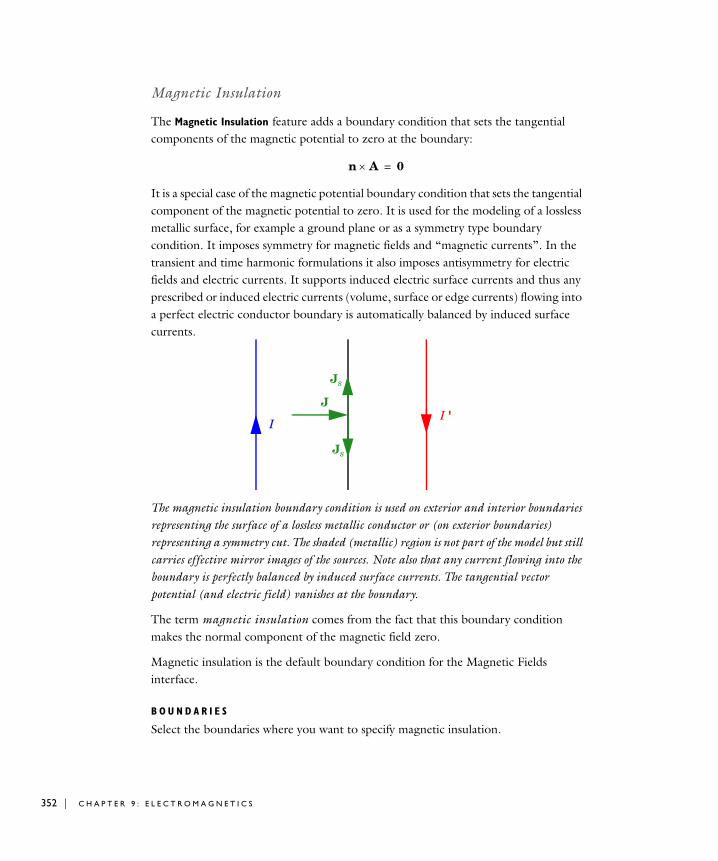
352 | C H A P T E
Magnetic Insulation
The Magnetic Insulation feature adds a boundary condition that sets the tangential components of the magnetic potential to zero at the boundary:
It is a special case of the magnetic potential boundary condition that sets the tangential component of the magnetic potential to zero. It is used for the modeling of a lossless metallic surface, for example a ground plane or as a symmetry type boundary condition. It imposes symmetry for magnetic fields and “magnetic currents”. In the transient and time harmonic formulations it also imposes antisymmetry for electric fields and electric currents. It supports induced electric surface currents and thus any prescribed or induced electric currents (volume, surface or edge currents) flowing into a perfect electric conductor boundary is automatically balanced by induced surface currents.
The magnetic insulation boundary condition is used on exterior and interior boundaries representing the surface of a lossless metallic conductor or (on exterior boundaries) representing a symmetry cut. The shaded (metallic) region is not part of the model but still carries effective mirror images of the sources. Note also that any current flowing into the boundary is perfectly balanced by induced surface currents. The tangential vector potential (and electric field) vanishes at the boundary.
The term magnetic insulation comes from the fact that this boundary condition makes the normal component of the magnetic field zero.
Magnetic insulation is the default boundary condition for the Magnetic Fields interface.
B O U N D A R I E S
Select the boundaries where you want to specify magnetic insulation.
n A 0=
II '
J
Js
Js
R 9 : E L E C T R O M A G N E T I C S
Magnetic Field
The Magnetic Field feature adds a boundary condition for specifying the tangential component of the magnetic field at the boundary:
B O U N D A R I E S
Select the boundaries where you want to specify the magnetic field.
M A G N E T I C F I E L D
Enter the value or expression for the components of the magnetic field H0.
Surface Current
The Surface Current feature adds a boundary condition for a surface current density Js:
B O U N D A R I E S
Select the boundaries where you want to specify a surface current.
S U R F A C E C U R R E N T
Enter values or expressions for the components of the surface current density in the Js edit fields.
Magnetic Potential
The Magnetic Potential feature adds a boundary condition for the magnetic vector potential:
B O U N D A R I E S
Select the boundaries where you want to specify the magnetic potential.
M A G N E T I C P O T E N T I A L
Enter a value or expression for the magnetic vector potential in the A0 edit field.
n H n H0=
n H– Js=
n H1 H2– Js=
n A n A0=
T H E M A G N E T I C F I E L D S I N T E R F A C E | 353

354 | C H A P T E
Perfect Magnetic Conductor
The perfect magnetic conductor boundary condition
is a special case of the surface current boundary condition that sets the tangential component of the magnetic field and thus also the surface current density to zero. On external boundaries, this can be interpreted as a “high surface impedance” boundary condition or used as a symmetry type boundary condition. It imposes symmetry for electric fields and electric currents. Electric currents (volume, surface, or edge currents) are not allowed to flow into a perfect magnetic conductor boundary as that would violate current conservation.
The perfect magnetic conductor boundary condition is used on exterior boundaries representing the surface of a high impedance region or a symmetry cut. The shaded (high impedance) region is not part of the model but nevertheless carries effective mirror images of the sources. Note also that any electric current flowing into the boundary is forbidden as it cannot be balanced by induced electric surface currents. The tangential magnetic field vanishes at the boundary.
B O U N D A R I E S
Select the boundaries that you want to model as perfect magnetic conductors.
Thin Low Permeability Gap
You can use the thin low permeability gap boundary condition
n H 0=
II '
Js=0
J=0
n H1 H2– td
0r------------t A=
R 9 : E L E C T R O M A G N E T I C S

to model gaps filled with a material with zero conductivity such as air. This boundary condition is only applicable on interior boundaries and pair boundaries.
B O U N D A R I E S
Select the boundaries where you want to model a thin low permeability gap.
T H I N L O W P E R M E A B I L I T Y G A P
Specify the relative permeability r (unitless) for the gap in the Relative permeability edit field. Select From material (the default) to use a value taken from the material. To specify another value f select User-defined and then enter a value or expression for the relative permeability in the edit field that appears. You can select Isotropic, Diagonal, Symmetric, or Anisotropic from the list under the edit field depending on the characteristics of the relative permeability.
You also specify the surface thickness ds (SI unit: m) for the gap in the Surface thickness
edit field.
Continuity (Pair Feature)
Continuity is available as an option at interfaces between parts in an assembly. Also see Defining an Identity Pair.
B O U N D A R I E S
Select individual boundaries in an existing identity pair. This pair first has to be created.
P A I R S E L E C T I O N
In this section you select the boundary pair where you want to define continuity. First an identity pair may have to be created.
Edge Current
The Edge Current feature allows you to specify a line current along one or more edges. Edges
Select the edges that you want to an edge current.
E D G E C U R R E N T
Specify the Edge current.
T H E M A G N E T I C F I E L D S I N T E R F A C E | 355

356 | C H A P T E
Line Current (Out of Plane)
The Line Current (out of Plane) feature allows you to specify a line current out of the modeling plane. In axially symmetric geometries this is the rotational direction, in 2D geometries this is the z-direction.
PO I N T S
Select the points where you want to add a line current.
L I N E C U R R E N T ( O U T O F P L A N E )
Specify the Out of plane current.
R 9 : E L E C T R O M A G N E T I C S

Fundamen t a l s o f E l e c t r omagne t i c s
Maxwell’s Equations
The problem of electromagnetic analysis on a macroscopic level is that of solving Maxwell’s equations subject to certain boundary conditions. Maxwell’s equations are a set of equations, written in differential or integral form, stating the relationships between the fundamental electromagnetic quantities. These quantities are:
• The electric field intensity, E
• The electric displacement or electric flux density, D
• The magnetic field intensity, H
• The magnetic flux density, B
• The current density, J
• The electric charge density,
You can formulate the equations in differential or integral form. This discussion presents them in differential form because it leads to differential equations that the finite element method can handle.
For general time-varying fields, Maxwell’s equations are
The first two equations are also referred to as Maxwell-Ampère’s law and Faraday’s law, respectively. The last two are forms of Gauss’ law in the electric and magnetic form, respectively.
Another fundamental relationship is the equation of continuity:
H J Dt
-------+=
E Bt
-------–=
D =
B 0=
J t
------–=
F U N D A M E N T A L S O F E L E C T R O M A G N E T I C S | 357

358 | C H A P T E
Out of these five equations only three are independent. The first two combined with either the electric form of Gauss’ law or the equation of continuity form an independent system.
Constitutive Relationships
To obtain a closed system, you need the constitutive relationships describing the macroscopic properties of the medium. They are
(9-1)
where 0 is the permittivity of vacuum, 0 is the permeability of vacuum, and is the electric conductivity. In the SI system the permeability of a vacuum is 4·107 H/m. The velocity of an electromagnetic wave in a vacuum is given as c0, and you can derive the permittivity of a vacuum from the relationship
The electromagnetic constants 0, 0, and c0 are available in COMSOL Multiphysics as predefined physical constants.
The electric polarization vector P describes how a material is polarized when an electric field E is present. It can be interpreted as the volume density of electric dipole moments. P is generally a function of E. Some materials can have a nonzero P in the absence of an electric field.
The magnetization vector M similarly describes how a material is magnetized when a magnetic field H is present. It can be interpreted as the volume density of magnetic dipole moments. M is generally a function of H. One use of the magnetization vector is to describe permanent magnets, which have a nonzero M when no magnetic field is present.
For linear materials the polarization is directly proportional to the electric field, P0eE, where e is the electric susceptibility. Similarly, in linear materials the magnetization is directly proportional to the magnetic field, MmH, where m is the magnetic susceptibility. For such materials the constitutive relations are
D 0E P+=
B 0 H M+ =
J E=
01
c020
---------- 8.854 10 12– F/m 136--------- 10 9– F/m= =
R 9 : E L E C T R O M A G N E T I C S

where r is the material’s relative permittivity, and r is its relative permeability. Usually these are scalar properties but can, in the general case, be 3-by-3 tensors when the material is anisotropic. The properties and (without subscripts) are the material’s permittivity and permeability.
G E N E R A L I Z E D C O N S T I T U T I V E R E L A T I O N S H I P S
For nonlinear materials, a generalized form of the constitutive relationships is useful. The relationship used for electric fields is
The field Dr is the remanent displacement, which is the displacement when no electric field is present.
Similarly, a generalized form of the constitutive relationship for the magnetic field is
where Br is the remanent magnetic flux density, which is the magnetic flux density when no magnetic field is present.
You can generalize the third line in Equation 9-1 by introducing an externally generated current Je. This relationship is then
Potentials
Under certain circumstances it can be helpful to formulate a problem in terms of the electric scalar potential V and magnetic vector potential A. They are given by the equalities
which are direct consequences of the magnetic case of Gauss’ law and Faraday’s law, respectively.
D 0 1 e+ E 0rE E= = =
B 0 1 m+ H 0rH H= = =
D 0rE Dr+=
B 0rH Br+=
J E Je+=
B A=
E V–At
-------–=
F U N D A M E N T A L S O F E L E C T R O M A G N E T I C S | 359
360 | C H A P T E
Material Properties
This discussion has so far only formally introduced the constitutive relationships. These seemingly simple relationships can be quite complicated at times. In fact, these relationships require some special considerations when working with four main groups of materials:
• Inhomogeneous materials
• Anisotropic materials
• Nonlinear materials
• Dispersive materials
A material can belong to one or more of these groups.
I N H O M O G E N E O U S M A T E R I A L S
Inhomogeneous materials are the least complicated. An inhomogeneous medium is one in which the constitutive parameters vary with the space coordinates so that different field properties prevail at different parts of the material structure.
A N I S O T R O P I C M A T E R I A L S
For anisotropic materials the field relationships at any point differ for different directions of propagation. This means that a 3-by-3 tensor is necessary to properly define the constitutive relationships. If this tensor is symmetric, the material is often referred to as reciprocal. In such cases you can rotate the coordinate system such that a diagonal matrix results. If two of the diagonal entries are equal, the material is uniaxially anisotropic; if none of the elements have the same value, the material is biaxially anisotropic (Ref. 2). You need anisotropic parameters, for instance, to examine permittivity in crystals (Ref. 2) and when working with conductivity in solenoids.
N O N L I N E A R M A T E R I A L S
In some nonlinear materials the permittivity or permeability depend on the intensity of the electromagnetic field. Nonlinearity also includes hysteresis effects where not only the existing field intensities influence a material’s physical properties but the history of the field distribution also plays a role.
R 9 : E L E C T R O M A G N E T I C S
D I S P E R S I V E M A T E R I A L S
Dispersion describes changes in a wave’s velocity with wavelength. In the frequency domain you can express dispersion with a frequency dependence of the constitutive laws.
Boundary and Interface Conditions
To get a full description of an electromagnetics problem, you must also specify boundary conditions at material interfaces and physical boundaries. At interfaces between two media, you can mathematically express the boundary conditions as
where s and Js denote the surface charge density and surface current density, respectively, and n2 is the outward normal from medium 2. Of these four equations, only two are independent. This is an overdetermined system of equations, so you need to reduce it. First select either equation one or equation four. Then select either equation two or equation three. Together these selections form a set of two independent conditions.
From these relationships, you can derive the interface condition for the current density,
Interface Between a Dielectric and a Perfect ConductorA perfect conductor has infinite electrical conductivity and as such has no internal electric field. Otherwise it would produce an infinite current density according to the third fundamental constitutive relationship. At an interface between a dielectric and a perfect conductor, the boundary conditions for the E and D fields are simplified. Assume that subscript 1 corresponds to a perfect conductor; then D10 and E10 in the relationships just given. If, in addition, you are dealing with a time-varying case, then B10 and H10, as well, as a consequence of Maxwell’s equations. The result is the following set of boundary conditions for the fields in the dielectric medium for the time-varying case:
n2 E1 E2– 0=
n2 D1 D2– s=
n2 H1 H2– Js=
n2 B1 B2– 0=
n2 J1 J2– st
--------–=
F U N D A M E N T A L S O F E L E C T R O M A G N E T I C S | 361

362 | C H A P T E
Electromagnetic Forces
The Magnetic Field interface contains a predefined domain-level variable for computing the Lorentz force, which gives the force distribution exerted on a current-carrying conductor placed in magnetic flux density B. The Lorentz force is defined as
(9-2)
The Lorentz force gives very good accuracy for electromagnetic force calculations in conducting domains. For nonconducting domains you can use a more general method: integrating the Maxwell stress tensor variables over the boundaries of the object for which to calculate the total force. The Maxwell surface stress tensor is available as a boundary variable.
R E F E R E N C E S F O R T H E A C D C I N T E R F A C E S
1. D.K. Cheng, Field and Wave Electromagnetics, Addison-Wesley, Reading, MA, 1989.
2. J. Jin, The Finite Element Method in Electromagnetics, John Wiley & Sons, New York, 1993.
3. B.D. Popovic, Introductory Engineering Electromagnetics, Addison-Wesley, Reading, MA, 1971.
n– 2 E2 0=
n– 2 H2 Js=
n– 2 D2 s=
n– 2 B2 0=
F J B=
R 9 : E L E C T R O M A G N E T I C S
E l e c t r o s t a t i c F i e l d s
Physics interfaces for the modeling of static electric fields and currents are offered in COMSOL Multiphysics. Physics interfaces for the modeling of dynamic, quasi-static (that is without including wave propagation effects) electric fields and currents are available in the AC/DC and MEMS Modules. What physics interface and study type to select for a particular modeling situation requires a basic understanding of the charge dynamics in conductors. This section is a brief introduction to that topic. After reading it, you should be more confident when deciding what physics interface and study type to use, depending on the material parameters and characteristic time scales involved.
Charge Relaxation Theory
The different physics interfaces involving only the scalar electric potential can be interpreted in terms of the charge relaxation process. The fundamental equations involved are Ohm’s law
the Equation of continuity
and Gauss’ law
By combining these, one can deduce the following differential equation for the space charge density in a homogeneous medium
This equation has the solution
where
J E=
t
------ + J 0=
E =
t
------ ---+ 0=
t 0e t –=
E L E C T R O S T A T I C F I E L D S | 363

364 | C H A P T E
is called the charge relaxation time. For a good conductor like copper, is of the order of 1019 s whereas for a good insulator like silica glass, it is of the order of 103 s. For a pure insulator, it becomes infinite.
When modeling real world devices, there is not only the intrinsic time scale of charge relaxation time but also an external time scale t at which a device is energized or the observation time. It is the relation between the external time scale and the charge relaxation time that determines what physics interface and study type to use. The results are summarized in Table 9-1 below,
First Case: >> tIf the external time scale is short compared to the charge relaxation time, the charges do not have time to redistribute to any significant degree.Thus the charge distribution can be considered as given model input and the best approach is to solve the Electrostatics formulation using the electric potential V.
By combining the definition of the potential with Gauss’ law, you can derive the classical Poisson’s equation. Under static conditions, the electric potential V is defined by the equivalence
Using this together with the constitutive relation D0EP between D and E, you can rewrite Gauss’ law as a variant of Poisson’s equation
This equation is used in the Electrostatics interface. It is worth noting that Gauss’ law does not require the charge distribution to be static. Thus, provided dynamics are slow enough that induced electric fields can be neglected and hence a scalar electric potential is justified, the formulation can be used also in the time dependent study type. That typically involves either prescribing the charge dynamics or coupling a
TABLE 9-1: SUITABLE PHYSICS INTERFACE AND STUDY TYPE FOR DIFFERENT TIME-SCALE REGIMES.
CASE PHYSICS INTERFACE STUDY TYPE
>>t Electrostatics Stationary
<<t Electric Currents Stationary
~t Electric Currents Time Dependent or Frequency Domain (in AC/DC Module or MEMS Module)
---=
E V–=
– 0 V P– =
R 9 : E L E C T R O M A G N E T I C S
separate formulation for this. Such separate charge transport formulations can be found in the Plasma Module and the Chemical Reaction Engineering Module.
Second Case: <<tIf the external time scale is long compared to the charge relaxation time, the stationary solution to the equation of continuity has been reached. In a stationary coordinate system, a slightly more general form than above of Ohm’s law states that
where Je is an externally generated current density. The static form of the equation of continuity then reads
To handle current sources the equation can be generalized to
This equation is used in the static study type for the Electric Currents interface.
J E Je+=
J – V Je– 0= =
– V Je– Qj=
E L E C T R O S T A T I C F I E L D S | 365

366 | C H A P T E
Th eo r y f o r t h e E l e c t r o s t a t i c s I n t e r f a c e
The Electrostatics interface is available for 3D, 2D in-plane, and 2D axisymmetric models.
E L E C T R O S T A T I C S E Q U A T I O N S
Under static conditions the electric potential, V, is defined by the relationship
Combining this equation with the constitutive relationship D0EP between the electric displacement D and the electric field E, it is possible to represent Gauss’ law as the following equation:
In this equation, 0 is the permittivity of vacuum (a physical constant; SI unit: F/m); P is the electric polarization vector (SI unit: C/m2); and is a space charge density (SI unit: C/m3).
This equation describes the electrostatic field in dielectric materials.
For in-plane 2D modeling, the Electrostatics interface assumes a symmetry where the electric potential varies only in the x and y directions and is constant in the z direction. This implies that the electric field, E, is tangential to the xy-plane. Given this symmetry, you solve the same equation as in the 3D case. The Electrostatics interface solves the following equation where d is the thickness in the z direction:
The axisymmetric version of the Electrostatics interface considers the situation where the fields and geometry are axially symmetric. In this case the electric potential is constant in the direction, which implies that the electric field is tangential to the rz-plane.
E V–=
– 0 V P– =
– d 0 V P– =
R 9 : E L E C T R O M A G N E T I C S

Th eo r y f o r t h e E l e c t r i c C u r r e n t s I n t e r f a c e
The Electric Currents interface solves a current conservation problem for the scalar electric potential V and is available for 3D, 2D in-plane, and 2D axisymmetric models. Electrolysis and the computation of resistances of grounding plates are examples that involve conductive media with electric conductivity and electric currents. If you are uncertain whether to use the Electric Currents interface or the Electrostatics interface which both solve for the scalar electric potential V, please refer to the preceding section on Charge Relaxation Theory.
E L E C T R I C C U R R E N T S E Q U A T I O N S I N S T E A D Y S T A T E
When handling stationary electric currents in conductive media you must consider the stationary equation of continuity. In a stationary coordinate system, the point form of Ohm’s law states that
where is the electric conductivity (SI unit: S/m), and Je is an externally generated current density (SI unit: A/m2). The static form of the equation of continuity then states
To handle current sources, you can generalize the equation to
In planar 2D the Electric Currents interface assumes that the model has a symmetry where the electric potential varies only in the x and y directions and is constant in the z direction. This implies that the electric field, E, is tangential to the xy-plane. The Electric Currents interface then solves the following equation where d is the thickness in the z direction:
(9-3)
In 2D axisymmetry, the Electric Currents interface considers the situation where the fields and geometry are axially symmetric. In this case the electric potential is constant in the direction, which implies that the electric field is tangential to the rz-plane.
J E Je+=
J – V Je– 0= =
– V Je– Qj=
– d V Je– dQj=
T H E O R Y F O R T H E E L E C T R I C C U R R E N T S I N T E R F A C E | 367
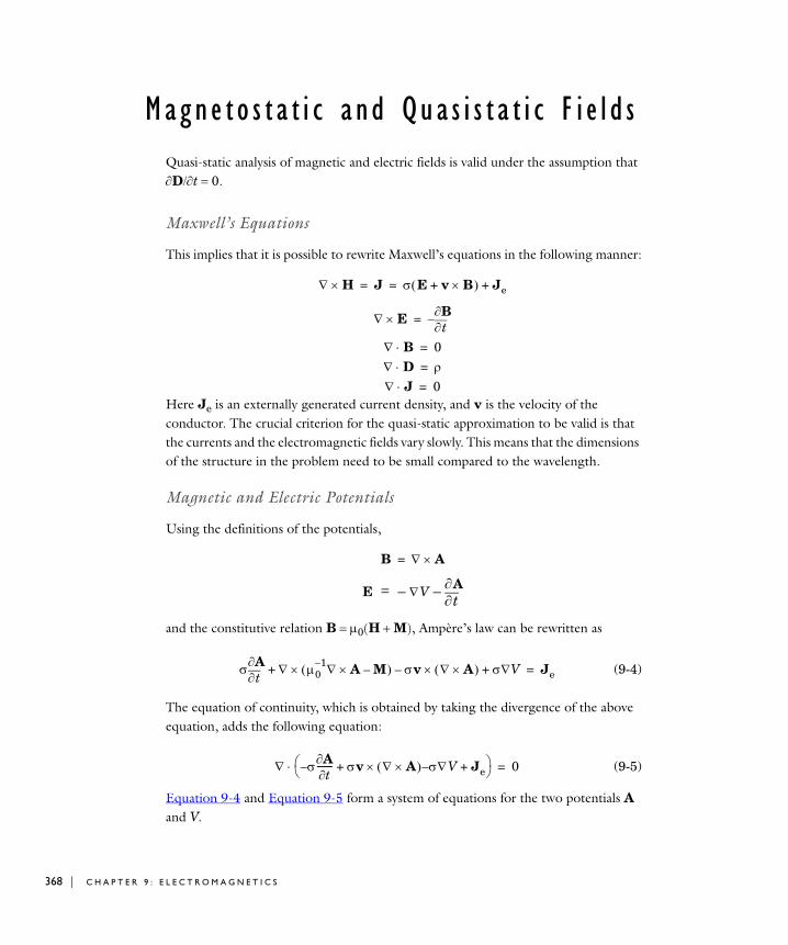
368 | C H A P T E
Magne t o s t a t i c and Qua s i s t a t i c F i e l d sQuasi-static analysis of magnetic and electric fields is valid under the assumption that Dt0.
Maxwell’s Equations
This implies that it is possible to rewrite Maxwell’s equations in the following manner:
Here Je is an externally generated current density, and v is the velocity of the conductor. The crucial criterion for the quasi-static approximation to be valid is that the currents and the electromagnetic fields vary slowly. This means that the dimensions of the structure in the problem need to be small compared to the wavelength.
Magnetic and Electric Potentials
Using the definitions of the potentials,
and the constitutive relation B0(HM), Ampère’s law can be rewritten as
(9-4)
The equation of continuity, which is obtained by taking the divergence of the above equation, adds the following equation:
(9-5)
Equation 9-4 and Equation 9-5 form a system of equations for the two potentials A and V.
H J E v B+ Je+= =
Et
B–=
B 0=
D =
J 0=
B A=
E V–t
A–=
t
A 01– A M– v A V+–+ Je=
–At
------- v A – V Je++ 0=
R 9 : E L E C T R O M A G N E T I C S

Gauge Transformations
The electric and magnetic potentials are not uniquely defined from the electric and magnetic fields through
Introducing two new potentials
gives the same electric and magnetic fields:
The variable transformation of the potentials is called a gauge transformation. To obtain a unique solution you need to choose the gauge, that is, put constraints on that make the solution unique. Another way of expressing this additional condition is to put a constraint on · A. A vector field is uniquely defined up to a constant if both · A and A are given. This is called Helmholtz’s theorem.
One particular gauge is the Coulomb gauge given by the constraint:
Selecting a Particular Gauge
Important observations are that in the dynamic case A and V are coupled via the selected gauge. For a dynamic formulation, it is also possible to select a such that the scalar electric potential vanishes and only the magnetic vector potential has to be considered. The dynamic formulations (frequency domain and time dependent study types) of the Magnetic Fields interface are operated in this gauge as it involves only A. In the static limit, A and V are not coupled via the gauge selection and thus any gauge can be chosen for A when performing magnetostatic modeling.
E At
-------– V–=
B A=
A˜
A +=
V˜
V t
-------–=
E At
-------– V–A˜
– t
---------------------------– V˜
t-------+
–A˜
t
-------– V˜
–= = =
B A A˜
– A˜
= = =
A 0=
M A G N E T O S T A T I C A N D Q U A S I S T A T I C F I E L D S | 369

370 | C H A P T E
The Gauge and the Equation of Continuity for Dynamic Fields
After eliminating the electric potential by choosing the appropriate gauge and disregarding the velocity term. The equation of continuity obtained by taking the divergence of Ampère’s law reads:
It is clear that unless the electrical conductivity is uniform, the particular gauge used to eliminate V cannot be the Coulomb gauge as that would violate the equation of continuity and would thereby also violate Ampère’s law.
Time-Harmonic Magnetic Fields
In the time-harmonic case, there is no computational cost for including the displacement current in Ampère’s law (then called Maxwell-Ampère’s law):
In the transient case the inclusion of this term would lead to a second-order equation in time, but in the harmonic case there are no such complications. Using the definition of the electric and magnetic potentials, the system of equations becomes
The constitutive relation D0EP has been used for the electric field.
You obtain a particular gauge that reduces the system of equation by choosing jV in the gauge transformation. This gives
When vanishes from the equations, you only need the second one,
Working with is often the best option when it is possible to specify all source currents as external currents Je or as surface currents on boundaries. This leads to the Magnetic Fields interface described in the next section.
–At
------- Je+ 0=
H J E v B+ jD J+e
+= =
– j 20– A v A j0+ V Je jP+ –+– 0=
j 20– A 01– A M– v A j0+ V+–+ Je jP+=
A˜
A j----V–= V
˜0=
V˜
j 20– A˜
01– A
˜M– v A
˜ –+ Je jP+=
A˜
R 9 : E L E C T R O M A G N E T I C S
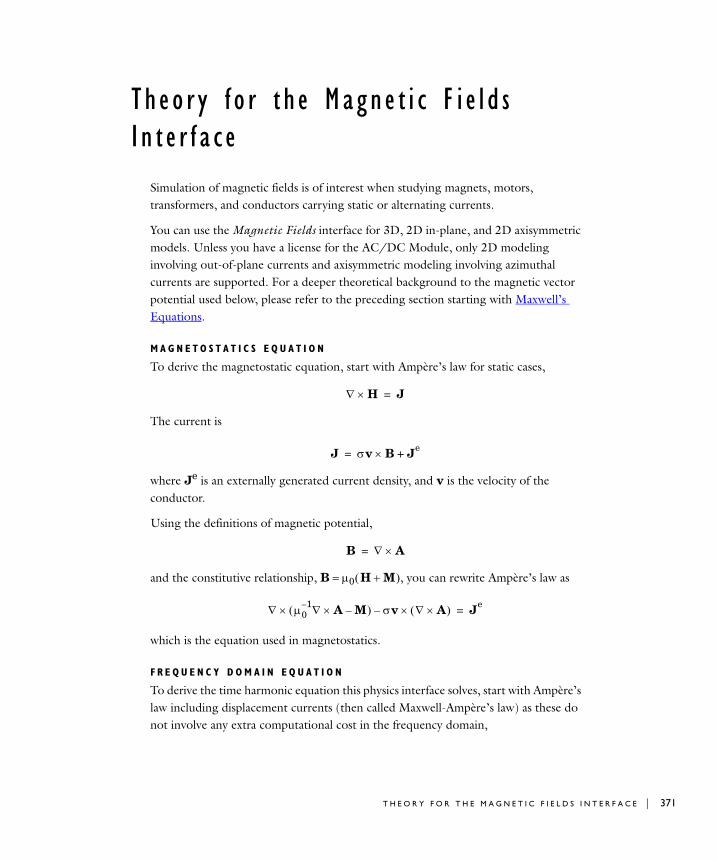
Th eo r y f o r t h e Magn e t i c F i e l d s I n t e r f a c e
Simulation of magnetic fields is of interest when studying magnets, motors, transformers, and conductors carrying static or alternating currents.
You can use the Magnetic Fields interface for 3D, 2D in-plane, and 2D axisymmetric models. Unless you have a license for the AC/DC Module, only 2D modeling involving out-of-plane currents and axisymmetric modeling involving azimuthal currents are supported. For a deeper theoretical background to the magnetic vector potential used below, please refer to the preceding section starting with Maxwell’s Equations.
M A G N E T O S T A T I C S E Q U A T I O N
To derive the magnetostatic equation, start with Ampère’s law for static cases,
The current is
where Je is an externally generated current density, and v is the velocity of the conductor.
Using the definitions of magnetic potential,
and the constitutive relationship, B0 HM, you can rewrite Ampère’s law as
which is the equation used in magnetostatics.
F R E Q U E N C Y D O M A I N E Q U A T I O N
To derive the time harmonic equation this physics interface solves, start with Ampère’s law including displacement currents (then called Maxwell-Ampère’s law) as these do not involve any extra computational cost in the frequency domain,
H J=
J v B Je+=
B A=
01– A M– v A – Je
=
T H E O R Y F O R T H E M A G N E T I C F I E L D S I N T E R F A C E | 371
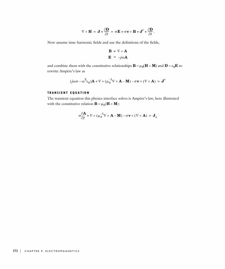
372 | C H A P T E
.
Now assume time-harmonic fields and use the definitions of the fields,
and combine them with the constitutive relationships B0HM and D0E to rewrite Ampère’s law as
TR A N S I E N T E Q U A T I O N
The transient equation this physics interface solves is Ampère’s law, here illustrated with the constitutive relation B0(HM):
H J Dt
-------+ E v B Je Dt
-------+ + += =
B A=
E j– A=
j 20– A 01– A M– v A –+ Je
=
t
A 01– A M– v A –+ Je=
R 9 : E L E C T R O M A G N E T I C S

10
A c o u s t i c s
This section describes how to use the Pressure Acoustics interface for modeling and simulation of acoustics and vibrations.
In this section:
• The Pressure Acoustics Interface
• Acoustics Theory
• Theory for the Pressure Acoustics Interface
373

374 | C H A P T E
Th e P r e s s u r e A c ou s t i c s I n t e r f a c e
The Pressure Acoustics interface ( ) has the equations, boundary conditions, and sources for modeling acoustics, solving for the sound pressure. For more information also see Acoustics Theory and Theory for the Pressure Acoustics Interface.
These default nodes are added when using this interface— Pressure Acoustics Model, Sound Hard Boundary (Wall), and Initial Values.
I N T E R F A C E I D E N T I F I E R
The unique physics interface identifier used to reach the fields and variables in expressions, for example. The default Identifier (for the first Pressure Acoustics interface in the model) is acpr. You can edit this to be any valid unique string.
D O M A I N S
Select the domains where you want to define a sound pressure field and the associated acoustics equation. The default setting includes all domains in the model.
S O U N D P R E S S U R E L E V E L S E T T I N G S
The zero level on the dB scale varies with the type of fluid. That value is a reference pressure that corresponds to 0 dB. This variable occurs in calculations of the sound pressure level based on the root mean square (rms) pressure,
an expression valid for the case of harmonically time-varying acoustic pressure, p.
From the Reference pressure for the sound pressure level list, three reference pressures are available for the sound pressure level depending on the fluid. Select:
• Use reference pressure for air to use a reference pressure of 0.02 mPa (20·106 Pa).
• Use reference pressure for water to use a reference pressure of 1 Pa (1·106 Pa).
• User defined reference pressure to enter a reference pressure pref (SI unit: Pa) in the Pref, SPL edit field. The default value is the same as for air, 0.02 mPa.
D E P E N D E N T V A R I A B L E S
This interface defines one dependent variable (field), the Pressure p. If required, edit the name, but dependent variables must be unique within a model.
p 12--- p conj p =
R 1 0 : A C O U S T I C S

A D V A N C E D S E T T I N G S A N D D I S C R E T I Z A T I O N
Normally these settings do not need to be changed. See Show More Options: Advanced Settings and Discretization. In addition, the Pressure Acoustics interface has the following settings:
Circumferential Wave Number (Axisymmetric Models Only)The circumferential wave number m is an integer-valued number used in axisymmetry and is by default 0. You can change the value in the Circumferential wave number field.
Out-of-plane Wave Number (2D and 1D Axisymmetric Models)The out-of-plane wave number kz is used in 2D and 1D axisymmetry and is by default 0. You can change the value in the Out-of-plane wave number field.
Pressure Acoustics Model
The Pressure Acoustics Model feature adds the equations for time-harmonic and eigenfrequency acoustics modeling. In the Settings window you define the properties for the acoustics model and model inputs including temperature.
D O M A I N S
Select the domains where you want to compute the acoustic pressure field and the equation that defines it. The default setting includes all domains in the model.
P R E S S U R E A C O U S T I C S M O D E L
The Fluid Model for pressure acoustics is a linear elastic fluid where you define the density and the speed of sound. By default the values for the density (SI unit: kg/m3) and the speed of sound c (SI unit: m/s) come from the material. Select User
defined to enter other values for these properties. Select Impedance and wave number to specify those properties as complex-valued data. By default the characteristic acoustic impedance Z (SI unit: Pa·s/m) is the value from the fluid material. The wave number k is a user defined value.
Monopole Source
Use the Monopole Source feature to radiate a uniform sound field in all directions.
cc2
cc2
---------=
T H E P R E S S U R E A C O U S T I C S I N T E R F A C E | 375
376 | C H A P T E
D O M A I N S
Select the domains where you want to define the monopole source.
M O N O P O L E S O U R C E
Enter a Monopole source, Q (SI unit: 1/s2). The default is 0.
Dipole Source
Use the Dipole Source feature to radiate a sound field that is typically stronger in two opposite directions.
D O M A I N S
Select the domains where you want to define the dipole source.
D I P O L E S O U R C E
Enter values in the Dipole source fields. These contain the individual components of the dipole source vector q (SI unit: N/m3), one for each space dimension. The default is 0.
Initial Values
The Initial Values feature node adds initial values for the sound Pressure p and the Pressure time derivative dpdt that can serve as an initial guess for a nonlinear solver. If you need to specify more than one initial value, right-click Pressure Acoustics to add more Initial Values nodes.
D O M A I N S
Select the domains where you want to define an initial value.
I N I T I A L V A L U E S
Enter a value or expression for the initial values.
• Pressure p (SI unit: Pa). The default is 0.
• Pressure time derivative, dpdt (SI unit: Pa/s). The default is 0.
Pressure Acoustics Boundary Conditions
The following boundary conditions are available:
• “Sound Hard Boundary (Wall)”
• Normal Acceleration
R 1 0 : A C O U S T I C S
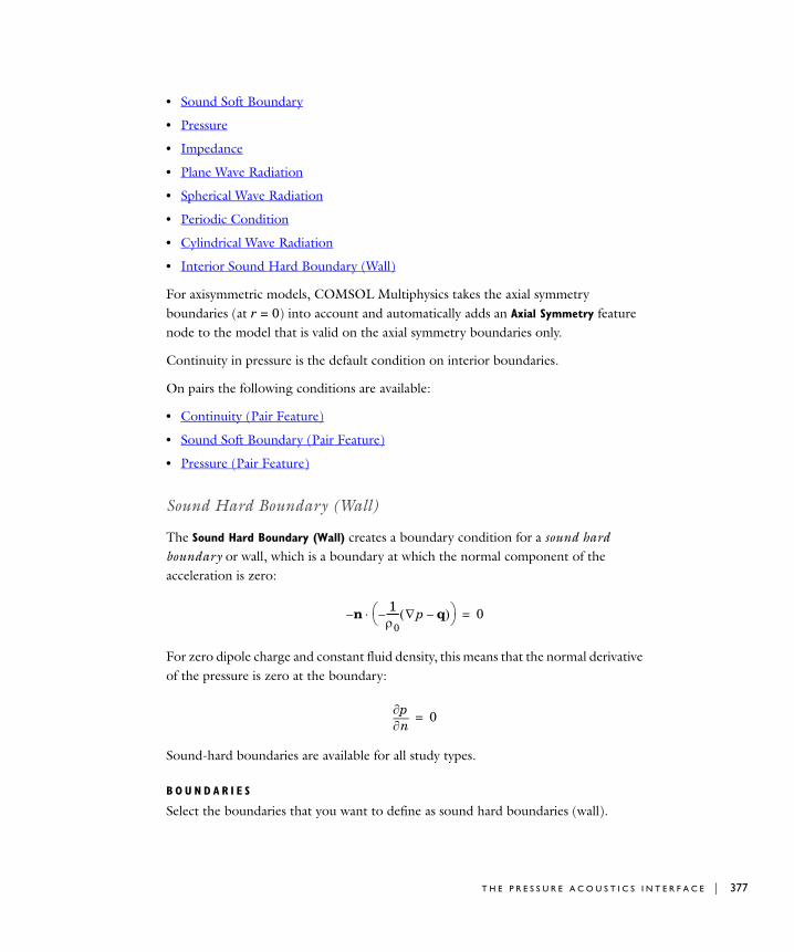
• Sound Soft Boundary
• Pressure
• Impedance
• Plane Wave Radiation
• Spherical Wave Radiation
• Periodic Condition
• Cylindrical Wave Radiation
• Interior Sound Hard Boundary (Wall)
For axisymmetric models, COMSOL Multiphysics takes the axial symmetry boundaries (at r = 0) into account and automatically adds an Axial Symmetry feature node to the model that is valid on the axial symmetry boundaries only.
Continuity in pressure is the default condition on interior boundaries.
On pairs the following conditions are available:
• Continuity (Pair Feature)
• Sound Soft Boundary (Pair Feature)
• Pressure (Pair Feature)
Sound Hard Boundary (Wall)
The Sound Hard Boundary (Wall) creates a boundary condition for a sound hard boundary or wall, which is a boundary at which the normal component of the acceleration is zero:
For zero dipole charge and constant fluid density, this means that the normal derivative of the pressure is zero at the boundary:
Sound-hard boundaries are available for all study types.
B O U N D A R I E S
Select the boundaries that you want to define as sound hard boundaries (wall).
n–10------– p q–
0=
np 0=
T H E P R E S S U R E A C O U S T I C S I N T E R F A C E | 377

378 | C H A P T E
Normal Acceleration
The Normal Acceleration adds an inward normal acceleration an:
Alternatively, specify the acceleration a of the boundary. The part in the normal direction is used to define the boundary condition:
This feature represents an external source term. It can also be used to couple an acoustics model with a structural analysis.
B O U N D A R I E S
Select the boundaries where you want to specify a normal acceleration boundary condition.
N O R M A L A C C E L E R A T I O N
From the Type list, select Inward Acceleration to enter the value of the inward normal acceleration an (SI unit: m/s2). Use a positive value for inward acceleration or a negative value for outward acceleration. Select Acceleration to enter values for the components of the acceleration a0.
Sound Soft Boundary
The Sound Soft Boundary creates a boundary condition for a sound soft boundary, where the acoustic pressure vanishes:
This boundary condition is an appropriate approximation for a liquid-gas interface and in some cases for external waveguide ports.
B O U N D A R I E S
Select the boundaries that you want to define as sound soft boundaries.
n–10------– p q–
an=
n 10------– p q–
n a 0=
p 0=
R 1 0 : A C O U S T I C S
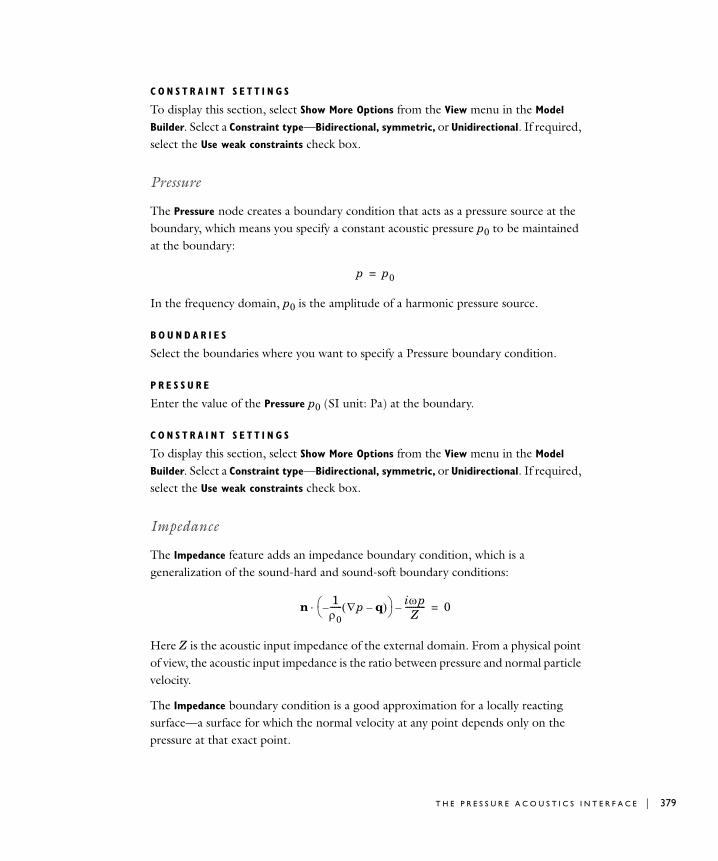
C O N S T R A I N T S E T T I N G S
To display this section, select Show More Options from the View menu in the Model
Builder. Select a Constraint type—Bidirectional, symmetric, or Unidirectional. If required, select the Use weak constraints check box.
Pressure
The Pressure node creates a boundary condition that acts as a pressure source at the boundary, which means you specify a constant acoustic pressure p0 to be maintained at the boundary:
In the frequency domain, p0 is the amplitude of a harmonic pressure source.
B O U N D A R I E S
Select the boundaries where you want to specify a Pressure boundary condition.
P R E S S U R E
Enter the value of the Pressure p0 (SI unit: Pa) at the boundary.
C O N S T R A I N T S E T T I N G S
To display this section, select Show More Options from the View menu in the Model
Builder. Select a Constraint type—Bidirectional, symmetric, or Unidirectional. If required, select the Use weak constraints check box.
Impedance
The Impedance feature adds an impedance boundary condition, which is a generalization of the sound-hard and sound-soft boundary conditions:
Here Z is the acoustic input impedance of the external domain. From a physical point of view, the acoustic input impedance is the ratio between pressure and normal particle velocity.
The Impedance boundary condition is a good approximation for a locally reacting surface—a surface for which the normal velocity at any point depends only on the pressure at that exact point.
p p0=
n 10------– p q–
ipZ
----------– 0=
T H E P R E S S U R E A C O U S T I C S I N T E R F A C E | 379

380 | C H A P T E
Note that in the two opposite limits Z and Z0, this boundary condition is identical to the Sound Hard boundary condition and the Sound Soft boundary condition, respectively.
B O U N D A R I E S
Select the boundaries where you want to specify an Impedance boundary condition.
I M P E D A N C E
Enter the value of the input impedance Zi (SI unit: Pa·s/m). The default value is 1.2[kg/m3]·343[m/s].
Plane, Spherical, and Cylindrical Radiation Boundary Conditions
Specify a Plane, Spherical, or Cylindrical Radiation boundary condition to allow an outgoing wave to leave the modeling domain with minimal reflections. The condition can be adapted to the geometry of the modeling domain. The Plane wave type is suitable for both far-field boundaries and ports. Because many waveguide structures are only interesting in the plane-wave region, it is particularly relevant for ports.
Radiation boundary conditions are available for all types of studies. For the Frequency domain study, Givoli and Neta’s reformulation of the Higdon conditions (Ref. 1) for plane waves has been implemented to the second order. For Cylindrical and Spherical waves COMSOL uses the corresponding 2nd-order expressions from Bayliss, Gunzburger, and Turkel (Ref. 2). The Eigenfrequency study implement the same expansions to the first order.
The first order radiation boundary conditions in the frequency domain read
where k is the wave number (a predefined variable; see Table 6-21 in the COMSOL Multiphysics Reference Guide or see Where Do I Access the Documentation and Model Library?) and ( r ) is a function whose form depends on the wave type:
• Plane wave: ( r )0 (see Plane Wave Radiation)
• Cylindrical wave: ( r )1(2 r) (see Cylindrical Wave Radiation)
• Spherical wave: ( r )1r (see Spherical Wave Radiation)
n 10------ p q– ik r + p
0------+ ik r +
pi0------ n
pi0
--------- +=
R 1 0 : A C O U S T I C S

In the latter two cases, r is the shortest distance from the point r(x, y, z) on the boundary to the source. The right-hand side of the equation represents an optional incoming pressure field pi (see Incident Pressure Field).
The second order radiation boundary conditions in the frequency domain are defined below. In these equations, T at a given point on the boundary denotes the Laplace operator in the tangent plane at that particular point.
• Plane wave:
In the notation of Givoli and Neta (Ref. 1), the above expressions correspond to the parameter choices C0 C1 C2 /k. For normally incident waves this gives a vanishing reflection coefficient.
• Cylindrical wave:
This boundary condition is based on a series expansion of the outgoing wave in cylindrical coordinates (Ref. 2), and it assumes the field is independent of the axial coordinate. You specify the axis of this coordinate system by giving an orientation (nx, ny, nz) and a point (x0, y0, z0) on the axis. In axisymmetric geometries the symmetry axis is the natural and only choice.
• Spherical wave:
Use this option to allow a radiated or scattered wave—emanating from an object centered at the point (x0, y0, z0) that you specify—to leave the modeling domain without reflections. The boundary condition is based on an expansion in spherical coordinates from Bayliss, Gunzburger, and Turkel (Ref. 2), implemented to the second order.
Plane Wave Radiation
The Plane Wave Radiation feature adds a radiation boundary condition for a plane wave. If required, right-click the main node to add an Incident Pressure Field (see Incident Pressure Field).
n 10------ p q– i k
0------p i
2k0-------------T p+ +
i2k0-------------T pi i k
0------pi n 1
0------ pi+ +=
n 10------ p q– ik 1
r---+
p0------
rTp20 ikr 1+ ---------------------------------–+
rTpi20 ikr 1+ ---------------------------------– ik 1
r---+
pi0------ n 1
0------ pi+ +=
T H E P R E S S U R E A C O U S T I C S I N T E R F A C E | 381

382 | C H A P T E
B O U N D A R I E S
Select the boundaries where you want to use a plane wave radiation condition.
Spherical Wave Radiation
The Spherical Wave Radiation feature adds a radiation boundary condition for a spherical wave. If required, right-click the main node to add an Incident Pressure Field (see Incident Pressure Field).
B O U N D A R I E S
Select the boundaries where you want to use a spherical wave radiation condition.
S P H E R I C A L WAV E R A D I A T I O N
Define the Source location r0.
Cylindrical Wave Radiation
The Cylindrical Wave Radiation feature adds a radiation boundary condition for a cylindrical wave. If required, right-click the main node to add an Incident Pressure Field (see Incident Pressure Field).
B O U N D A R I E S
Select the boundaries where you want to use a cylindrical wave radiation condition.
C Y L I N D R I C A L WA V E R A D I A T I O N
Define the Source location r0, and the Source axis direction raxis.
Incident Pressure Field
The Incident Pressure Field feature is a subfeature to all non-reflecting boundary conditions. Add an incident pressure field by right-clicking the boundary condition and selecting Incident Pressure Field.
B O U N D A R I E S
Select the boundaries where you want to include an incident pressure field in the boundary condition. By default, this feature node inherits the selection from its parent node, and you can only use a selection that is a subset of the parent node’s selection.
R 1 0 : A C O U S T I C S

I N C I D E N T P R E S S U R E F I E L D
From the Incident pressure field type list, select Plane wave to define a background pressure field of plane wave type. Enter a Pressure amplitude p0 (SI unit: Pa) and Wave
direction dir (SI unit: m).
Select User defined to enter the expression for pi (SI unit: Pa) as a function of space and in the Incident pressure field pi. The default is 0.
Periodic Condition
The Periodic Condition feature adds a periodic boundary condition. Right-click the main node to add a Destination Selection.
B O U N D A R I E S
Select the boundaries where you want to apply a periodic condition.
PE R I O D I C C O N D I T I O N
Select a Type of periodicity—Continuity or Antiperiodicity.
Interior Sound Hard Boundary (Wall)
This feature creates a boundary condition for the Interior Sound Hard Boundary (Wall). This boundary condition is only available on interior boundaries. A sound-hard boundary is a boundary at which the normal component of the acceleration is zero:
For zero dipole charge and constant fluid density, this means that the normal derivative of the pressure is zero at the boundary.
B O U N D A R I E S
Select the interior boundaries you want to define as sound hard boundaries (wall).
n 10------ p q–
1 0= n 1
0------ p q–
2 0=
n–10------– p q–
1
n a 0= n–10------– p q–
2
n a 0=
n–10------– p q–
1
an= n–10------– p q–
2
an=
T H E P R E S S U R E A C O U S T I C S I N T E R F A C E | 383

384 | C H A P T E
Axial Symmetry
The Axial symmetry node is a default node added for all 1D and 2D axisymmetric models. The boundary condition is active on all boundaries on the symmetry axis.
B O U N D A R I E S
The boundaries section shows on which boundaries the feature is active. All boundaries on the symmetry axis are automatically selected.
Continuity (Pair Feature)
Continuity is available as an option at interfaces between parts in an assembly. Also see Defining an Identity Pair.
This condition gives continuity in the normal acceleration over the pair (subscripts 1 and 2 in the equation refers to the two sides in the pair):
B O U N D A R I E S
This list cannot be edited. It shows the boundaries in the selected pairs.
P A I R S E L E C T I O N
Select the boundary pairs where you want to define continuity. First the pairs have to be defined.
C O N S T R A I N T S E T T I N G S
To display this section, select Show More Options from the View menu in the Model
Builder. Select a Constraint type—Bidirectional, symmetric, or Unidirectional. If required, select the Use weak constraints check box.
Sound Soft Boundary (Pair Feature)
The Sound Soft Boundary is available as an option at interfaces between parts in an assembly. Also see Defining an Identity Pair. It creates a boundary condition for a sound soft boundary, where the acoustic pressure vanishes:
n 10------ p q–
1
10------ p q–
2– 0=
p 0=
R 1 0 : A C O U S T I C S

B O U N D A R I E S
This list cannot be edited. It shows the boundaries in the selected pairs.
P A I R S E L E C T I O N
Select the boundary pairs that you want to define as sound soft boundaries. First the pairs have to be defined.
C O N S T R A I N T S E T T I N G S
To display this section, select Show More Options from the View menu in the Model
Builder. Select a Constraint type—Bidirectional, symmetric, or Unidirectional. If required, select the Use weak constraints check box.
Pressure (Pair Feature)
The Pressure pair feature is available as an option at interfaces between parts in an assembly. Also see Defining an Identity Pair. It creates a boundary condition that acts as a pressure source at the boundary, which means you specify a constant acoustic pressure p0 to be maintained at the boundary:
In the frequency domain, p0 is the amplitude of a harmonic pressure source.
B O U N D A R I E S
This list cannot be edited. It shows the boundaries in the selected pairs.
P A I R S E L E C T I O N
Select the boundary pairs where you want to specify a pressure boundary condition. First the pairs have to be defined.
P R E S S U R E
Enter the value of the Pressure p0 (SI unit: Pa) at the boundary.
C O N S T R A I N T S E T T I N G S
To display this section, select Show More Options from the View menu in the Model
Builder. Select a Constraint type—Bidirectional, symmetric, or Unidirectional. If required, select the Use weak constraints check box.
p p0=
T H E P R E S S U R E A C O U S T I C S I N T E R F A C E | 385

386 | C H A P T E
A c ou s t i c s T h e o r y
What is Acoustics?
Acoustics is the physics of sound. Sound is the sensation, as detected by the ear, of very small rapid changes in the air pressure above and below a static value. This static value is atmospheric pressure (about 100,000 pascals), which varies slowly. Associated with a sound pressure wave is a flow of energy. Physically, sound in air is a longitudinal wave where the wave motion is in the direction of the energy flow. The wave crests are the pressure maxima, while the troughs represent the pressure minima.
Sound results when the air is disturbed by some source. An example is a vibrating object, such as a speaker cone in a hi-fi system. It is possible to see the movement of a bass speaker cone when it generates sound at a very low frequency. As the cone moves forward, it compresses the air in front of it, causing an increase in air pressure. Then it moves back past its resting position and causes a reduction in air pressure. This process continues, radiating a wave of alternating high and low pressure at the speed of sound.
Five Standard Acoustics Problems
Five standard problems or scenarios occur frequently when analyzing acoustics:
• The radiation problem—A vibrating structure (a speaker, for example) radiates sound into the surrounding space. A far-away boundary condition is necessary to model the unbounded domain.
• The scattering problem—An incident wave impinges on a body and creates a scattered wave. A far-away radiation boundary condition is necessary.
• The sound field in an interior space (such as a room)—The acoustic waves stay in a finite volume so no radiation condition is necessary.
• Coupled fluid-elastic structure interaction (structural acoustics)—If the radiating or scattering structure consists of an elastic material, then you must consider the interaction between the body and the surrounding fluid. In the multiphysics coupling, the acoustic analysis provides a load (the sound pressure) to the structural analysis, and the structural analysis provides accelerations to the acoustic analysis.
• The transmission problem—The incident sound wave propagates into a body, which can have different acoustic properties. Pressure and acceleration are continuous on the boundary.
R 1 0 : A C O U S T I C S

Mathematical Models for Acoustic Analysis
Sound waves in a lossless medium are governed by the following equation for the (differential) pressure p (with SI unit N/m2):
Here 0 (kg/m3) refers to the density and cs (m/s) denotes the speed of sound. The dipole source q (N/m3) and the monopole source Q (1/s2) are both optional additional sources. The combination 0 cs
2 is called the bulk modulus, commonly denoted (N /m2).
A special case is a time-harmonic wave, for which the pressure varies with time as
where 2f (rad/s) is the angular frequency, f (Hz) as usual denoting the frequency. Assuming the same harmonic time-dependence for the source terms, the wave equation for acoustic waves reduces to an inhomogeneous Helmholtz equation:
(10-1)
With the source terms removed, you can also treat this equation as an eigenvalue PDE to solve for eigenmodes and eigenfrequencies.
Typical boundary conditions are:
• Sound-hard boundaries (walls)
• Sound-soft boundaries
• Impedance boundary conditions
• Radiation boundary conditions
These are described in more detail below.
In lossy media, an additional term of first order in the time derivative needs to be introduced to model attenuation of the sound waves:
1
0 cs2
--------------t2
2
p 10------– p q–
+ Q=
p x t p x eit=
10------– p q–
2p
0 cs2
--------------– Q=
1
0 cs2
-------------t2
2
p da tp
– 10------– p q–
+ Q=
A C O U S T I C S T H E O R Y | 387

388 | C H A P T E
Note also that even when the sound waves propagate in a lossless medium, attenuation frequently occurs by interaction with the surroundings at the boundaries of the system.
Acoustics Quantities and Their SI Units
The following table collects the names SI units for the most important physical quantities in the Pressure Acoustics interface:
QUANTITY SYMBOL SI UNIT ABBREVIATION
Pressure p pascal Pa
Density kilogram/meter3 kg/m3
Frequency f hertz Hz
Wave number k 1/meter 1/m
Dipole source q newton/meter3 N/m3
Monopole source Q 1/second2 1/s2
Speed of sound cs meter/second m/s
Acoustic impedance Z pascal-second/meter Pa·s/m
Normal acceleration an meter/second2 m/s2
Source location r0 meter m
Wave direction nk (dimensionless) 1
R 1 0 : A C O U S T I C S
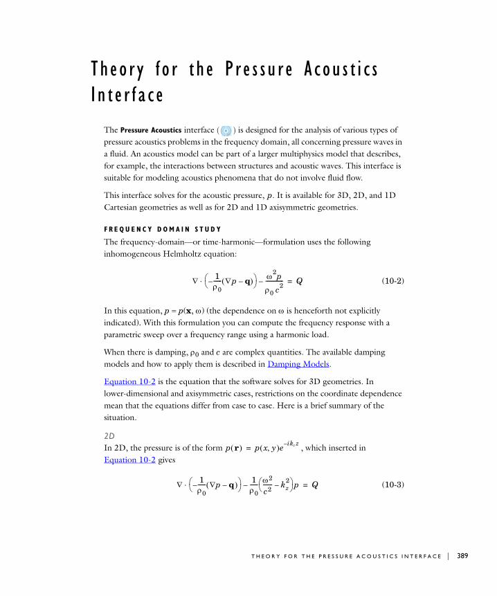
Th eo r y f o r t h e P r e s s u r e A c ou s t i c s I n t e r f a c e
The Pressure Acoustics interface ( ) is designed for the analysis of various types of pressure acoustics problems in the frequency domain, all concerning pressure waves in a fluid. An acoustics model can be part of a larger multiphysics model that describes, for example, the interactions between structures and acoustic waves. This interface is suitable for modeling acoustics phenomena that do not involve fluid flow.
This interface solves for the acoustic pressure, p. It is available for 3D, 2D, and 1D Cartesian geometries as well as for 2D and 1D axisymmetric geometries.
F R E Q U E N C Y D O M A I N S T U D Y
The frequency-domain—or time-harmonic—formulation uses the following inhomogeneous Helmholtz equation:
(10-2)
In this equation, p p(x, ) (the dependence on is henceforth not explicitly indicated). With this formulation you can compute the frequency response with a parametric sweep over a frequency range using a harmonic load.
When there is damping, 0 and c are complex quantities. The available damping models and how to apply them is described in Damping Models.
Equation 10-2 is the equation that the software solves for 3D geometries. In lower-dimensional and axisymmetric cases, restrictions on the coordinate dependence mean that the equations differ from case to case. Here is a brief summary of the situation.
2DIn 2D, the pressure is of the form , which inserted in Equation 10-2 gives
(10-3)
10------– p q–
2p
0 c2-------------– Q=
p r p x y e i– kz z=
10------ p q– –
10------ 2
c2------- kz
2–
p– Q=
T H E O R Y F O R T H E P R E S S U R E A C O U S T I C S I N T E R F A C E | 389
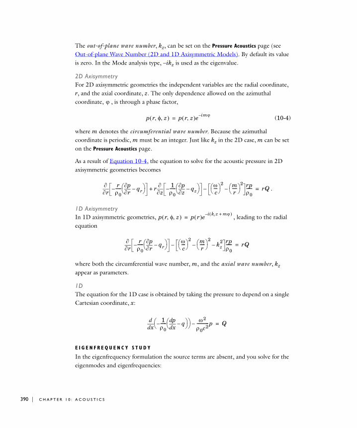
390 | C H A P T E
The out-of-plane wave number, kz, can be set on the Pressure Acoustics page (see Out-of-plane Wave Number (2D and 1D Axisymmetric Models). By default its value is zero. In the Mode analysis type, ikz is used as the eigenvalue.
2D AxisymmetryFor 2D axisymmetric geometries the independent variables are the radial coordinate, r, and the axial coordinate, z. The only dependence allowed on the azimuthal coordinate, , is through a phase factor,
(10-4)
where m denotes the circumferential wave number. Because the azimuthal coordinate is periodic, m must be an integer. Just like kz in the 2D case, m can be set on the Pressure Acoustics page.
As a result of Equation 10-4, the equation to solve for the acoustic pressure in 2D axisymmetric geometries becomes
.
1D AxisymmetryIn 1D axisymmetric geometries, , leading to the radial equation
where both the circumferential wave number, m, and the axial wave number, kz appear as parameters.
1DThe equation for the 1D case is obtained by taking the pressure to depend on a single Cartesian coordinate, x:
E I G E N F R E Q U E N C Y S T U D Y
In the eigenfrequency formulation the source terms are absent, and you solve for the eigenmodes and eigenfrequencies:
p r z p r z e im–=
r r
0------–
rp qr– r
z 1
0------–
zp qz–
c---- 2 m
r----- 2
–rp0------–+ rQ=
p r z p r ei kz z m+ –
=
r r
0------–
rp qr–
c---- 2 m
r----- 2
– kz2
–rp0------– rQ=
xdd 1
0------
xddp q– –
2
0c2------------ p– Q=
R 1 0 : A C O U S T I C S

(10-5)
The eigenvalue introduced in this equation is related to the eigenfrequency, f, and the angular frequency, , through i2fi. Because they are independent of the pressure, the solver ignores any dipole and monopole sources unless you are solving a coupled eigenvalue problem.
Equation 10-5 applies to the 3D case. The equations solved in eigenfrequency studies in lower dimensions and for axisymmetric geometries are obtained from their time-harmonic counterparts, given in the previous subsection, by the substitution 22.
You can switch between specifying the eigenvalues, the eigenfrequencies, or the angular frequencies by selecting from the Eigenvalue transformation list in the solver sequence’s Eigenvalue feature node’s Settings window.
R E F E R E N C E S F O R T H E P R E S S U R E A C O U S T I C S I N T E R F A C E
1. D. Givoli and B. Neta, “High-order non-reflecting boundary scheme for time-dependent waves”, J. Comput. Phys., vol. 186, pp. 24–46, 2004.
2. A. Bayliss, M. Gunzburger, and E. Turkel, “Boundary Conditions for the Numerical Solution of Elliptic Equations in Exterior Regions,” SIAM J. Appl. Math., vol. 42, no. 2, pp. 430–451, 1982.
3. A.B. Bauer, “Impedance theory and measurements on porous acoustic liners,” J. Aircr., vol. 14, pp. 720–728, 1977.
4. S. Temkin, Elements of Acoustics, Acoustical Society of America, 2001.
10------– p
2 p
0 c2-----------+ 0=
T H E O R Y F O R T H E P R E S S U R E A C O U S T I C S I N T E R F A C E | 391

392 | C H A P T E
R 1 0 : A C O U S T I C S
11
T h e C h e m i c a l S p e c i e s T r a n s p o r t I n t e r f a c e s
This section explains how to use the Transport of Diluted Species interface to model and simulate mass transfer (chemical species transport) by diffusion and convection based on Fick’s law of diffusion.
In this section:
• The Transport of Diluted Species Interface
• Theory for the Transport of Diluted Species Interface
393

394 | C H A P T E
Th e T r a n s p o r t o f D i l u t e d S p e c i e s I n t e r f a c e
Mass transfer is an important part of chemical engineering because this is the field that considers the conversion of one type of substance into another. A lot of this occurs through chemical reactions, although separation and other unit operations are an important part. You can use the Transport of Diluted Species interface to model transport of a diluted species in chemical systems by convection and diffusion.
In the Transport of Diluted Species interface, Fick’s law describes the diffusive transport in the flux vector. Fick’s law is adequate when the diffusing species is dilute with respect to a solvent. Assuming a binary mixture of solute A in solvent B, concentrations of up to 10 mol% of A can be considered dilute.
Note: The optional Chemical Reaction Engineering Module has an extension of this physics interface for modeling multicomponent convection, diffusion, and migration (electrokinetic flow).
The Transport of Diluted Species interface ( ) has the equations, boundary conditions, and rate expression terms for modeling mass transport of diluted species in mixtures, solutions and solids, solving for the species concentration.
The interface supports simulation of transport by convection and diffusion in 1D, 2D, and 3D as well as for axisymmetric models in 1D and 2D. The dependent variable is the mass concentration, c.
The following default nodes are added when using this interface—Convection and
Diffusion, No Flux, and Initial Values. Right-click the Transport of Diluted Species node to add other nodes with appropriate boundary conditions and rate expression terms.
I N T E R F A C E I D E N T I F I E R
This is the physics interface identifier, which you use to reach the fields and variables in expressions, for example.
R 1 1 : T H E C H E M I C A L S P E C I E S TR A N S P O R T I N T E R F A C E S
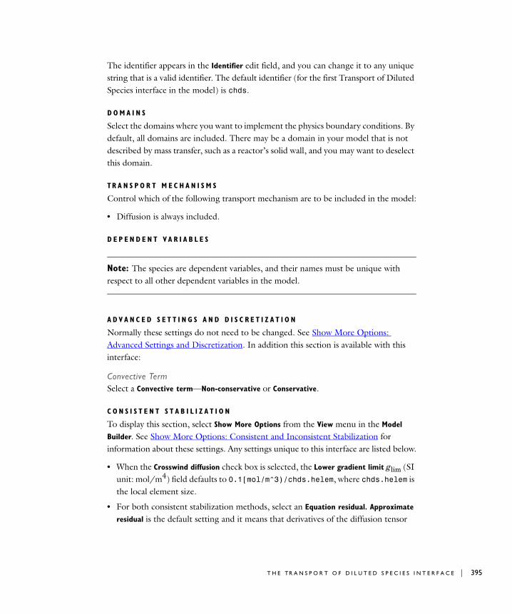
The identifier appears in the Identifier edit field, and you can change it to any unique string that is a valid identifier. The default identifier (for the first Transport of Diluted Species interface in the model) is chds.
D O M A I N S
Select the domains where you want to implement the physics boundary conditions. By default, all domains are included. There may be a domain in your model that is not described by mass transfer, such as a reactor’s solid wall, and you may want to deselect this domain.
TR A N S P O R T M E C H A N I S M S
Control which of the following transport mechanism are to be included in the model:
• Diffusion is always included.
D E P E N D E N T V A R I A B L E S
Note: The species are dependent variables, and their names must be unique with respect to all other dependent variables in the model.
A D V A N C E D S E T T I N G S A N D D I S C R E T I Z A T I O N
Normally these settings do not need to be changed. See Show More Options: Advanced Settings and Discretization. In addition this section is available with this interface:
Convective Term Select a Convective term—Non-conservative or Conservative.
C O N S I S T E N T S T A B I L I Z A T I O N
To display this section, select Show More Options from the View menu in the Model
Builder. See Show More Options: Consistent and Inconsistent Stabilization for information about these settings. Any settings unique to this interface are listed below.
• When the Crosswind diffusion check box is selected, the Lower gradient limit glim (SI unit: mol/m4) field defaults to 0.1[mol/m^3)/chds.helem, where chds.helem is the local element size.
• For both consistent stabilization methods, select an Equation residual. Approximate
residual is the default setting and it means that derivatives of the diffusion tensor
T H E TR A N S P O R T O F D I L U T E D S P E C I E S I N T E R F A C E | 395

396 | C H A P T E
components are neglected. This setting is usually accurate enough and is faster to compute. If required, select Full residual instead.
I N C O N S I S T E N T S T A B I L I Z A T I O N
To display this section, select Show More Options from the View menu in the Model
Builder. See Show More Options: Consistent and Inconsistent Stabilization for information about these settings.
Transport Feature Node
This node is dynamic in that it is dependent on the transport mechanisms that have been chosen in the Transport of Diluted Species physics interface (convection, diffusion and migration), and includes only the input fields required by the activated transport mechanisms. It has all the equations defining the transport of diluted species as well as inputs for the material properties. The name of the node also changes the activated transport mechanisms, and can be one of the following:
• Diffusion
• Convection and Diffusion
D O M A I N S
Select the domains where you want to define material properties and other parameters that govern the transport equations. As you may have more than one type of domain, with subsequent material properties, you may want to deselect some of the domains. These would then be defined in a subsequent Convection and Diffusion node.
M O D E L I N P U T S
If transport by convection is active the velocity field of the solvent needs to be specified as a model input.
Select the source of the Velocity field u:
• Select User defined to enter values or expressions for the velocity components (SI unit: m/s) in the edit fields or table that appears below the drop-down menu. This input option is always available.
• Select the velocity field solved by a fluid flow physics interface that has also been added to the model. These physics interfaces have their own tags or Interface Identifier, and they are available to choose in the Velocity field drop-down menu, if they are also active in the domains being defined here. This lists the variable names
R 1 1 : T H E C H E M I C A L S P E C I E S TR A N S P O R T I N T E R F A C E S

related to the fluid flow physics interface in the table underneath the drop-down menu.
D I F F U S I O N
Enter the Diffusion coefficient Dc (SI unit: m2/s), which can be a scalar value for isotropic diffusion or a tensor describing anisotropic diffusion. Select the appropriate tensor type that describes the diffusion transport, and then enter the values in the corresponding field.
Reactions
In order to account for the consumption or production of species, right-click on the Transport of Diluted Species node to add the Reactions node. This node contains an edit field to define the rate expression which in turn appear on the right hand side of the species transport equation.
D O M A I N S
Select the domains where you want to define rate expression that govern the source term in the transport equations. As you may have more than one type of domain, with subsequent and different reactions occurring within them, you may want to deselect some of the domains. These would then be defined in a subsequent Reactions node.
R E A C T I O N S
Add a rate expression, (SI unit: mol/(m3·s)), for the species to be solved for. Type a value or expression in the corresponding field.
Initial Values
The Initial Values feature allows the initial value or guess for the variables and species, nominally the concentration, to be solved for to be specified. This can serve as the an initial condition for a transient simulation.
D O M A I N S
Select the domains where you want to define an initial value. As you may have more than one type of domain, with subsequent and different initial values occurring within them, you may want to deselect some of the domains. These would then be defined in a subsequent Initial Value node.
T H E TR A N S P O R T O F D I L U T E D S P E C I E S I N T E R F A C E | 397

398 | C H A P T E
I N I T I A L V A L U E S
Enter a value or expression for the initial value of the concentration ci, in the Concentration edit field. The default value is 0 mol/m3.
Boundary Conditions
The following boundary conditions are available for the exterior boundaries:
• Concentration
• Flux
• Inflow
• No Flux (the default boundary condition)
• Outflow
• Symmetry
For interior boundaries, continuity in the species concentration is the default boundary condition. In addition, the following boundary condition is available on interior boundaries:
• Flux Discontinuity
For axisymmetric models, COMSOL Multiphysics takes the axial symmetry boundaries (at r0) into account and automatically adds an Axial Symmetry feature to the model that is valid on the this boundary.
Concentration
The Concentration boundary node adds a boundary condition for the species concentration; for example the following condition specifies the concentration of species c:
B O U N D A R I E S
Select the boundaries where you want to apply the concentration boundary condition.
C O N C E N T R A T I O N
You can specify the concentration for each species individually. Select the check box for the species for which you want to specify the concentration, and then enter a value or expression in the corresponding edit field. Conversely, if you want to use another
c c0=
R 1 1 : T H E C H E M I C A L S P E C I E S TR A N S P O R T I N T E R F A C E S
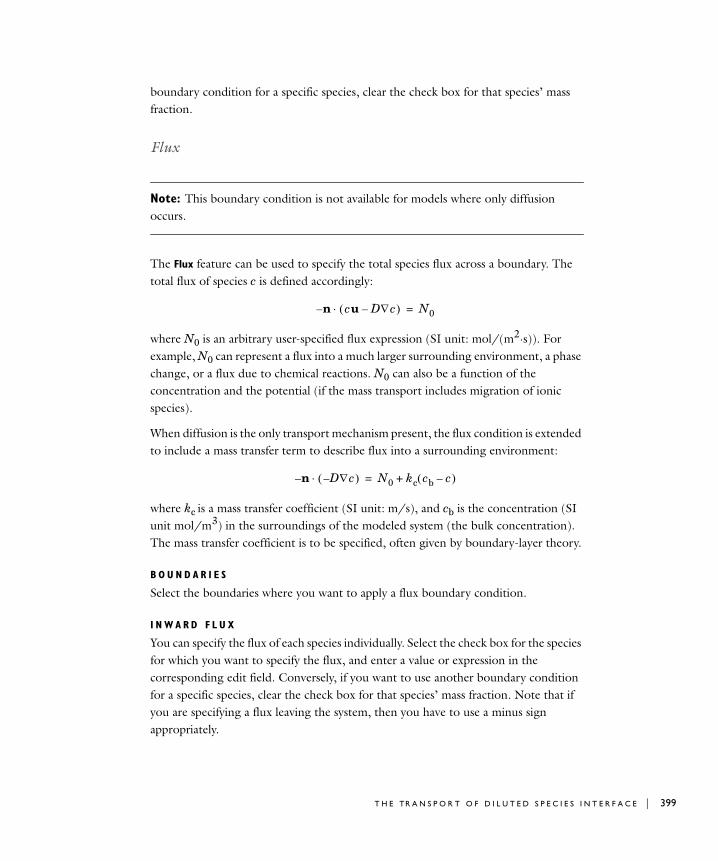
boundary condition for a specific species, clear the check box for that species’ mass fraction.
Flux
Note: This boundary condition is not available for models where only diffusion occurs.
The Flux feature can be used to specify the total species flux across a boundary. The total flux of species c is defined accordingly:
where N0 is an arbitrary user-specified flux expression (SI unit: mol/(m2·s)). For example, N0 can represent a flux into a much larger surrounding environment, a phase change, or a flux due to chemical reactions. N0 can also be a function of the concentration and the potential (if the mass transport includes migration of ionic species).
When diffusion is the only transport mechanism present, the flux condition is extended to include a mass transfer term to describe flux into a surrounding environment:
where kc is a mass transfer coefficient (SI unit: m/s), and cb is the concentration (SI unit mol/m3) in the surroundings of the modeled system (the bulk concentration). The mass transfer coefficient is to be specified, often given by boundary-layer theory.
B O U N D A R I E S
Select the boundaries where you want to apply a flux boundary condition.
I N W A R D F L U X
You can specify the flux of each species individually. Select the check box for the species for which you want to specify the flux, and enter a value or expression in the corresponding edit field. Conversely, if you want to use another boundary condition for a specific species, clear the check box for that species’ mass fraction. Note that if you are specifying a flux leaving the system, then you have to use a minus sign appropriately.
n– cu Dc– N0=
n– Dc– N0 kc cb c– +=
T H E TR A N S P O R T O F D I L U T E D S P E C I E S I N T E R F A C E | 399

400 | C H A P T E
Inflow
The Inflow feature adds a boundary condition for an inflow boundary, where you specify the concentration of all species:
This condition is similar to that of the Concentration feature, except that you must specify the concentrations of all species.
B O U N D A R I E S
Select the boundaries where you want to apply an inflow boundary condition.
C O N C E N T R A T I O N
Enter a value or expression for the concentration of each species.
No Flux
The No Flux node, which is the default boundary condition on exterior boundaries, represents boundaries where no mass flows in or out of this boundary, such that the total flux is zero:
B O U N D A R I E S
Select the boundaries where you want to apply a no-flux boundary condition.
N O F L U X
Select Apply for all species to from the drop-down menu list to specify that the boundary is completely impervious for all species. Select Apply for... and select the check boxes for the species for which you want to specify the No-flux condition.
Outflow
Note: This boundary condition is not available for models where only diffusion occurs.
c c0=
n– cu Dc– N0=
R 1 1 : T H E C H E M I C A L S P E C I E S TR A N S P O R T I N T E R F A C E S
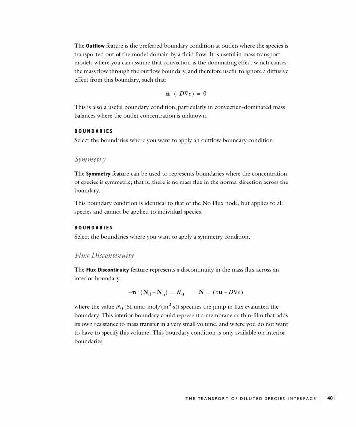
The Outflow feature is the preferred boundary condition at outlets where the species is transported out of the model domain by a fluid flow. It is useful in mass transport models where you can assume that convection is the dominating effect which causes the mass flow through the outflow boundary, and therefore useful to ignore a diffusive effect from this boundary, such that:
This is also a useful boundary condition, particularly in convection-dominated mass balances where the outlet concentration is unknown.
B O U N D A R I E S
Select the boundaries where you want to apply an outflow boundary condition.
Symmetry
The Symmetry feature can be used to represents boundaries where the concentration of species is symmetric; that is, there is no mass flux in the normal direction across the boundary.
This boundary condition is identical to that of the No Flux node, but applies to all species and cannot be applied to individual species.
B O U N D A R I E S
Select the boundaries where you want to apply a symmetry condition.
Flux Discontinuity
The Flux Discontinuity feature represents a discontinuity in the mass flux across an interior boundary:
where the value N0 (SI unit: mol/(m2·s)) specifies the jump in flux evaluated the boundary. This interior boundary could represent a membrane or thin-film that adds its own resistance to mass transfer in a very small volume, and where you do not want to have to specify this volume. This boundary condition is only available on interior boundaries.
n D c– 0=
n– Nd Nu– N0= N cu Dc– =
T H E TR A N S P O R T O F D I L U T E D S P E C I E S I N T E R F A C E | 401
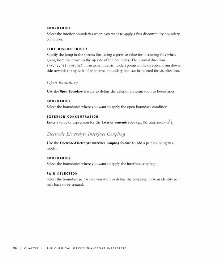
402 | C H A P T E
B O U N D A R I E S
Select the interior boundaries where you want to apply a flux discontinuity boundary condition.
F L U X D I S C O N T I N U I T Y
Specify the jump in the species flux, using a positive value for increasing flux when going from the down to the up side of the boundary. The normal direction (nx,ny,nz) ((nr,nz) in an axisymmetric model) points in the direction from down side towards the up side of an internal boundary and can be plotted for visualization.
Open Boundary
Use the Open Boundary feature to define the exterior concentration to boundaries.
B O U N D A R I E S
Select the boundaries where you want to apply the open boundary condition.
E X T E R I O R C O N C E N T R A T I O N
Enter a value or expression for the Exterior concentration c0,c (SI unit: mol/m3).
Electrode-Electrolyte Interface Coupling
Use the Electrode-Electrolyte Interface Coupling feature to add a pair coupling to a model.
B O U N D A R I E S
Select the boundaries where you want to apply the interface coupling.
P A I R S E L E C T I O N
Select the boundary pair where you want to define the coupling. First an identity pair may have to be created.
R 1 1 : T H E C H E M I C A L S P E C I E S TR A N S P O R T I N T E R F A C E S

Th eo r y f o r t h e T r a n s p o r t o f D i l u t e d S p e c i e s I n t e r f a c e
The Transport of Diluted Species interface ( ) provides a predefined modeling environment for studying the evolution of chemical species transported by diffusion, convection and migration due to an electric field. The interface assumes that all species present are dilute, that their concentration is small compared to a solvent fluid or solid. As a rule of thumb, a mixture containing several species can be considered dilute when the concentration of the solvent is more than 90 mol%. Due to the dilution, mixture properties such as density and viscosity, can be assumed to correspond to those of the solvent.
Fick’s law governs the diffusion of the solutes dilute mixtures or solutions, while the phenomenon of ionic migration is sometimes referred to as electrokinetic flow. The Transport of Diluted Species physics interface supports the simulation of chemical species transport by convection, diffusion, and migration in 1D, 2D, and 3D as well as for axisymmetric models in 1D and 2D.
M A S S B A L A N C E E Q U A T I O N
The default node attributed to the Transport of Diluted Species interface assumes chemical species transport through diffusion and convection (a button to activate migration is readily available) and implements the mass balance equation:
(11-1)
Equation 11-1 includes these quantities (with the SI unit in parentheses):
• c is the concentration of the species (mol/m3)
• D denotes the diffusion coefficient (m2/s)
• R is a reaction rate expression for the species (mol/(m3·s))
• u is the velocity vector (m/s)
The first term on the left-hand side of Equation 11-1 corresponds to the accumulation (or indeed consumption) of the species.
The second term accounts for the convective transport due to a velocity field u. This field can be expressed analytically or be obtained from coupling this physics interface
ct
----- u c+ D c R+=
T H E O R Y F O R T H E TR A N S P O R T O F D I L U T E D S P E C I E S I N T E R F A C E | 403
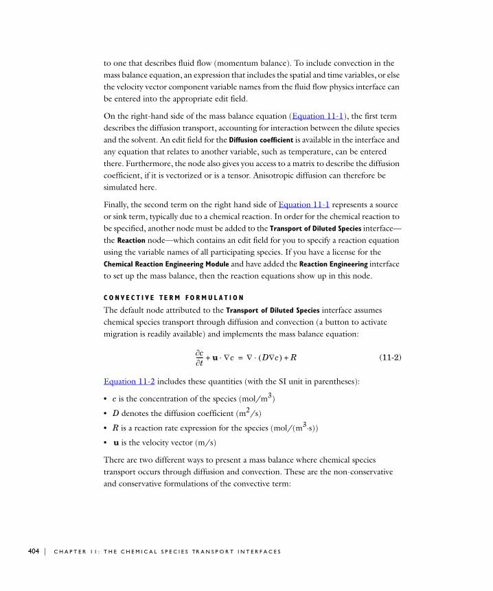
404 | C H A P T E
to one that describes fluid flow (momentum balance). To include convection in the mass balance equation, an expression that includes the spatial and time variables, or else the velocity vector component variable names from the fluid flow physics interface can be entered into the appropriate edit field.
On the right-hand side of the mass balance equation (Equation 11-1), the first term describes the diffusion transport, accounting for interaction between the dilute species and the solvent. An edit field for the Diffusion coefficient is available in the interface and any equation that relates to another variable, such as temperature, can be entered there. Furthermore, the node also gives you access to a matrix to describe the diffusion coefficient, if it is vectorized or is a tensor. Anisotropic diffusion can therefore be simulated here.
Finally, the second term on the right hand side of Equation 11-1 represents a source or sink term, typically due to a chemical reaction. In order for the chemical reaction to be specified, another node must be added to the Transport of Diluted Species interface—the Reaction node—which contains an edit field for you to specify a reaction equation using the variable names of all participating species. If you have a license for the Chemical Reaction Engineering Module and have added the Reaction Engineering interface to set up the mass balance, then the reaction equations show up in this node.
C O N V E C T I V E TE R M F O R M U L A T I O N
The default node attributed to the Transport of Diluted Species interface assumes chemical species transport through diffusion and convection (a button to activate migration is readily available) and implements the mass balance equation:
(11-2)
Equation 11-2 includes these quantities (with the SI unit in parentheses):
• c is the concentration of the species (mol/m3)
• D denotes the diffusion coefficient (m2/s)
• R is a reaction rate expression for the species (mol/(m3·s))
• u is the velocity vector (m/s)
There are two different ways to present a mass balance where chemical species transport occurs through diffusion and convection. These are the non-conservative and conservative formulations of the convective term:
ct
----- u c+ D c R+=
R 1 1 : T H E C H E M I C A L S P E C I E S TR A N S P O R T I N T E R F A C E S

non-conservative (11-3)
conservative (11-4)
and each is treated slightly differently by the solver algorithms. In these equations D is the diffusion coefficient (SI unit: m2/s), R is a production or consumption rate expression (SI unit: mol/(m3·s)), and u is the solvent velocity field (SI unit: m/s). The diffusion process can be anisotropic, in which case D is a tensor.
If you were to expand the conservative formulation using the chain rule, then one of the terms from the convection part, c·u, would equal zero for an incompressible fluid and would result in the non-conservative formulation above. This is in fact the default formulation in the Transport of Diluted Species interface and ensures that non-physical source terms cannot come from the solution of a flow field. to switch between the two formulations, you have to activate the Show More Options for this interface.
S O L V I N G A D I F F U S I O N E Q U A T I O N O N L Y
You can remove the convection term from the above equations by clearing the Convection button under the Transport Mechanisms section in the Transport of Diluted
Species feature. The equation then becomes
(11-5)
ct
----- u c+ D c R+=
ct
----- cu + D c R+=
ct
----- D c R+=
T H E O R Y F O R T H E TR A N S P O R T O F D I L U T E D S P E C I E S I N T E R F A C E | 405

406 | C H A P T E
R 1 1 : T H E C H E M I C A L S P E C I E S TR A N S P O R T I N T E R F A C E S
12
T h e F l u i d F l o w I n t e r f a c e
This section explains how to use the Laminar Flow interface for the modeling and simulation of fluid mechanics for laminar, incompressible fluids. Note that the engineering community often uses the term CFD, computational fluid dynamics, to refer to the numerical simulation of fluids.
In this section:
• The Single-Phase Flow, Laminar Flow Interface
• Theory for the Single-Phase, Laminar Flow Interface
407

408 | C H A P T E
Th e S i n g l e - Pha s e F l ow , L am i n a r F l ow I n t e r f a c e
The Laminar Flow interface ( ) has the equations, boundary conditions, and volume forces for modeling freely moving fluids using the Navier-Stokes equations, solving for the velocity field and the pressure.
The main node is Fluid Properties, which adds the Navier-Stokes equations and provides an interface for defining the fluid material and its properties.
The following default nodes are added when using this interface—Fluid Properties, Wall
(the default boundary condition is No slip) and Initial Values nodes.
Right-click the Laminar Flow node to add other feature nodes that implement, for example, boundary conditions and volume forces.
I N T E R F A C E I D E N T I F I E R
The interface identifier is a text string that can be used to reference the respective physics interface if appropriate. Such situations could occur when coupling this interface to another physics interface, or when trying to identify and use variables defined by this physics interface, which you use to reach the fields and variables in expressions, for example. You can change it to any unique string through the Identifier edit field.
The default identifier (for the first Laminar Flow or other single-phase flow interface in the model) is spf.
D O M A I N S
Select the domains where you want to define the fluid pressure and velocity and the Navier-Stokes equations that describe those fields. The default setting is to include all domains in the model.
P H Y S I C A L M O D E L
Control the properties of the Laminar Flow interface, which control the overall type of fluid-flow model:
R 1 2 : T H E F L U I D F L O W I N T E R F A C E
CompressibilityBy default the interface uses the Compressible flow (Ma<0.3) formulation of the Navier-Stokes equations. Select Incompressible to use the incompressible (constant density) formulation.
C O N S I S T E N T S T A B I L I Z A T I O N
To display this section, select Show More Options from the View menu in the Model
Builder. See Show More Options: Consistent and Inconsistent Stabilization for information about these settings.
I N C O N S I S T E N T S T A B I L I Z A T I O N
To display this section, select Show More Options from the View menu in the Model
Builder. See Show More Options: Consistent and Inconsistent Stabilization for information about these settings.
A D V A N C E D S E T T I N G S A N D D I S C R E T I Z A T I O N
To display this section, select Show More Options from the View menu in the Model
Builder. Normally these settings do not need to be changed.
The check box Use pseudo time stepping for stationary equation form adds pseudo time derivatives to the equation when the Stationary equation form is used. When selected, a Local CFL number list with the options
• Automatic
• User defined
The Automatic option calculates the local CFL number from a built-in expression while User defined makes it possible to manually define the local CFL number. See also Pseudo Time Stepping.
More information on advanced settings can be found in Show More Options: Advanced Settings and Discretization.
D E P E N D E N T V A R I A B L E S
This interface defines these dependent variables (fields):
• Velocity field u (SI unit: m/s)
• Pressure p (SI unit: Pa)
If required, edit the name, but dependent variables must be unique within a model.
T H E S I N G L E - P H A S E F L O W , L A M I N A R F L O W I N T E R F A C E | 409

410 | C H A P T E
Fluid Properties
The Fluid Properties feature adds the momentum equations solved by the interface, except for volume forces which are added by a separate feature (Volume Force), and provides an interface for defining the material properties of the fluid.
D O M A I N S
Select the domains where you want to apply the fluid properties defined in the Fluid
Properties feature.
M O D E L I N P U T S
In this section input variables to the momentum equations can be edited. For fluid flow, these are typically introduced when a material requiring inputs has been applied.
F L U I D P R O P E R T I E S
Specify the density and the dynamic viscosity of the fluid.
DensityThe default Density (SI unit: kg/m3) uses the value From material. Select User defined to enter a different value or expression.
Dynamic ViscosityThe dynamic viscosity describes the relationship between the shear rate and the shear stresses in a fluid. Intuitively, water and air have a low viscosity, and substances often described as thick, such as oil, have a higher viscosity.
For the Dynamic viscosity (SI unit: Pa·s), select from these options to model Newtonian fluids:
• The default uses the value From material. The value of the viscosity is then the value defined for the material that you select in the Material section.
• Select User defined to define a value or expression for the Dynamic viscosity. Using a built-in variable for the shear rate magnitude, sr_spf, makes it possible to define arbitrary expressions of the dynamics viscosity as a function of the shear rate.
Absolute Pressure This section controls both the variable as well as any property value (reference pressures) used when solving for pressure. There are usually two ways for including a variable in expressions describing fluid flow, and mass and heat transfer. You can solve for the absolute pressure or a pressure (often denoted gauge pressure) that relates back to the absolute pressure through a reference pressure.
R 1 2 : T H E F L U I D F L O W I N T E R F A C E

Using one or the other usually depends on the system and the equations you are solving for. For example, in a straight incompressible flow problem, the pressure drop over the modeled domain will probably be many orders of magnitude less than atmospheric pressure, which, if included, reduces the chances for stability and convergence during the solving process for this variable. In an other case, the absolute pressure may be required to be solved for, such as where pressure is a part of an expression for gas volume or diffusion coefficients.
The pressure as a variable input is controlled by both a drop-down list and a check box within this section. The User defined option requires that the equations will solve for the variable itself (the absolute pressure), which describes your system. You need to maintain control over any external pressures that may affect your system, if indeed there are any.
The default option, which is denoted Pressure nitf/fluid, also activates a check box for defining the reference pressure, where 1 [atm] has been automatically included. This will allow you to use a system-based (gauge) pressure as the pressure variable, while automatically including the reference pressure in places where it is required, such as for gas flow governed by the gas law. While this check box maintains control over the pressure variable and instances where absolute pressure is required within this respective physics interface, it may not with interfaces that you are coupling to, such as mass and heat transfer physics interfaces. You should check between the two that are solving for the same variable.
Volume Force
The Volume Force feature specifies the volume force F on the right-hand side of Equation 12-16. Use it, for example, to incorporate the effects of gravity in your model.
D O M A I N S
Select the domains where the volume force acts on the fluid.
VO L U M E F O R C E
Enter the components of the volume force F (SI unit: N/m3).
T H E S I N G L E - P H A S E F L O W , L A M I N A R F L O W I N T E R F A C E | 411

412 | C H A P T E
Initial Values
The Initial Values feature adds initial values for the velocity field u and the pressure P that can serve as an initial condition for a transient simulation or as an initial guess for a nonlinear solver.
D O M A I N S
Select the domains where you want to define initial values.
I N I T I A L V A L U E S
Enter values or expressions for the initial value of the Velocity field u (SI unit: m/s) and for the Pressure p (SI unit: Pa). The default values are 0.
Boundary Conditions
The following six features contain all boundary conditions for the single-phase flow interfaces and represent the major types of boundaries in a fluid-flow model:
• Wall (the default boundary condition feature).
• Inlet
• Outlet
• Symmetry
• Open Boundary
• Boundary Stress
• Periodic Flow Condition
For axisymmetric models, COMSOL Multiphysics takes the axial symmetry boundaries (at r = 0) into account and automatically adds an Axial Symmetry feature to the model that is valid on the axial symmetry boundaries only.
You find the theory of most boundary conditions in Gresho and Sani ().
Wall
The Wall feature includes a set of boundary conditions describing the fluid flow condition at a wall. The following boundary conditions are available:
In laminar flow interfaces the following wall boundary conditions are available:
• Slip
R 1 2 : T H E F L U I D F L O W I N T E R F A C E

• No Slip (Default)
• Moving Wall
• Leaking Wall
• Sliding Wall
B O U N D A R I E S
Select the boundaries that represent solid walls.
B O U N D A R Y C O N D I T I O N
Select a Boundary condition for the wall:
No SlipNo slip is the standard and default boundary condition for a stationary solid wall. The condition prescribes
that is, that the fluid at the wall is not moving.
SlipThe Slip condition assumes that there are no viscous effects at the slip wall and hence, no boundary layer develops. From a modeling point of view, this may be a reasonable approximation if the important effect of the wall is to prevent fluid from leaving the domain. Mathematically, the constraint can be formulated as:
where t is a tangential vector to the boundary.
Sliding WallThe Sliding wall boundary condition is appropriate if the wall behaves like a conveyor belt; that is, the surface is sliding in its tangential direction. The wall does not have to actually move in the coordinate system.
In 2D, the tangential direction is unambiguously defined by the direction of the boundary, but the situation becomes more complicated in 3D. For this reason, this boundary condition has slightly different definitions in the different space dimensions.
2D and Axial Symmetry The velocity is given as a scalar Uw and the condition prescribes
u 0=
u n 0,= t pI– u u T+ + n 0=
u n 0,= u t Uw=
T H E S I N G L E - P H A S E F L O W , L A M I N A R F L O W I N T E R F A C E | 413

414 | C H A P T E
where t(ny , -nx) for 2D and t(nz , -nr) for axial symmetry.
Enter the components of the Velocity of the tangentially moving wall Uw (SI unit: m/s).
3D The velocity is set equal to a given vector uw projected onto the boundary plane:
The denominator makes u have the same magnitude as uw even if uw is not exactly parallel to the wall.
Enter the components of the Velocity of the sliding wall uw (SI unit: m/s).
Moving WallIf the wall moves, so must the fluid. Hence, this boundary condition prescribes
Note: Specifying this boundary condition does not automatically cause the associated wall to move.
Enter the components of the Velocity of moving wall uw (SI unit: m/s).
Leaking WallUse this boundary condition to simulate a wall where fluid is leaking into or leaving through a perforated wall:
Enter the components of the Fluid velocity ul (SI unit: m/s).
Inlet
The Inlet feature includes a set of boundary conditions describing the fluid flow condition at an inlet. The following boundary condition are available:
• Velocity
• Pressure, No Viscous Stress
uuw n uw n–
1n uw
uw----------------–
---------------------------------------=
u uw=
u ul=
R 1 2 : T H E F L U I D F L O W I N T E R F A C E

• Laminar Inflow
• Normal Stress
The Velocity boundary condition is the default boundary condition for inlet boundaries.
Note: The formulations contained in this boundary type all appear, some of them slightly modified, in the Outflow type as well. This means that there is nothing in the mathematical formulations that prevents a fluid from leaving the domain through boundaries where you have specified the Inlet type.
B O U N D A R I E S
Select the boundaries that represent inlets.
B O U N D A R Y C O N D I T I O N
Select a Boundary condition for the inlet:
VelocityThis boundary condition offers two ways to specify an inlet velocity:
• Click Normal inflow velocity to specify a normal inflow velocity magnitude:
where n is the boundary normal pointing out of the domain.
Enter the velocity magnitude in the U0 field (SI unit: m/s).
• Click Velocity field to set the velocity equal to a given velocity vector u0:
Enter the velocity components in the u0 fields (SI unit: m/s).
Pressure, No Viscous StressThis boundary condition specifies vanishing viscous stress along with a Dirichlet condition on the pressure:
u nU0–=
u u0=
u u T+ 23--- u I–
n 0,= p p0=
T H E S I N G L E - P H A S E F L O W , L A M I N A R F L O W I N T E R F A C E | 415

416 | C H A P T E
using the compressible and the incompressible formulation respectively.
Enter the Pressure p0 (SI unit: Pa) at the boundary.
This boundary condition is physically equivalent to a boundary that is adjacent to a large container. It is numerically stable and admits total control of the pressure level along the entire inlet boundary; however, it can give artifacts on the inlet boundary if the viscous stresses just downstream the inlet are not zero. In such situations there are two choices. Either move the boundary farther away to a location where the artifacts do not matter or use a another stress type boundary condition present in the Boundary Stress feature.
Note: This condition is identical to the Pressure, no viscous stress condition in the Outflow feature. Depending on the pressure field in the rest of the domain, a boundary with this condition can become an outflow boundary.
Laminar InflowThis boundary prescribes a laminar velocity profiles using the implementation described in Laminar Inflow Condition.This condition is not valid for turbulent flows.
Use the following settings to specify a Laminar inflow boundary condition:
First select which flow quantity to specify for the inlet:
• Click Average velocity to enter an average velocity Uav (SI unit: m/s).
• Click Flow rate to enter the flow rate V0 (SI unit: m3/s).
• Click Entrance pressure to enter the entrance pressure pentr (SI unit: Pa) at the end of the inlet.
Second, you need to specify the following parameters and options:
• Enter the Entrance length Lentr (SI unit: m). This defines the length of the inlet channel outside the model domain. This value must be large enough so that the flow can reach a laminar profile. The default is 1.
• For 2D and 2D axisymmetric models, select the Constrain endpoints to zero check box to force the laminar profile to go to zero at the outer sides of the inlet channel. Otherwise the velocity is defined by the boundary condition of the adjacent boundary in the model. For example, if one end of a boundary with a Laminar
u u T+ n 0,= p p0=
R 1 2 : T H E F L U I D F L O W I N T E R F A C E

inflow condition connects to a Slip boundary condition, then the laminar profile has a maximum at that end.
• For 3D models, select the Constrain outer edges to zero check box, which has the same effect as described for 2D models.
Normal StressThe total stress on the boundary is set equal to a stress vector of magnitude f0, oriented in the negative normal direction:
using the compressible and the incompressible formulation respectively.
Enter the magnitude of Normal stress f0 (SI unit: N/m2).
This implies that the total stress in the tangential direction is zero. This boundary condition implicitly sets a constraint on the pressure that for 2D flows is
(12-1)
If unn is small, Equation 12-1 states that pf0.
Outlet
The Outlet feature includes a set of boundary conditions describing fluid flow conditions at an outlet. The following boundary condition are available:
• Velocity
• Pressure, No Viscous Stress
• Pressure
• No Viscous Stress
• Normal Stress
• Laminar Outflow
The Pressure, no viscous stress boundary condition is the default boundary condition for outlet boundaries.
pI– u u T+ 23--- u I–
+ n f0n–=
pI– u u T+ + n f0n–=
p 2un
n---------- f0+=
T H E S I N G L E - P H A S E F L O W , L A M I N A R F L O W I N T E R F A C E | 417

418 | C H A P T E
Selecting appropriate outlet conditions for the Navier-Stokes equations is not a trivial task. A general rule of thumb, however, is that if there is something interesting happening at an outflow boundary, extend the computational domain to include this phenomenon.
Note: All of the formulations for the Outlet type are also available, possibly slightly modified, in other boundary types as well. This means that there is nothing in the mathematical formulations that prevents a fluid from entering the domain through boundaries where you have specified the Outflow Boundary type.
B O U N D A R I E S
Select the boundaries that represent outlets.
B O U N D A R Y C O N D I T I O N
Select a Boundary condition for the outlet:
VelocityThis boundary condition offers two ways to specify an inlet velocity:
• Click Normal outflow velocity to specify a normal outflow velocity magnitude:
where n is the boundary normal pointing out of the domain.
Enter the magnitude of the Normal outflow velocity U0 (SI unit: m/s).
• Click Velocity field to set the velocity equal to a given velocity vector u0:
Enter the components of the Velocity field u0 (SI unit: m/s).
Pressure, No Viscous StressThis boundary condition specifies vanishing viscous stress along with a Dirichlet condition on the pressure:
u nU0–=
u u0=
u u T+ 23--- u I–
n 0,= p p0=
u u T+ n 0,= p p0=
R 1 2 : T H E F L U I D F L O W I N T E R F A C E
for the compressible and the incompressible formulation respectively.
Enter the Pressure p0 (SI unit: Pa) at the boundary.
This boundary condition is physically equivalent to the flow exiting into a large container. It is numerically stable and admits total control of the pressure level along the entire inlet boundary; however, it can give artifacts on the outlet boundary if the viscous stresses just inside the outlet are not zero. In such situations there are two choices. Either move the boundary farther away to a location where the artifacts do not matter or use a another stress type boundary condition present in the Boundary Stress feature.
Note: This condition is identical to the Pressure, no viscous stress condition in the Inflow feature. Depending on the pressure field in the rest of the domain, a boundary with this condition can become an inflow boundary.
PressureThis boundary condition prescribes only a Dirichlet condition for the pressure:
Enter the Pressure p0 (SI unit: Pa) at the boundary.
While this boundary condition is flexible and seldom give any artifacts on the boundary (compare to Pressure, No Viscous Stress), it can be numerically unstable. Theoretically, the stability is guaranteed by the streamline diffusion and a high enough cell Reynolds number Recuh21 (h is the local mesh element size). It does however work well in most other situations as well.
No Viscous StressThis boundary condition prescribes vanishing viscous stress:
using the compressible and the incompressible formulation respectively.
This condition can be useful in some situations because it does not impose any constraint on the pressure. A typical example is a model with volume forces that give
p p0=
u u T+ 23--- u I–
n 0=
u u T+ n 0=
T H E S I N G L E - P H A S E F L O W , L A M I N A R F L O W I N T E R F A C E | 419

420 | C H A P T E
rise to pressure gradients that are hard to prescribe in advance. To make the model numerically stable, you need to combine this boundary condition with a point constraint on the pressure (see Pressure Point Constraint).
Normal StressThe total stress on the boundary is set equal to a stress vector of magnitude f0, oriented in the negative normal direction:
using the compressible and the incompressible formulation respectively.
Enter the magnitude of the Normal stress f0 (SI unit: N/m2).
This condition implies that the total stress in the tangential direction is zero. It also implicitly sets a constraint on the pressure that for 2D flows is
(12-2)
If unn is small, Equation 12-2 states that pf0.
Laminar OutflowThis boundary prescribes a laminar velocity profiles using the implementation described in Laminar Outflow Condition. This condition is not valid for turbulent flows.
Use the following settings to specify a Laminar outflow boundary condition:
First select which flow quantity to specify for the outlet:
• Click Average velocity to enter an average velocity Uav (SI unit: m/s) through the outlet.
• Click Flow rate to enter the flow rate V0 (SI unit: m3/s) through the outlet.
• Click Exit pressure to specify the entrance pressure pexit (SI unit: Pa) at the end of the inlet.
Second, specify the following parameters and options:
pI– u u T+ 23--- u I–
+ n f0n–=
pI– u u T+ + n f0n–=
p 2unn
---------- f0+=
R 1 2 : T H E F L U I D F L O W I N T E R F A C E
• Enter the Exit length Lexit (SI unit: m). This defines the length of the inlet channel outside the model domain. This value must be large enough so that the flow can reach a laminar profile. The default is 1.
• For 2D and 2D axisymmetric models, select the Constrain endpoints to zero check box to force the laminar profile to go to zero at the outer sides of the outlet channel. Otherwise the velocity is defined by the boundary condition of the adjacent boundary in the model. For example, if one end of a boundary with a Laminar inflow condition connects to a Slip boundary condition, then the laminar profile has a maximum at that end.
• For 3D models, select the Constrain outer edges to zero check box, which has the same effect as described for 2D models.
Symmetry
The Symmetry feature adds a boundary conditions that describe symmetry boundaries in a fluid-flow simulation. The boundary condition for symmetry boundaries prescribes no penetration and vanishing shear stresses:
for the compressible and the incompressible formulation respectively.
B O U N D A R I E S
Select the boundaries that are symmetry boundaries.
Note: You do not need to specify a boundary condition for axial symmetry. For the symmetry axis at r0, the program automatically provides a condition that prescribes ur0 and vanishing stresses in the z direction and adds an Axial Symmetry feature that implements this condition on the axial symmetry boundaries only.
Open Boundary
The Open Boundary feature adds boundary conditions that describe boundaries that are open to large volumes of fluid. Fluid can both enter and leave the domain on
u n 0,= t pI– u u T+ 23--- u I–
+ n 0=
u n 0,= t pI– u u T+ + n 0=
T H E S I N G L E - P H A S E F L O W , L A M I N A R F L O W I N T E R F A C E | 421

422 | C H A P T E
boundaries with this type of condition. The following boundary condition are available:
• Normal Stress (the default)
• No Viscous Stress
B O U N D A R I E S
Select the boundaries that are open boundaries.
B O U N D A R Y C O N D I T I O N S
Select a Boundary condition for the open boundaries:
Normal StressThe total stress on the boundary is set equal to a stress vector of magnitude f0, oriented in the negative normal direction:
using the compressible and the incompressible formulation respectively.
Enter the magnitude of the Normal stress f0 (SI unit: N/m2).
This implies that the total stress in the tangential direction is zero. This boundary condition implicitly sets a constraint on the pressure that for 2D flows is
(12-3)
If unn is small, Equation 12-2 states that pf0.
No Viscous StressThis boundary condition prescribes vanishing viscous stress:
using the compressible and the incompressible formulation respectively.
pI– u u T+ 23--- u I–
+ n f0n–=
pI– u u T+ + n f0n–=
p 2unn
---------- f0+=
u u T+ 23--- u I–
n 0=
u u T+ n 0=
R 1 2 : T H E F L U I D F L O W I N T E R F A C E

This condition can be useful in some situations because it does not impose any constraint on the pressure. A typical example is a model with volume forces that give rise to pressure gradients that are hard to prescribe in advance. To make the model numerically stable, you need to combine this boundary condition with a point constraint on the pressure (see Pressure Point Constraint).
Boundary Stress
The Boundary Stress feature adds a boundary conditions that represent a very general class of conditions also known as traction boundary conditions. The following boundary condition are available:
• General Stress (the default)
• Normal Stress
• Normal Stress, Normal Flow
B O U N D A R I E S
Select the boundaries where you have boundary stress.
B O U N D A R Y C O N D I T I O N
Select a Boundary condition for the boundary stress:
General StressThe total stress on the boundary is set equal to a given stress F:
using the compressible and the incompressible formulation respectively.
Enter the components of the Stress F (SI unit: N/m2).
This boundary condition implicitly sets a constraint on the pressure that for 2D flows is
(12-4)
If unn is small, Equation 12-4 states that pn · F.
pI– u u T+ 23--- u I–
+ n F=
pI– u u T+ + n F=
p 2unn
---------- n F–=
T H E S I N G L E - P H A S E F L O W , L A M I N A R F L O W I N T E R F A C E | 423
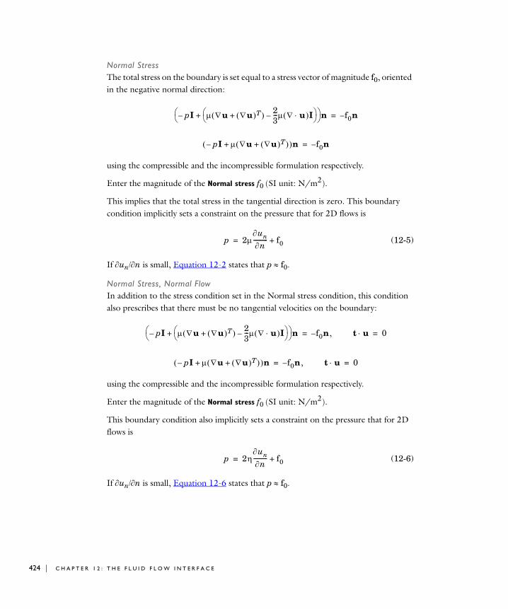
424 | C H A P T E
Normal StressThe total stress on the boundary is set equal to a stress vector of magnitude f0, oriented in the negative normal direction:
using the compressible and the incompressible formulation respectively.
Enter the magnitude of the Normal stress f0 (SI unit: N/m2).
This implies that the total stress in the tangential direction is zero. This boundary condition implicitly sets a constraint on the pressure that for 2D flows is
(12-5)
If unn is small, Equation 12-2 states that pf0.
Normal Stress, Normal FlowIn addition to the stress condition set in the Normal stress condition, this condition also prescribes that there must be no tangential velocities on the boundary:
using the compressible and the incompressible formulation respectively.
Enter the magnitude of the Normal stress f0 (SI unit: N/m2).
This boundary condition also implicitly sets a constraint on the pressure that for 2D flows is
(12-6)
If unn is small, Equation 12-6 states that pf0.
pI– u u T+ 23--- u I–
+ n f0n–=
pI– u u T+ + n f0n–=
p 2unn
---------- f0+=
pI– u u T+ 23--- u I–
+ n f0n,–= t u 0=
pI– u u T+ + n f0n,–= t u 0=
p 2unn
---------- f0+=
R 1 2 : T H E F L U I D F L O W I N T E R F A C E
Periodic Flow Condition
The Periodic Flow Condition splits its selection in two groups—a source and a destination group. Fluid that leaves the domain through one of the destination boundaries enters the domain over the corresponding source boundary. This corresponds to a situation that the geometry is a periodic part of a larger geometry. If the boundaries are not parallel to each other, the velocity vector is automatically transformed. If the boundaries are curved, it is recommended to only include two boundaries in this feature.
The Periodic Flow Condition has no input when the interface property Compressibility is set to Compressible flow (Ma<0.3). When Compressibility is set to Incompressible flow, it contains an input field for a Pressure difference, psrcpdst. This can be used to drive the flow in a fully developed channel flow. To control which sides that becomes the destination sides, add a Destination Domains subfeature to the Periodic Flow Condition feature. All destination sides must be connected.
Flow Continuity
The Flow Continuity node can be added to assembly pairs (see Pairs). It prescribes that the flow field is continuous across the pair. The feature is only suitable for pairs where the boundaries match.
B O U N D A R I E S
This section shows the boundaries for the selected pairs.
P A I R S E L E C T I O N
Select the Pairs where you want to impose continuity across the pair boundaries (Ctrl-click to deselect).
Pressure Point Constraint
The Pressure Point Constraint feature adds a pressure constraint at a point. If it is not possible to specify the pressure level using a boundary condition, you must set the pressure in some other way, for example, by specifying a fixed pressure at a point.
PO I N T S
Select the points where you want to use a pressure constraint.
P R E S S U R E C O N S T R A I N T
Enter a point constraint for the Pressure p0 (SI unit: Pa).
T H E S I N G L E - P H A S E F L O W , L A M I N A R F L O W I N T E R F A C E | 425

426 | C H A P T E
Th eo r y f o r t h e S i n g l e - Pha s e , L am i n a r F l ow I n t e r f a c e
Each of the Single-Phase Fluid Flow interfaces has underlying theory that is discussed in this section.
• Theory for all the Single-Phase Flow Interfaces
• Theory for the Laminar Flow Interface
Theory for all the Single-Phase Flow Interfaces
The single-phase fluid-flow interfaces are based on the Navier-Stokes equations, which in their most general form read
(12-7)
(12-8)
(12-9)
where
• is the density (SI unit: kg/m3)
• u is the velocity vector (SI unit: m/s)
• p is pressure (SI unit: Pa)
• is the viscous stress tensor (SI unit: Pa)
• F is the volume force vector (SI unit: N/m3)
• Cp is the specific heat capacity at constant pressure (SI unit: J/(kg·K))
• T is the absolute temperature (SI unit: K)
• q is the heat flux vector (SI unit: W/m2)
• Q contains the heat sources (SI unit: W/m3)
S is the strain rate tensor:
t------ u + 0=
ut------- u u+ pI– + F+=
CpTt------- u T+ q – :S T
---- T-------
p
pt------ u p+ – Q+ +=
R 1 2 : T H E F L U I D F L O W I N T E R F A C E

The operation “:” denotes a contraction between tensors defined by
(12-10)
Equation 12-7 is the continuity equation and represents the conservation of mass. Equation 12-8 is a vector equation and represents the conservation of momentum. Equation 12-9 describes the conservation of energy, formulated in terms of temperature. This is an intuitive formulation that facilities specification of boundary conditions.
To close the equation system 12-7 through 12-9, some constitutive relations are needed. A common relation is derived by assuming that the fluid is Newtonian. Together with Stokes’ assumption, the viscous stress tensor becomes:
(12-11)
The dynamic viscosity (SI unit: Pa·s) is allowed to depend on the thermodynamic state but not on the velocity field. All gases and many liquids can be considered Newtonian. Examples of non-Newtonian fluids are honey, mud, blood, liquid metals, and most polymer solutions.
Other commonly used constitutive relations are Fourier’s law of conduction and the ideal gas law.
There are several books where you find derivations of the Navier-Stokes equations and detailed explanations of concepts such as Newtonian fluids and the Stokes assumption. See, for example, the classical text by Batchelor (Ref. 1) and the more recent work by Panton (Ref. 2).
Many applications describe isothermal flows where Equation 12-9 is decoupled from Equation 12-7 and Equation 12-8.
Theory for the Laminar Flow Interface
Fluid mechanics deals with studies of gases and liquids either in motion (fluid dynamics) or at rest (fluid statics). When studying liquid flows, it is often safe to assume that the material’s density is constant or almost constant. You then have an
S 12--- u u T+ =
a:b anmbnm
m
n=
2S 23--- u I–=
T H E O R Y F O R T H E S I N G L E - P H A S E , L A M I N A R F L O W I N T E R F A C E | 427

428 | C H A P T E
incompressible fluid flow. Using the Incompressible Navier-Stokes interface you can solve transient and steady-state models of incompressible fluid dynamics.
In theory, the same equations describe laminar as well as turbulent flows. In practice, however, the mesh resolution required to simulate turbulence with the Laminar Flow interface makes such an approach impractical.
C O M P R E S S I B L E F L O W
The Navier-Stokes equations solved by default in all single-phase flow interfaces are the compressible formulation of the continuity:
(12-12)
and the momentum equations:
(12-13)
These equations holds for incompressible as well as compressible flows where the density varies.
T H E M A C H N U M B E R L I M I T
An important dimensionless number in fluid dynamics is the Mach number, Ma, defined by
(12-14)
where a is the speed of sound. A flow is formally incompressible when Ma0. This is theoretically achieved by letting the speed of sound tend to infinity. The Navier-Stokes equations will then have the numerical property that a disturbance anywhere in the computational domain will instantaneously spread to the entire domain. This results in a parabolic equation system.
The fully compressible Navier-Stokes equations, Equation 12-7 through Equation 12-9, have a finite speed of sound and hence a Mach number larger than zero. This will have no numerical significance as long as the Mach number is well below one. However, when the Mach number approaches unity, the equations turn from parabolic to hyperbolic. When this happens, the numerical properties of the equation change, one of several implications being that the boundary conditions used for incompressible Navier-Stokes equations become invalid. The compressible
t------ u + 0=
ut------- u u+ p– u u T+ 2
3--- u I–
F++=
Ma ua
-------=
R 1 2 : T H E F L U I D F L O W I N T E R F A C E
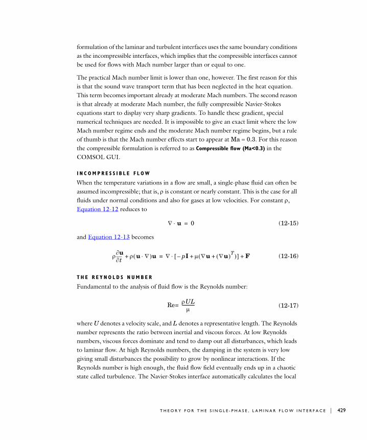
formulation of the laminar and turbulent interfaces uses the same boundary conditions as the incompressible interfaces, which implies that the compressible interfaces cannot be used for flows with Mach number larger than or equal to one.
The practical Mach number limit is lower than one, however. The first reason for this is that the sound wave transport term that has been neglected in the heat equation. This term becomes important already at moderate Mach numbers. The second reason is that already at moderate Mach number, the fully compressible Navier-Stokes equations start to display very sharp gradients. To handle these gradient, special numerical techniques are needed. It is impossible to give an exact limit where the low Mach number regime ends and the moderate Mach number regime begins, but a rule of thumb is that the Mach number effects start to appear at Ma 0.3. For this reason the compressible formulation is referred to as Compressible flow (Ma<0.3) in the COMSOL GUI.
I N C O M P R E S S I B L E F L O W
When the temperature variations in a flow are small, a single-phase fluid can often be assumed incompressible; that is, is constant or nearly constant. This is the case for all fluids under normal conditions and also for gases at low velocities. For constant , Equation 12-12 reduces to
(12-15)
and Equation 12-13 becomes
(12-16)
T H E R E Y N O L D S N U M B E R
Fundamental to the analysis of fluid flow is the Reynolds number:
(12-17)
where U denotes a velocity scale, and L denotes a representative length. The Reynolds number represents the ratio between inertial and viscous forces. At low Reynolds numbers, viscous forces dominate and tend to damp out all disturbances, which leads to laminar flow. At high Reynolds numbers, the damping in the system is very low giving small disturbances the possibility to grow by nonlinear interactions. If the Reynolds number is high enough, the fluid flow field eventually ends up in a chaotic state called turbulence. The Navier-Stokes interface automatically calculates the local
u 0=
t
u u u+ pI– u u T+ + F+=
Re UL
------------=
T H E O R Y F O R T H E S I N G L E - P H A S E , L A M I N A R F L O W I N T E R F A C E | 429

430 | C H A P T E
cell Reynolds number Recuh2 using the element length h for L and the magnitude of the velocity vector u for the velocity scale U. The cell Reynolds number is a predefined quantity available for visualization and evaluation.
N U M E R I C A L S T A B I L I T Y — S T A B I L I Z A T I O N TE C H N I Q U E S
The momentum equations (Equation 12-13 and Equation 12-16) are (nonlinear) convection-diffusion equations. As described in Stabilization Techniques in the COMSOL Multiphysics Reference Guide such equations are unstable if discretized using the Galerkin finite element method. Stabilized finite element methods are therefore necessary in order to obtain physical solutions. You find the stabilization settings in the main fluid-flow features. Also see Where Do I Access the Documentation and Model Library?.
There are three types of stabilization methods available for Navier-Stokes. Two of them are consistent stabilization methods:
• Streamline diffusion (GLS)
• Crosswind diffusion
There is also an inconsistent stabilization method: Isotropic diffusion
For optimal functionality, the exact weak formulations and constants of GLS and crosswind diffusion depend on the order of the basis functions (elements). The values of constants of GLS and crosswind diffusion follow Ref. 4 and Ref. 5.
Streamline DiffusionFor strongly coupled systems of equations, the streamline diffusion must be applied to the whole system of equations, not only to each equation separately. These ideas were first explored by Hughes and Mallet (Ref. 6) and were later extended to Galerkin least-squares (GLS) applied to the Navier-Stokes equations (Ref. 7), which is the form that COMSOL Multiphysics supports. The time-scale tensor is the diagonal tensor presented in Ref. 8.
Streamline diffusion is active per default because it is necessary when convection is the dominating part of the flow.
The unstabilized incompressible Navier-Stokes equations are subject the Babuska-Brezzi condition, which states that the basis functions for the pressure must be of lower order than the basis functions for the velocity. If the incompressible Navier-Stokes equations are stabilized by GLS, it is possible to use equal-order interpolation. Hence, streamline diffusion is necessary when using first order elements. This applies also if the model is solved using geometric multigrid (either as a solver or
R 1 2 : T H E F L U I D F L O W I N T E R F A C E
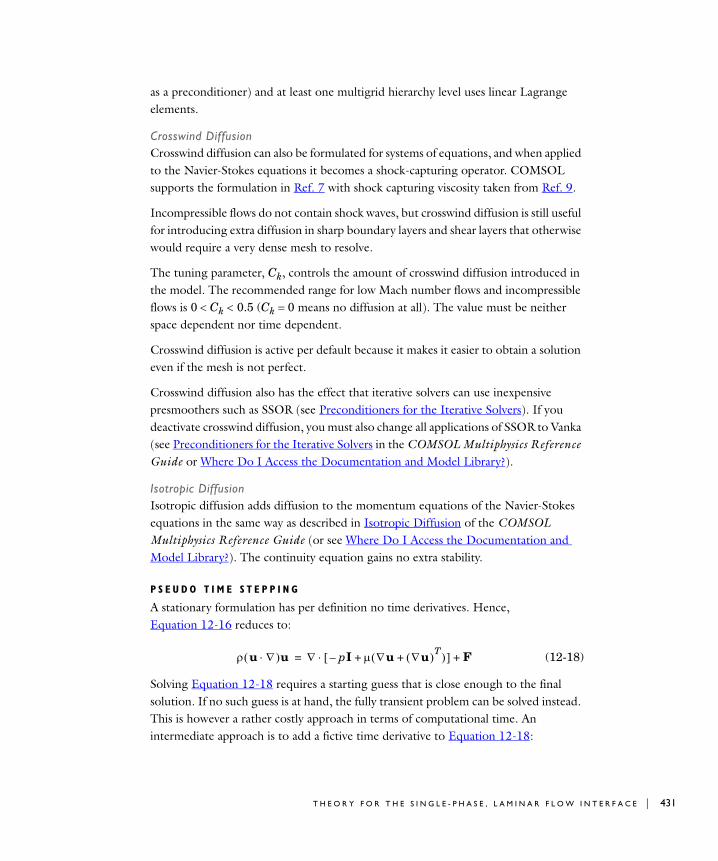
as a preconditioner) and at least one multigrid hierarchy level uses linear Lagrange elements.
Crosswind DiffusionCrosswind diffusion can also be formulated for systems of equations, and when applied to the Navier-Stokes equations it becomes a shock-capturing operator. COMSOL supports the formulation in Ref. 7 with shock capturing viscosity taken from Ref. 9.
Incompressible flows do not contain shock waves, but crosswind diffusion is still useful for introducing extra diffusion in sharp boundary layers and shear layers that otherwise would require a very dense mesh to resolve.
The tuning parameter, Ck, controls the amount of crosswind diffusion introduced in the model. The recommended range for low Mach number flows and incompressible flows is 0Ck 0.5 (Ck 0 means no diffusion at all). The value must be neither space dependent nor time dependent.
Crosswind diffusion is active per default because it makes it easier to obtain a solution even if the mesh is not perfect.
Crosswind diffusion also has the effect that iterative solvers can use inexpensive presmoothers such as SSOR (see Preconditioners for the Iterative Solvers). If you deactivate crosswind diffusion, you must also change all applications of SSOR to Vanka (see Preconditioners for the Iterative Solvers in the COMSOL Multiphysics Reference Guide or Where Do I Access the Documentation and Model Library?).
Isotropic DiffusionIsotropic diffusion adds diffusion to the momentum equations of the Navier-Stokes equations in the same way as described in Isotropic Diffusion of the COMSOL Multiphysics Reference Guide (or see Where Do I Access the Documentation and Model Library?). The continuity equation gains no extra stability.
P S E U D O T I M E S T E P P I N G
A stationary formulation has per definition no time derivatives. Hence, Equation 12-16 reduces to:
(12-18)
Solving Equation 12-18 requires a starting guess that is close enough to the final solution. If no such guess is at hand, the fully transient problem can be solved instead. This is however a rather costly approach in terms of computational time. An intermediate approach is to add a fictive time derivative to Equation 12-18:
u u pI– u u T+ + F+=
T H E O R Y F O R T H E S I N G L E - P H A S E , L A M I N A R F L O W I N T E R F A C E | 431

432 | C H A P T E
(12-19)
where is a pseudo time step. Since unojacu is always zero, this term does not affect the final solution. It does however affect the discrete equation system and will effectively transform a non-linear iteration into a time step of size .
The pseudo time step can be chosen individually for each element based on the local CFL number:
(12-20)
where h is the mesh cell size. A small CFL number means a small time step. It is hence practical to start with a small CFL number and gradually increase it as the solution approaches steady state. If the automatic expression for CFLloc is
(12-21)
The variable niterCMP is an integer that starts at one. CFLloc starts at 1.5 and increases with 50% each iteration until it reaches . It remains there until iteration 16 where it starts to increase unit it reaches approximately 1430. A final increase then takes it to 14400.
The continuity equation has a time derivative only in the incompressible case and it can then be written as
(12-22)
A pseudo time derivative can hence be written as
(12-23)
For incompressible flow, the following approximation is used:
(12-24)
while for compressible flows
u nojac u –
t--------------------------------- + u u pI– u u T+ + F+=
t
t
t
t CFLlochu-------=
1.5min niterCMP 12 +
if niterCMP 15 10 1.5min niterCMP 15– 12 0 +
if niterCMP 30 100 1.5min niterCMP 30– 12 0
1.512 130
p
------ pt
------
p
------p nojac p –
t-------------------------------
p
------ 0.11 atm ------------------
R 1 2 : T H E F L U I D F L O W I N T E R F A C E

(12-25)
Pseudo time stepping is active per default in 3D but can be activated also for 2D models.
Equation 12-21 can for some advanced flows increase CFLloc too quickly. CFLloc can then be prescribed manually.
T H E B O U S S I N E S Q A P P R O X I M A T I O N
The Boussinesq approximation is a way to treat some simple cases of buoyant flows without having to use a compressible formulation of the Navier-Stokes equations.
The Boussinesq approximation assumes that variations in density have no effect on the flow field except that they give rise to buoyant forces. The density is taken to be a reference value, 0, except in the body force term, which is set to
(12-26)
where g is the gravity vector. You can enter an expression for Equation 12-26 in the Volume force edit fields in the Volume Force feature; however, further simplifications are often possible. Because g can be written in terms of a potential, , it is possible to write Equation 12-26 as:
The first part can be canceled out by splitting the true pressure, p, as a sum of a hydrodynamic component, P, and a hydrostatic component, 0. Then you can write Equations 12-15 and 12-16 in terms of the hydrodynamic pressure Pp0:
(12-27)
(12-28)
To obtain the Boussinesq approximation on this form, you only have to enter the expression for g in the Volume force edit fields.
In practice, the shift from p to P can be ignored except where the pressure appears in boundary conditions. The pressure that you specify at boundaries is the hydrodynamic pressure in this case. For example, on a vertical outflow or inflow boundary, the hydrodynamic pressure is typically a constant, while the true pressure is a function of the vertical coordinate.
p
------ if p
------ 0=0.1
1 atm ------------------
p------
F 0 + g=
F 0 – g+=
u 0=
0ut------- 0u u+ P– u u T+ g ++=
T H E O R Y F O R T H E S I N G L E - P H A S E , L A M I N A R F L O W I N T E R F A C E | 433

434 | C H A P T E
The system that Equation 12-27 and Equation 12-28 form has its limitations. The main assumption is that the density fluctuations must be small; that is, 01. There are also some more subtle constraints that, for example, makes the Boussinesq approximation unsuitable for systems of very large dimensions. An excellent discussion of the Boussinesq approximation and its limitations appears in Chapter 14 of Ref. 10.
L A M I N A R I N F L O W C O N D I T I O N
In order to prescribe an inlet velocity profile, this boundary conditions adds a weak form contribution corresponding to a one-dimensional Navier-Stokes equations projected on the boundary. The applied condition corresponds to the situation shown in Figure 12-1: a fictitious domain of length Lentr is assumed to be attached to the inlet of the computational domain. This boundary condition uses the assumption that flow in this fictitious domain is a laminar plug flow. If you select the option that constrains outer edges or endpoints to zero, the assumption is instead that the flow in the fictitious domain is fully developed laminar channel flow (in 2D) or fully developed laminar internal flow (in 3D). This does not affect the boundary condition in the real domain, , where the boundary conditions are always fulfilled.
Figure 12-1: Sketch of the physical situation simulated when using the Laminar inflow boundary condition. is the actual computational domain while the dashed domain is a fictitious domain.
If you specify an average inlet velocity or inlet volume flow instead of the pressure, COMSOL Multiphysics adds an ODE that calculates a pressure, pentr, such that the desired inlet velocity or volume flow is obtained.
L A M I N A R O U T F L O W C O N D I T I O N
In order to prescribe an outlet velocity profile, this boundary conditions adds a weak form contribution corresponding to a one-dimensional Navier-Stokes equations projected on the boundary. The applied condition corresponds to the situation shown in Figure 12-2: assume that a fictitious domain of length Lexit is attached to the outlet of the computational domain. This boundary condition uses the assumption that the flow in this fictitious domain is laminar plug flow. If you select the option that constrains outer edges or endpoints to zero, the assumption is instead that the flow in the fictitious domain is fully developed laminar channel flow (in 2D) or fully developed
Lentr
pentr
R 1 2 : T H E F L U I D F L O W I N T E R F A C E

laminar internal flow (in 3D). This does not affect the boundary condition in the real domain, , where the boundary conditions are always fulfilled.
Figure 12-2: Sketch of the physical situation simulated when using Laminar outflow boundary condition. is the actual computational domain while the dashed domain is a fictitious domain.
If you specify an average outlet velocity or outlet volume flow instead of the pressure, the software adds an ODE that calculates pexit such that the desired outlet velocity or volume flow is obtained.
R E F E R E N C E S F O R T H E S I N G L E - P H A S E F L O W I N T E R F A C E S
1. G.K. Batchelor, An Introduction To Fluid Dynamics, Cambridge University Press, 1967.
2. R.L. Panton, Incompressible Flow, second edition, John Wiley & Sons, Inc., 1996.
3. P.M. Gresho and R.L. Sani, Incompressible Flow and the Finite Element Method, Volume 2: Isothermal Laminar Flow, John Wiley and Sons, LTD, 2000.
4. I. Harari and T.J.R. Hughes, “What are C and h? Inequalities for the analysis and design of finite element methods,” Comp. Meth. Appl. Mech. Engrg, vol. 97, pp. 157–192, 1992.
5. Y. Bazilevs, V.M. Calo, T.E. Tezduyar, and T.J.R. Hughes, “YZ discontinuity capturing for advection-dominated processes with application to arterial drug delivery,” Int.J.Num. Meth. Fluids, vol. 54, pp. 593–608, 2007.
6. T.J.R. Hughes and M. Mallet, “A new finite element formulation for computational fluid dynamics: III. The Generalized Streamline Operator for Multidimensional Advective-Diffusive System,” Comp. Meth. Appl. Mech. Engrg, vol. 58, pp. 305–328, 1986.
7. G. Hauke and T.J.R. Hughes, “A unified approach to compressible and incompressible flows,” Comp. Meth. Appl. Mech. Engrg, vol. 113, pp. 389–395, 1994.
pexit
Lexit
T H E O R Y F O R T H E S I N G L E - P H A S E , L A M I N A R F L O W I N T E R F A C E | 435

436 | C H A P T E
8. G. Hauke, “Simple stabilizing matrices for the computation of compressible flows in primitive variables,” Comp. Meth. Appl. Mech. Engrg, vol. 190, pp. 6881–6893, 2001.
9. A. Soulaïmani and M. Fortin, “Finite element solution of compressible viscous flows using conservative variables,” Comp. Meth. Appl. Mech. Engrg, vol. 118, pp. 319–350, 2001.
10. D.J. Tritton, Physical Fluid Dynamics, second edition, Oxford University Press, 1988.
11. J.M. Coulson and J.F. Richardson, “Particle Technology and Separation Processes,” Chemical Engineering, vol. 2, Butterworth-Heinemann.
12. P.M. Gresho and R.L. Sani, Incompressible Flow and the Finite Element Method, Volume 2: Isothermal Laminar Flow, John Wiley and Sons, LTD, 2000.
R 1 2 : T H E F L U I D F L O W I N T E R F A C E

13
H e a t T r a n s f e r I n t e r f a c e s
This section covers the Heat Transfer interface. It starts with some background on heat transfer. It then reviews the specifics of this physics interface. It also contains information about the predefined multiphysics interface for Joule heating.
In this section:
• See The Heat Transfer Interface for information about Heat Transfer in Solids (ht) ( ) and Heat Transfer in Fluids (ht) ( )
• The Joule Heating Interface
The underlying theory for these interface is also discussed:
• Theory for the Heat Transfer Interfaces
437

438 | C H A P T E
Th e Hea t T r a n s f e r I n t e r f a c e
The Heat Transfer interfaces model heat transfer by conduction and convection. You can also includes surface-to-ambient radiation effects around edges and boundaries. The interfaces are suitable for modeling heat transfer in solids and fluids. The interfaces are available in 1D, 2D, and 3D and or axisymmetric models with cylindrical coordinates in 1D and 2D. The default dependent variable is the temperature, T.
Accessing the Heat Transfer Interfaces via the Model Wizard
There are Heat Transfer interfaces displayed in the Model Builder with the same name but with different icons and default models. After selecting a Heat Transfer interface in the Model Wizard, default settings are added under the main node. For example, if you select Heat Transfer in Solids ( ), a Heat Transfer node is added with a default Heat Transfer in Solids model. If you select Heat Transfer in Fluids ( ), a Heat Transfer in Fluids model is added instead, but the parent nodes are both called Heat Transfer. All the interfaces that are based on the main Heat Transfer feature has the suffix ht.
Select:
• Heat Transfer in Solids (ht) ( ) to model mainly heat transfer in solid materials. A default Heat Transfer in Solids model is added, but all functionality for including fluid domains is also available.
• Heat Transfer in Fluids (ht) ( ) to model mainly heat transfer in fluid materials. A default Heat Transfer in Fluids model is added, but all functionality for including solid domains is also available.
Select the other available physics interfaces as required. Select:
• Joule Heating (jh) ( ) to combine all features from the Electric Currents interface with the Heat Transfer interface for modeling Joule heating (resistive heating or ohmic heating). See The Joule Heating Interface.
The Heat Transfer Interface
The Heat Transfer (ht) interface provides the equations, boundary conditions, and sources for modeling conductive and convective heat transfer, solving for the temperature.
R 1 3 : H E A T TR A N S F E R I N T E R F A C E S

This interface adds these default nodes based on your selection in the Model Wizard—Heat Transfer in Solids or Heat Transfer in Fluids, Thermal Insulation (the default boundary condition) and Initial Values.
Right-click the Heat Transfer node to add a Heat Transfer in Solids or Heat Transfer in
Fluids node or other feature that implements boundary conditions and sources.
The following sections provide information about all features available in the interface.
I N T E R F A C E I D E N T I F I E R
This is the physics interface identifier, which you use to reach the fields and variables in expressions, for example.
The identifier appears in the Identifier edit field, and you can change it to any unique string that is a valid identifier. The default identifier (for the first Heat Transfer interface in the model) is ht.
D O M A I N S
Select the domains where you want to define heat transfer and a temperature field. The default setting is to include all domains in the model.
P H Y S I C A L M O D E L
From the Default model list, select Heat transfer in solids if you want the Heat Transfer in Solids feature for heat conduction in solids as the default property group, or select Heat transfer in fluids if you want the Heat Transfer in Fluids feature for heat convection and conduction in fluids as the default property group.
D E P E N D E N T V A R I A B L E S
The Heat Transfer interface includes a dependent variable for the temperature T. You can change the default name T in the Temperature edit field. The surface radiosity J is not used.
A D V A N C E D S E T T I N G S A N D D I S C R E T I Z A T I O N
To display this section, select Show More Options from the View menu in the Model
Builder. Normally these settings do not need to be changed. More information on advanced settings can be found in Show More Options: Advanced Settings and Discretization.
T H E H E A T TR A N S F E R I N T E R F A C E | 439

440 | C H A P T E
C O N S I S T E N T S T A B I L I Z A T I O N
To display this section, select Show More Options from the View menu in the Model
Builder. Also see Show More Options: Consistent and Inconsistent Stabilization for information about these settings.
• The consistent stabilization methods take effect for fluids and for solids with translational motion (see Translational Motion). A stabilization method is active when the corresponding check box is selected. The Streamline diffusion check box is selected by default and should remain active for optimal performance for heat transfer in fluids or other applications that include a convective or translational term.
• The crosswind diffusion provides extra diffusion in the region of sharp gradients. The added diffusion is orthogonal to the streamline diffusion, so you can use streamline diffusion and crosswind diffusion simultaneously.
• If Crosswind diffusion is selected, enter a Lower gradient limit glim (SI unit: K/m). The default is 0.01[K]/ht.helem. The variable glim is needed because both Equation 13-1 and Equation 13-2 contain terms of the form 1T, which become singular if T0. Hence, all occurrences of 1T are replaced by 1maxTglim where glim is a measure of a small gradient.
The method in the Heat Transfer interfaces adds the following contribution to the weak formulation (see Codina in Ref. 2):
(13-1)
where R is the PDE residual, is the test function for T, h is the element size, and is defined as
(13-2)
I N C O N S I S T E N T S T A B I L I Z A T I O N
To display this section, select Show More Options from the View menu in the Model
Builder. Also see Show More Options: Consistent and Inconsistent Stabilization for information about these settings.
12---max 0 Ce 2k
h ----------–
h RT
----------- Tˆ
I u uu 2
---------------– T d
e
e 1=
Nel
–
Tˆ
Cp u T
T 2--------------------------------- T if T 0
0 if T 0=
=
R 1 3 : H E A T TR A N S F E R I N T E R F A C E S

Heat Transfer in Solids
The Heat Transfer in Solids model uses the following version of the heat equation as the mathematical model for heat transfer in solids.
(13-3)
with the following material properties:
• is the density
• Cp is the heat capacity
• k is the thermal conductivity (a scalar or a tensor if the thermal conductivity is anisotropic)
• Q is the heat source (or sink); one or more heat sources can be added separately
For a steady-state problem the temperature does not change with time and the first term disappears.
When parts of the model (for example, a heat source) is moving, you can add a Translational Motion subfeature to the Heat Transfer in Solids node to take this into account. See Translational Motion.
The Heat Transfer in Solids page contains the following sections:
D O M A I N S
Select the domains where you want to define the heat transfer.
M O D E L I N P U T S
This section contain fields and values that are inputs to expressions that define material properties. If you have added such user defined property groups, their model inputs appear here. Initially, this section is empty.
C O O R D I N A T E S Y S T E M S E L E C T I O N
Select the Coordinate system to use. The list has all available coordinate systems (except boundary coordinate systems). The default is to use the Global Cartesian coordinate system, which always exists. The coordinate system is used for interpreting directions of orthotropic and anisotropic thermal conductivity.
CpTt------- – kT Q=
T H E H E A T TR A N S F E R I N T E R F A C E | 441

442 | C H A P T E
H E A T C O N D U C T I O N
The default setting is to use the Thermal conductivity k (SI unit: W/(m·K)) From
material. Select User defined to enter another value or expression instead. Then, depending on the characteristics of the thermal conductivity, select Isotropic, Diagonal, Symmetric, or Anisotropic and enter values. The thermal conductivity describes the relationship between the heat flux vector q and the temperature gradient T as in
which is Fourier’s law of heat conduction. Enter this quantity as power per length and temperature.
T H E R M O D Y N A M I C S
The default Heat capacity at constant pressure Cp (SI unit: J/(kg·K)) and Density (SI unit: kg/m3) use values From material. Select User defined to enter other values. The heat capacity at constant pressure describes the amount of heat energy required to produce a unit temperature change in a unit mass.
Translational Motion
The Translational Motion feature provides movement by translation for modeling of heat transfer in solid. It adds the following contribution to the right hand side of Equation 13-3:
The contribution describes the effect of a moving coordinate system that is required to model, for example, a moving heat source.
Observe that special care must be taken at boundaries where n · u0. The Heat Flux boundary condition does not, for example, work at boundaries where n · u0.
D O M A I N S
Select the domains where you want to prescribe a translational. By default, the selection is the same as for the Heat Transfer in Solids node that it is attached to, but it is possible to use more than one Heat Translation subfeature, each covering a subset of the Heat Transfer in Solids node’s selection.
TR A N S L A T I O N A L M O T I O N
Enter component values for x, y, and z (in 3D) for the Velocity field u (SI unit: m/s).
q k T–=
– Cpu T
R 1 3 : H E A T TR A N S F E R I N T E R F A C E S

Heat Transfer in Fluids
The Heat Transfer in Fluids feature uses the following version of the heat equation as the mathematical model for heat transfer in fluids:
(13-4)
with the following material properties:
• is the density
• Cp is the fluid heat capacity at constant pressure and describes the amount of heat energy required to produce a unit temperature change in a unit mass
• k is the fluid thermal conductivity (a scalar or a tensor if the thermal conductivity is anisotropic)
• u is the fluid velocity field, which can be an analytic expression or a velocity field from a fluid-flow interface
• Q is the heat source (or sink); one or more heat sources can be added separately
For a steady-state problem the temperature does not change with time and the first term disappears.
Also, the ratio of specific heats is defined on this page. It is the ratio of heat capacity at constant pressure, Cp, to heat capacity at constant volume, Cv. When using the ideal gas law to describe a fluid, specifying is enough to evaluate Cp. For common diatomic gases such as air, 1.4 is the standard value. Most liquids have 1.1 while water has 1.0. is used in the streamline stabilization and in the postprocessing variables for heat fluxes and total energy fluxes.
The Heat Transfer in Fluids form contain the following sections:
D O M A I N S
Select the domains where you want to define the heat transfer.
M O D E L I N P U T S
This section has fields and values that are inputs to expressions that define material properties. If you have added such user defined property groups, their model inputs appear here.
There are also two standard model inputs—Absolute pressure and Velocity field. The absolute pressure is used in some postprocessing quantities that include the enthalpy (the energy flux, for example).
CpTt------- Cpu T+ kT Q+=
T H E H E A T TR A N S F E R I N T E R F A C E | 443

444 | C H A P T E
Enter the Absolute pressure pa (SI unit: Pa). The default is atmosphere pressure (101,325 Pa).
From the Velocity field list, select an existing velocity field in the model (for example, Velocity field (spf/fp1) from a Laminar Flow interface) or select User defined to enter values or expressions for the components of the Velocity field (SI unit: m/s).
C O O R D I N A T E S Y S T E M S E L E C T I O N
Select the Coordinate system to use. The list has all available coordinate systems (except boundary coordinate systems). The default is to use the Global Cartesian coordinate system, which always exists. The coordinate system is used for interpreting directions of orthotropic and anisotropic thermal conductivity.
H E A T C O N D U C T I O N
The default is to use the Thermal conductivity k (SI unit: W/(m·K)) From material. Select User defined to enter another value. Then, depending on the characteristics of the thermal conductivity, select Isotropic, Diagonal, Symmetric, or Anisotropic. The thermal conductivity describes the relationship between the heat flux vector q and the temperature gradient T as in
which is Fourier’s law of heat conduction. Enter this quantity as power per length and temperature.
T H E R M O D Y N A M I C S
The defaults in this section take values From material for the Density (SI unit: kg/m3), Heat capacity at constant pressure CP (SI unit: J/(kg·K)), and the Ratio of specific
heats (unitless) for a general gas or liquid. Select User defined to enter other values.
Heat Source
Add one or more Heat Source nodes. The heat source describes heat generation within the domain. Express heating and cooling with positive and negative values, respectively.
D O M A I N S
Select the domains where you want to add the heat source.
q k T–=
R 1 3 : H E A T TR A N S F E R I N T E R F A C E S

H E A T S O U R C E
Select either the General source or Linear source button.
If General source is selected, enter a value for Q (SI unit: W/m3).
If Linear source (Q=qs·T) is selected, enter the Production/absorption coefficient, qs (SI unit: W/(m3·K)).
Note: The advantage in writing the source in this form is that it can be stabilized by the streamline diffusion (see Stabilization Techniques in the COMSOL Multiphysics Reference Guide or Where Do I Access the Documentation and Model Library?). The theory covers qs that is independent of the temperature, but some stability can be gained as long as qs is only weakly dependent on the temperature.
Electromagnetic Heat Source
The Electromagnetic Heat Source node is added as a default node in the Joule Heating and Microwave Heating predefined multiphysics interfaces. Microwave Heating requires the RF Module.
The resistive heating (ohmic heating) due to the electric current is proportional to I2·R, where I is the electric current and R is the resistance.
Initial Values
The Initial Values node adds an initial value for the temperature T that can serve as an initial condition for a transient simulation or as an initial guess for a nonlinear solver. If you need to specify more than one set of initial values, you can add additional Initial
Values features.
D O M A I N S
Select the domains where you want to define an initial value.
I N I T I A L V A L U E S
Enter a value or expression for the initial value of the temperature T in the Temperature edit field. The default value is approximately room temperature, 293.15 K (20º C).
T H E H E A T TR A N S F E R I N T E R F A C E | 445

446 | C H A P T E
Boundary Conditions
The following boundary conditions are available:
• Temperature
• Thermal Insulation (the default boundary condition)
• Outflow
• Symmetry
• Heat Flux
• Surface-to-Ambient Radiation
• Surface-to-Ambient Radiation
• Heat Continuity
In addition, it is possible to specify boundary heat sources (see Boundary Heat Source). In 3D and 2D it is also possible to add point heat sources (see Point Heat Source). 3D furthermore supports line heat sources (Line Heat Source).
For axisymmetric models, COMSOL Multiphysics takes the axial symmetry boundaries into account and automatically adds an Axial Symmetry node to the model that is valid on the axial symmetry boundaries only.
Temperature
The Temperature feature prescribes a temperature on a boundary.
B O U N D A R I E S
Select the boundaries to which you want to apply a prescribed temperature.
TE M P E R A T U R E
The equation for this condition is
where T0 is the prescribed temperature (SI unit: K) on the boundary. Enter the value or expression for the Temperature T0. The default is 293.15 K.
T T0=
R 1 3 : H E A T TR A N S F E R I N T E R F A C E S

Thermal Insulation
The Thermal Insulation feature is the default boundary condition for all heat transfer interfaces. This boundary condition means that there is no heat flux across the boundary:
This condition specifies where the domain is well insulated. Intuitively this equation says that the temperature gradient across the boundary must be zero. For this to be true, the temperature on one side of the boundary must equal the temperature on the other side. Because there is no temperature difference across the boundary, heat cannot transfer across it.
An interesting numerical check for convergence is the numerical evaluation of Thermal Insulation condition along the boundary. Another check is to plot the temperature field as a contour plot. Ideally the contour lines are perpendicular to any insulated boundary.
The Thermal Insulation feature does not require any user input.
Outflow
The Outflow feature provides a suitable boundary condition for convection-dominated heat transfer at outlet boundaries. In a model with convective heat transfer, this condition states that the only heat transfer over a boundary is by convection. The temperature gradient in the normal direction is zero, and there is no radiation. This is usually a good approximation of the conditions at an outlet boundary in a heat transfer model with fluid flow.
The Outflow node does not usually require any user input.
B O U N D A R I E S
Select the boundaries that are convection-dominated outlet boundaries.
Heat Flux
Use the Heat Flux feature to add heat flux across boundaries. A positive heat flux adds heat to the domain. This feature is not applicable to inlet boundaries.
B O U N D A R I E S
Select the boundaries where you want to add the heat flux contribution.
n kT 0=
T H E H E A T TR A N S F E R I N T E R F A C E | 447

448 | C H A P T E
H E A T F L U X
Select either the General inward heat flux or Inward heat flux buttons.
If General inward heat flux q0 (SI unit: W/m2) is selected, it adds to the total flux across the selected boundaries. Enter a value for q0 to represent a heat flux that enters the domain. For example, any electric heater is well represented by this condition, and you can omit its geometry.
If Inward heat flux is selected (in the form q0h · TextT, enter the Heat transfer
coefficient h (SI unit: W/(m2·K). The default is 0.
Enter an External temperature Text (SI unit: K). The default is 293.15 K. The value depends on the geometry and the ambient flow conditions. For a thorough introduction on how to calculate heat transfer coefficients, see Incropera and DeWitt in Ref. 1.
Surface-to-Ambient Radiation
Use the Surface-to-Ambient Radiation boundary condition to add surface-to-ambient radiation to boundaries. The net inward heat flux from surface-to-ambient radiation is
where is the surface emissivity, is the Stefan–Boltzmann constant (a predefined physical constant), and Tamb is the ambient temperature.
B O U N D A R I E S
Select the boundaries where you want to add surface-to-ambient radiation contribution.
S U R F A C E - T O - A M B I E N T R A D I A T I O N
The default Surface emissivity e (a dimensionless number between 0 and 1) is taken From material. An emissivity of 0 means that the surface emits no radiation at all and an emissivity of 1 means that it is a perfect blackbody.
Enter an Ambient temperature Tamb (SI unit: K). The default is 293.15 K.
Periodic Heat Condition
Use the Periodic Heat Condition feature to add a periodic heat condition to boundaries.
q Tamb4 T4
– =
R 1 3 : H E A T TR A N S F E R I N T E R F A C E S
B O U N D A R I E S
Select the boundaries where you want to add a periodic heat condition.
Heat Continuity
The Heat Continuity node can be added to assembly pairs (see Pairs in the COMSOL Multiphysics Reference Guide or Where Do I Access the Documentation and Model Library?). It prescribes that the temperature field is continuous across the pair. The Heat Continuity is only suitable for pairs where the boundaries match.
B O U N D A R I E S
The selection list in this section shows the boundaries for the selected pairs.
P A I R S E L E C T I O N
Select the pairs where you want to impose continuity across the pair boundaries. Select the pairs from the Pairs list (Ctrl-click to deselect).
Symmetry
The Symmetry node provides a boundary condition for symmetry boundaries. This boundary condition is similar to an insulation condition, and it means that there is no heat flux across the boundary. In most cases, the Symmetry node does not require any user input.
B O U N D A R I E S
Define the symmetry boundaries as required.
Boundary Heat Source
The Boundary Heat Source node models a heat source (or heat sink) that is embedded in the boundary.
B O U N D A R I E S
Select the boundaries where you want to apply the heat source.
B O U N D A R Y H E A T S O U R C E
Enter the quantity Qb (SI unit: W/m2). A positive Qb means heating while a negative Qb means cooling. The default is 0.
T H E H E A T TR A N S F E R I N T E R F A C E | 449

450 | C H A P T E
Point Heat Source
The Point Heat Source node models a heat source (or sink) that is so small that it can be considered to have no spatial extension. It is available in 2D and 3D. It is not available in 1D since points are boundaries (possibly internal boundaries) there.
In theory, the temperature in a point source in 2D or 3D is plus or minus infinity (to compensate for the fact that the heat source does not have a spatial extension). The finite element discretization used in COMSOL returns a finite value, but that value must be interpreted in a weak sense.
PO I N T S
Select the points where you want to apply the heat source.
PO I N T H E A T S O U R C E
Enter the quantity Qp in unit power (W in SI units). Positive Qp means heating while a negative Qp means cooling.
Line Heat Source
The Line Heat Source node models a heat source (or sink) that is so thin that it has no thickness. It is available in 3D only since a line in 2D is a boundary and it is a domain in 1D.
In theory, the temperature in a line source in 3D is plus or minus infinity (to compensate for the fact that the heat source does not have any volume). The finite element discretization used in COMSOL returns a finite temperature distribution along the line, but that distribution must be interpreted in a weak sense.
E D G E S
Select the edges where you want to apply the heat source.
L I N E H E A T S O U R C E
Enter the quantity Ql in unit power per unit length (W/m in SI units). Positive Ql means heating while a negative Ql means cooling.
Pair Thin Thermally Resistive Layer
Use the Pair Thin Thermally Resisitive Layer feature to define the layer thickness and thermal conductivity on pair boundaries. It can be added to assembly pairs (see Pairs
R 1 3 : H E A T TR A N S F E R I N T E R F A C E S

in the COMSOL Multiphysics Reference Guide or Where Do I Access the Documentation and Model Library?)
B O U N D A R I E S
The selection list in this section shows the boundaries for the selected pairs.
P A I R S E L E C T I O N
Select the pairs where you want to impose a thermally resisitive layer across the pair boundaries. Select the pairs from the Pairs list (Ctrl-click to deselect).
P A I R T H I N T H E R M A L L Y R E S I S T I V E L A Y E R
Enter a value or expression for the Layer thickness ds (SI unit: m).
The default is to use the Thermal conductivity ks (SI unit: W/(m·K)) From material. Select User-defined to enter another value or expression.
T H E H E A T TR A N S F E R I N T E R F A C E | 451

452 | C H A P T E
Th e J o u l e Hea t i n g I n t e r f a c e
The Joule Heating predefined multiphysics interface ( ) combines all feature from the Electric Currents interface with the Heat Transfer interface for modeling of Joule heating (resistive heating or ohmic heating). The interaction is coupled in both directions:
• The resistive heating appears as a heat source in the default Electromagnetic Heat
Source node.
• The default setting is to use the value for the electric conductivity from the material. By selecting Linearized resistivity from the Electric conductivity list, the following temperature-dependent expression describes the electric conductivity: 1/(0(1(TTref))), where T is the dependent variable for temperature from the heat transfer part, which automatically appears as a model input. By default, the values for 0 (resistivity at reference temperature), (temperature coefficient), and Tref (reference temperature) are taken from the material. These settings are built into the Joule Heating Model node, which is the central feature in the Joule Heating interface.
The Joule Heating interface is available in 2D, axisymmetric 2D, and 3D. The default dependent variables is the temperature, T, and the electric potential, V.
The Joule Heating Interface
The Joule Heating interface provides the equations, boundary conditions, and sources for modeling Joule heating solving for the temperature and the electric potential. The main component is the Joule Heating Model, which adds the equation and interface for modeling of Joule heating. The Joule Heating interface adds a default Joule Heating
Model node, a default Electromagnetic Heat Source node, and a default boundary conditions: the Thermal Insulation node. There is also a default Initial Values node. Right-click the Joule Heating node to add a Heat Transfer in Solids or Heat Transfer in
Fluids node or other feature nodes that implements boundary conditions and sources The following sections provide information about the feature nodes that are available in the Joule Heating interface but not in the Heat Transfer or Electric Currents interfaces.
The Joule Heating form contains the following sections:
R 1 3 : H E A T TR A N S F E R I N T E R F A C E S
D O M A I N S
Select the domains where you want to define Joule heating. The default setting is to include all domains in the model.
D E P E N D E N T V A R I A B L E S
The interface includes a dependent variable for the Temperature T and the Electric
potential V. Depending on the license, there may also be a variable for the Surface
radiosity J.
A D V A N C E D S E T T I N G S A N D D I S C R E T I Z A T I O N
Normally these settings do not need to be changed. See Show More Options: Advanced Settings and Discretization.
C O N S I S T E N T S T A B I L I Z A T I O N
To display this section, select Show More Options from the View menu in the Model
Builder. Also see Show More Options: Consistent and Inconsistent Stabilization for information about these settings. Any settings unique to this interface are listed below.
• The consistent stabilization methods take effect for fluids and for solids with translational motion (see Translational Motion). A stabilization method is active when the corresponding check box is selected. The Streamline diffusion check box is selected by default and should remain active for optimal performance for heat transfer in fluids or other applications that include a convective or translational term.
• The crosswind diffusion provides extra diffusion in the region of sharp gradients. The added diffusion is orthogonal to the streamline diffusion, so you can use streamline diffusion and crosswind diffusion simultaneously.
• If Crosswind diffusion is selected, enter a Lower gradient limit glim (SI unit: K/m). The default is 0.01[K]/jh.helem. The variable glim is needed because both Equation 13-5 and Equation 13-6 contain terms of the form 1T, which become singular if T0. Hence, all occurrences of 1T are replaced by 1maxTglim where glim is a measure of a small gradient.
The method in the Heat Transfer interfaces adds the following contribution to the weak formulation (Ref. 2):
(13-5)12---max 0 Ce 2k
h ----------–
h RT
----------- Tˆ
I u uu 2
---------------– T d
e
e 1=
Nel
–
T H E J O U L E H E A T I N G I N T E R F A C E | 453

454 | C H A P T E
where R is the PDE residual, is the test function for T, h is the element size, and is defined as
(13-6)
I N C O N S I S T E N T S T A B I L I Z A T I O N
To display this section, select Show More Options from the View menu in the Model
Builder. Also see Show More Options: Consistent and Inconsistent Stabilization for information about these settings.
Joule Heating Model
The Joule Heating Model node uses the following version of the heat equation as the mathematical model for heat transfer in solids:
(13-7)
with the following material properties:
• is the density.
• Cp is the heat capacity.
• k is the thermal conductivity (a scalar or a tensor if the thermal conductivity is anisotropic).
• Q is the heat source (or sink). For Joule heating, it comes from the electric current and is added in the Electromagnetic Heat Source node.
For a steady-state problem the temperature does not change with time and the first term disappears. In addition, an equation for the electric current is also added.
D O M A I N S
Select the domains where you want to define the Joule heating.
M O D E L I N P U T S
The Model Inputs section contain fields and values that are inputs to expressions that define material properties. If you have added such user defined property groups, their model inputs appear here. Initially, this section is empty.
Tˆ
Cp u T
T 2--------------------------------- T if T 0
0 if T 0=
=
CpTt------- – kT Q=
R 1 3 : H E A T TR A N S F E R I N T E R F A C E S

C O N D U C T I O N C U R R E N T
In this section you define the electric conductivity (SI unit: S/m) from the Electric
conductivity list:
• Select From material (the default) to take the electric conductivity from the material.
• Select Linearized resistivity to use the following temperature-dependent expression to describe the electric conductivity: 1/(0(1(TTref))), where T is the dependent variable for temperature. By default, the values for 0 (resistivity at reference temperature), (temperature coefficient), and Tref (reference temperature) are taken from the material but you can select User defined to type in values or expressions for these properties.
• Select User defined to type in a value or expression for the electric conductivity in the associated edit field.
E L E C T R I C F I E L D
In this section you specify the constitutive relation that describe the macroscopic properties of the medium (relating the electric displacement D with the electric field E) and the applicable material properties, such as the relative permittivity.
Select one of the following constitutive relations from the list under Constitutive
relation (the corresponding equation appears underneath the list):
• Select Relative permittivity to use the constitutive relation D0 r E (the default). You then specify r , the relative permittivity (unitless). The default is to take its value from the material, but you can select User defined instead of From material from the list under Relative permittivity and then specify a value or expression for the relative permittivity in the edit field that appears.
• Select Polarization to use the constitutive relation D0 EP. You then specify P, the polarization vector (SI unit: C/m2). Enter its components (3 in 3D, 2 in 2D) in the corresponding edit fields under Polarization.
• Select Remanent displacement to use the constitutive relation D0 r EDr, where Dr (SI unit: C/m2) is the remanent displacement (the displacement when no electric field is present). In this case you specify r , the relative permittivity, and Dr, the remanent displacement. For the relative permittivity, use the list under Relative
permittivity: Select From material (the default) to use the value from the material or select User defined to specify a value or expression for the relative permittivity in the edit field that appears. For the remanent displacement, enter its components (3 in 3D, 2 in 2D) in the corresponding edit fields under Remanent displacement.
T H E J O U L E H E A T I N G I N T E R F A C E | 455
456 | C H A P T E
H E A T C O N D U C T I O N
The default setting is to use the thermal conductivity of the material. Select User
defined to enter another value or expression for the thermal conductivity (SI unit: W/(m·K)). You can select Isotropic, Diagonal, Symmetric, or Anisotropic from the associated list depending on the characteristics of the thermal conductivity. The thermal conductivity k describes the relationship between the heat flux vector q and the temperature gradient T as in
which is Fourier’s law of heat conduction. Enter this quantity as power per length and temperature.
T H E R M O D Y N A M I C S
The default uses the Heat capacity at constant pressure Cp (SI unit: J/(kg·K)) and Density (SI unit: kg/m3) values From material. Select User defined to enter other values or expressions for one or both variables.
Electromagnetic Heat Source
The Electromagnetic Heat Source feature is only available in the Joule Heating predefined multiphysics interface. It is added as a default node. The resistive heating (ohmic heating) due to the electric current is proportional to I2·R, where I is the electric current and R is the resistance.
Initial Values
The Initial Values node adds initial values for the temperature T and the electric potential V that can serve as an initial condition for a transient simulation or as an initial guess for a nonlinear solver. If you need to specify more than one set of initial values, you can add additional Initial Values features.
D O M A I N S
Select the domains where you want to define initial values.
I N I T I A L V A L U E S
Enter values or expressions for the initial values of the Temperature T and the Electric
potential V. The default value for the temperature is approximately room temperature, 293.15 K (20º C) and for the electric potential it is 0 V.
q k T–=
R 1 3 : H E A T TR A N S F E R I N T E R F A C E S

Th eo r y f o r t h e Hea t T r a n s f e r I n t e r f a c e s
Also see Ref. 1 and Ref. 3 For more detailed discussions.
What is Heat Transfer?
Heat transfer is defined as the movement of energy due to a difference in temperature. It is characterized by the following mechanisms:
• Conduction—Heat conduction takes place through different mechanisms in different media. Theoretically it takes place in a gas through collisions of the molecules; in a fluid through oscillations of each molecule in a “cage” formed by its nearest neighbors; in metals mainly by electrons carrying heat and in other solids by molecular motion which in crystals take the form of lattice vibrations known as phonons. Typical for heat conduction is that the heat flux is proportional to the temperature gradient.
• Convection—Heat convection (sometimes called heat advection) takes place through the net displacement of a fluid, which transports the heat content in a fluid through the fluid’s own velocity. The term convection (especially convective cooling and convective heating) also refers to the heat dissipation from a solid surface to a fluid, typically described by a heat transfer coefficient.
• Radiation—Heat transfer by radiation takes place through the transport of photons, which opaque surfaces can absorb or reflect. Surface-to-ambient radiation treats the ambient surroundings as a black body with known temperature.
The Heat Equation
The fundamental law governing all heat transfer is the first law of thermodynamics, commonly referred to as the principle of conservation of energy. However, internal energy, U, is a rather inconvenient quantity to measure and use in simulations. Therefore, the basic law is usually rewritten in terms of temperature, T. For a fluid, the resulting heat equation is:
(13-8)CpTt------- u T+ q – :S T
---- T-------
p
pt------ u p+ – Q+ +=
T H E O R Y F O R T H E H E A T TR A N S F E R I N T E R F A C E S | 457

458 | C H A P T E
where
• is the density (SI unit: kg/m3)
• Cp is the specific heat capacity at constant pressure (SI unit: J/(kg·K))
• T is absolute temperature (SI unit: K)
• u is the velocity vector (SI unit: m/s)
• q is the heat flux by conduction (SI unit: W/m2)
• p is pressure (SI unit: Pa)
• is the viscous stress tensor (SI unit: Pa)
• S is the strain rate tensor (SI unit: 1/s):
• Q contains heat sources other than viscous heating (SI unit: W/m3)
Note: Specific heat capacity at constant pressure is the amount of energy required to raise one unit of mass of a substance by one degree while maintained at constant pressure. This quantity is also commonly referred to as specific heat or specific heat capacity.
In deriving Equation 13-8, a number of thermodynamic relations have been used. The equation also assumes that mass is always conserved, which means that density and velocity must be related through:
The heat transfer interfaces use Fourier’s law of conduction, which states that the conductive heat flux, q, is proportional to the temperature gradient:
(13-9)
where k is the thermal conductivity (SI unit: W/(m·K)). In a solid, the thermal conductivity can be anisotropic (that is, it has different values in different directions). Then k becomes a tensor
S 12--- u u T+ =
t v + 0=
qi kTxi--------–=
R 1 3 : H E A T TR A N S F E R I N T E R F A C E S

and the conductive heat flux is given by
The second term on the right of Equation 13-8represents viscous heating of a fluid. An analogous term arises from the internal viscous damping of a solid. The operation “:” is a contraction and can in this case be written on the following form:
(13-10)
The third term represents pressure work and is responsible for the heating of a fluid under adiabatic compression and for some thermo-acoustic effects. It is generally small for low Mach number flows. A similar term can be included to account for thermo-elastic effects in solids.
Inserting Equation 13-9 into Equation 13-8, reordering the terms and ignoring viscous heating and pressure work puts the heat equation on a perhaps more familiar form:
(13-11)
The Heat Transfer interface with the Heat Transfer in Fluids feature solves this equation for the temperature, T. If the velocity is set to zero, you get the equation governing pure conductive heat transfer:
A Note on Heat Flux
The concept of heat flux is not as simple as it might first appear. The reason is that heat is not a conserved property. The conserved property is instead the total energy. There is hence heat flux and energy flux which are similar, but not identical.
k
kxx kxy kxz
kyx kyy kyz
kzx kzy kzz
=
qi kijTxj--------
j–=
a:b anmbnm
m
n=
CpTt------- Cpu T+ kT Q+=
CpTt------- k– T + Q=
T H E O R Y F O R T H E H E A T TR A N S F E R I N T E R F A C E S | 459

460 | C H A P T E
This section briefly describes the theory for the postprocessing variables for Total heat flux and Total energy flux. The approximations made do not affect the computational results, only postprocessing variables.
TO T A L E N E R G Y F L U X
The total energy flux is equal to (Ref. 4, chapter 3.5)
(13-12)
Above, H0 is the total enthalpy
(13-13)
where U is the internal energy. In Equation 13-12 is the viscous stress tensor and qr is the radiative heat flux.
The enthalpy, H, has the general form (Ref. 5)
(13-14)
This expression is not really useful since the reference enthalpy, Href, is not commonly available. There are some common approximations:
• For a calorically perfect gas, TT1 and Cp is constant. By taking HrefTref0, it follows from Equation 13-14 that
(13-15)
Using the ideal gas law, Equation 13-15 can be rewritten as
(13-16)
where is the ratio of specific heats, CpCv. Cv is the specific heat capacity at constant volume.
• It is also true that HUp. For an incompressible substance,
(13-17)
Selecting UrefTref0, it follows from Equation 13-17 that
u H0 + k T u qr++–
H0 H 12--- u u + U p
--- 1
2--- u u + += =
H Href Cp Td
Tref
T
1--- 1 T
----
T-------
p
+
pd
pref
p
+ +=
H CpT=
HCp
-------T=p---+
U Uref Cv Td
Tref
T
+=
R 1 3 : H E A T TR A N S F E R I N T E R F A C E S

(13-18)
Notice that this identical to Equation 13-16.
• For most solid materials, CpCv, that is, 1. Furthermore, the first term on the right hand side of Equation 13-18 is commonly much larger than the second term. Hence, for a solid material, Equation 13-18 can to a good approximation be reduced to
(13-19)
From above points, it follows that H is calculated from Equation 13-19 for Solid domains and Biological Tissue domains. For Fluid domain with ideal gas, H is calculated from Equation 13-15, otherwise from Equation 13-18.
in Equation 13-12 is the potential energy, or more accurately the force potential. It can be formulated in some special cases, for example, for gravitational effects (Chapter 1.4 in Ref. 4), but it is in general rather difficult to derive. Potential energy is therefore often excluded and the total energy flux is approximated by
(13-20)
H E A T F L U X
The total heat flux vector is defined as (Ref. 6):
(13-21)
What is the difference between Equation 13-20 and Equation 13-21? An example is a channel with fully developed incompressible flow. The walls are assumed to be insulated. Along the channel there is a pressure drop that drives the flow. Start by neglecting the viscous heating, so that the flow is isothermal. Equation 13-20 states that the energy flow in is larger than the energy flow out. The reason is that the work done by the pressure should have turned into heat (by viscous heating), but instead it just disappeared. Equation 13-21, however, says that the heat flux in equals the heat flux out. If viscous heat is included, Equation 13-20 states that the energy in equals energy out while Equation 13-21 says that the heat flux out is larger than the heat flux in.
HCp
-------T p
---+=
H CpT=
u H 12--- u u +
k T u qr++–
uU k T qr+–
T H E O R Y F O R T H E H E A T TR A N S F E R I N T E R F A C E S | 461

462 | C H A P T E
Boundary Conditions
The heat equation accepts two basic types of boundary conditions: specified temperature and specified heat flux. The former is of a constraint type and prescribes the temperature at a boundary:
while the latter specifies the inward heat flux
where
• q is the conductive heat flux vector (SI unit: W/m2)
• n is the normal vector of the boundary
• q0 is inward heat flux (SI unit: W/m2), normal to the boundary
The inward heat flux, q0, is often a sum of contributions from different heat transfer processes, for example radiation and convection. The special case q0 0 is called thermal insulation.
A common type of heat flux boundary conditions are those where q0h·TinfT, where Tinf is the temperature far away from the modeled domain and the heat transfer coefficient, h, represents all the physics occurring between the boundary and “far away.” It can include almost anything, but the most common situation is that h represents the effect of an exterior fluid cooling or heating the surface of solid, a phenomenon often referred to as convective cooling or heating.
Note: Heat flux on inlet boundaries are not covered by the arguments above.
Radiative Heat Transfer in Transparent Media
This discussion so far has considered heat transfer by means of conduction and convection. The third mechanism for heat transfer is radiation. Let’s consider an environment with fully transparent or fully opaque objects. Thermal radiation denotes the stream of electromagnetic waves emitted from a body at a certain temperature.
T T0= on
n– q q0= on
q k T–=
R 1 3 : H E A T TR A N S F E R I N T E R F A C E S

D E R I V I N G T H E R A D I A T I V E H E A T F L U X
Figure 13-1: Arriving irradiation (left), leaving radiosity (right).
Consider Figure 13-1. A point is located on a surface that has an emissivity , reflectivity , absorptivity , and temperature T. Assume the body is opaque, which means that no radiation is transmitted through the body. This is true for most solid bodies.
The total arriving radiative flux at is named the irradiation, G. The total outgoing radiative flux is named the radiosity, J. The radiosity is the sum of the reflected radiation and the emitted radiation:
(13-22)
The net inward radiative heat flux, q, is then given the difference between the irradiation and the radiosity:
(13-23)
Using Equation 13-22 and Equation 13-23 you can eliminate J and obtain a general expression for the net inward heat flux into the opaque body based on G and T.
(13-24)
Most opaque bodies also behave as ideal gray bodies, meaning that the absorptivity and emissivity are equal, and the reflectivity is therefore given from the following relation:
(13-25)
Thus, for ideal gray bodies, q is given by:
(13-26)
This is the equation used as a radiation boundary condition.
x T
G
J G T4+=
x T
x
xx
J G T4+=
q G J–=
q 1 – G T4–=
1 –= =
q G T4– =
T H E O R Y F O R T H E H E A T TR A N S F E R I N T E R F A C E S | 463
464 | C H A P T E
R A D I A T I O N TY P E S
It is common to differentiate between two types of radiative heat transfer: surface-to-ambient radiation and surface-to-surface radiation. Equation 13-26 holds for both radiation types, but the irradiation term, G, is different for each of them. The Heat Transfer interface supports radiation.
S U R F A C E - T O - A M B I E N T R A D I A T I O N
Surface-to-ambient radiation assumes the following:
• The ambient surroundings in view of the surface have a constant temperature, Tamb.
• The ambient surroundings behave as a black body. This means that the emissivity and absorptivity are equal to 1, and zero reflectivity.
These assumptions allow you to explicitly express the irradiation as
(13-27)
Inserting Equation 13-27 into Equation 13-26 results in the net inward heat flux for surface-to-ambient radiation
(13-28)
For boundaries where you have specified surface-to-ambient radiation, COMSOL Multiphysics adds this term to the right-hand side of Equation 13-28.
R E F E R E N C E S F O R T H E H E A T TR A N S F E R I N T E R F A C E S
1. F.P. Incropera and D.P. DeWitt, Fundamentals of Heat and Mass Transfer, 4th ed., John Wiley & Sons, 1996.
2. R. Codina, “Comparison of some finite element methods for solving the diffusion-convection-reaction equation,” Comp. Meth.Appl. Mech. Engrg, vol. 156, pp. 185–210, 1998.
3. A. Bejan, Heat Transfer, Wiley, 1993.
4. G.K. Batchelor, An Introduction to Fluid Dynamics, Cambridge University Press, 2000.
5. R.L. Panton, Incompressible Flow, Second edition, John Wiley and Sons, inc., 1996.
6. M. Kaviany, Principles of Convective Heat Transfer, Second edition, Springer, 2001.
G Tamb4
=
q Tamb4 T4
– =
R 1 3 : H E A T TR A N S F E R I N T E R F A C E S

14
T h e S t r u c t u r a l M e c h a n i c s I n t e r f a c e
This section explains how to use the Solid Mechanics physics interface, found under the Structural Mechanics branch in the Model Wizard, to simulate and analyze applications involving solid mechanics. The following sections describe these cases in detail and provide a theory background. The rest of the section describes the Solid Mechanics interface.
Note: The optional Structural Mechanics Module contains physics interfaces and models that allow for extended, specialized analyses of structural and solid mechanics problems.
In this section:
• Solid Mechanics Geometry
• The Solid Mechanics Interface
• Theory for the Solid Mechanics Interface
465

466 | C H A P T E
S o l i d Me chan i c s Geome t r y
The Solid Mechanics interface is used for stress analysis and general solid mechanics simulation. It supports the following geometry types:
• 3D solid
• 2D plane stress and plane stress
• 2D axial symmetry
The last cases are 2D simplifications of the full 3D equations; these simplifications are valid under certain assumptions.
3D Geometry
The degrees of freedom (dependent variables) in 3D are the global displacements u, v, and w in the global x, y, and z directions, respectively, and the pressure help variable (used only if a nearly incompressible material is selected).
Figure 14-1: Loads and constraints applied to a 3D solid using the Solid Mechanics interface.
R 1 4 : T H E S T R U C T U R A L M E C H A N I C S I N T E R F A C E

2D Geometry
P L A N E S T R E S S
The plane stress variant of the 2D interface is useful for analyzing thin in-plane loaded plates. For a state of plane stress, the out-of-plane components of the stress tensor are zero.
Figure 14-2: Plane stress models plates where the loads are only in the plane; it does not include any out-of-plane stress components.
The 2D interface for plane stress allows loads in the x and y directions, and it assumes that these are constant throughout the material’s thickness, which can vary with x and y. The plane stress condition prevails in a thin flat plate in the xy-plane loaded only in its own plane and without any z direction restraint.
P L A N E S T R A I N
The plane strain variant of the 2D interface that assumes that all out-of-plane strain components of the total strain z, yz, and xz are zero.
Figure 14-3: A geometry suitable for plane strain analysis.
Loads in the x and y directions are allowed. The loads are assumed to be constant throughout the thickness of the material, but the thickness can vary with x and y. The
S O L I D M E C H A N I C S G E O M E T R Y | 467

468 | C H A P T E
plane strain condition prevails in geometries, whose extent is large in the z direction compared to in the x and y directions, or when the z displacement is in some way restricted. One example is a long tunnel along the z-axis where it is sufficient to study a unit-depth slice in the xy-plane.
Axisymmetric Geometry
The axisymmetric variant of the Solid Mechanics interface uses cylindrical coordinates r, (phi), and z. Loads are independent of , and the axisymmetric variant of the
interface allows loads only in the r and z directions.
You can view the 2D axisymmetric geometry as the intersection between the original axially symmetric 3D solid and the half plane , r 0. You therefore draw the geometry only in the half plane r 0 and recover the original 3D solid by rotating the 2D geometry about the z-axis.
Figure 14-4: Rotating a 2D geometry to recover a 3D solid.
0=
R 1 4 : T H E S T R U C T U R A L M E C H A N I C S I N T E R F A C E

Th e S o l i d Me chan i c s I n t e r f a c e
The Solid Mechanics interface ( ) has the equations and features for stress analysis and general linear solid mechanics, solving for the displacements. The Linear Elastic Material
Model is the default material model, which adds a linear elastic equation for the displacements and has a Settings window to define the elastic material properties.
The following default nodes are added when using this interface—Linear Elastic
Material Model, Free (a boundary condition where boundaries are free, with no loads or constraints), and Initial Values.
Right-click the Solid Mechanics node to add other nodes.
I N T E R F A C E I D E N T I F I E R
This is the physics interface identifier, which you use to reach the fields and variables in expressions, for example.
The identifier appears in the Identifier field, and you can change it to any unique string that is a valid identifier. The default identifier (for the first Solid Mechanics interface in the model) is solid.
D O M A I N S
Select the domains where you want to define the displacements and the equations that describe the solid mechanics. The default setting is to include all domains in the model.
2 D A P P R O X I M A T I O N ( 2 D M O D E L S O N L Y )
From the 2D approximation list select Plane stress or Plane strain. For more information about these 2D plane conditions, see the Theory for the Solid Mechanics Interface. When you model using plane stress, the Solid Mechanics interface solves for the out-of-plane strain, ez, in addition to the displacement field u.
T H I C K N E S S ( 2 D M O D E L S O N L Y )
Define the Thickness d by entering a value or expression (SI unit: m). The default value of 1 m is suitable for plane strain models, where it represents a a unit-depth slice, for example. For plane stress models, enter the actual thickness, which should be small compared to the size of the plate for the plane stress assumption to be valid. In rare cases, you may want to change thickness in parts of the geometry; you can then use the Change Thickness feature (see Change Thickness).
T H E S O L I D M E C H A N I C S I N T E R F A C E | 469

470 | C H A P T E
R E F E R E N C E PO I N T F O R M O M E N T C O M P U T A T I O N
Enter the coordinates for the Reference point for moment computation refpnt (SI unit: m). All moments are then computed relative to this reference point.
D E P E N D E N T V A R I A B L E S
The Solid Mechanics interface includes a field variable for the Displacement field u. You can change the names in the corresponding edit fields, but the names of fields and dependent variables must be unique within a model.
A D V A N C E D S E T T I N G S A N D D I S C R E T I Z A T I O N
Normally these settings do not need to be changed. See Show More Options: Advanced Settings and Discretization. In addition, there is this section for this interface:
Displacements Control Spatial Frame The Displacements control spatial frame check box is selected by default. If required, click to clear the check box.
Linear Elastic Material Model
The Linear Elastic Material Model node adds the equations for a linear elastic solid, and the page contains the following sections for defining the related material properties:
D O M A I N S
Select the domains where you want to define a linear elastic solid and compute the displacements, stresses, and strains.
M O D E L I N P U T S
Define model inputs, for example, the temperature field if the material model uses a temperature-dependent material property. If no model inputs are required, this section is empty.
C O O R D I N A T E S Y S T E M S E L E C T I O N
Select the Coordinate system to use. The list has all available coordinate systems (except boundary coordinate systems). The default is to use the Global Cartesian coordinate system, which always exists. The coordinate system is used when stresses or strains are presented in a local system.
R 1 4 : T H E S T R U C T U R A L M E C H A N I C S I N T E R F A C E

L I N E A R E L A S T I C M A T E R I A L M O D E L
Define the solid model and the linear elastic material properties.
Solid ModelThe solid model is linear isotropic elastic.
Specification of Elastic Properties for Isotropic MaterialsIf Isotropic is selected, from the Specify list, select a pair of elastic properties for an isotropic material. Select:
• Young’s modulus and Poisson’s ratio to specify Young’s modulus (elastic modulus) E (SI unit: Pa) and Poisson’s ratio (dimensionless). For an isotropic material Young’s modulus is the spring stiffness in Hooke’s law, which in 1D form is
where is the stress and is the strain. Poisson’s ratio defines the normal strain in the perpendicular direction, generated from a normal strain in the other direction and follows the equation
• Bulk modulus and shear modulus to specify the bulk modulus K (SI unit: Pa) and the shear modulus G (SI unit: Pa). The bulk modulus is a measure of the solid’s resistance to volume changes. The shear modulus is a measure of the solid’s resistance to shear deformations.
• Lamé constants to specify the Lamé constants (SI unit: Pa) and (SI unit: Pa).
• Pressure-wave and shear-wave speeds to specify the pressure-wave speed (longitudinal wave speed) cp (SI unit: m/s) and the shear-wave speed (transverse wave speed) cs (SI unit: m/s).
For each pair of properties, select from the applicable list to use the value From material or enter a User defined value or expression.
Each of these pairs define the elastic properties and it is possible to convert from one set of properties to another (see Table 14-1).
DensityDefine the material Density (SI unit: kg/m3). Select From material to use the value from the material or select User defined and enter a value.
E=
l l–=
T H E S O L I D M E C H A N I C S I N T E R F A C E | 471
472 | C H A P T E
Damping
In time-dependent, eigenfrequency, and frequency domain studies you can model undamped or damped problems. The Damping node adds Rayleigh damping to Linear
Elastic Material Model solid mechanics models.
Right-click the Linear Elastic Material Model node to add a Damping node.
Note: The time-stepping algorithms also add numerical damping, which is independent of the explicit damping that you add. For the Generalized alpha time-stepping algorithm, it is possible to control the amount of numerical damping that it adds.
Rayleigh DampingIn the Rayleigh damping model, the damping parameter is expressed in terms of the mass m and the stiffness k as
That is, Rayleigh damping is proportional to a linear combination of the stiffness and mass, There is no direct physical interpretation of the mass damping parameter dM (SI unit: 1/s) and the stiffness damping parameter dM (SI unit: s).
The following sections are defined in the Damping node’s Settings window:
D O M A I N S
Select the domains where you want to add damping. By default, this feature node inherits the selection from its parent node, and you can only use a selection that is a subset of the parent node’s selection.
D A M P I N G S E T T I N G S
The only available Damping type is Rayleigh damping.
For Rayleigh damping, enter the Mass damping parameter dM and the Stiffness damping
parameter dK in the corresponding fields. The default values are 0, which is no damping.
dMm dKk+=
R 1 4 : T H E S T R U C T U R A L M E C H A N I C S I N T E R F A C E
Change Thickness
The Change Thickness feature models domains with a thickness other than the overall thickness defined in the interface Thickness section.
For the Solid Mechanics interface, this is available in 2D only.
D O M A I N S ( O R B O U N D A R I E S )
Select the domains (or boundaries with Shell models) and where you want use a different thickness.
C H A N G E T H I C K N E S S
Enter a value for the Thickness d (SI unit: m). This value replaces the overall thickness for the geometric entity selected above.
Initial Values
The Initial Values node adds an initial value for the displacement field u (the displacement components u, v, and w in 3D) that can serve as an initial condition for a transient simulation or as an initial guess for a nonlinear analysis. It also adds a Velocity field u/ t. If you need to specify more than one set of initial values, you can add additional Initial Values nodes.
D O M A I N S
Select the domains where you want to define an initial value.
I N I T I A L V A L U E S
Enter values or expressions for the initial values of the Displacement field (SI unit: m) and Velocity field (SI unit: m/s). The defaults are 0.
Body, Boundary, Edge, and Point Loads
Add force loads acting on all levels of the geometry. Add a:
• Body Loadto domains (gravity effects, for example).
• Boundary Loadto boundaries (a pressure acting on a boundary, for example).
• Edge Loadto edges in 3D (a force distributed along an edge, for example).
• Point Load to points (concentrated forces at points).
T H E S O L I D M E C H A N I C S I N T E R F A C E | 473

474 | C H A P T E
Body Load
Add a Body Load to domains for gravity effects, for example.
D O M A I N S
Select the domains where you want to define a body load.
C O O R D I N A T E S Y S T E M S E L E C T I O N
Select a Coordinate system. By default you use the Global coordinate system, and the list contains any additional coordinate systems that the model includes.
F O R C E
Select a Load type.
• (3D models) Load defined as force per unit volume (the default) (SI unit: N/m3).
• (2D models) Load defined as force per unit area (SI unit: N/m2). The body load as force per unit volume is then the value of F divided by the thickness.
The Load list normally only contains User defined. Enter values or expressions for the components of the body load F in the Load fields.
• Total force (SI unit: N). Enter values or expressions for the components of the Total
force F. COMSOL then divides the total force by the volume of the domains where the body load is active.
Boundary Load
Add a Boundary Load to boundaries for a pressure acting on a boundary, for example.
B O U N D A R I E S
Select the boundaries where you want to define a load.
C O O R D I N A T E S Y S T E M S E L E C T I O N
Specify the coordinate system to use for specifying the load. From the Coordinate
system list select from:
• Global coordinate system (the default)
• Boundary System (a predefined normal-tangential coordinate system)
• Any additional user defined coordinate systems
R 1 4 : T H E S T R U C T U R A L M E C H A N I C S I N T E R F A C E

F O R C E
Select a Load type.
• Load defined as force per unit area (SI unit: N/m2). The Load list normally only contains User defined. Enter values or expressions for the components of the Load F. When combining the Solid Mechanics interface with, for example, film damping, it is also possible to choose a predefined load from this list.
• (2D models) Load defined as force per unit length (SI unit: N/m). Enter values or expressions for the components of the Load F.
• Total force (SI unit: N). Enter values or expressions for the components of the Total
force F. COMSOL then divides the total force by the area of the surfaces where the body load is active.
• Follower pressure (SI unit: Pa). Enter a value or expression for the follower Pressure P. The pressure is positive when directed in towards the solid.
Edge Load
Add an Edge Load to edges in 3D for a force distributed along an edge, for example.
E D G E S
Select the edges (in 3D models) where you want to define an edge load.
C O O R D I N A T E S Y S T E M S E L E C T I O N
Select a Coordinate system. By default you use the Global coordinate system and the list contains any additional coordinate systems that the model includes.
F O R C E
Select a Load type.
• Load defined as force per unit length (SI unit: N/m). The Load list normally only contains User defined. Enter values or expressions for the components of the Load F. When combining the Solid Mechanics interface with, for example, film damping, it is also possible to choose a predefined load from this list.
• Total force (SI unit: N). Enter values or expressions for the components of the Total
force F. COMSOL then divides the total force by the area of the surfaces where the body load is active.
T H E S O L I D M E C H A N I C S I N T E R F A C E | 475

476 | C H A P T E
Point Load
Add a Point Load to points for concentrated forces at points.
PO I N T S
Select the points where you want to define a point load.
C O O R D I N A T E S Y S T E M S E L E C T I O N
Select a Coordinate system. By default you use the Global coordinate system and the list contains any additional coordinate systems that the model includes.
F O R C E
The list under Point load normally only contains User defined. Enter values or expressions for the components of the Point load F (SI unit: N).
Boundary Conditions
The following constraints are available on exterior boundaries, and in some cases on domains, edges or points:
• Free
• Fixed Constraint (available on domains, boundaries, edges, and points)
• Prescribed Displacement (available on domains, boundaries, edges, and points)
• Roller
If there are subsequent boundary conditions specified on the same geometrical entity, the last one will take precedence.
For axisymmetric models, COMSOL Multiphysics takes the axial symmetry boundaries (at r = 0) into account and automatically adds an Axial Symmetry feature to the model that is valid on the axial symmetry boundaries only.
Free
The Free feature is the default boundary condition. It means that there are no constraints and no loads acting on the boundary.
B O U N D A R I E S
Select the boundaries that are free.
R 1 4 : T H E S T R U C T U R A L M E C H A N I C S I N T E R F A C E

Fixed Constraint
The Fixed Constraint feature adds a condition that makes the geometric entity (domain, boundary, edge, or point) fixed (fully constrained); that is, the displacements are zero in all directions.
D O M A I N S , B O U N D A R I E S , E D G E S , O R PO I N T S
Select the geometric entity (domains, boundaries, edges, or points) that are fixed.
C O N S T R A I N T S E T T I N G S
To display this section, select Show More Options from the View menu in the Model
Builder. Select a Constraint type—Bidirectional, symmetric or Unidirectional. If required, select the Use weak constraints check box. See Using Weak Constraints.
Prescribed Displacement
The Prescribed Displacement feature adds a condition where you can prescribe the displacements in one or more directions to the geometric entity (domain, boundary, edge, or point).
If you prescribe a displacement in one direction, this leaves the solid free to deform in the other directions. You can also define more general displacements as a linear combination of the displacements in each direction.
• If a prescribed displacement is not activated in any direction, this is the same as a Free constraint.
• If a zero displacement is applied in all directions, this is the same as a Fixed
Constraint.
D O M A I N S , B O U N D A R I E S , E D G E S , O R PO I N T S
Select the geometric entity (domains, boundaries, edges, or points) on which you want to prescribe a displacement.
C O O R D I N A T E S Y S T E M S E L E C T I O N
Select a Coordinate system. By default you use the Global coordinate system and the list contains any additional coordinate systems that the model includes.
P R E S C R I B E D D I S P L A C E M E N T
Define the prescribed displacements using a Standard notation or a General notation.
T H E S O L I D M E C H A N I C S I N T E R F A C E | 477

478 | C H A P T E
Standard NotationTo define the displacements individually, click the Standard notation button (the default).
2D and 3D Models: To define a prescribed displacement for each space direction (x, y, and z for 3D), select one or all of the Prescribed in X, Y, and Z direction check boxes. Then enter a value or expression for the prescribed displacements U0, V0, or W0 (SI unit: m).
2D Axisymmetric Models: To define a prescribed displacement for each space direction (R and Z), select one or both of the Prescribed in R, and Z direction check boxes. Then enter a value or expression for the prescribed displacements U0, or W0 (SI unit: m).
General NotationTo specify the displacements using a General notation that includes any linear combination of displacement components, click the General notation Hu=R button. For example, for 2D models, use the relationship
Enter values in the H matrix and R vector fields. For the H matrix, also select an Isotropic, Diagonal, Symmetric, or Anisotropic matrix and enter values as required. For example, to achieve the condition u = v, use the settings
which force the domain to move only diagonally in the xy-plane.
C O N S T R A I N T S E T T I N G S
To display this section, select Show More Options from the View menu in the Model
Builder. Select a Constraint type—Bidirectional, symmetric or Unidirectional. If required, select the Use weak constraints check box. See Using Weak Constraints.
H uv
R=
H 1 1–
0 0= R 0
0=
R 1 4 : T H E S T R U C T U R A L M E C H A N I C S I N T E R F A C E

Roller
The Roller node adds a roller constraint as the boundary condition; that is, the displacement is zero in the direction perpendicular (normal) to the boundary, but the boundary is free to move in the tangential direction.
B O U N D A R I E S
Select the boundaries that have roller constraints.
C O N S T R A I N T S E T T I N G S
To display this section, select Show More Options from the View menu in the Model
Builder. Select a Constraint type—Bidirectional, symmetric or Unidirectional. If required, select the Use weak constraints check box. See Using Weak Constraints.
Periodic Condition
The Periodic Condition feature adds a periodic boundary condition. This periodicity make uix0uix1 for a displacement ui. You can control which of the directions that the periodic condition applies to. Right-click the Periodic Condition node to add a Destination Selection boundary condition. If the source and destination boundaries are rotated with respect to each other, this transformation is automatically performed, so that corresponding displacement components are connected.
B O U N D A R I E S
Select the boundaries where you want to define a periodic boundary condition. The software automatically identifies the boundaries as either source boundaries or destination boundaries. This works fine for cases like opposing parallel boundaries. In other cases you can use the Destination Selection subfeature to control the destination. By default it contains the selection that COMSOL Multiphysics has identified.
PE R I O D I C C O N D I T I O N
By default, there is no periodic condition is active in any of the directions.
2D and 3D Models: For each space direction (x, y, and z for 3D), select one or all of the Periodic in X, Y, and Z direction check boxes. Then select a Type of periodicity—Continuity or Antiperiodicity.
T H E S O L I D M E C H A N I C S I N T E R F A C E | 479

480 | C H A P T E
2D Axisymmetric Models: For each space direction (R and Z), select one or both of the Periodic in R direction and Periodic in Z direction check boxes. Then select a Type of
periodicity—Continuity or Antiperiodicity.
Destination Selection
The Destination Selection is a subfeature of the Periodic Condition and is used to control the destination. To add this to the Model Builder, right-click Periodic Condition and select Destination Selection.
B O U N D A R I E S
Select the boundaries where you want to define a periodic boundary condition. The software automatically identifies the boundaries as either source boundaries or destination boundaries. By default it contains the selection that COMSOL Multiphysics has identified.
Pairs
In the Identity and Contact Pairs section you can find general information about the usage of pairs in COMSOL. There are a several possible selections under Pairs. In the following, only Contact is described. All other loads, boundary conditions, and continuity conditions follow the general behavior of pairs. The loads and boundary conditions have the same data as described above.
Symmetry
The Symmetry feature adds a boundary condition, which must exist both in the geometry and in the loads. A symmetry condition is free in the plane and fixed in the out-of-plane direction.
B O U N D A R I E S
Select the boundaries that are symmetry boundaries.
C O N S T R A I N T S E T T I N G S
To display this section, select Show More Options from the View menu in the Model
Builder. Select a Constraint type—Bidirectional, symmetric or Unidirectional. If required, select the Use weak constraints check box.
R 1 4 : T H E S T R U C T U R A L M E C H A N I C S I N T E R F A C E
Antisymmetry
The Antisymmetry feature adds a boundary condition for an antisymmetry boundary, which must exist in both the geometry and in the loads. An antisymmetry condition is fixed in the plane and free in the out-of-plane direction.
In a geometrically non-linear analysis large rotations must not occur at the antisymmetry plane, since this will cause artificial straining.
B O U N D A R I E S
Select the boundaries that are antisymmetry boundaries.
C O N S T R A I N T S E T T I N G S
To display this section, select Show More Options from the View menu in the Model
Builder. Select a Constraint type—Bidirectional, symmetric or Unidirectional. If required, select the Use weak constraints check box.
Rigid Connector
The Rigid Connector is a boundary condition for modeling rigid regions and kinematic constraints such as prescribed rigid rotations. The rigid connector always takes finite rotations into account.
Forces and moments can be applied to the rigid connector.
B O U N D A R I E S
Select the boundaries to which you want to connect this rigid connector.
C O O R D I N A T E S Y S T E M S E L E C T I O N
Select a Coordinate system. By default you use the Global coordinate system. In addition, the Coordinate system list contains any additional coordinate systems that the model includes. Prescribed displacements or rotations are specified along the axes of this coordinate system.
C E N T E R O F R O T A T I O N
Select a Center of rotation—Automatic or User defined. Enter X, Y, and Z coordinates in the table. The default is Automatic, and the center of rotation is then at the geometrical centre of the selected boundaries. Any loads or constraints are applied at the centre of rotation.
T H E S O L I D M E C H A N I C S I N T E R F A C E | 481

482 | C H A P T E
P R E S C R I B E D D I S P L A C E M E N T
To define a prescribed displacement for each space direction (x, y, and z), select one or all of the Prescribed in X, Y, and Z direction check boxes. Then enter a value or expression for the prescribed displacements U0, V0, or W0 (SI unit: m).
P R E S C R I B E D R O T A T I O N
Select an option from the By list—Free, Constrained rotation, or Prescribed rotation. The default is Free.
If Constrained rotation is selected, select one or more of the Constrain rotation about X,
Y, and Z axis check boxes in order to enforce zero rotation around the corresponding axis in the selected coordinate system.
If Prescribed rotation is selected, enter an Axis of rotation and an Angle of rotation . The axis of rotation is given in the selected coordinate system.
R 1 4 : T H E S T R U C T U R A L M E C H A N I C S I N T E R F A C E

Th eo r y f o r t h e S o l i d Me chan i c s I n t e r f a c e
Frames and Coordinate Systems
The formulation used for structural analysis in COMSOL Multiphysics for both small and finite deformations is totally Lagrangian. The dependent variables are the displacement vector components, which are defined in the initial (or reference) configuration, for which the coordinate system on the material frame is always chosen to coincide with the coordinate system on the spatial frame.
The displacement gradients are computed on the material frame. All the material properties are also defined on the material frame.
It is possible to define any number of coordinate systems on the material frame. By default, in every domain the coordinate system is the same and defined by the material frame. In this document, this coordinate system is denoted by (G). In addition, the property groups can be applied in the local coordinate system that you can choose for each domain. In this document, it is denoted by (L). Loads on domains and boundaries can also be applied in their own local coordinate systems.
Linear Elastic Material
The total strain tensor is written in terms of the displacement gradient
or in components as
(14-1)
The Duhamel-Hooke’s law relates the stress tensor to the strain tensor and temperature:
12--- u u T
+ =
mn12---
xnum
xmun+
=
s s0 C 0– – +=
T H E O R Y F O R T H E S O L I D M E C H A N I C S I N T E R F A C E | 483

484 | C H A P T E
where is the 4th order elasticity tensor, “:” stands for the double-dot tensor product (or double contraction), s0 and 0 are initial stresses and strains, and is the thermal expansion tensor.
The elastic energy is
(14-2)
or using the tensor components:
TE N S O R V S . M AT R I X F O R M U L A T I O N S
Because of the symmetry, the strain tensor can be written as the following matrix:
Similar representation applies to the stress and the thermal expansion tensors:
Due to the symmetry, the elasticity tensor can be completely represented by a symmetric 6-by-6 matrix as:
which is the elasticity matrix.
C
T Tref–=
Ws12--- 0– – C 0– – =
Ws12---C
ijmnij ij
0– ij– mn mn
0– mn–
i j m n =
x xy xz
xy y yz
xz yz z
sx sxy sxz
sxy sy syz
sxz syz sz
x xy xz
xy y yz
xz yz z
D
D11 D12 D13 D14 D15 D16
D12 D22 D23 D24 D25 D26
D13 D23 D33 D34 D35 D36
D14 D24 D34 D44 D45 D46
D15 D25 D35 D45 D55 D56
D16 D26 D36 D46 D56 D66
C1111
C1122
C1133
C1112
C1123
C1113
C1122
C2222
C2233
C2212
C2223
C2213
C1133
C2233
C3333
C3312
C3323
C3313
C1112
C2212
C3312
C1212
C1223
C1213
C1123
C2223
C3323
C1223
C2323
C2313
C1113
C2213
C3313
C1213
C2313
C1313
= =
R 1 4 : T H E S T R U C T U R A L M E C H A N I C S I N T E R F A C E

The Hooke’s law can be presented then in the form involving the elasticity matrix and the following vectors:
Thus, the general conversion rule for indices is:
COMSOL Multiphysics uses the complete tensor representation internally to perform the coordinate system transformations correctly.
A N I S O T R O P I C M A T E R I A L
In the most general case of fully anisotropic material, you provide explicitly 21 components of the symmetric elasticity matrix D and 6 components of the symmetric thermal expansion matrix.
I S O T R O P I C M A T E R I A L A N D E L A S T I C M O D U L I
In this case, the elasticity matrix becomes
sx
sy
sz
sxy
syz
sxz
sx
sy
sz
sxy
syz
sxz 0
D
x
y
z
2xy
2yz
2xz
x
y
z
2xy
2yz
2xz 0
x
y
z
2xy
2yz
2xz
––
+=
112233
12 2123 3213 31
123456
xyz
xyyzxz
D E1 + 1 2–
---------------------------------------
1 – 0 0 0 1 – 0 0 0 1 – 0 0 0
0 0 0 1 2–2
---------------- 0 0
0 0 0 0 1 2–2
---------------- 0
0 0 0 0 0 1 2–2
----------------
=
T H E O R Y F O R T H E S O L I D M E C H A N I C S I N T E R F A C E | 485

486 | C H A P T E
and the thermal expansion matrix is:
You can use different pairs of elastic moduli, and as long as two of them are defined, the others can be computed according to Table 14-1.
O R T H O T R O P I C M A T E R I A L
The elasticity matrix for orthotropic material has the following structure:
TABLE 14-1: EXPRESSIONS FOR THE ELASTIC MODULI.
DESCRIPTION VARIABLE DE DKG D
Young’s modulus E
Poisson’s ratio
Bulk modulus K
Shear modulus G
Lamé constant
Lamé constant G
Pressure-wave speed
cp
Shear-wave speed
cs
0 00 00 0
9KG3K G+------------------- 3 2+
+--------------------
12--- 1 3G
3K G+-------------------–
2 + ---------------------
E3 1 2– ------------------------ 2
3-------+
E2 1 + ---------------------
E1 + 1 2–
--------------------------------------- K 2G3
--------–
E2 1 + ---------------------
K 4G 3+
--------------------------
G
R 1 4 : T H E S T R U C T U R A L M E C H A N I C S I N T E R F A C E

where the components are as follows:
where
where you supply the values of Ex, Ey, Ez, xy, yz, xz, Gxy, Gyz, and Gxz in designated edit fields in the user interface. COMSOL deduces the remaining components—yx, zx, and zy—using the fact that the matrices D and D1 are symmetric.
The thermal expansion matrix is diagonal:
E N T R O P Y A N D T H E R M O E L A S T I C I T Y
The free energy for the linear thermoelastic material can be written as:
D
D11 D12 D13 0 0 0
D12 D22 D23 0 0 0
D13 D23 D33 0 0 0
0 0 0 D44 0 0
0 0 0 0 D55 0
0 0 0 0 0 D66
=
D11Ex
2 Ezyz2 Ey–
Ddenom----------------------------------------,= D12
ExEy Ezyzxz Eyxy+ Ddenom
-----------------------------------------------------------------–=
D13ExEyEy xyyz xz+
Ddenom----------------------------------------------------------,–= D22
Ey2 Ezxz
2 Ex– Ddenom
----------------------------------------=
D23EyEz Eyxyxz Exyz+
Ddenom-----------------------------------------------------------------,–= D33
EyEz Eyxy2 Ex–
Ddenom-----------------------------------------------=
D44 Gxy= , D55 Gyz= , and D66 Gxz=
Ddenom EyEzxz2 ExEy– 2xyyzxzEyEz ExEzyz
2 Ey2xy
2+ + +=
x 0 0
0 y 0
0 0 z
F f0 T Ws T +=
T H E O R Y F O R T H E S O L I D M E C H A N I C S I N T E R F A C E | 487

488 | C H A P T E
where is given by Equation 14-2. Hence, the stress can be found as:
and the entropy per unit volume can be calculated as:
where T0 is a reference temperature, the volumetric heat capacity CP can be assumed independent of the temperature (Dulong-Petit law), and
For an isotropic material, it simplifies into:
The heat balance equation can be written as:
where k are the thermal conductivity matrix, and
where is the strain-rate tensor, tensor presents all possible inelastic stresses (for example, a viscous stress).
Using the tensor components, the heat balance can be rewritten as:
In many cases, you can neglect the second term in the left-hand side of the above equation because all are small. The resulting approximation is often called uncoupled thermoelasticity.
N E A R L Y I N C O M P R E S S I B L E M A T E R I A L S
Nearly incompressible materials can cause numerical problems if only displacements are used in the interpolating functions. Small errors in the evaluation of volumetric strain, due to the finite resolution of the discrete model, are exaggerated by the high
Ws T
s
F
T W
TC 0– – = = =
TF
– Cp T T0 log Selast+=
Selast s=
Selast sx sy sz+ + =
Cp tT T
t Selast+ k T Qh+=
Qh ·=
·
Cp tT Tmn t
smn
m n+ k T Qh+=
Tmn
R 1 4 : T H E S T R U C T U R A L M E C H A N I C S I N T E R F A C E

bulk modulus. This leads to an unstable representation of stresses, and in general to underestimation of the deformation since spurious volumetric stresses may balance also applied shear and bending loads.
In such cases, you may choose to use a mixed formulation which represents the pressure as a dependent variable in addition to the displacement components. This removes the effect of volumetric strain from the original stress tensor and replaces it with an interpolated pressure, pw. A separate equation constrains the interpolated pressure to equal (in a finite-element sense) the original pressure calculated from the strains.
For an isotropic linear elastic material, the second Piola-Kirchoff stress tensor S, computed directly from the strains, is replaced by a modified version:
where I is the unit tensor and the pressure p is calculated from the strains and material data as
The auxiliary dependent variable pw is set equal to p using the equation
(14-3)
where is the bulk modulus.
The modified stress tensor is used then in calculations of the energy variation.
For orthotropic and anisotropic materials, the auxiliary pressure equation is scaled so as to result in a symmetric stiffness matrix. Note, however, that the stiffness matrix in this formulation is not positive definite and even contains a zero block on the diagonal in the incompressible limit. This limits the possible choices of direct and iterative linear solver.
Plane Strain and Plane Stress Cases
For linear Elastic material in case of plane stress, COMSOL solves three equations si30 for i3 with i = 1, 2, 3, and uses the solution instead of Equation 14-1 for these
s s pI pwI–+=
p 13---trace s –=
pw
------- p---– 0=
s
T H E O R Y F O R T H E S O L I D M E C H A N I C S I N T E R F A C E | 489

490 | C H A P T E
three strain components. Thus, three components i3 are treated as extra degrees of freedom. The remaining three strain components are computed as in 3D case according to Equation 14-1. Note that for an isotropic material, only the normal out-of-plane component 33 needs to be solved for.
In case of plane strain, set i3 for i1, 2, 3. The out-of-plane stress components si3 are postprocessing variables.
Axial Symmetry
The axially symmetric geometry uses a cylindrical coordinate system. Such a coordinate system is orthogonal but curvilinear, and one can choose between a covariant basis e1, e2, e3 and a contravariant basis e1, e2, e3.
The metric tensor is
in the coordinate system given by e1, e2, e3, and
in e1, e2, e3.
The metric tensor plays the role of a unit tensor for a curvilinear coordinate system.
For any vector or tensor A, the metric tensor can be used for conversion between covariant, contravariant and mixed components:
gij 1 0 0
0 r2 00 0 1
=
gij
1 0 0
0 r 2– 00 0 1
=
Aij Aimgmj
m=
Aij Anmgnigmj
m n=
R 1 4 : T H E S T R U C T U R A L M E C H A N I C S I N T E R F A C E

In both covariant and contravariant basis, the base vector in the azimuthal direction has a non-unit length. To cope with this issue, the so called physical basis vectors of unit length are introduced. These are:
The corresponding components for any vector or tensor are called physical.
For any tensor, the physical components are defined as:
where no summation is done over repeated indices.
Mixed Components and Principal InvariantsThe mixed strain components:
The principal invariants are:
Displacements and Axial Symmetry assumptionsThe axial symmetry implementation in COMSOL Multiphysics assumes independence of the angle, and also that the torsional component of the displacement is identically zero. The physical components of the radial and axial displacement, u and w, are used as dependent variables for the axially symmetric geometry.
For the Linear Elastic material, the stress components in coordinate system (L) are:
:
where .
er e1 e1= e
1r---e
2re2= = ez e3= e3
= =
Aijphys gii gjjA
ij=
Aji gimAmj
m=
I1 A trace Aii Ai
i
i= A11 A22
1
r2----- A33+ += =
I2 A 12--- I1 A 2 Aj
iAij
i j–
=
I3 A det Aii =
sij s0ij
C+ijkl
kl kl– 0kl– =
T Tref–=
T H E O R Y F O R T H E S O L I D M E C H A N I C S I N T E R F A C E | 491

492 | C H A P T E
For anisotropic and orthotropic materials, the 4th-order elasticity tensor is defined from D matrix according to:
Note that the user input D matrix always contains the physical components of the elasticity tensor , and the corresponding tensor components are computed internally according to:
For an isotropic material:
where and are Lamé elastic constants.
Initial Stress and Strain
Initial stress refers to the stress before the system applies any loads, displacements, or initial strains. The initial strain is the one before the system has applied any loads, displacements, or initial stresses.
Both the initial stress and strains are tensor variables defined via components on the local coordinate system (L) for each subdomain. You input them as the following matrices:
sr
ssz
sr
sz
srz
sr
ssz
sr
sz
srz 0
D
r
z
2r
2z
2rz
r
z
2r
2z
2rz 0
r
z
2r
2z
2rz
––
+=
Cijklphys
Cijkl Cijkl
phys
gii gjj gkk gll
-----------------------------------------------=
Cijkl gijgkl gikgjl gilgjk
+ +=
0x 0xy 0xz
0xy 0y 0yz
0xz 0yz 0z
s0x s0xy s0xz
s0xy s0y s0yz
s0xz s0yz s0z
R 1 4 : T H E S T R U C T U R A L M E C H A N I C S I N T E R F A C E

Note that in case of nearly incompressible material (mixed formulation), you still input the components of the total initial stress (i.e without volumetric-deviatoric split). The initial pressure in the equation for the pressure help variable pw is computed as
Axial SymmetryUser inputs the physical components of 0 and s0:
Other Possible Uses of Initial Strains and StressesMany inelastic effects in solids and structure (such as creep, plasticity, damping, viscoelasticity, poroelasticity, and so on) are additive contributions to either the total strain or total stress. Then, the initial value input fields can be used for coupling the elastic equations (solid physics) to the constitutive equations (usually General Form PDEs) modeling such extra effects.
Loads
You can specify loads as
• Distributed loads. The load is a distributed force in a volume, on a face, or along an edge.
• Total force. The specification of the load is as the total force. The software then divides this value with the area or the volume where the force acts.
•
For 2D plane stress and plane strain models you can choose how to specify the distributed boundary load as a load defined as force per unit area or a load defined as force per unit length acting on boundaries. In the same way you can choose between defining the load as force per unit volume or force per unit area for body loads acting in a domain.
0r 0r 0rz
0r 0 0z
0rz 0z 0z
s0r s0r s0rz
s0r s0 s0z
s0rz s0z s0z
T H E O R Y F O R T H E S O L I D M E C H A N I C S I N T E R F A C E | 493
494 | C H A P T E
The following table shows how to define distributed loads on different geometric entity levels; the entries show the SI unit in parentheses.
For plane stress, plane strain, and axisymmetric models, the boundary loads apply on edges (boundaries). For 3D solids, the boundary loads apply on faces (boundaries).
Equation Implementation
The COMSOL Multiphysics implementation of the equations in the Solid Mechanics interface is based on the principle of virtual work.
The principle of virtual work states that the sum of virtual work from internal strains is equal to work from external loads.
The total stored energy, W, for a linear material from external and internal strains and loads equals:
The principle of virtual work states that
which leads to
GEOMETRIC ENTITY POINT EDGE FACE DOMAIN
Plane stress, plane strain
force (N) force/area (N/m2) or force/length (N/m)
force/volume (N/m3) or force/area (N/m2)
Axial symmetry total force along the circumferential (N)
force/area (N/m2)
force/volume (N/m3)
3D Solid force (N) force/length (N/m)
force/area (N/m2) force/volume (N/m3)
W – s u FV dv+V=
u FS sdS u FL ld
L Ut Fp
p+ + +
W 0=
R 1 4 : T H E S T R U C T U R A L M E C H A N I C S I N T E R F A C E

Setting up Equations for Different Studies
The Solid Mechanics interface supports stationary (static), eigenfrequency, time-dependent (transient), and frequency domain study types.
Stationary StudiesCOMSOL Multiphysics uses an implementation based on the stress and strain variables. The normal and shear strain variables depend on the displacement derivatives.
Using the tensor strain, stress, and displacement variables, you can express the principle of virtual work as:
Time-Dependent Studies
To model viscous damping, COMSOL Multiphysics uses Rayleigh damping, where you specify two damping coefficients. As an example, consider a system with a single degree of freedom. The equation of motion for such a system with viscous damping is
.
– tests utest FV utest utt– dv+V
utest FS sdS utest FL ld
L Utest
t Fp p+ + +
W – tests utest FV dv+V=
utest FS sdS utest FL ld
L Utest
t Fp p+ + +
– test s dMst+ utest FV utest utt dMutest ut–– dv+V
utest FS sdS utest FL ld
L Utest
t Fp p+ + +
md2u
dt2---------- du
dt------- ku+ + f t =
T H E O R Y F O R T H E S O L I D M E C H A N I C S I N T E R F A C E | 495

496 | C H A P T E
In the Rayleigh damping model, you express the damping parameter in terms of the mass m and the stiffness k as
The Rayleigh damping proportional to mass and stiffness is added to the static weak term. The default value for both dM and dK is zero; that is, the default settings add no damping.
Frequency Domain StudiesIn the frequency domain you can study the frequency response when applying harmonic loads. You specify harmonic loads using two components:
• The amplitude value, Fx
• The phase, FxPh
To derive the equations for the steady-state response from harmonic excitation loads
assume a harmonic response with the same angular frequency as the excitation load
You can also describe this relationship using complex notation
dMm dKk+=
Fxfreq Fx f t FxPh f 180----------+
cos=
Ffreq
Fxfreq
Fyfreq
Fzfreq
=
u uamp t u+ cos=
uuvw
=
u Re uampejuejt Re ue
jt where u uampe
ju= = =
u Re uejt
=
R 1 4 : T H E S T R U C T U R A L M E C H A N I C S I N T E R F A C E
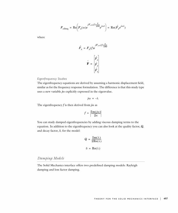
where
Eigenfrequency StudiesThe eigenfrequency equations are derived by assuming a harmonic displacement field, similar as for the frequency response formulation. The difference is that this study type uses a new variable j explicitly expressed in the eigenvalue.
The eigenfrequency f is then derived from j as
You can study damped eigenfrequencies by adding viscous damping terms to the equation. In addition to the eigenfrequency you can also look at the quality factor, Q, and decay factor, for the model:
Damping Models
The Solid Mechanics interface offers two predefined damping models: Rayleigh damping and loss factor damping.
Fxfreq Re Fx ejFxPh f
180----------
ejt
Re Fx˜ ejt = =
Fx˜ Fx f e
jFxPh f 180----------
=
F˜
Fx˜
Fy˜
Fz˜
=
j –=
f Im j 2
-------------------=
Q Im 2Re -------------------=
Re =
T H E O R Y F O R T H E S O L I D M E C H A N I C S I N T E R F A C E | 497

498 | C H A P T E
Rayleigh DampingTo model damping effects within the material, COMSOL Multiphysics uses Rayleigh damping, where you specify two damping coefficients. As an example, consider a system with a single degree of freedom. The equation of motion for such a system with viscous damping is
In the Rayleigh damping model you express the damping parameter in terms of the mass m and the stiffness k as
The Rayleigh damping proportional to mass and stiffness is added to the static weak term.
A complication with the Rayleigh damping model is to obtain good values for the damping parameters. A more physical damping measure is the damping ratio, the ratio between actual and critical damping, often expressed as a damping factor in percentage of the critical damping. You can find commonly used values of damping factors in the literature.
It is possible to transform damping factors to Rayleigh damping parameters. The damping factor, , for a specified pairs of Rayleigh parameters, dM and dK, at a frequency, f, is
Using this relationship at two frequencies, f1 and f2, with different damping factors, 1 and 2, results in an equation system that can be solved for dM and dK:
md2u
dt2---------- du
dt------- ku+ + f t =
dMm dKk+=
12---
dM2f----------- dK2f+ =
14f1------------ f1
14f2------------ f2
dM
dK
1
2
=
R 1 4 : T H E S T R U C T U R A L M E C H A N I C S I N T E R F A C E

Using the same damping factors, 1 = 2, does not result in a constant damping factor inside the interval f1 f f2. It can be shown that the damping factor is lower inside the interval, as the following figure shows.
Loss Factor DampingLoss factor damping (sometimes referred to as material or structural damping) can be applied in the frequency domain.
In COMSOL Multiphysics, the loss information appears as a multiplier of the total strain in the stress-strain relationship:
where s is the loss factor, and j is the imaginary unit.
If you model the damping in the structural analysis via the loss factor, use the following definition for the elastic part of the entropy:
This is because the entropy is a function of state and thus independent of the strain rate, while the damping represents the rate-dependent effects in the material, for example viscous or viscoelastic. The internal work of such inelastic forces averaged over the time period 2 can be computed as:
You can use the above expression as a heat source for modeling of the heat generation in vibrating structures, when coupled with the frequency domain analysis for the stresses and strains.
Dam
ping
fact
or
f
Rayleigh damping
Specified damping
f2f1
s s0 C 1 js+ 0– – +=
Selast s js C – =
Qh12---sReal Conj C =
T H E O R Y F O R T H E S O L I D M E C H A N I C S I N T E R F A C E | 499

500 | C H A P T E
R 1 4 : T H E S T R U C T U R A L M E C H A N I C S I N T E R F A C E
15
E q u a t i o n - B a s e d M o d e l i n g
This section describes the use of the mathematical interfaces for equation-based modeling. With those interfaces you can solve various types of PDEs using different formulations. You can also solve ODEs and other global equations.
In this section:
• The Mathematical Interfaces
• PDE Interfaces
• Weak Form Modeling
• Using Weak Constraints
• Solving ODEs and DAEs
• The Wall Distance Interface
501

502 | C H A P T E
Th e Ma t h ema t i c a l I n t e r f a c e s
Overview of the Mathematical Interfaces
The mathematical interfaces are physics interfaces for equation-based modeling. They support several PDE formulation as well as general ways of adding ODEs, algebraic equations, and other global (space-independent) equations. You find the following mathematical interfaces in the Model Wizard’s Mathematics section:
• PDE Interfaces. These are interfaces for solving PDEs in three different forms:
- Coefficient form for linear or almost linear PDEs, explained in detail in the section Coefficient Form PDE Interface (c).
- Weak form using the weak formulation of the PDE for maximum flexibility. For more information about the weak form, see Weak Form Modeling.
• ODEs and DAEs. Use this interface to solve space-independent equations that include ordinary differential equations (ODEs), differential-algebraic equations (DAEs), algebraic equations, and transcendental equations. For more information about global equations and ODEs, see Solving ODEs and DAEs.
• Optimization and Sensitivity. These are interfaces for optimization (requires the Optimization Module) and sensitivity analysis. See Sensitivity Analysis and Optimization.
• Classical PDEs. These specialized instances of the coefficient form PDE provide interfaces for a number of classical PDEs. See Classical PDEs for more information.
• Moving Interface. The Level Set interface and the Phase Field interface provide the possibility to track fluid-fluid interfaces or other moving interfaces for multiphase applications, for example. See the MEMS Module or the Chemical Reaction Engineering Module documentation as moving interfaces require these modules.
• Deformed Mesh. The Deformed Geometry interface makes it possible to model prescribed deformation of the mesh that represents the model domain. The Moving Mesh interface is vital for modeling moving meshes using the ALE (arbitrary Lagrangian-Eulerian) technique in applications such as fluid-structure interaction (FSI).
• Wall Distance. This interface, which computes the distance to the boundary (wall), is primarily intended for use in connection to turbulence modeling for fluid flow. See The Wall Distance Interface for details.
R 1 5 : E Q U A T I O N - B A S E D M O D E L I N G
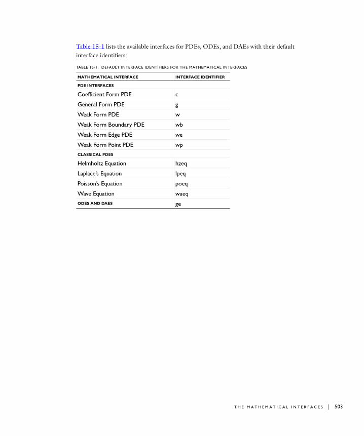
Table 15-1 lists the available interfaces for PDEs, ODEs, and DAEs with their default interface identifiers:
TABLE 15-1: DEFAULT INTERFACE IDENTIFIERS FOR THE MATHEMATICAL INTERFACES
MATHEMATICAL INTERFACE INTERFACE IDENTIFIER
PDE INTERFACES
Coefficient Form PDE c
General Form PDE g
Weak Form PDE w
Weak Form Boundary PDE wb
Weak Form Edge PDE we
Weak Form Point PDE wp
CLASSICAL PDES
Helmholtz Equation hzeq
Laplace’s Equation lpeq
Poisson’s Equation poeq
Wave Equation waeq
ODES AND DAES ge
T H E M A T H E M A T I C A L I N T E R F A C E S | 503

504 | C H A P T E
PDE I n t e r f a c e s
Starting a Model Using a PDE Interface
To create a new model using one of the equation interfaces:
1 In the Model Wizard, select a space dimension on the Select Space Dimension page. Click the Next button ( ).
2 Expand the Mathematics>PDE Interfaces node in the list of physics interfaces and select one of the PDE interface in the list.
3 Double-click the interface or click the Add Selected button ( ) underneath the list to add the selected PDE interface to the model. The interface is added to Selected
physics.
4 Click the Next button ( ) in the upper-right corner of the Model Wizard window.
5 Optionally, choose a Study Type.
6 Click the Finish button ( ) in the upper-right corner of the Model Wizard window.
S P E C I F Y I N G A S Y S T E M O F E Q U A T I O N S
COMSOL Multiphysics allows the creation of equations with more than one dependent variable. To do so, after Step 4 above, under Dependent variables type the number of dependent variables in the Number of dependent variables edit field. COMSOL Multiphysics then automatically assigns variable names, typically u1, u2, u3, and so on. You can also type the name of your choice (as long as they are valid and unique) in Variable names edit fields.
You can also couple several scalar PDEs using a multiphysics approach.
Note: Regardless if you start with a PDE interface in coefficient form or general form, you can add additional equation nodes in coefficient form, general form, or weak form to the same PDE interface.
R 1 5 : E Q U A T I O N - B A S E D M O D E L I N G
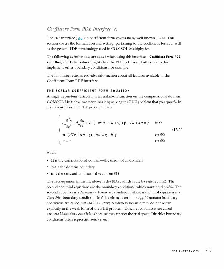
Coefficient Form PDE Interface (c)
The PDE interface ( ) in coefficient form covers many well-known PDEs. This section covers the formulation and settings pertaining to the coefficient form, as well as the general PDE terminology used in COMSOL Multiphysics.
The following default nodes are added when using this interface—Coefficient Form PDE, Zero Flux, and Initial Values. Right-click the PDE node to add other nodes that implement other boundary conditions, for example.
The following sections provides information about all features available in the Coefficient Form PDE interface.
T H E S C A L A R C O E F F I C I E N T F O R M E Q U A T I O N
A single dependent variable u is an unknown function on the computational domain.COMSOL Multiphysics determines it by solving the PDE problem that you specify. In coefficient form, the PDE problem reads
(15-1)
where
• is the computational domain—the union of all domains
• is the domain boundary
• n is the outward unit normal vector on
The first equation in the list above is the PDE, which must be satisfied in . The second and third equations are the boundary conditions, which must hold on . The second equation is a Neumann boundary condition, whereas the third equation is a Dirichlet boundary condition. In finite element terminology, Neumann boundary conditions are called natural boundary conditions because they do not occur explicitly in the weak form of the PDE problem. Dirichlet conditions are called essential boundary conditions because they restrict the trial space. Dirichlet boundary conditions often represent constraints.
eat2
2
u da+t
u + c u– u– + u au++ f= in
n c u u –+ qu = g hT–+ on
u r= on
P D E I N T E R F A C E S | 505
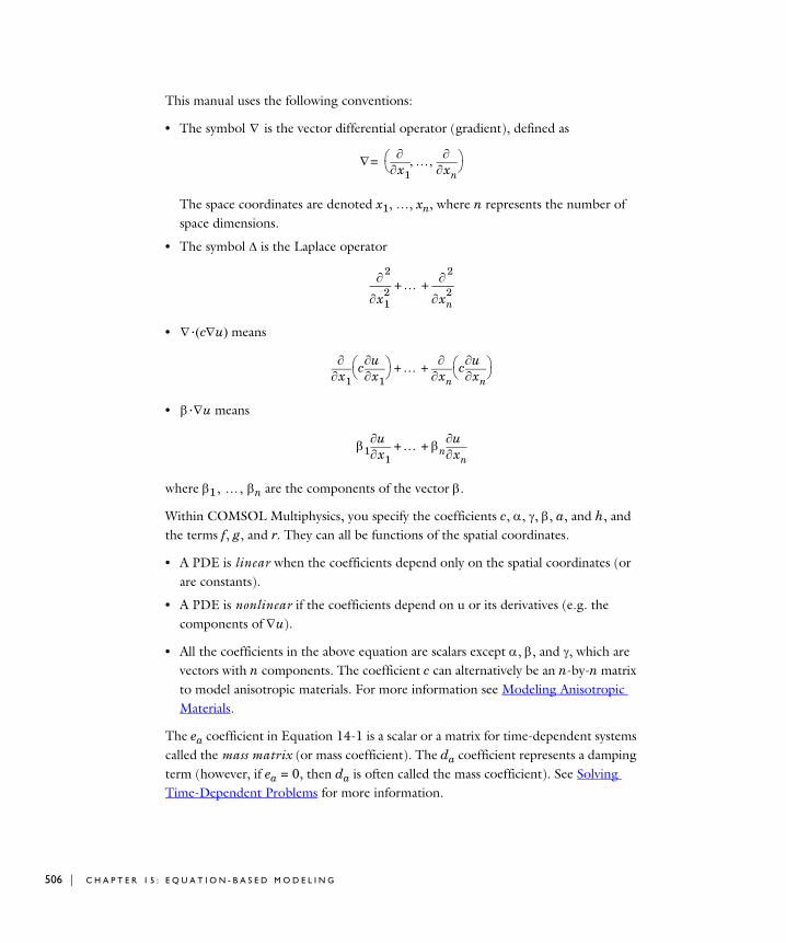
506 | C H A P T E
This manual uses the following conventions:
• The symbol is the vector differential operator (gradient), defined as
The space coordinates are denoted x1, …, xn, where n represents the number of space dimensions.
• The symbol is the Laplace operator
• · cu means
• · u means
where 1 , … , n are the components of the vector .
Within COMSOL Multiphysics, you specify the coefficients c, , , , a, and h, and the terms f, g, and r. They can all be functions of the spatial coordinates.
• A PDE is linear when the coefficients depend only on the spatial coordinates (or are constants).
• A PDE is nonlinear if the coefficients depend on u or its derivatives (e.g. the components of u).
• All the coefficients in the above equation are scalars except , , and , which are vectors with n components. The coefficient c can alternatively be an n-by-n matrix to model anisotropic materials. For more information see Modeling Anisotropic Materials.
The ea coefficient in Equation 14-1 is a scalar or a matrix for time-dependent systems called the mass matrix (or mass coefficient). The da coefficient represents a damping term (however, if ea = 0, then da is often called the mass coefficient). See Solving Time-Dependent Problems for more information.
x1
xn
=
x12
2
xn
2
2
+ +
x1 c
x1u
xn c
xnu
+ +
1 x1u + n xn
u+
R 1 5 : E Q U A T I O N - B A S E D M O D E L I N G

I N T E R F A C E I D E N T I F I E R
This is the identifier for the interface, which you use to reach the fields and variables in expressions, for example.
The identifier appears in the Identifier edit field, and you can change it to any unique string that is a valid identifier. The default identifier (for the first Coefficient Form PDE interface in the model) is c.
D O M A I N S
Select the domains where you want to define the PDE. The default setting is to include all domains in the model.
D E P E N D E N T V A R I A B L E S
Define the number of the dependent variables and the variable names. The default name for a scalar PDE variable is u.
A D V A N C E D S E T T I N G S A N D D I S C R E T I Z A T I O N
Select Show More Options from the View menu in the Model Builder. Normally these settings do not need to be changed. See Show More Options: Advanced Settings and Discretization for more information.
Coefficient Form PDE
This is the default equation for a Coefficient Form PDE interface. Here you specify the coefficients for a coefficient form PDE (see Equation 14-1), with the following equation coefficients (see also Interpreting Boundary Conditions):
• ea is the mass coefficient.
• da is a damping coefficient or a mass coefficient.
• c is the diffusion coefficient.
• is the conservative flux convection coefficient.
• is the convection coefficient.
• a is the absorption coefficient.
• is the conservative flux source term.
• f is the source term.
ea t2
2
u da+t
u + c u– u– + u au++ f=
P D E I N T E R F A C E S | 507

508 | C H A P T E
The Coefficient Form PDE page has these sections:
D O M A I N S
Select the domains where you want to define the coefficient form PDE. The default setting is to include all domains in the model.
E Q U A T I O N
This section displays the coefficient form PDE.
D I F F U S I O N C O E F F I C I E N T
Enter a value or expression for the diffusion coefficient c, which is a tensor. Select Isotropic, Diagonal, Symmetric, or Anisotropic and enter a c coefficient on various forms in 2D and 3D. If there are multiple dependent variables, there is a matrix of c component inputs.
A B S O R P T I O N C O E F F I C I E N T
Enter a value or expression for the absorption coefficient a. If there are multiple dependent variables, there is a matrix of a component inputs.
S O U R C E T E R M
Enter a value or expression for the source term f. If there are multiple dependent variables, there is a vector of f component inputs.
M A S S C O E F F I C I E N T
Enter a value or expression for the mass coefficient ea. If there are multiple dependent variables, there is a matrix of ea component inputs.
D A M P I N G O R M A S S C O E F F I C I E N T
Enter a value or expression for the damping (or mass) coefficient da. If there are multiple dependent variables, there is a matrix of da component inputs.
C O N S E R V A T I V E F L U X C O N V E C T I O N C O E F F I C I E N T
Enter values or expressions for the conservative flux convection coefficient vector’s components. If there are multiple dependent variables, there is a matrix of vector component inputs.
C O N V E C T I O N C O E F F I C I E N T
Enter values or expressions for the convection coefficient vector’s components. If there are multiple dependent variables, there is a matrix of vector component inputs.
R 1 5 : E Q U A T I O N - B A S E D M O D E L I N G

C O N S E R V A T I V E F L U X S O U R C E
Enter values or expressions for the conservative flux source term vector’s components. If there are multiple dependent variables, there is a vector of vector component inputs.
Using the General Form PDE Interface (g)
The PDE interface ( ) in general form provides a flexible way of specifying PDEs. This section covers the formulation and settings pertaining to the general form.
The following default nodes are added when using this interface—General Form PDE, Zero Flux, and Initial Values. Right-click General Form PDE to add other nodes that implement other boundary conditions, for example.
The following sections provides information about all feature nodes available in the General Form PDE interface.
T H E S C A L A R G E N E R A L F O R M E Q U A T I O N
Use the general form for nonlinear PDEs. Assuming that you are working with a single dependent variable u, then a stationary problem in general form reads
The first equation is the PDE. The second and third equations are the Neumann and Dirichlet boundary conditions, respectively. For information on the time-dependent general form equation, see Solving Time-Dependent Problems.
The terms , F, G, and R are coefficients. They can be functions of the spatial coordinates, the solution u, and the space derivatives of u. The coefficients F, G, and R are scalar, whereas is the flux vector. The superscript “T” in the Neumann boundary condition denotes the transpose. The variable is the Lagrange multiplier.
The General Form PDE page has these sections:
eat2
2
u da+t
u + F= in
n– Gu
R
T+= on
0 R= on
P D E I N T E R F A C E S | 509

510 | C H A P T E
I N T E R F A C E I D E N T I F I E R
This is the identifier for the interface, which you use to reach the fields and variables in expressions, for example.
The identifier appears in the Identifier edit field, and you can change it to any unique string that is a valid identifier. The default identifier (for the first General Form PDE interface in the model) is g.
D O M A I N S
Select the domains where you want to define the PDE. The default setting is to include all domains in the model.
D E P E N D E N T V A R I A B L E S
Define the number of the dependent variables and the variable names. The default name for a scalar PDE variable is u.
A D V A N C E D S E T T I N G S A N D D I S C R E T I Z A T I O N
Select Show More Options from the View menu in the Model Builder. Normally these settings do not need to be changed. See Show More Options: Advanced Settings and Discretization for more information.
General Form PDE
This is the default equation for a General Form PDE interface. Here you specify the coefficients for a general form PDE, with the following equation coefficients:
• ea is the mass coefficient.
• da is a damping coefficient or a mass coefficient.
• is the conservative flux vector.
• F is the source term.
The General Form PDE form has these sections:
D O M A I N S
Select the domains where you want to define the general form PDE. The default setting is to include all domains in the model.
ea t2
2
u da+t
u + F=
R 1 5 : E Q U A T I O N - B A S E D M O D E L I N G

E Q U A T I O N
This section displays the general form PDE.
C O N S E R V A T I V E F L U X
Enter a values or expressions for the components of the conservative flux vector . The default values -ux, -uy, and -uz (in 3D) represent the negative gradient of u and makes the left-hand side equal to the Laplace operator. If there are multiple dependent variables, there is one vector for each variable.
A B S O R P T I O N C O E F F I C I E N T
Enter a value or expression for the absorption coefficient a. If there are multiple dependent variables, there is a matrix of a component inputs.
S O U R C E TE R M
Enter a value or expression for the source term f. If there are multiple dependent variables, there is a vector of f component inputs.
D A M P I N G O R M A S S C O E F F I C I E N T
Enter a value or expression for the damping (or mass) coefficient da. If there are multiple dependent variables, there is a matrix of da component inputs.
M A S S C O E F F I C I E N T
Enter a value or expression for the mass coefficient ea. If there are multiple dependent variables, there is a matrix of ea component inputs.
Initial Values
The Initial Values feature adds initial values for the dependent variables that can server as an initial condition for a transient simulation or as an initial guess for a nonlinear solver. If you need to specify more than one set of initial values, you can add additional Initial Values features.
D O M A I N S
Select the domains where you want to define an initial value.
I N I T I A L V A L U E S
Enter a value or expression for the initial value of the dependent variables.
P D E I N T E R F A C E S | 511

512 | C H A P T E
Adding Extra Source Terms
You can add additional source term nodes on different geometry levels: Source on domains, Edge Source on edges in 3D models and Point Source at points.
D O M A I N S / E D G E S / PO I N T S
Select the geometric entities where you want to define a source.
S O U R C E T E R M
Enter a value or expression for the source term f.
Boundary Conditions
The PDE interfaces include the following boundary condition types:
• Zero Flux
• Dirichlet Boundary Condition
• Constraint
• Flux/Source
• No Flux
• Periodic Condition
Dirichlet Boundary Condition
The Dirichlet Boundary Condition specifies a value of u on the boundary of the domain: ur. This is the default boundary condition. It is a unidirectional constraint (see Bidirectional and Unidirectional Constraints).
B O U N D A R I E S
Select the boundaries where you want to define a Dirichlet boundary condition.
U N I D I R E C T I O N A L D I R I C H L E T B O U N D A R Y C O N D I T I O N
Enter a value or expression for the dependent variables on the boundary. To activate the Dirichlet boundary condition for a dependent variable (for example, u2), select the corresponding check box (Prescribed values for u2, for example). Then enter a value or expression for the prescribed value in the associated field.
R 1 5 : E Q U A T I O N - B A S E D M O D E L I N G

Constraint
The Constraint boundary condition specifies a value of R in the constraint R0. This is a bidirectional constraint (see Bidirectional and Unidirectional Constraints). You can use an expression for the constraint that, for example, implements a Robin boundary condition by including a term on the form qu, where u is the dependent variable.
B O U N D A R I E S
Select the boundaries where you want to define a constraint.
B I D I R E C T I O N A L C O N S T R A I N T , R = 0
Enter a value or expression for the value of R in the constraint R0. For example, to constrain u to 2, type 2-u in the edit field for R.
Flux/Source
The Flux/Source boundary condition adds a flux or source g on the boundary:
B O U N D A R I E S
Select the boundaries where you want to define a flux or source.
B O U N D A R Y F L U X / S O U R C E
Enter a value or expression for the value of the boundary flux or source g in the corresponding field. The default value is 0.
B O U N D A R Y A B S O R P T I O N / I M P E D A N C E T E R M
Enter a value or expression for the value of the coefficient q in the corresponding field. The default value is 0. It adds a term qu to the boundary flux or source, which can represent absorption or impedance at the boundary-
Zero Flux
The Zero Flux boundary condition is the default boundary condition and prescribes a zero flux (insulation) across the boundary:
n c u u –+ = g qu+
n c u u –+ = 0
P D E I N T E R F A C E S | 513

514 | C H A P T E
B O U N D A R I E S
Select the boundaries where you want to define a flux or source.
E Q U A T I O N
This section displays the equation for the zero flux.
Periodic Condition
The Periodic Condition feature adds a periodic boundary condition. This periodicity can be continuous (the default) so that ux0ux1 or anti-periodic so that ux0ux1. You can control which of the dependent variables that the periodic condition applies to.
B O U N D A R I E S
Select the boundaries where you want to define a periodic boundary condition. The software automatically identifies the boundaries as either source boundaries or destination boundaries. This works fine for cases like opposing parallel boundaries. In other cases you can use the Destination Selection subfeature (see below) to control the destination (right-click Periodic Condition in the Model Tree and choose Destination
Selection). By default it contains the selection that COMSOL Multiphysics has identified.
P E R I O D I C C O N D I T I O N
Select a Type of periodicity—Continuity (the default) to make the dependent variables equal, or Antiperiodicity to make them antiperiodic: ux0ux1.
For each dependent variable in the PDE you can choose to apply the periodic condition by selecting, for example, the Apply condition on variable u1 check box. By default, the periodic condition applies to all dependent variables.
Destination Selection
Using the Destination Selection feature to change the selection for the destination. The selection that COMSOL Multiphysics makes appears as the default selection in the Selection list (as Selection 1, for example).
R 1 5 : E Q U A T I O N - B A S E D M O D E L I N G

B O U N D A R I E S
Select the boundaries where you want to define a the destination for the periodic boundary condition. By default it contains the selection that COMSOL Multiphysics has identified.
Interpreting Boundary Conditions
The formulation of the boundary conditions imposes both Dirichlet and Neumann conditions. This combination is possible because of a new dependent variable , which is defined only on the boundary. The unknown variable is called a Lagrange multiplier. Often you can reformulate boundary conditions without Lagrange multipliers. In structural mechanics problems the Lagrange multiplier equals the reaction forces on the boundary. The factor hT in the Neumann boundary condition is the transpose of h. If h is a scalar, then hT = h.
How do the Lagrange multipliers relate to the conventional formulation with either a Dirichlet or a Neumann boundary condition?
• First, assume that h = 1. Then the Dirichlet condition is u = r. The Neumann condition becomes:
The Lagrange multiplier, , adjusts so as to satisfy the requested Dirichlet condition. Specifying a nonzero g changes the value of the Lagrange multiplier but does not affect the actual solution u. Therefore, this equation can usually be ignored, leaving a pure Dirichlet condition.
• Second, assume that h = 0 and r = 0. Then the Dirichlet condition reads 0 = 0, and the Neumann condition is
This is the generalized Neumann condition without a Lagrange multiplier. For more on the Lagrange multiplier formulation, see System for Two Variables in the General Form.
The vector cuu is the flux vector. In transport equations its first term describes diffusion, the second term describes convection with a velocity , and the third term is a source term.
In certain applications can be discontinuous across interior boundaries. There can be a jump in the normal component of across such a boundary. For instance, denote the
n c u u –+ qu = g –+
n c u u –+ qu g=+
P D E I N T E R F A C E S | 515

516 | C H A P T E
two adjacent subdomains as 1 and 2, and let i and ni be the values of and n from the two subdomains. Then you can state the jump condition as the Neumann condition
where n1 is the outward normal from Subdomain 1, and n2 is the outward normal from Subdomain 2 so that n1 = n2. At the same time there is a Dirichlet condition ur.
The rest of this section handles stationary problems where ut = 0 and transient effects have vanished.
Note: The c, , and coefficients in the equations for the boundary conditions come from the PDE specification.
Multiple Dependent Variables—Equation Systems
T H E C O E F F I C I E N T F O R M E Q U A T I O N S Y S T E M
With two dependent variables u1 and u2, the stationary PDE problem in coefficient form results in the following equation system:
where u = (u1, u2). The mass term is defined as
Similarly, the damping term is
n1 1 n2 2–– qu = g hT–+
eat2
2
u da tu c u u –+ – u au+ ++ f=
eat2
2
u ea11 ea12
ea21 ea22
t2
2
u1
t2
2
u2
ea11t2
2
u1 ea12t2
2
u2+
ea21t2
2
u1 ea22t2
2
u2+
= =
R 1 5 : E Q U A T I O N - B A S E D M O D E L I N G

However, if ea0, then da is often called the mass coefficient.
The diffusive flux is defined as
where u1 and u2 are column vectors. The flux matrix or flux tensor is a column vector in this presentation. For anisotropic materials, the components c11, c12, c21, and c22 can be matrices as described above for the one-variable coefficient form PDE. In this case, the diffusive flux reads
da tu da11 da12
da21 da22
tu1
tu2
da11 tu1 da12 t
u2+
da21 tu1 da22 t
u2+
= =
c uc11 c12
c21 c22
u1
u2
c11 c12
c21 c22
u1
u2
c11 u1 c12 u2+
c21 u1 c22 u2+= = =
c11x
u1
yu1
c12x
u2
yu2
+
c21x
u1
yu1
c22x
u2
yu2
+
c11 xu1 c12 x
u2+
c11 yu1 c12 y
u2+
c21 xu1 c22 x
u2+
c21 yu1 c22 y
u2+
cu1x
cu1y
cu2x
cu2y
= = =
P D E I N T E R F A C E S | 517
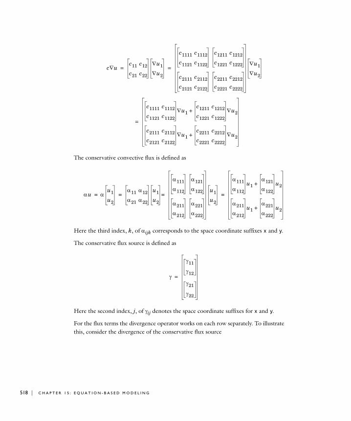
518 | C H A P T E
The conservative convective flux is defined as
Here the third index, k, of ijk corresponds to the space coordinate suffixes x and y.
The conservative flux source is defined as
Here the second index, j, of ij denotes the space coordinate suffixes for x and y.
For the flux terms the divergence operator works on each row separately. To illustrate this, consider the divergence of the conservative flux source
c uc11 c12
c21 c22
u1
u2
c1111 c1112
c1121 c1122
c1211 c1212
c1221 c1222
c2111 c2112
c2121 c2122
c2211 c2212
c2221 c2222
u1
u2= =
c1111 c1112
c1121 c1122
u1c1211 c1212
c1221 c1222
u2+
c2111 c2112
c2121 c2122
u1c2211 c2212
c2221 c2222
u2+
=
u u1
u2
11 12
21 22
u1
u2
111
112
121
122
211
212
221
222
u1
u2
=
111
112
u1121
122
u2+
211
212
u1221
222
u2+
= = =
11
12
21
22
=
R 1 5 : E Q U A T I O N - B A S E D M O D E L I N G

u2
u2
The convection term is defined as
The variable names for these components are beu1 and beu2.
The absorption term is defined as
The variable names for these components are au1 and au2.
The source term is defined as
The variable names for these components are f1 and f2.
The Boundary Condition TermsThe Dirichlet boundary condition, in expanded form, reads
If you choose the Dirichlet condition, you also get the generalized Neumann boundary condition, which reads
11
12
21
22
11
12
21
22
= =
u11 12
21 22
u1
u2
111
112
121
122
211
212
221
222
u1
u2
111
112
u1121
122
+
211
212
u1221
222
+
= = =
aua11 a12
a21 a22
u1
u2
a11u1 a12u2+
a21u1 a22u2+= =
ff1
f2
=
h11 h12
h21 h22
u1
u2
r1
r2
=
P D E I N T E R F A C E S | 519

520 | C H A P T E
The normal vector n(nx, ny) operates on the flux vector in the same way as the divergence operator as explained earlier. If h has full rank (as in the default identity matrix, for example) only the constraints from the Dirichlet condition are active.
If you choose the Neumann condition, you get only the boundary condition
The normal component of the diffusive flux is defined as
The normal component of the conservative convective flux is defined as
The normal component of the conservative flux source is defined as
The boundary absorption term is defined as
The boundary source term is defined as
n c u u –+ qu+ g hT–=
n c u u –+ qu+ g=
n c u nc11 c12
c21 c22
u1
u2
n c11 u1 c12 u2+
n c21 u1 c22 u2+ = =
n u n
111
112
u1121
122
u2+
211
212
u1221
222
u2+
nx ny 111
112
u1121
122
u2+
nx ny 211
212
u1221
222
u2+
= =
n nx ny
11
12
21
22
nx ny 11
12
nx ny 21
22
= =
quq11 q12
q21 q22
u1
u2
q11u1 q12u2+
q21u1 q22u2+= =
R 1 5 : E Q U A T I O N - B A S E D M O D E L I N G

T H E G E N E R A L F O R M E Q U A T I O N S Y S T E M
In the case of several dependent variables u1, u2, …, uN, the following system of equations represents a stationary problem in the general form:
The equation index l ranges from 1 to N, while the constraint index m ranges from 1 to M. This discussion uses the summation convention. Fl, Gl, and Rm are scalars, whereas l is a vector. In this case there are several Lagrange multipliers: 1, 2,…, M.
For a more compact form, let u be a vector with components uk, let be a vector with components l, and so on. Then the system of equations takes on the same form as given above for a single dependent variable.
It is possible to rewrite the system to introduce the components lj of the vector l and the components nj of the normal vector n. Then the system of equations becomes
System for Two Variables in the General FormThe following example of a PDE in the general form is a stationary system for N = 2 solution components in n = 2 space dimensions with M = 2 constraints:
gg1
g2
=
l Fl= in
n– l Gl ulRmm+= on
0 Rm= on
xjlj Fl= in
nj– lj Gl ulRmm+= on
0 Rm= on
P D E I N T E R F A C E S | 521

522 | C H A P T E
with the Neumann boundary conditions
and the Dirichlet boundary conditions
Specifying and Interpreting Boundary ConditionsYou have access to the same set of boundary conditions in all PDE interfaces. To illustrate the flexibility of the Constraint boundary condition R0, consider five cases:
1 Let R1 = R2 = 0. Then the Dirichlet boundary conditions give 0 = 0. In addition, the terms containing the Lagrange multipliers disappear from the Neumann boundary condition. Thus you have only the Neumann boundary conditions
2 Let R1 = r1u1 and R2 = r2 u2. Then the Dirichlet conditions are the usual u1 = r1 and u2 = r2. The Neumann boundary conditions become
1 F1= in
2 F2= in
n– 1 G1 u1R11 u1
R22+ += on
n– 2 G2 u2R11 u2
R22+ += on
0 R1= on
0 R2= on
n– 1 G1= on
n– 2 G2= on
R 1 5 : E Q U A T I O N - B A S E D M O D E L I N G
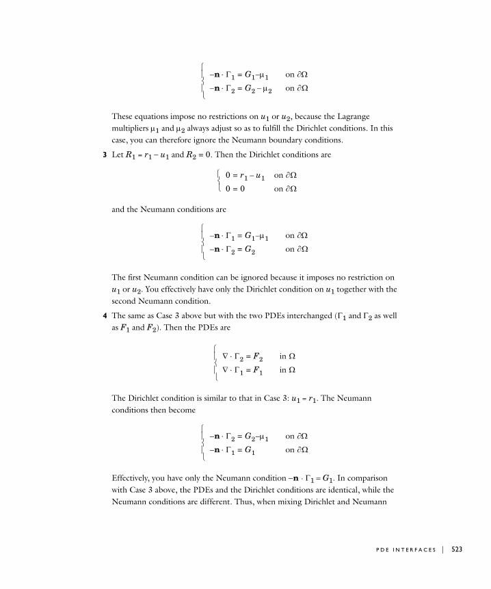
These equations impose no restrictions on u1 or u2, because the Lagrange multipliers 1 and 2 always adjust so as to fulfill the Dirichlet conditions. In this case, you can therefore ignore the Neumann boundary conditions.
3 Let R1 = r1u1 and R2 = 0. Then the Dirichlet conditions are
and the Neumann conditions are
The first Neumann condition can be ignored because it imposes no restriction on u1 or u2. You effectively have only the Dirichlet condition on u1 together with the second Neumann condition.
4 The same as Case 3 above but with the two PDEs interchanged (1 and 2 as well as F1 and F2). Then the PDEs are
The Dirichlet condition is similar to that in Case 3: u1 = r1. The Neumann conditions then become
Effectively, you have only the Neumann condition n · 1G1. In comparison with Case 3 above, the PDEs and the Dirichlet conditions are identical, while the Neumann conditions are different. Thus, when mixing Dirichlet and Neumann
n– 1 G1 1–= on
n– 2 G2 2–= on
0 r1 u1–= on
0 0= on
n– 1 G1 1–= on
n– 2 G2= on
2 F2= in
1 F1= in
n– 2 G2 1–= on
n– 1 G1= on
P D E I N T E R F A C E S | 523

524 | C H A P T E
conditions, the ordering of the equations and the dependent variables are important. However, the ordering of the Dirichlet conditions does not matter since the different Lagrange multipliers are for all practical purposes indistinguishable from each other.
5 Finally, let R1 = u2u1 and R2 = 0. Then the Dirichlet conditions are
and the Neumann conditions are
Note that the same Lagrange multiplier now appears in both Neumann conditions, which can have different definitions of and G. Therefore, contrary to Cases 2 and 3 above, the Neumann conditions cannot be ignored. Instead, adding the two conditions, it becomes apparent that the solution and flux on the boundary must fulfill
In these examples, the values of the Lagrange multipliers do not matter. However, they often have a physical significance. In structural mechanics, the term
in the Neumann condition is the reaction force necessary to satisfy the kinematic constraints described by the Dirichlet conditions. This term has a special form because of the variational principles that give rise to it.
C O E F F I C I E N T F O R M V S . G E N E R A L F O R M
The following substitutions show that the coefficient form and the general form are equivalent:
0 u2 u1–= on
0 0= on
n– 1 G1 1–= on
n– 2 G2 1+= on
0 u2 u1–= on
n– 2 n 2– G1 G2+= on
uR
T
c u–= u– F f u– au G,–=+ g R, r u–= =
R 1 5 : E Q U A T I O N - B A S E D M O D E L I N G

This duality lets you choose the representation that best suits a particular PDE.
Solving Time-Dependent Problems
To get the equation for a time-dependent PDE in COMSOL Multiphysics, add terms containing time derivatives to the left-hand side of the stationary equation. The time derivatives must appear linearly, and the Dirichlet conditions must be linear. A time-dependent problem in the coefficient form reads
If u is a vector of dependent variables then the mass coefficient ea is a matrix. All coefficients can depend on time. The name mass matrix or mass coefficient stems from the fact that in many physics applications ea contains the mass density. The da coefficient represents damping for wave-type equations. However, if ea = 0, then da is often called the mass coefficient. The default settings are ea = 0 and da = 1, representing a time-dependent PDE such as the heat equation. Using ea = 1 and da = 0 represents an undamped wave equation.
For a stationary model, COMSOL Multiphysics ignores any values or expressions that you enter in the edit field for the da and ea coefficient. To activate the da and ea coefficients and convert the model into a time-dependent model, select a time-dependent study.
The time-dependent problem in the general form is
The flux vector and the scalar coefficients F, G, and R can be functions of the spatial coordinates, the solution u, and the space and time derivatives of u. The superscript T
eat2
2
u da+t
u + c u– u– + u au++ f= in
n c u u –+ qu = g hT–+ on
u r= on
eat2
2
u da+t
u + F= in
n– Gu
R
T+= on
0 R= on
P D E I N T E R F A C E S | 525

526 | C H A P T E
1
2
in the Neumann boundary condition denotes the transpose. The variable is the Lagrange multiplier.
For the weak form, the time-dependent problem (in 2D) looks like
where the integrands W(it) depend bilinearly on the test functions vl and on the first and second time derivatives of the dependent variables and their space derivatives. For example,
Time-Dependent SystemsFor time-dependent systems of PDEs the da and ea coefficients are matrices. For example, for the system
the coefficient matrices are
W 2t Ad W 1t sd
B W 0t
P+ + W 2 Ad
W 1 sd
B W 0
+
P+ +=
vl ulRm
2
m2 Ad
vl ul
Rm1
m1 sd
B vl ul
Rm0
m0
P+ + +
0 R 2 = on
0 R 1 = on B
0 R 0 = on P
W 2t v1 tu2
xv1 3u1
tu1 v2 t y
2
u2+cos–=
e11t2
2
u e12t2
2
u2 d11+ +t
u1 d12 tu2 c11– u1 c12u2– a11u1 a12u2+ ++ + f=
e21t2
2
u e22t2
2
u2 d21+ +t
u1 d22 tu2 c21– u1 c22u2– a21u1 a22u2+ ++ + f=
eae11 e12
e21 e22
= dad11 d12
d21 d22
=
cc11 c12
c21 c22
= aa11 a12
a21 a22
=
R 1 5 : E Q U A T I O N - B A S E D M O D E L I N G

(where each element cij can be an n-by-n matrix). Many interesting problems have a singular da matrix (with ea = 0), or a singular nonzero ea matrix. Such problems are called differential-algebraic equation (DAE) systems. The COMSOL Multiphysics solvers for time-dependent problems handle DAEs.
Solving Eigenvalue Problems
COMSOL Multiphysics handles scalar eigenvalue problems for all PDE forms. These eigenvalue problems are related to time-dependent problems via the correspondence t , linking the time derivative to the eigenvalue (with the eigenvalue name lambda). An eigenvalue problem in the coefficient form reads
where 0 is the linearization point for the eigenvalue. The source terms are included if they depend on the solution components. If the coefficients depend on u or the eigenvalue , COMSOL Multiphysics performs a linearization of the problem about the linearization point u = u0, = 0. See Solving for information about linearization.
To specify the linearization point u0 and the linearization point 0, use the settings in the Linearization Point section in the Eigenvalue feature.
Interpreting PDE Coefficients
The COMSOL PDE formulations can model a variety of problems, but note that this documentation uses coefficient names that fall within the realm of continuum mechanics and mass transfer. For the coefficient form PDE:
• ea is the mass coefficient.
• da is a damping coefficient or a mass coefficient.
• c is the diffusion coefficient.
• is the conservative flux convection coefficient.
• is the convection coefficient.
• a is the absorption coefficient.
0– 2eau 0– d– au + c u– u– u au++ f= in
n c u u+ qu = hT–+ on
u r= on
P D E I N T E R F A C E S | 527
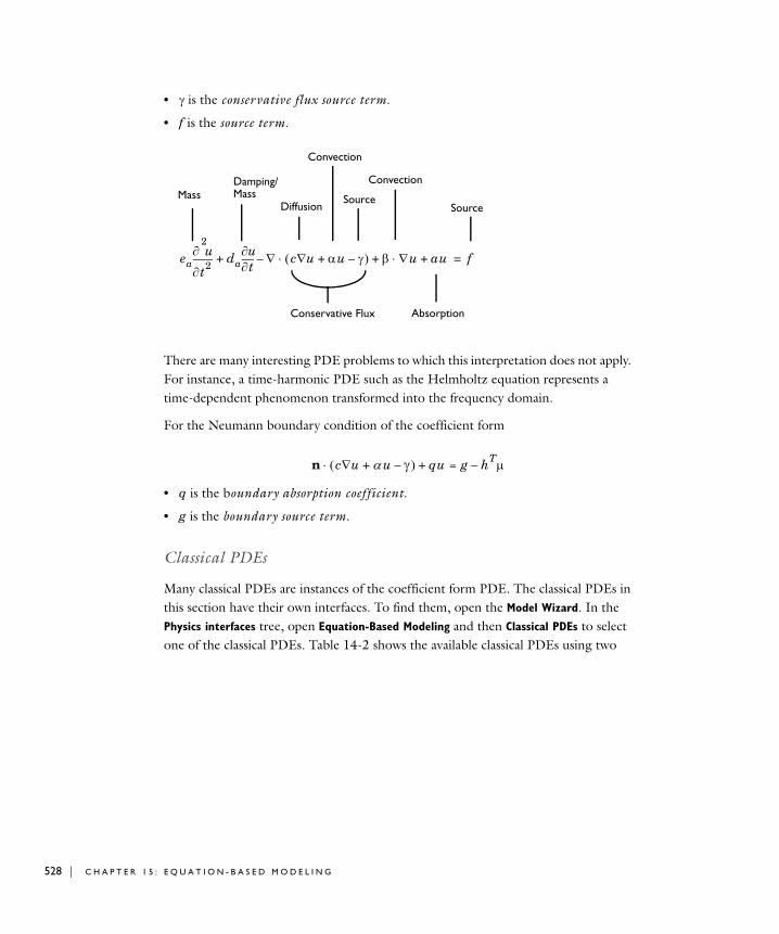
528 | C H A P T E
• is the conservative flux source term.
• f is the source term.
There are many interesting PDE problems to which this interpretation does not apply. For instance, a time-harmonic PDE such as the Helmholtz equation represents a time-dependent phenomenon transformed into the frequency domain.
For the Neumann boundary condition of the coefficient form
• q is the boundary absorption coefficient.
• g is the boundary source term.
Classical PDEs
Many classical PDEs are instances of the coefficient form PDE. The classical PDEs in this section have their own interfaces. To find them, open the Model Wizard. In the Physics interfaces tree, open Equation-Based Modeling and then Classical PDEs to select one of the classical PDEs. Table 14-2 shows the available classical PDEs using two
Diffusion
Convection
Source
Convection
Absorption
Source
eat2
2
u da+t
u c u u –+ – u au+ + f=
Conservative Flux
Damping/MassMass
n c u u –+ qu = g hT–+
R 1 5 : E Q U A T I O N - B A S E D M O D E L I N G

notations: the compact notation of vector analysis (used in this documentation) and an expanded mathematical notation.
The default values are 1 for f and c and 1 for a, so the default Helmholtz equation, for example, is uu1.
The Classical PDEs have the same boundary conditions and other settings as the Coefficient Form PDE (see Coefficient Form PDE Interface (c)).
Bidirectional and Unidirectional Constraints
Constraints formulated through the coefficients h and r in the Coefficient Form PDE interface and through the coefficient R in the General Form PDE interface give rise to constraints called bidirectional. A bidirectional constraint dictates exactly how the flux conditions (or Neumann boundary conditions) are influenced by the constraint force. For the coefficient form, the flux condition is
and for the general form, the flux condition is
The last term on the right-hand side in both expressions is the bidirectional constraint force. Thus, with bidirectional constraints you cannot enforce a flux condition independently of the constraints. In mathematics as well as in multiphysics modeling it is often necessary to enforce Neumann conditions and Dirichlet conditions more
TABLE 15-2: CLASSICAL PDES IN COMPACT AND STANDARD NOTATION
EQUATION COMPACT NOTATION STANDARD NOTATION (2D)
Laplace’s equation
Poisson’s equation
Helmholtz equation
Wave equation
u – 0=
x
xu
–y
yu
– 0=
c u – f=
x c
xu
y c
yu
–– f=
c u – au+ f=
x c
xu
y c
yu
–– au+ f=
eat2
2
u c u – f= eat2
2
ux c
xu
y c
yu
–– f=
n c u u+ qu = g hT–+
n– Gu
R
T+=
P D E I N T E R F A C E S | 529

530 | C H A P T E
freely than what is possible through bidirectional constraints. Assume that you want to enforce the boundary conditions
.
If r1r1(u2), the first condition is fulfilled but not the second. This is because the bidirectional constraint force is not zero:
.
To remedy this limitation with ideal constraints you can use unidirectional constraints, by which you can specify the constraint force independently of the constraints. The term unidirectional refers to the fact that the constraint force differs from hT for coefficient form and from for general form. In multiphysics modeling, unidirectional constraints are, for example, necessary for the following boundary conditions:
• Normal-direction constraints on a moving mesh, where the mesh motion is part of the problem. These conditions are of the type n · ur0 where nn(x) is the boundary normal, u is a vector field (displacements or velocity), and x is the mesh coordinate vector. Bidirectional constraints give constraint forces not only on the equations for u but also on the equations for x, which typically are not wanted.
• Wall boundary conditions for turbulent fluid flow. For the k-turbulence model this condition is of the type kr( ), n·, where r is a given function. Bidirectional constraints for the first relation imply that the second relation cannot hold.
Unidirectional constraints can be enforced in COMSOL Multiphysics both in a pointwise and in a weak sense. For descriptions of how to use pointwise and weak non-ideal constraints see Constraint Forces for PDEs and Weak Constraint, respectively.
0 r1 u1–= on
n– 2 G2= on
n– 2 G2 u2R11 u2
R22+ + G2 u2r1 1+ G2= =
uR
T
R 1 5 : E Q U A T I O N - B A S E D M O D E L I N G

PDE Interface Variables
The following list shows the variables that are available for results evaluation and visualization in addition to the other variables for PDEs:
PDE Coefficients and Boundary Conditions with Time Derivatives
The d coefficients relate to 1st-order time derivatives of the solution u. The only directly available d coefficient is da, the coefficient in front of ut; the subscript a is used because da is similar to the a coefficient in the absorption term except that it multiplies ut instead of u. In contrast, the coefficients dc, d, and d for ut—analogous to the coefficients c, , and for u, respectively—in the extended PDE formulation
NAME TYPE DESCRIPTION EXPRESSION
ui S, B The solution variable (dependent variable)
ui
uixj S, B The derivative of the solution variable ui with respect to the space coordinate xj, for example, uy
uixjxk S, B The second derivative of the solution variable ui with respect to the space coordinates xj and xk, for example, uxx, uxy
uit S, B The derivative of the solution variable ui with respect to time
uitt S, B The second derivative of the solution variable ui with respect to time
uixjt S, B The mixed derivative of the solution variable ui with respect to time and the space coordinate xj
uixi
--------
xj xk
2
ui
tui
t2
2
ui
xj t
2
ui
dcut------ d
ut------+
– d ut------ da
ut------ c– u + + + +
P D E I N T E R F A C E S | 531

532 | C H A P T E
are not directly available in the general or coefficient form PDE models. Instead, you can enter them in the existing and f terms:
• In 1D, add -d_c*uxt-d_al*ut to the term, and add -d_be*uxt to the f term.
• In 2D, add -d_c*uxt-d_al1*ut to the first component, and add -d_c*uyt-d_al2*ut to the second component. Add -d_be1*uxt-d_be2*uyt to the f term.
Replace the variables d_c, d_al, d_be, d_al1, d_al2, d_be1, and d_be2 with appropriate expressions.
You enter 2nd-order time derivative terms in an analogous manner.
To specify a boundary condition containing time-derivative terms as in
,
add the terms -e_q*utt-d_q*ut to the g term, and provide appropriate values or expressions for the coefficients eq and dq in, for instance, a Global Expressions node’s Settings window.
n cu + eq2u
t2--------- dq+
ut------ qu+ + g hT–=
R 1 5 : E Q U A T I O N - B A S E D M O D E L I N G

Weak Fo rm Mode l i n g
Introduction
Do not be misled by the term “weak;” the weak form is very powerful and flexible. The term weak form is borrowed from mathematics, but in this context it has a slightly different meaning; this implementation incorporates features in addition to those defined in the mathematical weak form. Moreover, knowledge of the mathematical weak form is not a prerequisite to using the COMSOL Multiphysics implementation.
The distinguishing features of the weak form in COMSOL Multiphysics are that it makes it possible to:
• Enter certain equations that can be derived from an energy principle in a very compact and convenient form. Such equations, for example, arise in structural mechanics.
• Add and modify nonstandard constraints, such as various contact and friction models.
• Build models with extra equations on boundaries, edges, and points.
• Use the test operator to conveniently work with problems in variational calculus and parametric optimization.
COMSOL Multiphysics provides the possibility to add weak form contributions to any physics interface in the model. In addition, you can add weak constraints, which, for example, provide accurate fluxes and reaction forces.
By default, COMSOL Multiphysics converts all models to the weak form before solving. Although this feature is a part of the solution technique rather than part of the modeling process, it nonetheless belongs in this discussion because it is based on the weak form implementation.
The discussion in this section reviews the ways to work with the weak form by adding weak form contributions.
The Weak Form Interfaces
In the Model Wizard, you can add weak form interfaces on all domain levels: Weak Form
PDE on domains, Weak Form Boundary PDE on boundaries, Weak Form Edge PDE on edges (in 3D models), and Weak Form Point for points. In all of them you can add weak
W E A K F O R M M O D E L I N G | 533
534 | C H A P T E
expressions, which COMSOL Multiphysics adds to the overall equation. Adding one of these interfaces creates a PDE node ( ) for PDE modeling using a weak formulation. You can also add a Weak Form PDE on the domain level to any other PDE interface.
The following default nodes are added when using these interfaces—Weak Form PDE, Zero Flux (for a Weak Form PDE on the domain level only), and Initial Values. Right-click the main PDE node to add other nodes that implement other boundary conditions, for example. On the domain level, edge, and boundary levels you can use the same boundary conditions as for the Coefficient Form PDE and General Form PDE.
The following sections provides information about the specific feature nodes available in the Weak Form PDE interface.
I N T E R F A C E I D E N T I F I E R
This is the identifier for the interface, which you use to reach the fields and variables in expressions, for example.
The identifier appears in the Identifier edit field, and you can change it to any unique string that is a valid identifier. The default identifier (for the first Weak Form PDE interface in the model) is w, wb, we, or wp, depending on the geometry level).
D O M A I N S , B O U N D A R I E S , E D G E S , O R PO I N T S
Select the domains (boundaries, edges, points) where you want to define the weak-form PDE. The default setting is to include all domains (boundaries, edges, points) in the model.
D E P E N D E N T V A R I A B L E S
Define the number of the dependent variables and the variable names. The default name for a scalar PDE variable is u.
A D V A N C E D S E T T I N G S A N D D I S C R E T I Z A T I O N
Select Show More Options from the View menu in the Model Builder. Normally these settings do not need to be changed. See Show More Options: Advanced Settings and Discretization for more information.
Weak Form PDE
Use Weak Form PDE to specify the PDE using a weak formulation.
R 1 5 : E Q U A T I O N - B A S E D M O D E L I N G

D O M A I N S / B O U N D A R I E S / E D G E S / P O I N T S
Select the geometric entities where you want to define the weak form PDE. The default setting is to include all selected geometric entities in the model.
E Q U A T I O N
This section displays the weak form PDE.
WE A K E X P R E S S I O N
Enter the weak expression that COMSOL Multiphysics (together with any other weak expressions on the same domain) sets equal to 0 in the weak field. On the domain level, the default expression is -test(ux)*ux-test(uy)*uy+test(u), which is the weak formulation of Poisson’s equation with f = 1. On other domain levels, the default weak expression is 0.
The Weak Contribution Feature
The Weak Contribution feature is available in all physics interfaces and for all geometry levels, including the global level.
To add a Weak Contribution feature to the main PDE, in the Model Builder, right-click the main PDE node. Depending on the geometric entity level, select More>Weak
Contribution, Edges>Weak Contribution or Points>Weak Contribution from the context menu. Or select Global>Weak Contribution option to apply it globally. To create an independent weak form equation rather than a weak form contribution, you need to add extra states (dependent variables) using the Auxiliary Dependent Variables subfeature.
The Weak Contribution page has these sections:
D O M A I N S , B O U N D A R I E S , E D G E S , O R PO I N T S
Select the geometric entity where you want to add a weak contribution—to domains, boundaries, edges in 3D models, and points in 2D and 3D models.
WE A K C O N T R I B U T I O N
Enter the weak form contribution in the Weak expression field. For example, -ux*test(ux)-uy*test(uy)+1*test(u) is the weak formulation of a Poisson’s equation with u as the dependent variable 1 as the source term on the right-hand side. To add a time derivative as in the time-dependent coefficient form PDE, add -ut*test(u) (notice the sign and the syntax ut for the time derivative of u).
W E A K F O R M M O D E L I N G | 535

536 | C H A P T E
Q U A D R A T U R E S E T T I N G S
These settings affect the numerical integration, and you do normally not need to change them.
Integration OrderThe integration order is typically twice the order of the shape function. For example, the default integration order for second-order Lagrange elements is 4. The integration order is a positive integer that you enter in the Integration order edit field.
Integrate on FrameThis setting determines which frame to base the integration on: the spatial frame, the material frame, or the mesh frame. The default is to use the default frame for the physics interface. You select the frame from the Integrate on frame list.
VA R I A T I O N A L C A L C U L U S
You can use the test operator to work with problems in variational calculus and optimization theory.
For more details about the Auxiliary Dependent Variable feature, see below.
Weak Contributions on Mesh Boundaries
To display this option, select Show More Options from the View menu in the Model
Builder. To add a Weak Contribution on Mesh Boundaries feature to the main PDE, in the Model Builder, right-click the main PDE node and select More>Weak Contribution
on Mesh Boundaries at the domain level.
This feature is similar to the Weak Contribution feature but is active on mesh boundaries. The settings are the same as for the Weak Contribution (see The Weak Contribution Feature).
The Auxiliary Dependent Variable Feature
To display this option, select Show More Options from the View menu in the Model
Builder.
If you specify a complete equation on weak form in a Weak Contribution feature and use a new dependent variable that is not part of the physics interface, right-click the Weak Contribution node to add an Auxiliary Dependent Variable.
R 1 5 : E Q U A T I O N - B A S E D M O D E L I N G

D O M A I N S , B O U N D A R I E S , E D G E S , O R PO I N T S
Select the geometric entity where you want to add the auxiliary dependent variable. The default geometric entity is the same as for the parent Weak Contribution feature (domains, boundaries, edges in 3D models, or points in 2D and 3D models). In rare cases, you can use more than one Auxiliary Dependent Variable feature on subsets of the Weak Contribution feature’s selection (to use different initial values, for example).
A U X I L I A R Y D E P E N D E N T V A R I A B L E
Define the name and properties of the auxiliary dependent variable.
Field Variable NameEnter the Field variable name (the dependent variable).
Initial ValueEnter the Initial value for the dependent variable. The default is 0.
Shape FunctionFrom the Shape function list, select from first-order to third-order Lagrange elements and form constant to second-order discontinuous elements. Quadratic Lagrange elements are the default elements for most physics interfaces.
Define Derivatives With Respect to FrameSelect an option from the Define derivatives with respect to frame list—Spatial, Material, or Mesh. The default is to use the default frame for the physics interface.
Modeling with PDEs on Boundaries, Edges, and Points
The weak form makes it possible to do equation modeling on boundaries, edges, and points, thus opening up a wider class of models than some of the physics interfaces cover. To add such equations, you can add auxiliary dependent variables to a Weak
Contribution feature. You can use such weak form equations as a way of handling thin layers; COMSOL Multiphysics then solves the problem by modeling rather than meshing. This approach reduces the solution time.
The model “Transport and Adsorption” in the COMSOL Multiphysics Model Library shows how to use the weak form boundary mode to model a thin adsorbtion layer with diffusion as a PDE on the boundary of a convection-diffusion problem. Another model using tangential derivative variables is “Shell Diffusion” in the COMSOL Multiphysics Model Library.
W E A K F O R M M O D E L I N G | 537

538 | C H A P T E
Specifying PDEs in Weak Form
In addition to shape function variables, you can use the test operator in the Weak
expression edit fields in the Weak Contribution features and the Constraint expression edit fields in the Weak Constraint features. The test operator can operate on the shape function variables: for example, test(u1). See Special Operators for more information about the test operator and other operators.
The test functions always occur linearly in the weak terms. You can use these weak terms either alone to define the problem (in the Weak Form PDE interface or by adding an auxiliary dependent variable), or in addition to the other equations defined by the physics interface.
R 1 5 : E Q U A T I O N - B A S E D M O D E L I N G

U s i n g Weak Con s t r a i n t s
The weak constraints feature in COMSOL Multiphysics implements constraints by using finite elements on the constrained domain for the Lagrange multipliers, and by solving for the Lagrange multipliers along with the original problem. The weak constraints have a number of distinct advantages. They can:
• Provide very accurate flux computations—the Lagrange multipliers along the constraints optimally balance the finite element projection of the applied loads (reaction forces). See Computing Accurate Fluxes for more information and an example. For computing integrals of reaction forces or fluxes, the reaction force operator (reacf) is a better alternative than weak constraints. See The Reacf Operator. The reaction force operator does not have the drawbacks discussed below.
• Handle nonlinear constraints—the nonlinear solver does not store the Lagrange multipliers arising from standard constraints from one step to the next, which affects the convergence when constraints are nonlinear. Weak constraints can handle general nonlinearities because the Lagrange multipliers are updated as a part of the solution vector and give correct contributions to the stiffness matrix.
• Implement constraints including derivatives—constraints only on the tangential component of the derivative work when using standard constraints, whereas you must use weak constraint to be able to handle nontangential constraints. Note that boundary conditions involving the normal component of the derivative can almost always be reformulated as a Neumann condition, which is usually preferable.
Weak constraints also come with the following drawbacks:
• Because extra unknowns are introduced for the Lagrange multipliers the problem size increases compared to when eliminating the constraints.
• The formulation normally implies that a saddle-point problem is introduced with zeros on the main diagonal of the Jacobian of the discretized equations. This class of problems is often more difficult to solve. Because iterative methods for linear systems are sensitive to the eigenvalue distribution of the system matrix, a weak constraint formulation can be much more difficult to solve than the corresponding pointwise constraint formulation.
• Discontinuous constraints result in (theoretically) infinite Lagrange multipliers. In practice you get large oscillations.
U S I N G W E A K C O N S T R A I N T S | 539

540 | C H A P T E
Weak Constraint
To add a Weak Constraint feature on the domain, boundary, edge, point, or global level, select Show More Options from the View menu in the Model Builder. Depending on the geometric entity level, select More>Weak Constraint, Edges>Weak Constraint or Points>Weak Constraint from the context menu. There is no global weak constraint option.
D O M A I N S , B O U N D A R I E S , E D G E S , O R PO I N T S
Select the geometric entity where you want to add a weak constraint—to domains, boundaries, edges in 3D models, and points in 2D and 3D models.
The default setting is to include all geometric entities in the model.
WE A K C O N S T R A I N T
Select a Constraint type—Bidirectional, symmetric or User defined. Enter a Constraint
expression. See Bidirectional and Unidirectional Constraints for more information. If User defined is selected, enter a Constraint force expression.
Q U A D R A T U R E S E T T I N G S
The Use automatic quadrature settings check box is selected by default. If required, click to clear the check box.
L A G R A N G E M U L T I P L I E R
Enter a Lagrange multiplier variable and an Initial value. The variable name using weak constraints, such as lm, correspond to the Lagrange multipliers. Change the name if required. The weak constraints supersede the original constraints and implement them using a weak formulation.
Select a Shape function—Linear Lagrange, Quadratic Lagrange (the default), Cubic
Lagrange, Constant discontinuous, Linear discontinuous, or Quadratic discontinuous.
From the Define derivatives with respect to frame list, select Spatial, Material, or Mesh.
Pointwise Constraint
To add a Pointwise Constraint feature on the domain, boundary, edge, or point level, select Show More Options from the View menu in the Model Builder. Depending on the geometric entity level, select More>Weak Constraint at the domain or boundary level, Edges>Weak Constraint or Points>Weak Constraint from the context menu. There is no global pointwise constraint option.
R 1 5 : E Q U A T I O N - B A S E D M O D E L I N G

You can also add pointwise (strong) constraints, which do not create Lagrange multipliers. The settings in the Pointwise Constraint section are similar to those for the weak constraints.
D O M A I N S , B O U N D A R I E S , E D G E S , O R PO I N T S
Select the geometric entity where you want to add to a pointwise constraint. The default setting is to include all selected geometric entities in the model.
PO I N T W I S E C O N S T R A I N T
Select a Constraint type—Bidirectional, symmetric or User defined. Enter a Constraint
expression. If User defined is selected, enter a Constraint force expression. See Bidirectional and Unidirectional Constraints for more information.
S H A P E F U N C T I O N
Select a Shape function—Linear Lagrange, Quadratic Lagrange (the default), Cubic
Lagrange, Constant discontinuous, Linear discontinuous, or Quadratic discontinuous.
From the Define derivatives with respect to frame list, select Spatial, Material, or Mesh.
Bidirectional and Unidirectional Constraints
The default constraint type is bidirectional, which means that COMSOL Multiphysics derives the constraint force directly from the constraint at a boundary, edge, or point. You can also use the unidirectional constraints, which for constraints written as 0R on , changes the constraint force according to
where I is an identity operator for points on the boundary . For example, using two variables u1 and u2 and the constraints
,
then the non-ideal constraint force is acting on both equations for the boundary .
uR
T I –
0 R1 u1 u2 = on
0 R2 u1 u2 = on
U S I N G W E A K C O N S T R A I N T S | 541

542 | C H A P T E
B I D I R E C T I O N A L V S . U N I D I R E C T I O N A L WE A K C O N S T R A I N T S
Bidirectional weak constraints in theory implement the same boundary conditions as the standard, pointwise, constraints. In some cases, the result may differ slightly, but this is only due to the different discretization. Using unidirectional constraints, on the other hand, modifies the way boundary conditions are interpreted. Switching from pointwise constraints to unidirectional weak constraints therefore can modify the physics of the model, while using bidirectional weak constraints only affects the numerics.
The difference between bidirectional and unidirectional constraints is the way the Lagrange multipliers—which can be interpreted as generalized reaction forces—are applied. In a bidirectional constraint, the Lagrange multipliers are applied symmetrically on all dependent variables involved in the constraint so as to keep symmetric problems symmetric. In a unidirectional constraint, the reaction forces are applied only on the physics interface’s dependent variable at the boundary where the constraint is specified.
Imagine a model with two physics interfaces A and B, with dependent variables u and v, respectively. If physics interface A specifies a standard constraint as R 2u3v = 0, COMSOL Multiphysics implements the ideal weak boundary constraint by adding the weak term
where and are the Lagrange multiplier and corresponding test function, and and are the test functions corresponding to u and v, respectively. Because multiplies both test functions in the second integral, both u and v are affected by the constraint, which is therefore bidirectional.
The corresponding non-ideal weak constraint adds the weak form contribution
Here, the Lagrange multiplier only multiplies the test function . All reaction forces therefore apply only to u, while v is left unaffected by the constraint. This makes the non-ideal constraint unidirectional. Note also that the non-ideal constraint does not consider the factor 2 in front of u when applying the forces. Even if the constraint would contain spatial derivatives, the Lagrange multiplier would still be applied only directly on the dependent variable itself.
2u 3v– B ds 2u 3v– sd
B+
uv
2u 3v– B ds u sd
B+
u
R 1 5 : E Q U A T I O N - B A S E D M O D E L I N G
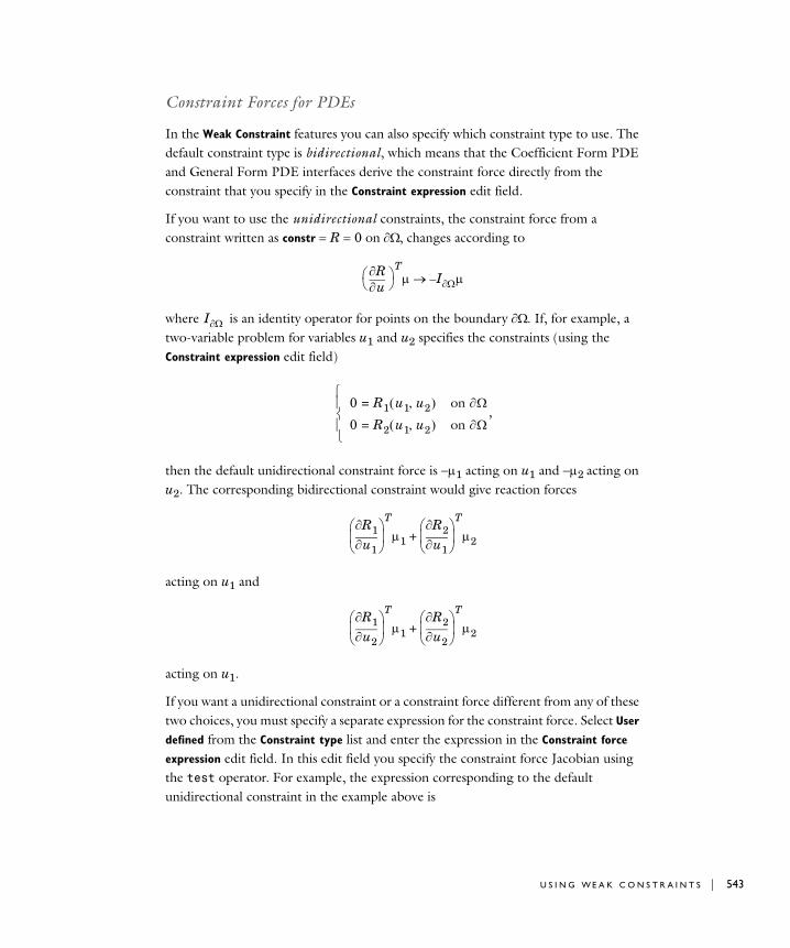
Constraint Forces for PDEs
In the Weak Constraint features you can also specify which constraint type to use. The default constraint type is bidirectional, which means that the Coefficient Form PDE and General Form PDE interfaces derive the constraint force directly from the constraint that you specify in the Constraint expression edit field.
If you want to use the unidirectional constraints, the constraint force from a constraint written as constr R 0 on , changes according to
where is an identity operator for points on the boundary . If, for example, a two-variable problem for variables u1 and u2 specifies the constraints (using the Constraint expression edit field)
,
then the default unidirectional constraint force is 1 acting on u1 and 2 acting on u2. The corresponding bidirectional constraint would give reaction forces
acting on u1 and
acting on u1.
If you want a unidirectional constraint or a constraint force different from any of these two choices, you must specify a separate expression for the constraint force. Select User
defined from the Constraint type list and enter the expression in the Constraint force
expression edit field. In this edit field you specify the constraint force Jacobian using the test operator. For example, the expression corresponding to the default unidirectional constraint in the example above is
uR
T I –
I
0 R1 u1 u2 = on
0 R2 u1 u2 = on
u1R1
T
1 u1R2
T
2+
u2R1
T
1 u2R2
T
2+
U S I N G W E A K C O N S T R A I N T S | 543

544 | C H A P T E
Note: The bidirectional constraint type normally generates a symmetric constraint Jacobian matrix and constraint force Jacobian matrix coupling for the discretized equations, while unidirectional constraints generate an unsymmetric coupling. See also Solving.
Limitations of Weak Constraints
Weak constraints are more difficult to use than conventional pointwise constraints. Notes these tips when using them:
• Pointwise and weak constraints on the same set of variables on adjacent boundaries (boundaries that share common node points in the mesh) do not work. This means that if you must constrain all boundaries on a solid and want to use a weak constraint on one boundary segment (one face), you must use the weak constraint on the entire boundary of the solid (if the boundary is connected).
• You must always have a nontrivial constraint (that is, a Dirichlet condition) on the boundaries where you enable the weak constraint for the constraint to take effect.
• Problems with the scaling of linear systems sometimes arise in conjunction with weak constraints. The Lagrange multiplier variables always have a different unit than the main system variables, and can therefore be of a completely different order of magnitude. Usually the automatic variable scaling in the solvers is sufficient, but there are cases when you might want to consider manual scaling.
• Always use the same shape function type for the weak constraint as for the variables that you constrain, possibly with lower-order elements for the weak constraint. In some cases (for example, when constraining derivatives) the system of equations can become singular. The reason is usually that there are redundant Lagrange multiplier degrees of freedom in the model. Try to lower the order of the Lagrange multiplier variables or use constraints on the Lagrange multiplier to remove some degrees of freedom.
• If you want to use iterative methods for the linear system and if the weak constraint formulation gives zeros on the diagonal of the system matrix, the SOR class of preconditioners and smoothers do not work. Instead try use the Vanka algorithm with the Lagrange multipliers as the Vanka variables or use the incomplete LU factorization algorithm.
test u1 –test u2 –
R 1 5 : E Q U A T I O N - B A S E D M O D E L I N G

S o l v i n g ODE s and DAE s
Adding ODEs, DAEs, and Other Global Equations
When working on complex models, you might need to introduce single named degrees of freedom, or states, which are not logically related to any particular point in space, and their corresponding equations. In particular, such situations arise when modeling physics in interaction with an external system, for example, a controller or an electrical circuit built from standard components. It is often possible to describe such external systems by a system of ordinary differential equations, ODEs, with a limited number of degrees of freedom.
The Global Equations and ODEs interface provides a Global Equations feature that is designed for implementing this type of external equation. Such equations are often tightly coupled to a model in a physical domain. The Global Equations feature is also available from any of the physics interfaces. You access it by right-clicking the main feature and then choosing Global>Global Equations. You can use it for ODEs, differential algebraic equations, purely algebraic equations and conditions, and transcendental equations, or to add degrees of freedom to a model using the introduced states. Possible uses include:
• Controllers
• Rigid-body mechanics
• Nonlinear eigenvalue problems
• Continuation
• Integral constraints
• Augmented or generalized equations
The ODEs and DAEs Interface
The ODEs and DAEs interface provides the possibility to add ODEs or other global equations to a model. The main feature is the Global Equations feature, where you define the global equations including the names of the variables (states), the required initial values, and an optional description. When you add the Global Equations and ODEs interface, it adds a default Global Equations feature. Right-click the Global Equations and
ODEs node to add additional Global Equations feature or a Weak Contribution feature.
S O L V I N G O D E S A N D D A E S | 545

546 | C H A P T E
The following sections provide information about the Global Equations and Weak
Contributions features.
Global Equations
To add a global (space-independent) equations such as ODEs, you add them in the Global Equations form, which contains the following section:
G L O B A L E Q U A T I O N S
The global equations that you can solve have the following form:
with the initial conditions ut0u0 and utt0ut,0 (where the subscript t indicates the time derivative). You can add several equations, and the equation can be coupled.
The first time derivative of u is specified as ut, and the second time derivative of u is utt. With time derivatives, this equation is an ODE (ordinary differential equation). With no time derivatives, the equation is an algebraic equation or a transcendental equation. The initial conditions are only necessary for ODEs.
In the table, each row corresponds to a named state, that is, a single degree of freedom and one equation. Fill in the name of the state variable in the Name column. This also defines time-derivative variables. If a state variable is called u, its first and second time derivatives are ut and utt, respectively. These variables become available in all geometries. Therefore the names must be unique.
Use the Equation f(u,ut,utt,t) column to specify the left side of the equation that is to be set equal to zero. The software then adds this global equation to the system of equations. When you solve the model, the value of the state variable u is adapted in such a way that the associated global equation is satisfied. You can use all state variables and their time derivatives as well as any parameters, global expression variables, and coupling operators with a scalar output and global destination in the f(u,ut,utt,t) column. Setting an equation for a state is optional. The default value of 0 means that the software does not add any additional condition to the model.
If the time derivative of a state variable appears somewhere in the model during a time-dependent solution, the state variable needs an initial condition. Models that contain second time derivatives also require an initial value for the first time derivatives of the state variables. You set these conditions in the third (Initial value (u)) and fourth
f u u· u·· t 0=
R 1 5 : E Q U A T I O N - B A S E D M O D E L I N G

(Initial value (ut)) columns. The last column, Description, gives you the option to enter comments about the state or the equation.
To add another equation, click the Add button. To remove an equation, select some part of that equation’s row in the table and click the Remove button.
Weak Contribution (ODEs and DAEs)
Another option is to enter equations in the weak form using the Weak Contribution feature. This can be convenient in advanced modeling because it gives you control over the test variables multiplying the equations. Wherever a test function of a state variable appears (in the Global Equations feature or elsewhere in the model), whatever it multiplies ends up in the same equation in the discrete system. Note that you can have zero or more weak expressions, regardless of the number of states.
WE A K C O N T R I B U T I O N
You type the expression that contains the weak formulation in the Weak expression edit field. See Adding an ODE to a Boundary for an example of how to write an ODE using a weak formulation.
Discretization
By right-clicking the main physics interface node and choosing Global>Discretization you can add extra Discretization nodes for use in, for example, multigrid hierarchy. You can select which discretization to use in the Multigrid Level subnodes for the study steps.
The Discretization form contains a single Discretization section, which is identical to the Discretization section in the main physics interface node’s Settings window.
Presenting Results for Global Equations
The state variables are scalar values and they are available globally. To view the results for an ODE, you can use the Line Graph, Point Graph, and Global plot types and Global Evaluation for displaying the numerical solution.
Solving ODEs
As an example of ODEs, the following equations are the Lotka-Volterra equations:
S O L V I N G O D E S A N D D A E S | 547

548 | C H A P T E
where r is the rabbit population, and f is the population of foxes. This is an example of a system of two coupled ODEs.
You enter these equations as rt-a*r+b*r*f and ft+c*f+d*r*f, where a, b, c, and d are scalar values defined using the Parameters feature. For this first-order ODE, you need to specify initial values for r and f.
Solving Algebraic and Transcendental Equations
As an example of an algebraic equation, consider the equation fu0 for
This equation has a single root at u1. To enter it into the Global Equations window, type u in the Name column and u^3+u-2 in the Equation f(u,ut,utt,t) column (both entries on the same row). Then solve this using a stationary solver. To display the solution value, right-click Numerical Results in the Results branch and select Global
Evaluation. In the Settings window, select u from the list of predefined quantities (click the down arrow in the Expression section and select ODEs and DAEs>(u)).Click the Evaluate button, and the value of the root appears in the Results section.
As an example of a transcendental equation, consider the equation fu0 for
A root to this equation is approximately 0.56714. To enter it into the Global Equations window, type u in the Name column and exp(-u)-u in the Equation f(u,ut,utt,t) column (both entries on the same row). Then compute the solution. To display the solution value, right-click Numerical Results in the Results branch and select Global
Evaluation. In the Settings window, select u from the list of predefined quantities (click the down arrow in the Expression section and select ODEs and DAEs>(u)). Click the Evaluate button, and the value of the root (rounded to 0.567) appears in the Results section.
r· ar br f–=
f· c f– dr f+=
f u u3 u 2–+=
f u e u– u–=
R 1 5 : E Q U A T I O N - B A S E D M O D E L I N G

Adding an ODE to a Boundary
Sometimes a boundary equation is coupled to a PDE in an adjacent subdomain. For example, adding an ODE for v on a boundary such that
where u is the dependent variable in an adjacent subdomain. To implement an ODE on a boundary, do the following:
1 In the physics interface where u is defined, right-click the main feature and select More>Weak Contribution from the boundary feature section (you might need to select Show More Options from the View menu in the Model Builder).
2 Select the boundary where you want to add the ODE.
3 Type (u-vt)*test(v) in the Weak expression field. This is the weak formulation of the ODE.
4 Right-click the Weak Contribution node and select Auxiliary Dependent Variable.
5 In the Auxiliary Dependent Variable section, type v in the Field variable name edit field. You can also specify an initial value for the variable (the default initial value is 0). You do not need to make a selection of boundaries for this variable; by default, it uses the same selection as for the weak contribution.
6 When done, solve the model.
Also keep in mind that there must be no constraint (Dirichlet condition) for u on the boundaries where you defined the ODE.
vt------ u=
S O L V I N G O D E S A N D D A E S | 549

550 | C H A P T E
Th e Wa l l D i s t a n c e I n t e r f a c e
The Wall Distance interface ( ) provides the equations and boundary conditions for computing the distance to walls in fluid-flow simulation using a modified Eikonal equation, solving for a dependent variable G that is related to the wall distance. The main feature is the Distance Equation node, which adds the distance equation (modified Eikonal equation) and provides an interface for defining the reference length scale.
When you add the Wall Distance interface, it creates the Wall Distance node with a default Distance Equation node added as well as default boundary conditions, which is a homogeneous Neumann condition that does not appear in the Model Tree. Right-click the Wall Distance node to add boundary conditions for walls. There is also a default Initial Values node. The following sections provide information about all features available in the Wall Distance interface.
D O M A I N S
Select the domains where you want to define the distance equation. The default setting is to include all domains in the model.
P H Y S I C A L M O D E L
Enter a Smoothing parameter w. in Equation 4-71. The default value is 0.1.
D E P E N D E N T V A R I A B L E S
The dependent variable (field variable) is for the Reciprocal wall distance G. You can change the name in the corresponding edit field, but the names of fields and dependent variables must be unique within a model.
A D V A N C E D S E T T I N G S A N D D I S C R E T I Z A T I O N
Normally these settings do not need to be changed. See Show More Options: Advanced Settings and Discretization.
Distance Equation
The Distance Equation node adds to Equation 4-71, and the Distance Equation form contains the following sections for defining the length scale:
R 1 5 : E Q U A T I O N - B A S E D M O D E L I N G

D O M A I N S
Select the domains where you want to use the distance equation with the length scale defined in this Distance Equation node.
D I S T A N C E E Q U A T I O N
Specify the length scale using the reference length lref. From the Length scale
specification you can choose from two methods to compute the reference length:
• Select Automatic to use Equation to compute lref. This is the default setting.
• Select Manual to specify the reference length (SI unit: m) manually in the lref edit field. The default value is 1.
Initial Values
The Initial Values node adds an initial value for the reciprocal wall distance that can serve as initial guess for a nonlinear solver.
D O M A I N S
Select the domains where you want to define an initial value.
I N I T I A L V A L U E S
Enter a value or expression for the initial value of the reciprocal wall distance G (SI unit: 1/m) in the Reciprocal wall distance edit field. The default value is G02lref.
Boundary Conditions
The following boundary conditions are available:
• The default boundary condition is a homogeneous Neumann condition, which applies to all boundaries that are not walls:
This boundary condition does appear as a node in the model tree.
• The Wall boundary condition (see below) for boundaries that are walls.
For axisymmetric models, COMSOL Multiphysics automatically takes the axial symmetry boundaries (at r0) into account, and prohibits the wall boundary feature from being defined here.
G n 0=
T H E W A L L D I S T A N C E I N T E R F A C E | 551

552 | C H A P T E
Wall
The Wall node implements the following boundary condition for walls:
B O U N D A R I E S
Select the boundaries that represent walls.
Theory for the Wall Distance Interface
Turbulence models often use the distance to the closest wall to approximate the mixing length or for regularization purposes. One way to compute the wall distance is to solve the Eikonal equation:
(15-2)
with D0 on solid walls and D · n0 on other boundaries. The Eikonal equation can be tricky to solve, and produces the exact distance to the closest wall. The modified equation described below is less computationally expensive to solve. It also uses a reference length to put more emphasis on solid objects larger than the reference length and reduce the emphasis on smaller objects. The introduction of a reference length produces a more relevant wall distance in the following instances:
• In convex regions of small dimensions, the wall distance is reduced to reflect the close proximity of several walls.
• When a small object, such as a thin wire for example, is present in free flow, the wall distance is affected only in a very small region around it.
M O D I F I E D E I K O N A L E Q U A T I O N
COMSOL Multiphysics uses a modified Eikonal equation based on the approach in Ref. . This modification changes the dependent variable from D to G1D. Equation 15-2 then transforms to
(15-3)
Additionally, the modification adds some diffusion and multiplies G4 by a factor to compensate for the diffusion. The result is the following equation, which the Wall Distance interface uses:
G G02
lref--------= =
D 1=
G G G4=
R 1 5 : E Q U A T I O N - B A S E D M O D E L I N G

(15-4)
where is a small constant. If w is less than 0.5, the maximum error falls of exponentially when w tends to zero. The default value of 0.1 is a good choice for both linear and quadratic elements.
The boundary conditions for Equation 15-4 is GG0Clref on solid walls and homogeneous Neumann conditions on other boundaries. The effect of C is that the solution becomes less smeared the higher the value of C. The error tends asymptotically to 0.2lref as C tends to infinity, but making it very large destabilizes Equation 15-4. C is 2 in the Wall Distance interface.
For a channel, lref should typically be set to the channel width or there about. lref has a lower bound in that it must be larger than all cells adjacent to any boundary where the boundary condition GG0 is applied; otherwise, the solution displays oscillations. lref is the only parameter in the model, and the default value is half the shortest side of the geometry bounding box. If the geometry consists of several very slender entities, or if the geometry contains very fine details, this measure can be too large. You can then define lref manually.
The initial value is by default defined as G02lref, in correspondence with the boundary conditions.
The wall distance Dw1G1G0 is a predefined variable that you can use for postprocessing. You have also access to a vector-valued variable that represents the direction toward the nearest wall, which is defined as
(15-5)
R E F E R E N C E F O R T H E WA L L D I S T A N C E I N T E R F A C E
E. Fares and W. Schröder, “A differential equation for approximate wall distance,” International Journal for Numerical Methods in Fluids, vol. 39, pp. 743–762, 2002.
G G w+ G G 1 2w+ G4=
G
max G2 eps -------------------------------------------
T H E W A L L D I S T A N C E I N T E R F A C E | 553

554 | C H A P T E
R 1 5 : E Q U A T I O N - B A S E D M O D E L I N G
16
S e n s i t i v i t y A n a l y s i s
This section describes how to perform sensitivity analysis using the Sensitivity interface. In this section:
• Sensitivity Problem Formulation
• Sensitivity Analysis in the General Case
• Specification of the Objective Function
• Methods for Performing Sensitivity Analysis
• Issues to Consider Regarding the Sensitivity Variable
• Issues to Consider Regarding the Objective Function
• Adding Sensitivity
• The Sensitivity Interface
• Integral Objective
• Probe Objective
• Control Variable Field
• Global Objective
• Global Control Variables
555

556 | C H A P T E
Abou t S e n s i t i v i t y Ana l y s i s
Introduction
The Sensitivity interface is different from most other physics interfaces in that it does not contain any physics of its own. Instead, it is a tool that makes it possible to evaluate the sensitivity of a model with respect to almost any variable.
Simulation is a powerful tool in science and engineering for predicting the behavior of physical systems, particularly those that are governed by partial differential equations. However, often a single simulation (or just a few) is not enough to provide sufficient understanding of system. Hence, a more exploratory process might be needed. Sensitivity analysis is an example of such an exploratory process. Here one is interested in the sensitivity of a specific quantity with respect to variations in certain parameters included in the model. Such an analysis can for example be used for estimating modeling errors caused by uncertainties in material properties, or for predicting the effect of a geometrical change.
Many times it is possible to reformulate problems of the above type as the problem of calculating derivatives, so differentiation plays a central role in solving such problems. In general, you have a variable, the sensitivity variable, and an objective function. The task is then to evaluate the derivative of the objective function with respect to the sensitivity variable at some point. The sensitivity variable can be a scalar, a vector, or even an element in some infinite-dimensional function space.
Furthermore, in many cases the objective function only depends implicitly on the scientific variable, say by means of a multiphysics model. The Sensitivity interface provides a framework for performing sensitivity analysis in this aforementioned setting.
Sensitivity Problem Formulation
Because the Sensitivity interface does not contain any physics, it is not intended for use on its own. When you add the Sensitivity interface to a multiphysics model, no new equations are introduced, and the set of solution variables remains the same. Instead, you have the possibility to specify an objective function and a sensitivity variable. To this end, the physics interface lets you perform three distinct tasks:
• Select a sensitivity variable and set its value
R 1 6 : S E N S I T I V I T Y A N A L Y S I S

• Define a scalar objective function
• Compute the sensitivities efficiently using the sensitivity solver
Note: Note that the sensitivity variable is on one hand an independent variable whose value is not affected by the solution process; on the other hand, it has degrees of freedom (DOFs) stored in the solution vector. When defining a sensitivity variable, you must therefore supply its initial value, which the software uses to initialize the sensitivity variable DOFs; these remain fixed during the solution step.
Sensitivity Analysis in the General Case
Analysis of the sensitivity of an objective function with respect to some sensitivity variable at a specific point can be rephrased as the problem of calculating the derivative Q0 where 0 denotes the value of sensitivity variable and Q is the scalar-valued objective function.
Often Q is not given solely in terms of explicit expressions in the sensitivity variable .Such sensitivity analysis problems arise especially when the response of the system against variations in the sensitivity variable is modeled by (partial) differential equations, thereby precluding the possibility to use explicit closed-form expression for the objective function and constraints. In such cases it is valuable to single out the parts of the objective function Q that are given implicitly from those that are explicit in . To do this, introduce an auxiliary variable u, which again can be scalar or vector-valued, encoding the implicit relation to . Now, the objective function Q is explicitly expressible in terms of u and and the resulting sensitivity analysis boils down to evaluating the derivative of Qu with respect to u and .
n many cases, the implicit relation of u to is given as by a system of equations Lu0. Furthermore, often this system of equations is given as a system of differential equations which in turn are defined through the general multiphysics model used for simulating the physical system in question. Thus, to perform sensitivity analysis in this setting one is required to calculate the derivative of Qu with respect to .
With the Sensitivity interface you can specify the objective function in terms of expressions that are explicit in and u. The relation between u and , which is a system of equations written here compactly as Lu0, is given by the multiphysics model that you define. Furthermore, you can use the Sensitivity interface to let each
A B O U T S E N S I T I V I T Y A N A L Y S I S | 557

558 | C H A P T E
component of the vectors and u be either globally defined or defined only on a specific domain.
Specification of the Objective Function
Each equation in the system Lu0 can be defined either globally or over a specific domain, which in turn is specified during the multiphysics modeling phase. It therefore makes sense to group all equations and expressions according to the dimension of their corresponding domains.
This previously mentioned principle yields the following representation for objective function Q:
where n is the space dimension of the multiphysics model and the various terms in the sum above are defined as follows:
• Qglobal is the global contribution to the objective function Q. It is given as a closed form expression in those components of and u that are global.
• Qprobe is a probe contribution to the objective function Q. It is a probe objective so its definition is restricted to a domain (that is, an n-dimensional set) and it is given as a point evaluation of a closed form expression in those components of and u that are either are either global or available in the domain in question. The probe point used for the point evaluation is a point given by the user and has to be contained in the domain.
• Qint,k is an integral contribution to the objective function Q. It is an integral objective so its definition is restricted to a specific k-dimensional domain where k is between 0 and n. It is given as the integral of a closed form expression in those components of and u that are either global or available in the domain in question. For the case k0, the integration reduces to a summation.
The user can define several global, probe, and integral contributions. In such case, the total global, probe, and integral contribution is given as the sum of the aforementioned global, probe, and integral contributions that you actively select in the solver feature settings for the optimization.
Q u Qglobal u Qprobe u Qint k u
k 0=
n
+ +=
R 1 6 : S E N S I T I V I T Y A N A L Y S I S

Methods for Performing Sensitivity Analysis
To perform a sensitivity analysis requires that it is possible to evaluate derivatives of Qu with respect to at a specific point 0 and under the constraint Lu, 0. The central difficulty is in the calculation of the derivative of the auxiliary variable u with respect to the sensitivity variable . This is the general form of the sensitivity analysis considered in the Sensitivity interface.
To evaluate the above derivative, an auxiliary linear problem is solved, in addition to the original equation Lu0. Here you can choose in-between two methods:
• Select the forward sensitivity method to evaluate the derivatives of all solution variables and an optional objective function.
• Select the adjoint sensitivity method to look only at derivatives of a scalar objective function.
Both methods have their benefits as are explained below.
F O R W A R D S E N S I T I V I T Y
Use the forward sensitivity method to solve for the derivatives of all dependent variables, plus an optional scalar objective function, with respect to a small number of sensitivity variables. The forward method requires one extra linear system solution for each sensitivity variable.
The linear system that must be solved is the same as the last linearization needed for solving the forward model. Thus, when using a direct solver (for example, PARDISO) the extra work amounts only to one back-substitution per sensitivity variable DOF. The iterative linear and segregated solvers can reuse preconditioners and other data but must otherwise perform a complete solution each time.
A D J O I N T S E N S I T I V I T Y
The adjoint method solves for the derivatives of a single scalar objective function with respect to any number of sensitivity variables, requiring only one single additional linear system solution. In addition to the objective function gradient, the discrete adjoint solution is computed. This quantity represents the sensitivity of the objective function with respect to an additional generalized force applied as a nodal force to the corresponding solution component.
The auxiliary linear system is in this case the transpose of the last linearization needed for solving the forward model. The UMFPACK linear solver can always solve the transposed problem at the cost of a back-substitution, while remaining direct solvers
A B O U T S E N S I T I V I T Y A N A L Y S I S | 559

560 | C H A P T E
need to do a new factorization if the problem is not symmetric or Hermitian. The iterative solvers can reuse most preconditioning information as can the segregated solver, which, however, loops over the segregated steps in reversed order.
Note: Sensitivity Analysis can be used together with all stationary and parametric standard solvers. The available solver settings are described in Solving. For technical details about the solution procedure, see the COMSOL Multiphysics Reference Guide (or see Where Do I Access the Documentation and Model Library?).
Issues to Consider Regarding the Sensitivity Variable
T H E E F F E C T O F D I S C R E T I Z A T I O N
The sensitivity analysis is always performed on the discretized system of equations. As already mentioned, the sensitivity variable can be a scalar/vector or an element in some infinite-dimensional function space. In the latter case it is represented on the finite element mesh, just like the solution variables, or global scalar quantities. When using a sensitivity variable field represented on the finite element mesh, the sensitivities are therefore associated with individual sensitivity variable degrees of freedom rather than with the field value at each point. This makes it difficult to interpret the result. For example, if you set up a subdomain sensitivity variable using a 1st-order Lagrange shape function representation to control the material density in your model, your solution contains the sensitivity of the objective function with respect to the discrete density value at each node point in the mesh. Because each node influences the density in a small surrounding region, the size of which varies from node to node, the individual sensitivities are not directly comparable to each other.
Displaying such subdomain sensitivity variables results in a plot that is not smooth due to the varying element size. It must therefore not be used to draw any conclusions about the physics and the effect of changing the physical field represented by the sensitivity variable. Some insight may, however, be gained by looking at the sensitivities divided by the mesh volume scale factor dvol. This makes the sensitivities in the plot comparable between different parts of the surface, but still not mathematically well defined. In particular, using discontinuous constant shape functions together with the division by dvol gives you a plot which is proportional to the true pointwise sensitivity.
R 1 6 : S E N S I T I V I T Y A N A L Y S I S
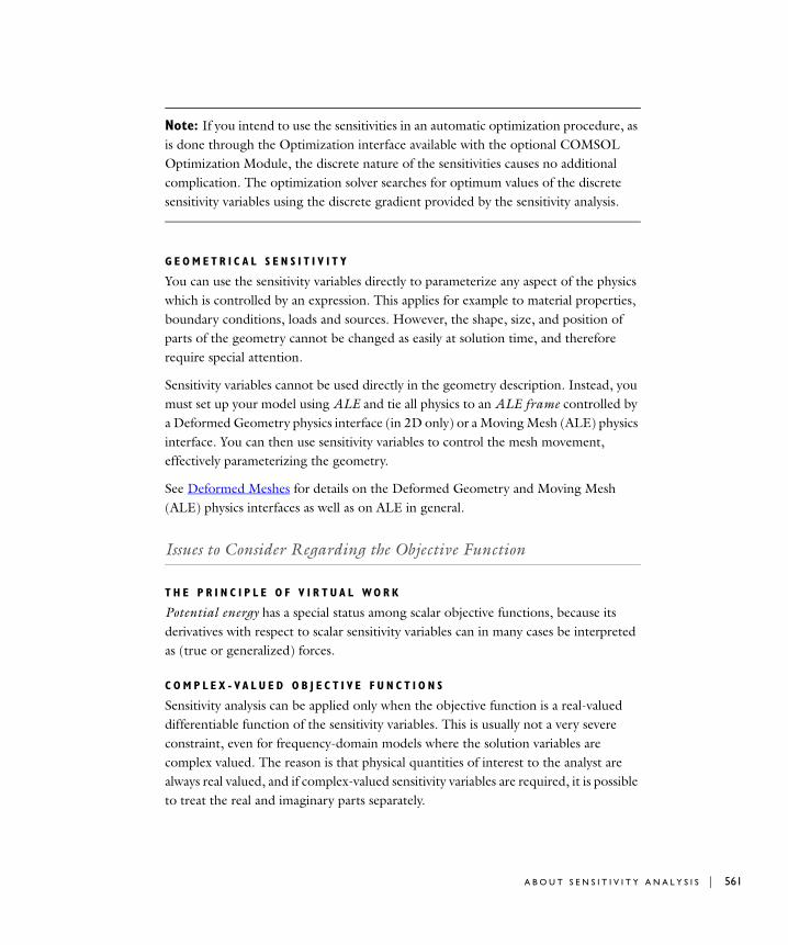
Note: If you intend to use the sensitivities in an automatic optimization procedure, as is done through the Optimization interface available with the optional COMSOL Optimization Module, the discrete nature of the sensitivities causes no additional complication. The optimization solver searches for optimum values of the discrete sensitivity variables using the discrete gradient provided by the sensitivity analysis.
G E O M E T R I C A L S E N S I T I V I T Y
You can use the sensitivity variables directly to parameterize any aspect of the physics which is controlled by an expression. This applies for example to material properties, boundary conditions, loads and sources. However, the shape, size, and position of parts of the geometry cannot be changed as easily at solution time, and therefore require special attention.
Sensitivity variables cannot be used directly in the geometry description. Instead, you must set up your model using ALE and tie all physics to an ALE frame controlled by a Deformed Geometry physics interface (in 2D only) or a Moving Mesh (ALE) physics interface. You can then use sensitivity variables to control the mesh movement, effectively parameterizing the geometry.
See Deformed Meshes for details on the Deformed Geometry and Moving Mesh (ALE) physics interfaces as well as on ALE in general.
Issues to Consider Regarding the Objective Function
T H E P R I N C I P L E O F V I R T U A L WO R K
Potential energy has a special status among scalar objective functions, because its derivatives with respect to scalar sensitivity variables can in many cases be interpreted as (true or generalized) forces.
C O M P L E X - V A L U E D O B J E C T I V E F U N C T I O N S
Sensitivity analysis can be applied only when the objective function is a real-valued differentiable function of the sensitivity variables. This is usually not a very severe constraint, even for frequency-domain models where the solution variables are complex valued. The reason is that physical quantities of interest to the analyst are always real valued, and if complex-valued sensitivity variables are required, it is possible to treat the real and imaginary parts separately.
A B O U T S E N S I T I V I T Y A N A L Y S I S | 561

562 | C H A P T E
Many common quantities of interest are time averages which can be written in the form Qreala·conjb, where a and b are complex-valued linear functions of the solution variables and therefore implicit functions of the sensitivity variables. The problem with this expression is that while Q is indeed a real-valued differentiable function of the sensitivity variables, it is not an analytical function of a and b. This complicates matters slightly because the sensitivity solver relies on partial differentiation and the chain rule.
While the partial derivatives of Q with respect to a and b are, strictly speaking, undefined, it can be proven that if they are chosen such that
(16-1)
for any small complex increments a and b, the final sensitivities are evaluated correctly. The special function realdot(a,b) is identical to real(a*conj(b)) when evaluated but implements partial derivatives according to Equation 16-1. For that reason, use it in the definition of any time-average quantity set as objective function in a sensitivity analysis.
Adding Sensitivity
You can add a Sensitivity interface ( ) when creating a new model or at any time during modeling. For a new model, you select physics interfaces as the second step in the Model Wizard (after specifying the space dimension). In an active model, right-click the model node in the Model Tree and choose Add Physics. In both cases, the Add
Physics page appears with a list of physics interfaces and mathematical interfaces. Take the following steps to add a Sensitivity interface to the model:
1 Expand the Mathematics>Optimization and Sensitivity node in the list of physics interfaces.
2 Select Sensitivity.
3 Click the Add Selected button ( ) underneath the list to add the selected physics interface to the model. The physics interface then appears in the list under Selected
physics.
4 When you are ready click the Next button ( ) in the upper-right corner of the Model Wizard window.
5 Optionally, choose an study type for the sensitivity analysis on the Select Study Type page.
Q a a+ b b+ Q a b a
Q ab
Q b+ real+
R 1 6 : S E N S I T I V I T Y A N A L Y S I S

6 Click the Finish button ( ) in the upper-right corner of the Model Wizard window.
The Sensitivity Interface
The Sensitivity interface ( ) provides the tools for defining and solving sensitivity problems. For a more extensive introduction to the mathematics implemented by this interface, see Sensitivity Analysis in the General Case.
You can define objective functions and constraints in terms of components of the control and auxiliary variable (the latter is given as the solution to the differential equations defined by the multiphysics model) and restrict these to specific domains or make them globally available. This flexibility is reflected in the user interface by grouping these settings according to the dimension of the domain to which they apply. In such group of settings you have the possibility to specify the following settings, to each of which corresponds a separate feature and its Settings window:
• Integral Objective
• Probe Objective
• Control Variable Field
I N T E R F A C E I D E N T I F I E R
This is the identifier for the physics interface, which you use to reach the fields and variables in expressions, for example.
The identifier appears in the Identifier edit field, and you can change it to any unique string that is a valid identifier. The default identifier (for the first Sensitivity interface in the model) is sens.
D O M A I N S
In this section you select the domains containing the control variables and expressions that enter into the formulation of the optimization problem. The default setting is to include all domains in the model. For information about selecting domains, see Selecting and Deselecting Geometric Entities.
Integral Objective
An integral objective is defined as the integral of a closed form expression of those components of the control and auxiliary variable (the latter is given as the solution to the differential equations defined by the multiphysics model) that are either global or available in the domain in question. Hence, its definition is restricted to a specific
A B O U T S E N S I T I V I T Y A N A L Y S I S | 563
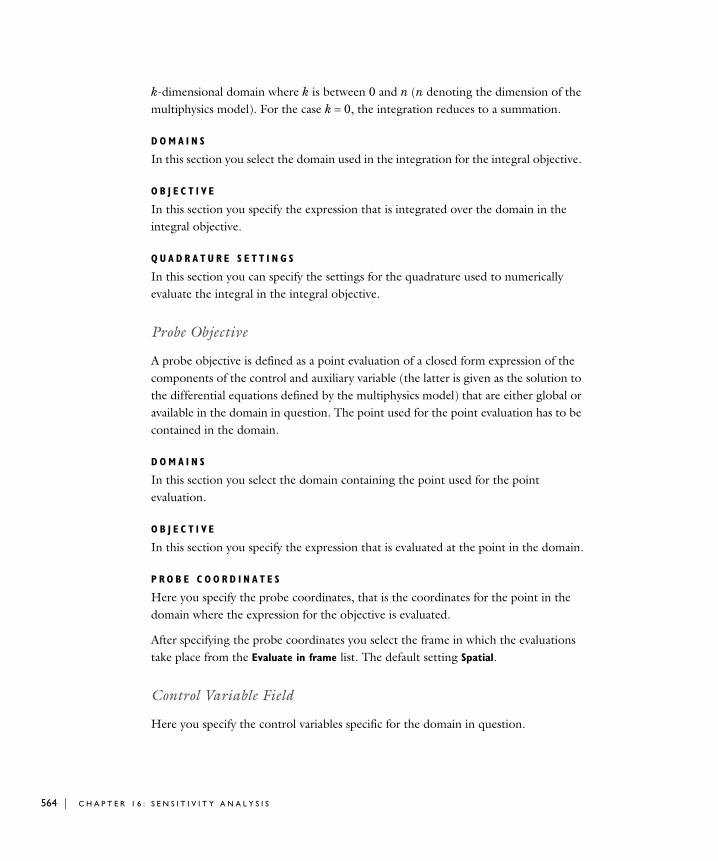
564 | C H A P T E
k-dimensional domain where k is between 0 and n (n denoting the dimension of the multiphysics model). For the case k0, the integration reduces to a summation.
D O M A I N S
In this section you select the domain used in the integration for the integral objective.
O B J E C T I V E
In this section you specify the expression that is integrated over the domain in the integral objective.
Q U A D R A T U R E S E T T I N G S
In this section you can specify the settings for the quadrature used to numerically evaluate the integral in the integral objective.
Probe Objective
A probe objective is defined as a point evaluation of a closed form expression of the components of the control and auxiliary variable (the latter is given as the solution to the differential equations defined by the multiphysics model) that are either global or available in the domain in question. The point used for the point evaluation has to be contained in the domain.
D O M A I N S
In this section you select the domain containing the point used for the point evaluation.
O B J E C T I V E
In this section you specify the expression that is evaluated at the point in the domain.
P R O B E C O O R D I N A T E S
Here you specify the probe coordinates, that is the coordinates for the point in the domain where the expression for the objective is evaluated.
After specifying the probe coordinates you select the frame in which the evaluations take place from the Evaluate in frame list. The default setting Spatial.
Control Variable Field
Here you specify the control variables specific for the domain in question.
R 1 6 : S E N S I T I V I T Y A N A L Y S I S

D O M A I N S
In this section you select the domain where the control variable is defined.
C O N T R O L V A R I A B L E
In this section you start out by providing the name and initial value of the control variable.
Next, you can specify the order of the shape functions used to discretize the control variable. The default is to use second-order Lagrange elements.
After specifying the order of the shape functions you select the frame in which the derivatives are to be evaluated from the Define derivatives with respect to frame list. The default setting Spatial.
Global Objective
Here you specify the global contribution to the objective function.
O B J E C T I V E
In this section you specify the expression that defines the contribution to the objective function. It can be an expression of those components of the control and auxiliary variable (the latter is given as the solution to the differential equations defined by the multiphysics model) that are globally available.
Global Control Variables
Here you specify those components of the control variable that are globally available.
C O N T R O L V A R I A B L E S
In the table that follows you list the names, initial values, upper bounds and lower bounds of those components of the control variable that are globally available. To specify equality constraints, simply make sure the upper and lower bounds have the same value.
A B O U T S E N S I T I V I T Y A N A L Y S I S | 565

566 | C H A P T E
R 1 6 : S E N S I T I V I T Y A N A L Y S I S
17
O p t i m i z a t i o n
With a license for the Optimization Module you get access to the Optimization interface in COMSOL Multiphysics. The Optimization interface is designed to facilitate setting up and solving optimization problems.
In this section:
• Overview of Optimization provides a quick introduction to the theory and terminology of optimization.
• The Optimization Interface describes all available features and their components in the COMSOL Desktop.
Note: The Optimization interface requires the Optimization Module.
567

568 | C H A P T E
Ove r v i ew o f Op t im i z a t i o n
Introduction
Simulation is a powerful tool in science and engineering for predicting the behavior of physical systems, particularly those governed by partial differential equations. In many cases a single or a few simulations are not enough to provide sufficient understanding of a system. Two important classes of problems whose resolution relies on a more systematic exploratory process are:
• Design problems with a single objective. Here, the problem is to find the values of some decision variables that yield the best performance of the output of a simulation model when the latter is quantified by means of a single function. Problems of this kind arise in structural optimization, antenna design, and process optimization.
• Inverse problems, and in particular parameter estimation in PDEs. Here, the problem is to reliably determine the values of a set of parameters that provide simulated data which best matches measured data. Such problems arise in geophysical imaging, nondestructive testing, biomedical imaging, and weather data assimilations.
It is often possible to reformulate problems of the above type as optimization problems. The Optimization interface in COMSOL Multiphysics is useful for solving design problems as well as inverse problems and parameter estimation.
Basic Optimization Concepts
In general there are two fundamental parts of an optimization problem:
• The control variable
• The objective function
The task is now to find the value of the control variable that minimizes (or maximizes) the objective function subject to a number of constraints. The constraints collectively define a set, feasible set, of permissible values for the control variable.
The control variable can be a scalar, a vector, or even an element in some infinite-dimensional function space. In the mathematical and engineering literature, the control variable is sometimes also referred to as the optimization variable or decision variable. Alternative, and frequently occurring, terminology used for the objective function is cost function, goal function, or quantity of interest.
R 1 7 : O P T I M I Z A T I O N

For design problems, the objective function is the aforementioned function quantifying the performance and the control variable is for such problems referred to as the decision variables. For parameter estimation in PDEs, the objective function defines a robust quantifier for how well simulated data matches measured data and the optimization variables are the parameters that are to be determined. The control variable is the unknown parameter in the parameter estimation problem that is to be recovered.
The Optimization interface provides a framework for specifying and solving optimization problems. The objective function and constraints can depend implicitly on the control variable by means of multiphysics models. For more information about the Optimization interfaces and its features, see The Optimization Interface.
Optimization Problem Formulation
The Optimization interface is built around a general formulation of a minimization problem (to perform maximization, simply minimize the negative of the objective function). You specify the objective function that is to be minimized and the constraints that apply on the control variable.
T H E G E N E R A L O P T I M I Z A T I O N P R O B L E M
The general formulation of an optimization problem can be written as
(17-1)
Here, the control variable is denoted by the scalar valued objective function by Q, and the feasible set, denoted by C, is assumed to be given by means of inequality constraints
where G is a vector-valued function (G is scalar-valued in case of a single constraint).
Note: For vectorial quantities, the inequality defining C is to be interpreted component-wise and lb and ub are the corresponding vectors containing the upper and lower bounds.
min Q
C
C : lb G ub =
O V E R V I E W O F O P T I M I Z A T I O N | 569

570 | C H A P T E
C L A S S I C A L O P T I M I Z A T I O N
In classical optimization, Q and G are given explicitly as closed-form expressions of the control variable . However, design and parameter estimation problems mentioned before often result in objective functions Q and constraints G that are not explicitly expressible by closed-form expressions of the control variable .
S I M U L A T I O N O P T I M I Z A T I O N
Simulation optimization problems refer to the case where Q or G are not given solely in terms of explicit expressions in the control variable Such optimization problems arise especially when the response of the system against variations in the control variable is modeled by (partial) differential equations, thereby precluding the possibility to use explicit closed-form expression for the objective function and constraints. In such cases it is valuable to single out the parts of the objective function Q and constraints G that are given implicitly from those that are explicit in . To do this, introduce an auxiliary variable u, which again can be scalar or vector-valued, encoding the implicit relation to . Now, the objective function Q and constraints G are explicitly expressible in terms of u and and the simulation optimization problem can be rephrased as classical optimization problem where the control variable is un many cases, the implicit relation of u to is given as by a system of equations Lu0.
P D E - C O N S T R A I N E D O P T I M I Z A T I O N
The system of equations Lu0 is often given as a system of differential equations, which in turn are defined through the general multiphysics model used for simulating the physical system in question. In such case, the simulation optimization problem is often referred to as PDE-constrained optimization.
The Optimization interface provides tools to define and solve general PDE-constrained optimization problems that are given as
(17-2)
It is advantageous to single out those constraints given by G that are defined as explicit expressions of only, and those that mix u and . Hence, the general constraint formulation lbGuub above is replaced by two classes of constraints:
min Q u
L u 0=
lb G u ub
R 1 7 : O P T I M I Z A T I O N
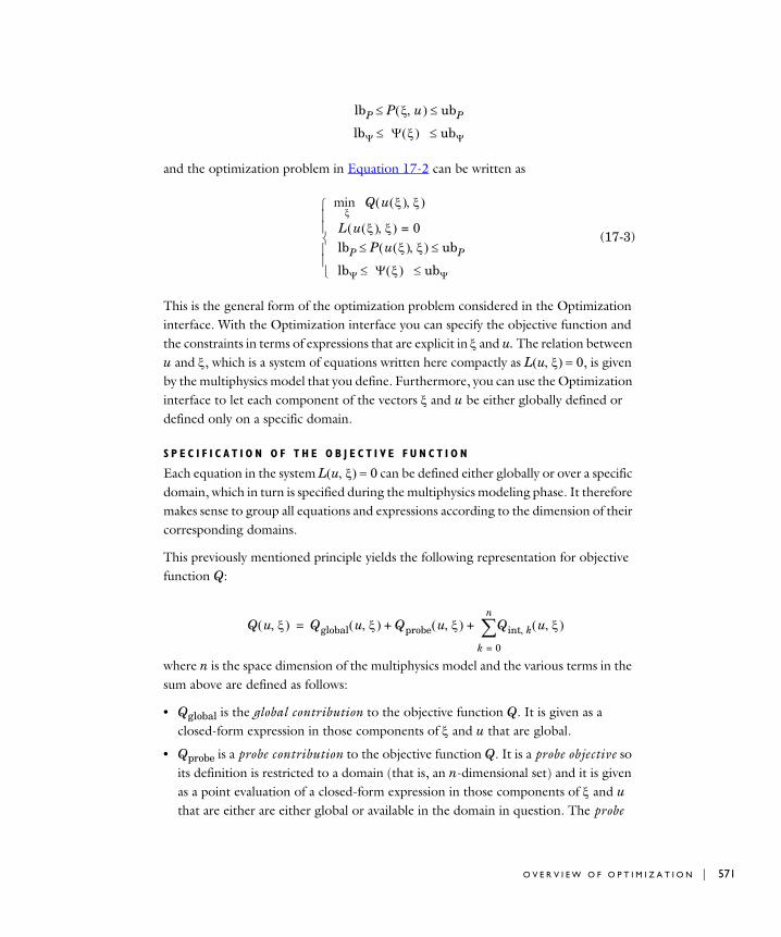
and the optimization problem in Equation 17-2 can be written as
(17-3)
This is the general form of the optimization problem considered in the Optimization interface. With the Optimization interface you can specify the objective function and the constraints in terms of expressions that are explicit in and u. The relation between u and , which is a system of equations written here compactly as Lu0, is given by the multiphysics model that you define. Furthermore, you can use the Optimization interface to let each component of the vectors and u be either globally defined or defined only on a specific domain.
S P E C I F I C A T I O N O F T H E O B J E C T I V E F U N C T I O N
Each equation in the system Lu0 can be defined either globally or over a specific domain, which in turn is specified during the multiphysics modeling phase. It therefore makes sense to group all equations and expressions according to the dimension of their corresponding domains.
This previously mentioned principle yields the following representation for objective function Q:
where n is the space dimension of the multiphysics model and the various terms in the sum above are defined as follows:
• Qglobal is the global contribution to the objective function Q. It is given as a closed-form expression in those components of and u that are global.
• Qprobe is a probe contribution to the objective function Q. It is a probe objective so its definition is restricted to a domain (that is, an n-dimensional set) and it is given as a point evaluation of a closed-form expression in those components of and u that are either are either global or available in the domain in question. The probe
lbP P u ubP
lb ub
min
Q u
L u 0=
lbP P u ubP
lb ub
Q u Qglobal u Qprobe u Qint k u
k 0=
n
+ +=
O V E R V I E W O F O P T I M I Z A T I O N | 571
572 | C H A P T E
point used for the point evaluation is a point given by the user and has to be contained in the domain.
• Qint,k is an integral contribution to the objective function Q. It is an integral objective so its definition is restricted to a specific k-dimensional domain where k is between 0 and n. It is given as the integral of a closed-form expression in those components of and u that are either global or available in the domain in question. For the case k0, the integration reduces to a summation.
It is possible to define several global, probe, and integral contributions. In such case, the total global, probe, and integral contribution is the sum of the aforementioned global, probe, and integral contributions that you actively select in the solver settings for the optimization.
S P E C I F I C A T I O N O F T H E C O N S T R A I N T S
As already mentioned, the constraints lbGuub in the general PDE-constrained optimization problem in Equation 17-2 are written as
The first row above constitutes the implicit constraints, which are given in terms of expressions involving both the auxiliary variable u and control variable The second row constitutes the explicit constraints that are those constraints given by explicit expressions only in the control variable .
Note: The motivation for this subdivision is computational. To properly account for implicit constraints within an optimization scheme is computationally expensive whereas the explicit constraints are much easier. As an example, in gradient-based optimization methods the successive iterates in the optimization depend on the sensitivities of the auxiliary variable u with respect to the control variable . To calculate this sensitivity is computationally demanding, see Methods for Performing Sensitivity Analysis.
Furthermore, the Optimization interface differs between thee following constraints (in the description that follows, n denotes the dimension of the multiphysics model):
lbP P u ubP
lb ub
R 1 7 : O P T I M I Z A T I O N
bound constraints, pointwise inequality constraints, and integral inequality constraints, each of which are described below
• Bound constraints, also called control variable bounds, are constraints defined for a specific k-dimensional domain where k is between 0 and n. A bound constraint is a restriction to the values of the control variable at all points in the k-dimensional domain. Hence, bound constraints correspond to constraints of the form lbub where the constraint is to be interpreted component-wise for vectorial quantities.
• Pointwise inequality constraints are restrictions to the values of a closed-form expression at all points in a specific k-dimensional domain where k is between 0 and n. The expression is a closed-form expression in those components of and u that are either global or available in the k-dimensional domain in question.
• Integral inequality constraints are restrictions to the values of the integral of a closed form expression taken over a specific k-dimensional domain where k is between 0 and n. The expression is a closed form expression in those components of and u that are either global or available in the domain in question. For the case k0, the integration reduces to a summation.
Note: The pointwise inequality constraint is actually one constraint for each point in the k-dimensional domain. The exact finite ensemble of points used to represent the continuum of such points in the k-dimensional domain is given by the node points. In almost all cases of interest there are a large number of node points, so a pointwise inequality constraint results in a large number of inequality constraints. Implicit constraints are computationally very expensive to account for, so even though the Optimization interface makes it possible to specify pointwise inequality constraints that are implicit, and even though such constraints do make sense from a mathematical (and perhaps also physics) point of view, in the actual computations ignore such constraints.
Methods for Solving Classical Optimization Problems
In the previous section the focus was on specifying which optimization problem to solve rather than how to solve it. This section describes the methods for how to solve the optimization problem.
O V E R V I E W O F O P T I M I Z A T I O N | 573
574 | C H A P T E
T H E G E N E R A L P D E - C O N S T R A I N E D O P T I M I Z A T I O N P R O B L E M
The approach taken by the Optimization interface in solving a general PDE-constrained optimization problem can be subdivided into two main steps.
1 Recast the PDE-constrained optimization problem into a classical optimization problem.
2 Solve the classical optimization problem.
The general PDE-constrained optimization problem that is to be solved is reformulated as a classical optimization problem, which in general form can be formulated as in Equation 17-3. The focus here is on how to perform (and configure) the second step.
G R A D I E N T - B A S E D M E T H O D S
Solving the equation Lu0 in the optimization problem Equation 17-3, which relates the auxiliary variable u to the control variable , can be quite costly, which in turn implies that evaluation of the objective and implicit constraints can be costly. Therefore, it is advantageous to select an algorithm for solving that minimizes the number of such evaluations.
It is well-known that gradient-based methods are the preferred methods in cases when the objective and constraints are expensive to evaluate because such methods often require a minimum number of evaluations of the objective function and constraints. However, usage of gradient-based methods requires that the objective and constraints have certain smoothness properties that are stated below:
• The equation Lu0 has a unique solution for all u in the relevant domain.
• The objective and constraints are twice continuously differentiable with respect to both and u on an open set.
• The inverse uLu exists for all u in an open set.
A central part in all gradient-based methods is the accurate and efficient calculation of the derivative of the auxiliary variable u with respect to the control variable when they are related to each other by a system of differential equations Lu0. This highly technical and nontrivial issue is automatically taken care of by the Optimization interface and is described in Methods for Solving Classical Optimization Problems.
The Optimization interface calls an external optimization software module, SNOPT (Sparse Nonlinear OPTimizer), for solving Equation 17-3. Below is a brief description of how SNOPT works.
R 1 7 : O P T I M I Z A T I O N
S Q P M E T H O D S A N D S N O P T
Sequential quadratic programming (SQP) methods have proved highly effective for solving constrained classical optimization problems with smooth nonlinear functions in the objective and constraints.
The idea of SQP methods is to solve the nonlinearly constrained problem, such as the one in Equation 17-3, using a sequence of quadratic programming (QP) subproblems. The constraints of each QP subproblem are linearizations of the constraints in the original problem, and the objective function of the subproblem is a quadratic approximation to the Lagrangian function of Equation 17-3:
Note that the dimension of the vector equals the number of user defined constraints. The dimension of the vector equals the dimension of the solution vector u to the system of differential equations Lu0 given by the Multiphysics model.
SNOPT is the implementation of a particular SQP algorithm that exploits sparsity in the constraint Jacobian and maintains a limited-memory quasi-Newton approximation to the Hessian of the above Lagrangian. A new method is used to update Hessian in the presence of negative curvature which is the case whenever Equation 17-3 is nonconvex. The QP subproblems are solved using an inertia-controlling reduced-Hessian active-set method (SQOPT) that allows for variables appearing linearly in the objective and constraint functions (in which case the limited-memory Hessian is semi-definite). Other features include the treatment of infeasible nonlinear constraints using elastic programming, use of a well-conditioned nonorthogonal basis for the null-space of the QP working set (assisted by sparse rank-revealing LU factors), early termination of the QP subproblems, and whenever necessary, finite-difference estimates of missing gradients. The method used by the QP solver SQOPT is based on solving a sequence of linear systems involving a reduced Hessian based on a sparse LU factorization. See References for a more detailed description of SNOPT.
R E F E R E N C E S
1. P.E. Gill, W. Murray, and M.A. Saunders, User’s Guide for SNOPT Version 7: Software for Large-Scale Nonlinear Programming, Systems Optimization Laboratory (SOL), Stanford University, 2006.
2. P.E. Gill, W. Murray, and M.A. Saunders, SNOPT: An SQP Algorithm for Large-Scale Constrained Optimization, SIAM Review, vol. 47, no. 1, pp. 99–13, 2005.
Q u P u L u ++=
O V E R V I E W O F O P T I M I Z A T I O N | 575
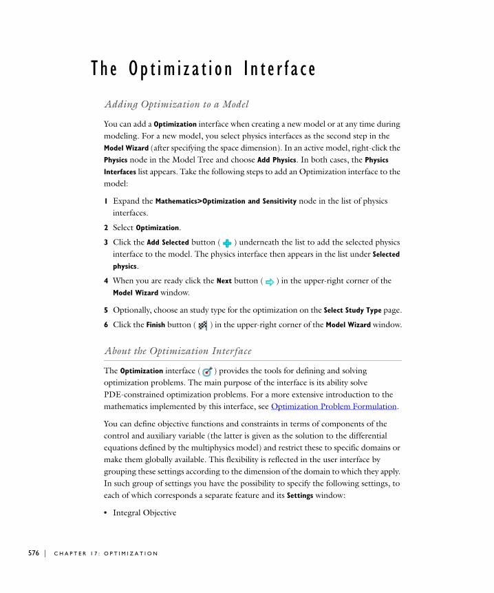
576 | C H A P T E
Th e Op t im i z a t i o n I n t e r f a c e
Adding Optimization to a Model
You can add a Optimization interface when creating a new model or at any time during modeling. For a new model, you select physics interfaces as the second step in the Model Wizard (after specifying the space dimension). In an active model, right-click the Physics node in the Model Tree and choose Add Physics. In both cases, the Physics
Interfaces list appears. Take the following steps to add an Optimization interface to the model:
1 Expand the Mathematics>Optimization and Sensitivity node in the list of physics interfaces.
2 Select Optimization.
3 Click the Add Selected button ( ) underneath the list to add the selected physics interface to the model. The physics interface then appears in the list under Selected
physics.
4 When you are ready click the Next button ( ) in the upper-right corner of the Model Wizard window.
5 Optionally, choose an study type for the optimization on the Select Study Type page.
6 Click the Finish button ( ) in the upper-right corner of the Model Wizard window.
About the Optimization Interface
The Optimization interface ( ) provides the tools for defining and solving optimization problems. The main purpose of the interface is its ability solve PDE-constrained optimization problems. For a more extensive introduction to the mathematics implemented by this interface, see Optimization Problem Formulation.
You can define objective functions and constraints in terms of components of the control and auxiliary variable (the latter is given as the solution to the differential equations defined by the multiphysics model) and restrict these to specific domains or make them globally available. This flexibility is reflected in the user interface by grouping these settings according to the dimension of the domain to which they apply. In such group of settings you have the possibility to specify the following settings, to each of which corresponds a separate feature and its Settings window:
• Integral Objective
R 1 7 : O P T I M I Z A T I O N

• Probe Objective
• Integral Inequality Constraint
• Pointwise Inequality Constraint
• Control Variable Field (which includes the settings for the associated bound constraints)
I N T E R F A C E I D E N T I F I E R
This is the identifier for the physics interface, which you use to reach the fields and variables in expressions, for example.
The identifier appears in the Identifier edit field, and you can change it to any unique string that is a valid identifier. The default identifier (for the first Optimization interface in the model) is opt.
D O M A I N S
In this section you select the domains containing the control variables and expressions that enter into the formulation of the optimization problem. The default setting is to include all domains in the model.
Integral Objective
An integral objective is defined as the integral of a closed form expression of those components of the control and auxiliary variable (the latter is given as the solution to the differential equations defined by the multiphysics model) that are either global or available in the domain in question. Hence, its definition is restricted to a specific k-dimensional domain where k is between 0 and n (n denoting the dimension of the multiphysics model). For the case k0, the integration reduces to a summation.
D O M A I N S
SelectionIn this section you select the domain used in the integration for the integral objective.
O B J E C T I V E
Objective ExpressionIn this section you specify the expression that is integrated over the domain in the integral objective.
T H E O P T I M I Z A T I O N I N T E R F A C E | 577

578 | C H A P T E
Q U A D R A T U R E S E T T I N G S
In this section you can specify the settings for the quadrature used to numerically evaluate the integral in the integral objective.
Probe Objective
A probe objective is defined as a point evaluation of a closed form expression of the components of the control and auxiliary variable (the latter is given as the solution to the differential equations defined by the multiphysics model) that are either global or available in the domain in question. The point used for the point evaluation has to be contained in the domain.
D O M A I N S
SelectionSelect the domain containing the point used for the point evaluation.
O B J E C T I V E
Objective ExpressionSpecify the expression that is evaluated at the point in the domain.
P R O B E C O O R D I N A T E S
Probe CoordinatesSpecify the probe coordinates, that is the coordinates for the point in the domain where the expression for the objective is evaluated.
Evaluate in FrameAfter specifying the probe coordinates you select the frame in which the evaluations take place from the Evaluate in frame list. The default setting Spatial.
Integral Inequality Constraints
Integral inequality constraints are given as restrictions to the values of the integral of a closed form expression taken over a specific k-dimensional domain where k is between 0 and n (n denoting the dimension of the multiphysics model). The expression is a closed form expression of those components of the control and auxiliary variable (the latter is given as the solution to the differential equations defined by the multiphysics model) that are either global or available in the domain in question. For the case k0, the integration reduces to a summation.
R 1 7 : O P T I M I Z A T I O N

D O M A I N S
SelectionIn this section you select the domain used in the integration for the integral objective.
C O N S T R A I N T
Constraint expressionIn the Constraint expression edit field you specify the expression that is integrated over the domain in the integral inequality constraint.
Q U A D R A T U R E S E T T I N G S
In this section you can specify the settings for the quadrature used to numerically evaluate the integral in the integral objective.
B O U N D S
In this section you can specify the upper and lower bounds for the integral inequality constraint. To specify equality constraints, simply make sure the upper and lower bounds have the same value.
Lower boundSelect the Lower bound check box to activate and provide the lower bound.
Upper boundSelect the Upper bound check box to activate and provide the upper bound.
Pointwise Inequality Constraints
A pointwise inequality constraint is given as a restriction to the values of a closed form expression at all points in a specific k-dimensional domain where k is between 0 and n. Due to computational issues, the expression has to be a closed form expression of only the control variable. Furthermore, only those components of the control variable that are either global or available in the domain in question are usable.
D O M A I N S
SelectionIn this section you select the domain over which the point inequality constraint is defined.
T H E O P T I M I Z A T I O N I N T E R F A C E | 579
580 | C H A P T E
C O N S T R A I N T
Constraint ExpressionIn this section you specify the expression whose values at all points in the domain are to be constrained.
S H A P E F U N C T I O N
Shape FunctionIn this section you can specify the order of the shape functions used to discretize the control variable. The default is to use second-order Lagrange elements.
Define Derivatives With Respect To FrameHere you select the frame in which the derivatives are to be evaluated from the Define
derivatives with respect to frame list. The default setting Spatial.
B O U N D S
In this section you can specify the upper and lower bounds for the pointwise inequality constraint. To specify equality constraints, simply make sure the upper and lower bounds have the same value.
Lower BoundSelect the Lower bound check box to activate and provide the lower bound.
Upper BoundSelect the Upper bound check box to activate and provide the upper bound.
Control Variable Field
Here you specify the control variables specific for the domain in question.
D O M A I N S
SelectionIn this section you select the domain where the control variable is defined.
C O N T R O L V A R I A B L E
In this section you specify the control variables.
Control Variable NameProvide the name of the control variable.
R 1 7 : O P T I M I Z A T I O N

Initial ValueProvide the initial value of the control variable.
Shape FunctionSpecify the order of the shape functions used to discretize the control variable. The default is to use second-order Lagrange elements.
Define Derivatives with Respect to FrameSelect the frame in which the derivatives are to be evaluated from the Define derivatives
with respect to frame list. The default setting is Spatial.
Control Variable Bounds
This feature is an attribute of the control variable feature and allows the user to specify the bounds for the bound constraint applied to the control variable in question.
D O M A I N S
SelectionIn this section you can further restrict the domain where the control variable is defined.
B O U N D S
In this section you can specify the upper and lower bounds for the bound constraint applied to the control variable in question. To specify equality constraints, simply make sure the upper and lower bounds have the same value.
Lower boundSelect the Lower bound check box to activate and provide the lower bound.
Upper boundSelect the Upper bound check box to activate and provide the upper bound.
Global Objective
Here you specify the global contribution to the objective function.
O B J E C T I V E
Objective ExpressionIn this section you specify the expression that defines the contribution to the objective function. It can be an expression of those components of the control and auxiliary
T H E O P T I M I Z A T I O N I N T E R F A C E | 581

582 | C H A P T E
variable (the latter is given as the solution to the differential equations defined by the multiphysics model) that are globally available.
Global Inequality Constraint
Here you specify the pointwise inequality constraint that applies globally. Due to computational issues, the expression has to be a closed form expression of only the control variable. Furthermore, only those components of the control variable that are global are usable.
C O N S T R A I N T
Constraint expressionIn the Constraint expression edit field you specify the expression whose values at all points in all domains are to be constrained.
B O U N D S
In this section you can specify the upper and lower bounds for the pointwise constraint applied to the expression in question. To specify equality constraints, simply make sure the upper and lower bounds have the same value.
Lower boundSelect the Lower bound check box to activate and provide the lower bound.
Upper boundSelect the Upper bound check box to activate and provide the upper bound.
Global Control Variables
Here you specify those components of the control variable that are globally available.
C O N T R O L V A R I A B L E S
In the table that appears in this section you list the variable names, initial values, lower bounds, and upper bounds of those components of the control variables that are globally available. To specify equality constraints, simply make sure the upper and lower bounds have the same value.
To add a control variable to the table, click the Add button ( ). To remove a control variable and its values from the table, click the Delete button ( ).
R 1 7 : O P T I M I Z A T I O N

18
M e s h i n g
This section summarizes how to create and control your mesh for 1D, 2D, and 3D geometries in COMSOL Multiphysics. It also explains the possibilities for importing and exporting meshes in different formats.
In this section:
• Mesh Elements
• Meshing Techniques
• Free Meshing in 2D
• Mapped Meshing in 2D
• Converting Meshes in 2D
• Creating Boundary Layer Meshes
• Free Tetrahedral Meshing in 3D
• Creating 3D Swept Meshes
583

584 | C H A P T E
C r e a t i n g Me s h e s
A mesh is a discretization of the geometry model into small units of simple shapes, referred to as mesh elements.
Mesh Elements
E L E M E N T S F O R 1 D G E O M E T R I E S
The mesh generator discretized the domains (intervals) into smaller intervals (or mesh elements). The endpoints of the mesh elements are called mesh vertices.
The boundaries (or vertices) defined in the geometry are represented in the mesh by boundary elements (or vertex elements).
E L E M E N T S F O R 2 D G E O M E T R I E S
The mesh generator discretizes the domains into triangular or quadrilateral mesh elements. If the boundary is curved, these elements represent only an approximation of the original geometry. The sides of the triangles and quadrilaterals are called mesh edges, and their corners are mesh vertices. A mesh edge must not contain mesh vertices in its interior.
The boundaries defined in the geometry are discretized (approximately) into mesh edges, referred to as boundary elements (or edge elements), which must conform with the mesh elements of the adjacent domains.
The geometry vertices are represented by vertex elements.
E L E M E N T S F O R 3 D G E O M E T R I E S
The mesh generator discretizes the domains into tetrahedral, hexahedral, prism, or pyramid mesh elements whose faces, edges, and corners are called mesh faces, mesh edges, and mesh vertices, respectively.
The boundaries in the geometry are discretized into triangular or quadrilateral boundary elements.
The geometry edges are discretized into edge elements.
Similar to 2D, the geometry vertices are represented by vertex elements.
R 1 8 : M E S H I N G
Pyramid ElementsPyramid elements appear in the mesh in the following situations.
• If you import a NASTRAN file containing pyramid elements.
• If you create a swept mesh where the source and destination faces share an edge and the source face contains a triangular mesh.
• If you convert a quad mesh to a triangular mesh for a face adjacent to a domain that contains a mesh.
• If you create a boundary layer mesh in 3D for a geometry with sharp edges.
Meshing Techniques
The following meshing techniques for creating a mesh are available in COMSOL Multiphysics:
• Free meshing
• Mapped meshing
• Boundary layer meshing
• Swept meshing
The mesh generator used for free meshing, also referred to as the free mesher, is the only mesher that can be used on all types of geometry objects.
2 D A N D 3 D M E S H I N G O P T I O N S
In a 2D geometry, choose between:
• Free meshing generating an unstructured mesh with triangular elements (see Free Meshing in 2D)
• Free meshing generating an unstructured mesh with quadrilateral elements (see Free Meshing in 2D)
• Mapped meshing generating a structured mesh with quadrilateral elements (see Mapped Meshing in 2D)
Compared to an unstructured mesh the interior mesh vertices in a structured mesh are adjacent to the same number of elements.
If you want to use mapped meshing on a geometry, you must build the geometry so that the domains are reasonably “regular” in shape and do not contain holes.
C R E A T I N G M E S H E S | 585

586 | C H A P T E
Note: You can create a structured triangular mesh by using the convert operation, which introduces a diagonal edge to each quadrilateral element.
In a 3D geometry, choose between:
• Free meshing generating an unstructured mesh with tetrahedral elements (see Free Tetrahedral Meshing in 3D)
• Swept meshing generating a structured mesh (at least in the direction of the sweep) with prism or hexahedral elements (see Creating 3D Swept Meshes)
• Boundary layer meshing generating structured layers of elements along specific boundaries integrating into an existing structured or unstructured mesh (see Creating Boundary Layer Meshes)
Note: Platforms handle floating-point operations differently, which sometimes results in slight differences between identical model files that are generated on two different computers.
A B O U T F R E E M E S H I N G
The free mesher is available in all dimensions, and you can use it for all types of geometries regardless of their topology or shape. If you have not defined or generated a mesh, the free mesher automatically creates an unstructured mesh and adds a corresponding node to the Model Builder window when you compute a study.
When you use the free mesher:
• The number of mesh elements is determined by the shape of the geometry and various mesh parameters.
• You control mesh parameters for the free mesher by Size and Distribution feature nodes in the meshing sequences.
You can also control the size of the mesh generated by a specific Free Triangular, Free Quadrilateral, or Free Tetrahedral node by adding a Size or Distribution subnode.
R 1 8 : M E S H I N G

A B O U T 2 D M A P P E D M E S H I N G
Geometry Requirements For the 2D mapped meshing technique to work properly, the geometry must be reasonably regular. The following conditions must be satisfied:
• Each domain must be bounded by at least four boundary segments.
• Each domain must be bounded by only one connected boundary component (that is, no holes are allowed).
• The domains must not contain isolated or embedded vertices or boundary segments.
• The shape of each domain must not differ significantly from a rectangle.
For a geometry model that does not initially meet these criteria, it is usually possible to modify it so that a mapped mesh is generated, usually this is done by splitting it into simpler domains.
A B O U T 2 D A N D 3 D B O U N D A R Y L A Y E R M E S H E S
A boundary layer mesh is a mesh with dense element distribution in the normal direction along specific boundaries. This type of mesh is typically used for fluid flow problems in order to resolve the thin boundary layers along the no-slip boundaries.
• In 2D, a layered quadrilateral mesh is used along the specified no-slip boundaries.
• In 3D, the boundary layer mesh is a layered prism mesh or a hexahedral mesh, depending on whether the corresponding boundary-layer boundaries contain a triangular or quadrilateral mesh.
Boundary layer meshes can also be used to resolve large temperature gradients close to heated surfaces subjected to sudden changes over time. In the heat sink model, you can see the introduction of a boundary layer mesh at the surfaces of the inner half-circle arc.
A B O U T 3 D S W E P T M E S H E S
The swept mesher operates on a 3D domain by meshing a source face and then sweeping the resulting face mesh along the domain to an opposite target face. A swept mesh is structured in the sweep direction and can be either structured or unstructured orthogonally to the sweep direction.
For straight and circular sweep paths, you can use several connected faces as source faces. Each face about a domain that is to be operated on by the swept mesher is classified as either a source face, a target face, or a boundary face. The boundary faces
C R E A T I N G M E S H E S | 587
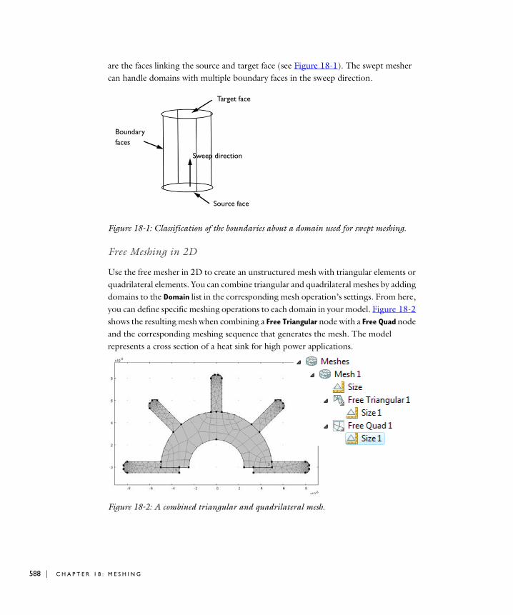
588 | C H A P T E
are the faces linking the source and target face (see Figure 18-1). The swept mesher can handle domains with multiple boundary faces in the sweep direction.
Figure 18-1: Classification of the boundaries about a domain used for swept meshing.
Free Meshing in 2D
Use the free mesher in 2D to create an unstructured mesh with triangular elements or quadrilateral elements. You can combine triangular and quadrilateral meshes by adding domains to the Domain list in the corresponding mesh operation’s settings. From here, you can define specific meshing operations to each domain in your model. Figure 18-2 shows the resulting mesh when combining a Free Triangular node with a Free Quad node and the corresponding meshing sequence that generates the mesh. The model represents a cross section of a heat sink for high power applications.
Figure 18-2: A combined triangular and quadrilateral mesh.
Target face
Source face
Sweep direction
Boundaryfaces
R 1 8 : M E S H I N G

Adding a Free Triangular or a Free Quad node to a 2D Model1 Open a 2D file or create a 2D object.
2 In the Model Builder, right-click Mesh 1 and select Free Triangular or Free Quad.
3 In the Settings window, under the Domains section, select Domain from the Geometric
entity level list.
4 In the Graphics window, left-click and then right-click any or all of the domains to add to the Selection list.
5 If the geometry requires it, you can now control the number of mesh elements along an edge.
Controlling the Number of Elements on EdgesIn this example, Figure 18-2 shows that the two cooling fins at 45 degrees to the horizontal are only meshed with one mesh element at their attachment to the base. Use the Edge operation to fine tune the mesh and to give you control over the number of elements along the edge separating the fins and the base.
1 Insert an Edge operation before the Free Triangular 1 operation to control the mesh at the interface between the base and the fin.
a Click the first Size node.
b Right-click and select Build Selected.
c Right-click Mesh 1 and select Edge from the More Operations submenu.
Note: When inserting a note to the sequence it appears after the current feature. The current feature is indicated by a quadratic frame around its icon. To make a feature become the current feature, select it, right-click, and select Build Selected. You can also move mesh nodes up and down in the sequence by right-clicking and selection Move Up or Move Down (or using the equivalent keyboard shortcuts).
2 In the Graphics window, left-click and then right-click the edges to add to the Selection list.
3 Right-click the Edge node and select Distribution. Note that the Distribution subnode inherits the selection from the Edge node.
4 Click Build Selected. In this example, three mesh elements are generated along the selected edges (Figure 18-3).
C R E A T I N G M E S H E S | 589

590 | C H A P T E
5 To copy an edge mesh from one edge to another:
a Right-click Mesh 1 and select Copy Edge from the More Operations submenu.
b In the Settings window, select the source and destination edge respectively. You can use the Copy Edge mesh operation to define periodic boundary conditions, where the solution on the two periodic boundaries has to be identical.
Figure 18-3: Adding a distribution attribute to an edge.
R 1 8 : M E S H I N G

Mapped Meshing in 2D
Figure 18-4 is an example of the combination of a mapped mesh for the base of a heat sink cross section, and a triangular mesh for the fins.
Figure 18-4: Mesh resulting from a combination of free triangular meshing and mapped quad meshing.
• To create a structured quad mesh on the base, right-click the Mesh node and select Mapped. In the Settings window, select the domain corresponding to the base and click the Build Selected button.
The quad mesh is generated using a mapping technique. For each domain, the mapping algorithm defines a regular grid on a logical unit square and then maps it onto the real geometry using transfinite interpolation.
Converting Meshes in 2D
You can create a structured triangular mesh by using the convert operation, which introduces a diagonal edge to each quadrilateral element.
• In the Model Builder window, right-click the Mesh node and select Convert from the More Operations submenu.
This operation should be placed in the sequence after the Mapped node as in Figure 18-5.
C R E A T I N G M E S H E S | 591

592 | C H A P T E
Figure 18-5: Example of a structured triangular mesh converted from a structured quad mesh.
Creating Boundary Layer Meshes
1 In the Model Builder window, right-click the Mesh node and select Boundary Layers.
2 Under the Boundary Layers node a Boundary Layer Properties node appears where you can select the boundaries where boundary layers should be applied. See Figure 18-6.
Figure 18-6: Adding a boundary layer elements.
R 1 8 : M E S H I N G

Free Tetrahedral Meshing in 3D
A D D I N G A F R E E TE T R A H E D R A L F E A T U R E
1 Open a 3D model or create a 3D model.
2 In the Model Builder, right-click the Mesh node and select Free Tetrahedral.
3 In the Settings window, under the Domains section, select Domain from the Geometric
entity level list.
4 In the Graphics window, left-click and then right-click any or all of the domains to add to the Selection list.
S P E C I F Y I N G T H E M E S H S I Z E
To adapt the mesh for the selected domains, add a Size feature as a subnode to the Free Tetrahedral node created. Otherwise the Size node directly following the main Mesh node governs the mesh-element size for all Free Tetrahedral nodes.
Figure 18-7 shows a meshing sequence consisting of two Free Tetrahedral mesh operations, one for each meshed domain that correspond to pillars in a heat sink geometry. The mesh sizes are assigned as follows:
• The first Size node (under Mesh1) is defined as Extra Coarse, which is selected from the Predefined Element Size list. In this example, the left pillar is selected to have the extra coarse mesh size and this is generated by the first Free Tetrahedral 1 operation.
• The mesh size of the second pillar is defined under the Free Tetrahedral 2 operation, it has its own Size 1 attribute (Coarser), a finer mesh that is also selected from the Predefined Element Size list.
C R E A T I N G M E S H E S | 593

594 | C H A P T E
Figure 18-7: An example of two free tetrahedral meshing sizes.
The difference between the two meshes is based on the following.
To Specify the Size1 In the Model Builder window, click the Size node to display the Settings window.
2 Select Custom in the Element Size section. In the Element Size Parameters section, define the mesh further by entering values in the following fields if required. Also see Figure 18-9.
- Maximum element size: specify the maximum allowed element size.
- Minimum element size: specify the minimum allowed element size. You can use this value to, for example, prevent the generation of many elements around small curved parts of the geometry.
- Maximum element growth rate: determine the maximum rate at which the element size can grow from a region with small elements to a region with larger elements. The value must be greater or equal to one. For example, with a maximum element growth rate of 1.5, the element size can grow by at most 50% (approximately) from one element to another. Figure 18-8 shows the base of the heat sink meshed using different two different element growth rates for otherwise identical settings.
- Resolution of curvature: determine the size of boundary elements compared to the curvature of the geometric boundary. The curvature radius multiplied by the resolution of curvature, which must be a positive scalar, gives the maximum
Extra Coarse
Coarser
R 1 8 : M E S H I N G

allowed element size along the boundary. A lower value gives a finer mesh along curved boundaries.
- Resolution of narrow regions: control the number of layers of elements that are created in narrow regions (approximately). The value must be a non-negative scalar. If the value of this parameter is less than one, the mesh generator might create elements that are anisotropic in size in narrow regions.
Figure 18-8: A comparison of mesh element growth rates in a heat sink.
Element growth rate = 1.9 Element growth rate = 1.1
C R E A T I N G M E S H E S | 595

596 | C H A P T E
Figure 18-9: An example of custom element mesh sizes.
S P E C I F Y I N G M E S H D I S T R I B U T I O N
In addition to customizing the mesh size, you can also add a Distribution attribute to a Free Tetrahedral feature. In the settings for this Distribution, constrain the number of elements for the selected edges. Figure 18-10 shows three heat sink pillars with different mesh sizes and distribution.
Note: The settings in the Distribution attribute overrule the settings in the Size node.
R 1 8 : M E S H I N G

.
Figure 18-10: Specifying element distribution in heat sink pillars.
Creating 3D Swept Meshes
Figure 18-11 shows the 3D swept mesh for a simple geometry but with a layered structure typical for printed circuit boards or MEMS geometries. In such cases, the swept mesh generation presents an alternative to using a free tetrahedral meshing.
Figure 18-11: An example of the layered geometry used for creating a swept mesh.
1 In the Model Builder window, right-click the Mesh node and select Free Triangular from the More Operations submenu to operate at the boundary level.
2 Add the first level boundary to the selection list (see Figure 18-11 for an example of a suitable geometry).
Normal
10 elementsalong edges
Coarser
First level
Second level
Third level
C R E A T I N G M E S H E S | 597

598 | C H A P T E
3 Click Build Selected. The mesh below displays.
4 Right-click the Mesh node and select Swept.
5 Select the domain in the first level.
6 In the Model Builder window, right-click Swept 1 and select Distribution.
7 Enter the Number of elements in the corresponding field (for example 2).
8 Click Build Selected.
9 Right-click the Mesh node and select Free Triangular from the More Operations submenu.
R 1 8 : M E S H I N G

10 Select the boundaries at the second level and click the Build Selected button.
11 Repeat the same swept operations for the first level domains but now for the second level.
12 Mesh the third level boundaries using the Free Triangular mesh operation.
C R E A T I N G M E S H E S | 599
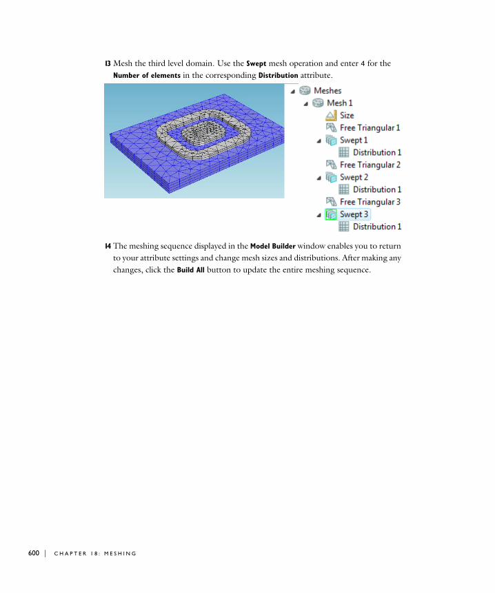
600 | C H A P T E
13 Mesh the third level domain. Use the Swept mesh operation and enter 4 for the Number of elements in the corresponding Distribution attribute.
14 The meshing sequence displayed in the Model Builder window enables you to return to your attribute settings and change mesh sizes and distributions. After making any changes, click the Build All button to update the entire meshing sequence.
R 1 8 : M E S H I N G

19
M u l t i p h y s i c s M o d e l i n g
This section covers the use of COMSOL Multiphysics for multiphysics modeling and coupled-field analyses. It describes various ways of building multiphysics models and provides an overview of the available predefined multiphysics interfaces in COMSOL Multiphysics and the add-on modules.
In this section:
• Multiphysics Modeling Approaches
• Using Predefined Multiphysics Interfaces
• Heat Transfer—Electromagnetic Heating Interfaces
• Structural Mechanics
• Acoustics
• Fluid Flow
• Adding Physics Sequentially
• Building a Multiphysics Model Directly
• Adding Multiphysics Couplings
• Removing Physics Interfaces
601

602 | C H A P T E
S
C r e a t i n g Mu l t i p h y s i c s Mode l s
Multiphysics Modeling Approaches
The ability to create multiphysics models—those with more than one type of physics or equation such as coupled-field problems—is one of COMSOL Multiphysics’ most powerful capabilities. In such a model, the software can solve all the equations, taken from various areas of physics, as one fully coupled system.
Within COMSOL Multiphysics you can choose from several ways to approach multiphysics modeling and coupled-field analysis.
Using Predefined Multiphysics Interfaces
COMSOL Multiphysics and the add-on modules provide a number of predefined multiphysics interfaces. They appear in the Model Wizard’s list of physics interfaces, in folders with the names in the Category/Folder column in Table 19-1. The multiphysics interfaces includes the functionality of two or more physics interfaces with additional features for the multiphysics couplings. Default settings provide the typical field couplings for the multiphysics application. The available multiphysics couplings vary depending on the installed modules (see Table 19-1 for details).
TABLE 19-1: PREDEFINED MULTIPHYSICS COUPLINGS
CATEGORY/ FOLDER NAME SPACE DIMENSION REQUIRED MODULES
OPTIONAL MODULES
Heat Transfer Joule Heating 2D, 2D Axi, 3D None AC/DC, HeatTransfer, MEM
Heat Transfer Induction Heating 2D, 2D Axi, 3D AC/DC Heat Transfer
Heat Transfer Microwave Heating
2D, 2D Axi, 3D RF Heat Transfer
Fluid Flow Fluid-Structure Interaction
2D, 2D Axi, 3D Structural Mechanics or MEMS
CFD
Fluid Flow Non-Isothermal Flow/Conjugate Heat Transfer
2D, 2D Axi, 3D CFD or Heat Transfer
Structural Mechanics
Thermal Stress 2D, 2D Axi, 3D Structural Mechanics or MEMS
Heat Transfer
R 1 9 : M U L T I P H Y S I C S M O D E L I N G

The predefined multiphysics interfaces include all features in the optional modules if your license includes them; otherwise they include the corresponding but more limited physics interface in COMSOL Multiphysics or the required module. The couplings are identical in both cases, but the optional modules typically offer additional functionality in other areas. These predefined multiphysics interfaces are quick entry points for common multiphysics applications. It is possible to create the same couplings using any of the other methods for multiphysics modeling, and you can continue to add, modify, disable, and remove physics interfaces in a model that you start using one of the predefined multiphysics interfaces. If you want to add additional physics interfaces in the Model Builder, right-click the model node, choose Add Physics and then use the Model Wizard that appears.
Heat Transfer—Electromagnetic Heating Interfaces
The multiphysics interfaces in the Electromagnetic Heating section couple electromagnetic fields and heat transfer:
• Joule Heating (part of the COMSOL Multiphysics base package)
• Induction Heating (requires the AC/DC Module)
• Microwave Heating (requires the RF Module)
They appear in the Heat Transfer branch.
J O U L E H E A T I N G
The Joule Heating predefined multiphysics interface ( ) combines all feature from the Electric Currents interface with the Heat Transfer interface for modeling of Joule
Structural Mechanics
Joule Heating and Thermal Expansion
2D, 2D Axi, 3D Structural Mechanics or MEMS
Heat Transfer,AC/DC
Structural Mechanics
Piezoelectric Devices
2D, 2D Axi, 3D Structural Mechanics, MEMS, or Acoustics
Acoustics Acoustic-Structure Interaction
2D, 2D Axi, 3D Acoustics Structural Mechanics, MEMS
TABLE 19-1: PREDEFINED MULTIPHYSICS COUPLINGS
CATEGORY/ FOLDER NAME SPACE DIMENSION REQUIRED MODULES
OPTIONAL MODULES
C R E A T I N G M U L T I P H Y S I C S M O D E L S | 603

604 | C H A P T E
heating (resistive heating or ohmic heating). The interaction is coupled in both directions:
• The resistive heating appears as a heat source in the default Electromagnetic Heat
Source node.
• The default setting is to use the value for the electric conductivity from the material. By selecting Linearized resistivity from the list, the following temperature-dependent expression describes the electric conductivity: 1/(0(1(T Tref))), where T is the dependent variable for temperature from the heat transfer part, which automatically appears as a model input. By default, the values for 0 (resistivity at reference temperature), (temperature coefficient), and Tref (reference temperature) are taken from the material. These settings are built into the Joule Heating Model node, which is the central feature in the Joule Heating interface.
You can use a stationary or time-dependent study.
For an example of a model using the Joule Heating predefined multiphysics coupling, see the thermal_actuator_jh model in the Multiphysics folder of the COMSOL Multiphysics Model Library.
I N D U C T I O N H E A T I N G
The Induction Heating predefined multiphysics interface ( ) combines the features of the Induction Currents interface with those of the Heat Transfer interface. The predefined interaction adds the resistive heating from the induction currents as a heat source.
For more information, see the AC/DC Module User’s Guide.
M I C R O W A V E H E A T I N G
The Microwave Heating predefined multiphysics interface ( ) combines the features of an Electromagnetic Waves interface from the RF Module with those of the Heat Transfer interface. The predefined interaction adds the resistive heating from the electromagnetic waves as a heat source.
For more information, see the RF Module User’s Guide.
R 1 9 : M U L T I P H Y S I C S M O D E L I N G

Structural Mechanics
The Structural Mechanics branch contains three multiphysics interfaces: Thermal Stress, Joule Heating and Thermal Expansion, and Piezoelectric Devices. All of these interfaces require additional modules.
T H E R M A L S T R E S S
The Thermal Stress multiphysics interface ( ) combines solid mechanics with heat transfer for modeling of thermal expansion. It combines the features of a Solid Mechanics interface with those of a Heat Transfer interface.
The interaction is a one-way coupling using the temperature from the heat transfer interface to define the strain temperature.
You can use a steady-state or time-dependent study. For the time-dependent study, the software by default treats the structural part as static (quasi-static transient behavior).
By default, COMSOL Multiphysics solves for the temperature and displacements simultaneously. For large problems, you can take advantage of the one-way coupling and solve the problem sequentially (unless there are thermal properties that depend on the displacements): first solve for temperature and then perform the stress-strain analysis using the computed temperature field from the heat transfer equation using a segregated solution scheme.
J O U L E H E A T I N G A N D T H E R M A L E X P A N S I O N
The Joule Heating and Thermal Expansion multiphysics interface ( ) combines Joule heating and thermal expansion for modeling, for example, thermoelectromechanical (TEM) effects. This interface requires the Structural Mechanics Module or the MEMS Module. It combines the features of a Heat Transfer interface and a Electric Currents interface with those of a Solid Mechanics interface from the Structural Mechanics Module or the MEMS Module.
The interactions include Joule heating, which is fully coupled in both directions (see Joule Heating), and thermal expansion, which is a one-way coupling (see Thermal Stress).
You can select a steady-state or transient analysis (where the conductive media and solid mechanics equations are stationary).
By default, COMSOL Multiphysics solves for the temperature, electric potential, and displacements simultaneously.
C R E A T I N G M U L T I P H Y S I C S M O D E L S | 605

606 | C H A P T E
P I E Z O E L E C T R I C D E V I C E S
The Piezoelectric Devices multiphysics interface ( ) combines Solid Mechanics and Electrostatics for modeling on piezoelectric devices where all or some of the domains contain a piezoelectric material. The piezoelectric coupling can be on stress-charge or stress-charge form. You also have access to all solid mechanics and electrostatics functionality.
Acoustics
The Acoustics branch contains multiphysics interfaces for acoustic-structure interaction.
A C O U S T I C - S T R U C T U R E I N T E R A C T I O N
The Acoustic-Structure Interaction multiphysics interface ( ) for acoustic-structural interaction is available with the Acoustics Module. This multiphysics interface combines Pressure Acoustics and Solid Mechanics and connects the acoustics pressure in a fluid domain with the structural deformation in a solid domain. Special interface conditions define the fluid loads on the solid domain and the structural acceleration’s effect on the fluid.
For more information, see the Acoustics Module documentation.
Fluid Flow
The following multiphysics interfaces appear in the Fluid Flow branch:
F L U I D - S T R U C T U R E I N T E R A C T I O N ( F S I )
The Fluid-Structure Interaction multiphysics interface ( ) for fluid-structure interaction (FSI) is available in the MEMS Module and the Structural Mechanics Module. FSI combines fluid flow with structural mechanics, using a moving mesh to capture the fluid movement. The interface provides a predefined interface condition for the solid-fluid boundary. For more information and example models, see the Structural Mechanics Module and MEMS Module documentation.
F L O W W I T H V A R I A B L E D E N S I T Y — N O N - I S O T H E R M A L F L O W
The CFD Module and the Heat Transfer Module include the laminar and turbulent Non-Isothermal Flow/Conjugate Heat Transfer predefined multiphysics interface. In the CFD Module you select both laminar and turbulent non-isothermal flow in the Non-Isothermal Flow folder ( ); in the Heat Transfer Module, you select a laminar or
R 1 9 : M U L T I P H Y S I C S M O D E L I N G

turbulent non-isothermal flow in the Conjugate Heat Transfer folder ( ). For more information about these predefined couplings, see the CFD Module and Heat Transfer Module documentation.
PO R O E L A S T I C I T Y
The Poroelasticity multiphysics interface ( ) is available in the Earth Science Module and combines the Darcy’s Law physics interface from that module with a structural mechanics physics interface from the Structural Mechanics Module, which is required in addition to the Earth Science Module. The Poroelasticity predefined multiphysics coupling is useful for modeling poroelastic phenomena such as diffusion in elastic solids or elasticity of fluid-infiltrated porous solids. For more information, see the Earth Science Module documentation.
Adding Physics Sequentially
With this approach you can verify that each type of physics or equation gives the expected results before adding more complexity to the model by adding another physics or coupling fields.
Use these steps to add one physics at the time:
1 Start a new model using the Model Wizard.
2 Draw the geometry.
3 Define the physics settings.
4 Solve and visualize the results.
Then add another physics interface:
5 Right-click the model node in the Model Builder and choose Add Physics.
6 Add one or more new physics interface using the Model Wizard.
7 Add and modify feature nodes in the physics interfaces, including couplings between the physics.
Building a Multiphysics Model Directly
Another approach is to include multiple physics interfaces when you start creating the model in the Model Wizard:
1 On the Add Physics page, select an physics interface for the model.
C R E A T I N G M U L T I P H Y S I C S M O D E L S | 607

608 | C H A P T E
2 Click the Add Selected button ( ) underneath the list of available physics interfaces. The physics interface then appears in the list under Selected Physics.
3 If needed, you can change the names of the dependent variables. For some physics interfaces and mathematical interfaces you can also adjust the number of dependent variables.
4 Continue selecting physics interfaces and adding them to the list under Selected
Physics by clicking the Add Selected button.
5 When done, continue in the Model Wizard by clicking the Next button ( ) at the top of the Add Physics page.
Adding Multiphysics Couplings
With more than one physics interface in the model, coupling of the fields is easy: all applicable fields that can serve as inputs in another physics interface automatically appears in the other physics interface’s Settings window’s Model Inputs section. For example, with a Heat Transfer (ht) interface for heat transfer in fluids and a Laminar Flow (spf) interface, you can select Velocity field (spf/fp1), which the Fluid Properties
(fp1) node in the Laminar Flow branch defines, from the Velocity field list.
Removing Physics Interfaces
To remove a physics interface from a model:
1 Select the main feature node for the physics interface under the model node in the Model Builder.
2 Right-click and choose Delete from the context menu or press the Delete key.
3 Click OK.
R 1 9 : M U L T I P H Y S I C S M O D E L I N G

20
D e f o r m e d M e s h e s
This section explains how to use the modeling interfaces that control mesh deformation: the Moving Mesh interface and the Deformed Geometry interface.
In this section:
• Deformed Mesh Fundamentals
• The Moving Mesh Interface
• The Deformed Geometry Interface
609

610 | C H A P T E
De f o rmed Me s h Fundamen t a l s
A deformed mesh can be useful if the boundaries of your computational domain are moving in time or deform as a function of some parameter. The point is that a new mesh need not be generated for each configuration of the boundaries—instead, the software simply perturbs the mesh nodes so they conform with the moved boundaries.
In COMSOL Multiphysics, you can control the movement of the interior nodes in two ways:
• By propagating the moving boundary displacement throughout the domain to obtain a smooth mesh deformation everywhere — this is done by solving PDEs for the mesh displacements (a Laplace or Winslow smoothing PDE) with boundary conditions given by the movement of the boundaries.
• By specifying an explicit formula for the mesh deformation. The formula can make use of other dependent variables, such as the displacement components of structural mechanics.
Arbitrary Lagrangian-Eulerian Formulation (ALE)
The partial differential equations of physics are usually formulated either in a spatial coordinate system, with coordinate axes fixed in space, or in a material coordinate system, fixed in the material in its reference configuration and following the material as it deforms. The former is often referred to as an Eulerian formulation, while the latter is Lagrangian.
Structural mechanics and other fields of physics dealing with a possibly anisotropic, normally solid, material are most conveniently simulated using material coordinates. The Lagrangian formulation makes the anisotropic material properties independent of the current spatial orientation of the material.
If, on the other hand, the focus is on simulating the physical state at fixed points in space, an Eulerian formulation is usually more convenient. In particular, when liquids and gases are involved, it is often unreasonable to follow the state of individual material particles. Rather, the quantities of interest are pressure, temperature, concentration, etc., at fixed positions in space.
An inherent problem with the pure Eulerian formulation is that it cannot handle moving domain boundaries, since physical quantities are referred to fixed points in space, while the set of spatial points currently inside the domain boundaries changes
R 2 0 : D E F O R M E D M E S H E S

with time. Therefore, to allow moving boundaries, the Eulerian equations must be rewritten so as to describe all physical quantities as functions of mesh coordinates instead of spatial coordinates. In the mesh coordinate system, the domain is fixed, and there is a one-to-one map from the mesh coordinates to the current spatial configuration of the domain. Otherwise, the mesh coordinate system can be defined freely and separately from both the spatial and material systems.
Rewriting physics equations in this way, on a freely moving mesh, results in an arbitrary Lagrangian-Eulerian (ALE) method. In the special case when the map from mesh coordinates to spatial coordinates follows the material deformation, a Lagrangian method is recovered. Similarly, when the map is an identity map, the ALE method becomes entirely Eulerian.
The ALE method is therefore an intermediate between the Lagrangian and Eulerian methods, and it combines the best features of both—it allows moving boundaries without the need for the mesh movement to follow the material.
Frames
COMSOL Multiphysics refers to the spatial, material/reference and mesh coordinate systems described above as Spatial frame, Material frame, and Mesh frame, respectively. Physics can be formulated on the Spatial frame or on the Material frame, depending on whether it is more convenient to interpret the equations as Eulerian or Lagrangian, respectively. The Mesh frame and its associated coordinates cannot be used to formulate physics since it is neither connected to the material, nor to the true Euclidean space.
Conceptually, all three frames always exist, but all or some of them may point to the same actual coordinate system. It is the actual coordinate system which decides the names of the independent variables (the coordinate names like x, y, z or r, phi, z). Before you add any Moving Mesh or Deformed Geometry interface to your model, all three frames coincide and use the spatial coordinate names. Also all interfaces based on solid mechanics include moving mesh functionality and by default behave much in the same way as a Moving Mesh interface.
When you add a Moving Mesh or Solid Mechanics interface, the Spatial frame is separated from the Material frame, which is given a new set of independent variable names (by default capital X, Y, Z or R, PHI, Z). From this point, Eulerian and Lagrangian formulations behave differently since they, among other things, define derivatives with respect to different sets of independent variables.
D E F O R M E D M E S H F U N D A M E N T A L S | 611
612 | C H A P T E
The Mesh and Material frames share coordinate system until you add a Deformed Geometry interface. At that point, a new mesh coordinate system is created and given a new set of independent variable names (by default Xm, Ym, Zm or Rm, PHIm, Zm). The new Mesh frame refers to the geometry as it is represented by the Geometry Sequence. By inserting a nontrivial transformation from mesh coordinates to material coordinates, you can effectively change the shape of the geometry without having to create a new mesh. This can in some situations be useful as a means of parameterizing the geometry before performing optimization or sensitivity analysis.
Note that using Deformed Geometry affects both Eulerian and Lagrangian physics in the same way. The reason is that the Deformed Geometry interface controls the Material frame in relation to the Mesh frame. Unless there is also a Moving Mesh or Solid Mechanics interface present, the Material and Spatial frames still refer to the same coordinate system. The three frames refer to three different sets of coordinates only when there is both a Deformed Geometry and some Moving Mesh interface active in the model.
Mathematical Description of the Mesh Movement
Though moving meshes are also possible in 3D, consider a 2D geometry for simplicity, where the spatial and material frame coordinates are called (x, y) and (X, Y), respectively. Let (X0, Y0) be the spatial coordinates of a mesh node in the initial material configuration. The spatial coordinates (x0, y0) of the same mesh node at some other time, t, are then given by the functions
(20-1)
These functions can be either explicit transformations (expressions) or be the solution to a mesh smoothing equation. The mesh node’s material coordinates (X0, Y0) may in turn bee seen as functions of an underlying system of mesh coordinates (Xm, Ym) and a parameter, p, such that
(20-2)
with similar options for the transformations. Obviously, the transformations can also be chained such that (x0, y0) are seen as functions of (Xm, Ym), t and p.
In addition to the different sets of coordinate variables, some other geometric variables that the software defines are available for both the spatial and the material frames (see Geometric Variables).
x0 x X0 Y0 t y0 y X0 Y0 t = =
X0 X Xm Ym p Y0 Y Xm Ym p = =
R 2 0 : D E F O R M E D M E S H E S

To avoid confusion, note that:
• The spatial frame is the usual, fixed, global, Euclidean coordinate system with the spatial coordinates (x, y). In the ALE context, the spatial coordinate system as such is fixed while the spatial coordinates (x,y) of each material point and mesh node may be functions of time. Therefore, it is correct to refer to the model as having a moving mesh.
• The material frame is a coordinate system which identifies material points by their spatial coordinates (X, Y) in some—actual or imagined—reference configuration. You can think of the material coordinate system as having been printed on the material in the reference configuration such that it follows it during deformation. It is therefore in general curvilinear and cannot be used directly to measure true distances and angles. See also Figure 20-1 and Figure 20-2
• The mesh frame is a coordinate system which identifies mesh points by their spatial coordinates (Xm, Ym) in the original mesh created from the geometry. It is often natural to use the original geometry also as reference state to define material coordinates. Therefore, the mesh frame and material frame usually coincide. The only exception is when you use a Deformed Geometry interface to deform or parameterize the original geometry.
D E F O R M E D M E S H F U N D A M E N T A L S | 613

614 | C H A P T E
Figure 20-1: An undeformed mesh. In the reference configuration, which may be the actual configuration at a reference time or a hypothetical state, the spatial frame (x, y) and the material frame (X, Y) coincide.
Figure 20-2: After deformation of the material, the spatial frame (x, y) remains the same, while the material coordinate system (X, Y) has been deformed, following the material. Meanwhile, the material coordinates of each material point remains the same, but its spatial coordinates have changed.
Derivatives of Dependent Variables
When solving for some physical quantity, u, COMSOL Multiphysics always stores the solution for a fixed set of mesh nodes. That is, the dependent variable u is treated internally as a function of the mesh coordinates, u (Xm, Ym, t). The essence of the ALE system is that it allows treating the physical quantities as functions of the material or spatial coordinates, u (X, Y, t) or u(x, y, t), instead. This transformation is possible only if the mappings given by Equation 20-1 and Equation 20-2 are invertible.
R 2 0 : D E F O R M E D M E S H E S

S P A T I A L D E R I V A T I V E S
With respect to spatial differentiation, each dependent variable is treated as a function of one of the frames present in the model. The choice of frame for each variable is either fixed by the physics interface, or coincides with the Frame type setting found under Discretization in the Physics interface which defines the variable. For a dependent variable u, there is typically two possibilities:
• The variable is defined on the spatial frame and its derivatives with respect to the spatial coordinates are denoted ux and uy in the software.
• The variable is defined on the material frame and its derivatives with respect to the material coordinates are denoted uX and uY in the software.
In COMSOL Multiphysics, it is only possible to use one of these types of derivatives of each dependent variable.
T I M E D E R I V A T I V E S
When using ALE, the software defines two kinds of time derivatives:
• The common frame time derivative, valid for a fixed point in the frame on which the variable is defined. This derivative is always denoted ut in the software. For example, for u defined on the spatial frame:
• The mesh time derivative, which is taken for a fixed point in the mesh:
This derivative is denoted uTIME in the software. Since internally, everything is formulated on the mesh frame, the mesh time derivative is the one computed by the solvers and stored in the solution vector.
The two derivatives are related by the chain rule:
where (xTIME, yTIME) is the mesh velocity. The mesh time derivative is often less important from the user point of view because its value depends on the mesh movement, which in itself has no physical significance. However, for the special case
ut x0 y0 t
u
x0 y0=
uTIME Xm Ym t
u
Xm Ym=
ut uTIME uxxTIME– uyyTIME–=
D E F O R M E D M E S H F U N D A M E N T A L S | 615

616 | C H A P T E
when the mesh follows the material’s motion, the mesh time derivative is physically significant and is also called the material time derivative.
Smoothing Methods
In the domains with free displacement, the Moving Mesh interface solves an equation for the mesh displacement. This equation smoothly deforms the mesh given the constraints you place on the boundaries. You can choose between Laplace smoothing and Winslow smoothing. To specify the smoothing methods, use the Mesh smoothing
type list in the Free Deformation Settings section of the Moving Mesh or Deformed
Geometry node.
To see how these smoothing methods differ, let x and y be the spatial coordinates of the spatial frame, and let X and Y be the reference coordinates of the material frame. If you choose Laplace smoothing, the software introduces deformed mesh positions x and y as degrees of freedom in the model. In the static case, it solves the equation
and in the transient case it solves the equation
Similar equations hold for the y coordinate.
If you choose Winslow smoothing, the software solves the equation
and does the same for Y. Equivalently, X and Y satisfy Laplace equations as functions of the x and y coordinates.
2x
X2---------- 2x
Y2---------+ 0=
X2
2
xt
-----Y2
2
xt
-----+ 0=
2X
x2---------- 2X
y2----------+ 0=
R 2 0 : D E F O R M E D M E S H E S

Limitations of the ALE Method
The following limitations apply to the ALE method in general and therefore to the Moving Mesh and Deformed Geometry interfaces:
• The connectivity of the mesh remains unchanged during the mesh deformation, which means that topological changes in the geometry are not allowed.
• When the mesh deformation becomes large, the quality of the mesh created by the smoothing equations can deteriorate. If this happens, the solver runs into convergence problems. Sometimes you see the warning Inverted mesh element in the Progress window for the solver, which means that a mesh element has (partially) warped inside-out. Sometimes, introducing extra boundaries with explicit deformation inside the domains can help.
• When using Geometry shape order larger than 1 in the Moving Mesh and Deformed Geometry interfaces, the mesh moving techniques often produce elements with distorted shapes. If you get warnings about inverted mesh elements, you may consider reducing the geometry shape order to 1. This, however, makes the geometry representation polygonal, which may affect accuracy. Note also that the measure of mesh quality does not capture these distorted shapes because it is computed from the positions of the corners of the mesh element (ignoring midside nodes, for instance).
D E F O R M E D M E S H F U N D A M E N T A L S | 617
618 | C H A P T E
Th e Mov i n g Me s h I n t e r f a c e
With the Moving Mesh interface ( ) you can create models where the geometry (actually the mesh) changes shape due to some physics in the model. You can study both stationary states and time-dependent deformations where the geometry changes its shape due to the dynamics of the problem. It contains the following features:
• “Moving Mesh”
• “Free Deformation”
• “Prescribed Deformation”
• “Fixed Mesh”
• “Prescribed Mesh Displacement”
• “Prescribed Mesh Velocity”
Moving Mesh
The Moving Mesh feature lets you specify the domains and properties of the moving mesh interface.
I N T E R F A C E I D E N T I F I E R
This is the identifier for the physics interface, which you use to reach the fields and variables in expressions, for example.
The identifier appears in the Identifier edit field, and you can change it to any unique string that is a valid identifier. The default identifier (for the first Moving Mesh interface in the model) is ale.
D O M A I N S
Specify the domains (extent) for the interface.
Note: The Moving Mesh interface requires a domain selection that covers all domains in which some physics is active.
R 2 0 : D E F O R M E D M E S H E S

F R A M E S E T T I N G S
Specify the space coordinates of the base frame for the interface; the material frame in the Material frame coordinates edit fields. The default is the coordinates of the spatial frame in uppercase letters.
The Geometry shape order setting controls the order of polynomials used for representing the geometry shape in the spatial frame. The same order is used for Lagrange shape functions defining the mesh position in domains where Free displacement has been activated.
F R E E D E F O R M A T I O N S E T T I N G S
Select the smoothing type for freely deformed domains from the Mesh smoothing type list. Choose between Lagrange and Winslow smoothing. For details, see Smoothing Methods.The default is Laplace smoothing.
A D V A N C E D S E T T I N G S
Normally these settings do not need to be changed. See Advanced Settings.
Free Deformation
The Free Deformation feature constrains the mesh displacement only by the boundary conditions on the surrounding boundaries. The displacement in the domain is obtained by solving a PDE (see Smoothing Methods).
D O M A I N S
Specify the domains where you want free displacement.
I N I T I A L D E F O R M A T I O N
Give initial values for mesh displacements, relative to the material frame, in the Initial
mesh displacement edit fields.
Prescribed Deformation
Use the Prescribed Deformation feature when you want to define the deformation explicitly using expressions, or want the spatial coordinates to follow a deformation computed by, for example, a Solid Mechanics interface.
D O M A I N S
Specify the domains where you want prescribed displacement.
T H E M O V I N G M E S H I N T E R F A C E | 619
620 | C H A P T E
P R E S C R I B E D M E S H D I S P L A C E M E N T
Specify expressions that define the deformation in the Prescribed mesh displacement fields. Use one expression per space coordinate.
Fixed Mesh
Use the Fixed Mesh feature to specify that the selected domains remain at their reference material shape, and do not move. This is the default.
D O M A I N S
Specify the domains where you want no displacement.
Prescribed Mesh Displacement
Use the Prescribed Mesh Displacement feature on the boundary of domains with free deformation. The spatial frame in the adjacent domain moves in accordance with the displacement.
C O O R D I N A T E S Y S T E M S E L E C T I O N
Specify the coordinate system to use for specifying the mesh displacement. From the Coordinate system list select from:
• Global coordinate system (the default)
• Boundary System (a predefined normal-tangential coordinate system)
• Any additional user defined coordinate systems
B O U N D A R I E S
Specify the boundaries where you want prescribed displacement.
P R E S C R I B E D M E S H D I S P L A C E M E N T
Select the check box for each coordinate direction where you want to prescribe the displacement. The default settings provide a fixed boundary (zero displacements in all directions).
C O N S T R A I N T S E T T I N G S
Select the Use weak constraints check box to use weak constraints instead of the default strong constraints.
R 2 0 : D E F O R M E D M E S H E S
Prescribed Mesh Velocity
On the boundary of domains with free displacement, you can specify the velocity of the boundary. Right-click the Free Deformation node to add a Prescribed Mesh Velocity node. The spatial frame in the adjacent domains moves in accordance with the velocity.
B O U N D A R I E S
Specify the boundaries where you want a prescribed velocity.
C O O R D I N A T E S Y S T E M S E L E C T I O N
Specify the coordinate system to use for specifying the mesh displacement. From the Coordinate system list select from:
• Global coordinate system (the default)
• Boundary System (a predefined normal-tangential coordinate system)
• Any additional user defined coordinate systems
P R E S C R I B E D M E S H VE L O C I T Y
Select the check box for each coordinate directory where you want to prescribe a velocity. The default settings provide zero velocities in all directions.
C O N S T R A I N T S E T T I N G S
Select the Use weak constraints check box to use weak constraints instead of the default strong constraints.
T H E M O V I N G M E S H I N T E R F A C E | 621

622 | C H A P T E
Th e De f o rmed Geome t r y I n t e r f a c e
Using the Deformed Geometry interface ( ) you can study how the physics changes when the geometry changes as a function of a parameter. The only real difference between the Deformed Geometry interface and the Moving Mesh interface is that the former defines a deformation of the material frame relative to the mesh frame, while the latter defines a displacement of the spatial frame relative to the material frame.
See also Selecting and Deselecting Geometric Entities for detailed information about selecting geometric entities (domains, boundaries, edges, and points), and The Moving Mesh Interface for more information about deformed meshes. The section about smoothing methods also applies to the Deformed Geometry interface.
This section contains the following features:
• “Deformed Geometry”
• “Free Deformation”
• “Free Deformation”
• “Prescribed Deformation”
• “Fixed Mesh”
• “Prescribed Mesh Displacement”
• “Prescribed Mesh Velocity”
Deformed Geometry
The Deformed Geometry feature lets you specify the domains and properties of the deformed geometry interface.
I N T E R F A C E I D E N T I F I E R
This is the identifier for the physics interface, which you use to reach the fields and variables in expressions, for example.
The identifier appears in the Identifier edit field, and you can change it to any unique string that is a valid identifier. The default identifier (for the first Deformed Geometry interface in the model) is dg.
D O M A I N S
Specify the domains (extent) for the interface.
R 2 0 : D E F O R M E D M E S H E S

Note: The Deformed Geometry interface requires a domain selection which covers all domains in which some physics is active.
F R A M E S E T T I N G S
Specify the space coordinates of the base frame for the interface: the mesh frame. The default is upper case versions of the spatial coordinates followed by a lowercase m (for example, Ym).
The Geometry shape order setting controls the order of polynomials used for representing the geometry shape in the material frame. The same order is used for Lagrange shape functions defining the mesh position in domains where Free displacement has been activated.
F R E E D E F O R M A T I O N S E T T I N G S
Select the smoothing type for freely deformed domains. Choose between Lagrange and Winslow smoothing. For details, see Smoothing Methods.
A D V A N C E D S E T T I N G S
Normally these settings do not need to be changed. See Advanced Settings.
Free Deformation
The Free Deformation feature constrains the mesh displacement only by the boundary conditions on the surrounding boundaries. The material frame displacement in the domain is obtained by solving a PDE (see Smoothing Methods).
D O M A I N S
Specify the domains where you want free displacement.
I N I T I A L D E F O R M A T I O N
Give initial values for mesh displacements, relative to the material frame, in the Initial
mesh displacement edit fields.
Prescribed Deformation
Use the Prescribed Deformation feature when you want to define the deformation of the material frame explicitly using expressions.
T H E D E F O R M E D G E O M E T R Y I N T E R F A C E | 623

624 | C H A P T E
D O M A I N S
Specify the domains where you want prescribed displacement.
P R E S C R I B E D M E S H D I S P L A C E M E N T
Specify expressions that define the deformation in the Prescribed mesh displacement edit fields. Select the check box to enable the prescribed mesh displacement in the directions where you want to use such a displacement condition. Use one expression per space coordinate.
Fixed Mesh
Use the Fixed feature to specify that the selected domains retain their original shape as defined by the geometry and original mesh. This is the default.
D O M A I N S
Specify the domains where you want no displacement.
Prescribed Mesh Displacement
Use the Prescribed Mesh Displacement feature on the boundary of domains with free deformation. The material frame in the adjacent domain moves in accordance with the displacement.
B O U N D A R I E S
Specify the boundaries where you want prescribed mesh displacement.
C O O R D I N A T E S Y S T E M S E L E C T I O N
Specify the coordinate system to use for specifying the mesh displacement. From the Coordinate system list select from:
• Global coordinate system (the default)
• Boundary System (a predefined normal-tangential coordinate system)
• Any additional user defined coordinate systems
P R E S C R I B E D M E S H D I S P L A C E M E N T
Select the check box for each coordinate direction where you want to prescribe the displacement. The default settings provide a fixed boundary (zero displacements in all directions).
R 2 0 : D E F O R M E D M E S H E S

C O N S T R A I N T S E T T I N G S
Select the Use weak constraints check box to use weak constraints instead of the default strong constraints.
Prescribed Mesh Velocity
Use the Prescribed Mesh Velocity feature on the boundary of domains with free displacement. The material frame in the adjacent domains moves in accordance with the velocity.
B O U N D A R I E S
Specify the boundaries where you want a prescribed velocity.
C O O R D I N A T E S Y S T E M S E L E C T I O N
Specify the coordinate system to use for specifying the mesh displacement. From the Coordinate system list select from:
• Global coordinate system (the default)
• Boundary System (a predefined normal-tangential coordinate system)
• Any additional user defined coordinate systems
P R E S C R I B E D VE L O C I T Y
Select the check box for each coordinate directory where you want to prescribe a velocity. The default settings provide zero velocities in all directions.
C O N S T R A I N T S E T T I N G S
Select the Use weak constraints check box to use weak constraints instead of the default strong constraints.
T H E D E F O R M E D G E O M E T R Y I N T E R F A C E | 625

626 | C H A P T E
R 2 0 : D E F O R M E D M E S H E S
21
S o l v i n g
This section lists the various study types in COMSOL Multiphysics and explains the study steps and solver configurations. It also describes the major solvers and settings as well as batch jobs, parametric sweeps, and cluster computing. Also see the COMSOL Multiphysics Reference Guide for other supplementary information.
In this section:
• Adding a Study
• Available Study Types
• Adding Study Steps
• Generating Solver- and Job Configurations
• Computing a Solution
• Updating the Model
• Computing the Initial Values
627

628 | C H A P T E
S o l v e r S t u d i e s and S t ud y T yp e s
Introduction
The process of solving a problem in COMSOL Multiphysics is divided into a hierarchy of varying details. On the coarsest level, containing the least amount of details, is the Study node. Selecting any of the predefined study types creates a Study node in the Model Builder’s model tree and also a corresponding study step and, in some cases, additional study steps. The study steps represent the next level of details. Most study steps are used to control the form of the equations, which physics interfaces are included and which meshes are used. These study steps correspond to a part of a solver sequence, which is the next level of details (there are also study steps that are used for, for example, cluster computing which correspond to a part of a job sequence). A solver sequence contains nodes that define variables to solve for, the solvers and their settings, and additional sequence nodes for storing the solution, for example. The solvers also contain nodes which allow you to control the solver settings at varying level of detail.
Solving a problem can amount to simply selecting a predefined study type and selecting Compute, which generates the corresponding study steps and the default solver sequence and compute the solution. But you may also control the settings at any level of detail. There might not be any predefined study type which corresponds to the simulations you are interested in doing, in which case you can add individual study steps. Also, by changing the settings in the solver sequence, you may for example control the desired tolerance for the error in the solution or which time-integration method or linear solver to use.
Adding a Study
There are two ways to add a study to a model:
• You can add a study when creating a model using the Model Wizard. The Model
Wizard includes a Select Study Type page (it is the last page), where you can select from preset studies for the selected physics interfaces and other, custom studies.
• You can also add a study by right-clicking the root node in the Model Builder and choose Add Study. This opens the Select Study Type page in the Model Wizard. The list of preset studies is then based on the physics interfaces in the model.
You can have more than one study (each generating one or more solutions) for different scenarios using the same geometry and physics.
R 2 1 : S O L V I N G

Available Study Types
The following study types are available in the Preset Studies branch of the Studies list on the Select Study Type page (however, some of them are only available with certain add-on modules):
• Stationary ( ): For a stationary or steady-state situation where you can use a stationary solver and an equation formulation where all time derivatives vanish. This study type is also used for optimization problems which are constrained with a stationary PDE problem. Adds a Stationary study step to the Study node.
• Time Dependent ( ): For a time-dependent or transient simulation using a time-dependent solver for computing the solution over time. Adds a Time Dependent
study step to the Study node.
• Eigenvalue ( ): This study uses a formulation to compute eigenvalues and eigenmodes using an eigenvalue solver. Adds an Eigenvalue study step to the Study node.
• Eigenfrequency ( ): Similar to an Eigenvalue study but computes the eigenfrequencies instead of the eigenvalues. Adds an Eigenfrequency study step to the Study node.
• Frequency Domain ( ): For a study in the frequency domain such as solutions to a wave equation or frequency response. Adds a Frequency Domain study step to the Study node.
• Transient with Initialization ( ): For time-dependent two-phase flow models that require an initialization of a level set function or phase field function. Adds a Transient Initialization study step followed by a Time Dependent study step to the Study node.
• Time-Dependent Modal ( ): For analyzing time-dependent wave problems using a modal solver, the Time-Dependent Modal study adds an Eigenfrequency study step followed by a Time-Dependent Modal study step to the Study node.
• Frequency Domain Modal ( ): For analyzing wave problems in the frequency domain using a modal solver, the Frequency Domain Modal study adds an Eigenfrequency study step followed by a Frequency Domain Modal study step to the Study node.
• Mode Analysis ( ): A mode analysis computes the modes for an acoustics or electromagnetic wave using an eigenvalue solver. Adds a Mode Analysis study step to the Study node.
S O L V E R S T U D I E S A N D S T U D Y TY P E S | 629
630 | C H A P T E
• Boundary Mode Analysis ( ): A boundary mode analysis combines a mode analysis on a port (boundary) (which can represent, for example, a cross section of a waveguide) with a frequency domain study for the full geometry. Adds a Boundary
Mode Analysis study step followed by a Frequency Domain study step to the Study node.
• Linear Buckling ( ): A linear buckling study for a structural model includes a Stationary study step followed by a Linear Buckling study step, which solves for the critical load factor using an eigenvalue solver.
• Empty Study ( ): An empty study that initially does not contain any study steps.
Adding Study Steps
The predefined study types correspond to the most commonly performed simulations for the different physics interfaces. However, sometimes you might want to do other investigations. For example, you may first want to solve a stationary problem for a physical quantity and use that solution as input to a time-dependent simulation for another physical quantity. You can do this by adding (by right-clicking on the study node) a Stationary study step followed by a Time Dependent study step and selecting in each study step which physics interfaces to include.
Most study steps correspond to a part of a solver sequence which includes a solver for the specific problem:
• Stationary: Generates equations without time derivatives. Corresponds to a Stationary solver or, if the check box Optimization is selected, an Optimization solver.
• Time dependent: Generates equations for transient simulations. Corresponds to an Time solver.
• Eigenvalue: Generates equations formulated for computing eigenvalues and eigenfunctions. Corresponds to an Eigenvalue solver.
• Eigenfrequency: Similar to an Eigenvalue study step. Corresponds to an Eigenvalue
solver which is set to transform eigenvalues to eigenfrequencies.
• Frequency Domain: Generates stationary equations which are used for a frequency sweep. Corresponds to a Stationary parametric solver which is preset to linearize the equations. By selecting the check box Use asymptotic waveform evaluation, this study step corresponds to an AWE solver.
R 2 1 : S O L V I N G

• Time-Dependent Modal: Generates equations for time-dependent modal analysis. Corresponds to a Modal solver with Study type set to Time dependent.
• Frequency Domain Modal: Generates equations for modal analysis in the frequency domain. Corresponds to a Modal solver with Study type set to Frequency domain.
There are some study steps that do not generate equations and which can only be used in combination with other study steps. These study steps do not correspond to any part of a solver sequence. Instead, they correspond to a part of a job sequence. The available study steps of this type are:
• Parametric Sweep ( ): Used to formulate a sequence of problems that arise when you vary some parameters. The problem at a fixed parameter value is defined by the rest of the study steps in the study. Generates a Parametric job sequence, unless the problem and parameters are such that the parametric sweep can be realized through a Stationary solver with a Parametric node, in which case such a solver is generated in the solver sequence.
• Batch ( ): Creates a job which can be run without the graphical user interface and which stores the solution on disk. Generates a Batch job sequence.
• Cluster Computing ( ): Used to solve the problem on a distributed-memory computer architecture. Generates a Cluster Computing job sequence and a Batch job sequence.
Generating Solver- and Job Configurations
When you have added the desired study steps to the study, a solver sequence (and possibly a job sequence) is generated by right-clicking on the study and selecting Compute. The generated solver sequence is placed under the Solver Configurations node and if a job sequence was generated, it is placed under the Job Configurations node.
It is possible to have several solver sequences under a Solver Configuration node. The particular sequence that is enabled and will be run when selecting Compute has a green border around its icon. An enabled sequence can be disabled by right-clicking it and selecting Disable. If no sequence is enabled when the study attempts to generate a sequence, a new sequence with default settings will be generated. Only one sequence per study can be enabled.
S O L V E R S T U D I E S A N D S T U D Y TY P E S | 631

632 | C H A P T E
Computing a Solution
Computing a solution can be done in a few different ways. As mentioned the most straightforward way is to select Compute ( ) from the Study node. This always runs the enabled solver sequence with a green border around its icon. However, you can also run a disabled solver sequence by right-clicking it and selecting Compute ( ).
Sometimes, the default settings in the study steps are not sufficient to specify the details of how to obtain a solution. For example, you may want to change a tolerance or use a different time-stepping method. This is done in the attached solver sequences. If you want to run such a solver sequence, which has been manually altered, right-click on the solver sequence and select Compute ( ). Alternatively, enable the solver sequence, right-click on the study, and select Compute ( ).
If your solver sequence consists of several solvers you can run a particular solver by right-clicking it and select Compute to Selected ( ). Choosing instead the other option Compute All ( ) will run all solvers in the solver sequence.
Updating the Model
Right-clicking a solver sequence and selecting Solution>Update updates the model. This is useful in the following situations:
• You have added or edited variables and want to use these during postprocessing without having to solve the model again.
• You have edited the equations, material properties, or boundary conditions and want to use these without having to solve the model again.
• You have changed the element order and want to interpolate the solution onto the new elements for postprocessing purposes.
• You have remeshed or modified a geometry and want to interpolate the solution onto the new geometry for postprocessing purposes.
In all these cases the software passes, or interpolates, the solution to postprocessing, but does not recompute it to reflect any changes in variables, equations, mesh or geometry.
Computing the Initial Values
In some situations you may want to evaluate and plot values, expressions, or functions that need not be solved for, such as initial values. To make the initial values available
R 2 1 : S O L V I N G

for results evaluation and visualization, generate a solver sequence, right-click the Dependent Variables node, and select Compute to Selected ( ). By default this plots the initial values of the variables solved for as specified by the Field subnode. (Note, however, that this will run everything above the Dependent Variables node, including any solvers, which might be computationally expensive.) More precisely, choosing Initial values from the Keep solution list makes the variables solved for available for results evaluation and visualization. To evaluate the initial values the settings of the corresponding Method list is used. The method Initial expression uses the settings of the Initial Values node, whereas Solution uses a solution object.
Also variables not solved for (for example, a solution from a previous time-dependent or parametric analysis) can be made available for results evaluation and visualization. To do so, select Variables not solved for from the Keep solution list and edit the corresponding Method list accordingly.
S O L V E R S T U D I E S A N D S T U D Y TY P E S | 633

634 | C H A P T E
R 2 1 : S O L V I N G
22
R e s u l t s
To help you analyze results COMSOL Multiphysics provides numerous result-evaluation and visualization tools, including advanced graphics, data display, and export functions. The following section gives details about how to use these tools.
• Processing and Analyzing Results
• Defining Data Sets
• Plot Groups and Plotting
• Creating 1D, 2D, and 3D Plots
• Creating Cross-Section Plots
• Defining Derived Values and Tables
• Creating Reports and Exporting Data
635

636 | C H A P T E
P r o c e s s i n g and Ana l y z i n g R e s u l t sD A T A S E T S
Data sets contain the source of data for plotting, for example, by indicating a solution and geometry or by transforming another data set.
DATA SET DESCRIPTION AND PLOT USE GO TO
Average or Integral Evaluation
Creates a data set that computes the average of another data set, for example if you want to plot the average.
page 643
Contour 2D To postprocess on 2D contour lines. Use this data set for 2D arrow plots, 2D line plots, and 1D global plots.
page 644
Cut Line
2D or 3D
To create lines through 2D and 3D geometry to visualize along the line. Use this data set to create 2D or 3D cross-sections line plots.
page 644
Cut Plane 3D Plots on cut planes are made on 3D data sets and can be visualized in either 2D or 3D plot groups.
page 645
Cut Point
1D, 2D or 3D
Plot and evaluate a value in a certain point along time or along a parametric solution. Use this data set to create 1D, 2D or 3D cross-sections point plots.
page 646
Function 1D, 2D, and 3D
Create a data set that can evaluate functions on a domain.
page 647
Isosurface 3D To visualize isosurfaces in 3D. Use this data set to create arrow surface plots, surface plots, and contour plots. In addition, the contour data set can be applied to the isosurface data set.
page 647
Maximum or Minimum Evaluation
Creates a data set that computes the maximum or minimum of another data set.
page 648
Mesh To make a mesh available for visualization and results analysis. Use a Mesh feature in a plot group to get the actual plot.
page 648
Mirror 2D To extend a solution defined on one side of an axis to the other side of the axis. Useful for visualization of a solution to an axisymmetric problem.
page 649
Parameterized Curve
2D or 3D
To visualize data along a general parameterized curve in 2D or 3D. Use this data set to create a line plot in its original dimension and as a line graph plot in 1D.
page 649
R 2 2 : R E S U L T S

P L O T S A N D P L O T G R O U P S
A plot group is a collection of plot features to display simultaneously in the Graphics window. You can enable or disable plots in a plot group to determine the most applicable final image for your model or project. Plot Groups and Plotting and Creating 1D, 2D, and 3D Plots. Use a combination of data sets and plot groups to create cross-section plots. Creating Cross-Section Plots.
Parameterized Surface
To visualize data on a general parameterized surface. Use this data set to with a surface plot in its original dimension and as any plot type in 2D.
page 650
Parametric Extrusion
1D or 2D
To extend another data set by using a parameter, such as time, as a dimension.
page 650
Revolution
1D and 2D
Use a revolution data set to visualize a 2D or 1D axisymmetric solution in 3D and 2D, respectively.
page 651
Solution To make solutions available for visualization and results analysis. Solvers create Solution data sets automatically.
page 652
DATA SET DESCRIPTION AND PLOT USE GO TO
PLOT NAME 1D, 2D OR 3D
DESCRIPTION GO TO
1D Plot Group 1D Use a 1D Plot Group to plot Global, Point, Line or Table graphs.
page 658
2D or 3D Plot Group
2D
3D
Use a 2D or 3D Plot Group to combine several plots into one to visualize all the plots simultaneously.
page 660
Arrow Line 2D 3D
Plot a vector quantity as arrows on lines or edges (3D). Add deformations or color expressions.
page 667
Arrow Surface 2D 3D
Visualize a vector quantity in arrows. Add deformations or color expressions.
page 669
Arrow Volume 3D Visualize a vector quantity as arrows in a volume. Add deformations or color expressions.
page 671
Color Expression 2D
3D
To add coloring to the shapes defined by a plot. Add attributes to these 2D and 3D plots—arrow, contour, isosurface, particle tracing, and streamline.
page 665
Contour 2D 3D
Visualize a scalar quantity as a contour plot. Add deformations or color expressions.
page 673
P R O C E S S I N G A N D A N A L Y Z I N G R E S U L T S | 637

638 | C H A P T E
Coordinate System Volume
3D To plot coordinate systems for 3D models. page 675
Coordinate System Surface
2D, 3D
To plot coordinate systems for 2D and 3D models.
page 675
Deformation 2D
3D
Deform the plot according to a vector quantity, for example, the displacement field in structural mechanics. Add this to most 2D and 3D plots—arrow, contour, isosurface, line, slice, streamline, surface, and volume.
page 663
Filter 2D
3D
Filter the element selection for a plot. Add this to 2D and 3D plots—arrow, contour, isosurface, line plot, slice, and volume.
page 667
Global 1D Plot a global scalar quantity as a function of time or a parameter.
page 676
Height Expression 2D Height attributes introduce a 3D height on a 2D surface plot. Only 2D surface plots support height attributes.
page 716
Isosurface 3D Plot a scalar quantity as an isosurface plot. Add deformations or color expressions.
page 678
Line Plot 2D 3D
Plot a quantity on lines, boundaries (2D), or edges (3D). Add deformations.
page 683
Line Graph 1D Plot a scalar quantity along a geometric line. The line can be a edge in the geometry, a parameterized curve, or a cut line.
page 680
Max/Min Volume 3D To plot the maximum and minimum of an expression and the points there they are attained within the geometry.
page 686
Max/Min SurfaceMax/Min Line
2D 3D
Mesh Plot 2D 3D
To display a mesh. page 687
Particle Tracing 2D 3D
Visualize the trajectory of a massless particle subject to a flow field. Add a color expression.
page 688
Particle Tracing with Mass
2D 3D
Make a particle tracing plot considering the particle’s mass. Add a color expression.
page 692
Point Graph 1D Visualize the value in a point along time or a parameter value. The point can be a point in the geometry or a cut point.
page 699
PLOT NAME 1D, 2D OR 3D
DESCRIPTION GO TO
R 2 2 : R E S U L T S

Principal Stress Volume
3D Plot principal stress and strain in structural mechanics models.
page 701
Principal Stress Surface
2D 3D
Plot principal stress and strain in structural mechanics models.
page 701
Scatter Surface 2D Visualize a scalar quantity as scattered spheres. The radius of the spheres is proportional to the value of the quantity.
page 702
Scatter Volume 3D Scatter plots can be used as alternatives to arrow plots or when you can to get a feeling for how entities correlate.
page 702
Slice 3D Display a scalar quantity on slices inside a 3D domain.
page 705
Streamline 2D 3D
Plot a vector field as a streamline plot. Add deformations or color expressions.
page 708
Surface 2D 3D
Display a quantity on a 2D domain or a 3D boundary. Add Deformations. Add Height Expressions for 2D plots.
page 714
Table 1D Table plots can be added to 1D plot groups and display data from a table with one line per output column.
page 718
Volume 3D To display a quantity inside a 3D domain. Add a deformation.
page 718
*Cross-section point plot
1D
2D
3D
View an expression at an arbitrary set of spatial coordinates.
page 728
*Cross-section line plot
2D
3D
Create lines through 2D and 3D geometries to visualize along the line. Also explains how to use the interactive cross-section toolbar buttons.
page 730
*Cross-section surface plot
3D Create planes through a 3D model in a 2D geometry to visualize on the plane. The cut plane corresponds to an orthogonal 2D coordinate system embedded in 3D. Also explains how to use the interactive cross-section toolbar buttons.
page 735
* Cross-section plots are not selected from this menu. Instead, you create it in two steps using data sets and plot groups to generate the plot or use interactive cross-section toolbar buttons.
PLOT NAME 1D, 2D OR 3D
DESCRIPTION GO TO
P R O C E S S I N G A N D A N A L Y Z I N G R E S U L T S | 639

640 | C H A P T E
D E R I V E D V A L U E S A N D T A B L E S
Derived values define the evaluation of values of integrals, variables in points, or global variables. The evaluation results are stored in Tables and displayed in the Results window. Defining Derived Values and Tables.
R E P O R T S
Create a variety of reports using data, images, or animations from plot groups. Creating Reports and Exporting Data.
V I E W S
For some plots, the View node displays under Results. For example, when 2D axisymmetric revolved plots or 2D cut plane plots for a 3D models are created.
For the majority of plots, go to the Definitions node to add views. See User-Defined Views for details.
DERIVED VALUE DESCRIPTION GO TO
Volume Integration To evaluate an integral over a set of domains in 3D models.
page 738
Surface Integration To evaluate an integral over a set of domains in 2D, 2D axisymmetric, or boundaries in 3D.
page 738
Line Integration To evaluate an integral over a set of domains in 1D, boundaries in 2D, or edges in 3D. Integrate over any data set of the right dimension. For example, make a volume integration of a 2D revolve, or a surface integration of a cut plane.
page 738
Point Evaluation To evaluate expressions or variables defined in a point. page 741
Global Evaluation To evaluate the numerical value of a global variable. page 742
REPORT DESCRIPTION GO TO
Animation To define and export a movie or series of images based on a plot group. Play the animation in a web browser or use it in presentations or on a web site.
page 745
Data Exports numerical data to file. Data export operates directly on data sets.
page 748
Image To export plot images from 1D, 2D and 3D Plot Groups page 750
Player To create interactive animations. page 752
Plot Data To export a plot from a 1D, 2D, or 3D Plot Group. page 751
R 2 2 : R E S U L T S

De f i n i n g Da t a S e t s
Data sets contain or refer to the source of data for plotting purposes. This can be the solution itself, a mesh, or some transformation or cut plane applied to other data sets—that is, create new data sets from other data sets.
All plots refer to data sets; the solutions are always available as default data sets. Characteristics of a data set include:
• Visualization mesh
• Mapping to a previous data set (except for solutions and meshes)
• Ability to refer the evaluation to the previous data set.
The base data sets map to a solution and geometry or some other source of data. An example of a transformation data set is Revolution 2D, which sweeps a 2D data set into 3D.
Note: Cut Point, Cut Line, and Cut Plane data sets are used in combination with Plot
Groups and Line, Point, and Surface graphs to create cross-section plots. This is done differently than in previous versions of COMSOL Multiphysics.
• In the Model Builder, under Results, right-click Data Sets. Select an option from the list and continue defining each data set as described in Table 22-1.
TABLE 22-1: DATA SET TYPES
DATA SET DESCRIPTION AND PLOT USE GO TO
Average or Integral Evaluation
Creates a data set that computes the average of another data set, for example if you want to plot the average.
page 643
Contour 2D To postprocess on 2D contour lines. Use this data set for 2D arrow plots, 2D line plots, and 1D global plots.
page 644
Cut Line
2D or 3D
To create lines through 2D and 3D geometry to visualize along the line. Use this data set to create 2D or 3D cross-sections line plots.
page 644
Cut Plane 3D Plots on cut planes are made on 3D data sets and can be visualized in either 2D or 3D plot groups.
page 645
D E F I N I N G D A T A S E T S | 641

642 | C H A P T E
Cut Point
1D, 2D, or 3D
Plot and evaluate a value in a certain point along time or along a parametric solution. Use this data set to create 1D, 2D or 3D cross-sections point plots.
page 646
Function 1D, 2D, or 3D
Create a data set that can evaluate functions on a domain.
page 647
Isosurface 3D To visualize isosurfaces in 3D. Use this data set to create arrow surface plots, surface plots, and contour plots. In addition, the contour data set can be applied to the isosurface data set.
page 647
Maximum or Minimum Evaluation
Creates a data set that computes the maximum or minimum of another data set.
page 648
Mesh To make a mesh available for visualization and results analysis. Use a Mesh feature in a plot group to get the actual plot.
page 648
Mirror 2D To extend a solution defined on one side of an axis to the other side of the axis. Useful for visualization of a solution to an axisymmetric problem.
page 649
Parameterized Curve
2D or 3D
To visualize data along a general parameterized curve in 2D or 3D. Use this data set to create a line plot in its original dimension and as a line graph plot in 1D.
page 649
Parameterized Surface To visualize data on a general parameterized surface. Use this data set to with a surface plot in its original dimension and as any plot type in 2D.
page 650
Parametric Extrusion
1D or 2D
To extend another data set by using a parameter, such as time, as a dimension.
page 650
Revolution
1D and 2D
Use a revolution data set to visualize a 2D or 1D axisymmetric solution in 3D and 2D, respectively.
page 651
Solution To make solutions available for visualization and results analysis. Solvers create Solution data sets automatically. All Model Library files have examples.
page 652
TABLE 22-1: DATA SET TYPES
DATA SET DESCRIPTION AND PLOT USE GO TO
R 2 2 : R E S U L T S

Defining an Average or Integral Evaluation for a Data Set
Use an Average or Integral Evaluation data set to compute the average or integral of another data set.
1 In the Model Builder, under Results, right-click Data Sets>Evaluation and select Average ( ) or Integral ( ).
The Average or Integral page opens in the Settings window and a node is added to the Model Builder.
2 Under Data select a Data set.
Note: If you want to integrate on a Solution data set, use a Selection to define the geometric entity (point, boundary, edge or domain) to integrate over. Right click the data set and select Add Selection.
3 Under Settings:
a Select a Method—Auto, Integration, or Summation.
- Auto—the default and computes the integral for fields by numerical integration and for reaction forces by summation. Predefined quantities for reaction forces use summation instead of integration. Also, if you specify an expression for the integrand using the reacf operator, the automatic setting chooses the summation method.
- Integration—the standard numerical integration method (quadrature).
- Summation—a summation method useful for computing reaction forces. The summation method finds all nodes on the boundary, evaluates the expression in the nodes and sum up the values. Reaction force variables are predefined in the structural mechanics interfaces.
b For Integration order, the check box is selected by default. COMSOL automatically determines an appropriate integration order for the expression. Clear the check box to make a different entry in the field. COMSOL then performs the integration elementwise using numeric quadrature of the selected order.
c Select a Geometry level—Data set highest, Volume, Surface, Line, or Point.
4 Click the Plot button ( ).
D E F I N I N G D A T A S E T S | 643

644 | C H A P T E
Defining a Contour Data Set (2D)
Use a Contour data set to postprocess on 2D contour lines. Contour lines cannot be parameterized in general, so only 2D arrow plots, 2D line plots, and 1D global plots can be used to visualize the data set.
1 In the Model Builder, under Results, right-click Data Sets and select Contour ( ).
The Contour page opens in the Settings window. A blank plot opens in the Graphics window.
2 Under Data select a Data set. Only 2D data sets can be used.
3 Under Expression:
a Click the Replace Expression ( ) or Replace Expression ( ) buttons to select predefined expressions based on the physics of the model. Or enter an Expression.
b Select a Unit.
c Select the Description check box to enter a description (or edit the default).
4 Enter a Level for the data set. Only one contour level is supported in the data set. The contour plot supports multiple levels.
5 Click the Plot button ( ).
Defining a Cut Line Data Set (2D or 3D)
Use a Cut Line data set to create lines through 2D or 3D geometries to visualize along the line. All plots and results analysis features available in 1D are available for cut line data sets as well as 3D plots and results analysis features for edges. These data sets are used to create cross-section line plots.
1 In the Model Builder, under Results, right-click Data Sets and select Cut Line 2D ( ) or Cut Line 3D ( ).
The Cut Line 2D or Cut Line 3D page opens in the Settings window. A blank plot opens in the Graphics window.
2 Under Data select a Data set.
3 To specify the cut line, under Line Data, select Two Points or Point and direction from the Line entry method list.
R 2 2 : R E S U L T S

4 If Two Points is selected:
a Enter coordinates x, y, and z coordinates as required for the space dimension in the Point 1 and Point 2 fields.
b Select the Bounded by points check box to constrain the line between the defined points.
c 2D only: Select the Additional parallel lines check box to define multiple lines for plotting or evaluation, for example. Enter Distances from the original line in the field.
5 If Point and direction is selected:
a Enter Point and Direction values for the x, y, and z coordinates as required for the space dimension.
b 2D only: Select the Additional parallel lines check box to define multiple lines for plotting or evaluation, for example. Enter Distances from the original line in the field.
6 Click the Plot button ( ).
Defining a Cut Plane Data Set (3D)
Use a Cut Plane data set to visualize plots on cut planes using 2D or 3D plot groups. All plots and results analysis features available in 2D are available for cut plane data sets as well as for surfaces in 3D. The cut plane corresponds to an orthogonal 2D coordinate system embedded in 3D. This data set is used to create 3D cross-section surface plots.
1 In the Model Builder, under Results, right-click Data Sets and select Cut plane ( ).
The Cut Plane page opens in the Settings window. A blank plot opens in the Graphics window.
2 Under Data select a Data set.
3 Under Plane Data, select Quick or General from the Plane type list.
The Plane Type consists of the sets of planes orthogonal to the coordinate axes applicable for the model geometry—for example, xy-planes, yz-planes, and zx-planes in 3D.
D E F I N I N G D A T A S E T S | 645

646 | C H A P T E
4 If Quick is selected, select a set of cut planes orthogonal to a coordinate axis and specify the transverse coordinate by entering the location along the transverse coordinate axis:
a Select xy-planes, yz-planes, or zx-planes from the Plane list.
b Enter the x-, y-, or z-coordinate in the field based on the Plane selection.
5 If General is selected, select a Plane entry method—Three points or Point and normal.
- If Three points is selected, enter Point 1, Point 2, and Point 3 in the x-, y-, and z-coordinate fields.
- If Point and normal is selected, enter Point and Normal data in the x-, y-, and z-coordinate fields.
6 Click the Plot button ( ).
Defining a Cut Point Data Set (1D, 2D, or 3D)
Use a Cut Point data set to visualize data on points in 1D, 2D, or 3D. You can plot and evaluate a value in a certain point along time or along a parametric solution, use the data set in its original dimension, or as cross-section data in 1D.
1 In the Model Builder, under Results, right-click Data Sets and select Cut Point 1D
( ), Cut Point 2D ( ), or Cut Point 3D ( ) to make a quantity at a point available for visualization and results analysis.
The choice of 1D, 2D, or 3D only controls the type of input the data set accepts. For example, a 1D cut point can only be added to 1D data sets, 2D can only be added to 2D data sets and so forth. Either of these can be used to make a point graph plot along time and so forth.
- Select Cut Point 1D for one point as cross-section data.
- Select Cut Point 2D or 3D, for example, to plot the value in a certain point along time or along a parametric solution and use the data set in its original dimension.
The Cut Point 1D, 2D, or 3D page opens in the Settings window and a node is added to the Model Builder.
2 Under Data select a Data set.
3 Under Point Data, enter x, y, and z coordinates as required for the space dimension.
4 Select the Snap to closest boundary check box to snap the selected points to the grid.
5 Click the Plot button ( ).
R 2 2 : R E S U L T S
Defining Function 1D, 2D, and 3D Data Sets
Use the Function 1D, Function 2D, or Function 3D features to create a data set that can evaluate functions on a domain. All functions in the same list as the selected function can be evaluated. The domain is an interval for Function 1D, a rectangle for Function 2D, and a block for Function 3D. The domain does not need to have the same dimension as the number of arguments to the function.
1 In the Model Builder, under Results, right-click Data Sets and select Function>Function 1D, Function 2D, or Function 3D.
The Function 1D, 2D, or 3D page opens in the Settings window and a node is added to the Model Builder.
2 Select a Function from the list.
3 Under Parameter Bounds enter the following. Available fields are based on the function dimension:
a Enter a Name. The First, Second, and Third Parameter default names are s, t, and u respectively.
b For each parameter, enter a Minimum lower bound for the first, second, and third dimension of the domain.
c For each parameter, enter a Maximum upper bound for the first, second, and third dimension of the domain.
4 Enter a Resolution. This is the number of points into which each dimension is discretized. The defaults are 1000 (1D), 100 (2D), and 30 (3D).
5 Click the Plot button ( ).
Defining an Isosurface Data Set (3D)
Use an Isosurface data set to visualize isosurfaces in 3D. Isosurfaces cannot be parameterized in general so only arrow surface plots, surface plots, and contour plots can be used to visualize the data set. The contour data set can be applied to the isosurface data set. Only one isosurface level is supported in the isosurface data set. The isosurface plot supports multiple levels.
1 In the Model Builder, under Results, right-click Data Sets and select Isosurface ( ).
The Isosurface page opens in the Settings window and a node is added to the Model
Builder.
2 Under Data select a Data set.
D E F I N I N G D A T A S E T S | 647

648 | C H A P T E
3 Under Expression:
a Click the Replace Expression ( ) or Insert Expression ( ) buttons to select predefined expressions based on the physics of the model. Or enter an Expression in the field.
b Select a Unit.
c Select the Description check box to enter a description (or edit the default).
4 Enter a Level for the data set. Only one isosurface level is supported in the data set. The isosurface plot supports multiple levels.
5 Click the Plot button ( ).
Defining a Maximum or Minimum Evaluation for a Data Set
The Maximum or Minimum data set creates a data set that computes the maximum or minimum of another data set.
1 In the Model Builder, under Results, right-click Data Sets>Evaluation and select Maximum ( ) or Minimum ( ).
The Maximum or Minimum page opens in the Settings window and a node is added to the Model Builder.
2 Under Data select a Data set.
3 Under Settings, select a Geometry level—Data set highest, Volume, Surface, Line, or Point.
4 Click the Plot button ( ).
Defining a Mesh Data Set
Use a Mesh data set to make a mesh available for visualization. Use a Mesh feature in a plot group to get the actual plot.
1 In the Model Builder, under Results, right-click Data Sets and select Mesh ( ).
The Mesh page opens in the Settings window and a node is added to the Model
Builder.
2 Select a Mesh from the list.
3 Click the Plot button ( ).
R 2 2 : R E S U L T S

Defining a Mirror 2D Data Set
Use a Mirror 2D data set to extend a solution defined on one side of an axis to the other side of the axis. This can be useful for visualization of a solution to an axisymmetric problem.
1 In the Model Builder, under Results, right-click Data Sets and select Mirror 2D ( ).
The Mirror 2D page opens in the Settings window and a node is added to the Model
Builder.
2 Under Data select a Data set.
3 Under Axis Data, select an Axis entry method—Two points or Point and direction. Select Two points to enter the mirror axis by specifying two points or Point and
direction to specify the mirror axis by specifying one point and a direction vector. Then:
- If Two points is selected, enter coordinates in the Point 1 and Point 2 fields for x and y coordinates.
- If Point and Direction is selected, enter Point and Direction vector for x and y coordinates.
4 Click the Plot button ( ).
Defining a Parameterized Curve Data Set (2D or 3D)
Use a Parameterized Curve data set to visualize data along a general parameterized curve in 2D or 3D. The parameterized curve is visualized as a line plot in its original dimension and as a line graph plot in 1D.
1 In the Model Builder, under Results, right-click Data Sets and select Parameterized
Curve 2D ( ) or Parameterized Curve 3D ( ).
The Parameterized Curve 2D or Parameterized Curve 3D page opens in the Settings window and a node is added to the Model Builder.
2 Under Data select a Data set.
3 Under Parameter, enter a Name and the Minimum and Maximum range of the parameter curve.
4 Under Expressions, enter functions for the x, y, and z coordinates as required for the space dimension.
5 In the Resolution field, enter the number of subdivisions of the parameter range. The default is 1000.
D E F I N I N G D A T A S E T S | 649

650 | C H A P T E
6 Click the Plot button ( ).
Defining a Parameterized Surface Data Set
Use a Parameterized Surface data sets to visualize data on a general parameterized surface. You can visualize the parameterized surface as a surface plot in its original dimension and as any plot type in 2D.
1 In the Model Builder, under Results, right-click Data Sets and select Parameterized
Surface ( ).
The Parameterized Surface page opens in the Settings window and a node is added to the Model Builder.
2 Under Data select a Data set.
3 Under Parameters, enter the following for both the First parameter and Second
parameter fields.
a Enter a Name.
b Enter a range of the parameter in the Minimum and Maximum fields.
4 Under Expressions, enter functions for coordinates of the two parameters in the x, y, and z fields.
5 In the Resolution field, enter the number of subdivisions of the parameter ranges. the default is 200.
6 Click the Plot button ( ).
Defining a Parametric Extrusion Data Set (1D or 2D)
A Parametric Extrusion data set extends another data set by using a parameter, such as time, as a dimension.
1 In the Model Builder, under Results, right-click Data Sets and select Parametric
Extrusion 1D or 2D ( ).
The Parametric Extrusion 1D or Parametric Extrusion 2D page opens in the Settings window and a node is added to the Model Builder.
2 Under Data select a Data set.
3 Under Settings:
a Select the Level scale factor check box to enter a value or edit the field.
b The Separate levels check box is selected by default. Click to clear the check box.
R 2 2 : R E S U L T S

4 Click the Plot button ( ).
Defining a Revolution Data Set (1D or 2D)
Use a Revolution data set to visualize a 2D or 1D axisymmetric solution in 3D and 2D, respectively. All plot group features in 3D or 2D are available for visualization through the revolution data set.
1 In the Model Builder, under Results, right-click Data Sets and select Revolution 1D ( ) or Revolution 2D ( ).
The Revolution 1D or Revolution 2D page opens in the Settings window and a node is added to the Model Builder.
2 Under Data select a Data set.
3 Under Axis Data, for 1D, enter a value in the x field to specify the revolution point. For 2D, from the Axis entry method list, select Two points to enter the revolution axis by specifying two points or Point and direction to specify the revolution axis by specifying one point and a direction vector. Then:
- If Two points is selected, enter coordinates in the Point 1 and Point 2 fields for x and y coordinates.
- If Point and Direction is selected, enter Point and Direction vector for x and y coordinates.
4 For both 1D and 2D, under Revolution Layers:
a In the Layers field, enter the number of subdivisions about the revolution axis.
b In the Revolution angle field, enter the angle to revolve the model to see into the geometry.
5 For both 1D and 2D, under Advanced:
a In the Space variables section, enter or edit the variable names for the revolved coordinate system. For 1D, enter x and y values. for 2D, enter x, y, and z values.
b Enter or edit the phi value. Phi is the name of the angle variable in the revolved coordinate system.
6 Click the Plot button ( ).
D E F I N I N G D A T A S E T S | 651

652 | C H A P T E
Defining a Solution Data Set
The Solution data sets make solutions available for visualization and results analysis. Solvers automatically create Solution data sets.
1 In the Model Builder, under Results, right-click Data Sets and select Solution ( ).
The Solution page opens in the Settings window and a node is added to the Model
Builder.
2 Select a Solution to make available for visualization and results analysis.
3 Select the Geometry to perform visualization and results analysis on—Mesh, Material, or Spatial.
4 Select the Frame to evaluate the coordinates in. This list is only visible when there are several frames in the model.
5 Enter a value for the Solution at angle (phase).
Use the Solution at angle (phase) option to integrate complex-valued expressions by multiplying the solution by a factor of exp(i*pi*phase/180) prior to expression evaluation.
6 Click the Plot button ( ).
R 2 2 : R E S U L T S
P l o t G r oup s and P l o t t i n g
A plot group contains one or more plots (for example, combining a surface plot and a streamline plot) using the same data set, such as a solution. You can define plot groups for 1D, 2D, and 3D plots. You then create individual or a series of plots in a plot group. Information in the form of data and images can be used to generate a report, or exported.
Before you begin creating plot groups and plots, this section provides you with basic plotting information about color tables, adding expressions, accurate derivative recovery, and defining vector inputs.
About Color Tables
For many plot types you can select the color table to use for coloring the surfaces, boundaries, contours, streamlines, slices, and so on. These color tables use 1024 colors each.
Note: The best way to compare the color tables is to open a model and experiment with the options.
R A I N B O W A N D R A I N B O W L I G H T
Rainbow is the default for plots that support color tables. The color ordering corresponds to the wavelengths of the visible part of the electromagnetic spectrum. It starts at the small-wavelength ends with dark blue. The colors range through shades of blue, cyan, green, yellow, and red. The disadvantage of this color table is that people with color vision deficiencies (affecting up to 10% of technical audiences) cannot see distinctions between reds and greens.
RainbowLight is similar but uses lighter colors.
T H E R M A L A N D T H E R M A L E Q U I D I S T A N T
Thermal colors range from black through red and yellow to white, corresponding to the colors iron takes as it heats up.
P L O T G R O U P S A N D P L O T T I N G | 653

654 | C H A P T E
ThermalEquidistant is similar but uses equal distances from black to red, yellow, and white, which means that the black and red regions become larger compared to the Thermal color table.
C Y C L I C
The Cyclic color table is useful for displaying periodic functions because it has a sharp color gradient —it varies the hue component of the hue-saturation-value color model, keeping the saturation and value constant (equal to 1). The colors begin with red, then pass through yellow, green, cyan, blue, magenta, and finally return to red.
WA V E A N D WA V E L I G H T
The Wave color table is useful for data that naturally have positive and negative attributes in addition to a magnitude. An example of a double-ended scheme, it ranges linearly from blue to light gray, and then linearly from white to red. When the range of the visualized quantity is symmetric around zero, the color red or blue indicates whether the value is positive or negative, and the saturation indicates the magnitude.
People with color vision deficiencies can interpret the Wave color table because it does not use red-green-gray distinctions, making it efficient for 99.98% of the population.
WaveLight is similar and ranges linearly from a lighter blue to white (instead of light gray) and then linearly from white to a lighter red.
TR A F F I C A N D TR A F F I C L I G H T
The Traffic color table spans from green through yellow to red. TrafficLight is similar but uses lighter colors.
D I S C O A N D D I S C O L I G H T
The Disco color table spans from red through magenta and cyan to blue. DiscoLight is similar but uses lighter colors.
G R A Y S C A L E
The Grayscale color table uses the linear gray scale from black to white—the easiest palette to understand and order.
These plots are often easier to use for publication in journal articles. People can also better perceive structural detail in a gray scale than with color. Use this plot to increase the probability that a plot is interpreted correctly by people with color vision deficiencies.
R 2 2 : R E S U L T S
G R A Y P R I N T
Grayprint varies linearly from dark gray (0.95, 0.95, 0.95) to light gray (0.05, 0.05, 0.05). Choose this to overcome two difficulties that the GrayScale has when used for printing on paper—it gives the impression of being dominated by dark colors, and white is indistinguishable from the background.
C U S T O M C O L O R TA B L E S
You can also add your own continuous and discrete color scales as files with RGB data. See Color Tables in the COMSOL Multiphysics Reference Guide for more information (or see Where Do I Access the Documentation and Model Library?).
Expressions and Predefined Quantities
When plotting and evaluating results, COMSOL Multiphysics provides a large number of predefined quantities that are specific to the physics interfaces in the model as well as general quantities for the geometry, coordinate systems, and mesh.
COMSOL Multiphysics does not limit the results calculations to predefined quantities; you can plot and evaluate any function by entering the corresponding expression. You can combine user defined variables, physics interface variables, standard variables, and mathematical and logical functions and numbers. The Expression edit field or list is available for most plot types as well as for integration and data display and evaluation. You can type any expression directly in the edit field or insert variables from a list of predefined quantities that you open by pressing Ctrl+Space or by clicking the Insert
Expression ( ) button.
In the Expression sections in the Settings windows for plot nodes you can:
• Click the Replace Expression ( ) button to select a predefined quantity and replace the contents of the Expression edit field with the corresponding variable
• Click the Insert Expression ( ) button to insert the corresponding variable at the current position in the Expression edit field.
E V A L U A T I O N O F U N D E F I N E D Q U A N T I T I E S
During the evaluation of expressions, by default COMSOL Multiphysics does not report partially undefined quantities, and the program plots a quantity where it is defined. If a results quantity is undefined everywhere, an error occurs for all plot types.
P L O T G R O U P S A N D P L O T T I N G | 655

656 | C H A P T E
A C C E S S I N G O T H E R S O L U T I O N S T H A N T H E S E L E C T E D S O L U T I O N
When you use the names of the dependent variables in a results expression, COMSOL Multiphysics uses the solution associated with the selected parameter value, eigenvalue, or time for a parametric analysis, eigenvalue analysis, or time-dependent analysis, respectively. To access other solutions in the model, use the with operator.
Accurate Derivative Recovery
Plotting and evaluating stresses or fluxes boils down to evaluating space derivatives of the dependent variables. By default, postprocessing of a derivative like ux or uxx (first and second derivatives of u with respect to x) is done by evaluating the derivative of the shape functions used in the finite element approximation. These values have poorer accuracy than the solution u itself. For example, uxx=0 if u has linear elements. COMSOL Multiphysics then evaluates the derivatives (and u itself) using a polynomial-preserving recovery technique by Z. Zhang (see Ref. 1). The recovery is only applied on variables that are discretized using Lagrange shape functions.
The polynomial-preserving recovery is a variant of the superconvergent patch recovery by Zienkiewicz and Zhu that forms a higher-order approximation of the solution on a patch of mesh elements around each mesh vertex. For regular meshes, the convergence rate of the recovered gradient is Ohp+1—the same as for the solution itself. However, near boundaries, the accuracy is not as good, and it might even be worse than without recovery. Postprocessing is about 2–5 times slower when using accurate derivative recovery. For this reason, prefer using recovery of stresses or fluxes for surface plots, contour plots, slice plots, and isosurface plots. Use recovery to a lesser extent for domain plots, boundary plots, and edge plots.
By default, the accurate derivative recovery smoothes the derivatives within each group of domains with equal settings. Thus, there is no smoothing across material discontinuities. You find the setting for accurate derivative recovery in the plot node’s Settings windows’ Quality section. Due to performance reason, the default value for Recover list is Off (that is, no accurate derivative recovery). Select Within domains to smooth the derivatives within each group of domains with equal settings. Select Everywhere to smooth the derivatives across the entire geometry.
Reference1. A. Naga and Z. Zhang, “The polynomial-preserving recovery for higher order finite element methods in 2D and 3D,” Discrete and continuous dynamical systems—series B, vol. 5, pp. 769–798, 2005.
R 2 2 : R E S U L T S

Vector Inputs and Parametric Sweep Studies
For transient time dependent problems, and when the parameter values are selected via Interpolated times, you can use the Vector Input window to enter expressions for the Times. See Entering Ranges and Vector-Valued Expressions for detailed information.
When setting parameters for parametric sweep studies in the Results node, the available settings depend on the problem type. A time-dependent problem, for example, allows you to select both time steps and parameter values. Similarly, an eigenvalue problem contains both eigenvalue and parameter settings. In results features, the time and eigenvalue settings are referred to as the inner solutions. Thus, in a graph plot for a parametric eigenvalue solution, for example the "Solution" setting in X-Axis Data controls whether you want the inner (that is to say, eigenvalue) or outer (that is to say, parametric) solutions on the x-axis.
P L O T G R O U P S A N D P L O T T I N G | 657

658 | C H A P T E
C r e a t i n g 1D , 2D , and 3D P l o t s
This section describes how to:
• Define 1D, 2D, and 3D plot groups
• Add and define the plots in each plot group
• Add deformations and color expressions to a plot
• Combine plots in a plot group.
Note: At any time during plot creation, you can click the Plot button ( ) to visualize a data set or plot.
Note: The time related settings only display on the interfaces for time dependent models.
Defining a 1D Plot Group and Adding Plots
Note: It is not possible to create plots in a higher dimension than the data set you want to visualize. For example, you cannot make a 2D plot group to visualize a solution for a 1D model. 1D plot groups can be used for all models.
1 Define one or more Data Sets.
2 In the Model Builder, right-click Results and add a 1D Plot Group ( ).
The 1D Plot Group page opens in the Settings window and a node is added to the Model Builder.
3 Under Data, select a Data set.
a For Parametric Sweep studies (see Solver Studies and Study Types) also select an option from the Select via list —Stored output times or Interpolated times. If
R 2 2 : R E S U L T S

Stored output times is selected, the Times section is auto-filled with information from the Data set selected.
b If Interpolated times is selected, enter Times or click the Vector Input button ( ) to select and define specific times. See Entering Ranges and Vector-Valued Expressions for details.
4 Under Plot Settings:
a The Title check box is selected by default. Click to clear if required.
b Enter x-axis and y-axis labels.
5 Under Axis and Grid Settings:
a In the Axis settings section, select the Manual axis limits check box to edit the x- and y minimum and maximum limits already assigned based on the Data Set.
b As required, select one or all of these check boxes: Preserve aspect ratio, x-axis log
scale, y-axis log scale.
c In the Grid setting section, select the Manual spacing check box to edit the predefined x spacing and y spacing fields.
d Enter values as required in the Extra x and Extra y fields.
6 Under Plot in Window Settings:
a Select a Plot window. New window is the default.
b Select the Window title check box to enter a custom title, which is then available in the Plot window list for all models. For example, if you add a window title, Global plot, when you right-click the 2D or 3D Plot Group and select Plot in
Window, a new window with this name displays in the Graphics window.
7 To add 1D plots, right-click the 1D Plot Group ( ) node and continue defining each type of plot as required. See Table 22-2.
TABLE 22-2: 1D PLOT TYPES
PLOT NAME DESCRIPTION GO TO
Global Plot a global scalar quantity as a function of time or a parameter.
page 676
Line Graph Plot a scalar quantity along a geometric line. The line can be a edge in the geometry, a parameterized curve, or a cut line.
page 680
Point Graph Visualize the value in a point along time or a parameter value. The point can be a point in the geometry or a cut point.
page 699
C R E A T I N G 1 D , 2 D , A N D 3 D P L O T S | 659

660 | C H A P T E
Defining a 2D or 3D Plot Group and Adding Plots
Note: It is not possible to create plots in a higher dimension than the data set you want to visualize. For example, you cannot make a 3D plot group to visualize a solution for a 3D model. For 3D models, all plot groups are available. Conversely, some data sets add dimensions to their parent, for example, Revolve 2D. In this case, the solutions is 2D, but the data set is 3D, which can be used for 3D plot groups.
Note: Similarly, 2D plot groups can be used for 3D solutions when there are e.g. cut planes or other data sets that remove a dimension.
Note: The time related settings only display on the interfaces for time dependent models.
1 Define one or more Data Sets.
2 In the Model Builder, right-click Results and select 2D Plot Group ( ) or 3D Plot
Group ( ).
The 2D Plot Group or 3D Plot Group page opens in the Settings window and a node is added to the Model Builder.
Under Data select a Data set, for Parametric Solver and Parametric Sweep studies, select Parameter values as required (see Solver Studies and Study Types). For time-dependent, Parametric Sweep problems, select a Time.
Table Plot Table plots can be added to 1D plot groups and display data from a table with one line per output column.
page 718
*Cross-section point plot
A point cross-section plot makes it easy to view an expression at an arbitrary set of spatial coordinates and results in a line plot.
page 728
* Cross-section plots are not selected from this menu. Instead, you create it in two steps using data sets and plot groups to generate the plot.
TABLE 22-2: 1D PLOT TYPES
PLOT NAME DESCRIPTION GO TO
R 2 2 : R E S U L T S
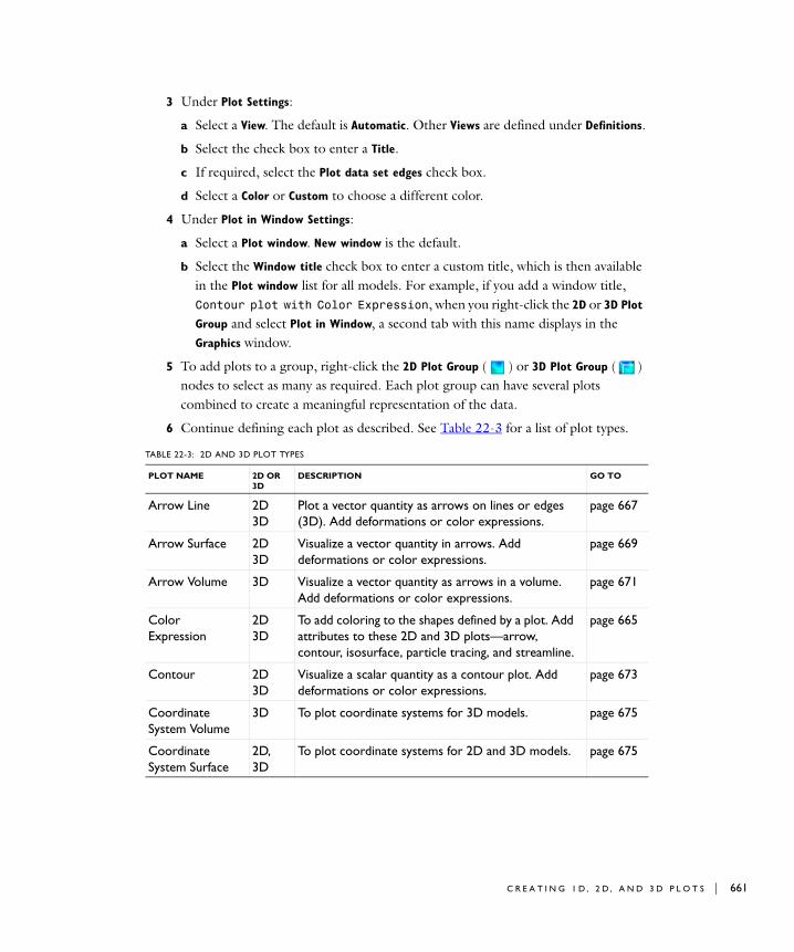
3 Under Plot Settings:
a Select a View. The default is Automatic. Other Views are defined under Definitions.
b Select the check box to enter a Title.
c If required, select the Plot data set edges check box.
d Select a Color or Custom to choose a different color.
4 Under Plot in Window Settings:
a Select a Plot window. New window is the default.
b Select the Window title check box to enter a custom title, which is then available in the Plot window list for all models. For example, if you add a window title, Contour plot with Color Expression, when you right-click the 2D or 3D Plot
Group and select Plot in Window, a second tab with this name displays in the Graphics window.
5 To add plots to a group, right-click the 2D Plot Group ( ) or 3D Plot Group ( ) nodes to select as many as required. Each plot group can have several plots combined to create a meaningful representation of the data.
6 Continue defining each plot as described. See Table 22-3 for a list of plot types.
TABLE 22-3: 2D AND 3D PLOT TYPES
PLOT NAME 2D OR 3D
DESCRIPTION GO TO
Arrow Line 2D 3D
Plot a vector quantity as arrows on lines or edges (3D). Add deformations or color expressions.
page 667
Arrow Surface 2D 3D
Visualize a vector quantity in arrows. Add deformations or color expressions.
page 669
Arrow Volume 3D Visualize a vector quantity as arrows in a volume. Add deformations or color expressions.
page 671
Color Expression
2D3D
To add coloring to the shapes defined by a plot. Add attributes to these 2D and 3D plots—arrow, contour, isosurface, particle tracing, and streamline.
page 665
Contour 2D 3D
Visualize a scalar quantity as a contour plot. Add deformations or color expressions.
page 673
Coordinate System Volume
3D To plot coordinate systems for 3D models. page 675
Coordinate System Surface
2D, 3D
To plot coordinate systems for 2D and 3D models. page 675
C R E A T I N G 1 D , 2 D , A N D 3 D P L O T S | 661

662 | C H A P T E
Deformation 2D3D
Deform the plot according to a vector quantity, for example, the displacement field in structural mechanics. Add this to most 2D and 3D plots—arrow, contour, isosurface, line, slice, streamline, surface, and volume.
page 663
Filter 2D3D
Filter the element selection for a plot. Add this to 2D and 3D plots—arrow, contour, isosurface, line plot, slice, and volume.
page 667
Height Expression
2D Height attributes introduce a 3D height on a 2D surface plot. Only 2D surface plots support height attributes.
page 716
Isosurface 3D Plot a scalar quantity as an isosurface plot. Add deformations or color expressions.
page 678
Line 2D 3D
Plot a quantity on lines, boundaries (2D), or edges (3D). Add deformations.
page 683
Max/Min Volume 3D To plot the maximum and minimum of an expression and the points there they are attained within the geometry.
page 686
Max/Min SurfaceMax/Min Line
2D 3D
Mesh 2D 3D
To display a mesh. page 687
Particle Tracing 2D 3D
Visualize the trajectory of a massless particle subject to a flow field. Add a color expression.
page 688
Particle Tracing with Mass
2D 3D
Make a particle tracing plot considering the particle’s mass. Add a color expression.
page 692
Principal Stress Volume
3D Plot principal stress and strain in structural mechanics models.
page 701
Principal Stress Surface
2D, 3D
Plot principal stress and strain in structural mechanics models.
page 701
Scatter Surface 2D Visualize a scalar quantity as scattered spheres. The radius of the spheres is proportional to the value of the quantity.
page 702
Scatter Volume 3D Scatter plots can be used as alternatives to arrow plots or when you can to get a feeling for how entities correlate.
page 702
Slice 3D Display a scalar quantity on slices inside a 3D domain.
page 705
TABLE 22-3: 2D AND 3D PLOT TYPES
PLOT NAME 2D OR 3D
DESCRIPTION GO TO
R 2 2 : R E S U L T S

Adding Deformations, Color Expressions, and Filters to Plots
Add attributes to a plot to modify the plot’s behavior—Deformation ( ) attributes deform a plot, Color Expression ( ) attributes modify the color of a plot, and element selection is selected using the Filter attribute. Select an appropriate Color Table for your plot based on your audience and what you plan to do with the final analysis.
A D D I N G D E F O R M A T I O N S T O 2 D A N D 3 D P L O T S
Add a Deformation ( ) to deform the plot according to a vector quantity, for example, the displacement field in structural mechanics. Add attributes to most 2D and 3D plots—arrow, contour, isosurface, line, particle tracing, slice, streamline, surface, and volume. By default, COMSOL scales the deformation to 10% of the geometry. This is useful for models that include structural mechanics and where displacements are computed. See Figure 22-1 and Figure 22-2 for examples from the Earth Science Module Model Library.
Streamline 2D 3D
Plot a vector field as a streamline plot. Add deformations or color expressions.
page 708
Surface 2D 3D
Display a quantity on a 2D domain or a 3D boundary. Add deformations or a filter. Add height expressions for 2D plots.
page 714
Volume 3D To display a quantity inside a 3D domain. Add a deformation.
page 718
*Cross-section point plot
1D2D3D
View an expression at an arbitrary set of spatial coordinates.
page 728
*Cross-section line plot
2D
3D
Create lines through 2D and 3D geometries to visualize along the line. Also explains how to use the interactive cross-section toolbar buttons.
page 730
*Cross-section surface plot
3D Create planes through a 3D model in a 2D geometry to visualize on the plane. The cut plane corresponds to an orthogonal 2D coordinate system embedded in 3D. Also explains how to use the interactive cross-section toolbar buttons.
page 735
* Cross-section plots are not selected from this menu. Instead, you create it in two steps using data sets and plot groups to generate the plot or use interactive cross-section toolbar buttons.
TABLE 22-3: 2D AND 3D PLOT TYPES
PLOT NAME 2D OR 3D
DESCRIPTION GO TO
C R E A T I N G 1 D , 2 D , A N D 3 D P L O T S | 663

664 | C H A P T E
1 In the Model Builder, add and define a 2D Plot Group ( ) or 3D Plot Group ( ). Right-click the plot node (for example, Arrow Surface) and select Deformation ( ).
The Deformation page opens in the Settings window and a node is added to the Model
Builder.
2 Define the Expression:
a Enter or select x, y, and z-components as required for the space dimension. Click the Replace Expression ( ) or Insert Expression ( ) buttons to select predefined expressions based on the physics of the model.
b To enter a Description (or edit the default), select the check box.
3 Under Scale, select the Scale factor check box to edit the default. Enter a value.
4 Click the Plot button ( ), or right-click the node and select Plot.
The plot displays in the Graphics window. To plot results in separate windows, right-click the plot node and select Plot in Window.
Figure 22-1: A 3D surface plot without deformation and using a cyclic color table. From the Model Library: Poroelastic Flow and Deformation: Open-Hole Multilateral Well.
R 2 2 : R E S U L T S

Figure 22-2: A 3D surface plot with deformation. From the Model Library: Poroelastic Flow and Deformation: Open-Hole Multilateral Well.
A D D I N G C O L O R E X P R E S S I O N S T O 2 D A N D 3 D P L O T S
Use Color Expressions ( ) to add coloring to the shapes defined by a plot. Add attributes to these 2D and 3D plots—arrow, contour, isosurface, particle tracing, and streamline. See Figure 22-3 and Figure 22-4 for examples from the Earth Science Module Model Library
1 In the Model Builder, add and define a 2D Plot Group ( ) or 3D Plot Group ( ). Right-click the plot node (for example, Streamline) and select Color Expression ( ).
The Color Expression page opens in the Settings window and a node is added to the Model Builder.
2 Under Expression:
a Click the Replace Expression ( ) buttons to select predefined expressions based on the physics of the model. Or enter an Expression.
b Select a Unit.
c To enter a Description (or edit the default), select the check box.
3 Under Range, manually override the Minimum and Maximum color range or data
range. Click to select the check box, then specify a range using the fields or use the sliders to control values.
C R E A T I N G 1 D , 2 D , A N D 3 D P L O T S | 665

666 | C H A P T E
4 Under Coloring and Style:
a Select a Color Table. If the default (Rainbow) is not suitable for the plot, try other options.
b The Color legend is selected by default. Click to clear the check box if required. The legend displays to the right of the plot.
5 Click the Plot button ( ), or right-click the node and select Plot.
The plot displays in the Graphics window. To plot results in separate windows, right-click the plot node and select Plot in Window.
.
Figure 22-3: A 3D streamline plot with no color expression. From the Model Library: Poroelastic Flow and Deformation: Open-Hole Multilateral Well.
R 2 2 : R E S U L T S

Figure 22-4: A 3D streamline plot with color expression. From the Model Library: Poroelastic Flow and Deformation: Open-Hole Multilateral Well.
A D D I N G F I L T E R S T O 2 D A N D 3 D P L O T S
Add a Filter ( ) to 2D and 3D plots—arrow, contour, isosurface, line plot, slice, and volume.
1 In the Model Builder, add and define a 2D Plot Group ( ) or 3D Plot Group ( ). Right-click the plot node (for example, 2D Surface) and select Filter ( ).
The Filter page opens in the Settings window and a Filter node is added to the Model
Builder.
2 Under Element Selection, enter a Logical expression for inclusion.
3 Select the Element nodes to fulfill expression—All, At least one, or At least one but not
all.
4 Click the Plot button ( ), or right-click the node and select Plot.
The plot displays in the Graphics window. To plot results in separate windows, right-click the plot node and select Plot in Window.
Creating a 2D or 3D Arrow Line Plot
Plot a vector quantity as arrows on lines (2D) or lines and edges (3D). See Figure 22-5, and Figure 22-6 for examples from the AC/DC Module Model Library. You can use a contour data set.
1 Define one or more Data Sets.
C R E A T I N G 1 D , 2 D , A N D 3 D P L O T S | 667

668 | C H A P T E
2 In the Model Builder, right-click Results and add a 2D Plot Group ( ) or 3D Plot
Group ( ). Right-click the plot node and select Arrow Line ( ).
The Arrow Line page opens in the Settings window and a node is added to the Model
Builder.
3 Under Data, select a Data set. From parent means that the plot uses the same data set as the plot group it belongs to.
4 Under Expression:
a Enter or select x, y, and z coordinates as required for the space dimension. Click the Replace Expression ( ) or Insert Expression ( ) buttons to select predefined expressions based on the physics of the model.
b To enter a Description (or edit the default), select the check box.
5 Under Coloring and Style:
a Select an Arrow length—select Proportional to use arrows with lengths proportional to the magnitude of the field, or Normalized for equal sized arrows.
b Enter a Scale factor or use the sliders to select a value.
c Select an arrow Color or Custom to choose a different color.
6 If required, add a Deformation, Color Expression and/or Filter.
7 Click the Plot button ( ), or right-click the node and select Plot.
The plot displays in the Graphics window. To plot results in separate windows, right-click the plot node and select Plot in Window.
Figure 22-5: A 2D arrow line plot. From the Model Library: Electromagnetic Forces on Parallel Current-Carrying Wires.
R 2 2 : R E S U L T S

Figure 22-6: A 2D arrow line plot combined with a surface plot. From the Model Library: Electromagnetic Forces on Parallel Current-Carrying Wires.
Creating a 2D or 3D Arrow Surface Plot
Use a 2D or 3D Arrow Surface to plot a vector quantity as arrows on a surface. See Figure 22-7, and Figure 22-8 and for examples from the COMSOL Multiphysics and Chemical Reaction Engineering or Earth Science Model Libraries. Use an isosurface data set.
1 Define one or more Data Sets.
2 In the Model Builder, right-click Results and add a 2D Plot Group ( ) or 3D Plot
Group ( ). Right-click the plot node and select Arrow Surface ( ).
The Arrow Surface page opens in the Settings window and a node is added to the Model Builder.
3 Under Data select a Data set. From parent means that the plot uses the same data set as the plot group it belongs to.
4 Under Expression:
a Enter or select x, y, and z-components as required for the space dimension. Click the Replace Expression ( ) or Insert Expression ( ) buttons to select predefined expressions based on the physics of the model.
b To enter a Description (or edit the default), select the check box.
C R E A T I N G 1 D , 2 D , A N D 3 D P L O T S | 669
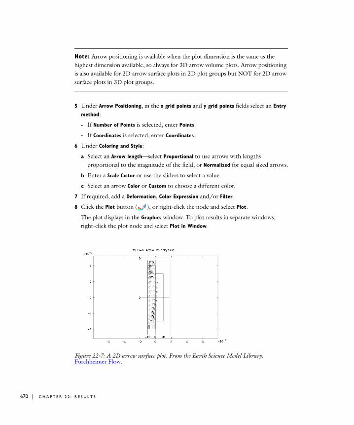
670 | C H A P T E
Note: Arrow positioning is available when the plot dimension is the same as the highest dimension available, so always for 3D arrow volume plots. Arrow positioning is also available for 2D arrow surface plots in 2D plot groups but NOT for 2D arrow surface plots in 3D plot groups.
5 Under Arrow Positioning, in the x grid points and y grid points fields select an Entry
method:
- If Number of Points is selected, enter Points.
- If Coordinates is selected, enter Coordinates.
6 Under Coloring and Style:
a Select an Arrow length—select Proportional to use arrows with lengths proportional to the magnitude of the field, or Normalized for equal sized arrows.
b Enter a Scale factor or use the sliders to select a value.
c Select an arrow Color or Custom to choose a different color.
7 If required, add a Deformation, Color Expression and/or Filter.
8 Click the Plot button ( ), or right-click the node and select Plot.
The plot displays in the Graphics window. To plot results in separate windows, right-click the plot node and select Plot in Window.
Figure 22-7: A 2D arrow surface plot. From the Earth Science Model Library: Forchheimer Flow.
R 2 2 : R E S U L T S

Figure 22-8: A 3D arrow surface plot with color expression.
Creating a 3D Arrow Volume Plot
Use a 3D Arrow Volume plot visualize a vector quantity as arrows in a volume. See Figure 22-9 and Figure 22-10 for examples from the Earth Science Module Model Library.
1 Define one or more Data Sets.
2 In the Model Builder, right-click Results and add a 3D Plot Group ( ). Right-click the plot node and select Arrow Volume ( ).
The Arrow Volume page opens in the Settings window and a node is added to the Model Builder.
3 Under Data select a Data set. From parent means that the plot uses the same data set as the plot group it belongs to.
4 Under Expression:
a Enter or select x-, y-, and z-components. Click the Replace Expression ( ) or Insert Expression ( ) buttons to select predefined expressions based on the physics of the model.
b To enter a Description (or edit the default), select the check box.
5 Under Arrow Positioning, in the x grid points, y grid points, and z grid points fields select an Entry method:
- If Number of Points is selected, enter Points.
- If Coordinates is selected, enter Coordinates.
C R E A T I N G 1 D , 2 D , A N D 3 D P L O T S | 671

672 | C H A P T E
6 Under Coloring and Style:
a Select an Arrow length—select Proportional to use arrows with lengths proportional to the magnitude of the field, or Normalized for equal sized arrows.
b Enter a Scale factor or use the sliders to select a value.
c Select an arrow Color or Custom to choose a different color.
7 If required, add a Deformation, Color Expression and/or Filter.
8 Click the Plot button ( ), or right-click the node and select Plot.
The plot displays in the Graphics window. To plot results in separate windows, right-click the plot node and select Plot in Window.
Figure 22-9: A 3D arrow volume plot. From the Model Library: Discrete Fracture.
R 2 2 : R E S U L T S

Figure 22-10: A 3D combined arrow volume and isosurface plot. From the Model Library: Discrete Fracture.
Creating a 2D or 3D Contour Plot
Visualize a scalar quantity as a Contour plot in 2D or 3D. A contour plot displays a quantity as a set of colored contour lines. The selected quantity has a constant value on these contour lines, optionally with a 3D height. See Figure 22-11 for an example from the Earth Science Module Model Library.
1 Define one or more Data Sets.
2 In the Model Builder, right-click Results and add a 2D Plot Group ( ) or 3D Plot
Group ( ). Right-click the plot node and select Contour ( ).
The Contour page opens in the Settings window and a Contour node is added to the Model Builder.
3 Under Data select a Data set. From parent means that the plot uses the same data set as the plot group it belongs to.
4 Under Expression, click the Replace Expression ( ) or Insert Expression ( ) buttons to select predefined expressions based on the physics of the model. Or enter an Expression.
a Select a Unit.
b To enter a Description (or edit the default), select the check box.
C R E A T I N G 1 D , 2 D , A N D 3 D P L O T S | 673

674 | C H A P T E
5 Select the number of contour Levels. From the Entry method list select Number of
Levels or Levels.
- If Number of Levels is selected, enter the Total levels (the number of bands of constant color contours) required.
- If Levels is selected, enter the number of contour Levels.
6 Under Coloring and Style:
a Select a Contour type—Lines or Filled.
b Select a Coloring—Color Table (default) or Uniform. If Uniform is selected, select a Color or Custom to choose a different color.
c Select a Color Table. If the default (Rainbow) is not suitable for the plot, try other options.
d The Color legend is selected by default. Click to clear the check box if required.
The legend displays to the right of the plot. In plots where each line represents a certain time value, eigenvalue, or parameter value, these values also display.
7 Under Quality, select a plot Resolution—Finer, Fine, Normal, Coarse, or No refinement. A higher resolution means that elements are split into smaller patches during rendering.
8 To enforce continuity on discontinuous data, under Quality, from the Smoothing list, select:
- None: to plot elements independently.
- Internal: to smooth the quantity inside the geometry but no smoothing takes place across borders between domains with different settings.
- Everywhere: to apply smoothing to the entire geometry.
9 Under Quality, the Recover default is Off because recovery takes processing time. See Accurate Derivative Recovery for more information.
To edit the default and use polynomial-preserving recovery and recover fields with derivatives such as stresses or fluxes with a higher theoretical convergence than smoothing, from the Recover list select:
- Within domains: to perform recovery inside domains.
- Everywhere: to apply recovery to all domain boundaries.
10 If required, add a Deformation, Color Expression and/or Filter.
11 Click the Plot button ( ), or right-click the node and select Plot.
The plot displays in the Graphics window. To plot results in separate windows, right-click the plot node and select Plot in Window.
R 2 2 : R E S U L T S

Figure 22-11: A 2D contour plot. From the Model Library: Buoyancy Flow with Darcy’s Law: The Elder Problem.
Creating Coordinate System Volume, Surface, and Line Plots
Use the Coordinate System Volume (3D), Coordinate System Surface (2D and 3D), and Coordinate System Line (3D) plots to plot coordinate systems.
1 Define one or more Data Sets.
2 In the Model Builder, right-click Results and add a 2D Plot Group ( ) or 3D Plot
Group ( ). Right-click the plot node and select More Plots>Coordinate System
Volume, Coordinate System Surface, or Coordinate System Line ( ).
The page with the same name opens in the Settings window and a node is added to the Model Builder.
3 Under Data select a Data set. From parent means that the plot uses the same data set as the plot group it belongs to.
a For Parametric Solver and Parametric Sweep studies, select an option from the Parameter values list. This section lists the associated parameter values.
b For Parametric Sweep studies (see Solver Studies and Study Types) also select a Time.
4 Select a Coordinate system to plot. By default the Global coordinate system is selected and the list contains any additional coordinate systems that the model includes.
C R E A T I N G 1 D , 2 D , A N D 3 D P L O T S | 675

676 | C H A P T E
5 For 3D Plot Groups - Coordinate System Volume plots or 2D Plot Groups - Coordinate
System Surface plots: Under Positioning, in the x grid points, y grid points, and z grid points (3D only) fields select an Entry method:
- If Number of Points is selected, enter Points.
- If Coordinates is selected, enter Coordinates (SI units: m).
6 Under Coloring and Style:
a Select an Arrow length—select Proportional to use arrows with lengths proportional to the magnitude of the field, or Normalized for equal sized arrows.
b Enter a Scale factor or use the sliders to select a value.
7 If required, add a Deformation.
8 Click the Plot button ( ), right-click the node and select Plot, or press F8.
The plot displays in the Graphics window. To plot results in separate windows, right-click the plot node and select Plot in Window.
Creating a 1D Global Plot
Use a Global graph to plot a scalar quantity as a function of time or a parameter. See Figure 22-12 for an example from the COMSOL Multiphysics Model Library. You can use a contour data set.
1 Define one or more Data Sets.
2 In the Model Builder, right-click Results and add a 1D Plot Group ( ). Right-click the plot node and select Global ( ).
The Global page opens in the Settings window and a node is added to the Model
Builder.
3 Under Data select a Data set. From Parent means that the plot uses the same data set as the plot group it belongs to.
For Parametric Solver and Parametric Sweep studies, the Parameter values section lists the associated parameter values.
a For time dependent Parametric Sweep studies (see Solver Studies and Study Types) also select an option from the Select via list —Stored output times or Interpolated times (time dependent models only).
The time steps cannot be selected directly because the different parametric solutions could have different time steps. Selecting Stored output times plots all
R 2 2 : R E S U L T S

of them, or select Interpolated times to get the same interpolated times for every parameter.
b If Interpolated times is selected, enter Times or click the Vector Input button ( ) to select and define specific times. See Entering Ranges and Vector-Valued Expressions for details.
4 Under Expressions, in the table or field, enter an Expression and Description. Click the Replace Expression ( ) or Add Expression ( ) buttons to select predefined expressions based on the physics of the model. Use the Move Up ( ), Move Down ( ), and Delete ( ) buttons as required to move rows in the table.
5 Under X-Axis Data:
a For Parametric Sweep studies, and when there are multiple inner solutions, select an option from the Solutions list—Inner or Outer. An example would be a time dependent problem with a geometric parametric sweep. The time steps are the inner solutions, the parameter sweep the outer solutions.
- If Inner is selected, and for time dependent studies, the Times steps are plotted on the x-axis and one line per parameter is included in the graph (as listed in the Data>Parameter values section on this page).
- If Outer is selected, one line in the graph is plotted for each inner solution and the Parameter values are plotted on the x-axis.
b From the Parameter list, select a Parameter value to use the x-axis data stored in the solution or Expression to specify an expression for the x-axis data.
c Click the Replace Expression ( ) or Insert Expression ( ) buttons to select predefined expressions based on the physics of the model.
d If Expression is selected, select a Unit and select the check box to enter a Description (or edit the default).
6 Under Coloring and Style, in the Line style section:
a Select a Line—Cycle, Solid, Dotted, Dashed, or Dash-dot. If Cycle is selected, it cycles through all the options.
b Select a Color or Custom to define another color.
c Enter a line Width or use the slider to select.
7 Under Coloring and Style, in the Line markers section:
a Select a Marker type—None, Cycle, Asterisk, Circle, or Diamond.
b Enter the Number of markers to display or use the slider to select.
C R E A T I N G 1 D , 2 D , A N D 3 D P L O T S | 677

678 | C H A P T E
8 Under Legends, the Show legends check box is selected by default to display to the right of the plot. In plots where each line represents a certain time value, eigenvalue, or parameter value, these values also display. For point plots, the legend displays the coordinate (or vertex number).
- If Manual is selected from the Legends list, enter your own legend text into the table. Use the Move Up ( ), Move Down ( ), and Delete ( ) buttons as required to move rows in the table.
9 Click the Plot button ( ), right-click the node and select Plot, or press F8.
The plot displays in the Graphics window. To plot results in separate windows, right-click the plot node and select Plot in Window.
Figure 22-12: A 1D global plot. From the Model Library: Fluid Valve.
Creating a 3D Isosurface Plot
Plot a scalar quantity as an Isosurface plot in 3D. An isosurface plot displays a quantity as a colored set of isosurfaces on which the result has constant value. The plot can also color isosurfaces based on an independent quantity. See Figure 22-13 for an example from the Acoustics Module Model Library.
1 Define one or more Data Sets.
R 2 2 : R E S U L T S

2 In the Model Builder, right-click Results and add a 3D Plot Group ( ). Right-click the plot group and select Isosurface ( ).
The Isosurface page opens in the Settings window and a node is added to the Model
Builder.
3 Under Data select a Data set. From parent means that the plot uses the same data set as the plot group it belongs to.
4 Under Expression:
a Click the Replace Expression ( ) or Insert Expression ( ) buttons to select predefined expressions based on the physics of the model. Or enter an Expression.
b Select a Unit.
c To enter a Description (or edit the default), select the check box.
5 Specify the Levels for the isosurfaces. From the Entry method list, select Number of
Levels or Levels.
- If Number of Levels is selected, enter the Total levels of isosurfaces (the default is 5).
- If Levels is selected, enter the number of isosurface Levels.
6 Under Coloring and Style:
a Select a Coloring—Color Table (default) or Uniform. If Uniform is selected, select a Color or Custom to choose a different color.
b Select a Color Table. If the default (Rainbow) is not suitable for the plot, try other options.
c The Color legend is selected by default. Click to clear the check box if required.
The legend displays to the right of the plot. In plots where each line represents a certain time value, eigenvalue, or parameter value, these values also display.
7 Under Quality, select a plot Resolution—Finer, Fine, Normal, Coarse, or No refinement. A higher resolution means that elements are split into smaller patches during rendering.
8 To enforce continuity on discontinuous data, under Quality, from the Smoothing list, select:
- None: to plot elements independently.
- Internal: to smooth the quantity inside the geometry but no smoothing takes place across borders between domains with different settings.
- Everywhere: to apply smoothing to the entire geometry.
C R E A T I N G 1 D , 2 D , A N D 3 D P L O T S | 679

680 | C H A P T E
9 Under Quality, the Recover default is Off because recovery takes processing time. See Accurate Derivative Recovery for more information.
To edit the default and use polynomial-preserving recovery and recover fields with derivatives such as stresses or fluxes with a higher theoretical convergence than smoothing, from the Recover list select:
- Within domains: to perform recovery inside domains.
- Everywhere: to apply recovery to all domain boundaries.
10 By default the Use derivatives check box is selected. To increase the speed of computation, click to clear the check box. However, this results in less smooth surfaces.
11 If required, add a Deformation, Color Expression and/or Filter.
12 Click the Plot button ( ), or right-click the node and select Plot.
The plot displays in the Graphics window. To plot results in separate windows, right-click the plot node and select Plot in Window.
Figure 22-13: A 3D isosurface plot. From the Model Library: Car Interior.
Creating a 1D Line Graph
Use a Line Graph to plot a scalar quantity along a geometric line. The line can be a edge in the geometry, a parameterized curve, or a cut line. Make a graph plot of a quantity versus another quantity (for example, time). See Figure 22-14 for an example from the COMSOL Multiphysics Model Library. You can use a parameterized curve data set.
R 2 2 : R E S U L T S

1 Define one or more Data Sets.
2 In the Model Builder, right-click Results and add a 1D Plot Group ( ). Right-click the plot node and select Line Graph ( ).
The Line Graph page opens in the Settings window and a node is added to the Model
Builder.
3 Under Data select a Data set. Select:
- From Parent to use the same data set as the plot group it belongs to.
- a Solution data set to visualize a quantity along a geometric edge.
- a Cut Line data set to visualize a quantity along the cut line (a cross-section).
- a Parameterized Curve data set to visualize a quantity along the parameterized curve.
4 If a Solution data set is selected, under Selection:
a Select All or Manual.
b If Manual is selected choose geometry directly from the Graphics window. Select All to add the applicable geometry or any other predefined grouping. Use the Add
to Selection ( ), Remove from Selection ( ), and Clear Selection ( ) buttons as required in the Settings window.
5 Under Y-Axis Data:
a Click the Replace Expression ( ) or Insert Expression ( ) buttons to select predefined expressions available based on the physics of the model. Or enter an Expression in the field.
b Select a Unit.
c To enter a Description (or edit the default), select the check box.
6 Under X-Axis Data, from the Parameter list, select Arc length to visualize along arc length, or Expression to visualize along, for example, a coordinate expression.
C R E A T I N G 1 D , 2 D , A N D 3 D P L O T S | 681

682 | C H A P T E
Note: For Parametric Sweep studies, for each pair of outer solution or inner solutions, one line is plotted on the graph. For example, if there are 10 outer solutions and each outer solution has five inner solutions, then 50 lines are drawn. The number of inner solutions can vary between outer solutions.
If Expression is selected:
a Click the Replace Expression ( ) or Insert Expression ( ) buttons to select predefined expressions based on the physics of the model. Or enter an Expression.
b Select a Unit.
c To enter a Description (or edit the default), select the check box.
7 Under Coloring and Style:
a Select a Line type—Cycle, Solid, Dotted, Dashed, or Dash-dot. If Cycle is selected, it cycles through all the options.
b Select a Color—Cycle, Black, Blue, Cyan, or Green.
c Enter a line Width or use the slider to select.
d In the Line markers section, select a Marker type—None, Cycle, Asterisk, Circle, or Diamond. Enter the Number of markers to display or use the slider to select.
8 If required, under Legends, select the Show legends check box to display a legend to the right of the plot. In plots where each line represents a certain time value, eigenvalue, or parameter value, these values also display. For point plots, the legend displays the coordinate (or vertex number).
- If Manual is selected from the Legends list, enter your own legend text into the table. Use the Move Up ( ), Move Down ( ), and Delete ( ) buttons as required to move rows in the table.
9 Under Quality, select a plot Resolution—Finer, Fine, Normal, Coarse, or No refinement. A higher resolution means that elements are split into smaller patches during rendering.
R 2 2 : R E S U L T S

10 Under Quality, the Recover default is Off because recovery takes processing time. See Accurate Derivative Recovery for more information.
To edit the default and use polynomial-preserving recovery and recover fields with derivatives such as stresses or fluxes with a higher theoretical convergence than smoothing, from the Recover list select:
- Within domains: to perform recovery inside domains.
- Everywhere: to apply recovery to all domain boundaries.
11 Click the Plot button ( ), right-click the node and select Plot, or press F8.
The plot displays in the Graphics window. To plot results in separate windows, right-click the plot node and select Plot in Window.
Figure 22-14: A 1D line graph. From the Model Library: Effective Diffusivity in Porous Materials.
Creating a 2D or 3D Line Plot
Use a Line plot to display a quantity on lines, that is, boundaries in 2D or edges in 3D. See Figure 22-15, and Figure 22-16 for examples from the Heat Transfer Module and Structural Mechanics Module model libraries. Use a parameterized curve data set or a contour data set.
1 Define one or more Data Sets.
C R E A T I N G 1 D , 2 D , A N D 3 D P L O T S | 683

684 | C H A P T E
2 In the Model Builder, right-click Results and add a 2D Plot Group ( ) or 3D Plot
Group ( ). Right-click the plot node and select Line ( ).
The Line page opens in the Settings window and a node is added to the Model Builder.
3 Under Data select a Data set. From parent means that the plot uses the same data set as the plot group it belongs to.
4 Under Expression:
a Click the Replace Expression ( ) or Insert Expression ( ) buttons to select predefined expressions based on the physics of the model.
b Select a Unit.
c To enter a Description (or edit the default), select the check box.
5 Under Range, manually override the Minimum and Maximum color range or data
range. Click to clear the check box, then specify a range using the fields or use the sliders to control values.
6 Under Coloring and Style, select a Line type—Line or Tube. If Tube is selected:
a Enter a Tube radius expression (the radius of the tube).
b To edit the Radius scale factor select the check box and enter a number.
7 Under Coloring and Style:
a Select a Coloring—Color Table (default) or Uniform. If Uniform is selected, select a Color or Custom to choose a different color.
b Select a Color Table. If the default (Rainbow) is not suitable for the plot, try other options.
c The Color legend is selected by default. Click to clear the check box if required.
The legend displays to the right of the plot. In plots where each line represents a certain time value, eigenvalue, or parameter value, these values also display.
8 Under Quality, select a plot Resolution—Finer, Fine, Normal, Coarse, or No refinement. A higher resolution means that elements are split into smaller patches during rendering.
9 To enforce continuity on discontinuous data, under Quality, from the Smoothing list, select:
- None: to plot elements independently.
- Internal: to smooth the quantity inside the geometry but no smoothing takes place across borders between domains with different settings.
- Everywhere: to apply smoothing to the entire geometry.
R 2 2 : R E S U L T S

10 Under Quality, the Recover default is Off because recovery takes processing time. See Accurate Derivative Recovery for more information.
To edit the default and use polynomial-preserving recovery and recover fields with derivatives such as stresses or fluxes with a higher theoretical convergence than smoothing, from the Recover list select:
- Within domains: to perform recovery inside domains.
- Everywhere: to apply recovery to all domain boundaries.
11 If required, add a Deformation and/or Filter.
12 Click the Plot button ( ), right-click the node and select Plot, or press F8.
The plot displays in the Graphics window. To plot results in separate windows, right-click the plot node and select Plot in Window.
Figure 22-15: A 2D line plot. From the Heat Transfer Model Library: Thermo-Photo-Voltaic Cell.
C R E A T I N G 1 D , 2 D , A N D 3 D P L O T S | 685
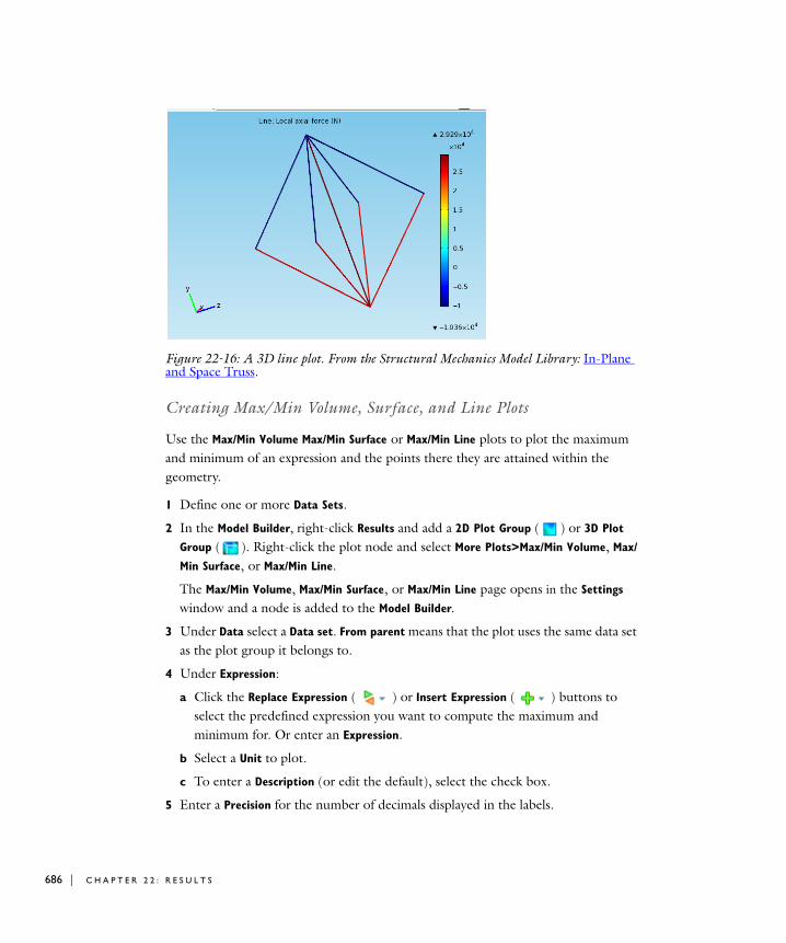
686 | C H A P T E
Figure 22-16: A 3D line plot. From the Structural Mechanics Model Library: In-Plane and Space Truss.
Creating Max/Min Volume, Surface, and Line Plots
Use the Max/Min Volume Max/Min Surface or Max/Min Line plots to plot the maximum and minimum of an expression and the points there they are attained within the geometry.
1 Define one or more Data Sets.
2 In the Model Builder, right-click Results and add a 2D Plot Group ( ) or 3D Plot
Group ( ). Right-click the plot node and select More Plots>Max/Min Volume, Max/
Min Surface, or Max/Min Line.
The Max/Min Volume, Max/Min Surface, or Max/Min Line page opens in the Settings window and a node is added to the Model Builder.
3 Under Data select a Data set. From parent means that the plot uses the same data set as the plot group it belongs to.
4 Under Expression:
a Click the Replace Expression ( ) or Insert Expression ( ) buttons to select the predefined expression you want to compute the maximum and minimum for. Or enter an Expression.
b Select a Unit to plot.
c To enter a Description (or edit the default), select the check box.
5 Enter a Precision for the number of decimals displayed in the labels.
R 2 2 : R E S U L T S

6 Under Advanced:
a The Recover default is Off because recovery takes processing time. To edit the default and use polynomial-preserving recovery and recover fields with derivatives such as stresses or fluxes with a higher theoretical convergence than smoothing, from the Recover list select:
- Within domains: to perform recovery inside domains.
- Everywhere: to apply recovery to all domain boundaries.
b Define the number of refinements of each mesh element when computing the maximum and minimum by entering a value in the Element refinement field.
7 Click the Plot button ( ), or right-click the node and select Plot.
The plot displays in the Graphics window. To plot results in separate windows, right-click the plot node and select Plot in Window.
Creating a 2D or 3D Mesh Plot
Use mesh plots to display a mesh in 2D or 3D.
1 Define one or more Data Sets.
Note: You can visualize the mesh without solving a model using a mesh data set.
2 In the Model Builder, right-click Results and add a 2D Plot Group ( ) or 3D Plot
Group ( ). Right-click the plot node and select Mesh.
The Mesh page opens in the Settings window and a node is added to the Model
Builder.
3 Under Data select a Data set. From parent means that the plot uses the same data set as the plot group it belongs to.
C R E A T I N G 1 D , 2 D , A N D 3 D P L O T S | 687

688 | C H A P T E
4 Under Level, select a Level to display the mesh—All, Volume (3D only), Surface, Line, or Point.
- If Surface is selected, select the base Element type to visualize—All, Triangle, or Quad.
- 3D only: If Volume is selected, select the base Element type to visualize—All, Tetrahedron, Prism, or Hex.
5 Under Color:
a From the Element color list, select:
- Quality to get an element quality plot.
- Custom to select a different color.
- None to plot with no color.
b Select a Color table for the element quality. If the default (Rainbow) is not suitable for the plot, try other options.
c From the Wireframe color list, select:
- Quality to get an element quality plot.
- Custom to select a different color.
- None to plot with no color.
6 Under Element Filter, specify the elements to display:
a Select the Enable filter check box.
b Select a Criterion—Random, Worst Quality, Best Quality, Size, Expression, or Logical
expression.
c If Expression or Logical expression is selected, enter an Expression in the field.
d Specify the Fraction of elements to show or use the slider to choose.
7 To scale elements in the mesh plot, under Shrink Elements, enter an Element scale
factor between 0 and 1.
8 Click the Plot button ( ), or right-click the node and select Plot.
The plot displays in the Graphics window. To plot results in separate windows, right-click the plot node and select Plot in Window.
Creating a 2D or 3D Particle Tracing Plot
Use a Particle Tracing plot to visualize the trajectory of a massless particle subject to a flow field. With this plot type, you can visualize pathlines, that is, trajectories of particles released in a flow field, which can be time-dependent or static. For
R 2 2 : R E S U L T S

time-dependent flows you can also use a snapshot in time of the flow field as a static field. The motion of the particles does not affect the flow field.
1 Define one or more Data Sets.
2 In the Model Builder, right-click Results and add a 2D Plot Group ( ) or 3D Plot
Group ( ). Right-click the plot node and select Particle Tracing ( ).
The Particle Tracing page opens in the Settings window and a node is added to the Model Builder.
3 Under Data select a Data set. From parent means that the plot uses the same data set as the plot group it belongs to.
4 Under Expression:
a Enter or select x-and y-components for 2D, x-, y-, and z-components for 3D. Click the Replace Expression ( ) or Insert Expression ( ) buttons to select predefined expressions based on the physics of the model.
b To enter a Description (or edit the default), select the check box.
5 Under Particle Positioning, for 3D only, enter the initial position of particles in the x, y, and z fields.
For 2D:
a From the Positioning list, select Start point controlled or Boundary coordinates. Boundary coordinates are useful, for example, for flow models with one or more inflow boundaries.
- If Start point controlled is selected, enter the initial position of particles in the x and y fields and go to the next step.
b If Boundary coordinates is selected, select an item from the Named selection list.
c Select an Entry method—Number of points or Boundary parameters.
- If Number of Points is selected, enter the number of grid Points.
- If Boundary parameters is selected, enter the Relative coordinates.
6 Under Release, specify when to Release particles:
- Select Once to release particles once at the first available time, typically at time 0 (zero). To delay the release, select the Start time check box and enter a time.
- Select At intervals to release particles at regular intervals starting at the first available time, typically at time 0 (zero). To delay the release, select the Start time check box and enter a time. Enter a Time between releases.
- Select At times to release particles at an arbitrary time point; enter multiple Times to release particles.
C R E A T I N G 1 D , 2 D , A N D 3 D P L O T S | 689

690 | C H A P T E
7 Under Coloring and Style, select a Line type—Line, Tube, or None. If Tube is selected:
a Enter a Tube radius expression (the radius of the tube).
b To edit the Radius scale factor select the check box and enter a number.
c Select a line Color or Custom to choose a different color.
8 Under Coloring and Style, select a Point style—Point or None.
9 If Point is selected:
a Enter a Point radius.
b To edit the Radius scale factor select the check box and enter a number.
c Select a point Color or Custom to choose a different color.
10 Under Coloring and Style, select a Point motion to specify what should happen as particles leave the domain—Stick to Boundary (to plot the points on the boundary at the exit point) or Disappear (to not render these points at all).
For static fields, specify the End time in the Advanced section. It is possible that all particles have left the domain at the selected time. In that case, all points appear at the outflow boundary if Stick to boundary is selected, and no points appear if Disappear is selected. To make the points appear, specify an earlier end time.
11 If you are planning to create an Animation report (see Defining and Exporting Plot Animations), and if required, select the Plot along lines when animating check box.
12 Under Quality, select a plot Resolution—Finer, Fine, Normal, Coarse, or No refinement. A higher resolution means that elements are split into smaller patches during rendering.
13 Under Quality, the Recover default is Off because recovery takes processing time. See Accurate Derivative Recovery for more information if you want to change the setting.
14 In the ODE solver settings section, enter a Relative tolerance for the ODE solver. The default is 0.001.
- When solving the 2nd-order ODE for x, the solver first rewrites it as two coupled 1st-order ODEs: one for position x and one for velocity , each with two components in 2D and three components in 3D.
- The Relative tolerance value is the relative error tolerance that the ODE solver uses. It applies to all components of the particle’s position and velocity. The solver
mx·· F t x x· =
x·
R 2 2 : R E S U L T S
controls the step size so that the estimated error e in each integration step satisfies
where rtol is the relative tolerance that you specify, atolpos is the absolute tolerance for the particle’s position components, and atolvel equals the absolute tolerance for the particle’s velocity components.
15 In the ODE solver settings section, specify the solver’s absolute tolerance. The default is Automatic. To enter different values, select Manual from the Absolute tolerance list and enter a Position.
- The Position field can contain a single value—it applies to all components of the position and is the absolute tolerance.
16 In the ODE solver settings section, specify the solver Step size. The default is Automatic—COMSOL uses the initial value of the acceleration (force divided by mass) and the relative and absolute tolerances to determine the initial time step.
- The automatic maximum step size is 10% of the total simulation time for time-dependent flows as well as for static flow fields where you can specify the end time manually in the Advanced section (in the Plot static flow field even when time
dependent>End Time field). For static flow fields where you do not set the end time manually, there is no upper limit of the step size. However, in this case, the initial time step is less than or equal to 0.1.
To edit the settings, select Manual from the Step size list and enter values in the Initial
time step and Maximum time step fields.
- The Maximum time step is the longest time step the solver takes. It has higher priority than the Initial time step; that is, if you specify an initial step size larger than the maximum step size, the solver lowers the initial step size to the maximum step size.
Note: The initial step size, whether entered manually or computed automatically, is not necessarily the first step the solver takes but is a first try. If this step leads to an error such that the tolerances are not met, COMSOL Multiphysics lowers it.
e max atolpos rtol xi (for all components xi of x)
e max atolvel rtol x·i (for all components x·i of x·)
C R E A T I N G 1 D , 2 D , A N D 3 D P L O T S | 691

692 | C H A P T E
Note: The Advanced section contains settings that do not normally need to be adjusted.
17 Under Advanced, the Termination section contains settings that determine when to end the particle tracing simulation.
a To specify an upper limit of the number of time steps, click to select the Maximum
number of steps check box and edit the default (1000). The particle simulation ends after this number of steps.
b To specify how close to the geometry boundary the path lines are cut when they exit the geometry, edit the Edge tolerance default (0.001). This is an absolute tolerance controlling how close to the geometry boundary the pathlines are cut when they exit the geometry. A lower value cuts the line closer to the geometry boundary.
18 Under Advanced, in the Instantaneous flow field section:
a To specify if you want to plot an instantaneous even if the solution is time dependent, select the Plot static flow field even when time dependent check box. This freezes the time selected previously— for example, from a Plot Group page in the Data>Time list—to the value specified and considers this a static flow field.
b Edit the Time variable default (partt) if required. Normally it is not necessary to change the default name but you can use the name in expressions as well as for the color when coloring the pathlines according to an expression.
c If required, select the End time check box and enter a value.
19 If required, add a Deformation and/or Color Expression.
20 Click the Plot button ( ), right-click the node and select Plot, or press F8.
The plot displays in the Graphics window. To plot results in separate windows, right-click the plot node and select Plot in Window.
Creating a 2D or 3D Particle Tracing with Mass Plot
Use a Particle Tracing with Mass plot to visualize the trajectory of a particle with mass and subject to a flow field. See Figure 22-17 and Figure 22-18 for examples from the COMSOL Multiphysics Model Library.
R 2 2 : R E S U L T S

B A C K G R O U N D I N F O R M A T I O N
For particles with mass, COMSOL generates the pathlines by solving the fundamental equation of motion:
for the pathline xt. Here, m is the particle’s mass, F equals the force acting upon the particle, and t is time. This is a system of ODEs for x, which COMSOL Multiphysics solves using a pair of Runge-Kutta methods of orders four and five. The solver advances the algorithm with the solution of order five and uses the difference between the order-five and order-four solutions to obtain the local error estimate.
For massless particles, the equation of motion is:
Note: The true formulation of Newton’s second law of motion is , that is, you must consider the time derivative of the mass. The
particle-tracing algorithm does not solve this equation. Thus, if you specify an expression for the particle mass that depends on time, you will not get correct results.
Axisymmetric ModelsFor 2D axisymmetric models, three components for the force are available for particles with mass. When specifying all three, the algorithm solves for a line in 3D in cylindrical coordinates, but the plot only shows the projection on the axisymmetry plane. In this case, the centripetal force is considered; that is, the algorithm solves the equation
,
where m is the particle mass and (r, , z are the cylindrical coordinates. Note that the variable corresponding to the velocity component in the direction (whose default name is partv) has the dimension length/time, and equals as has the dimension radians/time.
D E F I N I N G A P A R T I C L E TR A C I N G W I T H M A S S P L O T
1 Define one or more Data Sets.
mx·· F t x x· =
x· v t x =
ddt------ mx· F t x x· =
r··Fr
m------ r· 2+= ··
Frm-------- 2r··
r----------–= z··
Fz
m------=
r· ·
C R E A T I N G 1 D , 2 D , A N D 3 D P L O T S | 693

694 | C H A P T E
2 In the Model Builder, right-click Results and add a 2D Plot Group ( ) or 3D Plot
Group ( ). Right-click the plot node and select Particle Tracing with Mass ( ).
The Particle Tracing with Mass page opens in the Settings window and a node is added to the Model Builder.
3 Under Data select a Data set. From parent means that the plot uses the same data set as the plot group it belongs to.
4 Specify the force acting on the particles under Equation of Motion:
a Click the Replace Expression ( ) or Insert Expression ( ) buttons to select predefined expressions based on the physics of the model. Or enter an Expression—Fx, Fy, and Fz components of the force as required for the space dimension.
b Enter a Description (or edit the default).
c When some predefined forces are added, there are additional Parameters with a Value to enter into a table.
5 Under Mass and Velocity:
a Enter the particle’s Mass.
b Enter values in the Initial velocity section—for 2D enter x and y components; for 3D enter x, y, and z components.
6 Under Particle Positioning, for 3D only, enter the initial position of particles in the x, y, and z fields.
a From the Positioning list, select Start point controlled or Boundary coordinates. Boundary coordinates are useful, for example, for flow models with one or more inflow boundaries.
- If Start point controlled is selected, enter the initial position of particles in the x and y fields and go to the next step. Click the Range button ( ) to define a range using the Range window. See Entering Ranges and Vector-Valued Expressions for details.
- If Boundary coordinates is selected, select an item from the Named selection list.
b Select an Entry method—Number of points or Boundary parameters.
- If Number of Points is selected, enter the number of grid Points.
- If Boundary parameters is selected, enter the Relative coordinates.
R 2 2 : R E S U L T S
7 Under Release, specify when to Release particles—Once, At intervals, or At times.
Select:
- Once to release particles once at the first available time, typically at time 0 (zero). To delay the release, select the Start time check box and enter a time.
- At intervals to release particles at regular intervals starting at the first available time, typically at time 0 (zero). To delay the release, select the Start time check box and enter a time. Enter a Time between releases.
- At times to release particles at an arbitrary time point; enter multiple Times to release particles.
8 Under Coloring and Style, select a Line type—Line, Tube, or None. If Tube is selected:
a Enter a Tube radius expression (the radius of the tube).
b To edit the Radius scale factor select the check box and enter a number.
c Select a line Color or Custom to choose a different color.
9 Under Coloring and Style, select a Point style—Point or None. If Point is selected also enter a Point radius.
a To edit the Radius scale factor select the check box and enter a number.
b Select a point Color or Custom to choose a different color.
10 Under Coloring and Style, select a Point motion to specify what should happen as particles leave the domain—Stick to Boundary (to plot the points on the boundary at the exit point) or Disappear (to not render these points at all).
For static fields, specify the End time in the Advanced section. It is possible that all particles have left the domain at the selected time. In that case, all points appear at the outflow boundary if Stick to boundary is selected, and no points appear if Disappear is selected. To make the points appear, specify an earlier end time.
11 If you are planning to create an Animation (see Defining and Exporting Plot Animations), and if required, select the Plot along lines when animating check box.
12 Under Quality, to increase the number of output points by adding points between each time step taken in the ODE solver, using a 4th-order interpolation, and to produce a smoother output select a plot Resolution—Finer, Fine, Normal, Coarse, or No refinement. A higher resolution means that elements are split into smaller patches during rendering.
13 Under Quality, the Recover default is Off because recovery takes processing time. See Accurate Derivative Recovery for more information.
C R E A T I N G 1 D , 2 D , A N D 3 D P L O T S | 695

696 | C H A P T E
14 In the ODE solver settings section, enter a Relative tolerance for the ODE solver. The default is 0.001.
- When solving the 2nd-order ODE for x, the solver first rewrites it as two coupled 1st-order ODEs: one for position x and one for velocity , each with two components in 2D and three components in 3D.
- The Relative tolerance value is the relative error tolerance that the ODE solver uses. It applies to all components of the particle’s position and velocity. The solver controls the step size so that the estimated error e in each integration step satisfies
where rtol is the relative tolerance that you specify, atolpos is the absolute tolerance for the particle’s position components, and atolvel equals the absolute tolerance for the particle’s velocity components.
15 In the ODE solver settings section, specify the absolute tolerance. The default is Automatic. To enter different values, select Manual from the Absolute tolerance list and enter a Position or Velocity.
- The Position or Velocity field can contain a single value—it applies to all components of the position and is the absolute tolerance.
16 In the ODE solver settings section, specify the Step size. The default is Automatic—COMSOL uses the initial value of the acceleration (force divided by mass) and the relative and absolute tolerances to determine the initial time step.
- The automatic maximum step size is 10% of the total simulation time for time-dependent flows as well as for static flow fields where you can specify the end time manually in the Advanced section (in the Plot static flow field even when time
dependent>End Time field). For static flow fields where you do not set the end time manually, there is no upper limit of the step size. However, in this case, the initial time step is less than or equal to 0.1.
To edit the settings, select Manual from the Step size list and enter values in the Initial
time step and Maximum time step fields.
- The Maximum time step is the longest time step the solver takes. It has higher priority than the Initial time step; that is, if you specify an initial step size larger than the maximum step size, the solver lowers the initial step size to the maximum step size.
mx·· F t x x· =
x·
e max atolpos rtol xi (for all components xi of x)
e max atolvel rtol x·i (for all components x·i of x·)
R 2 2 : R E S U L T S

Note: The initial step size, whether entered manually or computed automatically, is not necessarily the first step the solver takes but is a first try. If this step leads to an error such that the tolerances are not met, COMSOL Multiphysics lowers it.
Note: The Advanced section contains settings that do not normally need to be adjusted.
17 Under Advanced, the Termination section contains settings that determine when to end the particle tracing simulation.
a To specify an upper limit of the number of time steps, select the Maximum number
of steps check box and edit the default (1000). The particle simulation ends after this number of steps.
b To specify how close to the geometry boundary the path lines are cut when they exit the geometry, edit the Edge tolerance default (0.001). This is an absolute tolerance controlling how close to the geometry boundary the pathlines are cut when they exit the geometry. A lower value cuts the line closer to the geometry boundary.
18 Under Advanced, in the Instantaneous flow field section:
a To specify if you want to plot an instantaneous even if the solution is time dependent, select the Plot static flow field even when time dependent check box. This freezes the time selected previously— for example, from a Plot Group page in the Data>Time list—to the value specified and considers this a static flow field.
b Edit the Time variable default (partt) if required. Normally it is not necessary to change the default name but you can use the name in expressions as well as for the color when coloring the pathlines according to an expression.
c If required, select the End time check box and enter a value.
19 Under Advanced, in the Particle velocity variables section, edit the default variable component names for each particle’s velocity. The default names are partu (x-component), partv (y-component), and partw (z-component).
20 If required, add a Deformation and/or Color Expression.
C R E A T I N G 1 D , 2 D , A N D 3 D P L O T S | 697

698 | C H A P T E
21 Click the Plot button ( ), right-click the node and select Plot, or press F8.
The plot displays in the Graphics window. To plot results in separate windows, right-click the plot node and select Plot in Window.
Figure 22-17: A 2D particle tracing with mass plot. From the Model Library: Flow Past a Cylinder.
Figure 22-18: A 2D particle tracing with mass combined with surface plot. From the Model Library: Flow Past a Cylinder.
R 2 2 : R E S U L T S

Creating a 1D Point Graph
Use a Point Graph plot to visualize the value in a point along time or a parameter value. The point can be a point in the geometry or a cut point. See Figure 22-19 for an example from the COMSOL Multiphysics Model Library.
1 Define one or more Data Sets.
2 In the Model Builder, right-click Results and add a 1D Plot Group ( ). Right-click the plot node and select Point Graph ( ).
The Point Graph page opens in the Settings window and a node is added to the Model
Builder.
3 Under Data select a Data set. Select:
- From Parent to use the same data set as the plot group it belongs to.
- a Solution data set to visualize a quantity along a geometric point.
- a Cut Point data set to visualize a quantity in the cut point.
- If a Parametric Solver or Parametric Sweep data set is selected, the Parameter values section lists the associated parameter values.
a For Parametric Sweep studies (see Solver Studies and Study Types) select an option from the Select via list —Stored output times or Interpolated times (time dependent models only).
The time steps cannot be selected directly because the different parametric solutions could have different time steps. Selecting Stored output times plots all of them, or select Interpolated times to get the same interpolated times for every parameter.
b If Interpolated times is selected, enter Times or click the Vector Input button ( ) to select and define specific times. See Entering Ranges and Vector-Valued Expressions for details.
C R E A T I N G 1 D , 2 D , A N D 3 D P L O T S | 699

700 | C H A P T E
4 Under X-axis Data, for Parametric Sweep studies, and when there are multiple inner solutions,
a Select an option from the Solutions list—Inner or Outer.
- If Inner is selected, the Times steps are plotted on the x-axis and one line per parameter is included in the graph (as listed in the Data>Parameter values section on this page).
- If Outer is selected, one line in the graph is plotted for each inner solution and the Parameter values are plotted on the x-axis.
b From the Parameter list, select Parameter value to use the x-axis data stored in the solution or Expression to specify an expression for the x-axis data.
5 If a Solution data set is selected, under Selection:
a Select All or Manual.
b If Manual is selected choose geometry directly from the Graphics window. Select All to add the applicable geometry or any other predefined grouping. Use the Add
to Selection ( ), Remove from Selection ( ), and Clear Selection ( ) buttons as required in the Settings window.
6 Under Expression:
a Click the Replace Expression ( ) or Insert Expression ( ) buttons to select predefined expressions based on the physics of the model. Or enter an Expression.
b Select a Unit.
c To enter a Description (or edit the default), select the check box.
7 Under X-Axis Data, from the Parameter list, select Parameter value to use the x-axis data stored in the solution or Expression to specify an expression for the x-axis data.
a Click the Replace Expression ( ) or Insert Expression ( ) buttons to select predefined expressions based on the physics of the model. Or enter an Expression.
b Select a Unit.
c To enter a Description (or edit the default), select the check box.
8 Under Coloring and Style, in the Line style section:
a Select a Line—None, Cycle, Solid, Dotted, Dashed, or Dash-dot. If Cycle is selected, it cycles through all the options.
b Select a line Color or Custom to define another color.
c Enter a line Width or use the slider to select.
R 2 2 : R E S U L T S

9 Under Coloring and Style, in the Line markers section:
a Select a Marker type—None, Cycle, Asterisk, Circle, or Diamond.
b Enter the Number of markers to display or use the slider to select.
10 If required, under Legends, select the Show legends check box to display a legend to the right of the plot. In plots where each line represents a certain time value, eigenvalue, or parameter value, these values also display. For point plots, the legend displays the coordinate (or vertex number).
- If Manual is selected from the Legends list, enter your own legend text into the table. Use the Move Up ( ), Move Down ( ), and Delete ( ) buttons as required to move rows in the table.
11 Click the Plot button ( ), or right-click the node and select Plot.
The plot displays in the Graphics window. To plot results in separate windows, right-click the plot node and select Plot in Window.
Figure 22-19: A 1D point graph. From the Model Library: Effective Diffusivity in Porous Materials.
Creating Principal Stress Volume or Principal Stress Surface Plots
Use the Principal Stress Volume (3D) and Principal Stress Surface (2D and 3D) to plot principal stress and strain in structural mechanics models.
1 Define one or more Data Sets.
C R E A T I N G 1 D , 2 D , A N D 3 D P L O T S | 701
702 | C H A P T E
2 In the Model Builder, right-click Results and add a 2D Plot Group ( ) or 3D Plot
Group ( ). Right-click the plot node and select More Plots>Principal Stress Volume ( ) or Principal Stress Surface ( ).
The page with the same name opens in the Settings window and a node is added to the Model Builder.
3 Under Data select a Data set. From parent means that the plot uses the same data set as the plot group it belongs to.
4 Under Principal Components:
a Select a Type—Principal stress or Principal strain.
b Under Principal values, enter First, Second, and Third in the Value fields.
c Under Principal directions, enter First, Second, and Third in the x, y, and z (for 3D) coordinate fields.
5 For transient problems, enter a Time.
6 For 3D Plot Groups - Principal Stress Volume plots or 2D Plot Groups - Principal Stress
Surface plots: Under Positioning, in the x grid points, y grid points, and z grid points fields select an Entry method:
- If Number of Points is selected, enter Points.
- If Coordinates is selected, enter Coordinates (SI units: m).
7 Under Coloring and Style:
a Select an Arrow length—select Proportional to use arrows with lengths proportional to the magnitude of the field, or Normalized for equal sized arrows.
b Enter a Scale factor or use the sliders to select a value.
c Select an arrow Color or Custom to choose a different color.
8 If required, add a Deformation and/or Color Expression.
9 Click the Plot button ( ), right-click the node and select Plot, or press F8.
The plot displays in the Graphics window. To plot results in separate windows, right-click the plot node and select Plot in Window.
Creating a 2D Scatter Surface or 3D Scatter Volume Plot
Use a 2D Scatter Surface plot to visualize a scalar quantity as scattered spheres on a 2D surface or on a 3D Scatter Volume plot. Scatter plots can be used as alternatives to arrow plots or when you can to get a feeling for how entities correlate. The radius and color
R 2 2 : R E S U L T S

can be functions of independent quantities. See Figure 22-20 and Figure 22-21 for examples from the Earth Science Module Model Library.
1 Define one or more Data Sets.
2 In the Model Builder, right-click Results and add a 2D Plot Group ( ) (Scatter Surface) or 3D Plot Group ( ) (Scatter Volume). Right-click the plot node and select More Plots>Scatter Surface ( ) or Scatter Volume ( ).
The Scatter Surface (2D) or Scatter Volume (3D) page opens in the Settings window and a node is added to the Model Builder.
3 Under Data select a Data set. From parent means that the plot uses the same data set as the plot group it belongs to.
4 Under Expression:
a Enter or select x-and y-components for 2D, x-, y-, and z-components for 3D. Click the Replace Expression ( ) or Insert Expression ( ) buttons to select predefined expressions based on the physics of the model.
b To enter a Description (or edit the default), select the check box.
5 Under Evaluation Points, select an Entry method for the x- and y-grid points (2D) or for the x-, y-, and z-grid points (3D). The evaluation points are located in a block-shaped grid.
- If Number of Points is selected, enter Points.
- If Coordinates is selected, enter Coordinates for each axis.
6 Under Radius:
a The default Expression is 1. But you can enter any Expression in the field.
b COMSOL automatically scales the radius. To edit the Radius scale factor, select the check box and enter a number.
7 Under Color:
a Click the Replace Expression ( ) or Insert Expression ( ) buttons to select predefined expressions based on the physics of the model. Or enter an Expression.
b Select a Unit.
c To enter a Description (or edit the default), select the check box.
C R E A T I N G 1 D , 2 D , A N D 3 D P L O T S | 703

704 | C H A P T E
8 Under Coloring and Style:
a Select a Coloring—Color Table (default) or Uniform. If Uniform is selected, select a Color or Custom to choose a different color.
b Select a Color Table. If the default (Rainbow) is not suitable for the plot, try other options.
c The Color legend is selected by default. Click to clear the check box if required.
The legend displays to the right of the plot. In plots where each line represents a certain time value, eigenvalue, or parameter value, these values also display.
9 Click the Plot button ( ), or right-click the node and select Plot.
The plot displays in the Graphics window. To plot results in separate windows, right-click the plot node and select Plot in Window.
Figure 22-20: A 2D scatter surface plot. From the Model Library: Forchheimer Flow.
R 2 2 : R E S U L T S

Figure 22-21: A 3D scatter volume plot. From the Model Library: Discrete Fracture.
Creating a 3D Slice Plot
Use Slice plots to display a scalar quantity on slices inside a 3D domain. See Figure 22-22 for an example from the Acoustic Module Model Library.
1 Define one or more Data Sets.
2 In the Model Builder, right-click Results and add a 3D Plot Group ( ). Right-click the plot group and select Slice ( ).
The Slice page opens in the Settings window and a node is added to the Model Builder.
3 Under Data select a Data set. From parent means that the plot uses the same data set as the plot group it belongs to.
4 Under Expression:
a Click the Replace Expression ( ) or Insert Expression ( ) buttons to select predefined expressions based on the physics of the model. Or enter an Expression.
b Select a Unit.
c To enter a Description (or edit the default), select the check box.
C R E A T I N G 1 D , 2 D , A N D 3 D P L O T S | 705

706 | C H A P T E
5 Under Plane Data, specify the slices from the Plane Type list. Quick is the default; it allows you to specify planes orthogonal to the coordinate axes.
If Quick is selected:
a From the Plane list, select xy-planes, yz-planes, or zx-planes as the set of planes orthogonal to the coordinate axes applicable for the model geometry.
b Select an Entry method.
- If Number of Planes is selected, enter Planes.
- If Coordinates is selected, enter the applicable (x, y, or z) grid Coordinates. Choose a set of cut plane slices to a coordinate axis, specify the transverse coordinate by entering the location along the transverse coordinate axis in the Coordinates field.
Select General to specify general planes. If General is selected:
a Select an option from the Plane entry method list—Three points or Point and
normal.
- If Three points is selected, enter x, y, or z coordinates in the Point 1, Point 2 and Point 3 fields.
- If Point and normal is selected, enter x, y, or z coordinates in both the Point and Normal sections.
b If required, select the Additional parallel planes check box and select an Entry
method from the specified plane— Number of planes or Distances.
- If Number of Planes is selected, enter the number of grid Planes.
- If Distances is selected, enter the Distances.
6 Under Range, manually override the Minimum and Maximum color range or data
range. Click to clear the check box, then specify a range using the fields or use the sliders to control values.
7 Under Coloring and Style:
a Select a Coloring—Color Table (default) or Uniform. If Uniform is selected, select a Color or Custom to choose a different color.
b Select a Color Table. If the default (Rainbow) is not suitable for the plot, try other options.
c The Color legend is selected by default. Click to clear the check box if required.
The legend displays to the right of the plot. In plots where each line represents a certain time value, eigenvalue, or parameter value, these values also display.
R 2 2 : R E S U L T S

8 Under Quality, select a plot Resolution—Finer, Fine, Normal, Coarse, or No refinement. A higher resolution means that elements are split into smaller patches during rendering.
9 To enforce continuity on discontinuous data, under Quality, from the Smoothing list, select:
- None: to plot elements independently.
- Internal: to smooth the quantity inside the geometry but no smoothing takes place across borders between domains with different settings.
- Everywhere: to apply smoothing to the entire geometry.
10 Under Quality, the Recover default is Off because recovery takes processing time. See Accurate Derivative Recovery for more information.
To edit the default and use polynomial-preserving recovery and recover fields with derivatives such as stresses or fluxes with a higher theoretical convergence than smoothing, from the Recover list select:
- Within domains: to perform recovery inside domains.
- Everywhere: to apply recovery to all domain boundaries.
11 If required, add a Deformation and/or Filter.
12 Click the Plot button ( ), or right-click the node and select Plot.
The plot displays in the Graphics window. To plot results in separate windows, right-click the plot node and select Plot in Window.
Figure 22-22: A 3D slice plot. From the Model Library: Car Interior.
C R E A T I N G 1 D , 2 D , A N D 3 D P L O T S | 707

708 | C H A P T E
Creating a 2D or 3D Streamline Plot
Streamlines visualize a vector quantity. A streamline is a curve everywhere tangent to an instantaneous vector field. The streamline plot in 3D is analogous to the 2D case except that there is no height data setting and the start point selection is different. See Figure 22-23 and Figure 22-24 for examples from the Earth Science Module and AC/DC Module Model Libraries.
1 Define one or more Data Sets.
2 In the Model Builder, right-click Results and add a 2D Plot Group ( ) or 3D Plot
Group ( ). Right-click the plot node and select Streamline ( ).
The Streamline page opens in the Settings window and a Streamline node is added to the Model Builder.
3 Under Data select a Data set. From parent means that the plot uses the same data set as the plot group it belongs to.
4 Under Expression:
a Enter or select x, y, and z coordinates as required for the space dimension. Click the Replace Expression ( ) or Insert Expression ( ) buttons to select predefined expressions based on the physics of the model.
b To enter a Description (or edit the default), select the check box.
5 Under Streamline Positioning, select one of these options from the Positioning list—Start point controlled, Uniform density, or Magnitude controlled. Then follow one of the methods described in Streamline Positioning Section (Continued):
- Method 1: Specifying Points by Entering Coordinates
- Method 2: Selecting the Specified Number of Start Points in the Geometry
- Method 3: Creating Streamlines with Uniform Density
- Method 4: Creating Streamlines with Variable Density and Magnitude Controlled
6 Under Coloring and Style, select a Line type—Line or Tube.
If Tube is selected:
a Enter a Tube radius expression (the radius of the tube).
b To edit the Radius scale factor select the check box and enter a number.
7 Under Coloring and Style, select a Color or select Custom to choose a different color.
R 2 2 : R E S U L T S

8 Under Quality, select a plot Resolution—Finer, Fine, Normal, Coarse, or No refinement. A higher resolution means that elements are split into smaller patches during rendering.
9 Under Quality, the Recover default is Off because recovery takes processing time. See Accurate Derivative Recovery for more information.
To edit the default and use polynomial-preserving recovery and recover fields with derivatives such as stresses or fluxes with a higher theoretical convergence than smoothing, from the Recover list select:
- Within domains: to perform recovery inside domains.
- Everywhere: to apply recovery to all domain boundaries.
10 Under Advanced set these general settings. Also see Advanced Section Setting Effects for more information.
a The Integration tolerance field default is 0.01 for 3D and 0.001 for 2D. Edit to specify how accurately streamlines are computed.
b The Maximum number of integration steps field makes sure that the integration does not continue indefinitely. Edit the default (5000) to control when the computation stops.
c The Maximum integration time field sets an upper time limit for the integration. The default is infinity (inf).
d The Stationary point stop tolerance can be adjusted to make sure the integration stops near a stationary point in the field. The default is 0.01.
e The Loop tolerance field default is 0.01. This is a fraction of the mean of the lengths of the bounding box of the geometry. If a streamline gets closer to its start point than this distance, the streamline snaps to its start point and is plotted as a connected loop. Also see Method 4: Creating Streamlines with Variable Density and Magnitude Controlled.
f Select the Allow backward time integration check box to integrate points from the starting points both in the direction of the vector field and in the opposite direction.
g Select the Normalize vector field check box if required.
11 If required, add a Deformation and/or Color Expression.
12 Click the Plot button ( ), or right-click the node and select Plot.
The plot displays in the Graphics window. To plot results in separate windows, right-click the plot node and select Plot in Window.
C R E A T I N G 1 D , 2 D , A N D 3 D P L O T S | 709

710 | C H A P T E
S T R E A M L I N E PO S I T I O N I N G S E C T I O N ( C O N T I N U E D )
Method 1: Specifying Points by Entering Coordinates 1 From the Positioning list, select Start point controlled.
2 Select Coordinates from the Entry method list.
3 Enter x and y coordinates. You can also use a scalar value to represent a fixed value for some of the coordinates.
Method 2: Selecting the Specified Number of Start Points in the Geometry1 From the Positioning list, select Start point controlled.
2 Select Number of points from the Entry method list.
3 Enter the number of Lines.
Method 3: Creating Streamlines with Uniform DensityThe algorithm saturates the entire domain with evenly spaced streamlines.
1 From the Positioning list, select Uniform density.
2 Enter the Separating distance between the streamlines.
The value for the separating distance is a fraction of the mean of the lengths of the bounding box of the geometry. In this case, a streamline stops whenever it gets too close to another streamline or itself (or if any of the general termination criteria specified in the Advanced section is fulfilled).
3 If required, under Streamline Positioning, from the Advanced parameters list, select Manual to set advanced parameters as follows.
a Edit the Boundary element refinement field if streamlines do not behave as expected near boundaries on a coarse mesh—try increasing this number. It is a measurement of the density of points on the boundaries used to set up the structure and is used to measure distances between streamlines. Refining the mesh in the problematic area can also resolve the problem.
b Edit the Fraction of streamline length to ignore field when a streamline is close to itself, typically for spiraling streamlines. This number controls how big part of the
R 2 2 : R E S U L T S
streamline, starting from its start point, that the streamline itself is allowed to get close to.
c The value in the Starting distance factor field is a factor multiplied with the distance specified in the Separating distance field, which sets the minimum distance between streamlines and the start point for the next streamline.
When the domain is close to be saturated with streamlines, new start points tend to be positioned where the streamline has nowhere to go before it gets too close other streamlines, resulting in short streamlines. The higher the value of this factor disqualifies the start point and thus reduces the number of short streamlines.
d The value in the Terminating distance factor field is a factor multiplied with the distance specified in the Separating distance field. It sets the minimum distance between any pair of streamlines. Thus, this distance is the minimal distance under which the integration of a streamline stops.
e By default the First start point list is the start point for the first streamline. It is chosen in the element where the highest value of the velocity of the specified vector field occurs. If required, select Manual from the list to override the default. then enter x and y coordinates.
Method 4: Creating Streamlines with Variable Density and Magnitude ControlledTo create streamlines with a variable density according to the magnitude of the specified vector field.
1 From the Positioning list, select Magnitude controlled.
2 The Magnitude controlled setting gives proper streamline plots only for incompressible flow fields. In this case, the algorithm places the streamlines so that the flow between each pair of adjacent streamlines is the same throughout the domain, giving streamlines that are more dense where the magnitude of the field is high. The next step is depends if you are working on a 2D or 3D model.
- 2D: Enter a Density. This value is roughly the number of streamlines. Prior to streamline generation, the software computes a rough estimate of the total flow of the flow field in the model, divides this value with the specified Density setting, and uses the resulting value as the flow between each pair of adjacent streamlines.
- 3D: Enter the Min (Minimum) distance and Max (Maximum) distance between streamlines. These distances are specified as fractions of the mean of the lengths of the bounding box of the geometry. The minimum velocity in the model is mapped to the minimum distance and the maximum velocity to the maximum distance. Thus every point on a streamline and on the boundary has a separating
C R E A T I N G 1 D , 2 D , A N D 3 D P L O T S | 711

712 | C H A P T E
distance associated with it. Given a set of streamlines, the start point for the next streamline is selected using these separating distances.
A streamline stops only if it exits the domain or gets too close to its own start point, using the Loop tolerance option in the Advanced section (or if any of the general termination criteria specified in the Advanced section is fulfilled).
3 If required, under Streamline Positioning, from the Advanced parameters list, select Manual to set advanced parameters as described in Method 3: Creating Streamlines with Uniform Density.
A D V A N C E D S E C T I O N S E T T I N G E F F E C T S
The Advanced settings have the following effects:
• When calculating streamlines, the software selects a set of starting points (controlled by the streamline start points and the number of start points)
• The algorithm then finds the vectors of the given vector field at these points by interpolation. It normalizes the vector field if that option is selected.
• The algorithm integrates the points along the direction of the vector using the integration tolerance using a second-order Runge-Kutta algorithm.
• At the new positions, the algorithm finds vector values by interpolation and performs another integration.
This process stops if:
• It reaches a predetermined number of integration steps (controlled by the maximum number of integration steps entry).
• The points end up outside the geometry.
• The points reach a “stationary point” where the vector field is zero. You control the meaning of “zero” with the stationary point stop tolerance.
• It has used a predetermined amount of “time” for integrating (you control this parameter with the Maximum integration time field).
Finally, the software connects the calculated points for each streamline consecutively with straight lines.
Note: When integrating, the software uses a pseudotime that has nothing to do with the time in time-dependent problems. Use the massless particle tracing tool to integrate in time-varying fields and to control the real time in stationary fields.
R 2 2 : R E S U L T S

Figure 22-23: A 2D streamline plot. From the Earth Science Model Library: Buoyancy Flow with Darcy’s Law: The Elder Problem.
Figure 22-24: A 3D streamline plot with color expression. From the AC/DC Model Library: Integrated Square-Shaped Spiral Inductor.
C R E A T I N G 1 D , 2 D , A N D 3 D P L O T S | 713
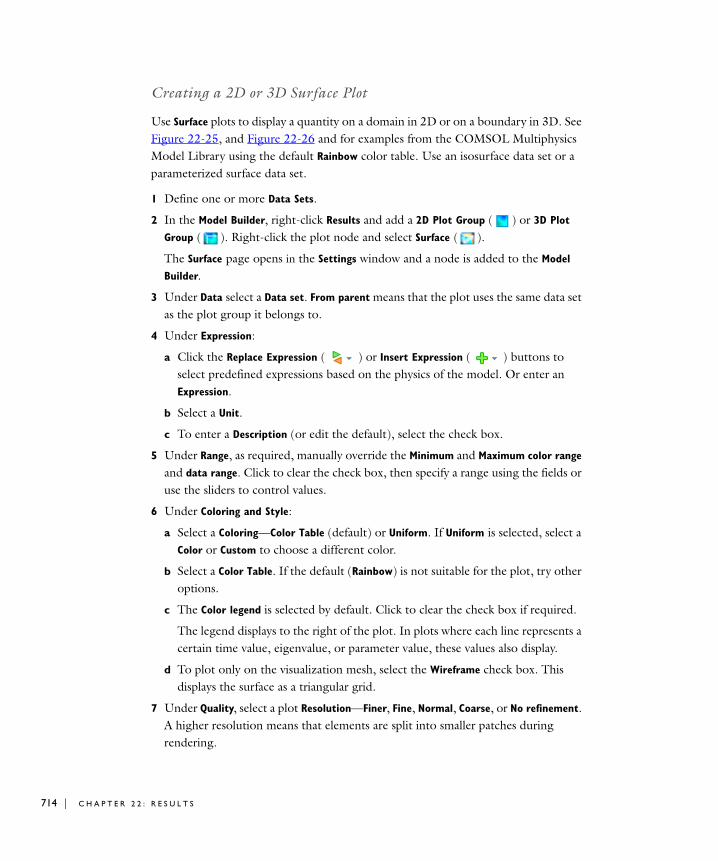
714 | C H A P T E
Creating a 2D or 3D Surface Plot
Use Surface plots to display a quantity on a domain in 2D or on a boundary in 3D. See Figure 22-25, and Figure 22-26 and for examples from the COMSOL Multiphysics Model Library using the default Rainbow color table. Use an isosurface data set or a parameterized surface data set.
1 Define one or more Data Sets.
2 In the Model Builder, right-click Results and add a 2D Plot Group ( ) or 3D Plot
Group ( ). Right-click the plot node and select Surface ( ).
The Surface page opens in the Settings window and a node is added to the Model
Builder.
3 Under Data select a Data set. From parent means that the plot uses the same data set as the plot group it belongs to.
4 Under Expression:
a Click the Replace Expression ( ) or Insert Expression ( ) buttons to select predefined expressions based on the physics of the model. Or enter an Expression.
b Select a Unit.
c To enter a Description (or edit the default), select the check box.
5 Under Range, as required, manually override the Minimum and Maximum color range and data range. Click to clear the check box, then specify a range using the fields or use the sliders to control values.
6 Under Coloring and Style:
a Select a Coloring—Color Table (default) or Uniform. If Uniform is selected, select a Color or Custom to choose a different color.
b Select a Color Table. If the default (Rainbow) is not suitable for the plot, try other options.
c The Color legend is selected by default. Click to clear the check box if required.
The legend displays to the right of the plot. In plots where each line represents a certain time value, eigenvalue, or parameter value, these values also display.
d To plot only on the visualization mesh, select the Wireframe check box. This displays the surface as a triangular grid.
7 Under Quality, select a plot Resolution—Finer, Fine, Normal, Coarse, or No refinement. A higher resolution means that elements are split into smaller patches during rendering.
R 2 2 : R E S U L T S
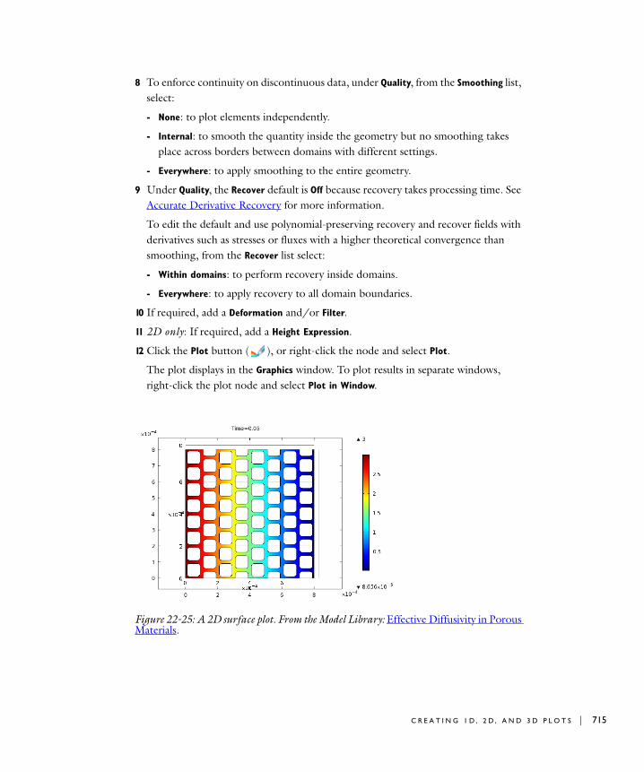
8 To enforce continuity on discontinuous data, under Quality, from the Smoothing list, select:
- None: to plot elements independently.
- Internal: to smooth the quantity inside the geometry but no smoothing takes place across borders between domains with different settings.
- Everywhere: to apply smoothing to the entire geometry.
9 Under Quality, the Recover default is Off because recovery takes processing time. See Accurate Derivative Recovery for more information.
To edit the default and use polynomial-preserving recovery and recover fields with derivatives such as stresses or fluxes with a higher theoretical convergence than smoothing, from the Recover list select:
- Within domains: to perform recovery inside domains.
- Everywhere: to apply recovery to all domain boundaries.
10 If required, add a Deformation and/or Filter.
11 2D only: If required, add a Height Expression.
12 Click the Plot button ( ), or right-click the node and select Plot.
The plot displays in the Graphics window. To plot results in separate windows, right-click the plot node and select Plot in Window.
Figure 22-25: A 2D surface plot. From the Model Library: Effective Diffusivity in Porous Materials.
C R E A T I N G 1 D , 2 D , A N D 3 D P L O T S | 715

716 | C H A P T E
Figure 22-26: A 3D surface plot. From the Model Library: Eigenvalue Analysis of a Crankshaft.
A D D I N G A H E I G H T E X P R E S S I O N T O A 2 D S U R F A C E P L O T
Height attributes introduce a 3D height on a 2D surface plot. Add a Height Expression so the height of the surface represents a scalar quantity. Only 2D surface plots support height attributes. See Figure 22-27 and Figure 22-28 for an example from the Acoustics Module Model Library.
1 In the Model Builder, add and define a 2D Surface plot ( ). Right-click the plot node and select Height Expression ( ).
The Height Expression page opens in the Settings window and a node is added to the Model Builder.
2 Under Expression, the Height data defaults to From parent to use the same data set as the plot group it belongs to. If Expression is selected instead:
a Enter an Expression or the Replace Expression ( ) or Insert Expression ( ) buttons to select predefined expressions based on the physics of the model.
b Select a Unit.
c To enter a Description (or edit the default), select the check box.
3 Under Scale:
a Enter a Scale factor or use the sliders to control height values.
b Enter an Offset or use the sliders to control values.
R 2 2 : R E S U L T S

4 Click the Plot button ( ), or right-click the node and select Plot.
The plot displays in the Graphics window. To plot results in separate windows, right-click the plot node and select Plot in Window.
Figure 22-27: A 2D surface plot before a height expression is added. From the Model Library: Transient Gaussian Explosion.
Figure 22-28: A 2D surface plot with height expression. From the Model Library: Transient Gaussian Explosion.
C R E A T I N G 1 D , 2 D , A N D 3 D P L O T S | 717
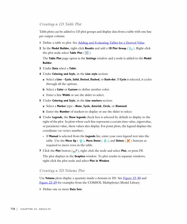
718 | C H A P T E
Creating a 1D Table Plot
Table plots can be added to 1D plot groups and display data from a table with one line per output column.
1 Define a table to plot. See Adding and Evaluating Tables for a Derived Value.
2 In the Model Builder, right-click Results and add a 1D Plot Group ( ). Right-click the plot node select Table Plot ( ).
The Table Plot page opens in the Settings window and a node is added to the Model
Builder.
3 Under Data select a Table.
4 Under Coloring and Style, in the Line style section:
a Select a Line—Cycle, Solid, Dotted, Dashed, or Dash-dot. If Cycle is selected, it cycles through all the options.
b Select a Color or Custom to define another color.
c Enter a line Width or use the slider to select.
5 Under Coloring and Style, in the Line markers section:
a Select a Marker type—None, Cycle, Asterisk, Circle, or Diamond.
b Enter the Number of markers to display or use the slider to select.
6 Under Legends, the Show legends check box is selected by default to display to the right of the plot. In plots where each line represents a certain time value, eigenvalue, or parameter value, these values also display. For point plots, the legend displays the coordinate (or vertex number).
- If Manual is selected from the Legends list, enter your own legend text into the table. Use the Move Up ( ), Move Down ( ), and Delete ( ) buttons as required to move rows in the table.
7 Click the Plot button ( ), right-click the node and select Plot, or press F8.
The plot displays in the Graphics window. To plot results in separate windows, right-click the plot node and select Plot in Window.
Creating a 3D Volume Plot
Use Volume plots display a quantity inside a domain in 3D. See Figure 22-30 and Figure 22-29 for examples from the COMSOL Multiphysics Model Library.
1 Define one or more Data Sets.
R 2 2 : R E S U L T S

2 In the Model Builder, right-click Results and add a 3D Plot Group ( ). Right-click the plot group and select Volume ( ).
The Volume page opens in the Settings window and a node is added to the Model
Builder.
3 Under Data select a Data set. From parent means that the plot uses the same data set as the plot group it belongs to.
4 Under Expression:
a Click the Replace Expression ( ) or Insert Expression ( ) buttons to select predefined expressions based on the physics of the model. Or enter an Expression.
b Select a Unit.
c To enter a Description (or edit the default), select the check box.
5 Under Range, as required, manually override the Minimum and Maximum color range and data range. Click to clear the check box, then specify a range using the fields or use the sliders to control values.
6 Under Coloring and Style:
a Select a Coloring—Color Table (default) or Uniform. If Uniform is selected, select a Color or Custom to choose a different color.
b Select a Color Table. If the default (Rainbow) is not suitable for the plot, try other options.
c The Color legend is selected by default. Click to clear the check box if required.
The legend displays to the right of the plot. In plots where each line represents a certain time value, eigenvalue, or parameter value, these values also display.
d To plot only on the visualization mesh, select the Wireframe check box. This displays the surface as a triangular grid. See Figure 22-29 for an example.
C R E A T I N G 1 D , 2 D , A N D 3 D P L O T S | 719
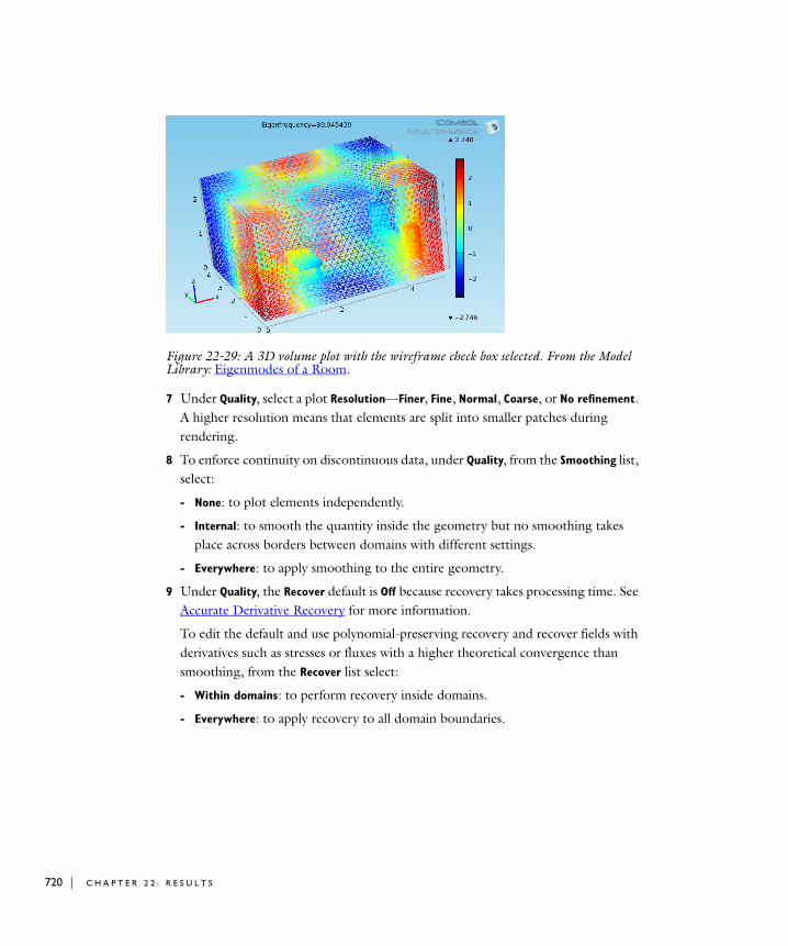
720 | C H A P T E
Figure 22-29: A 3D volume plot with the wireframe check box selected. From the Model Library: Eigenmodes of a Room.
7 Under Quality, select a plot Resolution—Finer, Fine, Normal, Coarse, or No refinement. A higher resolution means that elements are split into smaller patches during rendering.
8 To enforce continuity on discontinuous data, under Quality, from the Smoothing list, select:
- None: to plot elements independently.
- Internal: to smooth the quantity inside the geometry but no smoothing takes place across borders between domains with different settings.
- Everywhere: to apply smoothing to the entire geometry.
9 Under Quality, the Recover default is Off because recovery takes processing time. See Accurate Derivative Recovery for more information.
To edit the default and use polynomial-preserving recovery and recover fields with derivatives such as stresses or fluxes with a higher theoretical convergence than smoothing, from the Recover list select:
- Within domains: to perform recovery inside domains.
- Everywhere: to apply recovery to all domain boundaries.
R 2 2 : R E S U L T S

10 Under Element Filter, specify the elements to display:
a Select the Enable filter check box.
b From the Criterion list, select Random, Expression, or Logical expression.
c If Expression or Logical expression is selected, enter an Expression in the field.
d If Random or Expression is selected, specify the Fraction of elements to show or use the slider to choose.
11 To scale elements in the mesh plot, under Shrink Elements, enter an Element scale
factor between 0 and 1.
12 If required, add a Deformation and/or Filter.
13 Click the Plot button ( ), right-click the node and select Plot, or press F8.
The plot displays in the Graphics window. To plot results in separate windows, right-click the plot node and select Plot in Window.
Figure 22-30: A 3D volume plot. From the Model Library: Eigenmodes of a Room.
Combining Plots
1 Define one or more Data Sets.
2 In the Model Builder, add one or more 1D ( ), 2D ( ), or 3D Plot Groups ( ).
C R E A T I N G 1 D , 2 D , A N D 3 D P L O T S | 721
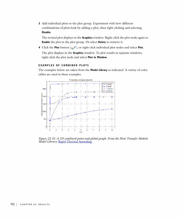
722 | C H A P T E
3 Add individual plots to the plot group. Experiment with how different combinations of plots look by adding a plot, then right-clicking and selecting Disable.
The revised plot displays in the Graphics window. Right-click the plot node again to Enable the plot in the plot group. Or select Delete to remove it.
4 Click the Plot button ( ), or right-click individual plot nodes and select Plot.
The plot displays in the Graphics window. To plot results in separate windows, right-click the plot node and select Plot in Window.
E X A M P L E S O F C O M B I N E D P L O T S
The examples below are taken from the Model Library as indicated. A variety of color tables are used in these examples.
Figure 22-31: A 1D combined point and global graph. From the Heat Transfer Module Model Library: Rapid Thermal Annealing.
R 2 2 : R E S U L T S
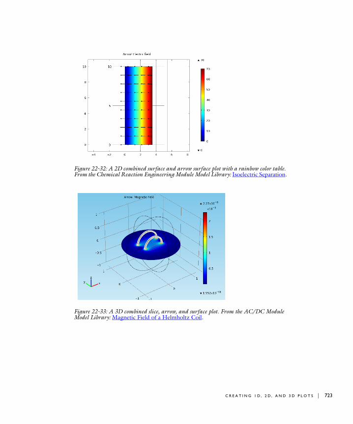
Figure 22-32: A 2D combined surface and arrow surface plot with a rainbow color table. From the Chemical Reaction Engineering Module Model Library: Isoelectric Separation.
Figure 22-33: A 3D combined slice, arrow, and surface plot. From the AC/DC Module Model Library: Magnetic Field of a Helmholtz Coil.
C R E A T I N G 1 D , 2 D , A N D 3 D P L O T S | 723

724 | C H A P T E
Figure 22-34: A 3D combined streamline and slice plot with a thermal color table. From the AC/DC Module Model Library: Cold Crucible.
Figure 22-35: A 3D combined isosurface and streamline plot with a wave color table. From the Heat Transfer Module Model Library: Isothermal Heat Exchanger.
R 2 2 : R E S U L T S

C r e a t i n g C r o s s - S e c t i o n P l o t s
Cross-section plots are created using a combination of data sets and plot groups. Cross-section plots show the values over time, along a parametric solution, or for several eigenvalues. Cross-section plots visualize a quantity as a family of plots on:
• An arbitrary set of points (in 1D, 2D, or 3D)
A point cross-section plot makes it easy to view an expression at an arbitrary set of spatial coordinates and results in a line plot. Note that expressions and variables that include derivatives of the dependent variables (for example, stresses in a structural analysis) are not available at isolated geometry vertices (points). See 1D, 2D, and 3D Cross-Section Point Plots.
• An arbitrary line (in 2D or 3D). See 2D Cross-Section Line Plots and 3D Cross-Section Line Plots.
Use cut line data sets to create lines through 2D or 3D geometries to visualize along the line. All plots and results analysis features available in 1D are available for cut line data sets as well as 3D plots and results analysis features for edges.
• Arbitrary planes (in 3D) using a surface plot and cut plane data set. See 3D Cross-Section Surface Plot.
Use cut plane data sets to create planes through a 3D in a 2D geometry to visualize on the plane. All plots and results analysis features available in 2D are available for cut plane data sets as well as for surfaces in 3D. The cut plane corresponds to an orthogonal 2D coordinate system embedded in 3D.
I N T E R A C T I V E C R O S S - S E C T I O N L I N E A N D S U R F A C E P L O T S
You can also interactively create cross-section line and surface plots using a combination of cross-section toolbar buttons and clicking on the geometry. When you use the cross-section toolbar, plot groups and data sets are automatically added and updated in the Model Builder whenever any line or plane is changed. As soon as a line or plane is completed, a rendering mesh snaps the entry and exit points to the faces of the domain containing the data and to computes the line. See Creating Interactive 2D Cross-Section Line Plots, Creating Interactive 3D Cross-Section Line Plots and Creating Interactive 3D Cross-Section Surface Plots.
C R E A T I N G C R O S S - S E C T I O N P L O T S | 725
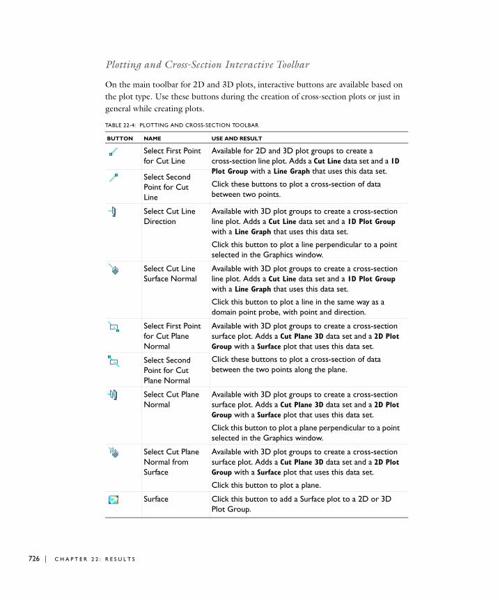
726 | C H A P T E
Plotting and Cross-Section Interactive Toolbar
On the main toolbar for 2D and 3D plots, interactive buttons are available based on the plot type. Use these buttons during the creation of cross-section plots or just in general while creating plots.
TABLE 22-4: PLOTTING AND CROSS-SECTION TOOLBAR
BUTTON NAME USE AND RESULT
Select First Point for Cut Line
Available for 2D and 3D plot groups to create a cross-section line plot. Adds a Cut Line data set and a 1D Plot Group with a Line Graph that uses this data set.
Click these buttons to plot a cross-section of data between two points.
Select Second Point for Cut Line
Select Cut Line Direction
Available with 3D plot groups to create a cross-section line plot. Adds a Cut Line data set and a 1D Plot Group with a Line Graph that uses this data set.
Click this button to plot a line perpendicular to a point selected in the Graphics window.
Select Cut Line Surface Normal
Available with 3D plot groups to create a cross-section line plot. Adds a Cut Line data set and a 1D Plot Group with a Line Graph that uses this data set.
Click this button to plot a line in the same way as a domain point probe, with point and direction.
Select First Point for Cut Plane Normal
Available with 3D plot groups to create a cross-section surface plot. Adds a Cut Plane 3D data set and a 2D Plot Group with a Surface plot that uses this data set.
Click these buttons to plot a cross-section of data between the two points along the plane.
Select Second Point for Cut Plane Normal
Select Cut Plane Normal
Available with 3D plot groups to create a cross-section surface plot. Adds a Cut Plane 3D data set and a 2D Plot Group with a Surface plot that uses this data set.
Click this button to plot a plane perpendicular to a point selected in the Graphics window.
Select Cut Plane Normal from Surface
Available with 3D plot groups to create a cross-section surface plot. Adds a Cut Plane 3D data set and a 2D Plot Group with a Surface plot that uses this data set.
Click this button to plot a plane.
Surface Click this button to add a Surface plot to a 2D or 3D Plot Group.
R 2 2 : R E S U L T S
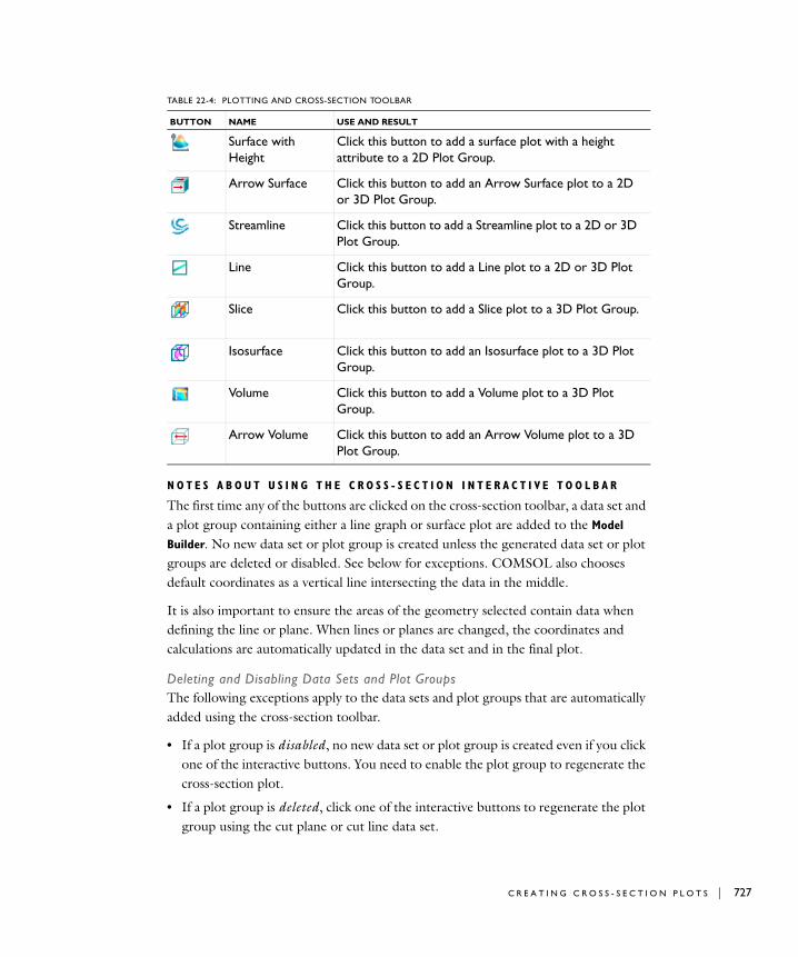
N O T E S A B O U T U S I N G T H E C R O S S - S E C T I O N I N T E R A C T I V E T O O L B A R
The first time any of the buttons are clicked on the cross-section toolbar, a data set and a plot group containing either a line graph or surface plot are added to the Model
Builder. No new data set or plot group is created unless the generated data set or plot groups are deleted or disabled. See below for exceptions. COMSOL also chooses default coordinates as a vertical line intersecting the data in the middle.
It is also important to ensure the areas of the geometry selected contain data when defining the line or plane. When lines or planes are changed, the coordinates and calculations are automatically updated in the data set and in the final plot.
Deleting and Disabling Data Sets and Plot GroupsThe following exceptions apply to the data sets and plot groups that are automatically added using the cross-section toolbar.
• If a plot group is disabled, no new data set or plot group is created even if you click one of the interactive buttons. You need to enable the plot group to regenerate the cross-section plot.
• If a plot group is deleted, click one of the interactive buttons to regenerate the plot group using the cut plane or cut line data set.
Surface with Height
Click this button to add a surface plot with a height attribute to a 2D Plot Group.
Arrow Surface Click this button to add an Arrow Surface plot to a 2D or 3D Plot Group.
Streamline Click this button to add a Streamline plot to a 2D or 3D Plot Group.
Line Click this button to add a Line plot to a 2D or 3D Plot Group.
Slice Click this button to add a Slice plot to a 3D Plot Group.
Isosurface Click this button to add an Isosurface plot to a 3D Plot Group.
Volume Click this button to add a Volume plot to a 3D Plot Group.
Arrow Volume Click this button to add an Arrow Volume plot to a 3D Plot Group.
TABLE 22-4: PLOTTING AND CROSS-SECTION TOOLBAR
BUTTON NAME USE AND RESULT
C R E A T I N G C R O S S - S E C T I O N P L O T S | 727

728 | C H A P T E
• If a data set is deleted, and it is used with a plot group, the plot group is also deleted at the same time. However, if the plot group is using another data set it is not deleted.
• If a data set is disabled, the associated plot group is not disabled. However, if you want to plot another cross-section, click one of the interactive buttons to create a new data set to use with the plot group.
1D, 2D, and 3D Cross-Section Point Plots
C R E A T I N G A 1 D C R O S S - S E C T I O N P L O T U S I N G A C U T PO I N T D A T A S E T
A 1D cross-section point plot visualizes a quantity in one or several points in time, along a parameter range, or for several different eigenvalues.
1 Create a Cut Point 1D data set.
- Under Point Data enter the x-coordinates for the plot. Enter one or several space-separated values or a vector of coordinates, for example, range(0,10,100).
2 Click the Plot button ( ).
3 Add a 1D Plot Group ( ). Select Cut Point 1D as the Data set. If required, right-click and Rename the plot group, for example, Cross-Section-1D Point.
4 Add a Point Graph to this 1D plot group and select Cut Point 1D as the Data set or From parent to use the same data set as the plot group it belongs to.
5 Continue to define the Point Graph as required.
6 Click the Plot button ( ), right-click the node and select Plot, or press F8.
The plot displays in the Graphics window. To plot results in separate windows, right-click the plot node and select Plot in Window.
C R E A T I N G A 2 D C R O S S - S E C T I O N P L O T U S I N G A C U T PO I N T D A T A S E T
The 2D point cross-section plot visualizes a quantity in one or several points in time, along a parameter range, or for several eigenvalues. This example uses the Stresses in a Pulley model from the COMSOL Multiphysics Model Library.
1 Create a Cut Point 2D data set.
- Under Point Data enter the x- and y-coordinate values for the plot. Enter the same number of space-separated values in the x and y fields. Alternatively, enter a vector of coordinates, for example, range(0,10,100).
2 Click the Plot button ( ).
R 2 2 : R E S U L T S

3 Add a 1D Plot Group ( ). Select Cut Point 2D as the Data set. If required, right-click and Rename the plot group, for example, Cross-Section-2D Point.
4 Add a Point Graph and select Cut Point 2D as the Data set or From parent to use the same data set as the plot group it belongs to.
- The x-axis corresponds to time, parameter values, or the eigenvalue number.
- The settings in the y-axis data area determine the quantity on the y-axis. Select from predefined quantities or enter an expression that contains variables.
5 Continue to define the Point Graph as required.
6 Click the Plot button ( ) right-click the node and select Plot, or press F8.
The plot displays in the Graphics window. To plot results in separate windows, right-click the plot node and select Plot in Window.
C R E A T I N G A 3 D C R O S S - S E C T I O N P L O T U S I N G A C U T P O I N T D A T A S E T
A 3D point cross-section plot visualizes a quantity in one or several points in time, along a parameter range, or for several eigenvalues. This example uses the Star-Shaped Microchannel Chipmodel from the MEMS Module Model Library.
1 Create a Cut Point 3D data set.
- Under Point Data enter the x-, y-, and z-coordinate values for the plot. Enter the same number of space-separated values in the x, y, and z fields. Alternatively, enter a vector of coordinates, for example, range(0,10,100).
2 Click the Plot button ( ).
3 Add a 1D Plot Group ( ). Select Cut Point 3D as the Data set. If required, right-click and Rename the plot group, for example, Cross-Section-3D Point.
C R E A T I N G C R O S S - S E C T I O N P L O T S | 729
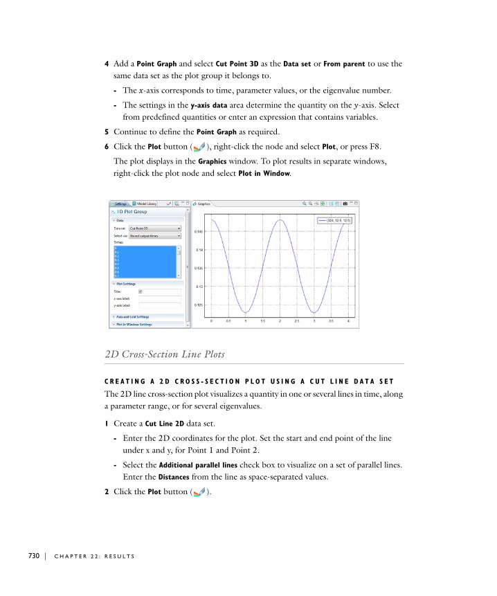
730 | C H A P T E
4 Add a Point Graph and select Cut Point 3D as the Data set or From parent to use the same data set as the plot group it belongs to.
- The x-axis corresponds to time, parameter values, or the eigenvalue number.
- The settings in the y-axis data area determine the quantity on the y-axis. Select from predefined quantities or enter an expression that contains variables.
5 Continue to define the Point Graph as required.
6 Click the Plot button ( ), right-click the node and select Plot, or press F8.
The plot displays in the Graphics window. To plot results in separate windows, right-click the plot node and select Plot in Window.
2D Cross-Section Line Plots
C R E A T I N G A 2 D C R O S S - S E C T I O N P L O T U S I N G A C U T L I N E D A T A S E T
The 2D line cross-section plot visualizes a quantity in one or several lines in time, along a parameter range, or for several eigenvalues.
1 Create a Cut Line 2D data set.
- Enter the 2D coordinates for the plot. Set the start and end point of the line under x and y, for Point 1 and Point 2.
- Select the Additional parallel lines check box to visualize on a set of parallel lines. Enter the Distances from the line as space-separated values.
2 Click the Plot button ( ).
R 2 2 : R E S U L T S

3 Add a 1D Plot Group ( ). Right-click the plot node and select Cut Line 2D as the Data set. If required, right-click and Rename the plot group, for example, Cross-Section-2D Line.
4 Add a Line Graph and select Cut Line 2D as the Data set or From parent to use the same data set as the plot group it belongs to.
- Settings under Y-Axis Data determine the quantity to display on that axis. Either select from predefined Expressions or enter an Expression containing variables.
- Settings under X-Axis Data determine the quantity on that axis. Select Arc length or Expression as required. Enter or select an Expression, Unit and Description.
5 Continue to define the Line Graph as required.
6 Click the Plot button ( ), right-click the node and select Plot, or press F8.
The plot displays in the Graphics window. To plot results in separate windows, right-click the plot node and select Plot in Window.
C R E A T I N G I N T E R A C T I V E 2 D C R O S S - S E C T I O N L I N E P L O T S
1 In the Model Builder, click a 2D Plot Group node to display the buttons available on the main toolbar.
2 On the main toolbar, click the Select First Point for Cut Line button ( ). Click a start point on the geometry. COMSOL chooses default coordinates as a vertical line intersecting the data in the middle.
3 Click the Select Second Point for Cut Line button ( ). Click an end point on the geometry.
A line connecting the two points is displayed in the Graphics window. The first time the cross-section toolbar buttons are clicked, a Cut Line 2D data set and a 1D Plot
Group with a Line Graph are added to the Model Builder.
4 Adjust the cut line as required by clicking the buttons, then clicking on the geometry to change where the first and second point start and end (respectively). The coordinates are updated automatically in the data set and plot group. Click the 1D Plot Group node to view the updates to the line graph.
5 Continue adjusting the cut line until the line graph representing the points plots the data as required.
C R E A T I N G C R O S S - S E C T I O N P L O T S | 731

732 | C H A P T E
3D Cross-Section Line Plots
C R E A T I N G A 3 D C R O S S - S E C T I O N P L O T U S I N G A C U T L I N E D A T A S E T
A 3D line/extrusion cross-section plot visualizes a quantity in one or several lines in time, along a parameter range, or for several eigenvalues. This example uses the Prestressed Micromirrormodel from the MEMS Module Model Library.
1 Create a Cut Line 3D data set.
- Enter the 3D coordinates for the plot. Set the start and end point of the line under x, y, and z for Point 1 and Point 2.
2 Click the Plot button ( ).
3 Add a 1D Plot Group ( ). Right-click the plot node and select Cut Line 3D as the Data set. If required, right-click and Rename the plot group, for example, Cross-Section-3D Line.
4 Add a Line Graph and select Cut Line 3D as the Data set or From parent to use the same data set as the plot group it belongs to.
- Settings under Y-Axis Data determine the quantity to display on the vertical axis. Either select from predefined Expressions or enter an Expression containing variables.
- Settings under X-Axis Data determine the quantity on the horizontal axis of the cross-section plot. Select Arc length or Expression as required. Enter or select an Expression, Unit and Description.
5 Continue to define the Line Graph as required (see Creating a 1D Line Graph).
R 2 2 : R E S U L T S

6 Click the Plot button ( ) right-click the node and select Plot, or press F8.
The plot displays in the Graphics window. To plot results in separate windows, right-click the plot node and select Plot in Window.
C R E A T I N G C R O S S - S E C T I O N P L O T S | 733

734 | C H A P T E
C R E A T I N G I N T E R A C T I V E 3 D C R O S S - S E C T I O N L I N E P L O T S
1 In the Model Builder, click a 3D Plot Group node to display the buttons available on the main toolbar. On the main toolbar, click the cross-section buttons as required.
The first time the cross-section toolbar buttons are clicked, a Cut Line 3D data set and a 1D Plot Group with a Line Graph are added to the Model Builder.
Defining a Cut Line:
a On the main toolbar, click the Select First Point for Cut Line button ( ). Click a start point on the geometry. COMSOL chooses default coordinates as a vertical line intersecting the data in the middle.
b Click the Select Second Point for Cut Line button ( ). Click an end point on the geometry. A line connecting the two points is created in the Graphics window.
c Click either of the buttons and then on the geometry to change the start and end points respectively.
d Click the 1D Plot Group to view the Line Graph based on the selected points.
Defining a Cut Line - Direction:
a On the main toolbar, click the Select Cut Line Direction button ( ).
b Click on the geometry to add a line perpendicular to where you clicked. COMSOL chooses default coordinates as a vertical line intersecting the data in the middle.
c Click the 1D Plot Group node to view the Line Graph based on the selected points.
Defining a Cut Line - Surface Normal:
a On the main toolbar, click the Select Cut Line Surface Normal button ( ).
b Click on the geometry to add a line with a point and direction. COMSOL chooses default coordinates as a vertical line intersecting the data in the middle.
c Click the 1D Plot Group node to view the Line Graph based on the selected points.
2 Adjust the cut line as required by clicking the buttons, then clicking on the geometry to change its coordinates. The data set and plot group are updated automatically with the cut line data. Click the 1D Plot Group node to view the updates to the line graph.
3 Continue adjusting the cut line until the line graph representing the points plots the data as required.
R 2 2 : R E S U L T S

3D Cross-Section Surface Plot
3 D C R O S S - S E C T I O N S U R F A C E P L O T U S I N G A C U T P L A N E D A T A S E T
A 3D surface cross-section plot visualizes a quantity in one or several planes in time, along a parameter range, or for several eigenvalues. This example uses the Airflow Over an Ahmed Bodyfile from the CFD Module Model Library.
1 Create a Cut Plane 3D data set.
2 Click the Plot button ( ), or right-click the node and select Plot.
3 Add a 2D Plot Group ( ). Right-click the plot node and select Cut Plane 3D as the Data set. If required, right-click and Rename the plot group, for example, Cross-Section-3D Surface.
4 Add a Surface plot and select Cut Plane 3D as the Data set or From parent to use the same data set as the plot group it belongs to.
5 Continue to define the Surface plot as required.
6 Click the Plot button ( ), or right-click the node and select Plot.
The plot displays in the Graphics window. To plot results in separate windows, right-click the plot node and select Plot in Window.
C R E A T I N G C R O S S - S E C T I O N P L O T S | 735

736 | C H A P T E
C R E A T I N G I N T E R A C T I V E 3 D C R O S S - S E C T I O N S U R F A C E P L O T S
1 In the Model Builder, click a 3D Plot Group node to display the buttons available on the main toolbar. On the main toolbar, click the cross-section buttons as required.
The first time the cross-section toolbar buttons are clicked, a Cut Plane 3D data set and a 2D Plot Group with a Surface plot are added to the Model Builder.
To Define a Cut Plane:
a Click the Select First Point for Cut Plane Normal button ( ). Click a start point on the geometry. COMSOL chooses default coordinates as a vertical line intersecting the data in the middle. The green highlighted areas show you what the cut plane will look like if this first click point is chosen for the surface plot.
b Click the Select Second Point for Cut Plane Normal button ( ). Click an end point on the geometry. The green highlighted areas show you what the cut plane will look like if this second click point is chosen for the surface plot.
c Click either of the buttons and then on the geometry to change the start and end points respectively.
d Click the 2D Plot Group to view the Surface plot based on the selected points.
To Define a Normal Cut Plane:
a Click the Select Cut Plane Normal button ( ).
b Click on the geometry to add a plane perpendicular to the click location. COMSOL chooses default coordinates as a vertical line intersecting the data in
R 2 2 : R E S U L T S

the middle. The green highlighted areas show you what the plot will look like if this normal cut plane is chosen for the surface plot.
c Click the 2D Plot Group to view the Surface plot based on the selected points.
To Define a Normal Cut Plane from Surface:
a Click the Select Cut Plane Normal from Surface button ( ).
b Click on the geometry to add a line with a point and direction starting at the click location. COMSOL chooses default coordinates as a vertical line intersecting the data in the middle. The green highlighted areas show you what the plot will look like if this normal from surface cut plane is chosen for the surface plot.
c Click the 2D Plot Group to view the Surface plot based on the selected points.
2 Adjust the cut plane as required by clicking the buttons, then clicking on the geometry to change the coordinates. The data set and plot group are updated automatically with the cut plane data. Click the 2D Plot Group node to view the updates to the surface plot.
3 Continue adjusting the cut plane until the surface plot representing the points plots the data as required.
C R E A T I N G C R O S S - S E C T I O N P L O T S | 737
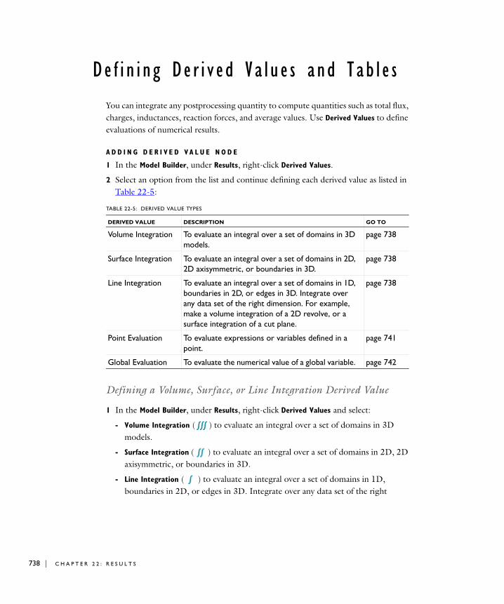
738 | C H A P T E
De f i n i n g De r i v e d V a l u e s and T ab l e s
You can integrate any postprocessing quantity to compute quantities such as total flux, charges, inductances, reaction forces, and average values. Use Derived Values to define evaluations of numerical results.
A D D I N G D E R I V E D V A L U E N O D E
1 In the Model Builder, under Results, right-click Derived Values.
2 Select an option from the list and continue defining each derived value as listed in Table 22-5:
Defining a Volume, Surface, or Line Integration Derived Value
1 In the Model Builder, under Results, right-click Derived Values and select:
- Volume Integration ( ) to evaluate an integral over a set of domains in 3D models.
- Surface Integration ( ) to evaluate an integral over a set of domains in 2D, 2D axisymmetric, or boundaries in 3D.
- Line Integration ( ) to evaluate an integral over a set of domains in 1D, boundaries in 2D, or edges in 3D. Integrate over any data set of the right
TABLE 22-5: DERIVED VALUE TYPES
DERIVED VALUE DESCRIPTION GO TO
Volume Integration To evaluate an integral over a set of domains in 3D models.
page 738
Surface Integration To evaluate an integral over a set of domains in 2D, 2D axisymmetric, or boundaries in 3D.
page 738
Line Integration To evaluate an integral over a set of domains in 1D, boundaries in 2D, or edges in 3D. Integrate over any data set of the right dimension. For example, make a volume integration of a 2D revolve, or a surface integration of a cut plane.
page 738
Point Evaluation To evaluate expressions or variables defined in a point.
page 741
Global Evaluation To evaluate the numerical value of a global variable. page 742
R 2 2 : R E S U L T S

dimension. For example, make a volume integration of a 2D revolve, or a surface integration of a cut plane.
The Volume, Surface, or Line Integration page opens in the Settings window and a node is added to the Model Builder.
2 Under Data, select a Data set. The result is computed by integrating over the data set selected.
Note: If None is selected from the Data set list, skip the next step.
For Parametric Solver and Parametric Sweep studies, the Parameter values section lists the associated parameter values.
a For Parametric Sweep studies (see Solver Studies and Study Types) select an option from the Select via list —Stored output times or Interpolated times (time dependent models only).
The time steps cannot be selected directly because the different parametric solutions could have different time steps. Selecting Stored output times plots all of them, or select Interpolated times to get the same interpolated times for every parameter.
b If Interpolated times is selected, enter Times or click the Vector Input button ( ) to select and define specific times. See Entering Ranges and Vector-Valued Expressions for details.
c When available, from the Table rows list, select Inner solutions or Outer solutions. These options are available when there is a Parametric Sweep problem with dynamic inner solutions (that is to say, time, eigenvalue, or parametric solutions).
- If Inner solutions is selected, when you click the Evaluate button ( ) the results table displays the dynamic value (for example, time, eigenvalue, or parametric) solutions in rows.
- If Outer solutions is selected, when you click the Evaluate button ( ) the results table displays the parameters in rows.
3 If a Solution data set is selected, under Selection:
a Select All or Manual.
b If Manual is selected choose geometry directly from the Graphics window. Select All to add the applicable geometry or any other predefined grouping. Use the Add
D E F I N I N G D E R I V E D V A L U E S A N D TA B L E S | 739

740 | C H A P T E
to Selection ( ), Remove from Selection ( ), and Clear Selection ( ) buttons as required in the Settings window.
4 Under Expression, for all data sets, including None:
a Click the Replace Expression ( ) or Insert Expression ( ) buttons to select predefined expressions based on the physics of the model. Or enter an Expression.
b Select a Unit.
c Select the Description check box to enter a description of the data set (or edit the default).
5 Under Integration Settings:
a Select a Method.
- Auto—the default and computes the integral for fields by numerical integration and for reaction forces by summation. Predefined quantities for reaction forces use summation instead of integration. Also, if you specify an expression for the integrand using the reacf operator, the automatic setting chooses the summation method.
- Integration—the standard numerical integration method (quadrature).
- Summation—a summation method useful for computing reaction forces. The summation method finds all nodes on the boundary, evaluates the expression in the nodes and sum up the values. Reaction force variables are predefined in the structural mechanics interfaces.
b COMSOL automatically determines an appropriate Integration order for the expression. To change this, click to clear the check box and enter a number. COMSOL performs the integration elementwise using numeric quadrature of the selected order.
Note: For 2D axisymmetric models, Volume and Surface Integration is available. COMSOL multiplies the expression (integrand) with 2*pi*r prior to integration to compute the corresponding volume or surface integral. Complete the next step.
c For Surface Integration, select the Compute volume integral (axial symmetry) check box.
d For Line Integration, select the Compute surface integral (axial symmetry) check box.
R 2 2 : R E S U L T S

6 Click the Evaluate button ( ).
7 The Results window opens to view a Table of the Derived values. By default four digits are displayed; click the Full precision button ( ) to display as many significant digits as possible. The Table display precision level can be changed from the Options>Preferences>General menu.
Defining a Point Evaluation Derived Value
1 In the Model Builder, under Results, right-click Derived Values and select Point
Evaluation ( ) to evaluate expressions or variables defined in a point.
The Point Evaluation page opens in the Settings window and a node is added to the Model Builder.
2 Under Data select a Data set.
If a Cut Point data set is selected, skip the next step.
3 If a Solution data set is selected, under Selection:
a Select All or Manual.
b If Manual is selected choose geometry directly from the Graphics window. Select All to add the applicable geometry or any other predefined grouping. Use the Add
to Selection ( ), Remove from Selection ( ), and Clear Selection ( ) buttons as required in the Settings window.
4 Under Expression:
a Click the Replace Expression ( ) or Insert Expression ( ) buttons to select predefined expressions based on the physics of the model. Or enter an Expression.
a Select a Unit.
b Select the Description check box to enter a description of the data set (or edit the default).
5 Click the Evaluate button ( ).
6 Open the Results window to view a Table of the Derived values. By default four digits are displayed; click the Full precision button ( ) to display as many significant digits as possible. The Table display precision level can be changed from the Options>Preferences>General menu.
D E F I N I N G D E R I V E D V A L U E S A N D TA B L E S | 741

742 | C H A P T E
Defining a Global Evaluation Derived Value
1 In the Model Builder, under Results, right-click Derived Values and select Global
Evaluation ( ).
The Global Evaluation page opens in the Settings window and a node is added to the Model Builder.
2 Under Data select a Data set. The result is computed by integrating over the data set selected.
3 Under Expression:
a Click the Replace Expression ( ) or Insert Expression ( ) buttons to select predefined expressions based on the physics of the model. Or enter an Expression.
b Select a Unit.
c Select the Description check box to enter a description of the data set (or edit the default).
4 Click the Evaluate button ( ).
5 Open the Results window to view a Table of the Derived values. By default four digits are displayed; click the Full precision button ( ) to display as many significant digits as possible. The Table display precision level can be changed from the Options>Preferences>General menu.
Adding and Evaluating Tables for a Derived Value
1 Add a Derived Value node to the model.
2 There are two ways to add a Table:
- In the right corner of the Volume, Surface, or Line Integration page, click the New
Table button ( ). This button is also used as the Evaluate button.
- In the Model Builder, right-click the Tables node, and select Table.
A Table node is added under Tables. Click the node to display a table with the selected integration feature’s description and values in the Results window—by default it opens below the Graphics window.
R 2 2 : R E S U L T S

3 There are two ways to evaluate a Table:
- In the right corner of the Volume, Surface, or Line Integration page, click the Evaluate button ( ). This button is also used as the New Table button.
- In the Model Builder, right-click the Derived Values node, and select Evaluate.
- After evaluating for the first time, you can click the Evaluate button ( ) a second time to evaluate the same table. Or you can click the down arrow next to the Evaluate button to select the target table on your own. This can be used, for example, to put the results from several evaluation features into the same table.
Editing and Organizing Results Tables
When a Table is generated and displays in the Results window, a variety of editing options are available as listed in Table 22-6 and in Figure 22-36.
TABLE 22-6: RESULTS TABLE EDITING BUTTONS
BUTTON AND FUNCTION DESCRIPTION
Full precision ( ) Click to display as many significant digits as possible.
Clear Table ( ) Click to clear the data from the table, but keep the table itself. Click the Evaluate button ( ) to regenerate the table data.
Delete Table ( ) Click to delete the table. There is no undo. If required, click the Evaluate button ( ) to regenerate the table.
Plot ( ) Click to plot the table in the Graphics window.
Copy Table to Clipboard ( ) Click the button or right-click anywhere in the table and select this option from the context menu. Paste the data in a spreadsheet, for example.
Delete column Right-click a column header or anywhere in the table, and select Delete column. There is no undo. If required, click the Evaluate button ( ) to regenerate the table.
Copy selection to clipboard Select the rows to copy, then right-click anywhere in the table and select this option from the context menu or press Ctrl C.
D E F I N I N G D E R I V E D V A L U E S A N D TA B L E S | 743

744 | C H A P T E
Figure 22-36: Context menu and button options for editing results tables.
R 2 2 : R E S U L T S

C r e a t i n g R epo r t s and Expo r t i n g Da t a
The Report node is where you can export data from plot groups as images, animations, and numerical data. You can export the Image, Plot, or Data information directly for use in external reports or COMSOL generated reports.
A D D I N G R E P O R T TY P E S
After a model is completed, you can add various components to the Report node and then generate report types (animation, data, images, player, plot, or export), or export the information to your computer for use in external reports.
• In the Model Builder, under the Report node, right-click and select an option—Animation, Player, Image 1D, 2D, or 3D, Plot, or Data.
Defining and Exporting Plot Animations
Use Animation to define and export a movie or series of images based on a plot group. Play the animation in a web browser or use it in presentations or on a web site.
1 In the Model Builder, right click Report and select Animation ( ).
The Animation page opens in the Settings window and a node is added to the Model
Builder.
2 Under Scene, select a Subject. The Subject list contains the 1D, 2D, or 3D Plot Groups previously defined.
TABLE 22-7: REPORT TYPES
REPORT DESCRIPTION GO TO
Animation To define and export a movie or series of images based on a plot group. Play the animation in a web browser or use it in presentations or on a web site.
page 745
Data Exports numerical data to file. Data export operates directly on data sets.
page 748
Image To export plot images from 1D, 2D and 3D Plot Groups page 750
Player To create interactive animations. page 752
Plot To export a plot from a 1D, 2D, or 3D Plot Group. page 751
C R E A T I N G R E P O R T S A N D E X P O R T I N G D A T A | 745
746 | C H A P T E
3 Under Output, select an Output type—Image sequence generates multiple image files; Movie generates a single file containing all the images. If Movie is selected, go to the next numbered step.
If Image sequence is selected:
- Enter a Filename including a path to save it to your computer.
- OR -
- Click Browse and navigate to where you want to Save the output. For example, navigate to the computer desktop and enter a File name in the Export Image
Sequence window then select an option from the Save as type list—.png, .bmp, or .jpg.
The text entered in the File name field is used for all the images generated. For example, if you enter image, select .png as the file type, and there are 11 frames in the movie, 11 files are created: image01.png, image02.png, …, image11.png.
4 If Movie is selected as the Output type, select a File type—GIF, Flash, or AVI.
a For all File types, enter a path and include a Filename. Or click Browse and navigate to where you want to Save the output. For example, navigate to the computer desktop and enter a File name in the Export Image Sequence window.
b For all File types, enter a number of Frames per second.
Enter information into the following fields based on the File type:
c If Flash is selected, the Interpolate between frames check box is selected by default. Click to clear the check box if required.
d If AVI is selected, enter a Quality. The default is 0.75.
AVI is a file format that can contain video encoded in different ways.
e For Flash and GIF, select the Open in browser check box to launch the default web browser to view the output file.
5 Under Frame Settings:
a Select the Lock aspect ratio check box to keep the original animation width and height.
b In the Width and Height fields, enter the number of pixels (px) for the generated image size.
c If required, select the Record in reverse order check box.
R 2 2 : R E S U L T S
6 Under Parameter Sweep, select a Sweep Type—Result parameter, Dynamic data
extension, or Stored solutions (the default). Each time selected creates a frame in the movie or an individual image file.
If Stored solutions is selected:
a Select Stored output times from the Select via list, and enter any vector of times in the Times field. For example, enter range(0,0.01,1) or 0 10^(range(-3,3)).
b For time-dependent problems, select Interpolated times from the Select via list. Enter Times or click the Vector Input button ( ) to select and define specific times. See Entering Ranges and Vector-Valued Expressions for details.
If Result parameter is selected:
a Enter a Parameter, Start, and Stop interval.
b Enter the Number of frames. The number of frames divided by the number of frames per second gives the total playing time for a movie of a static or eigenvalue solution.
If Dynamic data extension is selected:
a When animating static and eigenvalue solutions, select a Cycle type:
- Full harmonic—a full sine wave (the solution phase grows linearly from 0 to 360)
- Half harmonic—half a sine wave (the solution phase grows linearly from 0 to 180)
- Linear—a linear ramp (Reei, where is the phase) grows linearly from 0 to 1)
The cycle starts from the angle specified in the Solution at angle (phase) field when defining a Solution Data Set (see Defining a Solution Data Set).
b To visualize the time evolution of a time-harmonic model, enter the Number of
frames to include in the animation.
The number of frames divided by the number of frames per second gives the total playing time for a movie of a static or eigenvalue solution.
7 Under Parameter Sweep, for Parametric Sweep studies, select an option from the Solutions list—Inner solutions or Outer solutions.
- If Outer solutions is selected (that is to say, the parameters from the parametric sweep), the Parameter values section lists all options. Select as required, then select an option from the Inner type list—First, Last or All.
- If Inner solutions is selected, select the Parameter value to animate, then the time steps. See Defining a Volume, Surface, or Line Integration Derived Valueand Creating a 1D Global Plotfor more information about the inner and outer solutions.
C R E A T I N G R E P O R T S A N D E X P O R T I N G D A T A | 747

748 | C H A P T E
8 Under Layout:
a By default, the Title, Legend, and Axes text is included. To edit the default, select the Include check box and click to clear one or all of the Title, Legend, and Axes (3D only) check boxes.
b Enter a Font size (pt).
c Select a Background—Current or Color. Click Color to select a Custom color background to replace the default, which is blue.
9 Under Advanced, enter a Resolution. The default is 96 DPI (dots per inch).
10 Select the Antialiasing check box to reduce stairstep-like lines and to smooth lines and edges.
11 Click the Export button ( ) in the Settings window or right-click the node and select Export.
The file is exported to the location on your computer previously specified in Step 3. The Messages window confirms where the files are exported as specified in the Output section.
Note: Use Windows Media Player to play AVI files.
Exporting Data from Data Sets
The Data report exports numerical data to file. Data export operates directly on data sets.
1 In the Model Builder:
Right click Report and select Data ( ).
- OR -
Right-click any Data Set node, for example, Solution, and select Add to Report. Click the Data node under Report.
The Data page opens in the Settings window and a node is added to the Model Builder.
Note: The nodes are numbered sequentially. To make it easier to organize, you can right-click and Rename the node.
R 2 2 : R E S U L T S

2 Under Data select a Data set.
The Data set list contains the 1D, 2D, or 3D Data Sets previously defined, for example, Solution or Cut Line.
a For Parametric Sweep studies select an option from the Parameter values list, which has the associated data set values.
b Select an option from the Select via list —Stored output times or Interpolated times (time dependent models only). If Stored output times is selected, the Times section is auto-filled with information from the Data set selected.
c If Interpolated times is selected, enter Times or click the Vector Input button ( ) to select and define specific times. See Entering Ranges and Vector-Valued Expressions for details.
3 Under Expressions:
a Specify the Expression to output. Click the Replace Expression ( ) or Add Expression ( ) buttons to select predefined expressions based on the physics of the model. Or enter an Expression in the table or field.
b Enter a Description in the table or field.
Use the Move Up ( ), Move Down ( ), and Delete ( ) buttons as required to move rows in the table.
4 Under Output, enter a Filename including a path to save it to your computer.
- OR -
Click Browse and navigate to where you want to Save the output. For example, navigate to the computer desktop and enter a File name in the Export Data window. All are saved as .txt files.
5 Under Output:
a Select a Data format—Sectionwise or Spreadsheet.
b Select a Space dimension—Take from data set or Manual. If Manual is selected, enter a Dimension.
c Select a Geometry level—Take from data set, Volume, Surface, Line or Point.
6 Under Advanced:
a The Include header check box is selected by default. Click to clear the check box if required.
b Select a Resolution—Finer, Fine, Normal (default), or Custom. If Custom is selected, enter a Lagrange-element node-point order.
C R E A T I N G R E P O R T S A N D E X P O R T I N G D A T A | 749

750 | C H A P T E
7 Click the Export button ( ) in the Settings window or right-click the node and select Export.
The file is exported to the location on your computer previously specified. The Messages window confirms where the files are exported as specified in the Output section.
Exporting Plot Images (1D, 2D or 3D)
Use the Image report to export plot images from 1D, 2D and 3D Plot Groups.
1 In the Model Builder:
Right click Report and select Image 1D, Image 2D, or Image 3D ( ).
- OR -
Right-click any Plot Group node, for example, 3D Plot Group or 1D Plot Group and select Add Image to Report. Click the Image node under Report.
The Image page opens in the Settings window and a node is added to the Model
Builder.
Note: The nodes are numbered sequentially. To make it easier to organize, you can right-click and Rename the node.
2 Under Scene:
a Select a Subject from the list.
The Subject list contains the 1D, 2D, or 3D Plot Groups previously defined. Image 1D uses data from 1D Plot Groups, Image 2D uses data from 2D Plot Groups and Image 3D uses data from 3D Plot Groups.
b 2D and 3D only: Select a View—From plot group uses the plot group settings, or select a predefined View setting from the list.
On the toolbar, click the Refresh button ( ) to refresh the Graphics window with your settings. This is useful when you change the Plot group or View selection.
R 2 2 : R E S U L T S
3 Under Image:
a Select a Unit of dimension—Pixels (px), Millimeters (mm), or Inches (in).
b Select the Lock aspect ratio check box to keep the original image width and height.
c In the Width and Height fields, enter the number of pixels, millimeters, or inches for the final image size.
d Enter a Resolution. The default is 96 DPI (dots per inch).
e 2D and 3D only: Select the Antialiasing check box to reduces stairstep-like lines and smooth lines and edges.
4 Under File, enter a Filename including a path to save it to your computer.
- OR -
Click Browse and navigate to where you want to Save the output. For example, navigate to the computer desktop and enter a File name in the Export Image window then select an option from the Save as type list—.png, .bmp, or .jpg.
- The text entered in the File name field is used for all the images generated. For example, if you enter image, select .png as the file type, and there are 11 frames in the movie, 11 files are created: image01.png, image02.png, …, image11.png.
5 Under Layout:
a By default, the Title, Legend, and Axes (3D only) text is included. To edit the default, select the Include check box and click to clear one or all of the Title, Legend, and Axes (3D only) check boxes.
b Enter a Font size (pt).
c Select a Background—Current or Color. Click Color to select a Custom color background to replace the default, which is blue.
6 Click the Export button ( ) in the Settings window or right-click the node and select Export.
The file is exported to the location on your computer previously specified. The Messages window confirms where the files are exported as specified in the File section.
Exporting Individual Plot Data
Use the Plot feature to export a plot from a 1D, 2D, or 3D Plot Group.
C R E A T I N G R E P O R T S A N D E X P O R T I N G D A T A | 751

752 | C H A P T E
1 In the Model Builder:
Right click Report and select Plot ( ).
- OR -
Right-click any Plot type in any or all Plot Groups, for example, the Surface and Streamline plots in a 3D Plot Group, select Add Plot Data to Report. Click the Plot node under Report.
The Plot page opens in the Settings window and a node is added to the Model Builder.
Note: The nodes are numbered sequentially. To make it easier to organize, you can right-click and Rename the node.
2 Under Plot:
a Select a Plot group. The Plot group list contains the 1D, 2D, or 3D Plot Groups previously defined.
b Select a Plot to export its data. Plot Groups can contain one or more individual plots.
3 Under Output, enter a Filename including a path to save it to your computer.
- OR -
Click Browse and navigate to where you want to Save the output. For example, navigate to the computer desktop and enter a File name in the Export Data window. All are saved as .txt files.
4 Under Output, from the Data format list, select Sectionwise or Spreadsheet.
5 Under Advanced, the Include header check box is selected by default. Click to clear the check box if required.
6 Click the Export button ( ) in the Settings window or right-click the node and select Export.
The file is exported to the location on your computer previously specified. The Messages window confirms where the files are exported as specified in the File section.
Exporting Players
A Player report is used to create interactive animation.
R 2 2 : R E S U L T S
1 In the Model Builder, right click Report and select Player ( ).
The Player page opens in the Settings window and a node is added to the Model
Builder.
2 Under Scene, select a Subject. The Subject list contains the 1D, 2D, or 3D Plot Groups previously defined.
3 Under Parameter Sweep, select a Sweep Type—Model parameter, Dynamic data
extension, or Stored solutions (the default).
Note: Each time selected creates a frame in the movie or an individual image file.
If Stored solutions is selected and there is no data auto filled in the field:
a Select Stored output times from the Select via list, and enter any vector of times in the Times field. For example, enter range(0,0.01,1) or 0 10^(range(-3,3)).
b For time-dependent problems, select Interpolated times from the Select via list. Times are automatically added from the Stored solutions.
If Model parameter is selected:
a Enter a Parameter, Start, and Stop interval.
b Enter the Number of frames. The number of frames divided by the number of frames per second gives the total playing time for a movie of a static or eigenvalue solution.
If Dynamic data extension is selected:
a When animating static and eigenvalue solutions, select a Cycle type:
- Full harmonic—a full sine wave (the solution phase grows linearly from 0 to 360)
- Half harmonic—half a sine wave (the solution phase grows linearly from 0 to 180)
- Linear—a linear ramp ( grows linearly from 0 to 1)
The cycle starts from the angle specified in the Solution at angle (phase) field when defining a Solution Data Set.
b To visualize the time evolution of a time-harmonic model, enter the Number of
frames to include in the animation.
The number of frames divided by the number of frames per second gives the total playing time for a movie of a static or eigenvalue solution.
Re eiphase
C R E A T I N G R E P O R T S A N D E X P O R T I N G D A T A | 753

754 | C H A P T E
4 Under Settings:
a Enter the Maximum frames. The default is 25.
b Enter the Frame number or select it using the slider. Observe the geometry in the Graphics window to see the Shown frame number.
5 Click the Export button ( ) in the Settings window or right-click the node and select Export.
The file is exported to the location on your computer previously specified. The Messages window confirms where the files are exported as specified in the File section.
R 2 2 : R E S U L T S

23
R u n n i n g t h e C O M S O L S o f t w a r e
This section provides an overview of the different ways that you can run the COMSOL software in addition to the COMSOL Desktop graphical user interface, including:
• Running COMSOL
• COMSOL Client/Server Architecture
• Running COMSOL Client/Server
• Running COMSOL in Parallel
• Running COMSOL with MATLAB
• COMSOL API
• Running COMSOL as a Client/Server
• COMSOL Batch
755

756 | C H A P T E
Runn i n g COMSOL
The primary way to access COMSOL’s functionality is through the COMSOL Desktop. This section describes alternative means of accessing COMSOL’s functionality.
COMSOL Client/Server
COMSOL’s client/server architecture lets you access the COMSOL server - COMSOL’s computational engine - as a separate process. For example, the COMSOL Desktop can act as a COMSOL client when connected to a COMSOL server.
You must have a floating network license (FNL) to run the COMSOL server and the COMSOL client on separate computers. Any valid COMSOL license is sufficient to run the client and the server run on the same computer.
The client and server need not run on the same platform. For example, you can run the COMSOL Desktop on Windows connecting to a COMSOL server on a Linux or Mac server. In this way you can interactively access a more powerful remote computer.
To start the COMSOL server under windows, just click COMSOL Multiphysics Server in the Client Server folder under your COMSOL installation on the start menu. On Linux and Mac, type the command comsol server to start the COMSOL server. For more options for starting the COMSOL server, see the COMSOL Installation and Operations Guide for how to launch a COMSOL server on the different platforms. The section “The COMSOL Command” for your platform describes all options for launching the COMSOl server.
You can connect to a COMSOL server from the COMSOL Desktop by selecting Connect to Server on the File menu in the COMSOL desktop. Disconnect from the sever by selecting Disconnect from Server.
You can also export and import a model from the COMSOL desktop to a running COMSOL server and vice versa. This functionality is primarily intended for the LiveLink for MATLAB. Select Export Model to Server or Import Model from Server on the File menu to transfer a model between the COMSOL Desktop and the LiveLink for MATLAB.
R 2 3 : R U N N I N G T H E C O M S O L S O F T W A R E
Parallel COMSOL
COMSOL supports two mutual modes of parallel operation.
S H A R E D M E M O R Y C O M S O L
The shared memory parallel mode is suitable for running COMSOL on modern multicore or multiprocessor computers.
This parallel mode of operation is available for all platforms and all license types.
By default, COMSOL uses the shared memory parallel mode and allocates all cores on the computer.
D I S T R I B U T E D M E M O R Y C O M S O L
This parallel mode lets you run COMSOL on a Windows HPC cluster or a Linux cluster.
You must have a floating network license (FNL) to run COMSOL in distributed memory mode.
You can control the options for running COMSOL on a cluster from the Study node in the Model Builder. Activate Show More Options from the Model Builder’s View menu to see the Cluster Computing item when right clicking See the section Cluster Computing in the COMSOL Multiphysics Reference Guide to get more information on cluster computing (or see Where Do I Access the Documentation and Model Library?).
COMSOL API
The COMSOL API is a Java-based programming interface for COMSOL functionality. The COMSOL API can be used for developing standalone applications based on COMSOL functionality.
The most basic use of the COMSOL API is to run a Model Java-file from the COMSOL Desktop or with the COMSOL batch command.
To run a Model Java-file from the COMSOL Desktop, compile it using the COMSOL compile command. This gets you a model class file corresponding to the model Java-file. Launch the model class file by selecting Open on the File menu, and selecting a Model Class File under File name.
To create a standalone application using the COMSOL API you need to develop a command-line based or GUI-based interface to the functionality and compile it using
R U N N I N G C O M S O L | 757

758 | C H A P T E
the COMSOL compile command. The application needs to be run together with a COMSOL server.
The COMSOL API is described in the COMSOL Reference Guide (or see Where Do I Access the Documentation and Model Library?).
See the Installation Guide for how to launch the COMSOL compile command on the different platforms. The sections the COMSOL Command for the respective platforms describe how the COMSOL server can be launched.
COMSOL Batch
COMSOL batch allows you to run COMSOL without a graphical user interface. The COMSOL batch mode of operations allows you both to run Model class-files and Model MPH-files.
You can control the options for running COMSOL in batch mode from the Study node in the Model Builder. Activate Show More Options from the Model Builder’s View menu to see the Batch option when right-clicking the Study node. See the section Batch of the COMSOL Multiphysics Reference Guide to get more information on cluster computing (or see Where Do I Access the Documentation and Model Library?).
You can also run COMSOL batch entirely from a command prompt. See the COMSOL Installation and Operations Guide for how to launch the COMSOL batch command on the different platforms.
LiveLink for MATLAB
The LiveLink for MATLAB provides access to a COMSOL Model from MATLAB. On the MATLAB prompt you access the COMSOL model through a client/server connection to a running COMSOL server. You access the model through the COMSOL API and the MATLAB Java interface. In addition, there are M-file wrapper functions that help you perform tasks such as displaying graphics using MATLAB figure windows or fetching data from the model object.
R 2 3 : R U N N I N G T H E C O M S O L S O F T W A R E

COMSOL C l i e n t / S e r v e r A r c h i t e c t u r e
Standalone COMSOL
The most straightforward way of running COMSOL is as a standalone application.
Running COMSOL as a Client/Server
The COMSOL client and server applications are available on all platforms.
Note: The license server is not the same as a COMSOL server. The license manager can run on a computer different from both the ones used by COMSOL Desktop and COMSOL server.
Computer
Process (32- or 64-bit)
COMSOL Desktop(standalone mode)
C O M S O L C L I E N T / S E R V E R A R C H I T E C T U R E | 759

760 | C H A P T E
R U N N I N G C O M S O L M U L T I P H Y S I C S C L I E N T / S E R V E R O N T H E S A M E
C O M P U T E R
Both the COMSOL client and the COMSOL server can run on the same computer and with all available license types: named user license (NSL), CPU locked license (CPU), and floating network license (FNL).
R U N N I N G C O M S O L C L I E N T / S E R V E R O N D I F F E R E N T C O M P U T E R S
The COMSOL client and COMSOL Multiphysics server can also run on different computers, but this configuration requires a floating network license (FNL).
Running COMSOL with MATLAB
COMSOL can run together with MATLAB on the same machine using COMSOL’s client/server architecture. The command comsol server matlab launches this
Single computer
Process (32- or 64-bit)
COMSOL Desktop Server
Process (32- or 64-bit)
(client mode)
Computer
Process (32- or 64-bit)
COMSOL Desktop
Computer
Process (32- or 64-bit)
COMSOL server
(client mode)
R 2 3 : R U N N I N G T H E C O M S O L S O F T W A R E

configuration. The command comsol matlab can be use to launch just the client and to connect to a remote server.
R U N N I N G A T H I N C L I E N T
When running inside MATLAB the COMSOL client runs in a so-called thin client mode. This means that few COMSOL shared libraries are loaded. Thus all operations that required shared libraries are performed on the COMSOL server.
Computer
Process (32- or 64-bit)
MATLAB
Process (32- or 64-bit)
COMSOL server
C O M S O L C L I E N T / S E R V E R A R C H I T E C T U R E | 761

762 | C H A P T E
Runn i n g COMSOL C l i e n t / S e r v e r
The COMSOL Desktop can run in a separate process as a client to a COMSOL server. The COMSOL Desktop client uses a TCP/IP connection to connect to the COMSOL server. The client and server need not run on the same platform. You must have a floating network license (FNL) to run the COMSOL server and the COMSOL client on separate computers.
You can also use the COMSOL client/server when running COMSOL with MATLAB. To do so, start a COMSOL client on a separate computer and connect to a COMSOL server started from within a MATLAB process.
Advantages of Using COMSOL Client/Server
The COMSOL client/server configuration frees your desktop computer of lengthy computations, dispatching your jobs to a dedicated computer. The computer that runs the COMSOL server could have more memory and a faster CPU than your desktop computer.
Note, too, that running the COMSOL server and the COMSOL client separately on the same computer increases the total memory available to solve problems. This is particularly interesting because the 32-bit limit on addressable memory can be the limiting factor for complex models. The COMSOL server components do not use the memory required for the graphical user interface, freeing that memory for the actual computations on the server.
Running COMSOL Client/Server
S T A R T I N G A C O M S O L S E R V E R
When you have access to the Windows desktop, start the COMSOL server from the Start menu. Go to Programs, select COMSOL 4.0a, and then Server. If starting the COMSOL server from a terminal window in Windows, use the command <COMSOL installation directory>\bin\win32\comsolserver.exe.
On Linux, use the comsol server command to start a COMSOL server.
On Mac OS X, use the COMSOL Multiphysics Server application, or if you connect to Mac OS X from another computer, use the comsol server command in the terminal window.
R 2 3 : R U N N I N G T H E C O M S O L S O F T W A R E

I N I T I A L I Z I N G T H E C O M S O L S E R V E R
The first time you start a COMSOL server on a computer, you are asked for a user name and password. By default, your user name and a hashed password is stored on your computer’s hard drive. You can avoid storing user name and password on disk by providing the option -passwd nostore target option to the COMSOL server command. As the COMSOL server is started, the server displays the port number. The server also displays a message each time you login from a client.
C O N N E C T I N G T H E D E S K T O P T O A S E R V E R
From the COMSOL Desktop select Connect to Server on the File menu. In the Connect
to Server dialog box, specify the hostname of the server, the TCP/IP port number of the server (the port number of displayed by the server).
The user name and password are the ones you used when starting the server, and the port number is printed by the server when it is started.
D I S C O N N E C T I N G T H E D E S K T O P F R O M A S E R V E R
You can close the connection to the server or MATLAB using the menu item Disconnect from Server. Doing so transfers all data from the server to the client and makes it a standalone version of COMSOL Multiphysics. Unless the server was started with the option -multi on it will exit.
C O N N E C T I N G T O A S E R V E R F R O M M AT L A B
From MATLAB you can use the commands Modelutil.connect and Modelutil.disconnect to connect and disconnect from a COMSOL server. See the COMSOL Reference Guide for details (or see Where Do I Access the Documentation and Model Library?). The connection to the server is necessary to access and manipulate a model.
D I S C O N N E C T I N G M AT L A B F R O M A S E R V E R
To connect to a COMSOL server, use the menu item Connect to Server. This opens a dialog box where you can enter the server and login information
R U N N I N G C O M S O L C L I E N T / S E R V E R | 763

764 | C H A P T E
E X P O R T I N G T O A C O M S O L S E R V E R
Primarily for use with the LiveLink for MATLAB, use Export Model to Server to transfer the model in the COMSOL Desktop to a live MATLAB session. This model transfer works while another client is connected to the server. You have this situation when running the LiveLink for MATLAB.
I M P O R T I N G F R O M A C O M S O L S E R V E R
Primarily for use with the LiveLink for MATLAB, use Import Model to Server to transfer the model in the COMSOL Desktop to a live MATLAB session. This model transfer works while another client is connected to the server. You have this situation when running the LiveLink for MATLAB.
R 2 3 : R U N N I N G T H E C O M S O L S O F T W A R E
Runn i n g COMSOL i n Pa r a l l e l
COMSOL supports two mutual modes of parallel operation. One mode is based on the distributed memory model and runs on several nodes on a Linux or Windows cluster; see Distributed-Memory Parallel COMSOL. The other mode, described below, is based on the parallel shared memory model.
Shared-Memory Parallel COMSOL
Most multiprocessor machines and dual-core/multicore machines support the shared memory model, however, it is not supported by several nodes on a cluster. The solvers, assembly, and meshing in COMSOL Multiphysics benefit from shared memory parallelism. By default COMSOL uses all cores available on the machine for shared-memory parallelism.
B E N E F I T S O F R U N N I N G C O M S O L S H A R E D - M E M O R Y P A R A L L E L
All iterative solvers and smoothers except Incomplete LU are parallelized. Some smoothers have blocked versions. The blocked versions are usually more parallel than the nonblocked versions. The finite element assembly also runs in parallel. Usually the speedup depends on the problem size; problems using a lot of memory usually have better speedup.
The PARDISO sparse direct linear solver runs in parallel. The SPOOLES sparse direct linear solver also runs in parallel. The direct solver MUMPS benefit from shared memory parallelism; however, to a slightly lesser extent than PARDISO and SPOOLES.
The free mesher in 3D runs in parallel over the faces and subdomains of the geometry object being meshed. For this reason, the speedup when running on several processors depends strongly on the domain partitioning of the corresponding geometry. Meshing a geometry with only one subdomain, such as an imported CAD part, gives almost no speedup at all. On the other hand, meshing a geometry with several subdomains, such as an imported CAD assembly with many parts, can give significant speedup, especially if the number of elements in the mesh is large.
The following postprocessing plots run in parallel in 3D: slice plots, isosurface plots, subdomain plots, boundary plots, edge plots, deformed-shape plots, and streamline plots. In 2D, surface plots, contour plots, and boundary plots, and deformed-shape plots run in parallel.
R U N N I N G C O M S O L I N P A R A L L E L | 765

766 | C H A P T E
A significant part of the parallel speedup in computations comes from functions of the type BLAS (basic linear algebra subprogram; see the next section). If you want to run the software in parallel, it is important that the BLAS library you use supports parallelism. The BLAS libraries shipped with COMSOL do that.
Running in parallel usually requires extra memory. If you run out of memory, try to lower the number of used cores as explained in the Installation and Operations Guide. The speedup depends on the processor load. For instance, if your system has m processors and n of them are used by other active programs, do not set the number of processors to a number that is greater than mn. The reason is that the programs compete for the same resources, which slows all of them considerably.
COMSOL and BLAS
BLAS is a set of functions for basic linear algebra operations. Vendors often supply BLAS libraries optimized for their hardware. A large portion of the computational engine in COMSOL relies on BLAS. Included with COMSOL are the BLAS libraries ACML (AMD Core Math Library) optimized for AMD processors with SSE2 support, MKL (Math Kernel Library) optimized for Intel processors. You can also supply your own BLAS library optimized for your hardware. By default COMSOL automatically tries to detect an appropriate BLAS library. The defaults in COMSOL are:
• MKL on Intel processors.
• ACML on AMD processors that support SSE2 instructions; otherwise MKL is used.
You can override the default as explained in the Installation and Operations Guide. If the library you want to use is unavailable or incorrectly installed, COMSOL switches back to the default library.
Distributed-Memory Parallel COMSOL
The Linux and Windows versions of COMSOL support a distributed memory mode. The distributed mode starts a number of computational nodes set by the user. Each computational node is a separate process running a COMSOL instance. A computational node is not the same as a physical node (computer), but they can
R 2 3 : R U N N I N G T H E C O M S O L S O F T W A R E

coincide. When running in distributed mode, COMSOL uses MPI for communicating between the processes in the distributed environment.
Figure 23-1: Schematic of a cluster with 3 physical nodes (computers) with 4 processors each.
The distributed-memory mode can be combined with COMSOL’s ability to benefit from the shared-memory model. All modes that COMSOL can run in is able to use distributed memory mode.
Note: In client/server mode, the computer or cluster acting as server must be accessible from the client through a TCP/IP connection. If you are not able to connect to the server, you can use the COMSOL Batch to solve models on the cluster or do parametric sweeps. You can also use the Cluster Computing study to setup a COMSOL Batch job from within the GUI.
For the schematic in Figure 23-1, you can choose any number of computational nodes between 1 and 12. Each node, in turn, can use between 4 and 1 processors for shared memory. By default, COMSOL uses as many processors as are available on each physical node for shared-memory parallelism on Windows. This is suboptimal if the number of computational nodes is not the same as the number of physical nodes. Therefore we recommend that you explicitly set the number of processors. For the schematic example, if you run 6 computational nodes, the optimal value for number of processors is 2. The number of processors used is 6*2=12.
For the same example, assuming you are the sole user of the system for the duration of the computation and that your problem requires a lot of memory, use 3 computational nodes with 4 shared memory cores each. If, on the other hand, your problem is small, use 12 computational nodes with 1 shared memory core each. This way you make the best use of shared-memory and distributed-memory parallelism for each problem.
R U N N I N G C O M S O L I N P A R A L L E L | 767

768 | C H A P T E
You do not need a cluster to benefit from COMSOL’s ability to utilize the distributed-memory model. On a multiprocessor computer you can use multiple computational nodes. This can be useful for small-sized parameter sweeps, for example. Make sure that the number of computational nodes times the number of processors does not exceed the number of available processors; otherwise performance deteriorates significantly. See the section Benefits of Running COMSOL Shared-Memory Parallel.
B E N E F I T S O F R U N N I N G C O M S O L I N A D I S T R I B U T E D M O D E
The solvers MUMPS and SPOOLES run distributed when running COMSOL in distributed mode. COMSOL can runs parameter sweeps using the distributed mode. The simplest way to start a distributed parameter sweep is to check the distribute parameters check box in the Cluster Computing study. The simplest way to modify an existing model is to add the Cluster Computing study and Compute. Make sure that Show more options is enabled.
R 2 3 : R U N N I N G T H E C O M S O L S O F T W A R E

24
G l o s s a r y
This glossary contains terms related to finite element modeling, mathematics, geometry, and CAD as they relate to the COMSOL Multiphysics software and documentation. For more application-specific terms, see the glossaries in the documentation for the following modules: AC/DC Module, Acoustics Module, CAD Import Module, CFD Module, Chemical Reaction Engineering Module, Earth Science Module, Heat Transfer Module, MEMS Module, RF Module, and Structural Mechanics Module. For references to further information about a term, see the index.
769
770 | C H A P T E
G l o s s a r y o f T e rm sadaptive mesh refinement A method of improving solution accuracy by adapting the mesh to the problem’s physical behavior.
affine transformations Geometric transformations that are combinations of linear transformations and translations.
algebraic multigrid (AMG) An algebraic multigrid solver or preconditioner performs one or more cycles of a multigrid method using a coarsening of the discretization based on the coefficient matrix. Compare to geometric multigrid (GMG).
anisotropy Variation of material properties with direction.
application programming interface (API) An API provides a set of documented functions and methods for interacting with a software product.
arbitrary Lagrangian-Eulerian formulation (ALE formulation) A formulation for a moving mesh where dependent variables represent the mesh displacement or mesh velocity. The COMSOL Multiphysics solvers have built-in support for the mesh movement.
arc A segment of the circumference of a circle or ellipse.
Argyris element A 2D, 6-node triangular finite element with a 5th-order basis function providing continuous derivatives between elements.
aspect ratio The ratio between the longest and shortest element or geometry dimension.
assemble Taking the local element stiffnesses, masses, loads, and constraints to form the stiffness matrix, mass matrix, load vector, constraint matrix, and constraint residual vector.
associative geometry An algorithm that maps data associated with a geometry to the new geometry entities when the geometry is modified.
backward differentiation formula (BDF) A multistep formula based on numerical differentiation for solutions to ordinary differential equations. A BDF method of
R 2 4 : G L O S S A R Y
order n computes the solution using an nth-grade polynomial in terms of backward differences.
basis function A function in the finite element space such that the ith degree freedom is 1, while all other degrees of freedom are 0. For the Lagrange finite element space, is a linear or higher order polynomial on each mesh element with value 1 in node i and 0 in all other nodes.
Bernstein polynomial See Bézier basis.
Bézier basis A set of polynomial functions that occur in the definition of a Bézier curve. These polynomial functions are often called Bernstein polynomials.
Bézier curve A rational Bézier curve is a parameterized curve formed as the quotient of two polynomials expressed in the Bézier basis. It is a vector-valued function of one variable. The coefficients of a rational Bézier curve are geometrically interpreted as control points and control weights. A nonrational Bézier curve is a rational Bézier curve with all weights equal, thereby making the denominator polynomial equal to a constant. A nonrational Bézier curve is also called an integer Bézier curve.
Bézier patch, Bézier surface A Bézier patch or Bézier surface is a surface extension of the Bézier curve. The Bézier patch is a function of two variables with an array of control points.
bidirectional constraint See constraint.
Boolean operations Boolean operations are used to construct a geometry object from other solid geometry objects and rebuild it in a new form. At least two primary geometry objects are required to create a resultant new geometry object. That new object depends on the type of Boolean operation:
• Union (add): the resultant geometry object occupies all the space of the initial geometry objects
• Difference (subtract): the resultant geometry object occupies all the space of the first geometry object except for the space inside the second geometry object.
• Intersection: the resultant geometry object occupies only the space common to the initial geometry objects
boundary A geometric entity with a space dimension one less than the space dimension for the geometry (for example, a face in a 3D geometry). In a mathematical
i
i
G L O S S A R Y O F TE R M S | 771
772 | C H A P T E
context, the symbol represents the boundary of the domain . Sometimes boundary is used in a narrower sense meaning an exterior boundary. See also interior boundary, exterior boundary.
border The interface between two parts in an assembly.
boundary modeling A geometry modeling method to create a geometry by defining its boundaries. Compare to solid modeling and surface modeling.
brick element See hexahedral element.
chamfer A CAD feature that trims off a corner with a plane or straight line.
Cholesky factorization A memory-saving version of LU factorization where U is the transpose of L. It requires that the coefficient matrix A (A = LU) be a symmetric positive definite matrix. See also LU factorization and positive definiteness.
coefficient form PDE A PDE in the coefficient form is a PDE formulation suited for linear PDEs
coerce To convert a geometry object from one type to another, for example, from a curve object to s a solid object.
composite geometry object, composite solid object Geometric objects made up by combining primitive geometry objects and other composite objects. See also constructive solid geometry, primitive geometry object, and Boolean operations.
COMSOL Desktop The integrated simulation environment for the COMSOL Multiphysics products with a number of windows such as the Model Builder window, the Graphics window, and the Settings window.
eat2
2
u da+t
u + c u– u– + u au++ f= in
n c u u –+ qu = g hT–+ on
hu r= on
R 2 4 : G L O S S A R Y
COMSOL Multiphysics binary file A binary data file with the extension .mphbin that contains geometry objects or mesh objects. Earlier versions of COMSOL Multiphysics used the file extension .flb.
COMSOL Multiphysics text file A text data file with the extension .mphtxt that contains geometry objects or mesh objects.
condition number A measure of the possible error in a solution due to ill-conditioning of the equations. See also ill-conditioning.
constant A named model property that has a constant numeric value.
constraint Restriction imposed upon the dependent variables, typically as a Dirichlet boundary condition. Neumann boundary conditions are not regarded as constraints. When Dirichlet boundary conditions are introduced, the finite element algorithm makes a corresponding change to the Neumann boundary conditions so that the resulting model becomes solvable. For a bidirectional constraint, COMSOL Multiphysics accomplishes this change by adding the transpose of the constraint matrix h times a vector of Lagrange multipliers to the right-hand side of the Neumann boundary condition. For a unidirectional constraint, the extra term is often some matrix times the vector of Lagrange multipliers. In a mechanical model, the extra term is called a constraint force.
constructive solid geometry (CSG) A solid-modeling method that combines simple solid shapes, or primitives, to build more complex models using Boolean operations. See also solid modeling and primitive.
control point Bézier and NURBS curves and surfaces are defined by a set of points known as control points. The locations of the these points control the curve’s shape.
control weight Scalar values assigned to control points to further control the shape of a curve or surface.
contour plot A plot that shows the variation of a solution component or other quantity. Points with equal values of the plotted quantity are connected with contour lines.
convergence The tendency for a finite element solution to approach the exact solution within well-defined and specified tolerances, for example, by reducing the mesh element size or the time step.
G L O S S A R Y O F TE R M S | 773

774 | C H A P T E
coupling operator An operator used to couple data within a model (geometry) or between different models (geometries). See also extrusion coupling operator, projection coupling operator, and integration coupling operator. Coupling variables provided similar functionality in earlier version of COMSOL Multiphysics, but coupling operators can be reused with different arguments (for example, for integrating different quantities over the same domain).
curl element See vector element.
curve The path of a point moving through space. See also Bézier curve, NURBS, and manifold.
curve object A geometry object consisting of only edges and vertices, for example a geometry object representing a curve.
curve segment An individual polynomial or rational polynomial curve. Compounded curves consist of several curve segments.
degree of freedom (DOF) One of the unknowns in a discretized finite element model. A degree of freedom is defined by a name and a node point. The degree of freedom names often coincide with the names of the dependent variables. The local degrees of freedom are all degrees of freedom whose node points are in one mesh element.
deformed geometry A geometry where the shape changes with a moving-mesh algorithm. It also the name of a physics interface for modeling deforming geometries. This is similar to the Parameterized Geometry physics interface in earlier versions of COMSOL Multiphysics.
dependent variable A varying quantity whose changes are arbitrary, but they are regarded as produced by changes in other variables. For example, temperature is a function of the space coordinates and time. In a narrower sense, the dependent variables, or solution components, are the unknowns in a mathematical PDE model. Compare to independent variable.
differential-algebraic equation (DAE) A set of equations that includes both differential and algebraic equations. A DAE is classified in terms of its index, a positive integer, which is related to the minimum number of differentiations needed to transform a DAE to an ODE form.
R 2 4 : G L O S S A R Y
direct solver A solver for a system of linear equation that uses some variant of Gaussian elimination. Compare to iterative solver.
Dirichlet boundary condition A Dirichlet boundary condition specifies the value of the function (dependent variable) on a boundary. Dirichlet boundary conditions are sometimes called essential boundary conditions or constraints. For a coefficient form PDE the Dirichlet boundary condition is
.
See also constraint.
discretization The process of dividing a continuous system into a finite number of elements with finite size. The difference between the finite-element representation and the real system, the discretization error, drops as the size of the elements decrease. For a time-dependent analysis, a discretization of time into steps provides an idealized behavior of the variations in the solution during these steps.
divergence element A finite element often used for electromagnetic vector fields. The degrees of freedom on the boundary of a mesh element correspond to normal components of the field. Also Nédélec’s divergence element.
domain A topological part of the modeling space in a geometry model. The geometric representation of a domain is a line segment (interval) in 1D, an area in 2D, and a volume in 3D. In a mathematical context, the symbol represents the domain where the equations are defined.
drop tolerance A nonnegative scalar used in the incomplete LU preconditioner for the iterative solvers. See incomplete LU factorization.
dynamic model See time-dependent model.
edge, edge segment A geometric entity representing a bounded part of a curve. An edge or edge segment is a boundary in a 2D geometry. See also domain.
edge element See vector element.
eigenvalue PDE A PDE that describes an eigenvalue problem with unknown eigenmodes (eigenfunctions) u and eigenvalues . The coefficient form eigenvalue PDE is:
hu r=
G L O S S A R Y O F TE R M S | 775

776 | C H A P T E
elliptic PDE A linear stationary 2nd-order elliptic PDE has the form
where c is positive or negative definite, for example, Poisson’s equation.
embed To insert a 2D geometry into a 3D geometry model.
error Deviations from the correct solution, primarily due to: poor modeling; discretization (such as insufficiently fine mesh, poor elements, or insufficiently short time steps); and roundoff and truncation (depending on numerical representation, ill-conditioning, or the solution algorithms).
error estimate An estimation of the error in the numeric solution to a problem, either locally or globally, primarily for use by an adaptive mesh refinement. See also adaptive mesh refinement, error.
equivalent boundaries Boundaries that are rigid transformations of each other and have compatible meshes. See also periodic boundary condition.
essential boundary condition See Dirichlet boundary condition.
expression variable A user defined variable that is defined on any geometry domain in terms of dependent variables, independent variables, constants, application scalar variables, and other expression variables. Global expression variables are valid in all geometries; scalar expression variables are valid in the current geometry.
extended mesh A data structure that includes the full finite element mesh. See also mesh, node point.
extended multiphysics A model that includes nonlocal couplings and dependencies between variables, where the value at a point is the result of a computation elsewhere in the domain or in another geometry defined in the same model. Coupling variables provide the ability to project or extrude values from one geometry or domain to another. Compare to multiphysics.
2eau d– au + c u– u– u au++ 0=
c u– u– + u au++ f=
R 2 4 : G L O S S A R Y
exterior boundary An exterior boundary for a dependent variable u is a boundary such that u is defined only on one of the adjacent subdomains, that is, a boundary to the exterior of the computational domain. See also boundary.
extrude To create a 3D geometry object from a 2D geometry object in a work plane by translating (extruding) it along a path, often a straight line.
extruded mesh A 3D mesh created by extrusion of a 2D mesh. An extruded mesh can contain hexahedral elements and prism elements.
extrusion coupling operator An operator in the destination that takes values from the source by interpolation at points that depend on the position of the evaluation points in the destination.
face, face segment A domain describing a bounded part of a surface in a 3D geometry. A face or face segment is a boundary in a 3D geometry. See also domain.
face object A geometry object with no topological information on subdomains. Typically a trimmed surface is represented as a face object.
FEM See finite element method.
FEM structure The main data structure, containing all data for a model.
fillet A curved transition from one boundary to another, creating a rounded corner.
finite element In the mathematical sense, a mesh element together with a set of shape functions and corresponding degrees of freedom. The linear combinations of the shape functions form a space of functions called the finite element space. In the traditional FEA sense, the concept of a finite element also includes the discretized form of the PDEs that govern the physics. COMSOL Multiphysics generally uses finite element in the mathematical sense.
finite element analysis (FEA) A computer-based analysis method for field problems using the finite element method.
finite element method (FEM) A computational method that subdivides an object into very small but finite-size elements. The physics of one element is approximately described by a finite number of degrees of freedom (DOFs). Each element is assigned a set of characteristic equations (describing physical properties, boundary conditions,
G L O S S A R Y O F TE R M S | 777

778 | C H A P T E
and imposed forces), which are then solved as a set of simultaneous equations to predict the object’s behavior.
finite element space The linear space of functions where the finite element approximation to the solution of a PDE problem is sought. The functions in the finite element space are linear combinations of basis functions (shape functions).
flux vector The vector . See also generalized Neumann boundary condition and normal flux.
free mesh An unstructured mesh that can represent any geometry. Compare to mapped mesh.
free mesher The mesh generator creating free meshes. The mesh generator creating triangular elements is also referred to as the free triangle mesher, and the mesh generator creating quadrilateral elements is also referred to as the free quad mesher.
free quad mesher The mesh generator creating unstructured quadrilateral meshes.
free triangle mesher The mesh generator creating unstructured triangular meshes.
Gauss point Sometimes improperly used as a synonym for integration point. See also integration point.
general form PDE A PDE in the general form is a PDE formulation suited for nonlinear PDEs
generalized Neumann boundary condition A generalized Neumann boundary condition (also called a mixed boundary condition or a Robin boundary condition) specifies the value of a linear combination of the normal flux and the dependent variables on a boundary. For a coefficient form PDE, the generalized Neumann boundary condition is
cu– u– +=
eat2
2
u da+t
u + F= in
n– Gu
R
T+= on
0 R= on
R 2 4 : G L O S S A R Y
The generalized Neumann condition is often called just Neumann condition in the documentation.
geometric multigrid (GMG) A geometric multigrid solver or preconditioner performs one or more cycles of a multigrid method, using a coarsening of the discretization based on a coarsening of the mesh or a reduction in the order of the shape functions. Compare to algebraic multigrid (AMG).
geometry level The types of topological entities within a geometry model that describes bounded parts of the manifolds in the model, and also the relations between different manifolds in the geometry. The different geometry levels are the vertex, edge, face, and domain levels. An entity of dimension one less than the space dimension is referred to as a boundary. See also manifold.
geometry model A collection of topological and geometric entities that form a complete geometric description of the model.
geometry object The objects that represent a geometry model. See also curve object, face object, primitive geometry object, solid object.
grid A grid usually refers to sets of evenly-spaced parallel lines at particular angles to each other in a plane, or the intersections of such lines. Compare to mesh.
Hermite element A finite element similar to the Lagrange element. The difference is that there are degrees of freedom for the (1st-order) space derivatives at the mesh vertices. See also Lagrange element.
hexahedral element A 3D mesh element with eight corners and six faces, also referred to as brick element; sometimes also called hex element as a short form.
higher-order element A finite element with basis functions that consists of polynomials of degree 2 or higher.
hybrid geometry modeling Creating a geometry model using a combination of boundary modeling/surface modeling and solid modeling.
hyperbolic PDE A typical example of a linear 2nd-order hyperbolic PDEs is the wave equation
n c u u –+ qu = g hT–+
G L O S S A R Y O F TE R M S | 779

780 | C H A P T E
where ea and c are positive.
IGES file An IGES file contains 3D CAD data, including the 3D geometry, in an open format according to the Initial Graphics Exchange Specification. You can import an IGES file to COMSOL Multiphysics using the CAD Import Module.
ill-conditioning An ill-conditioned system is sensitive to small changes in the inputs and is susceptible to roundoff errors. See also condition number.
imprint An imprint of the smaller boundary on the larger boundary that makes the parts in a pair match. An imprint inserts points on the boundary in 2D and creates a curve on the boundary in 3D.
incomplete LU factorization An approximate LU factorization where small matrix elements are discarded to save memory and computation time. The drop tolerance is a relative measure of the smallness of the elements that should be discarded. See also LU factorization.
independent variable A variable that can cause variation in a second, dependent variable. The independent variables are most often space coordinates and time. Compare to dependent variable.
index, for DAE See differential-algebraic equation.
index vector See domain group.
initial condition The starting values for the dependent variables in a time-dependent analysis and for nonlinear iterations or other iterative solvers.
integration coupling operator An operator that evaluates integrals of expressions over the source and returns a single scalar value when used in the destination. Similar functionality is available to evaluate the average, minimum, and maximum values.
integration point See numerical integration formula.
interactive meshing Building a mesh in an incremental fashion where each meshing operation acts on a set of geometry domains.
eat2
2
u + c u– u– + u au++ f=
R 2 4 : G L O S S A R Y

interior boundary An interior boundary for a dependent variable u is a boundary such that u is defined on both adjacent subdomains or in no adjacent subdomain. See also boundary.
interval The domain between two vertices in a 1D geometry. Also called a subdomain.
isoparametric element A finite element that uses the same shape function for the element shape coordinates as for the dependent variables.
isosceles triangle A triangle with at least two equal sides (and two equal angles).
iteration See iterative solver.
iterative solver A solver for a system of linear equations that uses an iterative method, computing a sequence of more and more accurate approximations to the solution. Each step in this sequence is one linear iteration. This should not be confused with the Newtons iterations (nonlinear iterations) that occur in the solution of a nonlinear system of equations. Compare to direct solver and nonlinear iteration.
Jacobian matrix A matrix containing the first derivative of a vector-valued function of a vector variable. In particular, it is the derivative of the residual vector with respect to the solution vector. When used in this narrower sense, the term stiffness matrix is sometimes used.
Lagrange element A finite element with polynomial shape functions of a certain order. The value of the function is used as the degree of freedom, and the node points are evenly distributed within the mesh element.
Lagrange multiplier An extra dependent variable introduced in the Neumann boundary condition when a constraint is added. See also constraint.
linear iteration A step in a linear iterative solver. See iterative solver. Compare to nonlinear iteration.
linear PDE An equation where both sides are sums of a known function, the unknown functions, and their partial derivatives, multiplied by known coefficients that only depend on the independent variables. Other PDEs are called nonlinear.
G L O S S A R Y O F TE R M S | 781

782 | C H A P T E
LU factorization For a linear system of equations, a version of Gaussian elimination that produces a factorization A = LU of the coefficient matrix, where L and U are the lower and upper triangular matrices, respectively. This makes it easy to quickly solve a number of systems with the same coefficient matrix. See also direct solver.
manifold A mathematical function describing a surface, curve, or point in a geometry model of any dimension.
mapped mesh A structured mesh with quadrilateral elements generated by mapping using transfinite interpolation.
mapped mesher The mesh generator creating mapped meshes.
mass matrix The matrix E that multiplies the second time derivative of the solution vector in the linearized discretized form of a PDE problem. If there are no second time derivatives (that is, if E0), then the term mass matrix is often used for the matrix D that multiplies the first derivative of the solution vector (the D matrix is otherwise called the damping matrix).
mesh A subdivision of the domains of a geometric model into, for example, triangles (2D) or tetrahedra (3D). These are examples of mesh elements. See also grid, structured mesh, and unstructured mesh.
mesh element The individual elements in the mesh that together form a partitioning of the geometry, for example, triangular elements and tetrahedral elements. See also finite element.
mesh vertex An endpoint or corner of a mesh element. See also node point and vertex.
method of lines A method for solving a time-dependent PDE through a space discretization, resulting in a set of ODEs.
mixed boundary condition See generalized Neumann boundary condition.
mode reduction A model-reduction technique for reducing systems with many degrees of freedom, for example large finite element models, to a form with fewer degrees of freedom for dynamic system simulations and analysis. See also state-space model.
R 2 4 : G L O S S A R Y

model input Model inputs are fields such as temperature and velocities that act as inputs for material models and model equations. The model inputs can be fields computed by other physics interfaces or user defined values.
Model MPH-file A binary data file with the extension .mph that contains a COMSOL Multiphysics model. Often also just called model file. Earlier versions of COMSOL Multiphysics used the file extension .fl.
Model M-file An M-file containing commands that create a COMSOL Multiphysics model. Model M-files are text files that can be modified and used with MATLAB. If you have a MATLAB license and a license for the COMSOL LiveLink for MATLAB, the COMSOL Desktop can load a Model M-file. Compare with Model MPH-file.
MRI data Magnet resonance imaging (MRI) data is an image data format, primarily for medical use. MRI produces high-quality images of the inside of the human body. 3D MRI data is usually represented as a sequence of 2D images.
multidisciplinary models Multidisciplinary models combine PDE-based finite element modeling with other mathematical modeling techniques such as dynamic simulation in areas like automatic control and signal processing.
multigrid A solver or preconditioner for a linear system of equations that computes a sequence of increasingly accurate approximations of the solution by using a hierarchy of coarsened versions of the linear system (having fewer degrees of freedom). See also algebraic multigrid, geometric multigrid.
multiphysics Multiphysics models include more than one equation and variable from different types of physics. These variables can be defined in different subdomains. The equations can be coupled together through equation coefficients that depend on variables from other equations. Compare to extended multiphysics.
natural boundary condition See Neumann boundary condition.
Neumann boundary condition A Neumann boundary condition specifies the value of the normal flux across a boundary. Neumann boundary conditions are sometimes called natural boundary conditions. Compare to generalized Neumann conditions.
Newton’s method An iterative solver method, also called the Newton-Raphson method, for solving nonlinear equations. See also nonlinear iterations.
G L O S S A R Y O F TE R M S | 783

784 | C H A P T E
Newton-Raphson method See Newton’s method.
node point Any point in the mesh element where the degrees of freedom are defined. The node points often include the mesh vertices and possible interior or midpoint locations. See also degree of freedom (DOF) and mesh vertex.
nonlinear iteration A Newton step in the solution of a nonlinear PDE problem. Each nonlinear iteration involves the solution of a linear system of equations. Compare to linear iteration.
nonlinear PDE See linear PDE.
norm A scalar measure of the magnitude of a vector or a matrix. Several types of norms are used to measure the accuracy of numerical solutions.
numerical integration formula A numeric-integration method that approximates an integral by taking the weighted sum of the integrand evaluated at a finite number of points, the integration points (sometimes improperly called Gauss points). Also called quadrature formula.
normal flux The normal component of the flux vector at a boundary.
NURBS The nonuniform rational B-spline (NURBS) is a popular curve and surface representation scheme. A NURBS representation can be divided into a number of rational Bézier curves or surfaces.
order of a finite element The degree of the polynomials that define the shape functions (basis functions).
ordinary differential equation (ODE) An equation involving functions and their derivatives. The derivatives are with respect to one independent variable only. Compare to partial differential equation (PDE).
parabolic PDE A typical example of a linear 2nd-order parabolic PDE is the heat equation
where da and c are positive.
da tu + c u– u– + u au++ f=
R 2 4 : G L O S S A R Y

parameter A constant that takes on different values for each model in a parametric analysis. See also constant.
partial differential equation (PDE) An equation involving functions and their partial derivatives; that is, an equation that includes derivatives with respect to more than one independent variable. Compare to ordinary differential equation (ODE).
periodic boundary condition A boundary condition where the values of the solution appear in a periodic pattern, typically so that the value of the solution on one boundary is equal to the value on another boundary. See also equivalent boundaries.
phasor A complex number or a vector of complex numbers representing a sinusoidally varying current or voltage.
physics interfaces Sets of features for different types of physics in the COMSOL Desktop environment. The physics interfaces contain predefined equations and boundary conditions and a set of features for setting up models for a certain type of physics. The application modes in earlier versions of COMSOL Multiphysics provides similar functionality.
pivot Usually a value on the main diagonal of the stiffness matrix. Pivoting is the interchanging of rows and columns in order to place a particularly large element in the diagonal position. The value of the diagonal term when it is used to eliminate values below it is called the pivot value.
point A location in space.
point object A geometry object with only vertices.
positive definiteness A symmetric matrix is positive definite when all its eigenvalues are positive.
preconditioner The convergence rate of iterative methods depends on the spectral properties of the coefficient matrix. A preconditioner is a matrix that transforms the linear system into one that has the same solution but that has more favorable spectral properties. See also algebraic multigrid, geometric multigrid, incomplete LU factorization, iterative solver, and SSOR.
primitive, primitive geometry object A geometry object with a basic shape such as a cube or a sphere. You can add primitives to a model, using arbitrary sizes and positions,
G L O S S A R Y O F TE R M S | 785

786 | C H A P T E
and combine them to form complex shapes. See also constructive solid geometry, composite geometry object, and Boolean operations.
prism element A 3D mesh element with six corners and five faces, also referred to as wedge element.
projection coupling operator An operator that takes values from the source by evaluating line integrals over lines whose positions are dependent on the position of the evaluation points in the destination.
quadrature formula See numerical integration formula.
quadrilateral element A 2D mesh element with four corners and four edges; sometimes also called quad element as a short form.
rational Bézier curve See Bézier curve.
residual vector The vector L in the discretized form of a PDE problem. In the absence of constraints, the discrete form of a stationary equation is 0LU where U is the solution vector.
revolve To create a 3D geometry object from a 2D geometry object in a work plane by rotating it around an axis.
revolved mesh A 3D mesh created by revolving a 2D mesh. A revolved mesh can contain hexahedral elements and prism elements.
Robin boundary condition See generalized Neumann boundary condition.
shape function A basis function described in local element coordinates. See also basis function.
shift A value around which an eigensolver searches for eigenvalues.
simplex element Triangle element in 2D and tetrahedral element in 3D.
solid A description of a part of the modeling space. See also domain.
solid modeling A 3D geometry modeling method that describes both the boundary and interior of the geometry using solid objects. See also constructive solid geometry (CSG) and solid.
R 2 4 : G L O S S A R Y

solid object A geometry object representing one or several solids.
solution component See dependent variable.
solution matrix A matrix that contains a sequence of solutions as columns. A steady-state problem results in a solution vector, but eigenvalue problems, time-dependent problems, and parametric analyses produce a solution matrix. See also solution structure.
solution structure A data structure that includes the solution vector or solution matrix and any associated data such as parameter values, output times, or eigenvalues.
solution vector A vector with all the degrees of freedom (values of the dependent variables) as its components. See also solution matrix and solution structure.
solver sequence A recorded sequence of named solver settings and commands that can be replayed by a single solver call.
sparse matrix Matrix for which the number of zero elements is large enough to justify special data types and algorithms that avoid operations on zero elements.
split To divide a geometry object into its minimal parts.
stability A solver for a time-dependent model is unconditionally stable if the initial conditions are not amplified artificially and the roundoff errors do not grow, regardless of the size of the time step. A solver is conditionally stable if there is a maximum value of the time step above which the numerical solution is unstable.
state-space model A linear time-invariant representation of a dynamic system as a set of 1st-order ODEs of the form
where x is the state vector, u is the input, and y is the output. A, B, C, and D are the constant dynamics, input, output, and direct transmission matrices, respectively.
static model See stationary model.
stationary model A model where the dependent variables do not change over time. It typically represents a steady-state solution. Also called static model or steady model.
x· Ax Bu+=
y· Cx Du+=
G L O S S A R Y O F TE R M S | 787
788 | C H A P T E
steady model See stationary model.
stiffness matrix See Jacobian matrix.
streakline The locus of particles that have earlier passed through a prescribed point in space. See also streamline.
streamline A curve that is everywhere tangent to the vector field (in particular a velocity field) at a given instant of time. Sometimes called a flow line or flux line. See also streakline.
streamline-diffusion stabilization A numerical technique for stabilization of the numeric solution to a PDE by artificially adding diffusion in the direction of the streamlines.
strong form A partial differential equation in the strong form is the standard formulation as an equality of functions. The strong form is divided into the coefficient form and the general form. Compare to coefficient form, general form, and weak form.
structured mesh A mesh for which all elements and nodes have the same topology. Compare to unstructured mesh.
surface A mathematical function (manifold) from 2D to 3D space.
surface normal A vector perpendicular to the surface.
surface modeling A 3D geometry modeling method to describe a geometry by defining its bounding surfaces. Compare boundary modeling and solid modeling.
swept mesh A 3D mesh generated by sweeping a face mesh along a subdomain.
symmetric matrix A matrix that equals its own transpose.
symmetric successive overrelaxation (SSOR) A symmetric successive overrelaxation (SSOR) preconditioner uses classic SSOR iterations.
symmetry The invariance of an object attribute or of the object itself under a well-defined operation or transformation such as inversion, rotation, or reflection. A symmetry allows for a reduction of the model geometry so that appropriate boundary
R 2 4 : G L O S S A R Y

conditions account for the redundant portions of the geometry. Axisymmetry is a common type of symmetry.
symmetry boundaries See equivalent boundaries.
test function See weak form.
tetrahedral element A 3D mesh element with four corners, six edges, and four triangular faces.
time-dependent model See transient model.
transient model A model where at least one of the dependent variables changes over time, for example, the heat equation or the wave equation. Also called dynamic model, time-dependent model, or unsteady model.
triangular element A 2D mesh element with three corners and three edges.
trimmed surface If the parameter space of a surface is divided into “valid” and “invalid” regions, the image of the valid regions is called the trimmed surface. This corresponds to the part of the surface limited by a closed loop of edges lying on the surface.
unidirectional constraint See constraint.
unstructured mesh A mesh without a specific pattern where the elements can have different shapes and the nodes can have different connectivities. Compare to structured mesh.
unsteady model See time-dependent model.
vector element A finite element often used for electromagnetic vector fields. Each mesh element has degrees of freedom corresponding only to tangential components of the field. Also called curl element, Nédélec’s edge element, or just edge element.
vertex A point in a geometry model, often an endpoint of a geometry segment or an intersection of geometry entities of higher degree such as edges or faces. A vertex is referred to as a point for the specification of point sources and other PDE modeling. See also domain.
G L O S S A R Y O F TE R M S | 789
790 | C H A P T E
weak constraint A reformulation of a Dirichlet boundary condition as a weak form equation. When using a weak constraint, the corresponding Lagrange multiplier becomes a solution component (dependent variable).
weak form A partial differential equation in the weak form is a more general formulation than the strong form. It is produced by multiplying the strong form PDE with an arbitrary function called the test function and integrating over the computational domain. Most physics interfaces in COMSOL Multiphysics are implemented using a weak form. Compare to strong form.
wedge element See prism element.
work plane An embedded 2D work space that can be positioned relative to the coordinate planes or an already existing geometry. Using work planes makes it possible to define a geometry in terms of previously created geometry objects such as points, edges, and faces.
R 2 4 : G L O S S A R Y

I N D E X
0D spatial dimension 53
1D axisymmetric models 651
1D plot group 658, 718
2D and 3D plot groups 660
2D axisymmetric models 651, 693
A absolute IPS system 292
absolute tolerance 691, 696
AC/DC material database 225
adding nodes 58
advection 457
affine transformations 194
ALE 610
Ampère’s law 348, 357, 368, 370, 371, 372
analysis types
quasi-static transient 495
analytic function 102, 104, 250
animation, exporting 745
anisotropic 142, 196, 284, 359, 360, 517,
610
anisotropic material property group 248
antialiasing 186, 748
antisymmetry boundaries 481
arbitrary Lagrangian-Eulerian formula-
tion 610
arrow plot
line 667
surface 669
volume 671
artificial diffusion 318, 430
associative geometry 189
author name, resetting 261
average coupling operators 139
average evaluation 643
AVI 746
axial symmetry
boundary condition for 279
stress-strain 468
axisymmetric
physics interface default 276
axisymmetric models
2D or 1D 651
axial symmetry node 279
cylindrical coordinate system, and 192
model wizard 53
particle tracing with mass 693
physics interface, and 312
revolution data sets 637
B Babuska-Brezzi condition 430
base vector coordinate systems 145
basic material property group 247
batch command 758
BH curve property group 247
bidirectional constraints 541
BLAS libraries 766
for parallel speedup 766
Boolean operations 190, 193, 194
boundary 161
boundary conditions
for axial symmetry 279
specified heat flux 462
specified temperature 462
boundary coordinate systems 143
boundary element refinement 710
boundary elements 584
boundary layer meshes 587
creating 592
Boundary Similarity coupling operator
121
Boussinesq approximation 433
branches, model builder 56
British engineering unit system 292
special units in 300
I N D E X | 791

792 | I N D E X
British thermal unit 299
bulk modulus 387, 471, 486
bulk modulus and shear modulus proper-
ty group 247
C Cartesian coordinate system 142, 192,
390
cell Reynolds number 419, 430
CGS unit system 291
CGSA unit system
special units in 301
circumferential wave number 271, 375,
390
classical optimization 570
client/server
running COMSOL Multiphysics as 762
running COMSOL Multiphysics with
MATLAB as 762
client/server architecture 756
clusters 757
color expressions 665
color tables 653
combining plots 721
complex notation 496
composite geometry objects 193
composite solid object 190
computing a solution 632
computing initial values 632
COMSOL API 757
COMSOL batch 758
COMSOL Desktop
help window 62
language 52
layout 50, 51
model library 63
physics interfaces 310
selection window 164
COMSOL documentation, electronic 29
COMSOL Multiphysics
running with MATLAB as client/server
762
COMSOL Multiphysics server
initializing 763
COMSOL Server
importing from and exporting to 764
conduction
current 333, 349
Fourier’s law 427, 442, 456
heat 442, 444, 456
heat transfer 457
conductive media models 337
conductivity 332
contact impedance 341
electric 367
electric shielding 342
Joule heating 334
physics interface 332
temperature-dependent 334
thermal 442, 444, 456, 458
connected manifolds 161
conservative formulation, convective
term 404
consistent stabilization
equation residual for 395
consistent stabilization methods 269,
395, 409, 430, 440, 453
constraints
general notation 478
minimum 320
contact pairs 152
contact resistance 341
context help
strict refresh of 63
context menu, physics interfaces 274
context menus 58
continuity 278
continuity equation 333, 427

continuum physics interface 483
axial symmetry 468
plane strain 467
plane stress 467
contour data set 644
contour plot 673
contributing nodes 275
control variables 568
convection, heat transfer 457
convergence tests 317
converting geometry objects 197
converting meshes 591
coordinate systems
base vector 145
boundary 143
Cartesian 142
cylindrical 146
mapped 147, 151
rotated 148
user-defined 142
copying geometry objects 196
Coulomb gauge 369
coupling operators
Average 139
Boundary Similarity 121
General Extrusion 121
Integration 137
Linear Extrusion 121
Maximum 139
Minimum 139
creating, materials library 239
cross-section plots
cut plane data set 735
cut point data set 728
line 2D 730
line 3D 732
point 728
surface 735
crosswind diffusion 269, 430, 431, 440,
453
lower gradient limit 453
CSV files 108
cubic splines 110
current source 365
cut line data set 644, 730
cut plane data set 645, 735
cut point data set 646, 728
cyclic color table 654
cylindrical coordinate system 146, 192,
468
cylindrical wave 380
cylindrical wave radiation 382
D damping
factor 498
loss factor 499
material 499
model 472
ratio 498
Rayleigh 495, 498
structural 499
data set
average evaluation 643
contour 644
cut line 644
cut plane 645
cut point 646
integral evaluation 643
isosurface 647
maximum and minimum evaluation 648
mesh 648
parameterized curve 649
parameterized surface 650
parametric extrusion 650
revolution data 651
solution 652
data, exporting 748
I N D E X | 793

794 | I N D E X
decay factor 497
deformations, and plots 663
Deformed Geometry interface 622
degeneracies in the geometry 188
deleting
geometric entities 198
nodes 256
dependent variables 54
derivative recovery 656
derived value
global evaluation 742
point evaluation 741
volume, surface, and line integration
738
design problems 568
destination map 122
diatomic gases 443
dielectric losses property group 247
diffusion coefficient 403, 404
DIN number 228
disco and discolight color tables 654
disconnecting from server 763
displacements, prescribed 479
distributed capacitance 346
distributed impedance 340
distributed memory mode 757, 766
distributed parameter sweeps 768
documentation, location 29
domains 161, 197
associative geometry 189
coordinate systems 142
description 161
hiding 176
selecting 167
sensitivity 563
splitting 198
dynamic context help 62
dynamic viscosity 427
E edge tolerance 692, 697
edges 161
Eigenfrequency study 629
eigenvalue
acoustics study 390
initial values 283
preset studies 286
problem solving 527
studies 629
variable 88
with operator and 74
Eigenvalue study 629
Eikonal equation 550, 552
elastic modulus 471
elastic properties, specifying 471
elasticity matrix 484
elasticity tensor 492
elastoplastic material model 244
elastoplastic material model property
group 248
electromagnetic units 291
electrostatic units 292
EMU unit system 291
special units in 301
enthalpy 443, 460
equation of motion 495, 693
equation residual 270, 395
equation view 280
equations
changing 280
viewing 238, 280
ESU unit system 292
special units in 302
Euler angles 148, 150
evaluating, tables 742
excitation frequency 496
exclusive nodes 275
exporting
animations 745
data from data sets 748
images 750
players 752
plot data 751
expressions
in plots 655
when plotting 655
exterior boundaries 278
external function 102, 106
extrusion coupling operators 120
F faces 161
field components 54
field name 54
file formats
Model M-files 257
firewall security warnings 63
fixed displacement 620, 624
Flash 746
floating potential 345
flux
vector 509
flux discontinuity 401
focus, switching 52
follower pressure 475
foot-pound-second unit system 292
Fourier’s law of heat conduction 442,
444, 456, 458
FPS unit system 292
special units in 303
free deformation 619, 623
free meshing 586
in 2D 588
frequency response analysis 496
full harmonic, cycle type 747
functions
adding to materials
materials
adding functions to 104
analytic 102, 250
defining 102
external 106
Gaussian pulse 102
interpolation 102
materials, and 250
piecewise 103
plotting 104
ramp 103
random 103
rectangle 103
sawtooth 104
smoothing of 104
step 103
triangle 104
waveform 104
G gallon 299
gas models 245
gauge fixing 369
gauge transformation 369, 370
Gaussian pulse 102, 107
General Extrusion coupling operator 121
general form
for PDEs 509
general notation, constraints 478
geometric entities
context menu and 274
geometric entity level 229
geometric primitives 190
geometric scope 229, 233
geometric variables 89
geometry objects
array, creating 196
converting 197
copying and pasting 196
mirroring 194
moving 194
I N D E X | 795

796 | I N D E X
rotating 194
scaling 194
splitting 198
GIF 746
global
contribution 558, 571
coordinate system 192
equations 545, 546
evaluation, derived value 742
frequency variable 88
functions 102
optimization 576
plot 676
sensitivity 563
variable probe 158
global parameters 82
global variables 84
gradient, temperature 442, 444
Graphics window 61
Gravitational IPS unit system
special units in 304
gravitational IPS unit system 292
grayprint and grayscale color tables 654
Gregorian year 299
grid data format 108
guidelines, for modeling 315
H half harmonic cycle type 747
harmonic loads 496
HB curve property group 247
heat capacity 441, 442, 443, 444, 454, 456,
488
heat equation 441, 443, 454, 457
heat flux 442, 444, 457, 459, 461
boundary condition 448
heat source 444
heat transfer
advection 457
conduction 457
convection 457
radiation 457
height expression 716
Helmholtz’s theorem 369
help files, preloading 263
Help window 62
hexahedral elements 584
Higdon conditions 380
hybrid modeling 190
hyperelastic material model 244
hyperelastic material model property
group 248
I ideal gas property group 249
ideal gas, material property group 245
identifiers, viewing 238
image snapshots 186
images, exporting 750
importing, material library 238
inch-pound-second unit system 292
incompressible flow 425, 428, 429, 461
inconsistent stabilization methods 395,
409, 440, 453
independent variables 192
initial strain 492
initial stress 492
initial values
using as solution 632
initializing a COMSOL Multiphysics serv-
er 763
input properties, model 245
inputs, materials 231
instantaneous flow field 692, 697
integral evaluation 643
integration 643
integration coupling operators 137
integration order 643
interactive cross-section plots 730, 732
interior boundaries 278

keeping 194
intermediate mesh 122
interpolation functions 102, 107
interpolation, splines 110
inverse problems 568
IPS unit system 292
special units in 303
irradiation 463
isosurface data set 647
isosurface plot 678
isotropic
conductivity 333
diffusion 270
material 485
relative permittivity 325, 345
isotropic diffusion 431
J job sequences 631
Joule heating 334, 445, 452, 456
K keyboard shortcuts 64
L Lamé constants 243, 471, 486
Lamé constants property group 247
laminar flow 408, 427
language, GUI 52, 53
Laplace smoothing 616
line charge
electrostatic models 330
line graph plot 680
line integration, derived value 738
line plot 683
line source, electric currents models 343
linear cycle type 747
linear elastic material model 243
Linear Extrusion coupling operator 121
linear transformations 194
linearized resistivity property group 247
Linux cluster support 766
Linux cluster. 757
liquids and gases, material database 225
LiveLink for MATLAB 758
loads
distributed 493
total force 493
units for 494
local CFL number 409
local parameters, materials 231
local variables 84
loop tolerance 709, 712
loss factor damping. see damping.
loss tangent property group 247
lower gradient limit 269, 395, 453
M Mach number 428, 459
magnetic field
boundary condition for 353, 354
magnetic insulation 352
magnetic losses 348
magnetic losses property group 247
magnetic potential, boundary condition
for 353
magnitude controlled 711
mapped coordinate systems 147, 151
mapped meshing 587
in 2D 591
material browser 64, 227, 232
material library 224, 238
materials
adding functions 250
damping 499
local parameters 231
output properties 231, 241
predefined 232
properties 228, 233
property groups 247
search 228
selection 228
status 229
I N D E X | 797

798 | I N D E X
user-defined 238
MATLAB
connecting to a server from 763
disconnecting from 763
Java interface 758
LiveLink for 758
MATLAB functions 102, 111
MatWeb 239
maximum coupling operators 139
maximum evaluation, data set 648
Maxwell’s equations 357, 361
quasi-static approximation 368
memory use 316
MEMS material database 225
mesh data set 648
mesh distribution, specifying 596
mesh elements 584
mesh movement 612
mesh plot 687
mesh size, specifying 593
mesh smoothing 616
mesh vertices. 584
meshing techniques 585
meshing, running in parallel 765
messages window 61
M-files 257
minimum constraints 320
minimum coupling operators 139
minimum evaluation, data set 648
mirroring geometry objects 194
mixed formulation 489
MKL (Math Kernel Library) 766
model
images 259, 261
materials 232
tree 56
model builder 56
model couplings 118
model inputs 279, 608
Model Java-files
running 757
model library 30, 63
Model Library Update 262
Model M-files
format for 257
model tree
moving nodes in 59
Model Wizard 53
model wizard 192, 254
modeling guidelines 315
moments
reference point for computing 470
Mooney-Rivlin material property group
248
moving between windows 52
moving geometry objects 194
moving mesh 618
moving nodes 59
MPa unit system
special units in 304
MPa units 292
MPH-files 30, 257
multiphysics couplings
adding 608
multiphysics modeling 602
Murnaghan material property group 248
N nautical mile 299
Navier-Stokes equations 317, 426, 427
neo-Hookean material property group
248
node names, viewing 238
node properties 259
nodes
adding 58
moving 59
renaming 259

non-conservative formulation, convec-
tive term 405
non-Newtonian fluids 427
normal acceleration 378, 384
normal distribution, random function
114
numerical stability 430
O objective functions 568
ODE solver settings 690, 696
Ohm’s law 363, 365, 367
ohmic heating 452
online help 29
optimization
problem formulations for 569
Optimization interface 576
optimization problems 568
orthotropic 142, 486
orthotropic material property group 248
out-of-plane wave number 375, 390
output properties, materials 231, 241
overridden nodes 277
P pairs 151
parallel operations 757
parallel, running COMSOL in 765
parameter estimation 568
parameter sweeps, distributed 768
parameterization variables 91
parameterized curve data set 649
parameterized surface data set 650
parameters
global 82
loading from file 83
parametric extrusion data set 650
PARDISO 765
particle
positioning 694
release 695
tracing with mass, plot 692
velocity variables 697
particle tracing plot 688
pathline 693
PDE-constrained optimization 570
perfect magnetic conductor 354
periodic boundary conditions 479
phase
in harmonic loads 496
phase factor 390
phi 651
physical constants 80
physics interface
axial symmetry, stress-strain 468
axisymmetric models 312
continuum 483
laminar flow 427
plane strain 467
plane stress 467
physics interface selection 54
piecewise functions 103, 106
piezoelectric
material database 225
piezoelectric material properties 244
plane strain 467, 469
plane stress 467, 469
plane wave 380
players, exporting 752
plot data, exporting 751
plot in window 661
plots
arrow line 667
arrow surface 669
arrow volume 671
color expressions 665
combining 721
contour 673
cross-section 728, 735
cross-section, 2D 730
I N D E X | 799

800 | I N D E X
cross-section, 3D 732
deformations 663
derivative recovery 656
function preview 104
functions and 104
global 676
height expression 716
isosurface 678
line 683
line graph 680
mesh 687
particle tracing 688
particle tracing w mass 692
point graph 699
scatter surface 702
scatter volume 702
slice 705
streamline 708
surface 714
table 718
plotting
functions 104
PMC 354
point charge
electrostatic models 331
point evaluation derived value 741
point graph plot 699
point source, electric currents models
344
point sources 512
Poisson’s ratio 471, 486
polynomial-preserving recovery 75, 656
predefined materials 232
predefined quantities 655
predefined variables 85
prefixes, for units 293
prescribed displacement 619, 623
prescribed rigid rotations 481
pressure
source 379
specifying in a point 425
wave speed 471
pressure-wave and shear-wave speed
property group 248
pressure-wave speed 486
principle of virtual work 494
prism elements 584
Progress window 61
projection coupling operators 131
property group 230, 236, 237
pseudo time stepping 409
pyramid elements 584
Q quadrilateral elements 584
quality factor 497
quasi-static approximation 368
quasi-static time-harmonic 370
quasi-static transient analysis 495
R radiation
acoustics 380
heat transfer 457
surface-to-ambient 464
surface-to-surface 464
radiosity 463
rainbow and rainbow light color tables
653
ramp function 103, 115
random function 103, 114
ranges 97
ratio of specific heats 444, 460
Rayleigh damping 472, 495, 498
reacf operator 643
reaction forces 643
rectangle function 103, 115
refractive index property group 247
relative
permeability 347

permittivity 332, 334, 455
permittivity, isotropic 325, 345
tolerance 690, 696
renaming nodes 259
renaming, model builder nodes 238
rendering, detail 174, 263
repair tolerance 194, 198
reports
animation 745
data 748
player 752
plot data 751
plot images 750
resetting author name 261
residual 270
resistive heating 334, 452
results window 61
revolution data set 651
Reynolds number 429
rigid connector 481
Robin boundary condition 513
rotated coordinate systems 148
rotating geometry objects 194
Runge-Kutta methods 693
S saving
models on server 258
variables 100
scaling geometry objects 194
scatter surface plot 702
scatter volume plot 702
scope, for variables 85
screenshots 186
search materials 228
sectionwise data format 109, 749
selection
pasting from file 164
selections
creating from existing 177
not applicable 277
sequence of operations 256
sequences
for physics interfaces 274
sequencing 58
sequential quadratic programming 575
server
disconnecting from 763
settings window 60
shared memory mode 765
shared memory parallel mode 757
shear modulus 471, 486
shear rate 410
shear-wave speed 471, 486
shock capturing 431
singularities in geometry 188
slice plot 705
smoothing, of functions 104
SNOPT 574
solid mechanics 288, 317
solid mechanics material properties 243
solution at angle (phase) 652
solution data set 652
solver sequences 628, 630, 631
sound boundary
hard 377
soft 378
source map 122
source nodes, going to
nodes
going to referenced source 59
source terms, adding 512
space dimension
selecting 193
space dimension, selection 53
specific heat 458
specified heat flux 462
spherical wave 380
I N D E X | 801

802 | I N D E X
splitting geometry objects 198
SPOOLES 765
spreadsheet data format 108, 749
stabilization
crosswind diffusion 269, 430, 431, 440,
453
isotropic diffusion 431
streamline diffusion 269, 430
stationary studies 495
Stationary study 629
step function 103, 115
step size 691, 696
strain
energy 494
initial 492
rate tensor 426
strain-charge form property group 249
streamline diffusion 269, 430
streamline length 710
streamline plot 708
stress
initial 492
stress-charge form property group 248
stress-strain 468
strict help refresh 63
structural damping 499
studies node 55
study
adding 628, 633
study steps 628
adding 630
study type 55
study types 629
frequency domain 496
stationary 495
time-dependent 495
summation 643
surface
charge, boundary condition 328
current 353
surface integration, derived value 738
surface plot 714
surface-to-ambient radiation 464
surface-to-surface radiation 464
swept meshes 587
symmetry
using when modeling 315
symmetry boundaries 480
T table plot 718
tables
buffer size 264
tables, derived value 742
tags, viewing 238
temperature
boundary condition 446
coefficient 334, 349
gradient 442, 444, 447, 457
specified 462
temperature-dependent conductivity
334
terminating distance 711
tetrahedral elements 584
thermal
color table 653
conductivity 441, 442, 443, 444, 454,
456, 458
insulation 447, 462
thin client mode 761
thin low permittivity gap
electrostatic models 329
time-dependent general form equation
509
time-dependent studies 495
Time-dependent study 629
time-harmonic quasi-statics 370
tolerance
absolute 691, 696
edge 692, 697
loop 709, 712
relative 690, 696
repair 194, 198
top hat function 103
total energy flux 460
total enthalpy 460
total force 493
traction boundary conditions 423
traffic and traffic light color tables 654
transient studies 495
triangle function 104, 116
triangular elements 584
tuning parameter 269
types, viewing 238
U UMFPACK 765
unidirectional constraints 541
uniform distribution, random function
114
unit systems
British engineering units 292
CGS 291
EMU 291
ESU 292
FPS 292
gravitational IPS 292
IPS 292
MPa 292
selecting 292
SI 291
switching 304
units
standard prefixes 293
UNS number 228
updating model libraries 262
updating the model 632
user-defined
materials 238, 239
property group 237
V variables
benefits of defining 84
changing definition of 280
creating 84
eigenvalue 88
geometric 89
geometric scope for 86
global 84
loading 100
local 84
predefined 85
saving 100
scoping for 85
summary of predefined 101
wall distance 553
vector-valued expressions 97
vertex 161
viscoelastic material model property
group 248
viscous stress tensor 427
volume integration, derived value 738
volumetric heat capacity 488
W wall distance variable 553
wave and wavelight color tables 654
wave number, circumferential 390
wave number, out-of-plane 390
waveform function 104, 116
widescreen layout 52
window title, custom for plots 661
windows
moving between 52
Windows HPC cluster 757
Winslow smoothing 616
wireframe rendering 174, 263
Y year, unit for 299
I N D E X | 803

804 | I N D E X
Young’s modulus 471, 486
Young’s modulus and Poisson’s ratio
property group 247
Z zooming 172
Related Documents