Computing the Laplacian spectra of some graphs

PA

Mpre

pri

nt.

Collectio

n:

Cader

nos

de

Mate

matica

-Ser

iede

Inve

stig

aca

oIn

stit

utio

n:

Univ

ersi

tyofA

veiro

(subm

itted

May

9,2010)

http://pam.mathdir.org

Computing the Laplacian spectra of somegraphs

Domingos M. Cardoso(1)

Universidade de Aveiro, [email protected]

Enide Andrade Martins(1)

Universidade de Aveiro, [email protected]

Marıa Robbiano(2)

Universidad Catolica del Norte, [email protected]

Vilmar Trevisan(3)

Instituto de Matematica,Universidade Federal do Rio Grande do Sul

Porto Alegre, RS, Brazil [email protected]

May 5, 2010

Abstract

In this paper we give a simple characterization of the Laplacianspectra of a family of graphs as the eigenvalues of symmetric tridiago-nal matrices. In addition, we apply our result to obtain an upper andlower bounds for the Laplacian-energy-like invariant of these graphs.The class of graphs considered are obtained by copies of modified gen-eralized Bethe trees (obtained by joining the vertices at some level bypaths), identifying their roots with the vertices of regular graph or apath.


1 Introduction

Along this paper we deal with simple graphs, just called graphs. An (n,m)−graphG is a graph with n vertices and m edges. The vertex set of G is denoted byV (G) and its edge set is denote by E(G). Furthermore, D(G) denotes thediagonal matrix of vertex degrees and A(G) denotes the (0, 1)−adjacency ma-trix. The eigenvalues of A(G) are simple called the eigenvalues of G. The setof these eigenvalues, λ1, λ2, . . . , λn (together with their multiplicities) formthe spectrum of the graph G, σ(G). The matrix L(G) = D(G) − A(G) isthe Laplacian matrix of G. The eigenvalues of L(G), µ1, µ2, . . . , µn form theLaplacian spectrum of G.

The computation of the Laplacian spectrum of G is, in general, a hardproblem. However, there some classes of graphs for which its Laplacianspectrum is characterized, as it is the case of complete graphs, completebipartite graphs, cycles and paths.

There has been some significant work on the characterization of the Lapla-cian spectra of trees, which are connected acyclic graphs. However, very fewclasses of graphs containing cycles have their spectra explicitly computed.

In this paper the spectra of a family of graphs is characterized in terms ofthe eigenvalues of symmetric tridiagonal matrices, from which the Laplacianspectrum can be computed. These graphs contain many cycles and are ob-tained by copies of generalized Bethe trees, connecting the vertices at samelevel by edges and identifying its roots with the vertices of a regular graphor a path. As an application, upper and lower bounds on the Laplacian-energy-like (cf. [12]) are obtained and some inequalities, regarding Laplacianeigenvalues of particular cases of graphs obtained by the above graph oper-ations, are deduced.

2 Notation and basic definitions

We describe now the graphs considered in this note. The level of a vertex ona tree is one unit more than its distance from the root vertex. For k ≥ 2, ageneralized Bethe tree, Bk, of k levels [16] is a rooted tree in which verticesat same level have equal degrees. For j = 1, . . . , k, we denote by dk−j+1 andby nk−j+1 the degree of the vertices at level j and their number, respectively.Thus, d1 = 1 is the degree of the vertices at the level k and dk is the degreeof the root vertex.


In this paper we deal with generalized Bethe trees (herein called modifiedgeneralized Bethe trees) modified according to the following definition.

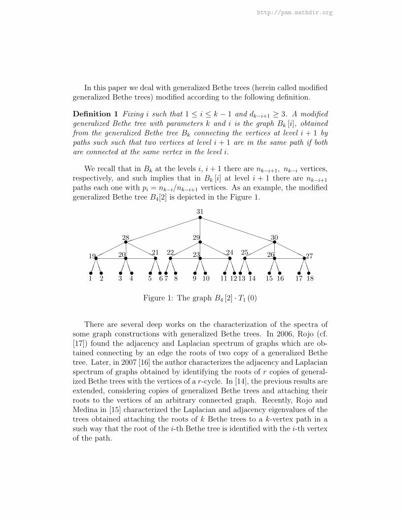
Definition 1 Fixing i such that 1 ≤ i ≤ k − 1 and dk−i+1 ≥ 3. A modifiedgeneralized Bethe tree with parameters k and i is the graph Bk [i], obtainedfrom the generalized Bethe tree Bk connecting the vertices at level i + 1 bypaths such such that two vertices at level i + 1 are in the same path if bothare connected at the same vertex in the level i.

We recall that in Bk at the levels i, i+ 1 there are nk−i+1, nk−i vertices,respectively, and such implies that in Bk [i] at level i + 1 there are nk−i+1

paths each one with pi = nk−i/nk−i+1 vertices. As an example, the modifiedgeneralized Bethe tree B4[2] is depicted in the Figure 1.

tt t t

t t t t t t t t tt t t t t t t t t t t t t t t t t t

31

28 29 30

19 20 21 22 23 24 25 26 27

1 2 3 4 5 6 7 8 9 10 11 12 13 14 15 16 17 18

PPPPPPPPPPPP

HHHHH

HHHHH

HHHHH

BBB

BBB

BBBBBB

BBB

BBB

BBB

BBB

BBB

Figure 1: The graph B4 [2] · T1 (0)

There are several deep works on the characterization of the spectra ofsome graph constructions with generalized Bethe trees. In 2006, Rojo (cf.[17]) found the adjacency and Laplacian spectrum of graphs which are ob-tained connecting by an edge the roots of two copy of a generalized Bethetree. Later, in 2007 [16] the author characterizes the adjacency and Laplacianspectrum of graphs obtained by identifying the roots of r copies of general-ized Bethe trees with the vertices of a r-cycle. In [14], the previous results areextended, considering copies of generalized Bethe trees and attaching theirroots to the vertices of an arbitrary connected graph. Recently, Rojo andMedina in [15] characterized the Laplacian and adjacency eigenvalues of thetrees obtained attaching the roots of k Bethe trees to a k-vertex path in asuch way that the root of the i-th Bethe tree is identified with the i-th vertexof the path.


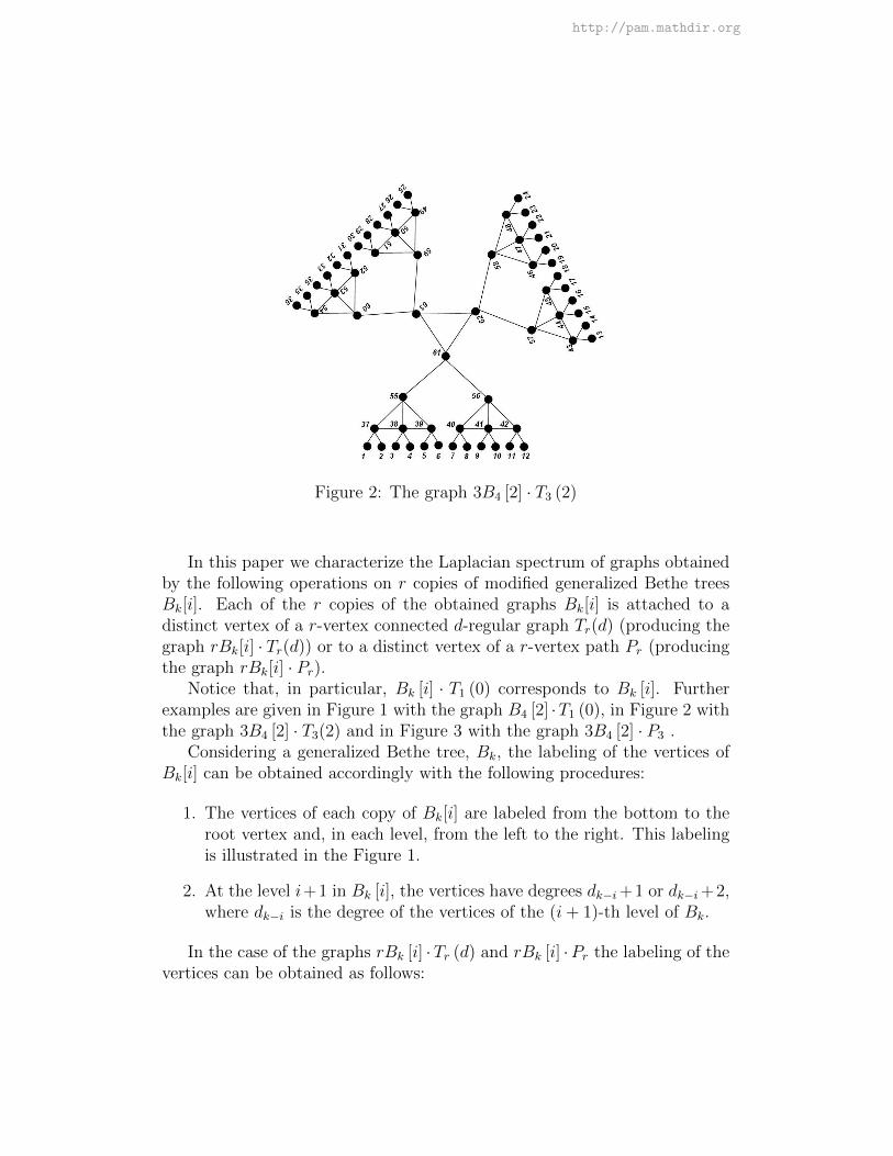
Figure 2: The graph 3B4 [2] · T3 (2)

In this paper we characterize the Laplacian spectrum of graphs obtainedby the following operations on r copies of modified generalized Bethe treesBk[i]. Each of the r copies of the obtained graphs Bk[i] is attached to adistinct vertex of a r-vertex connected d-regular graph Tr(d) (producing thegraph rBk[i] · Tr(d)) or to a distinct vertex of a r-vertex path Pr (producingthe graph rBk[i] · Pr).

Notice that, in particular, Bk [i] · T1 (0) corresponds to Bk [i]. Furtherexamples are given in Figure 1 with the graph B4 [2] ·T1 (0), in Figure 2 withthe graph 3B4 [2] · T3(2) and in Figure 3 with the graph 3B4 [2] · P3 .

Considering a generalized Bethe tree, Bk, the labeling of the vertices ofBk[i] can be obtained accordingly with the following procedures:

1. The vertices of each copy of Bk[i] are labeled from the bottom to theroot vertex and, in each level, from the left to the right. This labelingis illustrated in the Figure 1.

2. At the level i+1 in Bk [i], the vertices have degrees dk−i+1 or dk−i+2,where dk−i is the degree of the vertices of the (i+ 1)-th level of Bk.

In the case of the graphs rBk [i] ·Tr (d) and rBk [i] ·Pr the labeling of thevertices can be obtained as follows:


Figure 3: The graph 3B4 [2] · P3

1. We label the vertices of the first level, from the left to the right.

2. The vertices of the second level are labeled using rn1+1, rn1+2, . . . , rn1+rn2.

3. The labeling of the vertices of the higher levels can be done in the sameway.

4. Finally, the last vertex (which belongs to the regular graph or to thepath) is labeled using n.

For illustrative purpose, consider the graphs 3B4 [2]·T3 (2) and 3B4 [2]·P3

depicted in Figures 2 and 3, respectively.Since, the main results of the next sections are based in matricial tech-

niques related with the Kronecker product, let us define this product andreview some of its properties.

For the matrices A = (aij) ∈ Rr×s and B = (bij) ∈ Rp×q, the Kroneckerproduct is denoted A ⊗ B ∈ Rrp×sq. Several properties of the Kroneckerproduct may be found, for instance, in [11].

From now on, 0 denotes the all zero matrix with appropriate order, Im isthe identity matrix of order m and em denotes the all ones m− dimensionalvector. The Laplacian matrix of the q-vertex path Pq is denoted Lq, and then

Lq =

1 −1−1 2 −1

. . . . . . . . .

−1 2 −1−1 1

.


Considering a fixed i, 1 ≤ i ≤ k − 1 such that dk−i+1 ≥ 3, and taking intoaccount that

pi =nk−ink−i+1

,

let us define

mj = dj+1 − 1 =njnj+1

= pk−j, for j = 1, . . . , k − 2. (1)

mk−1 = dk = nk−1. (2)

Then, we are able to deal with the matrices

Jpi = Ink−i+1⊗ Lpi , (3)

of order nk−i and also with the matrices

Hpi = Ir ⊗ Jpi= Ir ⊗ Ink−i+1

⊗ Lpi ,

In the sequel, Cj ( 1 ≤ j ≤ k− 1) is the block diagonal matrix defined by

Cj = Inj+1⊗ emj

, (4)

with nj+1 diagonal blocks equals to emj. Thus, Cj is an nj × nj+1 matrix,

for j = 1, . . . , k − 1, where Ck−1 = enk−1. Let

Kj = Ir ⊗ Cj, (5)

the matrix of order rnj, where each of its r diagonal blocks is equal to Cj,that is, since Cj is composed by nj+1 diagonal blocks equal to emj

, in totalthe matrix Kj has rnj+1 diagonal blocks emj

.As direct consequence of the properties of the Kronecker product, we have

the following equalities:

KTj Kj = m

jIrnj+1

, for j = 1, . . . , k − 2, KTk−1Kk−1 = nk−1Ir = dkIr, (6)

KTj

(cIrnj

−Hpk−j

)= cKT

j for j = 1, . . . , k − 1, (7)

where c is an arbitrary polynomial.


Example 2 Let us consider a generalized Bethe tree Bk and the graph Tr(d).Then, in the particular case of k = 4, in B4 we have the following pairs(di, ni).

(d1, n1) = (1, 12), (d2, n2) = (3, 6), (d3, n3) = (4, 2), (d4, n4) = (2, 1).

In B4[2], at level 3, we have n3 = 2 paths with p2 = n2/n3 = 6/2 = 3vertices and also m1 = 2,m2 = 3 and m3 = 2. Therefore, J3 = Jp2 = I2⊗L3.Furthermore,

Hp2 = I3 ⊗ Jp2 = I3 ⊗ I2 ⊗ L3 = I6 ⊗ L3

and the matrices defined in (4) are C1 = I6 ⊗ e2, C2 = I2 ⊗ e3 and C3 = e2.Taking into account the above referred labeling for the vertices, the Lapla-

cian matrices L(3B4[2] · T3(2)) and L(3B4[2] · P3) become:I36 −K1 0 0−KT

1 3I18 +Hp2−K2 0

0 −KT2 4I6 −K3

0 0 −KT3 W

,

where in the case of the matrix L(3B4[2] · T3(2)), W = (2 + 2)I3 −A(T3(2)),and in the case of the matrix L(3B4[2] · P3), W = 2I3 + L3.

In the general case, the Laplacian matrices L(rBk [i]·Tr (d)) and L(rBk [i]·Pr) become:

d1Irn1 −K1

−KT1 d2Irn2

. . .. . . . . . −Kk−(i+1)

dk−iIrnk−i+Hpi −Kk−i

−KTk−i

. . . . . . −Kk−1

. . . −KTk−1 W

(8)

where in the case of the matrix L(rBk [i] ·Tr (d)), W = (dk +d)Ir−A(Tr (d))and in the case of the matrix L(rBk [i] · Pr), W = dkIr + Lr.


Lemma 3 Let M be the following block tridiagonal matrix

α1Irn1 K1

KT1 α2Irn2 K2

. . . . . . Kk−(i+1)

KTk−(i+1) αk−iIrnk−i

−Hpi Kk−i

KTk−i αk−i+1Irnk−i+1

. . .

. . .

αk−1Irnk−1Kk−1

. . . KTk−1 αkIr + L

,

where L is a r × r symmetric matrix. If

β1 = α1 6= 0

βj = αj −mj−11

βj−16= 0, 2 ≤ j ≤ k − 1,

βk = αk − dk 1βk−16= 0,

then

det(M) =

k−1∏j=1j 6=k−i

βnj

j

r(

pi∏l=1

(βk−i − νl)

)rnk−i+1(

r∏j=1

(βk + δj)

), (9)

where δ1, . . . , δr are the eigenvalues of L and ν1, . . . , νpi are the eigenvaluesof Lpi .

Proof. For this proof, we take into account the equalities (6) and (7). Then,performing elementary operation over the line blocks of M , the matricesKTj , for j = 1, . . . , k − 1 are eliminated using the blocks βjIrnj

, with βj 6= 0,excluding the matrix KT

k−i which is eliminated according to the item (c).Therefore, the matrix M is transformed according to the following items:

(a) For j = 1, . . . , k− (i+ 2), each diagonal block αj+1Irnj+1is replaced by

αj+1Irnj+1− β−1

j KTj Kj = αj+1Irnj+1

−mjβ−1j Irnj+1

= βj+1Irnj+1.

(b) For j = k−(i+1), the block αk−iIrnk−i−Hpi is replaced by βk−iIrnk−i

−Hpi .


(c) For j = k − i the block βk−iIrnk−i− Hpi is multiplied on left by(

−β−1k−i)KTk−i and added to the block KT

k−i. Then this block is elim-inated taking into account (7). Additionally, taking into account (6),the corresponding diagonal block is replaced by

αk−i+1Irnk−i+1− β−1

k−iKTk−iKk−i = βk−i+1Irnk−i+1

.

(d) For j = k − (i− 1), . . . , k − 1, the block Kj is eliminated by the blockβjIrnj

and the corresponding diagonal block is replaced by βj+1Irnj+1.

Observe that after the last operation of item (d), αk is replaced by αk −dkβ

−1k−1 = βk. Hence Eq. (9) follows.

3 The spectrum of the Laplacian matrix

The technics used in the proof of the next results are similar to those usedin [19, Th. 5]. In what follows, γ1, . . . , γr are the eigenvalues of Tr(d) andµj = 2 + 2 cos πj

r, for j = 1, . . . , r, are the eigenvalues of Lr. Furthermore,

considering Φ = 0, 1, 2, . . . , k − i− 1, k − i+ 1, . . . , k − 1, then

Ω = j ∈ Φ− 0 : nj > nj+1 ∪ 0 . (10)

Along this section we need also to define the following polynomials (wheremj is as (1)):

Q0 (λ) = 1, (11)

Q1 (λ) = λ− d1 (12)

Qj (λ) = (λ− dj)Qj−1 (λ)−mj−1Qj−2 (λ) , j = 2, . . . , k − 1, (13)

Qkj(λ) = (λ− dk − d+ γj)Qk−1 (λ)−mk−1Qk−2 (λ) , j = 1, . . . , r,(14)

Lkj(λ) = (λ− dk − µj)Qk−1 (λ)−mk−1Qk−2 (λ) , j = 1, . . . , r. (15)

Now we are able to introduce the main result of this section.

Theorem 4 If H is a graph belonging to the set rBk [i] ·Tr(d), rBk [i] ·Pr,with i ∈ 1, . . . , k − 1, then

det(λI − L(H)) =∏t∈Ω

Qrnt−rnt+1

t

pi−1∏l=1

(Qk−i − νlQk−i−1)rnk−i+1 Ψ(H),


where Ψ(H) =∏r

j=1 Qkj(λ) when H = rBk [i]·Tr(d) and Ψ(H) =∏r

j=1 Lkj(λ)when H = rBk [i] · Pr. Furthermore,

σ(L(H)) =⋃t∈Ω

λ : Qt(λ) = 0 ∪

(pi−1⋃l=1

λ : Qk−i(λ)− νlQk−i−1(λ) = 0

)∪X

where X =⋃rj=1 λ : Qkj(λ) = 0 when H = rBk [i] · Tr(d), and X =⋃r

j=1 λ : Lkj(λ) = 0 when H = rBk [i] · Pr.

Proof. For H ∈ rBk [i] · Tr(d), rBk [i] ·Pr, taking into account the expres-sion of L (H) in (8) and applying Lemma 3 to the matrix M = λI − L (H),we obtain

αj = λ− dj, j = 1, . . . , k − 1,

αk =

λ− d− dk, if H = rBk [i] · Tr(d);λ− dk, if H = rBk [i] · Pr.

Let βj be as in Lemma 3 and suppose that λ ∈ R is such that Qj (λ) 6= 0,when j = 1, . . . , k − 1. For the sake of simplicity, let us denote Qj(λ) andQkj(λ) by Qj and Qkj, respectively. Then

β1 = λ− 1 = Q1

Q06= 0,

βj = (λ− dj)−mj−11

βj−1=

(λ−d3)Qj−1−mj−1Qj−2

Qj−1

=Qj

Qj−16= 0, for j = 2, . . . , k − 1,

and, for i = 1, . . . , r,

βk + δi =

λ− d− dk + γi − dk 1

βk−1, if H = rBk [i] · Tr(d);

λ− dk + µi − dk 1βk−1

, if H = rBk [i] · Pr

=

(λ−d−dk+γj)Qk−1−dkQk−2

Qk−1, if H = rBk [i] · Tr(d);

(λ−dk+µi)Qk−1−dkQk−2

Qk−1, if H = rBk [i] · Pr

=

Qki

Qk−1, if H = rBk [i] · Tr(d);

Lki

Qk−1, if H = rBk [i] · Pr.

(16)

Therefore, using (9), it follows


detM =

k−1∏j=1j 6=k−i

βnj

j

r(

pi∏l=1

(βk−i − νl)

)rnk−i+1 r∏j=1

(βk + δj)

=

(Q

n11

Qn10

Qn22

Qn21

· · · Qnk−i−1k−i−1

Qnk−i−1k−i−2

)r( pi∏l=1

(Qk−i

Qk−i−1− νl)

)rnk−i+1 (Q

nk−i+1k−i+1

Qnk−i+1k−i

. . .Q

nk−1k−1

Qnk−1k−2

)r Ψ(H)

Qrk−1

= Qr(n1−n2)1 · · ·Qr(nk−i−1−nk−i)

k−i−1

pi−1∏l=1

(Qk−i − νlQk−i−1)rnk−i+1 Qrnk−i+1

k−i

(Q

nk−i+1k−i+1

Qnk−i+1k−i

· · · Qnk−1k−1

Qnk−1k−2

)r Ψ(H)

Qrk−1

= Qr(n1−n2)1 · · ·Qr(nk−i−1−nk−i)

k−i−1 Qr(nk−i+1−nk−i+2)

k−i+1 · · ·Qr(nk−1−nk)

k−1

pi−1∏l=1

(Qk−i − νlQk−i−1)rnk−i+1 Ψ(H). (17)

where Ψ(rBk [i] · Tr(d)) =∏r

j=1Qkj and Ψ(rBk [i] · Pr) =∏r

j=1 Lkj. Noticethat the above expression is obtained taking into account that (according toits definition) νpi = 0.

Consider now λ0 ∈ R such that Qt(λ0) = 0 for some t = 1, . . . , k−1. Sincethe zeros of any polynomial are isolated there exists a neighborhood V (λ0) ofλ0 such that Qj(λ) 6= 0, for all λ ∈ V (λ0)−λ0 and for all j = 1, . . . , k−1.

Hence, the equality (17) follows, for all λ ∈ V (λ0)−λ0 . By continuity,taking the limit as λ tends to λ0, we obtain the desired expression.

Corollary 5 If H ∈ rBk [k − 1] · Tr(d), rBk [k − 1] · Pr, with k ≥ 2, thenfor all 1 ≤ l ≤ pk−1 − 1, µl = 3 + 2 cos lπ

piis an eigenvalue with multiplicity

at least rn2 of H.

Proof. Taking into at level k ≥ 2 there are n2 ≥ 1 paths with pk−1 = n1

n2> 1

vertices, then by Theorem 4, we obtain λ : Q1 (λ)− νlQ0(λ) = 0 ⊆ σ(H).Hence since Q0(λ) = 1, using (12), the result follows.

Definition 6 For t = 1, . . . , k − 1, let Tt(H) be the t × t leading principal


submatrix of the k × k symmetric tridiagonal matrix

Tkj(H) =

d1

√d2 − 1√

d2 − 1 d2

. . .. . . . . .

√dk−1 − 1√

dk−1 − 1 dk−1

√dk√

dk dk + θj

where, for j = 1, . . . , r, θj =

d− γj, if H = rBk [k − 1] · Tr(d);2 + 2 cos πj

r, if H = rBk [k − 1] · Pr.

and for l = 1, . . . , pi−1, let consider the dk−i×dk−i symmetric tridiagonalmatrix

Sl =

d1

√d2 − 1

√d2 − 1 d2

. . .. . . . . .

√dk−i − 1√

dk−i − 1 dk−i + νl

.

Remark 7 We remark that σ(L(Tr(d))) = d− γj : 1 ≤ j ≤ r.

Lemma 8 If Tt, t = 1, . . . , k − 1, and Sl, l = 1, . . . , pi − 1 are the leadingprincipal submatrices of Tkj(H) and the dk−i × dk−i tridiagonal symmetricmatrices referred in Definition 6, respectively. Then

det(λI − Tt) = Qt (λ) , t = 1, . . . , k − 1, (18)

for j = 1, . . . , rdet (λI − Tkj(H)) = Qkj(λ) (19)

and for l = 1, . . . , pi − 1

det(λI − Sl) = Qk−i(λ)− νlQk−i−1(λ). (20)

Proof. Formulas in (18) and in (19) have already been proved in [19]. Toobtain (20) , we see that if i = k − 1 the result follows by Corollary 5. Nowwe suppose that i < k − 1. By (13) we see that

Qk−i − νlQk−i−1 = (λ− dk−i − νl)Qk−i−1 −mk−i−1Qk−i−2

= (λ− dk−i − νl)Qk−i−1 − (dk−i − 1)Qk−i−2,

which, by [20] implies the result.


Lemma 9 For t = 1, . . . , k − 1 , l = 1, . . . , pi − 1 and j = 1, . . . , r the zerosof the polynomials Qt, Qk−i−νlQk−i−1 and Qkj (or Lkj), respectively are realand simple.

Proof. In view of Lemma 8 and as the matrices in Definition 6 are symmetricand tridiagonal with nonzero codiagonal entries it follows that its eigenvaluesare simple (cf. [4]).

The next theorem gives a complete characterization of the eigenvalues ofthe Laplacian matrix in the case when H = rBk [i] ·Tr (d) or H = rBk [i] ·Pr.

Theorem 10 (a) σ (H) =(⋃

t∈Ω−0 σ (Tt))∪(⋃pi−1l=1 σ(Sl))∪

[⋃rj=1 σ(Tkj(H))

].

(b) The multiplicity of each eigenvalue of the matrix Tt as eigenvalue ofL(H) is at least rnt− rnt+1 for t ∈ Ω and the multiplicity of each eigenvalueof the matrices Tkj(H) for j = 1, . . . , r is at least 1.

(c) Each eigenvalue of Sl, for all 1 ≤ l ≤ pi−1, is an eigenvalue of L(H).(d) Each eigenvalue of Sl is an eigenvalue of L (H) with multiplicity at

least rnk−i+1.

Proof. (a), (b) and (d) are consequences of Theorem 4, Lemma 9 andLemma 8. The assertion in (c) is due to nk−i+1 ≥ 1.

Next we present an illustrative example for the case H = 3B4 [2] · T3 (2) .

Example 11 In the graph 3B4 [2] · T3 (2) let

Φ = 0, 1, 3 and

Ω = 0, 1, 3 . (21)

By Remark 7 we have d− γj : 1 ≤ j ≤ 3 = 0, 3, 3 . Thus the matrices inDefinition 6 correspond to,

T41 =

1√

2 0 0√2 3

√3 0

0√

3 4√

2

0 0√

2 5

, T42 =

1√

2 0 0√2 3

√3 0

0√

3 4√

2

0 0√

2 5

, T43 =

1√

2 0 0√2 3

√3 0

0√

3 4√

2

0 0√

2 2

,

and

S1 =

(1

√2√

2 3 + 3

), S2 =

(1

√2√

2 3 + 1

).


To four decimal places, the eigenvalues and its multiplicities are given by:

T41 : 0.0496 2.1456 4.3968 6.4080 1T42 : 0.0496 2.1456 4.3968 6.4080 1T43 : 0 1.2087 3 5.7913 1T1 : 1 rn1 − rn2 = 18T3 : 0.0746 2.4481 5.4774 rn3 − rn4 = 3S1 : 0.6277 6.3723 rn3 = 6S2 : 0.4384 4.5616 rn3 = 6.

The referred graph operations with modified generalized Bethe trees canbe generalized in the following way: for a fixed 1 ≤ s ≤ k − 1, let ı =(i1, i2, . . . , is) with 2 ≤ i1 < i2 < · · · < is ≤ k−1. We construct an unweighedgraph Bk [ı] obtained from a generalized Bethe tree Bk and the union of pathsat the level iq + 1 such that two vertices are in the same path if and onlyif both are connected at the same vertex at level iq, with 1 ≤ q ≤ s. Amore general graph operation rBk [ı] · Tr(d) obtained from r copies of Bk [ı]and a regular connected graph Tr(d) (or a path Pr) with r vertices, eachone of degree d, can be considered by identifying the root of each copy ofBk [ı] with each vertex of Tr(d) (Pr). The previous obtained results can beextended to the graphs produced by these more general graph operations,using techniques very similar to the ones above presented.

4 Some applications

In this section the singular values of the Laplacian matrices (and then theeigenvalues) of the graphs rBk [i] · Tr (d) and H = rBk [i] · Pr are compared,when Pr is isomorphic to an Hamiltonian path of Tr (d) (if there is). First, itis convenient to introduce the following notation (c.f. [1, 2]). A > 0 meansthat A is positive semidefinite and if A and B are hermitian matrices, thenA > B if A − B > 0. For a complex m × n matrix C we recall that itsnonzero singular values correspond to the nonzero eigenvalues of the positive

semidefinite matrix |C| =(CTC

)1/2, (see, e. g. [11]). The singular values of

a matrix C are enumerated as s1(C) ≥ · · · ≥ sn(C).Now, we are able to remind the following results (see [2, 1]).

Lemma 12 [2] Let X and Y be positive semidefite n × n hermitian ma-trices, with eigenvalues λ1(X) ≥ · · · ≥ λn(X) and λ1(Y ) ≥ · · · ≥ λn(Y ),respectively. If X > Y , then λj(X) ≥ λj(Y ) for j = 1, . . . , n.


Theorem 13 Consider a modified generalized Bethe tree Bk[i]. If a d-regulargraph of order r, Tr(d), has an Hamilton path isomorphic to Pr, then

λj(L(rBk[i] · Tr(d))) ≥ λj(L(rBk[i] · Pr)), for j = 1, . . . , n.

Proof. The Laplacian matrices of the graphs rBk[i] · Tr(d) and rBk[i] · Prare positive semidefinite. Taking into account the expression (8) for thesematrices, then

L(rBk[i] · Tr(d)))− L(rBk[i] · Pr) =

(0 00 L(Tr(d))− L(Pr)

).

Therefore, since L(Tr(d)) − L(Pr) = L(Tr(d) \ Pr), where Tr(d) \ Pr is thegraph obtained from Tr(d) after deleting the edges corresponding to Pr, itfollows that

L(rBk[i] · Tr(d)))− L(rBk[i] · Pr) > 0⇔ L(rBk[i] · Tr(d))) > L(rBk[i] · Pr).

Applying Lemma 12, the conclusion follows.The Laplacian-energy-like of an (n,m)−graph G (denoted by LEL [G]),

introduced by Liu and Liu [12] is defined as

LEL [G] =n∑j=1

√µj. (22)

where µj, for j = 1, . . . , n, are the eigenvalues of the Laplacian matrix of G.For a m×n complex matrix C, we define the Laplacian-energy-like of the

matrix C by

LEL(C) =∑j

√λj(|C|).

As a consequence of the previous definitions the Laplacian-energy-like ofany graph G is given by

LEL [G] = LEL(L(G)).

The next theorem obtains bounds for the Laplacian-energy-like for thegraphs studied in this paper.


Theorem 14 Let G be an (n,m)−graph such that

det(L(G)− λIn) = P1(λ)t1P2(λ)t2 · · ·Ps(λ)ts , (23)

where Pj(λ) = det(Mj−λIj), Mj are square matrices of order j, with tj > 0,for j = 1, . . . , s. Then

LEL [G] ≤s∑j=1

tj√j√trace(Mj) (24)

Proof. From the decomposition in (23) it is clear that

LEL [G] =s∑j=1

tjLEL (Mj)

=s∑j=1

tj∑

µ∈σ(Mj)

√µ

Thus, via Cauchy Schwarz inequality

LEL [G] ≤s∑j=1

tj√j

∑µ∈σ(Mj)

(√µ)2

1/2

=s∑j=1

tj√j√trace (Mj),

and the inequality holds.We fix i, 2 ≤ i ≤ k − 2. Now we consider the connected graph H ∈

Bk [i] · Tr (d) , Bk [i] · Pr. We shall take n and m as the number of verticesand of edges, respectively, of H.

Applying Theorem 4, Lemma 8 and Theorem 14 we obtain the followingresult.

Corollary 15 For 1 ≤ j ≤ r, 1 ≤ u ≤ k − 1 and 1 ≤ l ≤ pi − 1. LetTkj(H), Tu and Sl defined according to the Definition 6. Then

LEL (H) ≤

∑u∈Ω

√u(rnu−rnu+1)

√traceTu+rnk−i+1

√dk−i

pi−1∑l=1

√traceSl+

r∑j=1

√k√traceTkj(H).


Finally, as immediate consequence of Theorem 13, we have the followingcorollary.

Corollary 16 Under the conditions of Theorem 13,

LEL(rBk[i] · Tr(d)) ≥ LEL(rBk[i] · Pr).

Acknowledgements:(1) Research supported by the Center for Research and Development in Math-ematics and Applications from the Fundacao para a Ciencia e a Tecnologia,cofinanced by the European Community Fund FEDER/POCI 2010.(2) Research supported by Proyecto Mecesup 2 UCN 0605, Chile y Fondecyt-IC Project 11090211, Chile.(3) Research partially supported by CNPq - Grant 309531/2009-8.

References

[1] R. Bhatia, F. Kitaneh, The singular valuies of A+B and A+ iB. LinearAlgebra Appl. 431 (20019): 1502-1508.

[2] R. Bhatia, Matrix Analysis. Springer, 1997.

[3] D. Cvetkovic, M. Doob, H. Sachs. Spectra of Graphs - Theory and Ap-plications, Deutcher Verlag der Wissenschaften, Academic Press, Berlin-New York (1980), second ed. (1980), third ed. Verlag, Heidelberg -Leipzig (1995).

[4] G. H. Golub, C. F. Van Loan. Matrix Computations, second ed., JohnsHopkins University Press, Baltimore, 1989.

[5] I. Gutman, The energy of a graph, Ber. Math.-Statist. Sekt.Forschungszentrum Graz 103 (1978): 1-22.

[6] I. Gutman, The energy of a Graph: Old and New Results, Alge-braic Combinatorics and Applications (2001): 196-211. Springer-Verlag.Berlin.

[7] I. Gutman, S. Zare Firoozabadi, J. A. de la Pena, J. Rada, On theenergy of regular graphs, MATCH Commun. Math. Comput. Chem. 57(2007): 435-442.


[8] O. J. Heilmann, E. H. Lieb. Theory of monomer-dimer systems, Comm.Math. Phys. 25 (1972): 190-232.

[9] R. A. Horn, C. R. Johnson. Matrix Analysis. Cambridge University Press(1991). Cambridge.

[10] G. Indulal, A. Vijayakumar, A note on energy of some graphs, MATCHCommun. Math. Comput. Chem. 59 (2008): 269-274.

[11] P. Lancaster, M.Tismenetsky. The theory of matrices. Academic Press.INC.

[12] J. Liu, B. Liu, A Laplacian-energy-like invariant of a graph, MATCHCommun. Math. Comput. Chem. 59 v. 2 (2008): 355-372.

[13] V. Nikiforov, The energy of graphs and matrices, Journal of Mathemat-ical Analysis and Applications 326, Issue 2 (2007): 1472-1475.

[14] O. Rojo. Spectra of copies of a generalized Bethe tree attached to anygraph. Linear Algebra and its Appl. 431 (2009): 862-882.

[15] O. Rojo, L. Medina. Spectra of generalized Bethe trees attached to apath. Linear Algebra and its Appl. 430 (2009): 483-503.

[16] O. Rojo. The spectra of a graph obtained from copies of a generalizedBethe tree. Linear Algebra and its Appl. 420, I. 2-3 15 (2007): 490-507.

[17] O. Rojo. The spectra of some trees and bounds for the largest eigenvaluesof any tree. Linear Algebra Appl. 414 (2006): 199-217.

[18] O. Rojo and R. Soto. The spectra of the adjacency matrix and Laplacianmatrix for some balanced trees. Linear Algebra Appl. 403 (2005): 97-117.

[19] O. Rojo and M. Robbiano. On the spectra of some weighted rooted treeand applications, Linear Algebra Appl. 420 (2007): 310-328.

[20] L. N. Trefethen. D. Bau III, Numerical Linear Algebra, Society for In-dustrial and Applied Mathematics, 1997.

[21] R. S. Varga. Matrix Iterative Analysis. Prentice-Hall, Inc., 1965.

A principal intencao desta serie de publicacoes, Cadernos de Matematica, e de divulgar trabalho originaltao depressa quanto possıvel. Como tal, os artigos publicados nao sofrem a revisao usual na maior parte dasrevistas. Os autores, apenas, sao responsaveis pelo conteudo, interpretacao dos dados e opinioes expressasnos artigos. Todos os contactos respeitantes aos artigos devem ser enderecados aos autores.

The primary intent of this publication, Cadernos de Matematica, is to share original work as quickly aspossible. Therefore, articles which appear are not reviewed as is the usual practice with most journals. Theauthors alone are responsible for the content, interpretation of data, and opinions expressed in the articles.All communications concerning the articles should be addressed to the authors.

Computing the Laplacian spectra of some graphs

Documents