Computing Procedure Summaries for Interprocedural Analysis Sumit Gulwani 1 and Ashish Tiwari 2 1 Microsoft Research, Redmond, WA 98052 [email protected] 2 SRI International, Menlo Park, CA 94025 [email protected] Abstract. We describe a new technique for computing procedure sum- maries for performing an interprocedural analysis on programs. Proce- dure summaries are computed by performing a backward analysis of procedures, but there are two key new features: (i) information is prop- agated using “generic” assertions (rather than regular assertions that are used in intraprocedural analysis); and (ii) unification is used to sim- plify these generic assertions. We illustrate this general technique by applying it to two abstractions: unary uninterpreted functions and lin- ear arithmetic. In the first case, we get a PTIME algorithm for a special case of the long-standing open problem of interprocedural global value numbering (the special case being that we consider unary uninterpreted functions instead of binary). This also requires developing efficient algo- rithms for manipulating singleton context-free grammars, and builds on an earlier work by Plandowski [13]. In linear arithmetic case, we get new algorithms for precise interprocedural analysis of linear arithmetic pro- grams with complexity matching that of the best known deterministic algorithm [11]. 1 Introduction Precise interprocedural analysis (also referred to as full context-sensitive analysis) is provably harder than intraprocedural analysis [14]. One way to do precise in- terprocedural analysis is to do procedure-inlining followed by an intra-procedural analysis. There are two potential problems with this approach. First, in presence of recursive procedures, procedure-inlining may not be possible. Second, even if there are no recursive procedures, procedure-inlining may result in an exponen- tial blow-up of the program. For example, if procedure P 1 calls procedure P 2 two times, which in turn calls procedure P 3 two times, then procedure inlining will result in 4 copies of procedure P 3 inside procedure P 1 . In general, leaf procedures can be replicated an exponential number of times. A more standard way to do interprocedural analysis is by means of computing procedure summaries [20]. Each procedure is analyzed once (or a few times in Second author supported in part by the National Science Foundation under grant CCR-0326540. R. De Nicola (Ed.): ESOP 2007, LNCS 4421, pp. 253–267, 2007. c Springer-Verlag Berlin Heidelberg 2007

Welcome message from author
This document is posted to help you gain knowledge. Please leave a comment to let me know what you think about it! Share it to your friends and learn new things together.
Transcript

Computing Procedure Summaries forInterprocedural Analysis�
Sumit Gulwani1 and Ashish Tiwari2
1 Microsoft Research, Redmond, WA [email protected]
2 SRI International, Menlo Park, CA [email protected]
Abstract. We describe a new technique for computing procedure sum-maries for performing an interprocedural analysis on programs. Proce-dure summaries are computed by performing a backward analysis ofprocedures, but there are two key new features: (i) information is prop-agated using “generic” assertions (rather than regular assertions thatare used in intraprocedural analysis); and (ii) unification is used to sim-plify these generic assertions. We illustrate this general technique byapplying it to two abstractions: unary uninterpreted functions and lin-ear arithmetic. In the first case, we get a PTIME algorithm for a specialcase of the long-standing open problem of interprocedural global valuenumbering (the special case being that we consider unary uninterpretedfunctions instead of binary). This also requires developing efficient algo-rithms for manipulating singleton context-free grammars, and builds onan earlier work by Plandowski [13]. In linear arithmetic case, we get newalgorithms for precise interprocedural analysis of linear arithmetic pro-grams with complexity matching that of the best known deterministicalgorithm [11].
1 Introduction
Precise interprocedural analysis (also referred to as full context-sensitive analysis)is provably harder than intraprocedural analysis [14]. One way to do precise in-terprocedural analysis is to do procedure-inlining followed by an intra-proceduralanalysis. There are two potential problems with this approach. First, in presenceof recursive procedures, procedure-inlining may not be possible. Second, even ifthere are no recursive procedures, procedure-inlining may result in an exponen-tial blow-up of the program. For example, if procedure P1 calls procedure P2 twotimes, which in turn calls procedure P3 two times, then procedure inlining willresult in 4 copies of procedure P3 inside procedure P1. In general, leaf procedurescan be replicated an exponential number of times.
A more standard way to do interprocedural analysis is by means of computingprocedure summaries [20]. Each procedure is analyzed once (or a few times in� Second author supported in part by the National Science Foundation under grant
CCR-0326540.
R. De Nicola (Ed.): ESOP 2007, LNCS 4421, pp. 253–267, 2007.c© Springer-Verlag Berlin Heidelberg 2007

254 S. Gulwani and A. Tiwari
main(){1 x := 0; y := 1; a := 2; b := 4;2 P (); Assert(y = 2x + 1);3 x := 0; y := 0; a := ?; b := 2a;4 P (); Assert(y = 2x);5 y := x + 3; a := ?; b := a;6 P (); Assert(y = x + 3);7 }
P (){1 if (*) {2 x := x + a;3 y := y + b;4 }5 else P ()6 }
Fig. 1. An example program
case of recursive procedures) to build its summary. A procedure summary can bethought of as some succinct representation of the behavior of the procedure thatis also parametrized by any information about its input variables. However, thereis no automatic recipe to efficiently construct or even represent these proceduresummaries, and abstraction specific techniques are required.
The original formalism proposed by Sharir and Pnueli [20] for computing pro-cedure summaries was limited to finite lattices of dataflow facts. Sagiv, Repsand Horwitz generalized the Sharir-Pnueli framework to build procedure sum-maries using context-free graph reachability [15], even for some kind of infinitedomains. They successfully applied their technique to detect linear constantsinterprocedurally [17]. However, their generalized framework requires appropri-ate distributive transfer functions as input - and such transfer functions are notknown for any natural abstract domain more powerful than linear constants.
In this paper (Section 3), we describe a general technique for constructingprecise procedure summaries. This technique can be effectively used for a usefulclass of program abstractions (over infinite domains). We apply this techniqueto obtain precise interprocedural analyses for two useful abstractions - unaryuninterpreted functions, and linear arithmetic (which is more powerful thanthe domain of linear constants used by Sagiv, Reps and Horwitz). The former(described in Section 4) gives a polynomial-time algorithm for a special case ofthe long-standing open problem of interprocedural global value numbering, whilethe latter (described in Section 5) yields a new algorithm for interprocedurallinear arithmetic analysis with the same complexity as that of the best knowndeterministic algorithm [11].
Our procedure summaries are in the form of constraints (on the input vari-ables of the procedure) that must be satisfied to guarantee that some appropriategeneric assertion (involving output variables of the procedure) holds at the endof the procedure. A generic assertion is an assertion that involves some contextvariables that can be instantiated by symbols (or more formally, by terms withholes) of the underlying abstraction. For example, consider procedure P shownin Figure 1 with input variables x, y, a, b and output variables x, y. αx+βy = γ isa generic assertion in the theory of linear arithmetic involving variables x, y (andcontext variables α, β, γ, which denote unknown constants). Using the techniquedescribed in this paper, we compute the summary of procedure P as “αx+βy = γ

Computing Procedure Summaries for Interprocedural Analysis 255
(a) AssignmentNode
x := e
0
(d) Join Node
21
(c) Non-deterministicConditional Node
*True False
1 2
(b) Non-deterministicAssignment Node
x := ?
0
(e) ProcedureCall Node
Call P0( )
0
Fig. 2. Flowchart nodes in our abstracted program model
holds at the end of procedure P iff αa + βb = 0 ∧ αx + βy = γ holds at thebeginning of procedure P”. After computing such a procedure summary for P ,we can use it to verify the assertions in the Main procedure. To verify the firstassertion y = 2x + 1, we first match it with the generic assertion αx + βy = γto obtain the substitution α �→ −2, β �→ 1 and γ �→ 1 for the context variables.We then instantiate the procedure summary with this substitution to obtain theprecondition b − 2a = 0 ∧ y − 2x = 1. We then check that this preconditionis satisfied in procedure Main immediately before the first call to procedure P .Similarly, we can verify the other two assertions.
The key idea in computing such procedure summaries is to compute weak-est preconditions of generic assertions. However, a naive weakest preconditioncomputation may be exponential in the number of operations performed (eachconditional node can double the size of the precondition), and may not even ter-minate (in presence of loops). Hence we use some techniques for strengtheningand simplifying the weakest preconditions (without any loss of precision). Thissimplification is based on recent connections between unification and assertionchecking (described in Section 2.2). For example, consider computing the weakestprecondition of the generic assertion x = βy in the theory of unary uninterpretedfunctions for the procedure Q in Figure 3. (Here β represents some unknown se-quence of uninterpreted functions.) The naive weakest precondition computationwill not terminate and will yield x = βy∧fx = βfy∧ffx = βffy∧. . .. However,our simplification procedure will simply (and strengthen) the first two conjunctsto x = βy ∧ βf = fβ, denoting that the relationship x = βy holds at the endof procedure only if (β is of the form such that) βf = fβ and x = βy holds atthe beginning of the procedure. It turns out that the constraints thus obtainedβf = fβ ∧ x = βy form a fixed-point, and hence our weakest preconditioncomputation terminates immediately.
2 Preliminaries
2.1 Program Model
We assume that each procedure in a program is abstracted using the flowchartnodes shown in Figure 2. In the assignment node, x refers to a program variablewhile e denotes some expression in the underlying abstraction. We refer to thelanguage of such expressions as expression language of the program. Following

256 S. Gulwani and A. Tiwari
are examples of the expression languages for the abstractions that we refer to inthis paper:
– Linear arithmetic. e ::= y | c | e1 ± e2 | c × eHere y denotes some variable while c denotes some arithmetic constant.
– Unary Uninterpreted functions. e ::= y | f(e)Here f denotes some unary uninterpreted function.
A non-deterministic assignment x :=? denotes that the variable x can beassigned any value. Such non-deterministic assignments are used as a safe ab-straction of statements (in the original source program) that our abstractioncannot handle precisely.
A join node has two incoming edges. Note that a join node with more incomingedges can be reduced to multiple join nodes with two incoming edges.
Non-deterministic conditionals, represented by ∗, denote that the control canflow to either branch irrespective of the program state before the conditional.They are used as a safe abstraction of guarded conditionals, which our abstrac-tion cannot handle precisely. We abstract away the guards in conditionals be-cause otherwise the problem of assertion checking can be easily shown to beundecidable even when the program expressions involves operators from simpletheories like linear arithmetic [10] or uninterpreted functions [9]. This is a verycommonly used restriction for a program model while proving preciseness of aprogram analysis for that model.
For simplicity, we assume that the inputs and outputs of a procedure arepassed as global variables. Hence, the procedure call node simply denotes thename of the procedure to be called. Also, we assume that we are given the wholeprogram with a special entry procedure called Main.
2.2 Unification and Assertion Checking
A regular assertion is a conjunction of equalities e = e′ between two expressions.A substitution σ is a mapping from variables to expressions. A substitution σis applied to an expression e (or assertion ψ), by replacing all variables x byσ(x) in the expression (assertion). The result is denoted in postfix notation byeσ (or ψ[σ]). A program state is a substitution on program variables. A regularassertion ψ is said to hold at a program point π if ψ[σ] is valid (in the underlyingtheory) for every program state σ reached at π (along any path).
A substitution σ is a unifier for ψ if ψ[σ] is valid. A substitution σ1 is more-general than a substitution σ2 if there is a substitution σ3 s.t. xσ2 = xσ1σ3 forall x. A theory is unitary if for all equalities e = e′ in that theory, there existsa unifier that is more-general than any other unifier of e = e′. A substitution σcan be treated as the formula
∧x x = σ(x). For a unitary theory T, we denote
the conjunction representing the most-general unifier for ψ by UnifT(ψ).The formula Unif(ψ) logically implies ψ, but it is, in general, not equivalent to
ψ. Since it is often “simpler” than ψ, we may wish to replace ψ by Unif(ψ). Thebasic result formally stated in Property 1 is that, in many useful abstractions,the formulas ψ and Unif(ψ) are “equivalent” as far as invariance of assertionsis concerned.

Computing Procedure Summaries for Interprocedural Analysis 257
Property 1 ([5]). Let π be any location in a program that is specified using theflowchart nodes in Figure 2 and expressions from some unitary theory T. Anequality e = e′ holds at π iff UnifT(e = e′) holds at π.
The above property is stated and proved in [5]. The key insight is that runs of aprogram are just substitutions and if every run validates an assertion, then everyrun should also validate a more-general unifier of that assertion. Property 1 isused at two places in our generic weakest-precondition computation based tech-nique for interprocedural analysis: (a) for simplification of formulas for efficiencypurpose (Section 3.2), (b) for detecting fixed-point computation (Section 3.2).
Note that we present our results in the context of unitary theories for efficiencyreasons; otherwise both Property 1 and our general approach of Section 3 canbe generalized.
3 General Technique for Interprocedural Analysis
Our technique for interprocedural analysis uses the standard two phase summary-based approach. The two phases are described in Section 3.2 and Section 3.3.
3.1 Generic Assertions
A generic assertion is an assertion that involves context-variables apart fromregular program variables. A context-variable represents some unknown termwith holes, with the constraint that this unknown term does not involve anyprogram variables (i.e., it only involves symbols from the underlying theoryor abstraction). An important consequence of this constraint is that genericassertions are closed under weakest precondition computation across assignmentsto program variables.
We say that a generic assertion A1 is more general than another genericassertion A2 if there exists an instantiation σ of the context variables of A1 suchthat A2 = A1[σ]. We define a set of generic assertions to be complete w.r.t. agiven set of program variables V if for any generic assertion A1 in the underlyingtheory involving program variables V , there exists a generic assertion A2 in theset such that A2 is more general than A1.
For the theory of linear arithmetic, the singleton set {∑
i αixi = α} constitutesa complete set of generic assertions with respect to the set of variables {xi}i.Here α, αi denote unknown constants. For the theory of unary uninterpretedfunctions, the set {αx1 = βx2 | x1, x2 ∈ V, x1 �≡ x2} is a complete set ofgeneric assertions with respect to the set of variables V . Here α, β representunknown strings (applications) of unary uninterpreted functions.
3.2 Phase 1: Computing Procedure Summaries
Let P be a procedure with V as the set of its output variables. Let G be somecomplete set of generic assertions with respect to V for the underlying abstrac-tion. The summary of procedure P is a collection of formulas ψi, one for eachgeneric assertion Ai in G. The formula ψi is the weakest precondition of the

258 S. Gulwani and A. Tiwari
generic assertion Ai denoting that the generic assertion Ai holds at the end ofprocedure P only if the formula ψi holds at the beginning of procedure P . Eachformula ψi itself is a conjunction of generic assertions. (Observe that weakestprecondition computation involves substitution of regular variables by programexpressions and performing conjunctions of formulas. Hence, conjunctions ofgeneric assertions are closed under weakest precondition computation.)
Computing summary for procedure P requires computing the weakest pre-condition of each generic assertion in G one by one. The weakest preconditionof a given generic assertion A across a procedure is computed by computing aformula ψ at each procedure point using the following transfer functions acrossflowchart nodes. The correctness of the following transfer functions is immediate.
Initialization: The formula at all procedure points except the procedure exitpoint is initialized to true. The formula at the exit is initialized to the genericassertion A.
Assignment Node: See Figure 2(a). The formula ψ′ before an assignment nodex := e is obtained from the formula ψ after the assignment node by substitutingx by e in ψ, i.e. ψ′ = ψ[x �→ e].
Non-deterministic Assignment Node: See Figure 2(b). The formula ψ′ before anon-deterministic assignment node x :=? is obtained from the formula ψ after thenon-deterministic assignment node by universally quantifying out the variablex. However, for the case when program expressions come from a unitary theory,we can simplify ∀x(ψ) to ψ[x �→ c1]∧ψ[x �→ c2], where c1 and c2 are two distinctconstants (or provably unequal terms) in the underlying theory.
Non-deterministic Conditional Node: See Figure 2(c). The formula ψ before anon-deterministic conditional node is obtained by taking the conjunction of theformulas ψ1 and ψ2 on the two branches of the conditional, i.e., ψ = ψ1 ∧ ψ2.
Join Node: See Figure 2(d). The formulas ψ1 and ψ2 on the two predecessors of ajoin node are same as the formula ψ after the join node, i.e., ψ1 = ψ and ψ2 = ψ.
Procedure Call Node: See Figure 2(e). Let ψ ≡∧k
i=1 A′i. Let Ai ∈ G be such that
Ai is more general than A′i and let σi be the instantiation such that A′
i = Ai[σi].Let ψ′
i be the formula in the summary of procedure P ′ that represents theweakest precondition of Ai before procedure P ′. Then, ψ′ =
∧ki=1 ψ′
i[σi].
SimplificationProperty 1 says that we do not need to distinguish between two regular assertionsthat have the same set of unifiers. We can generalize this to generic assertions.We say two formulas (conjunctions of generic assertions) ψ and ψ′ are essentiallyequivalent, denoted by ψ � ψ′, if ψσ and ψ′σ have the same set of unifiers forevery substitution σ that assigns every context variable in ψ, ψ′ to a term with ahole (in the signature of the underlying theory). We denote by ψ ⇀ ψ′ the factthat every unifier of ψσ is also a unifier of ψ′σ (for every σ).

Computing Procedure Summaries for Interprocedural Analysis 259
We can simplify ψ at any program point by replacing it by another essentiallyequivalent formula ψ′. The soundness and completeness of this transformationfollows from Property 1. This simplification is needed to bound the size of theformula ψ because otherwise a naive computation of weakest precondition maylead to an exponential blowup in the number of operations performed. In case oflinear arithmetic, this simplification simply involves removing linearly dependentequations. In case of unary uninterpreted functions, this simplification involvesstrengthening the formula.
Observe that the number of conjuncts in the formula computed before anynode (in particular the procedure call node) is at most quadratic in the maxi-mum number of conjuncts in any simplified formula. Hence, the time requiredto simplify any such formula can be bounded by TT(k), which is as defined below.
Definition 1 (Simplification Cost TT(k)). For any theory T, let ST(k) denotethe maximum number of conjunctions (of generic assertions) in any simplifiedformula over k program variables. Let TT(k) denote the time required to simplifya formula over k program variables with at most (ST(k))2 generic assertions.
Fixed-Point ComputationIn presence of loops (inside procedures as well as in call-graphs), we iterateuntil fixed-point is reached. The standard way to perform such an iteration is tomaintain a worklist that stores all program points whose formulas have changedwith respect to the formulas in the previous iteration, but whose change has notyet been propagated to its predecessors.
Let ψ be the formula computed at some program point π, and let ψ′ be theformula at π in the previous iteration. If ψ and ψ′ are logically equivalent, thenit is intuitive that the formula at π has not changed from the previous itera-tion (and hence does not require any further propagation to the predecessors ofπ). However, it follows from Property 1 that we can strengthen this notion toconclude that the formula at π has not changed even if ψ � ψ′. This observa-tion is important because it allows to detect fixed-point faster. In case of unaryuninterpreted functions, this makes significant difference (E.g., for the loop inprocedure Q in Figure 3, fixed-point is not even reached with the former intuitivenotion of change, while it is reached in 2 steps with the latter stronger notion ofchange, as explained on Page 255). The number of times the formula ψ at eachpoint inside a procedure gets updated is bounded by the maximum unifier chainlength of the underlying theory as defined below.
Definition 2 (Maximum Unifier Chain Length MT(k)). We define themaximum unifier chain length of any theory T for k variables, denoted by MT(k),to be the maximum length of any chain ψ1, ψ2, . . . (where each ψi is a conjunctionof generic assertions over k variables) such that ψi ⇀ ψi+1 but ψi+1 �⇀ ψi.
Computational ComplexityThe number of updates performed during phase 1 is bounded above by n ×MT(k), where n is the total number of program points and k is the maximum

260 S. Gulwani and A. Tiwari
number of program variables that are live at any program point (This followsfrom Definition 2). The cost of each update is bounded above by TT(k). Hence,the cost of Phase 1 is O(n × MT(k) × TT(k)).
3.3 Phase 2: Using Procedure Summaries
We now show how to use the procedure summaries computed in phase 1 to verifyand discover assertions at different program points. The correctness of this phaseis easy to observe, while its computational complexity is bounded above by thatof phase 1.
Verifying a given assertion at a given program point. For this purpose,we can perform the weakest precondition computation of the given assertion asin Phase 1. However, there are two main differences. The formula computed ateach program point is a regular assertion instead of a generic assertion. Secondly,the preconditions computed at the beginning of the procedures are copied beforethe call sites of those procedures. When the process reaches a fixed-point, wedeclare the assertion to be true iff the precondition computed at the beginningof Main procedure is true.
Computing all invariants at a given program point. Instead of com-puting the weakest precondition of a given assertion at a program point π (asdescribed above), we can also compute the weakest preconditions of a completeset of generic assertions. The preconditions obtained at the beginning of Mainprocedure for each of these generic assertions will be in the form of constraintson the context variables. These constraints exactly characterize the invariantsthat hold at π.
Computing all invariants at all program points. We can repeat the aboveprocess for all program points to compute all invariants at all program points.However, when the expression language of the program comes from a unitary the-ory (e.g., linear arithmetic and uninterpreted functions), we can perform a moreefficient analysis based on a forward intraprocedural analysis for that abstractdomain. For this purpose, we simply run a forward intraprocedural analysis oneach procedure. The invariant at the entry point of Main procedure is initializedto true, while for all other procedures, it is obtained as the join of the invari-ants before all call sites of that procedure. We only need to describe the transferfunction for the procedure call node. Let F be the invariants computed beforethe procedure call node. Let σ = Unif(F ) be the substitution representing themost-general unifier of F . (Note that unitary theories have a single most-generalunifier). Let V be the set of variables that do not have a definition in σ, but arethe inputs to procedure P . Let the summary of procedure P be: “the assertionψi holds at the end of procedure iff the constraints ψ′
i hold at the beginning ofprocedure” (for all generic assertions ψi from some complete set G). The trans-fer function for the procedure call node then is: F ′
i =∧
i
Normalize(∀V ψ′i[σ], ψi).
The key idea here is to instantiate each of the constraints ψ′i with σ and uni-
versally quantify out the remaining input variables V (by using the same tech-nique described in weakest precondition computation across non-deterministic
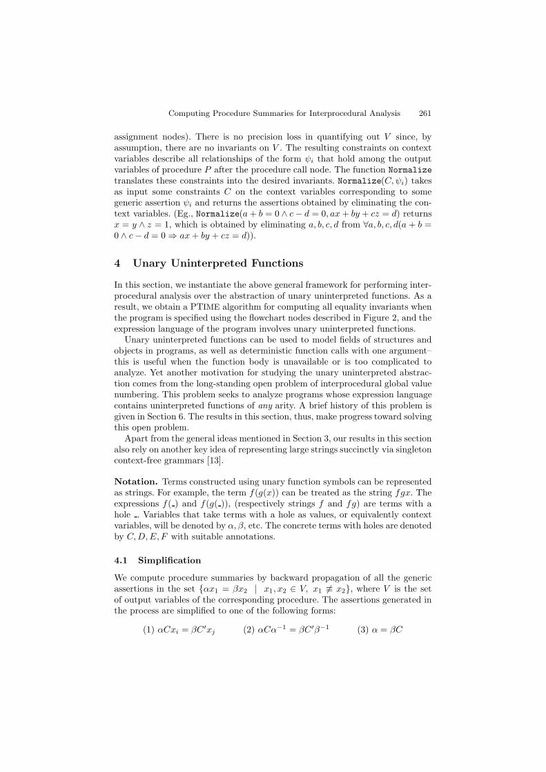
Computing Procedure Summaries for Interprocedural Analysis 261
assignment nodes). There is no precision loss in quantifying out V since, byassumption, there are no invariants on V . The resulting constraints on contextvariables describe all relationships of the form ψi that hold among the outputvariables of procedure P after the procedure call node. The function Normalizetranslates these constraints into the desired invariants. Normalize(C, ψi) takesas input some constraints C on the context variables corresponding to somegeneric assertion ψi and returns the assertions obtained by eliminating the con-text variables. (Eg., Normalize(a + b = 0 ∧ c − d = 0, ax + by + cz = d) returnsx = y ∧ z = 1, which is obtained by eliminating a, b, c, d from ∀a, b, c, d(a + b =0 ∧ c − d = 0 ⇒ ax + by + cz = d)).
4 Unary Uninterpreted Functions
In this section, we instantiate the above general framework for performing inter-procedural analysis over the abstraction of unary uninterpreted functions. As aresult, we obtain a PTIME algorithm for computing all equality invariants whenthe program is specified using the flowchart nodes described in Figure 2, and theexpression language of the program involves unary uninterpreted functions.
Unary uninterpreted functions can be used to model fields of structures andobjects in programs, as well as deterministic function calls with one argument–this is useful when the function body is unavailable or is too complicated toanalyze. Yet another motivation for studying the unary uninterpreted abstrac-tion comes from the long-standing open problem of interprocedural global valuenumbering. This problem seeks to analyze programs whose expression languagecontains uninterpreted functions of any arity. A brief history of this problem isgiven in Section 6. The results in this section, thus, make progress toward solvingthis open problem.
Apart from the general ideas mentioned in Section 3, our results in this sectionalso rely on another key idea of representing large strings succinctly via singletoncontext-free grammars [13].
Notation. Terms constructed using unary function symbols can be representedas strings. For example, the term f(g(x)) can be treated as the string fgx. Theexpressions f( ) and f(g( )), (respectively strings f and fg) are terms with ahole . Variables that take terms with a hole as values, or equivalently contextvariables, will be denoted by α, β, etc. The concrete terms with holes are denotedby C, D, E, F with suitable annotations.
4.1 Simplification
We compute procedure summaries by backward propagation of all the genericassertions in the set {αx1 = βx2 | x1, x2 ∈ V, x1 �≡ x2}, where V is the setof output variables of the corresponding procedure. The assertions generated inthe process are simplified to one of the following forms:
(1) αCxi = βC′xj (2) αCα−1 = βC′β−1 (3) α = βC

262 S. Gulwani and A. Tiwari
P (){1 x := fgx;2 y := gfy;3 if (*) { Q(); }4 else { P (); }5 }
Q(){1 while (*) {2 x := fx;3 y := fy;4 }5 }
main(){1 y := a;2 x := fa;3 P ();4 assert(x = fy);5 }
Fig. 3. Program
Thus, every ψ is simply a conjunction of assertions of these forms. The inverseoperator, −1, satisfies the intuitive axioms: (αβ)−1 = β−1α−1, αα−1 = ε, and(α−1)−1 = α.1 The strings C, C′ in Form 2 are allowed to contain the inverseoperator, whereas strings C, C′ in Form 1 and Form 3 do not contain the inverseoperator. Equations of Form 2 are an elegant way of encoding constraints on thecontext-variables α and β that are generated by the backward analysis.
We show now that weakest precondition computation across the various pro-gram nodes maintains assertions in one of these forms. We consider the caseof a Procedure Call node “Call P()” (the other cases are easy to verify). Atany stage of the fixpoint computation, the (partially computed) summary of aprocedure P will be given as: “α′xi = β′xj holds at the end of procedure P ifψ′′
ij holds at the beginning” for each pair xi, xj ∈ V . Equations of Form 2 andForm 3 are unchanged in the weakest precondition computation. The weakestprecondition of an equation αCxi = βC′xj is obtained by instantiating ψ′′
ij by{α′ �→ αC, β′ �→ βC′}. Applying this replacement in equations of Form 1 orForm 2 in ψ′′
ij gives back equations of the same form. When applied on equa-tions of Form 3, we get equations of the form αC = βC′. We remove the largestcommon suffix of C, C′ and if the equation does not reduce to Form 3, then theweakest precondition is false .
Bounding the size of ψ. We will show that any conjunction of equations ofForm 1, Form 2, and Form 3 over k variables can be simplified to contain atmost k(k − 1)/2 + 1 equations. Specifically,
– for each pair xi, xj of variables, there is at most one equation of Form 1; and– either there is at most one equation of Form 2, or there is at most one
equation of Form 3.2
The Simplification procedure uses unification to simplify the equations and keepsthe result essentially equivalent to the original set. It performs two main steps.For a fixed pair x, y of variables, let ψxy denote the set containing all equationsof Form 1 in ψ. First, by repeated use of Lemma 1 ψxy is simplified to a setcontaining at most one equation of Form 1 and either one equation of Form 3 or
1 Note that the inverse operator implicitly builds in simplification using unification.For instance, while fx = fy does not logically imply x = y, using the inverse axiomswe have fx = fy ⇒ f−1fx = f−1fy ⇒ x = y.
2 Note that an equation of Form 3 essentially gives a concrete solution, since we canassume, by Property 1, that one of α, β is ε.

Computing Procedure Summaries for Interprocedural Analysis 263
Ite Proc Current Summary for αx = βy Comment0 P, Q true Init1 Q Simp(αx = βy,αfx = βfy) = (αx = βy, αfα−1 = βfβ−1)2 P αfgx = βgfy,αfα−1 = βfβ−1 Use Q’s summary3 Q αx = βy, αfα−1 = βfβ−1 fixpoint for Q
4 P Simp(αfgfgx = βgfgfy,αfgx = βgfy, αfα−1 = βfβ−1) Use P ’s summary5 P αf = β, αfgx = βgfy fixpoint for P
Fig. 4. This figure illustrates summary computation for interprocedural analysis overthe unary abstraction. In Column 3, the summary consists of the constraints that musthold at the beginning of the procedure P/Q for αx = βy to be an invariant at the endof the procedure.
finitely many equations of Form 2. For example, in iteration 2 of Figure 4, the setof equations {αx = βy, αfx = βfy} is simplified to {αx = βy, αfα−1 = βfβ−1}.
Lemma 1. The equation set {αCix = βC′iy : i = 1, 2} either has no solutions,
or it has the same solutions as a set containing either one of these two equationsand at most one equation of Form 2 or Form 3.
Next, if there is an equation of Form 3 then it can be used to simplify an equationof Form 2 to either false or true. Otherwise, a set {αCiα
−1 = βC′iβ
−1, i =2, . . . , k} containing multiple equations of Form 2 is simplified by repeated useof Lemma 2.
Lemma 2. The equation set {αCiα−1 = βC′
iβ−1, i = 1, 2} is either unsatisfi-
able, or has the same solutions as a set containing at most one equation of eitherForm 2 or Form 3.
For example, in iteration 4-5 of Figure 4, {αfα−1 = βfβ−1, αfgα−1 = βgfβ−1}is simplified to {αf = β}. In this way, any conjunction ψ of equations of Form 1,Form 2, and Form 3 is simplified to a conjunction with at most k(k − 1)/2 + 1equations.3
The algorithms used in the proof of Lemma 1 and Lemma 2 use a constantnumber of string operations. Assuming the basic string operations take timeTbase, the time taken to simplify Suu(k)2 = O(k4) assertions is O(k4Tbase).
Maximum Unifier Chain Length. It is easy to see that the maximum unifierchain length for k variables is bounded by k(k − 1)/2 + 2. This is because thenumber of equations in ψ can increase only k(k − 1)/2 + 1 times, and beyondthat the formula either becomes unsatisfiable, or it is forced to have a uniquesolution for its variables. Note that it is not possible for the number of equationsto remain the same and the formula to get stronger. This is a consequence ofLemma 1.3 The observation that we need to keep only a small number of equations Cxi = αC′xj
intuitively means that we keep only a few runs. However, these runs in the simplifiedformula may not correspond to any real runs, but some equivalent hypothetical runs.

264 S. Gulwani and A. Tiwari
Hence, for the case of unary uninterpreted (uu) abstraction, we have:
Suu(k) = k(k−1)2 + 1 Tuu(k) = O(k4Tbase) Muu(k) = k(k−1)
2 + 2
4.2 Computational Complexity: Efficient Representations
We note that the time complexity of interprocedural analysis for the unaryuninterpreted abstraction is polynomial assuming that the string operations canbe performed efficiently. However, the length of strings can be exponential in thesize of the program, as the following example shows.
Example 1. Consider the n procedures P0, . . . , Pn−1 defined as
Pi(xi) { t := Pi−1(xi); yi := Pi−1(t); return(yi); }P0(x0) { y0 := fx0; return(y0); }
The summary of procedure Pi is: yi = αxi iff α = f2i
.
Hence, if we use a naive (explicit) representation, the size of ψ can grow exponen-tially (when we apply substitutions during transfer function computation acrossprocedure call nodes). Instead we appeal to shared representation of strings usingsingleton context-free grammars (SCFG). An SCFG is a context-free grammarwhere each nonterminal represents exactly one (terminal) string. An SCFG canrepresent strings in an exponentially succinct way. The strings Ci’s that arise inthe equations can be represented succinctly using SCFGs in size that is linearin the size of the program (because the program itself is an implicit succinctrepresentation of these strings using SCFGs).
Example 2. Following up on Example 1, we note that the string f2n
can berepresented by the SCFG with start symbol An and productions {Ai+1 → AiAi |1 ≤ i ≤ n} ∪ {A0 → f}. In particular, the summaries of the procedures can berepresented as: yi = αxi iff α = Ai.
A classic result by Plandowski [13] shows that equality of two strings representedas SCFGs can be checked in polynomial time. Apart from this, the simplificationprocedure implicit in the proofs of Lemma 1 and Lemma 2 require largest com-mon prefix/suffix computation and substring extraction. It is an easy exercise tosee that these string operations can also be performed on SCFG representationsin polynomial time. Hence, the computational procedure outlined above can beimplemented in polynomial time using the SCFG representation of strings. Inconclusion, this shows that summaries can be computed in PTIME on the ab-straction of unary symbols. We remark here that Plandowski’s result has beengeneralized to trees [19] suggesting that it may be possible to generalize ourresult to the interprocedural global value numbering problem (over binary un-interpreted functions).

Computing Procedure Summaries for Interprocedural Analysis 265
5 Linear Arithmetic
The technique described in Section 3.2 can also be used effectively to computeprocedure summaries for the abstraction of linear arithmetic. We compute theweakest precondition of the generic assertion α1x1 + · · · + αkxk = α (whichconstitutes a complete set by itself) where x1, . . . , xk are the output variables ofthe corresponding procedure.
The conjunction ψ of equations thus obtained at any point in the procedureduring the weakest precondition computation can be seen as linear equationsover the k2 + k + 1 variables: k2 variables representing the products αixj andthe k + 1 variables αi and α. We can simplify the equations thus obtained bymaintaining only the linearly independent (non-redundant) equations. We knowthat there can not be more than k2 + k + 1 linearly independent equations andhence ψ can have at most k2 + k + 1 equations. This shows that for the lineararithmetic (la) abstraction,
Sla(k) = k2 + k + 1 Tla(k) = O(Tbasek8) Mla(k) = k2 + k + 1,
where Tbase denotes the time to perform an arithmetic operation. Since con-stants can become large (programs can encode large numbers succinctly), we usemodulo arithmetic and randomization to get a true PTIME procedure, as in [11].
Muller-Olm and Seidl also gave a precise interprocedural algorithm for lin-ear arithmetic of similar complexity [11]. However, their algorithm is differentand is based on the the observation that runs of a procedure correspond to lin-ear transformations and there can be only quadratic many linearly-independenttransformations. In a certain sense, this is the dual of our approach.
6 Related Work and Discussion
Forward vs. Backward Analysis. The approach presented in this paper forcomputing procedure summaries is based on backward propagation of genericassertions. It is presently unclear how the dual approach, namely forward propa-gation of a complete set of generic assertions, can be effectively used. A forwardpropagation involves developing context-sensitive or distributive transfer func-tions for assignment nodes (usually involves existential quantifier elimination)and join nodes. Giving a general procedure for such operations appears to behard for regular assertions (intraprocedural case) and would be significantly moredifficult for generic assertions.
Nevertheless, these difficulties may be overcome for very specific abstractions,such as linear arithmetic [11,8]. In this case, the authors essentially look at a pro-cedure as a linear transformation and compute in the (k+1)2-dimensional vectorspace of these linear transformations. This allows them to perform abstract inter-pretation using either backward or forward analysis [11,8]. However, this generalapproach of developing interprocedural analysis by describing program behav-iors as transformations (in a finite dimensional vector space) is applicable onlyon arithmetic abstractions. In contrast, our approach promises to be simpler,and more generally applicable.

266 S. Gulwani and A. Tiwari
Weakest Precondition of Generic Assertions vs. Regular Assertions.To ensure termination of weakest precondition computation over generic as-sertions, we used some connections between unification and assertion checking.Similar connections have been used earlier for weakest precondition computationfor regular assertions in the intraprocedural case [5,6]. However, in the intrapro-cedural case, we just need to solve unification problems over regular assertions.These problems are well-studied and efficient algorithms are known for severaltheories. In the interprocedural case, we now have to solve unification problemsover generic assertions. In the theorem proving community, these are studiedunder the name of “second-order unification” and “context unification”. Theseproblems are known to be more difficult than their first-order counterparts. Thus,while our approach of backward analysis based on generic assertions provides auniform framework for developing interprocedural analyses, it also helps to as-certain the difficulty of interprocedural analysis over intraprocedural analysis bydrawing connections with the complexity of second-order unification vs. stan-dard unification in theorem proving. Templates, which are similar to genericassertions, have been used to generate invariants, but only in the context ofintraprocedural analysis and without any completeness guarantees [18].
History of Global Value Numbering. Since checking equivalence of pro-gram expressions is an undecidable problem, in general, program operators arecommonly abstracted as uninterpreted functions to detect expression equiva-lences. This form of equivalence is also called Herbrand equivalence [16] andthe process of discovering it is often referred to as value numbering. Kildall [7]gave the first intraprocedural algorithm for this problem based on performingabstract interpretation [2] over the lattice of Herbrand equivalences in expo-nential time. This was followed by several PTIME, but imprecise, intraproce-dural algorithms [1,16,3]. The first PTIME intraprocedural algorithm was givenby Gulwani & Necula [4], and then by Muller-Olm, Ruthing, & Seidl [9]. How-ever, PTIME interprocedural global value numbering algorithm has been elusive.There are some new results, but only under severe restrictions that functions areside-effect free and one side of the assertion is a constant [12]. Neither of theseassumptions is satisfied by the program in Figure 3. The technique described inthis paper yields a PTIME algorithm for the special case of unary uninterpretedfunctions.
7 Conclusion
Proving non-trivial properties of programs requires analyzing programs over richabstractions. The scalability of such program analyses depends upon the pos-sibility of constructing efficient and precise summaries of procedures over suchabstractions. In this paper, we have described a new technique for computingprocedure summaries for a class of program abstractions over infinite domains,thereby adding to some limited piece of work known in this area.
In the description of our technique, we assume at some places that condition-als are non-deterministic and expression language of the program comes from a
Computing Procedure Summaries for Interprocedural Analysis 267
unitary theory. These assumptions are needed to prove that our technique com-putes the most precise procedure summary in an efficient manner. We believethat the general ideas in our technique can be extended to reason about predi-cates in conditionals and handle expressions that are not from a unitary theory(e.g., as suggested in [6]), albeit with some (unavoidable) precision loss becausethe problem is undecidable in general.
References
1. B. Alpern, M. N. Wegman, and F. K. Zadeck. Detecting equality of variables inprograms. In 15th Annual ACM Symposium on POPL, pages 1–11, 1988.
2. P. Cousot and R. Cousot. Abstract interpretation: A unified lattice model for staticanalysis of programs by construction or approximation of fixpoints. In 4th AnnualACM Symposium on POPL, pages 234–252, 1977.
3. K. Gargi. A sparse algorithm for predicated global value numbering. In PLDI,volume 37, 5, pages 45–56. ACM Press, June 17–19 2002.
4. S. Gulwani and G. C. Necula. A polynomial-time algorithm for global value num-bering. In Static Analysis Symposium, volume 3148 of LNCS, pages 212–227, 2004.
5. S. Gulwani and A. Tiwari. Assertion checking over combined abstraction of lineararithmetic & uninterpreted functions. In ESOP, volume 3924 of LNCS, Mar. 2006.
6. S. Gulwani and A. Tiwari. Assertion checking unified. In Proc. VMCAI, LNCS4349. Springer, 2007. See also Microsoft Research Tech. Report MSR-TR-2006-98.
7. G. A. Kildall. A unified approach to global program optimization. In 1st ACMSymposium on POPL, pages 194–206, Oct. 1973.
8. M. Muller-Olm, M. Petter, and H. Seidl. Interprocedurally analyzing polynomialidentities. In STACS, volume 3884 of LNCS, pages 50–67. Springer, 2006.
9. M. Muller-Olm, O. Ruthing, and H. Seidl. Checking Herbrand equalities andbeyond. In VMCAI, volume 3385 of LNCS, pages 79–96. Springer, Jan. 2005.
10. M. Muller-Olm and H. Seidl. A note on Karr’s algorithm. In 31st InternationalColloquium on Automata, Languages and Programming, pages 1016–1028, 2004.
11. M. Muller-Olm and H. Seidl. Precise interprocedural analysis through linear alge-bra. In 31st ACM Symposium on POPL, pages 330–341, Jan. 2004.
12. M. Muller-Olm, H. Seidl, and B. Steffen. Interprocedural Herbrand equalities. InESOP, volume 3444 of LNCS, pages 31–45. Springer, 2005.
13. W. Plandowski. Testing equivalence of morphisms on context-free languages. InAlgorithms - ESA ’94, volume 855 of LNCS, pages 460–470. Springer, 1994.
14. T. Reps. On the sequential nature of interprocedural program-analysis problems.Acta Informatica, 33(8):739–757, Nov. 1996.
15. T. Reps, S. Horwitz, and M. Sagiv. Precise interprocedural dataflow analysis viagraph reachability. In 22nd ACM Symposium on POPL, pages 49–61, 1995.
16. O. Ruthing, J. Knoop, and B. Steffen. Detecting equalities of variables: Combiningefficiency with precision. In SAS, volume 1694 of LNCS, pages 232–247, 1999.
17. M. Sagiv, T. Reps, and S. Horwitz. Precise interprocedural dataflow analysis withapplications to constant propagation. TCS, 167(1–2):131–170, 30 Oct. 1996.
18. S. Sankaranarayanan, H. Sipma, and Z. Manna. Non-linear loop invariant genera-tion using grbner bases. In POPL, pages 318–329, 2004.
19. M. Schmidt-Schauß. Polynomial equality testing for terms with shared substruc-tures. Technical Report 21, Institut fur Informatik, November 2005.
20. M. Sharir and A. Pnueli. Two approaches to interprocedural data flow analysis.In Program Flow Analysis: Theory and Applications. Prentice-Hall, 1981.
Related Documents