Computing optimal recovery policies for financial markets

Computing optimal recovery policies forfinancial markets

Fred E. Benth∗ Geir Dahl† Carlo Mannino‡

March 22, 2011

AbstractThe current financial crisis motivates the study of correlated de-

faults in financial systems. In this paper we focus on such a modelwhich is based on Markov random fields. This is a probabilistic modelwhere uncertainty in default probabilities incorporates expert’s opin-ions on the default risk (based on various credit ratings). We considera bilevel optimization model for finding an optimal recovery policy:which companies should be supported given a fixed budget. This isclosely linked to the problem of finding a maximum likelihood esti-mator of the defaulting set of agents, and we show how to computethis solution efficiently using combinatorial methods. We also proveproperties of such optimal solutions. A practical procedure for estima-tion of model parameters is also given. Computational examples arepresented and experiments indicate that our methods can find optimalrecovery policies for up to about 100 companies. The overall approachis evaluated on a real-world problem concerning the major banks inScandinavia and public loans. To our knowledge this is a first attemptto apply combinatorial optimization techniques to this important, andexpanding, area of default risk analysis.

Keywords: Financial models, discrete optimization, bilevel program-ming, Markov random field.

∗Department of Mathematics, CMA, University of Oslo, Norway. [email protected]†Department of Mathematics and Department of Informatics, CMA, University of Oslo,

Norway. [email protected]‡University of Rome, La Sapienza, Department of Computer Science, Rome, Italy, and

visiting scientist at CMA. [email protected]

1

1 IntroductionIn financial transactions there is always a risk that the counter-party can notfullfill the obligations, and that the investment goes to default. In view of thecurrent crisis, the world financial markets have experienced companies withhigh credit rating to run into distress, and even defaulting. Examples in-clude apparently well-managed companies like the investment bank LehmanBrothers that defaulted due to large exposure in subprime loans, and theinsurance giant AIG that was rescued by the Government after huge lossesin the credit derivatives sector. Credit risk modeling is of vital importancefor investors in order to understand and manage their counter-party risk infinancial operations. In particular, understanding how the default risk of onecompany is linked to others is crucial.

In this paper we study a Markov random field model for the defaultrisk of each company, modelled as a Bernoulli random variable, which maybe dependent on the default risk of other companies in the market. Thewhole market is represented as vertices in a graph, with the directed arcs(edges) between the vertices describing dependency in terms of default risk.Moreover, we include uncertainty in the default probabilities, which may beinterpreted as a collection of expert’s opinions on the default risk, comingfrom various credit rating companies. The role of these companies in themarketplace were claimed to be one of the sources for creating the financialcrisis starting in 2007/2008. The special case of undirected graph model wasrecently analyzed in [10].

Our modelling approach is within the class of what is frequently referredto as Bernoulli mixture models (see [12]). We do not suppose that the de-fault probabilities and correlations come from any structural model (like forinstance the Merton model, see [17]), but consider a reduced-form modelinstead. In a Bayesian context, we are interested in the posterior defaultprobability distribution of the market, given the prior default probabilitydistribution and conditioning on expert judgements introduced as probabil-ity distributions on the default probabilities.

The main question we focus on in this paper is to use the graph approachto derive optimal recovery policies. A characteristic of the current financialcrisis is that governments world-wide try to resolve the turmoils by pumpingin money to recover various sectors which are believed to be crucial for themarket as a whole. We use our model to look for optimal policies in thesense of recovering as much of the potential loss as possible, given a fixed

2

budget for the government. Closely related to the recovery problem is the“default geometry” of the market in the sense of the most probable set ofdefaulted companies under the model assumed. This seems to be a questionwhich is rarely investigated in the literature, but turns out to be importantin order to understand the derivation of optimal recovery policies. Moreover,it is interesting in its own since it will provide investors guidelines for whichcompanies will most likely default, and which are more “safe havens”. Ofcourse, from the default probabilities of each firm this is simple to answeron an individual basis, but after introducing dependencies among companiesthe picture may be complicated significantly.

The two problems posed above result in discrete optimization problemsthat in general are highly non-trivial to solve. However, as we show in the pa-per as one of our main results, finding the most likely set of default companiescan be transformed into a well-known combinatorial optimization problemcalled the minimum cut problem. There exist very efficient combinatorialalgorithms for solving such problems, so that large-scale instances can besolved extremely fast; see [1] for a discussion of such algorithms, their com-plexity and implementations. It is therefore computationally feasible to studymarkets consisting of many companies with complex dependency structures.Furthermore, we are also able to prove a uniqueness-result for the most likelydefault set in the Markov random field model. Among all the most proba-ble configurations of companies defaulting, there is a unique one of maximalcardinality. This maximal set contains all the other most likely defaultingsets.

In the recent literature on credit risk modelling, the focus has been ondynamic portfolio credit risk models. Dynamical models based on point pro-cesses have been used in order to model the exposure to credit risk in aportfolio, with the aim of computing the loss distribution. One supposes aconditionally independent default structure among the firms in the portfolio.Dependencies in the credit situation of the different firms are modelled bythe default intensities being correlated stochastic processes (see Jarrow andTurnbull [14] and Duffie and Singleton [9]). Since typically it is hard to com-pute the loss distribution, approximations through limit theory or simulationare called for. For example, Deng, Giesecke and Lai [8] propose an impor-tance sampling technique to estimate rare events probabilities in a creditrisk portfolio. The method is based on a change of measure and resamplingto approximate the zero-variance importance measure connected to the rareevents.

3

The alternative to intensity-based models is structural modelling wherecredit events of a particular firm is modelled via the evolution of the firm’svalue and its capital structure. Typically one is interested in the firm’s de-fault, triggered by the value of the firm hitting a certain threshold. Recently,Carmona, Fouque and Vestal [5] presented an efficient numerical approach tocompute rare credit portfolio losses in a structural model based on interactingparticle systems.

Our model provides an explicit way to model statistically the impact ofa default of one company to another. In this respect, our approach placesitself in the stream of literature on credit contagion. For example, Gieseckeand Weber [13] study a dynamic reduced-form credit risk model based on theso-called voter model in the theory of interacting particle systems. Similarto our approach, they consider a lattice of companies which may be in twoliquidity states, “high” and “low”. To model contagion effects, a company i inthe lattice have a neighborhood of business partners j ∈ N(i) (being otherfirms in the lattice, of course), where N(i) is the set of labels of the partners.The transition between states of company i is a Poisson event with transitionrate depending on the states of the business partners j ∈ N(i). Although thecontagion effects in the lattice is dynamic and modelled differently than ours,the idea is somewhat similar to the approach proposed and analysed in thispaper. Giesecke and Weber [13] provide an explicit Gaussian approximationthe portfolio loss distribution, and analyse the effects of credit contagionbased on this.

In our approach, we allow explicitly for impacts between business partnerswhich are not necessarily mutual. We may have that a firm i is dependingon the credit situation of firm j, but not the other way around. Also, wemix in the possibility of firm’s exposure to macro-economic factors, as weassume these to be vertices in the graph. In this way, our model takes intoaccount both cyclical default dependence and credit contagion (see Giesckeand Weber [13] for more discussions on this). Different than most of theliterature on credit risk, we focus on providing an efficient computationalmethod for the model applied to studying recovery policies and most likelymarket scenarios, given impacts between business partners and from macro-economic variables.

Our modeling approach and analysis are illustrated with numerous ex-amples. In particular, we show how our graph representation of companiescan be used to include variables modelling the “state of the economy”, thatis, macro-economic factors. For example, we consider a graph consisting of a

4

bank with several clients borrowing money. The clients are divided into twogroups, one being “good” clients with low default probability and the other“bad” clients with high default probability. But, in addition, we supposethat the borrowers are dependent on a vertex in the graph representing the“state of the economy”, being for instance the interest rate in the market, orinflation. The state is either good or bad, and influencing the clients directly.In this way we can investigate the effect of, for instance, a change in the in-terest rate from “normal” to “high”, and study the impact on the bank. Theexample may be viewed as a simplified model for banks with subprime loansin their portfolio.

Another important issue that we study through examples is how the lossdistribution, defined as the number of defaulted companies, is dependenton the introduction of additional default uncertainty through expert judge-ments.

Finally, the overall approach is evaluated on a real-world problem con-cerning the major banks in Scandinavia and public loans. We discuss howthe data are obtained from ratings and annual reports and demonstrate howthe parameters of the model are estimated. Then we compute most likelydefault sets and optimal recovery policies for the actual situation and for amore pessimistic scenario.

The paper is organized as follows: In Section 2 our model is introducedand put into a proper statistical context. The analysis of the model andsome main results are presented in Section 3 where we discuss most likelydefault sets (of companies) and the connection to the minimum cut problem.The model includes certain parameters representing default probabilities anddependencies. The role of these parameters is discussed in Section 4 anda procedure for estimating the parameters is presented in Section 5. Ourmain issue concerning optimal recovery policies, is treated in Section 6, whileSection 7 presents computational experiments and some examples of ourmethodology and on a real-world case. Finally, some concluding remarksand future directions are given.

2 The modelThe purpose of this section is to introduce our mathematical model and todefine associated optimization problems. Our model belongs to the class ofMarkov random fields (MFR), which has proved to be useful in several areas,

5

for instance, in image segmentation ([2], [3], [6], [11], [20]), and statisticalphysics (the Ising model) [16].

The model is stochastic and represents a financial system consisting ofdifferent economic agents (companies, banks) and economic dependenciesbetween pairs of such agents. The main purpose of the model is to be able todetermine a most likely set of agents that will be defaulted at some specifiedfuture time. The financial system is represented by a directed graph G =(V,E) with vertex set V and arc set E. The vertices represent the agents, andthe arcs represent a dependency between pairs of agents. This dependencywill be explained below. Define n := |V | and m := |E|. An arc from vertexu to vertex v is denoted by (u, v) or uv. We consider a one-step dynamicalmodel, today is time t0 and t1 represents a specified future time (e.g. onemonth ahead). Associated with each v ∈ V is a random Bernoulli variablexv ∈ {0, 1} where xv = 1 means that agent v defaults at time t1, while xv = 0means that it survives. The vector x = (xv : v ∈ V ) is a random variable,and we refer to x as the default state vector.

At time t0 we have available certain information about the system whichspecifies the probability distribution of the random variable x. This infor-mation includes a real number zv ∈ [0, 1], for each vertex v, which may beconsidered as an approximation to xv. Thus, zv may be the result of ananalysis – made at time t0 – of the financial situation of the agent v. Forinstance, one may think of zv as the proportion of a group of analysts thatthink agent v will be default at time t1. We will treat z = (zv : v ∈ V ) as arandom vector and call it the judgement vector. The connection between xand z is given by a statistical model where the conditional probability distri-bution f(z|x) of z given x is specified. We assume conditional independencebetween agents in the sense that

f(z|x) =∏v∈V

fv(zv|xv) (1)

for some conditional probability functions fv (which we assume to be strictlypositive). This means that the judgement value zv depends on the future sta-tus xv; this reflects the knowledge of the experts. However, for a given defaultstate vector x, the judgements zv for the agents (v ∈ V ) are independent.

The model also includes dependencies among the agents as represented bythe arcs in the directed graph G. This is done using a so-called Ising model

6

which gives a prior probability distribution for the default state vector x

π(x) =1

sexp{

∑v∈V

[α1vxv + α0

v(1− xv)] +∑

(u,v)∈E

βuvI(xu ≤ xv)}. (2)

Here βuv ≥ 0 is a parameter indicating how dependent agent v is on agentu (for (u, v) ∈ E); the larger βuv is, the less likely are all events where udefaults but v does not. The constant s is a normalization constant makingπ(x) a proper probability distribution (i.e. total probability is 1) and theindicator function I(xu ≤ xv) equals 1 if xu ≤ xv and 0 otherwise. Theparameters α1

v and α0v reflect a priori information on the financial position

of agent v, independent of the expert judgement zv. Actually, we interpret(1/s)eα

1v (resp. (1/s)eα

0v) as an “a priori probability” that agent v defaults

(resp. survives) whenever βuv = 0. We may here assume that α1v, α

0v ≤ 0

since subtracting a (suitable large) number, say b, from each α1v and α0

v in(2) results in the exponential term being multiplied by the constant e−nb,and this number will be incorporated in the normalization constant s. As wenote later, the value of s is irrelevant for our method below.

We should remark that the Ising model (e.g. in image analysis) is mostfrequently used in connection with undirected graphs. Then the “correlation”term in (2) would be βuvI(xu = xv) summed over all edges in the graph.In our model, however, a directed graph is crucial for being able to modelasymmetric markets which should be more the rule than an exception.

The parameters in our model may therefore be summarized as follows:

(i) α1v, α

0v ≤ 0: prior parameters for agents

(ii) βuv ≥ 0: prior parameters reflecting dependencies between agents

(iii) zv ∈ [0, 1]: expert judgement of the robustness of agent v

(iv) fv(·|·): conditional probability functions used to describing xv and zv.

The posterior distribution π(x|z) for x given z may be determined throughBayes formula, and this gives

π(x|z) = φ(z)π(x)f(z|x)

where φ is a suitable normalization function. We now consider the judgementvector z as fixed, and therefore φ(z) is a constant. The Bayesian paradigm

7

([2]) is to base all inference on the posterior distribution π(x|z). A naturalestimate of x is the maximum a posteriori solution x. This solution x max-imizes π(x|z), or equivalently, π(x)f(z|x) (since φ(z) is a constant). Thus,the maximum a posteriori solution is an optimal solution of the discreteoptimization problem

(MLDS) max{F (x) : x ∈ {0, 1}n} (3)

where

F (x) = exp{∑v∈V

[α1vxv + α0

v(1− xv)] +∑

(u,v)∈E

βuvI(xu ≤ xv)} ·∏v∈V

fv(zv|xv)

An optimal solution x in MLDS is the incidence vector of a subset S ⊆ V(i.e., a (0, 1)-vector with ones in the positions of S) and we call S a most likelydefault set, defending the attribution (MLDS). Thus, the MLDS problem isto find a most likely default set. Note that – in MLDS – the judgement vectorz is given. An instance of MLDS will be denoted by the tuple (G, f, z, α, β)where all these components are described above.

Note that one may also interpret the MLDS problem more directly asfinding a maximum likelihood estimator x of the (unknown) default statevector x for the given probability distribution F (as mentioned, multiplyingF by a suitable constant gives a true probability distribution).

We remark that our prior distribution π coincides with the graphicalmodel investigated in [10]. A main result in [10] is that there is a one-to-onecorrespondence between the model parameters and certain probabilities: themarginal probabilities of default of agents and the probabilities of pairs ofagents defaulting simultaneously. Hence, the model can be fully specified bythese probabilities. The computation of the parameters, given these marginalprobabilities, can be solved by convex optimization, but with an exponentialnumber of constraints. We refer to [10] for details on this method and otherpractical estimation procedures.

Our main contributions are:

1. In contrast with [10] we consider a directed model which allows forasymmetric markets (see above).

2. We also extend the prior model compared to [10] so as to incorporateadditional expert judgement (via the posterior). We propose a practicalstatistical procedure for estimating all the model parameters. Thismethod is based on conditional probabilities of default.

8

3. We show how to compute efficiently a maximum likelihood estimatorin the model, both in the prior π and in the posterior F (in which casewe find an MLDS solution). This is done by a transformation into theminimum cut problem; a basic combinatorial optimization problem forwhich highly efficient algorithms exist.

4. We use the basic model as the core in another optimization modelwhose purpose is to find optimal recovery policies in financial systems.

3 Most likely default sets and minimum cutsWe now demonstrate that the MLDS problem may be reformulated as aminimum cut problem in a (directed) graph derived from G. This meansthat the problem may be solved efficiently by known algorithms, see e.g. [1].

Consider again the function F in (3) which is to be maximized. Equiva-lently, we may maximize its logarithm which is

L(x) =∑v∈V

[α1vxv +α0

v(1−xv)] +∑

(u,v)∈E

βuvI(xu ≤ xv) +∑v∈V

log fv(zv|xv) (4)

Sometimes this function (or its negative) is referred to as the energy functionof the MRF.

We now introduce an auxiliary graph G′ = (V ′, E ′) based on G. Let thevertex set be V ′ = V ∪ {s, t} where the vertices s and t are called terminalvertices. The arc set E ′ consists of all arcs in E and, in addition, arcs ofthe form (s, v) and (v, t) for each v ∈ V . Thus, G′ is obtained from G byadding two terminal vertices s and t as well as arcs connecting each originalvertex to the terminal vertices. We associate weights to the arcs in G′ as thefollowing table indicates:

arc e weight we(u, v) ∈ E wuv := −βuv(s, v) (v ∈ V ) wsv := α0

v + log fv(zv|xv = 0)(v, t) (v ∈ V ) wvt := α1

v + log fv(zv|xv = 1)

It is important to note that all these weights are nonpositive: f(zv|xv =1), f(zv|xv = 0) ≤ 1 as these are discrete probabilities, βuv ≥ 0 and α1

v, α0v ≤

0. This fact is crucial for the efficient solvability of the MLDS problem.

9

Consider a partition of the vertex set V ′ into two sets S and T = V ′ \ Swhere s ∈ S and t ∈ T . The set of arcs e = (u, v) in G′ with u ∈ S andv ∈ T is denoted by δ+(S), and it is called an st-cut (or simply a cut). Theweight of the cut δ+(S), denoted by w(δ+(S)), is the sum of the weights ofthe arcs in the cut, i.e.,

w(δ+(S)) =∑

e∈δ+(S)

we.

Let x ∈ {0, 1}n and define Sx = {s} ∪ {v ∈ V : xv = 1} and Tx = {t} ∪ {v ∈V : xv = 0}. Then we have

w(δ+(Sx)) =∑

v∈Sx\{s}wvt +∑

v∈Tx\{t}wsv +∑

(u,v)∈E∩δ+(Sx)wuv

=∑

v∈Sx\{s}(α1v + log f(zv|xv = 1)) +

∑v∈Tx\{t}(α

0v + log f(zv|xv = 0))

+∑

(u,v)∈E∩δ+(Sx)(−βuv)

=∑

v∈Sx\{s}(α1v + log f(zv|xv = 1)) +

∑v∈Tx\{t}(α

0v + log f(zv|xv = 0))

+∑

(u,v)∈E:xu≤xv βuv −∑

(u,v)∈E βuv

= L(x)− β∗

where β∗ =∑

(u,v)∈E βuv is a constant.Thus, up to a constant, the weight of the cut δ+(Sx) equals the value of

the function L at x. The calculation also shows that, conversely, the weightof cut δ+(S) equals L(x) − β∗ where x ∈ IRn is the incidence vector of S inV , i.e., xv = 1 if v ∈ S ∩ V and xv = 0 otherwise.

This discussion shows that the MLDS problem is equivalent to finding amaximum weight cut in the graph G′ with weights as defined above. As notedabove all these weights are nonpositive. Therefore the maximum weight cutproblem is equivalent to finding a minimum weight cut in G′ where theweights are nonnegative and given by w′e := −we (e ∈ E ′).

We have therefore shown the following theorem (see [18] for algorithmiccomplexity).

Theorem 1 The MLDS problem is solvable in polynomial time as a min-imum st-cut problem in the directed graph G′ with nonnegative weights w′e(e ∈ E ′).

10

The important consequence of this theorem is that we can solve MLDSefficiently for any given graph G. We refer to Section 7 for some computa-tional experiments where MLDS is solved for certain specific instances, ofvarying structure and size.

If δ+(S) is an optimal solution to the above minimum st-cut problem, thenS\{s} is an MLDS, a most likely default set. A relevant question concerns theuniqueness of the most likely default sets. In general, we may have severaloptimal solutions to the minimum st-cut problem, each corresponding todifferent most likely default sets. However, the following property holds:

Theorem 2 Let S∗ be a maximum cardinality most likely default set. ThenS∗ is unique, and it contains every other most likely default set.

Proof. In what follows, for each S ⊆ V we denote by f(S) the weightof the st-cut δ+(S ∪ {s}) (using the nonnegative weights w′e, e ∈ E ′). It iswell known (see [18]) that f is a submodular set function, that is, for everyS1, S2 ⊆ V we have

f(S1 ∪ S2) + f(S1 ∩ S2) ≤ f(S1) + f(S2).

Observe that if δ+(S1 ∪ {s}) and δ+(S2 ∪ {s}) are minimum st-cuts, withf(S1) = f(S2) = m, then we have f(S1 ∪ S2) ≥ m and f(S1 ∩ S2) ≥ m.Thus, 2m ≤ f(S1 ∪ S2) + f(S1 ∩ S2) ≤ f(S1) + f(S2) = 2m which impliesthat f(S1 ∪ S2) = m (and f(S1 ∩ S2) = m).

Let now S∗ be a maximum cardinality most likely default set, and let S bea most likely default set such that S * S∗. By optimality and submodularity,f(S∗) = f(S) = f(S∗ ∪ S). This implies that S∗ ∪ S is a most likely defaultset. Since S * S∗, we have |S∗ ∪ S| > |S∗|, a contradiction. So, every mostlikely default set is contained in S∗ and the theorem follows.

It is not difficult to modify the original arc weights so that the minimumst-cut is unique and therefore it corresponds to the maximum cardinalitymost likely default set S∗ discussed in Theorem 2. This can be done byincreasing, for each v ∈ V , the weight w′sv of arc (s, v) by a suitable smallquantity ε > 0, and we have the following result.

Proposition 3 Given an instance of the MLDS problem, let G′ be the cor-responding auxiliary graph, with weights w′. Then we can find weights w′′so that the minimum st-cut in (G′, w′′) is unique (and corresponds to themaximum cardinality most likely default set).

11

Proof. Consider the auxiliary graph G′ with weights w′, let m be theminimum cut weight, and let m be the weight of a second best minimumst-cut, meaning that m > m, and no other cut has weight in between (takem = +∞ if all cuts have equal value). It suffices to take 0 < ε < (m−m)/|V |,and define w′′sv = w′sv+ε, for v ∈ V , w′′uv = w′uv otherwise. Then, for any st-cutδ+(S) we have w′′(δ+(S)) = w′(δ+(S))+|V \S|·ε = w′(δ+(S))+|V |·ε−|S|·ε =K + w′(δ+(S))− |S| · ε, where K is constant.

First observe that every non-minimum st-cut D = δ+(S) in (G′, w′) (i.e.w′(D) ≥ m > m) is also a non-minimum st-cut in (G′, w′′). In fact, letC = δ+(S) be a minimum st-cut in (G′, w′). Then w′(D)−w′(C) ≥ m−m.It follows that w′′(D)−w′′(C) = K+w′(D)− ε · |S|− (K+w′(C)− ε · |S|) ≥m − m − ε · (|S| − |S|) ≥ m − m − ε · |V | > 0, implying that D is not aminimum st-cut of (G′, w′′).

So every minimum st-cut in (G′, w′′) is also minimum in (G′, w′).Now, let B∗ = δ+(S∗) and C = δ+(S) be two distinct minimum st-cut

in (G′, w′), and suppose |S∗| is the largest possible. By Theorem 2 we have|S∗| > |S|. It follows that w′′(B∗) − w′′(C) = K + w′(B∗) − ε · |S∗| − (K +w′(C)− ε · |S|) = ε · (|S| − |S∗|) < 0, and B∗ is the unique minimum st-cutin (G′, w′′).

In practice, weights are approximated and represented by rational num-bers; so they can always be scaled up to positive integers and m −m ≥ 1.Then it suffices to take ε < 1/|V |.

For the sake of simplicity, in the rest of the paper we will assume thatthe minimum st-cut in the auxiliary graph G′ with weights w′ is unique.

4 The role of the parametersIn order to better understand the role of the parameters α1

v, α0v and βuv in

our model, we study analytically the special case where the graph G has twovertices. Then it is possible to calculate explicit expressions for the priorprobabilities π. (The calculation of F also involves the functions fv, so it ismore complicated; for this reason we focus on the prior.)

So, assume that the graph G consists of two vertices v1 and v2 and arcs(v1, v2) and (v2, v1). Define p0

vi= eα

0vi and p1

vi= eα

1vi (i = 1, 2). Then the

12

prior (2) is given by

π(0, 0) = (1/s)p0v1p0v2eβ12+β12 π(0, 1) = (1/s)p0

v1p1v2eβ12

π(1, 0) = (1/s)p1v1p0v2eβ21 π(1, 1) = (1/s)p1

v1p1v2eβ12+β21 .

wheres = (p0

v1p0v2

+ p1v1p1v2

)eβ12+β21 + p0v1p1v2eβ12 + p1

v1p0v2eβ21

Then the marginal probability p(β12, β21) that xv2 = 1 (v2 defaults) becomes

p(β12, β21) =p0v1p1v2e−β21 + p1

v1p1v2

(p0v1p0v2

+ p1v1p1v2

) + p0v1p1v2e−β21 + p1

v1p0v2e−β12

which is an increasing function of β12 (for each β21) as one would expect.Now, fix β21 and take the limit as β12 →∞, so there is large influence of v1

on v2:

limβ12→∞

p(β12, β21) =p0v1p1v2e−β21 + p1

v1p1v2

(p0v1p0v2

+ p1v1p1v2

) + p0v1p1v2e−β21

Further, if we β21 tends towards 0, this gives

limβ21→0

limβ12→∞

p(β12, β21) =p0v1p1v2

+ p1v1p1v2

(p0v1p0v2

+ p1v1p1v2

) + p0v1p1v2

A more interesting case is when β21 tends towards infinity:

limβ21→∞

limβ12→∞

p(β12, β21) =p1v1p1v2

p0v1p0v2

+ p1v1p1v2

So for the highly correlated case, where β12 and β21 are large, this limitprobability of v2 defaulting is equal to the “a priori” conditional probabilityof both defaulting given that xv1 = xv2 (recall the interpretation of (1/s)p1

v1

as the a priori probability of v1 defaulting, see Section 2).It is also possible compute the prior analytically when G is a star, and

thereby analyze different questions, but we do not go into this here. Finally,we mention an observation concerning the parameters in the prior: (i) ifα1v ≥ α0

v + β|δ+(v)| where |δ+(v)| is the number of arcs leaving v, then thereis a maximizer x of the prior π with with xv = 1. (This follows by a simplevariation of the single variable xv in (2)). So, assuming F ≈ π, a similarproperty is likely for a MLDS solution. Also, we see that if α0

v ≥ α1v+β|δ−(v)|,

then there is a maximizer x of π with xv = 0.

13

5 Parameter estimationFor the practical usefulness of our model it is required to determine suitablevalues for the parameters (α’s and β’s). In particular, the agent dependencyparameters βuv may be hard to set “manually”. We here suggest a method-ology for parameter estimation which may be used in concrete situations tocalibrate the model.

First we discuss the situation when the number n of agents is “moder-ate”, so that all (0, 1)-vectors of length n may be enumerated. If some priorknowledge of default probabilities of agents is known, this may be reflectedin a choice of α0

v and α1v (see Section 2); otherwise they may all be set to

e.g. 0. Next, the expert judgement zv (v ∈ V ) is set based on the creditrisk rating of each bank v by assigning a default probability to each of thedifferent ratings used (typically very few classes). See Section 7 for detailson this approach. Values zv for other agents than banks must be set by someother/manual procedure for risk evaluation.

It remains to estimate the dependency parameters βuv’s. For this purposeone may specify certain conditional probabilities, based on our model. >Froman economic analysis one may find how “exposed” an agent v is to anotheragent u. More specifically, say that v is a bank that has public loans ofsize p million EURO, and let agent u correspond to “public loans”. Alsoassume bank v has total assets of value q million EURO. Then we considerthe fraction p∗uv := p/q as an estimate of the conditional probability thatbank v defaults given default of the public loans u. A similar idea may beused when u is another bank with loans in bank v. Thus, for each pair (u, v)of agents for which u may have such a negative influence on v, so βuv couldbe positive, we compute a number p∗uv using the same economic reasoning.This leads to the problem of choosing βuv ≥ 0 for each (u, v) ∈ E such that

g(β) :=∑

(u,v)∈E

(Pβ(xv = 1|xu = 1)− p∗uv)2

is minimized. Here β denotes a vector containing all the βuv’s, and Pβ(·|·)denotes the conditional probability in our model, indicating the dependenceon β (the dependence on α’s and z is not indicated).

In summary, economic analysis gives certain conditional probabilities p∗uv((u, v) ∈ E) that one believes are correct, and the βuv’s are adjusted to fitthese p∗uv’s best possible, using a least squares approach. The problem of

14

minimizing the function g, subject to the constraint that β is nonnegative,is a nonlinear constrained optimization problem. The computation of thefunction value g(β) may be done by enumeration of all possible state vectorsx ∈ {0, 1}n (recall, n is assumed moderate) and by suitable summations onecomputes the conditional probabilities Pβ(xv = 1|xu = 1). The function g isvery complicated, but there are few variables, so a good general optimizationcode should be able to solve the problem. In Section 7 we report this ap-proach for a realistic test case, and where we use the routines in the MatlabOptimization Toolbox for minimizing g.

We now discuss the case when n is too large for the approach aboveto be appropriate. Then one might split the graph into smaller pieces anduse the procedure above on each part. After this one may proceed with anadjustment procedure which we now discuss in detail. This procedure is anadaption of the parameter estimation method described in [3] and [4] forMarkov Random Field models in the image segmentation area. Let θ bea vector containing all α’s and β’s to be estimated, after (perhaps) settingsome parameters manually and grouping agents so that fewer parametersare needed. Again, we assume the judgement vector z is given (see above).Note that finding maximum likelihood estimator (MLE) in our model, whenz is given, is not possible because the default state vector x is also a part ofour model (1) and (2). We shall instead use the so-called pseudo-likelihoodfunction.

Consider the following procedure where, throughout, z is the fixed judge-ment vector:

1. Choose an initial estimate θ of θ.

2. For the given z and the current parameter θ, solve the MLDS problemto obtain the maximum a posteriori solution x.

3. For the given z and the current vector x, find a maximum pseudo-likelihood (MPLE) estimate θ of θ in the model (1), (2).

4. Return to Step 2 until convergence or a maximum number of iterationsis reached.

The MPLE problem in Step 3 may be treated as follows. Let f(x, z; θ)denote the joint probability density of the random variable (x, z) for the given

15

parameter θ. Then from (1), (2) (where dependency of θ is indicated in thenotation)

f θ(x, z) = πθ(x)f(z|x)

= (1/sθ) · eψθ(x) · f(z|x)(5)

whereψθ(x) =

∑v∈V

[α1vxv + α0

v(1− xv)] +∑

(u,v)∈E

βuvI(xu ≤ xv).

Note, in particular, that the summation constant s = sθ in the prior πθ(·)does depend on θ. But the conditional distribution f(z|x) is independent of θ.Let now z and x be fixed and consider the problem of maximizing f θ(x, z).It is equivalent to maximize ψθ(x) − log(sθ) w.r.t. θ. Since n is assumedlarge, sθ is hard to compute, and we adopt the maximum pseudo-likelihoodapproach (see [4]). The pseudo-likelihood pθ(x, z) is defined by

pθ(x, z) =∏v∈V

f θ(xv|xu(u 6= v), z)

so this is the product of the conditionals of each variable xv given the remain-ing variables xu for u 6= v (and z which is fixed here). The pseudo-likelihoodserves as an approximation to the likelihood function. A maximum pseudo-likelihood estimator (MPLE) θ maximizes pθ(x) (w.r.t. θ) for the given x.The main advantage of the MPLE approach is that one gets around thedifficulty caused by the normalization constant sθ. In fact, we have from (5)

f θ(xv = 0|xu(u 6= v), z)

= fθ(xv=0, xu(u6=v),z)fθ(xv=0;xu(u6=v),z)+fθ(xv=1;xu(u6=v),z)

= fv(zv |xv=0)·eψθ(xv=0,xu(u6=v))

fv(zv |xv=0)·eψθ(xv=0,xu(u6=v))+fv(zv |xv=1)·eψθ(xv=1,xu(u6=v))

which is independent of sθ (here 1/sθ and∏

u6=v fu(zu|xu) canceled). And, ofcourse, f θ(xv = 1|xu(u 6= v), z) = 1 − f θ(xv = 0|xu(u 6= v), z). So the con-ditional distribution can be computed efficiently (without knowing sθ). Thismeans that finding a MPLE becomes the nonlinear optimization problem ofmaximizing the logarithm of the pseudo-likelihood given above. Having inmind that there are rather few variables, and that a near-optimal solution isgood enough, this problem should be solvable by standard techniques in non-linear optimization. For further general comments and references on MPLEand the relation to MLE, see [4].

16

6 Optimal recovery policiesSo far we have considered the problem of finding a most likely default set inour financial system model. In this section we build on this model in orderto discuss an interesting extension of this problem: how can we “optimally”support the financial system by providing economic support to some subsetof the agents. We present a mixed integer linear programming model for thisproblem of finding an optimal recovery policy.

First we discuss a variation of the most likely default set problem MLDS.Consider again MLDS in (3) and let R ⊆ V . The R-saved MLDS problem is

(MLDS(R)) max{F (x) : x ∈ {0, 1}n, xv = 0 for all v ∈ R} (6)

An optimal solution x is the incidence vector of a subset S ⊆ V satisfyingS ∩ R = ∅, and we then call S an R-saved most likely default set. Thus, we“force” the agents in R to survive; otherwise the problem is similar to theMLDS problem.

The R-saved MLDS problem may also be solved as a minimum cut prob-lem as discussed next. Consider a fixed set R ⊆ V and consider again thedirected graph G′ defined in Section 3. A cut in G′ corresponds to a partition(S, T ) of V , so the cut is δ+(S ∪{s}). If R ⊆ T we call such a cut an sR-cut.Then, with the same arguments as in Section 3, it is clear that the R-savedMLDS problem corresponds to finding a minimum weight sR-cut, and thisproblem reduces to a minimum st-cut problem in a smaller graph obtainedfrom G′ by shrinking R ∪ {t} into a single vertex t.

Moreover, the following result holds on the connection between the R-saved MLDS problem and the ordinary MLDS problem.

Theorem 4 Let S∗ be the unique maximum cardinality most likely defaultset in the MLDS problem. Let R ⊆ V . Then there is a unique R-saved mostlikely default set SR of maximum cardinality. Moreover, SR ⊆ S∗.

Proof. As in the proof of Theorem 2 we let f(S), for each S ⊆ V , denotethe weight of the st-cut δ+(S ∪ {s}) in G′ (using the nonnegative weightsw′e, e ∈ E ′). Suppose SR * S∗. Since δ+(SR) is an sR-cut, R ∩ SR = ∅.If R ∩ S∗ = ∅ then SR = S∗ (since S∗ is optimal without the restrictioncorresponding to R), a contradiction. So, assume R ∩ S∗ 6= ∅. Clearly,f(SR) ≥ f(S∗). By submodularity we have f(S∗ ∪ SR) + f(S∗ ∩ SR) ≤

17

f(S∗) + f(SR). Both δ+(S∗ ∪ SR ∪ {s}) and δ+((S∗ ∩ SR) ∪ {s}) are st-cuts, and so f(S∗ ∪ SR) ≥ f(S∗) and f(S∗ ∩ SR) ≥ f(S∗) (by optimalityof S∗), which implies f(S∗ ∪ SR) ≤ f(SR) and f(S∗ ∩ SR) ≤ f(SR) (dueto the mentioned submodularity). Now, δ+((S∗ ∩ SR) ∪ {s}) is an sR-cut,since (S∗ ∩ SR) ∩ R = ∅. As a consequence f(S∗ ∩ SR) = f(SR) and thus(again by the submodularity and optimality of S∗) f(S∗ ∪ SR) = f(S∗). SoS∗∪SR is a most likely default set. Since SR * S∗, we have |S∗∪SR| > |S∗|,a contradiction. Uniqueness of SR can be easily derived as in the proof ofTheorem 2.

This theorem is important because it says that fixing (forcing) certainagents to survive does not add any agents to the maximum cardinality set ofmost likely agents that default.

Now, with each agent v ∈ V we associate a survival benefit bv and arecovery cost cv. This means that “the administration” can assure that vsurvives by paying a cost of cv. Moreover, for each surviving agent v there is asurvival benefit bv. Suppose the administration can allocate a limited amountof money to the system, sayK. We want to find an optimal allocation, i.e., wewant to establish which agents to be recovered (meaning: avoid defaulting) inorder to maximize the social benefit. This optimal recovery problem (ORP)can be restated as the problem of finding a set R ⊆ V of agents to berecovered so that the total benefit of the most likely nondefaulting (surviving)set of agents is maximized, and the total cost does not exceed K. Clearly, ifR is the set of recovered agents, and T the most likely set of surviving agents,then R ⊆ T .

We consider again the auxiliary graph G′ defined in Section 3. A cut inG′ corresponds to a partition (S, T ) of V , so the cut is δ+(S ∪ {s}). Notethat in order to recover a set R of agents, we can restrict the attention tothe case where R ⊆ T . The reader should keep in mind the interpretationthat vertices in S default while vertices in T survive.

As already mentioned, for fixed R ⊆ V , the maximizer of the (logarithmof the) likelihood function L in (4) can be found by solving a minimum cutproblem on a new graph obtained from G′ by shrinking the vertices in Rand vertex t into a single vertex. However, for our purposes it is convenientto let G′ remain unchanged and modify arc weights instead. We define newarc weights wR ∈ IRE′ by letting wRut = w′ut + M , for u ∈ R and wRuv =w′uv otherwise, where M is any constant satisfying M >

∑sv∈δ+(s)w

′sv =∑

sv∈δ+(s)wRsv. By this construction it is clear that no arc (u, t), for u ∈ R,

18

belongs to a minimum st-cut of (G′, wR). In other words, if (S∗, T ∗) is thepartition of V induced by a minimum st-cut in (G′, wR), then R ⊆ T ∗.

Finally, similarly to Proposition 3, one can show that there exist weightsw′ such that, for any R, there is a unique minimum st-cut in (G′, wR). Fromnow on we assume that this condition is satisfied.

The following result says that the ORP problem is computationally hard.

Theorem 5 The optimal recovery problem is NP-hard.

Proof. The proof is a reduction from the knapsack problem ([18]). Givennon-negative real numbers b1, . . . , bn (benefits), c1, . . . , cn (costs) and K (bud-get), the knapsack problem amounts to finding a subset R∗ ⊆ {1, . . . , n} suchthat

∑i∈R∗ ci ≤ K (i.e. the budget is not violated) and

∑i∈R∗ bi (overall ben-

efit) is maximized.Let us define an instance G′ = (V ′, E ′) of ORP as follows. V ′ = V ∪{s, t},

where V = {1, . . . , n} and E ′ = {si : i ∈ V } ∪ {it : i ∈ V }. With each i ∈ Vassociate a cost ci and a benefit bi, and suppose the budget is K. Finally,associate with the arcs of G′ the following weights: for i ∈ V , let w′si = ksand w′it = kt, with ks > kt > 0. With this setting, for every set R, there isa unique minimum sR-cut in G′, namely {si : i ∈ R} ∪ {it : i ∈ V − R}. Inother words, for every choice of R, the set T of surviving agents coincides withR. So, an optimal solution to ORP is simply a set R∗ satisfying the budgetconstraint and maximizing the overall benefit, which solves the knapsackproblem.

Next, we formulate ORP as a bilevel optimization problem. To this end,let yv be a binary variable which is 1 iff v ∈ R (i.e. v is recovered), and 0otherwise. Also, let q be the incidence vector of an st-cut of G′. According tothe modelling assumptions introduced in Section 3, qsv = 1 (qvt = 1) impliesthat v ∈ V survives (defaults); also, qsv = 1 − qvt. ORP can be formulatedas the following bilevel program:

max∑

v∈V bvqsv(y)

subject to ∑v∈V cvyv ≤ K

y ∈ {0, 1}n

(7)

where q(y) is the unique optimal solution to

minq∈Cst

∑uv∈E′

w′uvquv +∑v∈V

Myvqvt (8)

19

and Cst is the family of incidence vectors of st-cuts of G′. In fact, if we denoteby yR the incidence vector of R ⊆ V , then q(yR) is the incidence vector ofa minimum st-cut in (G′, wR), and it corresponds to a maximum cardinalityR-saved most likely default set. Also, if yR satisfies the budget constraint in(7), then the cost of R does not violate the budget and all agents in R canbe recovered. Finally, the objective function in (7) amounts to maximizingthe value of the surviving agents.

It is important to recall that, for each y ∈ {0, 1}n, the vector functionq(y) above is well-defined. Incidentally observe that our assumption on theweights w′ corresponds to what is known as the pessimistic paradigm [7]. Infact, among all possible solutions to (6) with the same F value, we choosethe one with the maximum number of defaulting agents.

Similarly to [15] we show how to reduce the above bilevel program toa mixed integer linear programming problem. First observe that the innerproblem can be formulated as a linear programming problem (LP). To thisend, suppose y is fixed to some (0, 1)-vector and introduce the vertex poten-tial vector p ∈ IRV ′ . Then (8) can be written as the following LP:

min∑

uv∈E′ w′uvquv +

∑v∈V Myvqvt

subject to

pv − pu + quv ≥ 0 (uv ∈ E ′)

ps = 1, pt = 0

q ≥ 0, p ∈ IRV ′ .

(9)

Let FP be the feasible set of (9). Then FP is a polyhedron and its verticesare (0, 1) vectors, in one-to-one correspondence with the st-cuts of G′ (see[19]). Since all weights in the objective function are strictly positive, the(unique) optimal value of (9) is attained in a vertex (q∗, p∗) and q∗ is theincidence vector of an st-cut of G′ (i.e. q∗ ∈ Cst). The dual of the above LPis:

max∑

su∈δ+(s) fsu

subject to ∑uv∈δ+(u) fuv −

∑vu∈δ−(u) fvu = 0 (u ∈ V )

0 ≤ fuv ≤ w′uv (uv ∈ E ′′)

0 ≤ fvt ≤ w′vt +Myv (v ∈ V )

(10)

20

where E ′′ = {uv ∈ E ′ : v 6= t}. Let FD be the feasible set of (10). Thenwe know that two feasible solutions (q∗, p∗) in (9) and f ∗ in (10) are bothoptimal in the respective problems if and only if the corresponding objectivefunctions coincide, i.e.∑

uv∈E′w′uvq

∗uv +

∑v∈V

Myvq∗vt =

∑su∈δ+(s)

f ∗su. (11)

We can then rewrite the bilevel program as the following nonlinear integerprogram:

max∑

v∈V bvqsv

subject to ∑v∈V cvyv ≤ K∑

uv∈E′ w′uvquv +

∑v∈V Myvqvt =

∑su∈δ+(s) fsu

y ∈ {0, 1}V , (q, p) ∈ FP , f ∈ FD.

(12)

This program is nonlinear due to the presence of the term yvqvt. A stan-dard way to linearize it requires the introduction of a new variable lv = yvqvtfor all v ∈ V (see [15]). However, we can take advantage of the specialstructure of our problem. In particular, let (y∗, q∗, p∗, f ∗) be an optimal so-lution of (12), with q∗ ∈ Cst. Now, we have

∑su∈δ+(s) f

∗su ≤

∑su∈δ+(s) fsu ≤∑

su∈δ+(s)w′sv < M . This implies, by (11), that y∗vq∗vt = 0, which in turn can

be expressed by the constraint yv + qvt ≤ 1, for all v ∈ V .Thus, we may remove the nonlinear term y∗vq

∗vt in (12), and we have

therefore obtained the following valid mixed integer linear programming for-mulation of the optimal recovery problem:

max∑

v∈V bvqsv

subject to ∑v∈V cvyv ≤ K∑

uv∈E′ w′uvquv =

∑su∈δ+(s) fsu

yv + qvt ≤ 1 (v ∈ V )

y ∈ {0, 1}V , (q, p) ∈ FP , f ∈ FD.

(13)

The above program can be solved for medium-sized instances by means ofthe commercial optimization solver ILOG CPLEX. We provide an examplein the next section.

21

7 Computational experimentsThis section has two major purposes. On one hand, we construct a number ofrealistic but artificial test cases to analyze the ability of the model to predictfuture crises and handle it. Also, the impact of systematic variations of themodel parameters on the overall response is investigated. On the other handwe analyze a real case involving the major Scandinavian banks to assess theability of our approach to cope with real-world problems. We forecast mostlikely default agents and identify possible recovery policies in this example.

7.1 Experiments on realistic scenarios

In this subsection we report on a number of tests performed on some small,but interesting problems. The main purpose is to show that our approach canbe used to indicate the risk of future crises and how to handle it. In addtion,we also investigate the effect of systematic changes of the parameters tobetter understand the role played in the model.

We decided to set up different scenarios that reflect some typical featuresof realistic financial systems and their systemic risk, thereby showing the po-tential usefulness of our approach. The model parameters were set manually,but we also tested the parameter estimation procedure introduced in Section5. We do not report extensive computational results for random test casessince, in our opinion, this has limited interest.

In order to build a suitable test-bed for our experiments, we generatedsome small-sized problems (instances), corresponding to some interesting sce-narios. To generate such instances we performed the following steps:

1. Specify the conditional probability distribution f(z|x).

2. Select the prior parameters α and β.

3. Find a default state vector x which maximizes, or nearly maximizes,the prior π.

4. Draw an expert judgement vector z according to the conditional dis-tribution f(z|x).

The choice of α and β in Step 2 is discussed below for different scenarios.In Step 1 we used again two continuous distributions (for each agent i ∈ V ),

22

namely f(zi|xi = 0) = ce−γzi and f(zi|xi = 1) = ceγ(zi−1), where c = γ/(1−e−γ) and γ is a given constant. To draw the observation vector z in Step4 we first draw with uniform probability a state x among the 6 most likelyones according only to the prior probability distribution π in (2). Note that,since we are dealing with small instances, the number of status vectors 2n

is not too large, and may be enumerated. The state x and the conditionalprobability distributions are then exploited to draw z.

Next we discuss more in detail our test cases. In all cases, the state x∗corresponding to the most likely default set is obtained by a single min-cutcomputation. We will present the following three scenarios:

(a) The bad path scenario

(b) The effect-vertex scenario

(c) The effect-vertex-many-banks scenario

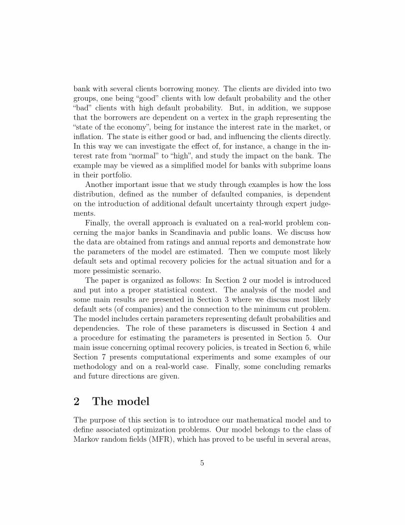
(a) The bad path scenario. This example illustrates how defaults maydevelop in a chain (path) of agents, each dependent only on its predecessor.The path consists of 10 vertices, and the graph is shown in Figure 1.

1 2 3 10β

Figure 1: The bad path scenario.

The default prior probability pv = eα1v for v = 2, . . . , 9 is drawn inde-

pendently with uniform distribution in the interval [0.4, 0.5]. Also, we let

23

p1 = 0.995 and p10 = 0.2. Finally, we let β4,5 = k whereas all other βs are2k. For low values of k, only vertex 1 defaults. When k increases (up toapprox. 3), then vertices 1 to 4 default. Finally, for larger values of k allvertices default.

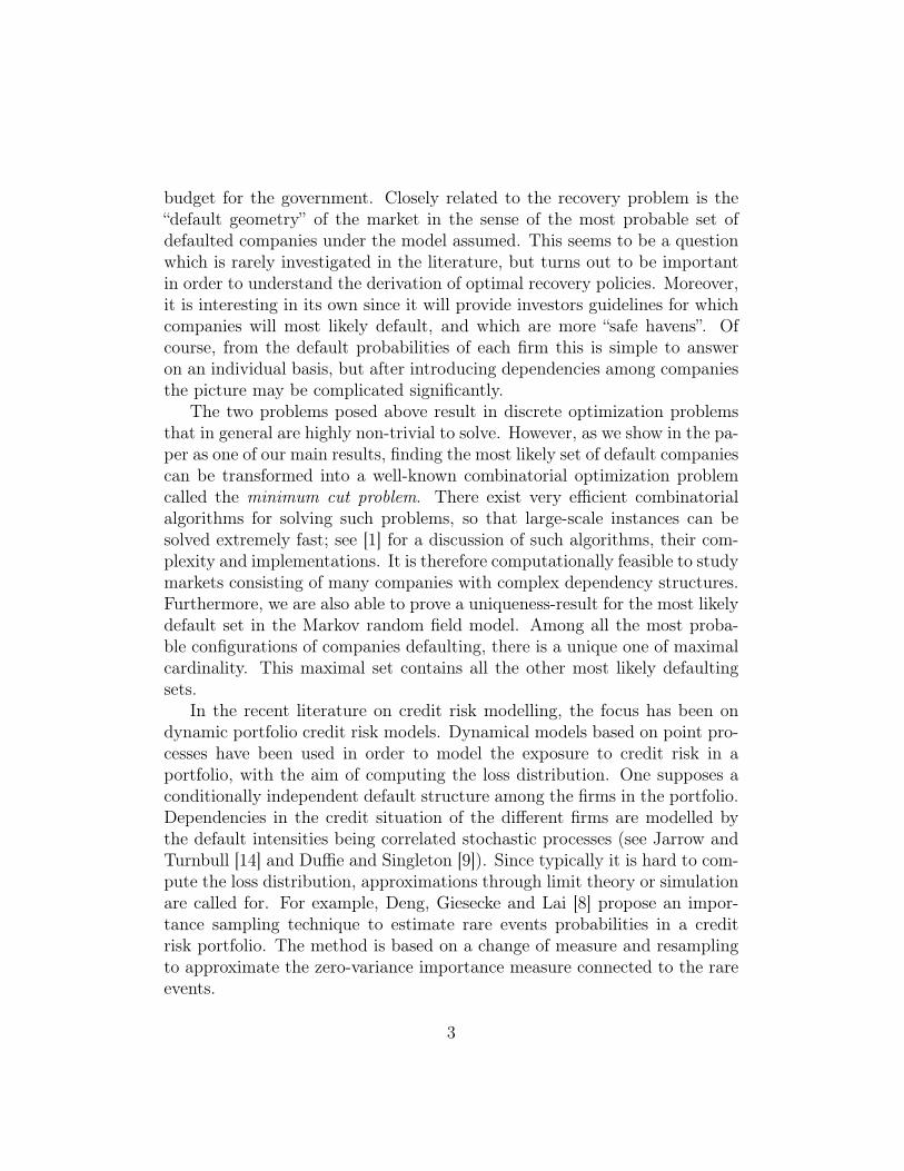
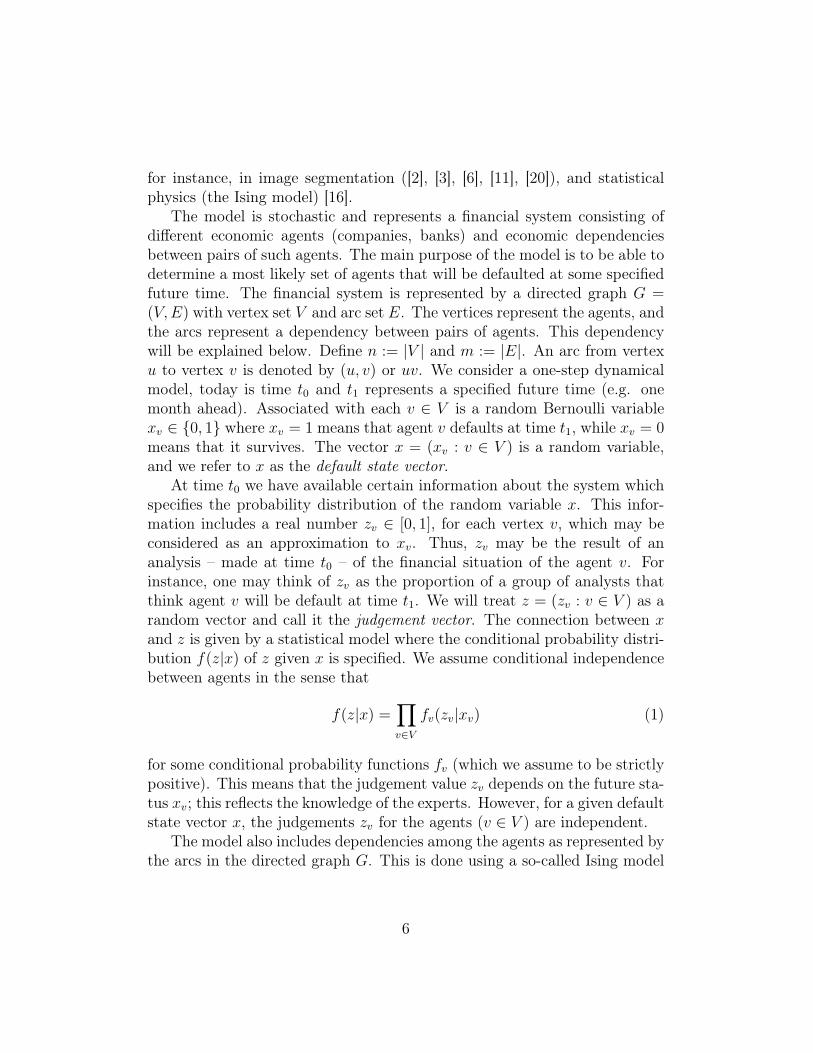
(b) The effect-vertex scenario. We consider 18 agents: 16 clients, onebank and one effect vertex (see Figure 2). Each client v obtains a loan fromthe bank; denote by βl the (constant) dependency of the bank on every client.The effect vertex represents the influence of the interest rate on the clients,which are partitioned into 6 good clients and 10 bad clients. The dependencyof the good clients on the interest rate is given by βg and is the same for allgood clients. The dependency of the bad clients on the interest rate is givenby βb and is the same for all bad clients.

e

b

lβ lβ

gβ bβ

Figure 2: The effect-vertex scenario.

The default prior probability pv = eα1v for each client v is drawn indepen-

dently with uniform distribution in the interval [0.3, 0.5] for the good clients,whereas is set equal to 0.5 for the bad ones. High interest rates are repre-sented by a high prior default probability for the effect vertex (0.995). Thebank vertex has a low prior default probability (0.2). Also we let βl = 0.25,whereas βg = 0.1.

In order to analyze the bank reaction to increasing influence of the interestrate on the bad clients, we let βb grow from 0 to a large value. Then, for low

24

values of βb, only the effect vertex is default. When βb reaches a thresholdvalue (here 0.15), then all bad clients and the bank are default, while forintermediate values only a subset of the bad clients default.

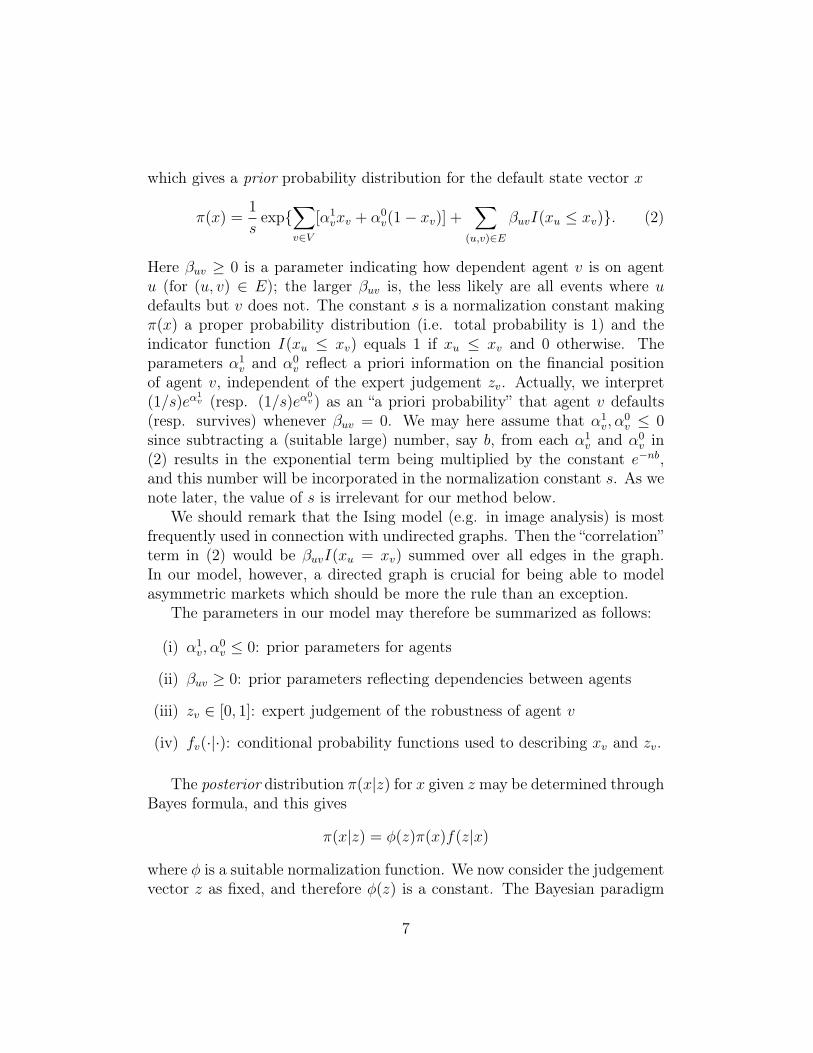
As a variation of scenario (b), we tested the parameter estimation pro-cedure described in Section 5. To this end we replace βl (which denotes theconstant dependency of the bank on the clients) with two different parame-ters, namely βlg and βlb, denoting the dependency on the good and the badclients, respectively. We consider as fixed all parameters except for βb andβlb; the parameters involving bad clients. The values for the fixed parametersare those given above. As initial values on the two unknown parameters weused βb = 0.1 and βlb = 0.25 and then the parameter estimation procedureof Section 5 was applied.

With this choice we obtained the MLE estimate βlb = 0.08 and βb = 0.The procedure converged in one step. The resulting default state vector x(the MLDS solution) has only 5 defaulting clients (all “bad” ones), and thebank is non-defaulting. (The default state vector was the same for these twoparameter vectors).

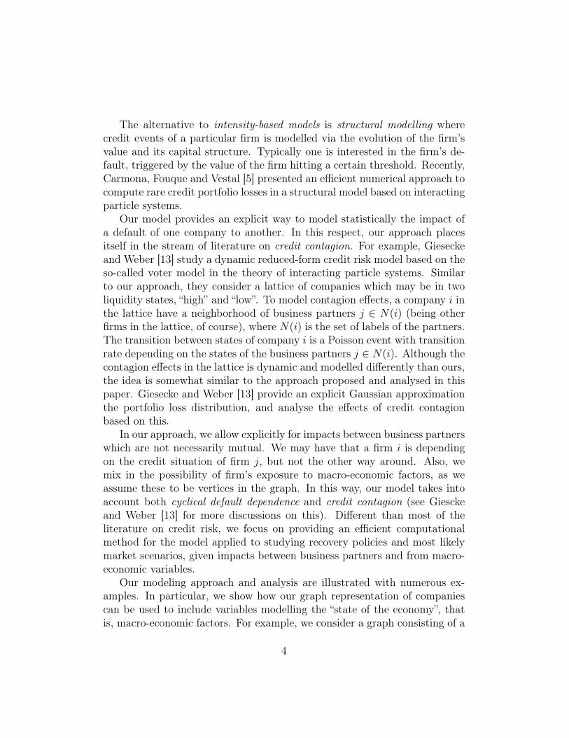
Since we have only two “variable parameters” to be determined, it ispossible to visualize the corresponding pseudo-likelihood function pθ(z, x),as a function of βb and βlb for the fixed x (just found). The values of thisfunction is shown in Figure 3 for βlb ∈ [0, 0.002] and βb ∈ [0, 0.2].

00.05

0.10.15

0.2

0

0.005

0.01

0.015

0.02−2.84

−2.838

−2.836

−2.834

−2.832

−2.83

βbβlb

Figure 3: Pseudo-likelihood

25

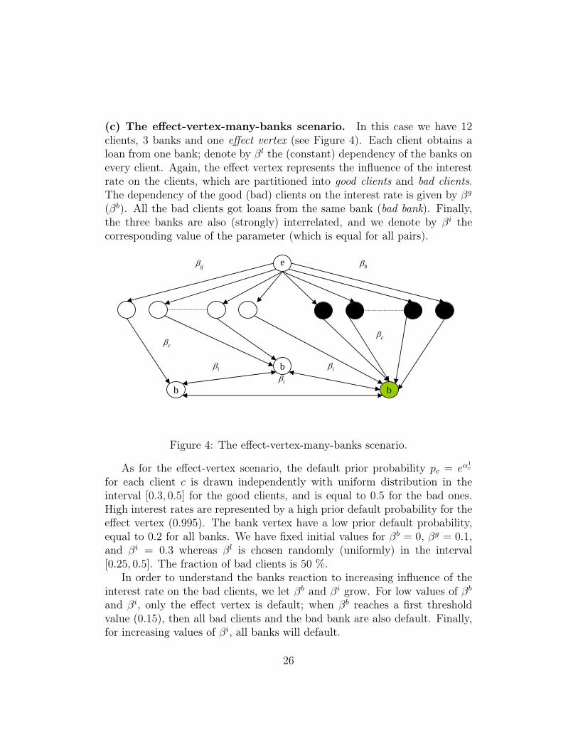
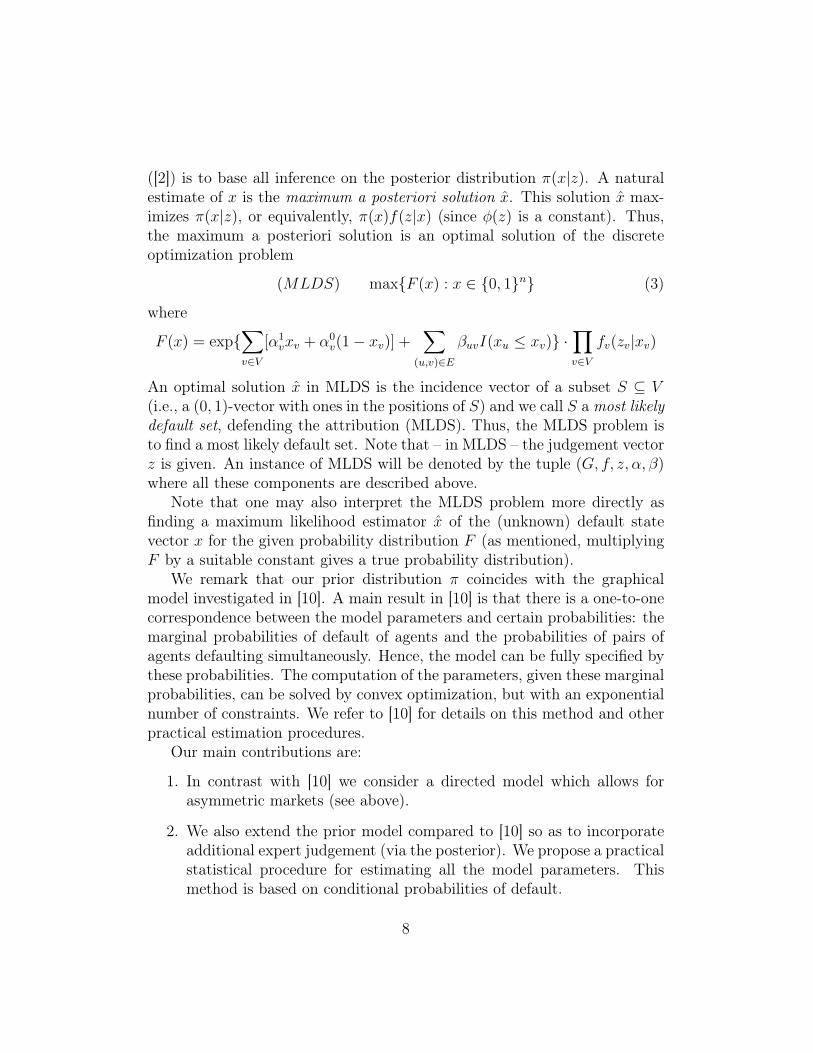
(c) The effect-vertex-many-banks scenario. In this case we have 12clients, 3 banks and one effect vertex (see Figure 4). Each client obtains aloan from one bank; denote by βl the (constant) dependency of the banks onevery client. Again, the effect vertex represents the influence of the interestrate on the clients, which are partitioned into good clients and bad clients.The dependency of the good (bad) clients on the interest rate is given by βg(βb). All the bad clients got loans from the same bank (bad bank). Finally,the three banks are also (strongly) interrelated, and we denote by βi thecorresponding value of the parameter (which is equal for all pairs).

eβg βb

b

βc

βc

b

bβi βi

βi

Figure 4: The effect-vertex-many-banks scenario.

As for the effect-vertex scenario, the default prior probability pc = eα1c

for each client c is drawn independently with uniform distribution in theinterval [0.3, 0.5] for the good clients, and is equal to 0.5 for the bad ones.High interest rates are represented by a high prior default probability for theeffect vertex (0.995). The bank vertex have a low prior default probability,equal to 0.2 for all banks. We have fixed initial values for βb = 0, βg = 0.1,and βi = 0.3 whereas βl is chosen randomly (uniformly) in the interval[0.25, 0.5]. The fraction of bad clients is 50 %.

In order to understand the banks reaction to increasing influence of theinterest rate on the bad clients, we let βb and βi grow. For low values of βband βi, only the effect vertex is default; when βb reaches a first thresholdvalue (0.15), then all bad clients and the bad bank are also default. Finally,for increasing values of βi, all banks will default.

26

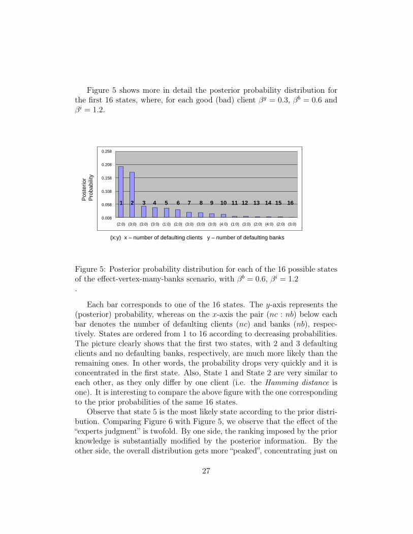
Figure 5 shows more in detail the posterior probability distribution forthe first 16 states, where, for each good (bad) client βg = 0.3, βb = 0.6 andβi = 1.2.

0.008

0.058

0.108

0.158

0.208

0.258

(2:0) (3:0) (3:0) (3:0) (1:0) (2:0) (3:0) (3:0) (3:0) (4:0) (1:0) (3:0) (2:0) (4:0) (2:0) (3:0)

1 2 3 4 5 6 7 8 9 10 11 12 13 14 15 16

Po

ste

rio

r

Pro

ba

bili

ty

(x:y) x – number of defaulting clients y – number of defaulting banks

Figure 5: Posterior probability distribution for each of the 16 possible statesof the effect-vertex-many-banks scenario, with βb = 0.6, βi = 1.2.

Each bar corresponds to one of the 16 states. The y-axis represents the(posterior) probability, whereas on the x-axis the pair (nc : nb) below eachbar denotes the number of defaulting clients (nc) and banks (nb), respec-tively. States are ordered from 1 to 16 according to decreasing probabilities.The picture clearly shows that the first two states, with 2 and 3 defaultingclients and no defaulting banks, respectively, are much more likely than theremaining ones. In other words, the probability drops very quickly and it isconcentrated in the first state. Also, State 1 and State 2 are very similar toeach other, as they only differ by one client (i.e. the Hamming distance isone). It is interesting to compare the above figure with the one correspondingto the prior probabilities of the same 16 states.

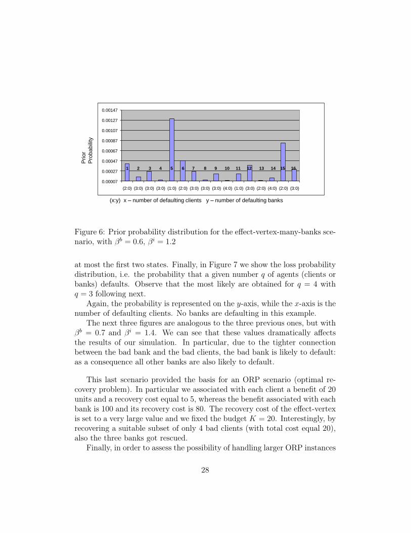
Observe that state 5 is the most likely state according to the prior distri-bution. Comparing Figure 6 with Figure 5, we observe that the effect of the“experts judgment” is twofold. By one side, the ranking imposed by the priorknowledge is substantially modified by the posterior information. By theother side, the overall distribution gets more “peaked”, concentrating just on

27

Pri

or

Pro

ba

bili

ty

(x:y) x – number of defaulting clients y – number of defaulting banks

0.00007

0.00027

0.00047

0.00067

0.00087

0.00107

0.00127

0.00147

(2:0) (3:0) (3:0) (3:0) (1:0) (2:0) (3:0) (3:0) (3:0) (4:0) (1:0) (3:0) (2:0) (4:0) (2:0) (3:0)

1 2 3 4 5 6 7 8 9 10 11 12 13 14 15 16

Figure 6: Prior probability distribution for the effect-vertex-many-banks sce-nario, with βb = 0.6, βi = 1.2

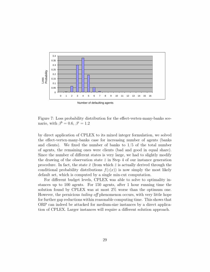
at most the first two states. Finally, in Figure 7 we show the loss probabilitydistribution, i.e. the probability that a given number q of agents (clients orbanks) defaults. Observe that the most likely are obtained for q = 4 withq = 3 following next.

Again, the probability is represented on the y-axis, while the x-axis is thenumber of defaulting clients. No banks are defaulting in this example.

The next three figures are analogous to the three previous ones, but withβb = 0.7 and βi = 1.4. We can see that these values dramatically affectsthe results of our simulation. In particular, due to the tighter connectionbetween the bad bank and the bad clients, the bad bank is likely to default:as a consequence all other banks are also likely to default.

This last scenario provided the basis for an ORP scenario (optimal re-covery problem). In particular we associated with each client a benefit of 20units and a recovery cost equal to 5, whereas the benefit associated with eachbank is 100 and its recovery cost is 80. The recovery cost of the effect-vertexis set to a very large value and we fixed the budget K = 20. Interestingly, byrecovering a suitable subset of only 4 bad clients (with total cost equal 20),also the three banks got rescued.

Finally, in order to assess the possibility of handling larger ORP instances

28

Lo

ss

Pro

ba

bili

ty

Number of defaulting agents

0

0.05

0.1

0.15

0.2

0.25

0.3

0.35

0.4

0 1 2 3 4 5 6 7 8 9 10 11 12 13 14 15 16

Figure 7: Loss probability distribution for the effect-vertex-many-banks sce-nario, with βb = 0.6, βi = 1.2

by direct application of CPLEX to its mixed integer formulation, we solvedthe effect-vertex-many-banks case for increasing number of agents (banksand clients). We fixed the number of banks to 1/5 of the total numberof agents, the remaining ones were clients (bad and good in equal share).Since the number of different states is very large, we had to slightly modifythe drawing of the observation state z in Step 4 of our instance generationprocedure. In fact, the state x (from which z is actually derived through theconditional probability distributions f(z|x)) is now simply the most likelydefault set, which is computed by a single min-cut computation.

For different budget levels, CPLEX was able to solve to optimality in-stances up to 100 agents. For 150 agents, after 1 hour running time thesolution found by CPLEX was at most 2% worse than the optimum one.However, the pernicious tailing off phenomenon occurs, with very little hopefor further gap reductions within reasonable computing time. This shows thatORP can indeed be attacked for medium-size instances by a direct applica-tion of CPLEX. Larger instances will require a different solution approach.

29

0.009

0.029

0.049

0.069

0.089

0.109

0.129

(6:3) (5:3) (7:3) (6:3) (7:3) (7:3) (5:0) (6:0) (6:3) (7:3) (6:3) (8:3) (8:3) (5:3) (5:3) (6:3)

1 2 3 4 5 6 7 8 9 10 11 12 13 14 15 16

Po

ste

rio

r

Pro

ba

bili

ty

(x:y) x – number of defaulting clients y – number of defaulting banks

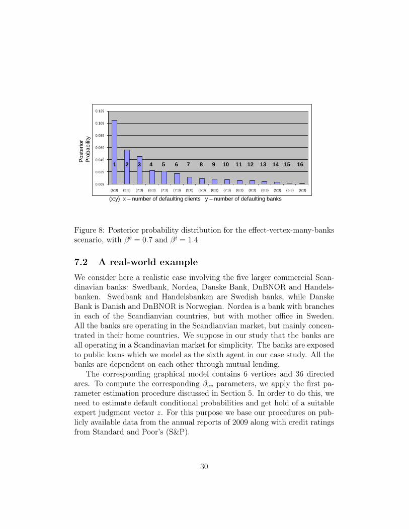
Figure 8: Posterior probability distribution for the effect-vertex-many-banksscenario, with βb = 0.7 and βi = 1.4

7.2 A real-world example

We consider here a realistic case involving the five larger commercial Scan-dinavian banks: Swedbank, Nordea, Danske Bank, DnBNOR and Handels-banken. Swedbank and Handelsbanken are Swedish banks, while DanskeBank is Danish and DnBNOR is Norwegian. Nordea is a bank with branchesin each of the Scandianvian countries, but with mother office in Sweden.All the banks are operating in the Scandianvian market, but mainly concen-trated in their home countries. We suppose in our study that the banks areall operating in a Scandinavian market for simplicity. The banks are exposedto public loans which we model as the sixth agent in our case study. All thebanks are dependent on each other through mutual lending.

The corresponding graphical model contains 6 vertices and 36 directedarcs. To compute the corresponding βuv parameters, we apply the first pa-rameter estimation procedure discussed in Section 5. In order to do this, weneed to estimate default conditional probabilities and get hold of a suitableexpert judgment vector z. For this purpose we base our procedures on pub-licly available data from the annual reports of 2009 along with credit ratingsfrom Standard and Poor’s (S&P).

30

0.00008

0.00013

0.00018

0.00023

0.00028

0.00033

0.00038

0.00043

0.00048

(6:3) (5:3) (7:3) (6:3) (7:3) (7:3) (5:0) (6:0) (6:3) (7:3) (6:3) (8:3) (8:3) (5:3) (5:3) (6:3)

1 2 3 4 5 6 7 8 9 10 11 12 13 14 15 16

Pri

or

Pro

ba

bili

ty

(x:y) x – number of defaulting clients y – number of defaulting banks

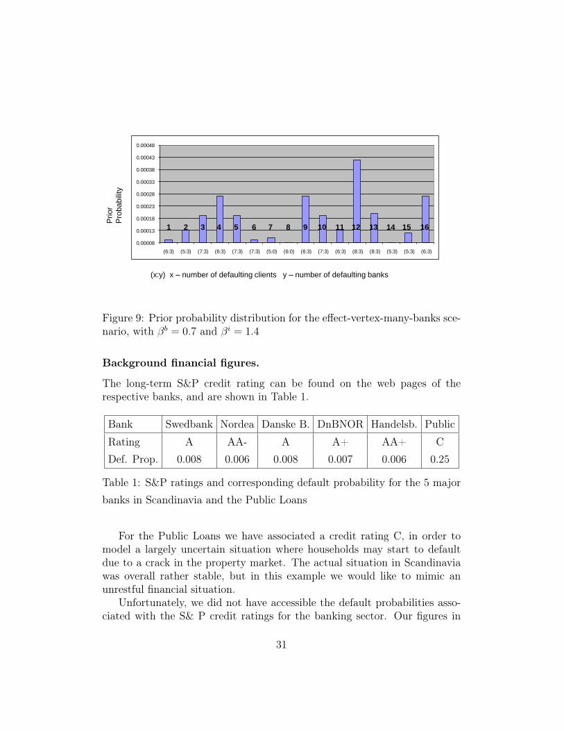
Figure 9: Prior probability distribution for the effect-vertex-many-banks sce-nario, with βb = 0.7 and βi = 1.4

Background financial figures.

The long-term S&P credit rating can be found on the web pages of therespective banks, and are shown in Table 1.

Bank Swedbank Nordea Danske B. DnBNOR Handelsb. Public

Rating A AA- A A+ AA+ CDef. Prop. 0.008 0.006 0.008 0.007 0.006 0.25

Table 1: S&P ratings and corresponding default probability for the 5 majorbanks in Scandinavia and the Public Loans

For the Public Loans we have associated a credit rating C, in order tomodel a largely uncertain situation where households may start to defaultdue to a crack in the property market. The actual situation in Scandinaviawas overall rather stable, but in this example we would like to mimic anunrestful financial situation.

Unfortunately, we did not have accessible the default probabilities asso-ciated with the S& P credit ratings for the banking sector. Our figures in

31

Lo

ss

Pro

ba

bili

ty

Number of defaulting agents

0

0.05

0.1

0.15

0.2

0.25

0.3

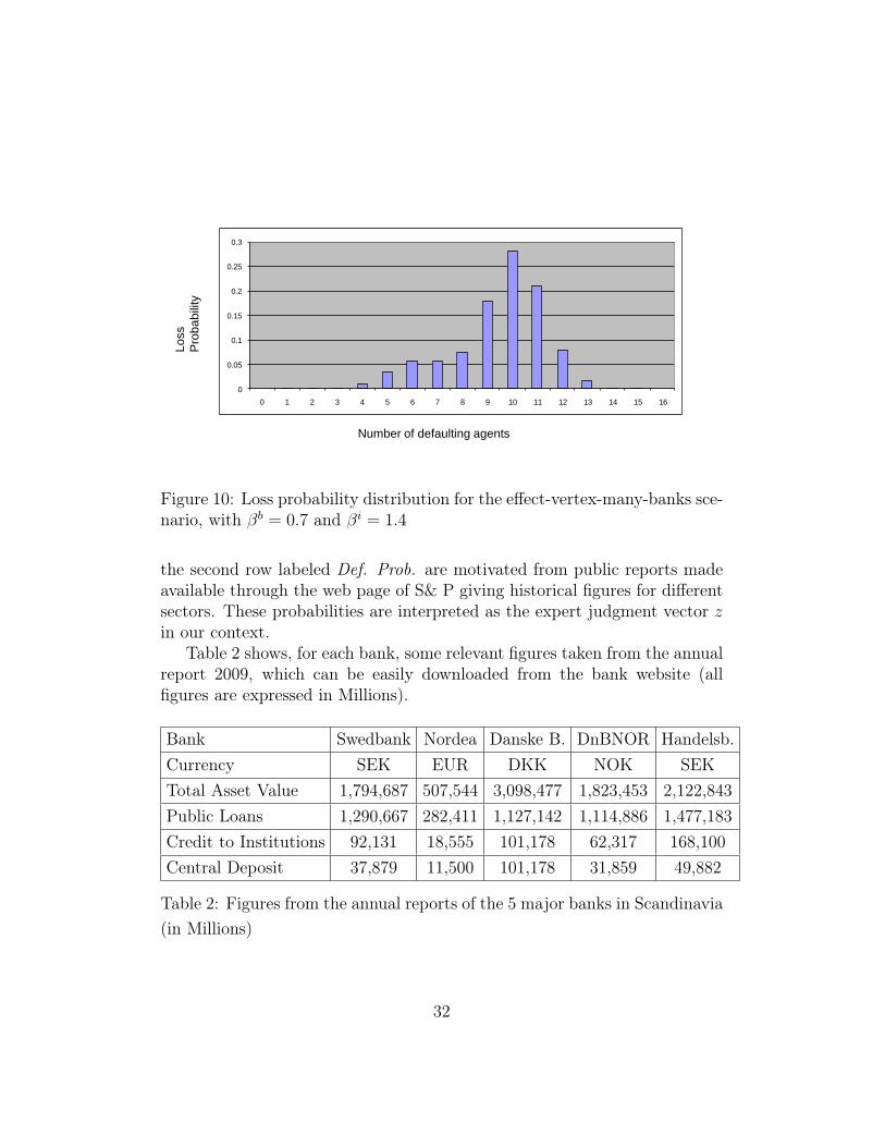
0 1 2 3 4 5 6 7 8 9 10 11 12 13 14 15 16

Figure 10: Loss probability distribution for the effect-vertex-many-banks sce-nario, with βb = 0.7 and βi = 1.4

the second row labeled Def. Prob. are motivated from public reports madeavailable through the web page of S& P giving historical figures for differentsectors. These probabilities are interpreted as the expert judgment vector zin our context.

Table 2 shows, for each bank, some relevant figures taken from the annualreport 2009, which can be easily downloaded from the bank website (allfigures are expressed in Millions).

Bank Swedbank Nordea Danske B. DnBNOR Handelsb.Currency SEK EUR DKK NOK SEKTotal Asset Value 1,794,687 507,544 3,098,477 1,823,453 2,122,843Public Loans 1,290,667 282,411 1,127,142 1,114,886 1,477,183Credit to Institutions 92,131 18,555 101,178 62,317 168,100Central Deposit 37,879 11,500 101,178 31,859 49,882

Table 2: Figures from the annual reports of the 5 major banks in Scandinavia(in Millions)

32

The Central Deposit is the amount of money the bank has deposited inthe Central Bank of their respective country. We point out that the figuresin the two last rows for Danske Bank are obtained by equally distributingthe cumulative figure given in the annual report, since they have reportedtheir credit to institutions and the central bank in one cumulative number.This is of course just chosen by us as a proxy.

Parameter estimation

The figures in Table 2 are exploited to derive suitable conditional defaultprobabilities. These are in turn used as data for determining the coefficientsof our model, according to the methodology described in Section 5.

First, for each bank B, the conditional probability for B to default givena default in Public Loans is computed as the ratio between the bank’s ex-posure in Public Loans and its total asset value. Next, we use the figuresin Credit to institutions as a proxy for the bank’s exposure to the otherbanks, and we assume a uniform distribution of this figure among the fourother banks: in other words, each bank has a fully diversified loan portfolioin the other banks. So, for instance, Swedbank’s total exposure is 92,131mill. SEK, which then under our assumptions gives an exposure of 23,032.75mill. SEK with each of the four other banks. To measure the vulnerabilityof Swedbank to the four others, we compute the ratio between its exposurewith its deposit in the central bank. For the case of Swedbank, this resultsin 23, 032.75/37, 879 ' 0.608, which we use as a proxy for the conditionalprobability of Swedbank defaulting, given that one of the other default (forexample, the default probability of Swedbank given that Handelsbanken de-faults, is 0.608). We compute these conditional default probabilities for allthe banks, and collect the figures in Table 3

Although the exposure in each of the other banks are minor compared tothe total asset holdings, we think of the lending to credit institutions as partof the liquid portfolio of the bank, which makes it highly vulnerable if biggerparts of this fall out in the sense of another bank defaulting.

The conditional probabilities of Table 3 and the "expert judgments" pro-vided by S&P and reported in Table 1 (Row Def. Prob.) are used as theinput data to our parameter estimation procedure (Section 5). Since wedo not have any a piori knowledge on the banks and the Public Loans de-fault probability, we let α0

i = α1i = 0 for i = 1, . . . , 6: this makes vectors

α0 and α1 irrelevant to determine the most likely defaulting set. Also, to

33

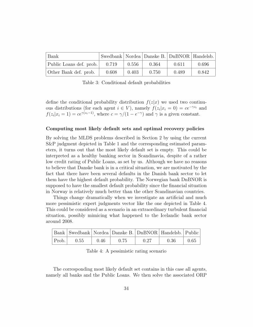
Bank Swedbank Nordea Danske B. DnBNOR Handelsb.

Public Loans def. prob. 0.719 0.556 0.364 0.611 0.696

Other Bank def. prob. 0.608 0.403 0.750 0.489 0.842

Table 3: Conditional default probabilities

define the conditional probability distribution f(z|x) we used two continu-ous distributions (for each agent i ∈ V ), namely f(zi|xi = 0) = ce−γzi andf(zi|xi = 1) = ceγ(zi−1), where c = γ/(1− e−γ) and γ is a given constant.

Computing most likely default sets and optimal recovery policies

By solving the MLDS problems described in Section 2 by using the currentS&P judgment depicted in Table 1 and the corresponding estimated param-eters, it turns out that the most likely default set is empty. This could beinterpreted as a healthy banking sector in Scandinavia, despite of a ratherlow credit rating of Public Loans, as set by us. Although we have no reasonsto believe that Danske bank is in a critical situation, we are motivated by thefact that there have been several defaults in the Danish bank sector to letthem have the highest default probability. The Norwegian bank DnBNOR issupposed to have the smallest default probability since the financial situationin Norway is relatively much better than the other Scandinavian countries.

Things change dramatically when we investigate an artificial and muchmore pessimistic expert judgments vector like the one depicted in Table 4.This could be considered as a scenario in an extraordinary turbulent financialsituation, possibly mimicing what happened to the Icelandic bank sectoraround 2008.

Bank Swedbank Nordea Danske B. DnBNOR Handelsb. Public

Prob. 0.55 0.46 0.75 0.27 0.36 0.65

Table 4: A pessimistic rating scenario

The corresponding most likely default set contains in this case all agents,namely all banks and the Public Loans. We then solve the associated ORP

34

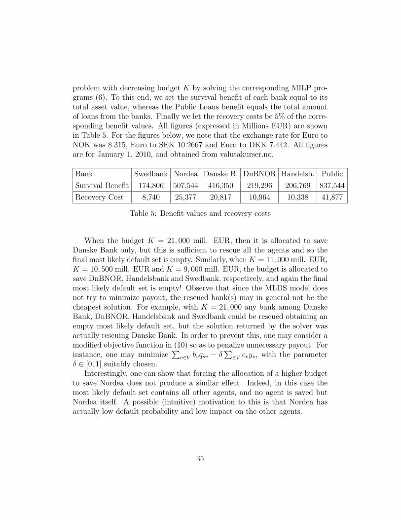
problem with decreasing budget K by solving the corresponding MILP pro-grams (6). To this end, we set the survival benefit of each bank equal to itstotal asset value, whereas the Public Loans benefit equals the total amountof loans from the banks. Finally we let the recovery costs be 5% of the corre-sponding benefit values. All figures (expressed in Millions EUR) are shownin Table 5. For the figures below, we note that the exchange rate for Euro toNOK was 8.315, Euro to SEK 10.2667 and Euro to DKK 7.442. All figuresare for January 1, 2010, and obtained from valutakurser.no.

Bank Swedbank Nordea Danske B. DnBNOR Handelsb. PublicSurvival Benefit 174,806 507,544 416,350 219,296 206,769 837,544Recovery Cost 8,740 25,377 20,817 10,964 10,338 41,877

Table 5: Benefit values and recovery costs

When the budget K = 21, 000 mill. EUR, then it is allocated to saveDanske Bank only, but this is sufficient to rescue all the agents and so thefinal most likely default set is empty. Similarly, whenK = 11, 000 mill. EUR,K = 10, 500 mill. EUR and K = 9, 000 mill. EUR, the budget is allocated tosave DnBNOR, Handelsbank and Swedbank, respectively, and again the finalmost likely default set is empty! Observe that since the MLDS model doesnot try to minimize payout, the rescued bank(s) may in general not be thecheapest solution. For example, with K = 21, 000 any bank among DanskeBank, DnBNOR, Handelsbank and Swedbank could be rescued obtaining anempty most likely default set, but the solution returned by the solver wasactually rescuing Danske Bank. In order to prevent this, one may consider amodified objective function in (10) so as to penalize unnecessary payout. Forinstance, one may minimize

∑v∈V bvqsv − δ

∑∈V cvyv, with the parameter

δ ∈ [0, 1] suitably chosen.Interestingly, one can show that forcing the allocation of a higher budget

to save Nordea does not produce a similar effect. Indeed, in this case themost likely default set contains all other agents, and no agent is saved butNordea itself. A possible (intuitive) motivation to this is that Nordea hasactually low default probability and low impact on the other agents.

35

8 Final commentsWe mention some possible directions of future work in this area.

Concerning the model it would be natural to investigate the case whennegative parameters βuv are allowed. This models decreased risk of defaultingwhen an agent defaults. Note, however, that negative βuv’s lead to computa-tional difficulties (as the MLDS problem with arbitrary weights is NP-hard).Another important extension would be a dynamic model where companiesmight default at different times and the risk of defaulting would vary withtime.

An interesting topic is a further study of the optimal recovery problemORP. We showed how to reformulate the ORP into a valid mixed integerlinear programming problem (13). We used standard methods to solve thisproblem, but one could investigate more advanced approaches where thespecific structure of the problem is exploited in order to solve larger problems.Finally, ORP is very natural to study in a dynamic extension of our model.

Acknowledgments. We appreciate several very useful comments fromthe referees, in particular for improving the analysis given in Sections 4 and7. The authors also wish to thank Anders Øksendal (DnBNOR) and GeirStorvik (University of Oslo) for very useful discussions and suggestions inconnection with Markov Random Field models.

References[1] R.K. Ahuja, T.L. Magnanti, and J.B. Orlin, Network Flows: Theory,

Algorithms, and Applications, Englewood Cliffs, New Jersey, Prentice-Hall, 1993.

[2] J. Besag, Towards Bayesian image analysis, Journal of Applied Statis-tics, 16(3) (1989), 395–407.

[3] J. Besag, On the statistical analysis of dirty pictures, Journal of RoyalStatistical Society, Series B 48(3) (1986), 259–302.

[4] J. Besag and J. Tantrum, Likelihood analysis of binary data in spaceand time, In P.J. Green, N.L. Hjort and S. Richardson (Eds.) Highly

36

Structured Stochastic Systems., Oxford Statistical Science Series, 27,Oxford University Press, Oxford, 2003. (p.289–295)

[5] R. Carmona, J.-P. Fouque and D. Vestal, Interacting particle systemsfor the computation of rare credit portfolio losses, Finance Stoch., vol.13 (2009), 613–633

[6] G. Dahl, G. Storvik and A. Fadnes, Large-scale integer programs inimage analysis, Operations Research, Vol.50 (2002), No.3, 490–500.

[7] S. Dempe, Foundation of Bilevel Programming, Kluwer Academic(2002).

[8] S. Deng, K. Giesecke and T. L. Lai, Sequential importance samplingand resampling for dynamic portfolio credit risk, Manuscript, (2010)

[9] D. Duffie and K. J. Singleton, Modeling term structures of defaultablebonds Rev. Financial Studies, Vol. 12 (1999), 687-720.

[10] I.O. Filiz, X. Guo, J. Morton, B. Sturmfels, Graphical Models for Cor-related Defaults, Technical report, Sept. 2008, arXiv:0809.1393. Toappear in Mathematical Finance.

[11] S. Geman and D. Geman, Stochastic relaxation, Gibbs distribution, andBayesian restoration of images, IEEE Trans. on Pattern Analysis andMachine Intelligence 6(6) (1984), 721–741.

[12] K. Giesecke, Credit risk modeling and valuation: an introduction, Tech-nical report, Cornell University, Oct. 2004.

[13] K. Giesecke and S. Weber, Credit contagion and aggregate losses, J.Econ. Dyn. Control, vol. 30 (2006), 741–767

[14] R. A. Jarrow and S. Turnbull, Pricing Derivatives on Financial SecuritiesSubject to Credit Risk, J. Finance, vol. 50, March (1995), 53–85

[15] M. Labbé, P. Marcotte, and G. Savard, A Bilevel Model of Taxationand Its Application to Optimal Highway Pricing, Management Science,Vol 44 (1998), No. 12, 1608–1622

[16] K.R. Mecke, D. Stoyan (Eds.) Statistical Physics and Spatial Statistics.Series: Lecture Notes in Physics, Vol. 554, Springer, 2000.

37

[17] R.C. Merton, On the pricing of corporate debt: The risk structure ofinterest rates, Journal of Finance 29 (1974), 449–470.

[18] G.L. Nemhauser and L. A. Wolsey, Integer and Combinatorial Opti-mization, Wiley, 1988.

[19] A. Schrijver, Theory of Linear and Integer Programming, Wiley, Chich-ester, 1998.

[20] G. Storvik and G. Dahl, Lagrangian based methods for finding MAPsolutions for MRF models, IEEE Transactions on Image Process-ing,Volume 9, No. 3 (2000), 469–479.

38