Computers, Obsolescence, and Productivity Karl Whelan Division of Research and Statistics Federal Reserve Board * February, 2000 Abstract What effect have computers had on U.S. productivity growth? This paper shows that increased productivity in the computer-producing sector and the effect of investment in computers on the productivity of those who use them together account for the re- cent acceleration in U.S. labor productivity. In calculating the computer-usage effect, standard NIPA measures of the computer capital stock are inappropriate because they do not account for technological obsolescence; this occurs when machines that are still productive are retired because they are no longer near the technological frontier. Us- ing a framework that accounts for technological obsolescence, alternative stocks are developed that imply larger computer-usage effects. * Mail Stop 80, 20th and C Streets NW, Washington DC 20551. Email: [email protected]. I wish to thank Eric Bartelsman, Darrel Cohen, Steve Oliner, Dan Sichel, Larry Slifman, Stacey Tevlin, and participants in seminars at the University of Maryland, the Federal Reserve Bank of St. Louis, and the 2000 AEA meetings for comments. I am particularly grateful to Steve Oliner for providing me with access to results from his computer depreciation studies. The views expressed in this paper are my own and do not necessarily reflect the views of the Board of Governors or the staff of the Federal Reserve System.

Welcome message from author
This document is posted to help you gain knowledge. Please leave a comment to let me know what you think about it! Share it to your friends and learn new things together.
Transcript
Computers, Obsolescence, and Productivity
Karl WhelanDivision of Research and Statistics
Federal Reserve Board ∗
February, 2000
Abstract
What effect have computers had on U.S. productivity growth? This paper shows that
increased productivity in the computer-producing sector and the effect of investment
in computers on the productivity of those who use them together account for the re-
cent acceleration in U.S. labor productivity. In calculating the computer-usage effect,
standard NIPA measures of the computer capital stock are inappropriate because they
do not account for technological obsolescence; this occurs when machines that are still
productive are retired because they are no longer near the technological frontier. Us-
ing a framework that accounts for technological obsolescence, alternative stocks are
developed that imply larger computer-usage effects.
∗Mail Stop 80, 20th and C Streets NW, Washington DC 20551. Email: [email protected]. I wish to thank
Eric Bartelsman, Darrel Cohen, Steve Oliner, Dan Sichel, Larry Slifman, Stacey Tevlin, and participants in
seminars at the University of Maryland, the Federal Reserve Bank of St. Louis, and the 2000 AEA meetings
for comments. I am particularly grateful to Steve Oliner for providing me with access to results from his
computer depreciation studies. The views expressed in this paper are my own and do not necessarily reflect
the views of the Board of Governors or the staff of the Federal Reserve System.
1 Introduction
Recent years have seen an explosion in the application of computing technologies by U.S.
businesses. Real business expenditures on computing equipment grew an average of 44
percent per year over 1992-98 as plunging computer prices allowed firms to take advantage of
ever more powerful hardware and, consequently, the ability to use increasingly sophisticated
software. These developments have helped improve the efficiency of many core business
functions such as quality control, communications, and inventory management, and, in the
case of the Internet, have facilitated new ways of doing business. They have also coincided
with an improved productivity performance for the U.S. economy: Private business output
per hour grew 2.2 percent per year over the period 1996-98, a rate of advance not seen
late into an expansion since the 1960s.1 This confluence of events raises some fascinating
questions. Are we finally seeing a resolution to the now-famous Solow Paradox that the
influence of computers is seen everywhere except in the productivity statistics? And if so,
is the recent pace of productivity growth likely to continue?
This paper addresses these questions by focusing on two separate computer-related
effects on aggregate productivity. First, there has been an enormous productivity increase
in the computer-producing sector, a development that on its own contributes to increased
aggregate productivity. Second, the resulting declines in computer prices have induced a
huge increase in the stock of computing capital. I show that this deepening of the computer
capital stock - the computer-using effect - combined with the direct effect of increased
productivity in the computer-producing sector together account for the improvement in
productivity growth over the period 1996-98 relative to the previous 20 years.
Most of the paper is devoted to analyzing and estimating the computer-using effect,
because it is here that the paper uses a new methodology. This effect has been the subject
of a number of previous studies, most notably the work of Steve Oliner and Dan Sichel
(1994), updated in Sichel (1997).2 Using a growth accounting framework, these studies
concluded that computer capital accumulation had only a small effect on aggregate pro-
ductivity because computers were a relatively small part of aggregate capital input: In this
1All figures in this paper refer to 1992-based National Income statistics, and not the 1996-based figures
published in October 1999. The paper relies extensively on NIPA capital stock data, and capital stocks
consistent with the revised NIPA figures will not be published until at least Spring 2000.2Other studies include Kevin Stiroh (1998) and Dale Jorgenson and Kevin Stiroh (1999).
1
sense, computers were not “everywhere”. This paper comes to a different conclusion, in part
because computer capital stocks, however measured, have become a more important part
of capital input in recent years, and in part because I use new estimates of the computer
capital stock that are larger than the conventionally used measures.
The new computer capital stocks used in this paper are motivated by the following
observation. The National Income and Product Accounts (NIPA) capital stock data used
in most growth accounting exercises are measures of the replacement value of the capital
stock and are thus measures of wealth: They weight past real investments according to a
schedule for economic depreciation, which describes how a unit of capital loses value as it
ages. However, in general, these wealth stocks will not equal the “productive” stock that
features in the production function: Productive stocks need to weight up past real invest-
ment according to a schedule for physical decay, which describes a unit’s loss in productive
capability as it ages. In this paper, I document the NIPA procedures for constructing com-
puter capital stocks, use the vintage capital model of Solow (1959) to derive the conditions
under which these wealth stocks equal their productive counterparts, and then show that
the evidence on computer depreciation is inconsistent with these conditions. An alterna-
tive vintage capital model is presented that explains the evidence on computer depreciation
by allowing for technological obsolescence: This occurs when computers are retired while
they still retain productive capacity. Alternative productive stocks are presented that are
consistent with this model and that are significantly larger than their NIPA counterparts.
The paper relates to a number of existing areas of research. First, in calculating both
computer-producing and computer-using effects, it updates the approach of Stiroh (1998).
Second, the focus on the retirement of capital goods as an endogenous decision and the
argument that explicit modelling of this decision can improve our understanding of the
evolution of productivity, echoes the conclusions of Feldstein and Rothschild (1974), and
also the contribution of Goolsbee (1998). Finally, the paper sheds new light on the recent
productivity performance of the U.S. economy, a topic also explored by Gordon (1999).
The contents are as follows. Sections 2 to 6 develop the new estimates of the contribution
of computer capital accumulation to output growth, defining wealth and productive capital
stocks, documenting the NIPA procedures for constructing computer stocks, and using a
new theoretical approach to develop alternative estimates. Section 7 calculates the direct
effect of increased productivity in the computer-producing sector and discusses the recent
productivity performance of the U.S. economy. Section 8 concludes.
2

2 Wealth and Productive Capital Stocks
We will start with some definitions.
Definition (Wealth Stock): The Nominal Wealth Stock for a type of capital is the total
current dollar cost of replacing all existing units of this type. The Real Wealth Stock is
the replacement value of all existing units expressed in terms of some base-year’s prices.
Economic Depreciation is the decline in the replacement value of a unit of capital (relative
to the price of new capital) that occurs as the unit ages.
Definition (Productive Stock): Assume there is a production function
Q(t) = F (Kp1 (t),Kp
2 (t), ....,Kpn(t),X1(t), ....,Xm(t))
describing real output as a function of capital and other inputs, such that
Kpj (t) =
∞∑τ=0
Ij (t− τ)λ (τ)
where Ij(t) is the number of units of capital of type j. Then Kpj (t) is defined as the Real
Productive Stock. The Nominal Productive Stock equals Pj (t)Kpj (t) where Pj (t) is the
current value of the price index for capital of type j. Physical Decay refers to the pattern
by which a unit of capital becomes less capable of producing output as it ages, as determined
by the sequence λ (τ).
In theory, nominal wealth stocks could be estimated by obtaining the current replace-
ment values for all units of capital, new and old, and adding them up. In practice, of course,
it is impossible to obtain all this information. Instead, these stocks have been constructed
from cross-sectional studies of economic depreciation based on used-asset prices, the most
important being those of Charles Hulten and Frank Wykoff (1981). These studies provide a
schedule for economic depreciation, δje (τ), which describes the value of a piece of capital of
type j and of age τ relative to a piece of type-j capital of age zero (δje (0) = 1,(δje)′
(τ) ≤ 0).
Using this schedule, the real wealth stock is defined as:
Kwj (t) =
∞∑τ=0
Ij (t− τ) (1− δe (τ))
The nominal wealth stock is then constructed as Pj (t)Kwj (t).
Examples of wealth stocks include the capital stock series of the U.S. National Income
and Product Accounts (NIPA), which are formally known as the “Fixed Reproducible
3

Tangible Wealth” data. These series, largely based on geometric depreciation rates from
the Hulten-Wykoff studies, are used to provide estimates of the current-dollar loss in the
value of the capital stock associated with production, the NIPA variable “Consumption of
Fixed Capital” that is subtracted from GDP to arrive at Net Domestic Product.3
Consider now the relationship between wealth and productive capital stocks. For the
moment, we will restrict discussion to the case where there is no embodied technological
change. Suppose that capital of type i physically decays at a geometric rate δi. Let piv(t) be
the price at time t of a unit of type-i capital produced in period v and assume there is an
efficient rental market for new and used capital goods, so that a new unit of type-i capital
is available for rent at rate ri(t) where this equals its marginal productivity. No-arbitrage
in the capital rental market requires that the present value of the stream of rental payments
for a capital good should equal the purchase price of the good. Given a discount rate r,
this implies
pit−v(t) =
∫ ∞t
ri(s)e−δi(t−v)e−(r+δi)(s−t)ds = e−δi(t−v)pit(t)
Under these circumstances, then, the rate of economic depreciation equals the rate of phys-
ical decay and thus the real wealth stock equals the real productive stock.
It is well known, however, that this identity rests upon the assumption of geometric
decay. For example, consider a one-time investment in an asset with a one-hoss-shay pattern
of physical decay, whereby the asset produces a fixed amount for n periods and then expires
(think of a light-bulb). In this case, the productive stock follows a one-zero path while the
wealth stock gradually declines as the asset approaches expiration.4 Nevertheless, despite
such counter-examples, the underlying pattern of economic depreciation has usually been
found to be close enough to geometric for real wealth stocks to be considered good proxies
for productive stocks; moreover, even those productivity studies that have constructed
productive stocks from non-geometric patterns of physical decay have based these stocks
on estimates of economic depreciation.5
3See Katz and Herman (1997) for a description of the NIPA capital stocks.4See Jorgenson (1973) for the general theory on the relationship between wealth and productive concepts
of the capital stock. Hulten and Wykoff (1996) and Triplett (1996) are two recent papers that articulately
explain the distinctions between physical decay and economic depreciation.5For example, the Bureau of Labor Statistics (BLS) publishes an annual Multifactor Productivity calcu-
lation using productive stocks constructed according to a non-geometric “beta-decay” schedule that falls off
to zero according to a specified service life. However, BLS uses the economic depreciation rates underlying
the NIPA wealth stocks to set their service life assumptions, and in practice the BLS and NIPA stocks are
4
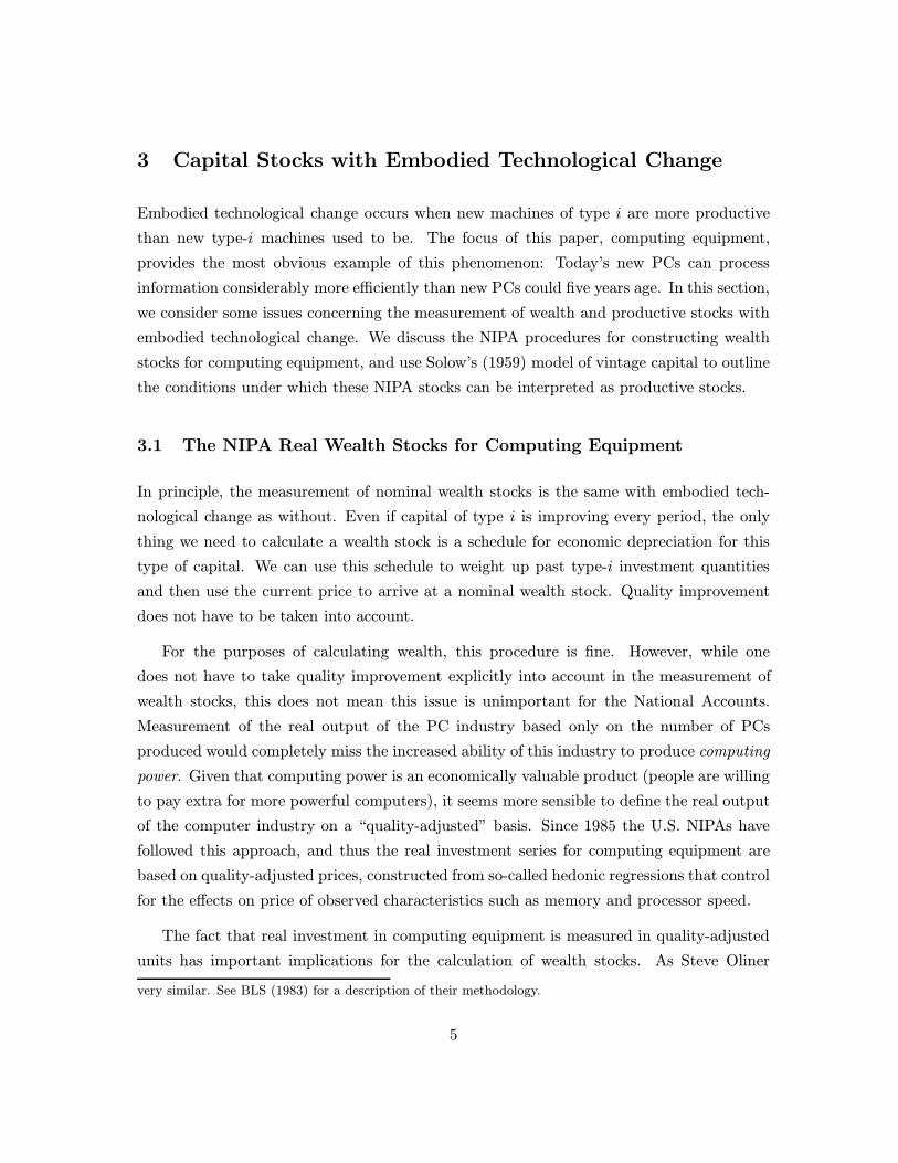
3 Capital Stocks with Embodied Technological Change
Embodied technological change occurs when new machines of type i are more productive
than new type-i machines used to be. The focus of this paper, computing equipment,
provides the most obvious example of this phenomenon: Today’s new PCs can process
information considerably more efficiently than new PCs could five years age. In this section,
we consider some issues concerning the measurement of wealth and productive stocks with
embodied technological change. We discuss the NIPA procedures for constructing wealth
stocks for computing equipment, and use Solow’s (1959) model of vintage capital to outline
the conditions under which these NIPA stocks can be interpreted as productive stocks.
3.1 The NIPA Real Wealth Stocks for Computing Equipment
In principle, the measurement of nominal wealth stocks is the same with embodied tech-
nological change as without. Even if capital of type i is improving every period, the only
thing we need to calculate a wealth stock is a schedule for economic depreciation for this
type of capital. We can use this schedule to weight up past type-i investment quantities
and then use the current price to arrive at a nominal wealth stock. Quality improvement
does not have to be taken into account.
For the purposes of calculating wealth, this procedure is fine. However, while one
does not have to take quality improvement explicitly into account in the measurement of
wealth stocks, this does not mean this issue is unimportant for the National Accounts.
Measurement of the real output of the PC industry based only on the number of PCs
produced would completely miss the increased ability of this industry to produce computing
power. Given that computing power is an economically valuable product (people are willing
to pay extra for more powerful computers), it seems more sensible to define the real output
of the computer industry on a “quality-adjusted” basis. Since 1985 the U.S. NIPAs have
followed this approach, and thus the real investment series for computing equipment are
based on quality-adjusted prices, constructed from so-called hedonic regressions that control
for the effects on price of observed characteristics such as memory and processor speed.
The fact that real investment in computing equipment is measured in quality-adjusted
units has important implications for the calculation of wealth stocks. As Steve Oliner
very similar. See BLS (1983) for a description of their methodology.
5
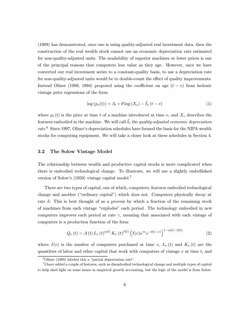
(1989) has demonstrated, once one is using quality-adjusted real investment data, then the
construction of the real wealth stock cannot use an economic depreciation rate estimated
for non-quality-adjusted units. The availability of superior machines at lower prices is one
of the principal reasons that computers lose value as they age. However, once we have
converted our real investment series to a constant-quality basis, to use a depreciation rate
for non-quality-adjusted units would be to double-count the effect of quality improvements.
Instead Oliner (1989, 1994) proposed using the coefficient on age (t − v) from hedonic
vintage price regressions of the form
log (pv(t)) = βt + θ log (Xv)− δe (t− v) (1)
where pv(t) is the price at time t of a machine introduced at time v, and Xv describes the
features embodied in the machine. We will call δe the quality-adjusted economic depreciation
rate.6 Since 1997, Oliner’s depreciation schedules have formed the basis for the NIPA wealth
stocks for computing equipment. We will take a closer look at these schedules in Section 4.
3.2 The Solow Vintage Model
The relationship between wealth and productive capital stocks is more complicated when
there is embodied technological change. To illustrate, we will use a slightly embellished
version of Solow’s (1959) vintage capital model.7
There are two types of capital, one of which, computers, features embodied technological
change and another (“ordinary capital”) which does not. Computers physically decay at
rate δ: This is best thought of as a process by which a fraction of the remaining stock
of machines from each vintage “explodes” each period. The technology embodied in new
computers improves each period at rate γ, meaning that associated with each vintage of
computers is a production function of the form
Qv (t) = A (t)Lv (t)α(t)Kv (t)β(t)(I(v)eγve−δ(t−v)
)1−α(t)−β(t)(2)
where I(v) is the number of computers purchased at time v, Lv (t) and Kv (t) are the
quantities of labor and other capital that work with computers of vintage v at time t, and
6Oliner (1989) labeled this a “partial depreciation rate”.7I have added a couple of features, such as disembodied technological change and multiple types of capital
to help shed light on some issues in empirical growth accounting, but the logic of the model is from Solow.
6

A (t) is disembodied technological change. Technology is of the putty-putty form, implying
flexible factor proportions. The price of output and ordinary capital are assumed to be
constant and equal to one. The price of computers (without adjusting for the value of
embodied features) changes at rate g (< γ). Finally, labor and capital are obtained from
spot markets with the wage rate being w (t), a unit of ordinary capital renting at a price
of ro (t), and a unit of computer capital of vintage v renting at rate rv (t).
The flow of profits obtained from operating computers of vintage v is
πv (t) = A (t)Lv (t)α(t)Kv (t)β(t)(I(v)eγve−δ(t−v)
)1−α(t)−β(t)
−rv (t) I(v)e−δ(t−v) − ro (t)Kv (t)− w (t)Lv (t) (3)
Firms choose how much labor and ordinary capital should work with vintage v so as to
maximize the profits generated by the vintage. Re-arranging first-order conditions, the
allocation of labor and ordinary capital to vintage v at time t is
Lv (t) =(I(v)eγve−δ(t−v)
)A (t)
11−α(t)−β(t)
(α (t)
w (t)
) 1−β(t)1−α(t)−β(t)
(β (t)
ro (t)
) β(t)1−α(t)−β(t)
(4)
Kv (t) =(I(v)eγve−δ(t−v)
)A (t)
11−α(t)−β(t)
(α (t)
w (t)
) α(t)1−α(t)−β(t)
(β (t)
ro (t)
) 1−α(t)1−α(t)−β(t)
(5)
So output from vintage v is
Qv (t) =(I(v)eγve−δ(t−v)
)A (t)
11−α(t)−β(t)
(α (t)
w (t)
) α(t)1−α(t)−β(t)
(β (t)
ro (t)
) β(t)1−α(t)−β(t)
(6)
Given this allocation of factors to each vintage, consider the determination of rental
rates and prices for computer capital. No-arbitrage in the rental market implies
rv(t) =∂Qv (t)
∂(I(v)e−δ(t−v)
)and that the price of a new unit of computer capital is
pv(v) =
∫ ∞v
rv(s)e−(r+δ)(s−v)ds
Differentiating this expression with respect to v we get
pv(v) = (r + δ)pv(v) +
∫ ∞v
e−(r+δ)(s−v) drv(s)
dvds− rv(v)
7
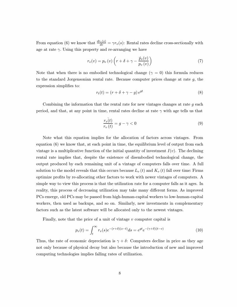
From equation (6) we know that drv(s)dv = γrv(s): Rental rates decline cross-sectionally with
age at rate γ. Using this property and re-arranging we have
rv(v) = pv (v)
(r + δ + γ −
pv(v)
pv (v)
)(7)
Note that when there is no embodied technological change (γ = 0) this formula reduces
to the standard Jorgensonian rental rate. Because computer prices change at rate g, the
expression simplifies to:
rt(t) = (r + δ + γ − g) egt (8)
Combining the information that the rental rate for new vintages changes at rate g each
period, and that, at any point in time, rental rates decline at rate γ with age tells us that
˙rv(t)
rv (t)= g − γ < 0 (9)
Note what this equation implies for the allocation of factors across vintages. From
equation (6) we know that, at each point in time, the equilibrium level of output from each
vintage is a multiplicative function of the initial quantity of investment I(v). The declining
rental rate implies that, despite the existence of disembodied technological change, the
output produced by each remaining unit of a vintage of computers falls over time. A full
solution to the model reveals that this occurs because Lv (t) and Kv (t) fall over time: Firms
optimize profits by re-allocating other factors to work with newer vintages of computers. A
simple way to view this process is that the utilization rate for a computer falls as it ages. In
reality, this process of decreasing utilization may take many different forms. As improved
PCs emerge, old PCs may be passed from high-human-capital workers to low-human-capital
workers, then used as backups, and so on. Similarly, new investments in complementary
factors such as the latest software will be allocated only to the newest vintages.
Finally, note that the price of a unit of vintage v computer capital is
pv(t) =
∫ ∞t
rv(s)e−(r+δ)(s−t)ds = egte−(γ+δ)(t−v) (10)
Thus, the rate of economic depreciation is γ + δ: Computers decline in price as they age
not only because of physical decay but also because the introduction of new and improved
computing technologies implies falling rates of utilization.
8

3.3 Wealth and Productive Stocks in the Solow Vintage Model
Consider now the calculation of aggregate capital stocks for computing equipment under
the conditions of the Solow vintage model.
Wealth Stocks
As described earlier, there are two ways to calculate wealth stocks when there is quality-
change. The first calculates a real wealth stock in terms of non-quality-adjusted units.
These units decline in value at rate γ + δ, implying an aggregate real wealth stock of
Kw (t) =
∫ t
−∞I(v)e−(γ+δ)(t−v)dv
This can be converted to a nominal wealth stock by multiplying by the non-quality-adjusted
price of computing equipment, pt(t) (which equals egt).
In contrast, the second method, implemented in the construction of the NIPA computer
stocks, uses quality-adjusted prices, quantities, and depreciation rates. By inserting the
quality variable Xv (such that θ log (Xv) = γv) into the vintage asset price equation, we
change the equation from
log (pv(t)) = gt− (γ + δ) (t− v)
to
log (pv(t)) = (g − γ) t− θ log (Xv)− δ (t− v)
Thus, adjusting for embodied features, the price index for new computers changes at rate
g − γ and, importantly, the quality-adjusted depreciation rate equals the rate of physical
decay. The quality-adjusted real wealth stock is
Kw (t) =
∫ t
−∞I(v)eγve−δ(t−v)dv = eγtKw (t)
As might have been expected, this real wealth stock grows γ percent faster than the non-
quality-adjusted version. Note though, that the nominal wealth stock obtained from mul-
tiplying Kw (t) by the quality-adjusted price index is the same as that obtained from the
using the non-quality-adjusted data.
9
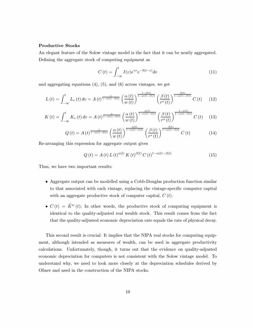
Productive Stocks
An elegant feature of the Solow vintage model is the fact that it can be neatly aggregated.
Defining the aggregate stock of computing equipment as
C (t) =
∫ t
−∞I(v)eγve−δ(t−v)dv (11)
and aggregating equations (4), (5), and (6) across vintages, we get
L (t) =
∫ t
−∞Lv (t) dv = A (t)
11−α(t)−β(t)
(α (t)
w (t)
) 1−β(t)1−α(t)−β(t)
(β (t)
ro (t)
) β(t)1−α(t)−β(t)
C (t) (12)
K (t) =
∫ t
−∞Kv (t) dv = A (t)
11−α(t)−β(t)
(α (t)
w (t)
) α(t)1−α(t)−β(t)
(β (t)
ro (t)
) 1−α(t)1−α(t)−β(t)
C (t) (13)
Q (t) = A (t)1
1−α(t)−β(t)
(α (t)
w (t)
) α(t)1−α(t)−β(t)
(β (t)
ro (t)
) β(t)1−α(t)−β(t)
C (t) (14)
Re-arranging this expression for aggregate output gives
Q (t) = A (t)L (t)α(t) K (t)β(t) C (t)1−α(t)−β(t) (15)
Thus, we have two important results:
• Aggregate output can be modelled using a Cobb-Douglas production function similar
to that associated with each vintage, replacing the vintage-specific computer capital
with an aggregate productive stock of computer capital, C (t).
• C (t) = Kw (t); In other words, the productive stock of computing equipment is
identical to the quality-adjusted real wealth stock. This result comes from the fact
that the quality-adjusted economic depreciation rate equals the rate of physical decay.
This second result is crucial: It implies that the NIPA real stocks for computing equip-
ment, although intended as measures of wealth, can be used in aggregate productivity
calculations. Unfortunately, though, it turns out that the evidence on quality-adjusted
economic depreciation for computers is not consistent with the Solow vintage model. To
understand why, we need to look more closely at the depreciation schedules derived by
Oliner and used in the construction of the NIPA stocks.
10

4 Evidence on Computer Depreciation
Oliner (1989, 1994) studied depreciation patterns for four categories of computing equip-
ment: Mainframes, storage devices, printers, and terminals. Figure 1 shows the quality-
adjusted depreciation schedules from these studies that the Commerce Department’s Bu-
reau of Economic Analysis (BEA) has used to construct the NIPA wealth stocks. Figure 2
shows the (negative of) the corresponding depreciation rates. Oliner found evidence that
quality-adjusted economic depreciation rates had increased over time and so BEA applies
different schedules to investment data from different vintages.8
If the Solow vintage capital model is correct, then these quality-adjusted economic
depreciation schedules should correspond to the schedules for physical decay. However,
these estimates do not seem to be measuring physical decay for computers. I will note
three facts that seem inconsistent with a physical decay interpretation, in ascending order
of importance. First, with the exception of printers, the schedules show a marked non-
geometric pattern, with depreciation rates increasing as the machines age. This contrasts
with the results for other assets, for which geometric depreciation has proved a useful
approximation. Second, the downward shifts over time in these schedules seem inconsistent
with a physical decay interpretation since one would expect that, if anything, computing
equipment has probably become more reliable over time, not less.
Third, and most serious, these numbers simply appear to be too high to be physical
decay rates. Table 1 shows the 1997 NIPA depreciation rates for all categories of equipment.
Remarkably, the quality-adjusted depreciation rates based on Oliner’s studies are higher
than the depreciation rates for all other categories of equipment except cars. This is all
the more notable when one considers that for all other types of equipment, the NIPA
depreciation rates are not based on a quality-adjustment approach and hence they combine
the effects of both physical decay and embodied technological change. Casual observation
suggests it is very unlikely that physical decay rates for computers are so much higher than
for other types of equipment. Adding to the puzzle is the fact that Oliner’s studies focused
on IBM equipment, which, at the time, was automatically sold with pre-packaged service
maintenance contracts: IBM guaranteed to repair or replace any damage due to equipment
due to wear and tear. Thus, for the equipment in these studies, the estimated physical
decay rates should have been zero since IBM absorbed the cost of physical decay. Oliner’s
8These depreciation schedules can be found in Department of Commerce (1999).
11
(1994) study of computer peripherals also argues that these figures do not measure physical
decay and in addition to the wealth stocks, presents productive stocks based on an assumed
physical decay rate of zero.
Together, these arguments strongly suggest that the data have not been generated by
the Solow vintage model. Next, we will present a simple extension to this model that
will explain all three of the patterns noted here about the quality-adjusted depreciation
schedules: The non-geometric shape, the downward shifts over time, and the fact that
quality-adjusted economic depreciation rates that are larger than the rates of physical
decay.
First, though, we need to point out an anomaly on Table 1, which is the NIPA depre-
ciation rate for Personal Computers (PCs). Oliner’s studies did not include PCs. In the
absence of evidence for this category, and thus evidence that PCs are depreciating faster
over time, BEA chose to use a schedule for mainframes estimated by Oliner (1989) that
did not allow the pace of depreciation to vary over time. Since the schedules for each of
the other categories of computing equipment have shifted down over time, this left PCs
as the slowest depreciating category. BEA has acknowledged that this is anomalous and
intends to introduce new capital stock estimates for PCs reflecting depreciation rates closer
to those used for the other computing categories.9
5 Computing Support Costs and Endogenous Retirement
The following extension of the Solow vintage model is motivated by two observations. The
first is that the basic model is inconsistent with technological obsolescence as defined in
the introduction. It predicts that firms will never choose to retire a machine that retains
productive capacity. Rather, it suggests the optimal strategy is simply to let the flow of
income from a computer gradually erode over time. The second observation is that computer
systems are usually complex in nature and can only be used successfully in conjunction
with technical support and maintenance. The explosion in demand in recent years for
Information Technology (IT) positions such as PC network managers is a clear indication
of the need to back up computer hardware investments with outlays on maintenance and
support. Indeed, research by the Gartner Group (1999), a private consulting firm, shows
9See Moulton and Seskin (1999), page 12.
12

that, as of 1998, for every dollar firms spent on computer hardware there was another 2.3
dollars spent on wages for IT employees and consultants. The model presented here uses
the existence of support costs to motivate the phenomenon of technological obsolescence:
Once the marginal productivity of a machine falls below the support cost, the firm will
choose to retire it.
5.1 Theory
I will use a very simple formulation of support costs: For each remaining computer from
vintage v, firms need to incur a support cost each period equal to a fraction s of the original
purchase price, pv (v). Thus, if the firm purchased the machine for $1000 and s = 0.15,
then the firm has to pay $150 per year to support it. The firm’s profit function can now be
expressed as
πv (t) = A (t)Lv (t)α(t)Kv (t)β(t)(I(v)eγve−δ(t−v)
)1−α(t)−β(t)
−rv (t) I(v)e−δ(t−v) − ro (t)Kv (t)− w (t)Lv (t)− spv (v) I(v)e−δ(t−v) (16)
How does the introduction of the support cost affect the model? First, note what has
not changed. The additive support cost has no direct effect on the marginal productivity
of the other factors that work with a vintage of computer capital. Thus, the first-order
conditions for the allocation of labor and ordinary capital across vintages are unchanged,
apart from one important new wrinkle. As before, declining utilization implies that the
marginal productivity of a unit of computer capital falls over time at rate γ − g. Now,
though, instead of allowing the marginal productivity to gradually erode towards zero,
once a computer reaches the age, T , where it cannot cover its support cost, it is considered
obsolete and is scrapped. The expression for the aggregate computer capital stock is changed
to
C (t) =
∫ t
t−TI(v)eγve−δ(t−v)dv (17)
and, given this new expression, aggregate output can still be described by the aggregate
Cobb-Douglas production function in equation (15).
Figure 3 helps to tease out the implications of this pattern for economic depreciation.
It shows the paths over time for the marginal productivity of a vintage of capital for a fixed
set of values of r, δ, and γ − g and for two values of the support cost parameter: s = 0,
13
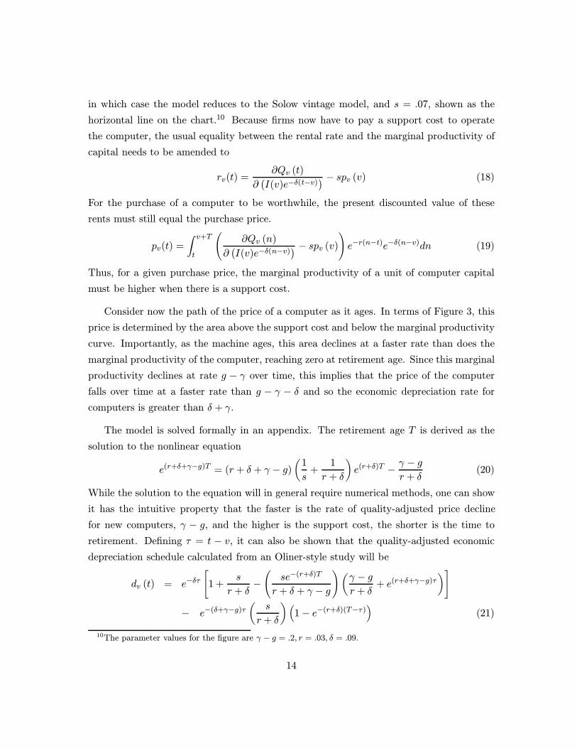
in which case the model reduces to the Solow vintage model, and s = .07, shown as the
horizontal line on the chart.10 Because firms now have to pay a support cost to operate
the computer, the usual equality between the rental rate and the marginal productivity of
capital needs to be amended to
rv(t) =∂Qv (t)
∂(I(v)e−δ(t−v)
) − spv (v) (18)
For the purchase of a computer to be worthwhile, the present discounted value of these
rents must still equal the purchase price.
pv(t) =
∫ v+T
t
(∂Qv (n)
∂(I(v)e−δ(n−v)
) − spv (v)
)e−r(n−t)e−δ(n−v)dn (19)
Thus, for a given purchase price, the marginal productivity of a unit of computer capital
must be higher when there is a support cost.
Consider now the path of the price of a computer as it ages. In terms of Figure 3, this
price is determined by the area above the support cost and below the marginal productivity
curve. Importantly, as the machine ages, this area declines at a faster rate than does the
marginal productivity of the computer, reaching zero at retirement age. Since this marginal
productivity declines at rate g − γ over time, this implies that the price of the computer
falls over time at a faster rate than g − γ − δ and so the economic depreciation rate for
computers is greater than δ + γ.
The model is solved formally in an appendix. The retirement age T is derived as the
solution to the nonlinear equation
e(r+δ+γ−g)T = (r + δ + γ − g)(
1
s+
1
r + δ
)e(r+δ)T −
γ − g
r + δ(20)
While the solution to the equation will in general require numerical methods, one can show
it has the intuitive property that the faster is the rate of quality-adjusted price decline
for new computers, γ − g, and the higher is the support cost, the shorter is the time to
retirement. Defining τ = t − v, it can also be shown that the quality-adjusted economic
depreciation schedule calculated from an Oliner-style study will be
dv (t) = e−δτ[1 +
s
r + δ−
(se−(r+δ)T
r + δ + γ − g
)(γ − g
r + δ+ e(r+δ+γ−g)τ
)]
− e−(δ+γ−g)τ(
s
r + δ
)(1− e−(r+δ)(T−τ)
)(21)
10The parameter values for the figure are γ − g = .2, r = .03, δ = .09.
14
This extension of the Solow vintage model (which we will call the “obsolescence model”)
can explain all three of the anomalies noted in our discussion of the evidence on computer
depreciation. Non-geometric quality-adjusted depreciation, shown formally in equation
(21), is an intuitive feature of the model, as explained by Figure 3. The downward shifts over
time in the quality-adjusted economic depreciation schedules are consistent with an increase
in the pace of embodied technological progress, a pattern that seems to fit with the apparent
acceleration in technological change in the computer industry since the early 1980s. Finally,
and most importantly, this model explains why the quality-adjusted economic depreciation
rates, used to construct the NIPA real wealth stocks, are so high. Even if the rate of physical
decay were zero, the expectation of early retirement would imply that computers still lose
value as they age at a faster rate than the decline in quality-adjusted prices. Combined
with significant anecdotal evidence for the importance of technological support and early
retirements of computing equipment, these patterns point towards the need to explicitly
account for technological obsolescence.
5.2 Alternative Estimates of Productive Stocks
The obsolescence model suggests that the quality-adjusted depreciation rates used to con-
struct the NIPA real wealth stocks for computing equipment will be higher than the cor-
responding rates of physical decay. Thus, these real wealth stocks will be smaller than the
appropriate productive stocks. The model also suggests an alternative strategy for estimat-
ing these productive stocks. Given values for s, δ, r, and γ − g, we can jointly simulate
equations (20) and (21) to obtain both the retirement age and the schedule for quality-
adjusted economic depreciation. Using the observed rate of quality-adjusted relative price
decline to estimate γ − g, and assuming a value for r, we can obtain the values of s and δ
that are most consistent with the observed depreciation schedules. The estimated δ’s can
then be used to construct productive stocks.
Table 2 shows the estimated values of s and δ obtained from this procedure for the
four classes of computing equipment in Oliner’s studies.11 These values were based on
the most recent depreciation schedules for each type of equipment and were obtained from
11A value of r = .0675 was used. As explained in Appendix B, this value was also used in the calibrations
of the marginal productivity of capital in our growth accounting exercises. The estimates of s and δ were
not sensitive to this choice.
15
a grid-search procedure to find the values giving the depreciation profiles that best fitted
Oliner’s schedules. The table shows that for mainframes, storage devices, and terminals, the
obsolescence model’s depreciation schedules fit far better than any geometric alternative:
Root-Mean-Squared-Errors of the predicted depreciation schedules relative to the observed
schedules are far lower for the obsolescence model. Also, for mainframes and terminals, the
parameter combinations that fit best are those that have a physical decay rate of zero. An
exception to these patterns is printers, which as seen on Figure 2, show an approximately
geometric pattern of decay. I have interpreted this as a rejection of the obsolescence model
for this category. The estimated values for the support cost parameters for mainframes
and terminals of 0.17 and 0.15 suggest a substantial additional expenditure, beyond the
purchase price, over the lifetime of the computing equipment, but are low relative to what
has been suggested by some studies, such as the Gartner Group research cited above.
The estimated values of s and δ imply a unique value of T , which was used to fit
the economic depreciation schedules. This value of T could also be used to calculate the
productive stock for each type of equipment according to equation (17). We can do a little
better, however. While the model predicts that all machines of a specific vintage are retired
on the same date, reality is never quite so simple: In practice, there is a distribution of
retirement dates. Given a survival probability distribution, d (τ) that declines with age, the
appropriate expression for the productive stock needs to be changed from equation (17) to
C (t) =
∫ t
−∞d (t− v) I(v)eγve−δ(t−v)dv (22)
This problem also needs to be confronted in the construction of economic depreciation
schedules. If these schedules are constructed using only information on prices of assets of
age τ , they will underestimate the average pace of depreciation: There is a “censoring”
bias because we do not observe the price (equal to zero) for those assets that have already
been retired. Hulten and Wykoff’s (1981) methodology corrects for this censoring problem
by multiplying the value of machines of age τ by the proportion of machines that remain
in use up to this age. Oliner’s depreciation studies followed the same approach and I have
used his retirement distributions to construct estimates of productive stocks for computing
equipment that are consistent with equation (22).12
Finally, we do not have a schedule to fit for PCs. As described in Section 4, the NIPA
12An implicit assumption here is that all retirements are voluntary, rather than being due to physical decay
“explosions”. However, given our very low estimates of physical decay, this is a reasonable simplification.
16
depreciation rate for PCs is far lower than for the other categories of computing equipment.
However, there is no evidence to support this assumption and BEA intends to revise the
NIPA stock for PCs to bring this category into line with the other types of computing
equipment. As a result, I have chosen to treat PCs symmetrically to mainframes, using the
depreciation schedule applied by BEA for mainframes to construct a “NIPA-style” stock
for PCs, and using identical schedules to derive the obsolescence model’s productive stocks
for both PCs and mainframes.
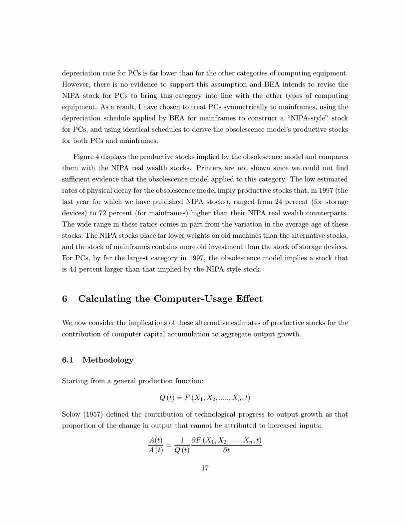
Figure 4 displays the productive stocks implied by the obsolescence model and compares
them with the NIPA real wealth stocks. Printers are not shown since we could not find
sufficient evidence that the obsolescence model applied to this category. The low estimated
rates of physical decay for the obsolescence model imply productive stocks that, in 1997 (the
last year for which we have published NIPA stocks), ranged from 24 percent (for storage
devices) to 72 percent (for mainframes) higher than their NIPA real wealth counterparts.
The wide range in these ratios comes in part from the variation in the average age of these
stocks: The NIPA stocks place far lower weights on old machines than the alternative stocks,
and the stock of mainframes contains more old investment than the stock of storage devices.
For PCs, by far the largest category in 1997, the obsolescence model implies a stock that
is 44 percent larger than that implied by the NIPA-style stock.
6 Calculating the Computer-Usage Effect
We now consider the implications of these alternative estimates of productive stocks for the
contribution of computer capital accumulation to aggregate output growth.
6.1 Methodology
Starting from a general production function:
Q (t) = F (X1,X2, .....,Xn, t)
Solow (1957) defined the contribution of technological progress to output growth as that
proportion of the change in output that cannot be attributed to increased inputs:
˙A(t)
A (t)=
1
Q (t)
∂F (X1,X2, .....,Xn, t)
∂t
17

Taking derivatives with respect to time we get
˙Q(t)
Q (t)=
˙A(t)
A (t)+
n∑i=1
Xi (t)
Q (t)
∂F (X1,X2, .....,Xn, t)
∂Xi
˙Xi(t)
Xi (t)(23)
The contribution to growth of technological progress, known also as Total Factor Productiv-
ity (TFP), is calculated by subtracting a weighted average of growth in inputs from output
growth, where each input’s weight is determined by the quantity of the input used times
its marginal productivity. As is well known, if the production function displays constant
returns to scale with respect to inputs and factors are being paid their marginal products
then these growth accounting weights will sum to one and the weight for a factor will equal
its share of aggregate income.
In the case where output is a function of labor input, L(t), and n capital inputs, Ki(t),
we have˙Q(t)
Q (t)=
˙A(t)
A (t)− α(t)
˙L(t)
L (t)−
n∑i=1
βi(t)˙Ki(t)
Ki (t)(24)
Since labor’s share of income is an observable parameter, we can use this as a time series
for α(t). While we cannot observe the actual payments of factor income to different types
of capital, the standard implementation of empirical growth accounting follows Jorgenson
and Grilliches (1967) and uses theoretically-based measures of the marginal productivity of
capital
ri (t) =∂F (X1,X2, .....,Xn, t)
∂Xi
to calculate growth accounting weights for each type of capital
βi (t) =ri (t)Ki (t)
Q (t)(25)
The contribution to growth of accumulation of capital of type i is defined as βi (t)˙Ki(t)
Ki(t).13
There are three areas where the calculation of the contribution of computer capital to growth
differs depending on whether we model the data as being generated by the Solow vintage
model or by the obsolescence model.
13Using theoretically-specified measures of the marginal productivity of each type of capital does not
ensure that our growth accounting weights sum to one. In practice, then, we force this to be the case by
restricting the weights for each type of capital to sum to capital’s share of income, with the relative size of
the weight for capital of type i being proportional to our estimate of ri (t)Ki (t). This procedure is discussed
in more detail in the appendix.
18

Computer Capital Stock Growth Rates (˙Ki(t)
Ki(t)): Perhaps surprisingly, these are almost
identical under both the Solow vintage model (in which case we use the NIPA stocks) and
the obsolescence model (in which case we use the alternative stocks). While the levels of
the alternative stocks are higher than the levels of the NIPA stocks, the growth rates in the
1990s are very similar.
The Marginal Productivity of Computer Capital: The productive stock of computer
capital is measured in quality-adjusted units. Thus, we need an estimate of the marginal
productivity of adding another quality-adjusted unit. For both models, we know that de-
clining utilization implies that the marginal productivity of non-quality-adjusted computer
units declines cross-sectionally with age at rate γ
rv (t) = rt (t) e−γ(t−v)
However, dividing by eγv, this means that, in terms of quality-adjusted units, the marginal
productivity of capital equals r(t) = rt (t) e−γt for all units.
The formula for rt (t) differs in our two models. In the Solow vintage model we have
rt(t) = (r + δ + γ − g) egt
Letting q(t) = e(g−γ)t be the quality-adjusted computer price index, r(t) is given by the
traditional Jorgensonian rental rate:
r(t) = qt (t)
(r + δ −
˙qt(t)
qt (t)
)(26)
In Appendix B, I show that the corresponding formula for the obsolescence model is
r(t) = qt (t)
[(r + δ −
˙qt(t)
qt (t)
)+ s
(1−
1− e−(r+δ)T
r + δ
˙qt(t)
qt (t)
)](27)
These equations are the algebraic expression of the pattern shown on Figure 3: Intro-
ducing a support cost implies that the marginal productivity of capital must be higher
to compensate for both the payment of the support cost and early retirement. Perhaps
surprisingly, then, Table 3 shows that the estimates of r(t) under the assumption that
the Solow vintage model is correct are fairly similar to the estimates for the obsolescence
19
model.14 The reason for this is that the models give very different estimates of δ, with the
obsolescence model being consistent with low values and the Solow model consistent with
very high values. So, because of the high rates of economic depreciation, both models agree
that the marginal productivity of computer investments should be high. However, they
arrive at this conclusion via different reasoning: The obsolescence model sees that firms
need to be compensated for support costs and early retirement, the Solow model that firms
need to be compensated for high rates of physical decay.
The calculated values for r(t) from the two models differ principally because of the effect
of quality-adjusted price declines,˙qt(t)
qt(t). This variable has a stronger effect on r(t) in the
obsolescence model because of the influence that faster embodied technological change has
in shortening service lives. Thus, the obsolescence model’s value of r(t) is notably higher
for PCs, because this is the category with the fastest rate of price decline.
The Level of Computer Capital Stocks: The final difference between these two models
in the calculation of the contribution to growth of computer capital accumulation is what
we have already shown - that the levels of the stocks consistent with the obsolescence model
are higher than the NIPA stocks consistent with the Solow vintage model. This results in
a higher contribution to growth for the obsolescence model for a simple reason: While both
models agree that the stock of computer capital is growing fast and has high marginal
productivity, this cannot have much effect on aggregate output if this stock is too small.
6.2 Results
Our empirical implementation is for the U.S. private business sector, the output of which
equals GDP minus output from government and nonprofit institutions and the imputed
income from owner-occupied housing.15 Table 4 gives a summary for both models of the
combined contributions to output growth of the five types of computer capital. Figure 5
gives a graphical illustration.
The results for both models show similar patterns over time with the contributions
from the obsolescence model consistently about 50 percent higher than those from the
Solow vintage model. The results from the Solow model for the 1980s are very similar
14The values in Table 3 use 1997-based prices. In other words, q (t) = 1 for each category.15Appendix B contains a detailed description of the empirical growth accounting calculations.
20
to those of Oliner and Sichel (1994), who, using essentially the same methodology, found
that during this period computer capital accumulation contributed about two-tenths of a
percentage point per year to aggregate output growth. However, both approaches agree
that the contribution of computer capital accumulation has picked up substantially over
the past few years, with average contributions over 1996-98 (in percentage points) of 0.57
for the Solow model and 0.82 for the obsolescence model.16 Both approaches also see this
contribution accelerating as computers become a more important part of capital input.
By 1998, the obsolescence model indicates that this contribution was worth almost a full
percentage point for economic growth, 0.32 percentage points higher than for the Solow
model. One interpretation of these results is that they provide a partial reversal of Oliner
and Sichel’s original resolution of the Solow paradox: Computers may not be everywhere
but they are more prevalent than the NIPA capital stocks suggest, and even the NIPA series
are growing very rapidly.
7 Computers and The Acceleration in Productivity
7.1 The Computer Sector and Aggregate TFP
Our results so far have suggested that the substantial investments in computing technologies
made by U.S. businesses in recent years have had a very important influence on output
growth. Note, though, that the models have been silent on the cause of this massive
accumulation of computing power: Why has the price of computing power fallen so rapidly?
Our models have assumed that output can be expressed in terms of an aggregate production
function, which allows for two possibilities. The first is that computers are produced using
the same technology as all other goods. However, this raises the question of why their
relative price would decline. The second is that all computers have been imported, which
clearly does not fit the reality of the U.S. economy. Thus, an alternative approach, which
recognizes that computers may be produced using a different technology to other goods,
seems appropriate.
Suppose that Sector 1 produces consumption goods and ordinary capital according to
16Oliner and Sichel (2000, forthcoming) also present figures for recent years that are very similar to those
presented here for the Solow vintage model.
21
an aggregated production function, derived from a vintage structure as in previous sections:
Q1 (t) = A1 (t)L1 (t)α(t)K1 (t)β(t)C1 (t)1−α(t)−β(t) (28)
and that Sector 2 produces quality-adjusted computers according to a production function
that is identical up to the multiplicative disembodied technology term:
Q2 (t) = A2 (t)L2 (t)α(t)K2 (t)β(t)C2 (t)1−α(t)−β(t) (29)
We are interested in estimating the behavior of A2 (t) relative to A1 (t). For the United
States, we do not have sufficient information on capital stocks by industry to allow for
direct estimation of this series for the computer industry using a growth accounting method.
Instead, I will estimate this series under the simplifying assumption that both sectors are
perfectly competitive, so prices are set equal to marginal cost. It is easily shown that, given
the wage rate, w (t), and the rental rates for ordinary capital, ro (t), and quality-adjusted
computer capital r(t), the cost function is
Ci (w (t) , ro (t) , r(t), Qi (t)) =Qi (t)
Ai (t)
(w (t)
α (t)
)α(t) (ro (t)
β (t)
)β(t) ( r(t)
1− α (t)− β (t)
)1−α(t)−β(t)
(30)
Thus, the ratio of Sector 1’s price to Sector 2’s is
p1 (t)
p2 (t)=∂C1 (t)
∂Q1 (t)/∂C2 (t)
∂Q2 (t)=A2 (t)
A1 (t)(31)
Under these assumptions, we can use the relative decline in quality-adjusted computer
prices to measure the relative rates of TFP growth in the computer and non-computer
sectors:˙A2(t)
A2 (t)−
˙A1(t)
A1 (t)= γ − g (32)
Consider now the behavior of a Tornqvist aggregate of Q1 (t) and Q2 (t). This aggrega-
tion procedure, which is a close theoretical approximation to the Fisher chain-aggregation
method that has been used to construct real GDP since 1996, weights the real growth
rates for each category according to its share in nominal output. The growth rate of this
aggregate will be:˙Q(t)
Q (t)= (1− µt)
˙Q1(t)
Q1 (t)+ µt
˙Q2(t)
Q2 (t)(33)
22

where µt is the share of the computer sector in nominal output. Applying the standard
growth accounting equation to each sector, we get
˙Qi(t)
Qi (t)=
˙Ai(t)
Ai (t)+ α (t)
˙Li(t)
Li (t)+ β (t)
˙Ki(t)
Ki (t)+ (1− α (t) + β (t))
˙Ci(t)
Ci (t)(34)
Performing an aggregate TFP calculation with the Tornqvist measure of aggregate output,
we get
˙Q(t)
Q (t)− α (t)
˙L(t)
L (t)− β (t)
˙K(t)
K (t)− (1− α (t)− β (t))
˙C(t)
C (t)
= (1− µt)˙A1(t)
A1 (t)+ µt
˙A2(t)
A2 (t)
=˙A1(t)
A1 (t)+ µt (γ − g) (35)
The effect of faster TFP growth in the computer sector in boosting aggregate TFP
growth can be measured as the product of the share of the computer industry in nom-
inal output (µt) times the rate of relative price decline for computers, (γ − g). Figure
6 describes this calculation.17 The upper panel shows that despite enormous declines in
quality-adjusted prices, the nominal output of the computer industry has fluctuated around
1.5 percent of business output since 1983, ticking up a bit since the mid-1990s. The middle
panel shows that the pace of quality-adjusted price declines accelerated rapidly after the
mid-1990s. As a result, the boost to aggregate TFP growth from the computer sector,
which had fluctuated around 0.25 percentage points a year between 1978 and 1995 has
picked up considerably in recent years, averaging almost 0.5 percentage points a year in
1997 and 1998.
These figures are likely to be a lower bound on the contribution of the computer sector to
aggregate TFP growth because of the assumption of perfect competition. Equating the TFP
growth differential between computer and non-computer sectors with the relative decline
in computer prices implies that a given set of factors’ ability to generate nominal output
should be the same in the computer and non-computer industry. However, even looking
only at the computer industry’s ability to produce nominal output, there still appears to
17There is no official measure of the output of the computer industry. The measure of nominal computer
output used here is the sum of consumption, investment, and government expenditures on computers plus
exports of computers and peripherals and parts minus imports for the same category. The measure of real
output is the Fisher chain-aggregate of these 5 components.
23
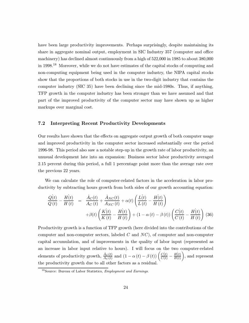
have been large productivity improvements. Perhaps surprisingly, despite maintaining its
share in aggregate nominal output, employment in SIC Industry 357 (computer and office
machinery) has declined almost continuously from a high of 522,000 in 1985 to about 380,000
in 1998.18 Moreover, while we do not have estimates of the capital stocks of computing and
non-computing equipment being used in the computer industry, the NIPA capital stocks
show that the proportions of both stocks in use in the two-digit industry that contains the
computer industry (SIC 35) have been declining since the mid-1980s. Thus, if anything,
TFP growth in the computer industry has been stronger than we have assumed and that
part of the improved productivity of the computer sector may have shown up as higher
markups over marginal cost.
7.2 Interpreting Recent Productivity Developments
Our results have shown that the effects on aggregate output growth of both computer usage
and improved productivity in the computer sector increased substantially over the period
1996-98. This period also saw a notable step-up in the growth rate of labor productivity, an
unusual development late into an expansion: Business sector labor productivity averaged
2.15 percent during this period, a full 1 percentage point more than the average rate over
the previous 22 years.
We can calculate the role of computer-related factors in the acceleration in labor pro-
ductivity by subtracting hours growth from both sides of our growth accounting equation:
˙Q(t)
Q (t)−
˙H(t)
H (t)=
AC(t)
AC (t)+ANC(t)
ANC (t)+ α(t)
(˙L(t)
L (t)−
˙H(t)
H (t)
)
+β(t)
(˙K(t)
K (t)−
˙H(t)
H (t)
)+ (1− α (t)− β (t))
(˙C(t)
C (t)−
˙H(t)
H (t)
)(36)
Productivity growth is a function of TFP growth (here divided into the contributions of the
computer and non-computer sectors, labeled C and NC), of computer and non-computer
capital accumulation, and of improvements in the quality of labor input (represented as
an increase in labor input relative to hours). I will focus on the two computer-related
elements of productivity growth, AC(t)AC(t) and (1− α (t)− β (t))
(˙C(t)
C(t) −˙H(t)
H(t)
), and represent
the productivity growth due to all other factors as a residual.
18Source: Bureau of Labor Statistics, Employment and Earnings.
24
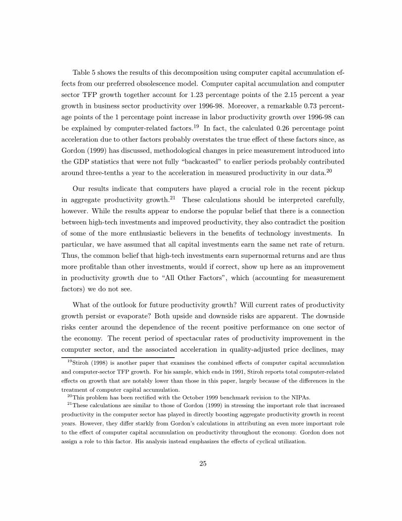
Table 5 shows the results of this decomposition using computer capital accumulation ef-
fects from our preferred obsolescence model. Computer capital accumulation and computer
sector TFP growth together account for 1.23 percentage points of the 2.15 percent a year
growth in business sector productivity over 1996-98. Moreover, a remarkable 0.73 percent-
age points of the 1 percentage point increase in labor productivity growth over 1996-98 can
be explained by computer-related factors.19 In fact, the calculated 0.26 percentage point
acceleration due to other factors probably overstates the true effect of these factors since, as
Gordon (1999) has discussed, methodological changes in price measurement introduced into
the GDP statistics that were not fully “backcasted” to earlier periods probably contributed
around three-tenths a year to the acceleration in measured productivity in our data.20
Our results indicate that computers have played a crucial role in the recent pickup
in aggregate productivity growth.21 These calculations should be interpreted carefully,
however. While the results appear to endorse the popular belief that there is a connection
between high-tech investments and improved productivity, they also contradict the position
of some of the more enthusiastic believers in the benefits of technology investments. In
particular, we have assumed that all capital investments earn the same net rate of return.
Thus, the common belief that high-tech investments earn supernormal returns and are thus
more profitable than other investments, would if correct, show up here as an improvement
in productivity growth due to “All Other Factors”, which (accounting for measurement
factors) we do not see.
What of the outlook for future productivity growth? Will current rates of productivity
growth persist or evaporate? Both upside and downside risks are apparent. The downside
risks center around the dependence of the recent positive performance on one sector of
the economy. The recent period of spectacular rates of productivity improvement in the
computer sector, and the associated acceleration in quality-adjusted price declines, may
19Stiroh (1998) is another paper that examines the combined effects of computer capital accumulation
and computer-sector TFP growth. For his sample, which ends in 1991, Stiroh reports total computer-related
effects on growth that are notably lower than those in this paper, largely because of the differences in the
treatment of computer capital accumulation.20This problem has been rectified with the October 1999 benchmark revision to the NIPAs.21These calculations are similar to those of Gordon (1999) in stressing the important role that increased
productivity in the computer sector has played in directly boosting aggregate productivity growth in recent
years. However, they differ starkly from Gordon’s calculations in attributing an even more important role
to the effect of computer capital accumulation on productivity throughout the economy. Gordon does not
assign a role to this factor. His analysis instead emphasizes the effects of cyclical utilization.
25

turn out to be a flash in the pan. Indeed, given historical patterns, it seems unlikely that
the recent pace of computer-related technological advance can be sustained. Given that we
did not find any evidence that TFP growth has picked up outside this sector, a slowdown
in aggregate productivity growth would be the most likely outcome.
The upside potential has two elements. First, the recent burst of productivity growth
does not appear to be particularly cyclical in nature: Increased utilization would show up
as an increase in productivity growth due to “All Other Factors”. Thus, there is little
reason to believe that we will see a period of sluggish productivity growth as “payback” for
the current period. Second, thus far, it does not appear as though the computer industry
is close to exhausting the potential for producing faster and cheaper computers. Moreover,
one lesson from the expansion of the Internet is that businesses are still taking advantage
of declines in the price of computing power by finding new and (hopefully) productive uses
for computing technologies.
8 Conclusions
The purpose of this paper has been part methodological, part substantive. The method-
ological contribution has been to outline the issues surrounding capital stock measurement
in the presence of embodied technological change and technological obsolescence. In par-
ticular, the paper provides a number of arguments against the use of the NIPA computer
capital stocks for growth accounting and suggests an alternative approach. The substan-
tive contribution has been to document the role that computers have played in the recent
productivity performance of the U.S. economy: A marked pickup in the rate of computer
capital deepening combined with improved productivity in the computer-producing indus-
try have accounted for almost all of the recent acceleration in aggregate productivity.
I will conclude by pointing to the need for further empirical research in this area. Most
of the calculations in this paper have relied on estimates of things that are difficult to
measure (quality-adjusted prices for computing equipment) or studies that may themselves
have become obsolete (Oliner’s depreciation schedules). Given the increasing importance
of computing technologies, further empirical work on the measurement of prices and depre-
ciation for computing equipment would be extremely useful for refining and extending the
analysis in this paper.
26
References
[1] Bureau of Labor Statistics (1983). Trends in Multifactor Productivity, 1948-1981. BLS
Bulletin No. 2178.
[2] Feldstein, Martin and Michael Rothschild (1974). “Towards an Economic Theory of
Replacement Investment”, Econometrica, 42, 393-423.
[3] Gartner Group (1999). 1998 IT Spending and Staffing Survey Results, report available
at www.gartnergroup.com.
[4] Goolsbee, Austan (1998). “The Business Cycle, Financial Performance, and the Re-
tirement of Capital Goods”, Review of Economic Dynamics.
[5] Gordon, Robert J. (1999). Has the New Economy Rendered the Productivity Slowdown
Obsolete?, mimeo, Northwestern University.
[6] Gravelle, Jane (1994). The Economic Effects of Taxing Capital Income, Cambridge:
MIT Press.
[7] Hulten, Charles and Frank Wykoff (1981a). “The Estimation of Economic Depreciation
Using Vintage Asset Prices: An Application of the Box-Cox Power Transformation”,
Journal of Econometrics, 15, 367-396.
[8] Hulten, Charles and Frank Wykoff (1981b). “The Measurement of Economic Depre-
ciation” in Charles Hulten, ed., Depreciation, Inflation, and the Taxation of Income
from Capital, Washington DC: The Urban Institute Press. 367-396.
[9] Hulten, Charles and Frank Wykoff (1996). “Issues in the Measurement of Economic
Depreciation: Introductory Remarks”, Economic Inquiry, 33, 10-23.
[10] Jorgenson, Dale (1973). “The Economic Theory of Replacement and Depreciation” in
W. Sellekaerts, ed., Econometrics and Economic Theory, New York: Macmillan.
[11] Jorgenson, Dale and Zvi Grilliches (1967). “The Explanation of Productivity Change”,
Review of Economic Studies, 34, 249-280.
[12] Jorgenson, Dale and Kevin Stiroh (1999). “Information Technology and Growth”,
American Economic Review, May, 109-115.
27
[13] Katz, Arnold and Shelby Herman (1997). “Improved Estimates of Fixed Reproducible
Tangible Wealth, 1929-95”, Survey of Current Business, May, 69-92.
[14] Moulton, Brent and Eugene Seskin (1999). “A Preview of the 1999 Comprehensive
Revision of the National Income and Product Accounts”, Survey of Current Business,
October, 6-17.
[15] Oliner, Stephen (1989). “Constant-Quality Price Change, Depreciation, and Retire-
ment of Mainframe Computers”, in Price Measurements and Their Uses, ed. Allan
Young, Murray Foss, and Marilyn Manser, Chicago: University of Chicago Press.
[16] Oliner, Stephen (1994). Measuring Stocks of Computer Peripheral Equipment: Theory
and Application, mimeo, Federal Reserve Board.
[17] Oliner, Stephen and Daniel Sichel (1994). “Computers and Output Growth Revisited:
How Big is the Puzzle?”, Brookings Papers on Economic Activity, 2, 273-317.
[18] Oliner, Stephen and Daniel Sichel (2000). “The Resurgence of Growth in the Late
1990s: Are Computers the Story?”, forthcoming, Journal of Economic Perspectives.
[19] Sichel, Daniel (1997). The Computer Revolution: An Economic Perspective, Washing-
ton DC: Brookings Institution Press.
[20] Solow, Robert (1957). “Technical Change and the Aggregate Production Function”,
Review of Economics and Statistics, 39, 312-320.
[21] Solow, Robert (1959). “Investment and Technical Progress” in Mathematical Methods
in the Social Sciences, 1959, eds. Kenneth Arrow, Samuel Karlin, and Patrick Suppes,
89-104. Stanford, CA: Stanford University Press.
[22] Stiroh, Kevin J. (1998). “Computers, Productivity, and Input Substitution”, Economic
Inquiry, 36, 175-191.
[23] Triplett, Jack (1996). “Depreciation in Production Analysis and in Income and Wealth
Accounts”, Economic Inquiry, 33, 93-115.
[24] U.S. Department of Commerce, Bureau of Economic Analysis (1999). Fixed Repro-
ducible Tangible Wealth, 1925-94, Washington DC: U.S. Government Printing Office.
28

A Solution to the Obsolescence Model
This appendix derives the formal solution for the depreciation schedule under the assump-
tions of the obsolescence model.
The Marginal Productivity of Capital: As described in the text, the computer price
arbitrage formula is
pv(t) =
∫ v+T
t
(∂Qv (n)
∂(I(v)e−δ(n−v)
) − spv (v)
)e−r(n−t)e−δ(n−v)dn
Denoting the marginal productivity of a unit of capital as
r∗v (t) =∂Qv (t)
∂(I(v)e−δ(t−v)
)We get the following formula for the purchase price
pv (v) =1
1 + sr+δ
(1− e−(r+δ)T
) ∫ v+T
vr∗v (n) e−(r+δ)(n−v)dn
Now, differentiating the price of new computers with respect to v we get
pv(v) = (r + δ + γ) pv (v)−r∗v (v)
1 + sr+δ
(1− e−(r+δ)T
) +r∗v (v + T ) e−(r+δ)T
1 + sr+δ
(1− e−(r+δ)T
)At the time of scrappage, the computer must be just covering the support cost, implying
r∗v(v + T ) = spv (v). Making this substitution, using pt (t) = egt and re-arranging gives us
the marginal productivity of new computer capital:
r∗v (v) =
[(r + δ + γ − g) + s
(1 +
γ − g
r + δ
(1− e−(r+δ)T
))]egv
This equation shows that the introduction of computing support costs implies a higher
marginal productivity of computer capital than in our previous model.
The Retirement Age: Since all the conditions for the allocation of other factors to each
vintage are as before, the marginal productivity of a unit of computer capital still declines
over time at rate g − γ, so we can now define the retirement age T from[(r + δ + γ − g) + s
(1 +
γ − g
r + δ
(1− e−(r+δ)T
))]e(g−γ)T egv = segv
29
Re-arranging, we get
e(r+δ+γ−g)T = (r + δ + γ − g)(
1
s+
1
r + δ
)e(r+δ)T −
γ − g
r + δ
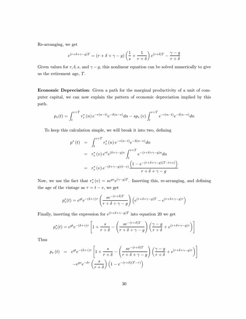
Given values for r, δ, s, and γ− g, this nonlinear equation can be solved numerically to give
us the retirement age, T .
Economic Depreciation: Given a path for the marginal productivity of a unit of com-
puter capital, we can now explain the pattern of economic depreciation implied by this
path.
pv(t) =
∫ v+T
tr∗v (n) e−r(n−t)e−δ(n−v)dn− spv (v)
∫ v+T
te−r(n−t)e−δ(n−v)dn
To keep this calculation simple, we will break it into two, defining
p∗ (t) =
∫ v+T
tr∗v (n) e−r(n−t)e−δ(n−v)dn
= r∗v (v) erte(δ+γ−g)v∫ v+T
te−(r+δ+γ−g)ndn
= r∗v (v) e−(δ+γ−g)(t−v)
(1− e−(r+δ+γ−g)(T−t+v)
)r + δ + γ − g
Now, we use the fact that r∗v (v) = segve(γ−g)T . Inserting this, re-arranging, and defining
the age of the vintage as τ = t− v, we get
p∗v(t) = egte−(δ+γ)τ
(se−(r+δ)T
r + δ + γ − g
)(e(r+δ+γ−g)T − e(r+δ+γ−g)τ
)Finally, inserting the expression for e(r+δ+γ−g)T into equation 20 we get
p∗v(t) = egte−(δ+γ)τ
[1 +
s
r + δ−
(se−(r+δ)T
r + δ + γ − g
)(γ − g
r + δ+ e(r+δ+γ−g)τ
)]
Thus
pv (t) = egte−(δ+γ)τ
[1 +
s
r + δ−
(se−(r+δ)T
r + δ + γ − g
)(γ − g
r + δ+ e(r+δ+γ−g)τ
)]
−egve−δτ(
s
r + δ
)(1− e−(r+δ)(T−τ)
)
30

And the quality-adjusted economic depreciation schedule calculated from an Oliner-style
study by comparing the price of an old vintage with the price of new computers and then
subtracting off the quality-improvement in the new computers gives
dv (t) = e−δτ[1 +
s
r + δ−
(se−(r+δ)T
r + δ + γ − g
)(γ − g
r + δ+ e(r+δ+γ−g)τ
)]
−e−(δ+γ−g)τ(
s
r + δ
)(1− e−(r+δ)(T−τ)
)
B Empirical Growth Accounting Details
Capital Stocks: The calculations used detailed disaggregated capital stock data: In ad-
dition to the 5 types of computing equipment, we use the 26 types of non-computing
equipment shown on Table 1, 11 types of non-residential structures, and tenant-occupied
housing (rental income from such housing is part of business output). For all non-computer
stocks, we use the NIPA real wealth capital stocks, altered in two ways. First, these data
are published through 1997. However, real investment data for 1998 are available. Thus,
I extended each of the published capital stock series by growing them out using the 1998
investment data and the depreciation rates published in Katz and Herman (1997). Sec-
ond, these stocks refer to year-end values. Since the growth accounting analysis seeks to
explain year-average growth rates, year-average stocks were constructed by averaging adja-
cent year-end stocks. The same transformation was applied to the computer stocks for the
obsolescence model.
Rental Rates: For all capital except computers in the obsolescence model, our empirical
analysis proxied the marginal productivity of capital using the Hall-Jorgenson tax-adjusted
rental rate
ri (t) = pi (t)
(r + δi −
pi(t)
pi (t)
)(1− ci − τzi
1− τ
)where pi (t) is the price of capital of type i relative to the price of output, r is the real
interest rate, δi is the NIPA depreciation rate for capital of type i, τ is the marginal
corporate income tax rate, zi is the present discounted value of depreciation allowances per
dollar invested, and ci is the investment tax credit.
The real rate of return on capital, r, was set equal to 6.75 percent: This produces a
series for the “required” income flow from capital that, on average, tracks with the observed
31

series for business sector capital income over our sample. The˙qt(t)
qt(t)term is calculated for
each type of capital as a three-year moving average of the rate of change of the price of
capital relative to the price of output. The tax terms were calculated for each type of
capital using the information on tax credit rates and depreciation service lives presented in
Gravelle (1994).
Growth Accounting Weights: We start by imputing factor shares for each type of
capital. For labor, we use α(t), the labor share of income in the business sector. For capital,
things are a bit more complicated. In theory, if we had perfect measures of the marginal
productivity of each type of capital, then we could just use equation (25) to estimate the
factor shares. In practice, theoretical estimates can produce a set of factor shares that do
not sum to one. There are two standard methods for dealing with this problem. One is to
vary the value of r each period so that∑nj=1 rj (t)Kj (t) equals total capital income. The
second method, implemented in this paper, is to define the growth accounting weights for
capital so that they sum to capital’s share of income, letting the share for capital of type i
be proportional to ri (t)Ki (t), by using the formula
βi (t) = (1− α(t))
(ri (t)Ki (t)∑nj=1 rj (t)Kj (t)
)
The final growth accounting weights were constructed by averaging factor shares from
adjacent years.
32

Computing Equipment: Electrical Transmission 0.05
Mainframes 0.30 Cars 0.28
Terminals 0.27 Trucks, Buses, and Trailers 0.18
Storage Devices 0.28 Aircraft 0.08
Printers 0.35 Ships and Boats 0.06
Personal Computers 0.11 Railroad Equipment 0.06
Other Office Equipment 0.31 Household Furniture 0.14
Communications Equipment 0.11 Other Furniture 0.12
Instruments 0.14 Farm Tractors 0.15
Photocopying Equipment 0.18 Construction Tractors 0.16
Fabricated Metals 0.09 Agricultural Machinery 0.12
Steam Engines and Turbines 0.05 Construction Machinery 0.16
Internal Combustion Engines 0.21 Mining and Oilfield Machinery 0.15
Metalworking Machinery 0.12 Service Industry Machinery 0.15
Special Industrial Machinery 0.10 Other Electrical Equipment 0.18
General Industrial Machinery 0.11 Miscellaneous Equipment 0.15
Table 1: 1997 NIPA Depreciation Rates for Equipment
Mainframes Storage Printers Terminals
s 0.17 0.05 0 0.15
δ 0 0.06 0.35 0
RMSE 0.01 0.04 0.02 0.01
RMSE - Geometric 0.06 0.10 0.02 0.06
Table 2: Calibrating The Obsolescence Model
33
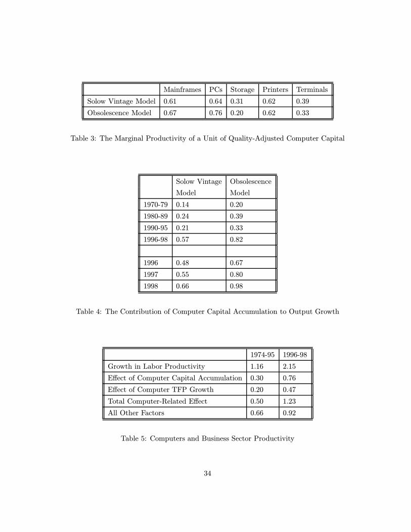
Mainframes PCs Storage Printers Terminals
Solow Vintage Model 0.61 0.64 0.31 0.62 0.39
Obsolescence Model 0.67 0.76 0.20 0.62 0.33
Table 3: The Marginal Productivity of a Unit of Quality-Adjusted Computer Capital
Solow Vintage Obsolescence
Model Model
1970-79 0.14 0.20
1980-89 0.24 0.39
1990-95 0.21 0.33
1996-98 0.57 0.82
1996 0.48 0.67
1997 0.55 0.80
1998 0.66 0.98
Table 4: The Contribution of Computer Capital Accumulation to Output Growth
1974-95 1996-98
Growth in Labor Productivity 1.16 2.15
Effect of Computer Capital Accumulation 0.30 0.76
Effect of Computer TFP Growth 0.20 0.47
Total Computer-Related Effect 0.50 1.23
All Other Factors 0.66 0.92
Table 5: Computers and Business Sector Productivity
34

Figure 1Depreciation Schedules for Computing Equipment
0 5 100.0
0.2
0.4
0.6
0.8
1.0
Age
19701980
Mainframes
0 5 100.0
0.2
0.4
0.6
0.8
1.0
Age
19801990
Storage Devices
0 5 100.0
0.2
0.4
0.6
0.8
1.0
Age
19801990
Printers
0 5 100.0
0.2
0.4
0.6
0.8
1.0
Age
19801990
Terminals
35
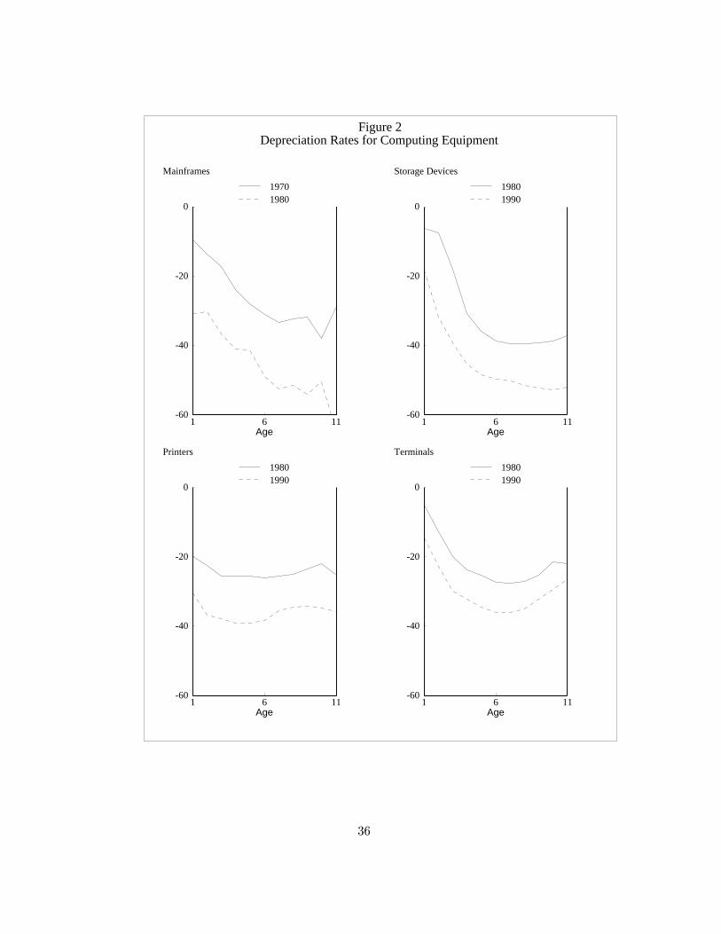
Figure 2Depreciation Rates for Computing Equipment
1 6 11-60
-40
-20
0
Age
19701980
Mainframes
1 6 11-60
-40
-20
0
Age
19801990
Storage Devices
1 6 11-60
-40
-20
0
Age
19801990
Printers
1 6 11-60
-40
-20
0
Age
19801990
Terminals
36
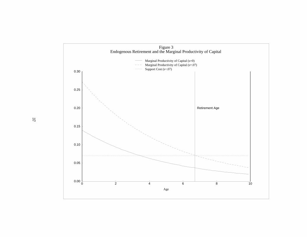
Figure 3Endogenous Retirement and the Marginal Productivity of Capital
0 2 4 6 8 100.00
0.05
0.10
0.15
0.20
0.25
0.30
Retirement Age
Marginal Productivity of Capital (s=0)Marginal Productivity of Capital (s=.07)Support Cost (s=.07)
Age
37
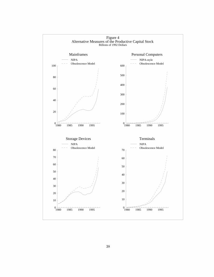
Figure 4Alternative Measures of the Productive Capital Stock
Billions of 1992 Dollars
1980 1985 1990 19950
20
40
60
80
100
NIPAObsolescence Model
Mainframes
1980 1985 1990 19950
100
200
300
400
500
600
NIPA-styleObsolescence Model
Personal Computers
1980 1985 1990 19950
10
20
30
40
50
60
70
80
NIPAObsolescence Model
Storage Devices
1980 1985 1990 19950
10
20
30
40
50
60
70
NIPAObsolescence Model
Terminals
38

Figure 5The Contribution of Computer Capital Accumulation to Aggregate Growth
1960 1962 1964 1966 1968 1970 1972 1974 1976 1978 1980 1982 1984 1986 1988 1990 1992 1994 1996 19980.0
0.2
0.4
0.6
0.8
1.0
1.2
Solow Vintage Model (Using NIPA Stocks) Obsolescence Model (Using Alternative Stocks)
39

Figure 6Computers and Aggregate TFP
1970 1972 1974 1976 1978 1980 1982 1984 1986 1988 1990 1992 1994 19960.000
0.004
0.008
0.012
0.016
Computer Share of Nominal Business Output
1970 1972 1974 1976 1978 1980 1982 1984 1986 1988 1990 1992 1994 1996-35
-30
-25
-20
-15
-10
-5
Rate of Relative Price Decline for Computer Output
1970 1972 1974 1976 1978 1980 1982 1984 1986 1988 1990 1992 1994 19960.0
0.1
0.2
0.3
0.4
0.5
Contribution of the Computer Sector to TFP Growth
40
Related Documents