Morphological convexity measures for terrestrial basins derived from digital elevation models Sin Liang Lim a,n , B.S. Daya Sagar b , Voon Chet Koo a , Lea Tien Tay c a Faculty of Engineering and Technology, Melaka Campus, Multimedia University, Jalan Ayer Keroh Lama, 75450 Melaka, Malaysia b Systems Science and Informatics Unit (SSIU), Indian Statistical Institute-Bangalore Centre, 8th Mile, Mysore Road, RV College PO, Bangalore 560059, India c School of Electrical and Electronic Engineering, Universiti Sains Malaysia, Engineering Campus, Nibong Tebal, 14300 Penang, Malaysia article info Article history: Received 26 April 2010 Received in revised form 12 October 2010 Accepted 15 October 2010 Available online 12 November 2010 Keywords: Convexity measures Spatial variability Mathematical morphology abstract Geophysical basins of terrestrial surfaces have been quantitatively characterized through a host of indices such as topological quantities (e.g. channel bifurcation and length ratios), allometric scaling exponents (e.g. fractal dimensions), and other geomorphometric parameters (channel density, Hack’s and Hurst exponents). Channel density, estimated by taking the ratio between the length of channel network (L) and the area of basin (A) in planar form, provides a quantitative index that has hitherto been related to various geomorphologically significant processes. This index, computed by taking the planar forms of channel network and its corresponding basin, is a kind of convexity measure in the two-dimensional case. Such a measure – estimated in general as a function of basin area and channel network length, where the important elevation values of the topological region within a basin and channel network are ignored – fails to capture the spatial variability between homotopic basins possessing different altitude-ranges. Two types of convexity measures that have potential to capture the terrain elevation variability are defined as the ratio of (i) length of channel network function and area of basin function and (ii) areas of basin and its convex hull functions. These two convexity measures are estimated in three data sets that include (a) synthetic basin functions, (b) fractal basin functions, and (c) realistic digital elevation models (DEMs) of two regions of peninsular Malaysia. It is proven that the proposed convexity measures are altitude- dependent and that they could capture the spatial variability across the homotopic basins of different altitudes. It is also demonstrated on terrestrial DEMs that these convexity measures possess relationships with other quantitative indexes such as fractal dimensions and complexity measures (roughness indexes). & 2010 Elsevier Ltd. All rights reserved. 1. Introduction Conventional geomorphometric quantities (e.g. Horton, 1945; Strahler, 1964) were previously computed based on the details available from two-dimensional topographic map-sources in order to quantitatively characterize terrestrial surfaces. These geomorpho- metric quantities include a host of indices such as channel bifurcation and length ratios, channel density, and Hack’s and Hurst exponents. Length of the channel network divided by the area of the basin in planar forms provides a quantitative index termed as channel density, which is defined here as a convexity measure of the basin in two dimensions. In the context of hydrogeology, the channel density is related to climate, geology, rainfall, erosion rate, and relief (e.g. Kirkby, 1980, 1993; Howard, 1997; Schumm et al., 1987; Montgomery and Dietrich, 1989, 1994). During the last two decades, several techniques have emerged to quantitatively characterize terrestrial surfaces. These geometrically rigorous techniques, to name a few, originated from fractal geometry (Mandelbrot, 1982) and mathematical morphological (Serra, 1982) concepts. Their potential were demonstrated in digital elevation models (DEMs) derived from multiscale multitemporal remotely sensed data acquired through various sensing mechanisms. In subsequent investigations, the importance of digital elevation models (DEMs) in deriving quantitative geomorphological indicators (e.g. roughness characteristics, channel densities) that exhibit rich scale-invariant properties is greatly realized (Tarboton et al., 1992; Tarboton, 1997; Tarboton and Ames, 2001). While explaining the importance of DEM analysis in understanding the landscape state and process interactions, Tucker and Bras (1998) have shown how drainage density is related to topographic relief through the sign of the predicted relationship between drainage density and relief. From their results, a positive sign of the predicted relationship implies low topographic relief, while a negative sign of the predicted relationship implies high topographic relief. Tucker et al. (2001) proposed to map drainage density using two scalar fields, namely: the local hillslope length from any unchannelled site to the channel network and the local hillslope Contents lists available at ScienceDirect journal homepage: www.elsevier.com/locate/cageo Computers & Geosciences 0098-3004/$ - see front matter & 2010 Elsevier Ltd. All rights reserved. doi:10.1016/j.cageo.2010.10.002 n Corresponding author. Tel.: + 60 3 8312 5367; fax: + 60 3 8318 3029. E-mail addresses: [email protected], [email protected] (S.L. Lim). Computers & Geosciences 37 (2011) 1285–1294

Welcome message from author
This document is posted to help you gain knowledge. Please leave a comment to let me know what you think about it! Share it to your friends and learn new things together.
Transcript
Computers & Geosciences 37 (2011) 1285–1294
Contents lists available at ScienceDirect
Computers & Geosciences
0098-30
doi:10.1
n Corr
E-m
sinliang
journal homepage: www.elsevier.com/locate/cageo
Morphological convexity measures for terrestrial basins derived from digitalelevation models
Sin Liang Lim a,n, B.S. Daya Sagar b, Voon Chet Koo a, Lea Tien Tay c
a Faculty of Engineering and Technology, Melaka Campus, Multimedia University, Jalan Ayer Keroh Lama, 75450 Melaka, Malaysiab Systems Science and Informatics Unit (SSIU), Indian Statistical Institute-Bangalore Centre, 8th Mile, Mysore Road, RV College PO, Bangalore 560059, Indiac School of Electrical and Electronic Engineering, Universiti Sains Malaysia, Engineering Campus, Nibong Tebal, 14300 Penang, Malaysia
a r t i c l e i n f o
Article history:
Received 26 April 2010
Received in revised form
12 October 2010
Accepted 15 October 2010Available online 12 November 2010
Keywords:
Convexity measures
Spatial variability
Mathematical morphology
04/$ - see front matter & 2010 Elsevier Ltd. A
016/j.cageo.2010.10.002
esponding author. Tel.: +60 3 8312 5367; fax
ail addresses: [email protected],
[email protected] (S.L. Lim).
a b s t r a c t
Geophysical basins of terrestrial surfaces have been quantitatively characterized through a host of indices
such as topological quantities (e.g. channel bifurcation and length ratios), allometric scaling exponents
(e.g. fractal dimensions), and other geomorphometric parameters (channel density, Hack’s and Hurst
exponents). Channel density, estimated by taking the ratio between the length of channel network (L)
and the area of basin (A) in planar form, provides a quantitative index that has hitherto been related to
various geomorphologically significant processes. This index, computed by taking the planar forms of
channel network and its corresponding basin, is a kind of convexity measure in the two-dimensional case.
Such a measure – estimated in general as a function of basin area and channel network length, where the
important elevation values of the topological region within a basin and channel network are ignored –
fails to capture the spatial variability between homotopic basins possessing different altitude-ranges. Two
types of convexity measures that have potential to capture the terrain elevation variability are defined
as the ratio of (i) length of channel network function and area of basin function and (ii) areas of basin and
its convex hull functions. These two convexity measures are estimated in three data sets that include
(a) synthetic basin functions, (b) fractal basin functions, and (c) realistic digital elevation models (DEMs)
of two regions of peninsular Malaysia. It is proven that the proposed convexity measures are altitude-
dependent and that they could capture the spatial variability across the homotopic basins of different
altitudes. It is also demonstrated on terrestrial DEMs that these convexity measures possess relationships
with other quantitative indexes such as fractal dimensions and complexity measures (roughness
indexes).
& 2010 Elsevier Ltd. All rights reserved.
1. Introduction
Conventional geomorphometric quantities (e.g. Horton, 1945;Strahler, 1964) were previously computed based on the detailsavailable from two-dimensional topographic map-sources in orderto quantitatively characterize terrestrial surfaces. These geomorpho-metric quantities include a host of indices such as channel bifurcationand length ratios, channel density, and Hack’s and Hurst exponents.Length of the channel network divided by the area of the basin inplanar forms provides a quantitative index termed as channel density,which is defined here as a convexity measure of the basin in twodimensions. In the context of hydrogeology, the channel density isrelated to climate, geology, rainfall, erosion rate, and relief (e.g. Kirkby,1980, 1993; Howard, 1997; Schumm et al., 1987; Montgomery andDietrich, 1989, 1994). During the last two decades, several techniques
ll rights reserved.
: +60 3 8318 3029.
have emerged to quantitatively characterize terrestrial surfaces. Thesegeometrically rigorous techniques, to name a few, originated fromfractal geometry (Mandelbrot, 1982) and mathematical morphological(Serra, 1982) concepts. Their potential were demonstrated in digitalelevation models (DEMs) derived from multiscale multitemporalremotely sensed data acquired through various sensing mechanisms.In subsequent investigations, the importance of digital elevationmodels (DEMs) in deriving quantitative geomorphological indicators(e.g. roughness characteristics, channel densities) that exhibit richscale-invariant properties is greatly realized (Tarboton et al., 1992;Tarboton, 1997; Tarboton and Ames, 2001). While explaining theimportance of DEM analysis in understanding the landscape state andprocess interactions, Tucker and Bras (1998) have shown how drainagedensity is related to topographic relief through the sign of the predictedrelationship between drainage density and relief. From their results, apositive sign of the predicted relationship implies low topographicrelief, while a negative sign of the predicted relationship implies hightopographic relief. Tucker et al. (2001) proposed to map drainagedensity using two scalar fields, namely: the local hillslope length fromany unchannelled site to the channel network and the local hillslope

S.L. Lim et al. / Computers & Geosciences 37 (2011) 1285–12941286
length to the valley networks. All these studies addressed the drainagedensity as either main topics or the subtopics of studies on fluvialbasins. In a recent study, Marani et al. (2003) addressed the problem ofestimation of drainage density of tidal basins.
No watershed or basin is fully convex due to the presence ofvalleys and ridges. A parameter that computes the degree ofconvexity of a watershed is the convexity measure, which is insome way related to channel (drainage) density estimated by takingtwo basic measures, the planar basin’s area and the planar network’slength, as major inputs. Drainage density, according to Horton(1945), is defined dimensionally as the ratio of the total networklength to its watershed area, DD¼L/A, where L and A, respectively,denote length of network and area of the basin. The basicparameters required to estimate this measurement heavily relyon plan-forms of basin and network. The plan-view of thebasin and its corresponding network provide the 2-dimensionalflat basin and the network. Hence, this definition, from the pointof convexity measure, has a limitation as it cannot capture theelevation variability among different drainage basins. The maps ofdrainage density do not carry information on terrain morphology ashigh drainage density may occur in flat, low relief basins as well as inmountainous, high relief basins. This type of estimation is of limiteduse as it cannot capture the basic difference involved in twoseemingly alike basins and their networks over a planar view. Itis intuitively true that the convexity measures of the seemingly alike(homotopic) basins with varied altitudes should be different in sucha way that it reflects the changes in the altitudes involved. Ourproposed method shows distinction between the cases that belongto two altitude-regions. Such a distinction could be shown throughalternative measures that we proposed in this paper. Here the inputsare represented as 3-dimensional functions and not as planar sets.
The three significant parameters, which require morphologicalquantities in the form of functions, include (i) basin function,
20
2020
20
20
20
20
20
20
20
20
20
1919
19
19
19
19
19
19
19
20
20
1918
18
18
18
18
18
18
19
20
20
1918
17
17
17
17
17
18
19
20
20
1918
17
16
16
16
17
18
19
20
20
1918
17
16
15
16
17
18
19
20
20
1918
17
16
16
16
17
18
19
20
20
1918
17
17
17
17
17
18
19
20
20
1918
18
18
18
18
18
18
19
20
20
1919
19
19
19
19
19
19
19
20
20
2020
20
20
20
20
20
20
20
20
15
1515
15
15
15
15
15
15
15
15
15
1414
14
14
14
14
14
14
14
15
15
1413
13
13
13
13
13
13
14
15
15
1413
12
12
12
12
12
13
14
15
15
1413
12
11
11
11
12
13
14
15
15
1413
12
11
10
11
12
13
14
15
15
1413
12
11
11
11
12
13
14
15
15
1413
12
12
12
12
12
13
14
15
15
1413
13
13
13
13
13
13
14
15
15
1414
14
14
14
14
14
14
14
15
15
1515
15
15
15
15
15
15
15
15
20
00
0
0
0
0
0
0
0
20
0
190
0
0
0
0
0
0
19
0
0
018
0
0
0
0
0
18
0
0
0
00
17
0
0
0
17
0
0
0
0
00
0
16
0
16
0
0
0
0
0
00
0
0
15
0
0
0
0
0
0
00
0
16
0
16
0
0
0
0
0
00
17
0
0
0
17
0
0
0
0
018
0
0
0
0
0
18
0
0
0
190
0
0
0
0
0
0
19
0
20
00
0
0
0
0
0
0
0
20
15
00
0
0
0
0
0
0
0
15
0
140
0
0
0
0
0
0
14
0
0
013
0
0
0
0
0
13
0
0
0
00
12
0
0
0
12
0
0
0
0
00
0
11
0
11
0
0
0
0
0
00
0
0
10
0
0
0
0
0
0
00
0
11
0
11
0
0
0
0
0
00
12
0
0
0
12
0
0
0
0
013
0
0
0
0
0
13
0
0
0
140
0
0
0
0
0
0
14
0
15
00
0
0
0
0
0
0
0
15
Fig. 1. (a, b) Synthetic basins depicted as discrete functions, in which the higher the value
with two different altitudes set-up, (c) typical planar form of drainage network that s
following morphology based transformations (e.g. Sagar et al., 2000). In Fig. 1c, 1s are chan
of the two synthetic basin functions, threshold value employed is o20 and o15 (resp
value(s), (e, f) the elevation values from basin functions shown in Fig. 1a, b corresponding
functions constructed according to a procedure due to Soille (1998). The step-wise pro
(ii) channel network function, and (iii) convex hull of basinfunction. These three functions are respectively denoted as f(x,y),g(x,y), and CH(f). The two alternative measures that we propose inthis paper for estimation of the convexity measures are mainlybased on estimations of the length of network function and that ofareas under basin and its convex hull functions. The basic measuresto compute these convexity measures include the basin area A(f),the length of the networks A(g), and the area of convex hull of basinA[CH(f)]. The convex hull of the basin is the smallest convexfunction containing f such that A(f)oA[CH(f)]. These two convexitymeasures include (i) ratio between the length of channel networkfunction A(g) and the area of basin function A(f) and (ii) ratiobetween the area of basin function A(f) and the area of itscorresponding convex hull A[CH(f)].
2. Data used and their specifications
We implement our proposed methods with two types of data,namely synthetic DEMs (simple synthetic functions and fractalbasin functions) and real world DEMs. These synthetic DEMsinclude: (i) rectangle-like discrete synthetic basin functions,denoted as basin functions f1 and f2, respectively, shown in(Fig. 1a and b), and (ii) fractal basin functions, indicated as basinfunctions f3 and f4 depicted in (Fig. 2a and b). In these basinfunctions, each discrete element with a specific numerical valuerepresents the elevation at spatial coordinates (x, y). These twopairs of synthetic basins possess a similar spatial organization ofnetworks, but it is obvious that they belong to two differentaltitudes. It is heuristically true that these two pairs of functionspossess different spatial organizations of hillslopes, and thusdifferent geomorphic processes, as they belong to differentcategories of elevations. The plan views of the basin and its
1
00
0
0
0
0
0
0
0
1
0
10
0
0
0
0
0
0
1
0
0
01
0
0
0
0
0
1
0
0
0
00
1
0
0
0
1
0
0
0
0
00
0
1
0
1
0
0
0
0
0
00
0
0
1
0
0
0
0
0
0
00
0
1
0
1
0
0
0
0
0
00
1
0
0
0
1
0
0
0
0
01
0
0
0
0
0
1
0
0
0
10
0
0
0
0
0
0
1
0
1
00
0
0
0
0
0
0
0
1
1
11
1
1
1
1
1
1
1
1
1
11
1
1
1
1
1
1
1
1
1
11
1
1
1
1
1
1
1
1
1
11
1
1
1
1
1
1
1
1
1
11
1
1
1
1
1
1
1
1
1
11
1
1
1
1
1
1
1
1
1
11
1
1
1
1
1
1
1
1
1
11
1
1
1
1
1
1
1
1
1
11
1
1
1
1
1
1
1
1
1
11
1
1
1
1
1
1
1
1
1
11
1
1
1
1
1
1
1
1
20
2020
20
20
20
20
20
20
20
20
20
2020
20
20
20
20
20
20
20
20
20
2020
20
20
20
20
20
20
20
20
20
2020
20
20
20
20
20
20
20
20
20
2020
20
20
20
20
20
20
20
20
20
2020
20
20
20
20
20
20
20
20
20
2020
20
20
20
20
20
20
20
20
20
2020
20
20
20
20
20
20
20
20
20
2020
20
20
20
20
20
20
20
20
20
2020
20
20
20
20
20
20
20
20
20
2020
20
20
20
20
20
20
20
20
15
1515
15
15
15
15
15
15
15
15
15
1515
15
15
15
15
15
15
15
15
15
1515
15
15
15
15
15
15
15
15
15
1515
15
15
15
15
15
15
15
15
15
1515
15
15
15
15
15
15
15
15
15
1515
15
15
15
15
15
15
15
15
15
1515
15
15
15
15
15
15
15
15
15
1515
15
15
15
15
15
15
15
15
15
1515
15
15
15
15
15
15
15
15
15
1515
15
15
15
15
15
15
15
15
15
1515
15
15
15
15
15
15
15
15
the higher is the elevation. In turn, these functions are treated as two different basins
ummarizes the connectivity and shape of these two functions. It is extracted by
nel subsets and 0s represent non-channel regions, (d) planar form of the basin areas
ectively, for two functions shown in (a, b)) and converted into 1s, and 0s for other
to the channel subsets shown in Fig. 1c, and (g, h) convex hulls of two synthetic basin
cedure to construct the convex hull is explained in Section 3.2 and Fig. 6.

123
456
789
1011
567
8910
111213
1415
Fig. 2. (a, b) Fractal basin functions with elevation ranges of 1–11 and 5–15 and (c, d) 3-D representation of fractal basin functions shown in (a, b).
S.L. Lim et al. / Computers & Geosciences 37 (2011) 1285–1294 1287
corresponding channel network are like sets that are decomposedfrom a function (f), where its landscape is represented by the digitalelevation model (DEM) (e.g. Fig. 2c–d).
DEM is denoted as a function represented by a non-negative 2-Dsequence f(m, n), which assumed I+1 possible intensity (elevation)values: i¼0, 1, 2, ..., I. The data range in synthetic data is within theinterval from 0 to 255 (I¼255) elevations. The function, f, isdiscrete, defined on a (rectangular) subset of the discrete planeZ2. The higher the intensity value, the higher is the topographicelevation, and vice versa. Fractal basin functions, f3 and f4, aresimulated by transforming a binary fractal shape into fractal basinfunctions (Fig. 2a, b) that mimic digital elevation models. Thetransformation process is performed in the following way. Firstly,the binary fractal shape, whose network follows the Hortonianlaws of morphometry (Sagar et al., 2001), is subjected to iterativemorphologic erosions by means of the structuring of an element ofoctagonal shape (Sagar and Tien, 2004; Chockalingam and Sagar,2005). Each eroded version is coded with a specific color to denotedifferent elevation level. Eleven iterative erosions are performed totransform binary fractal shape of size 256�256 into eleven erodedversions. Each eroded version is color-coded separately togenerate two fractal basin functions (Fig. 2a, b). The color-numbersemployed to respectively denote these two functions are in theranges of 1–11 and 5–15. These ranges are used to show that thesetwo homotopically similar synthetic fractal basin functions withsimilar geometric organizations possess different altitude-ranges.These two functions are also shown in 3-D representation (Fig. 2c, d).The real world DEMs correspond to the topographic syntheticaperture radar (TOPSAR) DEMs of the Cameron Highlands (Fig. 4a)and those of the Petaling regions (Fig. 4b) of Malaysia from Tay et al.(2007). The Cameron Highlands study area is enclosed by latitude41310–41360N and longitude 1011150–1011200E, while the Petaling
region is enclosed by latitude 21590–31020N and longitude 1011370–1011400E. Cameron Highlands is a highland region situated in thestate of Perak, Malaysia. It is a hilly terrain with elevation range inbetween 400 and 1800 m. The Petaling region is located in Selangorstate in Malaysia, and it is comparatively flat with an altitude of notmore than 215 m. The Cameron Highlands, DEM covers an area of900�900 pixels with 10 m resolution, while Petaling’s DEM coversa region of 750�800 pixels with 5 m resolution. Fourteen sub-basins were demarcated from the DEMs of Cameron Highlands andthose of the Petaling regions (Fig. 4a and b). Each of the 14 sub-basins has different values of I, depending on its maximum altitude.The Cameron Highlands sub-basins are high altitude basins,whereas the Petaling sub-basins have relatively lower altitudes;hence, the value I in Cameron Highlands sub-basins is generallygreater than that of the Petaling sub-basins. For instance, basin1 (of Cameron Highlands region) has a value of I of 1280 m, whilebasin 8 (of Petaling region) has maximum elevation (and thus I)of 208 m.
3. Methodology
In this section, we will briefly discuss the (i) derivation of achannel network from a basin function, (ii) derivation of a convexhull of a basin function, and (iii) area estimations of functions andconvexity measure computation.
3.1. Derivation of a channel network from a basin function
Drainage network and drainage basins were delineated fromthe DEMs via various methods (O’Callaghan and Mark, 1984;Jenson and Domingue, 1988; Tarboton et al., 1991; Band, 1993;

S.L. Lim et al. / Computers & Geosciences 37 (2011) 1285–12941288
Sagar et al., 2000; Lindsay, 2005). In this paper, the channelnetwork (e.g. Fig. 1c) is isolated from DEM via the (i) thresholddecomposition of the basin function into threshold elevation sets,(ii) isolation of channel subsets through skeletonization operationsfrom threshold elevation sets, (iii) subtraction of channel subsetsfrom immediate higher level threshold elevation sets, and(iv) composition of channel subsets obtained at step (iii) is super-posed on the basin function (e.g. Fig. 1a and b) to perform themaximum (3) operation between the network (subsets derived inthe form of a planar set) and their corresponding points from thebasin function. Such maxima form the network function (e.g. Fig. 1e–f).This method of obtaining the network function is applicable in bothsynthetic DEMs and real world DEMs of fluvial and tidal basins. Theplanar forms of networks extracted from fractal function (Fig. 2a, b)and real world DEMs (Fig. 4a, b) obtained by following an approachdue to Sagar et al. (2000) are shown in Figs. 3a, 4c and d. As theprocedure to extract channel networks from DEM is well estab-lished by various methods, we will not further elaborate it here.Besides, since the focus of this paper is not on channel networkextraction, the detailed procedure of extracting the channel net-work is omitted to avoid confusion.
Fig. 3. (a) Planar view of the network that represents channel network from both fracta
functions, (c, d) 3-D representation of channel network functions of the two fractal basin fu
functions.
3.2. Derivation of a convex hull of a basin function
A typical example of a function and its convex hull include a bowlwith open end (Fig. 5a) and a bowl with a closed lid (Fig. 5b).As another example, if the cloud surface is considered to be afunction, then its corresponding convex hull will be a blanket-likecover (Lim and Sagar, 2008). We derive the convex hull of a basinfunction by following an approach credited to Soille (1998). Thisapproach to generate convex hull requires two steps: (i) transforma-tion of a basin via closings using half planes of various directions and(ii) applying a point-wise minimum (4) operation between allversions of closing generated by half planes in all possible directions.The two-step process of convex hull, CH(f), construction is shown asCHðf Þ ¼Ly½fpy
þ ðf ÞLfpy� ðf Þ�, where ðpy
þ Þc¼ py
� denotes two halfplanes at the orientation y, and f(f) represents the closing of a basinfunction f. A more precise convex hull can be obtained by increasingthe number of directions of half planes. For better comprehension,the generation of convex hull on a synthetic basin function of size3�3 is illustrated in Fig. 6. The maximum value of the column beforethe first column is considered to be zero. Fig. 6a is the input function,while Fig. 6b–d depicts three required translations computed by
l basin functions, (b) planar view of the threshold basin region of both fractal basin
nctions, and (e, f) 3-D representation of convex hull functions of the two fractal basin

Fig. 4. (a) Seven delineated sub-basins of Cameron Highlands DEM, (b) seven delineated sub-basins of Petaling DEM, (c) stream networks extracted from Cameron Highlands
DEM, (d) stream networks extracted from Petaling DEM, (e) DEM of basin 1, and (f) convex hull of basin 1.
S.L. Lim et al. / Computers & Geosciences 37 (2011) 1285–1294 1289
following the left-vertical half-plane, and the resultant left-verticalhalf-plane is shown in Fig. 6e. The closings computed using thehalf planes of eight different directions are shown in Fig. 6(e–l).Fig. 6(e–h) shows closings of f by left (right)-vertical half planes andthere by the lower (upper)-horizontal half planes, accordingly.Fig. 6(i–l) presents the closings of the remaining two pairs oforientations, namely 3p/4 and p/4. Finally, the infimum ofFig. 6(e–l) results in the convex hull, as shown in Fig. 6m. Halfplanes of eight different directions are considered to generate asequence of closed versions of a function. These directions includevertical half planes of right and left, horizontal half planes of the topand bottom, and diagonal half planes of top-left, bottom-right, top-right, and bottom-left. To transform a function via a closing of theleft-vertical half-plane in the forward direction (shown as a darkline), the half-plane is moved to the first column of the function, as
shown in Fig. 6b. The values (elevation values) in that column thatcoincide with the half-plane are evaluated to find out the maximumvalues. The first translation involved replacing all the values in thatcolumn with the maximum value, if such a value is not lesser thanthe value in the previous translation (Fig. 6b). This is a recursiveprocess that is continued until the last column in that direction. Onceall the columns of the function in the left-right direction have beentranslated via the left-vertical half-plane (Fig. 6b–d), the result is aclosing function by left-vertical half-plane (Fig. 6e), and it is denotedby [fpy+(f)]. Similarly, by considering the right-vertical half-plane inthe direction right-left from the right most column, the values aretranslated until the left most column generates the closing functionby means of the right-vertical half-plane (Fig. 6f). In a similar fashion,closings of the function by other half planes are generated bychanging the directions. Finally, the convex hull is constructed by

Fig. 5. (a) 3-D representation of synthetic bowl-like function and (b) 3-D repre-
sentation of convex hull of synthetic bowl-like function from (a).
S.L. Lim et al. / Computers & Geosciences 37 (2011) 1285–12941290
taking the point-wise minimum among the considered eight half-plane closings. For more details on the convex hull construction viamathematical morphology, the reader may refer to Soille (1998);Lim and Sagar (2008).
As for discrete basin functions f1 and f2 (Fig. 1a and b), thecomputed convex hulls are shown, respectively, in Fig. 1g and h.The reason to obtain convex hulls with only 20s and 15s, respec-tively, in Fig. 1g and h, is that the highest elevation values of 20s and15s surround the outlets, which are located at the centers of thediscrete basin functions and are of lower elevation values. Thus, theconvex hull of these basin functions would look like ‘‘closed lids’’with higher altitude values than that of the centers of the basinfunctions. Here, the rectangles with the highest elevation of thebasins form the convex hulls of basins f1 and f2. Similarly in case ofthe fractal basin functions (f3 and f4) shown in Fig. 2a and b, thegenerated convex hulls are, respectively, shown in Fig. 3e and f,where convex polygons with eight straight line segments areobserved. Hence, from Fig. 1g and h and Fig. 3e and f, the hullsof the synthetic basin functions (f1 and f2) and fractal basinfunctions (f3 and f4) are obviously convex.
3.3. Area estimations for functions and convexity measure
computation
The area extent of functions is estimated using Aðf Þ ¼Pðx, yÞf ðx, yÞ,
AðgÞ ¼Pðx, yÞgðx, yÞ, and AðCHÞ ¼
Pðx, yÞCH½f ðx, yÞ�, according to
Maragos (1989). Obviously, the area of a convex hull of a functionis greater than its basin function, the area of whom is greater than itscorresponding channel network function, where the relationship canbe shown as A(CH)4A(f)4A(g). For instance, the area of an image ofsize 3�3 that depicts nine elevation values, shown in Fig. 6a, is 17and the area of its convex hull (Fig. 6m) is 20. The length of thenetwork function and the area of the basin function are significantlygreater than the length of the network and the area of the basinthat are depicted as planar sets, respectively. The areas of thesethree morphologically significant functions (i.e. A(f), A(g), andA(CH)) are evidently elevation dependent, and hence they are moreappropriate for use in the estimation of the convexity measure thatcan capture the basic spatial variability between the basins ofdifferent altitudes. This is unlike the Hortonian drainage densitycomputation, which does not consider the altitudes of the DEMs, andthus shows similar result with homotopic DEMs with different
heights, as seen in simple synthetic DEMs in Fig. 1a, b, 2a–d, theresults are given in Table 1. The units in Tables 1 and 2 are the sums ofpixels weighted by elevation in each pixel with ‘Areas of planar forms’and ‘Areas of functions’. ‘Convexity measures’, ‘Normalized complex-ity measures’, and ‘Fractal dimensions’ are dimensionless quantities(i.e. unitless) as they define the ratio of measurements.
To compute convexity measure (CMf), we consider the ratiobetween (i) length of channel network function and area ofcorresponding basin function, and (ii) area of basin function andarea of corresponding convex hull function, as shown in thefollowing equations: (i) CMf¼A(g)/A(f) and (ii) CMf¼A(f)/A(CH).Hereafter, we denote equation (i) as method-1, and equation (ii) asmethod-2.
4. Results and discussion
We demonstrate our proposed estimation first on two differentsimple synthetic functions (f1 and f2) that depict varied topographicelevations (Fig. 1a, b). Note that both basins, f1 and f2, have a similargeometrical arrangement (that simply, both are rectangular inshape). However, basin f1 has a higher elevation range than doesbasin f2: 15–20 versus 10–15. Their projections and correspondingchannel networks are in 2-dimensional space (or plan views). Theconventional Hortonian drainage density estimation relies on thearea and the length of planar sets (e.g. basin and channel network).In a flat surface form (i.e. in planar form), the areas of both basins, f1and f2, are the same, with a value of 121. Similarly, the length of theplanar networks extracted from corresponding basins is also thesame, which is 21. Therefore, it is obvious that Horton drainagedensity computed with both basins, f1 and f2, will also be the same,yielding (21/121)¼0.1736, although both basins possess differentelevation ranges. This clearly shows that Horton drainage density,where A(g1)¼A(g2) and A(f1)¼A(f2) on plan view, respectively,denote the length of networks and area of basins on plan view, isthe same with both functions f1 and f2. Here, we show syntheticDEMs (Fig. 1a, b), in whom the spatially distributed numerical valuesrepresent topographic elevations, the higher the numerical values,the higher the elevation, and vice versa. The DEM is represented bythe grayscale function (e.g. Fig. 1a, b), where each gray value(intensity I) at its respective spatial coordinates (x,y) denotes theelevation value. The area is nothing but the sum of those elevationvalues across all the spatial positions. Such areas of the syntheticDEMs shown in Fig. 1a, b are A(f1)¼2255 and A(f2)¼1650 in pixelunits, respectively. Similarly, the lengths of the channel networkfunctions A(g1) and A(g2), extracted by following morphology basedalgorithms (Sagar et al. 2000), are 375 and 270, respectively. Theareas of convex hulls of these two functions, A[CH(f1)] and A[CH(f2)],are obtained, respectively, as 2420 and 1815.
According to Horton’s definition, the drainage density of bothfunctions f1 and f2, is estimated to be 0.1736, which is similar to theother’s value irrespective of the elevations’ differences that exist inboth functions. This approach clearly could not capture the spatialvariability that is meaningful in basins with different elevations’set-ups. However, the convexity measures computed via ourtwo proposed methods clearly capture the spatial variability(see Table 1). Consider the two synthetic basins, f1 and f2; thedrainage densities according to the Hortonian method yield similarvalues (0.1736), whereas the values obtained through method-1are 0.1663 and 0.1636, respectively. According to method-2, thesevalues include 0.9318 and 0.9091. The ranges of elevation values offunctions f3 and f4 include 1–11 and 5–15. These ranges are used toshow that these two homotopically similar synthetic fractal basinfunctions with similar geometric organizations possess differentaltitude-ranges. These two functions are also shown in a 3-Drepresentation (Fig. 2c, d). The lengths of the planar network

Original image Previous value: 0 Previous value: 4 Previous value: 4 Max along line: 4 Max along line: 3 Max along line: 2 Current value: max(0,4) Current value: max(4,3) Current value: max(4,2)
4 3 2 1 2 1 3 1 0
4 3 2 1 2 1 3 1 0
4 3 2 4 2 1 4 1 0
4 4 24 4 14 4 0
Direction of translation
1st translation 2nd translation 3rd translation
Final result
4 4 44 4 44 4 4
4 3 24 3 24 3 2
4 4 43 3 33 3 3
4 4 44 4 44 4 4
Left vertical Right vertical Lower horizontal Upper horizontal
4 3 24 4 34 4 4
4 4 43 4 43 3 4
4 3 33 3 13 1 0
4 4 44 4 44 4 4
Right half-plane of orientation 3π/4
Left half-plane of orientation 3π/4
Right half-plane of orientation π/4
Left half-plane of orientation π/4
4 3 2 3 3 1 3 1 0
Convex hull of original image
Fig. 6. (a) 3�3 array depicting a synthetic basin function, (b) first translate—obtained via left-vertical half-plane by considering the previous value of the first column as 0,
(c, d) second and third translates obtained via left-vertical half-plane, (e) left-vertical half-plane closing after three translations from (b to d), (f) right-vertical half-plane
closing, (g) bottom–top horizontal half-plane closing, (h) top–bottom horizontal half-plane closing, (i) right half-plane (with 3p/4 orientation) closing, (j) left half-plane
(with 3p/4 orientation) closing, (k) right half-plane (with p/4 orientation) closing, (l) left half-plane (with orientation p/4) closing, and (m) convex hull constructed by
computing infimum values across the closing versions obtained by eight directional half planes, as shown in Fig. 6(e–l).
Table 1Comparison between drainage density and convexity measures of synthetic and fractal DEMs.
Basin Areas of planar forms Areas of functions Convexity measures
Basin Network Basin Network Convex hull Horton-DD Method-1 Method-2
f1 121 21 2255 375 2420 0.1736 0.1663 0.9318
f2 121 21 1650 270 1815 0.1736 0.1636 0.9091
f3 20,334 1838 152,844 12,132 396,814 0.0904 0.0794 0.3852
f4 20,334 1838 234,180 19,484 541,110 0.0904 0.0832 0.4328
S.L. Lim et al. / Computers & Geosciences 37 (2011) 1285–1294 1291
(Fig. 3a) (obtained by following the method proposed by Sagar et al.(2000)), and the areas of plan view of these two functions (Fig. 3b)are found to be the same. As a result, the Hortonian drainagedensities computed for f3 and f4 are the same (0.0904) althoughthey exhibit different altitude-ranges. In contrast, the lengths ofnetwork functions (Fig. 3c, d) and areas of basin functions and theircorresponding convex hull functions (Fig. 3e, f) show distinction inthe convexity measures of these two fractal basin functions. As
shown in Table 1, the convexity measures, respectively, of fractalbasin functions f3 and f4 are 0.0794 and 0.0832, according tomethod-1, and are 0.3852 and 0.4328 according to method-2 seenearly. We hypothesize that these convexity measures vary linearlywith elevations of the basins. As the fractal basin function f3 has alower altitude range than does f4, its convexity measures computedthrough methods-1 and -2 are lower than that of f4. In general, it isclearly visible in Tables 1 and 2 that values from method-1 are
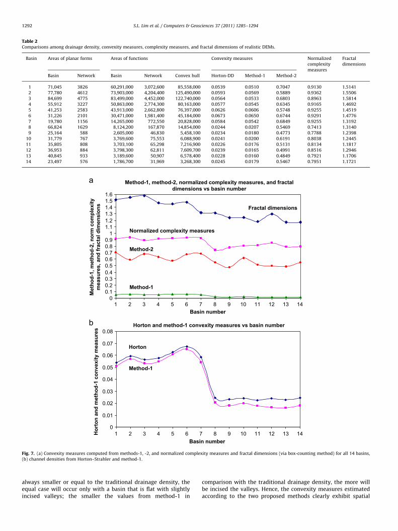
Table 2Comparisons among drainage density, convexity measures, complexity measures, and fractal dimensions of realistic DEMs.
Basin Areas of planar forms Areas of functions Convexity measures Normalized
complexity
measures
Fractal
dimensions
Basin Network Basin Network Convex hull Horton-DD Method-1 Method-2
1 71,045 3826 60,291,000 3,072,600 85,558,000 0.0539 0.0510 0.7047 0.9130 1.5141
2 77,780 4612 73,903,000 4,204,400 125,490,000 0.0593 0.0569 0.5889 0.9362 1.5506
3 84,699 4775 83,499,000 4,452,000 122,740,000 0.0564 0.0533 0.6803 0.8963 1.5814
4 55,912 3227 50,863,000 2,774,300 80,163,000 0.0577 0.0545 0.6345 0.9165 1.4692
5 41,253 2583 43,913,000 2,662,800 76,397,000 0.0626 0.0606 0.5748 0.9255 1.4519
6 31,226 2101 30,471,000 1,981,400 45,184,000 0.0673 0.0650 0.6744 0.9291 1.4776
7 19,780 1156 14,265,000 772,550 20,828,000 0.0584 0.0542 0.6849 0.9255 1.3192
8 66,824 1629 8,124,200 167,870 14,854,000 0.0244 0.0207 0.5469 0.7413 1.3140
9 25,164 588 2,605,000 46,830 5,458,100 0.0234 0.0180 0.4773 0.7788 1.2398
10 31,779 767 3,769,600 75,553 6,088,900 0.0241 0.0200 0.6191 0.8038 1.2445
11 35,805 808 3,703,100 65,298 7,216,900 0.0226 0.0176 0.5131 0.8134 1.1817
12 36,953 884 3,798,300 62,811 7,609,700 0.0239 0.0165 0.4991 0.8516 1.2946
13 40,845 933 3,189,600 50,907 6,578,400 0.0228 0.0160 0.4849 0.7921 1.1706
14 23,497 576 1,786,700 31,969 3,268,300 0.0245 0.0179 0.5467 0.7951 1.1721
Method-1, method-2, normalized complexity measures, and fractaldimensions vs basin number
00.10.20.30.40.50.60.70.80.91
1.11.21.31.41.51.6
1Basin number
Met
hod-
1, m
etho
d-2,
nor
m c
ompl
exity
mea
sure
s, a
nd fr
acta
l dim
ensi
ons
Horton and method-1 convexity measures vs basin number
0
0.01
0.02
0.03
0.04
0.05
0.06
0.07
0.08
1Basin number
Hor
ton
and
met
hod-
1 co
nvex
ity m
easu
res
Method-1
Method-2
Normalized complexity measures
Fractal dimensions
Horton
Method-1
2 3 4 5 6 7 8 9 10 11 12 13 14
2 3 4 5 6 7 8 9 10 11 12 13 14
Fig. 7. (a) Convexity measures computed from methods-1, -2, and normalized complexity measures and fractal dimensions (via box-counting method) for all 14 basins,
(b) channel densities from Horton–Strahler and method-1.
S.L. Lim et al. / Computers & Geosciences 37 (2011) 1285–12941292
always smaller or equal to the traditional drainage density, theequal case will occur only with a basin that is flat with slightlyincised valleys; the smaller the values from method-1 in
comparison with the traditional drainage density, the more willbe incised the valleys. Hence, the convexity measures estimatedaccording to the two proposed methods clearly exhibit spatial

S.L. Lim et al. / Computers & Geosciences 37 (2011) 1285–1294 1293
variability of the basins, especially with those homotopically similarbasins with different altitude-ranges.
On the basis of Table 2, we note that the Hortonian drainagedensity computed in case of Cameron basins have a range of0.0539–0.0673, while in Petaling basins, the range falls within0.0226 to 0.0245. All fourteen sub-basins have different areas ofplan views, and generally the Cameron basins have larger basinareas and network lengths than do Petaling basins. Thus, theHortonian drainage density ranges of Cameron basins are largerthan those of Petaling basins. In fact, the same trend is observedalso from the convexity measures obtained from methods-1 and -2.These convexity measures yield the ranges of 0.051–0.065 and0.0160–0.0207, and 0.5748–0.7047 and 0.4773–0.6191, withCameron basins and Petaling basins, respectively. These resultsmatch the trend observed from convexity measures computed viamethods-1 and -2 in cases of fractal basin functions, i.e. theconvexity measure varies with the altitude-ranges of the basins.The higher the altitude-range of the basin, the greater is theconvexity measure, and vice versa.
To investigate the relationship between these convexity mea-sures and complexity measures of Cameron basins and those ofPetaling basins, normalized complexity measures (roughnessvalues) are generated by following the method explained in Tayet al. (2007). Significantly, a clear distinction exists in the complex-ity measures between the Cameron basins and Petaling basins asthe Cameron basins are highland and mountainous regions, whilePetaling basins comprise relatively low and flat terrain. As such, theroughness values of Cameron basins are generally greater than thatof Petaling basins. This statement is justified by the result shown inTable 2, where the ranges of normalized complexity measures ofCameron basins are 0.8963–0.9362, and 0.7413–0.8516 withPetaling basins. Besides, the fractal dimensions of the basin-wisechannel networks (Fig. 4c, d) extracted from DEMs of CameronHighlands and Petaling regions also indicate a clear distinctionbetween these two regions (see last column of Table 2).Fractal dimensions of these networks are calculated using thebox-counting method, where extracted networks of both DEMsare taken as foreground objects. It is noticed from Fig. 4c, dthat Petaling sub-basins have a sparser network in comparisonto the intricate denser network found in Cameron sub-basins. Thisobservation is reflected in the fractal dimensions in Cameron basins(1.3192–1.5814) and Petaling (1.1706–1.314) basins. Fig. 7a, bshow a better view of the relationships among these variousparameters. From these graphs, we can infer that Cameron basins,which have higher altitude basins than do low-lying Petalingbasins, show higher drainage densities and convexity measures(whether Horton, method-1, or method-2), higher normalizedcomplexity measures, and also higher fractal dimension valuesthan do Petaling basins. Besides, unlike the case of synthetic basinand fractal basin functions, the convexity measures obtained frommethods-1 and -2 with Cameron and Petaling basins correspondwell with the Horton drainage density. Furthermore, it is interest-ing to note from Fig. 7b that the convexity measure from method-1follows closely the Horton drainage density. Hence, we conjecturethat our proposed methods-1 and -2 offer alternative ways toquantitatively characterize basins, complementing already exist-ing quantitative geomorphometric techniques.
5. Conclusion
Factors such as climate, soil permeability, and several otherhydrologically relevant parameters affect geomorphological pro-cesses within a basin, besides physical characteristics includingrelief levels. In this paper, we investigate the changes in convexitymeasures due to different elevation ranges of basins with similar
geometrical arrangement. From our results, it is conspicuousthat planimetric based Hortonian drainage density is of limiteduse. Our proposed function-based convexity measures not onlycould capture the spatial variability between basins with differentaltitudes, but they are also appropriate quantitative geomorpho-metric parameters. Many quantitative geomorphometric para-meters derived from conventional map-based feature analysisare terrain independent, whereas our proposed convexitymeasures, which are computed through these function-basedapproaches are clearly terrain dependent. An interesting openproblem is that of validation of the relationship between theseconvexity measures of realistic basins that possess differentphysiographic set-ups. In summary, we provide a method/approach to estimate the convexity measure of a basin when itis considered to be a function rather than a set. These convexitymeasures, which are related to fractals and granulometric analysis,derived via geometry-based techniques, provide new insights tothe exploration of further links with various other established andto be derived parameterized morphometric measures. The study onthe drawing of scale-invariant characteristics from these convexitymeasures has a potential scope in this investigation.
References
Band, L.E., 1993. Extraction of drainage networks and topographic parameters fromdigital elevation data, Channel Network Hydrology. Wiley, pp. 13–42.
Chockalingam, L., Sagar, B.S.D., 2005. Morphometry of networks and non-networkspaces. Journal of Geophysical Research 110, B08203.
Horton, R.E., 1945. Erosional development of streams and their drainage basins:hydrological approach to quantitative morphology. Bulletin of the GeophysicalSociety of America 56, 275–370.
Howard, A.D., 1997. Badland morphology and evolution: interpretation using asimulation model. Earth Surface Processes Landforms 22, 211–227.
Jenson, S.K., Domingue, J.O., 1988. Extraction of topographic structures from digitalelevation data and geographic information system analysis. PhotogrammetricEngineering and Remote Sensing 54 (11), 1593–1600.
Kirkby, M.J., 1993. Long term interactions between networks and hillslopes, ChannelNetwork Hydrology. John Wiley, New York, pp. 255–293.
Kirkby, M.J., 1980. The stream head as a significant geomorphic threshold, Thresh-olds in Geomorphology. Allen and Unwin, London, pp. 53–73.
Lim, S.L., Sagar, B.S.D., 2008. Cloud field segmentation via multiscale convexityanalysis. Journal of Geophysical Research 113 (D13208). doi:10.1029/2007JD009369.
Lindsay, J.B., 2005. The terrain analysis system: a tool for hydro-geomorphicapplications. Hydrological Processes 19, 1123–1130.
Mandelbrot, B.B., 1982. The Fractal Geometry of Nature. Freeman, San Francisco,California.
Maragos, P., 1989. Pattern spectrum and multiscale shape representation. IEEETransactions on Pattern Analysis and Machine Intelligence 11 (7), 701–716.
Marani, M., Belluco, E., D’Alpaos, A., Defina, A., Lanzoni, S., Rinaldo, A., 2003. On thedrainage density of tidal network. Water Resources Research 39 (2),4.1–4.11. doi:10.1029/2001WR001051.
Montgomery, D.R., Dietrich, W.E., 1994. Landscape dissection and drainage area-slope thresholds, Process Models and Theoretical Geomorphology. John Wiley,New York, pp. 221–246.
Montgomery, D.R., Dietrich, W.E., 1989. Source areas, drainage density, and channelinitiation. Water Resources Research 25 (8), 1907–1918.
O’Callaghan, J.F., Mark, D.M., 1984. The extraction of drainage networks from digitalelevation data. Computer Vision, Graphics, and Image Processing 28, 323–344.
Sagar, B.S.D., Srivinas, D., Rao, B.S.P., 2001. Fractal skeletal based channel networks ina triangular initiator basin. Fractals 9 (4), 429–437.
Sagar, B.S.D., Tien, T.L., 2004. Allometric power-law relationships in a HortonianFractal DEM. Geophysical Research Letters 31 (6), L06501.
Sagar, B.S.D., Venu, M., Srivinas, D., 2000. Morphological operators to extract channelnetworks from digital elevation models. International Journal of RemoteSensing 21 (1), 21–30.
Schumm, S.A., Mosley, M.P., Weaver, W.E., 1987. Experimental Fluvial Geomor-phology. John Wiley, New York.
Serra, J., 1982. Image Analysis and Mathematical Morphology. Academic Press,London.
Soille, P., 1998. Gray scale convex hulls: definition, implementation and application.In: Proceedings of the ISMM’ 98, Kluwer Academic Publishers.
Strahler, A.N., 1964. Quantitative geomorphology of drainage basins and channelnetworks. In: Chow, V.T. (Ed.), Handbook of Applied Hydrology. McGraw-Hill,New York.
Tarboton, D.G., 1997. A new method for the determination of flow direction andcontributing area in grid digital elevation models. Water Resources Research 33(2), 309–319.

S.L. Lim et al. / Computers & Geosciences 37 (2011) 1285–12941294
Tarboton, D.G., Ames, D.P., 2001. Advances in the mapping of flow networks fromdigital elevation data. World Water and Environmental Resources CongressMay, 20–24 Orlando, Florida.
Tarboton, D.G., Bras, R.L., Rodriguez-Iturbe, I., 1991. On the extraction of channelnetwork from digital elevation data. Hydrological Processes 5, 81–100.
Tarboton, D.G., Bras, R.L., Rodriguez-Iturbe, I., 1992. A physical basis for drainagedensity. Geomorphology 5 (1–2), 59–76.
Tay, L.T., Sagar, B.S.D., Chuah, H.T., 2007. Granulometric analyses of basin-wiseDEMs: a comparative study. International Journal of Remote Sensing 28 (15),3363–3378.
Tucker, G.E., Bras, R.L., 1998. Hillslope processes, drainage density, and landscapemorphology. Water Resources Research 34 (10), 2751–2764.
Tucker, G.E., Catani, F., Rinaldo, A., Bras, R.L., 2001. Statistical analysis of drainagedensity from digital terrain data. Geomorphology 36, 187–202.
Related Documents