Computers & Geosciences A work ow to facilitate three ...members.unine.ch/philippe.renard/articles/maxelon2009.pdfA work ow to facilitate three-dimensional geometrical modelling of

Author's personal copy

A workflow to facilitate three-dimensional geometrical modellingof complex poly-deformed geological units

Michael Maxelon a, Philippe Renard b,�, Gabriel Courrioux c,Martin Brandli d, Neil Mancktelow a

a Geological Institute, ETH Zurich, CH 8092 Zurich, Switzerlandb University of Neuchatel, Centre of Hydrogeology, Rue Emile Argand 11, CP-158, CH 2009 Neuchatel, Switzerlandc BRGM, B.P. 6009, F 45060 Orleans cedex, Franced WSL, Zurcherstrasse 111, CH 8903 Birmensdorf, Switzerland

a r t i c l e i n f o

Article history:

Received 5 October 2007

Received in revised form

30 May 2008

Accepted 11 June 2008

Keywords:

3D modelling

Workflow

Database

GIS

Visualization

Interpolation

Folds

a b s t r a c t

The three-dimensional (3D) geometry of complexly deformed regions is often beyond

the scope of simple 2D and 2.5D representation in cross-sections and block diagrams.

Methods must be developed for fully three-dimensional representation. A workflow for

such three-dimensional modelling of structurally complex areas is presented. Data

requirements are tailored to typical results of structural field work in strongly deformed

rocks from mid-crustal levels. The workflow is based on data evaluation and data export

using standard geographical information system and database management systems.

Three-dimensional modelling in polyphase deformed areas is highly dependent on the

correct interpretation of variations in the orientation of the dominant planar fabrics.

The computer-aided earth-modelling software 3D GeoModeller is well adapted for

managing this problem. It calculates the geometry of geological interfaces taking into

account simultaneously the foliation data and location of lithological contacts. The

workflow is based on iterative model refinement based on interactive editing of the

geometry in section and map views with data assessment and pre-processing using GIS

software. This approach assures internal consistency of the resulting three-dimensional

models. Modelling of the Lower Lepontine Nappes in the Central Alps is used as an

illustrative example from a complexly deformed terrain.

& 2008 Elsevier Ltd. All rights reserved.

1. Introduction

Disentangling the polyphase deformation history instructurally complex areas is always a challenging task(e.g., Ramsay, 1967). This is especially true in mid-crustallevels where several successive ductile deformationphases entailing km-scale isoclinal recumbent foldingand regional-scale thrusting may occur. Developing aninternally consistent model of such areas can be verydifficult (compare examples in Milnes, 1974; Steck, 1984;

Brunel, 1986; Pognante et al., 1990; Spring and Crespo,1992; Grujic and Mancktelow, 1996). Moreover, mid- andlower-crustal tectonic levels are generally dominated bymagmatic or metamorphic crystalline basement rockswith typically rather low contrasts in their geophysicalproperties. Reflection seismic investigations are thereforelimited in their ability to provide independent constrainton the scale of hundreds of metres or a few kilometres.However, it is specifically these tectonic levels thataccommodate much of the deformation occurring duringcontinental collision and they are key elements in under-standing the geodynamics and kinematics of orogenicbelts (e.g., Manatschal et al., 1998; Weijermars and Khan,2000; Gerya et al., 2002; Stockhert and Gerya, 2004). It is

Contents lists available at ScienceDirect

journal homepage: www.elsevier.com/locate/cageo

Computers & Geosciences

ARTICLE IN PRESS

0098-3004/$ - see front matter & 2008 Elsevier Ltd. All rights reserved.

doi:10.1016/j.cageo.2008.06.005

� Corresponding author. Tel.: +4132 718 26 90; fax: +4132 718 26 03.

E-mail address: [email protected] (P. Renard).

Computers & Geosciences 35 (2009) 644–658


therefore crucial to establish the three-dimensional (3D)geometry of such regions as exactly as possible, in order toprovide a reliable benchmark for models of continentalcollision.

In the absence of good geophysical control on thesubsurface geometry of geological units, it is left toborehole measurements, tunnelling data, remote sensingand especially field observations to provide the informa-tion required to build a three-dimensional geologicalmodel. Boundaries between different lithological units(i.e., lines of outcrop), knowledge about possible correla-tions of these units (mainly from petrological examina-tion) and recognition of geometric and kinematicconstraints (from structural observations) are the princi-pal inputs from field-based geological investigations.This information can be combined to develop a modelof the geometry of the geology in three dimensions,often illustrated in a series of cross-sections or as a blockdiagram (e.g., see the description and instructive exam-ples in Meyer, 1991; Steck and Hunziker, 1994 and Steck,1998). Agreement with outcrop lines and internal con-sistency provide important visual cross-checks, but theseare more readily and thoroughly controlled in truly three-dimensional models. Whereas a lack of data from areasthat are difficult to access can be partially compensatedby remote sensing (e.g., Alwash and Zakir, 1992), theinsufficient density of subsurface data cannot normallybe overcome, which generally leaves considerable free-dom for different possible interpretations (Renard andCourrioux, 1994).

Two main approaches to modelling such complexgeometries can be distinguished. Explicit modelling usesan explicit definition of each object in the model. Surfacesbounding the different formations are defined (forexample with triangulated surfaces, two-dimensionalgrids, or parametric surfaces) and constructed by inter-polation of the data (e.g., Renard and Courrioux, 1994). Inthis context, a wide variety of interpolation techniquesare used including geostatistics (Chiles and Delfiner,1999), splines, Bezier surfaces (de Kemp, 1999) or discretetechniques such as discrete smooth interpolation (Mallet,1989). This last method can accommodate many differenttypes of constraints involving a single object or relationsbetween different objects (Mallet, 2002). Implicit model-

ling uses an implicit definition of the geological interfaces,which are defined as the iso-surfaces of one or severalscalar fields in three-dimensional space. Orientation datarepresent normal vectors (dip direction, dip, youngingdirection/polarity) to these equipotential lines/planes andare thus regarded as the gradient of the correspondingscalar field. Again, the scalar field is obtained by three-dimensional interpolation, but one advantage of thisapproach is that it allows a set of surfaces accountingfor all orientation data to be modelled simultaneously(e.g., Cowan et al., 2003; Lajaunie et al., 1997; Turk andO’Brien, 2002).

There are advantages and disadvantages in bothapproaches. Explicit modelling allows a great deal ofinteractive modification of each interface. On the otherhand, the orientation constraints that can be regardeddirectly in an automated manner are restricted, because

these data need to be related to a well defined surface. Inorder to overcome this problem, different approaches andtools providing a means for independent evaluation oflarge datasets prior to modelling have been presented(e.g., Cobbold and Barbotin, 1988; de Kemp, 1999;de Kemp, 2000; Gumiaux et al., 2003). The explicitapproaches are implemented in computer programs likeSURPAC or GOCAD. With implicit modelling, both contactlocations and orientation constraints (not only on thecontact surfaces) can be considered simultaneously. Thisapproach provides less freedom to interactively modifyindividual surfaces once the model is set up and thiscan be a shortcoming if specific geometries are to bemodelled. On the other hand, this can be a significantadvantage because data updates or new constraints can beadded easily. The computer programs 3D GeoModellerand (to some extent) EarthVision follow such an approach.

While these techniques are nowadays available inseveral computer codes, their application to a specificcase study requires the collection and management of alarge amount of data. The preparation of the data, theirformatting, and their comparison or selection oftenrequires a considerable amount of work. In practice,these tasks require the use of geographic informationsystems (GIS) and database management systems (DBMS)(Schetselaar, 1995; McCaffrey et al., 2005; Bond et al.,2007). In this paper, we present a workflow to facilitatethe process of data acquisition, data management, andmodelling of complex poly-deformed geological forma-tions. The workflow is based on the use of GIS (ESRIArcGis) for the data management and pre- and post-processing, and on computer-aided earth-modellingtools (CAEM; mainly 3D GeoModeller) for the three-dimensional modelling. The workflow is focused onimplicit modelling with GeoModeller, since this programis the most convenient for handling the type of data that iscollected and used in such complexly deformed terrains(e.g., Martelet et al., 2004; Talbot et al., 2004; Maxelonand Mancktelow, 2005; Joly et al., 2008). The mainadvantage of 3D Geomodeller is its interpolation method,which uses a potential-field approach (Lajaunie et al.,1997; Chiles et al., 2006; Calcagno et al., in press).The method defines a function T(x, y, z) interpolated byco-kriging from points located on interfaces, considered ashaving a common (unknown) potential value for eachinterface, and directional data representing the gradient ofT. Thanks to the dual form of the co-kriging, it is possibleto solve the system just once, and then use it as aninterpolator to estimate T at any point p in space. Thisproperty allows each interface to be defined as a specificisovalue of the potential field, using algorithms such as amarching cube. The approach is particularly powerful inmodelling complex three-dimensional foliation trajec-tories, with only one point per trajectory (e.g., the gridcoordinates and height of a lithological contact in thefield) necessary to define a fully three-dimensional virtualinterface that accords with the regional orientationmeasurements.

After presenting an overview of the workflow, thepaper describes more precisely the different aspects ofthe proposed approach, from the database structure to the

ARTICLE IN PRESS

M. Maxelon et al. / Computers & Geosciences 35 (2009) 644–658 645


different stages involved in building a three-dimensionalmodel. The different steps are illustrated with an examplefrom the Pennine zone in the Central Alps, which isprobably the most extensively studied example of arefolded mid-crustal nappe sequence, with a very ex-tensive database of observations, maps and orientationmeasurements reflecting over 150 years of research.

2. Workflow overview

The proposed workflow (Figs. 1 and 8) facilitates thethree-dimensional modelling of geological formationsthat have been affected by polyphase deformation,resulting in a tectonostratigraphy that is characterizedby a pervasive planar fabric. This planar fabric is assumedto have formed coevally with the principal tectonic event(normally regional isoclinal folding or thrusting) and tohave obliterated older tectono-stratigraphic limits. Suchproblems can be addressed by a two-stage modellingprocedure, which first assesses the orientation field andsubsequently outlines geological limits according to theorientation field, constrained by further information(e.g., younging direction, cleavage/bedding intersection,vergence of parasitic folds).

The basic workflow (Fig. 1) uses available software(ESRI ArcGis, MS Access, and GeoModeller), complemen-ted by a set of programs and macro-routines for datapreparation, data exchange and necessary data interfaces,where these are not provided by the software packagesthemselves.1

Typical field-derived measurements and interpreta-tions are made consistent through the definition of a datastructure implemented in a DBMS. Interpretations, mostlyintroduced as cross-sections, are used to constrain themodel. MsAccess and ArcGIS are used for central dataorganization, for editing features in two dimension, suchas field data points, lines and polygons, as well as for pre-processing of the data. The GIS provides data interfaces toimport raw georeferenced one- and two-dimensional datathrough integrated database connections. Tabular data inASCII- or .dbf-format specifying x- and y-coordinates andother characteristic attributes (e.g., measurements) pro-vide another import possibility.

ARTICLE IN PRESS

Databasegeodatabase

includingstandard

database part(MS Access)

Data acquisition inthe field

(i.e. field work)

Aqcuisition ofexisting data

(literature work etc.)

Assessment ofdata quality and

relevance

Export filters written inVisual Basic for

Applications (VBA) tomeet data requirementsfor 3D GeoModeller

and assign spatial criteria(geologic affiliation,

polarity etc.)

3DGeoModeller

3D-modelling in 3DGeoModeller

GIScoeval and customisablevisualisation of data onmaps in GIS (ArcMap)

External sourceof DigitalElevationModels

ImportRoutine

provided byGIS

Export ofDigital

ElevationModels as

ASCII files instandardised

format

Externalexportroutine

written inVisual Basic

Export routine forMIF-file format (in

ArcToolbox):All 2D views canbe exported fromEG in MIF formatand imported into

GIS

DB-Queries

preselectingdata available

for visuali-sationin GIS

MS JetDatabase

Connection

Editing featuresin ArcMap (point, line and polygon

data)

Direct access tofeature data

(points, lines etc)

Digital ElevationModels already

available in ESRIASCII format

Fig. 1. Flow-chart describing our complete three-dimensional modelling procedure. Single processes are discussed in the text. Process labelled 3D

GeoModeller is described more precisely in Fig. 8.

1 Maxelon, M., 2004. Some tools for three-dimensional model-

ing in structural geology and tectonics. Available online through:

http://e-collection.ethbib.ethz.ch

M. Maxelon et al. / Computers & Geosciences 35 (2009) 644–658646


3. Data source and data structure

The diversity of data types that contribute to a three-dimensional model accentuates the need for a clear datastructure. In the rest of this paper, the word data will beused in a broad sense to describe any information usedand stored to build the three-dimensional model andincludes both measurements and interpretations. Not onlydo data differ in types of geometry (points, lines, areas),they can also have a vectorial meaning (lineations,cleavages) or only be relevant for specific steps in themodelling process (e.g., different generations of folia-tions). A further distinction should be made with respectto the origin of the data: they can originate from fieldwork (and are thus raw data) or from preliminaryinterpretation (e.g., cross-sections). Furthermore, digitalelevation models play an important role and need to beincorporated in the workflow.

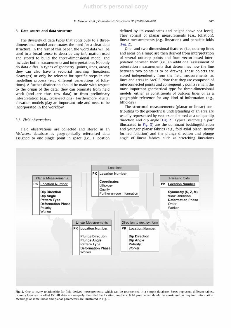
3.1. Field observations

Field observations are collected and stored in anMsAccess database as geographically referenced dataassigned to one single point in space (i.e., a location

defined by its coordinates and height above sea level).They consist of planar measurements (e.g., foliation),linear measurements (e.g., lineation), and parasitic folds(Fig. 2).

One- and two-dimensional features (i.e., outcrop linesand areas on a map) are then derived from interpretationof several outcrop points and from vector-based inter-polation between them (i.e., an additional assessment oforientation measurements that determines how the linebetween two points is to be drawn). These objects arestored independently from the field measurements, aslines and areas in ArcGIS. Note that they are composed ofinterconnected points and consequently points remain themost important geometrical type for three-dimensionalmodels, either as constituents of outcrop lines or as ageographic reference for any kind of information (e.g.,lithology).

The structural measurements (planar or linear) con-tributing to the geometrical understanding of an area areusually represented by vectors and stored as a unique dipdirection and dip angle (Fig. 2). Typical vectors (in partillustrated in Fig. 3) are the dominant bedding/foliationand younger planar fabrics (e.g., fold axial plane, newlyformed foliation) and the plunge direction and plungeangle of linear fabrics, such as stretching lineations

ARTICLE IN PRESS

Fig. 2. One-to-many relationship for field-derived measurements, which can be represented in a simple database. Boxes represent different tables,

primary keys are labelled PK. All data are uniquely identified by location numbers. Bold parameters should be considered as required information.

Meanings of some linear and planar parameters are illustrated in Fig. 3.



(also providing kinematic information) or fold axes(providing geometric information). Often a great deal ofsuch information is referenced to only one single location.As a consequence, multiple property assignments to asingle location are the rule.

In addition, there may be information about symmetry/asymmetry and geometry on a larger scale (cleavage/bedding intersections, parasitic folds; Figs. 3 and 4). Thisinformation is again represented by vectors, for exampleindicating the direction either to the next relevant syn- orantiform (as indicated in Fig. 3). Similarly, during theprocess of data preparation, planar measurements mustbe complemented by a declaration of their polarity

(or younging direction), since describing planar measure-ments in terms of dip direction and dip angle does not initself indicate if bedding or layering is overturned or not.These data dependencies are represented as a simple one-to-many data relationship in the database (Fig. 2). Thecoexistence of several generations of the same observationtype (e.g., foliations assigned to different deformationphases; S1, S2, etc.) at one single location requires that therespective deformation phases must also be recorded.Finally, it is quite common to have several measurementsof the same feature (e.g., fold axis of 2nd phase parasiticfolds) taken at one location. In this case, a decision hasto be made as to how a single representative piece of

ARTICLE IN PRESS

Direction to

next synform

Direction tonext antiform

Fold axis

Fold axial

plane

SnSn+1

Fig. 3. Relevant parameters to be recorded during field data acquisition with respect to an isoclinal parasitic fold. Direction to adjacent major syn-and

antiforms, fold axis, fold axial plane (parallel to a possible newly formed foliation Sn+1) and dominant orientation of folded planar fabric (Sn) are

illustrated. Sketch shows a situation after deformation phase Dn+1.



information can be derived from these multiple dataassignments (e.g., component-wise calculation of anarithmetic mean).

Point data from different workers are stored in thedatabase the same way as personal data are stored, with alocation number uniquely identifying the point and theworker’s name mentioned in the appropriate category(Fig. 2).

The proposed database structure for field observations(Fig. 2) has been kept very simple and limited for thepurposes of the present work. Note however that there is aconsiderable amount of existing work (see McCaffreyet al., 2005) providing more general data models for thedigital collection of geological observations.

3.2. Existing maps and cross-sections

Interpretations from previous studies (e.g., outcroplines and cross-sections) are important pieces of informa-tion that need to be stored in the database. Scannedimages of geological maps are georeferenced in the projectcoordinate system. Outcrop lines are then digitized in anappropriate file format (e.g., Shape file, MapInfo file). Forcross-section data, it is necessary to have the profiledefined by its start and end points (and intermediatepoints if need be), whereas the interpretations (lines onthe cross-section) themselves are recorded in a (u,v)-coordinate system, defined by distance from the origin ofthe cross-section (abscissa) and height above sea level(ordinate). Geometries digitized in this way can then beimported into 3D GeoModeller either to add additionalconstraints to the model or for comparison purposes.

3.3. Digital elevation models

The digital elevation models (DEMs) provide vitalinformation about exact positions of georeferenced datain the three-dimensional space. Advanced remote sensingtechniques (e.g., Franklin and Giles, 1995; Zomer et al.,2002) have made them available also in less developedcountries and in areas difficult of access. DEM data aremostly provided in formats that are compatible withstandard GIS software.

With the aid of the DEM, preliminary three-dimensionalassessment is possible by calculating a hill shade andcombining it with polygon geometries representing therespective geological units (two-dimensional image withshading, see Fig. 5). Alternatively, the DEM can be used asa source for elevation data that are then assigned to therespective points of the two-dimensional geometries inthe three-dimensional space (Fig. 6).

4. Data processing using GIS

The data described in the previous section are madeavailable by database connections between ArcGIS andMsAccess and can be exported in the appropriate fileformat using customized macro-routines (e.g. see footnote 1).Export from the GIS software works in two directions:backward into the DBMS and forward into the CAEM tool.The former case offers the opportunity to store additionalinformation (like polarities) and newly compiled geome-tries (like fold axial traces) in the database. The latterprovides the data input interface for introducing raw, pre-processed data, or interpretations into the CAEM tool.

ARTICLE IN PRESS

Sn

Sn+1 || FAP

n+1

Sn+1 || FAP

n+1 || Sn

Polar

ity S n

: -1

Polar

ity S n

: +1

Sn+1 crosscuts Sn

Fig. 4. Schematic sketch showing a folded older planar element (Sn; bedding or fabric) crosscut by a younger planar fabric (Sn+1) parallel to the fold axial

plane (FAPn+1) in an hinge region of the fold. In limb regions, Sn+1 approximately parallels Sn, but Sn has opposite younging directions (polarities). Such

folds often result in the identical geological interface occurring at two elevation levels (duplicate assignment of a z-value to an (x,y)-coordinate pair) and

are therefore difficult to visualize in 3D GIS viewers like ArcScene.



Furthermore, data evaluation within GIS using eitherthe built-in tools or the custom-made routines allowspreliminary assessment of structural data. This varietyof data management and processing tools makes GIS aconvenient data distributing centre for comprehensivethree-dimensional modelling.

4.1. Data analysis and preparation in GIS

Data management in GIS software involves twoimportant aspects. On the one hand, data can already beefficiently analyzed there, saving time during the latermodelling process. Such work takes advantage of the

possibility to display several different data types synopti-cally and then process them with Visual Basic forApplications (VBA) routines. On the other hand, topologi-cal relationships allow properties to be assigned to singlepoints, which is necessary for later processing during thethree-dimensional modelling (e.g., younging direction,geological affiliation).

4.2. Structural assessment and profile construction

A basic understanding of the geometry of the areaat the beginning of the actual three-dimensional model-ling procedure provides important insights for ensuring

ARTICLE IN PRESS

5/405/402/442/44

6/696/698/668/664/604/602/462/464/494/49

7/637/63

56/8656/8613/8013/8019/6419/6415/5715/57

42/7642/7617/5917/59

43/5443/5472/8072/8019/6919/6928/5228/5213/5913/5917/5417/5411/6311/63

97/4397/4347/8647/8679/8379/83

80/5580/5555/7055/7083/5583/55

85/4485/4480/3680/3697/3797/3796/7896/7885/7085/7059/6759/67

69/3769/3775/3075/3061/3161/3129/5029/5084/4484/4499/6699/6686/6586/6579/6979/69

84/3584/3558/2858/2889/6589/6583/6083/6084/5984/59

84/3484/3493/5293/5282/6482/6480/5080/5084/4484/44

66/1866/1879/5179/5179/6279/6292/3792/3791/4491/44

44/1944/1922/1722/1769/5069/5083/6083/6086/7186/7191/4191/4190/3890/38

15/1815/1877/2177/2185/1785/1770/5070/5088/5788/5789/5889/5882/5582/5583/3583/35

64/3264/3265/2165/2184/6184/6189/5789/5777/6577/6583/5583/5582/3782/37

79/2679/2676/6276/6248/2348/2384/5184/5170/5570/5587/4487/44

349/62349/62156/77156/77357/42357/42

359/51359/51148/68148/68153/47153/47132/54132/54359/42359/42355/56355/56349/77349/77

133/52133/52150/54150/54175/59175/59193/70193/70323/62323/62355/78355/78

130/38130/38151/45151/45188/49188/49190/53190/53174/60174/60236/37236/37201/31201/31201/41201/41234/52234/52184/65184/65113/64113/64

141/33141/33145/37145/37161/44161/44191/53191/53241/19241/19235/27235/27207/28207/28202/35202/35164/60164/60177/76177/76110/89110/89

126/20126/20309/34309/34270/16270/16232/20232/20227/27227/27225/37225/37161/66161/66167/82167/82

264/47264/47239/21239/21225/34225/34201/45201/45187/70187/70114/74114/74

226/34226/34222/32222/32233/34233/34232/33232/33234/32234/32210/34210/34169/43169/43104/66104/66

210/22210/22215/22215/22234/27234/27235/31235/31219/30219/30227/34227/34229/43229/43116/42116/42

197/32197/32250/23250/23245/23245/23243/11243/11204/20204/20132/36132/36246/30246/30216/57216/57

200/15200/15225/19225/19241/21241/21260/10260/10226/13226/13129/32129/32121/28121/28

353/26353/26235/30235/30221/17221/17221/17221/17206/21206/21

354/36354/36236/24236/24217/18217/18205/12205/12206/25206/25257/38257/38324/38324/38

211/19211/19190/17190/17221/20221/20181/26181/26194/74194/74109/78109/78101/38101/38

A

B

Fig. 5. Inset of a tectonic map from the Central Alps of Switzerland (simplified after Preiswerk et al., 1934), combined with a hill shade calculated from

corresponding DEM. Easier correlation of outcrop lines in space (compared to standard map views) facilitates a first visual three-dimensional assessment.

Orientation data are spatially averaged from a set of 2964 measurements with the VBA macro Profile Calculation (see footnote 1). SW–NE trending line

indicates location of cross-section shown in Fig. 7.



consistency and trustworthiness of the later modellingresults.

Two VBA routines (see footnote 1) help to envisagestructural relationships and speed up typical tasks duringtectonic assessment. The routine Orientation Averaging

produces an evenly spaced grid of average orientationscalculated from measurements situated within a givendistance (also inverse distance weighted if required). Fig. 5shows an example of the application of this tool. Theroutine Profile Calculation automatically creates a cross-section considering both the underlying DEM and thedifferent geological units crossed by the profile trace(Fig. 7). Averaged orientation values can be calculatedfrom measurements situated within a given circularregion (i.e., a buffer) around those points along the profiletrace. Furthermore, they can be assigned to the cross-section at equal intervals, also accounting for theirapparent dip angle (e.g., Flick et al., 1972).

4.3. Polarity assignments

In structurally complex areas characterized by mainlyductile deformation, regional-scale recumbent isoclinalfolding is frequently observed (e.g., Milnes, 1974). Suchdeformation typically entails the development of a new

pervasive planar fabric (Sn+1) parallel to the fold axialplanes of the respective folds (Fig. 4). If this new foliationis the dominant foliation, which is often the case, thelimits of the folded unit (i.e., Sn) are easily obliterated.However, in regionally important hinge zones, the olderfabric (or the bedding) is sometimes preserved and theposition and orientation of regional hinges can then bedetermined in the field. In limb regions, the younger fabricis often parallel to the older fabric (Fig. 4), but withrespect to this older fabric a change of the polarity has tobe taken into account. Therefore correct planar measure-ments can only be obtained in such regions if the positionrelative to regional fold structures is known (e.g., fromparasitic fold vergences or Sn/Sn+1 relationships; Figs. 3and 4).

The axial traces of regional-scale folds are linearfeatures that can usually be established in some detailduring a field study. Foliation measurements from eitherside of such an axial trace are assigned a different polarityreflecting their position on opposite limbs and polygonsdefining such areas of different polarity can be easilyconstructed in Arc Map. The result is a series of bands ofdifferent polarity separated by the axial trace of folds,which may even be isoclinal. This tedious work canbe readily done by a VBA routine (e.g., routine Export

Planar Measurements, see footnote 1). Such a routineallows topological relationships between planar measure-ments (i.e., point data) and areas of a constant property(i.e., polygons) to be considered and assigns geologicalaffiliations and polarity information to the respectiveplanar measurements (or other point data).

5. Three-dimensional modelling

For polyphase deformation, including regional devel-opment of a new pervasive planar fabric, a two-stepapproach is suggested. First, the younger deformationsrecorded in regional orientation pattern of planar mea-surements are investigated. Then, these results arecombined with information about older deformationphases, coeval with the formation of the dominantfoliation, so as to develop a comprehensive model of thetectono-stratigraphic relationships. The three-dimensionalmodelling part of the workflow (Fig. 8) will be discussedconsidering the map in Fig. 9 as an example.

ARTICLE IN PRESS

Fig. 6. Perspective view of two-dimensional map also shown in Fig. 5.

Polygons corresponding to geological units are draped onto DEM.

0

0

5000

5000

10000

10000

15000

15000

20000

20000

25000

25000

30000

30000

-2000 -2000

0 0

2000 2000

4000 4000A B

Fig. 7. Cross-section calculated with routine Profile Calculation developed in Arc Map (see footnote 1). Profile trace is indicated in Fig. 5. Affiliation with

different geological units (i.e., different colours in the section) and orientation indicators (i.e., black lines underlain in green) were produced automatically.

Units are metres.



5.1. Step 1—visualization of the foliation field

In 3D GeoModeller, a three-dimensional model can becalculated considering all available planar measurements

(i.e., typically foliations), but with only one (more or lessarbitrarily chosen) outcrop point per tectonic or litholo-gical unit fixing its structural level. To establish this, allgeological entities must be defined in the software as

ARTICLE IN PRESS

DigitalElevation

Model (DEM)

OutcropLines

Import into3D

GeoModeller

Create planar profiles in 3DGeoModeller according to trendsof orientation data in map view

Create as many artificial formationsin one ‚showcase series’ as

independent fold structures (coevalto the dominant foliation) exist

Create additional cross-sections needed for import

of 3rd party data (e.g. cross-sections of other workers)

Fold axialtraces

Yes No

Import into3D

GeoModeller

Orientations withpolarities recorded

in the field ordefault polarities

Assign each fold axialtrace to one formation

Calculate foliation field in3D GeoModeller only

taking data situated on thetopography into account

Calculate curved profilesfrom respective potential

field levels

Import into3D

GeoModeller

Delete data on thetopography (i.e. fold axialtraces and orientations

StoredMapInfo Files

Orientation data withpolarities respecting

fold axial traces coevalto the foliations

As backgroundinto planar

cross-sections

Outcrop lines

Geologic boundariesand orientation datafrom 3rd party cross-

sections

Import into3D

GeoModeller

Digitise geometries in planarcross-sections regarding

foliation field in the background

Digitise hinge-lines and specifycurvature in curved cross-

sections

Create as many series asgeologic units are to be modelledand name them according to theoutcrop line and orientation data

Visualise trajectories inall planar cross-sections

Export trajectories asMapInfo files

Import into3D

GeoModeller

Create additional cross-sections needed for import of

3rd party data (e.g. cross-sections of other workers)

Create planar cross-sections as developed

beforehand

Digitise geologicboundaries in cross-

sectionsCalculate 3D model in 3D

GeoModeller

Consistent 3Dmodel

Polyphased deformedtectonostratigraphy with

foliation?new pervasive

Fig. 8. Flow-chart of modelling procedure inside 3D GeoModeller. Data exchange to other software and data preparation outside GeoModeller are not

regarded in this diagram. Processing chain illustrated here corresponds to process labelled 3D GeoModeller in Fig. 1.



formations and be assigned to one combined series. Allfoliations are then considered in the calculation regard-less of their geological affiliation. The resulting modelledsurfaces represent the regional trend of the foliation fieldin three dimensions, passing through the single chosenoutcrop point. The intersection of a subset of such surfaceswith the topography results in a typical foliation trajec-tory map as illustrated in Fig. 10a.

Instead of being defined by one arbitrary outcrop point,the surfaces representing the foliation field can also beforced to contain more than one point, namely a linedefined by several connected points. This possibility isrelevant for modelling a fold structure coeval with apervasive foliation. If the line corresponds to a fold axialtrace on the topography, the surface created in thismanner will represent the fold axial plane of therespective fold (compare Figs. 4, 9 and 10b). Thus itprovides an important constraint with respect to thepossible fold geometry in three dimensions.

In the much simpler case where the regional trend ofthe dominant planar fabric is defined by the limits ofgeological units, it is obvious that a surface complyingwith the orientation field and forced to follow an outcropline will immediately represent the boundaries of geolo-gical units. It therefore immediately provides an initial,

valid, though probably preliminary, three-dimensionalmodel.

5.2. Step 2—confining the model

If the boundaries between geological units in a studyarea are obliterated by the dominant foliation, theirgeometry can be determined only by careful mapping oflithological limits. Unfortunately, mapping of boundariesmay be equivocal in gneissic units from typical basementterrains and correlations or distinctions between multiplydeformed and possibly polymetamorphic units are there-fore uncertain. In such terrains, structural data (Figs. 3 and4) are crucial for interpreting the geometry. In particular,the three-dimensional trends of fold axial planes, asoutlined in the previous section, can provide stronggeometric constraints throughout a whole volume.Such information helps to identify valid geometric inter-pretations in cross-sections, which can be created in3D GeoModeller in two ways.

(1) Planar profiles are straight cuts through a givenvolume. Their intersection with a horizontal surfaceresults in a straight line, completely described by a

ARTICLE IN PRESS

ID: 1ID: 1

ID: 2ID: 2

ID: 1ID: 1

ID: 2ID: 2

ID: 2ID: 2

Fig. 9. An example of a geological map, illustrating two hypothetical geological units (light and dark grey, corresponding to ID1 in footwall and ID2 in

hanging wall). They are draped upon a hill shade that was calculated from a DEM. Line patterns indicate regions of identical younging direction

(horizontal lines: overturned (i.e., polarity -1); vertical lines: not overturned (i.e., polarity 1). Indicated foliations are coeval with development of folds

(i.e., they are axial plane to these folds).



finite number of points. Typically they are constructedas vertical cuts, with a trace defined by only twopoints.

(2) Curved profiles follow a contorted surface through agiven volume. In 3D GeoModeller, the geometry ofsuch cross-sections can be defined in three-dimensionalspace as an isosurface from a previously calculatedorientation field. Their intersections with a horizontalsurface are mostly curved. They are generally morecomplicated than those of planar profiles, and arenormally not sufficiently described by a small numberof connected points.

5.3. Planar profiles

The trend of planar profiles should be defined withrespect to the regional trend of planar features in thestudy area. Generally it is more convenient to work oncross-sections that run (sub-) perpendicular to the dipdirections, because the effect of apparent dips alongthe profile is then minimized (Flick et al., 1972; Meyer,1991).

After a foliation field has been calculated, therespective foliation trajectories can be visualized in aplanar profile, stored in a MapInfo file, and thenre-imported as a background for the section (Fig. 11b).Such a background aids digitization of geologicalunits, because it depicts the trend of regional-scale foldaxial planes or their parallel translations intersecting thecross-section.

Curved profiles calculated with special attention tofold axial traces are an especially helpful feature, becausetheir intersection with the planar cross-sections providesan excellent guideline for delineating the trace ofregionally important fold axial planes (Fig. 11c).

In the workflow, several planar cross-sections shouldbe constructed in this way. They will act as principalconstituents of the actual modelling. Personally con-structed cross-sections can be complemented by cross-sections from other workers. Fig. 11a shows an example ofone such cross-section, while also presenting the three-dimensional modelling result in the subsurface. However,fold structures as shown in Fig. 13 often have ratherirregular and ragged hinge lines in models calculated onthe basis of planar cross-sections exclusively. This geo-metric shortcoming can be corrected with curved profiles(Fig. 12).

5.4. Curved profiles

As mentioned before, curved profiles are created frompreviously calculated foliation fields. Interface pointsspecifying different levels of this foliation field canbe grouped upon the fold axial traces coeval with thedevelopment of the dominant planar fabric. Then theresulting curved profiles calculated from these levels willcorrespond to the fold axial planes themselves. Forexample, the intersections of the meshed surfaces shownin Fig. 13a with the topography correspond to the foldaxial traces delineated in Fig. 9 (also compare Fig. 10b).

ARTICLE IN PRESS

Fig. 10. (a) Foliation trajectories calculated from planar measurements shown in Fig. 9. Connected point lines correspond to outcrop lines shown in Fig. 9.

Colouring is arbitrary. (b) Surfaces indicating trend of foliation field in three dimensions. Intersections of red, ochre, green and blue meshes with shaded

topography correspond to fold axial traces depicted in Fig. 9.



Two parameters of geometric significance for a fold can bedigitized on such cross-sections: hinge lines and thecurvature of hinges.

Hinge lines can be digitized as a series of equipoten-tial points, because in such a profile hinge linescorrespond to intersections of the geological boundarieswith the cross-section. Furthermore, irregularities inthe trend of such a hinge line can be smoothed outin this way. The lower limit of a folded series in thehinge region is usually defined by the hinge of the nextunit below (like ID1 defines the lower limit of ID2 inFig. 13b).

The curvature of hinges (and therefore the geometry ofthe folds) can additionally be specified by either one ortwo opening angles (angle a in Fig. 12). For each openingangle, the distance along the fold axial plane at which thetwo points situated symmetrically on opposite limbs anddefining the angle must also be specified (distance D inFig. 12).

However, the parameters provided have to be checkedto ensure that they are not in contradiction with the foldgeometries implied by the digitized forms in the (typicallyperpendicularly trending) planar profiles. In other words,digitizing an open fold in a planar profile and specifyingangular and distance parameters that define an isoclinalfold in a curved profile will obviously result in unrealisticthree-dimensional geometries.

5.5. Calculating the three-dimensional geometries

Once all planar and curved profiles are set up, themodel can be calculated considering all necessarycross-sections and the map section. The detailed work-flow within 3D GeoModeller (Fig. 8) distinguishes twocases: (1) deformation without regional developmentof a new pervasive planar fabric, and (2) deformationassociated with regional development of a new per-vasive planar fabric parallel to fold axial planes ofcoeval regional fold structures. The second case requiresthe assessment of additional information about theregional geometry (e.g., vergence of parasitic folds,younging directions) and entails more steps than the firstcase.

In case (1) (right part of Fig. 8), the trend of geologicalboundaries corresponds to the orientation field defined bythe planar fabrics. Therefore the model can be calculatedimmediately after all necessary data (e.g., outcrop lines,planar measurements, DEM) have been imported into3D GeoModeller.

In case (2) (left and central part of Fig. 8), theorientation field defined by the planar fabrics crosscutsgeological boundaries in the hinge regions of regionalfolds. However, it defines the regional trend of coevalfold axial planes. Therefore the model cannot becalculated before the orientation field (including the

ARTICLE IN PRESS

Fig. 11. (a) Three-dimensional view of a planar cross-section through the model. (b) Intersection of foliation field shown in Fig. 8 with cross-section of

(a). ‘‘Real’’ outlines of units are digitized in planar profile, considering foliation trajectories shown in three dimensions in Fig. 10b. (c) Cross-section in

three-dimensional space. Two meshes following the foliation field correspond to fold axial planes of digitized antiforms and were used as curved profiles.


Author's personal copyARTICLE IN PRESS

Fig. 13. (a) Three-dimensional model of lower unit indicated in Fig. 9 (ID1). Mesh represents foliation trajectories in three dimensions and corresponds to

fold axial planes of isoclinal folds affecting lithologies. Topography is shown as an ochre shaded surface. (b) Three-dimensional model of both units

indicated in Fig. 9 (ID1 and ID2). ID2 is shown as a light brown mesh to preserve visibility of topography (turquoise mesh).

Fig. 12. Schematic sketch of a curved and a perpendicular planar profile with a folded sequence of two lithologies (labelled A and B). Topography is

indicated only in planar profile. On the curved profile, the hinge line of the fold can be digitized. Fold shape is determined by (a) the geometry of

lithological units in planar profile as well as (b) by the opening angle a and distance D along the corresponding fold axial plane. Up to two such opening

angles, each of them referring to a specific distance D from hinge, can be defined and assigned to one digitized hinge in 3D GeoModeller.



three-dimensional trend of fold axial planes) has beencalculated regionally from foliation measurements andaxial traces (Fig. 10). Cross-sections regarding this resultare then constructed (Fig. 11b) and combined withadditional information like outcrop lines or fold struc-tures. Finally these ‘‘intermediate results’’ have to beincorporated in the calculation of three-dimensionalgeometric models of geological units (Fig. 13).

For the showcase model illustrated in Fig. 13, thecurved profiles shown in Figs. 10a and 11, the outcrop linesindicated in Fig. 9, as well as five north–south trendingplanar cross-sections (the one explained in Fig. 11 and twoparallel translations of it to the east and west, respec-tively) were considered. Digitization in these profiles wassupported by trajectories of the foliation field displayed asa background. Comparing Figs. 9 and 13 clearly illustratesthe correspondence between the outcrop lines derived frommapping and those produced by the three-dimensionalmodel.

6. Conclusion

Poly-deformed geological areas represent a challengefor three-dimensional modelling because of their complexgeometries, which display little regularity or symmetry.In addition, the complexity of the relationships linkingthe different structural field observations requires specificapproaches to develop a consistent three-dimensionalmodel. The workflow proposed in this paper is oneattempt to develop a systematic procedure: (1) to copewith the intricate geometric relationships typically foundin such mid-crustal levels, and (2) to ensure internalconsistency between the different structural data avail-able. The workflow is based on a simple database allowingthe storage of field data, previous interpretations anddigital elevation models. This workflow is intended to helpgeologists dealing with such complex three-dimensionalgeometries. The workflow is complemented by a numberof tools to prepare and analyze available data beforemodelling the geometry.

A number of features are not considered in thisworkflow and can be developed further in future. Oneimportant aspect is uncertainty. Currently, the workflowaims to provide a unique deterministic model thatshould be a rather good representation of the hiddenunderground geometry, constrained by the available dataand reasonable interpretations. However, because of thelack of sufficient underground data, the complexity ofthe geometry, and the different possible interpretations ofthe observations (e.g., as noted above, with regard tocorrelation of lithological boundaries), it would be usefulto build models in a probabilistic framework (Renard,2007). This is already partly possible because thegeostatistical kernel of the implicit approach can be usedin a stochastic manner (Chiles et al., 2006). However, whatstill needs to be done is to distinguish carefully during thedifferent steps between information that is really afield observation and information that is derived froman interpretation that could be replaced by anotherequally probable interpretation. Because interpretations

are typically interdependent, such an approach wouldrequire a very different type of database structure. Thiswould most likely be based on a tree-like structure, whichcould be explored in a semi-automated manner to build aseries of possibly radically different but still realisticthree-dimensional models.

Acknowledgements

The authors thank Philippe Calcagno and AntonioGuillen for patient help and support with 3D GeoModelleras well as E. de Kemp and one anonymous reviewer fortheir constructive comments. Financial support from ETHResearch Credit no. 0-20768-00 is acknowledged. PhilippeRenard acknowledges the Swiss National Science Founda-tion (Grant PP002-1065557).

References

Alwash, M.A., Zakir, F.A.R., 1992. Tectonic analysis of the Jeddah Taif areaon the basis of Landsat satellite data. Journal of African EarthSciences 15, 293–301.

Bond, C.E., Shipton, Z.K., Jones, R.R., Butler, R.W.H., Gibbs, A.D., 2007.Knowledge transfer in a digital world: field data acquisition,uncertainty, visualization, and data management. Geosphere 3,568–576.

Brunel, M., 1986. Ductile thrusting in the Himalayas: shear sense criteriaand stretching lineations. Tectonics 5, 247–265.

Calcagno, Ph., Chiles, J.P., Courrioux, G., Guillen, A., 2008. Geologicalmodelling from field data and geological knowledge Part I. Modellingmethod coupling 3D potential-field interpolation and geologicalrules. Physics of the Earth and Planetary Interiors 171, 147–157.

Chiles, J.-P., Delfiner, P., 1999. Geostatistics: Modeling Spatial Uncer-tainty. Wiley Series in Probability and Statistics. Wiley, New York, NY,695pp.

Chiles, J.P., Aug, C., Guillen, A., Lees, T., 2006. Modelling the geometry ofgeological units and its uncertainty in 3D from structural data: thepotential-field method. In: Dimitrakopoulos, R. (Ed.), OrebodyModelling and Strategic Mine Planning—Uncertainty and RiskManagement Models, Spectrum Series, Vol. 14. The AustralasianInstitute of Mining and Metallurgy (AusIMM), Carlton, Victoria,Australia, pp. 329–336.

Cobbold, P.R., Barbotin, E., 1988. The geometrical significance of straintrajectory curvature. Journal of Structural Geology 10, 211–218.

Cowan, E.J., Beatson, R.K., Ross, H.J., Fright, W.R., McLennan, T.J., Evans,T.R., Carr, J.C., Lane, R.G., Bright, D.V., Gillman, A.J., Oshust, P.A., Titley,M., 2003. Practical implicit geological modelling. In: CDROMProceedings of the 5th International Mining Geology Conference.Australian Institute of Mining and Metallurgy, Bendigo (Victoria).

de Kemp, E.A., 1999. Visualization of complex geological structures using3-D Bezier construction tools. Computers & Geosciences 25,581–597.

de Kemp, E.A., 2000. 3-D visualization of structural field data: examplesfrom the Archaean Caopatina formation, Abitibi greenstone belt,Quebec, Canada. Computers & Geosciences 26, 509–530.

Flick, H., Quade, H., Stache, G.A., 1972. Einfuhrung in die tektonischenArbeitsmethoden—Schichtenlagerung und bruchlose Verformung(Introduction to Tectonic Methods—Stratigraphic Orientation andNon-brittle Deformation). Clausthaler Tektonische Hefte, Vol. 12.Verlag Sven von Loga, Cologne, p. 90.

Franklin, S.E., Giles, P.T., 1995. Radiometric processing of aerial andsatellite remote-sensing imagery. Computers & Geosciences 21,413–423.

Gerya, T.V., Stockhert, B., Perchuk, A.L., 2002. Exhumation of high-pressure metamorphic rocks in a subduction channel; a numericalsimulation. Tectonics 21, 1056.

Grujic, D., Mancktelow, N.S., 1996. Structure of the northern Maggia andLebendun Nappes, Central Alps, Switzerland. Eclogae GeologicaeHelvetiae 89, 461–504.

Gumiaux, C., Gapais, D., Brun, J.P., 2003. Geostatistics applied to best-fitinterpolation of orientation data. Tectonophysics 376, 241–259.

ARTICLE IN PRESS



Joly, A., Martelet, G., Chen, Y., Faure, M., 2008. A multidisciplinary studyof a syntectonic pluton close to a major lithospheric-scale fault—

relationships between the Montmarault granitic massif and theSillon Houiller Fault in the Variscan French Massif Central: 2. Gravity,aeromagnetic investigations, and 3-D geologic modelling. Journal ofGeophysical Research 113, B01404.

Lajaunie, C., Courrioux, G., Manuel, L., 1997. Foliations field and 3Dcartography in geology: principles of a method based on potentialinterpolation. Mathematical Geology 29, 571–584.

Mallet, J.-L., 1989. Discrete smooth interpolation: association of comput-ing machines. Transactions on Graphics 8, 121–144.

Mallet, J.-L., 2002. Geomodeling. Applied Geostatistics Series. OxfordUniversity Press, Oxford, 624pp.

Manatschal, G., Ulfbeck, D., van Gool, J., 1998. Change from thrustingto syncollisional extension at a mid-crustal level: an example fromthe Palaeoproterozoic Nagssugtoqidian Orogen (West Greenland).Canadian Journal of Earth Sciences 35, 802–819.

Martelet, G., Calcagno, P., Gumiaux, C., Truffert, C., Bitri, A., Gapais, D.,Brun, J.P., 2004. Integrated 3D geophysical and geological modellingof the Hercynian Suture Zone in the Champtoceaux area. Tectono-physics 382, 117–128.

Maxelon, M., Mancktelow, N.S., 2005. Three-dimensional geometry andtectonostratigraphy of the Pennine zone, Central Alps, Switzerlandand Northern Italy. Earth-Science Reviews 71, 171–227.

McCaffrey, K.J.W., Jones, R.R., Holdsworth, R.E., Wilson, R.W., Clegg, P.,Imber, J., Holliman, N., Trinks, I., 2005. Unlocking the spatialdimension: digital technologies and the future of geoscience field-work. Journal of the Geological Society 1626, 927–938.

Meyer, W., 1991. , Fourth ed. Geologisches Zeichnen und Konstruieren(Geological Drawing and Geometrical Construction), Vol. 17 ofClausthaler Tektonische Hefte. Verlag Sven von Loga, Cologne, p. 89.

Milnes, A.G., 1974. Post-nappe folding in the western Lepontine Alps.Eclogae Geologicae Helvetiae 67, 333–348.

Pognante, U., Castelli, D., Benna, P., Genovese, G., Oberli, F., Meier, M.,Tonarini, S., 1990. The crystalline units of the High Himalayas in theLahul–Zanskar region (Northwest India); metamorphic–tectonichistory and geochronology of the collided and imbricated IndianPlate. Geological Magazine 127, 101–116.

Preiswerk, H., Bossard, L., Grutter, O., Niggli, P., Kundig, E., Ambuhl, E.,1934. Geologische Karte der Tessiner Alpen zwischen Maggia-undBleniotal (Geological Map of Ticino Alps between Maggia and Blenio

Valley). Geologische Spezialkarte. Vol. 116, scale 1:50000, Schwei-zerische Geologische Kommission.

Ramsay, J.G., 1967. Folding and Fracturing of Rocks. McGraw-Hill, NewYork, NY, 468pp.

Renard, P., Courrioux, G., 1994. Three dimensional geometric modelingof a faulted domain: the Soultz horst example. Computers &Geosciences 20, 1379–1390.

Renard, P., 2007. Stochastic hydrogeology: what professionals reallyneed? Ground Water 45, 531–541.

Schetselaar, E.M., 1995. Computerized field data capture and GIS analysisfor the generation of cross sections in 3-D perspective views.Computers & Geosciences 21, 687–701.

Spring, L., Crespo, B.A., 1992. Nappe tectonics, extension, and meta-morphic evolution in the Indian Tethys Himalaya (Higher Himalaya,SE Zanskar and NW Lahul). Tectonics 11, 978–989.

Steck, A., 1984. Structures de deformation tertiaires dans les AlpesCentrales (transversale Aar-Simplon-Ossola). (Structure and tertiarydeformations in the Central Alps (Aar–Simplon–Ossola cross sec-tion)) Eclogae Geologicae Helvetiae 77, 55–100.

Steck, A., 1998. The Maggia cross-fold: an enigmatic structure of thelower Penninic nappes of the Lepontine Alps. Eclogae GeologicaeHelvetiae 91, 333–343.

Steck, A., Hunziker, J., 1994. The Tertiary structural and thermal evolutionof the Central Alps—compressional and extensional structures in anorogenic belt. Tectonophysics 238, 229–254.

Stockhert, B., Gerya, T.V., 2004. Pre-collisional high pressure metamorph-ism and nappe tectonics at active continental margins: a numericalsimulation. Terra Nostra 1, 97.

Talbot, J.Y., Martelet, G., Courrioux, G., Chen, Y., Faure, M., 2004.Extensional emplacement of Mont-Lozere pluton (SE France)inferred from integrated AMS and gravity studies. Journal ofStructural Geology 206, 11–28.

Turk, G., O’Brien, J.F., 2002. Modeling with implicit surfaces thatinterpolate. ACM Transactions on Graphics 21, 855–873.

Weijermars, R., Khan, P.A., 2000. Mid-crustal dynamics and island-arcaccretion in the Arabian Shield: insight from the Earth’s naturallaboratory. Earth-Science Reviews 49, 77–120.

Zomer, R., Ustin, S., Ives, J., 2002. Using satellite remote sensing for DEMextraction in complex mountainous terrain: landscape analysis ofthe Makalu Barun National Park of eastern Nepal. InternationalJournal of Remote Sensing 23, 125–143.

ARTICLE IN PRESS


Computers & Geosciences A work ow to facilitate three ...members.unine.ch/philippe.renard/articles/maxelon2009.pdfA work ow to facilitate three-dimensional geometrical modelling of

Documents