COMPUTERS AND RELEVANT LOGIC: A PROJECT IN COMPUTING ...

COMPUTERS AND RELEVANT LOGIC:A PROJECT IN COMPUTING MATRIX MODEL STRUCTURES

FOR PROPOSITIONAL LOGICS.

John Keith Slaney.

Thesis submitted for the degree of Doctor of Philosophy of the Australian National University.

April 1930.

The work described in this thesis is entirely my own original work, except as detailed in the text, in references to the bibliography and in the Acknowledgements at the end of the Introduction below.

iii

ABSTRACT

I present and discuss four classes of algorithm designed as solutions to the problem of generating matrix representations of model structures for some non-classical propositional logics. I then go on to survey the output from implementations of these algorithms and finally exhibit some logical investigations suggested by that output.

All four algorithms traverse a search tree depth- first. In the case of the first and fourth methods the tree is fixed by imposing a lexicographic order on possible matrices, while the second and third create their search tree dynamically as the job progresses. The first algorithm is a simple "backtrack" with some pruning of the tree in response to refutations of possible matrices. The fourth, the most efficient we have for time, maximises the amount of pruning while keeping the same basic form. The second, which uses a large number of special properties of the logics in question, and so requires some logical and algebraic knowledge on the part of the programmer, finds the matrices at the tips of branches only, while the third, due to P.A. Pritchard, is far easier to program and tests a matrix at every node of the search tree.

The logics with which I am concerned are in the "relevant" group first seriously investigated by A.R. Anderson and N.D. Belnap (see their Entailment: the logic of relevance and necessity, 1975). The most surprising observation in my preliminary survey of the numbers of matrices validating such systems is that the typical models are not much like the models normally taken as canonical for the logics. In particular the

iv

proportion of inconsistent models (validating some cases of the scheme 'A & ~A') is much higher than might have been expected. Among the logical investigations already suggested by the quasi-empirical data now available in the form of matrices are some work on the system R-W, including my theorem, proved in chapter 2.3, that with the law of excluded middle it suffices to trivialise naive set theory, and the little-noticed subject of Ackermann constants (sentential constants) in these logics. The formula which collapses naive set theory in R-W plus

A v ~Ais the most damaging set-theoretic antinomy known. The theorem that there are at least 3088 Ackermann constants in the logic R (chapter 2.4) could not reasonably have been proved without the aid of a computer.

My major conclusion is that this work on applications of computers in logical research has reached a point where we are able not only to relieve logicians of some drudgery, but to suggest theorems and insights of new and possibly importantkinds.

V

CONTENTS

Page

Introduction 11 The Algorithms.1.1 A problem 121.2 The basic solution: Test and Change 161.3 Skippy 231.4 Cut and Guess 281.5 And Now For Something Completely Different 461.6 The method of transferred blocks 521.7 Conclusion to Part 1 612 The Output.2.1 Numbers of matrices 712.2 Observations on the numbers of matrices 852.3 The logic R-W 992.4 Ackermann constants 1172.5 Conclusion 142Notes 146Bibliography 152

1

INTRODUCTION

This is an investigation in two fields. Part 1 deals with the development of algorithms for the solution of the problem of computer generation of matrix model structures for some sentential logics, and is thus principally an essay in computing science. The project grew out of work in mathematical and philosophical logic, which subjects remain my primary interests. Part 2 of the present thesis is accordingly concerned with sentential logic, comprising an analysis of the crude output from the programs described in Part 1 and a report of some investigations suggested by that output. The two aspects of the work are by no means disjoint. The development of the algorithms was conditioned at several points by features of the logics for which matrices were required, and conversely some of the investigations reported in Part 2 were made with the aid of a computer.

Much of the ground covered here has been very little trodden. As I report in chapter 1.1 workers in computing science have generally neglected the kind of enumeration problem I consider. Moreover the logics with which I am concerned are almost unknown to most logicians, lying well out of the mainstream of modern logic. Even relevant logicians, concerned with logics of this class, have done little work on the system R-W which is central to my projects, and the subject of Ackermann constants has, except for one paper which I quote, barely been noted.There has been a curious reluctance on the part of logicians to harness the resources of computers. The flow

2

of ideas, indeed, has been in the opposite direction, computing scientists of a theoretical bent having helped themselves to some of the deep results of recursive function theory and the like. The lack of use of computers by logicians has, I think, at least two major causes: the problems actually occupying workers in modern logic, in the aforementioned recursive function theory for example, are not, given the current state of the art, helpfully programable; and the parts of logic which are accessible to computers - elementary propositional calculus, for instance - are widely regarded as trivial and so beneath the regard of fully qualified logicians.

Part of my claim is that the approach to computers in logic through the notion of recursive enumerability is a mistake. Computers are not good at proving theorems.They can be useful in producing crude disproofs, for instance by generating countermodels, but their better use lies in their ability to provide us for the first time in the history of logic with large amounts of quasi-empirical input data. It is for human logicians to make intelligent use of the shower of facts from the machine, whether by Baconian induction, informed conjecture or interpretation of the statistics. At the least, we have facts of a new kind demanding explanation. Why are most De Morgan monoids inconsistent (see chapters 2.1 and 2.2 below)? Why is the typical De Morgan monoid based on a lattice with few join-reducible elements? Such questions I cannot yet answer. They may not even be posed correctly, for the biggest task in this area is to develop the concepts and

3

perhaps vocabulary for a fresh approach to elementary logic.In the course of the thesis I use several notations

and refer to numerous logical systems and algebraic structures which are not generally well-known. Some definitions and conventions are now in order. Names of programming languages are given in upper case, while names of programs, procedures and algorithms are underscored.In writing out algorithms I use a version of the "Pidgin ALGOL" described by Aho, Hopcroft and Ullman in [74].Since I do not regard "go to" as, in the pejorative sense, a four-letter word, I use it to transfer control in some places where more orthodox style would prefer more elaborate devices. My aim is always that the algorithm should be readable.

My language for writing logical formulae haspropositional variables p,q,r,p',...... unary connectives~ and! , binary connectives &, v, and definitions:

ADB =df. ~AvB

A=B =df. (ADB) & (BdA)

A^B =df. (A+B) & (B >A) .

In addition I use A,B,C as variables over sentences of this language. Where I use quantifiers I take x,y,z,x', etc. as individual variables and write (v) and (3v) in the standard way to represent universal and particular quantification on variable v. As may be seen in this paragraph, I generally omit quotation marks where the context makes the meaning plain. I also adopt the following devices for simplifying formulae:

4

(i) extreme outside parentheses are omitted;

(ii) & and v bind more tightly than d and = , and these

more tightly than -* and +>;

(iii) unless otherwise determined, association is to

the left;

(iv) a dot after a connective may replace a left

parenthesis whose mate is to be imagined immediately

before the first following right parenthesis

unmatched by an intervening left parenthesis.

Thus:

for A-*A->B->B read ( ( (A->A)->B)+B)

for A A-*B-*B read (A-> ( (A->B) -*B) )

for (A-*B) & (A->C) ->. A-*B&C read ( C (A+B) & (A->C) ) -> (A-> (B&C) ) )

etc.

Metalogical principles such as "rules of inference" are

written A, A => B1 nand read

if A x is a theorem and .... A^ is a theorem then B

is a theorem.

Schematic rules and theorem schemes, of course, are to

be closed under uniform substitution.

My notation for abstract algebras is that of the

classical first-order predicate calculus with relation and

operation constants defined as required. I use x,y,z,x' etc.

for bound variables and a,b,c,d,a', etc. for free variables.

The universal closures of postulates should be assumed to

hold. Because the connective D may be confused with

object-level operation symbols, I here use =* for material

5

implication and Vx and 3x as quantifiers.

The logics with which I am concerned are in the

"relevant" group first systematically investigated by

Anderson and Belnap (see their [75] for the history and

more details) . The basic system T-W has the pure -> part:

axioms: A->A

A+B 3->C A->C

A+B O A C+B

rule: A+B, A => B.

The stronger systems investigated here add in the pure -*•

vocabulary:

E-W = T-W with the assertion rule

A => A+B+B.

R-W = T-W with the assertion axiom-> -y

A A->-B->B.

T = T-W with the axiom

(A + . A+B) A-*B

E-> = T^ plus the assertion rule.

R->

= T^ plus the assertion axiom.

In all systems conjunction and disjunction are governed by

the axioms

A&B-^A

A&B-^B

(A+B) & (A+C) A+BSC

A+AvB

B+AvB

(A-*C) & (B+C) AvB C

A& (BvC) -> (A&3) vC .

and the rule A,B =► A&B.

6

Where negation is present its postulates are:

A — A A+B ~3->~A,

and in the systems T, E and R:

A+~A + ~A.

TWX, EWX and RWX are defined as T~W, E-W and R-W respectively with the addition of "excluded middle":

Av~A.

Where L is any of the six systems, "L" without a subscript has -*■, &, v and "L, " has & and v; "L " has -> as its

T ->

sole connective.The fundamental algebraic structure to model logics

of this kind is the Ackermann groupoid, a quintuple < S, < , o , t> where :

S is a set, < is a partial order of S, ° and + are dyadic operations on S, teS, and:

t°a = a (left identity)

a < b ^ c»a < c<>b Cmonotonicity)

aob c ° a < b+c (residuation) .

A model of logic L is a homomorphism from the sentence algebra of L into an Ackermann groupoid, the operation modelling the connective -*. Formula A holds in model

m iff t m(A). A class of Ackermann groupoids characteristic for T-W^ is obtained by adding to the basic definition the postulates:

7

(a°b)°c < a«(boc)

(a°b)°c < b°(aoc).

For T add to these

a°b < (a°b)°b.

For E-W add the postulates for T-W^ and a < a°t,For E add all four of these. For R-W add to the basicstructure a°(b°c) = bo(aoc) anda°b = b°a,and for additionallya < a°a.The positive logics have models obtained by making < in Ackermann groupoids a distributive lattice order and also replacing the second (monotonicity) postulate by a« (bvc) < (aoc) v (b<>c) which givesa°(bvc) = (a°c) v (boc) and(avb)oc = (a°c) v (b°c).The extra postulates corresponding to particular systems are unaffected. For negation introduce a complement operation, , subject to the postulates a = a

a°b < c =* a°c < b.

The underlying structure is now a De Morgan lattice, which can be regarded as a structure < S, > where S is a set,< is a binary relation on S, is a unary operation on Sfand:

8

3x V y (y x y £ a & y < b)

aAb =df. lx Vy (y x ° y < a & y < b)

similarly avb =df. ix Vy (x < y ° a < y & b < y)

aA(bvc) = (aAb)v(aAc)

a = a

a £ b => b < a.

The quadruple ( S, < , , t > I call an ex tensiona1 setup,and a De Morgan groupoid resulting from it by the addition of ° and -> with their postulates is said to be based on the extensional setup. A De morgan groupoid satisfying all the postulates corresponding to the system R is called a De Morgan monoid in the standard literature on relevant logic. The terminology is taken from various sources including Belnap, Dunn, Meyer and Routley,

The concept of a matrix model structure for a propositional logic is at least as old as truth tables, and has been fostered in its modern form mainly by many­valued logicians following the pioneering work of Lukasiewicz and Post. It is now standard to regard such a structure as a triple <M,0,D> where M is a set, 0 a set of operations on M and D £ M. The operations in 0 are correlated 1-1 with the connectives of a language L and a model of L in the structure is a homomorphism with respect to this correlation from L into <M,0>. A sentence holds in a model iff it is mapped to a member of D by that model and is valid on the matrix iff it holds in all models. A matrix is sometimes said to satisfy a logic

9

iff all theorems of that logic are valid in the matrix, and to be characteristic for the logic iff exactly the theorems are valid. For present purposes, however, a stronger notion is required, since we must be able to recognise matrices which satisfy a given logic. I therefore require the set D of designated values to be closed under my canonical rules of inference adjunction and detachment. That is to say I am only concerned with finite strong models in the sense of Harrop (see [65]). Harrop's finite weak models, in which the rules of inference preserve validity but not designation are of less interest, if only because they are not in general recursively enumerable. Matrix models have a variety of uses, in disproving nontheorems, in showing independence of axioms, in demonstrating the non-equivalence of formulae (as in the chapter on Ackermann constants below) and in proving consistency, for example. They have also been used to establish syntactic properties of theorems, as in Belnap's proof in [75] that E and R-valid entailments satisfy variable-sharing conditions.

10

ACKNOWLEDGEMENTS

Where I have consciously used others' works, whether published or not, I record the fact either in my text or in references to such works, listed at the end of the thesis. I should, however, record my more general indebtedness to those who have contributed less specifically but equally importantly to my thinking. The greatest debt is to Dr. R.K. Meyer who supervised my work and who has contributed not only the idea of the matrix-generating project but also many of the formal and philosophical points making up the theory of the logics with which X am here concerned. My other supervisor, F.R. Routley, was responsible for arousing my interest in paraconsistent logic, which underlies the comments on R-W in chapter 2.3 below. For their discussion of such logical matters I am also indebted to Professor N.C.A. da Costa of the University of Sao Paulo, and to Dr. G.G. Priest of the University of Western Australia. The background to my algebraic work on the relevant logics is dominated by Professors N.D. Belnap and J.M. Dunn, with additional input from A. Urquhart, Routley and Meyer inter multis. My thanks go also to the members of the Australian National University logic group, among whom especially is Dr. E.P. Martin who collaborated with me for a while when I first began to use the computer to find matrices and who has acted as a sounding-board for my wilder ideas throughout the project. Dr. P.A. Pritchard, now of the University of Queensland, was a member of the logic group

11

for a while. His contribution to my present subject will be obvious from the ensuing pages. In particular the algorithms described in chapter 1.5 are entirely his.Among my Departmental colleagues outside the logic group I owe most to Professor J.J.C. Smart who, though my tastes in logic I fear are not his, has never failed with encouragement for my work. By no means the least of my debts is to Alice Duncanson, the typist of the present work, who cheerfully tackled a difficult manuscript, making the rough places plain; any residual unintelligibility is the fault of content alone.

Finally, I must acknowledge my debt to the staff of the Computing Services Section in the Research School of Social Sciences at the Australian National University, and of course to the electronic Beast in the Basement.sine qua non.

12

Chapter 1.1 A problem

In many cases problem-solving algorithms are required to return a single answer to each problem: thereis generally a unique shortest route for a travelling salesman, for instance, and the next move in a board game, though not uniquely determined by the rules, is uniquely selected. Sometimes, however, a problem has many solutions, all equally wanted. If, for example, we want to know what words can be constructed from a given set of letters it will not do for an algorithm to stop short of generating them all; if the problem is to find all the mappings of a given set onto itself which are isomorphisms with respect to some imposed structure then there is no preferred one which counts as the "best" solution. The present thesis is concerned with a problem in the latter category.

The general description of the multiple solution exhaustive search problem is:

given: a finite set {a ....a };i na set S of finite sets;

a function V: {a ....a } --*■ S;i nan open sentence (or "postulate") P(xi....x^);

define: a setup is a function f with domain {a^^.a }

such that for 1 < i < n, f(a^)e V(a^);the search space is the set of setups;a setup f is good iff P(f(ax)....f(a ));

13

problem: to find and accept all and only the goodsetups from the search space.

In actual cases the problem can be made more tractable by lettinq a ...,a be the variables x ..,,x which occur in

P and letting V assign to each variable a set of possible values. Then a setup is simply an assignment of possible values to the specified variables, and P can be regarded as a closed sentence. If each member of S is of cardinality k then there are kn setups in the search space, so in general exponential bounds on time complexity should be expected.

The reference points ax....a may be organised insuch a way as to simplify P, of course. Where they arevariables they might well be structured in arrays for easyreference, and this device underlies the special type ofmultiple solution exhaustive search considered here. Itake the variables a,....a to have canonical structuresi nbased on the first M+l natural numbers, 0....M. There may be integer variables, taking particular numbers as values; there may be Boolean arrays of the form [0:M,....,0:M] which take as values arrays of members of {True,False}; there may be integer arrays of the form [0:M,....,0:M] taking as values arrays of members of Intuitivelythe Boolean arrays represent relations defined on {0....M} and the integer arrays represent operations on the same set. Such setups are recognisable as matrix representations of abstract algebras of small sizes.

The algorithms described below are all fairly clearly adaptable to the general problem of searching for

14

such algebras, though the adaptation is easier in some cases, such as that of Pritchard's SCD (chapter 1.5), than in others, such as that of the Cut and Guess of chapter 4. They were designed, however, to solve a more specific problem, described in more detail in the appropriate places below. This concerned matrix model structures for sentential logics, and particularly for logics of the "relevant" group. The choice of logics was a result of historical accident, but turns out quite felicitous, since these logics have the right numbers of matrices of small sizes to be reasonably investigable (see chapter 2.1) and have postulates of sufficient complexity to make recognition of a good setup a nontrivial matter. The fundamental connective of the logics specified in the Introduction above is the implication and the hard problem is to find matrices for it. Under the influence of Polish notation Meyer (see chapter 1.2) dubbed the integer array representing the connective 'C' and this convention has stuck. No easy way is known of looking for satisfaction of the prefixing and suffixing axioms -

C[C[x,y], C[C[w,x], C[w,y]]]

C[C[x,y], C[C[y,z], C[x,z]]]

- which makes the problem interesting.

Combinatorial analysts, who own the subject of enumeration algorithms, of which my multiple solution exhaustive search is another description, have generally been reluctant to apply their methods to structures as complex as the logics in this thesis. They have

15

concentrated on enumerating some permutations of asequence or certain integers (such as primes) for example,rather than on rich algebraic structures. There isoccasional mention in the literature of problemsencountered in enumerating semigroups, which is gettingnear home, and I have found one paper (Plemmons [67]) ongenerating finite algebras in general. I cannot imaginethat techniques for enumerating latin squares are goingto be directly useful here, but one area in which someintellectual capital has been invested is the investigationof ways of finding - or avoiding - isomorphisms on a givenstructure and this may indeed provide my research programmewith some input. True, the going results are given in

*terms mainly of the queens problem , rotations of the n-cube and the like, but there is growing interest in applying them to generating semigroups, partial orders and so on, and once abstract structural similarities between the problem classes become evident there may be something of value to the enumeration problem for families of Ackermann groupoid.

the queens problem: how many configurations of n queenscan be placed on a nxn chessboard without any queen attacking another?

16

Chapter 1.2 The basic solution: Test and Change

In November 1976 Meyer began looking for all the small matrix models of the system E_ . His idea was to have a file of such matrices for the systems in which he was interested, partly for sundry purposes such as disproving the occasional nontheorem or distinguishing between non-equivalent formulae and partly for perusal, to help in gaining a "feel" for this or that system. In the three years since then we have indeed begun to make use of these matrices, as reported in part 2 of the present work. The problem of efficient generation of the matrices, however, has become interesting in its own right and has been pursued for its own sake and for the insight it gives into computing methods.

The algorithm Meyer proposed for generating good setups from the search space as defined in chapter 1.1 requires that the elements a1....a be placed in a linear order, which can be represented by the numerical order of their subscripts, and that the possible values of each a^ be ordered too: I shall write v^(a^) for the j-th memberof V(a^). The basic algorithm runs:

for i 1 until n do f (a ) «- v1 (a ) ;

! This is the initial setup,

f is a function variable ;

Test: if P(f(ax)....f(a )) then accept f ;

Change: for i «- 1 until n do

where f(a^) = v^(a^)

17

if V(A^) is of cardinality j then

else

f (ai) v2 (a J

begin

f(ai> " vj+i(ai> * go to Test

end

In the special case considered by Meyer the array to be filled with values is a 3x3 matrix. The outline of his algorithm is:

Declare: integer array C[0:2,0:2];

Initialise: for i 0,1,2 do for j «- 0,1,2 do

C [ i , j ] +■ 0 ;

Test: if C validates then accept (C);

Change: for i 0,1,2 do for j +- 0,1,2 do

if C[i,j] = 2 then C[i,j] 0

else begin

CCi,j ] + C[i,j] + 1;go to Testend

This original Test and Change routine, whichexamines all setups in a lexicographic order determined by an order imposed on the matrix cells, remains fundamental and informs some of the latest, most sophisticated algorithms for the job. As it stands it is very inefficient. Meyer's implementation of it, in what he cheerfully calls "High

13

School FORTRAN", produced 147 matrices for in a little over 6 seconds of runtime. Having disposed of the 3x3 problem Meyer, under the impression that he had banished hard work from logic for ever, revised his program to search the 4x4 space. The new program ran for some minutes without producing anything at all, so he did some elementary arithmetic. Calculating that about 4.5 times as many steps are involved in generating and testing a 4x4 matrix as are involved at 3x3 and multiplying 4.5 by 6 seconds by 416 divided by 39 he concluded that the new job should take approximately 69 days'*". Accordingly he set out to improve the algorithm.

Meyer's technical contribution was to note that the search space can be defined much more efficiently than in the naive way. All familiar logics with an implication connective, , have some useful properties. Define a < b in the algebra represented by a matrix m as m(a-*b)eD where D is the set of designated values. Now < is a weak partial order -

a < a

a < b , b ^ c ^ a ^ c

- and only in matrices with utterly superfluous values is it not the case that

a < b , b ^ a ^ a ^ b .

Any partial order can be embedded in a total order, so we may take the ordering of the elements represented by 0....M to be embedded in the numerical order. Thus theinitially possible values for the 4x4 search space are:

19

0123

0Duuu

1SDuu

2

SSDu

3SSSD

S - {0,1,2,3}D = designated values u = undesignated values.

Nothing is lost by assuming all designated values to be higher numbers than all undesignated ones, since clearly every matrix is isomorphic to one of this kind. With the designated values closed numerically upward there is no need ever to test the rule of detachment, since if A -*■ B takes a designated value then A takes a value not numerically greater than that of B, whence if A takes a designated value so does B.

There are now three search spaces for the 4x4 problem, determined by the three choices of D:

D # matrices{3} 2,985,984{2,3} 4,194,304{1,2,3} 331,776total 7,512,064

At the rate suggested by my earlier experiment (see note 1) this job should run in about 12% minutes, on the given hardware, which is quite acceptable. The time complexity of the algorithm, though, is still dictated by Test and Change to the extent that a similarly projected runtime for the 5x5 problem is in the region of 80 years!

It may be as well, before going on to examine later versions of the algorithm, to make a note of its immediate precursors. Meyer's interest in the application of

20

computers to matrix model structures followed the development of a FORTRAN program Tester by N.D. Belnap and D. Inser.Tester arrived in Canberra in 1976. It is a highly user- interactive program designed to test sets of postulates read in at runtime against matrix sets also entered at runtime. The details are of no importance for the present work but the program remains useful in everyday logical research after four years and Belnap is to be credited with having sparked interest in the nest of problems associated with computing and matrices. The only anticipation of their work known to Meyer and Pritchard (see chapter 1.3 below) was a paper by R.T. Brady (Brady [76]) on the question of generation of matrices satisfying sets of postulates.Brady describes some procedures for initialising the search space for designated and undesignated values which foreshadow the space-priming techniques of my later programs (see chapters 1.4 and 1.6 below). The type of job Brady considers is slightly different from that to which I have addressed myself, as he wants a program to accept, as Tester does, an arbitrary logic and search space read at runtime. This flexibility should be expected to come at the cost of some efficiency, for it is generally the case that the more problems an algorithm can tackle the less efficiently it tackles each one.

One unsettled debate raised by the Brady paper and continued in Meyer and Pritchard [77] is between the relative merits of high and low level languages for programming the jobs considered here. Brady states:

21

Any language used for this progam should preferably be a machine language with mnemonics and indirect addressing. If a language such as FORTRAN is used, the program would be less efficient and hence the range of problems it could tackle would be smaller.

Brady [76] p.248Pritchard replies:

Finally, we feel it necessary to take strong issue with Brady's claim that a matrix finding program should be written in an assembly (machine) language. Time is much better invested (we present our results as evidence!) in improving the efficiency of a matrix finding algorithm rather than that of a particular machine- implementation. A high-level language can then be used to quickly obtain a reliable, efficient and portable algorithm.

Meyer and Pritchard [77] p.10.In evaluating these contrary claims it must be rememberedthat the two authors are addressing rather differentproblems. Brady is not much concerned with the detailsof a matrix finding algorithm, but rather with those ofrendering an arbitrarily presented problem of the typetractable. And it is true that a program which startsby devising a piece of code to test the postulates andloads this into the core first will run markedly fasterthan one which, like Tester, represents each postulateas a string of numbers and tests by manipulating thesubscripts. Pritchard is certainly correct, however, inclaiming that the algorithm is much more important thanthe implementation. The naive search problem is dominated

/ _ 2 \by the 0(nv ) imposed by the number of possible matrices, while the speed-up due to assembler implementation is little better than linear, and thus in the long run irrelevant. There are many jobs which a high-level program

22

can do in a matter of minutes; there are many which a program ten times as fast could not do in a week; there are not many jobs between these two groups. Improved algorithm design must precede improved implementation, for only a better algorithm than the early ones can ever hope to take on the investigations at up to 30x30 considered in the sections on Ackermann constants below. A few pages back we met the jump between 12% minutes for the 4x4 problem and 80 years for 5x5. Now consider a hundredfold increase in speed: 12% minutes is hardly less feasible than7.8 seconds, and certainly 9% months is just as ludicrous as 80 years, so the cutoff point for E_ is 4x4 regardless of such an improvement. Yet the later algorithms can run cheerfully on the 7x7 or even 8x8 search spaces, though there, of course, the sheer numbers of good matrices impose enough limitations to ensure that such jobs will never be attempted. The important point is that the business of tinkering with the algorithm, which is essential to this kind of performance, is far easier with an implementation which wears that algorithm on its face, as my ALGOL and Pritchard's PASCAL programs do, than with a program which buries it under the details of assembly-level manipulations.

23

Chapter 1.3 Skippy

By early in 1977 Meyer had realised some of the limitations of the naive Test and Change algorithm and in an effort to improve it enlisted the help of P.A. Pritchard, then a student in computing science at the Australian National University. Pritchard's contributions to the subject have dominated it ever since. The first major advance due to Pritchard resulted in the algorithm I call Skippy and incorporates a device used in one form or another by all subsequent solutions.

I define a refutation of a setup f as a subset f of f such that for no good setup g is it the case that f S g. A refutation is a k-refutation iff its cardinality is k. Consider now an assignment of values to variables in the suffixing axiom which shows a particular matrix C to be bad. The assignment gives an undesignated value to

C[C[i,j], C[C[j,k], C[i,k]]]

and in the course of discovering this we have to "look up" at most four cells of C: we need values for C[i,j],

C[j,k], C[i,k] and C[C[j,k], CCi,k]]. Iftherefore we reject the matrix C because of this assignment we are rejecting it on a 4-refutation at most. Its failure is a property not of the whole of C but of these four cells. This fact is obvious once pointed out, but takes imagination to discover I add in proper immodesty since I rediscovered it two years later. Now one of the cells involved in the refutation occurs earelier in the change order than the rest. Let it be the i-th cell to

24

be changed. Clearly any matrix differing from C in at most the first i-1 places will contain the same refutation, and so all matrices can be skipped until the first one to change the i-th cell. A bad matrix will typically yield several refutations, so we should choose the best; the best is the one whose least cell (i.e. the earliest in the change order) is later than the least cell of the rest, so that we may maximise the number of useless matrices skipped before the next try.

Let us now think of the cells of C as given in a linear order - the order in which they are changed - and write C. for the i-th cell in this order. Where R is alrefutation of C we write RC for the set of indices of cellsused in R. Recall that R is a set of ordered pairs eachconsisting of a cell and its value. The procedure min(X)delivers the least of a set X of numbers, and max(X) likewisethe greatest. I sometimes write the parameter here as (a,b)instead of ({a,b}). Now the procedure Test delivers aninteger "index" being the index of the first cell to bechanged, and Change begins the search for the next matrixfrom C. , . There are n cells,indexProcedure Test

begin i a "found refutation" is the subset of Cactually looked up in a falsification of a postulate ;

for each found refutation R docindex max (index, min(R 1)

end;

25

Procedure Change;

begin

for i 1 until n do

if i < index or C. = M then 0

else begin

C . C . +1 ; i l

index 0 ;

go to E

end ;

finished true ;

E : end ;

Now the algorithm proper:

finished «- false ; index ^ 0 ;

for i *• 1 until n do 0 ;

while not finished do

begin

Test ;

if index = 0 then accept the matrix ;

Change

end

The Skippy algorithm given above is substantially as given in the unfinished paper by Pritchard and Meyer [77]. They spent some time experimenting with the order of changing cells in the 4x4 search space forE_ , discovering

26

that the choice of order can made a considerable difference to the time taken, but failing to find any general principle for determining a priori the best such order. I have given the algorithm for the "idiot" search as I did for Test and Change. As before, its efficiency is greatly improved by allowing only designated values on the main diagonal and only undesignated ones below it.

My contribution to Skippy was to complicate itsomewhat by adding a device for changing the change orderas the job progresses. The basic observation here is thatat the start of the job, when all cells have their initialvalues, the change order can be selected quite arbitrarily,though once some cells have non-initial values their orderbecomes fixed. The generalisation of this observation isthat if at any time during the loop there occur two cellsadjacent in the change order both of which hold their initialvalues then at that time those cells can be regarded asunordered relative to each other, though they are orderedrelative to any non-initial cells before or after. Thisfact is important when there is a string of cells with theirinitial values one of which is the cell C. , from whichindexthe change proper is to start, for maximal efficiency isgained by assuming to be the last cell in this string.Accordingly, in the case where C£ncjex holds its initial valueit is moved up the change order as far as the next non-initialcell. The other constraint is that it must not displace anyother cell used in the selected refutation, of course,since C. , is to be the least cell used. Other cells used indexin the refutation may however move up the order in the same

way to make room for it. A simple algorithm to implement the idea uses a Boolean flag ’swop,is,on' and an integer pointer 'ptr';

27

swop. is.on false ;

for i +• n step -1 until 1 do ,

if C. does not hold its initial valuel

then swop. is.on false

else if swop.is.on and was used in the refutation

then begin exchange Ck and in the change order ;

ptr + ptr-1

end

else if not (swop.is.on or was used in the refutation)

then begin swop,is.on «-= true ;

ptr 4- i

end ;

This is inserted at the start of the Change procedure.The device of changing the change order as the job

progresses can make an important difference in execution times, as may be seen from the figures given in chapter 1.7 below. It was never used much for serious programs, though, because the much more efficient algorithms described in chapter 1.5 and 1.6 became available very soon after its invention. The pleasing thing about it is that it provides a way for Skippy to optimise for itself its change order, removing the need for a great deal of quasi-empirical research, and answering one of Pritchard and Meyer's open questions from [77]: how should the change order be chosen?

28

Chapter 1.4 Cut and Guess

The problem which brought me into contact with the

matrix-generating programs concerned the logic RWX (see

Introduction above and chapter 2.3 below). I particularly

wanted to see some of the matrices which split RWX from

the logic R which is properly stronger. This posed two

serious problems. In the first place the extant programs

searched for -* matrices only, while RWX and R are full

logics with rich structure: conjunction, disjunction and

negation are all present as well as implication. The

additional connectives demanded new thoughts on organising

the search. In the second place, RWX matrices which fail

R are rare. There are only 7 pairwise non-isomorphic RWX

matrices of size 4x4 or less, only one of which fails R.

Here it is:

Hasse diagram

3

negation

01

*2*3

32

10

implication 0 1 2 3

01

*2*3

3 31 32 30 3

This matrix actually shows a good deal. It is based

on a Boolean algebra, and hence shows not only that RWX

is weaker than R but that CRWX is weaker than CR and even

that KRWX is weaker than KR.2 By itself, however, one

matrix does not tell much of the story. There are just

5 matrices of sizes up to 7x7 which split the two systems;

one of these is the 4x4 Boolean monoid just given and another

is a trivial embedding of it in the 6-element "crystal

lattice":

29

Hasse diagram012

*3*4*5

543210

-y 0 1 2 3 4 5Q 5 5 5 5 5 51 Q 4 4 4 4 52 0 1 3 2 4 5

*3 Q 1 2 3 4 5*4 0 1 1 1 4 5*5 0 0 Q 0 0 5

Thus I required the machine to search in the 8x8 search space at least - an impossibly vast task without using the richness of the logic's structure to impose tight constraints on the subspace actually searched. As an indication of the rarity of model structures for these logics, note that from all search spaces up to 10x10 - i.e. naively

10 1 0 0 + 9 8 1 + ___+ 39 + 24

possible matrices - fewer than 700 yield pairwise non­isomorphic model structures for R.

The first program designed to help in generating these matrices was due to E.P. Martin and called (rather euphemistically) Fast. Fast required a search space specified in full in an input file and worked by applying to it a fairly crude Test and Change loop. It tested only the suffixing axiom -

B->C "►. A->3 . A-*C

- assuming the rest of the R-W postulates to be written into the search space. That this can be done will be proved later. The significant innovation, Martin's technical contribution to the subject, was in holding in an array the possible values for each cell, so that in Change we stepto the next possible value, not the next number. This makes

30

possible much greater flexibility in the matter of the search spaces which can be represented and tested, and I now use it in all my matrix-finding algorithms.

Fast need not be detailed here; the ALGOL program Tnc given in chapter 1.7 below is very similar and may be examined to see the workings of the idea. The method of preparing the search spaces, though is very important and should be illustrated. Consider the job of looking for 8-element models of R-W, and think of these given algebraically, but with as the principal operationinstead of °. Now clearly the general case is far too big for Test and Change, so we must devise a series of smaller jobs and execute these in turn. As noted in the Introduction above, an algebraic model of R-W is based on an extensional setup, or quadruple <S, <, -, t> where S is, for the moment, constant as the set {0,1,2,3,4,5,6,7},< is a distributive lattice order on S, - is a De Morgan complement on S and teS. We may, for the 8-element De Morgan extensional setup case, assume that

(i) < is embedded in the numerical order;

(ii) if a is numerically greater than t then t < a;

(iii) a = 7-a if a ^ a.3

Now we determine the extensional setup for each job first, using the fact that we know all the 8-element De Morgan Lattices quite well. For a simple example consider the 8-element chain with the atom designated:

31

Hasse diagram complement

7> 6 0 : 7 t = 1T 5 1 : 6O 4 2 : 5 designated values:<> 3 3 : 4Y 2 1/2,3,4,5,6,7o 1

0 undesignated value:

One generally useful property of the complemented structures I consider in this thesis is contraposition: a+b = b->a.In the case of this chain contraposition means that we need only construct half a matrix since the cells below the top right-bottom left diagonal will be mere mirror-image copies of those above. The Change component of our program can easily allow for this by changing the cell C[7-b,7-a] every time it changes C[a,b], and running its recursion through the top left triangle of cells only. The initial search space is thus:

But now some theorems of R-W (given in algebraesel:

32

(x) (0 < x) so in particular 0 < 7 -* a

7 < 0 -> a by permutationand 7 < a -> 7 by contraposition, assuming 0 = 7.

t -> a = a and a -* f = a where f = t.1*

And a derivable rule:

a < b, c < d =>■ b c < a -> d.

From 7 < a -* 7 we have 0 -*■ a = 7; from t -* a = a we have 1 -*■ a = a; the rule of affixing gives us the important principle:

Aff. a < b, c < d => Vxe[be]3ye[ad] x < y£ Vxe[ad]3ye[bc] y < x.

Here I use [ab] to designate the set of possible values of C[a,b]. Applying all this to our initial search space we are able to remove some of the values to leave:

0 1 2 3 4 5 6 7

0 7 7 7 7 7 7 7 7

1 0 1 2 3 4 5 6

2 0 0 12 123 1234 12345

3 0 0 0 123 1234

4 0 0 0 0

5 0 0 0

6 0 0

7 0

Now there are 2x32x42x5 = 1440 possible matrices left in the space - a job which will not delay Fast for more than a few

seconds.

33

Not all the jobs are so simple to prepare. When the order is not a chain the complexities increase, and in most cases the first effort will not reduce the numbers of matrices below the 100,000 or so which can easily be tested. Some more principles useful for cutdown include:

Perm: a < b+c => b < a+c

RWP: aA(a^O) = 0 (this only holds of RWX)

ft: f < t => a+b < b->a.

At the time when I was using Fast I did not know about RWP (the second R-W paradox - see chapter 2.3 below) or ft,though the latter is easy enough to derive:suppose f < tthen a+f < a->tbut a+t < t->b ■>. a->bso a->f < t-*b ■*. a-*bbut a->f = a and t- b = bso a < b •>. a->bso a < a->b->-b (by contraposition)so a->-b < a->b (by permutation)i. e . a+b < b->a (by contraposition).

A very useful corollary of RWP for chains is that if a+b = 7 (7 being the top element) then either a = 0 or b = 7. The reasoning is:

34

suppose a ->b =5 7 i.e. 7 < a->bthen a < 7^b (by permutation)so a < b->-0 (by contraposition)but bA (b- 0) = 0 (RWP)so either b = 0 and b = 7, or b->0 = 0 and a = 0, since 0 is not. meet-reducible.In any case, if a-*b = 7 then aAb = 0. In that it appeals to RWP, this derivation requires that the extensional setup be such as to validate excluded middle.

Consider, then, the search space for R-W matrices on the 8-element chain with five elements designated - i.e. as before but with t = 3. Applying the above principles we eventually reach:

0 1 2 3 4 5 6 70 7 7 7 7 7 7 7 71 0 3456 3456 3456 6 6 62 0 12 345 345 5 563 0 1 2 3 44 0 01 012 0125 0 01 0126 0 017 0

Here there are 43x35x25 = 497,664 possible matrices, which makes the job a little too big for comfort. The answer is to divide and conquer. Choose a cell - cell [4,1] is a good choice - and produce two search spaces differing on that cell. Having removed possible values we give our cutdown principles something more to bite on, and are able to reduce the space further. The two resultant spaces are:

35

0 1 2 3 4 5 6 I 7

0 7 7 7 7 7 7r

7 7

1 0 3 345 345 6 6 6

2 0 12 345 345 5 56

3 0 1 2 3 4

4 0 0 012 012

5 0 0 012 4+1 = 0

6 0 07 0 2 2x3 7 = 8748

0 1 2 3 4 5 6 7

0 7 7 7 7 7 7 7 7

1 0 456 456 6 6 6 6

2 0 12 345 345 5 56

3 0 1 2 3 4

4 0 1 12 124+1 =5 0 01 012

6 0 017 0 2 5 x 3 5 = 15,5

The total for the two jobs is now 24,500 setups: atwentyfold reduction in job size at the cost of roughly doubled overheads and increased risk of human error.

Fast did indeed produce some results pertinent to my original project concerning RWX and R, but there were several drawbacks to the procedure:

36

1. Fast was rather specialised; a program to search for models of a greater range of logics would be an improvement.

2. The preliminary paperwork was tedious and time- consuming - more so than was justified by the results.

3. Garbage in: garbage out. Mistakes are very easily made in the preparation of the search spaces, and render the results meaningless.

4. The piecemeal approach was logistically inefficient;I kept losing the bits of paper.

5. After 8x8 I was going to have to search at 9x9 and 10x10, where problems 1, 2, 3 and 4 could be expected to be amplified exponentially.

The obvious solution was to program the initialisation and cutdown of the search space.

My first attempt to do so produced a program called Mag (Matrix generator). The input to Mag was an extensional setup in the form of a partial order table, complement table and choice of t, and the output all the R-W matrices on that setup. A simple variant which also applied

aA(a+b) < b

at the initialisation stage generated matrices for R.The overall logic of Mag was roughly:

37

begin

read in data on < S , <, t > ;

initialise: set [ab] as the designated (undesignated)

values if a < b (a J b) ;

set t-*a = a; set a->M = 0>a = M ;

if excluded middle holds then for each a,b

do if aAb ^ 0 then [ aO ]-*-[ aO ] - (b } ;

cutdown: apply principles like Aff to squeeze impossible

values out of the search space ;

pretest: if the number of matrices remaining in the

space is large then

begin

guess: find a cell <a,b> with as few values as possible,

given that it has at least 2 values ;

push the current space onto a stack with the

lowest value removed from [ab] ;

remove from the space all values of [ab]

except the lowest ;

go to cutdown

end ;

t e s t : run Test and Change on any matrices remaining

in the search space ;

pop: if the stack is nonempty then

begi n

pop the last stored space from the stack ;

rewrite the current space as this popped one ;

go to cutdown

end

end

38

ENTRY

read indata

stackempty

matricesleftmany

EXIT

split cell other way

split acell

test

change

set upsearchspace

applycutdownprinciples

printup

Mag

TOP LEVEL FLOWCHART

39

"The number of matrices is large" was determined empirically to mean "the number of matrices is greater than about 600", so a cutoff point was set at 600 for determining whether to "guess" at the value in some cell and cut the search space again or to test the remaining matrices. The Test and Change loop was taken from Fast.

The power of Mag comes from the Guess component, which divides the search space. Choosing a cell with only 2 values if possible is to try to keep the search tree balanced, as well as to achieve maximum effect from each cut. In the example given earlier the first division reduced the job size by a factor of 20; in larger jobs it is not unusual for a single Cut and Guess (more accurately Guess and Cut given that English "and" is not commutative) to reduce the search space by a factor of 1010 or more.

Later versions of Mag produced a series of programs under the title Bigmat (Big matrices), the first of which was compiled in May 1979. The improvements incorporated in Bigmat were sometimes fairly trivial - it gave a choice of systems, of fragments of systems and of output formats, for instance, and could take many extensional setups based on many partial orders in one execution - but some were of more significance. Mag had used an idiotic Test and Change loop, while more efficient ones were on the market at the time. Bigmat incorporated the device Skippy. Considerable space is saved during Cut and Guess by pushing onto the stack not the entire search space but simply each value at a cell as it is cut out, with a marker to show whether it was cut arbitrarily as a guess or whether it

40

was eliminated by an application of a cutdown principle. The cutdown loop, too, could be made more efficient, as suggested below.

Bigmat successfully investigated my chosen logics up to the limit of the number of matrices which could reasonably be held on an output file. Thus it produced all De Morgan monoids (R matrices) up to 11x11, R-W up to 10x10, E and T up to 8x8 and E-W and T-W up to 7^7. These were matrices for the full logics. I have not been much concerned with fragmentary systems, though my programs now are equipped to investigate them. Another significant use of Bigmat was in finding De Morgan monoids on large De Morgan lattices of sizes up to 18x18 and 20x20. These helped in the search for Ackermann constants (see Chapter 2,4 below), where an exhaustive search of one particular 14-element structure proved most fruitful. We have been able to view structures of much greater size and complexity than was possible with Fast or Mag, and while some of the results have surprised us it must be said that we have begun to outrun ourselves in that we lack the techniques to analyse such complex data or to pick out from it that which is of interest. Presumably manipulation of such large model structures will have to be by computer since most 20x20 matrices are machine-readable at best, being unintelligible to the human eye.

The first form of cutdown loop, used in Mag, was simply a check on the whole search space to ensure that all the principles were satisfied by all the values for cells, repeated until no more cuts were being made. In outlineit ran:

Al

begi n

repeat cut false ;for each cutdown principle p do for each cell ( a,b) do

for each possible value, x, in [ab] do

if C[a,b] = x is impossible because of p then

begin

cut out x from the possible values of <a,b> ;cut trueend

until not cut end

A typical cutdown principle is Aff (the affixing rule):

Aff: for i 0 until M do for j <- 0 until M dobegi n

for k 0 until i do for 1 Q until M do if k £ i and j < 1 then

begin

for each possible value, x, in [ij] do

if ~3y (yeCk'l]&x<y) then

begin

drop x from [ij]; cut true end ;

for each possible value, y, in [kl] do if ~3x(xe[ij]& x<y) then

begin

drop y from [kl]; cut 4- true end

end

end.

42

Remember that unless otherwise stipulated < refers to the imposed partial order, not numerical order. The loop is a search for 1-refutations only.

This early Cut and Guess routine was inefficient in several ways, and most significantly because the recursions on i,j,k and 1 in the above loop, for instance, run through all the values, meaning that every pair of cells related by affixing is examined on every pass. In fact there will be no values to drop unless one of the cells in the comparison has been cut either on the present pass through the loop or on the last (the arbitrary cut due to splitting a cell counts as the 0-th pass), Thus we find that efficiency is improved, especially on large jobs, by keeping a record of the cells cut on each pass, and only looking for further cuts where the record indicates their possibility.

The most time-efficient version of Cut I have treats it as a recursive procedure. The key insight here is that the cuts pursuant to a division of a cell are all in cells predictably related to that cell. Thus for instance if c is removed from [ab] and there remains no de[ab] such that d < c then there may be failures of affixing in cells <x,y> where x < a and b < y, while if there remains no de[ab] such that c < d then there may be affixing failures between <a,b> and <x,y> if a < x and y < b; no other failure of affixing can be caused immediately by that particular cut. Analogous methods pick out the values and cells to which a cut may spread by the other cutdown principles such as permutation, contraposition and the ft rule. The actual cases are a little too complicated to be

43

worth giving in full, and in general the programmer must use knowledge of logic and algebra to devise both the cutdown principles and the procedures for most efficient discovery of likely places to find derived cuts.

In broad outline, then, the recursive Cut procedure reads:

Procedure Cut (x,y,z); value x,y,z; begin

drop z from Cxy]; ! This may involve recording thecut, setting flags, etc. ;

for each cutdown principle, p, do

for each cell <a,b> related to <x,y> so that p applies do for each ce[ab] do

if p applied to <x,y> rules out c as a value of < a,b ) then

Cut (a,b,c)end .

In its latest implementation this Cut procedure occupies some 300 lines of rather densely written ALGOL, which is a measure of its complexity. It does simplify the logic of the main program greatly, of course. The drive down of the search now reads:

while the number of matrices remaining in the space is large do for some value, x, in a cell <a,b> with more

than one value do Cut (a,b,x).

By regarding the number 2 as "large" we may give Cut and Guess as a solution to the matrix-generation

44

problem: a solution by "divide and conquer". Beforethis will work, however, we have to put the tests for the actual axioms tried in Test and Change into the cutdown loop. This is not difficult. Consider the case of the suffixing axiom:

a+b < b->-c •*. a->c.

This does not easily yield a direct cutdown principle because of the nested arrows, but where [be] and [ac] are unit sets the values of b-*c and a+c are fixed, so we have:for i + - 0 until M do

for j ■*- 0 until M do

for k + ■ 0 until M do

if [jk] and [ik] have just one member each then

hegi n

Cut from Cij] any value not < some member of [ j-*k, i-*k];

Cut from [j+k,i->k] any value not > some member of [ij]

end .

Thus by the time only one matrix is left in the search space all instances of the axiom will have been tested. Other axioms are similarly easy to incorporate.

As detailed in chapter 1.7 below Cut and Guess in this form is moderately efficiently. It is very effective at cutting huge search spaces down to small ones, but far less efficient near the bottom of the search tree, actually being overtaken on numbers of matrices less than a hundred or so by the "idiot" Test and Change loop.

45

Thus my first instinct, to use Cut and Guess to prime the search space and some other method to do the fine search, was right. The other problem faced by Cut is its recursive procedure form is core usage. It takes a noticable amount of core just to load a procedure as big as Cut, and additionally every time it is entered 10 or 12 new variables are declared to avoid feedback problems. Thus on very large jobs, where calls 100 deep are not uncommon, this adds a significant burden to core usage, already running high to accommodate the search space and other arrays, and has sometimes pushed me over limits. It is often possible to buy space at the expense of time, but this is rather unsatisfactory. Cutdown as a mere loop is not subject to the same problem and has been used to examine structures of sizes up to 30x30.

46

Chapter 1.5 And Now for Something Completely Different,

The title of this chapter is that of a paper by

Pritchard dated October 1978 in which he outlines an

algorithm for finding matrices by a radically new method.

The algorithm works by repeatedly dividing the search

space S in response to refutations found. With a search

space S we associated a matrix C by setting

C[a,b] = min(S[a,b]).

Thus at any time the matrix being considered is that formed

by assigning each cell its lowest available value. The

matrix is tested (and if good then accepted) and a

refutation of it, as defined in chapter 1.3 above, selected,

A good matrix counts as a refutation involving all the cells

Now consider a

< x ,a > bad.

one of which lacks x

a at C 2:

Notice, though, that <y,b> occurs in both spaces, so if we

merely make these changes we may try the same matrix twice.

The answer is to keep the singleton of the "bad guy" only

at one of the cells while cutting the other:

with more than one possible value.

2-refutation involving cells C 1 and

S x,y,z a , b,c

We should now search two subspaces,

at C and the" other of which, lacks

Sj y , z

S2 x,y,z

a,b,c

b,c

47

Sj y,z a

s2 x,y,z b ,c

Here every pair of values except <x,a> occurs in just one of

the subspaces. An analogous device works for large

refutations. Suppose <x,a,i> is a 3-refutation of the setup

S x,y,z a,b,c

Then we shall split to give

c 3

if j fk

y,z

x,y, z

x , y , z

b , c

a,b,c

i

i

jfk

Pritchard's algorithm implements the search depth-first

via a stack of triples each representing a cell to be divided,

the values taken out and whether the branch thus represented

has yet been searched. The details of stack manipulations

are not important except for the note that they are very

simple and so can be performed extremely fast. In a later

note dated June 1979 Pritchard gives the algorithm in the

form:

48

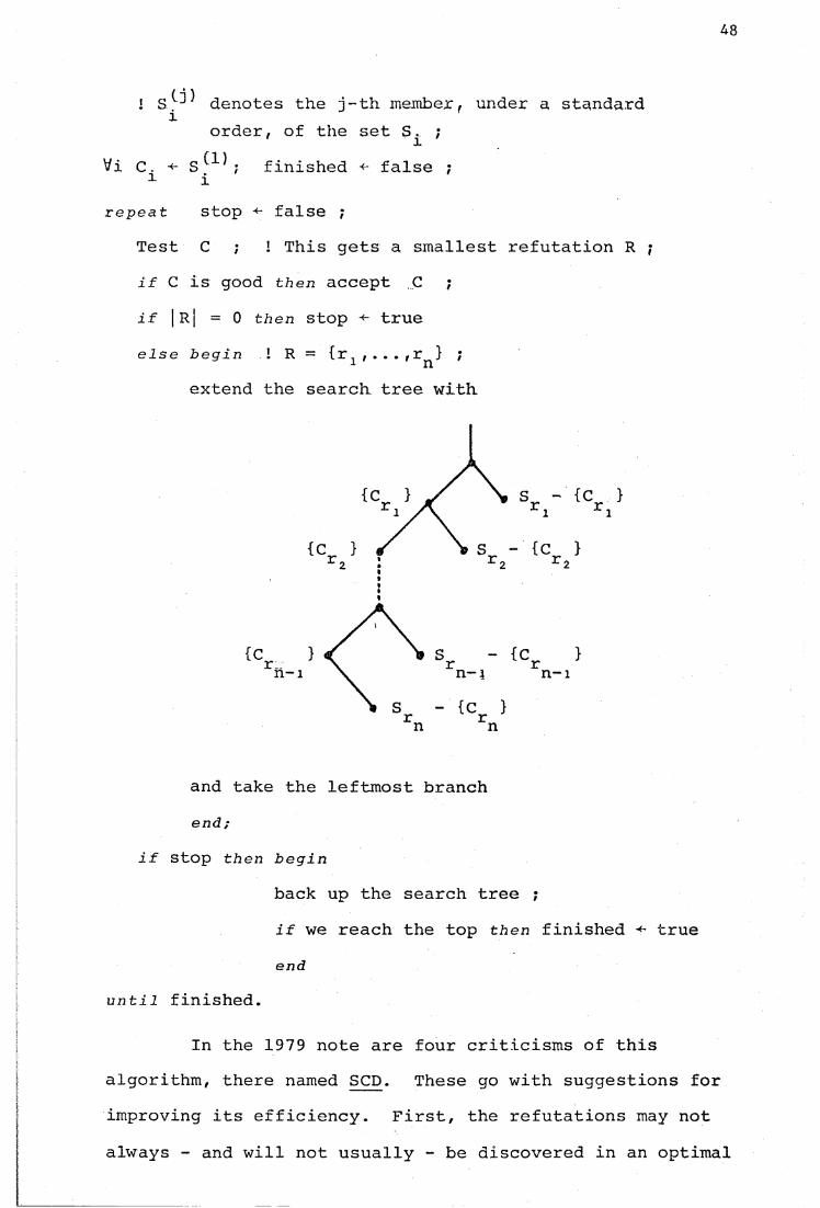
! S. denotes the j-th member, under a standard order, of the set ;

Vi C. S ; finished «- false ;1 irepeat stop «- false ;

Test C ; ! This gets a smallest refutation R ;if C is good then accept C ; if I Rj = 0 then stop true else begin ! R = (r1,...,r } ;

extend the search tree with

and take the leftmost branch end;

if stop then beginback up the search tree ;if we reach the top then finished trueend

until finished.

In the 1979 note are four criticisms of this algorithm, there named SCD. These go with suggestions for improving its efficiency. First, the refutations may not always - and will not usually - be discovered in an optimal

49

order. Smaller refutations are more significant than larger ones, and a more efficient search results if they are higher in the tree. This can be brought about by inserting refutations into the stack not necessarily at the end but above any larger refutations provided that these do not involve any of the values at cells (including cells with only one value) used in the given refutation. Thus the search tree is modified dynamically as the search progresses. Pritchard's second criticism is a minor matter of making the stacking procedure more elegant. The third and fourth are more important. It will often be possible to process several refutations from one test, where such refutations are all disjoint. This applies especially to 1-refutations, which of course are bound to be disjoint. Such mutiple processing should be done, or the next matrix will contain a refutation we already knew about, which is inefficient. The last point made in Pritchard's note is in the form of a question: in general what is the best refutation (of a given size) to choose. This is difficult, and perhaps no generally right answer exists. One suggestion of Pritchard's is to choose refutations involving cells with fewer possible values rather than those with more. In comparing two refutations it may be possible to devise a generally adequate answer, but the complexities which arise when comparing two sets of refutations may lead to a preference for "heuristic" rules of thumb.

Still, the algorithm is simple in outline, undeniably elegant and certainly very efficient for space, since the tape complexity is dominated by the array of possible values and the stack, both of which are bounded

50

by the number of values at cells - i.e, 0(.n3log n) where n is the number of values, for there are 0 (n) values at each of the n2 cells. On prepared search spaces such as those put out by Cut and Guess there will be many fewer values, of course.

At the time when I received a copy of the SCD algorithm (August 1979) Pritchard had not implemented it, so there was no empirical detail on its performance. My first reaction was to write a version of Fast (see chapter 1.4 above) to search prepared 8x8 spaces by SCD. What I implemented was a very crude first attempt at the algorithm, incorporating none of the suggested improvements and not even searching for a smallest refutation of each matrix but processing the first one found. This program was moderately efficient, but no faster than the later versions of Bigmat. It should not be concluded, though, that SCD is in any sense a failure. In the first place, the investment of some time in incorporating into my little program some of the known improvements to the algorithm must result in an order of magnitude drop in runtimes. In the second place one of the most exciting facts about SCD is that nothing in its construction turns on the nature of the algebraic structures for which it is to search, so it should be of very general application to problems in the classes defined in chapter 1.1 above. Moreover, even where the properties to be tested are very complex the algorithm remains simple and clean, making programs using it quick and easy to write and debug - a non-negligible consideration. For this kind of reason my current matrix-finding programs use SCD to

51

generate isomorphisms on extensional setups for the purposes of avoiding searching two isomorphic spaces and discovering quickly whether a generated matrix is isomosphic to one already accepted.

If I have reservations about the efficiency of SCD these spring from reflections on one of its strongest points: its space-efficiency. The information on thebasis of which the search is directed is held in a stack which rarely contains details of more than twelve or fifteen refutations. Quite normal jobs may yield a total of a thousand or more refutations in all, so very little of the total available information is applied at any one time. The search tree for SCD is generally short from root to leaves, but very wide, having perhaps some thousands of branches. Any refutation can occur only once in one branch, but in view of the shape of the tree this is not too reassuring. The search may well delete and rediscover the same piece of information many times, which is wasteful. It remains to be seen how far this problem canbe overcome.

52

Chapter 1.6 The method of transferred blocks

It is a waste of time to generate and test two matrices both containing the same refutation. For a matrix-finding algorithm to be maximally efficient for time, therefore, it must keep a record of every refutation found and avoid incorporating it again. The task is to devise a simple and fast way of doing just that. The search space can be thought of as an array S[1:N] of the sets of possible values of C[1:N]. Let us write S? for the j-th possible value of C^. Cells with only one possible value can be left out of this version of the array C. Test and Change respects the order of C, C^ being less significant than

i+1 for 1 < i < N-l. We may write Test and Change:Procedure Test; if C is good then accept C ;Procedure Search(S[1;x]); value x; search space S ;for each possible value of C dox x

begin

C <- S1 ; x xif x = 1 then Test else Search(S[1:x-l]) end ;

Search(S[1:N]).

Now consider a refutation {S? 3". . . S-111} , where S-?nll m mis the most significant value at a cell in the refutation.When C. becomes S-?n this value is fixed in its cell, so m inin searching the subspace S[l:(in-1)] we may regard {Sii**. S ^ j } as a (n-l)- refutation on this remaining space. When the value is subsequently inserted theremainder becomes a (n-2)-refutation on the still smaller

53

space and so on. When this process of transfer of therefutation eventually produces the refutation {S?^} onthe subspace SCI:(12—1)]r the value S?^ may be removed,temporarily, from S^, as there is a 1-refutation blocking it.When S^2 is taken out of C^2 as Change moves on, the2-refutation as recovere( anc tlie block removed,so S?^ goes back into as a possible value, provided,of course, no further refutation is still blocking S?^.This release of the subrefutations is repeated as thesuccessive values are taken out of the relevant cells,until when S?n is cleared from C. the whole n-refutation m magain applies to the search space.

Such is the reasoning behind the method of transferred blocks. The idea is implemented via two arrays: an integer array 'suspended' and a stack of pairs. The number

suspended?

records how many blocks are in force to prevent value S? from being inserted into cell C^. If suspended? > 0 then S? is, temporarily, not a possible value for C^. The stack, which for efficiency might well be a singly or doubly linked list, though such details are not my present concern, consists of pairs

< x,b)

where x is an integer and b is Boolean. Each pair is governed by a pair <i,j> of integers.

Recall that an n-refutation is one involving n open cells - i.e. cells each with more than one possible

54

value. Now to the method of stacking n-refutations, A O-refutation refutes the entire search space, so given a O-refutation simply skip out of the search. A 1-refutation could be recorded by removing the offending value S? from S^, but it is less messy to record it by setting

suspended? +- suspended? + 1.

For a 2-refutation we use the stack. Let a2-refutation with i < j. Then add to the stack the pair

<p(suspended?J), true>

governed by <i2,j2>. Here p(v) for variable v is a pointer to that variable. In practice it will consist of the pair <il,jl> in this case. Now when becomes S?^ the substackgoverned by <i2,j2> is scanned for pairs with 'true* in their Boolean field. This indicates that the refutations they represent are in force. The pair we have just seen stacked will be among those picked out and the refutation it represents will be implemented by downward transfer of the block to <il,jl>, by setting

suspended?^ «- suspended?^ + 1.

This makes {S?^} a 1-refutation on the subspace remaining after gets a value. When the value of CL 2 is changedagain, the block will be transferred back upwards to <i2,j2> by setting

suspended?^ ■*- suspended?^ - 1.

Now to stack a 3-refutation {S?^,S?^/S?^} , add to the stack the pairs:

55

position in stack pair governed by

kl < p (suspended^) , false ) < i2,j2 >k2 < p(kl), true > ( i3,j3 )

To stack a 4-refutation (S^, S;? / Sj3 sj4l 1.3' i4J add to thestack the pairs:

position pair governed bykl < p (suspended^) , false) ( i2,j2 )k2 < p(kl) , false ) ( i 3 , j 3 )k3 < p(k2), true ) < i4,j4 )

In general to stack an n-refutation for n > 4,

{Sjltbil ..... Sin>add to the stack:

position pair governed bykl < p (suspended^) , false) ( i2,j2 )k2 < p(kl) , false ) ( i3 , j 3 >

k(n-2) (p(k(n-3)), false) ( i(n-1),j(n-1) )k(n-l) (p(k(n-2)), true) <in,jn>

The operation of the stack can be seen from the procedures to insert and release values at cells:

56

procedure Insert(x,y) ;begin Cx +■ ;for each stack entry <p(v),b> governed by <x,y> do

if b then

begin if p (v) points to 'suspended' then v v+1else the Boolean field of stack ■*- truev

end

end;

procedure Release(x, y) ;for each stack entry <p(v),b> governed by <x,y> do

if b then

begin if p(v) points to 'suspended' then v •«- v-1else the Boolean field of stack •*- falsev

end ;

Note that a 3-refutation or larger is transferred by creating a temporary smaller refutation elsewhere in the stack. The Search procedure now reads:

procedure Search(S [ 1: x] ) ; search space S[l:x] ;for each possible value of C dox x

begin Insert(x,i) ;if x = 1 then Test else Search(SC1 :x-l]) ;Release(x, i)

end ;

And the main program still reads:

Search(S[l:N]).I have omitted the technical details which tend to

obscure the algorithm. There must, for instance, be some

57

form of index to the stack, so that the substack governed by a given pair can be scanned quickly. And there must be a device for recognising whether p(v) points to another entry in the stack or to a suspension number. Again, some form of Skippv should be incorporated, and will add complications, as Release must be applied to all the values in cells before the first one used.

One phenomenon which is important is what I have called the total suspension of a cell. It sometimes happens that a certain combination of values in cells late in the change order results in the suspension of every value in some S. earlier in the order. In such a case nolvalue is possible for the totally suspended cell, so the set of values causing the suspensions is a refutation and can be stacked as such. If, for instance, has three members, and we have the refutations

{Si' S3' S6}

<s?,

{S1' S 6 }4 2then when S. are placed in C^, there will be no

possible value for C, , so we should stack {S^, S^} as a1 J o2-refutation. I call the refutations resulting from total suspensions secondary refutations, and those resulting from bad assignments of values to subformulae of the postulates primary refutations. The stacking of secondary refutations greatly increases the efficiency of the algorithm.

Its efficiency is also increased by cutting down

58

the amount of testing which must be clone. To test a 10x10 matrix for satisfaction of the suffixing postulate, for example, one makes 1000 (= 103) assignments of values to the variables i,j,k and asks whether

C[i,j] < C[C[j,k], C[i,k]]

each time. If the matrix is bad perhaps ten cases will fail the axiom, whence 99% of the questions are wasted, giving no information. Maybe we have three possible values for C[l,2], and for each of them we ask thousands of times whether

C[1,2] < C[C[1,2], C[1,2]] .

This is a waste of time. It seems that the most efficient way to test is to take advantage of the fact that the transferred block method never loses any information and find all the primary refutations at the outset by testing all ascriptions of values from the search space to parts of postulates before a single matrix has been generated.The procedures I have for doing this do not look optimally efficient and are, apart from being complicated, each specific to a particular postulate. In fact my programs currently spend so long setting up primary refutations than even on search spaces as small as 108 possible matrices it is often more efficient to run Cut and Guess, dividing the space into two, and test the two separately than it is to run the test on the whole. For all that, the combination of a Cut and Guess outer loop and an inner test of the kind outlined in this chapter is the fastest algorithm known for jobs of the size normally encountered.

59

Observations on the runtimes of some implementations are given in the next chapter. The major drawback to the transferred block method is its space complexity, for every 4-refutation requires three stack entries, and there may well be a thousand primary refutations in quite a small search space, even if some procedure ensures that no refutation with a proper subrefutation is ever stacked.The space complexity for primary refutations is polynomially bounded, as all primary refutations are 4-refutations at most, so their number is bounded by the number of 4-tuples of values at cells, which is limited by a polynomial in the dimension of the matrix. In fact there will be much tighter bounds for actual logics, since by no means all 4-tuples can occur as the values of subformulae of postulates. Polynomial or not, the function determining numbers of refutations is too large to permit jobs with more than 25 to 30 cells with 3 or 4 values each to run in a reasonable amount of core (say 40K). This is unsatisfactory, and I am working on ways of decreasing the size of the stack without seriously interfering with speed.

Clearly, too, the time taken to generate and stack each primary refutation before starting the Change loop is at most a polynomial of the size of the job, and since each examination of a stack entry and transfer of a block can be done in constant time (ignoring the sizes of numbers), the time for inserting and deleting a value is likewise polynomially bounded, being of the order of the number of refutations stacked against that value at that cell. All that stands in the way of a polynomial upper bound on the

60

time complexity of the algorithm is the number and size of the secondary refutations. This is a little annoying, as in normal-sized jobs there are not very many such - usually at least 3/4 of the stack is taken up by primary refutations - and they tend to be quite small, only occasionally requiring anything more than a 5 or 6-refutation to be stacked. There is, however, no control over them and no clear reason why they should not proliferate exponentially as job sizes increase. It should be noted that the numbers of good matrices of given sizes for the logics investigated appear to be exponentially related to size, so bounds must be regarded as functions of the size of the matrices and their number, rather than just of size.

61

Chapter 1.7 Conclusions to Part 1.

The research programme in computer generation of matrix models began with two needs for such models. Meyer wanted little matrices (4x4) for a little logic, E , and I wanted big matrices (8x8, 10x10) for a big logic, RWX.Once it became evident that the problem of efficient matrix generation had two features of the great problems - idiot solutions do not work and clever solutions do - the project took on an independent interest. Most of the development of Cut and Guess and the transferred block method was conditioned by the aim of generating as many matrices to a specification as possible as quickly as possible, without much regard to their applications. Now that the generating problems are on the way to being solved, interest is starting to shift back to the uses of matrices. The second part of this thesis will be a report on some investigations suggested already by the output, but before that I want to give a brief survey of the performances of the algorithms discussed above and of the jobs for which they might be suitable.

Direct comparisons of runtimes of the going programs is made difficult by the fact that they are not all aimed at the same jobs. All my programs are designed to find Ackermann groupoids and the like, so they assume fusion will be defined along with implications, and require an element t such that for every a,

t < a iff a is designated.

Pritchard and Meyer, on the other hand, were mostly concerned

62

with pure implication systems where there might not be a least designated value in this sense in the models, and where there is it might not satisfy such additional postulates as

t ■> a < a

in E_ for example. Moreover the actual polished programs are in different languages and were designed to run on different machines.

As a partial solution I wrote a series of simple ALGOL-60 programs based on the idea of Fast to take a description of a search space from a file and search it for matrices satisfying

A-+B . B~>C . A->C

B-»C -*■. A->B ->■. A-*C.

The data structures are:integers siz, open, setmax, matno, tryno, runtime

siz: the highest value ("M" in the algorithms above).open: the number of cells with 2 or more possible values.setmax: the largest number of possible values for one

cell.matno: the number of matrices found, tryno: the number of matrices tried, runtime: the execution time for the main loop.

Boolean array partord [0: siz, 0: siz] integer arrays a,b,kount [1: (siz + ] )z]

c, call [0: siz, 0: siz] possval [1: (siz +1) ,1: setmax]

partord: the partial order - partord[i,j] = i < j.

63

possval: the possible values - possval[i,j] is the j-th possible value of the i--th cell.

kount: the numbers of possible values - the i-th cell has kountCi] possible values.

call: the change order of cells - call[i,j] = k iff i-*-j is the k-th cell.

a,b: the opposite of call - a[k] = i and b[k] « j in the last example.

so call[a[i], b[i]] is i.

The contents of all these variables are simple read from an input file, except in the obvious cases of 'matno', 'tryno' and 'runtime'. For each i-th cell then initially

c[a[i], b[i]] possval[i, 1 ] .There are two basic procedures:procedure Test ;begin

tryno ■*- tryno + 1 ;suffixing: for i ■*- 0 until siz do

for j -<- 0 until siz do

for k < - 0 until siz do

if not partord [c[i,j], c[c[j,k], c[i,k]]] then go to End.of.test ;

prefixing: for i «- 0 until siz do

for j ^ 0 until siz do

for k 0 until siz do

if not partord [c[j,k], c[c[i,j], c[i,k]]] then go to End.of.test ;

accept: matno matno + 1 ;End.of.test: end ;

64

procedure Search(x); integer x ;begin integer i ;for i 1 until kountCx] do

begin c[a[x]f b[x]] < ■ possval[x,i] ; if x = 1 then Test else Search(x-1) end

end ;

Now the main loop:runtime < - the current job time ;Search(open);runtime ■*- the current job time - runtime.All that then remains is to print out some statistics, such as 'runtime' and the search ratio, or 'tryno/'matno'.

The program I have given in some detail here is the "idiot" Test and Change implemented via a recursive procedure. The format lends itself to easy adaptations to other algorithms. To introduce Skippy add a new variable 'index' and amend Test so that instead of

go to End.of.testwe have

index «- min (callCi,j], call[j,k], call[i,k],callCcCj,k], c[i,k]], index)

for suffixing, and for prefixing:index •«- min (call[i,j], call[j,k], call[i,k],

call[c[i,j], c[i,k]], index),and just before 'Accept:' we add

65

if index < open then go to End.of.test.Before each test 'index' is initialised to 'open' + 1. Theamendment to Search is to add a skipout clause, so:procedure Search(x); integer x ;begin integer i ;for i < - 1 until kount [x] do

begin c[a[x], b[x]] •«- possval [x, i ] ; if X = 1 then Test else Search(x-l); if index < open and index > x then go to Eos end ;

Eos: end.

I wrote six little programs to do this same job, implementing six different algorithms. They were:

T&C the "idiot" Test and Change already given;Sk Skippy, as suggested above;Sw3 Skippy with a device to change the order of cells

as the job progresses (see chapter 1.3 above); the "3" records that three progressively better refutations (at most) are taken from each matrix tested;

C&G a Cut and Guess loop, applying the principle"Aff" (see chapter 1.4 above) and a test for the actual postulates on unit sets;

SCD Pritchard's algorithm (chapter 1.5 above), withmutiple processing (i.e. taking several refutations from each bad matrix) but without dynamic stacking;

Trb an implementation of the block transfer methodsubstantially as in the last chapter.

I had these programs search for Ackermann groupoidssatisfying the T-W^ postulates on extensional setups based

66

on chains. Chain models make fusion definable, by

a°b = df. Ac: a < b+c

and on finite chains generalised meets always exist. On

chains, too, the postulate

(a->b) a (a+c) = a^bAc,

which is needed for the given definition of fusion, holds

trivially. It suffices for fusion to be defined, given

these facts,- that where M is the top element, for every a:

a+M = M.

This is easily written into the search space. Only the

matrix for -> needs to be found. Thus on the extensional

setup

f 2<► 1 t = 1

v 0

for instance, we have the search space:

Hence in terms of the specific data structures for the

programs:

67

siz = 2 , open = 3 , setmax - 2f

1 2 3 4 5 6 7 8 9abkount possval 1

2

0 0 1O i l 2 2 2

1 1 1 2 2 2

O i l 2 0 2

1 1 1 2 0 2

2 2 2

0 1 2

1 1 1 0 0 2

partord 0 1 2 call 0 1 20 true true true 0 1 2 41 false true true 1 5 3 62 false false true 2 7 8 9

Such is the test I devised for the algorithms.The first results are the runtimes for the various cases and the search ratios.

Runtimes in seconds (to 2 signficant figures)

Number ofelements t T&C Sk Sw3 C&G SCD Trb

3 12 not measurable (less than 0.05

tot

4 1 0.22 0.72 0.26 0.18 0.06 0.052 1.4 0.98 0.26 0.36 0.12 0.133 0.40 0.46 0.34 0.32 0.18 0.14

tot 2.0 2.2 0.86 0.88 0.36 0.325 1 44 13 4.2 1.4 1.3

2 125 11 3.9 2.5 1.83 93 12 20 4.3 2.04 28 14 8.5 4.9 1.8tot 290 50 36 13 6.9

68

Cont' d

Number ofelements t T&C Sk Sw3 C&G SCD Trb

6 1 210 82 392 120 92 423 720 120 394 510 150 445 290 160 50

tot 1800 610 210

These are execution (cpu) times on the Australian National

University's DEC system KL10. The timesharing system

results in up to 6% variation in runtimes, so the figures

should not be taken to provide more than rough comparisons.

Search ratios (to 3 significant figures).

elements t T&C Sk

3 1 4.00 3.002 2.00 1.75

all 2.67 2.17

4 1 60.8 8.752 256 9.753 29.2 5.72

all 105 7.62

5 1 19.82 56.63 41.34 18.9

all 31.8

6 12345

all

Sw3 C&G SCD Trb

2.00 1.50 1.50 2.001.75 1.00 1.50 1.251.83 1.17 1.50 1.50

4.58 1.08 2.00 1.584.63 2.06 3.94 1.814.44 1.16 3.24 1.564.76 1.42 3.17 1.62

9.82 1.13 2.69 1.2211.0 11.1 5.95 1.3411.8 3.37 6.27 1.3410.7 1.51 5.32 1.3210.8 1.80 5.12 1.37

1.23 3.53 1.041.15 8.23 1.064.17 8.66 1.082.87 6.77 1.071.89 6.03 1.072.13 6.30 1.06

69

Search ratio is defined as the number of matrices tested divided by the number of good matrices. C&G does not actually test matrices, so there I define "the number tested" as the number of terminal nodes in the search tree. This gives a very low figure, as most of the work goes into processing the nonterminal nodes.The search ratio for T&C can be calculated without running the jobs, since it simply tests every matrix in the space, and the total of possible matrices is known.

With only four or five partial orders tested it is obviously hard to be confident about the shape of curves.We know that where there are n cells each with just k possible values T&C is bounded for time complexity and search ratio by 0(kn), so more complicated exponential functions of this kind should apply to it for all jobs. The search ratio of Sk and Sw3 are also fairly clearly exponentially bounded: witness the onset of the 69-day syndrome in their runtimes between the 5x5 and 6x6 cases. The long run increase in search ratio for SCD appears to be linear at worst, and it seems that the search ratio for Trb actually decreases as the size of the job grows. This is because the information we have - see chapter 2.1 below - suggests that for some positive constant K, the number of T-W matrices of size nxn for n > 2 is always greater than K x 2n, while it is easy to show that the number of primary refutations, which bounds the number of bad matrices tried, is polynomially bounded, for example by the number of 4-tuples of values at cells which is at worst of the order of n12.

(Kx2n) + K1n12 Kx2n

But

70

is asymptotically 1. So the proportion of bad matrices generated by Trb, if the observation on numbers of good matrices is correct, becomes vanishingly small as the job size increases. At the small sizes given in the table the search ratios for Trb are depressed by the fact that the program stacks failures of Aff first, before the search, and on small matrices Aff covers a large proportion of the refutations. This distorts the curve at its lower end. In large search spaces the preliminary stacking of the 2-refutations from Aff is proportionally much less important. Experiments with the 7-element chain suggest a search ratio there of about 1.0Q5, which is rather impressive. One job on the 7-element chain yields over 230,000 good matrices in finding which Tbl tries just over 900 bad ones.

Chapter 2.1. Numbers of matricessome tables and graphs.

Blanks in the table indicate jobs too big to be run in reasonable time.

72

Numbers of De Morgan groupoids validating six central systems of relevant logic.

Sy size of lattice.

log

17

16

15

14

13

12

11

10

9

8

7

6

5

4

3

2

1

0

73

GRAPH 1.

# matrices

GRAPH OF TABLE 1

11size

Note. An extensional setup s is "occupied" by logic L just in case

74

vO 00 CT* tn 4> tO hO

004PVO•oVO

ov (—• -otno

ov roVO VO Ov hO I—1• • • • •"J O Ui oho tn o O O1-3I3

O 4PO O -0ho to vo• • •OV 00 I—--J to 4P

4P I—*ho to O V - P ^ t —* ! —* ho t—> O O O Oo o o o o o

4PI—1 VD tn4P 00•-o to hotO O

t—14P 00 CO (—• •—*• • • • •to hO O tn Oto tn O O O

ho i—*Ov 4P 4Pt—• 00 ho• • •I—1 O tntn o o

hoCO 00 4P00 l—* tno o o

to I—• •o o oo o o

4>- 4> (—■ »—100 to ov to tn tnCO ho 4P Ov 00I—• O CO I—■ 03 tn

hO hO I— 1 t— ' I— 14P O tn O O-O O O O O

I3

to to t—1 t—*ho to O O tn• • • • •tn tn 4P tn toho to CO Ov to

to

tn 00O tnO OO OO oo

wU)H-NCD

0Hi

HftrfH-oCD

TABLE 2. Numbers of De Morgan groupoids per occupied extensional setup

l°g2

11

10

9

8

7

6

5

4

3

2

1

0

75

natrices GRAPH 2 (TABLE 2) E-W omitted.

size

ES: extensional

setups.

76

2ortCDW

CO "U CN On -O OO NO

h—*0n CO Ui OO NO t—* t—1ütr*

V£0 -O (so I— '> tdO NO NO O On NO l—* £/}

Of

CbH-inrthH-ercrtH-<CDMtbrtrtH-OCDin

roooOn v£5O On CNvo on <y> i—*i-3Is;

t—■ OOOn NO00 On toNO OO O -P- l—1

1-3

NOVO NOOO Oo NONO On NO OOO NO NO l—* l—■

wIs;

o On-r> CN -oNO OO OO ''O l— 1 CdNO. -P" NO 00 OO I—*

CN NOCN CN -l-On OO *-0 H-*CN OO I— 1 CN OO *

WIs:

■P- t—1NO O OO NOO 00 NO H-* 5ö

TABLE 3.

Numbers of positive Ackermann groupoids validating the

same systems as before.

By size of lattice*

#

17

16

15

14

13

12

11

10

9

8

7

6

5

4

3

2

1

0

77

i t r i c e s GRAPH 3 (TABLE 3 ) .

E-W o m i t t e d .

R-W

s i z e

setups

78

TABLE 4. Numbers of positive Ackermann groupoids per extensional setupfor the systems in table 3.

By size of lattice.

Note

79

rtort to t—1

ri­llfo U>

rtII■>rtIIUi

rtII

COH-U3PH-HiH*OP JPrt

HiH-vQ£H

CD10O3M

K>U>oLO

OU>

Ln oo Ui roLn vo o j r-* 00 U) H1—• I—1 O VO O N5

I—1 N5 4>VO VO VO t o I—■ Ln4>- O —J ~-J -P' I—' I

s:

td*<otroH-oCD

oHi

rt

(—• vO O (_0er» -l> Co -f> Ln I—■

TAB

LE 5

. N

umbers

of

tota

lly

ord

ere

d A

ckermann

gro

up

oid

s o

f o

rde

r

80

GRAPH 4 (TABLE 5).

Totally ordered Ackermann groupoids of order 7.

choice of t

81

Zort(D

r tOr t

t—1

r t r t r t r tII II II IIh- to CO

rtIICn

rtIIONrtII

co

COXo oo

(—* t—I> Cn vO• • • • •-C" o I—■ oo u>£ £ & s. £o o o o o'-j oo oo o>

asO

USO

wH*vQbH-MlH*O{DrtHiH-vQ£Hn>w

CO I—* I—■CO CO O O COVO vo oo O to o o o

00 I— »— CoI—' to 00 4>- t—* oo ►—*

W

Is:

bdo b* oH*O CD0Hirt• oo

to »—4> to oo co o o o W

TABLE 6. Numbers of totally ordered De Morgan groupoids of order

m is the highest element such that for every

82

r t r t r t r t r t r t r t r t r t r t r t r t r t

rt || II II II II II II II II II II II

Ln -t> OJ K> t—* * N3 OJ -F- Ln

TABLE 7. Numbers of R-W matrices based on total orders to 13x13.

By size and choice of t.

11

10

9

8

7

6

5

4

3

2

1

0

83

GRAPH 5 (TABLE 7).Matrices for given choices o f tsuch that m < t. x m+6

m+5

m+4

m+ 3

m+2

m+1

size

10

9

8

7

6

5

4

3

2

1

0

84

GRAPH 6.

The 26 De Morgan lattices of order 12.Numbers of De Morgan monoids yielded, by numbers of pairs of independent elements.

-I- 1— I— I- - 1— I— I_ _ I_ _ _ I_ _ 1 1 I I I I I » i i l 1 I i t I I

0 5 10 15 20 25independent elements

85

Chapter 2.2 Observations on the numbers of matrices

The simplest operation to perform on the small model structures for a set of systems such as the six I have been considering is to count them, or rather, having regard to one's sanity, have a machine count them.For this purpose they must be partitioned in suitable ways. I have given above tables representing gross numbers of model structures satisfying the postulates set out in the Introduction, divided by order (number of elements), and more detailed analyses of a few more specific cases. While division by order is the most obvious, it is not the only division possible; nor is it clearly the most revealing. The structures could be divided by length of longest chains in their partial orders, by smallest numbers of generators or by numbers of prime filters in the lattices, for instance, but this thesis is a preliminary survey, not the final word, and division by order is most simply managed.

My programs first generated partial order tables representing De Morgan or distributive lattices, for instance. Then for non-isomorphic choices of t, giving the exten- sional setups, they produced implication matrices with built-in assumptions that fusion would be defined. All the numbers in the tables are of pairwise non-isomorphic model structures. The postulates I used are:

86

For T-W: < is a partial order,

(a+b) a (a->c) < a->bAc

(a-^c) a (b-^c) < avb+c

aAb < a aAb < ba < avb b < avbaA(bvc) < (aAb)vc

ä = a

a->b = b-*a

a->b < b->c a-*c

b->c < a->b a-*c

t < a->b a < ba°b < c ° a < b-*c.

For T: T-W plus a a+b < a->ba- a < a.

For E-W: T-W plus t->a < a.

For E : T plus t->a < a.

For R-W: T-W plus t->a = a.

For R: T plus t-*a = a.

The positive logics simply drop the two negation postulates In the positive and full logics the existence of fusions is easily secured, for finite lattices are complete and have a greatest element, T. Fusion exists if and only if for

87

every element a, a-*T = T, Clearly if fusion exists then since everything is less than or equal to Tf

t°a < T

whence

T < a-*T

and T = a-*T.

For the converse we may define fusion in these finite positive-logic structures:

a ob =df. Ac: a < b->c.

Since a < b^T, the general meet of the definiens is always nonempty, so it remains to show

(Ac: a < b+c) < d ° a < b->d.

From right to left this is trivial, since d is an element of the meet. From left to right it suffices that

a < b-> (Ac: a < b-*c) ,

and this we prove by finitely many applications of

(b-*u) a (b-*d) - b+cAd

and meet semilattice properties.

For "pure" -* logics this move to define fusion is not available, for which reason I have not yet investigated Ackermann groupoids in general very much.I have given some results on totally ordered ones, for where the underlying order is a chain the operations a and v exist and moreover trivially satisfy the full postulates of the positive logics. Thus for chains

88

the definability of fusion is yery simply written into the search space. My further reasons for concentrating on chains are:

1. Since no two totally ordered model structures are isomorphic there is no need to worry about eliminating or accommodating isomorphisms, which cleans up a messy corner of the subject.

2. The chains form a clear sequence ascending by size:it is obvious which structure to choose as representing the "same but bigger".

3. The simplicity of the order also makes it clear how high or low in the structure each element is, so choices of t are subject to an obvious ordering by position, making graphs 4 and 5, for example, clearly 2-dimensional. Moreover, since chains force the full positive logic to hold, there is always a least designated value for t to take.

4. Chains, as suggested below, are in any case fairly typical underlying orders in the sense that they yield more model structures for these logics thando other configurations. Statistics based on chains therefore resemble those for all orders together.

The first point from table 1 is that the numbers of De Morgan groupoids of order n validating each of the given systems appears to be bounded below by an exponential function of n. This emerges more strongly from the graphs where all the numbers have been logged yet the lines are approximately straight. T-W has at sizes

89

n _2up to 8 about 2.5 x 2r distinct model structures, and Rn _ 2has about 1.2 x 2n at sizes from 3 to 12. A glance at

the other graphs will confirm this appearance of exponential order. If the numbers of good matrices do go up exponentially then, as noted in Part 1 above, this places an irreducible exponential lower bound on runtimes for the algorithms described earlier.

The "zigzag" pattern of the curves in graph 1 is partly due to the fact that there are more De Morgan lattices with even than with odd numbers of elements, as can be seen from table 1. In an effort to eliminate the resultant distortion from the figures I tabulated matrices per extensional setup, giving table 2. This .device also abstracts from the order of the groupoids, removing the effect of the greater number of extensional setups of greater order. The decision only to count occupied setups was based on the feeling that a setup on which it is impossible to base a model structure for logic L is not really an extensional setup in the sense given by L at all. Thus in the case of the system with reductio it is silly to look for matrices on setups which fail excluded middle.It is, of course, quite possible to tabulate and graph numbers of matrices per extensional setup, occupied or not. A slightly different set of curves results, and it is a matter of intuition which version gives a better impression of the way the numbers mount. In table 4 I have given the ratio of matrices to all extensional setups rather than just to occupied ones, though in fact without negation unoccupied setups are rare.

90

The next observation is that numbers of models giye a sense in which strictly independent systems can be compared for strength, Lj being stronger than L2 if it has fewer models of any given finite size greater than some n. There are obvious limits to the meaningfulness of such comparisons where the logics concerned take widely differing kinds of structure for their models. In the present case, however, we can see a clear sense in which R-W is stronger than E, for example, and we may likewise conjecture that T is stronger than E-W. Curiously, the evidence from the positive logics (tables 3 and 4) suggests that E-W+ is stronger than T+ in the same sense, so in the case of logics in the region of T reductio appears to be a very strong principle. The large numbers of T+ matrices come mainly from one type of extensional setup: the chain with theatom designated. This one case contributes 34,047 out of the 71,582 T+ algebras of order 8. E-W+ by contrast has only 551 matrices based on the same setup. Even discounting that one setup, however, E-W+ seems stronger than T+ in the suggested sense.

A related kind of observation has to do with the relative nearness of neighbouring systems. It is evident from graphs 1 and 2 that E, for example, is more like T than it is like R, though again the reductio postulate seems to play a large part in strengthening T. Even in its positive fragment, though, T appears to resemble E more than it does T-W. At 6*6 there are about 2.76 times as many T-W+ matrices as there are T+ matrices, and about 2.24 times as many of the latter as there are E matrices,

91

which places T slightly nearer to E than to T-W. Curiously enough, the same sort of reasoning places E+ closer to R_ than to T , the difference factors being 3.01 and 3.67

T"

respectively at 7x7. It is unclear what force these comparisons would have if it emerged that the systems in question lack the finite model property. Nothing is known of whether T, E and R do have the finite model property, although the systems have been investigated for some twenty years now.

One of the first observations I made on the numbers of matrices was that long thin structures like chains yield more matrices for the relevant logics than short wide ones like Boolean algebras. This impression has been confirmed repeatedly as more species of structure have been examined. Over 25% of the 10-element De Morgan monoids are chain-based, and over 20% of the 12-element ones. Yet the chain is only one of 13 De Morgan lattices of order 10, and of 26 of order 12. Graph 6 shows the distribution of De Morgan lattices at 12x12 by number of pairs of independent elements - i.e. pairs {a,b} such that a b and b a - and number of De Morgan monoids based thereon. The line joins the geometric means of the numbers of matrices yielded by De Morgan lattices with the same numbers of independent pairs. There is some scatter, but a general downward trend as the relation decreases. The other systems and the other sizes exhibit the same overall pattern, which seems independent of the presence or absences of De Morgan complement. The surprise here is that we have always

thought of the model structures for relevant logics as

92

resembling Boolean algebras and of the set of truths on a model as consistent. Now it appears that most model structures are more like chains, and since on such structures a < a quite often holds, if the law of excluded middle is to hold the truth according to such models is likely to be inconsistent. About 86% of 10-element De Morgan monoids are inconsistent. Thus the typical models are not much like the canonical models. At the moment observations like these stand as mere curiosities;I have not been able to harden them into theorems, and nor do I know of any concrete use to which they may be put. But they have changed my vision of R and its kin.

Another curiosity is the distribution of matrices according to the position of the least designated value, and on this I can offer some partial reasons why things should be as they are. The majority of matrices for logics with contraction, such as T, E and R, are to be found based on extensional setups in which t is low in the order.This may be because the rule of contraction operates to knock undesignated values out of the search space:

a b =*■ a a-*b.

Thus the more undesignated values there are the more grip contraction gets. This could be passed off also as an explanation of why chains and the like, where many ceils hold designated values, are most fruitful, were it not for the fact that R-W and T-W also exhibit a liking for strongly ordered lattices. It might well prove fruitful to examine matrix models for the contraction-free systems

93

to discover how many instances of contraction tend to hold, even if some instances fail. We know, for example, that R-W models which validate

Av~A

also validate

A& (A+F) ->F

where F is always assigned 0, and moreover validate

(A A-+F) A->F

(see next chapter). The pattern of occurrence of matrices with positions of t in R-W emerges clearly in table 7 and graph 5. There are many matrices with t low in the structure and with t high in the structure but very few with t in the middle. The illustration is the chains, but similar, if more complex, patterns exist for all structures. The reader is invited to find a function to predict the number of R-W matrices on a chain of n elements. Table 7 is full of tantalising almost-regularities and affords hours of innocent amusement.

Another exercise valuable for adding small fragments to our understanding of the relevant logics R-W and R is that of finding explanations of why certain extensional setups are unoccupied (yield no matrices for one system or another) or singly occupied (yield exactly one matrix).In the next chapter is a theorem explaining why there is only ever one R-W matrix based on the element m of a finite chain. A simpler theorem is that any distributive lattice with t as the top element yields exactly one Dunn

94

monoid (R+ algebra). In R+ anyway we have the theorem

A & B *>■ A o B

or algebraically

aAb < a<>b.

Now suppose for every element a

a < t.

Then since t < b-*b,

a < b+b and b < a-*b by permutation.

That is to say, residuating,

a°b < b and a°b < a.

Therefore

a°b < aAb so a«b = aAb.

Hence the one Dunn monoid on the setup is the Heyting lattice.

Explaining unoccupied setups is generally not so easy. There would be some interest in a theorem giving a straightforwardly extensional condition necessary and sufficient for the occupation of a setup by R-W or R.The best I have is a few piecemeal results. For example there is no Dunn monoid based on a positive extensional setup of the form

1

\ /

20

The argument is:

l A (1 +0) = 0 theorem of RT1+0 = 2 or 1+0 = 0.

Suppose 1+0 = 2.2 < 1+02 < 1+2 affixing2 = 1+2 since t 1+2

But 1+0 < 0+2 +. 1+22 < T+2 since 0+x = T2 < T+t affixing1 < 2+0 permutation of supposition1 < T+t by analogous argument

• 1 v2 < T+ti.e. t < T+ti.e. T < t which is false.

.*. 1- 0 = 0.But 1 < t and t < 2+2

1 < 2+22 < 1+2t < 1+1 and 2 < t2 < 1+12 < (1+ 1) A (1 + 2)2 < 1 + 1 A 2

i.e. 2 < 1+0.But 1+0 = 0, so 2 < 0 which is absurd.Unfortunately there is no obvious way of generalising the argument to take in a large number of cases of unoccupied setups.

96

Some interest also attaches to setups on which all matrices for one system validate another. For example, if t is the sole atom in a De Morgan groupoid then any E-W algebra based thereon also validates all of E. To show this it suffices to use E-W postulates and

t a or a = 0

to derive

a-*a aa -t. a->b < a->b.

The former is easy. Suppose t < a. Then

a+a < t->a and t- a < a a+a < a.

Now suppose a = 0. Then a < b, and in particular

a < a->aa+a < a by contraposition.

The proof I have of contraction goes through properties of the complement operation. Suppose a = 0.Now

boc < a.*. b ° a < c i.e. b < a+c

and in particulara a->b < a-*b.

Now suppose t < a. Thena a-*b < t +. a^b, and t ■>. a->b < a->b a + . a->b < a-*b.

Proofs of small-scale theorems like this may be sought

97

in cases where quasi-empirical ohsexvation of numbers of

matrices suggests they may hold. The same kind of

observation suggests that all chain-based matrices for

T where f < t are also matrices for E; no proof of this

conjecture is yet known.

The combinatorial analysis of propositional logic

has scarcely begun. The preliminary observations in this

chapter already suggest a number of promising lines for

future research. Firstly we may count different objects.

I have considered just species of Ackermann groupoid

modulo isomorphism. It is of course possible to drop t

and ° from the models, leaving the direct correlates of

the connectives only. Such a move gives many more models

for pure -*■ systems and for systems weaker than R-W and R.

Again, models validating exactly the same formulae are in

a sense duplicates, even if non-isomorphic. It might

be worthwhile eliminating from the counts direct product

algebras and the like; the effect of doing so is

uncalculated.

As noted earlier, many different selections of

classes of model are possible, and there are of course

a great many more systems of logic which could be

investigated. One line which may prove very fruitful is

the study of the results of representing each of a number

of postulate schemes by the generalised lattice meet of

its instances. A logic as naturally axiomatised emerges

as a filter in this treatment. The idea might well begin

to provide some measure of the relative strengths of

postulates. To date, however, I have done very little

98

work on it. Finally it must be confessed that we need some theorems. Most of the above observations on the numbers of models for systems are based on no more than intuitive extrapolation from a few brute facts. Some asymptotic bounds on the numbers would be welcome, for instance. I have no proof that the bounding functions are exponential, that R-W is "stronger" than E, that most De Morgan monoids are inconsistent or that chains are more productive than Boolean algebras. I repeat that we are at the start of combinatorial analysis of logics; my claim is to have unearthed enough facts - and to have provided the means for discovering more - to make numerical methods possible.

99

Chapter 2.3 The Logic R-W

Recall that the logic R-W has the postulatesaxioms: 1. A->A

2. A+B ->. B-*C -*■. A+C3. B-*C -*■. A- B ■>. A-*C4. A -*■. A-*B->B5. A&B-*A6. A&B-*B7. (A-*B) & (A->C) A+B&C8. A->AvB9. B-*AvB

10. (A->C) & (B->C) + . AvB-MS11. A& (BvC) (A&B) vC12. A+f+f-*A

rules: 1. A , B =» A&B2. A->B, A => B

definitions: 1. ~A =df. A-*f2. A°B =df. ~(A-*~B)3. t =df. ~f.

Some of the above are redundant, and there areways of shortening the list by combining somebut I believe particular axiomatisations to be of very little logical importance; my axioms and rules are chosen to give some feel for what is in the system. Axioms 1 to 4 with rule 1 given the pure -* system; axioms 1 to 11 with the two rules given the positive logic. Orthodox conservative extension results follow from considerations given, for instance, in the appropriate sections of

100

Anderson and Belnap [75] and Routley and Meyer [R], and are not my present concern.

In our paper on Abelian logic ([79]) Meyer and I have expressed our philosophical thoughts on R-W, which is indeed a curious system It is converted to R by the addition of any one of:

1. (A A-*-B) A->B2. A& (A+B) -> B3. A+~A ~A4 . A^B -> ~AvB5. (A-*B) & (B->C) A->C6. (A B+C) A&B+C

There are some well-loved principles in this list. 1, the contraction axiom of E and R, shows perhaps most clearly what divides the two systems R-W and R: in a relevantdeduction according to R a premiss must be used at least as many times as it is assumed (see Church [51] and Anderson and Belnap [75] for discussion of the "use criterion" for valid arguments); R-W, lacking contraction, goes further in requiring each premiss to be used exactly as many times as it is assumed. 2, roughly the rule form of 1, is the modus ponens theorem of the stronger systems, and recasts the points in disallowing, in systems where it holds, logical theories not closed under detachment, just as 5 legislates against theories not closed under transitivity. R-W is in general very careful to distinguish between the compounding of premisses truth functionally by conjunction and their intensional fusion, a distinction

101

which emerges clearly in the failure of 6, whose converse fails in all the relevant logics. The failure of 3 and 4, both of which fail in rule form also, has the important consequence that R-W has no theorems in the &,v,~ vocabulary at all. The contraposed version of 4 is the principle of material counterexample

A&~B ~(A->B)

and on the given definition of fusion the contrapositive of 3 is the square-increasing postulate

A A°A.

In view of the lack of all these supposed "laws" of logic it is tempting to dismiss R-W as a merely silly or at best partial system. This would be o'erhasty, for R-W is, as I have suggested in several places above, a strong system in other ways and embodies a philosophy of logic in many ways closer to the spirit of the motivation of relevant logic than is the more orthodox Anderson-Belnap line. The differences between R-W and R surround three very delicate questions: the role of contraction principlesin deductions, the logic of negation, and the place of "extensional" principles, such as the classical tautologies, in logic. On this last issue R-W represents a position opposed to Quine's remark that logic is concerned with the logical truths, for it is based rather on a catalogue of valid implications. And pv~p, though it might be a necessary truth of some sort, is not a record of an inference, and so perhaps should not be asserted by pure logic.

So much for the weakness of R-W. Its strength

102

lies in the fact that arbitrary permutation of antecedents tends to unify ordinarily diverse principles - witness the given list of "equivalents" of contraction - and thus greatly facilitates derivations. This flexibility in the way complex implications are taken emerges in the theoremhood of:

(A B+C) <* (B A-+C)

(A . B-*C) ** (A°B C)

Ao (BoC) ** (AoB) oC

A°B ** B°A.

The positive fragment of R-W is contained in both that of Heyting's intuitionist logic and that of L , the denumerable valued logic of Lukasiewicz. Both of those systems also validate

A -*. B->A,

and the addition of that scheme to R-W produces the logic RWK. Where A^B is defined as t&A-*B, RWK is just the fragment of R-W. While standard extensions of R-W go either in the direction of R or in that of Lukasiewicz's logics, it is possible to strengthen the double negation scheme

A-*f-*f-*A

to the general

A-»B+B->A

which produces the strangely beautiful Post-complete system A investigated by Meyer and me in the paper cited above.A, while fascinating, is too far from the purpose of this

103

thesis to be detailed here.My thumbnail sketch of R-W and its surroundings has

been one part of the scene-setting for the main theorem of this chapter, the second R-W paradox, which follows shortly. Before giving the proof, however, I should continue with its background by saying something briefly about the programme of paraconsistency. Where |- is a deducibility relation defined on a language S, T, a subset of S, is aI-theory just in case it is closed under |- . T isinconsistent with respect to monadic connective * iff for some AeS both AeT and *AeT and trivial iff T=S. |-is par aeons is tent with respect to * iff some |- theory is inconsistent with respect to * but nontrivial. The terminology is taken from da Costa. Evidently paraconsistency with respect to * comes to the invalidity of A , *A |- B. Thus where * is negation the paraconsistent logics are those which deny that from a contradiction anything follows, and among such logics those of the relevant group present an independently motivated line.

One project for which paraconsistent logics may be suitable is the formulation of a naive set theory. The natural axioms to govern the intuitive idea of sets are:

(z) (zex = zey) -* x=y (extensionality)

xe{y: A(y)} ** A(x) (abstraction).

These may be subject to appropriate restrictions on binding of variables and the like: these details arenot my present concern, and nor is the large subject of relevant quantification theory. To extract trouble from

104

the abstraction axiom it needs only a step of substitution to yield

xe{y: y^y) x^x

whence, using R for {y: y^y} and instantiating,

ReR <*■ R/R.

By reasoning valid by intuitionist (and relevant) lights this quickly yields

ReR & R^R

whence a negation paraconsistent logic is needed to avoid utter collapse. Interestingly, the contraction-free relevant logics do not permit the inference from the biconditional to the conjunction, and nor does their supersystem £ .

Since the contributions of Curry and Moh-Shaw-Kwei it has been fairly well-known that there are paradoxes in naive set theory which afflict not the theory of negation - which is not too hard to amend - but that of implication, Anderson and Belnap's "heart of logic". As Geach pointed out as long ago as 1955, there are analogous antinomies in the truth theories of semantically closed languages of which, as Tarski noted in [56], the natural languages are examples. The classic Curry paradoxes are recapitulated in the Meyer-Dunn-Routley paper in Analysis (1979) which, however, was written in 1975. One such paradox argument runs:

105

let a be {x: xex *> p} now aea *►. aea -> p so aea aea -*■ p.Given contraction this yields aea + pand from this and the biconditional

I aeawhence by detachment

P-

Similar arguments replace contraction by the weaker modus ponens theorem scheme, and where fusion is present as a connective some versions use only conjunctive syllogism as their contracting move. Hence a logic suitable for naive set theory has to be very weak, even lacking

A& (A-*B)-*B.

is such a logic, as are its subsystems such as R-W.It is not known whether R-W is weak enough to contain the naive axioms nontrivially, and nor is it known whether £ is strong enough to allow ordinary mathematics up to some large slice of analysis to be deduced from the naive axioms. The most important positive result yet available is that just announced by Brady (Brady [80]) that naive set theory is nontrivial in a logic which contains at least:

Av~AA&B^A A&B-*B(A+B) & (A+C) A+B&CA-> A v B B->AvB(A+C) & (B+C) AvB+C

A& (EvC) -► (A&B) vC

106

A-+~~A — A^AA^B -*■. ~B+~A (A+B)&(B+C) A+CA- B, A => BA+B, O D =* B-*C A+D A #B =* A&B

The curiosity here is that this system contains not only excluded middle but also the conjunctive syllogism, which principles are absent from R-W. The conjunctive syllogism is a contraction postulate of a sort, since it holds in just those Ackermann groupoids satisfying

a°b < a° (a°b) .

The contraction axiom itself corresponds exactly to

a°b < (a»b) °b

which at least looks related.5As noted earlier the conjunctive syllogism takes

R-W to R where naive set theory collapses to triviality, but Av~A, sufficient for all the tautologies in &, v and ~, can be added and produces the system RWX. I began to investigate RWX by looking at matrix models of the logic, and especially at those distinguishing RWX from R. I noticed that a high proportion of RWX matrices, including all the chain-based ones, are rigorously compact. That is to say that validate (where T and F are the top and bottom elements respectively) :

107

a+T = F-*a = T

a/T =*■ T->a - F

a/F =* a^F = F.

I started looking for an explanation, and soon discovered the little theorem

T -* (A->F A+F) .

This is the first R-w paradox and is proved:

F T-*-F because F+ anything

A-*F A T->F by prefixing

A-*F T -*, A- F by permutation

T A+F A+F by permutation.

This product of the permutation principle does not look too harmful on its own, but together with excluded middle it leads us astray:

(A->F) v (A/F) (using A/F for ~(A->F))

( (A-»F) v (A/F) A-KF) A+F

i.e. (A+F ->. A-*F)&(A/F A+F) A-*F

and so by the first R-W paradox

(A/F A-*F) A+F.

Now by permutation

(A A/F+F) A->F

and by contraposition, given T *>~F,

(A T A->F) A-+F

so by permuting again

108

CA A T->F) A+F,But

F T-*F as before

A-*F A T+F prefixing

CA -». A-*F) A A T->F prefixing

so

CA A-*F) A-KF.

This is the second R-W paradox or r w x paradox in the form of a contraction theorem for the absurd constant F. Notice that its derivation nowhere uses prefixing or suffixing in theorem form: premutation of antecedents is the onlyprinciple used not in the system DK6 for which Brady has proved the non-triviality of the naive comprehension and extensionality axioms. The assertion axiom of R-W requires the suffixing axiom to yield permutation in theorem form, but nothing prevents the last from being taken as an axiom.

Now in naive set theory the constant F is definable with its characteristic axiom scheme

F+A.We take F =df. (x)(y)xey. By instantiation,

F x e { y: A }but by the abstraction axiom

xs{y: A} A whence as required

F+A.Now let a be the set {x: xex+F). We have

aea aca+Fasa- -F aea.

109

From the former by the RWX paradox aea+F

and from this and the latter by detachment aea

and so by detachment again F

so naive set theory collapses.There are many variants of the argument, some

using distribution for & and v, some requiring contraposition in rule form only and so on. With fusion introduced by the residuation rule

A B+C ° A°B+C

permutation can be replaced in the derivation by the suffixing axiom and

A°(B°C) ** (A°B)°C.

Excluded middle can be replaced by

~ (A ** ~A) .

Proofs of these last assertions are easy enough to be left to the reader, but I should perhaps provide some hints. For the "associativity" version, then, note that the suffixing axiom is equivalent to

(A°B) °C + Bo(A ° C)

so th.e associativity scheme gives

(AoB) oC + (B°A) °c

alloying permutation back in except for the last place in compound fusions. The proof is then easy; further

110

hint: use T->F instead of F. As for using

~ (A ** ~A)

instead of excluded middle, my (large1 hint is to use the case

~(A->F «*. A/F)

and follow roughly the same argument as before.The paradox can be made to emerge in the forms

A& (A->F) ■> F

(A+B)& (B+F) + . A+F

(T-*A) & (A- B) T->B

T ° A T°AoA

T°A -> (T°A) ° (T°A)

(A°A **■. A->F) -*•. A->F

We might define a kind of negation

~1A =df. A->F

and, following Curry, we might dub it absurd negation. Then variants of the RWX paradox emerge as:

A-OA -> ~1A

A&1A B

“1 (A&~lA) and B -> ~l (A&~1A)

(A->B)&“1B -> ~1A

~“lA-tlA 1A.

Some of these start to look familiar.My result is the strongest negative result to date

Ill

limiting the set of logics within which naive set theory

is possible. We must either abandon the theoryr drop the

lattice operations & and v (without which the recovery

of ordinary mathematics hardly seems likely) , drop

De Morgan negation, lose excluded middle or cease to

permute antecedents in conditionals. Only the last two

look like viable ways of amending logic. As far as is

known either will do. None of the equivalents of the

RWX paradox given above is derivable in £ , which contains

R-W but lacks the law of excluded middle. Nor are they

derivable in the system I dubbed in the introduction to

this thesis EWX, for the following is a matrix set for EWX

in which they all fail:

0 31 2

*2 1*3 0

Hassediagram

T 3Ol<►0

2 __33 3 3 3 3 3 1 3

EWX does have, in addition to Av~A, at least some restricted

permutation principles, including:

A+B B->C A-*C

(A -*■. B~*C) -*■. D->B -*■, A ->. D+C

A =* A->B->B.

These do not appear strong enough to give any trouble. E-W

can be strengthened by the addition of the reductio axiom

a +~a ->-~a

without collapsing to E. EWR (E-W plus reductio) gives

112

the tautologies as deriyable theorems. It is not known

whether EWX or EWR will support a nontrivial naive set

theory, nor whether EWR contains the RWX paradox.

The RWX paradox can be used as a Lemma to prove

further metatheorems, particularly those which show

RWX to be closer to R than might have been thought. We

have already noted in chapter 2.1 and 2.2 that very few

small models distinguish between the systems, and in part

this is due just to the smallness of the models. That

ava be in the positive cone requires the identity t to

be fairly low in the order structure, and in any case

as we have seen most models of RWX are based on extensional

setups in which t is low. But t < a entails a+a < t->af

which is a-*a < a. And if a is very close to the bottom of

the lattice then usually a+a < a anyway. Thus the

requirement that there be elements high in the structure

outside the positive cone and the requirement that the

positive cone be large tend in small algebras to squeeze

each other out.

There are, however, some unexpected similarities

between RWX and R models which hold irrespective of the

size of the matrix. For example, consider finite models

in which the lattice order is a chain, in which every

ava is designated and in which f < t. It is known (see

Anderson and Belnap [ 75 ] §27.1) that the addition of

f+t

to R produces Dunn's semi-relevant system RM, whose

proper axiom is the "mingle" scheme

A **■. A-*A.

113

The derivation goes:

1. f+t

2. A-* f . A- t 1, prefixing

3. t A+A

4. A-*f **■. A . A- A 2,3r suffixing

5. ~A . A ->, A->A 4, def.~

6. (A ■>. A->A) ->-« A+A contraction

7. ~A •*-. A^A 5,6, transitivity

8. ~A ->. ~A- ~A 7, contraposition

9. A ->. A->A 8, subs ~A/A,double negation.

This derivation will not work in RWX, where the step 6 is unavailable. For a model splitting RWX plus f->t from RWX plus mingle consider:

S = the integers;

is numerical order;

a ,v are numerical minimum and maximum;

a — — a

a- b = b-a

t = f = 0

a ob = a+b

This is, as Meyer and I proved in [79], a characteristic model for the system A of Abelian 1-group logic with the canonical negation, group inverse. Where a is any positive integer, a < a+a fails, for a-* a is always 0. A has no

nontrivial finite model at all, for any finite lattice is

114

complete and has a greatest element T. As an instance of the "axiom of relativity"

A-*B->B+A

we have

a-*T-*T < a.

But a+T+T is designated, since a+T < T, whence every element is designated and the model is trivial. Now while I do not know whether RWX plus f+t has the finite model property and in particular whether

A -*. A->A

can be falsified in a finite model,7 we can show the partial result that every finite chain model satisfies all of RM.

RM is standardly algebraised by Sugihara chains: totally ordered De Morgan lattices where for every a,b, if a < b then a+b = avb and if b<a then a->b = aAb. I now show that every finite chain model of RWX in which f < t is a Sugihara chain. Proof is by induction on the length, n, of the chains. There are two base cases: n = 1 trivial;

n = 2 the only RWX model is truth tables - a Sugihara chain.

Now for the induction hypothesis suppose the only model on the (k-2)-element chain is the Sugihara matrix (known as RM(k-2)) . We must show for n=k that the only model on the n-chain consists of just RM(k-2) with new top and bottom elements T and F and the -* matrix extended by rigorous compactness:

115

RMk -*■ table F TF T • . . T, , . T

••F RM (k— 2)

•••

T••

T F 1..F... T

It suffices to show that any -> matrix on the k-element chain is rigorously compact and has a submatrix for its interior - i.e.

F->a = a+T = T

a^T =* T->a = F

a^F => a-KF = F (these define rigorous compactness)

a/{T,F} & b£{T,F} =► a+b£{T,F}.

Rigorous compactness is easy to show, for:

F < T->a because F < anything

so T < F->a permuting antecedents.

and T < a->T contraposing.

aA (a-*F) = F RWX paradox

so a = F or a-*F - F total order

and a = T or T-*a = F contraposing.

Now to demonstrate that T cannot occur in the interior:

suppose a+b = T - i.e. T < a-*b;then a < T-*b by permutationso a < b+F by contrapositionbut b = F or b+F = F as proved aboveso b = T or a = F,

116

To show, finally, that F cannot occur in the interiorf we must use the fact that f < t,

f < t t+b < f-*b b < f-*bb < a->f -*, a-*b b < a a->b a < b •>, a+b

Now suppose a-*b = F and b ^ F. Either b = F or b-*F =; F, by the RWX paradox, so b+F = F. But we are supposing a+b = F, so b a^b = b- F, so b a-*b = F, Therefore a < F, so a = T. Hence the interior is a submatrix, has the lav; of excluded middle and has f < t, so the interior is RM(k-2), and the whole matrix is RMk.

As noted in chapter 1.4 above, the RWX paradox and the rule

f < t =* a->b < b+aare very useful in speeding up the search for R-W matrices. These theorems were discovered after I entered the conjectures on the grounds that the search programs only produced matrices obeying them. In this way such programs can be improved through feedback from their own output.The investigations in this chapter are also intended to illustrate the process whereby theorems are not proved but suggested by examination of such quasi-empirical data as the machine produces, the analytic proofs coming after.

117

Chapter 2.4 Ackermann constants

The sentential constants t and f ("the true" and "the false") have made frequent appearances throughout this thesis, and indeed throughout the history of relevant logic. The true - or perhaps more accurately the logically true - is a natural identity for Ackermann groupoids, and the false has been used, as in the last chapter, to define negation for the R-like logics. These constants were part of Ackermann's original logical scenery (Ackermann [56]); Anderson and Belnap eliminated them from E and R in their early formulations; Dunn, algebraising R, began the rehabilitation of t, and Meyer, investigating further the notion of enthymematic implication, added more to its role.The story of the fall and rise of Ackermann's sentential constants is to be found scattered through Anderson and Belnap's [75].

Ackermann constants are hereby defined as formulae built up from t and f by closing under the logical connectives. They are to be distinguished from Church constants, which are built up from T and F in the same way, and mixed constants which are founded on all four of these. The governing postulates are:

A ° t-*A ~A o A-»fA-*TF-*A.

This study is concerned with Ackermann constants only.What there is to say about Ackermann constants in

118

classical logic can be said thus: t

fThis will also do for the Church constants, and direct products of it will famously complete the picture for the whole of that system. Classical logic is thus Ackermann saturated: the system which results from lettingpropositional variables range over the Ackermann constants (or indeed the Church constants) is the same as that resulting from their ranging over arbitrary propositions. Another Ackermann saturated logic is the system A which I developed with Meyer in our [79]. There (as we prove) the integers are a characteristic model, so since they only require one generator the one variable fragment is polynomially free for the whole system; and f behaves exactly like p, so Ackermann saturation is immediate. As examples of Ackermann unsaturated logics consider Heyting's intuitionist system J and the logic RM defined in chapter 2.3 above. For both these systems the Ackermann fragment, that part of logic consisting solely of Ackermann constants, is "truth tables" or the 2-element chain, as it is for classical logic, but both systems fail Pierce's "law" -

A+B-+A+A.

- which is a tautology. The Ackermann fragment of J is truth tables because there the Ackermann and Church constantsare identical, for:

119

\- A B+A

[- t A+t

but |- t

|- A+t whence t = T;

and “1 A =df. A+F i.e, f = F.

In RM the Sugihara chains are characteristic, and they force for every dyadic connective <j>:

<J> (A,B) e {A,~A,B,~B> .

Thus in RM every Ackermann constant is t or f; f < t, and the rest is easy.

No interesting general results about Ackermann saturation are to hand. The concept really only applies to systems with at least implication and negation and satisfying the postulates of B (see Routley and Meyer [F]), perhaps with a weakened negation part. Clearly Post-completeness is a sufficient condition for Ackermann saturation, for the Ackermann fragment gives rise to a supersystem of the base logic. I have no information on the converse conjecture. There seems no good reason why Post completeness should be necessary for Ackermann saturation, and systems like T-W and R-W might well provide counterexamples, as little is known of their constant structure beyond the fact that, since they are subsystems of A, they have infinitely many distinct constants.8 On the other hand I can see little chance of anything short of such a concrete counterexample showing that Post completeness is not necessary. For all the

120

contraction-free relevant logics the question of Ackermann saturation is open.

In systems weaker than R-W and R the properties of Ackermann constants are complicated by the fact that A+f and ~A are in general different formulae. The importance of f for the stronger systems lies in just this possibility of regarding relevant negation as inferrential in character; in E and its subsystems it is rather difficult to know how to think of the sentential constants, especially f.9 For this kind of reason, and because we wanted to begin with solvable cases, Meyer and I began the investigation of Ackermann constants with R and its variants.

The only paper, so far as I am aware, dealing solely with constants in relevant logic is Meyer's [79].There the constant structure of some fragments and extensions of R is settled, and the attack opened on R itself. The presence of f ensures that all fragments with constants have negation. Implication and negation suffice to define fusion, and conjunction and negation suffice for all the extensional connectives, so the two fragments worth investigating are the closures of {f} under the intensional fragment, and under -* and &, the full logic, t may be defined as f-*f. The intensional Ackermann constants in R are 6 in number and have the Hasse diagram:

121

( f 2 ). 2

5 C£+t-*U

> 4 (t)

(f) 1 Cf-*t)

/Q(Cf+t) of)

-> 0 1 2 3 4 50 5 5 5 5 5 51 3 4 5 3 3 52 3 3 5 3 3 53 0 2 2 5 5 5

*4 0 1 2 3 4 5*5 0 0 0 3 3 5

Note the notation of a2 for a°a. Generally we shall write a11 for a fused with itself n times. That these six formulas in fact constitute the Ackermann fragment of

follows from Meyer's [70], and is Theorem 1 of his [793. I do not propose to repeat the proof, as this intensional subsystem of R is not my main concern here.

completely is CR, introduced in Routley and Meyer's [74] under the name CR*. CR has the additional connective 1 whose postulates are:

One of the theorems fundamental to the constant structure of CR is

~t ** “It

Another system whose Ackermann fragment is known

ASHA rt B

A + BvlB.

122

which immediately gives the rather surprising

t&f -* B

A -* tvf.

The proof that the two negations of t are equivalent c

LEMMA 1~A ° ~1A.

Proof 1. A&~IA -*■ ~~I~A

2. “l~A -* ~ (A&~1A) 1, contraposition

3. -|~a -> ~Av~“lA 2, duality

4. “l~A&l~A -> ~~1A 3, Boolean laws

5. -|~a -> ~~IA 4, & idempotent

6. ~“I~A -> AvlA

7. ~(Av~lA) -> 1~A 6, contraposition

8. ~A&~’1A ~l~A 7, duality

9. ~~IA -> "l~Av~l~A 8, Boolean laws

10. ~~IA -> n~A 9, v idempotent

11. ~i~a ~ia 5,10, adjunction.

MAIN THEOREM ~t ^ “It.

Proof 1. t -* ~itv~“it excluded middle

2. t&t •> ~nt 1, Boolean laws

3. t -> ~nt 2, & idempotent

4. "it -* ~t 3, contraposition

5. t -* n~t 3, LEMMA

6. ~t -*• nt 5, contraposition

7. ~t it 4,6 adjunction.7

123

The structure of the constants in CR is the 8-element Boolean monoid:

Hasse diagram

This structure is readily seen to be a product algebra, decomposing into

0*1

1 1 0 1

t=lf=0

Ot=i f=2

Now the product is given by:

2-element 4-element 8-element constantalgebra algebra algebra

0 0 0 t&f0 1 1 t&f 20 2 2 f0 3 3 f 21 0 4 f+t1 1 5 t1 2 6 fv(f+t)1 3 7 tvf

124

Since the 8-element algebra given Is a De Morgan monoidwith Boolean complement it is a model of R and of CR, sothese 8 Ackermann constants are all distinct in CR, Toshow that there are no more than these 8 we prove that CRis the intersection of CR+f2 Ci.e, CR with f2 as a newadditional axiom) and CR+f-»-t, and then show that these twosystems have the constants fragments given by the 2 and4-element structures above. The first lemma is simple,for CR, like all the relevant logics, is the intersectionof its prime, regular theories10, and validates the lawof excluded middle, so in every prime model either f2 is verifiedor f->t is verified. We know that the addition of f->t to R,and hence also to CR, produces at least the system RM, whoseAckermann fragment we saw to be truth tables. It remainsto show that CR+f2 has just the 4 Ackermann constants

tft&f = f->t tvf = f2

and for this it suffices to show tvf = f2

for the set is then clearly closed under the connectives, t&f being lattice 0 as already shown. This is quite easy, for f-*f2 is a theorem of R anyway, and t-*f2 is f2 which holds as an axiom of CR+f2, whence

tvf < f2.And we know

f2 < tvf.

125

To complete closure under -* note that f-*t+t = fvt

since clearlyt < f+t+t

andf-*t < f-*t

SO (f-*t) of < t SO f o (f->t) < tso f < f-*t-*t so tvf < f-*t-*-t.

And of course again f-*t-*t < fvt.

Notice that the proof leans heavily on the "paradoxical" theorems of CR:

f&t -> A A -> fvt.

For this reason, as we shall see, it will not go through in the case of R. These theorems give us the bonus that the Church constants T and F are definable in CR as fvt and f&t respectively. As another bonus, notice that the De Morgan and Boolean negations as defined for the Ackermann constants are the same, so the same constant structure obtains in KR, which adds to CR the scheme

A+B -►. ~IB-*“1A.A similar line of argument shows that R is not Ackermann saturated: the Ackermann fragment of R+f-*t is truth tables,which validates Pierce’s law:

A^B^A-^Aand that of R+f2 of course validates f2, so

126

f2 v Cp+q+p+p)is a theorem of the Ackermann fragment of R, It is not a theorem of R, however, for the following is a De Morgan monoid

also begins to investigate the constant structure of R itself. Meyer notes that the following structure is also an f-generated De Morgan monoid:

>3 0 1 2 3]> 2 0 3 3 3 3*1 0 1 2 3

<>1 t= 1 *2 0 0 1 3<>0 f=2 *3 0 Q 0 3

& 0 1 2 3 O 0 1 2 30 0 0 0 0 0 0 0 0 0 0 3

*1 0 1 1 1 *1 0 1 2 3 *1 2*2 0 1 2 2 *2 0 2 3 3 *2 1*3 0 1 2 3 *3 0 3 3 3 *3 0

Notice that the implication table and the negation table are identical with those of the "diamond" structure given earlier for CR+f2, but that one extra element - f - is designated. This coincidence of tables with different order structures is not uncommon in R. Now the De Morgan

3 o 0 1 2 3 -* 0 1 2 32 t=2 0 0 0 0 0 0 3 3 3 3

* 2 0 1 2 31 0 1 1 3 1 0 2 2 3

* 2 0 1 2 3* 0 a=3-a * 3 0 3 3 3 * 3 0 0 0 3

and on assignment of 1 to p and 3 to q the suggestedformula takes the value 1, which is undesignated.

These results are all in Meyer's paper of 1979, which

127

monoid which is the direct product of this 4-chain with the 8-element Boolean monoid of CR is also f-generated, which accounts for Meyer's observation that there are at least 32 pairwise non-equivalent Ackermann constants in R. His crude proof was to have the computer generate formulae taking all values on the 32-element product algebra.

When he wrote [79] Meyer left open the questions of how many Ackermann constants R has and of whether in fact there are exactly 32. My first suggestion was to look at De Morgan monoids based on the 6-element extensional setup

t=2f=3

The idea immediately bore fruit. This "crystal lattice" can replace the 4-chain in the direct product algebra above, giving a 48-element f-generated De Morgan monoid. The implication table for the 6-element structure is:

The proof that the 48-element direct product is f-generated is quite elegant. Let each element be represented by an ordered pair <a,b> where a is an element of the 8 and b of the 6. First note that the element <7,0> is generable:

128

it isf2 -* fvt.

Its negation, of course is <0,5>. Now in general we can generate <a,0>: where A is the formula generating a in the8-element structure, <a,0> is generated by

A& (f2 -* fvt) .

Similarly, where B generates b in the 6, <0,b> is

B&(f2 o(f&t)).

But now all the 48 can be generated from what we have by closing under disjunction, for

<a,b> = <a,0>v<0/b>.

When these 48 were discovered I was working on the matrix-generating programs in the Bigmat series, which began producing De Morgan monoids on much larger structures, exhausting the possibilities at 10x10 and going on to 12x12 and beyond. Having become interested in the Ackermann constant question, I next wrote a little program to generate the Ackermann constants distinguished by a set of input matrices

m , . . . mi nEach matrix m^ gives the constant f a value f^ and consists of two tables, and &^. Every formula generated is represented by the sequence of the values it takes on the n matrices. Thus A is represented by

<vi (A) . . . vn (A) > .

The basic structure is a stack of such sequences representing the formulae generated so far. Let there be k of these.

129

Then the stack is

<S. . . .S. >1 kwhere each is

<sl . . . S*?>l l

and each S? is the value on the j-th matrix of the constant represented by S^. The basic algorithm is:

procedure Try (cn,x,y]; connective cn; local i;begin for i ■<- 1 until n do s +- cn.CS^S 3* l x yif s is not already in the stack then

begin k +■ k+1; put s into the stack; print out cn,x,y and s end ;

Now the main program, after reading in the data:

Initialise: k +■ 1; Si <f(. . .f >;Loop: for i •*- 1 until k do

for j •«- 1 until i do begin

try(&,i,j); try(-*,i,jl? try (+, j,i)end .

The actual algorithm used was more complex, as the stack entries were kept not in order of discovery but in a numerical order to facilitate a binary search. This required an index to the stack and so on. Moreover, to save space the entries were packed densely into core

130

words, only 5 bits being used to represent each integer.All these details are irrelevent to the general idea, though essential to its implementation.

All the 8-element De Morgan monoids were examined for constants and yielded nothing beyond the 48 we had already. Extensional setups with odd numbers of elements are of no interest for their Ackermann fragments, since they require the De Morgan complement to have at least one fixed point, a. Now

a = a

aAa = ava

aAa < f and t < ava

t < f

Thus conjunction gets no grip, as the intensional constants all satisfy

c < t or f < c,which makes the constant structure a chain. In fact the Ackermann fragment of any inconsistent De Morgan monoid is at most the 4-element chain which was used by Meyer to split the 32 Ackermann constants of the 1979 paper. The next matrices to try therefore were those of size 10*10,

The first structure of this size to produce any further constants was the "crystal Boolean lattice" which consists of the 8-element Boolean algebra with a new top element and a new bottom element, giving:

131

Hasse diagram negation implication~ -> 0 1 2 3 4 5 6 7 8 90 9 0 9 9 9 9 9 9 9 9 9 91 3 1 0 4 4 4 4 8 8 8 8 9*2 7 *2 Q 1 2 3 4 5 6 7 8 93 6 3 0 1 1 2 4 5 5 6 8 9

*4 5 *4 0 1 1 1 4 5 5 6 8 95 4 5 0 0 0 Q 0 4 4 4 4 9

*6 3 *6 0 0 0 Q 0 1 2 3 4 97 2 7 0 Q 0 0 Q 1 1 2 4 9

*8 1 *8 0 0 0 Q 0 1 1 1 4 9*9 Q *g 0 Q 0 0 0 0 0 0 0 9

Notice that the implication table is of the same overall form as those of the other De Morgan monoids specifiedin this chapter; this is the reason for my slightly odd placing of designated values. This form can be specified for a matrix of size (M+1)x (m +1); allow a to stand for {1...(M-l)/2} and $ to stand for {(M+l)/2...M-l} (assume M is odd); now the implication and negation tables are schematically11

0 a B M ~0 M M M M Q Ma 0 a B M a BB 0 0 a M B aM 0 0 0 M M Q

Moreover, except for the Boolean algebras, the conjunction table is

B0 0 0 00 a a a0 a B B0 a B M

132

In general, except, again, for the Boolean algebra of truth tables, t is one of the "a" elements and f correspondingly in the range of 0. The generalised structure is, of course, the 4-chain which Meyer used in splitting 32 constants in [79]. Any f-generated De Morgan monoid of this form clearly has the property that its direct product with the 8-element Boolean monoid characteristic for the Ackermann fragment of CR is likewise f-generated.The reason is, as before, that the formula

f&t f->t

is evaluated as some a -* 0, which is Q, but it is evaluated as the top element of the Boolean monoid. The argument then follows that which showed the 48 f-generated. Notice that any constant falls into the same class of values (.{0},a,3 or {M}) on all models of the given form.Thus there is no chance that the direct product of any two of them might be f-generated.

Consider, however, the 10-element structure just given and the 6-element crystal lattice given earlier.These are both of the form under discussion, and since it will be convenient to have the terminology I shall dub such structures Ackermann crystal monoids, As noted, the class of Ackermann crystal monoids is not closed under direct products, but it is closed under Ackermann products, which I symbolise with x^ and define:

133

let m and m 2 be Ackermann crystal monoids,

with element sets Q,al,31,M1 and

0,a2 ,$2,M2 respectively. Then m 1x m

has element sets 0x0, a 1X a 2 r ß x32, M 1x m 2.

In n^x m 2, we define

<a,b> = <a,b>

<a,b>-><c,d> = <a->c,b-*d>

<a,b>A<c,d> = <aAb,CAd> t = <t,t> and f = <f,f>,

It is merely tedious to verify that m^x m 2 is indeed an

Ackermann crystal monoid. Now the Ackermann product of

our 10- and 6-element Ackermann crystal monoids is an

Ackermann crystal monoid with 18 elements:

6-elementalgebra

10-elementalgebra

18-elementalgebra class

01111222233334 4 445

01234 1 23456785678 9

012345678 9

10111213141516 17

0aaaaaa

To generate all these elements it clearly suffices to

generate a, and by the usual construction this requires

only that the elements 4 and 5 of the Ackermann product

ö

ö ca ca ca ca ca oQ

cq c

q S

134

be generated. 4 is generated by (f& (f&t-*t) ) ° (f&t-»-t)

and 5 byf&t -* t -* t.

Further investigation pushed the number of known Ackermann constants beyond the 144 of the direct product of these 18 with the 8-element Boolean structure. First came another 10-element Ackermann crystal:

This yields the f-generated monoid with the -* table:

The Ackermann product of this with the 18-element Ackermann crystal monoid we already have is also

135

f-generated, and of course has 66 elements, so its product with the Boolean 8 gives 528 distinct Ackermann constants.The crucial elements for the usual proof of f-generation,abbreviating f&t-*t to g, are:

first second6-element 10-element 10-element formulaalgebra algebra algebra

1 4 4 (g°f) & g2 1 4 g g&f -*■ g&f2 4 1 g ■> g&f t2 1 1 g -> t1 4 1 Cgof) & (g -* g&f -* t)1 1 4 (gof) & g & (g&f -* g)

Only three of these, the first three (or the last three)are strictly required by the proof. The element g is thegreatest member of a in all these algebras.

The llxll and 13x13 matrices were no help, as already noted, and those at 12x12 yielded only products of thef-generated De Morgan monoids of smaller sizes. The next productive structure has 14 elements:

a = 13-a t = 2 f = 11

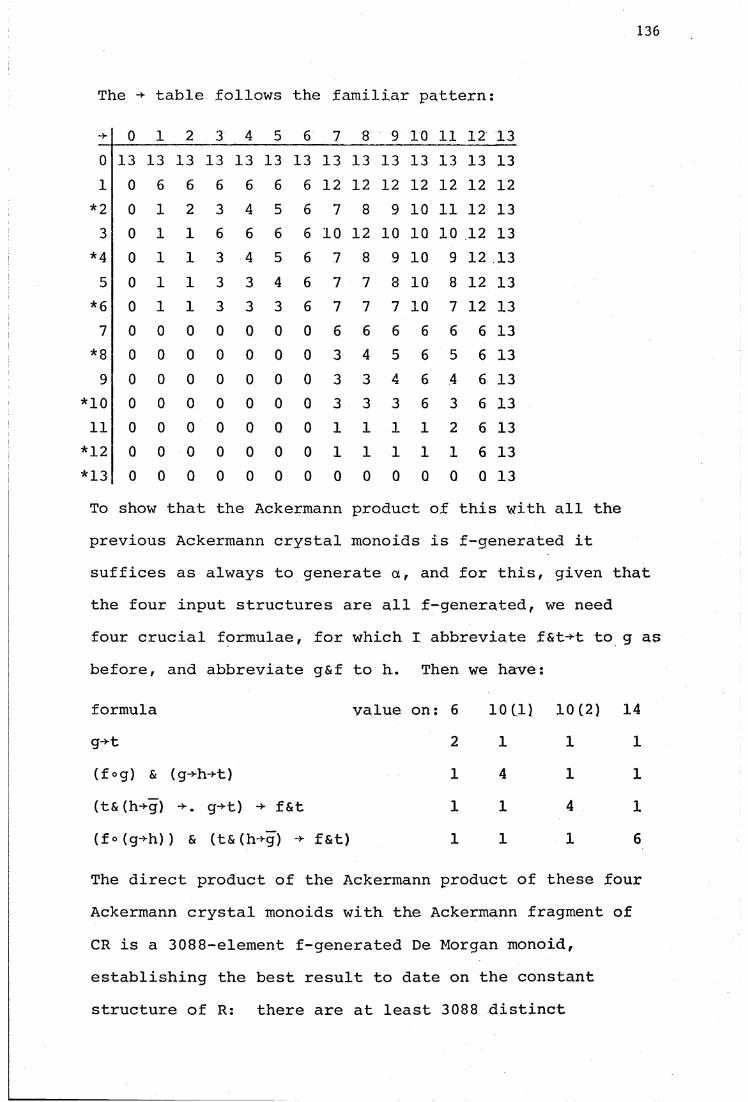
136

The table follows the familiar pattern:

9 10 11 12 1313 13 13 13 13 13 13 13 13 13 13 13

6 12 12 12 12 1210 11

6 10 12 10 10 10

To show that the Ackermann product of this with all theprevious Ackermann crystal monoids is f-generated itsuffices as always to generate a, and for this, given thatthe four input structures are all f-generated, we needfour crucial formulae, for which I abbreviate f&t-*t to g asbefore, and abbreviate g&f to h. Then we have:

formula value on: 6 10(1) 10(2) 14g+t 2 1 1 1(fog) & (g->h->t) 1 4 1 1(t&(h-*g) ->. g-*t) -* f&t 1 1 4 1(f o (g+h) ) & (t&(h->g) ■* f&t) 1 1 1 6

The direct product of the Ackermann product of these fourAckermann crystal monoids with the Ackermann fragment of CR is a 3088-element f-generated De Morgan monoid, establishing the best result to date on the constant structure of R: there are at least 3088 distinct

137

Ackermann constants in R.The immediate unanswered question is whethex" there

are exactly 3088 or whether some yet more devious ploy will increase the number again. The "empirical" evidence, for what it is worth, suggests that any further increase will be hard to find by the methods used thus far. I haye used a Cut and Guess algorithm to enumerate f-generated De Morgan monoids based on (substructures of) all likely-' looking extensional setups up to 18x18 and some at 20x20 and 22x22. I have even exhausted some of size 30x30 which at one time looked promising. So far no new constant has emerged. Elementary acquaintance with the natural numbers, however, suggests that even large amounts of such evidence are not particularly conclusive. The best hope of proving that there are infinitely many Ackermann constants in R seems to lie with the project of finding a sequence of progressively more complex constants no two of which are equivalent. The sequence

f, f2, f3...fn,fn+1...for instance does not terminate in R-W or RWX; in R we have

which blocks such a simple-minded approach, but there may be some recursive compounding procedure producing such a sequence. Perhaps some relatives of the formulae I used to generate the Ackermann product above would form the initial segment, but it must be said that there is no immediately obvious pattern. Our knowledge of the Ackermann

138

fragment of R has been produced mainly by the computer, and it may be that we should continue to use mechanical aids in searching for repeatable patterns of this kind.

In the months since the discovery of the 3088 known Ackermann constants in R there has been no progress to report on any of the conjectures Meyer and I made then. One conjecture was that there are infinitely many of these constants; the only observation I have to offer there is that the problem is nontrivial. Another conjecture of some interest is the torsion conjecture: for everyAckermann constant, c, of R there is some finite n such that

n n+1 c = c

A stronger form is

c o c = c °c °c -i.e. n-2.

If there are only finitely many Ackermann constants, of course, then the torsion conjecture is trivially true, and if there are exactly 3088 then its stronger form is true.The natural first thought on torsion is to find an inductive argument based on complexity of formulae. After all, f2=f3 is a convenient base case for such an induction, and clearly if an=an+ and bn=bn+ then (a°b)n = (a°b)n+ . Moreover,

n n+1 ,n ,n+l _ / 2n , w, Jn+1a = a , b = b =* (avb) = (avb)

so closure under disjunction preserves the torsion property. To prove the last statement, I first streamline notation a little by dropping the dot of fusion in favour of simple

139

juxtaposition. Now a basic property of De Morgan groupoids is

(avb)c = ac v be

whence

(avb)2 = a2 v ab v b 2

and in generali=n

(avb)n = V [a11 1 b1] i=0

where a^ = t. This expansion is unique as given for Rbecause fusion is unrestrictedly associative and commutativethere. Now suppose a11 = an+ and bn = bn+^, and consider

2 n(avb) . Its expansion isi=2n 0 w r 2n-i , 1-,V [a b ]i=0

which reduces, by identifying an+" with a11 and bn+ with , nb , to

i=n . i=nV [an b1 ] V V [a1 bn ].

i=0 i=02 n + -j_

Now consider (avb) , which results from fusing avb to

this big disjunction. It gives the 4-way disjunction

i=n . i=na ( V [a11 b1]) v a ( V [a1 b11])

i=0 i=0

i=nv b ( V

i=0r n , 1 -i \[a b ])

i=nv b ( V

i=0r i v n -,x[a b ])

which quickly reduces to

140

i=nV r nil . i n [a b ]

i=n v V r itl , n n [a b ]

i=Q i-Q

i=nV r n . iil_ C a b ]

i~n v V r i . n i l , [a b ]

i=0 i=Q

This is immediately

i=nV

i=0r n[a i—

i•HX

i

i=n v V

i~l[a1 bn]

i=nV

i=lr n[a b1]

i=n v V

i=0[a1 bn].

But the second and third large disjuncts are sub-disjunctions of the first and fourth, so we have

i=n . i=nV [a11 b1] V V [a1 bn]

i=0 i=0which is the formula we had before, completing the proof.I can, however, see no way of proving analogous induction steps for compounding under conjunction, implication or negation; the iductive proof of the torsion conjecture has poor prospects.

This chapter on the Ackermann constants thus ends on a failure to prove or disprove what ought apparently to be a readily decidable conjecture. And it is vexing to have found no answer, either, to the major problem of the number of such constants. Should their number be finite and as great as 3088 this I think would mean that the system is more complicated than we have thought, for its apparatus for distinguishing types of formula and types of model

141

structure would deliver large finite numbers. Thus failures to have found a decision procedure could easily be results of not having accounted for all the cases relevant to this or that, of not having appreciated the richness of the structure, suggesting that the number of such failures is less good inductive evidence for undecidability than has sometimes been thought.

142

Chapter 2.5 Conclusion.

Such is the state of the research programme in theapplication of computers to relevant logic. My thesis isat many points inconclusive, for I have opened more linesof inquiry than I have closed. The investigation closestto completion is that of the logic R-W, especially giventhe metacompleteness and other results for the system

*which I have reported elsewhere and which do not form part of Chapter 2.3. In the case of R-W the most important remaining open problem is that of the absolute consistency of its naive set theory; my intuition that it is absolutely consistent has no formal support. The study of Ackermann constants (Chapter 2.4) is much less advanced. The constant structure of R has been investigated in close collaboration with machines, but now what we need are some hard theorems, with which the computer will help us less, and some different approaches to generating more non-equivalent constants if there are any. Apart from the question of the number of R constants and the torsion conjecture (see Chapter 2.4) the problem of describing the constant structures of logics weaker than R remains completely open.

The really perplexing issues are those raised in Chapter 2.1 and 2.2 concerning the analysis of sheer numbers of model structures. By accident I stumbled into a field in which I have not been trained - something

In my [F2].

143

which also happened to Meyer and me when we "discovered"abelian groups last year. It is true that the characteristicinterests of logicians, especially those of a morephilosophical bent, can illuminate a familiar landscapefrom an unfamiliar angle and may produce some insights, butit is also true that to find oneself a rank amateur in asubject to which generations of good professionals havedevoted their working lives is somewhat unnerving. Thefeeling is that since there is an established scientificcommunity which has a name for what one is trying to do,someone somewhere must have had all one's good ideas twentyyears ago. In the case of the present project I appear tohave been saved by the complexity of the structures, forthe problem of enumerating semigroups, for instance, islargely one of avoiding isomorphisms, while the selectionof non-isomorphic extensional setups almost eliminatesisomorphisms from Dunn monoids and the like. Thus myactual techniques are new, though the notion of abacktrack search with pruning of the search tree, whichunderlies all the algorithms I discuss, is well worn

*indeed. It has emerged already from my investigations that there are strong patterns to the distribution of model structures among the available base setups. We have no deep theorems to explain these patterns; nor am I sure what such theorems would be like or what vocabulary they would use.The question, for example, of the senses in which R-W is

See e.g. the outline in Reingold, Nievergelt and Deo [77], especially their Chapter 4.

144

stronger than E "on the available evidence" feels strange, for we are accustomed to logic as a body of "analytic" knowledge not subject to statistics or experiments such as are now possible.

The situation with regard to the search programs is that while most of the algorithmic problems of generating matrix models have been solved the actual extant programs are less than optimally useful. I have not concentrated in the thesis on the matter of how to present matrices for easy readability, but this is a nontrivial aspect of the subject, if one of less theoretical importance than those treated here. No less difficult is the arrangement of the thousands of available matrices in some canonical or catalogued order, which must presumably be influenced by the uses to which they are to be put. One line to be pursued, then, is the construction of a program to rearrange the order, content and format of the output from matrix-finding programs either for readability or to make up input files for further programs such as those which split Ackermann constants.

Another important line has to do with some of the common uses to which matrices are put. The classic use of a matrix model is to refute a nontheorem of a given system, and I am now in a position to write a program to search for a matrix to refute a formula presented at runtime. Such a program would try to find a falsifying assignment from a search space and progressively reduce the space using techniques from Cut and Guess as the assignment toparts of the formula is built up. At some point a matrix

145

search by the transferred blocks, method or SCD could take over to produce the desired matrix if there is one. At present searching for refutations of formulae, using programs like Tester, is time-consuming and requires a good deal of human effort and ingenuity. It seems that some of the methods and procedures we now possess should be applicable to the practical problem of using such an intended application of a matrix to guide the search.

Finally, it should now be possible to take the algorithms we have and reconsider using them to find model structures for a much wider range of logics and other algebraic systems than I have considered in detail here.The modal logics and their fragments are well within range, as are other relevant logics and extensions thereof, many of which are detailed in Routley and Meyer's forthcoming volume [F]. It is perhaps time to write a fairly large program or package which should be marketable wherever logicians want mechanical assistance in finding models or "empirical" data on their systems. The future for my projects is at any rate nonempty.

146

Notes.

1. Page 18. I recently tested this calculation empirically with an "idiot" program of my own, and found it to be sadly astray. The figure of 4.5 seems to have been a mistake of simple arithmetic, but in any case the time of 6.3 seconds included some overheads not allowed for in the calculation. On rather more efficient hardware my idiot loop generated the 147 matrices for E_ at3x3 in just over 2 seconds cpu time, and at 4^4 was testing about 10,000 matrices per second, which suggests a runtime in the region of 5 days for my program and perhaps 15 days for Meyer's. Still, the story is a classic of its type. That our programs will often run in very reasonable time (like 6 seconds) for some nxn but become wildly unreasonable (like 69 days) at (n+l)x(n+l) has become knowrias the "69-day syndrome" in its honour.

2. Page 28. Where L is a relevant logic, CL results by adding Boolean negation with the postulates

A&-»A -> B

A -> Bv-iB.

KL is the system CL with the added axiom schemeA->B ■*. ~»B->- -\A.

These "classical relevent logics" were studied in the papers of that title by Routley and Meyer, [73] and [74],

147

3. Page 30. This happy state of affairs breaks down on the 9-element extensional setup:

Here if t, c, b, 0 are the highest numbers the complement table cannot be given by

x = 8-x.

4. Page 32. This suffices for R-W, given the choice ofextensional setup, the "symmetry" treatment of negation for contraposition and the suffixing axiom, since R-W results from the De Morgan lattice first degree entailments by the addition of:

1. (A+B)&(A+C) + . A+B&C

2. A-*B ~B->~A

3. A->B B-*C A->C

4 . A-*B ->. O A ->. O B

5. A A+B+B.

The third and fourth of these are interderivable given the second, which is accounted for by the "symmetry" property. 5 results from 3 and

t->a — aby substituting t for A, A for B and B for C. To establish the claim then it suffices to derive 1 from

148

the others. Note that fusion is definable in R-W by A°B -df. ~(A->~B)

since the following are all clearly equivalent;

A B->C

A ->. ~C-*~B

~C A+~B

~(A- ~B) -> C.

Now note the theorems

(A+B)«A -* B

(A+C) °A -* C

/. ( (A+B) & (A->C) ) °A -> B&C

(A->B) & (A->C) A B&C.

This justifies the earlier claim that given the initialisation moves and the treatment of negation only the suffixing axiom (number 3 of my list above) need to be tested.

5. Page 106. These equivalences were noted by Routleyand Meyer in [72]. The derivations are not difficult. The instance of

a°b < a°(aob)used to derive conjunctive syllogism is obtained by substituting

(a+b) a (b-*-c) for a a for b.

For the converse the relevant case of conjunctive syllogism is

149

Cb -* aob) a (a«b -> ao (a«b) ) < b -> ä« (a«b)

for a entails the left-hand side. The case of contraction is very easy. The following are equivalent:

c°a < (c°a)°a

(c°a) °a < b =* c°a < b

c°a < a->b =► c < a->b

c < a . a->b =* c < a->b

for all a,c

for all a,b,c

for all a,b,c

for all a,b,c.

6. Page 108. DK was introduced by Routley and Meyer in [76] where it was provided with quantifiers and relational ("worlds") semantics. Its propositional part is that given on p. above.

7. Page 114. I have had a program search all models up to 11x11 without finding a refutation, so the problem appears nontrivial.

8. Page 119. R-W and its subsystems are subsystems ofthe system A whose canonical model is the integers with t interpreted as 0, ° as +, -* as and & as numerical minimum. The constant f may be any integer in this model: let it be 1. Then all members of thesequence

f f2 f3 ... fn ...

are distinct. There are thus denumerably many distinct powers of f, and so denumerably distinct Ackermann constants, in all subsystems of A.

150

9. Page 120. Traditionally (see Ackermann [5G] and Anderson and Belnap [75] for instance) the constantst and f have been used in E and similar systems to define modality:

□A =df. t-tA

□~A =df. A->f.

This appears to be some form of modality and does provide a modal account of the constants, but the picture is unclear, especially as E does not seem to be a modalised form of its "de-modalisation", R.Routley gives some discussion of modal interpretations of the constants in Routley and Meyer [F], Ch. 4,

10. Page 124. The proof that any nontheorem C of a standardrelevant logic can be refuted in a prime regular theory (a theory is regular iff it contains the logical truths) is a simple Henkin construction: start with Tq as theset of theorems of logic and for some enumeration of the wffs define T.:l

if for some B, . . .B, e T. , I- B & . . . &B, &A. ->C i k l-i 1 i k lthen T . = T .l l-i

else T . = T . u {a .}.l l-i l00

Nov; T is u T., and T is easily shown to be the0) • 1 U)i=l

required prime theory. The construction does not yield a refuting theory with all the pleasant properties one might wish: for instance will not generally beconsistent with respect to negation, and in the case of the contraction-free systems it is not generally closed

151

under modus ponens , These are difficulties for some applications of the metatheorem, but not for the present one,

11. Page 131. The tables are read;

fl(X2...X ) = )s xi e )♦Thus there is an epimorphism from any model structure of the described form to the 4-element chain-based structure. This epimorphism is moreover 1-1 on the top and bottom elements.

152

REFERENCES

I have assumed that the reader has ready access to Anderson and Belnap [75] and to Routley and Meyer [72]r which are essential for the background to the formal systems studied in this thesis.

Ackermann, W.[56] 'Begründung einer Strengen Implikation',

Journal of Symbolic Logic 21 (1956), pp 113-128.Aho, A.V., Hopcroft, J.E. & Ullman, J.D.[74] The Design and Analysis of Computer Algorithms,

Addison-Wesley, Reading (Mass), 1974.Anderson, A.R. & Belnap, N.D.[75] Entailment: the logic of relevance and necessity,

Princeton University Press, Princeton, 1975.Belnap, N.D. & Inser, D.[76] TESTER: a program which interactively tests either

formula-sets or formulas against matrix-sets.Version of June 22 1976,University of Pittsburg Computer Center, 1976.

Brady, R.T.[71] 'The Consistency of the Axioms of Extensionality and

Abstraction in a Three-Valued Logic',Notre Dame Journal of Formal Logic 12 (1971), pp 447-453.

[76] 'A Computer Program for Determining Matrix Models of Propositional Calculi',Logigue et Analyse 19 (1976), pp 233-256.

153

[80] The Consistency of Set Theory,

(unpublished) paper read to the Australian National

University Logic Group, 1980.

Church, A.

[51] 'The Weak Theory of Implication',

Kontrolliertes Denken, Untersuchungen zum Logikkalkül

und der Logik der Einzelwissenschaften, pp 22-37,

Menne-Wilhelmy-Angsil (Kommissions-Verlag Karl Aber),

Munich, 1951.

Curry, H.B.

[63] Foundations of Mathematical Logic,

McGraw-Hill, New York, 1963.

Curry, H.B. & Feys, R.

[58] Combinatory Logic Vol. 1,

North Holland, Amsterdam, 1958.

Geach, P.T.

[55] 'On Insolubilia*,

Analysis 15 (1955), pp 71-72.

Harrop, R.

[65] 'Some Structure Results for Propositional Calculi',

Journal of Symbolic Logic 30 (1965), pp 271-292.

Hughes, G.E. & Cresswell, M.J.

[68] An Introduction to Modal Logic,

Methuen, London, 1968.

Martin, E.P.

[78] The P-W Problem,

doctoral dissertation, Australian National University,

1978.

154

Meyer, R.K.

[70] 'R j : the bounds of finitude',

Zeitschrift für mathematische Logik und grundlagen

der Mathematik 16 (1970), pp 385-387.

[79] Sentential Constants in R,

Logic Group Research Paper no.2,

Australian National University, Canberra, 1979.

Meyer, R.K., Routley, F.R. & Dunn, J.M.

[79] 'Curry's Paradox',

Analysis 39 (1979), pp 124-128.

Meyer, R.K. & Slaney, J.K.

[79] Abelian Logic (from A to Z),

Logic Group Research Paper n o .7,

Australian National University, Canberra, 1979.

Plemmons, R.J.

[67] 'On Computing Non-Equivalent Finite Algebraic Systems',

Mathematical Algorithms 2 (1967), pp 80-84.

Pritchard, P.A.

[78] And Now For Something Completely Different

and

Son of Something Completely Different,

manuscript notes, 1978 and 1979.

Pritchard, P.A. & Meyer, R.K.

[77] On Computing Matrix Models of Propositional Calculi,

typescript, fragment dated 1977.

Rasiowa, H.

[74] An Algebraic Approach to Non-Classical Logics,

North Holland, Amsterdam, 1974 .

155

Rescher, N.[69] Many-Valued Logic,

McGraw-Hill, New York, 1969.

Routley, F.R. & Meyer, R.K.[72] 'The Algebraic Analysis of Entailrnent' ,

Logique et Analyse 15 (1972), pp 407-428.

[73] 'Classical Relevant Logics I',

Studia Logica 32 (1973), pp 51-66.

[74] 'Classical Relevant Logics II',

Studia Logica 33 (1974), pp 183-194.

[76] 'Dialectical Logic, Classical Logic and the Consistency

of the World',

Studies in Soviet Thought 16 (1976), pp 1-25.

[F] Relevant Logics and their Rivals,

A.N.U. Press, Canberra, forthcoming.

Slaney, J.K. •[FI] 'RWX is not Curry Paraconsistent',

Priest, G.G. & Routley, F.R. (eds)

Paraconsistent Logic,

North Holland, forthcoming.

[F2] 'A Completeness Theorem for Contraction-Free Relevant

Logics',

to appear.

Tarski, A.[56] Logic, Semantics, Metamathematics,

Clarendon, Oxford, 1956.