Computers and intractability a guide to the theory of np completeness

A SERIES OF BOOKS IN THE MATHEMATICAL SCIENCES Victor Klee, Editor COMPUTERS AND INTRACTABILITY

A Guide to the Theory of NP-Completeness

Michael R. Garey / David S. Johnson

BELL LABORATORIES MURRAY HILL, NEW JERSEY

rn W. H. FREEMAN AND COMPANY

New York

Library of Congress Cataloging in Publication Data

Garey. M ichael R. Computers and Intractabil ity.

Bibliography: p. Includes index. I . Eleclronic digi1al computers--Programming.

2. Algori 1hms. 3. Computa1ional complexity. I. Johnson. David S .• joint author. II. Title. Ill. T i1 le: NP-completeness. QA76.6.G35 519.4 78-12361 ISBN 0-7167-1044-7 ISBN 0-7167-1045-5 pbk.

AMS Classification: Primary 68A20 Computer Science: Computational complexi1y and efficiency

Copyrigh1 I!> 1979 Bell Telephone Laboratories, Incorporated

No pan of this book may be reproduced by any mechanical, photographic, or electron ic process. or in the form of a phonographic recording, nor may ii be s1ored in a ret rieva l system . transmit1ed, or otherwise copied for public or pr iva te use. without writ1en permission from the publisher.

Printed in the United States of America

9 IO II 12 13 14 15 VB 5 4 3 2 I 0 8 9 8 7

Contents

Preface. . .. ....... ix

1 Computers, Complexity, and Intractability . l

I.I Introduction . . . . . . . . . . . . . . . . . . . . . I 1.2 Problems, Algorithms, and Complexity. . . . . 4 1.3 Polynomial Time Algorithms and Intractable Problems .. . ... 6 1.4 Provably Intractable Problems . ... ................. 11 1.5 NP-Complete Problems . . . . . . . . 13 1.6 An Outline of the Book . . . . . . . 14

2 The Theory of NP-Completeness ... . ...... .

2.1 Decision Problems , Languages, and Encoding Schemes . 2.2 Deterministic Turing Machines and the Class P ... 2.3 Nondeterministic Computation and the Class NP .. 2.4 The Relationship Between P and NP ......... . 2.5 Polynomial Transformations and NP-Completeness 2.6 Cook's Theorem ..... . ........ . ..... . .

. 17

. 18

. 23

. 27

.32

. 34

. 38

3 Proving NP-Completeness Results . . . . ...... . . 45

3.1 Six Basic NP-Complete Problems . . . . . . ... . .. . 46 3.1. l 3-SA TISFIABILITY . . . . . . . . . ............ 48 3.1.2 3-DIMENSIONAL MATCHING . . . 50 3.1.3 VERTEX COVER and CLIQUE ... . .... .. ..... 53 3.1.4 HAMILTONIAN CIRCUIT ................ . . 56 3.1.5 PARTITION . . . . . . . . . . . . . . . . . . . . 60

3.2 Some Techniques for Proving NP-Completeness . 63 3.2.l Restriction . . . . . . . . . . . . . . . . . . . . . 63 3.2.2 Local Replacement . . . . . . . . . . . . 66 3.2.3 Component Design . · 72

3.3 Some Suggested Exercises .... . .. . .......... 74

vi CONTENTS CONTENTS vii

4 Using NP-Completeness to Analyze Problems .......... 77

4.1 Analyzing Subproblems ......................... 80 4.2 Number Problems and Strong NP-Completeness ... .. .... 90

4.2. I Some Additional Definitions .................. 92 4.2.2 Proving Strong NP-Completeness Results ......... 9S

4.3 Time Complexity as a Function of Natural Parameters .... I 06

5 NP-Hardness ............................ . .... 109

S. I \ Turing Reducibility and NP-Hard Problems ........... I 09 S.2 A Terminological History ....................... 118

6 Coping with NP-Complete Problems ................ 121

6.1 Performance Guarantees for Approximation Algorithms ... 123 6.2 Applying NP-Completeness to Approximation Problems ... 137 6.3 Performance Guarantees and Behavior "In Practice" ..... 148

7 Beyond NP-Completeness ........................ IS3

7.1 TheStructureofNP .......................... 1S4

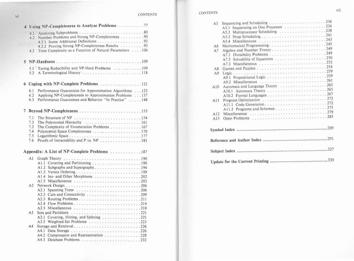
AS Sequencing and Scheduling ...... . ........ . · · . · · · 236 AS. I Sequencing on One Processor ...... . .... . ... . 236 AS.2 Multiprocessor Scheduling ... . .............. 238 AS.3 Shop Scheduling ............. . ... ... . . . . . 241 AS.4 Miscellaneous ........ . .......... .. .. . · . 243

A6 Mathematical Programming ....... . ... . .. . .. . .. . . 24S A 7 Algebra and Number Theory .... . ....... ... . . .... 249

A 7.1 Divisibility Problems . .... . ......... . .. . ... 249 A 7 .2 Solvability of Equations .... . ...... .. . . ... . · 2SO A 7·3 Miscellaneous ........... . ..... .. .. . . .. . 2S2

A8 Ga~es and Puzzles ....... . ....... . ... .. .. . ... 2S4 A9 Logic ...... . .............. · . .. · · · · · · · · · · · 2S9

A9. l Propositional Logic ......... .. . .... . .. . ... 2S9 A9.2 Miscellaneous ...... . ...... . .... . ... . ... 261

AlO Automata and Language Theory ............ · · . · · · 26S AlO.l Automata Theory . ............... . ... . .. 26S Al0.2 Formal Languages . . . . .. ...... . .. . ..... · · 267

Al 1 Program Optimization ................ . ........ 272 A 11 . l Code Generation .... . .... .. ........ .. · · · 272 All.2 Programs and Schemes ...... . ......... . ... 27S

Al 2 Miscellaneous ............. . .... . · · · · · · · · · · · 279 A 13 Open Problems ............. . ... · · · . · · · · · · · · 28S

7 .2 The Polynomial Hierarchy ...................... 161 7.3 The Complexity of Enumeration Problems ............ 167 7.4 Polynomial Space Completeness .................... 170

Symbol Index .... . ..... ... ......................... .. . .. ... ..... .. .... .... ... .. 289

7.S Logarithmic Space ............................ 177 7.6 Proofs of Intractability and P vs. NP ................ 181 Reference and Author Index ............ ............... · · .... · · .. ·· · · · · · · · · 291

Appendix: A List of NP-Complete Problems ............ 187 Subject Index ............... ...................... ... . . ................... ... .. 327

A I Graph Theory .............................. 190 A 1.1 Covering and Partitioning ................. .. 190

Update for the Current Printing ............... ..... .. .. ............ . . .. .. 339

A 1.2 Subgraphs and Supergraphs ............. ..... 194 A 1.3 Vertex Ordering ......................... 199 A 1.4 !so- and Other Morphisms .................. 202 Al .S Miscellaneous ................... , ...... 203

A2 Network Design .......... .. ................. 206 A2. I Spanning Trees ......................... 206 A2.2 Cuts and Connectivity ..................... 209 A2.3 Routing Problems ........................ 211 A2.4 Flow Problems .......................... 214 A2.S Miscellaneous .. .... ........ . .. ........ . 218

A3 Sets and Partitions .............. . ... ...... .. . 221 A3. l Covering, Hitting, and Splitting ............... 221 A3.2 Weighted Set Problems .................... 223

A4 Storage and Retrieval .......... . ..... . ..... .... 226 A4.1 Data Storage ........................... 226 A4.2 Compression and Representation .............. 228 A4.3 Database Problems .. ...... ......... .. .... 232

Preface

Few technical terms have gained such rapid notoriety as the appelation " NP-complete." In the short time since its introduction in the early l 970's, this term has come to symbolize the abyss of inherent intractability that algorithm designers increasingly face as they seek to solve larger and more complex problems. A wide variety of commonly encountered problems from mathematics, computer science, and operations research are now known to be NP-complete, and the collection of such problems continues to grow almost daily . Indeed, the NP-complete problems are now so pervasive that it is important for anyone concerned with the computational aspects of these fields to be familiar with the meaning and implications of this concept.

This book is intended as a detailed guide to the theory of NPcompleteness, emphasizing those concepts and techniques that seem to be most useful for applying the theory to practical problems. It can be viewed as consisting of three parts.

The first part, Chapters 1 through 5, covers the basic theory of NPcompleteness. Chapter 1 presents a relatively low-level introduction to some of the central notions of computational complexity and discusses the significance of NP-completeness in this context. Chapters 2 through 5 provide the detailed definitions and proof techniques necessary for thoroughly understanding and applying the theory.

The second part , Chapters 6 and 7, provides an overview of two alternative directions for further study. Chapter 6 concentrates on the search for efficient "approximation" algorithms for NP-complete problems, an area whose development has seen considerable interplay with the theory of NPcompleteness. Chapter 7 surveys a large number of theoretical tOpics in computational complexity, many of which have arisen as a consequence of previous work on NP-completeness. Both of these chapters (especially Chapter 7) are intended solely as introductions to these areas, with our expectation being that any reader wishing to pursue particular topics in more detail will do so by consulting the cited references.

The third and final part of the book is the Appendix, which contains an extensive list (more than 300 main entries, and several times this many results in total) of NP-complete and NP-hard problems. Annotations to the main entries discuss what is known about the complexity of subproblems and variants of the stated problems.

x PREFACE

The book should be suitable for use as a supplementary text in courses on algorithm design, computational complexity, operations research, or combinatorial mathematics. It also can be used as a starting point for seminars on approximation algorithms or computational complexity at the

·graduate or advanced undergraduate level. The second author has used a preliminary draft as the basis for a graduate seminar on approximation algorithms, covering Chapters 1 through 5 in about five weeks and then pursuing the topics in Chapter 6, supplementing them extensively with additional material from the references. A seminar on computational complexity might proceed similarly, substituting Chapter 7 for Chapter 6 as the initial access point to the literature. It is also possible to cover both chapters in a combineci seminar.

More generally, the book can serve both as a self-study text for anyone interested in learning about the subject of NP-completeness and as a reference book for researchers and practitioners who are concerned with algorithms and their complexity. The list of NP-complete problems in the Appendix can be used by anyone familiar with the central notions of NPcompleteness, even without having read the material in the main text. The novice can gain such familiarity by skimming the material in Chapters 1 through 5, concentrating on the informal discussions of definitions and techniques, and returning to the more formal material only as needed for clarification. To aid those using the book as a reference, we have included a substantial number of terms in the Subject Index, and the extensive Reference and Author Index gives the sections where each reference is mentioned in the text.

We are indebted to a large number of people who have helped us greatly in preparing this book. Hal Gabow, Larry Landweber, and Bob Tarjan taught from preliminary versions of the book and provided us with valuable suggestions based on their experience. The following people read preliminary drafts of all or part of the book and made constructive comments: Al Aho, Shimon Even, Ron Graham, Harry Hunt, Victor Klee, Albert Meyer, Christos Papadimitriou, Henry Pollak, Sartaj Sahni, Ravi Sethi , Larry Stockmeyer, and Jeff Ullman. A large number of researchers, too numerous to mention here (but see the Reference and Author Index) , responded to our call for NP-completeness results and contributed toward making our list of NP-complete problems as extensive as it is. Several of our colleagues at Bell Laboratories, especially Brian Kernighan, provided invaluable assistance with computer typesetting on the UNIX® system. Finally, special thanks go to Jeanette Reinbold, whose facility with translating our handwritten hieroglyphics into faultless input to the typesetting system made the task of writing this book so much easier.

Murray Hill, New Jersey October, 1978

MICHAEL R. GAREY

DAVIDS. JOHNSON

COMPUTERS AND INTRACTABILITY A Guide to the Theory of NP-Completeness

1.1 Introduction

1

Computers, Complexity, and Intractability

The subject matter of this book is perhaps best introduced through the following, somewhat whimsical , example.

Suppose that you, like the authors, are employed in the halls of industry. One day your boss calls you into his office and confides that the company is about to enter the highly competitive "bandersnatch" market. For this reason, a good method is needed for determining whether or not any given set of specifications for a new bandersnatch component can be met and, if so, for constructing a design that meets them. Since you are the company's chief algorithm designer, your charge is to find an efficient algorithm for doing this.

After consulting with the bandersnatch department to determine exactly what the problem is, you eagerly hurry back to your office, pull down your reference books, and plunge into the task with great enthusiasm. Some weeks later, your office filled with mountains of crumpled-up scratch paper, your enthusiasm has lessened considerably. So far you have not been able to come up with any algorithm substantially better than searching through all possible designs. This would not particularly endear you to your boss, since it would involve years of computation time for just one set of

2 COMPUTERS, COMPLEXITY, AND INTRACTABILITY

specifications, and the bandersnatch department is already 13 components behind schedule. You certainly don't want to return to his office and report :

" I can't find an efficient algorithm, I guess I'm just too dumb."

To avoid serious damage to your position within the company, it would be much better if you could prove that the bandersnatch problem is inherently intractable, that no algorithm could possibly solve it quickly. You then could stride confidently into the boss's office and proclaim:

"I can' t find an efficient algorithm, because no such algorithm is possible!"

Unfortunately, proving inherent intractability can be just as hard as finding efficient algorithms. Even the best theoreticians have been stymied in their attempts to obtain such proofs for commonly encountered hard problems. However, having read this book, you have discovered something

1.1 INTRODUCTION 3

almost as good. The theory of NP-completeness provides many straightforward techniques for proving that a given problem is "just as hard" as a large number of other problems that are widely recognized as being difficult and that have been confounding the experts for years. Armed with these techniques, you might be able to prove that the bandersnatch problem is NP-complete and, hence, that it is equivalent to all these other hard problems. Then you could march into your boss's office and announce:

" I can't find an efficient algorithm, but neither can all these famous people."

At the very least, this would inform your boss that it would do no good to fire you and hire another expert on algorithms.

Of course, our own bosses would frown upon our writing this book if its sole purpose was to protect the jobs of algorithm designers. Indeed, discovering that a problem is NP-complete is usually just the beginning of work on that problem. The needs of the bandersnatch department won't disappear overnight simply because their problem is known to be NPcomplete. However, the knowledge that it is NP-complete does provide valuable information about what lines of approach have the potential of being most productive. Certainly the search for an efficient, exact algorithm should be accorded low priority. It is now more appropriate to concentrate on other, less ambitious, approaches. For example, you might look for efficient algorithms that solve various special cases of the general problem. You might look for algorithms that, though not guaranteed to run quickly, seem likely to do so most of the time. Or you might even relax the problem somewhat, looking for a· fast algorithm that merely finds designs that


~eet most of the component specifications. In short, the primary applicat1_on ~f the t_heory of NP-completeness is to assist algorithm designers in dtrectmg their problem-solving efforts toward those approaches that have the greatest likelihood of leading to useful algorithms.

In the first chapter of this "guide" to NP-completeness we introduce many of t~e underlying concepts, discuss their applicability (~s well as give some cautions), and outline the remainder of the book.

1.2 Problems, Algorithms, and Complexity

In order to elaborate on what is meant by "inherently intractable" problems and problems having "equivalent" difficulty, it is important that we first agree on the meaning of several more basic terms.

. Let us begin with _t he notion of a problem. For our purposes, a problem · will be a general question to be answered, usually possessing several parameters,. or free _v~riables, whose values are left unspecified. A problem is described by g1vmg: (1) a general description of all its parameters, and (2) a sta_tement of what properties the answer, or solution, is required to satisfy. An instance of a problem is obtained by specifying particular values for all the problem parameters.

As an example, consider the classical " traveling salesman problem." Th7, ~a.ra~eters of this probl_em co~~ist of a finite set C = fci.c2, ... , cm} of c1t1es and, for each pair of c1t1es c;,c1 in C, the "distance" d(ci,c) b~twee~ . them. A solution is an ordering < crr(l).Crr(2), ... , crr(ml > of the given c1t1es that minimizes

[ mil d(c rr(i),C,,(;+I)) ) + d(crr(m).Crr(I)) 1- 1

This e_xpr~ssion gives the length of the "tour" that starts at c"m' visits each city m sequence, and then returns directly to crr(I) from the last city C,,(m)·

One instance of the traveling salesman problem illustrated in Figure 1.1, is given by C = {c"c2,c3,c4}, d(c"c2) '= IO, d(c"c) = 5, d(c1>c4) = 9, ~(c2,c3) =. 6, d(c2,~4)_ = 9, and d(c3,c4) = 3. The ordering <ci.c_2,~4,c3> is a solut10n for this instance, as the corresponding tour has the mm1mum possible tour length of 27.

Algorithms are general , step-by-step procedures for solving problems. Fo_r con~reteness, we can think of them simply as being computer programs, written m s~me precise computer language. An algorithm is said to solve a problem n 1f that algorithm can be applied to any instance / of n and is guaranteed always to produce a solution for that instance /. We emphasize that the term "solution" is intended here strictly in the sense introduced above, so that, in particular, an algorithm does not "solve" the traveling

r 1.2 PROBLEMS, ALGORITHMS, AND COMPLEXITY 5

Figure 1.1 An instance of the traveling salesman problem and a tour of length 27, which is the minimum possible in this case.

salesman problem unless it always constructs an ordering that gives a minimum length tour.

In general, we are interested in finding the most "efficient" algorithm for solving a problem. In its broadest sense, the notion of efficiency involves all the various computing resources needed for executing an algorithm. However, by the "most efficient" algorithm one normally means the fastest. Since time requirements are often a dominant factor determining whether or not a particular algorithm is efficient enough to be useful in practice, we shall concentrate primarily on this single resource.

The time requirements of an algorithm are conveniently expressed in terms of a single variable, the "size" of a problem instance, which is intended to reflect the amouni: of input data needed to describe the instance. This is convenient because we would expect the relative difficulty of problem instances to vary roughly with their size. Often the size of a problem instance is measured in an informal way. For the traveling salesman problem, for example, the number of cities is commonly used for this purpose. However, an m-city problem instance includes, in addition to the labels of them cities, a collection of m(m- 1)/2 numbers defining the inter-city distances, and the sizes of these numbers also contribute to the amount of input data. If we are to deal with time requirements in a precise, mathematical manner, we must take care to ·define instance size in such a way that all these factors are taken into account.

To do this, observe that the description of a problem instance that we provide as input to the computer can be viewed as a single finite string of symbols chosen from a finite input alphabet. Although there are many different ways in which instances of a given problem might be described, let us assume that one particular way has been chosen in advance and that each problem has associated with it a fixed encoding scheme , which maps problem


instances into the strings describing them. The input length for an instance I of a problem Il is defined to be the number of symbols in the description of I obtained from the encoding scheme for II. It is this number, the input length, that is used as the formal measure of instance size.

For example, instances of the traveling salesman problem might be described using the alphabet {c,[, ], /, 0, 1, 2, 3, 4, 5, 6, 7,8 , 9), with our previous example of a problem instance being encoded by the string "c[l]c[2]c[3]c[4]//10/ 5/ 9//6/ 9//3." More complicated instances would be encoded in analogous fashion. If this were the encoding scheme associated with the traveling salesman problem, then the input length for our example would be 32.

The time complexity function for an algorithm expresses its time requirements by giving, for each possible input length , the largest amount of time needed by the algorithm to solve a problem instance of that size. Of course, this function is not well-defined until one fixes the encoding scheme to be used for determining input length and the computer or computer model to be used for determining execution time. However, as we shall see, the particular choices made for these will have little effect on the broad distinctions made in the theory of NP-completeness. Hence, in what follows, the reader is advised merely to fix in mind a particular encoding scheme for each problem and a particular computer or computer model, and to think in terms of time complexity as determined from the corresponding input lengths and execution times.

1.3 Polynomial Time Algorithms and Intractable Problems

Different algorithms possess a wide variety of different time complexity functions, and the characterization of which of these are "efficient enough" and which are "too inefficient" will always depend on the situation at hand. However, computer scientists recognize a simple distinction that offers considerable insight into these matters. This is the distinction between polynomial time algorithms and exponential time algorithms.

Let us say that a function f (n) is 0 (g (n)) whenever there exists a constant c such that JJ(n) I ~ c-Jg(n) I for all values of n ~O. A polynomial time algorithm is defined to be one whose time complexity function is O(p(n)) for some polynomial function p , where n is used to denote the input length. Any algorithm whose time complexity function cannot be so bounded is called an exponential time algorithm (although it should be noted that this definition includes certain non-polynomial time complexity functions, like n logn , which are not normally regarded as exponential functions).

The distinction between these two types of algorithms has particular significance when considering the solution of large problem instances. Figure 1.2 illustrates the differences in growth rates among several typical complexity functions of each type, where the functions express execution time

POLYNOMIAL TIME ALGORITHMS AND INTRACTABLE PROBLEMS 1.3 7

. terms of microseconds. Notice the much more explosive growth rates 10 I . f . for the two exponential comp ex1ty unctions.

- Size n

Time complexity 10 20 30 40 50 60

function ~

.00001 .00002 .00003 .00004 .00005 .00006 n second second second second second second

-.0001 .0004 .0009 .0016 .0025 .0036

n2 second second second second second second

.001 .008 .027 .064 .125 .216 n3

second second second second second second

.1 3.2 24.3 1.7 5.2 13.0 n s

second seconds seconds minutes minutes minutes ~

.001 1.0 17.9 12.7 35.7 366 2n

second second minutes days years centuries

.059 58 6.5 3855 2X 108 1.3xl013

3n second minutes years centuries centuries centuries

Figure 1.2 Comparison of several polynomial and exponential time complexity functions.

Even more revealing is an examination of the effects of improved computer technology on algorithms having these time complexit?' functions. Figure 1.3 shows how the largest problem instance ~olvable m one hour would change if we had a computer 100 or 1000 times faster than ~ur present machine. Observe that with the 2n algorithm a thousand-fold in

crease in computing speed only adds 10 to .the size 5of the_ largest. pr?blem

instance we can solve in an hour, whereas with the n algorithm this size al-most quadruples. . .

These tables indicate some of the reasons why polynomial time algorithms are generally regarded as being much more desirable than exponential time algorithms. This view, and the distinction between the two types of algorithms, is central to our notion of inherent intractability and to the theory of NP-completeness. . .

The fundamental nature of this distinction was first discussed m [Cobham, 1964] and [Edmonds, 1965a]. Edmonds, in particular, equated poly-

8

Time complexity function

n

n2

n3

n5

2n

3n

COMPUTERS, COMPLEXITY, AND INTRACTABILITY

Size of Largest Problem Instance Solvable in l Hour

With present With computer With computer computer 100 times faster IOOO times faster

N i 100 Ni IOOO Ni

N2 IO N2 31.6 N2

N3 4.64 N3 IO N3

N4 2.5 N4 3.98 N4

Ns Ns+6.64 Ns+9.97

N6 N6 +4.19 N6+6.29

Figure 1.3 Effect of improved technology on several polynomial and exponential time algorithms.

nomial time algorithms with "good" algorithms and conjectured that certain integer programming problems might not be solvable by such "good" algorithms. This reflects the viewpoint that exponential time algorithms should not be considered "good" algorithms, and indeed this usually is the case. Most exponential time algorithms are merely variations on exhaustive search, whereas polynomial time algorithms generally are made possible only through the gain of some deeper insight into the structure of a problem. There is wide agreement that a problem has not been " well-solved" until a polynomial time algorithm is known for it. Hence, we .shall refer to a problem as intractable if it is so hard that no polynomial time algorithm can possibly solve it.

Of course, this formal use of "intractable" should be viewed only as a rough approximation to its dictionary meaning. The distinction between "efficient" polynomial time algorithms and "inefficient" exponential time algorithms admits of many exceptions when the problem instances of interest have limited size. Even in Figure 1.2, the 2n algorithm is faster than the n 5 algorithm for n .:::;; 20. More extreme examples can be constructed easily.

Furthermore, there are some exponential time algorithms that have been quite useful in practice. Time complexity as defined is a worst-case measure, and the fact that an algorithm has time complexity 2n means only that at least one problem instance of size n requires that much time. Most problem instances might actually require far less time than that, a situation

3 POLYNOMIAL TIME ALGORITHMS AND INTRACTABLE PROBLEMS

l. 9

that appears to hold for several well-known algorithms. The simpl~x a~go-'th for linear programming has been shown to have exponential time

ri m 973) · h · · complexity [Klee and Minty, 1972), [Zadeh, l . , but 1t as an 1mpress1ve record of running quickly in practice. Likewise, branch-and-bound al~o-'thms for the knapsack problem have been so successful that many cons1d

~1r it to be a "well-solved" problem, even though these algorithms, too,

have exponential time complexity. Unfortunately, examples like these are quite rare. Although exponen-

tial time algorithms are known for many problems, few of them ~re :egarded as being very useful in practice. Even the successful exponenlla~ t1~e algorithms mentioned above have not stopped re~earchers from contmumg to search for polynomial time algorithms for solving those pro?l~ms . In fact, the very success of these algorithms has led to the susp1c10n that they somehow capture a crucial property of the problems whose refinement could lead to still better methods. So far, little progress has been i:na.de t?ward explaining this success, and no method~ are ~nown fo: pre~1ctmg ~n advance that a given exponential time algori thm will run quickly m practice.

On the other hand, the much more stringent bounds on execution time satisfied by polynomial time algorithms often permit such predictions to be

. h . . 1 't 100 1099n2 made. Even though an algorithm avmg ttme comp ext Y n or . might not be considered likely to run quickly in practice, t.he. polynom1a~ly solvable problems that arise naturally tend to be solvable w1thm polynomial time bounds that have degree 2 or 3 at worst and that do not involve extremely large coefficients. Algorithms satisfying such bounds can be considered to be "provably efficient," and it is this much-desired property that makes polynomial time algorithms the preferred way to solve problems.

Our definition of " intractable" also provides a theoretical framework of considerable generality and power. The intractability of a problem turns out to be essentially independent of the particular encoding scheme and computer model used for determining time complexity.

Let us first consider encoding schemes. Suppose for example that we are dealing with a problem in which each instance is a graph G = (.V,E), where V is the set of vertices and E is the set of edges, each edge being an unordered pair of vertices. Such an instance might be described (see Figure l.4) by simply listing all the vertices and edges, or by listing the rows of the adjacency matrix for the graph, or by listing for each vertex all the other vertices sharing a common edge with it (a "neighbor" list) . Each of these encodings can give a different input length for the same graph. However, it is easy to verify (see Figure 1.5) that the input lengths they determine differ at most polynomially from one another, so that any algorithm having polynomial time complexity under one of these encoding schemes also will have polynomial time complexity under all the others. In fact, the standard encoding schemes used in practice for any particular problem always seem to differ at most polynomially from one another. It would be difficult to imagine a " reasonable" encoding scheme for a problem that differs more


than polynomially from the standard ones. Although what we mean here by "reasonable" cannot be formalized, the following two conditions capture much of the notion:

(1) the encoding of an instance I should be concise and not "padded" with unnecessary information or symbols, and

(2) numbers occurring in I should be represented in binary (or de-cimal, or octal, or in any fixed base other than 1).

If we restrict ourselves to encoding schemes satisfying these conditions, then the particular encoding scheme used should not affect the determination of whether a given problem is intractable.

Encoding Scheme String Length

Vertex list, Edge list V[l)V[2)V[3]V[4] (V[l]V[2]) (V[2]V[3]) 36

Neighbor list (V[2])(V[I]V[3])(V[2])() 24

Adjacency matrix rows 0100/1010/0010/0000 19

Figure 1.4 Descriptions of the graph G = ( V,E) where V = {Vi. V2, V3, V4 ) and E = { {Vi. V2) , { V2, V3)), under three different encoding schemes.

Encoding Scheme Lower Bound Upper Bound

Vertex list, Edge list 4v + lOe 4v + lOe + (v+2e)·rlog10vl

Neighbor list 2v + 8e 2v + 8e + 2e · rlog10vl

Adjacency matrix v2 + v - 1 v2 + v - 1

Figure 1.5 General bounds on input lengths for the three encoding schemes of Figure 1.4 for graphs G = ( V,E) with I VI= v, 1£1 = e. Since e < v2,

these show that the input lengths differ at most polynomially from each other. crxl denotes the least integer not less than x.)

Similar comments can be made concerning the choice of computer models. All the realistic models of computers studied so far, such as onetape Turing machines, multi-tape Turing machines, and random-access machines (RAMs), are equivalent with respect to polynomial time complexity (for example, see Figure 1.6). One would expect any other "reasonable" model to share in this equivalence. The notion of "reasonable" in-

PROVABLY INTRACTABLE PROBLEMS J.4

11

d d here is essentially that there is a polynomial bound on the amount of ten : that can be done in a single unit of time. Thus, for ex~mpl~, a model wor. the capability of performing arbitrarily many operat10ns m par~Llel havilndg t be considered " reasonable " and indeed no existing (or planned) wou no , . I

h S this capability At any rate so long as we restrict ourse ves to computer a · ' .

d rd models of realistic computers the class of intractable problems the stan a ' will be unaffected by the par~icular ~ode\ use~ , ~nd we can . ma~~ our choice on the basis of convenience without sacnficmg the appltcab1hty of

our results.

Simulating machine A

Simulated machine B lTM kTM RAM

1-Tape Turing Machine (lTM) - O(T(n)) O(T(n}logT(n)}

k-Tape Turing Machine (kTM) O(T2(n)) - O(T(n)logT(n))

Random Access Machine (RAM) O(T3(n)) O(T2( n)) -

Figure 1.6 Time required by machine A to simulate the execution of an algorithm of time complexity T(n) on Machine B (for example, see [Hopcroft and Ullman, 1969] and [Aho, Hopcroft, and Ullman, 1974]) .

1.4 Provably Intractable Problems

Now that we have discussed the formal meaning of "intractable problem," it is appropriate that we briefly survey the current state of knowledge about the existence of intractable problems.

It is useful to begin by distinguishing between two different causes of intractability allowed by our definition. The first, which is the one we us~ally have in mind, is that the problem is so difficult that an e.xponent1al amount of time is needed to discover a solution. The second is. that t.he solution itself is required to be so extensive that it c.annot b~ descnbed. with an expression having length bounded by a polynomial function of the input

length. 1· This second cause occurs, for example, in the variant of the trave mg salesman problem that includes a number B as an additi?nal parameter and that asks for all tours having total length B or less. It 1s easy to construct instances of this problem in which exponentially many tours are sho~ter than the given bound, so that no polynomial time algorithm could possibly

list them all. . . . Intractability of this sort is by no means insignificant, a~d it ~s 1mpo:-

tant to recognize it when it occurs. However, in most cases its existence is


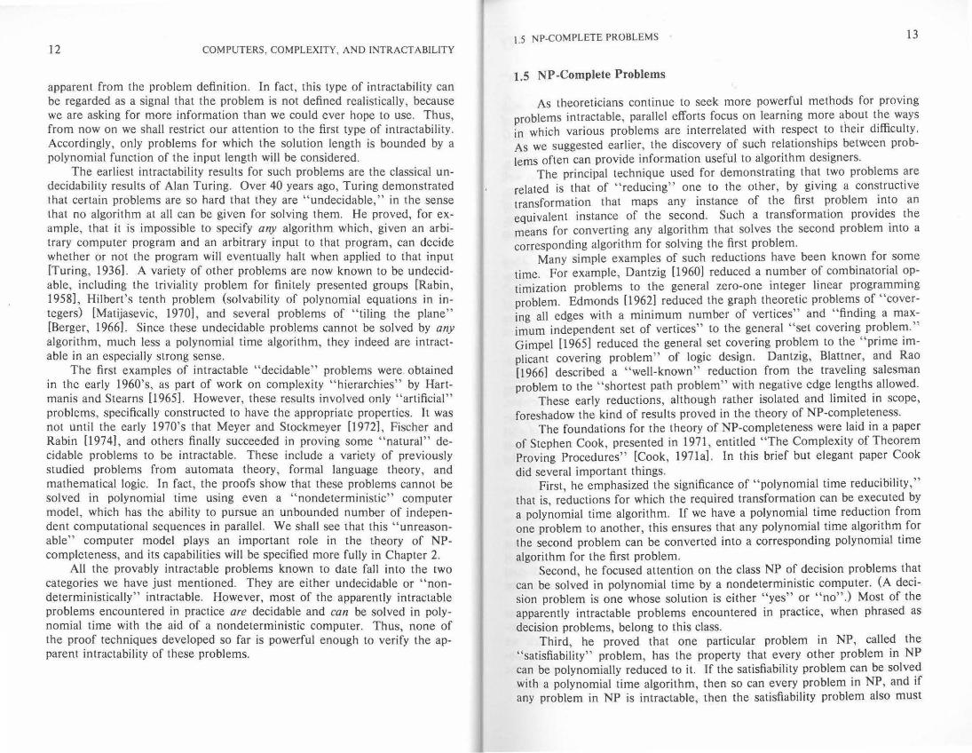
apparent from the problem definition. In fact, this type of intractability can be regarded as a signal that the problem is not defined realistically, because we are asking for more information than we could ever hope to use. Thus, from now on we shall restrict our attention to the first type of intractability. Accordingly, only problems for which the solution length is bounded by a polynomial function of the input length will be considered.

The earliest intractability results for such problems are the classical undecidability results of Alan Turing. Over 40 years ago, Turing demonstrated that certain problems are so hard that they are "undecidable," in the sense that no algorithm at all can be given for solving them. He proved, for example, that it is impossible to specify any algorithm which, given an arbitrary computer program and an arbitrary input to that program, can decide whether or not the program will eventually halt when applied to that input [Turing, 1936]. A variety of other problems are now known to be undecidable, including the triviality problem for finitely presented groups [Rabin, 1958), Hilbert's tenth problem (solvability of polynomial equations in integers) [Matijasevic, 1970], and several problems of "tiling the plane" [Berger, 1966]. Since these undecidable problems cannot be solved by any algorithm, much less a polynomial time algorithm, they indeed are intractable in an especially strong sense.

The first examples of intractable " decidable" problems were obtained in the early l 960's, as part of work on complexity "hierarchies" by Hartmanis and Stearns (1965]. However, these results involved only "artificial" problems, specifically constructed to have the appropriate properties. It was not until the early 1970's that Meyer and Stockmeyer [1972], Fischer and Rabin [1974] , and others finally succeeded in proving some "natural" decidable problems to be intractable. These include a variety of previously studied problems from automata theory, formal language theory, and mathematical logic. In fact, the proofs show that these problems cannot be solved in polynomial time using even a "nondeterministic" computer model, which has the ability to pursue an unbounded number of independent computational sequences in parallel. We shall see that this "unreasonable" computer model plays an important role in the theory of NPcompleteness, and its capabilities will be specified more fully in Chapter 2.

All the provably intractable problems known to date fall into the two categories we have just mentioned. They are either undecidable or "nondeterministically" intractable. However, most of the apparently intractable problems encountered in practice are decidable and can be solved in polynomial time with the aid of a nondeterministic computer. Thus, none of the proof techniques developed so far is powerful enough to verify the apparent intractability of these problems.

1.5 NP-COMPLETE PROBLEMS 13

t.5 NP-Complete Problems

As theoreticians continue to seek more powerful methods for proving problems int~actable, parallel eff ?rts focus on ~earning more a_bo_ut t~e ways in which vanous problems are interrelated with respect to their difficulty. As we suggested earlier, the discovery of such relationships between problems often can provide information useful to algorithm designers.

The principal technique used for demonstrating that two problems are related is that of " reducing" one to the other, by giving a constructive transformation that maps any instance of the first problem into an equivalent instance of the second. Such a transformation provide_s the means for converting any algorithm that solves the second problem mto a corresponding algorithm for solving the first problem.

Many simple examples of such reductions have been known for some time. For example, Dantzig [1960] reduced a number of combinatorial optimization problems to the general zero-one integer linear programming problem. Edmonds [1962] reduced the graph theoretic problems of " covering all edges with a minimum number of vertices" and "finding a maximum independent set of vertices" to the general " set covering problem." Gimpel [1965] reduced the general set covering problem to the "prime implicant covering problem" of logic design. Dantzig, Blattner, and Rao [1966] described a "well-known" reduction from the traveling salesman problem to the "shortest path problem" with negative edge lengths allowed.

These early reductions, although rather isolated and limited in scope, foreshadow the kind of results proved in the theory of NP-completeness.

The foundations for the theory of NP-completeness were laid in a paper of Stephen Cook, presented in 1971 , entitled "The Complexity of Theorem Proving Procedures" [Cook, 197la] . In this brief but elegant paper Cook did several important things.

First, he emphasized the significance of "polynomial time reducibility ," that is reductions for which the required transformation can be executed by a poly~omial time algorithm. If we have a polynomial time reduction from one problem to another, this ensures that any polynomial time algorithm for the second problem can be converted into a corresponding polynomial time algorithm for the first problem.

Second he focused attention on the class NP of decision problems that can be solv~d in polynomial time by a nondeterministic computer. (A decision problem is one whose solution is either "yes" or "no".) Most of the apparently intractable problems encountered in practice, when phrased as decision problems, belong to this class.

Third, he proved that one particular problem in NP, called the "satisfiability" problem, has the property that every other problem in NP can be polynomially reduced to it. If the satisfiability problem can be solved with a polynomial time algorithm, then so can every problem in NP, and if any problem in NP is intractable, then the satisfiability problem also must


be intractable. Thus, in a sense, the satisfiability problem is the " hardest" problem in NP.

Finally, Cook suggested that other problems in NP might share with the satisfiability problem this property of being the " hardest" member of NP. He showed this to be the case for the problem " Does a give n graph G contain a complete subgraph on a given number k of vertices?"

Subsequently, Richard Karp presented a collection of results [Karp, 1972) proving that indeed the decision problem versions of many well known combinatorial problems, including the traveling salesman problem, are just as "hard" as the satisfiability problem. Since then a wide variety of other problems have been proved equivalent in difficulty to these problems, and this equivalence class, consisting of the " hardest" problems in NP, has been given a name: the class of NP-complete problems.

Cook's original ideas have turned out to be remarkably powerful. They have provided the means for combining many individual complexity questions into the single question: Are the NP-complete problems intractable? The lists included in the Appendix of this book contain literally hundreds of different problems now known to be NP-complete. As more and more problems of independent interest are shown to belong to this equivalence class, its importance is continually reinforced.

The question of whether or not the NP-complete problems are intractable is now considered to be one of the foremost open questions of contemporary mathematics and computer science. Despite the willingness of most researchers to conjecture that the NP-complete problems are all intractable, little progress has yet been made toward establishing either a proof or a disproof of this far-reaching conjecture. However, even without a proof that NP-completeness implies intractability, the knowledge that a problem is NP-complete suggests, at the very least, that a major breakthrough will be needed to solve it with a polynomial time algorithm.

1.6 An Outline of the Book

Although this book is intended mainly as a primer on how to determine whether or not any particular problem is NP-complete (either by looking it up in the lists we present or by proving it yourself) , we shall also discuss some of the options available for dealing with a problem that is known to be NP-complete. A brief outline of subsequent chapters follows.

In Chapter 2, we present the formal underpinnings of NP-completeness and prove Cook's theorem. The central definitions involve certain theoretical concepts, such as "languages" and "Turing machines," which we develop in a straightforward manner, relating them to the notions of problems and computer models already discussed. This chapter should give the reader a good understanding of the technical meaning of NP-completeness.

I .6 AN OUTLINE OF THE BOOK 15

Chapter 3 is devoted to methods for proving a problem NP-complete. A number of examples are presented to illustrate the usual. structure of

h roofs and to indicate how one goes about generating one. In sue P ' · II

e one proves a new problem to be NP-complete by polynom1a Y essenc , . w h k NP

d ·ng a known NP-complete problem to 1t. e survey t e nown -re~ . d complete problems that have been most useful for this purpose and emon-

strate their use. . . . In Chapter 4, we examine the ways in . which th.e theory of NP-leteness can be used for conducting a detailed analysts of the complex

~t~m:r a problem, seeking to determine the "boundary" between those cases of the problem that are polynomially solvable and those that are NP-

complete. . . In Chapter 5, we show how the techniques used for ~roving .~P-

mpleteness can be generalized so that problems other than JUSt dec1s1on c~oblems can be proved to be "as hard as" the NP-complete problems. As ~n aid to reading the published literature on the theory of NP-completenes.s , we also provide a brief historical survey of the develop~ent ~f the main ideas and the varying tP.rminology that has been used for .d1scu~sin~ them.

In Chapter 6, we discuss several approaches for dealing with intractable problems, especially that of finding near-optimal solutions using fast algorithms. Examples of the successes and failures of each approach are described, and we illustrate how the theory of NP-completeness can be ap-

plied even here. . . . Chapter 7 is intended to acquaint the reader with some of the theoreti-

cal issues and ideas that have arisen in parallel with the theory of NPcompleteness. Among other topics we discuss the polyno,r;iial ~i~ra~ch~: #P-completeness, polynomial space completeness, and the relat1v1zat1on of the question of the intractability of the NP-complete problems.

The last third of the book consists of the Appendix, an extensive and annotated list of problems known to be NP-complete or harder. The list is divided into sections, each devoted to problems from a particular subj~ct area, such as graph theory, scheduling, algebra and number theory, covering and partitioning, mathematical programming, program optimization, .au~omata and language theory, and, of course, miscellaneous topics. The hst includes references to related problems known to be solvable in polynomial time and to problems whose status remains open in that neither polynomial time algorithms nor NP-completeness proofs are known for them.

Computers and intractability a guide to the theory of np completeness

Engineering