Computer Vision and Statistical Estimation Tools for In Situ ...

Computer Vision and Statistical Estimation Tools for In Situ,

Imaging-based Monitoring of Particulate Populations

by

Paul A. Larsen

A dissertation submitted in partial fulfillment

of the requirements for the degree of

DOCTOR OF PHILOSOPHY

(Chemical Engineering)

at the

UNIVERSITY OF WISCONSIN–MADISON

2007

c© Copyright by Paul A. Larsen 2007

All Rights Reserved

To Jenny

ii

Computer Vision and Statistical Estimation Tools for In Situ,

Imaging-based Monitoring of Particulate Populations

Paul A. Larsen

Under the supervision of Professor James B. Rawlings

At the University of Wisconsin–Madison

Solution crystallization is a commonly used but often poorly controlled process for separating

or purifying chemical species in the pharmaceutical, chemical, and food industries. The develop-

ment of effective solid-phase monitoring technology is a critical step to enable better understand-

ing and control of crystallization processes. Video imaging is a promising technology offering

the potential to monitor critical solid-phase properties, including particle size distribution (PSD),

shape distribution, and, in some cases, polymorphic fraction.

To address the challenges associated with effective use of video imaging for particulate

processes, this thesis focuses on the following areas:

1. Developing image analysis algorithms that enable segmentation of noisy, in situ video im-

ages of crystallization processes.

2. Developing statistical estimators to overcome the sampling biases inherent in imaging-based

measurement.

3. Characterizing the reliability and feasibility of imaging-based particle size distribution mea-

surement given imperfect image analysis.

We have developed two image analysis algorithms. The first algorithm is designed to

extract particle size and shape information from in situ images of suspended, high-aspect-ratio

iii

crystals. This particular shape class arises frequently in pharmaceutical and specialty chemical

applications and is problematic for conventional monitoring technologies that are based on the

assumption that the particles are spherical. The second algorithm is designed to identify crystals

having more complicated shapes. The effectiveness of both algorithms is demonstrated using

in situ images of crystallization processes and by comparing the algorithm results with results

obtained by human operators. The algorithms are sufficiently fast to enable real-time monitoring

for typical cooling crystallization processes.

We have derived a maximum likelihood estimator to estimate the particle size distribution

of needle-like particles. We benchmark the estimator against the conventional Miles-Lantuejoul

approach using several case studies. For needle-like particles, the MLE provides better estimates

than the Miles-Lantuejoul approach, but the Miles-Lantuejoul approach can be applied to a wider

class of shapes. Both methods assume perfect image segmentation, or that every particle appear-

ing in the image is identified correctly.

Given that perfect image segmentation is a reasonable assumption only at low solids con-

centrations, we have derived a descriptor that correlates with the reliability of the imaging-based

measurement (i.e. the quality of the image segmentation) based on the amount of particle overlap.

Also, we have developed a practical approach for estimating the number density of particles for

significant particle overlap and imperfect image analysis. The approach is developed for mono-

disperse particle systems.

Finally, this thesis demonstrates the feasibility of reconstructing a particle size distribu-

tion from imaging data for a well-studied industrial crystallization process and realistic imaging

conditions.

iv

v

AcknowledgmentsI am indebted to a great many people for the opportunity to come to the University of Wisconsin

and for the positive experience I have had while studying here. I am indebted first to God, who

has given me life, health, and the ability to think and be creative. I feel a debt of gratitude to my

parents and grandparents for their work and sacrifice to give me a life full of opportunity and

happiness. Grandpa Arch in particular had a strong desire to pursue a PhD but was unable. I

know he is pleased I have had the opportunity.

I am grateful to my advisor, Jim Rawlings, for giving me a rich and rewarding graduate

experience. He has taught me how to “first think clearly, then write clearly,” how to seek and value

experts without trusting them blindly, and how to make sense out of complicated and confusing

problems. Jim has motivated me with high expectations but also has been supportive of my family

situation. I will miss the opportunity to work with him so closely on challenging problems.

I am grateful for Nicola Ferrier’s invaluable guidance in developing effective image analy-

sis algorithms. Nicola also served as my wife’s adviser and has been a great friend to our family.

Lian Yu has freely given of his time and resources to help me carry out and analyze crystalliza-

tion experiments. His graduate student, Jun Huang, has also been a great help and good friend.

Professor Chuck Dyer of the Computer Science department also has provided helpful advice.

David Dahl, previously my friendly next-door neighbor and currently an assistant profes-

sor of statistics at Texas A&M, has given invaluable statistics consulting. I am also indebted to

Professor Antonio Torralba of the MIT Computer Science and Artificial Intelligence Laboratory

for the use of his LabelMe database and software.

Philip Dell’Orco at GlaxoSmithKline has helped me considerably by contributing the video

vi

imaging equipment and pharmaceutical material. Hiroya Seki and Shigeharu Katsuo of the Mit-

subishi Chemical Company have given me the chance to work on industrial projects that provided

excellent learning opportunities. I am also grateful to other members of the Texas-Wisconsin Mod-

eling and Control Consortium for financial support.

Despite being a long and often frustrating process, the commercialization of the SHARC

algorithm has been a source of excitement and satisfaction for me. I am grateful to John Hardiman

and Marnie Matt at WARF and our patent attorney Stephen Roe at Lathrop Clark for their work

in patenting SHARC and M-SHARC and licensing SHARC. Eric Hukkanen, Gregor Hsiao, Paul

Barrett, Ben Smith, and Nilesh Shah at Mettler-Toledo have each played important roles in this

process.

I am grateful to many of my fellow graduate students for friendship and assistance. I’ve

enjoyed immensely the opportunity to associate, both through church and through the depart-

ment, with Matt Tingey, George Huber, Tommy Knotts, Ethan Mastny, Nat Fredin, Clark Miller,

and Peter Ferrin. Mike Benton has been a thoughtful friend and a constant source of good con-

versation. The past and present members of the Rawlings group–Brian Odelson, Eric Haseltine,

Aswin Venkat, Ethan Mastny, Murali Rajamani, Brett Stewart, and Rishi Amrit–have been excel-

lent coworkers and friends. I only regret that my time with Brett and Rishi has been so short.

Mary Diaz has made my work life much more pleasant with her endless supply of candy

and plastic utensils, her willing assistance with administrative details, and her friendship. I wish

her and her sons Joshua and Jeremiah all the best.

Ethan Mastny and Murali Rajamani deserve special mention. Ethan has been my sounding

board, my one-man audience for countless practice talks, my neighbor, and my friend. Murali has

been my math consultant, my Linux troubleshooter, my office buddy, and the source of many fun

conversations. I will miss them both terribly.

Finally, I am grateful most of all to my wife Jenny. Her optimism, enthusiasm, wisdom,

and encouragement has made possible the happiness our family has enjoyed these past five years.

I am excited and comforted to have her at my side as we move to Michigan and begin a new phase

vii

of life. I’m grateful to our children, Beth, Benjamin, and Sophia, for making us laugh, reminding

us what’s really important, and bringing joy and purpose to our life.

PAUL ARCHIBALD LARSEN

University of Wisconsin–Madison

July 2007

viii

ix

Contents

Abstract ii

Acknowledgments v

List of Tables xv

List of Figures xvii

Notation xxiii

Chapter 1 Introduction 1

1.1 Project motivation and research objectives . . . . . . . . . . . . . . . . . . . . . . . . . 1

1.2 Thesis overview . . . . . . . . . . . . . . . . . . . . . . . . . . . . . . . . . . . . . . . . 4

Chapter 2 Literature Review 7

2.1 Crystallization overview and terminology . . . . . . . . . . . . . . . . . . . . . . . . . 7

2.2 Conventional practice in industry . . . . . . . . . . . . . . . . . . . . . . . . . . . . . . 9

2.2.1 Process development . . . . . . . . . . . . . . . . . . . . . . . . . . . . . . . . . 9

2.2.2 Controlled, measured, and manipulated variables . . . . . . . . . . . . . . . . 14

2.3 Recent advances in crystallization technology . . . . . . . . . . . . . . . . . . . . . . . 15

2.3.1 Spectroscopic and laser-based monitoring . . . . . . . . . . . . . . . . . . . . . 15

2.3.2 Imaging-based monitoring . . . . . . . . . . . . . . . . . . . . . . . . . . . . . 19

2.3.3 Manipulated variables for crystal shape and polymorphic form . . . . . . . . 22

x

2.3.4 Modeling and prediction of crystal size, shape, and polymorphic form . . . . 23

2.3.5 Control . . . . . . . . . . . . . . . . . . . . . . . . . . . . . . . . . . . . . . . . . 24

2.4 The future of crystallization . . . . . . . . . . . . . . . . . . . . . . . . . . . . . . . . . 25

Chapter 3 Crystallization Model Formulation and Solution 27

3.1 Model formulation . . . . . . . . . . . . . . . . . . . . . . . . . . . . . . . . . . . . . . 27

3.1.1 Population balance . . . . . . . . . . . . . . . . . . . . . . . . . . . . . . . . . . 27

3.1.2 Mass balance . . . . . . . . . . . . . . . . . . . . . . . . . . . . . . . . . . . . . 29

3.1.3 Energy balance . . . . . . . . . . . . . . . . . . . . . . . . . . . . . . . . . . . . 30

3.2 Model solution . . . . . . . . . . . . . . . . . . . . . . . . . . . . . . . . . . . . . . . . 30

3.2.1 Method of moments . . . . . . . . . . . . . . . . . . . . . . . . . . . . . . . . . 30

3.2.2 Orthogonal collocation . . . . . . . . . . . . . . . . . . . . . . . . . . . . . . . . 31

Chapter 4 Experimental and Simulated Image Acquisition 35

4.1 Crystallizer and imaging apparatus . . . . . . . . . . . . . . . . . . . . . . . . . . . . 35

4.1.1 Crystallizer . . . . . . . . . . . . . . . . . . . . . . . . . . . . . . . . . . . . . . 35

4.1.2 Data acquisition . . . . . . . . . . . . . . . . . . . . . . . . . . . . . . . . . . . . 36

4.1.3 Video image acquisition . . . . . . . . . . . . . . . . . . . . . . . . . . . . . . . 38

4.1.4 Operating procedure . . . . . . . . . . . . . . . . . . . . . . . . . . . . . . . . . 39

4.2 Chemical systems . . . . . . . . . . . . . . . . . . . . . . . . . . . . . . . . . . . . . . . 41

4.2.1 Industrial pharmaceutical . . . . . . . . . . . . . . . . . . . . . . . . . . . . . . 41

4.2.2 Industrial photochemical . . . . . . . . . . . . . . . . . . . . . . . . . . . . . . 41

4.2.3 Glycine . . . . . . . . . . . . . . . . . . . . . . . . . . . . . . . . . . . . . . . . . 42

4.3 Artificial image generation . . . . . . . . . . . . . . . . . . . . . . . . . . . . . . . . . . 44

4.3.1 Stochastic process model . . . . . . . . . . . . . . . . . . . . . . . . . . . . . . 44

4.3.2 Imaging model . . . . . . . . . . . . . . . . . . . . . . . . . . . . . . . . . . . . 45

4.3.3 Justifications for two-dimensional system model . . . . . . . . . . . . . . . . . 47

xi

Chapter 5 Two-dimensional Object Recognition for High-Aspect-Ratio Particles 49

5.1 Image analysis algorithm description . . . . . . . . . . . . . . . . . . . . . . . . . . . . 50

5.1.1 Overview . . . . . . . . . . . . . . . . . . . . . . . . . . . . . . . . . . . . . . . 50

5.1.2 Linear feature detection . . . . . . . . . . . . . . . . . . . . . . . . . . . . . . . 52

5.1.3 Identification of collinear line pairs . . . . . . . . . . . . . . . . . . . . . . . . . 54

5.1.4 Identification of parallel line pairs . . . . . . . . . . . . . . . . . . . . . . . . . 56

5.1.5 Clustering . . . . . . . . . . . . . . . . . . . . . . . . . . . . . . . . . . . . . . . 58

5.2 Experimental results . . . . . . . . . . . . . . . . . . . . . . . . . . . . . . . . . . . . . 59

5.2.1 Algorithm accuracy . . . . . . . . . . . . . . . . . . . . . . . . . . . . . . . . . 61

5.2.2 Algorithm speed . . . . . . . . . . . . . . . . . . . . . . . . . . . . . . . . . . . 65

5.3 Conclusion . . . . . . . . . . . . . . . . . . . . . . . . . . . . . . . . . . . . . . . . . . . 70

Chapter 6 Three-dimensional Object Recognition for Complex Crystal Shapes 71

6.1 Model-based recognition algorithm . . . . . . . . . . . . . . . . . . . . . . . . . . . . . 72

6.1.1 Preliminaries . . . . . . . . . . . . . . . . . . . . . . . . . . . . . . . . . . . . . 72

6.1.2 Linear feature detection . . . . . . . . . . . . . . . . . . . . . . . . . . . . . . . 75

6.1.3 Perceptual grouping . . . . . . . . . . . . . . . . . . . . . . . . . . . . . . . . . 76

6.1.4 Model-fitting . . . . . . . . . . . . . . . . . . . . . . . . . . . . . . . . . . . . . 77

6.1.5 Summary and example . . . . . . . . . . . . . . . . . . . . . . . . . . . . . . . 81

6.2 Results . . . . . . . . . . . . . . . . . . . . . . . . . . . . . . . . . . . . . . . . . . . . . 83

6.2.1 Visual evaluation . . . . . . . . . . . . . . . . . . . . . . . . . . . . . . . . . . . 84

6.2.2 Comparison with human analysis . . . . . . . . . . . . . . . . . . . . . . . . . 84

6.2.3 Algorithm speed . . . . . . . . . . . . . . . . . . . . . . . . . . . . . . . . . . . 91

6.3 Conclusions . . . . . . . . . . . . . . . . . . . . . . . . . . . . . . . . . . . . . . . . . . 92

Chapter 7 Statistical Estimation of PSD from Imaging Data 95

7.1 Previous work . . . . . . . . . . . . . . . . . . . . . . . . . . . . . . . . . . . . . . . . . 96

7.2 Theory . . . . . . . . . . . . . . . . . . . . . . . . . . . . . . . . . . . . . . . . . . . . . 98

xii

7.2.1 PSD Definition . . . . . . . . . . . . . . . . . . . . . . . . . . . . . . . . . . . . 98

7.2.2 Sampling model . . . . . . . . . . . . . . . . . . . . . . . . . . . . . . . . . . . 99

7.2.3 Maximum likelihood estimation of PSD . . . . . . . . . . . . . . . . . . . . . . 100

7.2.4 Confidence Intervals . . . . . . . . . . . . . . . . . . . . . . . . . . . . . . . . . 103

7.3 Results . . . . . . . . . . . . . . . . . . . . . . . . . . . . . . . . . . . . . . . . . . . . . 104

7.3.1 Case study 1: mono-disperse particles . . . . . . . . . . . . . . . . . . . . . . . 106

7.3.2 Case study 2: uniform distribution . . . . . . . . . . . . . . . . . . . . . . . . . 108

7.3.3 Case study 3: normal distribution . . . . . . . . . . . . . . . . . . . . . . . . . 109

7.3.4 Case study 4: uniform distribution with particles larger than image . . . . . . 111

7.4 Conclusion . . . . . . . . . . . . . . . . . . . . . . . . . . . . . . . . . . . . . . . . . . . 112

Chapter 8 Assessing the Reliability of Imaging-based, Number Density Measurement 115

8.1 Previous work . . . . . . . . . . . . . . . . . . . . . . . . . . . . . . . . . . . . . . . . . 116

8.2 Theory . . . . . . . . . . . . . . . . . . . . . . . . . . . . . . . . . . . . . . . . . . . . . 117

8.2.1 Particulate system definition . . . . . . . . . . . . . . . . . . . . . . . . . . . . 117

8.2.2 Sampling and measurement definitions . . . . . . . . . . . . . . . . . . . . . . 117

8.2.3 Descriptor for number density reliability . . . . . . . . . . . . . . . . . . . . . 118

8.2.4 Estimation of number density . . . . . . . . . . . . . . . . . . . . . . . . . . . . 120

8.3 Image analysis methods summary . . . . . . . . . . . . . . . . . . . . . . . . . . . . . 122

8.4 Results . . . . . . . . . . . . . . . . . . . . . . . . . . . . . . . . . . . . . . . . . . . . . 123

8.4.1 Descriptor comparison: solids concentration versus overlap . . . . . . . . . . 123

8.4.2 Estimation of number density . . . . . . . . . . . . . . . . . . . . . . . . . . . . 126

8.5 Conclusion . . . . . . . . . . . . . . . . . . . . . . . . . . . . . . . . . . . . . . . . . . . 130

Chapter 9 High-resolution PSD Measurement for Industrial Crystallization 133

9.1 Crystallizer model and imaging summary . . . . . . . . . . . . . . . . . . . . . . . . . 134

9.2 Results . . . . . . . . . . . . . . . . . . . . . . . . . . . . . . . . . . . . . . . . . . . . . 136

9.2.1 Process and imaging simulations . . . . . . . . . . . . . . . . . . . . . . . . . . 137

xiii

9.2.2 Absolute PSD measurement . . . . . . . . . . . . . . . . . . . . . . . . . . . . . 139

9.2.3 Measurements for product quality . . . . . . . . . . . . . . . . . . . . . . . . . 140

9.2.4 Discussion . . . . . . . . . . . . . . . . . . . . . . . . . . . . . . . . . . . . . . . 144

9.3 Conclusion . . . . . . . . . . . . . . . . . . . . . . . . . . . . . . . . . . . . . . . . . . . 147

Chapter 10 Conclusion 149

Appendix A Derivations for Maximum Likelihood Estimation of PSD 153

A.1 Maximum likelihood estimation of PSD . . . . . . . . . . . . . . . . . . . . . . . . . . 153

A.2 Derivation of probability densities . . . . . . . . . . . . . . . . . . . . . . . . . . . . . 155

A.2.1 Non-border particles . . . . . . . . . . . . . . . . . . . . . . . . . . . . . . . . . 155

A.2.2 Border particles . . . . . . . . . . . . . . . . . . . . . . . . . . . . . . . . . . . . 158

A.3 Validation of marginal densities . . . . . . . . . . . . . . . . . . . . . . . . . . . . . . . 163

Bibliography 173

Vita 185

xiv

xv

List of Tables

5.1 SHARC parameter values used to analyze images from pharmaceutical crystalliza-

tion experiment. . . . . . . . . . . . . . . . . . . . . . . . . . . . . . . . . . . . . . . . . 60

5.2 Comparison of results obtained from nine different persons manually sizing the

same ten images. . . . . . . . . . . . . . . . . . . . . . . . . . . . . . . . . . . . . . . . 63

5.3 Comparison of mean sizes obtained from manual sizing of crystals by a human

operator and from automatic sizing by SHARC. . . . . . . . . . . . . . . . . . . . . . 64

5.4 Computational requirements for analyzing image sets from pharmaceutical crystal-

lization experiment . . . . . . . . . . . . . . . . . . . . . . . . . . . . . . . . . . . . . . 68

5.5 Computational requirements for SHARC to achieve convergence of particle size

distribution mean and variance. . . . . . . . . . . . . . . . . . . . . . . . . . . . . . . . 69

6.1 Summary of comparison between M-SHARC results and human operator results

for in situ video images obtained at low, medium, and high solids concentrations . . 88

6.2 Average cputime required for M-SHARC to analyze single image for three different

image sets of increasing solids concentration . . . . . . . . . . . . . . . . . . . . . . . 92

8.1 Parameters used to simulate imaging of particle population at a given solids con-

centration. . . . . . . . . . . . . . . . . . . . . . . . . . . . . . . . . . . . . . . . . . . . 123

8.2 Parameter values used to analyze artificial images of overlapping particles. . . . . . 124

9.1 Parameters used to simulate industrial batch crystallization process . . . . . . . . . . 135

xvi

9.2 Parameters used to simulate imaging of particle population using industrial video

imaging probe. . . . . . . . . . . . . . . . . . . . . . . . . . . . . . . . . . . . . . . . . 136

xvii

List of Figures

1.1 Images of crystal populations. . . . . . . . . . . . . . . . . . . . . . . . . . . . . . . . . 2

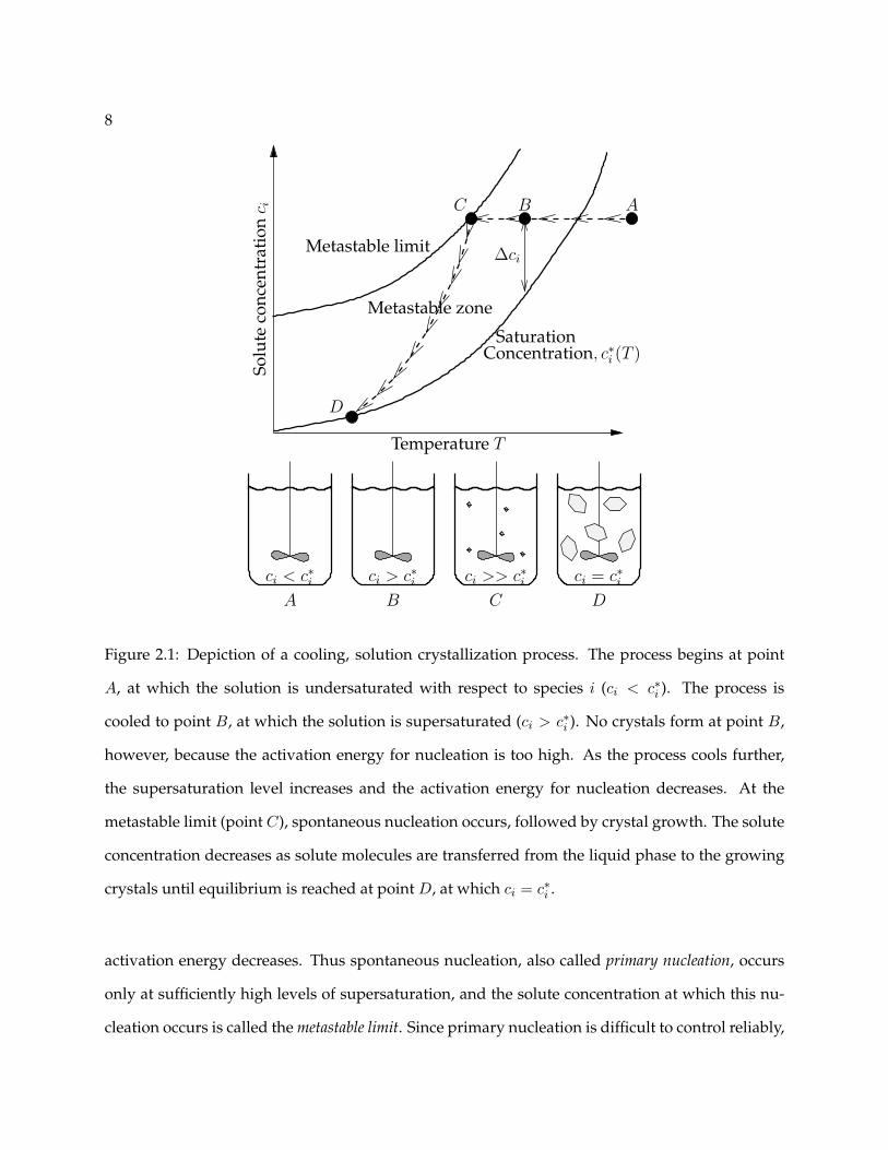
2.1 Depiction of solute concentration and temperature trajectories for a generic cooling

crystallization process . . . . . . . . . . . . . . . . . . . . . . . . . . . . . . . . . . . . 8

2.2 Photograph of production-scale, continuous crystallizer for ammonium sulfate . . . 10

2.3 Photograph of production-scale, continuous crystallizer for sodium chlorate . . . . . 11

2.4 Photograph of batch crystallizer used for high potency drug manufacturing . . . . . 12

2.5 Photographs of internals and exterior of multi-purpose batch crystallizer used for

pharmaceutical and specialty chemical manufacturing . . . . . . . . . . . . . . . . . 13

2.6 Depiction of effect of disturbances on supersaturation trajectory for a batch cooling

crystallization . . . . . . . . . . . . . . . . . . . . . . . . . . . . . . . . . . . . . . . . . 13

2.7 Comparison of particle size measurements obtained using laser backscattering ver-

sus those obtained using imaging . . . . . . . . . . . . . . . . . . . . . . . . . . . . . . 18

4.1 Experimental setup for obtaining in situ crystallization images. . . . . . . . . . . . . 36

4.2 Imaging system wiring. . . . . . . . . . . . . . . . . . . . . . . . . . . . . . . . . . . . 39

4.3 Chemical structure of glycine . . . . . . . . . . . . . . . . . . . . . . . . . . . . . . . . 42

4.4 Images illustrating morphology of α-glycine crystallized in water at room temper-

ature. . . . . . . . . . . . . . . . . . . . . . . . . . . . . . . . . . . . . . . . . . . . . . . 43

4.5 Images illustrating morphology of α-glycine crystallized in water at 55 C. . . . . . . 43

xviii

4.6 Images illustrating morphology of γ-glycine crystallized in water at room temper-

ature. . . . . . . . . . . . . . . . . . . . . . . . . . . . . . . . . . . . . . . . . . . . . . . 43

4.7 Depiction of the perspective projection of a cylindrical particle onto the image plane 46

4.8 Depiction of CCD image. . . . . . . . . . . . . . . . . . . . . . . . . . . . . . . . . . . . 46

5.1 Step-by-step example of SHARC algorithm applied to an in situ image of suspended

pharmaceutical crystals . . . . . . . . . . . . . . . . . . . . . . . . . . . . . . . . . . . . 51

5.2 Depiction of shifted gradient direction quantizations used to label pixels . . . . . . . 53

5.3 Step-by-step example of finding linear features using Burns line finder and blob

analysis . . . . . . . . . . . . . . . . . . . . . . . . . . . . . . . . . . . . . . . . . . . . . 54

5.4 Depiction of variables used for line pair classification scheme. . . . . . . . . . . . . . 55

5.5 Depiction of valid and invalid parallel line pairs . . . . . . . . . . . . . . . . . . . . . 57

5.6 Step-by-step example of clustering procedure for valid parallel pairs . . . . . . . . . 59

5.7 Temperature trajectory and image acquisition times for pharmaceutical crystalliza-

tion experiment . . . . . . . . . . . . . . . . . . . . . . . . . . . . . . . . . . . . . . . . 60

5.8 Algorithm performance on example image from video image set 3 . . . . . . . . . . . 61




5.12 Comparison of cumulative number fractions obtained from manual and automatic

sizing of crystals for video image sets 3–6 . . . . . . . . . . . . . . . . . . . . . . . . . 65

5.13 Comparison of crystals sized manually and using SHARC . . . . . . . . . . . . . . . 66

5.14 Zoomed-in view of crystals that SHARC failed to identify correctly . . . . . . . . . . 67

6.1 Parameterized, wire-frame model for glycine crystals . . . . . . . . . . . . . . . . . . 73

6.2 Depiction of the perspective projection of the glycine model onto the image plane . . 74

6.3 Depiction of different viewpoint-invariant line groups (VIGs) used by M-SHARC . . 76

6.4 Depiction of correspondence hypotheses . . . . . . . . . . . . . . . . . . . . . . . . . 78

xix

6.5 Depiction of variables used in mismatch calculation for a single line correspondence. 80

6.6 Step-by-step example of M-SHARC algorithm applied to image of α-glycine crystal. 83

6.7 M-SHARC segmentation results for selected images acquired at low solids concen-

tration (13 min. after appearance of crystals). . . . . . . . . . . . . . . . . . . . . . . . 85

6.8 M-SHARC segmentation results for selected images acquired at medium solids con-

centration (24 min. after appearance of crystals). . . . . . . . . . . . . . . . . . . . . . 85

6.9 M-SHARC segmentation results for selected images acquired at high solids concen-

tration (43 min. after appearance of crystals). . . . . . . . . . . . . . . . . . . . . . . . 86

6.10 Illustration of comparison between human operator results and M-SHARC results . 87

6.11 Comparison of Human and M-SHARC cumulative distribution functions . . . . . . 89

6.12 Results of linear feature detection for selected crystals missed by M-SHARC . . . . . 90

7.1 Depiction of methodology for calculating Miles-Lantuejoul correction factors for

particles of different lengths observed in an image of dimension b× a . . . . . . . . . 98

7.2 Example images for simulations of various particle populations . . . . . . . . . . . . 105

7.3 Comparison of sampling distributions for different PSD estimators: mono-disperse

population . . . . . . . . . . . . . . . . . . . . . . . . . . . . . . . . . . . . . . . . . . . 106

7.4 Fraction of confidence intervals containing the true parameter value as a function

of confidence level: mono-disperse population . . . . . . . . . . . . . . . . . . . . . . 107

7.5 Relative efficiencies of Miles-Lantuejoul and maximum likelihood estimators as a

function of particle size and sample size: uniformly-distributed population . . . . . 108


of confidence level: uniformly-distributed population and large sample size . . . . . 109


of confidence level: uniformly-distributed population and small sample size . . . . . 110

7.8 Analytical sampling distributions for the various size classes of a discrete normal

distribution . . . . . . . . . . . . . . . . . . . . . . . . . . . . . . . . . . . . . . . . . . 111

xx

7.9 Relative efficiencies of Miles-Lantuejoul and maximum likelihood estimators as a

function of particle size and sample size: normally-distributed population . . . . . . 112

7.10 Comparison of sampling distributions for different PSD estimators: particles larger

than image . . . . . . . . . . . . . . . . . . . . . . . . . . . . . . . . . . . . . . . . . . . 113

8.1 Geometric representation of admissible area, or region in which a particle is over-

lapped by another particle . . . . . . . . . . . . . . . . . . . . . . . . . . . . . . . . . . 119

8.2 Likelihood of observing n non-overlapping particles with example images of dif-

ferent number densities that give the same number of non-overlapping particles . . 121

8.3 Comparison of images generated for two different mono-disperse particle popula-

tions at the same solids concentration and at the same level of overlap . . . . . . . . 124

8.4 Comparison of average number of overlaps per crystal for images simulated at con-

stant overlap and at constants solids concentration . . . . . . . . . . . . . . . . . . . . 125

8.5 Comparison of percentage of particles missed by automated image analysis for im-

ages simulated at constant overlap and at constants solids concentration . . . . . . . 125

8.6 Examples of synthetic images generated at various particle sizes and degrees of

overlap . . . . . . . . . . . . . . . . . . . . . . . . . . . . . . . . . . . . . . . . . . . . . 127

8.7 Results of number density estimation using Miles-Lantuejoul method for various

particle sizes and various levels of particle overlap . . . . . . . . . . . . . . . . . . . . 128

8.8 Data and model prediction for number of particles with length≤ 0.1a identified per

image by automated image analysis . . . . . . . . . . . . . . . . . . . . . . . . . . . . 129

8.9 Data and model prediction for number of particles with lengths ≤ 0.3a or ≤ 0.5a

identified per image by automated image analysis . . . . . . . . . . . . . . . . . . . . 130

8.10 Ratio of estimated number density and true number density versus image difficulty

using SHARC data and empirical correction factors calculated for each different

particle size . . . . . . . . . . . . . . . . . . . . . . . . . . . . . . . . . . . . . . . . . . 131

9.1 Comparison of simulation results for optimal and linear temperature trajectories . . 137

xxi

9.2 Examples of images generated at various times during optimal cooling simulation . 138

9.3 Examples of images generated at various times during linear cooling simulation . . 139

9.4 Evolution of measured and estimated number-based PSD for optimal cooling and

perfect image analysis. . . . . . . . . . . . . . . . . . . . . . . . . . . . . . . . . . . . . 140

9.5 Evolution of measured and estimated weight PSD for optimal cooling and perfect

image analysis . . . . . . . . . . . . . . . . . . . . . . . . . . . . . . . . . . . . . . . . . 141

9.6 Evolution of measured and estimated weight PSD for optimal cooling and image

analysis using SHARC . . . . . . . . . . . . . . . . . . . . . . . . . . . . . . . . . . . . 142

9.7 Estimated ratios of nuclei mass to seed crystal mass for optimal and linear cooling . 143

9.8 Estimated mean crystal sizes for optimal and linear cooling . . . . . . . . . . . . . . . 143

9.9 Estimated coefficients of variation for optimal and linear cooling . . . . . . . . . . . 144

A.1 Depiction of hypothetical system of vertically-oriented particles randomly and uni-

formly distributed in space. . . . . . . . . . . . . . . . . . . . . . . . . . . . . . . . . . 156

A.2 Depiction of geometrical properties used to derive the non-border area function

Anb(l, θ). . . . . . . . . . . . . . . . . . . . . . . . . . . . . . . . . . . . . . . . . . . . . 157

A.3 Depiction of hypothetical system of vertically-oriented particles randomly and uni-

formly distributed in space. . . . . . . . . . . . . . . . . . . . . . . . . . . . . . . . . . 160

A.4 Depiction of non-border area for arbitrary length and orientation. . . . . . . . . . . . 161

A.5 Comparison of theoretical and simulated marginal densities for randomly-oriented,

monodisperse particles of length 0.5 and measured by partitioning [0.1 0.9] into ten

bins. Results are for non-border particles. . . . . . . . . . . . . . . . . . . . . . . . . . 164

A.6 Comparison of theoretical and simulated marginal densities for randomly-oriented,

monodisperse particles of length 0.5 and measured by partitioning [0.1 0.9] into ten

bins (results are shown only for bins 1–4 because the probability of observing a

border length in size class 5 or above is zero). Results are for border particles. . . . . 165

xxii

A.7 Comparison of theoretical and simulated marginal densities for randomly-oriented

particles distributed uniformly on [0.1 0.9] and measured by partitioning [0.1 0.9]

into ten bins. Results are for non-border particles. . . . . . . . . . . . . . . . . . . . . 166



into ten bins. Results are for border particles. . . . . . . . . . . . . . . . . . . . . . . . 167


particles distributed normally and measured by partitioning [0.1 0.9] into 10 bins.

Results are for non-border particles. . . . . . . . . . . . . . . . . . . . . . . . . . . . . 168


particles distributed normally and measured by partitioning [0.1 0.9] into 10 bins.

Results are for border particles. . . . . . . . . . . . . . . . . . . . . . . . . . . . . . . . 169



into 9 bins with a 10th bin spanning [1.0√

2]. Results are for non-border particles. . 170



into 9 bins with a 10th bin spanning [1.0√

2]. Results are for border particles. . . . . 171

xxiii

NotationUpper Case Letters

A surface area of slurry exposed to crystallizer jacket

AJ area of domain J

Aij i, jth element of collocation first derivative weight matrix

AFP projected area of IA false positives

AH projected area of IA hits

AM projected area of IA misses

ANB area of region inside which a particle does not touch the image border

Aovp area of region in which two particles of specific shape and orientation overlap

B crystal nucleation rate density at size L0

C solution phase concentration (mass solute/mass solvent)

Csat saturation concentration (mass solute/mass solvent)

D dimensionless parameter giving average number of particle overlaps

Dc set of data lines for which correspondence has been identified with wire-frame model lines

E set of edges defining wire-frame model

EP set of projected wire-frame model lines

Eg crystal growth activation energy

EJ edge J in wire-frame model

E2 Euclidean plane

F cumulative distribution function for particle orientation

G crystal growth rate

xxiv

H cumulative distribution function for particle length

∆Hc heat of crystallization

I two-dimensional image

J two-dimensional domain parameterized by (z,n,θn)

K random variable giving the number of times a particle is overlapped

L characteristic crystal length

L mean particle length

L0 initial size of nucleated crystals

Li random variable giving length of particle i

Li length of line i

Lj jth collocation location on length domain

LJ length of Jth wire-frame model line

Lmax size of the largest particle in the population

Lmax length of longest line in parallel line pair

Lmin length of shortest line in parallel line pair

LN (t) size of largest nucleated crystal

LSl(t) size of smallest seed crystal

LSu(t) size of largest seed crystal

LV length of virtual line

LPi length of projection of line i onto virtual line

L(ρ) likelihood function

M Miles-Lantuejoul weighting factor

MJ vector pointing from origin of image coordinate system to midpoint of Jth wire-frame model

line

MT solids concentration

N number of images

Nc random variable giving number of crystals in vicinity of imaging volume

NH number of hits by IA

xxv

NM number of misses by IA

NFP number of false positives by IA

Pi set of points comprising particle i

Q(x) sampling region centered at point x

Qk volumetric flow rate of kth stream

QP parallel line pair quality

Rg universal gas constant

R lower limit on resolution for camera lens

Rx rigid-body rotation matrix for transformation from world coordinate frame to camera coor-

dinate frame

S slurry system

S set of data lines

S relative supersaturation

S parallel line pair significance

S vector of breaks between discrete particle size classes

T temperature

T number of discrete particle size classes

T translation vector with elements (tx, ty, tz) for transformation from world coordinate frame

to camera coordinate frame

T0 initial temperature

Tj jacket temperature

T J unit tangent vector to Jth wire-frame model line

U overall heat transfer coefficient

V slurry volume

V set of vertices defining wire-frame model

VI imaging volume

X random variable giving number of observations of completely isolated, non-border particles

X random variable giving number of particles identified by image analysis algorithm

xxvi

X three-dimensional point in model coordinate frame

Xc three-dimensional point in camera coordinate frame with elements (Xc, Yc, Zc)

Xk random vector giving numbers of non-border particles of various size classes observed in

image k

Xik random variable giving number of non-border particles in size class i observed in image k

XΣ random vector giving total number of non-border particles of various size classes observed

in N images

Xw three-dimensional point in world coordinate frame with elements (Xw, Yw, Zw)

Xwi three-dimensional random vector with elements (Xwi, Ywi, Zwi) giving centroid location for

particle i in the world coordinate frame

XK [pm] vertex of wire-frame model in model coordinate frame

Y k random vector giving numbers of border particles of various observed lengths observed in

image k

Y Σ random vector giving total number of border particles of various observed lengths observed

in N images

Yik random variable giving number of border particles with observed length in size class i ob-

served in image k

Lower Case Letters

a horizontal image dimension

ap area of the two-dimensional projection of a particle

aS coefficient for quadratic function representing seed subpopulation

b supersaturation order of nucleation

b vertical image dimension

ci solute concentration of species i

ci chord length of crystal i

c∗i saturation concentration of species i

cp slurry heat capacity

xxvii

cv number-based coefficient of variation

cvw weight-based coefficient of variation

∆c saturation concentration (ci − c∗i )

df depth of field

dF,h horizontal Feret diameter

dF,v vertical Feret diameter

dPD perpendicular distance between two lines

dEP distance between endpoints of two lines

diffi difference between mean particle size values calculated by different operators

e1i first endpoint of ith data line

e2i second endpoint of ith data line

f(L, t) particle size distribution (PSD)

fc camera focal length

fk PSD of kth flow stream

fN (L, t) PSD of subpopulation of nucleated crystals

fN (ζ, t) PSD of subpopulation of nucleated crystals on scaled length domain

fS(L, t) PSD of subpopulation of seed crystals

fS0 initial PSD of seed subpopulation

g supersaturation order of growth

g(D) empirical function

h parametric particle length density function

h conversion from solvent mass to slurry volume

h(ρ, θ) model prediction of number of particles identified by IA

hm crystal body height for wire-frame crystal model

j third moment order of nucleation

ka area shape factor

kg growth rate constant

kb nucleation rate constant

xxviii

ku pixel horizontal scaling factor

kv volume shape factor

kv pixel vertical scaling factor

l length of particles in mono-disperse population

l(p) log likelihood function

li projected length of crystal i

lj(L) Lagrange interpolation polynomial of degree j

m length-to-pixel ratio

mN nucleus-grown crystal mass

mS seed-grown crystal mass

mX Poisson distribution parameter for X

mX Poisson distribution parameter for X

mXi Poisson parameter for distribution of Xi

mYj Poisson parameter for distribution of Yj

lj length of jth data line

mj vector pointing from origin of image coordinate system to midpoint of jth data line

mS(t) mass of seed-grown subpopulation

nc number of collocation points

n number of observations (particles)

n total number of particles in system

nb number of buckets for Burns line finder

nc number of collocation points

nd number of data points

nl estimate of number of lines identified in image

n∇ size of Sobel gradient operator

p vector of internal wire-frame model parameters and viewpoint parameters

pm internal parameters for wire-frame model

piso probability that a given particle is completely isolated

xxix

povp probability that a given particle is overlapped by a second, given particle

pXY joint probability density for X and Y

pXi probability density for Xi

pYi probability density for Yi

q discrete, relative PSD

r radius of cylindrical particles

sp perimeter of the two-dimensional projection of a particle

t time

tm crystal pyramid height for wire-frame crystal model

t(α, N − 1) Student’s t-distribution for confidence level α and number of samples N

tx translation in x-direction for transformation from world coordinate frame to camera coordi-

nate frame

tj unit tangent vector to jth data line

t⊥j unit vector perpendicular to jth data line

sN sample standard deviation

u horizontal pixel coordinate

u0 value of horizontal pixel coordinate corresponding to xc = (0, 0)

v vertical pixel coordinate

v0 value of vertical pixel coordinate corresponding to xc = (0, 0)

vmax number of vertical CCD pixels

w width of particles in mono-disperse population

wm crystal body width for wire-frame crystal model

w two-dimensional pixel coordinate vector with elements (u, v)

wi projected width of crystal i

x measured number of isolated, non-border particles, or the realization of X

x number of particles identified by IA, or the realization of X

xi horizontal centroid of line i

xmin lower bound on centroid location of particles in the x-dimension

xxx

xmax upper bound on centroid location of particles in the x-dimension

xc two-dimensional point in image coordinates with elements (xc, yc)

x two-dimensional point in image coordinates with elements (x, y)

xk realization of random variable Xk

xV horizontal centroid of virtual line

yi vertical centroid of line i

yk realization of random variable Y k

yV vertical centroid of virtual line

z center point of two-dimensional domain

z0 distance from camera lens to imaging volume

Greek Letters

α confidence level

αm assumed orientation in depth for wire-frame model projection

αi parameter for distribution function of Xi

βij parameter for distribution function of Yj

δ Dirac delta function

ε|∇| gradient magnitude threshold

εA pixel area threshold

εAR aspect ratio threshold for parallel line grouping

εθCorientation difference threshold for collinear line grouping

εθPorientation difference threshold for parallel line grouping

εPD threshold on perpendicular distance between two lines

εEP threshold on end-point distance between two lines

εQ parallel line pair quality threshold

ζ scaled particle size on [0,1] domain

θi orientation of line i

θn parameters necessary to specify two-dimensional domain of class n

xxxi

θV orientation of virtual line

θx particle orientation around x-axis of world coordinate frame

θz particle orientation around camera’s optical axis

Θzi random variable giving orientation of particle i around z-axis of world coordinate frame

λ Expected number of particle per image

λ Poisson distribution parameter for Nc

µi ith moment of the PSD

µNi ith moment of the PSD for nucleus-grown crystals only

µSi ith moment of the PSD for seed-grown crystals only

ρ number density of particles in mono-disperse population

ρ discrete absolute PSD

ρ estimate of number density

ρ maximum likelihood estimate of ρ using only non-border particle measurements

ρA area number density of particles in mono-disperse population

ρb maximum likelihood estimate of ρ using border and non-border particle measurements

ρc crystal density

ρi number density of particles in size class i

ρML Miles-Lantuejoul estimate of ρ

σ saturation concentration ((ci − c∗i )/c∗i )

Φ objective function for optimization

Φp stochastic spatial process describing particle population in vicinity of imaging volume

χ2(α, n− 1) chi-squared distribution for confidence level α and sample size n

ΩL particle length domain

Ω admissible area, or the expectation of Aovp

xxxii

1

Chapter 1

Introduction 1

1.1 Project motivation and research objectives

Crystallization plays a critical role in numerous industries for a variety of reasons. In the semi-

conductor industry, for example, crystallization is used to grow long, cylindrical, single crystals of

silicon with a mass of several hundred kilograms. These gigantic crystals, called boules, are sliced

into thin wafers upon which integrated circuits are etched. Prior to etching, crystallization is used

to grow thin layers of crystalline, semiconductor material onto the silicon wafer using a process

called chemical vapor deposition. In the food industry, crystallization is often used to give prod-

ucts the right texture, flavor, and shelf life. Crystallization is used to produce ice cream, frozen

dried foods, chewing gum, butter, chocolate, salt, cheese, coffee, and bread [47]. These examples

highlight the utility of crystallization in creating solids with desirable and consistent properties.

Crystallization is also widely used to separate and purify chemical species in the commod-

ity, petrochemical, specialty, and fine-chemical industries. In fact, DuPont, one of the world’s

largest chemical manufacturers, estimated in 1988 [43] that approximately 70% of its products

pass through a crystallization or precipitation stage. Crystallization is used in the pharmaceutical

industry to identify structure for use in drug design, to isolate chemical species from mixtures of

reaction products, and to achieve consistent and controlled drug delivery. The vast majority of

pharmaceuticals are manufactured in solid, generally crystalline, form.

Despite crystallization’s long history and widespread use, this process remains difficult to

1Portions of this chapter appear in Larsen, Patience, and Rawlings [65]

2

Figure 1.1: Images of crystal populations.

understand and control. To appreciate the challenges associated with this process, consider the

images of different crystal populations shown in Figure 1.1. The needle-like crystals on the left

are the active ingredient for a Parkinson’s disease treatment. The crystals in the image exhibit

a wide range of sizes and aspect ratios, indicating the distributed nature of crystallization pro-

cesses. This feature is one of the basic challenges associated with any dispersed-phase process.

Many of the key crystallizer states, including crystal size, shape, and purity, are distributed or

vary over the crystal population. The evolution of these states is affected by a variety of complex

phenomena, including nucleation, growth, agglomeration, and breakage. The sizes and shapes of

the crystals affect the efficiency of downstream processes such as solid-liquid separation, drying,

mixing, milling, granulation, and compaction. In some cases, particularly for chemicals having

low solubility or low permeability, the crystal size and shape affect product properties such as

bioavailability and tablet stability. Control of chemical purity is important for food and phar-

maceutical products intended for consumption and for semiconductor devices requiring highly

consistent properties.

The remaining two images in Figure 1.1 show crystals of glycine, an amino acid of inter-

est to the pharmaceutical community both as an excipient in pharmaceutical formulations and as

an active ingredient. The prismatic crystal shape in the center image corresponds to the α poly-

morphic form of glycine, while the bipyramidal shape in the other image corresponds to the γ

form. These images demonstrate that even molecules as simple as glycine exhibit polymorphism,

3

or the ability to crystallize into different crystal structures. Polymorphism must be controlled

because the polymorphic form affects product stability, hygroscopicity, saturation concentration,

dissolution rate, and bioavailability. The development of increasingly complex compounds in the

pharmaceutical and specialty chemical industries makes polymorphism a commonly observed

phenomenon for which control is essential. The recent disaster at Abbott Labs [10], in which the

appearance of an unknown polymorphic form of ritonavir in drug formulations threatened the

supply of the life-saving AIDS treatment Norvir, illustrates both the importance and difficulty of

controlling polymorphism.

Robust control of the solid-phase properties requires that they be measured. However,

conventional particle size distribution (PSD) monitoring technologies, such as laser diffraction and

laser backscattering, are based on assumptions of particle sphericity and thus do not provide the

monitoring capability necessary to achieve on-line PSD control for systems in which the particles

are highly non-spherical [136, 16]. Additionally, laser backscattering cannot measure the shape of

individual particles and therefore cannot measure the distribution of particles between different

shape classes (e.g. number of needles relative to number of spheres) nor shape factor distributions

(e.g. distribution of aspect ratios).

The limitations inherent in laser-scattering-based monitoring technologies motivate the use

of imaging-based methods, which allow direct visualization of particle size and shape. Obtaining

quantitative information from imaging-based methods, however, requires image segmentation.

Image segmentation means separating the objects of interest (e.g. the particles) from the back-

ground. Most commercial, imaging-based, on-line particle size and shape analyzers solve the

segmentation problem by imaging the particulate slurry as it passes through a specially-designed

flow cell under controlled lighting conditions [3, p. 167]. The images acquired in this way can be

segmented using simple thresholding methods. The drawback is that this approach requires sam-

pling, which is inconvenient, possibly hazardous, and raises concerns about whether the sample

is representative of the bulk slurry.

This thesis is focused on developing image segmentation algorithms that enable robust

4

segmentation of noisy, in situ images and statistical estimation methods that overcome the biases

inherent in imaging-based measurement. These tools are expected to aid practitioners in devel-

oping effective, imaging-based monitoring technology, resulting in improved understanding and

control of industrial crystallization processes.

1.2 Thesis overview

The thesis is organized as follows. Preliminary material is given in Chapters 2–4. Chapter 2 de-

scribes conventional industrial practices for designing and controlling crystallization processes.

Chapter 2 also reviews the state-of-the-art in crystallization design and control, with particular

emphasis given to sensor technology. Chapter 3 presents the batch crystallization model used in

this study and describes the methods used to solve the model. Chapter 4 describes the experimen-

tal apparatus used to conduct crystallization experiments and obtain in situ images. Chapter 4 also

discusses the simulation methods used to generate artificial in situ images.

Chapters 5 and 6 describe two novel algorithms that enable robust image analysis for noisy,

in situ images. The first algorithm, called SHARC (Segmentation for High Aspect Ratio Crystals),

can be used to find high-aspect-ratio crystals, a specific shape class that arises frequently in phar-

maceutical applications. This shape class is particularly problematic for standard image analysis

routines because it results in a high degree of particle overlap. The second algorithm, called M-

SHARC (Model-based SHApe Recognition for Crystals), is designed to identify and distinguish

between multiple shape classes, thereby enabling the measurement of polymorphic fraction for

systems in which the polymorphs exhibit different shapes. Chapters 5 and 6 also provide an eval-

uation of the algorithms in terms of their computational requirements and their accuracy relative

to measurements obtained by human operators.

Chapter 7 develops a maximum likelihood estimator for estimating the PSD from imag-

ing data and demonstrates how to obtain confidence intervals for the measured PSD using boot-

strapping. We benchmark the estimator against the conventional Miles-Lantuejoul approach. For

5

needle-like particles, our estimator provides better estimates than the Miles-Lantuejoul approach,

but the Miles-Lantuejoul approach can be applied to a wider class of shapes. Both methods assume

perfect image segmentation, or that every particle appearing in the image is identified correctly.

Chapter 8 develops a descriptor that correlates with the reliability of the imaging-based

measurement (i.e. the quality of the image segmentation) based on the amount of particle over-

lap. Chapter 8 demonstrates that both the Miles-Lantuejoul and maximum likelihood approaches

discussed above underestimate the number density of particles and develops a practical approach

for estimating the number density of particles for significant particle overlap and imperfect image

analysis. The approach is developed for mono-disperse particle systems.

Chapter 9 applies the tools developed in previous chapters to a well-studied batch crys-

tallization process of an industrial photochemical, demonstrating the feasibility of imaging-based

PSD measurement for industrial crystallization processes. Chapter 9 also demonstrates the ability

to monitor important product quality parameters, such as the ratio of nuclei mass to seed mass,

that cannot be monitored by conventional technologies.

Finally, Chapter 10 summarizes the contributions of this dissertation, presents conclusions,

and provides suggestions for future work.

6

7

Chapter 2

Literature Review 1

2.1 Crystallization overview and terminology

Crystallization is the formation of a solid state of matter in which the molecules are arranged in

a regular pattern. Crystallization can be carried out by a variety of methods, but the concepts

and terminology relevant to most crystallization processes can be understood by examining the

method of solution crystallization. In solution crystallization, the physical system consists of one

or more solutes dissolved in a solvent. The system can be undersaturated, saturated, or supersatu-

rated with respect to species i, depending on whether the solute concentration ci is less than, equal

to, or greater than the saturation concentration c∗i . Crystallization occurs only if the system is super-

saturated. The supersaturation level is the amount by which the solute concentration exceeds the

saturation concentration, and is commonly expressed as σ = ci−c∗ic∗i

, S = cic∗i

, or ∆c = ci − c∗i . The

supersaturation level can be increased either by lowering the saturation concentration (for exam-

ple, by cooling as depicted in Figure 2.1) or by increasing the solute concentration (by evaporating

the solvent, for example).

Crystallization moves a supersaturated solution toward equilibrium by transferring solute

molecules from the liquid phase to the solid, crystalline phase. This process is initiated by nucle-

ation, which is the birth or initial formation of a crystal. Nucleation occurs, however, only if the

necessary activation energy is supplied. A supersaturated solution in which the activation energy

is too high for nucleation to occur is called metastable. As the supersaturation level increases, the

1Portions of this chapter appear in Larsen, Patience, and Rawlings [65]

8

Solu

teco

ncen

trat

ion

c i

ci < c∗i

Temperature T

D

ABC

∆ci

B C DA

ci >> c∗i ci = c∗ici > c∗i

Metastable limit

Metastable zone

SaturationConcentration, c∗i (T )

Figure 2.1: Depiction of a cooling, solution crystallization process. The process begins at point

A, at which the solution is undersaturated with respect to species i (ci < c∗i ). The process is

cooled to point B, at which the solution is supersaturated (ci > c∗i ). No crystals form at point B,

however, because the activation energy for nucleation is too high. As the process cools further,

the supersaturation level increases and the activation energy for nucleation decreases. At the

metastable limit (point C), spontaneous nucleation occurs, followed by crystal growth. The solute

concentration decreases as solute molecules are transferred from the liquid phase to the growing

crystals until equilibrium is reached at point D, at which ci = c∗i .

activation energy decreases. Thus spontaneous nucleation, also called primary nucleation, occurs

only at sufficiently high levels of supersaturation, and the solute concentration at which this nu-

cleation occurs is called the metastable limit. Since primary nucleation is difficult to control reliably,

9

primary nucleation is often avoided by injecting crystal seeds into the supersaturated solution.

Crystal nuclei and seeds provide a surface for crystal growth to occur. Crystal growth

involves solute molecules attaching themselves to the surfaces of the crystal according to the crys-

talline structure. Crystals suspended in a well-mixed solution can collide with each other or with

the crystallizer internals, causing crystal attrition and breakage that results in additional nuclei.

Nucleation of this type is called secondary nucleation.

The rates at which crystal nucleation and growth occur are functions of the supersatura-

tion level. The goal of crystallizer control is to balance the nucleation and growth rates to achieve

the desired crystal size objective. Often, the size objective is to create large, uniformly sized crys-

tals. Well-controlled crystallization processes operate in the metastable zone, between the saturation

concentration and the metastable limit, to promote crystal growth while minimizing undesirable

nucleation.

2.2 Conventional practice in industry

The objective of every industrial crystallization process is to create crystals that meet specifications

on size, shape, composition, and internal structure. This objective is achieved using a variety

of methods and equipment configurations depending on the properties of the chemical system,

the end-product specifications, and the production scale. Continuous crystallizers, such as those

shown in Figures 2.2 and 2.3, are typically used for large-scale production, producing hundreds

of tons per day. In the specialty chemical, fine chemical, and pharmaceutical industries, batch

crystallizers (see Figures 2.4 and 2.5) are often used to produce low-volume, high-value-added

chemicals.

2.2.1 Process development

The first step in developing a control system for solution crystallization is to determine the sat-

uration concentration and metastable limit of the target species over a range of temperatures,

10

Figure 2.2: Production-scale draft tube crystallizer. This crystallizer is used to produce hundreds

of tons per day of ammonium sulfate, commonly used as fertilizer or as a precursor to other

ammonium compounds. The crystallizer body (a) widens at the lower section (b) to accommodate

the settling region, in which small crystals called fines are separated from the larger crystals by

gravitational settling. The slurry of saturated liquid and fines in the settling region is continuously

withdrawn (c), combined with product feed, and passed through a heater (d) that dissolves the

fines and heats the resulting solution prior to returning the solution to the crystallizer. The heat

generated by crystallization is removed as the solvent evaporates and exits through the top of

the crystallizer (e), to be condensed and returned to the process. Larger crystals are removed

continuously from the bottom of the crystallizer. Image courtesy of Swenson Technology, Inc.

11

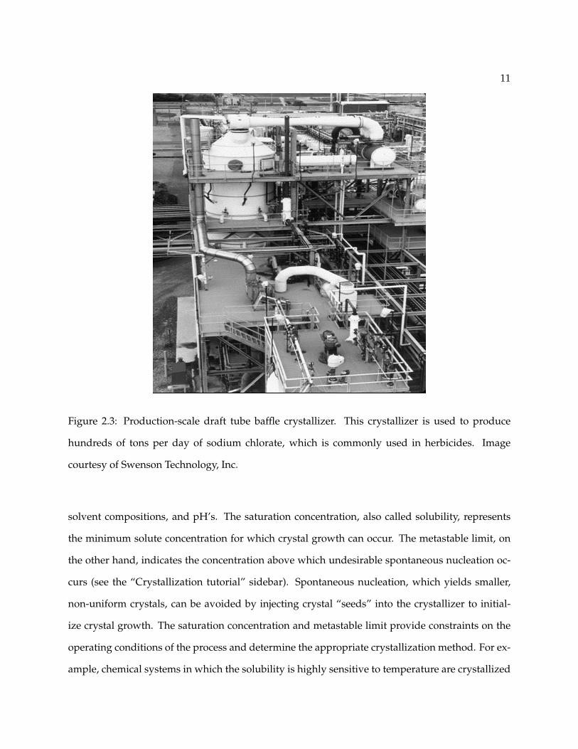
Figure 2.3: Production-scale draft tube baffle crystallizer. This crystallizer is used to produce

hundreds of tons per day of sodium chlorate, which is commonly used in herbicides. Image

courtesy of Swenson Technology, Inc.

solvent compositions, and pH’s. The saturation concentration, also called solubility, represents

the minimum solute concentration for which crystal growth can occur. The metastable limit, on

the other hand, indicates the concentration above which undesirable spontaneous nucleation oc-

curs (see the “Crystallization tutorial” sidebar). Spontaneous nucleation, which yields smaller,

non-uniform crystals, can be avoided by injecting crystal “seeds” into the crystallizer to initial-

ize crystal growth. The saturation concentration and metastable limit provide constraints on the

operating conditions of the process and determine the appropriate crystallization method. For ex-

ample, chemical systems in which the solubility is highly sensitive to temperature are crystallized

12

Figure 2.4: Small crystallizer used for high potency drug manufacturing. The portal (a) provides

access to the crystallizer internals. The crystallizer widens at the lower section (b) to accommodate

the crystallizer jacket, to which coolant (e) and heating fluid (h) lines are connected. Mixing is

achieved using an impeller driven from below (c). The process feed enters from above (f) and exits

below (d). The temperature sensor is inserted from above (g). Image courtesy of Ferro Pfanstiehl

Laboratories, Inc.

using cooling, while systems with low solubility temperature dependence employ anti-solvent or

evaporation crystallization. Automation tools greatly reduce the amount of time, labor, and mate-

rial previously required to characterize the solubility and metastable limit, enabling a wide range

of conditions to be tested in a parallel fashion [11].

Once a crystallization method and solvents are chosen, kinetic studies are carried out on a

13

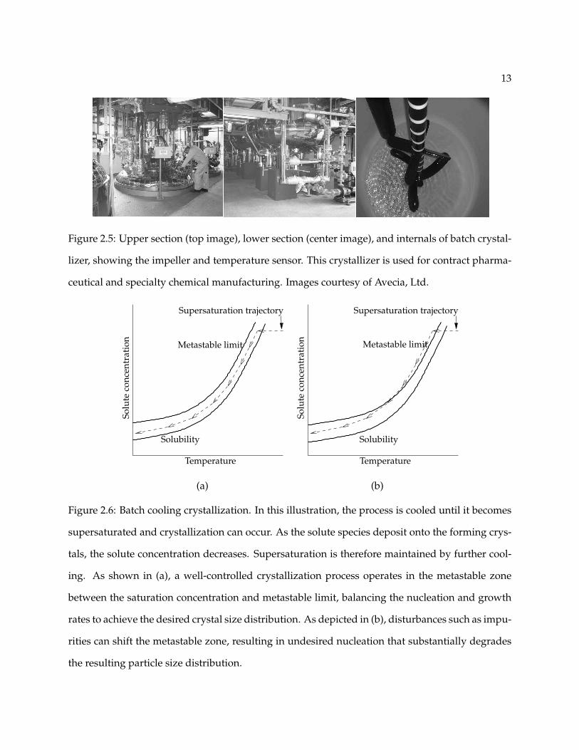
Figure 2.5: Upper section (top image), lower section (center image), and internals of batch crystal-

lizer, showing the impeller and temperature sensor. This crystallizer is used for contract pharma-

ceutical and specialty chemical manufacturing. Images courtesy of Avecia, Ltd.

Solu

teco

ncen

trat

ion

Temperature

Solubility

Supersaturation trajectory

Metastable limit

Solu

teco

ncen

trat

ion

Temperature

Solubility

Metastable limit

Supersaturation trajectory

(a) (b)

Figure 2.6: Batch cooling crystallization. In this illustration, the process is cooled until it becomes

supersaturated and crystallization can occur. As the solute species deposit onto the forming crys-

tals, the solute concentration decreases. Supersaturation is therefore maintained by further cool-

ing. As shown in (a), a well-controlled crystallization process operates in the metastable zone

between the saturation concentration and metastable limit, balancing the nucleation and growth

rates to achieve the desired crystal size distribution. As depicted in (b), disturbances such as impu-

rities can shift the metastable zone, resulting in undesired nucleation that substantially degrades

the resulting particle size distribution.

14

larger scale (tens to hundreds of milliliters) to characterize crystal growth and nucleation rates and

to develop an operating policy (see Figure 2.6) that is robust to variations in mixing, seeding, and

impurity levels. These studies minimize the difficulty in scaling up the process several orders of

magnitude to the pilot scale. The operating policy is usually determined semi-quantitatively, us-

ing trial-and-error or statistical-design-of-experiment approaches. Process robustness is achieved

by adopting a conservative operating policy at low supersaturation levels that minimize nucle-

ation events and thus achieve larger, more uniform crystals. Operating at low supersaturation

levels, far from the metastable limit, is important because the metastable limit is difficult to char-

acterize and is affected by various process conditions that change upon scaleup, such as the size

and type of vessel or impeller.

2.2.2 Controlled, measured, and manipulated variables

The primary concern of most industrial crystallization processes is generating crystals with a par-

ticle size distribution (PSD) that enables efficient downstream processing. The controlled variable

for most crystallization processes, however, is the supersaturation level, which is only indirectly

related to the PSD. The supersaturation level affects the relative rates of nucleation and growth

and thus determines the PSD. Because of its dependence on temperature and solution composi-

tion, the supersaturation level can be manipulated using various process variables such as the

flow rate of the cooling medium to the crystallizer jacket and the flow rate of anti-solvent to the

crystallizer.

Process development studies use a wide range of measurement technology. This technol-

ogy includes, for example, turbidity probes to detect the presence of solid material, laser scatter-

ing to characterize particle size distributions, and spectroscopic or absorbance probes to measure

solute concentrations. However, large-scale, industrial crystallizers rarely have these advanced

measurements available. In fact, controllers for most industrial crystallizers rely primarily on

temperature, pressure, and flow rate measurements.

15

2.3 Recent advances in crystallization technology

The above discussion illustrates the limited technology used to control industrial crystallization

processes. The obstacles that have hindered the implementation of advanced PSD control in in-

dustry, however, are being overcome by recent advances in measurement and computing technol-

ogy [17],[103].

With improved control technology, additional challenges can be addressed. One challenge

is to control shape, which, like PSD, affects the efficiency of downstream processes such as solid-

liquid separation, drying, mixing, milling, granulation, and compaction. In some cases, partic-

ularly for chemicals having low solubility or low permeability, the crystal size and shape affect

product properties such as bioavailability and tablet stability. Chemical purity must also be con-

trolled, especially for food and pharmaceutical products intended for consumption and for semi-

conductor devices requiring highly consistent properties.

Perhaps the most difficult and important challenge is controlling polymorphism, which is

the ability of a chemical species to crystallize into different crystal structures. The polymorphic

form affects product characteristics, including stability, hygroscopicity, saturation concentration,

dissolution rate, and bioavailability. The development of increasingly complex compounds in the

pharmaceutical and specialty chemical industries makes polymorphism a commonly observed

phenomenon for which control is essential. The recent disaster at Abbott Labs [10], in which the

appearance of an unknown polymorphic form of ritonavir in drug formulations threatened the

supply of the life-saving AIDS treatment Norvir, illustrates both the importance and difficulty of

controlling polymorphism. In the following sections, we describe recent advances that impact

industrial crystallizer control.

2.3.1 Spectroscopic and laser-based monitoring

One of the major challenges in implementing feedback control for crystallization processes is the

lack of adequate online sensors for measuring solid-state and solution properties. The United

16

States Food and Drug Administration’s (FDA) Process Analytical Technology initiative, aimed at

improving pharmaceutical manufacturing practices [138], has accelerated the development and

use of more advanced measurement technology. We describe several recently developed sensors

for achieving better control and understanding of crystallization processes.

ATR-FTIR Spectroscopy

Attenuated total reflectance Fourier transform infrared (ATR-FTIR) spectroscopy imposes a laser

beam on a sample and measures the amount of infrared light absorbed at different frequencies.

The frequencies at which absorption occurs indicate which chemical species are present, while

the absorption magnitudes indicate the concentrations of these species. As demonstrated in [32]

and [31], ATR-FTIR spectroscopy can be used to monitor solute concentration in a crystallization

process in situ.

ATR-FTIR spectroscopy offers advantages over prior techniques, such as refractometry,

densitometry, and conductivity measurements, for measuring solute concentration. Refractom-

etry works only if there is a significant change in the refractive index with solute concentration

and is sensitive to air bubbles. Densitometry requires sampling of the crystal slurry and filtering

out the crystals to accurately measure the liquid-phase density. This sampling process involves

an external loop that is sensitive to temperature fluctuations and subject to filter clogging. Con-

ductivity measurements, which are useful only for electrolytes, require frequent re-calibration.

ATR-FTIR spectroscopy overcomes these problems and can measure multiple solute concentra-

tions. Calibration of ATR-FTIR is usually rapid [72] and thus well suited for batch processes and

short production runs. In [119], linear chemometrics is applied to estimate solute concentration

with high accuracy (within 0.12%). Several applications for which ATR-FTIR monitoring is useful

are described in [37].

Unfortunately, ATR-FTIR spectroscopy is considerably more expensive than the alterna-

tives. Another drawback of ATR-FTIR is the vulnerability of the IR probe’s optical material to

chemical attack and fouling [30].

17

Raman spectroscopy

Raman spectroscopy imposes a monochromatic laser beam on a sample and measures the amount

of light scattered at different wavelengths. The differences in wavelength between the incident

light and the scattered light is a fingerprint for the types of chemical bonds in the sample. Raman

spectroscopy has been used to make quantitative polymorphic composition measurements since

1991 [26]. This technology has been applied to quantitative, in situ polymorphic composition

monitoring in solution crystallization since 2000 [125]–[91].

Raman spectroscopy is well suited to in situ polymorphism monitoring for several rea-

sons. Specifically, Raman analysis does not require sample preparation; the Raman signal can be

propagated with fiber optics for remote sensing; and Raman sampling probes are less chemically

sensitive than ATR-FTIR probes [30]. In addition, this technique can be used to monitor the solid

and liquid phases simultaneously [34],[50].

Like ATR-FTIR, Raman-based technologies are expensive. Furthermore, calibration of the

Raman signal for quantitative polymorphic composition measurements can be difficult because

the signal intensity is affected by the particle size distribution. Hence Raman’s utility for quanti-

tative monitoring depends on corrections for particle-size effects [93].

Near-Infrared Spectroscopy

Near-infrared (NIR) spectroscopy is also used to quantitatively monitor polymorphic composi-

tion [90]. Like Raman, NIR is well suited for in situ analysis. The main drawback of NIR is that

calibration is difficult and time consuming. In some cases, however, coarse calibration is sufficient

to extract the needed information [38].

Laser backscattering

Laser backscattering-based monitoring technology, such as Lasentec’s FBRM probe, has proven

useful for characterizing particle size and for determining saturation concentrations and metastable

18

w1

l1

c1

l2

w2

c2c3

l3

w3

Figure 2.7: Comparison of crystal size measurements obtained using laser backscattering versus

those obtained using vision. Laser backscattering provides chord lengths (c1, c2, c3) while vision-

based measurement provides projected lengths (l1, l2, l3) and projected widths (w1, w2, w3). The

chord-length measurement for each particle depends on its orientation with respect to the laser

path (depicted above using the red arrow), while the projected length and width measurements

are independent of in-plane orientation. Size measurements from both techniques are affected by

particle orientation in depth.

limits [8],[9]. This sensor measures particle chord lengths (see Figure 2.7) by moving a laser beam at

high velocity through the sample and recording the crossing times, that is, the time durations over

which light is backscattered as the laser passes over particles. The chord length of each particle

traversed by the laser is calculated as the product of the laser’s velocity and the crossing time of

the particle. This technique allows rapid, calibration-free acquisition of thousands of chord-length

measurements to robustly construct a chord length distribution (CLD). Laser backscattering tech-

nology can be applied in situ under high solids concentrations.

Because laser-backscattering provides a measurement of only chord length, this technique

cannot be used to measure particle shape directly. Laser-backscattering therefore cannot measure

the distribution of particles between different shape classes (e.g. number of needles relative to

number of spheres) nor shape factor distributions (e.g. distribution of aspect ratios). Also, infer-

ring the PSD from the CLD involves the solution of an ill-posed inversion problem. Although

19

methods for solving this inversion problem are developed in [107, 133, 73], these methods de-

pend on assumptions regarding particle shape. Successful application of these methods has been

demonstrated experimentally only for spheres [51] and octahedra [133], but has been demon-

strated for high-aspect-ratio particles using simulations only [73].

2.3.2 Imaging-based monitoring

Video microscopy can be used to characterize both crystal size and shape. Furthermore, for chem-

ical systems in which the polymorphs exhibit different shapes, such as glycine in water, video

microscopy can be used to monitor polymorphic composition [19]. Obtaining all three of these

measurements using a single probe reduces cost and simplifies the experimental setup. Video mi-

croscopy is also appealing because interpretation of image data is intuitive. Obtaining quantita-

tive information from video images, however, requires image segmentation. Image segmentation

means separating the objects of interest (e.g. the particles) from the background.

Commercial, imaging-based monitoring instruments

Most commercial, imaging-based, on-line particle size and shape analyzers solve the segmentation

problem by imaging the particulate slurry as it passes through a specially-designed flow cell un-

der controlled lighting conditions [3, p. 167]. Several commercial instruments of this type have re-

cently become available, such as Malvern’s Sysmex FPIA 3000 and Beckman-Coulter’s RapidVUE

(see [3] for a survey of other imaging-based instruments). The drawback of these instruments is

that they require sampling, which is inconvenient, possibly hazardous, and raises concerns about

whether the sample is representative of the bulk slurry [3, 7].One exception is the Mettler Toledo

Lasentec Particle Vision and Measurement (PVM) in situ probe. This probe is packaged with au-

tomatic image analysis software that does not give suitable results for most systems. The utility of

in situ video microscopy has been limited primarily to qualitative monitoring because the nature

of in situ images, which contain blurred, out-of-focus, and overlapping particles, has precluded

the successful application of image analysis to automatically quantify particle size and shape [16].

20

Challenges for segmentation of in situ images

Robust and efficient segmentation of in situ images is challenging for several reasons. First, in

situ imaging typically requires illumination by reflected light in order to handle high solids con-

centrations. Thus, the particles appear in the image with non-uniform color and intensity such

that thresholding methods are ineffective. The use of reflected light can also result in poorly-

defined particle outlines, thus limiting the robustness of methods based on closing the particle

outlines, such as the technique proposed by [20]. Segmentation is simplified considerably if parti-

cles are imaged using transmitted light because the particle outlines are easily distinguished [98].

Second, the crystals can have a large variation in size and are randomly-oriented in 3-D space,

which means the projections of the crystals onto the imaging plane can take on a wide variety of

shapes. Hough-transform-based methods [42, p. 587], which have been applied extensively to

segment images of circular or elliptical particles and droplets, involve exhaustive searches over

the particle location and shape parameter space and are therefore computationally infeasible for

randomly-oriented particles of complex shapes. The image segmentation problem is further com-

plicated by particle agglomeration, overlap, breakage, and attrition, which result in occluded or

poorly-defined particle boundaries.

Methods for segmenting in situ images have been developed for circular particles [113] and

elliptical particles [48]. In [20] a technique is presented for automatic segmentation of in-process

suspension crystallizer images, but the technique was demonstrated only on images that appear

to have been acquired at low solids concentration where there are no overlapping particles and

the particles’ edges are well-defined. Kaufman and Scott [62] used an in situ fluorescence imaging

method that caused the liquid phase of a fluidized bed to fluoresce while leaving the coal particles

opaque, thus enabling a gray-level threshold method to detect particle edges. However, for dense

particle volume fractions, manual intervention was required to determine which of the segmented

particles could be used for sizing.

21

Monitoring dynamic crystal populations

In situ video imaging is used by Scholl et al. [112] to observe the solvent-mediated polymorphic

transformation of L-glutamic acid from the α form with prismatic morphology to the β form with

needle-like morphology. Monnier et al. [86] use off-line image analysis to characterize the final

relative PSD of adipic acid crystals. Pollanen et al. [97] use video microscopy and automated

image analysis to characterize the sizes and shapes of sulphathiazole crystals. The application of

video imaging to these crystallization processes, however, is limited to qualitative monitoring or

characterization of end-product properties.

Only a few studies have used video imaging for on-line, quantitative monitoring of crys-

tal population dynamics. Patience et al. [95] used video microscopy to monitor the evolution of

crystal size mean and standard deviation for needle-like pharmaceutical particles. The slurry was

sampled periodically and allowed to settle on a microscope stage, and the images were analyzed

manually. Calderon De Anda et al. [19] used non-invasive imaging and automatic image analysis

to quantify the polymorphic fraction during the transformation from α to β L-glutamic acid. In a

follow-up study, Dharmayat et al. [27] monitored on-line the L-glutamic acid transformation using

both on-line video microscopy and X-ray diffraction, but were unable to compare quantitatively

the measurements of the two methods because the video microscopy technique failed at higher

solids concentrations and the X-ray diffraction method was not sufficiently sensitive at low solids

concentrations. Qu et al. [101] use in-line imaging to monitor the evolution of crystal length and

width CDFs at 10 to 20 minute intervals, determining width and length growth rates based on the

mean particle size.

Besides these crystallization applications, video imaging has been utilized to monitor dy-

namics of other particulate processes. Watano and Miyanami [127] demonstrated on-line moni-

toring of the median diameter and shape factor for a wet granulation process using in situ video

imaging and automatic image analysis. Blandin et al. [14] used non-invasive imaging of an ag-

glomeration process and automatic image analysis to track the evolution of the particle size num-

22

ber fractions at 30 minute intervals for about 4 hours. They validated their automated image

analysis method using comparisons with manual image analysis. Hukkanen et al. [52] used in

situ video microscopy and automated image analysis to monitor various PSD moments during

the early stages of a suspension polymerization processes.

2.3.3 Manipulated variables for crystal shape and polymorphic form

In advanced control implementations, the quality variables of interest (crystal size, shape, form,

and purity) are indirectly controlled using manipulated variables that affect the supersaturation

level in the crystallizer. For example, cooling crystallizers manipulate the crystallizer tempera-

ture to change the saturation concentration of the crystallizing species. Anti-solvent crystallizers

change the saturation concentration by manipulating the solvent composition.

Controlling the supersaturation level provides only limited control over the resulting crys-

tal shape distribution, size distribution, and polymorphic form. Progress is being made in this

area as well, however. Several research groups are investigating additives that bind to selected

crystal faces to inhibit growth of the faces, thereby promoting a desired crystal shape or polymor-

phic form [128],[13]. These additives, which are similar to the target-crystallizing species, can be

incorporated onto a growing crystal face. The remaining exposed portion of the additive consists

of chemical groups that hinder further growth on that face. Additives are also used as nucleation

promoters or inhibitors to obtain a desired polymorphic form [129]. Templates, such as single-

crystal substrates, are also being investigated as a means for manipulating nucleation events to

obtain desired polymorphs [85].

Additives are used in industry to help understand the effect of impurities on crystal growth

and polymorphism [13]. As yet, additives and templates are not widely used as manipulated

variables in industrial crystallizer control schemes. To use these methods as manipulated variables

for advanced control, models are needed to describe the effect of the manipulated variables on

crystal size, shape, and form.

23

2.3.4 Modeling and prediction of crystal size, shape, and polymorphic form

Process Modeling

Crystallizers have highly nonlinear, complex dynamics including multiple steady states, open-

loop instability, and long time delays; hence low-order, linear models are often inadequate for

control purposes. Furthermore, nonlinear black box models, such as neural networks, are also

inadequate in many cases because batch crystallizers have such a large operating region. Online,

optimal control of dynamic crystallization is thus enhanced by the ability to efficiently simulate

the underlying physical model, which is a system of partial integro-differential equations that cou-

ples mass and energy balances with a population balance describing the evolution of the crystal

population’s PSD.

The evolution of the PSD often involves sharp, moving fronts that are difficult to simulate

efficiently. Several software packages are now available for simulating crystallization processes.

The commercial software package PARSIVAL [135] is designed to handle the entire class of crys-

tallizer configurations and crystallization phenomena. AspenTech’s process simulation software

has specific tools for crystallization simulation and troubleshooting. The crystallizer simulator of

the GPROMS package can be interfaced with computational fluid dynamics (CFD) software, such

as FLUENT or STAR-CD. DYNOCHEM solves the population balance equations by applying the

commonly used method of moments, a model reduction technique. Researchers have developed

techniques that extend the applicability of the method of moments to systems involving length-

dependent crystal growth [79],[88], and these developments are being incorporated directly into

CFD software packages [111].

Shape Modeling

Models and methods for predicting crystal shape based solely on knowledge of the internal crys-

tal structure are available in software packages such as CERIUS2 and HABIT [23]. These methods

provide accurate shape predictions for vapor-grown crystals but, for solution-grown crystals, do

24

not take into account the effects of supersaturation, temperature, solvent, and additives or impu-

rities. Current shape-modeling research is focused on accounting for these effects [131]–[106].

Polymorphism Modeling

The ability to predict the crystal structure for a given molecule in a given environment would

represent a major advance in drug development. Although significant progress has been made

in making these predictions [99],[25], this problem is far from being solved. Most approaches

seek to find the crystal structure that corresponds to the global minimum in lattice energy, that

is, the most thermodynamically stable form at zero Kelvin. These approaches neglect entropic

contributions arising at higher temperatures as well as kinetic effects due to the experimental

crystallization conditions. Current polymorphism modeling methods thus cannot reliably predict

the polymorphs that are observed experimentally.

2.3.5 Control

The developments described above impact the way crystallizer control is approached in industry.

In particular, the development of better measurement technology enables the application of simple

but effective crystallizer control strategies. Most of these strategies focus on feedback control of

supersaturation using concentration (by means of ATR-FTIR) and temperature measurements to

follow a predefined supersaturation trajectory [74]–[40]. This approach is attractive because it

can be implemented without characterizing the nucleation and growth kinetics, using only the

saturation concentration and metastable zone width data. Furthermore, this approach results in

a temperature profile that can be used in large-scale crystallizers that do not have concentration-

measurement capabilities.

Laser backscattering measurements are used to control the number of particles in the sys-

tem [29]. This control strategy alternates between cooling and heating stages, allowing the heating

stage to continue until the particle count number measured by FBRM returns to its original value

upon seeding, indicating that all fine particles generated by secondary nucleation have been dis-

25

solved. In [96], online crystal shape measurements obtained by means of optical microscopy and

automated image processing are used to manipulate impurity concentration and thereby con-

trol crystal habit. The control schemes employed in these experimental studies are basic (usually

PID or on-off control), illustrating that, given adequate measurement technology, simple control

schemes can often provide an adequate level of control capability.

More sophisticated control methods have also been demonstrated for batch crystallizers.

Experimental results obtained in [84]–[134] demonstrate product improvement by using predic-

tive, first-principles models to determine open-loop, optimal cooling and seeding policies. Closed-

loop, optimal control of batch crystallizers is demonstrated using simulations in [105],[114].

For continuous crystallizers, various model-based, feedback controllers have been sug-

gested. In [124], an H∞ controller based on a linearized distributed parameter model is shown

to successfully stabilize oscillations in a simulated, continuous crystallizer using measurements

of the overall crystal mass, with the flow rate of fines (small crystals) to the dissolution unit as

the manipulated variable. In [114], a hybrid controller combining model predictive control with a

bounded controller is used to ensure closed-loop stability for continuous crystallizers.

2.4 The future of crystallization

As the chemical, pharmaceutical, electronics, and food industries continue to develop new prod-

ucts, crystallization will enjoy increasingly wide application as a means to separate and purify

chemical species and create solids with desirable properties. Sensor technology for crystallizers

will continue to improve, especially given the current emphasis by the FDA’s Process Analytical

Technology initiative. Industries that have used batch crystallizers to produce low-volume, high-

value-added chemicals might choose to move to continuous crystallizers to reduce operating costs

and enable more flexible and compact process design. Shape modeling and molecular modeling

tools offer tremendous potential for enabling robust process design and control, and these tools

can be expected to advance rapidly given the amount of interest and research in this area. These

26

developments will impact the way in which crystallization processes are designed and will enable

more effective control of size distribution, shape, and polymorphic form, leading to the creation

of crystalline solids that are useful for a wide variety of applications.

27

Chapter 3

Crystallization Model Formulation and

SolutionThis chapter presents the batch crystallization model used to demonstrate the value of the imaging-

based monitoring methods developed in this thesis. First, the mass, energy, and population bal-

ances describing the crystallizer are presented. Next, methods for solving the model are presented.

The first method, called the method of moments, is useful for simulating important characteristics

of the particle size distribution, such as the total number of particles per unit volume or the mean

particle size. The second method, orthogonal collocation on moving finite elements, simulates the

evolution of the particle size distribution directly.

3.1 Model formulation

The physical model of a batch crystallizer is a system of partial integro-differential equations that

couples mass and energy balances with a population balance describing the evolution of the crys-

tal population’s PSD. This section presents these equations.

3.1.1 Population balance

The population balance describes the population of crystals dispersed in the continuous liquid

phase. A complete description of the crystal population would include solid-phase properties

such as purity, polymorphic form, shape, and size. All of these properties can be included in the

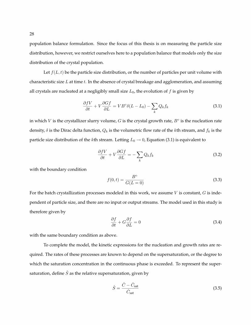
28

population balance formulation. Since the focus of this thesis is on measuring the particle size

distribution, however, we restrict ourselves here to a population balance that models only the size

distribution of the crystal population.

Let f(L, t) be the particle size distribution, or the number of particles per unit volume with

characteristic size L at time t. In the absence of crystal breakage and agglomeration, and assuming

all crystals are nucleated at a negligibly small size L0, the evolution of f is given by

∂fV

∂t+ V

∂Gf

∂L= V Bδ(L− L0)−

∑k

Qkfk (3.1)

in which V is the crystallizer slurry volume, G is the crystal growth rate, B is the nucleation rate

density, δ is the Dirac delta function, Qk is the volumetric flow rate of the kth stream, and fk is the

particle size distribution of the kth stream. Letting L0 → 0, Equation (3.1) is equivalent to

∂fV

∂t+ V

∂Gf

∂L= −

∑k

Qkfk (3.2)

with the boundary condition

f(0, t) =B

G(L = 0)(3.3)

For the batch crystallization processes modeled in this work, we assume V is constant, G is inde-

pendent of particle size, and there are no input or output streams. The model used in this study is

therefore given by

∂f

∂t+ G

∂f

∂L= 0 (3.4)

with the same boundary condition as above.

To complete the model, the kinetic expressions for the nucleation and growth rates are re-

quired. The rates of these processes are known to depend on the supersaturation, or the degree to

which the saturation concentration in the continuous phase is exceeded. To represent the super-

saturation, define S as the relative supersaturation, given by

S =C − Csat

Csat(3.5)

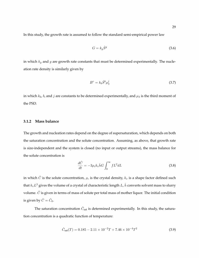
29

In this study, the growth rate is assumed to follow the standard semi-empirical power law

G = kgSg (3.6)

in which kg and g are growth rate constants that must be determined experimentally. The nucle-

ation rate density is similarly given by

B = kbSbµj

3 (3.7)

in which kb, b, and j are constants to be determined experimentally, and µ3 is the third moment of

the PSD.

3.1.2 Mass balance

The growth and nucleation rates depend on the degree of supersaturation, which depends on both

the saturation concentration and the solute concentration. Assuming, as above, that growth rate

is size-independent and the system is closed (no input or output streams), the mass balance for

the solute concentration is

dC

dt= −3ρckvhG

∫ ∞

0fL2dL (3.8)

in which C is the solute concentration, ρc is the crystal density, kv is a shape factor defined such

that kvL3 gives the volume of a crystal of characteristic length L, h converts solvent mass to slurry

volume. C is given in terms of mass of solute per total mass of mother liquor. The initial condition

is given by C = C0.

The saturation concentration Csat is determined experimentally. In this study, the satura-

tion concentration is a quadratic function of temperature:

Csat(T ) = 0.185− 2.11× 10−2T + 7.46× 10−4T 2 (3.9)

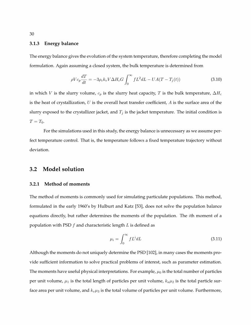
30

3.1.3 Energy balance

The energy balance gives the evolution of the system temperature, therefore completing the model

formulation. Again assuming a closed system, the bulk temperature is determined from

ρV cpdT

dt= −3ρckvV ∆HcG

∫ ∞

0fL2dL− UA(T − Tj(t)) (3.10)

in which V is the slurry volume, cp is the slurry heat capacity, T is the bulk temperature, ∆Hc

is the heat of crystallization, U is the overall heat transfer coefficient, A is the surface area of the

slurry exposed to the crystallizer jacket, and Tj is the jacket temperature. The initial condition is

T = T0.

For the simulations used in this study, the energy balance is unnecessary as we assume per-

fect temperature control. That is, the temperature follows a fixed temperature trajectory without

deviation.

3.2 Model solution

3.2.1 Method of moments

The method of moments is commonly used for simulating particulate populations. This method,

formulated in the early 1960’s by Hulburt and Katz [53], does not solve the population balance

equations directly, but rather determines the moments of the population. The ith moment of a

population with PSD f and characteristic length L is defined as

µi =∫ ∞

0fLidL (3.11)

Although the moments do not uniquely determine the PSD [102], in many cases the moments pro-

vide sufficient information to solve practical problems of interest, such as parameter estimation.

The moments have useful physical interpretations. For example, µ0 is the total number of particles

per unit volume, µ1 is the total length of particles per unit volume, kaµ2 is the total particle sur-

face area per unit volume, and kvµ3 is the total volume of particles per unit volume. Furthermore,

31

these quantities are required to complete the mass and energy balances given in Equations (3.8)

and (3.10).

To apply the method of moments to the model used in this study, we recall that for a batch

crystallizer with size-independent growth and no input or output streams, the population balance

is given by∂f

∂t= −G

∂f

∂L+ Bδ(L− L0) (3.12)

Multiplying this equation by Li and integrating over all sizes results in

∂

∂t

∫ ∞

0fLidL = −G

∫ ∞

0

∂f

∂LLidL +

∫ ∞

0Bδ(L− L0)LidL (3.13)

Applying integration by parts to the first term on the right hand side of this equation gives

−G

∫ ∞

0

∂f

∂LLidL = −GfLi

∣∣∞0

+ iG

∫ ∞

0fLi−1dL

Assuming a finite number of crystals at size 0 and zero crystals of infinite size, the first term on

the right hand side equals zero. Substituting these relationships into Equation (3.13) and letting

L0 → 0 givesd

dt

∫ ∞

0fLidL = iG

∫ ∞

0fLi−1dL + B0i (3.14)

In terms of the moments, Equation (3.14) can be expressed as

dµ0

dt= B (3.15)

dµi

dt= Gµi−1 i = 1, 2, 3 (3.16)

The method of moments therefore provides a set of coupled differential equations that can be

solved efficiently by standard ODE solvers.

3.2.2 Orthogonal collocation

The orthogonal collocation method, as explained in [123], consists of approximating the model

solution at each time step as an nth order polynomial. In our case, the PSD f is approximated as

f(L, t) =nc∑

j=1

f(Lj , t)lj(L) (3.17)

32

in which lj(L) is the Lagrange interpolation polynomial of degree j, nc is the number of collo-

cation points, and f(Lj , t) is the PSD evaluated at length Lj . Given this formulation, the spatial

derivative in Equation (3.4) can be calculated as a linear combination of the model solution values

at nc collocation locations along the crystal size domain, i.e.

df

dL

∣∣∣∣Li

=nc∑

j=1

Aijfj (3.18)

(3.19)

in which fj = f(Lj , t) and Aij = (dlj/dL)|Li is an element of the derivative weight matrix. Fur-

thermore, the integral of any function of the PSD over the domain ΩL can be calculated using

quadrature: ∫ΩL

g(f)dL =nc∑

j=1

Qjg(fj) (3.20)

in which Qj is the jth quadrature weight. The derivative and integral weight matrices can be com-

puted using the COLLOC function within OCTAVE. The matrices are computed for the domain

[0,1], so the model must be transformed onto the domain [0,1].

Neglecting crystal agglomeration and breakage, we expect the PSD to be non-zero on two

distinct domains along the length scale. The first domain corresponds to the subpopulation of

nucleated crystals while the second domain corresponds to the subpopulation of seeded crystals.

The limits of these domains change with time. In the following, we describe how the PSD can be

simulated using collocation on two distinct finite elements with time-varying domains.

Nucleated crystals

Let fN (L, t) denote the PSD of the subpopulation of nucleated crystals, and let LN (t) be the size

of the largest nucleated crystal, the evolution of which is given by

dLN

dt= G

with LN (0) = 0. Implementing the collocation method requires a change from the fixed coordinate

L, which denotes absolute particle size, to the moving coordinate ζ, which denotes a scaled particle

33

size on the domain [0,1]. Noting that the size domain of the nucleated crystals is bounded by

[0 LN ] (assuming crystals are nucleated at negligible size), we define the transformed variable

ζ(L, t) = L/LN (t). Equation (3.4) can be transformed to the new coordinate system as follows:

fN (L, t) = fN (ζ(L, t), t)

∂fN

∂t

∣∣∣∣L

=∂fN

∂ζ

∂ζ

∂t+

∂fN

∂t

∂fN

∂L

∣∣∣∣t

=∂fN

∂ζ

∂ζ

∂L

It is straightforward to show that

∂ζ

∂t= − ζG

LN

∂ζ

∂L=

1LN

These relationships can be substituted into Equation (3.4) to give the transformed population bal-

ance

∂fN

∂t=

G(ζ − 1)LN

∂fN

∂ζ(3.21)

with boundary condition fN (0, t) = B/G.

Applying the collocation equations to the transformed population balance results in the

following set of DAEs:

dfNi

dt=

G(ζi − 1)LN

nc∑j=1

Aij fNj , i = 2, . . . , nc (3.22)

fN1 =B(t)G(t)

(3.23)

in which fNj = fN (ζj , t) and ζj is the jth collocation location. The initial conditions are

fNi |t=0 =B(0)G(0)

, i = 1, . . . , nc (3.24)

34

This formulation is problematic at t = 0 because LN (0) = 0. Equation (3.22) can be integrated,

however, by noticing that ∂fN/∂ζ also equals zero at t = 0. Thus, L’Hopital’s rule can be applied

to replace the problematic ratio∑

j Aij fNj/LN with∑

j AijdfNj

dt /G for small t.

Seed crystals

Let fS(L, t) denote the PSD of the subpopulation of seed crystals. Let LSu(t) and LSlbe the char-

acteristic lengths of the largest and smallest seed crystals, respectively. The evolution of LSu and

LSlare given by

dLSu

dt= G

dLSl

dt= G

with initial values LSu(0) = LSu0 and LSl(0) = LSl0

assumed known. The initial seed distribution

is assumed to be a symmetric, quadratic function that equals zero at LSl0and LSu0 :

fS0(L) = aS(L2 − L(LSu + LSl) + LSuLSl

)

in which aS is a constant determined by solving the equation

ρckvV

∫ LSu0

LSl0

fSL3dL = mS(t = 0) (3.25)

in which mS(t = 0) is the mass of injected seeds. Equation (3.25) provides proper initialization

of the mass balance by ensuring that the mass corresponding to the third moment of the seed

distribution equals the mass of seeds injected into the crystallizer.

With the assumption of size-independent growth, fS(L, t) can be calculated simply by

shifting the initial seed distribution fS0(L) based on the value of LSu :

fS(L, t) = fS0(LSu0 − (LSu(t)− L)) (3.26)

35

Chapter 4

Experimental and Simulated Image

Acquisition

This chapter describes the experimental and simulation methods used to obtain imaging data.

First, the crystallizer and data acquisition hardware used to obtain in situ crystallization images

are described along with experimental procedures. The different chemical systems for which

imaging data are acquired are discussed next. Finally, the simulation methods used to generate

artificial images are presented.

4.1 Crystallizer and imaging apparatus

4.1.1 Crystallizer

The experimental setup for the crystallization experiments is depicted in Figure 4.1. The crystal-

lizer is a 500 mL, flat-bottomed, jacketed, glass vessel (Wilmad-LabGlass, LG-8079C). Mixing is

achieved in the crystallizer using a 3.8 cm marine-type stainless steel impeller driven by a motor

controller with a speed range of 0 to 1250 revolutions per minute. A stainless steel draft tube

is used to enhance mixing. The crystallizer temperature is controlled using automatic feedback

control.

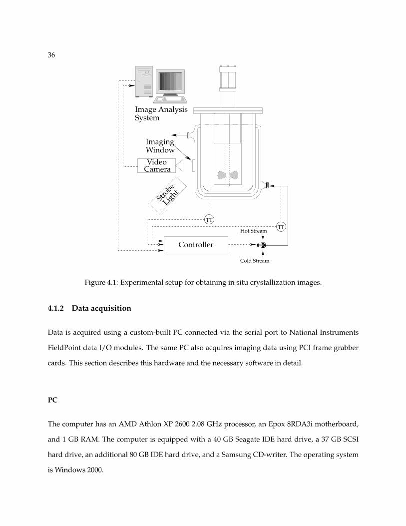
36

VideoCamera

ImagingWindow

Strobe

Light

Image AnalysisSystem

Controller

TTTT

Hot Stream

Cold Stream

Figure 4.1: Experimental setup for obtaining in situ crystallization images.

4.1.2 Data acquisition

Data is acquired using a custom-built PC connected via the serial port to National Instruments

FieldPoint data I/O modules. The same PC also acquires imaging data using PCI frame grabber

cards. This section describes this hardware and the necessary software in detail.

PC

The computer has an AMD Athlon XP 2600 2.08 GHz processor, an Epox 8RDA3i motherboard,

and 1 GB RAM. The computer is equipped with a 40 GB Seagate IDE hard drive, a 37 GB SCSI

hard drive, an additional 80 GB IDE hard drive, and a Samsung CD-writer. The operating system

is Windows 2000.

37

LabVIEW

National Instrument Measurement and Automation Explorer software (version 4.0) is used to con-

figure all I/O devices and interfaces. Once configured, the devices can be used for data acquisition

and control by setting up Virtual Instruments (VIs) using National Instruments LabVIEW software

(version 8.0). The VIs are programmed using the LabVIEW G Language and provide a convenient

operator interface for controlling and configuring experiments. For the experiments relevant to

this thesis, a VI called “Batch Crystallization Video.vi” has been set up that enables batch cool-

ing crystallization for a specified temperature trajectory while acquiring and analyzing images at

specified intervals. The setpoint trajectory tracking temperature controller is an LQR-PID cascade

controller and is described in [94, p. 147].

Signal conditioning with Compact FieldPoint

The signals from the various sensors are conditioned using National Instruments Compact Field-

Point (CFP) signal conditioning modules. Wire connections are made using CFP connector blocks

(cFP-CB-1). All connector blocks and conditioning modules are connected to a backplane (cFP-

1804), which transfers the signals to the PC via the serial port.

Temperature

Temperature measurements are made using Omega 3-wire, 100Ω, platinum resistance tempera-

ture detectors (RTDs) (model PR-13-2-100-1/8). A CFP signal conditioning module (cFP-RTD-122)

provides a 0.25 mA excitation current to each RTD and scales the voltage output signal.

pH

Measurements of pH are made using a double-junction, flat membrane pH electrode with epoxy

body (Weiss Research, PHF-0281-3B). The electrode mV signal is amplified using a pH preampli-

fier (Newport Electronics, PHAMP-1) to -2 to 2 V and connected to the CFP signal conditioning

38

module (cFP-AIO-600). The voltage signal is converted to pH using the LabVIEW VI “pH me-

ter.vi.”

4.1.3 Video image acquisition

The imaging system used in this study was developed by researchers at GlaxoSmithKline and

consists of a monochrome CCD video camera (Sony XC-55) synchronized with a xenon strobe

light (Active Silicon, Model No VS-200-30) and connected to the PC via a frame grabber (National

Instruments, PCI-1410). Images are acquired at a rate of 30 frames per second. The camera gives

images of 480 x 640 pixels and is fitted with a lens (Moritex, x2 magnification) providing a 280 µm

depth of field and 2.48 x 1.87 mm field of view. The camera and strobe are placed to the side of the

crystallizer roughly forty-five degrees apart using Manfrotto positioning arms.

The images are acquired through an “optical flat” attached to the side of the vessel to mini-

mize distortion due to the curved surface of the vessel. The optical flat is created by cutting a 1-in.

mounting square (Scotch) to form a U shape. This U-shaped double-sided adhesive is attached

(with the U upright) on one side to the crystallizer outer body, and on the other side to a 1 in (25

mm sq) microscope slide cover glass (Corning, No. 1). The small gap created by this arrangement

is filled with Permount and allowed to dry.

The camera and strobe are synchronized using a special-purpose cable (National Instru-

ments, Model IMAQ A8055) that consists of a main cable connecting the camera to the frame

grabber with break-out cables to access trigger lines and power supply lines. The wiring system is

shown in Figure 4.2, in which the IMAQ A8055 cable is shown as a dashed line. NI-IMAQ driver

software is required to trigger image acquisition and strobing. The VI “imacquire continuous.vi”

demonstrates image acquisition with synchronized strobing.

Although not used for the studies described in this thesis, an additional frame grabber

(National Instruments, PCI-1405) is installed in the PC that enables image acquisition from RGB

video devices, such as video cameras mounted to microscopes.

39

Camera

Strobe

18 V, 45 W supply 12 V supply

FrameGrabber

Trigger lines

Figure 4.2: Imaging system wiring.

4.1.4 Operating procedure

The following steps describe how the apparatus described above is operated for batch crystalliza-

tion.

1. Open the VI “Batch Crystallization Video.vi” (hereafter referred to as simply “VI”) in Lab-

VIEW 8.0. On the front panel, ensure all toggle switches are off (manual mode) and that the

manual control valve position is specified as closed (i.e. fraction open = 0). Start the VI to

apply the specified control valve position. Running the VI in manual mode is necessary also

to set the initial valve position required for subsequent PID controller calculations.

2. Load crystallizer with appropriate amounts of solvent and crystallizing species. Generally

600 mL of solvent are used. For the industrial pharmaceutical experiments, 17.7 g solid

material are added. For the glycine experiments, the vessel is charged with sufficient solid

material to achieve 20% supersaturation at the desired crystallization temperature.

3. Attach lower and upper jacket ports to jacket inlet and outlet streams, respectively.

4. Turn on impeller. Check slurry visually to ensure impeller speed is sufficiently high to pro-

duce a well-mixed suspension. A speed of 500-600 RPM is typically used for the industrial

pharmaceutical and glycine experiments.

40

5. Turn on 3-way 0.5 in. control valve (Badger Meter, Model 1002), water supply, and gear

pump (Baldor, Model 220/56C). The control valve should be closed such that only cold water

is fed to the crystallizer jacket initially, thereby allowing time to adjust the camera and strobe

before the solid material dissolves.

6. Adjust position of camera and strobe, using “imacquire continuous.vi” to preview image

quality. Superior image quality is generally achieved if the camera is focused at the slurry/glass

interface with the strobe at about a forty-five degree angle to the camera.

7. Turn on the electric heater (Advantage Sentra, Model S-925) and set the hot water setpoint.

The setpoint is 80 C for the industrial pharmaceutical and RT glycine experiments. For

glycine crystallization at higher temperature, a setpoint of 120 is used.

8. Set inputs for VI:

• Cooling profile input file

• Filename for temperature, transmittance, and control valve position data

• Imaging parameters:

– Number of images per acquisition

– Time between acquisitions

– Image analysis algorithm

– Filename for image analysis data

9. Stop VI, if running. Turn ”PID Control” toggle switch on. Set ”Manual Jacket Temp Set-

point” to desired temperature (60 C for industrial pharmaceutical, 55 C for RT glycine, 65

C for high temperature glycine). Run VI, allowing solid material to dissolve.

10. Stop VI. Turn ”MPC Control”, ”Store Data” and ”Acquire Images” toggle switches on. Run

VI. With these toggle switches on, the LQR-PID cascade setpoint trajectory tracking con-

41

troller attempts to follow the pre-specified temperature trajectory given in the cooling pro-

file input file, and all imaging and other data is stored on the hard drive according to the

specified data files.

11. Inject seeds at appropriate time. For the industrial pharmaceutical, 1.4 g of seeds are injected

160 minutes after the cooling process begins.

4.2 Chemical systems

Three different chemical compounds are considered in this work, including an industrial phar-

maceutical, an industrial photochemical, and glycine. This section describes important features

associated with the crystallization of these compounds.

4.2.1 Industrial pharmaceutical

The industrial pharmaceutical is a proprietary compound manufactured by GlaxoSmithKline. In

this study, the compound is crystallized in iso-propyl alcohol (IPA) and water (93/7 vol%), pro-

ducing a polymorph with parallelepiped, needle-like shape. This compound has been studied

extensively by Patience et al. [94, 95] and is used for image analysis algorithm validation in Chap-

ter 5.

4.2.2 Industrial photochemical

The industrial photochemical is a proprietary compound manufactured by Kodak in Rochester,

New York. The compound is crystallized in heptane and has a parallelepiped shape that impedes

accurate size distribution measurement. The nucleation and growth kinetics of this compound

have been characterized by Matthews [81]. This system is studied in Chapter 9.

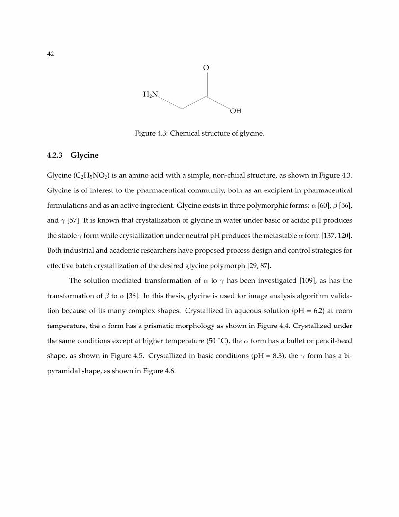
42

H2N

OH

O

Figure 4.3: Chemical structure of glycine.

4.2.3 Glycine

Glycine (C2H5NO2) is an amino acid with a simple, non-chiral structure, as shown in Figure 4.3.

Glycine is of interest to the pharmaceutical community, both as an excipient in pharmaceutical

formulations and as an active ingredient. Glycine exists in three polymorphic forms: α [60], β [56],

and γ [57]. It is known that crystallization of glycine in water under basic or acidic pH produces

the stable γ form while crystallization under neutral pH produces the metastable α form [137, 120].

Both industrial and academic researchers have proposed process design and control strategies for

effective batch crystallization of the desired glycine polymorph [29, 87].

The solution-mediated transformation of α to γ has been investigated [109], as has the

transformation of β to α [36]. In this thesis, glycine is used for image analysis algorithm valida-

tion because of its many complex shapes. Crystallized in aqueous solution (pH = 6.2) at room

temperature, the α form has a prismatic morphology as shown in Figure 4.4. Crystallized under

the same conditions except at higher temperature (50 C), the α form has a bullet or pencil-head

shape, as shown in Figure 4.5. Crystallized in basic conditions (pH = 8.3), the γ form has a bi-

pyramidal shape, as shown in Figure 4.6.

43

Figure 4.4: Images illustrating morphology of α-glycine crystallized in water at room temperature.

Figure 4.5: Images illustrating morphology of α-glycine crystallized in water at 55 C.

Figure 4.6: Images illustrating morphology of γ-glycine crystallized in water at room temperature.

44

4.3 Artificial image generation

This section describes the methods used to generate artificial images.

4.3.1 Stochastic process model

Consider a slurry S of volume V in which a solid phase of discrete particles is dispersed in a

continuous fluid phase. Let L be the characteristic length of a particle and define a shape factor kv

such that the volume of a single particle is given by kvL3. Let f(L) denote the PSD, or the number

of particles of characteristic length L per unit volume slurry. Let VI ∈ S denote an imaging

volume, and let I denote an image created by perspective projection of VI onto a two-dimensional

image plane. Let a and b denote the horizontal and vertical dimensions of VI , or the field of view,

and let df denote the depth dimension of VI , or the depth of field. Thus, the volume of VI is abdf .

To generate an artificial image, we simulate the particle population in a local region sur-

rounding the imaging volume VI . In this region, we model the particle population as a three-

dimensional stochastic process Φp = (Xwi, Li,Θzi) on R3 × R+ × (−π/2, π/2] for i = 1, . . . , Nc.

Xwi = (Xwi, Ywi, Zwi) gives the location of the centroid for particle i in the world coordinate frame,

Li gives the length, Θzi gives the orientation around the z-axis of the world coordinate frame, and

Nc gives the number of particles. Xwi, Li, Θzi, and Nc are distributed independently of each

other. Xwi, Ywi, Zwi, and Θzi are distributed uniformly on [xmin, xmax], [ymin, ymax], [zmin, zmax], and

(−π/2, π/2], respectively. Li has probability density function h and corresponding cumulative

distribution function H , given by

H(L) =

0 L ≤ R∫ LR f(l)dl/

∫ LmaxR f(l)dl R < L ≤ Lmax

1 L > Lmax

in which R is the lower limit of resolution of the camera and Lmax is the size of the largest particle

in the population. Nc has a Poisson distribution with parameter λ = λ(xmax−xmin)(ymax−ymin)/ab,

45

in which λ is the expected number of crystals per image, calculated from the PSD using

λ = VI

∫ ∞

Rf(L)dL

The size of the local region surrounding the imaging volume is defined by (xmin, xmax) = (−0.5Lmax, a+

0.5Lmax) and (ymin, ymax) = (−0.5Lmax, b + 0.5Lmax), in which Lmax is defined as the size of the

largest particle in the population.

4.3.2 Imaging model

Each particle is a convex, three-dimensional domain Pi ∈ V . To model the imaging process, Pi

is projected onto an imaging plane using a camera model. This projection is computed by first

applying rigid-body rotations and translations to change each point Xw in Pi from the world

coordinate frame to the camera coordinate frame:

Xc = RzRyRxXw + T (4.1)

in which Rz, Ry, and Rx are rigid-body rotation matrices, which are functions of the in-plane

orientation θz and the orientations in depth θy and θx, respectively. T = (tx, ty, tz) is a translation

vector. Next, each point is projected onto the image plane according to some imaging model.

Under perspective projection with a pinhole camera, the transformation from a 3-D point Xc =

(Xc, Yc, Zc) in camera coordinates to an image point xc = (xc, yc) is given by

xc =fc

ZcXc, yc =

fc

ZcYc (4.2)

in which fc is the focal length of the camera. Figure 4.7 depicts the perspective projection of

a cylindrical particle onto the image plane. Finally, to model CCD imaging, the image plane

coordinates xc must be converted to pixel coordinates w = (u, v) using

u = u0 + kuxc, v = v0 + kvyc (4.3)

in which (u0, v0) corresponds to xc = (0, 0) and ku and kv provide the necessary scaling based

on pixel size and geometry. The CCD image is depicted in Figure 4.8. For our purposes, the

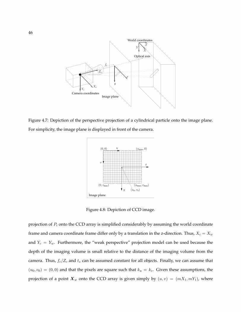
46

y

x

Zc

Optical axis

fc

Yc

Xc

Image plane

YX

Z

World coordinates

Camera coordinates

Figure 4.7: Depiction of the perspective projection of a cylindrical particle onto the image plane.

For simplicity, the image plane is displayed in front of the camera.

x

y

Image plane

v

u

(u0, v0)

(umax, 0)

(0, vmax) (umax, vmax)

(0, 0)

Figure 4.8: Depiction of CCD image.

projection of Pi onto the CCD array is simplified considerably by assuming the world coordinate

frame and camera coordinate frame differ only by a translation in the z-direction. Thus, Xc = Xw

and Yc = Yw. Furthermore, the “weak perspective” projection model can be used because the

depth of the imaging volume is small relative to the distance of the imaging volume from the

camera. Thus, fc/Zc and tz can be assumed constant for all objects. Finally, we can assume that

(u0, v0) = (0, 0) and that the pixels are square such that ku = kv. Given these assumptions, the

projection of a point Xw onto the CCD array is given simply by (u, v) = (mX1,mY1), where

47

m = kufc/Zc.

4.3.3 Justifications for two-dimensional system model

The assumptions justifying our use of a two-dimensional process to model a three-dimensional

system are as follows. First of all, we assume the camera is positioned a fixed distance z0 from the

imaging volume, and that df z0. This assumption means the particles in the imaging volume

are projected onto the image plane according to the weak perspective projection model. In other

words, the projected particle lengths measured in the image coordinate system can be related to

the true projected particle lengths by applying a constant magnification factor m, without regard

for the distance of the particle from the camera. Secondly, we assume all particles are oriented

in a plane orthogonal to the camera’s optical axis. This assumption, together with the weak per-

spective assumption, essentially reduces the 3-D process to a 2-D process, thereby simplifying the

analysis considerably. These assumptions are not used only for convenience, however, but rather

to reflect the actual conditions under which in situ imaging measurements are made in practice. To

obtain useful in situ images in high solids concentrations, the camera must have a small depth of

field and be focused only a small depth into the particulate slurry. It seems reasonable, therefore,

to expect the shear flow at the slurry-sensor interface to cause the particles to align orthogonal to

the interface, and thus orthogonal to the camera’s optical axis.

48

49

Chapter 5

Two-dimensional Object Recognition for

High-Aspect-Ratio Particles 1

Suspension crystallization processes often result in crystals having a high aspect ratio, a shape

commonly described as needle-like, rod-like, or acicular. High-aspect-ratio crystals are particu-

larly commonplace in the specialty chemical and pharmaceutical industries. As discussed in Sec-

tion 2.3.1, conventional PSD monitoring technologies, such as laser diffraction and laser backscat-

tering, are based on assumptions of particle sphericity [136, 89] and therefore do not provide the

monitoring capability necessary to achieve on-line PSD control for systems in which the parti-

cles are highly non-spherical. Several researchers have developed imaging-based methods for

sizing elongated crystals [100, 110, 94, 95], but none of these methods are sufficiently automated

to be suitable for on-line monitoring and control. Commercially available, imaging-based parti-

cle size and shape analyzers require sampling, which is inconvenient, possibly hazardous, and

raises concerns about whether the sample is representative of the bulk slurry [3, 7].The utility of

in situ video microscopy has been limited primarily to qualitative monitoring because the nature

of in situ images, which contain blurred, out-of-focus, and overlapping particles, has precluded

successful image segmentation.

This chapter demonstrates robust and efficient segmentation for in situ images of high-

aspect-ratio particles using a novel image analysis algorithm. We show that the algorithm’s PSD

measurements are consistent with measurements obtained through manual image analysis by

1Portions of this chapter appear in Larsen, Rawlings, and Ferrier [69]

50

human operators. The accuracy of the measured PSD, therefore, is established only with respect

to the PSD measured by human operators. The absolute accuracy of the measured PSD is the

subject of Chapters 7– 9. The chapter is organized as follows. Section 5.1 describes the algorithm,

and Section 5.2 presents the experimental studies used to evaluate the algorithm’s accuracy and

speed. Our findings are summarized in Section 5.3.

5.1 Image analysis algorithm description

This section describes the image analysis algorithm developed for the purpose of analyzing in

situ images of high-aspect-ratio crystals. The algorithm is referred to in this thesis as SHARC

(Segmentation for High-Aspect-Ratio Crystals) and has been implemented in MATLAB 7.1. We

present first an overview of SHARC and then describe in more detail each of SHARC’s compo-

nents.

5.1.1 Overview

The SHARC algorithm is built on the assumption that a needle-shaped crystal can be modeled

geometrically as a group of two or more spatially-proximate lines with similar orientation and

length. The SHARC algorithm searches for image features satisfying this model in the follow-

ing manner: First, SHARC detects linear features in the image, referred to as “elementary line

segments” or ELSs. Next, SHARC identifies collinear line pairs (lines that appear to belong to a

single crystal edge but have been broken up due to background noise, particle overlap, or crys-

tal defects) and creates a representative line, called a “base line,” for each pair. Given both the

ELSs and the base lines, SHARC identifies pairs of spatially-proximate, parallel lines of similar

length. Finally, SHARC identifies consistent groups of parallel lines and clusters the constituent

lines in each of these groups as belonging to a single crystal. The properties (e.g. length, aspect

ratio) of these line clusters are used as estimates of the properties of the crystals in the image. Fig-

ure 5.1 shows the result of applying these steps to a small section of an in situ image of needle-like

51

pharmaceutical crystals.

(a) (b)

(c) (d)

Figure 5.1: Example of SHARC algorithm applied to an in situ image of suspended pharmaceutical

crystals. (a) A region of interest in the original image. (b) Linear features (ELSs) extracted from the

original image. (c) ELSs (black lines) and lines representing each collinear line pair (white lines).

(d) Representative rectangles for clusters of spatially-proximate parallel lines with roughly equal

length. The lengths, widths, and aspect ratios of the rectangles are used as the crystal size and

shape measurements.

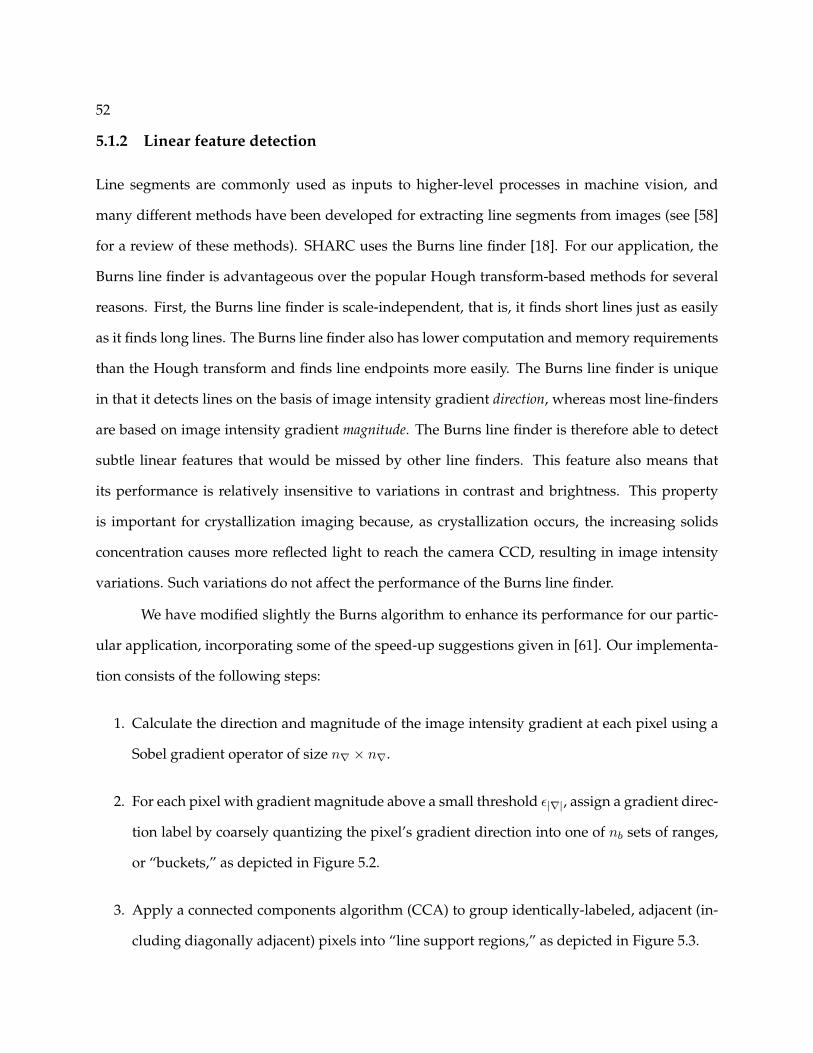
52

5.1.2 Linear feature detection

Line segments are commonly used as inputs to higher-level processes in machine vision, and

many different methods have been developed for extracting line segments from images (see [58]

for a review of these methods). SHARC uses the Burns line finder [18]. For our application, the

Burns line finder is advantageous over the popular Hough transform-based methods for several

reasons. First, the Burns line finder is scale-independent, that is, it finds short lines just as easily

as it finds long lines. The Burns line finder also has lower computation and memory requirements

than the Hough transform and finds line endpoints more easily. The Burns line finder is unique

in that it detects lines on the basis of image intensity gradient direction, whereas most line-finders

are based on image intensity gradient magnitude. The Burns line finder is therefore able to detect

subtle linear features that would be missed by other line finders. This feature also means that

its performance is relatively insensitive to variations in contrast and brightness. This property

is important for crystallization imaging because, as crystallization occurs, the increasing solids

concentration causes more reflected light to reach the camera CCD, resulting in image intensity

variations. Such variations do not affect the performance of the Burns line finder.

We have modified slightly the Burns algorithm to enhance its performance for our partic-

ular application, incorporating some of the speed-up suggestions given in [61]. Our implementa-

tion consists of the following steps:

1. Calculate the direction and magnitude of the image intensity gradient at each pixel using a

Sobel gradient operator of size n∇ × n∇.

2. For each pixel with gradient magnitude above a small threshold ε|∇|, assign a gradient direc-

tion label by coarsely quantizing the pixel’s gradient direction into one of nb sets of ranges,

or “buckets,” as depicted in Figure 5.2.

3. Apply a connected components algorithm (CCA) to group identically-labeled, adjacent (in-

cluding diagonally adjacent) pixels into “line support regions,” as depicted in Figure 5.3.

53

23

14

5

6 7

81

23

4

5

67

8

Figure 5.2: Depiction of different eight-bucket gradient direction quantizations used to label pix-

els. For the quantization on the left, pixels having gradient direction in the range of 0 to 45 degrees

are labeled as “1”, pixels with gradient direction in the range of 45 to 90 degrees are labeled as “2”,

and so forth. Quantization effects are mitigated by applying a second quantization, such as that

shown on the right, and subsequently resolving any conflicts between the results given by each

quantization.

4. Filter line support regions that have a pixel area less than some pre-defined threshold εA.

5. Fit a line to each remaining line support region, as depicted in Figure 5.3.

To eliminate quantization effects, steps 2–4 are performed twice before proceeding to step

5, each time using a different quantization in which the gradient direction partitioning is shifted by

half the bucket size, as shown in Figure 5.2. This procedure results in each pixel being associated

with two different line support regions, and this conflict is resolved through a voting process

designed to select the interpretation that results in the longest possible line support regions [18].

To reduce computation time, SHARC carries out this voting process on the basis of the pixel areas

of the conflicting line support regions, which in almost every case gives the same results as voting

based on length.

The line-fitting method used in step 5 is standard blob analysis, available in most image

analysis packages. Blob analysis fits a line to each region of pixels by determining an ellipse

having the same geometric moments as the region, as depicted in Figure 5.3. The ellipse’s major

axis length, minor axis length, orientation, and centroid are used respectively as the length, width,

orientation, and center of the corresponding line.

54

(a) (b)

(c) (d)

Figure 5.3: Example of finding linear features using Burns line finder and blob analysis. (a)

Grayscale image. (b) Regions of pixels having similar gradient orientation, determined using the

Burns line finder. (c) Best-fit ellipses for each region of pixels, determined using blob analysis. (d)

Major axes of the best-fit ellipses imposed on the original grayscale image.

5.1.3 Identification of collinear line pairs

During linear feature extraction, single edges are commonly broken up into multiple collinear

lines. This problem is common for systems of needle-like crystals because the particles are of-

ten touching or overlapping. Therefore, SHARC groups these collinear lines prior to searching

for groups of parallel lines having similar length and orientation. The problem of collinear line

grouping has been studied extensively. Jang and Hong [58] compare and evaluate a number of

the available methods. SHARC uses a straightforward, computationally inexpensive method de-

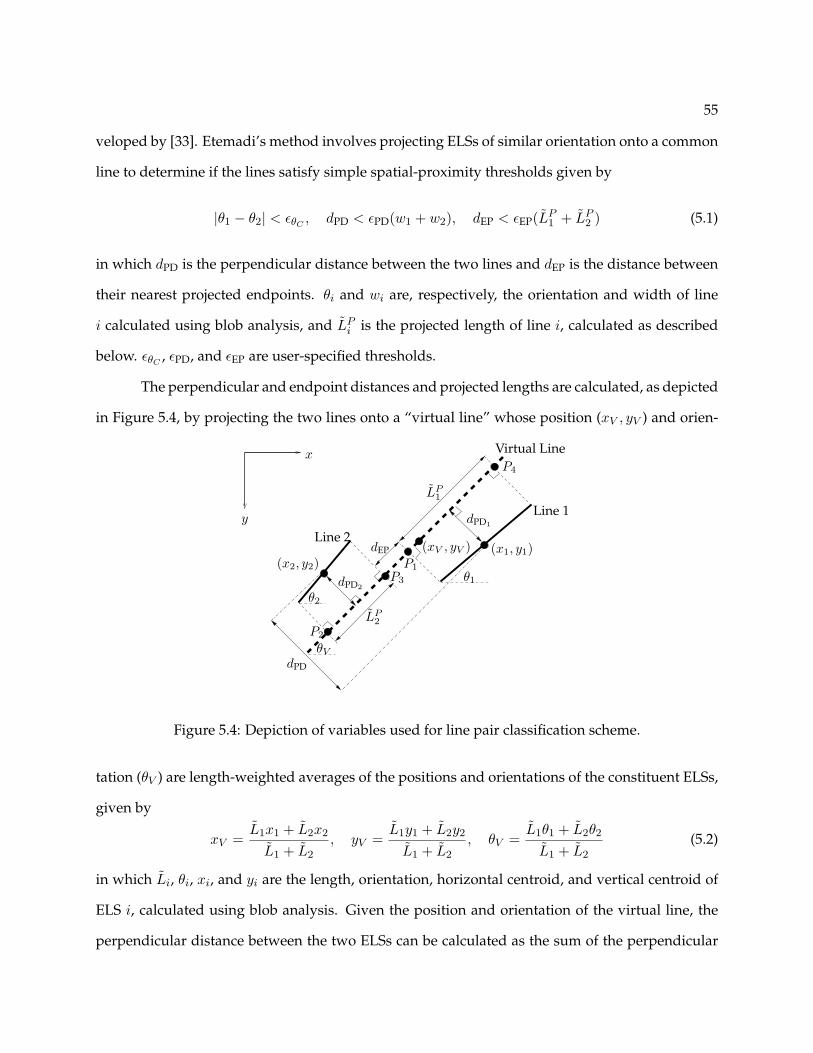
55

veloped by [33]. Etemadi’s method involves projecting ELSs of similar orientation onto a common

line to determine if the lines satisfy simple spatial-proximity thresholds given by

|θ1 − θ2| < εθC, dPD < εPD(w1 + w2), dEP < εEP(LP

1 + LP2 ) (5.1)

in which dPD is the perpendicular distance between the two lines and dEP is the distance between

their nearest projected endpoints. θi and wi are, respectively, the orientation and width of line

i calculated using blob analysis, and LPi is the projected length of line i, calculated as described

below. εθC, εPD, and εEP are user-specified thresholds.

The perpendicular and endpoint distances and projected lengths are calculated, as depicted

in Figure 5.4, by projecting the two lines onto a “virtual line” whose position (xV , yV ) and orien-

P4

P3

dPD

y

x

Line 2

Line 1

θ1

(x2, y2)(x1, y1)

dPD1

dPD2

θ2

dEP

Virtual Line

P2

LP2

LP1

θV

P1

(xV , yV )

Figure 5.4: Depiction of variables used for line pair classification scheme.

tation (θV ) are length-weighted averages of the positions and orientations of the constituent ELSs,

given by

xV =L1x1 + L2x2

L1 + L2

, yV =L1y1 + L2y2

L1 + L2

, θV =L1θ1 + L2θ2

L1 + L2

(5.2)

in which Li, θi, xi, and yi are the length, orientation, horizontal centroid, and vertical centroid of

ELS i, calculated using blob analysis. Given the position and orientation of the virtual line, the

perpendicular distance between the two ELSs can be calculated as the sum of the perpendicular

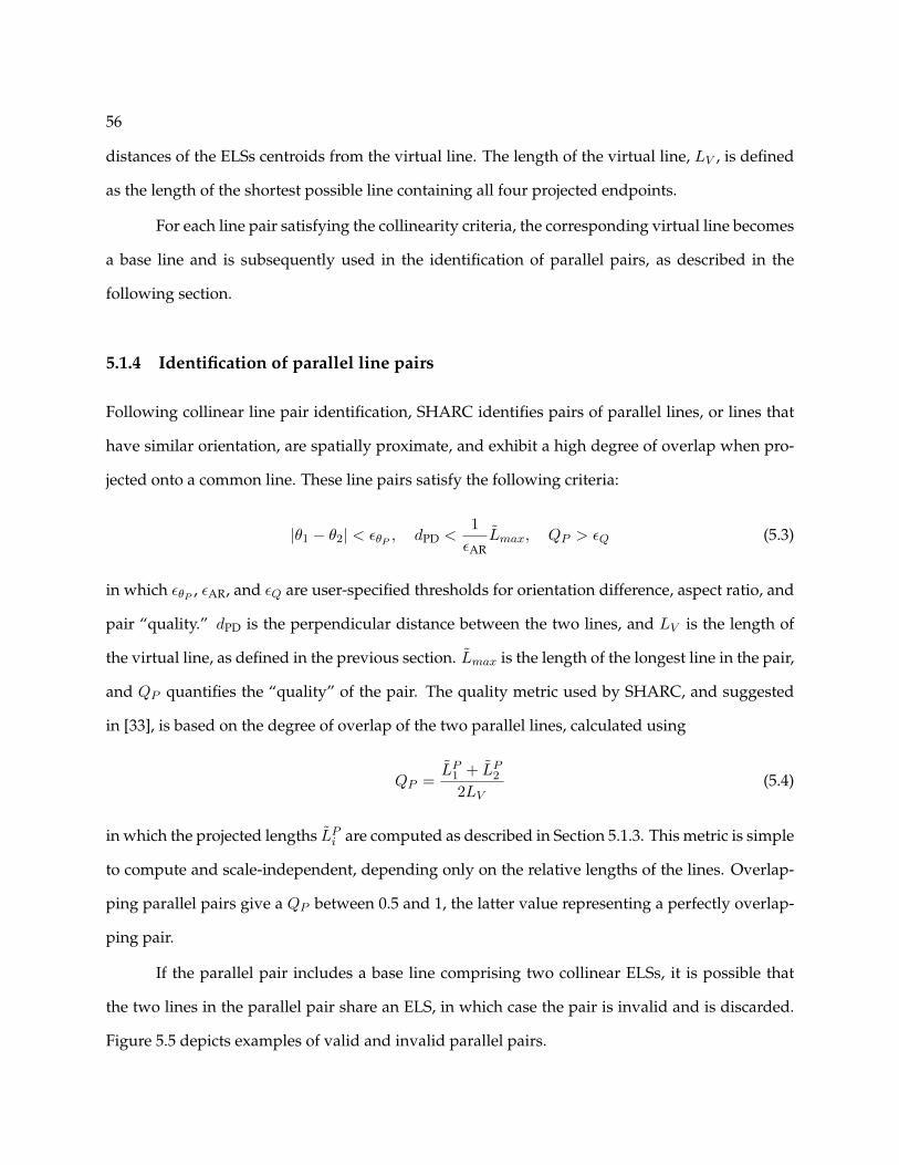
56

distances of the ELSs centroids from the virtual line. The length of the virtual line, LV , is defined

as the length of the shortest possible line containing all four projected endpoints.

For each line pair satisfying the collinearity criteria, the corresponding virtual line becomes

a base line and is subsequently used in the identification of parallel pairs, as described in the

following section.

5.1.4 Identification of parallel line pairs

Following collinear line pair identification, SHARC identifies pairs of parallel lines, or lines that

have similar orientation, are spatially proximate, and exhibit a high degree of overlap when pro-

jected onto a common line. These line pairs satisfy the following criteria:

|θ1 − θ2| < εθP, dPD <

1εAR

Lmax, QP > εQ (5.3)

in which εθP, εAR, and εQ are user-specified thresholds for orientation difference, aspect ratio, and

pair “quality.” dPD is the perpendicular distance between the two lines, and LV is the length of

the virtual line, as defined in the previous section. Lmax is the length of the longest line in the pair,

and QP quantifies the “quality” of the pair. The quality metric used by SHARC, and suggested

in [33], is based on the degree of overlap of the two parallel lines, calculated using

QP =LP

1 + LP2

2LV(5.4)

in which the projected lengths LPi are computed as described in Section 5.1.3. This metric is simple

to compute and scale-independent, depending only on the relative lengths of the lines. Overlap-

ping parallel pairs give a QP between 0.5 and 1, the latter value representing a perfectly overlap-

ping pair.

If the parallel pair includes a base line comprising two collinear ELSs, it is possible that

the two lines in the parallel pair share an ELS, in which case the pair is invalid and is discarded.

Figure 5.5 depicts examples of valid and invalid parallel pairs.

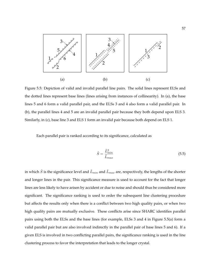
57

1

2

3

45

62

1

34

52

13

(a) (b) (c)

Figure 5.5: Depiction of valid and invalid parallel line pairs. The solid lines represent ELSs and

the dotted lines represent base lines (lines arising from instances of collinearity). In (a), the base

lines 5 and 6 form a valid parallel pair, and the ELSs 3 and 4 also form a valid parallel pair. In

(b), the parallel lines 4 and 5 are an invalid parallel pair because they both depend upon ELS 3.

Similarly, in (c), base line 3 and ELS 1 form an invalid pair because both depend on ELS 1.

Each parallel pair is ranked according to its significance, calculated as

S =L2

min

Lmax

(5.5)

in which S is the significance level and Lmin and Lmax are, respectively, the lengths of the shorter

and longer lines in the pair. This significance measure is used to account for the fact that longer

lines are less likely to have arisen by accident or due to noise and should thus be considered more

significant. The significance ranking is used to order the subsequent line clustering procedure

but affects the results only when there is a conflict between two high quality pairs, or when two

high quality pairs are mutually exclusive. These conflicts arise since SHARC identifies parallel

pairs using both the ELSs and the base lines (for example, ELSs 3 and 4 in Figure 5.5(a) form a

valid parallel pair but are also involved indirectly in the parallel pair of base lines 5 and 6). If a

given ELS is involved in two conflicting parallel pairs, the significance ranking is used in the line

clustering process to favor the interpretation that leads to the longer crystal.

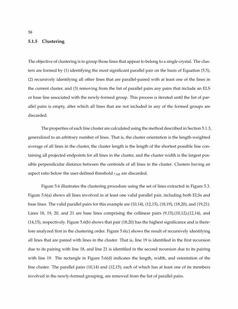
58

5.1.5 Clustering

The objective of clustering is to group those lines that appear to belong to a single crystal. The clus-

ters are formed by (1) identifying the most significant parallel pair on the basis of Equation (5.5),

(2) recursively identifying all other lines that are parallel-paired with at least one of the lines in

the current cluster, and (3) removing from the list of parallel pairs any pairs that include an ELS

or base line associated with the newly-formed group. This process is iterated until the list of par-

allel pairs is empty, after which all lines that are not included in any of the formed groups are

discarded.

The properties of each line cluster are calculated using the method described in Section 5.1.3,

generalized to an arbitrary number of lines. That is, the cluster orientation is the length-weighted

average of all lines in the cluster, the cluster length is the length of the shortest possible line con-

taining all projected endpoints for all lines in the cluster, and the cluster width is the largest pos-

sible perpendicular distance between the centroids of all lines in the cluster. Clusters having an

aspect ratio below the user-defined threshold εAR are discarded.

Figure 5.6 illustrates the clustering procedure using the set of lines extracted in Figure 5.3.

Figure 5.6(a) shows all lines involved in at least one valid parallel pair, including both ELSs and

base lines. The valid parallel pairs for this example are (10,14), (12,15), (18,19), (18,20), and (19,21).

Lines 18, 19, 20, and 21 are base lines comprising the collinear pairs (9,15),(10,12),(12,14), and

(14,15), respectively. Figure 5.6(b) shows that pair (18,20) has the highest significance and is there-

fore analyzed first in the clustering order. Figure 5.6(c) shows the result of recursively identifying

all lines that are paired with lines in the cluster. That is, line 19 is identified in the first recursion

due to its pairing with line 18, and line 21 is identified in the second recursion due to its pairing

with line 19. The rectangle in Figure 5.6(d) indicates the length, width, and orientation of the

line cluster. The parallel pairs (10,14) and (12,15), each of which has at least one of its members

involved in the newly-formed grouping, are removed from the list of parallel pairs.

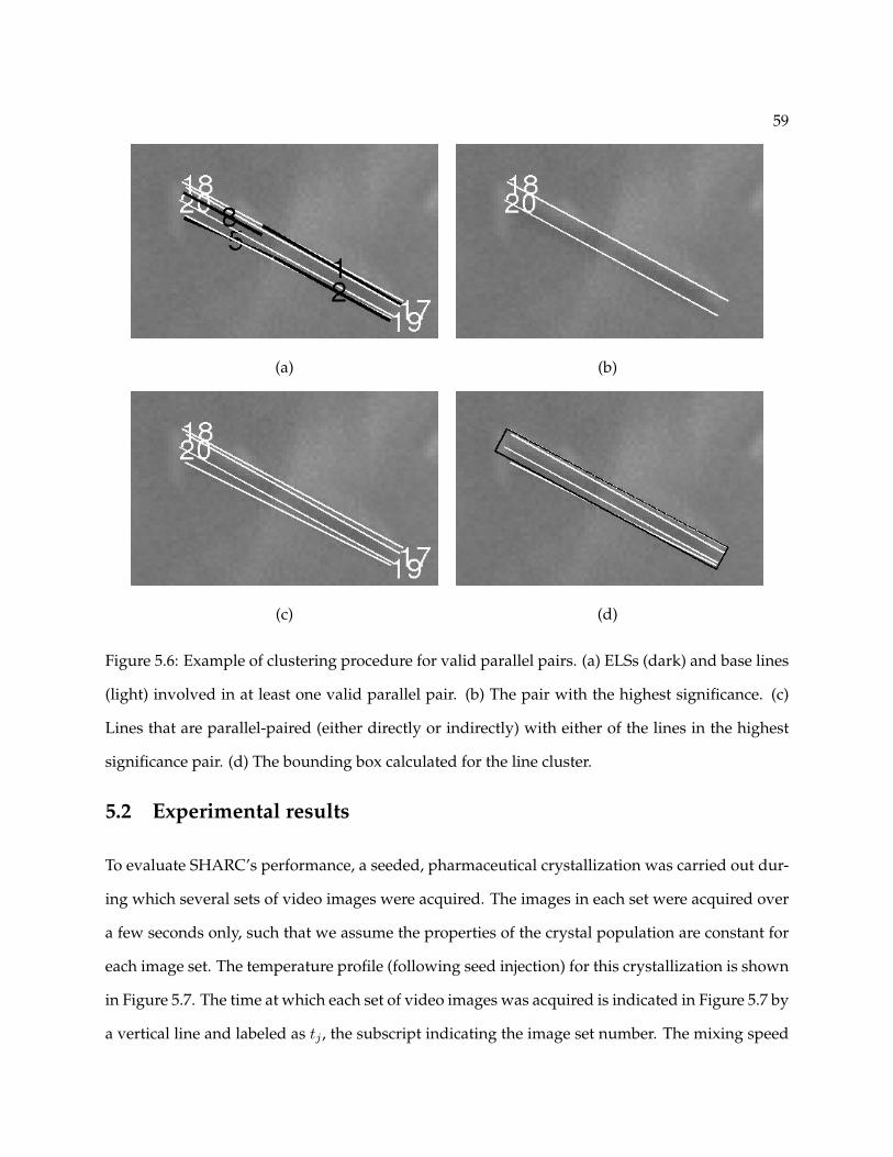
59

(a) (b)

(c) (d)

Figure 5.6: Example of clustering procedure for valid parallel pairs. (a) ELSs (dark) and base lines

(light) involved in at least one valid parallel pair. (b) The pair with the highest significance. (c)

Lines that are parallel-paired (either directly or indirectly) with either of the lines in the highest

significance pair. (d) The bounding box calculated for the line cluster.

5.2 Experimental results

To evaluate SHARC’s performance, a seeded, pharmaceutical crystallization was carried out dur-

ing which several sets of video images were acquired. The images in each set were acquired over

a few seconds only, such that we assume the properties of the crystal population are constant for

each image set. The temperature profile (following seed injection) for this crystallization is shown

in Figure 5.7. The time at which each set of video images was acquired is indicated in Figure 5.7 by

a vertical line and labeled as tj , the subscript indicating the image set number. The mixing speed

60

15

20

25

30

35

40

45

50

55

0 50 100 150 200 250 300

Tem

pera

ture

,[

C]

Time, [minutes]

t1 t2 t3 t4 t5 t6

Seeds injected

Figure 5.7: Temperature trajectory for crystallization experiment. The vertical lines indicate the

times at which sets of video images were acquired.

Line finder Collinearity Parallelism

Parameters Thresholds Thresholds

n∇ 5 εθC20 degrees εθP

5 degrees

ε|∇| 1 εEP 0.5 εQ 0.85

nb 6 buckets εPD 0.5 εAR 4.5

εA 20 pixels

Table 5.1: SHARC parameter values used to analyze images from pharmaceutical crystallization

experiment.

for this experiment was 550 RPM (1.1 m/s tip speed), sufficiently fast that the crystals could not

be tracked from one video frame to the next. The same parameter values were used to analyze all

images (see Table 5.2).

The following sections assess SHARC’s suitability for on-line monitoring and control with

respect to both accuracy and speed.

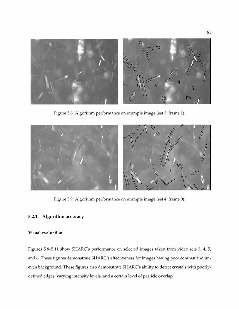
61

Figure 5.8: Algorithm performance on example image (set 3, frame 1).


5.2.1 Algorithm accuracy

Visual evaluation

Figures 5.8–5.11 show SHARC’s performance on selected images taken from video sets 3, 4, 5,

and 6. These figures demonstrate SHARC’s effectiveness for images having poor contrast and un-

even background. These figures also demonstrate SHARC’s ability to detect crystals with poorly-

defined edges, varying intensity levels, and a certain level of particle overlap.

62



Comparisons with manual sizing

We evaluate SHARC’s accuracy by comparing its PSD measurements with measurements ob-

tained through manual image analysis by human operators. Although the human vision system

is clearly more reliable than current computer vision systems, manual image analysis introduces

an undesirable level of subjectiveness into the measurement. The subjectiveness of manual sizing

is magnified for in situ images because the crystals often appear blurry, overlapping, and out-of-

focus. Thus, it can be difficult to decide whether or not a given crystal is sufficiently in focus and

well-defined to be sized accurately. To assess the subjectiveness involved in manually sizing in

63

Operator 1 2 3 4 5 6 7 8 9 Mean SD

Mean size [µm] 224 300 314 295 276 268 328 276 272 284 30

# of crystals 460 230 140 350 150 300 200 330 500 290 130

ave. % diff (Eq. 5.6) 26 10 13 10 9 10 17 9 9 12

Table 5.2: Comparison of results obtained from nine different persons manually sizing the same

ten images.

situ images and determine what constitutes “good” agreement between SHARC’s measurement

and a manual measurement, we asked nine different people to manually size crystals for the same

ten images from image set 3. We confirmed that ten images was sufficient to achieve convergence

of the overall mean size measurement for each operator. Table 5.2 shows the overall mean size

calculated for all ten images for each operator, the total number of crystals found by each opera-

tor, and the average percent difference in overall mean size between each operator and the other

operators. This latter value is calculated for operator i using the equation

diffi =100

Nop − 1

Nop∑j=1

|xi − xj |xi+xj

2

(5.6)

Table 5.2 shows that the mean size varied by as much as 37% between operators, and the number

of crystals found varied by over 100% between operators, illustrating the large degree of subjec-

tiveness associated with manual sizing of in situ images. However, the relatively small standard

deviation in overall mean size indicates that manual sizing constitutes a reasonably reliable stan-

dard provided the measurement is performed by a sufficient number of operators.

Based on the results shown in Table 5.2, we define “good” agreement between SHARC’s

results and a set of manual results to mean that their individual means are within approximately

12% of their combined mean value. Table 5.3 shows that the SHARC algorithm determines a

mean crystal size within 2% of that found by the nine manual operators, and Figure 5.12 shows a

good match between the cumulative distribution function found by SHARC and the cumulative

distribution functions of the nine manual operators.

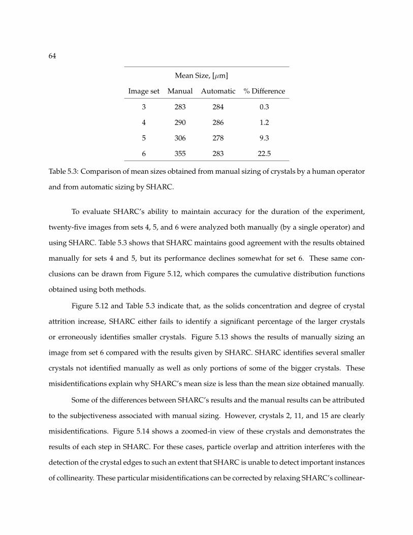
64

Mean Size, [µm]

Image set Manual Automatic % Difference

3 283 284 0.3

4 290 286 1.2

5 306 278 9.3

6 355 283 22.5

Table 5.3: Comparison of mean sizes obtained from manual sizing of crystals by a human operator

and from automatic sizing by SHARC.

To evaluate SHARC’s ability to maintain accuracy for the duration of the experiment,

twenty-five images from sets 4, 5, and 6 were analyzed both manually (by a single operator) and

using SHARC. Table 5.3 shows that SHARC maintains good agreement with the results obtained

manually for sets 4 and 5, but its performance declines somewhat for set 6. These same con-

clusions can be drawn from Figure 5.12, which compares the cumulative distribution functions

obtained using both methods.

Figure 5.12 and Table 5.3 indicate that, as the solids concentration and degree of crystal

attrition increase, SHARC either fails to identify a significant percentage of the larger crystals

or erroneously identifies smaller crystals. Figure 5.13 shows the results of manually sizing an

image from set 6 compared with the results given by SHARC. SHARC identifies several smaller

crystals not identified manually as well as only portions of some of the bigger crystals. These

misidentifications explain why SHARC’s mean size is less than the mean size obtained manually.

Some of the differences between SHARC’s results and the manual results can be attributed

to the subjectiveness associated with manual sizing. However, crystals 2, 11, and 15 are clearly

misidentifications. Figure 5.14 shows a zoomed-in view of these crystals and demonstrates the

results of each step in SHARC. For these cases, particle overlap and attrition interferes with the

detection of the crystal edges to such an extent that SHARC is unable to detect important instances

of collinearity. These particular misidentifications can be corrected by relaxing SHARC’s collinear-

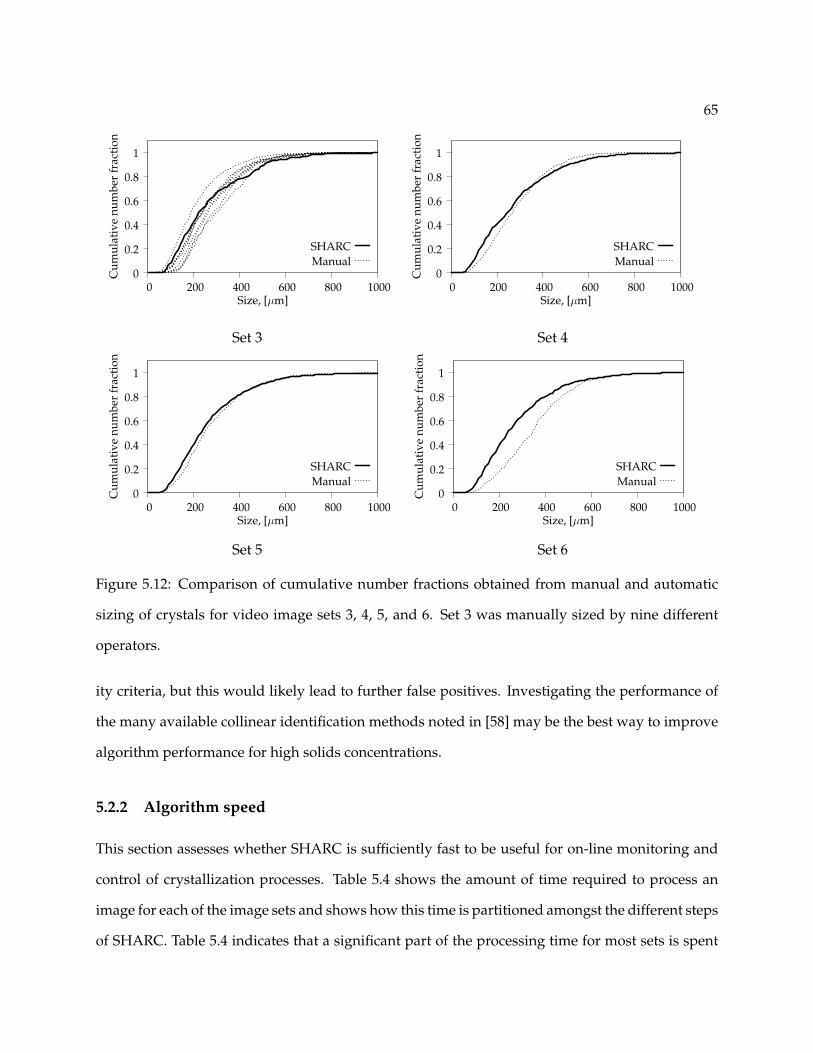
65

0

0.2

0.4

0.6

0.8

1

0 200 400 600 800 1000

Cum

ulat

ive

num

ber

frac

tion

Size, [µm]

SHARCManual

0

0.2

0.4

0.6

0.8

1

0 200 400 600 800 1000

Cum

ulat

ive

num

ber

frac

tion

Size, [µm]

SHARCManual

Set 3 Set 4

0

0.2

0.4

0.6

0.8

1

0 200 400 600 800 1000

Cum

ulat

ive

num

ber

frac

tion

Size, [µm]

SHARCManual

0

0.2

0.4

0.6

0.8

1

0 200 400 600 800 1000

Cum

ulat

ive

num

ber

frac

tion

Size, [µm]

SHARCManual

Set 5 Set 6

Figure 5.12: Comparison of cumulative number fractions obtained from manual and automatic

sizing of crystals for video image sets 3, 4, 5, and 6. Set 3 was manually sized by nine different

operators.

ity criteria, but this would likely lead to further false positives. Investigating the performance of

the many available collinear identification methods noted in [58] may be the best way to improve

algorithm performance for high solids concentrations.

5.2.2 Algorithm speed

This section assesses whether SHARC is sufficiently fast to be useful for on-line monitoring and

control of crystallization processes. Table 5.4 shows the amount of time required to process an

image for each of the image sets and shows how this time is partitioned amongst the different steps

of SHARC. Table 5.4 indicates that a significant part of the processing time for most sets is spent

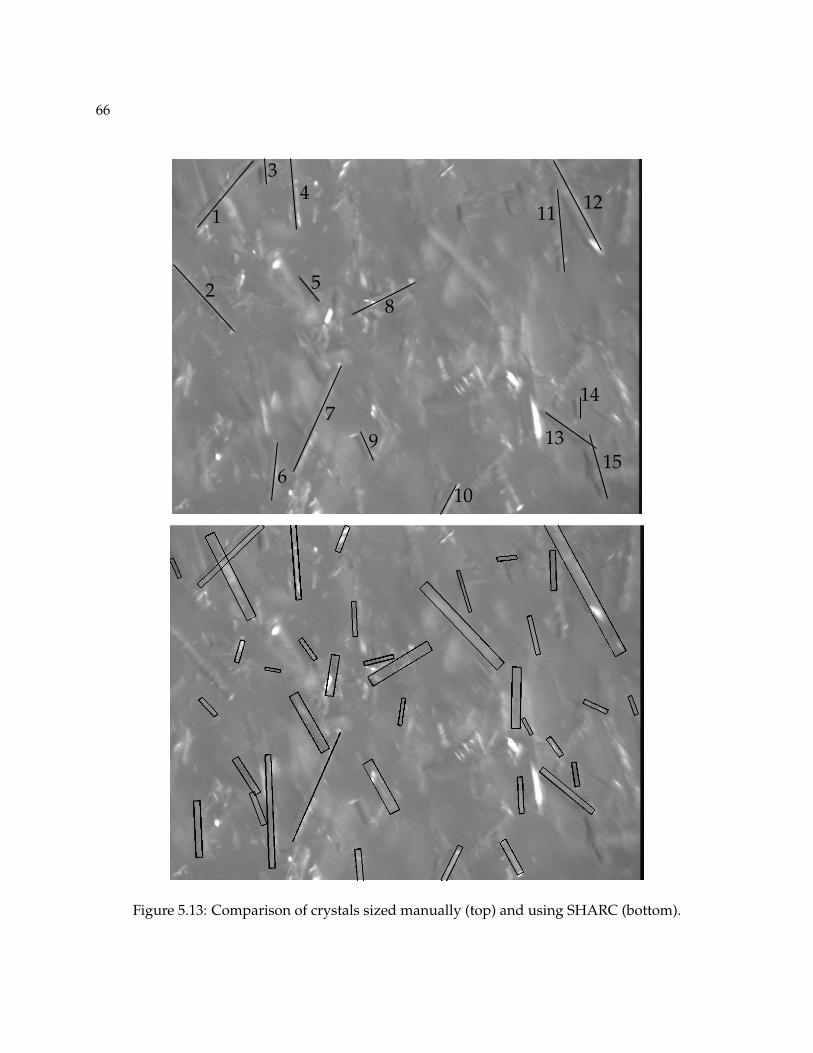
66

2

14

5

610

15

12

3

79

8

13

14

11

Figure 5.13: Comparison of crystals sized manually (top) and using SHARC (bottom).

67

(a) (b) (c) (d)

Figure 5.14: Zoomed-in view of crystals that SHARC failed to identify correctly. From top to

bottom, the crystal labels are two, eleven, and fifteen (according to labels in Figure 5.13). Column

(a): Original image. Column (b): ELS data. Column (c): ELSs and base lines. Column (d): Result

of clustering.

68

average average cputime per image [s]

total cputime linear feature collinearity parallelism

Set per image [s] detection identification identification clustering

2 1.9 1.8 (97) 0.0 (1) 0.0 (0) 0.0 (0)

3 3.1 2.0 (65) 0.4 (14) 0.6 (19) 0.0 (0)

4 4.3 2.1 (47) 0.8 (17) 1.5 (33) 0.0 (0)

5 7.1 2.5 (35) 1.4 (19) 3.2 (44) 0.0 (0)

6 10.8 2.9 (26) 2.2 (20) 5.6 (52) 0.1 (0)

Table 5.4: Computational requirements for analyzing different image sets (averaged over 10 im-

ages). The numbers in parentheses give the percentages of total cputime. Images are analyzed

using a 2.2 GHz AMD Athlon 64 processor.

on the collinear and parallel grouping operations. These operations can be made more efficient by

limiting the computations to line pairs that are spatially proximate using a data structure in which

the lines are sorted by their endpoint locations, as suggested in [75].

To determine how much time is required to obtain a sufficiently accurate estimate of the

mean particle length, we find the number of samples n such that the size of the 95% confidence

interval for the population mean particle length is less than 10% of the sample mean. That is, we

find the smallest n for which

t(α, n− 1)sn√n≤ 0.1ln (5.7)

in which t is the t-distribution, α is the confidence level, ln is the sample mean, and sn is the sample

standard deviation, defined as

ln =1n

n∑i=1

li (5.8)

sn =

√√√√ 1n− 1

n∑i=1

(li − ln

)2 (5.9)

in which li is the length of particle i. Similarly, to determine how much time is required to obtain

69

average # of crystals cputime to cputime to

# of crystals to converge converge to converge to

Set per image to mean mean [min.] variance [min.]

2 1 93 1.9 18.5

3 25 163 0.3 1.8

4 28 129 0.3 2.2

5 30 106 0.4 3.4

6 38 143 0.7 4.2

Table 5.5: Computational requirements for SHARC to achieve convergence of particle size distri-

bution mean and variance.

a sufficiently accurate estimate of the variance in particle length, we find n such that the size of

the 95% confidence interval for the population variance is less than 10% of the sample variance s2n,

satisfying

n− 1χ2(α, n− 1)

− 1 ≤ 0.1 (5.10)

in which χ2 is the chi-squared distribution (see [115, p.75]). Equation 5.10 is satisfied for n = 889

samples.

Given SHARC’s speed, the number of crystals per image, and the number of samples nec-

essary to obtain sufficient measurement accuracy, we can calculate the rate at which SHARC

provides accurate mean and variance measurements. Table 5.5 indicates that SHARC requires

approximately two minutes to measure the PSD mean and fifteen minutes to measure the PSD

variance. Given the time scales of most crystallization processes, SHARC is sufficiently fast to

provide measurements for a feedback control system based on measurements of the PSD mean

and variance. If necessary, the measurement rate can be increased by implementing SHARC in a

compiled language.

70

5.3 Conclusion

The SHARC algorithm can robustly and efficiently extract crystal size information from in situ

images of suspended, high-aspect-ratio crystals for moderate solids concentrations, giving re-

sults consistent with measurements obtained through manual image analysis by human opera-

tors. SHARC’s performance declines for high solids concentrations and high levels of particle

attrition because the degree of particle overlap and the noise arising from attrited particulate mat-

ter hinder the identification of the suspended crystals’ edges. Implementing improved methods

for identifying instances of collinearity may enable suitable performance for these conditions.

The speed with which SHARC analyzes the images is suitable for real-time monitoring and

control of PSD mean and variance.

71

Chapter 6

Three-dimensional Object Recognition

for Complex Crystal Shapes 1

The SHARC algorithm described in Chapter 5 handles only one of the many possible shapes that

can result from suspension crystallization processes. In this chapter, an image analysis algorithm

called M-SHARC (Model-based SHApe Recognition for Crystals) is developed that can be applied

to images of crystals of any shape, provided the shape can be represented as a wire-frame model.

The wire-frame models used by the algorithm are parameterized. Thus, a single model can be used

to identify crystal objects exhibiting a wide range of sizes and shapes within a given shape class.

The algorithm therefore enables the measurement of shape factor distributions. Furthermore, the

algorithm can be applied using multiple wire-frame models representing different shape classes

to measure the distribution of particles between different shape classes.

The algorithm described in this chapter is classified as a model-based object recognition

algorithm. Model-based object recognition is a widely-used approach to computer vision that has

been developed to enable automatic recognition of complex objects with unknown pose (i.e. ori-

entation with respect to the camera) in the presence of missing or occluded data [54, 75, 39, chapter

18]. The model-based object recognition approach is based on matching raw image features (such

as arcs or lines) with one of several pre-defined models. The model-based approach does not in-

volve exhaustive searches of the model parameter space and is therefore more efficient than purely

top-down approaches (such as Hough-transform-based methods). Model-based object recogni-

1Portions of this chapter appear in Larsen, Rawlings, and Ferrier [70]

72

tion is more robust to noise than purely bottom-up approaches because it can be applied even if

part of the object to be identified is occluded or missing. Furthermore, the model-based approach

leads to algorithms that can be implemented in a parallel fashion to enable real-time analysis.

Algorithms based on this approach have been developed and applied to systems of circular par-

ticles [113] and elliptical particles [48]. The SHARC algorithm is essentially a two-dimensional

model-based recognition algorithm.

The chapter is organized as follows. Section 6.1 describes the algorithm, and Section 6.2

discusses the algorithm’s accuracy and speed by comparing the algorithm results with those ob-

tained by manual, human analysis of in situ video images acquired at different solids concentra-

tions during an α-glycine cooling crystallization experiment.

6.1 Model-based recognition algorithm

This section describes the model-based recognition algorithm designed to extract crystal size and

shape information from in situ crystallization images. The algorithm is called M-SHARC (Model-

based SHApe Recognition for Crystals) and has been implemented in MATLAB 7.0.

6.1.1 Preliminaries

The model-based object recognition framework involves matching a set of primitive features ex-

tracted from an image (such as points, corners, or lines) to a pre-defined set of models. The prim-

itive image features used by M-SHARC are lines, and the models are parameterized, wire-frame

models. Wire-frame models consist of a set of q vertices V = XK [pm]K=1...q and a set of r

lines or edges E = EJJ=1...r. XK is a three-dimensional vector defined in a model-centered

coordinate system as a function of the model internal parameters pm. EJ is a set of two labels

pointing to the vertices in V that are connected by edge J . The model used in this study was de-

signed to capture the range of shapes exhibited by crystals of glycine, an amino acid of importance

in the pharmaceutical industry. The model, shown in Figure 6.1, has three internal parameters

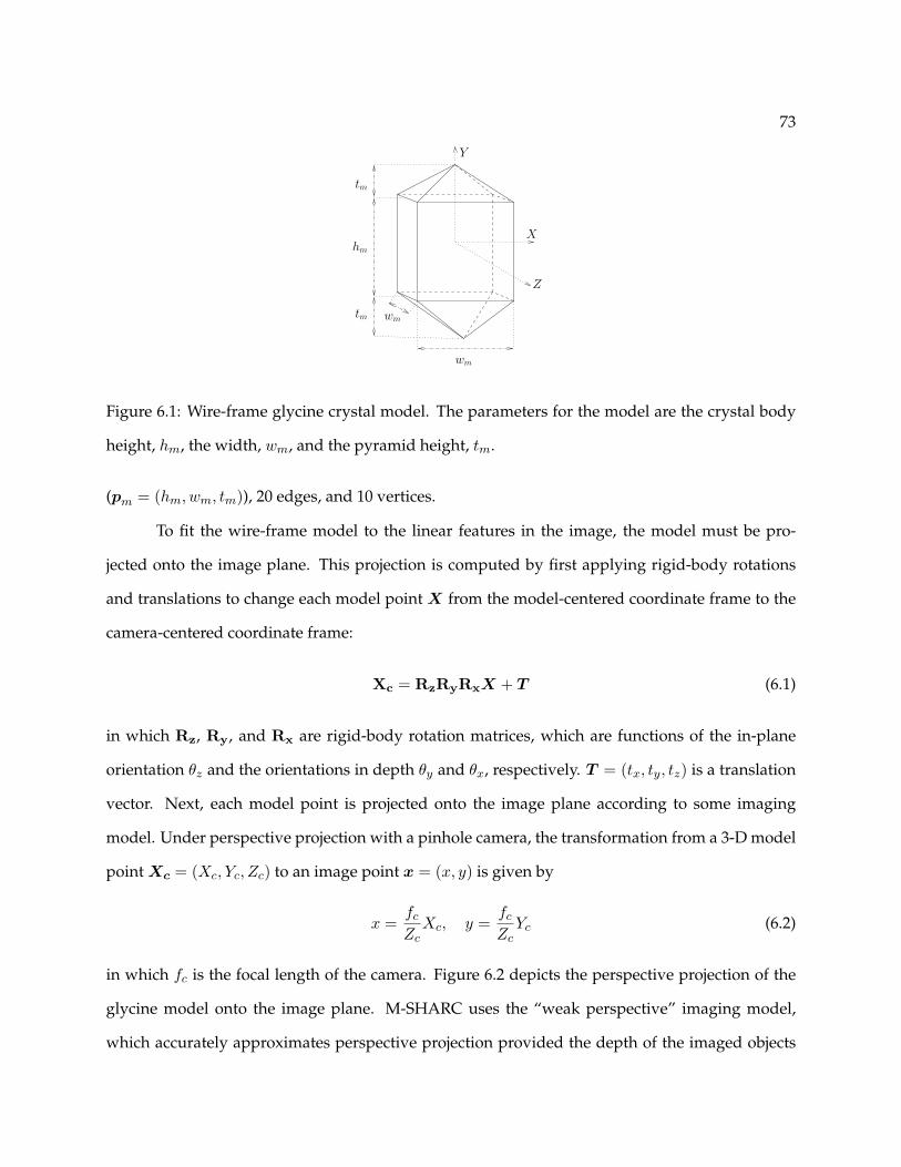
73

Y

X

Z

wm

wm

tm

tm

hm

Figure 6.1: Wire-frame glycine crystal model. The parameters for the model are the crystal body

height, hm, the width, wm, and the pyramid height, tm.

(pm = (hm, wm, tm)), 20 edges, and 10 vertices.

To fit the wire-frame model to the linear features in the image, the model must be pro-

jected onto the image plane. This projection is computed by first applying rigid-body rotations

and translations to change each model point X from the model-centered coordinate frame to the

camera-centered coordinate frame:

Xc = RzRyRxX + T (6.1)

in which Rz, Ry, and Rx are rigid-body rotation matrices, which are functions of the in-plane

orientation θz and the orientations in depth θy and θx, respectively. T = (tx, ty, tz) is a translation

vector. Next, each model point is projected onto the image plane according to some imaging

model. Under perspective projection with a pinhole camera, the transformation from a 3-D model

point Xc = (Xc, Yc, Zc) to an image point x = (x, y) is given by

x =fc

ZcXc, y =

fc

ZcYc (6.2)

in which fc is the focal length of the camera. Figure 6.2 depicts the perspective projection of the

glycine model onto the image plane. M-SHARC uses the “weak perspective” imaging model,

which accurately approximates perspective projection provided the depth of the imaged objects

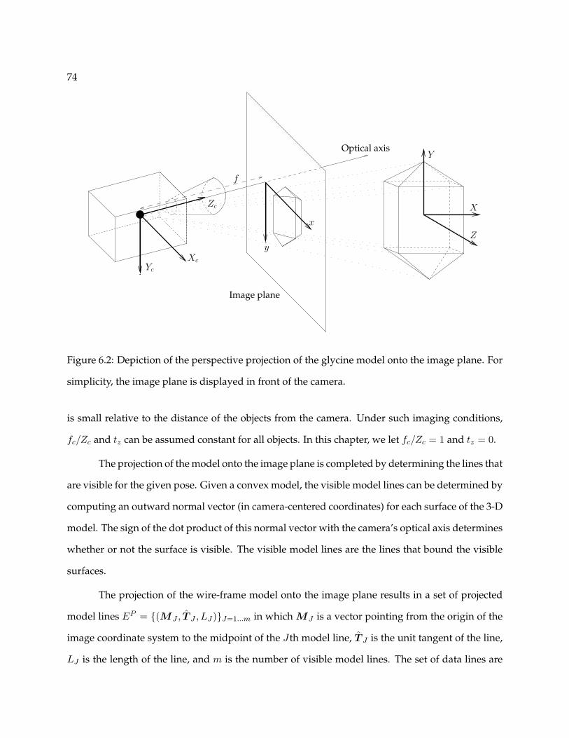
74

Zy

x

Zc

Optical axis

f

Yc

Xc

Image plane

Y

X

Figure 6.2: Depiction of the perspective projection of the glycine model onto the image plane. For

simplicity, the image plane is displayed in front of the camera.

is small relative to the distance of the objects from the camera. Under such imaging conditions,

fc/Zc and tz can be assumed constant for all objects. In this chapter, we let fc/Zc = 1 and tz = 0.

The projection of the model onto the image plane is completed by determining the lines that

are visible for the given pose. Given a convex model, the visible model lines can be determined by

computing an outward normal vector (in camera-centered coordinates) for each surface of the 3-D

model. The sign of the dot product of this normal vector with the camera’s optical axis determines

whether or not the surface is visible. The visible model lines are the lines that bound the visible

surfaces.

The projection of the wire-frame model onto the image plane results in a set of projected

model lines EP = (MJ , T J , LJ)J=1...m in which MJ is a vector pointing from the origin of the

image coordinate system to the midpoint of the Jth model line, T J is the unit tangent of the line,

LJ is the length of the line, and m is the number of visible model lines. The set of data lines are

75

defined similarly as S = (mj , tj , lj)j=1...n, in which n is the number of lines detected by the line

finder.

M-SHARC follows the approach developed by Lowe [75, 76], consisting of three main

steps: First, M-SHARC identifies linear features in the image. Second, M-SHARC identifies linear

feature clusters that appear significant on the basis of viewpoint-independent relationships such

as collinearity, parallelism, and end-point proximity. Third, M-SHARC fits a three-dimensional,

wire-frame model to each significant linear feature cluster. The following sections describe each

of these steps.

6.1.2 Linear feature detection

The M-SHARC algorithm uses the line finder proposed by Burns et al. [18], incorporating some

of the speed-up suggestions given by Kahn et al. [61] (see Chapter 5 for details). The Burns line

finder detects lines by identifying regions of pixels having similar image intensity gradient orien-

tation. By detecting lines on the basis of gradient orientation (as opposed to gradient magnitude),

the Burns line finder’s performance is relatively insensitive to variations in contrast and bright-

ness. This property is important for crystallization imaging because, as crystallization occurs,

the increasing solids concentration causes more reflected light to reach the camera CCD, which

increases the image brightness while decreasing the image contrast.

During linear feature extraction, single physical edges are commonly broken up into mul-

tiple collinear lines due to particle overlap, noise, or poor lighting. A key component of the algo-

rithm, therefore, is the grouping of these collinear lines prior to searching for viewpoint-invariant

line groups. The M-SHARC algorithm uses the method developed by Etemadi et al. [33] because

it is straightforward to implement and relatively inexpensive computationally. The method uses

simple thresholding on the angle, perpendicular distance, and endpoint distance between two

lines to determine whether or not the lines are collinear. If collinearity requirements are met, M-

SHARC creates a new line based on the collinear pair but also retains the two original lines in case

the instance of collinearity is accidental. Therefore, subsequent grouping operations operate on

76

(a) (b) (c)

(d) (e) (f)

Figure 6.3: Depiction of different viewpoint-invariant line groups (VIGs) used by M-SHARC. (a)

Junction. (b) Parallel pair. (c) Parallel triple. (d) C-triple. (e) C-square. (f) Arrow.

both the lines created from collinear grouping and all lines determined by the Burns line finder

(whether or not they are involved in a collinear group). Retaining the original lines involved in

collinear groups makes M-SHARC’s performance less sensitive to the collinear grouping thresh-

olds.

6.1.3 Perceptual grouping

Perceptual grouping refers to the task of organizing primitive objects, such as points or lines, into

higher-level, meaningful structures. These structures, or groups, are useful as visual cues for the

location, size, and orientation of a given object in the image. Viewpoint-invariant groups (VIGs),

or groups that maintain certain properties regardless of the camera viewpoint, are necessary be-

cause the orientation of the object with respect to the camera is generally unknown. M-SHARC

identifies line groups that can be assigned to one of the classifications depicted in Figure 6.3. The

groups are identified based on orientation differences, spatial differences, and connectivities be-

tween the lines in the image. For example, junctions are line pairs that satisfy angle dissimilarity

and endpoint proximity thresholds. Parallel line groups satisfy angle similarity and perpendicu-

lar distance thresholds. C-triples consist of three lines connected at two junctions where the angle

77

between the lines at each junction is greater than 90 degrees. C-squares consist of three lines con-

nected at two junctions with two of the lines being approximately parallel. Arrows are three lines

connected at a single junction where the angles between lines are less than 90 degrees.

M-SHARC calculates a significance measure for each VIG based on the line lengths, end-

point distances, and (for groups of parallel lines) orientation differences, as described by Lowe [75].

This significance measure is used to ensure that the most visually salient VIGs are considered first

in the model-fitting stage.

6.1.4 Model-fitting

The objective of the model-fitting process is to determine the model parameters and viewpoint

parameters such that the two-dimensional projection of the geometric model matches the low-

level features extracted from the image. The VIGs identified during the perceptual grouping

stage provide the starting point for the tasks associated with the model-fitting process. The first

task, called the correspondence problem, involves deciding which data lines correspond to which

model lines. In general, multiple correspondences are possible, so M-SHARC may generate mul-

tiple hypotheses for a given VIG. Next, M-SHARC uses the data lines’ positions and lengths to

estimate the model and viewpoint parameters for each correspondence hypothesis. Given these

parameters, M-SHARC projects the model into the image, identifies additional correspondences

between model lines and data lines, and calculates a verification score for the set of correspon-

dences. In the case of multiple hypotheses, M-SHARC chooses the correspondence hypothesis

that results in the highest verification score and performs a least-squares minimization to achieve

a better fit between the model and data lines. Finally, M-SHARC invalidates any VIGs that con-

tain lines that are completely enclosed within the bounding box of the projection of the optimized

model. These tasks are described in the following subsections.

78

(mi, ti, li)

(mj, tj, lj)

(mk, tk, lk)

E11E10E9

E13E14

E19E18E17

E5 E6

E2 E3E1

E17 E18 E19

E14

E13

E9 E10 E11

E6E5

E1 E2 E3

(a) (b) (c)

Figure 6.4: Depiction of two correspondence hypotheses. (a) Data line segments. (b) Hypothesis

1: Data lines i, j, and k correspond to model edges E1, E9, and E17, respectively. (c) Hypothesis 2:

Data lines i, j, and k correspond to model edges E9, E17, and E19, respectively.

Determining correspondences

The first step in the model-fitting process is to determine which of the model lines from the set

E correspond to the data lines in a given VIG. M-SHARC solves the correspondence problem by

rotating the data lines in the VIG into a standard position such that unambiguous descriptors

can be assigned to each line in the group. These descriptors are used to hypothesize one-to-one

correspondences between each data line in the VIG and a model line. M-SHARC currently has

methods for hypothesizing correspondences for parallel pairs, parallel triples, and C-triples. For

example, a triple of parallel lines is rotated such that all lines are basically vertical, and each line is

labeled as left-most, center, or right-most. These labels are used to assign each of the parallel data

lines to their corresponding model lines. In the case of a C-triple, the lines are rotated such that

the center line is vertical, and the lines are labeled as top, center, or bottom. The correspondence

remains ambiguous, however, so multiple hypotheses must be tested, as depicted in Figure 6.4. In

this figure, data lines i, j, and k could correspond, respectively, to either E1, E9, and E17, or E9,

E17, and E19.

79

Estimating model and viewpoint parameters

The problem of estimating viewpoint parameters, also referred to as pose estimation or alignment,

has been studied extensively in the literature. The research has focused on estimating pose from

both point correspondences [49, 55] and line correspondences [28, 21, 132]. A major drawback

of these methods is that the internal model parameters are assumed known. The utility of these

methods is therefore limited for the parameterized models of interest in our study.

M-SHARC estimates the internal model parameters using the properties of the data lines

and an assumed orientation in depth. For example, given the first hypothesis in Figure 6.4, the

model height hm is estimated as lj cos θx and the width wm is estimated as 2 cos θy(max(|ti · t⊥j |, |tk ·

t⊥j |), in which θy and θx are assumed orientations in depth and t

⊥j is a unit vector perpendicular to

tj . The pyramid height tm is estimated as wm tanαm/2, in which αm is assumed to be 45 degrees.

M-SHARC currently has methods for estimating model parameters on the basis of correspon-

dences for parallel pairs, parallel triples, and C-triples.

Given the correspondences, assumed orientations in depth, and model parameters, the

remaining viewpoint parameters are estimated in a straightforward manner. First, M-SHARC

projects the 3-D model onto the image plane using Equations (6.1) and (6.2), assuming θz = tx =

ty = 0. Next, the in-plane orientation θz is estimated using a weighted average of the orientation

differences between the data lines and their corresponding, projected model lines. Given the es-

timated θz , the 3-D model is then projected once again to the image plane and the translations tx

and ty are estimated from a weighted average of the spatial differences between the model line

midpoints and their corresponding data line midpoints.

Identifying additional correspondences

As described in section 6.1.1, the projection of the wire-frame model onto the image plane re-

sults in a set of projected model lines EP that can be compared directly with the set of data lines

S. M-SHARC identifies additional model-data line correspondences by identifying instances of

80

Correspondingmodel line

lie1i

e2i

Data line i

Figure 6.5: Depiction of variables used in mismatch calculation for a single line correspondence.

parallelism between the model lines and data lines.

Calculating the verification score

The purpose of the verification score is to quantify the amount of evidence in the image supporting

a given correspondence hypothesis. M-SHARC calculates the verification score as the percentage

of visible model line length that is supported or overlapped by data lines. The verification score

threshold is set based on experimentation. A more advanced method for setting this threshold is

described by Grimson and Huttenlocher [44], but their method is not generalized to parameterized

models.

Minimizing model-data mismatch

Once a suitable hypothesis is identified, M-SHARC minimizes the mismatch between correspond-

ing model and data lines by solving the optimization problem suggested by Lowe [76]

minp

Φ =∑i∈Dc

li(e1i + e2i)2 (6.3)

subject to the model and imaging constraints (Equations (6.1) and (6.2)). In Equation (6.3), Dc is

the set of data lines for which a correspondence has been identified, p is the parameter vector,

li is the length of data line i, and e1i and e2i are the perpendicular distances from data line i’s

endpoints to the corresponding model line, as depicted in Figure 6.5. The parameter vector for the

81

glycine model in Figure 6.1 is

p =[

hm tm wm θx θy θz tx ty

](6.4)

Invalidating overlapping VIGs

The VIGs identified during M-SHARC’s perceptual grouping stage can overlap, sharing lines.

We assume, however, that each line in the image can be attributed to only one crystal. Thus,

once a model is successfully fit to a set of lines, any VIG that contains one or more of those lines

is considered invalid. Furthermore, we assume that any line completely contained within the

bounding box of an identified crystal has arisen due to unmodeled features of that crystal. Thus,

any VIG that contains one or more of these lines is also considered invalid. M-SHARC does not

attempt to fit a model to invalid VIGs.

Applying this constraint on overlapping VIGs is advantageous in that it significantly re-

duces the number of VIGs investigated, thus increasing M-SHARC’s efficiency. Furthermore, ini-

tial studies indicated that a large number of false positives are identified if VIG invalidation is not

employed. Thus, the overlapping crystal constraint serves to increase the algorithm’s accuracy as

well as reduce the computational burden such that the algorithm can run in real-time on a single

processor. However, this feature requires M-SHARC to investigate each VIG serially, starting with

the most significant VIG and proceeding to the least significant, such that M-SHARC currently

cannot be implemented in parallel.

6.1.5 Summary and example

The M-SHARC algorithm can be summarized using the following pseudo-code:

1. Detect linear features in image

2. Identify and sort viewpoint-invariant line groups (VIG)

For each VIG

If VIG is valid

82

3. Generate correspondence hypotheses

For each hypothesis

4. Estimate model and viewpoint parameters

5. Project model into image

6. Search for additional correspondences

7. Compute verification score

Endfor

8. Select hypothesis with highest score

If (score > Verification threshold)

9. Minimize model-data mismatch

10. Save optimized model information

11. Invalidate overlapped VIGs

Endif

Endif

Endfor

Figure 6.6 shows the step-by-step results of applying the M-SHARC algorithm to a region

of interest from an image of α-glycine crystals. This region of interest contains a large, well-defined

crystal that is partially overlapped by a small, poorly-defined crystal. Applying the line finder to

the image in Figure 6.6(a) produces the dark lines shown in Figure 6.6(b). Because of overlap by

the smaller crystal, a few of the edges of the larger crystal are broken up into two or more lines.

Using collinear line grouping, these broken-up lines are combined into the single, light lines dis-

played in Figure 6.6(c). In the perceptual grouping stage, the line group that is identified as being

most significant is the triple of parallel lines shown in Figure 6.6(d). The lengths, spatial positions,

and relative distances between these lines provide the information necessary to estimate the inter-

nal model parameters and pose, resulting in the model projection shown in Figure 6.6(e). In this

figure, the gray, solid lines are the visible model lines and the hidden model lines are not shown.

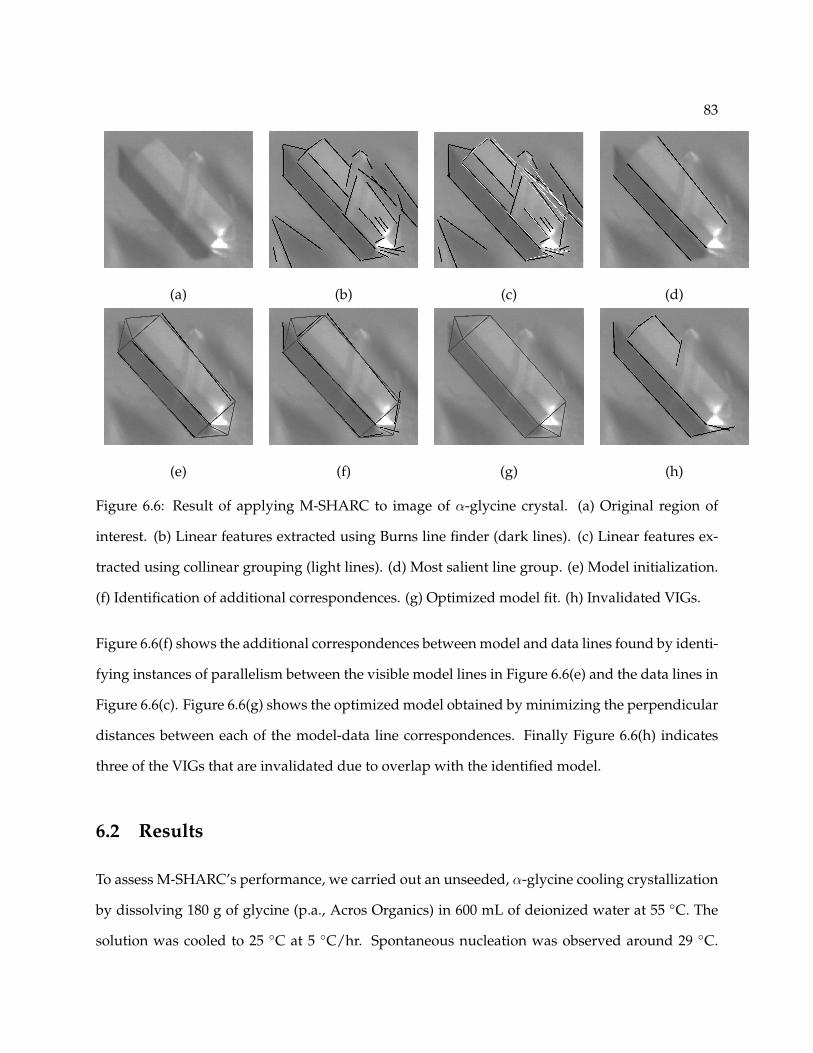
83

(a) (b) (c) (d)

(e) (f) (g) (h)

Figure 6.6: Result of applying M-SHARC to image of α-glycine crystal. (a) Original region of

interest. (b) Linear features extracted using Burns line finder (dark lines). (c) Linear features ex-

tracted using collinear grouping (light lines). (d) Most salient line group. (e) Model initialization.

(f) Identification of additional correspondences. (g) Optimized model fit. (h) Invalidated VIGs.

Figure 6.6(f) shows the additional correspondences between model and data lines found by identi-

fying instances of parallelism between the visible model lines in Figure 6.6(e) and the data lines in

Figure 6.6(c). Figure 6.6(g) shows the optimized model obtained by minimizing the perpendicular

distances between each of the model-data line correspondences. Finally Figure 6.6(h) indicates

three of the VIGs that are invalidated due to overlap with the identified model.

6.2 Results

To assess M-SHARC’s performance, we carried out an unseeded, α-glycine cooling crystallization

by dissolving 180 g of glycine (p.a., Acros Organics) in 600 mL of deionized water at 55 C. The

solution was cooled to 25 C at 5 C/hr. Spontaneous nucleation was observed around 29 C.

84

Three sets of video images were acquired during the course of the experiment, each set consisting

of 100 images acquired at a rate of 30 frames per second. Each set was acquired once a notice-

able increase in the solids concentration had occurred. The first set of video images was acquired

approximately 13 minutes after nucleation at low solids concentration with the draft tube in the

middle of the crystallizer clearly visible. The second set of images was acquired approximately

24 minutes after nucleation at medium solids concentration with the draft tube just barely visible.

The final set of images was acquired 43 minutes after nucleation at high solids concentration with

the draft tube completely obscured by the slurry. The polymorphic form of the observed crys-

tals was confirmed using X-ray powder diffraction. Given the rate of acquisition (30 frames per

second), each set of images essentially represents a snapshot in time. All images were analyzed

by M-SHARC using the same set of parameters. The VIGs used to initialize model-fitting were

parallel triples and C-triples.

6.2.1 Visual evaluation

Figures 6.7–6.9 show the results of applying M-SHARC to images acquired at low, medium, and

high solids concentrations. These figures demonstrate M-SHARC’s ability to identify crystals cov-

ering a wide range of sizes and orientations. These figures also demonstrate M-SHARC’s ability

to handle poor image quality. Although several options exist for improving the images, such as

lowering the mixing rate to decrease motion blur, successful image analysis of these low-quality

images demonstrates M-SHARC’s robustness and helps ensure success in the rugged industrial

environment.

6.2.2 Comparison with human analysis

To quantify M-SHARC’s performance, we compare its results with the results obtained by man-

ual analysis of the images by human operators. All 300 images acquired during the α-glycine

crystallization were analyzed both by M-SHARC and by a human operator. The human operator

annotated the images using LabelMe, a database and web-based image annotation tool developed

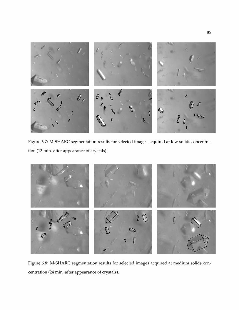
85

Figure 6.7: M-SHARC segmentation results for selected images acquired at low solids concentra-

tion (13 min. after appearance of crystals).

Figure 6.8: M-SHARC segmentation results for selected images acquired at medium solids con-

centration (24 min. after appearance of crystals).

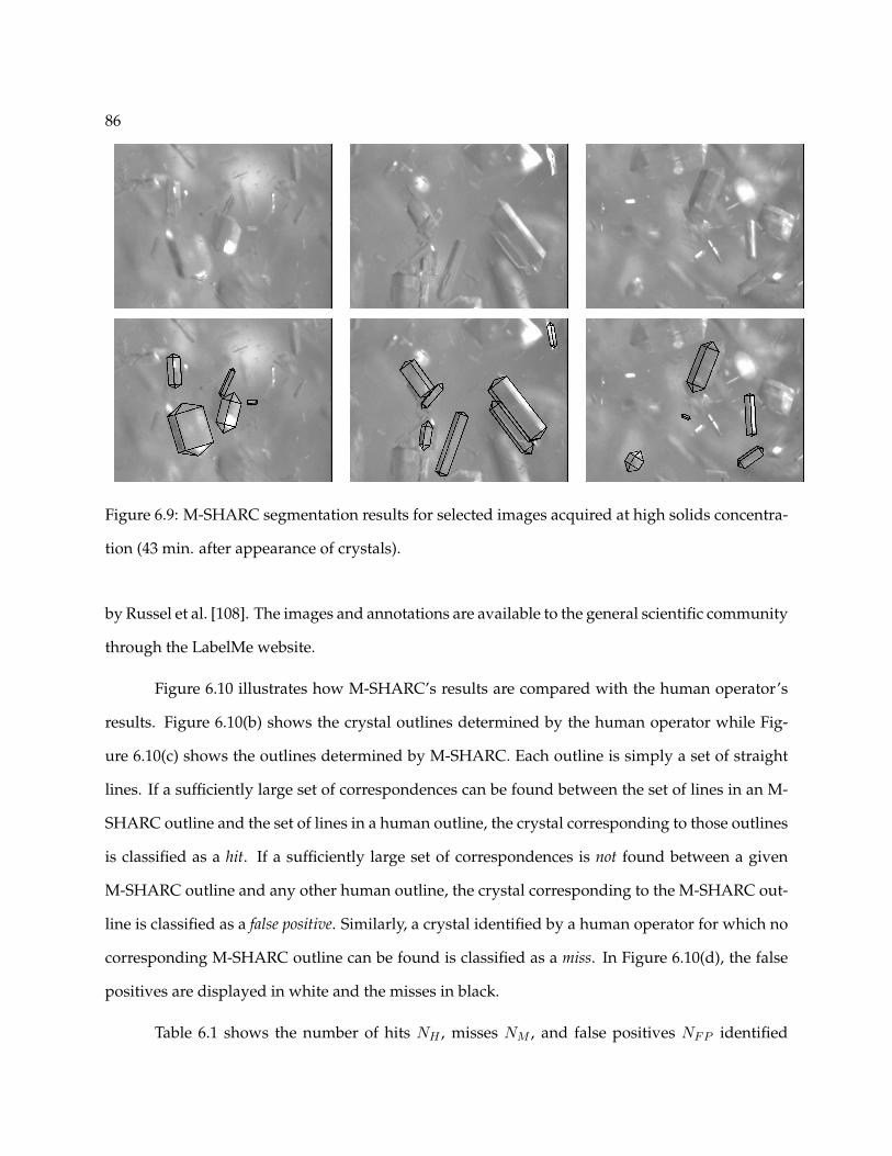
86

Figure 6.9: M-SHARC segmentation results for selected images acquired at high solids concentra-

tion (43 min. after appearance of crystals).

by Russel et al. [108]. The images and annotations are available to the general scientific community

through the LabelMe website.

Figure 6.10 illustrates how M-SHARC’s results are compared with the human operator’s

results. Figure 6.10(b) shows the crystal outlines determined by the human operator while Fig-

ure 6.10(c) shows the outlines determined by M-SHARC. Each outline is simply a set of straight

lines. If a sufficiently large set of correspondences can be found between the set of lines in an M-

SHARC outline and the set of lines in a human outline, the crystal corresponding to those outlines

is classified as a hit. If a sufficiently large set of correspondences is not found between a given

M-SHARC outline and any other human outline, the crystal corresponding to the M-SHARC out-

line is classified as a false positive. Similarly, a crystal identified by a human operator for which no

corresponding M-SHARC outline can be found is classified as a miss. In Figure 6.10(d), the false

positives are displayed in white and the misses in black.

Table 6.1 shows the number of hits NH , misses NM , and false positives NFP identified

87

(a) (b)

(c) (d)

Figure 6.10: Illustration of comparison between human operator results and M-SHARC results.

(a) Original image. (b) Outlines of crystals identified by human operator. (c) Outlines of crystals

identified by M-SHARC. (d) Result of comparison between human outlines and M-SHARC out-

lines. Crystals identified as false positives are outlined in white while those identified as misses

are outlined in black.

by comparing M-SHARC’s results with the human operator’s results for each of the three sets of

video images, along with number and area fractions for the hits and false positives. The hit, miss,

and false positive areas (AH , AM , and AFP , respectively) are calculated based on the areas of the

polygons defined by each crystal outline. For each level of solids concentration, the hit number

88

Low Med. High

Hits (NH ) 500 279 220

Misses (NM ) 514 657 445

False Positives (NFP ) 130 191 352

Hit number fraction (NH/(NH + NM )) 0.49 0.30 0.33

False Pos. number fraction (NFP /(NH + NFP )) 0.21 0.41 0.62

Hit area fraction (AH/(AH + AM )) 0.63 0.38 0.31

False Pos. area fraction (AFP /(AH + AFP )) 0.23 0.36 0.53

Table 6.1: Summary of comparison between M-SHARC results and human operator results for in

situ video images obtained at low, medium, and high solids concentrations (100 images at each

concentration).

fraction is significantly less than the hit area fraction while the false positive number fraction is

comparable to the false positive area fraction. Thus, we would expect the number-based area dis-

tribution to be biased towards larger particles. This expectation is verified by Figure 6.11, which

compares the number-based cumulative distribution functions (CDFs) for particle area. As a stan-

dard of comparison, Figure 6.11 also shows the CDFs constructed using only particles classified

as hits. The confidence interval displayed in these figures is calculated using the Kolmogorov-

Smirnov statistic [80, 24].

To identify possible improvements to the M-SHARC algorithm, we examined the results of

M-SHARC’s subroutines (line finding, perceptual grouping, and model fitting) for the 100 largest

misses and the 100 largest false positives. Examination of the large misses reveals that many of

the misses are particles that are somewhat blurry with low contrast edges that are difficult for

M-SHARC’s line finder to identify (see row 1 in Figure 6.12). Despite the low contrast, the visual

cues are sufficient that the outline of these particles can be discerned by a human operator. Par-

ticles that are clearly in-focus also sometimes exhibit low contrast edges and cause difficulties for

M-SHARC’s line finder (see row 2 in Figure 6.12). Particle agglomeration is another major source

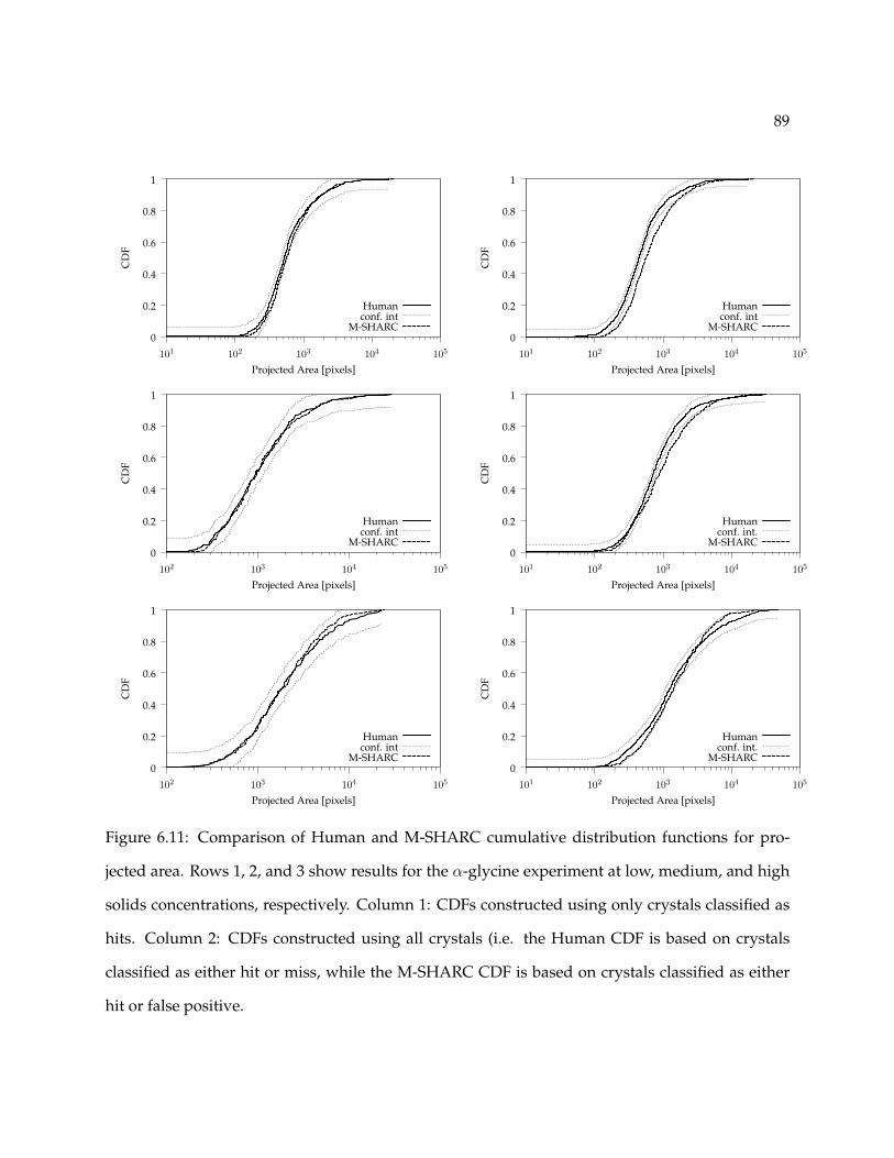
89

0

0.2

0.4

0.6

0.8

1

101 102 103 104 105

CD

F

Projected Area [pixels]

Humanconf. int

M-SHARC0

0.2

0.4

0.6

0.8

1

101 102 103 104 105

CD

F


Humanconf. int

M-SHARC

0

0.2

0.4

0.6

0.8

1

102 103 104 105

CD

F


Humanconf. int

M-SHARC0

0.2

0.4

0.6

0.8

1

101 102 103 104 105

CD

F


Humanconf. int.

M-SHARC

0

0.2

0.4

0.6

0.8

1

102 103 104 105

CD

F


Humanconf. int

M-SHARC0

0.2

0.4

0.6

0.8

1

101 102 103 104 105

CD

F


Humanconf. int.

M-SHARC

Figure 6.11: Comparison of Human and M-SHARC cumulative distribution functions for pro-

jected area. Rows 1, 2, and 3 show results for the α-glycine experiment at low, medium, and high

solids concentrations, respectively. Column 1: CDFs constructed using only crystals classified as

hits. Column 2: CDFs constructed using all crystals (i.e. the Human CDF is based on crystals

classified as either hit or miss, while the M-SHARC CDF is based on crystals classified as either

hit or false positive.

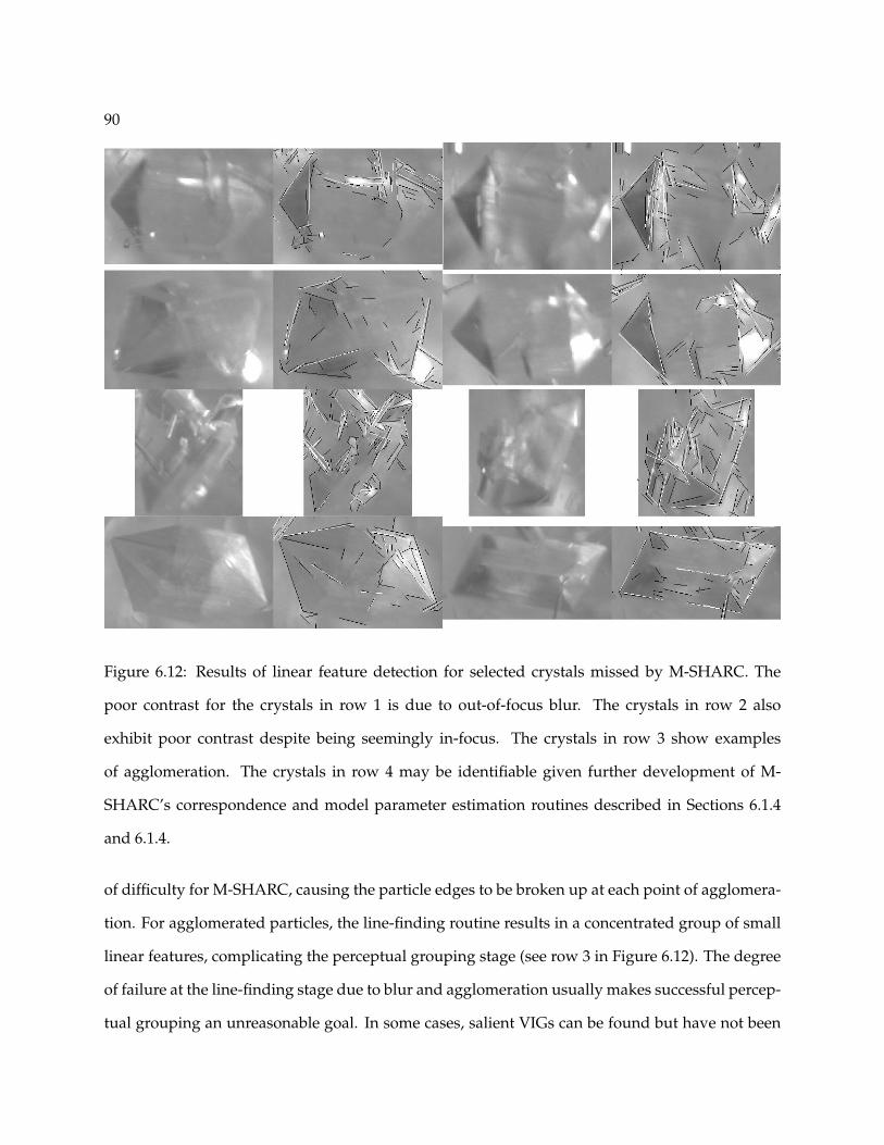
90

Figure 6.12: Results of linear feature detection for selected crystals missed by M-SHARC. The

poor contrast for the crystals in row 1 is due to out-of-focus blur. The crystals in row 2 also

exhibit poor contrast despite being seemingly in-focus. The crystals in row 3 show examples

of agglomeration. The crystals in row 4 may be identifiable given further development of M-

SHARC’s correspondence and model parameter estimation routines described in Sections 6.1.4

and 6.1.4.

of difficulty for M-SHARC, causing the particle edges to be broken up at each point of agglomera-

tion. For agglomerated particles, the line-finding routine results in a concentrated group of small

linear features, complicating the perceptual grouping stage (see row 3 in Figure 6.12). The degree

of failure at the line-finding stage due to blur and agglomeration usually makes successful percep-

tual grouping an unreasonable goal. In some cases, salient VIGs can be found but have not been

91

utilized because routines for solving the correspondence and model parameter estimation prob-

lems have not yet been developed. Row 4 in Figure 6.12 gives two examples of crystals resulting

in significant VIGs for which initialization routines have yet to be developed. The development

of such routines may be the best approach to minimize the number of misses.

Examination of the 100 largest false positives showed that a large fraction (more than 1/3)

of the false positives are agglomerated or blurry crystals. The ambiguity associated with deter-

mining an outline for blurry and agglomerated crystals caused the human operators to pass over

these crystals. Whether or not these false positives should be counted as false positives is unclear.

The other major source of false positives arises due to shortcomings in M-SHARC’s method of

verification. For many of the false positives, the model and data lines do not align well, indi-

cating that the orientational and spatial offset thresholds used in the verification process are not

sufficiently stringent. Another indication that more stringent thresholds are necessary in the veri-

fication stage is that many of the false positives have only 3 or 4 data lines that correspond to the

model lines. Unfortunately, this is also true for many of the hits, partly because the wire-frame

model is only a rough approximation of the α-glycine shape. Perhaps using wire-frame model that

more accurately represents the α-glycine shape would result in better fits for the hits, enabling the

use of more stringent verification thresholds to eliminate false positives.

6.2.3 Algorithm speed

The average cputimes required to analyze images from each of the three video sets from the α-

glycine experiment are shown in Table 6.2. The amount of time between each video acquisition

during the crystallization experiment was approximately 12 minutes. Based on the cputimes in

Table 6.2, M-SHARC can analyze approximately 10 images per minute, or 100 images every 10

minutes. This analysis speed is sufficiently fast for real-time implementation on chemical systems

with crystallization dynamics similar to glycine.

The results presented in this chapter are based on using a single wire-frame model. M-

SHARC can be applied, however, using multiple models to represent different shape classes. Us-

92

Set Line Finding Group Finding Initialization Optimization Total

1 2.6 (55) 1.2 (25) 0.2 (5) 0.7 (14) 4.8

2 3.3 (43) 3.3 (43) 0.3 (4) 0.7 (9) 7.6

3 3.3 (16) 15.4 (76) 0.4 (2) 1.0 (5) 20.2

Table 6.2: Average cputime required to analyze single image for three different image sets of in-

creasing solids concentration. The first number in each number pair is the cputime in seconds.

The second, parenthesized number gives the percentage of total cputime.

ing multiple models would affect the computational requirements in two ways. First, each ad-

ditional model may require the identification of additional VIGs to serve as visual cues for that

model. However, the increase in computation time for the VIG identification stage may be small

because many VIGs are identified using the same set of logical decisions. For instance, to identify

a C-triple, M-SHARC must determine whether a given triple of lines is connected at one or two

junctions. This same determination must be made to identify a C-square and an arrow. Second,

the number of hypotheses would likely increase linearly with the number of models, resulting in

a linear increase of computational requirements for the model initialization stage. In Table 6.2,

the requirements for the initialization stage represent a small fraction of the total computational

requirements, indicating that M-SHARC could accommodate several more models and remain

suitably fast for real-time implementation.

6.3 Conclusions

We have developed a model-based object recognition algorithm that is effective for extracting

crystal size and shape information from noisy, in situ crystallization images. The algorithm’s

accuracy has been assessed by comparing its results with those obtained by manual, human anal-

ysis of the images. At low solids concentrations, the algorithm identifies approximately half of the

crystals identified by humans, while at medium to high solids, the algorithm identifies approxi-

93

mately one-third of the crystals. At low solids, false positives constitute approximately one-fifth

of all identified crystals, while at medium to high concentrations the false positives constitute ap-

proximately half of the identified crystals. Despite the misses and false positives, the algorithm’s

cumulative size distribution measurements compare favorably with measurements obtained by

humans but are biased towards larger particles. To improve the algorithm’s accuracy, further

development should focus on the algorithm’s verification stage and on creating initialization rou-

tines for additional viewpoint-invariant line groups. The algorithm is sufficiently fast to provide

on-line measurements for typical cooling crystallization processes.

94

95

Chapter 7

Statistical Estimation of PSD from

Imaging Data 1

The methods described in Chapters 5 and 6 address the image segmentation problem, which is the

first of two main challenges that must be overcome to use in situ microscopy for PSD measure-

ment. The second challenge is to estimate the PSD given the size and shape information obtained

through successful image segmentation. Each segmented particle provides a single observation,

which can be either censored or uncensored. A censored observation refers to an observation in

which only partial information is obtained. For example, an observation of a particle touching

the image border is censored because only a portion of the particle is visible. An observation of

a particle with one end partially occluded by another particle is also censored. An observation

is uncensored only if the particle is enclosed entirely within the image frame, is not occluded by

other particles, and is oriented in a plane perpendicular to the optical axis of the camera.

A natural approach to estimate the PSD is to count only those particles appearing entirely

within the field of view, not touching the image boundary. This approach, called minus-sampling,

introduces sampling bias. Sampling bias occurs when the probability of observing an object de-

pends on its size or shape. For example, a small particle randomly located in the image has a

high probability of appearing entirely within the field of view, while a sufficiently large particle

randomly located in the image may have zero probability of appearing entirely within the field

of view. Miles [83] presented the first treatment of spatial sampling bias, developing a minus-

1Portions of this chapter are to appear in Larsen and Rawlings [68]

96

sampling estimator that corrects spatial sampling bias by weighting each observation by M−1,

with M being related to the sampling probability of the observed particle. Miles derived formulas

for M assuming a circular sampling region. Lantuejoul[64] extended Miles’ results by showing

how to calculate M for a rectangular sampling region. Baddeley [5] provides an excellent review

of various methods for correcting edge effects under a variety of situations.

The primary drawback of the Miles-Lantuejoul approach is that it uses only uncensored

observations. If the size of the particles is large relative to the size of the image window, using

censored observations (i.e. particles touching the image border) would be expected to result in

improved PSD estimation. The primary goal of this chapter is to develop a PSD estimator using

both censored and uncensored observations and to evaluate the benefits and drawbacks of this

estimator relative to the Miles-Lantuejoul approach. We assume the censoring is due only to par-

ticles touching the image border and not due to orientation or occlusion effects. A secondary goal

is to develop practical methods for determining confidence intervals for the estimated PSD. The

methods developed in this study are intended for systems of high-aspect-ratio particles, which are

commonplace in the pharmaceutical and specialty chemical industries.

This chapter is organized as follows. Section 7.1 describes previous work related to PSD

estimation of high-aspect-ratio particles and describes the application of the Miles-Lantuejoul es-

timator. Section 7.2 presents the formulation of the maximum likelihood PSD estimator. Sec-

tion 7.3 presents the results of applying the estimator to artificial images generated as described

in Chapter 4. Section 7.4 summarizes our findings. The full derivation of the maximum likelihood

estimator can be found in Appendix A.

7.1 Previous work

PSD estimation for high-aspect-ratio particles using imaging-based measurements is related to the

problem of estimating the cumulative length distribution function H of line segments observed

through a window, which has been investigated by several researchers. Laslett [71] was the first

97

to derive the log likelihood for this problem. Wijer [130] derived the non-parametric maximum

likelihood estimator (NPMLE) of H for a circular sampling region and an unknown orientation

distribution function F . For arbitrary convex sampling regions, Wijer shows how to estimate

H assuming F is known. Van Der Laan[121] studies the NPMLE of H for the one-dimensional

line segment problem (i.e. all line segments have same orientation) for a non-convex sampling

window, and Van Zwet[122] derives the NPMLE of H for the two-dimensional problem with

a non-convex, highly irregular sampling region and known F . Svensson et al.[118] derive an

estimator for a parametric length density function h using one-dimensional line segment data

from a circular sampling region. Hall [46] derived an estimator for the intensity of a planar Poisson

line segment process that is unbiased for any convex sampling region and any length distribution

function. All of the above studies utilize both censored and uncensored observations. Baddeley [5]

provides an excellent review of various spatial sampling estimation studies.

The goal of the current study is to estimate the particle size distribution f , which is related

to but different than the cumulative distribution function H or corresponding density function h

for a line segment process. The PSD f(L) is the number of particles of length L per unit volume

and is related to H via the relation H(L ≤ l) =∫ l0 f(L)dL/

∫∞0 f(L)dL. The approach commonly

used in practice to estimate the PSD from imaging-based measurements is the Miles-Lantuejoul

method [83]. As there is some confusion amongst practitioners regarding the implementation of

the Miles-Lantuejoul method, we describe the method here.

Let E2 be the Euclidean plane, and let J ⊂ E2 be a domain parameterized by (z, n,θn),

in which z gives the center point of the domain, n gives the class, and θn is a vector giving the

parameters necessary to completely specify a domain of class n. Let Q(x) ⊂ E2 be a sampling

region centered at x. For each domain J , define the set

Jα = x ∈ E2 : J ⊂ Q(x) (7.1)

Thus, Jα is a domain comprising all points at which the sampling region can be placed and enclose

entirely the domain J .

98

dF,h

b− dF,v

a− dF,h

dF,v

a

b

Mj

Lj

dF,v

dF,h

b− dF,v

a− dF,h

a

b

Lj

Mj

Figure 7.1: Depiction of methodology for calculating Miles-Lantuejoul M-values for particles of

different lengths observed in an image of dimension b× a.

Define MJ = AJα, where A· denotes area. Let MJj, j = 1 . . . n be the M-values

calculated for n observations of particles with lengths corresponding to size class i. Miles showed

that ρMLi =∑

j MJj is an unbiased estimator of ρi, the density of particles in size class i per

area, provided the minimum possible M-value for a particle in size class i is greater than zero.

In Miles’ original paper [83], he derived formulas for calculating M-values for arbitrary

domains assuming a circular sampling region. Later, Lantuejoul[64] extended Miles’ results by

showing how to calculate M for the rectangular sampling region typical of microscopy applica-

tions. For an image of size a× b, the M-value of a particle is calculated by subtracting the vertical

and horizontal Feret diameters of the particle (dF,v and dF,h) from, respectively, the vertical and

horizontal image dimensions b and a, as depicted in Figure 7.1.

7.2 Theory

7.2.1 PSD Definition

Consider a population of cylindrical or rod-like particles. The geometry of each particle is speci-

fied in terms of the cylinder height and radius. Let the characteristic length L for the population

of particles be the cylinder height.

Consider a slurry of volume V in which a solid phase of discrete particles is dispersed

99

in a continuous fluid phase. Let f(L) denote the continuous PSD, or the number of particles

of characteristic length L per unit volume slurry. Number-based PSDs are typically measured

by discretizing the characteristic length scale into T non-overlapping bins or size classes. We

therefore define the discrete PSD as

ρi =∫ Si+1

Si

f(l)dl, i = 1, . . . , T (7.2)

in which S = (S1, . . . , ST+1) is the vector of breaks between size classes.

The relative PSD q is a vector with elements

qi =ρi∑Tj ρj

, i = 1, . . . , T (7.3)

In this chapter, the term PSD is assumed to refer to the discrete, absolute PSD ρ unless specifically

noted otherwise.

7.2.2 Sampling model

The particle population is sampled using in situ imaging. Let VI ∈ V denote the imaging volume,

and assume VI is a rectangular region of dimensions a× b× d, in which a is the horizontal image

dimension, b is the vertical image dimension, and df is the depth of field. a and b determine

the field of view, and we assume a ≥ b. A single random sample of the population consists of an

image containing the two-dimensional projection of the portions of particles inside VI . We assume

the system is well-mixed such that the centroids of the particles are randomly and uniformly

distributed in space.

We assume the camera is positioned a fixed distance z0 from the imaging volume, and that

df z0. This assumption means the particles in the imaging volume are projected onto the image

plane according to the weak perspective projection model. In other words, the projected particle

lengths measured in the image coordinate system can be related to the true projected particle

lengths by applying a constant magnification factor m.

We assume all particles are oriented in a plane orthogonal to the camera’s optical axis. This

assumption, together with the weak perspective assumption, essentially reduces the 3-D process

100

to a 2-D process, thereby simplifying the analysis considerably. These assumptions are not used

only for convenience, however, but rather to reflect the actual conditions under which in situ

imaging measurements are made in practice. To obtain useful in situ images in high solids con-

centrations, the camera must have a small depth of field and be focused only a small depth into

the particulate slurry. It seems reasonable, therefore, to expect the shear flow at the slurry-sensor

interface to cause the particles to align orthogonal to the this interface, and thus orthogonal to the

camera’s optical axis.

7.2.3 Maximum likelihood estimation of PSD

Let Xk = (X1k, . . . , XTk) be a T -dimensional random vector in which Xik gives the number of

non-border particles of size class i observed in image k. A non-border particle is a particle that

is completely enclosed within the imaging volume. A border particle, on the other hand, is only

partially enclosed within the imaging volume such that only a portion of the particle is observable.

For border particles, only the observed length (i.e. the length of the portion of the particle that

is inside the imaging volume) can be measured. Accordingly, we let Y k = (Y1k, . . . , YTk) be a

T -dimensional random vector in which Yjk gives the number of border particles with observed

lengths in size class j that are observed in image k. We denote the observed data, or the realizations

of the random vectors Xk and Y k, as xk and yk, respectively.

The particle population is represented completely by the vectors ρ = (ρi, . . . , ρT ) and S =

(S1, . . . , ST+1) in which ρi represents the number of particles of size class i per unit volume and

Si is the lower bound of size class i. Given the data x and y (the subscript k denoting the image

index is removed for simplicity), the maximum likelihood estimator of ρ is defined as

ρb = arg maxρ

pXY (x1, y1, x2, y2, . . . , xT , yT |ρ) (7.4)

in which the subscript b indicates the use of border particle measurements and pXY is the joint

probability density for X and Y . In other words, we want to determine the value of ρ that maxi-

mizes the probability of observing exactly x1 non-border particles of size class 1, y1 border particles

101

of size class 1, x2 non-border particles of size class 2, y2 border particles of size class 2, and so on.

A simplified expression for pXY can be obtained by noting that, at least at low solids con-

centrations, the observations X1, Y1, . . . , XT , YT can be assumed to be independent. This as-

sumption means that the observed number of particles of a given size class depends only on the

density of particles in that same size class. At high solids concentrations, this assumption seems

unreasonable because the number of particle observations in a given size class is reduced due

to occlusions by particles in other size classes. At low concentrations, however, the likelihood

of occlusion is low. The independence assumption does not imply that the observations are not

correlated. Rather, the assumption implies that any correlation between observations is due to

their dependence on a common set of parameters. As an example, if we observe a large num-

ber of non-border particles, we would expect to also observe a large number of border particles.

This correlation can be explained by noting that the probability densities for both border and non-

border observations depend on a common parameter, namely, the density of particles. Given the

independence assumption, we express the likelihood function L(ρ) as

L(ρ) = pXY =T∏

i=1

pXi(xi|ρ)T∏

j=1

pYj (yj |ρ) (7.5)

in which pXi and pYj are the probability densities for the random variables Xi and Yj . The log

likelihood is defined as l(ρ) = log L(ρ). Maximizing the likelihood function is equivalent to min-

imizing the log likelihood. Using Equation (7.5), the estimator in Equation (7.4) can therefore be

reformulated as

ρb = arg minρ

T∑i=1

− log pXi(xi|ρ)−T∑

j=1

log pYj (yj |ρ) (7.6)

The probability densities pXi and pYj can be derived given the particle geometry and the

spatial and orientational probability distributions. In Appendix A, pXi and pYj are derived assum-

ing the particles have needle-like geometry, are uniformly distributed in space, and are uniformly

distributed in orientation. These derivations show that Xi ∼ Poisson(mXi), or that Xi has a Pois-

son distribution with parameter mXi = ρiαi, in which αi is a function of the field of view, depth of

102

field, and the lower and upper bounds of size class i. Furthermore, Yj ∼ Poisson(mYj ), in which

mYj =∑T

i=1 ρiβij

To extend the analysis to data collected from N images, we define two new random vectors

XΣ and YΣ for which XΣi =∑N

k=1 Xik and YΣj =∑N

k=1 Yjk. Here, the subscript k denotes the

image index. Given that Xik ∼ Poisson(mXi), it can be shown that XΣi ∼ Poisson(NmXi) [12, p.

440]. Likewise, YΣj ∼ Poisson(NmYj ).

Differentiating Equation (7.6) with respect to ρ and equating with zero results in a set of

coupled, nonlinear equations for which an analytical solution is not apparent. Equation (7.6) is

solved using MATLAB’s nonlinear optimization solver FMINCON with initial values obtained

from Equation (7.7).

If the border particles are ignored, the estimator reduces to

ρ = arg minρ

T∑i=1

(− log pXi(xi|ρ))

In this case, we can solve for ρ analytically:

ρi =Xi

αi, i = 1, . . . , T (7.7)

The probability density for this estimator can be computed analytically as

pρi(ρi) = pρi

(Xi/αi) = pXi(xi) (7.8)

with xi being a non-negative integer. It is straightforward to show that this estimator has the

following properties:

E[ρi] = ρi

V ar[ρi] = ρi/αi

For the case of multiple images, the maximum likelihood estimate is given by

ρi =XΣi

Nαi, i = 1, . . . , T (7.9)

103

which has the following properties:

E[ρi] = ρi

V ar[ρi] = ρi/(Nαi)

7.2.4 Confidence Intervals

Let χ = Z1,Z2, . . . ,ZN denote a dataset of N images, with Zk = (Xk,Y k) containing the data

for both border and non-border measurements for image k. Let Z1,Z2, . . . ,ZN be independent

and identically distributed (i.i.d.) with distribution function F . Let F be the empirical distribution

function of the observed data. Let R(χ, F ) be a random vector giving the PSD estimated using ei-

ther Miles-Lantuejoul or maximum likelihood. To construct confidence intervals for the estimated

PSD, we require the distribution of R(χ, F ). This distribution, called the sampling distribution,

is unknown because F is unknown, being a function of the unknown PSD ρ. As N → ∞, the

limiting distribution of the maximum likelihood estimates is a multivariate normal with mean ρ

and covariance I(ρ)−1, where I(ρ) is the Fisher information matrix, defined as

I(ρ) = −E[l′′(ρ)]

in which l′′(ρ) is a T ×T matrix with the (i, j)th element given by ∂2l(ρ)∂ρi∂ρj

. Approximate confidence

intervals for individual parameter estimates can be calculated as ρi = ρi±σizα in which σi is the ith

diagonal element of the observed Fisher information matrix −l′′(ρ) and zα gives the appropriate

quantile from the standard normal distribution for the confidence level α.

Given that the underlying distributions for Xk and Y k are Poisson, we expect the sampling

distributions to be non-normal in general. We therefore use bootstrapping [41, p.253] to approxi-

mate the distribution of R(χ, F ) and construct confidence intervals. Let χ∗ = Z∗1, . . . ,Z

∗N denote

a bootstrap sample of the dataset χ. The elements of χ∗ are i.i.d. with distribution function F . In

other words, χ∗ is obtained by sampling χ N times where, for each of the N samples, the probabil-

ity of selecting the data Zk is 1/N. We denote a set of B bootstrap samples as χ∗l = Z∗l1, . . . ,Z

∗lN

104

for l = 1, . . . , B. The empirical distribution function of R(χ∗l , F ) for l = 1, . . . , B approximates the

distribution function of R(χ, F ), enabling confidence intervals to be constructed.

For R(χ, F ) = ρ, the distribution function of R(χ∗, F ) is derived analytically using Equa-

tion (7.8). For R(χ, F ) = ρb and R(χ, F ) = ρML, the distribution of R(χ∗, F ) is estimated using

B = 1000 bootstrap samples. The confidence intervals are obtained using the percentile method,

which consists of reading the appropriate quantiles from the cumulative distribution of R(χ∗, F ).

To calculate confidence intervals using the normal approximation, the observed Fisher informa-

tion matrix −l′′(ρ), also called the Hessian, must be calculated. The (i, j)th element of this matrix

is given by

− ∂l(ρ)∂ρi∂ρj

=XΣi

ρ2i

δij +T∑k

βjkβikYΣk

m2Yk

(7.10)

7.3 Results

To investigate the performance of the maximum likelihood estimator relative to the standard

Miles-Lantuejoul approach, these estimators were applied in several case studies. In each case

study, 1000 simulations were carried out. Each simulation consists of generating a set of artificial

images and applying the estimators to the particle length measurements obtained from these im-

ages. The images were generated using the methods described in Section 4.3. Figure 7.2 shows

example images generated for each of these case studies. Each of these images has a horizontal im-

age dimension of a=480 pixels and a vertical dimension of b=480 pixels. The first row displays four

simulated images for mono-disperse particles of length 0.5a with Nc=25 crystals per image. The

second row shows images of particles uniformly distributed on [0.1a 0.9a] with Nc=25. The third

row shows images of particles normally-distributed with µ = 0.5a and σ = 0.4a/3 with Nc=25,

and the fourth row shows example images for simulations of particles uniformly-distributed on

[0.1a 2.0a] with Nc=15.

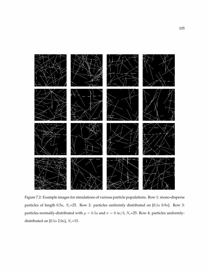
105

Figure 7.2: Example images for simulations of various particle populations. Row 1: mono-disperse

particles of length 0.5a, Nc=25. Row 2: particles uniformly distributed on [0.1a 0.9a]. Row 3:

particles normally-distributed with µ = 0.5a and σ = 0.4a/3, Nc=25. Row 4: particles uniformly-

distributed on [0.1a 2.0a], Nc=15.

106

0

50

100

150

200

250

300

20 22 24 26 28 30 32

coun

ts

ρi

MLE w/ bordersMiles

0

50

100

150

200

250

300

23 23.5 24 24.5 25 25.5 26 26.5 27

coun

ts

ρi

MLE w/ bordersMiles

(a) (b)

Figure 7.3: Comparison of estimated sampling distributions for absolute PSD for mono-disperse

particles. Results based on 1000 simulations, 10 size classes, Nc=25. (a) Results for 10 im-

ages/simulation. (b) Results for 100 images/simulation.

7.3.1 Case study 1: mono-disperse particles of length 0.5a

In the first case study, the particle population consists of mono-disperse particles of length 0.5a.

The first row in Figure 7.2 shows example images from these simulations. The length scale is

discretized on [0.1a√

2a] into T=10 size classes with the fourth size class centered at 0.5a. The

sampling distributions for the various estimators are shown in Figure 7.3 for 1000 simulations

using 10 images/simulation and 100 images/simulation. Including the border particle measure-

ments provides better estimates, as evidenced by the lower variance in the sampling distribution

for ρb relative to the other estimators. As a measure of the improvement gained by including the

border particle measurements, we calculate the relative efficiency of ρbiversus ρMLi for a given

size class i as

eff(ρbi, ρMLi) =

MSE(ρMLi)MSE(ρbi

)(7.11)

in which MSE(T ) = var(T ) + [bias(T )]2 = E[(T − ρ)2] is the mean-squared error for estimator T .

The MSE is estimated for size class i as

MSE(Ti) =1n

n∑j=1

(Tj − ρi)2 (7.12)

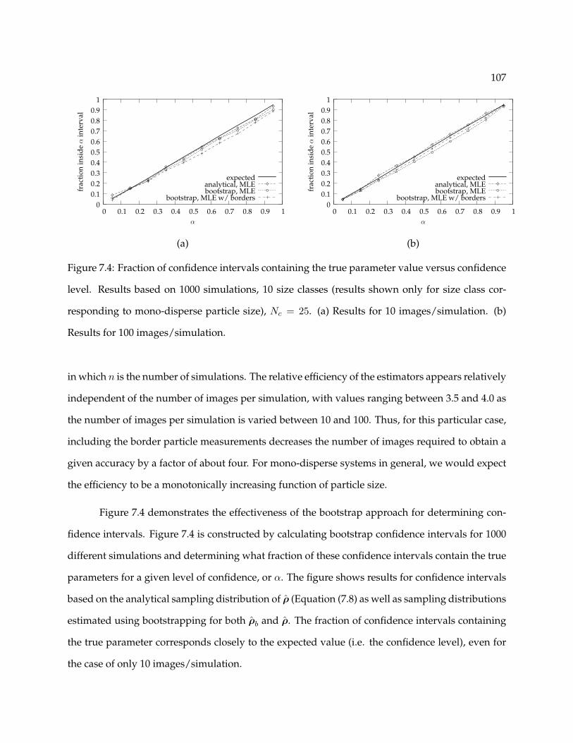
107

00.10.20.30.40.50.60.70.80.9

1

0 0.1 0.2 0.3 0.4 0.5 0.6 0.7 0.8 0.9 1

frac

tion

insi

deα

inte

rval

α

expectedanalytical, MLEbootstrap, MLE

bootstrap, MLE w/ borders0

0.10.20.30.40.50.60.70.80.9

1

0 0.1 0.2 0.3 0.4 0.5 0.6 0.7 0.8 0.9 1

frac

tion

insi

deα

inte

rval

α


bootstrap, MLE w/ borders

(a) (b)

Figure 7.4: Fraction of confidence intervals containing the true parameter value versus confidence

level. Results based on 1000 simulations, 10 size classes (results shown only for size class cor-

responding to mono-disperse particle size), Nc = 25. (a) Results for 10 images/simulation. (b)

Results for 100 images/simulation.

in which n is the number of simulations. The relative efficiency of the estimators appears relatively

independent of the number of images per simulation, with values ranging between 3.5 and 4.0 as

the number of images per simulation is varied between 10 and 100. Thus, for this particular case,

including the border particle measurements decreases the number of images required to obtain a

given accuracy by a factor of about four. For mono-disperse systems in general, we would expect

the efficiency to be a monotonically increasing function of particle size.

Figure 7.4 demonstrates the effectiveness of the bootstrap approach for determining con-

fidence intervals. Figure 7.4 is constructed by calculating bootstrap confidence intervals for 1000

different simulations and determining what fraction of these confidence intervals contain the true

parameters for a given level of confidence, or α. The figure shows results for confidence intervals

based on the analytical sampling distribution of ρ (Equation (7.8) as well as sampling distributions

estimated using bootstrapping for both ρb and ρ. The fraction of confidence intervals containing

the true parameter corresponds closely to the expected value (i.e. the confidence level), even for

the case of only 10 images/simulation.

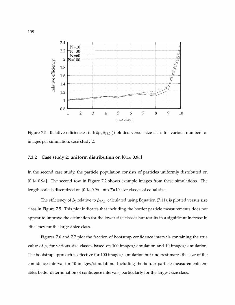
108

0.8

1

1.2

1.4

1.6

1.8

2

2.2

2.4

1 2 3 4 5 6 7 8 9 10

rela

tive

effic

ienc

y

size class

N=10N=30N=60

N=100

Figure 7.5: Relative efficiencies (eff(ρbi, ρMLi)) plotted versus size class for various numbers of

images per simulation: case study 2.

7.3.2 Case study 2: uniform distribution on [0.1a 0.9a]

In the second case study, the particle population consists of particles uniformly distributed on

[0.1a 0.9a]. The second row in Figure 7.2 shows example images from these simulations. The

length scale is discretized on [0.1a 0.9a] into T=10 size classes of equal size.

The efficiency of ρb relative to ρML, calculated using Equation (7.11), is plotted versus size

class in Figure 7.5. This plot indicates that including the border particle measurements does not

appear to improve the estimation for the lower size classes but results in a significant increase in

efficiency for the largest size class.

Figures 7.6 and 7.7 plot the fraction of bootstrap confidence intervals containing the true

value of ρi for various size classes based on 100 images/simulation and 10 images/simulation.

The bootstrap approach is effective for 100 images/simulation but underestimates the size of the

confidence interval for 10 images/simulation. Including the border particle measurements en-

ables better determination of confidence intervals, particularly for the largest size class.

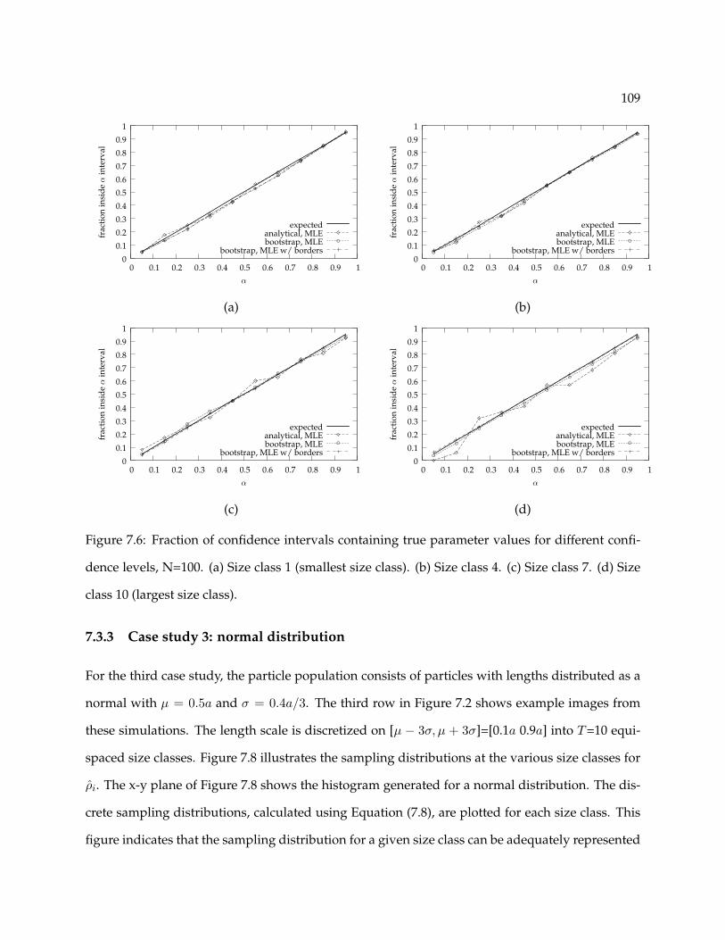
109

0

0.1

0.2

0.3

0.4

0.5

0.6

0.7

0.8

0.9

1

0 0.1 0.2 0.3 0.4 0.5 0.6 0.7 0.8 0.9 1

frac

tion

insi

deα

inte

rval

α



0.1

0.2

0.3

0.4

0.5

0.6

0.7

0.8

0.9

1

0 0.1 0.2 0.3 0.4 0.5 0.6 0.7 0.8 0.9 1

frac

tion

insi

deα

inte

rval

α



(a) (b)

0

0.1

0.2

0.3

0.4

0.5

0.6

0.7

0.8

0.9

1

0 0.1 0.2 0.3 0.4 0.5 0.6 0.7 0.8 0.9 1

frac

tion

insi

deα

inte

rval

α



0.1

0.2

0.3

0.4

0.5

0.6

0.7

0.8

0.9

1

0 0.1 0.2 0.3 0.4 0.5 0.6 0.7 0.8 0.9 1

frac

tion

insi

deα

inte

rval

α



(c) (d)

Figure 7.6: Fraction of confidence intervals containing true parameter values for different confi-

dence levels, N=100. (a) Size class 1 (smallest size class). (b) Size class 4. (c) Size class 7. (d) Size

class 10 (largest size class).

7.3.3 Case study 3: normal distribution

For the third case study, the particle population consists of particles with lengths distributed as a

normal with µ = 0.5a and σ = 0.4a/3. The third row in Figure 7.2 shows example images from

these simulations. The length scale is discretized on [µ − 3σ, µ + 3σ]=[0.1a 0.9a] into T=10 equi-

spaced size classes. Figure 7.8 illustrates the sampling distributions at the various size classes for

ρi. The x-y plane of Figure 7.8 shows the histogram generated for a normal distribution. The dis-

crete sampling distributions, calculated using Equation (7.8), are plotted for each size class. This

figure indicates that the sampling distribution for a given size class can be adequately represented

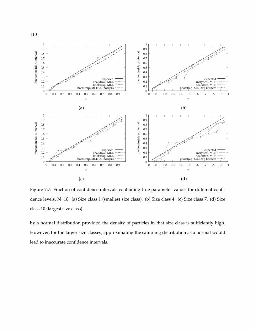
110

0

0.1

0.2

0.3

0.4

0.5

0.6

0.7

0.8

0.9

1

0 0.1 0.2 0.3 0.4 0.5 0.6 0.7 0.8 0.9 1

frac

tion

insi

deα

inte

rval

α



0.1

0.2

0.3

0.4

0.5

0.6

0.7

0.8

0.9

1

0 0.1 0.2 0.3 0.4 0.5 0.6 0.7 0.8 0.9 1

frac

tion

insi

deα

inte

rval

α



(a) (b)

0

0.1

0.2

0.3

0.4

0.5

0.6

0.7

0.8

0.9

1

0 0.1 0.2 0.3 0.4 0.5 0.6 0.7 0.8 0.9 1

frac

tion

insi

deα

inte

rval

α



0.1

0.2

0.3

0.4

0.5

0.6

0.7

0.8

0.9

1

0 0.1 0.2 0.3 0.4 0.5 0.6 0.7 0.8 0.9 1

frac

tion

insi

deα

inte

rval

α



(c) (d)

Figure 7.7: Fraction of confidence intervals containing true parameter values for different confi-

dence levels, N=10. (a) Size class 1 (smallest size class). (b) Size class 4. (c) Size class 7. (d) Size

class 10 (largest size class).

by a normal distribution provided the density of particles in that size class is sufficiently high.

However, for the larger size classes, approximating the sampling distribution as a normal would

lead to inaccurate confidence intervals.

111

01

23

45

67

02

46

8100

0.05

0.1

0.15

0.2

0.25

0.3

probability mass

absolute PSD size class

probability mass

Figure 7.8: Sampling distributions for the various size classes of a discrete normal distribution.

N = 100.

Figure 7.9 plots eff(ρbi, ρMLi) for various numbers of images per simulation. Comparing

Figure 7.9 with Figure 7.5 indicates that the relative efficiency for a given size class is a function of

both the size and the density of the particles in that size class.

7.3.4 Case study 4: uniform distribution on [0.4a 2.0a]

In the fourth case study, the particle population consists of particles uniformly distributed on [0.4a

2.0a]. The fourth row in Figure 7.2 shows example images from these simulations. The length scale

was discretized on [0.4a a] into T − 1 = 9 bins with the T th bin extending from a to Lmax. Lmax

was assumed unknown and estimated with initial value√

2a. That is, Equation (7.6) was solved

as before with the exception that the parameters mXi and mYj were updated at each iteration

based on the current estimate of Lmax. Figure 7.10 shows the sampling distributions for ρi for

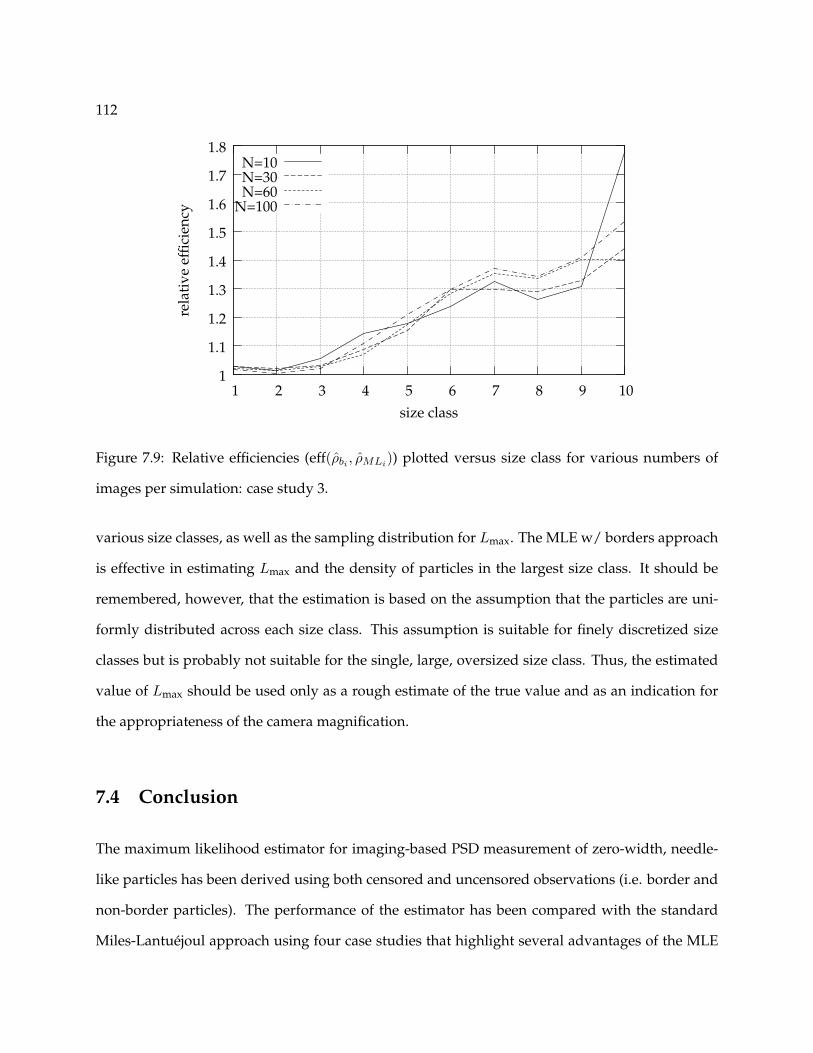
112

1

1.1

1.2

1.3

1.4

1.5

1.6

1.7

1.8

1 2 3 4 5 6 7 8 9 10

rela

tive

effic

ienc

y

size class

N=10N=30N=60

N=100

Figure 7.9: Relative efficiencies (eff(ρbi, ρMLi)) plotted versus size class for various numbers of

images per simulation: case study 3.

various size classes, as well as the sampling distribution for Lmax. The MLE w/ borders approach

is effective in estimating Lmax and the density of particles in the largest size class. It should be

remembered, however, that the estimation is based on the assumption that the particles are uni-

formly distributed across each size class. This assumption is suitable for finely discretized size

classes but is probably not suitable for the single, large, oversized size class. Thus, the estimated

value of Lmax should be used only as a rough estimate of the true value and as an indication for

the appropriateness of the camera magnification.

7.4 Conclusion

The maximum likelihood estimator for imaging-based PSD measurement of zero-width, needle-

like particles has been derived using both censored and uncensored observations (i.e. border and

non-border particles). The performance of the estimator has been compared with the standard

Miles-Lantuejoul approach using four case studies that highlight several advantages of the MLE

113

0

20

40

60

80

100

0 0.2 0.4 0.6 0.8 1 1.2 1.4

coun

ts

ρ1

MLE w/ bordersMiles

0

20

40

60

80

100

0 0.2 0.4 0.6 0.8 1 1.2 1.4

ρ5

MLE w/ bordersMiles

0

20

40

60

80

100

0 0.2 0.4 0.6 0.8 1 1.2 1.4

ρ9

MLE w/ bordersMiles

0

20

40

60

80

100

0 2 4 6 8 10 12

coun

ts

ρ10

MLE w/ bordersMiles

0

20

40

60

80

100

1.4 1.6 1.8 2 2.2 2.4 2.6

Lmax

MLE w/ borders

Figure 7.10: Comparison of sampling distributions for absolute PSD for particles distributed uni-

formly on [0.4a 2.0a]. Results based on 200 simulations, 100 images/simulation, 10 size classes,

Nc=15. (a) Size class 1. (b) Size class 5. (c) Size class 9. (d) Size class 10. (e) Lmax.

approach. The case studies indicate that MLE is more efficient than Miles-Lantuejoul, particularly

if the particle population is mono-disperse or contains particles that are large relative to the size of

the image. Furthermore, MLE can estimate the number density of over-sized particles (particles

bigger than the image dimension) along with the size Lmax of the largest particle while the Miles-

Lantuejoul approach can be applied only for particles smaller than the image dimension.

The limitations of the MLE approach should also be discussed. The primary limitation of

the MLE derived in this chapter is due to the assumption that the particles have needle-like geom-

etry. The Miles-Lantuejoul approach, on the other hand, can be applied to a much wider class of

geometries. Secondly, the MLE approach requires the solution of a nonlinear optimization prob-

lem. Thus, confidence interval determination by bootstrapping can be computationally-intensive.

Finally, it should be noted that the MLE estimates related to over-sized particles are obtained by

making the rather unrealistic assumption that over-sized particles are uniformly distributed in

length on [a Lmax]. The estimates related to over-sized particles are therefore biased in general but

may be useful for identifying whether or not the camera magnification is suitable for the given

system.

114

Several areas for future work are evident. Choosing the optimal number, location, and

size of bins for constructing histograms should be addressed. Integrating measurements taken

at multiple scales or magnifications is also important. For systems of high-aspect-ratio particles,

incorporating the width of border particles into the estimation could lead to increased efficiency

by narrowing down the number of size classes to which a border particle may correspond.

115

Chapter 8

Assessing the Reliability of

Imaging-based, Number Density

Measurement 1

The methods for PSD estimation in Chapter 7 are based on the assumption that image segmenta-

tion is perfect, or that every single particle appearing in the image is identified correctly. Achiev-

ing perfect image segmentation is a realistic assumption, however, only at low solids concentra-

tions. At higher solids concentrations, a significant fraction of the particles may be overlapping

or occluded, which often results in these particles being missed by the automated image analysis

algorithm. The density of particles is thus underestimated. The objective of this chapter is to ad-

dress this third challenge by developing a semi-empirical, probabilistic model that enables PSD

estimation for imperfect image analysis. This paper also presents a descriptor that can be used

to quantify the expected amount of particle overlap and thereby assess the reliability of the PSD

estimate.

The chapter is organized as follows. Section 8.1 presents previous work relevant to the

scope of this chapter. Section 8.2 presents theory related to particle overlap probabilities, proposes

a descriptor for measurement reliability, and presents an estimator for particle number density

that accounts for particle overlap. Section 8.3 describes the simulation studies used to determine


116

the conditions for which SHARC gives an accurate PSD measurement. Section 8.4 presents the

results of these simulation studies, and Section 8.5 summarizes our findings.

8.1 Previous work

Armitage [4] was one of the first to investigate the effects of particle overlap on particle num-

ber density estimation. Armitage derived formulas for the expected numbers of isolated clumps

(groups of one or more overlapping particles) for circular and rectangular particles, and used

these formulas to estimate the mean clump size and number density of particles. Mack [77, 78]

extended Armitage’s results to three-dimensional particles of any convex shape, deriving formu-

las for the expected numbers of clumps and isolated particles based on the perimeters and areas

of the two-dimensional projections of the particles. Roach [104] summarized the work of Mack

and Armitage, described several applications, and developed theory for specialized applications.

Kellerer [63] was the first to account for edge effects and overlap simultaneously and derived a

formula for the expected number of clumps minus the number of enclosed voids (i.e. regions of

the image completely enclosed by particles). To model the complicated, random shapes that form

due to the random placement and overlap of simple geometric objects, the Boolean model [1, 6]

can be used.

The methods cited above assume that a clear distinction can be made between the image

background and the objects of interest, or that the image can be segmented by simple threshold-

ing. In some applications, however, more advanced image analysis is required, and modeling the

output of a complicated image analysis algorithm to enable statistical inference is non-trivial. For

example, the SHARC algorithm described in Chapter 5 is a model-based vision algorithm that can

successfully identify overlapped particles provided the degree of overlap is minor. Initial studies

have shown that the methods cited above do not adequately model the output of the SHARC algo-

rithm. In this work, we extend these methods to enable statistical inference for SHARC’s output.

We expect the methodology developed here to be applicable to other situations in which advanced

117

image analysis is necessary to extract information from noisy images.

8.2 Theory

8.2.1 Particulate system definition

Consider a slurry S of volume V in which a solid phase of discrete particles is dispersed in a

continuous fluid phase. Let ρc be the solid phase density (mass solid/volume solid) and MT the

slurry density (mass solid/volume slurry), or solids concentration. The volume solids concen-

tration (volume solid/volume slurry) is given by MT /ρc. Let L be the characteristic length of a

particle and define a shape factor kv such that the volume of a single particle is given by kvL3. Let

f(L) denote the PSD, or the number of particles of characteristic length L per unit volume slurry.

The ith moment of the PSD is denoted µi =∫∞0 f(L)LidL. Given the PSD, the slurry density can

be calculated as MT = ρckvµ3 assuming kv is independent of length. The zeroth moment, µ0,

equals the number of particles per unit volume slurry. For a mono-disperse system in which all

particles have the same length l, µ0 = MT /ρckvl3.

8.2.2 Sampling and measurement definitions

Let VI ∈ S denote an imaging volume, and let I denote an image created by perspective projection

of VI onto a two-dimensional image plane. Let a and b denote the horizontal and vertical dimen-

sions of VI , or the field of view, and let df denote the depth dimension of VI , or the depth of field.

Thus, the volume of VI is abdf , and the average number of particles per image is λ = µ0abdf .

Number-based PSDs are typically measured by discretizing the characteristic length scale

into T non-overlapping bins or size classes. We therefore define the discrete PSD as

ρi =∫ Si+1

Si

f(l)dl, i = 1, . . . , T (8.1)

in which S = (S1, . . . , ST+1) is the vector of breaks between size classes. In this work, we consider

only mono-disperse populations, so we represent the PSD for a given system using a single scalar

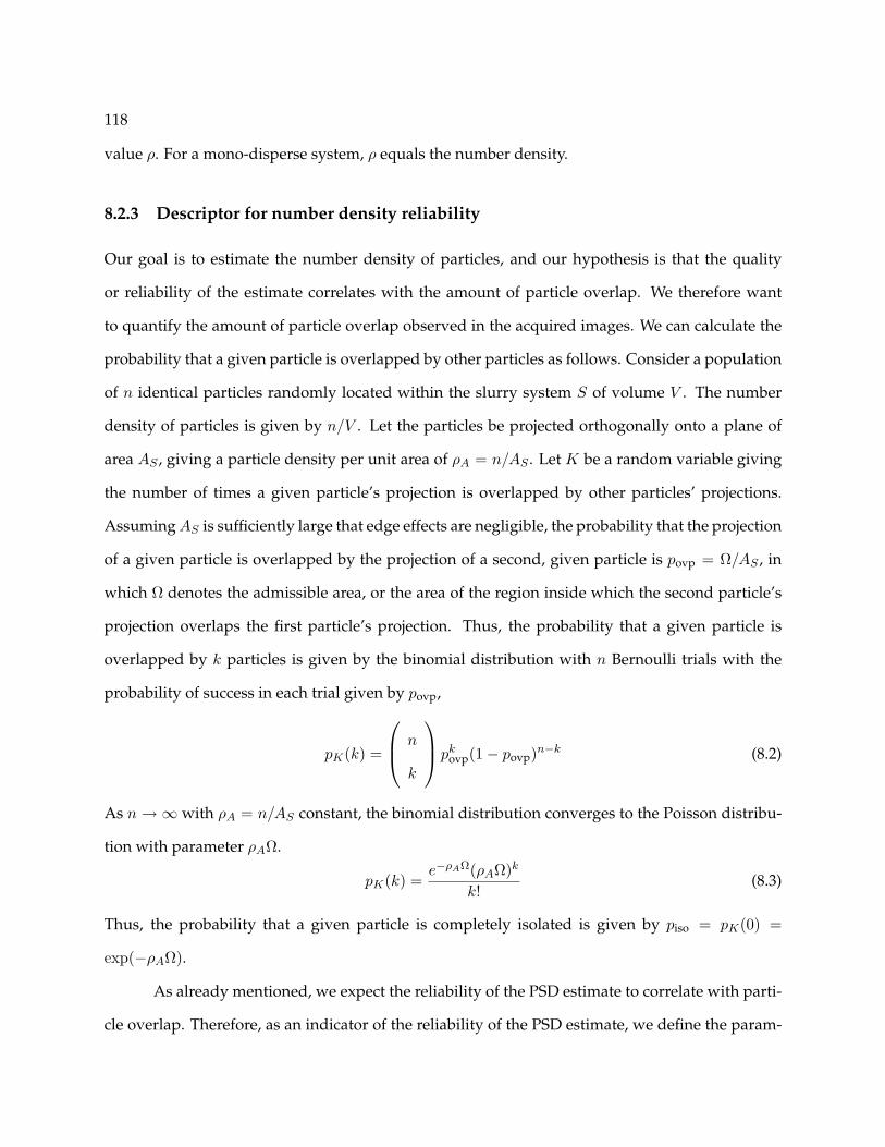
118

value ρ. For a mono-disperse system, ρ equals the number density.

8.2.3 Descriptor for number density reliability

Our goal is to estimate the number density of particles, and our hypothesis is that the quality

or reliability of the estimate correlates with the amount of particle overlap. We therefore want

to quantify the amount of particle overlap observed in the acquired images. We can calculate the

probability that a given particle is overlapped by other particles as follows. Consider a population

of n identical particles randomly located within the slurry system S of volume V . The number

density of particles is given by n/V . Let the particles be projected orthogonally onto a plane of

area AS , giving a particle density per unit area of ρA = n/AS . Let K be a random variable giving

the number of times a given particle’s projection is overlapped by other particles’ projections.

Assuming AS is sufficiently large that edge effects are negligible, the probability that the projection

of a given particle is overlapped by the projection of a second, given particle is povp = Ω/AS , in

which Ω denotes the admissible area, or the area of the region inside which the second particle’s

projection overlaps the first particle’s projection. Thus, the probability that a given particle is

overlapped by k particles is given by the binomial distribution with n Bernoulli trials with the

probability of success in each trial given by povp,

pK(k) =

n

k

pkovp(1− povp)n−k (8.2)

As n →∞ with ρA = n/AS constant, the binomial distribution converges to the Poisson distribu-

tion with parameter ρAΩ.

pK(k) =e−ρAΩ(ρAΩ)k

k!(8.3)

Thus, the probability that a given particle is completely isolated is given by piso = pK(0) =

exp(−ρAΩ).

As already mentioned, we expect the reliability of the PSD estimate to correlate with parti-

cle overlap. Therefore, as an indicator of the reliability of the PSD estimate, we define the param-

119

w

w sin θz

w cos θz

l cos θz

l sin θz

l

Aovp

w(1 + sin θz) + l cos θz

θz

l(1 + sin θz)+w cos θz

w

l

Aovp

(a) (b)

Figure 8.1: Geometric representation of admissible area, or region in which a particle is overlapped

by another particle.

eter D as

D = − log(piso) = ρAΩ (8.4)

The area number density ρA of particles in an image can be calculated as ρA = µ0df . The ad-

missible area Ω depends on the particle geometry. To illustrate how the admissible area can be

calculated, consider the rectangular particle of length l and width w in the center of Figure 8.1.

Next, consider a second particle of identical dimensions placed in the image with orientation θz .

If the midpoint of the second particle is placed anywhere inside the shaded region in Figure 8.1,

the first and second particles overlap. This fact is illustrated in Figure 8.1(b) using the various par-

ticles placed around the border of the shaded area. Using straightforward geometric relationships

(see Figure 8.1(a)), the area Aovp of this shaded region can be shown to be

Aovp = (w(1 + sin θz) + l cos θz)(l(1 + sin θz) + w cos θz)− l2 cos θz sin θz − w2 cos θz sin θz (8.5)

and Ω is obtained by integrating over θz

Ω = E[Aovp] =1π

∫ π/2

−π/2Aovpdθz =

2π

(l2 + w2 + lw(2 + π)

)(8.6)

120

in which a uniform distribution in orientation has been assumed.

Mack [77] (see also Roach [104, p.44]) derived a more general result that enables the calcu-

lation of the admissible area Ω for any set of convex bodies of identical size and shape and having

random orientation. Mack’s surprisingly simple result gives Ω based on the area ap and perimeter

sp of a two-dimensional domain:

Ω = 2ap +s2p

2π(8.7)

8.2.4 Estimation of number density

Given our hypothesis that particle overlap is the primary cause of failure for image analysis-based

measurement, it seems reasonable to estimate the number density of particles based on the num-

ber of completely isolated particles observed in the image. Letting X be a random variable giving

the number of observations of completely isolated, non-border particles, it can be shown that the

probability density for X is Poisson with parameter mX = ρdfNANB exp(−ρdfΩ), in which N is

the number of images, ANB is the area of the region inside which a particle does not touch the

image border (see Chapter 7 and Appendix A), Ω is the admissible area defined above, and ρ is

the number density as defined above. The maximum likelihood estimate of ρ is therefore

ρ = arg maxρ

e−mX mxX

x!(8.8)

in which x is the realization of X , or the measured number of isolated, non-border particles.

The likelihood function in Equation (8.8) gives the probability of observing the data as a

function of ρ and has unique properties that merit consideration. Consider a population of par-

ticles having lengths 1/10 the size of the image dimension and a number density corresponding

to about 10 particles per image. Under these conditions, the amount of particle overlap is small,

so the actual number of particles is essentially equal to the number of isolated, non-overlapping

particles. However, it is also likely that only 10 isolated particles would be observed if the number

density of particles is so high that nearly all particles are overlapping. Thus, in Figure 8.2, two

spikes are observed in the likelihood function: one corresponding to the low concentration case

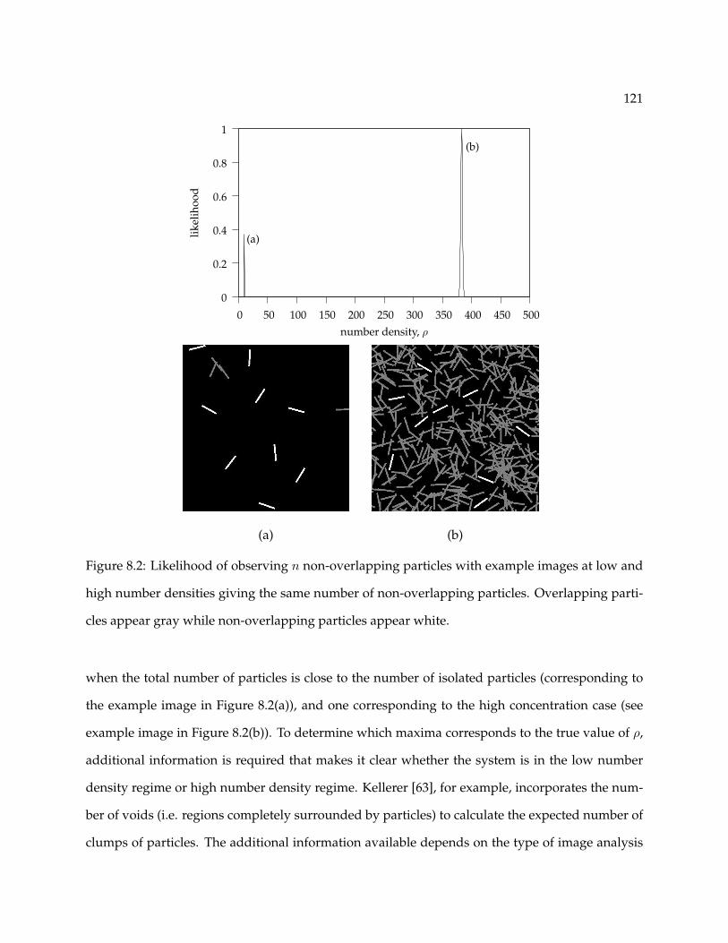
121

0

0.2

0.4

0.6

0.8

1

0 50 100 150 200 250 300 350 400 450 500

likel

ihoo

d

number density, ρ

(a)

(b)

(a) (b)

Figure 8.2: Likelihood of observing n non-overlapping particles with example images at low and

high number densities giving the same number of non-overlapping particles. Overlapping parti-

cles appear gray while non-overlapping particles appear white.

when the total number of particles is close to the number of isolated particles (corresponding to

the example image in Figure 8.2(a)), and one corresponding to the high concentration case (see

example image in Figure 8.2(b)). To determine which maxima corresponds to the true value of ρ,

additional information is required that makes it clear whether the system is in the low number

density regime or high number density regime. Kellerer [63], for example, incorporates the num-

ber of voids (i.e. regions completely surrounded by particles) to calculate the expected number of

clumps of particles. The additional information available depends on the type of image analysis

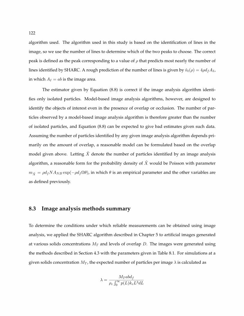
122

algorithm used. The algorithm used in this study is based on the identification of lines in the

image, so we use the number of lines to determine which of the two peaks to choose. The correct

peak is defined as the peak corresponding to a value of ρ that predicts most nearly the number of

lines identified by SHARC. A rough prediction of the number of lines is given by nl(ρ) = 4ρdfAI ,

in which AI = ab is the image area.

The estimator given by Equation (8.8) is correct if the image analysis algorithm identi-

fies only isolated particles. Model-based image analysis algorithms, however, are designed to

identify the objects of interest even in the presence of overlap or occlusion. The number of par-

ticles observed by a model-based image analysis algorithm is therefore greater than the number

of isolated particles, and Equation (8.8) can be expected to give bad estimates given such data.

Assuming the number of particles identified by any given image analysis algorithm depends pri-

marily on the amount of overlap, a reasonable model can be formulated based on the overlap

model given above. Letting X denote the number of particles identified by an image analysis

algorithm, a reasonable form for the probability density of X would be Poisson with parameter

mX = ρdfNANB exp(−ρdfΩθ), in which θ is an empirical parameter and the other variables are

as defined previously.

8.3 Image analysis methods summary

To determine the conditions under which reliable measurements can be obtained using image

analysis, we applied the SHARC algorithm described in Chapter 5 to artificial images generated

at various solids concentrations MT and levels of overlap D. The images were generated using

the methods described in Section 4.3 with the parameters given in Table 8.1. For simulations at a

given solids concentration MT , the expected number of particles per image λ is calculated as

λ =MT abdf

ρc

∫∞0 p(L)kvL3dL

123

Description Symbol Value

Horizontal dimension of imaging volume a 2 mm

Vertical dimension of imaging volume b 2 mm

Depth of field df 0.25 mm

Solid phase density ρc 2 mg/mm3

Number of horizontal CCD pixels umax 480

Number of vertical CCD pixels vmax 480

Table 8.1: Parameters used to simulate imaging of particle population at a given solids concentra-

tion.

For a mono-disperse population with p(L) = δ(L− l), λ is given by

λ =MT abdf

ρckvl3

For simulations at a given value of D, λ is calculated using Equation (8.4):

λ =Dab

Ω

The SHARC algorithm consists of three main steps. In the first step, SHARC identifies lines

in the image corresponding to the crystals’ edges. Because crystal edges are often broken due to

noise or overlap, SHARC attempts to complete these edges by identifying instances of collinearity

between the identified lines. Finally, SHARC identifies clusters of parallel lines having similar

lengths and fits a two-dimensional rectangle model to each cluster, giving the length and width of

the crystal. SHARC was applied to the artificial images using the parameters shown in Table 8.2.

8.4 Results

8.4.1 Descriptor comparison: MT versus D

Figure 8.3 compares images generated for two different mono-disperse particle populations gen-

erated at the same solids concentration MT and at the same D. The images generated at constant

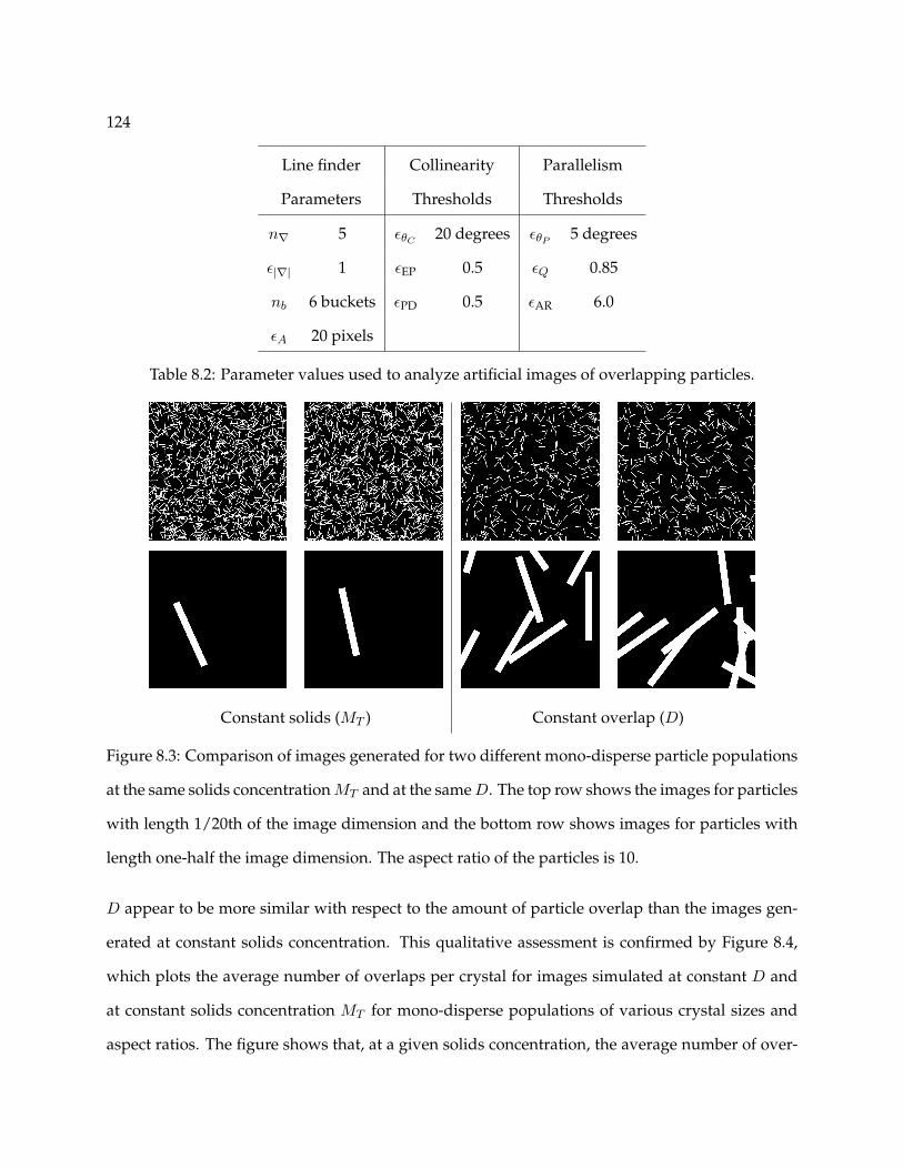
124

Line finder Collinearity Parallelism

Parameters Thresholds Thresholds

n∇ 5 εθC20 degrees εθP

5 degrees

ε|∇| 1 εEP 0.5 εQ 0.85

nb 6 buckets εPD 0.5 εAR 6.0

εA 20 pixels

Table 8.2: Parameter values used to analyze artificial images of overlapping particles.

Constant solids (MT ) Constant overlap (D)

Figure 8.3: Comparison of images generated for two different mono-disperse particle populations

at the same solids concentration MT and at the same D. The top row shows the images for particles

with length 1/20th of the image dimension and the bottom row shows images for particles with

length one-half the image dimension. The aspect ratio of the particles is 10.

D appear to be more similar with respect to the amount of particle overlap than the images gen-

erated at constant solids concentration. This qualitative assessment is confirmed by Figure 8.4,

which plots the average number of overlaps per crystal for images simulated at constant D and

at constant solids concentration MT for mono-disperse populations of various crystal sizes and

aspect ratios. The figure shows that, at a given solids concentration, the average number of over-

125

0

0.5

1

1.5

2

2.5

0 1 2 3 4 5 6

Ave

.no.

ofov

erla

ps

Percent solids, MT × 100

0.1a,AR=10

0.1a,AR=5

0.7a,AR=100.7a,AR=5

0

0.5

1

1.5

2

2.5

0 0.5 1 1.5 2 2.5

Ave

.no.

ofov

erla

ps

Image difficulty, D

L/a=0.1, AR=5L/a=0.7, AR=5L/a=0.1,AR=10L/a=0.7,AR=10

Figure 8.4: Comparison of average number of overlaps per crystal for images simulated at constant

D and at constants solids concentration for mono-disperse populations of various crystal sizes.

0

20

40

60

80

100

0 1 2 3 4 5 6

Perc

entm

isse

d

Percent solids, MT × 100

0.1a

0.4a

0.7a

0

20

40

60

80

100

0 0.5 1 1.5 2

Perc

entm

isse

d

Image difficulty, D

L/a = 0.10.40.7

Figure 8.5: Comparison of percentage of particles missed by automated image analysis for images

simulated at constant D and at constants solids concentration for mono-disperse populations of

various crystal sizes.

laps per crystal is a strong function of the particle size and shape while, at a given level of D, the

number of overlaps is independent of particle size and shape. If measurement failure is caused

by particle overlap, we would expect the results of automated image analysis at a given D to be

relatively independent of the size and shape of the particles. Figure 8.5 shows the percentage of

particles missed by automated image analysis at different levels of solids concentrations and D.

As expected, the percent missed is similar for various particle sizes when considered in terms of

D, but is vastly different when considered in terms of solids concentration.

126

8.4.2 Estimation of number density

In this section, we examine different methods for estimating the number density ρ. We first ex-

amine the behavior of the Miles-Lantuejoul estimator, which corrects for edge effects but not for

particle overlap. Next, we examine the performance of the maximum likelihood estimator pre-

sented in Section 8.2.4. The estimators are applied to data acquired by analyzing images using

SHARC. Example images for various levels of D and three different particle sizes (L/a = 0.1, 0.3,

and 0.5) are shown in Figure 8.6.

Miles-Lantuejoul method

Figure 8.7 shows the ratio of the estimated and true number density as a function of D for var-

ious particle sizes. In this figure, the number density of particles is estimated using the Miles-

Lantuejoul method [83, 64], which does not account for overlap. The particle size and shape

measurements are obtained using the SHARC algorithm. The estimator’s bias increases with D,

or as the amount of overlap increases. Given the well-behaved and relatively size-independent

correlation between ρ/ρ and D, one may attempt to correct ρ based on an estimated value of D.

The result of such an approach is shown in Figure 8.7(b). The number density estimates for this

figure are given by

ρ =ρML

g(D)

in which ρML denotes the Miles-Lantuejoul estimate, D is an estimate of D given by D = ρMLΩ,

and g is an empirical function generated by fitting g(D) = exp(−θD) to the data in Figure 8.7(a).

The parameter θ is determined using nonlinear least-squares minimization. This approach is inef-

fective because D cannot be estimated independently of ρ, so both D and ρ are underestimated.

Maximum likelihood method

To implement the maximum likelihood estimator given by Equation (8.8), we first need to com-

plete the probabilistic model by determining the empirical parameter θ. We determine θ by solving

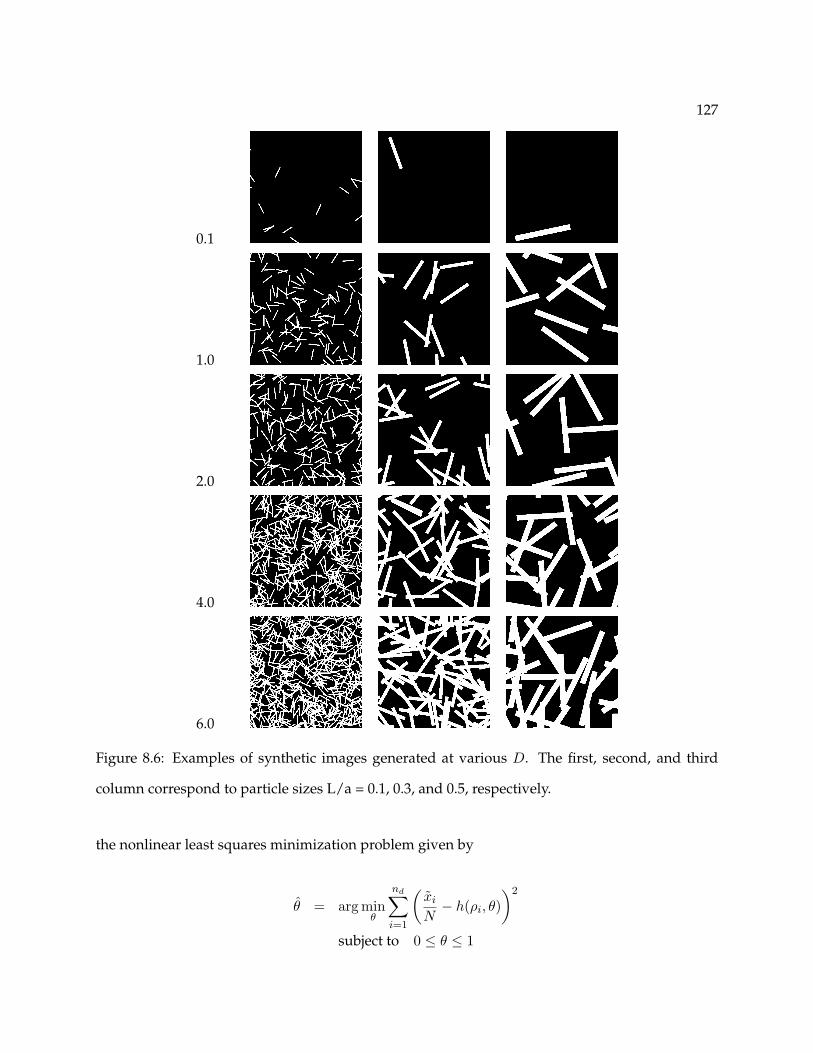
127

0.1

1.0

2.0

4.0

6.0

Figure 8.6: Examples of synthetic images generated at various D. The first, second, and third

column correspond to particle sizes L/a = 0.1, 0.3, and 0.5, respectively.

the nonlinear least squares minimization problem given by

θ = arg minθ

nd∑i=1

(xi

N− h(ρi, θ)

)2

subject to 0 ≤ θ ≤ 1

128

0

0.5

1

1.5

2

0 1 2 3 4 5 6

ρ/ρ

Image difficulty, D

L/a = 0.10.30.5

0

0.5

1

1.5

2

0 1 2 3 4 5 6

ρ/ρ

Image difficulty, D

L/a = 0.10.30.5

(a) (b)

Figure 8.7: Results of number density estimation using Miles-Lantuejoul method for various par-

ticle sizes and various levels of image difficulty. (a) Results for applying Miles-Lantuejoul method

directly to image analysis output. (b) Results for empirical correction of the Miles-Lantuejoul esti-

mate based on estimated value of D.

in which xi is the number of particles identified by analysis of N images acquired at a given

number density ρi, and h(ρ, θ) is the model prediction of the average number of particles identified

per image, given by

h(ρ, θ) = ρdfANB exp(−ρdfΩθ) (8.9)

A value of θ = 1 indicates that the image analysis algorithm finds only particles that are com-

pletely isolated while a value of θ = 0 indicates the image analysis algorithm identifies every

particle in the image, regardless of overlap.

Figure 8.8 shows the optimal fit of the model in Equation (8.9) to the data observed by

applying SHARC to artificial images generated at various number densities with particles of size

L/a = 0.1. The values of D corresponding to the number densities range from 0.1 to 6.0. Figure 8.8

indicates that the empirical overlap model with θ = 0.33 gives an excellent prediction of SHARC’s

behavior for a wide range of densities. Also shown in Figure 8.8 is the model prediction for θ = 0,

corresponding to perfect image analysis (i.e. the image analysis algorithm identifies every single

particle in the image). The slope of this line equals ANB , which is related to the magnitude of the

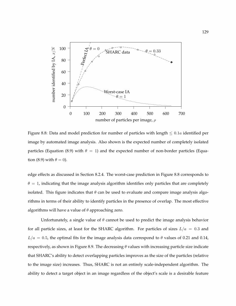
129

0

20

40

60

80

100

0 100 200 300 400 500 600 700

num

ber

iden

tifie

dby

IA,x

/N

number of particles per image, ρ

Perf

ect I

AWorst-case IA

SHARC data θ = 0.33θ = 0

θ = 1

Figure 8.8: Data and model prediction for number of particles with length ≤ 0.1a identified per

image by automated image analysis. Also shown is the expected number of completely isolated

particles (Equation (8.9) with θ = 1) and the expected number of non-border particles (Equa-

tion (8.9) with θ = 0).

edge effects as discussed in Section 8.2.4. The worst-case prediction in Figure 8.8 corresponds to

θ = 1, indicating that the image analysis algorithm identifies only particles that are completely

isolated. This figure indicates that θ can be used to evaluate and compare image analysis algo-

rithms in terms of their ability to identify particles in the presence of overlap. The most effective

algorithms will have a value of θ approaching zero.

Unfortunately, a single value of θ cannot be used to predict the image analysis behavior

for all particle sizes, at least for the SHARC algorithm. For particles of sizes L/a = 0.3 and

L/a = 0.5, the optimal fits for the image analysis data correspond to θ values of 0.21 and 0.14,

respectively, as shown in Figure 8.9. The decreasing θ values with increasing particle size indicate

that SHARC’s ability to detect overlapping particles improves as the size of the particles (relative

to the image size) increases. Thus, SHARC is not an entirely scale-independent algorithm. The

ability to detect a target object in an image regardless of the object’s scale is a desirable feature

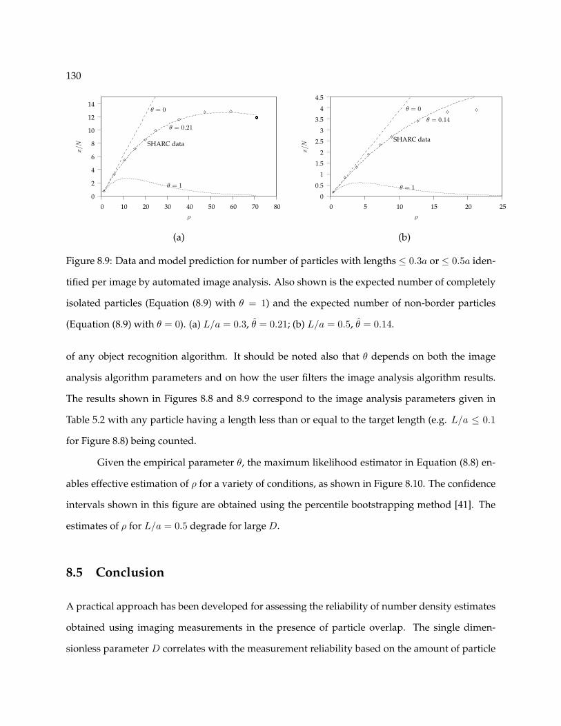
130

0

2

4

6

8

10

12

14

0 10 20 30 40 50 60 70 80

x/N

ρ

θ = 0

θ = 1

θ = 0.21

SHARC data

0

0.5

1

1.5

2

2.5

3

3.5

4

4.5

0 5 10 15 20 25

x/N

ρ

θ = 0

θ = 1

θ = 0.14

SHARC data

(a) (b)

Figure 8.9: Data and model prediction for number of particles with lengths ≤ 0.3a or ≤ 0.5a iden-

tified per image by automated image analysis. Also shown is the expected number of completely

isolated particles (Equation (8.9) with θ = 1) and the expected number of non-border particles

(Equation (8.9) with θ = 0). (a) L/a = 0.3, θ = 0.21; (b) L/a = 0.5, θ = 0.14.

of any object recognition algorithm. It should be noted also that θ depends on both the image

analysis algorithm parameters and on how the user filters the image analysis algorithm results.

The results shown in Figures 8.8 and 8.9 correspond to the image analysis parameters given in

Table 5.2 with any particle having a length less than or equal to the target length (e.g. L/a ≤ 0.1

for Figure 8.8) being counted.

Given the empirical parameter θ, the maximum likelihood estimator in Equation (8.8) en-

ables effective estimation of ρ for a variety of conditions, as shown in Figure 8.10. The confidence

intervals shown in this figure are obtained using the percentile bootstrapping method [41]. The

estimates of ρ for L/a = 0.5 degrade for large D.

8.5 Conclusion

A practical approach has been developed for assessing the reliability of number density estimates

obtained using imaging measurements in the presence of particle overlap. The single dimen-

sionless parameter D correlates with the measurement reliability based on the amount of particle

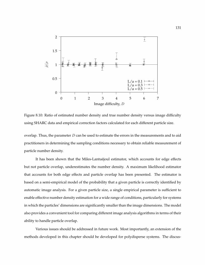
131

0

0.5

1

1.5

2

0 1 2 3 4 5 6 7

ρ/ρ

Image difficulty, D

L/a = 0.1L/a = 0.3L/a = 0.5

Figure 8.10: Ratio of estimated number density and true number density versus image difficulty

using SHARC data and empirical correction factors calculated for each different particle size.

overlap. Thus, the parameter D can be used to estimate the errors in the measurements and to aid

practitioners in determining the sampling conditions necessary to obtain reliable measurement of

particle number density.

It has been shown that the Miles-Lantuejoul estimator, which accounts for edge effects

but not particle overlap, underestimates the number density. A maximum likelihood estimator

that accounts for both edge effects and particle overlap has been presented. The estimator is

based on a semi-empirical model of the probability that a given particle is correctly identified by

automatic image analysis. For a given particle size, a single empirical parameter is sufficient to

enable effective number density estimation for a wide range of conditions, particularly for systems

in which the particles’ dimensions are significantly smaller than the image dimensions. The model

also provides a convenient tool for comparing different image analysis algorithms in terms of their

ability to handle particle overlap.

Various issues should be addressed in future work. Most importantly, an extension of the

methods developed in this chapter should be developed for polydisperse systems. The discus-

132

sions in Armitage [4] and Roach [104, p.46] may provide a good starting point for such investiga-

tions. The incorporation of these methods into a state estimator for feedback control of number

density should also be investigated.

133

Chapter 9

High-resolution PSD Measurement for

Industrial Crystallization 1

As discussed in Section 2.3.1, the imaging-based, particulate population dynamics studies in the

literature have focused on monitoring either the normalized PSD (i.e. number fraction), moments

of the PSD (e.g. mean size and variance), the particle length cumulative distribution function

(CDF), or the polymorphic fraction. Given that the dynamics of particle populations are modeled

in terms of the absolute PSD, it is desirable to monitor the absolute PSD to enable better model

identification and control. The objective of this chapter is to demonstrate the feasibility of imaging-

based PSD measurement for realistic and changing process and imaging conditions using the

methods developed in previous chapters. We achieve this objective by simulating a well-studied

industrial crystallization process and generating images of the process based on the specifications

of a commercially-available in situ imaging probe. Furthermore, this chapter shows the value of

imaging-based measurement by demonstrating the measurement of process properties that cannot

be measured by conventional technologies. Section 9.1 describes the crystallizer model used in this

study and the method for generating images corresponding to the current state of the crystallizer.

Section 9.2 presents the simulation results, demonstrating the measurement of important product-

quality metrics and multi-modal PSDs. Section 9.2 also offers general guidelines for designing

imaging-based PSD monitoring systems. Section 9.3 summarizes our conclusions.


134

9.1 Crystallizer model and imaging summary

Batch crystallization can be modeled using a system of partial integro-differential equations that

couples mass and energy balances with a population balance describing the evolution of the crys-

tal population’s PSD. The population balance used in this study is

∂f

∂t+ G

∂f

∂L= 0 (9.1)

in which f(L, t) is the PSD, L is the characteristic length, and G is the crystal growth rate. The

boundary condition is

f(0, t) =B

G(L = 0)(9.2)

in which B is the nucleation rate density. G and B depend on the relative supersaturation S and

are assumed to follow standard semi-empirical power laws:

S =C − Csat

CsatG = kgS

g B = kbSbµj

i (9.3)

in which C is the liquid-phase solute concentration, Csat is the saturation concentration, kg and g

are growth rate constants, and kb, b, and j are nucleation rate constants. The ith moment of the

PSD, µi, is defined as

µi =∫ ∞

0fLidL (9.4)

In this study, we also are concerned with moments corresponding to subsets of the total crystal

population. Moments corresponding to crystals grown from nuclei are denoted with a subscript

N (e.g. µN3) while moments corresponding to crystals grown from seeds are denoted with a

subscript S.

Assuming, as above, that growth rate is size-independent and the system is closed (no

input or output streams), the mass balance for the solute concentration is

dC

dt= −3ρckvhG

∫ ∞

0fL2dL (9.5)

in which C is the solute concentration, ρc is the crystal density, kv is a shape factor defined such

that kvL3 gives the volume of a crystal of characteristic length L, h converts solvent mass to slurry

135

Description Symbol Value Units

kinetic growth rate constant kg 0.3e-4 cm/min

power-law exponent g 2.0 dimensionless

kinetic nucleation rate constant kb 2.6e10 g solvent/cm3 min

power-law exponent b 3.0 dimensionless

moment exponent j 2.0 dimensionless

crystal density ρc 1.183 g / cm3

volumetric shape factor kv 0.93 dimensionless

area shape factor ka 9.8 dimensionless

Crystallizer volume V 2.3 L

Table 9.1: Parameters used to simulate industrial batch crystallization process of photochemi-

cal [81]. The characteristic length is the particle width and an aspect ratio of 10 is assumed.

volume. C is given in terms of mass of solute per total mass of solution or liquid phase. The initial

condition is given by C = C0.

For the simulations used in this study, the energy balance is unnecessary as we assume

perfect temperature control. The temperature follows a fixed temperature trajectory without de-

viation.

The model parameters used in this study correspond to a well-studied, industrial photo-

chemical crystallization process [81, 82]. The parameters for this process are given in Table 9.1.

The particles have a needle-like morphology and the characteristic length corresponds to the par-

ticle width. An aspect ratio of 10 is assumed. The saturation concentration Csat for this system is

given by

Csat(T ) = 0.185− 2.11× 10−2T + 7.46× 10−4T 2 (9.6)

The crystallizer model is solved using orthogonal collocation on moving finite elements. The

method is described in detail in Chapter 3.

136

Description Symbol Value

Horizontal dimension of imaging volume a 1075 µm

Vertical dimension of imaging volume b 850 µm

Depth of field df 10 µm

Number of horizontal CCD pixels umax 1360

Number of vertical CCD pixels vmax 1024

Micron to pixel ratio m 0.8

Table 9.2: Parameters used to simulate imaging of particle population using industrial video imag-

ing probe.

The images corresponding to a given crystallizer state are generated as described in Chap-

ter 4. The imaging parameters used in this study correspond to the specifications of a commercially-

available in situ video probe and are given in Table 9.2.

9.2 Results

This section presents simulation results illustrating the capabilities and limitations of imaging-

based PSD measurement for industrial crystallization processes. First, we present the process and

imaging simulation results for the batch crystallization process discussed in Section 9.1. Next, we

analyze the data from these simulations to demonstrate the measurements obtainable by imaging.

Specifically, we demonstrate both number and weight-based PSD monitoring as well as product

quality measurements that are difficult to obtain using alternative monitoring technologies. We

also discuss some of the limitations of current image analysis technology. Finally, we give general

considerations for the design of imaging-based PSD monitoring systems.

137

17.5

18

18.5

19

19.5

20

20.5

21

21.5

22

0 1 2 3 4 5 6 7 8 9 10

Tem

pera

ture

,T,[ C

]

time, t, [hr]

linearoptimal

00.10.20.30.40.50.60.70.80.9

1

0 1 2 3 4 5 6 7 8 9 10

Rel

ativ

esu

pers

atur

atio

n,S

time, t, [hr]

linearoptimal

(a) (b)

-5

0

5

10

15

20

25

30

35

0 50 100 150 200 250 300 350 400 450

wei

ghtP

SD,f

w,[

g/cm

3]

particle length, L, [µm]

linearoptimal

(c)

Figure 9.1: Comparison of simulation results for optimal and linear temperature trajectories. (a)

Temperature profiles. (b) Relative supersaturation profiles. (c) End-point PSDs.

9.2.1 Process and imaging simulations

In previous studies of the photochemical system considered here, an optimal cooling profile was

determined that minimized the ratio of the nucleus-grown and seed-grown crystal mass. The tem-

perature and relative supersaturation profiles associated with the optimal cooling profile are com-

pared against a linear cooling profile in Figure 9.1. This figure also shows the final weight PSDs

resulting from the linear and optimal cooling profiles. The optimal profile uses high supersatu-

ration at the beginning to maximize crystal growth. Despite the high supersaturation, secondary

nucleation is negligible because it depends not only on supersaturation but also on the amount of

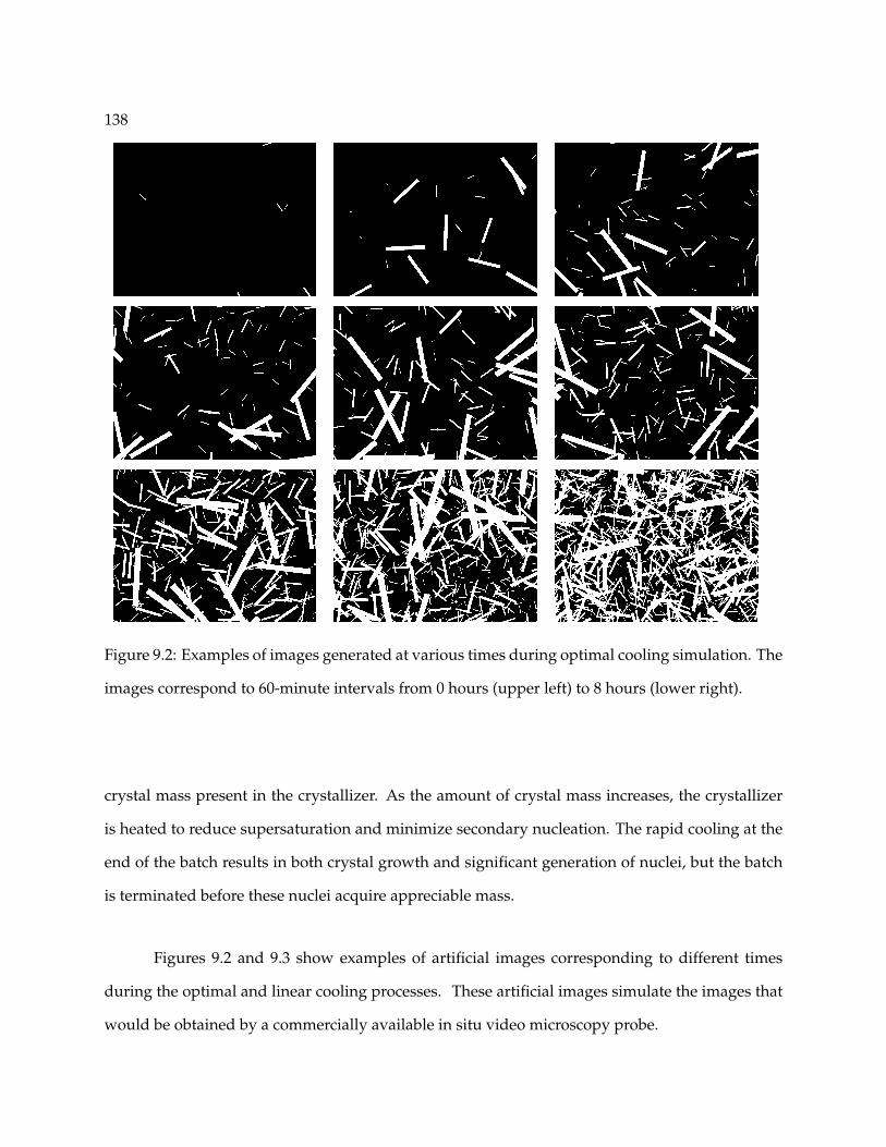
138

Figure 9.2: Examples of images generated at various times during optimal cooling simulation. The

images correspond to 60-minute intervals from 0 hours (upper left) to 8 hours (lower right).

crystal mass present in the crystallizer. As the amount of crystal mass increases, the crystallizer

is heated to reduce supersaturation and minimize secondary nucleation. The rapid cooling at the

end of the batch results in both crystal growth and significant generation of nuclei, but the batch

is terminated before these nuclei acquire appreciable mass.

Figures 9.2 and 9.3 show examples of artificial images corresponding to different times

during the optimal and linear cooling processes. These artificial images simulate the images that

would be obtained by a commercially available in situ video microscopy probe.

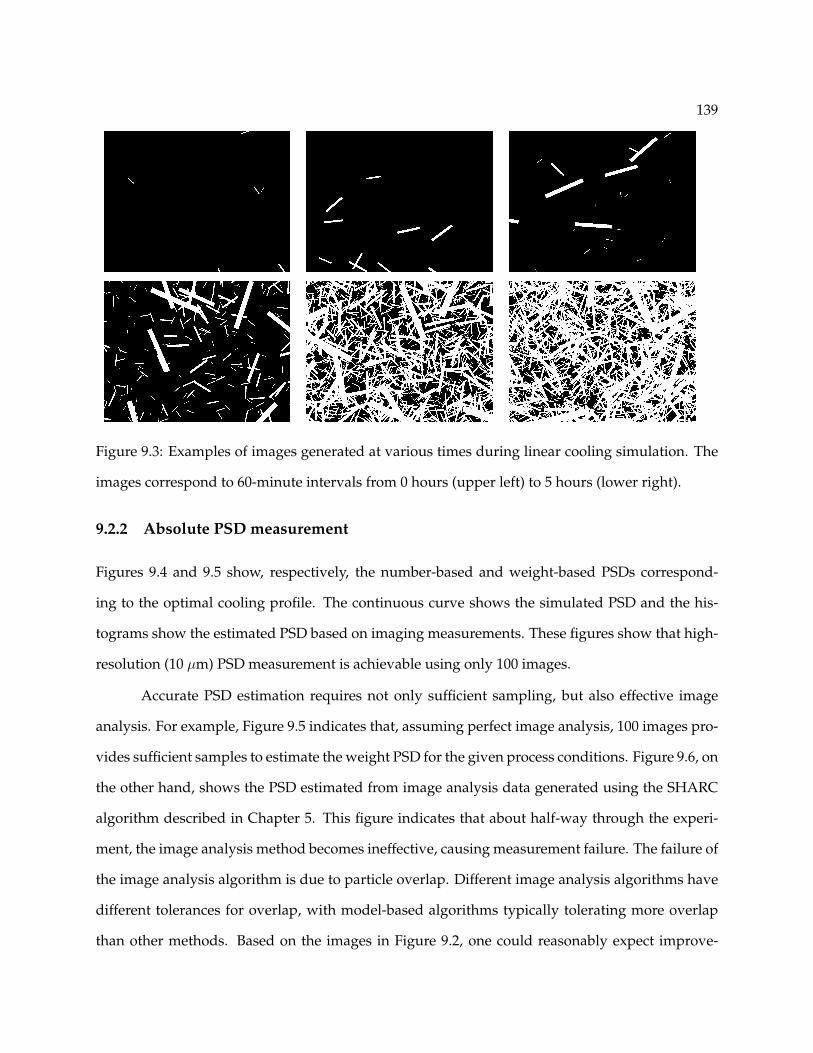
139

Figure 9.3: Examples of images generated at various times during linear cooling simulation. The

images correspond to 60-minute intervals from 0 hours (upper left) to 5 hours (lower right).

9.2.2 Absolute PSD measurement

Figures 9.4 and 9.5 show, respectively, the number-based and weight-based PSDs correspond-

ing to the optimal cooling profile. The continuous curve shows the simulated PSD and the his-

tograms show the estimated PSD based on imaging measurements. These figures show that high-

resolution (10 µm) PSD measurement is achievable using only 100 images.

Accurate PSD estimation requires not only sufficient sampling, but also effective image

analysis. For example, Figure 9.5 indicates that, assuming perfect image analysis, 100 images pro-

vides sufficient samples to estimate the weight PSD for the given process conditions. Figure 9.6, on

the other hand, shows the PSD estimated from image analysis data generated using the SHARC

algorithm described in Chapter 5. This figure indicates that about half-way through the experi-

ment, the image analysis method becomes ineffective, causing measurement failure. The failure of

the image analysis algorithm is due to particle overlap. Different image analysis algorithms have

different tolerances for overlap, with model-based algorithms typically tolerating more overlap

than other methods. Based on the images in Figure 9.2, one could reasonably expect improve-

140

0

0.2

0.4

0.6

0.8

1

1.2

1.4

0 100 200 300 400 500

PSD

,f,[

1/cm

3 ]

Length, [µm]

0

1

2

3

4

5

6

7

0 100 200 300 400 500

PSD

,f,[

1/cm

3 ]

Length, [µm]

02468

101214161820

0 100 200 300 400 500

PSD

,f,[

1/cm

3 ]

Length, [µm]

0

5

10

15

20

25

30

35

0 100 200 300 400 500

PSD

,f,[

1/cm

3 ]

Length, [µm]

0

10

20

30

40

50

60

0 100 200 300 400 500

PSD

,f,[

1/cm

3 ]

Length, [µm]

0102030405060708090

0 100 200 300 400 500

PSD

,f,[

1/cm

3 ]

Length, [µm]

0.001

0.01

0.1

1

10

100

1000

0 100 200 300 400 500

PSD

,f,[

1/cm

3 ]

Length, [µm]

0.001

0.01

0.1

1

10

100

1000

0 100 200 300 400 500

PSD

,f,[

1/cm

3 ]

Length, [µm]

0.001

0.01

0.1

1

10

100

1000

0 100 200 300 400 500

PSD

,f,[

1/cm

3 ]

Length, [µm]

Figure 9.4: Evolution of measured and estimated number-based PSD for optimal cooling and

perfect image analysis. Snapshots shown from t = 0 min. to t = 500 min. at 60 minute intervals.

Bin size = 10 µm and N = 100.

ments in model-based image analysis algorithms to enable effective measurement for almost the

entire duration of the process. On the other hand, as exemplified by the final image in Figure 9.3,

particle overlap can be so excessive that effective image analysis is unachievable.

9.2.3 Measurements for product quality

Product quality is often assessed based on the PSD. A variety of product quality metrics are used

in the crystallization optimal control literature (see Ward et al. [126] for a summary of this litera-

ture). The metrics involve both lower (number-based) and higher (weight-based) moments of the

PSD, as well as moments specific to the seed-grown crystals and nucleus-grown crystals. In the

141

0

0.02

0.04

0.06

0.08

0.1

0.12

0 100 200 300 400 500

wei

ghtP

SD,f

w,[

g/cm

3 ]

Length, [µm]

0

0.5

1

1.5

2

2.5

0 100 200 300 400 500

wei

ghtP

SD,f

w,[

g/cm

3 ]

Length, [µm]

0

1

2

3

4

5

6

0 100 200 300 400 500

wei

ghtP

SD,f

w,[

g/cm

3 ]

Length, [µm]

0

1

2

3

4

5

6

0 100 200 300 400 500

wei

ghtP

SD,f

w,[

g/cm

3 ]

Length, [µm]

0123456789

0 100 200 300 400 500

wei

ghtP

SD,f

w,[

g/cm

3 ]

Length, [µm]

0123456789

0 100 200 300 400 500

wei

ghtP

SD,f

w,[

g/cm

3 ]

Length, [µm]

0

2

4

6

8

10

12

0 100 200 300 400 500

wei

ghtP

SD,f

w,[

g/cm

3 ]

Length, [µm]

0

2

4

6

8

10

12

14

0 100 200 300 400 500

wei

ghtP

SD,f

w,[

g/cm

3 ]

Length, [µm]

02468

10121416

0 100 200 300 400 500

wei

ghtP

SD,f

w,[

g/cm

3 ]

Length, [µm]

Figure 9.5: Evolution of measured and estimated weight PSD for optimal cooling and perfect

image analysis. Snapshots shown from t = 0 min. to t = 500 min. at 60 minute intervals. Bin size

= 10 µm and N = 100.

following, we demonstrate the feasibility of monitoring a variety of these metrics using imaging.

Ratio of nuclei mass relative to seed mass

The ratio of nucleus-grown crystal mass mN to seed-grown crystal mass mS affects the efficiency of

downstream filtration processes [59, 82]. For the photochemical system considered here, mN/mS =

µN3/µS3 cannot be measured using conventional technologies. The needle-like habit violates the

sphericity assumption necessary for effective PSD measurement by light scattering. The needle-

like morphology also complicates mechanical sieving. In previous studies of this system, these

measurement difficulties motivated the use of scanning electron and optical microscopy to char-

acterize the PSD qualitatively in terms of habit and maximum size [81, p. 7]. Quantitative PSD

142

0

0.02

0.04

0.06

0.08

0.1

0.12

0.14

0 100 200 300 400 500

wei

ghtP

SD,f

w,[

g/cm

3 ]

Length, [µm]

00.20.40.60.8

11.21.41.61.8

2

0 100 200 300 400 500

wei

ghtP

SD,f

w,[

g/cm

3 ]

Length, [µm]

00.5

11.5

22.5

33.5

44.5

0 100 200 300 400 500

wei

ghtP

SD,f

w,[

g/cm

3 ]

Length, [µm]

0

1

2

3

4

5

6

0 100 200 300 400 500

wei

ghtP

SD,f

w,[

g/cm

3 ]

Length, [µm]

0

1

2

3

4

5

6

7

0 100 200 300 400 500

wei

ghtP

SD,f

w,[

g/cm

3 ]

Length, [µm]

02468

10121416

0 100 200 300 400 500

wei

ghtP

SD,f

w,[

g/cm

3 ]

Length, [µm]

0

2

4

6

8

10

12

0 100 200 300 400 500

wei

ghtP

SD,f

w,[

g/cm

3 ]

Length, [µm]

0

2

4

6

8

10

12

14

0 100 200 300 400 500

wei

ghtP

SD,f

w,[

g/cm

3 ]

Length, [µm]

02468

10121416

0 100 200 300 400 500

wei

ghtP

SD,f

w,[

g/cm

3 ]

Length, [µm]

Figure 9.6: Evolution of measured and estimated weight PSD for optimal cooling and image anal-

ysis using SHARC. Snapshots shown from t = 0 min. to t = 500 min. at 60 minute intervals. Bin

size = 10 µm and N = 100.

measurement by microscopy could not be achieved due to sampling limitations. Using high-

speed, in situ video microscopy, however, a sufficient number of samples can be obtained to enable

measurement of mN/mS .

In both cases, the images contain sufficient particles to enable estimation of mN/mS , as

shown in Figure 9.7. The estimates of mN/mS shown in Figure 9.7 are based on a sample size

of 100 images, corresponding to a sample time of approximately 3 seconds (assuming the stan-

dard 30 frames/second acquisition rate). The mN/mS estimates are also based on the assumption

that every particle appearing completely inside the imaging volume (not touching any borders) is

identified perfectly.

143

0

0.5

1

1.5

2

2.5

3

3.5

4

4.5

0 1 2 3 4 5 6 7 8 9

mN

/mS

time, t, [hr]

Linear, simLinear, measOptimal, sim

Optimal, meas

Figure 9.7: Estimated ratios of nuclei mass to seed crystal mass for optimal and linear cooling for

N = 100.

50

60

70

80

90

100

110

120

130

0 1 2 3 4 5 6 7 8 9

num

ber

mea

nsi

ze,[

µm

]

time, t, [hr]


Optimal, meas

60

80

100

120

140

160

180

200

220

240

0 1 2 3 4 5 6 7 8 9

wei

ghtm

ean

size

,[µ

m]

time, t, [hr]


Optimal, meas

(a) (b)

Figure 9.8: Estimated mean crystal sizes for optimal and linear cooling, N = 100. (a) Number-

based. (b) Weight-based.

Mean crystal size and coefficient of variation

The mean crystal size is commonly reported as an indication of product quality. Both the number-

based mean size (µ1/µ0) and weight-based mean size (µ4/µ3) can be estimated effectively using

imaging-based measurement, as shown in Figure 9.8. The coefficient of variation cv quantifies

the distribution spread. Typically a small cv is desired to improve the efficiency of downstream

manufacturing processes. Figure 9.9 demonstrates that both the number-based cv (µ2µ0/µ21) and

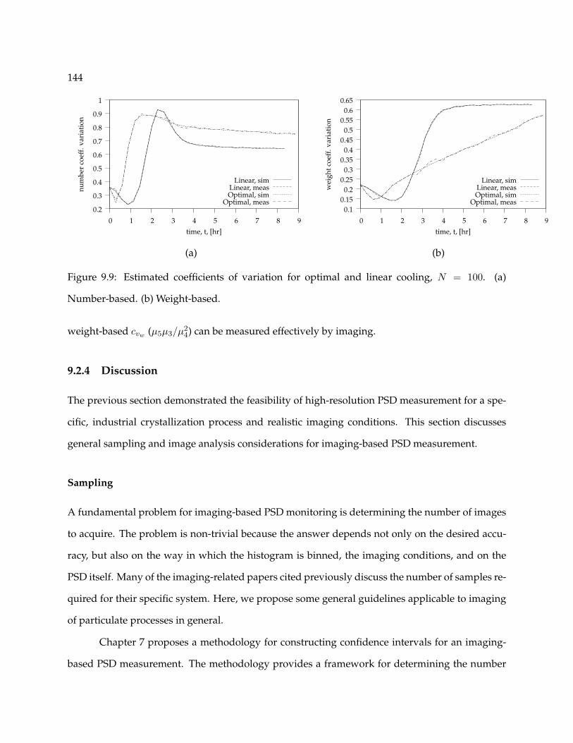
144

0.2

0.3

0.4

0.5

0.6

0.7

0.8

0.9

1

0 1 2 3 4 5 6 7 8 9

num

ber

coef

f.va

riat

ion

time, t, [hr]


Optimal, meas0.1

0.150.2

0.250.3

0.350.4

0.450.5

0.550.6

0.65

0 1 2 3 4 5 6 7 8 9

wei

ghtc

oeff

.var

iati

on

time, t, [hr]


Optimal, meas

(a) (b)

Figure 9.9: Estimated coefficients of variation for optimal and linear cooling, N = 100. (a)

Number-based. (b) Weight-based.

weight-based cvw (µ5µ3/µ24) can be measured effectively by imaging.

9.2.4 Discussion

The previous section demonstrated the feasibility of high-resolution PSD measurement for a spe-

cific, industrial crystallization process and realistic imaging conditions. This section discusses

general sampling and image analysis considerations for imaging-based PSD measurement.

Sampling

A fundamental problem for imaging-based PSD monitoring is determining the number of images

to acquire. The problem is non-trivial because the answer depends not only on the desired accu-

racy, but also on the way in which the histogram is binned, the imaging conditions, and on the

PSD itself. Many of the imaging-related papers cited previously discuss the number of samples re-

quired for their specific system. Here, we propose some general guidelines applicable to imaging

of particulate processes in general.

Chapter 7 proposes a methodology for constructing confidence intervals for an imaging-

based PSD measurement. The methodology provides a framework for determining the number

145

of images necessary to achieve a desired accuracy. Number-based PSDs are typically measured

by discretizing the characteristic length scale into T non-overlapping bins or size classes. We

therefore define the discrete PSD as

ρi =∫ Si+1

Si

f(l)dl, i = 1, . . . , T (9.7)

in which S = (S1, . . . , ST+1) is the vector of breaks between size classes. The maximum likelihood

estimate of ρi is calculated from imaging data using

ρi =XΣi

Nαi(9.8)

in which XΣi is the total number of particles observed in N images with lengths corresponding

to bin i, and αi is a scalar that corrects for edge effects due to the finite size of the imaging frame

(αi approaches 1 for infinitely-small particles and approaches 0 for particles the size of the image

field of view). The variance of this estimator, which is directly related to the confidence intervals,

is given by

V ar(ρi) =ρi

Nαi(9.9)

Equation (9.9) contains all the process, imaging, and sampling information necessary to assess

the accuracy of an imaging-based PSD measurement. As mentioned, the accuracy depends not

only on the number of images N and the desired resolution, but also on the imaging conditions,

particle size, and particle geometry (all of which are encapsulated in the correction factor αi) and

on the number density of particles ρi. As a result, the number of images required to obtain a given

accuracy changes as the particle population evolves.

To use Equation (9.9), one needs to know ρi. Batch crystallizations are typically seeded,

and usually some knowledge of the seed population is available. For example, if the seed crystal

population is prepared by sieving, the initial minimum crystal size and maximum size are known.

The mass of seed crystals injected into the crystallizer is also known. This information is sufficient

to obtain a rough estimate of ρi for the bins corresponding to the seed population, enabling cal-

culation of the N that gives a sufficiently small variance (i.e. confidence interval). It is, of course,

146

desirable to monitor the PSD of the nucleus-grown crystals also, but the number of the nucleus-

grown crystals typically is much greater than the number of the seed-grown crystals, as illustrated

in Figure 9.4. Thus, a value of N that enables accurate tracking of the seed PSD will, in most cases,

also enable accurate tracking of the nucleated crystals’ PSD.

Image analysis

As discussed in Section 9.2.2, imaging-based PSD measurement requires not only sufficient sam-

pling but also effective image analysis. The effectiveness of any image analysis algorithm de-

pends strongly on the amount of particle overlap. Chapter 8 gives an approach for quantifying

the amount of particle overlap for mono-disperse populations. With this approach, the average

number of overlaps per particle is predicted to be

D = µ0Ωdf (9.10)

in which D is the average number of overlaps, µ0 is the zeroth moment of the PSD, df is the

depth of field, and Ω is the “admissible area,” which is based on the particle geometry. Assuming

random orientation in the plane perpendicular to the camera’s optical axis, Ω is calculated using

Mack’s formula [77]:

Ω = 2ap +s2p

2π(9.11)

in which ap and sp are, respectively, the projected area and perimeter of a single particle in its

preferred (resting) orientation. Equation (8.4) can be used to determine appropriate sampling

conditions for imaging-based measurement. For example, one could assume the seed population

to be approximately mono-disperse and use Equation (8.4) to predict the number of overlaps per

particle for a given mass of seed. If the number of overlaps is too high for current image analysis

methods, one may choose to use dilution or an optical system with a smaller depth of field.

147

9.3 Conclusion

Video imaging is a viable technology for on-line PSD monitoring and control. The feasibility of

high-resolution, imaging-based PSD measurement has been demonstrated using a realistic indus-

trial crystallization process. Imaging-based measurement enables both number and weight-based

PSD monitoring as well as product quality measurements that are difficult to obtain using alter-

native monitoring technologies, such as the ratio of nuclei mass to seed mass. General recommen-

dations for determining appropriate sampling conditions for imaging-based PSD measurement

have also been given. The proposed tools facilitate the design of effective, imaging-based PSD

monitoring technology.

This chapter has also highlighted directions for future research to improve imaging-based

PSD measurement. Most importantly, advances in image analysis algorithms are needed to im-

prove image segmentation when particle overlap is significant. These advances will require fur-

ther statistical estimation studies to address sampling biases due to particle overlap or occlusion.

Current statistical methods adequately address edge effects (i.e. sampling bias associated with the

finite size of the imaging window), but further consideration is required for errors associated with

depth of field effects.

148

149

Chapter 10

ConclusionThis thesis has developed tools that enable effective use of video imaging technology for on-line

monitoring of particulate populations. These tools include (1) image analysis algorithms that en-

able segmentation of in situ video images of crystallization processes, (2) an easy-to-implement,

computationally inexpensive method for estimating the PSD from imaging data, and (3) a dimen-

sionless parameter that is useful for quantifying particle overlap and assessing the reliability of

imaging-based PSD measurement. In this chapter, we briefly review the contributions made by

these tools and discuss areas that merit further research.

The SHARC algorithm discussed in Chapter 5 can robustly and efficiently extract crystal

length and width information from in situ images of suspended, high-aspect-ratio crystals for

moderate solids concentrations, giving results consistent with measurements obtained through

manual image analysis by human operators. The speed with which SHARC analyzes the images

is suitable for real-time monitoring and control of PSD mean and variance. Implementation using

compiled code is expected to enable real-time, high-resolution PSD monitoring. SHARC has been

patented by the Wisconsin Alumni Research Foundation (WARF) and licensed by Mettler-Toledo

(MT). MT expects to include the SHARC algorithm in their next generation Particle and Vision

Measurement (PVM) in situ video probe.

SHARC’s performance declines for high solids concentrations and high levels of particle

attrition because the degree of particle overlap and the noise arising from attrited particulate mat-

ter hinder the identification of the suspended crystals’ edges. Implementing improved methods

for identifying instances of collinearity may enable suitable performance for these conditions.

150

SHARC currently performs collinear identification only once, but we expect iterative collinear

identification to improve SHARC’s performance in the presence of significant particle overlap.

The M-SHARC algorithm discussed in Chapter 6 is useful for extracting crystal size and

shape information from in situ crystallization images of particles with complex shapes. The algo-

rithm’s accuracy has been assessed by comparing its results with those obtained by manual, hu-

man analysis of the images. Despite a large number of misses and false positives, M-SHARC’s cu-

mulative size distribution (CDF) measurements compare favorably with measurements obtained

by humans. In general, the CDFs are biased towards larger particles. The algorithm is sufficiently

fast to provide on-line measurements for typical cooling crystallization processes. M-SHARC has

been patented by WARF.

To improve the algorithm’s accuracy, further development should focus on the algorithm’s

verification stage and on creating initialization routines for additional viewpoint-invariant line

groups. The images and human annotations that have been used to evaluate the M-SHARC algo-

rithm are available online via MIT’s LabelMe project (labelme.csail.mit.edu). We hope this data

set will be useful for benchmarking and comparing the performance of image analysis algorithms

developed in the future.

Chapter 7 developed the maximum likelihood estimator (MLE) for imaging-based PSD

measurement of needle-like particles. The estimator uses both censored and uncensored obser-

vations (i.e. border and non-border particles). MLE is more efficient than the standard Miles-

Lantuejoul approach, particularly if the particle population is mono-disperse or contains particles

that are large relative to the size of the image. Furthermore, MLE can estimate the number density

of over-sized particles (particles bigger than the image dimension) along with the size Lmax of the

largest particle while the Miles-Lantuejoul approach can be applied only for particles smaller than

the image dimension.

The primary limitation of the MLE derived in Chapter 7 is due to the assumption that the

particles have needle-like geometry. The Miles-Lantuejoul approach, on the other hand, can be

applied to a much wider class of geometries. Secondly, the MLE approach requires the solution

151

of a nonlinear optimization problem. To avoid the necessity of solving an optimization problem,

a simpler MLE was proposed in Chapter 7 that uses only non-border particle measurements. The

efficiency of the simple MLE is comparable to that of the Miles-Lantuejoul estimator.

Several areas for future work in the area of statistical estimation of PSD are evident. Choos-

ing the optimal number, location, and size of bins for constructing histograms should be ad-

dressed. Integrating measurements taken at multiple scales or magnifications is also important.

For systems of high-aspect-ratio particles, incorporating the width of border particles into the esti-

mation could lead to increased efficiency by narrowing down the number of size classes to which

a border particle may correspond.

In Chapter 8, a practical approach was developed for assessing the reliability of num-

ber density estimates obtained using imaging measurements in the presence of particle overlap.

The single dimensionless parameter D correlates with the measurement reliability based on the

amount of particle overlap. Thus, the parameter D can be used to estimate the errors in the mea-

surements and to aid practitioners in determining the sampling conditions necessary to obtain

reliable measurement of particle number density.

It was shown in Chapter 8 that the Miles-Lantuejoul estimator, which accounts for edge

effects but not particle overlap, underestimates the number density. Thus, a maximum likelihood

estimator that accounts for both edge effects and particle overlap has been presented. The esti-

mator is based on a semi-empirical model of the probability that a given particle will be correctly

identified by automatic image analysis. For a given particle size, a single empirical parameter

is sufficient to enable effective number density estimation for a wide range of conditions, par-

ticularly for systems in which the particles’ dimensions are significantly smaller than the image

dimensions.

Various issues related to statistical estimation in the presence of particle overlap should

be addressed in future work. Most importantly, an extension of the methods developed in this

paper should be developed for polydisperse systems. Armitage [4] and Roach [104, p.46] give

discussions that may provide a good starting point for such investigations. The incorporation

152

of these methods into a state estimator for feedback control of number density should also be

investigated.

Chapter 9 demonstrated the feasibility of high-resolution, imaging-based PSD measure-

ment using a realistic industrial crystallization process. Imaging-based measurement enables both

number and weight-based PSD monitoring as well as product quality measurements that are dif-

ficult to obtain using alternative monitoring technologies, such as the ratio of nuclei mass to seed

mass. Chapter 9 also discussed how the tools developed in this thesis can be used to determine

appropriate sampling conditions for imaging-based PSD measurement.

The results in Chapter 9 highlight directions for future research to improve imaging-based

PSD measurement. Most importantly, and as noted previously, advances in image analysis algo-

rithms are needed to improve image segmentation when particle overlap is significant. These ad-

vances will require further statistical estimation studies to address sampling biases due to particle

overlap or occlusion. Current statistical methods adequately address edge effects (i.e. sampling

bias associated with the finite size of the imaging window), but further consideration is required

for errors associated with depth of field effects.

In summary, the tools developed in this thesis facilitate the design of effective, imaging-

based PSD monitoring technology. As the advances discussed in this thesis are incorporated into

commercial sensor technology, we expect improved understanding and control of industrial crys-

tallization processes.

153

Appendix A

Derivations for Maximum Likelihood

Estimation of PSD

A.1 Maximum likelihood estimation of PSD

Let Xk = (X1k, . . . , XTk) be a T -dimensional random vector in which Xik gives the number of

non-border particles of size class i observed in image k. A non-border particle is a particle that

is completely enclosed within the imaging volume. A border particle, on the other hand, is only

partially enclosed within the imaging volume such that only a portion of the particle is observable.

For border particles, only the observed length (i.e. the length of the portion of the particle that

is inside the imaging volume) can be measured. Accordingly, we let Y k = (Y1k, . . . , YTk) be a

T -dimensional random vector in which Yjk gives the number of border particles with observed

lengths in size class j that are observed in image k. We denote the observed data, or the realizations

of the random vectors Xk and Y k, as xk and yk, respectively.

The particle population is represented completely by the vectors ρ = (ρi, . . . , ρT ) and S =

(S1, . . . , ST+1) in which ρi represents the number of particles of size class i per unit volume and

Si is the lower bound of size class i. Given the data x and y (the subscript k denoting the image

index is removed here for simplicity), the maximum likelihood estimator of ρ is defined as

ρb = arg maxρ

pXY (x1, y1, x2, y2, . . . , xT , yT |ρ) (A.1)

in which in which the subscript b indicates the use of border particle measurements and pXY is the

154

joint probability density for X and Y . In other words, we want to determine the value of ρ that

maximizes the probability of observing exactly x1 non-border particles of size class 1, y1 border

particles of size class 1, x2 non-border particles of size class 2, y2 border particles of size class 2,

and so on.

A simplified expression for pXY can be obtained by noting that, at least at low solids con-

centrations, the observations X1, Y1, . . . XT , YT can be assumed to be independent. This assump-

tion means that the observed number of particles of a given size class depends only on the density

of particles in that same size class. At high solids concentrations, this assumption seems unreason-

able because the number of particle observations in a given size class is reduced due to occlusions

by particles in other size classes. At low concentrations, however, the likelihood of occlusion

is low. The independence assumption does not imply that the observations are not correlated.

Rather, the assumption implies that any correlation between observations is due to their depen-

dence on a common set of parameters. As an example, if we observe a large number of non-border

particles, we would expect to also observe a large number of border particles. This correlation can

be explained by noting that the probability densities for both border and non-border observa-

tions depend on a common parameter, namely, the density of particles. Given the independence

assumption, we express pXY as

pXY =T∏

i=1

pXi(xi|ρ)T∏

j=1

pYj (yj |ρ) (A.2)

in which pXi and pYj are the probability densities for the random variables Xi and Yj . Using

Equation (A.2), the estimator in Equation (A.1) can be reformulated as

ρb = arg minρ

T∑i=1

− log pXi(xi|ρ)−T∑

j=1

log pYj (yj |ρ) (A.3)

The probability densities pXi and pYj are derived in the following sections. These deriva-

tions show that Xi ∼ Poisson(mXi), or that Xi has a Poisson distribution with parameter mXi =

ρiαi, in which αi is a function of the field of view, depth of field, and the lower and upper bounds

of size class i. Furthermore, Yj ∼ Poisson(mYj ), in which mYj =∑T

i=1 ρiβij

155

A.2 Derivation of probability densities

The probability densities pXi and pYi in Equation (A.3) can be derived given the particle geom-

etry and the spatial and orientational probability distributions. Here, we derive pXi and pYi for

needle-like particles assuming the particles are randomly, uniformly distributed, both in their 3-

dimensional spatial location and in their orientation in the plane perpendicular to the optical axis.

To simplify the discussion, we initially present the derivation assuming a 2-dimensional system

with monodisperse, vertically-oriented particles. Later, we relax these assumptions and present

the derivation for randomly-oriented, polydisperse particles in 3-dimensional space.

A.2.1 Non-border particles

Let S be a square domain in R2 with dimension B and area AS = B2. Let I be a rectangular

domain in R2 with horizontal and vertical dimensions a and b, respectively, and area AI = ab.

Assume AI AS and I ∈ S. Let ntot be the total number of vertically-oriented particles with

midpoints randomly and uniformly distributed in S, and define ρ = ntot/AS as the density of

particles per unit area. Let the length of all particles be l, with l < min (a, b), and define Anb as the

area of the domain in which particles are inside I but do not touch the border of I . Because the

particles are oriented vertically, it is easy to show that Anb = a(b− l), as depicted in Figure A.1(a).

Finally, let X be a random variable denoting the number of non-border particles appearing in I .

Assuming the location of each particle in S is independent of the remaining particles’ locations,

the probability that a specific particle will appear entirely within I is given by p = Anb/AS . Given

the above assumptions, this probability is constant for all particles. The probability of observing x

non-border particles in I is analogous to the probability of observing x successes in ntot Bernoulli

trials in which the probability of success in each trial is p. Thus, X is a binomial random variable

with probability distribution

pX(x) =

ntot

x

px(1− p)ntot−x

156

l/2I

b

a

Anb

l/2l

S

a

l l

I

b

S

Ab

(a) (b)

Figure A.1: Depiction of hypothetical system of vertically-oriented particles randomly and uni-

formly distributed in space.

Now, assume B →∞ while keeping ρ constant. Then ntot →∞ and p = Anb/AS = Anbρ/ntot → 0

while Np = ρAnb remains constant. The limiting distribution of X is therefore Poisson

pX(x) =e−mX mx

X

x!, mX = ρAnb

To extend the analysis to polydisperse, randomly-oriented needles, we discretize the length

scale into T size classes and let X = (X1, . . . , XT ) be a T -dimensional random vector in which Xi

gives the number of non-border particles of size class i observed in a single image. An orientation Θ

and length L are assigned to each particle, where Θ1,Θ2, . . . ,Θntot are i.i.d. with density function

pΘ(θ), θ ∈ [−π/2, π/2) and L1, L2, . . . , Lntot are i.i.d. with density function pL(l), l ∈ (0, inf). Θ and

L are independent of each other and independent of the particle’s spatial location. We define S as

the T+1-dimensional vector of breaks between size classes. A particle of length l belongs to size

class i if Si ≤ l < Si+1. Let ∆i = Si+1 − Si. Our goal is to determine the probability that a particle

of size class i will appear entirely inside the image I , given its density ρi. Following the approach

used to solve the Buffon-Laplace needle problem [116, p. 4], Figure A.2 shows geometrically that

157

l

Anb(l, θ)

a

b

θ

l/2 cos θ l/2 cos θ

l/2 sin θ

l/2 sin θ

Figure A.2: Depiction of geometrical properties used to derive the non-border area function

Anb(l, θ).

for a given orientation θ and length l, Anb(l, θ) can be calculated as

Anb(l, θ) =

(a− l cos θ)(b− l sin θ) 0 ≤ θ ≤ π/2

(a− l cos θ)(b + l sin θ) −π/2 ≤ θ ≤ 0(A.4)

The probability that a given particle in size class i will appear entirely within I is given by

pi =

∫ Si+1

Si

∫ π2

−π2

Anb(l, θ)pΘ(θ)pL(l)dθdl∫ Si+1

Si

∫ π2

−π2

ASpΘ(θ)pL(l)dθdl

(A.5)

Thus, the probability that a specific particle of size class i will appear entirely within the image is

given by pi = αi/AS , where αi is the numerator in Equation (A.5). Following the same arguments

as above, we can show that for an infinitely large system, Xi is a Poisson random variable with

parameter mXi = ρiαi.

Extending the analysis to three-dimensional space is trivial because we assume the parti-

cles are oriented in the plane perpendicular to the camera’s optical axis and assume no interaction

between particles. Thus, for a three-dimensional system, Xi is a Poisson random variable with

parameter mXi = ρiαi, with αi = αid, in which d is the depth of field.

Assuming Θ is distributed uniformly and L is distributed uniformly across each size class,

αi can be calculated as follows. Let ∆Si = Si+1 − Si, Smax =√

a2 + b2, ∆Si,max = Smax − Si, and

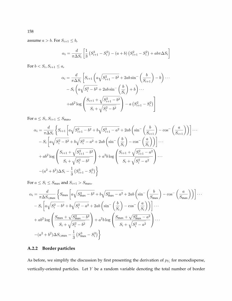
158

assume a > b. For Si+1 ≤ b,

αi =d

π∆Si

[13

(S3

i+1 − S3i

)− (a + b)

(S2

i+1 − S2i

)+ abπ∆Si

]For b < Si, Si+1 ≤ a,

αi =d

π∆Si

[Si+1

(a√

S2i+1 − b2 + 2ab sin−

(b

Si+1

)− b

)· · ·

− Si

(a√

S2i − b2 + 2ab sin−

(b

Si

)+ b

)· · ·

+ab2 log

Si+1 +√

S2i+1 − b2

Si +√

S2i − b2

− a(S2

i+1 − S2i

)For a ≤ Si, Si+1 ≤ Smax,

αi =d

π∆Si

Si+1

[a√

S2i+1 − b2 + b

√S2

i+1 − a2 + 2ab

(sin−

(b

Si+1

)− cos−

(a

Si+1

))]· · ·

− Si

[a√

S2i − b2 + b

√S2

i − a2 + 2ab

(sin−

(b

Si

)− cos−

(a

Si

))]· · ·

+ ab2 log

Si+1 +√

S2i+1 − b2

Si +√

S2i − b2

+ a2b log

Si+1 +√

S2i+1 − a2

Si +√

S2i − a2

· · ·

−(a2 + b2)∆Si −13

(S3

i+1 − S3i

)For a ≤ Si ≤ Smax and Si+1 > Smax,

αi =d

π∆Si,max

Smax

[a√

S2max − b2 + b

√S2

max − a2 + 2ab

(sin−

(b

Smax

)− cos−

(a

Smax

))]· · ·

− Si

[a√

S2i − b2 + b

√S2

i − a2 + 2ab

(sin−

(b

Si

)− cos−

(a

Si

))]· · ·

+ ab2 log

Smax +√

S2max − b2

Si +√

S2i − b2

+ a2b log

Smax +√

S2max − a2

Si +√

S2i − a2

· · ·

−(a2 + b2)∆Si,max −13

(S3

max − S3i

)

A.2.2 Border particles

As before, we simplify the discussion by first presenting the derivation of pYi for monodisperse,

vertically-oriented particles. Let Y be a random variable denoting the total number of border

159

particles appearing in I . Define Ab as the area of the domain in which particles touch the border

of I , as depicted in Figure A.3(a). For the present system, Ab = 2al. The probability that a specific

particle will touch the border of I is given by p = Ab/AS . Following the same arguments as above,

we can show that for an infinitely large system, Y is a Poisson random variable with parameter

mY = ρAb.

Now, assume we would like to incorporate additional information into our estimation by

taking into account not only the number of border particles, but also their observed lengths. For

a monodisperse population, these observed lengths can take on values anywhere between 0 and

l. We therefore discretize the length scale on [0 l] and let j denote the size class corresponding to

the observed length. We define Yj as a random variable denoting the number of border particles

appearing in I with observed length in size class j. Figure A.3(b) illustrates this approach for

two size classes. In this figure, Ab1 is the area of the region in which particles produce observed

lengths from 0 to l/2, corresponding to size class 1, while Ab2 is the area of the region in which

particles produce observed lengths from l/2 to l, corresponding to size class 2. The probability

that a specific particle will touch the border of I and produce an observed length in size class j is

p = Abj/AS . Thus, Yj is a Poisson random variable with parameter mYj = ρAbj

.

In Figure A.3(b), Ab1 = Ab2 . This equality between the areas of different observed length

size classes does not hold in general, however, as illustrated in Figure A.3(c). In this figure, we

assume all particles are oriented diagonally, at 45 degrees from the horizontal, and the figure

illustrates that Ab1 > Ab2 . Hence, in general, border particles are more likely to result in observed

lengths in the lower size classes.

To extend the analysis to polydisperse systems with random orientation, we define a new

random variable Yij that gives the number of particles in size class i that intersect the image bor-

der, producing an observed length in size class j. Given that the size class of each border particle

is unknown, we define the random variable Yj as the total number of border particles produc-

ing observed lengths in size class j, noting that Yj =∑

i Yij . Our approach is to determine the

probability density for Yij for all i and to use these densities to derive the probability density for

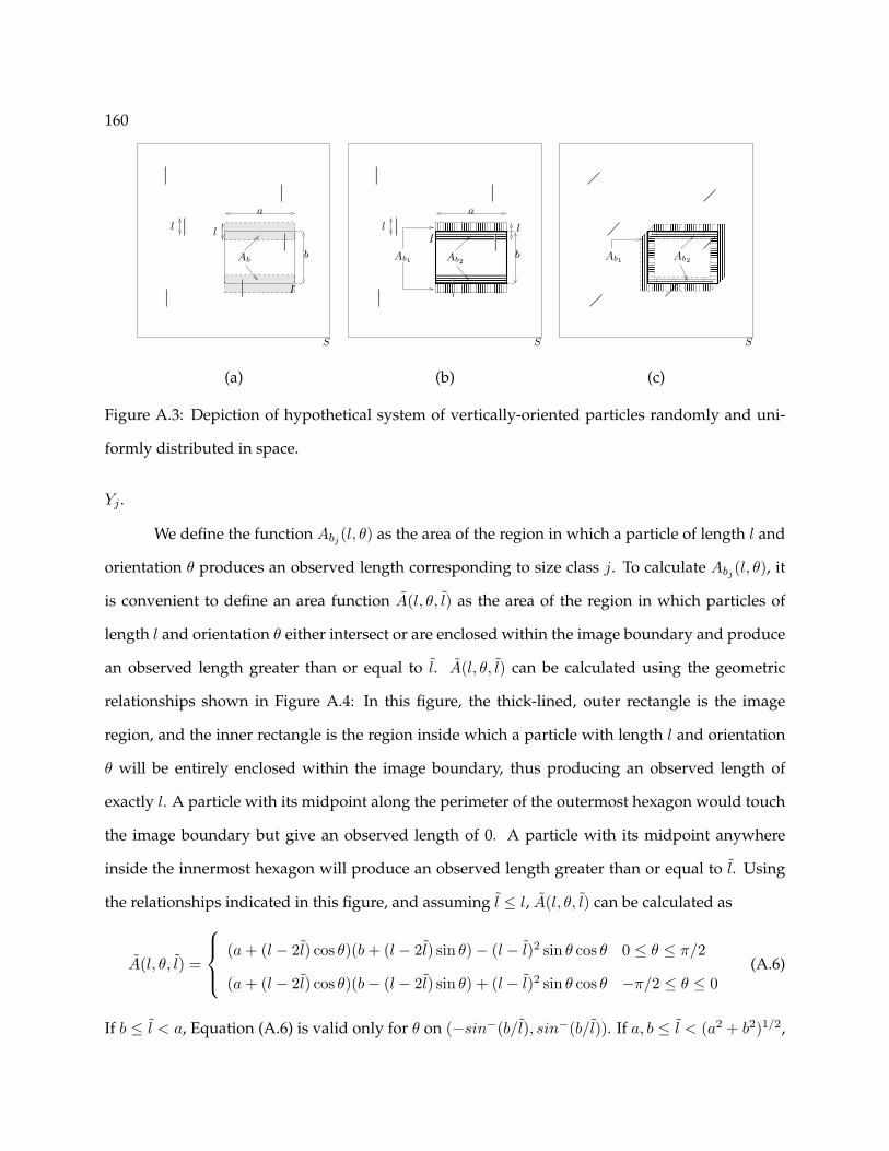
160

a

l l

I

b

S

Ab

a

l

b

S

Ab2

l

Ab1

I

S

Ab1 Ab2

(a) (b) (c)

Figure A.3: Depiction of hypothetical system of vertically-oriented particles randomly and uni-

formly distributed in space.

Yj .

We define the function Abj(l, θ) as the area of the region in which a particle of length l and

orientation θ produces an observed length corresponding to size class j. To calculate Abj(l, θ), it

is convenient to define an area function A(l, θ, l) as the area of the region in which particles of

length l and orientation θ either intersect or are enclosed within the image boundary and produce

an observed length greater than or equal to l. A(l, θ, l) can be calculated using the geometric

relationships shown in Figure A.4: In this figure, the thick-lined, outer rectangle is the image

region, and the inner rectangle is the region inside which a particle with length l and orientation

θ will be entirely enclosed within the image boundary, thus producing an observed length of

exactly l. A particle with its midpoint along the perimeter of the outermost hexagon would touch

the image boundary but give an observed length of 0. A particle with its midpoint anywhere

inside the innermost hexagon will produce an observed length greater than or equal to l. Using

the relationships indicated in this figure, and assuming l ≤ l, A(l, θ, l) can be calculated as

A(l, θ, l) =

(a + (l − 2l) cos θ)(b + (l − 2l) sin θ)− (l − l)2 sin θ cos θ 0 ≤ θ ≤ π/2

(a + (l − 2l) cos θ)(b− (l − 2l) sin θ) + (l − l)2 sin θ cos θ −π/2 ≤ θ ≤ 0(A.6)

If b ≤ l < a, Equation (A.6) is valid only for θ on (−sin−(b/l), sin−(b/l)). If a, b ≤ l < (a2 + b2)1/2,

161

θl

a

b−

lsin

θ

b

(l − l) sin θ

a− l cos θ

a

lθ

b

b

a

(l − l) cos θ

l −l

θ

Figure A.4: Depiction of non-border area for arbitrary length and orientation.

Equation (A.6) is valid only for θ on (−sin−(b/l),−cos−(a/l)) and (cos−(a/l), sin−(b/l)). Abj(l, θ)

is given by

Abj(l, θ) =

A(l, θ, Sj)− A(l, θ, Sj+1) l ≥ Sj+1

A(l, θ, Sj)−Anb(l, θ) Sj ≤ l < Sj+1

0 l < Sj

(A.7)

The probability that a given particle in size class i will appear within I and produce an

observed length in size class j is given by

pij =

∫ Si+1

Si

∫ π2

−π2

Abj(l, θ)pΘ(θ)pL(l)dθdl∫ Si+1

Si

∫ π2

−π2

ASpΘ(θ)pL(l)dθdl

(A.8)

The probability that a specific particle in size class i will touch the border of I and produce an

observed length in size class j is pij = βij/AS , with βij being the numerator in Equation (A.8).

Thus, for an infinitely large system, Yij is a Poisson random variable with parameter mYij = ρiβij .

Assuming Y1j , Y2j , . . . , YTj are independent, then Yj =∑

i Yij is also a Poisson random variable

162

with parameter mYj =∑

i ρiβij [12, p.440]. As in the non-border case, the analysis is extended

to three-dimensional space assuming the particles are oriented in the plane perpendicular to the

camera’s optical axis and that the particles do not interact. Thus, for a three-dimensional system,

Yj is a Poisson random variable with parameter mYj =∑

i ρiβij , with βij = βijd.

Assuming Θ is distributed uniformly and L is distributed uniformly across each size class,

βij is calculated as follows. Let the length scale discretization be the same for both border and

non-border particles. As before, let ∆Si = Si+1 − Si, Smax =√

a2 + b2, ∆Si,max = Smax − Si, and

assume a > b. Then βij is given by

βij =

A(i, Sj)− A(i, Sj+1) i > j

A(i, Sj)− αi i = j

0 i < j

(A.9)

in which A(i, S) is calculated as

A(i, S) =d

π∆Si

[∆Si

(2abγ1 − 4bSγ2 − 4aSγ3 + 3S2γ4

)+

(S2

i+1 − S2i

)(bγ2 + aγ3 − Sγ4)

]

γ1 =

π/2 S < b

sin− (b/S) b < S < a

sin− (b/S)− cos− (a/S) a < S < Smax

sin− (b/Smax)− cos− (a/Smax) S > Smax

γ2 =

1 S < b

b/S b < S < a(b−

√S2 − a2

)/S a < S < Smax(

b−√

S2max − a2

)/Smax S > Smax

γ3 =

1 S < b

1−√

S2 − b2/S b < S < a(a−

√S2 − b2

)/S a < S < Smax(

a−√

S2max − b2

)/Smax S > Smax

163

γ4 =

1 S < b

b2/S2 b < S < a

(a2 + b2 − S2)/S2 a < S < Smax

(a2 + b2 − S2max)/S2

max S > Smax

A.3 Validation of marginal densities

To ensure the correctness of the probability densities derived in the previous section, four different

Monte Carlo simulations were carried out in which artificial images of particulate populations

were generated. Figure 7.2 shows example images generated for each simulation. Each of these

images has a horizontal image dimension of a=480 pixels and a vertical dimension of b=480 pixels.

The first row displays four simulated images for monodisperse particles of length 0.5a with Nc=25

crystals per image. The second row shows images of particles uniformly distributed on [0.1a 0.9a]

with Nc=25. The third row shows images of particles normally-distributed with µ = 0.5a and

σ = 0.4a/3 with Nc=25, and the fourth row shows example images for simulations of particles

uniformly-distributed on [0.1a 2.0a] with Nc=15. For each simulation, 20,000 artificial images

were generated. Based on the observations in these 20,000 images, a histogram was generated

for each size class giving the frequency of observations for both border and non-border particles.

These histograms are compared with the theoretical marginal densities in Figures A.5– A.12.

164

0

0.1

0 5 10 15 20 25

prob

abili

tym

ass

Number of particles observed

TheorySimulation

Figure A.5: Comparison of theoretical and simulated marginal densities for randomly-oriented,

monodisperse particles of length 0.5 and measured by partitioning [0.1 0.9] into ten bins. Results

are for non-border particles.

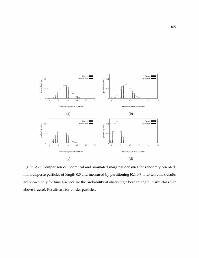
165

0

0.1

0.2

0 5 10 15 20 25

prob

abili

tym

ass


TheorySimulation

0

0.1

0.2

0 5 10 15 20 25

prob

abili

tym

ass


TheorySimulation

(a) (b)

0

0.1

0.2

0 5 10 15 20 25

prob

abili

tym

ass


TheorySimulation

0

0.1

0.2

0 5 10 15 20 25

prob

abili

tym

ass


TheorySimulation

(c) (d)

Figure A.6: Comparison of theoretical and simulated marginal densities for randomly-oriented,

monodisperse particles of length 0.5 and measured by partitioning [0.1 0.9] into ten bins (results

are shown only for bins 1–4 because the probability of observing a border length in size class 5 or

above is zero). Results are for border particles.

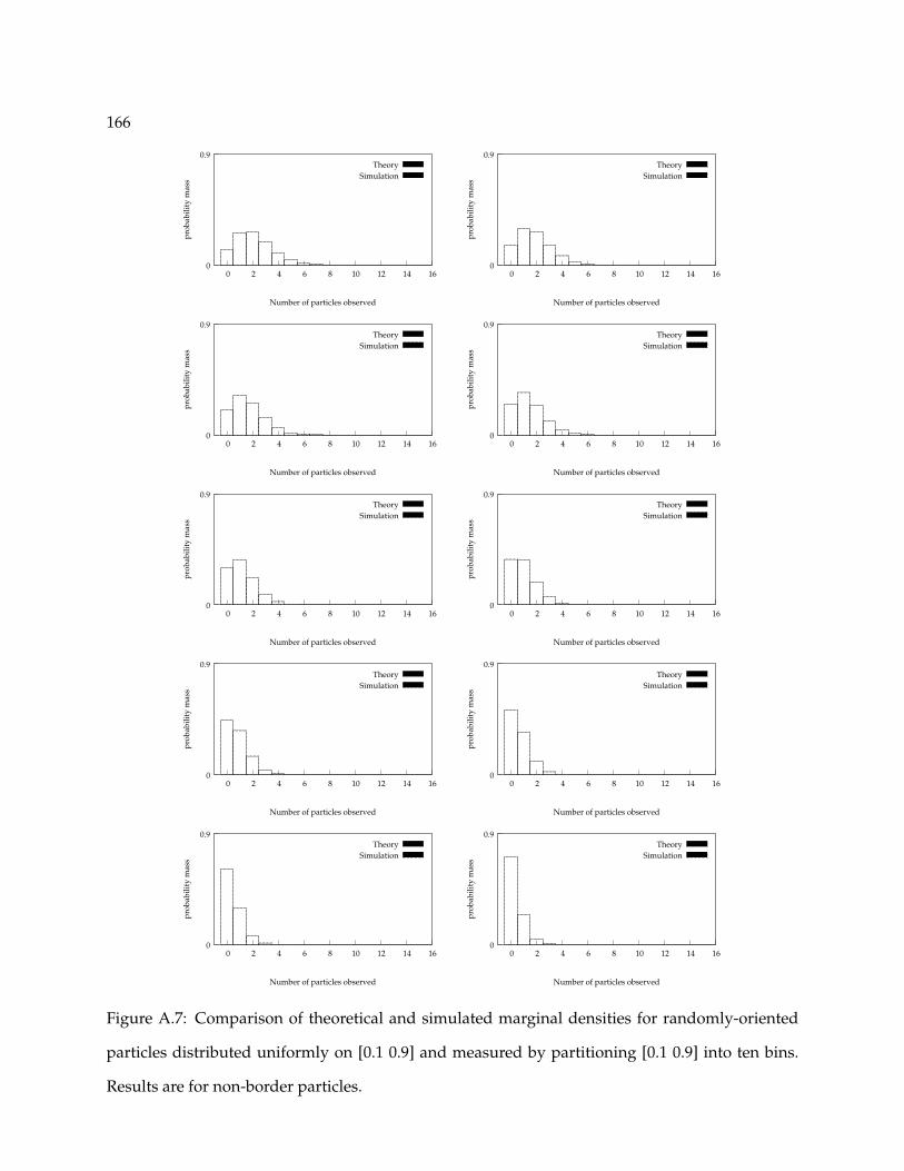
166

0

0.9

0 2 4 6 8 10 12 14 16

prob

abili

tym

ass


TheorySimulation

0

0.9

0 2 4 6 8 10 12 14 16

prob

abili

tym

ass


TheorySimulation

0

0.9

0 2 4 6 8 10 12 14 16

prob

abili

tym

ass


TheorySimulation

0

0.9

0 2 4 6 8 10 12 14 16

prob

abili

tym

ass


TheorySimulation

0

0.9

0 2 4 6 8 10 12 14 16

prob

abili

tym

ass


TheorySimulation

0

0.9

0 2 4 6 8 10 12 14 16

prob

abili

tym

ass


TheorySimulation

0

0.9

0 2 4 6 8 10 12 14 16

prob

abili

tym

ass


TheorySimulation

0

0.9

0 2 4 6 8 10 12 14 16

prob

abili

tym

ass


TheorySimulation

0

0.9

0 2 4 6 8 10 12 14 16

prob

abili

tym

ass


TheorySimulation

0

0.9

0 2 4 6 8 10 12 14 16

prob

abili

tym

ass


TheorySimulation

Figure A.7: Comparison of theoretical and simulated marginal densities for randomly-oriented

particles distributed uniformly on [0.1 0.9] and measured by partitioning [0.1 0.9] into ten bins.

Results are for non-border particles.

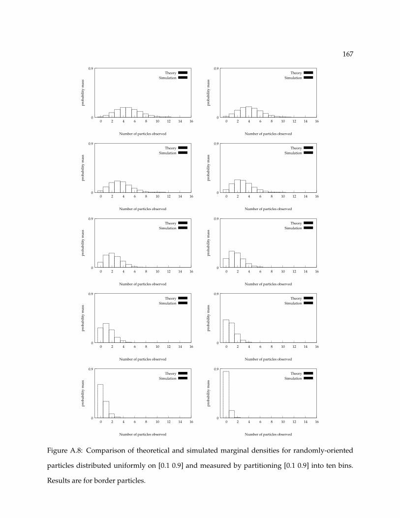
167

0

0.9

0 2 4 6 8 10 12 14 16

prob

abili

tym

ass


TheorySimulation

0

0.9

0 2 4 6 8 10 12 14 16

prob

abili

tym

ass


TheorySimulation

0

0.9

0 2 4 6 8 10 12 14 16

prob

abili

tym

ass


TheorySimulation

0

0.9

0 2 4 6 8 10 12 14 16

prob

abili

tym

ass


TheorySimulation

0

0.9

0 2 4 6 8 10 12 14 16

prob

abili

tym

ass


TheorySimulation

0

0.9

0 2 4 6 8 10 12 14 16

prob

abili

tym

ass


TheorySimulation

0

0.9

0 2 4 6 8 10 12 14 16

prob

abili

tym

ass


TheorySimulation

0

0.9

0 2 4 6 8 10 12 14 16

prob

abili

tym

ass


TheorySimulation

0

0.9

0 2 4 6 8 10 12 14 16

prob

abili

tym

ass


TheorySimulation

0

0.9

0 2 4 6 8 10 12 14 16

prob

abili

tym

ass


TheorySimulation


particles distributed uniformly on [0.1 0.9] and measured by partitioning [0.1 0.9] into ten bins.

Results are for border particles.

168

0

0.9

0 2 4 6 8 10 12 14 16

prob

abili

tym

ass


TheorySimulation

0

0.9

0 2 4 6 8 10 12 14 16

prob

abili

tym

ass


TheorySimulation

0

0.9

0 2 4 6 8 10 12 14 16

prob

abili

tym

ass


TheorySimulation

0

0.9

0 2 4 6 8 10 12 14 16

prob

abili

tym

ass


TheorySimulation

0

0.9

0 2 4 6 8 10 12 14 16

prob

abili

tym

ass


TheorySimulation

0

0.9

0 2 4 6 8 10 12 14 16

prob

abili

tym

ass


TheorySimulation

0

0.9

0 2 4 6 8 10 12 14 16

prob

abili

tym

ass


TheorySimulation

0

0.9

0 2 4 6 8 10 12 14 16

prob

abili

tym

ass


TheorySimulation

0

0.9

0 2 4 6 8 10 12 14 16

prob

abili

tym

ass


TheorySimulation

0

0.9

0 2 4 6 8 10 12 14 16

prob

abili

tym

ass


TheorySimulation


particles distributed normally and measured by partitioning [0.1 0.9] into 10 bins. Results are for

non-border particles.

169

0

0.9

0 2 4 6 8 10 12 14 16

prob

abili

tym

ass


TheorySimulation

0

0.9

0 2 4 6 8 10 12 14 16

prob

abili

tym

ass


TheorySimulation

0

0.9

0 2 4 6 8 10 12 14 16

prob

abili

tym

ass


TheorySimulation

0

0.9

0 2 4 6 8 10 12 14 16

prob

abili

tym

ass


TheorySimulation

0

0.9

0 2 4 6 8 10 12 14 16

prob

abili

tym

ass


TheorySimulation

0

0.9

0 2 4 6 8 10 12 14 16

prob

abili

tym

ass


TheorySimulation

0

0.9

0 2 4 6 8 10 12 14 16

prob

abili

tym

ass


TheorySimulation

0

0.9

0 2 4 6 8 10 12 14 16

prob

abili

tym

ass


TheorySimulation

0

0.9

0 2 4 6 8 10 12 14 16

prob

abili

tym

ass


TheorySimulation

0

0.9

0 2 4 6 8 10 12 14 16

prob

abili

tym

ass


TheorySimulation


particles distributed normally and measured by partitioning [0.1 0.9] into 10 bins. Results are for

border particles.

170

0

0.9

0 2 4 6 8 10 12 14 16

prob

abili

tym

ass


TheorySimulation

0

0.9

0 2 4 6 8 10 12 14 16

prob

abili

tym

ass


TheorySimulation

0

0.9

0 2 4 6 8 10 12 14 16

prob

abili

tym

ass


TheorySimulation

0

0.9

0 2 4 6 8 10 12 14 16

prob

abili

tym

ass


TheorySimulation

0

0.9

0 2 4 6 8 10 12 14 16

prob

abili

tym

ass


TheorySimulation

0

0.9

0 2 4 6 8 10 12 14 16

prob

abili

tym

ass


TheorySimulation

0

0.9

0 2 4 6 8 10 12 14 16

prob

abili

tym

ass


TheorySimulation

0

0.9

0 2 4 6 8 10 12 14 16

prob

abili

tym

ass


TheorySimulation

0

0.9

0 2 4 6 8 10 12 14 16

prob

abili

tym

ass


TheorySimulation

0

0.9

0 2 4 6 8 10 12 14 16

prob

abili

tym

ass


TheorySimulation


particles distributed uniformly on [0.4 2.0] and measured by partitioning [0.4 1.0] into 9 bins with

a 10th bin spanning [1.0√

2]. Results are for non-border particles.

171

0

0.9

0 2 4 6 8 10 12 14 16

prob

abili

tym

ass


TheorySimulation

0

0.9

0 2 4 6 8 10 12 14 16

prob

abili

tym

ass


TheorySimulation

0

0.9

0 2 4 6 8 10 12 14 16

prob

abili

tym

ass


TheorySimulation

0

0.9

0 2 4 6 8 10 12 14 16

prob

abili

tym

ass


TheorySimulation

0

0.9

0 2 4 6 8 10 12 14 16

prob

abili

tym

ass


TheorySimulation

0

0.9

0 2 4 6 8 10 12 14 16

prob

abili

tym

ass


TheorySimulation

0

0.9

0 2 4 6 8 10 12 14 16

prob

abili

tym

ass


TheorySimulation

0

0.9

0 2 4 6 8 10 12 14 16

prob

abili

tym

ass


TheorySimulation

0

0.9

0 2 4 6 8 10 12 14 16

prob

abili

tym

ass


TheorySimulation

0

0.9

0 2 4 6 8 10 12 14 16

prob

abili

tym

ass


TheorySimulation


particles distributed uniformly on [0.4 2.0] and measured by partitioning [0.4 1.0] into 9 bins with

a 10th bin spanning [1.0√

2]. Results are for border particles.

172

173

Bibliography[1] Stochastic Geometry and Its Applications. John Wiley & Sons, Chichester, 1987.

[2] P. Agarwal and K. A. Berglund. In situ monitoring of calcium carbonate polymorphs dur-ing batch crystallization in the presence of polymeric additives using Raman spectroscopy.Crystal Growth and Design, 3(6):941–946, 2003.

[3] T. Allen. Powder Sampling and Particle Size Determination. Elsevier, 2003.

[4] P. Armitage. An overlap problem arising in particle counting. Biometrika, 36(3/4):257–266,December 1949.

[5] A. J. Baddeley. Stochastic Geometry Likelihood and Computation, chapter Spatial sampling andcensoring, pages 37–78. Chapman and Hall/CRC, Boca Raton, FL, 1999.

[6] A. J. Baddeley. Stochastic Geometry Likelihood and Computation, chapter A crash course instochastic geometry, pages 1–35. Chapman and Hall/CRC, Boca Raton, FL, 1999.

[7] P. Barrett. Selecting in-process particle-size analyzers. Chemical Engineering Progress,99(8):26–32, August 2003.

[8] P. Barrett and B. Glennon. In-line FBRM monitoring of particle size in dilute agitated sus-pensions. Particle and Particle Systems Characterization, 16(5):207–211, 1999.

[9] P. Barrett and B. Glennon. Characterizing the metastable zone width and solubility curveusing Lasentec FBRM and PVM. Chemical Engineering Research and Design, 80(A7):799–805,2002.

[10] J. Bauer, S. Spanton, R. Henry, J. Quick, W. Dziki, W. Porter, and J. Morris. Ritonavir: Anextraordinary example of conformational polymorphism. Pharmaceutical Research, 18(6):859–866, 2001.

[11] M. Birch, S. J. Fussell, P. D. Higginson, N. McDowall, and I. Marziano. Towards a PAT-basedstrategy for crystallization development. Organic Process Research & Development, 9(3):360–364, 2005.

[12] Y. M. M. Bishop, S. E. Fienberg, and P. W. Holland. Discrete Multivariate Analysis: Theory andPractice. The MIT Press, Cambridge, Massachusetts, 1975.

174

[13] N. Blagden, R. Davey, R. Rowe, and R. Roberts. Disappearing polymorphs and the roleof reaction by-products: The case of sulphathiazole. International Journal of Pharmaceutics,172(1–2):169–177, 1998.

[14] A.-F. Blandin, A. Rivoire, D. Mangin, J.-P. Klein, and J.-M. Bossoutrot. Using in situ imageanalysis to study the kinetics of agglomeration in suspension. Particle and Particle SystemsCharacterization, 17:16–20, 2000.

[15] S. Boerrigter, G. Josten, J. van de Streek, F. Hollander, J.Los, H. Cuppen, P. Bennema, andH. Meekes. MONTY: Monte Carlo crystal growth on any crystal structure in any crystal-lographic orientation; application to fats. Journal of Physical Chemistry A, 108(27):5894–5902,2004.

[16] R. D. Braatz. Advanced control of crystallization processes. Annual Reviews in Control, 26:87–99, 2002.

[17] R. D. Braatz and S. Hasebe. Particle size and shape control in crystallization processes. InChemical Process Control—CPC 6, pages 307–327, Tucson, Arizona, January 2001.

[18] J. B. Burns, A. R. Hanson, and E. M. Riseman. Extracting straight lines. IEEE Transactions onPattern Analysis and Machine Intelligence, 8(4):425–455, July 1986.

[19] J. Calderon De Anda, X. Wang, X. Lai, and K. Roberts. Classifying organic crystals viain-process image analysis and the use of monitoring charts to follow polymorphic and mor-phological changes. Journal of Process Control, 15(7):785–797, 2005.

[20] J. Calderon De Anda, X. Wang, and K. Roberts. Multi-scale segmentation image analysisfor the in-process monitoring of particle shape with batch crystallizers. Chemical EngineeringScience, 60:1053–1065, 2005.

[21] S. Christy and R. Horaud. Iterative pose computation from line correspondences. ComputerVision and Image Understanding, 73(1):137–144, January 1999.

[22] S. H. Chung, D. L. Ma, and R. D. Braatz. Optimal seeding in batch crystallization. TheCanadian Journal of Chemical Engineering, 77(3):590–596, 1999.

[23] G. Clydesdale, R. Docherty, and K. J. Roberts. HABIT—a program for predicting the mor-phology of molecular crystals. Computer Physics Communications, 64(2):311–328, 1991.

[24] W. W. Daniel. Applied Nonparametric Statistics. Houghton Mifflin Company, Boston, MA,1978.

[25] S. Datta and D. J. W. Grant. Crystal structure of drugs: Advances in determination, predic-tion and engineering. Nature Reviews Drug Discovery, 3(1):42–57, January 2004.

175

[26] C. Deeley, R. Spragg, and T. Threlfall. A comparison of Fourier-Transform Infrared andNear-Infrared Fourier-Transform Raman-spectroscopy for quantitative measurements —An application in polymorphism. Spectrochimica Acta A, 47(9–10):1217–1223, 1991.

[27] S. Dharmayat, J. Calderon De Anda, R. B. Hammond, X. Lai, K. J. Roberts, and X. Z. Wang.Polymorphic transformation of L-glutamic acid monitored using combined on-line videomicroscopy and X-ray diffraction. Journal of Crystal Growth, 294:35–40, 2006.

[28] M. Dhome, M. Richetin, J.-T. Lapreste, and G. Rives. Determination of the attitude of 3-Dobjects from a single perspective view. IEEE Transactions on Pattern Analysis and MachineIntelligence, 11(12):1265–1278, December 1989.

[29] N. Doki, H. Seki, K. Takano, H. Asatani, M. Yokota, and N. Kubota. Process control of seededbatch cooling crystallization of the metastable α-form glycine using an in-situ ATR-FTIRspectrometer and an in-situ FBRM particle counter. Crystal Growth and Design, 4(5):949–953,2004.

[30] W. Doyle. Technical note AN-923. A user’s guide to: spectroscopic analysis for industrialapplications. Technical report, Axiom Analytical, Inc., Irvine, CA, January 2005.

[31] D. D. Dunuwila and K. A. Berglund. ATR FTIR spectroscopy for in situ measurement ofsupersaturation. Journal of Crystal Growth, 179(1–2):185–193, 1997.

[32] D. D. Dunuwila, L. B. Carroll II, and K. A. Berglund. An investigation of the applicabilityof attenuated total reflection infrared spectroscopy for measurement of solubility and su-persaturation of aqueous citric acid solutions. Journal of Crystal Growth, 137(3–4):561–568,1994.

[33] A. Etemadi, J.-P. Schmidt, G. Matas, J. Illingworth, and J. Kittler. Low-level grouping ofstraight line segments. In Proceedings of the British Machine Vision Conference, 1991.

[34] J. A. Falcon and K. A. Berglund. Monitoring of antisolvent addition crystallization withRaman spectroscopy. Crystal Growth and Design, 3(6):947–952, 2003.

[35] L. Feng and K. A. Berglund. ATR-FTIR for determining optimal cooling curves for batchcrystallization of succinic acid. Crystal Growth and Design, 2(5):449–452, 2002.

[36] E. S. Ferrari, R. J. Davey, W. I. Cross, A. L. Gillon, and C. S. Towler. Crystallization in poly-morphic systems: The solution-mediated transformation of β to α glycine. Crystal Growthand Design, 3(1):53–60, 2003.

[37] G. Fevotte. New perspectives for the on-line monitoring of pharmaceutical crystalliza-tion processes using in situ infrared spectroscopy. International Journal of Pharmaceutics,241(2):263–278, 2002.

176

[38] G. Fevotte, J. Calas, F. Puel, and C. Hoff. Applications of NIR spectroscopy to monitoringand analyzing the solid state during industrial crystallization processes. International Journalof Pharmaceutics, 273(1–2):159–169, 2004.

[39] D. A. Forsyth and J. Ponce. Computer Vision: A Modern Approach. Prentice Hall series inartificial intelligence. Prentice Hall, New Jersey, 2003.

[40] M. Fujiwara, P. S. Chow, D. L. Ma, and R. D. Braatz. Paracetamol crystallization usinglaser backscattering and ATR-FTIR spectroscopy: Metastability, agglomeration, and control.Crystal Growth and Design, 2(5):363–370, 2002.

[41] G. H. Givens and J. A. Hoeting. Computational Statistics. Wiley Series in Probability andStatistics. John Wiley & Sons, New Jersey, 2005.

[42] R. C. Gonzalez and R. E. Woods. Digital Image Processing. Prentice Hall, second edition, 2002.

[43] D. A. Green. Particle formation and morphology control. DuPont Magazine, College Reportsupplement, November/December 1988.

[44] W. Grimson and D. Huttenlocher. On the verification of hypothesized matches in model-based recognition. IEEE Transactions on Pattern Analysis and Machine Intelligence, 13(12):1201–1213, 1989.

[45] H. Gron, A. Borissova, and K. Roberts. In-process ATR-FTIR spectroscopy for closed-loopsupersaturation control of a batch crystallizer producing monosodium glutamate crystals ofdefined size. Industrial and Engineering Chemistry Research, 42(1):198–206, 2003.

[46] P. Hall. Correcting segment counts for edge effects when estimating intensity. Biometrika,72(2):459–63, 1985.

[47] R. W. Hartel. Crystallization in foods. In A. S. Myerson, editor, Handbook of industrial crys-tallization, pages 287–304. Butterworth-Heinemann, USA, 2nd edition, 2002.

[48] M. Honkanen, P. Saarenrinne, T. Stoor, and J. Niinimaki. Recognition of highly overlappingellipse-like bubble images. Measurement Science and Technology, 16(9):1760–1770, 2005.

[49] R. Horaud, B. Conio, O. Leboulleux, and B. Lacolle. An analytic solution for the perspective4-point problem. Computer Vision, Graphics, and Image Processing, 47:33–44, 1989.

[50] Y. Hu, J. K. Liang, A. S. Myerson, and L. S. Taylor. Crystallization monitoring by Ramanspectroscopy: Simultaneous measurement of desupersaturation profile and polymorphicform in flufenamic acid systems. Industrial and Engineering Chemistry Research, 44(5):1233–1240, 2005.

[51] E. J. Hukkanen and R. D. Braatz. Measurement of particle size distribution in suspensionpolymerization using in situ laser backscattering. Sensors and Actuators B, 96:451–459, 2003.

177

[52] E. J. Hukkanen, J. G. VanAntwerp, and R. D. Braatz. Determination of breakage and coales-cence kinetics in suspension polymerization reactors using in-situ laser backscattering andprocess video microscopy. Submitted to Chemical Engineering Science, 2007.

[53] H. M. Hulburt and S. Katz. Some problems in particle technology: A statistical mechanicalformulation. Chemical Engineering Science, 19:555–574, 1964.

[54] D. P. Huttenlocher. Recognition by alignment. In A. K. Jain and P. J. Flynn, editors, Three-dimensional object recognition systems, Advances in image communication, pages 311–326.Elsevier, Amsterdam, 1993.

[55] D. P. Huttenlocher and S. Ullman. Recognizing solid objects by alignment with an image.International Journal of Computer Vision, 5(2):195–212, 1990.

[56] Y. Iitaka. The crystal structure of β-glycine. Acta Crystallographica, 13:35–45, 1960.

[57] Y. Iitaka. The crystal structure of γ-glycine. Acta Crystallographica, 14:1–10, 1961.

[58] J.-H. Jang and K.-S. Hong. Fast line segment grouping method for finding globally morefavorable line segments. Pattern Recognition, 35:2235–2247, 2002.

[59] A. G. Jones, J. Budz, and J. W. Mullin. Batch crystallization and solid-liquid separation ofpotassium sulphate. Chemical Engineering Science, 42(4):619–629, 1987.

[60] P.-G. Jonsson and A. Kvick. Precision neutron diffraction structure determination of proteinand nucleic acid components. iii. the crystal and molecular structure of the amino acid α-glycine. Acta Crystallographica, B28:1827–1833, 1972.

[61] P. Kahn, L. Kitchen, and E. Riseman. A fast line finder for vision-guided robot navigation.IEEE Transactions on Pattern Analysis and Machine Intelligence, 12(11):1098–1102, November1990.

[62] E. N. Kaufman and T. C. Scott. In situ visualization of coal particle distribution in a liquidfluidized bed using fluorescence microscopy. Powder Technology, 78:239–246, 1994.

[63] A. Kellerer. On the number of clumps resulting from the overlap of randomly placed figuresin a plane. Journal of Applied Probability, 20(1):126–135, 1983.

[64] C. Lantuejoul. Computation of the histograms of the number of edges and neighbours ofcells in a tessellation. In R. Miles and J. Serra, editors, Geometrical Probability and BiologicalStructures: Buffon’s 200th Anniversary, number 23 in Lecture Notes in Biomathematics, pages323–329, Berlin-Heidelberg-New York, 1978. Springer-Verlag.

[65] P. A. Larsen, D. B. Patience, and J. B. Rawlings. Industrial crystallization process control.IEEE Control Systems Magazine, 26(4):70–80, August 2006.

178

[66] P. A. Larsen and J. B. Rawlings. Assessing the reliability of particle size distribution measure-ments obtained by image analysis. Submitted to Particle and Particle Systems Characterization,June 2007.

[67] P. A. Larsen and J. B. Rawlings. High-resolution imaging-based PSD measurement for in-dustrial crystallization. Submitted for publication in AIChE J., June 2007.

[68] P. A. Larsen and J. B. Rawlings. Maximum likelihood estimation of particle size distributionfor high-aspect-ratio particles using in situ video imaging. Submitted to Technometrics, April2007.

[69] P. A. Larsen, J. B. Rawlings, and N. J. Ferrier. An algorithm for analyzing noisy, in situimages of high-aspect-aspect ratio crystals to monitor particle size distribution. ChemicalEngineering Science, 61(16):5236–5248, 2006.

[70] P. A. Larsen, J. B. Rawlings, and N. J. Ferrier. Model-based object recognition to measurecrystal size and shape distributions from in situ video images. Chemical Engineering Science,62:1430–1441, 2007.

[71] G. Laslett. The survival curve under monotone density constraints with application to two-dimensional line segment processes. Biometrika, 69(1):153–160, 1982.

[72] F. Lewiner, J. P. Klein, F. Puel, and G. Fevotte. On-line ATR FTIR measurement of super-saturation during solution crystallization processes. Calibration and applications on threesolute/solvent systems. Chemical Engineering Science, 56(6):2069–2084, 2001.

[73] M. Li and D. Wilkinson. Determination of non-spherical particle size distribution fromchord length measurements. Part 1: Theoretical analysis. Chemical Engineering Science,60(12):3251–3265, 2005.

[74] V. Liotta and V. Sabesan. Monitoring and feedback control of supersaturation using ATR-FTIR to produce an active pharmaceutical ingredient of a desired crystal size. Organic ProcessResearch & Development, 8(3):488–494, 2004.

[75] D. G. Lowe. Three-dimensional object recognition from single two-dimensional images.Artificial Intelligence, 31(3):355–395, 1987.

[76] D. G. Lowe. Fitting parameterized three-dimensional models to images. IEEE Transactionson Pattern Analysis and Machine Intelligence, 13(5):441–450, 1991.

[77] C. Mack. The expected number of clumps when convex laminae are placed at random andwith random orientation on a plane area. Proceedings of the Cambridge Philosophical Society,50:581–585, 1954.

[78] C. Mack. On clumps formed when convex laminae or bodies are placed at random in twoor three dimensions. Proceedings of the Cambridge Philosophical Society, 52:246–256, 1956.

179

[79] D. L. Marchisio, R. D. Vigil, and R. O. Fox. Quadrature method of moments for aggregation–breakage processes. Journal of Colloid and Interface Science, 258(2):322–334, 2003.

[80] F. J. Massey. The Kolmogorov-Smirnov test for goodness of fit. Journal of the Americal Statis-tical Association, 46(253):68–78, March 1951.

[81] H. B. Matthews. Model Identification and Control of Batch Crystallization for an Industrial Chem-ical System. PhD thesis, University of Wisconsin–Madison, 1997.

[82] H. B. Matthews and J. B. Rawlings. Batch crystallization of a photochemical: Modeling,control and filtration. AIChE Journal, 44:1119–1127, 1998.

[83] R. Miles. Stochastic Geometry, chapter On the elimination of edge effects in planar sampling,pages 228–247. John Wiley & Sons, 1974.

[84] S. M. Miller and J. B. Rawlings. Model identification and control strategies for batch coolingcrystallizers. AIChE Journal, 40(8):1312–1327, August 1994.

[85] C. A. Mitchell, L. Yu, and M. D. Ward. Selective nucleation and discovery of organic poly-morphs through epitaxy with single crystal substrates. Journal of the American Chemical Soci-ety, 123(44):10830–10839, 2001.

[86] O. Monnier, G. Fevotte, C. Hoff, and J. P. Klein. Model identification of batch cooling crystal-lizations through calorimetry and image analysis. Chemical Engineering Science, 52(7):1125–1139, 1997.

[87] M. Moscosa-Santillan, O. Bals, H. Fauduet, C. Porte, and A. Delacroix. Study of batch crys-tallization and determination of an alternative temperature-time profile by on-line turbidityanalysis—application to glycine crystallization. Chemical Engineering Science, 55(18):3759–3770, 2000.

[88] S. Motz, S. Mannal, and E.-D. Gilles. Integral approximation—an approach to reduced mod-els for particulate processes. Chemical Engineering Science, 59(5):987–1000, 2004.

[89] M. Naito, O. Hayakawa, K. Nakahira, H. Mori, and J. Tsubaki. Effect of particle shape on theparticle size distribution measured with commercial equipment. Powder Technology, 100:52–60, 1998.

[90] T. Norris, P. K. Aldridge, and S. S. Sekulic. Determination of end-points for polymorphconversions of crystalline organic compounds using on-line near-infrared spectroscopy. TheAnalyst, 122(6):549–552, 1997.

[91] L. E. O’Brien, P. Timmins, A. C. Williams, and P. York. Use of in situ FT-Raman spectroscopyto study the kinetics of the transformation of carbamazepine polymorphs. Journal of Phar-maceutical and Biomedical Analysis, 36(2):335–340, 2004.

180

[92] T. Ono, J. ter Horst, and P. Jansens. Quantitative measurement of the polymorphic trans-formation of L-glutamic acid using in-situ Raman spectroscopy. Crystal Growth and Design,4(3):465–469, 2004.

[93] B. O’Sullivan, P. Barrett, G. Hsiao, A. Carr, and B. Glennon. In situ monitoring of polymor-phic transitions. Organic Process Research & Development, 7(6):977–982, 2003.

[94] D. B. Patience. Crystal Engineering Through Particle Size and Shape Monitoring, Modeling, andControl. PhD thesis, University of Wisconsin–Madison, 2002.

[95] D. B. Patience, P. C. Dell’Orco, and J. B. Rawlings. Optimal operation of a seeded phar-maceutical crystallization with growth-dependent dispersion. Organic Process Research &Development, 8(4):609–615, 2004.

[96] D. B. Patience and J. B. Rawlings. Particle-shape monitoring and control in crystallizationprocesses. AIChE Journal, 47(9):2125–2130, 2001.

[97] K. Pollanen, A. Hakkinen, S.-P. Reinikainen, M. Louhi-Kultanen, and L. Nystrom. A studyon batch cooling crystallization of sulphathiazole: process monitoring using ATR-FTIR andproduct characterization by automated image analysis. Chemical Engineering Research andDesign, 84(A1):47–59, 2006.

[98] M. Pons, H. Vivier, K. Belaroui, B. Bernard-Michel, F. Cordier, D. Oulhana, and J. Dodds.Particle morphology: from visualization to measurement. Powder Technology, 103:44–57,1999.

[99] S. L. Price. The computational prediction of pharmaceutical crystal structures and polymor-phism. Advanced Drug Delivery Reviews, 56(3):301–319, February 2004.

[100] F. Puel, P. Marchal, and J. Klein. Habit transient analysis in industrial crystallization us-ing two dimensional crystal sizing technique. Chemical Engineering Research and Design,75(A2):193–205, 1997.

[101] H. Qu, M. Louhi-Kultanen, and J. Kallas. In-line image analysis on the effects of additivesin batch cooling crystallization. Journal of Crystal Growth, 289:286–294, 2006.

[102] A. D. Randolph and M. A. Larson. Theory of Particulate Processes. Academic Press, San Diego,second edition, 1988.

[103] J. B. Rawlings, S. M. Miller, and W. R. Witkowski. Model identification and control ofsolution crystallization processes: A review. Industrial and Engineering Chemistry Research,32(7):1275–1296, July 1993.

[104] S. Roach. The Theory of Random Clumping. Methuen’s monographs on applied probabilityand statistics. Methuen & Company, London, 1968.

181

[105] S. Rohani and G. Zhang. On-line optimal control of a seeded batch cooling crystallizer.Chemical Engineering Science, 58(9):1887–1896, 2003.

[106] A. L. Rohl. Computer prediction of crystal morphology. Current Opinion in Solid State &Material Science, 7(1):21–26, 2003.

[107] A. Ruf, J. Worlitschek, and M. Mazzotti. Modeling and experimental analysis of PSD mea-surements through FBRM. Particle and Particle Systems Characterization, 17:167–179, 2000.

[108] B. C. Russell, A. Torralba, K. P. Murphy, and W. T. Freeman. LabelMe: a database and web-based tool for image annotation. MIT AI Lab Memo, AIM-2005-025, September 2005.

[109] H. Sakai, H. Hosogai, T. Kawakita, K. Onuma, and K. Tsukamoto. Transformation of α-glycine to γ-glycine. Journal of Crystal Growth, 116:421–426, 1992.

[110] K. Sakamoto and R. W. Rousseau. Sizing elongated crystals using a width distribution func-tion: Application to aspartame. Industrial and Engineering Chemistry Research, 39:3949–3952,2000.

[111] J. Sanyal, D. L. Marchisio, R. O. Fox, and K. Dhanasekharan. On the comparison betweenpopulation balance models for CFD simulation of bubble columns. Industrial and EngineeringChemistry Research, 44(14):5063–5072, 2005.

[112] J. Scholl, D. Bonalumi, L. Vicum, M. Mazzotti, and M. Muller. In situ monitoring and model-ing of the solvent-mediated polymorphic transformation of L-glutamic acid. Crystal Growthand Design, 6(4):881–891, 2006.

[113] L. Shen, X. Song, M. Iguchi, and F. Yamamoto. A method for recognizing particles in over-lapped particle images. Pattern Recognition Letters, 21(1):21–30, January 2000.

[114] D. Shi, N. H. El-Farra, M. Li, P. Mhaskar, and P. D. Christofides. Predictive control of particlesize distribution in particulate processes. Chemical Engineering Science, 61(1):268–281, 2006.

[115] G. W. Snedecor and W. G. Cochran. Statistical Methods. Iowa State University Press, Ames,Iowa, 8 edition, 1989.

[116] H. Solomon. Geometric Probability. SIAM Publications, Philadelphia, PA, 1978.

[117] C. Starbuck, A. Spartalis, L. Wai, J. Wang, P. Fernandez, C. M. Lindemann, G. X. Zhou, andZ. Ge. Process optimization of a complex pharmaceutical polymorphic system via in situRaman spectroscopy. Crystal Growth and Design, 2(6):515–522, 2002.

[118] I. Svensson, S. Sjostedt-De Luna, and L. Bondesson. Estimation of wood fibre length dis-tributions from censored data through an EM algorithm. Scandinavian Journal of Statistics,33:503–522, 2006.

182

[119] T. Togkalidou, M. Fujiwara, S. Patel, and R. D. Braatz. Solute concentration prediction usingchemometrics and ATR-FTIR spectroscopy. Journal of Crystal Growth, 231(4):534–543, 2001.

[120] C. S. Towler, R. J. Davey, R. W. Lancaster, and C. J. Price. Impact of molecular speciation oncrystal nucleation in polymorphic systems: the conundrum of γ glycine and molecular “selfpoisoning.”. Journal of the American Chemical Society, 126:13347–13353, 2004.

[121] M. J. Van Der Laan. The two-interval line-segment problem. Scandinavian Journal of Statistics,25:163–186, 1998.

[122] E. W. Van Zwet. Laslett’s line segment problem. Bernoulli, 10(3):377–396, 2004.

[123] J. Villadsen and M. L. Michelsen. Solution of Differential Equation Models by Polynomial Ap-proximation. Prentice-Hall, Englewood Cliffs New Jersey, 1978.

[124] U. Vollmer and J. Raisch. Population balance modelling and H-infinity—controller designfor a crystallization process. Chemical Engineering Science, 57(20):4401–4414, 2002.

[125] F. Wang, J. A. Wachter, F. J. Antosz, and K. A. Berglund. An investigation of solvent-mediated polymorphic transformation of progesterone using in situ Raman spectroscopy.Organic Process Research & Development, 4(5):391–395, 2000.

[126] J. D. Ward, D. A. Mellichamp, and M. F. Doherty. Choosing an operating policy for seededbatch crystallization. AIChE Journal, 52(6):2046–2054, June 2006.

[127] S. Watano and K. Miyanami. Image processing for on-line monitoring of granule size distri-bution and shape in fluidized bed granulation. Powder Technology, 83:55–60, 1995.

[128] I. Weissbuch, L. Addadi, M. Lahav, and L. Leiserowitz. Molecular recognition at crystalinterfaces. Science, 253(5020):637–645, 1991.

[129] I. Weissbuch, M. Lahav, and L. Leiserowitz. Toward stereochemical control, monitoring, andunderstanding of crystal nucleation. Crystal Growth and Design, 3(2):125–150, 2003.

[130] B. Wijers. Nonparametric estimation for a windowed line-segment process. Stichting Mathema-tisch Centrum, Amsterdam, Netherlands, 1997.

[131] D. Winn and M. Doherty. A new technique for predicting the shape of solution-grownorganic crystals. AIChE Journal, 44(11):2501–2514, 1998.

[132] K. C. Wong and J. Kittler. Recognition of polyhedral objects using triplets of projected spatialedges based on a single perspective image. Pattern Recognition, 34:561–586, 2001.

[133] J. Worlitschek, T. Hocker, and M. Mazzotti. Restoration of PSD from chord length distri-bution data using the method of projections onto convex sets. Particle and Particle SystemsCharacterization, 22(2):81–98, August 2005.

183

[134] J. Worlitschek and M. Mazzotti. Model-based optimization of particle size distribution inbatch-cooling crystallization of paracetamol. Crystal Growth and Design, 4(5):891–903, 2004.

[135] M. Wulkow, A. Gerstlauer, and U. Nieken. Modeling and simulation of crystallization pro-cesses using PARSIVAL. Chemical Engineering Science, 56(7):2575–2588, 2001.

[136] R. Xu and O. A. D. Guida. Comparison of sizing small particles using different technologies.Powder Technology, 132:145–153, 2003.

[137] L. Yu and K. Ng. Glycine crystallization during spray drying: The pH effect on salt andpolymorphic forms. Journal of Pharmaceutical Sciences, 91(11):2367–2375, 2002.

[138] L. X. Yu, R. A. Lionberger, A. S. Raw, R. D’Costa, H. Wu, and A. S. Hussain. Applications ofprocess analytical technology to crystallization processes. Advanced Drug Delivery Reviews,56(3):349–369, 2004.

184

185

VitaPaul A. Larsen was born in Blackfoot, Idaho to Stephen and Susan Larsen. In June 1996, he grad-uated as valedictorian of his class from Snake River High School in Blackfoot. After attendingRicks College for one year, Paul spent two years living in El Salvador, volunteering as a mis-sionary for the Church of Jesus Christ of Latter-Day Saints. Upon returning from El Salvador, hecompleted his Associate’s Degree in Chemical Engineering at Ricks College, receiving the SporiScholar award. Paul transferred to Brigham Young University (BYU) in Provo, UT and graduatedcum laude in 2002 with a Bachelor of Science degree in Chemical Engineering. During his under-graduate studies, Paul worked part-time and during two summers at Ceramatec in Salt Lake City,UT. In the fall of 2002, he began graduate studies in the Department of Chemical Engineering atthe University of Wisconsin–Madison under the direction of James B. Rawlings. Paul will beginwork in Separations R&D at Dow Chemical in Midland, Michigan this fall. Paul is married toJenny Cutler and has three children–Beth, Benjamin, and Sophia.

Permanent Address: 80 N 740 W

Blackfoot, ID 83221

This dissertation was prepared with LATEX 2ε1 by the author.

1This particular University of Wisconsin complient style was carved from The University of Texas at Austin stylesas written by Dinesh Das (LATEX 2ε), Khe–Sing The (LATEX), and John Eaton (LATEX). Knives and chisels wielded by JohnCampbell and Rock Matthews.

Computer Vision and Statistical Estimation Tools for In Situ ...

Documents