Computer Systems Modelling Case Studies Samuel Kounev Systems Research Group University of Cambridge – Computer Laboratory

Welcome message from author
This document is posted to help you gain knowledge. Please leave a comment to let me know what you think about it! Share it to your friends and learn new things together.
Transcript

Computer Systems ModellingCase Studies
Samuel KounevSystems Research Group
University of Cambridge – Computer Laboratory

Goals
© S. Kounev 2
Present some practical performance modelling case studies demonstrating:
Modelling of real-world distributed systemsWorkload characterizationModel development and validationModel analysis tools/techniquesPerformance prediction and capacity planning
Discuss trade-offs in using different modelling formalismsQueueing networksStochastic Petri nets

Motivation
© S. Kounev 3
Modern E-Business systems gaining in size and complexity.Quality of service requirements of crucial importance!
Hard to estimate the size and capacity of the deployment environment needed to meet Service Level Agreements (SLAs).
Deployers faced with questions such as the following:
- Does the system scale? Are there potential bottlenecks?
- What is the maximum load, the system is able to handle?
- What would be the avg. response time, throughput and utilization under the expected workload?

Motivation (2)
© S. Kounev 4
Problem: How to predict system performance under a given workload?
Will look at the different approaches to this problem, discussing the difficulties when applying them to large real-world systems.
Will study real-world e-business systems of a realistic complexity and show how performance models can be exploited for capacity planning.
Roadmap
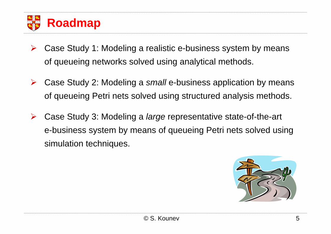
Case Study 1: Modeling a realistic e-business system by means of queueing networks solved using analytical methods.
Case Study 2: Modeling a small e-business application by means of queueing Petri nets solved using structured analysis methods.
Case Study 3: Modeling a large representative state-of-the-art e-business system by means of queueing Petri nets solved using simulation techniques.
© S. Kounev 5

Sizing and Capacity Planning
INTERNET
Client 1 Client 2 Client n
CLIENT SIDE
AS 1 AS m
Load Balancers
Database Servers
PresentationTier
Web Servers 1..k
Business LogicTier
ApplicationServers 1..m
Data Tier
Database Servers 1..p
Firewall
Legacy Systems
Web Routers
WS 1 WS 2 WS k
If (n = 1000)
k=? m=? p=?
so that all
SLAs
are fulfilled.
6

Approaches to Performance Prediction
Educated Guess+ Quick, easy and cheap.- Very inaccurate and risky.
Performance Modelling+ Cheaper and quicker than load-testing.
Could be applied at the design stage.- Accuracy depends on model representativeness.
Load Testing (brute force)+ Accurate. Helps to identify bottlenecks and
fine-tune system prior to production.- Expensive and time-consuming.
Assumes system availability for testing.
7

Space of Performance Models
8

Case Study 1: SPECjAppServer2002 (SjAS02)
Will study a deployment of SPECjAppServer2002
Industry standard application server benchmark
Measures performance and scalability of J2EE app. servers
Heavy-duty synthetic B2B e-commerce workload
More info at http://www.spec.org/osg/jAppServer/
Case study taken from “Performance Modeling and Evaluation of Large-Scale J2EE Applications” by S. Kounev and A. Buchmann, Proceedings of the 29th International CMG Conference, 2003. http://www.dvs1.informatik.tu-darmstadt.de/publications/pdf/03-cmg-SPECjAS02_QN.pdf
© S. Kounev 9
OSG Java Subcommittee
© S. Kounev 10

MANUFACTURING DOMAIN
Planned LinesLarge Order Line
Parts Widgets
- Create Large Order- Schedule Work Order- Update Work Order- Complete Work Order
CUSTOMER DOMAINOrder Entry Application
- Place Order- Change Order- Get Order Status- Get Customer Status
Create Large Order
CORPORATE DOMAINCustomer, Supplier and
Parts Information
- Register Customer- Determine Discount- Check Credit
SUPPLIER DOMAIN
- Select Supplier- Send Purchase Order- Deliver Purchase Order
PurchaseParts Deliver
Parts
11
SPECjAppServer Business Domains

Benchmark Components:
1. EJBs – J2EE application deployed on the System Under Test (SUT)
2. Supplier Emulator – web application simulatingexternal suppliers
3. Driver – Java application simulating clients interacting with the system
RDBMS used for persistence
Throughput is function of chosen Transaction Injection Rate
Performance metric is TOPS = Total Ops Per Second
© S. Kounev 12
SPECjAppServer Application Design

Web Container
Supplier Emulator
Emulator Servlet
Driver
Client JVM
RMI
HTTP
HTTP
EJB X
BuyerSes
J2EE AppServer
EJB Y
ReceiverSes
EJB Z
SUT
© S. Kounev 13
SPECjAppServer2002 Components

How many WLSs are needed to guarantee adequate performance under the expected workload?
For a given number of WLSs, what would be the average trans. response time, throughput and server utilization?
Will the capacity of the DBS suffice to handle the load?
Deployed SPECjAppServer2002 in:- Cluster of WebLogic Servers (WLS) as a J2EE container- Using a single Database Server (DBS) for persistence
Interested in knowing:
© S. Kounev 14
Goals of the Case Study
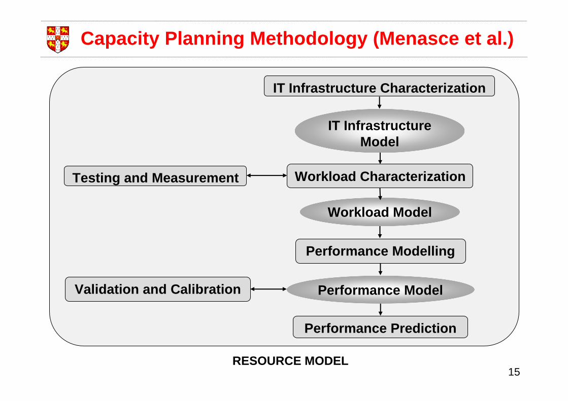
Performance Prediction
Performance Modelling
Performance ModelValidation and Calibration
Workload Characterization
Workload Model
Testing and Measurement
IT Infrastructure Characterization
IT InfrastructureModel
RESOURCE MODEL15
Capacity Planning Methodology (Menasce et al.)
Database Server
...
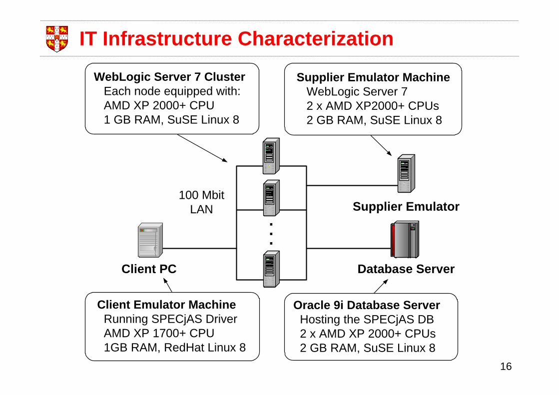
Oracle 9i Database Server Hosting the SPECjAS DB 2 x AMD XP 2000+ CPUs 2 GB RAM, SuSE Linux 8
WebLogic Server 7 Cluster Each node equipped with: AMD XP 2000+ CPU 1 GB RAM, SuSE Linux 8
100 MbitLAN
Client PC
Supplier Emulator
Supplier Emulator Machine WebLogic Server 7 2 x AMD XP2000+ CPUs 2 GB RAM, SuSE Linux 8
Client Emulator Machine Running SPECjAS Driver AMD XP 1700+ CPU 1GB RAM, RedHat Linux 8
16
IT Infrastructure Characterization
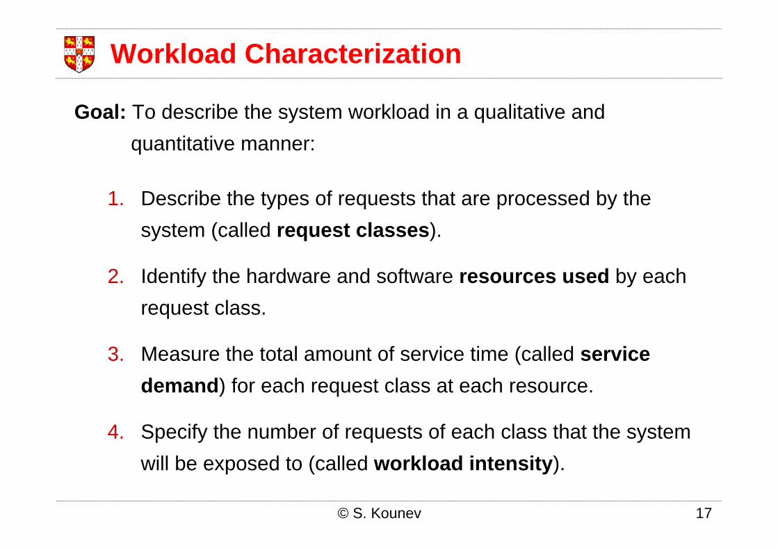
Goal: To describe the system workload in a qualitative andquantitative manner:
1. Describe the types of requests that are processed by the system (called request classes).
2. Identify the hardware and software resources used by each request class.
3. Measure the total amount of service time (called service demand) for each request class at each resource.
4. Specify the number of requests of each class that the system will be exposed to (called workload intensity).
© S. Kounev 17
Workload Characterization

We identify the following five request classes:
Order Entry Application1. NewOrder (NO) – places a new order in the system2. ChangeOrder (CO) – modifies an existing order3. OrderStatus (OS) – retrieves the status of a given order4. CustStatus (CS) – lists all orders of a given customer
Manufacturing Application5. WorkOrder (WO) – the unit of work at the production lines
© S. Kounev 18
Workload Characterization – Step 1

We identify the following resources:
1. The CPU of a WebLogic Server (WLS-CPU) 2. The Local Area Network (LAN)3. The CPUs of the database server (DBS-CPU)4. The disk drives of the database server (DBS-I/O)
We ignore network service demands, since over a 100 Mbit LAN all communication times were negligible.
© S. Kounev 19
Workload Characterization – Step 2

0 10 20 30 40 50 60 70
WorkOrder
CustStatus
OrderStatus
ChangeOrder
NewOrder
Service Demand (ms)
WLS-CPU DBS-CPU DBS-I/O
© S. Kounev 20
Workload Characterization – Step 3

Workload intensity is usually specified in one of two ways:Average request arrival rates (open QNs)Average number of requests in the system (closed QNs)
In our study, we quantify workload intensity by specifying:
The number of concurrent order entry clients
The average customer think time – Customer Think Time
Number of planned production lines in the Mfg domain
Average time production lines wait after processing a WorkOrder before starting a new one – Mfg Think Time
© S. Kounev 21
Workload Characterization – Step 4

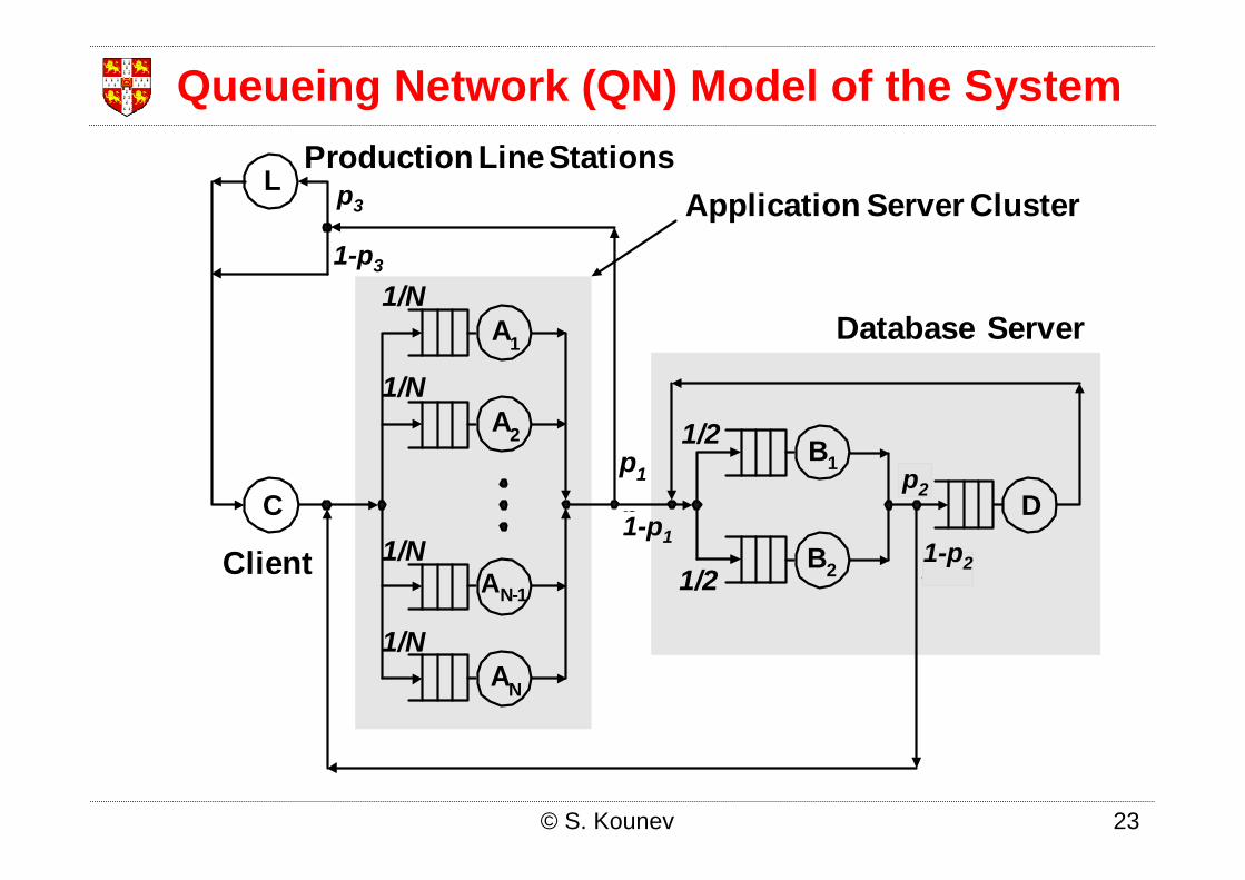
We model each processing resource using a queue:• The CPUs of the N WLSs in the cluster – N PS queues A1…AN
• The two CPUs of the DBS – 2 PS queues B1 and B2
• The disk drive of the DBS – 1 FCFS queue D
We model the client using a delay resource C- Delay of order requests at this queue = Customer Think Time- Delay of WorkOrder requests at this queue = Mfg Think Time
Each WorkOrder is delayed at the virtual production line stations duringprocessing. To model this we introduce an additional delay resource L.
© S. Kounev 22
Building a Performance Model
B2
C
B1
A1
A2
AN-1
AN
L
Dp1
p2
p5
p6
1/2
1/2
p7
p8
1/N
1/N
1/N
1/N
Database Server
Application Server Cluster
Client
Production Line Stations
© S. Kounev 23
1-p1
1-p3
p2
1-p2
p3
Queueing Network (QN) Model of the System

© S. Kounev 24
Formal Queue Definitions (Kendall's Notation)

B2
C
B1
A1
A2
AN-1
AN
L
D
1/2
p7
p8
1/N
1/N
1/N
1/N
Database Server
Application ServerCluster
Client
Production Line Stations
1/2
© S. Kounev 25
1-p3
p3
Simplified QN Model of the System

1. Number of order entry clients of each type –NewOrder, ChangeOrder, OrderStatus and CustStatus.
2. Average think time of order entry clients –Customer Think Time.
3. Number of planned production lines generating WorkOrder requests.
4. Average time production lines wait after processing a WorkOrderbefore starting a new one – Mfg Think Time.
5. Service demands of the 5 request classes at queues Ai, Bk and D (as measured during workload characterization).
© S. Kounev 26
Model Input Parameters

We will analyze several different instances of the model for different workload intensities – low, moderate and heavy:
In each case we will apply the model for different number of application servers – from 1 to 9. We will first consider the case without large order lines in the Mfg domain.
© S. Kounev 27
Scenarios that we will study

We have a closed non-product-form queueing networkmodel with five request classes to analyze.
We employed the PEPSY-QNS tool from the University of Erlangen-Nuernberg. For more information see:http://www4.informatik.uni-erlangen.de/Projects/PEPSY/en/pepsy.html
Available free of charge for non-commercial use
Supports a wide range of solution methods (over 30)
Offers both exact and approximate methods
© S. Kounev 28
G. Bolch and M. Kirschnick. “The Performance Evaluation and Prediction System for Queueing Networks –PEPSY-QNS”. TR-I4-94-18, University of Erlangen-Nuremberg, Germany, 1994.
Model Analysis and Validation

© S. Kounev 29
SHARPE (http://www.ee.duke.edu/~kst/software_packages.html)
C. Hirel, R. A. Sahner, X. Zang, and K. S. Trivedi. “Reliability and Performability Modeling Using SHARPE 2000”. In Computer Performance Evaluation / TOOLS 2000, Schaumburg, IL, USA, pages 345–349, 2000.See http://www.ee.duke.edu/~kst/.
QNAT (http://poisson.ecse.rpi.edu/~hema/qnat/)
H. T. Kaur, D. Manjunath, and S. K. Bose. “The Queuing Network Analysis Tool (QNAT)”. In Proceedings of the 8th International Symposium on Modeling, Analysis and Simulation of Computer and Telecommunication Systems, CA, USA, vol. 8, pages 341–347, 2000.
RAQS (http://www.okstate.edu/cocim/raqs/)
M. Kamath, S. Sivaramakrishnan, and G. Shirhatti. “RAQS: A software package to support instruction and research in queueing systems”. In Proceedings of the 4th Industrial Engineering Research Conference, IIE, Norcross, GA., pages 944–953, 1995.
Daniel Menasce’s MS Excel Workbooks: http://cs.gmu.edu/~menasce/webbook/index.htmlhttp://cs.gmu.edu/~menasce/ebook/index.htmlhttp://cs.gmu.edu/~menasce/webservices/index.htmlhttp://cs.gmu.edu/~menasce/perfbyd/
Other Queueing Network Analysis Tools

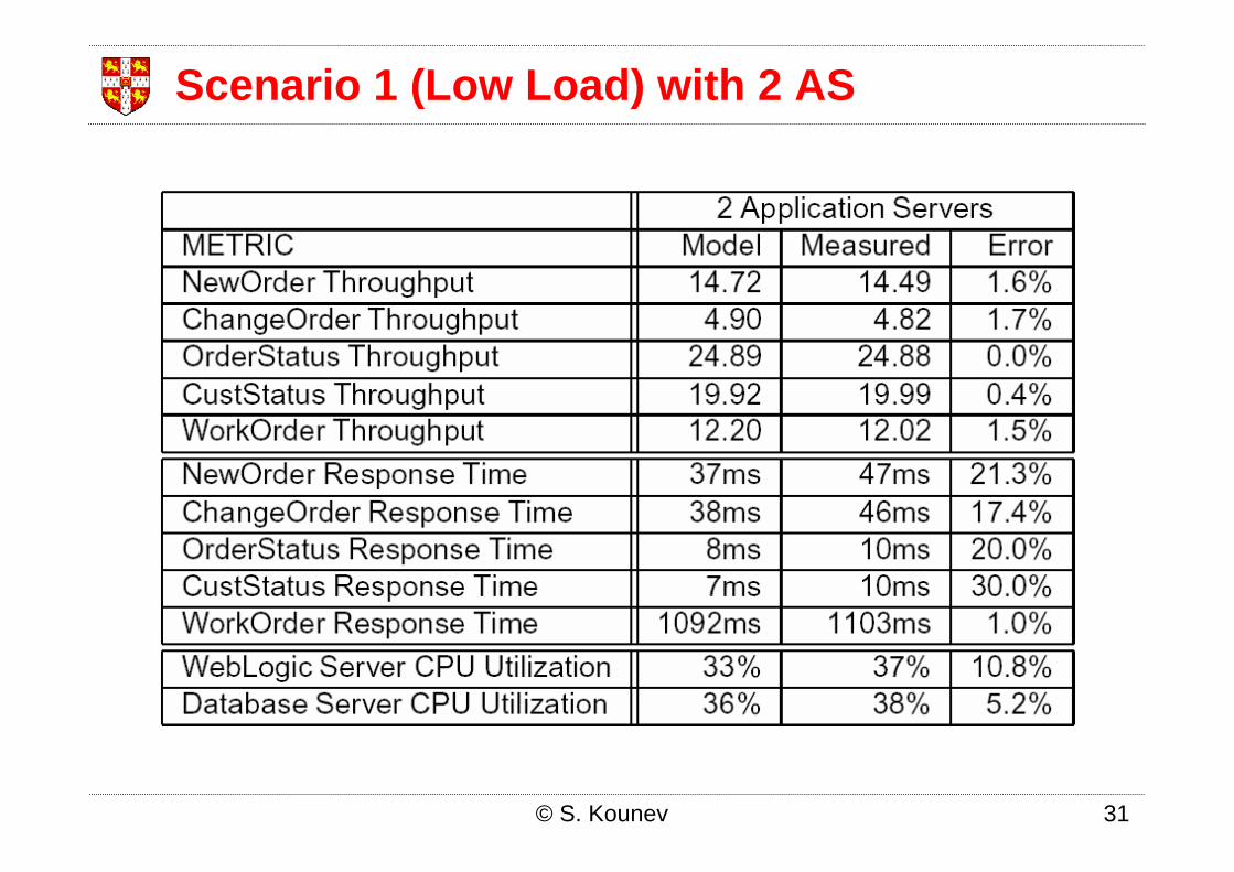
We have 130 concurrent clients and 50 planned production lines.
© S. Kounev 30
Scenario 1 (Low Load) with 1 AS
© S. Kounev 31
Scenario 1 (Low Load) with 2 AS
• Response time results much less accurate than throughput and utilization results:
- Running a transaction mix vs. single transaction
- Additional delays from software contention
• The lower the service demand the higher the response time error (e.g. WorkOrder vs. CustStatus)
© S. Kounev 32
Scenario 1 (Low Load) Observations

We have 260 concurrent clients and 100 planned production lines.
© S. Kounev 33
Scenario 2 (Moderate Load) with 3 and 6 AS
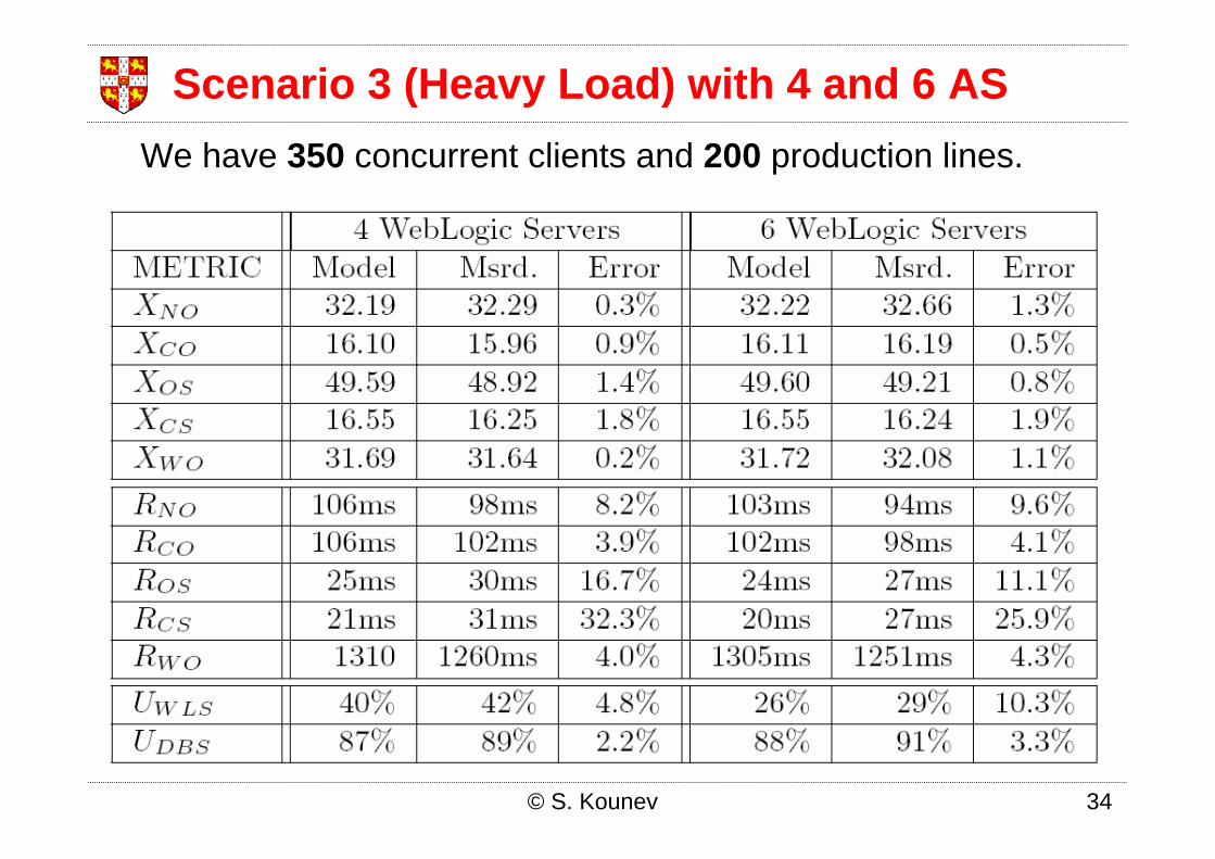
We have 350 concurrent clients and 200 production lines.
© S. Kounev 34
Scenario 3 (Heavy Load) with 4 and 6 AS

For models of this size the available algorithms do not produce reliable results for response time.
© S. Kounev 35
Scenario 3 (Heavy Load) with 9 AS

• Large order (LO) lines activated upon arrival of large orders in the customer domain. Each large order generates a separate work order.
• Since LO lines are triggered by NewOrder transactions we can integrate the load they produce into the service demands of NewOrder requests.
• We measure NewOrder’s service demand with the LOs enabled. The additional load impacts the service demands of NewOrderrequests. The latter no longer have the same semantics.
© S. Kounev 36
Scenarios with Large Order Lines

© S. Kounev 37
Scenarios with Large Order Lines (2)

0 20 40 60 80 100
1AS / LOW
*1AS / LOW
2AS / LOW
3AS / MODERATE
*3AS / MODERATE
6AS / MODERATE
4AS / HEAVY
6AS / HEAVY
9AS / HEAVY
*9AS / HEAVY
DATABASE CPUWEBLOGIC CPU * WITH LARGE ORDER LINES
© S. Kounev 38
Summarized Utilization Results
Conclusions From Case Study
Studied a realistic J2EE application and showed how to build a performance model and use it for capacity planning.
Model was extremely accurate in predicting transaction throughput and CPU utilization and less accurate for transaction response time.
Ignoring the scenarios with large orders, the average modelling error for throughput was 2%, for utilization 6% and for response time 18%.
Two problems encountered:
Poor model expressiveness: no way to accurately model asynchronous processing and software contention.
Problem solving large non-product form QNs analytically.
© S. Kounev 39
DISK
CPU1
CPU2 SERVICE STATION 2
SERVICE STATION 1
ArrivingRequests Waiting
Area
Servers
p1
p2
DepartingRequests
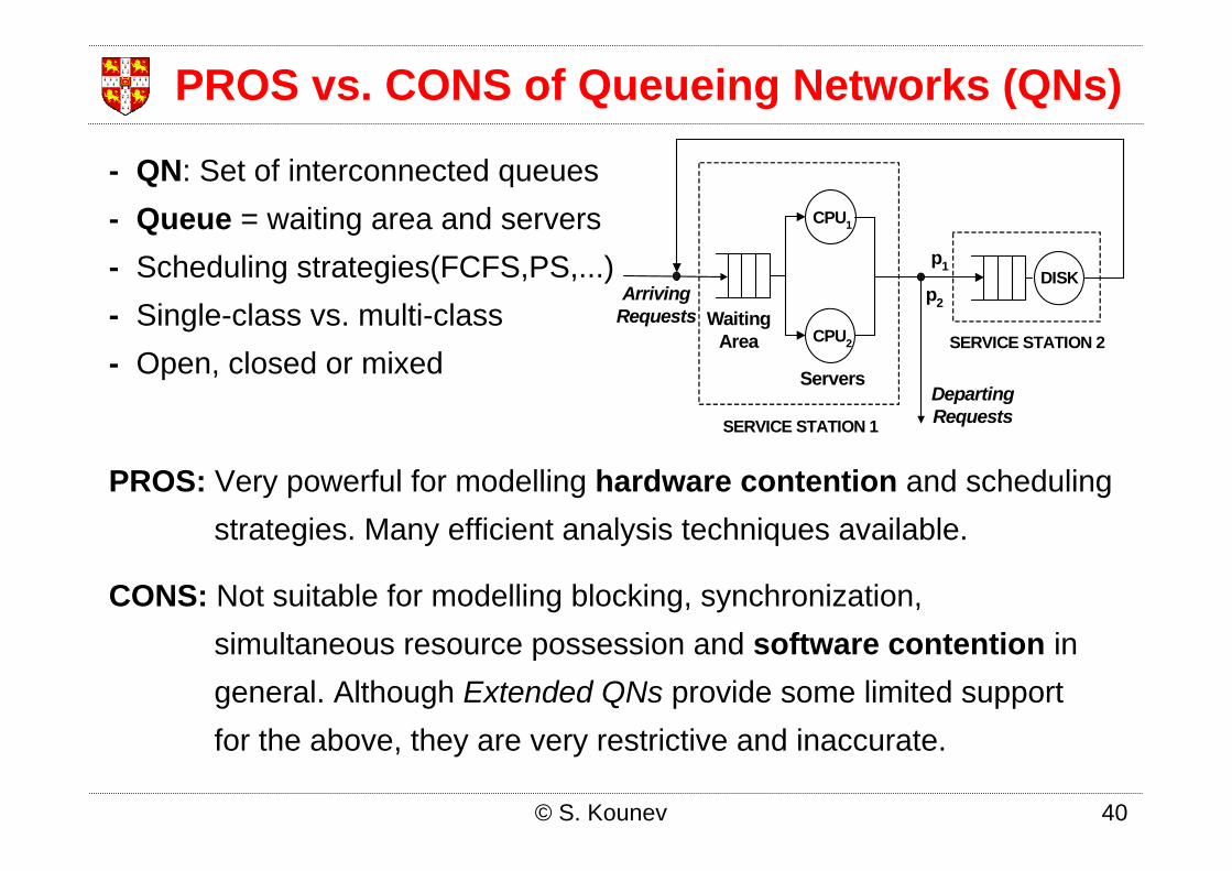
PROS: Very powerful for modelling hardware contention and schedulingstrategies. Many efficient analysis techniques available.
CONS: Not suitable for modelling blocking, synchronization,simultaneous resource possession and software contention ingeneral. Although Extended QNs provide some limited support for the above, they are very restrictive and inaccurate.
- QN: Set of interconnected queues- Queue = waiting area and servers- Scheduling strategies(FCFS,PS,...)- Single-class vs. multi-class- Open, closed or mixed
© S. Kounev 40
PROS vs. CONS of Queueing Networks (QNs)
t1t2
p1 p2
p3 p4
t1t2
p1 p2
p3 p4a). b).
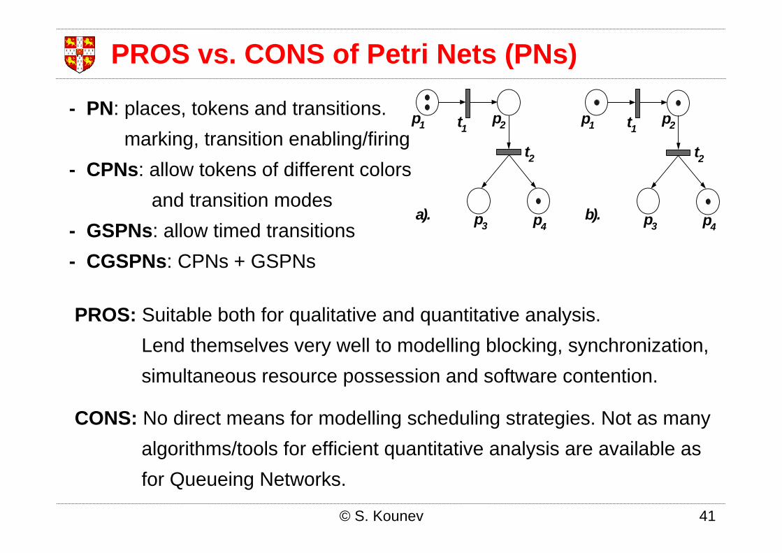
PROS: Suitable both for qualitative and quantitative analysis. Lend themselves very well to modelling blocking, synchronization,simultaneous resource possession and software contention.
CONS: No direct means for modelling scheduling strategies. Not as manyalgorithms/tools for efficient quantitative analysis are available asfor Queueing Networks.
- PN: places, tokens and transitions.marking, transition enabling/firing
- CPNs: allow tokens of different colorsand transition modes
- GSPNs: allow timed transitions- CGSPNs: CPNs + GSPNs
© S. Kounev 41
PROS vs. CONS of Petri Nets (PNs)

QUEUE DEPOSITORY
- Introduced by Falko Bause in 1993.- Combine Queueing Networks and Petri Nets- Allow integration of queues into places of PNs- Ordinary vs. Queueing Places- Queueing Place = Queue + Depository
PROS:
Combine the modelling power and expressiveness of QNs and PNs.
Easy to model synchronization, simultaneous resource possession,asynchronous processing and software contention.
Allow the integration of hardware and software aspects.CONS:
Analysis suffers the state space explosion problem.
© S. Kounev 42
Queueing Petri Nets (QPNs = QNs + PNs)

ACTUALPOPULATION
INPUT OUTPUT
USER SPECIFIEDPART OF THE
SUBNETGRAPHICAL NOTATION
FOR SUBNET PLACE
- Allow hierarchical model specification- Subnet Place: contains a nested QPN- Structured analysis methods alleviate the state space explosion problem
and enable larger models to be analyzed.
Analysis Tools for HQPNs
The HQPN-Tool from theUniversity of Dortmund. Supports a number of structuredanalysis methods. Available free of charge for non-commercial use.
© S. Kounev 43
Hierarchical Queueing Petri Nets (HQPNs)

QPME (http://www.dvs1.informatik.tu-darmstadt.de/staff/skounev/QPME)
S. Kounev, C. Dutz and A. Buchmann“. QPME - Queueing Petri Net Modeling Environment”. Proceedings of the 3rd International Conference on Quantitative Evaluation of SysTems (QEST-2006), Riverside, USA, September 11-14, September 2006.
TimeNET (http://pdv.cs.tu-berlin.de/~timenet/)
A. Zimmermann, J. Freiheit, R. German, and G. Hommel. “Petri Net Modelling and PerformabilityEvaluation with TimeNET 3.0”. In Proceedings of the 11th International Conference on Modelling Techniques and Tools for Computer Performance Evaluation (TOOLS’2000), Schaumburg, Illinois, USA, LNCS 1786, pages 188–202, Mar. 2000.
Möbius (http://www.mobius.uiuc.edu/)
T. Courtney, D. Daly, S. Derisavi, S. Gaonkar, M. Griffith, V. Lam, and W. Sanders. “The M¨obiusModeling Environment: Recent Developments”. In Proceedings of the 1st International Conference on Quantitative Evaluation of Systems (QEST 2004), Enschede, The Netherlands, pages 328–329, Sept. 2004.
SPNP (http://www.ee.duke.edu/~kst/software_packages.html)
C. Hirel, B. Tuffin, and K. Trivedi. “SPNP: Stochastic Petri Nets”. Version 6.0. In B. Haverkort, H. Bohnenkamp, and C. Smith, editors, Computer performance evaluation: Modelling tools and techniques; 11th International Conference; TOOLS 2000, Schaumburg, Illinois, USA, LNCS 1786. Springer Verlag, 2000.
GreatSPN (http://www.di.unito.it/greatspn/index.html)
G. Chiola, G. Franceschinis, R. Gaeta, and M. Ribaudo. GreatSPN 1.7: Graphical Editor and Analyzer for Timed and Stochastic Petri Nets. Performance Evaluation, 24(1-2):47–68, Nov. 1995.
44
Stochastic Petri Net Analysis Tools

Oracle 9i DBSLoad Balancer
WLS 1
...
Oracle 9i (9.0.1) Database Server Hosting the SPECjAppServer DB 1,7 GHz AMD XP CPU, 1 GB RAM Running on Red Hat Linux 7.2
WebLogic Server 7.0 Cluster Each node equipped with: AMD XP 2000+ CPU, 1 GB RAM Running on SuSE Linux 8.0
LAN
WLS 2
WLS N
InternetClient 2
Client K
Client 1
...
Case study taken from “Performance Modeling of Distributed E-Business Applications using Queueing Petri Nets”. S. Kounev and A. Buchmann. Proc. of the 2003 IEEE International Symposium on Performance Analysis of Systems and Software (ISPASS). http://www.dvs1.informatik.tu-darmstadt.de/publications/pdf/03-ispass-QPNs.pdf
Case Study 2: Cust. App. of SPECjAppServer

We are interested in finding answers to the following questions:
What level of performance does the system provide under load?Average response time, throughput and utilization = ?Are there potential system bottlenecks? How many application servers would be needed to guarantee adequate performance?
Need also optimal values for the following configuration parameters:
Number of threads in WebLogic (WLS) thread poolsNumber of connections in WLS database connection poolsNumber of processes of the Oracle server instance
© S. Kounev 46
Capacity Planning Issues

1. Describe the types of requests (request classes) that arrive at the system: NewOrder, ChangeOrder, OrderStatus, CustStatus.
2. Identify the hardware and software resources used by each request class: HW: WLS-CPU, Network, DBS-CPU, DBS-Disk, SW: WLS Thread, DB Connection, DBS Process.
3. Measure the total service time (service demand) of each request class at each processing resource:
© S. Kounev 47
Workload Characterization

WLS-CPU DBS-PQ DBS-CPU DBS-I/O
DBS-Process-Pool
Client
Database Server
t1 t2 t3 t4 t5
WLS-Thread-Pool
DB-Conn-Poolxx
x x x x x x x
c
x
c
t tt
t t
pp p
cc c
xx
p p
© S. Kounev 48
First Cut System Model
WLS-CPU DBS
t1 t2 t5
DB-Conn-Pool
Client
WLS-Thread-Pool
tt t
xx
x x
cc c
t t
x x x x
c c
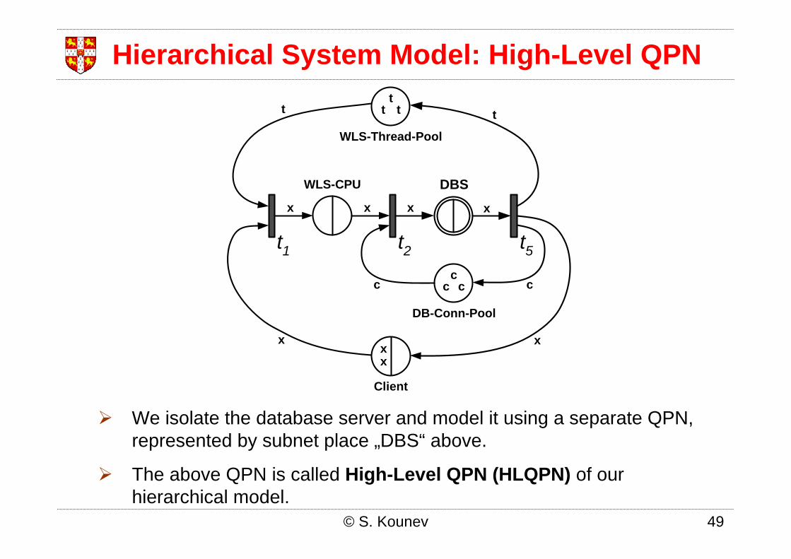
We isolate the database server and model it using a separate QPN, represented by subnet place „DBS“ above.
The above QPN is called High-Level QPN (HLQPN) of our hierarchical model.
© S. Kounev 49
Hierarchical System Model: High-Level QPN

DBS-PQ DBS-CPU DBS-I/O
DBS-Process-Pool
t3 t4
Actual Population
Input Output
tinput toutputx x x x
x
x
x
x
x
pp p
x
pp
The nested DBS subnet of our HQPN - called Low-Level QPN (LLQPN).
Places Input, Output and Actual Population are standard for each subnet.
© S. Kounev 50
Hierarchical System Model: Low-Level QPN

Through analysis of the underlying Markov Chain, we can obtain for each place, queue and depository its average token population N and utilization U in steady state.
From the „Flow-In=Flow-Out“ Principle Places Client, WLS-CPU, DBS-PQ, DBS-CPU and DBS-I/O have the same request throughput X.
For the rest of places, queues and depositories, we get:
The total end-to-end request response time is then:
Applying Little‘s Law to place Client, we get:
© S. Kounev 51
Model Analysis

Single request class – the NewOrder TX80 concurrent clients with avg. client think time of 200ms60 WLS Threads, 40 JDBC Connections, 30 Oracle processes
Analysis Results
Modelling Error
© S. Kounev 52
Scenario 1: Single Request Class
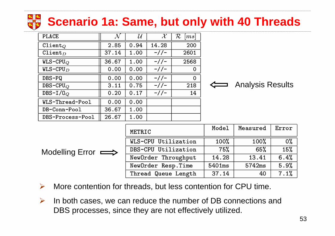
Analysis Results
Modelling Error
More contention for threads, but less contention for CPU time.
In both cases, we can reduce the number of DB connections and DBS processes, since they are not effectively utilized.
53
Scenario 1a: Same, but only with 40 Threads

Two request classes – NewOrder and ChangeOrderSome simplifications needed to avoid explosion of the Markov ChainAssume that there are plenty of JDBC connections and DBS processesDrop places DB-Conn-Pool and DBS-Process-Pool20 clients: 10 NewOrder and 10 ChangeOrder, Avg. think time = 1 secOnly 10 WLS Threads
© S. Kounev 54
Scenario 2: Multiple Request Classes
t2_1
t5
CLIENTDBS
WLS 1
WLS 2
WLS n
WLS (n-1)
t2_2
t2_(n-1)
t2_n
t1_1
t1_2
t1_(n-1)
t1_n
xx
x
x
x
x
x x
x x
x x
x x
x
x
x
x
x
x
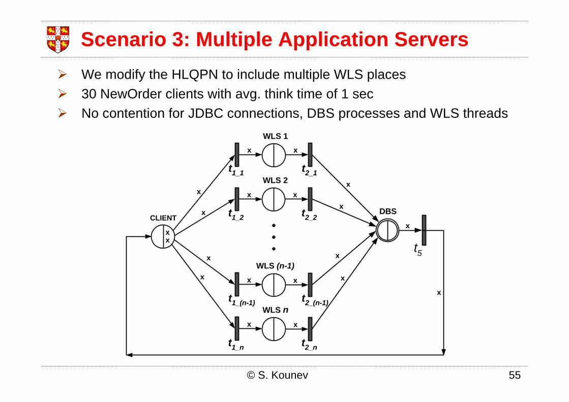
We modify the HLQPN to include multiple WLS places30 NewOrder clients with avg. think time of 1 secNo contention for JDBC connections, DBS processes and WLS threads
© S. Kounev 55
Scenario 3: Multiple Application Servers

© S. Kounev 56
Scenario 3: Modelling Error
QPN models enable us to integrate both hardware and software aspects of system behavior in the same model.
Combining the expressiveness of Queueing Networks and Petri Nets, QPNs are not just powerful as a specification mechanism, but are also very powerful as a performance analysis and prediction tool.
Improved solution methods and software tools for QPNsneeded to enable larger models to be analyzed.
© S. Kounev 57
Conclusions from Case Study
SimQPN – Simulator for QPNs
Tool and methodology for analyzing QPNs using simulation.
Provides a scalable simulation engine optimized for QPNs.
Circumvents the state-space explosion problem.
Can be used to analyze models of realistic size and complexity.
Extremely light-weight and fast.
Portable across platforms.
Validated in a number of realistic scenarios.
• “SimQPN - a tool and methodology for analyzing queueing Petri net models by means of simulation”, Performance Evaluation, Vol. 63, No. 4-5, pp. 364-394, May 2006.
© S. Kounev 58
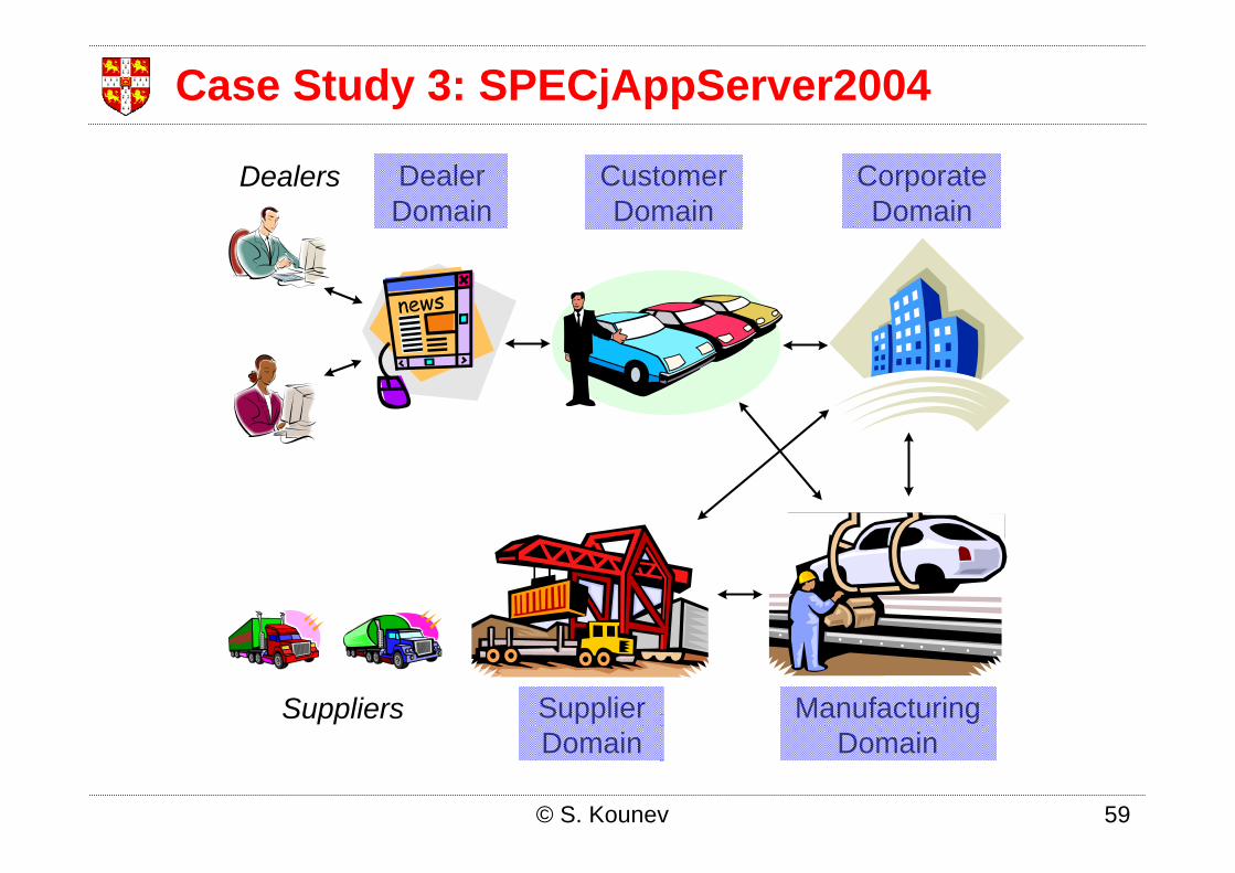
Case Study 3: SPECjAppServer2004
CorporateDomain
CustomerDomain
DealerDomain
Dealers
Suppliers ManufacturingDomain
SupplierDomain
© S. Kounev 59

SPECjAppServer2004 Business Domains
MANUFACTURING DOMAIN
Planned LinesLarge Order Line
Parts Vehicles
- Create Large Order- Schedule Work Order- Update Work Order- Complete Work Order
CUSTOMER DOMAINOrder Entry Application
- Place Order- Get Order Status- Get Customer Status- Cancel Order
CORPORATE DOMAINCustomer, Supplier and
Parts Information
- Register Customer- Determine Discount- Check Credit
SUPPLIER DOMAIN
- Select Supplier- Send Purchase Order- Deliver Purchase Order
PurchaseParts Deliver
Parts

SPECjAppServer2004 Application Design
Benchmark Components:
1. EJBs – J2EE application deployed on the System Under Test (SUT)
2. Supplier Emulator – web application emulatingexternal suppliers
3. Driver – Java application emulating clients interacting with the system and driving production lines
• RDBMS used for persistence
• Asynchronous-messaging used for inter-domain communication
• Throughput is function of chosen Transaction Injection Rate
• Performance metric is JOPS = JAppServerOpsPerSecond
© S. Kounev 61

SPECjAppServer2004 Application Design (2)
Web Container
Supplier Emulator
Emulator Servlet
Driver
Client JVM
HTTP / RMI
HTTP
HTTP
EJB X
BuyerSes
J2EE AppServer
EJB Y
ReceiverSes
EJB Z
SUT
© S. Kounev 62

Sample Deployment Environment (IBM)
© S. Kounev 63
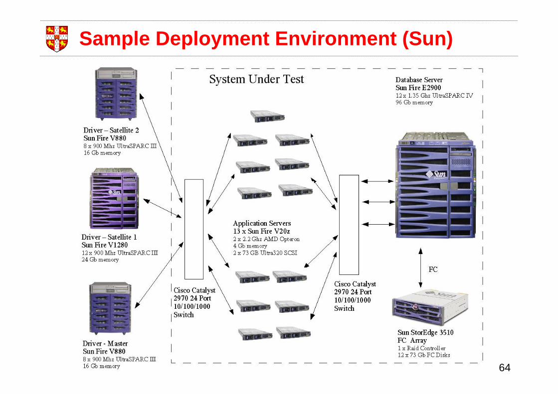
Sample Deployment Environment (Sun)
64
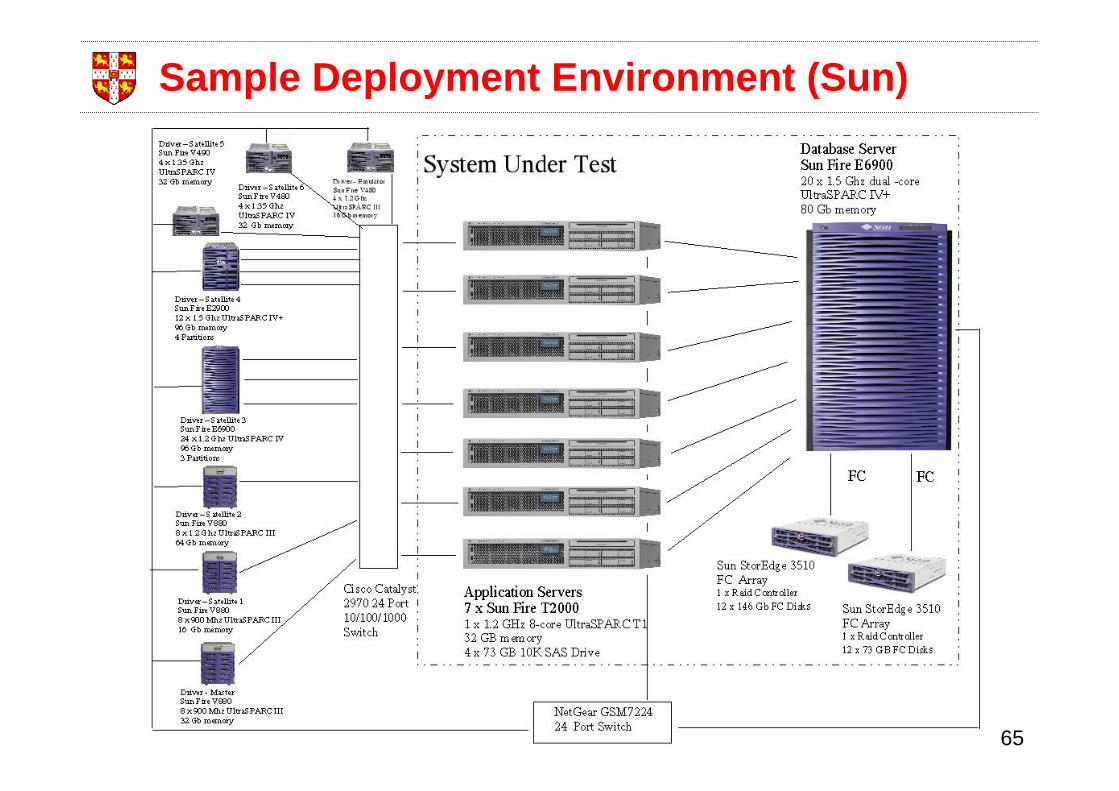
Sample Deployment Environment (Sun)
65

Performance Modelling Methodology
1. Establish performance modelling objectives.
2. Characterize the system in its current state.
3. Characterize the workload.
4. Develop a performance model.
5. Validate, refine and/or calibrate the model.
6. Use model to predict system performance.
7. Analyze results and address modelling objectives.
S. Kounev. “Performance Modeling and Evaluation of Distributed
Component-Based Systems using Queueing Petri Nets”. IEEE
Transactions on Software Engineering, Vol. 32, No. 7, pp. 486-502, 2006.
© S. Kounev 66

Deployment Environment
© S. Kounev 67

1. Establish Modelling Objectives
Normal Conditions: 72 concurrent dealer clients (40 Browse, 16 Purchase, 16 Manage) and 50 planned production lines in the mfg domain.
Peak Conditions: 152 concurrent dealer clients (100 Browse, 26 Purchase, 26 Manage) and 100 planned production lines in the mfg domain.
Goals:
• Predict system performance under normal operating conditions with 4 and 6 application servers.
• Predict how much system performance would improve if the load balancer is upgraded with a slightly faster CPU.
• Study the scalability of the system as the workload increases and additional application server nodes are added.
• Determine which servers would be most utilized under heavy load and investigate if they are potential bottlenecks.
© S. Kounev 68

2. Characterize the System
© S. Kounev 69
3. Characterize the Workload
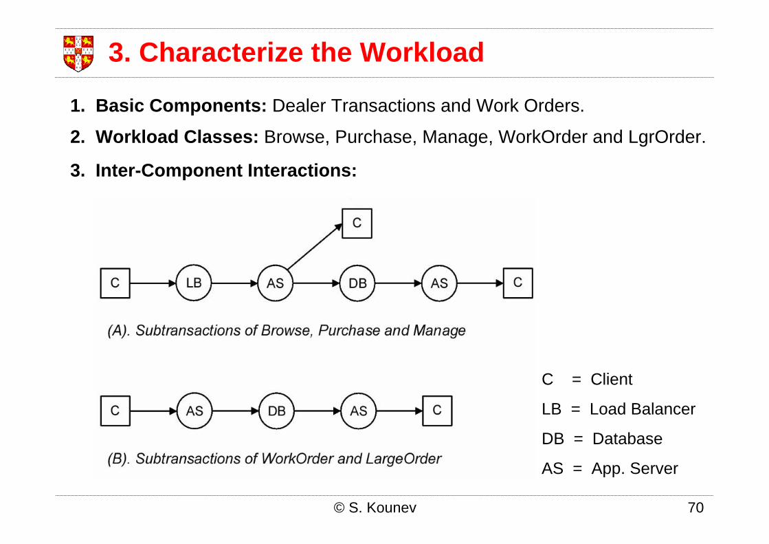
1. Basic Components: Dealer Transactions and Work Orders.
3. Inter-Component Interactions:
2. Workload Classes: Browse, Purchase, Manage, WorkOrder and LgrOrder.
© S. Kounev 70
C = Client
LB = Load Balancer
DB = Database
AS = App. Server

3. Characterize the Workload (2)
Describe the processing steps (subtransactions).

3. Characterize the Workload (3)
Workload Service Demand Parameters (ms)
© S. Kounev 72

3. Characterize the Workload (4)
© S. Kounev 73

4. Develop a Performance ModelQueueing Petri Net
74
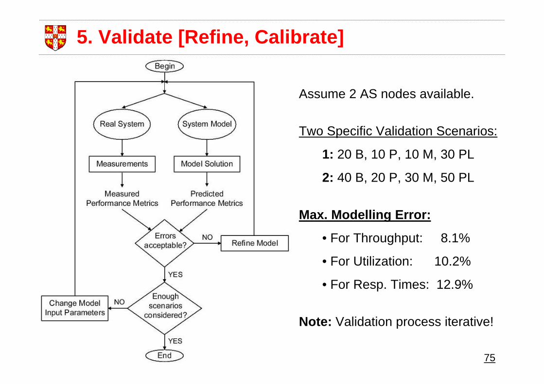
5. Validate [Refine, Calibrate]
Assume 2 AS nodes available.
Two Specific Validation Scenarios:
1: 20 B, 10 P, 10 M, 30 PL
2: 40 B, 20 P, 30 M, 50 PL
Max. Modelling Error:
• For Throughput: 8.1%
• For Utilization: 10.2%
• For Resp. Times: 12.9%
Note: Validation process iterative!
75

6. Predict System Performance
© S. Kounev 76

6. Predict System Performance (2)
© S. Kounev 77

6. Predict System Performance (3)
150 Browse Clients 200 Browse Clients
© S. Kounev 78
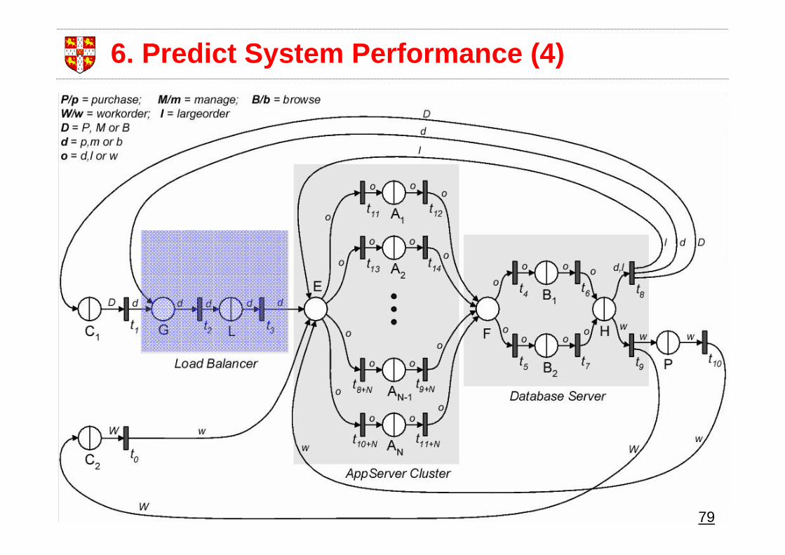
6. Predict System Performance (4)
79
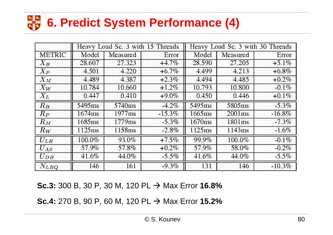
6. Predict System Performance (4)
Sc.3: 300 B, 30 P, 30 M, 120 PL Max Error 16.8%
Sc.4: 270 B, 90 P, 60 M, 120 PL Max Error 15.2%
© S. Kounev 80

7. Analyze Results & Address Objectives
0 20 40 60 80 100
4AS / NORMAL
6AS / NORMAL
6AS / PEAK / ORIG. LB
6AS / PEAK / UPG. LB
8AS / HEAVY 1
8AS / HEAVY 2
8AS / HEAVY 3
8AS / HEAVY 4
LB-C AS-C DB-C
© S. Kounev 81

Benefits of using QPNs
1. QPN models allow the integration of hardware and software
aspects of system behavior.
2. Using QPNs, DCS can be modeled accurately.
3. The knowledge of the structure and behavior of QPNs can be
exploited for efficient simulation using SimQPN.
4. QPNs can be used to combine qualitative and quantitative
system analysis.
5. QPN models have an intuitive graphical representation
facilitating model development.
© S. Kounev 82
Summary & Conclusions from Case Study
Presented a systematic approach for performance prediction.
Studied a representative application and predicted its
performance under realistic load conditions.
Model predictions were validated against measurements on the
real system. The modelling error did not exceed 21.2%!
QPN models can be exploited for accurate performance
prediction in realistic scenarios.
Proposed methodology provides a powerful tool for sizing and
capacity planning.
© S. Kounev 83

References
“Performance Modeling of Distributed E-Business Applications using Queueing Petri Nets”, S. Kounev and A. Buchmann. Proceedings of the 2003 IEEE International Symposium on Performance Analysis of Systems and Software (ISPASS).
“Performance Modeling and Evaluation of Large-Scale J2EE Applications”, S. Kounev and A. Buchmann, Proceedings of the 29th International CMG Conference on Resource Management and Performance Evaluation of Enterprise Computing Systems, 2003.
“Performance Modeling and Evaluation of Distributed Component-Based Systems using Queueing Petri Nets”, S. Kounev. IEEE Transactions on Software Engineering, Vol. 32, No. 7, pp. 486-502, July 2006.
“J2EE Performance and Scalability - From Measuring to Predicting”, S. Kounev. In Proceedings of the 2006 SPEC Benchmark Workshop, Austin, Texas, January 23, 2006.
© S. Kounev 84

Further Reading
"Performance by Design: Computer Capacity Planning by Example“ by D. Menascé, V.A.F. Almeida and L. W. Dowdy. Prentice Hall, ISBN 0-13-090673-5, 2004
"Performance Engineering of Distributed Component-Based Systems -Benchmarking, Modeling and Performance Prediction“ by S. Kounev, Shaker Verlag, ISBN: 3832247130, 2005
"Scaling for E-Business: Technologies, Models, Performance, and Capacity Planning“ by D. Menascé and V.A.F. Almeida, Prentice Hall, ISBN 0-13-086328-9, 2000
“Capacity Planning for Web Performance: Metrics, Models and Methods“by D. Menascé and V.A.F. Almeida, Prentice Hall, Upper Saddle River, NJ, 1998.
© S. Kounev 85

Further Reading
“Queueing Networks and Markov Chains: Modeling and Performance Evaluation with Computer Science Applications” by G. Bolch, S. Greiner, H. de Meer, K. Trivedi; Wiley-Interscience, 2 Edition, ISBN: 0471565253, 2006
“Probability and Statistics with Reliability, Queuing and Computer Science Applications” by K. S. Trivedi, John Wiley & Sons, Inc., Second edition, 2002.
© S. Kounev 86
Related Documents