COMPUTER SCIENCE 349A SAMPLE EXAM QUESTIONS WITH …ess.uvic.ca/exams/CSC/Csc 349a/Csc 349a Final Sample - 2007.pdf · COMPUTER SCIENCE 349A SAMPLE EXAM QUESTIONS WITH SOLUTIONS CHAPTER

COMPUTER SCIENCE 349A

SAMPLE EXAM QUESTIONS WITH SOLUTIONS CHAPTER 1. 1.1 (a) Define the term “ill-conditioned problem”. (b) Give an example of a polynomial that has ill-conditioned zeros. 1.2 Consider evaluation of

)tanh(1

1)(x

xf−

= , where xx

xx

eeeex −

−

+−

=)tanh( .

If )(xf is to be evaluated in floating-point arithmetic (e.g., k = 4 decimal digit, idealized, rounding floating-point), for each of the following ranges of values of x, specify whether the computed floating-point result will be accurate or inaccurate. (a) x is large and positive (for example, 4>x if k = 4) (b) x is close to 0 (for example, 001.0≤x if k = 4) (c) x is large and negative (for example, 4−<x if k = 4) 1.3 Consider

0,)1sin()1sin()( ≠−+

= hh

hhg

where the arguments for sin are in radians. When h is close to 0, evaluation of )(hg is inaccurate in floating-point arithmetic. In (a) and (d) below, use 4 decimal digit, idealized, rounding floating-point arithmetic. If x is a floating-point number, assume that

)(sin xfl is determined by rounding the exact value of xsin to 4 significant digits. (a) Evaluate ))(( hgfl for 00351.0=h . Note that L843088.0)003.1sin( = ,

L843625.0)004.1sin( = and L841470.0)1sin( = . (b) Taylor's Theorem can be expressed in two equivalent forms: given any fixed value 0x ,

L+′′′−+′′−

+′−+= )(!3

)()(

!2)(

)()()()( 0

30

0

20

000 xfxx

xfxx

xfxxxfxf

or, using a change of variable (replacing x by hx +0 , so that 0xxh −= is the independent variable),

L+′′′+′′+′+=+ )(!3

)(!2

)()()( 0

3

0

2

000 xfhxfhxfhxfhxf .

Using the latter form of Taylor's Theorem (without the remainder term), determine the quadratic (in h) Taylor polynomial approximation to )1sin( h+ . Note: leave your answer in terms of )1cos( and sin(1); do not evaluate these numerically. (c) Use the Taylor polynomial approximation from (b) to obtain a polynomial approximation, say )(hp , to )(hg . (d) Show that )(hp is much better than )(hg for floating-point evaluation when h is close to 0 by evaluating ))00351.0(( pfl . Note that L841470.0)1sin( = and

L540302.0)1cos( = . 1.4 If fedcba ,,,,, have known values, then

⎥⎦

⎤⎢⎣

⎡=⎥

⎦

⎤⎢⎣

⎡⎥⎦

⎤⎢⎣

⎡fe

yx

dcba

is a system of 2 linear equations in the 2 unknowns x and y. If 0≠− bcad , then the solution is

bcadbfdex

−−

= and bcadceafy

−−

= .

Consider the linear system

⎥⎦

⎤⎢⎣

⎡−−

=⎥⎦

⎤⎢⎣

⎡⎥⎦

⎤⎢⎣

⎡−−

38.127.0

29.691.423.196.0

yx

.

Show that the problem of computing the solution ⎥⎦

⎤⎢⎣

⎡yx

is ill-conditioned.

1.5 (a) For what values of the real variable x , where 1>x , is the following expression subject to subtractive cancellation that will produce a very inaccurate result (in terms of relative error) using floating-point arithmetic? 1)( −−= xxxf , where 1>x . (b) How should )(xf be evaluated in floating-point arithmetic in order to avoid the subtractive cancellation in (a)? 1.6 Let

0,1)(sin)( 2 ≠+−

= xx

exxfx

.

Note: x is in radians (for the sine function). (a) In the following, use 4 decimal digit, idealized, chopping floating-point arithmetic. If w is a floating-point number, compute )( wefl and )(sin wfl by chopping the exact value of we and wsin , respectively, to 4 significant digits. For the sine function, w is in radians. Evaluate ))123.0(( ffl . Note that L122690.0)123.0sin( = and

L13088.1123.0 =e . (b) To 4 significant digits, the exact value of )123.0(f is -0.5416, so the computation in (a) is inaccurate. In order to obtain a better formula for approximating

)(xf when x is close to 0, use the Taylor polynomial approximations for xe and xsin (both expanded about 00 =x ) in order to obtain a quadratic polynomial approximation for )(xf . Note: if you know these required Taylor expansions, it is not necessary to show their derivations. (c) Use the polynomial approximation for )(xf from (b) (which is accurate when x is close to 0) to show that the computation of ))123.0(( ffl in (a) is unstable.

Note: consider the perturbed problem with ε+= 123.0x̂ , where 123.0ε

is small.

1.7 (a) Use 4 decimal digit, idealized, chopping floating-point arithmetic in the following. If w is a floating-point number, approximate )( 4/1wfl by chopping the exact value of 4/1w to 4 significant decimal digits. The evaluation of

11)(

4/1

−−

=x

xxg

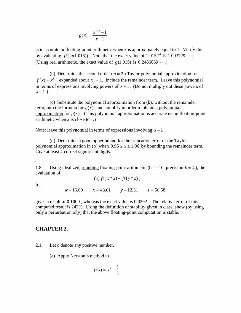
is inaccurate in floating-point arithmetic when x is approximately equal to 1. Verify this by evaluating ))015.1(( gfl . Note that the exact value of 4/1015.1 is L003729.1 . (Using real arithmetic, the exact value of )015.1(g is L2486059.0 .) (b) Determine the second order ( 2=n ) Taylor polynomial approximation for

4/1)( xxf = expanded about x0 = 1. Include the remainder term. Leave this polynomial in terms of expressions involving powers of x −1. (Do not multiply out these powers of x −1.) (c) Substitute the polynomial approximation from (b), without the remainder term, into the formula for g(x) , and simplify in order to obtain a polynomial approximation for g(x) . (This polynomial approximation is accurate using floating-point arithmetic when x is close to 1.) Note: leave this polynomial in terms of expressions involving x −1. (d) Determine a good upper bound for the truncation error of the Taylor polynomial approximation in (b) when 06.195.0 ≤≤ x by bounding the remainder term. Give at least 4 correct significant digits. 1.8 Using idealized, rounding floating-point arithmetic (base 10, precision k = 4 ), the evaluation of ))*()*(( zyfxwff lll − for 68.5631.1261.4300.16 ==== zyxw gives a result of 0.1000 , whereas the exact value is 0.0292 . The relative error of this computed result is 242%. Using the definition of stability given in class, show (by using only a perturbation of y) that the above floating-point computation is stable. CHAPTER 2. 2.1 Let c denote any positive number. (a) Apply Newton’s method to

c

xxf 1)( 2 −=

in order to determine an iterative formula for computing c/1 . (b) For arbitrary 0>c , let 0p be the initial approximation to c/1 , let

{ }L,,, 321 ppp be the sequence of computed approximations to c/1 using the iterative formula from (a), and let

K,3,2,1,0for ,1=−= n

cpe nn

Show (using algebra) that

1

21

2 −

−=n

nn p

ee .

(Note: from this, it follows that 22

1limlim1

21

cpe

e

nn

n

n

n==

−∞→

−∞→

, proving that the iterative

formula in (a) is quadratically convergent.) 2.2 (a) If Newton’s method is used to compute an approximation to a zero of 4880405)( 245 −−−+= xxxxxP using the initial approximation 10 −=p , convergence is obtained to the zero 2−=p of

)(xP . If this computation is carried out, what is the order of convergence? Justify your answer. (b) Give 1 or 2 MATLAB statements that could be used to compute all of the zeros of the polynomial 4880405)( 245 −−−+= xxxxxP using the MATLAB function roots. 2.3 (a) Let R denote any positive number. Apply Newton’s method to

xRxxf −= 2)(

in order to determine an iterative formula for computing 3 R . Simplify the formula so that it is in the form

⎟⎟⎠

⎞⎜⎜⎝

⎛×

)()(

n

nn xh

xgx

where )( and )( nn xhxg are simple polynomials in nx . (b) Consider the case 2=R . Given some initial value 0x , if the iterative

formula in (a) converges to 3 2 , what will be the order of convergence? Very briefly justify your answer, referring to any results from your class notes or the textbook. 2.4 (a) With regard to an algorithm for computing a root p of 0)( =xf , what is the definition of order of convergence? (b) The following sequence of values is converging to a root at p = 1.895494 . What is the order of convergence? n np 0 1.80000 1 1.85078 2 1.87375 3 1.88476 4 1.89016 5 1.89284 6 1.89417 7 1.89483 8 1.89516 9 1.89533 10 1.89541 (c) Could the computed approximations in (b) have been computed using Newton’s method? Justify your answer. 2.5 (a) Show how to evaluate n

n xaxaxaaxP ++++= L2210)(

using nested multiplication. (b) Give pseudocode for the computation in (a).

2.6 A good approximation to one of the zeros of 776)( 234 −−−+= xxxxxP is 64.20 =x . If 0x is used as an approximation to a zero of )(xP , use synthetic division (that is, Horner's algorithm) to determine the associated deflated polynomial. Show all of your calculations. Note: do not do any computations with Newton’s method. 2.7 (a) Fill in the 7 blanks in the following MATLAB code so that the function M-files f.m and secant.m could be used to compute one zero of xexxf −−= sin)( using the Secant method. The function M-file secant.m has the following input parameters: initial approximations p0 and p1 maximum number of iterations N error tolerance tol and it prints each successive computed approximation to a zero of )(xf . If the function doesn’t converge within N iterations, then an error message is printed. The M-file f.m : function y = f(x) y = _____________________________________ ; The M-file secant.m : function secant ( p0, p1, N, tol ) i = 2; q0 = f(p0); q1 = f(p1); while i <= N p = __________________________________________ ; fprintf('i = %g',i),fprintf(' approximation = %18.10f\n',p) if _____________________ < tol return end i = i+1; p0 = _______________________ ; q0 = _______________________ ; p1 = _______________________ ; q1 = ________________________ ; end fprintf('method failed to converge in %g',N),fprintf(' iterations\n') (b) If the above MATLAB M-files f.m and secant.m are used to compute one zero of

xexxf −−= sin)( with initial approximations p0 = 0 and p1 = 1, N = 20 and tol = 610− , then a computed approximation of p = 0.5885327440 is obtained. What is the order of convergence for this computation of this zero of )(xf ? Briefly justify your answer using results given in class. 2.8 Use Taylor’s Theorem to derive Newton’s method for computing a root a

0)( =xf . CHAPTER 3. 3.1 (a) Give the Lagrange form of the quadratic ( 2=n ) interpolating polynomial

)(xP that interpolates xexf −=)( at 4.0 and 2.0,0 === xxx . Note: Do not numerically evaluate )(xf ; instead, give your answer in terms of values such as 2.0−e . Also, do not simplify the expression for )(xP . (b) Using the error term for polynomial interpolation, determine a good upper bound for 1.0)1.0( −− eP . Note: Do not determine an upper bound for xexP −−)( for all ]4.0,0[∈x , only for

1.0=x . 3.2 Let )(xP denote the (linear) polynomial of degree 1 that interpolates

xxf cos)( = at the points 1.0 and 1.0 10 =−= xx (where x is in radians). Use the error term of polynomial interpolation to determine an upper bound for )()( xfxP − , where

]1.0,1.0[−∈x . Do not construct )(xP . 3.3 (a) Fill in the blanks below so that the following MATLAB statements could be used to compute the value of )(πPz = , where )(xP is the piecewise linear interpolating polynomial that interpolates )(xnxy l= at 31 equally-spaced points 0.4,,2.1,1.1,1 31321 ==== xxxx K in the interval [1, 4]. X = linspace ( ___________ , ____________ , ____________ ) ; Y = ___________________________________ ; z = interp1 ( ___________ , ____________ , ___________ , ‘linear’ )

(b) Use the error term for polynomial interpolation to determine a good upper bound for the error when )()( xnxxf l= is approximated by the above piecewise linear interpolating polynomial )(xP , where x is any value in [3, 3.1]. That is, determine a value of ε such that ]1.3,3[ever when)()( ∈≤− xxPxnx εl . 3.4 Determine values for the parameters edcba and ,,, so that

⎩⎨⎧

≤≤++≤≤−++

=10,01,

)( 2

2

xedxcxxbxax

xQ

is a quadratic spline function that interpolates )(xf , where 1)1(,1)0(,1)1( ===− fff . Show all of the equations that the unknowns must satisfy, and then solve these equations. 3.5 Determine 1111000 and ,,,,, dcbadba so that

⎩⎨⎧

≤≤+++≤≤−+−+

=10,01,3

)( 31

2111

30

200

xxdxcxbaxxdxxba

xS

is the natural cubic spline function such that 1)1(and2)0(,1)1( −===− SSS . Clearly identify the 8 conditions that the unknowns must satisfy, and then solve for the 7 unknowns. SECTIONS 4.1 AND 4.2 4.1 Construct the Taylor polynomial approximations of order 3 (with their remainder terms simply written as )( 4hO ) for both of )2( and )( 00 hxfhxf ++ expanded about

0x . Derive a numerical differentiation formula for )( 0xf ′ (and its truncation error term in a form )( khO ) as follows: substitute the above Taylor polynomial approximations (with their remainder terms) into the expression )2()(4)(3 000 hxfhxfxf +−++− and solve for )( 0xf ′ .

4.2 It can be shown that

,22lim

/1

0e

hh h

h=⎟

⎠⎞

⎜⎝⎛

−+

→

where L7182818.2=e . If

h

hhhN

/1

22)( ⎟

⎠⎞

⎜⎝⎛

−+

=

denotes a formula for approximating the value of e, then it can be shown that the truncation error of this approximation is of the form L+++ 6

64

42

2 hKhKhK for some constants iK ; that is, L++++= 6

64

42

2)( hKhKhKhNe . Note that

718372.202.0202.02)02.0(

718644.204.0204.02)04.0(

02.0/1

04.0/1

=⎟⎠⎞

⎜⎝⎛

−+

=

=⎟⎠⎞

⎜⎝⎛

−+

=

N

N

Apply Richardson's extrapolation to the above two values in order to obtain an )( 4hO approximation to the value of e.

4.3 Fill in the three blanks in the following Richardson’s Extrapolation table, given that the truncation error of the formula )(1 hN is of the form L+++ 6

34

22

1 hKhKhK for some constants iK . h )(1 hN

0.45 2.766013

0.15 2.723401 _________________ 0.05 2.718848 _________________ ___________________ Show the formulas that you use to compute these three entries.

4.4 (a) Let 0>h . Suppose you are given 3 values of a function )(xf , namely

)(),0( hff and )3( hf . Construct )(xP , the Lagrange form of the interpolating polynomial at the three points hhx 3 and ,0= . Then differentiate )(xP in order to obtain a numerical differentiation formula )(xP′ for approximating )(xf ′ . (This formula will be a function of x, h and the values )(),0( hff and )3( hf .) (b) Given the following data:

15.015.011.005.012.00

)(xfx

use the numerical differentiation formula from (a) to approximate )0(f ′ by )0(P′ . SECTIONS 4.3-4.6 4.5 Determine the degree of precision of the quadrature formula

( ))3()(34

3 hfhfh+

which is an approximation to ∫h

dxxf3

0

)( . Show all of your work.

4.6 The open Newton-Cotes quadrature formula for 3=n is

[ ])(11)()()(11245)( 3210

4

1

xfxfxfxfhdxxfx

x

+++≈∫−

.

Use this formula to approximate

dxx

x∫− −

1

121)cos( ,

given the following values:

013345.15.0031670.16.0070993.17.0161179.18.0426071.19.0

1/)cos( 2

±±±±±

− xxx

000000.10.0000017.11.0000276.12.0001465.13.0004960.14.0

1/)cos( 2

±±±±

− xxx

4.7 Consider approximating ∫b

a

dxxf )( using Romberg integration. Denote the

Romberg table by

OMMM3,32,31,3

2,21,2

1,1

RRRRR

R

where

1,kR = the trapezoidal rule approximation to ∫b

a

dxxf )( using 12 −k subintervals on

[a,b] . Use 1,21,1 and RR and Richardson extrapolation to show that 2,2R is equal to the Simpson

rule approximation to ∫b

a

dxxf )( .

4.8 If

∫b

a

dxxf )(

is approximated by the Composite Simpson's rule (that is, using m applications of

Simpson's rule on ],[ ba with stepsize m

abh2−

= ) , then the truncation error is

)(180

)( )4(4 μfhab −− ,

for some ),( ba∈μ . Use this error term in order to determine the smallest value of m for which the truncation error is guaranteed to be 810−≤ when the Composite Simpson's rule is used to approximate

dxx∫

5.1

5.0

1 .

4.9 The MATLAB function quad uses a recursive adaptive quadrature algorithm based on Simpson's rule. Fill in the blanks in the following MATLAB statements so that they could be used to approximate

dxexx x∫ −−4

0

5.1)1(13

using the MATLAB function quad and a relative error tolerance of 410− . function y = f(x) y = _________________________________________ ; quad ( _________ , ________, _________, _________ ) 4.10 (a) If Simpson’s rule is applied 1≥m times on subintervals of ],[ ba , the resulting composite Simpson’s rule approximation is of the following form:

⎟⎟⎠

⎞⎜⎜⎝

⎛+++≈ ∑ ∑∫

= =

p

j

q

jmtr

b

a

ffcfcfchdxxf

1 12320

1

)( ,

where m

abh2−

= and )()( khafxff kk +== . Specify the values of the parameters

trqpccc and ,,,,, 321 . (b) Given that a MATLAB function )(xf has been defined, fill in the blanks in the following MATLAB function comptrap so that it will implement the composite Simpson’s rule.

function approx = comptrap (a , b , m) h = __________________ ; sum1 = 0 ; for j = 1 : _________ sum1 = sum1 + f ( _______________ ) ; end sum2 = 0 ; for j = 1 : _______________ sum2 = sum2 + f ( ________________ ) ; end approx = ( h / _____ )*( f(a) + ____________ + ___________ + f(b) ) ; 4.11 Suppose that only the following values of )(xf are known:

153.0033.0328.0683.00.1)(0.175.05.025.00

−xfx

As in the Adaptive Quadrature algorithm based on Simpson’s rule, compute two

approximations 21 and SS to ∫=1

0

)( dxxfI , and estimate (as in the Adaptive Quadrature

algorithm) the error of the computed approximation 2S . SECTIONS 5.1-5.5 5.1 Consider the initial-value problem

( )

2)1(

,1)( 2

−=

+=′

y

yyt

ty

(a) Use the Taylor method of order n = 2 with h = 0.1 to approximate y(1.1). Show all of your work and the iterative formula. (b) Approximate y(1.1) using h = 0.1 and the following second-order Runge-Kutta method:

( ))),(,(),(2 11 iiiiiiii wthfwtfwtfhww +++= ++

(c) What is the order of the local truncation error of the Runge-Kutta method in (b) (as a function of h)? No justification required.

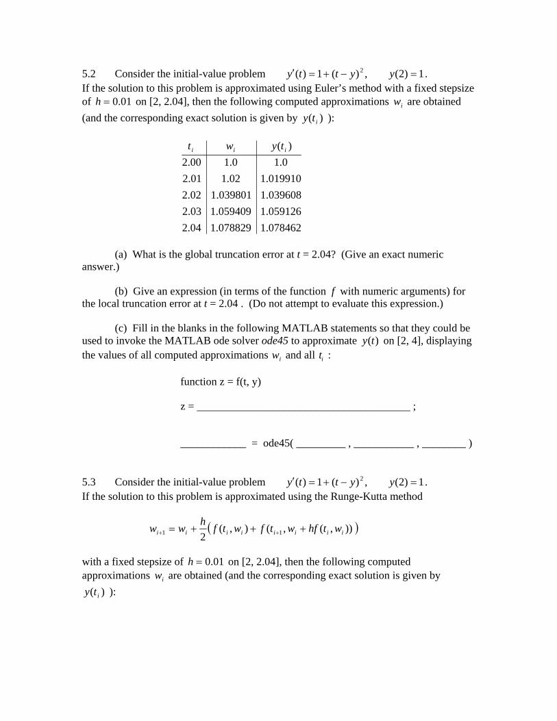
5.2 Consider the initial-value problem 1)2(,)(1)( 2 =−+=′ yytty . If the solution to this problem is approximated using Euler’s method with a fixed stepsize of 01.0=h on [2, 2.04], then the following computed approximations iw are obtained (and the corresponding exact solution is given by )( ity ):

078462.1078829.104.2059126.1059409.103.2039608.1039801.102.2019910.102.101.2

0.10.100.2)( iii tywt

(a) What is the global truncation error at t = 2.04? (Give an exact numeric answer.) (b) Give an expression (in terms of the function f with numeric arguments) for the local truncation error at t = 2.04 . (Do not attempt to evaluate this expression.) (c) Fill in the blanks in the following MATLAB statements so that they could be used to invoke the MATLAB ode solver ode45 to approximate )(ty on [2, 4], displaying the values of all computed approximations wi and all ti : function z = f(t, y) z = _______________________________________ ; ____________ = ode45( _________ , ___________ , ________ ) 5.3 Consider the initial-value problem 1)2(,)(1)( 2 =−+=′ yytty . If the solution to this problem is approximated using the Runge-Kutta method

( ))),(,(),(2 11 iiiiiiii wthfwtfwtfhww +++= ++

with a fixed stepsize of 01.0=h on [2, 2.04], then the following computed approximations iw are obtained (and the corresponding exact solution is given by

)( ity ):

07846154.107845974.104.205912621.105912483.103.203960784.103960689.102.201990099.101990050.101.2

0.10.100.2)( iii tywt

(a) What is the global truncation error at t = 2.04? (Give an exact numeric answer.) (b) Give an expression (in terms of the function f with numeric arguments) for the local truncation error at t = 2.04 . (Do not attempt to evaluate this expression.) 5.4 (a) Give the iterative formula for the Taylor method of order 2=n for approximating the solution of the initial-value problem

2)1(,)(1)( =+=′ yttyty .

(Determine any required derivatives.) (b) Complete the specification of the following MATLAB M-file taylor.m so that it will compute an approximate solution to the above initial-value problem on [1, 2] using a step size of 01.0=h and the Taylor method of order 2=n . Instead of using one-dimensional arrays to store the values ii wt and , this M-file uses only two (scalar) variables, t and w (that is, w is initialized to 0w , the computed approximation 1w is also stored as w and is printed, then the computed approximation 2w is stored as w and printed, and so on). Do not print any of the values of t. function taylor t = 1 ; w = 2 ; h = 0.01 ; for i = end

SECTIONS 6.1-6.4 6.1 Consider the following data:

321101

)(−

ii xfx

Suppose that a function )(xg of the form xx ececcxg 210)( ++= − is to be determined so that )(xg interpolates the above data at the specified points ix . Write down a system of linear equations (in matrix/vector form bAc = ) whose solution will give the values of the unknowns 210 and , ccc that solve this interpolation problem. Note: Leave your answer in terms of e and powers of e . Do not solve the resultant linear system. 6.2 Suppose that a computer program, using the Gaussian elimination algorithm, is to be written to accurately solve a system of linear equations bAx = , where A is an arbitrary nn× nonsingular matrix. Give two reasons why it is necessary to incorporate a pivoting strategy (such as partial pivoting) into the algorithm. 6.3 Let

⎥⎥⎥

⎦

⎤

⎢⎢⎢

⎣

⎡−=

⎥⎥⎥

⎦

⎤

⎢⎢⎢

⎣

⎡−

−=

35.01

,220101012

bA

and suppose that bAx 1−= . Use Gaussian elimination without pivoting to compute x. Do not compute 1−A . Show all of your work. 6.4 Consider the following system of linear equations bAx = :

0422

32422

321

321

32

=++−=+−=+−

xxxxxxxx

Specify the augmented matrix for this linear system, and use Gaussian elimination with partial pivoting to compute the solution vector x. Show all of your work.

6.5 Suppose that the following MATLAB statement has been executed. A = [-1 2 3 4 ; 5 6 7 8 ; 9 8 7 6 ; 5 4 3 1 ] ; Specify 1 or 2 MATLAB statements that could be used to efficiently compute the second column vector of 1−A . Do not compute the entire matrix 1−A . 6.6 Let 2≥n , let A denote an nn× nonsingular, upper triangular matrix:

⎥⎥⎥⎥⎥⎥

⎦

⎤

⎢⎢⎢⎢⎢⎢

⎣

⎡

Ο=

nn

n

n

n

a

aaaaaaaaa

AMO

L

L

L

333

22322

1131211

,

and let T

nyyyyy ),,,,( 321 K= denote a column vector with n entries. The most efficient way to compute yAx 1−= is to use the back-substitution algorithm. Assuming that n, A and y are specified, write a MATLAB function M-file function x = solve ( n , A , y ) that will compute yAx 1−= using the back-substitution algorithm. Note: do not use the MATLAB operator \ or the MATLAB function inv.

SOLUTIONS CHAPTER 1. 1.1 (a) A problem is ill-conditioned if its exact solution can change greatly with a small change in the data defining the problem. (b) 5)1()( −= xxP 1.2 (a) inaccurate, since tanh(x) is approximately equal to 1. (b) accurate, since tanh(x) is approximately equal to 0 (although ))(tanh(xfl may not be too accurate) (c) accurate, since tanh(x) is approximately equal to 1− . 1.3 (a)

5983.0)598290.0()00351.0/0021.0()/))1sin()1((sin(102100.0or002100.0or0021.0)8415.08436.0())1sin()1(sin(

8415.0)841470.0())1(sin(8436.0)843625.0()004.1())1(sin(

004.1)00351.1()00351.01()1(

2

===−+×=−=−+

=====+

==+=+

−

Llll

ll

Lll

Llll

lll

ffhhffhf

ffffhfffhf

Note: exact value of )(hg is 0.538824... and the relative error in the above

computed approximation is 11.0538824.0

5983.01 ≈− or 11%.

(b)

))1sin((2

)1cos()1sin()1sin(2

−++≈+hhh

(c)

)1sin(2

)1cos()1sin()1sin(

2)1cos()1sin(

)(

2

hh

hhhp −=

−⎟⎟⎠

⎞⎜⎜⎝

⎛−+

=

(d)

5388.0)538823.0()001477.05403.0())1sin()2/()1(cos(101477.0or 001477.0)0014768325.0()8415.0001755.0())1sin()2/((

8415.0)841471.0())1(sin(101755.0or001755.0)2/00351.0()2/(

5403.0)540302.0()1(cos(

2

2

==−=−×==×=×

==×==

==

−

−

lll

lll

Lll

ll

Lll

ffhfffhf

fffhfff

which has all 4 significant digits correct.

1.4 Almost any perturbation of the 6 constants in the data ⎥⎦

⎤⎢⎣

⎡−−

⎥⎦

⎤⎢⎣

⎡−−

38.127.0

,29.691.423.196.0

will do: for example,

⎥⎦

⎤⎢⎣

⎡−−

=⎥⎦

⎤⎢⎣

⎡⎥⎦

⎤⎢⎣

⎡−−

38.127.0

ˆˆ

29.689.423.1961.0

yx

has exact solution ⎥⎦

⎤⎢⎣

⎡−≈

196.003.0

whereas the given system has solution ⎥⎦

⎤⎢⎣

⎡11

.

1.5 (a) For x sufficiently large and positive. (Note that there is no problem when

1≈x since then 1))(( ≈xffl , which is accurate.)

(b) ( )1

1111)(

−+=

−+−+

×−−=xxxx

xxxxxf

1.6 (a)

4629.0)462962.0()01512.0/007.0())((01512.0)015129.0()(

007000.0or 007.)1007.1()1(sin007.1)0074.1()130.11226.0()(sin

130.1...)13088.1()(1226.0...)122690.0()(sin

2

−=−=−===

−−=+−=+−

−=−=−=−

==

==

flflxfflflxfl

flexflflflexfl

fleflflxfl

x

x

x

(b)

24321

2432

24621

6)(

24621,

6sin

2

2

432

2

4323

4323

xxx

xxxx

xxxxxxxf

xxxxexxx x

−−−=

−−−=

⎟⎟⎠

⎞⎜⎜⎝

⎛++++−−

≈

++++≈−≈

(c)

4629.0123.0

solution computedproblemgiven −=

→x

ε+=

+−=→

123.0ˆˆ

1ˆsin)ˆ(problem perturbed 2

ˆ

xx

exxfx

And

small. is 123.0

such that allfor 5416.0

)(34358.054163.024

)123.0(3

123.021

0 toclose is ˆ if 24ˆ

3ˆ

21)ˆ(

2

2

2

εε

εε

εε

−≈

+−−=

+−

+−−=

−−−≈

O

xxxxf

Since this is not close to 4629.0− for all small ε , the computation is unstable. 1.7 (a)

0

1

24/1

4/1

102000.0or 2.0)015.0/003.0())((101500.0or 015.0)000.1015.1()1(

103000.0or 003.0)000.1003.1()1(003.1)003729.1()(

×==

×=−=−

×=−=−

==

−

−

ll

ll

ll

Lll

fxgffxf

fxffxf

(b)

4/11

4/7

4/3

4/1

6421)(

16/3)1(163)(

4/1)1(41)(

1)1()(

−

−

−

=′′′

−=′′−=′′

=′=′

==

xxf

fxxf

fxxf

fxxf

Thus

[ ] 34/112

32

)1()(128

7)1(323)1(

411

)1(!3

))(()1(!2

)1()1()1()1()(

−+−−−+=

−′′′

+−′′

+−′+=

− xxxx

xxfxfxffxf

ξ

ξ

(c)

)1(323

41

1

1)1(323)1(

411

11)(

24/1

−−=−

−−−−+≈

−−

= xx

xx

xxxg

(d)

[ ] [ ]

0.0000136 approx. is which ,)106.1()95.0(

1128

7

)1(max)(max128

7)1()(128

7

34/11

3

06.195.0

4/11

06.1)(95.0

34/11

−≤

−≤−≤≤

−

≤≤

− xxxxxx

ξξξ

1.8 To show stability, find a value ε for which the exact value of )68.56()31.12()61.43()00.16( ε+− is approx. equal to 0.1 By continuity, any such value must be approx. equal to the value ε such that 1.0)68.56()31.12()61.43()00.16( =+− ε Solving for ε gives

0012491.031.1268.56

1.061.4316−=−

−×=ε

Thus, for example, if 31.12=y is perturbed to 00125.031.12ˆ −=+= εyy (or you could use 0012491.0−=ε ), then the exact value of 10005.0ˆ =×−× zyxw ,

which is very close to 0.1 . And since 31.12

00125.031.12

=ε is small, the computation in (a)

is stable.

CHAPTER 2. 2.1 (a)

⎟⎟⎠

⎞⎜⎜⎝

⎛+

+=

−−=

=′−=

−−

−

−

−

−−

11

1

21

1

21

1

2

121or

2/1

2/1

2)(/1)(

nn

n

n

n

nnn pc

pp

cpp

cppp

xxfcxxf

(b)

( )1

21

1

2

1

1

121

1

12

1

1

21

22/1

2

12

22/1

(a) from 12

/1

/1

−

−

−

−

−

−−

−

−−

−

−

=−

=

⎟⎟⎠

⎞⎜⎜⎝

⎛+−

=

−+=

−+

=

−=

n

n

n

n

n

nn

n

nn

n

n

nn

pe

pcp

cpcc

ppc

cppcpc

cpcp

cpe

2.2 (a) 8080205)( 34 −−+=′ xxxxP , so 08016016080)2( =−+−=−′P . Thus, the zero at 2−=p has multiplicity 2≥m , which implies that Newton’s method has linear convergence (that is, the order of convergence is 1). (b) roots ( [ 1 5 0 40− 4880 −− ] ) or p = [ 1 5 0 40− 4880 −− ] ; roots ( p )

2.3 (a)

⎟⎟⎠

⎞⎜⎜⎝

⎛++

=⎟⎟⎠

⎞⎜⎜⎝

⎛+

+−+=⎟⎟

⎠

⎞⎜⎜⎝

⎛+−

−=

⎟⎟⎠

⎞⎜⎜⎝

⎛+⎟⎟

⎠

⎞⎜⎜⎝

⎛ −−=

+

−−=

′−=+

RxRx

xRx

RxRxx

RxRx

x

Rxx

xRx

x

xRx

xRx

xxfxf

xx

n

nn

n

nnn

n

nn

n

n

n

nn

nn

nn

nn

nnn

3

3

3

33

3

3

3

23

2

2

1

22

22

21

22)()(

(b)

2.10 Thm.by zero simple a is 20

2222)2(

,2root at the so ,222)(

33/2

33

322

⇒≠+=′

=+=+=′

f

xx

xxRxxf

(that is, the multiplicity of the root is 1) and thus Newton’s method converges quadratically (the order of convergence is 2=α ) 2.4 (a) The order of convergence is α if there exist constants 0>λ and 1≥α such that

λα =−

−+

∞→ pp

pp

n

n

n

1lim

(b) The order of convergence is 1 (linear convergence). (c) Yes, these approximations could have been computed with Newton’s method if the root p has multiplicity 2≥m , since in this case, the order of convergence of Newton’s method is only 1. 2.5 (a) ( )( )( )( )nn xaaxxaxaxaxP +++++= −1210)( L (b)

xbab

nnkab

kkk

nn

1

0,1,,2,1for

++←−−=

←K

2.6

322532.0)64.2)(529344.2(7529344.2)64.2)(6096.3(7

6096.3)64.2)(64.3(664.3)64.2)(1(1

1

0100

0211

0322

0433

4

−=+−=+==+−=+=

=+−=+==+=+=

=

xbabxbabxbabxbab

b

The deflated polynomial is 529344.26096.364.3 23 +++ xxx 2.7 (a) y = sin(x) – exp(-x) ; p = p1 – q1 * (p1 – p0)/(q1 – q0) ; if abs(p – p1) < tol p0 = p1 ; q0 = q1 ; p1 = p ; q1 = f(p) ; (b) Order of convergence is 1.618 since this is the order of convergence of the Secant method for a simple zero (multiplicity = 1). The multiplicity is 1 because 0)( ≠′ pf , since clearly 0 and 0)cos( >> − pep . 2.8 The linear ( 1=n ) Taylor Theorem expansion for )(xf expanded about 0p is

)(!2

)()()()()(

20

000 ξfpx

pfpxpfxf ′′−

+′−+= ,

for some value 0 and between pxξ . If we take px = (where p is a root of the equation

0)( =xf ), then from above

).( of zero a is since ,0

)(!2

)()()()()(

20

000

xfp

fpp

pfpppfpf

=

′′−+′−+= ξ

On dropping the remainder term, this gives 0)()()( 000 ≈′−+ pfpppf ,

which implies that )()(

0

00 pf

pfpp

′−≈ . This suggests computing

)()(

0

001 pf

pfpp

′−= ,

which is the first step of Newton's method, and then continue iterating with

)()(

1

11

−

−− ′−=

n

nnn pf

pfpp .

CHAPTER 3. 3.1 (a)

4.02.00

)2.04.0)(04.0()2.0)(0(

)4.02.0)(02.0()4.0)(0(

)4.00)(2.00()4.0)(2.0()( −−

−−−−

+−−

−−+

−−−−

= exxexxexxxP

or

4.02.0

08.0)2.0(

04.0)4.0()1(

08.0)4.0)(2.0()( −− −

+−−

+−−

= exxexxxxxP

(b)

error = ∏=

+

−+

n

ii

n

xxn

xf0

)1(

)()!1(

))((ξ

For 2=n ,

error = )4.0)(2.0)(0(6

))((−−−

′′′xxxxf ξ

For xexf −=)( and 1.0=x ,

error = )4.01.0)(2.01.0)(01.0(6

)1.0(

−−−− −ξe .

Since 4.0)(0 ≤≤ xξ for all values of x,

0005.0)3.0)(1.0)(1.0(6

error0

=≤e

3.2

005.0

0at attained ismax thissince 01.0021

01.0max2

)0cos(

)01.0(2

)cos(

1.01.0 with )1.0()1.0(!2

)()()(

2

1.01.0

2

=

=−=

−≤

−−

=

≤≤−+−′′

=−

≤≤−

x

x

x

xxfxfxP

ξ

ξ

ξξ

3.3 (a) X = linspace ( 1 , 4 , 31 ) ; Y = X .* log(X) z = interp1( X , Y , pi , ‘linear’ ) (b) ./1)(,1)(,)( xxfxnxfxnxxf =′′+=′= ll The error term of polynomial interpolation (n = 1) is

]1.3,3[ where, )1.3()3(!2

)()()( ∈−−′′

=− ξξ xxfxPxf .

Thus,

00041667.0)1.305.3()305.3(61

)1.3()3(max31

21

)1.3()3(121)()(

1.33

=−−≤

−−≤

−−≤−

≤≤xx

xxxPxf

x

ξ

3.4 Let .)(,)( 2

12

0 edxcxxQbxaxxQ ++=++= Then

1)1()1(1 and 1)0()0( and )0()0(

11)1()1(10at 212)0()0(

)0()0(

1

10

0

10

10

=++⇒===⇒==

=+−⇒−=−=⇒=+=+⇒′=′

=⇒=

edcfQebfQfQ

bafQdxdcxaxQQ

ebQQ

Solution: 1,1,1,1,1 −===== caebd Thus,

⎩⎨⎧

≤≤++−≤≤−++

=10,101,1

)( 2

2

xxxxxx

xQ

3.5

xdcxSxdxS

xdxcbxSxdxbxS

11100

21111

2000

62)(66)(32)(36)(

+=′′+−=′′++=′+−=′

The 8 conditions are

1 condition,fifth theFrom 14 condition,first theFrom

10660620)1(10660)1(

362)0()0()0()0(

2)0()0(311)1(

22)0(4131)1(

101

000

11111

000

1101

0101

00101

11111111

11

0000000

−=⇒=−=−−=

=⇒=+−⇒=+⇒=′′−=⇒=−−⇒=−′′

−=⇒−=⇒′′=′′=⇒′=′

=⇒=⇒=−=++⇒−=+++⇒−=

=⇒==−−⇒=−−−⇒=−

bbbdab

dddcSddS

ccSSbbSS

aaaSSdcbdcbaS

aSdbadbaS

SECTIONS 4.1-4.2 4.1

).()(32)(2

)()(34)(2)(2)(

)()(3

2)(2)(4)(4

)(3)2()(4)(3

Thus

)()(6

8)(2

4)(2)()2(

)()(6

)(2

)()()(

40

30

40

30

200

40

3

02

00

0

000

40

3

0

2

000

40

3

0

2

000

hOxfhxfh

hOxfhxfhxfhxf

hOxfhxfhxfhxf

xfhxfhxfxf

hOxfhxfhxfhxfhxf

hOxfhxfhxfhxfhxf

+′′′−′=

+′′′−′′−′−−

+′′′+′′+′++

−=+−++−

+′′′+′′+′+=+

+′′′+′′+′+=+

)()(

32)2()(4)(3

)(

Therefore,

30

2000

0 hOxfhh

hxfhxfxfxf +′′′+

+−++−=′

4.2 If h = 0.04, then h/2 = 0.02 and the given approximations (with their truncation errors) are L++++= 6

64

42

2)04.0( hKhKhKNe and L++++= 6

64

42

2 )2/()2/()2/()02.0( hKhKhKNe Multiplying the second equation by 4, and subtracting gives

)(3

)04.0()02.0()02.0(

or )(3

)04.0()02.0(4)()04.0()02.0(43

4

4

4

hONNNe

hONNe

hONNe

+−

+=

+−

=

+−=

Thus, the )( 4hO approximation to e is

...718281333.23

718644.2718372.2718372.2 =−

+

4.3 The three answers are 2.7180745 2.7182789 2.7182815 The justification is as follows. Entries in column 2: (a) L+++= 4

22

11 )( hKhKhNM

(b) L+⎟⎠⎞

⎜⎝⎛+⎟

⎠⎞

⎜⎝⎛+=

4

2

2

11 33)3/( hKhKhNM

Calculate 9 * (b) – (a): )()()3/(98 4

11 hOhNhNM +−= which implies that

8

)()3/(9 11 hNhNM −= or

8)()3/()3/( 11

1hNhNhNM −

+= .

Thus, the two required values in the second column of the table are computed as follows:

7180745.28

766013.2723401.2723401.2 =−

+

7182789.28

723401.2718848.2718848.2 =−

+

For the entry in the third column: (c) L+′+′+= 6

24

12 )( hKhKhNM

(d) L+⎟⎠⎞

⎜⎝⎛′+⎟

⎠⎞

⎜⎝⎛′+=

6

2

4

12 33)3/( hKhKhNM

Calculate 81*(d)-(c): )()()3/(8180 6

22 hOhNhNM +−= which implies that

80

)()3/(81 22 hNhNM −= or

80)()3/()3/( 22

2hNhNhNM −

+=

Thus, the required value in the third column is

7182815.280

7180745.27182789.27182789.2 =−

+

4.4 (a)

)3(6

)(2

3)0(3

34

)3()3)(03(

))(0()()3)(0()3)(0()0(

)30)(0()3)(()(

2

2

2

2

2

22

hfh

hxxhfh

hxxfh

hhxx

hfhhh

hxxhfhhhhxxf

hhhxhxxP

−+

−−

+−=

−−−−

+−−−−

+−−−−

=

Thus,

)3(6

2)(2

32)0(3

42)( 222 hfh

hxhfh

hxfh

hxxP −+

−−

−=′

(b) At 0=x ,

)3(61)(

23)0(

34)0( hf

hhf

hf

hP −+

−=′ .

With 05.0=h and the given data,

4.05.03.32.3)15.0()05.0(6

1)11.0()05.0(2

3)12.0()05.0(3

4)0()0( −=−+−=−+−

=′≈′ Pf

SECTIONS 4.3-4.6 4.5

( )

( )

( )

( )2 isprecision of degree thus

481

245273

43

481)(

9934

39)(

2933

43

29)(

3134

331)(

4433

3

0

433

3223

0

322

223

0

3

0

hhhhhhdxxxxf

hhhhhdxxxxf

hhhhhdxxxxf

hhhdxxf

h

h

h

h

≠=+==

=+==

=+==

=+==

∫

∫

∫

∫

4.6

( )

( )

058108.2

form in thisanswer your leave )031670.1(11000276.1000276.1)031670.1(11121

)6.0(11)2.0()2.0()6.0(1152

245

6.0,2.0,2.0,6.0,5/2 3210

=

←+++=

++−+−≈

==−=−==

ffffI

xxxxh

4.7

( ) ( )

( ) ( )[ ]

[ ]

( )2

with 43

46

226

32

24

4

3or

34

210

210

20210

20210

112121

112122

abhfffh

fffab

fffffab

ffabfffab

RRRRRR

−=++=

++−

=

+−++−

=

+−

−⎥⎦⎤

⎢⎣⎡ ++

−

=

−+

−=

4.8 If ./24)(then ,/1)( 5)4( xxfxxf == Thus

.768)5.0(

24)(max 5)4(

5.15.0==

<<μ

μf

So

).768(2880

1)()2(

1180

1)(180

error 4)4(

4)4(4

mf

mfhab

≤=−

−= μμ

Therefore, 810error −≤ implies that 84 10

2880768 −≤

m, which gives

.86.712880

10768or 66.266666662880

107684/188

4 =⎟⎟⎠

⎞⎜⎜⎝

⎛ ×≥=

×≥ mm L

NOTE: leave your answer in this ⇑ form 4.9

function y = f(x) y = 13*x.*(1-x).*exp(-1.5*x) quad ( ' f ' , 0 , 4, 1e-4 ) OR quad ( @f , 0 , 4 , 1e-4 ) NOTE: 1e-4 can also be written as 0.0001

4.10 (a)

⎟⎟⎠

⎞⎜⎜⎝

⎛+++≈ ∑ ∑∫

−

= =−

1

1 121220 42

3)(

m

j

m

jmjj

b

a

ffffhdxxf

That is, 12,2,,1,4,2,3 321 −===−==== jtjrmqmpccc (b) function approx = comptrap (a , b, m) h = ( b - a ) / ( 2 * m ) ; sum1 = 0 ; for j = 1 : m-1 sum1 = sum1 + f ( a + 2 * j * h ) ; end sum2 = 0 ; for j = 1 : m sum2 = sum2 + f ( a + (2*j-1) * h ) ; end approx = ( h / 3 ) * ( f(a) + 2*sum1 + 4*sum2 + f(b) ) ;

4.11 [ ] [ ] 3598.0153.0)328.0(4161)1()5.0(4)0(

31 =−+=++= fffhS

[ ]

[ ] 3639.0153.0)033.0(4)328.0(2)683.0(41121

)1()75.0(4)5.0(2)25.0(4)0(32

=−+++=

++++= fffffhS

Error estimate is 00027.0)0041.0(151

151

12 ==− SS

SECTIONS 5.1-5.5 5.1 (a)

( )

( ) ( ) ( )( ) )1(21121121))(,( so

1))(,(

2

22

22

2

2

+=−++=+⎟⎠⎞

⎜⎝⎛ −+′+′=′

+=

ytyyyy

tyy

tyyy

ttytf

yyt

tytf

The iterative formula for the Taylor method of order 2 is

( ) ( )

( ) ( )11

12

2

),(2

),(

2

22

2

222

2

1

++++=

++++=

′++=+

ii

ii

i

ii

ii

iii

ii

iiiiii

wtwh

wt

hww

wtwhww

thw

wtfhwthfww

So

( ) ( )

84.1

)12()1(

)4)(01.0()12()1(

)2)(1.0(2

11

2

020

20

2

00

001

−=

+−++−−

+−=

++++= wtwh

wt

hwww

(b)

[ ]

[ ]

( )

allowed.not are scalculator ifanswer your for OK is ** Line

8345.1)309090.12)(05.0(2

8.1)8.1(1.1

12)05.0(2

))2)(1.0(2,1.1()24(11)05.0(2

**))2,1()1.0(2,1.1()2,1(21.02

)),(,(),(2

2

00010001

−=++−=

⎥⎦⎤

⎢⎣⎡ −−++−=

⎥⎦⎤

⎢⎣⎡ +−+−+−=

−+−+−+−=

+++=

f

fff

wthfwtfwtfhww

(c) )( 3hO 5.2 (a) 000367.0078829.1078462.1)04.2( 4 =−=− wy

(b) Use the exact value 059126.1)03.2( =y to define

( )

allowed.not are scalculator ifanswer your for OK is ** Line

078552.1)942596.1)(01.0(059126.1**)059126.103.2(1)01.0(059126.1)059126.1,03.2()03.2( 2

=+=−++=+= fhyv

Then

allowed.not are scalculator ifanswer your for OK is ** Line

000090.0078552.1078462.1

**078462.1)04.2( t.e.local

=−=

−=−= vvy

(c) function z = f( t , y) z = 1 + (t – y)^2 [ t , y ] = ode45 ( @f , [ 2 , 4 ] , 1 ) NOTE. z = 1 + (t – y ).^2 is OK, but the .^ is not required. @f can also be ‘ f ‘ . [ 2 , 4 ] can also be [ 2 4 ] . 5.3 (a) 00000180.007845974.107846154.1)04.2( 4 =−=− wy (b) Use the exact value 05912621.1)03.2( =y to define

( )

( )( )

allowed.not are scalculator ifanswer your for OK is ** Line

07846110.107855217.1,04.2(94259592.1005.005912621.1

))05912621.1,03.2(01.005912621.1,04.2()05912621.1,03.2(005.005912621.1

**)))03.2(,03.2()03.2(,04.2())03.2(,03.2(2

)03.2(

=++=

+++=

+++=

ffff

yfhyfyfhyv

Then

allowed.not are scalculator ifanswer your for OK is ** Line

00000044.007846110.107846154.1

**07846154.1)04.2( t.e.local

=−=

−=−= vvy

5.4 (a)

[ ]

tttyttyt

ttytytty 1)(/)(1)()()( 22 =

−+=

−′=′′

The iterative formula is

⎥⎦

⎤⎢⎣

⎡+⎥

⎦

⎤⎢⎣

⎡++=+

ii

iii t

htw

hww 12

12

1

(b) function taylor t = 1 ; w = 2 ; h = 0.01 ; for i = 1 : 100 w = w + h * (1 + w / t ) + h ^ 2 / (2 * t ) t = t + h ; end SECTIONS 6.1-6.4 6.1

⎥⎥⎥

⎦

⎤

⎢⎢⎢

⎣

⎡=

⎥⎥⎥

⎦

⎤

⎢⎢⎢

⎣

⎡

⎥⎥⎥

⎦

⎤

⎢⎢⎢

⎣

⎡

−

−

−

310

111

2

1

0

22

1

1

ccc

eeee

ee

6.2 -- to avoid possible division by 0 (that is, a pivot that is exactly equal to 0) -- to avoid using pivots that are very small in magnitude, since they may cause the computation to be unstable

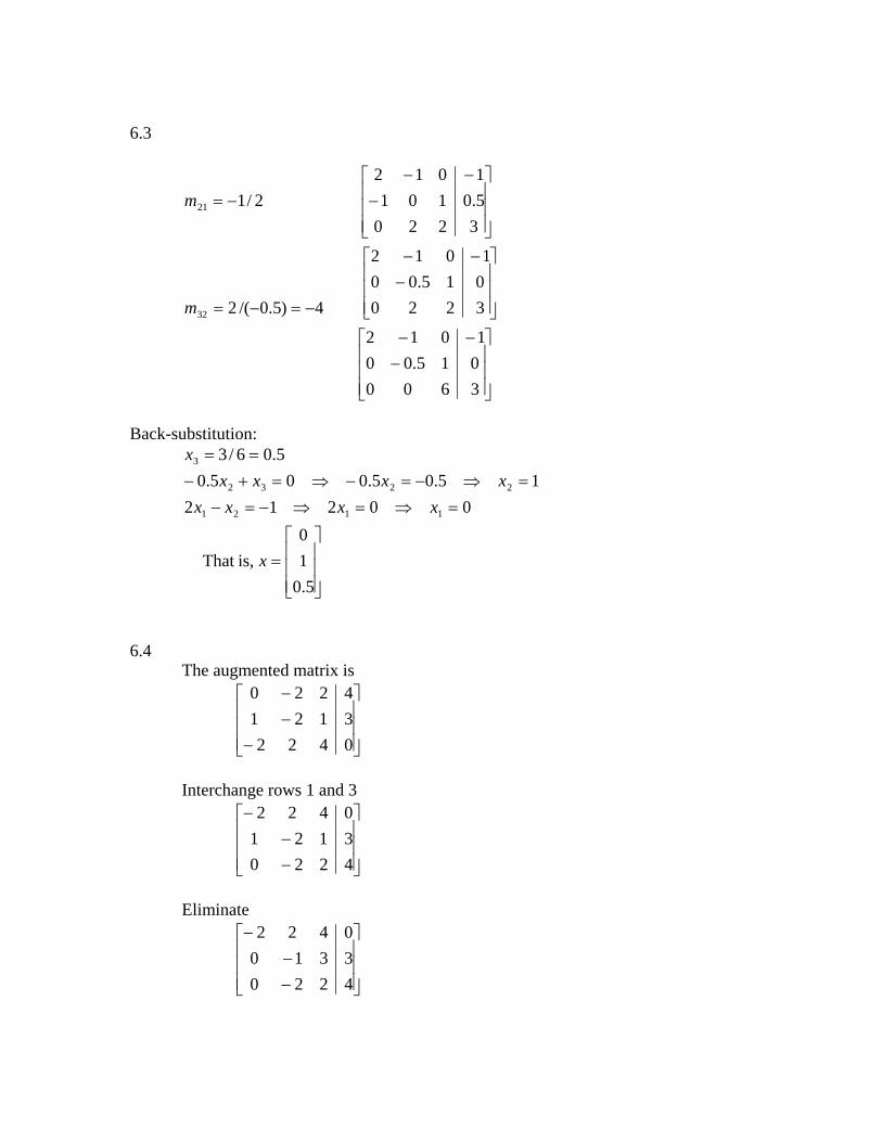
6.3

⎥⎥⎥

⎦

⎤

⎢⎢⎢

⎣

⎡−

−−

⎥⎥⎥

⎦

⎤

⎢⎢⎢

⎣

⎡−

−−

−=−=

⎥⎥⎥

⎦

⎤

⎢⎢⎢

⎣

⎡−

−−−=

3600015.001012

3220015.001012

4)5.0/(2

32205.01011012

2/1

32

21

m

m

Back-substitution:

⎥⎥⎥

⎦

⎤

⎢⎢⎢

⎣

⎡=

=⇒=⇒−=−=⇒−=−⇒=+−

==

5.010

is,That

0021215.05.005.0

5.06/3

1121

2232

3

x

xxxxxxxx

x

6.4 The augmented matrix is

⎥⎥⎥

⎦

⎤

⎢⎢⎢

⎣

⎡

−−−

042231214220

Interchange rows 1 and 3

⎥⎥⎥

⎦

⎤

⎢⎢⎢

⎣

⎡

−−

−

422031210422

Eliminate

⎥⎥⎥

⎦

⎤

⎢⎢⎢

⎣

⎡

−−

−

422033100422

Interchange rows 2 and 3

⎥⎥⎥

⎦

⎤

⎢⎢⎢

⎣

⎡

−−

−

331042200422

Eliminate

⎥⎥⎥

⎦

⎤

⎢⎢⎢

⎣

⎡−

−

120042200422

Back-substitution

2/12

420

2/3224

2/1

321

32

3

−=−−−

=

−=−−

=

=

xxx

xx

x

6.5 A \ [ 0 1 0 0 ]’ or A \ [ 0 ; 1 ; 0 ; 0 ] or the two statements b = [ 0 1 0 0 ]’; A \ b 6.6 % Use back-substitution to solve Ax = y for x. function x = solve(n, A, y) x(n) = y(n) / A(n, n); for i = n-1 : -1 : 1 sum = 0; for j = i+1 : n sum = sum + A(i, j) * x(j); end x(i) = (y(i) – sum)/A(i, i); end