Paul Jenkins ([email protected]) Computer Intensive Statistics APTS 2020–21 Preliminary Material May 2021

Welcome message from author
This document is posted to help you gain knowledge. Please leave a comment to let me know what you think about it! Share it to your friends and learn new things together.
Transcript

Paul Jenkins ([email protected])
Computer Intensive Statistics
APTS 2020–21 Preliminary Material
May 2021
apts.ac.ukAcademyforPhDTraininginStatistics

1. Introduction
The principal aim of these notes is to provide context and motivation for the APTS Computer Inten-
sive Statistics Module, and to make the module as self-contained as is feasible. Statistics is a broad
discipline and the APTS cohort naturally has a diverse range of backgrounds. If you have attended
the earlier APTS modules this year, especially Statistical Computing and Statistical Inference, then
you should be well prepared for this module.
Although it is likely that everyone attending the module will know everything they need to follow
the lectures, there is one area which will require some preparation if it’s something with which you
are not already comfortable. Indeed, there is one thing from which there is no escaping in computer
intensive methods of any sort: implementation. It’s impossible to really understand the ideas which
we’ll be discussing without experimenting with them yourself. As such, perhaps the most important
prerequisite is competence with basic computer programming. In addition to the material described
here, it is important that you are able to use the R (R Core Team, 2013) programming language. If
you haven’t already done so, then do please complete the R Programming Course for APTS Students
before the start of the APTS week itself.
Two appendices are provided. You might very well already know everything in these appendices—
if that’s the case, then great. If you have a less conventional statistical background and haven’t
managed to attend the earlier APTS modules then you may find some parts of these notes less
familiar in which case some references are provided, but rest assured that the module should be
accessible to anyone who is pursuing a PhD in any aspect of statistics or applied probability (both
interpreted broadly). Appendix A provides a compact summary of some statistical tasks which we
will aim to address in this module. It is likely that anyone pursuing a PhD in statistics—especially
anyone who has attended an APTS module on Statistical Inference—will be familiar with this
material, and (re)reading the notes provided for that module would be good preparation for the
present one, but it is also convenient to have a compact summary on hand. Appendix B summarises
some basic notions of convergence of stochastic quantities. This is here only to ensure that everyone
has had the opportunity to see these ideas before the week. If everything it contains is obvious to
you then great; if it’s not then don’t panic, we will make limited use of these results and their friends

1. Introduction 3
to motivate and justify some of what we do in this module. But we won’t spend time proving them
or focussing heavily on their technical consequences1. If you’re prepared to believe, in particular,
that sample averages of collections of random variables might be expected to become close to the
population average for large enough samples of sufficiently regular random variables then you can
dispense with the detailed contents of Appendix B entirely. A few exercises are provided in each
chapter for anyone who does want to revise these ideas or gain some exposure to them.
Before going any further, we need to establish what, exactly, computer intensive statistics actually
is. Clearly, it is statistics and this must be borne in mind throughout: the computer is a tool
which we are using to resolve statistical problems as well as we are able to. When we can dispense
with complicated computational procedures without sacrificing accuracy or power then we should
probably do so.
So what sorts of statistics are computer intensive? There are several situations in which we are
likely to find ourself needing substantial computing power:
Big Data. A current buzzword, sometimes unhelpful, but it would be negligent not to mention
in the current climate. Situations in which we have very large data sets necessarily involve
substantial computational challenges: storing the data produced in fractions of a second at the
large hadron collider at CERN is already a (computational) challenge; computing the sample
moments of a set of 1012 observations is not trivial. Doing anything interesting with such data
is certainly computer intensive.
Big Models. If having a large and complicated data set is the characteristic of Big Data then the
alternative position of having a large and complicated model can presumably be characterised
as having big models. There are lots of subtly different situations which can be characterised as
being difficult because of the complexity of the model. These include:
– large, hierarchical Bayesian models with many levels of uncertainty and many latent variables;
– latent variable models such as phylogenetic trees in which we have a parametric generative
model for the process by which the tree was generated and observations of the leaves of the tree
(the current generation of a population) but no measurements of the intermediate variables;
– scientific models from which we can sample but which are so complicated that we can’t write
down the likelihood—think of models in climate science, numerically solved differential equa-
tion models in physics and that sort of thing.
We will at least touch on all of these things at some point during the module. Roughly speaking,
everything which we will discuss can be thought of as being computer intensive for one of two
reasons: because we want to deal with so much data (in some sense) that doing anything with it is
difficult or because what we want to do is intrinsically complicated.
Acknowledgements The figure on the front cover is the work of Dr Ludger Evers (University of
Glasgow). The rest of the materials are closely based on those developed by the previous module
leader, Dr Adam Johansen (University of Warwick), to whom I am superlatively grateful.
1 Apologies to those of you who are disappointed by this. There will be copious references to places which do.

2. Towards Computer Intensive Statistics
This chapter aims to introduce a few of the ideas which will be important in this module and to
provide some pointers to directions which will be looked at during the week.
There are a great many books on simulation-based computational statistics; some good examples
are those of Voss (2013) which provides a gentle introduction to simulation-based computational
methods, Robert and Casella (2004) which takes a rigorous but approachable look at the area from
a mathematical/statistical perspective and Liu (2001) which many with backgrounds in the natural
sciences find to be very accessible.
2.1 Simulation and the Monte Carlo Method
Simulation will occupy most of our time in this module. The idea of drawing random variables from
specified distributions and using the resulting ensemble of realisations to approximate quantities of
interest is intoxicatingly powerful for a method which, at least in principle, is very simple.
Methods based around simulation are typically termed Monte Carlo1 methods, following Metropo-
lis and Ulam (1949). One characterization of such methods was given by Halton (1970):
Representing the solution of a problem as a parameter of a hypothetical population, and
using a random sequence of numbers to construct a sample of the population, from which
statistical estimates of the parameter can be obtained.
In some ways this is doing statistics backwards: rather than taking a real sample (of data) and
attempting to infer parameters of an underlying population using analytical techniques, we devise a
representation of a quantity of interest as a parameter of a hypothetical population and then obtain,
artificially, a sample from that population before using the properties of this sample as a proxy for
those of the population itself.
1 Metropolis (1987) has this explanation: “It was at that time that I suggested an obvious name for the statistical
method — a suggestion not unrelated to the fact that Stan had an uncle who would borrow money from relatives
because he ‘just had to go to Monte Carlo.’ The name seems to have endured.”

2. Towards Computer Intensive Statistics 5
Perhaps an example might make it clear how simple this approach really is. You may well have
seen this example before, but try to see it as a prototype for a general approach to approximate
computation.
Example 2.1 (Computing π in the rain). Suppose we want to obtain an approximation of π using
a simple experiment. Assume that we are able to produce “uniform rain” on the square extending
to ±1 in two orthogonal directions, [−1, 1]2 = [−1, 1] × [−1, 1] = (x, y) : x ∈ [−1, 1], y ∈ [−1, 1],such that the probability of a raindrop falling into a region R ⊆ [−1, 1]2 is proportional to the
area of R, but independent of the position of R. It is easy to see that this is the case iff the two
coordinates X,Y are independent realisations of uniform distributions on the interval [−1, 1] (in
short X,Yiid∼ U[−1,+1]).
1−1
1
−1
Fig. 2.1. Illustration of the estimation π using uniform rain.
Now consider the probability that a raindrop falls into the unit circle (see Figure 2.1). It is
P(drop within circle) =area of the unit circle
area of the square=
∫ ∫x2+y2≤1
1 dxdy∫ ∫−1≤x,y≤1
1 dxdy=
π
2 · 2 =π
4.
In other words,
π = 4 · P(drop within circle),
i.e. there is an expression for the desired quantity π as a function of a probability.
Of course we cannot compute P(drop within circle) without knowing π. However, we can es-
timate the probability using our raindrop experiment. If we observe n raindrops, then the num-
ber of raindrops M that fall inside the circle is a binomial random variable, M ∼ Bin (n, p) with
p = P(drop within circle).
Thus, if we observe that m raindrops fall within the circle, we approximate p using its maximum-
likelihood estimate p = m/n, and we can estimate π by π = 4p = 4 · mn . Assume we have observed,
as in Figure 2.1, that 77 of the 100 raindrops were inside the circle. In this case, our estimate of π
is π = 4× 77/100 = 3.08, which is clearly some way from the truth.

2. Towards Computer Intensive Statistics 6
However the strong law of large numbers (Theorem B.2) guarantees that the estimator π = 4M/n
converges almost surely to π. Figure 2.2 shows the estimate obtained after n iterations as a function
of n for n = 1, . . . , 2000. You can see that the estimate improves as n increases.
0 500 1000 1500 2000
2.0
2.5
3.0
3.5
4.0
Sample size
Estim
ateof
π
Monte Carlo estimate of π (and 90% confidence interval)
Fig. 2.2. Estimate of π together with approximate confidence intervals resulting from the raindrop
experiment. Notice the jagged evolution of the confidence interval estimate: this is something which
must be borne in mind when using simulation, if we use uncertainty estimates based upon estimated
values then the quality of the estimate will determine also the quality of the uncertainty estimate.
We can dramatically underestimate our own uncertainty if we are not careful.
We can assess the quality of our estimate by computing a confidence interval for π. As we have
X ∼ Bin (100, p), we can obtain a 95% confidence interval for p using a Normal approximation:[0.77− 1.96 ·
√0.77 · (1− 0.77)
100, 0.77 + 1.96 ·
√0.77 · (1− 0.77)
100
]= [0.6875, 0.8525],
As our estimate of π is four times the estimate of p, we now also have a confidence interval for π
which is simply [2.750, 3.410].
In more general terms, let πn = 4pn denote the estimate after having observed n raindrops. A
(1− 2α) confidence interval for π is[πn − z1−α
√πn(4− πn)
n, πn + z1−α
√πn(4− πn)
n
]/
Recall the main steps of this process:

2. Towards Computer Intensive Statistics 7
– We have written the quantity of interest (in our case π) as an expectation (a probability is a
special case of an expectation as P(A) = E [IA] where IA(x) is the indicator function which takes
value 1 if x ∈ A and 0 otherwise).
– We have replaced this algebraic representation of the quantity of interest with a sample approxi-
mation. The strong law of large numbers guaranteed that the sample approximation converges to
the algebraic representation, and thus to the quantity of interest. Furthermore, the central limit
theorem (Theorem B.3) allows us to assess the speed of convergence.
Of course we’d never use a method like this one to estimate π; there are much faster ways of
getting good estimates. Indeed, the rate of convergence here illustrates that these methods can be
really computationally intensive. One major advantage of such methods, as we shall see, is that the
rate of convergence of Monte Carlo estimates of expectations is independent of the dimension of the
space on which the integral is defined, unlike more traditional approaches to numerical integration,
and it is for hard problems in which other methods fail to produce any meaningful solution that
simulation-based strategies are most useful.
2.2 Bootstrap Methods
Bootstrap methods are based around the, at first rather fanciful, idea that if we sample n times with
replacement from a simple random sample of size n then the relationship between our resampled
set of n points and the empirical distribution of the original sample is the same as the relationship
between the original sample and its true distribution. This can be justified, at least asymptotically
under regularity conditions via the Glivenko–Cantelli theorem (Theorem B.4) and its relatives.
Sampling with replacement from a sample is equivalent to sampling from the distribution with its
empirical distribution function.
There are many applications of bootstrap techniques, and many variations on the basic idea.
In broad terms, the approach can be most useful when we want to construct confidence intervals
without being able to compute the distribution of the test statistic. They can allow us:
– to mitigate certain types of bias; and
– to obtain similar results to those yielded by higher order asymptotic theory without doing the
analysis that would be required to obtain them.
The paper of Efron (1979) is a reasonable first reference; a number of books on the subject have
been written, including Efron (1982). If you already have Wasserman (2004) then you may find the
informal introduction to these techniques presented in Chapter 8 helpful.
Bootstrap methods—and their strengths and limitations—will be discussed in the lectures.
2.3 Markov chains and Monte Carlo
Markov chains are objects with which you will become familiar during the APTS week, if you are
not already. Roughly speaking, a Markov chain is a stochastic process for which the distribution of

2. Towards Computer Intensive Statistics 8
its future states is independent of its past given its current value. A more formal coverage of Markov
chains was provided by the Applied Stochastic Processes module which took place in the previous
APTS week.
The ergodic hypothesis was originally the work of Boltzmann and was intended to provide a char-
acterisation of the long term average behaviour of a thermodynamic system. It said, approximately,
that the time averaged behaviour of the microscopic configuration of a system was the same as
the instantaneous average over a hypothetical ensemble of systems prepared in a particular way. In
modern terms we would think of that hypothetical ensemble as a way of describing a probability
distribution and we could think of the ergodic hypothesis as telling us (assuming it to be true) that
the long-time-average behaviour of the stochastic process describing the evolution of the system
coincided with an expectation with respect to that probability distribution.
The previous paragraph appears to be hinting at something like a law of large numbers and,
indeed, that’s what a modern ergodic theorem describes. From a simulation point of view this is a
tremendously powerful concept and there is an enormous literature on Markov chain Monte Carlo
methods in which the trajectories of Markov chains are simulated for a long period of time and
averages over these trajectories are calculated as a proxy for the expectation with respect to a
particular distribution. A major contributing factor to the popularity and pre-eminence of these
methods amongst computational statistics is that there exist recipes for the construction of Markov
chains whose ergodic averages coincide with expectations with respect to essentially any distribution
of interest, particularly the Metropolis (Metropolis et al., 1953) algorithm and its variants such as the
Metropolis–Hastings algorithm (Hastings, 1970) and the reversible jump algorithm (Green, 1995).
For some well-behaved statistical problems, the so-called Gibbs sampler (Geman and Geman, 1984)
provides what may seem an even more automatic approach, but it does come at the cost of some
additional human calculation.
During the course of the APTS week we’ll see how to construct Markov chains to answer particular
questions of interest and touch on all of the algorithms mentioned above.
There are vast numbers of resources which provide information on Markov chain Monte Carlo
methods. I find that Robert and Casella (2004) covers this particular sub-field of Monte Carlo very
well, but many other resources exist. For many years Gilks et al. (1996) has been something of a
canonical reference, but has perhaps aged a little since its publication; perhaps less venerable but
undoubtedly more up to date is Brooks et al. (2011).
2.4 Big Data is a Big Problem
Here’s the description of a dataset from a piece of work in which I was involved (Chan et al., 2012):
We applied our method to samples from two populations of D. melanogaster [fruit flies]:
Raleigh, USA (RAL) and Gikongoro, Rwanda (RG). The RAL dataset consisted of the
genomes of 37 inbred lines sequenced at a coverage of ≥10× by the Drosophila Population
2. Towards Computer Intensive Statistics 9
Genomics Project. The RG dataset comprised 22 genomes from haploid embryos sequenced
at a coverage of ≥25× by the Drosophila Population Genomics Project 2. . . we were able to
designate the ancestral allele in 1,755,040 of 2,475,674 high quality (quality score Q ≥ 30)
SNPs [single nucleotide polymorphisms] in the RAL sample (70.9%), and 2,213,312 out of
3,134,295 high quality SNPs in the RG sample (70.6%).
Each genome is summarised by its positions that differ from some other members of the sample
(“SNPs”), so the data can be summarised by tables of size 37×2, 475, 674 (RAL) and 22×3, 134, 295
(RG). By the standards of modern statistics, these aren’t particularly large data sets, yet managing,
storing and performing inference for data sets on this scale required considerable thought and effort.
The need for tools which can deal efficiently with data sets of this magnitude (and, indeed, much
larger ones) is one of the reasons that computer intensive statistics is important. It would not be
feasible to compute the sample mean of a data set with a quarter of a million elements without
making use of a computer; of course, performing meaningful inference typically requires much more
sophisticated computations than that.
A question to think about: from your personal perspective: how big is a large data set and how
big is an enormous data set?
2.5 Warm-Up Exercises
Exercise 2.1 (Preliminary Simulation). Familiarise yourself with the support provided by R
for simple simulation tasks. In particular:
1. Generate a large sample of N (3, 7) random variables (see rnorm); plot a histogram (hist with
sensibly-chosen bins) of your sample and overlay a normal density upon it (see dnorm, lines).
2. Use sample to simulate the rolling of 1,000 dice; use your sample to estimate the average value
obtained when rolling a standard die. Show how the estimate obtained using n dice behaves for
n ∈ [0, 1000] using a simple plot.
Exercise 2.2 (Towards Bootstrap Methods). Imagine that you have a sample of 1,000 values
from a population of unknown distribution (for our purposes, you can obtain such a sample using
rnorm as in the previous question and pretending that the distribution is unknown).
1. Write code to repeat the following 1,000 times:
(a) Sample 1,000 times with replacement from the original sample to obtain 1, 000 resampled
sets of values.
(b) Compute the sample mean of your resampled set.
2. You now have 1,000 sample means for resampled subsets of your data. Find the 5th and 95th
percentile of this collection of resampled means.
3. How does this compare with a standard 90% confidence interval for the mean of a sample of size
1,000 from your chosen distribution?

2. Towards Computer Intensive Statistics 10
4. Repeat the above using the median rather than mean.
5. Why might this be a useful technique? Note that we haven’t done anything to justify the approach
yet.
Exercise 2.3 (Transformation Methods). The Box–Muller method transforms a pair of uniformly-
distributed random variables to obtain a pair of independent standard normal random variates. If
U1, U2iid∼ U[0, 1],
and
X1 =√−2 log(U1) · cos(2πU2),
X2 =√−2 log(U1) · sin(2πU2),
then X1, X2iid∼ N (0, 1).
(a) Write a function which takes as arguments two vectors (U1,U2) of uniformly distributed random
variables, and returns the two vectors (X1,X2) obtained by applying the Box–Muller transform
elementwise.
(b) The R function runif provides access to a ‘pseudo-random number generator’ (PRNG), which
we’ll discuss further during the module. Generate 10,000 U[0, 1] random variables using this
function, and transform this vector to two vectors, each of 5,000 normal random variates.
(c) Check that the result from (b) is plausibly distributed as pairs of independent, standard normal
random variables, by creating a scatter plot of your data.
Exercise 2.4 (Simulating Markov chains). Consider a simple board game in which players take
it in turns to move around a circular board in which an annulus is divided into 40 segments. Players
move by rolling two standard dice and moving their playing piece, clockwise around the annulus,
the number of spaces indicated. For simplicity we’ll neglect the game’s other features.
1. All players begin in a common space. Write R code to simulate a player’s position after three
moves of the game and repeat this 1,000 or so times. Plot a histogram to show the distribution
of player positions after three moves. Is this consistent with your expectations?
2. Now modify your code to simulate the sequence of spaces occupied by a player over their first
10,000 moves. Plot a histogram to show the occupancy of each of the forty spaces during these
10,000 moves. Are there any interesting features?
3. If a player’s score increases by 1 every time they land on the first space (the starting space),
2 every time they land in the space after that and so on up to 40 for landing in the space
immediately before that space then approximately what would be the long-run average number
of points per move (use your simulation to obtain an approximate answer).

Bibliography
Athreya, K. (2003) A simple proof of the Glivenko–Cantelli theorem. Technical report, Cornell University Operations
Research and Industrial Engineering.
Brooks, S., Gelman, A., Jones, G. L. and Meng, X.-L. (eds.) (2011) Handbook of Markov Chain Monte Carlo. CRC
Press.
Chan, A. H., Jenkins, P. A. and Song, Y. S. (2012) Genome-wide fine-scale recombination rate variation in Drosophila
melanogaster. PLoS Genetics, 8, e1003090.
Efron, B. (1979) Bootstrap methods: Another look at the jackknife. Annals of Statistics, 7, 1–26.
— (1982) The Jackknife, The Bootstrap and Other Resampling Techniques, vol. 39 of CBMS-NSF Regional Conference
Series in Applied Mathematics. Society for Industrial and Applied Mathematics.
Geman, S. and Geman, D. (1984) Stochastic relaxation, Gibbs distributions, and the Bayesian restoration of images.
IEEE Transactions on Pattern Analysis and Machine Intelligence, 6, 721–741.
Gilks, W. R., Richardson, S. and Spiegelhalter, D. J. (eds.) (1996) Markov Chain Monte Carlo In Practice. Chapman
and Hall, first edn.
Green, P. J. (1995) Reversible jump Markov Chain Monte Carlo computation and Bayesian model determination.
Biometrika, 82, 711–732.
Halton, J. H. (1970) A retrospective and prospective survey of the Monte Carlo method. SIAM Review, 12, 1–63.
Hastings, W. K. (1970) Monte Carlo sampling methods using Markov Chains and their applications. Biometrika, 52,
97–109.
Liu, J. S. (2001) Monte Carlo Strategies in Scientific Computing. Springer Series in Statistics. New York: Springer
Verlag.
Metropolis, N. (1987) The beginnings of the Monte Carlo method. Los Alamos Science, 15, 125–130. URL http:
//library.lanl.gov/cgi-bin/getfile?number15.htm.
Metropolis, N., Rosenbluth, A. W., Rosenbluth, M. N. and Teller, A. H. (1953) Equation of state calculations by fast
computing machines. Journal of Chemical Physics, 21, 1087–1092.
Metropolis, N. and Ulam, S. (1949) The Monte Carlo method. Journal of the American Statistical Association, 44,
335–341. URL http://links.jstor.org/sici?sici=0162-1459%28194909%2944%3A247%3C335%3ATMCM%3E2.0.CO%
3B2-3.
R Core Team (2013) R: A Language and Environment for Statistical Computing. R Foundation for Statistical Com-
puting, Vienna, Austria. URL http://www.R-project.org/.
Robert, C. P. (2001) The Bayesian Choice. Springer Texts in Statistics. New York: Springer Verlag, 2nd edn.
Robert, C. P. and Casella, G. (2004) Monte Carlo Statistical Methods. New York: Springer Verlag, second edn.
Shao, J. (1999) Mathematical Statistics. Springer Texts in Statistics. Springer.
Shiryaev, A. N. (1995) Probability. No. 95 in Graduate Texts in Mathematics. New York: Springer Verlag, second edn.
Voss, J. (2013) An Introduction to Statistical Computing: A Simulation-based Approach. Wiley.
Wasserman, L. (2004) All of Statistics: A Concise Course in Statistical Inference. Springer Texts in Statistics. Springer.

A. Inference and Estimators
Computer intensive statistics is still statistics, and it is important not to lose sight of that fact. It’s
necessary to focus on the core ideas of computer intensive statistics in this module due to the limited
time available, but it is important to remember why we want to address the problems we consider.
One of the major tasks of computer intensive statistics is to provide (approximate) estimates
in situations in which the estimators of interest are analytically intractable. This chapter provides
a short reminder of some of the estimators of widespread use in statistics that will feature in this
module.
Most if not all of this material was covered in much greater depth in the Statistical Inference
module.
A.1 Inference and Some Common Estimators
Computationally intensive methods are extremely prevalent in Bayesian statistics and people often
make the mistake of thinking the two are synonymous. This is not the case. We will see in this
module that computer intensive methods can be very useful in other areas of statistics, including
likelihood-based inference. With this in mind, it is useful to recall a number of common estimation
tasks we might want to carry out. It is very likely that you’ve come across all of these things before;
the particular character of our interest is that we shall seek to find approximate solutions to these
estimation problems in settings in which they are not analytically tractable (either because the
computation is apparently not possible even in abstract terms or because carrying it out would take
many times the age of the universe).
A.1.1 Maximum Likelihood Estimates
Given a generative model for our data, X ∼ f(· | θ), the likelihood is the function L(θ;x) viewed
as a function of the parameter vector, θ, with the observed data, x, treated as fixed.
The maximum likelihood estimator is:
θMLE := arg maxθ
L(θ;x). (A.1)

A. Inference and Estimators 13
It is common to work with the logarithm of the likelihood, `(θ;x) = logL(θ;x) for numerical
reasons. In particular, if x = (x1, . . . , xn) and Xiiid∼ f(·|θ) then:
L(θ;x) =n∏i=1
f(xi | θ), `(θ;x) =n∑i=1
log f(xi | θ),
and it is typically much easier to work with ` than L. By the strict monotonicity of the logarithm
(and non-negativity of the likelihood) it is clear that:
arg maxθ
L(θ;x) = arg maxθ
`(θ;x).
For complex models, obtaining this maximiser analytically can be impossible; we’ll see that there
are (at least approximate) computational solutions to this problem during this module.
A.1.2 Confidence Intervals
A confidence interval is a random set which will contain the true value of the parameter with a
specified probability with respect to replication of the sampling experiment.
If we are interested in a (real-valued) parameter θ and a density f(x; θ) describing a data-
generating process then we seek random variables L(X) and U(X) such that P(L(X) ≤ θ ≤U(X)) = 1− α for some confidence level α. Note that θ is not treated as random here, but as fixed
and unknown; it is L(X) and U(X) that are random and the probability is with respect to their
distribution under repeated realisations of the experiment which realises the random variable X
describing the data.
A level α confidence interval for θ, then, is a random interval [L(X), U(X)] which would contain
the true parameter a proportion (approximately / exactly) α of the time if we carried out the whole
procedure (a very large number of / infinitely many) times.
A.1.3 Hypothesis Tests
Closely related to the notion of a confidence interval is the hypothesis test. In order to distinguish
between two possible explanations for observed data, a default scenarioH0 termed the null hypothesis
and an alternative H1, this procedure seeks to reject H0 when the data is in an appropriate sense
unlikely to have arisen if H0 is true and not to reject H0 otherwise.
More precisely, given a test statistic T (X), we seek a set of values Cα such that
P(T (X) ∈ Cα | H0 is true) = α, P(T (X) ∈ Cα | H1 is true) > α.
Often Cα is obtained as the complement of an interval of values which are likely under the null
hypothesis (viewed relatively, contrasting with the plausibility of those values under the particular
alternative hypothesis). See Figure A.1 for an illustration.
Computing the distribution of T (X) under H0 can be difficult (essentially impossible) in com-
plicated situations. We will see that there are computational solutions to this problem.

A. Inference and Estimators 14
-T
6fT (t)
if H0
is true
Density of T under H0
Area = α
-
Cα
Fig. A.1. The critical or rejection region associated with a particular test; Cα = [c,∞) in this case.
A.1.4 Bayesian Point Estimates
In Bayesian statistics we summarise the state of knowledge about unknown variables using a prob-
ability distribution. The prior distribution specifies the state of knowledge about an unknown pa-
rameter vector θ prior to the current experiment; again a generative model f(x | θ) then describes
the distribution of the data given a particular value for this parameter. Combining these according
to the standard probability calculus gives rise to the celebrated Bayes rule:
p(θ | x) =p(θ)f(x | θ)
p(x), (A.2)
which connects the posterior distribution p(θ | x) (summarising knowledge about the parameter
vector after the assimilation of the current data) to those quantities. Here, p(x) =∫p(θ)f(x | θ)dθ
is sometimes known as the evidence or marginal likelihood and allows the comparison of different
models: it tells us how likely particular data is given a particular model (and given a prior distribution
over the parameters of that model).
There are some estimates which are very commonly used (posterior mean and median, for exam-
ple) but in principle one should proceed by specifying a loss (or cost) function C : Θ ×Θ → [0,∞)
where C(θ, ϑ) specifies the cost of estimating a value of θ when the true parameter value is ϑ. See
Robert (2001) for an in depth discussion of this approach. We’ll settle in this module for obtaining
approximations of these estimates by computational methods.
A.1.5 Credible Intervals
Bayesian interval estimates are especially simple. A credible interval of level α for a real-valued
parameter θ is an interval [L(x), U(x)] that contains the parameter θ with probability α conditional
upon having observed the particular data x, i.e. P(θ ∈ [L(x), U(x)] | X = x) = α. As in the
Bayesian paradigm, θ is itself a random variable, so this probabilistic statement makes sense and
credible intervals admit a much simpler interpretation than the confidence intervals which they
superficially resemble.
We’ll see that credible intervals can be obtained from essentially the same computational methods
as Bayesian point estimates.

A. Inference and Estimators 15
A.2 Variability of Estimators and Uncertainty Quantification
A theme that turns out to be important in a number of forms in computer intensive statistics is
the variability of estimate and the quantification of uncertainty. In classical statistics, the sampling
distribution of an estimator is often used to provide some measure of uncertainty, perhaps via
confidence intervals. The sampling distribution of a statistic T (X) is simply the distribution which
it has under repeated sampling of the data itself X from the model. In Bayesian statistics, the
posterior distribution itself, p(θ | x), summarises the uncertainty we have about the value of any
parameter after incorporating the information contained in the data we have available. Both of these
are things which we may wish to estimate using computer intensive statistics.
It is important to distinguish between the sampling distribution of a statistic or the posterior
variance, which summarise in different ways the degree of uncertainty which must accompany any
point estimate, and additional variability introduced by the procedure used to approximate an
estimator. In particular, we will see that we often introduce additional auxiliary stochasticity during
the computational procedures we use; this is undesirable and we seek to minimise it and to mitigate
any influence it may have upon our estimation.
A.3 Warm-Up Exercises
The main purpose of the following is to show some places in which it quickly becomes difficult to
proceed analytically, but for which computational methods might work well, and to highlight the
types of quantities which we will want to be able to compute or approximate in this module.
Exercise A.1. What are the maximum likelihood estimators for the parameters in the following
situations:
(a) X1, . . . , Xniid∼ N
(µ, σ2
)where µ and σ2 are unknown;
(b) X1, . . . , Xniid∼ U[0, θ] where θ is unknown.
(c) X1, . . . , Xniid∼ f(x;µ1, µ2, w) where f(x;µ1, µ2, w) := wN (x;µ1, 1) + (1 − w)N (x;µ2, 1) , with
w ∈ (0, 1) and µ1, µ2 ∈ R?
Exercise A.2. Find the estimators which minimise the posterior expected loss for the following
loss functions for continuous parameters:
(a) Squared-error (or quadratic) loss: C(θ, ϑ) = (θ − ϑ)2.
(b) Absolute-error loss: C(θ, ϑ) = |θ − ϑ|.
and for discrete parameters:
(c) Squared-error (or quadratic) loss: C(θ, ϑ) = (θ − ϑ)2.
(d) Zero-one loss:
C(θ, ϑ) =
0 if θ = ϑ
1 otherwise.

B. Convergence
Recall that a sequence of real numbers, x1, x2, . . . is said to converge to a limit x, written
limn→∞ xn = x or xn → x, if for every ε > 0 there exists some n0 such that, for all n > n0
we have that |xn − x| < ε.
When we deal instead with stochastic objects—random variables or empirical distributions, for
example—we need to expand upon this idea somewhat and there are a number of natural exten-
sions. Below we recall some common stochastic notions of convergence together with some key
theorems about these types of convergence. These are of great importance in statistics in general
and computational statistics in particular.
Here we consider only real-valued random variables. In computational statistics it is often nec-
essary to consider the convergence of more complicated stochastic quantities, but in the current
module a qualitative understanding of the following notions of convergence should be more than
sufficient and so we avoid technical details. There are many excellent books on these topics; Shiryaev
(1995) provides a rigorous but accessible treatment.
B.1 A Word on Probability
We won’t see technical (measure theoretic) probability in this module—we can manage without it
for our purposes. There are a few places where this may cause us a slightly loss of generality, but
these will be highlighted.
When we talk about probability we assume that there is some underlying sample space, Ω, from
which exactly one outcome occurs every time our experiment is realised: an elementary event, ω ∈ Ω.
A random variable can be thought of as a measurement which we could make when the experiment
is carried out and can be modelled mathematically as a function which maps the sample space to
the real numbers, X : Ω → R (see Figure B.1).
When we talk about the probability of some event B ⊆ Ω we mean exactly P(B) := P(ω ∈ B),
i.e. the probability that the elementary outcome which occurs is contained within B. When we talk
about the probability of a random variable, X, taking a value in a set, e.g. P(X ∈ A) we really
mean the probability that the elementary outcome that occurs is such that X takes a value in A:
B. Convergence 17
X(ω)
AX−1(A) X
X
ω
Ω
R
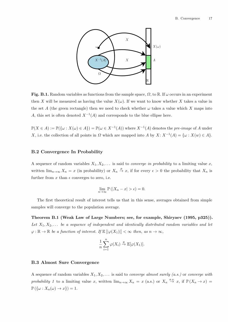
Fig. B.1. Random variables as functions from the sample space,Ω, to R. If ω occurs in an experiment
then X will be measured as having the value X(ω). If we want to know whether X takes a value in
the set A (the green rectangle) then we need to check whether ω takes a value which X maps into
A, this set is often denoted X−1(A) and corresponds to the blue ellipse here.
P(X ∈ A) := P(ω : X(ω) ∈ A) = P(ω ∈ X−1(A)) where X−1(A) denotes the pre-image of A under
X, i.e. the collection of all points in Ω which are mapped into A by X: X−1(A) = ω : X(w) ∈ A.
B.2 Convergence In Probability
A sequence of random variables X1, X2, . . . is said to converge in probability to a limiting value x,
written limn→∞Xn = x (in probability) or Xnp→ x, if for every ε > 0 the probability that Xn is
further from x than ε converges to zero, i.e.
limn→∞
P (|Xn − x| > ε) = 0.
The first theoretical result of interest tells us that in this sense, averages obtained from simple
samples will converge to the population average.
Theorem B.1 (Weak Law of Large Numbers; see, for example, Shiryaev (1995, p325)).
Let X1, X2, . . . be a sequence of independent and identically distributed random variables and let
ϕ : R→ R be a function of interest. If E [|ϕ(X1)|] <∞ then, as n→∞,
1
n
n∑i=1
ϕ(Xi)p→ E[ϕ(X1)].
B.3 Almost Sure Convergence
A sequence of random variables X1, X2, . . . is said to converge almost surely (a.s.) or converge with
probability 1 to a limiting value x, written limn→∞Xn = x (a.s.) or Xna.s.→ x, if P (Xn → x) =
P (ω : Xn(ω)→ x) = 1.

B. Convergence 18
Almost sure convergence is strictly stronger than convergence in probability. We can, however,
be sure that under weak assumptions the average from a simple random sample will convergence
almost surely to the underlying population average.
Theorem B.2 (Strong Law of Large Numbers; see, for example Shiryaev (1995, p391)).
Let X1, X2, . . . be a sequence of independent and identically distributed random variables and let
ϕ : R→ R with E [|ϕ(X1)|] <∞. The sample average of ϕ converges, as n→∞, to its expectation
under the common distribution of the Xi with probability 1:
1
n
n∑i=1
ϕ(Xi)a.s.→ E [ϕ(X1)] .
B.4 Some Ideas Related to Convergence of Distributions
B.4.1 Convergence In Distribution
A sequence of random variables X1, . . . is said to converge in distribution to another random variable
X if, for every continuous bounded function ϕ : R → R we have that E [ϕ(Xi)] → E [ϕ(X)]. If we
allow Fi to denote the distribution function of Xi and F that of X then this mode of convergence
is equivalent to the pointwise convergence of Fi to F (except at an at most countable collection of
points of discontinuity).
Although this may seem an esoteric idea, it’s really just telling us that the distribution of the
sequence of random variables becomes arbitrary close to that of X, eventually. Any statistician is
familiar with the following example of convergence in distribution.
Theorem B.3 (Central Limit Theorem; see Shao (1999, Corollary 1.2) for example). Let
X1, . . . be independent and identically distributed k-dimensional random vectors (i.e. random ele-
ments in Rk which can be viewed as a vector of K random variables) with finite covariance matrix
Σ, then as n→∞,
√n
[1
n
n∑i=1
Xi − E [X1]
]D→ N (0, Σ) ,
where 0 denotes the zero element of Rk.
B.4.2 Glivenko–Cantelli Theorems
The following result isn’t cast as convergence in distribution but it does tell us something very
closely related and so it is included here. This result is perhaps slightly less widely known than
those mentioned above, but it is tremendously informative for many of the methods which we will
consider in this module.
Theorem B.4 (Glivenko–Cantelli; see Athreya (2003) for a self-contained proof). Let
X1, . . . be a sequence of independent and identically distributed random variables with distribution

B. Convergence 19
function F . Let Fn(x) denote the empirical distribution functions associated with the first n elements
in this sequence, i.e. let
Fn(x) =1
n
n∑i=1
I(−∞,Xi](x),
where
I(−∞,Xi](x) =
1 if x ∈ (−∞, Xi]
0 otherwise.
Then, as n→∞,
supx|Fn(x)− F (x)| a.s.→ 0.
This tells us that if we construct a probability distribution by placing a mass of 1/n at the
location of every one of a sample of n independent and identically distributed replicates of a random
variable with a given distribution function then, for large enough samples, that empirical distribution
function converges uniformly to the underlying distribution function. Which tells us in a precise sense
something which we might intuitively have believed: if we replace the original probability distribution
with that obtained from a large enough sample then for most practical purposes we will obtain a
good approximation.
B.5 Warm-Up Exercises
If you feel like you could do with reminding yourself how these ideas of stochastic convergence work
then you might like to have a go at the following; if you already know how to answer them then
don’t waste your time and, similarly, if you have no interest in such things then it won’t be essential
to the lectures for this module that you have worked these out.
Exercise B.1. Given an example of a sequence of random variables which:
(a) converge to a limit with probability one;
(b) converge to a limit in probability but not almost surely; and
(c) converge to a limit in distribution but not in probability.
Related Documents