Computer Graphics Recitation 11

Computer Graphics Recitation 11. 2 The plan today Least squares approach General / Polynomial fitting Linear systems of equations Local polynomial.
Dec 22, 2015
Welcome message from author
This document is posted to help you gain knowledge. Please leave a comment to let me know what you think about it! Share it to your friends and learn new things together.
Transcript

Computer Graphics
Recitation 11
2
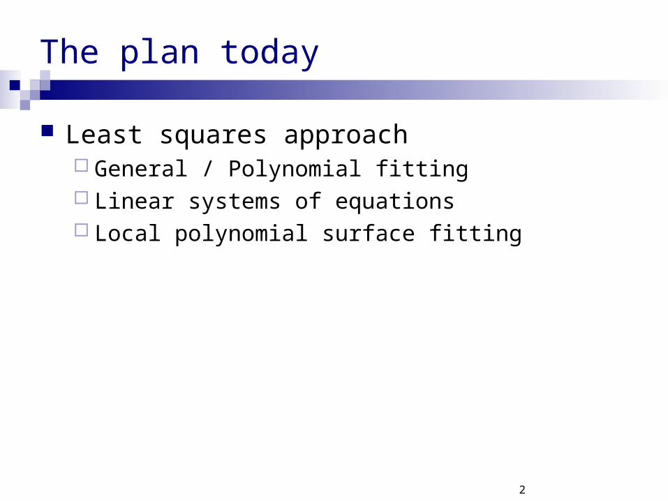
The plan today
Least squares approach General / Polynomial fitting Linear systems of equations Local polynomial surface fitting
3
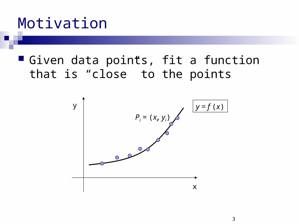
y = f (x)
Motivation
Given data points, fit a function that is “close” to the points
y
x
Pi = (xi, yi)
4
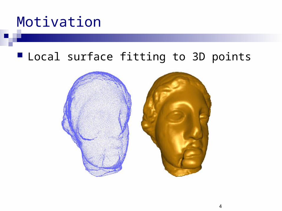
Motivation
Local surface fitting to 3D points

5
Line fitting
Orthogonal offsets minimization – we learned
x
y
Pi = (xi, yi)

6
Line fitting
The origin of the line is the center of mass
The direction v is the eigenvector corresponding to the largest
eigenvalue of the scatter matrix S (22)
In 2D this requires solving a square characteristic equation In higher dimensions – higher order equations…
n
iiP
nm
1
1
dc
ba
yyy
xxx
yyy
xxxS
n
n
n
n
T
21
21
21
21

7
Line fitting
y-offsets minimization
x
y
Pi = (xi, yi)

8
Line fitting
Find a line y = ax + b that minimizes
Err(a, b) = [yi – (axi + b)]2
Err is quadratic in the unknown parameters a, b
Another option would be, for example:
But – it is not differentiable, harder to minimize…
n
i 1
n
iii baxybaAbsErr
1
)(),(
9
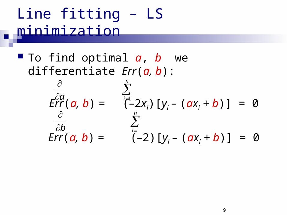
Line fitting – LS minimization
To find optimal a, b we differentiate Err(a, b):
Err(a, b) = (–2xi)[yi – (axi + b)] = 0
Err(a, b) = (–2)[yi – (axi + b)] = 0
a
n
i 1
n
i 1b

10
Line fitting – LS minimization
We get two linear equations for a, b:
(–2xi)[yi – (axi + b)] = 0
(–2)[yi – (axi + b)] = 0
n
i 1
n
i 1
11
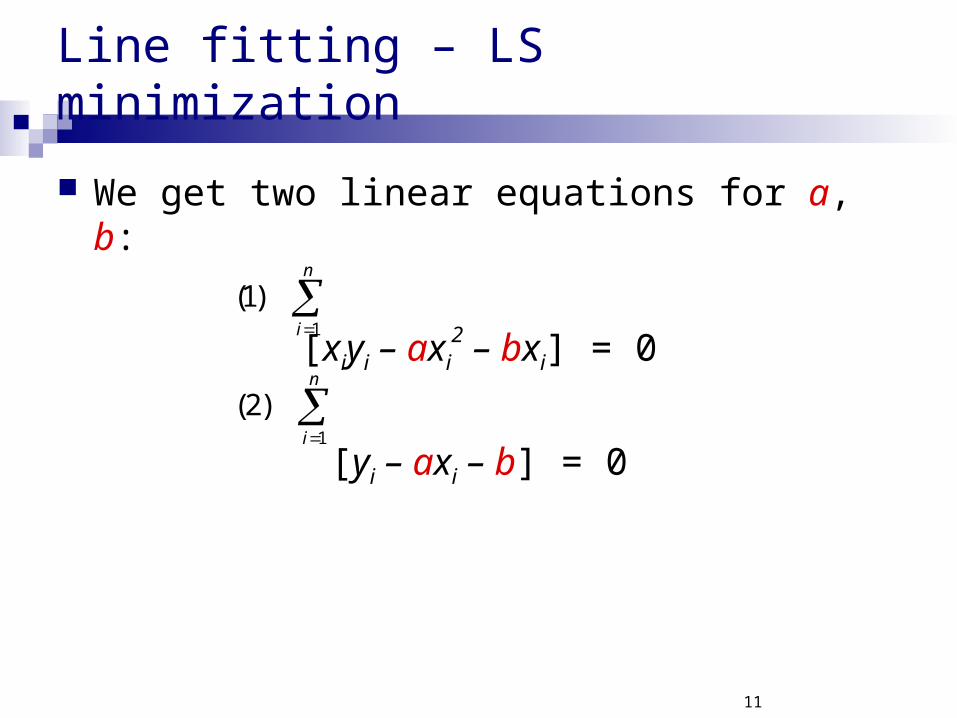
Line fitting – LS minimization
We get two linear equations for a, b:
[xiyi – axi2 – bxi] = 0
[yi – axi – b] = 0
n
i 1
)1(
n
i 1
)2(
12
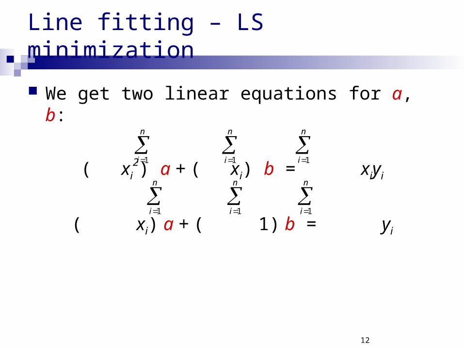
Line fitting – LS minimization
We get two linear equations for a, b:
( xi2) a + ( xi) b = xiyi
( xi) a + ( 1) b = yi
n
i 1
n
i 1
n
i 1
n
i 1
n
i 1
n
i 1

13
Line fitting – LS minimization
Solve for a, b using e.g. Gauss elimination
Question: why the solution is minimum for the error function?
Err(a, b) = [yi – (axi + b)]2
n
i 1

14
Fitting polynomials
y
x
15
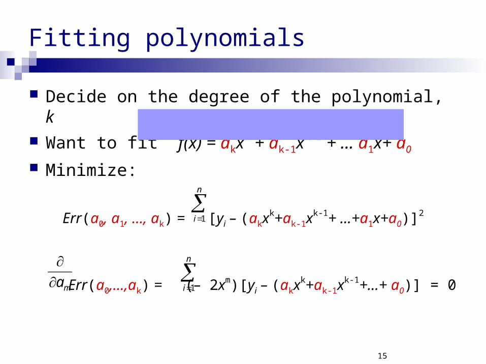
Fitting polynomials
Decide on the degree of the polynomial, k Want to fit f(x) = akx
k + ak-1xk-1 + … a1x+ a0
Minimize:
Err(a0, a1, …, ak) = [yi – (akxk+ak-1x
k-1+ …+a1x+a0)]2
Err(a0,…,ak) = (– 2xm)[yi – (akxk+ak-1x
k-1+…+ a0)] = 0
n
i 1
n
i 1ma

16
Fitting polynomials
We get a linear system of k+1 in k+1 variables
n
ii
ki
n
iii
n
ii
k
n
i
ki
n
i
ki
n
i
ki
n
i
ki
n
ii
n
ii
n
i
ki
n
ii
n
i
yx
yx
y
a
a
a
xxx
xxx
xx
1
1
11
0
1
2
1
1
1
1
1
1
2
1
111
11

17
General parametric fitting
We can use this approach to fit any function f(x) Specified by parameters a, b, c, … The expression f(x) linearly depends on the
parameters a, b, c, …
18
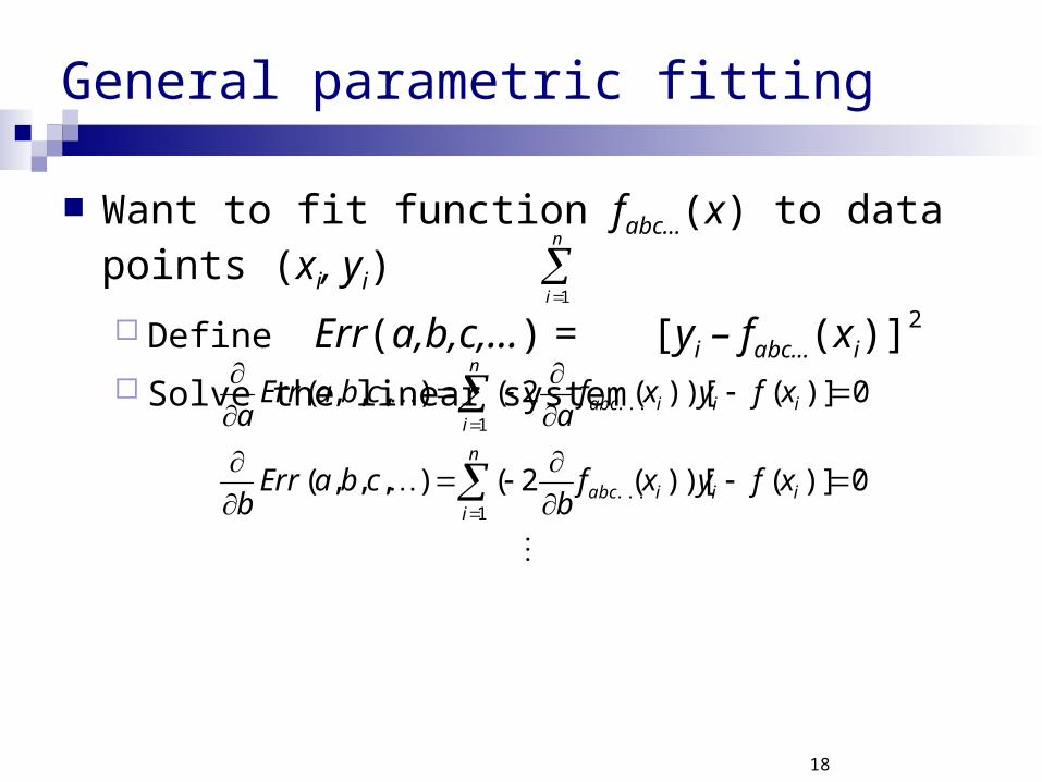
General parametric fitting
Want to fit function fabc…(x) to data points (xi, yi)
Define Err(a,b,c,…) = [yi – fabc…(xi)]2
Solve the linear system
0)]())[(2(),,,(
0)]())[(2(),,,(
...1
...1
iiiabc
n
i
iiiabc
n
i
xfyxfb
cbaErrb
xfyxfa
cbaErra
n
i 1
19
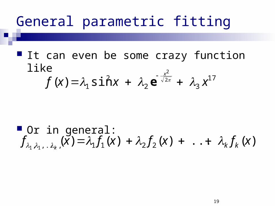
General parametric fitting
It can even be some crazy function like
Or in general:
1732
21
2
2
sin)( xxxfx
e
)(...)()()( 2211,...,, 11xfxfxfxf kkk
20
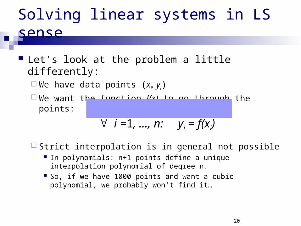
Solving linear systems in LS sense
Let’s look at the problem a little differently: We have data points (xi, yi)
We want the function f(x) to go through the points:
i =1, …, n: yi = f(xi)
Strict interpolation is in general not possible In polynomials: n+1 points define a unique interpolation
polynomial of degree n. So, if we have 1000 points and want a cubic polynomial, we
probably won’t find it…
21
Solving linear systems in LS sense
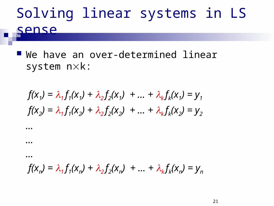
We have an over-determined linear system nk:
f(x1) = 1 f1(x1) + 2 f2(x1) + … + k fk(x1) = y1
f(x2) = 1 f1(x2) + 2 f2(x2) + … + k fk(x2) = y2
…
…
…
f(xn) = 1 f1(xn) + 2 f2(xn) + … + k fk(xn) = yn
22
Solving linear systems in LS sense
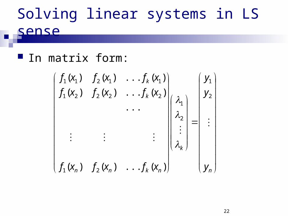
In matrix form:
n
k
nknn
k
k
y
y
y
xfxfxf
xfxfxf
xfxfxf
2
1
2
1
21
22221
11211
)(...)()(
...
)(...)()(
)(...)()(
23
Solving linear systems in LS sense
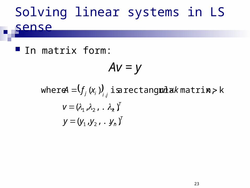
In matrix form:
Av = y
Tn
Tk
jiij
yyyy
v
knxfA
),...,,(
),...,,(
kn matrix, r rectangula a is )( where
21
21
.
24
Solving linear systems in LS sense
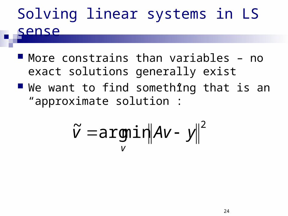
More constrains than variables – no exact solutions generally exist
We want to find something that is an “approximate solution”:
2minarg~ yAvvv

25
Finding the LS solution
v Rk
Av Rn As we vary v, Av varies over the linear subspace
of Rn spanned by the columns of A:
Av = A2A1 Ak
1
2
.
. k
= 1A 1 A 2 A k + 2 +…+ k
26
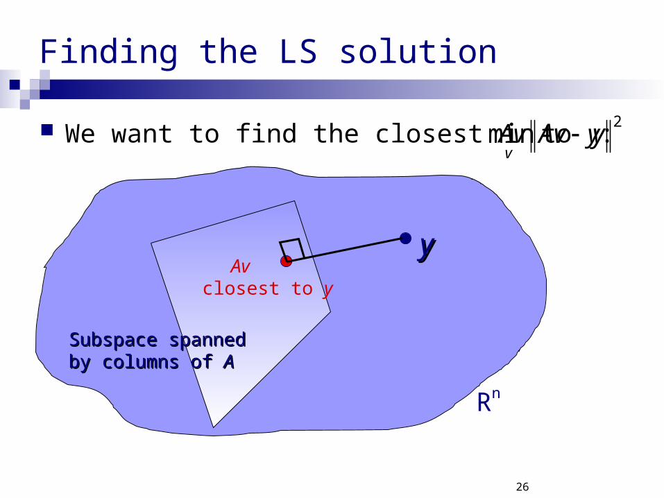
Finding the LS solution
We want to find the closest Av to y:2
min yAvv
Subspace spannedSubspace spannedby columns of by columns of AA
yy
Rn
Avclosest to y

27
Finding the LS solution
The vector Av closest to y satisfies:
(Av – y) {subspace of A’s columns}
column Ai, <Ai, Av – y> = 0
i, AiT(Av – y) = 0
AT(Av – y) = 0
(ATA)v = ATy
These arecalled the
normal equations
28
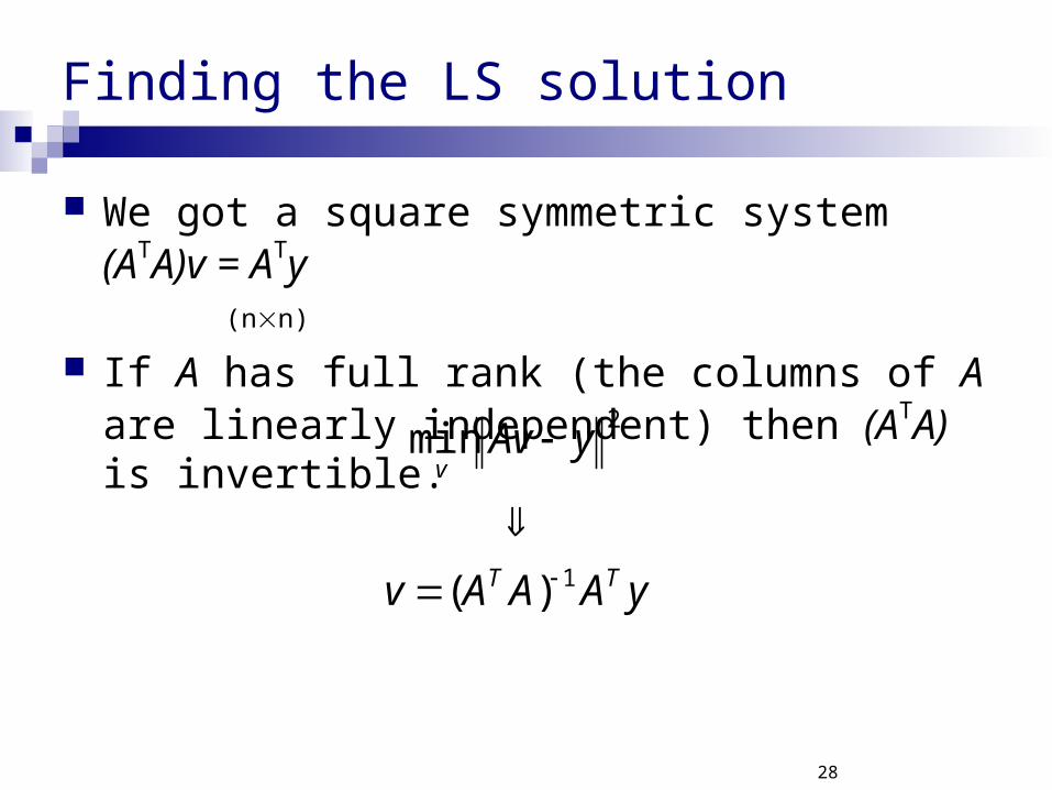
Finding the LS solution
We got a square symmetric system (ATA)v = ATy (nn)
If A has full rank (the columns of A are linearly independent) then (ATA) is invertible.
yAAAv
yAv
TT
v
1
2
)(
min
29
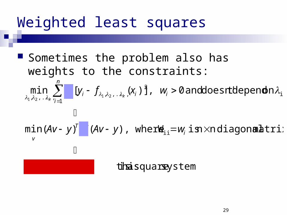
Weighted least squares
Sometimes the problem also has weights to the constraints:
system square a is this)(
matrix diagonaln n is W where),()(min
on dependt doesn' and 0,)]([min
ii
i2
,...,,1
,...,, 2121
WyAvWAA
wyAvWyAv
wxfyw
TT
iT
v
iii
n
ii k
k

30
Local surface fitting to 3D points
Normals? Lighting? Upsampling?

31
Local surface fitting to 3D points
Locally approximate
a polynomial surface
from points
32
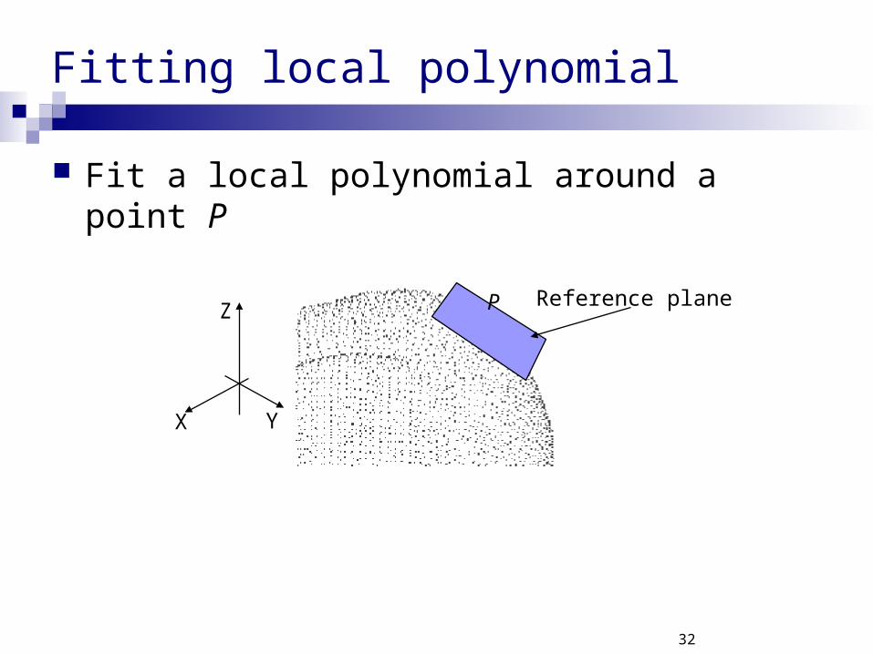
Fitting local polynomial
X Y
ZReference plane
Fit a local polynomial around a point P
P

33
Fitting local polynomial surface
Compute a reference plane that fits the points close to P Use the local basis defined by the normal to the plane!
z
x y

34
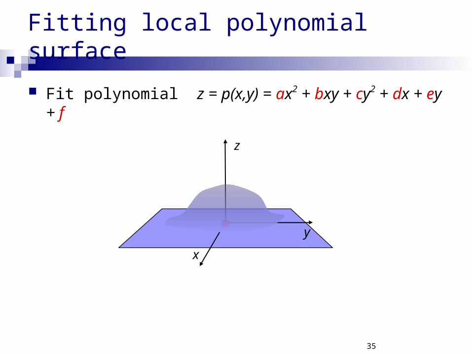
Fitting local polynomial surface
Fit polynomial z = p(x,y) = ax2 + bxy + cy2 + dx + ey + f
z
x y
35
Fitting local polynomial surface
Fit polynomial z = p(x,y) = ax2 + bxy + cy2 + dx + ey + f
z
x
y
36
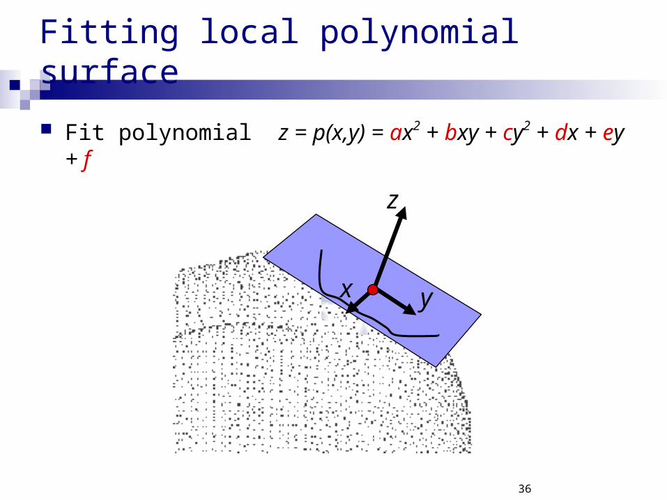
Fitting local polynomial surface
Fit polynomial z = p(x,y) = ax2 + bxy + cy2 + dx + ey + f
z
x y
37
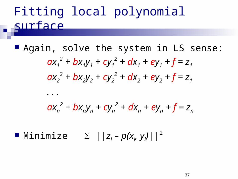
Fitting local polynomial surface
Again, solve the system in LS sense:
ax12 + bx1y1 + cy1
2 + dx1 + ey1 + f = z1
ax22 + bx2y2 + cy2
2 + dx2 + ey2 + f = z1
. . .
axn2 + bxnyn + cyn
2 + dxn + eyn + f = zn
Minimize ||zi – p(xi, yi)||2
38
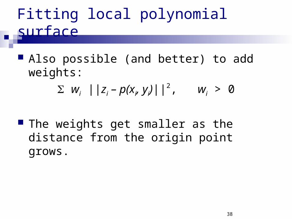
Fitting local polynomial surface
Also possible (and better) to add weights:
wi ||zi – p(xi, yi)||2, wi > 0
The weights get smaller as the distance from the origin point grows.

39
Geometry compression using relative coordinates
Given a mesh: Connectivity Geometry – (x, y, z) of each vertex

40
Geometry compression using relative coordinates
The size of the geometry is large (compared to connectivity)
(x, y, z) coordinates are hard to compress Floating-point numbers – have to quantize No correlation
41
Geometry compression using relative coordinates
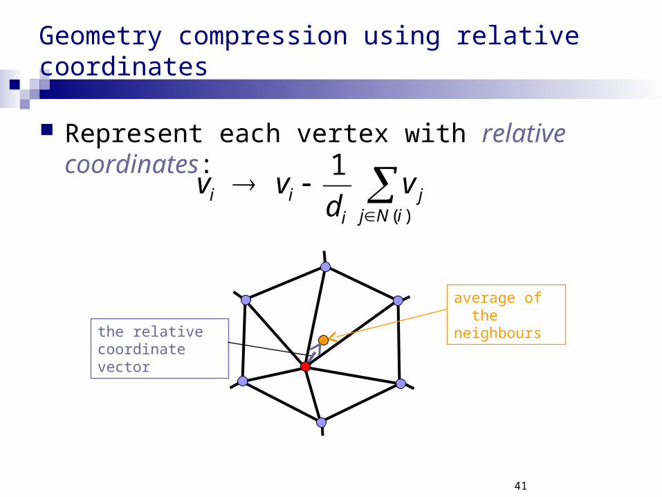
Represent each vertex with relative coordinates:
)(
1
iNjj
iii v
dvv
average of the neighbours
the relative coordinate vector

42
Geometry compression using relative coordinates
We call them –coordinates:
),,(),,( )()()( zi
yi
xiiii zyx
average of the neighbours
the relative coordinate vector

43
Geometry compression using relative coordinates
When the mesh is smooth, the –coordinates are small.
–coordinates can be better compressed.

44
Geometry compression using relative coordinates
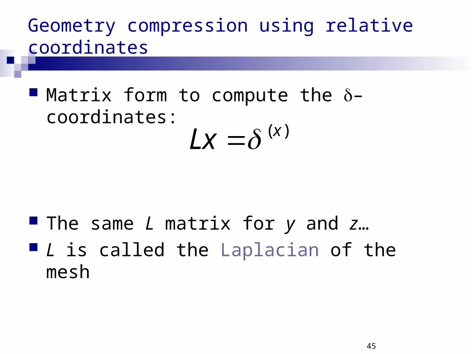
Matrix form to compute the –coordinates:
)(
)(1
)(2
)(1
1
2
1
111
111
11
11
1
10
1
1
1
1
10
001
111
22
11
xn
xn
x
x
n
n
ddd
ddd
dd
dd
x
x
x
x
nnn
nnn
45
Geometry compression using relative coordinates
Matrix form to compute the –coordinates:
The same L matrix for y and z… L is called the Laplacian of the mesh
)( xLx

46
Geometry compression using relative coordinates
How do we restore the (x, y, z) from the –coordinates?
Need to solve the linear system:
Lx = (x)

47
Geometry compression using relative coordinates
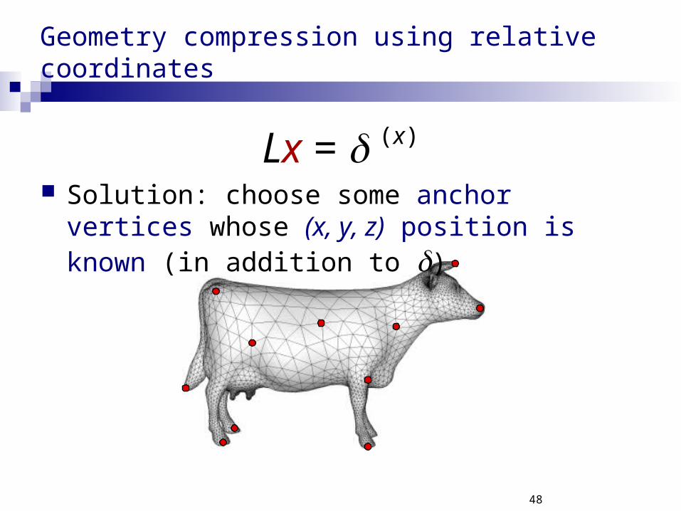
Lx = (x)
But: L is singular (x) contains quantization error
48
Geometry compression using relative coordinates
Lx = (x)
Solution: choose some anchor vertices whose (x, y, z) position is known (in addition to )

49
Geometry compression using relative coordinates
We add the anchor vertices to our linear system:
0100
0010
nx
x
x
2
1
known
known
xn
x
x
x
x
2
1
)(
)(2
)(1
constrainedanchor vertices
L
)(~ xxL
50
Geometry compression using relative coordinates
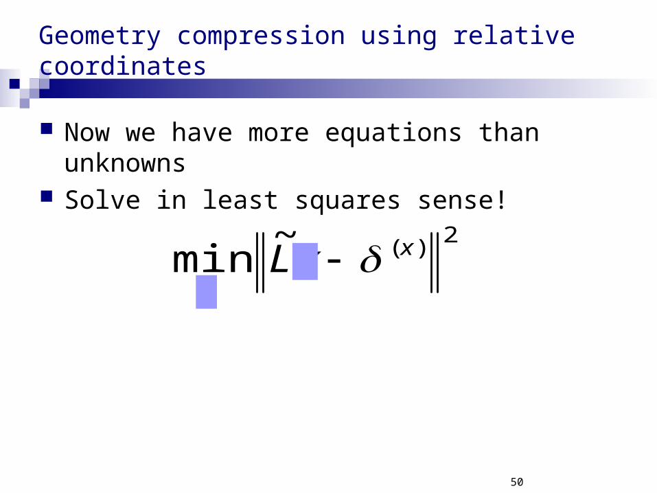
Now we have more equations than unknowns Solve in least squares sense!
2)(~
min x
xxL

See you next time
Related Documents


![ON SUMS OF SQUARES OF - Departamento de Matemática · 2019. 12. 3. · sums of squares is found in [2]. A polynomial pis called a scaled diagonally dominant sum of squares (sd-sos)](https://static.cupdf.com/doc/110x72/60a95c6da5720d5a7452b2ba/on-sums-of-squares-of-departamento-de-matem-2019-12-3-sums-of-squares-is.jpg)