Computer Graphics: Graphics Output Primitives Line Drawing Algorithms By: A. H. Abdul Hafez [email protected], March 8, 2017 1 CG, by Dr. A.H. Abdul Hafez, CE Dept. HKU

Welcome message from author
This document is posted to help you gain knowledge. Please leave a comment to let me know what you think about it! Share it to your friends and learn new things together.
Transcript

Computer Graphics: Graphics Output Primitives
Line Drawing Algorithms
By: A. H. Abdul Hafez
March 8, 2017 1 CG, by Dr. A.H. Abdul Hafez, CE Dept. HKU

Outlines
March 8, 2017 CG, by Dr. A.H. Abdul Hafez, CE Dept. HKU 2
1. Basic concept of lines in OpenGL
2. Line Equation
3. DDA Algorithm
4. DDA Algorithm implementation
5. Bresenham's Line Algorithm
6. Circle generation algorithms
7. Circle midpoint algorithm
8. End

Basic concept of lines in OpenGL
March 8, 2017 CG, by Dr. A.H. Abdul Hafez, CE Dept. HKU 3
To display the line on a raster monitor, the graphics system must first project the
endpoints to integer screen coordinates
Next, it determines the nearest pixel positions along the line path between the
two endpoints.
Then the line color is loaded into the frame buffer at the corresponding pixel
coordinates.

Basic concept of lines in OpenGL
March 8, 2017 CG, by Dr. A.H. Abdul Hafez, CE Dept. HKU 4
Reading from the frame buffer, the video controller plots the screen pixels.
This process digitizes the line into a set of discrete integer positions that, in
general, only approximates the actual line path.
This rounding of coordinate values to integers causes all but horizontal and
vertical limes to be displayed with a stair-step appearance ("the jaggies").

Line Equation
March 8, 2017 CG, by Dr. A.H. Abdul Hafez, CE Dept. HKU 5
The Cartesian slope-intercept equation for a straight line is
we can determine values for the slope m and y intercept b with the following calculations:
For any given x interval δx along a line, we can compute the corresponding y interval δy
On raster systems, lines are plotted with pixels. That is, we must "sample" a line at discrete positions and determine the nearest pixel to the line at each sampled position.
Discrete sample positions along the x axis is shown.

general Line drawing
March 8, 2017 CG, by Dr. A.H. Abdul Hafez, CE Dept. HKU 6
Case 1 and 2: m>1, while Case 3 and 8: m<1.
Case 1: unit step through +x, increment y.
Case 2: unit step through +y, increment x.
Case 3: unit step through +y, decrement x.
Case 8: unit step through +x, decrement y.
Cases 4,5,6,7: swap end coordinates & use the algorithm for the symmetric quadrants.

DDA Algorithm
March 8, 2017 CG, by Dr. A.H. Abdul Hafez, CE Dept. HKU 7
We consider first a line with positive slope; start is at left:
1. If the slope is less than or equal to 1, we sample at unit x intervals (δx = 1)
and compute successive y values as
2. For lines with a positive slope greater than 1, we reverse the roles of x and y.
That is, we sample at unity intervals (δy = 1) and calculate consecutive x
values as
x
y
δx = 1
δy = 1

DDA Algorithm
March 8, 2017 CG, by Dr. A.H. Abdul Hafez, CE Dept. HKU 8
We consider second a line with positive slope; start is at right:
If the slope m <= 1, we sample at unit x intervals (δx = -1) and compute
successive y values as
If the slope m is greater than 1, we sample at unity intervals (δy = -1) and
calculate consecutive x values as
x δx =-1
δy =-m
y
δy = -1 δy =-1
δx =-1/m

DDA Algorithm
March 8, 2017 CG, by Dr. A.H. Abdul Hafez, CE Dept. HKU 9
We consider first a line with negative slope; start is at left:
1. If the absolute slope |m| is less than or equal to 1, we sample at unit x
intervals (δx = 1) and compute successive y values as
2. For lines with absolute slope |m| greater than 1, we reverse the roles of x and
y. That is, we sample at unity intervals (δy = -1) and calculate consecutive x
values as
x
y
δx = 1
δy = m
δy = - 1
δx = -1/m

DDA Algorithm
March 8, 2017 CG, by Dr. A.H. Abdul Hafez, CE Dept. HKU 10
We consider second a line with negative slope; start is at right:
If the slope m <= 1, we sample at unit x intervals (δx = -1) and compute
successive y values as
If the slope m is greater than 1, we sample at unity intervals (δy = +1) and
calculate consecutive x values as
x δx =-1
δy =-m
y
δy = 1
δx =1/m

DDA Algorithm implementation
March 8, 2017 CG, by Dr. A.H. Abdul Hafez, CE Dept. HKU 11
This algorithm is summarized in the following procedure, which accepts as input two integer screen positions for the endpoints of a line segment.
Horizontal and vertical differences between the endpoint positions are assigned to parameters dx and dy. The difference with the greater magnitude determines the value of parameter steps.
Starting with pixel position (x0, y0), we determine the offset needed at each step to generate the next pixel position along the line path.
We loop through this process steps times.
1. If the magnitude of dx is greater than the magnitude of dy and x0 is less than xEnd, the values for the increments in the x and y directions are 1 and m=dy/dx, respectively.
2. If the greater change is in the x direction, but x0 is greater than xEnd, then the decrements -1 and –m=dy/dx are used to generate each new point on the line.
3. Otherwise, we use a unit increment (or decrement) in the y direction and an x increment (or decrement) of 1/m=dx/dy.

DDA Algorithm implementation
March 8, 2017 CG, by Dr. A.H. Abdul Hafez, CE Dept. HKU 12

DDA Algorithm advantages and dis.
March 8, 2017 CG, by Dr. A.H. Abdul Hafez, CE Dept. HKU 13
Advantage
Does not calculate coordinates based on the complete equation (uses offset
method)
Disadvantage
Round-off errors are accumulated, thus line diverges more and more from
straight line
Round-off operations take time
Perform integer arithmetic by storing float as integers in numerator and
denominator and performing integer arithmetic.

Bresenham's Line Algorithm
March 8, 2017 CG, by Dr. A.H. Abdul Hafez, CE Dept. HKU 14
Motivation:
A section of the screen showing a pixel in column xk on scan line yk that is to be plotted along the path of a line segment with slope 0 < m < 1.
Assuming we have determined that
the pixel at (xk, yk) is to be displayed, we next need to decide which pixel to plot in column xk+l = xk + 1. Our choices are the pixels at positions (xk + 1, yk) and (xk + 1, yk+1).

Bresenham's Line Algorithm
March 8, 2017 CG, by Dr. A.H. Abdul Hafez, CE Dept. HKU 15
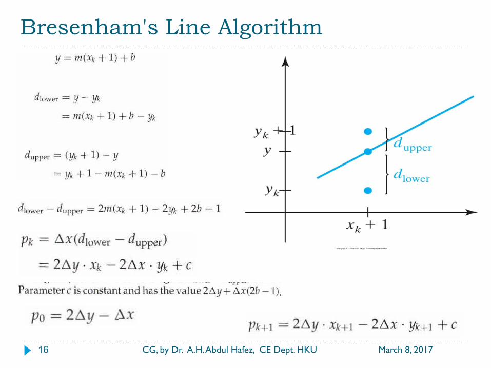
To determine which of the two
pixels is closest to the line path, we
can set up an efficient test that is
based on the difference between the
two pixel separations, and defining
the decision parameter as
Vertical distances between pixel
positions and the line y coordinate
at sampling position xk + 1.
Bresenham's Line Algorithm
March 8, 2017 CG, by Dr. A.H. Abdul Hafez, CE Dept. HKU 16

Bresenham's Line Algorithm
March 8, 2017 CG, by Dr. A.H. Abdul Hafez, CE Dept. HKU 17

Bresenham's Line Algorithm
March 8, 2017 CG, by Dr. A.H. Abdul Hafez, CE Dept. HKU 18

Bresenham's Line Algorithm
March 8, 2017 CG, by Dr. A.H. Abdul Hafez, CE Dept. HKU 19
EXAMPLE 3-1 from the text

Bresenham's Line Algorithm
March 8, 2017 CG, by Dr. A.H. Abdul Hafez, CE Dept. HKU 20
EXAMPLE 3-1 cont.

Bresenham's Line Algorithm
March 8, 2017 CG, by Dr. A.H. Abdul Hafez, CE Dept. HKU 21
Pixel positions along the line path between endpoints (20, 10) and
(30, 18), plotted with Bresenham’s line algorithm.

Bresenham's Line Algorithm Code
March 8, 2017 CG, by Dr. A.H. Abdul Hafez, CE Dept. HKU 22

Bresenham's Line Algorithm Code
March 8, 2017 CG, by Dr. A.H. Abdul Hafez, CE Dept. HKU 23

The end of the Lecture
March 8, 2017 CG, by Dr. A.H. Abdul Hafez, CE Dept. HKU 24
Thanks for your time
Questions are welcome
Related Documents