Computer Graphics From Vertices to Fragments: Clipping, HSR, Rasterization and Anti-aliasing Based on slides by Dianna Xu, Bryn Mawr College

Welcome message from author
This document is posted to help you gain knowledge. Please leave a comment to let me know what you think about it! Share it to your friends and learn new things together.
Transcript

Computer Graphics From Vertices to Fragments:
Clipping, HSR, Rasterization and Anti-aliasing
Based on slides by Dianna Xu, Bryn Mawr College

Rendering Algorithms
• Rendering a scene with opaque objects – For every pixel, determine which object that projects on the pixel is closest to the viewer and compute the shade of this pixel
– Ray tracing paradigm – For every object, determine which pixels it covers and shade these pixels
• Pipeline approach • Must keep track of depths

Common Tasks • Clipping • Hidden surface removal • Rasterization or scan conversion • Antialiasing

Clipping • 2D against clipping window • 3D against clipping volume • Easy for line segments polygons • Hard for curves and text
– Convert to lines and polygons first

Clipping 2D Line Segments
• Brute force approach: compute intersections with all sides of clipping window – Inefficient: one division per intersection

Cohen-Sutherland Algorithm
• Idea: eliminate as many cases as possible without computing intersections
• Start with four lines that determine the sides of the clipping window
x = xmax x = xmin
y = ymax
y = ymin

The Cases
• Case 1: both endpoints of line segment inside all four lines
– Draw (accept) line segment as is
• Case 2: both endpoints outside all lines and on same side of a line
– Discard (reject) the line segment
x = xmax x = xmin
y = ymax
y = ymin

The Cases • Case 3: One endpoint inside, one outside
– Must do at least one intersection • Case 4: Both outside
– May have part inside – Must do at least one intersection
x = xmax x = xmin
y = ymax

Defining Outcodes
• For each endpoint, define an outcode
• Outcodes divide space into 9 regions • Computation of outcode requires at most 4 subtractions
b0b1b2b3
b0 = 1 if y > ymax, 0 otherwise b1 = 1 if y < ymin, 0 otherwise b2 = 1 if x > xmax, 0 otherwise b3 = 1 if x < xmin, 0 otherwise

Using Outcodes
• Consider the 5 cases below • AB: outcode(A) = outcode(B) = 0
– Accept line segment

Using Outcodes • CD: outcode (C) = 0, outcode(D) ≠ 0
– Compute intersection – Location of 1 in outcode(D) determines which
edge to intersect with – Note if there were a segment from C to a point
in a region with 2 ones in outcode, we might have to do two intersections

Using Outcodes
• EF: outcode(E) & outcode(F) (bitwise) != 0 – Both outcodes have a 1 bit in the same place – Line segment is outside of corresponding
side of clipping window – reject

Using Outcodes • GH and IJ: same outcodes, neither zero but
logical AND yields zero • Shorten line segment by intersecting with
one of sides of window • Compute outcode of intersection (new
endpoint of shortened line segment) • Re-execute algorithm

Cohen Sutherland in 3D • Use 6-bit outcodes • When needed, clip line segment against planes

Liang-Barsky Clipping • Consider the parametric form of a line segment
• We can distinguish between the cases by looking at the ordering of the values of α where the line determined by the line segment crosses the lines that determine the window
p(α) = (1-α)p1+ αp2 1 ≥ α ≥ 0
p1
p2
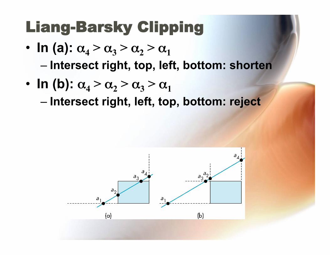
Liang-Barsky Clipping • In (a): α4 > α3 > α2 > α1
– Intersect right, top, left, bottom: shorten • In (b): α4 > α2 > α3 > α1
– Intersect right, left, top, bottom: reject

Advantages • Can accept/reject as easily as with Cohen-
Sutherland • Using values of α, we do not have to use
algorithm recursively as with C-S • Extends to 3D

Clipping and Normalization
• General clipping in 3D requires intersection of line segments against arbitrary plane
• Example: oblique view

Plane-Line Intersections

Normalized Form
before normalization after normalization
Normalization is part of viewing (pre clipping) but after normalization, we clip against sides of right parallelepiped
Typical intersection calculation now requires only a floating point subtraction, e.g. is x > xmax ?
top view
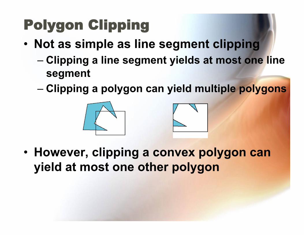
Polygon Clipping • Not as simple as line segment clipping
– Clipping a line segment yields at most one line segment
– Clipping a polygon can yield multiple polygons
• However, clipping a convex polygon can yield at most one other polygon

Tessellation and Convexity
• One strategy is to replace nonconvex (concave) polygons with a set of triangular polygons (a tessellation)
• Also makes fill easier • Tessellation code in GLU library

Clipping as a Black Box • Can consider line segment clipping as a
process that takes in two vertices and produces either no vertices or the vertices of a clipped line segment

Pipeline Clipping of Line Segments
• Clipping against each side of window is independent of other sides – Can use four independent clippers in a
pipeline

Pipeline Clipping of Polygons
• Three dimensions: add front and back clippers • Strategy used in SGI Geometry Engine • Small increase in latency

Bounding Boxes • Rather than doing clipping on a complex
polygon, we can use an axis-aligned bounding box or extent – Smallest rectangle aligned with axes that
encloses the polygon – Simple to compute: max and min of x and y
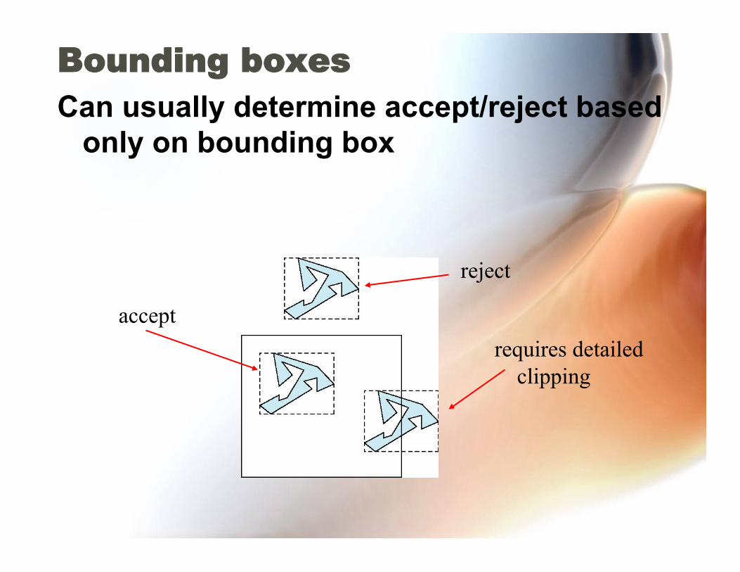
Bounding boxes Can usually determine accept/reject based
only on bounding box
reject
accept requires detailed clipping

Clipping and Visibility
• Clipping has much in common with hidden-surface removal
• In both cases, we are trying to remove objects that are not visible to the camera
• Often we can use visibility or occlusion testing early in the process to eliminate as many polygons as possible before going through the entire pipeline

Hidden Surface Removal
• Object-space approach: use pairwise testing between polygons (objects)
• Worst case complexity O(n2) for n polygons
partially obscuring can draw independently

Image Space Approach • Look at each projector (nm for an n x m
frame buffer) and find closest of k polygons
• Complexity O(nmk) • Ray tracing • z-buffer

Visible Surface Algorithms
Roberts ‘63 Warnock ‘68 Watkins ‘70 Ray Casting ~‘71
Complexity grows O(n2) (n=number of objects)
Complexity ~ visual complexity Bounded by sorting cost O(n log n)
Object or Edge-Edge comparisons
Image space (pixel) comparisons

Polyhedral Object Model Assumptions
• Clip geometry to view volume. • Planar polygon faces (convex or concave). • Consistent edge traversal order -- to
establish uniform notion of inside and outside. – Surface normal points outward in a right-
handed world modeling coordinate system.
– In GL, make sure you list the vertices in a consistent order (all clockwise or counterclockwise (default) when viewed from outside).

Polygon Model Conceptualization

ATTRIBUTES: name = ‘floor’, normal = (0, 0, -1), color = (R=0.1, G=0.1, B=0.1), fill = yes, edge-color = (R=1, G=1, B=1), ...
A Polygonal Model
X
Y
Z
1 5
10
6
2
3
4
8
9 7
POINTS P1 = (1, 2, 0) P2 = (1, 2, 3) P3 = (0, 2, 5) P4 = (-1, 2, 3) P5 = (-1, 2, 0) P6 = (1, -2, 0) P7 = (1, -2, 3) P8 = (0, -2, 5) P9 = (-1, -2, 3) P10 = (-1, -2, 0)
POLYGONS P1 P5 P4 P3 P2 P6 P7 P8 P9 P10 P1 P2 P7 P6 P2 P3 P8 P7 P3 P4 P9 P8 P4 P5 P10 P9 P1 P6 P10 P5

Back Face Cull • glEnable(GL_CULL_FACE); • Throw out polygons facing away from eye -- that
is, any polygon with a BACK-facing normal:

Back Face Cull • Only FRONT-facing ones left to process
further.
THIS IS ONLY SUFFICIENT AS A VISIBLE SURFACE DISPLAY FOR A SCENE CONSISTING OF A SINGLE CONVEX
POLYHEDRON

Depth or Z-Buffer
• Each pixel stores COLOR and DEPTH.
• Algorithm: Initialize all elements of buffer (COLOR(row, col),
DEPTH(row, col)) to (background-color, maximum-depth);
FOR EACH polygon: Rasterize polygon to frame; FOR EACH pixel center (x, y) that is covered:
IF polygon depth at (x, y) < DEPTH(x, y) THEN COLOR(x, y) := polygon color at (x, y) AND DEPTH(x, y) := polygon depth at (x, y)

Depth Buffer Operation
Frame Depth
Initialize (“New Frame”)
∞
∞ ∞
∞ ∞ ∞ ∞ ∞
∞ ∞ ∞ ∞ ∞
∞
∞ ∞
∞ ∞
∞
∞

Depth Buffer Operation – First Polygon
Frame Depth
Pink Triangle -- depths computed at pixel centers
∞
∞ ∞
∞ ∞ ∞
∞ ∞
∞
∞
∞ ∞
∞
∞
24
26
28
27
29 30

Depth Buffer Operation -- First Polygon
Frame Depth
Pink Triangle -- pixel values assigned
∞
∞ ∞
∞ ∞ ∞
∞ ∞
∞
∞
∞ ∞
∞
∞
24
26
28
27
29 30

Depth Buffer Operation – Second Polygon
Frame Depth
Green Rectangle -- depths computed at pixel centers
∞
∞
∞ ∞
∞ ∞
∞
∞ ∞
24
26
28
10
9
9
8
7 8
7 6

Depth Buffer Operation – Second Polygon
Frame Depth
Green Rectangle -- pixel values assigned: NOTE REPLACEMENTS!
∞
∞
∞ ∞
∞ ∞
∞
∞ ∞
24
26
28
10
9
9
8
7 8
7 6

Depth Buffer Operation – Third Polygon
Frame Depth
∞
∞ ∞
∞ ∞
∞
∞
24
26
28
10
9
9
8
7 8
7 6
Blue Pentagon -- depths computed at pixel centers
72
75
68 not stored
71 not stored

Depth Buffer Operation – Third Polygon
Frame Depth
∞
∞ ∞
∞ ∞
∞
∞
24
26
28
10
9
9
8
7 8
7 6
72
75
Blue Pentagon -- pixel values assigned: NOTE ‘GOES BEHIND’!

Static Screen Subdivision • Use smaller depth buffer and repeat
multiple times
1/16th size Depth buffer

Adaptive Screen Subdivision
• Subdivide frame buffer into smaller chunks in detail areas.
• Implement as a recursive algorithm -- Warnock. – If frame area is simple, then just draw it. – If complex, then subdivide into quadrants
and recurse. • Simple = all background
covered entirely by one polygon split into two regions by one polygon
edge

Warnock’s Algorithm: Adaptive Screen Subdivision
Neat algorithm, but slow because recursion gets deep at many edges.
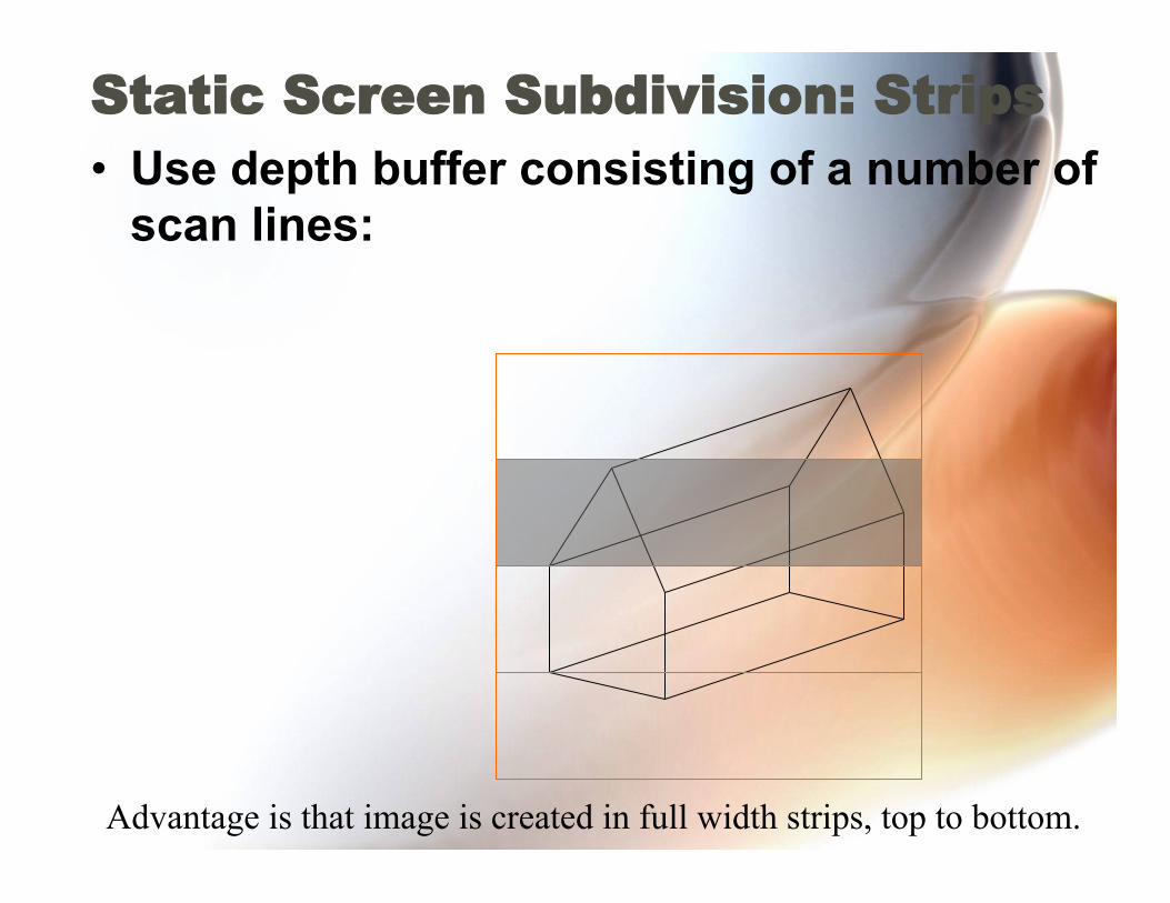
Static Screen Subdivision: Strips • Use depth buffer consisting of a number of
scan lines:
Advantage is that image is created in full width strips, top to bottom.

Static Screen Subdivision: Scan-Lines • In the limit, the strip can be a single scan-line. • All polygons need be processed for each scan-
line!
Watkins came up with a data structure that avoided this overhead.

Scan-Line Algorithm Definitions • Scan-Plane : The projection of the scan line
into the world. • Edge : Line between two polygon vertices. • Active Edge : An edge intersected by the
scan-plane. • Segment : Portion of a polygon between two
active edges.

Scan-Line Algorithm Definitions
screen segment
scan-plane
polygon
projection of active segment onto scan-line
active edge
active edge
eye
scan-line
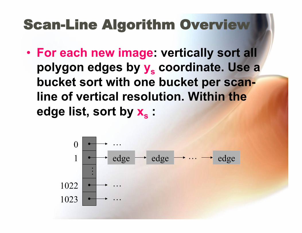
Scan-Line Algorithm Overview
• For each new image: vertically sort all polygon edges by ys coordinate. Use a bucket sort with one bucket per scan-line of vertical resolution. Within the edge list, sort by xs :
…
0 1
1022 1023
edge edge edge … …
… …

For each new image... • For each new scan-line: Advance the active scan-
line downward from the top. At each scan-line generate the active edge list based on additions, deletions, and modifications to the edge blocks already stored in that bucket.
• Let’s do an example with 10 scan-lines and just 2 triangle polygons called T and P: – T has three edges T1, T2, and T3 – P has three edges P1, P2, and P3

Initial State of Scan-Line Buckets (y-x sort)
T P
0 1
3 4
2
5 6
8 9
7
(Left-Right keeps track of which side the edge bounds.)
T1
T1-left
T2
T2-left
T3
T3-right
P1
P1-left
P2
P2-left P3
P3-right

For each Scan-Line, Build the Active Edge List
• No additions • No deletions • No updates
0
Scan-line 0

For each Scan-Line, Build the Active Edge List
T3-right 1
Scan-line 1
• 2 additions • No deletions • No updates
T1-left
New New

For each Scan-Line, Build the Active Edge List
T3-right 2
Scan-line 2
• No additions • No deletions • 2 updates
Update x Update x
T1-left

For each Scan-Line, Build the Active Edge List
T3-right 3
Scan-line 3
• 2 additions • No deletions • 2 updates
Update x Update x
P1-left P3-right T1-left
New New

For each Scan-Line, Build the Active Edge List
P1-left 4
Scan-line 4
• 1 addition • 1 deletion • 3 updates
Update x Update x
T3-right P3-right
Update x
T2-left
Note that these two blocks are re-sorted to maintain x order.
New

For each Scan-Line, Build the Active Edge List
T2-left 5
Scan-line 5
• No additions • No deletions • 4 updates
Update x Update x
T3-right P3-right P1-left
Update x Update x
Note that these two blocks are re-sorted to maintain x order.

For each Scan-Line, Build the Active Edge List
T2-left 6
Scan-line 6
• No additions • No deletions • 4 updates
Update x Update x
T3-right P3-right P1-left
Update x Update x
No re-sorting is needed.

For each Scan-Line, Build the Active Edge List
P3-right 7
Scan-line 7
• 1 addition • 3 deletions • 1 update
New Update x
P2-left

For each Scan-Line, Build the Active Edge List
P3-right 8
Scan-line 8
• No additions • No deletions • 2 updates
Update x Update x
P2-left
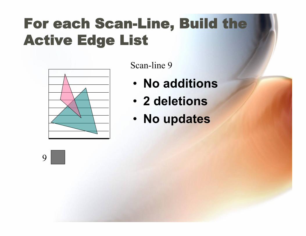
For each Scan-Line, Build the Active Edge List
9
Scan-line 9
• No additions • 2 deletions • No updates

Generate the Segment List
• For each scan line: scan the active scan-line left to right to determine visible segments or segment fragments, based on depth (smallest z) comparisons.
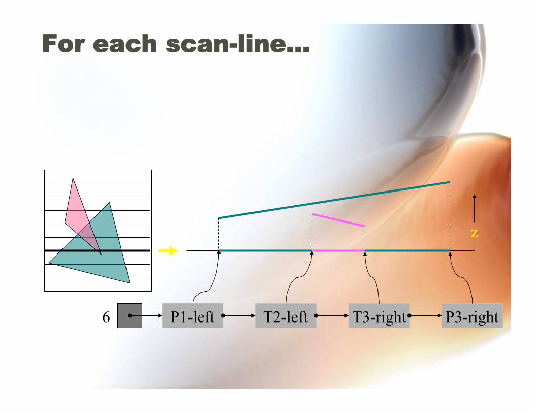
For each scan-line...
T2-left 6 T3-right P3-right P1-left
z

Painter’s Algorithm
• Sort polygons on distance from viewer. • Rasterize polygons into frame buffer in
sorted order from furthest to closest.
• Doesn’t always work, why do it? – Sorting is done prior to rendering. – No extra depth buffer memory or pixel
depth checking (i.e., no special hardware needed –this was before OpenGL cards…)

Painter’s Example -- House

Exact Algorithm -- Atherton and Weiler
• Screen subdivision by projected polygon outlines.
• Uses each polygon as a cookie-cutter on remainder of scene.
• Within each cookie-cutter polygon: if remainder of scene is behind cookie-
cutter polygon, then draw the cookie-cutter polygon
else re-enter the algorithm with another polygon as the cookie-cutter.

Clipping a Polygon with ClipPoly
Outside fragments
Append these to OutList
Inside fragments
ClipPoly Poly
Projected clip lines

Clipping a Polygon with ClipPoly
Clip to plane of ClipPoly (yields Nil)
Append to InList (Nil)
Poly
Projected clip lines
Inside fragments Poof!
Outside fragments
Append these to OutList
ClipPoly

Clipping a Penetrating Polygon with ClipPoly
ClipPoly Poly
Outside fragments
Append these to OutList
Inside fragments
Projected clip lines

Clipping a Penetrating Polygon with ClipPoly
ClipPoly Poly
Clip to plane of ClipPoly
Append this fragment to InList
Inside fragments
Outside fragments
Append these to OutList
Projected clip lines
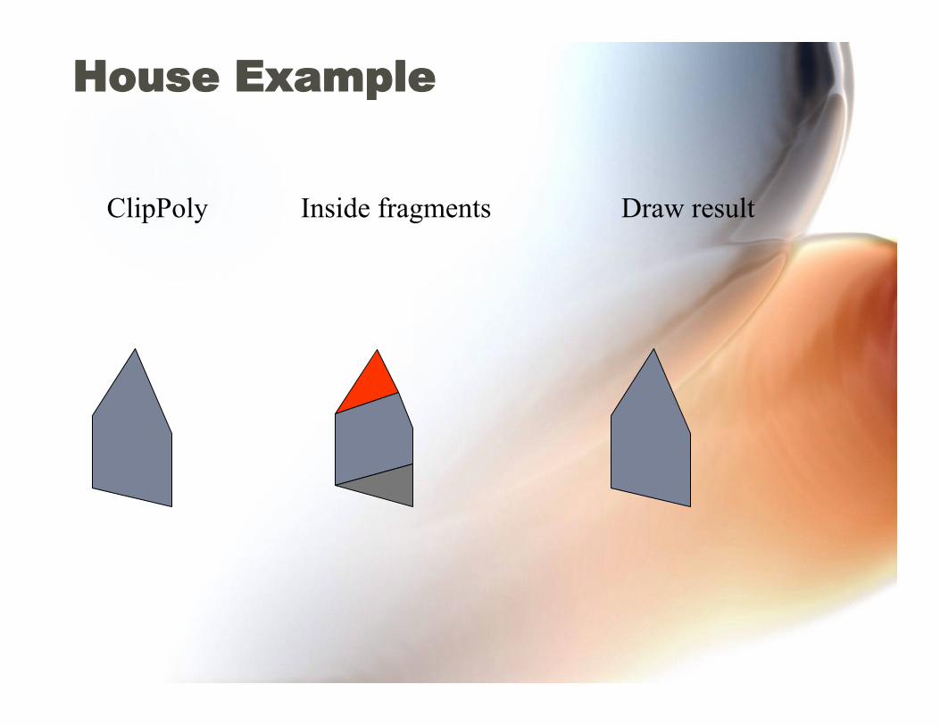
House Example
ClipPoly Inside fragments Draw result

House Example
ClipPoly Inside fragments Draw result

House Example
ClipPoly Inside fragments Draw result

Pre-Visibility Culling
• A family of techniques the attempt to cull as many invisible polygons BEFORE they are even sent into the rendering pipeline.
• Enhanced rendering performance, e.g., for games.
• Often combined with binary space partitioning

Binary Space Partitioning
• There exist scenes in which visibility can be predetermined and is independent of view (camera) viewpoint.
• Main requirement is linear separability: polygons are either on one side of a separating plane or another.
• Basic idea: compute visibility in advance, then use this structure to pre-define the display ordering (back to front).
• Data structure built is called a binary space partition tree or BSP-tree.

Separating Planes and the Viewpoint
• Find separating planes (m, n) such that each object (A, B, C) is in its own region of space.
A
B
C
m
(B, C) > A wrt m
Viewpoint
n
B > C wrt n
Therefore B > C > A wrt Viewpoint: m+, n+
: m+, n+
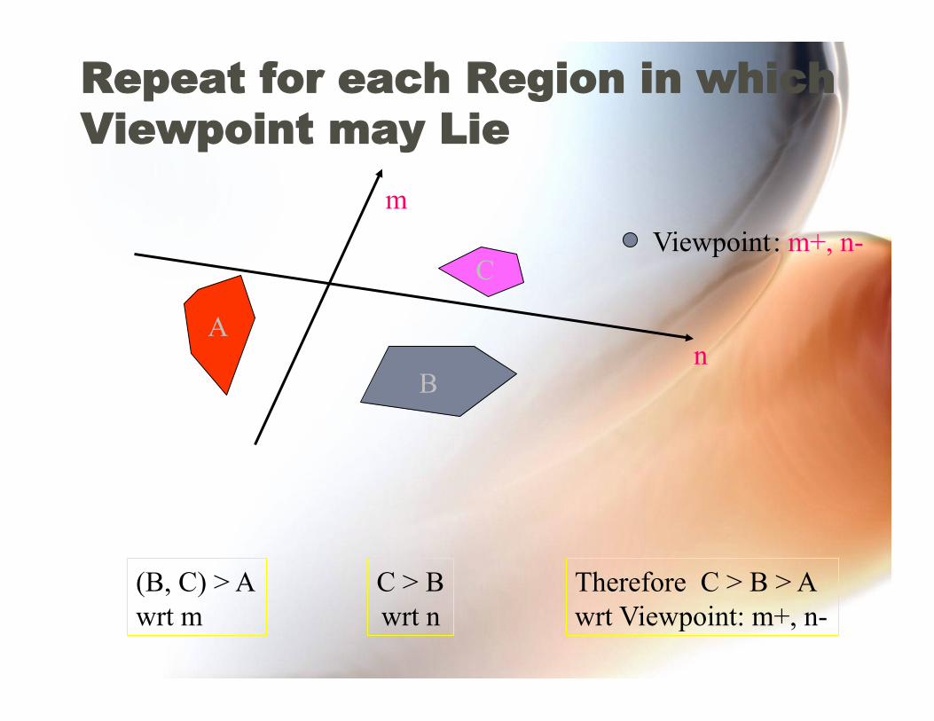
Repeat for each Region in which Viewpoint may Lie
A
B
C
m
(B, C) > A wrt m
Viewpoint
n
C > B wrt n
Therefore C > B > A wrt Viewpoint: m+, n-
: m+, n-

A
B
C
m
A > (B, C) wrt m
Viewpoint
n
B > C wrt n
Therefore A > B > C wrt Viewpoint: m-, n+
: m-, n+

A
B
C
m
A > (B, C) wrt m
Viewpoint
n
C > B wrt n
Therefore A > C > B wrt Viewpoint: m-, n-
: m-, n-

Combine all into a Binary Space Partition (BSP) Tree
m+ m-
n+ n+ n-
B > C > A C > B > A A > B > C A > C > B
So as soon as we compute what sides of the separating planes the viewpoint is on, we immediately know the object rendering order that guarantees correct visibility.
n- n-
m+
C > B > A

Display in Back-to-Front Order
Order: C > B > A
A
B C
Assume that back faces are culled; A, B, C may even be convex clusters of polygons

B
C
Order: A > C > B
A

This is Basically the “DOOM” Graphics Engine!
• Extend to 3D polygons. • Complex environments are pre-processed
to create the BSP tree. • In practice, slightly more complicated trees
are build to allow crossing features (walls). • Use nice textures on surfaces (see this
later).
http://symbolcraft.com/pjl/graphics/bsp/

Rasterization • Rasterization (scan conversion)
– Shade pixels that are inside object specified by a set of vertices • Line segments • Polygons: scan conversion = fill
• Shades determined by color, texture, shading model
• Here we study algorithms for determining the correct pixels starting with the vertices

Scan Conversion of Line Segments • Start with line segment in window
coordinates with integer values for endpoints
• Assume implementation has a write_pixel function
y = mx + h

DDA Algorithm • Digital Differential Analyzer
– DDA was a mechanical device for numerical solution of differential equations
– Line y=mx+ h satisfies differential equation dy/dx = m = Δy/Δx = y2-y1/x2-x1
• Along scan line Δx = 1
for(x=x1; x<=x2; x++) { y+=m; write_pixel(x, round(y), line_color) }

Problem • DDA = for each x plot pixel at closest y
– Problems for steep lines

Using Symmetry • Use for 1 ≥ m ≥ 0 • For m > 1, swap role of x and y
– For each y, plot closest x

Bresenham’s Algorithm • DDA requires one floating point addition per step • We can eliminate all fp through Bresenham’s algorithm
• Consider only 1 ≥ m ≥ 0 – Other cases by symmetry
• Assume pixel centers are at half integers • If we start at a pixel that has been written, there are only two candidates for the next pixel to be written into the frame buffer

Candidate Pixels
1 ≥ m ≥ 0
last pixel
candidates
Note that line could have passed through any part of this pixel
-

Decision Variable
d = Δx(a-b)
d is an integer d < 0 use upper pixel d > 0 use lower pixel -

Incremental Form • More efficient if we look at dk, the value of the decision variable at x = k
dk+1= dk –2Δy, if dk > 0 dk+1= dk –2(Δy- Δx), otherwise
• For each x, we need do only an integer addition and a test • Single instruction on graphics chips

Polygon Scan Conversion • Scan Conversion = Fill • How to tell inside from outside
– Convex easy – Nonsimple difficult – Odd even test
• Count edge crossings
– Winding number
odd-even fill

Winding Number • Count clockwise encirclements of point
• Alternate definition of inside: inside if winding number ≠ 0
winding number = 2
winding number = 1

Filling in the Frame Buffer • Fill at end of pipeline
– Convex Polygons only – Nonconvex polygons assumed to have been
tessellated – Shades (colors) have been computed for
vertices (Gouraud shading) – Combine with z-buffer algorithm
• March across scan lines interpolating shades
• Incremental work small

Using Interpolation
span
C1
C3
C2
C5
C4 scan line
C1 C2 C3 specified by glColor or by vertex shading C4 determined by interpolating between C1 and C2 C5 determined by interpolating between C2 and C3 interpolate between C4 and C5 along span

Flood Fill • Fill can be done recursively if we know a seed point located inside (WHITE)
• Scan convert edges into buffer in edge/inside color (BLACK)
flood_fill(int x, int y) { if(read_pixel(x,y)= = WHITE) { write_pixel(x,y,BLACK); flood_fill(x-1, y); flood_fill(x+1, y); flood_fill(x, y+1); flood_fill(x, y-1); } }

Scan Line Fill • Can also fill by maintaining a data structure of all intersections of polygons with scan lines – Sort by scan line – Fill each span
vertex order generated by vertex list desired order

Data Structure

Aliasing
• Ideal rasterized line should be 1 pixel wide
• Choosing best y for each x (or visa versa) produces aliased raster lines

Antialiasing by Area Averaging • Color multiple pixels for each x depending on coverage by ideal line
original antialiased
magnified

Polygon Aliasing • Aliasing problems can be serious for
polygons – Jaggedness of edges – Small polygons neglected – Need compositing so color of one polygon does not totally determine color of pixel
All three polygons should contribute to color
Related Documents