COMPUTER ASSISTED HYDRAULIC DESIGN OF TYROLEAN …etd.lib.metu.edu.tr/upload/12618706/index.pdf · computer assisted hydraulic design of tyrolean weirs a thesis submitted to the graduate

COMPUTER ASSISTED HYDRAULIC DESIGN OF TYROLEAN WEIRS

A THESIS SUBMITTED TO

THE GRADUATE SCHOOL OF NATURAL AND APPLIED SCIENCES

OF

MIDDLE EAST TECHNICAL UNIVERSITY

BY

EMRAH UTKU ÖZKAYA

IN PARTIAL FULLFILLMENT OF THE REQUIREMENTS

FOR

THE DEGREE OF MASTER OF SCIENCE

IN

CIVIL ENGINEERING

MAY 2015

Approval of the thesis:

COMPUTER ASSISTED HYDRAULIC DESIGN OF TYROLEAN WEIRS

submitted by EMRAH UTKU ÖZKAYA in partial fulfillment of the requirements

for the degree of Master of Science in Civil Engineering Department, Middle

East Technical University by,

Prof. Dr. Gülbin Dural Ünver

Dean, Graduate School of Natural and Applied Sciences

Prof. Dr. Ahmet Cevdet Yalçıner

Head of Department, Civil Engineering Department

Prof. Dr. A. Melih Yanmaz

Supervisor, Civil Engineering Dept., METU

Examining Committee Members:

Prof. Dr. A. Burcu Altan Sakarya

Civil Engineering Dept., METU

Prof. Dr. A. Melih Yanmaz

Civil Engineering Dept., METU

Assoc. Prof. Dr. Şahnaz Tiğrek

Civil Engineering Dept., METU

Assist Prof. Dr. Müsteyde Koçyiğit

Civil Engineering Dept., Gazi University

Dr. K. Hakan Turan

Mimpaş Inc. Co.

Date:

iv

I hereby declare that all information in this document has been obtained and

presented in accordance with academic rules and ethical conduct. I also declare

that, as required by these rules and conduct, I have fully cited and referenced

all material and results that are not original to this work.

Name, Last name: Emrah Utku Özkaya

Signature:

v

ABSTRACT

COMPUTER ASSISTED HYDRAULIC DESIGN OF TYROLEAN WEIRS

Özkaya, Emrah Utku

M.S., Department of Civil Engineering

Supervisor: Prof. Dr. A. Melih Yanmaz

May 2015, 109 pages

Tyrolean weir is a type of water intake structure in which water is taken into the

channel by bottom racks built on the stream bed. It is generally preferred in order to

divert water to run-off river plants on mountainous regions with steep slopes where

bed sediment concentration is rather high. In this study; a literature research is

conducted in terms of assumptions, approaches, and different calculation methods

used for designing a Tyrolean type of intake structure. Broadly accepted and tested

design studies in literature are presented, practiced and compared regarding the type

of approaches and assumptions made for related methods. A computer program is

developed to perform design and analysis. In the design part, number of bars, their

thickness, spacing and length are determined for the given design discharge to be

diverted. In the analysis part of the program, flow depth over the trash rack is

obtained and discharge taken into the intake channel is calculated by using stream

discharge, trash rack length, bar types, and bar cross-sections as input values. An

application study conducted to guide through the stages of analysis and design

calculation methods.

Keywords: Tyrolean weir, intake structure, bottom intake, trash rack.

vi

ÖZ

TİROL TİPİ SAVAKLARIN BİLGİSAYAR DESTEKLİ HİDROLİK

TASARIMI

Özkaya, Emrah Utku

Yüksek Lisans, İnşaat Mühendisliği Bölümü

Tez Yöneticisi: Prof. Dr. A. Melih Yanmaz

Mayıs 2015, 109 sayfa

Tirol tipi bağlamalar, suyun kanala akarsu tabanına kurulmuş ızgaralardan alındığı su

alma yapılarıdır. Nehir tipi santrallerde, genellikle sürüntü yükünün nispeten fazla

olduğu dağlık bölgelerdeki dik eğimli akarsularda tercih edilirler. Bu çalışmada;

Tirol tipi su alma yapılarının tasarımı için kullanılan kabuller, yaklaşımlar ve farklı

hesap yöntemleri üzerine bir literatür araştırması yapılmıştır. Literatürdeki ilgili

metotların yaklaşım yöntemlerine ve varsayımlarına ilişkin kabul gören ve test

edilmiş çalışmalar sunulmuş, uygulamaları yapılmış ve bu metotlar karşılaştırılmıştır.

Tirol tipi su alma yapılarının tasarım ve analizini yapan bir bilgisayar programı

geliştirilmiştir. Tasarım aşamasında, tasarım debisinin sağlanması için gerekli ızgara

çubuklarının adedi, kalınlıkları, boşlukları ve uzunlukları belirlenmektedir.

Programın analiz aşamasında ise akarsuyun debisini, ızgara uzunluğunu, çubukların

boyu ve kesitlerini kullanarak ızgara üzerindeki su yüksekliği elde edilmekte ve su

alma yapısına giren suyun debisi hesaplanmaktadır. Analiz ve tasarım hesap

yöntemlerine rehberlik etmesi amacıyla bir de uygulama çalışması yapılmıştır.

Anahtar Kelimeler: Tirol tipi bağlama, su alma yapısı, tabandan su alma, ızgara.

vii

ACKNOWLEDGEMENTS

I would like to express my sincere gratitude to Prof. Dr. A. Melih Yanmaz, for his

support, patience, encouragement and confidence on me from the very first day.

Then, my deepest gratitude goes to my mother for her endless support during this

study as in my entire lifetime.

viii

TABLE OF CONTENTS

ABSTRACT ............................................................................................................... V

ÖZ ........................................................................................................................ VI

ACKNOWLEDGEMENTS ................................................................................... VII

TABLE OF CONTENTS ......................................................................................VIII

LIST OF TABLES ..................................................................................................... X

LIST OF FIGURES ................................................................................................ XII

1. INTRODUCTION AND GENERAL INFORMATION ............................. 1

1.1 INTRODUCTION ................................................................................................ 1

1.2 GENERAL INFORMATION .................................................................................. 2

2 LITERATURE REVIEW .............................................................................. 3

3 DESIGN AND ANALYSIS APPROACHES ............................................. 11

3.1 The First Assumption: Constant Energy Level ......................................... 11

3.2 The Second Assumption: Constant Energy Head Value ........................... 17

3.3 Trash Rack Design ..................................................................................... 27

4 DEVELOPMENT OF COMPUTER PROGRAM .................................... 32

4.1 INTRODUCTION .............................................................................................. 32

4.2 PROGRAM INTERFACE .................................................................................... 33

4.2.1 DESIGN INTERFACE ..................................................................................... 33

4.2.2 ANALYSIS INTERFACE ................................................................................. 34

5 APPLICATION ............................................................................................ 37

5.1 INTRODUCTION .............................................................................................. 37

5.2 ANALYSIS APPLICATION ................................................................................ 38

5.2.1 The First Assumption: Constant Energy Level ...................................... 39

ix

5.2.2 The Second Assumption: Constant Energy Head .................................. 48

5.3 DESIGN APPLICATION .................................................................................... 60

5.3.1 The First Assumption: Constant Energy Level ...................................... 61

5.3.2 The Second Assumption: Constant Energy Head .................................. 70

6 CONCLUSIONS AND FURTHER RECOMMENDATIONS ................ 76

APPENDIX ............................................................................................................... 81

x

LIST OF TABLES

TABLES

Table 3.1 Solutions of functions ϕ and β (Noseda, 1955) .......................................... 20

Table 3.2 Nature of flow over a bottom rack (After Subramanya 1990, 1994) ......... 22

Table 3.3 n, bar spacing and m, bar distance values for different site conditions ...... 30

Table 5.1 Constant Energy Level – Iterative Solution Method, Given, calculated and

assumed values ................................................................................................... 43

Table 5.2 Constant Energy Level – Iterative Solution Method, First Three Intervals44

Table 5.3 Constant Energy Level – Iterative Solution Method, Fourth Interval and

Results ................................................................................................................ 45

Table 5.4 Constant Energy Level – Closed Form Method, Given Values and Results

............................................................................................................................ 47

Table 5.5 Constant Energy Head – Iterative Solution Method, First Part (Using h1 in

s Formula - s Constant).................................................................................. 54

Table 5.6 Constant Energy Head – Iterative Solution Method, Second Part (Using h1

in s Formula - s Constant) ............................................................................ 55

Table 5.7 Constant Energy Head – Iterative Solution Method, (Using have in s

Formula - s Not Constant)................................................................................ 56

Table 5.8 Constant Energy Head – Iterative Solution Method, (Using have in s

Formula - s Not Constant)................................................................................ 57

Table 5.9 Constant Energy Head – Closed Form Solution Method, .......................... 59

Table 5.10 Comparison of Results – Analysis Application ....................................... 59

xi

Table 5.11 Given input values for the design application.......................................... 61

Table 5.12 Calculated and assumed input values for the design application ............. 62

Table 5.13 Rack length results with respect to the researcher and assumption ..................... 62

Table 5.14 First stage for the design application, first interval .............................................. 64

Table 5.15 First stage for the design application, second interval ......................................... 64

Table 5.16 First stage for the design application, third interval ............................................ 65

Table 5.17 First stage for the design application, fourth interval .......................................... 65

Table 5.18 First stage for the design application, discharge diverted to the intake channel .. 66

Table 5.19 Second stage for the design application, first interval ......................................... 66

Table 5.20 Second stage for the design application, second, third and fourth intervals ........ 67

Table 5.21 Second stage for the design application, discharge values .................................. 68

Table 5.22 First stage for the design application ................................................................... 69

Table 5.23 Second stage for the design application. .............................................................. 69

Table 5.24 First stage for the design application, flow depth values. .................................... 70

Table 5.25 Second stage for the design application, discharge values. ................................. 71

Table 5.26 First stage for the design application ................................................................... 72

Table 5.27 Second stage for the design application ............................................................... 73

Table 5.28 Comparison of rack length values obtained by direct calculations given by

researchers ..................................................................................................................... 74

Table 5.29 Comparison of results obtained from four different solution methods ................ 74

xii

LIST OF FIGURES

FIGURES

Figure 2.1 Sketch of rack lengths L1 and L2 of a Tyrolean screen (Drobir et al., 1999)

.............................................................................................................................. 6

Figure 2.2 Tyrolean weirs with a) inclined and b) horizontal approaches .................. 8

Figure 2.3 Types of rack bars with different profile a) Rectangular Bars b) Bulb-

ended Bars c) Round-Headed Bars (Andaroodi, 2006) ........................................ 9

Figure 3.1 Bar types and related (contraction coefficient) values for calculation

methods (Schmidt and Lauterjung, 1989) .......................................................... 12

Figure 3.2 Constant energy level, weir system cross-section (Noseda, 1955) ........... 13

Figure 3.3 Hydraulic system of trash rack in closed form solution (Frank, 1956) .... 14

Figure 3.4 Elliptic curve approach, in cases where the total flow cannot be diverted

(Frank, 1956) ...................................................................................................... 16

Figure 3.5 Constant energy approach scheme (Noseda, 1956) .................................. 18

Figure 3.6 Constant energy head approach closed form solution scheme (Noseda,

1956) ................................................................................................................... 21

Figure 3.7 Verification of Subramanya’s (1990) relationship for Cd ......................... 24

Figure 4.1 Welcome screen of the program ............................................................... 32

Figure 4.2 Design interface view .............................................................................. 33

Figure 4.3 Analysis interface view ............................................................................. 35

Figure 4.4 Program output data table ......................................................................... 36

Figure 5.1 Sketch for Tyrolean weir analysis application .......................................... 38

Figure 5.2 Constant energy level approach iterative solution sketch ......................... 39

s

xiii

Figure 5.3 Constant energy head approach iterative solution sketch ......................... 48

Figure 5.4 Sketch for Tyrolean weir design example ................................................ 60

xiv

LIST OF SYMBOLS

Cd : Discharge coefficient for an inclined Tyrolean screen

D : Diameter of the rack bars

d50 : Median gravel size

(Fr)e : Froude number based on bar spacing

g : Gravitational acceleration

h0 : Flow depth at just upstream of the screen

hc : Critical flow depth

H0 : The energy head of the flow at upstream of the screen

Hc : Critical energy head

ℓ : The required rack length to divert all incoming discharge

L : Length of the Tyrolean screen

L1 : distance where the axis of the trash rack crossed with the flow

L2 : Total wetted rack length

m : Clearance distance between bars of the Tyrolean screen

n : Center distance between two adjacent bars of the Tyrolean screen

(qw)i : Diverted unit discharge by the Tyrolean screen

qmax : Maximum discharge for the energy head

(qw)out : The discharge that passes over the trash rack

(qw)T : Total unit discharge in the main channel

s : Distance of any point away from the origin of ellipse

SL : Slope of rack bars

t : Thickness of the bar

V0 : Velocity at approach

β : A function in Table 3.1

Ԑ : Angle of inclination of the screen

λ : Discharge coefficient parameter

μs : Contraction coefficient

xv

φ : A parameter which depends on maximum discharge

χ : Correction factor

ψ : The net rack opening area per unit width of the rack

ϕ : A function in Table 1

xvi

1

CHAPTER 1

1. INTRODUCTION AND GENERAL INFORMATION

1.1 Introduction

For water diversion purpose, many different types of intakes are being used

depending on the geographical conditions, hydraulic factors, sediment concentrations

and economical concerns.

Intake structure types can be mainly listed as follows (Yanmaz, 2013):

I. Lateral intakes

II. Frontal intakes

III. Bottom intakes

Tyrolean weirs are included in bottom intake type. The general working principle of

a Tyrolean type of bottom intake is transferring the flow into the channel through the

trash rack placed at the bed of the stream.

Tyrolean intakes are suitable for mountainous regions due to their ability to filter

sediments by rack bars. They are mostly suited to run-off river power plants, which

have limited storage capacity or no storage at all. This feature makes the structure

cheaper and reduces the environmental impact on the nature.

However, the main handicap of run-off rivers is the sediment intrusion, since water is

taken into the channel directly. Although settling basins are constructed after the

intake section, their effectiveness in capturing the sediment is based on the amount

and type of sediment entering the settling basin. As the slope of the river increases,

2

sediment carrying capacity of the river increases and this situation becomes a very

important problem since even a small particle of sediment can damage the turbine in

a hydropower plant.

1.2 General Information

The trash rack in a Tyrolean weir is generally made of stainless bars in selected cross

sections and lined in the same direction with the stream flow. Bars are placed with a

constant spacing in-between which is wide enough to let the water pass through with

the desired amount but also narrow enough to prevent coarse sediments to pass. The

rack is placed with an inclination smoothly adapted to the stream bed and positioned

above the channel which transfers the flow to the hydropower station.

Gravity is the governing force that diverts water into the channel by the spacing

between bars. Sediment particles larger than the spacing are kept out of the system

and excess water with the sediment load of the river follow the original stream

direction over the inclined rack directly to the downstream.

In this study; a literature research is conducted and presented in chapter 2 in terms of

assumptions, approaches, and different calculation methods used for designing a

Tyrolean type of intake structure. In chapter 3, broadly accepted and tested design

studies in literature are presented, practiced and compared regarding the type of

approaches and assumptions made for related methods. Finally, a computer program

is developed to design and analyze Tyrolean intakes and its working principles are

explained in chapter 4. In the design interface of the program, inputs about the river

are given and necessary parameters are selected. Then, dimensions and properties of

rack bars are defined. In the analysis interface of the program, discharge taken into

the channel and water surface profile is determined according to the predefined

variable parameters by using different related studies, methods, and assumptions. An

example study is conducted for both parts of this study to guide through the general

design and analysis stages and to explain the working principles of the computer

program in detail. These two application studies are presented in chapter 6 and

finally in chapter 7 conclusions and recommendations are mentioned.

3

CHAPTER 2

2 LITERATURE REVIEW

Orth et al. (1954) provided the first study which describes bottom intakes. The study

was on five different transverse rack geometries which are the simple T, the T with a

top triangle profile, the semicircular shape with a vertical bar, the fully circular

shape, and the ovoid profile. Flows on a 20% sloping channel are investigated and

results have shown that, the worst water capture efficiency belonged to T-shaped bar,

whereas the ovoid bar could satisfy the minimum structural length. In terms of

clogging, the bottom slope had only a small effect when compared to the bar shape

(Orth,et al., 1954).

The free surface profile over bottom racks have been presented for the first time in a

computational approach by Kuntzmann and Bouvard (1954), assuming a

conventional orifice equation and constant energy. Results gave an ordinary

differential equation of the sixth degree which represents the distribution of the flow

over the horizontal bottom rack (Kuntzmann and Bouvard, 1954).

Savoy region of the French Alps was chosen by Ract-Madoux et al. (1955) as the

study area and bottom intakes are investigated in that location. Results of this study

had shown that; for the design, discharge and sediment content is essential; bottom

racks should be in the direction of flow and bar profile should be in rounded shape.

To minimize the clogging, slope of the bars should be above 20%, and finally, for

mountainous regions considering availability of coarse sediment, a clear bar spacing

less than 0.10 m is appropriate (Ract-Madoux et al., 1955).

Noseda (1956) predicted the free-surface profile h(x), with h as local flow depth and

x as the stream wise coordinate by choosing trash rack slopes of 0, 0.1 and 0.2 with

4

bars having T and L cross-sections. Noseda (1956) decided on an orifice equation. In

contrast to usual orifice flow, the integrated flow depth over the outflow length was

found to differ significantly with the upstream flow depth. The free-surface profile

departed from the prediction involving hydrostatic pressure distribution (Noseda,

1956).

Effect of non-hydrostatic pressure distribution on racks is investigated by Mostkow

(1957). Pressure distributions of the flow over the rack are also studied and surface

curvature effect on the bottom rack is demonstrated (Mostkow, 1957).

Discharge coefficient is stated as a dependent variable which changes according to

the flow depth by Dagan (1963). He assumed the velocity of flow in the stream only

has horizontal components and by using that assumption, a first-order nonlinear

differential equation is obtained (Dagan, 1963).

Venkataraman et al. (1979) studied on bottom racks which are used in small scale

models with 25 l/s and lesser discharge values and width of 30 cm. Sharp crested

rack profiles and a horizontal channel cross-section is used in experiments. Results

show that, the flow depth decrease with increase in discharge coefficient. However,

Froude number has no effect on discharge coefficient. In subcritical flow, energy

decreases in a small amount but when the flow is supercritical the decrease in the

energy is in a considerable amount (Venkatamaran et al., 1979).

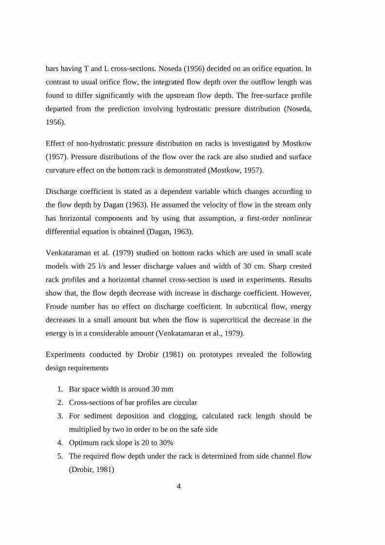
Experiments conducted by Drobir (1981) on prototypes revealed the following

design requirements

1. Bar space width is around 30 mm

2. Cross-sections of bar profiles are circular

3. For sediment deposition and clogging, calculated rack length should be

multiplied by two in order to be on the safe side

4. Optimum rack slope is 20 to 30%

5. The required flow depth under the rack is determined from side channel flow

(Drobir, 1981)

5

Subramanya and Shukla (1988) conducted their experiments on horizontal channel

cross-section and subcritical upstream, supercritical downstream flows. The

efficiency, which is the ratio of the discharge taken into the channel and the upstream

discharge is considered and demonstrated to increase significantly as the ratio of the

rack length and critical flow depth increases. Moreover, ratio of the clear bar spacing

to bar diameter also increases with efficiency. Depending on the upstream and

downstream flow conditions, Subramanya and Shukla (1988) classified flows over

bottom racks into five categories and these categories are used to define the

calculation approach. They also defined the required trash rack length to take all the

discharge to the intake channel (Subramanya and Shukla, 1988).

Bianco and Ripellino (1994) conducted experiments on a model which is larger than

the model used by Noseda (1956). Studies have shown that, scale does not have a

significant effect on the results. Cross-section of the bar profiles used in these

observations was semicircular with rectangular bottom reinforcement at the bottom

(Bianco and Ripellino, 1994).

Özcan (1999) presented the theoretical solutions in two separate approaches which

are based on constant energy level and constant energy head hypothesis.

Drobir et al. (1999) studied on a model with a scale of 1:10. The model’s purpose

was to measure the wetted rack length and to determine the effect of bar spacing.

Four different slopes were used which are between 0 and 30% and five different unit

discharge values are analyzed which are 0.25, 0.50, 1.00, 1.50 and 2.00 m3/s/m.

Drobir et al. (1999) divided the total rack length into two and defined them as L1 and

L2 which are the distance where the axis of the trash rack crossed with the flow and

the total wetted length over the trash rack, respectively (See Figure 2.1) (Drobir et

al., 1999). In Figure 2.1, (qw)T and (qw)i are unit discharge in the river and unit

discharge in the intake channel, respectively.

6

Figure 2.1 Sketch of rack lengths L1 and L2 of a Tyrolean screen (Drobir et al., 1999)

A rectangular channel with 0.5 m width and 7.0 m length was used in the

experiments conducted by Brunella et al. (2003). The objective was to determine the

effect of porosity, slope and geometry of the trash rack. The diameters of the bars

were 12 mm and 6 mm and lengths of bars were 0.60 m and 0.45 m. They were

placed with 6 mm and 3 mm clearance spacing with respect to each other. Angles of

rack inclinations used in the experiment were Ԑ = 0, 7, 19, 28, 35, 39, 44 and 51

degrees. Results have shown that, surface profiles of the systems with large and

small bottom slopes were almost identical.

Ghosh and Ahmad (2006) have studied on flat bars and they determined that the

specific energy over the racks was nearly constant.

Kamanbedast and Bejestan (2008) conducted a series of experiments to determine

the effects of screen slope and area opening of the screen on the diverted discharge.

Dimensions of the model were 60 cm width, 8 m length and 60 cm height. Diameters

of the bars used were 6 and 8 mm and spacing between bars were 30, 35 and 40% of

total length. Inclinations were 10, 20, 30 and 40% and the model is tested by five

different discharge values. Results have shown that, the discharge ratio increases as

7

the slope of the rack increases. In addition to the slope, spacing is the second factor

that affects the total flow taken into the channel. When the inclination is 30% and the

spacing is 40% the discharge ratio reaches to a maximum value of 0.8. If the

sediment is considered in the experiments it is observed that discharge ratio

decreases to 90% of the without sediment condition. The reason of that reduction is

the clogging of the bars (Kamanbedast and Bejestan, 2008).

A model is built and its behaviors are observed by Yılmaz (2010). In the

experiments, circular bars with 1 cm diameter were used and three different spacing

values and slopes are tested which are 3 mm, 6 mm and 10 mm; 14.5°, 9.6° and 4.8°,

respectively (Yılmaz, 2010).

Metal panels with 3 mm, 6 mm and 10 mm diameter circular openings are tested as a

trash rack on the same model by Şahiner (2012). Different than Yılmaz (2010),

Şahiner (2012) used more steep slopes in his experiments, such as 37, 32.8 and 27.8

degrees.

Yılmaz (2010) and Şahiner (2012) prepared the graphs of variations of the discharge

coefficient Cd, the ratio of the diverted discharge to the total water discharge,

[(qw)i/(qw)T], and the dimensionless wetted rack length, L2/n, where n is the spacing

between bars. The discharge taken into the channel can be calculated by using those

graphs.

By experiments and investigations, many results have been obtained and different

methods are designed to calculate the optimum parameters of Tyrolean intakes.

Every approach has some assumptions and paths, so results can vary according to the

method used. For example, friction effects are ignored due to small friction length

over the trash rack. Surface tension of water between bars is also ignored.

Furthermore, fluctuations in the flow depths over the rack bars are not considered in

calculations.

In this study, design parameters and methods used in the past studies are collected

and analyzed in detail. Solution methods can be summarized in four separate titles:

8

1. First Assumption: Constant Energy Level

1.1 Iterative Method

1.2 Closed Form Method

2. Second Assumption: Constant Energy Head

2.1 Iterative Method

2.2 Closed Form Method

If the trash rack is placed horizontally, both hypotheses become equal. But, the trash

racks are designed to be inclined in projects. When the trash rack is arranged

inclined, both hypothesis appear as boundary conditions. However, neither represents

the exact solution.

These methods are used to determine the bars’ length and spacing according to the

desired discharge. For the sake of construction the upstream side of the trash rack can

be considered horizontal or inclined as seen in Figure 2.2. In Figure 2.2.a, the critical

depth and minimum energy is observed somewhere close to point A. However, in

Figure 2.2.b, the critical depth is reached much earlier from point A and in this spot

the flow has smaller depth. These two conditions must be separated from each other

in hydraulic calculations.

a) b)

Figure 2.2 Tyrolean weirs with a) inclined and b) horizontal approaches

9

Calculation of the discharge that passes through the trash rack depends on the water

surface profile over the weir. The discharge that passes from point A starts to drop

into the collection channel and the discharge over the weir reduces along the trash

rack. Flow over the trash rack is affected by friction of the bars and surface tension.

Trash racks are the most important part of Tyrolean Weirs. Efficiency as being the

ratio of discharge transferred to the intake channel and total river flow is mostly

related to the characteristics of rack bars. Bars are designed in three aspects which

are; bar shape, spacing between bars, and bar length.

To increase the efficiency, screens should be stable and resistant to vibrations. Steel

is mostly used as the material type of bars to be resistant to corrosion. If the gaps

between bars are filled with sediment, less water passes through screens. This

situation decreases the performance of the turbine since actual water amount is lesser

than the desired discharge amount. The trash rack functions essentially as a filter.

Any solid particle larger than the bar spacing are kept above the screen. So, bar type

and dimensions should be carefully selected to prevent sediment transition and

clogging of the racks.

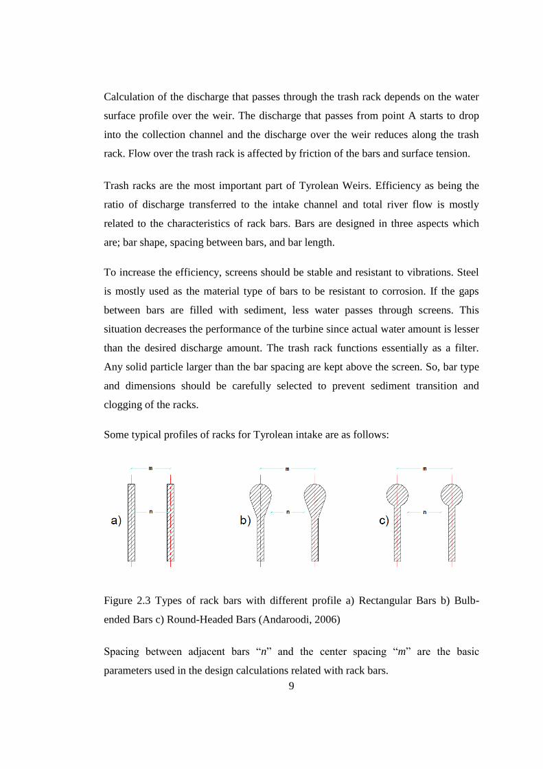
Some typical profiles of racks for Tyrolean intake are as follows:

Figure 2.3 Types of rack bars with different profile a) Rectangular Bars b) Bulb-

ended Bars c) Round-Headed Bars (Andaroodi, 2006)

Spacing between adjacent bars “n” and the center spacing “m” are the basic

parameters used in the design calculations related with rack bars.

10

Andaroodi (2006) does not recommend the usage of rectangular bars due to their

tendency to be clogged by stones. The bulb-ended bars can be preferred due to their

higher performance and rigidity rates. However, the third alternative which is the

round-head bars have more resistance to clogging and with higher moment of inertia

they have more carrying capacity of heavy bed sediment loads (Andaroodi, 2006).

In experimental setups and models, bars with circular cross section can be used.

However, streams can carry large amount of heavy boulders rolling and moving

along the bed. The bottom rack bars have to be strong enough to carry the entire bed

load which can contain big and heavy boulders (Ahmad and Mittal, 2006). So,

round-head bars are the most suitable shape to be used in Tyrolean intake racks. The

spacing between bars is recommended as 2 to 4 cm (Andaroodi, 2006).

Circular bars by rectangular reinforcement extension are the most efficient cross

section. Moreover, circular bars extended by reinforcement give better performance

rates in terms of clogging and vibration related problems. 30 to 40% bar spacing to

avoid excessive clogging should be used. Gaps between bars are around 3 cm,

depending on site conditions (Brunella et al., 2003).

11

CHAPTER 3

3 DESIGN AND ANALYSIS APPROACHES

This chapter provides basic information on computation of flow rate and water

surface profile of Tyrolean Weirs. In the first two parts, constant energy level and

constant energy head assumptions are explained in iterative and closed form solution

methods. In the third part, trash rack design is described according to the past studies

and assumptions made for the most efficient design.

3.1 The First Assumption: Constant Energy Level

As the solution procedures of the first assumption, calculations can be made

iteratively or by a closed form method.

3.1.1 Iterative Solution Method:

As seen in Figure 3.2, the depth h1 which occurs at the head of the trash rack is lower

than h0 which is the flow depth at approach. Firstly, the flow depth h0 and the energy

head H0 must be calculated according to the unit discharge (qw)T. The energy level is

constant along the trash rack and calculations begin where the water depth is h1.

Equation (3.1) can be written by using the energy equation according to the unit

width with length xi, depth hi and unit discharge qi over the trash rack (Noseda,

1956).

)cos(2 iiii hHghq (3.1)

In Equation (3.1), Ԑ is the angle of inclination of the bars with respect to the

horizontal axis. To find the energy head Hi, elevation difference xi.sin(Ԑ) must be

12

added to the energy head H0. After that, for depth hi+1, which is searched for, a new

assumption is made. To calculate the discharge (qw)i that passes through Δxi, system

is solved as an orifice flow, and the following equation is given by using the flow

depth at that section (Noseda, 1956).

iiw xhq (3.2)

where

cos2gs (3.3)

The net rack opening area per unit width of the rack is mn / in which n is the

clearance distance and m is the center to center distance between two adjacent bars of

the rack.

Figure 3.1 Bar types and related (contraction coefficient) values for calculation

methods (Schmidt and Lauterjung, 1989)

s

13

For 5.32.0 m

h, Noseda (1956) defines μs as follows;

13.0

16.066.0

h

ms (3.4)

Figure 3.2 Constant energy level, weir system cross-section (Noseda, 1955)

In Equation (3.2) and Equation (3.4) the flow depth (h) is assumed as the average

depth of hi and hi+1 for Δxi interval. Then, (qw)i the discharge that passes between bars

and goes into the intake channel is calculated and subtracted from the discharge

passing over the interval Δx which is qi, to calculate the discharge passing over the

next interval, qi+1. For each interval step, this iteration is applied.

3.1.2 Closed Form Solution Method:

Iterative method needs a freat amount of time and effort to solve. Frank (1956)

developed a closed solution with some assumptions (Çeçen, 1962). In this approach,

the change in the flow depth is accepted as elliptic. As seen in Figure 3.3, when all

14

the incoming discharge is diverted, ((qw)T=(qw)i), and h1 and axis of the ellipse are

defined, it is possible to write Equation (3.5)

2

1

2

1

2

2

2h

h

h

h

l

s (3.5)

Figure 3.3 Hydraulic system of trash rack in closed form solution (Frank, 1956)

For (qw)T=(qw)i, any distance se away from the origin of the ellipse can be computed

by using Equation (3.6) (Frank, 1956)

2

2

1

2

1

2

2 eee hh

lh

h

ls (3.6)

where he is the flow depth at distance se. The amount of water entered the collection

channel through the distance dse can be found with the help of Equation (3.6)

e

ee

ee dh

hhh

hh

h

lds

2

1

1

1 2

(3.7)

15

The differential discharge can be written as:

e

ee

ee

e dhhhh

hhh

h

ldshdq

2

1

1

1

0

2

(3.8)

Equation (3.8) can be integrated as follows:

e

ee

ee

hh

h

iw dhhhh

hhh

h

ldqq

e

e

2

1

1

01 2)(

1

(3.9)

which can finally result in:

1

011

1 213

2)(

hh

h

eeiw

e

e

h

h

h

hlhq

(3.10)

or this equation can be simplified to

lhlhq iw 11 391.0223

2)( (3.11)

For (qw)i =(qw)T, the wetted length can be computed as shown in Equation (3.12)

(Frank, 1956).

1

)(561.2

h

ql Tw

(3.12)

As seen in Figure 3.4, if the total discharge (qw)T is not taken into the collection

channel, according to Frank (1956), elliptic approach can be used to calculate the

design parameters. In these cases, the length of the elliptic curve is computed by

16

using the incoming discharge, (qw)T and energy H0. The length between where the

flow depth is zero and the end of trash rack is Ls .

The diverted discharge (qw)i can be calculated by making the following assumptions

about elliptic curve approach (Frank, 1956).

1. The hatched area under the elliptic curve after the depth h2 is accepted as the

total discharge that goes to downstream (See Figure 3.4).

2. The area under the elliptic curve between the depth h1 and h2 is accepted as

the discharge diverted into the collection channel.

Figure 3.4 Elliptic curve approach, in cases where the total flow cannot be diverted

(Frank, 1956)

By modifying Equation (3.10), Equation (3.13) is obtained.

1

211

1 213

2)(

hh

hh

eeiw

e

e

h

h

h

hlhq

(3.13)

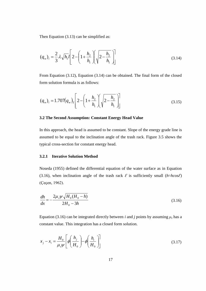
17

Then Equation (3.13) can be simplified as:

1

2

1

21 212

3

2)(

h

h

h

hlhq iw (3.14)

From Equation (3.12), Equation (3.14) can be obtained. The final form of the closed

form solution formula is as follows:

1

2

1

2 212707.1)(h

h

h

hqq

Twiw (3.15)

3.2 The Second Assumption: Constant Energy Head Value

In this approach, the head is assumed to be constant. Slope of the energy grade line is

assumed to be equal to the inclination angle of the trash rack. Figure 3.5 shows the

typical cross-section for constant energy head.

3.2.1 Iterative Solution Method

Noseda (1955) defined the differential equation of the water surface as in Equation

(3.16), when inclination angle of the trash rack Ԑ is sufficiently small (h≈hcosԐ)

(Çeçen, 1962).

hH

hHH

dx

dh s

32

)(2

0

00

(3.16)

Equation (3.16) can be integrated directly between i and j points by assuming μs has a

constant value. This integration has a closed form solution.

00

0

H

h

H

hHxx ij

s

ij

(3.17)

18

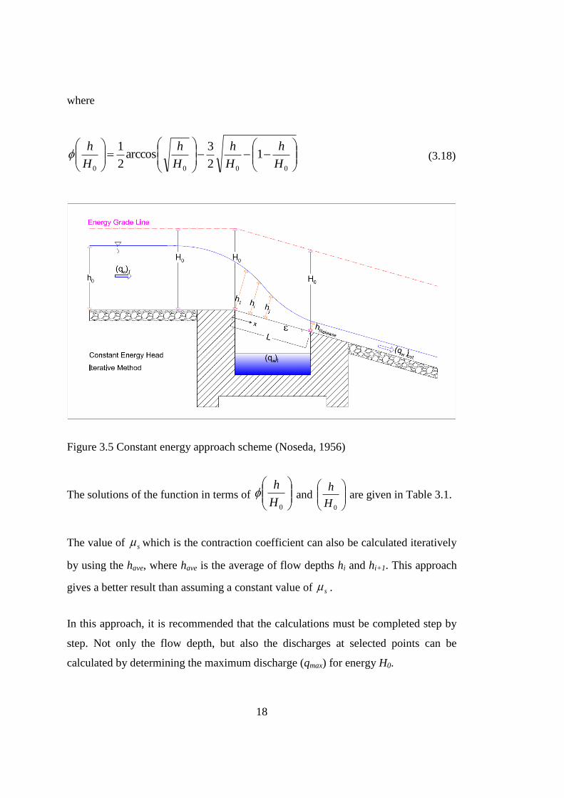
where

0000

12

3arccos

2

1

H

h

H

h

H

h

H

h (3.18)

Figure 3.5 Constant energy approach scheme (Noseda, 1956)

The solutions of the function in terms of

0H

h and

0H

h are given in Table 3.1.

The value of s which is the contraction coefficient can also be calculated iteratively

by using the have, where have is the average of flow depths hi and hi+1. This approach

gives a better result than assuming a constant value of .

In this approach, it is recommended that the calculations must be completed step by

step. Not only the flow depth, but also the discharges at selected points can be

calculated by determining the maximum discharge (qmax) for energy H0.

s

19

2/3

0

2/3

0000max 705.133

22

3

22

3

2HH

gHHgHVhq cc

(3.19)

When Equation (3.17) is modified for qmax, Equation (3.20) is obtained.

maxmax

0

q

q

q

qHxx ij

s

ij

(3.20)

The closed form of Equation (3.20) can be written as;

cos11cos22

21cos2

3

1arccos

2

1

max

q

q (3.21)

where φ angle is a parameter which depends on maximum discharge.

Solutions of function in terms of

maxq

q are given in Table 3.1.

φ is calculated separately for subcritical and supercritical flow cases.

For subcritical flow case:

2

max

21arccos3

1

q

q (3.22)

For supercritical flow case:

2

max

21arccos3

1

q

q +240

o (3.23)

20

Table 3.1 Solutions of functions ϕ and β (Noseda, 1955)

0H

h

0H

h

maxq

q

maxq

q

Subcritical Supercritical

0 0.7854 0 0 0.7854

0.05 0.3457 0.05 -0.0192 0.5084

0.10 0.1745 0.10 -0.0385 0.3937

0.15 0.0510 0.15 -0.0578 0.3072

0.20 -0.0464 0.20 -0.0771 0.2342

0.25 -0.1259 0.25 -0.0965 0.1702

0.30 -0.1921 0.30 -0.1158 0.1127

0.35 -0.2466 0.35 -0.1352 0.0617

0.40 -0.2918 0.40 -0.1546 0.0117

0.45 -0.3290 0.45 -0.1742 -0.0337

0.50 -0.3573 0.50 -0.1938 -0.0762

0.55 -0.3791 0.55 -0.2134 -0.1162

0.60 -0.3925 0.60 -0.2332 -0.1543

0.65 -0.3989 0.65 -0.2532 -0.1904

0.70 -0.3976 0.70 -0.2732 -0.2247

0.75 -0.3877 0.75 -0.2934 -0.2575

0.80 -0.3682 0.80 -0.3139 -0.2887

0.85 -0.3367 0.85 -0.3346 -0.3187

0.90 -0.2891 0.90 -0.3556 -0.3471

0.95 -0.2142 0.95 -0.3771 -0.3743

1.00 0 1.00 -0.3994 -0.3994

21

3.2.2 Closed Form Solution Method:

The closed form solution of constant energy method is produced by ignoring

headlosses in the system. Slope of the energy grade line is assumed to be equal to the

slope of the trash rack.

Figure 3.6 Constant energy head approach closed form solution scheme (Noseda,

1956)

Assuming the specific energy of flow to be constant all over the longitudinal bottom

rack, Mostkow (1957) proposed the following equation for the diverted discharge

into the trench:

02)( gHBLCQ diw (3.24)

where ψ = ratio of clear opening area and total area of the rack; B = length of the

trench; L = length of the rack bars; g = acceleration due to gravity; H0 = specific

energy at approach; and Cd = coefficient of discharge. Based on limited experimental

study, Mostkow (1957) suggested that Cd varies from 0.435, for a sloping rack 1 in 5,

to 0.497 for a horizontal rack. However, geometrical and hydraulic aspects of the

22

phenomenon were not completely considered by him. Noseda (1956), with an

additional assumption of critical approach flow condition, analyzed the flow over

longitudinal racks and presented a design chart relating the diverted flow to the total

stream flow (Ahmad and Mittal, 2006).

White et al. (1972) conducted experiments and compared the trash racks with

different lengths of bars, bar spacing and slope, with those resulted by Noseda’s

method. They suggested a different chart based on their studies, but their design chart

is of limited application capability (White et al., 1972).

Subramanya and Shukla (1988) and Subramanya (1990, 1994) classified the flows

over horizontal and sloping racks of rounded bars, which are listed in Table 3.2.

Table 3.2 Nature of flow over a bottom rack (After Subramanya 1990, 1994)

Type Approach Flow Over The Rack Downstream State

AA1 Subcritical Supercritical May be a jump

AA2 Subcritical Partially Supercritical Subcritical

AA3 Subcritical Subcritical Subcritical

BB1 Supercritical Supercritical May be a jump

BB2 Supercritical Partially Supercritical Subcritical

The functional relationships for the variation of Cd in various types of flows are as

follows:

a) Inclined Racks (Subramanya, 1994):

AA1 Type Flow

𝐶𝑑 = 0.53 + 0.4 log𝐷

𝑛− 0.61𝑆𝐿 (3. 25)

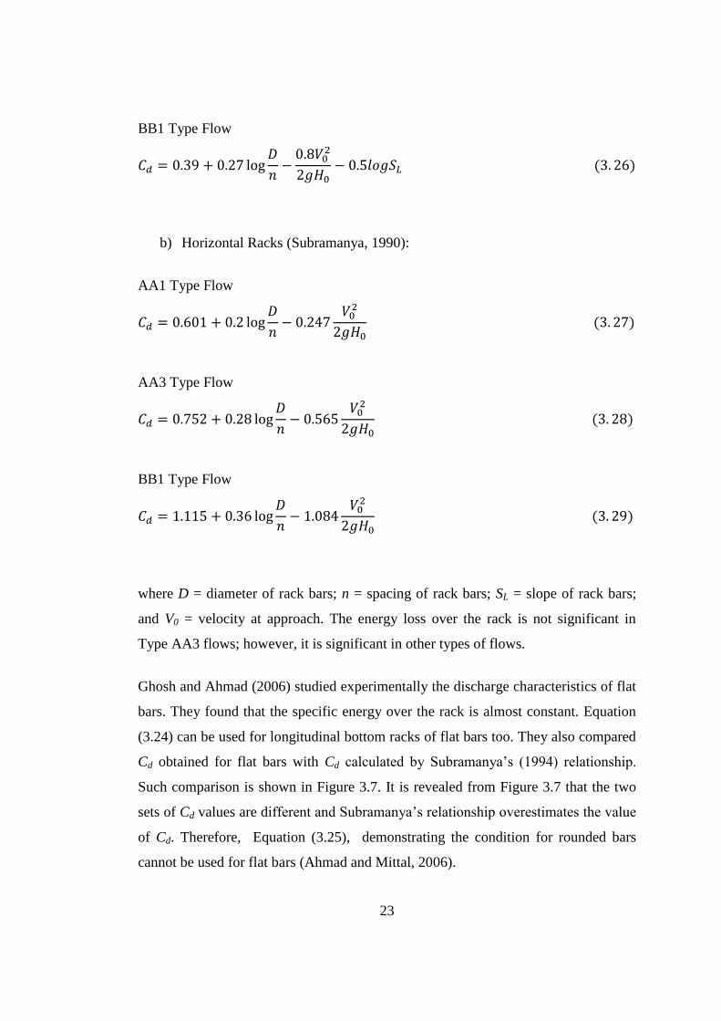
23

BB1 Type Flow

𝐶𝑑 = 0.39 + 0.27 log𝐷

𝑛−

0.8𝑉02

2𝑔𝐻0− 0.5𝑙𝑜𝑔𝑆𝐿 (3. 26)

b) Horizontal Racks (Subramanya, 1990):

AA1 Type Flow

𝐶𝑑 = 0.601 + 0.2 log𝐷

𝑛− 0.247

𝑉02

2𝑔𝐻0 (3. 27)

AA3 Type Flow

𝐶𝑑 = 0.752 + 0.28 log𝐷

𝑛− 0.565

𝑉02

2𝑔𝐻0 (3. 28)

BB1 Type Flow

𝐶𝑑 = 1.115 + 0.36 log𝐷

𝑛− 1.084

𝑉02

2𝑔𝐻0 (3. 29)

where D = diameter of rack bars; n = spacing of rack bars; SL = slope of rack bars;

and V0 = velocity at approach. The energy loss over the rack is not significant in

Type AA3 flows; however, it is significant in other types of flows.

Ghosh and Ahmad (2006) studied experimentally the discharge characteristics of flat

bars. They found that the specific energy over the rack is almost constant. Equation

(3.24) can be used for longitudinal bottom racks of flat bars too. They also compared

Cd obtained for flat bars with Cd calculated by Subramanya’s (1994) relationship.

Such comparison is shown in Figure 3.7. It is revealed from Figure 3.7 that the two

sets of Cd values are different and Subramanya’s relationship overestimates the value

of Cd. Therefore, Equation (3.25), demonstrating the condition for rounded bars

cannot be used for flat bars (Ahmad and Mittal, 2006).

24

Figure 3.7 Verification of Subramanya’s (1990) relationship for Cd

There is considerable effect of ratio of bar thickness t and clear spacing. The value of

Cd increases with increase of t/n ratio; however, it decreases with the increase of

inclination of bars (SL) for constant value of t/n ratio. Ghosh and Ahmad (2006)

proposed the following equation for Cd for flat bars:

𝐶𝑑 = 0.1296 (𝑡

𝑛) − 0.4284 ∗ 𝑆𝐿

2 + 0.1764 (3. 30)

25

Equation (3.30) calculates the value of Cd for flat bars within ±10% error. Thus for

the design of bottom racks with flat bars Equation (3.30) is recommended. The above

equations can only be applied for free flow condition in the trench. However, if the

discharge in the stream is more than the withdrawal discharge, submerged flow

situation occurs and Equation (3.24) will be no more applicable. Submerged

conditions need further studies.

Once the value of Cd is known, the length of the bottom rack is calculated using

Equation (3.24). The optimum length of bottom rack which is also equal to the width

of the channel trench, is obtained when diverted discharge is equal to the incoming

discharge in the stream (Ahmad and Mittal, 2006).

For a given x interval, to determine the amount of water that passes through the trash

rack, (qw)i, can be calculated as an orifice flow, by the following formula;

xgHCq diw 02)( (3.31)

(qw)T can be written as follows with the help of Equation (3.1) for Ԑ=0o.

)(2 0 hHghqTw (3.32)

For an interval dx, the reduction in amount of water that passes over the trash rack

equals to the amount of diverted water through the trash rack.

02gHC

dx

qd

dx

qdd

Twiw (3.33)

and the derivative of the stream discharge with respect to the depth of water is

ghgH

ghgH

dh

qdTw

22

32

0

0

(3.34)

26

By inserting Equation (3.33) into Equation (3.34), Equation (3.35) is obtained.

dxgHCdhghgH

gHghd 0

0

0 222

23

(3.35)

By using Equation (3.35), the relation between the head of the trash rack (h=h1 and

x=0) and any point on the trash rack at distance x from the head with the flow depth h

can be written as follows;

xx

x

d

hh

hh

dxHCdhhH

Hh

0

0

0

0 2)(

23

1

(3.36)

after integrating the left side of the equation, the following equation is obtained.

xHChHh d

hh

hh

00 22

1

(3.37)

This equation is simplified as follows:

xCH

hh

H

hh d

00

1

1 11 (3.38)

By multiplying each side of the equation with0

1

H, the expression for

0H

x can be

obtained as follows.

000

1

0

1

0

111

H

h

H

h

H

h

H

h

CH

x

d (3.39)

27

By using Equation (3.39) water surface profile of the flow can be calculated. When x

is selected as the full length of the trash rack, (L), the flow depth h2 can also be

computed.

)(2 202 hHghqoutw (3.40)

So the discharge that is diverted into the collection channel can be calculated by

outwTwiw qqq (3.41)

3.3 Trash Rack Design

The discharge taken into the intake channel of a Tyrolean weir mostly depends on

the trash rack properties. Its length, slope and spacing and diameter of bars are the

main parameters which affect the water taking efficiency of a Tyrolean intake

structure.

The design discharge which will be taken into the turbine should be determined

according to the assumption that, at least the 10% of water will pass to the

downstream of the structure as should be in any hydraulic structure for the sake of

protection of the environment.

To design the Tyrolean intake, best approach is to assume a 100% intake ratio to

supply the design discharge (Brunella et al., 2003). So, rack length and other design

parameters are determined according to the scenario that all of the stream flow is

transferred to the intake channel. Although, the real discharge will be larger than the

design discharge and at least 10% of the flow should be passing to the downstream

since the design will be done in order to take only the required amount of water. This

procedure is the main idea of the design stage.

There are different methods to calculate the necessary rack length which will be

required to take the design discharge into the intake channel. Frank (1956) assumed

28

no head loss while water is passing over bars and derived a formula to obtain the

length of the rack. By using Equation (3.12), rack length can be calculated. (qw)T is

the total discharge flowing in the stream, λ is as described in Equation (3.3) and h1 is

the flow depth just at the upstream of the rack. h1=χ hcr , where χ is the reduction

factor. This factor can be calculated by using Equation (3.42).

(2𝑐𝑜𝑠𝜀)𝜒3 − 𝜒2 + 1 = 0 (3.42)

in which Ԑ is the inclination angle of bars and hcr is the critical flow depth.

ℎ𝑐𝑟 = √(𝑞𝑤)𝑇

2

𝑔

3

Noseda (1956), derived the Equation (3.43) to calculate the trash rack length by

assuming constant energy head.

𝐿 = 1.185𝐻0

1.22𝜇𝜓 (3. 43)

However, this equation is based on the horizontal rack assumption.

Another study, submitted by Mostkow (1957) which is shown in Equation (3.44) is

obtained according to the constant energy level assumption.

𝐿 =𝑞

𝐶𝑑 𝜓 𝑐𝑜𝑠𝜀 √2𝑔𝐻0

(3. 44)

Mostkow (1957) suggested the discharge coefficient, Cd between 0.497 and 0.609 for

horizontal racks, 0.435 and 0.519 for 20% inclined rectangular bars.

Finally, the formula suggested by Brunella et al. (2003) for the calculation of rack

length is given in Equation (3.45).

𝐿 = 0.83𝐻0

𝐶𝑑𝜓 (3. 45)

29

where Cd, the discharge coefficient is equal to 1.1 for porosity values, Ѱ = 0.35 and

Cd = 0.87 for , Ѱ = 0.664. The constant value, 0.83 in Equation (3.45) can be taken as

1.0 for the design calculation to be on the safe side in terms of clogging issues

(Brunella et al., 2003).

Formulae which are used for calculating the rack length give overestimated results.

However, the formula given by Mostkow (1957) and Brunella et al. (2003) gives

logical results (Jiménez and Vargas, 2006).

There are many approaches to calculate the length of bars and they depend on

variables varying according to the researcher’s assumptions and design criteria. So,

while designing the intake, rack length is not only calculated by these formulae but

also checked by using the previously explained analysis methods.

Rack length will be just long enough to take the necessary discharge. To calculate the

rack length, other design parameters like bar diameters, bar spacing and slope of the

rack should be known.

To begin with, some specific assumptions can be made to determine bar dimensions.

According to experiments and studies, to obtain the most efficient hydraulic design

bar spacing ratio should be 40% (Aghamajidi and Heydari, 2014).

So, the ratio mn / should be equal to 40%. The purpose of bar spacing n, is to

prevent entry of large bed load particles. Common practice is to block particles larger

than median gravel size which are between 2 and 4 cm. So, a spacing of 3 cm is

advised (Raudkivi, 1993). In the design stage, designer should know the median

gravel size to decide on the bar spacing or manually a predefined bar spacing can be

assumed and calculations can be made accordingly. If 4 cm spacing between bars is

assumed, then a diameter of 6 cm gives the most hydraulic performance according to

the suggested 40% ratio.

Also, according to Brunella et al. (2003), circular bars by rectangular reinforcement

extension are the most efficient cross section. Moreover, circular bars extended by

30

reinforcement give better performance rates in terms of clogging and vibration

related problems. 30 to 40% bar spacing to avoid excessive clogging should be used.

Gaps between bars should be around 3 cm, depending on site conditions (Brunella et

al., 2003).

Andaroodi (2006) suggested round-head bars as being the most appropriate type in

terms of clogging and durability against heavy and large bed load elements because

of higher moment of inertia. The recommended bar spacing for circular bars with

reinforcement is 2 to 4 cm (Andaroodi, 2006).

In this study, rack openings are designed according to the median gravel size. If it is

below 2 cm, spacing between bars are 2 cm. If it is above 4 cm, gaps are decided to

be 4 cm, since these values are the suggested range. Any other gravel sizes between

these values will be rounded to the closest integer and bar spacing will be decided

accordingly.

According to the 40% void ratio design assumption, n and m values are shown on

Table 3.3 in which d50 is median gravel size.

Table 3.3 n, bar spacing and m, bar distance values for different site conditions

Median Gravel Size d50 ≤ 2 cm 2 cm < d50< 4 cm d50 ≥ 4 cm

n ( bar spacing in cm) 2 3 4

m ( bar distance in cm) 5 8 10

D (bar diameter in cm) 3 5 6

For very long trash racks, if heavy boulders are present in the bed load; even the

stiffness of 6 cm diameter bars can be a problem. In that condition, perpendicular

stiffening bars can be placed in the rack or diameters can be increased to overcome

that issue.

After deciding on the bar type and dimensions, slope of the rack is the next criteria

that affects the behavior of the system. Past studies show that, the best hydraulic

performance is supplied when the rack slope is 30% (Aghamajidi and Heydari,

2014).

31

Also according to Drobir (1981) in the design of Tyrolean intakes, optimum rack

slope is 20% to 30%.

When the slope is 30%, discharge ratio makes a peak and highest efficiency results

are obtained (Kamanbedast and Bejestan, 2008).

The meaning of 30% slope is 3 vertical 10 horizontal, which means 16.7 degrees of

inclination angle. In this study, bar angle is decided as 16.7 degrees while designing

the intake structure.

Iterative and closed form methods are described in this chapter. These methods are

used to develop the computer program to analyze Tyrolean weirs. Formulae

developed in past studies are given, and assumptions and design criteria are

explained which are used in the design interface of the software. Two stages of the

computer program which are analysis and design interfaces will be explained in the

next chapter.

32

CHAPTER 4

4 DEVELOPMENT OF COMPUTER PROGRAM

4.1 Introduction

For the analysis and design of a Tyrolean intake, a computer software named Tyrol is

developed and adopted to the Visual Basic programming language. The reason for

selecting Visual Basic language is the sentence-like phrase usage for developing

algorithms which make the programing easier for the programmer and the reader.

In addition to its simplicity in writing, Visual Basic can supply an environment

suitable for designing the software window visually in a quick and user friendly

manner. Moreover, those advantages do not make it a low level program for

developing engineering applications since the developer is still able to code complex

formulas and the software can easily handle them within a quite short time.

Figure 4.1 Welcome screen of the program

33

4.2 Program Interface

The “Welcome” screen of the program is shown in Figure 4.1. When the Tyrol

Software is opened, the user is asked for selecting the purpose of calculation. There

are two options for that stage. When the selection is made, a new window opens

according to the clicked button.

4.2.1 Design Interface

If the user clicks the “Design” button, Tyrol opens a new window developed for the

design purpose (See Figure 4.2). In that window there are text boxes on a grey

background for the user to enter input values. For stream information frame, these

input values are median gravel size in mm, stream discharge in m3/s, channel width

of the stream in m, flow depth of water in m. Below stream information frame,

design discharge frame is given. User is asked to give an input value for the desired

discharge to be taken into intake channel.

Solution methods described in chapter 3 are used in the Tyrol program and same

procedures are applied explained in chapter 5. User chooses a method from the list,

otherwise constant energy level, iterative method is randomly selected.

Figure 4.2 Design interface view

34

On the right hand side of design window, there is a frame for the bar type selection.

When the dropdown list is clicked, user can select one bar type from the list. Bar

types in the list are; rectangular reinforced circular bars, ovoid bars, rectangular bars

and circular bars. Rectangular reinforced circular bars item is randomly selected

since it is the recommended bar type.

In the same frame, user is asked to choose between two options for the calculation of

contraction coefficient. Program can make calculations according to the bar type

based predefined constant values or a variable depending on the bar spacing, central

bar distance and flow depth.

There are some assumptions made according to the recommendations explained in

Chapter 3. Median gravel size defines the bar spacing since the main idea between

the bar spacing distance is to avoid the bed sediment entrance into the intake channel

(See Table 3.3).

Another assumption is used to determine the central bar distance. Ratio of spacing to

total rack width is assumed to be 40%. Moreover, trash rack slope is taken as 30%

which needs an inclination angle of 16.7 degrees.

Finally, when the Compute button is clicked Tyrol program runs and calculates rack

length according to the selected solution method and given input values.

4.2.2 Analysis Interface

Program asks user to enter the necessary input values to calculate the water surface

profile and the discharge taken into the channel. Inputs are bar spacing n, central

distance of bars m, trash tack inclination angle Ԑ, trash rack length L, stream

discharge Q0, channel width B, and the water depth at the beginning of the trash rack

h1 (See Figure 4.3).

Trash rack bar type should also be selected. If no custom selection is made, program

will select rectangular reinforced circular bar type as the default choice.

35

When the user selects a custom bar type, picture showing the cross-section of the bar

changes according to the selection. As can be seen in Figure 4.3, “Rectangular

Reinforced Circular Bars” option is selected and on the right hand side of the

dropdown menu, cross section of the bar type is shown.

Figure 4.3 Analysis interface view

Bar type selection also affects the formulae and constants within the program

algorithms. Also, contraction coefficient is to be decided; it can be calculated from

the formula or predefined constant values can be used.

Then, the user selects a Δx value to decide the computation or in other terms iteration

steps to be applied. L/100 is again the default selection decided for the program. User

is free to select from different unit distances other than the default value that will be

used in the calculation steps.

Finally, user selects one of the methods which are previously described in this study.

When the “Compute” button is clicked, then the program calculates the results

according to the selected design criteria and method.

36

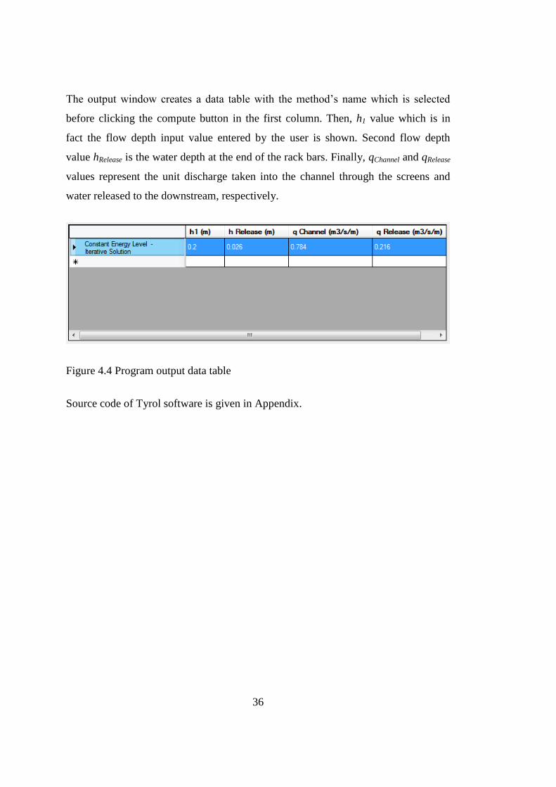
The output window creates a data table with the method’s name which is selected

before clicking the compute button in the first column. Then, h1 value which is in

fact the flow depth input value entered by the user is shown. Second flow depth

value hRelease is the water depth at the end of the rack bars. Finally, qChannel and qRelease

values represent the unit discharge taken into the channel through the screens and

water released to the downstream, respectively.

Figure 4.4 Program output data table

Source code of Tyrol software is given in Appendix.

37

CHAPTER 5

5 APPLICATION

5.1 Introduction

In Chapter 3, solution methods are mentioned and formulae are given to calculate the

water surface profile over the trash rack and discharge taken into the channel. To

create a better understanding of the methods, two examples will be presented and

solved below.

In the first example, a Tyrolean weir structure is analyzed. Solution methods

described in Chapter 3 are used to calculate the discharge taken into the intake

channel and to determine the water surface profile. Methods are applied according to

the two basic assumptions which are shown below:

1. First Assumption: Constant Energy Level

1.1 Iterative Method

1.2 Closed Form Method

2. Second Assumption: Constant Energy Head

2.1 Iterative Method

2.2 Closed Form Method

In the second example, a Tyrolean weir structure is designed. The discharge taken

into the intake channel is known. Inclination angle, diameter, spacing and length of

trash rack bars are determined in the solution. Second example shows the design

38

stage of a Tyrolean intake according to the assumptions and recommendations

described in past studies which are explained in Chapters 2 and 3.

5.2 Analysis Application

In this part of the study, a Tyrolean weir is analyzed with reference to a sketch shown

in Figure 5.1 using to the methods explained in Chapter 3.

Figure 5.1 Sketch for Tyrolean weir analysis application

Total discharge (qw)T of the Tyrolean weir shown in Figure 5.1 is 1.00 m3/s/m. If the

flow depth at the head of the trash rack (h1) is 0.20 m, the length of the trash rack (L)

is 4.0 m, the inclination of the trash rack (Ԑ) is 30.0o

and m and n values of the rack

bars are 4 mm and 16.0 mm, respectively, calculate the diverted discharge (qw)i and

the flow depth at the end of the trash rack.

39

5.2.1 The First Assumption: Constant Energy Level

5.2.1.1 Iterative Solution Method

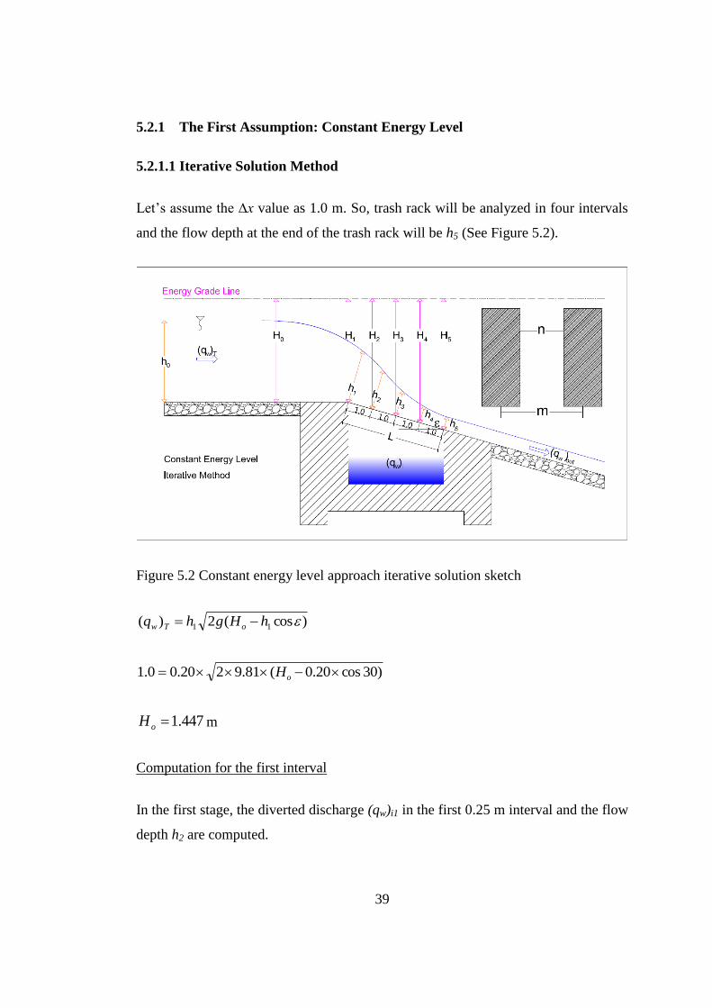
Let’s assume the ∆x value as 1.0 m. So, trash rack will be analyzed in four intervals

and the flow depth at the end of the trash rack will be h5 (See Figure 5.2).

Figure 5.2 Constant energy level approach iterative solution sketch

)cos(2)( 11 hHghq oTw

)30cos20.0(81.9220.00.1 oH

447.1oH m

Computation for the first interval

In the first stage, the diverted discharge (qw)i1 in the first 0.25 m interval and the flow

depth h2 are computed.

40

xhq aveiw .)( 1. , 2

21 hhhave

and cos2gs

25.016

4

m

n

13.0

13.0

16.0

13.0

16.0 481.0016.025.066.066.0

aveaveave

shhh

m

First iteration, assume h2=0.14 m

17.02

14.020.0

2

21

hh

have m

606.017.0

54.013.0s

624.030cos81.92606.025.0

257.000.117.0624.0)( 1. iwq m 3/ s / m

743.0257.000.1)()()( 11 iwTww qqq m 3/ s / m

(qw)1 is the remaining discharge that moves towards downstream after the first

interval. The assumption made is to be checked considering whether or not the

energy level is constant.

)cossin(2)( 221 hxHghq ow

)30cos30sin00.1447.1(81.92743.0 22 hh

14.0124.02 mh m

Second iteration, assume h2 = 0.124 m

41

162.02

124.020.0

2

21

hh

have m

610.0162.0

481.013.0s

628.00.30cos81.92610.025.0

253.000.1162.0628.0)( 1 iwq m 3/ s / m

747.0253.00.1)()()( 11 iwTww qqq m 3/ s / m

)cossin(2)( 221 hxHghq ow

)0.30cos0.30sin00.1447.1(81.92747.0 22 hh

124.02 h m (Assumption is converged)

So, in the first 1.00 m interval 0.253 m3/s/m discharge is diverted and the remaining

discharge (qw)1 0.747 m3/s/m moves towards downstream. The flow depth h2 was

verified as 0.124 m.

Computation for the second interval

First iteration, assume h3=0.08 m,

102.02

08.0124.0

2

32

hh

have m

647.0102.0

608.013.0s

667.00.30cos81.92647.025.0

42

213.000.1102.0667.0)( 2 iwq m3

/ s / m

534.0213.0747.0)()()( 212 iwww qqq m3

/ s / m

)cossin2(2)( 332 hxHghq ow

)0.30cos0.30sin00.12447.1(81.92361.0 33 hh

080.0078.03 h m

By assuming h3=0.078 m, the same procedure is followed and verification is made.

Final values are found as;

078.03 h m

213.02

iwq m3

/ s / m (diverted discharge in the second interval)

535.02wq m

3 / s / m (remaining discharge after the second interval)

Similar computations are made for each interval and the outcome is given below.

Computation for the third interval

047.04 h m

(qw)i.3 = 0.178 m3

/ s / m (diverted discharge in the third interval)

(qw)3 = 0.357 m3

/ s / m (remaining discharge after the third interval)

Computation for the fourth interval

026.05 h m

43

m3

/ s / m (diverted discharge in the fourth interval)

212.0outwq m

3 / s / m (remaining discharge after the fourth interval, end of the

trash rack)

So water diverted to the collection channel can be summed up,

4321 iwiwiwiwiw qqqqq

788.0145.0178.0213.0253.0 iwq m

3 / s / m

Discharge that passes over the trash rack and moves towards downstream is (qw)out =

0.212 m3

/ s / m

Flow depth at the end of the trash rack ℎ5 = 0.026 m

Given values, assumptions, and calculated results are shown in Tables 5.1 - 5.3.

Table 5.1 Constant Energy Level – Iterative Solution Method, Given, calculated and

assumed values

Given values

(qw)T (m

3/s/m)

L (m) Ԑ (degree) Ԑ (radians) h1 (m) n (mm) m (mm)

1.000 4.000 30.000 0.524 0.200 4.000 16.000

Calculated & Assumed Values

H0 (m) Δx (m) ψ µs * have

0.13 g (m/s

2)

1.447 1.000 0.250 0.481 9.810

145.04

iwq

44

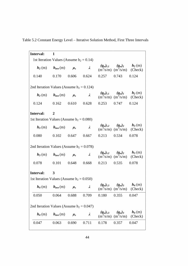
Table 5.2 Constant Energy Level – Iterative Solution Method, First Three Intervals

Interval: 1

1st Iteration Values (Assume h2 = 0.14)

h2 (m) have (m) µs λ

(qw)i.1 (m

3/s/m)

(qw)1 (m

3/s/m)

h2 (m)

(Check)

0.140 0.170 0.606 0.624 0.257 0.743 0.124

2nd Iteration Values (Assume h2 = 0.124)

h2 (m) have (m) µs λ

(qw)i.1 (m

3/s/m)

(qw)1 (m

3/s/m)

h2 (m)

(Check)

0.124 0.162 0.610 0.628 0.253 0.747 0.124

Interval: 2

1st Iteration Values (Assume h2 = 0.080)

h3 (m) have (m) µs λ

(qw)i.2 (m

3/s/m)

(qw)2 (m

3/s/m)

h3 (m)

(Check)

0.080 0.102 0.647 0.667 0.213 0.534 0.078

2nd Iteration Values (Assume h2 = 0.078)

h3 (m) have (m) µs λ

(qw)i.2 (m

3/s/m)

(qw)2 (m

3/s/m)

h3 (m)

(Check)

0.078 0.101 0.648 0.668 0.213 0.535 0.078

Interval: 3

1st Iteration Values (Assume h2 = 0.050)

h4 (m) have (m) µs λ

(qw)i.3 (m

3/s/m)

(qw)3 (m

3/s/m)

h4 (m)

(Check)

0.050 0.064 0.688 0.709 0.180 0.355 0.047

2nd Iteration Values (Assume h2 = 0.047)

h4 (m) have (m) µs λ

(qw)i.3 (m

3/s/m)

(qw)3 (m

3/s/m)

h4 (m)

(Check)

0.047 0.063 0.690 0.711 0.178 0.357 0.047

45

Table 5.3 Constant Energy Level – Iterative Solution Method, Fourth Interval and

Results

Interval: 4

1st Iteration Values (Assume h2 = 0.040)

h5 (m) have (m) µs λ

(qw)i.4 (m

3/s/m)

(qw)4 (m

3/s/m)

h5 (m)

(Check)

0.040 0.044 0.723 0.745 0.156 0.201 0.025

2nd Iteration Values (Assume h2 = 0.025)

h5 (m) have (m) µs λ

(qw)i.4 (m

3/s/m)

(qw)4 (m

3/s/m)

h5 (m)

(Check)

0.025 0.036 0.742 0.764 0.145 0.212 0.026

Water diverted to the collection channel is:

(qw)i.1 = 0.253 m3/s/m

(qw)i.2 = 0.213 m3/s/m

(qw)i.3 = 0.178 m3/s/m

(qw)i.4 = 0.145 m3/s/m

(qw)i = 0.788 m3/s/m

Discharge that passes over the trash rack and moves towards downstream is:

(qw)out = 0.212 m3/s/m

Flow depth at the end of the trash rack is:

h5 = 0.026 m

5.2.1.2 Closed Form Solution

(𝑞𝑤)𝑇 = 1.0 𝑚3 𝑠⁄ /𝑚 and ℎ1 = 0.20 m

cos2gs , 25.016

4

m

n

46

593.020.0

016.025.066.066.0

13.0

16.0

13.0

1

16.0

h

ms

611.00.30cos81.92.593.025.0

Flow length over the trash rack is computed as

366.920.0611.0

00.1561.2

)(561.2

1

h

qL Tw

𝑚 > 4 m

It is seen that, some portion of the incoming discharge is diverted to the collection

channel while the remaining discharge flows towards downstream. To determine the

diverted discharge (qw)i, the depth at the end of trash rack h2 is to be calculated.

2

1

2

2

1

2

2

2

2h

h

h

h

L

s , s = 9.366 − 4 = 5.366 m

2

2

22

2

2

20.020.02

366.9

366.5 hh , ℎ2 = 0.036 m

After completing calculation of h2

1

2

1

2 212707.1)(h

h

h

hqq

Twiw

20.0

036.02

20.0

036.012707.1)(

Twiw qq

(qw)i = 0.698 m3

/ s / m

(qw)T = 0.304 m3

/ s / m

47

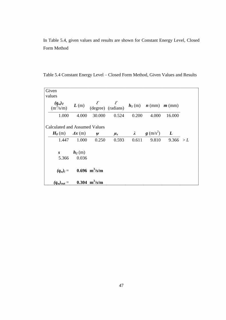
In Table 5.4, given values and results are shown for Constant Energy Level, Closed

Form Method

Table 5.4 Constant Energy Level – Closed Form Method, Given Values and Results

Given

values

(qw)T (m

3/s/m)

L (m) Ԑ

(degree)

Ԑ

(radians) h1 (m) n (mm) m (mm)

1.000 4.000 30.000 0.524 0.200 4.000 16.000

Calculated and Assumed Values

H0 (m) Δx (m) ψ µs λ g (m/s2) L

1.447 1.000 0.250 0.593 0.611 9.810 9.366 > L

s h2 (m)

5.366 0.036

(qw)i = 0.696 m3/s/m

(qw)out = 0.304 m3/s/m

48

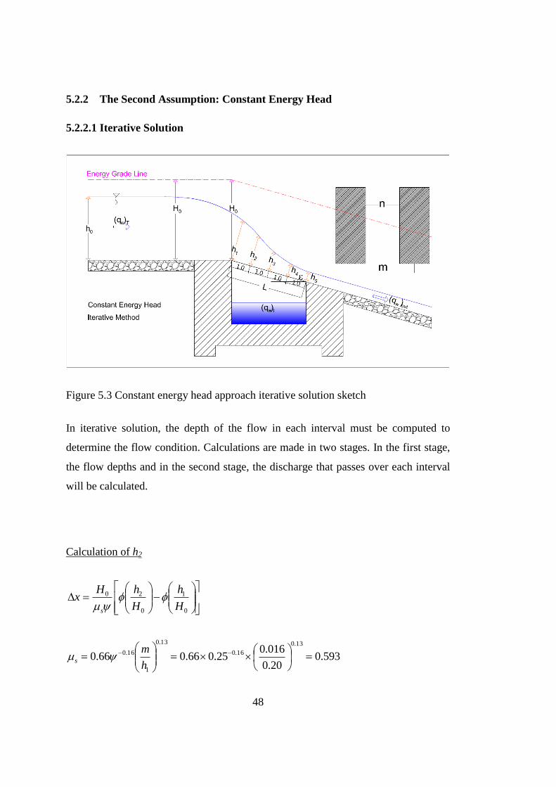
5.2.2 The Second Assumption: Constant Energy Head

5.2.2.1 Iterative Solution

Figure 5.3 Constant energy head approach iterative solution sketch

In iterative solution, the depth of the flow in each interval must be computed to

determine the flow condition. Calculations are made in two stages. In the first stage,

the flow depths and in the second stage, the discharge that passes over each interval

will be calculated.

Calculation of h2

0

1

0

20

H

h

H

hHx

s

593.020.0

016.025.066.066.0

13.0

16.0

13.0

1

16.0

h

ms

49

mHo 447.1 , mh 20.01 , 25.016

4

m

n

447.1

20.0

447.125.0593.0

447.100.1 2

h

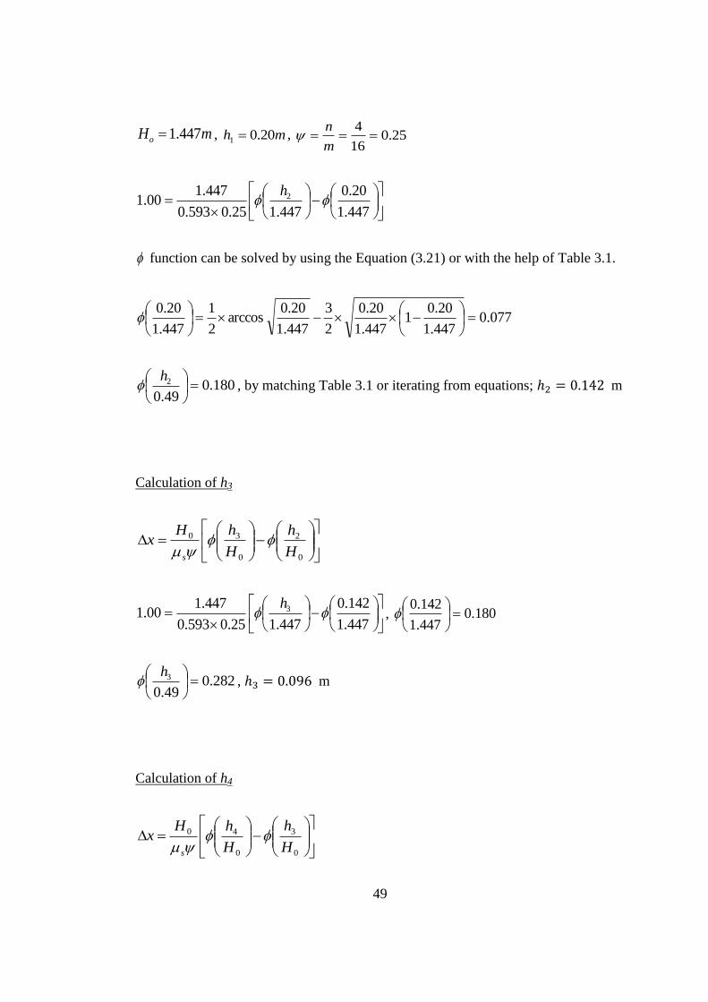
function can be solved by using the Equation (3.21) or with the help of Table 3.1.

077.0447.1

20.01

447.1

20.0

2

3

447.1

20.0arccos

2

1

447.1

20.0

180.049.0

2

h , by matching Table 3.1 or iterating from equations; ℎ2 = 0.142 m

Calculation of h3

0

2

0

30

H

h

H

hHx

s

447.1

142.0

447.125.0593.0

447.100.1 3

h, 180.0

447.1

142.0

282.049.0

3

h , ℎ3 = 0.096 m

Calculation of h4

0

3

0

40

H

h

H

hHx

s

50

447.1

096.0

447.125.0593.0

49.000.1 4

h, 282.0

447.1

096.0

385.0447.0

1 4

h , ℎ4 = 0.060 m

Calculation of h5

0

4

0

50

H

h

H

hHx

s

447.1

060.0

447.125.0593.0

447.100.1 5

h, 385.0

49.0

060.0

487.0447.1

5

h , ℎ5 = 0.033 m

Flow depths (h1, h2, h3, h4, h5) are calculated.

In the second step the discharges will be calculated and the flow depth found in the

first step will be used to check the flow condition.

Calculation of q2

max

1

max

20

q

q

q

qHx

s

𝑞𝑚𝑎𝑥 = 1.705 𝑥 𝐻0

32⁄

= 1.705 𝑥 1.4473

2⁄ = 2.969 m3 / s / m

51

function can be solved by using the Equation (3.21) or with the help of Table 3.1.

But to solve function, first the flow condition must be determined.

467.081.9

0.13

2

3

2

1 g

qhcr

m

ℎ𝑐𝑟 = √𝑞1

2

𝑔

3= √

1.02

9.81

3= 0.467 m

ℎ𝑐𝑟 > ℎ1 = 0.20 𝑚, flow is supercritical.

cos11cos22

21cos2

3

1arccos

2

1

max

1

q

q

oo 122.253240969.2

0.121arccos

3

12

,074.0max

1

q

q ,176.0

max

2

q

q by matching Table 3.1 or iterating from

Equation (3.21).

𝑞2 = 0.727 m3 / s / m

Calculation of q3

max

2

max

30

q

q

q

qHx

s

ℎ𝑐𝑟 = √𝑞2

2

𝑔

3= √

0.7272

9.81

3= 0.378 m

52

ℎ𝑐𝑟 > ℎ2 = 0.142 𝑚, flow is supercritical.

oo 445.249240969.2

727.021arccos

3

12

,177.0max

2

q

q ,279.0

max

3

q

q by matching Table 3.1 or iterating from

equations.

𝑞3 = 0.500 m3 / s / m

Calculation of q4

max

3

max

40

q

q

q

qHx

s

ℎ𝑐𝑟 = √𝑞3

2

𝑔

3

= √0.5002

9.81

3

= 0.294 m

ℎ𝑐𝑟 > ℎ3 = 0.096 𝑚, flow is supercritical.

oo 464.246240969.2

500.021arccos

3

12

,279.0max

3

q

q ,382.0

max

4

q

q by matching Table 3.1 or iterating from

equations.

𝑞4 = 0.316 m3 / s / m

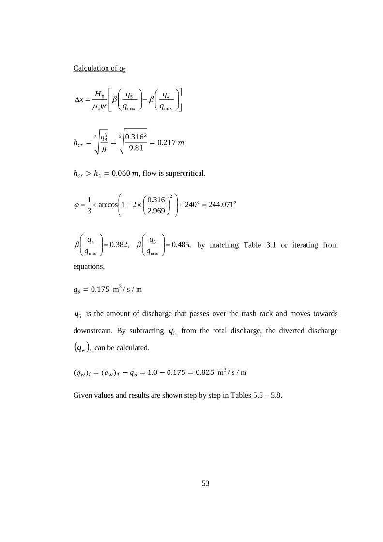
53

Calculation of q5

max

4

max

50

q

q

q

qHx

s

ℎ𝑐𝑟 = √𝑞4

2

𝑔

3

= √0.3162

9.81

3

= 0.217 𝑚

ℎ𝑐𝑟 > ℎ4 = 0.060 𝑚, flow is supercritical.

oo 071.244240969.2

316.021arccos

3

12

,382.0max

4

q

q ,485.0

max

5

q

q by matching Table 3.1 or iterating from

equations.

𝑞5 = 0.175 m3 / s / m

5q is the amount of discharge that passes over the trash rack and moves towards

downstream. By subtracting 5q from the total discharge, the diverted discharge

iwq can be calculated.

(𝑞𝑤)𝑖 = (𝑞𝑤)𝑇 − 𝑞5 = 1.0 − 0.175 = 0.825 m3 / s / m

Given values and results are shown step by step in Tables 5.5 – 5.8.

54

Table 5.5 Constant Energy Head – Iterative Solution Method, First Part (Using h1 in

s Formula - s Constant)

Given values

(qw)T (m

3/s/m)

L (m) ε

(radians) h1 (m) n (mm) m (mm) g (m/s

2)

1.000 4.000 0.524 0.200 4.000 16.000 9.810

Calculation of h2

H0 (m) Δx (m) ψ µs φ (h1/H0) φ (h2/H0) h2 (m)

1.447 1.000 0.250 0.593 0.077 0.180 0.142

Calculation of h3

φ (h3/H0) h3 (m)

0.282 0.096

Calculation of h4

φ (h4/H0) h4 (m)

0.385 0.060

Calculation of h5

φ (h5/H0) h5 (m)

0.487 0.033

Calculation of q2

qmax (m

3/s/m)

hcr (m)

2.969 0.467

> h2 ,

Supercritical

ϕ (degree) ϕ (radians) β1 β2

ϕ

(degree) ϕ

(radians) (qw)2

(m3/s/m)

253.122 4.418 0.074 0.176 249.445 4.354 0.727

55

Table 5.6 Constant Energy Head – Iterative Solution Method, Second Part (Using h1

in s Formula - s Constant)

Calculation of q3

qmax (m

3/s/m)

hcr (m)

2.969 0.378

> h2 ,

Supercritical

ϕ

(degree) ϕ

(radians) β2 β3

ϕ

(degree) ϕ

(radians) (qw)3

(m3/s/m)

249.445 4.354 0.177 0.279 246.464 4.302 0.500

Calculation of q4

qmax (m

3/s/m)

hcr (m)

2.969 0.294

> h2 ,

Supercritical

ϕ

(degree) ϕ

(radians) β3 β4

ϕ

(degree) ϕ

(radians) (qw)4

(m3/s/m)

246.464 4.302 0.279 0.382 244.071 4.260 0.316

Calculation of q5

qmax (m

3/s/m)

hcr (m)

2.969 0.217

> h2 ,

Supercritical

ϕ

(degree) ϕ

(radians) β4 β5

ϕ

(degree) ϕ

(radians) (qw)5

(m3/s/m)

244.071 4.260 0.382 0.485 242.249 4.228 0.175

(qw)i = 0.825 m3/s/m

(qw)out = 0.175 m3/s/m

56

s is obtained by using h1 to make steps easier in hand calculation. However, to get

better results s can be calculated by using have rather than h1.

13.0

13.0

16.0

13.0

16.0 481.0016.025.066.066.0

aveaveave

shhh

m

In Table 5.7, Calculations made by using have in s formula are shown.

Table 5.7 Constant Energy Head – Iterative Solution Method, (Using have in s

Formula - s Not Constant)

Given values

(qw)T (m

3/s/m)

L (m) ε

(radians) h1 (m) n (mm) m (mm) H0 (m)

1.000 4.000 0.524 0.200 4.000 16.000 1.447

Calculation of h2

Δx (m) ψ have (m) µs φ (h1/H0) φ (h2/H0) h2 (m)

1.000 0.250 0.170 0.606 0.077 0.182 0.141

Calculation of h3

have (m) µs φ (h3/H0) h3 (m)

0.116 0.637 0.292 0.092

Calculation of h4

have (m) µs φ (h4/H0) h4 (m)

0.072 0.677 0.409 0.052

Calculation of h5

have (m) µs φ (h5/H0) h5 (m)

0.038 0.737 0.536 0.023

57

Table 5.8 Constant Energy Head – Iterative Solution Method, (Using have in s

Formula - s Not Constant)

Calculation of q2

qmax (m

3/s/m)

hcr (m)

2.969 0.467 > h1 , Supercritical

ϕ

(degree) ϕ

(radians) β1 β2 ϕ (degree)

ϕ (radians)

(qw)2 (m

3/s/m)

253.122 4.418 0.074 0.178 249.401 4.353 0.723

Calculation of q3

qmax (m

3/s/m)

hcr (m)

2.969 0.376 > h2 , Supercritical

ϕ

(degree) ϕ

(radians) β2 β3 ϕ (degree)

ϕ (radians)

(qw)3 (m

3/s/m)

249.401 4.353 0.178 0.288 246.232 4.298 0.482

Calculation of q4

qmax (m

3/s/m)

hcr (m)

2.969 0.287 > h3 , Supercritical

ϕ

(degree) ϕ

(radians) β3 β4 ϕ (degree)

ϕ (radians)

(qw)4 (m

3/s/m)

246.232 4.298 0.288 0.405 243.611 4.252 0.280

Calculation of q5

qmax (m

3/s/m)

hcr (m)

2.969 0.200 > h4 , Supercritical

ϕ

(degree) ϕ

(radians) β4 β5 ϕ (degree)

ϕ (radians)

(qw)5 (m

3/s/m)

243.611 4.252 0.405 0.533 241.586 4.216 0.123

(qw)i = 0.877 m3/s/m

(qw)out = 0.123 m3/s/m

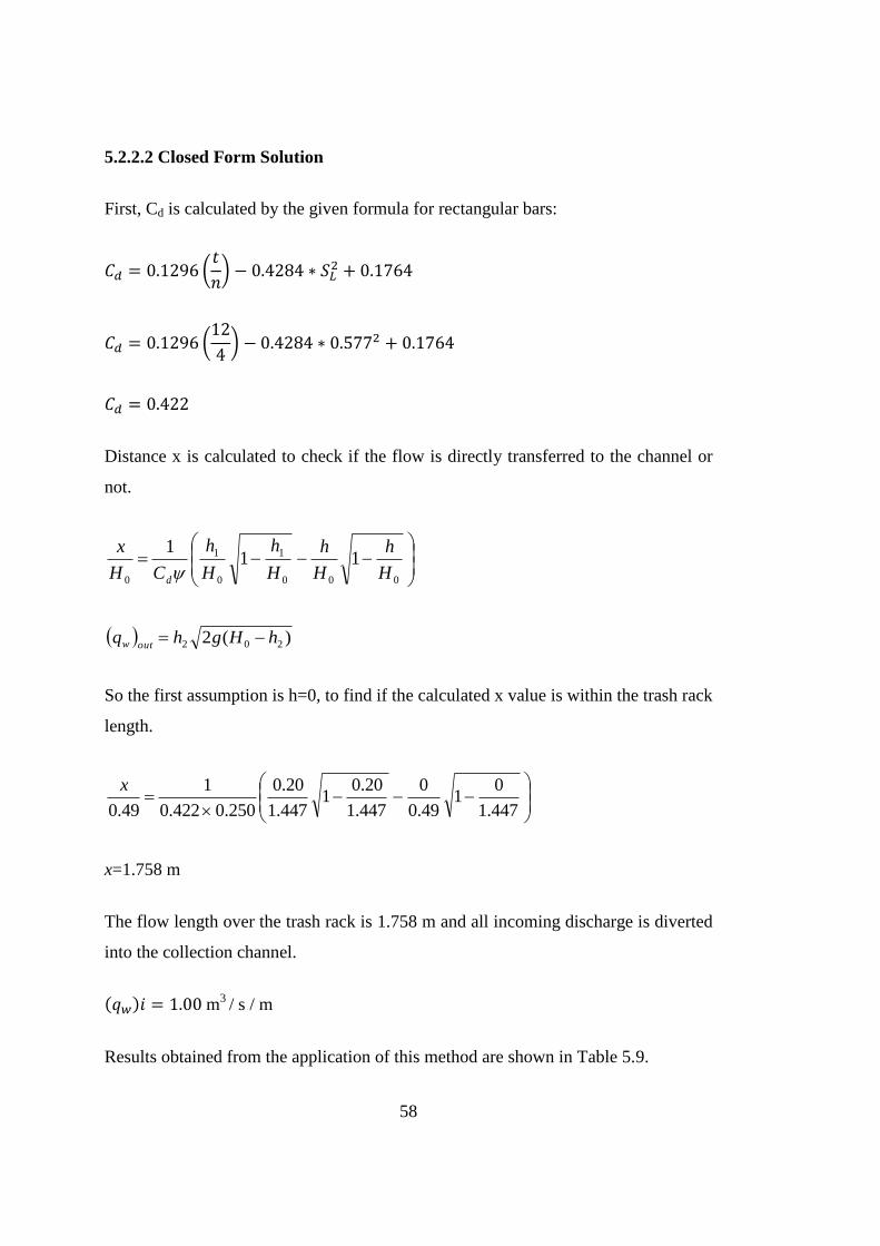
58

5.2.2.2 Closed Form Solution

First, Cd is calculated by the given formula for rectangular bars:

𝐶𝑑 = 0.1296 (𝑡

𝑛) − 0.4284 ∗ 𝑆𝐿

2 + 0.1764

𝐶𝑑 = 0.1296 (12

4) − 0.4284 ∗ 0.5772 + 0.1764

𝐶𝑑 = 0.422

Distance x is calculated to check if the flow is directly transferred to the channel or

not.

000

1

0

1

0

111

H

h

H

h

H

h

H

h

CH

x

d

)(2 202 hHghqoutw

So the first assumption is h=0, to find if the calculated x value is within the trash rack

length.

447.1

01

49.0

0

447.1

20.01

447.1

20.0

250.0422.0

1

49.0

x

x=1.758 m

The flow length over the trash rack is 1.758 m and all incoming discharge is diverted

into the collection channel.

(𝑞𝑤)𝑖 = 1.00 m3 / s / m

Results obtained from the application of this method are shown in Table 5.9.

59

Table 5.9 Constant Energy Head – Closed Form Solution Method,

Given values

(qw)T (m

3/s/m)

L (m) Ԑ

(degree)

Ԑ

(radians) h1 (m) n (mm) m (mm) g (m/s

2)

1.000 4.000 30.000 0.524 0.200 4.000 16.000 9.810

H0 (m) Δx (m) ψ µs

1.447 1.000 0.250 0.593

hcr (m) SL t (mm) Cd x

0.467 0.577 12.000 0.422 1.758 < L All flow is diverted to

the channel

(qw)out

(m3/s/m) h2 (m)

0.000 0.000

(qw)i = 1.000 m3/s/m

(qw)out = 0.000 m3/s/m

Discharge taken into the channel, discharge passing over the trash rack to the

downstream and the flow depth at the end of the rack are given in Table 5.10 with

respect to the method used in calculation.

Table 5.10 Comparison of Results – Analysis Application

h (m)

(qw)i (m

3/s/m)

(qw)out (m

3/s/m)

Constant Energy Level

Iterative Solution Method 0.026 0.788 0.212

Closed Form Solution Method 0.036 0.696 0.304

Constant Energy Head

Iterative Solution Method 0.023 0.877 0.123

Closed Form Solution Method 0.000 1.000 0.000

60

5.3 Design Application

In this part of the study, a Tyrolean weir is designed according to the methods and

assumptions shown in chapters 2 and 3. An example is solved below for better

understanding of the design procedures. A definition sketch characterizing the design

is shown in Figure 5.4.

Figure 5.4 Sketch for Tyrolean weir design example

Total discharge (qw)T of the Tyrolean weir shown in Figure 5.4 is 1.00 m3/s/m. If the

flow depth at the upstream of the trash rack (h0) is 0.50 m, find the required length of

the trash rack (L) to divert the design discharge into the intake channel of the

structure. The design discharge is 0.80 m3/s/m and the median gravel size of the

stream is 40 mm.

To begin with, some assumptions should be made according to the recommendations.

First, bar type is selected as rectangular reinforced circular bar as the most efficient

cross section which is shown on the right hand side of Figure 5.4. It is recommended

by researchers according to the various experiments and studies mentioned in

Chapter 3.

61

Moreover, according to past studies described in Chapter 3; n, the clear spacing

between bars is selected same as the median gravel size of the stream bed sediment

and m, the central distance of bars are calculated in a way that to obtain the 40%

recommended void ratio. In addition to that, slope of the rack is selected as 30%,

which means an inclination angle of 16.7 degrees as being recommended as the most

efficient slope.

5.3.1 The First Assumption: Constant Energy Level

5.3.1.1 Iterative Solution Method:

Iterative solution method is applied twice for the design stage. At the first

application, stream discharge is assumed to be equal to the design discharge to

calculate the required rack length which is long enough to divert the total flow. Then

in the second stage, stream discharge is taken as it is and discharge taken into the

intake channel is calculated by using the rack length value obtained in the first stage.

If the design discharge is supplied and water given to the downstream of the structure

is appropriate for the protection of the environment, results are decided to be suitable

for design. Input values to be used in the application are summarized in Table 5.11.

Table 5.11 Given input values for the design application

(qw)T (m

3/s/m)

(qw)i (m

3/s/m)

h0 (m) Median Gravel

Size (mm) g (m/s

2)

1.000 0.8 0.500 40.000 9.810

Assumed and calculated values for other necessary input values are shown below in

Table 5.12 in which, Ԑ = inclination angle of the rack, n = clear spacing between

bars, m = central distance of bars, D = diameter of bars, SL = rack slope, Δx =

calculation interval, ψ = n/m void ratio, H0 = head at the upstream of the rack, hcr =

critical flow depth, χ = correction factor described in Equation (3.42), h1 = flow

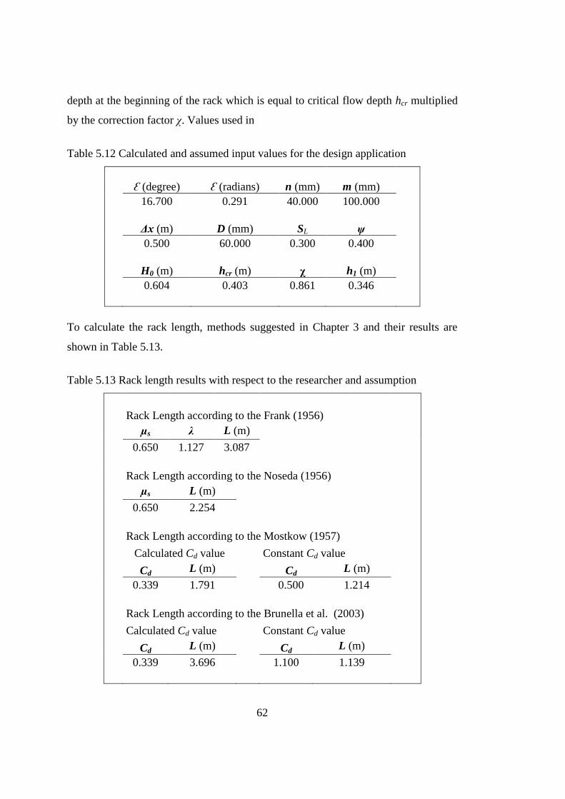
62

depth at the beginning of the rack which is equal to critical flow depth hcr multiplied

by the correction factor χ. Values used in

Table 5.12 Calculated and assumed input values for the design application

Ԑ (degree) Ԑ (radians) n (mm) m (mm)

16.700 0.291 40.000 100.000

Δx (m) D (mm) SL ψ

0.500 60.000 0.300 0.400

H0 (m) hcr (m) χ h1 (m)

0.604 0.403 0.861 0.346

To calculate the rack length, methods suggested in Chapter 3 and their results are

shown in Table 5.13.

Table 5.13 Rack length results with respect to the researcher and assumption

Rack Length according to the Frank (1956)

µs λ L (m)

0.650 1.127 3.087

Rack Length according to the Noseda (1956)

µs L (m)

0.650 2.254

Rack Length according to the Mostkow (1957)

Calculated Cd value

Constant Cd value

Cd L (m)

Cd L (m)

0.339 1.791

0.500 1.214

Rack Length according to the Brunella et al. (2003)

Calculated Cd value

Constant Cd value

Cd L (m)

Cd L (m)

0.339 3.696

1.100 1.139

63

In the first one of the four different methods, Frank’s approach is applied according

to Equation (3.12). In the second one, the formula proposed by Noseda (1956) is

used as shown in Equation (3.43). In the third approach, Equation (3.44) given by

Mostkow (1957) is applied and in the last one, the method given by Brunella et al.

(2003) is used. In the third and fourth approaches, the discharge coefficient value Cd

is used. Mostkow (1957) suggested that Cd varies from 0.435, for a sloping rack 1 in

5, to 0.497 for a horizontal rack. Furthermore, Brunella et al. (2003) recommended

that Cd is equal to 1.1 for porosity values, Ѱ = 0.35 and Cd = 0.87 for Ѱ = 0.664.

Rack length is calculated in two different ways for Mostkow (1957) and Brunella et

al. (2003). The first one is calculated by assumed discharge coefficients

recommended by the related researcher and the second one is obtained by using the

Cd values calculated from the formulae shown in Equation (3.25) and Equation

(3.26).

Table 5.12 shows that there are many ways to calculate rack length and obtained

results are quite different from each other. Although, formula given by Mostkow

(1957) and Brunella et al. (2003) are approved by Jiménes and Vargas (2006), to

give logical results, none of the methods are reliable enough to decide on the length

of rack bars to divert the required design discharge from the stream in the present

stage. So, four approaches described and used in analysis section will also be used in

the design stage to get more consistent results. Selection of an appropriate value for

L is recommended to be case sensitive considering local site characteristics.

Therefore, final decision on L value is to be given by the designer.

Δx interval is decided as 0.5 m which seems to be logical according to the rack length

values shown in Table 5.12. Calculation procedure is the same as the steps described

in the analysis application. An assumption is made for the flow depth and for the first

interval and the same procedure in the analysis stage is applied to calculate the

discharge taken into the intake channel. When the assumed flow depth is obtained,

iteration stops and calculations for the next interval starts. Results obtained from the

first interval are shown in the Table 5.14 below.

64

Table 5.14 First stage for the design application, first interval

Interval: 1

1st Iteration Values -Assume h2 = 0.150

h2 (m) have (m) µs λ

(qw)i.1 (m

3/s/m)

(qw)1 (m

3/s/m)

h2 (m)

(Check)

0.150 0.248 0.679 1.177 0.293 0.507 0.147

2nd Iteration Values

h2 (m) have (m) µs λ

(qw)i.1 (m

3/s/m)

(qw)1 (m

3/s/m)

h2 (m)

(Check)

0.147 0.247 0.680 1.178 0.293 0.507 0.147

When the flow depth is approximately zero, rack length is said to be long enough to

take the whole discharge into the weir. In Table 5.15, h3 is calculated.

Table 5.15 First stage for the design application, second interval

Interval: 2

1st Iteration Values -Assume h3 = 0.070

h3 (m) have (m) µs λ

(qw)i.2 (m

3/s/m)

(qw)2 (m

3/s/m)

h3 (m)

(Check)

0.070 0.108 0.756 1.311 0.216 0.291 0.072

2nd Iteration Values

h3 (m) have (m) µs λ

(qw)i.2 (m

3/s/m)

(qw)2 (m

3/s/m)

h3 (m)

(Check)

0.072 0.110 0.755 1.309 0.217 0.291 0.073

65

Flow depth h3 is still not close to zero. So that means rack length should be longer

than the summation of two interval lengths which is 1 m. So, calculations are

proceeded with the third interval which is shown in Table 5.16.

Table 5.16 First stage for the design application, third interval

Interval: 3

1st Iteration Values -Assume h4 = 0.030

h4 (m) have (m) µs λ

(qw)i.3 (m

3/s/m)

(qw)3 (m

3/s/m)

h4 (m)

(Check)

0.030 0.051 0.833 1.445 0.164 0.127 0.029

2nd Iteration Values

h4 (m) have (m) µs λ

(qw)i.3 (m

3/s/m)

(qw)3 (m

3/s/m)

h4 (m)

(Check)

0.029 0.051 0.835 1.448 0.163 0.128 0.029

Flow depth becomes close to zero but not enough to stop the calculations. So, one

more interval is checked which is shown in Table 5.17.

Table 5.17 First stage for the design application, fourth interval

Interval: 4

1st Iteration Values -Assume h5 = 0.005

h5 (m) have (m) µs λ

(qw)i.4 (m

3/s/m)

(qw)4 (m

3/s/m)

h5 (m)

(Check)

0.005 0.017 0.963 1.670 0.109 0.019 0.004

2nd Iteration Values

h5 (m) have (m) µs λ

(qw)i.4 (m

3/s/m)

(qw)4 (m

3/s/m)

h5 (m)

(Check)

0.004 0.016 0.967 1.677 0.107 0.020 0.004

Finally, flow depth is 4 mm which is almost zero. Four 0.5 m long intervals are

analyzed, so the total rack length is 2 m. The discharge taken into the intake channel

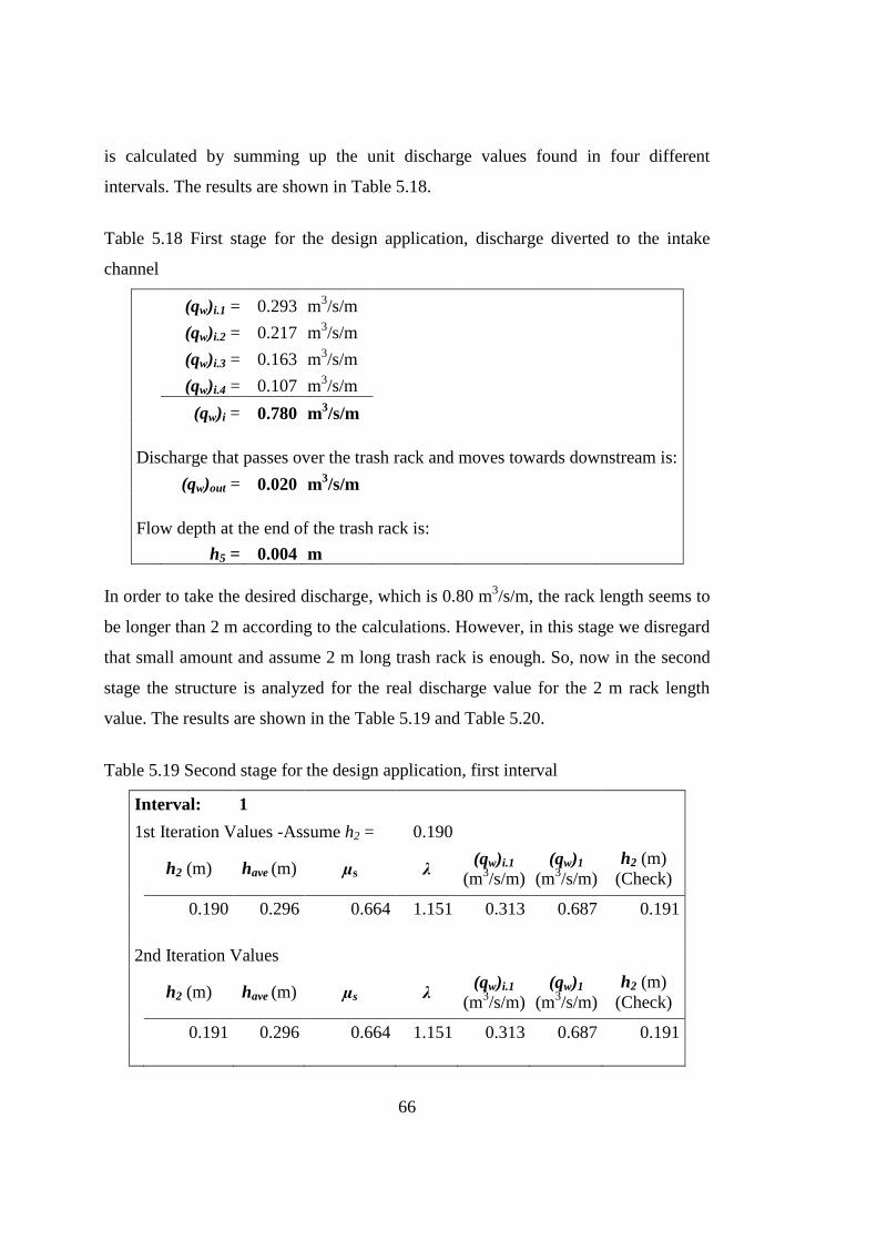
66

is calculated by summing up the unit discharge values found in four different

intervals. The results are shown in Table 5.18.

Table 5.18 First stage for the design application, discharge diverted to the intake

channel

(qw)i.1 = 0.293 m3/s/m

(qw)i.2 = 0.217 m3/s/m

(qw)i.3 = 0.163 m3/s/m

(qw)i.4 = 0.107 m3/s/m

(qw)i = 0.780 m3/s/m

Discharge that passes over the trash rack and moves towards downstream is:

(qw)out = 0.020 m3/s/m

Flow depth at the end of the trash rack is:

h5 = 0.004 m

In order to take the desired discharge, which is 0.80 m3/s/m, the rack length seems to

be longer than 2 m according to the calculations. However, in this stage we disregard

that small amount and assume 2 m long trash rack is enough. So, now in the second

stage the structure is analyzed for the real discharge value for the 2 m rack length

value. The results are shown in the Table 5.19 and Table 5.20.

Table 5.19 Second stage for the design application, first interval

Interval: 1

1st Iteration Values -Assume h2 = 0.190

h2 (m) have (m) µs λ

(qw)i.1 (m

3/s/m)

(qw)1 (m

3/s/m)

h2 (m)

(Check)

0.190 0.296 0.664 1.151 0.313 0.687 0.191

2nd Iteration Values

h2 (m) have (m) µs λ

(qw)i.1 (m

3/s/m)

(qw)1 (m

3/s/m)

h2 (m)

(Check)

0.191 0.296 0.664 1.151 0.313 0.687 0.191

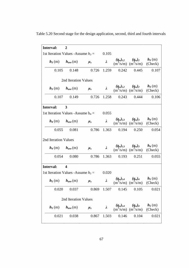
67

Table 5.20 Second stage for the design application, second, third and fourth intervals

Interval: 2

1st Iteration Values -Assume h3 = 0.105

h3 (m) have (m) µs λ

(qw)i.2 (m

3/s/m)

(qw)2 (m

3/s/m)

h3 (m)

(Check)

0.105 0.148 0.726 1.259 0.242 0.445 0.107

2nd Iteration Values

h3 (m) have (m) µs λ

(qw)i.2 (m

3/s/m)

(qw)2 (m

3/s/m)

h3 (m)

(Check)

0.107 0.149 0.726 1.258 0.243 0.444 0.106

Interval: 3

1st Iteration Values -Assume h4 = 0.055

h4 (m) have (m) µs λ

(qw)i.3 (m

3/s/m)

(qw)3 (m

3/s/m)

h4 (m)

(Check)

0.055 0.081 0.786 1.363 0.194 0.250 0.054

2nd Iteration Values

h4 (m) have (m) µs λ

(qw)i.3 (m

3/s/m)

(qw)3 (m

3/s/m)

h4 (m)

(Check)

0.054 0.080 0.786 1.363 0.193 0.251 0.055

Interval: 4

1st Iteration Values -Assume h5 = 0.020

h5 (m) have (m) µs λ

(qw)i.4 (m

3/s/m)

(qw)4 (m

3/s/m)

h5 (m)

(Check)

0.020 0.037 0.869 1.507 0.145 0.105 0.021

2nd Iteration Values

h5 (m) have (m) µs λ

(qw)i.4 (m

3/s/m)

(qw)4 (m

3/s/m)

h5 (m)

(Check)

0.021 0.038 0.867 1.503 0.146 0.104 0.021

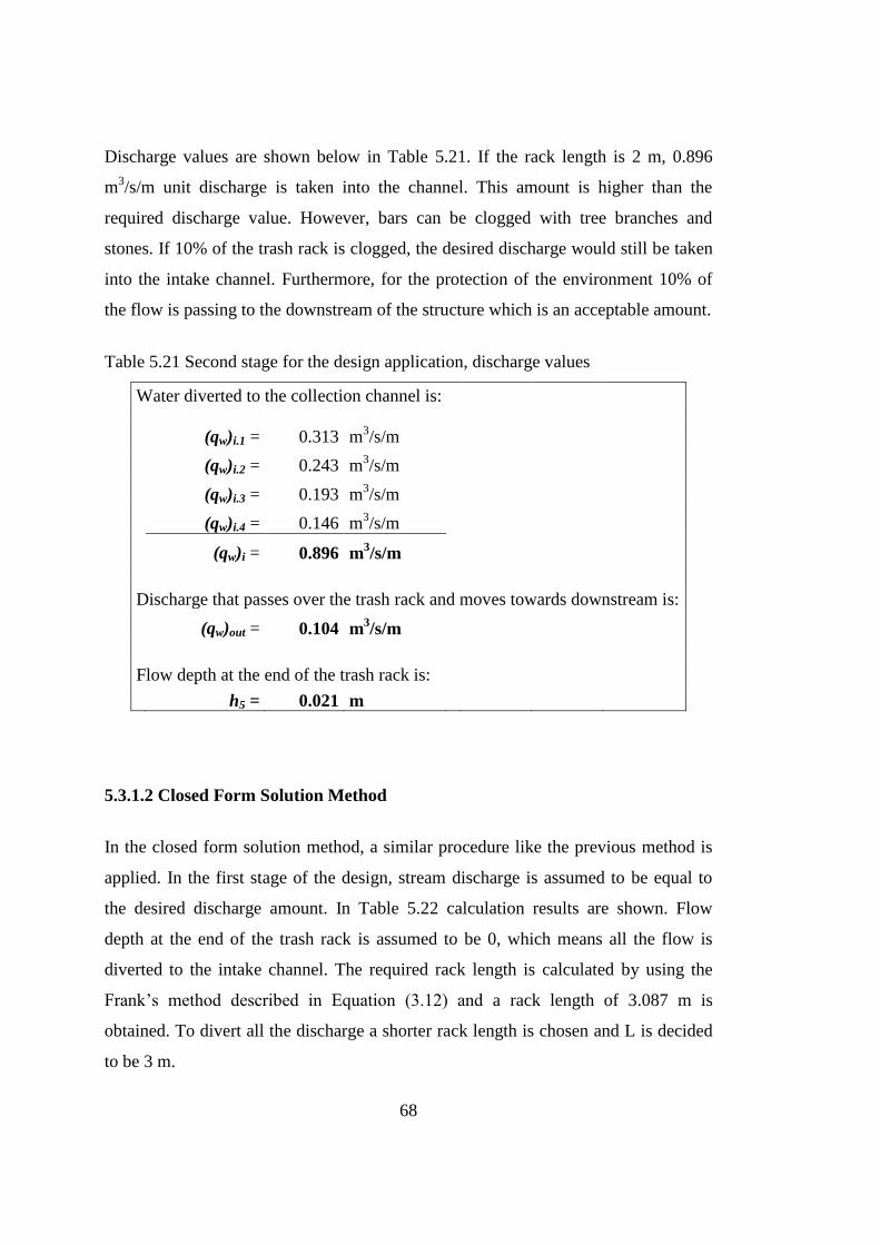
68

Discharge values are shown below in Table 5.21. If the rack length is 2 m, 0.896

m3/s/m unit discharge is taken into the channel. This amount is higher than the

required discharge value. However, bars can be clogged with tree branches and

stones. If 10% of the trash rack is clogged, the desired discharge would still be taken

into the intake channel. Furthermore, for the protection of the environment 10% of

the flow is passing to the downstream of the structure which is an acceptable amount.

Table 5.21 Second stage for the design application, discharge values

Water diverted to the collection channel is:

(qw)i.1 = 0.313 m3/s/m

(qw)i.2 = 0.243 m3/s/m

(qw)i.3 = 0.193 m3/s/m

(qw)i.4 = 0.146 m3/s/m

(qw)i = 0.896 m3/s/m

Discharge that passes over the trash rack and moves towards downstream is:

(qw)out = 0.104 m3/s/m

Flow depth at the end of the trash rack is:

h5 = 0.021 m

5.3.1.2 Closed Form Solution Method

In the closed form solution method, a similar procedure like the previous method is

applied. In the first stage of the design, stream discharge is assumed to be equal to

the desired discharge amount. In Table 5.22 calculation results are shown. Flow

depth at the end of the trash rack is assumed to be 0, which means all the flow is

diverted to the intake channel. The required rack length is calculated by using the

Frank’s method described in Equation (3.12) and a rack length of 3.087 m is

obtained. To divert all the discharge a shorter rack length is chosen and L is decided

to be 3 m.

69

Table 5.22 First stage for the design application

H0 (m) hcr (m) χ h1 (m)

0.604 0.403 0.861 0.346

L (m) µs λ L

3.000 0.650 1.127 3.087 > L

h2 (m) s

0.000 0.087

(qw)i = 0.799 m3/s/m

(qw)out = 0.001 m3/s/m

By assuming the design discharge is equal to the stream discharge, 3 m rack length is

obtained. In the second stage, the real stream discharge is used in the calculation and

the flow amount taken into the intake channel and the flow depth value at the end of

the rack is obtained as shown in Table 5.23.

Table 5.23 Second stage for the design application.

hcr (m) χ h1 (m) H0 (m)

0.467 0.861 0.402 0.700

L (m) µs λ L

3.000 0.638 1.106 3.652 > L

h2 (m) s

0.006 0.652

(qw)i = 0.971 m3/s/m

(qw)out = 0.029 m3/s/m

Discharge taken into the weir is 0.971 m3/s/m which is a higher value than expected.

The structure seems to be on the safe side in terms of clogging but the downstream

discharge is not enough for the sake of environmental aspects.

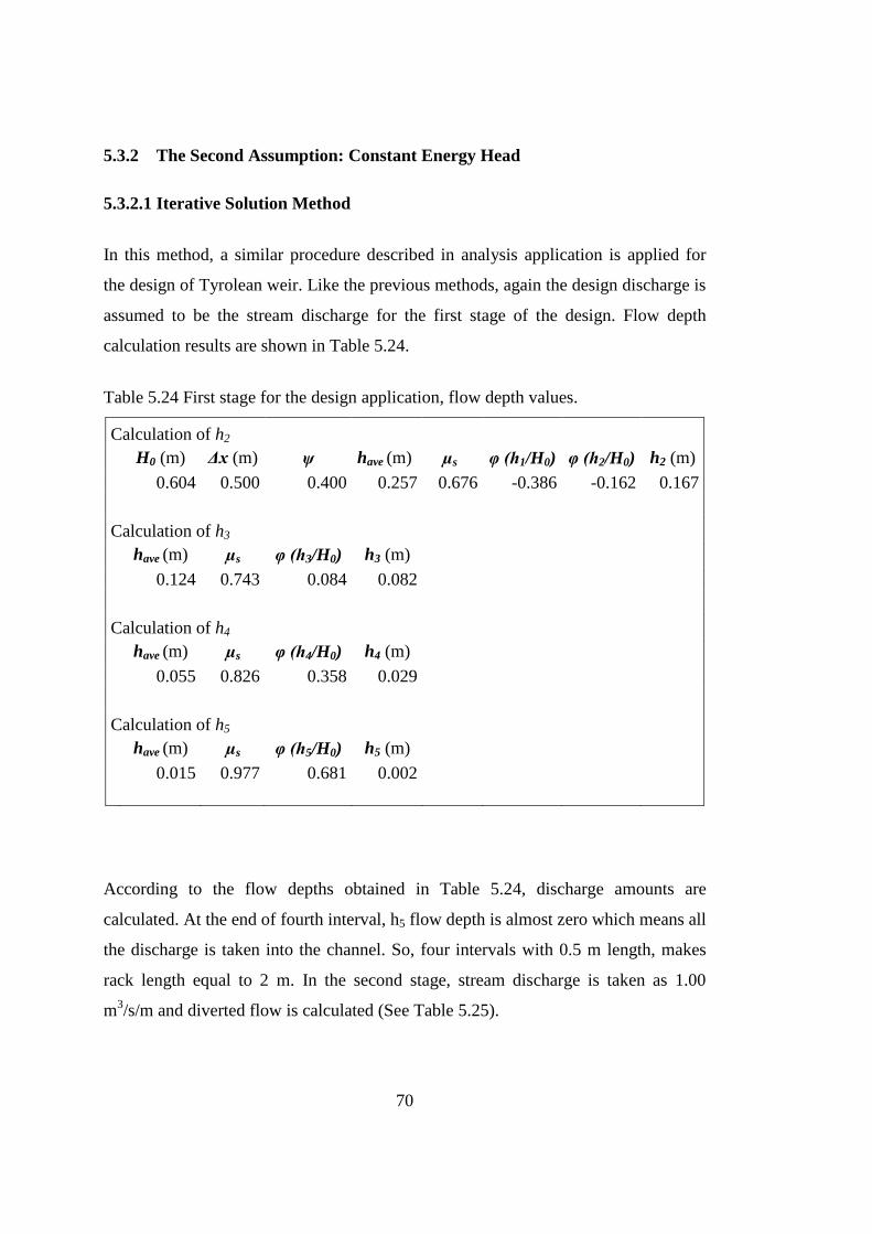
70

5.3.2 The Second Assumption: Constant Energy Head

5.3.2.1 Iterative Solution Method

In this method, a similar procedure described in analysis application is applied for

the design of Tyrolean weir. Like the previous methods, again the design discharge is

assumed to be the stream discharge for the first stage of the design. Flow depth

calculation results are shown in Table 5.24.

Table 5.24 First stage for the design application, flow depth values.

Calculation of h2

H0 (m) Δx (m) ψ have (m) µs φ (h1/H0) φ (h2/H0) h2 (m)

0.604 0.500 0.400 0.257 0.676 -0.386 -0.162 0.167

Calculation of h3

have (m) µs φ (h3/H0) h3 (m)

0.124 0.743 0.084 0.082

Calculation of h4

have (m) µs φ (h4/H0) h4 (m)

0.055 0.826 0.358 0.029

Calculation of h5

have (m) µs φ (h5/H0) h5 (m)

0.015 0.977 0.681 0.002

According to the flow depths obtained in Table 5.24, discharge amounts are

calculated. At the end of fourth interval, h5 flow depth is almost zero which means all

the discharge is taken into the channel. So, four intervals with 0.5 m length, makes

rack length equal to 2 m. In the second stage, stream discharge is taken as 1.00

m3/s/m and diverted flow is calculated (See Table 5.25).

71

Table 5.25 Second stage for the design application, discharge values.

Calculation of q2

qmax (m

3/s/m)

hcr (m)

1.000 0.467 > h1 , Supercritical

ϕ

(degree) ϕ

(radians) β1 β2 ϕ (degree)

ϕ (radians)

(qw)2 (m

3/s/m)

300.000 5.236 -0.399 -0.217 268.958 4.694 0.688

Calculation of q3

qmax (m

3/s/m)

hcr (m)

1.000 0.364 > h2 , Supercritical

ϕ

(degree) ϕ

(radians) β2 β3 ϕ (degree)

ϕ (radians)

(qw)3 (m

3/s/m)

268.958 4.694 -0.216 -0.034 257.842 4.500 0.450

Calculation of q4

qmax (m

3/s/m)

hcr (m)

1.000 0.274 > h3 , Supercritical

ϕ

(degree) ϕ

(radians) β3 β4 ϕ (degree)

ϕ (radians)

(qw)4 (m

3/s/m)

257.842 4.500 -0.034 0.148 250.365 4.370 0.268

Calculation of q5

qmax (m

3/s/m)

hcr (m)

1.000 0.194 > h4 , Supercritical

ϕ

(degree) ϕ

(radians) β4 β5 ϕ (degree)

ϕ (radians)

(qw)5 (m

3/s/m)

250.365 4.370 0.149 0.331 245.184 4.279 0.135

(qw)i = 0.865 m3/s/m

(qw)out = 0.135 m3/s/m

72

Discharge values are shown above in Table 5.25. If the rack length is 2 m, 0.865

m3/s/m unit discharge is taken into the channel. This amount is higher than the

required discharge value. However, bars can be clogged with tree branches and

stones. If approximately 7% of the trash rack is clogged, the desired discharge would

still be taken into the intake channel. Furthermore, for the protection of the

environment 10% of the flow is passing to the downstream of the structure which is

an acceptable amount.

5.3.2.2 Closed Form Solution Method:

This method is also applied in two stages. For the first stage again stream discharge

is assumed the same as the desired discharge of the intake. First required rack length

is studied as shown in the Table 5.26.

Table 5.26 First stage for the design application

hcr (m) h1 (m) H0 (m)

0.403 0.346 0.604

SL D (mm) Cd L (m)

0.300 60.000 0.417 1.354

(qw)out (m3/s/m) h2 (m)

0.000 0.000

(qw)i = 0.800 m3/s/m

(qw)out = 0.000 m3/s/m

The required length of the rack is calculated for the 0.80 m3/s/m intake amount. For

1.354 m long rack, discharge passing to the downstream of the weir and h2 the flow

73

depth is at the end of the rack is both equal to 0. For the calculation of the discharge

coefficient Cd, a different formula than the analysis application is used since in

design example bar cross section is selected as circular. For the circular type,

Equation (3.25) is used for obtaining Cd. The second stage calculations are shown in

the Table 5.27.

Table 5.27 Second stage for the design application

hcr (m) h1 (m) H0 (m)

0.467 0.402 0.700

SL D (mm) Cd L (m)

0.300 60.000 0.417 1.400

x

h2 (m) (qw)out (m3/s/m)

1.572 > L , Some part of

the flow passes

over the rack

0.029 0.106

(qw)i = 0.894 m3/s/m

(qw)out = 0.106 m3/s/m

In the second stage, stream discharge is 1.00 m3/s/m and rack length value obtained

in the first stage 1.354 m is rounded to 1.4 m for the ease of application. x value is

the rack length required for diverting 1.00 m3/s/m stream discharge and since it is

higher than the decided rack length of 1.4 m, it is obvious that some part of the flow

passes over the rack. According to the Equation (3.39), the flow depth at the end of

trash rack is calculated and flow passing to the downstream is obtained by using

Equation (3.40).

Discharge values are shown above in Table 5.27. If the rack length is 1.4 m, 0.894

m3/s/m unit discharge is taken into the channel. This amount is higher than the

required discharge value. However, bars can be clogged with tree branches and

74

stones. If approximately 10% of the trash rack is clogged, the desired discharge

would still be taken into the intake channel. Moreover, for the protection of the

environment 10% of the flow is passing to the downstream of the structure, which is

a reasonable amount.

In Table 5.28, one digit rack length values are listed according to the direct

calculation methods. Lengths vary between 1.1 m and 3.8 m which is a high range

for a reliable design.

Table 5.28 Comparison of rack length values obtained by direct calculations given by

researchers

Method by Researcher Rack Length

Frank 3.1 m

Noseda 2.3 m

Mostkow ( Calculated Cd) 1.8 m

Mostkow ( Constant Cd) 1.2 m

Brunella et al. ( Calculated Cd) 3.7 m

Brunella et al. ( Constant Cd) 1.1 m

Discharge values obtained by four different solution methods are listed below in

Table 5.29 with rack lengths calculated by those methods.

Table 5.29 Comparison of results obtained from four different solution methods

(qw)i (m

3/s/m)

(qw)out (m

3/s/m)

h (m) L (m)

Constant Energy Level

Iterative Solution Method 0.896 0.104 0.021 2.000

Closed Form Solution Method 0.971 0.029 0.006 3.000

Constant Energy Head

Iterative Solution Method 0.865 0.135 0.017 2.000

Closed Form Solution Method 0.894 0.106 0.029 1.400

Closed form methods are developed for easier hand calculations so iterative methods

give more precise results.

75

In this chapter two applications are presented. In these applications, analysis and

design procedures are explained in terms of four different methods developed in past

studies.

The first two methods assume constant energy level i.e. no headloss is considered

throughout the rack length. In fact, the length of racks is relatively small for practical

applications. Therefore, ignoring headloss may be assumed to yield insignificant

error in computations. The consecutive methods assume constant energy head. So,

this approach considers headloss but the energy grade line is assumed to be parallel

to the rack surface. This assumption normally holds true for uniform flow. However,

the flow rate along the rack decreases in flow direction which is accompanied by a

decreasing non-uniform water surface profile along the flow direction. Hence,

neither assumption is thoroughly correct. Therefore, the validity of the proposed

approaches needs verification with reference to elaborated physical model studies.

76

CHAPTER 6

6 CONCLUSIONS AND FURTHER RECOMMENDATIONS

Tyrolean weirs are one of the most suitable structures for runoff river plants. If they

are designed properly structure can work efficiently without high investment and

environmental impact. Use of the program enables a designer to perform quick

successive runs such that hydraulic conformity and cost aspects are easily assessed.

In the present study, design and analysis solution methods for Tyrolean intakes are

researched and presented. A computer program named “Tyrol” is developed and

application studies are demonstrated with step by step calculations for each method.

Tyrol is easily applicable and user friendly.

In the analysis of the structure, usage of iterative methods for both constant energy

level and constant energy head assumptions give similar results when compared to

closed form solution methods. Closed form methods can misguide the designer if the

structure is analyzed by using only closed form methods. In order to guide through

the complex calculation procedure, a step by step solution is given for the analysis

application.

In the design of the structure, most efficient values and ratios of parameters are

presented according to the research made in past studies. With respect to these

assumptions, most efficient design of a Tyrolean weir structure is given in detail and

explained with a design application in Chapter 5. Formulae developed for the

calculation of trash rack length give different results. So, calculated rack length

results are compared with the results obtained from solution methods to give a better

understanding. Selection of an appropriate value for L is recommended to be case

77

sensitive considering local site characteristics. Therefore, final decision on L value is

to be given by the designer.

Furthermore, the computer program Tyrol is developed for this study for an easy and

user friendly way of analysis and design of Tyrolean weirs.

Recommendations for further studies can be as follows:

Models can be built for different slopes, bar types and gaps since these are the

governing properties of results.

These models can be experimentally tested and results can be compared by

the fast calculations made by using the computer program developed and

presented in this study.

So, different solution methods and assumptions can be compared and results

can be checked in terms of their accuracy according to the real situations and

values observed and obtained from physical models.

78

REFERENCES

Aghamajidi, R., and Heydari, M. M. (2014). Simulation of Flow on Bottom Turn out

Structures with Flow 3D. Bull. Env. Pharmacol. Life Sci., Vol 3 (3), 173-181.

Ahmad Z. and Mittal M. (2006). Hydraulic Design Of Trench Weir On Dabka River

A Case Study. Water And Energy International, CBIP 2004 60 (4), 28 - 37.

Andaroodi, M. (2006). Standardization of Civil Engineering Works of Small High-

Head Hydropower Plants and Development of an Optimization Tool. Switzerland:

LCH, Laboratoire de Constructions Hydrauliques, Ecole Polytechnique Fédérale de

Lausanne

Bianco, G. and Ripellino, P. G. (1994). Attualita` Delle Opere Di Presa A Traversa

Derivante E Studio Con Modello Idraulico Di Un Tipo Di Griglia Suborizzontale.

Idrotecnica, 21(1), 3-12 (in Italian).

Brunella, S., Hager, W. H. and Hans-Erwin Minor, H.E. (2003). Hydraulics of

bottom rack Intake. J. of Hyd. Eng. ASCE, 129 (1), 1-10.

Çeçen K. (1962). Vahşi Derelerden Su Alma, İstanbul: Publications of İstanbul

Technical University. (in Turkish).

Dagan, G. (1963). Notes Sur Le Calcul Hydraulique Des Grilles, Pardessous. La

Houille Blanche, 18 (1), 59–65 (in French).

Drobir, H. (1981). Entwurf von Wasserfassungen im Hochgebirge. Österr.

Wasserwirtsch, 33 (11/12), 243–253 (in German).

Drobir, H., Kienberger, V. and Krouzecky, N. (1999). The Wetted Rack Length of the

Tyrolean Weir. Proceedings XXVIII IAHR congress, IAHR.

Frank, J. (1956) Hydraulische Untersuchungen für das Tiroler Wehr. Der

Bauingenieur, 31 (3), 96-101 (in German).

79

Ghosh, S. and Ahmad Z. (2006). Characteristics of Flow Over Bottom Racks. Water

and Energy International, CBIP, 63 (2), 47-55.

Jiménez, O. and, and Vargas, O. (2006). Some Experiences in the Performance of

Bottom Intakes. International Symposium On Hydraulic Structures Ciudad Guayana,

Venezuela.

Kamanbedast, A. A. and Bejestan, M. S. (2008). Effects of Slope and Area Opening

on the Discharge Ratio in Bottom Intake Structures. J. of Applied Sciences; 8 (14),

2631-2635.

Kuntzmann, J. and Bouvard, M. (1954). Etude the´orique des grilles de prises d’eau

du type ‘en-dessous. La Houille Blanche, 9 (9/10), 569–574 (in French).

Mostkow, M. A. (1957). Sur le Calcul des Grilles de Prise D’eau. La Houille

Blanche, 12 (4), 570–580 (in French).

Noseda, G. (1955). Operation and Design of Bottom Intake Racks. 6th

International

Association of Hydraulic Research Congress, La Haye, (17), 1–11.

Noseda, G. (1956). Correnti permanenti con portata progressivamente decrescente,

defluenti su griglie di fondo. L’Energia Elettrica, 33 (1), 41–51 (in Italian).

Orth, J., Chardonnet, E. and Meynardi, G. (1954). Etude de grilles pour prises d’eau

du type ‘en-dessous. La Houille Blanche, 9 (6), 343– 351 (in French).

Özcan, Ç. (1999). Tirol Tipi Bağlamalarin Hidrolik Hesabi ile İlgili İrdelemeler.

Gazi Üniversitesi İnşaat Mühendisliği Bölümü Yüksek Lisans Tezi, Ankara, Turkey.

Ract-Madoux, X., Bouvard, M., Molbert, J., and Zumstein, J. (1955). Quelques

Re´alisations Re´centes de Prises En-dessous a` Haute Altitudeen Savoie. La Houille

Blanche 10 (6), 852- 878 (in French).

Raudkivi, A. J. (1993). Hydraulic Structures Design Manual: Sedimentation:

Exclusion and Removal of Sediment from Diverted Water. Taylor & Francis, New

York.

80

Schmidt, G. and Lauterjung, H. (1989). Planning of Water Intake Structures for

Irrigation or Hydropower. A Publication of GTZ-Postharvest Project in: Deutsche

Gesellschaft für Technische Zusammenarbeit (GTZ) GmbH.

Subramanya, K. (1990). Trench Weir Intake for Mini Hydro Projects. Proc.

Hydromech and Water Resources Conf. IISc, Banglore.

Subramanya, K. (1994). Hydraulic Characteristics of Inclined Bottom Racks. Nat.

Symp. on Design of Hydraulic Structures, Dept. of Civil Eng., Univ. of Roorkee.

Subramanya, K., and Shukla, S. K. (1988). Discharge diversion characteristics of

trench weirs. J. of Civ. Eng. Div., Inst. of Engrs., (India), Vol. 69, (3), 163-168.

Şahiner, H. (2012). Hydraulic Characteristics of Tyrolean Weirs Having Steel Racks

and Circular-Perforated Entry. Thesis Submitted in Partial Fulfillment of The

Requirements for the Degree of Master of Science in the Department of Civil

Engineering The Middle East Technical University, Ankara,Turkey.

Venkatamaran, P., Nasser, M. S. and Ramamurthy, A. S. (1979). Flow Behavior in

Power Channels with Bottom Diversion. 18th Int. Association of Hydraulic Research

Congress Cagliari 2, 115-122

White, J. K., Charlton, J. A., and Ramsay, C. A. W. (1972). On the Design of Bottom

Intakes for Diverting Stream Flows. Proc. Inst. of Civil Engrs. (London). Vol. 51,

337-345.

Yanmaz, A.M. (2013). Applied Water Resources Engineering (4th Edition). Ankara:

METU Press.

Yılmaz, N.A. (2010). Hydraulic Characteristics of Tyrolean Weirs. Thesis Submitted

in Partial Fulfillment of the Requirements for the Degree of Master of Science in the

Department of Civil Engineering The Middle East Technical University, Ankara,

Turkey.

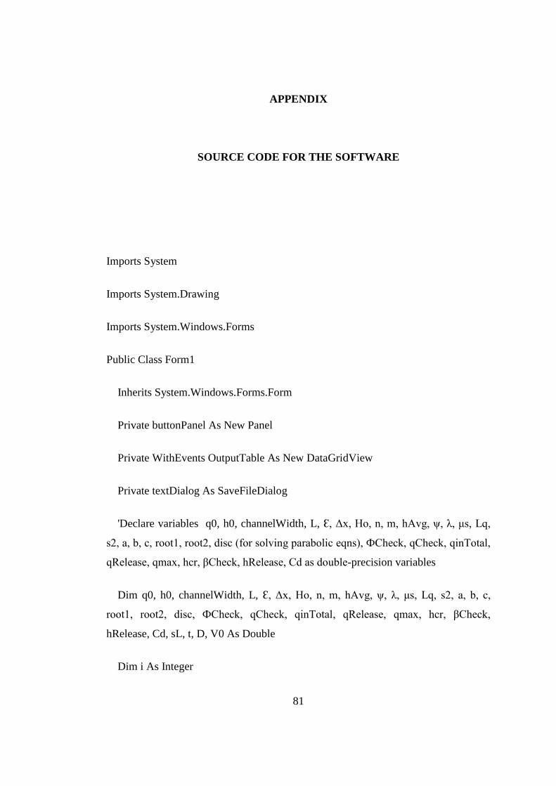
81

APPENDIX

SOURCE CODE FOR THE SOFTWARE

Imports System

Imports System.Drawing

Imports System.Windows.Forms

Public Class Form1

Inherits System.Windows.Forms.Form

Private buttonPanel As New Panel

Private WithEvents OutputTable As New DataGridView

Private textDialog As SaveFileDialog

'Declare variables q0, h0, channelWidth, L, Ԑ, Δx, Ho, n, m, hAvg, ψ, λ, μs, Lq,

s2, a, b, c, root1, root2, disc (for solving parabolic eqns), ФCheck, qCheck, qinTotal,

qRelease, qmax, hcr, βCheck, hRelease, Cd as double-precision variables

Dim q0, h0, channelWidth, L, Ԑ, Δx, Ho, n, m, hAvg, ψ, λ, μs, Lq, s2, a, b, c,

root1, root2, disc, ФCheck, qCheck, qinTotal, qRelease, qmax, hcr, βCheck,

hRelease, Cd, sL, t, D, V0 As Double

Dim i As Integer

82

Dim q(1000), h(1000), qIn(1000), Ф(1000), β(1000), ϕ(1000) As Double

Const g As Double = 9.81

Const degToRad As Double = 0.0174532925199433

Private Sub Button1_Click(sender As Object, e As EventArgs) Handles

Button1.Click

If (String.IsNullOrEmpty(h1Height.Text)) Then

MessageBox.Show("Please Enter a Water Height Value")

Return

End If

If (String.IsNullOrEmpty(barDistFromEdge.Text)) Then

MessageBox.Show("Please Enter n Value")

Return

End If

If (String.IsNullOrEmpty(barDistFromCenter.Text)) Then

MessageBox.Show("Please Enter m Value")

Return

End If

If (String.IsNullOrEmpty(angleOfBars.Text)) Then

MessageBox.Show("Please Enter a Trash Rack Slope Angle")

83

Return

End If

If (String.IsNullOrEmpty(rackLength.Text)) Then

MessageBox.Show("Please enter a Bar Length (L) Value")

Return

End If

If (String.IsNullOrEmpty(Discharge0.Text)) Then

MessageBox.Show("Please Enter a Discharge Value")

Return

End If

If (String.IsNullOrEmpty(Wdth.Text)) Then

MessageBox.Show("Please Enter a Channel Width (B) Value ")

Return

End If

If ComboBox1.Text = "Rectangular Reinforced Circular Bars (Recomended)"

Then

If (String.IsNullOrEmpty(rndBarDia.Text)) Then

MessageBox.Show("Please Enter a Bar Diameter Value ")

Return

84

End If

End If

If ComboBox1.Text = "Ovoid Bars" Then

If (String.IsNullOrEmpty(rndBarDia.Text)) Then

MessageBox.Show("Please Enter a Bar Diameter Value ")

Return

End If

End If

If ComboBox1.Text = "Circular Bars" Then

If (String.IsNullOrEmpty(rndBarDia.Text)) Then

MessageBox.Show("Please Enter a Bar Diameter Value ")

Return

End If

End If

'Constant Energy Level - Iterative Method Condition

If ConsELIterativeRadioBtn.Checked Then Solution1()

'Constant Energy Level - Closed Form Method Condition

If ConsELClosedRadioBtn.Checked Then Solution2()

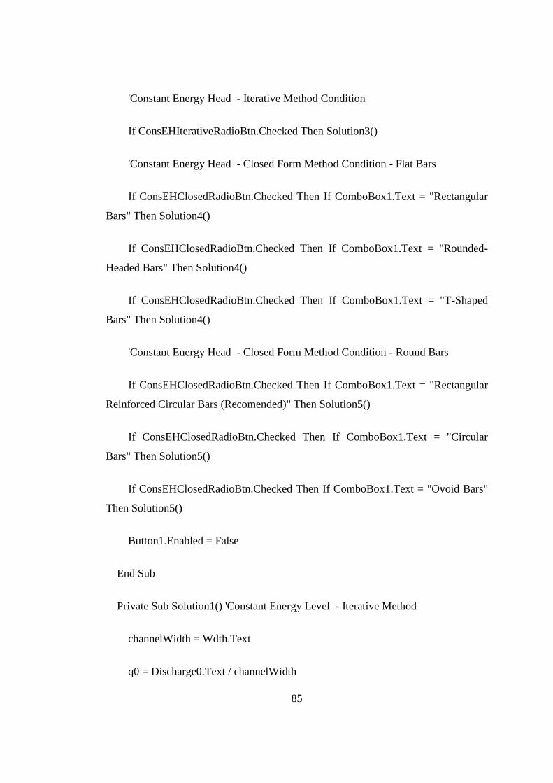
85

'Constant Energy Head - Iterative Method Condition

If ConsEHIterativeRadioBtn.Checked Then Solution3()

'Constant Energy Head - Closed Form Method Condition - Flat Bars

If ConsEHClosedRadioBtn.Checked Then If ComboBox1.Text = "Rectangular

Bars" Then Solution4()

If ConsEHClosedRadioBtn.Checked Then If ComboBox1.Text = "Rounded-

Headed Bars" Then Solution4()

If ConsEHClosedRadioBtn.Checked Then If ComboBox1.Text = "T-Shaped

Bars" Then Solution4()

'Constant Energy Head - Closed Form Method Condition - Round Bars

If ConsEHClosedRadioBtn.Checked Then If ComboBox1.Text = "Rectangular

Reinforced Circular Bars (Recomended)" Then Solution5()

If ConsEHClosedRadioBtn.Checked Then If ComboBox1.Text = "Circular

Bars" Then Solution5()

If ConsEHClosedRadioBtn.Checked Then If ComboBox1.Text = "Ovoid Bars"

Then Solution5()

Button1.Enabled = False

End Sub

Private Sub Solution1() 'Constant Energy Level - Iterative Method

channelWidth = Wdth.Text

q0 = Discharge0.Text / channelWidth

86

h(1) = h1Height.Text

m = barDistFromCenter.Text

n = barDistFromEdge.Text

L = rackLength.Text

If deltaxCheckBox.CheckState = CheckState.Checked Then If

deltaxComboBox.Text = "L / 2" Then Δx = L / 2

If deltaxCheckBox.CheckState = CheckState.Checked Then If

deltaxComboBox.Text = "L / 4" Then Δx = L / 4

If deltaxCheckBox.CheckState = CheckState.Checked Then If

deltaxComboBox.Text = "L / 5" Then Δx = L / 5

If deltaxCheckBox.CheckState = CheckState.Checked Then If

deltaxComboBox.Text = "L / 10" Then Δx = L / 10

If deltaxCheckBox.CheckState = CheckState.Unchecked Then Δx = L / 100

Ԑ = angleOfBars.Text

ψ = n / m

i = 1

q(1) = q0

Ho = (q(1) / h(1)) ^ 2 / (2 * g) + h(1) * System.Math.Cos(Ԑ * degToRad)

Do Until i = L / Δx + 1

87

h(i + 1) = h(i)

Do

h(i + 1) = h(i + 1) - 0.000001

hAvg = (h(i) + h(i + 1)) / 2

If NosedasContractionCoeffRadioBtn.Checked Then μs = 0.66 * ψ ^ (-

0.16) * (m / 1000 / hAvg) ^ 0.13

If ConstantContractionCoeffRadioBtn.Checked Then μs =

ConstantContractionCoeffValue.Text

λ = ψ * μs * (2 * g * System.Math.Cos(Ԑ * degToRad)) ^ 0.5

qIn(i) = λ * hAvg ^ 0.5 * Δx

q(i + 1) = q(i) - qIn(i)

qCheck = h(i + 1) * (2 * g * ((Ho + Δx * i * System.Math.Sin(Ԑ *

degToRad)) - h(i + 1) * System.Math.Cos(Ԑ * degToRad))) ^ 0.5

Loop While qCheck - q(i + 1) > 0.0001 And qCheck > 0 And q(i + 1) > 0

i += 1

Loop

If q(i + 1) < 0 Then q(i) = 0 And qIn(i) = 0 And h(i) = 0 And qIn(i + 1) = 0 And

h(i + 1) = 0 And q(i + 1) = 0

For Each item In qIn

qinTotal = qinTotal + item

88

Next

If qinTotal > q0 Then qinTotal = q0

qRelease = q0 - qinTotal

h(1) = System.Math.Round(h(1), 3)

h(i) = System.Math.Round(h(i), 3)

qinTotal = System.Math.Round(qinTotal, 3)

qRelease = System.Math.Round(qRelease, 3)

SetupDataGridView()

PopulateDataGridView()

OutputTable.Rows(0).HeaderCell.Value = "Constant Energy Level - Iterative

Solution"

End Sub

Private Sub Solution2() 'Constant Energy Level - Closed Form Method

'Assign textbox values to variables

channelWidth = Wdth.Text

q0 = Discharge0.Text / channelWidth

h(1) = h1Height.Text

m = barDistFromCenter.Text

n = barDistFromEdge.Text

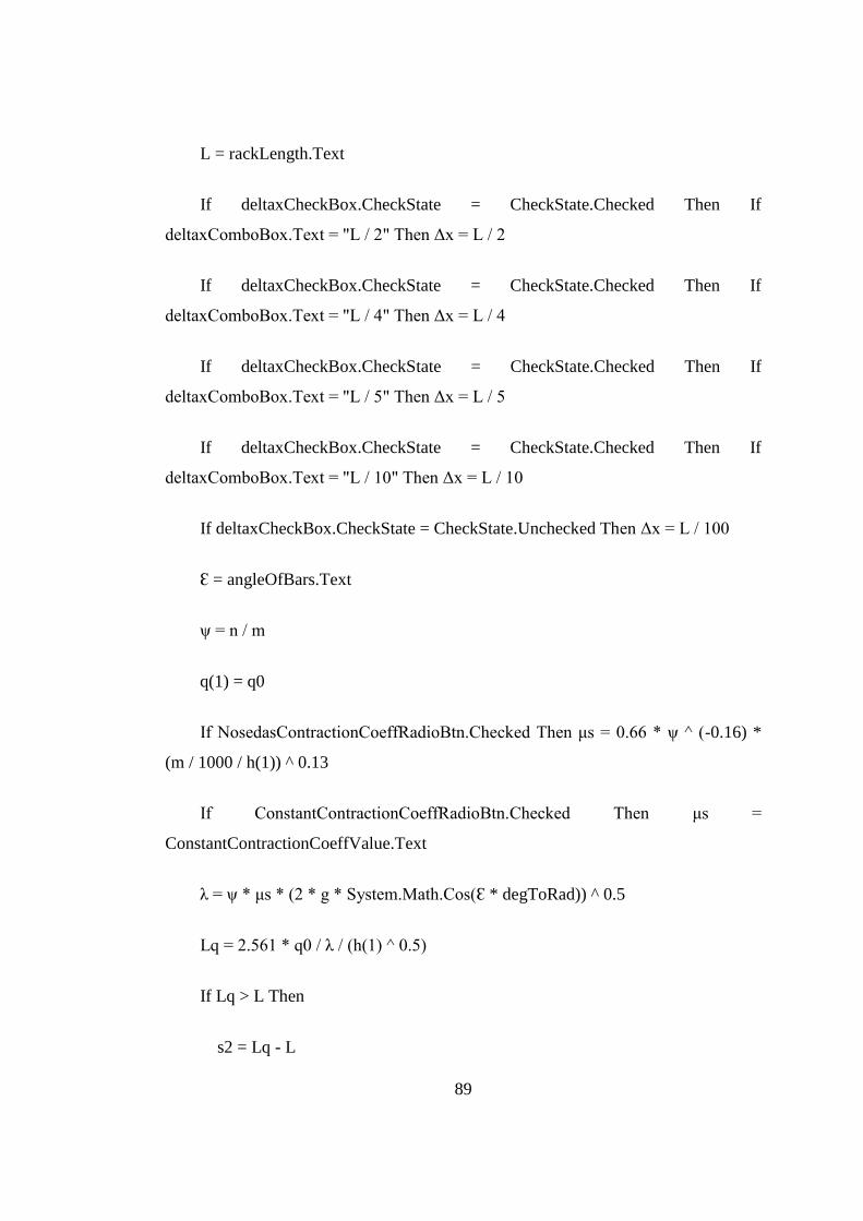
89

L = rackLength.Text

If deltaxCheckBox.CheckState = CheckState.Checked Then If

deltaxComboBox.Text = "L / 2" Then Δx = L / 2

If deltaxCheckBox.CheckState = CheckState.Checked Then If

deltaxComboBox.Text = "L / 4" Then Δx = L / 4

If deltaxCheckBox.CheckState = CheckState.Checked Then If

deltaxComboBox.Text = "L / 5" Then Δx = L / 5

If deltaxCheckBox.CheckState = CheckState.Checked Then If

deltaxComboBox.Text = "L / 10" Then Δx = L / 10

If deltaxCheckBox.CheckState = CheckState.Unchecked Then Δx = L / 100

Ԑ = angleOfBars.Text

ψ = n / m

q(1) = q0

If NosedasContractionCoeffRadioBtn.Checked Then μs = 0.66 * ψ ^ (-0.16) *

(m / 1000 / h(1)) ^ 0.13

If ConstantContractionCoeffRadioBtn.Checked Then μs =

ConstantContractionCoeffValue.Text

λ = ψ * μs * (2 * g * System.Math.Cos(Ԑ * degToRad)) ^ 0.5

Lq = 2.561 * q0 / λ / (h(1) ^ 0.5)

If Lq > L Then

s2 = Lq - L

90

' h2^2 - 2*h2*h1 + s2^2 / Lq^2 = 0

Else

s2 = Lq

End If

a = 1

b = -2 * h(1)

c = h(1) ^ 2 * s2 ^ 2 / Lq ^ 2

disc = b ^ 2 - 4 * a * c

If disc >= 0 Then

root1 = (-b + disc ^ 0.5) / (2 * a)

root2 = (-b - disc ^ 0.5) / (2 * a)

Else

MessageBox.Show("No Real Root for h!")

End If

If System.Math.Abs(root1) < h(1) Then

hRelease = root1

Else

hRelease = root2

91

End If

qinTotal = 1.707 * q0 * (2 - (1 + hRelease / h(1)) * ((2 - hRelease / h(1)) ^ 0.5))

qRelease = q0 - qinTotal

h(1) = System.Math.Round(h(1), 2)

h(i) = System.Math.Round(hRelease, 2)

qinTotal = System.Math.Round(qinTotal, 2)

qRelease = System.Math.Round(qRelease, 2)

SetupDataGridView()

PopulateDataGridView()

OutputTable.Rows(0).HeaderCell.Value = "Constant Energy Level - Closed

Form Solution"

End Sub

Private Sub Solution3() 'Constant Energy Head - Iterative Method

'Assign textbox values to variables

channelWidth = Wdth.Text

q0 = Discharge0.Text / channelWidth

h(1) = h1Height.Text

m = barDistFromCenter.Text

n = barDistFromEdge.Text

92

L = rackLength.Text

If deltaxCheckBox.CheckState = CheckState.Checked Then If

deltaxComboBox.Text = "L / 2" Then Δx = L / 2

If deltaxCheckBox.CheckState = CheckState.Checked Then If

deltaxComboBox.Text = "L / 4" Then Δx = L / 4

If deltaxCheckBox.CheckState = CheckState.Checked Then If

deltaxComboBox.Text = "L / 5" Then Δx = L / 5

If deltaxCheckBox.CheckState = CheckState.Checked Then If

deltaxComboBox.Text = "L / 10" Then Δx = L / 10

If deltaxCheckBox.CheckState = CheckState.Unchecked Then Δx = L / 100

Ԑ = angleOfBars.Text

ψ = n / m

i = 1

q(1) = q0

Ho = (q(1) / h(1)) ^ 2 / (2 * g) + h(1) * System.Math.Cos(Ԑ * degToRad)

Do Until i = L / Δx + 1

h(i + 1) = h(i)

Do

h(i + 1) = h(i + 1) - 0.000001

hAvg = (h(i) + h(i + 1)) / 2

93

If NosedasContractionCoeffRadioBtn.Checked Then μs = 0.66 * ψ ^ (-

0.16) * (m / 1000 / hAvg) ^ 0.13

If ConstantContractionCoeffRadioBtn.Checked Then μs =

ConstantContractionCoeffValue.Text

Ф(i) = (System.Math.Acos((h(i) / Ho) ^ 0.5)) / 2 - 3 / 2 * (h(i) / Ho * (1 -

h(i) / Ho)) ^ 0.5

Ф(i + 1) = (System.Math.Acos((h(i + 1) / Ho) ^ 0.5)) / 2 - 3 / 2 * (h(i + 1) /

Ho * (1 - h(i + 1) / Ho)) ^ 0.5

ФCheck = Δx * μs * ψ / Ho + Ф(i)

Loop While ФCheck > Ф(i + 1)

i += 1

Loop

i = 1

Do Until i = L / Δx + 1

q(i + 1) = q(i)

Do

q(i + 1) = q(i + 1) - 0.000001

hAvg = (h(i) + h(i + 1)) / 2

μs = 0.66 * ψ ^ (-0.16) * (m / 1000 / hAvg) ^ 0.13

qmax = 2 * ((2 * g) ^ 0.5) / 3 / (3 ^ 0.5) * Ho ^ (3 / 2)

94

hcr = (q(i) ^ 2 / g) ^ (1 / 3)

If h(i) < hcr Then

'Supercritical Flow

ϕ(i) = 1 / 3 * System.Math.Acos(1 - 2 * (q(i) / qmax) ^ 2) / degToRad +

240

ϕ(i + 1) = 1 / 3 * System.Math.Acos(1 - 2 * (q(i + 1) / qmax) ^ 2) /

degToRad + 240

ElseIf h(i) > hcr Then

'Subcritical Flow

ϕ(i) = 1 / 3 * System.Math.Acos(1 - 2 * (q(i) / qmax) ^ 2) / degToRad

ϕ(i + 1) = 1 / 3 * System.Math.Acos(1 - 2 * (q(i + 1) / qmax) ^ 2) /

degToRad

End If

β(i) = 1 / 2 * System.Math.Acos(1 / (3 ^ 0.5) * (2 * System.Math.Cos(ϕ(i)

* degToRad) + 1) ^ 0.5) - 2 ^ 0.5 / 2 * ((2 * System.Math.Cos(ϕ(i) * degToRad) + 1)

* (1 - System.Math.Cos(ϕ(i) * degToRad))) ^ 0.5

β(i + 1) = 1 / 2 * System.Math.Acos(1 / (3 ^ 0.5) * (2 *

System.Math.Cos(ϕ(i + 1) * degToRad) + 1) ^ 0.5) - 2 ^ 0.5 / 2 * ((2 *

System.Math.Cos(ϕ(i + 1) * degToRad) + 1) * (1 - System.Math.Cos(ϕ(i + 1) *

degToRad))) ^ 0.5

βCheck = Δx * μs * ψ / Ho + β(i)

Loop While βCheck > β(i + 1)

95

i += 1

Loop

qinTotal = q0 - q(i)

qRelease = q(i)

h(1) = System.Math.Round(h(1), 3)

h(i) = System.Math.Round(h(i), 3)

qinTotal = System.Math.Round(qinTotal, 3)

qRelease = System.Math.Round(qRelease, 3)

SetupDataGridView()

PopulateDataGridView()

OutputTable.Rows(0).HeaderCell.Value = "Constant Energy Head - Iterative

Solution"

End Sub

Private Sub Solution4() 'Constant Energy Head - Closed Form Method - Flat Bars

channelWidth = Wdth.Text

q0 = Discharge0.Text / channelWidth

h(1) = h1Height.Text

m = barDistFromCenter.Text

n = barDistFromEdge.Text

96

L = rackLength.Text

If deltaxCheckBox.CheckState = CheckState.Checked Then If

deltaxComboBox.Text = "L / 2" Then Δx = L / 2

If deltaxCheckBox.CheckState = CheckState.Checked Then If

deltaxComboBox.Text = "L / 4" Then Δx = L / 4

If deltaxCheckBox.CheckState = CheckState.Checked Then If

deltaxComboBox.Text = "L / 5" Then Δx = L / 5

If deltaxCheckBox.CheckState = CheckState.Checked Then If

deltaxComboBox.Text = "L / 10" Then Δx = L / 10

If deltaxCheckBox.CheckState = CheckState.Unchecked Then Δx = L / 100

Ԑ = angleOfBars.Text

D = Double.Parse(rndBarDia.Text)

ψ = n / m

h0 = h(1)

Ho = (q(1) / h(1)) ^ 2 / (2 * g) + h(1) * System.Math.Cos(Ԑ * degToRad)

hRelease = h(1)

sL = System.Math.Tan(Ԑ * degToRad) 'Slope of rack bars

t = m - n

hcr = (q0 ^ 2 / g) ^ (1 / 3)

V0 = q0 / h0

97

Cd = 0.1296 * (t / n) - 0.4284 * sL ^ 2 + 0.1764

Lq = Ho / Cd / ψ * (h(1) / Ho * (1 - h(1) / Ho) ^ 0.5)

If (Lq < L) Then

qinTotal = q0

qRelease = 0

hRelease = 0

ElseIf (Lq > L) Then

Do Until System.Math.Round(Lq, 2) = System.Math.Round(L, 2)

hRelease = hRelease - 0.001

Lq = Ho / Cd / ψ * (h(1) / Ho * (1 - h(1) / Ho) ^ 0.5 - hRelease / Ho * (1 -

hRelease / Ho) ^ 0.5)

Loop

qRelease = hRelease * (2 * g * (Ho - hRelease)) ^ 0.5

End If

qinTotal = q0 - qRelease

h(1) = System.Math.Round(h(1), 3)

h(i) = System.Math.Round(hRelease, 3)

qinTotal = System.Math.Round(qinTotal, 3)

qRelease = System.Math.Round(qRelease, 3)

98

SetupDataGridView()

PopulateDataGridView()

OutputTable.Rows(0).HeaderCell.Value = "Constant Energy Head - Closed

Form Solution (Flat Bars)"

End Sub

Private Sub Solution5() 'Constant Energy Head - Closed Form Method - Round

Bars

channelWidth = Wdth.Text

q0 = Discharge0.Text / channelWidth

h(1) = h1Height.Text

m = barDistFromCenter.Text

n = barDistFromEdge.Text

L = rackLength.Text

If deltaxCheckBox.CheckState = CheckState.Checked Then If

deltaxComboBox.Text = "L / 2" Then Δx = L / 2

If deltaxCheckBox.CheckState = CheckState.Checked Then If

deltaxComboBox.Text = "L / 4" Then Δx = L / 4

If deltaxCheckBox.CheckState = CheckState.Checked Then If

deltaxComboBox.Text = "L / 5" Then Δx = L / 5

99

If deltaxCheckBox.CheckState = CheckState.Checked Then If

deltaxComboBox.Text = "L / 10" Then Δx = L / 10

If deltaxCheckBox.CheckState = CheckState.Unchecked Then Δx = L / 100

Ԑ = angleOfBars.Text

D = Double.Parse(rndBarDia.Text)

ψ = n / m

Ho = (q(1) / h(1)) ^ 2 / (2 * g) + h(1) * System.Math.Cos(Ԑ * degToRad)

hRelease = h(1)

sL = System.Math.Tan(Ԑ * degToRad) 'Slope of rack bars

t = m - n

hcr = (q0 ^ 2 / g) ^ (1 / 3)

V0 = q0 / h0

If h0 > hcr Then

Cd = 0.53 + 0.4 * System.Math.Log10(D / n) - 0.61 * sL

Else : Cd = 0.39 + 0.27 * System.Math.Log10(D / n) - 0.8 * V0 ^ 2 / (2 * g *

Ho) - 0.5 * System.Math.Log10(sL)

End If

Lq = Ho / Cd / ψ * (h(1) / Ho * (1 - h(1) / Ho) ^ 0.5)

If (Lq < L) Then

100

qinTotal = q0

qRelease = 0

hRelease = 0

ElseIf (Lq > L) Then

Do Until System.Math.Round(Lq, 2) = System.Math.Round(L, 2)

hRelease = hRelease - 0.001

Lq = Ho / Cd / ψ * (h(1) / Ho * (1 - h(1) / Ho) ^ 0.5 - hRelease / Ho * (1 -

hRelease / Ho) ^ 0.5)

Loop

qRelease = hRelease * (2 * g * (Ho - hRelease)) ^ 0.5

End If

qinTotal = q0 - qRelease

h(1) = System.Math.Round(h(1), 3)

h(i) = System.Math.Round(hRelease, 3)

qinTotal = System.Math.Round(qinTotal, 3)

qRelease = System.Math.Round(qRelease, 3)

SetupDataGridView()

PopulateDataGridView()

101

OutputTable.Rows(0).HeaderCell.Value = "Constant Energy Head - Closed

Form Solution (Round Bars)"

End Sub

Private Sub SetupDataGridView()

Me.Controls.Add(OutputTable)

OutputTable.ColumnCount = 4

With OutputTable.ColumnHeadersDefaultCellStyle

.BackColor = Color.Navy

.ForeColor = Color.White

.Font = New Font(OutputTable.Font, FontStyle.Bold)

End With

With OutputTable

.Name = "Results"

.Location = New Point(595, 358)

.Size = New Size(668, 75)

.AutoSizeColumnsMode = DataGridViewAutoSizeColumnsMode.AllCells

.AutoSizeRowsMode = DataGridViewAutoSizeRowsMode.AllCells

.ColumnHeadersBorderStyle = DataGridViewHeaderBorderStyle.Single

.CellBorderStyle = DataGridViewCellBorderStyle.Single

102

.GridColor = Color.Black

.RowHeadersVisible = True

.RowHeadersWidthSizeMode =

DataGridViewRowHeadersWidthSizeMode.AutoSizeToAllHeaders

.Columns(0).Name = "h1 (m)"

.Columns(1).Name = "h Release (m)"

.Columns(2).Name = "q Channel (m3/s/m)"

.Columns(3).Name = "q Release (m3/s/m)"

.SelectionMode = DataGridViewSelectionMode.FullRowSelect

.MultiSelect = True

.ReadOnly = True

.BringToFront()

.Dock = DockStyle.None

End With

End Sub

Private Sub PopulateDataGridView()

Dim row0 As String() = {h(1), h(i), qinTotal, qRelease}

With Me.OutputTable.Rows

.Add(row0)

103

End With

With Me.OutputTable

.Columns(0).DisplayIndex = 0

.Columns(1).DisplayIndex = 1

.Columns(2).DisplayIndex = 2

.Columns(3).DisplayIndex = 3

End With

End Sub

Private Sub NewToolStripButton_Click(sender As Object, e As EventArgs)

Handles NewToolStripButton.Click

If MsgBox("Do you want to save before quit?", MsgBoxStyle.YesNo, "Program

will close!") = MsgBoxResult.Yes Then

SaveFileDialog1.Filter = "Text Document|*.txt; *.txt"

If SaveFileDialog1.ShowDialog = Windows.Forms.DialogResult.OK _

Then

My.Computer.FileSystem.WriteAllText _

(SaveFileDialog1.FileName, RichTextBox1.Text, True)

End If

Else

104

Application.Restart()

End If

End Sub

Private Sub NewToolStripMenuItem_Click(sender As Object, e As EventArgs)

Handles NewToolStripMenuItem.Click

If MsgBox("Do you want to save before quit?", MsgBoxStyle.YesNo, "Program

will close!") = MsgBoxResult.Yes Then

SaveFileDialog1.Filter = "Text Document|*.txt; *.txt"

If SaveFileDialog1.ShowDialog = Windows.Forms.DialogResult.OK _

Then

My.Computer.FileSystem.WriteAllText _

(SaveFileDialog1.FileName, RichTextBox1.Text, True)

End If

Else

Application.Restart()

End If

End Sub

Private Sub ExitToolStripMenuItem_Click(sender As Object, e As EventArgs)

Handles ExitToolStripMenuItem.Click

Close()

105

End Sub

Private Sub SaveToolStripMenuItem_Click(sender As Object, e As EventArgs)

Handles SaveToolStripMenuItem.Click

SaveFileDialog1.Filter = "Text Document|*.txt; *.txt"

If SaveFileDialog1.ShowDialog = Windows.Forms.DialogResult.OK _

Then

My.Computer.FileSystem.WriteAllText _

(SaveFileDialog1.FileName, RichTextBox1.Text, True)

End If

End Sub

Private Sub SaveToolStripButton_Click(sender As Object, e As EventArgs)

Handles SaveToolStripButton.Click

SaveFileDialog1.Filter = "Text Document|*.txt; *.txt"

If SaveFileDialog1.ShowDialog = Windows.Forms.DialogResult.OK _

Then

My.Computer.FileSystem.WriteAllText _

(SaveFileDialog1.FileName, RichTextBox1.Text, True)

End If

106

End Sub

Private Sub ComboBox1_SelectedIndexChanged(sender As Object, e As

EventArgs) Handles ComboBox1.SelectedIndexChanged

If ComboBox1.Text = "Rectangular Reinforced Circular Bars (Recomended)"

Then ConstantContractionCoeffValue.Text = 0.85

If ComboBox1.Text = "Rectangular Reinforced Circular Bars (Recomended)"

Then barTypePicBox.Image = My.Resources.circularWithRectangular

If ComboBox1.Text = "Rectangular Reinforced Circular Bars (Recomended)"

Then rndBarDia.Enabled = True

If ComboBox1.Text = "Rectangular Reinforced Circular Bars (Recomended)"

Then rndBarDiaLabel.Enabled = True

If ComboBox1.Text = "Rectangular Reinforced Circular Bars (Recomended)"

Then rndBarUnitLabel.Enabled = True

If ComboBox1.Text = "Circular Bars" Then barTypePicBox.Image =

My.Resources.circular

If ComboBox1.Text = "Circular Bars" Then

ConstantContractionCoeffValue.Text = 0.85

If ComboBox1.Text = "Circular Bars" Then rndBarDia.Enabled = True

If ComboBox1.Text = "Circular Bars" Then rndBarDiaLabel.Enabled = True

If ComboBox1.Text = "Circular Bars" Then rndBarUnitLabel.Enabled = True

If ComboBox1.Text = "Ovoid Bars" Then ConstantContractionCoeffValue.Text

= 0.9

107

If ComboBox1.Text = "Ovoid Bars" Then barTypePicBox.Image =

My.Resources.Ovoid

If ComboBox1.Text = "Ovoid Bars" Then rndBarDia.Enabled = True

If ComboBox1.Text = "Ovoid Bars" Then rndBarDiaLabel.Enabled = True

If ComboBox1.Text = "Ovoid Bars" Then rndBarUnitLabel.Enabled = True

If ComboBox1.Text = "Rectangular Bars" Then

ConstantContractionCoeffValue.Text = 0.63

If ComboBox1.Text = "Rectangular Bars" Then barTypePicBox.Image =

My.Resources.Rectangular

If ComboBox1.Text = "Rectangular Bars" Then rndBarDia.Enabled = False

If ComboBox1.Text = "Rectangular Bars" Then rndBarDiaLabel.Enabled =

False

If ComboBox1.Text = "Rectangular Bars" Then rndBarUnitLabel.Enabled =

False

If ComboBox1.Text = "Rounded-Headed Bars" Then

ConstantContractionCoeffValue.Text = 0.8

If ComboBox1.Text = "Rounded-Headed Bars" Then barTypePicBox.Image =

My.Resources.roundedHeaded

If ComboBox1.Text = "Rounded-Headed Bars" Then rndBarDia.Enabled =

False

If ComboBox1.Text = "Rounded-Headed Bars" Then rndBarDiaLabel.Enabled

= False

108

If ComboBox1.Text = "Rounded-Headed Bars" Then rndBarUnitLabel.Enabled

= False

If ComboBox1.Text = "T-Shaped Bars" Then

ConstantContractionCoeffValue.Text = 0.63

If ComboBox1.Text = "T-Shaped Bars" Then barTypePicBox.Image =

My.Resources.tShaped

If ComboBox1.Text = "T-Shaped Bars" Then rndBarDia.Enabled = False

If ComboBox1.Text = "T-Shaped Bars" Then rndBarDiaLabel.Enabled = False

If ComboBox1.Text = "T-Shaped Bars" Then rndBarUnitLabel.Enabled = False

End Sub

Private Sub ConsELIterativeRadioBtn_CheckedChanged(sender As Object, e As

EventArgs) Handles ConsELIterativeRadioBtn.CheckedChanged

If ConsELIterativeRadioBtn.Checked Then PictureBox1.Image =

My.Resources.constantEnergyLevel1

End Sub

Private Sub ConsELClosedRadioBtn_CheckedChanged(sender As Object, e As

EventArgs) Handles ConsELClosedRadioBtn.CheckedChanged

If ConsELClosedRadioBtn.Checked Then PictureBox1.Image =

My.Resources.constantEnergyLevel1

End Sub

Private Sub ConsEHIterativeRadioBtn_CheckedChanged(sender As Object, e As

EventArgs) Handles ConsEHIterativeRadioBtn.CheckedChanged

109

If ConsEHIterativeRadioBtn.Checked Then PictureBox1.Image =

My.Resources.constantEnergyHead1

End Sub

Private Sub ConsEHClosedRadioBtn_CheckedChanged(sender As Object, e As

EventArgs) Handles ConsEHClosedRadioBtn.CheckedChanged

If ConsEHClosedRadioBtn.Checked Then PictureBox1.Image =

My.Resources.constantEnergyHead1

End Sub

Private Sub valueΔx_CheckedChanged(sender As Object, e As EventArgs)

Handles deltaxCheckBox.CheckedChanged

If deltaxCheckBox.Checked Then deltaxComboBox.Enabled = True

If deltaxCheckBox.Checked Then deltaxLabel.Enabled = True

If deltaxCheckBox.Checked Then deltaxUnitLabel.Enabled = True

If deltaxCheckBox.CheckState = CheckState.Unchecked Then

deltaxComboBox.Enabled = False

If deltaxCheckBox.CheckState = CheckState.Unchecked Then

deltaxLabel.Enabled = False

If deltaxCheckBox.CheckState = CheckState.Unchecked Then

deltaxUnitLabel.Enabled = False

End Sub

End Class