Mar. 2011 Computer Arithmetic, Addition/Subtraction Slide 1 Part II Addition / Subtraction Number Representation Numbers and Arithmetic Representing Signed Numbers Redundant Number Systems Residue Number Systems Addition / Subtraction Basic Addition and Counting Carry-Look ahead Adders Variations in Fast Adders Multioperand Addition Multiplication Basic Multiplication Schemes High-Radix Multipliers Tree and Array Multipliers Variations in Multipliers Division Basic Division Schemes High-Radix Dividers Variations in Dividers Division by Convergence Real Arithmetic Floating-Point Reperesentations Floating-Point Operations Errors and Error Control Precise and Certifiable Arithmetic Function Evaluation Square-Rooting Methods The CORDIC Algorithms Variations in Function Evaluation Arithmetic by Table Lookup Implementation Topics High-Throughput Arithmetic Low-Power Arithmetic Fault-Tolerant Arithmetic Parts Chapters I. II. III. IV. V. VI. VII. 1. 2. 3. 4. 5. 6. 7. 8. 9. 10. 11. 12. 25. 26. 27. 21. 22. 23. 24. 17. 18. 19. 20. 13. 14. 15. 16. Elementary Operations 28. Reconfigurable Arithmetic Appendix: Past, Present, and Future

Welcome message from author
This document is posted to help you gain knowledge. Please leave a comment to let me know what you think about it! Share it to your friends and learn new things together.
Transcript

Mar. 2011 Computer Arithmetic, Addition/Subtraction Slide 1
Part IIAddition / Subtraction
Number Representation Numbers and Arithmetic Representing Signed Numbers Redundant Number Systems Residue Number Systems
Addition / Subtraction Basic Addition and Counting Carry-Lookahead Adders Variations in Fast Adders Multioperand Addition
Multiplication Basic Multiplication Schemes High-Radix Multipliers Tree and Array Multipliers Variations in Multipliers
Division Basic Division Schemes High-Radix Dividers Variations in Dividers Division by Convergence
Real Arithmetic Floating-Point Reperesentations Floating-Point Operations Errors and Error Control Precise and Certifiable Arithmetic
Function Evaluation Square-Rooting Methods The CORDIC Algorithms Variations in Function Evaluation Arithmetic by Table Lookup
Implementation Topics High-Throughput Arithmetic Low-Power Arithmetic Fault-Tolerant Arithmetic Past, Present, and Future
Parts Chapters
I.
II.
III.
IV.
V.
VI.
VII.
1. 2. 3. 4.
5. 6. 7. 8.
9. 10. 11. 12.
25. 26. 27. 28.
21. 22. 23. 24.
17. 18. 19. 20.
13. 14. 15. 16.
Ele
men
tary
Ope
ratio
ns
28. Reconfigurable Arithmetic
Appendix: Past, Present, and Future

Mar. 2011 Computer Arithmetic, Addition/Subtraction Slide 2
About This Presentation
This presentation is intended to support the use of the textbookComputer Arithmetic: Algorithms and Hardware Designs (Oxford U. Press, 2nd ed., 2010, ISBN 978-0-19-532848-6). It is updated regularly by the author as part of his teaching of the graduate course ECE 252B, Computer Arithmetic, at the University of California, Santa Barbara. Instructors can use these slides freely in classroom teaching and for other educational purposes. Unauthorized uses are strictly prohibited. © Behrooz Parhami
Edition Released Revised Revised Revised RevisedFirst Jan. 2000 Sep. 2001 Sep. 2003 Oct. 2005 Apr. 2007
Apr. 2008 Apr. 2009
Second Apr. 2010 Mar. 2011

Mar. 2011 Computer Arithmetic, Addition/Subtraction Slide 3
II Addition /Subtraction
Topics in This PartChapter 5 Basic Addition and CountingChapter 6 Carry-Lookahead AddersChapter 7 Variations in Fast AdderChapter 8 Multioperand Addition
Review addition schemes and various speedup methods• Addition is a key op (in itself, and as a building block)• Subtraction = negation + addition• Carry propagation speedup: lookahead, skip, select, …• Two-operand versus multioperand addition

Mar. 2011 Computer Arithmetic, Addition/Subtraction Slide 4
“You can’t add apples and oranges, son; only the government can do that.”
“You can’t add apples and oranges, son; only the government can do that.”

Mar. 2011 Computer Arithmetic, Addition/Subtraction Slide 5
5 Basic Addition and Counting
Chapter GoalsStudy the design of ripple-carry adders, discuss why their latency is unacceptable,and set the foundation for faster adders
Chapter HighlightsFull adders are versatile building blocksLongest carry chain on average: log2k bitsFast asynchronous adders are simpleCounting is relatively easy to speed upKey part of a fast adder is its carry network

Mar. 2011 Computer Arithmetic, Addition/Subtraction Slide 6
Basic Addition and Counting: Topics
Topics in This Chapter
5.1 Bit-Serial and Ripple-Carry Adders
5.2 Conditions and Exceptions
5.3 Analysis of Carry Propagation
5.4 Carry Completion Detection
5.5 Addition of a Constant
5.6 Manchester Carry Chains and Adders

Mar. 2011 Computer Arithmetic, Addition/Subtraction Slide 7
5.1 Bit-Serial and Ripple-Carry Adders
Half-adder (HA): Truth table and block diagram
Full-adder (FA): Truth table and block diagram
x y c c s ---------------------- 0 0 0 0 0 0 0 1 0 1 0 1 0 0 1 0 1 1 1 0 1 0 0 0 1 1 0 1 1 0 1 1 0 1 0 1 1 1 1 1
Inputs Outputs
c out c in
out in x
y
s
FA
x y c s ---------------- 0 0 0 0 0 1 0 1 1 0 0 1 1 1 1 0
Inputs Outputs
HA
x y
c
s

Mar. 2011 Computer Arithmetic, Addition/Subtraction Slide 8
Half-Adder Implementations
Fig. 5.1 Three implementations of a half-adder.
c
s
(b) NOR-gate half-adder.
xy
xy
(c) NAND-gate half-adder with complemented carry.
x
y
c
s
s
c xy
xy
(a) AND/XOR half-adder._
__c

Mar. 2011 Computer Arithmetic, Addition/Subtraction Slide 9
Full-Adder Implementations
Fig. 5.2 Possible designs for a full-adder in terms of half-adders, logic gates, and CMOS transmission gates.
HA
HA
xy
cin
cout
(a) Built of half-adders.s
(b) Built as an AND-OR circuit.
(c) Suitable for CMOS realization.
cout
s
cin
xy
0 1 2 3
0 1 2 3
xy
cin
cout
s
0
1
Mux
Mar. 2011 Computer Arithmetic, Addition/Subtraction Slide 10
Full-Adder Implementations
Fig. 5.2 (alternate version) Possible designs for a full-adder in terms of half-adders, logic gates, and CMOS transmission gates.
(a) FA built of two HAs
(c) Two-level AND-OR FA (b) CMOS mux-based FA
1
0
3
2
HA
HA
1
0
3
2
0
1
x y
x y
x y
s
s s
c out
c out
c out
c in
c in
c in

Mar. 2011 Computer Arithmetic, Addition/Subtraction Slide 11
Some Full-Adder Details
CMOS transmission gate and its use in a 2-to-1 mux.
z
x
x
0
1
(a) CMOS transmission gate: circuit and symbol
(b) Two-input mux built of two transmission gates
TG
TG TG
y P
N
Logic equations for a full-adder:s = x ⊕ y ⊕ cin (odd parity function)
= xycin ∨ x ′y ′cin ∨ x ′y cin′ ∨ x y ′cin′
cout = x y ∨ x cin ∨ y cin (majority function)

Mar. 2011 Computer Arithmetic, Addition/Subtraction Slide 12
Simple Adders Built of Full-Adders
Fig. 5.3 Using full-adders in building bit-serial and ripple-carry adders.
x y
c
x
s
y
c
x
s
y
c out c in
0 0
0
c 0
31
31
31
31
FA
s
c c
1 1
1
1 2 FA FA
32 . . .
s 32
x
s
y
c c
i i
i
i i+1 FA Carry
FF Shift
Shift
x
y
s
(a) Bit-serial adder.
(b) Ripple-carry adder.
Clock

Mar. 2011 Computer Arithmetic, Addition/Subtraction Slide 13
VLSI Layout of a Ripple-Carry Adder
Fig. 5.4 The layout of a 4-bit ripple-carry adder in CMOS implementation [Puck94].
xy 11 x0y0
c1c2cout cinc3
x2y2x3y3
Clock
s 1 s 0s 2s 3
150
760λ
λ
7 inverters
Two 4-to-1 Mux's
VDDV SS
Mar. 2011 Computer Arithmetic, Addition/Subtraction Slide 14
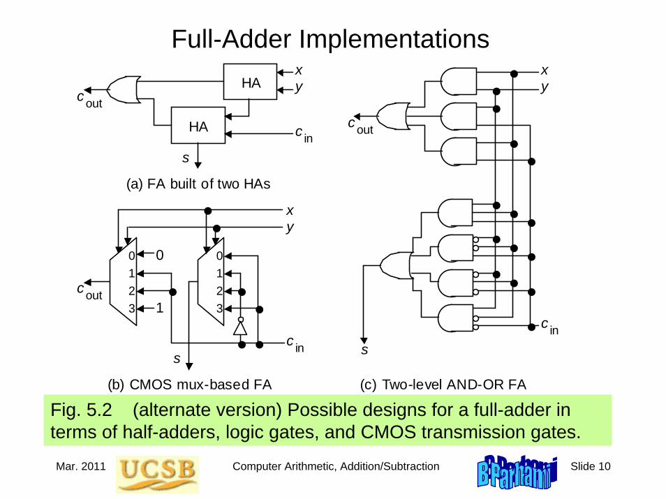
Critical Path Through a Ripple-Carry Adder
Fig. 5.5 Critical path in a k-bit ripple-carry adder.
x
s
y
c
x
s
y
c
x
s
y
c
x
s
y
c
c out c in
0 0
0
c 0
1 1
1
1
k-2 k–2
k–2
2 k
k–1
k–1
k–1
k–1
FA FA FA FA . . . c k–2
s k
Tripple-add = TFA(x,y→cout) + (k – 2)×TFA(cin→cout) + TFA(cin→s)

Mar. 2011 Computer Arithmetic, Addition/Subtraction Slide 15
x y c c s ---------------------- 0 0 0 0 0 0 0 1 0 1 0 1 0 0 1 0 1 1 1 0 1 0 0 0 1 1 0 1 1 0 1 1 0 1 0 1 1 1 1 1
Inputs Outputs
c out c in
out in x
y
s
FA
Binary Adders as Versatile Building Blocks
Fig. 5.6 Four-bit binary adder used to realize the logic function f = w + xyz and its complement.
c
3
c
4
c
2
c
1
c
0
0
1 w
1 z
0 y
x Bit 3 Bit 2 Bit 1 Bit 0
w ∨ xyz
(w ∨ xyz)′
w ∨ xyz xyz xy 0
Set one input to 0: cout = AND of other inputs
Set one input to 1: cout = OR of other inputs
Set one input to 0 and another to 1: s = NOT of third input

Mar. 2011 Computer Arithmetic, Addition/Subtraction Slide 16
5.2 Conditions and Exceptions
Fig. 5.7 Two’s-complement adder with provisions for detecting conditions and exceptions.
FAFA
xy 11 x0y0
c0c1
s 0s 1
FAc2
s k–1
cout cin...
ck–1ck–2
s k–2
ck
xk–2yk–2xk–1yk–1
FA
Overflow
Negative
Zero
overflow2’s-compl = xk–1 yk–1 sk–1′ ∨ xk–1′ yk–1′ sk–1
overflow2’s-compl = ck ⊕ ck–1 = ck ck–1′ ∨ ck′ ck–1

Mar. 2011 Computer Arithmetic, Addition/Subtraction Slide 17
Saturating AddersSaturating (saturation) arithmetic: When a result’s magnitude is too large, do not wrap around; rather, provide the most positive or the most negative value that is representable in the number format
Designing saturating adders
Saturating arithmetic in desirable in many DSP applications
Saturation value
Overflow
0
1
AdderUnsigned (quite easy)
Signed (only slightly harder)
Example – In 8-bit 2’s-complement format, we have:120 + 26 18 (wraparound); 120 +sat 26 127 (saturating)
Mar. 2011 Computer Arithmetic, Addition/Subtraction Slide 18
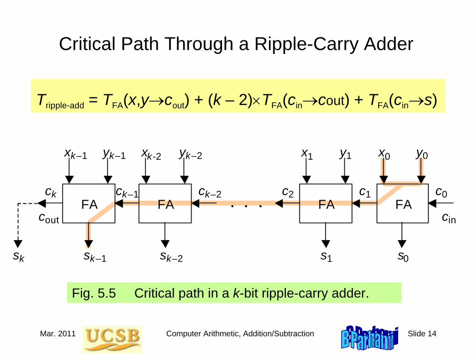
5.3 Analysis of Carry Propagation
Bit positions15 14 13 12 11 10 9 8 7 6 5 4 3 2 1 0----------- ----------- ----------- -----------1 0 1 1 0 1 1 0 0 1 1 0 1 1 1 0
cout 0 1 0 1 1 0 0 1 1 1 0 0 0 0 1 1 cin\__________/\__________________/ \________/\____/
4 6 3 2Carry chains and their lengths
Fig. 5.8 Example addition and its carry propagation chains.
Mar. 2011 Computer Arithmetic, Addition/Subtraction Slide 19
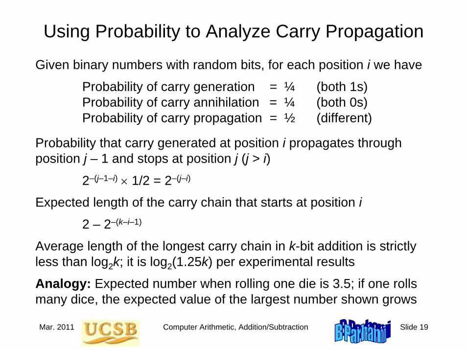
Using Probability to Analyze Carry Propagation
Given binary numbers with random bits, for each position i we have
Probability of carry generation = ¼ (both 1s)Probability of carry annihilation = ¼ (both 0s)Probability of carry propagation = ½ (different)
Probability that carry generated at position i propagates through position j – 1 and stops at position j (j > i)
2–(j–1–i) × 1/2 = 2–(j–i)
Expected length of the carry chain that starts at position i
2 – 2–(k–i–1)
Average length of the longest carry chain in k-bit addition is strictly less than log2k; it is log2(1.25k) per experimental results
Analogy: Expected number when rolling one die is 3.5; if one rolls many dice, the expected value of the largest number shown grows
Mar. 2011 Computer Arithmetic, Addition/Subtraction Slide 20
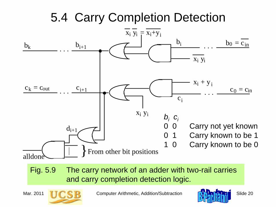
5.4 Carry Completion Detection
Fig. 5.9 The carry network of an adder with two-rail carries and carry completion detection logic.
. . .
. . .
. . .
. . .
x y = x +y
alldoneFrom other bit positions
i+1
c = c
b = c
b = 1: No carry c = 1: Carry
b
i+1c 0
i i i i
ib
ic
x + yi i
x y i i
x y i i
0
in
in
}
di+1 ii
c = c k out
b k
bi ci0 0 Carry not yet known0 1 Carry known to be 11 0 Carry known to be 0

Mar. 2011 Computer Arithmetic, Addition/Subtraction Slide 21
5.5 Addition of a Constant: Counters
Count register
Mux
Incrementer (Decrementer)
+1 (−1)
Data in
Load
Count / Initialize _____
x + 1
x
0 1
Data out
Reset Clear Enable Clock
Counter overflow
(x − 1)
c out
Fig. 5.10 An up (down) counter built of a register, an incrementer (decrementer), and a multiplexer.
Mar. 2011 Computer Arithmetic, Addition/Subtraction Slide 22
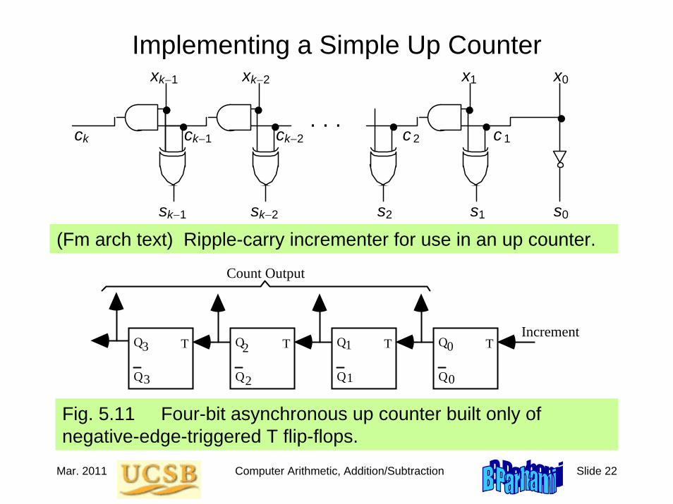
Implementing a Simple Up Counter
Fig. 5.11 Four-bit asynchronous up counter built only of negative-edge-triggered T flip-flops.
T
Q
Q T
Q
Q T
Q
Q T
Q
QIncrement
0
0
1
1
2
2
3
3
Count Output
(Fm arch text) Ripple-carry incrementer for use in an up counter.
1
0
k−2
k−1
. . . c
k−1
c
k
c
k−2
c
1
x
x
x
x
c
2
1 0 k−2 k−1 s s s s 2 s

Mar. 2011 Computer Arithmetic, Addition/Subtraction Slide 23
Faster and Constant-Time Counters
Any fast adder design can be specialized and optimized to yield a fast counter (carry-lookahead, carry-skip, etc.)
Fig. 5.12 Fast (constant-time) three-stage up counter.
Load
Load Increment
Control 1
Control 2
Incrementer
1
Incrementer
1
Count register divided into three stages
One can use redundant representation to build a constant-time counter, but a conversion penalty must be paid during read-out

Mar. 2011 Computer Arithmetic, Addition/Subtraction Slide 24
5.6 Manchester Carry Chains and Adders
Sum digit in radix r si = (xi + yi + ci) mod rSpecial case of radix 2 si = xi ⊕ yi ⊕ ci
Computing the carries ci is thus our central problem For this, the actual operand digits are not important What matters is whether in a given position a carry is
generated, propagated, or annihilated (absorbed)
For binary addition:gi = xi yi pi = xi ⊕ yi ai = xi′yi ′ = (xi ∨ yi) ′
It is also helpful to define a transfer signal:ti = gi ∨ pi = ai′ = xi ∨ yi
Using these signals, the carry recurrence is written asci+1 = gi ∨ ci pi = gi ∨ ci gi ∨ ci pi = gi ∨ ci ti

Mar. 2011 Computer Arithmetic, Addition/Subtraction Slide 25
Manchester Carry Network
Fig. 5.13 One stage in a Manchester carry chain.
p
g
a
Logic 1
Logic 0
c
c
i+1
i
i
i
i
0
1
0
1
0 1
(a) Conceptual representation
c'i+1 ic'
Clock
ip
VDD
VSS
ig
(b) Possible CMOS realization.
The worst-case delay of a Manchester carry chain has three components:
1. Latency of forming the switch control signals2. Set-up time for switches3. Signal propagation delay through k switches

Mar. 2011 Computer Arithmetic, Addition/Subtraction Slide 26
Details of a 5-Bit Manchester Carry Network
Carry chain of a 5-bit Manchester adder.
The transistors must be sized appropriately for maximum speed
k
ip
VDD
VSS
ig
k
ip
VDD
VSS
ig
k
ip
VDD
VSS
ig
k
ip
VDD
VSS
ig
k
ip
VDD
VSS
ig
k
ip
VDD
VSS
igc0
c5
Smaller transistors Larger transistors
i = 4
c0c1c2c3c4
i = 3 i = 2 i = 1 i = 0

Mar. 2011 Computer Arithmetic, Addition/Subtraction Slide 27
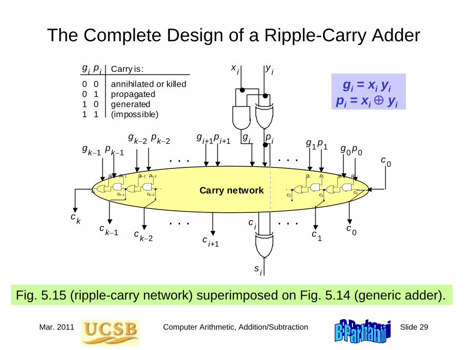
Carry Network is the Essence of a Fast Adder
Fig. 5.14 Generic structure of a binary adder, highlighting its carry network.
Carry network
. . . . . .
x i y i
g p
s
i i
i
c i c i+1
c k−1
c k c k−2 c 1
c 0
g p 1 1 g p 0 0
g p k−2 k−2 g p i+1 i+1 g p k−1 k−1
c 0 . . . . . .
0 0 0 1 1 0 1 1
annihilated or killed propagated generated (impossible)
Carry is: g i p i gi = xi yi
pi = xi ⊕ yi
Ripple; Skip;Lookahead;Parallel-prefix

Mar. 2011 Computer Arithmetic, Addition/Subtraction Slide 28
Ripple-Carry Adder Revisited
Fig. 5.15 Alternate view of a ripple-carry network in connection with the generic adder structure shown in Fig. 5.14.
. . . c
k−1
c
k c k−2
c 1
g
p
1
1
g
p
0
0
g
p
k−2
k−2
g
p
k−1
k−1
c
0 c 2
The carry recurrence: ci+1 = gi ∨ pi ci
Latency of k-bit adder is roughly 2k gate delays:
1 gate delay for production of p and g signals, plus 2(k – 1) gate delays for carry propagation, plus1 XOR gate delay for generation of the sum bits
Mar. 2011 Computer Arithmetic, Addition/Subtraction Slide 29
The Complete Design of a Ripple-Carry Adder
Fig. 5.15 (ripple-carry network) superimposed on Fig. 5.14 (generic adder).
Carry network
. . . . . .
x i y i
g p
s
i i
i
c i c i+1
c k−1
c k c k−2 c 1
c 0
g p 1 1 g p 0 0
g p k−2 k−2 g p i+1 i+1 g p k−1 k−1
c 0 . . . . . .
0 0 0 1 1 0 1 1
annihilated or killed propagated generated (impossible)
Carry is: g i p i gi = xi yi
pi = xi ⊕ yi
. c
1
g
p
1
1
g
p
0
0
c
0 c
2
.c
k−1
c
k c
k−2
g
p
k−2
k−2
g
p
k−1
k−1

Mar. 2011 Computer Arithmetic, Addition/Subtraction Slide 30
6 Carry-Lookahead Adders
Chapter GoalsUnderstand the carry-lookahead method and its many variationsused in the design of fast adders
Chapter HighlightsSingle- and multilevel carry lookaheadVarious designs for log-time addersRelating the carry determination problem
to parallel prefix computationImplementing fast adders in VLSI
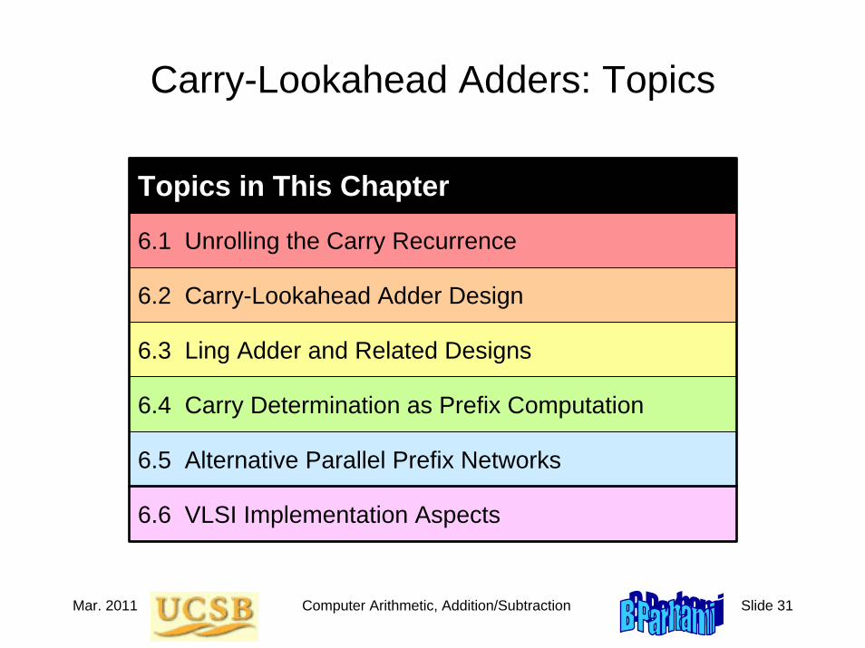
Mar. 2011 Computer Arithmetic, Addition/Subtraction Slide 31
Carry-Lookahead Adders: Topics
Topics in This Chapter
6.1 Unrolling the Carry Recurrence
6.2 Carry-Lookahead Adder Design
6.3 Ling Adder and Related Designs
6.4 Carry Determination as Prefix Computation
6.5 Alternative Parallel Prefix Networks
6.6 VLSI Implementation Aspects

Mar. 2011 Computer Arithmetic, Addition/Subtraction Slide 32
6.1 Unrolling the Carry RecurrenceRecall the generate, propagate, annihilate (absorb), and transfer signals:
Signal Radix r Binarygi is 1 iff xi + yi ≥ r xi yipi is 1 iff xi + yi = r – 1 xi ⊕ yiai is 1 iff xi + yi < r – 1 xi′yi ′ = (xi ∨ yi) ′ti is 1 iff xi + yi ≥ r – 1 xi ∨ yi
si (xi + yi + ci) mod r xi ⊕ yi ⊕ ci
The carry recurrence can be unrolled to obtain each carry signal directly from inputs, rather than through propagation
ci = gi–1 ∨ ci–1 pi–1= gi–1 ∨ (gi–2 ∨ ci–2 pi–2)pi–1= gi–1 ∨ gi–2pi–1 ∨ ci–2 pi–2pi–1= gi–1 ∨ gi–2pi–1 ∨ gi–3 pi–2pi–1 ∨ ci–3 pi–3 pi–2pi–1= gi–1 ∨ gi–2pi–1 ∨ gi–3 pi–2pi–1 ∨ gi–4 pi–3 pi–2pi–1 ∨ ci–4 pi–4 pi–3 pi–2pi–1= . . .
Note:Addition symbol vs logical OR

Mar. 2011 Computer Arithmetic, Addition/Subtraction Slide 33
Full Carry Lookahead
Theoretically, it is possible to derive each sum digit directly from the inputs that affect it
Carry-lookahead adder design is simply a way of reducing the complexity of this ideal, but impractical, arrangement by hardware sharing among the various lookahead circuits
s0s1s2s3
y0y1y2y3 x0x1x2x3
cin
. . .
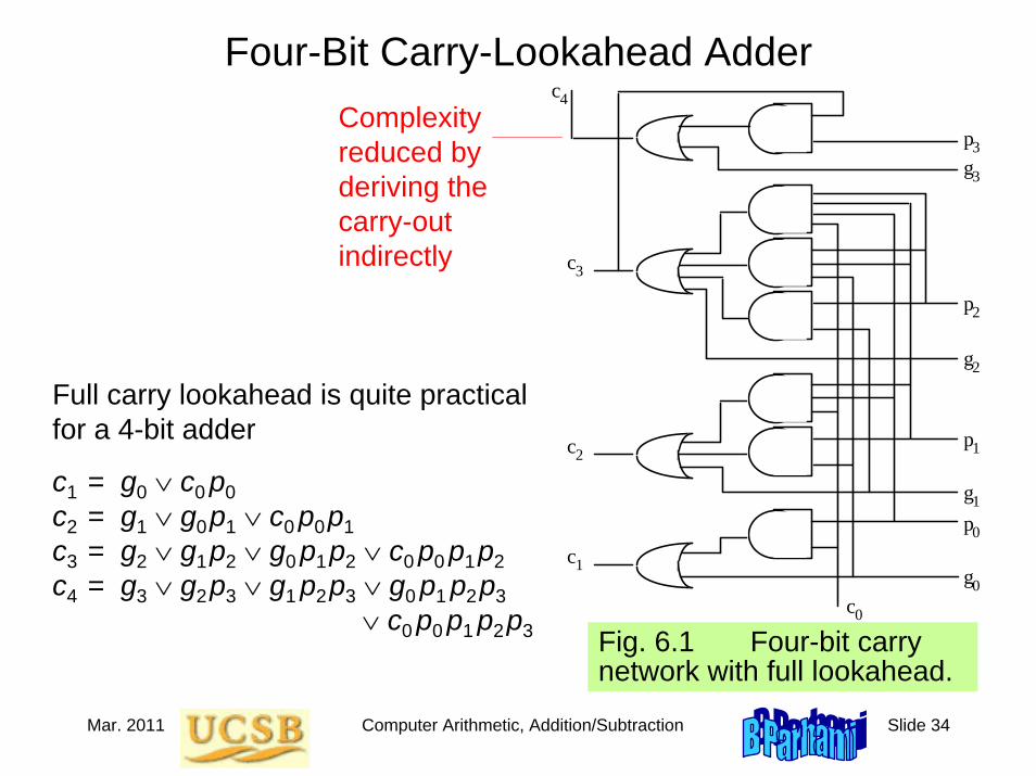
Mar. 2011 Computer Arithmetic, Addition/Subtraction Slide 34
Four-Bit Carry-Lookahead AdderComplexity reduced by deriving the carry-out indirectly
Fig. 6.1 Four-bit carry network with full lookahead.
g0
g1
g2
g3
c0
c4
c1
c2
c3
p3
p2
p1
p0
Full carry lookahead is quite practical for a 4-bit adder
c1 = g0 ∨ c0 p0c2 = g1 ∨ g0p1 ∨ c0 p0p1c3 = g2 ∨ g1p2 ∨ g0 p1p2 ∨ c0 p0 p1p2c4 = g3 ∨ g2p3 ∨ g1 p2p3 ∨ g0 p1 p2p3
∨ c0 p0 p1 p2p3

Mar. 2011 Computer Arithmetic, Addition/Subtraction Slide 35
Carry Lookahead Beyond 4 Bits
32-input AND
Consider a 32-bit adder
c1 = g0 ∨ c0 p0c2 = g1 ∨ g0p1 ∨ c0 p0p1c3 = g2 ∨ g1p2 ∨ g0 p1p2 ∨ c0 p0 p1p2
.
.
.
c31 = g30 ∨ g29p30 ∨ g28 p29p30 ∨ g27 p28 p29p30 ∨ . . . ∨ c0 p0 p1p2p3 ... p29p30
32-input OR. . . High fan-ins necessitate
tree-structured circuits
Mar. 2011 Computer Arithmetic, Addition/Subtraction Slide 36
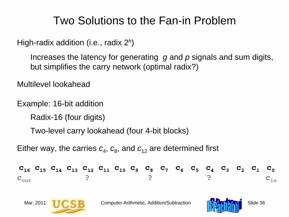
Two Solutions to the Fan-in Problem
High-radix addition (i.e., radix 2h)
Increases the latency for generating g and p signals and sum digits,but simplifies the carry network (optimal radix?)
Multilevel lookahead
Example: 16-bit addition
Radix-16 (four digits)
Two-level carry lookahead (four 4-bit blocks)
Either way, the carries c4, c8, and c12 are determined first
c16 c15 c14 c13 c12 c11 c10 c9 c8 c7 c6 c5 c4 c3 c2 c1 c0
cout ? ? ? cin

Mar. 2011 Computer Arithmetic, Addition/Subtraction Slide 37
6.2 Carry-Lookahead Adder Design
Block generate and propagate signals
g [i,i+3] = gi+3 ∨ gi+2pi+3 ∨ gi+1 pi+2pi+3 ∨ gi pi+1 pi+2pi+3
p [i,i+3] = pi pi+1 pi+2pi+3
ic4-bit lookahead carry generator
g p g p g p g p
[i,i+3]p
i+1c i+2c i+3c
g
iii+1i+1i+2 i+2 i+3 i+3
[i,i+3]
Fig. 6.2b Schematic diagram of a 4-bit lookahead carry generator.

Mar. 2011 Computer Arithmetic, Addition/Subtraction Slide 38
A Building Block for Carry-Lookahead Addition
Fig. 6.2a A 4-bit lookahead carry generator
g0
g1
g2
g3
c0
c4
c1
c2
c3
p3
p2
p1
p0
gi
gi+1
gi+2
gi+3
ci
ci+1
ci+2
ci+3
pi+3
pi+2
pi+1
pi
g
p[i,i+3]
Block Signal GenerationIntermediate Carries
[i,i+3]
Fig. 6.1A 4-bit carry network

Mar. 2011 Computer Arithmetic, Addition/Subtraction Slide 39
Combining Block g and p Signals
Block generate and propagate signals can be combined in the same way as bit g and p signals to form g and p signals for wider blocks
Fig. 6.3 Combining of g and p signals of four (contiguous or overlapping) blocks of arbitrary widths into the g and p signals for the overall block [i0, j3].
j +1j +1 c0
ic4-bit lookahead carry generator
g p
0
i 0i 1
i 2i 3
j 0j 1
j 2j 3
j +1c1c
2
g pg p g p
g p

Mar. 2011 Computer Arithmetic, Addition/Subtraction Slide 40
A Two-Level Carry-Lookahead Adder
cccc
4-bit lookahead carry generator
4-bit lookahead carry generator
g p
ccc
g p
12 8 4 0
48 32 16
[0,63]
16-bit Carry-Lookahead Adder
[0,63]
[48,63][48,63] g
p[32,47][32,47] g
p[0,15][0,15]g
p[16,31][16,31]
g p [12,15]
[12,15] g p [8,11]
[8,11] g p [4,7]
[4,7] g p [0,3]
[0,3]
Fig. 6.4 Building a 64-bit carry-lookahead adder from 16 4-bit adders and 5 lookahead carry generators.
Carry-out: cout = g [0,k–1] ∨ c0 p [0,k–1] = xk–1yk–1 ∨ sk–1′ (xk–1 ∨ yk–1)
Mar. 2011 Computer Arithmetic, Addition/Subtraction Slide 41
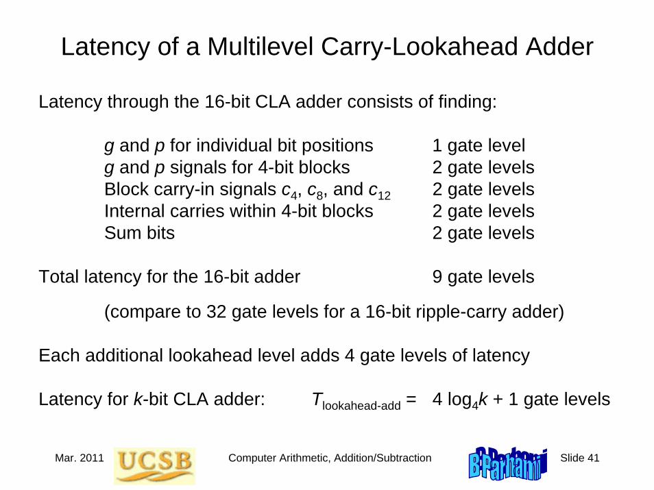
Latency of a Multilevel Carry-Lookahead Adder
Latency through the 16-bit CLA adder consists of finding:
g and p for individual bit positions 1 gate levelg and p signals for 4-bit blocks 2 gate levelsBlock carry-in signals c4, c8, and c12 2 gate levelsInternal carries within 4-bit blocks 2 gate levelsSum bits 2 gate levels
Total latency for the 16-bit adder 9 gate levels
(compare to 32 gate levels for a 16-bit ripple-carry adder)
Each additional lookahead level adds 4 gate levels of latency
Latency for k-bit CLA adder: Tlookahead-add = 4 log4k + 1 gate levels

Mar. 2011 Computer Arithmetic, Addition/Subtraction Slide 42
6.3 Ling Adder and Related DesignsConsider the carry recurrence and its unrolling by 4 steps:
ci = gi–1 ∨ ci–1 ti–1= gi–1 ∨ gi–2 ti–1 ∨ gi–3 ti–2 ti–1 ∨ gi–4 ti–3 ti–2 ti–1 ∨ ci–4 ti–4 ti–3 ti–2 ti–1
Ling’s modification: Propagate hi = ci ∨ ci–1 instead of cihi = gi–1 ∨ hi–1 ti–2
= gi–1 ∨ gi–2 ∨ gi–3 ti–2 ∨ gi–4 ti–3 ti–2 ∨ hi–4 ti–4 ti–3 ti–2
CLA: 5 gates max 5 inputs 19 gate inputsLing: 4 gates max 5 inputs 14 gate inputsThe advantage of hi over ci is even greater with wired-OR: CLA: 4 gates max 5 inputs 14 gate inputsLing: 3 gates max 4 inputs 9 gate inputsOnce hi is known, however, the sum is obtained by a slightly more complex expression compared with si = pi ⊕ ci
si = pi ⊕ hi ti–1
Propagate harry, not carry!

Mar. 2011 Computer Arithmetic, Addition/Subtraction Slide 43
6.4 Carry Determination as Prefix Computation
Fig. 6.5 Combining of g and p signals of two (contiguous or overlapping) blocks B' and B" of arbitrary widths into the g and p signals for block B.
g" p"
i 0i 1
j 0j 1
g p
g' p'
Block B'Block B"
Block B(g, p)
(g", p") (g', p')
¢g = g" + g'p" p = p'p"
g p
g″ p″ g′ p′
Mar. 2011 Computer Arithmetic, Addition/Subtraction Slide 44
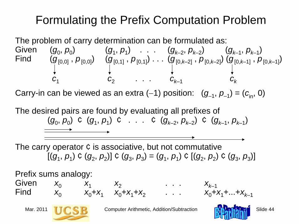
Formulating the Prefix Computation Problem
The problem of carry determination can be formulated as:Given (g0, p0) (g1, p1) . . . (gk–2, pk–2) (gk–1, pk–1) Find (g [0,0] , p [0,0]) (g [0,1] , p [0,1]) . . . (g [0,k–2] , p [0,k–2]) (g [0,k–1] , p [0,k–1])
c1 c2 . . . ck–1 ck
Carry-in can be viewed as an extra (−1) position: (g–1, p–1) = (cin, 0)
The desired pairs are found by evaluating all prefixes of(g0, p0) ¢ (g1, p1) ¢ . . . ¢ (gk–2, pk–2) ¢ (gk–1, pk–1)
The carry operator ¢ is associative, but not commutative[(g1, p1) ¢ (g2, p2)] ¢ (g3, p3) = (g1, p1) ¢ [(g2, p2) ¢ (g3, p3)]
Prefix sums analogy:Given x0 x1 x2 . . . xk–1Find x0 x0+x1 x0+x1+x2 . . . x0+x1+...+xk–1

Mar. 2011 Computer Arithmetic, Addition/Subtraction Slide 45
g0, p0g1, p1g2, p2g3, p3
g[0,0], p[0,0]= (c1, --)
g[0,1], p[0,1]= (c2, --)
g[0,2], p[0,2]= (c3, --)
g[0,3], p[0,3]= (c4, --)
Example Prefix-Based Carry Network
g p
g″ p″ g′ p′
++
++
26 5−1
712 56g0, p0g1, p1g2, p2g3, p3
g[0,0], p[0,0]= (c1, --)
g[0,1], p[0,1]= (c2, --)
g[0,2], p[0,2]= (c3, --)
g[0,3], p[0,3]= (c4, --)
¢¢
¢¢
(a) A 4-input prefix sums network
Scan order
(b) A 4-bitCarry lookahead network
Fig. 6.6 Four-input parallel prefix sums network and its corresponding carry network.

Mar. 2011 Computer Arithmetic, Addition/Subtraction Slide 46
6.5 Alternative Parallel Prefix Networks
Delay recurrence D(k) = D(k/2) + 1 = log2kCost recurrence C(k) = 2C(k/2) + k/2 = (k/2) log2k
Fig. 6.7 Ladner-Fischer parallel prefix sums network built of two k/2-input networks and k/2 adders.
. . .
Prefix Sums k/2 Prefix Sums k/2
. . .
xk–1 xk/2 xk/2–1 x0
s k–1 s k/2
s k/2–1 s 0+ +. . .
. . .
. . . . . .
. . .
. . .. . .

Mar. 2011 Computer Arithmetic, Addition/Subtraction Slide 47
The Brent-Kung Recursive Construction
Delay recurrence D(k) = D(k/2) + 2 = 2 log2k – 1 (–2 really)Cost recurrence C(k) = C(k/2) + k – 1 = 2k – 2 – log2k
Fig. 6.8 Parallel prefix sums network built of one k/2-input network and k – 1 adders.
Prefix Sums k/2
xk–1 xk–2 x3 x2 x1 x0
s k–1 s k–2 s 3 s 2 s 1 s 0
++
+
+
+
. . .
. . .
. . .
. . .

Mar. 2011 Computer Arithmetic, Addition/Subtraction Slide 48
Brent-Kung Carry Network (8-Bit Adder)
¢ ¢ ¢ ¢
¢ ¢
¢ ¢
¢ ¢ ¢
[7, 7 ] [6, 6 ] [5, 5 ] [4, 4 ] [3, 3 ] [2, 2 ] [1, 1 ] [0, 0 ]
[0, 7 ] [0, 6 ] [0, 5 ] [0, 4 ] [0, 3 ] [0, 2 ] [0, 1 ] [0, 0 ]
g p [0,1] [0,1]
g p [1,1] [1,1] g p [0,0] [0,0]
[2, 3 ] [4, 5 ]
[6, 7 ]
[4, 7 ] [0, 3 ]
[0, 1 ]

Mar. 2011 Computer Arithmetic, Addition/Subtraction Slide 49
Brent-Kung Carry Network (16-Bit Adder)x0x1x2x3x4x5x6x7
x8x9x10x11x12x13x14x15
s0s1s2s3s4s5s6s7s8s9s10s11
s12s13s14s15
1 2 3 4 5 6
Level
Fig. 6.9 Brent-Kung parallel prefix graph for 16 inputs.
Reason for latency being 2 log2k – 2

Mar. 2011 Computer Arithmetic, Addition/Subtraction Slide 50
Kogge-Stone Carry Network (16-Bit Adder)
Fig. 6.10 Kogge-Stone parallel prefix graph for 16 inputs.
x0x1x2x3x4x5x6x7x8x9x10x11
x12x13x14x15
s0s1s2s3s4s5s6s7s8s9s10s11
s12s13s14s15
log2k levels (minimum possible)
Cost formulaC(k) = (k – 1)
+ (k – 2) + (k – 4) + . . . + (k – k/2)
= k log2k – k + 1

Mar. 2011 Computer Arithmetic, Addition/Subtraction Slide 51
Speed-Cost Tradeoffs in Carry Networks
Method Delay CostLadner-Fischer log2k (k/2) log2k
Kogge-Stone log2k k log2k – k + 1
Brent-Kung 2 log2k – 2 2k – 2 – log2k
. . .
Prefix Sums k/2 Prefix Sums k/2
. . .
xk–1 xk/2 xk/2–1 x0
s k–1 s k/2
s k/2–1 s 0+ +. . .
. . .
. . . . . .
. . .
. . .. . .Improving the Ladner/Fischer design
These outputs can be produced one time unit later without increasing the overall latency
This strategy saves enough to make the overall cost linear (best possible)

Mar. 2011 Computer Arithmetic, Addition/Subtraction Slide 52
Hybrid B-K/K-S Carry Network (16-Bit Adder)x0x1x2x3x4x5x6x7
x8x9x10x11x12x13x14x15
s0s 1s2s 3s4s5s 6s7s8s9s 10s11s12s 13s14s 15
x0
x1
x2
x3
x4
x5
x6
x7
x8
x9
x10
x11
x12
x13
x14
x15
s0s1s2s3s4s5s6s7s8s 9s10s11s12s13s14s15
1 2 3 4 5 6
Level
x0x1x2x3x4x5x6x7x8x9x10x11
x12x13x14x15
s0s1s2s3s4s5s6s7s8s9s10s11
s12s13s14s15
Brent- Kung
Brent- Kung
Kogge- Stone
Fig. 6.11 A Hybrid Brent-Kung/ Kogge-Stone parallel prefix graph for 16 inputs.
Brent-Kung: 6 levels
26 cells
Kogge-Stone: 4 levels
49 cells
Hybrid: 5 levels
32 cells
Mar. 2011 Computer Arithmetic, Addition/Subtraction Slide 53
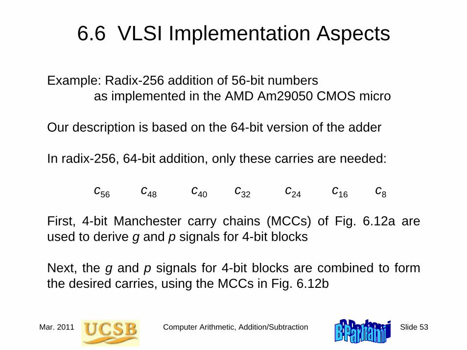
6.6 VLSI Implementation Aspects
Example: Radix-256 addition of 56-bit numbers as implemented in the AMD Am29050 CMOS micro
Our description is based on the 64-bit version of the adder
In radix-256, 64-bit addition, only these carries are needed:
c56 c48 c40 c32 c24 c16 c8
First, 4-bit Manchester carry chains (MCCs) of Fig. 6.12a are used to derive g and p signals for 4-bit blocks
Next, the g and p signals for 4-bit blocks are combined to form the desired carries, using the MCCs in Fig. 6.12b
Mar. 2011 Computer Arithmetic, Addition/Subtraction Slide 54
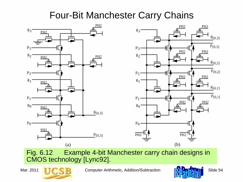
Four-Bit Manchester Carry Chains
Fig. 6.12 Example 4-bit Manchester carry chain designs in CMOS technology [Lync92].
PH2g2
PH2g3
PH2g1
PH2g0
p3
p2
p1
p0
g[0,3]
PH2p[0,3]
(a)
PH2
PH2
g2
g3
g1
g0
p3
p2
p1
p0
g[0,3]
p[0,3]
g[0,2]
p[0,2]
g[0,1]
p[0,1]
PH2PH2
(b)
PH2 PH2
PH2 PH2
PH2 PH2
PH2PH2

Mar. 2011 Computer Arithmetic, Addition/Subtraction Slide 55
Carry Network for 64-Bit Adder
Fig. 6.13 Spanning-tree carry-lookahead network [Lync92]. Type-a and Type-b MCCs refer to the circuits of Figs. 6.12a and 6.12b, respectively.
[48, 55] [32, 47] [16, 31] [-1, 15]
[32, 39] [16, 31] [16, 23] [-1, 15]
[-1, 55] [-1, 47] [-1, 31]
[-1, 39] [-1, 31] [-1, 23]
[48, 63] [48, 59] [48, 55]
[32, 47] [32, 43] [32, 39]
[16, 31] [16, 27] [16, 23]
[-1, 15] [-1, 11] [-1, 7]
[60, 63] [56, 59] [52, 55] [48, 51]
[44, 47] [40, 43] [36, 39] [32, 35]
[28, 31] [24, 27] [20, 23] [16, 19]
[12, 15] [8, 11] [4, 7] [0, 3]
[-1, -1]
Type-b MCC
Type-b MCC
Type-b MCC
Type-b MCC Type-b
MCC
c 56c 48
c 40c 32c 24
c 16
c 8
c 0 c in
16 Type-a MCC
blocks
Type-b* MCC
Level 1 Level 2
Level 3
Legend: [i, j] represents the pair of signals p and g [i, j] [i, j]

Mar. 2011 Computer Arithmetic, Addition/Subtraction Slide 56
7 Variations in Fast Adders
Chapter GoalsStudy alternatives to the carry-lookahead method for designing fast adders
Chapter HighlightsMany methods besides CLA are available
(both competing and complementary)Best design is technology-dependent
(often hybrid rather than pure)Knowledge of timing allows optimizations

Mar. 2011 Computer Arithmetic, Addition/Subtraction Slide 57
Variations in Fast Adders: Topics
Topics in This Chapter
7.1 Simple Carry-Skip Adders
7.2 Multilevel Carry-Skip Adders
7.3 Carry-Select Adders
7.4 Conditional-Sum Adder
7.5 Hybrid Designs and Optimizations
7.6 Modular Two-Operand Adders

Mar. 2011 Computer Arithmetic, Addition/Subtraction Slide 58
7.1 Simple Carry-Skip Adders
Fig. 7.1 Converting a 16-bit ripple-carry adder into a simple carry-skip adder with 4-bit skip blocks.
(a) Ripple-carry adder
(b) Simple carry-skip adder
Ripple-carry stages
4-bit block
4-bit block
4-bit block
c0c4c12c16 c8 3 2 1 0
c03 2 1 0c4
01
p[0,3]
4-bit block
01
p[4,7]
c84-bit block
01
p[8,11]
c124-bit block
01
p[12,15]
c16

Mar. 2011 Computer Arithmetic, Addition/Subtraction Slide 59
Another View of Carry-Skip Addition
Street/freeway analogy for carry-skip adder.
One-way street
Freeway
01
4-bit block4-bit block
01
01

Mar. 2011 Computer Arithmetic, Addition/Subtraction Slide 60
Skip Carry Logic with OR Gate vs. Mux
The carry-skip adder with “OR combining” works fine if we begin with a clean slate, where all signals are 0s at the outset; otherwise, it will run into problems, which do not exist in mux-based version
c
g
p
4j+1
4j+1
g
p
4j
4j
g
p
4j+2
4j+2
g
p
4j+3
4j+3
c
4j
4j+4
c
4j+3
c
4j+2
c
4j+1
01
p[4j, 4j+3]
c4j+4
c
g
p
4j+1
4j+1
g
p
4j
4j
g
p
4j+2
4j+2
g
p
4j+3
4j+3
c
4j
4j+4
c
4j+3
c
4j+2
c
4j+1
Fig. 10.7 of arch book

Mar. 2011 Computer Arithmetic, Addition/Subtraction Slide 61
Carry-Skip Adder with Fixed Block SizeBlock width b; k/b blocks to form a k-bit adder (assume b divides k)
Example: k = 32, b opt = 4, T opt = 13 stages(contrast with 32 stages for a ripple-carry adder)
Tfixed-skip-add = (b – 1) + (k/b – 1) + (b – 1) in block 0 skips in last block
≅ 2b + k/b – 3 stages
dT/db = 2 – k/b2 = 0 ⇒ b opt = √k/2
T opt = 2√2k – 3
. . .

Mar. 2011 Computer Arithmetic, Addition/Subtraction Slide 62
Carry-Skip Adder with Variable-Width Blocks
Fig. 7.2 Carry-skip adder with variable-size blocks and three sample carry paths.
b b b b. . .
RippleSkip
Carry path (1)
01t–1 t–2 Block widths
Carry path (3)
Carry path (2)
The total number of bits in the t blocks is k:
2[b + (b + 1) + . . . + (b + t/2 – 1)] = t(b + t/4 – 1/2) = k
b = k/t – t/4 + 1/2
Tvar-skip-add = 2(b – 1) + t – 1 = 2k/t + t/2 – 2
dT/db = –2k/t 2 + 1/2 = 0 ⇒ t opt = 2√k
T opt = 2√k – 2 (a factor of √2 smaller than for fixed-block)

Mar. 2011 Computer Arithmetic, Addition/Subtraction Slide 63
7.2 Multilevel Carry-Skip Adders
Fig. 7.3 Schematic diagram of a one-level carry-skip adder. S 1
c out c in
S 1 S 1 S 1 S 1
Fig. 7.4 Example of a two-level carry-skip adder.
S 2
S 1
c out c in
S 1 S 1 S 1 S 1
c out c in
S 2
S
1
S
1
S
1
Fig. 7.5 Two-level carry-skip adder optimized by removing the short-block skip circuits.

Mar. 2011 Computer Arithmetic, Addition/Subtraction Slide 64
Designing a Single-Level Carry-Skip Adder
Each of the following takes one unit of time: generation of gi and pi, generation of level-i skip signal from level-(i–1) skip signals, ripple, skip, and formation of sum bit once the incoming carry is known
Build the widest possible one-level carry-skip adder with total delay of 8
Example 7.1
Fig. 7.6 Timing constraints of a single-level carry-skip adder with a delay of 8 units.
c cbbbbbbb 0
2345678
2
inout
S1 S1 S1 S1 S1
0123456
Max adder width = 18(1 + 2 + 3 + 4 + 4 + 3 + 1)
Generalization of Example 7.1 for total time T (even or odd)1 2 3 . . . T/2 T/2 . . . 4 3 11 2 3 . . . (T + 1)/2 . . . 4 3 1
Thus, for any T, the total width is ⎣(T + 1)2/4⎦ – 2

Mar. 2011 Computer Arithmetic, Addition/Subtraction Slide 65
Designing a Two-Level Carry-Skip Adder
Each of the following takes one unit of time: generation of gi and pi, generation of level-i skip signal from level-(i–1) skip signals, ripple, skip, and formation of sum bit once the incoming carry is known
Build the widest possible two-level carry-skip adder with total delay of 8
Example 7.2
Max adder width = 30(1 + 3 + 6 + 8 + 8 + 4)
c c
80
7 6 5 34 3
b b b b b b{8, 1} {7, 2} {6, 3} {5, 4} {4, 5} {3, 8}
inoutABCDEF
S2 S2 S2 S2 S2
Tproduce Tassimilate
(a)
3457 6
2 t=0t=8cout cin2
3
Block E Block D Block C Block B Block AF
Fig. 7.7 Two-level carry-skip adder with a delay of 8 units.
(a) Initial timing constraints
(b) Final design

Mar. 2011 Computer Arithmetic, Addition/Subtraction Slide 66
Elaboration on Two-Level Carry-Skip Adder
c cbb
0123
αinout
S1 S1 S1 S1 S1
12
– 1α – 2αS1
b0
S1
b –1α b –2α
Given the delay pair {β, α} for a level-2 block in Fig. 7.7a, the number of level-1 blocks that can be accommodated is γ = min(β–1, α)
Example 7.2
c cbb
234β
inout
S1 S1 S1 S1 S1
12
– 1β – 2β
b –3βb –2β
S1
b0
S1
1Single-level carry-skip adder with Tassimilate = α
Single-level carry-skip adder with Tproduce = β
Width of the ith level-1 block in the level-2 block characterized by {β, α} is bi = min(β – γ + i + 1, α – i); the total block width is then ∑i=0 to γ–1 bi

Mar. 2011 Computer Arithmetic, Addition/Subtraction Slide 67
Carry-Skip Adder Optimization Scheme
Fig. 7.8 Generalized delay model for carry-skip adders.
Inputs
Level-h skip
Block of b full-adder uni ts
I(b)
A(b)
G(b)
E (b) h S (b) h

Mar. 2011 Computer Arithmetic, Addition/Subtraction Slide 68
7.3 Carry-Select Adders
Cselect-add(k) = 3Cadd(k/2) + k/2 + 1
Tselect-add(k) = Tadd(k/2) + 1
k/2-bit adder k /2-bit adder
k - 1 k/2 k - 1 0
0 1
k/2+1 k/2+1 k/2
1 0 Mux
k/2 c out
c k/2
c in
High k /2 bits Low k /2 bits
k/2-bit adder
Fig. 7.9 Carry-select adder for k-bit numbers built from three k/2-bit adders.
Mar. 2011 Computer Arithmetic, Addition/Subtraction Slide 69
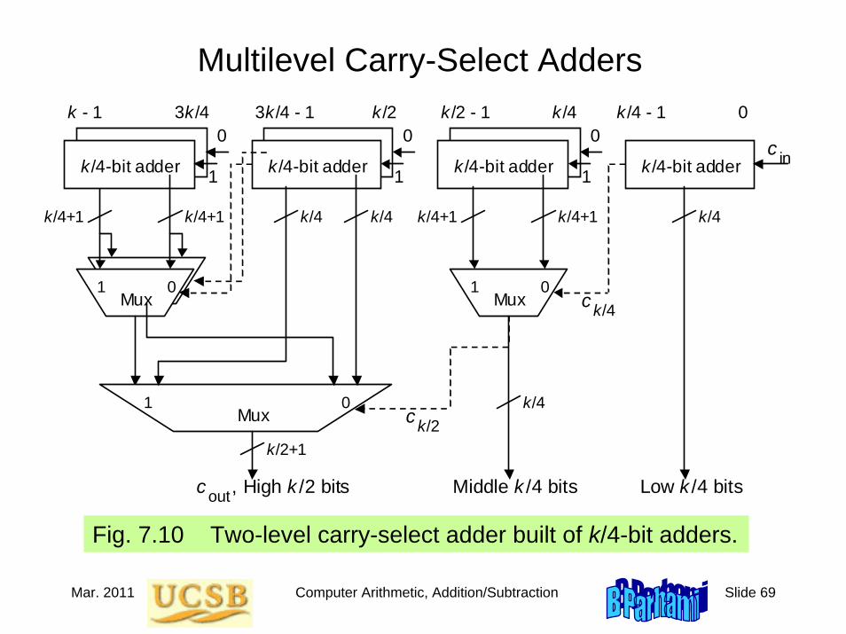
Multilevel Carry-Select Adders
k /4-bit adder k/4-bit adder
k /2 - 1 k /4 k /4 - 1 0
0 1
k/4+1 k/4+1 k/4
1 0 Mux
k/4
k/4-bit adder
k - 1 3k/4 0 1
k/4+1 k/4+1 k/4
1 0 Mux
k /4-bit adder
3k/4 - 1 k /2 0 1
1 0 Mux
k/2+1
k/4
c k/2
c k/4
c out
c in
, High k /2 bits Middle k /4 bits Low k /4 bits
Fig. 7.10 Two-level carry-select adder built of k/4-bit adders.

Mar. 2011 Computer Arithmetic, Addition/Subtraction Slide 70
7.4 Conditional-Sum Adder
Fig. 7.11 Top-level block for one bit position of a conditional-sum adder.
Multilevel carry-select idea carried out to the extreme (to 1-bit blocks.
C(k) ≅ 2C(k/2) + k + 2 ≅ k (log2k + 2) + k C(1)
T(k) = T(k/2) + 1 = log2k + T(1)
where C(1) and T(1) are the cost and delay of the circuit of Fig. 7.11 for deriving the sum and carry bits with a carry-in of 0 and 1
sc
xy
sc
ii
ii+1 i+1 i
For c = 0iFor c = 1i
k + 2 is an upper bound on number of single-bit 2-to-1 multiplexers needed for combining two k/2-bit adders into a k-bit adder

Mar. 2011 Computer Arithmetic, Addition/Subtraction Slide 71
Conditional-Sum Addition Example
Table 7.2
Conditional-sum addition of two 16-bit numbers. The width of the block for which the sum and carry bits are known doubles with each additional level, leading to an addition time that grows as the logarithm of the word width k.
x 0 0 1 0 0 1 1 0 1 1 1 0 1 0 1 0 y 0 1 0 0 1 0 1 1 0 1 0 1 1 1 0 1
1 0 s 0 1 1 0 1 1 0 1 1 0 1 1 0 1 1 1 c 0 0 0 0 0 0 1 0 0 1 0 0 1 0 0 0 0
1 s 1 0 0 1 0 0 1 0 0 1 0 0 1 0 0 c 0 1 1 0 1 1 1 1 1 1 1 1 1 1 1
2 0 s 0 1 1 0 1 1 0 1 0 0 1 1 0 1 1 1 c 0 0 0 1 1 0 1 0
1 s 1 0 1 1 0 0 1 0 0 1 0 0 1 0 c 0 0 1 1 1 1 1
4 0 s 0 1 1 0 0 0 0 1 0 0 1 1 0 1 1 1 c 0 1 1 1
1 s 0 1 1 1 0 0 1 0 0 1 0 0 c 0 1 1
8 0 s 0 1 1 1 0 0 0 1 0 1 0 0 0 1 1 1 c 0 1
1 s 0 1 1 1 0 0 1 0 c 0
16 0 s 0 1 1 1 0 0 1 0 0 1 0 0 0 1 1 1 c 0
1 s c
Block width
Block carry-in
Block sum and block carry-out 15 14 13 12 11 10 9 8 7 6 5 4 3 2 1 0
c in
c out

Mar. 2011 Computer Arithmetic, Addition/Subtraction Slide 72
Elaboration on Conditional-Sum Addition
Two adjacent 4-bit blocks, forming an 8-bit block
1 1 1 18j + 3 . . . 8j
0 0
0 0 0 01 1
0 0 1 18j + 7 . . . 8j + 4
0 0
0 1 0 00 1
0 0 1 10
0 1 0 00
Left 4-bit block Right 4-bit block
Two versions of sum bits
and carry-out in 4-bit blocks
1 1 1 18j + 3 . . . 8j8j + 7 . . .
0
0 0 0 0 1
Two versions of sum bits
and carry-out in 8-bit block
Mar. 2011 Computer Arithmetic, Addition/Subtraction Slide 73
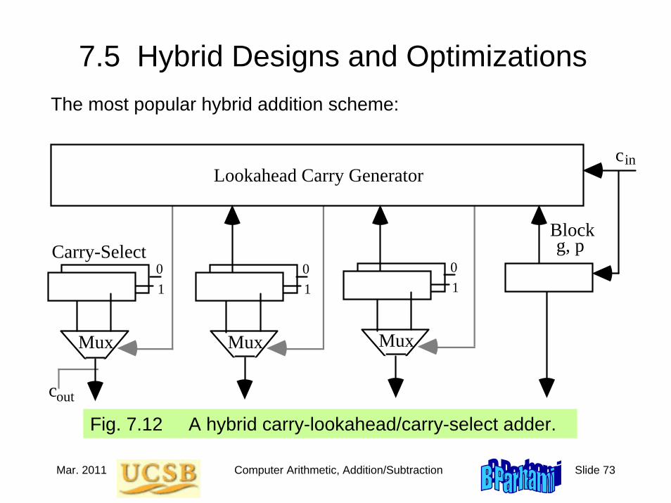
7.5 Hybrid Designs and Optimizations
Fig. 7.12 A hybrid carry-lookahead/carry-select adder.
Lookahead Carry Generator
Carry-Select
c
g, p
in
MuxMuxMux
cout
01
01
01
Block
The most popular hybrid addition scheme:

Mar. 2011 Computer Arithmetic, Addition/Subtraction Slide 74
Details of a 64-Bit Hybrid CLA/Select Adder
Fig. 6.13 [Lync92].
[48, 55] [32, 47] [16, 31] [-1, 15]
[32, 39] [16, 31] [16, 23] [-1, 15]
[-1, 55] [-1, 47] [-1, 31]
[-1, 39] [-1, 31] [-1, 23]
[48, 63] [48, 59] [48, 55]
[32, 47] [32, 43] [32, 39]
[16, 31] [16, 27] [16, 23]
[-1, 15] [-1, 11] [-1, 7]
[60, 63] [56, 59] [52, 55] [48, 51]
[44, 47] [40, 43] [36, 39] [32, 35]
[28, 31] [24, 27] [20, 23] [16, 19]
[12, 15] [8, 11] [4, 7] [0, 3]
[-1, -1]
Type-b MCC
Type-b MCC
Type-b MCC
Type-b MCC Type-b
MCC
c 56c 48
c 40c 32c 24
c 16
c 8
c 0 c in
16 Type-a MCC
blocks
Type-b* MCC
Level 1 Level 2
Level 3
Legend: [i, j] represents the pair of signals p and g [i, j] [i, j]
Each of the carries c8j, produced by the tree network above is used to select one of the two versions of the sum in positions 8j to 8j + 7

Mar. 2011 Computer Arithmetic, Addition/Subtraction Slide 75
Any Two Addition Schemes Can Be Combined
Other possibilities: hybrid carry-select/ripple-carryhybrid ripple-carry/carry-select. . .
Fig. 7.13 Example 48-bit adder with hybrid ripple-carry/carry-lookahead design.
cccc
4-Bit Lookahead Carry Generator
c12 8 4 016
16-bit Carry-Lookahead Adder
g p [12,15]
[12,15] g p [8,11]
[8,11] g p [4,7]
[4,7] g p [0,3]
[0,3]
c32c48
(with carry-out)

Mar. 2011 Computer Arithmetic, Addition/Subtraction Slide 76
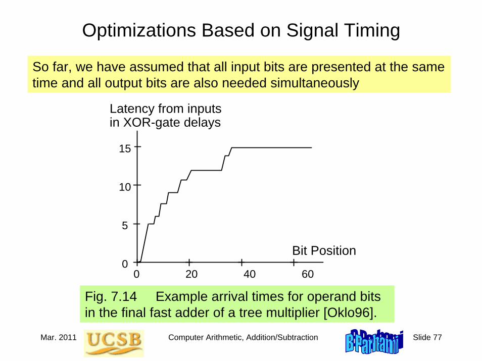
Optimizations in Fast Adders
What looks best at the block diagram or gate level may not be best when a circuit-level design is generated (effects of wire length, signal loading, . . . )
Modern practice: Optimization at the transistor level
Variable-block carry-lookahead adder
Optimizations for average or peak power consumption
Timing-based optimizations (next slide)
Mar. 2011 Computer Arithmetic, Addition/Subtraction Slide 77
Optimizations Based on Signal Timing
So far, we have assumed that all input bits are presented at the same time and all output bits are also needed simultaneously
Fig. 7.14 Example arrival times for operand bits in the final fast adder of a tree multiplier [Oklo96].
15 10 5 0
Bit Position
Latency from inputs in XOR-gate delays
0 20 40 60
Mar. 2011 Computer Arithmetic, Addition/Subtraction Slide 78
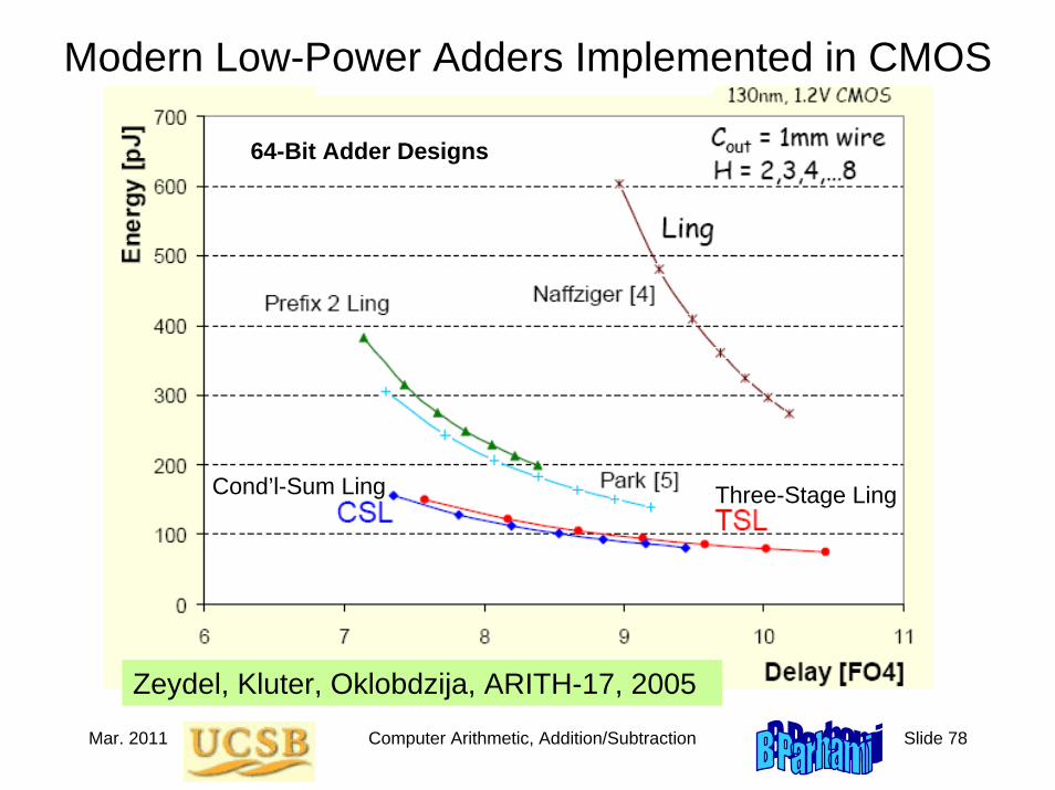
Modern Low-Power Adders Implemented in CMOS
Zeydel, Kluter, Oklobdzija, ARITH-17, 2005
Cond’l-Sum Ling Three-Stage Ling
64-Bit Adder Designs
Mar. 2011 Computer Arithmetic, Addition/Subtraction Slide 79
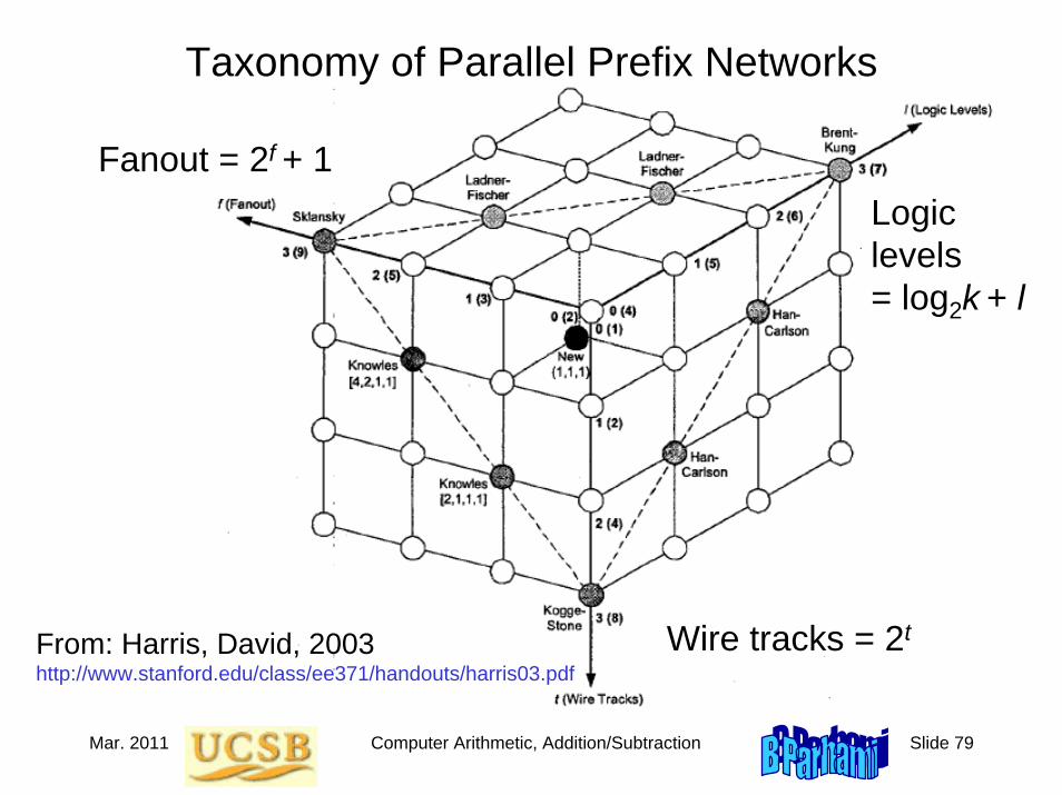
From: Harris, David, 2003http://www.stanford.edu/class/ee371/handouts/harris03.pdf
Taxonomy of Parallel Prefix Networks
Fanout = 2f + 1Logic levels = log2k + l
Wire tracks = 2t

Mar. 2011 Computer Arithmetic, Addition/Subtraction Slide 80
7.6 Modular Two-Operand Addersmod-2k: Ignore carry out of position k – 1
mod-(2k – 1): Use end-around carry because 2k = (2k – 1) + 1
Std. binary0 0 . . . 0 0 00 0 . . . 0 0 10 0 . . . 0 1 0...0 1 . . . 1 1 11 0 . . . 0 0 0
Diminished-11 x . . . x x x0 0 . . . 0 0 00 0 . . . 0 0 1...0 1 . . . 1 1 00 1 . . . 1 1 1
mod-(2k + 1): Residue representation needs k + 1 bits
Number012...2k–12k
x + y ≥ 2k + 1 iff (x–1) + (y–1) + 1 ≥ 2k
(x + y ) – 1 =(x – 1) + (y – 1) +1
xy – 1 =(x–1)(y–1)+(x–1)+(y–1)

Mar. 2011 Computer Arithmetic, Addition/Subtraction Slide 81
General Modular Adders
(x + y) mod m
if x + y ≥ mthen x + y – melse x + y Carry-Save Adder
–mx y
MuxSign bit
(x + y) mod m
x + y – mx + y
Adder Adder
Fig. 7.15 Fast modular addition.

Mar. 2011 Computer Arithmetic, Addition/Subtraction Slide 82
8 Multioperand Addition
Chapter GoalsLearn methods for speeding up the addition of several numbers (needed for multiplication or inner-product)
Chapter HighlightsRunning total kept in redundant formCurrent total + Next number → New total Deferred carry assimilationWallace/Dadda trees, parallel countersModular multioperand addition
Mar. 2011 Computer Arithmetic, Addition/Subtraction Slide 83
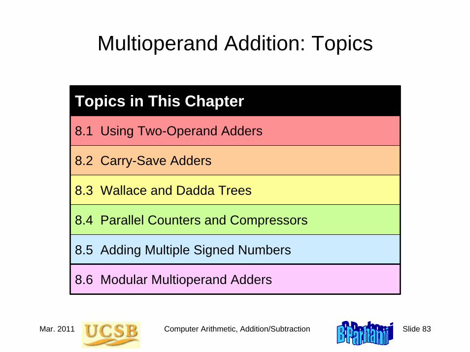
Multioperand Addition: Topics
Topics in This Chapter
8.1 Using Two-Operand Adders
8.2 Carry-Save Adders
8.3 Wallace and Dadda Trees
8.4 Parallel Counters and Compressors
8.5 Adding Multiple Signed Numbers
8.6 Modular Multioperand Adders

Mar. 2011 Computer Arithmetic, Addition/Subtraction Slide 84
8.1 Using Two-Operand Adders
Some applications of multioperand addition
• • • • a • • • • x ---------- • • • • x a • • • • x a • • • • x a • • • • x a ---------------- • • • • • • • • p
×
0 1 2 3
0 1 2 3
2 2 2 2
• • • • • • p • • • • • • p • • • • • • p • • • • • • p • • • • • • p • • • • • • p • • • • • • p ----------------- • • • • • • • • • s
(0) (1) (2) (3) (4) (5) (6)
Fig. 8.1 Multioperand addition problems for multiplication or inner-product computation in dot notation.

Mar. 2011 Computer Arithmetic, Addition/Subtraction Slide 85
Serial Implementation with One Adder
Tserial-multi-add = O(n log(k + log n))
= O(n log k + n log log n)
Therefore, addition time grows superlinearly with n when k is fixed and logarithmically with k for a given n
Adder x
k bits
k + log n bits∑ x j=0 i–1
(i)
2 (j)
Partial sum register
Fig. 8.2 Serial implementation of multioperand addition with a single 2-operand adder.

Mar. 2011 Computer Arithmetic, Addition/Subtraction Slide 86
Pipelined Implementation for Higher Throughput
Fig. 8.3 Serial multioperand addition when each adder is a 4-stage pipeline.
(i–10)(i–9)
Delay
DelaysReady to compute s (i–12)
x(i–1)
x(i)
x +(i) x(i–1)
x +(i–8) x + (i–11)x + x
(i–7)x +(i–6) x
(i–5)x +(i–4) x
Problem to think about: Ignoring start-up and other overheads, this scheme achieves a speedup of 4 with 3 adders. How is this possible?

Mar. 2011 Computer Arithmetic, Addition/Subtraction Slide 87
Parallel Implementation as Tree of Adders
Fig. 8.4 Adding 7 numbers in a binary tree of adders.
Adder Adder Adder
AdderAdder
Adder
k
k+1
k+2
k+3
k+2
k+1k+1
k kk kk k
Ttree-fast-multi-add = O(log k + log(k + 1) + . . . + log(k + ⎡log2n⎤ – 1))
= O(log n log k + log n log log n)
Ttree-ripple-multi-add = O(k + log n) [Justified on the next slide]
⎡log2n⎤adder levelsn – 1
adders

Mar. 2011 Computer Arithmetic, Addition/Subtraction Slide 88
Elaboration on Tree of Ripple-Carry Adders
Ttree-ripple-multi-add = O(k + log n)
Adder Adder Adder
AdderAdder
Adder
k
k+1
k+2
k+3
k+2
k+1k+1
k kk kk k
Fig. 8.5 Ripple-carry adders at levels i and i + 1 in the tree of adders used for multi-operand addition.
. . .
. . . Level i
Level i+1
HAFA
HAFA
t
t+1
tt+1t+1
t+1
t+1
t+2
t+2 t+2
t+2
t+3t+2t+3
The absolute best latency that we can hope for is O(log k + log n)
There are kn data bits to process and using any set of computation elements with constant fan-in, this requires O(log(kn)) time
We will see shortly that carry-save adders achieve this optimum time

Mar. 2011 Computer Arithmetic, Addition/Subtraction Slide 89
8.2 Carry-Save Adders
FA FAFA FA FAFA
FA FAFA FA FAFA
CutFig. 8.6 A ripple-carry adder turns into a carry-save adder if the carries are saved (stored) rather than propagated.
Carry-propagate adder
Carry-save adder (CSA) or (3; 2)-counter or 3-to-2 reduction circuit
c
in
c
out
Fig. 8.7 Carry-propagate adder (CPA) and carry-save adder (CSA) functions in dot notation.
Half-adder
Full-adder
Fig. 8.8 Specifying full-and half-adder blocks, with their inputs and outputs, in dot notation.

Mar. 2011 Computer Arithmetic, Addition/Subtraction Slide 90
Multioperand Addition Using Carry-Save Adders
Fig. 8.9 Tree of carry-save adders reducing seven numbers to two.
CSACSA
CSA
CSA
CSA
Tcarry-save-multi-add = O(tree height + TCPA)
= O(log n + log k)
Ccarry-save-multi-add = (n – 2)CCSA + CCPA
Carry-propagate adder
Fig. 8.13 Serial carry-save addition using a single CSA.
CSA
Input
Sum registerCarry register
Output
CPA

Mar. 2011 Computer Arithmetic, Addition/Subtraction Slide 91
Example Reduction by a CSA Tree
12 FAs
6 FAs
6 FAs
4 FAs + 1 HA
7-bit adder
Total cost = 7-bit adder + 28 FAs + 1 HA
Fig. 8.10 Addition of seven 6-bit numbers in dot notation.
8 7 6 5 4 3 2 1 0 Bit position
7 7 7 7 7 7 6×2 = 12 FAs2 5 5 5 5 5 3 6 FAs3 4 4 4 4 4 1 6 FAs
1 2 3 3 3 3 2 1 4 FAs + 1 HA 2 2 2 2 2 1 2 1 7-bit adder
--Carry-propagate adder--
1 1 1 1 1 1 1 1 1
Fig. 8.11 Representing a seven-operand addition in tabular form.
A full-adder compacts 3 dots into 2(compression ratio of 1.5)
A half-adder rearranges 2 dots(no compression, but still useful)

Mar. 2011 Computer Arithmetic, Addition/Subtraction Slide 92
Width of Adders in a CSA TreeFig. 8.12 Adding seven k-bit numbers and the CSA/CPA widths required.
Due to the gradual retirement (dropping out) of some of the result bits, CSA widths do not vary much as we go down the tree levels
k-bit CPA
k-bit CSA k-bit CSA
k-bit CSA
k-bit CSA
0k+2
The index pair [i, j] means that bit positions from i up to j are involved.
k-bit CSA
[0, k–1] [0, k–1]
[0, k–1] [0, k–1]
[0, k–1] [0, k–1]
[0, k–1] [0, k–1]
[0, k–1]
[1, k] [1, k]
[1, k]
[1, k]
[0, k–1]
[2, k+1] [2, k+1]
[2, k+1]
[2, k+1] [1, k–1]
1
[1, k+1]
k+1 k k–1 1 3 2 4

Mar. 2011 Computer Arithmetic, Addition/Subtraction Slide 93
8.3 Wallace and Dadda Trees
h(n) = 1 + h(⎡2n/3⎤)
n(h) = ⎣3n(h – 1)/2⎦
2×1.5h–1< n(h) ≤ 2×1.5h
. . . inputsn
2 outputs
levelshh levels
Table 8.1 The maximum number n(h) of inputs for an h-level CSA tree
––––––––––––––––––––––––––––––––––––h n(h) h n(h) h n(h)––––––––––––––––––––––––––––––––––––0 2 7 28 14 4741 3 8 42 15 7112 4 9 63 16 10663 6 10 94 17 15994 9 11 141 18 23985 13 12 211 19 35976 19 13 316 20 5395––––––––––––––––––––––––––––––––––––n(h): Maximum number of inputs for h levels

Mar. 2011 Computer Arithmetic, Addition/Subtraction Slide 94
Example Wallace and Dadda Reduction Trees
6 FAs
11 FAs
7 FAs
4 FAs + 1 HA
7-bit adder
Total cost = 7-bit adder + 28 FAs + 1 HA
Fig. 8.14 Adding seven 6-bit numbers using Dadda’s strategy.
12 FAs
6 FAs
6 FAs
4 FAs + 1 HA
7-bit adder
Total cost = 7-bit adder + 28 FAs + 1 HA
Fig. 8.10 Addition of seven 6-bit numbers in dot notation.
Wallace tree: Reduce the number of operands at the earliest possible opportunity
Dadda tree: Postpone the reduction to the extent possible without causing added delay
h n(h)2 43 64 95 136 19

Mar. 2011 Computer Arithmetic, Addition/Subtraction Slide 95
A Small Optimization in Reduction Trees
6 FAs
11 FAs
7 FAs
4 FAs + 1 HA
7-bit adder
Total cost = 7-bit adder + 28 FAs + 1 HA
Fig. 8.14 Adding seven 6-bit numbers using Dadda’s strategy.
Fig. 8.15 Adding seven 6-bit numbers by taking advantage of the final adder’s carry-in.
6 FAs
11 FAs
6 FAs + 1 HA
3 FAs + 2 HA
7-bit adder
Total cost = 7-bit adder + 26 FAs + 3 HA

Mar. 2011 Computer Arithmetic, Addition/Subtraction Slide 96
8.4 Parallel Counters and Compressors
Fig. 8.16 A 10-input parallel counter also known as a (10; 4)-counter.
0
1 0 1 0 1 0
2 1 1 0
1
0
2
13 2
3-bit ripple-carry adder
FA FA
HA
HA
FA
FAFAFA1-bit full-adder = (3; 2)-counter
Circuit reducing 7 bits to their3-bit sum = (7; 3)-counter
Circuit reducing n bits to their ⎡log2(n + 1)⎤-bit sum
= (n; ⎡log2(n+1)⎤)-counter

Mar. 2011 Computer Arithmetic, Addition/Subtraction Slide 97
Accumulative Parallel Counters
Possible application: Compare Hamming weight of a vector to a constant
True generalization of sequential counters
FA FA FA FA
FA FA FA
FA FA
FAFA
FA FA
FAFA
q-bitinitial
count x
n increment signals vi, 2q–1 < n ≤ 2q
q-bit tally of up to 2q – 1 of the increment signals
Ignore, or use for decision
q-bit final count y
cq
nincrement signals vi
q-bit final count y = x + Σvi
Parallel incrementer
q-bit initial count x
Count register

Mar. 2011 Computer Arithmetic, Addition/Subtraction Slide 98
Up/Down Parallel CountersGeneralization of up/down counters
Possible application: Compare Hamming weights of two input vectors

Mar. 2011 Computer Arithmetic, Addition/Subtraction Slide 99
8.5 Generalized Parallel Counters
(5, 5; 4)-counter Fig. 8.17 Dot notation for a (5, 5; 4)-counter and the use of such counters for reducing five numbers to two numbers.
. . .
Multicolumn reduction
(2, 3; 3)-counter
Unequal columns
Gen. parallel counter = Parallel compressor

Mar. 2011 Computer Arithmetic, Addition/Subtraction Slide 100
A General Strategy for Column Compression
n + ψ1 + ψ2 + ψ3 + . . . ≤ 3 + 2ψ1 + 4ψ2 + 8ψ3 + . . .
n – 3 ≤ ψ1 + 3ψ2 + 7ψ3 + . . .
. . . i – 3 i – 2 i – 1 i
n inputs
To i + 1
To i + 2
To i + 3
One circuit slice
ψ 1 ψ 2
ψ 3
ψ 1 ψ 2 ψ 3
(n; 2)-counters
Example: Design a bit-slice of an (11; 2)-counterSolution: Let’s limit transfers to two stages. Then, 8 ≤ ψ1 + 3ψ2Possible choices include ψ1 = 5, ψ2 = 1 or ψ1 = ψ2 = 2
Fig. 8.18 Schematic diagram of an (n; 2)-counter built of identical circuit slices

Mar. 2011 Computer Arithmetic, Addition/Subtraction Slide 101
8.5 Adding Multiple Signed Numbers---------- Extended positions ---------- Sign Magnitude positions ---------
xk–1 xk–1 xk–1 xk–1 xk–1 xk–1 xk–2 xk–3 xk–4 . . .yk–1 yk–1 yk–1 yk–1 yk–1 yk–1 yk–2 yk–3 yk–4 . . .zk–1 zk–1 zk–1 zk–1 zk–1 zk–1 zk–2 zk–3 zk–4 . . .
(a) Using sign extension
---------- Extended positions ---------- Sign Magnitude positions ---------
1 1 1 1 0 xk–1' xk–2 xk–3 xk–4 . . .yk–1' yk–2 yk–3 yk–4 . . .zk–1' zk–2 zk–3 zk–4 . . . 1
(b) Using negatively weighted bits
Fig. 8.19 Adding three 2's-complement numbers.
–b = (1 – b) + 1 – 2

Mar. 2011 Computer Arithmetic, Addition/Subtraction Slide 102
8.6 Modular Multioperand Adders
Fig. 8.20 Modular carry-save addition with special moduli.
(a) m = 2k
Drop
(b) m = 2k – 1 (c) m = 2k + 1
Invert

Mar. 2011 Computer Arithmetic, Addition/Subtraction Slide 103
Modular Reduction with Pseudoresidues
Fig. 8.21 Modulo-21 reduction of 6 numbers taking advantage of the fact that 64 = 1 mod 21 and using 6-bit pseudoresidues.
Final pseudoresidue (to be reduced)
Six inputs in the range
[0, 20]
Pseudoresiduesin the range
[0, 63]
Add with end-around carry
Related Documents


![배우자의퇴직금과연금에내몫은없는가?newfl.or.kr/admin/sub4/files/1452651512.pdf[공무원연금법] 제46조 제1항에 따라 공무원으로 20년 이상 재직한](https://static.cupdf.com/doc/110x72/5e50e75a302bcd06e13de334/eeeeeeeenewflorkradminsub4files.jpg)