Computations of Fluid Dynamics using the Interface Tracking Method Zhiliang Xu Email: [email protected]@nd.edu Department of Mathematics University of Notre.

Computations of Fluid Dynamics using the Interface Tracking

Method

Zhiliang Xu

Email: [email protected]

Department of Mathematics

University of Notre Dame

Outline

Computational Fluid Dynamics Compressible & incompressible flows Governing equations Numerical methodology

Front Tracking Method Formulation Improving the accuracy

Conclusions and Future Plans

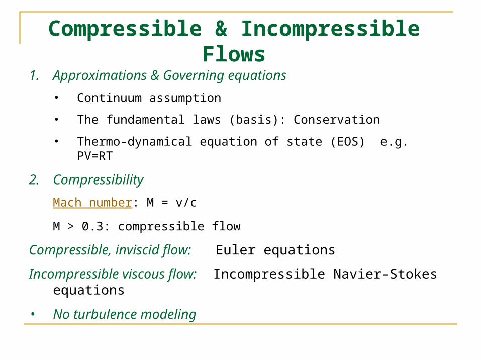
Compressible & Incompressible Flows

1. Approximations & Governing equations

• Continuum assumption

• The fundamental laws (basis): Conservation

• Thermo-dynamical equation of state (EOS) e.g. PV=RT

2. Compressibility

Mach number: M = v/c

M > 0.3: compressible flow

Compressible, inviscid flow: Euler equations

Incompressible viscous flow: Incompressible Navier-Stokes equations

• No turbulence modeling

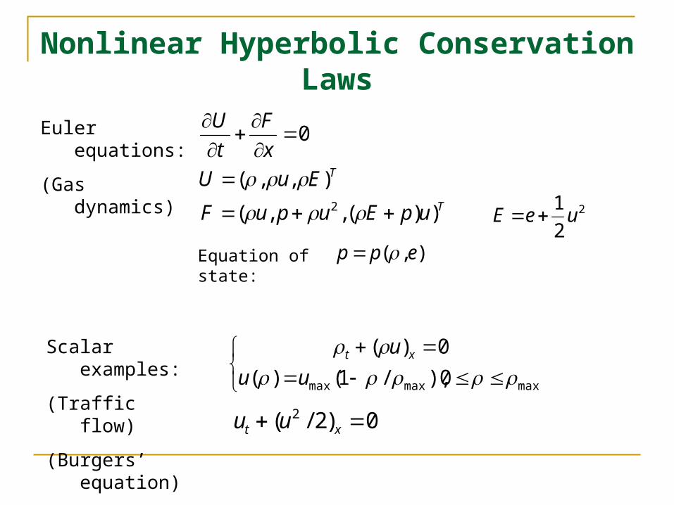
Nonlinear Hyperbolic Conservation Laws

maxmaxmax 0),/1()(

0)(

uu

u xt

T

T

upEupuF

EuU

x

F

t

U

))(,,(

),,(

0

2

Euler equations:

(Gas dynamics)

Equation of state: ),( epp

2

2

1ueE

Scalar examples:

(Traffic flow)

(Burgers’ equation) 0)2/( 2 xt uu

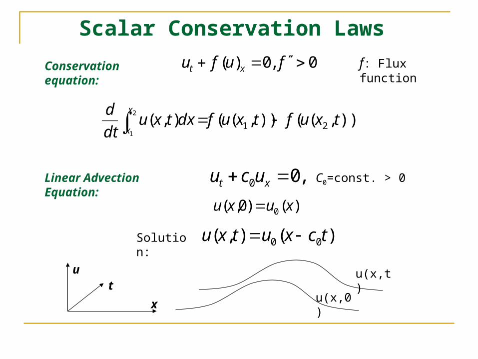
Scalar Conservation Laws

,00 xt ucu C0=const. > 0Linear Advection Equation:

)(),( 00 tcxutxu Solution:

u(x,t)

u(x,0)

0,0)( fufu xt

u

x

t

)),,(()),((),( 21

2

1

txuftxufdxtxudt

d x

x

f: Flux function

)()0,( 0 xuxu

Conservation equation:

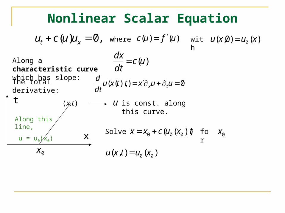
Nonlinear Scalar Equation

)()( ufuc ,0)( xt uucu

)(ucdt

dxAlong a characteristic curve

which has slope:

The total derivative:

txucxx ))(( 000

x0

x

t

Along this line,

u = u0(x0)

)()0,( 0 xuxu with

)(),( 00 xutxu

Solve for 0x

is const. along this curve.u(x,t)

where

0)),(( uuxttxudt

dtx

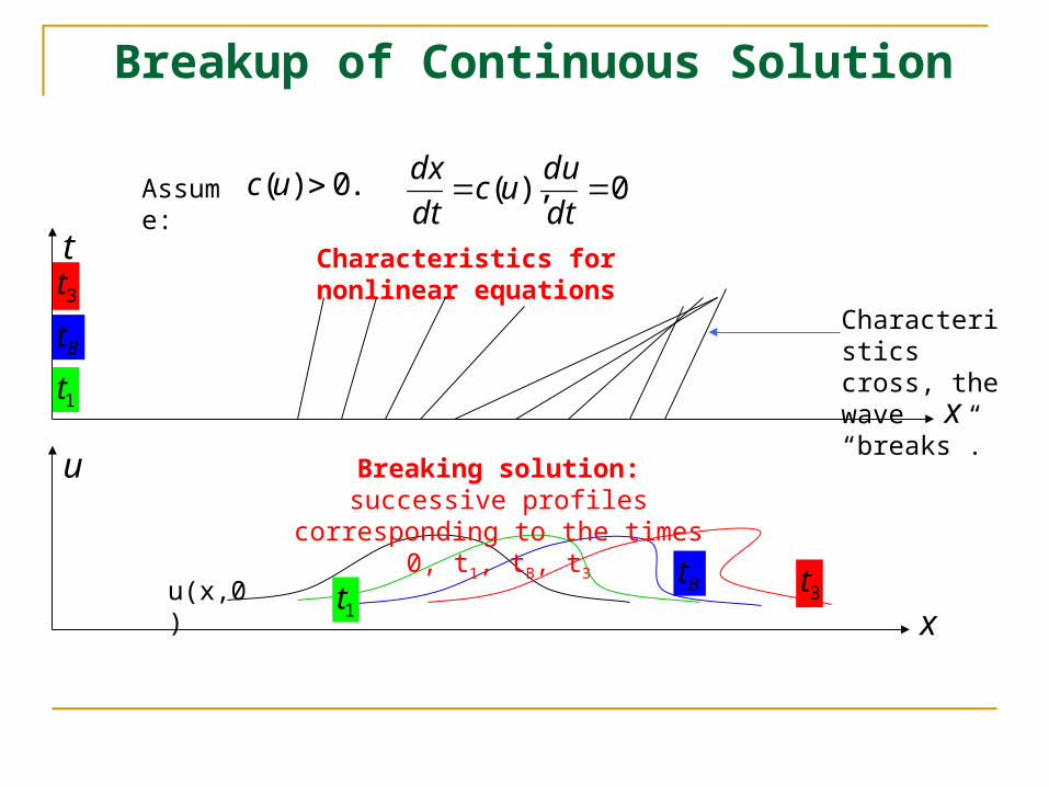
Breakup of Continuous Solution

Characteristics for nonlinear equations

x

t

1t

Bt

3t

x

u

u(x,0)1t

Bt 3t

Characteristics cross, the wave “breaks”.

0),( dt

duuc

dt

dx

Breaking solution: successive profiles corresponding to the times 0, t1, tB, t3

.0)( ucAssume:

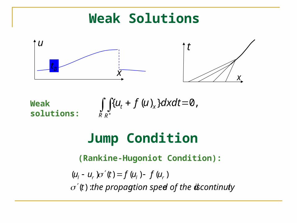
Weak Solutions

R R

xt dxdtufu ,0})({Weak solutions:

Jump Condition (Rankine-Hugoniot Condition):

tyiscontinuid of the dation speethe propagt

ufuftuu rlrl

:)(

)()()()(

)(t

t x

rM

lM

ru

lu

Bt x

u

t x

t

x

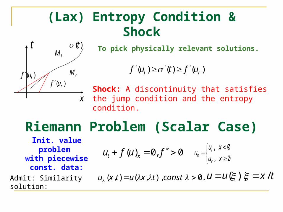
(Lax) Entropy Condition & Shock

)(t

t x

rM

lM

)(luf

)(ruf

To pick physically relevant solutions.

)()()( rl uftuf

Shock: A discontinuity that satisfies the jump condition and the entropy condition.

Riemann Problem (Scalar Case)

.0 ),,(),( consttxutxu

0,0)( fufu xtInit. value problem

with piecewise const. data:

0 ,

0 ,0 xu

xuu

r

l

txuu /),( Admit: Similarity solution:

)(tt

x

rM

lM

)( luf )( ruf

Riemann Solution (Scalar Case)

))((,

)(

)()(

)(

,

),/(

,

),( vf

tufx

tufxtuf

tufx

u

txv

u

txu

r

rl

l

r

l

stx

stx

u

utxu

r

l

,

,),(Case 2: Shock wave:

t

x

0

Shock speed s

Case 3: Rarefaction wave:t

x0

Case 1: Const. State:

rl

rl

uu

ufufs

)()(

rl uu

rl uu

.)( constu

))(( uf 0)( ufu

rl uu

Rarefaction wave

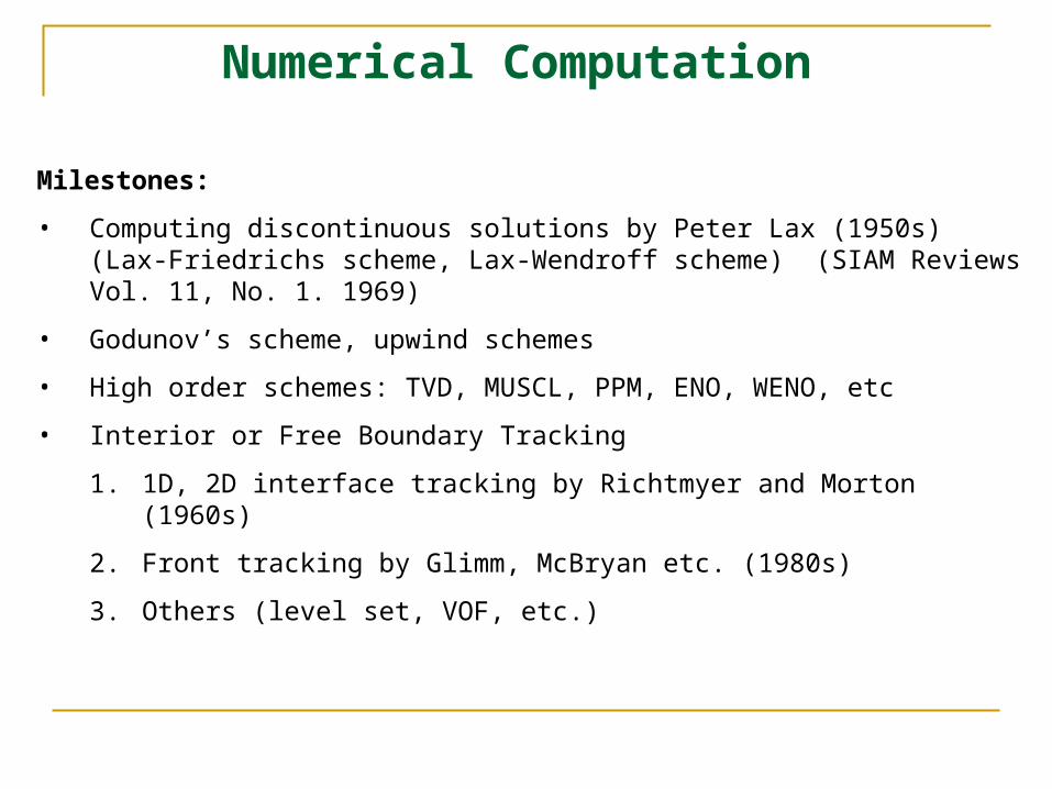
Numerical Computation

Milestones:

• Computing discontinuous solutions by Peter Lax (1950s) (Lax-Friedrichs scheme, Lax-Wendroff scheme) (SIAM Reviews Vol. 11, No. 1. 1969)

• Godunov’s scheme, upwind schemes

• High order schemes: TVD, MUSCL, PPM, ENO, WENO, etc

• Interior or Free Boundary Tracking

1. 1D, 2D interface tracking by Richtmyer and Morton (1960s)

2. Front tracking by Glimm, McBryan etc. (1980s)

3. Others (level set, VOF, etc.)

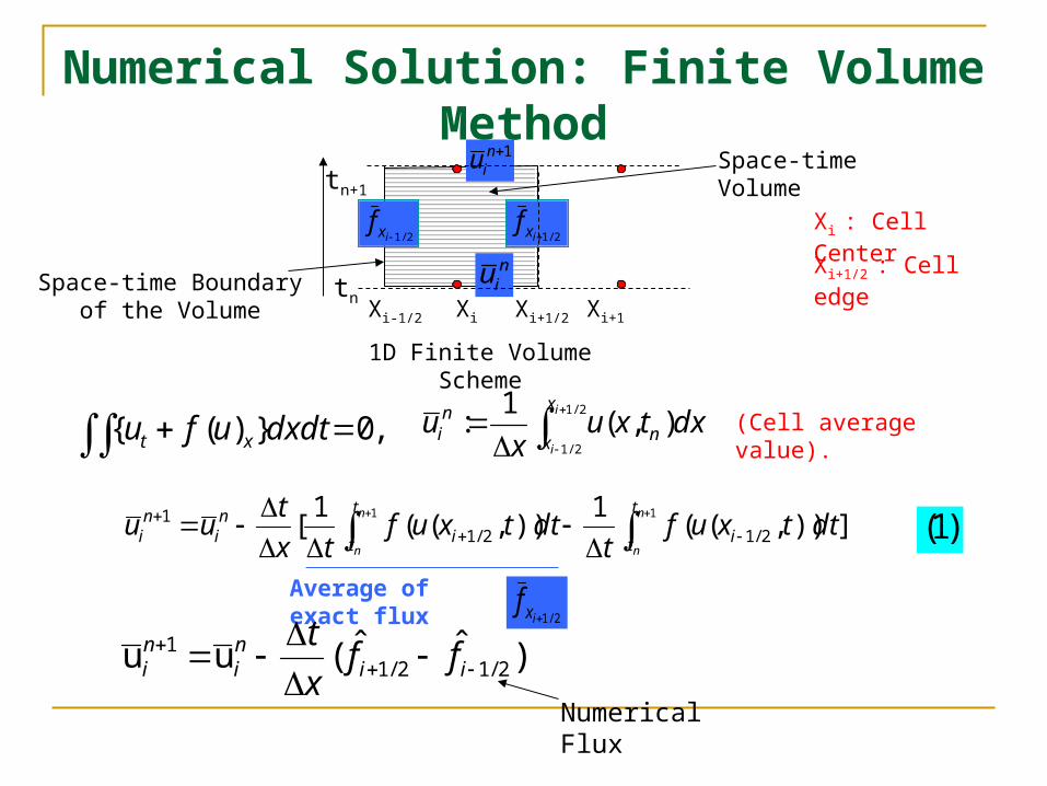
Numerical Solution: Finite Volume Method

2/1

2/1

),(1

:i

i

x

x nn

i dxtxux

u

])),((1

)),((1

[11

2/12/11

n

n

n

n

t

t i

t

t in

in

i dttxuft

dttxuftx

tuu

1D Finite Volume Scheme

)1(

Average of exact flux

1niu

niu

Space-time Volume

Space-time Boundary of the Volume

(Cell average value).,0})({ dxdtufu xt

2/1ixf

2/1ixf

Xi+1/2 : Cell edge

Xi : Cell Center

tnXi-1/2 Xi+1/2

tn+1

Xi Xi+1

2/1ixf

Numerical Flux

)ˆˆ(uu 2/12/11

iini

ni ff

x

t

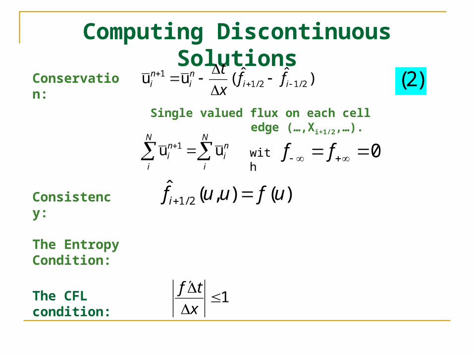
Computing Discontinuous Solutions

)ˆˆ(uu 2/12/11

iini

ni ff

x

tConservation:

Single valued flux on each cell edge (…,Xi+1/2,…).

)2(

N

i

ni

N

i

ni uu 1

)(),(ˆ2/1 ufuufi Consistency:

The CFL condition: 1x

tf

The Entropy Condition:

with 0 ff

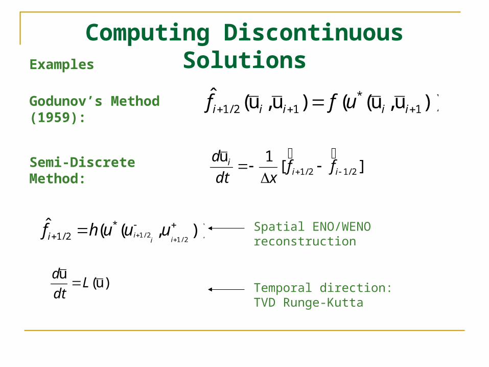
Computing Discontinuous Solutions

][1u

2/12/1

iii ff

xdt

d

)),((ˆ2/1

2/1*

2/1

iii uuuhfi

Godunov’s Method (1959): ))u,u(()u,u(ˆ1

*12/1 iiiii uff

Semi-Discrete Method:

Spatial ENO/WENO reconstruction

Temporal direction: TVD Runge-Kutta

)u(u

Ldt

d

Examples

Dynamic Interface Tracking

Rayleigh-Taylor Mixing

The Level Set Method

d0),( tx

0v

t

Level Set:

Interface : 0:)( t

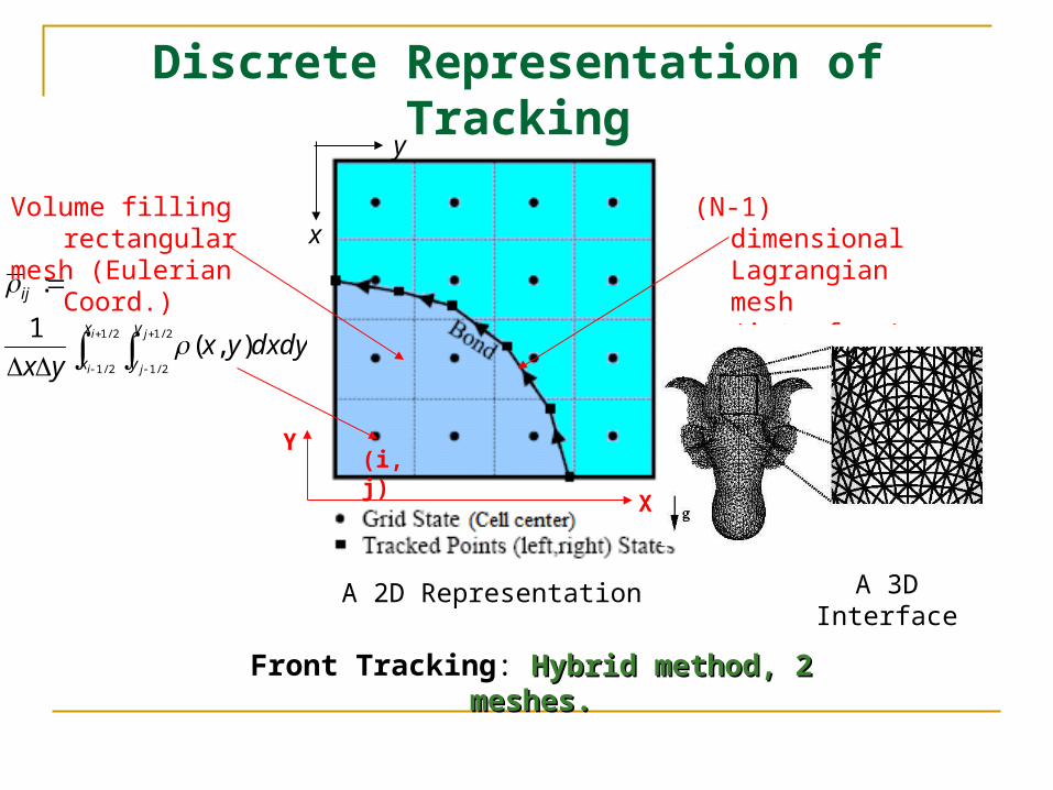
Discrete Representation of Tracking

2/1

2/1

2/1

2/1

),(1

:

i

i

j

j

x

x

y

y

ij

dxdyyxyx

Volume filling rectangularmesh (Eulerian Coord.)

(N-1) dimensional Lagrangian mesh (interface)

Front Tracking: Hybrid method, 2 meshes.Hybrid method, 2 meshes.

A 3D InterfaceA 2D Representation

Y

X

(i,j)

x

y

Time Marching & Coupling

1nI

nItn Xi-1 Xi Xi+1

tn+1

To advance the numerical solution in Front Tracking:

(1) Explicit procedure for interface propagation + (2) Updating states (grid cell center)

Two way coupling:

1. Interface dynamics to ambient region (interior).

2. Non-interface solution variation to interface dynamics.

Advancing solution in 1D

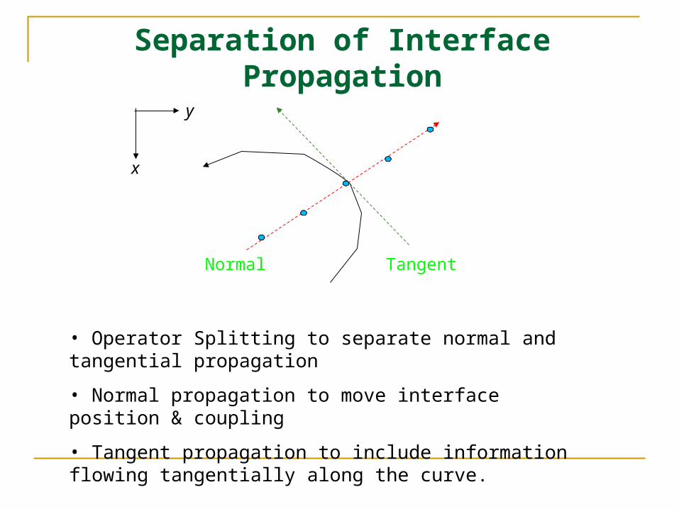
Separation of Interface Propagation

Normal Tangent

• Operator Splitting to separate normal and tangential propagation

• Normal propagation to move interface position & coupling

• Tangent propagation to include information flowing tangentially along the curve.

x

y

Normal Propagation of Interface Point

Move the point position and couple the interior wave solution to interface dynamics.

Riemann solutionMethod of characteristics

(Coupling)

Step 1: Step 2:

SlSr

Left and right states of the point

Updated left and right states of the

point

0S 1S 2S1S2S

n

tt

t

Contact

0S

(Material interface)

New positionSl0 Sr0

udt

dx

0S 1S 2S1S2S bSn

tt

t

cudt

dx

cudt

dx

0SfS

Sl Sr

Advancing Eulerian Grid Solution

Ghost cell method: Coupling interface dynamics to interior

: Fluid 1

: Fluid 2

: Interface

tn+1

tn

Xi Xi+1Xi-1

Extrapolate

Cell edge

)( 2/12/11

iL

in

in

i FFx

tUU

),(ˆ12/1

lefti

ni

Li UUFF

)( 2/12/311

1R

iin

in

i FFx

tUU

),(ˆ12/1

nrighti

Ri i

UUFF

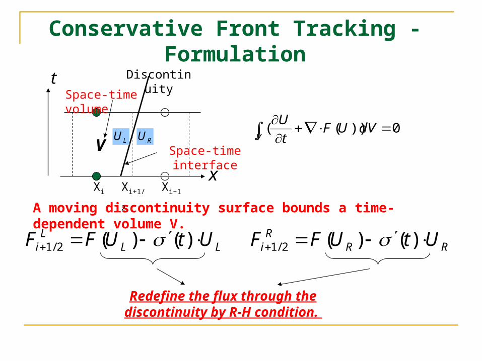
Conservative Front Tracking - Formulation

0))((

dVUFt

UV

x

t

A moving discontinuity surface bounds a time-dependent volume V.

V

Discontinuity

Space-time interface

Redefine the flux through the discontinuity by R-H condition.

LU RU

LLL

i UtUFF )()(2/1 RRR

i UtUFF )()(2/1

Xi Xi+1

Space-time volume

Xi+1/2

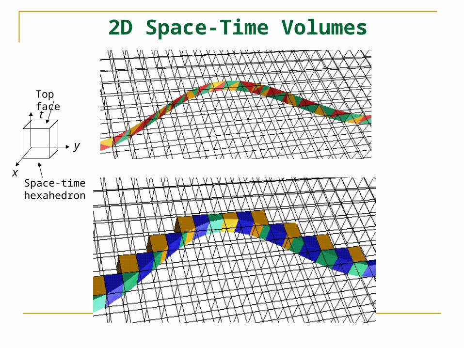
2D Space-Time Volumes

x

y

t

Space-time hexahedron

Top face

Improved Accuracy

Theorem: The conservative tracking method improves accuracy by at least one order.

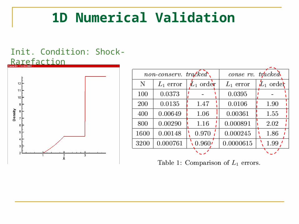
1D Numerical Validation

Init. Condition: Shock-Rarefaction

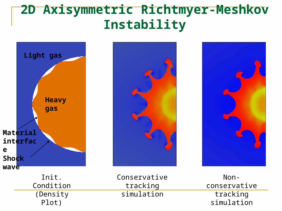
2D Axisymmetric Richtmyer-Meshkov Instability

Init. Condition (Density Plot)

Conservative tracking simulation

Non-conservative tracking simulation

Heavy gas

Light gas

Shock wave

Material interface

2D Axisymmetric Richtmyer-Meshkov Instability

)( bbsp hha

h_sp and h_bb are distances from origin to the tips of the

spike and the bubble respectively.

Amplitude (a): the height of the interface

perturbation.

Conservative Tracking, 100*200 grid

Non-Conservative Tracking, 100*200 grid

Non-Conservative Tracking, 200*400 grid

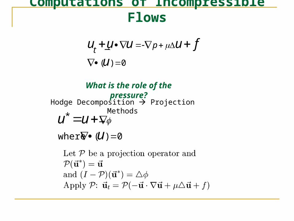
Computations of Incompressible Flows

0)(

u

fuuuu pt

What is the role of the pressure?

Hodge Decomposition Projection Methods

0)(where

*

u

uu

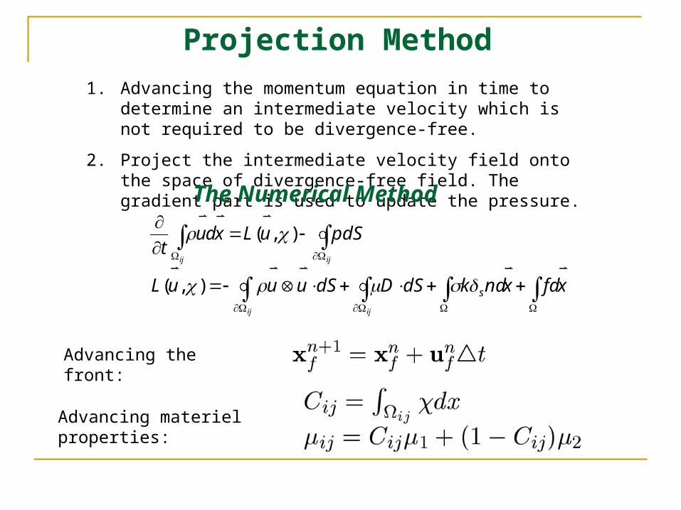
Projection Method

1. Advancing the momentum equation in time to determine an intermediate velocity which is not required to be divergence-free.

2. Project the intermediate velocity field onto the space of divergence-free field. The gradient part is used to update the pressure.

The Numerical Method

Advancing the front:

Advancing materiel properties:

xfdxndkdSDdSuuuL

pdSuLxdut

s

ij ij

ij ij

),(

),(

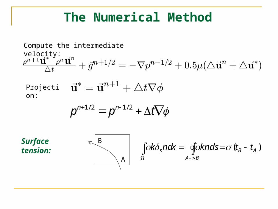
The Numerical Method

Projection:

Compute the intermediate velocity:

tpp nn 2/12/1

Surface tension:

A

B)( AB

BA

s ttkndsxndk

The Blood Flow Modelling

0)(

)(

u

fuuuu pt

ccuc Dt

Conclusions & Future PlansThe front tracking method to describe the interface.

On the tracking method:To achieve uniform high order accuracy.

On the application:To develop a blood flow model in the multiscale context