Computational Topology for Data Analysis Tamal Krishna Dey Department of Computer Science Purdue University West Lafayette, Indiana, USA 47907 Yusu Wang Halıcıo˘ glu Data Science Institute University of California, San Diego La Jolla, California, USA 92093

Welcome message from author
This document is posted to help you gain knowledge. Please leave a comment to let me know what you think about it! Share it to your friends and learn new things together.
Transcript
Computational Topology for Data Analysis
Tamal Krishna DeyDepartment of Computer Science
Purdue UniversityWest Lafayette, Indiana, USA 47907
Yusu WangHalıcıoglu Data Science Institute
University of California, San DiegoLa Jolla, California, USA 92093

ii Computational Topology for Data Analysis
c©Tamal Dey and Yusu Wang 2016-2021
This material has been / will be published by Cambridge University Press as ComputationalTopology for Data Analysis by Tamal Dey and Yusu Wang. This pre-publication version is freeto view and download for personal use only. Not for re-distribution, re-sale, or use in derivativeworks.
Contents
1 Basics 31.1 Topological space . . . . . . . . . . . . . . . . . . . . . . . . . . . . . . . . . . 31.2 Metric space topology . . . . . . . . . . . . . . . . . . . . . . . . . . . . . . . . 61.3 Maps, homeomorphisms, and homotopies . . . . . . . . . . . . . . . . . . . . . 91.4 Manifolds . . . . . . . . . . . . . . . . . . . . . . . . . . . . . . . . . . . . . . 13
1.4.1 Smooth manifolds . . . . . . . . . . . . . . . . . . . . . . . . . . . . . 151.5 Functions on smooth manifolds . . . . . . . . . . . . . . . . . . . . . . . . . . . 16
1.5.1 Gradients and critical points . . . . . . . . . . . . . . . . . . . . . . . . 161.5.2 Morse functions and Morse Lemma . . . . . . . . . . . . . . . . . . . . 181.5.3 Connection to topology . . . . . . . . . . . . . . . . . . . . . . . . . . . 19
1.6 Notes and Exercises . . . . . . . . . . . . . . . . . . . . . . . . . . . . . . . . . 21
2 Complexes and Homology Groups 232.1 Simplicial complex . . . . . . . . . . . . . . . . . . . . . . . . . . . . . . . . . 232.2 Nerves, Cech and Rips complex . . . . . . . . . . . . . . . . . . . . . . . . . . 272.3 Sparse complexes . . . . . . . . . . . . . . . . . . . . . . . . . . . . . . . . . . 29
2.3.1 Delaunay complex . . . . . . . . . . . . . . . . . . . . . . . . . . . . . 292.3.2 Witness complex . . . . . . . . . . . . . . . . . . . . . . . . . . . . . . 312.3.3 Graph induced complex . . . . . . . . . . . . . . . . . . . . . . . . . . 33
2.4 Chains, cycles, boundaries . . . . . . . . . . . . . . . . . . . . . . . . . . . . . 362.4.1 Algebraic structures . . . . . . . . . . . . . . . . . . . . . . . . . . . . 362.4.2 Chains . . . . . . . . . . . . . . . . . . . . . . . . . . . . . . . . . . . 382.4.3 Boundaries and cycles . . . . . . . . . . . . . . . . . . . . . . . . . . . 39
2.5 Homology . . . . . . . . . . . . . . . . . . . . . . . . . . . . . . . . . . . . . . 412.5.1 Induced homology . . . . . . . . . . . . . . . . . . . . . . . . . . . . . 432.5.2 Relative homology . . . . . . . . . . . . . . . . . . . . . . . . . . . . . 442.5.3 Singular Homology . . . . . . . . . . . . . . . . . . . . . . . . . . . . . 452.5.4 Cohomology . . . . . . . . . . . . . . . . . . . . . . . . . . . . . . . . 46
2.6 Notes and Exercises . . . . . . . . . . . . . . . . . . . . . . . . . . . . . . . . . 48
3 Topological Persistence 513.1 Filtrations and persistence . . . . . . . . . . . . . . . . . . . . . . . . . . . . . 52
3.1.1 Space filtration . . . . . . . . . . . . . . . . . . . . . . . . . . . . . . . 523.1.2 Simplicial filtrations and persistence . . . . . . . . . . . . . . . . . . . . 54
iii
iv Computational Topology for Data Analysis
3.2 Persistence . . . . . . . . . . . . . . . . . . . . . . . . . . . . . . . . . . . . . 583.2.1 Persistence diagram . . . . . . . . . . . . . . . . . . . . . . . . . . . . 59
3.3 Persistence algorithm . . . . . . . . . . . . . . . . . . . . . . . . . . . . . . . . 653.3.1 Matrix reduction algorithm . . . . . . . . . . . . . . . . . . . . . . . . . 683.3.2 Efficient implementation . . . . . . . . . . . . . . . . . . . . . . . . . . 72
3.4 Persistence modules . . . . . . . . . . . . . . . . . . . . . . . . . . . . . . . . . 753.5 Persistence for PL-functions . . . . . . . . . . . . . . . . . . . . . . . . . . . . 79
3.5.1 PL-functions and critical points . . . . . . . . . . . . . . . . . . . . . . 803.5.2 Lower star filtration and its persistent homology . . . . . . . . . . . . . 843.5.3 Persistence algorithm for 0-th persistent homology . . . . . . . . . . . . 86
3.6 Notes and Exercises . . . . . . . . . . . . . . . . . . . . . . . . . . . . . . . . . 89
4 General Persistence 934.1 Stability of towers . . . . . . . . . . . . . . . . . . . . . . . . . . . . . . . . . . 944.2 Computing persistence of simplicial towers . . . . . . . . . . . . . . . . . . . . 97
4.2.1 Annotations . . . . . . . . . . . . . . . . . . . . . . . . . . . . . . . . . 974.2.2 Algorithm . . . . . . . . . . . . . . . . . . . . . . . . . . . . . . . . . . 984.2.3 Elementary inclusion . . . . . . . . . . . . . . . . . . . . . . . . . . . . 994.2.4 Elementary collapse . . . . . . . . . . . . . . . . . . . . . . . . . . . . 100
4.3 Persistence for zigzag filtration . . . . . . . . . . . . . . . . . . . . . . . . . . . 1034.3.1 Approach . . . . . . . . . . . . . . . . . . . . . . . . . . . . . . . . . . 1064.3.2 Zigzag persistence algorithm . . . . . . . . . . . . . . . . . . . . . . . . 108
4.4 Persistence for zigzag towers . . . . . . . . . . . . . . . . . . . . . . . . . . . . 1104.5 Levelset zigzag persistence . . . . . . . . . . . . . . . . . . . . . . . . . . . . . 114
4.5.1 Simplicial levelset zigzag filtration . . . . . . . . . . . . . . . . . . . . . 1154.5.2 Barcode for levelset zigzag filtration . . . . . . . . . . . . . . . . . . . . 1164.5.3 Correspondence to sublevel set persistence . . . . . . . . . . . . . . . . 1174.5.4 Correspondence to extended persistence . . . . . . . . . . . . . . . . . . 118
4.6 Notes and Exercises . . . . . . . . . . . . . . . . . . . . . . . . . . . . . . . . . 119
5 Generators and Optimality 1235.1 Optimal generators/basis . . . . . . . . . . . . . . . . . . . . . . . . . . . . . . 124
5.1.1 Greedy algorithm for optimal Hp(K)-basis . . . . . . . . . . . . . . . . . 1255.1.2 Optimal H1(K)-basis and independence check . . . . . . . . . . . . . . . 128
5.2 Localization . . . . . . . . . . . . . . . . . . . . . . . . . . . . . . . . . . . . . 1305.2.1 Linear program . . . . . . . . . . . . . . . . . . . . . . . . . . . . . . . 1325.2.2 Total unimodularity . . . . . . . . . . . . . . . . . . . . . . . . . . . . . 1335.2.3 Relative torsion . . . . . . . . . . . . . . . . . . . . . . . . . . . . . . . 134
5.3 Persistent cycles . . . . . . . . . . . . . . . . . . . . . . . . . . . . . . . . . . . 1365.3.1 Finite intervals for weak (p + 1)-pseudomanifolds . . . . . . . . . . . . 1385.3.2 Algorithm correctness . . . . . . . . . . . . . . . . . . . . . . . . . . . 1415.3.3 Infinite intervals for weak (p + 1)-pseudomanifolds embedded in Rp+1 . . 143
5.4 Notes and Exercises . . . . . . . . . . . . . . . . . . . . . . . . . . . . . . . . . 144
Computational Topology for Data Analysis v
6 Topological Analysis of Point Clouds 1476.1 Persistence for Rips and Cech filtrations . . . . . . . . . . . . . . . . . . . . . . 1486.2 Approximation via data sparsification . . . . . . . . . . . . . . . . . . . . . . . 150
6.2.1 Data sparsification for Rips filtration via reweighting . . . . . . . . . . . 1516.2.2 Approximation via simplicial tower . . . . . . . . . . . . . . . . . . . . 156
6.3 Homology inference from PCDs . . . . . . . . . . . . . . . . . . . . . . . . . . 1586.3.1 Distance field and feature sizes . . . . . . . . . . . . . . . . . . . . . . . 1586.3.2 Data on manifold . . . . . . . . . . . . . . . . . . . . . . . . . . . . . . 1606.3.3 Data on a compact set . . . . . . . . . . . . . . . . . . . . . . . . . . . 161
6.4 Homology inference for scalar fields . . . . . . . . . . . . . . . . . . . . . . . . 1626.4.1 Problem setup . . . . . . . . . . . . . . . . . . . . . . . . . . . . . . . 1636.4.2 Inference guarantees . . . . . . . . . . . . . . . . . . . . . . . . . . . . 164
6.5 Notes and Exercises . . . . . . . . . . . . . . . . . . . . . . . . . . . . . . . . . 166
7 Reeb Graphs 1697.1 Reeb graph: Definitions and properties . . . . . . . . . . . . . . . . . . . . . . . 1707.2 Algorithms in the PL-setting . . . . . . . . . . . . . . . . . . . . . . . . . . . . 172
7.2.1 An O(m log m) time algorithm via dynamic graph connectivity . . . . . . 1737.2.2 A randomized algorithm with O(m log m) expected time . . . . . . . . . 1767.2.3 Homology groups of Reeb graphs . . . . . . . . . . . . . . . . . . . . . 179
7.3 Distances for Reeb graphs . . . . . . . . . . . . . . . . . . . . . . . . . . . . . 1827.3.1 Interleaving distance . . . . . . . . . . . . . . . . . . . . . . . . . . . . 1827.3.2 Functional distortion distance . . . . . . . . . . . . . . . . . . . . . . . 184
7.4 Notes and Exercises . . . . . . . . . . . . . . . . . . . . . . . . . . . . . . . . . 186
8 Topological Analysis of Graphs 1918.1 Topological summaries for graphs . . . . . . . . . . . . . . . . . . . . . . . . . 192
8.1.1 Combinatorial graphs . . . . . . . . . . . . . . . . . . . . . . . . . . . . 1928.1.2 Graphs viewed as metric spaces . . . . . . . . . . . . . . . . . . . . . . 193
8.2 Graph comparison . . . . . . . . . . . . . . . . . . . . . . . . . . . . . . . . . . 1968.3 Topological invariants for directed graphs . . . . . . . . . . . . . . . . . . . . . 197
8.3.1 Simplicial complexes for directed graphs . . . . . . . . . . . . . . . . . 1978.3.2 Path homology for directed graphs . . . . . . . . . . . . . . . . . . . . . 1988.3.3 Computation of (persistent) path homology . . . . . . . . . . . . . . . . 201
8.4 Notes and Exercises . . . . . . . . . . . . . . . . . . . . . . . . . . . . . . . . . 206
9 Cover, Nerve, and Mapper 2099.1 Covers and nerves . . . . . . . . . . . . . . . . . . . . . . . . . . . . . . . . . . 210
9.1.1 Special case of H1 . . . . . . . . . . . . . . . . . . . . . . . . . . . . . 2149.2 Analysis of persistent H1-classes . . . . . . . . . . . . . . . . . . . . . . . . . . 2179.3 Mapper and multiscale mapper . . . . . . . . . . . . . . . . . . . . . . . . . . . 219
9.3.1 Multiscale Mapper . . . . . . . . . . . . . . . . . . . . . . . . . . . . . 2229.3.2 Persistence of H1-classes in mapper and multiscale mapper . . . . . . . . 223
9.4 Stability . . . . . . . . . . . . . . . . . . . . . . . . . . . . . . . . . . . . . . . 2259.4.1 Interleaving of cover towers and multiscale mappers . . . . . . . . . . . 225
vi Computational Topology for Data Analysis
9.4.2 (c, s)-good covers . . . . . . . . . . . . . . . . . . . . . . . . . . . . . . 2269.4.3 Relation to intrinsic Cech filtration . . . . . . . . . . . . . . . . . . . . . 228
9.5 Exact Computation for PL-functions on simplicial domains . . . . . . . . . . . . 2299.6 Approximating multiscale mapper for general maps . . . . . . . . . . . . . . . . 231
9.6.1 Combinatorial mapper and multiscale mapper . . . . . . . . . . . . . . . 2329.6.2 Advantage of combinatorial multiscale mapper . . . . . . . . . . . . . . 233
9.7 Notes and Exercises . . . . . . . . . . . . . . . . . . . . . . . . . . . . . . . . . 234
10 Discrete Morse Theory and Applications 23710.1 Discrete Morse function . . . . . . . . . . . . . . . . . . . . . . . . . . . . . . 238
10.1.1 Discrete Morse vector field . . . . . . . . . . . . . . . . . . . . . . . . . 23910.2 Persistence based DMVF . . . . . . . . . . . . . . . . . . . . . . . . . . . . . . 241
10.2.1 Persistence-guided cancellation . . . . . . . . . . . . . . . . . . . . . . 24210.2.2 Algorithms . . . . . . . . . . . . . . . . . . . . . . . . . . . . . . . . . 244
10.3 Stable and unstable manifolds . . . . . . . . . . . . . . . . . . . . . . . . . . . 24810.3.1 Morse theory revisited . . . . . . . . . . . . . . . . . . . . . . . . . . . 24810.3.2 (Un)Stable manifolds in DMVF . . . . . . . . . . . . . . . . . . . . . . 249
10.4 Graph reconstruction . . . . . . . . . . . . . . . . . . . . . . . . . . . . . . . . 25010.4.1 Algorithm . . . . . . . . . . . . . . . . . . . . . . . . . . . . . . . . . . 25010.4.2 Noise model . . . . . . . . . . . . . . . . . . . . . . . . . . . . . . . . 25210.4.3 Theoretical guarantees . . . . . . . . . . . . . . . . . . . . . . . . . . . 253
10.5 Applications . . . . . . . . . . . . . . . . . . . . . . . . . . . . . . . . . . . . . 25510.5.1 Road network . . . . . . . . . . . . . . . . . . . . . . . . . . . . . . . . 25510.5.2 Neuron network . . . . . . . . . . . . . . . . . . . . . . . . . . . . . . 257
10.6 Notes and Exercises . . . . . . . . . . . . . . . . . . . . . . . . . . . . . . . . . 258
11 Multiparameter Persistence and Decomposition 26111.1 Multiparameter persistence modules . . . . . . . . . . . . . . . . . . . . . . . . 264
11.1.1 Persistence modules as graded modules . . . . . . . . . . . . . . . . . . 26411.2 Presentations of persistence modules . . . . . . . . . . . . . . . . . . . . . . . . 267
11.2.1 Presentation and its decomposition . . . . . . . . . . . . . . . . . . . . . 26811.3 Presentation matrix: diagonalization and simplification . . . . . . . . . . . . . . 270
11.3.1 Simplification . . . . . . . . . . . . . . . . . . . . . . . . . . . . . . . . 27211.4 Total diagonalization algorithm . . . . . . . . . . . . . . . . . . . . . . . . . . . 274
11.4.1 Running TotDiagonalize on the working example in Figure 11.5 . . . . . 28211.5 Computing presentations . . . . . . . . . . . . . . . . . . . . . . . . . . . . . . 285
11.5.1 Graded chain, cycle, and boundary modules . . . . . . . . . . . . . . . . 28511.5.2 Multiparameter filtration, zero-dimensional homology . . . . . . . . . . 28711.5.3 2-parameter filtration, multi-dimensional homology . . . . . . . . . . . . 28711.5.4 d > 2-parameter filtration, multi-dimensional homology . . . . . . . . . 28811.5.5 Time complexity . . . . . . . . . . . . . . . . . . . . . . . . . . . . . . 289
11.6 Invariants . . . . . . . . . . . . . . . . . . . . . . . . . . . . . . . . . . . . . . 29011.6.1 Rank invariants . . . . . . . . . . . . . . . . . . . . . . . . . . . . . . . 29011.6.2 Graded Betti numbers and blockcodes . . . . . . . . . . . . . . . . . . . 291
11.7 Notes and Exercises . . . . . . . . . . . . . . . . . . . . . . . . . . . . . . . . . 295
Computational Topology for Data Analysis 7
12 Multiparameter Persistence and Distances 29912.1 Persistence modules from categorical viewpoint . . . . . . . . . . . . . . . . . . 30112.2 Interleaving distance . . . . . . . . . . . . . . . . . . . . . . . . . . . . . . . . 30212.3 Matching distance . . . . . . . . . . . . . . . . . . . . . . . . . . . . . . . . . . 303
12.3.1 Computing matching distance . . . . . . . . . . . . . . . . . . . . . . . 30412.4 Bottleneck distance . . . . . . . . . . . . . . . . . . . . . . . . . . . . . . . . . 307
12.4.1 Interval decomposable modules . . . . . . . . . . . . . . . . . . . . . . 30812.4.2 Bottleneck distance for 2-parameter interval decomposable modules . . . 30912.4.3 Algorithm to compute dI for intervals . . . . . . . . . . . . . . . . . . . 314
12.5 Notes and Exercises . . . . . . . . . . . . . . . . . . . . . . . . . . . . . . . . . 315
13 Topological Persistence and Machine Learning 31913.1 Feature vectorization of persistence diagrams . . . . . . . . . . . . . . . . . . . 320
13.1.1 Persistence landscape . . . . . . . . . . . . . . . . . . . . . . . . . . . . 32013.1.2 Persistence scale space (PSS) kernel . . . . . . . . . . . . . . . . . . . . 32213.1.3 Persistence images . . . . . . . . . . . . . . . . . . . . . . . . . . . . . 32313.1.4 Persistence weighted Gaussian kernel (PWGK) . . . . . . . . . . . . . . 32413.1.5 Sliced Wasserstein kernel . . . . . . . . . . . . . . . . . . . . . . . . . . 32613.1.6 Persistence Fisher kernel . . . . . . . . . . . . . . . . . . . . . . . . . . 327
13.2 Optimizing topological loss functions . . . . . . . . . . . . . . . . . . . . . . . 32813.2.1 Topological regularizer . . . . . . . . . . . . . . . . . . . . . . . . . . . 32813.2.2 Gradients of a persistence-based topological function . . . . . . . . . . . 330
13.3 Statistical treatment of topological summaries . . . . . . . . . . . . . . . . . . . 33213.4 Bibliographical notes . . . . . . . . . . . . . . . . . . . . . . . . . . . . . . . . 334

8 Computational Topology for Data Analysis
Preface
In recent years, the area of topological data analysis (TDA) has emerged as a viable tool for an-alyzing data in applied areas of science and engineering. The area started in the 90’s with thecomputational geometers finding an interest in studying the algorithmic aspect of classical sub-ject of algebraic topology in mathematics. The area of computational geometry flourished in80’s and 90’s by addressing various practical problems and enriching the area of discrete geom-etry in the course. Handful of computational geometers felt that, analogous to this development,computational topology has the potential of addressing the area of shape and data analysis whiledrawing upon and perhaps developing further the area of topology in the discrete context; seee.g. [27, 117, 120, 188, 292]. The area gained the momentum with the introduction of persistenthomology in early 2000 followed by a series of mathematical and algorithmic developments onthe topic. The book by Edelsbrunner and Harer [149] presents these fundamental developmentsquite nicely. Since then, the area has grown both in its methodology and applicability. One conse-quence of this growth has been the development of various algorithms which intertwine with thediscoveries of various mathematical structures in the context of processing data. The purpose ofthis book is to capture these algorithmic developments with the associated mathematical guaran-tees. It is appropriate to mention that there is an emerging sub-area of TDA which centers morearound statistical aspects. This book does not deal with these developments though we mentionsome of it in the last chapter where we describe the recent results connecting TDA and machinelearning.
We have 13 chapters in the book listed in the table of contents. After developing the basicsof topological spaces, simplicial complexes, homology groups, and persistent homology in thefirst three chapters, the book is then devoted to presenting algorithms and associated mathemat-ical structures in various contexts of topological data analysis. These chapters present materialsmostly not covered in any book in the market. To elaborate on this claim, we briefly give anoverview of the topics covered by the present book. The fourth chapter presents generalizationof the persistence algorithm to extended settings such as to simplicial maps (instead of inclu-sions), zigzag sequences both with inclusions and simplicial maps. Chapter 5 covers algorithmson computing optimal generators both for persistent and non-persistent homology. Chapter 6 fo-cuses on algorithms that infer homological information from point cloud data. Chapter 7 presentsalgorithms and structural results for Reeb graphs. Chapter 8 considers general graphs includingdirected ones. Chapter 9 focuses on various recent results on characterizing nerves of covers in-cluding the well known Mapper and its multiscale version. Chapter 10 devotes to the importantconcept discrete Morse theory, its connection to persistent homology, and its applications to graphreconstruction. Chapter 11 and 12 introduce multiparameter persistence. The standard persistence
9
10 Computational Topology for Data Analysis
is defined over a 1-parameter index set such as Z or R. Extending this index set to a poset suchas Zd or Rd, we get d-parameter or multiparameter persistence. Chapter 11 focuses on computingindecomposables for multiparameter persistence that are generalizations of bars in 1-parametercase. Chapter 12 focuses on various definitions of distances among multiparameter persistencemodules and their computations. Finally, we conclude with Chapter 13 that presents some recentdevelopment of incorporating persistence into the machine learning (ML) framework.
This book is intended for the audience comprising researchers and teachers in computer sci-ence and mathematics. The graduate students in both fields will benefit from learning the newmaterials in topological data analysis. Because of the topics, the book plays a role of a bridgebetween mathematics and computer science. Students in computer science will learn the math-ematics in topology that they are usually not familiar with. Similarly, students in mathematicswill learn about designing algorithms based on mathematical structures. The book can be usedfor a graduate course in topological data analysis. In particular, it can be part of a curriculum indata science which has been/is being adopted in universities. We are including exercises for eachchapter to facilitate teaching and learning.
There are currently few books on computational topology/topological data analysis in the mar-ket to which our book will be complementary. The materials covered in this book predominatelyare new and have not been covered in any of the previous books. The book by Edelsbrunner andHarer [149] mainly focuses on early developments in persistent homology and do not cover thematerials in Chapters 4 to 13 in this book. The recent book of Boissonnat et al.[40] focuses mainlyon reconstruction, inference, and Delaunay meshes. Other than the Chapter 6 which focuses onpoint cloud data and inference of topological properties and Chapter 1-3 which focus on prelim-inaries about topological persistence, there are hardly any overlap. The book by Oudot [249]mainly focuses on algebraic structures of persistence modules and inference results. Again, otherthan preliminary Chapters 1-3 and Chapter 6, there are hardly any overlap. Finally, unlike ours,the books by Tierny [286] and by Rabadán and Blumberg [260] mainly focus on applying TDAto specific domains of scientific visualizations and genomics respectively.
This book, as any other, is not created in isolation. Help coming from various corners con-tributed to its creation. It was seeded by the class notes that we developed for our introductorycourse on Computational Topology and Data Analysis which we taught at the Ohio State Univer-sity. During this teaching, the class feedback from students gave us the hint that a book coveringincreasingly diversified repertoire of topological data analysis is necessary at this point. We thankall those students who had to bear with the initial disarray that was part of freshly gathering acoherent material on a new subject. This book would not have been possible without our owninvolvement with TDA which was mostly supported by grants from National Science Foundation(NSF). Many of our PhD students worked through these projects that helped us consolidate ourfocus on TDA. In particular, Tao Hou, Ryan Slechta, Cheng Xin, and Soham Mukherjee gavetheir comments on drafts of some of the chapters. We thank all of them. We thank everyone fromthe TGDA@OSU group for creating one of the best environments for carrying out research inapplied and computational topology. Our special thanks go to Facundo Mémoli, who has been agreat colleague (collaborated with us on several topics) as well as a wonderful friend at OSU. Wealso acknowledge the support of the department of CSE at the Ohio State University where a largeamount of the contents of this book were planned and written. The finishing came to fruition afterwe moved to our current institutions.

Computational Topology for Data Analysis 11
Finally, it is our pleasure to acknowledge the support of our families that kept us motivatedand engaged throughout the marathon of writing this book, especially during the last stretch over-lapping the 2020-2021 Coronavirus pandemic. Tamal recalls his daughter Soumi and son Sounakasking him continuously about the progress of the book. His wife Kajari extended all the helpnecessary to make space for extra time needed for the book. Despite suffering from the reducedattention to family matters, all of them offered their unwavering support and understanding gra-ciously. Tamal dedicates this book to his family and his late parents Gopal Dey and Hasi Deywithout whose encouragement and love, he would not have been in a position to take up thisproject. Yusu thanks her husband Mikhail Belkin for his never-ending support and encouragementthroughout writing this book and beyond. Their two children Alexander and Julia contributed intheir typical ways by making everyday delightful and unpredictable for her. Without their supportand love, she would not be able to finish this book. Finally, Yusu dedicates this book to her par-ents Qingfen Wang and Jinlong Huang, who always gave her space to grow and encouraged herto do her best in life, as well as to her great aunt Zhige Zhao and great uncle Humin Wang, whokindly took her under their care when she was 13. She can never repay their kindness.

12 Computational Topology for Data Analysis

Prelude
We make sense of the world around us primarily by understanding and studying the “shape" ofthe objects that we encounter in real life or in a digital environment. Geometry offers a commonlanguage that we usually use to model and describe shapes. For example, the familiar descriptorssuch as distances, coordinates, angles and so on from this language assist us to provide detailedinformation of a shape of interest. Not surprisingly, mankind has used geometry for thousands ofyears to describe objects in his/her surrounding.
Figure 1: “Map of Königsbergin Euler’s time showing the ac-tual layout of the seven bridges,highlighting the river Pregel andthe bridges" by Bogdan Giuscais licensed under CC BY-SA 3.0.
However, there are many situations where the detailed ge-ometric information is not needed and may even obscure thereal useful structure that is not so explicit. A notable exampleis the Seven Bridges of Königsberg problem, where in the cityof Königsberg, Pregel river separated the city into four regions,connected by seven bridges as shown in Figure 1 (taken fromthe Wikipedia page for "Seven bridge of Königsberg"). Thequestion is to find a walk through the city that crosses eachbridge exactly once. Story goes that mathematician LeonhardEuler observed that factors such as the precise shape of theseregions and the exact path taken are not important. What isimportant is the connectivity among the different regions ofthe city as connected by the bridges. In particular, the problemcan be modeled abstractly using a graph with four nodes, rep-resenting the four regions in the city of Königsberg, and sevenedges representing the bridges connecting them. The problemthen reduces to what’s later known as finding the Euler tour (orEulerian cycle) in this graph, which can be easily solved.
For another example, consider animation in computer graphics where one wants to develop asoftware that can continuously deform one object to another (in the sense that one can stretch andchange the shape, but cannot break and add to the shape). Can we continuously deform a frog toa prince this way1? Is it possible to continuously deform a tea cup to a bunny? It turns out thelatter is not possible.
In these examples, the core structure of interest behind the input object or space is character-ized by the way the space is connected, and the detailed geometric information may not matter. Ingeneral, topology intuitively models and studies properties that are invariant as long as the con-nectivity of space does not change. As a result, topological language and concepts can provide
1Yes according to Disney movies.
13
14 Computational Topology for Data Analysis
powerful tools to characterize, identify, and process essential features of both spaces and functionsdefined on them. However, to bring topological methods to the realm of practical applications,not only do we need new ideas to make topological concepts and resulting structures more suit-able for modern data analysis tasks, but also algorithms to compute these structures efficiently. Inthe past two decades, the field of applied and computational topology has developed rapidly, pro-ducing many fundamental results and algorithms that have advanced both fronts. These progressfurther fueled the significant growth of topological data analysis (TDA) which has already foundapplications in various domains such as computer graphics, visualization, material science, com-putational biology, neuroscience and so on.
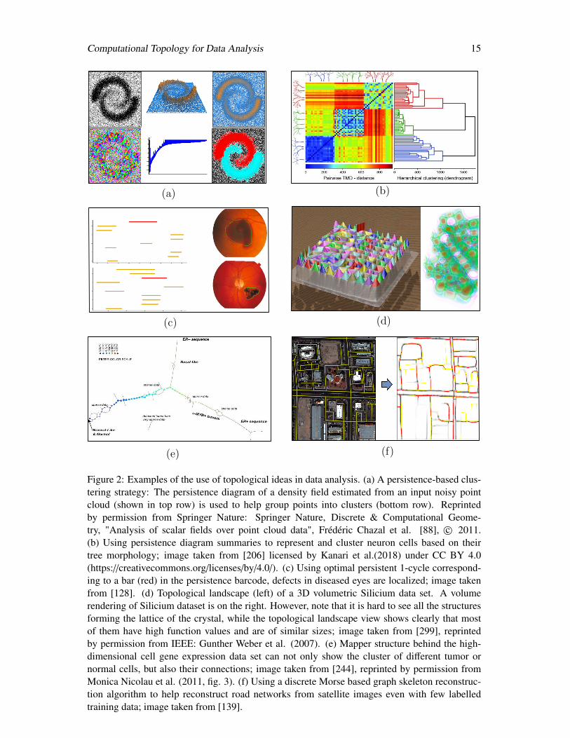
Examples. In Figure 2, we present some examples of the use of topological methodologies inapplications. The topological structures involved will be described later in the book.
An important development in applied and computational topology in the past two decadescenters around the concept of persistent homology which generalizes the classic algebraic struc-ture of homology groups to the multi-scale setting aided by the concept of so-called filtrationand persistence modules (discussed in Chapters 2 and 3). This helps significantly to broaden theapplications of homological features to characterizing shapes/spaces of interest. Figure 2(a) givesan example where persistent homology of a density field is used to develop a clustering strategyfor the points [88]. In particular, at the beginning, each point is in its own cluster. Then, theseclusters are grown using persistent homology which identifies their importance and merges themaccording to this importance. The final output captures key clusters which may look like ‘blobs’or ‘curvy strips’–intuitively, they comprise dense regions separated by sparse regions.
Figure 2(b) gives an example where the resulting topological summaries from persistent ho-mology have been used for clustering a collection of neurons, each of which is represented by arooted tree (as neuron cells have tree morphology). We will see in Chapter 13, persistent homol-ogy can serve as a general way to vectorize features of such complex input objects.
In Figure 2(c), diseased parts of retinal degeneracy in eyes are localized from image data. Al-gorithms for computing optimal cycles for bars in the persistent barcode as described in Chapter 5are used for this purpose.
In Figure 2(d), we present an example where the topological object of contour tree (the specialloop-free case of the so-called Reeb graph as discussed in Chapter 7) has been used to give low-dimensional terrain metaphor of a potentially high dimensional scalar field. To illustrate further,suppose that we are given a scalar field f : X → R where X is a space of potentially highdimension. To visualize and explore X and f in R2 and R3, just mapping X to R2 can causesignificant geometric distortion, which in turn leads to artifacts in the visualization of f over theprojection. Instead, we can create a 2D terrain metaphor f ′ : R2 → R for f which preservesthe contour tree information as proposed in [299]; intuitively, this preserves the valleys/mountainpeaks and how they merge and split. In this example, the original scalar field is in R3. However,in general, the idea is applicable to higher dimensional scalar fields (e.g., the protein energylandscape considered in [184]).
In Figure 2(e), we give an example of an alternative approach of exploring a high-dimensionalspace X or functions defined on it via the Mapper methodology (introduced in Chapter 9). In par-ticular, the Mapper methodology constructs a representation of the essential structure behind X
Computational Topology for Data Analysis 15
(a) (b)
(c) (d)
(e) (f)
Figure 2: Examples of the use of topological ideas in data analysis. (a) A persistence-based clus-tering strategy: The persistence diagram of a density field estimated from an input noisy pointcloud (shown in top row) is used to help group points into clusters (bottom row). Reprintedby permission from Springer Nature: Springer Nature, Discrete & Computational Geome-try, "Analysis of scalar fields over point cloud data", Frédéric Chazal et al. [88], c© 2011.(b) Using persistence diagram summaries to represent and cluster neuron cells based on theirtree morphology; image taken from [206] licensed by Kanari et al.(2018) under CC BY 4.0(https://creativecommons.org/licenses/by/4.0/). (c) Using optimal persistent 1-cycle correspond-ing to a bar (red) in the persistence barcode, defects in diseased eyes are localized; image takenfrom [128]. (d) Topological landscape (left) of a 3D volumetric Silicium data set. A volumerendering of Silicium dataset is on the right. However, note that it is hard to see all the structuresforming the lattice of the crystal, while the topological landscape view shows clearly that mostof them have high function values and are of similar sizes; image taken from [299], reprintedby permission from IEEE: Gunther Weber et al. (2007). (e) Mapper structure behind the high-dimensional cell gene expression data set can not only show the cluster of different tumor ornormal cells, but also their connections; image taken from [244], reprinted by permission fromMonica Nicolau et al. (2011, fig. 3). (f) Using a discrete Morse based graph skeleton reconstruc-tion algorithm to help reconstruct road networks from satellite images even with few labelledtraining data; image taken from [139].

Computational Topology for Data Analysis 1
via a pull-back of a covering of Z through a map f : X → Z. This intuitively captures thecontinuous structure of X at coarser level via the discretization of Z. See Figure 2(e), where the1-dimensional skeleton of the Mapper structure behind a breast cancer microarray gene expres-sion data set is shown [244]. This continuous space representation not only shows “clusters" ofdifferent groups of tumors and of normal cells, but also how they connect in the space of cells,which are typically missing in standard cluster analysis.
Finally, Figure 2(f) shows an example of combining topological structures from the discreteMorse theory (Chapter 10) with convolutional neural networks to infer road networks from satel-lite images [139]. In particular, the so-called 1-unstable manifolds from discrete Morse theorycan be used to extract hidden graph skeletons from noisy data.
We conclude this prelude by summarizing the aim of this book: introduce the recent progressin applied and computational topology for data analysis with an emphasis on the algorithmicaspect.

2 Computational Topology for Data Analysis
Chapter 1
Basics
Topology–mainly algebraic topology, is the fundamental mathematical subject that topologicaldata analysis bases on. In this chapter, we introduce some of the very basics of this subject thatare used in this book. First, in Section 1.1, we give the definition of a topological space and othernotions such as open and closed sets, covers, subspace topology that are derived from it. Thesenotions are quite abstract in the sense that it does not require any geometry. However, the intuitionof topology becomes more concrete to non-mathematicians when we bring geometry into the mix.Section 1.2 is devoted to make the connection between topology and geometry through what iscalled metric spaces.
Maps such as homeomorphism and homotopy equivalence play a significant role to relatetopological spaces. They are introduced in Section 1.3. At the heart of these definitions sits theimportant notion of continuous functions which generalizes the concept mainly known for Eu-clidean domains to topological spaces. Certain categories of topological spaces become importantfor their wide presence in applications. Manifolds are one such category which we introduce inSection 1.4. Functions on them satisfying certain conditions are presented in Section 1.5. Theyare well known as Morse functions. The critical points of such functions relate to the topol-ogy of the manifold they are defined on. We introduce these concepts in the smooth setting inthis chapter, and later adapt them for the piecewise linear domains that are amenable for finitecomputations.
1.1 Topological space
The basic object in a topological space is a ground set whose elements are called points. Atopology on these points specifies how they are connected by listing out what points constitutea neighborhood – the so-called an open set. The expression “rubber-sheet topology” commonlyassociated with the term ‘topology’ exemplifies this idea of connectivity of neighborhoods. If webend and stretch a sheet of rubber, it changes shape but always preserves the neighborhoods interms of the points and how they are connected.
We first introduce basic notions from point set topology. These notions are prerequisites formore sophisticated topological ideas—manifolds, homeomorphism, isotopy, and other maps—used later to study algorithms for topological data analysis. Homeomorphisms, for example, offera rigorous way to state that an operation preserves the topology of a domain, and isotopy offers
3
4 Computational Topology for Data Analysis
a rigorous way to state that the domain can be deformed into a shape without ever colliding withitself.
Perhaps, it is more intuitive to understand the concept of topology in presence of a metricbecause then we can use the metric balls such as Euclidean balls in an Euclidean space to defineneighborhoods – the open sets. Topological spaces provide a way to abstract out this idea withouta metric or point coordinates, so they are more general than metric spaces. In place of a metric, weencode the connectivity of a point set by supplying a list of all of the open sets. This list is calleda system of subsets of the point set. The point set and its system together describe a topologicalspace.
Definition 1.1 (Topological space). A topological space is a point set T endowed with a systemof subsets T , which is a set of subsets of T that satisfies the following conditions.
• ∅,T ∈ T .
• For every U ⊆ T , the union of the subsets in U is in T .
• For every finite U ⊆ T , the common intersection of the subsets in U is in T .
The system T is called a topology on T. The sets in T are called the open sets in T. Aneighborhood of a point p ∈ T is an open set containing p.
First, we give examples of topological spaces to illustrate the definition above. These exam-ples have the set T to be finite.
Example 1.1. Let T = 0, 1, 3, 5, 7. Then, T = ∅, 0, 1, 5, 1, 5, 0, 1, 0, 1, 5, 0, 1, 3, 5, 7is a topology because ∅ and T is in T required by the first axiom, union of any sets in T is in Trequired by the second axiom, and intersection of any two sets is also in T required by the thirdaxiom. However, T = ∅, 0, 1, 1, 5, 0, 1, 5, 0, 1, 3, 5, 7 is not a topology because the set0, 1 = 0 ∪ 1 is missing.
Example 1.2. Let T = u, v,w. The power set 2T = ∅, u, v, w, u, v, u,w, v,w, u, v,wis a topology. For any ground set T, the power set is always a topolgy on it which is called thediscrete topology.
One may take a subset of the power set as a ground set and define a topology as the nextexample shows. We will recognize later that the ground set here corresponds to simplices in asimplicial complex and the ’stars’ of simplices generate all open sets of a topology.
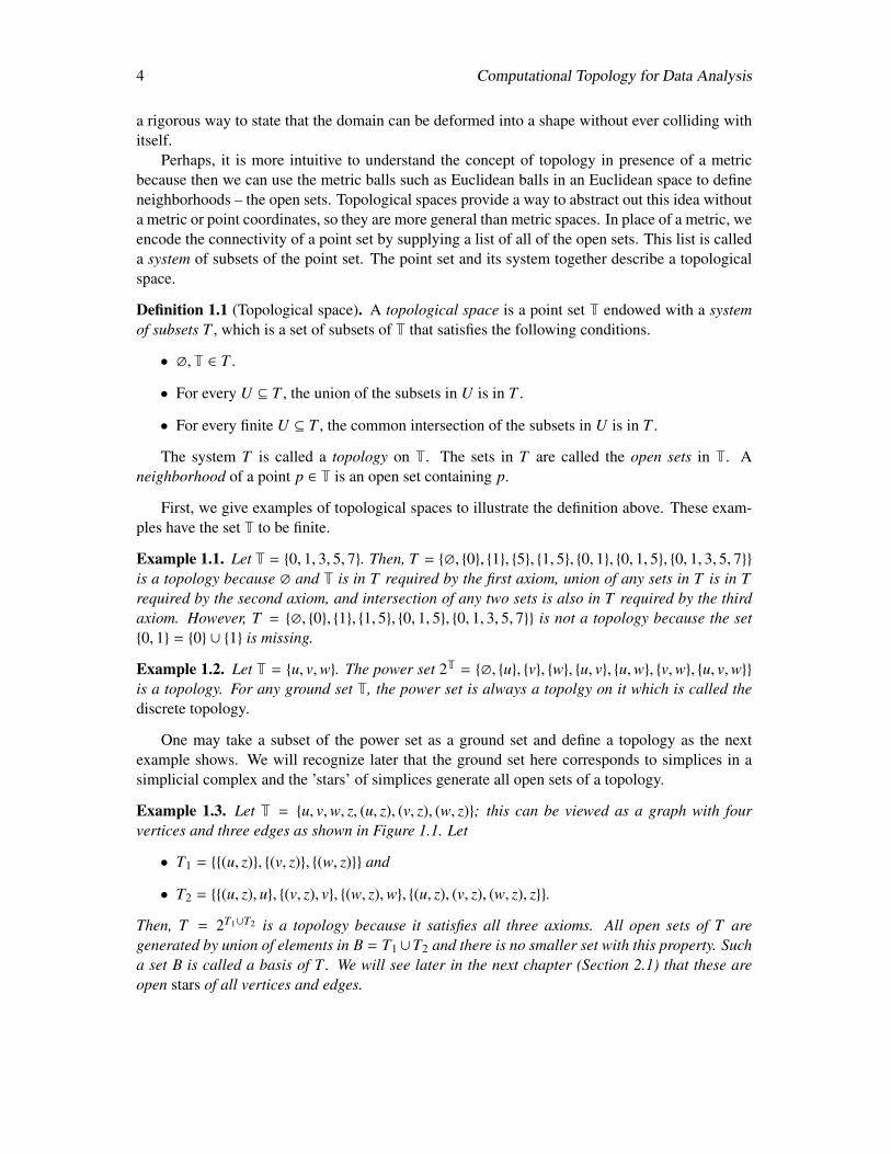
Example 1.3. Let T = u, v,w, z, (u, z), (v, z), (w, z); this can be viewed as a graph with fourvertices and three edges as shown in Figure 1.1. Let
• T1 = (u, z), (v, z), (w, z) and
• T2 = (u, z), u, (v, z), v, (w, z),w, (u, z), (v, z), (w, z), z.
Then, T = 2T1∪T2 is a topology because it satisfies all three axioms. All open sets of T aregenerated by union of elements in B = T1∪T2 and there is no smaller set with this property. Sucha set B is called a basis of T . We will see later in the next chapter (Section 2.1) that these areopen stars of all vertices and edges.

Computational Topology for Data Analysis 5
z
uv
w
z
uv
w
z
uv
w
(a) (b) (c)
Figure 1.1: Example 3: (a) a graph as a topological space, stars of the vertices and edges as opensets, (b) a closed cover with three elements, (c) an open cover with four elements.
We now present some more definitions that will be useful later.
Definition 1.2 (Closure; Closed sets). A set Q is closed if its complement T \ Q is open. Theclosure Cl Q of a set Q ⊆ T is the smallest closed set containing Q.
In Example 1.1, the set 3, 5, 7 is closed because its complement 0, 1 in T is open. Theclosure of the open set 0 is 0, 3, 7 because it is the smallest closed set (complement of open set1, 5) containing 0. In Example 1.2, all sets are both open and closed. In Example 1.3, the setu, z, (u, z) is closed, but the set z, (u, z) is neither open nor closed. Interestingly, observe thatz is closed. The closure of the open set u, (u, z) is u, z, (u, z). In all examples, the sets ∅ andT are both open and closed.
Definition 1.3. Given a topological space (T,T ), the interior Int A of a subset A ⊆ T is the unionof all open subsets of A. The boundary of A is Bd A = Cl A \ Int A.
The interior of the set 3, 5, 7 in Example 1.1 is 5 and its boundary is 3, 7.
Definition 1.4 (Subspace topology). For every point set U ⊆ T, the topology T induces a subspacetopology on U, namely the system of open subsets U = P∩U : P ∈ T . The point set U endowedwith the system U is said to be a topological subspace of T.
In Example 1.1, consider the subset U = 1, 5, 7. It has the subspace topology
U = ∅, 1, 5, 1, 5, 1, 5, 7.
In Example 1.3, the subset U = u, (u, z), (v, z) has the subspace topology
∅, u, (u, z), (u, z), (v, z), (u, z), (v, z), u, (u, z), (v, z).
Definition 1.5 (Connected). A topological space (T,T ) is disconnected if there are two disjointnon-empty open sets U,V ∈ T so that T = U ∪ V . A topological space is connected if its notdisconnected.
6 Computational Topology for Data Analysis
The topological space in Example 1.1 is connected. However, the topological subspace (Def-inition 1.4) induced by the subset 0, 1, 5 is disconnected because it can be obtained as the unionof two disjoint open sets 0, 1 and 5. The topological space in Example 1.3 is also connected,but the subspace induced by the subset (u, z), (v, z), (w, z) is disconnected.
Definition 1.6 (Cover; Compact). An open (closed) cover of a topological space (T,T ) is a col-lection C of open (closed) sets so that T =
⋃c∈C c. The topological space (T,T ) is called compact
if every open cover C of it has a finite subcover, that is, there exists C′ ⊆ C such that T =⋃
c∈C′ cand C′ is finite.
In Figure 1.1(b), the cover consisting of u, z, (u, z), v, z, (v, z), w, z, (w, z) is a closed coverwhereas the cover consisting of u, (u, z), v, (v, z), w, (w, z), z, (u, z), (v, z), (w.z) in Figure 1.1(c)is an open cover. Any topological space with finite point set T is compact because all of its cov-ers are finite. Thus, all topological spaces in the discussed examples are compact. We will seeexample of non-compact topological spaces where the ground set is infinite.
In the above examples, the ground set T is finite. It can be infinite in general and topologymay have uncountably infinitely many open sets containing uncountably infinitely many points.
Next, we introduce the concept of quotient topology. Given a space (T,T ) and an equivalencerelation ∼ on elements in T, one can define a topology induced by the original topology T on thequotient set T/ ∼ whose elements are equivalence classes [x] for every point x ∈ T.
Definition 1.7 (Quotient topology). Given a topological space (T,T ) and an equivalence relation∼ defined on the set T, a quotient space (S, S ) induced by ∼ is defined by the set S = T/ ∼ andthe quotient topology S where
S :=U ⊆ S | x : [x] ∈ U ∈ T
.
We will see the use of quotient topology in Chapter 7 when we study Reeb graphs.Infinite topological spaces may seem baffling from a computational point of view, because
they may have uncountably infinitely many open sets containing uncountably infinitely manypoints. The easiest way to define such a topological space is to inherit the open sets from a metricspace. A topology on a metric space excludes information that is not topologically essential. Forinstance, the act of stretching a rubber sheet changes the distances between points and therebychanges the metric, but it does not change the open sets or the topology of the rubber sheet. Inthe next section, we construct such a topology on a metric space and examine it from the conceptof limit points.
1.2 Metric space topology
Metric spaces are a special type of topological space commonly encountered in practice. Sucha space admits a metric that specifies the scalar distance between every pair of points satisfyingcertain axioms.
Definition 1.8 (Metric space). A metric space is a pair (T, d) where T is a set and d is a distancefunction d : T × T→ R satisfying the following properties:

Computational Topology for Data Analysis 7
• d(p, q) = 0 if and only if p = q ∀p ∈ T;
• d(p, q) = d(q, p) ∀p, q ∈ T;
• d(p, q) ≤ d(p, r) + d(r, q) ∀p, q, r ∈ T.
It can be shown that three axioms above imply that d(p, q) ≥ 0 for every pair p, q ∈ T. Ina metric space T, an open metric ball with center c and radius r is defined to be the point setBo(c, r) = p ∈ T : d(p, c) < r. Metric balls define a topology on a metric space.
Definition 1.9 (Metric space topology). Given a metric space T, all metric balls Bo(c, r) | c ∈T and 0 < r ≤ ∞ and their union constituting the open sets define a topology on T.
All definitions for general topological spaces apply to metric spaces with the above definedtopology. However, we give alternative definitions using the concept of limit points which maybe more intuitive.
As we mentioned already, the heart of topology is the question of what it means for a setof points to be connected. After all, two distinct points cannot be adjacent to each other; theycan only be connected to another by passing through an uncountably many intermediate points.The idea of limit points helps express this concept more concretely, specifically in case of metricspaces.
We use the notation d(·, ·) to express minimum distances between point sets P,Q ⊆ T,
d(p,Q) = infd(p, q) : q ∈ Q and
d(P,Q) = infd(p, q) : p ∈ P, q ∈ Q.
Definition 1.10 (Limit point). Let Q ⊆ T be a point set. A point p ∈ T is a limit point of Q, alsoknown as an accumulation point of Q, if for every real number ε > 0, however tiny, Q contains apoint q , p such that that d(p, q) < ε.
In other words, there is an infinite sequence of points in Q that gets successively closer andcloser to p—without actually being p—and gets arbitrarily close. Stated succinctly, d(p,Q\p) =
0. Observe that it doesn’t matter whether p ∈ Q or not.To see the parallel between definitions given in this subsection and the definitions given be-
fore, it is instructive to define limit points also for general topological spaces. In particular, apoint p ∈ T is a limit point of a set Q ⊆ T if every open set containing p intersect Q.
Definition 1.11 (Connected). A point set Q ⊆ T is called disconnected if Q can be partitionedinto two disjoint non-empty sets U and V so that there is no point in U that is a limit point of V ,and no point in V that is a limit point of U. (See the left in Figure 1.2 for an example.) If no suchpartition exists, Q is connected, like the point set at right in Figure 1.2.
We can also distinguish between closed and open point sets using the concept of limit points.Informally, a triangle in the plane is closed if it contains all the points on its edges, and open if itexcludes all the points on its edges, as illustrated in Figure 1.3. The idea can be formally extendedto any point set.
8 Computational Topology for Data Analysis
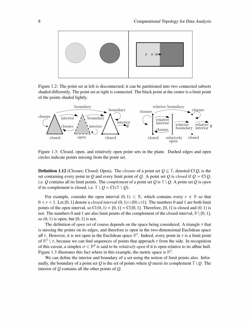
Figure 1.2: The point set at left is disconnected; it can be partitioned into two connected subsetsshaded differently. The point set at right is connected. The black point at the center is a limit pointof the points shaded lightly.
interior
closure
closed open closed
boundary
interiorinterior
∅
closure
boundaryboundary
closed relatively closedopen
relativeinterior
closurerelativeboundary
closurerelative boundary
relativeinterior ∅
closure
Figure 1.3: Closed, open, and relatively open point sets in the plane. Dashed edges and opencircles indicate points missing from the point set.
Definition 1.12 (Closure; Closed; Open). The closure of a point set Q ⊆ T, denoted Cl Q, is theset containing every point in Q and every limit point of Q. A point set Q is closed if Q = Cl Q,i.e. Q contains all its limit points. The complement of a point set Q is T \Q. A point set Q is openif its complement is closed, i.e. T \ Q = Cl (T \ Q).
For example, consider the open interval (0, 1) ⊂ R, which contains every r ∈ R so that0 < r < 1. Let [0, 1] denote a closed interval (0, 1)∪ 0 ∪ 1. The numbers 0 and 1 are both limitpoints of the open interval, so Cl (0, 1) = [0, 1] = Cl [0, 1]. Therefore, [0, 1] is closed and (0, 1) isnot. The numbers 0 and 1 are also limit points of the complement of the closed interval, R \ [0, 1],so (0, 1) is open, but [0, 1] is not.
The definition of open set of course depends on the space being considered. A triangle τ thatis missing the points on its edges, and therefore is open in the two-dimensional Euclidean spaceaff τ. However, it is not open in the Euclidean space R3. Indeed, every point in τ is a limit pointof R3 \ τ, because we can find sequences of points that approach τ from the side. In recognitionof this caveat, a simplex σ ⊂ Rd is said to be relatively open if it is open relative to its affine hull.Figure 1.3 illustrates this fact where in this example, the metric space is R2.
We can define the interior and boundary of a set using the notion of limit points also. Infor-mally, the boundary of a point set Q is the set of points where Q meets its complement T \Q. Theinterior of Q contains all the other points of Q.
Computational Topology for Data Analysis 9
Definition 1.13 (Boundary; Interior). The boundary of a point set Q in a metric space T, denotedBd Q, is the intersection of the closures of Q and its complement; i.e. Bd Q = Cl Q ∩ Cl (T \ Q).The interior of Q, denoted Int Q, is Q \ Bd Q = Q \ Cl (T \ Q).
For example, Bd [0, 1] = 0, 1 = Bd (0, 1) and Int [0, 1] = (0, 1) = Int (0, 1). The boundaryof a triangle (closed or open) in the Euclidean plane is the union of the triangle’s three edges, andits interior is an open triangle, illustrated in Figure 1.3. The terms boundary and interior havesimilar subtlety as open sets: the boundary of a triangle embedded in R3 is the whole triangle,and its interior is the empty set. However, relative to its affine hull, its interior and boundary aredefined exactly as in the case of triangles embedded in the Euclidean plane. Interested readerscan draw the analogy between this observation and the definition of interior and boundary of amanifold that appear later in Definition 1.23.
We have seen a definition of compactness of a point set in a topological space (Definition 1.6).We define it differently here for the metric space. It can be shown that the two definitions areequivalent.
Definition 1.14 (Bounded; Compact). The diameter of a point set Q is supp,q∈Q d(p, q). The setQ is bounded if its diameter is finite, and is unbounded otherwise. A point set Q in a metric spaceis compact if it is closed and bounded.
In the Euclidean space Rd we can use the standard Euclidean distance as the choice of metric.On the surface of the coffee mug, we could choose the Euclidean distance too; alternatively, wecould choose the geodesic distance, namely the length of the shortest path from p to q on themug’s surface.
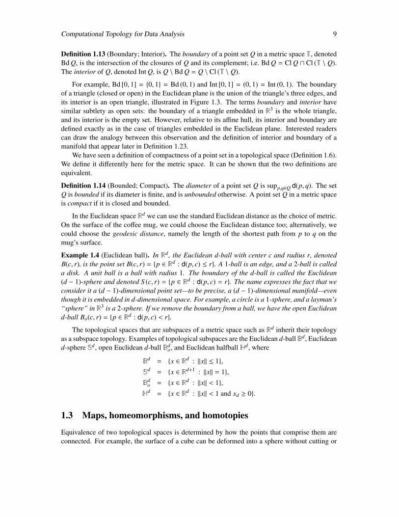
Example 1.4 (Euclidean ball). In Rd, the Euclidean d-ball with center c and radius r, denotedB(c, r), is the point set B(c, r) = p ∈ Rd : d(p, c) ≤ r. A 1-ball is an edge, and a 2-ball is calleda disk. A unit ball is a ball with radius 1. The boundary of the d-ball is called the Euclidean(d − 1)-sphere and denoted S (c, r) = p ∈ Rd : d(p, c) = r. The name expresses the fact that weconsider it a (d − 1)-dimensional point set—to be precise, a (d − 1)-dimensional manifold—eventhough it is embedded in d-dimensional space. For example, a circle is a 1-sphere, and a layman’s“sphere” in R3 is a 2-sphere. If we remove the boundary from a ball, we have the open Euclideand-ball Bo(c, r) = p ∈ Rd : d(p, c) < r.
The topological spaces that are subspaces of a metric space such as Rd inherit their topologyas a subspace topology. Examples of topological subspaces are the Euclidean d-ball Bd, Euclideand-sphere Sd, open Euclidean d-ball Bd
o, and Euclidean halfball Hd, where
Bd = x ∈ Rd : ‖x‖ ≤ 1,
Sd = x ∈ Rd+1 : ‖x‖ = 1,
Bdo = x ∈ Rd : ‖x‖ < 1,
Hd = x ∈ Rd : ‖x‖ < 1 and xd ≥ 0.
1.3 Maps, homeomorphisms, and homotopies
Equivalence of two topological spaces is determined by how the points that comprise them areconnected. For example, the surface of a cube can be deformed into a sphere without cutting or
10 Computational Topology for Data Analysis
gluing it because they are connected the same way. They have the same topology. This notionof topological equivalence can be formalized via functions that send the points of one space topoints of the other while preserving the connectivity.
This preservation of connectivity is achieved by preserving the open sets. A function from onespace to another that preserves the open sets is called a continuous function or a map. Continuityis a vehicle to define topological equivalence, because a continuous function can send many pointsto a single point in the target space, or send no points to a given point in the target space. If theformer does not happen, that is, when the function is injective, we call it an embedding of thedomain into the target space. True equivalence is given by a homeomorphism, a bijective functionfrom one space to another which has continuity as well as a continuous inverse. This ensures thatopen sets are preserved in both directions.
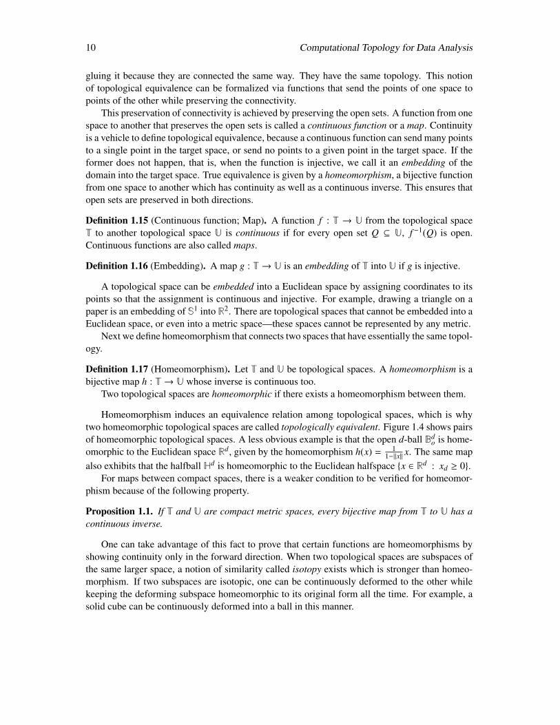
Definition 1.15 (Continuous function; Map). A function f : T → U from the topological spaceT to another topological space U is continuous if for every open set Q ⊆ U, f −1(Q) is open.Continuous functions are also called maps.
Definition 1.16 (Embedding). A map g : T→ U is an embedding of T into U if g is injective.
A topological space can be embedded into a Euclidean space by assigning coordinates to itspoints so that the assignment is continuous and injective. For example, drawing a triangle on apaper is an embedding of S1 into R2. There are topological spaces that cannot be embedded into aEuclidean space, or even into a metric space—these spaces cannot be represented by any metric.
Next we define homeomorphism that connects two spaces that have essentially the same topol-ogy.
Definition 1.17 (Homeomorphism). Let T and U be topological spaces. A homeomorphism is abijective map h : T→ U whose inverse is continuous too.
Two topological spaces are homeomorphic if there exists a homeomorphism between them.
Homeomorphism induces an equivalence relation among topological spaces, which is whytwo homeomorphic topological spaces are called topologically equivalent. Figure 1.4 shows pairsof homeomorphic topological spaces. A less obvious example is that the open d-ball Bd
o is home-omorphic to the Euclidean space Rd, given by the homeomorphism h(x) = 1
1−‖x‖ x. The same mapalso exhibits that the halfball Hd is homeomorphic to the Euclidean halfspace x ∈ Rd : xd ≥ 0.
For maps between compact spaces, there is a weaker condition to be verified for homeomor-phism because of the following property.
Proposition 1.1. If T and U are compact metric spaces, every bijective map from T to U has acontinuous inverse.
One can take advantage of this fact to prove that certain functions are homeomorphisms byshowing continuity only in the forward direction. When two topological spaces are subspaces ofthe same larger space, a notion of similarity called isotopy exists which is stronger than homeo-morphism. If two subspaces are isotopic, one can be continuously deformed to the other whilekeeping the deforming subspace homeomorphic to its original form all the time. For example, asolid cube can be continuously deformed into a ball in this manner.
Computational Topology for Data Analysis 11
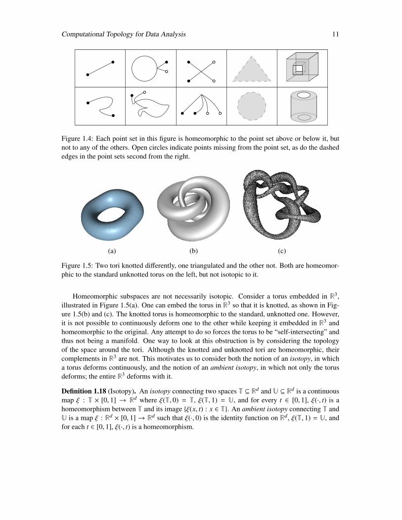
Figure 1.4: Each point set in this figure is homeomorphic to the point set above or below it, butnot to any of the others. Open circles indicate points missing from the point set, as do the dashededges in the point sets second from the right.
(a) (b) (c)
Figure 1.5: Two tori knotted differently, one triangulated and the other not. Both are homeomor-phic to the standard unknotted torus on the left, but not isotopic to it.
Homeomorphic subspaces are not necessarily isotopic. Consider a torus embedded in R3,illustrated in Figure 1.5(a). One can embed the torus in R3 so that it is knotted, as shown in Fig-ure 1.5(b) and (c). The knotted torus is homeomorphic to the standard, unknotted one. However,it is not possible to continuously deform one to the other while keeping it embedded in R3 andhomeomorphic to the original. Any attempt to do so forces the torus to be “self-intersecting” andthus not being a manifold. One way to look at this obstruction is by considering the topologyof the space around the tori. Although the knotted and unknotted tori are homeomorphic, theircomplements in R3 are not. This motivates us to consider both the notion of an isotopy, in whicha torus deforms continuously, and the notion of an ambient isotopy, in which not only the torusdeforms; the entire R3 deforms with it.
Definition 1.18 (Isotopy). An isotopy connecting two spaces T ⊆ Rd and U ⊆ Rd is a continuousmap ξ : T × [0, 1] → Rd where ξ(T, 0) = T, ξ(T, 1) = U, and for every t ∈ [0, 1], ξ(·, t) is ahomeomorphism between T and its image ξ(x, t) : x ∈ T. An ambient isotopy connecting T andU is a map ξ : Rd × [0, 1] → Rd such that ξ(·, 0) is the identity function on Rd, ξ(T, 1) = U, andfor each t ∈ [0, 1], ξ(·, t) is a homeomorphism.
12 Computational Topology for Data Analysis
For an example, consider the map
ξ(x, t) =1 − (1 − t)‖x‖
1 − ‖x‖x
that sends the open d-ball Bdo to itself if t = 0, and to the Euclidean space Rd if t = 1. The
parameter t plays the role of time, that is, ξ(Bdo, t) deforms continuously from a ball at time zero
to Rd at time one. Thus, there is an isotopy between the open d-ball and Rd.Every ambient isotopy becomes an isotopy if its domain is restricted from Rd × [0, 1] to
T × [0, 1]. It is known that if there is an isotopy between two subspaces, then there exists anambient isotopy between them. Hence, the two notions are equivalent.
There is another notion of similarity among topological spaces that is weaker than homeo-morphism, called homotopy equivalence. It relates spaces that can be continuously deformed toone another but the transformation may not preserve homeomorphism. For example, a ball canshrink to a point, which is not homeomorphic to it because a bijective function from an infinitepoint set to a single point cannot exist. However, homotopy preserves some form of connectivity,such as the number of connected components, holes, and/or voids. This is why a coffee cup ishomotopy equivalent to a circle, but not to a ball or a point.
To get to homotopy equivalence, we first need the concept of homotopies, which are isotopiessans the homeomorphism.
Definition 1.19 (Homotopy). Let g : X → U and h : X → U be maps. A homotopy is a mapH : X × [0, 1] → U such that H(·, 0) = g and H(·, 1) = h. Two maps are homotopic if there is ahomotopy connecting them.
For example, let g : B3 → R3 be the identity map on a unit ball and h : B3 → R3 be the mapsending every point in the ball to the origin. The fact that g and h are homotopic is demonstratedby the homotopy H(x, t) = (1− t) ·g(x). Observe that H(B3, t) deforms continuously a ball at timezero to a point at time one. A key property of a homotopy is that, as H is continuous, at everytime t the map H(·, t) remains continuous.
For developing more intuition, consider two maps that are not homotopic. Let g : S1 → S1
be the identity map from the circle to itself, and let h : S1 → S1 map every point on the circle toa single point p ∈ S1. Although apparently it seems that we can contract a circle to a point, thatview is misleading because the map H is required to map every point on the circle at every timeto a point on the circle. The contraction of the circle to a point is possible only if we break thecontinuity, say by cutting or gluing the circle somewhere.
Observe that a homeomorphism relates two topological spaces T and U whereas a homotopyor an isotopy (which is a special kind of homotopy) relates two maps, thereby indirectly estab-lishing a relationship between two subspaces g(X) ⊆ U and h(X) ⊆ U. That relationship is notnecessarily an equivalent one, but the following is.
Definition 1.20 (Homotopy equivalent). Two topological spaces T and U are homotopy equivalentif there exist maps g : T → U and h : U → T such that h g is homotopic to the identity mapιT : T→ T and g h is homotopic to the identity map ιU : U→ U.
Homotopy equivalence is indeed an equivalence relation, that is, if A, B and B,C are homo-topy equivalent spaces, so are the pairs A,C. Homeomorphic spaces necessarily have the same
Computational Topology for Data Analysis 13
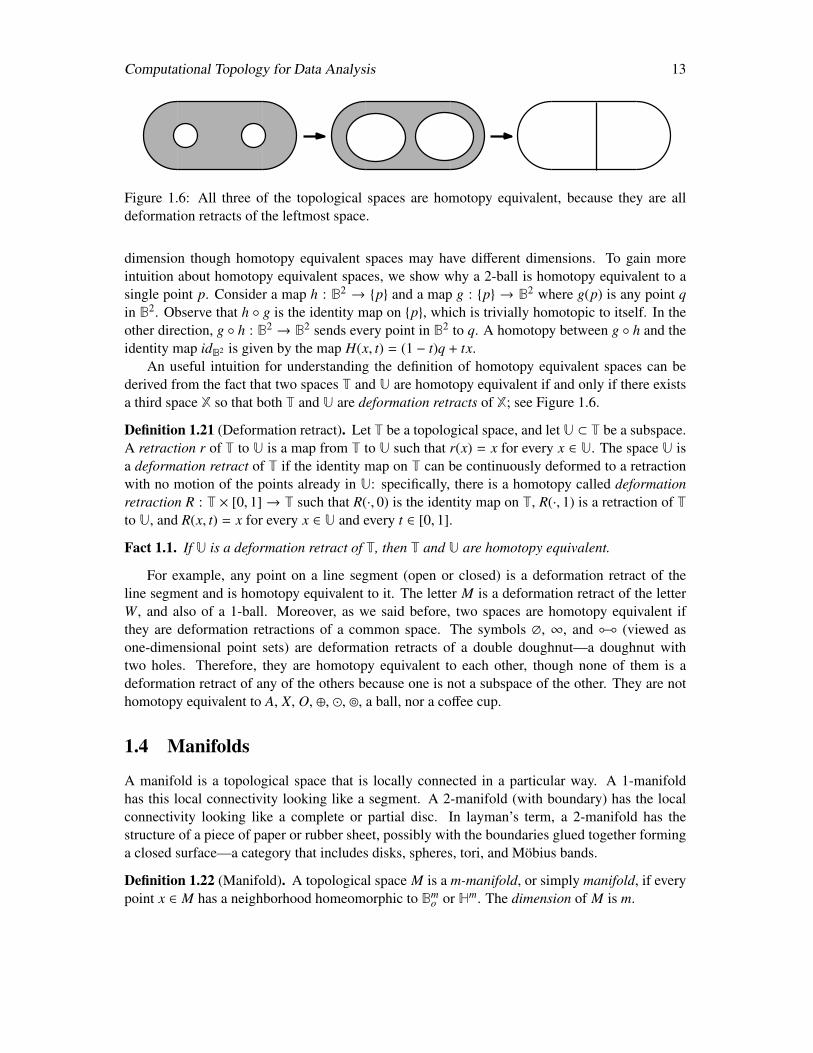
Figure 1.6: All three of the topological spaces are homotopy equivalent, because they are alldeformation retracts of the leftmost space.
dimension though homotopy equivalent spaces may have different dimensions. To gain moreintuition about homotopy equivalent spaces, we show why a 2-ball is homotopy equivalent to asingle point p. Consider a map h : B2 → p and a map g : p → B2 where g(p) is any point qin B2. Observe that h g is the identity map on p, which is trivially homotopic to itself. In theother direction, g h : B2 → B2 sends every point in B2 to q. A homotopy between g h and theidentity map idB2 is given by the map H(x, t) = (1 − t)q + tx.
An useful intuition for understanding the definition of homotopy equivalent spaces can bederived from the fact that two spaces T and U are homotopy equivalent if and only if there existsa third space X so that both T and U are deformation retracts of X; see Figure 1.6.
Definition 1.21 (Deformation retract). Let T be a topological space, and let U ⊂ T be a subspace.A retraction r of T to U is a map from T to U such that r(x) = x for every x ∈ U. The space U isa deformation retract of T if the identity map on T can be continuously deformed to a retractionwith no motion of the points already in U: specifically, there is a homotopy called deformationretraction R : T × [0, 1] → T such that R(·, 0) is the identity map on T, R(·, 1) is a retraction of Tto U, and R(x, t) = x for every x ∈ U and every t ∈ [0, 1].
Fact 1.1. If U is a deformation retract of T, then T and U are homotopy equivalent.
For example, any point on a line segment (open or closed) is a deformation retract of theline segment and is homotopy equivalent to it. The letter M is a deformation retract of the letterW, and also of a 1-ball. Moreover, as we said before, two spaces are homotopy equivalent ifthey are deformation retractions of a common space. The symbols ∅, ∞, and (viewed asone-dimensional point sets) are deformation retracts of a double doughnut—a doughnut withtwo holes. Therefore, they are homotopy equivalent to each other, though none of them is adeformation retract of any of the others because one is not a subspace of the other. They are nothomotopy equivalent to A, X, O, ⊕, , , a ball, nor a coffee cup.
1.4 Manifolds
A manifold is a topological space that is locally connected in a particular way. A 1-manifoldhas this local connectivity looking like a segment. A 2-manifold (with boundary) has the localconnectivity looking like a complete or partial disc. In layman’s term, a 2-manifold has thestructure of a piece of paper or rubber sheet, possibly with the boundaries glued together forminga closed surface—a category that includes disks, spheres, tori, and Möbius bands.
Definition 1.22 (Manifold). A topological space M is a m-manifold, or simply manifold, if everypoint x ∈ M has a neighborhood homeomorphic to Bm
o or Hm. The dimension of M is m.

14 Computational Topology for Data Analysis
Every manifold can be partitioned into boundary and interior points. Observe that these wordsmean very different things for a manifold than they do for a metric space or topological space.
Definition 1.23 (Boundary; Interior). The interior Int M of a m-manifold M is the set of points inM that have a neighborhood homeomorphic to Bm
o . The boundary Bd M of M is the set of pointsM \ Int M. The boundary Bd M, if not empty, consists of the points that have a neighborhoodhomeomorphic to Hm. If Bd M is the empty set, we say that M is without boundary.
A single point, a 0-ball, is a 0-manifold without boundary according to this definition. Theclosed disk B2 is a 2-manifold whose interior is the open disk B2
o and whose boundary is the circleS1. The open disk B2
o is a 2-manifold whose interior is B2o and whose boundary is the empty set.
This highlights an important difference between Definitions 1.13 and 1.23 of “boundary”: whenB2
o is viewed as a point set in the space R2, its boundary is S1 according to Definition 1.13; butviewed as a manifold, its boundary is empty according to Definition 1.23. The boundary of amanifold is always included in the manifold.
The open disk B2o, the Euclidean space R2, the sphere S2, and the torus are all connected 2-
manifolds without boundary. The first two are homeomorphic to each other, but the last two arenot. The sphere and the torus in R3 are compact (bounded and closed with respect to R3) whereasB2
o and R2 are not.A d-manifold, d ≥ 2 can have orientations whose formal definition we skip here. Informally,
we say that a 2-manifold M is non-orientable if, starting from a point p, one can walk on oneside of M and end up on the opposite side of M upon returning to p. Otherwise, M is orientable.Spheres and balls are orientable, whereas the Möbius band in Figure 1.7 (a) is a non-orientable2-manifold with boundary.
(a) (b) (c) (d)
Figure 1.7: (a) A Möbius band. (b) Removal of the red and green loops opens up the torus into atopological disk. (c) A double torus: every surface without boundary in R3 resembles a sphere ora conjunction of one or more tori. (d) Double torus knotted.
A surface is a 2-manifold that is a subspace of Rd. Any compact surface without boundary inR3 is an orientable 2-manifold. To be non-orientable, a compact surface must have a nonemptyboundary (like the Möbius band) or be embedded in a 4- or higher-dimensional Euclidean space.
A surface can sometimes be disconnected by removing one or more loops (connected 1-manifolds without boundary) from it. The genus of an orientable and compact surface without
Computational Topology for Data Analysis 15
boundary is g if 2g is the maximum number of loops that can be removed from the surface withoutdisconnecting it; here the loops are permitted to intersect each other. For example, the sphere hasgenus zero as every loop cuts it into two discs. The torus has genus one: a circular cut aroundits neck and a second circular cut around its circumference, illustrated in Figure 1.7(b), allow itto unfold into a topological disk. A third loop would cut it into two pieces. Figure 1.7(c) and (d)each shows a 2-manifold without boundary of genus 2. Although a high-genus surface can havea very complex shape, all compact 2-manifolds in R3 that have the same genus and no boundaryare homeomorphic to each other.
1.4.1 Smooth manifolds
A purely topological manifold has no geometry. But if we embed it in a Euclidean space, it couldappear smooth or wrinkled. We now introduce a “geometric” manifold by imposing a differentialstructure on it. For the rest of this chapter, we focus on only manifolds without boundary.
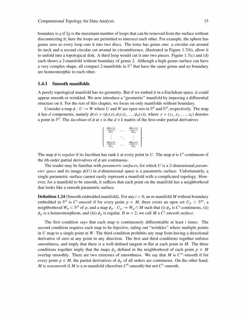
Consider a map φ : U → W where U and W are open sets in Rk and Rd, respectively. The mapφ has d components, namely φ(x) = (φ1(x), φ2(x), . . . , φd(x)), where x = (x1, x2, . . . , xk) denotesa point in Rk. The Jacobian of φ at x is the d × k matrix of the first-order partial derivatives
∂φ1(x)∂x1
. . .∂φ1(x)∂xk
.... . .
...∂φd(x)∂x1
. . .∂φd(x)∂xk
.The map φ is regular if its Jacobian has rank k at every point in U. The map φ is Ci-continuous ifthe ith-order partial derivatives of φ are continuous.
The reader may be familiar with parametric surfaces, for which U is a 2-dimensional param-eter space and its image φ(U) in d-dimensional space is a parametric surface. Unfortunately, asingle parametric surface cannot easily represent a manifold with a complicated topology. How-ever, for a manifold to be smooth, it suffices that each point on the manifold has a neighborhoodthat looks like a smooth parametric surface.
Definition 1.24 (Smooth embedded manifold). For any i > 0, an m-manifold M without boundaryembedded in Rd is Ci-smooth if for every point p ∈ M, there exists an open set Up ⊂ Rm, aneighborhood Wp ⊂ Rd of p, and a map φp : Up → Wp ∩M such that (i) φp is Ci-continuous, (ii)φp is a homeomorphism, and (iii) φp is regular. If m = 2, we call M a Ci-smooth surface.
The first condition says that each map is continuously differentiable at least i times. Thesecond condition requires each map to be bijective, ruling out “wrinkles” where multiple pointsin U map to a single point in W. The third condition prohibits any map from having a directionalderivative of zero at any point in any direction. The first and third conditions together enforcesmoothness, and imply that there is a well-defined tangent m-flat at each point in M. The threeconditions together imply that the maps φp defined in the neighborhood of each point p ∈ Moverlap smoothly. There are two extremes of smoothness. We say that M is C∞-smooth if forevery point p ∈ M, the partial derivatives of φp of all orders are continuous. On the other hand,M is nonsmooth if M is a m-manifold (therefore C0-smooth) but not C1-smooth.
16 Computational Topology for Data Analysis
1.5 Functions on smooth manifolds
R
R
f
(a) (b)
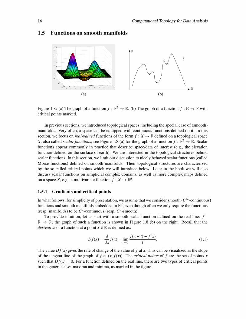
Figure 1.8: (a) The graph of a function f : R2 → R. (b) The graph of a function f : R → R withcritical points marked.
In previous sections, we introduced topological spaces, including the special case of (smooth)manifolds. Very often, a space can be equipped with continuous functions defined on it. In thissection, we focus on real-valued functions of the form f : X → R defined on a topological spaceX, also called scalar functions; see Figure 1.8 (a) for the graph of a function f : R2 → R. Scalarfunctions appear commonly in practice that describe space/data of interest (e.g., the elevationfunction defined on the surface of earth). We are interested in the topological structures behindscalar functions. In this section, we limit our discussion to nicely behaved scalar functions (calledMorse functions) defined on smooth manifolds. Their topological structures are characterizedby the so-called critical points which we will introduce below. Later in the book we will alsodiscuss scalar functions on simplicial complex domains, as well as more complex maps definedon a space X, e.g., a multivariate function f : X → Rd.
1.5.1 Gradients and critical points
In what follows, for simplicity of presentation, we assume that we consider smooth (C∞-continuous)functions and smooth manifolds embedded in Rd, even though often we only require the functions(resp. manifolds) to be C2-continuous (resp. C2-smooth).
To provide intuition, let us start with a smooth scalar function defined on the real line: f :R → R; the graph of such a function is shown in Figure 1.8 (b) on the right. Recall that thederivative of a function at a point x ∈ R is defined as:
D f (x) =ddx
f (x) = limt→0
f (x + t) − f (x)t
. (1.1)
The value D f (x) gives the rate of change of the value of f at x. This can be visualized as the slopeof the tangent line of the graph of f at (x, f (x)). The critical points of f are the set of points xsuch that D f (x) = 0. For a function defined on the real line, there are two types of critical pointsin the generic case: maxima and minima, as marked in the figure.
Computational Topology for Data Analysis 17
Now suppose we have a smooth function f : Rd → R defined on Rd. Fix an arbitrary pointx ∈ Rd. As we move a little around x within its local neighborhood, the rate of change of f differsdepending on which direction we move. This gives rise to the directional derivative Dv f (x) at xin direction (i.e., a unit vector) v ∈ Sd−1, where Sd−1 is the unit (d − 1)-sphere, defined as:
Dv f (x) = limt→0
f (x + t · v) − f (x)t
(1.2)
The gradient vector of f at x ∈ Rd intuitively captures the direction of steepest increase of functionf . More precisely, we have:
Definition 1.25 (Gradient for functions on Rd). Given a smooth function f : Rd → R, the gradientvector field ∇ f : Rd → Rd is defined as follows: for any x ∈ Rd,
∇ f (x) =[ ∂ f∂x1
(x),∂ f∂x2
(x), · · ·∂ f∂xd
(x)]T , (1.3)
where (x1, x2, . . . , xd) represents an orthonormal coordinate system for Rd. The vector ∇ f (x) ∈ Rd
is called the gradient vector of f at x. A point x ∈ Rd is a critical point if ∇ f (x) = [0 0 · · · 0]T ;otherwise, x is regular.
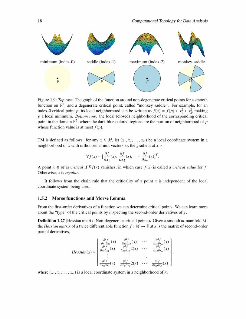
Observe that for any v ∈ Rd, the directional derivative satisfies that Dv f (x) = 〈∇ f (x), v〉.It then follows that ∇ f (x) ∈ Rd is along the unit vector v where Dv f (x) is maximized amongthe directional derivatives in all unit directions around x; and its magnitude ‖∇ f (x)‖ equals thevalue of this maximum directional derivative. The critical points of f are those points wherethe directional derivative vanishes in all directions – locally, the rate of change for f is zero nomatter which direction one deviates from x. See Figure 1.9 for the three types of critical points,minimum, saddle point, and maximum, for a generic smooth function f : R2 → R.
Finally, we can extend the above definitions of gradients and critical points to a smooth func-tion f : M → R defined on a smooth Riemannian m-manifold M. Here, a Riemannian manifoldis a manifold equipped with a Riemannian metric, which is a smoothly varying inner product de-fined on the tangent spaces. This allows the measurements of length so as to define gradient. At apoint x ∈ M, denote the tangent space of M at x by TMx, which is the m-dimensional vector spaceconsisting of all tangent vectors of M at x. For example, TMx is a m-dimensional linear space Rm
for a m-dimensional manifold M embedded in the Euclidean space Rd, with Riemannian metric(inner product in the tangent space) induced from Rd.
The gradient ∇ f is a vector field on M, that is, ∇ f : M → TM maps every point x ∈ M toa vector ∇ f (x) ∈ TMx in the tangent space of M at x. Similar to the case for a function definedon Rd, the gradient vector field ∇ f satisfies that for any x ∈ M and v ∈ TMx, 〈∇ f (x), v〉 givesrise to the directional derivative Dv f (x) of f in direction v, and ∇ f (x) still specifies the directionof steepest increase of f along all directions in TMx with its magnitude being the maximum rateof change. More formally, we have the following definition, analogous to Definition 1.25 for thecase of a smooth function on Rd.
Definition 1.26 (Gradient vector field; Critical points). Given a smooth function f : M → Rdefined on a smooth m-dimensional Riemannian manifold M, the gradient vector field ∇ f : M →
18 Computational Topology for Data Analysis
minimum (index-0) saddle (index-1) maximum (index-2) monkey-saddle
p p p p
Figure 1.9: Top row: The graph of the function around non-degenerate critical points for a smoothfunction on R2, and a degenerate critical point, called “monkey saddle”. For example, for anindex-0 critical point p, its local neighborhood can be written as f (x) = f (p) + x2
1 + x22, making
p a local minimum. Bottom row: the local (closed) neighborhood of the corresponding criticalpoint in the domain R2, where the dark blue colored regions are the portion of neighborhood of pwhose function value is at most f (p).
TM is defined as follows: for any x ∈ M, let (x1, x2, . . . , xm) be a local coordinate system in aneighborhood of x with orthonormal unit vectors xi, the gradient at x is
∇ f (x) =[ ∂ f∂x1
(x),∂ f∂x2
(x), · · ·∂ f∂xm
(x)]T .
A point x ∈ M is critical if ∇ f (x) vanishes, in which case f (x) is called a critical value for f .Otherwise, x is regular.
It follows from the chain rule that the criticality of a point x is independent of the localcoordinate system being used.
1.5.2 Morse functions and Morse Lemma
From the first-order derivatives of a function we can determine critical points. We can learn moreabout the “type" of the critical points by inspecting the second-order derivatives of f .
Definition 1.27 (Hessian matrix; Non-degenerate critical points). Given a smooth m-manifold M,the Hessian matrix of a twice differentiable function f : M → R at x is the matrix of second-orderpartial derivatives,
Hessian(x) =
∂2 f∂x1∂x1
(x) ∂2 f∂x1∂x2
(x) · · ·∂2 f
∂x1∂xm(x)
∂2 f∂x2∂x1
(x) ∂2 f∂x2∂x2
2(x) · · ·∂2 f
∂x2∂xm(x)
......
. . ....
∂2 f∂xm∂x1
(x) ∂2 f∂xm∂x2
2(x) · · · ∂2 f∂xm∂xm
(x)
,
where (x1, x2, . . . , xm) is a local coordinate system in a neighborhood of x.
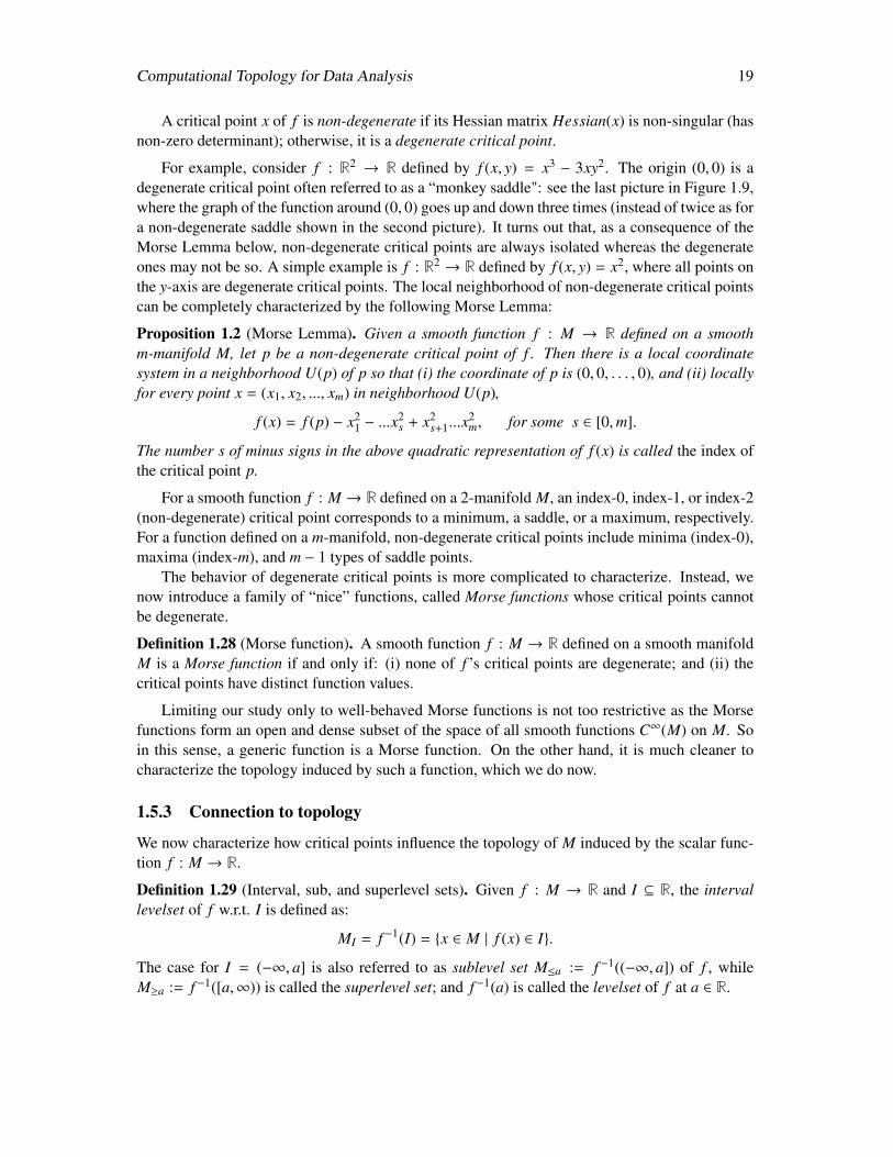
Computational Topology for Data Analysis 19
A critical point x of f is non-degenerate if its Hessian matrix Hessian(x) is non-singular (hasnon-zero determinant); otherwise, it is a degenerate critical point.
For example, consider f : R2 → R defined by f (x, y) = x3 − 3xy2. The origin (0, 0) is adegenerate critical point often referred to as a “monkey saddle": see the last picture in Figure 1.9,where the graph of the function around (0, 0) goes up and down three times (instead of twice as fora non-degenerate saddle shown in the second picture). It turns out that, as a consequence of theMorse Lemma below, non-degenerate critical points are always isolated whereas the degenerateones may not be so. A simple example is f : R2 → R defined by f (x, y) = x2, where all points onthe y-axis are degenerate critical points. The local neighborhood of non-degenerate critical pointscan be completely characterized by the following Morse Lemma:
Proposition 1.2 (Morse Lemma). Given a smooth function f : M → R defined on a smoothm-manifold M, let p be a non-degenerate critical point of f . Then there is a local coordinatesystem in a neighborhood U(p) of p so that (i) the coordinate of p is (0, 0, . . . , 0), and (ii) locallyfor every point x = (x1, x2, ..., xm) in neighborhood U(p),
f (x) = f (p) − x21 − ...x
2s + x2
s+1...x2m, for some s ∈ [0,m].
The number s of minus signs in the above quadratic representation of f (x) is called the index ofthe critical point p.
For a smooth function f : M → R defined on a 2-manifold M, an index-0, index-1, or index-2(non-degenerate) critical point corresponds to a minimum, a saddle, or a maximum, respectively.For a function defined on a m-manifold, non-degenerate critical points include minima (index-0),maxima (index-m), and m − 1 types of saddle points.
The behavior of degenerate critical points is more complicated to characterize. Instead, wenow introduce a family of “nice” functions, called Morse functions whose critical points cannotbe degenerate.
Definition 1.28 (Morse function). A smooth function f : M → R defined on a smooth manifoldM is a Morse function if and only if: (i) none of f ’s critical points are degenerate; and (ii) thecritical points have distinct function values.
Limiting our study only to well-behaved Morse functions is not too restrictive as the Morsefunctions form an open and dense subset of the space of all smooth functions C∞(M) on M. Soin this sense, a generic function is a Morse function. On the other hand, it is much cleaner tocharacterize the topology induced by such a function, which we do now.
1.5.3 Connection to topology
We now characterize how critical points influence the topology of M induced by the scalar func-tion f : M → R.
Definition 1.29 (Interval, sub, and superlevel sets). Given f : M → R and I ⊆ R, the intervallevelset of f w.r.t. I is defined as:
MI = f −1(I) = x ∈ M | f (x) ∈ I.
The case for I = (−∞, a] is also referred to as sublevel set M≤a := f −1((−∞, a]) of f , whileM≥a := f −1([a,∞)) is called the superlevel set; and f −1(a) is called the levelset of f at a ∈ R.
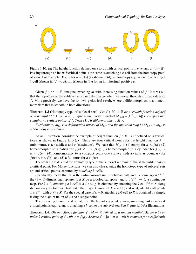
20 Computational Topology for Data Analysis
u
v
w
zf
u u
v
u
v
u
v
z
w
(a) (b) (c) (d) (e)
u
v
w
z
(f)
Figure 1.10: (a) The height function defined on a torus with critical points u, v, w, and z. (b) – (f):Passing through an index-k critical point is the same as attaching a k-cell from the homotopy pointof view. For example, M≤a+ε for a = f (v) (as shown in (d)) is homotopy equivalent to attaching a1-cell (shown in (c)) to M≤a−ε (shown in (b)) for an infinitesimal positive ε.
Given f : M → R, imagine sweeping M with increasing function values of f . It turns outthat the topology of the sublevel sets can only change when we sweep through critical values off . More precisely, we have the following classical result, where a diffeomorphism is a homeo-morphism that is smooth in both directions.
Theorem 1.3 (Homotopy type of sublevel sets). Let f : M → R be a smooth function definedon a manifold M. Given a < b, suppose the interval levelset M[a,b] = f −1([a, b]) is compact andcontains no critical points of f . Then M≤a is diffeomorphic to M≤b.
Furthermore, M≤a is a deformation retract of M≤b, and the inclusion map i : M≤a → M≤b isa homotopy equivalence.
As an illustration, consider the example of height function f : M → R defined on a verticaltorus as shown in Figure 1.10 (a). There are four critical points for the height function f , u(minimum), v,w (saddles) and z (maximum). We have that M≤a is (1) empty for a < f (u); (2)homeomorphic to a 2-disk for f (u) < a < f (v); (3) homeomorphic to a cylinder for f (v) <
a < f (w); (4) homeomorphic to a compact genus-one surface with a circle as boundary forf (w) < a < f (z); and (5) a full torus for a > f (z).
Theorem 1.3 states that the homotopy type of the sublevel set remains the same until it passesa critical point. For Morse functions, we can also characterize the homotopy type of sublevel setsaround critical points, captured by attaching k-cells.
Specifically, recall that Bk is the k-dimensional unit Euclidean ball, and its boundary is Sk−1,the (k − 1)-dimensional sphere. Let X be a topological space, and g : Sk−1 → X a continuousmap. For k > 0, attaching a k-cell to X (w.r.t. g) is obtained by attaching the k-cell Bk to X alongits boundary as follows: first, take the disjoint union of X and Bk, and next, identify all pointsx ∈ Sk−1 with g(x) ∈ X. For the special case of k = 0, attaching a 0-cell to X is obtained by simplytaking the disjoint union of X and a single point.
The following theorem states that, from the homotopy point of view, sweeping past an index-kcritical point is equivalent to attaching a k-cell to the sublevel set. See Figure 1.10 for illustrations.
Theorem 1.4. Given a Morse function f : M → R defined on a smooth manifold M, let p be anindex-k critical point of f with α = f (p). Assume f −1([α − ε, α + ε]) is compact for a sufficiently

Computational Topology for Data Analysis 21
small ε > 0 such that there is no other critical points of f contained in this interval-level set otherthan p. Then the sublevel set M≤α+ε has the same homotopy type as M≤α−ε with a k-cell attachedto its boundary Bd M≤α−ε.
Finally, we state the well-known Morse inequalities, connecting critical points with the so-called Betti numbers of the domain which we will define formally in Section 2.5. In particular,fixing a field coefficient, the i-th Betti number is the rank of the so-called i-th (singular) homologygroup of a topological space X.
Theorem 1.5 (Morse inequalities). Let f be a Morse function on a smooth compact d-manifoldM. For 0 ≤ i ≤ d, let ci denote the number of critical points of f with index i, and βi be the i-thBetti number of M. We then have:
• ci ≥ βi for all i ≥ 0; and∑d
i=0(−1)ici =∑d
i=0(−1)iβi. (weak Morse inequality)
• ci − ci−1 + ci−2 − · · · ± c0 ≥ βi − βi−1 + βi−2 · · · ± β0 for all i ≥ 0. (strong Morse inequality)
1.6 Notes and Exercises
A good source on point set topology is Munkres [242]. The concepts of various maps and man-ifolds are well described in Hatcher [186]. Books by Guillemin and Pollack [179] and Mil-nor [232, 233] are good sources for Morse theory on smooth manifolds and differential topologyin general.
Exercises
1. A space is called Hausdorff if every two disjoint point sets have disjoint open sets containingthem.
(a) Give an example of a space that is not Hausdorff.
(b) Give an example of a space that is Hausdorff.
(c) Show the above examples on the same ground set T.
2. In every space T, the point sets ∅ and T are both closed and open.
(a) Give an example of a space that has more than two sets that are both closed and open,and list all of those sets.
(b) Explain the relationship between the idea of connectedness and the number of setsthat are both closed and open.
3. A topological space T is called path connected if any two points x, y ∈ T can be joined bya path, i.e. there exists a continuous map f : [0, 1] → T of the segment [0, 1] ⊂ R onto Tso that f (0) = x and f (1) = y. Prove that a path connected space is also connected but theconverse may not be true; however, if T is finite, then the two notions are equivalent.
4. Prove that for every subset X of a metric space, Cl Cl X = Cl X. In other words, augmentinga set with its limit points does not give it more limit points.

22 Computational Topology for Data Analysis
5. Show that any metric on a finite set induces a discrete topology.
6. Prove that the metric is a continuous function on the Cartesian space T×T of a metric spaceT.
7. Give an example of a bijective function that is continuous, but its inverse is not. In light ofProposition 1.1, the spaces need to be non-compact.
8. A space is called normal if it is Hausdorff and for any two disjoint closed sets X and Y ,there are disjoint open sets UX ⊃ X and UY ⊃ Y . Show that any metric space is normal.Show the same for any compact space.
9. Let f : T → U be a continuous function of a compact space T into another space U. Provethat the image f (T) is compact.
10. (a) Construct an explicit deformation retraction of Rk \ o onto Sk−1 where o denotes theorigin. Also, show Rk ∪ ∞ is homeomorphic to Sk.
(b) Show that any d-dimensional finite convex polytope is homeomorphic to the d-dimensionalunit ball Bd.
11. Deduce that homeomorphism is an equivalence relation. Show that the relation of homo-topy among maps is an equivalence relation.
12. Consider the function f : R3 → R defined as f (x1, x2, x3) = 3x21 + 3x2
2 − 9x23. Show that
the origin (0, 0, 0) is a critical point of f . Give the index of this critical point. Let S denotethe unit sphere centered at the origin. Show that f (−∞,0] ∩ S is homotopy equivalent to twopoints, whereas f [0,∞) ∩ S is homotopy equivalent to S1, the unit 1-sphere (i.e., circle).

Chapter 2
Complexes and Homology Groups
This chapter introduces two very basic tools on which topological data analysis (TDA) is built.One is simplicial complexes and the other is homology groups. Data supplied as a discrete setof points do not have an interesting topology. Usually, we construct a scaffold on top of it whichis commonly taken as a simplicial complex. It consists of vertices at the data points, edges con-necting them, triangles, tetrahedra and their higher dimensional analogues that establish higherorder connectivity. Section 2.1 formalizes this construction. There are different kinds of simpli-cial complexes. Some are easier to compute, but take more space. The others are more sparse,but take more time to compute. Section 2.2 presents an important construction called the nerveand a complex called the Cech complex which is defined on this construction. This section alsopresents a commonly used complex in topological data analysis called the Vietoris-Rips complexthat interleaves with the Cech complexes in terms of containment. In Section 2.3, we introducesome of the complexes which are sparser in size than the Vietoris-Rips or Cech complexes.
The second topic of this chapter, the homology groups of a simplicial complex, are the essen-tial algebraic structures with which TDA analyzes data. Homology groups of a topological spacecapture the space of cycles up to the ones called boundaries that bound “higher dimensional” sub-sets. For simplicity, we introduce the concept in the context of simplicial complexes instead oftopological spaces. This is called simplicial homology. The essential entities for defining the ho-mology groups are chains, cycles, and boundaries which we cover in Section 2.4. For simplicityand also for the relevance in TDA, we define these structures under Z2-additions.
Section 2.5 defines the simplicial homology group of a simplicial complex as the quotientspace of the cycles with respect to the boundaries. Some of the related concepts to homologygroups such as induced homology under a map, singular homology groups for general topologicalspaces, relative homology groups of a complex with respect to a subcomplex, and the dual conceptof homology groups called cohomology groups are also introduced in this section.
2.1 Simplicial complex
A complex is a collection of some basic elements that satisfy certain properties. In a simplicialcomplex, these basic elements are simplices.
23

24 Computational Topology for Data Analysis
Definition 2.1 (Simplex). For k ≥ 0, a k-simplex σ in an Euclidean space Rm is the convex hull1
of a set P of k + 1 affinely independent points in Rm. In particular, a 0-simplex is a vertex, a1-simplex is an edge, a 2-simplex is a triangle, and a 3-simplex is a tetrahedron. A k-simplex issaid to have dimension k. For 0 ≤ k′ ≤ k, a k′-face (or, simply a face) of σ is a k′-simplex thatis the convex hull of a nonempty subset of P. Faces of σ come in all dimensions from zero (σ’svertices) to k; and σ is a face of σ. A proper face of σ is a simplex that is the convex hull of aproper subset of P; i.e. any face except σ. The (k − 1)-faces of σ are called facets of σ; σ hask + 1 facets.
In Figure 2.1(left), triangle abc is a 2-simplex which has three vertices as 0-faces and threeedges as 1-faces. These are proper faces out of which edges are its facets. Similarly, a tetra-hedron has four 0-faces (vertices), six 1-faces (edges), four 2-faces (triangles), and one 3-face(tetrahedron itself) out of which vertices, edges, triangles are proper. The triangles are facets.
Definition 2.2 (Geometric simplicial complex). A geometric simplicial complex K, also knownas a triangulation, is a set containing finitely2 many simplices that satisfies the following tworestrictions.
• K contains every face of each simplex in K.
• For any two simplices σ, τ ∈ K, their intersection σ ∩ τ is either empty or a face of both σand τ.
The dimension k of K is the maximum dimension of any simplex in K which is why we also referit as a simplicial k-complex.
The above definition of simplicial complexes is very geometric which is why they are referredas geometric simplicial complexes. Figure 2.1 shows such a geometric simplicial 2-complex inR2 (left) and another in R3 (right). There is a parallel notion of simplicial complexes that is devoidof geometry.
Definition 2.3 (Abstract simplex and simplicial complex). A collection K of non-empty subsetsof a given set V(K) is an abstract simplicial complex if every element σ ∈ K has all of its non-empty subsets σ′ ⊆ σ also in K. Each such element σ with |σ| = k + 1 is called a k-simplex (orsimply a simplex). Each subset σ′ ⊆ σ with |σ′| = k′ + 1 is called a k′-face (or, simply a face)of σ and σ with |σ| = k + 1 is called a k-coface (or, simply a coface) of σ′. Sometimes, σ′ isalso called a face of σ with co-dimension k − k′. Also, a (k − 1)-face ((k + 1)-coface resp.) ofa k-simplex is called its facet (cofacet resp.). The elements of V(K) are the vertices of K. Eachk-simplex in K is said to have dimension k. We also say K is a simplicial k-complex if the topdimension of any simplex in K is k.
Remark 2.1. The collection K can possibly be empty in which case V(K) is empty though anon-empty K cannot have the empty set as one of its elements by definition.
1Convex hull of a set of given points p0, . . . , pk in Rm is the set of all points x ∈ Rm that are convex combination ofthe given points, i.e., x = Σk
i=0αi pi for αi ≥ 0 and Σαi = 1.2Topologists usually define complexes so they have countable cardinality. We restrict complexes to finite cardinality
here.
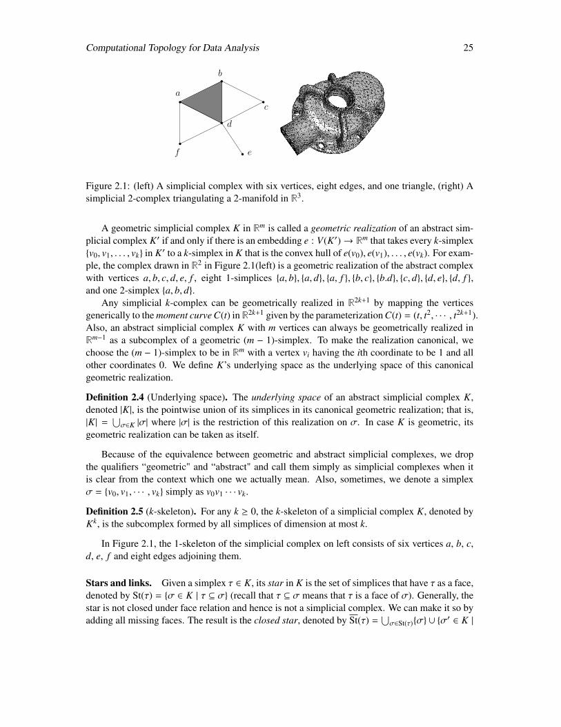
Computational Topology for Data Analysis 25
a
b
c
d
ef
Figure 2.1: (left) A simplicial complex with six vertices, eight edges, and one triangle, (right) Asimplicial 2-complex triangulating a 2-manifold in R3.
A geometric simplicial complex K in Rm is called a geometric realization of an abstract sim-plicial complex K′ if and only if there is an embedding e : V(K′)→ Rm that takes every k-simplexv0, v1, . . . , vk in K′ to a k-simplex in K that is the convex hull of e(v0), e(v1), . . . , e(vk). For exam-ple, the complex drawn in R2 in Figure 2.1(left) is a geometric realization of the abstract complexwith vertices a, b, c, d, e, f , eight 1-simplices a, b, a, d, a, f , b, c, b.d, c, d, d, e, d, f ,and one 2-simplex a, b, d.
Any simplicial k-complex can be geometrically realized in R2k+1 by mapping the verticesgenerically to the moment curve C(t) in R2k+1 given by the parameterization C(t) = (t, t2, · · · , t2k+1).Also, an abstract simplicial complex K with m vertices can always be geometrically realized inRm−1 as a subcomplex of a geometric (m − 1)-simplex. To make the realization canonical, wechoose the (m − 1)-simplex to be in Rm with a vertex vi having the ith coordinate to be 1 and allother coordinates 0. We define K’s underlying space as the underlying space of this canonicalgeometric realization.
Definition 2.4 (Underlying space). The underlying space of an abstract simplicial complex K,denoted |K|, is the pointwise union of its simplices in its canonical geometric realization; that is,|K| =
⋃σ∈K |σ| where |σ| is the restriction of this realization on σ. In case K is geometric, its
geometric realization can be taken as itself.
Because of the equivalence between geometric and abstract simplicial complexes, we dropthe qualifiers “geometric" and “abstract" and call them simply as simplicial complexes when itis clear from the context which one we actually mean. Also, sometimes, we denote a simplexσ = v0, v1, · · · , vk simply as v0v1 · · · vk.
Definition 2.5 (k-skeleton). For any k ≥ 0, the k-skeleton of a simplicial complex K, denoted byKk, is the subcomplex formed by all simplices of dimension at most k.
In Figure 2.1, the 1-skeleton of the simplicial complex on left consists of six vertices a, b, c,d, e, f and eight edges adjoining them.
Stars and links. Given a simplex τ ∈ K, its star in K is the set of simplices that have τ as a face,denoted by St(τ) = σ ∈ K | τ ⊆ σ (recall that τ ⊆ σ means that τ is a face of σ). Generally, thestar is not closed under face relation and hence is not a simplicial complex. We can make it so byadding all missing faces. The result is the closed star, denoted by St(τ) =
⋃σ∈St(τ)σ ∪ σ
′ ∈ K |
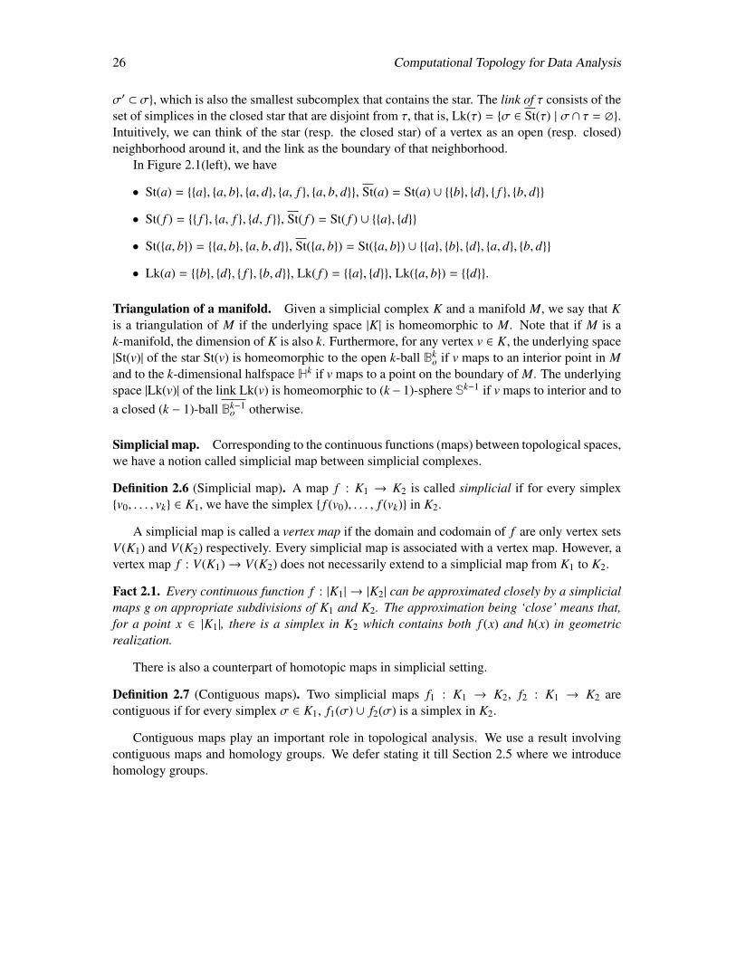
26 Computational Topology for Data Analysis
σ′ ⊂ σ, which is also the smallest subcomplex that contains the star. The link of τ consists of theset of simplices in the closed star that are disjoint from τ, that is, Lk(τ) = σ ∈ St(τ) | σ∩ τ = ∅.Intuitively, we can think of the star (resp. the closed star) of a vertex as an open (resp. closed)neighborhood around it, and the link as the boundary of that neighborhood.
In Figure 2.1(left), we have
• St(a) = a, a, b, a, d, a, f , a, b, d, St(a) = St(a) ∪ b, d, f , b, d
• St( f ) = f , a, f , d, f , St( f ) = St( f ) ∪ a, d
• St(a, b) = a, b, a, b, d, St(a, b) = St(a, b) ∪ a, b, d, a, d, b, d
• Lk(a) = b, d, f , b, d, Lk( f ) = a, d, Lk(a, b) = d.
Triangulation of a manifold. Given a simplicial complex K and a manifold M, we say that Kis a triangulation of M if the underlying space |K| is homeomorphic to M. Note that if M is ak-manifold, the dimension of K is also k. Furthermore, for any vertex v ∈ K, the underlying space|St(v)| of the star St(v) is homeomorphic to the open k-ball Bk
o if v maps to an interior point in Mand to the k-dimensional halfspace Hk if v maps to a point on the boundary of M. The underlyingspace |Lk(v)| of the link Lk(v) is homeomorphic to (k − 1)-sphere Sk−1 if v maps to interior and toa closed (k − 1)-ball Bk−1
o otherwise.
Simplicial map. Corresponding to the continuous functions (maps) between topological spaces,we have a notion called simplicial map between simplicial complexes.
Definition 2.6 (Simplicial map). A map f : K1 → K2 is called simplicial if for every simplexv0, . . . , vk ∈ K1, we have the simplex f (v0), . . . , f (vk) in K2.
A simplicial map is called a vertex map if the domain and codomain of f are only vertex setsV(K1) and V(K2) respectively. Every simplicial map is associated with a vertex map. However, avertex map f : V(K1)→ V(K2) does not necessarily extend to a simplicial map from K1 to K2.
Fact 2.1. Every continuous function f : |K1| → |K2| can be approximated closely by a simplicialmaps g on appropriate subdivisions of K1 and K2. The approximation being ‘close’ means that,for a point x ∈ |K1|, there is a simplex in K2 which contains both f (x) and h(x) in geometricrealization.
There is also a counterpart of homotopic maps in simplicial setting.
Definition 2.7 (Contiguous maps). Two simplicial maps f1 : K1 → K2, f2 : K1 → K2 arecontiguous if for every simplex σ ∈ K1, f1(σ) ∪ f2(σ) is a simplex in K2.
Contiguous maps play an important role in topological analysis. We use a result involvingcontiguous maps and homology groups. We defer stating it till Section 2.5 where we introducehomology groups.
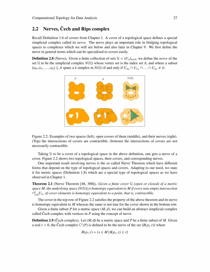
Computational Topology for Data Analysis 27
2.2 Nerves, Cech and Rips complex
Recall Definition 1.6 of covers from Chapter 1. A cover of a topological space defines a specialsimplicial complex called its nerve. The nerve plays an important role in bridging topologicalspaces to complexes which we will see below and also later in Chapter 9. We first define thenerve in general terms which can be specialised to covers easily.
Definition 2.8 (Nerve). Given a finite collection of sets U = Uαα∈A, we define the nerve of theset U to be the simplicial complex N(U) whose vertex set is the index set A, and where a subsetα0, α1, . . . , αk ⊆ A spans a k-simplex in N(U) if and only if Uα0 ∩ Uα1 ∩ . . . ∩ Uαk , ∅.
UM N(U)
Figure 2.2: Examples of two spaces (left), open covers of them (middle), and their nerves (right).(Top) the intersections of covers are contractible, (bottom) the intersections of covers are notnecessarily contractible.
Taking U to be a cover of a topological space in the above definition, one gets a nerve of acover. Figure 2.2 shows two topological spaces, their covers, and corresponding nerves.
One important result involving nerves is the so called Nerve Theorem which have differentforms that depend on the type of topological spaces and covers. Adapting to our need, we stateit for metric spaces (Definition 1.8) which are a special type of topological spaces as we haveobserved in Chapter 1.
Theorem 2.1 (Nerve Theorem [46, 300]). Given a finite cover U (open or closed) of a metricspace M, the underlying space |N(U)| is homotopy equivalent to M if every non-empty intersection∩k
i=0Uαi of cover elements is homotopy equivalent to a point, that is, contractible.
The cover in the top row of Figure 2.2 satisfies the property of the above theorem and its nerveis homotopy equivalent to M whereas the same is not true for the cover shown in the bottom row.
Given a finite subset P for a metric space (M, d), we can build an abstract simplicial complexcalled Cech complex with vertices in P using the concept of nerve.
Definition 2.9 (Cech complex). Let (M, d) be a metric space and P be a finite subset of M. Givena real r > 0, the Cech complex Cr(P) is defined to be the nerve of the set B(pi, r) where
B(pi, r) = x ∈ M | d(pi, x) ≤ r
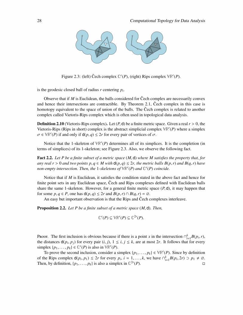
28 Computational Topology for Data Analysis
Figure 2.3: (left) Cech complex Cr(P), (right) Rips complex VRr(P).
is the geodesic closed ball of radius r centering pi.
Observe that if M is Euclidean, the balls considered for Cech complex are necessarily convexand hence their intersections are contractible. By Theorem 2.1, Cech complex in this case ishomotopy equivalent to the space of union of the balls. The Cech complex is related to anothercomplex called Vietoris-Rips complex which is often used in topological data analysis.
Definition 2.10 (Vietoris-Rips complex). Let (P, d) be a finite metric space. Given a real r > 0, theVietoris-Rips (Rips in short) complex is the abstract simplicial complex VRr(P) where a simplexσ ∈ VRr(P) if and only if d(p, q) ≤ 2r for every pair of vertices of σ.
Notice that the 1-skeleton of VRr(P) determines all of its simplices. It is the completion (interms of simplices) of its 1-skeleton; see Figure 2.3. Also, we observe the following fact.
Fact 2.2. Let P be a finite subset of a metric space (M, d) where M satisfies the property that, forany real r > 0 and two points p, q ∈ M with d(p, q) ≤ 2r, the metric balls B(p, r) and B(q, r) havenon-empty intersection. Then, the 1-skeletons of VRr(P) and Cr(P) coincide.
Notice that if M is Euclidean, it satisfies the condition stated in the above fact and hence forfinite point sets in any Euclidean space, Cech and Rips complexes defined with Euclidean ballsshare the same 1-skeleton. However, for a general finite metric space (P, d), it may happen thatfor some p, q ∈ P, one has d(p, q) ≤ 2r and B(p, r) ∩ B(q, r) = ∅.
An easy but important observation is that the Rips and Cech complexes interleave.
Proposition 2.2. Let P be a finite subset of a metric space (M, d). Then,
Cr(P) ⊆ VRr(P) ⊆ C2r(P).
Proof. The first inclusion is obvious because if there is a point x in the intersection ∩ki=1B(pi, r),
the distances d(pi, p j) for every pair (i, j), 1 ≤ i, j ≤ k, are at most 2r. It follows that for everysimplex p1, . . . , pk ∈ Cr(P) is also in VRr(P).
To prove the second inclusion, consider a simplex p1, . . . , pk ∈ VRr(P). Since by definitionof the Rips complex d(pi, p1) ≤ 2r for every pi, i = 1, . . . , k, we have ∩k
i=1B(pi, 2r) ⊃ p1 , ∅.Then, by definition, p1, . . . , pk is also a simplex in C2r(P).
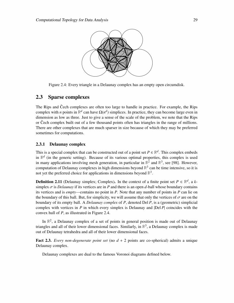
Computational Topology for Data Analysis 29
Figure 2.4: Every triangle in a Delaunay complex has an empty open circumdisk.
2.3 Sparse complexes
The Rips and Cech complexes are often too large to handle in practice. For example, the Ripscomplex with n points in Rd can have Ω(nd) simplices. In practice, they can become large even indimension as low as three. Just to give a sense of the scale of the problem, we note that the Ripsor Cech complex built out of a few thousand points often has triangles in the range of millions.There are other complexes that are much sparser in size because of which they may be preferredsometimes for computations.
2.3.1 Delaunay complex
This is a special complex that can be constructed out of a point set P ∈ Rd. This complex embedsin Rd (in the generic setting). Because of its various optimal properties, this complex is usedin many applications involving mesh generation, in particular in R2 and R3, see [98]. However,computation of Delaunay complexes in high dimensions beyond R3 can be time intensive, so it isnot yet the preferred choice for applications in dimensions beyond R3.
Definition 2.11 (Delaunay simplex; Complex). In the context of a finite point set P ∈ Rd, a k-simplex σ is Delaunay if its vertices are in P and there is an open d-ball whose boundary containsits vertices and is empty—contains no point in P. Note that any number of points in P can lie onthe boundary of this ball. But, for simplicity, we will assume that only the vertices of σ are on theboundary of its empty ball. A Delaunay complex of P, denoted Del P, is a (geometric) simplicialcomplex with vertices in P in which every simplex is Delaunay and |Del P| coincides with theconvex hull of P, as illustrated in Figure 2.4.
In R2, a Delaunay complex of a set of points in general position is made out of Delaunaytriangles and all of their lower dimensional faces. Similarly, in R3, a Delaunay complex is madeout of Delaunay tetrahedra and all of their lower dimensional faces.
Fact 2.3. Every non-degenerate point set (no d + 2 points are co-spherical) admits a uniqueDelaunay complex.
Delaunay complexes are dual to the famous Voronoi diagrams defined below.
30 Computational Topology for Data Analysis
Definition 2.12 (Voronoi diagram). Given a finite point set P ⊂ Rd in generic position, theVoronoi diagram Vor (P) of P is the tessellation of the embedding space Rd into convex cellsVp for every p ∈ P where
Vp = x ∈ Rd | d(x, p) ≤ d(x, q)∀q ∈ P.
A k-face of Vor (P) is the intersection of (d − k + 1) Voronoi cells.
Fact 2.4. For P ⊂ Rd, Del (P) is the nerve of the set of Voronoi cells Vpp∈P which is a closedcover of Rd.
The above fact actually provides a duality between Delaunay complex and Voronoi diagram.It is expresed by the duality among their faces. Specifically, a Delaunay k-simplex in Del (P) isdual to a Voronoi (d − k)-face in Vor (P). The Voronoi diagram dual to the Delaunay complex inFigure 2.4 is shown in Figure 2.5.
The following optimality properties make Delaunay complexes useful for applications.
Fact 2.5. A triangulation of a point set P ⊂ Rd is a geometric simplicial complex whose vertexset is P and whose simplices tessellate the convex hull of P. Among all triangulations of a pointset P ⊂ Rd, Del P achieves the following optimized criteria:
1. In R2, Del P maximizes the minimum angle of triangles in the complex.
2. In R2, Del P minimizes the largest circumcircle for triangles in the complex.
3. For a simplex in Del P, let its min-ball be the smallest ball that contains the simplex in it.In all dimensions, Del P minimizes the largest min-ball.
1-skeletons of Delaunay complexes in R2 are plane graphs and hence Delaunay complexes inR2 have size Θ(n) for n points. They can be computed in Θ(n log n) time. In R3, their size growsto Θ(n2) and they can be computed in Θ(n2) time. In Rd, d ≥ 3, Delaunay complexes have sizeΘ(ndd/2e) and can be computed in optimal time Θ(ndd/2e) [93].
Alpha complex. Alpha complexes are subcomplexes of the Delaunay complexes which areparameterized by a real α ≥ 0. For a given point set P and α ≥ 0, an alpha complex consistsof all simplices in Del (P) that have a circumscribing ball of radius at most α. It can also bedescribed alternatively as a nerve. For each point p ∈ P, let B(p, α) denote a closed ball of radiusα centering p. Consider the closed set Dα
p defined as follows:
Dαp = x ∈ B(p, α) | d(x, p) ≤ d(x, q)∀q ∈ P
The alpha complex Del α(P) is the nerve of the closed sets Dαpp∈P. Another interpretation for
alpha complex stems from its relation to the Voronoi diagram of the point set P. Alpha complexcontains a k-simplex σ = p0, . . . , pk if and only if ∪p∈PB(p, α) meets the intersection of Voronoicells Vp0 ∩ Vp1 · · · ∩ Vpk . Figure 2.5 shows an alpha complex for the point set in Figure 2.4 for anα. The Voronoi diagram is shown with the dotted segments.

Computational Topology for Data Analysis 31
α
Figure 2.5: Alpha complex of the point set in Figure 2.4 for an α indicated in the figure. TheVoronoi diagram of the point set is shown with dotted edges. The triangles and edges in thecomplex are shown with solid edges which are subset of the Delaunay complex.
2.3.2 Witness complex
The witness complex defined by de Silva and Carlsson [114] sidesteps the size problem by asubsampling strategy. First, we define the witness complex with two point sets, P called thewitnesses and Q called the landmarks. The complex is built with vertices in the landmarks wherethe simplices are defined with a notion of witness from the witness set. Given a point set Pequipped with pairwise distances d : P × P → R, we can build the witness complex on a finitesubsample Q ⊆ P.
Definition 2.13 (Weak witness). Let P be a point set with a real valued function on pairs d :P × P → R and Q ⊆ P be a finite subset . A simplex σ = q1, . . . , qk with qi ∈ Q is weaklywitnessed by x ∈ P \ Q if d(q, x) ≤ d(p, x) for every q ∈ q1, . . . , qk and p ∈ Q \ q1, . . . , qk.
We now define the witness complex using the notion of weak witnesses.
Definition 2.14 (Witness complex). Let P,Q be point sets as in Definition 2.13. The witnesscomplex W(Q, P) is defined as the collection of all simplices whose all faces are weakly witnessedby a point in P \ Q.
Observe that a simplex which is weakly witnessed may not have all its faces weakly witnessed(Exercise 7). This is why the definition above forces the condition to have a simplicial complex.
When P = Rd equipped with Euclidean distance and Q is a finite subset of it, we have thenotion of strong witness.
Definition 2.15 (Strong witness). Let Q ⊂ Rd be a finite set. A simplex σ = q1, . . . , qd withqi ∈ Q is strongly witnessed by x ∈ Rd if d(q, x) ≤ d(p, x) for every q ∈ q1, . . . , qd andp ∈ Q \ q1, . . . , qd and additionally, d(q1, x) = · · · = d(qd, x).
When Q ⊂ Rd as in the above definition, the following fact holds [113].
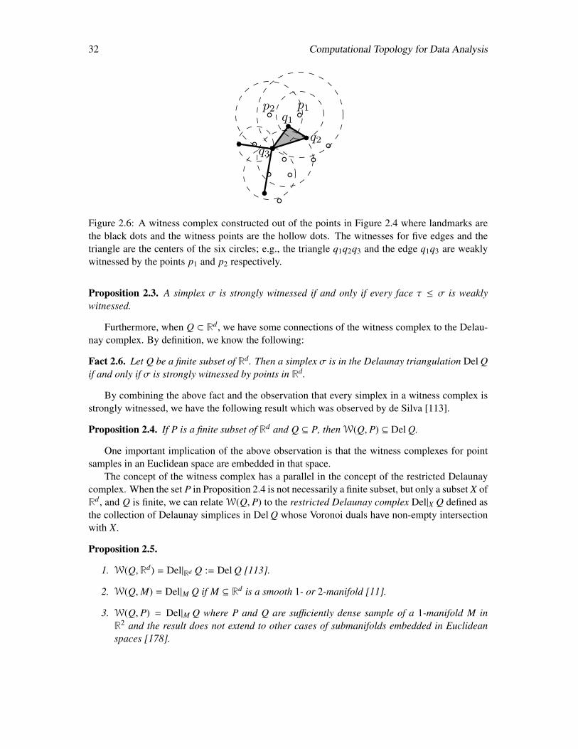
32 Computational Topology for Data Analysis
q1
q2q3
p1p2
Figure 2.6: A witness complex constructed out of the points in Figure 2.4 where landmarks arethe black dots and the witness points are the hollow dots. The witnesses for five edges and thetriangle are the centers of the six circles; e.g., the triangle q1q2q3 and the edge q1q3 are weaklywitnessed by the points p1 and p2 respectively.
Proposition 2.3. A simplex σ is strongly witnessed if and only if every face τ ≤ σ is weaklywitnessed.
Furthermore, when Q ⊂ Rd, we have some connections of the witness complex to the Delau-nay complex. By definition, we know the following:
Fact 2.6. Let Q be a finite subset of Rd. Then a simplex σ is in the Delaunay triangulation Del Qif and only if σ is strongly witnessed by points in Rd.
By combining the above fact and the observation that every simplex in a witness complex isstrongly witnessed, we have the following result which was observed by de Silva [113].
Proposition 2.4. If P is a finite subset of Rd and Q ⊆ P, then W(Q, P) ⊆ Del Q.
One important implication of the above observation is that the witness complexes for pointsamples in an Euclidean space are embedded in that space.
The concept of the witness complex has a parallel in the concept of the restricted Delaunaycomplex. When the set P in Proposition 2.4 is not necessarily a finite subset, but only a subset X ofRd, and Q is finite, we can relate W(Q, P) to the restricted Delaunay complex Del|X Q defined asthe collection of Delaunay simplices in Del Q whose Voronoi duals have non-empty intersectionwith X.
Proposition 2.5.
1. W(Q,Rd) = Del|Rd Q := Del Q [113].
2. W(Q,M) = Del|M Q if M ⊆ Rd is a smooth 1- or 2-manifold [11].
3. W(Q, P) = Del|M Q where P and Q are sufficiently dense sample of a 1-manifold M inR2 and the result does not extend to other cases of submanifolds embedded in Euclideanspaces [178].
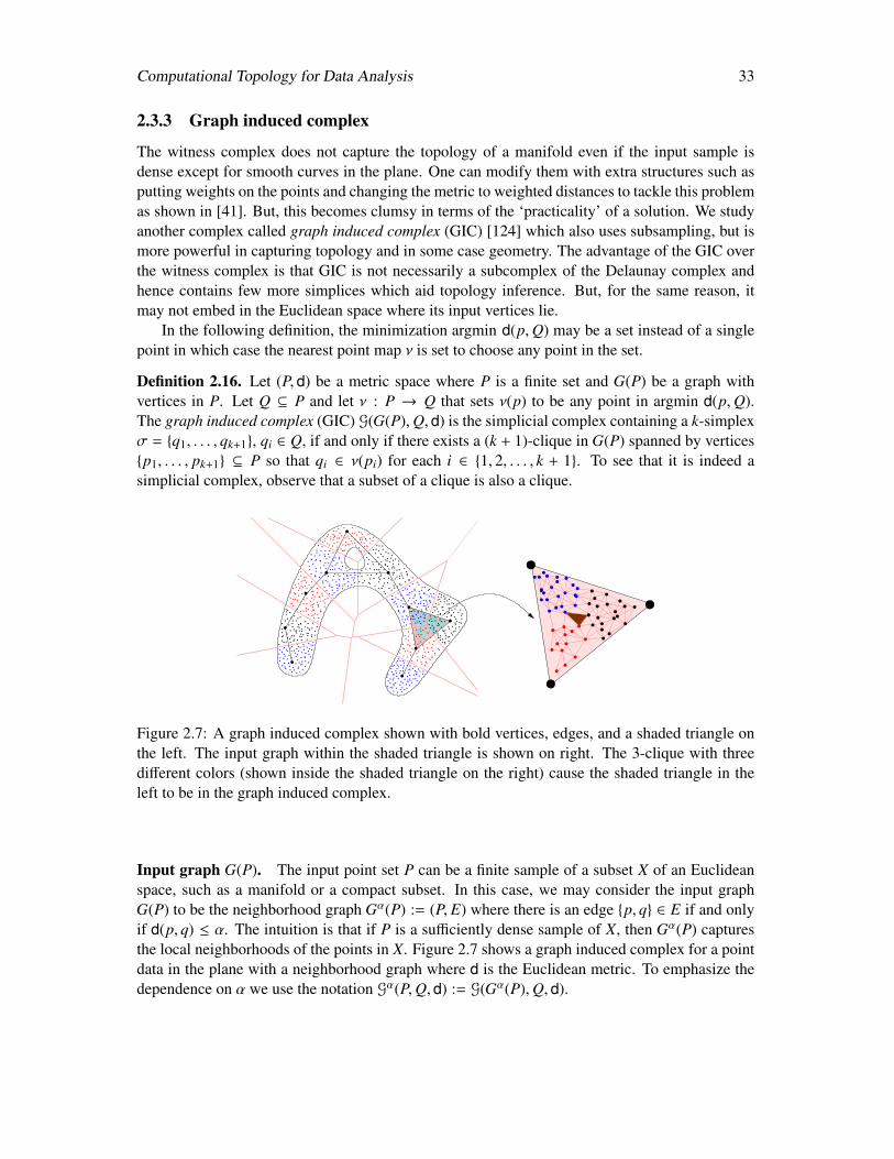
Computational Topology for Data Analysis 33
2.3.3 Graph induced complex
The witness complex does not capture the topology of a manifold even if the input sample isdense except for smooth curves in the plane. One can modify them with extra structures such asputting weights on the points and changing the metric to weighted distances to tackle this problemas shown in [41]. But, this becomes clumsy in terms of the ‘practicality’ of a solution. We studyanother complex called graph induced complex (GIC) [124] which also uses subsampling, but ismore powerful in capturing topology and in some case geometry. The advantage of the GIC overthe witness complex is that GIC is not necessarily a subcomplex of the Delaunay complex andhence contains few more simplices which aid topology inference. But, for the same reason, itmay not embed in the Euclidean space where its input vertices lie.
In the following definition, the minimization argmin d(p,Q) may be a set instead of a singlepoint in which case the nearest point map ν is set to choose any point in the set.
Definition 2.16. Let (P, d) be a metric space where P is a finite set and G(P) be a graph withvertices in P. Let Q ⊆ P and let ν : P → Q that sets ν(p) to be any point in argmin d(p,Q).The graph induced complex (GIC) G(G(P),Q, d) is the simplicial complex containing a k-simplexσ = q1, . . . , qk+1, qi ∈ Q, if and only if there exists a (k + 1)-clique in G(P) spanned by verticesp1, . . . , pk+1 ⊆ P so that qi ∈ ν(pi) for each i ∈ 1, 2, . . . , k + 1. To see that it is indeed asimplicial complex, observe that a subset of a clique is also a clique.
Figure 2.7: A graph induced complex shown with bold vertices, edges, and a shaded triangle onthe left. The input graph within the shaded triangle is shown on right. The 3-clique with threedifferent colors (shown inside the shaded triangle on the right) cause the shaded triangle in theleft to be in the graph induced complex.
Input graph G(P). The input point set P can be a finite sample of a subset X of an Euclideanspace, such as a manifold or a compact subset. In this case, we may consider the input graphG(P) to be the neighborhood graph Gα(P) := (P, E) where there is an edge p, q ∈ E if and onlyif d(p, q) ≤ α. The intuition is that if P is a sufficiently dense sample of X, then Gα(P) capturesthe local neighborhoods of the points in X. Figure 2.7 shows a graph induced complex for a pointdata in the plane with a neighborhood graph where d is the Euclidean metric. To emphasize thedependence on α we use the notation Gα(P,Q, d) := G(Gα(P),Q, d).
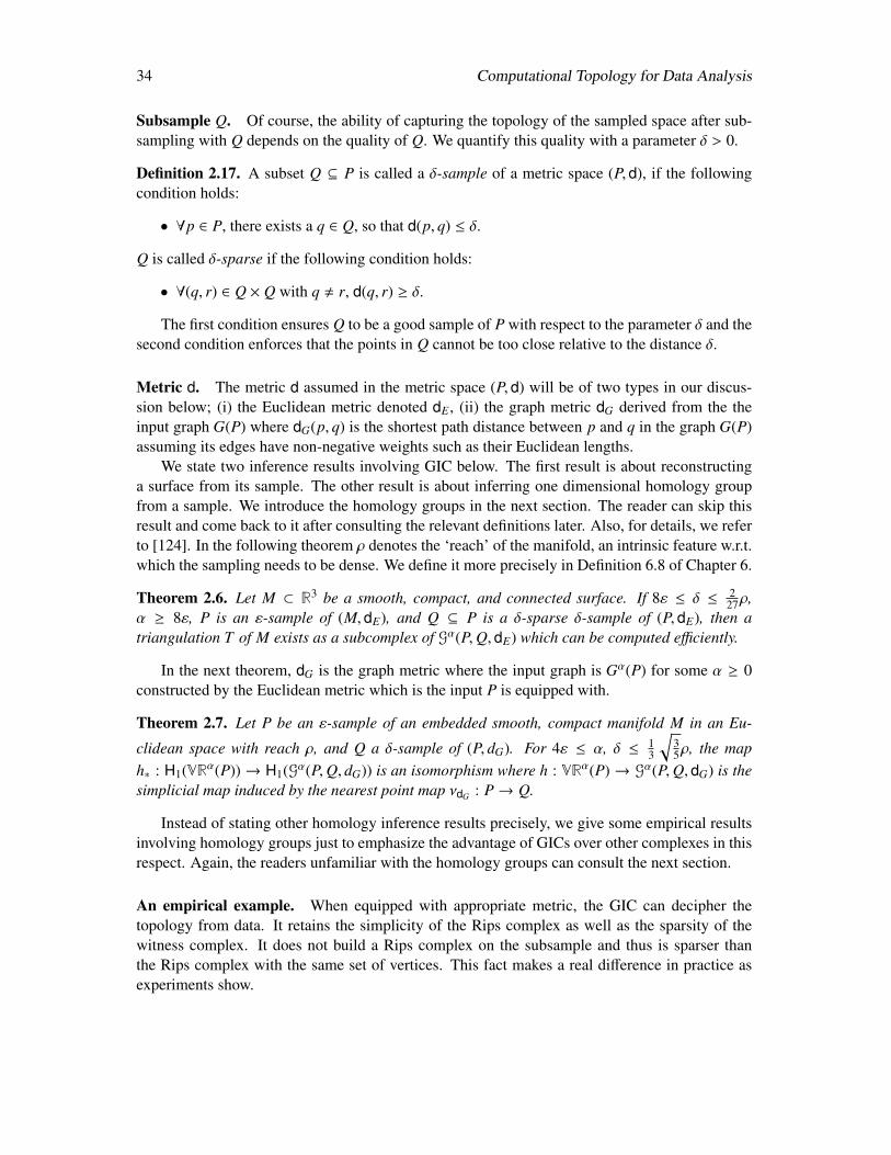
34 Computational Topology for Data Analysis
Subsample Q. Of course, the ability of capturing the topology of the sampled space after sub-sampling with Q depends on the quality of Q. We quantify this quality with a parameter δ > 0.
Definition 2.17. A subset Q ⊆ P is called a δ-sample of a metric space (P, d), if the followingcondition holds:
• ∀p ∈ P, there exists a q ∈ Q, so that d(p, q) ≤ δ.
Q is called δ-sparse if the following condition holds:
• ∀(q, r) ∈ Q × Q with q , r, d(q, r) ≥ δ.
The first condition ensures Q to be a good sample of P with respect to the parameter δ and thesecond condition enforces that the points in Q cannot be too close relative to the distance δ.
Metric d. The metric d assumed in the metric space (P, d) will be of two types in our discus-sion below; (i) the Euclidean metric denoted dE , (ii) the graph metric dG derived from the theinput graph G(P) where dG(p, q) is the shortest path distance between p and q in the graph G(P)assuming its edges have non-negative weights such as their Euclidean lengths.
We state two inference results involving GIC below. The first result is about reconstructinga surface from its sample. The other result is about inferring one dimensional homology groupfrom a sample. We introduce the homology groups in the next section. The reader can skip thisresult and come back to it after consulting the relevant definitions later. Also, for details, we referto [124]. In the following theorem ρ denotes the ‘reach’ of the manifold, an intrinsic feature w.r.t.which the sampling needs to be dense. We define it more precisely in Definition 6.8 of Chapter 6.
Theorem 2.6. Let M ⊂ R3 be a smooth, compact, and connected surface. If 8ε ≤ δ ≤ 227ρ,
α ≥ 8ε, P is an ε-sample of (M, dE), and Q ⊆ P is a δ-sparse δ-sample of (P, dE), then atriangulation T of M exists as a subcomplex of Gα(P,Q, dE) which can be computed efficiently.
In the next theorem, dG is the graph metric where the input graph is Gα(P) for some α ≥ 0constructed by the Euclidean metric which is the input P is equipped with.
Theorem 2.7. Let P be an ε-sample of an embedded smooth, compact manifold M in an Eu-
clidean space with reach ρ, and Q a δ-sample of (P, dG). For 4ε ≤ α, δ ≤ 13
√35ρ, the map
h∗ : H1(VRα(P)) → H1(Gα(P,Q, dG)) is an isomorphism where h : VRα(P) → Gα(P,Q, dG) is thesimplicial map induced by the nearest point map νdG : P→ Q.
Instead of stating other homology inference results precisely, we give some empirical resultsinvolving homology groups just to emphasize the advantage of GICs over other complexes in thisrespect. Again, the readers unfamiliar with the homology groups can consult the next section.
An empirical example. When equipped with appropriate metric, the GIC can decipher thetopology from data. It retains the simplicity of the Rips complex as well as the sparsity of thewitness complex. It does not build a Rips complex on the subsample and thus is sparser thanthe Rips complex with the same set of vertices. This fact makes a real difference in practice asexperiments show.
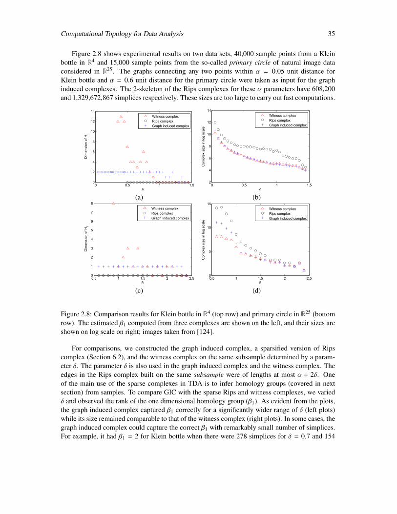
Computational Topology for Data Analysis 35
Figure 2.8 shows experimental results on two data sets, 40,000 sample points from a Kleinbottle in R4 and 15,000 sample points from the so-called primary circle of natural image dataconsidered in R25. The graphs connecting any two points within α = 0.05 unit distance forKlein bottle and α = 0.6 unit distance for the primary circle were taken as input for the graphinduced complexes. The 2-skeleton of the Rips complexes for these α parameters have 608,200and 1,329,672,867 simplices respectively. These sizes are too large to carry out fast computations.
0 0.5 1 1.50
2
4
6
8
10
12
14
δ
Dim
ensi
on o
f H1
Witness complexRips complexGraph induced complex
0 0.5 1 1.52
4
6
8
10
12
14
δ
Com
plex
siz
e in
log
scal
e
Witness complexRips complexGraph induced complex
(a) (b)
0.5 1 1.5 2 2.50
1
2
3
4
5
6
7
8
δ
Dim
ensi
ondo
fdH1
WitnessdcomplexRipsdcomplexGraphdinduceddcomplex
0.5 1 1.5 2 2.50
5
10
15
δ
Com
plex
siz
e in
log
scal
e
Witness complexRips complexGraph induced complex
(c) (d)
Figure 2.8: Comparison results for Klein bottle in R4 (top row) and primary circle in R25 (bottomrow). The estimated β1 computed from three complexes are shown on the left, and their sizes areshown on log scale on right; images taken from [124].
For comparisons, we constructed the graph induced complex, a sparsified version of Ripscomplex (Section 6.2), and the witness complex on the same subsample determined by a param-eter δ. The parameter δ is also used in the graph induced complex and the witness complex. Theedges in the Rips complex built on the same subsample were of lengths at most α + 2δ. Oneof the main use of the sparse complexes in TDA is to infer homology groups (covered in nextsection) from samples. To compare GIC with the sparse Rips and witness complexes, we variedδ and observed the rank of the one dimensional homology group (β1). As evident from the plots,the graph induced complex captured β1 correctly for a significantly wider range of δ (left plots)while its size remained comparable to that of the witness complex (right plots). In some cases, thegraph induced complex could capture the correct β1 with remarkably small number of simplices.For example, it had β1 = 2 for Klein bottle when there were 278 simplices for δ = 0.7 and 154
36 Computational Topology for Data Analysis
simplices for δ = 1.0. In both cases Rips and witness complexes had wrong β1 while the Ripscomplex had a much larger size (loge scale plot) and the witness complex had comparable size.This illustrates why the graph induced complex can be a better choice than the Rips and witnesscomplexes.
Constructing a GIC. One may wonder how to efficiently construct the graph induced com-plexes in practice. Experiments show that the following procedure runs quite efficiently in prac-tice. It takes advantage of computing nearest neighbors within a range and, more importantly,computing cliques only in a sparsified graph.
Let the ball B(q, δ) in metric d be called the δ-cover for the point q. A graph induced complexGα(P,Q, d) where Q is a δ-sparse δ-sample can be built easily by identifying δ-covers with arather standard greedy (farthest point) iterative algorithm. Let Qi = q1, . . . , qi be the point setsampled so far from P. We maintain the invariants (i) Qi is δ-sparse and (ii) every point p ∈ Pthat are in the union of δ-covers
⋃q∈Qi B(q, δ) have their closest point ν(p) ∈ argminq∈Qi
d(p, q) inQi identified. To augment Qi to Qi+1 = Qi ∪ qi+1, we choose a point qi+1 ∈ P that is outside theδ-covers
⋃q∈Qi B(q, δ). Certainly, qi+1 is at least δ units away from all points in Qi thus satisfying
the first invariant. For the second invariant, we check every point p in the δ-cover of qi+1 andupdate ν(p) to include qi+1 if its distance to qi+1 is smaller than the distance d(p, ν(p)). At theend, we obtain a sample Q ⊆ P whose δ-covers cover the entire point set P and thus is a δ-sampleof (P, d) which is also δ-sparse due to the invariants maintained. Next, we construct the simplicesof Gα(P,Q, d). This needs identifying cliques in Gα(P) that have vertices with different closestpoints in Q. We delete every edge pp′ from Gα(P) where ν(p) = ν(p′). Then, we determine everyclique p1, . . . pk in the remaining sparsified graph and include the simplex ν(p1), . . . , ν(pk) inGα(P,Q, d). The main saving here is that many cliques of the original graph are removed beforeit is processed for clique computation.
Next, we focus on the second topic of this chapter, namely homology groups.They are algebraicstructures to quantify topological features in a space. It does not capture all topological aspectsof a space in the sense that two spaces with the same homology groups may not be topologicallyequivalent. However, two spaces that are topologically equivalent must have isomorphic homol-ogy groups. It turns out that the homology groups are computationally tractable in many cases,thus making them more attractive in topological data analysis. Before we introduce its definitionand variants in Section 2.5, we need the important notions of chains, cycles, and boundaries givenin the following section.
2.4 Chains, cycles, boundaries
2.4.1 Algebraic structures
First, we recall briefly the definitions of some standard algebraic structures that are used in thebook. For details we refer the reader to any standard book on algebra, e.g. [14].
Definition 2.18 (Group; Homomorphism; Isomorphism). A set G together with a binary operation‘+’ is a group if it satisfies the following properties: (i) for every a, b ∈ G, a + b ∈ G, (ii) forevery a, b, c ∈ G, (a + b) + c = a + (b + c), (iii) there is an identity element denoted 0 in G so that
Computational Topology for Data Analysis 37
a + 0 = 0 + a = a for every a ∈ G, and (iv) there is an inverse −a ∈ G for every a ∈ G so thata + (−a) = 0. If the operation + commutes, that is, a + b = b + a for every a, b ∈ G, then G iscalled abelian. A subset H ⊆ G is a subgroup of (G,+) if (H,+) is also a group.
Definition 2.19 (Free abelian group; Basis; Rank; Generator). An abelian group G is called freeif there is a subset B ⊆ G so that every element of G can be written uniquely as a finite sum ofelements in B and their inverses disregarding trivial cancellations a + b = a + c − c + b. Such aset B is called a basis of G and its cardinality is called its rank. If the condition of uniqueness isdropped, then B is called a generator of G and we also say B generates G.
Definition 2.20 (Coset; Quotient). For a subgroup H ⊆ G and an element a ∈ G, the left cosetis aH = a + b | b ∈ H and the right coset is Ha = b + a | b ∈ H. For abelian groups, theleft and right cosets are identical and hence are simply called cosets. If G is abelian, the quotientgroup of G with a subgroup H ⊆ G is given by G/H = aH | a ∈ G where the group operationis inherited from G as aH + bH = (a + b)H for every a, b ∈ G.
Definition 2.21 (Homomorphism; Isomorphism; Kernel; Image; Cokernel). A map h : G → Hbetween two groups (G,+) and (H, ∗) is called a homomorphism if h(a + b) = h(a) ∗ h(b) forevery a, b ∈ G. If, in addition, h is bijective, it is called an isomorphism. Two groups G andH with an isomorphism are called isomorphic and denoted as G H. The kernel, image, andcokernel of a homomorphism h : G → H are defined as subgroups ker h = a ∈ G | h(a) = 0,Im h = b ∈ H | ∃ a ∈ G with h(a) = b, and the quotient group coker h = H/im h respectively.
Definition 2.22 (Ring). A set R equipped with two binary operations, addition ‘+’ and multiplica-tion ‘·’ is called a ring if (i) R is an abelian group with the addition, (ii) the multiplication is asso-ciative, that is, (a ·b) ·c = a ·(b ·c) and is distributive with the addition, that is, a ·(b+c) = a ·b+a ·c,∀a, b, c ∈ R, and (iii) there is an identity for the multiplication.
The additive identity of a ring R is usually denoted as 0 whereas the multiplicative identity isdenoted as 1. Observe that, by the definition of abelian group, the addition is commutative. How-ever, the multiplication need not be so. When the multiplication is also commutative, R is calleda commutative ring. A commutative ring in which every nonzero element has a multiplicativeinverse is called a field.
Definition 2.23 (Module). Given a commutative ring R with multiplicative identity 1, an R-module M is an abelian group with an operation R × M → M which satisfies the followingproperties ∀r, r′ ∈ R and x, y ∈ M:
• r · (x + y) = r · x + r · y
• (r + r′)x = r · x + r · x′
• 1 · x = x
• (r · r′) · x = r · (r′ · x)
Essentially, in an R-module, elements can be added and multiplied with coefficients in R.However, if R is taken as a field k, each non-zero element acquires a multiplicative inverse andwe get a vector space.
38 Computational Topology for Data Analysis
Definition 2.24 (Vector space). An R-module V is called a vector space if R is a field. A set ofelements g1, . . . , gk is said to generate the vector space V if every element a ∈ V can be writtenas a = α1g1 + . . . + αkgk for some α1, . . . , αk ∈ R. The set g1, . . . , gk is called a basis of V ifevery a ∈ V can be written in the above way uniquely. All bases of V have the same cardinalitywhich is called the dimension of V . We say a set g1, . . . , gm ⊆ V is independent if the equationα1g1 + . . . + αmgm = 0 can only be satisfied by setting αi = 0 for i = 1, . . . ,m.
Fact 2.7. A basis of a vector space is a generating set of minimal cardinality and an independentset of maximal cardinality.
2.4.2 Chains
Let K be a simplicial k-complex with mp number of p-simplices, k ≤ p ≤ 0. A p-chain c in K isa formal sum of p-simplices added with some coefficients, that is, c =
∑mp
i=1 αiσi where σi are thep-simplices and αi are the coefficients. Two p-chains c =
∑αiσi and c′ =
∑α′iσi can be added
to obtain another p-chain
c + c′ =
mp∑i=1
(αi + α′i)σi.
In general, coefficients can come from a ring R with its associated additions making the chainsconstituting an R-module. For example, these additions can be integer additions where the coef-ficients are integers; e.g., from two 1-chains (edges) we get
(2e1 + 3e2 + 5e3) + (e1 + 7e2 + 6e4) = 3e1 + 10e2 + 5e3 + 6e4.
Notice that while writing a chain, we only write the simplices that have non-zero coefficient inthe chain. We follow this convention all along. In our case, we will focus on the cases where thecoefficients come from a field k. In particular, we will mostly be interested in k = Z2. This meansthat the coefficients come from the field Z2 whose elements can only be 0 or 1 with the modulo-2additions 0 + 0 = 0, 0 + 1 = 1, and 1 + 1 = 0. This gives us Z2-additions of chains, for example,we have
(e1 + e3 + e4) + (e1 + e2 + e3) = e2 + e4.
Observe that p-chains with Z2-coefficients can be treated as sets: the chain e1 + e3 + e4 is theset e1, e3, e4, and Z2-addition between two chains is simply the symmetric difference betweenthe corresponding sets.
From now on, unless specified otherwise, we will consider all chain additions to be Z2-additions. One should keep in mind that one can have parallel concepts for coefficients andadditions coming from integers, reals, rationals, fields, and other rings. Under Z2-additions, wehave
c + c =
mp∑i=1
0σi = 0.
Below, we show addition of chains shown in Figure 2.9:
0-chain: (b + d) + (d + e) = b + e (left)1-chain: (a, b + b, d) + (b, c + b, d) = a, b + b, c (left)2-chain: (a, b, c + b, c, e) + (b, c, e) = a, b, c (right)
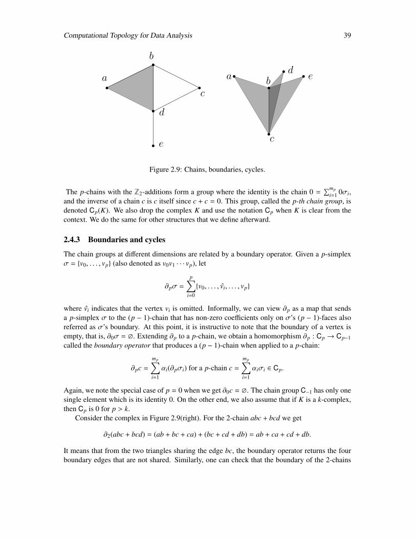
Computational Topology for Data Analysis 39
a
b
c
d
e
a
c
ed
b
Figure 2.9: Chains, boundaries, cycles.
The p-chains with the Z2-additions form a group where the identity is the chain 0 =∑mp
i=1 0σi,and the inverse of a chain c is c itself since c + c = 0. This group, called the p-th chain group, isdenoted Cp(K). We also drop the complex K and use the notation Cp when K is clear from thecontext. We do the same for other structures that we define afterward.
2.4.3 Boundaries and cycles
The chain groups at different dimensions are related by a boundary operator. Given a p-simplexσ = v0, . . . , vp (also denoted as v0v1 · · · vp), let
∂pσ =
p∑i=0
v0, . . . , vi, . . . , vp
where vi indicates that the vertex vi is omitted. Informally, we can view ∂p as a map that sendsa p-simplex σ to the (p − 1)-chain that has non-zero coefficients only on σ’s (p − 1)-faces alsoreferred as σ’s boundary. At this point, it is instructive to note that the boundary of a vertex isempty, that is, ∂0σ = ∅. Extending ∂p to a p-chain, we obtain a homomorphism ∂p : Cp → Cp−1called the boundary operator that produces a (p − 1)-chain when applied to a p-chain:
∂pc =
mp∑i=1
αi(∂pσi) for a p-chain c =
mp∑i=1
αiσi ∈ Cp.
Again, we note the special case of p = 0 when we get ∂0c = ∅. The chain group C−1 has only onesingle element which is its identity 0. On the other end, we also assume that if K is a k-complex,then Cp is 0 for p > k.
Consider the complex in Figure 2.9(right). For the 2-chain abc + bcd we get
∂2(abc + bcd) = (ab + bc + ca) + (bc + cd + db) = ab + ca + cd + db.
It means that from the two triangles sharing the edge bc, the boundary operator returns the fourboundary edges that are not shared. Similarly, one can check that the boundary of the 2-chains

40 Computational Topology for Data Analysis
consisting of all three triangles in Figure 2.9(right) contains all 7 edges. In particular, the edge bcdoes not get cancelled because of all three (odd) triangles adjoin it.
∂2(abc + bcd + bce) = ab + bc + ca + be + ce + bd + dc.
One important property of the boundary operator is that, applying it twice produces an emptychain.
Proposition 2.8. For p > 0 and any p-chain c, ∂p−1 ∂p(c) = 0.
Proof. Observe that ∂0 is a zero map by definition. Also, for a k-complex, ∂p operates on a zeroelement for p > k by definition. Then, it is sufficient to show that, for 1 ≤ p ≤ k, ∂p−1 ∂p(σ) = 0for a p-simplex σ. Observe that ∂pσ is the set of all (p − 1)-faces of σ and every (p − 2)-faces ofσ is contained in exactly two (p − 1)-faces. Thus, ∂p−1(∂pσ) = 0.
Extending the boundary operator to the chains groups, we obtain the following sequence ofhomomorphisms satisfying Proposition 2.8 for a simplicial k-complex; such a sequence is alsocalled a chain complex:
0 = Ck+1∂k+1 // Ck
∂k // Ck−1∂k−1 // Ck−2 · · · C1
∂1 // C0∂0 // C−1 = 0. (2.1)
Fact 2.8.
1. For p ≥ −1, Cp is a vector space because the coefficients are drawn from a field Z2–it has abasis so that every element can be expressed uniquely as a sum of the elements in the basis.
2. There is a basis for Cp where every p-simplex form a basis element because any p-chainis a unique subset of the p-simplices. The dimension of Cp is therefore n, the number of p-simplices. When p = −1 and p ≥ k + 1, Cp is trivial with dimension 0. In Figure 2.9(right)abc, bcd, bce is a basis for C2 and so is abc, (abc + bcd), bce.
Cycle and boundary groups.
Definition 2.25 (Cycle and cycle group). A p-chain c is a p-cycle if ∂c = 0. In words, a chainthat has empty boundary is a cycle. All p-cycles together form the p-th cycle group Zp underthe addition that is used to define the chain groups. In terms of the boundary operator, Zp is thesubgroup of Cp which is sent to the zero of Cp−1, that is, ker ∂p = Zp.
For example, in Figure 2.9(right), the 1-chain ab + bc + ca is a 1-cycle since
∂1(ab + bc + ca) = (a + b) + (b + c) + (c + a) = 0.
Also, observe that the above 1-chain is the boundary of the triangle abc. It’s not accident thatthe boundary of a simplex is a cycle. Thanks to Proposition 2.8, the boundary of a p-chain is a(p − 1)-cycle. This is a fundamental fact in homology theory.
The set of (p − 1)-chains that can be obtained by applying the boundary operator ∂p on p-chains form a subgroup of (p− 1)-chains, called the (p− 1)-th boundary group Bp−1 = ∂p(Cp); orin other words, the image of the boundary homomorphism is the boundary group, Bp−1 = im ∂p.We have ∂p−1Bp−1 = 0 for p > 0 due to Proposition 2.8 and hence Bp−1 ⊆ Zp−1. Figure 2.10illustrates cycles and boundaries.
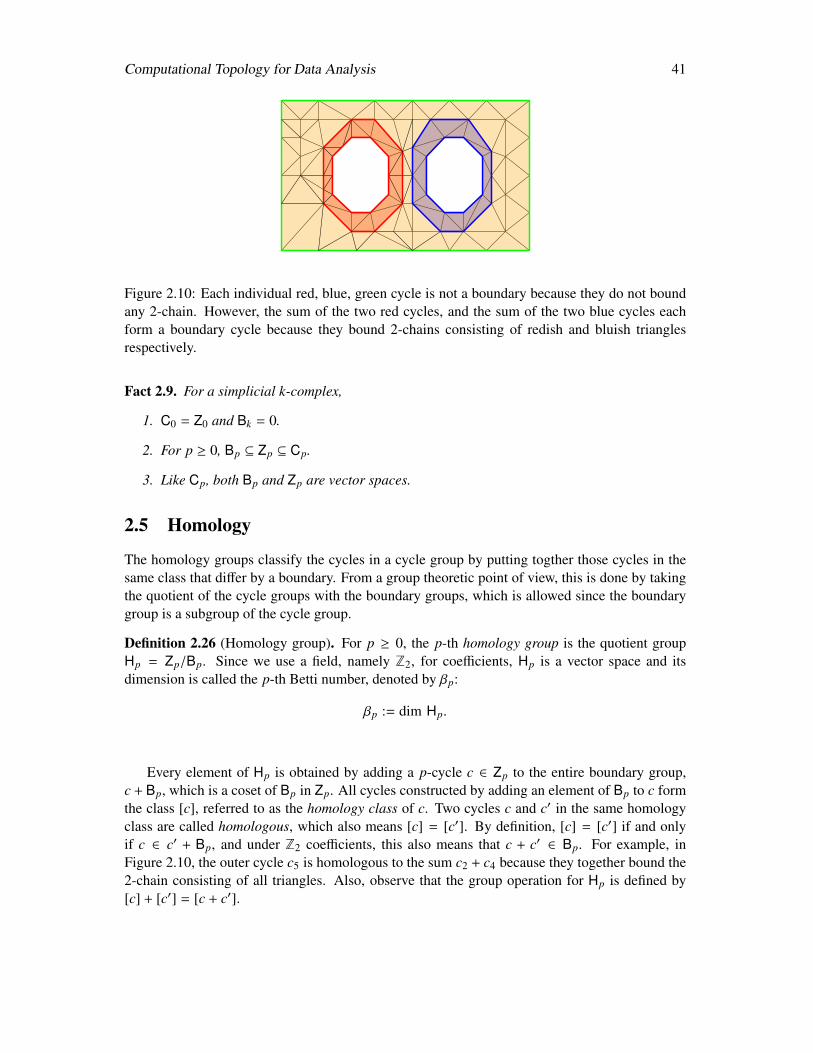
Computational Topology for Data Analysis 41
Figure 2.10: Each individual red, blue, green cycle is not a boundary because they do not boundany 2-chain. However, the sum of the two red cycles, and the sum of the two blue cycles eachform a boundary cycle because they bound 2-chains consisting of redish and bluish trianglesrespectively.
Fact 2.9. For a simplicial k-complex,
1. C0 = Z0 and Bk = 0.
2. For p ≥ 0, Bp ⊆ Zp ⊆ Cp.
3. Like Cp, both Bp and Zp are vector spaces.
2.5 Homology
The homology groups classify the cycles in a cycle group by putting togther those cycles in thesame class that differ by a boundary. From a group theoretic point of view, this is done by takingthe quotient of the cycle groups with the boundary groups, which is allowed since the boundarygroup is a subgroup of the cycle group.
Definition 2.26 (Homology group). For p ≥ 0, the p-th homology group is the quotient groupHp = Zp/Bp. Since we use a field, namely Z2, for coefficients, Hp is a vector space and itsdimension is called the p-th Betti number, denoted by βp:
βp := dim Hp.
Every element of Hp is obtained by adding a p-cycle c ∈ Zp to the entire boundary group,c + Bp, which is a coset of Bp in Zp. All cycles constructed by adding an element of Bp to c formthe class [c], referred to as the homology class of c. Two cycles c and c′ in the same homologyclass are called homologous, which also means [c] = [c′]. By definition, [c] = [c′] if and onlyif c ∈ c′ + Bp, and under Z2 coefficients, this also means that c + c′ ∈ Bp. For example, inFigure 2.10, the outer cycle c5 is homologous to the sum c2 + c4 because they together bound the2-chain consisting of all triangles. Also, observe that the group operation for Hp is defined by[c] + [c′] = [c + c′].
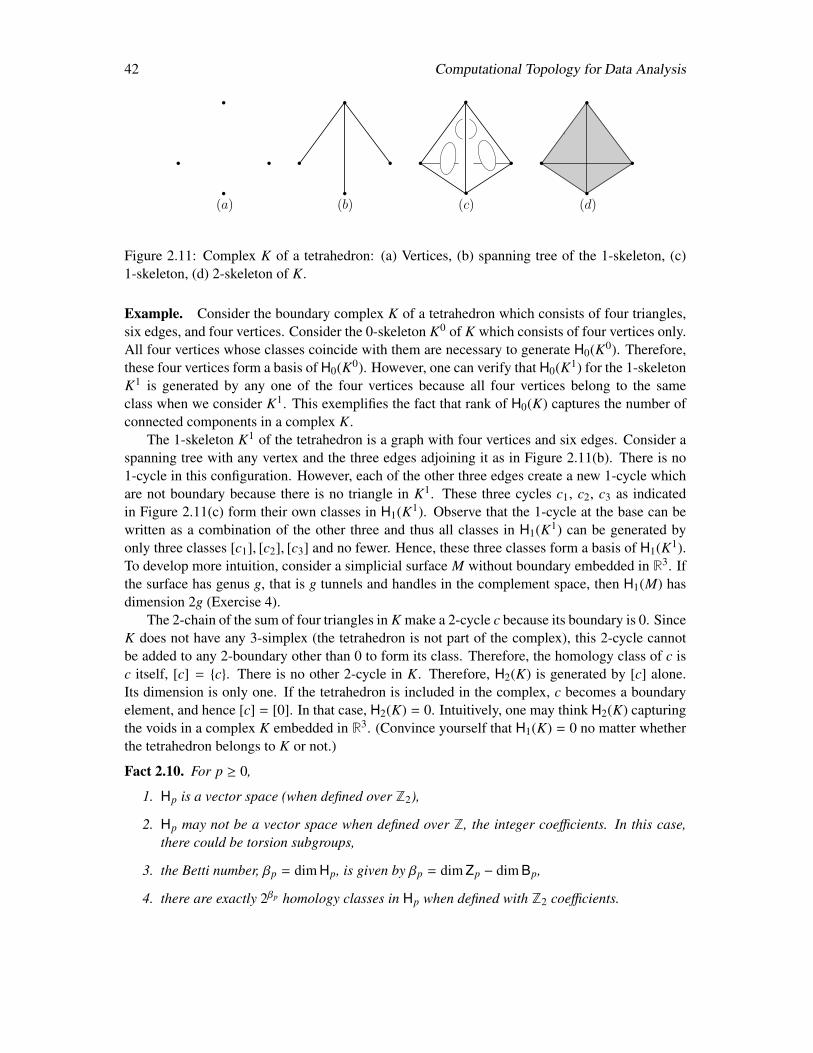
42 Computational Topology for Data Analysis
(a) (b) (c) (d)
Figure 2.11: Complex K of a tetrahedron: (a) Vertices, (b) spanning tree of the 1-skeleton, (c)1-skeleton, (d) 2-skeleton of K.
Example. Consider the boundary complex K of a tetrahedron which consists of four triangles,six edges, and four vertices. Consider the 0-skeleton K0 of K which consists of four vertices only.All four vertices whose classes coincide with them are necessary to generate H0(K0). Therefore,these four vertices form a basis of H0(K0). However, one can verify that H0(K1) for the 1-skeletonK1 is generated by any one of the four vertices because all four vertices belong to the sameclass when we consider K1. This exemplifies the fact that rank of H0(K) captures the number ofconnected components in a complex K.
The 1-skeleton K1 of the tetrahedron is a graph with four vertices and six edges. Consider aspanning tree with any vertex and the three edges adjoining it as in Figure 2.11(b). There is no1-cycle in this configuration. However, each of the other three edges create a new 1-cycle whichare not boundary because there is no triangle in K1. These three cycles c1, c2, c3 as indicatedin Figure 2.11(c) form their own classes in H1(K1). Observe that the 1-cycle at the base can bewritten as a combination of the other three and thus all classes in H1(K1) can be generated byonly three classes [c1], [c2], [c3] and no fewer. Hence, these three classes form a basis of H1(K1).To develop more intuition, consider a simplicial surface M without boundary embedded in R3. Ifthe surface has genus g, that is g tunnels and handles in the complement space, then H1(M) hasdimension 2g (Exercise 4).
The 2-chain of the sum of four triangles in K make a 2-cycle c because its boundary is 0. SinceK does not have any 3-simplex (the tetrahedron is not part of the complex), this 2-cycle cannotbe added to any 2-boundary other than 0 to form its class. Therefore, the homology class of c isc itself, [c] = c. There is no other 2-cycle in K. Therefore, H2(K) is generated by [c] alone.Its dimension is only one. If the tetrahedron is included in the complex, c becomes a boundaryelement, and hence [c] = [0]. In that case, H2(K) = 0. Intuitively, one may think H2(K) capturingthe voids in a complex K embedded in R3. (Convince yourself that H1(K) = 0 no matter whetherthe tetrahedron belongs to K or not.)
Fact 2.10. For p ≥ 0,
1. Hp is a vector space (when defined over Z2),
2. Hp may not be a vector space when defined over Z, the integer coefficients. In this case,there could be torsion subgroups,
3. the Betti number, βp = dim Hp, is given by βp = dim Zp − dim Bp,
4. there are exactly 2βp homology classes in Hp when defined with Z2 coefficients.
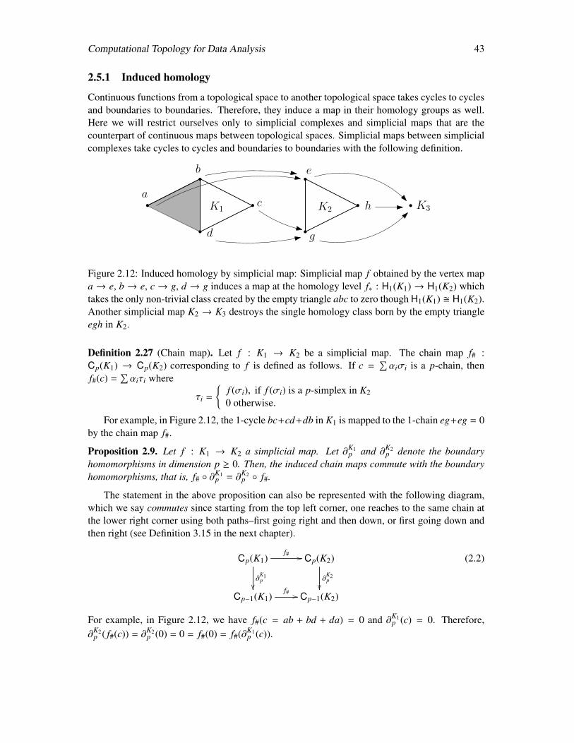
Computational Topology for Data Analysis 43
2.5.1 Induced homology
Continuous functions from a topological space to another topological space takes cycles to cyclesand boundaries to boundaries. Therefore, they induce a map in their homology groups as well.Here we will restrict ourselves only to simplicial complexes and simplicial maps that are thecounterpart of continuous maps between topological spaces. Simplicial maps between simplicialcomplexes take cycles to cycles and boundaries to boundaries with the following definition.
a
b
c
d
e
g
K1 K2 K3h
Figure 2.12: Induced homology by simplicial map: Simplicial map f obtained by the vertex mapa → e, b → e, c → g, d → g induces a map at the homology level f∗ : H1(K1) → H1(K2) whichtakes the only non-trivial class created by the empty triangle abc to zero though H1(K1) H1(K2).Another simplicial map K2 → K3 destroys the single homology class born by the empty triangleegh in K2.
Definition 2.27 (Chain map). Let f : K1 → K2 be a simplicial map. The chain map f# :Cp(K1) → Cp(K2) corresponding to f is defined as follows. If c =
∑αiσi is a p-chain, then
f#(c) =∑αiτi where
τi =
f (σi), if f (σi) is a p-simplex in K20 otherwise.
For example, in Figure 2.12, the 1-cycle bc+cd+db in K1 is mapped to the 1-chain eg+eg = 0by the chain map f#.
Proposition 2.9. Let f : K1 → K2 a simplicial map. Let ∂K1p and ∂K2
p denote the boundaryhomomorphisms in dimension p ≥ 0. Then, the induced chain maps commute with the boundaryhomomorphisms, that is, f# ∂
K1p = ∂K2
p f#.
The statement in the above proposition can also be represented with the following diagram,which we say commutes since starting from the top left corner, one reaches to the same chain atthe lower right corner using both paths–first going right and then down, or first going down andthen right (see Definition 3.15 in the next chapter).
Cp(K1)
∂K1p
f# // Cp(K2)
∂K2p
Cp−1(K1)f# // Cp−1(K2)
(2.2)
For example, in Figure 2.12, we have f#(c = ab + bd + da) = 0 and ∂K1p (c) = 0. Therefore,
∂K2p ( f#(c)) = ∂K2
p (0) = 0 = f#(0) = f#(∂K1p (c)).
44 Computational Topology for Data Analysis
Since Bp(K1) ⊆ Zp(K1), we have that f#(Bp(K1)) ⊆ f#(Zp(K1)). Thus, the induced map in thequotient space, namely,
f∗(Zp(K1)/Bp(K1)) := f#(Zp(K1))/ f#(Bp(K1))
is well defined. Furthermore, by the commutativity of the Diagram (2.2), f#(Zp(K1)) ⊆ Zp(K2)and f#(Bp(K1)) ⊆ Bp(K2), which gives an induced homomorphism in the homology groups:
f∗ : Zp(K1)/Bp(K1)→ Zp(K2)/Bp(K2) or equivalently f∗ : Hp(K1)→ Hp(K2)
A homology class [c] = c + Bp in K1 is mapped to the homology class f#(c) + f#(Bp) in K2by f∗. In Figure 2.12, we have B1 = 0, ab + bd + da. Then, for c = bd + dc + cb, we havef∗([c]) = f#(c), f#(c) + f#(ab + bd + da) = 0, 0 = [0].
Now we can state a result relating contiguous maps (Definition 2.7) and homology groupsthat we promised in Section 2.1.
Fact 2.11. For two contiguous maps f1 : K1 → K2 and f2 : K1 → K2, the induced mapsf1∗ : Hp(K1)→ Hp(K2) and f2∗ : Hp(K1)→ Hp(K2) are equal.
2.5.2 Relative homology
As the name suggests, we can define a homology group of a complex relative to a subcomplex.Let K0 be a subcomplex of K. By definition, the chain group Cp(K0) is a subgroup of Cp(K).Therefore, the quotient group Cp(K)/Cp(K0) is well defined which is called a relative chain groupand is denoted Cp(K,K0). It is an abelian group whose elements are the cosets [cp] = cp +Cp(K0)for every chain cp ∈ Cp(K).
The boundary operator ∂p : Cp(K) → Cp−1(K) extends to the relative chain groups in anatural way:
∂K,K0p : Cp(K,K0)→ Cp−1(K,K0), [cp] 7→ [∂pcp].
One may verify that ∂K,K0p−1 ∂
K,K0p = 0 as before. Therefore, we can define
Zp(K,K0) = ker ∂K,K0p , the p-th relative cycle group
Bp(K,K0) = Im ∂K,K0p+1 , the p-th relative boundary group
Hp(K,K0) = Zp(K,K0)/Bp(K,K0), the p-th relative homology group.
The relative homology Hp(K,K0) is related to a coned complex K∗. A coned complex K∗ of asimplicial complex K w.r.t. to the pair (K,K0) is a simplicial complex which has all simplicesfrom K and every coned simplex σ ∪ x from an additional vertex x to every simplex σ ∈ K0.Figure 2.13 shows the coned complexes on right in each case. The following fact is useful to buildan intuition about relative homology groups.
Fact 2.12. Hp(K,K0) Hp(K∗) for all p > 0 and β0(H0(K,K0)) = β0(H0(K∗)) − 1.
For example, consider K to be an edge a, b, ab with K0 = a, b as in Figure 2.13(left). The1-chain ab is a relative 1-cycle because ∂1(ab) = a + b ∈ C0(K0) and hence ∂K,K0
1 ([ab]) is 0 inC0(K,K0). This is indicated by the presence of the loop in the coned space.
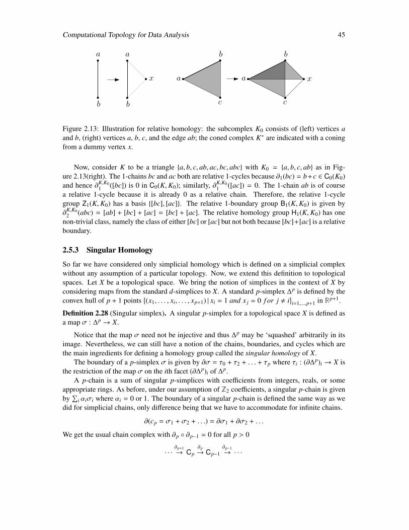
Computational Topology for Data Analysis 45
a
b
c
a
b
a
b
c
a
b
x x
Figure 2.13: Illustration for relative homology: the subcomplex K0 consists of (left) vertices aand b, (right) vertices a, b, c, and the edge ab; the coned complex K∗ are indicated with a coningfrom a dummy vertex x.
Now, consider K to be a triangle a, b, c, ab, ac, bc, abc with K0 = a, b, c, ab as in Fig-ure 2.13(right). The 1-chains bc and ac both are relative 1-cycles because ∂1(bc) = b+c ∈ C0(K0)and hence ∂K,K0
1 ([bc]) is 0 in C0(K,K0); similarly, ∂K,K01 ([ac]) = 0. The 1-chain ab is of course
a relative 1-cycle because it is already 0 as a relative chain. Therefore, the relative 1-cyclegroup Z1(K,K0) has a basis [bc], [ac]. The relative 1-boundary group B1(K,K0) is given by∂K,K0
2 (abc) = [ab] + [bc] + [ac] = [bc] + [ac]. The relative homology group H1(K,K0) has onenon-trivial class, namely the class of either [bc] or [ac] but not both because [bc]+[ac] is a relativeboundary.
2.5.3 Singular Homology
So far we have considered only simplicial homology which is defined on a simplicial complexwithout any assumption of a particular topology. Now, we extend this definition to topologicalspaces. Let X be a topological space. We bring the notion of simplices in the context of X byconsidering maps from the standard d-simplices to X. A standard p-simplex ∆p is defined by theconvex hull of p + 1 points
(x1, . . . , xi, . . . , xp+1) | xi = 1 and x j = 0 f or j , i
i=1,...,p+1 in Rp+1.
Definition 2.28 (Singular simplex). A singular p-simplex for a topological space X is defined asa map σ : ∆p → X.
Notice that the map σ need not be injective and thus ∆p may be ‘squashed’ arbitrarily in itsimage. Nevertheless, we can still have a notion of the chains, boundaries, and cycles which arethe main ingredients for defining a homology group called the singular homology of X.
The boundary of a p-simplex σ is given by ∂σ = τ0 + τ2 + . . . + τp where τi : (∂∆p)i → X isthe restriction of the map σ on the ith facet (∂∆p)i of ∆p.
A p-chain is a sum of singular p-simplices with coefficients from integers, reals, or someappropriate rings. As before, under our assumption of Z2 coefficients, a singular p-chain is givenby
∑i αiσi where αi = 0 or 1. The boundary of a singular p-chain is defined the same way as we
did for simplicial chains, only difference being that we have to accommodate for infinite chains.
∂(cp = σ1 + σ2 + . . .) = ∂σ1 + ∂σ2 + . . .
We get the usual chain complex with ∂p ∂p−1 = 0 for all p > 0
· · ·∂p+1→ Cp
∂p→ Cp−1
∂p−1→ · · ·
46 Computational Topology for Data Analysis
and can define the cycle and boundary groups as Zp = ker ∂p and Bp = im ∂p+1. We have thesingular homology defined as the quotient group Hp = Zp/Bp.
A useful fact is that singular and simplicial homology coincide when both are well defined.
Theorem 2.10. Let X be a topological space with a triangulation K, that is, the underlying space|K| is homeomorphic to X. Then Hp(K) Hp(X) for any p ≥ 0.
Note that the above theorem also implies that different triangulations of the same topologicalspace give rise to isomorphic simplicial homology.
2.5.4 Cohomology
There is a dual concept to homology called cohomology. Although cohomology can be definedwith coefficients in rings as in the case of homology groups, we will mainly focus on defining itover a field thus becoming a vector space.
A vector space V defined with a field k admits a dual vector space V∗ whose elements arelinear functions φ : V → k. These linear functions themselves can be added and multiplied overk forming the dual vector space V∗. The homology group Hp(K) as we defined in Definition 2.26over the field Z2 is a vector space and hence admits a dual vector space which is usually denotedas Hom(Hp(K),Z2). The p-th cohomology group denoted Hp(K) is not equal to this dual space,though over the coefficient field Z2, one has that Hp(K) is isomorphic to Hom(Hp(K),Z2) andHp(K) is also defined with spaces of linear maps.
Cochains, cobounadries, and cocycles. A p-cochain is a homomorphism φ : Cp → Z2 fromthe chain group to the coefficient ring over which Cp is defined which is Z2 here. In this case, ap-cochain φ is given by its evaluation φ(σ) (0 or 1) on every p-simplex σ in K, or more precisely,a p-chain c =
∑mp
i=1 αiσi gets a value
φ(c) = α1φ(σ1) + α2φ(σ2) + · · · + αmpφ(σmp).
Also, verify that φ(c + c′) = φ(c) + φ(c′) satisfying the property of group homomorphism. For achain c, the particular cochain that assigns 1 to a simplex if and only if it has a non-zero coefficientin c, is called its dual cochain c∗. The p-cochains form a cochain group Cp dual to Cp where theaddition is defined by (φ + φ′)(c) = φ(c) + φ′(c) by taking Z2-addition on the right. We can alsodefine a scalar multiplication (αφ)(c) = αφ(c) by using the Z2-multiplication. This makes Cp avector space.
Similar to boundaries of chains, we have the notion of coboundaries of cochains δp : Cp →
Cp+1. Specifically, for a p-cochain φ, its (p + 1)-coboundary is given by the homomorphismδφ : Cp+1 → Z2 defined as δφ(c) = φ(∂c) for any (p + 1)-chain c. Therefore, the coboundaryoperator δ takes a p-cochain and produces a (p + 1)-cochain giving the sequence for a simplicialk-complex:
0 = C−1 δ−1−−→ C0 δ0
−→ C1 δ1−→ · · ·
δk−1−−−→ Ck δk
−→ Ck+1 = 0
The set of p-coboundaries forms the coboundary group (vector space) Bp where the groupaddition and scalar multiplication are given by the same in Cp.
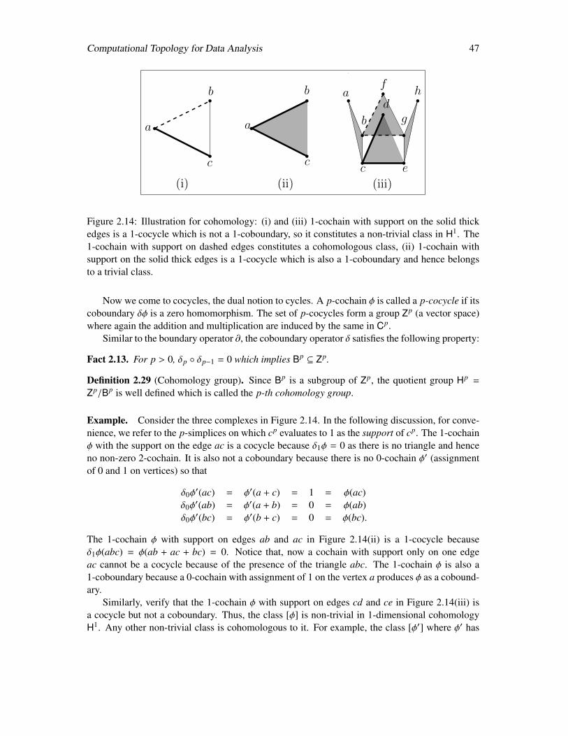
Computational Topology for Data Analysis 47
a
b
c
a
b
c
a
b
c
d
e
f
g
h
(i) (ii) (iii)
Figure 2.14: Illustration for cohomology: (i) and (iii) 1-cochain with support on the solid thickedges is a 1-cocycle which is not a 1-coboundary, so it constitutes a non-trivial class in H1. The1-cochain with support on dashed edges constitutes a cohomologous class, (ii) 1-cochain withsupport on the solid thick edges is a 1-cocycle which is also a 1-coboundary and hence belongsto a trivial class.
Now we come to cocycles, the dual notion to cycles. A p-cochain φ is called a p-cocycle if itscoboundary δφ is a zero homomorphism. The set of p-cocycles form a group Zp (a vector space)where again the addition and multiplication are induced by the same in Cp.
Similar to the boundary operator ∂, the coboundary operator δ satisfies the following property:
Fact 2.13. For p > 0, δp δp−1 = 0 which implies Bp ⊆ Zp.
Definition 2.29 (Cohomology group). Since Bp is a subgroup of Zp, the quotient group Hp =
Zp/Bp is well defined which is called the p-th cohomology group.
Example. Consider the three complexes in Figure 2.14. In the following discussion, for conve-nience, we refer to the p-simplices on which cp evaluates to 1 as the support of cp. The 1-cochainφ with the support on the edge ac is a cocycle because δ1φ = 0 as there is no triangle and henceno non-zero 2-cochain. It is also not a coboundary because there is no 0-cochain φ′ (assignmentof 0 and 1 on vertices) so that
δ0φ′(ac) = φ′(a + c) = 1 = φ(ac)
δ0φ′(ab) = φ′(a + b) = 0 = φ(ab)
δ0φ′(bc) = φ′(b + c) = 0 = φ(bc).
The 1-cochain φ with support on edges ab and ac in Figure 2.14(ii) is a 1-cocycle becauseδ1φ(abc) = φ(ab + ac + bc) = 0. Notice that, now a cochain with support only on one edgeac cannot be a cocycle because of the presence of the triangle abc. The 1-cochain φ is also a1-coboundary because a 0-cochain with assignment of 1 on the vertex a produces φ as a cobound-ary.
Similarly, verify that the 1-cochain φ with support on edges cd and ce in Figure 2.14(iii) isa cocycle but not a coboundary. Thus, the class [φ] is non-trivial in 1-dimensional cohomologyH1. Any other non-trivial class is cohomologous to it. For example, the class [φ′] where φ′ has
48 Computational Topology for Data Analysis
support on edges b f and bg is cohomologous to [φ]. This follows from the fact that [φ] + [φ′] =
[φ + φ′] = [0] because φ + φ′ is a 1-coboundary obtained by assigning 1 to vertices a, b, and c.Similar to the homology groups, a simplicial map f : K1 → K2 also induces a homomorphism
f ∗ between the two cohomology groups, but in the opposite direction. To see this, consider thechain map f# induced by f (Definition 2.27). Then, a cochain map f # : Cp(K2) → Cp(K1) isdefined as f #(φ)(c) = φ( f#(c)). The cochain map f # in turn defines the induced homomorphismbetween the respective cohomology groups. We will use the following fact in Section 4.2.1.
Fact 2.14. A simplicial map f : K1 → K2 induces a homomorphism f ∗ : Hp(K2) → Hp(K1) forevery p ≥ 0.
2.6 Notes and Exercises
Simplicial complexes is a fundamental structure in algebraic topology. A good source for thesubject is Munkres [241].
The concept of nerve is credited to Aleksandroff [7]. The nerve theorem has different versions.It holds for open covers for topological spaces with some mild conditions [300]. Borsuk provedit for closed covers again with some conditions on the space and covers [46]. The assumptions ofboth are satisfied by metric spaces and finite covers with which we state the theorem in section 2.2.A version of the theorem is also credited to Leray [219].
Cech and Vietoris-Rips complexes have turned out to be a very effective data structure intopological data analysis. Cech complexes were introduced to define Cech homology. LeonidVietoris [293] introduced Vietoris complex for extending the homology theory from simplicialcomplexes to metric spaces. Later, Eliyahu Rips used it in hyperbolic group theory [176]. Jean-Claude Hausmann named it as Vietoris-Rips complex and showed that it is homotopoy equivalentto a compact Riemannian manifold when the vertex set spans all points of the manifold and the pa-rameter to build it is sufficiently small [187]. This result was further improved by Latschev [217]who showed that the homotopy equivalence holds even when the vertex set is finite.
Delaunay complex is a very well known and useful data structure for various geometric ap-plications in two and three dimensions. They enjoy various optimal properties. For example, fora given point set P ⊂ R2, among all simplicial complexes linearly embedded in R2 with vertexset P, the Delaunay complex maximizes the minimum angle over all triangles as stated in Fact2.5. Many such properties and algorithms for computing Delaunay complexes are described inbooks by Edelsbrunner [148] and Cheng et al. [97]. Alpha complex was proposed in [151] andfurther developed in [153]. The first author of this book can attest to the historic fact that the de-velopment of the persistence algorithm was motivated by the study of alpha complexes and theirBetti numbers. The book by Edelsbrunner and Harer [149] confirms this. Witness complexes areproposed by de Silva and Carlsson [114] in an attempt to build a sparser complex out of a densepoint sample. The graph induced complex is also another such construction proposed in [124].
Homology groups and its associated concepts are main algebraic tools used in topological dataanalysis. Many associated structures and results about them exist in algebraic topology. We onlycover the main necessary concepts that are used in this book and leave others. Interested readerscan familiarize themselves with these omitted topics by reading Munkres [241], Hatcher [186],or Ghrist [170] among many other excellent sources.

Computational Topology for Data Analysis 49
Exercises
1. Suppose we have a collection of sets U = Uαα∈A where there exists an element U ∈ U
that contains all other elements in U. Show that the nerve complex N(U) is contractible toa point.
2. Given a parameter α and a set of points P ⊂ Rd, show that the alpha complex Del α(P) iscontained in the intersection of Delauney complex and Cech complex at scale α; that is,Del α(P) ⊆ Del (P) ∩ Cα(P).
3. Let K be the simplicial complex of a tetrahedron. Write a basis for the chain groups C1,C2, boundary groups B1, B2, and cycle groups Z1, Z2. Write the boundary matrix repre-senting the boundary operator ∂2 with rows and columns representing bases of C1 and C2respectively.
4. Let K be a triangulation of an orientable surface without boundary that has genus g. Provethat β1(K) = 2g.
5. Let K be a triangulation of a 2-dimensional sphere S2. Now remove h number of vertex-disjoint triangles from K, and let the resulting simplicial complex be K′. Describe the Bettinumbers of K′, and justify your answer.
6. We state the nerve theorem (Theorem 2.1) for covers where either all cover elements areclosed or all cover elements are open. Show that the theorem does not hold if we mix openand closed elements in the cover.
7. Give an example where a simplex which is weakly witnessed may not have all its facesweakly witnessed. Show that (i) W(Q, P′) ⊆W(Q, P) for P′ ⊆ P, (ii) W(Q′, P) may not bea subcomplex of W(Q, P) where Q′ ⊆ Q.
8. Consider Definition 2.16 for Graph induced complex. Let VR(G) be the clique complexgiven by the input graph G(P). Assume that the map ν : P → 2Q sends every point to asingleton under input metric d. Then, ν : P→ ν(P) is a well defined vertex map. Prove thatthe vertex map ν : P → Q extends to a simplicial map ν : VR(G) → G(G(P),Q, d). Also,show that every simplicial complex K(Q) with the vertex set Q for which ν : VR(G) →K(Q) becomes simplicial must contain G(G(P),Q, d).
9. Prove Proposition 2.9.
10. Consider a complex K = a, b, c, ab, bc, ca, abc. Enumerate all elements in the 1-chain,1-cycle, 1-boundary groups defined on K under Z2 coefficient. Do the same for cochains,cocycles, and coboundaries.
11. Show an example for the following:
• a chain that is a cycle but its dual cochain is not a cocycle.
• a chain that is a cycle and its dual cochain is a cocycle.
• a chain that is a boundary and its dual cochain is not a coboundary.

50 Computational Topology for Data Analysis
• a chain that is a boundary and its dual cochain is a coboundary.
12. Prove that ∂p−1 ∂p = 0 for relative chain groups and also δp δp−1 = 0 for cochain groups.
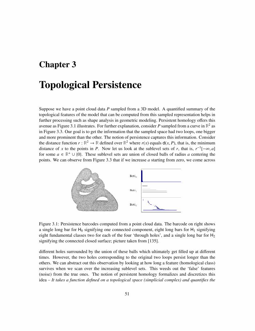
Chapter 3
Topological Persistence
Suppose we have a point cloud data P sampled from a 3D model. A quantified summary of thetopological features of the model that can be computed from this sampled representation helps infurther processing such as shape analysis in geometric modeling. Persistent homology offers thisavenue as Figure 3.1 illustrates. For further explanation, consider P sampled from a curve in R2 asin Figure 3.3. Our goal is to get the information that the sampled space had two loops, one biggerand more prominent than the other. The notion of persistence captures this information. Considerthe distance function r : R2 → R defined over R2 where r(x) equals d(x, P), that is, the minimumdistance of x to the points in P. Now let us look at the sublevel sets of r, that is, r−1[−∞, a]for some a ∈ R+ ∪ 0. These sublevel sets are union of closed balls of radius a centering thepoints. We can observe from Figure 3.3 that if we increase a starting from zero, we come across
Figure 3.1: Persistence barcodes computed from a point cloud data. The barcode on right showsa single long bar for H0 signifying one connected component, eight long bars for H1 signifyingeight fundamental classes two for each of the four ‘through holes’, and a single long bar for H2signifying the connected closed surface; picture taken from [135].
different holes surrounded by the union of these balls which ultimately get filled up at differenttimes. However, the two holes corresponding to the original two loops persist longer than theothers. We can abstract out this observation by looking at how long a feature (homological class)survives when we scan over the increasing sublevel sets. This weeds out the ‘false’ features(noise) from the true ones. The notion of persistent homology formalizes and discretizes thisidea – It takes a function defined on a topological space (simplicial complex) and quantifies the
51
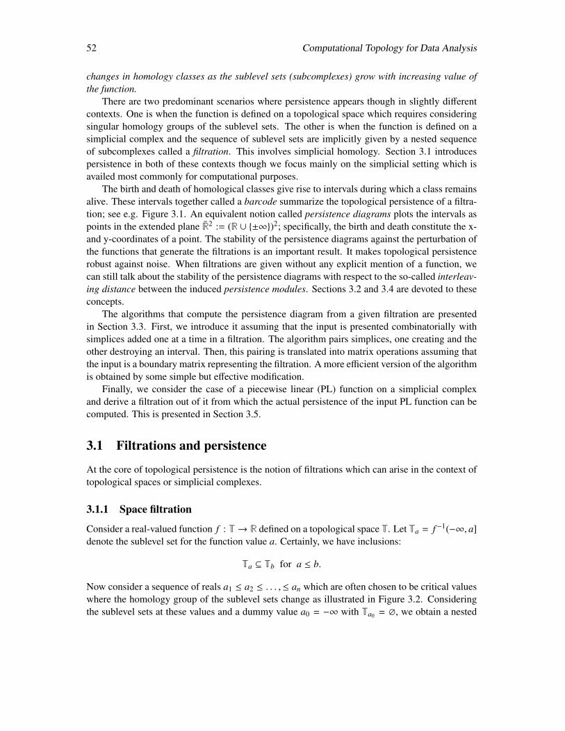
52 Computational Topology for Data Analysis
changes in homology classes as the sublevel sets (subcomplexes) grow with increasing value ofthe function.
There are two predominant scenarios where persistence appears though in slightly differentcontexts. One is when the function is defined on a topological space which requires consideringsingular homology groups of the sublevel sets. The other is when the function is defined on asimplicial complex and the sequence of sublevel sets are implicitly given by a nested sequenceof subcomplexes called a filtration. This involves simplicial homology. Section 3.1 introducespersistence in both of these contexts though we focus mainly on the simplicial setting which isavailed most commonly for computational purposes.
The birth and death of homological classes give rise to intervals during which a class remainsalive. These intervals together called a barcode summarize the topological persistence of a filtra-tion; see e.g. Figure 3.1. An equivalent notion called persistence diagrams plots the intervals aspoints in the extended plane R2 := (R ∪ ±∞)2; specifically, the birth and death constitute the x-and y-coordinates of a point. The stability of the persistence diagrams against the perturbation ofthe functions that generate the filtrations is an important result. It makes topological persistencerobust against noise. When filtrations are given without any explicit mention of a function, wecan still talk about the stability of the persistence diagrams with respect to the so-called interleav-ing distance between the induced persistence modules. Sections 3.2 and 3.4 are devoted to theseconcepts.
The algorithms that compute the persistence diagram from a given filtration are presentedin Section 3.3. First, we introduce it assuming that the input is presented combinatorially withsimplices added one at a time in a filtration. The algorithm pairs simplices, one creating and theother destroying an interval. Then, this pairing is translated into matrix operations assuming thatthe input is a boundary matrix representing the filtration. A more efficient version of the algorithmis obtained by some simple but effective modification.
Finally, we consider the case of a piecewise linear (PL) function on a simplicial complexand derive a filtration out of it from which the actual persistence of the input PL function can becomputed. This is presented in Section 3.5.
3.1 Filtrations and persistence
At the core of topological persistence is the notion of filtrations which can arise in the context oftopological spaces or simplicial complexes.
3.1.1 Space filtration
Consider a real-valued function f : T→ R defined on a topological space T. Let Ta = f −1(−∞, a]denote the sublevel set for the function value a. Certainly, we have inclusions:
Ta ⊆ Tb for a ≤ b.
Now consider a sequence of reals a1 ≤ a2 ≤ . . . ,≤ an which are often chosen to be critical valueswhere the homology group of the sublevel sets change as illustrated in Figure 3.2. Consideringthe sublevel sets at these values and a dummy value a0 = −∞ with Ta0 = ∅, we obtain a nested
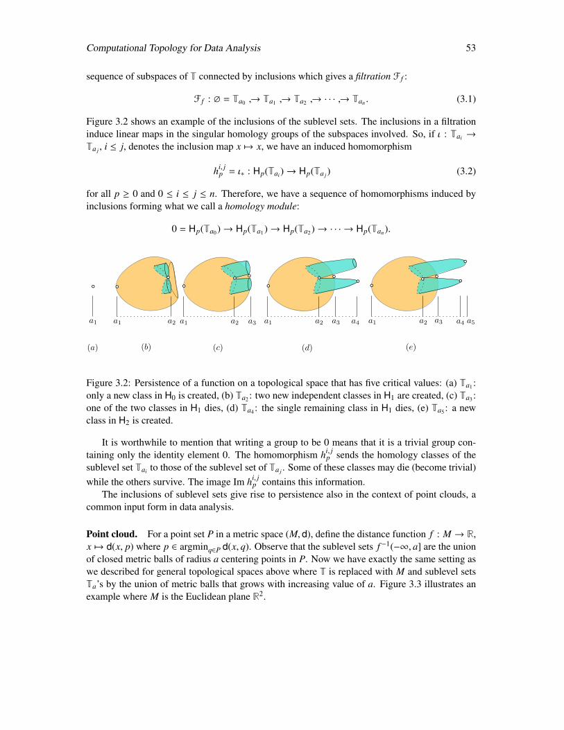
Computational Topology for Data Analysis 53
sequence of subspaces of T connected by inclusions which gives a filtration F f :
F f : ∅ = Ta0 → Ta1 → Ta2 → · · · → Tan . (3.1)
Figure 3.2 shows an example of the inclusions of the sublevel sets. The inclusions in a filtrationinduce linear maps in the singular homology groups of the subspaces involved. So, if ι : Tai →
Ta j , i ≤ j, denotes the inclusion map x 7→ x, we have an induced homomorphism
hi, jp = ι∗ : Hp(Tai)→ Hp(Ta j) (3.2)
for all p ≥ 0 and 0 ≤ i ≤ j ≤ n. Therefore, we have a sequence of homomorphisms induced byinclusions forming what we call a homology module:
0 = Hp(Ta0)→ Hp(Ta1)→ Hp(Ta2)→ · · · → Hp(Tan).
(b) (c) (d) (e)
a1 a2 a3 a2a1 a3 a5a1 a2 a1 a2 a3 a4 a4a1
(a)
Figure 3.2: Persistence of a function on a topological space that has five critical values: (a) Ta1 :only a new class in H0 is created, (b) Ta2 : two new independent classes in H1 are created, (c) Ta3 :one of the two classes in H1 dies, (d) Ta4 : the single remaining class in H1 dies, (e) Ta5 : a newclass in H2 is created.
It is worthwhile to mention that writing a group to be 0 means that it is a trivial group con-taining only the identity element 0. The homomorphism hi, j
p sends the homology classes of thesublevel set Tai to those of the sublevel set of Ta j . Some of these classes may die (become trivial)while the others survive. The image Im hi, j
p contains this information.The inclusions of sublevel sets give rise to persistence also in the context of point clouds, a
common input form in data analysis.
Point cloud. For a point set P in a metric space (M, d), define the distance function f : M → R,x 7→ d(x, p) where p ∈ argminq∈P d(x, q). Observe that the sublevel sets f −1(−∞, a] are the unionof closed metric balls of radius a centering points in P. Now we have exactly the same setting aswe described for general topological spaces above where T is replaced with M and sublevel setsTa’s by the union of metric balls that grows with increasing value of a. Figure 3.3 illustrates anexample where M is the Euclidean plane R2.
54 Computational Topology for Data Analysis
Figure 3.3: Noisy sample of a curve with two loops and the growing sublevel sets of the distancefunction to the sample points: The larger loop appearing as the bigger hole in the complement ofthe union of balls persists longer than the same for the smaller loop while other spurious holespersist even shorter.
3.1.2 Simplicial filtrations and persistence
Persistence on topological spaces involves computing singular homology groups for sublevel sets.Computationally, this is cumbersome. So, we take refuge in the discrete analogue of the topolog-ical persistence. This involves two important adaptations: first, the topological space is replacedwith a simplicial complex; second, singular homology groups are replaced with simplicial homol-ogy groups. This means that the topological space T considered before is replaced with one of itstriangulations as Figure 3.4 illustrates. For point cloud data, the union of balls can be replaced bytheir nerve, the Cech complex or its cousin Vietoris-Rips complex introduced in Section 2.2. Fig-ure 3.5 illustrates this conversion for example in Figure 3.3. Of course, these replacements needto preserve the original persistence in some sense, which is addressed in general by the notion ofstability introduced in Section 3.4.
The nested sequence of topological spaces that arise with growing sublevel sets translates intoa nested sequence of simplicial complexes in the discrete analogue. This brings in the concept offiltration of simplicial complexes that allows defining the persistence using simplicial homologygroups.
Definition 3.1 (Simplicial filtration). A filtration F = F(K) of a simplicial complex K is a nestedsequence of its subcomplexes
F : ∅ = K0 ⊆ K1 ⊆ · · · ⊆ Kn = K
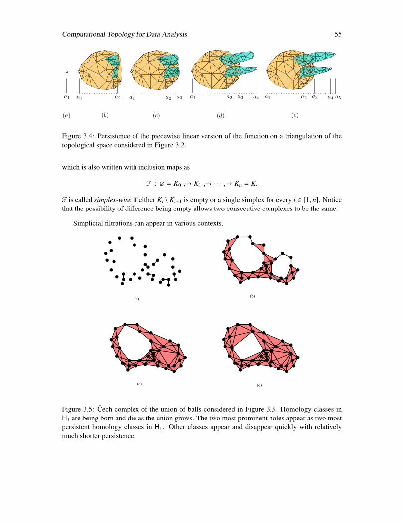
Computational Topology for Data Analysis 55
(b) (c) (d) (e)
a2a1 a3 a5a1 a2 a4a1
(a)
a2a1 a3 a4a2a1 a3
Figure 3.4: Persistence of the piecewise linear version of the function on a triangulation of thetopological space considered in Figure 3.2.
which is also written with inclusion maps as
F : ∅ = K0 → K1 → · · · → Kn = K.
F is called simplex-wise if either Ki \Ki−1 is empty or a single simplex for every i ∈ [1, n]. Noticethat the possibility of difference being empty allows two consecutive complexes to be the same.
Simplicial filtrations can appear in various contexts.
(a)(b)
(c) (d)
Figure 3.5: Cech complex of the union of balls considered in Figure 3.3. Homology classes inH1 are being born and die as the union grows. The two most prominent holes appear as two mostpersistent homology classes in H1. Other classes appear and disappear quickly with relativelymuch shorter persistence.
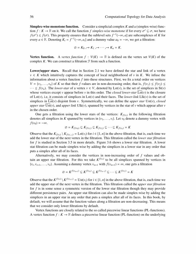
56 Computational Topology for Data Analysis
Simplex-wise monotone function. Consider a simplicial complex K and a (simplex-wise) func-tion f : K → R on it. We call the function f simplex-wise monotone if for every σ′ ⊆ σ, we havef (σ′) ≤ f (σ). This property ensures that the sublevel sets f −1(−∞, a] are subcomplexes of K forevery a ∈ R. Denoting Ki = f −1(−∞, ai] and a dummy value a0 = −∞, we get a filtration:
∅ = K0 → K1 → · · · → Kn = K.
Vertex function. A vertex function f : V(K) → R is defined on the vertex set V(K) of thecomplex K. We can construct a filtration F from such a function.
Lower/upper stars. Recall that in Section 2.1 we have defined the star and link of a vertexv ∈ K which intuitively captures the concept of local neighborhood of v in K. We infuse theinformation about a vertex function f into these structures. First, we fix a total order on verticesV = v1, . . . , vn of K so that their f -values are in non-decreasing order, that is, f (v1) ≤ f (v2) ≤· · · ≤ f (vn). The lower-star of a vertex v ∈ V , denoted by Lst(v), is the set of simplices in St(v)whose vertices except v appear before v in this order. The closed lower-star Lst(v) is the closureof Lst(v), i.e, it consists of simplices in Lst(v) and their faces. The lower-link Llk(v) is the set ofsimplices in Lst(v) disjoint from v. Symmetrically, we can define the upper star Ust(v), closedupper star Ust(v), and upper link Ulk(v), spanned by vertices in the star of v which appear after vin the chosen order.
One gets a filtration using the lower stars of the vertices: K f (vi) in the following filtrationdenotes all simplices in K spanned by vertices in v1, . . . , vi. Let v0 denote a dummy vertex withf (v0) = −∞.
∅ = K f (v0) ⊆ K f (v1) ⊆ K f (v2) ⊆ · · · ⊆ K f (vn) = K
Observe that the K f (vi) \K f (vi−1) = Lst(vi) for i ∈ [1, n] in the above filtration, that is, each time weadd the lower star of the next vertex in the filtration. This filtration called the lower star filtrationfor f is studied in Section 3.5 in more details. Figure 3.6 shows a lower star filtration. A lowerstat filtration can be made simplex-wise by adding the simplices in a lower star in any order thatputs a simplex after all of its faces.
Alternatively, we may consider the vertices in non-increasing order of f values and ob-tain an upper star filtration. For this we take K f (vi) to be all simplices spanned by vertices invi, vi+1, . . . , vn. Assuming a dummy vertex vn+1 with f (vn+1) = ∞, one gets a filtration
∅ = K f (vn+1) ⊆ K f (vn) ⊆ K f (vn−1) ⊆ · · · ⊆ K f (v1) = K
Observe that the K f (vi) \K f (vi+1) = Ust(vi) for i ∈ [1, n] in the above filtration, that is, each time weadd the upper star of the next vertex in the filtration. This filtration called the upper star filtrationfor f is in some sense a symmetric version of the lower star filtration though they may providedifferent persistence pairs. An upper stat filtration can also be made simplex-wise by adding thesimplices in an upper star in any order that puts a simplex after all of its faces. In this book, bydefault, we will assume that the function values along a filtration are non-decreasing. This meansthat we consider only lower filtrations by default.
Vertex functions are closely related to the so called piecewise linear functions (PL-functions).A vertex function f : K → R defines a piecewise linear function (PL-function) on the underlying
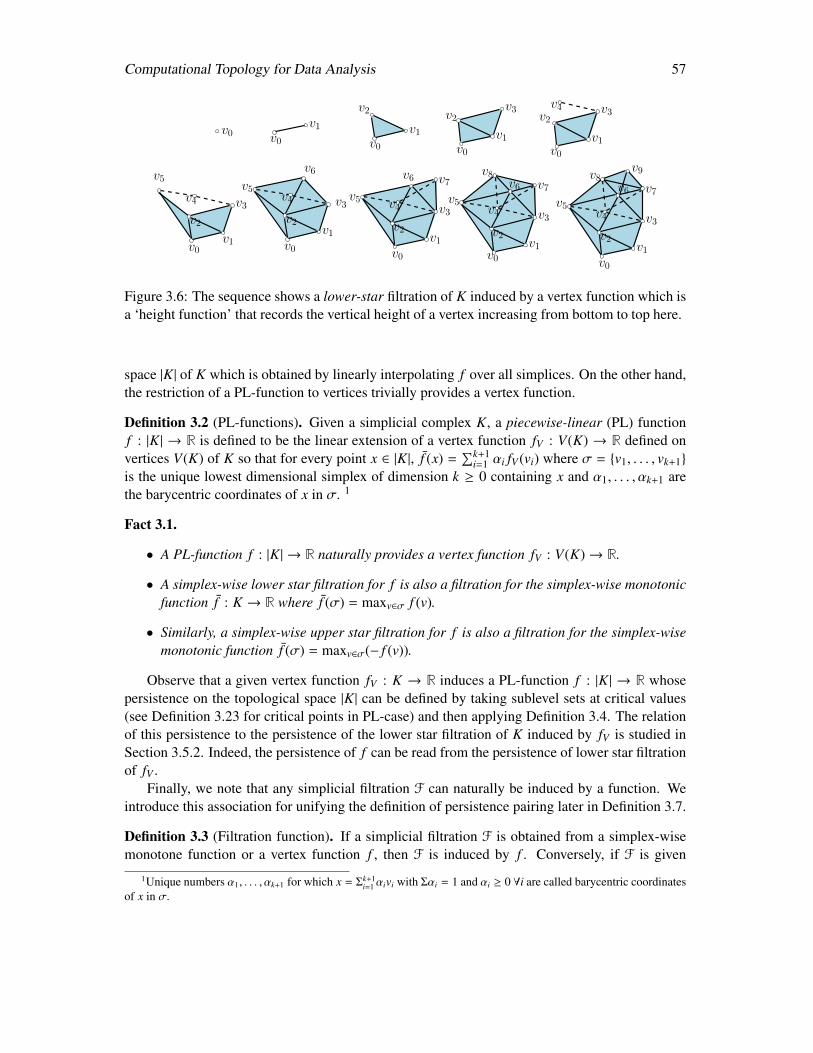
Computational Topology for Data Analysis 57
v0
v1
v3v2
v4v5
v6 v7v8
v9
v0 v0v1
v0v1
v2
v0v1
v3v2
v1
v3v2v4
v0v1
v3v2
v4
v5
v0
v1
v3v2
v4v5
v6
v0
v1
v3v2
v4v5
v6 v7
v0v1
v3v2
v4v5
v6 v7v8
v0
Figure 3.6: The sequence shows a lower-star filtration of K induced by a vertex function which isa ‘height function’ that records the vertical height of a vertex increasing from bottom to top here.
space |K| of K which is obtained by linearly interpolating f over all simplices. On the other hand,the restriction of a PL-function to vertices trivially provides a vertex function.
Definition 3.2 (PL-functions). Given a simplicial complex K, a piecewise-linear (PL) functionf : |K| → R is defined to be the linear extension of a vertex function fV : V(K) → R defined onvertices V(K) of K so that for every point x ∈ |K|, f (x) =
∑k+1i=1 αi fV (vi) where σ = v1, . . . , vk+1
is the unique lowest dimensional simplex of dimension k ≥ 0 containing x and α1, . . . , αk+1 arethe barycentric coordinates of x in σ. 1
Fact 3.1.
• A PL-function f : |K| → R naturally provides a vertex function fV : V(K)→ R.
• A simplex-wise lower star filtration for f is also a filtration for the simplex-wise monotonicfunction f : K → R where f (σ) = maxv∈σ f (v).
• Similarly, a simplex-wise upper star filtration for f is also a filtration for the simplex-wisemonotonic function f (σ) = maxv∈σ(− f (v)).
Observe that a given vertex function fV : K → R induces a PL-function f : |K| → R whosepersistence on the topological space |K| can be defined by taking sublevel sets at critical values(see Definition 3.23 for critical points in PL-case) and then applying Definition 3.4. The relationof this persistence to the persistence of the lower star filtration of K induced by fV is studied inSection 3.5.2. Indeed, the persistence of f can be read from the persistence of lower star filtrationof fV .
Finally, we note that any simplicial filtration F can naturally be induced by a function. Weintroduce this association for unifying the definition of persistence pairing later in Definition 3.7.
Definition 3.3 (Filtration function). If a simplicial filtration F is obtained from a simplex-wisemonotone function or a vertex function f , then F is induced by f . Conversely, if F is given
1Unique numbers α1, . . . , αk+1 for which x = Σk+1i=1αivi with Σαi = 1 and αi ≥ 0 ∀i are called barycentric coordinates
of x in σ.
58 Computational Topology for Data Analysis
without any explicit input function, we say F is induced by the simplex-wise monotone functionf where every simplex σ ∈ (Ki \ Ki−1) for Ki , Ki+1 is given the value f (σ) = i.
Naturally, every simplicial filtration gives rise to a sequence of homomorphisms hi, jp as in
Equation 3.2 induced by inclusions again forming a homology module
0 = Hp(K0)→ Hp(K1)→ · · · → Hp(Ki)→hi, j
p· · ·→ Hp(K j) · · · → Hp(Kn) = Hp(K).
3.2 Persistence
In both cases of space and simplicial filtration F, we arrive at a homology module:
HpF : 0 = Hp(X0)→ Hp(X1)→ · · · → Hp(Xi)→hi, j
p· · ·→ Hp(X j) · · · → Hp(Xn) = Hp(X) (3.3)
where Xi = Tai if F is a space filtration of a topological space X = T or Xi = Ki if F is a simplicialfiltration of a simplicial complex X = K. Persistent homology groups for a homology moduleare algebraic structures capturing the survival of the homology classes through this sequence. Ingeneral, we will call homology modules as persistence modules in Section 3.4 recognizing thatwe can replace homology groups with vector spaces.
Definition 3.4 (Persistent Betti number). The p-th persistent homology groups are the images ofthe homomorphisms; Hi, j
p = im hi, jp , for 0 ≤ i ≤ j ≤ n. The p-th persistent Betti numbers are the
dimensions βi, jp = dim Hi, j
p of the vector spaces Hi, jp .
The p-th persistent homology groups contain the important information of when a homologyclass is born or when it dies. The issue of birth and death of a class becomes more subtle becausewhen a new class is born, many other classes that are sum of this new class and any other exist-ing class also are born. Similarly, when a class ceases to exist, many other classes may cease toexist along with it. Therefore, we need a mechanism to pair births and deaths canonically. Fig-ure 3.7 illustrates birth and death of a class though the pairing of birth and death events is morecomplicated as stated in Fact 3.3.
Observe that the non trivial elements of p-th persistent homology groups Hi, jp consist of classes
that survive from Xi to X j, that is, the classes which do not get ‘quotient out’ by the boundaries inX j. So, one can observe:
Fact 3.2. Hi, jp = Zp(Xi)/(Bp(X j) ∩ Zp(Xi)) and βi, j
p = dim Hi jp .
Notice that Zp(Xi) is a subgroup of Zp(X j) because Xi ⊆ X j and hence the above quotient iswell defined. We now formally state when a class is born or dies.
Definition 3.5 (Birth and death). A non-trivial p-th homology class ξ ∈ Hp(Xa) is born at Xi,i ≤ a, if ξ ∈ Hi,a
p but ξ < Hi−1,ap . Similarly, a non-trivial p-th homology class ξ ∈ Hp(Xa) dies
entering X j, a < j, if ha, j−1p (ξ) is not zero (non-trivial) but ha, j
p (ξ) = 0.
Observe that not all classes that are born at Xi necessarily die entering some X j though morethan one such may do so.
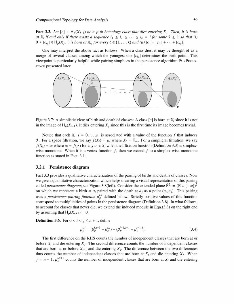
Computational Topology for Data Analysis 59
Fact 3.3. Let [c] ∈ Hp(X j−1) be a p-th homology class that dies entering X j. Then, it is bornat Xi if and only if there exists a sequence i1 ≤ i2 ≤ · · · ≤ ik = i for some k ≥ 1 so that (i)0 , [ci`] ∈ Hp(X j−1) is born at Xi` for every ` ∈ 1, . . . , k and (ii) [c] = [ci1] + · · · + [cik ].
One may interpret the above fact as follows. When a class dies, it may be thought of as amerge of several classes among which the youngest one [cik ] determines the birth point. Thisviewpoint is particularly helpful while pairing simplices in the persistence algorithm PairPersis-tence presented later.
Hp(Xi−1) Hp(Xi) Hp(Xj−1) Hp(Xj)
[c]
Figure 3.7: A simplistic view of birth and death of classes: A class [c] is born at Xi since it is notin the image of Hp(Xi−1). It dies entering X j since this is the first time its image becomes trivial.
Notice that each Xi, i = 0, . . . , n, is associated with a value of the function f that inducesF. For a space filtration, we say f (Xi) = ai where Xi = Tai . For a simplicial filtration, we sayf (Xi) = ai where ai = f (σ) for any σ ∈ Xi when the filtration function (Definition 3.3) is simplex-wise monotone. When it is a vertex function f , then we extend f to a simplex-wise monotonefunction as stated in Fact 3.1.
3.2.1 Persistence diagram
Fact 3.3 provides a qualitative characterization of the pairing of births and deaths of classes. Nowwe give a quantitative characterization which helps drawing a visual representation of this pairingcalled persistence diagram; see Figure 3.8(left). Consider the extended plane R2 := (R ∪ ±∞)2
on which we represent a birth at ai paired with the death at a j as a point (ai, a j). This pairinguses a persistence pairing function µ
i, jp defined below. Strictly positive values of this function
correspond to multiplicities of points in the persistence diagram (Definition 3.8). In what follows,to account for classes that never die, we extend the induced module in Eqn.(3.3) on the right endby assuming that Hp(Xn+1) = 0.
Definition 3.6. For 0 < i < j ≤ n + 1, define
µi, jp = (βi, j−1
p − βi, jp ) − (βi−1, j−1
p − βi−1, jp ). (3.4)
The first difference on the RHS counts the number of independent classes that are born at orbefore Xi and die entering X j. The second difference counts the number of independent classesthat are born at or before Xi−1 and die entering X j. The difference between the two differencesthus counts the number of independent classes that are born at Xi and die entering X j. Whenj = n + 1, µi,n+1
p counts the number of independent classes that are born at Xi and die entering
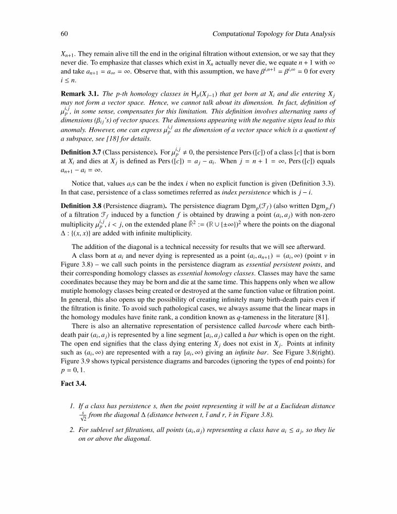
60 Computational Topology for Data Analysis
Xn+1. They remain alive till the end in the original filtration without extension, or we say that theynever die. To emphasize that classes which exist in Xn actually never die, we equate n + 1 with∞and take an+1 = a∞ = ∞. Observe that, with this assumption, we have βi,n+1 = βi,∞ = 0 for everyi ≤ n.
Remark 3.1. The p-th homology classes in Hp(X j−1) that get born at Xi and die entering X j
may not form a vector space. Hence, we cannot talk about its dimension. In fact, definition ofµ
i, jp , in some sense, compensates for this limitation. This definition involves alternating sums of
dimensions (βi j’s) of vector spaces. The dimensions appearing with the negative signs lead to thisanomaly. However, one can express µi, j
p as the dimension of a vector space which is a quotient ofa subspace, see [18] for details.
Definition 3.7 (Class persistence). For µi, jp , 0, the persistence Pers ([c]) of a class [c] that is born
at Xi and dies at X j is defined as Pers ([c]) = a j − ai. When j = n + 1 = ∞, Pers ([c]) equalsan+1 − ai = ∞.
Notice that, values ais can be the index i when no explicit function is given (Definition 3.3).In that case, persistence of a class sometimes referred as index persistence which is j − i.
Definition 3.8 (Persistence diagram). The persistence diagram Dgmp(F f ) (also written Dgmp f )of a filtration F f induced by a function f is obtained by drawing a point (ai, a j) with non-zeromultiplicity µi, j
p , i < j, on the extended plane R2 := (R ∪ ±∞)2 where the points on the diagonal∆ : (x, x) are added with infinite multiplicity.
The addition of the diagonal is a technical necessity for results that we will see afterward.A class born at ai and never dying is represented as a point (ai, an+1) = (ai,∞) (point v in
Figure 3.8) – we call such points in the persistence diagram as essential persistent points, andtheir corresponding homology classes as essential homology classes. Classes may have the samecoordinates because they may be born and die at the same time. This happens only when we allowmutiple homology classes being created or destroyed at the same function value or filtration point.In general, this also opens up the possibility of creating infinitely many birth-death pairs even ifthe filtration is finite. To avoid such pathological cases, we always assume that the linear maps inthe homology modules have finite rank, a condition known as q-tameness in the literature [81].
There is also an alternative representation of persistence called barcode where each birth-death pair (ai, a j) is represented by a line segment [ai, a j) called a bar which is open on the right.The open end signifies that the class dying entering X j does not exist in X j. Points at infinitysuch as (ai,∞) are represented with a ray [ai,∞) giving an infinite bar. See Figure 3.8(right).Figure 3.9 shows typical persistence diagrams and barcodes (ignoring the types of end points) forp = 0, 1.
Fact 3.4.
1. If a class has persistence s, then the point representing it will be at a Euclidean distances√2
from the diagonal ∆ (distance between t, t and r, r in Figure 3.8).
2. For sublevel set filtrations, all points (ai, a j) representing a class have ai ≤ a j, so they lieon or above the diagonal.
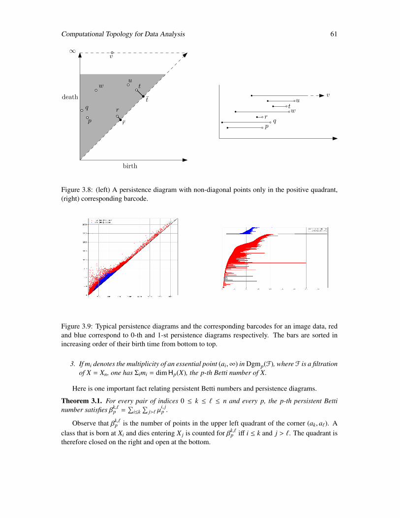
Computational Topology for Data Analysis 61
birth
death
r
t
r
t
p
q
wu
pq
rwt
u
∞v
v
Figure 3.8: (left) A persistence diagram with non-diagonal points only in the positive quadrant,(right) corresponding barcode.
Figure 3.9: Typical persistence diagrams and the corresponding barcodes for an image data, redand blue correspond to 0-th and 1-st persistence diagrams respectively. The bars are sorted inincreasing order of their birth time from bottom to top.
3. If mi denotes the multiplicity of an essential point (ai,∞) in Dgmp(F), where F is a filtrationof X = Xn, one has Σimi = dim Hp(X), the p-th Betti number of X.
Here is one important fact relating persistent Betti numbers and persistence diagrams.
Theorem 3.1. For every pair of indices 0 ≤ k ≤ ` ≤ n and every p, the p-th persistent Bettinumber satisfies βk,`
p =∑
i≤k∑
j>` µi, jp .
Observe that βk,`p is the number of points in the upper left quadrant of the corner (ak, a`). A
class that is born at Xi and dies entering X j is counted for βk,`p iff i ≤ k and j > `. The quadrant is
therefore closed on the right and open at the bottom.
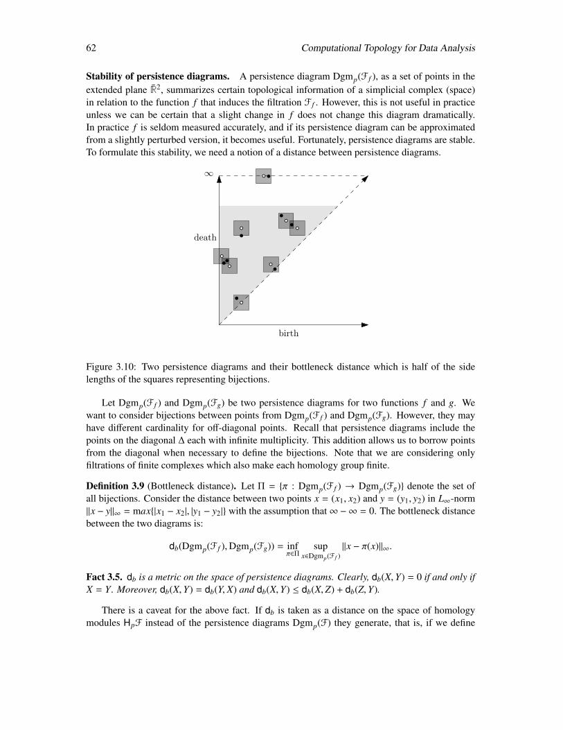
62 Computational Topology for Data Analysis
Stability of persistence diagrams. A persistence diagram Dgmp(F f ), as a set of points in theextended plane R2, summarizes certain topological information of a simplicial complex (space)in relation to the function f that induces the filtration F f . However, this is not useful in practiceunless we can be certain that a slight change in f does not change this diagram dramatically.In practice f is seldom measured accurately, and if its persistence diagram can be approximatedfrom a slightly perturbed version, it becomes useful. Fortunately, persistence diagrams are stable.To formulate this stability, we need a notion of a distance between persistence diagrams.
birth
death
∞
Figure 3.10: Two persistence diagrams and their bottleneck distance which is half of the sidelengths of the squares representing bijections.
Let Dgmp(F f ) and Dgmp(Fg) be two persistence diagrams for two functions f and g. Wewant to consider bijections between points from Dgmp(F f ) and Dgmp(Fg). However, they mayhave different cardinality for off-diagonal points. Recall that persistence diagrams include thepoints on the diagonal ∆ each with infinite multiplicity. This addition allows us to borrow pointsfrom the diagonal when necessary to define the bijections. Note that we are considering onlyfiltrations of finite complexes which also make each homology group finite.
Definition 3.9 (Bottleneck distance). Let Π = π : Dgmp(F f ) → Dgmp(Fg) denote the set ofall bijections. Consider the distance between two points x = (x1, x2) and y = (y1, y2) in L∞-norm‖x − y‖∞ = max|x1 − x2|, |y1 − y2| with the assumption that∞−∞ = 0. The bottleneck distancebetween the two diagrams is:
db(Dgmp(F f ),Dgmp(Fg)) = infπ∈Π
supx∈Dgmp(F f )
‖x − π(x)‖∞.
Fact 3.5. db is a metric on the space of persistence diagrams. Clearly, db(X,Y) = 0 if and only ifX = Y. Moreover, db(X,Y) = db(Y, X) and db(X,Y) ≤ db(X,Z) + db(Z,Y).
There is a caveat for the above fact. If db is taken as a distance on the space of homologymodules HpF instead of the persistence diagrams Dgmp(F) they generate, that is, if we define
Computational Topology for Data Analysis 63
db(HpF f ,HpFg) := db(Dgmp(F f ),Dgmp(Fg)), then it may not be a metric. The first axiom formetric becomes false if the homology modules are allowed to have classes created and destroyedat the same function values. These classes of zero persistence generate points on the diagonal ∆
in the diagram. Since points on the diagonal have infinite multiplicity, two modules differing inthe number of such classes of zero persistence may have diagrams with zero bottleneck distance.If we allow such cases, db becomes a pseudometric on the space of homology modules meaningthat it satisfies all axioms of a metric except the first one.
The following theorems originally proved in [102] and further detailed in [149] quantify thenotion of the stability of the persistence diagram. There are two versions, one involves simplicialfiltrations and the other involves space filtrations. For two functions, f , g : X → R, the infinitynorm is defined as ‖ f − g‖∞ := supx∈X | f (x) − g(x)|.
Theorem 3.2 (Stability for simplicial filtrations). Let f , g : K → R be two simplex-wise monotonefunctions giving rise to two simplicial filtrations F f and Fg. Then, for every p ≥ 0,
db(Dgmp(F f ),Dgmp(Fg)) ≤ ‖ f − g‖∞.
For the second version of the stability theorem, we require that the functions referred in thetheorem are ‘nice’ in the sense that they are tame. A function f : X → R is tame if the homologygroups of its sublevel sets have finite ranks and they change via inclusion-induced maps only atfinitely many values called critical.
Theorem 3.3 (Stability for space filtrations). Let X be a triangulable space and f , g : X → R betwo tame functions giving rise to two space filtrations F f and Fg where the values for sublevelsets include critical values. Then, for every p ≥ 0,
db(Dgmp(F f ),Dgmp(Fg)) ≤ ‖ f − g‖∞.
There is another distance called q-Wasserstein distance with which persistence diagrams arealso compared.
Definition 3.10 (Wasserstein distance). Let Π be the set of bijections as defined in Definition 3.9.For any p ≥ 0, q ≥ 1, the q-Wasserstein distance is define as
dW,q(Dgmp(F f ),Dgmp(Fg)) = infπ∈Π
[Σx∈Dgmp(F f )
(‖x − π(x)‖q
)q]1/q.
The distance dW,q also is a metric on the space of persistence diagrams just like the bottleneckdistance. It also enjoys a stability property though it is not as strong as in Theorem 3.3.
Fact 3.6. Let f , g : X → R be two Lipschitz functions defined on a triangulable compact metricspace X. Then, there exist constants C and k depending on X and the Lipschitz constants of f andg so that for every p ≥ 0 and q ≥ k,
dW,q(Dgmp(F f ),Dgmp(Fg)) ≤ C · ‖ f − g‖1− k
q∞ .
64 Computational Topology for Data Analysis
The above result got improved recently [278] by considering the Lq-distance between func-tions defined on a common domain X:
‖ f − g‖q =(Σx∈X | f (x) − g(x)|q
)1/q .
Theorem 3.4 (Stability for Wasserstein distance). Let f , g : K → R be two simplex-wise mono-tone functions on a simplicial complex K. Then, one has
dW,q(Dgmp(F f ),Dgmp(Fg)) ≤ ‖ f − g‖q.
Bottleneck distances can be computed using perfect matchings in bipartite graphs. ComputingWasserstein distances become more difficult. It can be computed using an algorithm for minimumweight perfect matching in weighted bipartite graphs. We leave it as an Exercise question (Exer-cise 5).
Computing bottleneck distances.
Let A and B be the non-diagonal points in two persistence diagrams Dgmp(F f ) and Dgmp(Fg)respectively. For a point a ∈ A, let a denote the nearest point of a on the diagonal. Define b forevery point b ∈ B similarly. Let A = a and B = b. Let A = A ∪ B and B = B ∪ A. We wantto bijectively match points in A and B. Let Π = π denote such a matching. It follows from thedefinition that
db(Dgmp(F f ),Dgmp(Fg)) = minπ∈Π
supa∈A,π(a)∈B
‖a − π(a)‖∞.
Then, the bottleneck distance we want to compute must be L∞ distance max|xa − xb|, |ya − yb|
for two points a ∈ A and b ∈ B. We do a binary search on all such possible O(n2) distances where|A| = |B| = n. Let δ0, δ1, · · · , δn′ be the sorted sequence of these distances in a non-decreasingorder.
Given a δ = δi ≥ 0 where i is the median of the index in the binary search interval [`, u],we construct a bipartite graph G = (A ∪ B, E) where an edge e = (a, b)a∈A,b∈B is in E if andonly if either both a ∈ A and b ∈ B (weight(e) = 0) or ‖a − b‖∞ ≤ δ (weight(e) = ‖a − b‖∞).A complete matching in G is a set of n edges so that every vertex in A and B is incident toexactly one edge in the set. To determine if G has a complete matching, one can use an O(n2.5)algorithm of Hopcroft and Karp [198] for complete matching in a bipartite graph. However,exploiting the geometric embedding of the points in the persistence diagrams, we can apply anO(n1.5) time algorithm of Efrat et al. [154] for the purpose. If such an algorithm affirms that acomplete matching exists, we do the following: if ` = u we output δ, otherwise we set u = iand repeat. If no matching exists, we set ` = i and repeat. Observe that matching has to existfor some value of δ, in particular for δn′ and thus the binary search always succeeds. Algorithm1: Bottleneck lays out the pseudocode for this matching. The algorithm runs in O(n1.5 log n)time accounting for the O(log n) probes for binary search each applying O(n1.5) time matchingalgorithm. However, to achieve this complexity, we have to avoid sorting n′ = O(n2) values takingO(n2 log n) time. Again, using the geometric embedding of the points, one can perform the binaryprobes without incurring the cost for sorting. For details and an efficient implementation of thisalgorithm see [208].
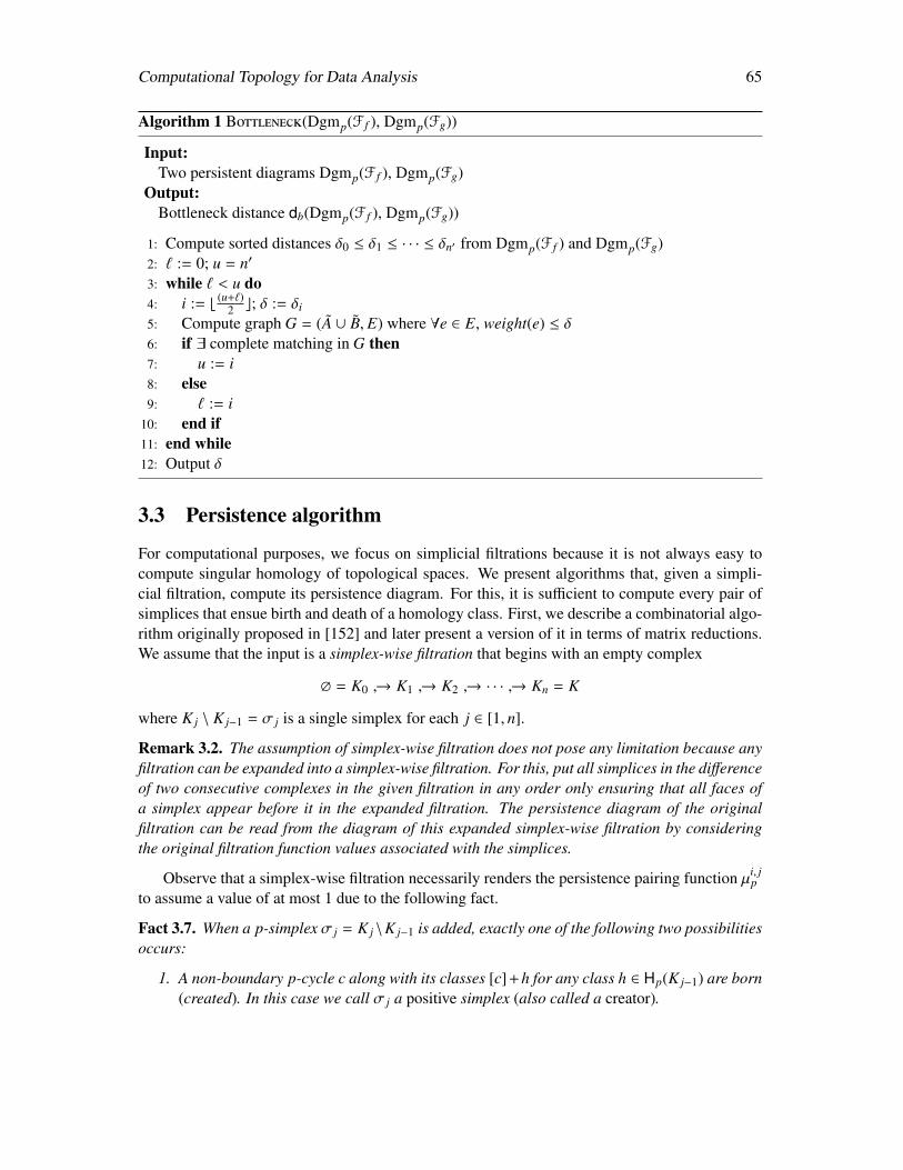
Computational Topology for Data Analysis 65
Algorithm 1 Bottleneck(Dgmp(F f ), Dgmp(Fg))
Input:Two persistent diagrams Dgmp(F f ), Dgmp(Fg)
Output:Bottleneck distance db(Dgmp(F f ), Dgmp(Fg))
1: Compute sorted distances δ0 ≤ δ1 ≤ · · · ≤ δn′ from Dgmp(F f ) and Dgmp(Fg)2: ` := 0; u = n′
3: while ` < u do4: i := b (u+`)
2 c; δ := δi
5: Compute graph G = (A ∪ B, E) where ∀e ∈ E, weight(e) ≤ δ6: if ∃ complete matching in G then7: u := i8: else9: ` := i
10: end if11: end while12: Output δ
3.3 Persistence algorithm
For computational purposes, we focus on simplicial filtrations because it is not always easy tocompute singular homology of topological spaces. We present algorithms that, given a simpli-cial filtration, compute its persistence diagram. For this, it is sufficient to compute every pair ofsimplices that ensue birth and death of a homology class. First, we describe a combinatorial algo-rithm originally proposed in [152] and later present a version of it in terms of matrix reductions.We assume that the input is a simplex-wise filtration that begins with an empty complex
∅ = K0 → K1 → K2 → · · · → Kn = K
where K j \ K j−1 = σ j is a single simplex for each j ∈ [1, n].
Remark 3.2. The assumption of simplex-wise filtration does not pose any limitation because anyfiltration can be expanded into a simplex-wise filtration. For this, put all simplices in the differenceof two consecutive complexes in the given filtration in any order only ensuring that all faces ofa simplex appear before it in the expanded filtration. The persistence diagram of the originalfiltration can be read from the diagram of this expanded simplex-wise filtration by consideringthe original filtration function values associated with the simplices.
Observe that a simplex-wise filtration necessarily renders the persistence pairing function µi, jp
to assume a value of at most 1 due to the following fact.
Fact 3.7. When a p-simplex σ j = K j \K j−1 is added, exactly one of the following two possibilitiesoccurs:
1. A non-boundary p-cycle c along with its classes [c] +h for any class h ∈ Hp(K j−1) are born(created). In this case we call σ j a positive simplex (also called a creator).
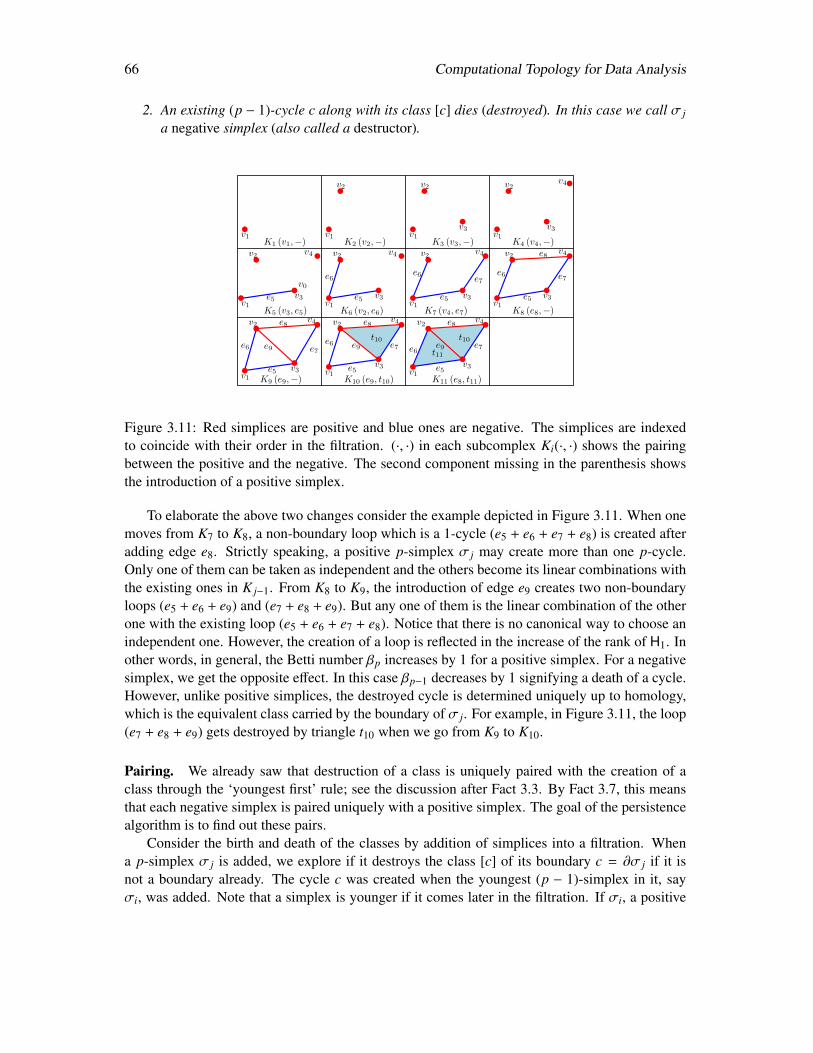
66 Computational Topology for Data Analysis
2. An existing (p − 1)-cycle c along with its class [c] dies (destroyed). In this case we call σ j
a negative simplex (also called a destructor).
v1
v0
v1 v1 v1
v1 v1 v1 v1
v1v1 v1
v2 v2 v2
v2 v2 v2 v2
v2 v2 v2
v3 v3
v3 v3 v3 v3
v3v3 v3
v4
v4 v4 v4 v4
v4 v4 v4
e5 e5 e5 e5
e5 e5 e5
e6e6 e6
e6e6
e6
e7
e7e7 e7
e8
e8 e8 e8
e9 e9 e9t10 t10
t11
K1 (v1,−) K2 (v2,−) K3 (v3,−) K4 (v4,−)
K5 (v3, e5) K6 (v2, e6) K7 (v4, e7) K8 (e8,−)
K9 (e9,−) K10 (e9, t10) K11 (e8, t11)
e7
Figure 3.11: Red simplices are positive and blue ones are negative. The simplices are indexedto coincide with their order in the filtration. (·, ·) in each subcomplex Ki(·, ·) shows the pairingbetween the positive and the negative. The second component missing in the parenthesis showsthe introduction of a positive simplex.
To elaborate the above two changes consider the example depicted in Figure 3.11. When onemoves from K7 to K8, a non-boundary loop which is a 1-cycle (e5 + e6 + e7 + e8) is created afteradding edge e8. Strictly speaking, a positive p-simplex σ j may create more than one p-cycle.Only one of them can be taken as independent and the others become its linear combinations withthe existing ones in K j−1. From K8 to K9, the introduction of edge e9 creates two non-boundaryloops (e5 + e6 + e9) and (e7 + e8 + e9). But any one of them is the linear combination of the otherone with the existing loop (e5 + e6 + e7 + e8). Notice that there is no canonical way to choose anindependent one. However, the creation of a loop is reflected in the increase of the rank of H1. Inother words, in general, the Betti number βp increases by 1 for a positive simplex. For a negativesimplex, we get the opposite effect. In this case βp−1 decreases by 1 signifying a death of a cycle.However, unlike positive simplices, the destroyed cycle is determined uniquely up to homology,which is the equivalent class carried by the boundary of σ j. For example, in Figure 3.11, the loop(e7 + e8 + e9) gets destroyed by triangle t10 when we go from K9 to K10.
Pairing. We already saw that destruction of a class is uniquely paired with the creation of aclass through the ‘youngest first’ rule; see the discussion after Fact 3.3. By Fact 3.7, this meansthat each negative simplex is paired uniquely with a positive simplex. The goal of the persistencealgorithm is to find out these pairs.
Consider the birth and death of the classes by addition of simplices into a filtration. Whena p-simplex σ j is added, we explore if it destroys the class [c] of its boundary c = ∂σ j if it isnot a boundary already. The cycle c was created when the youngest (p − 1)-simplex in it, sayσi, was added. Note that a simplex is younger if it comes later in the filtration. If σi, a positive
Computational Topology for Data Analysis 67
(p − 1)-simplex, has already been paired with a p-simplex σ′j, then a class also created by σi gotdestroyed when σ′j appeared. We can get the (p − 1)-cycle representing this destroyed class andadd it to ∂σ j. The addition provides a cycle that existed before σi. We update c to be this newcycle and look for the youngest (p − 1)-simplex σi in c and continue the process till we find onethat is unpaired, or the cycle c becomes empty. In the latter case, we discover that c = ∂σ j was aboundary cycle already and thus σ j creates a new class in Hp(K j). In the other case, we discoverthat σ j is a negative p-simplex which destroys a class created by σi. We pair σ j with σi. Indeed,one can show that the above algorithm produces the persistence pairs according to Definition 3.11below, that is, their function values lead to the persistence diagram (Definition 3.8). We give aproof for a matrix version of the algorithm later (Theorem 3.6).
Definition 3.11 (Persistence pairs). Given a simplex-wise filtration F : K0 → K1 → · · · → Kn,for 0 < i < j ≤ n, we say a p-simplex σi = Ki \ Ki−1 and a (p + 1)-simplex σ j = K j \ K j−1 form apersistence pair (σi, σ j) if and only if µi, j
p > 0.
The full algorithm is presented in Algorithm 2:PairPersistence, which takes as input a se-quence of simplices σ1, σ2, · · · , σn ordered according to the filtration of a complex whose persis-tence diagram is to be computed. It assumes that the complex is represented combinatorially withadjacency structures among its simplices.
Algorithm 2 PairPersistence(σ1, σ2, · · · , σn)
Input:An ordered sequence of simplices forming a filtration of a complex
Output:Determine if a simplex is ‘positive’ or ‘negative’ and generate persistent pairs
1: for j = 1 to n do2: c := ∂pσ j
3: σi is the youngest positive (p − 1)-simplex in c4: while σi is paired and c is not empty do5: Let c′ be the cycle destroyed by the simplex paired with σi \∗ computed previously in
step 10 ∗\6: c := c′ + c \∗ this addition may cancel simplices ∗\7: Update σi to be the youngest positive (p − 1)-simplex in c8: end while9: if c is not empty then
10: σ j is a negative p-simplex; generate pair (σi, σ j); associate c with σ j as destroyed11: else12: σ j is a positive p-simplex \∗ σ j may get paired later ∗\13: end if14: end for
Let us again consider the example in Figure 3.11 and see how the algorithm Pair works. FromK7 to K8, e8 is added. Its boundary is c = (v2 + v4). The vertex v4 is the youngest positive vertexin c but it is paired with e7 in K7. Thus, c is updated to (v3 + v4 + v4 + v2) = (v3 + v2). The vertexv3 becomes the youngest positive one but it is paired with e5. So, c is updated to (v1 + v2). The
68 Computational Topology for Data Analysis
vertex v2 becomes the youngest positive one but it is paired with e6. So, c is updated to be empty.Hence e8 is a positive edge. Now we examine the addition of the triangle t11 from K10 to K11.The boundary of t11 is c = (e5 + e6 + e9). The youngest positive edge e9 is paired with t10. Thus,c is updated by adding the cycle destroyed by t10 to (e5 + e6 + e7 + e8). Since e8 is the youngestpositive edge that is not yet paired, t11 finds e8 as its paired positive edge. Observe that, we finallyobtain a loop that is destroyed by adding the negative triangle. For example, we obtain the loop(e5 + e6 + e7 + e8) by adding t11.
3.3.1 Matrix reduction algorithm
There is a version of the algorithm PairPersistence that uses only matrix operations. First noticethe following:
• The boundary operator ∂p : Cp → Cp−1 can be represented by a boundary matrix Dp wherethe columns correspond to the p-simplices and rows correspond to (p − 1)-simplices.
• It represents the transformation of a basis of Cp given by the set of p-simplices to a basisof Cp−1 given by the set of (p − 1)-simplices.
Dp[i, j] =
1 if σi ∈ ∂pσ j
0 otherwise.
• One can combine all boundary matrices into a single matrix D that represents all linearmaps
⊕p ∂p =
⊕p(Cp → Cp−1), that is, transformation of a basis of all chain groups
together to a basis of itself, but with a shift to a one lower dimension.
D[i, j] =
1 if σi ∈ ∂∗σ j
0 otherwise.
Definition 3.12 (Filtered boundary matrix). Let F : ∅ = K0 → K1 → . . . → Kn = K be afiltration induced by an ordering of simplices (σ1, σ2, . . . , σn) in K. Let D denote the boundarymatrix for simplices in K that respects the ordering of the simplices in the filtration, that is, thesimplex σi in the filtration occupies column and row i in D. We call D the filtered boundarymatrix for F.
Given any matrix A, let rowA[i] and colA[ j] denote the ith row and jth column of A, respec-tively. We abuse the notation slightly to let colA[ j] denote also the chain σi | A[i, j] = 1, whichis the collection of simplices corresponding to 1’s in the column colA[ j].
Definition 3.13 (Reduced matrix). Let lowA[ j] denote the row index of the last 1 in the jth columnof A, which we call the low-row index of the column j. It is undefined for empty columns (markedwith −1 in Algorithm 3). The matrix A is reduced (or is in reduced form) if lowA[ j] , lowA[ j′]for any j , j′; that is, no two columns share the same low-row indices.
Fact 3.8. Given a matrix A in reduced form, we have that the set of non-zero columns in A are alllinearly independent over Z2.
Computational Topology for Data Analysis 69
We define a matrix A over Z2 to be upper-triangular if all of its diagonal elements are 1,and there is no entry A[i, j] = 1 with i > j. We will compute a reduced matrix from a givenboundary matrix by left-to-right column additions. A series of such column additions is equivalentto multiplying the boundary matrix on right with an upper triangular matrix.
Now, we state a result saying that if a reduced form is obtained via only left-to-right columnadditions, then for each column, the low-row index is unique in the sense that it does not depend onhow the reduced form is obtained. Using this result we show that persistence pairing of simplicescan be obtained from these low-row indices. Given an n1×n2 matrix A, let A[c,d]
[a,b], a ≤ b and c ≤ d,denote the sub-matrix formed by rows a to b, and columns from c to d. In cases when b = n2 andc = 1, we also write it as Ad
a := A1,da,n2 for simplicity. For any 1 ≤ i < j ≤ n, define the quantity
rA(i, j) as follows:
rA(i, j) = rank (A ji ) − rank (A j
i+1) + rank (A j−1i+1 ) − rank (A j−1
i ). (3.5)
Proposition 3.5 (Paring Uniqueness [106]). Let R = DV, where R is in reduced form and V isupper triangular. Then for any 1 ≤ j ≤ n, lowR[ j] = i if and only if rD(i, j) = 1.
Next, we show that a pairing based on low-row indices indeed provides the persistent pairsaccording to Definition 3.11.
Theorem 3.6. Let D be the m × m filtered boundary matrix for a filtration F (Definition 3.12).Let R = DV , where R is in reduced form and V is upper triangular. Then, the simplices σi and σ j
in F form a persistent pair if and only if lowR[ j] = i.
Proof. First, it is easy to verify that rR(i, j) = rD(i, j) for any 1 ≤ i < j ≤ n (in particular,rank (Rd
a) = rank (Dda) as the effect of V is to add columns of D to columns on the right only).
Combining this and Proposition 3.5, we only need to show that there is a persistent pair (σi, σ j)(i.e., µi, j
p = 1) if and only if rR(i, j) = 1.Next, we observe that due to the uniqueness of the entry lowR[ j] (Proposition 3.5), if we
prove the theorem for a specific reduced matrix R′ = DV ′, then it holds for any reduced formR = DV . In what follows, we assume that the reduced form R = DV is obtained by Algorithm3:MatPersistence(D). For this specific reduction algorithm, it is easy to see that if a simplexσ j is of dimension p, then all columns ever added to the j-th column correspond to simplicesof dimension p. In particular, let Dp denote the matrix obtained by setting all columns in Dcorresponding to simplices of dimension , p to be all-zero; hence all non-zero columns in Dp
represents the p-th boundary operator ∂p : Cp(K)→ Cp−1(K). Define Rp similarly. Then observethat algorithm MatPersistence simply reduces each matrix Dp independently, for all dimensionsp, and the reduced form for Dp is Rp.
In what follows, we assume that the dimension of simplex σ j (corresponding to the j-thcolumn of D) is p; and for simplicity, set R := Rp. We leave the proof of the following claim asan exercise (Exercise 5).
Proposition 3.7. Let the dimension for σ j be p and construct R = Rp as described above. Forany 1 ≤ i < j, we have that rR(i, j) = rR(i, j).
To this end, let Zkp−1 and Bk
p−1 denote the (p − 1)-th cycle group and the (p − 1)-th boundarygroup for Kk, respectively. Consider the persistence pairing function for 1 ≤ i < j ≤ n:
µi, jp−1 = (βi, j−1
p−1 − βi, jp−1) − (βi−1, j−1
p−1 − βi−1, jp−1 ). (3.6)
70 Computational Topology for Data Analysis
On the other hand, note that for any 1 ≤ a < b ≤ n,
βa,bp−1 := rank (Ha,b
p−1) = rank( Za
p−1
Zap−1 ∩ Bb
p−1
)= rank (Za
p−1) − rank (Zap−1 ∩ Bb
p−1). (3.7)
Let Γba := colR[k] | k ∈ [1, b] and 1 ≤ lowR[k] ≤ a. Using the facts that all non-zero columns
in R with index at most b form a basis for Bbp−1, and that each low-row index for every non-
zero column is unique, one can show that rank (Zap−1 ∩ Bb
p−1) = |Γba|. Now consider the set of
all non-zero columns in R with index at most b that are not in Γba, denoted by Γb
a. Note that|Γb
a| = rank (Rba+1) = rank (Bb
p−1) − |Γba|; hence
rank (Zap−1 ∩ Bb
p−1) = |Γba| = rank (Bb
p−1) − |Γba| = rank (Rb
1) − rank (Rba+1).
Combining the above with Proposition 3.7, Eqn. (3.6) and Eqn. (3.7), we thus have that:
µi, jp−1 = rank (Zi
p−1) − rank (Zip−1 ∩ B j−1
p−1) −(rank (Zi
p−1) − rank (Zip−1 ∩ B j
p−1))
−(rank (Zi−1
p−1) − rank (Zi−1p−1 ∩ B j−1
p−1))
+ rank (Zi−1p−1) − rank (Zi−1
p−1 ∩ B jp−1)
= rank (Zip−1 ∩ B j
p−1) − rank (Zip−1 ∩ B j−1
p−1) + rank (Zi−1p−1 ∩ B j−1
p−1) − rank (Zi−1p−1 ∩ B j
p−1)
= − rank (R ji+1) + rank (R j−1
i+1 ) − rank (R j−1i ) + rank (R j
i ) = rR(i, j) = rR(i, j) = rD(i, j).
By Proposition 3.5, the theorem then follows.
Algorithm 3 MatPersistence(D)
Input:Boundary matrix D of a complex with columns and rows ordered by a given filtration
Output:Reduced matrix with each column j either being empty or having a unique lowD[ j] entity
1: for j = 1→ |colD| do2: while ∃ j′ < j s.t. lowD[ j′] == lowD[ j] and lowD[ j] , −1 do3: colD[ j] := colD[ j] + colD[ j′]4: end while5: if lowD[ j] , −1 then6: i := lowD[ j] ; generate pair (σi, σ j)7: end if8: end for
Matrix reduction algorithm. Notice that there are possibly many R and V for a fixed D forminga reduced-form decomposition. Theorem 3.6 implies that the persistent pairing is independent ofthe particular contents of R and V as long as R is reduced and V is upper triangular. If we reducea given filtered boundary matrix D to a reduced form R only with left-to-right column additions,
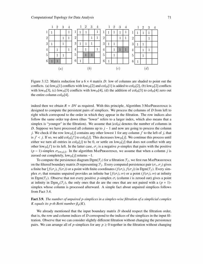
Computational Topology for Data Analysis 71
1
1
1
1
1
1
1
1
1
1
1
1
1 2 3 4
1
2
3
4
5
6
1
1
1
1
1
1
1
1
1
1
1
1 2 3 4
1
2
3
4
5
6
1
1
1
1
1
1
1
1 1
1
1
1 2 3 4
1
2
3
4
5
6
1
1
1
1
1
1
1
1
1 2 3 4
1
2
3
4
5
6
1
1
1
(a) (b) (c) (d)
1 1 1
Figure 3.12: Matrix reduction for a 6 × 4 matrix D: low of columns are shaded to point out theconflicts. (a) lowD[1] conflicts with lowD[2] and colD[1] is added to colD[2], (b) lowD[2] conflictswith lowD[3], (c) lowD[3] conflicts with lowD[4], (d) the addition of colD[3] to colD[4] zero outthe entire column colD[4].
indeed then we obtain R = DV as required. With this principle, Algorithm 3:MatPersistence isdesigned to compute the persistent pairs of simplices. We process the columns of D from left toright which correspond to the order in which they appear in the filtration. The row indices alsofollow the same order top down (thus “lower" refers to a larger index, which also means that asimplex is “younger" in the filtration). We assume that |colD| denotes the number of columns inD. Suppose we have processed all columns up to j − 1 and now are going to process the columnj. We check if the row lowD[ j] contains any other lowest 1 for any column j′ to the left of j, thatis j′ < j. If so, we add colD[ j′] to colD[ j]. This decreases lowD[ j]. We continue this process untileither we turn all entries in colD[ j] to be 0, or settle on lowD[ j] that does not conflict with anyother lowD[ j′] to its left. In the latter case, σ j is a negative p-simplex that pairs with the positive(p − 1)-simplex σlowD[ j]. In the algorithm MatPersistence, we assume that when a column j iszeroed out completely, lowD[ j] returns −1.
To compute the persistence diagram Dgm(F f ) for a filtration F f , we first run MatPersistenceon the filtered boundary matrix D representing F f . Every computed persistence pair (σi, σ j) givesa finite bar [ f (σ j), f (σi)) or a point with finite coordinates ( f (σi), f (σ j)) in Dgm(F f ). Every sim-plex σi that remains unpaired provides an infinite bar [ f (σi),∞) or a point ( f (σi),∞) at infinityin Dgm(F f ). Observe that not every positive p-simplex σi (column i is zeroed out) gives a pointat infinity in Dgmp(F f ), the only ones that do are the ones that are not paired with a (p + 1)-simplex whose column is processed afterward. A simple fact about unpaired simplices followsfrom Fact 3.4.
Fact 3.9. The number of unpaired p-simplices in a simplex-wise filtration of a simplicial complexK equals its p-th Betti number βp(K).
We already mentioned that the input boundary matrix D should respect the filtration order,that is, the row and column indices of D correspond to the indices of the simplices in the input fil-tration. Observe that we can consider slightly different filtration without changing the persistencepairs. We can arrange all of p-simplices for any p ≥ 0 together in the filtration without changing
72 Computational Topology for Data Analysis
their relative orders as follows where σij denotes the jth i-simplex among all i-simplices in the
original filtration.
(σ01, σ
02 . . . , σ
0n0
), . . . , (σp1 , σ
p2 , . . . , σ
pnp), . . . , (σd
1, σd2, . . . , σ
dnd
) (3.8)
This means columns and rows of p-simplices in D become adjacent though retaining their relativeordering from the original matrix. Observe that, by this rearrangement, all columns that are addedto a column j in the original D still remain to the left of j in their newly assigned indices. In otherwords, processing the rearranged matrix D can be thought of as processing each individual p-boundary matrix Dp = [∂p] separately where the column and row indices respect the relativeorders of p and (p − 1)-simplices in the original filtration.
Complexity of MatPersistence. Let the filtration F based on which the boundary matrix D isconstructed insert n simplices. This means that D has at most n rows and columns. Then, the outerfor loop is executed at most O(n) times. Within this for loop, steps 5-7 takes only O(1) time. Thecomplexity is indeed determined by the while loop (steps 2-4). We argue that this loop iteratesat most O(n) times. This follows from the fact that each column addition in step 3 decreaseslowD[ j] by at least one and over the entire algorithm it cannot decrease by more than the lengthof the column which is O(n). Each column addition in step 3 takes at most O(n) time giving atotal time of O(n2) for the while loop. Accounting for the outer for loop, we get a complexity ofO(n3) for MatPersistence.
One can implement the above matrix reduction algorithm with a more efficient data structurenoting that most of the entries in the input matrix D is empty. A linked list representing thenon-zero entries in the columns of D is space-wise more efficient. Edelsbrunner and Harer [149]present a clever implementation of MatPersistence using such a sparse matrix representation. Forevery column j, the algorithm executes O( j− i) column additions of O( j− i) length each incurringa cost O(( j− i)2) where i = 1 if σ j is positive and is the index of the simplex σi with which it pairsin case σ j is negative. Therefore, the total time complexity becomes O(
∑j∈[1,n]( j− i)2). Here, we
assume that the dimension of the complex K is a constant.It is worth noting that essentially the matrix reduction algorithm is a version of the classical
Gaussian elimination method with a given column order and a specific choice of row pivots. Inthis respect, persistence of a given filtration can be computed by the PLU factorization of a matrixfor which Bunch and Hopcroft [58] gives an O(M(n)) time algorithm where M(n) is the time tomultiply two n × n matrices. It is known that M(n) = O(nω) where ω ∈ [2, 2.373) is called theexponent for matrix multiplication.
3.3.2 Efficient implementation
The matrix reduction algorithm considers a column from left to right and reduces it by left-to-right additions. As we have observed, every addition to a column with index j pushes lowD[ j]upward. In the case, that σ j is a positive simplex, the entire column is zeroed out. In general,positive simplices incur more cost than the negative ones because lowD[·] needs to be pushed allthe way up for zeroing out the entire column. However, they do not participate in any futureleft-to-right column additions. Therefore, if it is known beforehand that the simplex σ j will be apositive simplex, then the costly step of zeroing out the column j can be avoided.
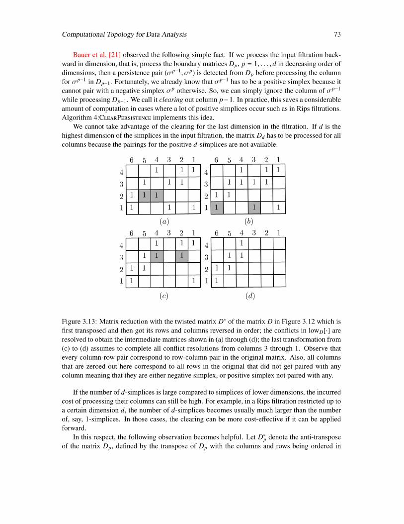
Computational Topology for Data Analysis 73
Bauer et al. [21] observed the following simple fact. If we process the input filtration back-ward in dimension, that is, process the boundary matrices Dp, p = 1, . . . , d in decreasing order ofdimensions, then a persistence pair (σp−1, σp) is detected from Dp before processing the columnfor σp−1 in Dp−1. Fortunately, we already know that σp−1 has to be a positive simplex because itcannot pair with a negative simplex σp otherwise. So, we can simply ignore the column of σp−1
while processing Dp−1. We call it clearing out column p−1. In practice, this saves a considerableamount of computation in cases where a lot of positive simplices occur such as in Rips filtrations.Algorithm 4:ClearPersistence implements this idea.
We cannot take advantage of the clearing for the last dimension in the filtration. If d is thehighest dimension of the simplices in the input filtration, the matrix Dd has to be processed for allcolumns because the pairings for the positive d-simplices are not available.
1
1 1
1
1
1
11
1
1
11
1
2
3
4
1234561
1 1
11
1
11
1
1
11
1
2
3
4
123456
1
1
11
1
1
1
1
11
1
2
3
4
123456
1
11
1 1
1
1
2
3
4
123456
(a) (b)
(c) (d)
Figure 3.13: Matrix reduction with the twisted matrix D∗ of the matrix D in Figure 3.12 which isfirst transposed and then got its rows and columns reversed in order; the conflicts in lowD[·] areresolved to obtain the intermediate matrices shown in (a) through (d); the last transformation from(c) to (d) assumes to complete all conflict resolutions from columns 3 through 1. Observe thatevery column-row pair correspond to row-column pair in the original matrix. Also, all columnsthat are zeroed out here correspond to all rows in the original that did not get paired with anycolumn meaning that they are either negative simplex, or positive simplex not paired with any.
If the number of d-simplices is large compared to simplices of lower dimensions, the incurredcost of processing their columns can still be high. For example, in a Rips filtration restricted up toa certain dimension d, the number of d-simplices becomes usually much larger than the numberof, say, 1-simplices. In those cases, the clearing can be more cost-effective if it can be appliedforward.
In this respect, the following observation becomes helpful. Let D∗p denote the anti-transposeof the matrix Dp, defined by the transpose of Dp with the columns and rows being ordered in
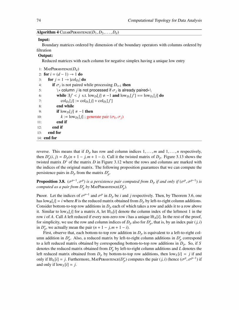
74 Computational Topology for Data Analysis
Algorithm 4 ClearPersistence(D1,D2, . . . ,Dd)
Input:Boundary matrices ordered by dimension of the boundary operators with columns ordered by
filtrationOutput:
Reduced matrices with each column for negative simplex having a unique low entry
1: MatPersistence(Dd)2: for i = (d − 1)→ 1 do3: for j = 1→ |colDi | do4: if σ j is not paired while processing Di+1 then5: \∗ column j is not processed if σ j is already paired∗\6: while ∃ j′ < j s.t. lowD[ j] , −1 and lowDi[ j′] == lowDi[ j] do7: colDi[ j] := colDi[ j] + colDi[ j′]8: end while9: if lowD[ j] , −1 then
10: k := lowDi[ j] ; generate pair (σk, σ j)11: end if12: end if13: end for14: end for
reverse. This means that if Dp has row and column indices 1, . . . ,m and 1, . . . , n respectively,then D∗p(i, j) = Dp(n + 1 − j,m + 1 − i). Call it the twisted matrix of Dp. Figure 3.13 shows thetwisted matrix D∗ of the matrix D in Figure 3.12 where the rows and columns are marked withthe indices of the original matrix. The following proposition guarantees that we can compute thepersistence pairs in Dp from the matrix D∗p.
Proposition 3.8. (σp−1, σp) is a persistence pair computed from Dp if and only if (σp, σp−1) iscomputed as a pair from D∗p by MatPersistence(D∗p).
Proof. Let the indices of σp−1 and σp in Dp be i and j respectively. Then, by Theorem 3.6, onehas lowR[ j] = i where R is the reduced matrix obtained from Dp by left-to-right column additions.Consider bottom-to-top row additions in Dp each of which takes a row and adds it to a row aboveit. Similar to lowA[ j] for a matrix A, let lftA[i] denote the column index of the leftmost 1 in therow i of A. Call A left reduced if every non-zero row i has a unique lftA[i]. In the rest of the proof,for simplicity, we use the row and column indices of Dp also for D∗p, that is, by an index pair ( j, i)in D∗p, we actually mean the pair (n + 1 − j,m + 1 − i).
First, observe that, each bottom-to-top row addition in Dp is equivalent to a left-to-right col-umn addition in D∗p. Also, a reduced matrix by left-to-right column additions in D∗p correspondto a left reduced matrix obtained by corresponding bottom-to-top row additions in Dp. So, if Sdenotes the reduced matrix obtained from D∗p by left-to-right column additions and L denotes theleft reduced matrix obtained from Dp by bottom-to-top row additions, then lowS [i] = j if andonly if lftL[i] = j. Furthermore, MatPersistence(D∗p) computes the pair ( j, i) (hence (σp, σp−1) ifand only if lowS [i] = j.
Computational Topology for Data Analysis 75
Therefore, to prove the proposition, it is sufficient to argue that lowR[ j] = i if and only iflftL[i] = j. By Proposition 3.5, lowR[ j] = i if and only if rDp(i, j) as defined in Eqn. (3.5) equals1. Therefore, it is sufficient to show that lftL[i] = j if and only if rDp(i, j) = 1.
The above claim can be proved exactly the same way as Proposition 3.5 is proved in [106]while replacing the role of lowR[ j] with lftL[i]. Observe that bottom-to-top row additions do notchange the rank of the lower left minors. Hence, rDp = rL. Therefore, it is sufficient to showthat lftL[i] = j if and only if rL(i, j) = 1. Assume first lftL[i] = j. The rows of L j
i (see thedefinitions above Eqn. (3.5)) are linearly independent and hence rank (L j
i ) − rank (L ji+1) = 1.
Now delete the last column in L ji which leaves the top row to have only zeroes. This im-
plies that rank (L j−1i ) − rank (L j−1
i+1 ) = 0. This gives rL(i, j) = 1 as needed. Next, assume thatlftL[i] , j. Consider L j
i and L j−1i . If lftL[i] > j, the top row in both matrices is zero. Therefore,
rank (L ji ) − rank (L j
i+1) = 0 and also rank (L j−1i ) = rank (L j−1
i+1 ) giving rL(i, j) = 0 as required.If lftL[i] < j, the top row in both matrices are non-zero giving rank (L j
i ) − rank (L ji+1) = 1 and
rank (L j−1i ) − rank (L j−1
i+1 ) = 1 giving again rL(i, j) = 0 as required.
To apply clearing we process D∗p+1 after D∗p by calling ClearPersistence(D∗d, · · · ,D∗2,D
∗1)
because if we get a pair (σp+1, σp) while processing D∗p, we already know that σp+1 is a negativesimplex and its column in D∗p+1 cannot contain a defined low entry. This means that the columnof σp+1 in D∗p+1 can be zeroed out and hence can be ignored. Now, the only boundary matrix thatneeds to be processed without any clearing is D∗1. So, depending on whether Dd or D1 is large,one can choose to process the filtration in increasing or decreasing dimensions respectively.
3.4 Persistence modules
We have seen in Section 3.2.1 that persistence diagrams are stable with respect to the perturbationof the function that defines the filtration on a given simplicial complex or a space. This requires thedomain of the function to be fixed. The result depends on the observation that perturbations in thefiltrations are bounded by the perturbations in the function which in turn also results into boundedperturbations at the homology level. A natural follow up is to derive a bound of the perturbationsof the persistence diagrams directly in terms of the perturbations at the homology level. Towardthis goal, we now define a generalized notion of homology modules called persistence modulesand a distance among them called the interleaving distance.
Recall that a filtration gives rise to a homology module which is a sequence of homologygroups connected by homomorphisms that are induced by inclusions defining the filtration. Thesehomology groups when defined over a field (e.g. Z2) can be thought of as vector spaces connectedby linear maps. Persistence modules extend homology modules by taking vector spaces in placeof homology groups and linear maps in place of inclusion induced homomorphisms.
We make one more extension. So far, the sequences in a filtration and homology moduleshave been indexed over a finite subset of natural numbers. It turns out that we can enlarge theindex set to be any subposet A of R. In the following definition persistence modules and theirinterleaving distance are defined over the poset (A,≤).
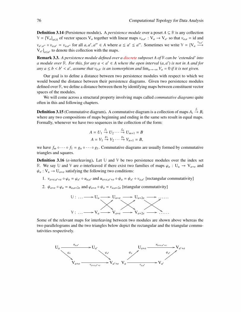
76 Computational Topology for Data Analysis
Definition 3.14 (Persistence module). A persistence module over a poset A ⊆ R is any collectionV =
Va
a∈A of vector spaces Va together with linear maps va,a′ : Va → Va′ so that va,a = id and
va′,a′′ va,a′ = va,a′′ for all a, a′, a′′ ∈ A where a ≤ a′ ≤ a′′. Sometimes we write V =Va
va,a′−→
Va′a≤a′ to denote this collection with the maps.
Remark 3.3. A persistence module defined over a discrete subposet A of R can be ‘extended’ intoa module over R. For this, for any a < a′ ∈ A where the open interval (a, a′) is not in A and forany a ≤ b < b′ < a′, assume that vb,b′ is an isomorphism and lima→−∞ Va = 0 if it is not given.
Our goal is to define a distance between two persistence modules with respect to which wewould bound the distance between their persistence diagrams. Given two persistence modulesdefined over R, we define a distance between them by identifying maps between constituent vectorspaces of the modules.
We will come across a structural property involving maps called commutative diagrams quiteoften in this and following chapters.
Definition 3.15 (Commutative diagram). A commutative diagram is a collection of maps Aifi→ Bi
where any two compositions of maps beginning and ending in the same sets result in equal maps.Formally, whenever we have two sequences in the collection of the form:
A = U1f1→ U2 · · ·
fm→ Um+1 = B
A = V1g1→ V2 · · ·
gn→ Vn+1 = B,
we have fm · · · f1 = gn · · · g1. Commutative diagrams are usually formed by commutativetriangles and squares.
Definition 3.16 (ε-interleaving). Let U and V be two persistence modules over the index setR. We say U and V are ε-interleaved if there exist two families of maps ϕa : Ua → Va+ε andψa : Va → Ua+ε satisfying the following two conditions:
1. va+ε,a′+ε ϕa = ϕa′ ua,a′ and ua+ε,a′+ε ψa = ψa′ va,a′ [rectangular commutativity]
2. ψa+ε ϕa = ua,a+2ε and ϕa+ε ψa = va,a+2ε [triangular commutativity]
U : . . . // Ua //
""
Ua+ε//
$$
Ua+2ε //
%%
. . . . . .
V : . . . // Va //
<<
Va+ε//
::
Va+2ε //
99
. . . . . .
Some of the relevant maps for interleaving between two modules are shown above whereas thetwo parallelograms and the two triangles below depict the rectangular and the triangular commu-tativities respectively.
Uaϕa
""
ua,a′ // Ua′
ϕa′
""Va+ε va+ε,a′+ε
// Va′+ε
Ua+ε
ua+ε,a′+ε // Va′+ε
Va
ψa<<
va,a′// Va′
ψa′<<
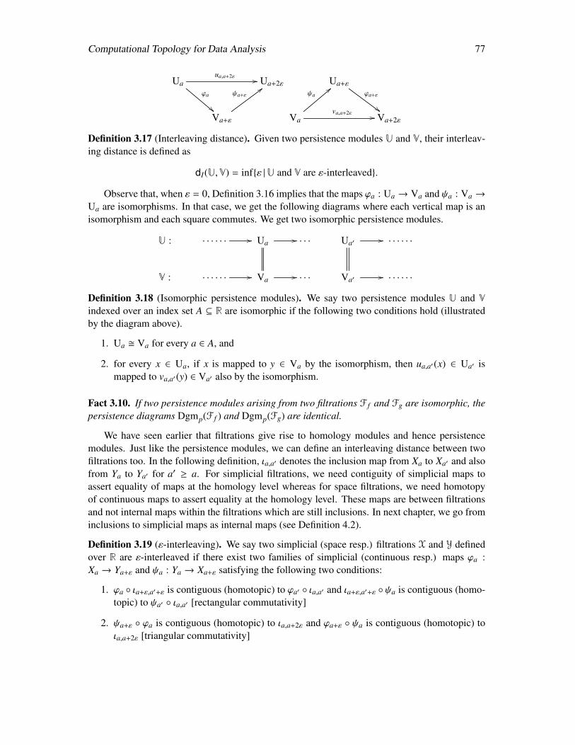
Computational Topology for Data Analysis 77
Uaϕa
""
ua,a+2ε // Ua+2ε
Va+ε
ψa+ε
;; Ua+ε
ϕa+ε
##Va
ψa<<
va,a+2ε // Va+2ε
Definition 3.17 (Interleaving distance). Given two persistence modules U and V, their interleav-ing distance is defined as
dI(U,V) = infε |U and V are ε-interleaved.
Observe that, when ε = 0, Definition 3.16 implies that the maps ϕa : Ua → Va and ψa : Va →
Ua are isomorphisms. In that case, we get the following diagrams where each vertical map is anisomorphism and each square commutes. We get two isomorphic persistence modules.
U : · · · · · · // Ua // · · · Ua′ // · · · · · ·
V : · · · · · · // Va // · · · Va′ // · · · · · ·
Definition 3.18 (Isomorphic persistence modules). We say two persistence modules U and Vindexed over an index set A ⊆ R are isomorphic if the following two conditions hold (illustratedby the diagram above).
1. Ua Va for every a ∈ A, and
2. for every x ∈ Ua, if x is mapped to y ∈ Va by the isomorphism, then ua,a′(x) ∈ Ua′ ismapped to va,a′(y) ∈ Va′ also by the isomorphism.
Fact 3.10. If two persistence modules arising from two filtrations F f and Fg are isomorphic, thepersistence diagrams Dgmp(F f ) and Dgmp(Fg) are identical.
We have seen earlier that filtrations give rise to homology modules and hence persistencemodules. Just like the persistence modules, we can define an interleaving distance between twofiltrations too. In the following definition, ιa,a′ denotes the inclusion map from Xa to Xa′ and alsofrom Ya to Ya′ for a′ ≥ a. For simplicial filtrations, we need contiguity of simplicial maps toassert equality of maps at the homology level whereas for space filtrations, we need homotopyof continuous maps to assert equality at the homology level. These maps are between filtrationsand not internal maps within the filtrations which are still inclusions. In next chapter, we go frominclusions to simplicial maps as internal maps (see Definition 4.2).
Definition 3.19 (ε-interleaving). We say two simplicial (space resp.) filtrations X and Y definedover R are ε-interleaved if there exist two families of simplicial (continuous resp.) maps ϕa :Xa → Ya+ε and ψa : Ya → Xa+ε satisfying the following two conditions:
1. ϕa ιa+ε,a′+ε is contiguous (homotopic) to ϕa′ ιa,a′ and ιa+ε,a′+ε ψa is contiguous (homo-topic) to ψa′ ιa,a′ [rectangular commutativity]
2. ψa+ε ϕa is contiguous (homotopic) to ιa,a+2ε and ϕa+ε ψa is contiguous (homotopic) toιa,a+2ε [triangular commutativity]
78 Computational Topology for Data Analysis
Similar to the persistence modules, we can define the interleaving distance between two fil-trations:
dI(X,Y) = infε |X and Y are ε-interleaved
Two ε-interleaved filtrations give rise to ε-interleaved persistence modules at the homology level.Since contiguous simplicial (homotopic continuous resp.) maps become equal at the homologylevel, we obtain the following inequality.
Proposition 3.9. dI(HpX,HpY) ≤ dI(X,Y) for any p ≥ 0 where HpX and HpY denote the persis-tence modules of X and Y respectively at the homology level.
Now we relate the interleaving distance between two persistence modules and the persistencediagrams they define. For this, we consider a special type of a persistence module called intervalmodule. Below, we use the standard convention that an open end of an interval is denoted withthe first brackets ‘(’ or ‘)’ and a closed end of an interval with the third brackets ‘[’ or ‘]’.
Definition 3.20 (Interval module). Given an index set A ⊆ R and a pair of indices b, d ∈ A,b ≤ d, four types of interval modules denoted I[b, d), I(b, d], I[b, d], I(b, d) respectively are specialpersistence modules defined as:
• (closed-open): I[b, d) : Vava,a′−→ Va′a,a′∈A where (i) Va = Z2 for all a ∈ [b, d)∩A and
Va = 0 otherwise, (ii) va,a′ is identity map for b ≤ a ≤ a′ < d and zero map otherwise.
• (open-closed): I(b, d] : Vava,a′−→ Va′a,a′∈A where (i) Va = Z2 for all a ∈ (b, d]∩A and
Va = 0 otherwise, (ii) va,a′ is identity map for b < a ≤ a′ ≤ d and zero map otherwise.
• (closed-closed): I[b, d] : Vava,a′−→ Va′a,a′∈A where (i) Va = Z2 for all a ∈ [b, d]∩A and
Va = 0 otherwise, (ii) va,a′ is identity map for b ≤ a ≤ a′ ≤ d and zero map otherwise.
• (open-open): I(b, d) : Vava,a′−→ Va′a,a′∈A where (i) Va = Z2 for all a ∈ (b, d)∩A and Va = 0
otherwise, (ii) va,a′ is identity map for b < a ≤ a′ < d and zero map otherwise.
In general, we denote the four types of interval modules as I〈b, d〉 being oblivious to theparticular type. The two end points b, d signify the birth and the death points of the intervalin analogy to the bars we have seen for persistence diagrams. This is why sometimes we alsowrite I〈b, d〉 = 〈b, d〉. Gabriel [163] showed that a persistence module decomposes uniquely intointerval modules when the index set is finite. This condition can be relaxed further as stated inproposition below. A persistence module U for which each of the vectors spaces Ua, a ∈ A ⊆ Rhas finite dimension is called a pointwise finite dimensional (p.f.d. in short) persistence module.A persistence module for which the connecting linear maps have finite rank is called q-tame. Theresults below are part of a more general concept called quiver theory.
Proposition 3.10.
• Any persistence module over a finite index set decomposes uniquely up to isomorphism intoclosed-closed interval modules, that is, U
⊕j∈J I[b j, d j] [163].
Computational Topology for Data Analysis 79
• Any p.f.d. persistence module decomposes uniquely into interval modules, that is, U ⊕j∈J I〈b j, d j〉 [111, 298].
• Any q-tame persistence module decomposes uniquely into interval modules [81].
The birth and death points of the interval modules that a given persistence module U decom-poses into (Proposition 3.10) can be plotted as points in R2. This defines a persistence diagramDgmU for a persistence module U. We aim to relate the interleaving distance between persistencemodules and the bottleneck distance between their persistence diagram thus defined.
Definition 3.21 (PD for persistence module). Let U ⊕
j〈b j, d j〉 be the interval decompositionof a given persistence module U (Proposition 3.10). The collection of points (b j, d j) with propermultiplicity and the points on the diagonal ∆ : (x, x) with infinite multiplicity constitute thepersistence diagram DgmU of the persistence module U.
For the index set A = R, Chazal et al. [78] showed that the bottleneck distance between twopersistence diagrams of p.f.d. modules is bounded from above by their interleaving distance. Theresult also holds for q-tame modules. It is proved in [24, 220] that the two distances are indeedequal.
Theorem 3.11. Given two q-tame persistence modules defined over the totally ordered index setR, dI(U,V) = db(Dgm U,Dgm V).
Remark 3.4. The isometry theorem stated for the index set R does not apply directly to the per-sistence modules that are not defined over the index set R. In this case, to define the interleavingdistance, we can extend the module to be indexed over R as described in Remark 3.3. For exam-ple, consider a persistence module HpF obtained from a filtration F defined on a finite index setA or when A = Z. Observe that, all interval modules for HpF (without extension) are of closed-closed type [b, d] for some b, d ∈ A. This brings out a subtlety. The intervals of the form [b, d]where b = d are mapped to the diagonal ∆ in the persistence diagram. These points get ignoredwhile computing the bottleneck distance as both diagrams have the diagonal points with infinitemultiplicity. In fact, the isometry theorem (Theorem 3.11) does not hold if this is not taken careof. To address the issue, for persistence modules HpF generated by a finite filtration F, we mapeach interval [b, d] in the decomposition of HpF to a point (b, d + 1) in Dgmp(F) (Definition 3.8).This aligns with the observation that, after the extension over the index set R, the interval [b, d]indeed stretches to [b, d + 1).
3.5 Persistence for PL-functions
Given a PL-function f : |K| → R on a simplicial complex K (Definition 3.2), we can produce asimplicial filtration of K as well as a space filtration of the topological space |K|. In this section,we study the relation between the persistent homology of the two noting that the former involvessimplicial homology and the latter singular homology. Observe that the PL framework allows usto inspect the topological space |K| through the lens of the function f , and is useful in practice asone can describe different properties of K by designing appropriate (descriptor) function f .
80 Computational Topology for Data Analysis
In Section 3.5.1, we describe critical points of such functions. The restriction of f on thevertex set of K is a vertex function fV : V(K) → R which naturally induces a simplicial filtration(the lower-star filtration). In Section 3.5.2, we relate the space filtration of the PL-function f :|K| → R with the simplicial filtration induced by fV , which in turn allows us to apply the output ofthe persistence algorithm run on F fV to the space filtration. Finally, in Section 3.5.3, we present asimple algorithm to compute the 0-th persistence diagram induced by a PL-function (thus also avertex function).
3.5.1 PL-functions and critical points
In Section 1.5, we discussed smooth functions defied on smooth manifolds. However, oftenthe domain is a piecewise-linear domain such as a simplicial complex, and a natural family offunctions defined on a simplicial complex is a piecewise-linear (PL) function as introduced inDefinition 3.2; in particular, recall that a PL-function f : |K| → R is determined by its restrictionon vertices f |V(K) : V(K) → R and linearly extending it within each simplex σ ∈ K. From nowon, we will simplify notations and use f to denote the vertex function f |V(K) as well; that is, writethe vertex function also as f : V(K)→ R.
PL-critical points. For a Morse function f defined on a smooth d-manifold M, the MorseLemma (see Proposition 1.2) suggests that the index of a critical point p is completely determinedby its local neighborhood within the sub-level set M≤ f (p). For PL-functions, this is captured bylower-star and lower-link. We define the PL-critical points for PL-functions using homologygroups. However, as the neighborhood of a point is not necessarily a topological ball, we nowneed to consider both the lower and upper links. In this context, it is more convenient to use thep-th reduced Betti number βp(X) of a space/complex X.
Definition 3.22 (Reduced Betti number). βp(X) = βp(X) for p > 0. For p = 0, β0(X) = β0(X) − 1and β−1(X) = 0 if X is not empty; otherwise, β0(X) = 0 and β−1(X) = 1.
Definition 3.23 (PL-critical points). Given a PL-function f : |K| → R, we say that a vertex v ∈ Kis a regular vertex or point if βp(Llk(v)) = 0 and βp(Ulk(v)) = 0 for any p ≥ −1. Otherwise, it isa PL-critical (or simply critical) vertex or point. Furthermore, we say that v has lower-link-indexp if βp−1(Llk(v)) > 0 . Similarly v has upper-link-index p if βp−1(Ulk(v)) > 0.
The function value of a critical point is a critical value for f .
Discussions of PL-critical points. Some examples of PL-critical points are given in Figure3.14. As mentioned above, in the smooth case for a Morse function defined on a m-manifold M,the type of a non-degenerate critical point v is completely defined by its local neighborhood lowerthan f (v) (as the portion higher than f (v) is its complement w.r.t. a m-ball). This is no longerthe case for the PL case, as we see in Figure 3.14. We also note that a PL-critical point couldhave multiple lower-link-indices and upper-link-indices. Nevertheless, as we will see later (e.g.,Theorem 3.13), these PL-critical points are related to the change of homology groups within thesublevel-sets or superlevel-sets, somewhat analogous to the smooth setting.
We note that there are other concepts of “critical values" exist in the literature. In particular,the concept of homological critical values is introduced in [102] for a function f : M → R defined
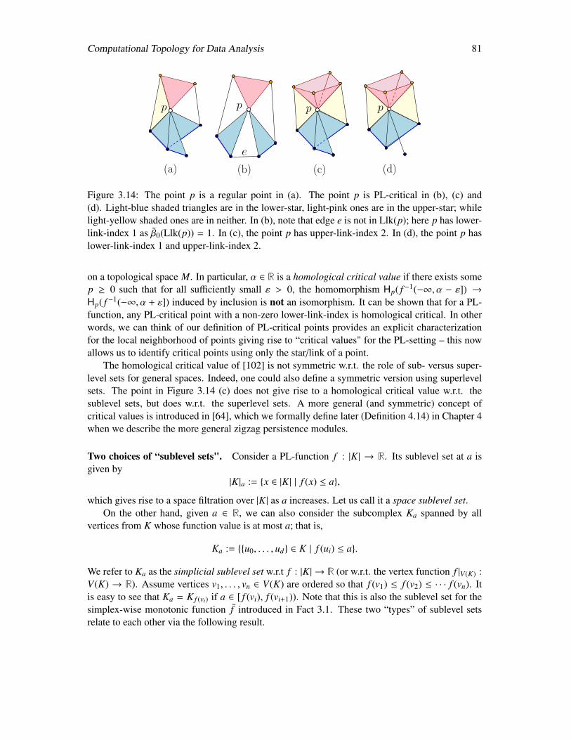
Computational Topology for Data Analysis 81
p pp p
e
(a) (b) (c) (d)
Figure 3.14: The point p is a regular point in (a). The point p is PL-critical in (b), (c) and(d). Light-blue shaded triangles are in the lower-star, light-pink ones are in the upper-star; whilelight-yellow shaded ones are in neither. In (b), note that edge e is not in Llk(p); here p has lower-link-index 1 as β0(Llk(p)) = 1. In (c), the point p has upper-link-index 2. In (d), the point p haslower-link-index 1 and upper-link-index 2.
on a topological space M. In particular, α ∈ R is a homological critical value if there exists somep ≥ 0 such that for all sufficiently small ε > 0, the homomorphism Hp( f −1(−∞, α − ε]) →Hp( f −1(−∞, α + ε]) induced by inclusion is not an isomorphism. It can be shown that for a PL-function, any PL-critical point with a non-zero lower-link-index is homological critical. In otherwords, we can think of our definition of PL-critical points provides an explicit characterizationfor the local neighborhood of points giving rise to “critical values" for the PL-setting – this nowallows us to identify critical points using only the star/link of a point.
The homological critical value of [102] is not symmetric w.r.t. the role of sub- versus super-level sets for general spaces. Indeed, one could also define a symmetric version using superlevelsets. The point in Figure 3.14 (c) does not give rise to a homological critical value w.r.t. thesublevel sets, but does w.r.t. the superlevel sets. A more general (and symmetric) concept ofcritical values is introduced in [64], which we formally define later (Definition 4.14) in Chapter 4when we describe the more general zigzag persistence modules.
Two choices of “sublevel sets". Consider a PL-function f : |K| → R. Its sublevel set at a isgiven by
|K|a := x ∈ |K| | f (x) ≤ a,
which gives rise to a space filtration over |K| as a increases. Let us call it a space sublevel set.On the other hand, given a ∈ R, we can also consider the subcomplex Ka spanned by all
vertices from K whose function value is at most a; that is,
Ka := u0, . . . , ud ∈ K | f (ui) ≤ a.
We refer to Ka as the simplicial sublevel set w.r.t f : |K| → R (or w.r.t. the vertex function f |V(K) :V(K) → R). Assume vertices v1, . . . , vn ∈ V(K) are ordered so that f (v1) ≤ f (v2) ≤ · · · f (vn). Itis easy to see that Ka = K f (vi) if a ∈ [ f (vi), f (vi+1)). Note that this is also the sublevel set for thesimplex-wise monotonic function f introduced in Fact 3.1. These two “types” of sublevel setsrelate to each other via the following result.
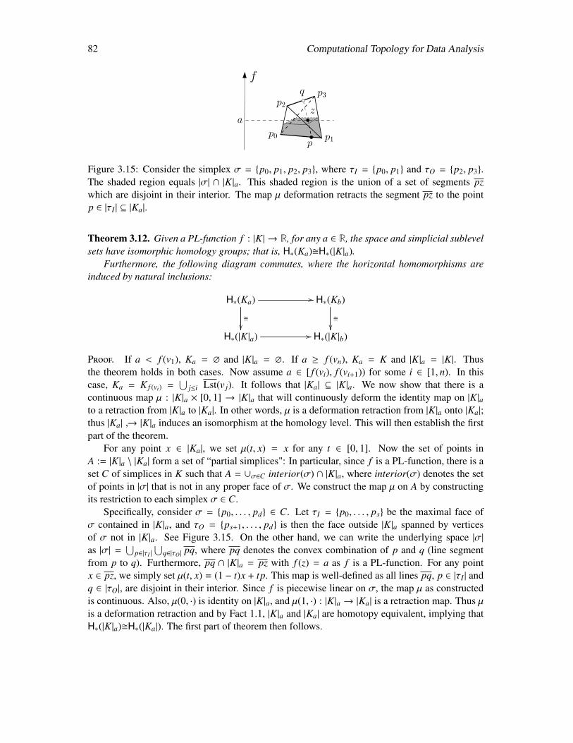
82 Computational Topology for Data Analysis
f
p0 p1
p2p3
p
q
za
Figure 3.15: Consider the simplex σ = p0, p1, p2, p3, where τI = p0, p1 and τO = p2, p3.The shaded region equals |σ| ∩ |K|a. This shaded region is the union of a set of segments pzwhich are disjoint in their interior. The map µ deformation retracts the segment pz to the pointp ∈ |τI | ⊆ |Ka|.
Theorem 3.12. Given a PL-function f : |K| → R, for any a ∈ R, the space and simplicial sublevelsets have isomorphic homology groups; that is, H∗(Ka)H∗(|K|a).
Furthermore, the following diagram commutes, where the horizontal homomorphisms areinduced by natural inclusions:
H∗(Ka)
// H∗(Kb)
H∗(|K|a) // H∗(|K|b)
Proof. If a < f (v1), Ka = ∅ and |K|a = ∅. If a ≥ f (vn), Ka = K and |K|a = |K|. Thusthe theorem holds in both cases. Now assume a ∈ [ f (vi), f (vi+1)) for some i ∈ [1, n). In thiscase, Ka = K f (vi) =
⋃j≤i Lst(v j). It follows that |Ka| ⊆ |K|a. We now show that there is a
continuous map µ : |K|a × [0, 1] → |K|a that will continuously deform the identity map on |K|ato a retraction from |K|a to |Ka|. In other words, µ is a deformation retraction from |K|a onto |Ka|;thus |Ka| → |K|a induces an isomorphism at the homology level. This will then establish the firstpart of the theorem.
For any point x ∈ |Ka|, we set µ(t, x) = x for any t ∈ [0, 1]. Now the set of points inA := |K|a \ |Ka| form a set of “partial simplices": In particular, since f is a PL-function, there is aset C of simplices in K such that A = ∪σ∈C interior(σ) ∩ |K|a, where interior(σ) denotes the setof points in |σ| that is not in any proper face of σ. We construct the map µ on A by constructingits restriction to each simplex σ ∈ C.
Specifically, consider σ = p0, . . . , pd ∈ C. Let τI = p0, . . . , ps be the maximal face ofσ contained in |K|a, and τO = ps+1, . . . , pd is then the face outside |K|a spanned by verticesof σ not in |K|a. See Figure 3.15. On the other hand, we can write the underlying space |σ|as |σ| =
⋃p∈|τI |
⋃q∈|τO | pq, where pq denotes the convex combination of p and q (line segment
from p to q). Furthermore, pq ∩ |K|a = pz with f (z) = a as f is a PL-function. For any pointx ∈ pz, we simply set µ(t, x) = (1 − t)x + tp. This map is well-defined as all lines pq, p ∈ |τI | andq ∈ |τO|, are disjoint in their interior. Since f is piecewise linear on σ, the map µ as constructedis continuous. Also, µ(0, ·) is identity on |K|a, and µ(1, ·) : |K|a → |Ka| is a retraction map. Thus µis a deformation retraction and by Fact 1.1, |K|a and |Ka| are homotopy equivalent, implying thatH∗(|K|a)H∗(|Ka|). The first part of theorem then follows.
Computational Topology for Data Analysis 83
Furthermore, given that µ is a deformation retraction, the natural inclusion |Ka| ⊆ |K|a inducesan isomorphism at the homology level. The second part of the theorem follows from this, com-bined with the naturality of the isomorphism H∗(Ka)H∗(|Ka|).
We note that we can also inspect the superlevel sets for the underlying space |K| and for thesimplicial setting in a symmetric manner. A result analogous to the above theorem also holds forthe superlevel sets.
Relation to PL-critical points. Similar to critical points for smooth functions, the homologygroup of the sublevel sets can only change at the PL-critical points. For simplicity, in what followswe set Ki := K f (vi), for any i ∈ [1, n]. Observe that for any a ∈ R, if complex Ka is non-empty,then it equals Ki for some i; in particular, Ka = Ki where a ∈ [ f (vi), f (vi+1)).
Theorem 3.13 (PL-critical Points). Let f : |K| → R be a PL-function defined on a simplicialcomplex K. For any index r ∈ [2, n] and dimension p ≥ 0, the inclusion Kr−1 → Kr induces anisomorphism Hp(Kr−1)Hp(Kr) unless vr is a PL-critical point of lower-link-index p or p + 1.
A symmetric statement for the superlevel sets and PL-critical points of non-zero upper-link-index also holds.
Proof. Let A = Lst(vr) be the closed lower-star of vr, and B = Kr−1. Set U = A ∪ B andV = A ∩ B; it is easy to see that U = Kr; while V = Llk(vr). Furthermore, by the definition oflower-stars and lower-links over a simplicial complex, A = Lst(vr) equals the coning of vr andLlk(vr). It follows that A has trivial reduced homology for all dimensions. Now consider thefollowing (Mayer-Vietoris) exact sequence:
· · · −→ Hp(V) −→ Hp(A) ⊕ Hp(B)φ−→ Hp(U) −→ Hp−1(V) −→ · · · (3.9)
Assume vr is neither an lower-link-index-(p + 1) PL-critical point, nor an index-p one. Since vr
is not lower-link-index-(p + 1) PL-critical, Hp(V) is trivial. Thus by exactness of the sequence,the homomorphism φ must be injective. Similarly, as vr is not lower-link-index-p PL-critical,Hp−1(V) is trivial; thus φ must be surjective. Hence φ is an isomorphism. Furthermore, note thatHp(A) ⊕ Hp(B) = 0 ⊕ Hp(B) as A has trivial homology. It then follows that Hp(Kr−1)Hp(Kr)induced by inclusion map Kr−1 → Kr. The claim then follows.
Corollary 3.14. Given a PL-function f : |K| → R defined on a finite simplicial complex K, let[a, b] ⊂ R be such that it does not contain any PL-critical value for f .
(1) Then the inclusion map Ka → Kb induces isomorphism between the simplicial homologygroups, that is, Hp(Ka)Hp(Kb) for any dimension p ≥ 0.
(2) This also implies that |K|a → |K|b induces isomorphism between the singular homologygroups, that is, Hp(|K|a)Hp(|K|b) for any dimension p ≥ 0.
Again, a version of the above Corollary also holds for superlevel sets.
84 Computational Topology for Data Analysis
3.5.2 Lower star filtration and its persistent homology
Let f : |K| → R be a PL-function. Recall that Ki := K f (vi) where v1, . . . , vn are ordered in non-decreasing values of f . Setting ai = f (vi), we write |K|ai = |K| f (vi). The two different types ofsublevel sets give rise to two sequences of growing spaces:
Lower star simplicial filtration F f : ∅ → K1 → K2 → · · · → Kn−1 → Kn = K; (3.10)
Sublevel set space filtration F f : ∅ → |K|a1 → |K|a2 → · · · → |K|an−1 → |K|an = |K| (3.11)
As Ki :=⋃
j≤i Lst(v j) is the union of the lower-stars of v1, . . . , vi, we call the filtration in Eqn.(3.10) the lower star filtration for f ; see also Section 3.1.2 and Figure 3.6. The two homologymodules HpF f and HpF f can be shown to be isomorphic due to Theorem 3.12, and thus theyproduce identical persistence diagrams (Fact 3.10).
Corollary 3.15. The homology module HpF f is isomorphic to the homology module HpF f forevery p ≥ 0. This implies that these two persistence modules have the same persistence diagrams.
Intuitively, the lower-star filtration of the simplicial complex K can be thought of as the dis-crete version of the sublevel set filtration of the space |K| w.r.t. the PL-function f . By Corollary3.15, the lower star simplicial filtratoin F f and the sublevel set space filtration F f have identicalpersistence diagrams. We refer to this common persistence diagram as the persistence diagram ofthe PL-function f , denoted by Dgm f .
For a space filtration induced by a Morse function defined on a Riemannian manifold, thebirth- and death-coordinates of the points in the persistence diagrams correspond to critical valuesof this Morse function. A similar result holds for the PL-case. In particular, one can prove, usingCorollary 3.14 that, for a PL-function f , the persistence pairings for F f occur only between PL-critical points. That is:
Fact 3.11. Given a PL-function f : |K| → R and its associated filtration F f , let µi, jf ,p denote the
corresponding p-th persistence pairing function w.r.t. F f . If µi, jf ,p , 0, then vertices vi and v j must
be PL-critical.
However, not all PL-critical points necessarily appear in persistence pairings w.r.t. the lowerstar filtration F f .
Computing persistence diagram induced by F f and F f . By Corollary 3.15, we only need todescribe how to compute the persistence diagram for the lower star filtration F f . We will do so viaAlgorithm 3:MatPersistence from Section 3.3. However, recall that algorithm MatPersistenceworks on simplex-wise filtrations (Definition 3.1). The algorithm either pairs each simplex withanother simplex producing a persistence pairing, or leaves it unpaired producing an essentialpersistent point (b,∞) in the persistence diagram. To compute Dgm f , we first expand F f into asimplex-wise filtration Fs induced by a total ordering of all m simplices in K
σ1, . . . σI1 , σI1+1, . . . , σI2 , σI2+1, . . . , σI j , σI j+1, . . . , σI j+1 , . . . , σIn−‘ , σIn−1+1, . . . , σIn=m (3.12)
so that following two conditions hold:
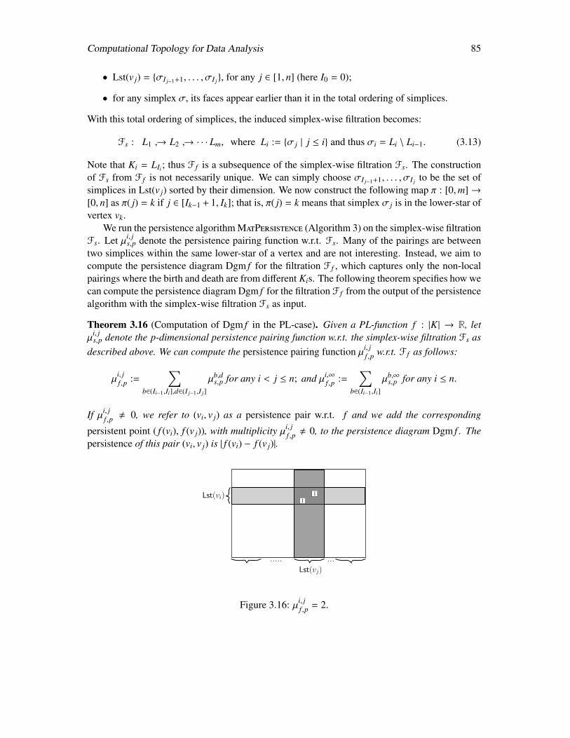
Computational Topology for Data Analysis 85
• Lst(v j) = σI j−1+1, . . . , σI j, for any j ∈ [1, n] (here I0 = 0);
• for any simplex σ, its faces appear earlier than it in the total ordering of simplices.
With this total ordering of simplices, the induced simplex-wise filtration becomes:
Fs : L1 → L2 → · · · Lm, where Li := σ j | j ≤ i and thus σi = Li \ Li−1. (3.13)
Note that Ki = LIi ; thus F f is a subsequence of the simplex-wise filtration Fs. The constructionof Fs from F f is not necessarily unique. We can simply choose σI j−1+1, . . . , σI j to be the set ofsimplices in Lst(v j) sorted by their dimension. We now construct the following map π : [0,m]→[0, n] as π( j) = k if j ∈ [Ik−1 + 1, Ik]; that is, π( j) = k means that simplex σ j is in the lower-star ofvertex vk.
We run the persistence algorithm MatPersistence (Algorithm 3) on the simplex-wise filtrationFs. Let µi, j
s,p denote the persistence pairing function w.r.t. Fs. Many of the pairings are betweentwo simplices within the same lower-star of a vertex and are not interesting. Instead, we aim tocompute the persistence diagram Dgm f for the filtration F f , which captures only the non-localpairings where the birth and death are from different Kis. The following theorem specifies how wecan compute the persistence diagram Dgm f for the filtration F f from the output of the persistencealgorithm with the simplex-wise filtration Fs as input.
Theorem 3.16 (Computation of Dgm f in the PL-case). Given a PL-function f : |K| → R, letµ
i, js,p denote the p-dimensional persistence pairing function w.r.t. the simplex-wise filtration Fs as
described above. We can compute the persistence pairing function µi, jf ,p w.r.t. F f as follows:
µi, jf ,p :=
∑b∈(Ii−1,Ii],d∈(I j−1,I j]
µb,ds,p for any i < j ≤ n; and µi,∞
f ,p :=∑
b∈(Ii−1,Ii]
µb,∞s,p for any i ≤ n.
If µi, jf ,p , 0, we refer to (vi, v j) as a persistence pair w.r.t. f and we add the corresponding
persistent point ( f (vi), f (v j)), with multiplicity µi, jf ,p , 0, to the persistence diagram Dgm f . The
persistence of this pair (vi, v j) is | f (vi) − f (v j)|.
..... ...Lst(vj)
Lst(vi)1
1
Figure 3.16: µi, jf ,p = 2.
86 Computational Topology for Data Analysis
Remark 3.5. As an example, see Figure 3.16 which shows the reduced matrix after runningAlgorithm 3:MatPersistence on the filtered boundary matrix D for Fs where ‘1’ indicates thelowest ‘1’ in the shaded columns. Only columns corresponding to p-simplices are shown. Wehave µi, j
f ,p = 2. One can have an alternate view of the persistence pairs given by µi, jf ,p as follows:
for each persistence index pair (i, j) ∈ Dgm(Fs) (i.e., µi, jp > 0 w.r.t. Fs), one has a persistence
pair (vπ(i), vπ( j)) for F f if an only if π(i) , π( j). In other words, all local pairs (i, j) ∈ Dgm(Fs)with π(i) = π( j) signifying that σi and σ j are from the lower-star of the same vertex are ignoredfor the persistence diagram Dgm(F f ).
Proof. [Proof of Theorem 3.16.] Recall that µi, jf ,p and µi, j
s,p are the persistence pairing functions
induced by the filtration F f and Fs, respectively. Similarly, we use βi, jf ,p and βi, j
s,p to denote thepersistent Betti numbers induced by filtrations F f and Fs, respectively. In what follows, we willjust prove that, for any dimension p ≥ 0 and i, j ∈ [1, n], we have that µi, j
f ,p can be computed asstated in the theorem. The case when j = ∞ can be handled in a similar manner and is left as anexercise.
For any i ∈ [1, n], let Ii be as defined in Eqn. (3.12). Given the relation of F f and Fs, it followsthat for any i′, j′ ∈ [1, n], we have that Ki′ = LIi′ , K j′ = LI j′ , and thus βi′, j′
f ,p = βIi′ ,I j′
s,p as F f is asubsequence of Fs.
Now fix the dimension p ≥ 0, and for simplicity, omit p from all subscripts. Given anyi, j ∈ [1, n], we have that:
µi, jf = (βi, j−1
f − βi, jf ) − (βi−1, j−1
f − βi−1, jf )
= (βIi,I j−1s − β
Ii,I js ) − (βIi−1,I j−1
s − βIi−1,I js ) = µ
Ii,I js .
Hence we aim to show µIi,I js =
∑b∈(Ii−1,Ii],d∈(I j−1,I j] µ
b,ds which then proves the theorem. To this end,
note that by Theorem 3.1, we have the following:
βIi,I j−1s − β
Ii,I js =
∑b≤Ii,d>I j−1
µb,ds −
∑b≤Ii,d>I j
µb,ds =
∑b≤Ii,d∈(I j−1,I j]
µb,ds ;
βIi−1,I j−1s − β
Ii−1,I js =
∑b≤Ii−1,d>I j−1
µb,ds −
∑b≤Ii−1,d>I j
µb,ds =
∑b≤Ii−1,d∈(I j−1,I j]
µb,ds ;
⇒ µIi,I js =
∑b≤Ii,d∈(I j−1,I j]
µb,ds −
∑b≤Ii−1,d∈(I j−1,I j]
µb,ds =
∑b∈(Ii−1,Ii],d∈(I j−1,I j]
µb,ds .
The theorem then follows.
An implication of the above result is that any simplex-wise filtration Fs obtained from thelower star filtration F f produces the same pairing between critical points and the same persistencediagram.
3.5.3 Persistence algorithm for 0-th persistent homology
The best known running time for general persistence algorithm is O(nω), where n is the totalnumber of simplicies in the filtration. However, the 0-th persistent homology (0-th persistence
Computational Topology for Data Analysis 87
diagram Dgm0 f ) for a PL-function f : |K| → R can be computed efficiently in O(n log n + mα(n))time, where n and m are the number of vertices and edges in K, respectively.
Indeed, first observe that we only need the 1-skeleton of K to compute Dgm0 f . So, in whatfollows, assume that K contains only vertices V and edges E. Assume that all vertices in V aresorted in non-decreasing order of their f -values. As before, let Ki be the union of lower-stars ofall vertices v j where j ≤ i. Since we are only interested in the 0-th homology, we only need totrack the 0-th homology group of Ki, which essentially embodies the information about connectedcomponents.
Assume we are at vertex v j. Consider Lst(v j). There are three cases.
Case-1 : Lst(v j) = v j. Then v j starts a new connected component in K j. Hence v j is a creator.
Case-2 : All edges in Lst(v j) connect to vertices from the same connected component C in K j−1.In this case, the component C grows in the sense that it now includes also vertex v j andits incident edges in the lower-star. However, H0(K j−1) and H0(K j) are isomorphic whereK j−1 ⊆ K j induces an isomorphism.
Case-3 : Edges in Lst(v j) link to two or more components, say C1, . . . ,Cr, in K j−1. In this case,after the addition of Lst(v j), all C1, . . . ,Cr are merged into a single component
C′ = C1 ∪C2 ∪ · · · ∪Cr ∪ Lstv j.
Hence inclusion K j−1 → K j induces a surjective homomorphism ξ : H0(K j−1) → H0(K j)and β0(K j) = β0(K j−1) − (r − 1). That is, we can consider that r − 1 number of componentsare destroyed, only one stays on as C′.
Proposition 3.17. Suppose Case-3 happens where edges in Lst(v j) merges components C1, . . . ,Cr
in K j−1. Let vki be the global minimum of component Ci for i ∈ [1, r]. Assume w.l.o.g thatf (vk1) ≤ f (vk2) ≤ · · · ≤ f (vkr ). Then the node v j participates in exactly r−1 number of persistencepairings (vk2 , v j), . . . , (vkr , v j) for the 0-dimensional persistent diagram Dgm0 f , corresponding topoints ( f (vk2), f (v j)), . . . , ( f (vkr ), f (v j)) in Dgm0 f .
Intuitively, when Case-3 happens, consider the set of 0-cycles c2 = vk2 + vk1 , c3 = vk3 +
vk1 , . . . , cr = vkr + vk1 . On one hand, it is easy to see that their corresponding homology classes[ci]’s are independent within H0(K j−1). Furthermore, each ci is created upon entering Kki for eachi ∈ [1, r]. On the other hand, the homology classes [c2], . . . , [cr] become trivial in H0(K j) (thusthey are destroyed upon entering K j). Hence µki, j
0 > 0 for i ∈ [2, r], corresponding to persistencepairings (vk2 , v j), . . . , (vkr , v j). Furthermore, consider any 0-cycle c1 = vk1 + c where c is a 0-chainfrom Kk1−1. The class [c1] is created at Kk1 yet remains non-trivial at K j. Hence there is nopersistence pairing (vk1 , v j).
Based on Proposition 3.17 we can compute the persistence pairings for the 0-dimensionalpersistent homology without the matrix reduction algorithm. We only need to maintain connectedcomponents information for each Ki, and potentially merge multiple components. We would alsoneed to be able to query the membership of a given vertex u in the components of the currentsublevel set. Such operations can be implemented by a standard union-find data structure.
Specifically, a union-find data structure is a standard data structure that maintains dynamicdisjoint sets [109]. Given a set of elements U called the universe, this data structure typically
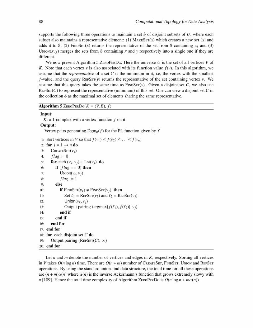
88 Computational Topology for Data Analysis
supports the following three operations to maintain a set S of disjoint subsets of U, where eachsubset also maintains a representative element: (1) MakeSet(x) which creates a new set x andadds it to S; (2) FindSet(x) returns the representative of the set from S containing x; and (3)Union(x, y) merges the sets from S containing x and y respectively into a single one if they aredifferent.
We now present Algorithm 5:ZeroPerDg. Here the universe U is the set of all vertices V ofK. Note that each vertex v is also associated with its function value f (v). In this algorithm, weassume that the representative of a set C is the minimum in it, i.e, the vertex with the smallestf -value, and the query RepSet(v) returns the representative of the set containing vertex v. Weassume that this query takes the same time as FindSet(v). Given a disjoint set C, we also useRepSet(C) to represent the representative (minimum) of this set. One can view a disjoint set C inthe collection S as the maximal set of elements sharing the same representative.
Algorithm 5 ZeroPerDg(K = (V, E), f )
Input:K: a 1-complex with a vertex function f on it
Output:Vertex pairs generating Dgm0( f ) for the PL function given by f
1: Sort vertices in V so that f (v1) ≤ f (v2) ≤ . . . ≤ f (vn)2: for j = 1→ n do3: CreateSet(v j)4: f lag := 05: for each (vk, v j) ∈ Lst(v j) do6: if ( f lag == 0) then7: Union(vk, v j)8: f lag := 19: else
10: if FindSet(vk) , FindSet(v j) then11: Set `1 = RepSet(vk) and `2 = RepSet(v j)12: Union(vk, v j)13: Output pairing (argmax f (`1), f (`2), v j)14: end if15: end if16: end for17: end for18: for each disjoint set C do19: Output pairing (RepSet(C),∞)20: end for
Let n and m denote the number of vertices and edges in K, respectively. Sorting all verticesin V takes O(n log n) time. There are O(n + m) number of CreateSet, FindSet, Union and RepSetoperations. By using the standard union-find data structure, the total time for all these operationsare (n + m)α(n) where α(n) is the inverse Ackermann’s function that grows extremely slowy withn [109]. Hence the total time complexity of Algorithm ZeroPerDg is O(n log n + mα(n)).
Computational Topology for Data Analysis 89
Note that lines 18-20 of algorithm ZeroPerDg inspect all disjoint sets after processing allvertices and their lower-stars; each of such disjoint sets corresponds to a connected component inK. Hence each of them generates an essential pair in the 0-th persistence diagram.
Theorem 3.18. Given a PL-function f : |K| → R, the 0-dimensional persistence diagram Dgm0 ffor the lower-star filtration of f can be computed by the algorithm ZeroPerDg in O(n log n +
mα(n)) time, where n and m are the number of vertices and edges in K respectively.
Connection to minimum spanning tree. If we view the 1-skeleton of K as a graph G = (V, E),then ZeorPerDg(K, f ) essentially computes the minimum spanning forest of G with the followingedge weights: for every edge e = (u, v), we set its weight w(e) = max f (u), f (v). Then, we canget the persistent pairs output of ZeroPerDg by running the well known Kruskal’s algorithm onthe weighted graph G. When we come across an edge e = (u, v) that joins two disjoint componentsin this algorithm, we determine the two minimum vertices `1, `2 in these two components and paire with the one among `1, `2 that has the larger f -value. After generating all such vertex-edge pairs(u, e), we convert them to vertex-vertex pairs (u, v) where e ∈ Lst(v). We throw away any pair ofthe form (u, u) because they signify local pairs.
Graph filtration. The algorithm ZeroPerDg can be easily adapted to compute persistence fora given filtration of a graph. In this case, we process the vertices and edges in their order in thefiltration and maintain connected components using union-find data structure as in ZeroPerDg.For each edge e = (u, v), we check if it connects two disconnected components represented byvertices `1 and `2 (line 11) and if so, e is paired with the younger vertex between `1 and `2 (line13). We output all vertex-edge pairs thus computed. The vertices and edges that remain unpairedprovide the infinite bars in the 0-th and 1-st persistence diagrams. The algorithm runs in O(nα(n))time if the graph has n vertices and edges in total. The O(n log n) term in the complexity iseliminated because sorting of the vertices is implicitly given by the input filtration.
3.6 Notes and Exercises
The concept of topological persistence came to the fore in early 2000 with the paper by Edels-brunner, Letscher, and Zomorodian [152] though the concept was proposed in a rudimentary form(e.g. 0-dimensional homology) in other papers by Frosini [162] and Robins [266]. The persistencealgorithm as described in this chapter was presented in [152] which has become the cornerstoneof topological data analysis. The original algorithm was described without any matrix reductionwhich first appeared in [106]. Since then various versions of the algorithm has been presented.We already saw that persistence for filtrations of simplicial 1-complexes (graphs) with n simplicescan be computed in O(nα(n)) time. Persistence for filtrations of simplicial 2-manifolds also canbe computed in O(nα(n)) time algorithm by essentially reducing the problem to computing per-sistence on a dual graph. In general, for any constant d ≥ 1, the persistence pairs between d- and(d − 1)-simplices of a simplicial d-manifold can be computed in O(nα(n)) time by consideringthe dual graph. If the manifold has boundary, then one has to consider a ‘dummy’ vertex thatconnects to every dual vertex of a d-simplex adjoining a boundary (d − 1)-simplex.
90 Computational Topology for Data Analysis
For efficient implementation, clearing strategy as described in Section 3.3.2 was presentedin [21]. We have given a proof based on matrix reduction that the same persistent pairs canbe computed by considering the anti-transpose of the boundary matrix. This is termed as thecohomology algorithm first introduced in [115]. The name is justified by the fact that consideringcohomology groups and the resulting persistence module that reverses the arrows (Fact 2.14),we obtain the same barcode. The anti-transpose of the boundary matrix indeed represents thecoboundary matrix filtered reversely. These tricks are further used by Bauer for processing Ripsfiltration efficiently in the Ripser software [19]; see also [304]. Boissonnat et al. [42, 43] havesuggested a technique to reduce the size of a given filtration using strong collapse of Barmakand Minian [17]. The collapse on the complex can be efficiently achieved only through simplemanipulations of the boundary matrix.
The concept of bottleneck distance for persistence diagrams was first proposed by Cohen-Steiner et al. [102] who also showed the stability of such diagrams in terms of bottleneck dis-tances with respect to the infinity norm of the difference between functions generating them. Thisresult was extended to Wassrstein distance though in a weaker form in [104] which got improvedrecently [278]. The more general concept of interleaving distance between persistence modulesand the stability of persistence diagrams with respect them was presented by Chazal et al. [78].The fact that bottleneck distance between persistence diagrams is not only bounded from aboveby interleaving distance but is indeed equal to it was shown by Lesnick [220] which was furtherstudied by Bauer and Lesnick [24] later. Also, see [55] for more generalization at algebraic level.
The use of the reduced Betti numbers for lower-link of a vertex to quantify its criticality wasoriginally introduced in [150] for a PL-function defined on a triangulation of a d-manifold. OurPL-criticality considers both the lower-link and upper-link for more general simplicial complexes.As far as we know, the relations between such PL-critical points and homology groups of sublevel-sets for the PL-setting have not been stated explicitly elsewhere in the literature. The concept ofhomological critical values was first introduced in [102], and the more general concept of “levelsetcritical values" (and levelset tame functions) was originally introduced in [64].
The idea of using union-find data structure to compute the 0-th persistent homology group wasalready introduced in the original persistence algorithm paper [152]. In this chapter, we present amodification for the PL-function setting.
Exercises
1. Let K be a p-complex with every (p − 1)-simplex incident to exactly two p-simplices. LetM be a boundary matrix of the boundary operator ∂p for K. We run a different version ofthe persistence algorithm on M. We scan its columns from left to right as before, but weadd the current column to its right to resolve conflict, i.e., for each i = 1, · · · , n in this orderif there exists j > i so that lowM[i] = lowM[ j], then add colM[i] to colM[ j]. Show that:
(a) There can be at most one such j,
(b) At termination, every column of M is either empty or has a unique low entry,
(c) The algorithm outputs in O(n2) time the same lowM[i] as the original persistencealgorithm returns on M.
Computational Topology for Data Analysis 91
2. For a given matrix with binary entries, a valid column operation is one that adds a columnto its right (Z2-addition). Similarly, define a valid row operation is the one that adds a rowto another one above it. Show that there exists a set of valid column and row operationsthat leave every row and column either empty or with a single non-zero entry.
3. Let D be a boundary matrix of a simplicial complex K. Modify the algorithm MatPer-sistence to compute a set of p-cycles, p ≥ 0, whose classes form a basis of Hp(K) (Hint:consider interpreting the role of the matrix V in the decomposition R = DV of the reducedmatrix R).
4. Prove Theorem 3.1.
5. Give a polynomial time algorithm for computing dW,q.
6. Prove Proposition 3.7.
7. Let mq and βq be the number of q-simplices and qth Betti number of a simplicial complexof dimension p. Using pairing in persistence, show that
mp − mp−1 + · · · + ±m0 = βp − βp−1 + · · · ± β0.
8. Let F be a filtration where every p-simplex appear only after all (p − 1)-simplices like inEqn. (3.8). Let F′ be a modified filtration of F as follows. For every p ≥ 0, all p-simplicesin F are ordered in non-decreasing order of their persistence values in F′ assuming thatunpaired p-simplices have persistence value ∞. Show that the persistence pairing remainsthe same for F and F′.
9. Let F be a simplex-wise filtration F of complex K induced by the sequence of simplices:σ1, . . . , σN . Let F′ be a modification of F where only two consecutive simplices σk andσk+1 swap their order, that is, F′ is induced by the sequence:
σ1, . . . , σk−1, σk+1, σk, σk+2, . . . , σN .
Describe the relation between their corresponding persistence diagrams Dgm(F) and Dgm(F′).
10. Give an example of a piecewise linear function f : |K| → R where a vertex vi is a PL-criticalpoint, but H∗(Ki−1)H∗(Ki) as induced by inclusion.
11. Let f : V(K) → R be a vertex function defined on the vertex set V(K) of complex K.Consider g = h f + a, where h : R→ R is a monotone function and a ∈ R is a real value.Consider the lower-star filtrations F f and Fg induced by induced PL-functions f , g : |K| →R as in Eqn. 3.10. Describe the relation between their corresponding persistence diagramsDgm(F f ) and Dgm(Fg).
12. Consider two PL-functions f , g : |K| → R on K induced by vertex functions f , g : V(K)→R, respectively. Suppose ‖ f −g‖∞ = δ, where ‖ f −g‖∞ = maxv∈V | f (v)−g(v)|. Consider thepersistence modules P f and Pg induced by the lower-star filtration for f and g respectively.
• Show that dI(P f ,Pg) ≤ δ.

92 Computational Topology for Data Analysis
• Give an example of K, f , and g so that dI(P f ,Pg) < δ.
13. For a PL-function f : |K| → R, we know how to produce a simplex-wise filtration F so thatthe barcode for f can be read from the barcode of F. Design an algorithm to do the reverse,that is, given a filtration F on a complex K, produce a filtration G of a simplicial complexK′ so that G is indeed a simplex-wise filtration of a PL function g : |K′| → R where barsfor F can be obtained from those for G. (Hint: use barycentric subdivision of K).
14. Prove Proposition 3.9.
15. Consider the two persistence modules U and V as shown below and a sequence of linearmaps fi : Ui → Vi so that all squares commute.
U : U1 //
f1
U2 //
f2
U3 //
f3
. . . . . . // Um
fm
V : V1 // V2 // V3 // . . . . . . // Vm
Consider the sequences
kerF : ker fi ⊆ Ui → ker fi+1 ⊆ Ui+1
where the maps are induced from the module U. Prove that kerF is a persistence module.Show the same for the sequences
imF : im fi ⊆ Vi → im fi+1 ⊆ im Vi+1 and
coker F : coker fi = Vi/im fi → coker fi+1 = Vi+1/im fi+1.
Chapter 4
General Persistence
We have considered filtrations so far for defining persistence and its stability. In a filtration, theconnecting maps between consecutive spaces or complexes are inclusions. Assuming a discretesubset of reals, A : a0 ≤ a1 ≤ · · · ≤ an, as an index set, we write a filtration as:
F : Xa0 → Xa1 → · · · → Xan .
A more generalized scenario occurs when the inclusions are replaced with continuous maps forspace filtrations and simplicial maps for simplicial filtrations: xi j : Xai → Xa j . In that case, wecall the sequence a space and a simplicial tower respectively:
X : Xa0
x01−→ Xa1
x12−→ · · ·
x(n−1)n−→ Xan . (4.1)
Considering the homology group of each space (complex resp.) in the sequence, we obtain asequence of vector spaces connected with linear maps, which we have seen before. Specifically,we obtain the following tower of vector spaces:
HpX : Hp(Xa0)x01∗−→ Hp(Xa1)
x12∗−→ · · ·
x(n−1)n∗−→ Hp(Xan).
In the above sequence each linear map xi j∗ is the homomorphism induced by the map xi j. Wehave already seen that persistent homology of such a sequence of vector spaces and linear mapsare well defined. However, since the linear maps here are not induced by inclusions, the originalpersistence algorithm as described in the previous chapter does not work. In Section 4.2, wedescribe a new algorithm to compute the persistence diagram of simplicial towers. Next, wegeneralize a filtration by allowing the inclusion maps to be directed either way giving rise to whatis called a zigzag filtration:
F : Xa0 ↔ Xa1 ↔ · · · ↔ Xan . (4.2)
where each bidirectional arrow ‘↔’ is either a forward or a backward inclusion map. In Sec-tion 4.3, we present an algorithm to compute the persistence of a zigzag filtration. A juxtapositionof a zigzag filtration with a tower provides a further generalization referred to as a zigzag tower.Section 4.4 presents an approach for computing the persistence of such a tower.
Before presenting the algorithms, we generalize the notion of stability for towers. We haveseen such a notion in Section 3.4 for persistence modules arising out of filtrations. Here, we adaptit to a tower.
93
94 Computational Topology for Data Analysis
4.1 Stability of towers
Just like the previous chapter, we define the stability with respect to the perturbation of the towersthemselves forgetting the functions who generate them. This requires a definition of a distancebetween towers at simplicial (space) levels and homology levels.
It turns out that it is convenient and sometimes appropriate if the objects (spaces, simplicialcomplexes, or vector spaces) in a tower are indexed over the positive real axis instead of a discretesubset of it. This, in turn, requires to spell out the connecting map between every pair of objects.
Definition 4.1 (Tower). A tower indexed in an ordered set A ⊆ R is any collection T =Ta
a∈A of
objects Ta, a ∈ A, together with maps ta,a′ : Ta → Ta′ so that ta,a = id and ta′,a′′ ta,a′ = ta,a′′ for
all a ≤ a′ ≤ a′′. Sometimes we write T =Ta
ta,a′−→ Ta′
a≤a′ to denote the collection with the maps.
We say that the tower T has resolution r if a ≥ r for every a ∈ A.When T is a collection of topological spaces connected with continuous maps, we call it a
space tower. When it is a collection of simplicial complexes connected with simplicial maps, wecall it a simplicial tower, and when it is a collection of vector spaces connected with linear maps,we call it a vector space tower.
Remark 4.1. As we have already seen, in practice, it may happen that a tower needs to be definedover a discrete index set A that is only a subposet of R. In such a case, one can ‘embed’ A into Rand convert the input to a tower according to Definition 4.1 by assuming that for any a < a′ ∈ Awith (a, a′) < A and for any a ≤ b < b′ < a′, tb,b′ is an isomorphism.
Definition 4.2 (Interleaving of simplicial (space) towers). Let X =Xa
xa,a′−→ Xa′
a≤a′ and Y =
Yaya,a′−→ Ya′
a≤a′ be two towers of simplicial complexes (spaces resp.) indexed in R. For any real
ε ≥ 0, we say that they are ε-interleaved if for every a one can find simplicial maps (continuousmaps resp.) ϕa : Xa → Ya+ε and ψa : Ya → Xa+ε so that
(i) for all a ∈ real, ψa+ε ϕa and xa,a+2ε are contiguous (homotopic resp.),
(ii) for all a ∈ R, ϕa+ε ψa and ya,a+2ε are contiguous (homotopic resp.),
(iii) for all a′ ≥ a, ϕa′ xa,a′ and ya+ε,a′+ε ϕa are contiguous (homotopic resp.),
(iv) for all a′ ≥ a, xa+ε,a′+ε ψa and ψa′ ya,a′ are contiguous (homotopic resp.).
If no such finite ε exists, we say the two towers are∞-interleaved.
These four conditions are summarized by requiring that the four diagrams below commute upto contiguity (homotopy resp.):
Xaϕa
!!
xa,a+2ε // Xa+2ε
Ya+ε
ψa+ε
;; Xa+ε
ϕa+ε
##Ya
ψa==
ya,a+2ε // Ya+2ε
(4.3)
Computational Topology for Data Analysis 95
Xaϕa
!!
xa,a′ // Xa′
ϕa′
""Ya+ε ya+ε,a′+ε
// Ya′+ε
Xa+ε
xa+ε,a′+ε // Xa′+ε
Ya
ψa==
ya,a′// Ya′
ψa′<<
If we replace the operator ‘+’ by the multiplication ‘·’ with respect to the indices in the abovedefinition, then we say that X and Y are multiplicatively ε-interleaved. By interleaving we willmean additive interleaving by default and use the term multiplicative interleaving where necessaryto signify that the shift is multiplicative rather than additive.
Definition 4.3 (Interleaving distance between simplicial (space) towers). The interleaving dis-tance between two simplicial (space) towers X and Y is:
dI(X,Y) = infεX and Y are ε−interleaved.
Similar to the simplicial (space) towers, we can define interleaving of vector space towers.But, in that case, we replace contiguity (homotopy) with equality in conditions (i) through (iv).
Definition 4.4 (Interleaving of vector space towers). Let U =Ua
ua,a′−→ Ua′
a≤a′ and V =
Va
va,a′−→
Va′a≤a′ be two vector space towers indexed in R. For any real ε ≥ 0, we say that they are ε-
interleaved if for each a ∈ R one can find linear maps ϕa : Ua → Va+ε and ψa : Va → Ua+ε sothat
(i) for all a ∈ R, ψa+ε ϕa = ua,a+2ε,
(ii) for all a ∈ R, ϕa+ε ψa = va,a+2ε.
(iii) for all a′ ≥ a, ϕa′ ua,a′ = va+ε,a′+ε ϕa,
(iv) for all a′ ≥ a, ua+ε,a′+ε ψa = ψa′ va,a′ .
If no such finite ε exists, we say the two towers are∞-interleaved.
Analogous to the simplicial (space) towers, if we replace the operator ‘+’ by the multiplication‘·’ in the above definition, then we say that U and V are multiplicatively ε-interleaved.
Definition 4.5 (Interleaving distance between vector space towers). The interleaving distancebetween two towers of vector spaces U and V is:
dI(U,V) = infεU and V are ε−interleaved.
Suppose that we have two simplicial (space) towers X = Xaxa,a′→ Xa′ and Y = Ya
ya,a′→
Ya′. Consider the two vector space towers also called homology towers obtained by taking thehomology groups of the complexes (spaces), that is,
VX = Hp(Xa)x(a,a′)∗→ Hp(Xa′) and VY = Hp(Ya)
y(a,a′)∗→ Hp(Ya′).
The following should be obvious because simplicial (continuous resp.) maps become linear mapsand contiguous (homotopic resp.) maps become equal at the homology level.
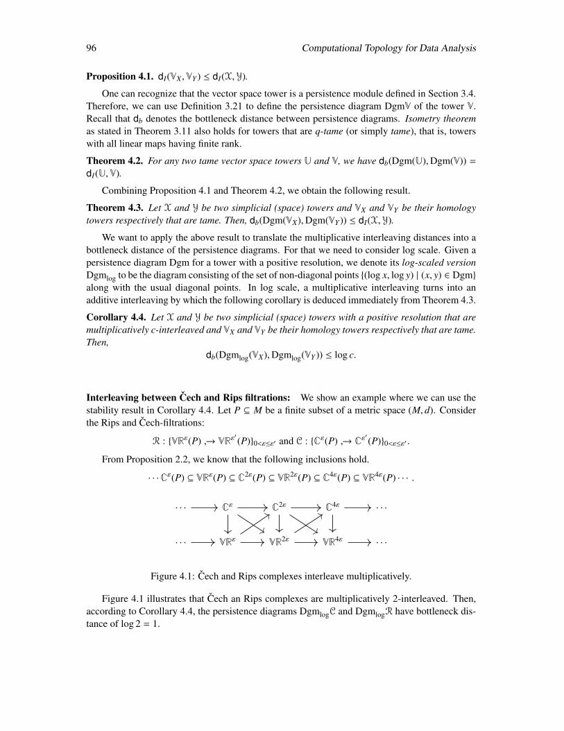
96 Computational Topology for Data Analysis
Proposition 4.1. dI(VX ,VY ) ≤ dI(X,Y).
One can recognize that the vector space tower is a persistence module defined in Section 3.4.Therefore, we can use Definition 3.21 to define the persistence diagram DgmV of the tower V.Recall that db denotes the bottleneck distance between persistence diagrams. Isometry theoremas stated in Theorem 3.11 also holds for towers that are q-tame (or simply tame), that is, towerswith all linear maps having finite rank.
Theorem 4.2. For any two tame vector space towers U and V, we have db(Dgm(U),Dgm(V)) =
dI(U,V).
Combining Proposition 4.1 and Theorem 4.2, we obtain the following result.
Theorem 4.3. Let X and Y be two simplicial (space) towers and VX and VY be their homologytowers respectively that are tame. Then, db(Dgm(VX),Dgm(VY )) ≤ dI(X,Y).
We want to apply the above result to translate the multiplicative interleaving distances into abottleneck distance of the persistence diagrams. For that we need to consider log scale. Given apersistence diagram Dgm for a tower with a positive resolution, we denote its log-scaled versionDgmlog to be the diagram consisting of the set of non-diagonal points (log x, log y) | (x, y) ∈ Dgmalong with the usual diagonal points. In log scale, a multiplicative interleaving turns into anadditive interleaving by which the following corollary is deduced immediately from Theorem 4.3.
Corollary 4.4. Let X and Y be two simplicial (space) towers with a positive resolution that aremultiplicatively c-interleaved and VX and VY be their homology towers respectively that are tame.Then,
db(Dgmlog(VX),Dgmlog(VY )) ≤ log c.
Interleaving between Cech and Rips filtrations: We show an example where we can use thestability result in Corollary 4.4. Let P ⊆ M be a finite subset of a metric space (M, d). Considerthe Rips and Cech-filtrations:
R : VRε(P) → VRε′(P)0<ε≤ε′ and C : Cε(P) → Cε′(P)0<ε≤ε′ .
From Proposition 2.2, we know that the following inclusions hold.
· · ·Cε(P) ⊆ VRε(P) ⊆ C2ε(P) ⊆ VR2ε(P) ⊆ C4ε(P) ⊆ VR4ε(P) · · · .
· · · Cε C2ε C4ε · · ·
· · · VRε VR2ε VR4ε · · ·
Figure 4.1: Cech and Rips complexes interleave multiplicatively.
Figure 4.1 illustrates that Cech an Rips complexes are multiplicatively 2-interleaved. Then,according to Corollary 4.4, the persistence diagrams DgmlogC and DgmlogR have bottleneck dis-tance of log 2 = 1.
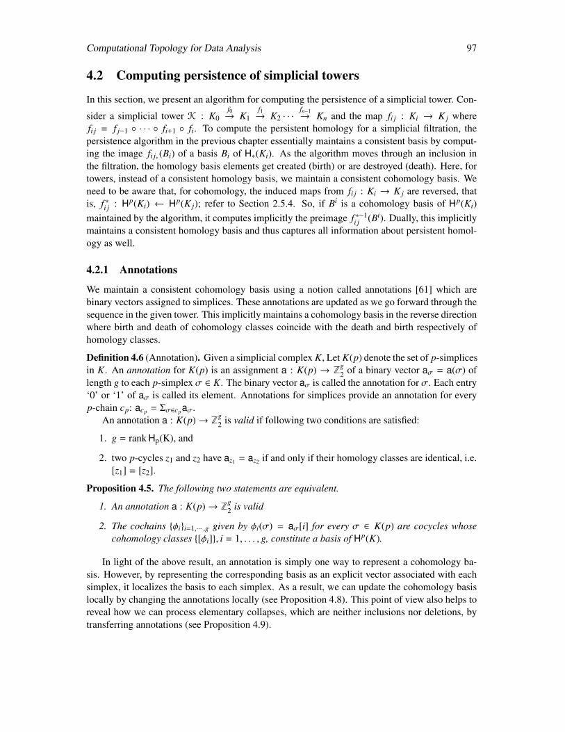
Computational Topology for Data Analysis 97
4.2 Computing persistence of simplicial towers
In this section, we present an algorithm for computing the persistence of a simplicial tower. Con-
sider a simplicial tower K : K0f0→ K1
f1→ K2 · · ·
fn−1→ Kn and the map fi j : Ki → K j where
fi j = f j−1 · · · fi+1 fi. To compute the persistent homology for a simplicial filtration, thepersistence algorithm in the previous chapter essentially maintains a consistent basis by comput-ing the image fi j∗(Bi) of a basis Bi of H∗(Ki). As the algorithm moves through an inclusion inthe filtration, the homology basis elements get created (birth) or are destroyed (death). Here, fortowers, instead of a consistent homology basis, we maintain a consistent cohomology basis. Weneed to be aware that, for cohomology, the induced maps from fi j : Ki → K j are reversed, thatis, f ∗i j : Hp(Ki) ← Hp(K j); refer to Section 2.5.4. So, if Bi is a cohomology basis of Hp(Ki)maintained by the algorithm, it computes implicitly the preimage f ∗−1
i j (Bi). Dually, this implicitlymaintains a consistent homology basis and thus captures all information about persistent homol-ogy as well.
4.2.1 Annotations
We maintain a consistent cohomology basis using a notion called annotations [61] which arebinary vectors assigned to simplices. These annotations are updated as we go forward through thesequence in the given tower. This implicitly maintains a cohomology basis in the reverse directionwhere birth and death of cohomology classes coincide with the death and birth respectively ofhomology classes.
Definition 4.6 (Annotation). Given a simplicial complex K, Let K(p) denote the set of p-simplicesin K. An annotation for K(p) is an assignment a : K(p) → Zg
2 of a binary vector aσ = a(σ) oflength g to each p-simplex σ ∈ K. The binary vector aσ is called the annotation for σ. Each entry‘0’ or ‘1’ of aσ is called its element. Annotations for simplices provide an annotation for everyp-chain cp: acp = Σσ∈cpaσ.
An annotation a : K(p)→ Zg2 is valid if following two conditions are satisfied:
1. g = rank Hp(K), and
2. two p-cycles z1 and z2 have az1 = az2 if and only if their homology classes are identical, i.e.[z1] = [z2].
Proposition 4.5. The following two statements are equivalent.
1. An annotation a : K(p)→ Zg2 is valid
2. The cochains φii=1,··· ,g given by φi(σ) = aσ[i] for every σ ∈ K(p) are cocycles whosecohomology classes [φi], i = 1, . . . , g, constitute a basis of Hp(K).
In light of the above result, an annotation is simply one way to represent a cohomology ba-sis. However, by representing the corresponding basis as an explicit vector associated with eachsimplex, it localizes the basis to each simplex. As a result, we can update the cohomology basislocally by changing the annotations locally (see Proposition 4.8). This point of view also helps toreveal how we can process elementary collapses, which are neither inclusions nor deletions, bytransferring annotations (see Proposition 4.9).
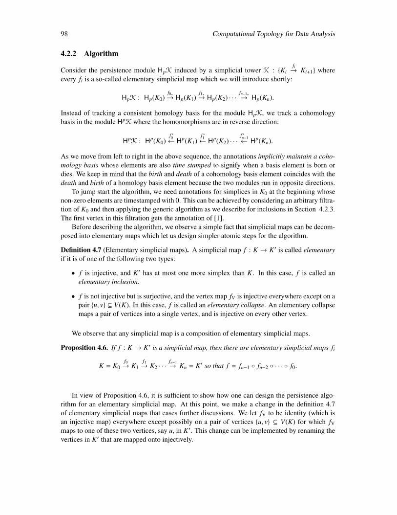
98 Computational Topology for Data Analysis
4.2.2 Algorithm
Consider the persistence module HpK induced by a simplicial tower K : Kifi→ Ki+1 where
every fi is a so-called elementary simplicial map which we will introduce shortly:
HpK : Hp(K0)f0∗→ Hp(K1)
f1∗→ Hp(K2) · · ·
fn−1∗→ Hp(Kn).
Instead of tracking a consistent homology basis for the module HpK, we track a cohomologybasis in the module HpK where the homomorphisms are in reverse direction:
HpK : Hp(K0)f ∗0← Hp(K1)
f ∗1← Hp(K2) · · ·
f ∗n−1← Hp(Kn).
As we move from left to right in the above sequence, the annotations implicitly maintain a coho-mology basis whose elements are also time stamped to signify when a basis element is born ordies. We keep in mind that the birth and death of a cohomology basis element coincides with thedeath and birth of a homology basis element because the two modules run in opposite directions.
To jump start the algorithm, we need annotations for simplices in K0 at the beginning whosenon-zero elements are timestamped with 0. This can be achieved by considering an arbitrary filtra-tion of K0 and then applying the generic algorithm as we describe for inclusions in Section 4.2.3.The first vertex in this filtration gets the annotation of [1].
Before describing the algorithm, we observe a simple fact that simplicial maps can be decom-posed into elementary maps which let us design simpler atomic steps for the algorithm.
Definition 4.7 (Elementary simplicial maps). A simplicial map f : K → K′ is called elementaryif it is of one of the following two types:
• f is injective, and K′ has at most one more simplex than K. In this case, f is called anelementary inclusion.
• f is not injective but is surjective, and the vertex map fV is injective everywhere except on apair u, v ⊆ V(K). In this case, f is called an elementary collapse. An elementary collapsemaps a pair of vertices into a single vertex, and is injective on every other vertex.
We observe that any simplicial map is a composition of elementary simplicial maps.
Proposition 4.6. If f : K → K′ is a simplicial map, then there are elementary simplicial maps fi
K = K0f0→ K1
f1→ K2 · · ·
fn−1→ Kn = K′ so that f = fn−1 fn−2 · · · f0.
In view of Proposition 4.6, it is sufficient to show how one can design the persistence algo-rithm for an elementary simplicial map. At this point, we make a change in the definition 4.7of elementary simplicial maps that eases further discussions. We let fV to be identity (which isan injective map) everywhere except possibly on a pair of vertices u, v ⊆ V(K) for which fVmaps to one of these two vertices, say u, in K′. This change can be implemented by renaming thevertices in K′ that are mapped onto injectively.
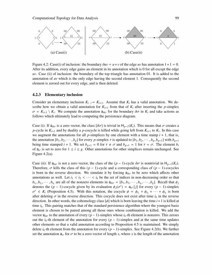
Computational Topology for Data Analysis 99
0 0
10
1 1
00 00
1000
1 101u v u v
00 00
1000
01u v
00
1000
00u v
00 0
10
0u v
0
(a) Case(i) (b) Case(ii)
Figure 4.2: Case(i) of inclusion: the boundary ∂uv = u+v of the edge uv has annotation 1+1 = 0.After its addition, every edge gains an element in its annotation which is 0 for all except the edgeuv. Case (ii) of inclusion: the boundary of the top triangle has annotation 01. It is added to theannotation of uv which is the only edge having the second element 1. Consequently the secondelement is zeroed out for every edge, and is then deleted.
4.2.3 Elementary inclusion
Consider an elementary inclusion Ki → Ki+1. Assume that Ki has a valid annotation. We de-scribe how we obtain a valid annotation for Ki+1 from that of Ki after inserting the p-simplexσ = Ki+1 \ Ki. We compute the annotation a∂σ for the boundary ∂σ in Ki and take actions asfollows which ultimately lead to computing the persistence diagram.
Case (i): If a∂σ is a zero vector, the class [∂σ] is trivial in Hp−1(Ki). This means that σ creates ap-cycle in Ki+1 and by duality a p-cocycle is killed while going left from Ki+1 to Ki. In this casewe augment the annotations for all p-simplices by one element with a time stamp i + 1, that is,the annotation [b1, b2, · · · , bg] for every p-simplex τ is updated to [b1, b2, · · · , bg, bg+1] with bg+1being time stamped i + 1. We set bg+1 = 0 for τ , σ and bg+1 = 1 for τ = σ. The element bi
of aσ is set to zero for 1 ≤ i ≤ g. Other annotations for other simplices remain unchanged. SeeFigure 4.2(a).
Case (ii): If a∂σ is not a zero vector, the class of the (p − 1)-cycle ∂σ is nontrivial in Hp−1(Ki).Therefore, σ kills the class of this (p − 1)-cycle and a corresponding class of (p − 1)-cocyclesis born in the reverse direction. We simulate it by forcing a∂σ to be zero which affects otherannotations as well. Let i1 < i2 < · · · < ik be the set of indices in non-decreasing order so thatbi1 , bi2 , · · · , bik are all of the nonzero elements in a∂σ = [b1, b2, · · · , bik , · · · , bg]. Recall that φ j
denotes the (p − 1)-cocycle given by its evaluation φ j(σ′) = aσ′[ j] for every (p − 1)-simplexσ′ ∈ Ki (Proposition 4.5). With this notation, the cocycle φ = φi1 + φi2 + · · · + φik is bornafter deleting σ in the reverse direction. This cocycle does not exist after time ik in the reversedirection. In other words, the cohomology class [φ] which is born leaving the time i+1 is killed attime ik. This pairing matches that of the standard persistence algorithm where the youngest basiselement is chosen to be paired among all those ones whose combination is killed. We add thevector a∂σ to the annotation of every (p− 1)-simplex whose ik-th element is nonzero. This zeroesout the ik-th element of the annotation for every (p − 1)-simplex and at the same time updatesother elements so that a valid annotation according to Proposition 4.5 is maintained. We simplydelete ik-th element from the annotation for every (p − 1)-simplex. See Figure 4.2(b). We furtherset the annotation aσ for σ to be a zero-vector of length s, where s is the length of the annotation

100 Computational Topology for Data Analysis
vector of every p-simplex at this point.Notice that determining if we have case (i) or (ii) can be done easily in O(pg) time by check-
ing the annotation of ∂σ. Indeed, this is achieved because the annotation already localizes thecohomology basis to each individual simplex.
Before going to the next case of elementary collapse, here we present Algorithm 6:Annotfor computing the annotations for all simplices in a given simplicial complex using the steps ofelementary inclusions. The algorithm proceeds in the order of increasing dimension because itneeds to have the annotations of (p − 1)-simplices before dealing with p-simplices. It starts withvertices whose annotations are readily computable. In the following algorithm K p denotes thep-skeleton of the input simplicial d-complex K.
Algorithm 6 Annot(K)
Input:K: input complex
Output:Annotation for every simplex in K
1: Let m := |K0|
2: For every vertex vi ∈ K0, assign an m-vector a(vi) where a(vi)[ j] = 1 iff j = i3: for p = 1→ d do4: for all simplex σ ∈ K p do5: Let annotation of every p-simplex be a vector of length g so far6: if a(∂σ) , 0 then7: assign a(σ) to be a 0 vector of size g8: pick any non-zero entry bu in a(∂σ)9: add a(∂σ) to every (p − 1)-simplex σ′ s.t. a(σ′)[u] = 1
10: delete u-th entry from annotation of every (p − 1)-simplex11: else12: extend a(τ) for every p-simplex τ so far added by appending a 0 bit13: create vector a(σ) of length g + 1 with only the last bit being 114: end if15: end for16: end for
4.2.4 Elementary collapse
The case for handling collapse is more interesting. It has three distinct steps, (i) elementaryinclusions to satisfy the so called link condition, (ii) local annotation transfer to prepare for thecollapse, and (iii) collapse of the simplices with updated annotations. We explain each of thesesteps now.
The elementary inclusions that may precede the final collapse are motivated by a result that
connects collapses with the change in cohomology. Consider an elementary collapse Kifi→ Ki+1
where the vertex pair (u, v) collapses to u. The following link condition, introduced in [121] andlater used to preserve homotopy [12], becomes relevant.
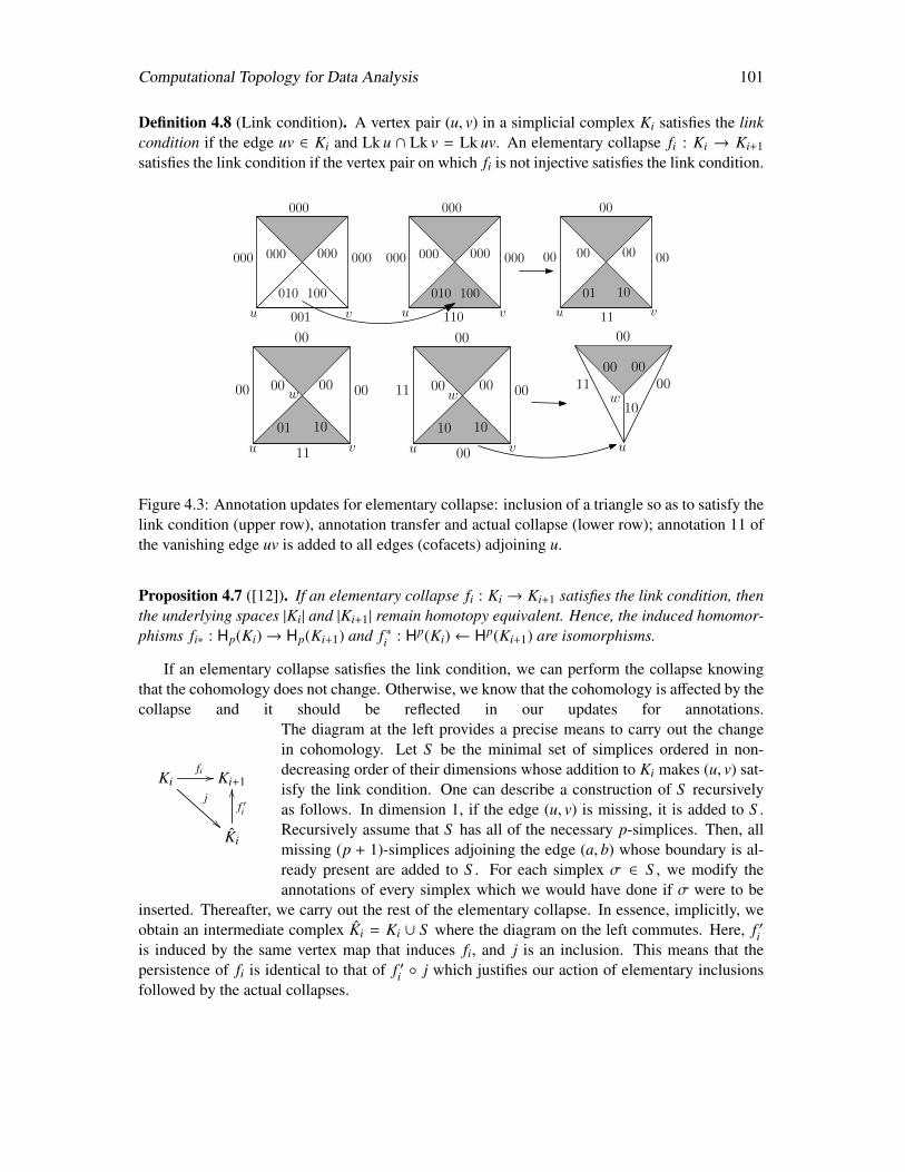
Computational Topology for Data Analysis 101
Definition 4.8 (Link condition). A vertex pair (u, v) in a simplicial complex Ki satisfies the linkcondition if the edge uv ∈ Ki and Lk u ∩ Lk v = Lk uv. An elementary collapse fi : Ki → Ki+1satisfies the link condition if the vertex pair on which fi is not injective satisfies the link condition.
000
000 000
001
000 000
010 100
000
000 000
110
000 000
010 100
00
00 00
11
00 00
01 10
u v u v u v
00
11 00
u
00
00 00
11
00 00
01 10
u v
00
11 00
00
00 00
10 10
u v
10
00 00
w w w
Figure 4.3: Annotation updates for elementary collapse: inclusion of a triangle so as to satisfy thelink condition (upper row), annotation transfer and actual collapse (lower row); annotation 11 ofthe vanishing edge uv is added to all edges (cofacets) adjoining u.
Proposition 4.7 ([12]). If an elementary collapse fi : Ki → Ki+1 satisfies the link condition, thenthe underlying spaces |Ki| and |Ki+1| remain homotopy equivalent. Hence, the induced homomor-phisms fi∗ : Hp(Ki)→ Hp(Ki+1) and f ∗i : Hp(Ki)← Hp(Ki+1) are isomorphisms.
If an elementary collapse satisfies the link condition, we can perform the collapse knowingthat the cohomology does not change. Otherwise, we know that the cohomology is affected by thecollapse and it should be reflected in our updates for annotations.
Kifi //
j
!!
Ki+1
Ki
f ′i
OO
The diagram at the left provides a precise means to carry out the changein cohomology. Let S be the minimal set of simplices ordered in non-decreasing order of their dimensions whose addition to Ki makes (u, v) sat-isfy the link condition. One can describe a construction of S recursivelyas follows. In dimension 1, if the edge (u, v) is missing, it is added to S .Recursively assume that S has all of the necessary p-simplices. Then, allmissing (p + 1)-simplices adjoining the edge (a, b) whose boundary is al-ready present are added to S . For each simplex σ ∈ S , we modify theannotations of every simplex which we would have done if σ were to be
inserted. Thereafter, we carry out the rest of the elementary collapse. In essence, implicitly, weobtain an intermediate complex Ki = Ki ∪ S where the diagram on the left commutes. Here, f ′iis induced by the same vertex map that induces fi, and j is an inclusion. This means that thepersistence of fi is identical to that of f ′i j which justifies our action of elementary inclusionsfollowed by the actual collapses.
102 Computational Topology for Data Analysis
We remark that this is the only place where we may insert implicitly a simplex σ in the currentapproach. The number of such σ is usually much smaller than the number of simplices that onemay need for a coning strategy detailed in Section 4.4 to process simplicial towers.
After constructing Ki with annotations, we transfer annotations to prepare for the collapse.This step locally changes the annotations for simplices containing the vertices u and/or v. Thefollowing definition facilitates the description.
Definition 4.9 (Vanishing; Mirror simplices). For the elementary collapse f ′i : Ki → Ki+1, asimplex σ ∈ Ki is called vanishing if the cardinality of f ′i (σ) is one less than that of σ. Twosimplices σ and σ′ are called mirror partners if one contains u and the other v, and share restof the vertices. In Figure 4.3 (lower row), the vanishing simplices are uv, uvw and the mirrorpartners are u, v, uw, vw.
In an elementary collapse that sends (u, v) to u, all vanishing simplices need to be deleted, andall simplices containing v need to be pulled to corresponding ones containing the vertex u (whichare their mirror partners). We update the annotations in such a way that the annotations of allvanishing simplices become zero, and those of both mirror partners become the same. Once thisis achieved, the collapse is implemented by simply deleting the vanishing simplices and replacingv with u in all simplices containing v (effectively this identifies mirror partners) without changingtheir annotations. The following proposition provides the justification behind the specific updateoperations that we perform.
Proposition 4.8. Let K be a simplicial complex and a : K(p) → Zg2 be a valid annotation. Let
σ ∈ K(p) be any p-simplex and τ any of its (p − 1)-faces. Then, adding aσ to the annotation forall cofacets of τ including σ produces a valid annotation for K(p). Furthermore, the cohomologybasis corresponding to the annotations (Proposition 4.5) remains unchanged by this modification.
Consider now the elementary collapse f ′i : Ki → Ki+1 that sends (u, v) to u. We update theannotations for simplices in Ki as follows. First, note that the vanishing simplices are exactlythose simplices containing the edge u, v. For every p-simplex containing u, v, i.e., a vanishingsimplex, exactly two of its (p−1)-faces are mirror simplices, and all other remaining (p−1)-facesare vanishing simplices. Let σ be a vanishing p-simplex and τ be its (p − 1)-face that is a mirrorsimplex containing u. We add aσ to the annotations for all cofacets (cofaces of codimension 1)of τ including σ. This implements the annotation transfer for σ. By Proposition 4.8, the newannotation generated by this process corresponds to the old cohomology basis for Ki. This newannotation has aσ as zero since aσ + aσ = 0. See the the lower row of Figure 4.3. We perform theabove operation for each vanishing simplex. It turns out that by using the relations of vanishingsimplices and mirror simplices, each mirror simplex eventually acquires an identical annotationto that of its partner. Specifically, we have the following observation.
Proposition 4.9. After all possible annotation transfers involved in a collapse, (i) each vanishingsimplex has a zero annotation; and (ii) each mirror simplex τ has the same annotation as itsmirror partner simplex τ′.
Subsequent to the annotation transfer, the annotation of Ki fits for actual collapse since eachpair of mirror simplices which are collapsed to a single simplex get the identical annotation and
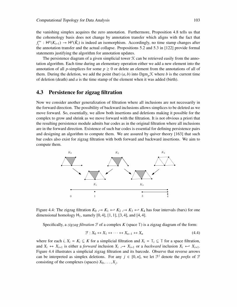
Computational Topology for Data Analysis 103
the vanishing simplex acquires the zero annotation. Furthermore, Proposition 4.8 tells us thatthe cohomology basis does not change by annotation transfer which aligns with the fact thatf ′∗i : Hp(Ki+1) → Hp(Ki) is indeed an isomorphism. Accordingly, no time stamp changes afterthe annotation transfer and the actual collapse. Propositions 5.2 and 5.3 in [122] provide formalstatements justifying the algorithm for annotation updates.
The persistence diagram of a given simplicial tower K can be retrieved easily from the anno-tation algorithm. Each time during an elementary operation either we add a new element into theannotation of all p-simplices for some p ≥ 0 or delete an element from the annotations of all ofthem. During the deletion, we add the point (bar) (a, b) into DgmpK where b is the current timeof deletion (death) and a is the time stamp of the element when it was added (birth).
4.3 Persistence for zigzag filtration
Now we consider another generalization of filtration where all inclusions are not necessarily inthe forward direction. The possibility of backward inclusions allows simplices to be deleted as wemove forward. So, essentially, we allow both insertions and deletions making it possible for thecomplex to grow and shrink as we move forward with the filtration. It is not obvious a priori thatthe resulting persistence module admits bar codes as in the original filtration where all inclusionsare in the forward direction. Existence of such bar codes is essential for defining persistence pairsand designing an algorithm to compute them. We are assured by quiver theory [163] that suchbar codes also exist for zigzag filtration with both forward and backward insertions. We aim tocompute them.
K0
K1
K2
K3
K4
0 1 3 4
Figure 4.4: The zigzag filtration K0 → K1 ← K2 → K3 ← K4 has four intervals (bars) for onedimensional homology H1, namely [0, 4], [1, 1], [3, 4], and [4, 4].
Specifically, a zigzag filtration F of a complex K (space T) is a zigzag diagram of the form:
F : X0 ↔ X1 ↔ · · · ↔ Xn−1 ↔ Xn (4.4)
where for each i, Xi = Ki ⊆ K for a simplicial filtration and Xi = Ti ⊆ T for a space filtration,and Xi ↔ Xi+1 is either a forward inclusion Xi → Xi+1 or a backward inclusion Xi ← Xi+1.Figure 4.4 illustrates a simplicial zigzag filtration and its barcode. Observe that reverse arrowscan be interpreted as simplex deletions. For any j ∈ [0, n], we let F j denote the prefix of F
consisting of the complexes (spaces) X0, . . . , X j.
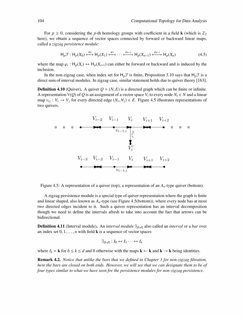
104 Computational Topology for Data Analysis
For p ≥ 0, considering the p-th homology groups with coefficient in a field k (which is Z2here), we obtain a sequence of vector spaces connected by forward or backward linear maps,called a zigzag persistence module:
HpF : Hp(X0)ϕ0←−→ Hp(X1)
ϕ1←−→ · · ·
ϕn−2←−−→ Hp(Xn−1)
ϕn−1←−−→ Hp(Xn) (4.5)
where the map ϕi : Hp(Xi) ↔ Hp(Xi+1) can either be forward or backward and is induced by theinclusion.
In the non-zigzag case, when index set for HpF is finite, Proposition 3.10 says that HpF is adirect sum of interval modules. In zigzag case, similar statement holds due to quiver theory [163].
Definition 4.10 (Quiver). A quiver Q = (N, E) is a directed graph which can be finite or infinite.A representation V(Q) of Q is an assignment of a vector space Vi to every node Ni ∈ N and a linearmap vi j : Vi → V j for every directed edge (Ni,N j) ∈ E. Figure 4.5 illustrates representations oftwo quivers.
Vi Vi+1 Vi+2Vi−1Vi−2
V ′i
vi−1,i vi,i
′
Vi Vi+1 Vi+2Vi−1Vi−2
vi−1,i
Vi−3
Figure 4.5: A representation of a quiver (top); a representation of an An-type quiver (bottom).
A zigzag persistence module is a special type of quiver representation where the graph is finiteand linear shaped, also known as An-type (see Figure 4.5(bottom)), where every node has at mosttwo directed edges incident to it. Such a quiver representation has an interval decompositionthough we need to define the intervals afresh to take into account the fact that arrows can bebidirectional.
Definition 4.11 (Interval module). An interval module I[b,d] also called an interval or a bar overan index set 0, 1, . . . , n with field k is a sequence of vector spaces
I[b,d] : I0 ↔ I1 · · · ↔ In
where Ik = k for b ≤ k ≤ d and 0 otherwise with the maps k← k and k→ k being identities.
Remark 4.2. Notice that unlike the bars that we defined in Chapter 3 for non-zigzag filtration,here the bars are closed on both ends. However, we will see that we can designate them to be offour types similar to what we have seen for the persistence modules for non-zigzag persistence.
Computational Topology for Data Analysis 105
Theorem 4.10 ([13, 265, 163]). Every quiver representation V(Q) for an An-type quiver Q hasan interval decomposition, that is, V(Q)
⊕i I[bi,di]. Furthermore, this decomposition is unique
up to isomorphism and permutation of the intervals.
The underlying graph of a zigzag persistence module as shown in Eqn. (4.5) is of An-type.Hence, we have the decomposition HpF
⊕i I[bi,di] that provides the bar code for zigzag per-
sistence. Notice that Theorem 4.10 does not require the vector spaces to be finite dimensional.Hence, we still have a valid decomposition even if the vector spaces in the zigzag persistence mod-ule are not finite dimensional. However, for finite computation, we will assume that our zigzagpersistence module is finite both in terms of the index set and also in terms of the dimension ofthe vector spaces.
Recall from Section 3.2.1 that each bar (interval) in a barcode (interval decomposition) corre-sponds to a point in the persistence diagram Dgmp(F) and thus we also say that the bar belongs tothe diagram. Sometimes, we also abuse the notation [b, d] to denote both an interval in the indexset and an interval module in a p-th zigzag persistent module.
Types of bars. A bar [b, d] for a zigzag persistence module HpF can be of four types dependingon the direction of the arrow between Xb−1 and Xb and the arrow between Xd and Xd+1 in F. Theyare:
closed-closed [b, d]: Xb−1 → Xb · · · Xd ← Xd+1: Either b = 0 or the inclusion Xb−1 → Xb isa forward arrow; and d < n with the inclusion Xd ← Xd+1 being a backward arrow;
closed-open [b, d]: Xb−1 → Xb · · · Xd → Xd+1: Either b = 0 or the inclusion Xb−1 → Xb is aforward arrow; and either d = n or the inclusion Xd → Xd+1 is a forward arrow;
open-closed [b, d]: Xb−1 ← Xb · · · Xd ← Xd+1: b > 0 and the inclusion Xb−1 ← Xb is abackward arrow; and d < n with the inclusion Xd ← Xd+1 being a backward arrow;
open-open [b, d]: Xb−1 ← Xb · · · Xd → Xd+1: b > 0 and the inclusion Xb−1 ← Xb is a back-ward arrow; and either d = n or the inclusion Xd → Xd+1 is a forward arrow.
With the four types of bars, when we compute the bottleneck distance between persistencediagrams for two zigzag persistence modules, we consider matching between bars of similartypes. That is, db(Dgmp(F1),Dgmp(F2)) is computed with the understanding that only similartypes of bars are compared while matching the bars and the points on the diagonal are assumed tohave any type. We face a difficulty in defining an interleaving distance between zigzag modulesbecause of the the zigzag nature of the arrows. However, one can define such an interleavingdistance by mapping the module to a 2-parameter persistence module. See the notes in Chapter 12for more details.
106 Computational Topology for Data Analysis
4.3.1 Approach
We briefly describe an overview of our approach for computing zigzag persistent intervals for asimplicial zigzag filtration:
F : ∅ = K0 ↔ K1 ↔ · · · ↔ Kn−1 ↔ Kn. (4.6)
We assume that the filtration is simplex-wise, which means that Ki, Ki+1 differ by only one simplexσi and also begins with the empty complex. We have seen similar conditions before for the non-zigzag case in Section 3.1.2. This is not a serious restriction because we can expand an inclusionof a set of simplices to a series of inclusions by a single simplex while using any order that puts asimplex after all its faces and we can always pad an empty complex at the beginning with the firstinclusion being forward.
The method we describe is derived from maintaining a consistent basis with a set of represen-tative cycles over the intervals as we define now. These cycles generate an interval module in astraightforward way by associating a cycle to a homology class at each position.
Definition 4.12 (Representative cycles). Let p ≥ 0, F : K0 ↔ · · · ↔ Kn be a zigzag filtration and
HpF = Hp(Ki)φi↔ Hp(Ki+1)i=0,...,n−1 be the corresponding zigzag persistence module. Let [b, d]
be an interval in Dgmp(F). A set of representative p-cycles for [b, d] is an indexed set of p-cyclesci ⊆ Ki | i ∈ [b, d]
so that
1. For b > 0, [cb] is not in the image of ϕb−1 if Kb−1 ↔ Kb is a forward inclusion, or [cb] isthe non-zero class mapped to 0 by ϕb−1 otherwise.
2. For d < n, [cd] is not in the image of ϕd if Kd ↔ Kd+1 is a backward inclusion, or [cd] isthe non-zero class mapped to 0 by ϕd otherwise.
3. For each i ∈ [b, d−1], [ci]↔ [ci+1] by ϕi, that is, either [ci] 7→ [ci+1] or [ci]← [ [ci+1] by ϕi.
The interval module induced by the representative p-cycles is a zigzag persistence module I :I0 ↔ I1 · · · ↔ In such that Ii equals the 1-dimensional vector space generated by [ci] ∈ Hp(Ki)for i ∈ [b, d] and equals 0 otherwise.
The following theorem justifies the definition of representative cycles, which says that repre-sentative cycles always produce an interval decomposition of a zigzag module and vice versa:
Theorem 4.11. Let p ≥ 0, F : K0 ↔ · · · ↔ Kn be a zigzag filtration with Hp(K0) = 0 and A bean index set. One has that HpF is equal to (not merely isomorphic to) a direct sum of intervalsubmodules
⊕α∈A I[bα,dα] if and only if for each α ∈ A, I[bα,dα] is an interval module induced by
a set of representative p-cycles for [bα, dα] where Dgmp(F) =[bα, dα] |α ∈ A
.
We now present an abstract algorithm based on an approach in [228] which helps us designa concrete algorithm later. Given a filtration F : ∅ = K0 ↔ · · · ↔ Kn starting with an emptycomplex, first let Dgmp(F0) = ∅. The algorithm then iterates for i ← 0, . . . , n − 1. At thebeginning of the i-th iteration, inductively assume that the intervals and their representative cyclesfor HpF
i have already been computed. The aim of the i-th iteration is to compute these for HpFi+1.
Let Dgmp(Fi) =[bα, dα] |α ∈ Ai be indexed by a set Ai, and let
cαk ⊆ Kk | k ∈ [bα, dα]
be a
Computational Topology for Data Analysis 107
set of representative p-cycles for each [bα, dα]. For ease of presentation, we also let cαk = 0 foreach α ∈ Ai and each k ∈ [0, i] not in [bα, dα]. We call intervals of Dgmp(Fi) ending with ias surviving intervals at index i. Each non-surviving interval of Dgmp(Fi) is directly includedin Dgmp(Fi+1) and its representative cycles stay the same. For surviving intervals of Dgmp(Fi),the i-th iteration proceeds with the following cases determined by the types of the linear mapsϕi : Hp(Ki)↔ Hp(Ki+1).
ϕi is isomorphic: In this case, no intervals are created or cease to persist. For each surviv-ing interval [bα, dα] in Dgmp(Fi), [bα, dα] now corresponds to an interval [bα, i + 1] inDgmp(Fi+1). The representative cycles for [bα, i + 1] are set by the following rule:
Trivial setting rule of representative cycles: For each j with bα ≤ j ≤ i, the representativecycle for [bα, i + 1] at index j stays the same. The representative cycle for [bα, i + 1] at i + 1is set to a cαi+1 ⊆ Ki+1 such that [cαi ]↔ [cαi+1] by ϕi.
ϕi points forward and is injective: A new interval [i + 1, i + 1] is added to Dgmp(Fi+1) and itsrepresentative cycle at i + 1 is set to a p-cycle in Ki+1 containing σi. All surviving intervalsof Dgmp(Fi) persist to index i+1 and their representative cycles are set by the trivial settingrule.
ϕi points backward and is surjective: A new interval [i + 1, i + 1] is added to Dgmp(Fi+1) andits representative cycle at i+1 is set to a p-cycle homologous to ∂(σi) in Ki+1. All survivingintervals of Dgmp(Fi) persist to index i + 1 and their representative cycles are set by thetrivial setting rule.
ϕi points forward and is surjective: A surviving interval of Dgmp(Fi) does not persist to i + 1.Let Bi ⊆ Ai consist of indices of all surviving intervals. We have that
[cαi ] |α ∈ Bi forms
a basis of Hp(Ki). Suppose that ϕi([cα1
i ] + · · · + [cα`i ])
= 0, where α1, . . . , α` ∈ Bi. We can
rearrange the indices such that bα1 < bα2 < · · · < bα` and α1 < α2 < · · · < α`. Let λ beα1 if the arrow bα−1 ↔ bα points backward for every α ∈ α1, . . . , α` and otherwise bethe largest α ∈ α1, . . . , α` such that bα−1 ↔ bα points forward. Then, [bλ, i] forms aninterval of Dgmp(Fi+1). For each k ∈ [bλ, i], let zk = cα1
k + · · ·+cα`k ; then,zk | k ∈ [bλ, i]
is a
set of representative cycles for [bλ, i]. All the other surviving intervals of Dgmp(Fi) persistto i + 1 and their representative cycles are set by the trivial setting rule.
ϕi points backward and is injective: A surviving interval of Dgmp(Fi) does not persist to i + 1.Let Bi ⊆ Ai consist of indices of all surviving intervals, and let cα1
i , . . . , cα`i be the cycles in
cαi |α ∈ Bi containing σi. We can rearrange the indices such that bα1 < bα2 < · · · < bα`and α1 < α2 < · · · < α`. Let λ be α1 if the arrow bα−1 ↔ bα points forward for everyα ∈ α1, . . . , α` and otherwise be the largest α ∈ α1, . . . , α` such that bα−1 ↔ bα pointsbackward. Then, [bλ, i] forms an interval of Dgmp(Fi+1) and the representative cycles for[bλ, i] stay the same. For each α ∈ α1, . . . , α` not equal to λ, let zk = cαk + cλk for each ksuch that bα ≤ k ≤ i, and let zi+1 = zi; then,
zk | k ∈ [bα, i + 1]
is a set of representative
cycles for [bα, i + 1]. For the other surviving intervals, the setting of representative cyclesfollows the trivial setting rule.
Remark 4.3. Note that in the above algorithm, there is no canonical choice for the representativeclasses. However, all choices produce the same intervals.
108 Computational Topology for Data Analysis
4.3.2 Zigzag persistence algorithm
We now present a concrete version of our approach which runs in cubic time. In this algorithm,given a zigzag filtration F : ∅ = K0 ↔ K1 ↔ · · · ↔ Kn, the main loop iterates for i← 0, . . . , n−1so that the i-th iteration takes care of the changes from Ki to Ki+1. A unique integral id less than nis assigned to each simplex in Ki and id[σ] is used to record the id of a simplex σ. Note that theid of a simplex is subject to change during the execution. For each dimension p, a cycle matrixZp and a chain matrix Cp+1 with entries in Z2 are maintained. The number of columns of Zp andCp+1 equals rank Zp(Ki) and the number of rows of Zp and Cp+1 equals n. We will see that certaincolumns j of Cp+1 maintain a (p + 1)-chain whose boundary is in column j of Zp. Each columnof Zp and Cp represents a p-chain in Ki such that for each simplex σ ∈ Ki, σ belongs to thep-chain if and only if the bit with index id[σ] in the column equals 1. For convenience, we makeno distinction between a column of the matrix Zp or Cp and the chain it represents. We use Zp[ j]to denote the j-th column of Zp (columns of Cp are denoted similarly). For each column Zp[ j],a birth timestamp bp[ j] is maintained. This timestamp is usually non-negative, but can possiblybe negative one (−1). We will see that this special negative value is assigned only to indicate thatthe column represents a boundary cycle. Moreover, we let the pivot of Zp[ j] be the largest indexwhose corresponding bit equals to 1 in Zp[ j] and denote it as pivot(Zp[ j]). At the start of the i-thiteration, for each p, the following properties for the matrices are preserved:
1. The columns of Zp form a basis of Zp(Ki) and have distinct pivots.
2. The columns of Zp with negative birth timestamps form a basis of Bp(Ki). Moreover, foreach column Zp[ j] of Zp with a negative birth timestamp, one has that Zp[ j] = ∂
(Cp+1[ j]
).
3. For columns of Zp with non-negative birth timestamps, their birth timestamps bijectivelymap to the starting indices of the intervals of Dgmp(Fi) ending with i. Moreover, for eachcolumn Zp[ j] of Zp such that bp[ j] is non-negative, one has that Zp[ j] is a representativecycle at index i for the interval
[bp[ j], i
].
The above properties indicate that a column Zp[ j] of Zp is a boundary if bp[ j] < 0 and isnot a boundary otherwise. Furthermore, we have that columns of Zp with non-negative birthtimestamps represent a homology basis for Hp(Ki) at the start of the i-th iteration.
Zigzag algorithm.For each i← 0, . . . , n − 1, the algorithm does the following:
• Case ϕi is forward: From Ki to Ki+1, a p-simplex σi is added and the id of σi is set asid[σi] = i. Since the columns of Zp−1 form a basis of Zp−1(Ki) and have distinct pivots,∂(σi) can be represented as a sum of the columns of Zp−1 by a reduction algorithm. Supposethat ∂(σi) =
∑α∈I Zp−1[α] where I is a set of column indices of Zp−1. The algorithm then
checks the timestamp of Zp−1[α] for each α ∈ I to see whether all of them are boundaries.After this, it is known whether or not ∂(σi) is a boundary in Ki. An interval in dimension pgets born if ∂(σi) is a boundary in Ki and an interval in dimension p − 1 dies otherwise.
– Birth: Append a new column σi +∑α∈I Cp[α] with birth timestamp i + 1 to Zp.

Computational Topology for Data Analysis 109
– Death: Let J consist of indices in I whose corresponding columns in Zp−1 have non-negative birth timestamps. If ϕbp−1[α]−1 points backward ∀α ∈ J, let λ be the smallestindex in J; otherwise, let λ be the largest α in J such that ϕbp−1[α]−1 points forward.Then, do the following:
1. Output the (p − 1)-th interval[bp−1[λ], i
].
2. Set Zp−1[λ] = ∂(σi), Cp[λ] = σi, and bp−1[λ] = −1.
Since the pivot of the column ∂(σi) may conflict with that of another column in Zp−1,we perform steps 1-13 described next to keep the pivots distinct. The total order b
used in step 10 and later is defined as follows.
Definition 4.13. Let I ⊆1, . . . , n − 1
be a set of indices. For i, j ∈ I, i b j in the
total order if and only if one of the following holds:
∗ i = j.∗ i < j and the function ϕ j−1 points forward.∗ j < i and the function ϕi−1 points backward.
1. while there are two columns Zp−1[α], Zp−1[β] with the same pivot do2. if bp−1[α] < 0 and bp−1[β] < 0 then3. Zp−1[α]← Zp−1[α] + Zp−1[β]4. Cp[α]← Cp[α] + Cp[β]5. if bp−1[α] < 0 and bp−1[β] ≥ 0 then6. Zp−1[β]← Zp−1[α] + Zp−1[β]7. if bp−1[α] ≥ 0 and bp−1[β] < 0 then8. Zp−1[α]← Zp−1[α] + Zp−1[β]9. if bp−1[α] ≥ 0 and bp−1[β] ≥ 0 then
10. if bp−1[α] b bp−1[β] then11. Zp−1[β]← Zp−1[α] + Zp−1[β]12. else13. Zp−1[α]← Zp−1[α] + Zp−1[β]
• Case ϕi is backward: From Ki to Ki+1, a p-simplex σi is deleted. If there is a column in Zp
containing σi, then there are some p-cycles missing going from Ki to Ki+1 and an intervalin dimension p dies. Otherwise, an interval in dimension p − 1 gets born.
– Birth: First, the boundaries in Zp−1 need to be updated so that they form a basis ofBp−1(Ki+1):
1. while there are two columns Zp−1[α], Zp−1[β] with negative birth timestamps s.t.Cp[α], Cp[β] contain σi do
2. if pivot(Zp−1[α]) > pivot(Zp−1[β]) then3. Zp−1[α]← Zp−1[α] + Zp−1[β]4. Cp[α]← Cp[α] + Cp[β]5. else6. Zp−1[β]← Zp−1[α] + Zp−1[β]
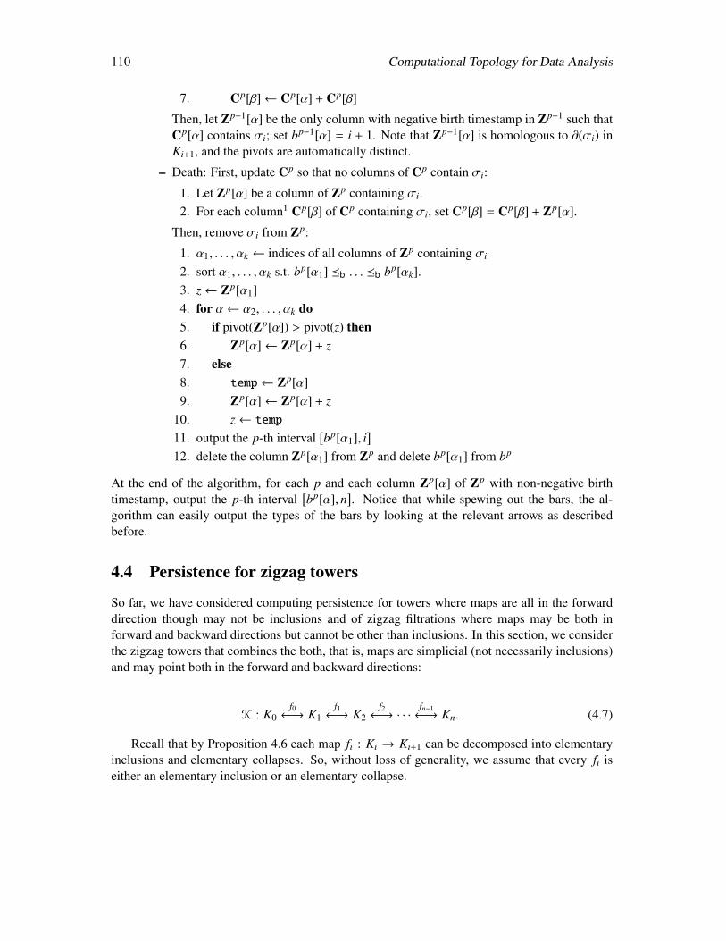
110 Computational Topology for Data Analysis
7. Cp[β]← Cp[α] + Cp[β]
Then, let Zp−1[α] be the only column with negative birth timestamp in Zp−1 such thatCp[α] contains σi; set bp−1[α] = i + 1. Note that Zp−1[α] is homologous to ∂(σi) inKi+1, and the pivots are automatically distinct.
– Death: First, update Cp so that no columns of Cp contain σi:
1. Let Zp[α] be a column of Zp containing σi.2. For each column1 Cp[β] of Cp containing σi, set Cp[β] = Cp[β] + Zp[α].
Then, remove σi from Zp:
1. α1, . . . , αk ← indices of all columns of Zp containing σi
2. sort α1, . . . , αk s.t. bp[α1] b . . . b bp[αk].3. z← Zp[α1]4. for α← α2, . . . , αk do5. if pivot(Zp[α]) > pivot(z) then6. Zp[α]← Zp[α] + z7. else8. temp← Zp[α]9. Zp[α]← Zp[α] + z
10. z← temp11. output the p-th interval
[bp[α1], i
]12. delete the column Zp[α1] from Zp and delete bp[α1] from bp
At the end of the algorithm, for each p and each column Zp[α] of Zp with non-negative birthtimestamp, output the p-th interval
[bp[α], n
]. Notice that while spewing out the bars, the al-
gorithm can easily output the types of the bars by looking at the relevant arrows as describedbefore.
4.4 Persistence for zigzag towers
So far, we have considered computing persistence for towers where maps are all in the forwarddirection though may not be inclusions and of zigzag filtrations where maps may be both inforward and backward directions but cannot be other than inclusions. In this section, we considerthe zigzag towers that combines the both, that is, maps are simplicial (not necessarily inclusions)and may point both in the forward and backward directions:
K : K0f0←→ K1
f1←→ K2
f2←→ · · ·
fn−1←→ Kn. (4.7)
Recall that by Proposition 4.6 each map fi : Ki → Ki+1 can be decomposed into elementaryinclusions and elementary collapses. So, without loss of generality, we assume that every fi iseither an elementary inclusion or an elementary collapse.
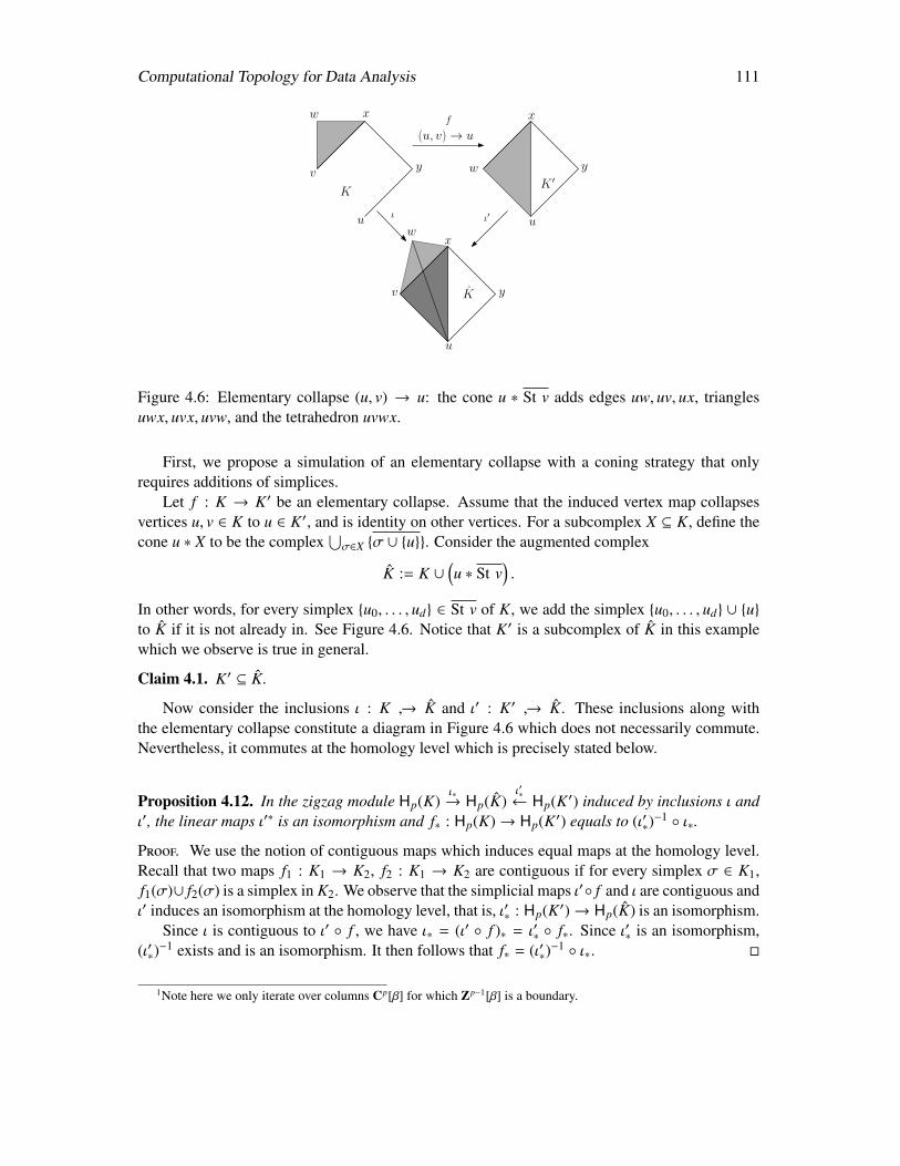
Computational Topology for Data Analysis 111
u
v
w x
y
u
w
x
y
(u, v) → u
u
v
wx
y
KK ′
K
ι ι′
f
Figure 4.6: Elementary collapse (u, v) → u: the cone u ∗ St v adds edges uw, uv, ux, trianglesuwx, uvx, uvw, and the tetrahedron uvwx.
First, we propose a simulation of an elementary collapse with a coning strategy that onlyrequires additions of simplices.
Let f : K → K′ be an elementary collapse. Assume that the induced vertex map collapsesvertices u, v ∈ K to u ∈ K′, and is identity on other vertices. For a subcomplex X ⊆ K, define thecone u ∗ X to be the complex
⋃σ∈X σ ∪ u. Consider the augmented complex
K := K ∪(u ∗ St v
).
In other words, for every simplex u0, . . . , ud ∈ St v of K, we add the simplex u0, . . . , ud ∪ uto K if it is not already in. See Figure 4.6. Notice that K′ is a subcomplex of K in this examplewhich we observe is true in general.
Claim 4.1. K′ ⊆ K.
Now consider the inclusions ι : K → K and ι′ : K′ → K. These inclusions along withthe elementary collapse constitute a diagram in Figure 4.6 which does not necessarily commute.Nevertheless, it commutes at the homology level which is precisely stated below.
Proposition 4.12. In the zigzag module Hp(K)ι∗→ Hp(K)
ι′∗← Hp(K′) induced by inclusions ι and
ι′, the linear maps ι′∗ is an isomorphism and f∗ : Hp(K)→ Hp(K′) equals to (ι′∗)−1 ι∗.
Proof. We use the notion of contiguous maps which induces equal maps at the homology level.Recall that two maps f1 : K1 → K2, f2 : K1 → K2 are contiguous if for every simplex σ ∈ K1,f1(σ)∪ f2(σ) is a simplex in K2. We observe that the simplicial maps ι′ f and ι are contiguous andι′ induces an isomorphism at the homology level, that is, ι′∗ : Hp(K′)→ Hp(K) is an isomorphism.
Since ι is contiguous to ι′ f , we have ι∗ = (ι′ f )∗ = ι′∗ f∗. Since ι′∗ is an isomorphism,(ι′∗)−1 exists and is an isomorphism. It then follows that f∗ = (ι′∗)
−1 ι∗.
1Note here we only iterate over columns Cp[β] for which Zp−1[β] is a boundary.
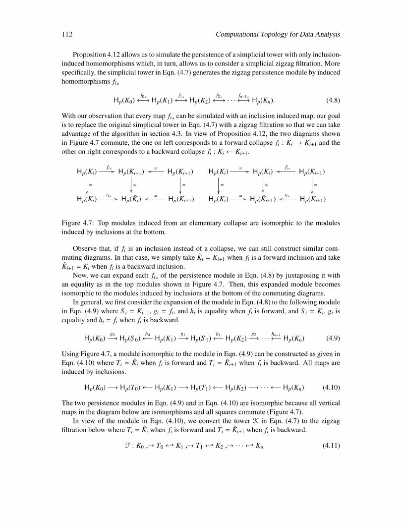
112 Computational Topology for Data Analysis
Proposition 4.12 allows us to simulate the persistence of a simplicial tower with only inclusion-induced homomorphisms which, in turn, allows us to consider a simplicial zigzag filtration. Morespecifically, the simplicial tower in Eqn. (4.7) generates the zigzag persistence module by inducedhomomorphisms fi∗
Hp(K0)f0∗←→ Hp(K1)
f1∗←→ Hp(K2)
f2∗←→ · · ·
fn−1∗←→ Hp(Kn). (4.8)
With our observation that every map fi∗ can be simulated with an inclusion induced map, our goalis to replace the original simplicial tower in Eqn. (4.7) with a zigzag filtration so that we can takeadvantage of the algorithm in section 4.3. In view of Proposition 4.12, the two diagrams shownin Figure 4.7 commute, the one on left corresponds to a forward collapse fi : Ki → Ki+1 and theother on right corresponds to a backward collapse fi : Ki ← Ki+1.
Hp(Ki)fi∗ //
=
Hp(Ki+1)
'
Hp(Ki+1)=oo
=
Hp(Ki)
ιi∗ // Hp(Ki) Hp(Ki+1)'oo
Hp(Ki)= //
=
Hp(Ki)
'
Hp(Ki+1)fi∗oo
=
Hp(Ki)
' // Hp(Ki+1) Hp(Ki+1)ιi∗oo
Figure 4.7: Top modules induced from an elementary collapse are isomorphic to the modulesinduced by inclusions at the bottom.
Observe that, if fi is an inclusion instead of a collapse, we can still construct similar com-muting diagrams. In that case, we simply take Ki = Ki+1 when fi is a forward inclusion and takeKi+1 = Ki when fi is a backward inclusion.
Now, we can expand each fi∗ of the persistence module in Eqn. (4.8) by juxtaposing it withan equality as in the top modules shown in Figure 4.7. Then, this expanded module becomesisomorphic to the modules induced by inclusions at the bottom of the commuting diagrams.
In general, we first consider the expansion of the module in Eqn. (4.8) to the following modulein Eqn. (4.9) where S i = Ki+1, gi = fi, and hi is equality when fi is forward, and S i = Ki, gi isequality and hi = fi when fi is backward.
Hp(K0)g0−→ Hp(S 0)
h0←− Hp(K1)
g1−→ Hp(S 1)
h1←− Hp(K2)
g2−→ · · ·
hn−1←− Hp(Kn) (4.9)
Using Figure 4.7, a module isomorphic to the module in Eqn. (4.9) can be constructed as given inEqn. (4.10) where Ti = Ki when fi is forward and Ti = Ki+1 when fi is backward. All maps areinduced by inclusions.
Hp(K0) −→ Hp(T0)←− Hp(K1) −→ Hp(T1)←− Hp(K2) −→ · · · ←− Hp(Kn) (4.10)
The two persistence modules in Eqn. (4.9) and in Eqn. (4.10) are isomorphic because all verticalmaps in the diagram below are isomorphisms and all squares commute (Figure 4.7).
In view of the module in Eqn. (4.10), we convert the tower K in Eqn. (4.7) to the zigzagfiltration below where Ti = Ki when fi is forward and Ti = Ki+1 when fi is backward:
F : K0 → T0 ← K1 → T1 ← K2 → · · · ← Kn (4.11)
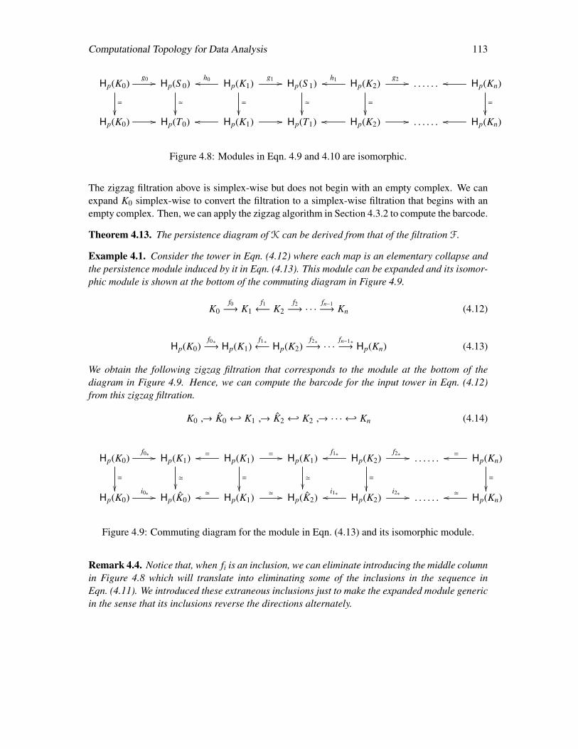
Computational Topology for Data Analysis 113
Hp(K0)g0 //
=
Hp(S 0)
'
Hp(K1)h0oo g1 //
=
Hp(S 1)
'
Hp(K2)h1oo g2 //
=
. . . . . . Hp(Kn)oo
=
Hp(K0) // Hp(T0) Hp(K1)oo // Hp(T1) oo Hp(K2) // . . . . . . Hp(Kn)oo
Figure 4.8: Modules in Eqn. 4.9 and 4.10 are isomorphic.
The zigzag filtration above is simplex-wise but does not begin with an empty complex. We canexpand K0 simplex-wise to convert the filtration to a simplex-wise filtration that begins with anempty complex. Then, we can apply the zigzag algorithm in Section 4.3.2 to compute the barcode.
Theorem 4.13. The persistence diagram of K can be derived from that of the filtration F.
Example 4.1. Consider the tower in Eqn. (4.12) where each map is an elementary collapse andthe persistence module induced by it in Eqn. (4.13). This module can be expanded and its isomor-phic module is shown at the bottom of the commuting diagram in Figure 4.9.
K0f0−→ K1
f1←− K2
f2−→ · · ·
fn−1−→ Kn (4.12)
Hp(K0)f0∗−→ Hp(K1)
f1∗←− Hp(K2)
f2∗−→ · · ·
fn−1∗−→ Hp(Kn) (4.13)
We obtain the following zigzag filtration that corresponds to the module at the bottom of thediagram in Figure 4.9. Hence, we can compute the barcode for the input tower in Eqn. (4.12)from this zigzag filtration.
K0 → K0 ← K1 → K2 ← K2 → · · · ← Kn (4.14)
Hp(K0)f0∗ //
=
Hp(K1) oo =
'
Hp(K1) = //
=
Hp(K1) oof1∗
'
Hp(K2)f2∗ //
=
. . . . . . oo= Hp(Kn)
=
Hp(K0)
i0∗ // Hp(K0) oo ' Hp(K1) ' // Hp(K2) ooi1∗ Hp(K2)
i2∗ // . . . . . . oo' Hp(Kn)
Figure 4.9: Commuting diagram for the module in Eqn. (4.13) and its isomorphic module.
Remark 4.4. Notice that, when fi is an inclusion, we can eliminate introducing the middle columnin Figure 4.8 which will translate into eliminating some of the inclusions in the sequence inEqn. (4.11). We introduced these extraneous inclusions just to make the expanded module genericin the sense that its inclusions reverse the directions alternately.

114 Computational Topology for Data Analysis
4.5 Levelset zigzag persistence
Now, we consider a special type of zigzag persistence stemming from a function over a topologicalspace. In standard persistence, growing sublevel sets of the function constitute the filtration overwhich the persistence is defined. In levelset zigzag persistence, we replace the sublevel sets withlevel sets and interval sets and the maps going from the level sets to the adjacent interval sets giverise to a zigzag filtration. To produce a zigzag filtration corresponding to a level set persistence,we consider a PL-function on the underlying space of a simplicial complex and then convert azigzag sequence of subspaces (level and interval sets) into subcomplexes. This is similar to whatwe did while considering the standard persistence for a PL-function in Sections 3.1 and 3.5.
Before we focus on a PL-function, let us consider a more general real-valued continuousfunction f : X → R on a topological space X. We need a restriction on f that keeps all homologygroups being considered to be finite. For a real value s ∈ R and an interval I ⊆ R, we denote thelevel set f −1(s) by X=s and the interval set f −1(I) by XI .
Definition 4.14 (Critical, regular value). An open interval I ⊆ R is called a regular interval ifthere exist a topological space Y and a homeomorphism Φ : Y × I → XI so that f Φ is theprojection onto I and Φ extends to a continuous function Φ : Y × I → XI where I is the closure ofI. We assume that f is of Morse type [64] meaning that each levelset X=s has finitely-generatedhomology groups and there are finitely many values called critical a0 = −∞ < a1 < · · · <
an < an+1 = +∞, so that each interval (ai, ai+1) is a maximal interval that is regular. A values ∈ (ai, ai+1) is then called a regular value.
The original construction [64] of level set (henceforth written levelset) zigzag persistencepicks regular values s0, s1, . . . , sn so that each si ∈ (ai, ai+1). Then, the levelset zigzag filtration off is defined as follows:
X[s0,s1] ← · · · → X[si−1,si] ← X=si → X[si,si+1] ← · · · → X[sn−1,sn].
This construction relies on a choice of regular values and there is no canonical choice. As wework on simplicial complexes, different regular values can result in different complexes in thefiltration. Therefore, we adopt the following alternative definition of a levelset zigzag filtration X,which does not rely on a choice of regular values:
X : X(a0,a2) ← · · · → X(ai−1,ai+1) ← X(ai,ai+1) → X(ai,ai+2) ← · · · → X(an−1,an+1). (4.15)
The space of the type X(ai−1,ai+1) contains a critical value ai and hence is called a critical space.For a similar reason a space of the type X(ai,ai+1) is called regular space which does not containany critical value. Considering the homology groups of the spaces, we get the zigzag persistencemodule:
HpX : Hp(X(a0,a2))← · · · → Hp(X(ai−1,ai+1))← Hp(X(ai,ai+1))→ Hp(X(ai,ai+2))← · · · → Hp(X(an−1,an+1)).
Note that X(ai,ai+1) deformation retracts to X=si and X(ai−1,ai+1) deformation retracts to X[si−1,si],so the zigzag modules induced by the two diagrams are isomorphic, i.e., equivalent at the persis-tent homology level. See Figure 4.10 for an example of a levelset zigzag filtration.
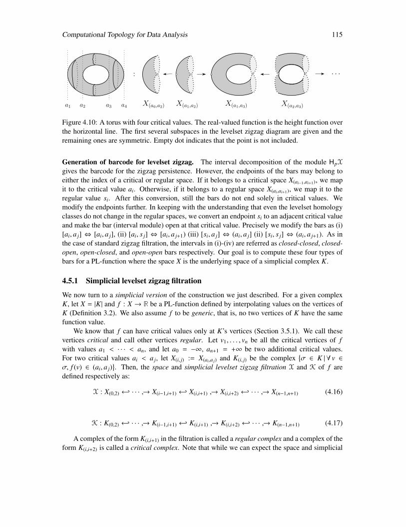
Computational Topology for Data Analysis 115
a2 a3 a4a1 X(a0,a2) X(a1,a2) X(a1,a3) X(a2,a3)
: · · ·
Figure 4.10: A torus with four critical values. The real-valued function is the height function overthe horizontal line. The first several subspaces in the levelset zigzag diagram are given and theremaining ones are symmetric. Empty dot indicates that the point is not included.
Generation of barcode for levelset zigzag. The interval decomposition of the module HpX
gives the barcode for the zigzag persistence. However, the endpoints of the bars may belong toeither the index of a critical or regular space. If it belongs to a critical space X(ai−1,ai+1), we mapit to the critical value ai. Otherwise, if it belongs to a regular space X(ai,ai+1), we map it to theregular value si. After this conversion, still the bars do not end solely in critical values. Wemodify the endpoints further. In keeping with the understanding that even the levelset homologyclasses do not change in the regular spaces, we convert an endpoint si to an adjacent critical valueand make the bar (interval module) open at that critical value. Precisely we modify the bars as (i)[ai, a j] ⇔ [ai, a j], (ii) [ai, s j] ⇔ [ai, a j+1) (iii) [si, a j] ⇔ (ai, a j] (ii) [si, s j] ⇔ (ai, a j+1). As inthe case of standard zigzag filtration, the intervals in (i)-(iv) are referred as closed-closed, closed-open, open-closed, and open-open bars respectively. Our goal is to compute these four types ofbars for a PL-function where the space X is the underlying space of a simplicial complex K.
4.5.1 Simplicial levelset zigzag filtration
We now turn to a simplicial version of the construction we just described. For a given complexK, let X = |K| and f : X → R be a PL-function defined by interpolating values on the vertices ofK (Definition 3.2). We also assume f to be generic, that is, no two vertices of K have the samefunction value.
We know that f can have critical values only at K’s vertices (Section 3.5.1). We call thesevertices critical and call other vertices regular. Let v1, . . . , vn be all the critical vertices of fwith values a1 < · · · < an, and let a0 = −∞, an+1 = +∞ be two additional critical values.For two critical values ai < a j, let X(i, j) := X(ai,a j) and K(i, j) be the complex
σ ∈ K | ∀ v ∈
σ, f (v) ∈ (ai, a j). Then, the space and simplicial levelset zigzag filtration X and K of f are
defined respectively as:
X : X(0,2) ← · · · → X(i−1,i+1) ← X(i,i+1) → X(i,i+2) ← · · · → X(n−1,n+1) (4.16)
K : K(0,2) ← · · · → K(i−1,i+1) ← K(i,i+1) → K(i,i+2) ← · · · → K(n−1,n+1) (4.17)
A complex of the form K(i,i+1) in the filtration is called a regular complex and a complex of theform K(i,i+2) is called a critical complex. Note that while we can expect the space and simplicial
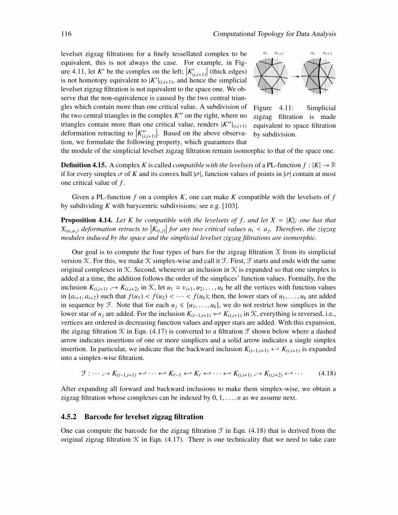
116 Computational Topology for Data Analysis
ai ai+1 ai ai+1
Figure 4.11: Simplicialzigzag filtration is madeequivalent to space filtrationby subdivision.
levelset zigzag filtrations for a finely tessellated complex to beequivalent, this is not always the case. For example, in Fig-ure 4.11, let K′ be the complex on the left;
∣∣∣K′(i,i+1)
∣∣∣ (thick edges)is not homotopy equivalent to |K′|(i,i+1), and hence the simpliciallevelset zigzag filtration is not equivalent to the space one. We ob-serve that the non-equivalence is caused by the two central trian-gles which contain more than one critical value. A subdivision ofthe two central triangles in the complex K′′ on the right, where notriangles contain more than one critical value, renders |K′′|(i,i+1)deformation retracting to
∣∣∣K′′(i,i+1)
∣∣∣. Based on the above observa-tion, we formulate the following property, which guarantees thatthe module of the simplicial levelset zigzag filtration remain isomorphic to that of the space one.
Definition 4.15. A complex K is called compatible with the levelsets of a PL-function f : |K| → Rif for every simplex σ of K and its convex hull |σ|, function values of points in |σ| contain at mostone critical value of f .
Given a PL-function f on a complex K, one can make K compatible with the levelsets of fby subdividing K with barycentric subdivisions; see e.g. [103].
Proposition 4.14. Let K be compatible with the levelsets of f , and let X = |K|; one has thatX(ai,a j) deformation retracts to
∣∣∣K(i, j)∣∣∣ for any two critical values ai < a j. Therefore, the zigzag
modules induced by the space and the simplicial levelset zigzag filtrations are isomorphic.
Our goal is to compute the four types of bars for the zigzag filtration X from its simplicialversion K. For this, we make K simplex-wise and call it F. First, F starts and ends with the sameoriginal complexes in K. Second, whenever an inclusion in K is expanded so that one simplex isadded at a time, the addition follows the order of the simplices’ function values. Formally, for theinclusion K(i,i+1) → K(i,i+2) in K, let u1 = vi+1, u2, . . . , uk be all the vertices with function valuesin [ai+1, ai+2) such that f (u1) < f (u2) < · · · < f (uk); then, the lower stars of u1, . . . , uk are addedin sequence by F. Note that for each u j ∈
u1, . . . , uk
, we do not restrict how simplices in the
lower star of u j are added. For the inclusion K(i−1,i+1) ← K(i,i+1) in K, everything is reversed, i.e.,vertices are ordered in decreasing function values and upper stars are added. With this expansion,the zigzag filtration K in Eqn. (4.17) is converted to a filtration F shown below where a dashedarrow indicates insertions of one or more simplices and a solid arrow indicates a single simplexinsertion. In particular, we indicate that the backward inclusion K(i−1,i+1) c K(i,i+1) is expandedinto a simplex-wise filtration.
F : · · · d K(i−1,i+1) ← · · · ← K`−1 ← K` ← · · · ← K(i,i+1) d K(i,i+2) c · · · (4.18)
After expanding all forward and backward inclusions to make them simplex-wise, we obtain azigzag filtration whose complexes can be indexed by 0, 1, . . . , n as we assume next.
4.5.2 Barcode for levelset zigzag filtration
One can compute the barcode for the zigzag filtration F in Eqn. (4.18) that is derived from theoriginal zigzag filtration K in Eqn. (4.17). There is one technicality that we need to take care
Computational Topology for Data Analysis 117
of. To apply the algorithm in Section 4.3.2, we need the input zigzag filtration to begin with anempty complex. The filtration F as constructed from expanding K has the first complex K(0,2) thatis non-empty. So, as before, we expand K(0,2) simplex-wise and begin F with an empty complex.We assume below this is the case for F.
The bars in the barcode for F do not necessarily coincide with the four types of bars for Kwith endpoints only in critical values. However, we can read the bars for K from the bars of F.
First, assume that F is indexed as
F : ∅ = K0 ↔ K1 ↔ · · · ↔ Kn−1 ↔ Kn.
This means that a complex K j, j > 0, is of the four categories, (i) it is a complex in the expansionof the backward inclusion K(i−1,i+1) c K(i,i+1), (ii) it is a complex in the expansion of the forwardinclusion K(i,i+1) d K(i,i+2), (iii) it is a regular complex K(i,i+1) for some i > 0, (iv) it is a criticalcomplex K(i−1,i+1) for some i > 0. The types of complexes where the endpoints of a bar [b, d] forF are located determine the bars for K and hence X which can be of four types: closed-closed[ai, a j], closed-open [ai, a j), open-closed (ai, a j], and open-open (ai, a j).
Let [b, d] be a bar for F. If both Kb and Kd appear in the expansion of a forward inclusionK(i,i+1) d K(i,i+2), we ignore the bar because it is an artificial bar created due to expanding thefiltration K into the filtration F. Similarly, we ignore the bar if both Kb and Kd appear in theexpansion of a backward inclusion K(i−1,i+1) c K(i,i+1). We explain other cases below.
(Case 1.) Kb is either a regular complex K(i,i+1) or in the expansion of K(i−1,i+1) c K(i,i+1): thecomplex Kb is a subcomplex of the critical complex K(i−1,i+1) which stands for the critical valueai. So, the end b is mapped to ai and made open because the class for the bar [b, d] does not existin K(i−1,i+1).
(Case 2.) Kb is either the critical complex K(i,i+2) or in the expansion of K(i,i+1) d K(i,i+2): thecomplex is a subcomplex of the critical complex K(i,i+2) which stands for the critical value ai+1.So, the end b is mapped to ai+1 and is closed because the class for [b, d] is alive in K(i,i+2)
(Case 3.) Kd is the critical complex K(i−1,i+1) or is in the expansion of the backward inclusionK(i−1,i+1) c K(i,i+1): the complex is a subcomplex of the critical complex K(i−1,i+1) which standsfor the critical value ai. So, the end d is mapped to ai and made closed because the class for thebar [b, d] exists in K(i−1,i+1).
(Case 4.) Kd is either the regular complex K(i,i+1) or in the expansion of K(i,i+1) d K(i,i+2): thecomplex is a subcomplex of the critical complex K(i,i+2) which stands for the critical value ai+1.So, the end d is mapped to ai+1 and is open because the class for [b, d] is not alive in K(i,i+2).
4.5.3 Correspondence to sublevel set persistence
Standard persistence as we have seen already is defined by considering the sublevel sets of f , thatis, X[0,i] = f −1[s0, si] = f −1(−∞, si] where si ∈ (ai, ai+1) is a regular value. We get the followingsublevel set diagram:
X : X[0,0] → X[0,1] → · · · → X[0,n].
118 Computational Topology for Data Analysis
Then, considering f to be a PL-function on X = |K|, we have already seen in Section 3.5 that Xcan be converted to a simplicial filtration K shown below where K[0,i] = σ ∈ K | f (σ) ≤ ai. Thisfiltration can further be converted into a simplex-wise filtration which can be used for computingDgmp(K) for p ≥ 0.
K : K[0,0] → K[0,1] → K[0,2] · · · → K[0,n]
The bars for this case have the form [ai, a j) where a j can be an+1 = ∞. Each such bar is closed atthe left endpoint because the homology class being born exists at K[0,i]. However, it is open at theright endpoint because it does not exist at K[0, j].
One can see that there are two types of bars in the sublevel set persistence, one of the type[ai, a j), j ≤ n, which is bounded on the right, and the other of the type [ai,∞) = [ai, an+1)which is unbounded on the right. The unbounded bars are the infinite bars we introduced inSection 3.2.1. They correspond to the essential homology classes since Hp(K)
⊕i[ai,∞). The
work of [60, 64] imply that both types of barcodes of the standard persistence can be recoveredfrom those of the levelset zigzag persistence as the theorem below states:
Theorem 4.15. Let K and K′ denote the filtrations for the sublevel sets and level sets respectivelyinduced by a continuous function f on a topological space with critical values a0, a1, · · · , an+1where a0 = −∞ and an+1 = ∞. For every p ≥ 0,
1. [ai, a j), j , n + 1 is a bar for Dgmp(K) iff it is so for Dgmp(K′),
2. [ai, an+1) is a bar for Dgmp(K) iff either [ai, a j] is a closed-closed bar for Dgmp(K′) forsome a j > ai, or (a j, ai) is an open-open bar for Dgmp−1(K′) for some a j < ai.
4.5.4 Correspondence to extended persistence
There is another persistence considered in the literature under the name extended persistence [103],and it turns out that there is a correspondence between extended persistence and level set zigzagpersistence. For a real-valued function f : X → R, let X[0,i] denote the sublevel set f −1[s0, si] asbefore and X[i,n] denote the superlevel set f −1[si, sn]. Then, a persistence module that considersthe sublevel set filtration first and then juxtaposes it with a filtration of quotient spaces of X asshown below gives the notion of extended persistence:
X : X[0,0] → · · · → X[0,n] → (X[0,n], X[n,n]) → · · · → (X[0,n], X[0,n]).
Observe that each inclusion map between two quotient spaces induces a linear map in their relativehomology groups. One can read that the above sequence arises by first growing the space to thefull space X[0,n] with sublevel sets and then shrinking it by quotienting with the superlevel sets.Again, taking f : X → R as a PL-function on X = |K|, we get the simplicial extended filtrationwhere K[0,i] = σ ∈ K | ∀v ∈ σ, f (v) ≤ ai and K[i,n] = σ ∈ K | ∀v ∈ σ, f (v) ≥ ai.
E : K[0,0] → · · · → K[0,n] → (K[0,n],K[n,n]) → · · · → (K[0,n],K[0,n]).
The decomposition of the persistence module HpE arising out of E provides the bars in Dgmp(E).For the first part of the sequence, the endpoints of the bars are designated with respective function
Computational Topology for Data Analysis 119
values ai as before. For the second part, the birth or death point of a bar is designated as an+i if itsclass either is born in (K[0,n],K[i,n]) or dies entering into (K[0,n],K[i,n]) respectively for 0 ≤ i ≤ n.We leave the proof of the following theorem as an exercise; see also [64].
Theorem 4.16. Let K and E denote the simplicial levelset zigzag filtration and the extendedfiltration of a PL-function f : |K| → R. Then, for every p ≥ 0,
1. [ai, a j) is a bar for Dgmp(K) iff it is a bar for Dgmp(E),
2. (ai, a j] is a bar for Dgmp(K) iff [an+ j, an+i) is a bar for Dgmp+1(E),
3. [ai, a j] is a bar for Dgmp(K) iff [ai, an+ j) is a bar for Dgmp(E),
4. (ai, a j) is a bar for Dgmp(K) iff [a j, an+i) is a bar for Dgmp+1(E).
Clearly, for two persistence modules HpE and HpE′ arising out of two extended filtrations E
and E′, the stability of persistence diagrams holds, that is, db(DgmpE,DgmpE′) = dI(HpE,HpE
′)(Theorem 3.11).
4.6 Notes and Exercises
Computation of persistent homology induced by simplicial towers generalizing filtrations wereconsidered in the context of TDA by Dey, Fan, Wang [122]. They gave two approaches to computepersistence diagrams for such towers, one by converting a tower to a zigzag filtration whichwe described in Section 4.4 and the other by considering annotations in combination with thelink conditions allowing edge collapses without altering homotopy types which is described inSection 4.2.1. The first approach apparently increases the size of the filtration which motivatedthe second approach. Kerber and Schreiber showed that indeed the first approach can be leveragedto produce filtrations instead of zigzag filtrations and without blowing up sizes [210].
The concept of zigzag modules obtained from a zigzag filtration by taking the homologygroups and linear maps induced by inclusions is closely related to quiver theory due to Gabriel [163]which was brought to the attention of TDA community by Carlsson and de Silva [63]. They werethe first to propose the concept of zigzag persistence and its computation [63]. They observedthat any zigzag module can be decomposed into a set of other zigzag modules where the forwardnon-zero maps are only injective and the backward non-zero maps are only surjective. Althoughthey did not compute this decomposition, they used its existence to design an algorithm for com-puting the interval decomposition of a given zigzag module. Later, with Morozov, they used theseconcepts to present an O(n3) algorithm for computing the persistence of a simplex-wise zigzagfiltration with n arrows [64]. Milosavljevic et al. [234] improved the algorithm for any zigzagfiltration with n arrows to have a time complexity of O(nω+n2 log2 n), where ω ∈ [2, 2.373) is theexponent for matrix multiplication. Maria and Oudot [228] presented a different algorithm wherethey showed how a filtration of the last complex in the prefix of a zigzag filtration can help com-puting the persistence incrementally. The algorithm in this chapter draws upon these approachesthough is presented quite differently. Indeed, adaptation of the presented approach on graphs ledto recent near-linear time algorithms for zigzag persistence on graphs [127].

120 Computational Topology for Data Analysis
Given a real valued function f : X → R on a topological space X, the level sets at the criticaland intermediate values give rise to a levelset zigzag filtration as shown in Section 4.5. Carlsson,de Silva, and Morozov [64] introduced this set up and observed the decomposition of the zigzagmodule into interval modules with open or closed ends. The four types of bars arising out ofthis zigzag module give more information than the standard sublevel set persistence which onlyoutputs closed-open and infinite bars. It was observed in [60] that the open-open and closed-closed bars indeed capture the infinite bars of the sublevel set persistence with an appropriatedimension shift. Theorem 4.15 summarizes this connection. The extended persistence originallyproposed for surfaces [5] and later extended for filtrations [103] also computes all four types ofbars, but they are described differently using the persistence diagrams rather than open and closedends.
Exercises
1. Show that the inequality in Proposition 4.1 cannot be improved to equality by giving acounterexample.
2. Prove Proposition 4.5.
3. Prove Proposition 4.6.
4. Prove Proposition 4.7.
5. Prove Proposition 4.8.
6. For computing the persistence of a simplicial tower, we checked the link condition in alldimensions. Argue that it is sufficient to check the condition only for three relevant dimen-sions.
7. Let K be a triangulated 2-manifold of genus g without boundary. Consider the followingtasks:
• Compute the genus g by the formula 2 − 2g = #vertices − #edges + #triangles.
• Compute a spanning tree T of the 1-skeleton of K, and a spanning tree T ∗ of the dualgraph none of whose edges are dual to any edge in T .
• Annotate the edges in T with zero vector of length g, index the edges not in T andwhose duals are not in T ∗ as e1, . . . , e2g. Annotate ei with a vector that has the ithentry 1 and all other entries 0.
• Propagate systematically the annotation to the rest of the edges.
Complete the above approach with a proof of correctness into an algorithm that computesthe annotation for edges in O(gn) time if K has n simplices.
8. Do we get the same barcode if we run the zigzag persistence algorithm given in Sec-tion 4.3.1 and the standard persistence algorithm on a non-zigzag filtration? If so, prove it.If not, show the difference and suggest a modification to the zigzag persistence algorithmso that the both output become the same.

Computational Topology for Data Analysis 121
9. Suppose that a persistence module Vifi→ Vi+1 is presented with the linear maps fi as
matrices whose columns and rows are fixed bases of Vi and Vi+1 respectively. Design analgorithm to compute the barcode for the input module. Do the same when the input moduleis a zigzag tower.
10. ([127]) We have seen that for graphs a near-linear time algorithm exists for computing non-zigzag persistence. Design a near-linear time algorithm for computing zigzag persistencefor graphs.
11. Consider a PL-function f : |K| → R.
(a) Design an algorithm to compute the barcode of − f from a level set zigzag filtrationof f .
(b) Show that f and − f produce the same closed-closed and open-open bars for the lev-elset zigzag filtration.
(c) In general, given a zigzag filtration F, consider the filtration F′ = −F in oppositedirection from right to left. What is the relation between the barcodes of these twofiltrations?
12. We computed persistence of zigzag towers by first converting it into a zigzag filtration andthen using the algorithm in section 4.3 to compute the bars. Design an algorithm that skipsthe intermediate conversion to a filtration.
13. Design an algorithm for computing the extended persistence from a given PL-function onan input simplicial complex.
14. ([64]) Prove Theorem 4.16.

122 Computational Topology for Data Analysis

Chapter 5
Generators and Optimality
So far we have focused mainly on the rank of the homology groups. However, the homologygenerators, that is, the cycles whose classes constitute the elements of the homology groups carryinformation about the space. Computing just some generating cycles (cycle basis) typically can
Figure 5.1: Double torus has 1-st homology group of rank four meaning that classes of fourrepresentative cycles generate H1; (left) A non-optimal cycle basis, (right) optimal cycle basis.
be done by the standard algorithms for computing homology groups such as the persistence al-gorithms. In practice, however, we may sometimes be interested in generating cycles that havesome optimal property; see Figure 5.1.
In particular, if the space has a metric associated with it, one may associate a measure withthe cycles that can differentiate them in terms of their ‘size’. For example, if K is a simplicialcomplex embedded in Rd, the measure of a 1-cycle can be its length. Then, we can ask to computea set of 1-cycles whose classes generate H1(K) and has minimum total length among all such setsof cycles. Typically, the locality of these cycles capture interesting geometric features of thespace |K|. Some applications may benefit from computing such cycles respecting geometry. Forexample, in computer graphics often a surface is cut along a set of cycles to make it flat forparameterization. The classes of these cycles constitute a basis of the 1-st homology group. Ingeneral, shortest (optimal) cycle basis is desired because they produce good parameterzation forgraphic rendering. Figure 5.2 shows examples of such cycles for three kinds of input wherea shortest (optimal) cycle basis has been computed with an algorithm that we describe in thischapter. The algorithm works for simplicial complexes though we can apply it on point clouddata as well after computing an appropriate complex such as Cech or Rips complex on top of theinput points.
123
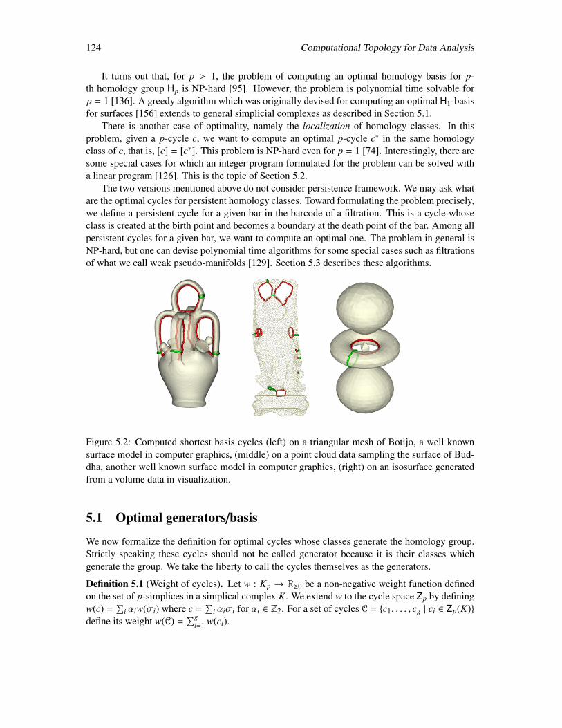
124 Computational Topology for Data Analysis
It turns out that, for p > 1, the problem of computing an optimal homology basis for p-th homology group Hp is NP-hard [95]. However, the problem is polynomial time solvable forp = 1 [136]. A greedy algorithm which was originally devised for computing an optimal H1-basisfor surfaces [156] extends to general simplicial complexes as described in Section 5.1.
There is another case of optimality, namely the localization of homology classes. In thisproblem, given a p-cycle c, we want to compute an optimal p-cycle c∗ in the same homologyclass of c, that is, [c] = [c∗]. This problem is NP-hard even for p = 1 [74]. Interestingly, there aresome special cases for which an integer program formulated for the problem can be solved witha linear program [126]. This is the topic of Section 5.2.
The two versions mentioned above do not consider persistence framework. We may ask whatare the optimal cycles for persistent homology classes. Toward formulating the problem precisely,we define a persistent cycle for a given bar in the barcode of a filtration. This is a cycle whoseclass is created at the birth point and becomes a boundary at the death point of the bar. Among allpersistent cycles for a given bar, we want to compute an optimal one. The problem in general isNP-hard, but one can devise polynomial time algorithms for some special cases such as filtrationsof what we call weak pseudo-manifolds [129]. Section 5.3 describes these algorithms.
Figure 5.2: Computed shortest basis cycles (left) on a triangular mesh of Botijo, a well knownsurface model in computer graphics, (middle) on a point cloud data sampling the surface of Bud-dha, another well known surface model in computer graphics, (right) on an isosurface generatedfrom a volume data in visualization.
5.1 Optimal generators/basis
We now formalize the definition for optimal cycles whose classes generate the homology group.Strictly speaking these cycles should not be called generator because it is their classes whichgenerate the group. We take the liberty to call the cycles themselves as the generators.
Definition 5.1 (Weight of cycles). Let w : Kp → R≥0 be a non-negative weight function definedon the set of p-simplices in a simplical complex K. We extend w to the cycle space Zp by definingw(c) =
∑i αiw(σi) where c =
∑i αiσi for αi ∈ Z2. For a set of cycles C = c1, . . . , cg | ci ∈ Zp(K)
define its weight w(C) =∑g
i=1 w(ci).
Computational Topology for Data Analysis 125
Definition 5.2 (Optimal generator). A set of cycles C = c1, c2, . . . , cg | ci ∈ Zp(K) is an Hp(K)-generator if the classes [ci] | i = 1, . . . , g generate Hp(K). An Hp(K)-generator is optimal ifthere is no other generator C′ with w(C′) < w(C).
Observe that, an optimal generator may not have minimal number of cycles whose classesgenerate the homology group because we allow zero weights and hence an optimal generator maycontain extra cycles with zero weights. This prompts us to define the following.
Definition 5.3 (Optimal basis). An Hp(K)-generator C = c1, c2, . . . , cg | ci ∈ Zp(K) is an Hp(K)-cycle basis or Hp(K)-basis in short if g = dim Hp(K). The classes of cycles in such a cycle basisconstitute a basis for Hp(K). An optimal Hp(K)-generator that is also an Hp(K)-basis is called anoptimal Hp(K)-basis.
We observe that optimal Hp(K)-generators with positively weighted cycles are necessarilycycle bases. Notice that to generate Hp(K), the number of cycles in any Hp(K)-generator has tobe at least βp(K) = dim Hp(K). On the other hand, an optimal Hp(K)-generator with positivelyweighted cycles cannot have more than βp cycles because such a generator must contain a cyclewhose class is a linear combination of the classes of other cycles in the generator. Thus, omissionof this cycle still generates Hp(K) while decreasing the weight of the generator. For 1-dimension,similar reasoning can also be applied to conclude that each cycle in an H1(K)-cycle basis nec-essarily contains a simple cycle which together form a cycle basis (Exercise 1). A 1-cycle issimple if it has a single connected component (viewed as a graph) and every vertex has exactlytwo incident edges.
Fact 5.1.
(i) An optimal Hp(K)-generator with positively weighted cycles is an optimal Hp(K)-basis.
(ii) Every cycle ci in an H1(K)-basis has a simple cycle c′i ⊆ ci so that c′ii form an H1(K)-basis.
We now focus on computing an optimal Hp(K)-basis also known as the optimal homologybasis problem or OHBP in short. One may observe that Definition 5.3 formulates OHBP as aweighted `1-optimization of representatives of bases. This allows for different types of optimalityto be achieved by choosing different weights. For example, assume that the simplicial complex Kof dimension p or greater is embedded in Rd, where d ≥ p + 1. Let the Euclidean p-dimensionalvolume of p-simplices be their weights. This specializes OHBP to the Euclidean `1-optimizationproblem. The resulting optimal Hp(K)-basis has the smallest p-dimensional volume amongst allsuch bases. If the weights are taken to be unit, the resulting optimal solution has the smallestnumber of p-simplices amongst all Hp(K)-bases.
5.1.1 Greedy algorithm for optimal Hp(K)-basis
Consider the following greedy algorithm in which we first sort the input cycles in non-decreasingorder of their weights, and then choose a cycle following this order if its class is independent ofthe classes of the cycles chosen before.
The greedy algorithm Algorithm 7:GreedyBasis is motivated by Proposition 5.1. The specificimplementation of line 4 (on independence test) will be given in Section 5.1.2.
126 Computational Topology for Data Analysis
Algorithm 7 GreedyBasis(C)
Input:A set of p-cycles C in a complex
Output:A maximal set of cycles from C whose classes are independent and total weight is minimum
1: Sort the cycles from C in non-decreasing order of their weights; that is, C = c1, . . . , cn
implies w(ci) ≤ w(c j) for i ≤ j2: Let B := c1
3: for i = 2 to n do4: if [ci] is independent w.r.t. B then5: B := B ∪ ci
6: end if7: end for8: if [c1] is trivial (boundary), output B \ c1 else output B
Proposition 5.1. Suppose that C, the input to the algorithm GreedyBasis, contains an optimalHp(K)-basis. Then, the output of GreedyBasis is an optimal Hp(K)-basis.
Proof. Let C contain an optimal Hp(K)-basis C∗ = c∗1, . . . , c∗g sorted according to their ap-
pearance in the ordered sequence of C = c1, . . . , cn. Let C′ = c′1, . . . , c′g′ be the output of
GreedyBasis again sorted according to the appearance of the cycles in C. By Definition 5.3, g,the cardinality of C∗, is the dimension of Hp(K) and hence g′ ≤ g because g + 1 or more classescannot be independent in Hp(K).
Among all optimal Hp(K)-basis that C contains, take C∗ to be lexicographically smallest, thatis, there is no other sorted C∗ = c∗1, . . . , c
∗g so that there exists a j ≥ 1 where c∗1 = c∗1, . . . , c
∗j−1 =
c∗j−1 and c∗j = ck and c∗j = c` with k < `.First, we show that C′ is a prefix of C∗. If not, there is a least index j ≥ 1 so that c∗j , c′j.
Since the classes of the cycles in C∗ form a basis for Hp(K), and C′ cannot contain any trivial cycle(ensured by step 8), the class [c′j] can be written as a linear combination of the classes of the cyclesin C∗. Consider the class [c∗k] in this linear combination with the largest index k. It is not possiblethat c∗k appears before c′j in the order. This is because then [c′j] will be a linear combination of theclasses of the cycles appearing before c′j in C′ which is impossible by the construction of C′. So,assume that c∗k appears after c′j. Then, consider the sorted sequence of cycles C∗ constructed byreplacing c∗k in C∗ with c′j. First, notice that C∗ is lexicographically smaller than C∗ and it is alsoan Hp(K)-basis contradicting the fact that C∗ is the lexicographically smallest optimal cycle basis.The fact that C∗ is an Hp(K)-cycle basis follows from the observation that [c′j] is independentof the classes of the cycles in C∗ \ c∗k because [c′j] is a linear combination of the classes thatnecessarily include [c∗k].
Now, to complete the proof, we note that g′ = g. If not, then g′ < g and C′ is a prefix of C∗.But, then one can add c∗g′+1 from C∗ to C′ where [c∗g′+1] is independent of all classes of the cyclesalready in C′. This suggests that the algorithm GreedyBasis cannot stop without enlarging C′.
The above proposition suggests that GreedyBasis can compute an optimal cycle basis if its
Computational Topology for Data Analysis 127
input set C contains one. We show next that such an input (i.e, a set of 1-cycles containing anoptimal H1(K)-basis) can be computed for H1(K) in O(n2 log n) time where the 2-skeleton of Khas n simplices.
Specifically, given a simplicial complex K, notice that H1(K) is completely determined bythe 2-skeleton of K and hence without loss of generality we can assume K to be a 2-complex.Algorithm 8:Generator computes a set C of 1-cycles from such a complex which includes anoptimal basis.
Algorithm 8 Generator(K)
Input:A 2-complex K
Output:A set of 1-cycles containing an optimal H1(K)-basis
1: Let K1 be the 1-skeleton of K with vertex set V and edge set E2: C := ∅3: for all v ∈ V do4: compute a shortest path tree Tv rooted at v in K1 = (V, E)5: for all e = (u,w) ∈ E \ Tv s.t. u,w ∈ Tv do6: Compute cycle ce = πu,w ∪ e where πu,w is the unique path connecting u and w in Tv
7: C := C ∪ ce
8: end for9: end for
10: Output C
Proposition 5.2. Generator(K) computes an H1(K)-generator C with their weights in O(n2 log n)time for a 2-complex K with n vertices and edges. Furthermore, the set C contains an optimal basiswhere |C| = O(n2).
Proof. We prove that any cycle c in an optimal H1-basis C∗ that is not computed by Generator canbe replaced by a cycle computed by Generator while keeping C∗ optimal. This proves the claimthat the output of Generator contains an optimal basis (and thus C is necessarily a H1-generator).
First, assume that C∗ consists of simple cycles because otherwise we can choose such cyclesfrom the cycles of C∗ due to Fact 5.1(ii). So, assume that c ∈ C∗ is simple. Let v be any vertex inc. There exists at least one edge e in c which is not in the shortest path tree Tv. Let e = u,w.Consider the shortest paths πv,u and πv,w in Tv from the root v to the vertices u and w respectively.Notice that even though K1 may be disconnected, vertices u,w are necessarily in Tv. Also, let π′v,uand π′v,w be the paths from v to u and w respectively in the cycle c. If πv,u = π′v,u and πv,w = π′v,wwe have c = ce computed by Generator. So, assume that at least one path does not satisfy thiscondition, say πv,u , π
′v,u. See Figure 5.3.
Consider the two cycles c1 and c2 where c1 consists of the paths π′v,w, πv,u and e; c2 consistsof the paths πv,u and π′v,u. Observe that c = c1 + c2. Also, w(c1) ≤ w(c) and w(c2) ≤ w(c). If both[c1] and [c2] are dependent on the classes of the cycles in C∗ \ c, we will have [c] dependent onthem as well. This contradicts that C∗ is an H1(K)-basis.
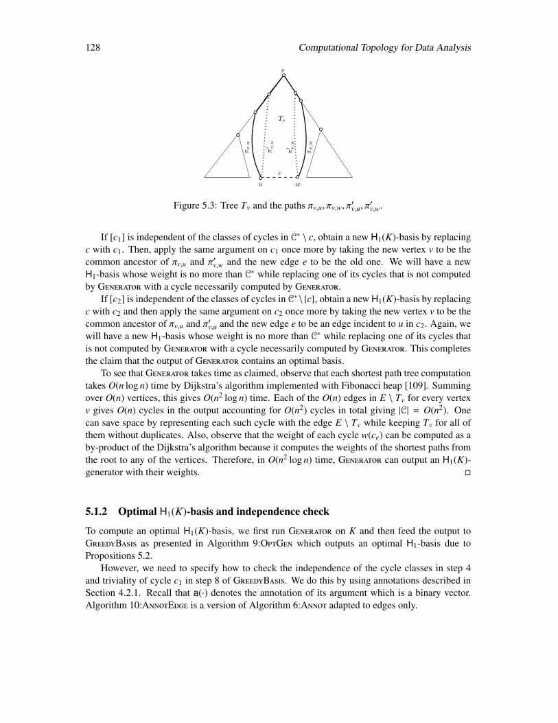
128 Computational Topology for Data Analysis
Tv
v
u w
e
π′ v,u
πv,u
πv,w
π′ v,w
Figure 5.3: Tree Tv and the paths πv,u, πv,w, π′v,u, π
′v,w.
If [c1] is independent of the classes of cycles in C∗ \ c, obtain a new H1(K)-basis by replacingc with c1. Then, apply the same argument on c1 once more by taking the new vertex v to be thecommon ancestor of πv,u and π′v,w and the new edge e to be the old one. We will have a newH1-basis whose weight is no more than C∗ while replacing one of its cycles that is not computedby Generator with a cycle necessarily computed by Generator.
If [c2] is independent of the classes of cycles in C∗\c, obtain a new H1(K)-basis by replacingc with c2 and then apply the same argument on c2 once more by taking the new vertex v to be thecommon ancestor of πv,u and π′v,u and the new edge e to be an edge incident to u in c2. Again, wewill have a new H1-basis whose weight is no more than C∗ while replacing one of its cycles thatis not computed by Generator with a cycle necessarily computed by Generator. This completesthe claim that the output of Generator contains an optimal basis.
To see that Generator takes time as claimed, observe that each shortest path tree computationtakes O(n log n) time by Dijkstra’s algorithm implemented with Fibonacci heap [109]. Summingover O(n) vertices, this gives O(n2 log n) time. Each of the O(n) edges in E \ Tv for every vertexv gives O(n) cycles in the output accounting for O(n2) cycles in total giving |C| = O(n2). Onecan save space by representing each such cycle with the edge E \ Tv while keeping Tv for all ofthem without duplicates. Also, observe that the weight of each cycle w(ce) can be computed as aby-product of the Dijkstra’s algorithm because it computes the weights of the shortest paths fromthe root to any of the vertices. Therefore, in O(n2 log n) time, Generator can output an H1(K)-generator with their weights.
5.1.2 Optimal H1(K)-basis and independence check
To compute an optimal H1(K)-basis, we first run Generator on K and then feed the output toGreedyBasis as presented in Algorithm 9:OptGen which outputs an optimal H1-basis due toPropositions 5.2.
However, we need to specify how to check the independence of the cycle classes in step 4and triviality of cycle c1 in step 8 of GreedyBasis. We do this by using annotations described inSection 4.2.1. Recall that a(·) denotes the annotation of its argument which is a binary vector.Algorithm 10:AnnotEdge is a version of Algorithm 6:Annot adapted to edges only.

Computational Topology for Data Analysis 129
Algorithm 9 OptGen(K)
Input:A 2-complex K
Output:An optimal H1(K)-basis
1: C:= Generator(K)2: Output C∗:=GreedyBasis(C)
Algorithm 10 AnnotEdge(K)
Input:A simplicial 2-complex K
Output:Annotations for edges in K
1: Let K1 be the 1-skeleton of K with edge set E2: Compute a spanning forest T of K1; m = |E| − |T |3: For every edge e ∈ E ∩ T , assign an m-vector a(e) where a(e) = 04: Index remaining edges in E \ T as e1, . . . , em
5: For every edge ei, assign a(ei)[ j] = 1 iff j = i6: for all triangle t ∈ K do7: if a(∂t) , 0 then8: pick any non-zero entry bu in a(∂t)9: add a(∂t) to every edge e s.t. a(e)[u] = 1
10: delete u-th entry from annotation of every edge11: end if12: end for
Assume that each cycle ce ∈ C output by Generator is represented by e and implicitly bythe path πu,w in Tv. Assume that an annotation of edges has already been computed. This can bedone by the algorithm AnnotEdge. A straightforward analysis shows that AnnotEdge takes O(n3)time where n is the total number of vertices, edges, and triangles in K. However, for achievingbetter time complexity, we can use the earliest basis algorithm described in [61] which runs intime O(nω).
Once the annotations for edges are computed, we need to compute the annotations for the setC of cycles computed by Generator to check independence among them in GreedyBasis. Wefirst describe how do we compute the annotations for a cycle in C. We compute an auxiliaryannotation of the vertices in Tv from the annotations of its edges to facilitate computing a(ce) forcycles ce ∈ C. We traverse the tree Tv top-down and compute the auxiliary annotation a(x) of avertex x in Tv as a(x) = a(y) + a(exy) where y is the parent of x and exy is the edge connectingx and y. The process is initiated by assigning a(v) for the root v to be the zero vector. It shouldbe immediately clear that all auxiliary annotations of the vertices can be computed in O(gn) timewhere g, the length of the annotation vectors, equals β1(K). The annotation of each cycle ce ∈ C
is computed as a(ce) = a(u) + a(w) + a(e) where e = (u,w). Again, this takes O(g) time per edge
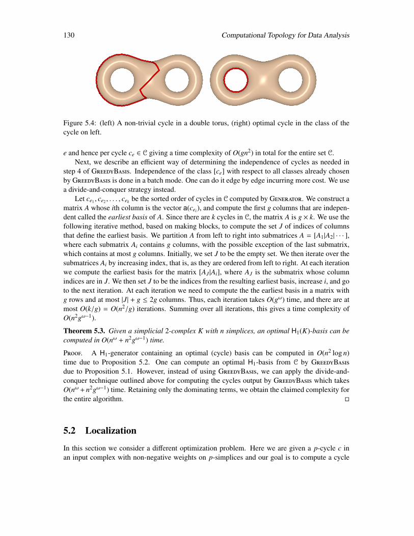
130 Computational Topology for Data Analysis
Figure 5.4: (left) A non-trivial cycle in a double torus, (right) optimal cycle in the class of thecycle on left.
e and hence per cycle ce ∈ C giving a time complexity of O(gn2) in total for the entire set C.Next, we describe an efficient way of determining the independence of cycles as needed in
step 4 of GreedyBasis. Independence of the class [ce] with respect to all classes already chosenby GreedyBasis is done in a batch mode. One can do it edge by edge incurring more cost. We usea divide-and-conquer strategy instead.
Let ce1 , ce2 , . . . , cek be the sorted order of cycles in C computed by Generator. We construct amatrix A whose ith column is the vector a(cei), and compute the first g columns that are indepen-dent called the earliest basis of A. Since there are k cycles in C, the matrix A is g × k. We use thefollowing iterative method, based on making blocks, to compute the set J of indices of columnsthat define the earliest basis. We partition A from left to right into submatrices A = [A1|A2| · · · ],where each submatrix Ai contains g columns, with the possible exception of the last submatrix,which contains at most g columns. Initially, we set J to be the empty set. We then iterate over thesubmatrices Ai by increasing index, that is, as they are ordered from left to right. At each iterationwe compute the earliest basis for the matrix [AJ |Ai], where AJ is the submatrix whose columnindices are in J. We then set J to be the indices from the resulting earliest basis, increase i, and goto the next iteration. At each iteration we need to compute the the earliest basis in a matrix withg rows and at most |J| + g ≤ 2g columns. Thus, each iteration takes O(gω) time, and there are atmost O(k/g) = O(n2/g) iterations. Summing over all iterations, this gives a time complexity ofO(n2gω−1).
Theorem 5.3. Given a simplicial 2-complex K with n simplices, an optimal H1(K)-basis can becomputed in O(nω + n2gω−1) time.
Proof. A H1-generator containing an optimal (cycle) basis can be computed in O(n2 log n)time due to Proposition 5.2. One can compute an optimal H1-basis from C by GreedyBasisdue to Proposition 5.1. However, instead of using GreedyBasis, we can apply the divide-and-conquer technique outlined above for computing the cycles output by GreedyBasis which takesO(nω + n2gω−1) time. Retaining only the dominating terms, we obtain the claimed complexity forthe entire algorithm.
5.2 Localization
In this section we consider a different optimization problem. Here we are given a p-cycle c inan input complex with non-negative weights on p-simplices and our goal is to compute a cycle
Computational Topology for Data Analysis 131
c∗ that is of optimal (minimal) weight in the homology class [c], see Figure 5.4. We extend thislocalization problem from cycles to chains. For this, first we extend the concept of homologouscycles in Section 2.5 to chains straightforwardly. Two p-chains c, c′ ∈ Cp are called homologousif and only if they differ by a boundary, that is, c ∈ c′ + Bp. We ask for computing a chain ofminimal weight which is homologous to a given chain.
Definition 5.4. Let w : K(p) → R≥0 be a non-negative weight function defined on the set ofp-simplices in a simplicial complex K. We extend w to the chain group Cp by defining w(c) =∑
i ciw(σi) where c =∑
i ciσi.
Definition 5.5 (OHCP). Given a non-negative weight function w : K(p) → R≥0 defined on theset of p-simplices in a simplicial complex K and a p-chain c in Cp(K), the optimal homologouschain problem (OHCP) is to find a chain c∗ which has the minimal weight w(c∗) among all chainshomologous to c.
If we use Z2 as the coefficient ring for defining homology classes, the OHCP becomes NP-hard. We are going to show that it becomes polynomial time solvable if (i) the coefficient ring ischosen to be integers Z and (ii) the complex K is such that Hp(K) does not have a torsion whichmay be introduced because of using Z as the coefficient ring.
We will formulate OHCP as an integer program which requires the chains to be representedas an integer vector. Given a p-chain x =
∑m−1i=0 xi σi with integer coefficients xi, we use x ∈ Zm
to denote the vector formed by the coefficients xi. Thus, x is the representation of the chain x inthe elementary p-chain basis, and we will use x and x interchangeably.
Recall that for a vector x ∈ Rm, the 1-norm (or `1-norm) ‖x‖1 is∑
i |xi|. Let W be any realm × m diagonal matrix with diagonal entries wi. Then, the 1-norm of W x, that is, ‖W x‖1 is∑
i |wi||xi|. (If W is a general m ×m nonsingular matrix then ‖W x‖1 is called the weighted 1-normof x.) We now state in words our approach to the optimal homologous chains and later formalizeit in Eqn. (5.1). The main idea is to cast OHCP as an integer program. Unfortunately, integerprograms are in general NP-hard and thus cannot be solved in polynomial time unless P=NP. Wesolve it by a linear program and identify a class of integer programs called totally unimodularfor which linear programs give exact solution. Then, we interpret total unimodularity in terms oftopology. Our approach to solve OHCP can be succinctly stated by the following steps:
• write OHCP as an integer program involving 1-norm minimization, subject to linear con-straints;
• convert the integer program into an integer linear program by converting the 1-norm costfunction to a linear one using the standard technique of introducing some extra variablesand constraints;
• find the conditions under which the constraint matrix of the integer linear program is totallyunimodular; and
• for this class of problems, relax the integer linear program to a linear program by droppingthe constraint that the variables be integral. The resulting optimal chain obtained by solvingthe linear program will be an integer valued chain homologous to the given chain.
132 Computational Topology for Data Analysis
5.2.1 Linear program
Now we formally pose OHCP as an optimization problem. After showing existence of solutionswe reformulate the optimization problem as an integer linear program and eventually as a linearprogram.
Assume that the number of p- and (p + 1)-simplices in K is m and n respectively, and let Wbe a diagonal m×m matrix. Using the notation from Section 3.3.1, let Dp represent the boundarymatrix for the boundary operator ∂p : Cp → Cp−1 in the elementary chain bases. With thesenotations, given a p-chain c represented with an integral vector, the optimal homologous chainproblem in dimension p is to solve:
minx, y‖W x‖1 such that x = c + Dp+1 y, and x ∈ Zm, y ∈ Zn . (5.1)
We assume that W is a diagonal matrix obtained from non-negative weights on simplices. Letw be a non-negative real-valued weight function on the oriented p-simplices of K and let W bethe corresponding diagonal matrix (the i-th diagonal entry of W is w(σi) = wi).
The resulting objective function ‖W x‖1 =∑
i wi |xi| in (5.1) is not linear in xi because it usesthe absolute value of xi. However, it is piecewise-linear in these variables. As a result, Eqn. (5.1)can be reformulated as an integer linear program by splitting every variable xi into two parts x+
iand x−i [28, page 18]:
min∑
i
wi (x+i + x−i )
subject to x+ − x− = c + Dp+1 y (5.2)
x+, x− ≥ 0x+, x− ∈ Zm, y ∈ Zn .
Comparing the above formulation to the standard form integer linear program in Eqn. (5.4), wenotice that the vector x in Eqn. (5.4) corresponds to [x+, x−, y]T in Eqn. (5.2) above. Thus, theminimization is over x+, x− and y, and the coefficients of x+
i and x−i in the objective function arewi, but the coefficients corresponding to y j are zero. The linear programming relaxation of thisformulation just removes the constraints about the variables being integral. The resulting linearprogram is:
min∑
i
wi (x+i + x−i )
subject to x+ − x− = c + Dp+1 yx+, x− ≥ 0 .
To cast the program in standard form [28], we can eliminate the free (unrestricted in sign)variables y by replacing these by y+ − y− and imposing the non-negativity constraints on thenew variables. The resulting linear program has the same objective function, and the equality
Computational Topology for Data Analysis 133
constraints:
min∑
i
wi (x+i + x−i )
subject to x+ − x− = c + Dp+1 (y+ − y−)
x+, x−, y+, y− ≥ 0 .
We can write the above program as
min fT z subject to Az = c, z ≥ 0 (5.3)
where f = [w, 0]T , z = [x+, x−, y+, y−]T , and the equality constraint matrix is A =[I −I −B B
],
where B = Dp+1. This is exactly in the form we want the linear program to be in view ofEqn. (5.4). We now prove a result about the total unimodularity of this matrix that allows us tosolve the optimization by a linear program.
5.2.2 Total unimodularity
A matrix is called totally unimodular if the determinant of each square submatrix is 0, 1, or −1.The significance of total unimodularity in our setting is due to the following Theorem 5.4 whichfollows immediately from known results in optimization [201].
Consider an integral vector b ∈ Zm and a real vector f ∈ Rn. Consider the integer linearprogram
min fT x subject to Ax = b, x ≥ 0 and x ∈ Zn . (5.4)
Theorem 5.4. Let A be a m × n totally unimodular matrix. Then the integer linear program (5.4)can be solved in time polynomial in the dimensions of A.
Proposition 5.5. If B = Dp+1 is totally unimodular then so is the matrix[I −I −B B
].
Proof. The proof uses operations that preserve the total unimodularity of a matrix. These arelisted in [272, page 280]. If B is totally unimodular then so is the matrix
[−B B
]since scalar
multiples of columns of B are being appended on the left to get this matrix. The full matrix inquestion can be obtained from this one by appending columns with a single ±1 on the left, whichproves the result.
As a result of Theorem 5.4 and Proposition 5.5, we have the following algorithmic result.
Theorem 5.6. If the boundary matrix Dp+1 of a finite simplicial complex of dimension greaterthan p is totally unimodular, the optimal homologous chain problem (5.1) for p-chains can besolved in polynomial time.
Proof. We have seen above that a reformulation of OHCP without the integrality constraintsleads to the linear program (5.3). By Proposition 5.5, the equality constraint matrix of this linearprogram is totally unimodular. Then, by Theorem 5.4, the linear program (5.3) can be solved inpolynomial time, while achieving an integral solution.
134 Computational Topology for Data Analysis
Manifolds. Our results in the next section (Section 5.2.3) are valid for any finite simplicialcomplex. But first we consider a simpler case – simplicial complexes that are triangulations ofmanifolds. We show that for finite triangulations of compact p-dimensional orientable manifolds,the top non-trivial boundary matrix Dp is totally unimodular irrespective of the orientations of itssimplices. There are examples of non-orientable manifolds where total unimodularity does nothold (Exercise 7). Further examination of why total unimodularity does not hold in these casesleads to the results in Theorem 5.9.
Let K be a finite simplicial complex that triangulates a (p+1)-dimensional compact orientablemanifold M.
Theorem 5.7. For a finite simplicial complex triangulating a (p + 1)-dimensional compact ori-entable manifold, Dp+1 is totally unimodular irrespective of the orientations of the simplices.
As a result of the above theorem and Theorem 5.6 we have the following result.
Corollary 5.8. For a finite simplicial complex triangulating a (p + 1)-dimensional compact ori-entable manifold, the optimal homologous chain problem can be solved for p-dimensional chainsin polynomial time.
5.2.3 Relative torsion
Now we consider the more general case of simplicial complexes. We characterize the total uni-modularity of boundary matrices for arbitrary simplicial complexes. This characterization leadsto a torsion-related condition for the complexes; see [241] for the definition of torsion. Since wedo not use any conditions about the geometric realization or embedding in Rp for the complex,the result is also valid for abstract simplicial complexes. As a corollary of the characterizationwe show that the OHCP can be solved in polynomial time as long as the input complex satisfies atorsion-related condition.
TU and relative torsion
Definition 5.6 (Pure simplicial complex). A pure simplicial complex of dimension p is a simpli-cial complex formed by a collection of p-simplices and their faces. Similarly, a pure subcomplexis a subcomplex that is a pure simplicial complex.
An example of a pure simplicial complex of dimension p is one that triangulates a p-dimensionalmanifold. Another example, relevant to our discussion, is a subcomplex formed by a collectionof some p-simplices of a simplicial complex and their faces.
Let K be a finite simplicial complex of dimension greater than p. Let L ⊆ K be a puresubcomplex of dimension p + 1 and L0 ⊂ L be a pure subcomplex of dimension p. Recallthe definition of relative boundary operator in Section 2.5.2 used for defining relative homology.Then, the matrix DL,L0
p+1 representing the relative boundary operator
∂L,L0p+1 : Cp+1(L, L0)→ Cp(L, L0) ,
is obtained by first including the columns of Dp+1 corresponding to (p + 1)-simplices in L andthen, from the submatrix so obtained, excluding the rows corresponding to the p-simplices in L0
Computational Topology for Data Analysis 135
and any zero rows. The zero rows correspond to p-simplices that are not faces of any of the(p + 1)-simplices of L. Then the following holds.
Theorem 5.9. Dp+1 is totally unimodular if and only if Hp(L, L0) is torsion-free, for all puresubcomplexes L0, L of K of dimensions p and p + 1 respectively, where L0 ⊂ L.
Proof. (only if): We show that if Hp(L, L0) has torsion for some L, L0 then Dp+1 is not totallyunimodular. Let DL,L0
p+1 be the corresponding relative boundary matrix. Bring DL,L0p+1 to the so called
Smith normal form which is a block matrix [∆ 00 0
]where ∆ = diag(d1, . . . , dl) is a diagonal matrix with di ≥ 1 being integers. The row or columnof zero matrices in the block shown above may be empty, depending on the dimension of thematrix. This can be done, for example, by using the reduction algorithm [241][pages 55–57]. Theconstruction of the Smith normal form implies that dk > 1 for some 1 ≤ k ≤ l because Hp(L, L0)has torsion. Thus, the product d1 . . . dk is greater than 1. By a result of Smith [281] mentionedin [272, page 50], this product is the greatest common divisor of the determinants of all k × ksquare submatrices of DL,L0
p+1 . It follows that some square submatrix of DL,L0p+1 , and hence of Dp+1,
has determinant value greater than 1. Then, Dp+1 is not totally unimodular.
(if): Assume that Dp+1 is not totally unimodular. We show that, in that case, there exist sub-complexes L0 and L of dimensions p and (p + 1) respectively, with L0 ⊂ L, so that Hp(L, L0) hastorsion. Let S be a square submatrix of Dp+1 so that |det(S )| > 1. Let L correspond to the columnsof Dp+1 that are included in S and let BL be the submatrix of Dp+1 formed by these columns. Thissubmatrix BL may contain zero rows. Those zero rows (if any) correspond to p-simplices that arenot a facet of any of the (p + 1)-simplices in L. To form S from BL, we first discard the zero rowsto form a submatrix B′L. This is safe because det(S ) , 0 and so these zero rows cannot occur inS .
The rows in B′L correspond to p-simplices that adjoin some (p + 1)-simplex in L. Let L0correspond to rows of B′L which are excluded to form S . Observe that S is the relative boundarymatrix DL,L0
p . Consider the Smith normal form of S . This normal form is a square diagonal matrixobtained by reducing S . Since the elementary row and column operations used for this reductionpreserve determinant magnitude, the determinant of the resulting diagonal matrix has magnitudegreater than 1. It follows that, at least one of the diagonal entries in the normal form is greaterthan 1. Then, by [241, page 61] Hp(L, L0) has torsion.
Corollary 5.10. For a simplicial complex K of dimension greater than p, there is a polynomialtime algorithm for answering the following question: Is Hp(L, L0) torsion-free for all subcom-plexes L0 and L of dimensions p and (p + 1) such that L0 ⊂ L?
Proof. Seymour’s decomposition theorem for totally unimodular matrices [273],[272, Theorem19.6] yields a polynomial time algorithm for deciding if a matrix is totally unimodular or not[272, Theorem 20.3]. That algorithm applied on the boundary matrix Dp+1 proves the above as-sertion.
136 Computational Topology for Data Analysis
A special case. In Section 5.2.2, we have seen the special case of compact orientable manifolds.We saw that the top dimensional boundary matrix of a finite triangulation of such a manifold istotally unimodular. Now we show another special case for which the boundary matrix is totallyunimodular and hence OHCP is polynomial time solvable. This case occurs when we ask foroptimal p-chains in a simplicial complex K which is embedded in Rp+1. In particular, OHCP canbe solved by linear programming for 2-chains in 3-complexes embedded in R3. This follows fromthe following result:
Theorem 5.11. Let K be a finite simplicial complex embedded in Rp+1. Then, Hp(L, L0) is torsion-free for all pure subcomplexes L0 and L of dimensions p and p + 1 respectively, such that L0 ⊂ L.
Corollary 5.12. Given a p-chain c in a weighted finite simplicial complex embedded in Rp+1, anoptimal chain homologous to c can be computed by a linear program.
5.3 Persistent cycles
So far, we have considered optimal cycles in a given complex. Now, we consider optimal cyclesin the context of a filtration. We know that a filtration of a complex gives rise to persistenceof homology classes. An interval module which appears as a bar in the barcode are created byhomology classes that get born and die at the endpoints. However, the bar is not associated withthe class of a particular cycle because more than one cycle may get born and die at the endpoints.Among all these cycles, we want to identify the cycle that is optimal with respect to a weightassignment as defined earlier. Note that, by Remark 3.4 in Section 3.4, an interval [b, d − 1] inthe interval decomposition of a persistence module Hp(F) arising from a simplicial filtration F
corresponds to a closed-open interval [b, d) contributing a point (b, d) in the persistence diagramDgmp(F) as defined in Definition 3.8. We also say that the interval [b, d) belongs to Dgmp(F).
Let the cycles be weighted with a weight function w : K(p) → R≥0 defined on the set ofp-simplices in a simplicial complex K as before.
Definition 5.7 (Persistent cycle). Given a filtration F : ∅ = K0 → K1 → . . . → Kn = K, and afinite interval [b, d) ∈ Dgmp(F), we say a cycle c is a persistent cycle for [b, d) if c is born at Kb
and becomes a boundary in Kd. For an infinite interval [b,∞) ∈ Dgmp(F), we say a cycle c is apersistent cycle for [b,∞) if c is born at Kb. In both cases, a persistent cycle is called optimal if ithas the least weight among all such cycles for a bar.
Depending on whether the interval is finite or not, we have two cases captured in the followingdefinitions.
Problem 1 (PCYC-FINp). Given a finite filtration F and a finite interval [b, d) ∈ Dgmp(F), thisproblem asks for computing an optimal persistent p-cycle for the bar [b, d).
Problem 2 (PCYC-INFp). Given a finite filtration F and an infinite interval [b,∞) ∈ Dgmp(F),this problem asks for computing an optimal persistent p-cycle for the bar [b,∞).
When p ≥ 2, computing optimal persistent p-cycles for both finite and infinite intervals isNP-hard in general. We identify a special but important class of simplicial complexes, which weterm as weak (p + 1)-pseudomanifolds, whose optimal persistent p-cycles can be computed in
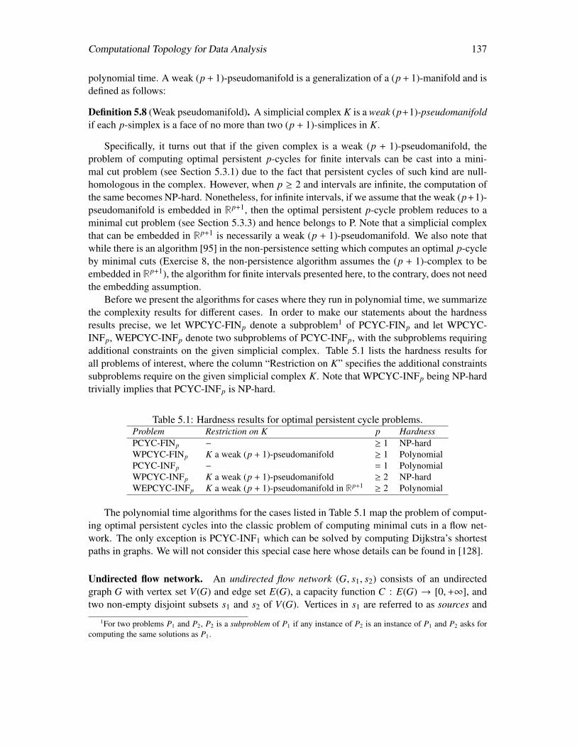
Computational Topology for Data Analysis 137
polynomial time. A weak (p + 1)-pseudomanifold is a generalization of a (p + 1)-manifold and isdefined as follows:
Definition 5.8 (Weak pseudomanifold). A simplicial complex K is a weak (p+1)-pseudomanifoldif each p-simplex is a face of no more than two (p + 1)-simplices in K.
Specifically, it turns out that if the given complex is a weak (p + 1)-pseudomanifold, theproblem of computing optimal persistent p-cycles for finite intervals can be cast into a mini-mal cut problem (see Section 5.3.1) due to the fact that persistent cycles of such kind are null-homologous in the complex. However, when p ≥ 2 and intervals are infinite, the computation ofthe same becomes NP-hard. Nonetheless, for infinite intervals, if we assume that the weak (p+1)-pseudomanifold is embedded in Rp+1, then the optimal persistent p-cycle problem reduces to aminimal cut problem (see Section 5.3.3) and hence belongs to P. Note that a simplicial complexthat can be embedded in Rp+1 is necessarily a weak (p + 1)-pseudomanifold. We also note thatwhile there is an algorithm [95] in the non-persistence setting which computes an optimal p-cycleby minimal cuts (Exercise 8, the non-persistence algorithm assumes the (p + 1)-complex to beembedded in Rp+1), the algorithm for finite intervals presented here, to the contrary, does not needthe embedding assumption.
Before we present the algorithms for cases where they run in polynomial time, we summarizethe complexity results for different cases. In order to make our statements about the hardnessresults precise, we let WPCYC-FINp denote a subproblem1 of PCYC-FINp and let WPCYC-INFp, WEPCYC-INFp denote two subproblems of PCYC-INFp, with the subproblems requiringadditional constraints on the given simplicial complex. Table 5.1 lists the hardness results forall problems of interest, where the column “Restriction on K” specifies the additional constraintssubproblems require on the given simplicial complex K. Note that WPCYC-INFp being NP-hardtrivially implies that PCYC-INFp is NP-hard.
Table 5.1: Hardness results for optimal persistent cycle problems.Problem Restriction on K p HardnessPCYC-FINp − ≥ 1 NP-hardWPCYC-FINp K a weak (p + 1)-pseudomanifold ≥ 1 PolynomialPCYC-INFp − = 1 PolynomialWPCYC-INFp K a weak (p + 1)-pseudomanifold ≥ 2 NP-hardWEPCYC-INFp K a weak (p + 1)-pseudomanifold in Rp+1 ≥ 2 Polynomial
The polynomial time algorithms for the cases listed in Table 5.1 map the problem of comput-ing optimal persistent cycles into the classic problem of computing minimal cuts in a flow net-work. The only exception is PCYC-INF1 which can be solved by computing Dijkstra’s shortestpaths in graphs. We will not consider this special case here whose details can be found in [128].
Undirected flow network. An undirected flow network (G, s1, s2) consists of an undirectedgraph G with vertex set V(G) and edge set E(G), a capacity function C : E(G) → [0,+∞], andtwo non-empty disjoint subsets s1 and s2 of V(G). Vertices in s1 are referred to as sources and
1For two problems P1 and P2, P2 is a subproblem of P1 if any instance of P2 is an instance of P1 and P2 asks forcomputing the same solutions as P1.
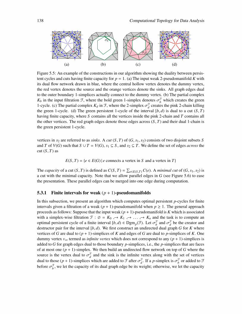
138 Computational Topology for Data Analysis
σb
σd
(a) (b) (c) (d)
Figure 5.5: An example of the constructions in our algorithm showing the duality between persis-tent cycles and cuts having finite capacity for p = 1. (a) The input weak 2-pseudomanifold K withits dual flow network drawn in blue, where the central hollow vertex denotes the dummy vertex,the red vertex denotes the source and the orange vertices denote the sinks. All graph edges dualto the outer boundary 1-simplices actually connect to the dummy vertex. (b) The partial complexKb in the input filtration F, where the bold green 1-simplex denotes σF
b which creates the green1-cycle. (c) The partial complex Kd in F, where the 2-simplex σF
d creates the pink 2-chain killingthe green 1-cycle. (d) The green persistent 1-cycle of the interval [b, d) is dual to a cut (S ,T )having finite capacity, where S contains all the vertices inside the pink 2-chain and T contains allthe other vertices. The red graph edges denote those edges across (S ,T ) and their dual 1-chain isthe green persistent 1-cycle.
vertices in s2 are referred to as sinks. A cut (S ,T ) of (G, s1, s2) consists of two disjoint subsets Sand T of V(G) such that S ∪ T = V(G), s1 ⊆ S , and s2 ⊆ T . We define the set of edges across thecut (S ,T ) as
E(S ,T ) = e ∈ E(G) | e connects a vertex in S and a vertex in T
The capacity of a cut (S ,T ) is defined as C(S ,T ) =∑
e∈E(S ,T ) C(e). A minimal cut of (G, s1, s2) isa cut with the minimal capacity. Note that we allow parallel edges in G (see Figure 5.6) to easethe presentation. These parallel edges can be merged into one edge during computation.
5.3.1 Finite intervals for weak (p + 1)-pseudomanifolds
In this subsection, we present an algorithm which computes optimal persistent p-cycles for finiteintervals given a filtration of a weak (p + 1)-pseudomanifold when p ≥ 1. The general approachproceeds as follows: Suppose that the input weak (p + 1)-pseudomanifold is K which is associatedwith a simplex-wise filtration F : ∅ = K0 → K1 → . . . → Kn and the task is to compute anoptimal persistent cycle of a finite interval [b, d) ∈ Dgmp(F). Let σF
b and σFd be the creator and
destructor pair for the interval [b, d). We first construct an undirected dual graph G for K wherevertices of G are dual to (p + 1)-simplices of K and edges of G are dual to p-simplices of K. Onedummy vertex v∞ termed as infinite vertex which does not correspond to any (p + 1)-simplices isadded to G for graph edges dual to those boundary p-simplices, i.e., the p-simplices that are facesof at most one (p + 1)-simplex. We then build an undirected flow network on top of G where thesource is the vertex dual to σF
d and the sink is the infinite vertex along with the set of verticesdual to those (p + 1)-simplices which are added to F after σF
d . If a p-simplex is σFb or added to F
before σFb , we let the capacity of its dual graph edge be its weight; otherwise, we let the capacity
Computational Topology for Data Analysis 139
of its dual graph edge be +∞. Finally, we compute a minimal cut of this flow network and returnthe p-chain dual to the edges across the minimal cut as an optimal persistent cycle of the interval.
The intuition of the above algorithm is best explained by an example illustrated in Figure 5.5,where p = 1. The key to the algorithm is the duality between persistent cycles of the inputinterval and cuts of the dual flow network having finite capacity. To see this duality, first considera persistent p-cycle c of the input interval [b, d). There exists a (p + 1)-chain A in Kd createdby σF
d whose boundary equals c, making c killed. We can let S be the set of graph verticesdual to the simplices in A and let T be the set of the remaining graph vertices, then (S ,T ) is acut. Furthermore, (S ,T ) must have finite capacity as the edges across it are exactly dual to thep-simplices in c and the p-simplices in c have indices in F less than or equal to b. On the otherhand, let (S ,T ) be a cut with finite capacity, then the (p + 1)-chain whose simplices are dual tothe vertices in S is created by σF
d . Taking the boundary of this (p + 1)-chain, we get a p-cycle c.Because p-simplices of c are exactly dual to the edges across (S ,T ) and each edge across (S ,T )has finite capacity, c must reside in Kb. We only need to ensure that c contains σF
b in order toshow that c is a persistent cycle of [b, d). In Section 5.3.2, we argue that c indeed contains σF
b(proof of Theorem 5.14), so c is a persistent cycle.
In the dual graph, an edge is created for each p-simplex. If a p-simplex has two (p + 1)-cofaces, we simply let its dual graph edge connect the two vertices dual to its two (p + 1)-cofaces;otherwise, its dual graph edge has to connect to the infinite vertex on one end. A problem aboutthis construction is that some weak (p + 1)-pseudomanifolds may have p-simplices being faceof no (p + 1)-simplices and these p-simplices may create self loops around the infinite vertex.To avoid self loops, we simply ignore these p-simplices. The reason why we can ignore thesep-simplices is that they cannot be on the boundary of a (p + 1)-chain and hence cannot be on apersistent cycle of minimal weight. Algorithmically, we ignore these p-simplices by constructingthe dual graph only from what we call the (p + 1)-connected component of K containing σF
d .
Definition 5.9 (q-connected). Let K be a simplicial complex. For q ≥ 1, two q-simplices σ andσ′ of K are q-connected in K if there is a sequence of q-simplices of K, (σ0, . . . , σl), such thatσ0 = σ, σl = σ′, and for all 0 ≤ i < l, σi and σi+1 share a (q − 1)-face. The property ofq-connectedness defines an equivalence relation on q-simplices of K. Each set in the partitioninduced by the equivalence relation constitutes a q-connected component of K. We say K is q-connected if any two q-simplices of K are q-connected in K. See Figure 5.6 for an example of1-connected components and 2-connected components.
We present the pseudo-code in Algorithm 11:MinPersCycFin and it works as follows: Line 1and 2 set up a complex K that the algorithm mainly works on, where K is taken as the closureof the (p + 1)-connected component of σF
d . Line 3 constructs the dual graph G from K andlines 4−15 build the flow network on top of G. Note that we denote the infinite vertex by v∞.Line 16 computes a minimal cut for the flow network and line 17 returns the p-chain dual tothe edges across the minimal cut. In the pseudo-codes, to make presentation of algorithms andsome proofs easier, we treat a mathematical function as a programming object. For example, thefunction θ returned by DualGraphFin in MinPersCycFin denotes the correspondence between thesimplices of K and their dual vertices or edges (see Section 5.3.1 for details). In practice, theseconstructs can be easily implemented in any programming language.
140 Computational Topology for Data Analysis
Algorithm 11 MinPersCycFin(K, p,F, [b, d))
Input:K: finite p-weighted weak (p + 1)-pseudomanifoldp: integer ≥ 1F: filtration K0 ⊆ K1 ⊆ . . . ⊆ Kn of K[b, d): finite interval of Dgmp(F)
Output:An optimal persistent p-cycle for [b, d)
1: Lp+1 ← (p + 1)-connected component of K containing σFd \∗ set up K ∗\
2: K ← closure of the simplicial set Lp+1
3: (G, θ)← DualGraphFin(K, p) \∗ construct dual graph ∗\4: for all e ∈ E(G) do5: if index(θ−1(e)) ≤ b then6: C(e)← w(θ−1(e)) \∗assign finite capacity∗\7: else8: C(e)← +∞ \∗assign infinite capacity∗\9: end if
10: end for11: s1 ← θ(σF
d ) \∗set the source∗\12: s2 ← v ∈ V(G) | v , v∞, index(θ−1(v)) > d \∗set the sink∗\13: if v∞ ∈ V(G) then14: s2 ← s2 ∪ v∞15: end if16: (S ∗,T ∗)← min-cut of (G, s1, s2)17: Output θ−1(E(S ∗,T ∗))
Complexity. The time complexity of MinPersCycFin depends on the encoding scheme of theinput and the data structure used for representing a simplicial complex. For encoding the input,we assume K and F are represented by a sequence of all the simplices of K ordered by theirindices in F, where each simplex is denoted by its set of vertices. We also assume a simple yetreasonable simplicial complex data structure as follows: In each dimension, simplices are mappedto integral identifiers ranging from 0 to the number of simplices in that dimension minus 1; eachq-simplex has an array (or linked list) storing all the id’s of its (q + 1)-cofaces; a hash map foreach dimension is maintained for the query of the integral id of each simplex in that dimensionbased on the spanning vertices of the simplex. We further assume p to be constant. By the aboveassumptions, let n be the size (number of bits) of the encoded input, then there are no more thann elementary O(1) operations in line 1 and 2 so the time complexity of line 1 and 2 is O(n). It isnot hard to verify that the flow network construction also takes O(n) time so the time complexityof MinPersCycFin is determined by the minimal cut algorithm. Using the max-flow algorithm byOrlin [248], the time complexity of MinPersCycFin becomes O(n2).
Computational Topology for Data Analysis 141
In the rest of this section, we first describe the subroutine DualGraphFin, then close the sectionby proving the correctness of the algorithm.
Dual graph construction. We describe the DualGraphFin subroutine used in Algorithm Min-PersCycFin, which returns a dual graph G and a θ denoting two bijections which we use to provethe correctness. Given the input (K, p), DualGraphFin constructs an undirected connected graphG as follows:
• Let each vertex v of V(G) correspond to each (p + 1)-simplex σp+1 of K. If there is anyp-simplex of K which has less than two (p + 1)-cofaces in K, we add an infinite vertex v∞to V(G). Simultaneously, we define a bijection
θ : (p + 1)-simplices of K → V(G) r v∞
by letting θ(σp+1) = v. Note that in the above range notation of θ, v∞ may not be a subsetof V(G).
• Let each edge e of E(G) correspond to each p-simplex σp of K. Note that σp has at leastone (p + 1)-coface in K. If σp has two (p + 1)-cofaces σp+1
0 and σp+11 in K, then let e
connect θ(σp+10 ) and θ(σp+1
1 ); if σp has one (p + 1)-coface σp+10 in K, then let e connect
θ(σp+10 ) and v∞. We define another bijection
θ : p-simplices of K → E(G)
using the same notation as the bijection for V(G), by letting θ(σp) = e.
Note that we can take the image of a subset of the domain under a function. Therefore, if(S ,T ) is a cut for a flow network built on G, then θ−1(E(S ,T )) denotes the set of p-simplicesdual to the edges across the cut. Also note that since simplicial chains with Z2 coefficients can beinterpreted as sets, θ−1(E(S ,T )) is also a p-chain.
5.3.2 Algorithm correctness
In this subsection, we prove the correctness of the algorithm MinPersCycFin. Some of the sym-bols we use refer to the pseudocode of the algorithm.
Proposition 5.13. In the algorithm MinPersCycFin, s2 is not an empty set.
Proof. For contradiction, suppose that s2 is an empty set. Then v∞ < V(G) and σFd is the (p + 1)-
simplex of K with the greatest index in F. Since v∞ < V(G), any p-simplex of K must be a faceof two (p + 1)-simplices of K, so the set of (p + 1)-simplices of K forms a (p + 1)-cycle createdby σF
d . Then σFd must be a positive simplex in F, which is a contradiction.
The following two propositions specify the duality mentioned at the beginning of Section 5.3.1:
Proposition 5.14. For any cut (S ,T ) of (G, s1, s2) with finite capacity, the p-chain c = θ−1(E(S ,T ))is a persistent p-cycle of [b, d) and w(c) = C(S ,T ).
142 Computational Topology for Data Analysis
Proof. Let A = θ−1(S ), it is easy to check that c = ∂(A). The key is to show that c is createdby σF
b which we show now. Suppose that c is created by a p-simplex σp , σFb . Since C(S ,T )
is finite, we have that index(σp) < b. We can let c′ be a persistent cycle of [b, d) and c′ = ∂(A′)where A′ is a (p + 1)-chain of Kd. Then we have c + c′ = ∂(A + A′). Since A and A′ are bothcreated by σF
d , then A+ A′ is created by a (p + 1)-simplex with an index less than d in F. So c+c′
is a p-cycle created by σFb which becomes a boundary before σF
d is added. This means that σFb
is already paired when σFd is added, contradicting the fact that σF
b is paired with σFd . Similarly,
we can prove that c is not a boundary until σFd is added, so c is a persistent cycle of [b, d). Since
(S ,T ) has finite capacity, we must have
C(S ,T ) =∑
e∈θ(c)
C(e) =∑
θ−1(e)∈c
w(θ−1(e)) = w(c)
Proposition 5.15. For any persistent p-cycle c of [b, d), there exists a cut (S ,T ) of (G, s1, s2) suchthat C(S ,T ) ≤ w(c).
Proof. Let A be a (p + 1)-chain in Kd such that c = ∂(A). Note that A is created by σFd and c
is the set of p-simplices which are face of exactly one (p + 1)-simplex of A. Let c′ = c ∩ K andA′ = A∩ K, we claim that c′ = ∂(A′). To prove this, first let σp be any p-simplex of c′, then σp isa face of exactly one (p + 1)-simplex σp+1 of A. Since σp ∈ K, it is also true that σp+1 ∈ K, andso σp+1 ∈ A′. Then σp is a face of exactly one (p + 1)-simplex of A′, so σp ∈ ∂(A′). On the otherhand, let σp be any p-simplex of ∂(A′), then σp is a face of exactly one (p + 1)-simplex σp+1
0 ofA′. Note that σp+1
0 ∈ A, and we want to prove that σp is a face of exactly one (p + 1)-simplexσ
p+10 of A. Suppose that σp is a face of another (p + 1)-simplex σp+1
1 of A, then σp+11 ∈ K because
σp+10 ∈ K. So we have σp+1
1 ∈ A ∩ K = A′, contradicting the fact that σp is a face of exactly one(p + 1)-simplex of A′. Then we have σp ∈ ∂(A). Since σp+1
0 ∈ K, we have σp ∈ K, which meansthat σp ∈ c′.
Let S = θ(A′) and T = V(G) r S , then it is true that (S ,T ) is a cut of (G, s1, s2) because A′
is created by σFd . We claim that θ−1(E(S ,T )) = ∂(A′). The proof of the equality is similar to the
one in the proof of Proposition 5.14. It follows that E(S ,T ) = θ(c′). We then have that
C(S ,T ) =∑
e∈θ(c′)
C(e) =∑
θ−1(e)∈c′w(θ−1(e)) = w(c′)
because each p-simplex of c′ has an index less than or equal to b in F.Finally, since c′ is a subchain of c, we must have C(S ,T ) = w(c′) ≤ w(c).
Combining the above results, we conclude:
Theorem 5.16. Algorithm MinPersCycFin computes an optimal persistent p-cycle for the giveninterval [b, d).
Proof. First, the flow network (G, s1, s2) constructed by the algorithm MinPersCycFin must bevalid by Proposition 5.13. Since the interval [b, d) must have a persistent cycle, the flow network
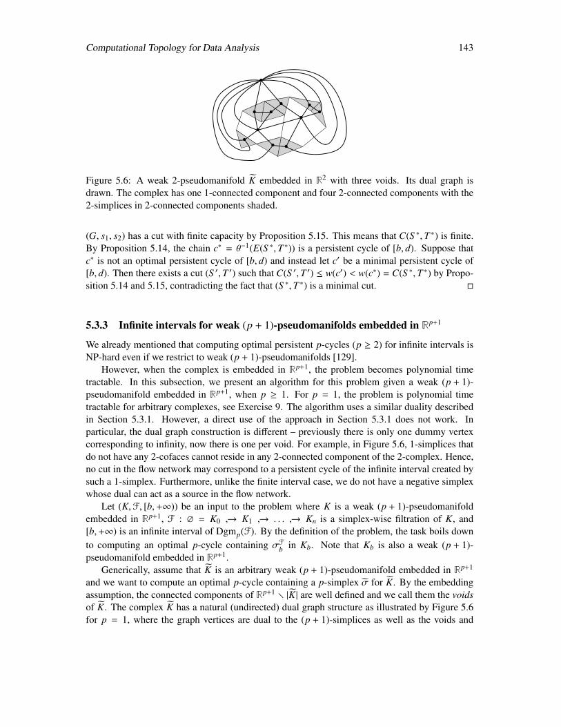
Computational Topology for Data Analysis 143
Figure 5.6: A weak 2-pseudomanifold K embedded in R2 with three voids. Its dual graph isdrawn. The complex has one 1-connected component and four 2-connected components with the2-simplices in 2-connected components shaded.
(G, s1, s2) has a cut with finite capacity by Proposition 5.15. This means that C(S ∗,T ∗) is finite.By Proposition 5.14, the chain c∗ = θ−1(E(S ∗,T ∗)) is a persistent cycle of [b, d). Suppose thatc∗ is not an optimal persistent cycle of [b, d) and instead let c′ be a minimal persistent cycle of[b, d). Then there exists a cut (S ′,T ′) such that C(S ′,T ′) ≤ w(c′) < w(c∗) = C(S ∗,T ∗) by Propo-sition 5.14 and 5.15, contradicting the fact that (S ∗,T ∗) is a minimal cut.
5.3.3 Infinite intervals for weak (p + 1)-pseudomanifolds embedded in Rp+1
We already mentioned that computing optimal persistent p-cycles (p ≥ 2) for infinite intervals isNP-hard even if we restrict to weak (p + 1)-pseudomanifolds [129].
However, when the complex is embedded in Rp+1, the problem becomes polynomial timetractable. In this subsection, we present an algorithm for this problem given a weak (p + 1)-pseudomanifold embedded in Rp+1, when p ≥ 1. For p = 1, the problem is polynomial timetractable for arbitrary complexes, see Exercise 9. The algorithm uses a similar duality describedin Section 5.3.1. However, a direct use of the approach in Section 5.3.1 does not work. Inparticular, the dual graph construction is different – previously there is only one dummy vertexcorresponding to infinity, now there is one per void. For example, in Figure 5.6, 1-simplices thatdo not have any 2-cofaces cannot reside in any 2-connected component of the 2-complex. Hence,no cut in the flow network may correspond to a persistent cycle of the infinite interval created bysuch a 1-simplex. Furthermore, unlike the finite interval case, we do not have a negative simplexwhose dual can act as a source in the flow network.
Let (K,F, [b,+∞)) be an input to the problem where K is a weak (p + 1)-pseudomanifoldembedded in Rp+1, F : ∅ = K0 → K1 → . . . → Kn is a simplex-wise filtration of K, and[b,+∞) is an infinite interval of Dgmp(F). By the definition of the problem, the task boils downto computing an optimal p-cycle containing σF
b in Kb. Note that Kb is also a weak (p + 1)-pseudomanifold embedded in Rp+1.
Generically, assume that K is an arbitrary weak (p + 1)-pseudomanifold embedded in Rp+1
and we want to compute an optimal p-cycle containing a p-simplex σ for K. By the embeddingassumption, the connected components of Rp+1 r |K| are well defined and we call them the voidsof K. The complex K has a natural (undirected) dual graph structure as illustrated by Figure 5.6for p = 1, where the graph vertices are dual to the (p + 1)-simplices as well as the voids and
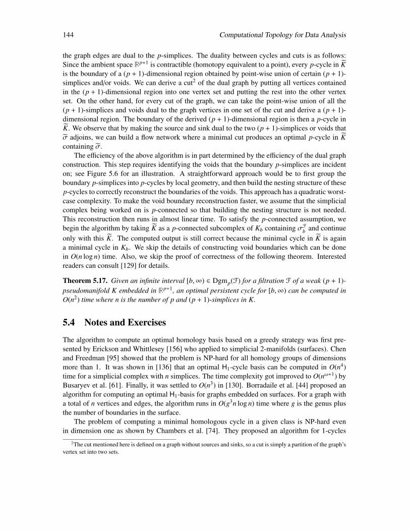
144 Computational Topology for Data Analysis
the graph edges are dual to the p-simplices. The duality between cycles and cuts is as follows:Since the ambient space Rp+1 is contractible (homotopy equivalent to a point), every p-cycle in Kis the boundary of a (p + 1)-dimensional region obtained by point-wise union of certain (p + 1)-simplices and/or voids. We can derive a cut2 of the dual graph by putting all vertices containedin the (p + 1)-dimensional region into one vertex set and putting the rest into the other vertexset. On the other hand, for every cut of the graph, we can take the point-wise union of all the(p + 1)-simplices and voids dual to the graph vertices in one set of the cut and derive a (p + 1)-dimensional region. The boundary of the derived (p + 1)-dimensional region is then a p-cycle inK. We observe that by making the source and sink dual to the two (p + 1)-simplices or voids thatσ adjoins, we can build a flow network where a minimal cut produces an optimal p-cycle in Kcontaining σ.
The efficiency of the above algorithm is in part determined by the efficiency of the dual graphconstruction. This step requires identifying the voids that the boundary p-simplices are incidenton; see Figure 5.6 for an illustration. A straightforward approach would be to first group theboundary p-simplices into p-cycles by local geometry, and then build the nesting structure of thesep-cycles to correctly reconstruct the boundaries of the voids. This approach has a quadratic worst-case complexity. To make the void boundary reconstruction faster, we assume that the simplicialcomplex being worked on is p-connected so that building the nesting structure is not needed.This reconstruction then runs in almost linear time. To satisfy the p-connected assumption, webegin the algorithm by taking K as a p-connected subcomplex of Kb containing σF
b and continueonly with this K. The computed output is still correct because the minimal cycle in K is againa minimal cycle in Kb. We skip the details of constructing void boundaries which can be donein O(n log n) time. Also, we skip the proof of correctness of the following theorem. Interestedreaders can consult [129] for details.
Theorem 5.17. Given an infinite interval [b,∞) ∈ Dgmp(F) for a filtration F of a weak (p + 1)-pseudomanifold K embedded in Rp+1, an optimal persistent cycle for [b,∞) can be computed inO(n2) time where n is the number of p and (p + 1)-simplices in K.
5.4 Notes and Exercises
The algorithm to compute an optimal homology basis based on a greedy strategy was first pre-sented by Erickson and Whittlesey [156] who applied to simplicial 2-manifolds (surfaces). Chenand Freedman [95] showed that the problem is NP-hard for all homology groups of dimensionsmore than 1. It was shown in [136] that an optimal H1-cycle basis can be computed in O(n4)time for a simplicial complex with n simplices. The time complexity got improved to O(nω+1) byBusaryev et al. [61]. Finally, it was settled to O(n3) in [130]. Borradaile et al. [44] proposed analgorithm for computing an optimal H1-basis for graphs embedded on surfaces. For a graph witha total of n vertices and edges, the algorithm runs in O(g3n log n) time where g is the genus plusthe number of boundaries in the surface.
The problem of computing a minimal homologous cycle in a given class is NP-hard evenin dimension one as shown by Chambers et al. [74]. They proposed an algorithm for 1-cycles
2The cut mentioned here is defined on a graph without sources and sinks, so a cut is simply a partition of the graph’svertex set into two sets.
Computational Topology for Data Analysis 145
on surfaces utilizing the duality between minimal cuts of a surface-embedded graph and optimalhomologous cycles of a dual complex. A better algorithm is proposed in [75]. Both algorithmsare fixed parameter tractable running in time exponential in the genus of the surface. For gen-eral dimension, Borradaile et al. [45] showed that the OHCP problem in dimension p can beO(
√log n)-approximated and is fixed-parameter tractable for weak (p + 1)-pseudomanifolds. The
only polynomial-time exact algorithm [95] in general dimension for OHCP works for p-cycles incomplexes embedded in Rp+1, which uses a reduction to minimal (s, t)-cuts. Interestingly, whenthe coefficient is chosen to be Z instead of Z2 for the homology groups, the problem becomespolynomial time solvable if there is no relative torsion as shown in [126]. The material presentedin Section 5.2 is taken from this paper.
Persistence added an extra layer of complexity to the problem of computing minimal repre-sentative cycles. Escolar and Hiraoka [157] and Obayashi [247] formulated the problem as aninteger program by adapting a similar formulation for the non-persistent case. Wu et. al [302]adapted the algorithm of Busaryev et al. [61] to present an exponential-time algorithm, as wellas an A∗ heuristics in practice. The problem of computing optimal persistent cycle is NP-hardeven for H1 [128]. The problem becomes polynomial time solvable for some special cases suchas computing optimal persistent 2-cycles in a 3-complex embedded in 3-dimension [129]. Thematerials in Section 5.3 are taken from this source.
Exercises
1. Show that every cycle in a H1(K)-basis contains a simple cycle which together form aH1(K)-basis themselves.
2. Design an O(n2 log n + n2g) algorithm to compute the shortest non-trivial 1-cycle in a sim-plicial 2-complex K with n simplices and g = β1(K). Do the same in O(n2 log n) time whenK is a 1-complex (a graph).
3. ([130]) We have given an O(nω + n2gω−1) algorithm for computing an optimal H1-basis fora complex with n simplices. Taking g = Ω(n), this runs in O(nω+1) worst-case time. Givean O(n3) algorithm for the problem.
4. How can one make the algorithm in [130] more efficient for a weighted graph G with nvertices and edges? For this, show that (i) an annotation for G can be computed in O(n2)time, (ii) this annotation can be utilized to compute the annotations for O(n2) candidatecycles in O(n3) time, (iii) finally, an optimal basis can be computed in O(n3) time by thedivide-and-conquer greedy algorithm in [130] though more efficiently.
5. Define a minmax basis of Hp(K) as the set of cycles which generate Hp(K) and the maxi-mum weight of the cycles is minimized among all such generators. Prove that an optimalHp-cycle basis defined in Definition 5.3 is also a minmax basis.
6. Prove that a simplicial p-complex embedded in Rp cannot have torsion in Hp−1 and henceOHCP for (p − 1)-cycles can be solved in polynomial time in this case.
7. Take an example of a triangulation of Möbius strip and show that the integer programformulation of OHCP for it is not totally unimodular.
146 Computational Topology for Data Analysis
8. Professor Optimist claims that an optimal Hp-generator for K embedded in Rp+1 can beobtained by computing optimal persistent p-cycles for infinite bars in any filtration of K.Show that he is wrong. Give a polynomial time algorithm for computing a non-trivialp-cycle that has the least weight in K.
9. Consider computing a persistent 1-cycle for a bar [b, d) given a filtration of an edge-weighted complex K. Let c be a cycle created by the edge e = (u, v) at the birth time bwhere c is formed by the edge e and the shortest path between u and v in the 1-skeletonof the complex Kb. If [c] = 0 at Kd, prove that c is an optimal persistent cycle for the bar[b, d).
10. Give an example where the above computed cycle using shortest path at the birth time isnot a persistent cycle.
11. For a finite interval [b, d) ∈ Dgmp(F) of a filtration F of a weak (p + 1)-pseudomanifold,one can take the two vertices of the dual edge of the creator p-simplex σb in the algorithmMinPersCycFin (Section 5.3.1) as source and sink respectively. Give an example to showthat this does not work for computing a minimal persistent cycle for [b, d). What abouttaking the dual vertex of the destroyer simplex σd and the infinite vertex as the source andthe sink respectively?
12. ([94]) For a vertex v in a complex with non-negative weights on edges, let discrete geodesicball Br
v of radius r be the maximal subcomplex L ⊆ K so that the shortest path from v toevery vertex in L is at most r. For a cycle c, let w(c) = minr | c ⊆ Br
v. Give a polynomialtime algorithm to compute an optimal Hp-cycle basis for any p ≥ 1 with these weights.
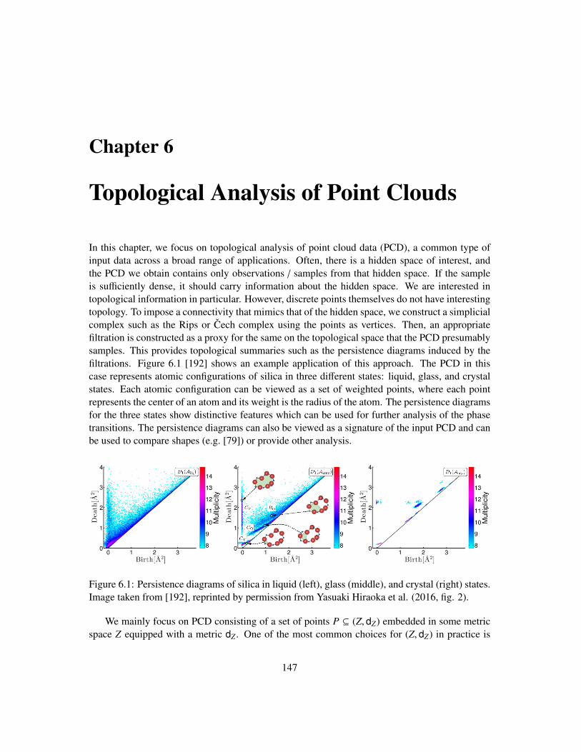
Chapter 6
Topological Analysis of Point Clouds
In this chapter, we focus on topological analysis of point cloud data (PCD), a common type ofinput data across a broad range of applications. Often, there is a hidden space of interest, andthe PCD we obtain contains only observations / samples from that hidden space. If the sampleis sufficiently dense, it should carry information about the hidden space. We are interested intopological information in particular. However, discrete points themselves do not have interestingtopology. To impose a connectivity that mimics that of the hidden space, we construct a simplicialcomplex such as the Rips or Cech complex using the points as vertices. Then, an appropriatefiltration is constructed as a proxy for the same on the topological space that the PCD presumablysamples. This provides topological summaries such as the persistence diagrams induced by thefiltrations. Figure 6.1 [192] shows an example application of this approach. The PCD in thiscase represents atomic configurations of silica in three different states: liquid, glass, and crystalstates. Each atomic configuration can be viewed as a set of weighted points, where each pointrepresents the center of an atom and its weight is the radius of the atom. The persistence diagramsfor the three states show distinctive features which can be used for further analysis of the phasetransitions. The persistence diagrams can also be viewed as a signature of the input PCD and canbe used to compare shapes (e.g. [79]) or provide other analysis.
Figure 6.1: Persistence diagrams of silica in liquid (left), glass (middle), and crystal (right) states.Image taken from [192], reprinted by permission from Yasuaki Hiraoka et al. (2016, fig. 2).
We mainly focus on PCD consisting of a set of points P ⊆ (Z, dZ) embedded in some metricspace Z equipped with a metric dZ . One of the most common choices for (Z, dZ) in practice is
147
148 Computational Topology for Data Analysis
the d-dimensional Euclidean space Rd equipped with the standard Lp-distance. We review therelevant concepts of constructing Rips and Cech complexes, their filtrations, and describe theproperties of the resulting persistence diagrams in Section 6.1. In practice, the size of a filtrationcan be prohibitively large. In Section 6.2, we discuss data sparsification strategies to approximatetopological summaries much more efficiently and with theoretical guarantees.
As we have mentioned, a PCD can be viewed as a window through which we can peek at topo-logical properties of the hidden space. In particular, we can infer about the hidden homologicalinformation using the PCD at hand if it samples the hidden space sufficiently densely. In Section6.3, we provide such inference results for the cases when the hidden space is a manifold or is acompact set embedded in the Euclidean space. To obtain theoretical guarantees, we also need tointroduce the language of sampling conditions to describe the quality of point samples. Finally,in Section 6.4, we focus on the inference of scalar field topology from a set of point samples P,as well as function values available at these samples. More precisely, we wish to estimate thepersistent homology of a real-valued function f : X → R from a set of discrete points P ⊂ X aswell as the values of f over P.
6.1 Persistence for Rips and Cech filtrations
Suppose we are given a finite set of points P in a metric space (Z, dZ). Consider a closed ballBZ(p, r) with radius r centered at each point p ∈ P and consider the space Pr := ∪p∈PBZ(p, r).The Cech complex w.r.t. P and a parameter r ≥ 0 is defined as (Definition 2.9)
CrZ(P) = σ = p0, . . . , pk | ∩i∈[0,k]BZ(p, r) , ∅. (6.1)
We often omit Z from the subscript when its choice is clear. As mentioned in Chapter 2.2, theCech complex Cr(P) is the nerve of the union of balls Pr. If the metric balls centered at pointsin P in the metric space (Z, dZ) are convex, then the Nerve Theorem (Theorem 2.1) gives thefollowing corollary.
Corollary 6.1. For a fixed r ≥ 0, if the metric ball BZ(x, r) is convex for every x ∈ P, then Cr(P)is homotopy equivalent to Pr, and thus Hk(Cr(P)) Hk(Pr) for any dimension k ≥ 0.
The above result justifies the utility of Cech complexes. For example, if P ⊆ Rd and dZ is thestandard Lp-distance for p > 0, then the Cech complex Cr(P) becomes homotopy equivalent to theunion of r-radius balls centering at points in P. Later in this chapter, we will also see an examplewhere the points P are taken from a Riemannian manifold X equipped with the Riemannian metricdX . When the radius r is small enough, the intrinsic metric balls also become convex. In bothcases, the resulting Cech complex captures information of the union of r-balls Pr.
In general, it is not clear at which scale (radius r) one should inspect the input PCD. Varyingthe scale parameter r, we obtain a filtration of spaces P := Pα → Pα
′
α≤α′ as well as a filteredsequence of simplicial complexes C(P) := Cα(P) → Cα′(P)α≤α′ . The homotopy equivalencebetween Pr and Cr, if holds, further induces an isomorphism between the persistence modulesobtained from these two filtrations.
Proposition 6.2 ([92]). If the metric ball B(x, r) is convex for every x ∈ P and all r ≥ 0, then thepersistence module HkP is isomorphic to the persistence module HkC(P). This also implies that
Computational Topology for Data Analysis 149
their corresponding persistence diagrams are identical; that is, DgmkP = DgmkC(P), for anydimension k ≥ 0.
A related persistence-based topological invariant is given by the Vietoris-Rips filtration R(P) =
VRα(P) → VRα′(P)α≤α′ , where the Vietoris-Rips complex VRr(P) for a finite subset P ⊆ (Z, dZ)at scale r is defined as (Definition 2.10):
VRr(P) = σ = p0, . . . , pk | dZ(pi, p j) ≤ 2r for any i, j ∈ [0, k]. (6.2)
Recall from Chapter 4.1 that the Cech filtration and Vietoris-Rips filtration are multiplicatively2-interleaved, meaning that their persistence modules are log 2-interleaved at the log-scale, and
db(DgmlogC(P),DgmlogR(P)) ≤ log 2, (Corollary 4.4). (6.3)
Finite metric spaces. The above definitions of Cech or Rips complexes assume that P is em-bedded in an ambient metric space (Z, dZ). It is possible that Z = P and we simply have a discretemetric space spanned by points in P, which we denote by (P, dP). Obviously, the construction ofCech and Rips complexes can be extended to this case. In particular, the Cech complex Cr
P(P) isnow defined as
CrP(P) = σ = p0, . . . , pk | ∩i∈[0,k]BP(p; r) , ∅, (6.4)
where BP(p, r) := q ∈ P | dP(p, q) ≤ r. However, note that when P ⊂ Z and dP is the restrictionof the metric dZ to points in P, the Cech complex Cr
P(P) defined above can be different from theCech complex Cr
Z(P), as the metric balls (BP vs. BZ) are different. In particular, in this case, wehave the following relation between the two types of Cech complexes:
CrP(P) ⊆ Cr
Z(P) ⊆ C2rP (P). (6.5)
On the other hand, in this setting, the two Rips complexes are the same because the definition ofRips complex involves only pairwise distance between input points, not metric balls.
The persistence diagrams induced by the Cech and the Rips filtrations can be used as topologi-cal summaries for the input PCD P. We can then for example, compare input PCDs by comparingthese persistence diagram summaries.
Definition 6.1 (Cech, Rips distance). Given two finite point sets P and Q, equipped with appro-priate metrics, the Cech distance between them is a pseudo-distance defined as:
dCech(P,Q) = maxk
dB(DgmkC(P),DgmkC(Q))).
Similarly, the Rips distance between P and Q is a pseudo-distance defined as:
dRips(P,Q) = maxk
dB(DgmkR(P),DgmkR(Q))).
These distances are stable with respect to the Hausdorff or the Gromov-Hausdorff distancebetween P and Q depending on whether they are embedded in a common metric space or areviewed as two discrete metric spaces (P, dP) and (Q, dQ)). We introduce the Hausdorff andGromov-Hausdorff distances now. Given a point x and a set A from a metric space (X, d), letd(x, A) := infa∈A d(x, a) denote the closest distance from x to any point in A.
150 Computational Topology for Data Analysis
Definition 6.2 (Hausdorff distance). Given two compact sets A, B ⊆ (Z, dZ), the Hausdorff dis-tance between them is defined as:
dH(A, B) = max maxa∈A
dZ(a, B), maxb∈B
dZ(b, A) .
Note that the Hausdorff distance requires the input objects are embedded in a common am-bient space. In case they are not embedded in any common ambient space, we use Gromov-Hausdorff distance, which intuitively measures how much two input metric spaces differ frombeing isometric.
Definition 6.3 (Gromov-Hausdorff distance). Given two metric spaces (X, dX) and (Y, dY ), a cor-respondence C is a subset C ⊆ X × Y so that (i) for every x ∈ X, there exists some (x, y) ∈ C; and(ii) for every y′ ∈ Y , there exists some (x′, y′) ∈ C. The distortion induced by C is
distortC(X,Y) :=12
sup(x,y),(x′,y′)∈C
|dX(x, x′) − dY (y, y′)|.
The Gromov-Hausdorff distance between (X, dX) and (Y, dY ) is the smallest distortion possible byany correspondence; that is,
dGH(X,Y) := infC⊆X×Y
distortC(X,Y).
Theorem 6.3. Cech- and Rips-distances satisfy the following stability statements:
1. Given two finite sets P,Q ⊆ (Z, dZ), we have
dCech(P,Q) ≤ dH(P,Q); and dRips(P,Q) ≤ dH(P,Q).
2. Given two finite metric spaces (P, dP) and (Q, dQ), we have
dCech(P,Q) ≤ 2dGH((P, dP), (Q, dQ)), and dRips(P,Q) ≤ dGH((P, dP), (Q, dQ)).
Note that the bound on dCech(P,Q) in statement (2) of the above theorem has an extra factorof 2, which comes due to the difference in metric balls – see the discussions after Eqn (6.4). Wealso remark that (2) in the above theorem can be extended to the so-called totally bounded metricspaces (which are not necessarily finite) (P, dP) and (Q, dQ) defined as follows. First, recall thatan ε-sample (Definition 2.17) of a metric space (Z, dZ) is a finite set S ⊆ Z so that for everyz ∈ Z, dZ(z, S ) ≤ ε. A metric space (Z, dZ) is totally bounded if there exists a finite ε-sample forevery ε > 0. Intuitively, such a metric space can be approximated by a finite metric space for anyresolution.
6.2 Approximation via data sparsification
One issue with using the Vietoris-Rips or Cech filtrations in practice is that their sizes can becomehuge, even for moderate number of points. For example, when the scale r is larger than thediameter of a point set P, the Cech and the Vietoris-Rips complexes of P contain every simplex

Computational Topology for Data Analysis 151
(a) (b) (c)
Figure 6.2: Vietoris-Rips complex: (b) at small scale, the Rips complex of points shown in (a)requires the two white points; (c) the two white points become redundant at larger scale.
spanned by points in P, in which case the size of d-skeleton of Cr(P) or VRr(P) is Θ(nd+1) forn = |P|.
On the other hand, as shown in Figure 6.2, as the scale r increases, certain points couldbecome “redundant”, e.g, having no or little contribution to the underlying space of the union ofall r-radius balls. Based on this observation, one can approximate these filtrations with sparsifiedfiltrations of much smaller size. In particular, as the scale r increases, the point set P with whichone constructs a complex is gradually sparsified keeping the total number of simplicies in thecomplex linear in the input size of P where the dimension of the embedding space is assumed tobe fixed.
We describe two data sparsification schemes in Sections 6.2.1 and 6.2.2, respectively. Wefocus on the Vietoris-Rips filtration for points in a Euclidean space Rd equipped with the standardEuclidean distance d.
6.2.1 Data sparsification for Rips filtration via reweighting
Most of the concepts presented in this section apply to general finite metric spaces though wedescribe them for finite point sets equipped with an Euclidean metric. The reason for this choiceis that the complexity analysis draws upon the specific property of Euclidean space. The reader isencouraged to think about generalizing the definitions and the technique to other metric spaces.
First we restate the definition of δ-sample and δ-sparse sample in Definition 2.17 slightlydifferently.
Definition 6.4 (Nets and net-tower). Given a finite set of points P ⊂ (Rd, d) and γ, γ′ ≥ 0, asubset Q ⊆ P is a (γ, γ′)-net of P if the following two conditions hold:
Covering condition: Q is a γ-sample for (P, d), i.e., for every p ∈ P, d(p,Q) ≤ γ.
Packing condition: Q is also γ-sparse, i.e., for every q , q′ ∈ Q, d(q, q′) ≥ γ′.
If γ = γ′, we also refer to Q as a γ-net of P.A single-parameter family of nets Nγγ is called a net-tower of P if (i) there is a constant
c > 0 so that for all γ ∈ R, Nγ is a (γ, γ/c)-net for P, and (ii) Nγ ⊇ Nγ′ for any γ ≤ γ′.
152 Computational Topology for Data Analysis
Intuitively, a γ-net approximates a PCD P at resolution γ (Covering condition), while alsobeing sparse (Packing condition). A net-tower provides a sequence of increasingly sparsifiedapproximation of P.
Net-tower via farthest point sampling. We now introduce a specific net-tower constructed viathe classical strategy of farthest point sampling, also called greedy permutation e.g. in [57, 71].Given a point set P ⊂ (Rd, d), choose an arbitrary point p1 from P and set P1 = p1. Pick pi
recursively as pi ∈ argmaxp∈P\Pi−1d(p, Pi−1)1, and set Pi = Pi−1 ∪ pi. Now set tpi = d(pi, Pi−1),
which we refer to as the exit-time of pi. Based on these exit-times, we construct the following twofamilies of sets:
Open net-tower N = Nγγ∈R where Nγ := p ∈ P | tp > γ. (6.6)
Closed net-tower N = Nγγ∈R where Nγ := p ∈ P | tp ≥ γ. (6.7)
It is easy to verify that both Nγ and Nγ are γ-nets, and the families N and N are indeed two net-towers as γ increases. As γ increases, Nγ and Nγ can only change when γ = tp for some p ∈ P.Hence the sequence of subsets P = Pn ⊃ Pn−1 ⊇ · · · ⊇ P2 ⊇ P1 contain all the distinct sets in theopen and closed net-towers Nγ and Nγ.
In what follows, we discuss a sparsification strategy for the Rips filtration of P using the abovenet-towers. The approach can be extended to other net-towers, such as the net-tower constructedusing the net-tree data structure of [182].
Weights, weighted distance, and sparse Rips filtration. Given the exit-time tps for all pointsp ∈ P, we now associate a weight wp(α) for each point p at a scale α as follows (the graph of thisweight function is shown on the right): for some constant 0 < ε < 1,
wp(α) =
0 tp
ε ≥ α
α −tpε
tpε < α <
tpε(1−ε)
εαtp
ε(1−ε) ≤ αα
wα(p)
tpε
tpε(1−ε)
tp(1−ε)
0
Claim 6.1. The weight function wp is a continuous, 1-Lipschitz, and non-decreasing function.
The parameter ε controls the resolution of the sparsification. The net-induced distance atscale α between input points is defined as:
dα(p, q) := d(p, q) + wp(α) + wq(α). (6.8)
Definition 6.5 (Sparse (Vietoris-)Rips). Given a set of points P ⊂ Rd, a constant 0 < ε < 1, andthe open net-tower Nγ as well as the closed net-tower Nγ for P as introduced above, the opensparse-Rips complex at scale α is defined as
Qα := σ ⊆ Nε(1−ε)α | ∀p, q ∈ σ, dα(p, q) ≤ 2α; (6.9)
1Note that there may be multiple points that maximize d(p, Pi−1) making argmaxp∈P\Pi−1d(p, Pi−1) a set. We can
choose pi to be any point in this set.
Computational Topology for Data Analysis 153
while the closed sparse-Rips at scale α is defined as
Qα
:= σ ⊆ Nε(1−ε)α | ∀p, q ∈ σ, dα(p, q) ≤ 2α. (6.10)
Set Sα := ∪β≤αQα, which we call the cumulative complex at scale α. The (ε-)sparse Rips filtration
then refers to the R-indexed filtration S = Sα → Sβα≤β.
Obviously, Qα ⊆ Qα. Note that for α < β, Qα is not necessarily included in Qβ (neither is Q
α
in Qβ); while the inclusion Sα ⊆ Sβ always holds.
In what follows, we show that the sparse Rips filtration approximates the standard Vietoris-Rips filtration VRr(P) defined over P, and that the size of the sparse Rips filtration is only linearin n for any fixed dimension d which is assumed to be constant. The main results are summarizedin the following theorem.
Theorem 6.4. Let P ⊂ Rd be a set of n points where d is a constant, and R(P) = VRr(P) be theVietoris-Rips filtration over P. Given net-towers Nγ and Nγ induced by exit-times tpp∈P, letS(P) = Sα be its corresponding ε-sparse Rips filtration as defined in Definition 6.5. Then, for afixed 0 < ε < 1
3 ,
(i) S(P) and R(P) are multiplicatively 11−ε -interleaved at the homology level. Thus, for any
k ≥ 0, the persistence diagram DgmkS(P) is a log 11−ε -approximation of DgmkR(P) at the
log-scale.
(ii) For any fixed dimension k ≥ 0, the total number of k-simplices ever appeared in S(P) isΘ(( 1
ε )kdn).
In the remainder of this section, we sketch the proof of the above theorem.
Proof of part (i) of Theorem 6.4. To relate S(P) to R(P), we need to go through a sequence ofintermediate steps. First, we define the relaxed Rips complex at scale α as
VRα(P) := σ ⊂ P | ∀p, q ∈ σ, dα(p, q) ≤ 2α.
The following claim ensures that the relaxed Rips complexes form a valid filtration connected byinclusions R(P) = VR
α(P) → VR
β(P)α≤β, which we call the relaxed Rips filtration.
Claim 6.2. If dα(p, q) ≤ 2α ≤ 2β, then dβ(p, q) ≤ 2β.
Proof. The weight function wp is 1-Lipschitz for any p ∈ P (Claim 6.1). Thus we have that
dβ(p, q) = d(p, q) + wp(β) + wq(β)
≤ d(p, q) + wp(α) + (β − α) + wq(α) + (β − α)
≤ d(p, q) + wp(α) + wq(α) − 2α + 2β ≤ 2β.
The last inequality follows from d(p, q) + wp(α) + wq(α) = dα(p, q) ≤ 2α.
In what follows, we drop the argument P from notations such as in complexes VRα(P) or insparse Rips filtration S(P) when the point set in question is understood.
154 Computational Topology for Data Analysis
Proposition 6.5. Let C = 11−ε . Then for any α ≥ 0 we have that VRα/C ⊆ VR
α⊆ VRα.
Next, we relate filtrations S and R via the relaxed Rips filtration R by connecting the sparseRips complexes Qαs and Q
αs. Consider the following projection of P to points in the net Nε(1−ε)α
which are also vertices of Qα:
πα(p) =
p if p ∈ Nε(1−ε)α
argminq∈Nεαd(p, q) otherwise
Again, if argminq∈Nεαd(p, q) contains more than one point, we set πα(p) to be an arbitrary one.
This projection is well-defined as Nεα ⊆ Nε(1−ε)α given that 0 < ε < 1/3 < 1. We need sev-eral technical results on this projection map, which we rely on later to construct maps betweenappropriate versions of Rips complexes. First, the following two results are easy to show.
Fact 6.1. For every p ∈ P, d(p, πα(p)) ≤ wp(α) − wπα(p)(α) ≤ εα.
Fact 6.2. For every pair p, q ∈ P, we have that dα(p, πα(q)) ≤ dα(p, q).
We are now ready to show that inclusion induces an isomorphism between the homologygroups of the sparse Rips complex and the relaxed Rips complex.
Proposition 6.6. For any α ≥ 0, the inclusion i : Qα → VRα
induces an isomorphism at thehomology level; that is, H∗(Qα) H∗(VR
α) under the homomorphism i∗ induced by i.
Proof. First, we consider the projection map πα and argue that it induces a simplicial mapπα : VR
α→ Qα which is in fact a simplicial retraction2. Next, we show that the map i πα :
VRα→ VR
αis contiguous to the identity map id : VR
α→ VR
α. As πα is a simplicial retraction,
it follows that i∗ is an isomorphism (Lemma 2 of [275]).To see that πα is a simplicial map, apply Fact 6.2 twice to have that
dα(πα(p), πα(q)) ≤ dα(p, πα(q)) ≤ dα(p, q). (6.11)
Since both Qα and VRα
are clique complexes, this then implies that πα is a simplicial map. Fur-thermore, it is easy to see that it is a retraction as πα(q) = q for any q in the vertex set of Qα
(which is Nε(1−ε)α).Now to show that iπα is contiguous to id, we observe that for any p, q ∈ P with dα(p, q) ≤ 2α,
all edges among p, q, πα(p), πα(q) exist and thus all simplices spanned by them exist in VRα.
Indeed, that dα(πα(p), πα(q)) ≤ 2α is already shown above in Eqn (6.11). Combining Fact 6.1with the fact that wp(α) ≤ εα, we have that
dα(p, πα(p)) = d(p, πα(p)) + wp(α) + wπα(p)(α) ≤ 2wp(α) ≤ 2εα < 2α.
Furthermore, by Fact 6.2, dα(p, πα(q)) ≤ dα(p, q) ≤ 2α. Symmetric arguments can be applied toshow that dα(q, πα(q)), dα(q, πα(p)) ≤ 2α. This establishes that i πα is contiguous to id. Thisproves the proposition.
2A simplicial retraction f : K → L is a simplicial map from K ⊆ L to L so that f (σ) = σ for any σ ∈ K.
Computational Topology for Data Analysis 155
The closed sparse-Rips complex Qα
is the relaxed Rips complex over the vertex set Nε(1−ε)α,which is a superset of the vertex set of Qα. Hence the above proposition also holds for theinclusion Qα → Q
α. It then follows that H∗(Qα) H∗(Q
α). Finally, we show that the inclusion
also induces an isomorphism between H∗(Qα) and H∗(Sα), which when combined with the above
results connects Sα and VRα.
Proposition 6.7. For any α ≥ 0, the inclusion h : Qα→ Sα induces an isomorphism at the
homology level, that is, H∗(Qα) H∗(Sα) under h∗.
Proof. Consider the sequence Sαα∈R. First, we discretize α to have distinct values α0 < α1 <
α2 . . . αm so that Sα0 = ∅, and αis are exactly the time when the combinatorial structure of Sα
changes. As Sα =∑β≤α Q
β, these are also exactly the moments when the combinatorial structure
of Qα
changes. Hence we only need to prove the statement for such αi’s, and it will then work forall α’s. Set λi := ε(1 − ε)αi. Note that the vertex set for Q
αi is Nλi by the definition of Qα
in Eqn(6.10).
Now fix a k ≥ 0. We will show that h : Qαk→ Sαk induces an isomorphism at the homololgy
level. We use some intermediate complexes
Ti,k :=k⋃
j=i
Qα j, for i ∈ [1, k].
Obviously, T1,k = Sαk where Tk,k = Qαk . Set hi : Ti+1,k → Ti,k. The inclusion h : Q
αk→ Sαk can
then be written as h = h1 h2 · · · hk−1. In what follows, we prove that hi : Ti+1,k → Ti,k inducesan isomorphism at the homology level for each i ∈ [1, k − 1], which then proves the proposition.
First, note that while Ti,k is not necessarily the same as Qαi , they share the same vertex set.
Now, because of our choices of αis and λis, the vertex set of Ti+1,k, which is the vertex set of Qαi+1 ,
namely Nλi+1 , equals Nλi . Hence we can consider the projection παi : Ti,k → Ti+1,k given by theprojection of the vertex set Nλi−1 = Nλi of Ti,k to the vertex set Nλi = Nλi+1 of Ti+1,k. To prove thathi induces an isomorphism at the homology level, by Lemma 2 of [275], it suffices to show that(i) παi is a simplicial retraction, and (ii) hi παi is contiguous to the identity map id : Ti,k → Ti,k.
To prove (i), it is easy to verify that παi is a retraction. To see that παi induces a simplicial map,we need to show that for every σ ∈ Ti,k, παi(σ) ∈ Ti+1,k. As παi is a retraction, we only need toprove this for every σ ∈ Ti,k \Ti+1,k. On the other hand, note that by definition, Ti,k \Ti+1,k ⊆ Q
αi .To this end, the argument in Proposition 6.6 also shows that παi : Q
αi→ Qαi is a simplicial map,
and furthermore, h′ παi is contiguous to id′ : Qαi→ Q
αi , where h′ : Qαi → Qαi . Because of
our choice of αis, Qαi and Qαi+1 have the same vertex set, which is Nλi . Furthermore, for every
edge (p, q) ∈ Qαi , we have that dαi(p, q) ≤ 2αi. As αi < αi+1, it follows from Claim 6.2 thatdαi+1(p, q) ≤ 2αi+1. Hence, the edge (p, q) is in Q
αi+1 . This implies that Qαi ⊆ Qαi+1 . Putting
everything together, it follows that, for every σ ∈ Ti,k \ Ti+1,k ⊆ Qαi , we have
παi(σ) ∈ Qαi ⊆ Qαi+1⊆ Ti+1,k.
Therefore, παi is a simplicial map. This finishes the proof of (i).
156 Computational Topology for Data Analysis
Now we prove (ii), that is, hi παi is contiguous to the identity map id : Ti,k → Ti,k. Thismeans that we need to show for every σ ∈ Ti,k, σ ∪ παi(σ) ∈ Ti,k. Again, as παi is a simplicial re-traction, we only need to show this for σ ∈ Ti,k\Ti+1,k ⊆ Q
αi . As mentioned above, using the sameargument as in Proposition 6.6, we know that h′παi is contiguous to the identity id′ : Q
αi→ Q
αi .Hence we have that for every σ ∈ Q
αi , σ ∪ παi(σ) ∈ Qαi . It follows that σ ∪ παi(σ) ∈ Ti,k as
Qαi⊆ Ti,k. This proves (ii) completing the proof of the proposition.
Combining Propositions 6.6 (as well as the discussion after this proposition) and 6.7, we havethat Sα and VR
α induces isomorphic persistence modules. This, together with Proposition 6.5,
implies part (i) of Theorem 6.4.
Proof of part (ii) of Theorem 6.4. Let S(k) denote the set of k-simplices ever appeared in S(P),which is also the set of k-simplices in the last complex S∞ of S(P). To bound the size of S(k), wecharge each simplex in S(k) to the vertex of it with smallest exit-time. Observe that a point p ∈ Pdoes not contribute to any new edge in the sparse Rips complex Q
βfor β > tp
ε(1−ε) . This means
that to bound the number of simplices charged to p, we only need to bound such simplices in Qαp
with αp =tp
ε(1−ε) .
Set E(p) = q ∈ P | (p, q) ∈ Qαp and tp ≤ tq. We add p to E(p) too. We claim that
|E(p)| = O(( 1ε )d). In particular, consider the closed net-tower Nγ; recall that Nγ is a γ-net. As
E(p) ⊆ N tp , the packing-condition of the net implies that the closest pair in E(p) has distanceat least tp between them. On the other hand, for each (p, q) ∈ Q
αp , we have dαp(p, q) ≤ 2αp
implying that the E(p) ⊆ B(p, 2αp). A simple packing argument then implies that the number ofpoints in E(p) is
O
(2αp
tp
)d = O
( 2ε(1 − ε)
)d = O
(1ε
)d .The last equality follows because ε < 1/3 and thus 1 − ε ≥ 2/3. The total number of k-simplicescharged to p is bounded by O(( 1
ε )kd), and the total number k-simplices in S(P) is O(( 1ε )kdn),
proving part (ii) of Theorem 6.4.
6.2.2 Approximation via simplicial tower
We now describe a different sparsification strategy by directly building a simplicial tower of Ripscomplexes connected by simplicial maps (Definition 4.1 and the discussion below it) whose per-sistent homology also approximates that of the standard Rips-filtration. This sparsification is con-ceptually simpler, but its approximation quality is worse than the one introduced in the previoussection.
Given a set of points P ⊂ Rd, α > 0, and some 0 < ε < 1, we are interested in the followingfiltration (which is a subsequence of the standard Rips filtration)
VRα(P) → VRα(1+ε)(P) → VRα(1+ε)2(P) → · · · → VRα(1+ε)m
(P). (6.12)
We now construct a sparsified sequence by setting P0 := P, building a sequence of point setsPk, k = 0, 1, . . . ,m where Pk+1 is a αε
2 (1 + ε)k−1-net of Pk, and terminating the process when Pm
is of constant size.
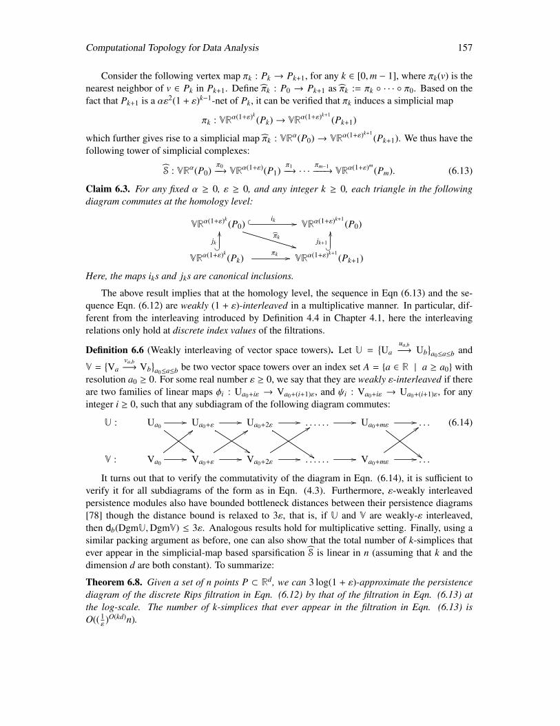
Computational Topology for Data Analysis 157
Consider the following vertex map πk : Pk → Pk+1, for any k ∈ [0,m − 1], where πk(v) is thenearest neighbor of v ∈ Pk in Pk+1. Define πk : P0 → Pk+1 as πk := πk · · · π0. Based on thefact that Pk+1 is a αε2(1 + ε)k−1-net of Pk, it can be verified that πk induces a simplicial map
πk : VRα(1+ε)k(Pk)→ VRα(1+ε)k+1
(Pk+1)
which further gives rise to a simplicial map πk : VRα(P0) → VRα(1+ε)k+1(Pk+1). We thus have the
following tower of simplicial complexes:
S : VRα(P0)π0−−→ VRα(1+ε)(P1)
π1−−→ · · ·
πm−1−−−→ VRα(1+ε)m
(Pm). (6.13)
Claim 6.3. For any fixed α ≥ 0, ε ≥ 0, and any integer k ≥ 0, each triangle in the followingdiagram commutes at the homology level:
VRα(1+ε)k(P0)
ik //
πk
**
VRα(1+ε)k+1(P0)
VRα(1+ε)k(Pk)
?jk
OO
πk // VRα(1+ε)k+1(Pk+1)
?jk+1
OO
Here, the maps iks and jks are canonical inclusions.
The above result implies that at the homology level, the sequence in Eqn (6.13) and the se-quence Eqn. (6.12) are weakly (1 + ε)-interleaved in a multiplicative manner. In particular, dif-ferent from the interleaving introduced by Definition 4.4 in Chapter 4.1, here the interleavingrelations only hold at discrete index values of the filtrations.
Definition 6.6 (Weakly interleaving of vector space towers). Let U =Ua
ua,b−→ Ub
a0≤a≤b and
V =Va
va,b−→ Vb
a0≤a≤b be two vector space towers over an index set A = a ∈ R | a ≥ a0 with
resolution a0 ≥ 0. For some real number ε ≥ 0, we say that they are weakly ε-interleaved if thereare two families of linear maps φi : Ua0+iε → Va0+(i+1)ε, and ψi : Va0+iε → Ua0+(i+1)ε, for anyinteger i ≥ 0, such that any subdiagram of the following diagram commutes:
U : Ua0//
##
Ua0+ε//
%%
Ua0+2ε //
%%
. . . . . . // Ua0+mε //
##
. . .
V : Va0//
;;
Va0+ε//
99
Va0+2ε //
99
. . . . . . // Va0+mε //
;;
. . .
(6.14)
It turns out that to verify the commutativity of the diagram in Eqn. (6.14), it is sufficient toverify it for all subdiagrams of the form as in Eqn. (4.3). Furthermore, ε-weakly interleavedpersistence modules also have bounded bottleneck distances between their persistence diagrams[78] though the distance bound is relaxed to 3ε, that is, if U and V are weakly-ε interleaved,then db(DgmU,DgmV) ≤ 3ε. Analogous results hold for multiplicative setting. Finally, using asimilar packing argument as before, one can also show that the total number of k-simplices thatever appear in the simplicial-map based sparsification S is linear in n (assuming that k and thedimension d are both constant). To summarize:
Theorem 6.8. Given a set of n points P ⊂ Rd, we can 3 log(1 + ε)-approximate the persistencediagram of the discrete Rips filtration in Eqn. (6.12) by that of the filtration in Eqn. (6.13) atthe log-scale. The number of k-simplices that ever appear in the filtration in Eqn. (6.13) isO(( 1
ε )O(kd)n).
158 Computational Topology for Data Analysis
6.3 Homology inference from PCDs
So far, we considered the problem of approximating the persistence diagram of a filtration createdout of a given PCD. Now we consider the problem of inferring certain homological structure ofa (hidden) domain where the input PCD presumably is sampled from. More specifically, theproblem we consider is: Given a finite set of points P ⊂ Rd, residing on or around a hiddendomain X ⊆ Rd of interest, compute or approximate the rank of H∗(X) using input PCD P. Laterin this chapter, X is assumed to be either a smooth Riemannian manifold embedded in Rd, orsimply a compact set of Rd.
Main ingredients. Since points themselves do not have interesting topology, we first constructa certain simplicial complex K, typically a Cech or a Vietoris-Rips complex from P. Next, wecompute the homological information of K as a proxy for the same of X. Of course, the approx-imation becomes faithful only when the given sample P is sufficiently dense and the parametersused for building the complexes are appropriate. The high level approach works as follows.
Input: A finite point set P ⊂ Rd “approximating” a hidden space X ⊂ Rd.
Step 1. Compute the Cech complex Cα(P), or a pair of Rips complexes VRα(P) and VRα′(P) forsome appropriate 0 < α < α′.
Step 2. In the case of Cech complex, return dim(H∗(Cα(P))) as an approximation of dim(H∗(X)).In the case of Rips complex, return rank (im (i∗)), where the homomorphism
i∗ : H∗(VRα(P))→ H∗(VRα′(P)) is induced by the inclusion VRα(P) ⊆ VRα′(P).
To provide quantitative statements on the approximation quality of the outcome of the aboveapproach, we need to describe first what the quality of the input PCD P is, often referred to asthe sampling conditions. Intuitively, a better approximation in homology is achieved if the inputpoints P “approximates” or “samples” X better. The quality of input points is often measured bythe Hausdorff distance w.r.t. the Euclidean distances between PCD P and the hidden domain X ofinterest (Definition 6.2), such as requiring that dH(P, X) ≤ ε for some ε > 0. Note that points inP do not necessarily lie in X. The approximation guarantee for dim(H∗(X)) relies on relating thedistance fields induced by X and by the sample P. We describe the distance field and feature sizesof X in Section 6.3.1. We present how to infer homology for smooth manifolds and compact setsfrom data in Section 6.3.2 and Section 6.3.3 respectively. In Section 6.4, we discuss inferring thepersistent homology induced by a scalar function f : X → R on X.
6.3.1 Distance field and feature sizes
To describe how well P samples X, we introduce two notions of the so-called “feature size" of X:the local feature size and the weak feature size, both related to the distance field dX w.r.t. X.
Definition 6.7 (Distance field). Given a compact set X ⊂ Rd, the distance field (w.r.t. X) is
dX : Rd → R, x 7→ d(x, X),
where d is the Euclidean distance associated to Rd. The α-offset of X is defined as Xα := x ∈ Rd |
dX(x) ≤ α, which is simply the sub-level set d−1X ((−∞, α]) of dX .

Computational Topology for Data Analysis 159
Given x ∈ Rd, let Π(x) ∈ X denote the set of closest points of x in X; that is,
Π(x) = y ∈ X | d(x, y) = dX(x).
The medial axis of X, denoted by MX , is the closure of the set of points with more than one closestpoint in X; that is,
MX = closurex ∈ Rd | |Π(x)| ≥ 2.
Intuitively, |Π(x)| ≥ 2 implies that the maximal Euclidean ball centered at x whose interior is freeof points in X meets X in more than one point on its boundary. Hence, MX is the closure of thecenters of such maximal empty balls.
Definition 6.8 (Local feature size and reach). For a point x ∈ X, the local feature size at x,denoted by lfs(x), is defined as the minimum distance to the medial axis MX; that is,
lfs(x) := d(x,MX).
The reach of X, denoted by ρ(X), is the minimum local feature size of any point in X.
The concept has been primarily developed for the case when X is a smooth manifold embed-ded in Rd. Indeed, the local feature size can be zero at a non-smooth point: consider a planarpolygon; its medial axis intersects its vertices, and the local feature size at a vertex is thus zero.The reach of a smoothly embedded manifold could also be zero; see Section 1.2 of [119] for anexample. Next, we describe a “weaker" notion of feature size [90, 91], which is more suitable forcompact subsets of Rd.
Critical points of distance field. The distance function dX introduced above is not everywheredifferentiable. Its gradient is defined on Rd \X∪MX. However, one can still define the followingvector which extends the notion of gradient of dX to include the medial axis MX: Given any pointx ∈ Rd \ X, there exists a unique closed ball with minimal radius that encloses Π(x) [225]. Letc(x) denote the center of this minimal enclosing ball, and r(x) its radius. It is easy to see that forany x ∈ Rd \MX , this ball and c(x) degenerates to the unique point in Π(x).
Definition 6.9 (Generalized vector field). Define the following vector field ∇d : Rd \ X → Rd
where the (generalized) gradient vector at x ∈ Rd \ X is:
∇d(x) =x − c(x)dX(x)
.
The critical points of ∇d are points x for which ∇d(x) = 0. We also call the critical points of ∇d
the critical points of the distance function dX .
This generalized gradient field ∇d coincides with the gradient of the distance function dX forpoints in Rd \ X ∪MX. The distance field (distance function) and its critical points were previ-ously studied in e.g., [177], and have played an important role in sampling theory and homologyinference. In general, a point x is a critical point if and only if x ∈ Rd\X is contained in the convexhull of Π(x) (The convex hull of a compact set A ⊂ Rd is the smallest convex set that containsA). It is necessary that all critical points of ∇d belong to the medial axis MX of X. For the casewhere X is a finite set of points in Rd, the critical points of dX are the non-empty intersections ofthe Delaunay simplices with their dual Voronoi cells (if exist) [119].
160 Computational Topology for Data Analysis
Definition 6.10 (Weak feature size). Let C denote the set of critical points of ∇d. The weakfeature size of X, denoted by wfs(X), is the distance between X and C; that is,
wfs(X) = minx∈X
infc∈C
d(x, c).
Proposition 6.9. If 0 < α < α′ are such that there is no critical value of dX in the closed interval[α, α′], then Xα′ deformation retracts onto Xα. In particular, this implies that H∗(Xα) H(Xα′).
In the homology inference frameworks, the reach is usually used for the case when X is asmoothly embedded manifold, while the weak feature size is used for general compact spaces.
6.3.2 Data on manifold
We now consider the problem of homology inference from a point sample of a manifold. We firststate a standard result from linear algebra (see also the Sandwich Lemma from [92]), which weuse several times in homology inference.
Fact 6.3. Given a sequence A → B → C → D → E → F of homomorphisms (linear maps)between finite-dimensional vector spaces over some field, if rank (A → F) = rank (C → D), thenthis quantity also equals rank (B→ E).
Specifically, if A→ B→ C → E → F is a sequence of homomorphisms such that rank (A→F) = dim C, then rank (B→ E) = dim C.
Let P be a point set sampled from a manifold X ⊂ Rd. We construct either the Cech complexCα(P), or a pair of Rips complexes VRα(P) → VR2α(P) for some parameter α > 0. The homologygroups of these spaces are related as follows.
H(X) ooProp. 6.10 // H(Pα) oo Nerve Thm // H(Cα(P)) oo Fact 6.3 // image
(H(VRα)→ H(VR2α)
)(6.15)
Specifically, recall that Ar is the r-offset of A which also equals the union of balls ∪a∈AB(a, r).The connection between the discrete samples P and the manifold X is made through the union ofballs Pα. The following result is a variant of a result by Niyogi, Smale, Weinberger [245]3.
Proposition 6.10. Let P ⊂ Rd be a finite point set such that dH(X, P) ≤ ε where X ⊂ Rd is a
smooth manifold with reach ρ(X). If 3ε ≤ α ≤ 34
√35ρ(X), then H∗(Pα) is isomorphic to H∗(X).
The Cech complex Cα(P) is the nerve complex for the set of balls B(p, α), p ∈ P. AsEuclidean balls are convex, Nerve Theorem implies that Cα(P) is homotopy equivalent to Pα.It follows that we can use the Cech complex Cα(P), for an appropriate α, to infer homology ofX using the isomorphisms H∗(X) H∗(Pα) H∗(Cα(P)). The first isomorphism follows fromProposition 6.10 and the second one from the homotopy equivalence between the nerve and space.
A stronger statement in fact holds: For any α ≤ β, the following diagram commutes:
H∗(Pα)i∗ //
h∗
H∗(Pβ)
h∗
H∗(Cα(P))i∗ // H∗(Cβ(P))
(6.16)
3The result of [245] assumes that P ⊆ X, in which case it shows that Pα deformation retracts to X. In our statementP is not necessarily from X, and the isomorphism follows from results of [245] and Fact 6.3.

Computational Topology for Data Analysis 161
Here, i∗ stands for the homomorphism induced by inclusions, and h∗ is the homomorphism in-duced by the homotopy equivalence h : Pα → Cα(P) given by the Nerve Theorem. This leads tothe following theorem on estimating H∗(X) from a pair of Rips complexes.
Theorem 6.11. Given a smooth manifold X embedded in Rd, let ρ(X) be its reach. Let P ⊂ Rd be
finite sample such that dH(P, X) ≤ ε. For any 3ε ≤ α ≤ 316
√35ρ(X), let i∗ : H∗(VRα)→ H∗(VR2α)
be the homomorphism induced by the inclusion i : VRα → VR2α. We have that
rank (im (i∗)) = dim(H∗(Cα(P))) = dim(H∗(X)).
Proof. By Eqn. (6.16) and Proposition 6.10, we have that for 3ε ≤ α ≤ β ≤ 34
√35ρ(X),
H∗(X) H∗(Pα) H∗(Cα(P)) H∗(Cβ(P)), (6.17)
where the last isomorphism is induced by inclusion. On the other hand, recall the interleavingrelation between the Cech and the Rips complexes:
· · ·Cα(P) ⊆ VRα(P) ⊆ C2α(P) ⊆ VR2α(P) ⊆ C4α(P) · · · .
We thus have the following sequence of homomorphisms induced by inclusion:
H∗(Cα(P))→ H∗(VRα(P))→ H∗(C2α(P))→ H∗(VR2α(P))→ H∗(C4α(P)).
We have H∗(Cα(P)) H∗(C2α(P)) H∗(C4α(P)) by Eqn. (6.17). Thus we have
rank(H∗(Cα(P))→ H∗(C4α(P))) = dim(H∗(Cα(P))).
The theorem then follows from the second part of Fact 6.3.
6.3.3 Data on a compact set
We now consider the case when we are given a finite set of points P sampling a compact subsetX ⊂ Rd. It is known that an offset Xα for any α > 0 may not be homotopy equivalent to X forevery compact set X. In fact, there exist compact sets so that H∗(Xλ) is not isomorphic to H∗(X) nomatter how small λ > 0 is (see Figure 4 of [91]). So, in this case we aim to recover the homologygroups of an offset Xλ of X for a sufficiently small λ > 0.
The high level framework is in Eqn (6.18). Here we have 0 < λ < wfs(X), while Cα andVRα stand for the Cech and Rips complexes Cα(P) and VRα(P) over the point set P. For any0 < λ < wfs(X):
H∗(Xλ) ooProp. 6.12// image
(H∗(Cα → H∗(C2α)
) ooEqn. (6.21)
Fact 6.3// image
(H∗(VRα)→ H∗(VR4α)
). (6.18)
It is similar to Eqn (6.15) for the manifold case. However, we no longer have the isomorphismbetween H∗(Pα) and H∗(X). To overcome this difficulty, we leverage Proposition 6.9. This in turn
162 Computational Topology for Data Analysis
requires us to consider a pair of Cech complexes to infer homology of Xλ, instead of a single Cechcomplex as in the case of manifolds.
More specifically, suppose that the point set P satisfies that dH(P, X) ≤ ε; then we have thefollowing nested sequence for α > ε and α′ ≥ α + 2ε:
Xα−ε ⊆ Pα ⊆ Xα+ε ⊆ Pα′
⊆ Xα′+ε. (6.19)
By Proposition 6.9, we know that if it also holds that α′ + ε < wfs(X), then the inclusionsbetween Xα−ε ⊆ Xα+ε ⊆ Xα′+ε induce isomorphisms between their homology groups, which arealso isomorphic to H∗(Xλ) for λ ∈ (0,wfs(X)). It then follows from the second part of Fact 6.3that, for α, α′ ∈
(ε,wfs(X) − ε
)and α′ − α ≥ 2ε, we have
H∗(Xλ) im (i∗), where i∗ : H∗(Pα)→ H∗(Pα′
) is induced by inclusion i : Pα ⊆ Pα′
. (6.20)
Combining the above with the commutative diagram in Eqn. (6.16), we obtain the followingresult on inferring homology of Xλ using a pair of Cech complexes.
Proposition 6.12. Let X be a compact set in Rd and P ⊂ Rd a finite set of points with dH(X, P) < εfor some ε < 1
4 wfs(X). Then, for all α, α′ ∈(ε,wfs(X) − ε
)such that α′ − α ≥ 2ε, and any λ ∈
(0,wfs(X)), we have H∗(Xλ) im (i∗), where i∗ : H∗(Cα(P))→ H∗(Cα′(P)) is the homomorphismbetween homology groups induced by the inclusion i : Cα(P) → Cα′(P).
Finally, to perform homology inference with the Rips complexes, we again resort to the in-terleaving relation between Cech and Rips complexes, and apply the first part of Fact 6.3 to thefollowing sequence
H∗(Cα/2(P))→ H∗(VRα/2(P))→ H∗(Cα(P))→ H∗(C2α(P))→ H∗(VR2α(P))→ H∗(C4α(P)).(6.21)
If 2ε ≤ α ≤ 14 (wfs − ε), both H∗(Cα/2(P)) → H∗(C4α(P)) and H∗(Cα(P)) → H∗(C2α(P)) have
ranks equal to dim(H∗(Xλ)) by Proposition 6.12. Applying Fact 6.3, we then obtain the followingresult.
Theorem 6.13. Let X be a compact set in Rd and P a finite point set with dH(X, P) < ε for someε < 1
9 wfs(X). Then, for all α ∈(2ε, 1
4 (wfs(X) − ε))
and all λ ∈ (0,wfs(X)), we have H∗(Xλ) im ( j∗), where j∗ is the homomorphism between homology groups induced by the inclusion j :VRα/2(P) → VR2α(P).
6.4 Homology inference for scalar fields
Suppose we are only given a finite sample P ⊂ X from a smooth manifold X ⊂ Rd together witha potentially noisy version f of a smooth function f : X → R presented as a vertex functionf : P → R. We are interested in recovering the persistent homology of the sub-level filtrationof f from f . That is, the goal is to approximate the persistent homology induced by f from thediscrete sample P and function values f on points in P.
Computational Topology for Data Analysis 163
6.4.1 Problem setup
Set Fα = f −1(−∞, α] = x ∈ X | f (x) ≤ α as the sublevel set of f w.r.t. α. The sublevel setfiltration of X induced by f , denoted by F f = Fα; iα,βα≤β, is a family of sets Fα totally orderedby inclusion map iα,β : Fα → Fβ for any α ≤ β (Section 3.1). This filtration induces the followingpersistence module:
HpF f = Hp(Fα)iα,β∗→ Hp(Fβ) α≤β, where iα,β∗ is induced by inclusion map iα,β. (6.22)
For simplicity, we often write the filtration and the corresponding persistence module as F f =
Fαα∈R and HpF f = H(Fα)α∈R, when the choices of maps connecting their elements are clear.Our goal is to approximate the persistence diagram Dgmp(F f ) from point samples P and
f : P → R. Intuitively, we construct a specific Cech (or Rips) complex Cr(P), use f to in-duce a filtration of Cr(P), and then use its persistent homology to approximate Dgmp(F f ). Morespecifically, we need to consider nested pair filtration for either Cr(P) or VRr(P).
Nested pair filtration. Let Pα = p ∈ P | f (p) ≤ α be the set of sample points with the func-tion value for f at most α, which presumably samples the sublevel set Fα of X w.r.t. f . To estimatethe topology of Fα from these discrete sample Pα, we consider either the Cech complex Cr(Pα)or the Rips complex VRr(Pα). For the time being, consider VRr(Pα). As we already saw in pre-vious sections, the topological information of Fα can be inferred from a pair of nested complexes
VRr(Pα)jα→ VRr′(Pα) for some appropriate r < r′. To study F f , we need to inspect Fα → Fβ for
α ≤ β. To this end, fixing r and r′, for any α ≤ β, consider the following commutative diagraminduced by inclusions:
H∗(VRr(Pα)) //
iα∗
H∗(VRr(Pβ))
iβ∗
H∗(VRr′(Pα))jβα∗ // H∗(VRr′(Pβ))
(6.23)
Set φβα : im (iα∗) → im (iβ∗) to be φβα = jβα∗|im (iα∗), that is, the restriction of jβα∗ to im (iα∗). Thismap is well-defined as the diagram above commutes. This gives rise to a persistence moduleim (iα∗); φ
βαα≤β, that is, a family of totally ordered vector spaces
im (iα)
with commutative ho-
momorphisms φβα between any two elements. We formalize and generalize the above constructionbelow.
Definition 6.11 (Nested pair filtration). A nested pair filtration is a sequence of pairs of com-
plexes ABα = (Aα, Bα)α∈R where (i) Aαiα→ Bα is inclusion for every α and (ii) ABα → ABβ for
α ≤ β is given by Aα → Aβ and Bαjβα→ Bβ. The p-th persistence module of the filtration ABαα∈R
is given by the homology module im (Hp(Aα) → Hp(Bα)); φβαα≤β where φβα is the restrictionof jβα∗ on the im iα∗. For simplicity, we say the module is induced by the nested pair filtrationAα → Bα.
The high level approach of inferring persistent homology of a scalar field f : X → R from aset of points P equipped with f : P→ R involves the following steps:
164 Computational Topology for Data Analysis
Step 1. Sort all points of αi in non-decreasing f -values, P = p1, . . . , pn. Set αi = f (pi) fori ∈ [1, n].
Step 2. Compute the persistence diagram induced by the filtration of nested pairs VRr(Pαi) →VRr′(Pαi)i∈[1,n] (or Cr(Pαi) → Cr′(Pαi)i∈[1,n]) for appropriate parameters 0 < r < r′.
The persistent homology (as well as persistence diagram) induced by the filtration of nestedpairs is computed via the algorithm in [105]. To obtain an approximation guarantee for the aboveapproach, we consider an intermediate object defined by the intrinsic Riemannian metric on themanifold X. Indeed, note that the filtration of X w.r.t. f is intrinsic in the sense that it is indepen-dent of how X is embedded in Rd. Hence it is more natural to approximate its persistent homologywith an object defined intrinsically for X.
Given a compact Riemannian manifold X ⊂ Rd embedded in Rd, let dX be the Riemannianmetric of X inherited from the Euclidean metric dE of Rd. Let BX(x, r) := y ∈ X | dX(x, y) ≤ r bethe geodesic ball on X centered at x and with radius r, and Bo
X(x, r) be the open geodesic ball. Incontrast, BE(x, r) (or simply B(x, r)) denotes the Euclidean ball in Rd. A ball Bo
X(x, r) is stronglyconvex if for every pair y, y′ ∈ BX(x, r), there exists a unique minimizing geodesic between y andy′ whose interior is contained within Bo
X(x, r). For details on these concepts, see [77, 164].
Definition 6.12 (Strong convexity). For x ∈ X, let ρc(x; X) denote the supreme of radius r suchthat the geodesic ball Bo
X(x, r) is strongly convex. The strong convexity radius of (X, dX) is definedas ρc(X) := infx∈X ρc(x; X).
Let dX(x, P) := infp∈P dX(x, p) denote the closest geodesic distance between x and the setP ⊆ X.
Definition 6.13 (ε-geodesic sample). A point set P ⊂ X is an ε-geodesic sample of (X, dX) if forall x ∈ X, dX(x, P) ≤ ε.
Recall that Pα is the set of points in P with f -value at most α. The union of geodesic ballsPδ;Xα =
⋃p∈Pα BX(p, δ) is intuitively the “δ-thickening" of Pα within the manifold X. We use two
kinds of Cech and Rips complexes. One is defined with the metric dE of the ambient Euclideanspace which we call (extrinsic) Cech complex Cδ(Pα) and (extrinsic) Rips complex VRδ(Pα). Theother is intrinsic Cech complex Cδ
X(Pα) and intrinsic Rips complex VRδX(Pα) that are defined with
the intrinsic metric dX . Note that CδX(Pα) is the nerve complex of the union of geodesic balls
forming Pδ;Xα . Also the interleaving relation between the Cech and Rips complexes remains thesame as for general geodesic spaces; that is, Cδ
X(Pα) ⊆ VRδX(Pα) ⊆ C2δ
X (Pα) for any α and δ.
6.4.2 Inference guarantees
Recall from Chapter 4.1 that two ε-interleaved filtrations lead to ε-interleaved persistence mod-ules, which further mean that the bottleneck distance between their persistence diagrams arebounded by ε. Here we first relate the space filtration with the intrinsic Cech filtrations and thenrelate these intrinsic ones with the extrinsic Cech or Rips filtrations of nested pairs as illustratedin Eqn. 6.24 below.
Fα oo // Pr;Xα oo // Cr
X(Pα) oo // Cr(Pα) → Cr′(Pα) or VRr(Pα) → VRr′(Pα) (6.24)
Computational Topology for Data Analysis 165
Proposition 6.14. Let X ⊂ Rd be a compact Riemannian manifold with intrinsic metric dX , andlet f : X → R be a C-Lipschitz function. Suppose P ⊂ X is an ε-geodesic sample of X, equippedwith f : P → R so that f = f |P. Then, for any fixed δ ≥ ε, the filtration Fαα and the filtrationPδ;Xα α are (Cδ)-interleaved w.r.t. inclusions.
The intrinsic Cech complex CδX(Pα) is the nerve complex for BX(p, δ)p∈Pα . Furthermore,
for δ < ρc(X), the family of geodesic balls in BX(p, δ)p∈Pα form a cover of the union Pδ;Xαthat satisfies the condition of the Nerve Theorem (Theorem 2.1). Hence, there is a homotopyequivalence between the nerve complex Cδ
X(Pα) and Pδ;Xα . Furthermore, using the same argumentfor showing that diagram in Eqn. (6.16) commutes (Lemma 3.4 of [92]), one can show that thefollowing diagram commutes for any α ≤ β ∈ R and δ ≤ ξ < ρc(X):
H∗(Pδ;Xα )
i∗ //
h∗
H∗(Pξ;Xβ )
h∗
H∗(CδX(Pα))
i∗ // H∗(CξX(Pβ))
(6.25)
Here the horizontal homomorphisms are induced by inclusions, and the vertical ones are isomor-phisms induced by the homotopy equivalence between a union of geodesic balls and its nervecomplex. The above diagram leads to the following result (see Lemma 2 of [88] for details):
Corollary 6.15. Let X, f , and P be as in Proposition 6.14 (although f does not need to be C-Lipschitz). For any δ < ρc(X), Pδ;Xα α∈R and Cδ
X(Pα)α∈R are 0-interleaved. Hence they induceisomorphic persistence modules which have identical persistence diagrams.
Combining with Proposition 6.14, this implies that the filtration CδX(Pα)α and the filtration
Fαα are Cδ-interleaved for ε ≤ δ < ρc(X).
However, we cannot access the intrinsic metric dX of the manifold X and thus cannot directlyconstruct intrinsic Cech complexes. It turns out that for points that are sufficiently close, theirEuclidean distance forms a constant factor approximation of the geodesic distance between themon X.
Proposition 6.16. Let X ⊂ Rd be an embedded Riemannian manifold with reach ρX . For any twopoints x, y ∈ X with dE(x, y) ≤ ρX/2, we have that:
dE(x, y) ≤ dX(x, y) ≤1 +
4d2E(x, y)
3ρ2X
dE(x, y) ≤43
dE(x, y).
This implies the following nested relation between the extrinsic and intrinsic Cech complexes:
CδX(Pα) ⊆ Cδ(Pα) ⊆ C
43 δ
X (Pα) ⊆ C43 δ(Pα) ⊆ C
169 δ
X (Pα); for any δ <38ρX. (6.26)
Note that a similar relation also holds between the intrinsic Cech filtration and the extrinsic Ripscomplexes due to the nested relation between extrinsic Cech and Rips complexes. To infer persis-tent homology from nested pairs filtrations for complexes constructed under the Euclidean metric,we use the following key lemma from [88], which can be thought of as a persistent version as wellas a generalization of Fact 6.3.
166 Computational Topology for Data Analysis
Proposition 6.17. Let X, f , and P be as in Proposition 6.14. Suppose that there exist ε′ ≤ ε′′ ∈[ε, ρc(X)) and two filtrations Gαα and G′αα, so that
for all α ∈ R, CεX(Pα) ⊆ Gα ⊆ Cε′
X (Pα) ⊆ G′α ⊆ Cε′′
X (Pα).
Then the persistence module induced by the filtration Fαα for f and that induced by the nestedpairs of filtrations Gα → G′αα are Cε′′-interleaved, where f is C-Lipschitz.
Combining this proposition with the sequences in Eqn. (6.26), we obtain the following resultson inferring the persistent homology induced by a function f : X → R.
Theorem 6.18. Let X ⊂ Rd be a compact Riemannian manifold with intrinsic metric dX , andf : X → R a C-Lipschitz function on X. Let ρX and ρc(X) be the reach and the strong convexityradius of (X, dX) respectively. Suppose P ⊂ X is an ε-geodesic sample of X, equipped withf : P→ R such that f = f |P. Then:
(i) for any fixed r such that ε ≤ r ≤ min 916ρc(X), 9
32ρX, the persistent homology moduleinduced by the sublevel-set filtration of f : X → R and that induced by the filtration ofnested pairs Cr(Pα) → C
43 r(Pα)α are 16
9 Cr-interleaved; and
(ii) for any fixed r such that 2ε ≤ r ≤ min 932ρc(X), 9
64ρX, the persistent homology moduleinduced by the sublevel set filtration of f and that induced by the filtration of nested pairsVRr(Pα) → VR
83 r(Pα)α are 32
9 Cr-interleaved.
In particular, in each case above, the bottleneck distance between their respective persistencediagrams is bounded by the stated interleaving distance between persistence modules.
6.5 Notes and Exercises
Part of Theorem 6.3 is proved in [78, 79]. A complete proof as well as a thorough treatment forgeometric complexes such as Rips and Cech complexes can be found in [82]. The first approachon data sparsification for Rips filtrations is proposed by Sheehy [274]. The presentation of Chap-ter 6.2.1 is based on a combination of the treatments of sparsification in [57] and [275] (in [275],a net-tower created via net-tree data structure (e.g., [182]) is used for constructing sparse Ripsfiltration). Extension of such sparsification to Cech complexes and a geometric interpretation areprovided in [71]. The Rips sparsification is extended to handle weighted Rips complexes derivedfrom distance to measures in [57]. Sparsification via simplicial towers is introduced in [125].This is an application of the algorithm we presented in Section 4.2 for computing persistent ho-mology for a simplicial tower. Simplicial maps allow batch-collapse of vertices and leads to moreaggressive sparsification. However, in practice it is observed that it also has the over-connectionissues as one collapses the vertices. This issue is addressed in [135]. In particular, the SimBaalgorithm of [135] exploits the simplicial maps for sparsification, but connects vertices at sparserlevels based on a certain distance between two sets (each of which intuitively is the set of originalpoints mapped to a vertex at the present sparsified level). While SimBa has similar approximationguarantees in sparsification, in practice, the sparsified sequence of complexes has much smallersize compared to prior approaches.
Computational Topology for Data Analysis 167
Much of the materials in Section 6.3 are taken from [82, 88, 92, 245]. We remark that therehave been different variations of the medial axis in the literature. We follow the notation from[119]. We also note that there exists a robust version of the medial axis, called the λ-medial axis,proposed in [90]. The concept of the local feature size was originally proposed in [270] in thecontext of mesh generation and a different version that we describe in this chapter was introducedin [8] in the context of curve/surface reconstruction. The local feature size has been widely usedin the field of surface reconstruction and mesh generation; see the books [98, 119]. Critical pointsof the distance field were originally studied in [177]. See [90, 91, 225] for further studies as wellas the development on weak feature sizes.
In homology inference for manifolds, we note that Niyogi, Smale and Weinberger in [245]provide two deformation retract results from union of balls over P to a manifold X; Proposition3.1 holds for the case when P ⊂ X, while Proposition 7.1 holds when P is within a tubularneighborhood of X. The latter has much stronger requirement on the radius α. In our presentation,Proposition 6.10 uses a corollary of Proposition 3.1 of [245] to obtain an isomorphism betweenthe homology groups of union of balls and of X. This allows a better range of the parameterα – however, we lose the deformation retraction here; see the footnote above Proposition 6.10.Results in Chapter 6.4 are mostly based on the work in [88].
This chapter focuses on presenting the main framework behind homology (or persistent ho-mology) inference from point cloud data. The current theoretical guarantees hold when inputpoints sample the hidden domain well within Hausdorff distance. For more general noise modelsthat include outliers and statistical noise, we need a more robust notion of distance field than whatwe used in Section 6.3.1. To this end, an elegant concept called distance to measures (DTM)has been proposed in [80], which has many nice properties and can lead to more robust homo-logical inferences; see, e.g., [83]. An alternative approach using kernel-distance is proposed in[256]. See also [57, 80, 246] for data sparsification or homology inference for points corruptedwith more general noise, and [56] for persistent homology inference under more general noise forinput scalar fields.
Exercise
1. Prove Part (i) of Theorem 6.3.
2. Prove the bound on the Rips pseudo-distance dRips(P,Q) in Part (ii) of Theorem 6.3.
3. Given two finite sets of points P,Q ⊂ Rd, let dP and dQ denote the restriction of the Eu-clidean metric over P and Q respectively. Consider the Hausdorff distance δH = dH(P,Q)between P and Q, as well as the Gromov-Hausdorff distance δGH = dGH((P, dP), (Q, dQ)).
(i) Prove that δGH ≤ δH .
(ii) Assume P,Q ⊂ R2. Let T stand for the set of rigid transformations over R2 (rotation,reflection, translations and their combinations). Let δ∗H := in ft∈TδH(P, t(Q)) denotethe smallest Hausdorff distance possible between P and a copy of Q under rigid trans-formation. Give an example of P,Q ⊂ R2 such that δ∗H is much larger than δGH , sayδ∗H ≥ 10δGH (in fact, this can hold for any fixed constant).
168 Computational Topology for Data Analysis
4. Prove Proposition 6.5.
5. Consider the greedy permutation approach introduced in Chapter 6.2, and the assignmentof exit-times for points p ∈ P. Construct the open tower Nγ and closed tower Nγ asdescribed in the chapter. Prove that both Nγ and Nγ are γ-nets for P.
6. Suppose we are given P0 ⊃ P1 sampled from a metric space (Z, d) where P1 is a γ-net ofP0. Define π : P0 → P1 as π(p) 7→ argminq∈P1
d(p, q) (if argminq∈P1d(p, q) contains more
than one point, then set π(p) to be any point q that minimizes d(p, q)).
(a) Prove that the vertex map π induces a simplicial map π : VRα(P0)→ VRα+γ(P1).
(b) Consider the following diagram. Prove that the map jπ is contiguous to the inclusionmap i.
VRα(P0) i //
π
&&
VRα+γ(P0)
VRα+γ(P1)?
j
OO (6.27)
7. Let P be a set of points in Rd. Let d2 and d1 denote the distance metric under L2 normand under L1 norm respectively. Let C2(P) and C1(P) be the Cech filtration over P inducedby d2 and d1 respectively. Show the relation between the log-scaled version of persistencediagrams DgmlogC2(P) and DgmlogC1(P), that is, bound db(DgmlogC2(P),DgmlogC1(P))(see the discussion above Corollary 4.4 in Chapter 4).
8. Prove Proposition 6.14. Using the fact that Diagram 6.25 commutes, prove Corollary 6.15.
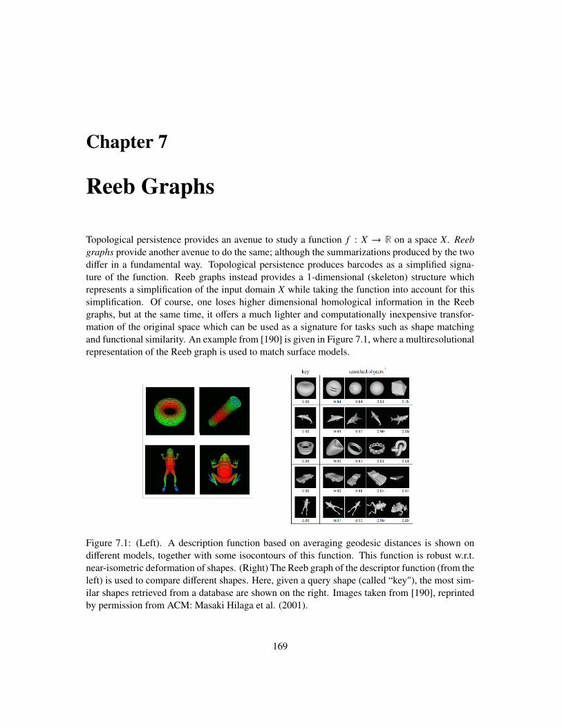
Chapter 7
Reeb Graphs
Topological persistence provides an avenue to study a function f : X → R on a space X. Reebgraphs provide another avenue to do the same; although the summarizations produced by the twodiffer in a fundamental way. Topological persistence produces barcodes as a simplified signa-ture of the function. Reeb graphs instead provides a 1-dimensional (skeleton) structure whichrepresents a simplification of the input domain X while taking the function into account for thissimplification. Of course, one loses higher dimensional homological information in the Reebgraphs, but at the same time, it offers a much lighter and computationally inexpensive transfor-mation of the original space which can be used as a signature for tasks such as shape matchingand functional similarity. An example from [190] is given in Figure 7.1, where a multiresolutionalrepresentation of the Reeb graph is used to match surface models.
Figure 7.1: (Left). A description function based on averaging geodesic distances is shown ondifferent models, together with some isocontours of this function. This function is robust w.r.t.near-isometric deformation of shapes. (Right) The Reeb graph of the descriptor function (from theleft) is used to compare different shapes. Here, given a query shape (called “key"), the most sim-ilar shapes retrieved from a database are shown on the right. Images taken from [190], reprintedby permission from ACM: Masaki Hilaga et al. (2001).
169
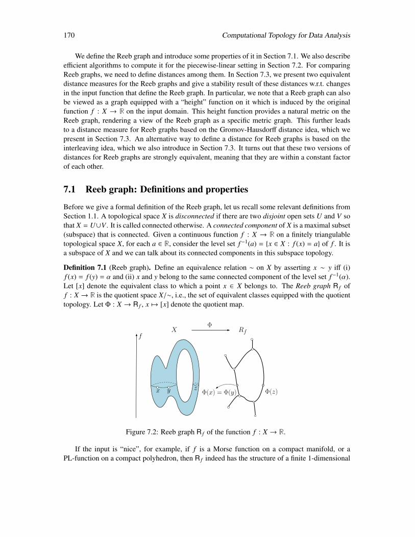
170 Computational Topology for Data Analysis
We define the Reeb graph and introduce some properties of it in Section 7.1. We also describeefficient algorithms to compute it for the piecewise-linear setting in Section 7.2. For comparingReeb graphs, we need to define distances among them. In Section 7.3, we present two equivalentdistance measures for the Reeb graphs and give a stability result of these distances w.r.t. changesin the input function that define the Reeb graph. In particular, we note that a Reeb graph can alsobe viewed as a graph equipped with a “height” function on it which is induced by the originalfunction f : X → R on the input domain. This height function provides a natural metric on theReeb graph, rendering a view of the Reeb graph as a specific metric graph. This further leadsto a distance measure for Reeb graphs based on the Gromov-Hausdorff distance idea, which wepresent in Section 7.3. An alternative way to define a distance for Reeb graphs is based on theinterleaving idea, which we also introduce in Section 7.3. It turns out that these two versions ofdistances for Reeb graphs are strongly equivalent, meaning that they are within a constant factorof each other.
7.1 Reeb graph: Definitions and properties
Before we give a formal definition of the Reeb graph, let us recall some relevant definitions fromSection 1.1. A topological space X is disconnected if there are two disjoint open sets U and V sothat X = U∪V . It is called connected otherwise. A connected component of X is a maximal subset(subspace) that is connected. Given a continuous function f : X → R on a finitely triangulabletopological space X, for each a ∈ R, consider the level set f −1(a) = x ∈ X : f (x) = a of f . It isa subspace of X and we can talk about its connected components in this subspace topology.
Definition 7.1 (Reeb graph). Define an equivalence relation ∼ on X by asserting x ∼ y iff (i)f (x) = f (y) = α and (ii) x and y belong to the same connected component of the level set f −1(α).Let [x] denote the equivalent class to which a point x ∈ X belongs to. The Reeb graph R f off : X → R is the quotient space X/∼, i.e., the set of equivalent classes equipped with the quotienttopology. Let Φ : X → R f , x 7→ [x] denote the quotient map.
fX Rf
Φ
x y zΦ(x) = Φ(y) Φ(z)
Figure 7.2: Reeb graph R f of the function f : X → R.
If the input is “nice”, for example, if f is a Morse function on a compact manifold, or aPL-function on a compact polyhedron, then R f indeed has the structure of a finite 1-dimensional
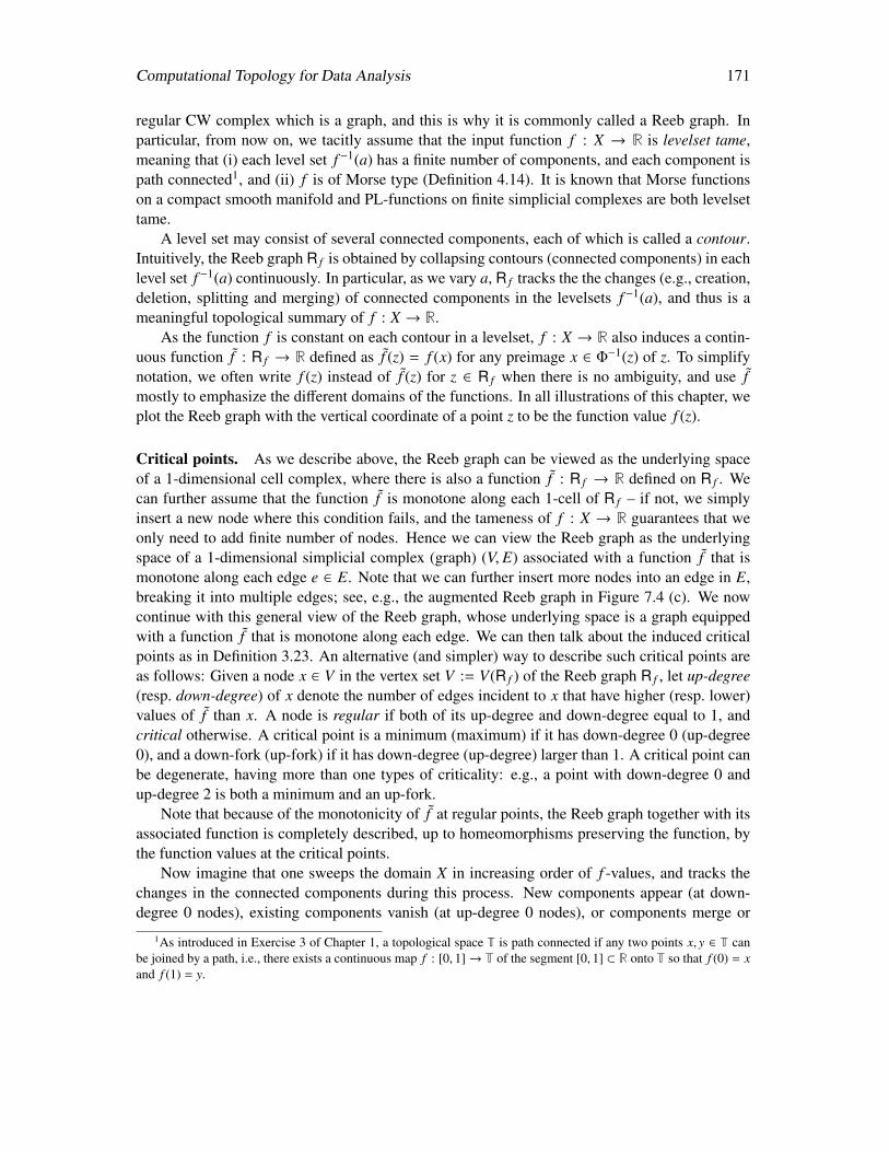
Computational Topology for Data Analysis 171
regular CW complex which is a graph, and this is why it is commonly called a Reeb graph. Inparticular, from now on, we tacitly assume that the input function f : X → R is levelset tame,meaning that (i) each level set f −1(a) has a finite number of components, and each component ispath connected1, and (ii) f is of Morse type (Definition 4.14). It is known that Morse functionson a compact smooth manifold and PL-functions on finite simplicial complexes are both levelsettame.
A level set may consist of several connected components, each of which is called a contour.Intuitively, the Reeb graph R f is obtained by collapsing contours (connected components) in eachlevel set f −1(a) continuously. In particular, as we vary a, R f tracks the the changes (e.g., creation,deletion, splitting and merging) of connected components in the levelsets f −1(a), and thus is ameaningful topological summary of f : X → R.
As the function f is constant on each contour in a levelset, f : X → R also induces a contin-uous function f : R f → R defined as f (z) = f (x) for any preimage x ∈ Φ−1(z) of z. To simplifynotation, we often write f (z) instead of f (z) for z ∈ R f when there is no ambiguity, and use fmostly to emphasize the different domains of the functions. In all illustrations of this chapter, weplot the Reeb graph with the vertical coordinate of a point z to be the function value f (z).
Critical points. As we describe above, the Reeb graph can be viewed as the underlying spaceof a 1-dimensional cell complex, where there is also a function f : R f → R defined on R f . Wecan further assume that the function f is monotone along each 1-cell of R f – if not, we simplyinsert a new node where this condition fails, and the tameness of f : X → R guarantees that weonly need to add finite number of nodes. Hence we can view the Reeb graph as the underlyingspace of a 1-dimensional simplicial complex (graph) (V, E) associated with a function f that ismonotone along each edge e ∈ E. Note that we can further insert more nodes into an edge in E,breaking it into multiple edges; see, e.g., the augmented Reeb graph in Figure 7.4 (c). We nowcontinue with this general view of the Reeb graph, whose underlying space is a graph equippedwith a function f that is monotone along each edge. We can then talk about the induced criticalpoints as in Definition 3.23. An alternative (and simpler) way to describe such critical points areas follows: Given a node x ∈ V in the vertex set V := V(R f ) of the Reeb graph R f , let up-degree(resp. down-degree) of x denote the number of edges incident to x that have higher (resp. lower)values of f than x. A node is regular if both of its up-degree and down-degree equal to 1, andcritical otherwise. A critical point is a minimum (maximum) if it has down-degree 0 (up-degree0), and a down-fork (up-fork) if it has down-degree (up-degree) larger than 1. A critical point canbe degenerate, having more than one types of criticality: e.g., a point with down-degree 0 andup-degree 2 is both a minimum and an up-fork.
Note that because of the monotonicity of f at regular points, the Reeb graph together with itsassociated function is completely described, up to homeomorphisms preserving the function, bythe function values at the critical points.
Now imagine that one sweeps the domain X in increasing order of f -values, and tracks thechanges in the connected components during this process. New components appear (at down-degree 0 nodes), existing components vanish (at up-degree 0 nodes), or components merge or
1As introduced in Exercise 3 of Chapter 1, a topological space T is path connected if any two points x, y ∈ T canbe joined by a path, i.e., there exists a continuous map f : [0, 1]→ T of the segment [0, 1] ⊂ R onto T so that f (0) = xand f (1) = y.
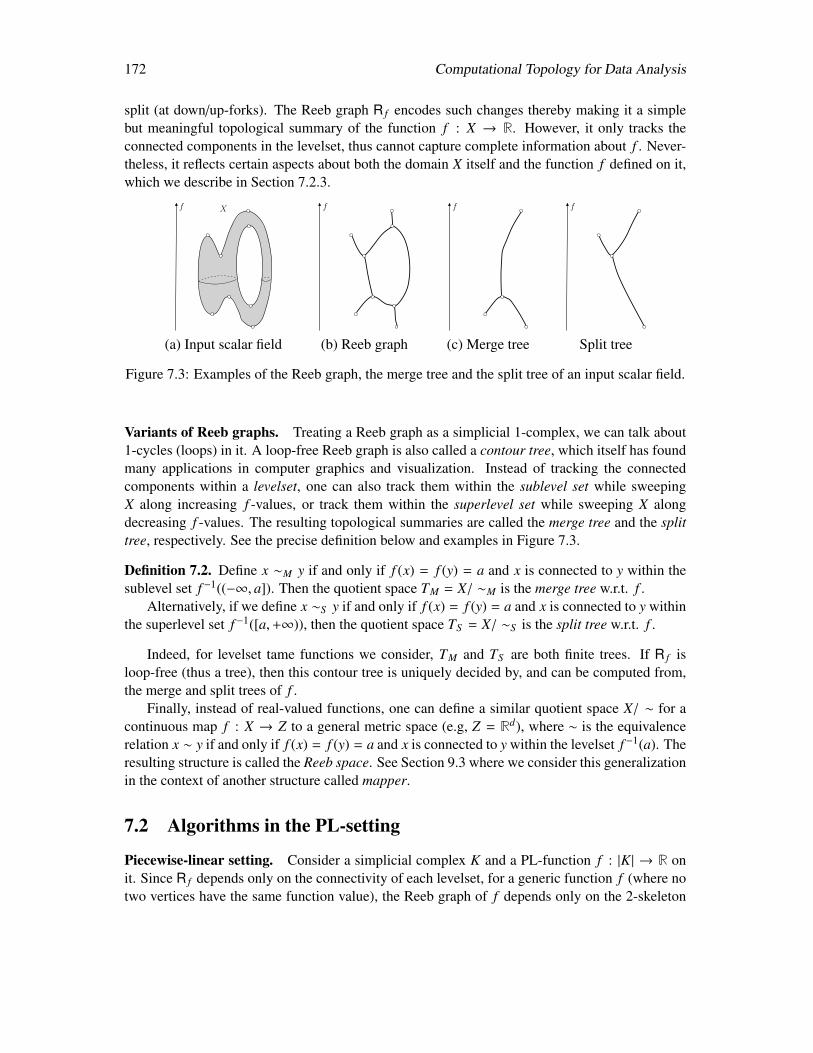
172 Computational Topology for Data Analysis
split (at down/up-forks). The Reeb graph R f encodes such changes thereby making it a simplebut meaningful topological summary of the function f : X → R. However, it only tracks theconnected components in the levelset, thus cannot capture complete information about f . Never-theless, it reflects certain aspects about both the domain X itself and the function f defined on it,which we describe in Section 7.2.3.
f X f f f
(a) Input scalar field (b) Reeb graph (c) Merge tree Split tree
Figure 7.3: Examples of the Reeb graph, the merge tree and the split tree of an input scalar field.
Variants of Reeb graphs. Treating a Reeb graph as a simplicial 1-complex, we can talk about1-cycles (loops) in it. A loop-free Reeb graph is also called a contour tree, which itself has foundmany applications in computer graphics and visualization. Instead of tracking the connectedcomponents within a levelset, one can also track them within the sublevel set while sweepingX along increasing f -values, or track them within the superlevel set while sweeping X alongdecreasing f -values. The resulting topological summaries are called the merge tree and the splittree, respectively. See the precise definition below and examples in Figure 7.3.
Definition 7.2. Define x ∼M y if and only if f (x) = f (y) = a and x is connected to y within thesublevel set f −1((−∞, a]). Then the quotient space TM = X/ ∼M is the merge tree w.r.t. f .
Alternatively, if we define x ∼S y if and only if f (x) = f (y) = a and x is connected to y withinthe superlevel set f −1([a,+∞)), then the quotient space TS = X/ ∼S is the split tree w.r.t. f .
Indeed, for levelset tame functions we consider, TM and TS are both finite trees. If R f isloop-free (thus a tree), then this contour tree is uniquely decided by, and can be computed from,the merge and split trees of f .
Finally, instead of real-valued functions, one can define a similar quotient space X/ ∼ for acontinuous map f : X → Z to a general metric space (e.g, Z = Rd), where ∼ is the equivalencerelation x ∼ y if and only if f (x) = f (y) = a and x is connected to y within the levelset f −1(a). Theresulting structure is called the Reeb space. See Section 9.3 where we consider this generalizationin the context of another structure called mapper.
7.2 Algorithms in the PL-setting
Piecewise-linear setting. Consider a simplicial complex K and a PL-function f : |K| → R onit. Since R f depends only on the connectivity of each levelset, for a generic function f (where notwo vertices have the same function value), the Reeb graph of f depends only on the 2-skeleton
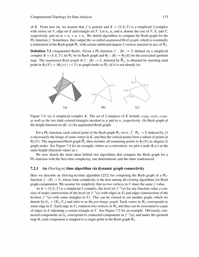
Computational Topology for Data Analysis 173
of K. From now on, we assume that f is generic and K = (V, E,T ) is a simplicial 2-complexwith vertex set V , edge set E and triangle set T . Let nv, ne and nt denote the size of V , E, and T ,respectively, and set m = nv + ne + nt. We sketch algorithms to compute the Reeb graph for thePL-function f . Sometimes, they output the so-called augmented Reeb graph, which is essentiallya refinement of the Reeb graph R f with certain additional degree-2 vertices inserted in arcs of R f .
Definition 7.3 (Augmented Reeb). Given a PL-function f : |K| → R defined on a simplicialcomplex K = (V, E,T ), let R f be its Reeb graph and Φ f : |K| → R f (K) be the associated quotientmap. The augmented Reeb graph of f : |K| → R, denoted by R f , is obtained by inserting eachpoint in Φ f (V) := Φ f (v) | v ∈ V as graph nodes to R f (if it is not already in).
r
q
p
w
Φf(p)
Φf(w)
Φf(p)
Φf(q)
Φf(r)
Φf(w)
(a) (b) (c)
Figure 7.4: (a) A simplicial complex K. The set of 2-simpices of K include 4rpq,4rpw,4rqw,as well as the two dark-colored triangles incident to p and to w, respectively. (b) Reeb graph ofthe height function on |K|. (c) Its augmented Reeb graph.
For a PL-function, each critical point of the Reeb graph R f (w.r.t. f : R f → R induced by f )is necessarily the image of some vertex in K, and thus the critical points form a subset of points inΦ f (V). The augmented Reeb graph R f then includes all remaining points in Φ f (V) as (degree-2)graph nodes. See Figure 7.4 for an example, where as a convention, we plot a node Φ f (v) at thesame height (function value) as v.
We now sketch the main ideas behind two algorithms that compute the Reeb graph for aPL-function with the best time complexity, one deterministic and the other randomized.
7.2.1 An O(m log m) time algorithm via dynamic graph connectivity
Here we describe an O(m log m)-time algorithm [252] for computing the Reeb graph of a PL-function f : |K| → R, whose time complexity is the best among all existing algorithms for Reebgraph computation. We assume for simplicity that no two vertices in V share the same f -value.
As K = (V, E,T ) is a simplicial 2-complex, the level set f −1(a) for any function value a con-sists of nodes (intersection of the level set f −1(a) with edges in E) and edges (intersection of thelevelset f −1(a) with some triangles in T ). This can be viewed as yet another graph, which wedenote by Ga = (Wa, Fa) and refer to as the pre-image graph: Each vertex in Wa corresponds tosome edge in E. Each edge in Fa connects two vertices in Wa and thus can be associated to a pairof edges in E adjoining a certain triangle in T . See Figure 7.5 for an example. Obviously, con-nected components in Ga correspond to connected components in f −1(a), and under the quotientmap Φ, each component is mapped to a single point in the Reeb graph R f .
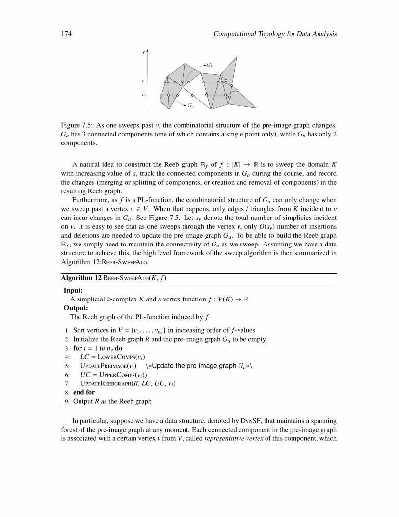
174 Computational Topology for Data Analysis
v
f
a
Ga
b
Gb
Figure 7.5: As one sweeps past v, the combinatorial structure of the pre-image graph changes.Ga has 3 connected components (one of which contains a single point only), while Gb has only 2components.
A natural idea to construct the Reeb graph R f of f : |K| → R is to sweep the domain Kwith increasing value of a, track the connected components in Ga during the course, and recordthe changes (merging or splitting of components, or creation and removal of components) in theresulting Reeb graph.
Furthermore, as f is a PL-function, the combinatorial structure of Ga can only change whenwe sweep past a vertex v ∈ V . When that happens, only edges / triangles from K incident to vcan incur changes in Ga. See Figure 7.5. Let sv denote the total number of simplicies incidenton v. It is easy to see that as one sweeps through the vertex v, only O(sv) number of insertionsand deletions are needed to update the pre-image graph Ga. To be able to build the Reeb graphR f , we simply need to maintain the connectivity of Ga as we sweep. Assuming we have a datastructure to achieve this, the high level framework of the sweep algorithm is then summarized inAlgorithm 12:Reeb-SweepAlg.
Algorithm 12 Reeb-SweepAlg(K, f )
Input:A simplicial 2-complex K and a vertex function f : V(K)→ R
Output:The Reeb graph of the PL-function induced by f
1: Sort vertices in V = v1, . . . , vnv in increasing order of f -values2: Initialize the Reeb graph R and the pre-image grpah Ga to be empty3: for i = 1 to nv do4: LC = LowerComps(vi)5: UpdatePreimage(vi) \∗Update the pre-image graph Ga∗\
6: UC = UpperComps(vi))7: UpdateReebgraph(R, LC, UC, vi)8: end for9: Output R as the Reeb graph
In particular, suppose we have a data structure, denoted by DynSF, that maintains a spanningforest of the pre-image graph at any moment. Each connected component in the pre-image graphis associated with a certain vertex v from V , called representative vertex of this component, which
Computational Topology for Data Analysis 175
indicates that this component is created when passing through v. We assume that the data structureDynSF allows the following operations: First, assume that a graph node ea ∈ Wa in the pre-imagegraph Ga is generated by edge e ∈ K, that is, ea is the intersection of e with the levelset f −1(a).
• Find(e): given an edge e ∈ E, returns the representative vertex of the component in thecurrent pre-image graph Ga containing the node ea ∈ Wa generated by e.
• Insert(e, e′), Delete(e, e′): inserts an edge (ea, e′a) into Ga and deletes (ea, e′a) from Ga
respectively while still maintaining a spanning forest for Ga under these operations.
Using these operations, the pseudo-codes for the subroutines called in algorithm Reeb-SweepAlgare given in Algorithms 13:LowerComps, 14:UpdatePreImage, and 15:UpdateReebGraph. (Theroutine UpperComps is symmetric to LowerComps and thus omitted.) These codes assume thatedges of K not intersecting the levelsets are still in the pre-image graphs as isolated nodes; hencethere is no need to add or remove isolated nodes.
Algorithm 13 LowerComps(v)
Input:a vertex v ∈ K
Output:A list Lc of connected components in the pre-image graph generated by the lower-star of v
1: LC = empty list2: for all edges e in the lower-star of v do3: c = DynSF.Find(e)4: if c is not marked ‘listed’ then5: LC.add(c); and mark c as ’listed’6: end if7: end for
Time complexity analysis. Suppose the input simplicial 2-complex K = (V, E,T ) has n verticesand m simplices in total. Sorting the vertices takes O(n log n) time. Then steps 4 to 7 of thealgorithm Reeb-SweepAlg performs O(m) numbers of Find, Insert and Delete operations usingthe data structure DynSF.
One could use state-of-the-art data structure for dynamic graph connectivity as DynSF – in-deed, this is the approach taken in [146]. However, note that this is an offline version of thedynamic graph connectivity problem, as all insertions / deletions are known in advance and thuscan be pre-computed. To this end, we assign each edge in the pre-image graph a weight, which isthe time ( f -value) it will be deleted from the pre-image graph Ga. We then maintain a maximumspanning forest of Ga during the sweeping to maintain connectivity. In general, a deletion of amaximum-spanning tree edge (u, v) can incur expensive search in the pre-image graph for a re-placement edge (as u and v may still be connected). However, because of the specific assignmentof edge weights, this expensive search is avoided in this case. If a maximum spanning tree edgeis to be deleted, it will simply break the tree in the maximum spanning forest containing thisedge, and no replacement edge needs to be identified. One can use a standard dynamic tree data

176 Computational Topology for Data Analysis
Algorithm 14 UpdatePreImage(v)
Input:A vertex v ∈ K
Output:Update the pre-image graph after sweeping past v
1: for all triangles uvw incident on v do2: \∗ w.l.o.g. assume f (u) < f (w) ∗\3: if f (v) < f (u) then4: DynSF.Insert(vu, vw)5: else6: if f (v) > f (w) then7: DynSF.Delete(vu, vw)8: else9: DynSF.Delete(uv, uw)
10: DynSF.Insert(vw, uw)11: end if12: end if13: end for
Algorithm 15 UpdateReebGraph(R, LC, UC, v)
Input:Current Reeb graph R for f −1(−∞, f (v)), a vertex v, the list LC (resp. UC) of components in
the lower-star (resp. upper-star) of vOutput:
Update Reeb graph R to be that for sublevel set f −1(−∞, f (v) + ε] for an infinitesimally smallε > 0
1: Create a new node v in R corresponding to v2: Assign node v to each component in UC3: Create an arc in R between v and the Reeb graph node corresponding to the representative
vertex of each c in LC4: Return updated Reeb graph R
structure, such as the Link-Cut trees [280], to maintain the maximum spanning forest efficiently inO(log m) amortized time for each find / insertion / deletion operation. Putting everything together,it takes O(m log m) time to compute the Reeb graph by the sweep.
Theorem 7.1. Given a PL-function f : |K| → R, let m denote the total number of simplices in the2-skeleton of K. One can compute the (augmented) Reeb graph R f of f in O(m log m) time.
7.2.2 A randomized algorithm with O(m log m) expected time
In this section we describe a randomized algorithm [185] whose expected time complexity matchesthe previous algorithm. However, it uses a strategy different from sweeping: Intuitively, it directly
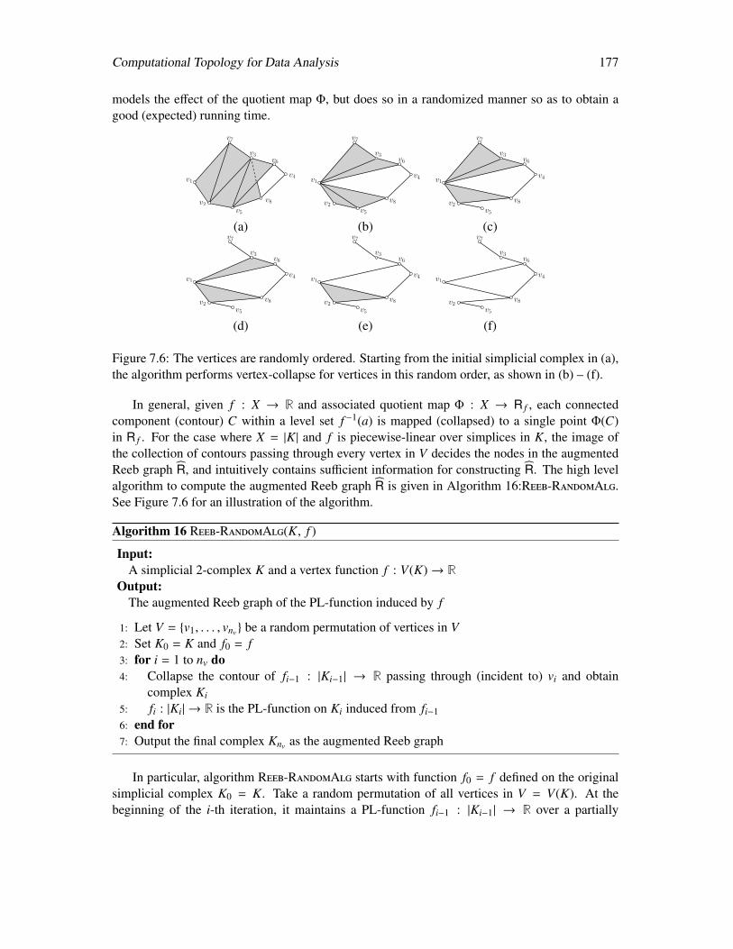
Computational Topology for Data Analysis 177
models the effect of the quotient map Φ, but does so in a randomized manner so as to obtain agood (expected) running time.
v1
v2
v7
v3v6
v4
v8v5
v1
v2
v7
v3v6
v4
v8v5
v1
v2
v7
v3v6
v4
v8v5
(a) (b) (c)
v1
v2
v7
v3v6
v4
v8v5
v1
v2
v7
v3v6
v4
v8v5
v1
v2
v7
v3v6
v4
v8v5
(d) (e) (f)
Figure 7.6: The vertices are randomly ordered. Starting from the initial simplicial complex in (a),the algorithm performs vertex-collapse for vertices in this random order, as shown in (b) – (f).
In general, given f : X → R and associated quotient map Φ : X → R f , each connectedcomponent (contour) C within a level set f −1(a) is mapped (collapsed) to a single point Φ(C)in R f . For the case where X = |K| and f is piecewise-linear over simplices in K, the image ofthe collection of contours passing through every vertex in V decides the nodes in the augmentedReeb graph R, and intuitively contains sufficient information for constructing R. The high levelalgorithm to compute the augmented Reeb graph R is given in Algorithm 16:Reeb-RandomAlg.See Figure 7.6 for an illustration of the algorithm.
Algorithm 16 Reeb-RandomAlg(K, f )
Input:A simplicial 2-complex K and a vertex function f : V(K)→ R
Output:The augmented Reeb graph of the PL-function induced by f
1: Let V = v1, . . . , vnv be a random permutation of vertices in V2: Set K0 = K and f0 = f3: for i = 1 to nv do4: Collapse the contour of fi−1 : |Ki−1| → R passing through (incident to) vi and obtain
complex Ki
5: fi : |Ki| → R is the PL-function on Ki induced from fi−16: end for7: Output the final complex Knv as the augmented Reeb graph
In particular, algorithm Reeb-RandomAlg starts with function f0 = f defined on the originalsimplicial complex K0 = K. Take a random permutation of all vertices in V = V(K). At thebeginning of the i-th iteration, it maintains a PL-function fi−1 : |Ki−1| → R over a partially
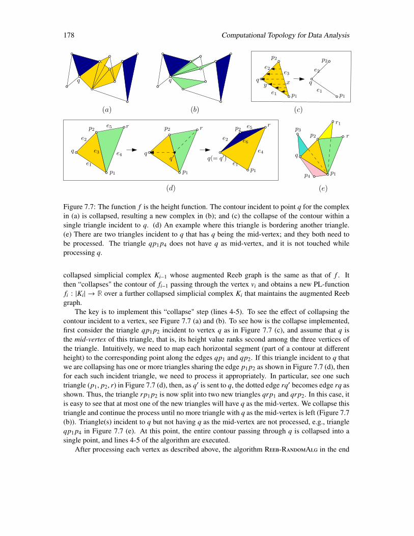
178 Computational Topology for Data Analysis
q q
p2
e2
qe3
x
p1
ye1
p2
e2
qe1
p1
(a) (b) (c)
(d) (e)
re5p2
e2
q
e1
e4
p1
rp2
qq′
p1
r
e4
p1e1
p2 e5
e2
q(= q′)e3
e6
r1
r
p1
p3
q
p2
p4
Figure 7.7: The function f is the height function. The contour incident to point q for the complexin (a) is collapsed, resulting a new complex in (b); and (c) the collapse of the contour within asingle triangle incident to q. (d) An example where this triangle is bordering another triangle.(e) There are two triangles incident to q that has q being the mid-vertex; and they both need tobe processed. The triangle qp1 p4 does not have q as mid-vertex, and it is not touched whileprocessing q.
collapsed simplicial complex Ki−1 whose augmented Reeb graph is the same as that of f . Itthen “collapses" the contour of fi−1 passing through the vertex vi and obtains a new PL-functionfi : |Ki| → R over a further collapsed simplicial complex Ki that maintains the augmented Reebgraph.
The key is to implement this “collapse" step (lines 4-5). To see the effect of collapsing thecontour incident to a vertex, see Figure 7.7 (a) and (b). To see how is the collapse implemented,first consider the triangle qp1 p2 incident to vertex q as in Figure 7.7 (c), and assume that q isthe mid-vertex of this triangle, that is, its height value ranks second among the three vertices ofthe triangle. Intuitively, we need to map each horizontal segment (part of a contour at differentheight) to the corresponding point along the edges qp1 and qp2. If this triangle incident to q thatwe are collapsing has one or more triangles sharing the edge p1 p2 as shown in Figure 7.7 (d), thenfor each such incident triangle, we need to process it appropriately. In particular, see one suchtriangle (p1, p2, r) in Figure 7.7 (d), then, as q′ is sent to q, the dotted edge rq′ becomes edge rq asshown. Thus, the triangle rp1 p2 is now split into two new triangles qrp1 and qrp2. In this case, itis easy to see that at most one of the new triangles will have q as the mid-vertex. We collapse thistriangle and continue the process until no more triangle with q as the mid-vertex is left (Figure 7.7(b)). Triangle(s) incident to q but not having q as the mid-vertex are not processed, e.g., triangleqp1 p4 in Figure 7.7 (e). At this point, the entire contour passing through q is collapsed into asingle point, and lines 4-5 of the algorithm are executed.
After processing each vertex as described above, the algorithm Reeb-RandomAlg in the end
Computational Topology for Data Analysis 179
computes the final complex Knv in line 7. It is necessarily a simplicial 1-complex because novertex can be the mid-vertex of any triangle, implying that there is no triangle left. It is easy tosee that, by construction, Knv is the augmented Reeb graph w.r.t. f : |K| → R.
Time complexity. For each vertex v, the time complexity of the collapse is proportional tothe number of triangles Tv intersected by the contour Cv passing through v. In the worst case,Tv = |nt|, giving rise to O(nvnt) worst case running time for algorithm Reeb-RandomAlg. Thisworst case time complexity turns out to be tight. However, if one processes the vertices in arandom order, then the worst case behavior is unlikely to happen, and the expected running timecan be proven to be O(m log nv) = O(m log m). Essentially, one argues that an original trianglefrom the input simplicial complex is split only O(log nv) = O(log m) expected number of timesthus creating O(log m) expected number of intermediate triangles which takes O(log m) expectedtime to collapse. The argument is in spirit similar to the analysis of the path length in a randomlybuilt binary search tree [109].
Theorem 7.2. Given a PL-function f : |K| → R defined on a simpicial 2-complex K with msimplices, one can compute the (augmented) Reeb graph in O(m log m) expected time.
7.2.3 Homology groups of Reeb graphs
Homology groups for a graph can have non-trivial ranks only in dimension zero and one. There-fore, for a Reeb graph R f , we only need to consider H0(R f ) and H1(R f ). In particular, their rankβ0(R f ) and β1(R f ) are simply the number of connected components and the number of indepen-dent loops in R f respectively.
Fact 7.1. For a tame function f : X → R, β0(X) = β0(R f ) and β1(X) ≥ β1(R f ).
The equality β0(X) = β0(R f ) in the above statement follows from the fact that R f is the quo-tient space X/ ∼ and each equivalent class itself is connected (it is a connected component in somelevelset). The relation on β1 can be proven directly, and it is also a by-product of Theorem 7.4below (combined with Fact 7.2). The above statement also implies that if X is simply connected,then R f is loop-free.
For the case where X is a 2-manifold, more information about X can be recovered from theReeb graph of a Morse function defined on it.
Theorem 7.3 ([107]). Let f : X → R be a Morse function defined on a connected and compact2-manifold.
(i) if X is orientable, β1(R f ) = β1(X)/2; and
(ii) if X is non-orientable, β1(R f ) ≤ β1(X)/2.
We now present a result that characterizes H1(R f ) w.r.t. H1(X) in a more precise manner,which also generalizes Theorem 7.3.
180 Computational Topology for Data Analysis
Horizontal and vertical homology. Given a continuous function f : X → R, let X=a :=f −1(a) and XI := f −1(I) denote its levelset and interval set as before for a ∈ R and for an open orclosed interval I ⊆ R respectively. We first define the so-called horizontal and vertical homologygroups with respect to f .
A p-th homology class h ∈ Hp(X) is horizontal if there exists a finite set of values ai ∈ Ri∈A,where A is a finite index set, such that h has a pre-image under the map Hp(
⋃i∈A X=ai) → Hp(X)
induced by inclusion. The set of horizontal homology classes form a subgroup Hp(X) of Hp(X)since the trivial homology class is horizontal, and the addition of any two horizontal homologyclasses is still horizontal. We call this subgroup Hp(X) the horizontal homology group of X withrespect to f . The vertical homology group of X with respect to f is then defined as:
Hp(X) := Hp(X)/Hp(X), the quotient of Hp(X) with Hp(X).
The coset ω + Hp(X) for every class ω ∈ Hp(X) provides an equivalence class in Hp(X). We callh a vertical homology class if h + Hp(X) is not 0 in Hp(X). In other words, h < Hp(X). Twohomology classes h1 and h2 are vertically homologous if h1 ∈ h2 + Hp(X).
Fact 7.2. By definition, rank (Hp(X)) = rank (Hp(X)) + rank (Hp(X)).
Let I be a closed interval of R. We define the height of I = [a, b] to be height(I) = |b−a|; notethat the height could be 0. Given a homology class h ∈ Hp(X) and an interval I, we say that h issupported by I if h ∈ im (i∗) where i∗ : Hp(XI) → Hp(X) is the homomorphism induced by thecanonical inclusion XI → X. In other words, XI contains a p-cycle γ from the homology class h.We define the height of a homology class h ∈ Hp(X) to be
height(h) = infI supports h
height(I).
Isomorphism between H1(X) and H1(R f ). The surjection Φ : X → R f (X) induces a chain mapΦ# from the 1-dimensional singular chain group of X to the 1-dimensional singular chain group ofR f (X) which eventually induces a homomorphism Φ∗ : H1(X) → H1(R f (X)). For the horizontalsubgroup H1(X), we have that Φ∗(H1(X)) = 0 ∈ H1(R f (X)). Hence Φ∗ induces a well-definedhomomorphism between the quotient groups
Φ : H1(X) =H1(X)
H1(X)→
H1(R f (X))
H1(R f (X))= H1(R f (X)).
The right equality above follows from that H1(R f (X)) = 0, which holds because every level setof R f (X) consists only of a finite set of disjoint points due to the levelset-tameness of functionf : X → R. It turns out that Φ is an isomorphism – Intuitively, this is not surprising as Φ mapseach contour in the level set to a single point, which in turn collapses every horizontal cycle.
Theorem 7.4. Given a levelset tame function f : X → R, let Φ : H1(X) → H1(R f (X)) bethe homomorphism induced by the surjection Φ : X → R f (X) as defined above. Then the mapΦ is an isomorphism. Furthermore, for any vertical homology class h ∈ H1(X), we have thatheight(h) = height(Φ(h)).
Computational Topology for Data Analysis 181
Persistent homology for f : R f → R. We have discussed earlier that the Reeb graph of alevelset tame function f : X → R can be represented by a graph whose edges have monotonefunction values. Then, the function f : R f → R can be treated as a PL-function on the simpli-cial 1-complex R f . This gives rise to the standard setting where a PL-function f is defined on asimplicial 1-complex R f whose persistence is to be computed. We can apply algorithm ZeroP-erDg from Section 3.5.3 to compute the 0-th persistence diagram Dgm0( f ). For computing onedimensional persistence diagram Dgm1( f ), one can modify this algorithm slightly by registeringthe function values of the edges that create cycles. These are edges that connect vertices in thesame component. The function values of these edges are the birth points of the 1-cycles that neverdie. This algorithm takes O(n log n + mα(n)) time where m and n are the number of vertices andedges respectively in R f .
We can also compute the levelset zigzag persistence of f (Section 4.5) using the zigzag per-sistence algorithm in Section 4.3.2. However, taking advantage of the graph structures, one cancompute the levelset zigzag persistence for a Reeb graph with n vertices and edges in O(n log n)time using an algorithm of [5] that takes advantage of mergeable tree data structure [169]. Onlythe 0-th persistence diagram Dgm0( f ) is nontrivial in this case. We can read the zeroth persistencediagram for the standard persistence using Theorem 4.15 from this level set persistence diagram.Furthermore, for every infinite bar [ai,∞) in the standard one dimensional persistence diagram,we get a pairing (a j, ai) (open-open bar) in the zeroth levelset diagram Dgm0( f ).
Reeb graphs can be a useful tool to compute the zeroth levelset zigzag persistence diagramof a function on a topological space. Let f : X → R be a continuous function whose zerothpersistence diagram we want to compute. We already observed that the function f induces acontinuous function on the Reeb graph R f . To distinguish the two domains more explicitly, wedenote the former function f X and the latter as f R. The following observation helps computing thezeroth levelset zigzag persistence diagram Dgm0( f X) because computationally it is much harderto process a space, say the underlying space of a simplicial complex than only a graph (simplicial1-complex).
Proposition 7.5. Dgm0( f X) = Dgm0( f R) where the diagrams are for the zeroth levelset zigzagpersistence.
The result follows from the following observation. Consider the levelset zigzag filtrations FX
and FR for the two functions as in sequence (4.15).
FX : X(a0,a2) ← · · · → X(ai−1,ai+1) ← X(ai,ai+1) → X(ai,ai+2) ← · · · → X(an−1,an+1)
FR : R f (a0,a2) ← · · · → R f (ai−1,ai+1) ← R f (ai,ai+1) → R f (ai,ai+2) ← · · · → R f (an−1,an+1)
Using notation for interval sets X ji = X(ai,a j) and R j
i = R f (ai,a j), we have the following com-
mutative diagram between the 0-th levelset zigzag persistence modules.
H0FX : H0(X0
0) // H0(X10) H0(X1
1) · · ·oo // H0(Xnn−1) H0(Xn
n)oo
H0FR : H0(R0
0) // H0(R10) H0(R1
1) · · ·oo // H0(Rnn−1) H0(Rn
n)oo
182 Computational Topology for Data Analysis
All vertical maps are isomorphism because the number of components in Xij is exactly equal to
the number of components in the quotient space Rij = Xi
j/ ∼ which is used to define the Reebgraph. All horizontal maps are induced by inclusions. It follows that every square in the abovediagram commutes. Therefore the above two modules are isomorphic.
7.3 Distances for Reeb graphs
Several distance measures have been proposed for Reeb graphs. In this section, we introduce twodistances, one based on a natural interleaving idea, and the other based on the Gromov-Hausdorffdistance idea. It has been shown that these two distance measures are strongly equivalent, that is,they are within a constant factor of each other for general Reeb graphs. For the special case ofmerge trees, the two distance measures are exactly the same.
So far, we have used R f to denote the Reeb graph of a function f . For notational convenience,in the following we use a different notation F for R f . Suppose we are given two Reeb graphs Fand G with the functions f : F → R and g : G → R associated to them. To emphasize theassociated functions we write (F, f ) and (G, g) in place of F and G when convenient. Again, weassume that each Reeb graph is a finite simplicial 1-complex and the function is strictly monotoneon each edges. Our goal is to develop a concept of distance d(F,G) between them. Intuitively, iftwo Reeb graphs are “the same”, then they are isomorphic and the function value of each point isalso preserved under the isomorphism. If two Reeb graphs are not the same, we aim to measurehow far it deviates from being “isomorphic". The two distances we introduce below both followthis intuition, but measures the “deviation” differently.
7.3.1 Interleaving distance
We borrow the idea of interleaving between persistence modules (Section 3.4) to define a dis-tance between Reeb graphs. Roughly speaking, instead of requiring that there is an isomorphismbetween the two Reeb graphs, which would give rise to a pair of maps between them, φ : F → Gand φ−1 : G → F that is function preserving, we look for the existence of a pair of “compatible”maps between appropriately “thickened" versions of F and G and the distance is measured by theminimum amount of the “thickening" needed. We make this more precise below. First, given anyspace X, set Xε := X × [−ε, ε].
Definition 7.4. Given a Reeb graph (F, f ), its ε-smoothing, denoted by Sε(F, f ), is the Reebgraph of the function fε : Fε → R where fε(x, t) = f (x) + t for x ∈ F and t ∈ [−ε, ε]. In otherwords, Sε(F, f ) = Fε/ ∼ fε , where ∼ fε denotes the equivalence relation where x ∼ fε y if and onlyif x, y ∈ Fε are from the same contour of fε.
See Figure 7.8 for an example. As Sε(F, f ) is the quotient space Fε/ ∼ fε , we use [x, t],x ∈ F, t ∈ [−ε, ε], to denote a point in Sε(F, f ), which is the equivalent class of (x, t) ∈ Fεunder the equivalence relation ∼ fε . Also, note that there is a natural “quotiented-inclusion” mapι : (F, f )→ Sε(F, f ) defined as ι(x) = [x, 0], for any x ∈ F.
Suppose we have two Reeb graphs (A, fa) and (B, fb). A map µ : (A, fa) → (B, fb) betweenthem is function-preserving if fa(x) = fb(µ(x)) for each x ∈ A. A function-preserving map µ be-tween (A, fa) and Sε(B, fb) induces a function-preserving map µε between Sε(A, fa) and S2ε(B, fb)
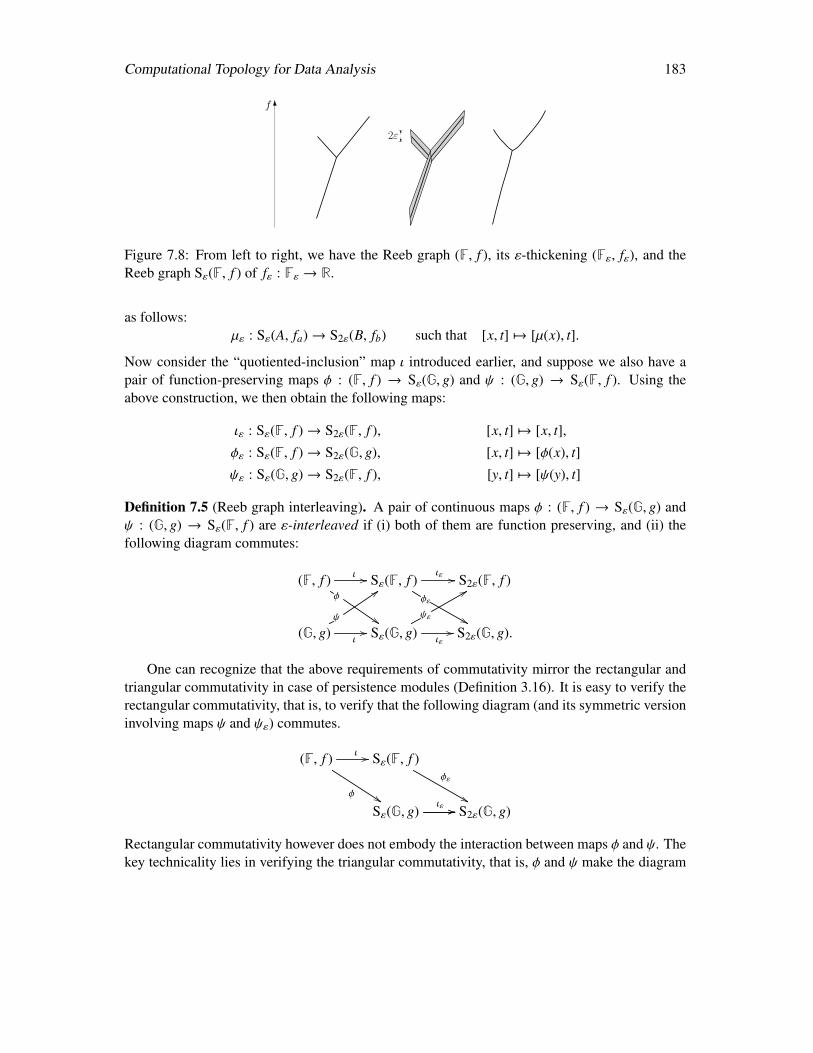
Computational Topology for Data Analysis 183
f
2ε
Figure 7.8: From left to right, we have the Reeb graph (F, f ), its ε-thickening (Fε, fε), and theReeb graph Sε(F, f ) of fε : Fε → R.
as follows:µε : Sε(A, fa)→ S2ε(B, fb) such that [x, t] 7→ [µ(x), t].
Now consider the “quotiented-inclusion” map ι introduced earlier, and suppose we also have apair of function-preserving maps φ : (F, f ) → Sε(G, g) and ψ : (G, g) → Sε(F, f ). Using theabove construction, we then obtain the following maps:
ιε : Sε(F, f )→ S2ε(F, f ), [x, t] 7→ [x, t],
φε : Sε(F, f )→ S2ε(G, g), [x, t] 7→ [φ(x), t]
ψε : Sε(G, g)→ S2ε(F, f ), [y, t] 7→ [ψ(y), t]
Definition 7.5 (Reeb graph interleaving). A pair of continuous maps φ : (F, f ) → Sε(G, g) andψ : (G, g) → Sε(F, f ) are ε-interleaved if (i) both of them are function preserving, and (ii) thefollowing diagram commutes:
(F, f ) ι //
φ
$$
Sε(F, f )ιε //
φε
&&
S2ε(F, f )
(G, g) ι//
ψ
::
Sε(G, g) ιε//
ψε
88
S2ε(G, g).
One can recognize that the above requirements of commutativity mirror the rectangular andtriangular commutativity in case of persistence modules (Definition 3.16). It is easy to verify therectangular commutativity, that is, to verify that the following diagram (and its symmetric versioninvolving maps ψ and ψε) commutes.
(F, f ) ι //
φ $$
Sε(F, f )φε
&&Sε(G, g)
ιε //// S2ε(G, g)
Rectangular commutativity however does not embody the interaction between maps φ and ψ. Thekey technicality lies in verifying the triangular commutativity, that is, φ and ψ make the diagram
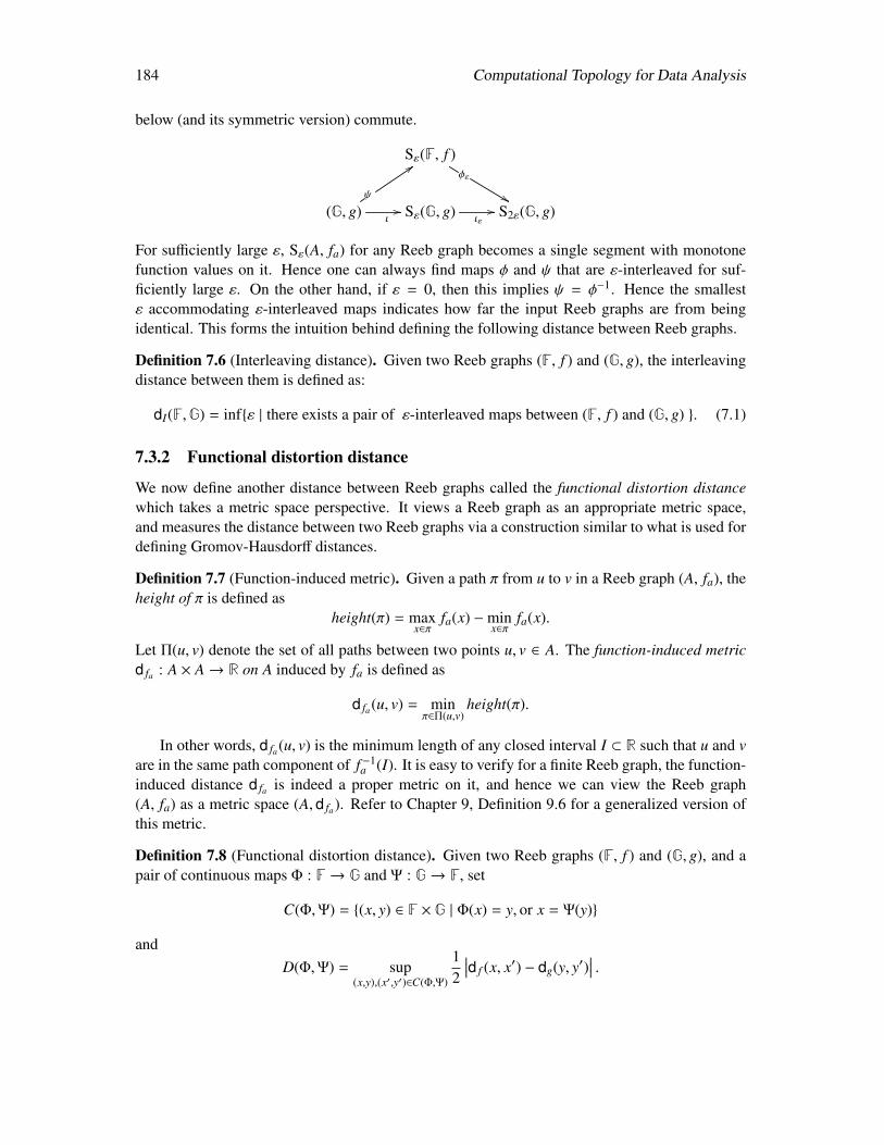
184 Computational Topology for Data Analysis
below (and its symmetric version) commute.
Sε(F, f )φε
&&(G, g) ι
//ψ
::
Sε(G, g) ιε// S2ε(G, g)
For sufficiently large ε, Sε(A, fa) for any Reeb graph becomes a single segment with monotonefunction values on it. Hence one can always find maps φ and ψ that are ε-interleaved for suf-ficiently large ε. On the other hand, if ε = 0, then this implies ψ = φ−1. Hence the smallestε accommodating ε-interleaved maps indicates how far the input Reeb graphs are from beingidentical. This forms the intuition behind defining the following distance between Reeb graphs.
Definition 7.6 (Interleaving distance). Given two Reeb graphs (F, f ) and (G, g), the interleavingdistance between them is defined as:
dI(F,G) = infε | there exists a pair of ε-interleaved maps between (F, f ) and (G, g) . (7.1)
7.3.2 Functional distortion distance
We now define another distance between Reeb graphs called the functional distortion distancewhich takes a metric space perspective. It views a Reeb graph as an appropriate metric space,and measures the distance between two Reeb graphs via a construction similar to what is used fordefining Gromov-Hausdorff distances.
Definition 7.7 (Function-induced metric). Given a path π from u to v in a Reeb graph (A, fa), theheight of π is defined as
height(π) = maxx∈π
fa(x) −minx∈π
fa(x).
Let Π(u, v) denote the set of all paths between two points u, v ∈ A. The function-induced metricd fa : A × A→ R on A induced by fa is defined as
d fa(u, v) = minπ∈Π(u,v)
height(π).
In other words, d fa(u, v) is the minimum length of any closed interval I ⊂ R such that u and vare in the same path component of f −1
a (I). It is easy to verify for a finite Reeb graph, the function-induced distance d fa is indeed a proper metric on it, and hence we can view the Reeb graph(A, fa) as a metric space (A, d fa). Refer to Chapter 9, Definition 9.6 for a generalized version ofthis metric.
Definition 7.8 (Functional distortion distance). Given two Reeb graphs (F, f ) and (G, g), and apair of continuous maps Φ : F→ G and Ψ : G→ F, set
C(Φ,Ψ) = (x, y) ∈ F × G | Φ(x) = y, or x = Ψ(y)
andD(Φ,Ψ) = sup
(x,y),(x′,y′)∈C(Φ,Ψ)
12
∣∣∣d f (x, x′) − dg(y, y′)∣∣∣ .
Computational Topology for Data Analysis 185
The functional distortion distance between (F, f ) and (G, g) is defined as:
dFD(F,G) = infΦ,Ψ
max D(Φ,Ψ), ‖ f − g Φ‖∞, ‖g − f Ψ‖∞ . (7.2)
Note that the maps Φ and Ψ are not required to preserve function values; however the terms‖ f −gΦ‖∞ and ‖g− f Ψ‖∞ bound the difference in function values under the maps Φ and Ψ. Ifwe ignore these two terms ‖ f − g Φ‖∞ and ‖g − f Ψ‖∞, and if we do not assume that Φ and Ψ
have to be continuous, then dFD is the simply the Gromov-Hausdorff distance between the metricspaces (F, d f ) and (G, dg) [175]. The above definition is thus a function-adapted version of thecontinuous Gromov-Hausdorff distance 2.
Properties of the distances. The two distances we introduced turn out to be strongly equivalent.
Theorem 7.6 (Bi-Lipschitz equivalence). dFD ≤ 3dI ≤ 3dFD.
Furthermore, it is known that for Reeb graphs F,G derived from two “nice” functions f , g :X → R defined on the same domain X, both distances are stable [20, 116].
Definition 7.9 (Stable distance). Given f , g : X → R, let (F, f ) and (G, g) be the Reeb graph of fand g, respectively.
We say that a Reeb graph distance dR is stable if
dR((F, f ), (G, g)
)≤ ‖ f − g‖∞.
Finally, it is also known that these distances are bounded from below (up to a constant factor)by the bottleneck distance between the persistence diagrams associated to the two input Reebgraphs. In particular, given (F, f ) (and similarly for (G, g)), consider the 0-th persistence diagramDgm0( f ) induced by the levelset zigzag-filtration of f as in previous section. We consider onlythe 0-th persistence homology as each levelset f −1(a) consisting of only a finite set of points. Wehave the following result (see Theorem 3.2 of [33]).
Theorem 7.7. db(Dgm0( f ),Dgm0(g)) ≤ 2dI(F,G) ≤ 2dFD(F,G).
Universal Reeb graph distance. We introduced two Reeb graph distances above. There areother possible distances for Reeb graphs, such as the edit distance originally developed for Reebgraphs induced by functions on curves and surfaces. All these distances are stable, which is an im-portant property to have. The following concept allows one to identify the most “discriminative"Reeb graph distance among all stable distances.
Definition 7.10. A Reeb graph distance dU is universal if and only if (i) dU is stable; and (ii) forany other stable Reeb graph distance dS , we have dS ≤ dU .
2It turns out that if one removes the requirement of continuity on Φ and Ψ, the resulting functional distortiondistance takes values within a constant factor of dFD we defined for the case of Reeb graphs.
186 Computational Topology for Data Analysis
It has been shown that neither the interleaving distance nor the functional distortion distanceis universal. On the other hand, for Reeb graphs of piecewise-linear functions defined on com-pact triangulable spaces, such universal Reeb graph distance indeed exists. In particular, onecan construct a universal Reeb graph distance via a pullback idea to a common space; see [22].The authors of [22] propose two further edit-like distances for Reeb graphs, both of which areuniversal.
Computation. Unfortunately, except for the bottleneck distance db, the computation of any ofthe distances mentioned above is at least as hard as graph isomorphism. In fact, even for mergetrees (which are simpler variant of the Reeb graph, described in Definition 7.2 at the end ofSection 7.1), it is NP-hard to compute the interleaving distance between them [6]. But for thisspecial case, a fixed-parameter tractable algorithm exists [289].
7.4 Notes and Exercises
The Reeb graph was originally introduced for Morse functions [261]. It was naturally extendedto more general spaces as it does not rely on smooth / differential structures. This graph, asa summary of a scalar field, has found many applications in graphics, visualization and morerecently in data analysis; see e.g. [31, 32, 89, 123, 167, 189, 190, 276, 285, 290, 301]. Its loopfree version, the contour tree, has many applications of its own. Properties of the Reeb graph hasbeen studied in [107, 140]. The concept of Reeb space was introduced in [150]. The relations ofMerge, Split and Contour trees are studied in [67, 296].
An O(m log m) algorithm to compute the Reeb graph of a function on a triangulation of a2-manifold is given in [107], where m is the size of the triangulation: In particular, it follows asimilar high level framework as in Algorithm 12:Reeb-SweepAlg. For the case where K representsthe triangulation of a 2-manifold, the pre-image graph Ga has a simpler structure (a collection ofdisjoint loops for a generic value a). Hence the connectivity of Gas can be maintained efficientlyin O(log nv) time, rendering an O(m log nv) = O(m log m) time algorithm to compute the Reebgraph [107]. Several subsequent algorithms are proposed to handle more general cases; e.g,[145, 146, 253, 287]. The best existing algorithm for computing the Reeb graph of a PL-functiondefined on a simplicial complex, as described in Section 7.2.1, was proposed by Parsa in [252].The randomized algorithm with the same time complex (in expectation) described in Section7.2.2 was given in [185]. The loop-free version of the Reeb graph, namely, the contour tree, canbe computed much more efficiently in O(n log n) time, where n is the total number of vertices andedges in the input simplicial complex domain [67]. As a by-product, this algorithm also computesboth the merge tree and split tree of the input PL-function within the same time complexity.
The concepts of horizontal and vertical homology groups were originally introduced in [103]for any dimensions. The specific connection of the 1-dimensional case to the Reeb graphs (e.g.,Theorem 7.4) was described in [140]. The 0-th levelset zigzag persistence (or equivalently, the0-th and 1-st extended persistence) for the Reeb graph can be computed in O(n log n) time usingan algorithm of Agarwal et al. [5] originally proposed for computing persistence of functionson surfaces based on mergeable tree data structures [169]. For the correctness proof of thisalgorithm, see [127].
Computational Topology for Data Analysis 187
The interleaving distance of merge trees was originally introduced by Morozov et al. in[237]. The interleaving distance for the Reeb graphs is more complicated, and was introducedby de Silva et al. [116]. There is also an equivalent cosheave-theoretical way of defining theinterleaving distance. Its description involves the sheaf theory [112]. The functional distortiondistance for Reeb graphs was originally introduced in [20], and its relation to interleaving distancewas studied in [25]. The lower-bound in Theorem 7.7 was proven in [33]; while some weakerbounds were earlier given in [48, 25]. An interesting distance between Reeb graphs can be definedby mapping its levelset zigzag persistence module to a 2-parameter persistence module. See theNotes in Chapter 12 for more details. The edit distance for Reeb graphs induced by functionson curves or surfaces has been proposed in [158, 159]. Finally, the universality of Reeb graphdistance and universal (edit-like) distance for Reeb graphs was proposed and studied in [22].It remains an interesting open question whether the interleaving distance (and thus functionaldistortion distance) is within a constant factor of the universal Reeb graph distance.
Exercise
1. Suppose we are given a triangulation K of a 2-dimensional square. Let f : |K| → R be aPL-function on K induced by a vertex function f : V(K) → R. Assume that all verticeshave distinct function values.
(1.a) Given a value a ∈ R, describe the topology of the contour f −1(a).
(1.b) As we vary a continuously from −∞ to +∞, show that the connectivity of f −1(a) canonly change when a equals f (v) for some v ∈ V(K).
(1.c) Enumerate all cases of topological changes of contours when a passes through f (v)for some v ∈ V .
2. Given a finite simplicial complex K and a PL-function f induced by f : V(K) → R, letR f (K) be the Reeb graph w.r.t. f . Suppose we add a new simplex σ of dimension 1 or 2 toK, and let K′ be the new simplicial complex. Describe how to obtain the new Reeb graphR f (K′) from R f (K).
3. Recall the vertical homology group introduced in Section 7.2.3. Suppose we are givencompact spaces X ⊂ Y and a function f : Y → R; without loss of generality, denote therestriction of f over X also by f : X → R. Prove that the inclusion induces a well-definedhomomorphism ι∗p : Hp(X) → Hp(Y) between the vertical homology groups Hp(X) andHp(Y) w.r.t. f .
4. Recall the concept of merge tree introduced in Definition 7.2 and Figure 7.3 (c). An alter-native way to define interleaving distance for merge trees is as follows [237]:
First, a merge tree (T, h) can be treated as a rooted tree where the function h serves as theheight function, and the function value from the root to any leaf is monotonically decreas-ing. We also extend the root upward to +∞. See Figure 7.9 (a). Given any point x ∈ |T |,we can then refer to any point along the path from x to +∞ as its ancestor; in particular, wedefine xa, called the a-shift of x, as the ancestor of x with function value h(x) + a.
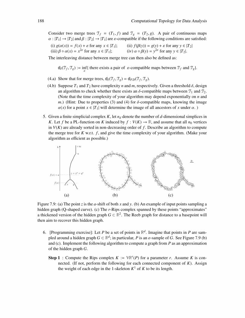
188 Computational Topology for Data Analysis
Consider two merge trees T f = (T1, f ) and Tg = (T2, g). A pair of continuous mapsα : |T1| → |T2| and β : |T2| → |T1| are ε-compatible if the following conditions are satisfied:
(i) g(α(x)) = f (x) + ε for any x ∈ |T1|; (ii) f (β(y)) = g(y) + ε for any y ∈ |T2|
(iii) β α(x) = x2ε for any x ∈ |T1|; (iv) α β(y) = y2ε for any y ∈ |T2|.
The interleaving distance between merge tree can then also be defined as:
dI(T f ,Tg) := infε there exists a pair of ε-compatible maps between T f and Tg.
(4.a) Show that for merge trees, dI(T f ,Tg) = dFD(T f ,Tg).
(4.b) Suppose T1 and T2 have complexity n and m, respectively. Given a threshold δ, designan algorithm to check whether there exists an δ-compatible maps between T1 and T2.(Note that the time complexity of your algorithm may depend exponentially on n andm.) (Hint: Due to properties (3) and (4) for δ-compatible maps, knowing the imageα(x) for a point x ∈ |T1| will determine the image of all ancestors of x under α. )
5. Given a finite simplicial complex K, let nd denote the number of d-dimensional simplices inK. Let f be a PL-function on K induced by f : V(K) → R, and assume that all n0 verticesin V(K) are already sorted in non-decreasing order of f . Describe an algorithm to computethe merge tree for K w.r.t. f , and give the time complexity of your algorithm. (Make youralgorithm as efficient as possible.)
h
u
+∞
x yf (x)
f (x) + az = xa = ya
2r
(a) (b) (c)
Figure 7.9: (a) The point z is the a-shift of both x and y. (b) An example of input points sampling ahidden graph (Q-shaped curve). (c) The r-Rips complex spanned by these points “approximates"a thickened version of the hidden graph G ⊂ R2. The Reeb graph for distance to a basepoint willthen aim to recover this hidden graph.
6. [Programming exercise]: Let P be a set of points in Rd. Imagine that points in P are sam-pled around a hidden graph G ⊂ Rd; in particular, P is an ε-sample of G. See Figure 7.9 (b)and (c). Implement the following algorithm to compute a graph from P as an approximationof the hidden graph G.
Step 1 : Compute the Rips complex K := VRr(P) for a parameter r. Assume K is con-nected. (If not, perform the following for each connected component of K). Assignthe weight of each edge in the 1-skeleton K1 of K to be its length.

Computational Topology for Data Analysis 189
Step 2 : Choose a point q ∈ P as the base point. Let f : P → R be the shortest pathdistance function from any point p ∈ P to the base point q in the weighted graph K1.
Step 3 : Compute the Reeb graph G of the PL-function induced by f , and return G.
The returned Reeb graph G can serve as an approximation of the hidden graph G. See[167, 89] for analysis of variants of the above procedure.

190 Computational Topology for Data Analysis
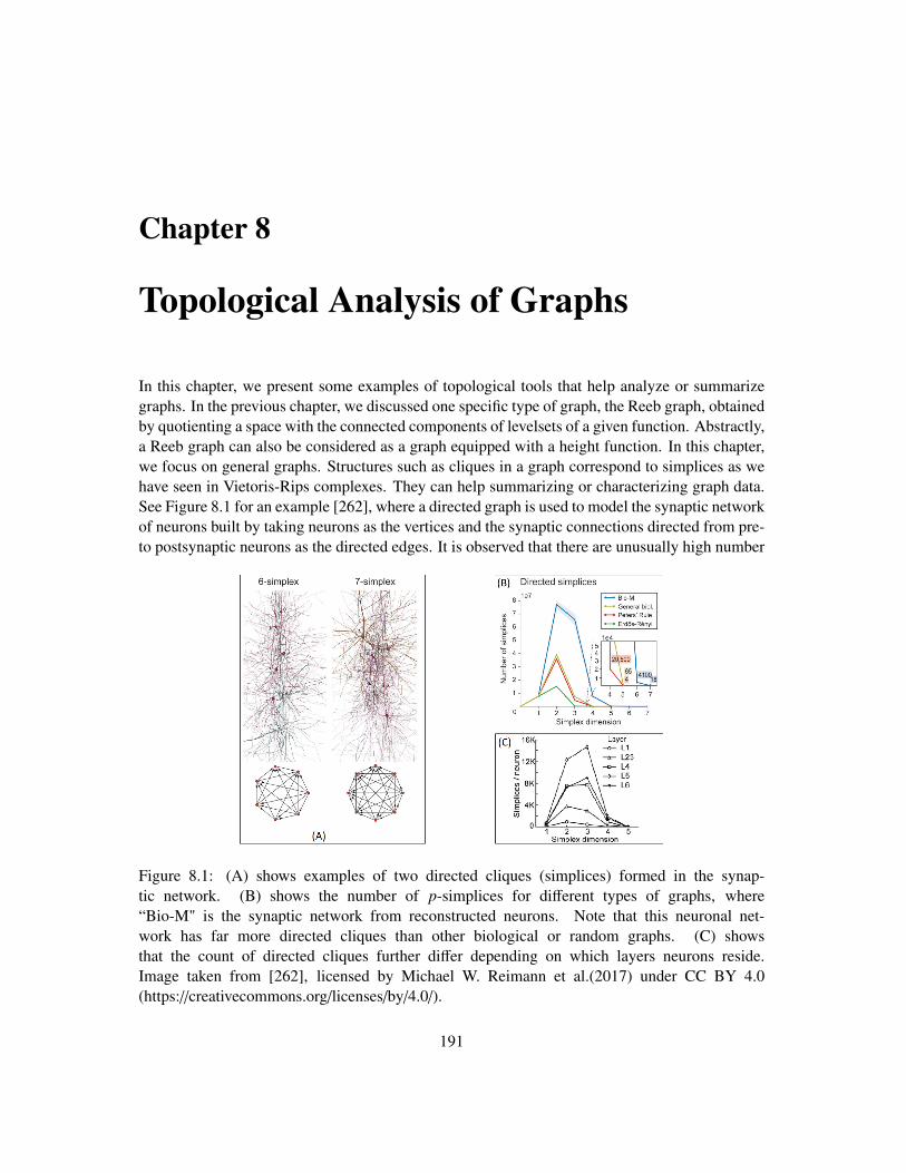
Chapter 8
Topological Analysis of Graphs
In this chapter, we present some examples of topological tools that help analyze or summarizegraphs. In the previous chapter, we discussed one specific type of graph, the Reeb graph, obtainedby quotienting a space with the connected components of levelsets of a given function. Abstractly,a Reeb graph can also be considered as a graph equipped with a height function. In this chapter,we focus on general graphs. Structures such as cliques in a graph correspond to simplices as wehave seen in Vietoris-Rips complexes. They can help summarizing or characterizing graph data.See Figure 8.1 for an example [262], where a directed graph is used to model the synaptic networkof neurons built by taking neurons as the vertices and the synaptic connections directed from pre-to postsynaptic neurons as the directed edges. It is observed that there are unusually high number
Figure 8.1: (A) shows examples of two directed cliques (simplices) formed in the synap-tic network. (B) shows the number of p-simplices for different types of graphs, where“Bio-M" is the synaptic network from reconstructed neurons. Note that this neuronal net-work has far more directed cliques than other biological or random graphs. (C) showsthat the count of directed cliques further differ depending on which layers neurons reside.Image taken from [262], licensed by Michael W. Reimann et al.(2017) under CC BY 4.0(https://creativecommons.org/licenses/by/4.0/).
191
192 Computational Topology for Data Analysis
of directed cliques (viewed as a simplex as we show in Section 8.3.1) in such networks, comparedto other biological networks or random graphs. Topological analysis such as the one described inSection 8.3 can facilitate such applications.
Before considering directed graphs, we focus on topological analysis of undirected graphs inSections 8.1 and 8.2. We present topological approaches to summarize and compare undirectedgraphs. In Section 8.3, we discuss how to obtain topological invariants for directed graphs. Inparticular, we describe two ways of defining homology for directed graphs. The first approachconstructs an appropriate simplicial complex over an input directed graph and then takes the cor-responding simplicial homology of this simplicial complex (Section 8.3.1). The second approachconsiders the so-called path homology for directed graphs, which differs from the simplicial ho-mology. It is based on constructing a specific chain complex directly from directed paths in theinput graph, and defining a homology group using the boundary operators associated with theresulting chain complex (Section 8.3.2). It turns out that both path homology and the persistentversion of it can be computed via a matrix reduction algorithm similar to the one used in thestandard persistence algorithm for simplicial filtrations though with some key differences. We de-scribe this algorithm in Section 8.3.3, and mention an improved algorithm for the 1-st homology.
8.1 Topological summaries for graphs
We have seen graphs in various contexts so far. Here we consolidate some of the persistenceresults that specifically involve graphs. Sometimes graphs appear as abstract objects devoid ofany geometry where they are described only combinatorially. At other times, graphs are equippedwith a function or a metric. Reeb graphs studied in the previous chapter fall into this lattercategory. Combinatorial graphs (weighted or unweighted) can also be viewed as metric graphs,by associating them with an appropriate shortest path metric (Section 8.1.2).
8.1.1 Combinatorial graphs
A graph G is combinatorially presented as a pair G = (V, E), where V is a set called nodes/verticesof G and E ⊆ V ×V is a set of pairs of vertices called edges of G. We now introduce two commonways to obtain a persistence-based topological summary for G.
Graphs viewed as a simplicial 1-complex. We can view G as a simplicial 1-complex with Vand E being the set of 0-simplices and 1-simplices respectively. Using tools such as the per-sistence algorithm for graph filtration mentioned in Chapter 3, we can summarize G w.r.t. agiven PL-function f : |G| → R by the persistence diagram Dgm f . This is what was done inSection 7.2.3 in the previous chapter while describing persistent homology for Reeb graphs. Inpractice, the chosen PL-functions are sometimes called descriptor functions. For example, wecan choose f : |G| → R to be given by a vertex function called the degree-function, where f (v)equals the degree of the graph node v in G. Some other choices for the descriptor function includethe heat-kernel signature function [284] used in [68] and the Ollivier Ricci curvature of graphs[226] used in [305]. Note that, under this view, given that the domain is a simplicial 1-complex,there is only zeroth and 1-st persistent homology to consider.
Computational Topology for Data Analysis 193
Clique complex view. Given a graph G = (V, E), its induced clique complex, also called theflag complex, is defined as follows.
Definition 8.1 (Clique complex). Given a graph G = (V, E), a clique simplex σ of dimension k is
σ = vi0 , . . . , vik where either k = 0 or for any j , j′ ∈ [0, k], (vi j , vi j′ ) ∈ E.
By definition, every face of a clique simplex is also a clique simplex. Therefore, the collection ofall clique simplices form a simplicial complex CG called the clique complex of G. In other words,the vertices of any (k + 1)-clique in G spans a k-simplex in CG.
Given a weighted graph G = (V, E, ω) with ω : E → R, let Ga denote the subgraph of Gspanned by all edges with weight at most a; that is, Ga = (Va, Ea) where Ea = (u, v) | ω(u, v) ≤ aand Va is the vertex set adjoining Ea. Let CGa be the clique complex induced by Ga. It is easyto see that CGa ⊆ CGb for any a ≤ b. Assuming all edges E = e1, . . . , em are sorted in non-decreasing order of their weights and setting ai = ω(ei), we thus obtain the following clique-complex filtration:
CGa1 → CGa2 → · · · → CGam .
The persistent homology induced by the clique-complex filtration can be used to summarize theweighted graph G = (V, E, ω). Here one can consider the k-th homology groups for k up to |V |−1.
8.1.2 Graphs viewed as metric spaces
A finite metric graph is a metric space (|G|, dG) where the space is the underlying space of afinite graph G, equipped with a length metric dG [59]. We have already seen metric graphsin the previous chapter where Reeb graphs are equipped with a metric induced by a function(Definition 7.7). We can also obtain a metric graph from a (positively) weighted combinatorialgraph.
Given a graph G = (V, E, ω) where the weight of each edge is positive1, we can view it as ametric graph (|G|, dG) obtained by gluing a set of length segments (edges), where intuitively dG isthe shortest path metric on |G| induced by edge lengths ω(e)s.
Fact 8.1. A positively weighted graph G = (V, E, ω) induces a metric graph (|G|, dG).
Indeed, viewing G as a simplicial 1-complex, let |G| be the underlying space of G. For everyedge e ∈ E, consider the arclength parameterization e : [0, ω(e)] → |e|, and define dG(x, y) =
|e−1(y) − e−1(x)| for every pair x, y ∈ |e|. The length of any path π(u, v) between two pointsu, v ∈ |G| is the sum of the lengths of the restrictions of π to edges in G. The distance dG(u, v)between any two points u, v ∈ |G| is the minimum length of any path connecting u to v in |G|which is a metric. The metric space (|G|, dG) is the metric graph of G.
Intrinsic Cech and Vietoris-Rips filtrations. Given a metric graph (|G|, dG), let Bo|G|(x; r) :=
y ∈ |G| | dG(x, y) < r denote the radius-r open metric ball centered at x ∈ |G|. Following
1If G is unweighted, then ω : E → R is the constant function ω(e) = 1 for any e ∈ E.
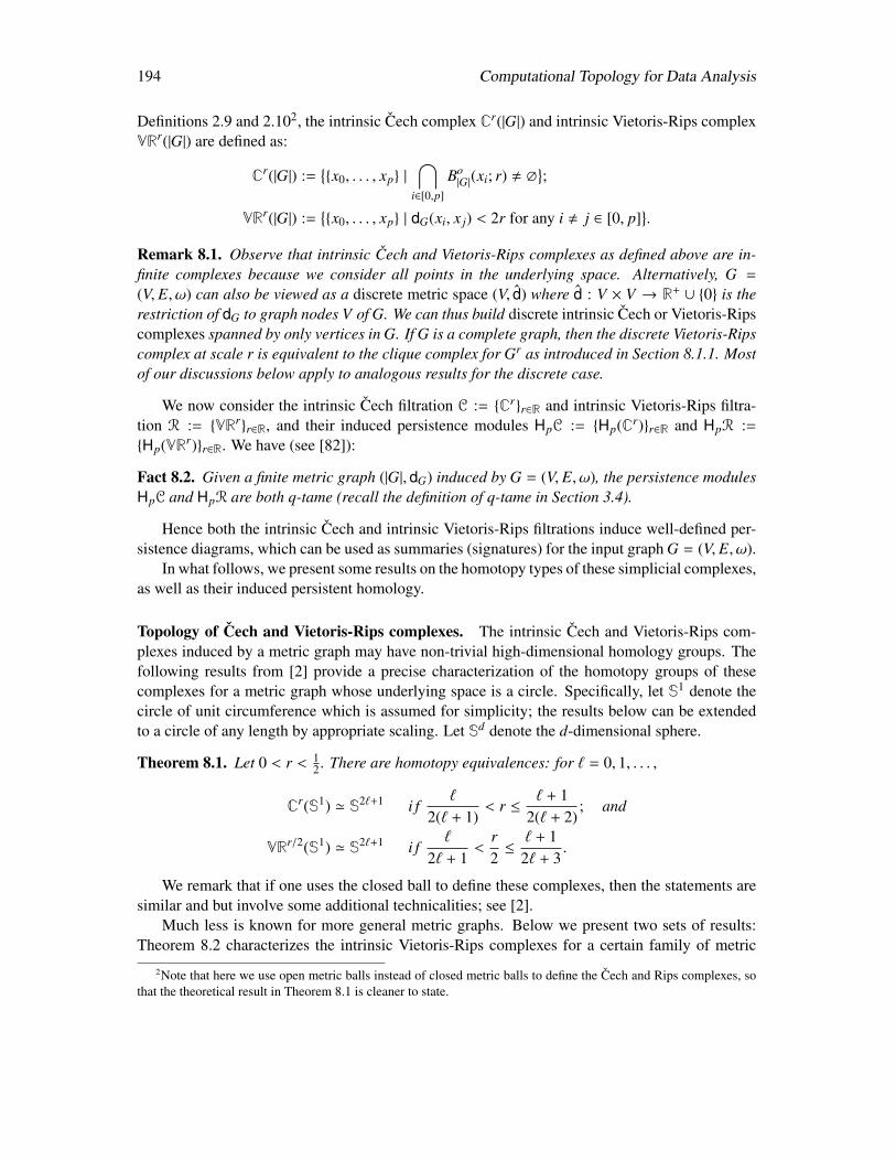
194 Computational Topology for Data Analysis
Definitions 2.9 and 2.102, the intrinsic Cech complex Cr(|G|) and intrinsic Vietoris-Rips complexVRr(|G|) are defined as:
Cr(|G|) :=x0, . . . , xp |
⋂i∈[0,p]
Bo|G|(xi; r) , ∅
;
VRr(|G|) :=x0, . . . , xp | dG(xi, x j) < 2r for any i , j ∈ [0, p]
.
Remark 8.1. Observe that intrinsic Cech and Vietoris-Rips complexes as defined above are in-finite complexes because we consider all points in the underlying space. Alternatively, G =
(V, E, ω) can also be viewed as a discrete metric space (V, d) where d : V × V → R+ ∪ 0 is therestriction of dG to graph nodes V of G. We can thus build discrete intrinsic Cech or Vietoris-Ripscomplexes spanned by only vertices in G. If G is a complete graph, then the discrete Vietoris-Ripscomplex at scale r is equivalent to the clique complex for Gr as introduced in Section 8.1.1. Mostof our discussions below apply to analogous results for the discrete case.
We now consider the intrinsic Cech filtration C := Crr∈R and intrinsic Vietoris-Rips filtra-tion R := VRrr∈R, and their induced persistence modules HpC := Hp(Cr)r∈R and HpR :=Hp(VRr)r∈R. We have (see [82]):
Fact 8.2. Given a finite metric graph (|G|, dG) induced by G = (V, E, ω), the persistence modulesHpC and HpR are both q-tame (recall the definition of q-tame in Section 3.4).
Hence both the intrinsic Cech and intrinsic Vietoris-Rips filtrations induce well-defined per-sistence diagrams, which can be used as summaries (signatures) for the input graph G = (V, E, ω).
In what follows, we present some results on the homotopy types of these simplicial complexes,as well as their induced persistent homology.
Topology of Cech and Vietoris-Rips complexes. The intrinsic Cech and Vietoris-Rips com-plexes induced by a metric graph may have non-trivial high-dimensional homology groups. Thefollowing results from [2] provide a precise characterization of the homotopy groups of thesecomplexes for a metric graph whose underlying space is a circle. Specifically, let S1 denote thecircle of unit circumference which is assumed for simplicity; the results below can be extendedto a circle of any length by appropriate scaling. Let Sd denote the d-dimensional sphere.
Theorem 8.1. Let 0 < r < 12 . There are homotopy equivalences: for ` = 0, 1, . . . ,
Cr(S1) ' S2`+1 i f`
2(` + 1)< r ≤
` + 12(` + 2)
; and
VRr/2(S1) ' S2`+1 i f`
2` + 1<
r2≤
` + 12` + 3
.
We remark that if one uses the closed ball to define these complexes, then the statements aresimilar and but involve some additional technicalities; see [2].
Much less is known for more general metric graphs. Below we present two sets of results:Theorem 8.2 characterizes the intrinsic Vietoris-Rips complexes for a certain family of metric
2Note that here we use open metric balls instead of closed metric balls to define the Cech and Rips complexes, sothat the theoretical result in Theorem 8.1 is cleaner to state.
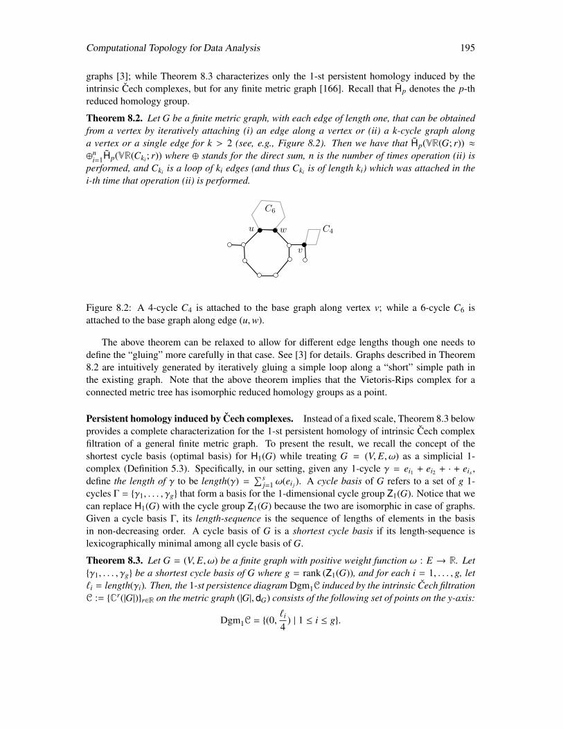
Computational Topology for Data Analysis 195
graphs [3]; while Theorem 8.3 characterizes only the 1-st persistent homology induced by theintrinsic Cech complexes, but for any finite metric graph [166]. Recall that Hp denotes the p-threduced homology group.
Theorem 8.2. Let G be a finite metric graph, with each edge of length one, that can be obtainedfrom a vertex by iteratively attaching (i) an edge along a vertex or (ii) a k-cycle graph alonga vertex or a single edge for k > 2 (see, e.g., Figure 8.2). Then we have that Hp(VR(G; r)) ≈⊕n
i=1Hp(VR(Cki ; r)) where ⊕ stands for the direct sum, n is the number of times operation (ii) isperformed, and Cki is a loop of ki edges (and thus Cki is of length ki) which was attached in thei-th time that operation (ii) is performed.
C4
v
u w
C6
Figure 8.2: A 4-cycle C4 is attached to the base graph along vertex v; while a 6-cycle C6 isattached to the base graph along edge (u,w).
The above theorem can be relaxed to allow for different edge lengths though one needs todefine the “gluing” more carefully in that case. See [3] for details. Graphs described in Theorem8.2 are intuitively generated by iteratively gluing a simple loop along a “short” simple path inthe existing graph. Note that the above theorem implies that the Vietoris-Rips complex for aconnected metric tree has isomorphic reduced homology groups as a point.
Persistent homology induced by Cech complexes. Instead of a fixed scale, Theorem 8.3 belowprovides a complete characterization for the 1-st persistent homology of intrinsic Cech complexfiltration of a general finite metric graph. To present the result, we recall the concept of theshortest cycle basis (optimal basis) for H1(G) while treating G = (V, E, ω) as a simplicial 1-complex (Definition 5.3). Specifically, in our setting, given any 1-cycle γ = ei1 + ei2 + · + eis ,define the length of γ to be length(γ) =
∑sj=1 ω(ei j). A cycle basis of G refers to a set of g 1-
cycles Γ = γ1, . . . , γg that form a basis for the 1-dimensional cycle group Z1(G). Notice that wecan replace H1(G) with the cycle group Z1(G) because the two are isomorphic in case of graphs.Given a cycle basis Γ, its length-sequence is the sequence of lengths of elements in the basisin non-decreasing order. A cycle basis of G is a shortest cycle basis if its length-sequence islexicographically minimal among all cycle basis of G.
Theorem 8.3. Let G = (V, E, ω) be a finite graph with positive weight function ω : E → R. Letγ1, . . . , γg be a shortest cycle basis of G where g = rank (Z1(G)), and for each i = 1, . . . , g, let`i = length(γi). Then, the 1-st persistence diagram Dgm1C induced by the intrinsic Cech filtrationC := Cr(|G|)r∈R on the metric graph (|G|, dG) consists of the following set of points on the y-axis:
Dgm1C = (0,`i
4) | 1 ≤ i ≤ g.
196 Computational Topology for Data Analysis
Unfortunately, no such characterization is available for high-dimensional cases. Some partialresults on the higher-dimensional persistent homology induced by intrinsic Cech filtration aregiven in [133].
8.2 Graph comparison
The topological invariants described in the previous section can be used as signatures to comparegraphs. For example, given two graphs G1 = (V1, E1, ω1) and G2 = (V2, E2, ω2) with positiveweight functions, let C(G1) and C(G2) denote the intrinsic Cech filtrations for (|G1|, dG1) and(|G2|, dG2), respectively. We can then define dIC(G1,G2) = db(Dgm1C(G1),Dgm1C(G2)) anddIC gives rise to a pseudo-distance (a metric for which the first axiom may hold only with ‘if’condition) for the family of finite graphs with positive weights. Furthermore, this pseudo-distanceis stable w.r.t. the Gromov-Hausdorff distance by a generalization of Theorem 6.3 (ii) to totallybounded metric spaces (see the discussions after Theorem 6.3).
Persistence-distortion distance. In what follows, we introduce another pseudo-distance formetric graphs, called the persistence distortion distance, which, instead of mapping the entiregraph into a single persistence diagram, maps each point in the graph to such a summary. Thisdistance can thus compare (metric) graphs at a more refined level.
First, given a finite metric graph (|G|, dG), for any point s ∈ |G|, consider the shortest pathdistance function fs : |G| → R defined as: x 7→ dG(x, s). Let
Ps := Dgm0 fs, the 0-th persistence diagram induced by the function fs. (8.1)
Let G and D denote the space of finite metric graphs and the space of finite persistence diagrams,respectively; and let 2D denote the space of all subsets of D. We define:
φ : G→ 2D where for any |G| ∈ G, φ(|G|) 7→ Ps | s ∈ |G| . (8.2)
In other words, φ maps a metric graph |G| to a set of (infinitely many) points φ(|G|) in the space ofpersistence diagrams D. The image φ(|G|) is another graph in the space of persistence diagramsthough this map φ is not necessarily injective.
Now let (|G1|, dG1) and (|G2|, dG2) denote the metric graphs induced by finite graphs G1 =
(V1, E1, ω1) and G2 = (V2, E2, ω2) with positive edge weights.
Definition 8.2 (Persistence distortion distance). Given finite metric graphs (|G1|, dG1) and (|G2|, dG2),the persistence-distortion distance between them, denoted by dPD(G1,G2), is the Hausdorff dis-tance dH(φ(|G1|), φ(|G2|) between the two image sets φ(|G1|) and φ(|G2|) in the space of persistencediagrams (D, db) equipped with the bottleneck distance db. In other words, setting A := φ(|G1|)and B := φ(|G2|), we have
dPD(G1,G2) := dH(φ(|G1|), φ(|G2|)
)= max
maxP∈A
minQ∈B
db(P,Q); maxQ∈B
minP∈A
db(P,Q).
The persistence distortion dPD is a pseudo-metric. It can be computed in polynomial time forfinite input graphs. It is stable w.r.t. the Gromov-Hausdorff distance between the two input metricgraphs.
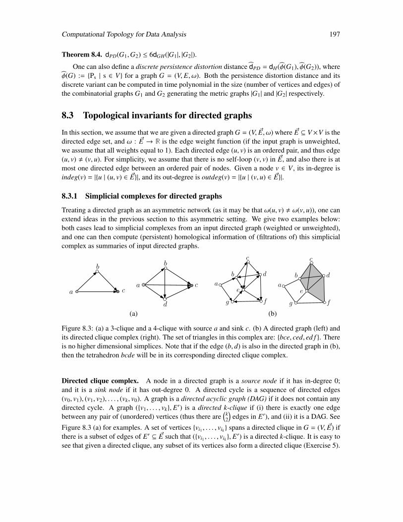
Computational Topology for Data Analysis 197
Theorem 8.4. dPD(G1,G2) ≤ 6dGH(|G1|, |G2|).
One can also define a discrete persistence distortion distance dPD = dH(φ(G1), φ(G2)), whereφ(G) := Ps | s ∈ V for a graph G = (V, E, ω). Both the persistence distortion distance and itsdiscrete variant can be computed in time polynomial in the size (number of vertices and edges) ofthe combinatorial graphs G1 and G2 generating the metric graphs |G1| and |G2| respectively.
8.3 Topological invariants for directed graphs
In this section, we assume that we are given a directed graph G = (V, ~E, ω) where ~E ⊆ V×V is thedirected edge set, and ω : ~E → R is the edge weight function (if the input graph is unweighted,we assume that all weights equal to 1). Each directed edge (u, v) is an ordered pair, and thus edge(u, v) , (v, u). For simplicity, we assume that there is no self-loop (v, v) in ~E, and also there is atmost one directed edge between an ordered pair of nodes. Given a node v ∈ V , its in-degree isindeg(v) = |u | (u, v) ∈ ~E|, and its out-degree is outdeg(v) = |u | (v, u) ∈ ~E|.
8.3.1 Simplicial complexes for directed graphs
Treating a directed graph as an asymmetric network (as it may be that ω(u, v) , ω(v, u)), one canextend ideas in the previous section to this asymmetric setting. We give two examples below:both cases lead to simplicial complexes from an input directed graph (weighted or unweighted),and one can then compute (persistent) homological information of (filtrations of) this simplicialcomplex as summaries of input directed graphs.
aa
cc
b b
d
a
b
c
d
f
e
g
a
b
c
d
f
e
g
(a) (b)
Figure 8.3: (a) a 3-clique and a 4-clique with source a and sink c. (b) A directed graph (left) andits directed clique complex (right). The set of triangles in this complex are: bce, ced, ed f . Thereis no higher dimensional simplices. Note that if the edge (b, d) is also in the directed graph in (b),then the tetrahedron bcde will be in its corresponding directed clique complex.
Directed clique complex. A node in a directed graph is a source node if it has in-degree 0;and it is a sink node if it has out-degree 0. A directed cycle is a sequence of directed edges(v0, v1), (v1, v2), . . . , (vk, v0). A graph is a directed acyclic graph (DAG) if it does not contain anydirected cycle. A graph (v1, . . . , vk, E′) is a directed k-clique if (i) there is exactly one edgebetween any pair of (unordered) vertices (thus there are
(k2
)edges in E′), and (ii) it is a DAG. See
Figure 8.3 (a) for examples. A set of vertices vi1 , . . . , vik spans a directed clique in G = (V, ~E) ifthere is a subset of edges of E′ ⊆ ~E such that (vi1 , . . . , vik , E
′) is a directed k-clique. It is easy tosee that given a directed clique, any subset of its vertices also form a directed clique (Exercise 5).
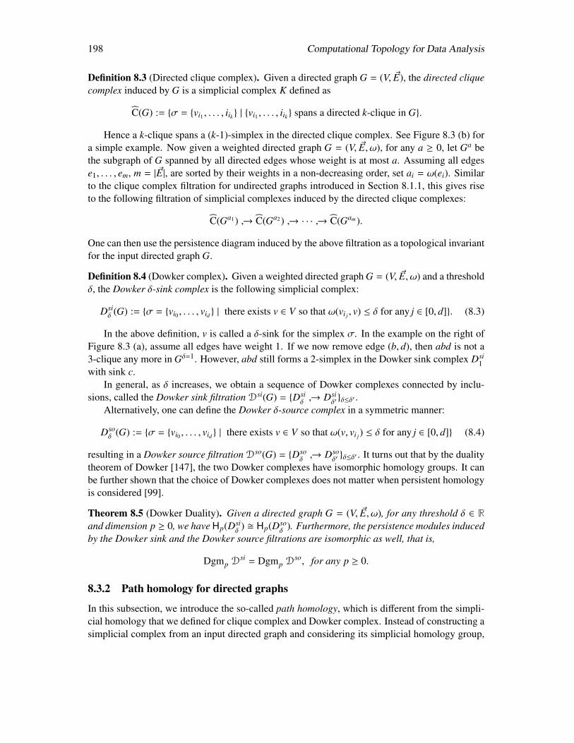
198 Computational Topology for Data Analysis
Definition 8.3 (Directed clique complex). Given a directed graph G = (V, ~E), the directed cliquecomplex induced by G is a simplicial complex K defined as
C(G) := σ = vi1 , . . . , iik | vi1 , . . . , iik spans a directed k-clique in G.
Hence a k-clique spans a (k-1)-simplex in the directed clique complex. See Figure 8.3 (b) fora simple example. Now given a weighted directed graph G = (V, ~E, ω), for any a ≥ 0, let Ga bethe subgraph of G spanned by all directed edges whose weight is at most a. Assuming all edgese1, . . . , em, m = |~E|, are sorted by their weights in a non-decreasing order, set ai = ω(ei). Similarto the clique complex filtration for undirected graphs introduced in Section 8.1.1, this gives riseto the following filtration of simplicial complexes induced by the directed clique complexes:
C(Ga1) → C(Ga2) → · · · → C(Gam).
One can then use the persistence diagram induced by the above filtration as a topological invariantfor the input directed graph G.
Definition 8.4 (Dowker complex). Given a weighted directed graph G = (V, ~E, ω) and a thresholdδ, the Dowker δ-sink complex is the following simplicial complex:
Dsiδ (G) := σ = vi0 , . . . , vid | there exists v ∈ V so that ω(vi j , v) ≤ δ for any j ∈ [0, d]. (8.3)
In the above definition, v is called a δ-sink for the simplex σ. In the example on the right ofFigure 8.3 (a), assume all edges have weight 1. If we now remove edge (b, d), then abd is not a3-clique any more in Gδ=1. However, abd still forms a 2-simplex in the Dowker sink complex Dsi
1with sink c.
In general, as δ increases, we obtain a sequence of Dowker complexes connected by inclu-sions, called the Dowker sink filtration Dsi(G) = Dsi
δ → Dsiδ′δ≤δ′ .
Alternatively, one can define the Dowker δ-source complex in a symmetric manner:
Dsoδ (G) := σ = vi0 , . . . , vid | there exists v ∈ V so that ω(v, vi j) ≤ δ for any j ∈ [0, d] (8.4)
resulting in a Dowker source filtration Dso(G) = Dsoδ → Dso
δ′ δ≤δ′ . It turns out that by the dualitytheorem of Dowker [147], the two Dowker complexes have isomorphic homology groups. It canbe further shown that the choice of Dowker complexes does not matter when persistent homologyis considered [99].
Theorem 8.5 (Dowker Duality). Given a directed graph G = (V, ~E, ω), for any threshold δ ∈ Rand dimension p ≥ 0, we have Hp(Dsi
δ ) Hp(Dsoδ ). Furthermore, the persistence modules induced
by the Dowker sink and the Dowker source filtrations are isomorphic as well, that is,
Dgmp Dsi = Dgmp D
so, for any p ≥ 0.
8.3.2 Path homology for directed graphs
In this subsection, we introduce the so-called path homology, which is different from the simpli-cial homology that we defined for clique complex and Dowker complex. Instead of constructing asimplicial complex from an input directed graph and considering its simplicial homology group,
Computational Topology for Data Analysis 199
here, we use the directed graph to define a chain complex directly. The resulting path homol-ogy group has interesting mathematical structures behind, e.g., there is a concept of homotopy indirected graphs under which the path homology is preserved, and it accommodates the Künnethformula [186].
Note that in this chapter, we have assumed that a given directed graph G = (V, ~E) does notcontain self-loops (where a self-loop is an edge (u, u) from u to itself). For notational simplicity,below we sometimes use index i to refer to vertex vi ∈ V = v1, . . . , vn.
Let k be a field with 0 and 1 being the additive and multiplicative identities respectively. Weuse −a to denote the additive inverse of a in k. An elementary p-path on V is an ordered sequencevi0 , vi1 , · · · , vip of p + 1 of vertices of V , which we denote by evi0 ,vi1 ,...,vid
, or just ei0,i1,··· ,ip forsimplicity. Let Λp = Λp(G,k) denote the k-linear space of all linear combinations of elementaryp-paths with coefficients from k. The set ei0,··· ,ip | i0, · · · , ip ∈ V forms a basis for Λp. Eachelement c of Λd is called a p-path or p-chain, and it can be written as
c =∑
i0,··· ,ip∈Vai0···ipei0···ip , where ai0···ip ∈ k.
Similar to the case of simplicial complexes, we can define boundary map ∂p : Λp → Λp−1 as:
∂p ei0···ip =∑
i0,··· ,ip∈V
(−1)kei0···i j···ip, for any elementary p -path ei0···ip ,
where ik means the removal of index ik. The boundary of a p-path c =∑
ai0···ip · ei0···ip , is thus∂pc =
∑ai0···ip · ∂pei0···ip . For convenience, we set Λ−1 = 0 and note that Λ0 is the set of k-linear
combinations of vertices in V . It is easy to show that ∂p−1 ·∂p = 0, for any p > 0. In what follows,we often omit the dimension p from ∂p when it is clear from the context.
Next, we restrict the consideration to real paths in directed graphs formed by consecutivedirected edges. Specifically, given a directed graph G = (V, ~E), call an elementary p-path ei0,··· ,ip
allowed if there is an edge from ik to ik+1 for all k ∈ [0, p − 1]. Define Ap as the space spannedby all allowed elementary p-paths, that is, Ap := spanei0···ip : ei0···ip is allowed. An elementaryp-path i0 · · · ip is called regular if ik , ik+1 for all k, and is irregular otherwise. Clearly, everyallowed path is regular since there is no self-loop. However, applying the boundary map ∂ to Λp
may create irregular paths. For example, ∂euvu = evu − euu + euv is irregular because of the termeuu. To deal with this case, the term containing consecutive repeated vertices is taken as 0. Thus,for the previous example, we have ∂euvu = evu − 0 + euv = evu + euv. The boundary map ∂ onAp is now taken to be the boundary map for Λp restricted on Ap with this modification, whereall terms with consecutive repeated vertices created by the boundary map ∂ are replaced with 0’s.For simplicity, we still use the same symbol ∂ to represent this modified boundary map on thespace of allowed paths.
After restricting the boundary operator to the space of allowed paths Aps, the inclusion that∂Ap ⊂ Ap−1 may not hold; that is, the boundary of an allowed p-path is not necessarily an allowed(p − 1)-path. To this end, we adopt a stronger notion of allowed paths: a path c is ∂-invariantif both c and ∂c are allowed. Let Ωp := c ∈ Ap | ∂c ∈ Ap−1 be the space generated by all∂-invariant p-paths. Note that ∂Ωp ⊂ Ωp−1 (as ∂2 = 0). This gives rise to the following chaincomplex of ∂-invariant allowed paths:
· · ·Ωp∂−→ Ωp−1
∂−→ · · ·Ω1
∂−→ Ω0
∂−→ 0.
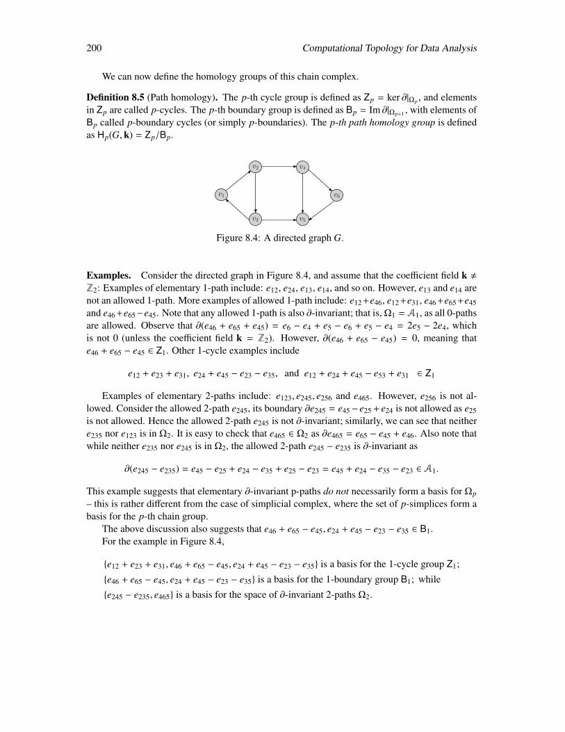
200 Computational Topology for Data Analysis
We can now define the homology groups of this chain complex.
Definition 8.5 (Path homology). The p-th cycle group is defined as Zp = ker ∂|Ωp , and elementsin Zp are called p-cycles. The p-th boundary group is defined as Bp = Im ∂|Ωp+1 , with elements ofBp called p-boundary cycles (or simply p-boundaries). The p-th path homology group is definedas Hp(G,k) = Zp/Bp.
v2
v3
v4
v1 v6
v5
Figure 8.4: A directed graph G.
Examples. Consider the directed graph in Figure 8.4, and assume that the coefficient field k ,
Z2: Examples of elementary 1-path include: e12, e24, e13, e14, and so on. However, e13 and e14 arenot an allowed 1-path. More examples of allowed 1-path include: e12 +e46, e12 +e31, e46 +e65 +e45and e46 +e65−e45. Note that any allowed 1-path is also ∂-invariant; that is, Ω1 = A1, as all 0-pathsare allowed. Observe that ∂(e46 + e65 + e45) = e6 − e4 + e5 − e6 + e5 − e4 = 2e5 − 2e4, whichis not 0 (unless the coefficient field k = Z2). However, ∂(e46 + e65 − e45) = 0, meaning thate46 + e65 − e45 ∈ Z1. Other 1-cycle examples include
e12 + e23 + e31, e24 + e45 − e23 − e35, and e12 + e24 + e45 − e53 + e31 ∈ Z1
Examples of elementary 2-paths include: e123, e245, e256 and e465. However, e256 is not al-lowed. Consider the allowed 2-path e245, its boundary ∂e245 = e45− e25 + e24 is not allowed as e25is not allowed. Hence the allowed 2-path e245 is not ∂-invariant; similarly, we can see that neithere235 nor e123 is in Ω2. It is easy to check that e465 ∈ Ω2 as ∂e465 = e65 − e45 + e46. Also note thatwhile neither e235 nor e245 is in Ω2, the allowed 2-path e245 − e235 is ∂-invariant as
∂(e245 − e235) = e45 − e25 + e24 − e35 + e25 − e23 = e45 + e24 − e35 − e23 ∈ A1.
This example suggests that elementary ∂-invariant p-paths do not necessarily form a basis for Ωp
– this is rather different from the case of simplicial complex, where the set of p-simplices form abasis for the p-th chain group.
The above discussion also suggests that e46 + e65 − e45, e24 + e45 − e23 − e35 ∈ B1.For the example in Figure 8.4,
e12 + e23 + e31, e46 + e65 − e45, e24 + e45 − e23 − e35 is a basis for the 1-cycle group Z1;
e46 + e65 − e45, e24 + e45 − e23 − e35 is a basis for the 1-boundary group B1; while
e245 − e235, e465 is a basis for the space of ∂-invariant 2-paths Ω2.
Computational Topology for Data Analysis 201
Persistent path homology for directed graphs. Given a weighted directed graph G = (V, ~E, ω),let Ga denote the subgraph of G containing all directed edges with weight at most a. This givesrise to a filtration of graphs G : Ga → Gba≤b. Let Hp(Ga) denote the p-th path homologyinduced by graph Ga. It can be shown [100] that the inclusion Ga → Gb induces a well-definedhomormorphism ξa,b
p : Hp(Ga) → Hp(Gb), and the sequence G : Ga → Gba≤b leads to apersistence module HpG : Hp(Ga)→ Hp(Gb)a≤b.
8.3.3 Computation of (persistent) path homology
The example in the previous section illustrates the challenge for computing path homology in-duced by a directed graph G in comparison to simplicial homology. In particular, the set ofelementary allowed d-paths may no longer form a basis for the space of the ∂-invariant d-pathsΩd: Indeed, recall that for the graph in Figure 8.4, e465, e245 − e235 form a basis for Ω2, yet,neither e245 nor e235 belongs to Ω2.
We now present an algorithm to compute the persistent path homology of a given weighteddirected graph G = (V, ~E, ω). Note that as a byproduct, this algorithm can also compute the pathhomology of a directed graph.
Algorithm setup. Given a p-path τ, its allowed-time is set to be the smallest value (weight)a when it belongs to Ap(Ga); and we denote it by at(τ) = a. Let Ap = τ1, . . . , τt denotethe set of elementary allowed p-paths, sorted by their allowed-times in a non-decreasing order.Similarly, set Ap−1 = σ1, . . . , σs to be the sequence of elementary allowed (p − 1)-paths sortedby their allowed-times in a non-decreasing order. Let a1 < a2 < · · · < at be the sequence ofdistinct allowed-times of elementary p-paths in Ap in increasing orders. Obviously, t ≤ t = |Ap|.Similarly, let b1 < b2 < · · · < bs be the sequence of distinct allowed-times for (p − 1)-paths inAp−1 sorted in increasing order.
Note that Ap (resp. Ap−1) forms a basis for Ap(G) (resp. Ap−1(G)). In fact, for any i, setAai
p := τ j | at(τ j) ≤ ai. It is easy to see that Aaip equals τ1, . . . , τρi, where
ρi ∈ [1, t] is the largest index of any elementary p-path whose allowed-time is at most ai; (8.5)
and Aaip forms a basis for Ap(Gai). Note that the cardinality of Aai
p \Aai−1p could be larger than 1 and
that is why ρi is not necessarily equal to i. A symmetric statement holds for Ab j
p−1 and Ap−1(Gb j).From now on, we fix a dimension p. At high level, the algorithm for computing the p-th
persistent path homology has the following three steps, which looks similar to the algorithmthat computes standard persistent homology for simplicial complexes. However, there are keydifferences in the implementation of these steps.
Step 1. Set up a “boundary matrix” M = Mp.
Step 2. Perform left-to-right matrix reduction to transform M to a reduced form M.
Step 3. Construct the persistence diagram from the reduced matrix M.
The details of these steps are given as follows.

202 Computational Topology for Data Analysis
Description of Step 1. The columns of M correspond to Ap, ordered by their allowed-times.We would like colM[i] = ∂τi. However, the boundary of an allowed path may not be allowed.Hence the rows of the matrix need to correspond to not only the elementary allowed (p− 1)-pathsin Ap−1 (ordered by their allowed-times), but also any elementary (non-allowed) (p − 1)-paththat appears in the boundary of any τ j ∈ Ap: we assign the allowed-times for such paths tobe +∞. The rows of M are ordered in non-decreasing allowed-times from top to bottom. LetAp−1 = σ1, . . . , σs, σs+1, . . . , σ` be the final set of elementary (p − 1)-paths corresponding torows of M. Note that the first s elements are from Ap−1, while those in σs+1, . . . , σ` are not-allowed, and have allowed-time +∞. See an example in Figure 8.5 (a) and (b).
The matrix M represents the boundary operator ∂p restricted to Ap. In other words, the i-th column of M, denoted by colM[i], contains the boundary of τi, represented using the basiselements in Ap−1; that is, ∂pτi =
∑`j=1 colM[i][ j]σ j. From a vector representation point of view,
we will also simply say that ∂pτi = colM[i]. The allowed time for the (p−1)-path represented by acolumn vector C is simply the allowed time at(σ j) associated to the low-row index j = lowId(C)in this vector: It is important to note that the rows of M are ordered in increasing indices from topdown. Hence lowId of a column means the largest index in Ap−1 for which this column containsa non-zero entry. We further associate a p-path γi with the i-th column of M for each i ∈ [1, t],with the property ∂pγi = colM[i]. At the beginning of the algorithm, γi is initialized to be τi andlater will be updated through the reduction process in (Step 2) below.
1 2
3 4
10
G
5
d e
a
b c
eabecbeadeedeceebd
10−1001
010001
ecdeced eabd ecbd
00011
−10
0 −1
eabecbeadeedeceebd
10−1001
11
0ecd
eced eabd ecbd
00011
−10
0 0
−1
−1−1
(a) graph G (b) original boundary matrix M (c) reduced matrix M
Figure 8.5: The input is the weighted directed graph in (a). Its 1-dimensional boundary matrixM as constructed in (Step 1) is shown in (b). Note that at(ecd) = +∞ (so ecd < A1(G)). Foreach edge (i.e, elementary allowed 1-path) in G, its allowed-time is simply its weight. There areonly three elementary allowed 2-paths, and their allowed-times are: at(eced) = 5, at(eabd) = 10and at(ecbd) = 10. (c) shows the reduced matrix. From this matrix, we can deduce that the 1-th persistence diagram (for path homology) includes two points: (10, 10) and (5, 10) (generatedby the second and third columns). Note that for the first column (corresponding to eced), asat(colM[1]) = ∞; hence the corresponding γ1 is not ∂-invariant.
Description of Step 2. We now perform the standard left-to-right matrix reduction to M, wherethe only allowed operation is to add a column to some column on its right. We convert M to itsreduced form M (Definition 3.13); and through this process, we also update γi accordingly sothat at any moment, ∂pγi = colM′[i] where M′ is the updated boundary matrix at that point. Inparticular, if we add column j to column i > j, then we will update γi = γi + γ j. We note that
Computational Topology for Data Analysis 203
other than the additional maintenance of γs, this reduction step of M is the same as the reductionin Algorithm 3:MatPersistence given in Section 3.3. The following claim follows easily fromthat there are only left-to-right column additions, and that the allowed-times of γis are initiallysorted in non-decreasing order.
Claim 8.1. For any i ∈ [1, t], the allowed-time of γi remains the same through any sequence ofleft-to-right column additions.
Let Ωip denote the space of ∂-invariant p-paths w.r.t. Gai ; that is, Ωi
p = Ωp(Gai). Given ap-path τ, let ent(τ) be its entry-time, which is the smallest value a such that τ ∈ Ωp(Ga). It iseasy to see that for any p-path τ, we have that
ent(τ) = maxat(τ), at(∂pτ). (8.6)
Recall that each column vector colM[i] is in fact the vector representation of a (p − 1)-path(with respect to basis elements in A = σ1, . . . , σ`). Also, the allowed time for a column colM[i]is given by at(colM[i]) = at(σh) where h = lowId(colM[i]).
Claim 8.2. Given a reduced matrix M, let C =∑t
i=1 cicolM[i] be a (p − 1)-path. Let colM[ j] bethe column with lowest (i.e, largest) lowId among all columns colM[i]s such that ci , 0, and seth = lowId(colM[ j]). It then follows that at(C) = at(σh).
Now for the reduced matrix M, given any i ∈ [1, t], we set ρi to be the largest index j ∈ [1, t]such that at(γ j) ≤ ai. By Claim 8.1, for each j there is a fixed allowed time associated to thep-path γ j associated to it, which stays invariant through the reduction process. So this quantityρi is well defined, consistent with what we defined earlier in Eqn. (8.5), and remains invariantthrough the reduction process. Now set:
Γi := γ1, . . . , γρi,
Ii := j ≤ ρi | at(colM[ j]) ≤ ai , and
Σi := γ j | ent(γ j) ≤ ai = γ j | j ∈ Ii.
Theorem 8.6. For any k ∈ [1, t], Γk forms a basis for Akp := A(Gak ); while Σk forms a basis for
Ωkp = Ωp(Gak ).
Proof. That Γk forms a basis for Akp follows easily from the facts that originally, τ1, . . . , τρk
form a basis for Akp, and the left-to-right column additions maintain this. In what follows, we
prove that Σk forms a basis for Ωkp. First, note that all elements in Σk represent paths in Ωk
p andthey are linearly independent by construction (as their low-row indices are distinct). So we onlyneed to show that any element in Ωk
p can be represented by a linear combination of vectors in Σk.Let ξk denote the largest index j ∈ [1, s] such that at(σ j) ≤ ak. In other words, an equivalent
formulation for Ik is that Ik = j ≤ ρk | lowId(colM[ j]) ≤ ξk.Now consider any γ ∈ Ωk
p ⊆ Akp. As Γk forms a basis for Ak
p, we have that
γ =
ρk∑i=1
ciγi and ∂γ =
ρk∑i=1
ci∂γi =
ρk∑i=1
cicolM[i].
204 Computational Topology for Data Analysis
As γ ∈ Ωkp and ent(γ) = maxat(γ), at(∂γ) (see Eqn. (8.6)), we have at(γ) ≤ ak and at(∂γ) ≤
ak. By Claim 8.2, it follows that for any j ∈ [1, ρk] with c j , 0, its lowId satisfies lowId(colM[ j]) ≤ξk. Hence each such index j with c j , 0 must belong to Ik, and as a result, γ can be written asa linear combination of p-paths in Σk. Combined with that all vectors in Σk are in Ωk
p and arelinearly independent, it follows that Σk forms a basis for Ωk
p.
Corollary 8.7. Set Jk := j ∈ Ik | colM[ j] is all zeros. Further we set Zk := γ j | j ∈ Jk;and Bk := colM[ j] | j ∈ Ik \ Jk. Then (i) Zk forms a basis for the p-dimensional cycle groupZp(Gak ); and (ii) Bk forms a basis for the (p − 1)-dimensional boundary group Bp−1(Gak ).
Proof. Let ∂p denote the restriction of ∂p over Ωp. Recall that Zp = Ker∂p, while Bp−1 = Im∂p.Easy to see that by construction of Zk, we have Zk ⊆ Span(Zk) ⊆ Zp(Gak ). Since all Γis arelinearly independent, we thus have that vectors in Zk are linearly independent. It then follows that|Zk| ≤ rank (Zp(Gak )) where |Zk| stands for the cardinality of Zk.
Similarly, as the matrix M is reduced, all non-zero columns of M are linearly independent, andthus vectors in Bk are linearly independent. Furthermore, by Theorem 8.6, each vector in Bk is inBp−1(Gak ) (as it is the boundary of a p-path from Ωk
p). Hence we have that Span(Bk) ⊆ Bp−1(Gak ),and |Bk| ≤ rank (Bp−1(Gak )).
On the other hand, let ∂p|Ωkp
denote the restriction of ∂p to only Ωkp ⊆ Ωp. Note that by Rank
Nullity Theorem,
|Σkp| = rank (Ωk
p) = rank (ker(∂p|Ωkp)) + rank (im (∂p|Ωk
p)) = rank (Zp(Gak )) + rank (Bp−1(Gak )).
As rank (Σkp) = |Zk| + |Bk|, and combining the above equation with the inequalities obtained
in the previous paragraphs, it follows that it must be that |Zk| = rank (Zp(Gak )) and |Bk| =
rank (Bp−1(Gak )). The claim then follows.
Description of Step 3: constructing persistence diagram from the reduced matrix M. Givena weighted directed graph G = (V, ~E, ω), for each dimension p ≥ 0, construct the boundarymatrix Mp+1 as described above in (Step 1). Perform the left-to-right column reduction to Mp+1
to obtain a reduced form M = Mp+1 as in (Step 2). The p-th persistence diagram DgmpG whereG : Ga → Gba≤b can be computed as follows.
Let µa,bp denote the persistence pairing function: that is, the persistence point (a, b) is in
DgmpG with multiplicity µa,bp if and only if µa,b
p > 0. At the beginning, µa,bp is initialized to
be 0 for all a, b ∈ R. We then inspect every non-zero column colM[i], and take the followingactions.
• If at(colM[i]) , ∞, then we increase the pairing function µat(colM[i]),ent(γi) by 1, whereγi is the allowed elementary (p + 1)-path corresponding to this column. Observe that,at(colM[i]) ≤ ent(γi) because
ent(γi) = maxat(γi), at(∂γi) = maxat(τi), at(colM[i]).
• Otherwise, the path γi corresponds to this column is not ∂-invariant (i.e, not in Ωp), and wedo nothing.
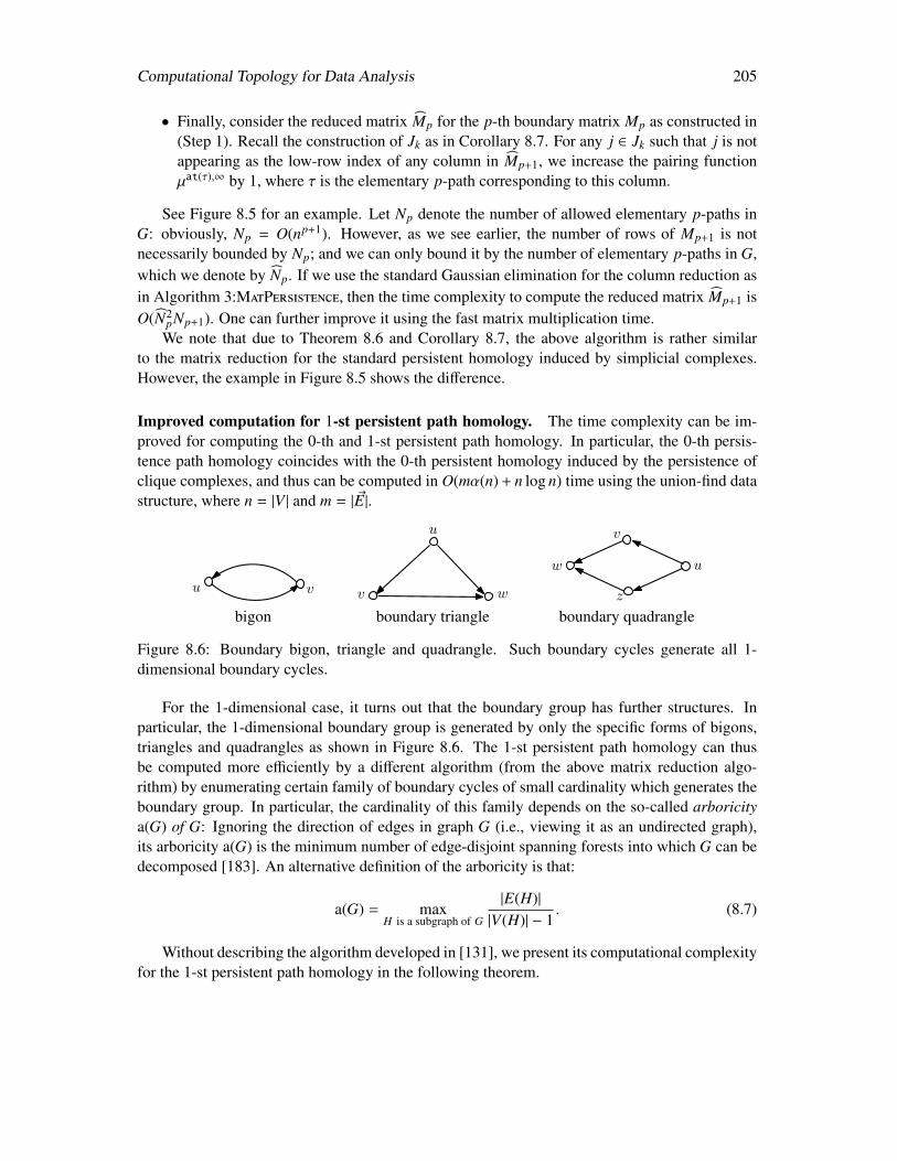
Computational Topology for Data Analysis 205
• Finally, consider the reduced matrix Mp for the p-th boundary matrix Mp as constructed in(Step 1). Recall the construction of Jk as in Corollary 8.7. For any j ∈ Jk such that j is notappearing as the low-row index of any column in Mp+1, we increase the pairing functionµat(τ),∞ by 1, where τ is the elementary p-path corresponding to this column.
See Figure 8.5 for an example. Let Np denote the number of allowed elementary p-paths inG: obviously, Np = O(np+1). However, as we see earlier, the number of rows of Mp+1 is notnecessarily bounded by Np; and we can only bound it by the number of elementary p-paths in G,which we denote by Np. If we use the standard Gaussian elimination for the column reduction asin Algorithm 3:MatPersistence, then the time complexity to compute the reduced matrix Mp+1 isO(N2
pNp+1). One can further improve it using the fast matrix multiplication time.We note that due to Theorem 8.6 and Corollary 8.7, the above algorithm is rather similar
to the matrix reduction for the standard persistent homology induced by simplicial complexes.However, the example in Figure 8.5 shows the difference.
Improved computation for 1-st persistent path homology. The time complexity can be im-proved for computing the 0-th and 1-st persistent path homology. In particular, the 0-th persis-tence path homology coincides with the 0-th persistent homology induced by the persistence ofclique complexes, and thus can be computed in O(mα(n) + n log n) time using the union-find datastructure, where n = |V | and m = |~E|.
u v
u
v w
u
v
w
z
bigon boundary triangle boundary quadrangle
Figure 8.6: Boundary bigon, triangle and quadrangle. Such boundary cycles generate all 1-dimensional boundary cycles.
For the 1-dimensional case, it turns out that the boundary group has further structures. Inparticular, the 1-dimensional boundary group is generated by only the specific forms of bigons,triangles and quadrangles as shown in Figure 8.6. The 1-st persistent path homology can thusbe computed more efficiently by a different algorithm (from the above matrix reduction algo-rithm) by enumerating certain family of boundary cycles of small cardinality which generates theboundary group. In particular, the cardinality of this family depends on the so-called arboricitya(G) of G: Ignoring the direction of edges in graph G (i.e., viewing it as an undirected graph),its arboricity a(G) is the minimum number of edge-disjoint spanning forests into which G can bedecomposed [183]. An alternative definition of the arboricity is that:
a(G) = maxH is a subgraph of G
|E(H)||V(H)| − 1
. (8.7)
Without describing the algorithm developed in [131], we present its computational complexityfor the 1-st persistent path homology in the following theorem.
206 Computational Topology for Data Analysis
Theorem 8.8. Given a directed weighted graph G = (V, ~E,w) with n = |V |, m = |~E|, and Np =
O(np+1) the number of allowed elementary p-paths, assume that the time to compute the rank ofa r × r matrix is rω. Let din(v) and dout(u) denote the in-degree and out-degree of a node v ∈ V,and a(G) be the arboricity of G. Set K = mina(G)m,
∑(u,v)∈~E (din(u) + dout(u)). Then we can
compute the p-th persistent path homology:
• in O(mα(n) + n log n) time when p = 0;
• in O(Kmω−1 + a(G)m) time when p = 1; and
In particular, the arboricity a(G) = O(1) for plannar graphs, thus it takes O(nω) time tocompute the 1-st persistent path homology for a planar directed graph G.
8.4 Notes and Exercises
The clique complex (also called the flag complex) is one of the most common ways to constructa simplicial complex from a graph. Recent years have seen much work on using the topologicalprofiles associated with the clique complex for network analysis; e.g., one of the early applicationsin [255]. Most materials covered in Section 8.1.2 come from [2, 3, 82]; note that [82] providesa detailed exposition for the intrinsic Cech and Vietoris-Rips filtrations of general metric spaces(beyond merely metric graphs). Theorem 8.2 comes as a corollary of Proposition 4 in [3], which isa stronger result than this theorem: In particular, Proposition 4 of [3] characterizes the homotopytype of the family of graphs described in Theorem 8.2.
The comparison of graphs via persistence distortion was proposed in [134].Topological analysis for directed graphs and asymmetric networks is more recent. Neverthe-
less, the clique complex for directed graphs has already found applications in practical domains;e.g., [144, 229, 262]. The path homology was originally proposed in [171], and further studiedand developed in [172, 173, 174]. Its persistent version is proposed and studied in [100]. Notethat as mentioned earlier, the path homology is not a simplicial homology. Nevertheless, we haveshown in this chapter that there is still a matrix reduction algorithm to compute it for any dimen-sion, with the same time complexity required for computing the homology groups for simplicialcomplexes. The path homology also has a rich mathematical structure: There is a concept ofhomotopy theory for digraphs under which the path homology is preserved [172], and it is alsodual to the cohomology theory of diagrams introduced in [173]. Note that in this chapter, wehave assumed that the input directed graph does not have self-loops. Additional care is needed tohandle such loops.
The matrix reduction algorithm for computing the persistent path homology that we describedin Section 8.3.3 is based on the work in [100]. The algorithm of [100] assumes that the input graphis a complete and weighted directed graph; or equivalently, is a finite set V with a weight functionw : V × V → R that may be asymmetric. We modify it so that the algorithm works with anarbitrary weighted directed graph. Finally, a hypergraph G = (V, E) consists of a finite set ofnodes V , and a collection E ⊆ 2V of subsets of V , each such subset called a hyper-edge. (In otherwords, a graph is a hypergraph where every hyper-edge has cardinality 2.) We remark that theidea behind path homology has also been extended to defining the so-called embedded homologyfor hypergraphs [49].
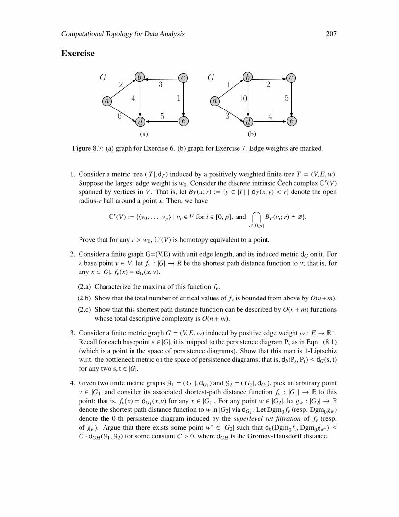
Computational Topology for Data Analysis 207
Exercise
2 3
6 5
4
G
1a
d e
cb1 2
3 4
10
G
5a
d
b
e
c
(a) (b)
Figure 8.7: (a) graph for Exercise 6. (b) graph for Exercise 7. Edge weights are marked.
1. Consider a metric tree (|T |, dT ) induced by a positively weighted finite tree T = (V, E,w).Suppose the largest edge weight is w0. Consider the discrete intrinsic Cech complex Cr(V)spanned by vertices in V . That is, let BT (x; r) := y ∈ |T | | dT (x, y) < r denote the openradius-r ball around a point x. Then, we have
Cr(V) := 〈v0, . . . , vp〉 | vi ∈ V for i ∈ [0, p], and⋂
i∈[0,p]
BT (vi; r) , ∅.
Prove that for any r > w0, Cr(V) is homotopy equivalent to a point.
2. Consider a finite graph G=(V,E) with unit edge length, and its induced metric dG on it. Fora base point v ∈ V , let fv : |G| → R be the shortest path distance function to v; that is, forany x ∈ |G|, fv(x) = dG(x, v).
(2.a) Characterize the maxima of this function fv.
(2.b) Show that the total number of critical values of fv is bounded from above by O(n+m).
(2.c) Show that this shortest path distance function can be described by O(n + m) functionswhose total descriptive complexity is O(n + m).
3. Consider a finite metric graph G = (V, E, ω) induced by positive edge weight ω : E → R+.Recall for each basepoint s ∈ |G|, it is mapped to the persistence diagram Ps as in Eqn. (8.1)(which is a point in the space of persistence diagrams). Show that this map is 1-Liptschizw.r.t. the bottleneck metric on the space of persistence diagrams; that is, db(Ps,Pt) ≤ dG(s, t)for any two s, t ∈ |G|.
4. Given two finite metric graphs G1 = (|G1|, dG1) and G2 = (|G2|, dG2), pick an arbitrary pointv ∈ |G1| and consider its associated shortest-path distance function fv : |G1| → R to thispoint; that is, fv(x) = dG1(x, v) for any x ∈ |G1|. For any point w ∈ |G2|, let gw : |G2| → Rdenote the shortest-path distance function to w in |G2| via dG2 . Let Dgm0 fv (resp. Dgm0gw)denote the 0-th persistence diagram induced by the superlevel set filtration of fv (resp.of gw). Argue that there exists some point w∗ ∈ |G2| such that db(Dgm0 fv,Dgm0gw∗) ≤C · dGH(G1,G2) for some constant C > 0, where dGH is the Gromov-Hausdorff distance.

208 Computational Topology for Data Analysis
5. Show that given a directed clique, any subset of its vertices span a directed subgraph witha unique source and a unique sink.
6. Consider the graph in Figure 8.7 (a). Compute the 0-th and 1-st persistence diagrams forthe filtrations induced by (i) the directed clique complexes; (ii) the Dowker-sink complexes;and (iii) the Dowker-source complexes.
7. Consider the graph in Figure 8.7 (b). Compute the 1-st persistence diagram for the filtra-tions (i) induced by directed clique complexes; and (ii) induced by path homology.
8. Consider a pair of directed graphs G = (V, E) and G′ = (V, E′) spanned by the same set ofvertices V , and E′ = E ∪ (u, v); that is, G′ equals to G with an additional directed edgee = (u, v). Consider path homology. Consider the 1st cycle and boundary groups for G andfor G′.
(i) Show that rank (Z1(G′)) ≤ rank (Z1(G)) + 1.
(ii) Give an example of G and G′ where rank (B1(G′)) − rank (B1(G)) ∈ Θ(n), wheren = |V |.
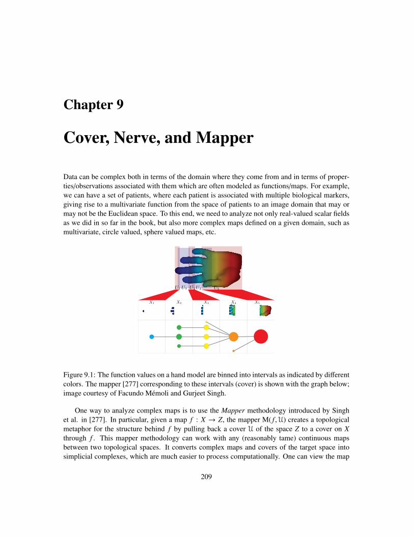
Chapter 9
Cover, Nerve, and Mapper
Data can be complex both in terms of the domain where they come from and in terms of proper-ties/observations associated with them which are often modeled as functions/maps. For example,we can have a set of patients, where each patient is associated with multiple biological markers,giving rise to a multivariate function from the space of patients to an image domain that may ormay not be the Euclidean space. To this end, we need to analyze not only real-valued scalar fieldsas we did in so far in the book, but also more complex maps defined on a given domain, such asmultivariate, circle valued, sphere valued maps, etc.
U1 U2 U3 U4 U5
Figure 9.1: The function values on a hand model are binned into intervals as indicated by differentcolors. The mapper [277] corresponding to these intervals (cover) is shown with the graph below;image courtesy of Facundo Mémoli and Gurjeet Singh.
One way to analyze complex maps is to use the Mapper methodology introduced by Singhet al. in [277]. In particular, given a map f : X → Z, the mapper M( f ,U) creates a topologicalmetaphor for the structure behind f by pulling back a cover U of the space Z to a cover on Xthrough f . This mapper methodology can work with any (reasonably tame) continuous mapsbetween two topological spaces. It converts complex maps and covers of the target space intosimplicial complexes, which are much easier to process computationally. One can view the map
209
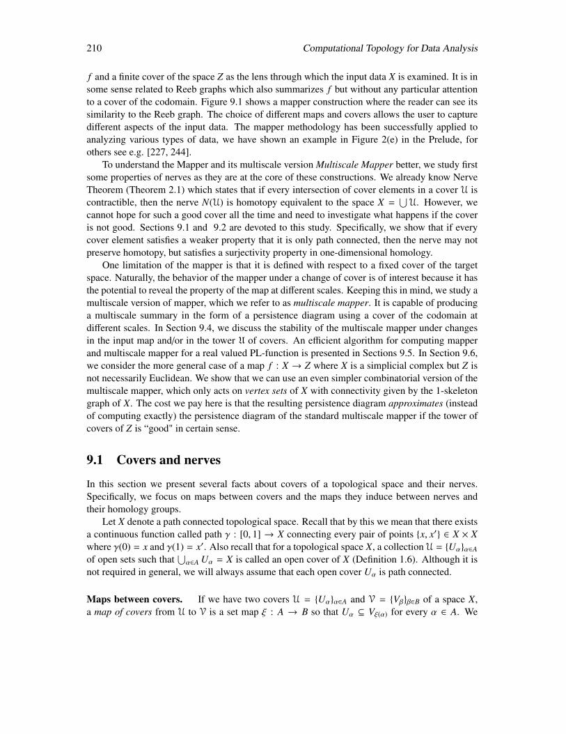
210 Computational Topology for Data Analysis
f and a finite cover of the space Z as the lens through which the input data X is examined. It is insome sense related to Reeb graphs which also summarizes f but without any particular attentionto a cover of the codomain. Figure 9.1 shows a mapper construction where the reader can see itssimilarity to the Reeb graph. The choice of different maps and covers allows the user to capturedifferent aspects of the input data. The mapper methodology has been successfully applied toanalyzing various types of data, we have shown an example in Figure 2(e) in the Prelude, forothers see e.g. [227, 244].
To understand the Mapper and its multiscale version Multiscale Mapper better, we study firstsome properties of nerves as they are at the core of these constructions. We already know NerveTheorem (Theorem 2.1) which states that if every intersection of cover elements in a cover U iscontractible, then the nerve N(U) is homotopy equivalent to the space X =
⋃U. However, we
cannot hope for such a good cover all the time and need to investigate what happens if the coveris not good. Sections 9.1 and 9.2 are devoted to this study. Specifically, we show that if everycover element satisfies a weaker property that it is only path connected, then the nerve may notpreserve homotopy, but satisfies a surjectivity property in one-dimensional homology.
One limitation of the mapper is that it is defined with respect to a fixed cover of the targetspace. Naturally, the behavior of the mapper under a change of cover is of interest because it hasthe potential to reveal the property of the map at different scales. Keeping this in mind, we study amultiscale version of mapper, which we refer to as multiscale mapper. It is capable of producinga multiscale summary in the form of a persistence diagram using a cover of the codomain atdifferent scales. In Section 9.4, we discuss the stability of the multiscale mapper under changesin the input map and/or in the tower U of covers. An efficient algorithm for computing mapperand multiscale mapper for a real valued PL-function is presented in Sections 9.5. In Section 9.6,we consider the more general case of a map f : X → Z where X is a simplicial complex but Z isnot necessarily Euclidean. We show that we can use an even simpler combinatorial version of themultiscale mapper, which only acts on vertex sets of X with connectivity given by the 1-skeletongraph of X. The cost we pay here is that the resulting persistence diagram approximates (insteadof computing exactly) the persistence diagram of the standard multiscale mapper if the tower ofcovers of Z is “good" in certain sense.
9.1 Covers and nerves
In this section we present several facts about covers of a topological space and their nerves.Specifically, we focus on maps between covers and the maps they induce between nerves andtheir homology groups.
Let X denote a path connected topological space. Recall that by this we mean that there existsa continuous function called path γ : [0, 1] → X connecting every pair of points x, x′ ∈ X × Xwhere γ(0) = x and γ(1) = x′. Also recall that for a topological space X, a collection U = Uαα∈A
of open sets such that⋃α∈A Uα = X is called an open cover of X (Definition 1.6). Although it is
not required in general, we will always assume that each open cover Uα is path connected.
Maps between covers. If we have two covers U = Uαα∈A and V = Vββ∈B of a space X,a map of covers from U to V is a set map ξ : A → B so that Uα ⊆ Vξ(α) for every α ∈ A. We
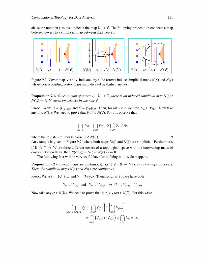
Computational Topology for Data Analysis 211
abuse the notation ξ to also indicate the map U → V. The following proposition connects a mapbetween covers to a simplicial map between their nerves.
UN(U) V N(V) UN(U) V N(V)ξ UN(U) V N(V)ζ
Figure 9.2: Cover maps ξ and ζ indicated by solid arrows induce simplicial maps N(ξ) and N(ζ)whose corresponding vertex maps are indicated by dashed arrows.
Proposition 9.1. Given a map of covers ξ : U → V, there is an induced simplicial map N(ξ) :N(U)→ N(V) given on vertices by the map ξ.
Proof. Write U = Uαα∈A and V = Vββ∈B. Then, for all α ∈ A we have Uα ⊆ Vξ(α). Now takeany σ ∈ N(U). We need to prove that ξ(σ) ∈ N(V). For this observe that
⋂β∈ξ(σ)
Vβ =⋂α∈σ
Vξ(α) ⊇⋂α∈σ
Uα , ∅,
where the last step follows because σ ∈ N(U). An example is given in Figure 9.2, where both maps N(ξ) and N(ζ) are simplicial. Furthermore,
if Uξ→ V
ζ→ W are three different covers of a topological space with the intervening maps of
covers between them, then N(ζ ξ) = N(ζ) N(ξ) as well.The following fact will be very useful later for defining multiscale mappers.
Proposition 9.2 (Induced maps are contiguous). Let ζ, ξ : U → V be any two maps of covers.Then, the simplicial maps N(ζ) and N(ξ) are contiguous.
Proof. Write U = Uαα∈A and V = Vββ∈B. Then, for all α ∈ A we have both
Uα ⊆ Vζ(α) and Uα ⊆ Vξ(α); ⇒ Uα ⊆ Vζ(α) ∩ Vξ(α).
Now take any σ ∈ N(U). We need to prove that ζ(σ) ∪ ξ(σ) ∈ N(V). For this write
⋂β∈ζ(σ)∪ξ(σ)
Vβ =
⋂α∈σ
Vζ(α)
∩ ⋂α∈σ
Vξ(α)
=
⋂α∈σ
(Vζ(α) ∩ Vξ(α)
)⊇
⋂α∈σ
Uα , ∅,
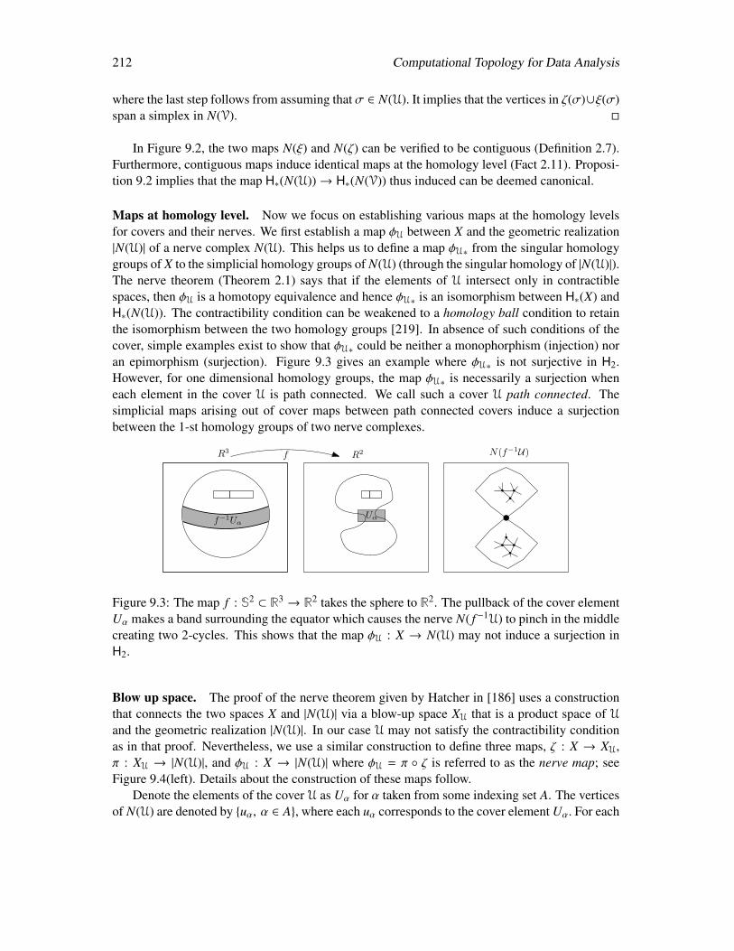
212 Computational Topology for Data Analysis
where the last step follows from assuming that σ ∈ N(U). It implies that the vertices in ζ(σ)∪ξ(σ)span a simplex in N(V).
In Figure 9.2, the two maps N(ξ) and N(ζ) can be verified to be contiguous (Definition 2.7).Furthermore, contiguous maps induce identical maps at the homology level (Fact 2.11). Proposi-tion 9.2 implies that the map H∗(N(U))→ H∗(N(V)) thus induced can be deemed canonical.
Maps at homology level. Now we focus on establishing various maps at the homology levelsfor covers and their nerves. We first establish a map φU between X and the geometric realization|N(U)| of a nerve complex N(U). This helps us to define a map φU∗ from the singular homologygroups of X to the simplicial homology groups of N(U) (through the singular homology of |N(U)|).The nerve theorem (Theorem 2.1) says that if the elements of U intersect only in contractiblespaces, then φU is a homotopy equivalence and hence φU∗ is an isomorphism between H∗(X) andH∗(N(U)). The contractibility condition can be weakened to a homology ball condition to retainthe isomorphism between the two homology groups [219]. In absence of such conditions of thecover, simple examples exist to show that φU∗ could be neither a monophorphism (injection) noran epimorphism (surjection). Figure 9.3 gives an example where φU∗ is not surjective in H2.However, for one dimensional homology groups, the map φU∗ is necessarily a surjection wheneach element in the cover U is path connected. We call such a cover U path connected. Thesimplicial maps arising out of cover maps between path connected covers induce a surjectionbetween the 1-st homology groups of two nerve complexes.
Uαf−1Uα
R3 R2f N(f−1U)
Figure 9.3: The map f : S2 ⊂ R3 → R2 takes the sphere to R2. The pullback of the cover elementUα makes a band surrounding the equator which causes the nerve N( f −1U) to pinch in the middlecreating two 2-cycles. This shows that the map φU : X → N(U) may not induce a surjection inH2.
Blow up space. The proof of the nerve theorem given by Hatcher in [186] uses a constructionthat connects the two spaces X and |N(U)| via a blow-up space XU that is a product space of Uand the geometric realization |N(U)|. In our case U may not satisfy the contractibility conditionas in that proof. Nevertheless, we use a similar construction to define three maps, ζ : X → XU,π : XU → |N(U)|, and φU : X → |N(U)| where φU = π ζ is referred to as the nerve map; seeFigure 9.4(left). Details about the construction of these maps follow.
Denote the elements of the cover U as Uα for α taken from some indexing set A. The verticesof N(U) are denoted by uα, α ∈ A,where each uα corresponds to the cover element Uα. For each
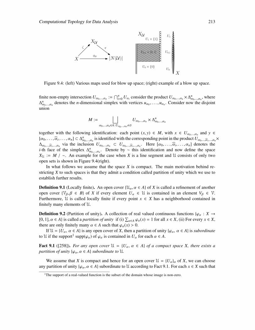
Computational Topology for Data Analysis 213
U0 × 0
U1 × 1XU
U0,1 × [0, 1]
U1
U0,1
U0
X
X |N(U)|
XUζ π
φU
Figure 9.4: (left) Various maps used for blow up space; (right) example of a blow up space.
finite non-empty intersection Uα0,...,αn :=⋂n
i=0 Uαi consider the product Uα0,...,αn ×∆nα0,...,αn
, where∆nα0,...,αn
denotes the n-dimensional simplex with vertices uα0 , . . . , uαn . Consider now the disjointunion
M :=⊔
α0,...,αn∈A: Uα0 ,...,αn,∅
Uα0,...,αn × ∆nα0,...,αn
together with the following identification: each point (x, y) ∈ M, with x ∈ Uα0,...,αn and y ∈[α0, . . . , αi, . . . , αn] ⊂ ∆n
α0,...,αnis identified with the corresponding point in the product Uα0,...,αi,...,αn×
∆α0,...,αi,...,αn via the inclusion Uα0,...,αn ⊂ Uα0,...,αi,...,αn . Here [α0, . . . , αi, . . . , αn] denotes thei-th face of the simplex ∆n
α0,...,αn. Denote by ∼ this identification and now define the space
XU := M / ∼. An example for the case when X is a line segment and U consists of only twoopen sets is shown in Figure 9.4(right).
In what follows we assume that the space X is compact. The main motivation behind re-stricting X to such spaces is that they admit a condition called partition of unity which we use toestablish further results.
Definition 9.1 (Locally finite). An open cover Uα, α ∈ A of X is called a refinement of anotheropen cover Vβ, β ∈ B of X if every element Uα ∈ U is contained in an element Vβ ∈ V.Furthermore, U is called locally finite if every point x ∈ X has a neighborhood contained infinitely many elements of U.
Definition 9.2 (Partition of unity). A collection of real valued continuous functions ϕα : X →[0, 1], α ∈ A is called a partition of unity if (i)
∑α∈A ϕα(x) = 1 for all x ∈ X, (ii) For every x ∈ X,
there are only finitely many α ∈ A such that ϕα(x) > 0.If U = Uα, α ∈ A is any open cover of X, then a partition of unity ϕα, α ∈ A is subordinate
to U if the support1 supp(ϕα) of ϕα is contained in Uα for each α ∈ A.
Fact 9.1 ([258]). For any open cover U = Uα, α ∈ A of a compact space X, there exists apartition of unity ϕα, α ∈ A subordinate to U.
We assume that X is compact and hence for an open cover U = Uαα of X, we can chooseany partition of unity ϕα, α ∈ A subordinate to U according to Fact 9.1. For each x ∈ X such that
1The support of a real-valued function is the subset of the domain whose image is non-zero.
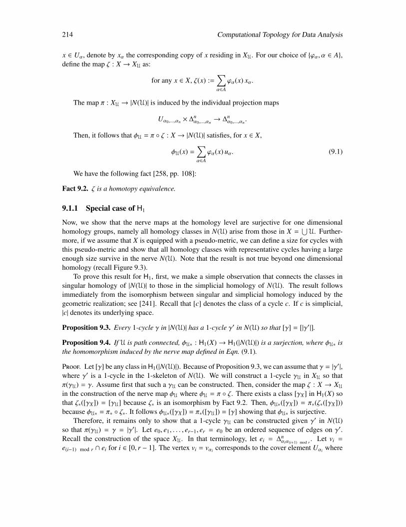
214 Computational Topology for Data Analysis
x ∈ Uα, denote by xα the corresponding copy of x residing in XU. For our choice of ϕα, α ∈ A,define the map ζ : X → XU as:
for any x ∈ X, ζ(x) :=∑α∈A
ϕα(x) xα.
The map π : XU → |N(U)| is induced by the individual projection maps
Uα0,...,αn × ∆nα0,...,αn
→ ∆nα0,...,αn
.
Then, it follows that φU = π ζ : X → |N(U)| satisfies, for x ∈ X,
φU(x) =∑α∈A
ϕα(x) uα. (9.1)
We have the following fact [258, pp. 108]:
Fact 9.2. ζ is a homotopy equivalence.
9.1.1 Special case of H1
Now, we show that the nerve maps at the homology level are surjective for one dimensionalhomology groups, namely all homology classes in N(U) arise from those in X =
⋃U. Further-
more, if we assume that X is equipped with a pseudo-metric, we can define a size for cycles withthis pseudo-metric and show that all homology classes with representative cycles having a largeenough size survive in the nerve N(U). Note that the result is not true beyond one dimensionalhomology (recall Figure 9.3).
To prove this result for H1, first, we make a simple observation that connects the classes insingular homology of |N(U)| to those in the simplicial homology of N(U). The result followsimmediately from the isomorphism between singular and simplicial homology induced by thegeometric realization; see [241]. Recall that [c] denotes the class of a cycle c. If c is simplicial,|c| denotes its underlying space.
Proposition 9.3. Every 1-cycle γ in |N(U)| has a 1-cycle γ′ in N(U) so that [γ] = [|γ′|].
Proposition 9.4. If U is path connected, φU∗ : H1(X) → H1(|N(U)|) is a surjection, where φU∗ isthe homomorphism induced by the nerve map defined in Eqn. (9.1).
Proof. Let [γ] be any class in H1(|N(U)|). Because of Proposition 9.3, we can assume that γ = |γ′|,where γ′ is a 1-cycle in the 1-skeleton of N(U). We will construct a 1-cycle γU in XU so thatπ(γU) = γ. Assume first that such a γU can be constructed. Then, consider the map ζ : X → XU
in the construction of the nerve map φU where φU = π ζ. There exists a class [γX] in H1(X) sothat ζ∗([γX]) = [γU] because ζ∗ is an isomorphism by Fact 9.2. Then, φU∗([γX]) = π∗(ζ∗([γX]))because φU∗ = π∗ ζ∗. It follows φU∗([γX]) = π∗([γU]) = [γ] showing that φU∗ is surjective.
Therefore, it remains only to show that a 1-cycle γU can be constructed given γ′ in N(U)so that π(γU) = γ = |γ′|. Let e0, e1, . . . , er−1, er = e0 be an ordered sequence of edges on γ′.Recall the construction of the space XU. In that terminology, let ei = ∆n
αiα(i+1) mod r. Let vi =
e(i−1) mod r ∩ ei for i ∈ [0, r − 1]. The vertex vi = vαi corresponds to the cover element Uαi where
Computational Topology for Data Analysis 215
Uαi ∩ Uα(i+1) mod r , ∅ for every i ∈ [0, r − 1]. Choose a point xi in the common intersectionUαi ∩Uα(i+1) mod r for every i ∈ [0, r − 1]. Then, the edge path ei = ei × xi is in XU by construction.Also, letting xαi to be the lift of xi in the lifted Uαi , we can choose a vertex path xαi xα(i+1) mod r
residing in the lifted Uαi and hence in XU because Uαi is path connected. Consider the followingcycle obtained by concatenating the edge and vertex paths
γU = e0xα0 xα1 e1 · · · er−1xαr−1 xα0
By projection, we have π(ei) = ei for every i ∈ [0, r − 1] and π(xαi xα(i+1) mod r ) = vαi and thusπ(γU) = γ as required.
Since we are eventually interested in the simplicial homology groups of the nerves ratherthan the singular homology groups of their geometric realizations, we make one more transitionusing the known isomorphism between the two homology groups (Theorem 2.10). Specifically,if ιU : Hp(|N(U)|)→ Hp(N(U)) denotes this isomorphism, we let
φU∗ : H1(X)→ H1(N(U)) denote the composition ιU φU∗. (9.2)
As a corollary to Proposition 9.4, we obtain:
Theorem 9.5. If U is path connected, φU∗ : H1(X)→ H1(N(U)) is a surjection.
U1
X
U2
ξ1
N(ξ1)
U3
ξ2
N(ξ2)
N(U2)N(U1) N(U3)
Figure 9.5: Sequence of cover maps induce a simplicial tower and hence a persistence module:classes in H1 can only die.
From nerves to nerves. We now extend the result in Theorem 9.5 to simplicial maps betweentwo nerves induced by cover maps. Figure 9.5 illustrates this fact. The following proposition iskey to establishing the result.
Proposition 9.6 (Coherent partitions of unity). Suppose Uαα∈A = Uθ−→ V = Vββ∈B are open
covers of a compact topological space X and θ : A → B is a map of covers. Then there exists apartition of unity ϕαα∈A subordinate to the cover U such that if for each β ∈ B we define
ψβ := ∑
α∈θ−1(β) ϕα if β ∈ im(θ);0 otherwise.
216 Computational Topology for Data Analysis
then the set of functions ψββ∈B is a partition of unity subordinate to the cover V.
Proof. The proof closely follows that of [258, Corollary pp. 97]. Since X is compact, thereexists a partition of unity ϕαα∈A subordinate to U. The fact that the sum in the expression of ψβis well defined and continuous follows from the fact that the family supp(ϕα)α is locally finite.Let Cβ :=
⋃α∈θ−1(β) supp(ϕα). The set Cβ is closed, Cβ ⊂ Uβ, and ψβ(x) = 0 for x < Cβ so that
supp(ψβ) ⊂ Cβ ⊂ Vβ. Now, to check that the family Cββ∈B is locally finite pick any point x ∈ X.Since supp(ϕα)α is locally finite there is an open set O containing x such that O intersects onlyfinitely many elements in U. Denote these cover elements by Uα1 , . . . ,Uα` . Now, notice if β ∈ Band β < θ(αi), i = 1, . . . , `, then O does not intersect Cβ. Then, the family supp(ψβ)β∈B islocally finite. It then follows that for x ∈ X one has∑
β∈B
ψβ(x) =∑β∈B
∑α∈θ−1(β)
ϕα(x) =∑α∈A
ϕα(x) = 1.
We have obtained that ψββ∈B is a partition of unity subordinate to V as needed by the propo-sition.
Let Uαα∈A = Uθ−→ V = Vββ∈B be two open covers of X connected by a map of covers
θ : A → B. Apply Proposition 9.6 to obtain coherent partitions of unity ϕαα∈A and ψββ∈B
subordinate to U and V, respectively. Let the nerve maps φU : X → |N(U)| and φV : X → |N(V)|be defined as in Eqn. (9.1) using these coherent partitions of unity. Let N(U)
τ→ N(V) be the
simplicial map induced by the cover map θ. The map τ can be extended to a (linear) continuousmap τ : |N(U)|→|N(V)| by assigning y ∈ |N(U)| to τ(y) ∈ |N(V)| where
y =∑
tαuα =⇒ τ(y) =∑
tατ(uα), with∑
tα = 1.
Claim 9.1. The map τ satisfies the property that, for x ∈ X, τ(φU(x)) = φV(x).
Proof. For any point x ∈ X, one has φU(x) = Σα∈Aϕα(x)uα where uα is the vertex correspondingto Uα ∈ U in |N(U)|. Then,
τ φU(x) = τ
∑α∈A
ϕα(x)uα
=∑α∈A
ϕα(x)τ(uα) =∑α∈A
ϕα(x) vθ(α)
=∑β∈B
∑α∈θ−1(β)
ϕα(x) vθ(α) =∑β∈B
ψβ(x)vβ = φV(x)
An immediate corollary of the above claim is:
Corollary 9.7. The induced maps of φU∗ : Hp(X)→ Hp(|N(U)|), φV∗ : Hp(X)→ Hp(|N(V)|), andτ∗ : Hp(|N(U)|)→ Hp(|N(V)|) commute, that is, φV∗ = τ∗ φU∗.
With the fact that isomorphism between singular and simplicial homology commutes withsimplicial maps and their linear continuous extensions, Corollary 9.7 implies that:
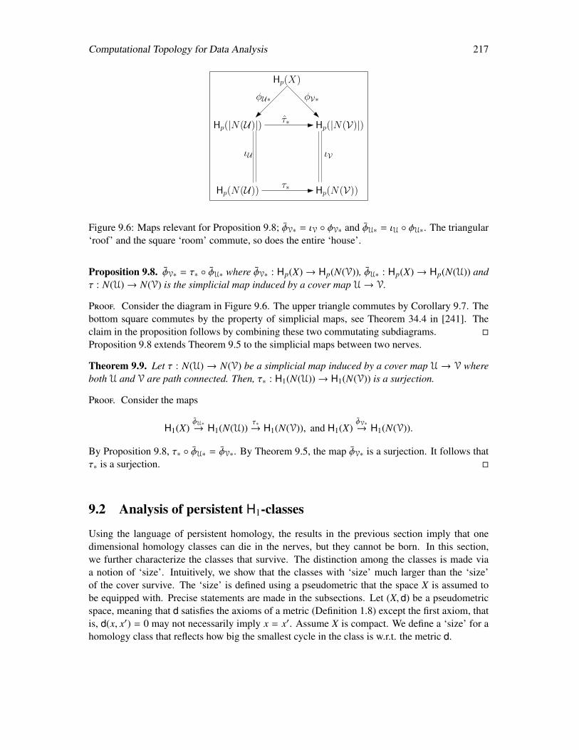
Computational Topology for Data Analysis 217
Hp(X)
Hp(|N(U)|) Hp(|N(V)|)τ∗
φU∗ φV∗
ιU ιV
Hp(N(U)) Hp(N(V))τ∗
Figure 9.6: Maps relevant for Proposition 9.8; φV∗ = ιV φV∗ and φU∗ = ιU φU∗. The triangular‘roof’ and the square ‘room’ commute, so does the entire ‘house’.
Proposition 9.8. φV∗ = τ∗ φU∗ where φV∗ : Hp(X)→ Hp(N(V)), φU∗ : Hp(X)→ Hp(N(U)) andτ : N(U)→ N(V) is the simplicial map induced by a cover map U→ V.
Proof. Consider the diagram in Figure 9.6. The upper triangle commutes by Corollary 9.7. Thebottom square commutes by the property of simplicial maps, see Theorem 34.4 in [241]. Theclaim in the proposition follows by combining these two commutating subdiagrams. Proposition 9.8 extends Theorem 9.5 to the simplicial maps between two nerves.
Theorem 9.9. Let τ : N(U) → N(V) be a simplicial map induced by a cover map U → V whereboth U and V are path connected. Then, τ∗ : H1(N(U))→ H1(N(V)) is a surjection.
Proof. Consider the maps
H1(X)φU∗→ H1(N(U))
τ∗→ H1(N(V)), and H1(X)
φV∗→ H1(N(V)).
By Proposition 9.8, τ∗ φU∗ = φV∗. By Theorem 9.5, the map φV∗ is a surjection. It follows thatτ∗ is a surjection.
9.2 Analysis of persistent H1-classes
Using the language of persistent homology, the results in the previous section imply that onedimensional homology classes can die in the nerves, but they cannot be born. In this section,we further characterize the classes that survive. The distinction among the classes is made viaa notion of ‘size’. Intuitively, we show that the classes with ‘size’ much larger than the ‘size’of the cover survive. The ‘size’ is defined using a pseudometric that the space X is assumed tobe equipped with. Precise statements are made in the subsections. Let (X, d) be a pseudometricspace, meaning that d satisfies the axioms of a metric (Definition 1.8) except the first axiom, thatis, d(x, x′) = 0 may not necessarily imply x = x′. Assume X is compact. We define a ‘size’ for ahomology class that reflects how big the smallest cycle in the class is w.r.t. the metric d.
218 Computational Topology for Data Analysis
Definition 9.3. The size s(X′) of a subset X′ of the pseudometric space (X, d) is defined to beits diameter, that is, s(X′) = supx,x′∈X′×X′ d(x, x′). The size of a class c ∈ Hp(X) is defined ass(c) = infz∈c s(z). According to Definition 5.3, a set of p-cycles z1, z2, . . . , zn of Hp(X) is called acycle basis if the classes [z1], [z2], . . . , [zn] together form a basis of Hp(X). It is called an optimalcycle basis if Σn
i=1s(zi) is minimal among all cycle bases.
Lebesgue number of a cover. Our goal is to characterize the classes in the nerve of U withrespect to the sizes of their preimages in X via the map φU. The Lebesgue number of a cover Ubecomes useful in this characterization. It is the largest real number λ(U) so that any subset of Xwith size at most λ(U) is contained in at least one element of U. Formally, the Lebesgue numberλ(U) of U is defined as:
λ(U) = supδ | ∀X′ ⊆ X with s(X′) ≤ δ,∃Uα ∈ U where X′ ⊆ Uα.
As we will see below, a homology class of size no more than λ(U) cannot survive in the nerve(Proposition 9.12). Further, the homology classes whose sizes are significantly larger than themaximum size of a cover do necessarily survive where we define the maximum size of a cover as
smax(U) := maxU∈Us(U).
Theorem 9.10 summarizes these observations.Let z1, z2, . . . , zg be a non-decreasing sequence of the cycles with respect to their sizes in an
optimal cycle basis of H1(X). Consider the map φU : X → |N(U)| as introduced in Eqn. (9.1), andthe map φU∗ as defined by Eqn. (9.2). We have the following result.
Theorem 9.10. Let U be a path connected cover of X and z1, z2, . . . , zg be a sequence of anoptimal cycle basis of H1(X) as stated above.
i. Let ` = g + 1 if λ(U) > s(zg). Otherwise, let ` ∈ [1, g] be the smallest integer so thats(z`) > λ(U). If ` , 1, then we have that the class φU∗[z j] = 0 for j = 1, . . . , ` − 1.Moreover, if ` , g + 1, then the classes φU∗[z j] j=`,...,g generate H1(N(U)).
ii. The classes φU∗[z j] j=`′,...,g are linearly independent where s(z`′) > 4smax(U).
The result above says that only the classes of H1(X) generated by cycles of large enough sizesurvive in the nerve. To prove this result, we use a map ρ that sends each 1-cycle in N(U) toa 1-cycle in X. We define a chain map ρ : C1(N(U)) → C1(X) among one dimensional chaingroups as follows. It is sufficient to exhibit the map for an elementary chain of an edge, saye = uα, uα′ ∈ C1(N(U)). Since e is an edge in N(U), the two cover elements Uα and Uα′ in Xhave a common intersection. Let a ∈ Uα and b ∈ Uα′ be two points that are arbitrary but fixedfor Uα and Uα′ respectively. Pick a path ξ(a, b) (viewed as a singular chain) in the union of Uα
and Uα′ which is path connected as both Uα and Uα′ are. Then, define ρ(e) = ξ(a, b). A cycle γwhen pushed back by ρ and then pushed forward by φU remains in the same class. The followingproposition states this fact whose proof appears in [133].
Proposition 9.11. Let γ be any 1-cycle in N(U). Then, [φU(ρ(γ))] = [|γ|].
Computational Topology for Data Analysis 219
The following proposition provides a sufficient characterization of the cycles whose classesbecome trivial after the push forward.
Proposition 9.12. Let z be a 1-cycle in C1(X). Then, [φU(z)] = 0 if λ(U) > s(z).
Proof. It follows from the definition of the Lebesgue number that there exists a cover elementUα ∈ U such that z ⊆ Uα because s(z) < λ(U). We claim that there is a homotopy equivalencethat sends φU(z) to a vertex in N(U) and hence [φU(z)] is trivial.
Let x be any point in z. Recall that φU(x) = Σiϕi(x)uαi . Since Uα has a common intersectionwith each Uαi so that ϕαi(x) , 0, we can conclude that φU(x) is contained in a simplex with thevertex uα. Continuing this argument with all points of z, we observe that φU(z) is contained insimplices that share the vertex uα. It follows that there is a homotopy that sends φU(z) to uα, avertex of N(U).
Proof. [Proof of Theorem 9.10]Proof of (i): By Proposition 9.12, we have φU∗[z] = [φU(z)] = 0 if λ(U) > s(z). This establishesthe first part of the assertion because φU∗ = ιφU∗ where ι is an isomorphism between the singularhomology of |N(U)| and the simplicial homology of N(U). To see the second part, notice that φU∗is a surjection by Theorem 9.5. Therefore, the classes φU∗(z) where s(z) ≥ λ(U) contain a basisfor H1(N(U)). Hence they generate it.
Proof of (ii): For a contradiction, assume that there is a subsequence `1, . . . , `t ⊂ `′, . . . , g
so that Σtj=1[φU(z` j)] = 0. Let z = Σt
j=1φU(z` j). Let γ be a 1-cycle in N(U) so that [z] = [|γ|]whose existence is guaranteed by Proposition 9.3. As Σt
j=1[φU(z` j)] = 0, it must be that there isa 2-chain D in N(U) so that ∂D = γ. Consider a triangle t = uα1 , uα2 , uα3 contributing to D.Let a′i = φ−1
U(uαi). Since t appears in N(U), the covers Uα1 ,Uα2 ,Uα3 containing a′1, a′2, and a′3
respectively have a common intersection in X. This also means that each of the paths a′1 a′2,a′2 a′3, a′3 a′1 has size at most 2smax(U). Then, ρ(∂t) is mapped to a 1-cycle in X of size atmost 4smax(U). It follows that ρ(∂D) can be written as a linear combination of cycles of size atmost 4smax(U). Since z1, . . . , zg form an optimal cycle basis of H1(X), each of the 1-cycles of sizeat most 4smax(U) is generated by basis elements z1, . . . , zk where s(zk) ≤ 4smax(U). Therefore, theclass of z′ = φU(ρ(γ)) is generated by a linear combination of the basis elements whose preimageshave size at most 4smax(U). The class [z′] is same as the class [|γ|] by Proposition 9.11. But, byassumption [|γ|] = [z] is generated by a linear combination of the basis elements whose sizes arelarger than 4smax(U) reaching a contradiction. Hence the assumption cannot hold and (ii) is true.
9.3 Mapper and multiscale mapper
In this section we extend the previous results to the structures called mapper and multiscale map-per. Recall that X is assumed to be compact. Consider a cover of X obtained indirectly as apullback of a cover of another space Z. This gives rise to the so-called Mapper. More precisely,let f : X → Z be a continuous map where Z is equipped with an open cover U = Uαα∈A forsome index set A. Since f is continuous, the sets f −1(Uα), α ∈ A form an open cover of X. For
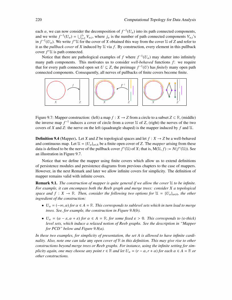
220 Computational Topology for Data Analysis
each α, we can now consider the decomposition of f −1(Uα) into its path connected components,and we write f −1(Uα) =
⋃ jαi=1 Vα,i, where jα is the number of path connected components Vα,i’s
in f −1(Uα). We write f ∗U for the cover of X obtained this way from the cover U of Z and refer toit as the pullback cover of X induced by U via f . By construction, every element in this pullbackcover f ∗U is path connected.
Notice that there are pathological examples of f where f −1(Uα) may shatter into infinitelymany path components. This motivates us to consider well-behaved functions f : we requirethat for every path connected open set U ⊆ Z, the preimage f −1(U) has finitely many open pathconnected components. Consequently, all nerves of pullbacks of finite covers become finite.
f
X Z
f
X Z
f−1
X Z
Figure 9.7: Mapper construction: (left) a map f : X → Z from a circle to a subset Z ⊂ R, (middle)the inverse map f −1 induces a cover of circle from a cover U of Z, (right) the nerves of the twocovers of X and Z: the nerve on the left (quadrangle shaped) is the mapper induced by f and U.
Definition 9.4 (Mapper). Let X and Z be topological spaces and let f : X → Z be a well-behavedand continuous map. Let U = Uαα∈A be a finite open cover of Z. The mapper arising from thesedata is defined to be the nerve of the pullback cover f ∗(U) of X; that is, M(U, f ) := N( f ∗(U)). Seean illustration in Figure 9.7.
Notice that we define the mapper using finite covers which allow us to extend definitionsof persistence modules and persistence diagrams from previous chapters to the case of mappers.However, in the next Remark and later we allow infinite covers for simplicity. The definition ofmapper remains valid with infinite covers.
Remark 9.1. The construction of mapper is quite general if we allow the cover U to be infinite.For example, it can encompass both the Reeb graph and merge trees: consider X a topologicalspace and f : X → R. Then, consider the following two options for U = Uαα∈A, the otheringredient of the construction:
• Uα = (−∞, α) for α ∈ A = R. This corresponds to sublevel sets which in turn lead to mergetrees. See, for example, the construction in Figure 9.8(b).
• Uα = (α − ε, α + ε) for α ∈ A = R, for some fixed ε > 0. This corresponds to (ε-thick)level sets, which induce a relaxed notion of Reeb graphs. See the description in “Mapperfor PCD” below and Figure 9.8(a).
In these two examples, for simplicity of presentation, the set A is allowed to have infinite cardi-nality. Also, note one can take any open cover of R in this definition. This may give rise to otherconstructions beyond merge trees or Reeb graphs. For instance, using the infinite setting for sim-plicity again, one may choose any point r ∈ R and let Uα = (r − α, r + α) for each α ∈ A = R orother constructions.
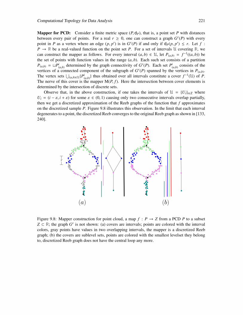
Computational Topology for Data Analysis 221
Mapper for PCD: Consider a finite metric space (P, dP), that is, a point set P with distancesbetween every pair of points. For a real r ≥ 0, one can construct a graph Gr(P) with everypoint in P as a vertex where an edge (p, p′) is in Gr(P) if and only if dP(p, p′) ≤ r. Let f :P → R be a real-valued function on the point set P. For a set of intervals U covering R, wecan construct the mapper as follows. For every interval (a, b) ∈ U, let P(a,b) = f −1((a, b)) bethe set of points with function values in the range (a, b). Each such set consists of a partitionP(a,b) = tPi
(a,b) determined by the graph connectivity of Gr(P). Each set Pi(a,b) consists of the
vertices of a connected component of the subgraph of Gr(P) spanned by the vertices in P(a,b).The vertex sets
⋃(a,b)∈UPi
(a,b) thus obtained over all intervals constitute a cover f −1(U) of P.The nerve of this cover is the mapper M(P, f ). Here the intersection between cover elements isdetermined by the intersection of discrete sets.
Observe that, in the above construction, if one takes the intervals of U = Uii∈Z whereUi = (i − ε, i + ε) for some ε ∈ (0, 1) causing only two consecutive intervals overlap partially,then we get a discretized approximation of the Reeb graphs of the function that f approximateson the discretized sample P. Figure 9.8 illustrates this observation. In the limit that each intervaldegenerates to a point, the discretized Reeb converges to the original Reeb graph as shown in [133,240].
(a) (b)
r
Figure 9.8: Mapper construction for point cloud, a map f : P → Z from a PCD P to a subsetZ ⊂ R; the graph Gr is not shown: (a) covers are intervals; points are colored with the intervalcolors, gray points have values in two overlapping intervals, the mapper is a discretized Reebgraph; (b) the covers are sublevel sets, points are colored with the smallest levelset they belongto, discretized Reeb graph does not have the central loop any more.
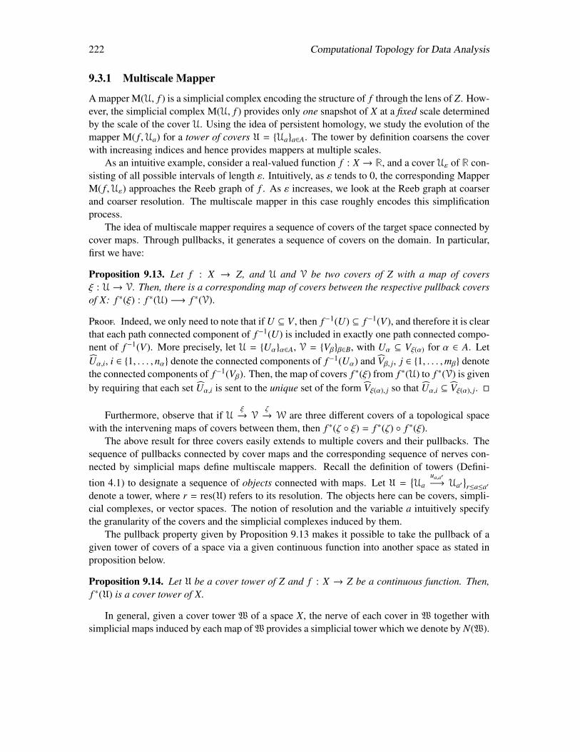
222 Computational Topology for Data Analysis
9.3.1 Multiscale Mapper
A mapper M(U, f ) is a simplicial complex encoding the structure of f through the lens of Z. How-ever, the simplicial complex M(U, f ) provides only one snapshot of X at a fixed scale determinedby the scale of the cover U. Using the idea of persistent homology, we study the evolution of themapper M( f ,Ua) for a tower of covers U = Uaa∈A. The tower by definition coarsens the coverwith increasing indices and hence provides mappers at multiple scales.
As an intuitive example, consider a real-valued function f : X → R, and a cover Uε of R con-sisting of all possible intervals of length ε. Intuitively, as ε tends to 0, the corresponding MapperM( f ,Uε) approaches the Reeb graph of f . As ε increases, we look at the Reeb graph at coarserand coarser resolution. The multiscale mapper in this case roughly encodes this simplificationprocess.
The idea of multiscale mapper requires a sequence of covers of the target space connected bycover maps. Through pullbacks, it generates a sequence of covers on the domain. In particular,first we have:
Proposition 9.13. Let f : X → Z, and U and V be two covers of Z with a map of coversξ : U→ V. Then, there is a corresponding map of covers between the respective pullback coversof X: f ∗(ξ) : f ∗(U) −→ f ∗(V).
Proof. Indeed, we only need to note that if U ⊆ V , then f −1(U) ⊆ f −1(V), and therefore it is clearthat each path connected component of f −1(U) is included in exactly one path connected compo-nent of f −1(V). More precisely, let U = Uαα∈A, V = Vββ∈B, with Uα ⊆ Vξ(α) for α ∈ A. LetUα,i, i ∈ 1, . . . , nα denote the connected components of f −1(Uα) and Vβ, j, j ∈ 1, . . . ,mβ denotethe connected components of f −1(Vβ). Then, the map of covers f ∗(ξ) from f ∗(U) to f ∗(V) is givenby requiring that each set Uα,i is sent to the unique set of the form Vξ(α), j so that Uα,i ⊆ Vξ(α), j.
Furthermore, observe that if Uξ→ V
ζ→ W are three different covers of a topological space
with the intervening maps of covers between them, then f ∗(ζ ξ) = f ∗(ζ) f ∗(ξ).The above result for three covers easily extends to multiple covers and their pullbacks. The
sequence of pullbacks connected by cover maps and the corresponding sequence of nerves con-nected by simplicial maps define multiscale mappers. Recall the definition of towers (Defini-
tion 4.1) to designate a sequence of objects connected with maps. Let U =Ua
ua,a′−→ Ua′
r≤a≤a′
denote a tower, where r = res(U) refers to its resolution. The objects here can be covers, simpli-cial complexes, or vector spaces. The notion of resolution and the variable a intuitively specifythe granularity of the covers and the simplicial complexes induced by them.
The pullback property given by Proposition 9.13 makes it possible to take the pullback of agiven tower of covers of a space via a given continuous function into another space as stated inproposition below.
Proposition 9.14. Let U be a cover tower of Z and f : X → Z be a continuous function. Then,f ∗(U) is a cover tower of X.
In general, given a cover tower W of a space X, the nerve of each cover in W together withsimplicial maps induced by each map ofW provides a simplicial tower which we denote by N(W).
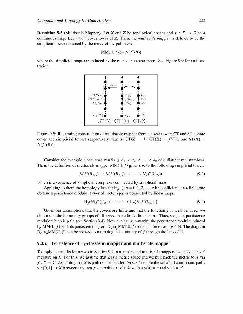
Computational Topology for Data Analysis 223
Definition 9.5 (Multiscale Mapper). Let X and Z be topological spaces and f : X → Z be acontinuous map. Let U be a cover tower of Z. Then, the multiscale mapper is defined to be thesimplicial tower obtained by the nerve of the pullback:
MM(U, f ) := N( f ∗(U))
where the simplicial maps are induced by the respective cover maps. See Figure 9.9 for an illus-tration.
CT(Z)
Ua
Ua′
ua,a′
Ur
f ∗Ua
f ∗Ua′
f ∗(ua,a′)
f ∗Ur
f−1
ST(X)
N(f ∗Ua)
N(f ∗Ua′)
N(f ∗(ua,a′))
N(f ∗Ur)
Nerve
CT(X)
Figure 9.9: Illustrating construction of multiscale mapper from a cover tower; CT and ST denotecover and simplicial towers respectively, that is, CT(Z) = U, CT(X) = f ∗(U), and ST(X) =
N( f ∗(U)).
Consider for example a sequence res(U) ≤ a1 < a2 < . . . < an of n distinct real numbers.Then, the definition of multiscale mapper MM(U, f ) gives rise to the following simplicial tower:
N( f ∗(Ua1))→ N( f ∗(Ua2))→ · · · → N( f ∗(Uan)). (9.3)
which is a sequence of simplicial complexes connected by simplicial maps.Applying to them the homology functor Hp(·), p = 0, 1, 2, . . ., with coefficients in a field, one
obtains a persistence module: tower of vector spaces connected by linear maps.
Hp(N( f ∗(Ua1))
)→ · · · → Hp
(N( f ∗(Uan))
). (9.4)
Given our assumptions that the covers are finite and that the function f is well-behaved, weobtain that the homology groups of all nerves have finite dimensions. Thus, we get a persistencemodule which is p.f.d.(see Section 3.4). Now one can summarize the persistence module inducedby MM(U, f ) with its persistent diagram DgmpMM(U, f ) for each dimension p ∈ N. The diagramDgmpMM(U, f ) can be viewed as a topological summary of f through the lens of U.
9.3.2 Persistence of H1-classes in mapper and multiscale mapper
To apply the results for nerves in Section 9.2 to mappers and multiscale mappers, we need a ‘size’measure on X. For this, we assume that Z is a metric space and we pull back the metric to X viaf : X → Z. Assuming that X is path connected, let ΓX(x, x′) denote the set of all continuous pathsγ : [0, 1]→ X between any two given points x, x′ ∈ X so that γ(0) = x and γ(1) = x′.
224 Computational Topology for Data Analysis
Definition 9.6 (Pullback metric). Given a metric space (Z, dZ), we define its pullback metric asthe following pseudometric d f on X: for x, x′ ∈ X,
d f (x, x′) := infγ∈ΓX(x,x′)
diamZ( f γ).
Consider the Lebesgue number of the pullback covers of X. The following observation in thisrespect is useful.
Proposition 9.15. Let U be a cover for the codomain Z and U′ be its restriction to f (X). Then,the pullback cover f ∗U has the same Lebesgue number as that of U′; that is λ( f ∗U) = λ(U′).
Proof. First, observe that, for any path connected cover of X, a subset of X that realizes theLebesgue number can be taken as path connected because, if not, this subset can be connectedby a path entirely lying within the cover element containing it. Let X′ ⊆ X be any subset wheres(X′) ≤ λ(U′). Then, f (X′) ⊆ Z has a diameter at most λ(U′) by the definitions of size (Definition9.3) and pullback metric. Therefore, by the definition of Lebesgue number, f (X′) is contained ina cover element U′ ∈ U′. Since X′ is path connected, a path connected component of f −1(U′)contains X′. It follows that there is a cover element in f ∗U that contains X′. Since X′ was chosenas an arbitrary path connected subset of size at most λ(U′), we have λ( f ∗U) ≥ λ(U′). At the sametime, it is straightforward from the definition of size that each cover element in f −1(U′) has atmost the size of U′ for any U′ ∈ U′. Combining with the fact that U′ is the restriction of U tof (X), we have λ( f ∗U) ≤ λ(U′), establishing the equality as claimed.
Given a cover U of Z, consider the mapper N( f ∗U). Let z1, . . . , zg be a set of optimal cyclebasis for H1(X) where the metric used to define optimality is the pullback metric d f . Then, as aconsequence of Theorem 9.10 we have:
Theorem 9.16. Let f : X → Z be a map from a path connected space X to a metric space Zequipped with a cover U (i and ii below) or a tower of covers Ua (iii below). Let U′ be therestriction of U to f (X).
i Let ` = g + 1 if λ(U′) > s(zg). Otherwise, let ` ∈ [1, g] be the smallest integer so thats(z`) > λ(U′). If ` , 1, the class φU∗[z j] = 0 for j = 1, . . . , `− 1. Moreover, if ` , g + 1, theclasses φU∗[z j] j=`,...,g generate H1(N( f ∗U)).
ii The classes φU∗[z j] j=`′,...,g are linearly independent where s(z`′) > 4smax(U).
iii Consider a H1-persistence module of a multiscale mapper induced by a tower of path con-nected covers:
H1(N( f ∗Ua0)
) s1∗→ H1
(N( f ∗Ua1)
) s2∗→ · · ·
sn∗→ H1
(N( f ∗Uan)
)(9.5)
Let si∗ = si∗ s(i−1)∗ · · · φUa0∗. Then, the assertions in (i) and (ii) hold for H1(N( f ∗Uai))
with the map si∗ : X → N( f ∗Uai).
Computational Topology for Data Analysis 225
9.4 Stability
To be useful in practice, the multiscale mapper should be stable against the perturbations in themaps and the covers. we show that such a stability is enjoyed by the multiscale mapper undersome natural condition on the tower of covers. Recall that previous stability results for towers asdescribed in section 4.1 were drawn on the notion of interleaving. We identify compatible notionsof interleaving for cover towers as a way to measure the “closeness" between two cover towers.
9.4.1 Interleaving of cover towers and multiscale mappers
In this section we consider cover and simplicial towers indexed over R. In practice, we often have
a cover tower U =Ua
ua,a′−→ Ua′
a≤a′ indexed by a discrete set in A ⊂ R. Any such tower can be
extended to a cover tower indexed over R by taking Uε = Ua for each index ε ∈ (a, a′) where a, a′
are any two consecutive indices in the ordered set A.
Definition 9.7 (Interleaving of cover towers). Let U = Ua and V = Va be two cover towersof a topological space X so that res(U) = res(V) = r. Given η ≥ 0, we say that U and V areη-interleaved if one can find cover maps ζa : Ua → Va+η and ξa′ : Va′ → Ua′+η for all a, a′ ≥ r;see the diagram below.
· · · −→ Ua
ζa
// Ua+η//
ζa+η
,,
Ua+2η −→ · · ·
· · · −→ Va //
ξa
>>
Va+η
ξa+η
22
// Va+2η −→ · · ·
Analogously, if we replace the operator ‘+’ by the multiplication ‘·’ in the above definition, thenwe say that U and V are multiplicatively η-interleaved.
Proposition 9.17. (i) If U and V are (multiplicative) η1-interleaved and V and W are (multi-plicative) η2-interleaved, then, U andW are (multiplicative (η1η2)-) (η1 + η2)-interleaved. (ii) Letf : X → Z be a continuous function and U and V be two (multiplicative) η-interleaved tower ofcovers of Z. Then, f ∗(U) and f ∗(V) are also (multiplicative) η-interleaved.
Note that in the definition of interleaving cover towers, we do not have explicit requirementthat maps need to make sub-diagrams commute unlike the the interleaving between simplicialtowers (Definition 4.2). However, it follows from Proposition 9.2 that interleaving cover towerslead to interleaving between simplicial towers for N(U) and N(V) as shown in the propositionbelow.
Proposition 9.18. Let U and V be two (multiplicatively) η-interleaved cover towers of X withres(U) = res(V). Then, N(U) and N(V) are also (multiplicatively) η-interleaved.
Proof. We prove the proposition for additive interleaving. Replacing the ‘+’ operator with ‘·’gives the proof for multiplicative interleaving. Let r denote the common resolution of U and V.
Write U =Ua
ua,a′−→ Ua′
r≤a≤a′ and V =
Va
va,a′−→ Va′
r≤a≤a′ , and for each a ≥ r let ζa : Ua → Va+η
and ξa : Va → Ua+η be given as in Definition 9.7. To define interleaving between the towers ofnerves arising out of covers, we consider similar diagrams to (4.3) at the level of covers involving
226 Computational Topology for Data Analysis
covers of the form Ua and Va, and apply the nerve construction. This operation yields diagramsidentical to those in (4.3) where for every a, a′ where a′ ≥ a ≥ r:
• Ka := N(Ua), La := N(Va),
• xa,a′ := N(ua,a′), for r ≤ a ≤ a′; ya,a′ := N(va,a′), for r ≤ a ≤ a′; ϕa := N(ζa), andψa := N(ξa).
To satisfy Definition 4.2, it remains to verify conditions (i) to (iv). We only verify (i), since theproof of the others follows the same arguments. For this, notice that both the composite mapξa+η ζa and ua,a+2η are maps of covers from Ua to Ua+2η. By Proposition 9.2 we then have thatN(ξa+η ζa) and N(ua,a+2η) = fa,a+2η are contiguous. But, by the properties of the nerve construc-tion N(ξa+η ζa) = N(ξa+η) N(ζa) = ψa+η ϕa, which completes the claim.
Combining Proposition 9.17 and Proposition 9.18, we get that the two multiscale mappers un-der cover perturbations stay stable, which is the first part of Corollary 9.19. Recall from Chapter 4that, for a finite simplicial tower S and p ∈ N, we denote by Dgmp(S) the p-th persistence dia-gram of the tower S with coefficients in a fixed field. Using Proposition 9.18 and Theorem 4.3, wehave a stability result for DgmpMM(U, f ) when f is kept fixed but the cover tower U is perturbed,which is the second part of the corollary below.
Corollary 9.19. For η ≥ 0, let U and V be two finite cover towers of Z with res(U) = res(V) >0. Let f : X → Z be well-behaved and U and V be η-interleaved. Then, MM(U, f ) andMM(V, f ) are η-interleaved. In particular, the bottleneck distance between the persistence di-agrams DgmpMM(U, f ) and DgmpMM(V, f ) is at most η for all p ∈ N.
9.4.2 (c, s)-good covers
Although DgmpMM(U, f ) is stable under perturbations of the covers U as we showed, it is notnecessarily stable under perturbations of the map f . To address this issue, we introduce a specialfamily of covers called (c,s)-good covers. To define these covers, we use the index value of thecovers to denote their scales. The notation ε for indexing is chosen to emphasize this meaning.
Definition 9.8 ((c, s)-good cover tower). Given a cover tower U = Uεε≥s>0, we say that it is(c,s)-good if for any ε ≥ s > 0, we have that (i) smax(Uε) ≤ ε and (ii) λ(Ucε) ≥ ε.
As an example, consider the cover tower U = Uεε≥s with Uε := Bε/2(z) | z ∈ Z. It is a(2, s)-good cover tower of the metric space (Z, dZ).
We now characterize the persistent homology of multiscale mappers induced by (c, s)-goodcover towers. Theorem 9.20 states that the multiscale-mappers induced by any two (c, s)-goodcover towers interleave with each other, implying that their respective persistence diagrams arealso close under the bottleneck distance. From this point of view, the persistence diagrams in-duced by any two (c, s)-good cover towers contain roughly the same information.
Theorem 9.20. Given a map f : X → Z, let U = Uε
uε,ε′−→ Uε′
ε≤ε′ and V = Vε
vε,ε′−→ Vε′
ε≤ε′
be two (c, s)-good cover towers of Z. Then the corresponding multiscale mappers MM(U, f ) andMM(V, f ) are multiplicatively c-interleaved.
Computational Topology for Data Analysis 227
Proof. First, we make the following observation.
Claim 9.2. Any two (c, s)-good cover towers U and V are multiplicatively c-interleaved.
Proof. It follows easily from the definitions of (c, s)-good cover tower. Specifically, first weconstruct ζε : Uε → Vcε. For any U ∈ Uε, we have that diam(U) ≤ ε. Furthermore, since V is(c, s)-good, there exists V ∈ Vcε such that U ⊆ V . Set ζε(U) = V; if there are multiple choice ofV , we can choose an arbitrary one. We can construct ξε′ : Vε′ → Ucε′ in a symmetric manner, andthe claim then follows. This claim, combined with Propositions 9.17 and 9.18, prove the theorem.
We also need the following definition in order to state the stability results precisely.
Definition 9.9. Given a tower of covers U = Uε and ε0 ≥ res(U), we define the ε0-truncation ofU as the tower Trε0(U) :=
Uε
ε0≤ε
. Observe that, by definition res(Trε0(U)) = ε0.
Proposition 9.21. Let X be a compact topological space, (Z, dZ) be a compact path connectedmetric space, and f , g : X → Z be two continuous functions such that for some δ ≥ 0 one has thatδ = maxx∈X dZ( f (x), g(x)). LetW be any (c, s)-good cover tower of Z. Let ε0 = max(1, s). Then,the ε0-truncations of f ∗(W) and g∗(W) are multiplicatively
(2c max(δ, s) + c
)-interleaved.
Proof. For notational convenience write η := 2c max(δ, s) + c, Ut = U := f ∗(W), and Vt =
V := g∗(W). With regards to satisfying Definition 4.2 for U and V, for each ε ≥ ε0 we need onlyexhibit maps of covers ζε : Uε → Vηε and ξε : Vε → Uηε. We first establish the following, whererecall that the offset Or is defined as Or := z ∈ Z | dZ(z,O) ≤ r.
Claim 9.3. For all O ⊂ Z, and all δ′ ≥ δ, f −1(O) ⊆ g−1(Oδ′).
Proof. Let x ∈ f −1(O), then dZ( f (x),O) = 0. Thus,
dZ(g(x),O) ≤ dZ( f (x),O) + dZ(g(x), f (x)) ≤ δ,
which implies the claim.
Now, pick any ε ≥ ε0, any U ∈ Uε, and fix δ′ := max(δ, s). Then, there exists W ∈ Wε suchthat U ∈ cc( f −1(W)), where cc(Y) stands for the set of path connected components of Y . Claim9.3 implies that f −1(W) ⊆ g−1(Wδ′). Since W is a (c, s)-good cover of the connected space Zand s ≤ max(δ, s) ≤ 2δ′ + ε, there exists at least one set W′ ∈ Wc(2δ′+ε) such that Wδ′ ⊆ W′.This means that U is contained in some element of cc(g−1(W′)) where W′ ∈Wc(2δ′+ε). But, also,since c(2δ′ + ε) ≤ c(2δ′ + 1)ε for ε ≥ ε0 ≥ 1, there exists W′′ ∈ Wc(2δ′+1)ε such that W′ ⊆ W′′.This implies that U is contained in some element of cc(g−1(W′′)) where W′′ ∈ Wc(2δ′+1)ε. Thisprocess, when applied to all U ∈ Uε, all ε ≥ ε0, defines a map of covers ζt : Ut → V(2cδ′+c)ε. Asimilar observation produces for each ε ≥ ε0 a map of covers ξε from Vε to V(2cδ′+c)ε.
So we have in fact proved that ε0-truncations of U and V are multiplicatively η-interleaved.
Applying Proposition 9.21, Proposition 9.18, and Corollary 4.4, we get the following result,where Dgmlog stands for the persistence diagram at the log-scale (of coordinates).
228 Computational Topology for Data Analysis
Corollary 9.22. LetW be a (c, s)-good cover tower of the compact connected metric space Z andlet f , g : X → Z be any two well-behaved continuous functions such that maxx∈X dZ( f (x), g(x)) =
δ. Then, the bottleneck distance between the persistence diagrams
db(DgmlogMM(W, f),DgmlogMM
(W, g
)) ≤ log(2c max(s, δ) + c) + max(0, log
1s
).
Proof. We use the notation of Proposition 9.21. Let U = f ∗(W) andV = g∗(W). If max(1, s) = s,then U andV are multiplicatively (2c max(s, δ) + c)-interleaved by Proposition 9.21 which gives abound on the bottleneck distance of log(2c max(s, δ) + c) between the corresponding persistencediagrams at the log-scale by Corollary 4.4. In the case when s < 1, the bottleneck distanceremains the same only for the 1-truncations of U and V. Shifting the starting point of the twofamilies to the left by at most s can introduce barcodes of lengths at most log 1
s or can stretchthe existing barcodes to the left by at most log 1
s for the respective persistence modules at thelog-scale. To see this, consider the persistence module below where ε1 = s:
Hk(N( f ∗(Uε1))
)→ Hk
(N( f ∗(Uε2))
)→ · · · · · · → Hk
(N( f ∗(U1))
)→ · · · → Hk
(N( f ∗(Uεn))
)A homology class born at any index in the range [s, 1) either dies at or before the index 1 or
is mapped to a homology class of Hk(N( f ∗(U1))
). In the first case we have a bar code of length at
most | log s| = log 1s at the log-scale. In the second case, a bar code of the persistence module
Hk(N( f ∗(Uε1))
)→ · · · → Hk
(N( f ∗(Uεn))
)starting at index 1 gets stretched to the left by at most | log s| = log 1
s . The same conclusion canbe drawn for the persistence module induced by V. Therefore the bottleneck distance betweenthe respective persistence diagrams at log-scale changes by at most log 1
s .
9.4.3 Relation to intrinsic Cech filtration
In Section 9.3.2, we have seen that given a tower of covers U and a map f : X → Z there exists anatural pull-back pseudo-metric d f defined on the input domain X (Definition 9.6). With such apseudo-metric on X, we can now construct the standard (intrinsic) Cech filtration C(X) = Cε(X)ε(or Rips filtration) in X directly, instead of computing the Nerve complex of the pull-back coversas required by mapper. The resulting filtration C(X) is connected by inclusion maps instead ofsimplicial maps. This is easier for computational purposes even though one has a method tocompute the persistence diagram of a tower involving arbitrary simplicial maps (Section 4.2 and4.4). Furthermore, it turns out that the resulting sequence of Cech complexes C interleaves withthe sequence of complexes MM(U, f ), implying that their corresponding persistence diagramsapproximate each other. Specifically, in Theorem 9.23, we show that when the codomain ofthe function f : X → Z is a metric space (Z, dZ), the multiscale mapper induced by any (c, s)-good cover tower interleaves (at the homology level) with an intrinsic Cech filtration of X definedbelow. We have already considered Cech filtrations before (Section 6.1). However, we consideredonly a finite subset of a metric space to define the Cech complex (Definition 2.9). Here we redefineit again to account for the fact that each point of the (pseudo-)metric space is considered and callit intrinsic Cech complex (see an earlier example of intrinsic Cech complex when we analyzegraphs in Section 8.1.2)).
Computational Topology for Data Analysis 229
Definition 9.10. Given a (pseudo)metric space (Y, dY ), its intrinsic Cech complex Cr(Y) at scale ris defined as the nerve complex of the set of intrinsic r-balls B(y; r)y∈Y defined using (pseudo)metricdY .
The above definition gives way to defining a Cech filtration.
Definition 9.11 (Intrinsic Cech filtration). The intrinsic Cech filtration of the (pseudo)metricspace (Y, dY ) is
C(Y) = Cr(Y) → Cr′(Y)0<r<r′ .
The intrinsic Cech filtration at resolution s is defined as Cs(Y) = Cr(Y) → Cr′(Y)s≤r<r′ .
Recall the definition of the pseudometric d f on X (Definition 9.6) induced from a metric on Z.Applying Definition 9.10 on the pseudometric space (X, d f ), we obtain its intrinsic Cech complexCr(X) at scale r and then its Cech filtration Cs(X).
Theorem 9.23. Let Cs(X) be the intrinsic Cech filtration of (X, d f ) starting with resolution s. Let
U = Uε
uε,ε′−→ Uε′
s≤ε≤ε′ be a (c, s)-good cover tower of the compact connected metric space Z.
Then the multiscale mapper MM(U, f ) and Cs(X) are multiplicatively 2c-interleaved.
By Corollary 4.4 on multiplicative interleaving, the following result is deduced immediatelyfrom Theorem 9.23.
Corollary 9.24. Given a continuous map f : X → Z and a (c, s)-good cover tower U of Z,let DgmlogMM(U, f ) and DgmlogCs denote the log-scaled persistence diagram of the persistencemodules induced by MM(U, f ) and by the intrinsic Cech filtration Cs of (X, d f ) respectively. Wehave that
db(DgmlogMM(U, f ),DgmlogCs) ≤ 2c.
9.5 Exact Computation for PL-functions on simplicial domains
The stability result in Theorem 9.23 further motivates us to design efficient algorithms for con-structing multiscale mapper or its approximation in practice. A priori, the construction of themapper and multiscale mapper may seem clumsy. Even for PL-functions defined on a simplicialcomplex, the standard algorithm needs to determine for each simplex the subset (partial simplex)on which the function value falls within a certain range. We observe that for such an input, it issufficient to consider the restriction of the function to the 1-skeleton of the complex for computingthe mapper and the multiscale mapper. Since the 1-skeleton (a graph) is typically much smallerin size than the full complex, this helps improving the time efficiency of computing the mapperand multiscale mapper.
Consider one of the most common types of input in practice, a real-valued PL-function f :|K| → R defined on the underlying space |K| of a simplicial complex K given as a vertex function.In what follows, we consider this PL setting, and show that interestingly, if the input functionsatisfies a mild “minimum diameter" condition, then we can compute both mapper and multiscalemapper from simply the 1-skeleton (graph structure) of K. This makes the computation of themultiscale mapper from a PL-function significantly faster and simpler as its time complexity
230 Computational Topology for Data Analysis
depends on the size of the 1-skeleton of K, which is typically orders of magnitude smaller thanthe total number of simplices (such as triangles, tetrahedra, etc) in K.
Recall that K1 denote the 1-skeleton of a simplicial complex K: that is, K1 contains the set ofvertices and edges of K. Define f : |K1| → R to be the restriction of f to |K1|; that is, f is the PLfunction on |K1| induced by function values at vertices.
Condition 9.1 (Minimum diameter condition). For a cover tower W of a compact connectedmetric space (Z, dZ), let
κ(W) := infdiam(W); W ∈W ∈ W
denote the minimum diameter of any element of any cover of the tower W. Given a simplicialcomplex K with a function f : |K| → Z and a tower of covers W of the metric space Z, we saythat (K, f ,W) satisfies the minimum diameter condition if diam( f (σ)) ≤ κ(W) for every simplexσ ∈ K.
In our case, f is a PL-function, and thus satisfying the minimum diameter condition meansthat for every edge e = (u, v) ∈ K1, | f (u) − f (v)| ≤ κ(W). In what follows we assume that K isconnected. We do not lose any generality by this assumption because the arguments below can beapplied to each connected component of K.
Definition 9.12 (Isomorphic simplicial towers). Two simplicial towers S =S ε
sε,ε′−→ S ε′
and
T =Tε
tε,ε′−→ Tε′
are isomorphic, denoted S T, if res(S) = res(T), and there exist simplicial
isomorphisms ηε and ηε′ such that the diagram below commutes for all res(S) ≤ ε ≤ ε′.
S ε
sε,ε′ //
ηε
S ε′
ηε′
Tεtε,ε′ // Tε′
Our main result in this section is the following theorem which enables us to compute the mapper,multiscale mapper, as well as the persistence diagram for the multiscale mapper of a PL functionf from its restriction f to the 1-skeleton of the respective simplicial complex.
Theorem 9.25. Given a PL-function f : |K| → R and a tower of covers W of the image of fwith (K, f ,W) satisfying the minimum diameter condition, we have that MM(W, f ) MM(W, f ),where f is the restriction of f to |K1|.
We show in Proposition 9.26 that the two mapper outputs M(W, f ) and M(W, f ) are identicalup to a relabeling of their vertices (hence simplicially isomorphic) for every W ∈ W. Also, sincethe simplicial maps in the filtrations MM(W, f ) and MM(W, f ) are induced by the pullback of thesame tower of covers W, they are identical again up to the same relabeling of the vertices. Thisthen establishes the theorem.
In what follows, for clarity of exposition, we use X and X1 to denote the underlying space |K|and |K1| of K and K1, respectively. Also, we do not distinguish between a simplex σ ∈ K and itsimage |σ| ⊆ X and thus freely say σ ⊆ X when it actually means that |σ| ⊆ X for a simplex σ ∈ K.
Computational Topology for Data Analysis 231
Proposition 9.26. If (K, f ,W) satisfies the minimum diameter condition, then for every W ∈ W,M(W, f ) is identical to M(W, f ) up to relabeling of the vertices.
Proof. Let U = f ∗W and U = f ∗W. By definition of f , each U ∈ U is a connected component ofsome U ∩ X1 for some U ∈ U. In Proposition 9.27, we show that U ∩ X1 is connected for everyU ∈ U. Therefore, for every element U ∈ U, there is a unique element U = U ∩ X1 in U and viceversa. It is not hard to show that
⋂ki=1 Ui , ∅ if and only if
⋂ki=1 Ui , ∅. This finishes the proof.
Proposition 9.27. If (X, f ,W) satisfies the minimum diameter condition, then for every W ∈ W
and every U ∈ f ∗(W), the set U ∩ X1 is connected.
Proof. Fix U ∈ f ∗(W). If U ∩ X1 is not connected, let C1, . . . ,Ck denote its k ≥ 2 connectedcomponents. First, we show that each Ci contains at least one vertex of X1. Let e = (u, v)be any edge of X1 that intersects U. If both ends u and v lie outside U, then | f (u) − f (v)| >|maxU f −minU f | ≥ κ(W). But, this violates the minimum diameter condition. Thus, at least onevertex of e is contained in U. It immediately follows that Ci contains at least one vertex of X1.
Let ∆ be the set of all simplices σ ⊆ X so that σ ∩ U , ∅. Fix σ ∈ ∆ and let x be any pointin σ ∩ U. We defer the proof of the following claim as an exercise.
Claim 9.4. There exists a point y in an edge of σ so that f (x) = f (y).
Since σ contains an edge e that is intersected by U, it contains a vertex of e that is containedin U. This means every simplex σ ∈ ∆ has a vertex contained in U. For each i = 1, . . . , k let∆i := σ ⊆ X |V(σ) ∩ Ci , ∅. Since every simplex σ ∈ ∆ has a vertex contained in U, we have∆ =
⋃i ∆i. We argue that the sets ∆1, . . . ,∆k are disjoint from each other. Otherwise, there exist
i , j and a simplex σ with a vertex u in ∆i and another vertex v in ∆ j. Then, the edge (u, v) mustbe in U because f is PL. But, this contradicts that Ci and C j are disjoint. This establishes thateach ∆i is disjoint from each other and hence ∆ is not connected contradicting that U is connected.Therefore, our initial assumption that U ∩ X1 is disconnected is wrong.
9.6 Approximating multiscale mapper for general maps
While results in the previous section concern real-valued PL-functions, we now provide a sig-nificant generalization for the case where f maps the underlying space of K into an arbitrarycompact metric space Z. We present a “combinatorial” version of the (multiscale) mapper whereeach connected component of a pullback f −1(W) for any cover W in the cover of Z consists ofonly vertices of K. Hence, the construction of the Nerve complex for this modified (multiscale)mapper is purely combinatorial, simpler, and more efficient to implement. But we lose the “ex-actness”, that is, in contrast with the guarantees provided by Theorem 9.25, the combinatorialmapper only approximates the actual multiscale mapper at the homology level. Also, it requiresa (c, s)-good tower of covers of Z. One more caveat is that the towers of simplicial complexesarising in this case do not interleave in the (strong) sense of Definition 4.4 but in a weaker sense(Definition 6.6). This limitation worsens the approximation result by a factor of 3.
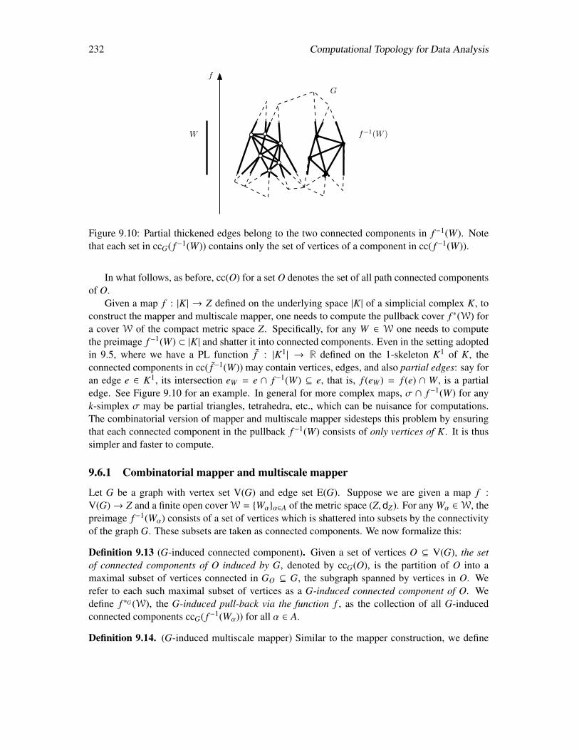
232 Computational Topology for Data Analysis
W
f
G
f−1(W )
Figure 9.10: Partial thickened edges belong to the two connected components in f −1(W). Notethat each set in ccG( f −1(W)) contains only the set of vertices of a component in cc( f −1(W)).
In what follows, as before, cc(O) for a set O denotes the set of all path connected componentsof O.
Given a map f : |K| → Z defined on the underlying space |K| of a simplicial complex K, toconstruct the mapper and multiscale mapper, one needs to compute the pullback cover f ∗(W) fora cover W of the compact metric space Z. Specifically, for any W ∈ W one needs to computethe preimage f −1(W) ⊂ |K| and shatter it into connected components. Even in the setting adoptedin 9.5, where we have a PL function f : |K1| → R defined on the 1-skeleton K1 of K, theconnected components in cc( f −1(W)) may contain vertices, edges, and also partial edges: say foran edge e ∈ K1, its intersection eW = e ∩ f −1(W) ⊆ e, that is, f (eW) = f (e) ∩ W, is a partialedge. See Figure 9.10 for an example. In general for more complex maps, σ ∩ f −1(W) for anyk-simplex σ may be partial triangles, tetrahedra, etc., which can be nuisance for computations.The combinatorial version of mapper and multiscale mapper sidesteps this problem by ensuringthat each connected component in the pullback f −1(W) consists of only vertices of K. It is thussimpler and faster to compute.
9.6.1 Combinatorial mapper and multiscale mapper
Let G be a graph with vertex set V(G) and edge set E(G). Suppose we are given a map f :V(G)→ Z and a finite open cover W = Wαα∈A of the metric space (Z, dZ). For any Wα ∈W, thepreimage f −1(Wα) consists of a set of vertices which is shattered into subsets by the connectivityof the graph G. These subsets are taken as connected components. We now formalize this:
Definition 9.13 (G-induced connected component). Given a set of vertices O ⊆ V(G), the setof connected components of O induced by G, denoted by ccG(O), is the partition of O into amaximal subset of vertices connected in GO ⊆ G, the subgraph spanned by vertices in O. Werefer to each such maximal subset of vertices as a G-induced connected component of O. Wedefine f ∗G (W), the G-induced pull-back via the function f , as the collection of all G-inducedconnected components ccG( f −1(Wα)) for all α ∈ A.
Definition 9.14. (G-induced multiscale mapper) Similar to the mapper construction, we define
Computational Topology for Data Analysis 233
Algorithm 17 MMapper( f ,K,W)
Input:f : |K| → Z given by fV : V(K)→ Z, a cover towerW = W1, . . . ,Wt
Output:Persistence diagram Dgm∗(MMK1(W, fV )) induced by the combinatorial MM of f w.r.t. W
1: for i = 1, . . . , t do2: compute VW ⊆ V(K) where f (VW) = f (V(K)) ∩W and V j
W j = ccK1(VW), ∀W ∈Wi;3: compute Nerve complex Ni = N(V j
W j,W).4: end for5: compute the filtration F : Ni→Ni+1, i ∈ [1, t − 1]6: compute Dgm∗(F).
the G-induced mapper MG(W, f ) as the nerve complex N( f ∗G(W)).Given a tower of coversW = Wε of Z, we define the G-induced multiscale mapper MMG(W, f )
as the tower of G-induced nerve complexes N( f ∗G(Wε)) |Wε ∈ W.
Given a map f : |K| → Z defined on the underlying space |K| of a simplicial complex K, letfV : V(K) → R denote the restriction of f to the vertices of K. Consider the 1-skeleton graphK1 that provides the connectivity information for vertices in V(K). Given any cover tower W ofthe metric space Z, the K1-induced multiscale mapper MMK1(W, fV ) is called the combinatorialmultiscale mapper of f w.r.t. W.
9.6.2 Advantage of combinatorial multiscale mapper
A simple description of the computation of the combinatorial mapper is in Algorithm 17. For thesimple PL example in Figure 9.10, f −1(W) contains two connected components, one consists ofthe set of white dots, while the other consists of the set of black dots. More generally, the con-struction of the pullback cover needs to inspect only the 1-skeleton K1 of K, which is typically ofsignificantly smaller size. Furthermore, the construction of the Nerve complex Ni as in Algorithm17 is also much simpler: We simply remember, for each vertex v ∈ V(K), the set Iv of ids ofconnected components V j
W j,W∈Wi which contain it. Any subset of Iv gives rise to a simplex inthe Nerve complex Ni.
Let MM(W, f ) denote the standard multiscale mapper as introduced in 9.3.1. Our main resultin this section is that if W is a (c, s)-good cover tower of Z, then the resulting two simplicialtowers, MM(W, f ) and MMK1(W, fV ) weakly interleave (Definition 6.6), and admits a boundeddistance between their respective persistence diagrams as a consequence of the weak-interleavingresult of [78]. This weaker setting of interleaving worsens the approximation by a factor of 3.
Theorem 9.28. Assume that (Z, dZ) is a compact and connected metric space. Given a mapf : |K| → Z, let fV : V(K)→ Z be the restriction of f to the vertex set V(K) of K.
Given a (c, s)-good cover tower W of Z such that (K, f ,W) satisfies the minimum diam-eter condition (cf. Condition 9.1), the bottleneck distance between the persistence diagramsDgmlogMM
(W, f
)and DgmlogMMK1
(W, fV
)is at most 3 log(3c) + 3 max(0, log 1
s ) for all k ∈ N.
234 Computational Topology for Data Analysis
9.7 Notes and Exercises
A corollary of the nerve theorem is that the space and the nerve have isomorphic homology groupsif all intersections of cover elements are homotopically trivial. This chapter studies a case whencovers do not necessarily satisfy this property. The result that for path connected covers, nonew 1-dimensional homology class is created in the nerve is proved in [133]. The materials insections 9.1 and 9.2 are taken from there. This result can be generalized for other dimensions; seeExercise 5.
The concept of mapper was introduced by Singh, Mémoli, and Carlsson [277], and has sincebeen used in diverse applications, e.g [224, 227, 244, 288]. The authors of [277] showed for thefirst time that a cover for the codomain in addition to domains can be useful for data analysis. Themapper in some sense is connected to Reeb graphs (spaces) where the cover elements degenerateto points in the codomain, see [240] for example. The structure and stability of 1-dimensionalmapper is studied in great details by Carrièr and Oudot in [70]. They showed that given a realvalued function f : X → R and an appropriate cover U, the extended persistence diagram of amapper M(U, f ) is a subset of the same of the Reeb graph R f . Furthermore, they characterized thefeatures of the Reeb graph that may disappear from the mapper. The mapper (for a real-valuedfunction f ) can also be viewed as a Reeb graph R f ′ of a perturbed function f ′ : X′ → R. Itis shown in [70] how one can track the changes between R f and the mapper by computing thefunctional distortion distance (Definition 7.8) between R f and R f ′ . In [15], the author establisheda convergence result between Mapper for a real valued f and the Reeb graph R f . Specifically,the mapper is characterized with a zigzag persistence module that is a coarsening of the zigzagpersistence module for R f . It is shown that the mapper converges to R f in the bottleneck dis-tance of the corresponding zigzag persistence diagrams as the lengths of the intervals in the coverapproaches zero. Munch and Wang [240] showed a similar convergence in interleaving distance(Definition 7.6) using sheaf theory [112].
The multiscale mapper which work on the notion of a filtration of covers was developedin [132]. Most of the materials in this chapter are taken from this paper. The results on the classof 1-cycles that persist through multiscale mapper are taken from [133].
Exercises
1. For a simplicial complex K, simplices with no cofacet are called maximal simplices. Con-sider a closed cover of |K|with the closures of the maximal simplices as the cover elements.Let N(K) denote the nerve of this cover. Prove that N(N(K)) is isomorphic to a subcomplexof K.
2. ([17]) A vertex v in K is called dominated by a vertex v′ if every maximal simplex con-taining v also contains v′. We say K collapses strongly to a complex L if L is obtained bya series of deletions of dominated vertices with all their incident simplices. Show that Kstrongly collapses to N(N(K)).
3. We say a cover U of a metric space (Y, d) is (α, β)-cover if α ≤ λ(U) and β ≥ smax(U).
• Consider a δ-sample P of Y , that is, every metric ball B(y; δ), y ∈ Y , contains a pointin P. Prove that the cover U = B(p; 2δ)p∈P is a (δ, 4δ)-cover of Y .

Computational Topology for Data Analysis 235
• Prove that the infinite cover U = B(y; δ)y∈Y is a (δ, 2δ)-cover of Y .
4. Theorem 9.5 requires that the cover to be path connected. Show that this condition isnecessary by presenting a counterexample otherwise.
5. One may generalize Theorem 9.5 as follows: If for any k ≥ 0, t-wise intersections of coverelements for all t > 0 have trivial reduced homology for Hk−t, then the nerve map induces asurjection in Hk. Prove or disprove it.
6. Consider a function f : X → Z from a path connected space X to a metric space Z. Definitethe equivalence relation ∼ f such that x ∼ f x′ holds if and only if f (x) = f (x′) and thereexists a continuous path γ ∈ ΓX(x, x′) such that f γ is constant. The Reeb space R f is thequotient of X under this equivalence relation.
• Prove that the quotient map q : X → R f is surjective and also induces a surjectionq∗ : H1(X)→ H1(R f ).
• Call a class [c] ∈ H1(X) vertical if and only if there is no c′ ∈ C1(X) so that [c] = [c′]and f σ is constant for every σ ∈ c′. Show that q∗([c]) , 0 if and only if c is vertical.
• Let z1, . . . , zg be an optimal cycle basis (Definition 9.3) of H1(X) defined with respectto the pseudometric d f (Definition 9.6). Let ` ∈ [1, g] be the smallest integer so thats(z`) , 0. Prove that if no such ` exists, H1(R f ) is trivial, otherwise, [q(zi)]i=`,...g isa basis for H1(R f ).
7. Let us endow R f with a distance d f that descends via the map q: for any equivalence classesr, r′ ∈ R f , pick x, x′ ∈ X with r = q(x) and r′ = q(x′), then define
d f (r, r′) := d f (x, x′).
Prove that d f is a pseudo-metric.
8. Prove Proposition 9.17.
9. Prove Theorem 9.23.
10. Prove Claim 9.4.

236 Computational Topology for Data Analysis
Chapter 10
Discrete Morse Theory andApplications
Discrete Morse theory is a combinatorial version of the classical Morse theory. Invented by For-man [161], the theory combines topology with the combinatorial structure of a cell complex.Specifically, much like the fact that critical points of a smooth Morse function on a manifold de-termines its topological entities such as homology groups and Euler Characteristics, an analogousconcept called critical simplices of a discrete Morse function also determine similar structuresfor the complex it is defined on. Gradient vectors associated with smooth Morse functions giverise to integral lines and eventually the notion of stable and unstable manifolds [232]. Similarly,a discrete Morse function defines discrete gradient vectors leading to V-paths analogous to theintegral lines. Using these V-paths, one can define the analogues of stable and unstable manifoldsof the critical simplices.
It turns out that an acyclic pairing between simplices and their faces so that every simplexparticipates in at most one pair provides a discrete Morse function and conversely a discrete Morsefunction defines such a pairing. This pairing termed as a Morse matching is a main buildingblock of the discrete Morse theory. In this chapter, we connect this matching with the pairingobtained through persistence algorithm. Specifically, we present an algorithm for computing aMorse matching and hence a discrete Morse vector field by connecting persistent pairs throughV-paths. This requires an operation called critical pair cancellation which may not succeed allthe time. However, for 1-complexes and simplicial 2-manifolds (pseudomanifolds), it alwayssucceeds. Section 10.1 and 10.2 are devoted to these results.
In Section 10.4, we apply our persistence based discrete Morse vector field to reconstructgeometric graphs from their noisy samples. Here we show that unstable manifolds of criticaledges can recover a graph with guarantees from a density data that captures the hidden graph rea-sonably well. We provide two applications of using this graph reconstruction algorithm, one forroad network reconstructions from GPS trajectories and satellite images and another for neuronreconstructions from their images. Section 10.5 describes these applications.
237

238 Computational Topology for Data Analysis
10.1 Discrete Morse function
Following Forman [161] we define a discrete Morse function (henceforth called Morse functionin this chapter) as a function f : K → R on a simplicial complex K where for every p-simplexσp ∈ K the following two conditions hold1; recall that every (p − 1)-face of σp is called its facetand every (p + 1)-simplex adjoining σp called its cofacet.
• #σp−1 |σp−1 is a facet of σp and f (σp−1) ≥ f (σp) ≤ 1
• #σp+1 |σp+1 is a coface of σp and f (σp+1) ≤ f (σp) ≤ 1
The first condition says that at most one facet of a simplex σ has higher or equal functionvalue than f (σ) and the second condition says that at most one cofacet of a simplex σ can havelower or equal function value than f (σ). By a result of Chari [76], the two conditions imply thatthe two sets above are disjoint, that is, if a pair (σp−1, σp) satisfies the first condition, there is nopair (σp, σp+1) satisfying the second condition and vice versa. This means that a Morse functionf induces a matching:
Definition 10.1 (Matching). A set of ordered pairs M = (σ, τ) is a matching in K if the followingconditions hold:
1. For any (σ, τ) ∈ M, σ is a facet of τ.
2. Any simplex in K can appear in at most one pair in M.
Such a matching M defines two disjoint subsets L ⊆ K,U ⊆ K where there is a bijection µ : L→U such that M = (σ, µ(σ)) | σ ∈ L.
In Figure 10.1, we indicate a matching by putting an arrow from the lower dimensional sim-plex to the higher dimensional simplex. Observe that the source of each arrow is a facet of thetarget of the arrow.
Note however, the matching in K defined by a Morse function has an additional property ofacyclicity which we show next. First, let us define a relation σi ≺ σi+1 if σi+1 = µ(σi) or σi+1 isa facet of σi but σi , µ(σi+1).
Definition 10.2 (V-path and Morse matching). Given a matching M in K, for k > 0, a V-path πis a sequence
π : σ0 ≺ σ1 ≺ · · ·σi−1 ≺ σi ≺ σi+1 · · · ≺ σk (10.1)
where for 0 < i < k, σi , µ(σi−1) implies σi+1 = µ(σi). In other words, a V-path is an alternatingsequence of facets and cofacets thus alternating in dimensions where every consecutive pair alsoalternates between matched and unmatched pairs. A V-path is cyclic if the first simplex σ0 is afacet of the last simplex σk or σ0 = µ(σk) and the matching M is called cyclic if there is such apath in it. Otherwise, M is called acyclic. An acyclic matching in K is called a Morse matching.
1Forman formulated discrete Morse function for more general cell complexes.
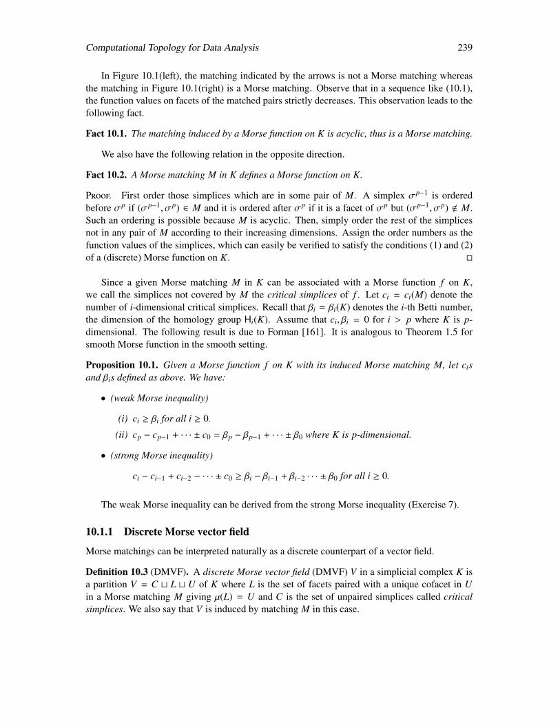
Computational Topology for Data Analysis 239
In Figure 10.1(left), the matching indicated by the arrows is not a Morse matching whereasthe matching in Figure 10.1(right) is a Morse matching. Observe that in a sequence like (10.1),the function values on facets of the matched pairs strictly decreases. This observation leads to thefollowing fact.
Fact 10.1. The matching induced by a Morse function on K is acyclic, thus is a Morse matching.
We also have the following relation in the opposite direction.
Fact 10.2. A Morse matching M in K defines a Morse function on K.
Proof. First order those simplices which are in some pair of M. A simplex σp−1 is orderedbefore σp if (σp−1, σp) ∈ M and it is ordered after σp if it is a facet of σp but (σp−1, σp) < M.Such an ordering is possible because M is acyclic. Then, simply order the rest of the simplicesnot in any pair of M according to their increasing dimensions. Assign the order numbers as thefunction values of the simplices, which can easily be verified to satisfy the conditions (1) and (2)of a (discrete) Morse function on K.
Since a given Morse matching M in K can be associated with a Morse function f on K,we call the simplices not covered by M the critical simplices of f . Let ci = ci(M) denote thenumber of i-dimensional critical simplices. Recall that βi = βi(K) denotes the i-th Betti number,the dimension of the homology group Hi(K). Assume that ci, βi = 0 for i > p where K is p-dimensional. The following result is due to Forman [161]. It is analogous to Theorem 1.5 forsmooth Morse function in the smooth setting.
Proposition 10.1. Given a Morse function f on K with its induced Morse matching M, let cisand βis defined as above. We have:
• (weak Morse inequality)
(i) ci ≥ βi for all i ≥ 0.
(ii) cp − cp−1 + · · · ± c0 = βp − βp−1 + · · · ± β0 where K is p-dimensional.
• (strong Morse inequality)
ci − ci−1 + ci−2 − · · · ± c0 ≥ βi − βi−1 + βi−2 · · · ± β0 for all i ≥ 0.
The weak Morse inequality can be derived from the strong Morse inequality (Exercise 7).
10.1.1 Discrete Morse vector field
Morse matchings can be interpreted naturally as a discrete counterpart of a vector field.
Definition 10.3 (DMVF). A discrete Morse vector field (DMVF) V in a simplicial complex K isa partition V = C t L t U of K where L is the set of facets paired with a unique cofacet in Uin a Morse matching M giving µ(L) = U and C is the set of unpaired simplices called criticalsimplices. We also say that V is induced by matching M in this case.
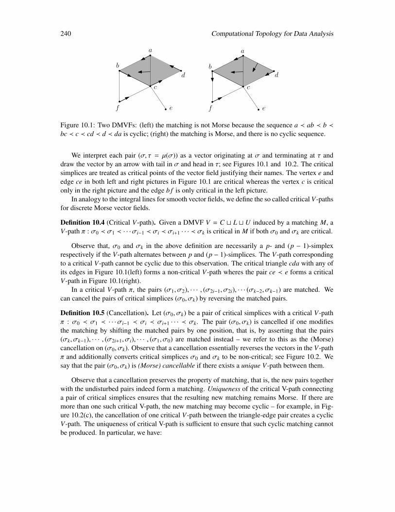
240 Computational Topology for Data Analysis
a
b
c
d
ef
a
b
c
d
ef
Figure 10.1: Two DMVFs: (left) the matching is not Morse because the sequence a ≺ ab ≺ b ≺bc ≺ c ≺ cd ≺ d ≺ da is cyclic; (right) the matching is Morse, and there is no cyclic sequence.
We interpret each pair (σ, τ = µ(σ)) as a vector originating at σ and terminating at τ anddraw the vector by an arrow with tail in σ and head in τ; see Figures 10.1 and 10.2. The criticalsimplices are treated as critical points of the vector field justifying their names. The vertex e andedge ce in both left and right pictures in Figure 10.1 are critical whereas the vertex c is criticalonly in the right picture and the edge b f is only critical in the left picture.
In analogy to the integral lines for smooth vector fields, we define the so called critical V-pathsfor discrete Morse vector fields.
Definition 10.4 (Critical V-path). Given a DMVF V = C t L t U induced by a matching M, aV-path π : σ0 ≺ σ1 ≺ · · ·σi−1 ≺ σi ≺ σi+1 · · · ≺ σk is critical in M if both σ0 and σk are critical.
Observe that, σ0 and σk in the above definition are necessarily a p- and (p − 1)-simplexrespectively if the V-path alternates between p and (p − 1)-simplices. The V-path correspondingto a critical V-path cannot be cyclic due to this observation. The critical triangle cda with any ofits edges in Figure 10.1(left) forms a non-critical V-path wheres the pair ce ≺ e forms a criticalV-path in Figure 10.1(right).
In a critical V-path π, the pairs (σ1, σ2), · · · , (σ2i−1, σ2i), · · · (σk−2, σk−1) are matched. Wecan cancel the pairs of critical simplices (σ0, σk) by reversing the matched pairs.
Definition 10.5 (Cancellation). Let (σ0, σk) be a pair of critical simplices with a critical V-pathπ : σ0 ≺ σ1 ≺ · · ·σi−1 ≺ σi ≺ σi+1 · · · ≺ σk. The pair (σ0, σk) is cancelled if one modifiesthe matching by shifting the matched pairs by one position, that is, by asserting that the pairs(σk, σk−1), · · · , (σ2i+1, σi), · · · , (σ1, σ0) are matched instead – we refer to this as the (Morse)cancellation on (σ0, σk). Observe that a cancellation essentially reverses the vectors in the V-pathπ and additionally converts critical simplices σ0 and σk to be non-critical; see Figure 10.2. Wesay that the pair (σ0, σk) is (Morse) cancellable if there exists a unique V-path between them.
Observe that a cancellation preserves the property of matching, that is, the new pairs togetherwith the undisturbed pairs indeed form a matching. Uniqueness of the critical V-path connectinga pair of critical simplices ensures that the resulting new matching remains Morse. If there aremore than one such critical V-path, the new matching may become cyclic – for example, in Fig-ure 10.2(c), the cancellation of one critical V-path between the triangle-edge pair creates a cyclicV-path. The uniqueness of critical V-path is sufficient to ensure that such cyclic matching cannotbe produced. In particular, we have:
Computational Topology for Data Analysis 241
(a) (b) (c)
Figure 10.2: Critical vertices and edges are marked red; (a) before cancellation of edge-vertexpair (v2, e2); (b) after cancellation, the path from e2 to v2 is inverted, giving rise to a critical V-path from e1 to v1, making (v1, e1) now potentially cancellable; (c) the edge-triangle pair (e, t), ifcancelled, creates cycle as there are two V-paths between them.
Proposition 10.2. Given a Morse matching M, suppose we cancel a pair of critical simplices σand σ′ in a DMVF V via a critical V-path to obtain a new matching M′. Then M′ remains aMorse matching if and only if this V-path is the only critical V-path connecting σ and σ′ in V(i.e., the pair (σ,σ′) is cancellable as per Definition 10.5).
Proof. First, assume that there are two V-paths π and π′ originating at σ and ending at σ′. Sinceπ and π′ are distinct and have common simplices σ at the beginning and σ′ at the end, there aresimplices τ and τ′ where the two paths differ for the first time after τ and join again for the firsttime at τ′. Reversing one V-path, say π, creates a V-path from τ′ to τ. This sub-path along withthe V-path from τ to τ′ on π′ creates a cyclic V-path, thus proving the ’only if’ part.
Next, suppose that there is only a single V-path from σ to σ′. After reversing this path, weclaim that no cyclic V-path is created. For contradiction, assume that a cyclic V-path is createdas the result of reversal of π. Let the maximal sub-path of reversed π on this cyclic path startsat τ and ends at τ′. We have τ , τ′ because otherwise the original matching needs to be cyclicin the first place. But, then the cyclic V-path has a sub-path from τ′ to τ that is not in π. Sincethe reversed V-path π has a sub-path from τ to τ′, the original path has a sub-path from τ′ toτ. It means that the DMVF V originally had two V-paths from σ to σ′, with one of them beingπ while the other one containing a sub-path not in π. This forms a contradiction that there is asingle V-path from σ to σ′. Hence the assumption that a cyclic V-path is created is wrong, whichcompletes the proof of the ’if’ part.
10.2 Persistence based DMVF
Given a simplicial complex K, one can set up a trivial DMVF where every simplex is critical, thatis, V = K t ∅ t ∅. Then, one may use cancellations to build vector field further by constructingmore matchings. The key to the success of this approach is to identify pairs of critical simplicesthat can be cancelled without creating cyclic paths. One way to do this is by taking advantage ofpersistence pairs among simplices.
242 Computational Topology for Data Analysis
10.2.1 Persistence-guided cancellation
First, we consider the case of simplicial 1-complexes which consist of only vertices and edges.Such a complex admits a DMVF obtained by cancelling the persistence pairs successively. Herewe consider pairs with finite persistence only. Recall that some of the creator simplices are neverpaired with a destructor because the class created by them never dies. They are paired with ∞.Such essential pairs are not considered in the following proposition.
Proposition 10.3. Let (v1, e1), (v2, e2), · · · , (vn, en) be the sequence of all non-essential persis-tence pairs of vertices and edges sorted in increasing order of the appearance of the edges ei’s ina filtration of a 1-complex K. Let V0 be the DMVF in K with all simplices being critical. Sup-pose DMVF Vi−1 can be obtained by cancelling successively (v1, e1), (v2, e2), · · · (vi−1, ei−1). Then,(vi, ei) can be cancelled in Vi−1 providing a DMVF Vi for all i ≥ 1.
Proof. Inductively assume that (i) Vi−1 is a DMVF obtained as claimed in the proposition and(ii) any matched edge in Vi−1 is a paired edge in a persistence pair. We argue that these twohypotheses hold for Vi proving the claim due to the hypothesis (i).
The base case for i = 1 is true trivially because V0 is a DMVF and there is no matched edge.Inductively assume that Vi−1 satisfies the inductive hypothesis for i > 1. Consider the persistencepair (vi, ei). First, we observe that a V-path ei = ei1 ≺ vi1 ≺ . . . ≺ ein ≺ vin = vi exists inVi−1. If not, starting from the two endpoints of ei, we attempt to follow the two V-paths and letv, v′ , vi be the first two critical vertices encountered during this construction. Without loss ofgenerality, assume that v′ appears before v in the filtration. Then, the 0-dimensional class [v + v′]is born when v is introduced. It is destroyed by ei. It follows that (v, ei) is a persistence pair(Fact 3.3) contradicting that actually (vi, ei) is a persistence pair. For induction, consider the V-path ei = ei1 ≺ vi1 ≺ . . . ≺ ein ≺ vin = vi in Vi−1 which is cancelled to create Vi. For Vi not tobe a DMVF, due to Proposition 10.2, we must have another distinct V-path from ei to vi in Vi−1,ei = e j1 ≺ v j1 ≺ . . . ≺ e jn′ ≺ vin′ = vi. These two non-identical paths form a 1-cycle. Every edgein this cycle except possibly ei are matched edges in Vi−1 and hence participates in a persistencepair by the inductive hypothesis. Then, all edges in the 1-cycle participate in some persistencepair because ei is also such an edge by assumption. But, this is impossible because in any 1-cycleat least one edge has to remain unpaired in persistence. It follows that by cancelling (vi, ei), weobtain a DMVF Vi satisfying the inductive hypothesis (i). Also, inductive hypothesis (ii) followsbecause the new matched pairs in Vi involve edges that were already matched in Vi−1 and the edgeei which participates in a persistence pair by assumption.
The result above holds for vertex-edge pairing in any simplicial complex. Furthermore, usingdual graphs, it can be used for edge-triangle pairing in triangulations of 2-manifolds. Given asimplicial 2-complex K whose underlying space is a 2-manifold without boundary, consider thedual graph (1-complex) K∗ where each triangle t ∈ K becomes a vertex t∗ ∈ K∗ and two verticest∗1 and t∗2 are joined with an edge e∗ if triangles t1 and t2 share an edge e in K.
The following result connects the persistence of a filtration of K and its dual graph K∗.
Proposition 10.4. Let σ1, σ2, · · · , σn be a subsequence of a simplex-wise filtration F of K con-sisting of all edges and triangles. An edge-triangle pair (σi, σ j) is a persistence pair for F if andonly if (σ∗j , σ
∗i ) is a persistence pair for the filtration σ∗n, σ
∗n−1, · · · , σ
∗1 of the dual graph K∗.
Computational Topology for Data Analysis 243
Proof. Recall Proposition 3.8. An edge-triangle persistence pair produced by the filtered bound-ary matrix D2 for filtration of K are exactly same as the triangle-edge persistence pair obtainedfrom the twisted (transposed and reversed) matrix D∗2 by left-to-right column additions. Thematrix D∗2 is exactly the filtered boundary matrix of a filtration F(K∗) of K∗ that reverses the sub-sequence of triangle and edges. Dualizing a triangle t to a vertex t∗ and an edge e to an edge e∗,we can view F(K∗) as a filtration on a 1-complex (graph). Then, applying Theorem 3.6, we getthat (t∗, e∗) is indeed a persistence pair for the filtration F(K∗).
We can compute a DMVF V∗ for K∗ by cancelling all persistence pairs as stated in Propo-sition 10.3. By duality, this also produces a DMVF V for the 2-manifold K. The action ofcancelling a vertex-edge pair in K∗ can be translated into a cancellation of an edge-triangle pairin K. Combining Propositions 10.3 and 10.4, we obtain the following result.
Theorem 10.5. Let K be a finite simplicial 2-complex whose underlying space is a 2-manifoldwithout boundary and F be a simplex-wise filtration of K (Definition 3.1). Starting from the trivialDMVF where each simplex is critical, one can obtain a DMVF in K by cancelling the vertex-edgeand edge-triangle persistence pairs given by F.
In general, by duality one can apply the above theorem to cancel all persistence pairs be-tween (d − 1)-simplices and d-simplices in a filtration of a simplicial d-complex where each(d − 1)-simplex has at most two d-simplices as cofacets. This includes simplicial d-manifoldswith boundary. We call a (d − 1)-simplex boundary if it adjoins exactly one d-simplex. Forthis extension, one has to introduce a ‘dummy’ vertex in the dual graph that connects to all dualvertices of d-simplices incident to a boundary (d − 1)-simplex. We leave it as an exercise (Exer-cise 11).
Unfortunately, it does not extend any further. In particular, the result in Theorem 10.5 doesnot extend to arbitrary simplicial 2-complexes and hence arbitrary simplicial complexes. Themain difficulty arises because such a complex does not admit a dual graph in general. Indeed,there are counterexamples which exhibit that every persistence pair for a filtration of a simplicial2-complex cannot be cancelled leading to a DMVF. The following Dunce hat example exhibitsthis obstruction.
Dunce hat. Consider a 2-manifold with boundary which is a cone with apex v and the boundarycircle c. Let u be a point on c. Modify the cone by identifying the line segment uv with thecircle c. Because of the similarity, the space obtained by this identification is called the Duncehat. Consider a triangulation K of the Dunce hat. Notice that Dunce hat and hence |K| is not a2-manifold. The edges discretizing uv in K have three triangles incident to them. We show thatthere is no DMVF without any critical edge and triangle for K. The complex K is known to haveβi(K) = 0 for all i > 0 and has two or more triangles adjoining every edge in it. For any filtrationof K, there cannot be any edge or triangle that remains unpaired because otherwise that wouldcontradict that β1(K) = 0 and β2(K) = 0 (Fact 3.9 in Chapter 3). If a DMVF V were possibleto be created by cancelling persistence pairs, there would be a finite maximal V-path that cannotbe extended any further. Consider such a path π starting at a simplex σ. If σ is a triangle, theedge µ−1(σ) matched with it can be added before it to extend π. If σ is an edge, there is a triangleadjoining σ not in the V-path because at least two triangles adjoin e and the V-path starting at
244 Computational Topology for Data Analysis
e cannot be cyclic. We can add that triangle to extend π. In both cases, we contradict that π ismaximal.
10.2.2 Algorithms
The above results naturally suggest an algorithm for computing a persistence based DMVF fora simplicial 2-manifold K. We compute the persistence pairs on a chosen filtration F of K andthen cancel them successively as Theorem 10.5 suggests. Both of these tasks can be combined bymodifying the well known Kruskal’s algorithm for computing minimum spanning tree of a graph.
Consider a graph G = (U, E) which can be either the 1-skeleton of a complex K or the dualgraph K∗ if K is a simplicial 2-manifold. Assume that u1, u2, . . . , uk and e1, e2, . . . , e` be anordered sequence of vertices and edges in G. For minimum spanning tree, the sequence of edgesare taken in non-decreasing order of their weights. Here we describe the algorithm by assumingany order. Kruskal’s algorithm maintains a spanning forest of the vertex set. It brings one edgee at a time in the given order either to join two trees in the current forest or to discover that theedge makes a cycle and hence does not belong to the spanning forest. If the two endpoints ofe belong to two different trees in the forest, then it joins those two trees. Otherwise, e connectstwo vertices in the same tree creating a cycle. The main computation involves determining if twovertices of an edge belong to the same tree or not. Algorithm 18:PersDMVF does it by union-finddata structure which maintains the set of vertices of a tree in a single set and two sets are unitedif an edge joins the two respective trees. This is similar to FindSet and Union operations in thealgorithm ZeroPerDg described in Section 3.5.3. All such find and union operations can be donein O(k + `α(`)) time assuming that there are k vertices and ` edges in the graph which dominatesthe overall complexity.
We can incorporate the persistence computation and Morse cancellations simultaneously inthe above algorithm with some simple modifications. We process the vertices and edges in theirorder of the input filtration. Usually, the filtration F = F f is given by a simplex-wise monotonefunction f as described in Section 3.1.2. We compute the persistence Pers (e) of an edge e asPers (e) = | f (e) − f (r)| if e pairs with the vertex r and∞ otherwise.
For a vertex u in the filtration F f , we do not do anything other than creating a new set con-taining u only. When an edge e = (u, u′) comes in, we check if u and u′ belong to the sametree by using the union-find data structure. If they do, the edge e is designated as a creator forpersistence and as a critical edge in DMVF that is being built on G. Otherwise, we computePers (e) after finding the persistence pair for e and at the same time cancel e with its pair inthe DMVF as follows. Assume inductively that the current DMVF matches every vertex otherthan the roots of the trees to one of its adjacent edge as follows. For a leaf vertex v, con-sider the path v = v1, e1, . . . , ek−1, vk = r from v to the root r which consist of matched pairs(v1, e1), . . . , (vk−1, ek−1) and the critical vertex r. For the edge e = (u, u′), let the roots of the twotrees Tu and Tu′ containing u and u′ be r and r′ respectively. Assume without loss of generalitythat r succeeds r′ in the input filtration. Then, e pairs with r in persistence because e joins thetwo components created by r and r′ between which r comes later in the filtration. We cancel thepersistence pair (r, e) by shifting the matched pairs on the path from u to r as stated in Defini-tion 10.5. We join the two trees Tu and Tu′ into one tree by calling the routine Join. The root ofthe joined tree becomes r′. Cancelling (r, e) maintains the invariant that every path from the leafto the root of the new tree remains a V-path. See Figure 10.3 for an illustration.
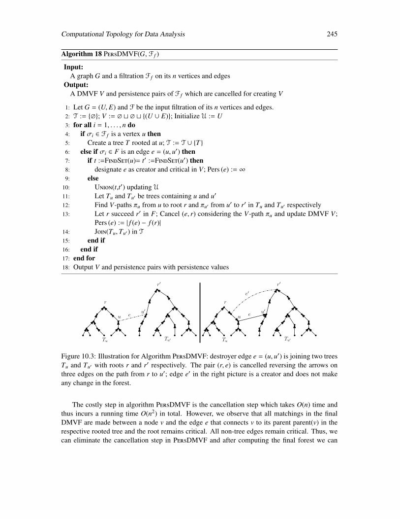
Computational Topology for Data Analysis 245
Algorithm 18 PersDMVF(G, F f )
Input:A graph G and a filtration F f on its n vertices and edges
Output:A DMVF V and persistence pairs of F f which are cancelled for creating V
1: Let G = (U, E) and F be the input filtration of its n vertices and edges.2: T := ∅; V := ∅ t ∅ t (U ∪ E); Initialize U := U3: for all i = 1, . . . , n do4: if σi ∈ F f is a vertex u then5: Create a tree T rooted at u; T := T ∪ T 6: else if σi ∈ F is an edge e = (u, u′) then7: if t :=FindSet(u)= t′ :=FindSet(u′) then8: designate e as creator and critical in V; Pers (e) := ∞9: else
10: Union(t,t′) updating U
11: Let Tu and Tu′ be trees containing u and u′
12: Find V-paths πu from u to root r and πu′ from u′ to r′ in Tu and Tu′ respectively13: Let r succeed r′ in F; Cancel (e, r) considering the V-path πu and update DMVF V;
Pers (e) := | f (e) − f (r)|14: Join(Tu,Tu′) in T
15: end if16: end if17: end for18: Output V and persistence pairs with persistence values
r
r′
uu′
Tu Tu′
r
r′
uu′
Tu Tu′
e e
e′
Figure 10.3: Illustration for Algorithm PersDMVF: destroyer edge e = (u, u′) is joining two treesTu and Tu′ with roots r and r′ respectively. The pair (r, e) is cancelled reversing the arrows onthree edges on the path from r to u′; edge e′ in the right picture is a creator and does not makeany change in the forest.
The costly step in algorithm PersDMVF is the cancellation step which takes O(n) time andthus incurs a running time O(n2) in total. However, we observe that all matchings in the finalDMVF are made between a node v and the edge e that connects v to its parent parent(v) in therespective rooted tree and the root remains critical. All non-tree edges remain critical. Thus, wecan eliminate the cancellation step in PersDMVF and after computing the final forest we can

246 Computational Topology for Data Analysis
Algorithm 19 SimplePersDMVF(G, F f )
Input:A graph G and a filtration F f on its n vertices and edges
Output:A DMVF V and persistence pairs of F f which are cancelled for creating V
1: Let G = (U, E) and F f be the input filtration of its n vertices and edges.2: T := ∅; V := ∅; Initialize U := U3: for all i = 1, . . . , n do4: if σi ∈ F f is a vertex u then5: Create a tree T rooted at u; T := T ∪ T 6: else if σi ∈ F is an edge e = (u, u′) then7: if t :=FindSet(u)= t′ :=FindSet(u′) then8: designate e as creator and critical in V; Pers (e) := ∞9: else
10: Union(t,t′) updating U
11: Let Tu and Tu′ be trees containing u and u′ with roots r and r′
12: Let r succeed r′ in F; Pers (e) := | f (e) − f (r)|13: Join(Tu,Tu′) in T with edge e14: end if15: end if16: end for17: for each tree T ∈ T do18: for each node v in T do19: e := (v, parent(v)), V := V t (v, e)20: end for21: Put the root of T as a critical vertex in V22: end for23: Output V and persistence pairs with persistence values
determine all matched pairs by traversing the trees upward from the leaves to the roots whilematching a vertex with the edge visited next in this upward traversal. This matching takes O(n)time. Accounting for the union-find operations, all other steps in PersDMVF take O(nα(n)) timein total. The simplified version Algorithm 19:SimplePersDMVF incorporates these changes. Wehave the following result.
Theorem 10.6. Given a simplicial 1-complex or a simplicial 2-manifold K with n simplices, onecan compute
1. a DMVF by cancelling all persistence pairs resulting from a given filtration of K in O(nα(n))time;
2. a DMVF as above when the filtration is induced by a given PL-function on K in O(n log n)time.
Computational Topology for Data Analysis 247
Proof. We argue for all statements in the theorem when K is a 1-complex. By considering thedual graph K∗, and combining Propositions 10.3 and Proposition 10.4, the arguments also holdfor K when it is a simplicial 2-manifold. The algorithm SimplePersDMVF outputs the same asthe algorithm PersDMVF whose correctness follows from Theorem 10.5 because it cancels thepersistence pairs exactly as the theorem dictates. The complexity analysis of the algorithm Sim-plePersDMVF establishes the first statement. For the second statement, given the function valuesat the vertices of K, we can compute a simplex-wise lower star filtration (Section 3.5) in O(n log n)time after sorting these function values. A subsequent application of SimplePersDMVF on thislower star filtration provides us the desired DMVF.
We can modify SimplePersDMVF slightly to take into account a threshold δ for persistence,that is, we can cancel pairs only with persistence up to δ. To do this, we need a slightly differentversion of Proposition 10.3. The cancellation also succeeds if we cancel persistent pairs in theorder of their persistence values. The proof of Proposition 10.3 can be adapted for the followingproposition.
Proposition 10.7. Let (v1, e1), (v2, e2), · · · , (vn, en) be the sequence of all non-essential persis-tence pairs of vertices and edges sorted in non-decreasing order of their persistence for a givenfiltration of K. Let V0 be the DMVF in K with all simplices being critical. Suppose DMVF Vi−1can be obtained by cancelling successively (v1, e1), (v2, e2), · · · (vi−1, ei−1). Then, (vi, ei) can becancelled in Vi−1 providing a DMVF Vi for all i ≥ 1.
The modified algorithm proceeds as in SimplePersDMVF, but designate those edges criticalwhose persistence is more than δ. Then, before traversing the edges of the trees in the forest Tto output the vertex-edge pairs, we delete all these critical edges from T. This splits the trees inT and creates more trees. We need to determine the roots of these trees. Observe that, had wedone the cancellations as in PersDMVF, the roots of the trees would have been the vertices thatappear the earliest in the filtration among all vertices in the respective trees. So, all trees in T
obtained after deleting all critical edges are rooted at the vertices that appear the earliest in thefiltration. Then, the steps 17 to 22 in SimplePersDMVF compute the vertex-edge matchings intothe DMVF from these rooted trees. The new algorithm called PartialPersDMVF modifies step13 of the algorithm SimplePersDMVF as:
• if Pers (e) > δ then designate e critical in V endif; Join(Tu,Tu′)
Also, PartialPersDMVF introduces a step before step 17 of SimplePersDMVF as:
• delete all critical edges from T and create new rooted trees in T as described
We claim that PartialPersDMVF indeed computes a DMVF guaranteed by Proposition 10.7(Exercise 9).
Claim 10.1. PartialPersDMVF(F,δ) computes a DMVF obtained by cancelling persistence pairsin non-decreasing order of persistence values which do not exceed the input threshold δ.
Let Vδ denote the resulting DMVF after canceling all vertex-edge persistence pairs with per-sistence at most δ.
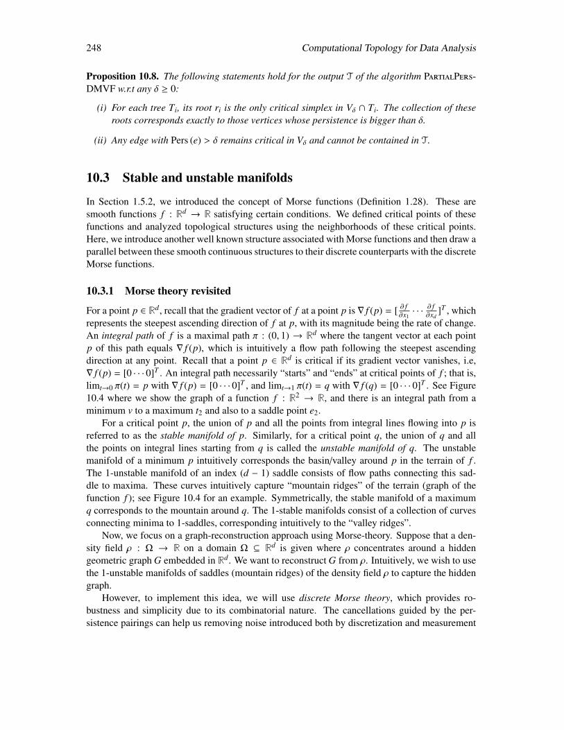
248 Computational Topology for Data Analysis
Proposition 10.8. The following statements hold for the output T of the algorithm PartialPers-DMVF w.r.t any δ ≥ 0:
(i) For each tree Ti, its root ri is the only critical simplex in Vδ ∩ Ti. The collection of theseroots corresponds exactly to those vertices whose persistence is bigger than δ.
(ii) Any edge with Pers (e) > δ remains critical in Vδ and cannot be contained in T.
10.3 Stable and unstable manifolds
In Section 1.5.2, we introduced the concept of Morse functions (Definition 1.28). These aresmooth functions f : Rd → R satisfying certain conditions. We defined critical points of thesefunctions and analyzed topological structures using the neighborhoods of these critical points.Here, we introduce another well known structure associated with Morse functions and then draw aparallel between these smooth continuous structures to their discrete counterparts with the discreteMorse functions.
10.3.1 Morse theory revisited
For a point p ∈ Rd, recall that the gradient vector of f at a point p is ∇ f (p) = [ ∂ f∂x1· · ·
∂ f∂xd
]T , whichrepresents the steepest ascending direction of f at p, with its magnitude being the rate of change.An integral path of f is a maximal path π : (0, 1) → Rd where the tangent vector at each pointp of this path equals ∇ f (p), which is intuitively a flow path following the steepest ascendingdirection at any point. Recall that a point p ∈ Rd is critical if its gradient vector vanishes, i.e,∇ f (p) = [0 · · · 0]T . An integral path necessarily “starts” and “ends” at critical points of f ; that is,limt→0 π(t) = p with ∇ f (p) = [0 · · · 0]T , and limt→1 π(t) = q with ∇ f (q) = [0 · · · 0]T . See Figure10.4 where we show the graph of a function f : R2 → R, and there is an integral path from aminimum v to a maximum t2 and also to a saddle point e2.
For a critical point p, the union of p and all the points from integral lines flowing into p isreferred to as the stable manifold of p. Similarly, for a critical point q, the union of q and allthe points on integral lines starting from q is called the unstable manifold of q. The unstablemanifold of a minimum p intuitively corresponds the basin/valley around p in the terrain of f .The 1-unstable manifold of an index (d − 1) saddle consists of flow paths connecting this sad-dle to maxima. These curves intuitively capture “mountain ridges” of the terrain (graph of thefunction f ); see Figure 10.4 for an example. Symmetrically, the stable manifold of a maximumq corresponds to the mountain around q. The 1-stable manifolds consist of a collection of curvesconnecting minima to 1-saddles, corresponding intuitively to the “valley ridges”.
Now, we focus on a graph-reconstruction approach using Morse-theory. Suppose that a den-sity field ρ : Ω → R on a domain Ω ⊆ Rd is given where ρ concentrates around a hiddengeometric graph G embedded in Rd. We want to reconstruct G from ρ. Intuitively, we wish to usethe 1-unstable manifolds of saddles (mountain ridges) of the density field ρ to capture the hiddengraph.
However, to implement this idea, we will use discrete Morse theory, which provides ro-bustness and simplicity due to its combinatorial nature. The cancellations guided by the per-sistence pairings can help us removing noise introduced both by discretization and measurement
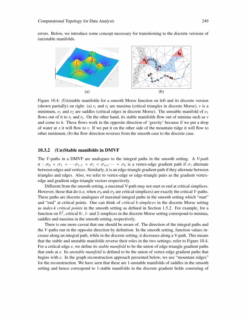
Computational Topology for Data Analysis 249
errors. Below, we introduce some concept necessary for transitioning to the discrete versions of(un)stable manifolds.
(a) (b)
Figure 10.4: (Un)stable manifolds for a smooth Morse function on left and its discrete version(shown partially) on right: (a) t1 and t2 are maxima (critical triangles in discrete Morse), v is aminimum, e1 and e2 are saddles (critical edges in discrete Morse). The unstable manifold of e1flows out of it to t1 and t2. On the other hand, its stable manifolds flow out of minima such as vand come to it. These flows work in the opposite direction of ‘gravity’ because if we put a dropof water at x it will flow to v. If we put it on the other side of the mountain ridge it will flow toother minimum; (b) the flow direction reverses from the smooth case to the discrete case.
10.3.2 (Un)Stable manifolds in DMVF
The V-paths in a DMVF are analogues to the integral paths in the smooth setting. A V-pathπ : σ0 ≺ σ1 ≺ · · ·σi−1 ≺ σi ≺ σi+1 · · · ≺ σk is a vertex-edge gradient path if σi alternatebetween edges and vertices. Similarly, it is an edge-triangle gradient path if they alternate betweentriangles and edges. Also, we refer to vertex-edge or edge-triangle pairs as the gradient vertex-edge and gradient edge-triangle vectors respectively.
Different from the smooth setting, a maximal V-path may not start or end at critical simplices.However, those that do (i.e, when σ0 and σk are critical simplices) are exactly the critical V-paths.These paths are discrete analogues of maximal integral paths in the smooth setting which “start”and “end” at critical points. One can think of critical k-simplices in the discrete Morse settingas index-k critical points in the smooth setting as defined in Section 1.5.2. For example, for afunction on R2, critical 0-, 1- and 2-simplices in the discrete Morse setting correspond to minima,saddles and maxima in the smooth setting, respectively.
There is one more caveat that one should be aware of. The direction of the integral paths andthe V-paths run in the opposite direction by definition: In the smooth setting, function values in-crease along an integral path, while in the discrete setting, it decreases along a V-path. This meansthat the stable and unstable manifolds reverse their roles in the two settings; refer to Figure 10.4.For a critical edge e, we define its stable manifold to be the union of edge-triangle gradient pathsthat ends at e. Its unstable manifold is defined to be the union of vertex-edge gradient paths thatbegins with e. In the graph reconstruction approach presented below, we use “mountain ridges”for the reconstruction. We have seen that these are 1-unstable manifolds of saddles in the smoothsetting and hence correspond to 1-stable manifolds in the discrete gradient fields consisting of
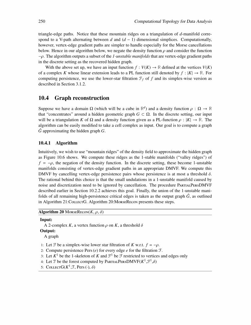
250 Computational Topology for Data Analysis
triangle-edge paths. Notice that these mountain ridges on a triangulation of d-manifold corre-spond to a V-path alternating between d and (d − 1) dimensional simplices. Computationally,however, vertex-edge gradient paths are simpler to handle especially for the Morse cancellationsbelow. Hence in our algorithm below, we negate the density function ρ and consider the function−ρ. The algorithm outputs a subset of the 1-unstable manifolds that are vertex-edge gradient pathsin the discrete setting as the recovered hidden graph.
With the above set up, we have an input function f : V(K) → R defined at the vertices V(K)of a complex K whose linear extension leads to a PL function still denoted by f : |K| → R. Forcomputing persistence, we use the lower-star filtration F f of f and its simplex-wise version asdescribed in Section 3.1.2.
10.4 Graph reconstruction
Suppose we have a domain Ω (which will be a cube in Rd) and a density function ρ : Ω → Rthat “concentrates” around a hidden geometric graph G ⊂ Ω. In the discrete setting, our inputwill be a triangulation K of Ω and a density function given as a PL-function ρ : |K| → R. Thealgorithm can be easily modified to take a cell complex as input. Our goal is to compute a graphG approximating the hidden graph G.
10.4.1 Algorithm
Intuitively, we wish to use “mountain ridges” of the density field to approximate the hidden graphas Figure 10.6 shows. We compute these ridges as the 1-stable manifolds (“valley ridges") off = −ρ, the negation of the density function. In the discrete setting, these become 1-unstablemanifolds consisting of vertex-edge gradient paths in an appropriate DMVF. We compute thisDMVF by cancelling vertex-edge persistence pairs whose persistence is at most a threshold δ.The rational behind this choice is that the small undulations in a 1-unstable manifold caused bynoise and discretization need to be ignored by cancellation. The procedure PartialPersDMVFdescribed earlier in Section 10.2.2 achieves this goal. Finally, the union of the 1-unstable mani-folds of all remaining high-persistence critical edges is taken as the output graph G, as outlinedin Algorithm 21:CollectG. Algorithm 20:MorseRecon presents these steps.
Algorithm 20 MorseRecon(K, ρ, δ)
Input:A 2-complex K, a vertex function ρ on K, a threshold δ
Output:A graph
1: Let F be a simplex-wise lower star filtration of K w.r.t. f = −ρ.2: Compute persistence Pers (e) for every edge e for the filtration F.3: Let K1 be the 1-skeleton of K and F1 be F restricted to vertices and edges only4: Let T be the forest computed by PartialPersDMVF(K1,F1,δ)5: CollectG(K1,T, Pers (·), δ)

Computational Topology for Data Analysis 251
Algorithm 21 CollectG(K1,T, Pers (·), δ)
Input:A 1-skeleton K1, a forest T ⊆ K1, persistence values for edges in K1, a threshold δ
Output:A graph
1: G := ∅
2: for every edge e = (u, v) ∈ K1 \ T do3: if Pers (e) > δ then4: Let π(u) and π(v) be the two paths from u and v to the roots respectively;5: Set G := G ∪ π(u) ∪ π(v) ∪ e6: end if7: end for8: Return G
Since we only need 1-unstable manifolds, K is assumed to be a 2-complex. Notice thatone only needs to cancel vertex-edge pairs – this is because only vertex-edge gradient vectorscontribute to the 1-unstable manifolds, and also new vertex-edge vectors can only be generatedwhile canceling other vertex-edge pairs.
Let T1,T2, . . . ,Tk be the set of trees returned by PartialPersDMVF. The routine CollectGoutputs the 1-unstable manifold of every edge e = (u, v) with Pers (e) > δ, which is simply theunion of e and the unique paths from u and v to root of the tree containing them respectively.
Notice that we still need to compute the persistence for all edges. If it were only for thoseedges that pair with vertices, we could have eliminated step 2 in MorseRecon and computed thepersistence of these edges in PartialPersDMVF in almost linear time (Theorem 10.6). However,to compute persistence for edges that pair with triangles, we have to use the standard persistencealgorithm whose complexity again depends on the complex K. For example, if K is a simplicial2-manifold, this can run in O(nα(n)) time (Section 3.6–Notes and Exercises in Chapter 3); but thistime complexity does not hold for general 2-complex K. To take into account this dependabilityof the time complexity on the type of K, we simply denote the time for computing persistencewith Pert(K) in the following theorem.
Theorem 10.9. The time complexity of the algorithm MorseRecon is O(Pert(K)), where Pert(K)is the time to compute persistence pairings for K.
We remark that, for K with n vertices and edges, collecting all 1-unstable manifolds takesO(n) time if one avoids revisiting edges while tracing paths. This O(n) term is subsumed byPert(K) because there are at least n/2 such pairs.
Consider the DMVF Vδ computed by PartialPersDMVF. Notice that, Proposition 10.8(i)implies that for each Ti, any V-path of Vδ starting at a vertex or an edge in Ti terminates at itsroot ri. See figure 10.3 for an example. Hence for any vertex v ∈ Ti, the path π(v) computed byCollectG is the unique V-path starting at v. This immediately leads to the following result:
Corollary 10.10. For each critical edge e = (u, v) with Pers (e) ≥ δ, π(u) ∪ π(v) ∪ e computedby the algorithm CollectG is the 1-unstable manifold of e in Vδ.
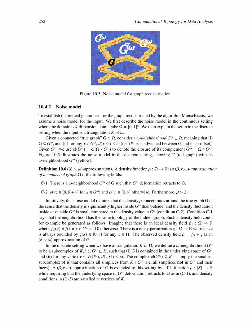
252 Computational Topology for Data Analysis
Figure 10.5: Noise model for graph reconstruction.
10.4.2 Noise model
To establish theoretical guarantees for the graph reconstructed by the algorithm MorseRecon, weassume a noise model for the input. We first describe the noise model in the continuous settingwhere the domain is k-dimensional unit cube Ω = [0, 1]k. We then explain the setup in the discretesetting when the input is a triangulation K of Ω.
Given a connected “true graph” G ⊂ Ω, consider a ω-neighborhood Gω ⊆ Ω, meaning that (i)G ⊆ Gω, and (ii) for any x ∈ Gω, d(x,G) ≤ ω (i.e, Gω is sandwiched between G and its ω-offset).Given Gω, we use cl(Gω) = cl(Ω \ Gω) to denote the closure of its complement Gω = Ω \ Gω.Figure 10.5 illustrates the noise model in the discrete setting, showing G (red graph) with itsω-neighborhood Gω (yellow).
Definition 10.6 ((β, ν, ω)-approximation). A density function ρ : Ω→ R is a (β, ν, ω)-approximationof a connected graph G if the following holds:
C-1 There is a ω-neighborhood Gω of G such that Gω deformation retracts to G.
C-2 ρ(x) ∈ [β, β + ν] for x ∈ Gω; and ρ(x) ∈ [0, ν] otherwise. Furthermore, β > 2ν.
Intuitively, this noise model requires that the density ρ concentrates around the true graph G inthe sense that the density is significantly higher inside Gω than outside; and the density fluctuationinside or outside Gω is small compared to the density value in Gω (condition C-2). Condition C-1says that the neighborhood has the same topology of the hidden graph. Such a density field couldfor example be generated as follows: Imagine that there is an ideal density field fG : Ω → Rwhere fG(x) = β for x ∈ Gω and 0 otherwise. There is a noisy perturbation g : Ω→ R whose sizeis always bounded by g(x) ∈ [0, ν] for any x ∈ Ω. The observed density field ρ = fG + g is an(β, ν, ω)-approximation of G.
In the discrete setting when we have a triangulation K of Ω, we define a ω-neighborhood Gω
to be a subcomplex of K, i.e, Gω ⊆ K, such that (i) G is contained in the underlying space of Gω
and (ii) for any vertex v ∈ V(Gω), d(v,G) ≤ ω. The complex cl(Gω) ⊆ K is simply the smallestsubcomplex of K that contains all simplices from K \ Gω (i.e, all simplices not in Gω and theirfaces). A (β, ν, ω)-approximation of G is extended to this setting by a PL-function ρ : |K| → Rwhile requiring that the underlying space of Gω deformation retracts to G as in (C-1), and densityconditions in (C-2) are satisfied at vertices of K.
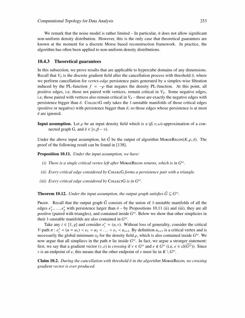
Computational Topology for Data Analysis 253
We remark that the noise model is rather limited – In particular, it does not allow significantnon-uniform density distribution. However, this is the only case that theoretical guarantees areknown at the moment for a discrete Morse based reconstruction framework. In practice, thealgorithm has often been applied to non-uniform density distributions.
10.4.3 Theoretical guarantees
In this subsection, we prove results that are applicable to hypercube domains of any dimensions.Recall that Vδ is the discrete gradient field after the cancellation process with threshold δ, wherewe perform cancellation for vertex-edge persistence pairs generated by a simplex-wise filtrationinduced by the PL-function f = −ρ that negates the density PL-function. At this point, allpositive edges, i.e, those not paired with vertices, remain critical in Vδ. Some negative edges,i.e, those paired with vertices also remain critical in Vδ – these are exactly the negative edges withpersistence bigger than δ. CollectG only takes the 1-unstable manifolds of those critical edges(positive or negative) with persistence bigger than δ; so those edges whose persistence is at mostδ are ignored.
Input assumption. Let ρ be an input density field which is a (β, ν, ω)-approximation of a con-nected graph G, and δ ∈ [ν, β − ν).
Under the above input assumption, let G be the output of algorithm MorseRecon(K, ρ, δ). Theproof of the following result can be found in [138].
Proposition 10.11. Under the input assumption, we have:
(i) There is a single critical vertex left after MorseRecon returns, which is in Gω.
(ii) Every critical edge considered by CollecG forms a persistence pair with a triangle.
(iii) Every critical edge considered by CollectG is in Gω.
Theorem 10.12. Under the input assumption, the output graph satisfies G ⊆ Gω.
Proof. Recall that the output graph G consists of the union of 1-unstable manifolds of all theedges e∗1, . . . , e
∗g with persistence larger than δ – by Propositions 10.11 (ii) and (iii), they are all
positive (paired with triangles), and contained inside Gω. Below we show that other simplicies intheir 1-unstable manifolds are also contained in Gω.
Take any i ∈ [1, g] and consider e∗i = (u, v). Without loss of generality, consider the criticalV-path π : e∗i ≺ (u = u1) ≺ e1 ≺ u2 ≺ . . . ≺ es ≺ us+1. By definition us+1 is a critical vertex and isnecessarily the global minimum v0 for the density field ρ, which is also contained inside Gω. Wenow argue that all simpliecs in the path π lie inside Gω. In fact, we argue a stronger statement:first, we say that a gradient vector (v, e) is crossing if v ∈ Gω and e < Gω (i.e, e ∈ cl(Gω)). Sincev is an endpoint of e, this means that the other endpoint of e must lie in K \Gω.
Claim 10.2. During the cancellation with threshold δ in the algorithm MorseRecon, no crossinggradient vector is ever produced.
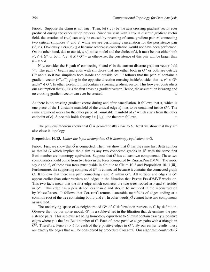
254 Computational Topology for Data Analysis
Proof. Suppose the claim is not true. Then, let (v, e) be the first crossing gradient vector everproduced during the cancellation process. Since we start with a trivial discrete gradient vectorfield, the creation of (v, e) can only be caused by reversing of some gradient path π′ connectingtwo critical simplices v′ and e′ while we are performing cancellation for the persistence pair(v′, e′). Obviously, Pers (e′) ≤ δ because otherwise cancellation would not have been performed.On the other hand, due to our (β, ν, ω)-noise model and the choice of δ, it must be that either bothv′, e′ ∈ Gω or both v′, e′ ∈ K \ Gω – as otherwise, the persistence of this pair will be larger thanβ − ν > δ.
Now consider the V-path π′ connecting e′ and v′ in the current discrete gradient vector fieldV ′. The path π′ begins and ends with simplices that are either both in Gω or both are outsideGω and also it has simplices both inside and outside Gω. It follows that the path π′ contains agradient vector (v′′, e′′) going in the opposite direction crossing inside/outside, that is, v′′ ∈ Gω
and e′′ < Gω. In other words, it must contain a crossing gradient vector. This however contradictsour assumption that (v, e) is the first crossing gradient vector. Hence, the assumption is wrong andno crossing gradient vector can ever be created.
As there is no crossing gradient vector during and after cancellation, it follows that π, which isone piece of the 1-unstable manifold of the critical edge e∗i , has to be contained inside Gω. Thesame argument works for the other piece of 1-unstable manifold of e∗i which starts from the otherendpoint of e∗i . Since this holds for any i ∈ [1, g], the theorem follows.
The previous theorem shows that G is geometrically close to G. Next we show that they arealso close in topology.
Proposition 10.13. Under the input assumption, G is homotopy equivalent to G.
Proof. First we show that G is connected. Then, we show that G has the same first Betti numberas that of G which implies the claim as any two connected graphs in Rk with the same firstBetti number are homotopy equivalent. Suppose that G has at least two components. These twocomponents should come from two trees in the forest computed by PartialPersDMVF. The roots,say r and r′, of these two trees must reside in Gω due to Claim 10.2 and Proposition 10.11(iii).Furthermore, the supporting complex of Gω is connected because it contains the connected graphG. It follows that there is a path connecting r and r′ within Gω. All vertices and edges in Gω
appear earlier than other vertices and edges in the filtration that PartialPersDMVF works on.This two facts mean that the first edge which connects the two trees rooted at r and r′ residesin Gω. This edge has a persistence less than δ and should be included in the reconstructionby MorseRecon. It follows that CollectG returns 1-unstable manifolds of edges ending at acommon root of the tree containing both r and r′. In other words, G cannot have two componentsas assumed.
The underlying space of ω-neighborhood Gω of G deformation retracts to G by definition.Observe that, by our noise model, Gω is a sublevel set in the filtration that determines the per-sistence pairs. This sublevel set being homotopy equivalent to G must contain exactly g positiveedges where g is the first Betti number of G. Each of these positive edges pairs with a triangle inGω. Therefore, Pers (e) > δ for each of the g positive edges in Gω. By our earlier results, theseare exactly the edges that will be considered by procedure CollectG. Our algorithm constructs G
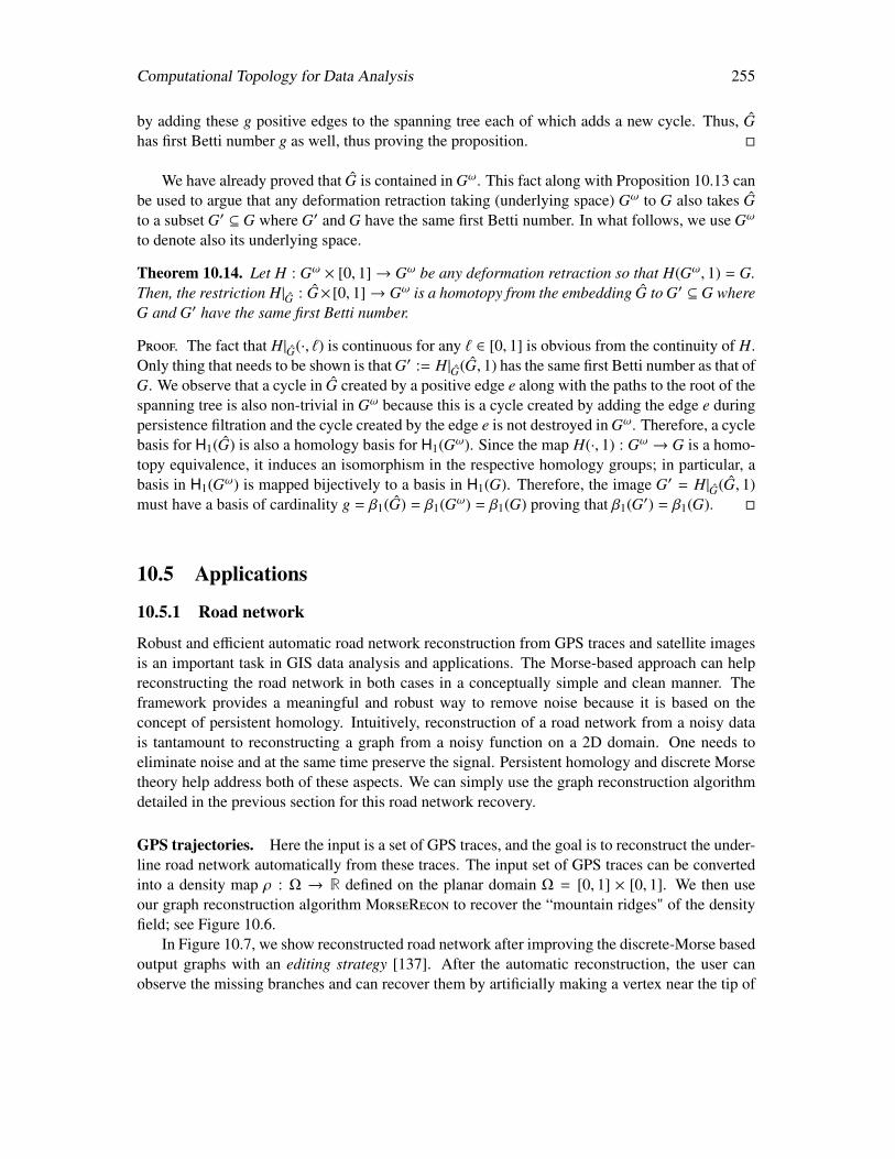
Computational Topology for Data Analysis 255
by adding these g positive edges to the spanning tree each of which adds a new cycle. Thus, Ghas first Betti number g as well, thus proving the proposition.
We have already proved that G is contained in Gω. This fact along with Proposition 10.13 canbe used to argue that any deformation retraction taking (underlying space) Gω to G also takes Gto a subset G′ ⊆ G where G′ and G have the same first Betti number. In what follows, we use Gω
to denote also its underlying space.
Theorem 10.14. Let H : Gω × [0, 1]→ Gω be any deformation retraction so that H(Gω, 1) = G.Then, the restriction H|G : G× [0, 1]→ Gω is a homotopy from the embedding G to G′ ⊆ G whereG and G′ have the same first Betti number.
Proof. The fact that H|G(·, `) is continuous for any ` ∈ [0, 1] is obvious from the continuity of H.Only thing that needs to be shown is that G′ := H|G(G, 1) has the same first Betti number as that ofG. We observe that a cycle in G created by a positive edge e along with the paths to the root of thespanning tree is also non-trivial in Gω because this is a cycle created by adding the edge e duringpersistence filtration and the cycle created by the edge e is not destroyed in Gω. Therefore, a cyclebasis for H1(G) is also a homology basis for H1(Gω). Since the map H(·, 1) : Gω → G is a homo-topy equivalence, it induces an isomorphism in the respective homology groups; in particular, abasis in H1(Gω) is mapped bijectively to a basis in H1(G). Therefore, the image G′ = H|G(G, 1)must have a basis of cardinality g = β1(G) = β1(Gω) = β1(G) proving that β1(G′) = β1(G).
10.5 Applications
10.5.1 Road network
Robust and efficient automatic road network reconstruction from GPS traces and satellite imagesis an important task in GIS data analysis and applications. The Morse-based approach can helpreconstructing the road network in both cases in a conceptually simple and clean manner. Theframework provides a meaningful and robust way to remove noise because it is based on theconcept of persistent homology. Intuitively, reconstruction of a road network from a noisy datais tantamount to reconstructing a graph from a noisy function on a 2D domain. One needs toeliminate noise and at the same time preserve the signal. Persistent homology and discrete Morsetheory help address both of these aspects. We can simply use the graph reconstruction algorithmdetailed in the previous section for this road network recovery.
GPS trajectories. Here the input is a set of GPS traces, and the goal is to reconstruct the under-line road network automatically from these traces. The input set of GPS traces can be convertedinto a density map ρ : Ω → R defined on the planar domain Ω = [0, 1] × [0, 1]. We then useour graph reconstruction algorithm MorseRecon to recover the “mountain ridges" of the densityfield; see Figure 10.6.
In Figure 10.7, we show reconstructed road network after improving the discrete-Morse basedoutput graphs with an editing strategy [137]. After the automatic reconstruction, the user canobserve the missing branches and can recover them by artificially making a vertex near the tip of
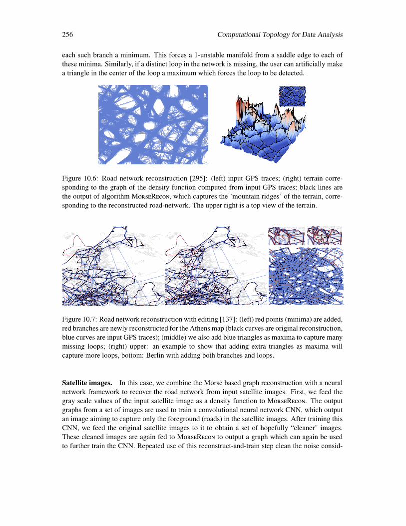
256 Computational Topology for Data Analysis
each such branch a minimum. This forces a 1-unstable manifold from a saddle edge to each ofthese minima. Similarly, if a distinct loop in the network is missing, the user can artificially makea triangle in the center of the loop a maximum which forces the loop to be detected.
Figure 10.6: Road network reconstruction [295]: (left) input GPS traces; (right) terrain corre-sponding to the graph of the density function computed from input GPS traces; black lines arethe output of algorithm MorseRecon, which captures the ’mountain ridges’ of the terrain, corre-sponding to the reconstructed road-network. The upper right is a top view of the terrain.
Figure 10.7: Road network reconstruction with editing [137]: (left) red points (minima) are added,red branches are newly reconstructed for the Athens map (black curves are original reconstruction,blue curves are input GPS traces); (middle) we also add blue triangles as maxima to capture manymissing loops; (right) upper: an example to show that adding extra triangles as maxima willcapture more loops, bottom: Berlin with adding both branches and loops.
Satellite images. In this case, we combine the Morse based graph reconstruction with a neuralnetwork framework to recover the road network from input satellite images. First, we feed thegray scale values of the input satellite image as a density function to MorseRecon. The outputgraphs from a set of images are used to train a convolutional neural network CNN, which outputan image aiming to capture only the foreground (roads) in the satellite images. After training thisCNN, we feed the original satellite images to it to obtain a set of hopefully “cleaner" images.These cleaned images are again fed to MorseRecon to output a graph which can again be usedto further train the CNN. Repeated use of this reconstruct-and-train step clean the noise consid-
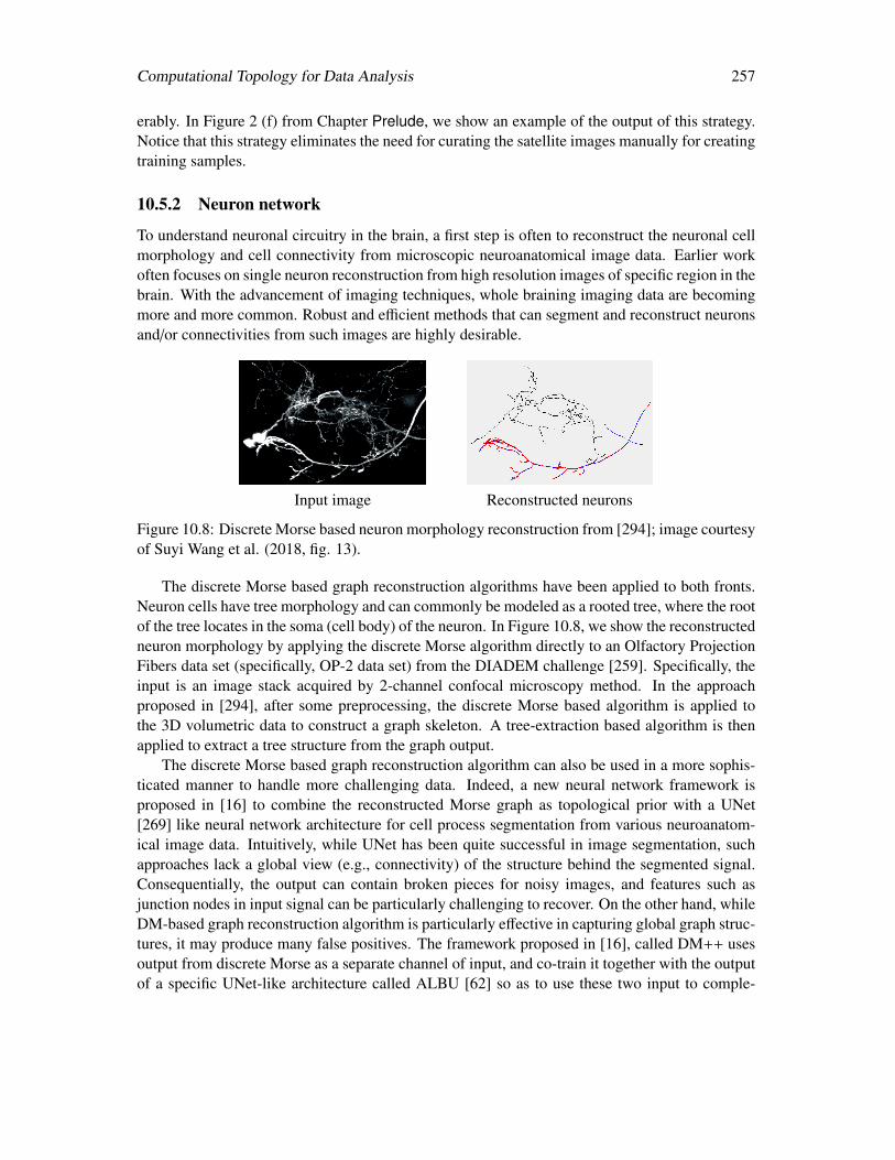
Computational Topology for Data Analysis 257
erably. In Figure 2 (f) from Chapter Prelude, we show an example of the output of this strategy.Notice that this strategy eliminates the need for curating the satellite images manually for creatingtraining samples.
10.5.2 Neuron network
To understand neuronal circuitry in the brain, a first step is often to reconstruct the neuronal cellmorphology and cell connectivity from microscopic neuroanatomical image data. Earlier workoften focuses on single neuron reconstruction from high resolution images of specific region in thebrain. With the advancement of imaging techniques, whole braining imaging data are becomingmore and more common. Robust and efficient methods that can segment and reconstruct neuronsand/or connectivities from such images are highly desirable.
Input image Reconstructed neurons
Figure 10.8: Discrete Morse based neuron morphology reconstruction from [294]; image courtesyof Suyi Wang et al. (2018, fig. 13).
The discrete Morse based graph reconstruction algorithms have been applied to both fronts.Neuron cells have tree morphology and can commonly be modeled as a rooted tree, where the rootof the tree locates in the soma (cell body) of the neuron. In Figure 10.8, we show the reconstructedneuron morphology by applying the discrete Morse algorithm directly to an Olfactory ProjectionFibers data set (specifically, OP-2 data set) from the DIADEM challenge [259]. Specifically, theinput is an image stack acquired by 2-channel confocal microscopy method. In the approachproposed in [294], after some preprocessing, the discrete Morse based algorithm is applied tothe 3D volumetric data to construct a graph skeleton. A tree-extraction based algorithm is thenapplied to extract a tree structure from the graph output.
The discrete Morse based graph reconstruction algorithm can also be used in a more sophis-ticated manner to handle more challenging data. Indeed, a new neural network framework isproposed in [16] to combine the reconstructed Morse graph as topological prior with a UNet[269] like neural network architecture for cell process segmentation from various neuroanatom-ical image data. Intuitively, while UNet has been quite successful in image segmentation, suchapproaches lack a global view (e.g., connectivity) of the structure behind the segmented signal.Consequentially, the output can contain broken pieces for noisy images, and features such asjunction nodes in input signal can be particularly challenging to recover. On the other hand, whileDM-based graph reconstruction algorithm is particularly effective in capturing global graph struc-tures, it may produce many false positives. The framework proposed in [16], called DM++ usesoutput from discrete Morse as a separate channel of input, and co-train it together with the outputof a specific UNet-like architecture called ALBU [62] so as to use these two input to comple-

258 Computational Topology for Data Analysis
Figure 10.9: The DM++ framework proposed by [16], which combines both the DM output withstandard neural-network based output together via a Siamese neural network stack so as to usethese two inputs to augment each other and obtain better connected final segmentation; imagecourtesy of Samik Banerjee et al. (2020, fig. 2b).
ment each other. See Figure 10.9. In particular, UNet output helps to remove false positives fromdiscrete Morse output, while the Morse graph output helps to obtain better connectivity.
10.6 Notes and Exercises
Forman [161] developed the discrete analogue of the classical Morse theory in mathematics. Thisanalogy is exemplified by the following fact. Let Cp denote the p-th chain group formed by thep-dimensional critical cells in a discrete Morse vector field. It means that Cp is a free Abeliangroup with critical p-cells forming a basis assuming Z2-additions. For a critical cell cp, definethe boundary operator ∂pcp = Σi(mp mod 2)ci
p−1 where cip is a critical (p − 1)-cell reachable
by mp number of V-paths from cp. Extending the boundary operator to the chains we get theboundary homomorphism ∂p : Cp → Cp−1. One can verify that ∂p−1 ∂p = 0 (Exercise 12) thusleading to a valid discrete Morse chain complex. Naturally, we get a homology group Hp fromthis construction. It turns out that this homology group is isomorphic to the homology group ofthe complex on which the DMVF is defined.
Several researchers brought the concept to the area of topological data analysis [23, 213, 223,235]. King et al. [213] presented an algorithm to produce a discrete Morse function on a complexfrom a given real-valued function on its vertices. Bauer et al. [23] showed that persistent pairs canbe cancelled in order of their persistence values for any simplicial 2-manifolds. They also gavean O(n log n)-time algorithm for cancelling pairs that have persistence below a given threshold.The cancellation algorithm and its analysis in this chapter follow this result though with a slightlydifferent presentation. This cancellation does not generalize to simplicial 2-complexes and beyondas we have illustrated. Mischaikow and Nanda [235] proposed Morse cancellation as a tool tosimplify an input complex before computing persistence pairs. The combinatorial view of thevector field given by the discrete Morse theory has recently been extended to dynamical systems,see, e.g., [39, 238].
Starting with Lewiner et al. [223], several researchers proposed discrete Morse theory for ap-plications in visualization and image processing. Gyulassy et al. [181], Delgado-Friedricks etal. [118] and Robins et al. [267] used discrete Morse theory in conjunction with persistence basedcancellations for processing images and analyzing features for e.g., porous solids. Sousbie [282]

Computational Topology for Data Analysis 259
proposed using the theory for detecting filamentary structures in data for cosmic webs. Thesework proposed using cancellations as long as they are permitted acknowledging the fact that allcancellations in a 2- or 3-complex may not be possible. Wang et al. proposed to use discreteMorse complexes to compute unstable 1-manifolds as an output for a road network from GPSdata [295]. Using unstable 1-manifolds in a discrete Morse complex defined on a triangulationin R2 to capture the hidden road network was proposed in this paper. Ultimately, this proposedapproach was implemented with a simplified algorithm and a proof of guarantee in [138]. Thematerial in Section 10.4 is taken from this paper. The application to road network reconstructionfrom GPS trajectories and satellite images in Section 10.5 appeared in [137] and [139] respec-tively. The application to neuron imaging data is taken from [16, 294].
Exercises
1. A Hasse diagram of a simplicial complex K is a directed graph that has a vertex vσ forevery simplex σ in K and a directed edge from vσ to vσ′ if and only if σ′ is a cofacet ofσ. Let M be a matching in K. Modify the Hasse diagram by reversing every edge that isdirected from vσ to vσ′ and (σ′, σ) is in the matching M. Show that M induces a DMVF ifand only if the modified Hasse diagram does not have any directed cycle.
2. Let f be a Morse function defined on a simplicial complex K. We say K collapses to K′
if there is a simplex σ with a single cofacet σ′ and K′ = K \ σ,σ′. Let Ka ⊆ K be thesubcomplex where Ka = σ | f (σ) ≤ a. Show that there is a series of collapses (possiblyempty) that brings Ka to Kb for any b ≤ a if there is no critical simplex with function valuec where b < c < a.
3. Call a V-path extendible if it can be extended by a simplex at any of the two ends.
(a) Show an example of a non-extendible V-path that is not critical.
(b) Show that every non-extendible V-path in a simplicial 2-manifold without boundarymust have at least one critical simplex.
4. Show that a discrete Morse function defines a Morse matching.
5. Let K be a simplicial Möbius strip with all its vertices on the boundary. Design a DMVF onK so that there is only one critical edge and only one critical vertex and no critical triangle.
6. Prove that two V-paths that meet must have a common suffix.
7. Show the following:
(a) The strong Morse inequality implies the weak Morse inequality in Proposition 10.1.
(b) A matching which is not Morse may not satisfy Morse inequalities as in Proposi-tion 10.1 but always satisfies the equality cp − cp−1 + · · · ± c0 = βp − βp−1 + · · · ± β0for a p-dimensional complex K.

260 Computational Topology for Data Analysis
8. Consider a filtration of a simplicial complex K embedded in R3. We want to create a DMVFwhere all persistent triangle-tetrahedra pairs with persistence less than a threshold can becancelled. Show that this is always possible. Write an algorithm to compute the stablemanifolds for each of the critical tetrahedra in the resulting DMVF.
9. Prove Claim 10.1.
10. We propose a different version of PartialPersDMVF by changing only step 13 of Sim-plePersDMVF as:
• if Pers (e) > δ then designate e critical in V else Join(Tu,Tu′) endif
Prove that this simple modification produces the same DMVF as the PartialPersDMVFdescribed in the text.
11. Let K be a simplicial d-complex that has every (d − 1)-simplex incident to at most two d-simplices. Extend Theorem 10.5 to prove that all persistent pairs between (d− 1)-simplicesand d-simplices arising from a filtration of K can be cancelled.
12. Prove ∂p−1 ∂p = 0 for the boundary operator defined for chain groups of critical cells asdescribed for discrete Morse chain complex in the notes above.
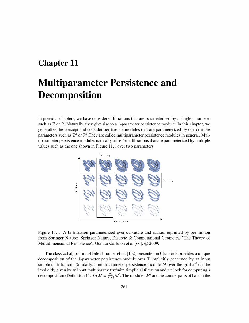
Chapter 11
Multiparameter Persistence andDecomposition
In previous chapters, we have considered filtrations that are parameterised by a single parametersuch as Z or R. Naturally, they give rise to a 1-parameter persistence module. In this chapter, wegeneralize the concept and consider persistence modules that are parameterized by one or moreparameters such as Zd or Rd.They are called multiparameter persistence modules in general. Mul-tiparameter persistence modules naturally arise from filtrations that are parameterized by multiplevalues such as the one shown in Figure 11.1 over two parameters.
Figure 11.1: A bi-filtration parameterized over curvature and radius, reprinted by permissionfrom Springer Nature: Springer Nature, Discrete & Computational Geometry, "The Theory ofMultidimensional Persistence", Gunnar Carlsson et al.[66], c© 2009.
The classical algorithm of Edelsbrunner et al. [152] presented in Chapter 3 provides a uniquedecomposition of the 1-parameter persistence module over Z implicitly generated by an inputsimplicial filtration. Similarly, a multiparameter persistence module M over the grid Zd can beimplicitly given by an input multiparameter finite simplicial filtration and we look for computing adecomposition (Definition 11.10) M
⊕i Mi. The modules Mi are the counterparts of bars in the
261
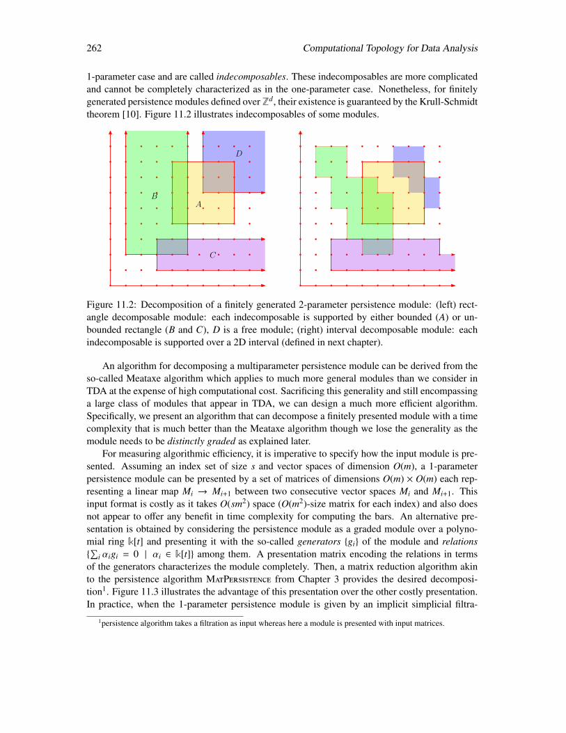
262 Computational Topology for Data Analysis
1-parameter case and are called indecomposables. These indecomposables are more complicatedand cannot be completely characterized as in the one-parameter case. Nonetheless, for finitelygenerated persistence modules defined over Zd, their existence is guaranteed by the Krull-Schmidttheorem [10]. Figure 11.2 illustrates indecomposables of some modules.
AB
C
D
Figure 11.2: Decomposition of a finitely generated 2-parameter persistence module: (left) rect-angle decomposable module: each indecomposable is supported by either bounded (A) or un-bounded rectangle (B and C), D is a free module; (right) interval decomposable module: eachindecomposable is supported over a 2D interval (defined in next chapter).
An algorithm for decomposing a multiparameter persistence module can be derived from theso-called Meataxe algorithm which applies to much more general modules than we consider inTDA at the expense of high computational cost. Sacrificing this generality and still encompassinga large class of modules that appear in TDA, we can design a much more efficient algorithm.Specifically, we present an algorithm that can decompose a finitely presented module with a timecomplexity that is much better than the Meataxe algorithm though we lose the generality as themodule needs to be distinctly graded as explained later.
For measuring algorithmic efficiency, it is imperative to specify how the input module is pre-sented. Assuming an index set of size s and vector spaces of dimension O(m), a 1-parameterpersistence module can be presented by a set of matrices of dimensions O(m) × O(m) each rep-resenting a linear map Mi → Mi+1 between two consecutive vector spaces Mi and Mi+1. Thisinput format is costly as it takes O(sm2) space (O(m2)-size matrix for each index) and also doesnot appear to offer any benefit in time complexity for computing the bars. An alternative pre-sentation is obtained by considering the persistence module as a graded module over a polyno-mial ring k[t] and presenting it with the so-called generators gi of the module and relations∑
i αigi = 0 | αi ∈ k[t] among them. A presentation matrix encoding the relations in termsof the generators characterizes the module completely. Then, a matrix reduction algorithm akinto the persistence algorithm MatPersistence from Chapter 3 provides the desired decomposi-tion1. Figure 11.3 illustrates the advantage of this presentation over the other costly presentation.In practice, when the 1-parameter persistence module is given by an implicit simplicial filtra-
1persistence algorithm takes a filtration as input whereas here a module is presented with input matrices.
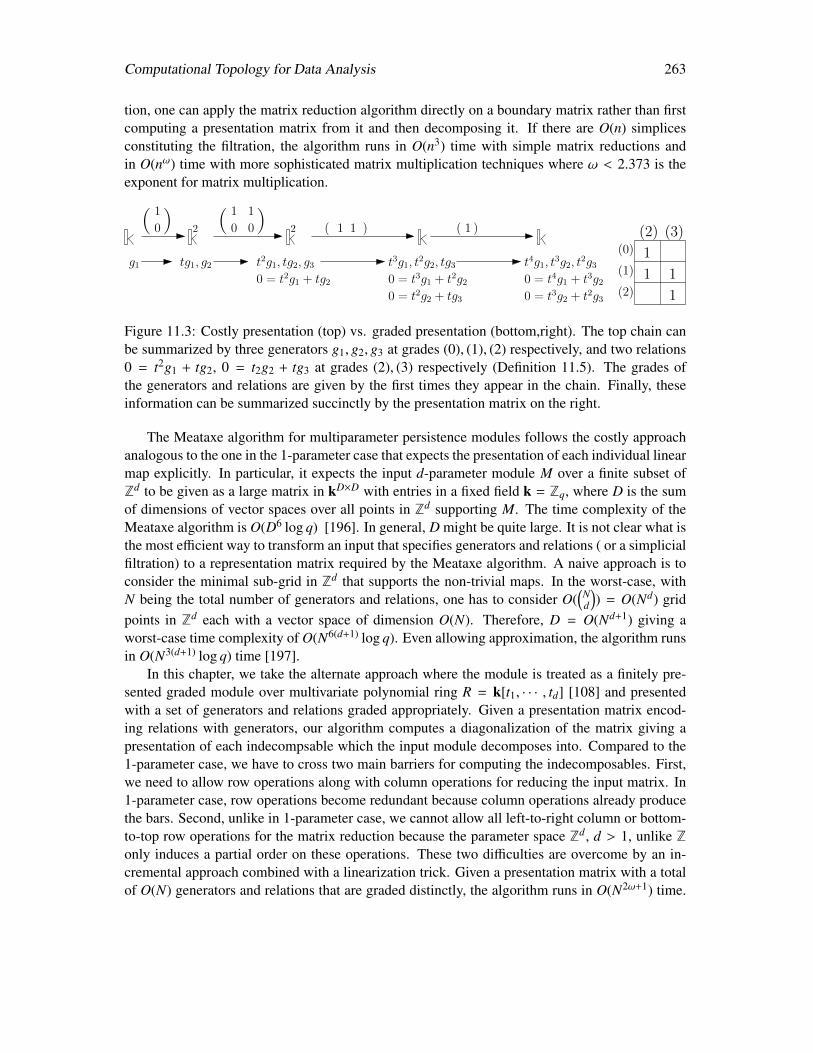
Computational Topology for Data Analysis 263
tion, one can apply the matrix reduction algorithm directly on a boundary matrix rather than firstcomputing a presentation matrix from it and then decomposing it. If there are O(n) simplicesconstituting the filtration, the algorithm runs in O(n3) time with simple matrix reductions andin O(nω) time with more sophisticated matrix multiplication techniques where ω < 2.373 is theexponent for matrix multiplication.
g1 tg1, g2 t2g1, tg2, g30 = t2g1 + tg2
t3g1, t2g2, tg3
0 = t3g1 + t2g20 = t2g2 + tg3
t4g1, t3g2, t
2g30 = t4g1 + t3g20 = t3g2 + t2g3
1
0
1
0
1
0 1 1( ) ( ) ( ) 1( )
1
1 1
1
(2) (3)(0)
(1)
(2)
2 2
Figure 11.3: Costly presentation (top) vs. graded presentation (bottom,right). The top chain canbe summarized by three generators g1, g2, g3 at grades (0), (1), (2) respectively, and two relations0 = t2g1 + tg2, 0 = t2g2 + tg3 at grades (2), (3) respectively (Definition 11.5). The grades ofthe generators and relations are given by the first times they appear in the chain. Finally, theseinformation can be summarized succinctly by the presentation matrix on the right.
The Meataxe algorithm for multiparameter persistence modules follows the costly approachanalogous to the one in the 1-parameter case that expects the presentation of each individual linearmap explicitly. In particular, it expects the input d-parameter module M over a finite subset ofZd to be given as a large matrix in kD×D with entries in a fixed field k = Zq, where D is the sumof dimensions of vector spaces over all points in Zd supporting M. The time complexity of theMeataxe algorithm is O(D6 log q) [196]. In general, D might be quite large. It is not clear what isthe most efficient way to transform an input that specifies generators and relations ( or a simplicialfiltration) to a representation matrix required by the Meataxe algorithm. A naive approach is toconsider the minimal sub-grid in Zd that supports the non-trivial maps. In the worst-case, withN being the total number of generators and relations, one has to consider O(
(Nd
)) = O(Nd) grid
points in Zd each with a vector space of dimension O(N). Therefore, D = O(Nd+1) giving aworst-case time complexity of O(N6(d+1) log q). Even allowing approximation, the algorithm runsin O(N3(d+1) log q) time [197].
In this chapter, we take the alternate approach where the module is treated as a finitely pre-sented graded module over multivariate polynomial ring R = k[t1, · · · , td] [108] and presentedwith a set of generators and relations graded appropriately. Given a presentation matrix encod-ing relations with generators, our algorithm computes a diagonalization of the matrix giving apresentation of each indecompsable which the input module decomposes into. Compared to the1-parameter case, we have to cross two main barriers for computing the indecomposables. First,we need to allow row operations along with column operations for reducing the input matrix. In1-parameter case, row operations become redundant because column operations already producethe bars. Second, unlike in 1-parameter case, we cannot allow all left-to-right column or bottom-to-top row operations for the matrix reduction because the parameter space Zd, d > 1, unlike Zonly induces a partial order on these operations. These two difficulties are overcome by an in-cremental approach combined with a linearization trick. Given a presentation matrix with a totalof O(N) generators and relations that are graded distinctly, the algorithm runs in O(N2ω+1) time.
264 Computational Topology for Data Analysis
Surprisingly, the complexity does not depend on the parameter d.Computing presentation matrix from a multiparameter simplicial filtration is not easy. For
d-parameter filtrations with n simplices, a presentation matrix of size O(nd−1) × O(nd−1) canbe computed in O(nd+1) time by adapting an algorithm of Skryzalin [279] as detailed in [142].We will not present this construction here. Instead, we focus on the two cases, 2-parameterpersistence modules where the homology groups could be multi-dimensional and d-parameterpersistence modules where the homology group is only zero dimensional. For these two cases,we can compute the presentation matrices more efficiently. For the 2-parameter case, Lesnickand Wright [222] gives an efficient O(n3) algorithm for computing a presentation matrix from aninput filtration. In this case, N, the total number of generators and relations, is O(n). For the 0-thhomology groups, presentation matrices are given by the boundary matrices straightforwardly asdetailed in Section 11.5.2 giving N = O(n).
11.1 Multiparameter persistence modules
We define persistence modules in this chapter differently using the definition of graded modulesin algebra. Graded module structures provide an appropriate framework for defining the mul-tiparameter persistence, in particular, for the decomposition algorithm that we present. Also,navigating between the simplicial filtration and the module induced by it becomes natural withthe graded module structure.
11.1.1 Persistence modules as graded modules
First, we recollect the definition of modules from section 2.4.1. It requires a ring. We consider amodule where the ring R is taken as the polynomial ring.
Definition 11.1 (Polynomial ring). Given a variable t and a field k, the set of polynomials givenby
k[t] = a0 + a1t + a2t2 + · · · + antn | n ≥ 0, ai ∈ k
forms a ring with usual polynomial addition and multiplication operations. The definition can beextended to multivariate polynomials
k[t] = k[t1, · · · , tk] = Σi1,··· ,ik ai1,··· ,ik ti11 · · · t
i jj · · · t
ikk | i1, · · · , ik ≥ 0, ai1,··· ,ik ∈ k.
We use polynomial ring to define multiparameter persistence modules. Specifically, let R =
k[t1, · · · , td] be the d-variate Polynomial ring for some d ∈ Z+ with k being a field. Throughoutthis chapter, we assume coefficients are in k. Hence homology groups are vector spaces.
Definition 11.2 (Graded module). A Zd-graded R-module (graded module in brief) is an R-module M that is a direct sum of k-vector spaces Mu indexed by u = (u1, u2, . . . , ud) ∈ Zd,i.e. M =
⊕u Mu, such that the ring action satisfies that ∀i,∀u ∈ Zd, ti ·Mu ⊆ Mu+ei , where ei
di=1
is the standard basis in Zd. The indices u ∈ Zd are called grades.
Another interpretation of graded module is that, for each u ∈ Zd, the action of ti on Mudetermines a linear map ti• : Mu → Mu+ei by (ti•)(m) = ti · m. So, we can also describe a graded
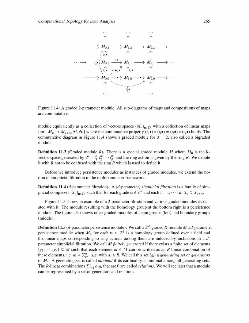
Computational Topology for Data Analysis 265
· · · · · · · · ·
· · · M0,2 M1,2 M2,2 · · ·
· · · −→ M0,1 M1,1 M2,1 · · ·
· · · M0,0 M1,0 M2,0 · · ·
· · · ↑ · · ·
t2•
t1•
t1•
t2• t1•t2•
t22•
t21•
t1•
t2•
Figure 11.4: A graded 2-parameter module. All sub-diagrams of maps and compositions of mapsare commutative.
module equivalently as a collection of vectors spaces Muu∈Zd with a collection of linear mapsti• : Mu → Mu+ei ,∀i,∀u where the commutative property (t j•) (ti•) = (ti•) (t j•) holds. Thecommutative diagram in Figure 11.4 shows a graded module for d = 2, also called a bigradedmodule.
Definition 11.3 (Graded module R). There is a special graded module M where Mu is the k-vector space generated by tu = tu1
1 tu22 · · · t
udd and the ring action is given by the ring R. We denote
it with R not to be confused with the ring R which is used to define it.
Before we introduce persistence modules as instances of graded modules, we extend the no-tion of simplicial filtration to the multiparameter framework.
Definition 11.4 (d-parameter filtration). A (d-parameter) simplicial filtration is a family of sim-plicial complexes Xuu∈Zd such that for each grade u ∈ Zd and each i = 1, · · · , d, Xu ⊆ Xu+ei .
Figure 11.5 shows an example of a 2-parameter filtration and various graded modules associ-ated with it. The module resulting with the homology group at the bottom right is a persistencemodule. The figure also shows other graded modules of chain groups (left) and boundary groups(middle).
Definition 11.5 (d-parameter persistence module). We call a Zd-graded R-module M a d-parameterpersistence module when Mu for each u ∈ Zd is a homology group defined over a field andthe linear maps corresponding to ring actions among them are induced by inclusions in a d-parameter simplicial filtration. We call M finitely generated if there exists a finite set of elementsg1, · · · , gn ⊆ M such that each element m ∈ M can be written as an R-linear combination ofthese elements, i.e. m =
∑ni=1 αigi with αi ∈ R. We call this set gi a generating set or generators
of M. A generating set is called minimal if its cardinality is minimal among all generating sets.The R-linear combinations
∑ni=1 αigi that are 0 are called relations. We will see later that a module
can be represented by a set of generators and relations.
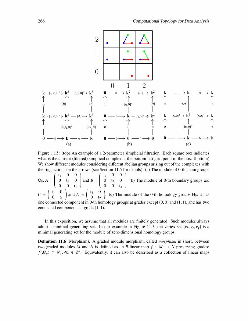
266 Computational Topology for Data Analysis
0 1 2
0
1
2
k k3 k3
k k3 k3
0 k k
[t1,0,0]> [t1,0,0]>
t2
[t1,0,0]>
[B]
[A]
[B]
0
0
t1
[0,t2,0]> [0,t2,0]
0 k2 k2
0 k k2
0 0 0
0 [C]
1
0
[t2,0]>
[t1,0]>
[D]
0
0
0
0 0
k k k
k k2 k
0 k k
t1 t1
t2
[t1,0]>
[t2,t2]
[t1,t1]
t2
0
0
t1
[t2,0]> t2
(a) (b) (c)
Figure 11.5: (top) An example of a 2-parameter simplicial filtration. Each square box indicateswhat is the current (filtered) simplical complex at the bottom left grid point of the box. (bottom)We show different modules considering different abelian groups arising out of the complexes withthe ring actions on the arrows (see Section 11.5 for details): (a) The module of 0-th chain groups
C0, A =
t1 0 00 t1 00 0 t1
and B =
t2 0 00 t2 00 0 t2
. (b) The module of 0-th boundary groups B0,
C =
(t1 00 t1
)and D =
(t2 00 t2
). (c) The module of the 0-th homology groups H0, it has
one connected component in 0-th homology groups at grades except (0, 0) and (1, 1), and has twoconnected components at grade (1, 1).
In this exposition, we assume that all modules are finitely generated. Such modules alwaysadmit a minimal generating set. In our example in Figure 11.5, the vertex set vb, vr, vg is aminimal generating set for the module of zero-dimensional homology groups.
Definition 11.6 (Morphism). A graded module morphism, called morphism in short, betweentwo graded modules M and N is defined as an R-linear map f : M → N preserving grades:f (Mu) ⊆ Nu,∀u ∈ Zd. Equivalently, it can also be described as a collection of linear maps
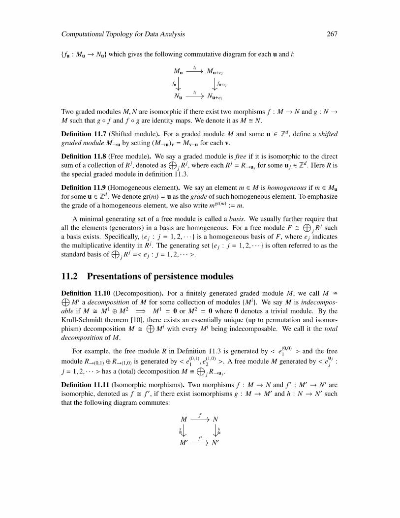
Computational Topology for Data Analysis 267
fu : Mu → Nu which gives the following commutative diagram for each u and i:
Mu Mu+ei
Nu Nu+ei
ti
fu fu+ei
ti
Two graded modules M,N are isomorphic if there exist two morphisms f : M → N and g : N →M such that g f and f g are identity maps. We denote it as M N.
Definition 11.7 (Shifted module). For a graded module M and some u ∈ Zd, define a shiftedgraded module M→u by setting (M→u)v = Mv−u for each v.
Definition 11.8 (Free module). We say a graded module is free if it is isomorphic to the directsum of a collection of R j, denoted as
⊕j R j, where each R j = R→u j for some u j ∈ Zd. Here R is
the special graded module in definition 11.3.
Definition 11.9 (Homogeneous element). We say an element m ∈ M is homogeneous if m ∈ Mufor some u ∈ Zd. We denote gr(m) = u as the grade of such homogeneous element. To emphasizethe grade of a homogeneous element, we also write mgr(m) := m.
A minimal generating set of a free module is called a basis. We usually further require thatall the elements (generators) in a basis are homogeneous. For a free module F
⊕j R j such
a basis exists. Specifically, e j : j = 1, 2, · · · is a homogeneous basis of F, where e j indicatesthe multiplicative identity in R j. The generating set e j : j = 1, 2, · · · is often referred to as thestandard basis of
⊕j R j =< e j : j = 1, 2, · · · >.
11.2 Presentations of persistence modules
Definition 11.10 (Decomposition). For a finitely generated graded module M, we call M ⊕Mi a decomposition of M for some collection of modules Mi. We say M is indecompos-
able if M M1 ⊕ M2 =⇒ M1 = 0 or M2 = 0 where 0 denotes a trivial module. By theKrull-Schmidt theorem [10], there exists an essentially unique (up to permutation and isomor-phism) decomposition M
⊕Mi with every Mi being indecomposable. We call it the total
decomposition of M.
For example, the free module R in Definition 11.3 is generated by < e(0,0)1 > and the free
module R→(0,1) ⊕ R→(1,0) is generated by < e(0,1)1 , e(1,0)
2 >. A free module M generated by < eu jj :
j = 1, 2, · · · > has a (total) decomposition M ⊕
j R→u j .
Definition 11.11 (Isomorphic morphisms). Two morphisms f : M → N and f ′ : M′ → N′ areisomorphic, denoted as f f ′, if there exist isomorphisms g : M → M′ and h : N → N′ suchthat the following diagram commutes:
M N
M′ N′
f
g
h
f ′
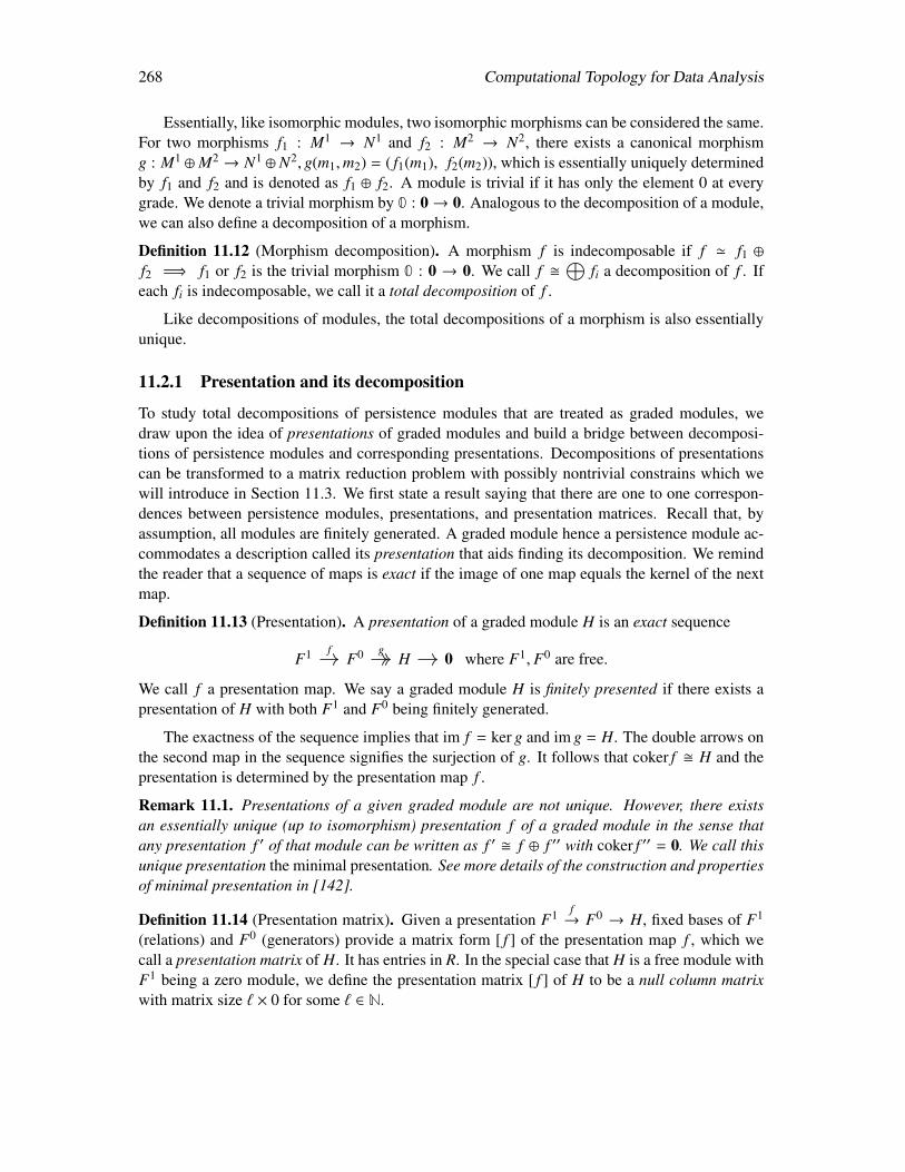
268 Computational Topology for Data Analysis
Essentially, like isomorphic modules, two isomorphic morphisms can be considered the same.For two morphisms f1 : M1 → N1 and f2 : M2 → N2, there exists a canonical morphismg : M1 ⊕M2 → N1 ⊕ N2, g(m1,m2) = ( f1(m1), f2(m2)), which is essentially uniquely determinedby f1 and f2 and is denoted as f1 ⊕ f2. A module is trivial if it has only the element 0 at everygrade. We denote a trivial morphism by 0 : 0→ 0. Analogous to the decomposition of a module,we can also define a decomposition of a morphism.
Definition 11.12 (Morphism decomposition). A morphism f is indecomposable if f ' f1 ⊕f2 =⇒ f1 or f2 is the trivial morphism 0 : 0 → 0. We call f
⊕fi a decomposition of f . If
each fi is indecomposable, we call it a total decomposition of f .
Like decompositions of modules, the total decompositions of a morphism is also essentiallyunique.
11.2.1 Presentation and its decomposition
To study total decompositions of persistence modules that are treated as graded modules, wedraw upon the idea of presentations of graded modules and build a bridge between decomposi-tions of persistence modules and corresponding presentations. Decompositions of presentationscan be transformed to a matrix reduction problem with possibly nontrivial constrains which wewill introduce in Section 11.3. We first state a result saying that there are one to one correspon-dences between persistence modules, presentations, and presentation matrices. Recall that, byassumption, all modules are finitely generated. A graded module hence a persistence module ac-commodates a description called its presentation that aids finding its decomposition. We remindthe reader that a sequence of maps is exact if the image of one map equals the kernel of the nextmap.
Definition 11.13 (Presentation). A presentation of a graded module H is an exact sequence
F1 F0 H 0 where F1, F0 are free.f g
We call f a presentation map. We say a graded module H is finitely presented if there exists apresentation of H with both F1 and F0 being finitely generated.
The exactness of the sequence implies that im f = ker g and im g = H. The double arrows onthe second map in the sequence signifies the surjection of g. It follows that coker f H and thepresentation is determined by the presentation map f .
Remark 11.1. Presentations of a given graded module are not unique. However, there existsan essentially unique (up to isomorphism) presentation f of a graded module in the sense thatany presentation f ′ of that module can be written as f ′ f ⊕ f ′′ with coker f ′′ = 0. We call thisunique presentation the minimal presentation. See more details of the construction and propertiesof minimal presentation in [142].
Definition 11.14 (Presentation matrix). Given a presentation F1 f→ F0 → H, fixed bases of F1
(relations) and F0 (generators) provide a matrix form [ f ] of the presentation map f , which wecall a presentation matrix of H. It has entries in R. In the special case that H is a free module withF1 being a zero module, we define the presentation matrix [ f ] of H to be a null column matrixwith matrix size ` × 0 for some ` ∈ N.
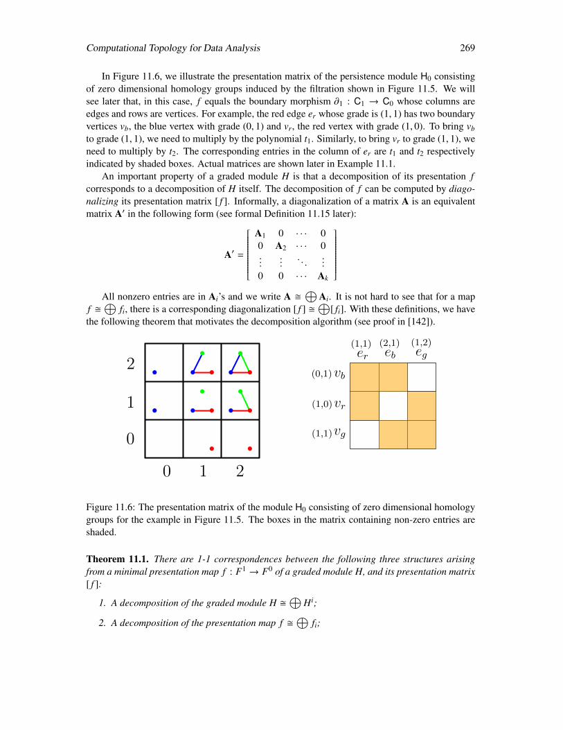
Computational Topology for Data Analysis 269
In Figure 11.6, we illustrate the presentation matrix of the persistence module H0 consistingof zero dimensional homology groups induced by the filtration shown in Figure 11.5. We willsee later that, in this case, f equals the boundary morphism ∂1 : C1 → C0 whose columns areedges and rows are vertices. For example, the red edge er whose grade is (1, 1) has two boundaryvertices vb, the blue vertex with grade (0, 1) and vr, the red vertex with grade (1, 0). To bring vb
to grade (1, 1), we need to multiply by the polynomial t1. Similarly, to bring vr to grade (1, 1), weneed to multiply by t2. The corresponding entries in the column of er are t1 and t2 respectivelyindicated by shaded boxes. Actual matrices are shown later in Example 11.1.
An important property of a graded module H is that a decomposition of its presentation fcorresponds to a decomposition of H itself. The decomposition of f can be computed by diago-nalizing its presentation matrix [ f ]. Informally, a diagonalization of a matrix A is an equivalentmatrix A′ in the following form (see formal Definition 11.15 later):
A′ =
A1 0 · · · 00 A2 · · · 0...
.... . .
...
0 0 · · · Ak
All nonzero entries are in Ai’s and we write A
⊕Ai. It is not hard to see that for a map
f ⊕
fi, there is a corresponding diagonalization [ f ] ⊕
[ fi]. With these definitions, we havethe following theorem that motivates the decomposition algorithm (see proof in [142]).
er eb eg
vb
vr
vg
(1,1) (2,1) (1,2)
(0,1)
(1,0)
(1,1)
0 1 2
0
1
2
Figure 11.6: The presentation matrix of the module H0 consisting of zero dimensional homologygroups for the example in Figure 11.5. The boxes in the matrix containing non-zero entries areshaded.
Theorem 11.1. There are 1-1 correspondences between the following three structures arisingfrom a minimal presentation map f : F1 → F0 of a graded module H, and its presentation matrix[ f ]:
1. A decomposition of the graded module H ⊕
Hi;
2. A decomposition of the presentation map f ⊕
fi;
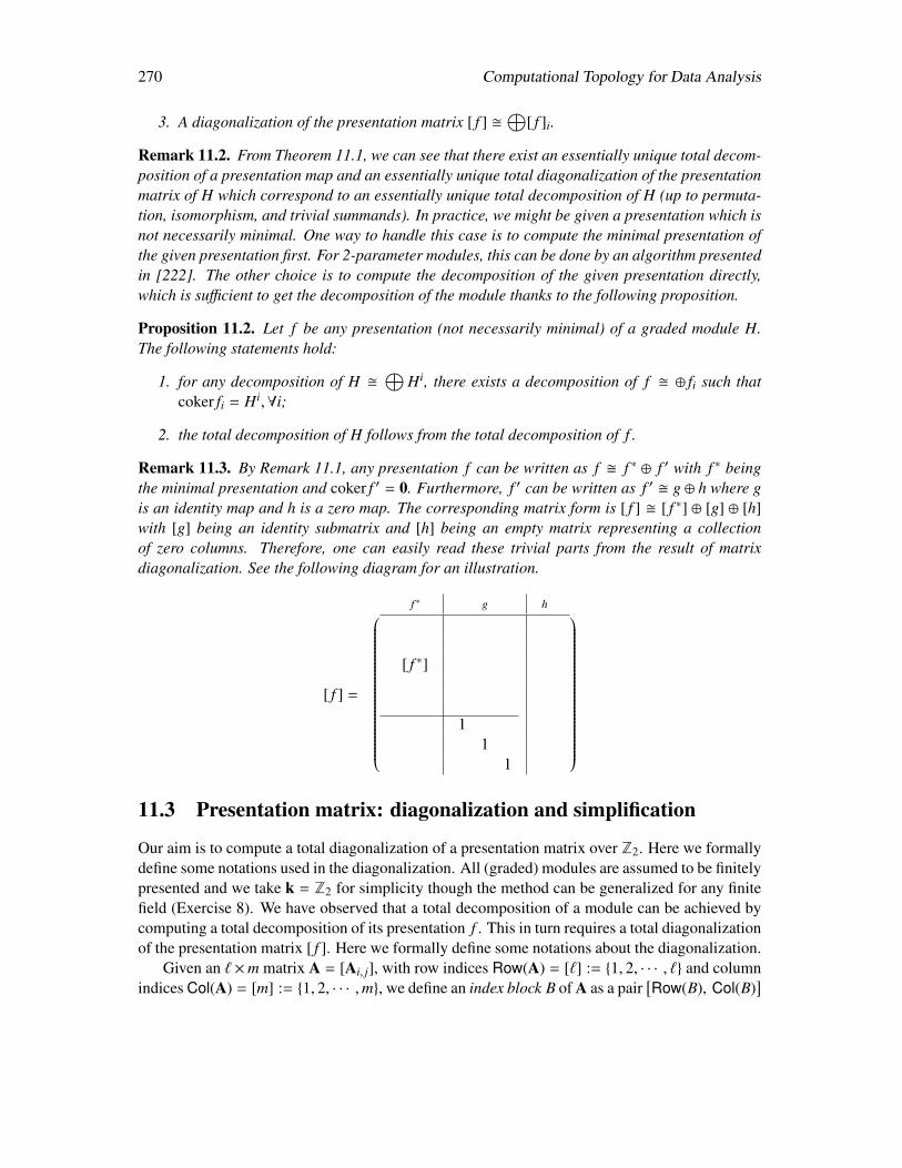
270 Computational Topology for Data Analysis
3. A diagonalization of the presentation matrix [ f ] ⊕
[ f ]i.
Remark 11.2. From Theorem 11.1, we can see that there exist an essentially unique total decom-position of a presentation map and an essentially unique total diagonalization of the presentationmatrix of H which correspond to an essentially unique total decomposition of H (up to permuta-tion, isomorphism, and trivial summands). In practice, we might be given a presentation which isnot necessarily minimal. One way to handle this case is to compute the minimal presentation ofthe given presentation first. For 2-parameter modules, this can be done by an algorithm presentedin [222]. The other choice is to compute the decomposition of the given presentation directly,which is sufficient to get the decomposition of the module thanks to the following proposition.
Proposition 11.2. Let f be any presentation (not necessarily minimal) of a graded module H.The following statements hold:
1. for any decomposition of H ⊕
Hi, there exists a decomposition of f ⊕ fi such thatcoker fi = Hi,∀i;
2. the total decomposition of H follows from the total decomposition of f .
Remark 11.3. By Remark 11.1, any presentation f can be written as f f ∗ ⊕ f ′ with f ∗ beingthe minimal presentation and coker f ′ = 0. Furthermore, f ′ can be written as f ′ g ⊕ h where gis an identity map and h is a zero map. The corresponding matrix form is [ f ] [ f ∗] ⊕ [g] ⊕ [h]with [g] being an identity submatrix and [h] being an empty matrix representing a collectionof zero columns. Therefore, one can easily read these trivial parts from the result of matrixdiagonalization. See the following diagram for an illustration.
[ f ] =
f ∗ g h
[ f ∗]
11
1
11.3 Presentation matrix: diagonalization and simplification
Our aim is to compute a total diagonalization of a presentation matrix over Z2. Here we formallydefine some notations used in the diagonalization. All (graded) modules are assumed to be finitelypresented and we take k = Z2 for simplicity though the method can be generalized for any finitefield (Exercise 8). We have observed that a total decomposition of a module can be achieved bycomputing a total decomposition of its presentation f . This in turn requires a total diagonalizationof the presentation matrix [ f ]. Here we formally define some notations about the diagonalization.
Given an ` ×m matrix A = [Ai, j], with row indices Row(A) = [`] := 1, 2, · · · , ` and columnindices Col(A) = [m] := 1, 2, · · · ,m, we define an index block B of A as a pair
[Row(B), Col(B)
]
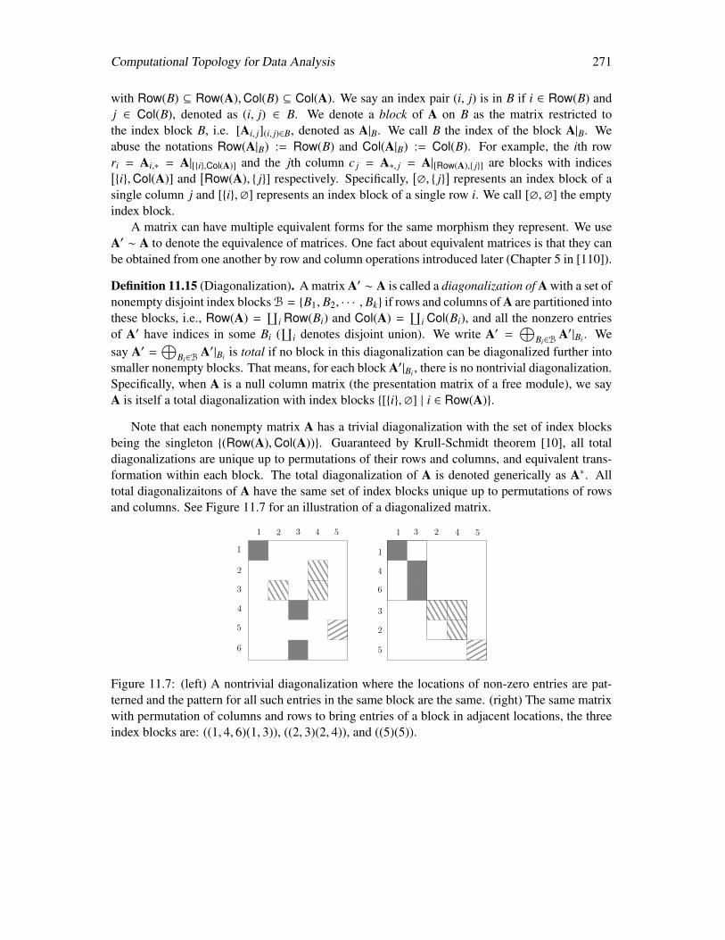
Computational Topology for Data Analysis 271
with Row(B) ⊆ Row(A),Col(B) ⊆ Col(A). We say an index pair (i, j) is in B if i ∈ Row(B) andj ∈ Col(B), denoted as (i, j) ∈ B. We denote a block of A on B as the matrix restricted tothe index block B, i.e. [Ai, j](i, j)∈B, denoted as A|B. We call B the index of the block A|B. Weabuse the notations Row(A|B) := Row(B) and Col(A|B) := Col(B). For example, the ith rowri = Ai,∗ = A|[i,Col(A)] and the jth column c j = A∗, j = A|[Row(A), j] are blocks with indices[i,Col(A)] and
[Row(A), j] respectively. Specifically,
[∅, j
]represents an index block of a
single column j and [i,∅] represents an index block of a single row i. We call [∅,∅] the emptyindex block.
A matrix can have multiple equivalent forms for the same morphism they represent. We useA′ ∼ A to denote the equivalence of matrices. One fact about equivalent matrices is that they canbe obtained from one another by row and column operations introduced later (Chapter 5 in [110]).
Definition 11.15 (Diagonalization). A matrix A′ ∼ A is called a diagonalization of A with a set ofnonempty disjoint index blocks B = B1, B2, · · · , Bk if rows and columns of A are partitioned intothese blocks, i.e., Row(A) =
∐i Row(Bi) and Col(A) =
∐i Col(Bi), and all the nonzero entries
of A′ have indices in some Bi (∐
i denotes disjoint union). We write A′ =⊕
Bi∈BA′|Bi . We
say A′ =⊕
Bi∈BA′|Bi is total if no block in this diagonalization can be diagonalized further into
smaller nonempty blocks. That means, for each block A′|Bi , there is no nontrivial diagonalization.Specifically, when A is a null column matrix (the presentation matrix of a free module), we sayA is itself a total diagonalization with index blocks [i,∅] | i ∈ Row(A).
Note that each nonempty matrix A has a trivial diagonalization with the set of index blocksbeing the singleton (Row(A),Col(A)). Guaranteed by Krull-Schmidt theorem [10], all totaldiagonalizations are unique up to permutations of their rows and columns, and equivalent trans-formation within each block. The total diagonalization of A is denoted generically as A∗. Alltotal diagonalizaitons of A have the same set of index blocks unique up to permutations of rowsand columns. See Figure 11.7 for an illustration of a diagonalized matrix.
1 2 43 5
1
2
3
4
5
6
1 2 43 5
1
2
3
4
5
6
Figure 11.7: (left) A nontrivial diagonalization where the locations of non-zero entries are pat-terned and the pattern for all such entries in the same block are the same. (right) The same matrixwith permutation of columns and rows to bring entries of a block in adjacent locations, the threeindex blocks are: ((1, 4, 6)(1, 3)), ((2, 3)(2, 4)), and ((5)(5)).
272 Computational Topology for Data Analysis
11.3.1 Simplification
First we want to transform the diagonalization problem to an equivalent problem that involvesmatrices with a simpler form. The idea is to simplify the presentation matrix to have entries onlyin k which is taken as Z2. There is a correspondence between diagonalizations of the originalpresentation matrix and certain constrained diagonalizations of the corresponding transformedmatrix.
We first make some observations about the homogeneous property of presentation maps andpresentation matrices. Equivalent matrices actually represent isomorphic presentations f ′ fthat admit commutative diagram,
F1 F0
F1 F0
f
h1
h0
f ′
where h1 and h0 are endomorphisms on F1 and F0 respectively. The endomorphisms are realizedby basis changes between corresponding presentation matrices [ f ] [ f ′]. Since all morphismsbetween graded modules are required to be homogeneous (preserve grades) by definition, we canuse homogeneous bases (all the basis elements chosen are homogeneous elements2) for F0 andF1 to represent matrices. Let F0 =< g1, · · · , g` > and F1 =< s1, · · · , sm > where gi and si arehomogeneous elements for every i. With this choice, we can consider only equivalent presentationmatrices under homogeneous basis changes. Each entry [ f ]i, j is also homogeneous. That means,[ f ]i, j = tu1
1 tu22 · · · t
udd where (u1, u2, · · · , ud) = gr(s j) − gr(gi). Writing u = (u1, u2, · · · , ud) and
tu = tu11 tu2
2 · · · tudd , we get [ f ]i, j = tu where u = gr(s j) − gr(gi) called the grade of [ f ]i, j. We call
such presentation matrix homogeneous presentation matrix.For example, given F0 =< g(1,1)
1 , g(2,2)2 >, the basis change g(2,2)
2 ← g(2,2)2 + g(1,1)
1 is nothomogeneous since g(2,2)
2 + g(1,1)1 is not a homogeneous element. However, g(2,2)
2 ← g(2,2)2 +
t(1,1)g(1,1)1 is a homogeneous change with gr(g(2,2)
2 + t(1,1)g(1,1)1 ) = gr(g(2,2)
2 ) = (2, 2), which resultsin a new homogeneous basis, g(1,1)
1 , g(2,2)2 + t(1,1)g(1,1)
1 . Homogeneous basis changes always resultin homogeneous bases.
Let [ f ] be a homogeneous presentation matrix of f : F1 → F0 with bases F0 =< g1, · · · , g` >and F1 =< s1, · · · , sm >. We extend the notation of grading to every row ri and every columnc j from the basis elements gi and s j they represent respectively, that is, gr(ri) := gr(gi) andgr(c j) := gr(s j). We define a strict partial order <gr on rows ri by asserting ri <gr r j if and onlyif gr(ri) < gr(r j). Similarly, we define a strict partial order on columns c j.
For such a homogeneous presentation matrix [ f ], we aim to diagonalize it totally by homoge-neous change of basis while trying to zero out entries by column and row operations that includeadditions and scalar multiplication of columns and rows as done in well known Gaussian elimi-nation. We have the following observations:
1. gr([ f ]i, j) = gr(c j) − gr(ri)
2. a nonzero entry [ f ]i, j can only be zeroed out by column operations from columns ck <gr c j
or by row operations from rows r` >gr ri.
2Recall that an element m ∈ M is homogeneous with grade gr(m) = u for some u ∈ Zd if m ∈ Mu.
Computational Topology for Data Analysis 273
Observation (2) indicates which subset of column and row operations is sufficient to zero outthe entry [ f ]i, j. We restate the diagonalization problem as follows:
Given an n×m homogeneous presentation matrix A = [ f ] consisting of entries in k[t1, · · · , td]with grading on rows and columns, find a total diagonalization of A under the following admissi-ble row and column operations:
• multiply a row or column by nonzero α ∈ k; (For k = Z2, we can ignore these operations),
• for two rows ri, r j with j , i, r j <gr ri, set r j ← r j + tu · ri where u = gr(ri) − gr(r j),
• for two columns ci, c j with j , i, ci <gr c j, set c j ← c j + tv · ci where v = gr(c j) − gr(ci).
The above operations realize all possible homogeneous basis changes. That means, any ho-mogeneous presentation matrix can be realized by a combination of the above operations.
In fact, the values of nonzero entries in the matrix are redundant under the homogeneous prop-erty gr(Ai, j) = gr(c j) − gr(ri) given by observation (1). So, we can further simplify the matrix byreplacing all the nonzero entries with their k-coefficients. For example, we can replace 2·tu with2. What really matters are the partial orders defined by the grading of rows and columns. Withour assumption of k = Z2, all nonzero entries are replaced with 1. Based on above observations,we further simplify the diagonalization problem to be the one as follows.
Given a k-valued matrix A with a partial order on rows and columns, find a total diagonaliza-tion A∗ ∼ A with the following admissible operations:
• multiply a row or column by nonzero α ∈ k; (For k = Z2, we can ignore these operations).
• Adding ci to c j only if j , i and gr(ci) < gr(c j); denoted as ci → c j.
• Adding rk to rl only if l , k and gr(r`) < gr(rk); denoted as rk → rl.
The assumption of k = Z2 allows us to ignore the first set of multiplication operations on thebinary matrix obtained after transformation. We denote the set of all admissible column and rowoperations as
Colop =(i, j) | ci → c j is an admissible column operation
Rowop =(k, l) | rk → rl is an admissible row operation
Under the assumption that no two columns nor rows have same grades, Colop and Rowop areclosed under transitive relation.
Proposition 11.3. If (i, j), ( j, k) ∈ Colop (Rowop) then (i, k) ∈ Colop (Rowop).
Given a solution of the diagonalization problem in the simplified form, one can reconstruct asolution of the original problem on the presentation matrix by reversing the above process of sim-plification. We will illustrate it by running the algorithm on the working example in Figure 11.5at the end of this section. The matrix reduction we employ for diagonalization may be viewed asa generalized matrix reduction because the matrix is reduced under constrained operations Colopand Rowop which might be a nontrivial subset of all basic operations.

274 Computational Topology for Data Analysis
vb(0, 1)
vr(1, 0)
vg(1, 1)
vb + vr = 0(1, 1)
vb + vg = 0(1, 2)
vr + vg = 0(2, 1)
0 1 2
0
1
2
Figure 11.8: The persistence module corresponding to the presentation matrix [∂1] shown inExample 11.1. The generators are given by the three vertices with grades (0, 1), (1, 0), (1, 1) andthe relations are given by the edges with grades (1, 1), (1, 2), (2, 1).
Remark 11.4. There are two extreme but trivial cases: (i) there are no <gr-comparable pair ofrows and columns. In this case, Colop = Rowop = ∅ and the original matrix is a trivial solution.(ii) All pairs of rows and all pairs of columns are <gr-comparable. Or equivalently, both Colopand Rowop are totally ordered. In this case, one can apply traditional matrix reduction algorithmto reduce the matrix to a diagonal matrix with all nonzero blocks being 1 × 1 minors. This is alsothe case for 1-parameter persistence module if one further applies row reduction after columnreduction. Note that row reductions are not necessary for reading out persistence informationbecause it essentially does not change the persistence information. However, in multiparametercases, both column and row reductions are necessary to obtain a diagonalization from whichthe persistence information can be read. From this view-point, the algorithm we present can bethought of as a generalization of the traditional persistence algorithm.
Example 11.1. Consider our working example in Figure 11.5. One can see later in Section 11.5(Case 1) that the presentation matrix of this example can be chosen to be the same as the matrixof the boundary morphism ∂1 : C1 → C0. With fixed bases C0 =< v(0,1)
b , v(1,0)r , v(1,1)
g > andC1 =< e(1,1)
r , e(1,2)b , e(2,1)
g >, this presentation matrix [∂1] and the corresponding binary matrix Acan be written as follows (recall that superscripts indicate the grades) :
[∂1] e(1,1)
r e(1,2)b e(2,1)
g
v(0,1)b t(1,0) t(1,1) 0
v(1,0)r t(0,1) 0 t(1,1)
v(1,1)g 0 t(0,1) t(1,0)
−→
A c(1,1)1 c(1,2)
2 c(2,1)3
r(0,1)1 1 1 0
r(1,0)2 1 0 1
r(1,1)3 0 1 1
Four admissible operations are: r3 → r1, r3 → r2, c1 → c2, c1 → c3. Figure 11.8 shows thepersistence module H0 whose presentation matrix is [∂1].
11.4 Total diagonalization algorithm
Assume that no two columns nor rows have the same grades. Without this assumption, the prob-lem of total diagonalization becomes more complicated. At this point, we do not know how to
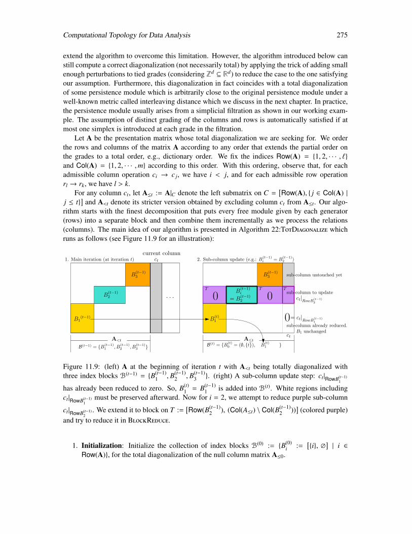
Computational Topology for Data Analysis 275
extend the algorithm to overcome this limitation. However, the algorithm introduced below canstill compute a correct diagonalization (not necessarily total) by applying the trick of adding smallenough perturbations to tied grades (considering Zd ⊆ Rd) to reduce the case to the one satisfyingour assumption. Furthermore, this diagonalization in fact coincides with a total diagonalizationof some persistence module which is arbitrarily close to the original persistence module under awell-known metric called interleaving distance which we discuss in the next chapter. In practice,the persistence module usually arises from a simplicial filtration as shown in our working exam-ple. The assumption of distinct grading of the columns and rows is automatically satisfied if atmost one simplex is introduced at each grade in the filtration.
Let A be the presentation matrix whose total diagonalization we are seeking for. We orderthe rows and columns of the matrix A according to any order that extends the partial order onthe grades to a total order, e.g., dictionary order. We fix the indices Row(A) = 1, 2, · · · , `and Col(A) = 1, 2, · · · ,m according to this order. With this ordering, observe that, for eachadmissible column operation ci → c j, we have i < j, and for each admissible row operationrl → rk, we have l > k.
For any column ct, let A≤t := A|C denote the left submatrix on C =[Row(A), j ∈ Col(A) |
j ≤ t]
and A<t denote its stricter version obtained by excluding column ct from A≤t. Our algo-rithm starts with the finest decomposition that puts every free module given by each generator(rows) into a separate block and then combine them incrementally as we process the relations(columns). The main idea of our algorithm is presented in Algorithm 22:TotDiagonalize whichruns as follows (see Figure 11.9 for an illustration):
ct
B(t−1)i
A≤t
TT T
current column
B(t−1)2
B1(t−1)
B(t−1)3
A<t
0 0 ct|RowB(t−1)2
1. Main iteration (at iteration t)
B(t−1) = B(t−1)1 , B
(t−1)2 , B
(t−1)3
. . .
2. Sub-column update (e.g.: B(t−1)i = B
(t−1)2 )
B(t) = B(t)0 = (∅, t), B
(t)1
sub-column to update
B(t)1
B(t−1)3
sub-column already reduced.B1 unchanged
= B(t−1)2
sub-column untouched yet
0
ct
= ct|RowB(t−1)1
Figure 11.9: (left) A at the beginning of iteration t with A<t being totally diagonalized withthree index blocks B(t−1) = B(t−1)
1 , B(t−1)2 , B(t−1)
3 . (right) A sub-column update step: ct|RowB(t−1)1
has already been reduced to zero. So, B(t)1 = B(t−1)
1 is added into B(t). White regions includingct|RowB(t−1)
1must be preserved afterward. Now for i = 2, we attempt to reduce purple sub-column
ct|RowB(t−1)2
. We extend it to block on T :=[Row(B(t−1)
2 ), (Col(A≤t) \ Col(B(t−1)2 ))
](colored purple)
and try to reduce it in BlockReduce.
1. Initialization: Initialize the collection of index blocks B(0) := B(0)i :=
[i, ∅
]| i ∈
Row(A), for the total diagonalization of the null column matrix A≤0.
276 Computational Topology for Data Analysis
2. Main iteration: Process A from left to right incrementally by introducing a column ct andconsidering left submatrices A≤t for t = 1, 2, · · · ,m. We update and maintain the collectionof index blocks B(t) ← B(t)
i for the current submatrix A≤t in each iteration by using columnand block updates stated below. Here we use upper index (·)(t) to emphasize the iteration t.
2(a). Sub-column update: Partition the column ct into sub-columns
ct|RowB(t−1)i
:= A[Row(B(t−1)i ), t],
one for the set of rows Row(B(t−1)i ) for each block from the previous iteration. We
process each such sub-column ct|RowB(t−1)i
one by one, checking whether there existsa sequence of admissible operations that are able to reduce the sub-column to zerowhile preserving the prior as defined below.
Definition 11.16. We say a prior with respect to a sub-column ct|RowB(t−1)i
is the leftsubmatrix A<t and sub-columns ct|RowB(t−1)
jfor all j < i.
Prior preservation means that the operations together change neither A<t nor othersub-columns ct|RowB(t−1)
jfor every j < i. If such operations exist, we apply them on
the current A to get an equivalent matrix with the sub-column ct|RowB(t−1)i
being zeroed
out and we set B(t)i ← B(t−1)
i . Otherwise, we leave the matrix A unchanged and addthe column index t to those of B(t−1)
i , i.e., we set B(t)i ←
[Row(B(t−1)
i ),Col(B(t−1)i ) ∪
t]. After processing every sub-column ct|RowB(t−1)
ione by one, all index blocks B(t)
icontaining column index t are merged into one single index block. At the end ofiteration t, we get an equivalent matrix A with A≤t being totally diagonalized withindex blocks B(t).
2(b). Block reduce: To update the entries of each sub-column of ct described in 2(a), wepropose a block reduction algorithm ALgorithm 24:BlockReduce to compute the cor-rect entries. Given T :=
[Row(B(t−1)
i ), (Col(A≤t) \ Col(B(t−1)i ))
], this routine checks
whether the block T can be zeroed out by some collection of admissible operations.If so, ct does not join the block B(t)
i and A is updated with these operations.
For two index blocks B1, B2, we denote the merging B1 ⊕ B2 of these two index blocks asan index block
[Row(B1) ∪ Row(B2), Col(B1) ∪ Col(B2)
]. In the following algorithm, we treat
the given matrix A to be a global variable which can be visited and modified anywhere by everysubroutines called. Consequently, every time we update values on A by some operations, theseoperations are applied to the latest A.
The outer loop is the incremental step for main iteration introducing a new column ct whichupdates the diagonalization of A≤t from the last iteration. The inner loop corresponds to blockupdates which checks the intersection of the current column and the rows of each previous blockone by one.
Remark 11.5. The algorithm TotDiagonalize does not require the input presentation matrix tobe minimal. As indicated in Remark 11.3, the trivial parts result in either identity blocks or singlecolumn blocks like
[∅, j
]. Such a single column block corresponds to a zero morphism and
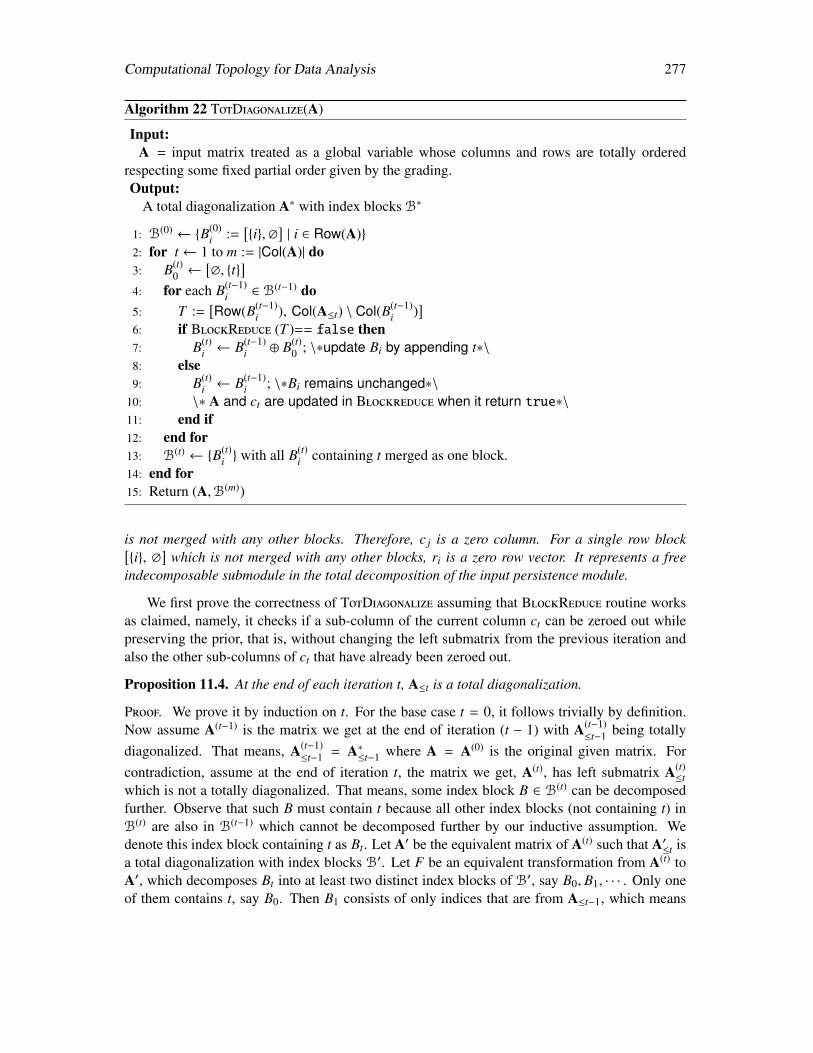
Computational Topology for Data Analysis 277
Algorithm 22 TotDiagonalize(A)
Input:A = input matrix treated as a global variable whose columns and rows are totally ordered
respecting some fixed partial order given by the grading.Output:
A total diagonalization A∗ with index blocks B∗
1: B(0) ← B(0)i :=
[i,∅
]| i ∈ Row(A)
2: for t ← 1 to m := |Col(A)| do3: B(t)
0 ←[∅, t
]4: for each B(t−1)
i ∈ B(t−1) do5: T :=
[Row(B(t−1)
i ), Col(A≤t) \ Col(B(t−1)i )
]6: if BlockReduce (T )== false then7: B(t)
i ← B(t−1)i ⊕ B(t)
0 ; \∗update Bi by appending t∗\8: else9: B(t)
i ← B(t−1)i ; \∗Bi remains unchanged∗\
10: \∗ A and ct are updated in Blockreduce when it return true∗\11: end if12: end for13: B(t) ← B(t)
i with all B(t)i containing t merged as one block.
14: end for15: Return (A,B(m))
is not merged with any other blocks. Therefore, c j is a zero column. For a single row block[i, ∅
]which is not merged with any other blocks, ri is a zero row vector. It represents a free
indecomposable submodule in the total decomposition of the input persistence module.
We first prove the correctness of TotDiagonalize assuming that BlockReduce routine worksas claimed, namely, it checks if a sub-column of the current column ct can be zeroed out whilepreserving the prior, that is, without changing the left submatrix from the previous iteration andalso the other sub-columns of ct that have already been zeroed out.
Proposition 11.4. At the end of each iteration t, A≤t is a total diagonalization.
Proof. We prove it by induction on t. For the base case t = 0, it follows trivially by definition.Now assume A(t−1) is the matrix we get at the end of iteration (t − 1) with A(t−1)
≤t−1 being totallydiagonalized. That means, A(t−1)
≤t−1 = A∗≤t−1 where A = A(0) is the original given matrix. For
contradiction, assume at the end of iteration t, the matrix we get, A(t), has left submatrix A(t)≤t
which is not a totally diagonalized. That means, some index block B ∈ B(t) can be decomposedfurther. Observe that such B must contain t because all other index blocks (not containing t) inB(t) are also in B(t−1) which cannot be decomposed further by our inductive assumption. Wedenote this index block containing t as Bt. Let A′ be the equivalent matrix of A(t) such that A′≤t isa total diagonalization with index blocks B′. Let F be an equivalent transformation from A(t) toA′, which decomposes Bt into at least two distinct index blocks of B′, say B0, B1, · · · . Only oneof them contains t, say B0. Then B1 consists of only indices that are from A≤t−1, which means
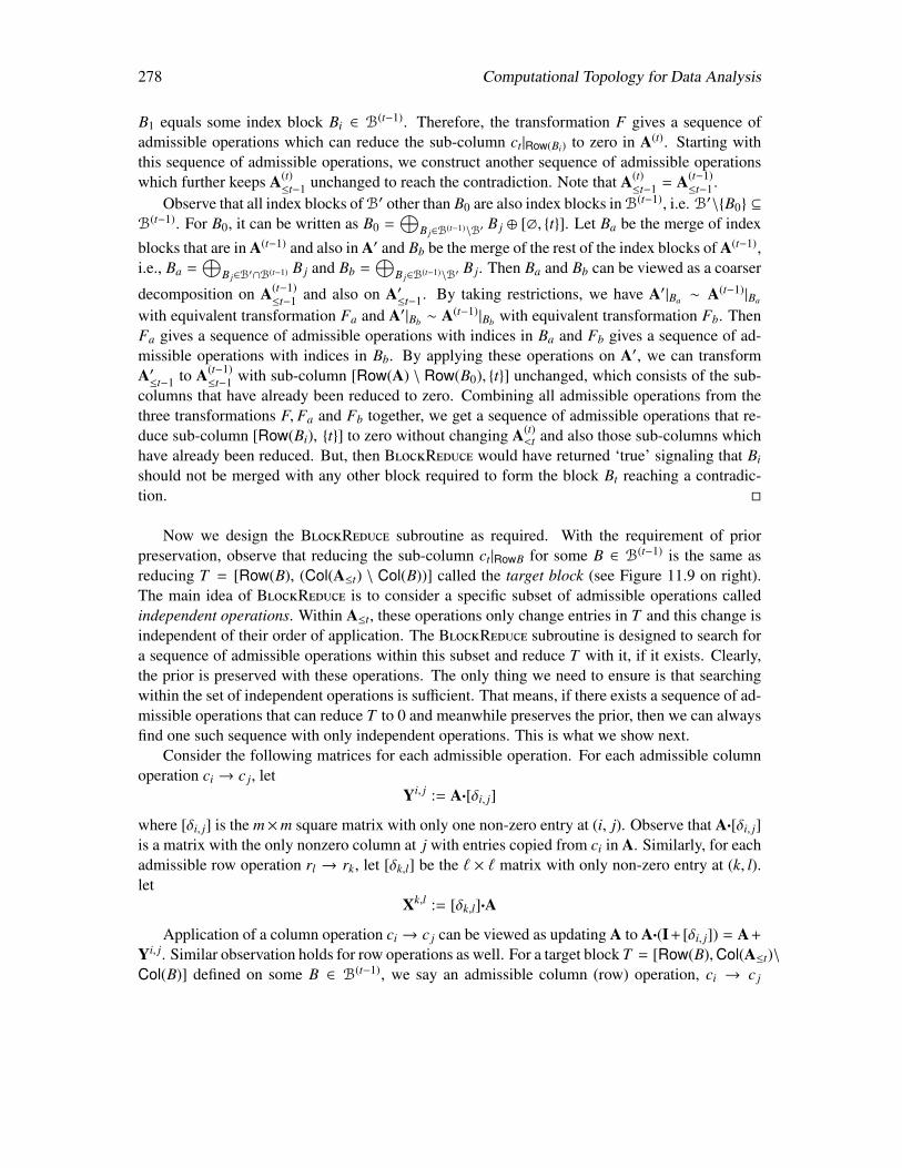
278 Computational Topology for Data Analysis
B1 equals some index block Bi ∈ B(t−1). Therefore, the transformation F gives a sequence ofadmissible operations which can reduce the sub-column ct|Row(Bi) to zero in A(t). Starting withthis sequence of admissible operations, we construct another sequence of admissible operationswhich further keeps A(t)
≤t−1 unchanged to reach the contradiction. Note that A(t)≤t−1 = A(t−1)
≤t−1.Observe that all index blocks of B′ other than B0 are also index blocks in B(t−1), i.e. B′\B0 ⊆
B(t−1). For B0, it can be written as B0 =⊕
B j∈B(t−1)\B′B j ⊕ [∅, t]. Let Ba be the merge of index
blocks that are in A(t−1) and also in A′ and Bb be the merge of the rest of the index blocks of A(t−1),i.e., Ba =
⊕B j∈B′∩B(t−1) B j and Bb =
⊕B j∈B(t−1)\B′
B j. Then Ba and Bb can be viewed as a coarser
decomposition on A(t−1)≤t−1 and also on A′
≤t−1. By taking restrictions, we have A′|Ba ∼ A(t−1)|Ba
with equivalent transformation Fa and A′|Bb ∼ A(t−1)|Bb with equivalent transformation Fb. ThenFa gives a sequence of admissible operations with indices in Ba and Fb gives a sequence of ad-missible operations with indices in Bb. By applying these operations on A′, we can transformA′≤t−1 to A(t−1)
≤t−1 with sub-column [Row(A) \ Row(B0), t] unchanged, which consists of the sub-columns that have already been reduced to zero. Combining all admissible operations from thethree transformations F, Fa and Fb together, we get a sequence of admissible operations that re-duce sub-column [Row(Bi), t] to zero without changing A(t)
<t and also those sub-columns whichhave already been reduced. But, then BlockReduce would have returned ‘true’ signaling that Bi
should not be merged with any other block required to form the block Bt reaching a contradic-tion.
Now we design the BlockReduce subroutine as required. With the requirement of priorpreservation, observe that reducing the sub-column ct|RowB for some B ∈ B(t−1) is the same asreducing T = [Row(B), (Col(A≤t) \ Col(B))] called the target block (see Figure 11.9 on right).The main idea of BlockReduce is to consider a specific subset of admissible operations calledindependent operations. Within A≤t, these operations only change entries in T and this change isindependent of their order of application. The BlockReduce subroutine is designed to search fora sequence of admissible operations within this subset and reduce T with it, if it exists. Clearly,the prior is preserved with these operations. The only thing we need to ensure is that searchingwithin the set of independent operations is sufficient. That means, if there exists a sequence of ad-missible operations that can reduce T to 0 and meanwhile preserves the prior, then we can alwaysfind one such sequence with only independent operations. This is what we show next.
Consider the following matrices for each admissible operation. For each admissible columnoperation ci → c j, let
Yi, j := A·[δi, j]
where [δi, j] is the m×m square matrix with only one non-zero entry at (i, j). Observe that A·[δi, j]is a matrix with the only nonzero column at j with entries copied from ci in A. Similarly, for eachadmissible row operation rl → rk, let [δk,l] be the ` × ` matrix with only non-zero entry at (k, l).let
Xk,l := [δk,l]·A
Application of a column operation ci → c j can be viewed as updating A to A·(I+ [δi, j]) = A+
Yi, j. Similar observation holds for row operations as well. For a target block T = [Row(B),Col(A≤t)\Col(B)] defined on some B ∈ B(t−1), we say an admissible column (row) operation, ci → c j
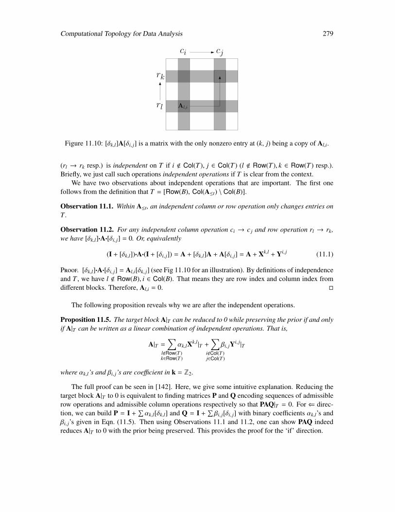
Computational Topology for Data Analysis 279
rk
rl
ci cj
Al,i
Figure 11.10: [δk,l]A[δi, j] is a matrix with the only nonzero entry at (k, j) being a copy of Al,i.
(rl → rk resp.) is independent on T if i < Col(T ), j ∈ Col(T ) (l < Row(T ), k ∈ Row(T ) resp.).Briefly, we just call such operations independent operations if T is clear from the context.
We have two observations about independent operations that are important. The first onefollows from the definition that T = [Row(B), Col(A≤t) \ Col(B)].
Observation 11.1. Within A≤t, an independent column or row operation only changes entries onT .
Observation 11.2. For any independent column operation ci → c j and row operation rl → rk,we have [δk,l]·A·[δi, j] = 0. Or, equivalently
(I + [δk,l])·A·(I + [δi, j]) = A + [δk,l]A + A[δi, j] = A + Xk,l + Yi, j (11.1)
Proof. [δk,l]·A·[δi, j] = Al,i[δk, j] (see Fig 11.10 for an illustration). By definitions of independenceand T , we have l < Row(B), i ∈ Col(B). That means they are row index and column index fromdifferent blocks. Therefore, Al,i = 0.
The following proposition reveals why we are after the independent operations.
Proposition 11.5. The target block A|T can be reduced to 0 while preserving the prior if and onlyif A|T can be written as a linear combination of independent operations. That is,
A|T =∑
l<Row(T )k∈Row(T )
αk,lXk,l|T +∑
i<Col(T )j∈Col(T )
βi, jYi, j|T
where αk,l’s and βi, j’s are coefficient in k = Z2.
The full proof can be seen in [142]. Here, we give some intuitive explanation. Reducing thetarget block A|T to 0 is equivalent to finding matrices P and Q encoding sequences of admissiblerow operations and admissible column operations respectively so that PAQ|T = 0. For⇐ direc-tion, we can build P = I +
∑αk,l[δk,l] and Q = I +
∑βi, j[δi, j] with binary coefficients αk,l’s and
βi, j’s given in Eqn. (11.5). Then using Observations 11.1 and 11.2, one can show PAQ indeedreduces A|T to 0 with the prior being preserved. This provides the proof for the ‘if’ direction.
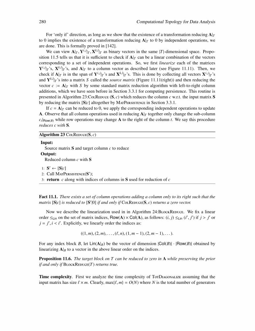
280 Computational Topology for Data Analysis
For ‘only if’ direction, as long as we show that the existence of a transformation reducing A|Tto 0 implies the existence of a transformation reducing A|T to 0 by independent operations, weare done. This is formally proved in [142].
We can view A|T ,Yi, j|T ,Xk,l|T as binary vectors in the same |T |-dimensional space. Propo-sition 11.5 tells us that it is sufficient to check if A|T can be a linear combination of the vectorscorresponding to a set of independent operations. So, we first linearize each of the matricesYi, j|T ’s, Xk,l|T ’s, and A|T to a column vector as described later (see Figure 11.11). Then, wecheck if A|T is in the span of Yi, j|T ’s and Xk,l|T ’s. This is done by collecting all vectors Xi, j|T ’sand Yk,l|T ’s into a matrix S called the source matrix (Figure 11.11(right)) and then reducing thevector c := A|T with S by some standard matrix reduction algorithm with left-to-right columnadditions, which we have seen before in Section 3.3.1 for computing persistence. This routine ispresented in Algorithm 23:ColReduce (S, c) which reduces the column c w.r.t. the input matrix Sby reducing the matrix [S|c] altogether by MatPersistence in Section 3.3.1.
If c = A|T can be reduced to 0, we apply the corresponding independent operations to updateA. Observe that all column operations used in reducing A|T together only change the sub-columnct|Row(B) while row operations may change A to the right of the column t. We say this procedurereduces c with S.
Algorithm 23 ColReduce(S, c)
Input:Source matrix S and target column c to reduce
Output:Reduced column c with S
1: S′ ← [S|c]2: Call MatPersistence(S′);3: return c along with indices of columns in S used for reduction of c
Fact 11.1. There exists a set of column operations adding a column only to its right such that thematrix [S|c] is reduced to [S′|0] if and only if ColReduce(S, c) returns a zero vector.
Now we describe the linearization used in in Algorithm 24:BlockReduce. We fix a linearorder ≤Lin on the set of matrix indices, Row(A) × Col(A), as follows: (i, j) ≤Lin (i′, j′) if j > j′ orj = j′, i < i′. Explicitly, we linearly order the indices as:
((1,m), (2,m), . . . , (`, n), (1,m − 1), (2,m − 1), . . . ).
For any index block B, let Lin(A|B) be the vector of dimension |Col(B)| · |Row(B)| obtained bylinearizing A|B to a vector in the above linear order on the indices.
Proposition 11.6. The target block on T can be reduced to zero in A while preserving the priorif and only if BlockReduce(T ) returns true.
Time complexity. First we analyze the time complexity of TotDiagonalize assuming that theinput matrix has size ` ×m. Clearly, max`,m = O(N) where N is the total number of generators

Computational Topology for Data Analysis 281
000 00
cjci
cj := ci
A
Lin(A)T
Yij
Lin(Yij)T
ck := c`
cj := ci
cj := ct
ST
Figure 11.11: (top) Matrix A is linearized to the vector Lin(A) in middle; (bottom) the columnoperation ci → c j is captured by Yi j whose linearization is illustrated in middle; (right) sourcematrix S combining all operations (row operations not shown). In the picture, (·)T denotes trans-posed matrices.
Algorithm 24 BlockReduce(T )
Input:Index of target block T to be reduced; Given matrix A is assumed to be a global variable
Output:A boolean to indicate whether A|T can be reduced and reduced block A|T if possible.
1: Compute c := Lin(A|T ) and initialize empty matrix S2: for each admissible column operation ci → c j with i < Col(T ), j ∈ Col(T ) do3: compute Yi, j|T := (A·[δi, j])|T and yi, j = Lin(Yi, j|T ); update S← [S|yi, j]4: end for5: for each admissible row operation rl → rk with l < Row(T ), k ∈ Row(T ) do6: compute Xk,l|T := ([δk,l]·A)|T and xk,l := Lin(Xk,l|T ); update S← [S|xk,l]7: end for8: ColReduce (S, c) returns indices of yi, j’s and xk,l’s used to reduce c (if possible)9: For every returned index of yi, j or xk,l apply ci → c j or rl → rk to transform A
10: return A|T == 0
and relations. For each of O(N) columns, we attempt to zero out every sub-column with rowindices coinciding with each block B of the previously determined O(N) blocks. Let B has NB
rows. Then, the block T has NB rows and O(N) columns.To zero-out a sub-column, we create a source matrix out of T which has size O(NNB) ×
O(N2) because each of O((
N2
)) possible operations is converted to a column of size O(NNB) in
the source matrix. The source matrix S with the target vector c can be reduced with an efficientalgorithm [58, 200] in O(a + N2(NNB)ω−1) time where a is the total number of nonzero elementsin [S|c] and ω ∈ [2, 2.373) is the exponent for matrix multiplication. We have a = O(NNB · N2) =
O(N3NB). Therefore, for each block B we spend O(N3NB + N2(NNB)ω−1) time. Then, observing∑B∈B NB = O(N), for each column we spend a total time of∑
B∈B
O(N3NB + N2(NNB)ω−1) = O(N4 + Nω+1∑B∈B
Nω−1B ) = O(N4 + N2ω) = O(N2ω).
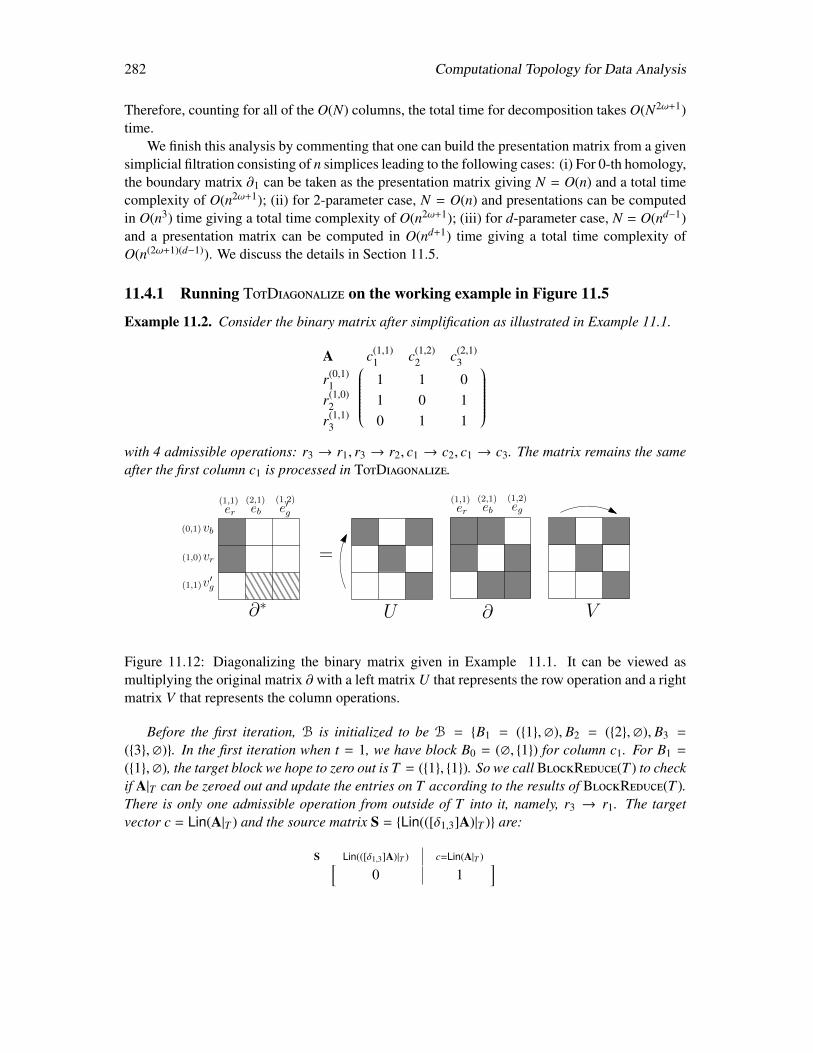
282 Computational Topology for Data Analysis
Therefore, counting for all of the O(N) columns, the total time for decomposition takes O(N2ω+1)time.
We finish this analysis by commenting that one can build the presentation matrix from a givensimplicial filtration consisting of n simplices leading to the following cases: (i) For 0-th homology,the boundary matrix ∂1 can be taken as the presentation matrix giving N = O(n) and a total timecomplexity of O(n2ω+1); (ii) for 2-parameter case, N = O(n) and presentations can be computedin O(n3) time giving a total time complexity of O(n2ω+1); (iii) for d-parameter case, N = O(nd−1)and a presentation matrix can be computed in O(nd+1) time giving a total time complexity ofO(n(2ω+1)(d−1)). We discuss the details in Section 11.5.
11.4.1 Running TotDiagonalize on the working example in Figure 11.5
Example 11.2. Consider the binary matrix after simplification as illustrated in Example 11.1.
A c(1,1)
1 c(1,2)2 c(2,1)
3
r(0,1)1 1 1 0
r(1,0)2 1 0 1
r(1,1)3 0 1 1
with 4 admissible operations: r3 → r1, r3 → r2, c1 → c2, c1 → c3. The matrix remains the sameafter the first column c1 is processed in TotDiagonalize.
er eb e′gvb
vr
v′g
(1,1) (2,1) (1,2)
(0,1)
(1,0)
(1,1)
=
er eb eg(1,1) (2,1) (1,2)
∂U V∂∗
Figure 11.12: Diagonalizing the binary matrix given in Example 11.1. It can be viewed asmultiplying the original matrix ∂ with a left matrix U that represents the row operation and a rightmatrix V that represents the column operations.
Before the first iteration, B is initialized to be B = B1 = (1,∅), B2 = (2,∅), B3 =
(3,∅). In the first iteration when t = 1, we have block B0 = (∅, 1) for column c1. For B1 =
(1,∅), the target block we hope to zero out is T = (1, 1). So we call BlockReduce(T ) to checkif A|T can be zeroed out and update the entries on T according to the results of BlockReduce(T ).There is only one admissible operation from outside of T into it, namely, r3 → r1. The targetvector c = Lin(A|T ) and the source matrix S = Lin(([δ1,3]A)|T ) are:
[S Lin(([δ1,3]A)|T ) c=Lin(A|T )
0 1]
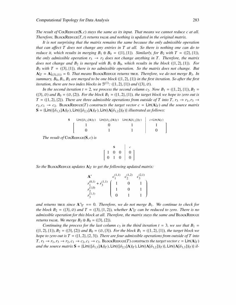
Computational Topology for Data Analysis 283
The result of ColReduce(S, c) stays the same as its input. That means we cannot reduce c at all.Therefore, BlockReduce(T, t) returns false and nothing is updated in the original matrix.
It is not surprising that the matrix remains the same because the only admissible operationthat can affect T does not change any entries in T at all. So there is nothing one can do toreduce it, which results in merging B1 ⊕ B0 = (1, 1). Similarly, for B2 with T = (2, 1),the only admissible operation r3 → r2 does not change anything in T . Therefore, the matrixdoes not change and B2 is merged with B1 ⊕ B0, which results in the block (1, 2, 1). ForB3 with T = (3, 1), there is no admissible operation. So the matrix does not change. ButA|T = A|(3,1) = 0. That means BlockReduce returns true. Therefore, we do not merge B3. Insummary, B0, B1, B2 are merged to be one block (1, 2, 1) in the first iteration. So after the firstiteration, there are two index blocks in B(1): (1, 2, 1) and (3,∅).
In the second iteration t = 2, we process the second column c2. Now B1 = (1, 2, 1), B2 =
(3,∅) and B0 = (∅, 2). For the block B1 = (1, 2, 1), the target block we hope to zero out isT = (1, 2, 2). There are three admissible operations from outside of T into T , r3 → r1, r3 →
r2, c1 → c2. BlockReduce(T ) constructs the target vector c = Lin(A|T ) and the source matrixS = Lin(([δ1,3]A)|T ), Lin(([δ2,3]A)|T ), Lin((A[δ1,2])|T ) illustrated as follows:
[S Lin(([δ1,3]A)|T ) Lin([(δ2,3]A)|T ) Lin((A[δ1,2])|T ) c=Lin(A|T )
1 0 1 10 1 1 0
]The result of ColReduce(S, c) is
[ S c
1 0 0 00 1 0 0
]So the BlockReduce updates A|T to get the following updated matrix:
A′ c(1,1)
1 c(1,2)2 c(2,1)
3
r(0,1)1 + r(1,1)
3 1 0 1r(1,0)
2 1 0 1r(1,1)
3 0 1 1
and returns true since A′|T == 0. Therefore, we do not merge B1. We continue to check forthe block B2 = (3,∅) and T = (3, 1, 2), whether A′|T can be reduced to zero. There is noadmissible operation for this block at all. Therefore, the matrix stays the same and BlockReducereturns false. We merge B2 ⊕ B0 = (3, 2).
Continuing the process for the last column c3 in the third iteration t = 3, we see that B1 =
(1, 2, 1), B2 = (3, 2) and B0 = (∅, 3). For the block B1 = (1, 2, 1), the target block wehope to zero out is T = (1, 2, 2, 3). There are four admissible operations from outside of T intoT , r3 → r1, r3 → r2, c1 → c2, c1 → c3. BlockReduce(T ) constructs the target vector c = Lin(A|T )and the source matrix S = Lin(([δ1,3]A)|T ), Lin(([δ2,3]A)|T ), Lin((A[δ1,2])|T ), Lin((A[δ1,3])|T ) il-
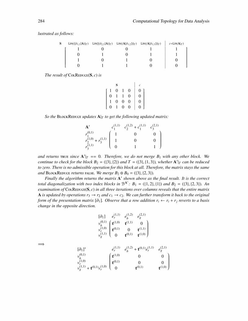
284 Computational Topology for Data Analysis
lustrated as follows:
S Lin(([δ1,3]A)|T ) Lin([(δ2,3]A)|T ) Lin((A[δ1,2])|T ) Lin((A[δ1,3])|T ) c=Lin(A|T )
1 0 0 1 10 1 0 1 11 0 1 0 00 1 1 0 0
The result of ColReduce(S, c) is
S c
1 0 1 0 00 1 1 0 01 0 0 0 00 1 0 0 0
So the BlockReduce updates A|T to get the following updated matrix:
A′ c(1,1)
1 c(1,2)2 + c(1,1)
1 c(2,1)3
r(0,1)1 1 0 0
r(1,0)2 + r(1,1)
3 1 0 0r(1,1)
3 0 1 1
and returns true since A′|T == 0. Therefore, we do not merge B1 with any other block. Wecontinue to check for the block B2 = (3, 2) and T = (3, 1, 3), whether A′|T can be reducedto zero. There is no admissible operation for this block at all. Therefore, the matrix stays the sameand BlockReduce returns false. We merge B2 ⊕ B0 = (3, 2, 3).
Finally the algorithm returns the matrix A′ shown above as the final result. It is the correcttotal diagonalization with two index blocks in BA∗: B1 = (1, 2, 1) and B2 = (3, 2, 3). Anexamination of ColReduce(S, c) in all three iterations over columns reveals that the entire matrixA is updated by operations r3 → r2 and c1 → c2. We can further transform it back to the originalform of the presentation matrix [∂1]. Observe that a row addition ri ← ri + r j reverts to a basischange in the opposite direction.
[∂1] e(1,1)
r e(1,2)b e(2,1)
g
v(0,1)b t(1,0) t(1,1) 0
v(1,0)r t(0,1) 0 t(1,1)
v(1,1)g 0 t(0,1) t(1,0)
=⇒
[∂1]∗ e(1,1)r e(1,2)
b + t(0,1)e(1,1)r e(2,1)
g
v(0,1)b t(1,0) 0 0
v(1,0)r t(0,1) 0 0
v(1,1)g + t(0,1)v(1,0)
r 0 t(0,1) t(1,0)
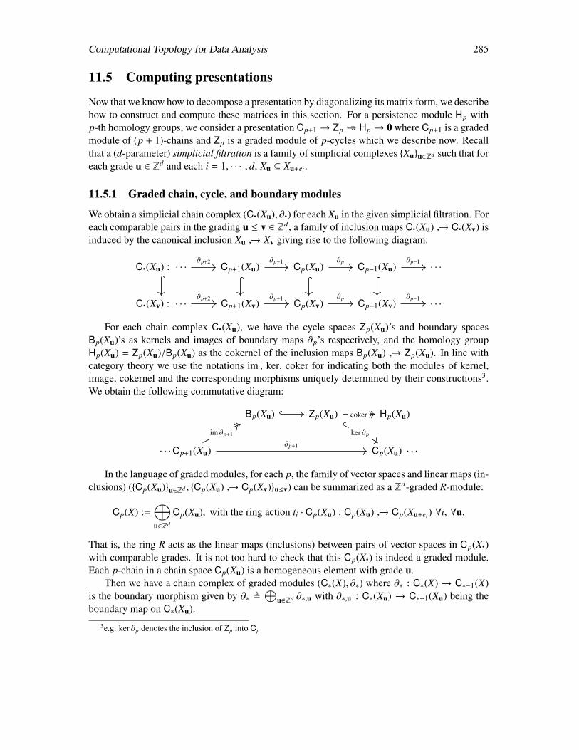
Computational Topology for Data Analysis 285
11.5 Computing presentations
Now that we know how to decompose a presentation by diagonalizing its matrix form, we describehow to construct and compute these matrices in this section. For a persistence module Hp withp-th homology groups, we consider a presentation Cp+1 → Zp Hp → 0 where Cp+1 is a gradedmodule of (p + 1)-chains and Zp is a graded module of p-cycles which we describe now. Recallthat a (d-parameter) simplicial filtration is a family of simplicial complexes Xuu∈Zd such that foreach grade u ∈ Zd and each i = 1, · · · , d, Xu ⊆ Xu+ei .
11.5.1 Graded chain, cycle, and boundary modules
We obtain a simplicial chain complex (C·(Xu), ∂·) for each Xu in the given simplicial filtration. Foreach comparable pairs in the grading u ≤ v ∈ Zd, a family of inclusion maps C·(Xu) → C·(Xv) isinduced by the canonical inclusion Xu → Xv giving rise to the following diagram:
C·(Xu) : · · · Cp+1(Xu) Cp(Xu) Cp−1(Xu) · · ·
C·(Xv) : · · · Cp+1(Xv) Cp(Xv) Cp−1(Xv) · · ·
∂p+2 ∂p+1 ∂p ∂p−1
∂p+2 ∂p+1 ∂p ∂p−1
For each chain complex C·(Xu), we have the cycle spaces Zp(Xu)’s and boundary spacesBp(Xu)’s as kernels and images of boundary maps ∂p’s respectively, and the homology groupHp(Xu) = Zp(Xu)/Bp(Xu) as the cokernel of the inclusion maps Bp(Xu) → Zp(Xu). In line withcategory theory we use the notations im , ker, coker for indicating both the modules of kernel,image, cokernel and the corresponding morphisms uniquely determined by their constructions3.We obtain the following commutative diagram:
Bp(Xu) Zp(Xu) Hp(Xu)
· · ·Cp+1(Xu) Cp(Xu) · · ·
ker ∂p
coker
∂p+1
im ∂p+1
In the language of graded modules, for each p, the family of vector spaces and linear maps (in-clusions) (Cp(Xu)u∈Zd , Cp(Xu) → Cp(Xv)u≤v) can be summarized as a Zd-graded R-module:
Cp(X) :=⊕u∈Zd
Cp(Xu), with the ring action ti · Cp(Xu) : Cp(Xu) → Cp(Xu+ei) ∀i, ∀u.
That is, the ring R acts as the linear maps (inclusions) between pairs of vector spaces in Cp(X·)with comparable grades. It is not too hard to check that this Cp(X·) is indeed a graded module.Each p-chain in a chain space Cp(Xu) is a homogeneous element with grade u.
Then we have a chain complex of graded modules (C∗(X), ∂∗) where ∂∗ : C∗(X) → C∗−1(X)is the boundary morphism given by ∂∗ ,
⊕u∈Zd ∂∗,u with ∂∗,u : C∗(Xu) → C∗−1(Xu) being the
boundary map on C∗(Xu).
3e.g. ker ∂p denotes the inclusion of Zp into Cp
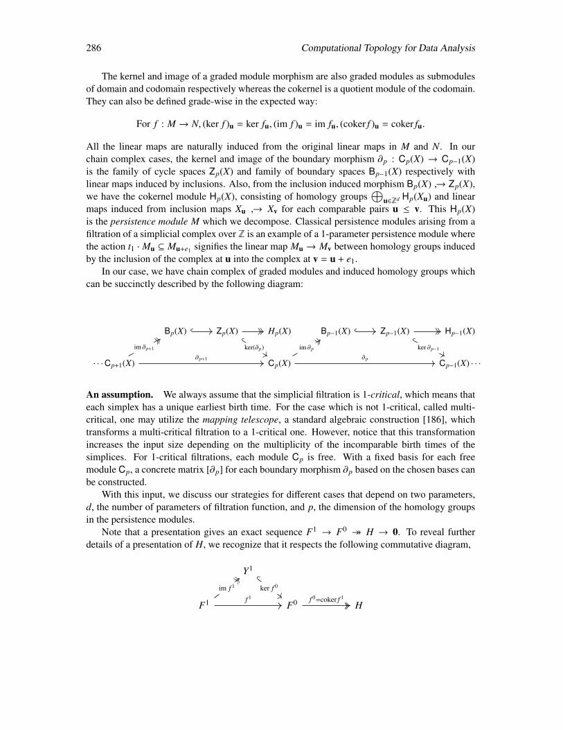
286 Computational Topology for Data Analysis
The kernel and image of a graded module morphism are also graded modules as submodulesof domain and codomain respectively whereas the cokernel is a quotient module of the codomain.They can also be defined grade-wise in the expected way:
For f : M → N, (ker f )u = ker fu, (im f )u = im fu, (coker f )u = coker fu.
All the linear maps are naturally induced from the original linear maps in M and N. In ourchain complex cases, the kernel and image of the boundary morphism ∂p : Cp(X) → Cp−1(X)is the family of cycle spaces Zp(X) and family of boundary spaces Bp−1(X) respectively withlinear maps induced by inclusions. Also, from the inclusion induced morphism Bp(X) → Zp(X),we have the cokernel module Hp(X), consisting of homology groups
⊕u∈Zd Hp(Xu) and linear
maps induced from inclusion maps Xu → Xv for each comparable pairs u ≤ v. This Hp(X)is the persistence module M which we decompose. Classical persistence modules arising from afiltration of a simplicial complex over Z is an example of a 1-parameter persistence module wherethe action t1 · Mu ⊆ Mu+e1 signifies the linear map Mu → Mv between homology groups inducedby the inclusion of the complex at u into the complex at v = u + e1.
In our case, we have chain complex of graded modules and induced homology groups whichcan be succinctly described by the following diagram:
Bp(X) Zp(X) Hp(X) Bp−1(X) Zp−1(X) Hp−1(X)
· · ·Cp+1(X) Cp(X) Cp−1(X) · · ·
ker(∂p) ker ∂p−1
∂p+1
im ∂p+1
∂p
im ∂p
An assumption. We always assume that the simplicial filtration is 1-critical, which means thateach simplex has a unique earliest birth time. For the case which is not 1-critical, called multi-critical, one may utilize the mapping telescope, a standard algebraic construction [186], whichtransforms a multi-critical filtration to a 1-critical one. However, notice that this transformationincreases the input size depending on the multiplicity of the incomparable birth times of thesimplices. For 1-critical filtrations, each module Cp is free. With a fixed basis for each freemodule Cp, a concrete matrix [∂p] for each boundary morphism ∂p based on the chosen bases canbe constructed.
With this input, we discuss our strategies for different cases that depend on two parameters,d, the number of parameters of filtration function, and p, the dimension of the homology groupsin the persistence modules.
Note that a presentation gives an exact sequence F1 → F0 H → 0. To reveal furtherdetails of a presentation of H, we recognize that it respects the following commutative diagram,
Y1
F1 F0 H
ker f 0
f 1
im f 1
f 0=coker f 1
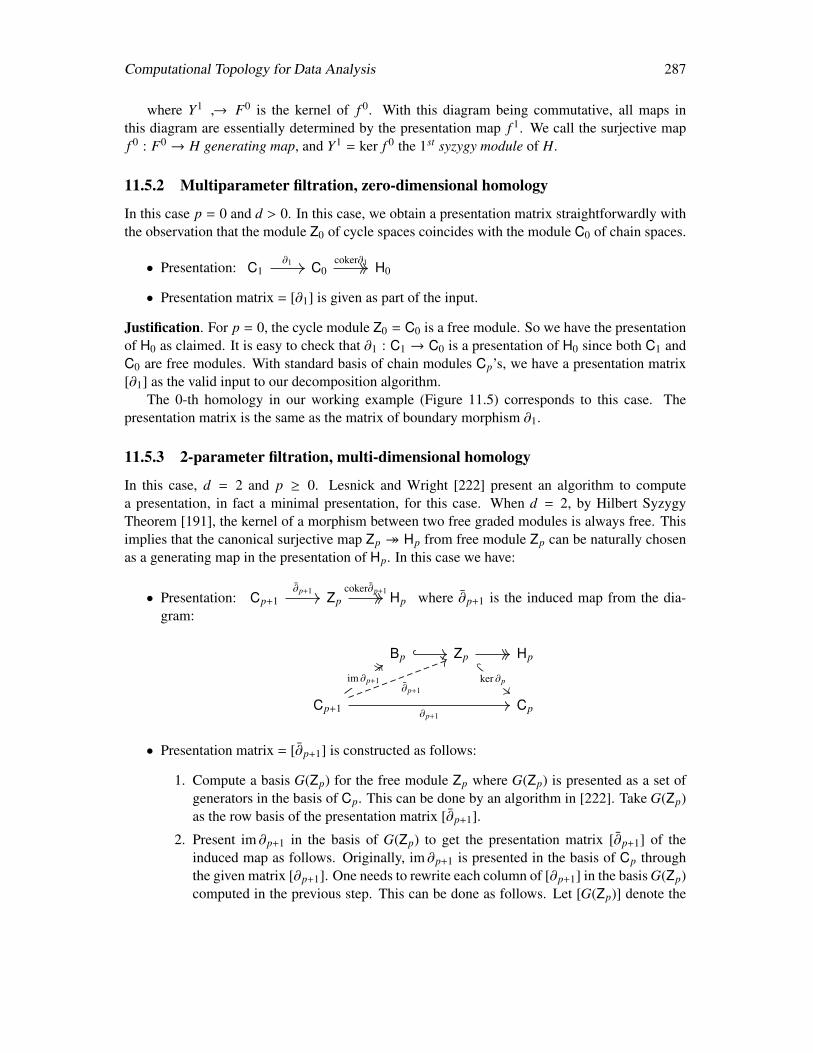
Computational Topology for Data Analysis 287
where Y1 → F0 is the kernel of f 0. With this diagram being commutative, all maps inthis diagram are essentially determined by the presentation map f 1. We call the surjective mapf 0 : F0 → H generating map, and Y1 = ker f 0 the 1st syzygy module of H.
11.5.2 Multiparameter filtration, zero-dimensional homology
In this case p = 0 and d > 0. In this case, we obtain a presentation matrix straightforwardly withthe observation that the module Z0 of cycle spaces coincides with the module C0 of chain spaces.
• Presentation: C1 C0 H0∂1 coker∂1
• Presentation matrix = [∂1] is given as part of the input.
Justification. For p = 0, the cycle module Z0 = C0 is a free module. So we have the presentationof H0 as claimed. It is easy to check that ∂1 : C1 → C0 is a presentation of H0 since both C1 andC0 are free modules. With standard basis of chain modules Cp’s, we have a presentation matrix[∂1] as the valid input to our decomposition algorithm.
The 0-th homology in our working example (Figure 11.5) corresponds to this case. Thepresentation matrix is the same as the matrix of boundary morphism ∂1.
11.5.3 2-parameter filtration, multi-dimensional homology
In this case, d = 2 and p ≥ 0. Lesnick and Wright [222] present an algorithm to computea presentation, in fact a minimal presentation, for this case. When d = 2, by Hilbert SyzygyTheorem [191], the kernel of a morphism between two free graded modules is always free. Thisimplies that the canonical surjective map Zp Hp from free module Zp can be naturally chosenas a generating map in the presentation of Hp. In this case we have:
• Presentation: Cp+1 Zp Hp∂p+1 coker∂p+1
where ∂p+1 is the induced map from the dia-gram:
Bp Zp Hp
Cp+1 Cp
ker ∂p
∂p+1
im ∂p+1∂p+1
• Presentation matrix = [∂p+1] is constructed as follows:
1. Compute a basis G(Zp) for the free module Zp where G(Zp) is presented as a set ofgenerators in the basis of Cp. This can be done by an algorithm in [222]. Take G(Zp)as the row basis of the presentation matrix [∂p+1].
2. Present im ∂p+1 in the basis of G(Zp) to get the presentation matrix [∂p+1] of theinduced map as follows. Originally, im ∂p+1 is presented in the basis of Cp throughthe given matrix [∂p+1]. One needs to rewrite each column of [∂p+1] in the basis G(Zp)computed in the previous step. This can be done as follows. Let [G(Zp)] denote the
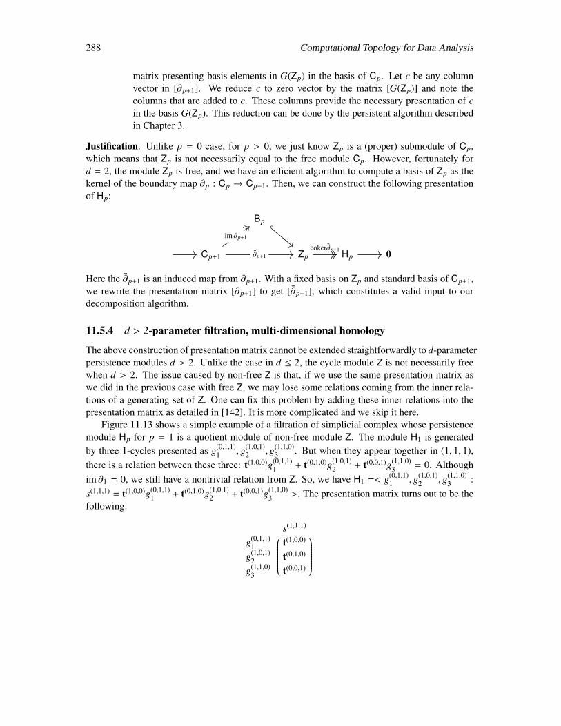
288 Computational Topology for Data Analysis
matrix presenting basis elements in G(Zp) in the basis of Cp. Let c be any columnvector in [∂p+1]. We reduce c to zero vector by the matrix [G(Zp)] and note thecolumns that are added to c. These columns provide the necessary presentation of cin the basis G(Zp). This reduction can be done by the persistent algorithm describedin Chapter 3.
Justification. Unlike p = 0 case, for p > 0, we just know Zp is a (proper) submodule of Cp,which means that Zp is not necessarily equal to the free module Cp. However, fortunately ford = 2, the module Zp is free, and we have an efficient algorithm to compute a basis of Zp as thekernel of the boundary map ∂p : Cp → Cp−1. Then, we can construct the following presentationof Hp:
Bp
Cp+1 Zp Hp 0∂p+1
im ∂p+1
coker∂p+1
Here the ∂p+1 is an induced map from ∂p+1. With a fixed basis on Zp and standard basis of Cp+1,we rewrite the presentation matrix [∂p+1] to get [∂p+1], which constitutes a valid input to ourdecomposition algorithm.
11.5.4 d > 2-parameter filtration, multi-dimensional homology
The above construction of presentation matrix cannot be extended straightforwardly to d-parameterpersistence modules d > 2. Unlike the case in d ≤ 2, the cycle module Z is not necessarily freewhen d > 2. The issue caused by non-free Z is that, if we use the same presentation matrix aswe did in the previous case with free Z, we may lose some relations coming from the inner rela-tions of a generating set of Z. One can fix this problem by adding these inner relations into thepresentation matrix as detailed in [142]. It is more complicated and we skip it here.
Figure 11.13 shows a simple example of a filtration of simplicial complex whose persistencemodule Hp for p = 1 is a quotient module of non-free module Z. The module H1 is generatedby three 1-cycles presented as g(0,1,1)
1 , g(1,0,1)2 , g(1,1,0)
3 . But when they appear together in (1, 1, 1),there is a relation between these three: t(1,0,0)g(0,1,1)
1 + t(0,1,0)g(1,0,1)2 + t(0,0,1)g(1,1,0)
3 = 0. Althoughim ∂1 = 0, we still have a nontrivial relation from Z. So, we have H1 =< g(0,1,1)
1 , g(1,0,1)2 , g(1,1,0)
3 :s(1,1,1) = t(1,0,0)g(0,1,1)
1 + t(0,1,0)g(1,0,1)2 + t(0,0,1)g(1,1,0)
3 >. The presentation matrix turns out to be thefollowing:
s(1,1,1)
g(0,1,1)1 t(1,0,0)
g(1,0,1)2 t(0,1,0)
g(1,1,0)3 t(0,0,1)
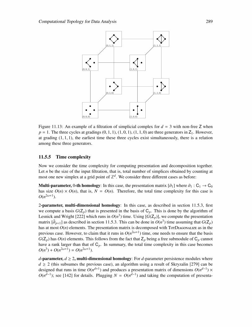
Computational Topology for Data Analysis 289
(0, 0, 0)
(0, 1, 0)
(0, 0, 1)
(1, 0, 0)
(1, 1, 0)
(1, 0, 1)
(0, 1, 1) (1, 1, 1)
Figure 11.13: An example of a filtration of simplicial complex for d = 3 with non-free Z whenp = 1. The three cycles at gradings (0, 1, 1), (1, 0, 1), (1, 1, 0) are three generators in Z1. However,at grading (1, 1, 1), the earliest time these three cycles exist simultaneously, there is a relationamong these three generators.
11.5.5 Time complexity
Now we consider the time complexity for computing presentation and decomposition together.Let n be the size of the input filtration, that is, total number of simplices obtained by counting atmost one new simplex at a grid point of Zd. We consider three different cases as before:
Multi-parameter, 0-th homology: In this case, the presentation matrix [∂1] where ∂1 : C1 → C0has size O(n) × O(n), that is, N = O(n). Therefore, the total time complexity for this case isO(n2ω+1).
2-parameter, multi-dimensional homology: In this case, as described in section 11.5.3, firstwe compute a basis G(Zp) that is presented in the basis of Cp. This is done by the algorithm ofLesnick and Wright [222] which runs in O(n3) time. Using [G(Zp)], we compute the presentationmatrix [∂p+1] as described in section 11.5.3. This can be done in O(n3) time assuming that G(Zp)has at most O(n) elements. The presentation matrix is decomposed with TotDiagonalize as in theprevious case. However, to claim that it runs in O(n2ω+1) time, one needs to ensure that the basisG(Zp) has O(n) elements. This follows from the fact that Zp being a free submodule of Cp cannothave a rank larger than that of Cp. In summary, the total time complexity in this case becomesO(n3) + O(n2ω+1) = O(n2ω+1).
d-parameter, d ≥ 2, multi-dimensional homology: For d-parameter persistence modules whered ≥ 2 (this subsumes the previous case), an algorithm using a result of Skryzalin [279] can bedesigned that runs in time O(nd+1) and produces a presentation matrix of dimensions O(nd−1) ×O(nd−1); see [142] for details. Plugging N = O(nd−1) and taking the computation of presenta-
290 Computational Topology for Data Analysis
tion matrix into consideration, we get a time complexity bound of O(nd+1) + O(n(2ω+1)(d−1)) =
O(n(2ω+1)(d−1)).
11.6 Invariants
For a given persistence module, it is useful to compute invariants that in some sense summarizethe information contained in them. Ideally, these invariants should characterize the input mod-ule completely, meaning that the two invariants should be equal if and only if the modules areisomophic. Persistence diagrams for 1-parameter tame persistence modules are such invaraints.For multiparameter persistence modules, no such complete invariants exist that are finite andhence computable. However, we can still aim for invariants that are computable and characterizethe modules in some limited sense, meaning that these invariants remain equal for isomorphicmodules though may not differentiate non-isomorphic modules. Of course, their effectiveness inpractice is determined by their discriminative power. We present two such invariants below: thefirst one rank invariant was suggested in [66] whereas the second one graded Betti number wasbrought to TDA by [214] and studied further in [221].
11.6.1 Rank invariants
Assume that the input graded module M is finitely generated as before and additionally finitelysupported. For this we need to define the support of M.
Definition 11.17 (Support). Let M be a Zd-graded module. Its support is defined as the graphsupp(M) = (V, E ⊆ V × V) where a node v ∈ V if and only if Mv , 0 and an edge (u, v) ∈ E ifand only if (i) u < v and there is no s ∈ Zd satisfying u < s < v, and (ii) rank(Mu → Mv) , 0.We say M is finitely supported if supp(M) is finite.
Fact 11.2. supp(M) is disconnected if there exist two grades u < v in supp(M) so that rank(Mu →
Mv) = 0.
For a finitely generated and finitely supported module M, we can compute a finite number ofranks of linear maps which collectively form the rank invariant of M. For two grades u v, thelinear maps between Mu and Mv are not defined. In the following definitions, we take them aszero maps.
Definition 11.18 (Rank invariant). Let ruv(M) = rank(Mu → Mv) for any pair u, v ∈ supp(M).The collection ruv(M)u,v∈supp(M) is called the rank invariant of M.
Fact 11.3. Rank invariant of a 1-parameter module is a complete invariant. For a 1-parameterpersistence module Hp, it is given by persistent Betti numbers βi, j
p as defined in Definition 3.4.
Although in 1-parameter case, the rank invariant provides complete information about themodule, it does not do so for multiparameter persistence modules. For example, it cannot provideinformation about ‘birth’ and ‘death’ of the generators. This information can be deduced from awider collection of rank invariant data called multirank invariant where we compute ranks of thelinear maps between vector spaces at multiple grades. Multirank invariant is still not a completeinvariant.
Computational Topology for Data Analysis 291
Definition 11.19 (Multirank invariant). The collection rUV(M) for every pair U ⊆ supp(M) andV ⊆ supp(M) where rUV(M) = rank
(⊕u∈U Mu →
⊕v∈V Mv
)is called the multirank invariant
of M.
We can retrieve the information about birth and death of generators from the multirank. For agrade u, define its immediate predecessors Pu and immediate successors S u as:
Pu = u′ ∈ supp(M) |u′ < u and @u′′ with u′ < u′′ < uS u = u′ ∈ supp(M) |u′ > u and @u′′ with u < u′′ < u′.
Fact 11.4.
1. We have that m generators get born at grade u if and only if coker(⊕
u′∈PuMu′ → Mu
)has
dimension m.
2. We have that m generators die leaving grade u if and only if ker(Mu →
⊕u′∈S u
Mu′)
hasdimension m.
Although multirank invariants cannot characterize multiparameter persistence modules com-pletely in general, they do so for the special case of interval decomposable modules. We willdescribe these modules in details in the next chapter. Here we introduce them briefly.
We call I ⊆ supp(M) an interval if I is connected and for every u, v ∈ I, if u < w < v,then w ∈ I. We call a persistence module with support on an interval an interval module if Muis unit dimensional for every vertex u ∈ supp(M). A persistence module M is called intervaldecomposable if there is a decomposition M =
⊕Mi where each Mi is an interval module.
Fact 11.5. Two interval decomposable modules are isomorphic if and only if they have the samemultirank invariants.
11.6.2 Graded Betti numbers and blockcodes
For 1-parameter persistence modules, the barcodes provide a complete invariant. For multipa-rameter persistence, we first introduce an invariant called graded Betti number, which we refinefurther to define persistent graded Betti numbers as a generalization of persistence diagrams. Thedecomposition of a module also allows us to define blockcodes as a generalization of barcodes.Both of them depend on the ideas of free resolution and graded Betti numbers which are wellstudied in commutative algebra and are first introduced in topological data analysis by Knud-son [214].
Definition 11.20 (Free resolution). For a graded module M, a free resolution F → M is an exactsequence:
· · · F2 F1 F0 M 0f 2 f 1 f 0
where each Fi is a free graded R-module.
Now we observe that a free resolution can be obtained as an extension of a free presentation.Consider a free presentation of M as depicted below.
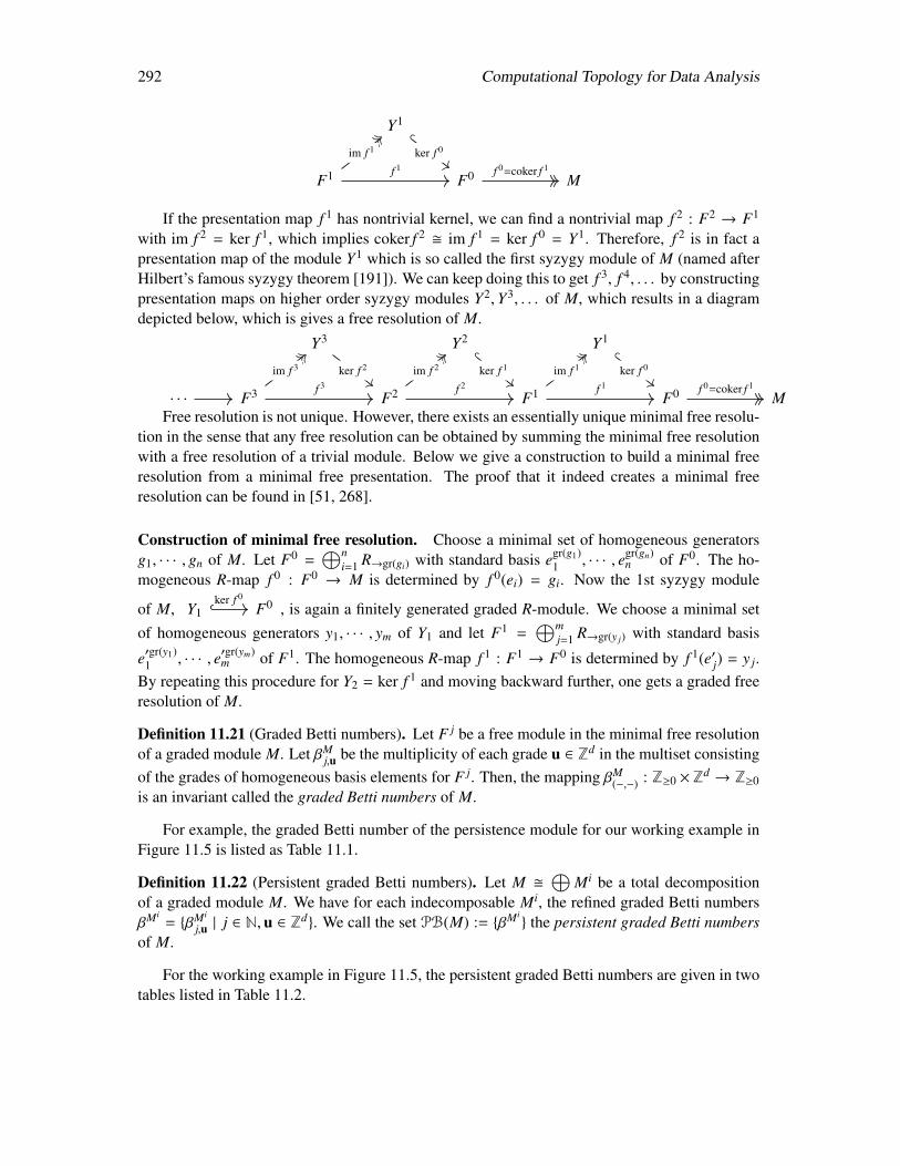
292 Computational Topology for Data Analysis
Y1
F1 F0 M
ker f 0
f 1
im f 1
f 0=coker f 1
If the presentation map f 1 has nontrivial kernel, we can find a nontrivial map f 2 : F2 → F1
with im f 2 = ker f 1, which implies coker f 2 im f 1 = ker f 0 = Y1. Therefore, f 2 is in fact apresentation map of the module Y1 which is so called the first syzygy module of M (named afterHilbert’s famous syzygy theorem [191]). We can keep doing this to get f 3, f 4, . . . by constructingpresentation maps on higher order syzygy modules Y2,Y3, . . . of M, which results in a diagramdepicted below, which is gives a free resolution of M.
Y3 Y2 Y1
· · · F3 F2 F1 F0 M
ker f 2 ker f 1 ker f 0
f 3
im f 3
f 2
im f 2
f 1
im f 1
f 0=coker f 1
Free resolution is not unique. However, there exists an essentially unique minimal free resolu-tion in the sense that any free resolution can be obtained by summing the minimal free resolutionwith a free resolution of a trivial module. Below we give a construction to build a minimal freeresolution from a minimal free presentation. The proof that it indeed creates a minimal freeresolution can be found in [51, 268].
Construction of minimal free resolution. Choose a minimal set of homogeneous generatorsg1, · · · , gn of M. Let F0 =
⊕ni=1 R→gr(gi) with standard basis egr(g1)
1 , · · · , egr(gn)n of F0. The ho-
mogeneous R-map f 0 : F0 → M is determined by f 0(ei) = gi. Now the 1st syzygy module
of M, Y1 F0ker f 0
, is again a finitely generated graded R-module. We choose a minimal setof homogeneous generators y1, · · · , ym of Y1 and let F1 =
⊕mj=1 R→gr(y j) with standard basis
e′gr(y1)1 , · · · , e′gr(ym)
m of F1. The homogeneous R-map f 1 : F1 → F0 is determined by f 1(e′j) = y j.By repeating this procedure for Y2 = ker f 1 and moving backward further, one gets a graded freeresolution of M.
Definition 11.21 (Graded Betti numbers). Let F j be a free module in the minimal free resolutionof a graded module M. Let βM
j,u be the multiplicity of each grade u ∈ Zd in the multiset consistingof the grades of homogeneous basis elements for F j. Then, the mapping βM
(−,−) : Z≥0 ×Zd → Z≥0is an invariant called the graded Betti numbers of M.
For example, the graded Betti number of the persistence module for our working example inFigure 11.5 is listed as Table 11.1.
Definition 11.22 (Persistent graded Betti numbers). Let M ⊕
Mi be a total decompositionof a graded module M. We have for each indecomposable Mi, the refined graded Betti numbersβMi
= βMi
j,u | j ∈ N,u ∈ Zd. We call the set PB(M) := βMi the persistent graded Betti numbers
of M.
For the working example in Figure 11.5, the persistent graded Betti numbers are given in twotables listed in Table 11.2.
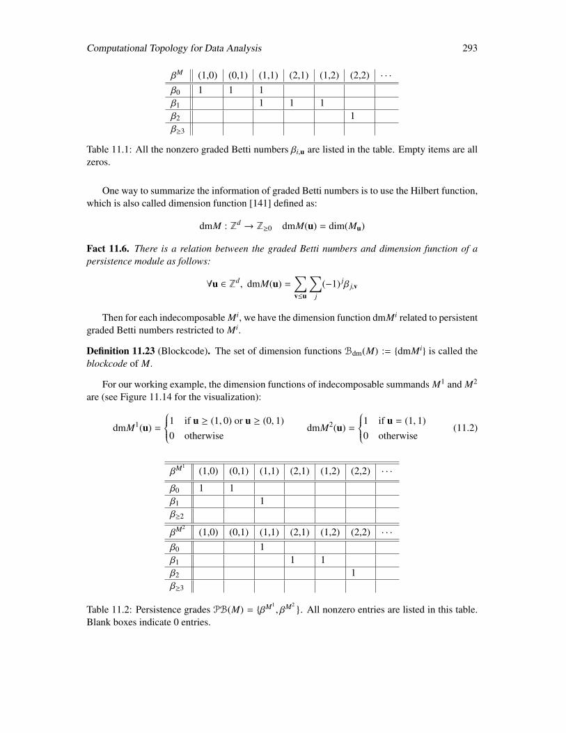
Computational Topology for Data Analysis 293
βM (1,0) (0,1) (1,1) (2,1) (1,2) (2,2) · · ·
β0 1 1 1β1 1 1 1β2 1β≥3
Table 11.1: All the nonzero graded Betti numbers βi,u are listed in the table. Empty items are allzeros.
One way to summarize the information of graded Betti numbers is to use the Hilbert function,which is also called dimension function [141] defined as:
dmM : Zd → Z≥0 dmM(u) = dim(Mu)
Fact 11.6. There is a relation between the graded Betti numbers and dimension function of apersistence module as follows:
∀u ∈ Zd, dmM(u) =∑v≤u
∑j
(−1) jβ j,v
Then for each indecomposable Mi, we have the dimension function dmMi related to persistentgraded Betti numbers restricted to Mi.
Definition 11.23 (Blockcode). The set of dimension functions Bdm(M) := dmMi is called theblockcode of M.
For our working example, the dimension functions of indecomposable summands M1 and M2
are (see Figure 11.14 for the visualization):
dmM1(u) =
1 if u ≥ (1, 0) or u ≥ (0, 1)0 otherwise
dmM2(u) =
1 if u = (1, 1)0 otherwise
(11.2)
βM1(1,0) (0,1) (1,1) (2,1) (1,2) (2,2) · · ·
β0 1 1β1 1β≥2
βM2(1,0) (0,1) (1,1) (2,1) (1,2) (2,2) · · ·
β0 1β1 1 1β2 1β≥3
Table 11.2: Persistence grades PB(M) = βM1, βM2
. All nonzero entries are listed in this table.Blank boxes indicate 0 entries.
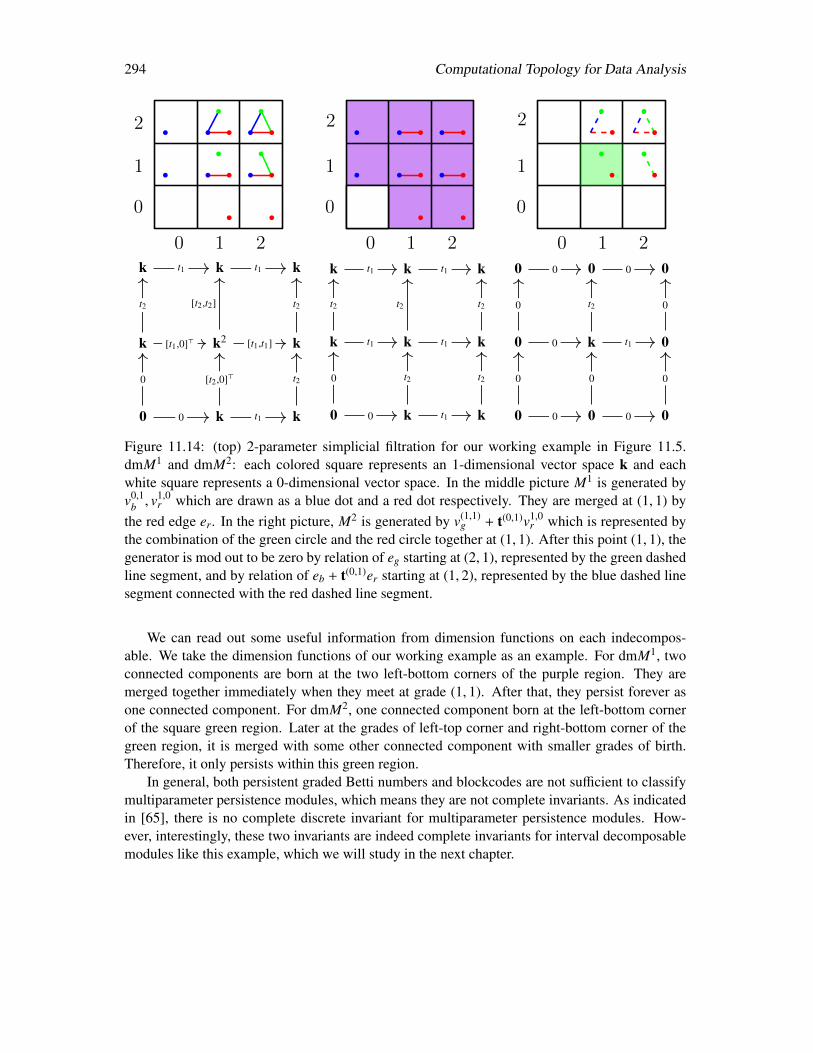
294 Computational Topology for Data Analysis
0 1 2
0
1
2
0 1 2
0
1
2
0 1 2
0
1
2
k k k
k k2 k
0 k k
t1 t1
t2
[t1,0]>
[t2,t2]
[t1,t1]
t2
0
0
t1
[t2,0]> t2
k k k
k k k
0 k k
t1 t1
t2
t1
t2
t1
t2
0
0
t1
t2 t2
0 0 0
0 k 0
0 0 0
0 0
0
0
t2
t1
0
0
0
0
0 0
Figure 11.14: (top) 2-parameter simplicial filtration for our working example in Figure 11.5.dmM1 and dmM2: each colored square represents an 1-dimensional vector space k and eachwhite square represents a 0-dimensional vector space. In the middle picture M1 is generated byv0,1
b , v1,0r which are drawn as a blue dot and a red dot respectively. They are merged at (1, 1) by
the red edge er. In the right picture, M2 is generated by v(1,1)g + t(0,1)v1,0
r which is represented bythe combination of the green circle and the red circle together at (1, 1). After this point (1, 1), thegenerator is mod out to be zero by relation of eg starting at (2, 1), represented by the green dashedline segment, and by relation of eb + t(0,1)er starting at (1, 2), represented by the blue dashed linesegment connected with the red dashed line segment.
We can read out some useful information from dimension functions on each indecompos-able. We take the dimension functions of our working example as an example. For dmM1, twoconnected components are born at the two left-bottom corners of the purple region. They aremerged together immediately when they meet at grade (1, 1). After that, they persist forever asone connected component. For dmM2, one connected component born at the left-bottom cornerof the square green region. Later at the grades of left-top corner and right-bottom corner of thegreen region, it is merged with some other connected component with smaller grades of birth.Therefore, it only persists within this green region.
In general, both persistent graded Betti numbers and blockcodes are not sufficient to classifymultiparameter persistence modules, which means they are not complete invariants. As indicatedin [65], there is no complete discrete invariant for multiparameter persistence modules. How-ever, interestingly, these two invariants are indeed complete invariants for interval decomposablemodules like this example, which we will study in the next chapter.
Computational Topology for Data Analysis 295
11.7 Notes and Exercises
In one of the first extensions of the persistence algorithm for 1-parameter, the authors in [9]presented a matrix reduction based algorithm which applies to a very special case of commutativeladder Cn for n ≤ 4 defined on a subgrid of Z2. This matrix construction and the algorithm arevery different from the one presented here. This algorithm may not terminate if the input does notsatisfy the stated assumption.
We have already mentioned that the Meataxe algorithm [251] known in the computationalalgebra community can be used for more general modules and hence for persistence modules.The main advantage of this algorithm is that it applies to general persistence modules, but a majordisadvantage is that it runs very slow. Even allowing approximation, the algorithm [197] runs inO(N3(d+1) log q) time (or O(N4(d+1) log q) as conjectured in [196] because of some special casesmentioned in [197]) where N is the number of generators and relations in the input module that isdefined with polynomial ring Zq[t1t2 . . . td].
Under suitable finiteness condition, the fact that persistence modules are indeed finitely pre-sented graded modules over multivariate polynoimials was first recognized by Carlsson et al. [65,66] and Knudson [214] and further studied by Lesnick et al. [220, 222]. The graded modulestructure studied in algebraic geometry and commutative algebra [155, 231] encodes a lot of in-formation and thus can be leveraged for designing efficient algorithms. Lesnick and Wright [222]leveraged this fact to design an efficient algorithm for computing minimal presentations for 2-parameter persistence modules from an input 2-parameter simplicial filtration. Recognizing thepower of expressing graded modules in terms of presentations, Dey and Xin [142] proposed thedecomposition algorithm using matrix equivalents of presentations and their direct sums. Thematerials in this chapter are mostly taken from this paper. This decomposition algorithm can beviewed as a generalization of the classical persistence algorithm for 1-parameter though the ma-trix reduction technique is more involved because it has to accommodate constraints on grades.The algorithm in [142] handled these constraints using the technique of matrix linearization asdescribed in Section 11.4.
As a generalization of the 1-parameter persistence algorithm, it is expected that the algorithmin [142] is interpreted as computing invariants such as persistence diagrams or barcodes. A road-block to this goal is that d-parameter persistence modules do not have complete discrete invariantsfor d ≥ 2 [66, 220]. Consequently, one needs to invent other invariants suitable for multiparame-ter persistence modules. The rank invariants and multirank invariants described in Section 11.6.1serve this purpose. There is a related notion of generalized persistence diagram introduced byPatel [254] and further studied in [212].
One natural approach taking advantage of a decomposition algorithm would be to considerthe decomposition and take the discrete invariants in each indecomposable component. This givesinvariants which may not be complete but still contain rich information. We mentioned two in-terpretations of the output of the algorithm presented in this chapter as two different invariants:persistent graded Betti numbers as a generalization of persistence diagrams and blockcodes as ageneralization of barcodes. The persistent graded Betti numbers are linked to the graded Bettinumbers studied in commutative algebra brought to TDA by [214]. The bigraded Betti numbersare further studied in [222]. By constructing the free resolution of a persistence module, we cancompute its graded Betti numbers and then decompose them according to each indecomposable

296 Computational Topology for Data Analysis
module, which results into the presistent graded Betti numbers. For each indecomposable, weapply dimension function [141], which is also known as the Hilbert function in commutative al-gebra to summarize the graded Betti numbers for each indecomposalbe module. This constitutesa blockcode for indecomposable module of the persistence module. The blockcode is a good ve-hicle for visualizing lower dimensional persistence modules such as 2- or 3-parameter persistencemodules. For details on these invariants, see [142].
Exercises
1. Using the matrix diagonalization algorithm as described in this chapter, devise an algo-rithm to compute a minimal presentation of a 2-parameter persistence module given by asimplicial filtration over Z2.
2. Give an example of a 2-parameter simplicial filtration over Z2 at least one of whose decom-posables is not free.
3. Give an example of a 2-parameter simplicial filtration over Z2 at least one of whose decom-posables does not have all of its non-trivial vector spaces over the grades being isomorphic.
4. Give an example of a 2-parameter persistence module M with three generators and relationsthat have the following properties: (i) M is indecomposable, (ii) M has two indecompos-ables, (iii) M has three indecomposables.
5. Prove that the cycle module Zp arising from a 2-parameter simplicial filtration is alwaysfree.
6. Design a polynomial time algorithm for computing decomposition of the persistence mod-ule induced by a given simplicial filtration over Z2 when a simplex can be a generator atdifferent grades.
7. Let A a presentation matrix with n generators and relations whose grades are distinct andtotally ordered. Design an O(n3) time algorithm to decompose A. Interpret types of eachindecomposable in such a case.
8. The algorithm TotDiagonalize has been written assuming that the field of the polynomialring is Z2. Write it for a general finite field.
9. Give and example of two non-isomorphic 2-parameter persistence modules which have thesame rank invariant.
10. Design an efficient algorithm to compute the rank invariant of a module from the simplicialfiltration inducing it.
11. Prove that a 2-parameter persistence module M is an interval (see Section 11.6.1) if andonly if supp(M) is connected and each Mu for u ∈ supp(M) has dimension 1.

Computational Topology for Data Analysis 297
12. Suppose that a 2-parameter persistence module is given by a presentation matrix. Design analgorithm to determine if M is interval or not without decomposing the input matrix (hint:consider computing graded Betti numbers from the grades of the rows and columns of thematrix).
13. Show that for a finitely presented (finite number of generators and relations) graded moduleM, there exist two interval decomposable graded modules M1 and M2 so that the rankinvariants (Definition 11.18) satisfy ruv(M) = ruv(M1) − ruv(M2) for every u, v ∈ supp(M).Given a presentation matrix for M, compute such M1 and M2 efficiently.
14. Write a pseudocode for the construction of a minimal free resolution given in Section 11.6.2.Analyze its complexity.

298 Computational Topology for Data Analysis
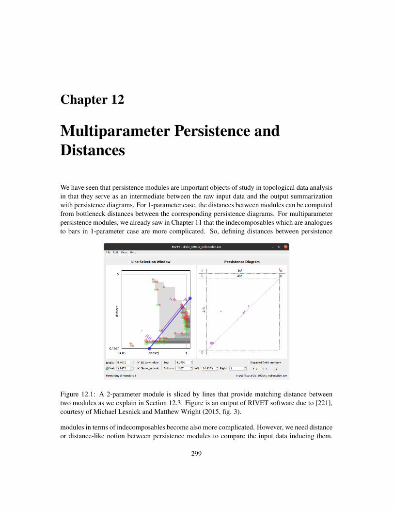
Chapter 12
Multiparameter Persistence andDistances
We have seen that persistence modules are important objects of study in topological data analysisin that they serve as an intermediate between the raw input data and the output summarizationwith persistence diagrams. For 1-parameter case, the distances between modules can be computedfrom bottleneck distances between the corresponding persistence diagrams. For multiparameterpersistence modules, we already saw in Chapter 11 that the indecomposables which are analoguesto bars in 1-parameter case are more complicated. So, defining distances between persistence
Figure 12.1: A 2-parameter module is sliced by lines that provide matching distance betweentwo modules as we explain in Section 12.3. Figure is an output of RIVET software due to [221],courtesy of Michael Lesnick and Matthew Wright (2015, fig. 3).
modules in terms of indecomposables become also more complicated. However, we need distanceor distance-like notion between persistence modules to compare the input data inducing them.
299
300 Computational Topology for Data Analysis
Figure 12.1 shows an output of RIVET software [221] that implemented the so-called matchingdistance between 2-parameter persistence modules. In this chapter, we describe some of thesedistances proposed in the literature and algorithms for computing them efficiently (polynomialtime).
The interleaving distance dI between 1-parameter persistence modules as defined in Chapter 3provides a useful means to compare them. Fortunately, for 1-parameter persistence modules,they can be computed exactly by computing the bottleneck distance db between their persistencediagrams thanks to the isometry theorem [220] (see also [24, 81]). Chapter 3 gives a polynomialtime algorithm O(n1.5 log n) for computing bottleneck distance. The status however is not so wellsettled for multiparameter persistence modules.
One of the difficulties facing the definition and computation of distances among multiparame-ter persistence modules is the fact that their indecomposables do not have a finite characterizationas indicated in Chapter 11. Even for finitely generated modules, this is true though a unique de-composition is guaranteed by Krull-Schmidt Theorem [10]. Despite this difficulty, one can definean interleaving distance dI for multiparameter persistence modules which can be viewed as anextension of the interleaving distance defined for 1-parameter persistence modules. Shown byLesnick [220], this distance is the most fundamental one because it is the most discriminativedistance among persistence modules that is also stable with respect to functions or simplicial fil-trations that give rise to the modules. Unfortunately, it turns out that computing dI for n-parameterpersistence modules and even approximating it within a factor less than 3 is NP-hard for n ≥ 2.For a special case of modules called interval modules, dI can be computed in polynomial time.In Section 12.2, we introduce the interleaving distance for multiparameter persistence modules.We follow it with a polynomial time algorithm [141] in Section 12.4.3 which computes dI for2-parameter interval modules.
To circumvent the problem of computing interleaving distances, several other distances havebeen proposed in the literature that is computable in polynomial time and bounds the interleavingdistance either from above or below, but not both in the general case. Given the NP-hardness ofapproximating interleaving distance, there cannot exist any polynomial time computable distancethat bounds dI both from above and below within a constant factor of 3 unless P = NP. Thematching distance dm as defined in Section 12.3 bounds dI from below, that is, dm ≤ dI , and itcan be computed in polynomial time.
Finally, in Section 12.4, we extend the definition of the bottleneck distance to multiparam-eter persistence modules. Extending the concept from 1-parameter case, one can define db asthe supremum of the pairwise interleaving distances between indecomposables under an opti-mal matching. Then, straightforwardly, dI ≤ db but the converse is not necessarily true. It isknown that no lower bound in terms of db for dI may exist even for a special class of 2-parameterpersistence modules called interval decomposable modules [48]. However, db can be useful asa reasonable upper bound to dI . Unfortunately, a polynomial time algorithm for computing db
is not known for general persistence modules. For some persistence modules whose indecom-posables have constant description such as block decomposable modules, one can compute db inpolynomial time simply because the interleaving distance between any two modules with constantdescription cannot take more than O(1) time.
In Section 12.4, we consider a special class of persistence modules whose indecomposablesare intervals and present a polynomial time algorithm for computing db for them. These are mod-
Computational Topology for Data Analysis 301
ules whose indecomposables are supported by “stair-case" polyhedra. Our algorithm assumesthat all indecomposables are given and computes db exactly for 2-parameter interval decompos-able modules. Although the algorithm can be extended to persistence modules with larger numberof parameters, we choose to present it only for 2-parameter case for simplicity while not losingthe essential ingredients for the general case. The indecomposables required as input can becomputed by the decomposition algorithm presented in the previous chapter (Chapter 11).
12.1 Persistence modules from categorical viewpoint
In this chapter we define the persistence modules as categorical structures which are different fromthe graded structures used in the previous chapter. Other than introducing a different viewpointof persistence modules, we do so because this definition becomes more amenable to definingdistances. Thanks to representation theory [66, 108, 214], these two notions coincide when themodules are finitely generated in the graded module definition (Definition 11.5) and are of finitetype (Definition 12.5) in the categorical definition. Let us recall the definition in 1-parametercase. A persistence module M parameterized over A = Z, or R is defined by a sequence of vectorspaces Mx, x ∈ A with linear maps ρx,y : Mx → My so that ρx,x is identity for every x ∈ A and forall x, y, z ∈ A with x ≤ y ≤ z, one has ρx,z = ρy,z ρx,y. These conditions can be formulated usingcategory theory.
Definition 12.1 (Category). A category C is a set of objects ObjC with a set of morphismshom(x, y) for every pair of elements x, y ∈ ObjC where
1. for every x ∈ ObjC, there is a special identity morphism 1x ∈ hom(x, x);
2. if f ∈ hom(x, y) and g ∈ hom(y, z), then g f ∈ hom(x, z);
3. for homomorphisms f , g, h, the compositions wherever defined are associative, that is, ( f g) h = f (g h);
4. 1x fx,y = fx,y and fx,y 1y = fx,y for every pair x, y ∈ ObjC.
All sets form a category Set with functions between them playing the role of morphisms. Topo-logical spaces form a category Top with continuous maps between them being the morphisms.Vector spaces form the category Vec with linear maps between them being the morphisms. Aposet P form a category with every pair x, y ∈ P admitting at most one morphism; hom(x, y)has one element if x ≤ y and empty otherwise. Such a category is called a thin category in theliterature for which composition rules take trivial form.
Definition 12.2 (Functor). A functor between two categories C and D is an assignment F : C →D satisfying the following conditions:
1. for every x ∈ ObjC, F(x) ∈ ObjD;
2. for every morphism f ∈ hom(x, y), F( f ) ∈ hom(F(x), F(y));
3. F respects composition, that is, F( f g) = F( f ) F(g);
302 Computational Topology for Data Analysis
4. F preserves identity morphisms, that is, F(1x) = 1F(x) for every x ∈ ObjC.
One can observe that the 1-parameter persistence module is a functor from the category of totallyordered set of Z (or R) to the category of Vec. Homology groups with a field coefficient fortopological spaces provide a functor from category Top to the category of vectors spaces Vec. Wecan define maps between functors themselves.
Definition 12.3 (Natural transformation). Given two functors F,G : C → D, a natural transfor-mation η from F to G, denoted as η : F =⇒ G, is a family of morphisms ηx : F(x) → G(x) forevery x ∈ ObjC so that the following diagram commutes:
F(x)
ηx
F(ρ) // F(y)
ηy
G(x)
G(ρ) // G(y)
Let k be a field, Vec be the category of vector spaces over k, and vec be the subcategory offinite dimensional vector spaces. As usual, for simplicity, we assume k = Z2.
Definition 12.4 (Persistence module). Let P be a poset category. A P-indexed persistence moduleis a functor M : P → Vec. If M takes values in vec, we say M is pointwise finite dimensional(p.f.d.). The P-indexed persistence modules themselves form another category where the naturaltransformations between functors constitute the morphisms.
Definition 12.5 (Finite type). A P-indexed persistence module M is said to have finite type if Mis p.f.d. and all morphisms M(x ≤ y) are isomorphisms outside a finite subset of P.
Here we consider the poset category to be Rd with the standard partial order and all modulesto be of finite type. We call Rd-indexed persistence modules as d-parameter modules in short.The reader can recognize that this is a shift from our assumption in the last chapter where weconsidered Zd-indexed modules. The category of d-parameter modules in this chapter is denotedas Rd-mod. For a d-parameter module M ∈ Rd-mod, we use notations Mx := M(x) and ρM
x→y :=M(x ≤ y).
Definition 12.6 (Shift). For any δ ∈ R, we denote ~δ = (δ, · · · , δ) = δ ·~e, where ~e = (e1, e2, . . . , ed)with ei
di=1 being the standard basis of Rd. We define a shift functor (·)→δ : Rd-mod → Rd-mod
where M→δ := (·)→δ(M) is given by M→δ(x) = M(x + ~δ) and M→δ(x ≤ y) = M(x + ~δ ≤ y + ~δ). Inother words, M→δ is the module M shifted diagonally by ~δ.
12.2 Interleaving distance
The following definition of interleaving adapts the original definition designed for 1-parametermodules in [78, 81] to d-parameter modules.
Definition 12.7 (Interleaving). For two d-parameter persistence modules M and N, and δ ≥ 0,a δ-interleaving between M and N are two families of linear maps φx : Mx → Nx+~δx∈Rd andψx : Nx → Mx+~δx∈Rd satisfying the following two conditions; see Figure 12.2:
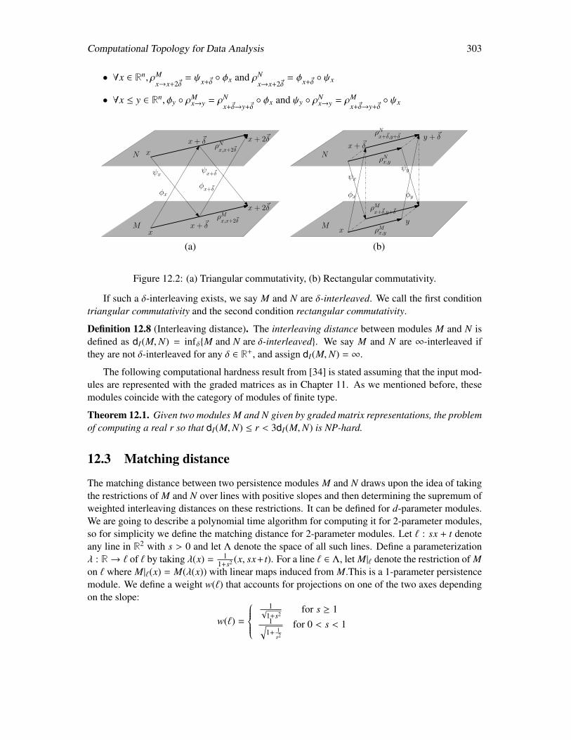
Computational Topology for Data Analysis 303
• ∀x ∈ Rn, ρMx→x+2~δ
= ψx+~δ φx and ρNx→x+2~δ
= φx+~δ ψx
• ∀x ≤ y ∈ Rn, φy ρMx→y = ρN
x+~δ→y+~δ φx and ψy ρ
Nx→y = ρM
x+~δ→y+~δ ψx
N
Mx
x+ 2~δ
x+ ~δ
x
x+ ~δ x+ 2~δ
φxφx+~δ
ψx ψx+~δ
ρMx,x+2~δ
ρNx,x+2~δ
xy
x+ ~δy + ~δ
ρMx,y
ρNx+~δ,y+~δ
φyφx
ρNx,y
ρMx+~δ,y+~δ
ψx
ψy
N
M
(a) (b)
Figure 12.2: (a) Triangular commutativity, (b) Rectangular commutativity.
If such a δ-interleaving exists, we say M and N are δ-interleaved. We call the first conditiontriangular commutativity and the second condition rectangular commutativity.
Definition 12.8 (Interleaving distance). The interleaving distance between modules M and N isdefined as dI(M,N) = infδM and N are δ-interleaved. We say M and N are ∞-interleaved ifthey are not δ-interleaved for any δ ∈ R+, and assign dI(M,N) = ∞.
The following computational hardness result from [34] is stated assuming that the input mod-ules are represented with the graded matrices as in Chapter 11. As we mentioned before, thesemodules coincide with the category of modules of finite type.
Theorem 12.1. Given two modules M and N given by graded matrix representations, the problemof computing a real r so that dI(M,N) ≤ r < 3dI(M,N) is NP-hard.
12.3 Matching distance
The matching distance between two persistence modules M and N draws upon the idea of takingthe restrictions of M and N over lines with positive slopes and then determining the supremum ofweighted interleaving distances on these restrictions. It can be defined for d-parameter modules.We are going to describe a polynomial time algorithm for computing it for 2-parameter modules,so for simplicity we define the matching distance for 2-parameter modules. Let ` : sx + t denoteany line in R2 with s > 0 and let Λ denote the space of all such lines. Define a parameterizationλ : R→ ` of ` by taking λ(x) = 1
1+s2 (x, sx+ t). For a line ` ∈ Λ, let M|` denote the restriction of Mon ` where M|`(x) = M(λ(x)) with linear maps induced from M.This is a 1-parameter persistencemodule. We define a weight w(`) that accounts for projections on one of the two axes dependingon the slope:
w(`) =
1√
1+s2for s ≥ 1
1√1+ 1
s2
for 0 < s < 1
304 Computational Topology for Data Analysis
Definition 12.9. The matching distance dm(M,N) between two persistence modules is defined as
dm(M,N) = sup`∈Λw(`) · dI(M|`,N |`).
The weight w(`) is introduced to make the matching distance stable with respect to the inter-leaving distance.
12.3.1 Computing matching distance
We define a point-line duality in R2: a line ` ⊂ R2 is dual to a point `∗ = (s, t) where ` : y = sx− tand a point p = (s, t) is dual to a line p∗ : y = sx − t. Following facts can be deduced from thedefinition easily (Exercise 4).
Fact 12.1.
1. For a point p and a line `, one has (p∗)∗ = p and (`∗)∗ = `.
2. If a point p is in a line `, then point `∗ is in line p∗.
3. If a point p is above (below) a line `, then point `∗ is above (below) the line p∗.
Consider the open half-plane Ω of R2 where Ω = x, y | x > 0. Let α denote the bijective mapbetween Ω and the space Λ of lines with positive slopes where α(p) = p∗.
The representation theory [66, 108, 214] tells us that finitely generated graded modules asdefined in Chapter 11 are essentially equivalent to persistence modules as defined in this chapteras long as they are of finite type (Definition 12.5). Then, if a persistence module M is a functoron the poset P = R2 or Z2, we can talk about the grades (elements of P) of a generating set of Mand the relations which are combinations of generators that become zero. A mindful reader canrecognize these are exactly the grades of the rows and columns of the presentation matrix for M(Definition 11.14).
Given two 2-parameter persistence modules M and N, let gr(M) and gr(N) denote the gradesof all generators and relations in M and N respectively. Consider the set of lines L dual to thepoints in gr(M) ∪ gr(N). These lines together create a line arrangement in Ω which is a partitionof Ω into vertices, edges, and faces. The vertices are points where two lines meet, the edges aremaximal connected subset of the lines excluding the vertices, and faces are maximal connectedsubsets of Ω excluding the vertices and edges. Let A0 denote this initial arrangement. We refinethis arrangement further later. First, we observe an invariant property of the arrangemnt for whichwe need the following definition.
Definition 12.10 (Point pair type). Given two points p, q and a line `, we say (p, q) has thefollowing types with respect to ` : (i) Type-1 if both p and q lie above `, (ii) Type-2 if both p andq lie below `, (iii) Type-3 if p lies above and q lies below `, and (iv) Type-4 if p lies below and qlies above `.
The following proposition follows from Fact 12.1.
Proposition 12.2. For two points p, q ∈ gr(M) ∪ gr(N) and a face τ ∈ A0, the type of (p, q) withrespect to the line z∗ is the same for all z ∈ τ.
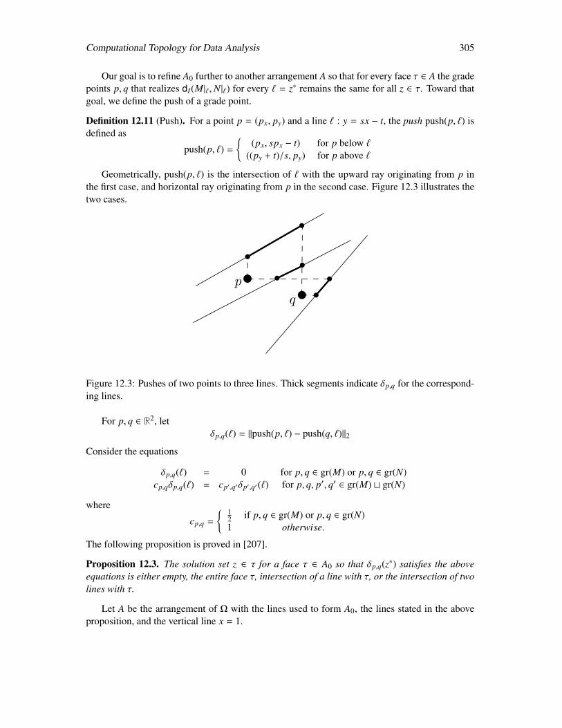
Computational Topology for Data Analysis 305
Our goal is to refine A0 further to another arrangement A so that for every face τ ∈ A the gradepoints p, q that realizes dI(M|`,N |`) for every ` = z∗ remains the same for all z ∈ τ. Toward thatgoal, we define the push of a grade point.
Definition 12.11 (Push). For a point p = (px, py) and a line ` : y = sx − t, the push push(p, `) isdefined as
push(p, `) =
(px, spx − t) for p below `
((py + t)/s, py) for p above `
Geometrically, push(p, `) is the intersection of ` with the upward ray originating from p inthe first case, and horizontal ray originating from p in the second case. Figure 12.3 illustrates thetwo cases.
p
q
Figure 12.3: Pushes of two points to three lines. Thick segments indicate δp,q for the correspond-ing lines.
For p, q ∈ R2, letδp,q(`) = ‖push(p, `) − push(q, `)‖2
Consider the equations
δp,q(`) = 0 for p, q ∈ gr(M) or p, q ∈ gr(N)cp,qδp,q(`) = cp′,q′δp′,q′(`) for p, q, p′, q′ ∈ gr(M) t gr(N)
where
cp,q =
12 if p, q ∈ gr(M) or p, q ∈ gr(N)1 otherwise.
The following proposition is proved in [207].
Proposition 12.3. The solution set z ∈ τ for a face τ ∈ A0 so that δp,q(z∗) satisfies the aboveequations is either empty, the entire face τ, intersection of a line with τ, or the intersection of twolines with τ.
Let A be the arrangement of Ω with the lines used to form A0, the lines stated in the aboveproposition, and the vertical line x = 1.
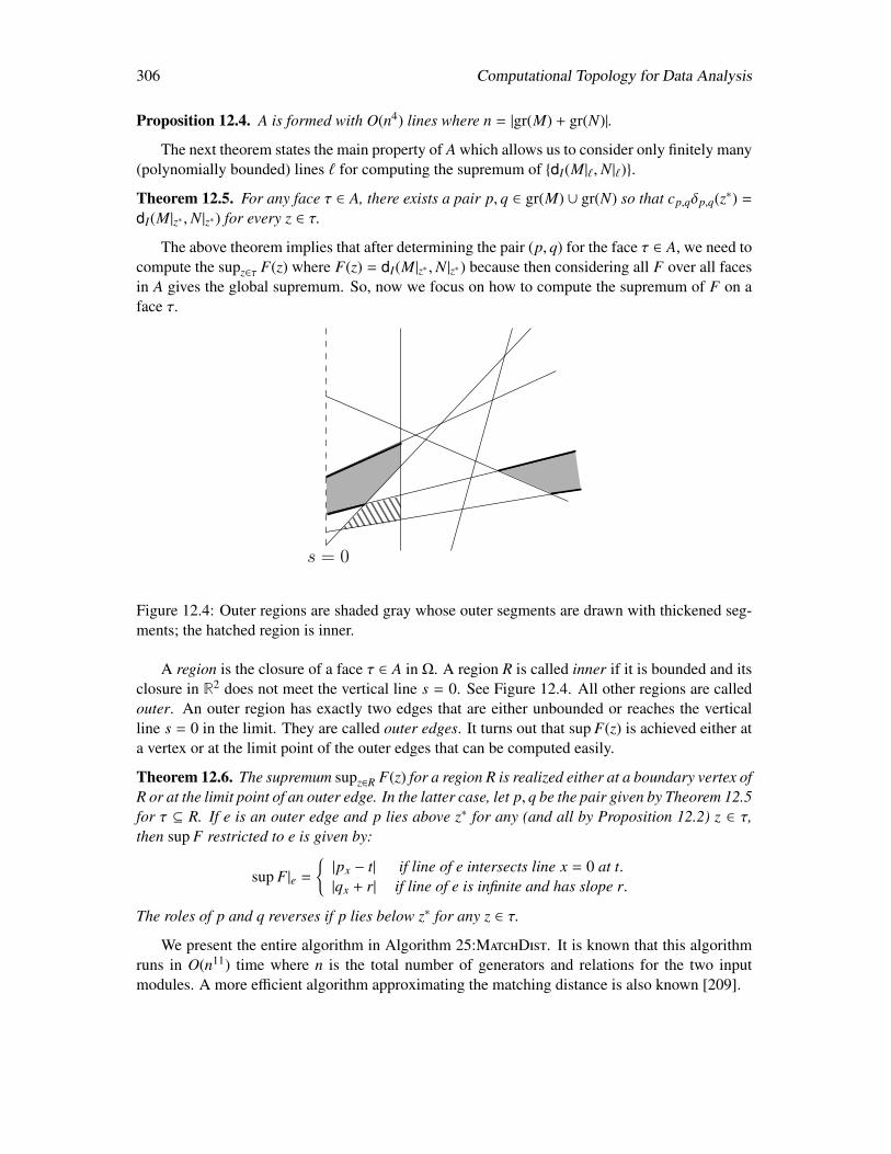
306 Computational Topology for Data Analysis
Proposition 12.4. A is formed with O(n4) lines where n = |gr(M) + gr(N)|.
The next theorem states the main property of A which allows us to consider only finitely many(polynomially bounded) lines ` for computing the supremum of dI(M|`,N |`).
Theorem 12.5. For any face τ ∈ A, there exists a pair p, q ∈ gr(M) ∪ gr(N) so that cp,qδp,q(z∗) =
dI(M|z∗ ,N |z∗) for every z ∈ τ.
The above theorem implies that after determining the pair (p, q) for the face τ ∈ A, we need tocompute the supz∈τ F(z) where F(z) = dI(M|z∗ ,N|z∗) because then considering all F over all facesin A gives the global supremum. So, now we focus on how to compute the supremum of F on aface τ.
s = 0
Figure 12.4: Outer regions are shaded gray whose outer segments are drawn with thickened seg-ments; the hatched region is inner.
A region is the closure of a face τ ∈ A in Ω. A region R is called inner if it is bounded and itsclosure in R2 does not meet the vertical line s = 0. See Figure 12.4. All other regions are calledouter. An outer region has exactly two edges that are either unbounded or reaches the verticalline s = 0 in the limit. They are called outer edges. It turns out that sup F(z) is achieved either ata vertex or at the limit point of the outer edges that can be computed easily.
Theorem 12.6. The supremum supz∈R F(z) for a region R is realized either at a boundary vertex ofR or at the limit point of an outer edge. In the latter case, let p, q be the pair given by Theorem 12.5for τ ⊆ R. If e is an outer edge and p lies above z∗ for any (and all by Proposition 12.2) z ∈ τ,then sup F restricted to e is given by:
sup F|e =
|px − t| if line of e intersects line x = 0 at t.|qx + r| if line of e is infinite and has slope r.
The roles of p and q reverses if p lies below z∗ for any z ∈ τ.
We present the entire algorithm in Algorithm 25:MatchDist. It is known that this algorithmruns in O(n11) time where n is the total number of generators and relations for the two inputmodules. A more efficient algorithm approximating the matching distance is also known [209].
Computational Topology for Data Analysis 307
Algorithm 25 MatchDist(M, N)
Input:Two modules M and N with grades of their generators and relations
Output:Matching distance between M and N
1: Compute arrangement A as described from gr(M) ∪ gr(N);2: Let V be the vertex set of A;3: Compute maximum m = maxz∈V F(z∗) over all vertices z ∈ V;4: for every outer region R do5: Pick a point z ∈ R;6: Compute the pair p, q ∈ gr(M) ∪ gr(N) that realizes dI(M|z∗ ,N |z∗);7: if p is above z∗ then8: if e as defined in Theorem 12.6 is infinite then9: m := max(m, qx + r) where r is the slope of e
10: else11: m := max(m, px − t) where e meets line x = 0 at t12: end if13: else14: reverse roles of p and q15: end if16: end for17: return m
12.4 Bottleneck distance
Definition 12.12 (Matching). A matching µ : A 9 B between two multisets A and B is a partialbijection, that is, µ : A′ → B′ for some A′ ⊆ A and B′ ⊆ B. We say im µ = B′, coim µ = A′.
For the next definition, we call a d-parameter module M δ-trivial if ρMx→x+~δ
= 0 for all x ∈ Rd.
Definition 12.13 (Bottleneck distance). Let M ⊕m
i=1 Mi and N ⊕n
j=1 N j be two persistencemodules, where Mi and N j are indecomposable submodules of M and N respectively. Let I =
1, · · · ,m and J = 1, · · · , n. We say M and N are δ-matched for δ ≥ 0 if there exists a matchingµ : I 9 J so that, (i) i ∈ I \ coim µ =⇒ Mi is 2δ-trivial, (ii) j ∈ J \ im µ =⇒ N j is 2δ-trivial,and (iii) i ∈ coim µ =⇒ Mi and Nµ(i) are δ-interleaved.
The bottleneck distance is defined as
db(M,N) = infδ | M and N are δ-matched.
The following fact observed in [48] is straightforward from the definition.
Fact 12.2. dI ≤ db.
308 Computational Topology for Data Analysis
12.4.1 Interval decomposable modules
We present a polynomial time algorithm for computing the bottleneck distances for a class of per-sistence modules called interval decomposable modules which we have seen in the previous chap-ter (Section 11.6.1). For ease of description, we will describe the algorithm for the 2-parametercase though an extension to multiparameter case exists.
Persistence modules whose indecomposables are interval modules (Definition 12.15) are calledinterval decomposable modules. To account for the boundaries of free modules, we enrich theposet Rd by adding points at ±∞ and consider the poset Rn = R × . . . × R where R = R ∪ ±∞with the usual additional rule a ±∞ = ±∞.
Definition 12.14 (Interval). An interval is a subset ∅ , I ⊂ Rd that satisfies the following:
1. If p, q ∈ I and p ≤ r ≤ q, then r ∈ I (convexity condition);
2. If p, q ∈ I, then there exists a sequence (p = p0, . . . , pm = q) ∈ I for some m ∈ N so thatfor every i ∈ [0, k − 1] either pi ≤ pi+1 or pi ≥ pi+1 (connectivity condition). We call thesequence (p = p0, . . . , pm = q) a path from p to q (in I).
Let I denote the closure of an interval I in the standard topology of Rd. The lower and upperboundaries of I are defined as
L(I) = x = (x1, · · · , xd) ∈ I | ∀y = (y1, · · · , yd) with yi < xi ∀i =⇒ y < I
U(I) = x = (x1, · · · , xd) ∈ I | ∀y = (y1, · · · , yd) with yi > xi ∀i =⇒ y < I.
Let B(I) = L(I) ∪ U(I). According to this definition, Rd is an interval with boundary B(Rd)that consists of all the points with at least one coordinate ∞. The vertex set V(Rd) consists of 2d
corner points with coordinates (±∞, · · · ,±∞).
Definition 12.15 (d-parameter interval module). A d-parameter interval persistence module, orinterval module in short, is a persistence module M that satisfies the following condition: for aninterval IM ⊆ Rd, called the interval of M,
Mx =
k if x ∈ IM
0 otherwiseρM
x→y =
1 if x, y ∈ IM
0 otherwise
where 1 and 0 denote the identity and zero maps respectively.
It is known that an interval module is indecomposable [48].
Definition 12.16 (Interval decomposable module). A d-parameter interval decomposable moduleis a persistence module that can be decomposed into interval modules.
Definition 12.17 (Rectangle). A k-dimensional rectangle, 0 ≤ k ≤ d , or k-rectangle, in Rd, is aset I = [a1, b1]×, · · · ,×[ad, bd], ai, bi ∈ R, such that, there exists a size k index set Λ ⊆ [d] where∀i ∈ Λ, ai , bi, and ∀ j ∈ [d] \ Λ, a j = b j.
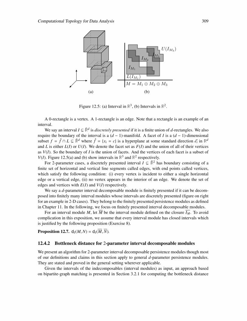
Computational Topology for Data Analysis 309
M = M1 ⊕M2 ⊕M3
IM1
IM2
IM3
L(IM1)
U(IM3)
(a) (b)
Figure 12.5: (a) Interval in R3, (b) Intervals in R2.
A 0-rectangle is a vertex. A 1-rectangle is an edge. Note that a rectangle is an example of aninterval.
We say an interval I ⊆ Rd is discretely presented if it is a finite union of d-rectangles. We alsorequire the boundary of the interval is a (d − 1)-manifold. A facet of I is a (d − 1)-dimensionalsubset f = f ∩ L ⊆ Rd where f = xi = c is a hyperplane at some standard direction ~ei in Rd
and L is either L(I) or U(I). We denote the facet set as F(I) and the union of all of their verticesas V(I). So the boundary of I is the union of facets. And the vertices of each facet is a subset ofV(I). Figure 12.5(a) and (b) show intervals in R3 and R2 respectively.
For 2-parameter cases, a discretely presented interval I ⊆ R2 has boundary consisting of afinite set of horizontal and vertical line segments called edges, with end points called vertices,which satisfy the following condition: (i) every vertex is incident to either a single horizontaledge or a vertical edge, (ii) no vertex appears in the interior of an edge. We denote the set ofedges and vertices with E(I) and V(I) respectively.
We say a d-parameter interval decomposable module is finitely presented if it can be decom-posed into finitely many interval modules whose intervals are discretely presented (figure on rightfor an example in 2-D cases). They belong to the finitely presented persistence modules as definedin Chapter 11. In the following, we focus on finitely presented interval decomposable modules.
For an interval module M, let M be the interval module defined on the closure IM. To avoidcomplication in this exposition, we assume that every interval module has closed intervals whichis justified by the following proposition (Exercise 8).
Proposition 12.7. dI(M,N) = dI(M,N).
12.4.2 Bottleneck distance for 2-parameter interval decomposable modules
We present an algorithm for 2-parameter interval decomposable persistence modules though mostof our definitions and claims in this section apply to general d-parameter persistence modules.They are stated and proved in the general setting wherever applicable.
Given the intervals of the indecomposables (interval modules) as input, an approach basedon bipartite-graph matching is presented in Section 3.2.1 for computing the bottleneck distance
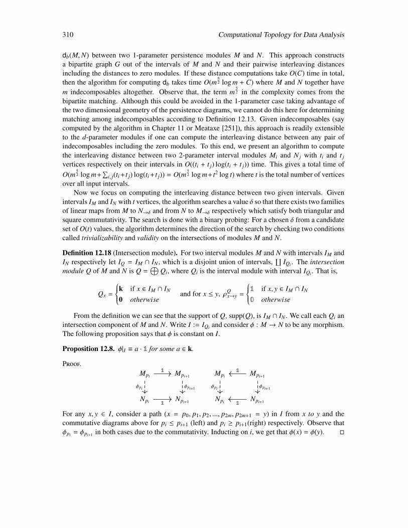
310 Computational Topology for Data Analysis
db(M,N) between two 1-parameter persistence modules M and N. This approach constructsa bipartite graph G out of the intervals of M and N and their pairwise interleaving distancesincluding the distances to zero modules. If these distance computations take O(C) time in total,then the algorithm for computing db takes time O(m
52 log m + C) where M and N together have
m indecomposables altogether. Observe that, the term m52 in the complexity comes from the
bipartite matching. Although this could be avoided in the 1-parameter case taking advantage ofthe two dimensional geometry of the persistence diagrams, we cannot do this here for determiningmatching among indecomposables according to Definition 12.13. Given indecomposables (saycomputed by the algorithm in Chapter 11 or Meataxe [251]), this approach is readily extensibleto the d-parameter modules if one can compute the interleaving distance between any pair ofindecomposables including the zero modules. To this end, we present an algorithm to computethe interleaving distance between two 2-parameter interval modules Mi and N j with ti and t j
vertices respectively on their intervals in O((ti + t j) log(ti + t j)) time. This gives a total time ofO(m
52 log m+
∑i, j(ti +t j) log(ti +t j)) = O(m
52 log m+t2 log t) where t is the total number of vertices
over all input intervals.Now we focus on computing the interleaving distance between two given intervals. Given
intervals IM and IN with t vertices, the algorithm searches a value δ so that there exists two familiesof linear maps from M to N→δ and from N to M→δ respectively which satisfy both triangular andsquare commutativity. The search is done with a binary probing: For a chosen δ from a candidateset of O(t) values, the algorithm determines the direction of the search by checking two conditionscalled trivializability and validity on the intersections of modules M and N.
Definition 12.18 (Intersection module). For two interval modules M and N with intervals IM andIN respectively let IQ = IM ∩ IN , which is a disjoint union of intervals,
∐IQi . The intersection
module Q of M and N is Q =⊕
Qi, where Qi is the interval module with interval IQi . That is,
Qx =
k if x ∈ IM ∩ IN
0 otherwiseand for x ≤ y, ρQ
x→y =
1 if x, y ∈ IM ∩ IN
0 otherwise
From the definition we can see that the support of Q, supp(Q), is IM ∩ IN . We call each Qi anintersection component of M and N. Write I := IQi and consider φ : M → N to be any morphism.The following proposition says that φ is constant on I.
Proposition 12.8. φ|I ≡ a · 1 for some a ∈ k.
Proof.Mpi Mpi+1 Mpi Mpi+1
Npi Npi+1 Npi Npi+1
1
φpi φpi+1 φpi
1
φpi+1
1 1
For any x, y ∈ I, consider a path (x = p0, p1, p2, ..., p2m, p2m+1 = y) in I from x to y and thecommutative diagrams above for pi ≤ pi+1 (left) and pi ≥ pi+1(right) respectively. Observe thatφpi = φpi+1 in both cases due to the commutativity. Inducting on i, we get that φ(x) = φ(y).
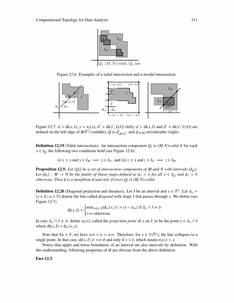
Computational Topology for Data Analysis 311
Q1 (M,N)-valid, Q2 not
IQ1
IQ2
IM
IN
Figure 12.6: Examples of a valid intersection and a invalid intersection.
Id′
x′y
∆x = ∆x′
(−∞,−∞)
(−∞,∞)
x′
y
d′
(∞,∞)
(∞,−∞)
IM
IN IQ2d
dxd
x∆x = ∆x′
2d′
I
Figure 12.7: d = dl(x, I), y = πI(x), d′ = dl(x′, L(I)) (left); d = dl(x, I) and d′ = dl(x′,U(I)) aredefined on the left edge of B(R2) (middle); Q is d′(M,N)- and d(N,M)-trivializable (right).
Definition 12.19 (Valid intersection). An intersection component Qi is (M,N)-valid if for eachx ∈ IQi the following two conditions hold (see Figure 12.6):
(i) y ≤ x and y ∈ IM =⇒ y ∈ IN , and (ii) z ≥ x and z ∈ IN =⇒ z ∈ IM
Proposition 12.9. Let Qi be a set of intersection components of M and N with intervals IQi.Let φx : M → N be the family of linear maps defined as φx = 1 for all x ∈ IQi and φx = 0otherwise. Then φ is a morphism if and only if every Qi is (M,N)-valid.
Definition 12.20 (Diagonal projection and distance). Let I be an interval and x ∈ Rn. Let ∆x =
x + ~α | α ∈ R denote the line called diagonal with slope 1 that passes through x. We define (seeFigure 12.7)
dl(x, I) =
miny∈∆x∩Id∞(x, y) := |x − y|∞ if ∆x ∩ I , ∅+∞ otherwise.
In case ∆x ∩ I , ∅, define πI(x), called the projection point of x on I, to be the point y ∈ ∆x ∩ Iwhere dl(x, I) = d∞(x, y).
Note that ∀α ∈ R, we have ±∞ + α = ±∞. Therefore, for x ∈ V(Rn), the line collapses to asingle point. In that case, dl(x, I) , +∞ if and only if x ∈ I, which means πI(x) = x.
Notice that upper and lower boundaries of an interval are also intervals by definition. Withthis understanding, following properties of dl are obvious from the above definition.
Fact 12.3.
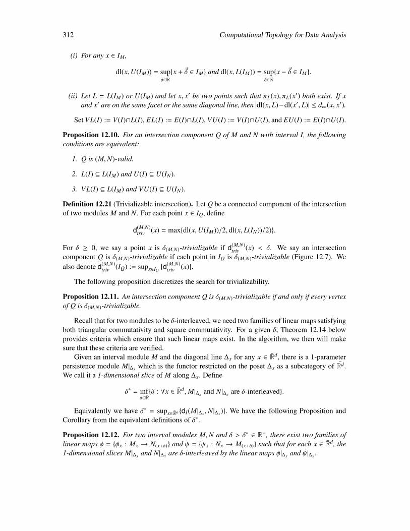
312 Computational Topology for Data Analysis
(i) For any x ∈ IM,
dl(x,U(IM)) = supδ∈Rx + ~δ ∈ IM and dl(x, L(IM)) = sup
δ∈Rx − ~δ ∈ IM.
(ii) Let L = L(IM) or U(IM) and let x, x′ be two points such that πL(x), πL(x′) both exist. If xand x′ are on the same facet or the same diagonal line, then |dl(x, L)−dl(x′, L)| ≤ d∞(x, x′).
Set VL(I) := V(I)∩L(I), EL(I) := E(I)∩L(I), VU(I) := V(I)∩U(I), and EU(I) := E(I)∩U(I).
Proposition 12.10. For an intersection component Q of M and N with interval I, the followingconditions are equivalent:
1. Q is (M,N)-valid.
2. L(I) ⊆ L(IM) and U(I) ⊆ U(IN).
3. VL(I) ⊆ L(IM) and VU(I) ⊆ U(IN).
Definition 12.21 (Trivializable intersection). Let Q be a connected component of the intersectionof two modules M and N. For each point x ∈ IQ, define
d(M,N)triv (x) = maxdl(x,U(IM))/2, dl(x, L(IN))/2).
For δ ≥ 0, we say a point x is δ(M,N)-trivializable if d(M,N)triv (x) < δ. We say an intersection
component Q is δ(M,N)-trivializable if each point in IQ is δ(M,N)-trivializable (Figure 12.7). Wealso denote d(M,N)
triv (IQ) := supx∈IQd(M,N)
triv (x).
The following proposition discretizes the search for trivializability.
Proposition 12.11. An intersection component Q is δ(M,N)-trivializable if and only if every vertexof Q is δ(M,N)-trivializable.
Recall that for two modules to be δ-interleaved, we need two families of linear maps satisfyingboth triangular commutativity and square commutativity. For a given δ, Theorem 12.14 belowprovides criteria which ensure that such linear maps exist. In the algorithm, we then will makesure that these criteria are verified.
Given an interval module M and the diagonal line ∆x for any x ∈ Rd, there is a 1-parameterpersistence module M|∆x which is the functor restricted on the poset ∆x as a subcategory of Rd.We call it a 1-dimensional slice of M along ∆x. Define
δ∗ = infδ∈Rδ : ∀x ∈ Rd,M|∆x and N|∆x are δ-interleaved.
Equivalently we have δ∗ = supx∈RndI(M|∆x ,N |∆x). We have the following Proposition andCorollary from the equivalent definitions of δ∗.
Proposition 12.12. For two interval modules M,N and δ > δ∗ ∈ R+, there exist two families oflinear maps φ = φx : Mx → N(x+δ) and ψ = ψx : Nx → M(x+δ) such that for each x ∈ Rd, the1-dimensional slices M|∆x and N|∆x are δ-interleaved by the linear maps φ|∆x and ψ|∆x .
Computational Topology for Data Analysis 313
Corollary 12.13. dI(M,N) ≥ δ∗.
Theorem 12.14. For two interval modules M and N, dI(M,N) ≤ δ if and only if the followingtwo conditions are satisfied:
(i) δ ≥ δ∗,(ii) ∀δ′ > δ, each intersection component of M and N→δ′ is either (M,N→δ′)-valid or δ(M,N→δ′ )-
trivializable, and each intersection component of M→δ′ and N is either (N,M→δ′)-valid or δ(N,M→δ′ )-trivializable.
Proof. Note that dI(M,N) ≤ δ if and only if ∀δ′ > δ,M,N is δ′-interleaved.
‘only if’ direction: Given M and N are δ-interleaved. The part (i) follows from Corol-lary 12.13 directly. For part (ii), by definition of interleaving, ∀δ′ > δ, we have two familiesof linear maps φx and ψx which satisfy both triangular and square commutativities. Let themorphisms between the two persistence modules constituted by these two families of linear mapsbe φ = φx and ψ = ψx respectively. For each intersection component Q of M and N→δ′ withinterval I := IQ, consider the restriction φ|I . By Proposition 12.8, φ|I is constant, that is, φ|I ≡ 0or 1. If φ|I ≡ 1, by Proposition 12.9, Q is (M,N→δ′)-valid. If φ|I ≡ 0, by the triangular commuta-tivity of φ, we have that ρM
x→x+2~δ′= ψx+~δ′ φx = 0 for each point x ∈ I. That means x + 2~δ′ < IM.
By Fact 12.3(i), dl(x,U(IM))/2 < δ′. Similarly, ρNx−~δ′→x+~δ′
= φx ψx−~δ′ = 0 =⇒ x − ~δ′ < IN ,
which is the same as to say x − 2~δ′ < IN→δ′ . By Fact 12.3(i), dl(x, L(IN→δ′ ))/2 < δ′. So ∀x ∈ I,we have d(M,N→δ′ )
triv (x) < δ′. This means Q is δ′(M,N→δ′ )-trivializable. Similar statement holds for
intersection components of M→δ′ and N.‘if’ direction: We construct two families of linear maps φx, ψx as follows: On the interval
I := IQi of each intersection component Qi of M and N→δ′ , set φ|I ≡ 1 if Qi is (M,N→δ′)-validand φ|I ≡ 0 otherwise. Set φx ≡ 0 for all x not in the interval of any intersection component.Similarly, construct ψx. Note that, by Proposition 12.9, φ := φx is a morphism between Mand N→δ′ , and ψ := ψx is a morphism between N and M→δ′ . Hence, they satisfy the squarecommutativity. We show that they also satisfy the triangular commutativity.
We claim that ∀x ∈ IM, ρMx→x+2~δ′
= 1 =⇒ x + ~δ′ ∈ IN and similar statement holds forIN . From condition that δ′ > δ ≥ δ∗ and by proposition 12.12, we know that there exist twofamilies of linear maps satisfying triangular commutativity everywhere, especially on the pair of1-parameter persistence modules M|∆x and N |∆x . From triangular commutativity, we know thatfor ∀x ∈ IM with ρM
x→x+2~δ′= 1, x + ~δ′ ∈ IN since otherwise one cannot construct a δ-interleaving
between M|∆x and N |∆x . So we get our claim.Now for each x ∈ IM with ρM
x→x+2~δ′= 1, we have dl(x,U(IM))/2 ≥ δ′ by Fact 12.3, and
x + ~δ′ ∈ IN by our claim. This implies that x ∈ IM ∩ IN→δ′ is a point in an interval of an intersec-tion component Qx of M,N→δ′ which is not δ′(M,N→δ′ )
-trivializable. Hence, it is (M,N→δ′)-valid bythe assumption. So, by our construction of φ on valid intersection components, φx = 1. Symmet-rically, we have that x+ ~δ′ ∈ IN ∩ IM→δ′ is a point in an interval of an intersection component of Nand M→δ′ which is not δ′(N,M→δ′ )-trvializable since dl(x+ ~δ′, L(IM))/2 ≥ δ′. So by our constructionof ψ on valid intersection components, ψx+~δ′ = 1. Then, we have ρM
x→x+2~δ′= ψx+~δ′ φx for ev-
ery nonzero linear map ρMx→x+2~δ′
. The statement also holds for any nonzero linear map ρNx→x+2~δ′
.

314 Computational Topology for Data Analysis
Therefore, the triangular commutativity holds.
Note that the above proof provides a construction of the interleaving maps for any specificδ′ if it exists. Furthermore, the interleaving distance dI(M,N) is the infimum of all δ′ satisfyingthe two conditions in the theorem, which means dI(M,N) is the infimum of all δ′ ≥ δ∗ satisfyingcondition 2 in Theorem 12.14.
12.4.3 Algorithm to compute dI for intervals
In practice, we cannot verify all those infinitely many values δ′ > δ∗. But we propose a finitecandidate set of potentially possible interleaving distance values and prove later that our finaltarget, the interleaving distance, is always contained in this finite set. Surprisingly, the size of thecandidate set is only O(n) with respect to the number of vertices for 2-parameter interval modules.
Based on our results, we propose a search algorithm for computing the interleaving distancedI(M,N) for interval modules M and N.
Definition 12.22 (Candidate set). For two interval modules M and N, and for each point x inIM ∪ IN , let
D(x) = dl(x, L(IM)), dl(x, L(IN)), dl(x,U(IM)), dl(x,U(IN)) and
S = d | d ∈ D(x) or 2d ∈ D(x) for some vertex x ∈ V(IM) ∪ V(IN) and
S ≥δ := d | d ≥ δ, d ∈ S .
Algorithm 26 Interleaving(IM, IN)
Input:IM and IN with t vertices in total
Output:dI(M,N)
1: Compute the candidate set S and let ε be the half of the smallest difference between any twonumbers in S . /* O(t) time */
2: Compute δ∗; Let δ = δ∗. /* O(t) time */
3: Let δ∗ = δ0, δ1, · · · , δk be numbers in S ≥δ∗ in non-decreasing order. /*O(t log t) time */
4: ` := 0; u = k;5: while ` < u /* O(log t) probes*/ do6: i := b (u+`)
2 c; δ := δi; δ′ := δ + ε;7: Compute intersections Q := IM ∩ IN→δ′ ∪ IN ∩ IM→δ′ . /* O(t) time */
8: if every Q ∈ Q is valid or trivializable according to Theorem 12.14 /* O(t) time*/ then9: u := i
10: else11: ` := i12: end if13: end while14: Output δ
Computational Topology for Data Analysis 315
In Algorithm 26:Interleaving, the following generic task of computing diagonal span is per-formed for several steps. Let L and U be any two chains of vertical and horizontal edges that areboth x- and y-monotone. Assume that L and U have at most t vertices. Then, for a set X of O(t)points in L, one can compute the intersection of ∆x with U for every x ∈ X in O(t) total time. Theidea is to first compute by a binary search a point x in X so that ∆x intersects U if at all. Then, forother points in X, traverse from x in both directions while searching for the intersections of thediagonal line with U in lock steps.
Now we analyze the complexity of the algorithm Interleaving. The candidate set, by def-inition, has O(t) values which can be computed in O(t) time by the diagonal span procedure.By Proposition 12.15, δ∗ is in S and can be determined by computing the interleaving distancesdI(M|∆x ,N |∆x) for modules indexed by diagonal lines passing through O(t) vertices of IM and IN .This can be done in O(t) time by diagonal span procedure. Once we determine δ∗, we performa binary search (while loop) with O(log t) probes for δ = dI(M,N) in the truncated set S δ≥δ∗
to satisfy the first condition of Theorem 12.14. Intersections between two polygons IM and IN
bounded by x- and y-monotone chains can be computed in O(t) time by a simple traversal of theboundaries. The validity and trivializability of each intersection component can be determined intime linear in the number of its vertices due to Proposition 12.10 and Proposition 12.11 respec-tively. Since the total number of intersection points is O(t), validity check takes O(t) time in total.The check for trivializabilty also takes O(t) time if one uses the diagonal span procedure. So thetotal time complexity of the algorithm is O(t log t).
Proposition 12.15 below says that δ∗ is determined by a vertex in IM or IN and δ∗ ∈ S .
Proposition 12.15. (i) δ∗ = maxx∈V(IM)∪V(IN )dI(M|∆x ,N |∆x), (ii) δ∗ ∈ S .
The correctness of the algorithm Interleaving already follows from Theorem 12.14 as longas the candidate set contains the distance dI(M,N). This is indeed true as shown in [141].
Theorem 12.16. dI(M,N) ∈ S .
Remark 12.1. Our main theorem and algorithm consider the persistence modules defined on R2.For a persistence module defined on a finite or discrete poset like Z2, one can extend it to a persis-tence module M on R2 to apply our theorem and algorithm. This extension is achieved by assum-ing that all morphisms outside the given persistence module are isomorphisms and Mx→−∞ = 0if it is not given otherwise. The reader can draw the analogy between this extension and the onewe had for 1-parameter persistence modules (Remark 3.3).
12.5 Notes and Exercises
We already mentioned in Chapter 3 that for 1-parameter persistence modules, Chazal et al. [78]showed that the bottleneck distance is bounded from above by the interleaving distance dI; seealso [47, 54, 116] for further generalizations. Lesnick [220] established the isometry theoremwhich showed that indeed dI = db. Consequently, dI for 1-parameter persistence modules can becomputed exactly by efficient algorithms known for computing db. In Section 3.2.1, we presentan algorithm for computing db from two given persistence diagrams.
Lesnick defined the interleaving distance for multiparameter persistence modules, and provedits stability and universality [220]. Specifically, he established that interleaving distance between
316 Computational Topology for Data Analysis
persistence modules is the best discriminating distance between modules having the property ofstability. It is straightforward to observe that dI ≤ db. For some special cases, results in thereverse direction exist. Botnan and Lesnick [48] proved that, for the special class of 2-parameterpersistence modules, called block decomposable modules, db ≤
52dI . The support of each inde-
composable in such modules consists of the intersection of a bounded or unbounded axis-parallelrectangle with the upper halfplane supported by the diagonal line x1 = x2. Bjerkevik [33] im-proved this result to db ≤ dI thereby extending the isometry theorem dI = db to 2-parameterblock decomposable persistence modules.
Interestingly, a zigzag persistence module (Chapter 4) can be mapped to a block decompos-able module [48]. Therefore, one can define an interleaving and a bottleneck distance betweentwo zigzag persistence modules by the same distances on their respective block decomposablemodules. Suppose that M1 and M2 denote the block decomposable modules corresponding to twozigzag filtration F1 and F2 respectively. Bjerkevik’s result implies that db(Dgmp(F1),Dgmp(F2)) ≤2db(M1,M2) = 2dI(M1,M2). The factor of 2 comes due to the difference between how distancesto a null module are computed in 1-parameter and 2-parameter cases. It is important to note thatthe bottleneck distance db for persistence diagrams here takes into account the types of the bars asdescribed in Section 4.3. This means, while matching the bars for computing this distance, onlybars of similar types are matched.
A similar conclusion can also be derived for the bottleneck distance between the levelset per-sistence diagrams of Reeb graphs. Mapping the 0-th levelset zigzag modules Z f ,Zg of two Reebgraphs (F, f ) and (G, g) to block decomposable modules M f and Mg respectively, one gets thatdb(Dgm0(Z f ),Dgm0(Zg)) ≤ 2db(M f ,Mg) = 2dI(M f ,Mg). The interleaving distance dI(M f ,Mg)between block decomposable modules is bounded from above (not necessarily equal) by the in-terleaving distance between Reeb graphs given by Definition 7.6, that is, dI(M f ,Mg) ≤ dI(F,G).
Bjerkevik also extended his result to rectangle decomposable d-parameter modules (inde-composables are supported on bounded or unbounded rectangles). Specifically, he showed thatdb ≤ (2d − 1)dI for rectangle decomposable d-parameter modules and db ≤ (d − 1)dI for freed-parameter modules. He gave an example for exactness of this bound when d = 2.
Multiparameter matching distance dm introduced in [72] provides a lower bound to interleav-ing distance [216]. This matching distance can be approximated within any error threshold byalgorithms proposed in [30, 73]. But, it cannot provide an upper bound like db. The algorithmfor computing dm exactly as presented in Section 12.3 is taken from [207]. The complexity ofthis algorithm is rather high. To address this issue, an approximation algorithm with better timecomplexity has been proposed in [209] which builds on the result in [30].
For free, block, rectangle, and triangular decomposable modules, one can compute db bycomputing pairwise interleaving distances between indecomposables in constant time becausethey have a description of constant complexity. Due to the results mentioned earlier, dI can be es-timated within a constant or dimension-dependent factors by computing db for these modules. Onthe other hand, Botnan and Lesnick [48] observed that even for interval decomposable modules,db cannot approximate dI by any constant factor approximation.
Bjerkevik et al. [34] showed that computing interleaving distance for 2-parameter intervaldecomposable persistence modules as considered in this chapter is NP-hard. Worse, it cannot beapproximated within a factor of 3 in polynomial time. In this context, the fact that db does notapproximate dI within any factor for 2-parameter interval decomposable modules [48] turns out
Computational Topology for Data Analysis 317
to be a boon in disguise because otherwise a polynomial time algorithm for computing it by thealgorithm as presented in Section 12.4 would not have existed. This algorithm is taken from [141]whose extension to the multiparameter persistence modules is available on arxiv.
Exercises
1. Show that dI and db are pseudo-metrics on the space of finitely generated multiparameterpersistence modules. Show that if the grades of generators and relations of the modules donot coincide, both become metrics.
2. Give an example of two persistence modules M and N for which dm(M,N) = 0 butdI(M,N) , 0.
3. Prove dI ≤ db and dm ≤ dI .
4. Prove Fact 12.1 for point-line duality.
5. The algorithm MatchDist computes dm in O(n11) time where n is the total number of gen-erators and relations with which the input modules are described. Design an algorithm forcomputing dm that runs in o(n11) time.
6. Consider the matching distance dm between two interval modules. Compute dm in this casein O(n4) time.
7. Given an interval decomposable persistence module M ∈ Rd-mod and the subcategory B ⊆Rd-mod of rectangle decomposable modules, let M∗ denote an optimal approximation of Mwith a module in B w.r.t. the bottleneck distance db, that is, M∗ = argminM′∈B db(M,M′).Show that if M =
⊕Mi, then M∗ =
⊕Mi∗.
8. Prove Proposition 12.7.
9. For two points x, y ∈ R2, the `∞ distance between x, y is given by `∞(x, y) = maxx1 −
y1, x2 − y2. Given a non-negative real δ ≥ 0, we can define an `∞ δ-ball centered at a pointx ∈ R2 as δ(x) = x′ ∈ R2 : `∞(x, x′) ≤ δ. We can further extend this idea to a set I ∈ R2
as I+δ =⋃
x∈I δ(x), which is the union of all `∞ δ-balls centered at all points in I. For twointervals I, J ⊂ R2, the `∞ Hausdorff distance is defined as dH(I, J) = infδI ⊆ J+δ, J ⊆I+δ. Show that:
(a) For two interval modules M and N, we have dI(M,N) ≤ dH(IM, IN).
(b) dI(M,N) dH(IM, IN) strictly.
(Hint: show that dH(IM, IN) ≥ δ∗ and ∀δ ≤ dH(IM, IN) each intersection component be-tween M,N→δ, and between N,M→δ is valid.)

318 Computational Topology for Data Analysis
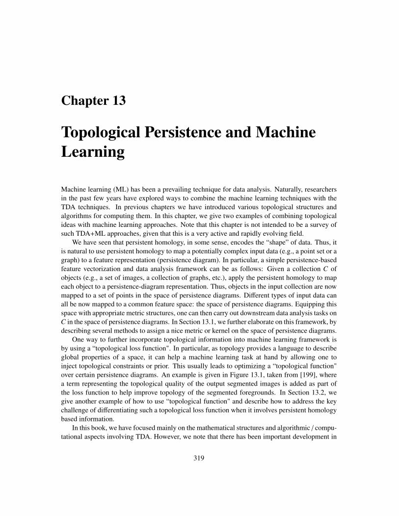
Chapter 13
Topological Persistence and MachineLearning
Machine learning (ML) has been a prevailing technique for data analysis. Naturally, researchersin the past few years have explored ways to combine the machine learning techniques with theTDA techniques. In previous chapters we have introduced various topological structures andalgorithms for computing them. In this chapter, we give two examples of combining topologicalideas with machine learning approaches. Note that this chapter is not intended to be a survey ofsuch TDA+ML approaches, given that this is a very active and rapidly evolving field.
We have seen that persistent homology, in some sense, encodes the “shape” of data. Thus, itis natural to use persistent homology to map a potentially complex input data (e.g., a point set or agraph) to a feature representation (persistence diagram). In particular, a simple persistence-basedfeature vectorization and data analysis framework can be as follows: Given a collection C ofobjects (e.g., a set of images, a collection of graphs, etc.), apply the persistent homology to mapeach object to a persistence-diagram representation. Thus, objects in the input collection are nowmapped to a set of points in the space of persistence diagrams. Different types of input data canall be now mapped to a common feature space: the space of persistence diagrams. Equipping thisspace with appropriate metric structures, one can then carry out downstream data analysis tasks onC in the space of persistence diagrams. In Section 13.1, we further elaborate on this framework, bydescribing several methods to assign a nice metric or kernel on the space of persistence diagrams.
One way to further incorporate topological information into machine learning framework isby using a “topological loss function". In particular, as topology provides a language to describeglobal properties of a space, it can help a machine learning task at hand by allowing one toinject topological constraints or prior. This usually leads to optimizing a “topological function"over certain persistence diagrams. An example is given in Figure 13.1, taken from [199], wherea term representing the topological quality of the output segmented images is added as part ofthe loss function to help improve topology of the segmented foregrounds. In Section 13.2, wegive another example of how to use “topological function" and describe how to address the keychallenge of differentiating such a topological loss function when it involves persistent homologybased information.
In this book, we have focused mainly on the mathematical structures and algorithmic / compu-tational aspects involving TDA. However, we note that there has been important development in
319
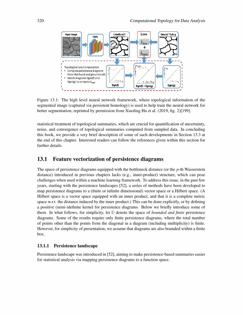
320 Computational Topology for Data Analysis
Figure 13.1: The high level neural network framework, where topological information of thesegmented image (captured via persistent homology) is used to help train the neural network forbetter segmentation; reprinted by permission from Xiaoling Hu et al. (2019, fig. 2)[199].
statistical treatment of topological summaries, which are crucial for quantification of uncertainty,noise, and convergence of topological summaries computed from sampled data. In concludingthis book, we provide a very brief description of some of such developments in Section 13.3 atthe end of this chapter. Interested readers can follow the references given within this section forfurther details.
13.1 Feature vectorization of persistence diagrams
The space of persistence diagrams equipped with the bottleneck distance (or the p-th Wassersteindistance) introduced in previous chapters lacks (e.g., inner-product) structure, which can posechallenges when used within a machine learning framework. To address this issue, in the past fewyears, starting with the persistence landscapes [52], a series of methods have been developed tomap persistence diagrams to a (finite or infinite dimensional) vector space or a Hilbert space. (AHilbert space is a vector space equipped with an inner product, and that it is a complete metricspace w.r.t. the distance induced by the inner product.) This can be done explicitly, or by defininga positive (semi-)definite kernel for persistence diagrams. Below we briefly introduce some ofthem. In what follows, for simplicity, let D denote the space of bounded and finite persistencediagrams. Some of the results require only finite persistence diagrams, where the total numberof points other than the points from the diagonal in a diagram (including multiplicity) is finite.However, for simplicity of presentation, we assume that diagrams are also bounded within a finitebox.
13.1.1 Persistence landscape
Persistence landscape was introduced in [52], aiming to make persistence-based summaries easierfor statistical analysis via mapping persistence diagrams to a function space.
Computational Topology for Data Analysis 321
Birth-time
Death-time
(1, 4)
(2, 6)
(3, 5)
(1, 4)
(2, 6)
(3, 5)λ1
λ2
λ3
(a) (b)Figure 13.2: (a) A persistence diagram D and its corresponding landscape functions are in (b),where λk := λD(k, ·) for k = 1, 2, and 3.
Definition 13.1 (Persistence landscape). Given a finite persistence diagram D = (bi, di)i∈[1,n]from D, the persistence landscape w.r.t. D is a function λD : N × R→ R where
λD(k, t) := k-th largest value of [mint − bi, di − t]+ for i ∈ [1, n].
Here, [c]+ = max(c, 0).
For a fixed k, λD(k, ·) : R→ R is a function on R. In particular, one can think of each persistentpoint (bi, di) giving rise to a triangle whose upper boundary is traced out by points
(t, [mint − bi, di − t]+) | t ∈ R;
see Fig. 13.2. There are n such triangles, and the function λD(k, ·) is the k-th upper envelop in thearrangement formed by the union of these triangles, which intuitively are points on the boundaryof the k-th layer of these triangles.
The persistence landscape maps the persistence diagrams to a linear function space. Thep-norm on persistence landscapes is defined as
‖λD‖pp =
∞∑k=1
‖λD(k, ·)‖pp.
Given two persistence diagrams D1 and D2, their p-landscape distance is defined by
Λp(D1,D2) = ‖λD1 − λD2‖p. (13.1)
Note that for any k > n, λD(k, ·) ≡ 0. One can recognize that persistence landscapes forfinite persistence diagrams lie in the so-called Lp-space Lp(N × R) 1. If p = 2, then this is aHilbert space. Given a set of persistence diagrams, one can compute their mean or carry out otherstatistical analysis in Lp(N × R). For example, given a set of ` finite diagrams D1, . . . ,D` ∈ D,one can define the mean landscape λ of their corresponding landscapes λD1 , . . . , λD` to be
λ(k, t) =1`
∑i=1
λDi(k, t).
1For 1 ≤ p < ∞, Lp(X) is defined as Lp(X) := f : X → R | ‖ f ‖p ≤ +∞. For example, L2(Rd) is the space ofstandard square-integrable functions on Rd. Then Lp(X) is defined as Lp(X) = Lp(X)/ ∼ where f ∼ g if ‖ f − g‖p = 0.
322 Computational Topology for Data Analysis
The following claim states that the map from the space of finite persistence diagrams D to thespace of persistence landscapes is injective, and this map is lossless in terms of the informationencoded in the persistence diagram.
Claim 13.1. Given a persistence diagram D, let λD be its persistence landscape. Then from λD
one can uniquely recover the persistence diagram D.
However, a function λ : N × R → R may not be the image of any valid persistence diagram.For example, the mean landscape introduced above may not be the image of any persistencediagram.
Finally, in addition to being injective, under appropriate norms, the map from persistencediagram to persistence landscape is also stable (1-Lipschitz w.r.t. the bottleneck distance betweenpersistence diagrams):
Theorem 13.1. For persistence diagrams D and D′, Λ∞(D,D′) ≤ dB(D,D′).
Additional stability results for Λp are given in [52], relating it to the p-th Wasserstein distancefor persistence diagrams, or for the case where the persistence diagrams are induced by tameLipschitz functions.
13.1.2 Persistence scale space (PSS) kernel
In the previous subsection, we introduced a way to map persistence diagrams into a functionspace Lp(N,R) (which is a Hilbert space when p = 2). One can also map persistence diagramsto a so-called Reproducing Kernel Hilbert Space via the use of kernels. The work of [263] is thefirst of a line of work defining a (positive semi-definite) kernel on persistence diagrams.
Definition 13.2 (Positive, negative semi-definite kernel). Given a topological space X, a functionk : X × X → R is a positive semi-definite kernel if it is symmetric and for any integer n > 0, anyx1, . . . , xn ∈ X, and any a1, . . . , an ∈ R, it holds that
∑i, j aia jk(xi, x j) ≥ 0. Analogously, k is a
negative semi-definite kernel if it is symmetric and any integer n > 0, any x1, . . . , xn ∈ X and anya1, . . . , an ∈ R, it holds that
∑i, j aia jk(xi, x j) ≤ 0. The function k is called conditionally negative
semi-definite if∑
i, j aia jk(xi, x j) ≤ 0 only holds for a1, . . . , an ∈ R with∑
i ai = 0.
Now, given a set X and a Hilbert space H of real-valued functions on X, the evaluationfunctional over H is a linear functional that evaluates each function in f at a point x: that is,given x, Lx : H → R is defined as Lx( f ) = f (x) for any f ∈ H. The Hilbert space H is called aReproducing Kernel Hilbert Space (RKHS) if Lx is continuous for all x ∈ X. It is known that givena positive semi-definite kernel k, there is a unique Reproducing Kernel Hilbert Space (RKHS) Hk
such that k(x, y) = 〈k(·, x), k(·, y)〉Hk . We call k the reproducing kernel for Hk. From now on,we simply use “kernel" to refer to a positive semi-definite kernel. See [271] for more detaileddiscussions of kernels, RKHS, and related concepts.
Equivalently, a kernel can be thought of as the inner product k(x, y) = 〈Φ(x),Φ(y)〉H aftermapping X to some Hilbert space H via a feature map Φ : X → H. With this inner product, onecan also further induce a pseudo-metric2 by:
d2k(x, y) := k(x, x) + k(y, y) − 2k(x, y), or equivalently, dk(x, y) = ‖x − y‖H.
2Recall that different from a metric, for a pseudo-metric, d(x, y) = 0 may not imply that x = y. All other conditionsfor a metric holds for a pseudo-metric.
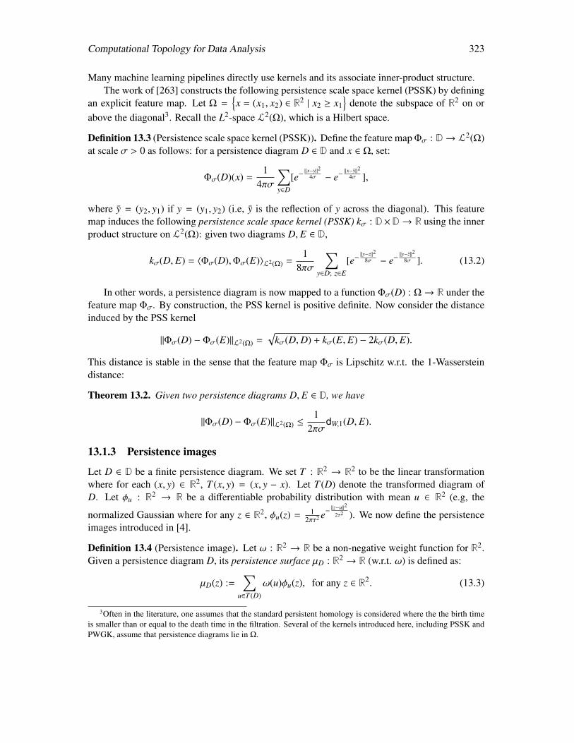
Computational Topology for Data Analysis 323
Many machine learning pipelines directly use kernels and its associate inner-product structure.The work of [263] constructs the following persistence scale space kernel (PSSK) by defining
an explicit feature map. Let Ω =x = (x1, x2) ∈ R2 | x2 ≥ x1
denote the subspace of R2 on or
above the diagonal3. Recall the L2-space L2(Ω), which is a Hilbert space.
Definition 13.3 (Persistence scale space kernel (PSSK)). Define the feature map Φσ : D→ L2(Ω)at scale σ > 0 as follows: for a persistence diagram D ∈ D and x ∈ Ω, set:
Φσ(D)(x) =1
4πσ
∑y∈D
[e−||x−y||2
4σ − e−||x−y||2
4σ ],
where y = (y2, y1) if y = (y1, y2) (i.e, y is the reflection of y across the diagonal). This featuremap induces the following persistence scale space kernel (PSSK) kσ : D×D→ R using the innerproduct structure on L2(Ω): given two diagrams D, E ∈ D,
kσ(D, E) = 〈Φσ(D),Φσ(E)〉L2(Ω) =1
8πσ
∑y∈D; z∈E
[e−||y−z||2
8σ − e−||y−z||2
8σ ]. (13.2)
In other words, a persistence diagram is now mapped to a function Φσ(D) : Ω→ R under thefeature map Φσ. By construction, the PSS kernel is positive definite. Now consider the distanceinduced by the PSS kernel
‖Φσ(D) − Φσ(E)‖L2(Ω) =√
kσ(D,D) + kσ(E, E) − 2kσ(D, E).
This distance is stable in the sense that the feature map Φσ is Lipschitz w.r.t. the 1-Wassersteindistance:
Theorem 13.2. Given two persistence diagrams D, E ∈ D, we have
‖Φσ(D) − Φσ(E)‖L2(Ω) ≤1
2πσdW,1(D, E).
13.1.3 Persistence images
Let D ∈ D be a finite persistence diagram. We set T : R2 → R2 to be the linear transformationwhere for each (x, y) ∈ R2, T (x, y) = (x, y − x). Let T (D) denote the transformed diagram ofD. Let φu : R2 → R be a differentiable probability distribution with mean u ∈ R2 (e.g, the
normalized Gaussian where for any z ∈ R2, φu(z) = 12πτ2 e−
‖z−u‖2
2τ2 ). We now define the persistenceimages introduced in [4].
Definition 13.4 (Persistence image). Let ω : R2 → R be a non-negative weight function for R2.Given a persistence diagram D, its persistence surface µD : R2 → R (w.r.t. ω) is defined as:
µD(z) :=∑
u∈T (D)
ω(u)φu(z), for any z ∈ R2. (13.3)
3Often in the literature, one assumes that the standard persistent homology is considered where the the birth timeis smaller than or equal to the death time in the filtration. Several of the kernels introduced here, including PSSK andPWGK, assume that persistence diagrams lie in Ω.
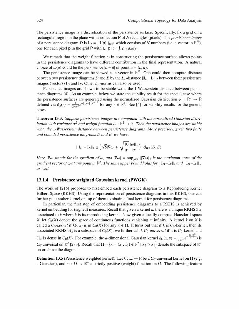
324 Computational Topology for Data Analysis
The persistence image is a discretization of the persistence surface. Specifically, fix a grid on arectangular region in the plane with a collection P of N rectangles (pixels). The persistence imageof a persistence diagram D is ID = I[p] p∈P which consists of N numbers (i.e, a vector in RN),one for each pixel p in the grid P with ID[p] :=
∫p ρD dxdy.
We remark that the weight function ω in constructing the persistence surface allows pointsin the persistence diagrams to have different contribution in the final representation. A naturalchoice of ω(u) could be the persistence |b − d| of point u = (b, d).
The persistence image can be viewed as a vector in RN . One could then compute distancebetween two persistence diagrams D and E by the L2-distance ‖ID−IE‖2 between their persistenceimages (vectors) ID and IE . Other Lp-norms can also be used.
Persistence images are shown to be stable w.r.t. the 1-Wasserstein distance between persis-tence diagrams [4]. As an example, below we state the stability result for the special case wherethe persistence surfaces are generated using the normalized Gaussian distribution φu : R2 → Rdefined via φu(z) = 1
2πσ2 e−‖z−u‖22/2σ2
for any z ∈ R2. See [4] for stability results for the generalcases.
Theorem 13.3. Suppose persistence images are computed with the normalized Gaussian distri-bution with variance σ2 and weight function ω : R2 → R. Then the persistence images are stablew.r.t. the 1-Wasserstein distance between persistence diagrams. More precisely, given two finiteand bounded persistence diagrams D and E, we have:
‖ ID − IE‖1 ≤(√
5|∇ω| +
√10π
‖ω‖∞σ
)· dW,1(D, E).
Here, ∇ω stands for the gradient of ω, and |∇ω| = supz∈R2 ‖∇ω‖2 is the maximum norm of thegradient vector ofω at any point in R2. The same upper bound holds for ‖ ID−IE‖2 and ‖ ID−IE‖∞
as well.
13.1.4 Persistence weighted Gaussian kernel (PWGK)
The work of [215] proposes to first embed each persistence diagram to a Reproducing KernelHilbert Space (RKHS). Using the representation of persistence diagrams in this RKHS, one canfurther put another kernel on top of them to obtain a final kernel for persistence diagrams.
In particular, the first step of embedding persistence diagrams to a RKHS is achieved bykernel embedding for (signed) measures. Recall that given a kernel k, there is a unique RKHS Hk
associated to k where k is its reproducing kernel. Now given a locally compact Hausdorff spaceX, let C0(X) denote the space of continuous functions vanishing at infinity. A kernel k on X iscalled a C0-kernel if k(·, x) is in C0(X) for any x ∈ Ω. It turns out that if k is C0-kernel, then itsassociated RKHS Hk is a subspace of C0(X); we further call k C0-universal if it is C0-kernel and
Hk is dense in C0(X). For example, the d-dimensional Gaussian kernel kG(x, y) = 12πτ2 e−
‖x−y‖2
2τ2 ) isC0-universal on Rd [283]. Recall that Ω =
x = (x1, x2) ∈ R2 | x2 ≥ x1
denote the subspace of R2
on or above the diagonal.
Definition 13.5 (Persistence weighted kernel). Let k : Ω→ R be a C0-universal kernel on Ω (e.g,a Gaussian), and ω : Ω → R+ a strictly positive (weight) function on Ω. The following feature
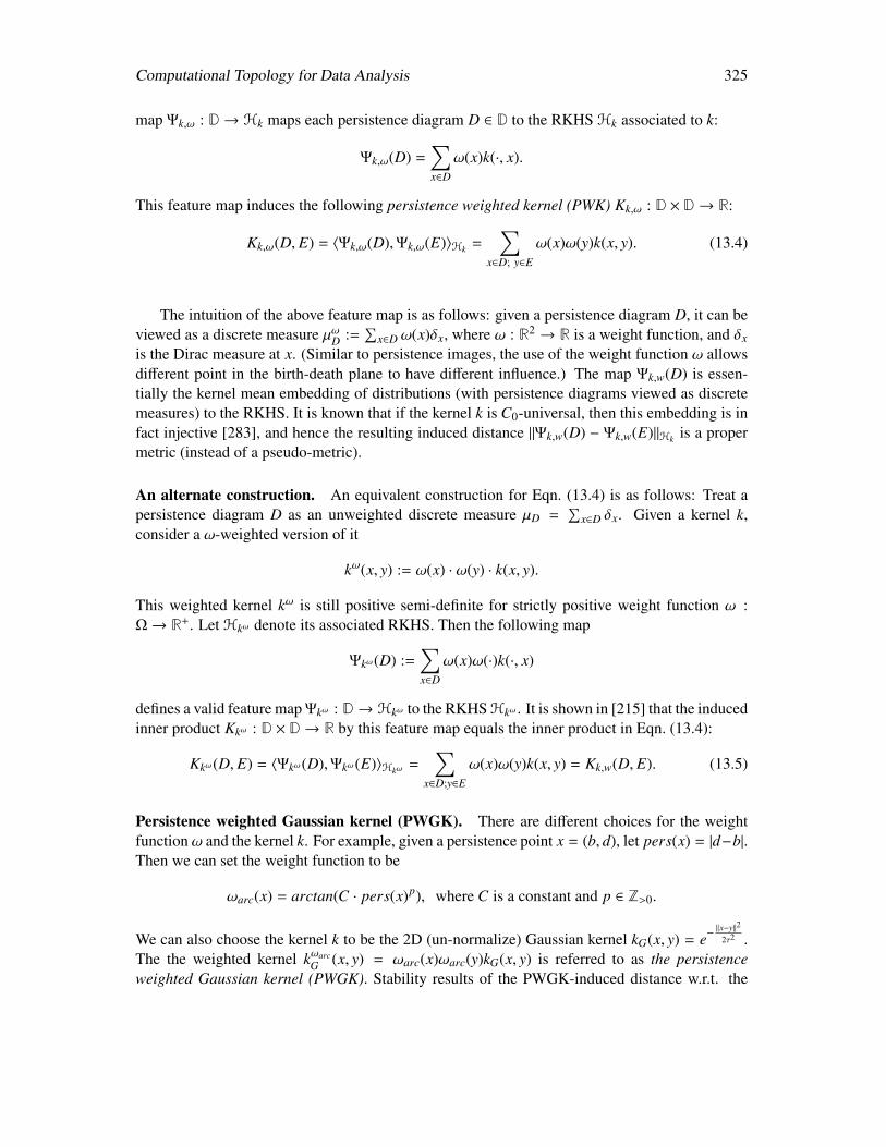
Computational Topology for Data Analysis 325
map Ψk,ω : D→ Hk maps each persistence diagram D ∈ D to the RKHS Hk associated to k:
Ψk,ω(D) =∑x∈D
ω(x)k(·, x).
This feature map induces the following persistence weighted kernel (PWK) Kk,ω : D × D→ R:
Kk,ω(D, E) = 〈Ψk,ω(D),Ψk,ω(E)〉Hk =∑
x∈D; y∈E
ω(x)ω(y)k(x, y). (13.4)
The intuition of the above feature map is as follows: given a persistence diagram D, it can beviewed as a discrete measure µωD :=
∑x∈D ω(x)δx, where ω : R2 → R is a weight function, and δx
is the Dirac measure at x. (Similar to persistence images, the use of the weight function ω allowsdifferent point in the birth-death plane to have different influence.) The map Ψk,w(D) is essen-tially the kernel mean embedding of distributions (with persistence diagrams viewed as discretemeasures) to the RKHS. It is known that if the kernel k is C0-universal, then this embedding is infact injective [283], and hence the resulting induced distance ‖Ψk,w(D) − Ψk,w(E)‖Hk is a propermetric (instead of a pseudo-metric).
An alternate construction. An equivalent construction for Eqn. (13.4) is as follows: Treat apersistence diagram D as an unweighted discrete measure µD =
∑x∈D δx. Given a kernel k,
consider a ω-weighted version of it
kω(x, y) := ω(x) · ω(y) · k(x, y).
This weighted kernel kω is still positive semi-definite for strictly positive weight function ω :Ω→ R+. Let Hkω denote its associated RKHS. Then the following map
Ψkω(D) :=∑x∈D
ω(x)ω(·)k(·, x)
defines a valid feature map Ψkω : D→ Hkω to the RKHS Hkω . It is shown in [215] that the inducedinner product Kkω : D × D→ R by this feature map equals the inner product in Eqn. (13.4):
Kkω(D, E) = 〈Ψkω(D),Ψkω(E)〉Hkω =∑
x∈D;y∈E
ω(x)ω(y)k(x, y) = Kk,w(D, E). (13.5)
Persistence weighted Gaussian kernel (PWGK). There are different choices for the weightfunctionω and the kernel k. For example, given a persistence point x = (b, d), let pers(x) = |d−b|.Then we can set the weight function to be
ωarc(x) = arctan(C · pers(x)p), where C is a constant and p ∈ Z>0.
We can also choose the kernel k to be the 2D (un-normalize) Gaussian kernel kG(x, y) = e−‖x−y‖2
2τ2 .The the weighted kernel kωarc
G (x, y) = ωarc(x)ωarc(y)kG(x, y) is referred to as the persistenceweighted Gaussian kernel (PWGK). Stability results of the PWGK-induced distance w.r.t. the
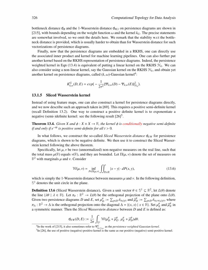
326 Computational Topology for Data Analysis
bottleneck distance dB and the 1-Wasserstein distance dW,1 on persistence diagrams are shown in[215], with bounds depending on the weight function ω and the kernel kG. The precise statementsare somewhat involved, so we omit the details here. We remark that the stability w.r.t the bottle-neck distance is provided, which is usually harder to obtain than for Wasserstein distance for suchvectorizations of persistence diagrams.
Finally, now that the persistence diagrams are embedded in a RKHS, one can directly usethe associated inner product and kernel for machine learning pipelines. One can also further putanother kernel based on the RKHS representation of persistence diagrams. Indeed, the persistenceweighted kernel in Eqn (13.4) is equivalent of putting a linear kernel on the RKHS Hk. We canalso consider using a non-linear kernel, say the Gaussian kernel on the RKHS Hk, and obtain yetanother kernel on persistence diagrams, called (k, ω)-Gaussian kernel4:
KGk,w(D, E) = exp
(−
12τ2 ‖Ψk,w(D) − Ψk,w(E)‖2Hk
).
13.1.5 Sliced Wasserstein kernel
Instead of using feature maps, one can also construct a kernel for persistence diagrams directly,and we now describe such an approach taken in [69]. This requires a positive semi-definite kernel(recall Definition 13.2). One way to construct a positive definite kernel is to exponentiate anegative (semi-)definite kernel: see the following result [26]5.
Theorem 13.4. Given X and φ : X × X → R, the kernel φ is conditionally negative semi-definiteif and only if e−tφ is positive semi-definite for all t > 0.
In what follows, we construct the so-called Sliced Wasserstein distance dS W for persistencediagrams, which is shown to be negative definite. We then use it to construct the Sliced Wasser-stein kernel following the above theorem.
Specifically, let µ, ν be two (unnormalized) non-negative measures on the real line, such thatthe total mass µ(R) equals ν(R), and they are bounded. Let Π(µ, ν) denote the set of measures onR2 with marginals µ and ν. Consider
W(µ, ν) = infP∈Π(µ,ν)
"R×R|x − y| · dP(x, y), (13.6)
which is simply the 1-Wasserstein distance between measures µ and ν. In the following definition,S1 denotes the unit circle in the plane.
Definition 13.6 (Sliced Wasserstein distance). Given a unit vector θ ∈ S1 ⊆ R2, let L(θ) denotethe line λθ | λ ∈ R. Let πθ : R2 → L(θ) be the orthogonal projection of the plane onto L(θ).Given two persistence diagrams D and E, set µθD :=
∑p∈D δπθ(p) and µθD :=
∑p∈D δπθπ∆(p), where
π∆ : R2 → ∆ is the orthogonal projection onto the diagonal ∆ = (x, x) | x ∈ R. Set µθE and µθE ina symmetric manner. Then the Sliced Wasserstein distance between D and E is defined as:
dS W(D, E) :=1
2π
∫S1
W(µθD + µθE , µθE + µθD)dθ.
4In the work of [215], it also sometimes refer to ΨGkG ,warc
as the persistence weighted Gaussian kernel.5In [26], the use of positive (negative) positive kernel is the same as our positive (negative) semi-positive kernel.
Computational Topology for Data Analysis 327
In the above definition, the sums µθD +µθE and µθE +µθD ensure the resulting two measures havethe same total mass.
Proposition 13.5. dS W is negative semi-definite on D where D is the space of bounded and finitepersistence diagrams.
Combining the above proposition with Theorem 13.4, we can now define the positive semi-definite Sliced Wasserstein kernel kS W on D as:
kS W(D, E) := e−dS W (D,E)
2σ2 , for σ > 0. (13.7)
The Sliced Wasserstein distance is not only stable, but also strongly equivalent to 1-Wassersteindistance dW,1 on bounded persistence diagrams in the following sense:
Theorem 13.6. Let DN be the set of bounded persistence diagrams with cardinalities at most N.For any D, E ∈ DN , one has:
dW,1(D, E)4N(4N − 1) + 2
≤ dS W(D, E) ≤ 2√
2 · dW,1(D, E).
13.1.6 Persistence Fisher kernel
The construction of persistence Fisher (PF) kernel, proposed by [218], uses a similar idea as theSliced Wasserstein (SW) distance in the sense that it will also leverage Theorem 13.4 to constructa positive definite kernel on persistence diagrams. However, it uses Fisher information metricfrom information geometry (usually used for probability measures) to derive the kernel. First,given a persistence diagram D, we map it to a function µD : R2 → R+ ∪ 0 as follows:
µD(x) :=1Z
∑z∈D
φG,σ(x, u),
where φG,σ(x, u) = e−‖x−u‖2
2σ and Z =
∫R2
∑u∈D
φG,σ(x, u)dx.
This function is similar to the persistence surface used in [4]. Recall that ∆ denotes the diagonalin the plane. Given a diagram D, let D∆ := π∆(u) | u ∈ D where π∆ denotes the orthogonalprojection onto the diagonal ∆.
Definition 13.7 (Persistence Fisher (PF) kernel). Given two persistence diagrams D, E, the Fisherinformation metric between their corresponding persistence surfaces µD and µE is defined as:
dFIM(D, E) := dFIM(µD∪E∆, µE∪D∆
) = arccos( ∫
R2
√µD∪E∆
(x)µE∪D∆(x) dx
).
The Persistence Fisher (PF) kernel for persistence diagrams is then defined as:
kPF(D, E) := e−t·dFIM(D,E), for some t > 0.
Note that similar to the Sliced-Wasserstein distance, the use of D ∪ E∆ (resp. E ∪ D∆) is toaddress the issue that D and E may have different cardinality.
328 Computational Topology for Data Analysis
Proposition 13.7. The function (dFIM − τ) is negative definite on the set of bounded and finitepersistence diagrams D for any τ ≥ π
2 .
By the above result and Theorem 13.4, we have that e−t(dFIM−τ) is positive definite for t > 0and τ ≥ π
2 . Furthermore, by definition, we can rewrite the Persistence Fisher kernel as:
kPF(D, E) = e−t·dFIM(D,E) = α · e−t·(dFIM(D,E)−τ), where τ ≥π
2and α = e−tτ > 0.
As α > 0 is a fixed constant, it then follows that:
Corollary 13.8. The Persistence Fisher kernel kPF is positive definite on D.
The work of [218] provides interesting analysis of the eigen system of the integral opera-tor induced by kPF . Furthermore, both persistence Fisher kernel and Sliced-Wasserstein kernelare infinitely divisible. This could bring computational advantages when using them in kernelmachines. The PSS kernel and PWGK kernels do not have this property.
We remark that there are other vectorization approaches of persistence diagrams developed.Very recently, there have also been several pieces of work on learning the representation of per-sistence diagrams in an end-to-end manner using labelled data. We will mention some of thesework in the Bibliography notes later.
13.2 Optimizing topological loss functions
Topology provides a language to describe global properties of a space. One could envision toadd topological constraints or priors for a machine learning task at hand. This usually leads tooptimizing a “topological function" over certain persistence diagrams. To motivate this, in Section13.2.1 we give an example where one aims to regularize the topological complexity of a classifierthat leads to a topological loss function. We then describe how a resulting topological functioncan be optimized in Section 13.2.2. We briefly discuss some other recent work on injectingtopological constraints / loss in machine learning pipelines at the end of this section.
13.2.1 Topological regularizer
We describe the work of [96], which uses persistent homology to regularize classifiers as anexample to illustrate the occurrence of topological functions. For simplicity, we consider thebinary classification problem, and assume that the domain X (where the input data is sampledfrom) is a d-dimensional hypercube. A classifier function is a smooth scalar function f : X→ R,which provides the prediction for a training/testing data point x ∈ X by evaluating sign( f (x)).In other words, the classification boundary (separating the positive and negative classificationregions), denoted by S f , is simply the 0-level set (i.e, the level set at function value 0):
S f = f −1(0) = x ∈ X | f (x) = 0.
See Fig. 13.3 (a) for an example, where the classification boundary S f consists of the U-shapedcurve and two closed loops.
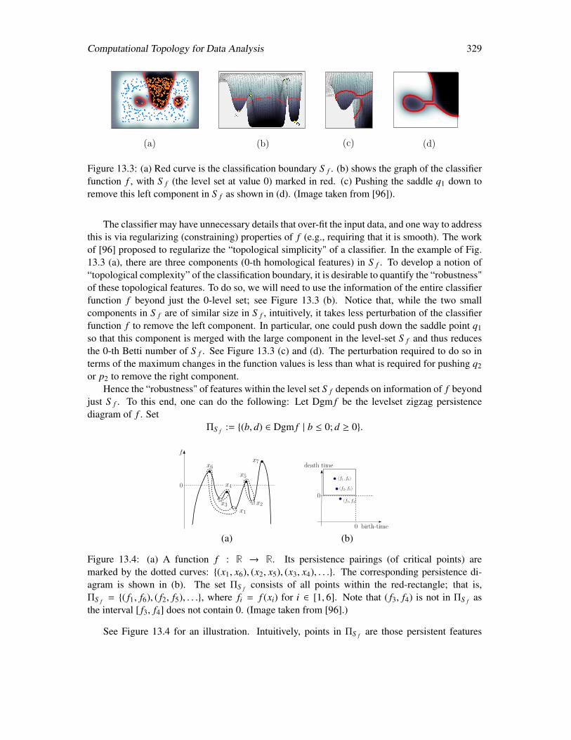
Computational Topology for Data Analysis 329
(a) (b) (c) (d)
Figure 13.3: (a) Red curve is the classification boundary S f . (b) shows the graph of the classifierfunction f , with S f (the level set at value 0) marked in red. (c) Pushing the saddle q1 down toremove this left component in S f as shown in (d). (Image taken from [96]).
The classifier may have unnecessary details that over-fit the input data, and one way to addressthis is via regularizing (constraining) properties of f (e.g., requiring that it is smooth). The workof [96] proposed to regularize the “topological simplicity" of a classifier. In the example of Fig.13.3 (a), there are three components (0-th homological features) in S f . To develop a notion of“topological complexity” of the classification boundary, it is desirable to quantify the “robustness"of these topological features. To do so, we will need to use the information of the entire classifierfunction f beyond just the 0-level set; see Figure 13.3 (b). Notice that, while the two smallcomponents in S f are of similar size in S f , intuitively, it takes less perturbation of the classifierfunction f to remove the left component. In particular, one could push down the saddle point q1so that this component is merged with the large component in the level-set S f and thus reducesthe 0-th Betti number of S f . See Figure 13.3 (c) and (d). The perturbation required to do so interms of the maximum changes in the function values is less than what is required for pushing q2or p2 to remove the right component.
Hence the “robustness" of features within the level set S f depends on information of f beyondjust S f . To this end, one can do the following: Let Dgm f be the levelset zigzag persistencediagram of f . Set
ΠS f := (b, d) ∈ Dgm f | b ≤ 0; d ≥ 0.
f
x1
x2x3
x4
x5
x6x7
0
birth-time
death time
(f3, f4)
(f2, f5)
(f1, f6)
0
0
(a) (b)
Figure 13.4: (a) A function f : R → R. Its persistence pairings (of critical points) aremarked by the dotted curves: (x1, x6), (x2, x5), (x3, x4), . . .. The corresponding persistence di-agram is shown in (b). The set ΠS f consists of all points within the red-rectangle; that is,ΠS f = ( f1, f6), ( f2, f5), . . ., where fi = f (xi) for i ∈ [1, 6]. Note that ( f3, f4) is not in ΠS f asthe interval [ f3, f4] does not contain 0. (Image taken from [96].)
See Figure 13.4 for an illustration. Intuitively, points in ΠS f are those persistent features
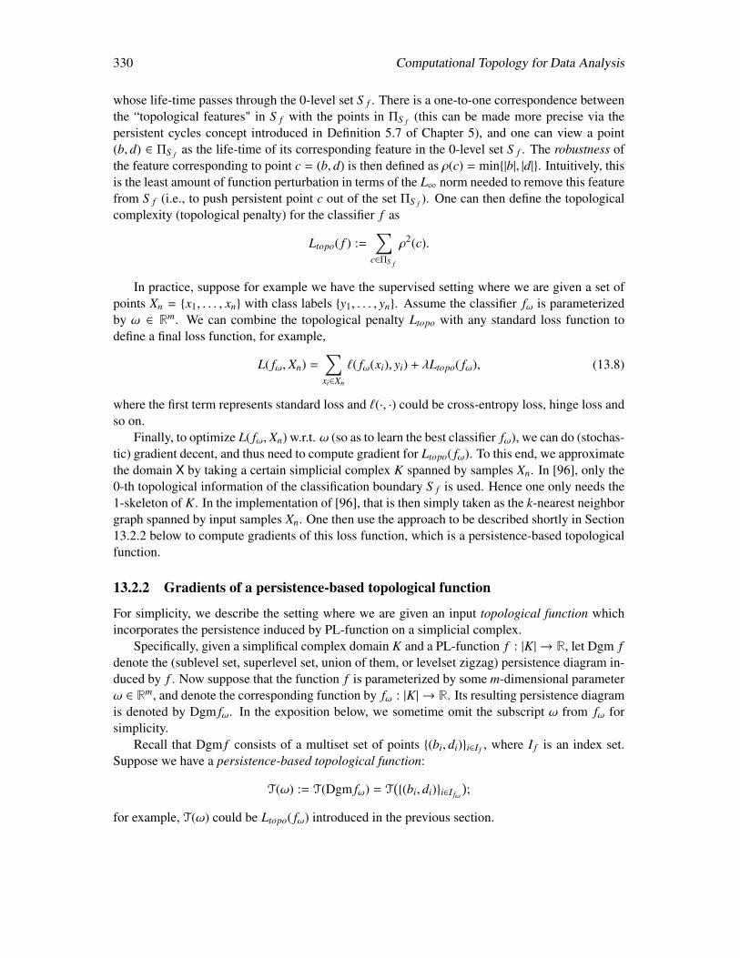
330 Computational Topology for Data Analysis
whose life-time passes through the 0-level set S f . There is a one-to-one correspondence betweenthe “topological features" in S f with the points in ΠS f (this can be made more precise via thepersistent cycles concept introduced in Definition 5.7 of Chapter 5), and one can view a point(b, d) ∈ ΠS f as the life-time of its corresponding feature in the 0-level set S f . The robustness ofthe feature corresponding to point c = (b, d) is then defined as ρ(c) = min|b|, |d|. Intuitively, thisis the least amount of function perturbation in terms of the L∞ norm needed to remove this featurefrom S f (i.e., to push persistent point c out of the set ΠS f ). One can then define the topologicalcomplexity (topological penalty) for the classifier f as
Ltopo( f ) :=∑
c∈ΠS f
ρ2(c).
In practice, suppose for example we have the supervised setting where we are given a set ofpoints Xn = x1, . . . , xn with class labels y1, . . . , yn. Assume the classifier fω is parameterizedby ω ∈ Rm. We can combine the topological penalty Ltopo with any standard loss function todefine a final loss function, for example,
L( fω, Xn) =∑xi∈Xn
`( fω(xi), yi) + λLtopo( fω), (13.8)
where the first term represents standard loss and `(·, ·) could be cross-entropy loss, hinge loss andso on.
Finally, to optimize L( fω, Xn) w.r.t. ω (so as to learn the best classifier fω), we can do (stochas-tic) gradient decent, and thus need to compute gradient for Ltopo( fω). To this end, we approximatethe domain X by taking a certain simplicial complex K spanned by samples Xn. In [96], only the0-th topological information of the classification boundary S f is used. Hence one only needs the1-skeleton of K. In the implementation of [96], that is then simply taken as the k-nearest neighborgraph spanned by input samples Xn. One then use the approach to be described shortly in Section13.2.2 below to compute gradients of this loss function, which is a persistence-based topologicalfunction.
13.2.2 Gradients of a persistence-based topological function
For simplicity, we describe the setting where we are given an input topological function whichincorporates the persistence induced by PL-function on a simplicial complex.
Specifically, given a simplifical complex domain K and a PL-function f : |K| → R, let Dgm fdenote the (sublevel set, superlevel set, union of them, or levelset zigzag) persistence diagram in-duced by f . Now suppose that the function f is parameterized by some m-dimensional parameterω ∈ Rm, and denote the corresponding function by fω : |K| → R. Its resulting persistence diagramis denoted by Dgm fω. In the exposition below, we sometime omit the subscript ω from fω forsimplicity.
Recall that Dgm f consists of a multiset set of points (bi, di)i∈I f , where I f is an index set.Suppose we have a persistence-based topological function:
T(ω) := T(Dgm fω) = T((bi, di)i∈I fω
);
for example, T(ω) could be Ltopo( fω) introduced in the previous section.
Computational Topology for Data Analysis 331
To optimize the topological function T(ω) one may need to compute gradient of T w.r.t. theparameter ω. Applying the chain rule, this means that one needs to be able to compute ∂bi
∂ω and∂di∂ω for certain points (bi, di) in the persistence diagram. (Terms such as ∂T
∂bican be computed
easily if the analytic form of T w.r.t. bis and dis are given; again, consider Ltopo( f ) from previoussection as an example.) Intuitively, this requires the “inverse” of the map which maps fω to itspersistence diagram Dgm fω. This inverse in general does not exists. However, assuming that fωis a PL function defined on K, then it turns out one can map bis and dis back to vertices of K andthis map is locally constant if all vertices of K have distinct function values.
More specifically, suppose Dgm f is generated by the persistent homology of the sublevelset filtration induced by f . Recall as described in Section 3.5.2, from the algorithmic point ofview, the sublevel set filtration is simulated by the so-called lower-star filtration of K. Usingnotations from Section 3.5.2, let Vi be the first i vertices of V , sorted in non-decreasing order oftheir function values, and Ki =
⋃j≤i Lst(vi) the set of all simplices spanned by vertices in Vi (i.e,
by vertices whose function value is at most f (vi)). The sublevel set filtration F is constructedby adding vi and all simplices in its lower-star in increasing order of i; recall Eqn. (3.10). Fur-thermore, recall that (Theorem 3.16) each persistent point in the diagram Dgm f is in fact of theform (bi, di) = ( f (v`i), f (vri)) such that the pairing function µ`i,ri
f > 0, and vertices v`i and vri areboth homological critical points for the PL-function f . We use the map ρ : Dgm f → V × V todenote this correspondence6 with ρ(bi, di) = (v`i , vri). We will also abuse notation slightly andwrite ρ(bi) = v`i and ρ(di) = vri . In other words, birth and death points in the persistence diagramDgm f can be mapped back to unique vertices in the vertex set of K.
This gives us a map ξ : Rm → 2V×V that map any parameter ω ∈ Rm to a collection ofpairs ξ(ω) := ρ(Dgm fω) ⊆ V × V . Assume that as the parameter ω ∈ Rm changes, the function fωchanges continuously (w.r.t the L∞ norm on the function space). It then follows that its persistencediagram Dgm fω also changes continuously due to the Stability result of persistence [102]. Theimage of Dgm fω under ρω also changes, although not necessarily continuously. Nevertheless, fora PL function fω, this image set stays fixed (constant) within a small neighborhood of ω if fω is“nice”. More specifically,
Proposition 13.9. Suppose fω : |K| → R is a PL-function with distinct values on all verticesV of K, and K is a finite simplicial complex. Then there exists a neighborhood of ω in theparameter space such that ξ remains constant within this neighborhood; that is, the image setξ(ω) = ρω(Dgm fω) remains the same for all parameters within this neighborhood.
Recall that bi = fω(ρω(bi)) = fω(v`i). It follows that, if conditions on fω in Proposition 13.9holds, then within a sufficiently small neighborhood of ω, even though bi moves continuously, theidentify of v`i remains the same and bi = fω(v`i) as ω varies within this neighborhood. Hence wehave
∂bi
ω=∂ fω(ρω(bi))
ω=∂ fω(v`i)ω
=∂ fωω
(v`i).
The derivative ∂di∂ω can be computed in an analogous manner by ∂ fω
∂ω (vri). This in turn leads to thecomputation of the derivative ∂T
∂ω for the persistence-based topological function T(ω).
6Note that while formulated differently, this map is the same as the one used in [257].
332 Computational Topology for Data Analysis
13.3 Statistical treatment of topological summaries
This book has been focused on the mathematical structures and computational aspects of varioustopological objects useful for topological data analysis. Topological methods help us to map aninput object to its topological summaries, and thus it is natural to compute statistics or performstatistical analysis of a collection of objects over their topological summaries. In this last sectionof the book, we briefly mention some developments regarding stochastic and statistical aspects oftopological summaries. We note that while the main content of this book does not focus on them,these are important topics for the development of topological data analysis, e.g., leading to morerigorous quantification of uncertainty, noise, consistency and so on.
Performing statistics on space of persistence diagrams. One key objective in data analysis isto model and quantify variations in data, such as computing the mean or variance of a collectionof data. Given the power of persistent homology in mapping an input complex object to itspersistence diagram summary, it’s natural to whether we can compute mean / variance in thespace of persistence diagrams. This question was first studied in [230], and to answer it, oneneeds to study the property of the space of persistence diagrams equipped with certain metrics.To state the results, we first need to refine the definition of Wasserstein distance of persistencediagrams (Definition 3.10) to allow different norms for measuring the distance between two pointsin the persistence diagram. The definition below assumes that we take the general view where apersistence diagram includes infinitely many copies of the diagonal.
Definition 13.8. Let P and Q be two persistence diagrams. The (p, q)-Wasserstein distance be-tween these two diagrams is:
dpW,q(P,Q) := inf
Π:P→Q
∑x∈P
‖x − Π(x)‖qp
1q
, (13.9)
where Π ranges over all bijections from P to Q.Note that our q-Wasserstein distance introduced in Definition 3.10 is simply d∞W,q under this
definition.
Now, let D∅ denote the trivial persistence diagram which contains only infinite copies of thediagonal.
Definition 13.9. Given p, q, the space of persistence diagrams Dpq consists of all persistence
diagrams within finite distance to the trivial persistence diagram D∅; that is,
Dpq :=
P | dp
W,q(P,D∅) < ∞.
In what follows, for simplicity, we abuse the notations slightly and let Dpq denote the met-
ric space (Dpq , d
pW,q) equipped with dp
W,q. It is shown in [230] that D∞q is a so-called Polish (i.e,complete and separable) space, and probability measures can be defined. It is later shown thatmore can be said about the space D2
2 (Theorem 2.5, [291]), which is a non-negatively curvedAlexandrov space (i.e., a geodesic space with curvature bounded from below by zero).
Computational Topology for Data Analysis 333
Furthermore, in both cases, the concept of “mean" and “variance" can be introduced using thenotion of Fréchet function. Specifically, in what follows, we use D to denote either D∞q and D2
2with metric dD be the corresponding metric d∞W,q or d2
W,2. We will consider probability measuresdefined on (D,B(D)), where B(D) is the Borel σ-algebra on D.
Definition 13.10. Given a probability distribution ρ on (D,B(D)), its Fréchet function Fρ : D→R is defined as, for any X ∈ D,
Fρ(X) :=∫D
d2D(X,Y)dρ(Y). (13.10)
The Fréchet variance of ρ is defined as the quantity
Varρ := infX∈D
Fρ(X),
while the set at which this variance is obtained, i.e.,
E(ρ) = X | Fρ(X) = Varρ,
is called the Fréchet expectation, or alternatively, the Fréchet mean set of ρ.
Often in the literature, one uses the Fréchet mean to refer to an element in the Fréchet meanset. Intuitively, the Fréchet function is a generalization of the arithmetic mean in the sense thatit minimizes the sum of the square distances to all points in the distribution. If the input is acollection of persistence diagrams Ω = D1,D2, . . . ,Dm, then we can talk about the mean of thiscollection as the mean of the discrete measure ρΩ = 1
m∑m
i=1 δDi induced by them, where δX is theDirac measure centered at X ∈ D.
In general, it is not clear whether Fréchet mean even exists. However, for the space D asdefined above, it is shown [230, 291] that Fréchet mean set is not empty under mild conditions onthe distribution.
Theorem 13.10. Let ρ be a probability measure on (D,B(D)) with a finite second moment, thatis, Fρ(X) < ∞ for any X ∈ D. If ρ has compact support, then E(ρ) , ∅.
In the case when D = D22, leveraging the property of D2
2, Turner et al. developed an iterativealgorithm to compute a local minimum of the Fréchet functional [291]. The computational ques-tion for Fréchet mean however remains open. We also note that in general, the Fréchet mean isnot unique. This becomes undesirable for example when tracking the mean of a set of varyingpersistence diagrams. To address this issue, a modified concept of probabilistic Fréchet mean isproposed in [239], which intuitively is a probabilistic measure on D2
2, and the authors show howto use this to build useful statistics on the vineyard (the time-varying persistence diagrams).
Other statistical analysis of topological summaries. Another line of statistical treatment oftopological objects concerns relating the estimation of them when input data is assumed to besampled from a target space / distribution. For example, a common setting is that suppose weobserve a sample x1, . . . , xn ∼ P, drawn i.i.d. from a distribution P supported on a compactset X ⊂ Rd. One can then ask questions of how to relate the topological summaries estimated
334 Computational Topology for Data Analysis
from these samples to that of X (when appropriate), whether such estimates converge, or how tocompute confidence interval (set) and so on.
We will not review the results here, as that would require careful description of the modelsused: We refer the readers to the nice survey by Wasserman in [297], which discussed the sta-tistical estimation for various topological objects, including (hierarchical) clustering (related tomerge trees), persistence diagrams, and ridge estimation. We will just mention that in the contextof persistence diagram and its variants (e.g, persistence landscapes), there has been work to ana-lyze their concentration and convergence behavior as the number of samples n tends to infinity fordifferent settings [86, 85], or to obtain confidence set for them via bootstrapping or subsampling[35, 84, 160].
The inference and estimation of topological information has been discussed earlier in Chap-ter 6; however we have assumed that the samples are deterministic there. Also note that as thedistribution P (where input points are sampled from) deviates further from the true distributionwe are interested in, the standard construction based on the Rips or Cech complexes to approx-imate the sublevel sets of the distance field (recall Definition 6.7 in Section 6.3.1) is not longerappropriate. Instead, one now needs to use more robust notions of “distance field". To this end,an elegant concept called distance to measures (DTM) has been proposed [80], which has manynice properties and can lead to more robust topology inferences; e.g., [83]. An alternative is touse kernel-distance as proposed in [256].
Finally, we note that there also has been a line of work to study topological properties (e.g.,Betti numbers, or the largest persistence in the persistence diagram) of random simplicial com-plexes [36, 37, 38, 202, 203, 204]. We will not describe this interesting line of work in this book.
13.4 Bibliographical notes
The persistence landscape proposed by Bubenik [52] is perhaps the first to map persistence dia-grams into a function space, which may often be taken to be a Banach space or a Hilbert space, soas to facilitate statistical analysis (e.g, computing mean) of persistence-based summaries. The per-sistence scale space (PSS) kernel, the persistence images, persistence weighted Gaussian kernel,sliced Wasserstein kernel, and persistence Fisher kernel described in this chapter are introducedin [263], [4], [215], [69], and [218], respectively. Note that this chapter does not aim to pro-vide a complete survey on vectorization frameworks for persistence diagrams; and in addition tothose presented in Chapter 13.1, there are other similar approaches such as [1, 143, 205, 250]. Asmentioned in Section 13.3, there has also been work exploring how to perform statistical analysisin the space of persistence diagrams equipped with standard bottleneck distance or Wassersteindistance; e.g. [35, 53, 87, 160, 230, 239, 291], and see more details in Section 13.3.
Recently, there has been a line of work to learn the representation of persistence diagramsin an end-to-end manner using labelled data. The work by Hofer et al. [194] was one of thefirst along this direction, and the authors developed a neural network layer for this purpose (andthe work is later refined in [195]). Later, an alternative layer (based on the Deep Sets architec-ture [303]) was proposed and developed in [68], which provides a rather general and versatileframework to learn vector representation for persistence diagrams. For example, the representa-tion learning can be based on several existing vectorization/kernelization of persistence diagrams,including the persistence landscapes, persistence surfaces and sliced Wasserstein. In a related
Computational Topology for Data Analysis 335
work [305], learning the best representation based on persistence images is formulated as an op-timization problem and solved directly via (stochastic) gradient descents. The resulting learnedvector representations can be combined simply with kernel-SVM for different tasks such as graphclassification.
Differentiating a function involving persistence has been independently proposed and studiedin several work from different communities, first in [165] for continuation of point clouds, then in[257] for continuous shape matching and in [96] for topological regularization of classifiers. Thegradients computation of a persistence-based topological function presented in Section 13.2.2follows mostly from the discussion in [257]. The general topological optimization frameworkis rather general and powerful. Several recent work apply such ideas to different stages of ma-chine learning applications. For example, [101, 199] used topological loss terms to help enforcea topological prior on individual input object for deep-learning based image segmentation. Thework of [101] assumed certain prior knowledge of the topology of the segmented images. Insteadof assuming this prior-knowledge, [199] proposed to learn to segment with correct topology byusing a topological loss function to help ensure that the topology of segmented images is thesame as the ground-truth for labelled images. The potential applications of these ideas has beenfurther broadened in [50], where the authors introduced and developed a topological layer forfunction-induced persistence and for distance-based filtration induced persistence. Such a persis-tence layer idea is further developed in [211] using the persistence landscape representation ofgeneral filtrations. Instead of having a topological constraint on individual input data point, onecan also consider using it for the latent space behind data. For example, [193, 236] applied suchideas with auto-encoders.
There has also been some recent work on using (persistent) homology to help characterizethe complexity of a neural network (or its training process). For example, [264] proposed the so-called neural persistence, to characterize the structural complexity of neural networks. [29, 180]proposed to measure the capacity of an architecture by the topological complexity of the classifiersit can produce. [168] proposed to study the topology of the activation networks (neural networkswith node activation for specific inputs), and used such patterns to help understand adversarialexamples. [243] studied the change of the topology of the transformed data space across differentlayers of a deep neural network. While overall, exploration in this direction is still in the initialstage, these are exciting ideas and there is much potential in using topological tools to understandneural networks.

336 Computational Topology for Data Analysis
Bibliography
[1] Aaron Aadcock, Erik Carlsson, and Gunnar Carlsson. The ring of algebraic functions onpersistence barcodes. Homology, Homotopy and Applications, 18:381–402, 2016.
[2] Michal Adamaszek and Henry Adams. The Vietoris-Rips complexes of a circle. Pacific J.Math., 290:1–40, 2017.
[3] Michal Adamaszek, Henry Adams, Ellen Gasparovic, Maria Gommel, Emilie Purvine,Radmila Sazdanovic, Bei Wang, Yusu Wang, and Lori Ziegelmeier. On homotopytypes of Vietoris-Rips complexes of metric gluings. J. Appl. Comput. Topology, 2020.https://doi.org/10.1007/s41468-020-00054-y.
[4] Henry Adams, Tegan Emerson, Michael Kirby, Rachel Neville, Chris Peterson, PatrickShipman, Sofya Chepushtanova, Eric Hanson, Francis Motta, and Lori Ziegelmeier. Persis-tence images: a stable vector representation of persistent homology. J. Machine LearningResearch, 18:218–252, 2017.
[5] Pankaj K. Agarwal, Herbert Edelsbrunner, John Harer, and Yusu Wang. Extreme elevationon a 2-manifold. Discrete Comput. Geom., 36(4):553–572, 2006.
[6] Pankaj K. Agarwal, Kyle Fox, Abhinandan Nath, Anastasios Sidiropoulos, and Yusu Wang.Computing the Gromov-Hausdorff distance for metric trees. ACM Trans. Algorithms,14(2):24:1–24:20, 2018.
[7] Paul Aleksandroff. Über den allgemeinen dimensionsbegriff und seine beziehungen zurelementaren geometrischen anschauung. Mathematische Annalen, 98:617–635, 1928.
[8] Nina Amenta, Marshall W. Bern, and David Eppstein. The crust and the beta-skeleton:Combinatorial curve reconstruction. Graphical Models Image Processing, 60(2):125–135,1998.
[9] Hideto Asashiba, Emerson G. Escolar, Yasuaki Hiraoka, and Hiroshi Takeuchi. Matrixmethod for persistence modules on commutative ladders of finite type. J. Industrial AppliedMath., 36(1):97–130, 2019.
[10] Michael Atiyah. On the Krull-Schmidt theorem with application to sheaves. Bulletin de laSociété Mathématique de France, 84:307–317, 1956.
337
338 Computational Topology for Data Analysis
[11] Dominique Attali, Herbert Edelsbrunner, and Yuriy Mileyko. Weak witnesses for Delaunaytriangulations of submanifolds. In Proc. ACM Sympos. Solid Physical Model., pages 143–150, 2007.
[12] Dominique Attali, André Lieutier, and David Salinas. Efficient data structure for represent-ing and simplifying simplicial complexes in high dimensions. In Proc. 27th Annu. Sympos.Comput. Geom. (SoCG), pages 501–509, 2011.
[13] Maurice Auslander. Representation theory of Artin Algebras II. Communications in Alge-bra, 1(4):269–310, 1974.
[14] Maurice Auslander and David Buchsbaum. Groups, rings, modules. Dover Publications,2014.
[15] Aravindakshan Babu. Zigzag coarsenings, mapper stability and gene-network analyses,2013. PhD thesis, Stanford University.
[16] Samik Banerjee, Lucas Magee, Dingkang Wang, Xu Li, Bing xing Huo, Jaikishan Jayaku-mar, Katherine Matho, Meng-Kuan Lin, Keerthi Ram, Mohanasankar Sivaprakasam,Josh Huang, Yusu Wang, and Partha Mitra. Semantic segmentation of microscopicneuroanatomical data by combining topological priors with encoder-decoder deep net-works. Nature Machine Intelligence, 2:585–594, 2020. Also available on biorxiv at2020.02.18.955237.
[17] Jonathan Ariel Barmak and Elias Gabriel Minian. Strong homotopy types, nerves andcollapses. Discret. Comput. Geom., 47(2):301–328, 2012.
[18] Saugata Basu and Negin Karisani. Efficient simplicial replacement of semi-algebraic setsand applications. CoRR, arXiv:2009.13365, 2020.
[19] Ulrich Bauer. Ripser: efficient computation of Vietoris-Rips persistence barcodes. CoRR,arXiv:1908.02518, 2019.
[20] Ulrich Bauer, Xiaoyin Ge, and Yusu Wang. Measuring distance bewteen Reeb graphs. InProc. 30th Annu. Sympos. Comput. Geom. (SoCG), pages 464–473, 2014.
[21] Ulrich Bauer, Michael Kerber, and Jan Reininghaus. Clear and compress: Computingpersistent homology in chunks. In Topological methods in data analysis and visualizationIII, pages 103–117. Springer, 2014.
[22] Ulrich Bauer, Claudia Landi, and Facundo Mémoli. The Reeb graph edit distance is uni-versal. In Proc. 36th Internat. Sympos. Comput. Geom. (SoCG), pages 15:1–15:16, 2020.
[23] Ulrich Bauer, Carsten Lange, and Max Wardetzky. Optimal topological simplification ofdiscrete functions on surfaces. Discrete Comput. Geom., 47(2):347–377, 2012.
[24] Ulrich Bauer and Michael Lesnick. Induced matchings of barcodes and the algebraic sta-bility of persistence. In Proc. 13th Annu. Sympos. Comput. Geom. (SoCG), pages 355–364,2014.

Computational Topology for Data Analysis 339
[25] Ulrich Bauer, Elizabeth Munch, and Yusu Wang. Strong equivalence of the interleavingand functional distortion metrics for Reeb graphs. In Proc. 31st Annu. Sympos. Comput.Geom. (SoCG), pages 461–475, 2015.
[26] Christian Berg, Jens P. R. Christensen, and Paul Ressel. Harmonic analysis on semigroups:Theory of positive definite and related functions. Springer, 1984.
[27] Marshall W. Bern, David Eppstein, Pankaj K. Agarwal, Nina Amenta, L. Paul Chew,Tamal K. Dey, David P. Dobkin, Herbert Edelsbrunner, Cindy Grimm, Leonidas J. Guibas,John Harer, Joel Hass, Andrew Hicks, Carroll K. Johnson, Gilad Lerman, David Letscher,Paul E. Plassmann, Eric Sedgwick, Jack Snoeyink, Jeff Weeks, Chee-Keng Yap, and DenisZorin. Emerging challenges in computational topology. CoRR, arXiv:cs/9909001, 1999.
[28] Dimitris Bertsimas and John N. Tsitsiklis. Introduction to Linear Optimization. AthenaScientific, Belmont, MA, 1997.
[29] Monica Bianchini and Franco Scarselli. On the complexity of neural network classifiers:A comparison between shallow and deep architectures. IEEE Trans. Neural NetworksLearning Sys., 25(8):1553–1565, 2014.
[30] Silvia Biasotti, Andrea Cerri, Patrizio Frosini, and Daniela Giorgi. A new algorithm forcomputing the 2-dimensional matching distance between size functions. Pattern Recogni-tion Letters, 32(14):1735–1746, 2011.
[31] Silvia Biasotti, Bianca Falcidieno, and Michela Spagnuolo. Extended Reeb graphs for sur-face understanding and description. In Proc. 9th Internat. Conf. Discrete Geom. ComputerImagery, pages 185–197, 2000.
[32] Silvia Biasotti, Daniela Giorgi, Michela Spagnuolo, and Bianca Falcidieno. Reeb graphsfor shape analysis and applications. Theor. Comput. Sci., 392(1-3):5–22, 2008.
[33] Håvard Bjerkevik. Stability of higher-dimensional interval decomposable persistence mod-ules. CoRR, arXiv:1609.02086, 2020.
[34] Håvard Bjerkevik, Magnus Botnan, and Michael Kerber. Computing the interleaving dis-tance is NP-hard. Found. Comput. Math., 2019.
[35] Ander J. Blumberg, Itamar Gal, Michael A. Mandell, and Matthew Pancia. Robust statis-tics, hypothesis testing, and confidence intervals for persistent homology on metric mea-sure spaces. Found. Comput. Math., 14:745–789, 2014.
[36] Omer Bobrowski and Matthew Kahle. Topology of random geometric complexes: a survey.J. Applied Comput. Topology, 1(3):331–364, 2018.
[37] Omer Bobrowski, Matthew Kahle, and Primoz Skraba. Maximally persistent cycles inrandom geometric complexes. Ann. Appl. Probab., 27(4):2032–2060, 2017.
[38] Omer Bobrowski and Primoz Skraba. Homological percolation and the Euler characteris-tic. Phys. Rev. E, 101:032304, 2020.
340 Computational Topology for Data Analysis
[39] Erik Boczko, William D. Kalies, and Konstantin Mischaikow. Polygonal approximation offlows. Topology and its Applications, 154:2501–2520, 2007.
[40] Jean-Daniel Boissonnat, Frédéric Chazal, and Mariette Yvinec. Geometric and TopologicalInference. Cambride Texts in Applied Mathematics. Cambridge U. Press, 2018.
[41] Jean-Daniel Boissonnat, Leonidas J. Guibas, and Steve Y. Oudot. Manifold reconstructionin arbitrary dimensions using witness complexes. In Proc. 23rd Annu. Sympos. Comput.Geom. (SoCG), pages 194–203, 2007.
[42] Jean-Daniel Boissonnat and Siddharth Pritam. Edge collapse and persistence of flag com-plexes. In 36th Internat. Sympos. Comput. Geom., (SoCG), volume 164 of LIPIcs, pages19:1–19:15, 2020.
[43] Jean-Daniel Boissonnat, Siddharth Pritam, and Divyansh Pareek. Strong collapse for per-sistence. In 26th Annu. European Sympos. Algorithms, ESA, volume 112 of LIPIcs, pages67:1–67:13, 2018.
[44] Glencora Borradaile, Erin Wolf Chambers, Kyle Fox, and Amir Nayyeri. Minimum cycleand homology bases of surface-embedded graphs. J. Comput. Geom. (JoCG), 8(2):58–79,2017.
[45] Glencora Borradaile, William Maxwell, and Amir Nayyeri. Minimum bounded chainsand minimum homologous chains in embedded simplicial complexes. In 36th Internat.Sympos. Comput. Geom., (SoCG), volume 164 of LIPIcs, pages 21:1–21:15, 2020.
[46] Karol Borsuk. On the imbedding of systems of compacta in simplicial complexes. Funda-menta Mathematicae, 35:217–234, 1948.
[47] Magnus Botnan, Justin Curry, and Elizabeth Munch. The poset interleaving distance, 2016.
[48] Magnus Botnan and Michael Lesnick. Algebraic stability of zigzag persistence modules.Algebraic & Geometric Topology, 18:3133–3204, 2018.
[49] Stephane Bressan, Jingyan Li, Shiquan Ren, and Jie Wu. The embedded homology ofhypergraphs and applications. Asian J. Math., 23(3):479–500, 2019.
[50] Rickard Brüel-Gabrielsson, Bradley J. Nelson, Anjan Dwaraknath, Primoz Skraba,Leonidas J. Guibas, and Gunnar Carlsson. A topology layer for machine learn-ing. CoRR, arXiv:1905.12200, 2019. Code available at https://github.com/bruel-gabrielsson/TopologyLayer.
[51] Winfried Bruns and H Jürgen Herzog. Cohen-Macaulay Rings. Cambridge UniversityPress, 1998.
[52] Peter Bubenik. Statistical topological data analysis using persistence landscapes. J. Ma-chine Learning Research, 16(1):77–102, 2015.
[53] Peter Bubenik and Peter T. Kim. A statistical approach to persistent homology. Homology,Homotopy, and Applications, 9(2):337–362, 2007.
Computational Topology for Data Analysis 341
[54] Peter Bubenik and Jonathan Scott. Categorification of persistent homology. Discrete Com-put. Geom., 51(3):600–627, 2014.
[55] Peter Bubenik, Jonathan A. Scott, and Donald Stanley. Wasserstein distance for generalizedpersistence modules and abelian categories. arXiv: Rings and Algebras, arxiv:1809.09654,2018.
[56] Michaël Buchet, Frédéric Chazal, Tamal K. Dey, Fengtao Fan, Steve Y. Oudot, and YusuWang. Topological analysis of scalar fields with outliers. In Proc. 31st Annu. Sympos.Comput. Geom. (SoCG), pages 827–841, 2015.
[57] Mickaël Buchet, Frédéric Chazal, Steve Y. Oudot, and Donald Sheehy. Efficient and ro-bust persistent homology for measures. In Proc. 26th Annu. ACM-SIAM Sympos. DiscreteAlgorithms (SODA), pages 168–180, 2015.
[58] James R. Bunch and John E. Hopcroft. Triangular factorization and inversion by fast matrixmultiplication. Mathematics of Computation, 28(125):231–236, 1974.
[59] Dmitri Burago, Yuri Burago, and Sergei Ivanov. A course in metric geometry. volume 33of AMS Graduate Studies in Math. American Mathematics Society, 2001.
[60] Dan Burghelea and Tamal K. Dey. Topological persistence for circle-valued maps. DiscreteComput. Geom., 50(1):69–98, 2013.
[61] Oleksiy Busaryev, Sergio Cabello, Chao Chen, Tamal K. Dey, and Yusu Wang. Annotatingsimplices with a homology basis and its applications. In Algorithm Theory - SWAT 2012 -13th Scandinavian Sympos. Workshops, pages 189–200, 2012.
[62] Alexander Buslaev, Selim S Seferbekov, Vladimir Iglovikov, and Alexey Shvets. Fullyconvolutional network for automatic road extraction from satellite imagery. In CVPR Work-shops, pages 207–210, 2018.
[63] Gunnar Carlsson and Vin de Silva. Zigzag persistence. Found. Comput. Math., 10(4):367–405, Aug 2010.
[64] Gunnar Carlsson, Vin de Silva, and Dmitriy Morozov. Zigzag persistent homology andreal-valued functions. In Proc. 26th Annu. Sympos. Comput. Geom. (SoCG), pages 247–256, 2009.
[65] Gunnar Carlsson, Gurjeet Singh, and Afra Zomorodian. Computing multidimensional per-sistence. In Proc. Internat. Sympos. Algorithms Computation (ISAAC), pages 730–739.Springer, 2009.
[66] Gunnar Carlsson and Afra Zomorodian. The theory of multidimensional persistence. Dis-crete Comput. Geom., 42(1):71–93, 2009.
[67] Hamish Carr, Jack Snoeyink, and Ulrike Axen. Computing contour trees in all dimensions.Comput. Geom.: Theory and Applications, 24(2):75–94, 2003.
342 Computational Topology for Data Analysis
[68] Mathieu Carrière, Frédéric Chazal, Yuichi Ike, Théo Lacombe, Martin Royer, and YuheiUmeda. Perslay: a neural network layer for persistence diagrams and new graph topologi-cal signatures. In Proc. 23rd Internat. Conf. Artificial Intelligence Stat. (AISTATS), volume108, pages 2786–2796, 2020.
[69] Mathieu Carrière, Marco Cuturi, and Steve Y. Oudot. Sliced Wasserstein kernel for persis-tence diagrams. In Proc. Internat. Conf. Machine Learning, pages 664–673, 2017.
[70] Mathieu Carrière and Steve Oudot. Structure and stability of the one-dimensional mapper.Found. Comput. Math., 18(6):1333–1396, 2018.
[71] Nicholas J. Cavanna, Mahmoodreza Jahanseir, and Donald R. Sheehy. A geometric per-spective on sparse filtrations. In Proc. Canadian Conf. Comput. Geom. (CCCG), 2015.
[72] Andrea Cerri, Barbara Di Fabio, Massimo Ferri, Patrizio Frosini, and Claudia Landi. Bettinumbers in multidimensional persistent homology are stable functions. MathematicalMethods in the Applied Sciences, 36(12):1543–1557, 2013.
[73] Andrea Cerri and Patrizio Frosini. A new approximation algorithm for the matching dis-tance in multidimensional persistence. J. Comput. Math., pages 291–309, 2020.
[74] Erin W. Chambers, Jeff Erickson, and Amir Nayyeri. Minimum cuts and shortest homolo-gous cycles. In Proc. 25th Annu. Sympos. Comput. Geom. (SoCG), pages 377–385, 2009.
[75] Erin W. Chambers, Jeff Erickson, and Amir Nayyeri. Homology flows, cohomology cuts.SIAM J. Comput., 41(6):1605–1634, 2012.
[76] Manoj K. Chari. On discrete Morse functions and combinatorial decompositions. DiscreteMath., 217(1-3):101–113, 2000.
[77] Isaac Chavel. Riemannian Geometry: A Modern Introduction, 2nd Ed. Cambridge univer-sity press, 2006.
[78] Frédéric Chazal, David Cohen-Steiner, Marc Glisse, Leonidas J. Guibas, and Steve Oudot.Proximity of persistence modules and their diagrams. In Proc. 25th Annu. Sympos. Comput.Geom. (SoCG), pages 237–246, 2009.
[79] Frédéric Chazal, David Cohen-Steiner, Leonidas J. Guibas, Facundo Mémoli, and Steve Y.Oudot. Gromov-Hausdorff stable signatures for shapes using persistence. Comput. Graph-ics Forum, 28(5):1393–1403, 2009.
[80] Frédéric Chazal, David Cohen-Steiner, and Quentin Mérigot. Geometric inference forprobability distributions. Found. Comput. Math., 11(6):733–751, 2011.
[81] Frédéric Chazal, Vin de Silva, Marc Glisse, and Steve Oudot. The structure and stabilityof persistence modules. CoRR, arXiv:1207.3674, 2012.
[82] Frédéric Chazal, Vin de Silva, and Steve Oudot. Persistence stability for geometric com-plexes. Geometriae Dedicata, 173(1):193–214, Dec 2014.
Computational Topology for Data Analysis 343
[83] Frédéric Chazal, Brittany Fasy, Fabrizio Lecci, Bertr, Michel, Aless, ro Rinaldo, and LarryWasserman. Robust topological inference: Distance to a measure and kernel distance. J.Machine Learning Research, 18(159):1–40, 2018.
[84] Frédéric Chazal, Brittany Fasy, Fabrizio Lecci, Alessandro Rinaldo, Aarti Singh, and LarryWasserman. On the bootstrap for persistence diagrams and landscapes. Modeling AnalysisInfo. Sys., 20(6):96–105, 2013. Also available at arXiv:1311.0376.
[85] Frédéric Chazal, Brittany Terese Fasy, Fabrizio Lecci, Alessandro Rinaldo, and Larry A.Wasserman. Stochastic convergence of persistence landscapes and silhouettes. J. Comput.Geom. (JoCG), 6(2):140–161, 2015.
[86] Frédéric Chazal, Marc Glisse, Catherine Labruère, and Bertrand Michel. Convergencerates for persistence diagram estimation in topological data analysis. J. Machine LearningResearch, 16(110):3603–3635, 2015.
[87] Frédéric Chazal, Marc Glisse, Catherine Labruère, and Bertrand Michel. Convergencerates for persistence diagram estimation in Topological Data Analysis. J. Machine Learn-ing Research, 16:3603–3635, 2015.
[88] Frédéric Chazal, Leonidas J. Guibas, Steve Oudot, and Primoz Skraba. Analysis of scalarfields over point cloud data. Discrete Comput. Geom., 46(4):743–775, 2011.
[89] Frédéric Chazal, Ruqi Huang, and Jian Sun. Gromov-Hausdorff approximation of filamen-tary structures using Reeb-type graphs. Discrete Comput. Geom., 53:621–649, 2015.
[90] Frédéric Chazal and André Lieutier. Weak feature size and persistent homology: com-puting homology of solids in Rn from noisy data samples. In Proc. 21st Annu. Sympos.Comput. Geom. (SoCG), pages 255–262, 2005.
[91] Frédéric Chazal and André Lieutier. Stability and computation of topological invariants ofsolids in Rn. Discrete Comput. Geom., 37(4):601–617, 2007.
[92] Frédéric Chazal and Steve Y. Oudot. Towards persistence-based reconstruction in Eu-clidean spaces. In Proc. 24th Annu. Sympos. Comput. Geom. (SoCG), pages 232–241,2008.
[93] Bernard Chazelle. An optimal convex hull algorithm in any fixed dimension. DiscreteComput. Geom., 10:377–409, 1993.
[94] Chao Chen and Daniel Freedman. Measuring and computing natural generators for homol-ogy groups. Comput. Geom.: Theory & Applications, 43 (2):169–181, 2010.
[95] Chao Chen and Daniel Freedman. Hardness results for homology localization. DiscreteComput. Geometry, 45 (3):425–448, 2011.
[96] Chao Chen, Xiuyan Ni, Qinxun Bai, and Yusu Wang. A topological regularizer for clas-sifiers via persistent homology. In Proc. 22nd Internat. Conf. Artificial Intelligence Stat.(AISTATS), pages 2573–2582, 2019.
344 Computational Topology for Data Analysis
[97] Siu-Wing Cheng, Tamal K. Dey, and Edgar A. Ramos. Manifold reconstruction from pointsamples. In Proc. 16th Annu. ACM-SIAM Sympos. Discrete Algorithms (SODA), pages1018–1027, 2005.
[98] Siu-Wing Cheng, Tamal K. Dey, and Jonathan R. Shewchuk. Delaunay Mesh Generation.CRC Press, 2012.
[99] Samir Chowdhury and Facundo Mémoli. Persistent homology of asymmetric networks:An approach based on Dowker filtrations. CoRR, arXiv:1608.05432, 2018.
[100] Samir Chowdhury and Facundo Mémoli. Persistent path homology of directed networks.In Proc. 29th Annu. ACM-SIAM Sympos. Discrete Algorithms (SODA), pages 1152–1169.SIAM, 2018.
[101] James R. Clough, Ilkay Oksuz, Nicholas Byrne, Veronika A. Zimmer, Julia A. Schnabel,and Andrew P. King. A topological loss function for deep-learning based image segmen-tation using persistent homology. CoRR, 2019.
[102] David Cohen-Steiner, Herbert Edelsbrunner, and John Harer. Stability of persistence dia-grams. Discrete Comput. Geom., 37(1):103–120, Jan 2007.
[103] David Cohen-Steiner, Herbert Edelsbrunner, and John Harer. Extending persistence usingPoincaré and Lefschetz duality. Found. Comput. Math., 9(1):79–103, 2009.
[104] David Cohen-Steiner, Herbert Edelsbrunner, John Harer, and Yuriy Mileyko. Lipschitzfunctions have Lp-stable persistence. Found. Comput. Math., 10(2):127–139, 2010.
[105] David Cohen-Steiner, Herbert Edelsbrunner, John Harer, and Dmitriy Morozov. Persistenthomology for kernels, images, and cokernels. In Proc. 20th Annu. ACM-SIAM Sympos.Discrete Algorithms (SODA), pages 1011–1020, 2009.
[106] David Cohen-Steiner, Herbert Edelsbrunner, and Dmitriy Morozov. Vines and vineyards byupdating persistence in linear time. In Proc. 22nd Annu. Sympos. Comput. Geom. (SoCG),pages 119–126, 2006.
[107] Kree Cole-McLaughlin, Herbert Edelsbrunner, John Harer, Vijay Natarajan, and ValerioPascucci. Loops in Reeb graphs of 2-manifolds. Discrete Comput. Geom., 32(2):231–244,2004.
[108] René Corbet and Michael Kerber. The representation theorem of persistence revisited andgeneralized. J. Appl. Comput. Topology, 2(1):1–31, Oct 2018.
[109] Thomas H. Cormen, Charles E. Leiserson, Ronald L. Rivest, and Clifford Stein. Introduc-tion to Algorithms, Third Edition. The MIT Press, 3rd edition, 2009.
[110] David A Cox, John Little, and Donal O’shea. Using Algebraic Geometry, volume 185.Springer Science & Business Media, 2006.
[111] William Crawley-Boevey. Decomposition of pointwise finite-dimensional persistencemodules. J. Algebra and Its Applications, 14(05):1550066, 2015.
Computational Topology for Data Analysis 345
[112] Justin Curry. Sheaves, cosheaves and applications. CoRR, arXiv:1303.3255, 2013.
[113] Vin de Silva. A weak definition of Delaunay triangulation. CoRR, arXiv:cs/0310031, 2003.
[114] Vin de Silva and Gunnar Carlsson. Topological estimation using witness complexes. InProc. Sympos. Point-Based Graphics., 2004.
[115] Vin de Silva, Dmitriy Morozov, and Mikael Vejdemo-Johansson. Dualities in persistent(co)homology. Inverse Problems, 27:124003, 2011.
[116] Vin de Silva, Elizabeth Munch, and Amit Patel. Categorified Reeb graphs. Discrete Com-put. Geom., 55(4):854–906, 2016.
[117] Cecil Jose A. Delfinado and Herbert Edelsbrunner. An incremental algorithm for Bettinumbers of simplicial complexes on the 3-sphere. Comput. Aided Geom. Design,12(7):771–784, 1995.
[118] Olaf Delgado-Friedrichs, Vanessa Robins, and Adrian P. Sheppard. Skeletonization andpartitioning of digital images using discrete Morse theory. IEEE Trans. Pattern Anal. Ma-chine Intelligence, 37(3):654–666, 2015.
[119] Tamal K. Dey. Curve and Surface Reconstruction: Algorithms with Mathematical Analy-sis. Cambridge Monographs Applied Comput. Math. Cambridge University Press, 2006.
[120] Tamal K. Dey, Herbert Edelsbrunner, and Sumanta Guha. Computational topology. Ad-vances in Discrete Comput. Geom., 1999.
[121] Tamal K. Dey, Herbert Edelsbrunner, Sumanta Guha, and Dmitry V. Nekhayev. Topologypreserving edge contraction. Publications de l’ Institut Mathematique (Beograd), 60:23–45, 1999.
[122] Tamal K. Dey, Fengtao Fan, and Yusu Wang. Computing topological persistence for sim-plicial maps. CoRR, arXiv:1208.5018, 2012.
[123] Tamal K. Dey, Fengtao Fan, and Yusu Wang. An efficient computation of handle and tunnelloops via reeb graphs. ACM Trans. Graph., 32(4):32, 2013.
[124] Tamal K. Dey, Fengtao Fan, and Yusu Wang. Graph induced complex for point data. InProc. 29th. Annu. Sympos. Comput. Geom. (SoCG), pages 107–116, 2013.
[125] Tamal K. Dey, Fengtao Fan, and Yusu Wang. Computing topological persistence for simpli-cial maps. In Proc. 13th Annu. Sympos. Comput. Geom. (SoCG), pages 345:345–345:354,2014.
[126] Tamal K. Dey, Anil N. Hirani, and Bala Krishnamoorthy. Optimal homologous cycles,total unimodularity, and linear programming. SIAM J. Comput., 40(4):1026–1044, 2011.
[127] Tamal K. Dey and Tao Hou. Computing zigzag persistence on graphs in near-linear time.In Proc. 37th Internat. Sympos. Comput. Geom. (SoCG), 2021.
346 Computational Topology for Data Analysis
[128] Tamal K. Dey, Tao Hou, and Sayan Mandal. Persistent 1-cycles: Definition, computation,and its application. In Comput. Topology Image Context - 7th Internat. Workshop, pages123–136, 2019.
[129] Tamal K. Dey, Tao Hou, and Sayan Mandal. Computing minimal persistent cycles: Poly-nomial and hard cases. In Proc. ACM-SIAM Sympos. Discrete Algorithms (SODA), pages2587–2606. SIAM, 2020.
[130] Tamal K. Dey, Tianqi Li, and Yusu Wang. Efficient algorithms for computing a minimalhomology basis. In LATIN 2018: Theoretical Informatics - 13th Latin American Sympo-sium, pages 376–398, 2018.
[131] Tamal K. Dey, Tianqi Li, and Yusu Wang. An efficient algorithm for 1-dimensional (per-sistent) path homology. In Proc. 36th. Internat. Sympos. Comput. Geom. (SoCG), pages36:1–36:15, 2020.
[132] Tamal K. Dey, Facundo Mémoli, and Yusu Wang. Multiscale mapper: Topological sum-marization via codomain covers. In Proc. 27th Annu. ACM-SIAM Symposium on DiscreteAlgorithms (SODA), pages 997–1013, 2016.
[133] Tamal K. Dey, Facundo Mémoli, and Yusu Wang. Topological analysis of nerves, Reebspaces, mappers, and multiscale mappers. In Proc. 33rd Internat. Sympos. Comput. Geom.(SOCG), pages 36:1–36:16, 2017.
[134] Tamal K. Dey, Dayu Shi, and Yusu Wang. Comparing graphs via persistence distortion. InProc. 31st Annu. Sympos. Comput. Geom. (SoCG), pages 491–506, 2015.
[135] Tamal K. Dey, Dayu Shi, and Yusu Wang. SimBa: An efficient tool for approximatingRips-filtration persistence via simplicial batch-collapse. In Proc. 24th Annu. EuropeanSympos. Algorithms (ESA 2016), volume 57 of LIPIcs, pages 35:1–35:16, 2016.
[136] Tamal K. Dey, Jian Sun, and Yusu Wang. Approximating loops in a shortest homologybasis from point data. In Proc. 26th Annu. Sympos. Comput. Geom. (SoCG), pages 166–175, 2010.
[137] Tamal K. Dey, Jiayuan Wang, and Yusu Wang. Improved road network reconstructionusing discrete Morse theory. In Proc. 25th ACM SIGSPATIAL Internat. Conf. Advances inGIS, pages 58:1–58:4, 2017.
[138] Tamal K. Dey, Jiayuan Wang, and Yusu Wang. Graph reconstruction by discrete Morsetheory. In Proc. 34th Internat. Sympos. Comput. Geom. (SoCG), pages 31:1–31:15, 2018.
[139] Tamal K. Dey, Jiayuan Wang, and Yusu Wang. Road network reconstruction from satel-lite images with machine learning supported by topological methods. In Proc. 27th ACMSIGSPATIAL Internat. Conf. Advances in GIS, pages 520–523, 2019.
[140] Tamal K. Dey and Yusu Wang. Reeb graphs: Approximation and persistence. DiscreteComput. Geom., 49(1):46–73, 2013.
Computational Topology for Data Analysis 347
[141] Tamal K. Dey and Cheng Xin. Computing bottleneck distance for 2-D interval decompos-able modules. In Proc. 34th Internat. Sympos. Comput. Geom. (SoCG), pages 32:1–32:15,2018.
[142] Tamal K. Dey and Cheng Xin. Generalized persistence algorithm for decomposing multi-parameter persistence modules. CoRR, arXiv:1904.03766, 2019.
[143] Barbara Di Fabio and Massimo Ferri. Comparing persistence diagrams through complexvectors. In Vittorio Murino and Enrico Puppo, editors, Image Analysis and Processing —ICIAP 2015, pages 294–305, 2015.
[144] Pawel Dlotko, Kathryn Hess, Ran Levi, Max Nolte, Michael Reimann, Martina Sco-lamiero, Katharine Turner, Eilif Muller, and Henry Markram. Topological analysis of theconnectome of digital reconstructions of neural microcircuits. CoRR, arXiv:1601.01580,2016.
[145] Harish Doraiswamy and Vijay Natarajan. Efficient output-sensitive construction of Reebgraphs. In Proc. 19th Internat. Sympos. Algorithms Computation, pages 556–567, 2008.
[146] Harish Doraiswamy and Vijay Natarajan. Efficient algorithms for computing Reeb graphs.Comput. Geom.: Theory and Applications, 42:606–616, 2009.
[147] Clifford H. Dowker. Homology groups of relations. Annals of Maths, 56:84–95, 1952.
[148] Herbert Edelsbrunner. Geometry and Topology for Mesh Generation, volume 7 of Cam-bridge Monographs Applied Comput. Math. Cambridge University Press, 2001.
[149] Herbert Edelsbrunner and John Harer. Computational Topology: An Introduction. AppliedMathematics. American Mathematical Society, 2010.
[150] Herbert Edelsbrunner, John Harer, and Amit K. Patel. Reeb spaces of piecewise linearmappings. In Proc. 24th Annu. Sympos. Comput. Geom. (SoCG), pages 242–250, 2008.
[151] Herbert Edelsbrunner, David G. Kirkpatrick, and Raimund Seidel. On the shape of a set ofpoints in the plane. IEEE Trans. Info. Theory, 29(4):551–558, 1983.
[152] Herbert Edelsbrunner, David Letscher, and Afra Zomorodian. Topological persistence andsimplification. Discrete Comput. Geom., 28:511–533, 2002.
[153] Herbert Edelsbrunner and Ernst P. Mücke. Three-dimensional alpha shapes. ACM Trans.Graph., 13(1):43–72, 1994.
[154] Alon Efrat, Alon Itai, and Matthew J. Katz. Geometry helps in bottleneck matching andrelated problems. Algorithmica, 31(1):1–28, 2001.
[155] David Eisenbud. The Geometry of Syzygies: A Second Course in Algebraic Geometry andCommutative Algebra, volume 229. Springer Science & Business Media, 2005.
[156] Jeff Erickson and Kim Whittlesey. Greedy optimal homotopy and homology generators.In Proc. 16th Annu. ACM-SIAM Sympos. Discrete Algorithms (SODA), pages 1038–1046,2005.
348 Computational Topology for Data Analysis
[157] Emerson G. Escolar and Yasuaki Hiraoka. Optimal cycles for persistent homology vialinear programming. Optimization in the Real World, 13:79–96, 2016.
[158] Barbara Di Fabio and Claudia Landi. Reeb graphs of curves are stable under functionperturbations. Mathematical Methods in Applied Sciences, 35:1456–1471, 2012.
[159] Barbara Di Fabio and Claudia Landi. The edit distance for Reeb graphs of surfaces. Dis-crete Comput. Geom., 55:423–461, 2016.
[160] Brittany Terese Fasy, Fabrizio Lecci, Alessandro Rinaldo, Larry Wasserman, SivaramanBalakrishnan, and Aarti Singh. Confidence sets for persistence diagrams. The Annal. Stat.,42(6):2301–2339, 2014.
[161] Robin Forman. Morse theory for cell complexes. Adv. Math., 134:90–145, 1998.
[162] Patrizio Frosini. A distance for similarity classes of submanifolds of a Euclidean space.Bulletin of the Australian Mathematical Society, 42(3):407–415, 1990.
[163] Peter Gabriel. Unzerlegbare Darstellungen I. Manuscripta Mathematica, 6(1):71–103,1972.
[164] Sylvestre Gallot, Dominique Hulin, and Jacques Lafontaine. Riemannian Geometry.Springer-Verlag, 2nd edition, 1993.
[165] Marcio Gameiro, Yasuaki Hiraoka, and Ippei Obayashi. Continuation of point clouds viapersistence diagrams. Physica D: Nonlinear Phenomena, 334:118 – 132, 2016. Topologyin Dynamics, Differential Equations, and Data.
[166] Ellen Gasparovic, Maria Gommel, Emilie Purvine, Radmila Sazdanovic, Bei Wang, YusuWang, and Lori Ziegelmeier. The relationship between the intrinsic Cech and persistencedistortion distances for metric graphs. J. Comput. Geom. (JoCG), 10(1), 2019. DOI:https://doi.org/10.20382/jocg.v10i1a16.
[167] Xiaoyin Ge, Issam Safa, Mikhail Belkin, and Yusu Wang. Data skeletonization via Reebgraphs. In Proc. 25th Annu. Conf. Neural Info. Processing Sys. (NIPS), pages 837–845,2011.
[168] Thomas Gebhart, Paul Schrater, and Alan Hylton. Characterizing the shape of activationspace in deep neural networks. CoRR, arXiv:1901.09496, 2019.
[169] Loukas Georgiadis, Robert Endre Tarjan, and Renato Fonseca F. Werneck. Design ofdata structures for mergeable trees. In Proc. 17th Annu. ACM-SIAM Sympos. DiscreteAlgorithms (SODA), pages 394–403, 2006.
[170] Robert Ghrist. Elementary Applied Topology. CreateSpace Independent Publishing Plat-form, 2014.
[171] Alexander Grigor’yan, Yong Lin, Yuri Muranov, and Shing-Tung Yau. Homologies of pathcomplexes and digraphs. CoRR, arXiv:1207.2834, 2012.
Computational Topology for Data Analysis 349
[172] Alexander Grigor’yan, Yong Lin, Yuri Muranov, and Shing-Tung Yau. Homotopy theoryfor digraphs. CoRR, arXiv:1407.0234, 2014.
[173] Alexander Grigor’yan, Yong Lin, Yuri Muranov, and Shing-Tung Yau. Cohomology ofdigraphs and (undirected) graphs. Asian J. Math, 19(5):887–931, 2015.
[174] Alexander Grigor’yan, Yuri Muranov, and Shing-Tung Yau. Homologies of digraphs andKünneth formulas. Communications in Analysis and Geometry, 25(5):969–1018, 2017.
[175] Mikhail Gromov. Groups of polynomial growth and expanding maps (with an appendix byJacques Tits). Publications Mathématiques de I’Institut des Hautes Études Scientifiques,53(1):53–78, 1981.
[176] Mikhail Gromov. Hyperbolic groups. In S.M. Gersten, editor, Essays in Group Theory,volume 8, pages 75–263. Mathematical Sciences Research Institute Publications, Springer,1987.
[177] Karsten Grove. Critical point theory for distance functions. Proc. Sympos. Pure. Math.,54(3):357–385, 1993.
[178] Leonidas J. Guibas and Steve Y. Oudot. Reconstructing using witness complexes. Discrete.Comput. Geom., 30:325–356, 2008.
[179] Victor Guillemin and Alan Pollack. Differential Topology. Prentice Hall, 1974.
[180] William H. Guss and Ruslan Salakhutdinov. On characterizing the capacity of neural net-works using algebraic topology. CoRR, arXiv:1802.04443, 2018.
[181] Attila Gyulassy, Natallia Kotava, Mark Kim, Charles Hansen, Hans Hagen, and ValerioPascucci. Direct feature visualization using Morse-Smale complexes. IEEE Trans. Visual-ization Comput. Graphics (TVCG), 18(9):1549–1562, 2012.
[182] Sariel Har-Peled and Manor Mendel. Fast construction of nets in low-dimensional metricsand their applications. SIAM J. Comput., 35(5):1148–1184, 2006.
[183] Frank Harary. Graph Theory. Addison Wesley series in mathematics. Addison-Wesley,1971.
[184] William Harvey, In-Hee Park, Oliver Rübel, Valerio Pascucci, Peer-Timo Bremer, Cheng-long Li, and Yusu Wang. A collaborative visual analytics suite for protein folding research.J. Mol. Graph. Modeling (JMGM), 53:59–71, 2014.
[185] William Harvey, Raphael Wenger, and Yusu Wang. A randomized O(m log m) time algo-rithm for computing Reeb graph of arbitrary simplicial complexes. In Proc. 25th Annu.ACM Sympos. Compu. Geom. (SoCG), pages 267–276, 2010.
[186] Allen Hatcher. Algebraic Topology. Cambridge University Press, Cambridge, 2002.
[187] Jean-Claude Hausmann. On the Vietoris-Rips complexes and a cohomology theory formetric spaces. Annals Math. Studies, 138:175–188, 1995.
350 Computational Topology for Data Analysis
[188] John Hershberger and Jack Snoeyink. Computing minimum length paths of a given homo-topy class. Comput. Geom.: Theory and Applications, 4:63–97, 1994.
[189] Franck Hétroy and Dominique Attali. Topological quadrangulations of closed triangulatedsurfaces using the Reeb graph. Graph. Models, 65(1-3):131–148, 2003.
[190] Masaki Hilaga, Yoshihisa Shinagawa, Taku Kohmura, and Tosiyasu L Kunii. Topologymatching for fully automatic similarity estimation of 3D shapes. In Proc. 28th Annu. Conf.Comput. Graphics Interactive Techniques, pages 203–212, 2001.
[191] David Hilbert. Über die theorie der algebraischen formen. Mathematische Annalen,36:473–530, 1890.
[192] Yasuaki Hiraoka, Takenobu Nakamura, Akihiko Hirata, Emerson G. Escolar, Kaname Mat-sue, and Yasumasa Nishiura. Hierarchical structures of amorphous solids characterized bypersistent homology. Proc. National Academy Sci., 113(26):7035–7040, 2016.
[193] Christoph Hofer, Roland Kwitt, Marc Niethammer, and Mandar Dixit. Connectivity-optimized representation learning via persistent homology. In Proc. 36th Internat. Conf.Machine Learning, volume 97 of Proceedings of Machine Learning Research, pages 2751–2760. PMLR, 2019.
[194] Christoph Hofer, Roland Kwitt, Marc Niethammer, and Andreas Uhl. Deep learning withtopological signatures. In Proc. Advances Neural Information Processing Sys., pages1634–1644, 2017.
[195] Christoph D. Hofer, Roland Kwitt, and Marc Niethammer. Learning representations ofpersistence barcodes. J. Machine Learning Research, 20(126):1–45, 2019.
[196] Derek F. Holt. The Meataxe as a tool in computational group theory. London MathematicalSociety Lecture Note Series, pages 74–81, 1998.
[197] Derek F. Holt and Sarah Rees. Testing modules for irreducibility. J. Australian Math.Society, 57(1):1–16, 1994.
[198] John E. Hopcroft and Richard M. Karp. An n5/2 algorithm for maximum matchings inbipartite graphs. SIAM J. Comput., 2(4):225–231, 1973.
[199] Xiaoling Hu, Fuxin Li, Dimitris Samaras, and Chao Chen. Topology-preserving deepimage segmentation. In Proc. 33rd Annu. Conf. Neural Info. Processing Sys. (NeuRIPS),pages 5658–5669, 2019.
[200] Oscar H Ibarra, Shlomo Moran, and Roger Hui. A generalization of the fast lup matrixdecomposition algorithm and applications. J. Algorithms, 3(1):45 – 56, 1982.
[201] Arthur F. Veinott Jr. and George B. Dantzig. Integral extreme points. SIAM Review, 10(3):371–372, 1968.
[202] Matthew Kahle. Topology of random clique complexes. Discrete Mathematics,309(6):1658–1671, 2009.
Computational Topology for Data Analysis 351
[203] Matthew Kahle. Sharp vanishing thresholds for cohomology of random flag complexes.Annal. Math., pages 1085–1107, 2014.
[204] Matthew Kahle and Elizabeth Meckes. Limit theorems for betti numbers of random sim-plicial complexes. Homology, Homotopy and Applications, 15(1):343–374, 2013.
[205] Sara Kališnik. Tropical coordinates on the space of persistence barcodes. Found. Comput.Math., 19:101–129, 2019.
[206] Lida Kanari, Paweł Dłotko, Martina Scolamiero, Ran Levi, Julian Shillcock, Kathryn Hess,and Henry Markram. A topological representation of branching neuronal morphologies.Neuroinformatics, 16(1):3–13, 2018.
[207] Michael Kerber, Michael Lesnick, and Steve Oudot. Exact computation of the matchingdistance on 2-parameter persistence modules. In Proc. 35th Internat. Sympos. Comput.Geom. (SoCG), volume 129 of LIPIcs, pages 46:1–46:15, 2019.
[208] Michael Kerber, Dmitriy Morozov, and Arnur Nigmetov. Geometry helps to comparepersistence diagrams. J. Experimental Algo. (JEA), 22(1):1–4, 2017.
[209] Michael Kerber and Arnur Nigmetov. Efficient approximation of the matching distance for2-parameter persistence. CoRR, arXiv:1912.05826, 2019.
[210] Michael Kerber and Hannah Schreiber. Barcodes of towers and a streaming algorithm forpersistent homology. Discrete Comput. Geom., 61(4):852–879, 2019.
[211] Kwangho Kim, Jisu Kim, Manzil Zaheer, Joon Kim, and Larry WassermanFrédéric Chazal. PLLay: Efficient topological layer based on persistent landscapes. InProc. 33rd Annu. Conf. Advances Neural Info. Processing Sys. (NeurIPS), 2020.
[212] Woojin Kim and Facundo Mémoli. Generalized persistence diagrams for persistence mod-ules over posets. CoRR, arXiv:1810.11517, 2018.
[213] Henry King, Kevin P. Knudson, and Neza Mramor. Generating discrete Morse functionsfrom point data. Exp. Math., 14(4):435–444, 2005.
[214] Kevin P. Knudson. A refinement of multi-dimensional persistence. CoRR,arXiv:0706.2608, 2007.
[215] Genki Kusano, Kenji Fukumizu, and Yasuaki Hiraoka. Kernel method for persistencediagrams via kernel embedding and weight factor. Journal of Machine Learning Research,18(189):1–41, 2018.
[216] Claudia Landi. The rank invariant stability via interleavings. CoRR, arXiv:1412.3374,2014.
[217] Janko Latschev. Vietoris-Rips complexes of metric spaces near a closed Riemannian man-ifold. Archiv der Mathematik, 77(6):522–528, 2001.
352 Computational Topology for Data Analysis
[218] Tam Le and Makoto Yamada. Persistence Fisher kernel: A Riemannian manifold kernelfor persistence diagrams. In Proc. Advances Neural Info. Processing Sys. (NIPS), pages10028–10039, 2018.
[219] Jean Leray. Sur la forme des espaces topologiques et sur les points fixes des représenta-tions. J. Math. Pure Appl., 24:95–167, 1945.
[220] Michael Lesnick. The theory of the interleaving distance on multidimensional persistencemodules. Found. Comput. Math., 15(3):613–650, 2015.
[221] Michael Lesnick and Matthew Wright. Interactive visualization of 2-d persistence modules.CoRR, arXiv:1512.00180, 2015.
[222] Michael Lesnick and Matthew Wright. Computing minimal presentations and betti num-bers of 2-parameter persistent homology. CoRR, arXiv:1902.05708, 2019.
[223] Thomas Lewiner, Hélio Lopes, and Geovan Tavares. Applications of Forman’s discreteMorse theory to topology visualization and mesh compression. IEEE Trans. Vis. Comput.Graph., 10(5):499–508, 2004.
[224] Li Li, Wei-Yi Cheng, Benjamin S. Glicksberg, Omri Gottesman, Ronald Tamler, RongChen, Erwin P. Bottinger, and Joel T. Dudley. Identification of type 2 diabetes sub-groups through topological analysis of patient similarity. Science Translational Medicine,7(311):311ra174, 2015.
[225] André Lieutier. Any open bounded subset of Rn has the same homotopy type as its medialaxis. Computer-Aided Design, 36(11):1029–1046, 2004.
[226] Yong Lin, Linyuan Lu, and Shing-Tung Yau. Ricci curvature of graphs. Tohoku Mathe-matical Journal, Second Series, 63(4):605–627, 2011.
[227] P.Y. Lum, G. Singh, A. Lehman, T. Ishkhanikov, M. Vejdemo-Johansson, M. Alagap-pan,J. Carlsson, and G. Carlsson. Extracting insights from the shape of complex data usingtopology. Scientific reports, 3, 2013.
[228] Clément Maria and Steve Y. Oudot. Zigzag persistence via reflections and transpositions.In Proc. 26th Annu. ACM-SIAM Sympos. Discrete Algorithms (SODA), pages 181–199,2015.
[229] Paolo Masulli and Alessandro EP Villa. The topology of the directed clique complex as anetwork invariant. SpringerPlus, 5(1):388, 2016.
[230] Yuriy Mileyko, Sayan Mukherjee, and John Harer. Probability measures on the space ofpersistence diagrams. Inverse Problems, 27(12):124007, 2011.
[231] Ezra Miller and Bernd Sturmfels. Combinatorial Commutative Algebra. Springer-VerlagNew York, 2004.
[232] John W. Milnor. Topology from a differentiable viewpoint. Virginia Univ. Press, 1965.
Computational Topology for Data Analysis 353
[233] John W. Milnor. Morse Theory. Annals of Mathematics Studies. Princeton UniversityPress, 5th edition, 1973.
[234] Nikola Milosavljevic, Dmitriy Morozov, and Primoz Skraba. Zigzag persistent homologyin matrix multiplication time. In Proc. 27th Annu. Sympos. Comput. Geom. (SoCG), pages216–225, 2011.
[235] Konstantin Mischaikow and Vidit Nanda. Morse theory for filtrations and efficient compu-tation of persistent homology. Discrete Comput. Geom., 50(2):330–353, 2013.
[236] Michael Moor, Max Horn, Bastian Rieck, and Karsten Borgwardt. Topological autoen-coders. CoRR, arXiv:1906.00722, 2019.
[237] Dmitriy Morozov, Kenes Beketayev, and Gunther H. Weber. Interleaving distance betweenmerge trees. In Workshop on Topological Methods in Data Analysis and Visualization:Theory, Algorithms and Applications, 2013.
[238] Marian Mrozek. Conley-Morse-Forman theory for combinatorial multivector fields onLefschetz complexes. Found. Comput. Math., 17(6):1585–1633, 2017.
[239] Elizabeth Munch, Katharine Turner, Paul Bendich, Sayan Mukherjee, Jonathan Mattingly,and John Harer. Probabilistic Fréchet means for time varying persistence diagrams. Elec-tron. J. Statist., 9(1):1173–1204, 2015.
[240] Elizabeth Munch and Bei Wang. Convergence between categorical representations ofReeb space and mapper. In 32nd Internat. Sympos. Comput. Geom. (SoCG), volume 51of LIPIcs, pages 53:1–53:16, 2016.
[241] James R. Munkres. Elements of Algebraic Topology. Addison–Wesley Publishing Com-pany, Menlo Park, 1984.
[242] James R. Munkres. Topology, 2nd Edition. Prentice Hall, Inc., 2000.
[243] Gregory Naitzat, Andrey Zhitnikov, and Lek-Heng Lim. Topology of deep neural networks.J. Mach. Learn. Res., 21:184:1–184:40, 2020.
[244] Monica Nicolau, Arnold J. Levine, and Gunnar Carlsson. Topology based data analysisidentifies a subgroup of breast cancers with a unique mutational profile and excellent sur-vival. Proc. National Acad. Sci., 108.17:7265–7270, 2011.
[245] Partha Niyogi, Stephen Smale, and Shmuel Weinberger. Finding the homology of subman-ifolds with high confidence from random samples. Discrete Comput. Geom., 39(1-3):419–441, 2008.
[246] Partha Niyogi, Stephen Smale, and Shmuel Weinberger. A topological view of unsuper-vised learning from noisy data. SIAM J. Comput., 40(3):646–663, 2011.
[247] Ippei Obayashi. Volume-optimal cycle: Tightest representative cycle of a generator inpersistent homology. SIAM J. Appl. Algebra Geom., 2(4):508–534, 2018.
354 Computational Topology for Data Analysis
[248] James B. Orlin. Max flows in O(nm) time, or better. In Proc. 45th Annu. ACM Sympos.Theory Comput. (STOC), pages 765–774, 2013.
[249] Steve Oudot. Persistence Theory: From Quiver Representations to Data Analysis, volume209. AMS Mathematical Surveys and Monographs, 2015.
[250] Deepti Pachauri, Chris Hinrichs, Moo K. Chung, Sterling C. Johnson, and Vikas Singh.Topology-based kernels with application to inference problems in Alzheimer’s disease.IEEE Trans. Med. Imaging, 30(10):1760–1770, 2011.
[251] Richard A. Parker. The computer calculation of modular characters (the Meataxe). Comput.Group Theory, pages 267–274, 1984.
[252] Salman Parsa. A deterministic O(m log m) time algorithm for the Reeb graph. DiscreteComput. Geom., 49(4):864–878, Jun 2013.
[253] Valerio Pascucci, Giorgio Scorzelli, Peer-Timo Bremer, and Ajith Mascarenhas. Robuston-line computation of Reeb graphs: simplicity and speed. ACM Trans. Graph., 26(3):58,2007.
[254] Amit Patel. Generalized persistence diagrams. J. Appl. Comput. Topology, 1:397–419,2018.
[255] Giovanni Petri, Martina Scolamiero, Irene Donato, and Francesco Vaccarino. Topologicalstrata of weighted complex networks. PLOS ONE, 8:1–8, 06 2013.
[256] Jeff M. Phillips, Bei Wang, and Yan Zheng. Geometric inference on kernel density esti-mates. In Lars Arge and János Pach, editors, Proc. 31st Internat. Sympos. Comput. Geom.(SoCG), volume 34 of LIPIcs, pages 857–871, 2015.
[257] Adrien Poulenard, Primoz Skraba, and Maks Ovsjanikov. Topological function optimiza-tion for continuous shape matching. Comput. Graphics Forum, 37(5):13–25, 2018.
[258] Victor V. Prasolov. Elements of combinatorial and differential topology, volume 74. Amer.Math. Soc., 2006.
[259] Diadem challenge. http://diademchallenge.org.
[260] Raúl Rabadán and Andrew J. Blumberg. Topological Data Analysis for Genomics andEvolution: Topology in Biology. Cambridge University Press, 2019.
[261] Geoge Reeb. Sur les points singuliers d’une forme de Pfaff complètement intégrable oud’une fonction numérique. Comptes Rendus Hebdomadaires des Séances de l’Académiedes Sciences, 222:847–849, 1946.
[262] Michael W Reimann, Max Nolte, Martina Scolamiero, Katharine Turner, Rodrigo Perin,Giuseppe Chindemi, Paweł Dłotko, Ran Levi, Kathryn Hess, and Henry Markram. Cliquesof neurons bound into cavities provide a missing link between structure and function. Fron-tiers Comput. Neuroscience, 11:48, 2017.
Computational Topology for Data Analysis 355
[263] Jan Reininghaus, Stefan Huber, Ulrich Bauer, and Roland Kwitt. A stable multi-scalekernel for topological machine learning. In Proc. Comput. Vision Pattern Recognition,pages 4741–4748, 2015.
[264] Bastian Rieck, Matteo Togninalli, Christian Bock, Michael Moor, Max Horn, ThomasGumbsch, and Karsten Borgwardt. Neural persistence: A complexity measure for deepneural networks using algebraic topology. In Proc. Internat. Conf. Learning Representa-tions (ICLR), 2019.
[265] Claus M. Ringel and Hiroyuki Tachikawa. Q-F3 rings. J. für die Reine und AngewandteMathematik, 272:49–72, 1975.
[266] Vanessa Robins. Towards computing homology from finite approximations. TopologyProceedings, 24(1):503–532, 1999.
[267] Vanessa Robins, Peter J. Wood, and Adrian P. Sheppard. Theory and algorithms for con-structing discrete Morse complexes from grayscale digital images. IEEE Trans. PatternAnal. Machine Intelligence, 33(8):1646–1658, 2011.
[268] Tim Römer. On minimal graded free resolutions. Illinois J. Math, 45(2):1361–1376, 2001.
[269] Olaf Ronneberger, Philipp Fischer, and Thomas Brox. U-net: Convolutional networksfor biomedical image segmentation. In Proc. Internat. Conf. Medical Image Comput.Computer-Assisted Intervention, pages 234–241. Springer, 2015.
[270] Jim Ruppert. A Delaunay refinement algorithm for quality 2-dimensional mesh generation.J. Algorithms, 18:548–585, 1995.
[271] Bernhard Schölkopf and Alexander J. Smola. Learning with Kernels: Support Vector Ma-chines, Regularization, Optimization, and Beyond. The MIT Press, 1998.
[272] Alexander Schrijver. Theory of Linear and Integer Programming. John Wiley & Sons Ltd.,Chichester, 1986.
[273] Paul D. Seymour. Decomposition of regular matroids. J. Combin. Theory Ser. B,28(3):305–359, 1980.
[274] Donald R. Sheehy. Linear-size approximations to the Vietoris-Rips filtration. In Proc.28th. Annu. Sympos. Comput. Geom. (SoCG), pages 239–248, 2012.
[275] Donald R. Sheehy. Linear-size approximations to the Vietoris-Rips filtration. DiscreteComput. Geom., 49:778–796, 2013.
[276] Yoshihisa Shinagawa, Tosiyasu L. Kunii, and Yannick L. Kergosien. Surface coding basedon Morse theory. IEEE Comput. Graph. Appl., 11(5):66–78, 1991.
[277] Gurjeet Singh, Facundo Mémoli, and Gunnar Carlsson. Topological methods for the analy-sis of high dimensional data sets and 3D object recognition. In Proc. Eurographics Sympos.Point-Based Graphics (2007), pages 91–100, 2007.
356 Computational Topology for Data Analysis
[278] Primoz Skraba and Katharine Turner. Wasserstein stability for persistence diagrams. CoRR,arXiv:2006.16824, 2021.
[279] Jacek Skryzalin. Numeric invariants from multidimensional persistence, 2016. PhD thesis,Stanford University.
[280] Daniel D. Sleator and Robert Endre Tarjan. A data structure for dynamic trees. J. Comput.Syst. Sci., 26(3):362–391, June 1983.
[281] Henry J. S. Smith. On systems of linear indeterminate equations and congruences. Philo-sophical Transactions of the Royal Society of London, 151:293–326, 1861.
[282] Thierry Sousbie. The persistent cosmic web and its filamentary structure - I. theory andimplementation. Monthly Notices Royal Astronomical Soc., 414(1):350–383, 2011.
[283] Bharath K. Sriperumbudur, Kenji Fukumizu, and Gert R.G. Lanckriet. Universality, char-acteristic kernels and RKHS embedding of measures. J. Machine Learning Research,12(70):2389–2410, 2011.
[284] Jian Sun, Maks Ovsjanikov, and Leonidas Guibas. A concise and provably informativemulti-scale signature based on heat diffusion. In Proceedings of the Symposium on Geom-etry Processing (SGP), page 1383âAS1392, Goslar, DEU, 2009. Eurographics Association.
[285] Julien Tierny. Reeb graph based 3D shape modeling and applications. PhD thesis, Uni-versite des Sciences et Technologies de Lille, 2008.
[286] Julien Tierny. Topological Data Analysis for Scientific Visualization. Springer Internat.Publishing, 2017.
[287] Julien Tierny, Attila Gyulassy, Eddie Simon, and Valerio Pascucci. Loop surgery for vol-umetric meshes: Reeb graphs reduced to contour trees. IEEE Trans. Vis. Comput. Graph.,15(6):1177–1184, 2009.
[288] Brenda Y. Torres, Jose H. M. Oliveira, Ann Thomas Tate, Poonam Rath, Katherine Cum-nock, and David S. Schneider. Tracking resilience to infections by mapping disease space.PLOS Biology, 14(4):1–19, 2016.
[289] Elena Farahbakhsh Touli and Yusu Wang. FPT-algorithms for computing gromov-hausdorff and interleaving distances between trees. CoRR, arXiv:1811.02425, 2018. inProc. European Sympos. Algorithms (ESA) 2019.
[290] Tony Tung and Francis Schmitt. The augmented multiresolution Reeb graph approach forcontent-based retrieval of 3d shapes. Internat. J. Shape Modeling, 11(1):91–120, 2005.
[291] Katharine Turner, Yuriy Mileyko, Sayan Mukherjee, and John Harer. Fréchet means fordistributions of persistence diagrams. Discrete Comput. Geom., 52(1):44–70, 2014.
[292] Gert Vegter and Chee K. Yap. Computational complexity of combinatorial surfaces. InProc. 6th Annu. Sympos. Comput. Geom. (SoCG), pages 102–111, 1990.
Computational Topology for Data Analysis 357
[293] Leopold Vietoris. Über den höheren zusammenhang kompakter räume und eine klasse vonzusammenhangstreuen abbildungen. Mathematische Annalen, 97:454–472, 1927.
[294] Suyi Wang, Xu Li, Partha Mitra, and Yusu Wang. Topological skeletonization and tree-summarization of neurons using discrete Morse theory. CoRR, arXiv:1805.04997, 2018.
[295] Suyi Wang, Yusu Wang, and Yanjie Li. Efficient map reconstruction and augmentationvia topological methods. In Jie Bao, Christian Sengstock, Mohammed Eunus Ali, YanHuang, Michael Gertz, Matthias Renz, and Jagan Sankaranarayanan, editors, Proc. 23rdSIGSPATIAL Internat. Conf. Advances in GIS, pages 25:1–25:10, 2015.
[296] Suyi Wang, Yusu Wang, and Rephael Wenger. The JS-graph of join and split trees. InProc. 30th Annu. Sympos. Comput. Geom. (SoCG), pages 539–548, 2014.
[297] Larry Wasserman. Topological data analysis. Annual Review of Statistics and Its Applica-tion, 5(1):501–532, 2018. Available at SSRN: https://ssrn.com/abstract=3156968.
[298] Carry Webb. Decomposition of graded modules. Proc. American Math. Soc., 94(4):565–571, 1985.
[299] Gunther Weber, Peer-Timo Bremer, and Valerio Pascucci. Topological landscapes: A ter-rain metaphor for scientific data. IEEE Trans. Vis. Comput. Graphics, 13(6):1416–1423,2007.
[300] André Weil. Sur les théoréms de de Rham. Commentarii Mathematici Helvetici, 26:119–145, 1952.
[301] Zoë Wood, Hugues Hoppe, Mathieu Desbrun, and Peter Schröder. Removing excess topol-ogy from isosurfaces. ACM Trans. Graph., 23(2):190–208, 2004.
[302] Pengxiang Wu, Chao Chen, Yusu Wang, Shaoting Zhang, Changhe Yuan, Zhen Qian, Dim-itris N. Metaxas, and Leon Axel. Optimal topological cycles and their application in cardiactrabeculae restoration. In Info. Processing Medical Imaging - 25th Internat. Conf., IPMI,pages 80–92, 2017.
[303] Manzil Zaheer, Satwik Kottur, Siamak Ravanbakhsh, Barnabas Poczos, Ruslan Salakhut-dinov, and Alexander Smola. Deep sets. In Proc. Advances Neural Info. Processing Sys.,pages 3391–3401, 2017.
[304] Simon Zhang, Mengbai Xiao, and Hao Wang. GPU-accelerated computation of Vietoris-Rips persistence barcodes. In 36th Internat. Sympos. Comput. Geom. (SoCG), volume 164,pages 70:1–70:17, 2020.
[305] Qi Zhao and Yusu Wang. Learning metrics for persistence-based summaries and appli-cations for graph classification. In Proc. 33rd Annu. Conf. Neural Info. Processing Sys.(NeuRIPS), pages 9855–9866, 2019.
Index
(c, s)-good cover, 226B(c, r), 9Bo(c, r), 9Ci-smooth manifold, 15Ci-smooth surface, 15S (c, r), 9V-path, 238Int ·, 8, 14Bd ·, 8, 14Cl ·, 8ε-interleaving, 76m-manifold, 13Bd, 9Bd
o, 9Hd, 9Sd, 9d-parameter persistence module, 265k-simplex, 23, 24p-coboundary, 46p-cochain, 46p-cocycle, 46p-cycle, 40q-connected component, 139PL-critical
points, 80Cech complex, 27Cech distance, 149
accumulation point, 7alpha complex, 30ambient isotopy, 11annotation, 97arboricity, 205attaching cells, 19
bar, 104barcode, 60
levelset zigzag, 115barycentric coordinates, 57basis, 37, 267birth, 58blockcode, 293bottleneck distance, 62, 307boundary, 243
of a manifold, 14of a point set, 8
boundary matrix, 68filtered, 68
bounded, 9
cancellation, 240category, 301
thin, 301chain complex, 40chain map, 43class persistence, 60clearing, 73clique complex, 193
directed, 198closed
interval, 8set, 8star, 25
closure, 8coface
of a simplex, 24cofacet
of a simplex, 24cohomology, 46cohomology group, 47cokernel, 37commutative diagram, 43, 76compact, 9complement, 8
358
Computational Topology for Data Analysis 359
complexsimplicial, 24
connected, 7connected space, 5contiguous maps, 26continuous function, 10contour, 171contour tree, 172convex hull, 24coset, 37cover
path connected, 212maps, 210
criticalV-path, 240point, 16, 17point index, 19simplices, 239value, 17, 114
cut, 137cycle group, 40
death, 58deformation retract, 13deformation retraction, 13Delaunay
complex, 29simplex, 29
derivative, 16diameter of a point set, 9dimension, 24
of a manifold, 13of a simplex, 23, 24
disconnected, 7discrete Morse
field, 239function, 238
distance field, 158DMVF, 239Dowker complex, 198
edge, 23elementary simplicial map, 98embedding, 10Euclidean
ball, 9sphere, 9
exact sequence, 268extended persistence, 118extended plane, 52, 59
faceof a simplex, 23, 24
facetof a simplex, 23, 24
field, 37filtration, 54
function, 57nested pair, 163simplex-wise, 54
finite type, 302finitely generated, 265flag complex, 193free group, 37free module, 267free resolution, 291function-induced metric, 184functional distortion distance, 184functor, 301
generalized vector field, 159generating set, 265
minimal, 266generator, 37, 265genus, 14geodesic
distance, 9geometric realization, 25grade, 264graded Betti number, 292graded module, 264gradient, 331
vector field, 17path, 249vector, 17, 237, 248, 249
gradient vector, 17gradient vector field, 17Gromov-Hausdorff distance, 150group, 36
Hausdorff, 21
360 Computational Topology for Data Analysis
Hausdorff distance, 150Hessian matrix, 18Hessian, degenerate critical points, 18Hilbert space, 320homeomorphic, 10homeomorphism, 10homogeneous
presentation matrix, 272homology
group, 41module, 53towers, 95
homomorphism, 37homotopic, 12homotopy, 12
equivalent, 12horizontal homology, 180
image, 37inclusion, 52indecomposable, 267infinite bar, 60, 118integral path, 248interior
of a manifold, 14of a point set, 8
interleavingvector space towers, 95distance, 77, 303multiparameter persistence, 302Reeb graph, 183simplicial towers, 94space towers, 94
interleaving distancesimplicial towers, 95Reeb graph, 184simplicial towers, 95vector space towers, 95
intersection module, 310interval, 104, 291, 308interval decomposable module, 291interval levelset, 19interval module, 78, 104, 291, 308intrinsic
Cech complex, 164
Rips complex, 164isomorphic modules, 267isomorphism, 37isotopic, 11isotopy, 11
Jacobian matrix, 15
kernel, 37, 322
Lebesgue number, 218levelset, 19, 114
persistence, 114tame, 171
limit point, 7link, 26link condition, 101local feature size, 159locally finite, 213loop, 14lower star, 56
filtration, 56lower-link-index, 80
Möbius band, 14manifold, 13
without boundary, 14map, 10
regular, 15mapper, 220matching, 238, 307merge tree, 172metric, 6
ball, 7graph, 193space, 6
minimal cut, 137minimal generating set, 265module, 37
decomposition, 267interval decomposable, 308
morphism, 266decomposition, 268
Morsefunction, 18, 19, 238inequality, 239
Computational Topology for Data Analysis 361
Lemma, 18, 19matching, 238
multiparameterfiltration, 265interval module, 308persistence module, 265
multiplicatively interleaved, 95multirank invariant, 291multiscale mapper, 223
natural transformation, 302neighborhood, 4nerve, 27
map, 212Nerve Theorem, 27net-tower, 151nets, 151non-orientable manifold, 14nonsmooth manifold, 15
openball, 9interval, 8set, 4, 8triangle, 9
optimalcycle basis, 218basis, 125cycle basis, 125generator, 125persistent cycle, 136
orientable manifold, 14
p.f.d. persistence module, 78parametric surface, 15partition of unity, 213path connected, 21path homology, 200persistence, 58
diagram, 60, 79distortion distance, 196Fisher kernel, 327image, 323landscape, 320module, 75, 79, 302
pair, 67pairing function, 59scale space kernel, 323weighted kernel, 324
persistentgraded Betti number, 292Betti number, 58cycle, 136homology groups, 58
piecewise-linear function, 80PL-function, 57point cloud, 53polynomial ring, 264presentation, 268
matrix, 268proper face
of a simplex, 23pullback
cover, 220metric, 224
pure simplicial complex, 134push operation, 305
quiver, 104quotient, 37
topology, 6
rank, 37invariant, 290
reach, 159rectangular commutativity, 76, 303reduced Betti number, 80reduced matrix, 68Reeb graph, 170
augmented, 173interleaving, 183
Reeb space, 172regular map, 15regular value, 114relations, 265relative homology, 44resolution, 94, 222restricted Delaunay complex, 32retraction, 13Riemannian manifold, 17
362 Computational Topology for Data Analysis
ring, 37Rips distance, 149
sampling conditions, 34shifted module M→u, 267simplex, 23, 24simplex-wise, 54
monotone function, 56simplicial
map, 26retraction, 154
simplicial complex, 25abstract, 24geometric, 24
singularhomology, 45simplex, 45
skeleton, 25Sliced Wasserstein
distance, 326kernel, 327
Smith normal form, 135smooth
manifold, 15surface, 15
sparse Rips, 152filtration, 152
split tree, 172stability
persistence diagram, 62star, 25strong convexity, 164strong witness, 31sublevel set, 19, 52subordinate, 213subspace topology, 5superlevel set, 19support, 290surface, 14system of subsets, 4
tame, 63persistence module, 78
tetrahedron, 23topological
space, 4subspace, 5
topologically equivalent, 10topology, 4, 6total decomposition
module, 267morphism, 268
totally unimodular, 133tower, 94triangle, 23triangular commutativity, 76, 303triangulation, 24, 26trivial module, 268
unbounded, 9underlying space, 25union-find, 87unit ball, 9upper star, 56
filtration, 56upper-link-index, 80
valid annotation, 97vector space, 38, 46vertex, 23
function, 56map, 26
vertical homology, 180Vietoris-Rips complex, 28Voronoi diagram, 30
Wasserstein distance, 63weak
feature size, 160interleaving
vector space towers, 157pseudomanifold, 137witness, 31
weight of cycle, 124without boundary, 14witness complex, 31
zigzagfiltration, 103module, 104
Related Documents