Computational study of multiple impinging jets on heat transfer

Master program in Energy Systems

Examiner: Taghi Karimipanah

Supervisor: Mathias Cehlin

FACULTY OF ENGINEERING AND SUSTAINABLE DEVELOPMENT

Computational study of multiple impinging jets

on heat transfer

Mohammad Jahedi

January 2013

Master’s Thesis in Energy systems, 30 ECTS

Abstract

This numerical study presents investigation of impinging jets cooling effect on a hot flat

plate. Different configuration of single jet, 5-cross and 9-square setups have been studied

computationally in order to understand about their behaviour and differences behind their

physics. Moreover, a specific confined wall was designed to increase two crucial parameters

of the cooling effect of impinging jets; average heat transfer coefficient of impingement wall

and average air temperature difference of outlet the domain and jet inlet.

The 2-D simulation has been performed to design the confined wall to optimise the domain

geometry to achieve project goals contains highest average heat transfer coefficient of hot

plate in parallel to highest average air temperature difference of outlet. Different effective

parameters were chosen after 2-D simulation study and literature review; Jet to wall

distance H/D = 5, Radial distance from centre of plate R/D = 20, jet diameter D = 10 mm.

The 3-D computational study was performed on single jet, 5-cross and 9-square

configurations to investigate the differences of results and find best setup for the specific

boundary condition in this project.

Single jet geometry reveals high temperature level in the outlet, but very low average heat

transfer coefficient due to performance of a single jet in a domain (Re= 17,232).

In the other side, 5-cross setup has been studied for Reynolds number of 9,828, 11,466,

17,232 and 20,000 and it was found that range of 11,466 to 17,232 performs very well to

achieve the purposes in this study. Moreover, turbulence models of , and

have been used to verify the models (Re=17,232) with available experimental data for

fully developed profile of the jets inlets and wall jet velocity and Reynolds stress

components near the wall boundary condition. All three turbulence models predict well

the velocity components for jets fully developed profile and for wall boundary condition of

the target plate. But since model has been validated with the Reynolds stress

components by experimental data, therefore is more reliable to continue the study with

verified simulation.

Finally 9-square configuration was investigated (Re=17,232) and the result compared with

other setups. It was concluded that 5-cross multiple jets is best design for this project while

9-square multiple impinging jets also fulfils the project purpose, but for extended

application in industry each setup is suitable for specific conditions. 5-cross multiple jets is

good choice for large cooling area which can be used in number of packages to cover the

area, while 9-square jets setup performs well where very high local heat transfer is needed

in a limited area.

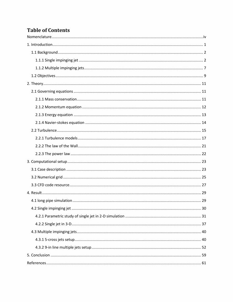
Table of Contents Nomenclature ................................................................................................................................................ iv

1. Introduction ............................................................................................................................................... 1

1.1 Background .......................................................................................................................................... 2

1.1.1 Single impinging jet ...................................................................................................................... 2

1.1.2 Multiple impinging jets ................................................................................................................. 7

1.2 Objectives ............................................................................................................................................ 9

2. Theory ...................................................................................................................................................... 11

2.1 Governing equations ......................................................................................................................... 11

2.1.1 Mass conservation ...................................................................................................................... 11

2.1.2 Momentum equation ................................................................................................................. 12

2.1.3 Energy equation ......................................................................................................................... 13

2.1.4 Navier-stokes equation .............................................................................................................. 14

2.2 Turbulence ......................................................................................................................................... 15

2.2.1 Turbulence models ..................................................................................................................... 17

2.2.2 The law of the Wall ..................................................................................................................... 21

2.2.3 The power law ............................................................................................................................ 22

3. Computational setup ............................................................................................................................... 23

3.1 Case description ................................................................................................................................ 23

3.2 Numerical grid ................................................................................................................................... 25

3.3 CFD code resource ............................................................................................................................. 27

4. Result ....................................................................................................................................................... 29

4.1 long pipe simulation .......................................................................................................................... 29

4.2 Single impinging jet ........................................................................................................................... 30

4.2.1 Parametric study of single jet in 2-D simulation ........................................................................ 31

4.2.2 Single jet in 3-D ........................................................................................................................... 37

4.3 Multiple impinging jets ...................................................................................................................... 40

4.3.1 5-cross jets setup ........................................................................................................................ 40

4.3.2 9-in line multiple jets setup ........................................................................................................ 52

5. Conclusion ............................................................................................................................................... 59

References ................................................................................................................................................... 61

iv

Nomenclature

English Symbols

Symbol Definition

Low-Re correction

Centigrade degree

Diameter

Cross diffusion term

Elliptic relation function

Generation of turbulence kinetic energy and specific dissipation rate

Heat transfer coefficient

Normalized jet to wall distance by nozzle diameter

Average heat transfer coefficient on plate surface

Maximum heat transfer coefficient on plate surface

Turbulence kinetic energy

Length scale

Normalized pipe length

Mean Nusselt number

Root-mean-square Nusselt number

Stagnation point Nusselt number

Pressure

Surface heat flux

Normalized radial distance from stagnation point by nozzle diameter

Reynolds number

User defined source term

v

Jet to jet distance normalized by jet diameter

Time

Temperature, turbulent time scale

Jet inlet temperature

Local wall temperature

Reference temperature (nozzle reference temperature)

Fluctuating velocity in vector notation

Dimensionless velocity

Friction velocity

Mean velocity in vector notation

Average velocity magnitude in outlet boundary condition

Bulk velocity

Jet core velocity,

Shear layer edge velocity

Velocity variance scale

Instantaneous velocity components in directions

Rectangular Cartesian coordinates

Dimensionless distance

Dissipation of turbulence kinetic energy and specific dissipation rate

Greek Symbols

Symbol Definition

Average temperature difference of outlet and inlet temperature

Dissipation rate

Thermal conductivity

vi

Molecular viscosity

Turbulent viscosity

Density

A value of a property per unit of volume

Specific normal Reynolds stresses,

Specific Reynolds stresses,

Specific dissipation rate

Effective diffusivity

Subscripts

Symbol Definition

DNS Direct Numerical Simulation

LCT Liquid Crystal Thermography

LDA Laser Doppler Anemometry

LES Large Eddy Simulation

PIV Particle Image Velocimetry

RSM Reynolds Stress Model

1

1. Introduction In the last two decades, the impinging jet technique has been become popular due to

widespread cooling, heating and drying industrial application. The unique inherent

characteristics of impinging jet are high local heat and mass transfer that is due to flow is

directed to the target surface. The applications examples are cooling the gas turbine blades

and vanes, drying papers and food products, cooling the electronic devices, quenching

operation in glass industry. Also in laser or plasma cutting process, the impinging jet is used

to cool down the products locally in order to avoid deformation. Figure 1 illustrates the

simple schematic of round impinging jet on a target plate.

Figure 1: Schematic of a single round impinging jet path lines simulation

Despite the single impinging jet applications, in some specific purposes multiple impinging

jets can be used where the target heat transfer area is large and it is needed to cover with

number of jets in order to increase heat transfer coefficient. Therefore multiple impinging

jets with variable setup are more efficient in local heat and mass transfer point of view in

these cases due to more uniformity of heat transfer by several neighbour impingement

zones in target area.

In the recent years, many attentions to the impinging jet has been paid by researchers not

only because of effect of different parameters and interesting physic of impinging jet, but

because of effort to validate turbulence models to predict impinging jet characteristic and

complex pattern in different zones from free shear layer to near wall boundary condition.

2

1.1 Background

1.1.1 Single impinging jet

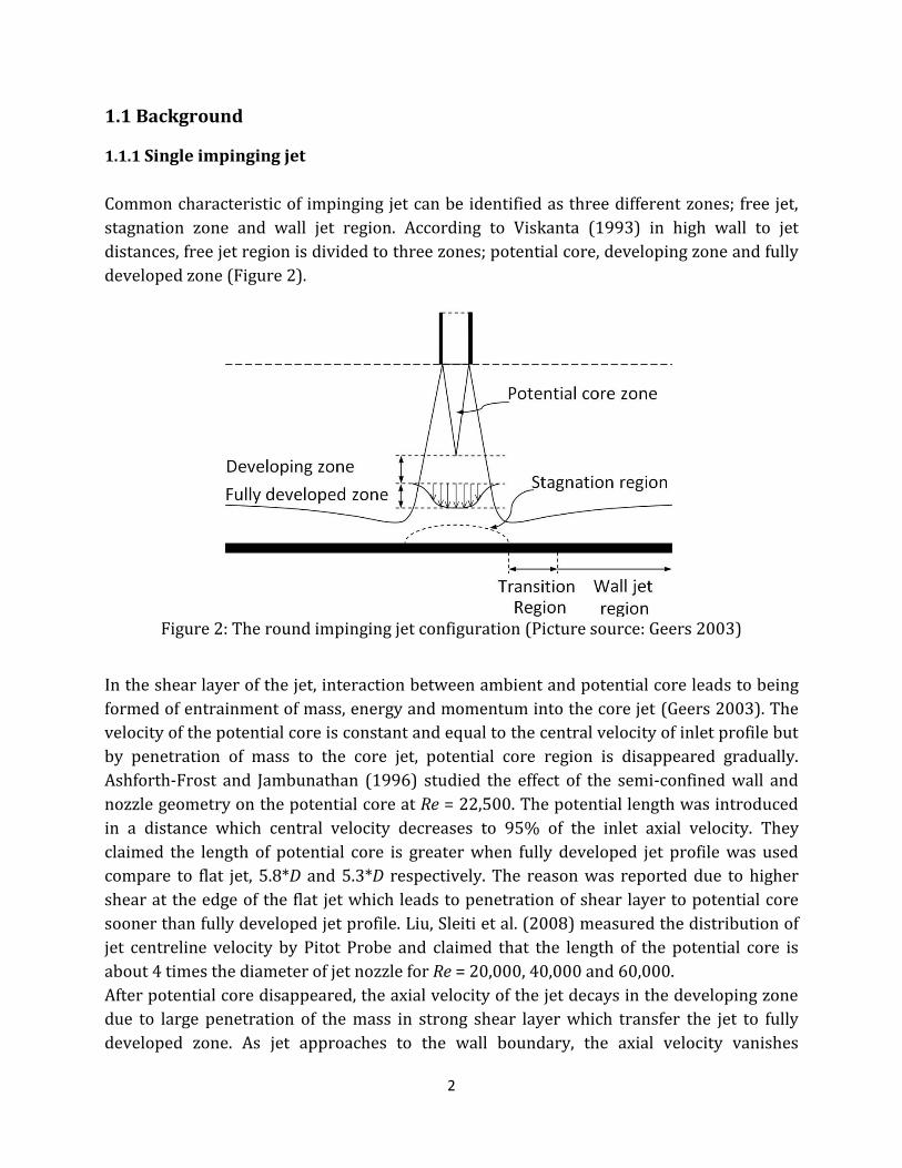
Common characteristic of impinging jet can be identified as three different zones; free jet,

stagnation zone and wall jet region. According to Viskanta (1993) in high wall to jet

distances, free jet region is divided to three zones; potential core, developing zone and fully

developed zone (Figure 2).

Figure 2: The round impinging jet configuration (Picture source: Geers 2003)

In the shear layer of the jet, interaction between ambient and potential core leads to being

formed of entrainment of mass, energy and momentum into the core jet (Geers 2003). The

velocity of the potential core is constant and equal to the central velocity of inlet profile but

by penetration of mass to the core jet, potential core region is disappeared gradually.

Ashforth-Frost and Jambunathan (1996) studied the effect of the semi-confined wall and

nozzle geometry on the potential core at Re = 22,500. The potential length was introduced

in a distance which central velocity decreases to 95% of the inlet axial velocity. They

claimed the length of potential core is greater when fully developed jet profile was used

compare to flat jet, 5.8*D and 5.3*D respectively. The reason was reported due to higher

shear at the edge of the flat jet which leads to penetration of shear layer to potential core

sooner than fully developed jet profile. Liu, Sleiti et al. (2008) measured the distribution of

jet centreline velocity by Pitot Probe and claimed that the length of the potential core is

about 4 times the diameter of jet nozzle for Re = 20,000, 40,000 and 60,000.

After potential core disappeared, the axial velocity of the jet decays in the developing zone

due to large penetration of the mass in strong shear layer which transfer the jet to fully

developed zone. As jet approaches to the wall boundary, the axial velocity vanishes

3

following the reduction of radial velocity in stagnation region where static pressure is high

in the geometric centre zone. The jet deflects to radial direction because of stagnation

region characteristic and wall boundary condition will be thin due to high streamline

curvature (HadŽIabdiĆ and HanjaliĆ 2008). At stagnation point, because of penetration of

mass flow to jet, the flow is highly turbulent. After air flow escaped from effect of jet, it is

joined to wall jet boundary condition and transition to turbulent flow is occurred for wall

jet. The flow velocity is raised from zero at stagnation point and with further increase in

radial distance, the velocity decays in radial and flow fluctuation is diminished (O’Donovan

and Murray 2007).

Heat transfer at stagnation and jet deflection region is higher than wall jet region. Therefore

maximum Nusselt number occurs in this region which is defined as:

(1.1)

where local heat transfer coefficient of the target plate is defined as

(1.2)

After short description of the jet structure, the different parameters will be discussed which

effect on the jet behaviour as well as heat transfer on the stagnation point and radial

distance of the plate. The most effective parameters which have significant effect on

impinging jet are jet to wall distance (H/D), Reynolds number (Re), jet diameter (D), jet inlet

profile, confined and unconfined impinging jet and radial distance of the plate (R/D).

O’Donovan and Murray (2007) studied the mean and root-mean-square Nusselt number

distribution (Nu, N ) on a plate and compared the result of the different Reynolds numbers

(Re=10,000, 20,000 and 30,000) with different non-dimensionalised nozzle to impingement

surface spacing (H/D=0.5, 1, 2, 4, 6, 8) for unconfined jet. A maximum Nusselt number

distribution was reported at stagnation point in all measurement cases due to high

instantaneous velocity and large temperature difference at the stagnation point. In this

point at H/D of 0.5, it was found that pressure on the wall jet from the free jet leads to low

and constant heat transfer fluctuation but at H/D of 6, shear layer was penetrated to centre

of the jet. Therefore the high turbulent flow causes to high heat transfer fluctuation in

stagnation point. The result shown at 2 ≤ H/D ≤ 4, N was low and by increasing the height

of the nozzle and Reynolds numbers, Nu and N peak’s location is moved in positive radial

direction.

Also Katti and Prabhu (2008) studied the heat transfer at stagnation point by static

pressure measurement. They investigated the Nusselt number at stagnation point for

different H/D (0.5 to 8) with Re =16,000 and 23,000. The maximum Nu occurred in H/D=6

in geometry centre of the plate where the initial wall temperature was considered 35°C in

4

the experiment and it was concluded the reason may be due to higher turbulence intensities

near wall with increasing H/D.

In the study of effect of H/D on the stagnation point Nusselt number , Liu, Sleiti et al.

(2008) measured maximum at about H/D=5 for Re=20,000, 40,000 and 60,000. The

reason was reported due to the length of the potential core (L=4*D) and interaction

between diminished axial jet velocity and the increasing of turbulence intensity of

centreline lead to heat transfer peak at H/D ~ 5. Some other experimental and numerical

studies reported that maximum Nu occurs at H/D = 6 to 7 (e.g.; Behnia, Parneix et al.

(1999),Baughn and Shimizu (1989) and Martin (1977)). Also Goldstein, Behbahani et al.

(1986) claimed that H/D ~ 8 is the jet distance where maximum heat transfer measured.

The velocity components study always is interesting to understand the physic of the free jet

as well as wall jet flow both in axial and radial directions (perpendicular and parallel to wall

respectively). O’Donovan and Murray (2007) reported that at the stagnation region, where

the axial velocity is a maximum in radial distance point of view, Nu and N peak while the

radial velocity is zero and is increased by following the radial distance from centreline of

the jet. They have found that in low H/D, the axial velocity is more uniform by R/D<0.5

which shows potential core reaches to wall boundary condition.

They also studied the second Nusselt number peak in radial distances and found that it

depends on the Reynolds number and H/D. They claimed this peak is due to transition to

turbulence in the wall jet region and the combination of high local velocity and turbulence

intensity which was confirmed later by Katti and Prabhu (2008). In the Nusselt number

distribution measurement, they found greater nozzle to plate spacing (H/D) effects on the

magnitude of the second peak and its location. In the other word, they shown that highest

second peak occurs at H/D = 0.5 as it is closest peak to stagnation point peak (R/D = 1.6)

and then by increasing the H/D, second peak magnitude decreases and is shifted away in

further radial distance.

In pressure gradient point of view, Liu, Sleiti et al. (2008) reported that after negative

pressure gradient in wall boundary, this peak is occurred because transition from laminar

to turbulent condition is existed due to diminishing of pressure gradient along the wall.

The relation between Reynolds number and local heat transfer distribution has been

studied by several experimental measurements and computational studies. Katti and

Prabhu (2008) shown their linear correlation of Reynolds number and Nusselt number on

stagnation point; higher Reynolds Number, greater Nusselt number in stagnation point and

the result was verified with those of Lytle and Webb (1994). Moreover other researchers

confirmed numerically and experimentally that the higher Reynolds number contribute to

greater Nusselt number distribution in radial distances (e.g. ;Behnia, Parneix et al. (1998),

O’Donovan and Murray (2007), Behnia, Parneix et al. (1999),San and Shiao (2006)).

5

As a crucial region of simulation, stagnation point prediction is always interesting to study.

Behnia, Parneix et al. (1998) reported that turbulence model predicts turbulent

kinetic energy well in stagnation region compare to over prediction result of models

with high magnitude of turbulent kinetic energy at stagnation region.

In the study of nozzle diameter impact, Lee, Song et al. (2004) performed the measurement

to study the effect on jet diameter on heat transfer and fluid flow. They used fully developed

jet profile at inlet in a constant Re = 23,000 with three different nozzle diameter (1.36, 2.16

and 3.4 cm) and the result shown that increasing the diameter lead to greater jet potential

core. Also Nusselt number at stagnation point was increased with larger jet diameter due to

increase the jet momentum and turbulence intensity. But for local Nu at wall jet region, the

effect of diameter was found negligible. Also the result of an experiment by Stevens and

Webb (1991) by using fully developed liquid jet verified increasing the local Nu distribution

by larger jet diameter.

Gulati, Katti et al. (2009) studied three different inlet shape of jet: circular, square and

rectangular nozzle for Re= 5000, 10,000, 12,000 and 15,000 in Different jet to wall

distances (0.5 to 12) experimentally. They have found that for H/D=0.5, rectangular jet

increases local Nu distribution compare to square and circular shape while by rising the jet

height above the plate (bigger H/D), this enhancement is diminished. For circular and

square jets, the result presented similar local Nu distribution in all jet to wall distances. In

heat transfer coefficient point of view, Zhao, Kumar et al. (2004) simulated different shape

of inlet to investigate their characteristics. They reported for circular inlet, 5*D to 6*D jet to

wall distance lead to highest heat transfer while for square, elliptic and rectangular shapes,

lower H/D presents higher heat transfer.

The effect of jet profile as inlet boundary condition has been studied by Xu and Antonia

(2002). An experiment was performed to compare the result of fully developed profile from

a long pipe with top hat profile from a conventional contraction jet (Figure 3).

They reported fully developed profile has the larger initial shear layer thickness which

leads to longer wavelengths in large downstream distances. The radial profiles of Reynolds

stresses ( and ) are wider in top hat profile and peak values are greater compare to fully

developed jet which shows the stronger shear layer in jet mixing layer for the contraction

jet.

The effect of confining wall on the round impinging jet was investigated by Gao, Sun et al.

(2003) experimentally. They concluded for Re of 17,000 to 28,000 there are no large

difference of heat transfer coefficient of jet for H/D ≥ 1 but it differs for H/D ≤ 0.5. Also in

confined jet close to the impingement wall, turbulent fluctuations was found lower and

convected slower.

6

Figure 3: Mean velocity profile of top hat (□), fully developed (∆), Xu and Antonia (2002)

Moreover Behnia, Parneix et al. (1999) studied the effect of confined wall with

model and reported the same conclusion as Gao, Sun et al. (2003) for heat transfer

coefficient distribution. They also claimed two reasons for lower average heat transfer rate

in confined jet cases in some experiments. First, the jet temperature (as reference

temperature which is coming from ambient) is evaluated for Nu, may not be same with air

flow temperature in more radial distances from jet, because it is heated up in confined

region and temperature difference between plate and air flow temperature will be lower

close to outlet. Secondly, because of confining wall, the entrainment of external fluid is

reduced (less mass flow rate) which lead to lower heat transfer on the plate.

The influence of radial distance of outlet boundary condition on Nusselt number at

stagnation point has been investigated by San and Shiao (2006) experimentally. They

claimed that increasing the plate length in both two horizontal directions causes to

decrease stagnation point Nusselt number for Re=10,000, 15,000 and 30,000 effectively.

Heat transfer distribution in radial distance was investigated by Katti and Prabhu (2008)

for different jet to wall distances. The similar fashion drop in heat transfer was reported for

all H/D (0.5 to 8) due to decreasing the radial flow velocity over the plate in downstream.

They divided the wall jet flow in to two parts: inner layer where wall boundary layer is

located and outer layer where there is interaction by surrounding fluid. They modified an

equation of maximum radial velocity prediction (Govindan and Raju 1974) for H/D ,

0

0.1

0.2

0.3

0.4

0.5

0.6

0.7

0.8

0.9

1

1.1

-0.6 -0.5 -0.4 -0.3 -0.2 -0.1 0 0.1 0.2 0.3 0.4 0.5 0.6

U/U

cen

tre

Radial distance from jet centre, R/D

Top hat profile Fully developed profile

7

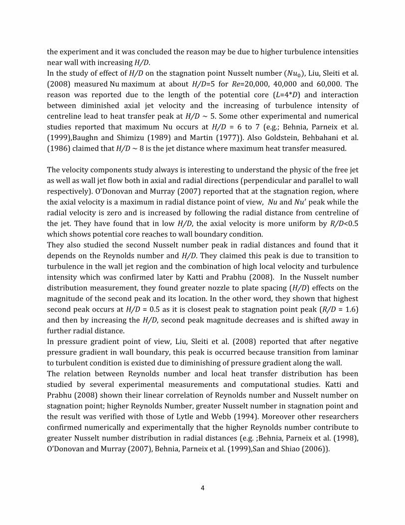
(1.3)

1.1.2 Multiple impinging jets

The flow pattern and impingement characteristic of multiple jets are similar to the single

impinging jet but there are some phenomena are occurred in multiple jets which it cannot

be seen in single jet. Viskanta (1993) claimed that there are two type of interaction between

jets in multiple impingement of jets; firstly, possibility of interaction of neighbour jets on

their impingement. The possibility of this phenomenon is increased for closer jets and

bigger jet to wall distances. Secondly interaction of wall jets due to encounter area between

adjacent jets spaces and it increases in cases with high jets velocity and small jet to wall

distance.

First mechanism can shorten the jets potential core and reduce jet core strength which is

identified as negative impact on the heat transfer of the target plate. But on the other side,

second phenomenon make second peak of heat transfer between stagnation points which

increases the average heat transfer rate of the plate.

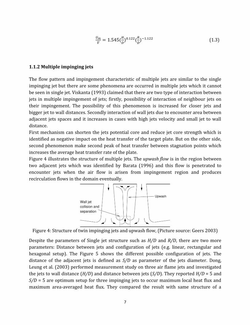
Figure 4 illustrates the structure of multiple jets. The upwash flow is in the region between

two adjacent jets which was identified by Barata (1996) and this flow is penetrated to

encounter jets when the air flow is arisen from impingement region and produces

recirculation flows in the domain eventually.

Figure 4: Structure of twin impinging jets and upwash flow, (Picture source: Geers 2003)

Despite the parameters of Single jet structure such as H/D and R/D, there are two more

parameters: Distance between jets and configuration of jets (e.g. linear, rectangular and

hexagonal setup). The Figure 5 shows the different possible configuration of jets. The

distance of the adjacent jets is defined as S/D as parameter of the jets diameter. Dong,

Leung et al. (2003) performed measurement study on three air flame jets and investigated

the jets to wall distance (H/D) and distance between jets (S/D). They reported H/D = 5 and

S/D = 5 are optimum setup for three impinging jets to occur maximum local heat flux and

maximum area-averaged heat flux. They compared the result with same structure of a

8

single jet and found the higher values of heat transfer rate and maximum heat transfer

point in multiple impinging jets.

Also San and Lai (2001) studied different jet to jet and jet to wall distances to optimise the

heat transfer in stagnation point. They showed that for H/D of 5, highest Nusselt number in

stagnation point occurs at 5<S/D<7 with maximum at S/D=6, while it differs for other

H/D = 2 to 4. They also correlated all case studies together and define an equation for

Nusselt number of stagnation point depends on S/D and Reynolds number of jets. It was

also verified that for small S/D, interference between shear layers of jets happens before

impingement to wall and the jets strength will be weaken (Figure 5). On the other side, Jet

fountain effect can be occurred for bigger S/D, where heated upwash flow is penetrated to

right and left jets cores (Figure 5) and leads to reduction of heat transfer from wall.

Figure 5: Interaction of shear layers of jets in small S/D before impingement (left), fountain in shear layer of jet for bigger S/D (right)

Figure 6: Different configuration of multiple impinging jets (Bottom row circular 9 jets, square 9 jets and hexagonal jets, second row: twin jets, 4 jets and 5-cross jets.)

Thielen (2003) studied the three different configuration of round multiple jets

computationally: circular 9 jets, square 9 jets and hexagonal 9 jets, see Figure 6. The result

Interaction

area

Fountain

area

9

of square and hexagonal setup were verified by an experimental study (Geers 2003) which

was done by Laser Doppler Anemometry (LDA), Particle Image Velocimetry (PIV) and

Liquid Crystal Thermography (LCT).

Thielen (2003) concluded that computational study of multiple jets are more difficult rather

than single jet due to 3-D simulation limitation and and model simulation result

of heat transfer and Reynolds stress components have better accuracy compare to

model. In heat transfer rate point of view, in circular setup outer jets has lower peak of heat

transfer compare to central jets while in square configuration, all jets have same peak value

compare by central jet.

1.2 Objectives

The purpose of this study is to understand more about impinging jet characteristics in high

temperature condition of target plate (300˚C). Moreover the other aim is to design an

optimized structure of confined wall boundary condition for the impinging jet to increase

and optimize average heat transfer coefficient as well as outgoing air temperature from

boundary condition in parallel. The goal is to reach at least 150˚C temperature difference

between the average outlet temperature and inlet temperature of domain. In parallel high

average heat transfer coefficient distribution over the plate ( 200 ) is the second

goal of the project.

This setup of impinging jet will be used for measurement study in future to validate the

numerical simulation results.

10

11

2. Theory

2.1 Governing equations

The fluid flow governing equations are mathematical equations which are called

conservation laws of physics. These equations describe the flow behaviour in microscopic

level, i.e. velocity, temperature, density and pressure. By using these equations, three types

of equation are defined; mass conservation, momentum and energy equations. In three

dimensions, the smallest element of the fluid is introduced as a point or particle in

microscopic level. Figure 7 illustrates the fluid element which includes six boundary

conditions. The mathematical equations are represented according to mass, momentum

and energy changes across these boundaries (faces). Also a point ( ) is known as

centre of element.

Figure 7: Fluid element in conservation laws of physics

2.1.1 Mass conservation

The mass balance of the element becomes as increasing rate of mass in fluid element is

equal to net rate of mass flow into the element. Therefore mass conservation equation

mathematically becomes

(

) (

) (

)

(

) (

) (

) (2.1)

In equation above, the incoming mass to the element gives the positive sign and the flows

with negative sign are out coming mass from boundaries (see Figure 8).

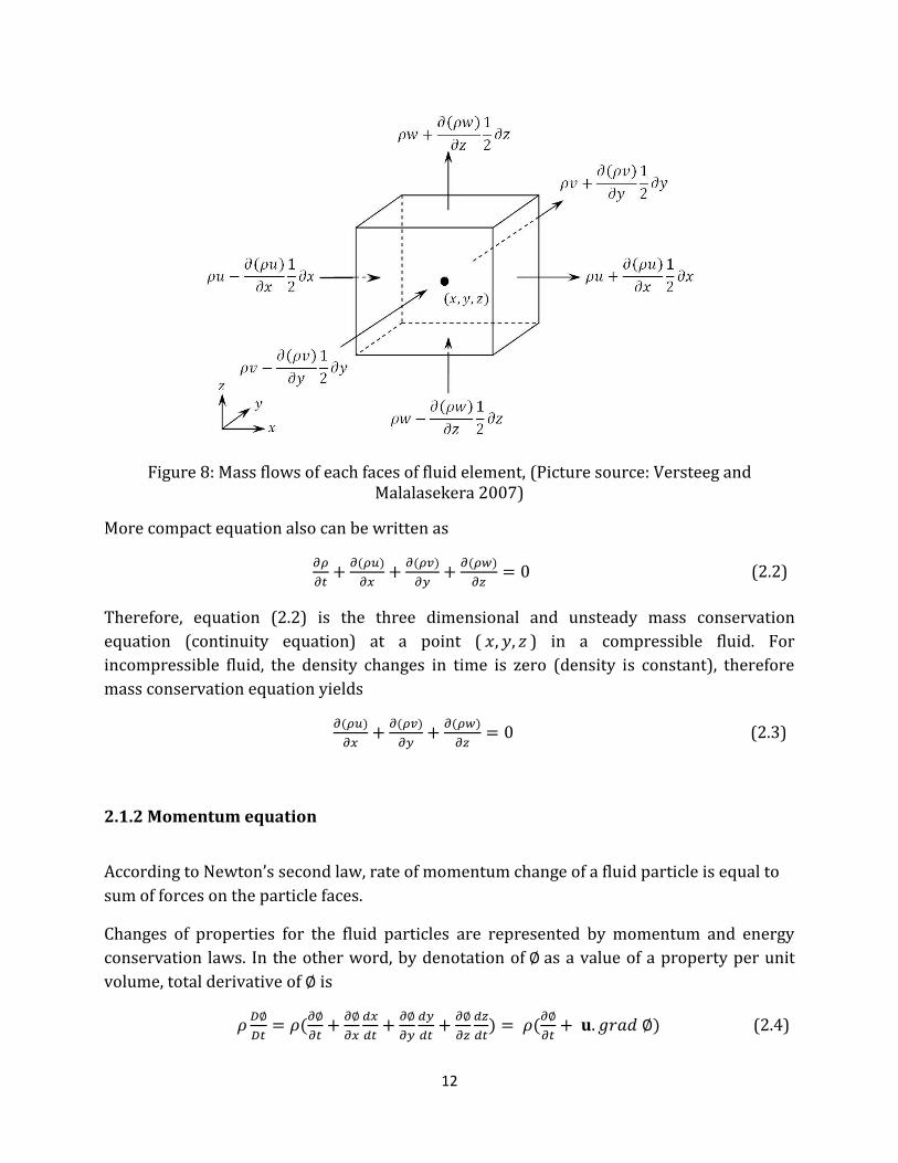
12

Figure 8: Mass flows of each faces of fluid element, (Picture source: Versteeg and Malalasekera 2007)

More compact equation also can be written as

(2.2)

Therefore, equation (2.2) is the three dimensional and unsteady mass conservation

equation (continuity equation) at a point ( ) in a compressible fluid. For

incompressible fluid, the density changes in time is zero (density is constant), therefore

mass conservation equation yields

(2.3)

2.1.2 Momentum equation

According to Newton’s second law, rate of momentum change of a fluid particle is equal to

sum of forces on the particle faces.

Changes of properties for the fluid particles are represented by momentum and energy

conservation laws. In the other word, by denotation of as a value of a property per unit

volume, total derivative of is

(2.4)

13

Therefore by replace the denotation of , and as a property, the rate of increasing of -,

- and -momentum per unit volume of a fluid is written by

Two types of forces effects on fluid particles; surface forces and body forces. The surface

forces are pressure and viscous forces while the body forces include gravity, centrifugal,

coriolis and electromagnetic forces. Here surface forces are considered as a separate term

in momentum equation and body forces as a source term . Therefore surface forces are

a normal stress of pressure and nine viscous stress components on fluid element.

By summation of all net forces in and direction, total force per unit volume is

given by

(2.5)

By using equations (2.4) and (2.5), the x-component of the momentum equation becomes

(2.6a)

The y-component and z-component of the momentum equations also yield respectively

(2.6b)

(2.6c)

where are the nine viscous stress components of the fluid element.

2.1.3 Energy equation

First law of thermodynamics states that rate of energy change of a fluid particle is equal to

net rate of heat added to fluid particle plus net rate of work which is done on fluid particle.

According to equation (2.4), the rate of energy increasing of a fluid particle is given by

On the other side, the total rate of work that is done on the fluid particle by surface stresses

after collecting the pressure terms together becomes

14

[ ] [

( )

( )

( )

] (2.7)

Also the rate of heat added to the fluid particle from all boundary condition faces yields

(2.8)

By defining a source term of as potential energy changes and according to energy

balance of fluid particle, the energy equation is given by

[ ] [

( )

( )

( )

]

(2.9)

Where energy of a fluid ( ) is the sum of internal (thermal) energy, kinetic energy and

gravitational potential energy.

2.1.4 Navier-stokes equation

The fluid motion is described by solving the five governing equations; mass conservation,

and momentum equations and energy equation. Also four thermodynamic

variables of pressure ( ), Density ( ), internal energy ( ) and temperature ( ) can be solved

by using the equation of states. For example if we use and as state variables, then the

relation between these variables becomes

and (2.10)

But governing equations include unknown’s viscous stress components according to

equations (2.6a-c). These viscous stress components are proportional to deformation rate

in a Newtonian fluid.

(

) (

) (

) (2.11)

Therefore, by substitution of above viscous stresses into the momentum equations, the

Navier-stokes equations are given by

15

[

]

[ (

)]

[ (

)] (2.12a)

[ (

)]

[

]

[ (

)] (2.12b)

[ (

)]

[ (

)]

[

] (2.12c)

Which by re-arrange the shear stress terms, the most useful form of Navier-stokes

equations are written,

(2.13a)

(2.13b)

(2.13c)

2.2 Turbulence

In our surrounding, fluid flows are divided in two different regimes; Laminar and turbulent

flows. As a good measure, Reynolds number states the critical boundary which at values

below that, the fluid flow is laminar with smooth and stable pattern. By increasing the

Reynolds number, the irregularity and instability is taken place and more complicated

events is occurred and laminar flow is changed to turbulent flow.

Most of the flows in our surrounding are turbulent flows which has irregular, random and

unstable behaviour with unpredictable eddies (Figure 9). Some example of turbulence flows

are outgoing plume of solid rocket jets, smoke from a chimney, river flow, etc. For the first

time, von Karman (1937) presented basic definition of turbulence;

“Turbulence is an irregular motion which in general makes its appearance in fluids, gaseous

or liquid, when they flow past solid surfaces or even when neighbouring streams of the same

fluid flow past or over one another”

16

Figure 9: Image of a turbulent jet, (Picture source: Dahm and Dimotakis 1990)

As the Figure 10 shows, the flow velocity varies irregularly both in time and position which

is denoted by . In this Figure, the horizontal line is the mean axial velocity of centre

line of a turbulent single jet and the flow velocity fluctuates in the time variation compare to

mean velocity. Therefore the flow velocity equation is given by

(2.14)

where is a fluctuation velocity component with properties of .

Figure 10: Axial velocity component ( on centre line of a turbulent jet, Re=17232

25

26

27

28

29

30

31

32

33

34

35

0 0.01 0.02 0.03 0.04 0.05 0.06 0.07 0.08 0.09 0.1

Axi

al v

elo

city

var

iati

on

of

a si

ngl

e im

pin

gin

g je

t, (

m/s

)

time (s)

17

Particle of fluid follows the eddy motions in turbulent flow; mass, momentum and heat are

changed effectively. These eddy motions which can be seen in flow visualization, made by

rotational flow structures with a wide range of length scales. The largest turbulent eddies

interact with the energy that is extracted from mean flow by process of vortex stretching.

Smaller eddies are stretched by larger eddies strongly rather than mean flow and it leads to

transfer kinetic energy from larger eddies to smaller eddies which this process called

energy cascade. The Figure 11 illustrates the kinetic energy handing down from large

eddies to small eddies. The characteristic length and velocity of eddies are of the same

order of mean flow length scale and velocity . Therefore Reynolds number of large eddy

is defined as

(2.15)

Figure 11: Energy cascade illustration, (Picture source: Rundstrom and Moshfegh 2004)

In a turbulent flow, all variable properties contain energy in a wide range of wavenumbers.

The Reynolds number of smallest eddies is equal to 1 where length scale is on the order of

0.01-0.1 mm and eddies motion is due to viscosity in this level of eddy’s size (Versteeg and

Malalasekera 2007).

2.2.1 Turbulence models

In a century, it was shown experimentally that turbulence problem is always hard to be

analysed. But there is a hope to analyse and simulate the turbulent flows more accurate by

power of digital computer’s improvement. Therefore turbulence models are improved day

by day, to predict turbulent flows in wide range of flows.

Turbulence models solve mean flow equations (2.2), (2.6a-c) and (2.9) in a computational

procedure. The velocity field is in three-dimensional as well as dependents to time.

Therefore for a CFD code to be useful, it should be able to challenge in some criteria: level of

18

description (mean quantities, instantaneous quantities), applicability, accuracy (solving

wide range of flow conditions), cost and completeness.

Totally turbulence models are classified as

Classical models: based on time averaged Reynolds equations

1. Zero equation model

2. Two-equation models

3. Reynolds stress equation model

4. Algebraic stress model

Large eddy simulation (LES)

Direct numerical simulation (DNS)

Classical models use time-averaged Reynolds number equations to make basis turbulence

calculation in CFD codes. For example in two-equation models, two transport equations will

be solved. While Large eddy simulations solve time-depended flow equations and large

eddies, therefore smaller eddies also are simulated. In this case, the level of approximation

is good because of modelling the large eddies in flow lead to model the energy transfer

among eddies; but the simulation is highly expensive in time consumption point of view. In

higher level of prediction, Direct Numerical Simulation solve the unsteady Navier-Stock

equations directly, therefore no turbulence model is needed because fluid flows are

described by equations. But the computational cost is more expensive compare to LES

models.

In this part, two equation models and Reynolds stress equation model are presented

because of these models have be used in this study. All turbulence model equations in this

part have been summarized from ANSYS® (2011), therefore for more details about

constants and equation, reader is referred to the document.

2.2.1.1 The models

In this category two models are presented: Standard and shear-stress transport (SST)

model. These models have similar forms of and transport equations, but there are two

main differences

Changes from Standard model to a high Reynolds number version

Modification of turbulence viscosity formulation

19

The standard model

This model was written by Wilcox (1998) combines modified low-Re effects and shear flow

spreading. This model has weak solution values of and in free stream (outside the shear

layer) but some improvement has been added to ANSYS FLUENT software to reduce the

free shear flows effects (ANSYS® 2011).

The turbulent kinetic energy equation base on the velocity scales becomes

(2.16)

The transport equations of turbulence kinetic energy ( ) and specific dissipation rate ( )

are as follows:

[

] (2.17)

and

[

] (2.18)

Also turbulent viscosity is given by

(2.19)

where coefficient is the low-Re correction in the model. In high-Reynolds number is

equal to 1, but for low-Reynolds numbers it is defined as follows:

(

) ,

(2.20)

The Shear Stress Transport (SST) model

The shear-stress transport model was improved by Menter (1994) to increase accuracy of

solution in near-wall region without the free-stream dependency. The developments in this

model are:

Both Standard and SST models were added together by a blending function.

Therefore the blending function is one in near-wall region that leads to the Standard

model activation, and zero away from near-wall region which activates SST

model.

In equation, there is a derivative term of damped cross-diffusion.

20

Modification of the turbulent viscosity definition

Similar forms of transport equations compare to Standard model are presented for this

model:

[(

)

] (2.21)

and

[(

)

] (2.22)

where turbulent viscosity is computed by a formula.

2.2.1.2 Model

The model (V2F) is based on model by Durbin (1995) and is a four

equation model of transport equations compare to two equations models which described

before. The two more transport equations are for a velocity variance scale ( ) and an

elliptic relation function ( ). The transport equations of the model for , , and

are as follows respectively:

[(

)

] (2.23)

[(

)

] (2.24)

( )

( )

[(

)

] (2.25)

(2.26)

where the turbulent viscosity is defined as

(2.27)

21

2.2.1.3 RSM Model

Model is known as most elaborated mode in RANS turbulence models. It solves

transport equation of Reynolds stresses as well as one equation of the dissipation rate,

therefore in 3-D flows. The Reynolds stresses ( transport equation becomes

(

)

(

)

[

(

) ]

[

(

)]

(

) – (

) (

)

(

) (2.28)

Low-Re Stress-Omega Model

In order to model the pressure-strain term there are three options in model. The third

option is the Low-Re Stress-Omega model which is based on the model and LRR

model. The wide range of flows can be predicted by this model due to resemblance of model

by model (ANSYS® 2011).

2.2.2 The law of the Wall

In wall boundary condition, the flow is affected by the viscous effects the flow pattern is not

depended on the free stream condition. The law of the wall is one of known relationship for

flow close to wall surface. The dimensionless velocity and dimensionless distance are

defined as

(2.29)

where is called friction velocity and represents the velocity close to wall boundary.

Therefore the law of the wall yields

(2.30)

The dimensional integration constant C is suggested with measurement correlations. The

Figure 12 shows typical velocity profile close to solid wall. Turbulent boundary layer of a

wall surface is divided in two regions:

22

Inner region, which contains 10-20% of total boundary layer thickness. In this

region, shear stress is approximately constant and equal to wall shear stress and

includes three zones from near wall to boundary layer respectively:

o The linear sub-layer: Viscous stresses effects dominate on flow, (

o The buffer layer: Influence of viscous and turbulent stresses are same,

(

o The log-law layer: Turbulence stresses affects strongly, (

Outer region (law of the wake layer): Far from viscous stress directly (Versteeg and

Malalasekera 2007),(Wilcox 1998) .

Figure 12: Velocity profile of a turbulent boundary condition, (Picture source: Schlichting 1979)

2.2.3 The power law

Turbulent boundary layer profile can be represented by an approximation,

(2.31)

which was defined for the first time by Prandtl (Schlichting 1979). It was found that the

power law correlates measurement of pipe flow profile better and release more realistic

description of turbulence in the inner layer (Wilcox 1998).

23

3. Computational setup

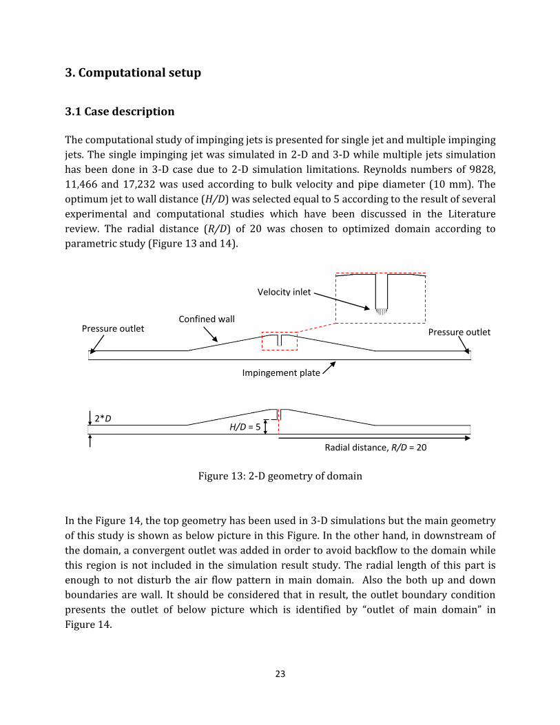
3.1 Case description

The computational study of impinging jets is presented for single jet and multiple impinging

jets. The single impinging jet was simulated in 2-D and 3-D while multiple jets simulation

has been done in 3-D case due to 2-D simulation limitations. Reynolds numbers of 9828,

11,466 and 17,232 was used according to bulk velocity and pipe diameter (10 mm). The

optimum jet to wall distance (H/D) was selected equal to 5 according to the result of several

experimental and computational studies which have been discussed in the Literature

review. The radial distance (R/D) of 20 was chosen to optimized domain according to

parametric study (Figure 13 and 14).

Figure 13: 2-D geometry of domain

In the Figure 14, the top geometry has been used in 3-D simulations but the main geometry

of this study is shown as below picture in this Figure. In the other hand, in downstream of

the domain, a convergent outlet was added in order to avoid backflow to the domain while

this region is not included in the simulation result study. The radial length of this part is

enough to not disturb the air flow pattern in main domain. Also the both up and down

boundaries are wall. It should be considered that in result, the outlet boundary condition

presents the outlet of below picture which is identified by “outlet of main domain” in

Figure 14.

Pressure outlet Pressure outlet

Velocity inlet

Impingement plate

Confined wall

Radial distance, R/D = 20

H/D = 5 2*D

24

In 3-D simulation, single jet, 5 and 9 multiple jets have been studied computationally. For

configuration of 9 jets, the result of circular and square configurations in literature review

has been investigated and finally square setup was chosen according the previous study

results.

Figure 14: Geometry of symmetric 3-D case of 5-cross jets

Confined wall

Pressure outlet

Pressure outlet

Velocity inlets

Symmetry

Impingement plate

Wall

Outlet of main domain

Impingement plate

25

Figure 15: 3-D geometry of single and 9 multiple jets domain

The long pipe (L/D=25) simulation produced the fully developed profile as inlet of the

domain both in 2-D and 3-D cases for single and multiple jets. The grid of pipe flow in outlet

is same as inlet of the domain to increase the accuracy of simulation.

Boundary conditions in the energy and radiation equations become:

Inlet air temperature = 20˚C

Impingement plate temperature constant = 300˚C

Insulated confinement wall in top side the rig (heat flux = 0)

Internal emissivity for walls boundary conditions = 0.6

Internal emissivity for inlet and outlet boundary conditions = 0.8

Impingement steel plate (thermal conductivity = 55 )

3.2 Numerical grid

The numerical grid of the domain is clustered in crucial regions near wall boundary

condition and edge of the pipe shear layer where there are high velocity gradients. The

Figure 16 shows these regions in 2-D mesh of the domain. In order to increase the accuracy

of the prediction, low Reynolds correction option was used, therefore the mesh size of the

wall boundary conditions in all 2-D and 3-D meshes fulfils condition for this option.

For the whole mesh domain, it was tried to keep rate of increasing cell area lower than 20%

of their neighbour cells.

Plate 1

26

Figure 16: Clustered mesh in crucial regions and details in 2-D geometry

Also in Figure 17, 3-D mesh of the final optimized domain is shown. The zoom pictures of

the mapped mesh of the pipe circular surface can be seen in Figure 18.

Figure 17: 3-D mesh of the symmetric finalized domain

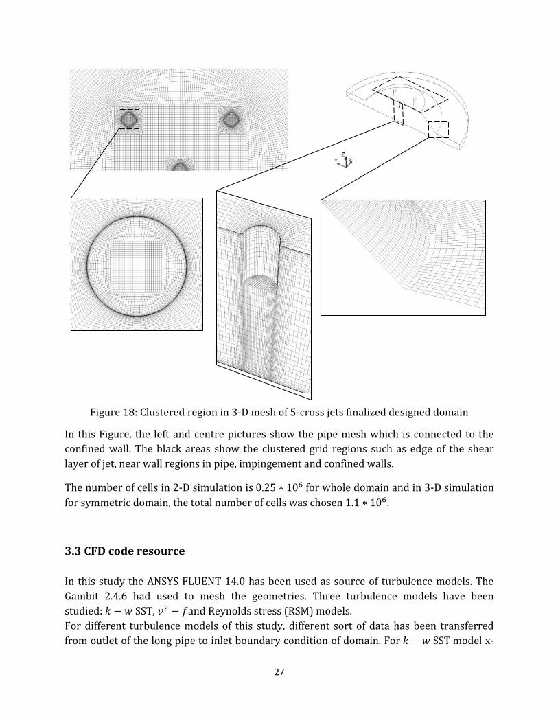
27

Figure 18: Clustered region in 3-D mesh of 5-cross jets finalized designed domain

In this Figure, the left and centre pictures show the pipe mesh which is connected to the

confined wall. The black areas show the clustered grid regions such as edge of the shear

layer of jet, near wall regions in pipe, impingement and confined walls.

The number of cells in 2-D simulation is for whole domain and in 3-D simulation

for symmetric domain, the total number of cells was chosen .

3.3 CFD code resource

In this study the ANSYS FLUENT 14.0 has been used as source of turbulence models. The

Gambit 2.4.6 had used to mesh the geometries. Three turbulence models have been

studied: , and Reynolds stress ( ) models.

For different turbulence models of this study, different sort of data has been transferred

from outlet of the long pipe to inlet boundary condition of domain. For model x-

28

velocity, y-velocity (also z-velocity in 3-D simulation), turbulent kinetic energy ( ) and

specific dissipation rate ( ) were used. For model simulation, velocity,

velocity, velocity, turbulent kinetic energy ( ), dissipation rate ( ), velocity variance

scale ( ) were extracted from long pipe outlet boundary condition. And finally for

model, velocity, velocity, velocity, turbulent kinetic energy ( ), specific

dissipation rate ( ) and Reynolds stress components was considered for inlet boundary

condition.

29

4. Result

The result of computational study is presented in this chapter. Firstly long pipe simulation

result is presented to produce fully developed velocity profile at end of the pipes. Then

Single impinging jet simulation’s result is presented both in 2-D and 3-D simulations. Finally

the result of effect of Reynolds number and turbulence models on configuration of 5 jets is

shown respectively and 9 square multiple impinging jets result is presented for one of

turbulence model which has been verified for 5 multiple jets setup.

4.1 long pipe simulation

The normalized outlet profile of the long pipe (L/D=25) in 3-D simulations with different

RANS turbulence models is shown in Figure 19. The result is compared with the 1/6 power

of law for Re=15,000 as Milanovic and Hammad (2010) reported good correlation of n=6

with their experimental data.

Figure 19: The normalized axial velocity profile of pipe outlet by maximum velocity compare to available experimental data and 1/6th power law

The result of velocity profile of turbulence models are following to each other. There is good

agreement in wall boundary layer with 1/6th power law while in core region the results of

0

0.2

0.4

0.6

0.8

1

-0.5 -0.4 -0.3 -0.2 -0.1 0 0.1 0.2 0.3 0.4 0.5

U/U

max

Radial distance from jet center, R/D

Milanovic and Hammad (2010), Re=14,602 1/6 power law

k-w sst, Re=9828 RSM, Re=17232

k-w sst, Re=11466 V2f, Re=17232

k-w sst, Re=17232

Re=14,602

SST, Re=9828

SST, Re=11466

SST, Re=17232

Re=17232

Re=17232

30

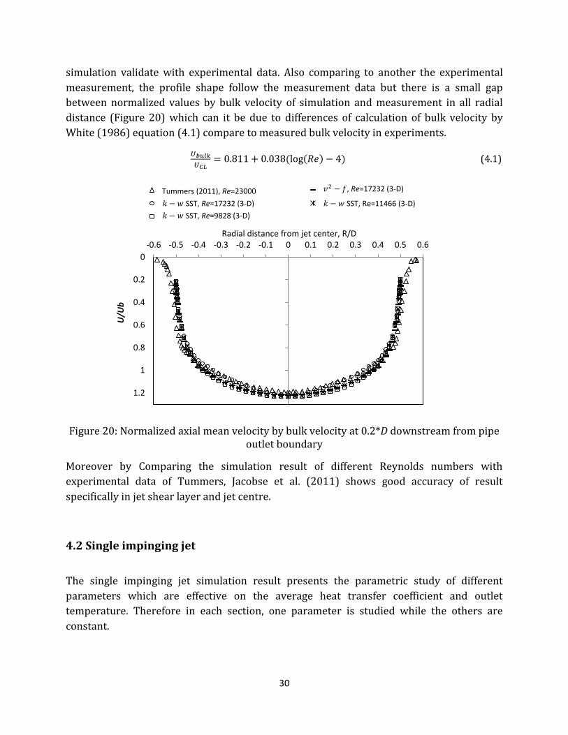
simulation validate with experimental data. Also comparing to another the experimental

measurement, the profile shape follow the measurement data but there is a small gap

between normalized values by bulk velocity of simulation and measurement in all radial

distance (Figure 20) which can it be due to differences of calculation of bulk velocity by

White (1986) equation (4.1) compare to measured bulk velocity in experiments.

(4.1)

Figure 20: Normalized axial mean velocity by bulk velocity at 0.2*D downstream from pipe outlet boundary

Moreover by Comparing the simulation result of different Reynolds numbers with

experimental data of Tummers, Jacobse et al. (2011) shows good accuracy of result

specifically in jet shear layer and jet centre.

4.2 Single impinging jet

The single impinging jet simulation result presents the parametric study of different

parameters which are effective on the average heat transfer coefficient and outlet

temperature. Therefore in each section, one parameter is studied while the others are

constant.

0

0.2

0.4

0.6

0.8

1

1.2

-0.6 -0.5 -0.4 -0.3 -0.2 -0.1 0 0.1 0.2 0.3 0.4 0.5 0.6

U/U

b

Radial distance from jet center, R/D

Tummers (2011), Re=23,000 v2f, Re=17,232 (3D)

K-w sst, Re=17,232 (3D) K-w sst, Re=11,466 (3D)

K-w sst, Re= 9828 (3D)

Tummers (2011), Re=23000

SST, Re=17232 (3-D)

SST, Re=9828 (3-D)

, Re=17232 (3-D)

SST, Re=11466 (3-D)

31

As it discussed before some parameters are fixed according to previous experimental and

computational studies which are relevant to project objectives: jet to wall distance (H/D=5),

Reynolds number (Re=11,466), D=10 mm, Impingement plate temperature of 300˚C and

fully developed velocity profile at domain inlet. Also due to limitation of vertical distance of

outlet and impingement plate, outlet height varies between 16 to 20 mm in 2-D geometry

and is constant of 20 mm in 3-D geometry. Other parameters (which need to be studied) are

Geometry of the domain, Radial distance of plate (R/D) and ventilated/unventilated

impinging jet.

4.2.1 Parametric study of single jet in 2-D simulation

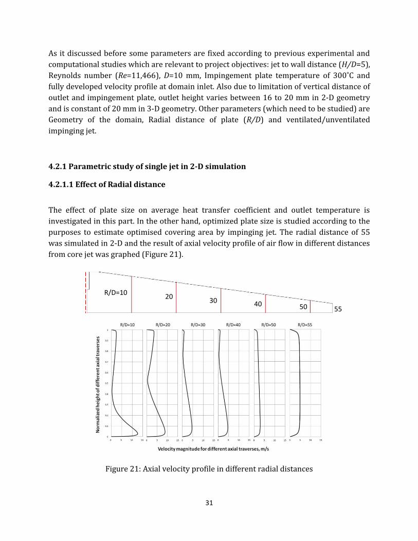
4.2.1.1 Effect of Radial distance

The effect of plate size on average heat transfer coefficient and outlet temperature is

investigated in this part. In the other hand, optimized plate size is studied according to the

purposes to estimate optimised covering area by impinging jet. The radial distance of 55

was simulated in 2-D and the result of axial velocity profile of air flow in different distances

from core jet was graphed (Figure 21).

Figure 21: Axial velocity profile in different radial distances

R/D=10 20

30 40

0 50 55

32

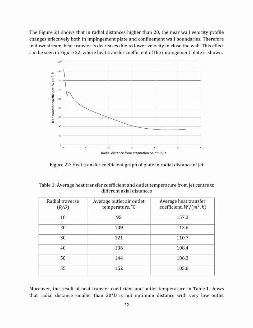
The Figure 21 shows that in radial distances higher than 20, the near wall velocity profile

changes effectively both in impingement plate and confinement wall boundaries. Therefore

in downstream, heat transfer is decreases due to lower velocity in close the wall. This effect

can be seen in Figure 22, where heat transfer coefficient of the impingement plate is shown.

Figure 22: Heat transfer coefficient graph of plate in radial distance of jet

Table 1: Average heat transfer coefficient and outlet temperature from jet centre to different axial distances

Radial traverse (R/D)

Average outlet air outlet temperature, ˚C

Average heat transfer coefficient,

10 95 157.3

20 109 113.6

30 121 110.7

40 136 108.4

50 144 106.3

55 152 105.8

Moreover, the result of heat transfer coefficient and outlet temperature in Table.1 shows

that radial distance smaller than 20*D is not optimum distance with very low outlet

Hea

t tr

ansf

er c

oef

fici

en

t, W

/𝑚 𝑘

Radial distance from stagnation point, R/D

33

temperature while in higher radial distance the heat transfer drops dramatically. Therefore

by comparing the result of average heat transfer coefficient, average outlet temperature,

velocity profile in wall boundary condition and drop the heat transfer coefficient, the radial

distance of 20*D is chosen.

4.2.1.2 Geometry of the domain

The geometry of the domain effects on the result of both heat transfer coefficient and outlet

air temperature. The backflow can disturb the flow pattern and decrease the average outlet

temperature due to high temperature difference of backflow and interior air flow of

domain. The Figure 23 shows simple idea of using the single round jet in a confined

boundary condition. The backflow phenomenon is one of most important factor on

impinging jet therefore convergent outlet region was studied instead of horizontal outlet

shape for two different outlet and the result is shown in Figure 24 in 2-D coordinate. The

result can be seen in Figure 25 for both convergent shapes.

Figure 23: Simple structure of the single confined round impinging jet on a flat plate

Long pipe Confined wall

Outlet

Impingement plate

34

Figure 24: Schematic of two different convergent geometries in 2-D

Figure 25: Axial velocity and temperature outlet profile

In the Figure above, both velocity and temperature profiles at outlet in both cases are close

to each other by a small higher value in horizontal convergent outlet. The average outlet

temperature for convergent and horizontal convergent outlets is 135 and 152 ˚C

respectively while average heat transfer is 113 and 103 W/m2.C. Therefore by considering

Convergent outlet

Horizontal Convergent outlet

35

15˚C higher average temperature as most important parameter of the design and avoidance

of backflow to domain, finally the second shape of outlet (horizontal convergent outlet) has

been chosen as a part of domain design. In the Figure 25, Normalized height of outlet is

height of each position divided by total height of the outlet.

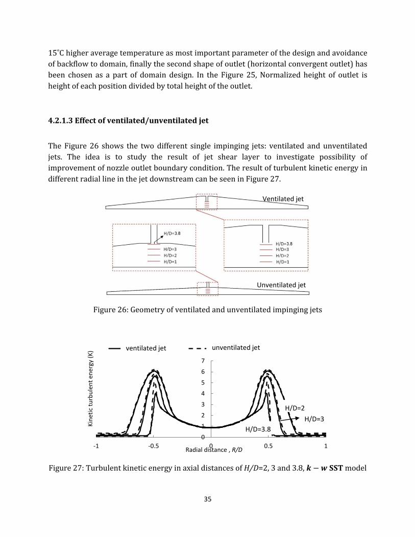
4.2.1.3 Effect of ventilated/unventilated jet

The Figure 26 shows the two different single impinging jets: ventilated and unventilated

jets. The idea is to study the result of jet shear layer to investigate possibility of

improvement of nozzle outlet boundary condition. The result of turbulent kinetic energy in

different radial line in the jet downstream can be seen in Figure 27.

Figure 26: Geometry of ventilated and unventilated impinging jets

Figure 27: Turbulent kinetic energy in axial distances of H/D=2, 3 and 3.8, model

0

1

2

3

4

5

6

7

-1 -0.5 0 0.5 1

Kin

etic

tu

rbu

len

t en

ergy

(K

)

Radial distance , R/D

vent-Hd=3.8 unvent-HD=3.8ventilated jet unventilated jet

H/D=3.8

H/D=3

H/D=2

Ventilated jet

Unventilated jet

36

In turbulent kinetic energy profiles, it can be seen that near jet inlet, there is a difference

magnitude close to shear layer of the jets between ventilated and unventilated jets, but in

jet’s cores and outer area of shear layers there is no significant differences in profiles which

means that unventilated jet contains higher turbulent kinetic energy in shear layer in

downstream, specifically close to nozzle outlet. In order to understand the reason of the

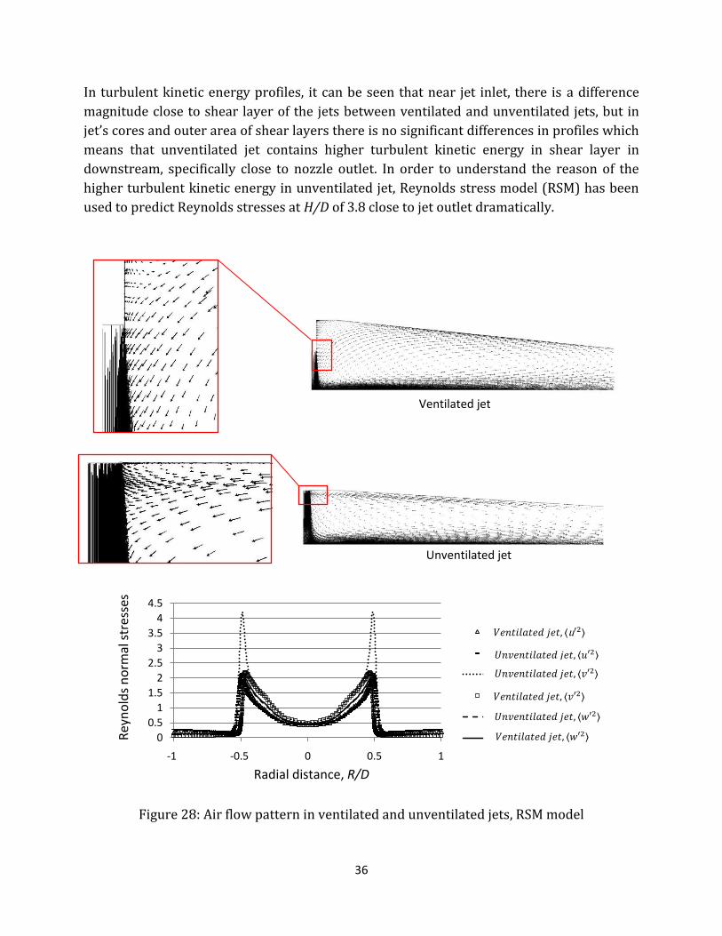
higher turbulent kinetic energy in unventilated jet, Reynolds stress model (RSM) has been

used to predict Reynolds stresses at H/D of 3.8 close to jet outlet dramatically.

Figure 28: Air flow pattern in ventilated and unventilated jets, model

0

0.5

1

1.5

2

2.5

3

3.5

4

4.5

0.84 0.845 0.85 0.855 0.86

ventilated jet -uu

unventilated-uu

unventilated-vv

ventilated-vv

unventilated-ww

ventilated-ww

𝑉 𝑗 ⟨ ⟩

Radial distance, R/D

Ventilated jet

Unventilated jet

𝑈𝑛𝑣𝑒𝑛𝑡𝑖𝑙𝑎𝑡𝑒𝑑 𝑗𝑒𝑡 ⟨𝑢 ⟩

𝑈𝑛𝑣𝑒𝑛𝑡𝑖𝑙𝑎𝑡𝑒𝑑 𝑗𝑒𝑡 ⟨𝑣 ⟩

𝑉𝑒𝑛𝑡𝑖𝑙𝑎𝑡𝑒𝑑 𝑗𝑒𝑡 ⟨𝑣 ⟩

𝑈𝑛𝑣𝑒𝑛𝑡𝑖𝑙𝑎𝑡𝑒𝑑 𝑗𝑒𝑡 ⟨𝑤 ⟩

𝑉𝑒𝑛𝑡𝑖𝑙𝑎𝑡𝑒𝑑 𝑗𝑒𝑡 ⟨𝑤 ⟩

-1 -0.5 0 0.5 1

Rey

no

lds

no

rmal

str

esse

s

37

The result in Figure 28 shows that close to nozzle jet in two cases, the flow pattern of mass

penetration is different and by comparing the result of Reynolds normal stresses it can be

seen that Reynolds normal stress of ⟨ ⟩ has very higher magnitude in shear layer of the

unventilated jet in downstream. The zoomed region of the unventilated jet shows that due

to effect of confined wall boundary condition close to nozzle outlet, the air flow has to

penetrate to jet in horizontal direction which influence on the Reynolds normal stress in

coordinate. Moreover, turbulent kinetic energy is calculated by equation (2.16) and

therefore it is concluded that the component of ⟨ ⟩ leads to higher turbulent kinetic

energy in unventilated jet outlet.

The result of thermal simulation shows the average and maximum heat transfer coefficient

in ventilated jet domain are higher than unventilated (113 compare to 107 ), but

in average of outlet temperature point of view, unventilated geometry has higher outlet

temperature. In ventilated jet, there is a bigger eddy on centre of the domain which

improves the mixing the wall jet shear layer with surrounding fluid that increases heat

transfer coefficient on impingement plate which might be due to more penetration of mass

in the developing zone of jet. But the bigger eddy in the domain can contribute to exit air

flow faster which decreases the average temperature of the outlet. Finally due to higher

average and maximum heat transfer on plate, the ventilated jet is selected as last step of

single jet region design.

4.2.2 Single jet in 3-D

After finalize the geometry shape, 3-D simulation result is shown for single impinging jet. As

it can be seen in Figure 29, the normalized axial velocity by bulk velocity realizes potential

core of the jet clearly. Also the eddy close to confined wall boundary condition can be seen

where wall jet flow separates from impingement wall and makes this eddy in centre of the

medium. This phenomenon is clearer in the contour of the normalized velocity magnitude

by bulk velocity where visualisation of wall jet flow is clearer due to radial velocity

component in velocity magnitude.

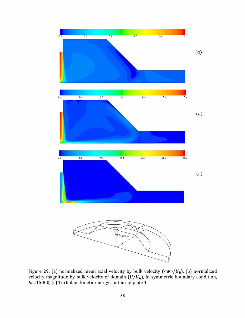
38

Figure 29: (a) normalized mean axial velocity by bulk velocity (< >/ ), (b) normalized velocity magnitude by bulk velocity of domain ( / ), in symmetric boundary condition, Re=15000, (c) Turbulent kinetic energy contour of plate 1

𝑎

𝑏

𝑐

Plate 1

39

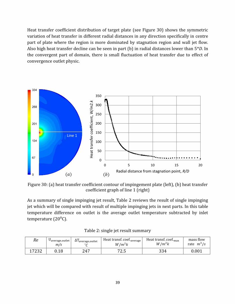
Heat transfer coefficient distribution of target plate (see Figure 30) shows the symmetric

variation of heat transfer in different radial distances in any direction specifically in centre

part of plate where the region is more dominated by stagnation region and wall jet flow.

Also high heat transfer decline can be seen in part (b) in radial distances lower than 5*D. In

the convergent part of domain, there is small fluctuation of heat transfer due to effect of

convergence outlet physic.

Figure 30: (a) heat transfer coefficient contour of impingement plate (left), (b) heat transfer coefficient graph of line 1 (right)

As a summary of single impinging jet result, Table 2 reviews the result of single impinging

jet which will be compared with result of multiple impinging jets in next parts. In this table

temperature difference on outlet is the average outlet temperature subtracted by inlet

temperature (20⁰C).

Table 2: single jet result summary

Re

m/s

˚C

mass flow rate

17232 0.18 247 72.5 334 0.001

0

50

100

150

200

250

300

350

0 5 10 15 20

Hea

t tr

ansf

er c

oef

fici

ent,

W/m

2.k

Radial distance from stagnation point, R/D

Line 1

𝑎 𝑏

40

4.3 Multiple impinging jets

4.3.1 5-cross jets setup

In this part, computational result of multiple impinging jets is presented in order to

compare the result with single impinging jet. It should be considered that the optimized

design of 2-D simulations is applied in 3-D cases to study the domain in 3-D dimensions.

Therefore, the geometry contains ventilated jet with radial distance of 20*D from jet centre

with the convergent outlet.

According to previous studies (Tummers, Jacobse et al. (2011), Thielen (2003)) on multiple

impinging jets, two types of configurations are used: 5-cross jets and 9 square jets (see

Figure below).

Figure 31: Multiple impinging jets configuration in 3-D simulation study, 5-cross and 9 jets setup

Effect of different Reynolds number on average heat transfer coefficient and average outlet

temperature is studied in multiple 5-cross jets setup. Then the result of three turbulence

model of , and Reynolds stress model ( ) are compared and verified

with two series of experimental data. Finally the result of 5 and 9 jets configuration will

compare together to understand more about multiple jets phenomena.

4.3.1.1 Study of different Reynolds numbers

Influence of different Reynolds number of 9828, 11,466, 17,232 and 20,000 is shown in this

part to find a correlation between Reynolds number, average heat transfer coefficient and

average air outlet temperature difference. In these cases, turbulence model was

used with low-Re correction option to increase the prediction accuracy nearby to

impingement plate in wall boundary condition. The configuration of 5-cross jets (see Figure

31) is used in this study.

41

In the Table 3, result shows that higher the Reynolds number, higher average velocity of

outlet and it contributes to effect on the outlet temperature due to reduction of wall jet air

flow entrainment with air flow of domain. But on the other side, due to higher wall jet

velocity and higher convection with impingement plate, average heat transfer coefficient

rises. Therefore there is a correlation between these physical parameters of domain (Figure

32) and depend on the purpose of impinging, best Reynolds number can be chosen. In this

case, the range of Reynolds number 11000 to 17000 contains best optimised result.

Table 3: The summary of effect of different Reynolds number on heat transfer

Reynolds number

m/s

˚C

9,828 0.17 194.1 146

11,466 0.21 202 158

17,232 0.30 187 206

20,000 0.42 176 227

In the Table 3, is defined as

Figure 32: Correlation of average heat transfer coefficient and air outlet temperature difference for different Reynolds number in 5-cross jets setup

140

150

160

170

180

190

200

210

220

230

240

140 150 160 170 180 190 200 210 220 230

Air

tem

per

atu

re d

iffe

ren

ce a

vera

ge

Heat transfer coefficient average, W/m2.k

9,828

11,466

17,232

20,000

Heat transfer coefficient average,

Air

tem

per

atu

re d

iffe

ren

ce a

vera

ge, ᵒC

42

4.3.1.2 Study of different turbulence models

Three turbulence models of , and Reynolds stress model ( ) are

compared for 5-cross jets configuration. As it shown in Table 3 that Reynolds number in

range of 11000 to 17000 contains best result to aim of the simulation, therefore for

verification of turbulence models with available experimental data (Reynolds number

23,000) Reynolds number 17,232 is verified in order to predict similar air flow compare to

experimental data.

Different parameters of domain are studied by comparing the turbulence models result. The

normalized mean radial and axial velocity components by pipe bulk velocity

⟨ ⟩ ⟨ ⟩ ⟨ ⟩ are verified with experimental data (Tummers, Jacobse et al.

(2011) in radial lines from jet centre to R/D = 2. Moreover for the Reynolds stress model

( ), result of Reynolds normal stresses and Reynolds shear stress, in

same axial lines are verified by the available measurement data (Cooper, Jackson et al.

(1993), Tummers, Jacobse et al. (2011)) . Cooper, Jackson et al. (1993) have done their

measurement study by using hot wire and recently Tummers, Jacobse et al. (2011)

improved the near wall measurement by two-component Laser Doppler Anemometry

( ) and reported the result is in very good agreement with previous experimental study.

The Figure 33 shows the radial lines in both and coordinates which different

parameters are verified in these lines. The reason to choose the corner jet compare to

centre jet is that available experimental data is valid for single impinging jet , therefore it

has found that simulation result of corner jet in the side in front of outlet surface deos not

disturb as much as the side of jet in region neighbouring to centre jet. The reason to verify

the 5 multiple jets results with available experimental data instead of single impinging jet is

that due to objectives of the project, single impinging jet deosn’t satisfy the minimum

limitation of the aims, therefore main focus of the project is on the multiple jets. It can be

seen in this figure that axial red lines extend from stagnation point of corner jet to outlet

direction in and coordinate.

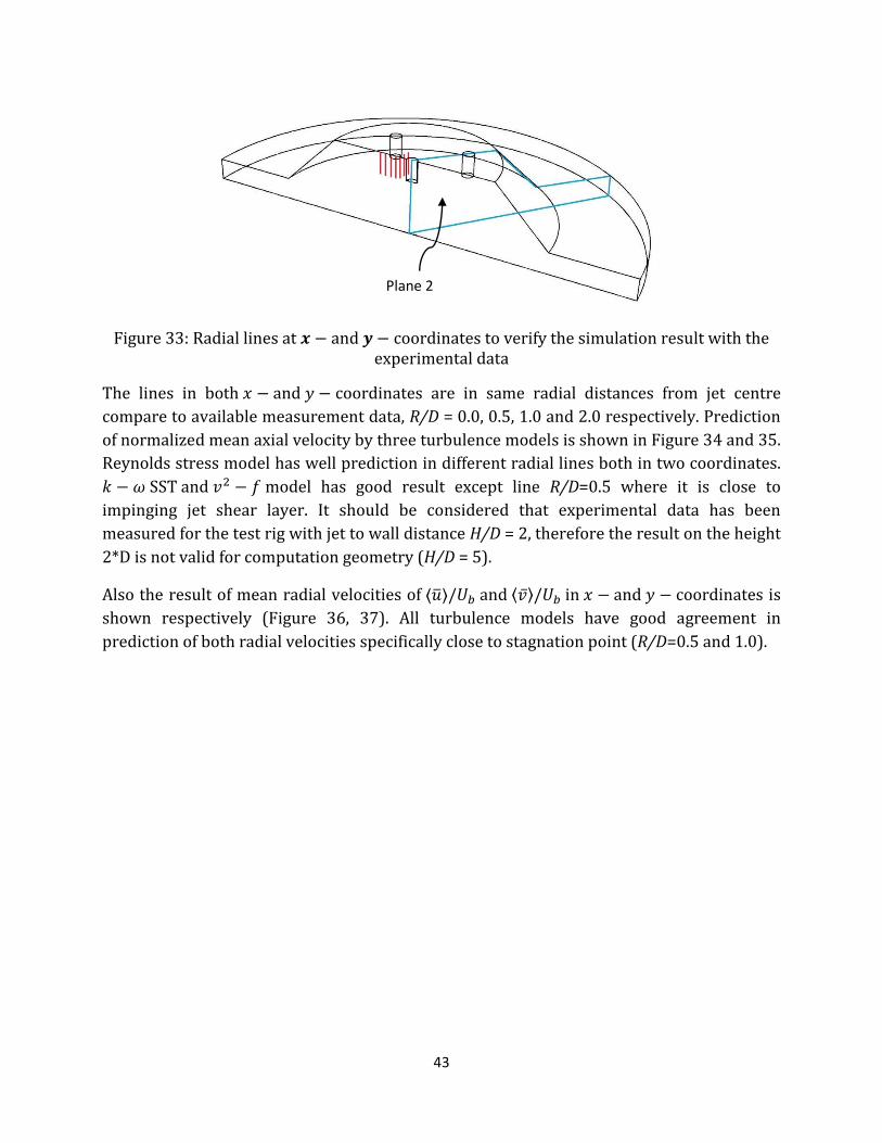
43

Figure 33: Radial lines at and coordinates to verify the simulation result with the experimental data

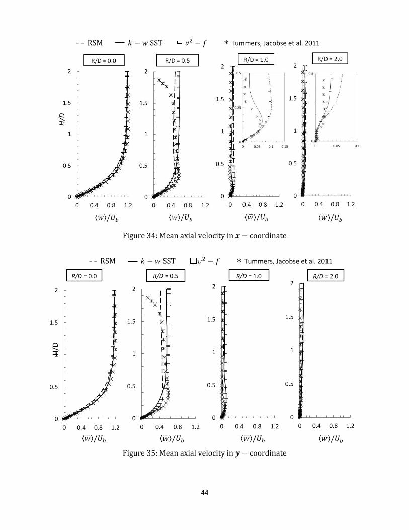
The lines in both and coordinates are in same radial distances from jet centre

compare to available measurement data, R/D = 0.0, 0.5, 1.0 and 2.0 respectively. Prediction

of normalized mean axial velocity by three turbulence models is shown in Figure 34 and 35.

Reynolds stress model has well prediction in different radial lines both in two coordinates.

and model has good result except line R/D=0.5 where it is close to

impinging jet shear layer. It should be considered that experimental data has been

measured for the test rig with jet to wall distance H/D = 2, therefore the result on the height

2*D is not valid for computation geometry (H/D = 5).

Also the result of mean radial velocities of ⟨ ⟩ and ⟨ ⟩ in and coordinates is

shown respectively (Figure 36, 37). All turbulence models have good agreement in

prediction of both radial velocities specifically close to stagnation point (R/D=0.5 and 1.0).

Plane 2

44

Figure 34: Mean axial velocity in coordinate

Figure 35: Mean axial velocity in coordinate

0

0.5

1

1.5

2

0 0.4 0.8 1.2

H/D

R/D = 0.0

0

0.5

1

1.5

2

0 0.4 0.8 1.2

R/D = 0.5

0

0.5

1

1.5

2

0 0.4 0.8 1.2

R/D = 1.0

0

0.5

1

1.5

2

0 0.4 0.8 1.2

R/D = 2.0

- - 𝑘 𝑤 𝑣 𝑓 Tummers, Jacobse et al. 2011

- - 𝑘 𝑤 𝑣 𝑓 Tummers, Jacobse et al. 2011

⟨��⟩ 𝑈𝑏 ⟨��⟩ 𝑈𝑏 ⟨��⟩ 𝑈𝑏 ⟨��⟩ 𝑈𝑏

45

Figure 36: Mean radial velocity component in coordinate

Figure 37: Mean radial velocity component in coordinate

0

0.5

1

1.5

2

-0.1 0.3 0.7 1.1

H/D

R/D = 0.0

0

0.5

1

1.5

2

-0.1 0.3 0.7 1.1

R/D = 0.5

0

0.5

1

1.5

2

-0.1 0.3 0.7 1.1

R/D = 1.0

0

0.5

1

1.5

2

-0.1 0.3 0.7 1.1

R/D = 2.0

0

0.5

1

1.5

2

-0.1 0.3 0.7 1.1

H/D

R/D = 0.0

0

0.5

1

1.5

2

-0.1 0.3 0.7 1.1

R/D = 0.5

0

0.5

1

1.5

2

-0.1 0.3 0.7 1.1

R/D = 1.0

0

0.5

1

1.5

2

-0.1 0.3 0.7 1.1

R/D = 2.0

- - 𝑘 𝑤 𝑣 𝑓 Tummers, Jacobse et al. 2011

- - 𝑘 𝑤 𝑣 𝑓 Tummers, Jacobse et al. 2011

⟨��⟩ 𝑈𝑏

⟨��⟩ 𝑈𝑏 ⟨��⟩ 𝑈𝑏 ⟨��⟩ 𝑈𝑏 ⟨��⟩ 𝑈𝑏

⟨��⟩ 𝑈𝑏 ⟨��⟩ 𝑈𝑏 ⟨��⟩ 𝑈𝑏

46

The result of Reynolds normal stress of ⟨ ⟩ shows poor prediction of near wall

region (Figure 38) in R/D 1.0 in axial traverses of H/D 0.4, from stagnation point to the

region close to jet edge (R/D=0.5) where there is shear layer of jet which penetrates mass

flow from surrounding media the simulation result is over predicted. But in downstream of

stagnation region in R/D=2.0 the prediction is in good agreement with experimental data.

Figure 38: Reynolds normal stress in axial direction

The prediction of Reynolds normal stresses of ⟨ ⟩ and ⟨ ⟩

in Figure 39 shows

that stagnation point simulation result is verified well in both coordinates while in

coordinate in more radial distances from jet, ⟨ ⟩ follow a same profile in

different axial traverses, but the values has differences from measurement data. On the

other side in coordinate, prediction of the Reynolds stress of ⟨ ⟩ shows good

agreement with experimental data.

0

0.5

1

1.5

2

0 0.02 0.04

H/D

R/D = 0.0

0

0.5

1

1.5

2

0 0.02 0.04

R/D = 0.5

0

0.5

1

1.5

2

0 0.02 0.04

R/D = 1.0

0

0.5

1

1.5

2

0 0.02 0.04

R/D = 2.0

- - - ⟨𝑤 ⟩ 𝑈𝑏 , x-coordinate ⟨𝑤 ⟩ 𝑈𝑏

, y-coordinate Tummers, Jacobse et al.

2011

⟨𝑤 ⟩ 𝑈𝑏 ⟨𝑤 ⟩ 𝑈𝑏

⟨𝑤 ⟩ 𝑈𝑏 ⟨𝑤 ⟩ 𝑈𝑏

47

Figure 39: Reynolds normal stress in and coordinates

Figure 40: Reynolds shear stress in and coordinates

0

0.5

1

1.5

2

-0.01 0.02 0.05

H/D

R/D = 0.0

0

0.5

1

1.5

2

-0.01 0.02 0.05

R/D = 0.5

0

0.5

1

1.5

2

-0.01 0.02 0.05

R/D = 1.0

0

0.5

1

1.5

2

-0.01 0.02 0.05

R/D = 2.0

0

0.5

1

1.5

2

-0.016 0 0.016

H/D

R/D = 0.0

0

0.5

1

1.5

2

-0.016 0 0.016

R/D = 0.5

0

0.5

1

1.5

2

-0.016 0 0.016

R/D = 1.0

0

0.5

1

1.5

2

-0.016 0 0.016

R/D = 2.0

- - - ⟨𝑢 ⟩ 𝑈𝑏 , x-coordinate ⟨𝑣 ⟩ 𝑈𝑏

, y-coordinate Tummers, Jacobse et al. (2011)

□ Cooper, Jackson et al. (1993)

- - - ⟨𝑢 𝑤 ⟩ 𝑈𝑏 , x-coordinate ⟨𝑣 𝑤 ⟩ 𝑈𝑏

, y-coordinate Tummers, Jacobse et al. 2011

48

Finally in verification of Reynolds stresses, Reynolds shear stresses of ⟨ ⟩ and

⟨ ⟩ is seen in Figure 40. In coordinate, the ⟨ ⟩

result is verified well

except in region close to jet shear layer (R/D 0.5). In the other direction, ⟨ ⟩

profile has very good agreement with the measurement data profile.

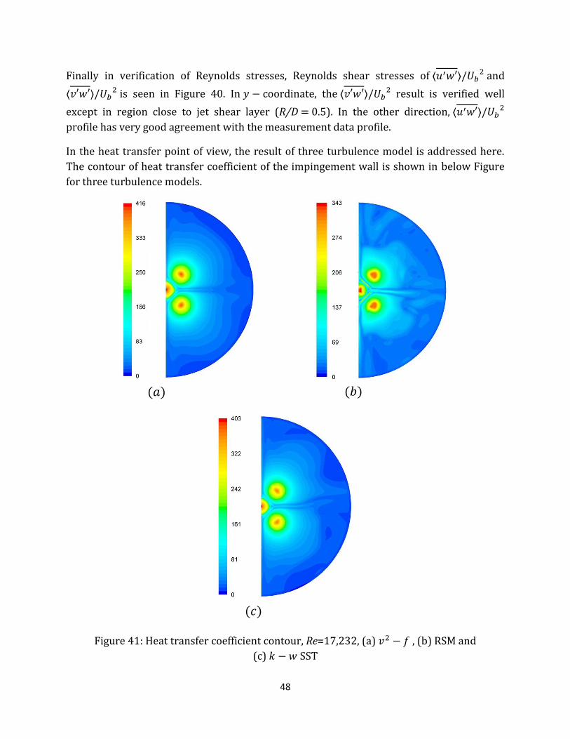
In the heat transfer point of view, the result of three turbulence model is addressed here.

The contour of heat transfer coefficient of the impingement wall is shown in below Figure

for three turbulence models.

Figure 41: Heat transfer coefficient contour, Re=17,232, (a) , (b) and

(c)

𝑎

𝑅𝑆𝑀

𝑏

𝑐

49

In heat transfer coefficient result, peak values of turbulence models are different;

model shows highest peak compare to other models. On the other side, model predicts

different heat transfer coefficient distribution compare to circular variation of and

models. In between the neighbour jets, heat transfer increases in a line when

upwash flow is emerged by wall jet flow. As heat transfer coefficient is calculated by

temperature difference between hot plate and air flow temperature, temperature

distribution contour is similar to heat transfer coefficient contour.

Moreover Table 4 shows the summary of result of simulation for Re=17,232 for the three

turbulence models. The average of outlet air temperature of three models is presented in a

same order while the result of heat transfer coefficient average of impingement plate differs

for each model.

Table 4: Result summary of , and turbulence models for Re=17,232

( ))

( ))

(˚C)

416 225.5 193.4

343 186 187

389 210 176

By comparing the simulation result, it was found that centre jet heat transfer coefficient

peak is higher than corner jets peaks in all three turbulence models predictions.

Turbulent kinetic energy contour of vertical plane 2 (see Figure 42) has very good

agreement of prediction in stagnation point region (without any over prediction of

turbulent kinetic energy peak at this region) with previous Computational studies for

and models (Behnia, Parneix et al. (1998), Thielen (2003)).

50

Figure 42: Turbulent kinetic energy contour in plane 1, Re=17232, (a) , (b) and (c) models

𝑎

𝑏

𝑐

Plane 2

51

Figure 43: Mean axial velocity ⟨ ⟩ in plane 1, Re=17,232, (a) , (b) and (c)

Turbulence models

In the developing zone of the jets near the stagnation region, higher level of turbulent

kinetic energy can be seen, where axial velocity of jet is decreasing in this zone (around

potential core length). This effect is shown in Figure 43, where potential core is vanished in

this zone near to stagnation region. The interaction of two neighbour jets also can be seen

in the mean axial velocity contour and it is interesting that upwash flow due to wall jets

interaction inclines and penetrates to the centre jet and peak value of turbulent kinetic

energy occurs in shear layer of the centre jet in all predictions. In the other hand, more

penetration of mass flow into the centre jet shear layer, higher level of turbulent kinetic

energy.

𝑎

𝑏

𝑐

52

Therefore it’s concluded that this phenomenon can be one of the reasons of highest peak

value of heat transfer coefficient in centre jet compare to corner jets. All three turbulence

models predict the interaction of the wall jets, but and models show the

similar pattern of distribution. On the other side, peak value of turbulent kinetic energy

prediction of and models are in a same level.

Finally by comparing the result of different turbulence models contains mean velocity

components and Reynolds stresses with experimental data, it’s concluded that model

is more reliable model compare to other models due to verification of Reynolds stresses

components in isothermal prediction. It should be considered that and

models can only predict mean velocity components while model can predict the

Reynolds stresses. Therefore by verification the model result, it’s more reasonable to

lean on this model result in isothermal simulation and continue computational study on the

thermal case where there is no available experimental data to verify the thermal result.

4.3.2 9-in line multiple jets setup

After computational study of 5-cross jets setup and find the best turbulence model, the 9-multiple jets configuration result is shown in this part in order to study the effect of higher mass flow rate to the domain by increasing the number of jets and dominating more effective cooling area and compare it by single jet and 5-cross jets setup.

The normalized centre line velocity of jets in axial traverse line by centre jet’s core velocity

magnitude is plotted in Figure 44 where each jet in symmetric boundary condition is

identified by its direction compare to centre jet. The interaction between configurations of

jets reveals interesting physic of multiple impinging jets. As in this figure is shown, all jets

behave same pattern in jet to wall distances greater than 2, but in region of stagnation point

the magnitude of the velocity is different in an interesting order. The centre jet has greatest

velocity in axial traverse distances in this region while the lower velocity magnitude is

belong to the corner jets (NE and SE) and the jets in the neighbourhood (N, E and S) are

located in the between of those profiles. Therefore it is concluded that the position of the

jets in this configuration shows the symmetric flow pattern of the jets respectively and

centre jet velocity profile is greater than other surrounding jets.

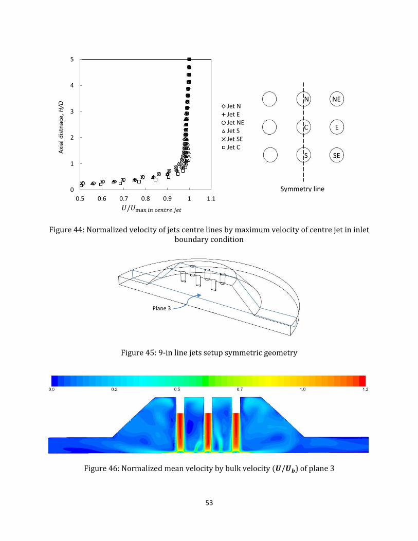
53

Figure 44: Normalized velocity of jets centre lines by maximum velocity of centre jet in inlet boundary condition

Figure 45: 9-in line jets setup symmetric geometry

Figure 46: Normalized mean velocity by bulk velocity ) of plane 3

0

1

2

3

4

5

0.5 0.6 0.7 0.8 0.9 1 1.1

Axi

al d

istn

ace,

H/D

Jet NJet EJet NEJet SJet SEJet C

𝑗

N NE

C

S

E

SE

Symmetry line

Plane 3

54

In the interaction of the wall jets point of view, the normalized mean velocity by bulk

velocity ( contour (Figure 46) shows the same phenomenon in 5-cross jets setup

which upwash flow is penetrated to the centre jet from surrounding. Also there is a region

at end of effective length of wall jet which flow is separated from wall boundary condition

and divided into two flows; one is penetrated to the eddy inside the convergent space and

has convection heat transfer with confined wall and then followed the wall jet flow, and the

other enters to horizontal convergent outlet. A part of the second flow goes to pass outlet

condition and other part establishes an eddy and interacts with wall jet flow and probably

the interaction of this eddy with wall jet is one of the reasons for the flow separation. The

zoomed area in Figure 47 reveals this interaction, where velocity vectors are coloured by

air temperature. The well mixing is happened in this region due to convection of air flows

with wall boundaries conditions and mixing the flows in interaction area.

Figure 47: velocity vector of plane 3 coloured by air temperature and zoomed region of wall jet flow

As confirmation of interaction of eddies and wall jet flow in discussed region, the contour of

air temperature verifies this influence to heat transfer to air flow. The contour of

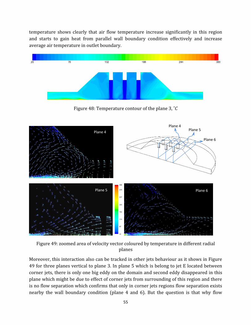
55

temperature shows clearly that air flow temperature increase significantly in this region

and starts to gain heat from parallel wall boundary condition effectively and increase

average air temperature in outlet boundary.

Figure 48: Temperature contour of the plane 3, ˚C

Figure 49: zoomed area of velocity vector coloured by temperature in different radial planes

Moreover, this interaction also can be tracked in other jets behaviour as it shows in Figure

49 for three planes vertical to plane 3. In plane 5 which is belong to jet E located between

corner jets, there is only one big eddy on the domain and second eddy disappeared in this

plane which might be due to effect of corner jets from surrounding of this region and there

is no flow separation which confirms that only in corner jets regions flow separation exists

nearby the wall boundary condition (plane 4 and 6). But the question is that why flow

Plane 6

Plane 5 Plane 4

Plane 4

Plane 5 Plane 6

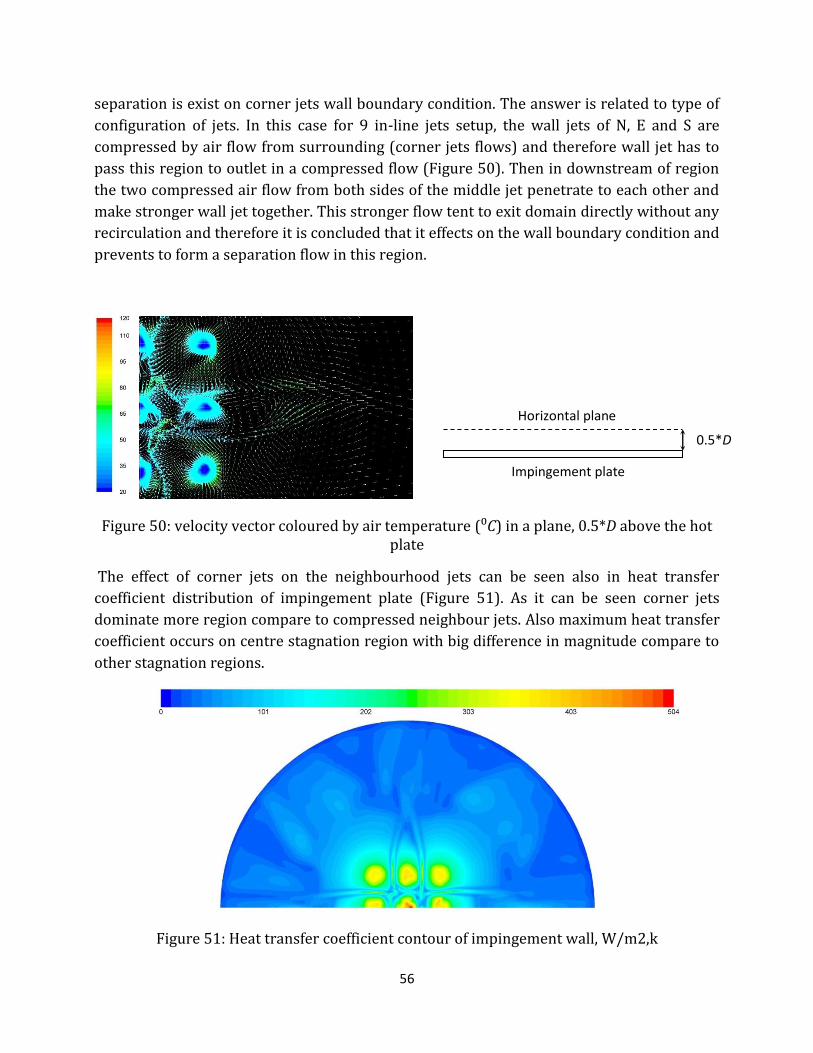
56

separation is exist on corner jets wall boundary condition. The answer is related to type of

configuration of jets. In this case for 9 in-line jets setup, the wall jets of N, E and S are

compressed by air flow from surrounding (corner jets flows) and therefore wall jet has to

pass this region to outlet in a compressed flow (Figure 50). Then in downstream of region

the two compressed air flow from both sides of the middle jet penetrate to each other and

make stronger wall jet together. This stronger flow tent to exit domain directly without any

recirculation and therefore it is concluded that it effects on the wall boundary condition and

prevents to form a separation flow in this region.

Figure 50: velocity vector coloured by air temperature (⁰C) in a plane, 0.5*D above the hot plate

The effect of corner jets on the neighbourhood jets can be seen also in heat transfer

coefficient distribution of impingement plate (Figure 51). As it can be seen corner jets

dominate more region compare to compressed neighbour jets. Also maximum heat transfer

coefficient occurs on centre stagnation region with big difference in magnitude compare to

other stagnation regions.

Figure 51: Heat transfer coefficient contour of impingement wall, W/m2,k

0.5*D

Impingement plate

Horizontal plane

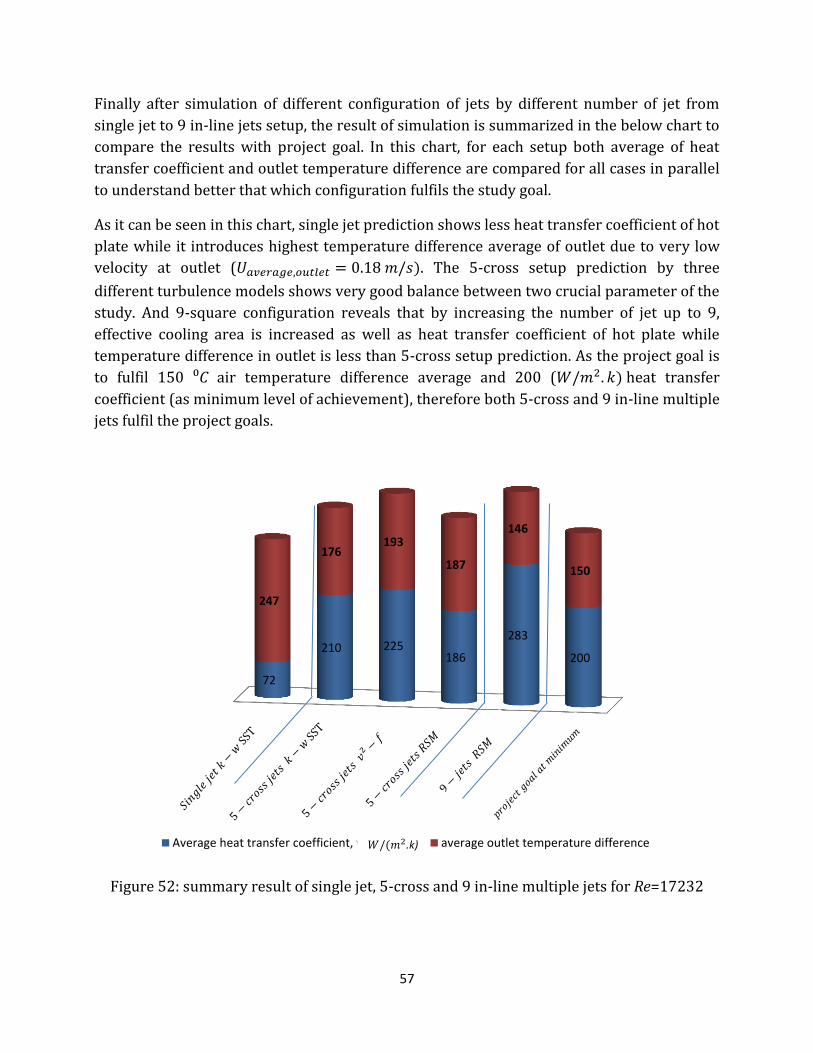
57

Finally after simulation of different configuration of jets by different number of jet from

single jet to 9 in-line jets setup, the result of simulation is summarized in the below chart to

compare the results with project goal. In this chart, for each setup both average of heat

transfer coefficient and outlet temperature difference are compared for all cases in parallel

to understand better that which configuration fulfils the study goal.

As it can be seen in this chart, single jet prediction shows less heat transfer coefficient of hot

plate while it introduces highest temperature difference average of outlet due to very low

velocity at outlet ( . The 5-cross setup prediction by three

different turbulence models shows very good balance between two crucial parameter of the

study. And 9-square configuration reveals that by increasing the number of jet up to 9,

effective cooling area is increased as well as heat transfer coefficient of hot plate while

temperature difference in outlet is less than 5-cross setup prediction. As the project goal is

to fulfil 150 ⁰C air temperature difference average and 200 ( heat transfer

coefficient (as minimum level of achievement), therefore both 5-cross and 9 in-line multiple

jets fulfil the project goals.

Figure 52: summary result of single jet, 5-cross and 9 in-line multiple jets for Re=17232

72

210 225 186

283

200

247

176 193

187

146

150

Average heat transfer coefficient, w/m2,k average outlet temperature difference .k)

58

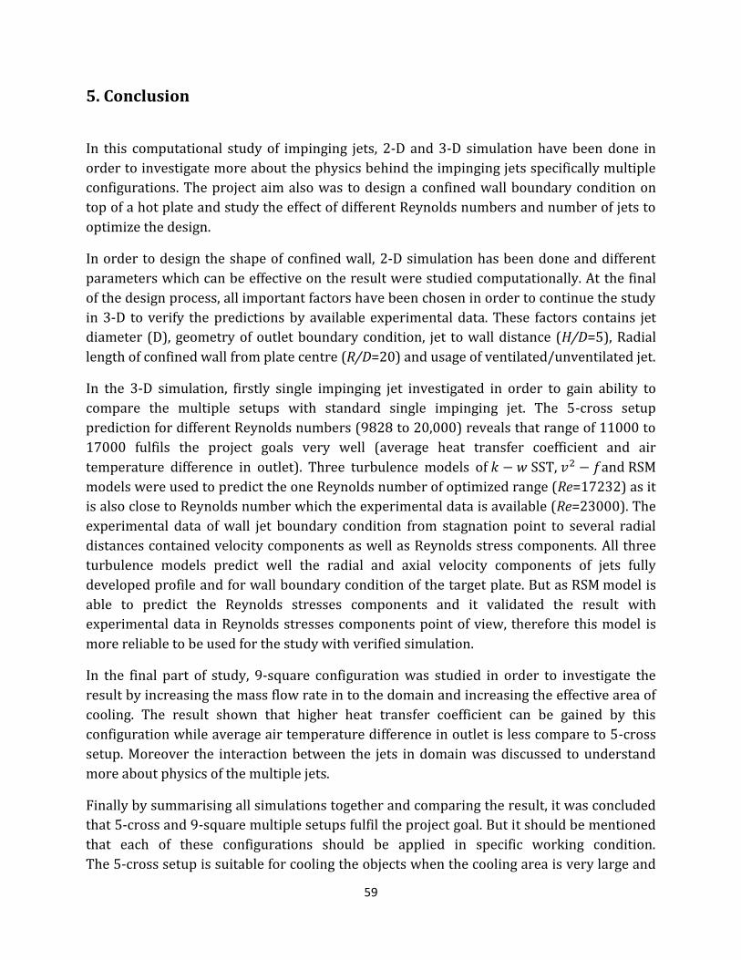
59

5. Conclusion

In this computational study of impinging jets, 2-D and 3-D simulation have been done in

order to investigate more about the physics behind the impinging jets specifically multiple

configurations. The project aim also was to design a confined wall boundary condition on

top of a hot plate and study the effect of different Reynolds numbers and number of jets to

optimize the design.

In order to design the shape of confined wall, 2-D simulation has been done and different

parameters which can be effective on the result were studied computationally. At the final

of the design process, all important factors have been chosen in order to continue the study

in 3-D to verify the predictions by available experimental data. These factors contains jet

diameter (D), geometry of outlet boundary condition, jet to wall distance (H/D=5), Radial

length of confined wall from plate centre (R/D=20) and usage of ventilated/unventilated jet.

In the 3-D simulation, firstly single impinging jet investigated in order to gain ability to

compare the multiple setups with standard single impinging jet. The 5-cross setup

prediction for different Reynolds numbers (9828 to 20,000) reveals that range of 11000 to

17000 fulfils the project goals very well (average heat transfer coefficient and air

temperature difference in outlet). Three turbulence models of , and

models were used to predict the one Reynolds number of optimized range (Re=17232) as it

is also close to Reynolds number which the experimental data is available (Re=23000). The

experimental data of wall jet boundary condition from stagnation point to several radial

distances contained velocity components as well as Reynolds stress components. All three

turbulence models predict well the radial and axial velocity components of jets fully

developed profile and for wall boundary condition of the target plate. But as model is

able to predict the Reynolds stresses components and it validated the result with

experimental data in Reynolds stresses components point of view, therefore this model is

more reliable to be used for the study with verified simulation.

In the final part of study, 9-square configuration was studied in order to investigate the

result by increasing the mass flow rate in to the domain and increasing the effective area of

cooling. The result shown that higher heat transfer coefficient can be gained by this

configuration while average air temperature difference in outlet is less compare to 5-cross

setup. Moreover the interaction between the jets in domain was discussed to understand

more about physics of the multiple jets.

Finally by summarising all simulations together and comparing the result, it was concluded

that 5-cross and 9-square multiple setups fulfil the project goal. But it should be mentioned

that each of these configurations should be applied in specific working condition.

The 5-cross setup is suitable for cooling the objects when the cooling area is very large and

60

it needs to cover the area by several packages of 5-cross setups. The 9-square configuration

is not suitable for this condition due to higher mass flow of jets by 45% and it is preferred

to use this setup in condition which high local heat transfer is needed. Therefore as final

conclusion, it is summarized that for current project goal the 5-cross jets setup gain best

results by fulfilment of both crucial goals of the project; average of heat transfer coefficient

and average of air temperature difference in outlet.

Also it is suggested that to continue the study, effect of number of jets be studied by

comparing the different mass flow rate for different number of jets. In this case, for a

constant mass flow rate, two different numbers of jets can be compared to study the direct

effect of number of jets with a same mass flow rate on heat transfer of impinging jet. Also

constant heat flux boundary condition in impingement plate boundary can be interesting to

study, since this condition is more accurate in reality compare to temperature constant

boundary condition.

61

References

ANSYS® (2011). Academic Research. ANSYS FLUENT THEORY GUIDE, ANSYS, Inc.

Ashforth-Frost, S. and K. Jambunathan (1996). "Effect of nozzle geometry and semi-confinement on the potential core of a turbulent axisymmetric free jet." International Communications in Heat and Mass Transfer 23(2): 155-162.

BARATA, J. M. M. (1996). Fountain flows produced by multiple impinging jets in a crossflow. Reston, VA, ETATS-UNIS, American Institute of Aeronautics and Astronautics.

Baughn, J. W. and S. Shimizu (1989). "Heat transfer measurements from a surface with uniform heat flux and an impinging jet." Journal Name: Journal of Heat Transfer (Transactions of the ASME (American Society of Mechanical Engineers), Series C); (United States); Journal Volume: 111:4: Medium: X; Size: Pages: 1096-1098.

Behnia, M., S. Parneix, et al. (1998). "Prediction of heat transfer in an axisymmetric turbulent jet impinging on a flat plate." International Journal of Heat and Mass Transfer 41(12): 1845-1855.

Behnia, M., S. Parneix, et al. (1999). "Numerical study of turbulent heat transfer in confined and unconfined impinging jets." International Journal of Heat and Fluid Flow 20(1): 1-9.

Cooper, D., D. C. Jackson, et al. (1993). "Impinging jet studies for turbulence model assessment—I. Flow-field experiments." International Journal of Heat and Mass Transfer 36(10): 2675-2684.

Dahm, W. J. A. and P. E. Dimotakis (1990). "Mixing at large Schmidt number in the self-similar far field of turbulent jets." Journal of Fluid Mechanics 217: 299-330.

Dong, L. L., C. W. Leung, et al. (2003). "Heat transfer of a row of three butane/air flame jets impinging on a flat plate." International Journal of Heat and Mass Transfer 46(1): 113-125.

Durbin, P. A. (1995). "Separated Flow Computations with the k − epsilon − w − squared Model." AIAA Journal 33: 659-664.

62

Gao, N., H. Sun, et al. (2003). "Heat transfer to impinging round jets with triangular tabs." International Journal of Heat and Mass Transfer 46(14): 2557-2569.

Geers, L. F. G. (2003). "<Multiple impinging jet arrays an experimental study on flow and heat transfer>."

Goldstein, R. J., A. I. Behbahani, et al. (1986). "Streamwise distribution of the recovery factor and the local heat transfer coefficient to an impinging circular air jet." International Journal of Heat and Mass Transfer 29(8): 1227-1235.

Govindan, A. P. and K. S. Raju (1974). "Hydrodynamics of a Radial Wall Jet." Journal of Applied Mechanics 41(2): 518-519.

Gulati, P., V. Katti, et al. (2009). "Influence of the shape of the nozzle on local heat transfer distribution between smooth flat surface and impinging air jet." International Journal of Thermal Sciences 48(3): 602-617.

HadŽIabdiĆ, M. and K. HanjaliĆ (2008). "Vortical structures and heat transfer in a round impinging jet." Journal of Fluid Mechanics 596.

Katti, V. and S. V. Prabhu (2008). "Experimental study and theoretical analysis of local heat transfer distribution between smooth flat surface and impinging air jet from a circular straight pipe nozzle." International Journal of Heat and Mass Transfer 51(17-18): 4480-4495.

Lee, D. H., Song, et al. (2004). The effects of nozzle diameter on impinging jet heat transfer and fluid flow. New York, NY, ETATS-UNIS, American Society of Mechanical Engineers.

Liu, Q., A. K. Sleiti, et al. (2008). "Application of pressure and temperature sensitive paints for study of heat transfer to a circular impinging air jet." International Journal of Thermal Sciences 47(6): 749-757.

Lytle, D. and B. W. Webb (1994). "Air jet impingement heat transfer at low nozzle-plate spacings." International Journal of Heat and Mass Transfer 37(12): 1687-1697.

Martin, H. (1977). Heat and Mass Transfer between Impinging Gas Jets and Solid Surfaces. Advances in Heat Transfer. P. H. James and F. I. Thomas, Elsevier. Volume 13: 1-60.

63

Milanovic, I. M. and K. J. Hammad (2010). "PIV Study of the Near-Field Region of a Turbulent Round Jet." ASME Conference Proceedings 2010(49484): 1353-1361.

O’Donovan, T. S. and D. B. Murray (2007). "Jet impingement heat transfer – Part I: Mean and root-mean-square heat transfer and velocity distributions." International Journal of Heat and Mass Transfer 50(17-18): 3291-3301.

Rundstrom, D. and B. Moshfegh (2004). Investigation of flow and heat transfer of an impinging jet in a cross-flow for cooling of a heated cube. Thermal and Thermomechanical Phenomena in Electronic Systems, 2004. ITHERM '04. The Ninth Intersociety Conference on.

San, J.-Y. and M.-D. Lai (2001). "Optimum jet-to-jet spacing of heat transfer for staggered arrays of impinging air jets." International Journal of Heat and Mass Transfer 44(21): 3997-4007.

San, J.-Y. and W.-Z. Shiao (2006). "Effects of jet plate size and plate spacing on the stagnation Nusselt number for a confined circular air jet impinging on a flat surface." International Journal of Heat and Mass Transfer 49(19–20): 3477-3486.

Schlichting, H. (1979). Boundary layer theory. McGraw-Hill. New York.

Stevens, J. and B. W. Webb (1991). "Local heat transfer coefficients under an axisymmetric, single-phase liquid jet." Journal Name: Journal of Heat Transfer (Transcations of the ASME (American Society of Mechanical Engineers), Series C); (United States); Journal Volume: 113:1: Medium: X; Size: Pages: 71-78.

Thielen, L. (2003). "<modelling and calculation of flow and heat transfer in multiple impinging jets Thielen.pdf>."

Tummers, M. J., J. Jacobse, et al. (2011). "Turbulent flow in the near field of a round impinging jet." International Journal of Heat and Mass Transfer 54(23-24): 4939-4948.

Versteeg, H. K. and W. Malalasekera (2007). An Introduction to Computational Fluid Dynamics. The Finite Volume Method, Longman Group Ltd.

Viskanta, R. (1993). "Heat transfer to impinging isothermal gas and flame jets." Experimental Thermal and Fluid Science 6(2): 111-134.

64

von Karman, T. (1937). Turbulence. Twenty-Fifth Wilbur Wright Memorial Lecture, Journal of the Arenatical Sciences.

White, F. M. (1986). Fluid mechanics, WCB. New York, McGraw-Hill, Boston: 310.

Wilcox, D. (1998). Turbulence modeling for CFD. La Canada, California, DCW Industries, Inc.

Xu, G. X. and R. A. Antonia (2002). "Effect of different initial conditions on a turbulent round free jet." Experiments in Fluids 33(5): 677-683.

Zhao, W., K. Kumar, et al. (2004). "Flow and Heat Transfer Characteristics of Confined Noncircular Turbulent Impinging Jets." Drying Technology 22(9): 2027-2049.