Computational physics and Astrophysics

Computational Physics and AstrophysicsPartial Differential Equations

Kostas KokkotasUniversity of Tubingen, Germany

and

Pablo LagunaGeorgia Institute of Technology, USA

Spring 2012

Kokkotas & Laguna Computational Physics and Astrophysics

Introduction

A differential equation involving more than one independentvariable is called a partial differential equation (PDE)Many problems in applied science, physics and engineering aremodeled mathematically with PDE.We will mostly focus on finite-difference methods to solvenumerically PDEs.PDEs are classified as one of three types, with terminologyborrowed from the conic sections.That is, for a 2nd-degree polynomial in x and y

Ax2 + Bxy + Cy2 + D = 0

the graph is a quadratic curve, and whenB2 − 4AC < 0 the curve is a ellipse,B2 − 4AC = 0 the curve is a parabolaB2 − 4AC > 0 the curve is a hyperbola


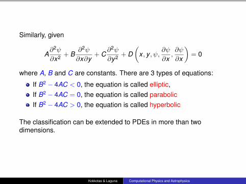
Similarly, given

A∂2ψ

∂x2 + B∂2ψ

∂x∂y+ C

∂2ψ

∂y2 + D(

x , y , ψ,∂ψ

∂x,∂ψ

∂x

)= 0

where A, B and C are constants. There are 3 types of equations:

If B2 − 4AC < 0, the equation is called elliptic,If B2 − 4AC = 0, the equation is called parabolicIf B2 − 4AC > 0, the equation is called hyperbolic

The classification can be extended to PDEs in more than twodimensions.


Two classic examples of elliptic PDEs are the Laplace and Poissonequations:

∇2φ = 0 and ∇2φ = ρ

where in 3D

∇2 =∂2

∂x2 +∂2

∂y2 +∂2

∂z2

∇2 =1r2

∂

∂rr2 ∂

∂r+

1r2 sin θ

∂2

∂φ2 +∂2

∂z2

∇2 =1r∂

∂rr∂

∂r+

1r2 sin θ

∂

∂θsin θ

∂

∂θ+

1r2 sin2 θ

∂2

∂φ2


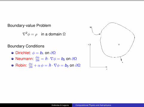
Boundary-value Problem

∇2φ = ρ in a domain Ω

Boundary Conditions

Dirichlet: φ = b1 on ∂Ω

Neumann: ∂φ∂n = n · ∇φ = b2 on ∂Ω

Robin: ∂φ∂n + αφ = n · ∇φ = b3 on ∂Ω


Classic examples of hyperbolic PDEs are:

− 1c2∂2ψ

∂t2 +∇2ψ = 0 wave equation

∂ψ

∂t+ ~V · ∇ψ = 0 advection equation

Classic example of parabolic PDEs are

∂ψ

∂t−∇ · (D∇ψ) = 0 diffusion equation

∂ψ

∂t− α∇2ψ = 0 heat equation

Notice from the diffusion equation that

∂ψ

∂t+∇ · ~J = 0 continuity equation

~J = −D∇ψ Fick’s first law


Advection or Convection Equation

Let’s consider the 1D case

∂tφ+ v ∂xφ = 0

with v = const > 0, t ≥ 0 andx ∈ [0,1]

Initial data: φ(0, x) = φ0(x)

Boundary conditions:φ(t ,0) = α(t) andφ(t ,1) = β(t)Solutions to this equationhave the formφ(t , x) = φ(x − v t)Therefore, the solution φ(t , x)is constant along the linesx − v t = const calledcharacteristics


Forward-Time Center-Space (FTCS) Discretization

Let’s consider the following discretization of the differentialoperators

∂tφni =

φn+1i − φn

i

∆t+ O(∆t)

∂xφni =

φni+1 − φn

i−1

2 ∆x+ O(∆x2)

where we have used the notation φni ≡ φ(tn, xi )

Therefore, the finite difference approximation to ∂tφ+ v ∂xφ = 0is

(φn+1i − φn

i )

∆t+ v

(φni+1 − φn

i−1)

2 ∆x= 0

Notice that we are making a distinction between the solutionφ(t , x) to the continuum equation and φn

i the solution to thediscrete equation.


Solving(φn+1

i − φni )

∆t+ v

(φni+1 − φn

i−1)

2 ∆x= 0

for φn+1i , one gets the following relationship to update the solution

φn+1i = φn

i −12

C(φn

i+1 − φni−1)

where C ≡ ∆t v/∆x


Stability

The tendency for any perturbation in the numerical solution todecay.That is, given a discretization scheme, we need to evaluate thedegree to which errors introduced at any stage of thecomputation will grow or decay.We are then concerned with the behavior of the solution error

εni = φni − φn

i

Substitution of φni = φn

i − εni into

φn+1i = φn

i −12

C(φn

i+1 − φni−1)

yields

φn+1i − εn+1

i = φni − εni −

12

C(φn

i+1 − εni+1 − φni−1 + εni−1

)Kokkotas & Laguna Computational Physics and Astrophysics

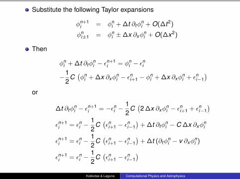
Substitute the following Taylor expansions

φn+1i = φn

i + ∆t ∂tφni + O(∆t2)

φni±1 = φn

i ±∆x ∂xφni + O(∆x2)

Then

φni + ∆t ∂tφ

ni − εn+1

i = φni − εni

−12

C(φn

i + ∆x ∂xφni − εni+1 − φn

i + ∆x ∂xφni + εni−1

)or

∆t ∂tφni − εn+1

i = −εni −12

C(2 ∆x ∂xφ

ni − εni+1 + εni−1

)εn+1

i = εni −12

C(εni+1 − εni−1

)+ ∆t ∂tφ

ni − C ∆x ∂xφ

ni

εn+1i = εni −

12


)+ ∆t (∂tφ

ni − v ∂xφ

ni )

εn+1i = εni −

12


)Kokkotas & Laguna Computational Physics and Astrophysics

That is, the solution error satisfies also the discrete finitedifferences approximation

εn+1i = εni −

12


)Von Neumann stability analysis: Assume that the errors satisfy a“separation-of-variables” of the form

εni = ξn eI xj = ξn eI k ∆x j

where I =√−1, k = 2π/λ and ξ is a complex amplitude. The n

in ξn is understood to be a power.The condition of stability is |ξ| ≤ 1 for all k .


Substitution of εni = ξn eI k ∆x i into the finite difference equation yields

ξn+1 eI k ∆x i = ξn eI k ∆x i − 12

C(ξn eI k ∆x (i+1) − ξn eI k ∆x (i−1)

)ξn+1 = ξn − 1

2C(ξn eI k ∆x − ξn e−I k ∆x

)ξ = 1− 1

2C(

eI k ∆x − e−I k ∆x)

ξ = 1− 12

C 2 I sin (k ∆x)

ξ = 1− I C sin (k ∆x)

|ξ|2 = 1 + C2 sin2 (k ∆x)

Therefore FTCS discretization applied to the advection equation isunstable.


Forward-Time Forward-Space (FTFS) DiscretizationApproximate the advection equation as

(φn+1i − φn

i )

∆t+ v

(φni+1 − φn

i )

∆x= 0

thusφn+1

i = φni − C

(φn

i+1 − φni)



FTFS Stability

Substitute εni = ξn eI k ∆x i into

εn+1i = (1 + C)εni − C εni+1

ξn+1 eI k ∆x i = (1 + C)ξn eI k ∆x i − C ξn eI k ∆x (i+1)

ξn+1 = (1 + C)ξn − C ξn eI k ∆x

ξ = (1 + C)− C eI k ∆x

|ξ|2 =[(1 + C)− C eI k ∆x

] [(1 + C)− C e−I k ∆x

]|ξ|2 = (1 + C)2 + C2 − (1 + C)C (eI k ∆x + e−I k ∆x )

|ξ|2 = (1 + C)2 + C2 − 2 (1 + C)C cos (k ∆x)

|ξ|2 = 1 + 2 (1 + C)C [1− cos (k ∆x)] ≥ 1

the method is unstable


Forward-Time Backward-Space (FTFS) DiscretizationApproximate the advection equation as

(φn+1i − φn

i )

∆t+ v

(φni − φn

i−1)

∆x= 0

thusφn+1

i = φni − C

(φn

i − φni−1)



FTBS Stability

Substitute εni = ξn eI k ∆x i into

εn+1i = (1− C)εni + C εni−1

ξn+1 eI k ∆x i = (1− C)ξn eI k ∆x i + C ξn eI k ∆x (i−1)

ξn+1 = (1− C)ξn + C ξn e−I k ∆x

ξ = (1− C) + C e−I k ∆x

|ξ|2 =[(1− C) + C e−I k ∆x

] [(1− C) + C eI k ∆x

]|ξ|2 = (1− C)2 + C2 + (1− C)C (eI k ∆x + e−I k ∆x )

|ξ|2 = (1− C)2 + C2 + 2 (1− C)C cos (k ∆x)

|ξ|2 = 1− 2 (1− C)C [1− cos (k ∆x)]


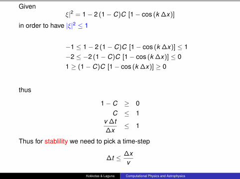
Givenξ|2 = 1− 2 (1− C)C [1− cos (k ∆x)]

in order to have |ξ|2 ≤ 1

−1 ≤ 1− 2 (1− C)C [1− cos (k ∆x)] ≤ 1−2 ≤ −2 (1− C)C [1− cos (k ∆x)] ≤ 01 ≥ (1− C)C [1− cos (k ∆x)] ≥ 0

thus

1− C ≥ 0C ≤ 1

v ∆t∆x

≤ 1

Thus for stablility we need to pick a time-step

∆t ≤ ∆xv


The stablility condition

∆t ≤ ∆xv

implies that the numerical characteristics are contained within thephysical characteristics since

∆t∆x≤ 1

v


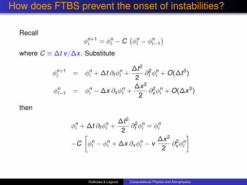
How does FTBS prevent the onset of instabilities?

Recallφn+1

i = φni − C

(φn

i − φni−1)

where C ≡ ∆t v/∆x . Substitute

φn+1i = φn

i + ∆t ∂tφni +

∆t2

2∂2

t φni + O(∆t3)

φni−1 = φn

i −∆x ∂xφni +

∆x2

2∂2

xφni + O(∆x3)

then

φni + ∆t ∂tφ

ni +

∆t2

2∂2

t φni = φn

i

−C[φn

i − φni + ∆x ∂xφ

ni − v

∆x2

2∂2

xφni

]


Then

∆t ∂tφ+∆t2

2∂2

t φ = −v∆t∆x

[∆x ∂xφ−

∆x2

2∂2

xφ

]∂tφ+

∆t2∂2

t φ = −v[∂xφ−

∆x2∂2

xφ

]∂tφ+ v ∂xφ+

∆t2∂2

t φ− v∆x2∂2

xφ = 0

but from ∂tφ = −v ∂xφ we have that

∂2t φ = −v ∂t∂xφ = −v ∂x∂tφ = v2 ∂2

xφ

thus

∂tφ+ v ∂xφ+ v2 ∆t2∂2

xφ− v∆x2∂2

xφ = 0

∂tφ+ v ∂xφ+

(v2 ∆t

2− v

∆x2

)∂2

xφ = 0


∂tφ+ v ∂xφ+

(v2 ∆t

2− v

∆x2

)∂2

xφ = 0

∂tφ+ v ∂xφ− v∆x2

(1− v

∆t∆x

)∂2

xφ = 0

∂tφ+ v ∂xφ− v∆x2

(1− C) ∂2xφ = 0

This equation has the form

∂tφ+ v ∂xφ− α∂2xφ = 0

advection-diffusion equation with

α ≡ v∆x2

(1− C)

Recall that for stability C ≤ 1, thus α ≥ 0.


Givenφ(t , x) = φ0 e−pt e−i k(x−q t)

Substitution into

∂tφ+ v ∂xφ = 0 ⇒ p = 0 q = v

∂tφ+ v ∂xφ− α∂2xφ = 0 ⇒ p = α k2 q = v dissipation

∂tφ+ v ∂xφ− β ∂3xφ = 0 ⇒ p = 0 q = v − β k2 dispersion

That is, the FTBS discretization introduces artificial numericaldissipation to prevent the growth of instabilities.Notice that the dissipation coefficient α ∝ ∆t .Therefore, in the continuum limit lim∆x→0 α = 0


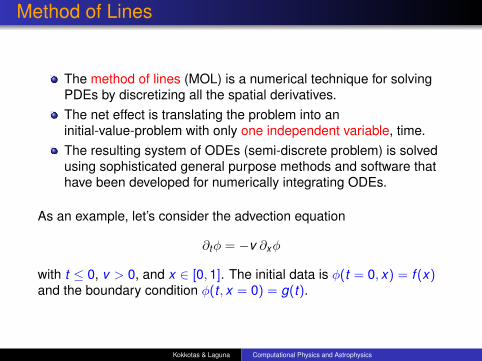
Method of Lines

The method of lines (MOL) is a numerical technique for solvingPDEs by discretizing all the spatial derivatives.The net effect is translating the problem into aninitial-value-problem with only one independent variable, time.The resulting system of ODEs (semi-discrete problem) is solvedusing sophisticated general purpose methods and software thathave been developed for numerically integrating ODEs.

As an example, let’s consider the advection equation

∂tφ = −v ∂xφ

with t ≤ 0, v > 0, and x ∈ [0,1]. The initial data is φ(t = 0, x) = f (x)and the boundary condition φ(t , x = 0) = g(t).


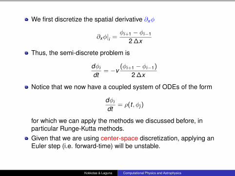
We first discretize the spatial derivative ∂xφ

∂xφ|i =φi+1 − φi−1

2 ∆x

Thus, the semi-discrete problem is

dφi

dt= −v

(φi+1 − φi−1)

2 ∆x

Notice that we now have a coupled system of ODEs of the form

dφi

dt= ρ(t , φj )

for which we can apply the methods we discussed before, inparticular Runge-Kutta methods.Given that we are using center-space discretization, applying anEuler step (i.e. forward-time) will be unstable.


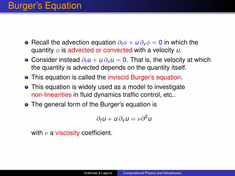
Burger’s Equation

Recall the advection equation ∂tφ+ u ∂xφ = 0 in which thequantity φ is advected or convected with a velocity u.Consider instead ∂tu + u ∂xu = 0. That is, the velocity at whichthe quantity is advected depends on the quantity itself.This equation is called the inviscid Burger’s equation.This equation is widely used as a model to investigatenon-linearities in fluid dynamics traffic control, etc..The general form of the Burger’s equation is

∂tu + u ∂xu = ν∂2u

with ν a viscosity coefficient.


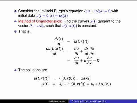
Consider the inviscid Burger’s equation ∂tu + u ∂xu = 0 withinitial data u(t = 0, x) = u0(x)

Method of Characteristics: Find the curves x(t) tangent to thevector ∂t + u ∂x , such that u(t , x(t)) is constant.That is,

dx(t)dt

= u(t , x(t))

du(t , x(t))

dt=

∂u∂t

+dxdt∂u∂x

=∂u∂t

+ u∂u∂x

= 0

The solutions are

u(t , x(t)) = u(0, x(0)) = u0(x0)

x(t) = x0 + t u(0, x(0)) = x0 + t u0(x0)


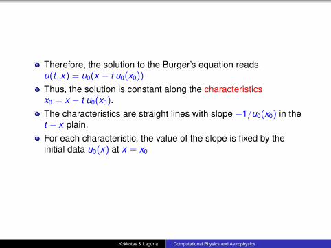
Therefore, the solution to the Burger’s equation readsu(t , x) = u0(x − t u0(x0))

Thus, the solution is constant along the characteristicsx0 = x − t u0(x0).The characteristics are straight lines with slope −1/u0(x0) in thet − x plain.For each characteristic, the value of the slope is fixed by theinitial data u0(x) at x = x0




Consider initial data of the form


The pulse evolves as

Notice that the larger the value of u the more advected that portion ofthe solutions gets.


Let S ≡ ∂xu, then

dSdt

= ∂tS +dxdt∂xS = ∂tS + u ∂xS

= ∂t∂xu + u ∂2x u = ∂x (∂tu + u ∂xu)− (∂xu)2

= −S2

The solution to this equation is

S =S0

t S0 + 1or ∂xu =

∂xu0

t ∂xu0 + 1

Therefore, as t → −1/∂xu0 the slope of the solution diverges, that is,∂xu →∞. In other words, the solution develops a shock discontinuity.

In the case of the general viscous Burger’s equation (ν 6= 0), theshock profile gets smoothed out due to the dissipation.


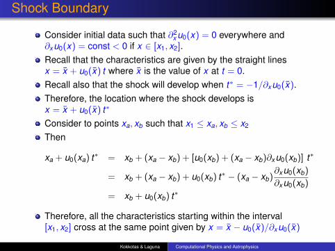
Shock Boundary

Consider initial data such that ∂2x u0(x) = 0 everywhere and

∂xu0(x) = const < 0 if x ∈ [x1, x2].Recall that the characteristics are given by the straight linesx = x + u0(x) t where x is the value of x at t = 0.Recall also that the shock will develop when t∗ = −1/∂xu0(x).Therefore, the location where the shock develops isx = x + u0(x) t∗

Consider to points xa, xb such that x1 ≤ xa, xb ≤ x2

Then

xa + u0(xa) t∗ = xb + (xa − xb) + [u0(xb) + (xa − xb)∂xu0(xb)] t∗

= xb + (xa − xb) + u0(xb) t∗ − (xa − xb)∂xu0(xb)

∂xu0(xb)

= xb + u0(xb) t∗

Therefore, all the characteristics starting within the interval[x1, x2] cross at the same point given by x = x − u0(x)/∂xu0(x)


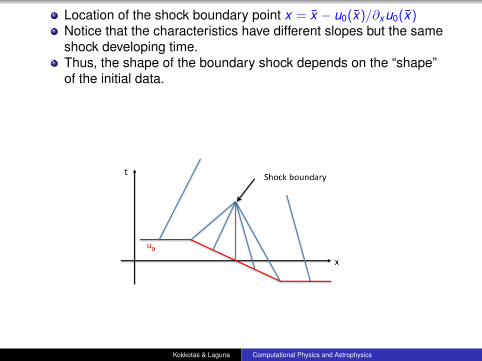
Location of the shock boundary point x = x − u0(x)/∂xu0(x)Notice that the characteristics have different slopes but the sameshock developing time.Thus, the shape of the boundary shock depends on the “shape”of the initial data.


Computational physics and Astrophysics

Documents