Computational Photography Image-based Modeling (Cont.)

Computational PhotographyImage-based Modeling (Cont.)

Jinxiang Chai

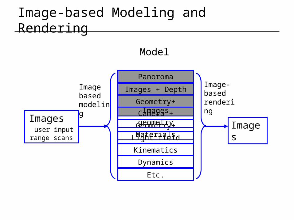
Image-based Modeling and Rendering

Images user input range

scans

Model

Images

Image based modeling

Image-based renderingGeometry+ Images

Geometry+ Materials

Images + Depth

Light field

Panoroma

Kinematics

Dynamics

Etc.

Camera + geometry

Stereo reconstruction

Given two or more images of the same scene or object, compute a representation of its shape

knownknowncameracamera

viewpointsviewpoints

Stereo reconstruction

Given two or more images of the same scene or object, compute a representation of its shape

knownknowncameracamera

viewpointsviewpoints

How to estimate camera parameters?

- where is the camera?

- where is it pointing?

- what are internal parameters, e.g. focal length?

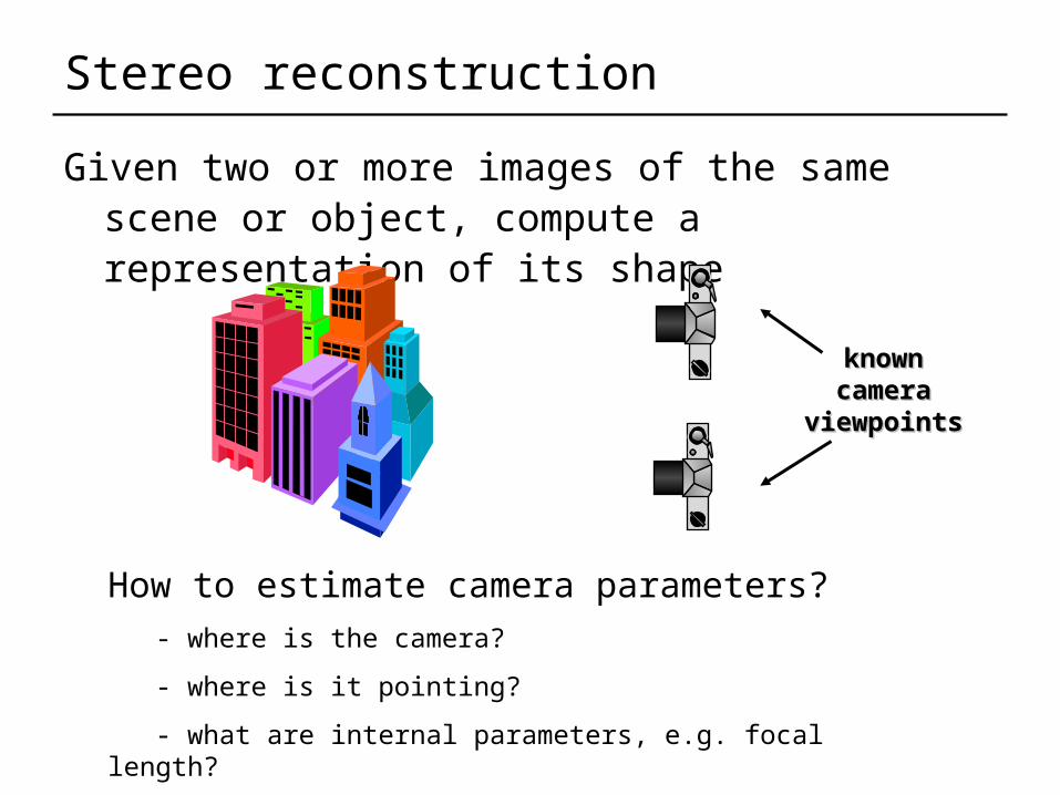
Spectrum of IBMR

Images user input range

scans

Model

Images

Image based modeling

Image-based renderingGeometry+ Images

Geometry+ Materials

Images + Depth

Light field

Panoroma

Kinematics

Dynamics

Etc.

Camera + geometry

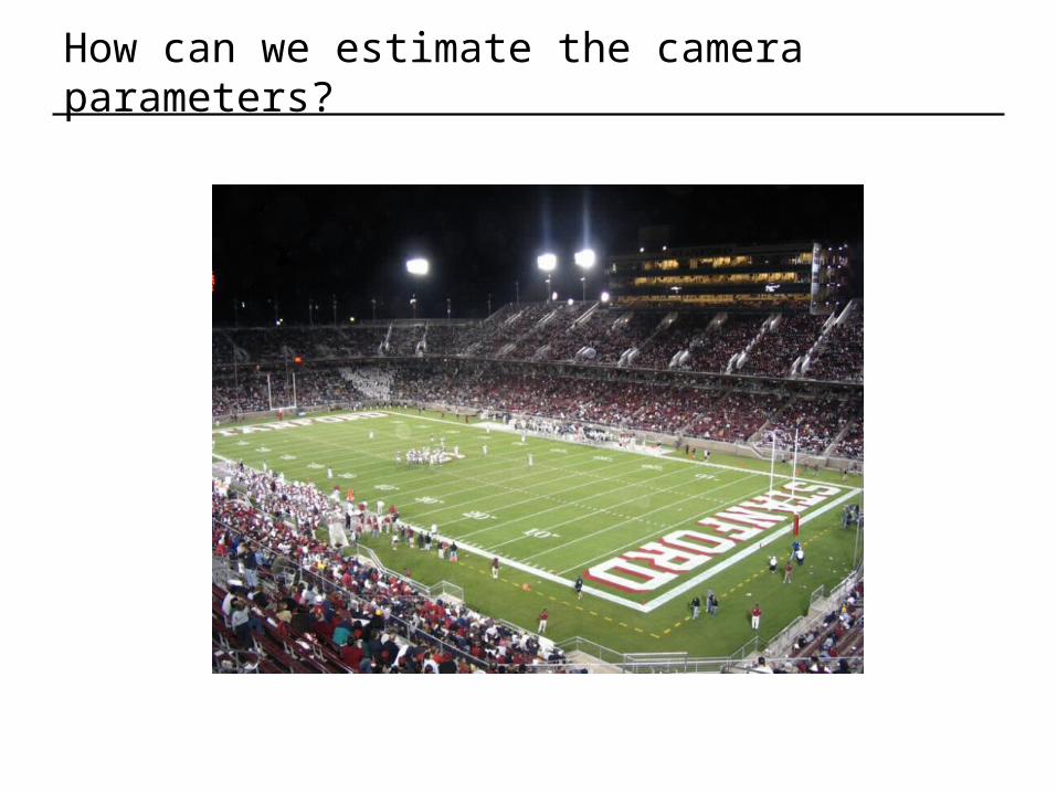
How can we estimate the camera parameters?

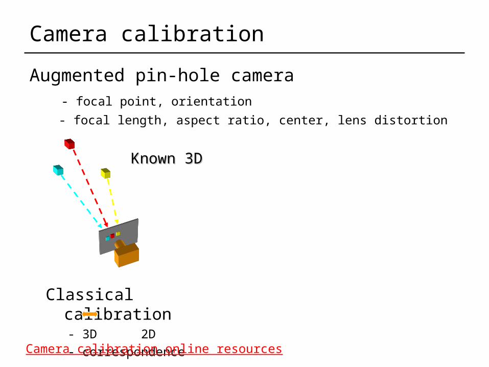
Camera calibration

Augmented pin-hole camera - focal point, orientation

- focal length, aspect ratio, center, lens distortion

Known 3DKnown 3D

Classical calibration - 3D 2D

- correspondenceCamera calibration online resources

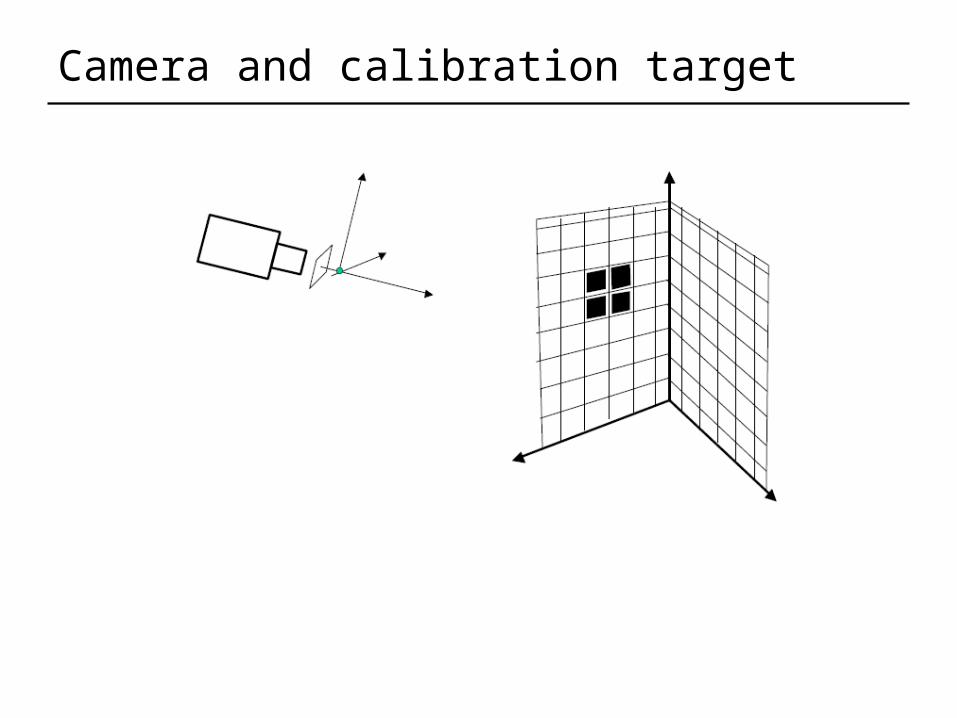
Camera and calibration target

Classical camera calibration

Known 3D coordinates and 2D coordinates - known 3D points on calibration targets

- find corresponding 2D points in image using feature detection

algorithm

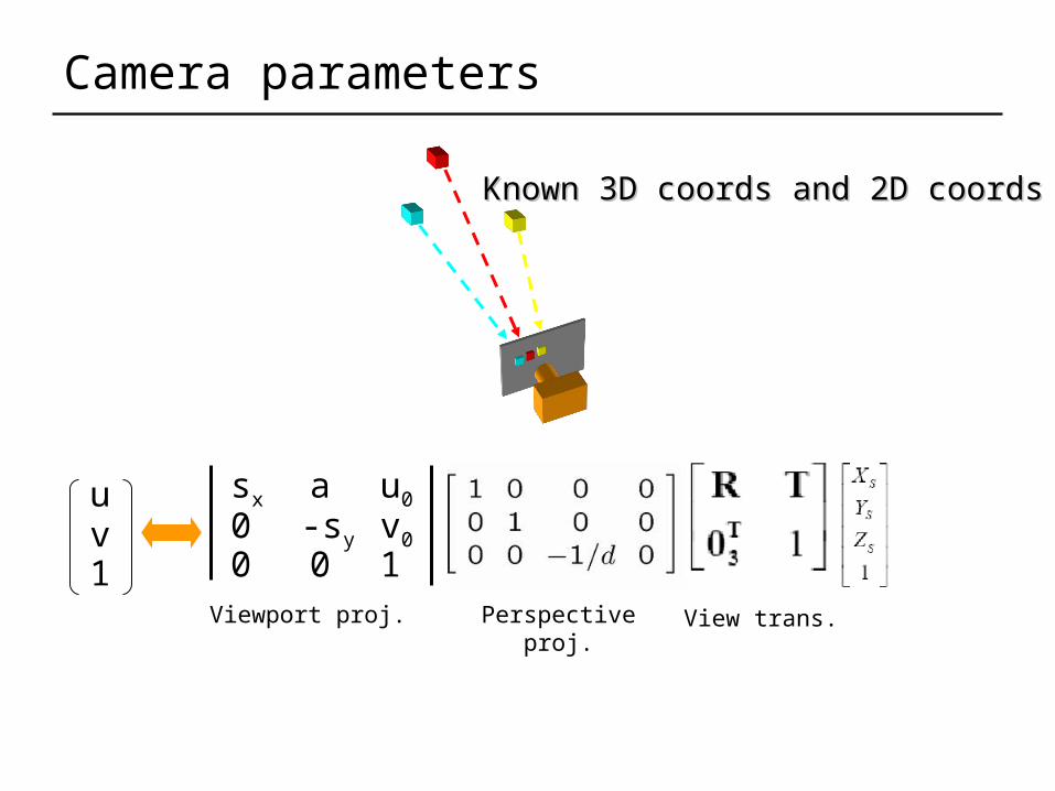
Camera parameters

u0

v0

100-sy0

sx аuv1

Perspective proj. View trans.Viewport proj.

Known 3D coords and 2D coordsKnown 3D coords and 2D coords

Camera parameters

u0

v0

100-sy0

sx аuv1

Perspective proj. View trans.Viewport proj.

Known 3D coords and 2D coordsKnown 3D coords and 2D coords

Intrinsic camera parameters (5 parameters)

extrinsic camera parameters (6 parameters)

Camera matrix

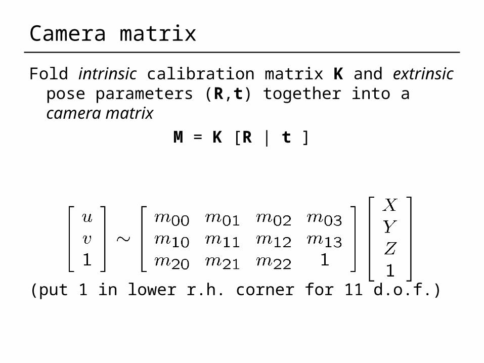
Fold intrinsic calibration matrix K and extrinsic pose parameters (R,t) together into acamera matrix

M = K [R | t ]

(put 1 in lower r.h. corner for 11 d.o.f.)

Camera matrix calibration

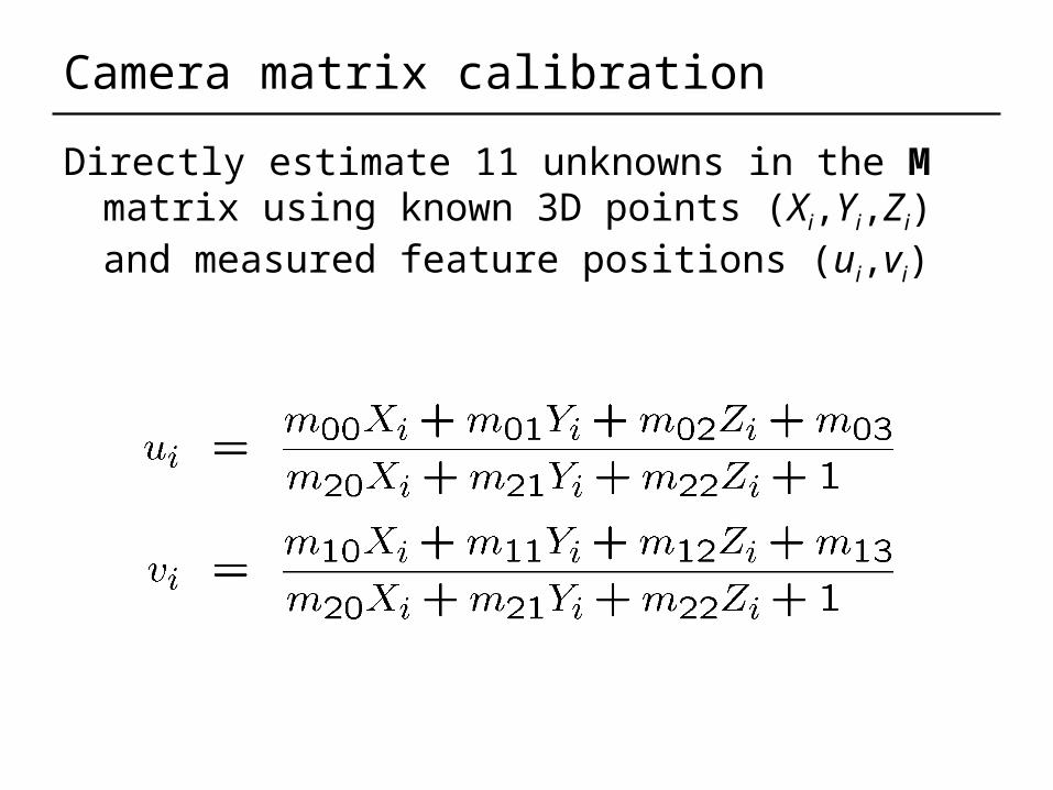
Directly estimate 11 unknowns in the M matrix using known 3D points (Xi,Yi,Zi) and measured feature positions (ui,vi)

Camera matrix calibration

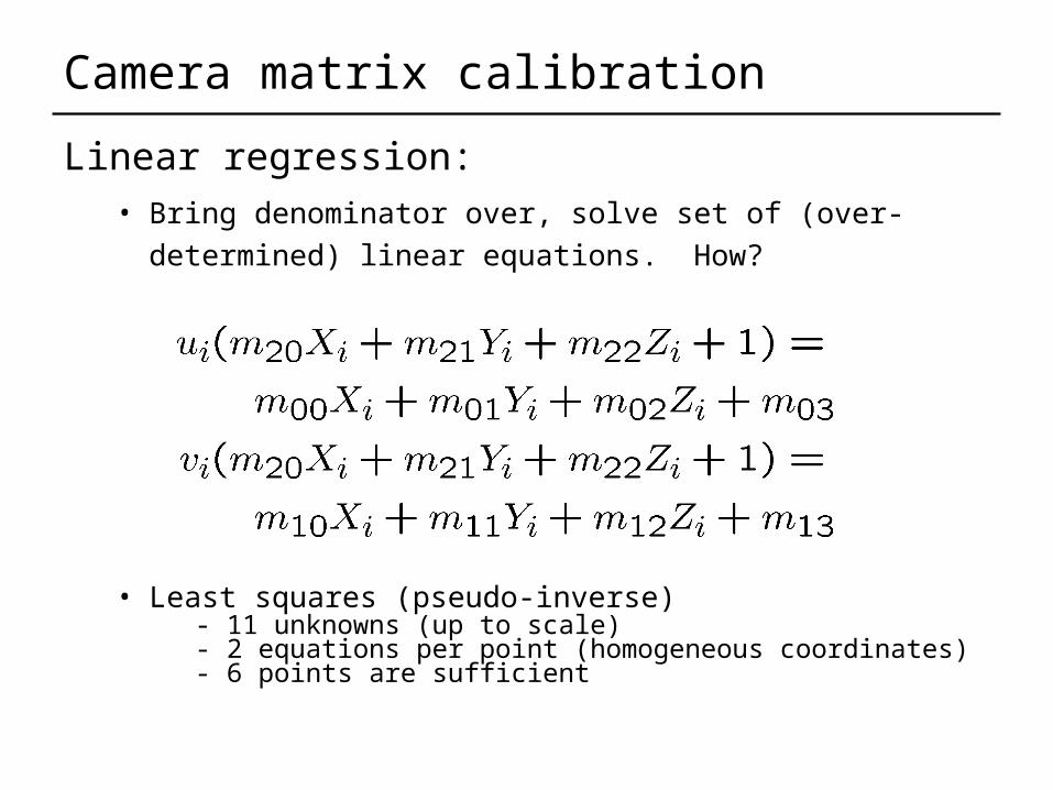
Linear regression:• Bring denominator over, solve set of (over-determined) linear

equations. How?

Camera matrix calibration

Linear regression:• Bring denominator over, solve set of (over-determined) linear

equations. How?

• Least squares (pseudo-inverse) - 11 unknowns (up to scale) - 2 equations per point (homogeneous coordinates) - 6 points are sufficient

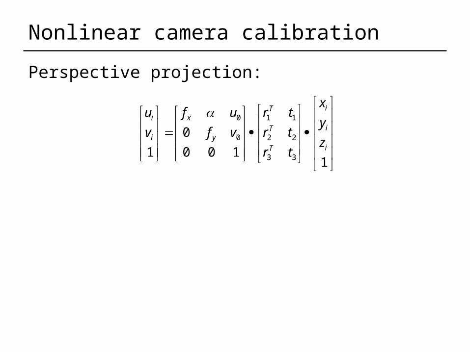
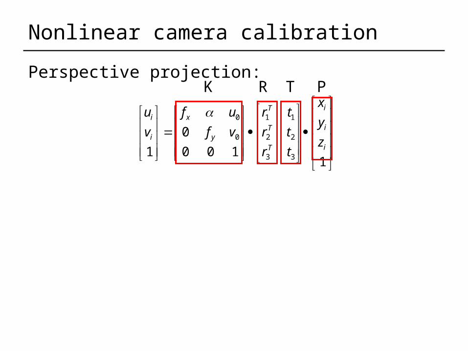
Nonlinear camera calibration

Perspective projection:

1100

0

1 3

2

1

3

2

1

0

0

i

i

i

T

T

T

y

x

i

i

z

y

x

t

t

t

r

r

r

vf

uf

v

u

Nonlinear camera calibration

Perspective projection:

1100

0

1 3

2

1

3

2

1

0

0

i

i

i

T

T

T

y

x

i

i

z

y

x

t

t

t

r

r

r

vf

uf

v

u

K R T P

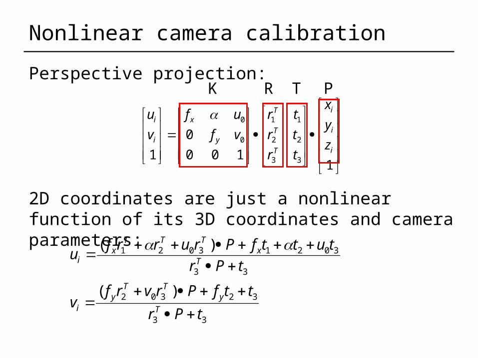
Nonlinear camera calibration

Perspective projection:

2D coordinates are just a nonlinear function of its 3D coordinates and camera parameters:

1100

0

1 3

2

1

3

2

1

0

0

i

i

i

T

T

T

y

x

i

i

z

y

x

t

t

t

r

r

r

vf

uf

v

u

K R T P

33

32302

33

30213021

)(

)(

tPr

ttfPrvrfv

tPr

tuttfPrurrfu

T

yTT

yi

Tx

TTTx

i

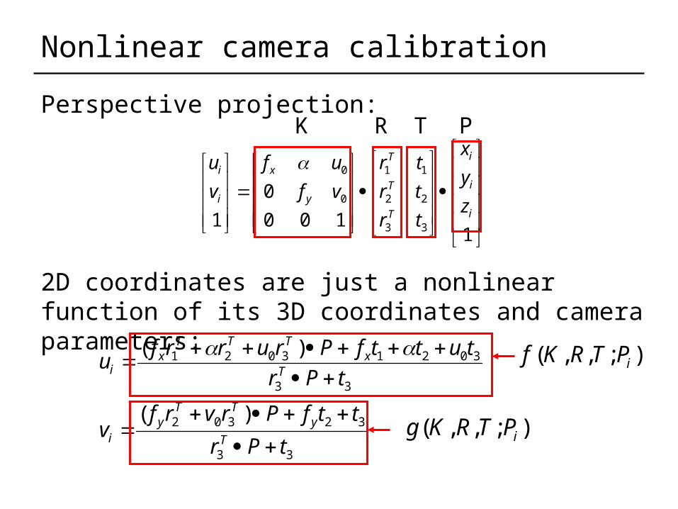
Nonlinear camera calibration

Perspective projection:

2D coordinates are just a nonlinear function of its 3D coordinates and camera parameters:

1100

0

1 3

2

1

3

2

1

0

0

i

i

i

T

T

T

y

x

i

i

z

y

x

t

t

t

r

r

r

vf

uf

v

u

33

32302

33

30213021

)(

)(

tPr

ttfPrvrfv

tPr

tuttfPrurrfu

T

yTT

yi

Tx

TTTx

i

K

);,,( iPTRKf

);,,( iPTRKg

R T P

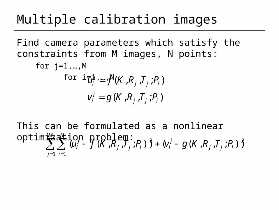
Multiple calibration images

Find camera parameters which satisfy the constraints from M images, N points: for j=1,…,M

for i=1,…,N

This can be formulated as a nonlinear optimization problem:

);,,(

);,,(

ijjji

ijjji

PTRKgv

PTRKfu

M

j

N

iijj

jiijj

ji PTRKgvPTRKfu

1 1

22 ));,,(());,,((

Multiple calibration images

Find camera parameters which satisfy the constraints from M images, N points: for j=1,…,M for i=1,…,N

This can be formulated as a nonlinear optimization problem:

);,,(

);,,(

ijjji

ijjji

PTRKgv

PTRKfu

M

j

N

iijj

jiijj

ji PTRKgvPTRKfu

1 1

22 ));,,(());,,((

Solve the optimization using nonlinear optimization techniques:

- Gauss-newton

- Levenberg-Marquardt

Nonlinear approach

Advantages:• can solve for more than one camera pose at a time

• fewer degrees of freedom than linear approach

• Standard technique in photogrammetry, computer vision, computer graphics

- [Tsai 87] also estimates lens distortions (freeware @ CMU)http://www.cs.cmu.edu/afs/cs/project/cil/ftp/html/v-source.html

Disadvantages:• more complex update rules

• need a good initialization (recover K [R | t] from M)

How can we estimate the camera parameters?

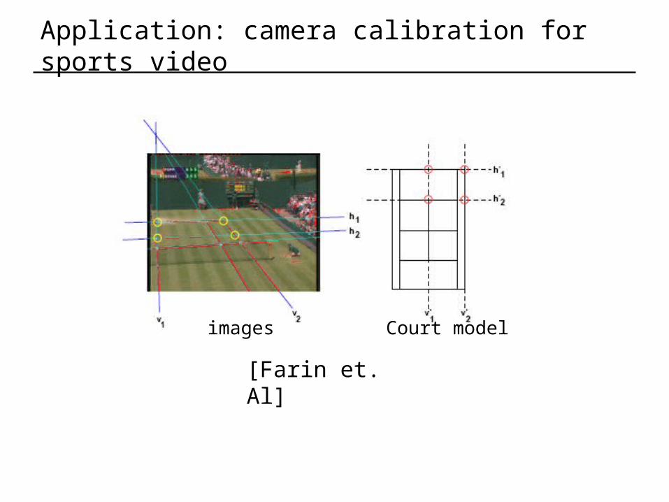
Application: camera calibration for sports video

[Farin et. Al]

images Court model

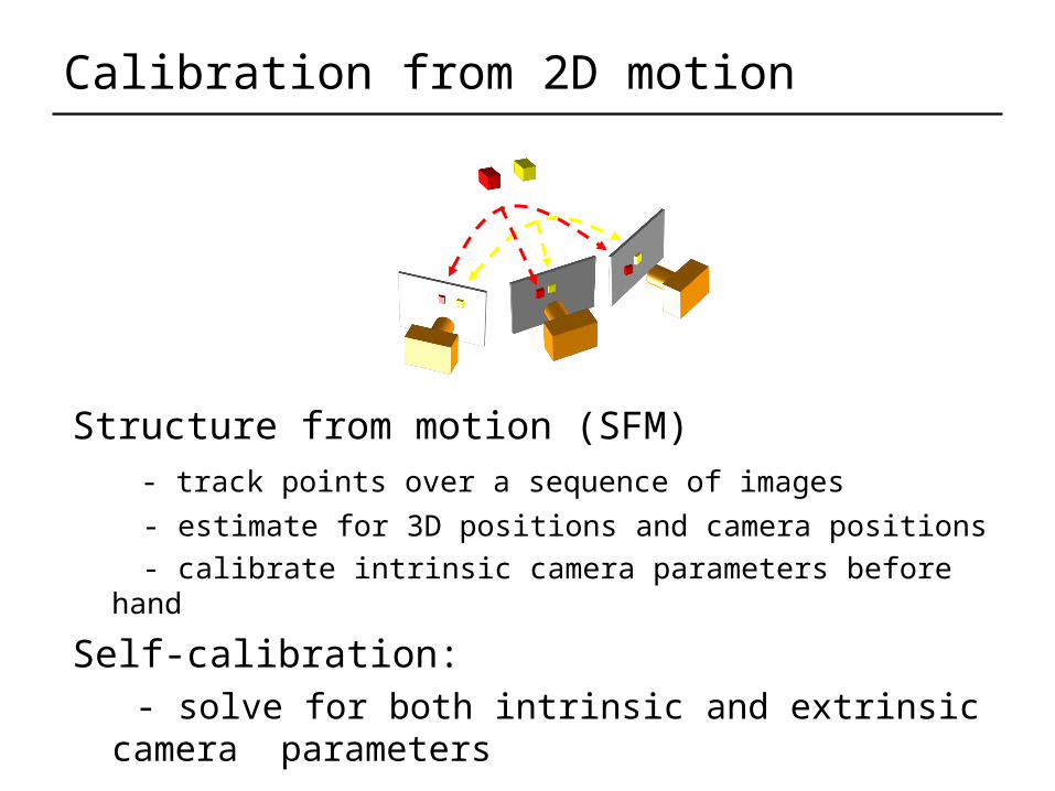
Calibration from 2D motion

Structure from motion (SFM) - track points over a sequence of images

- estimate for 3D positions and camera positions

- calibrate intrinsic camera parameters before hand

Self-calibration: - solve for both intrinsic and extrinsic camera parameters

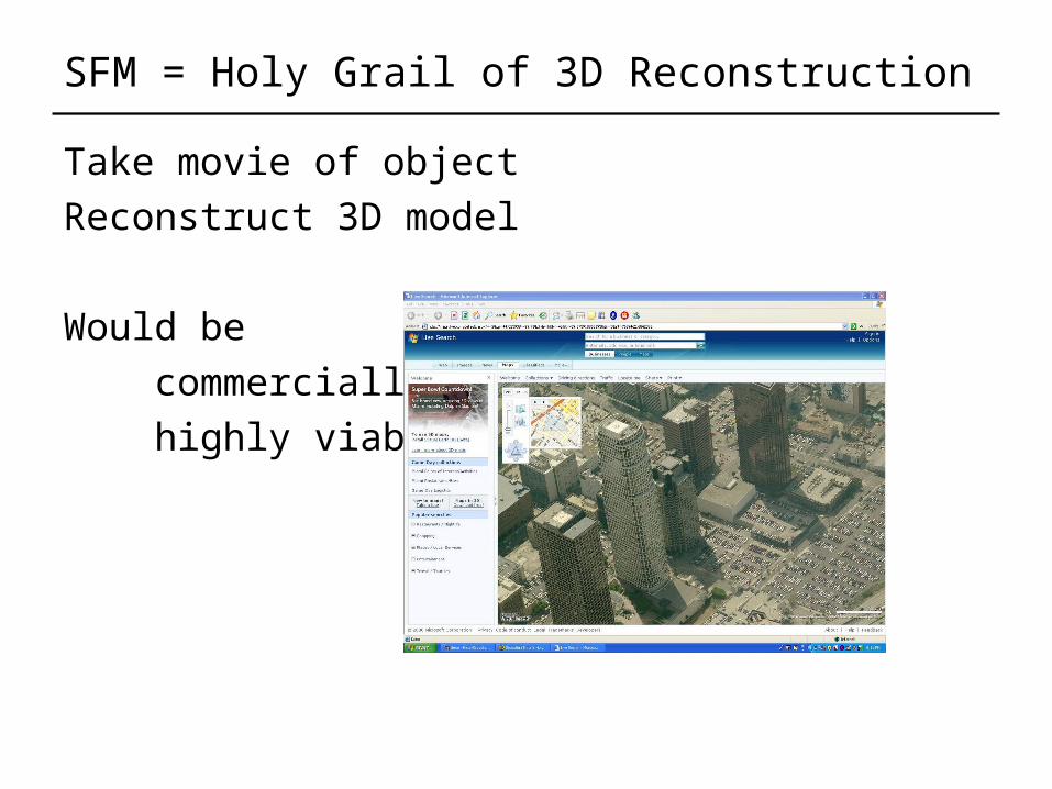
SFM = Holy Grail of 3D Reconstruction

Take movie of object

Reconstruct 3D model

Would be

commercially

highly viable

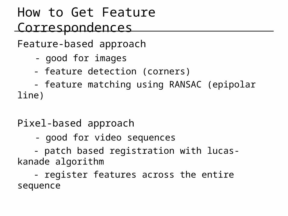
How to Get Feature Correspondences

Feature-based approach

- good for images

- feature detection (corners)

- feature matching using RANSAC (epipolar line)

Pixel-based approach

- good for video sequences

- patch based registration with lucas-kanade algorithm

- register features across the entire sequence

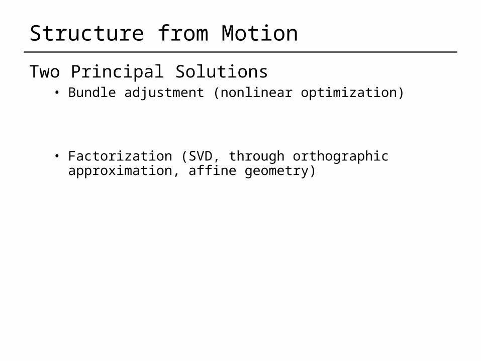
Structure from Motion

Two Principal Solutions• Bundle adjustment (nonlinear optimization)

• Factorization (SVD, through orthographic approximation, affine geometry)

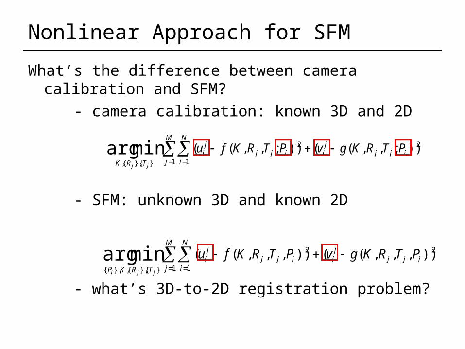
Nonlinear Approach for SFM

What’s the difference between camera calibration and SFM?

Nonlinear Approach for SFM

M

j

N

iijj

jiijj

ji

TRK

PTRKgvPTRKfujj

1 1

22

}{},{,

));,,(());,,((minarg

What’s the difference between camera calibration and SFM?

- camera calibration: known 3D and 2D

Nonlinear Approach for SFM

M

j

N

iijj

jiijj

ji

TRKP

PTRKgvPTRKfujji

1 1

22

}{},{,},{

)),,,(()),,,((minarg

M

j

N

iijj

jiijj

ji

TRK

PTRKgvPTRKfujj

1 1

22

}{},{,

));,,(());,,((minarg

What’s the difference between camera calibration and SFM?

- camera calibration: known 3D and 2D

- SFM: unknown 3D and known 2D

Nonlinear Approach for SFM

M

j

N

iijj

jiijj

ji

TRKP

PTRKgvPTRKfujji

1 1

22

}{},{,},{

)),,,(()),,,((minarg

M

j

N

iijj

jiijj

ji

TRK

PTRKgvPTRKfujj

1 1

22

}{},{,

));,,(());,,((minarg

What’s the difference between camera calibration and SFM?

- camera calibration: known 3D and 2D

- SFM: unknown 3D and known 2D

- what’s 3D-to-2D registration problem?

Nonlinear Approach for SFM

M

j

N

iijj

jiijj

ji

TRKP

PTRKgvPTRKfujji

1 1

22

}{},{,},{

)),,,(()),,,((minarg

M

j

N

iijj

jiijj

ji

TRK

PTRKgvPTRKfujj

1 1

22

}{},{,

));,,(());,,((minarg

What’s the difference between camera calibration and SFM?

- camera calibration: known 3D and 2D

- SFM: unknown 3D and known 2D

- what’s 3D-to-2D registration problem?

SFM: Bundle Adjustment

SFM = Nonlinear Least Squares problem

Minimize through• Gradient Descent

• Conjugate Gradient

• Gauss-Newton

• Levenberg Marquardt common method

Prone to local minima

M

j

N

iijj

jiijj

ji

TRKP

PTRKgvPTRKfujji

1 1

22

}{},{,},{

)),,,(()),,,((minarg

Count # Constraints vs #Unknowns

M camera poses

N points

2MN point constraints

6M+3N unknowns

Suggests: need 2mn 6m + 3n

But: Can we really recover all parameters???

M

j

N

iijj

jiijj

ji

TRKP

PTRKgvPTRKfujji

1 1

22

}{},{,},{

)),,,(()),,,((minarg

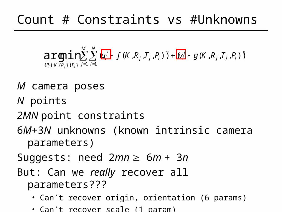
Count # Constraints vs #Unknowns

M camera poses

N points

2MN point constraints

6M+3N unknowns (known intrinsic camera parameters)

Suggests: need 2mn 6m + 3n

But: Can we really recover all parameters???• Can’t recover origin, orientation (6 params)

• Can’t recover scale (1 param)

Thus, we need 2mn 6m + 3n - 7

M

j

N

iijj

jiijj

ji

TRKP

PTRKgvPTRKfujji

1 1

22

}{},{,},{

)),,,(()),,,((minarg

Are We Done?

No, bundle adjustment has many local minima.

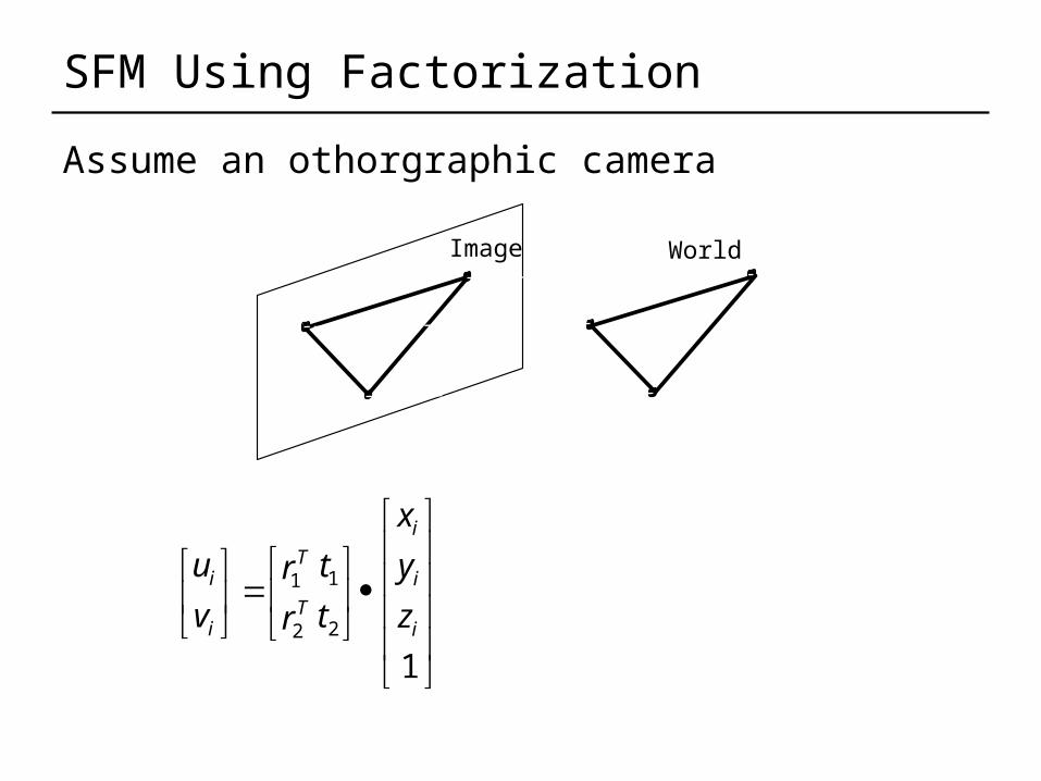
SFM Using Factorization

12

1

2

1

i

i

i

T

T

i

i

z

y

x

t

t

r

r

v

u

Assume an othorgraphic camera

Image World

SFM Using Factorization

12

1

2

1

i

i

i

T

T

i

i

z

y

x

t

t

r

r

v

u

Assume othorgraphic camera

Image World

i

i

i

T

T

N

ii

i

N

ii

i

z

y

x

r

r

N

vv

N

uu

2

1

1

1

Subtract the mean

SFM Using Factorization

N

N

N

T

T

N

N

z

y

x

z

y

x

z

y

x

r

r

v

u

v

u

v

u

...

...

...

~

~

...

...~

~

~

~

2

2

2

1

1

1

2

1

2

2

1

1

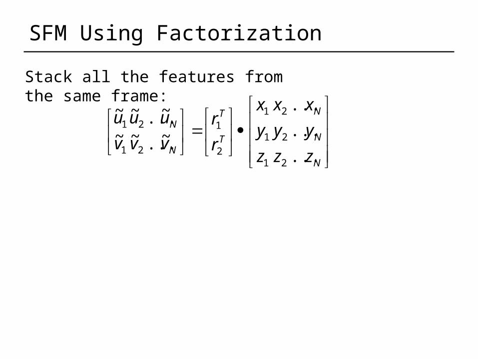
Stack all the features from the same frame:

SFM Using Factorization

N

N

N

T

T

N

N

z

y

x

z

y

x

z

y

x

r

r

v

u

v

u

v

u

...

...

...

~

~

...

...~

~

~

~

2

2

2

1

1

1

2

1

2

2

1

1

N

N

N

TF

TF

T

T

NF

NF

F

F

F

F

NF

NF

F

F

F

F

z

y

x

z

y

x

z

y

x

r

r

r

r

v

u

v

u

v

u

v

u

v

u

v

u

...

...

...

~

~

...

...~

~

~

~

~

~

...

...~

~

~

~

2

2

2

1

1

1

2,

1,

2,1

1,1

,

,

2,

2,

1,

1,

,

,

2,

2,

1,

1,

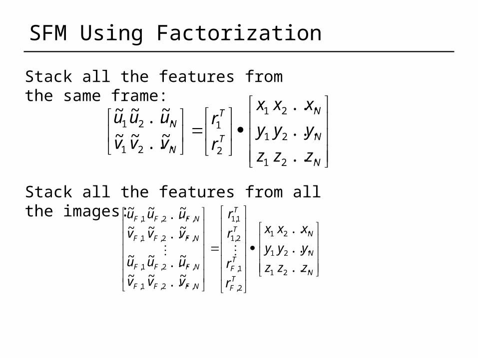
Stack all the features from the same frame:

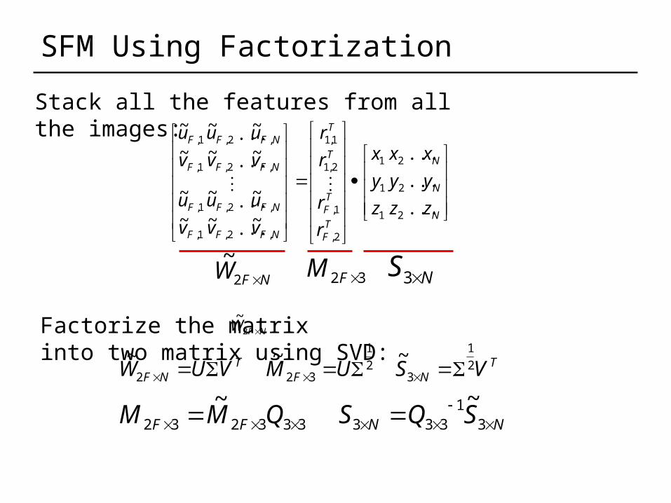
Stack all the features from all the images:

W

SFM Using Factorization

N

N

N

T

T

N

N

z

y

x

z

y

x

z

y

x

r

r

v

u

v

u

v

u

...

...

...

~

~

...

...~

~

~

~

2

2

2

1

1

1

2

1

2

2

1

1

N

N

N

TF

TF

T

T

NF

NF

F

F

F

F

NF

NF

F

F

F

F

z

y

x

z

y

x

z

y

x

r

r

r

r

v

u

v

u

v

u

v

u

v

u

v

u

...

...

...

~

~

...

...~

~

~

~

~

~

...

...~

~

~

~

2

2

2

1

1

1

2,

1,

2,1

1,1

,

,

2,

2,

1,

1,

,

,

2,

2,

1,

1,

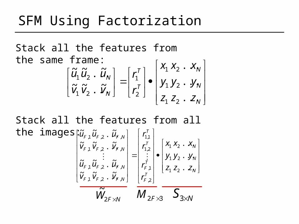
NFW 2

~

Stack all the features from the same frame:

Stack all the features from all the images:

W

32 FM NS 3

SFM Using Factorization

N

N

N

TF

TF

T

T

NF

NF

F

F

F

F

NF

NF

F

F

F

F

z

y

x

z

y

x

z

y

x

r

r

r

r

v

u

v

u

v

u

v

u

v

u

v

u

...

...

...

~

~

...

...~

~

~

~

~

~

...

...~

~

~

~

2

2

2

1

1

1

2,

1,

2,1

1,1

,

,

2,

2,

1,

1,

,

,

2,

2,

1,

1,

NFW 2

~32 FM

Stack all the features from all the images:

W

NS 3

Factorize the matrix into two matrix using SVD:

NFW 2

~

TNF

TNF VSUMVUW 2

1

32

1

322

~~~

SFM Using Factorization

N

N

N

TF

TF

T

T

NF

NF

F

F

F

F

NF

NF

F

F

F

F

z

y

x

z

y

x

z

y

x

r

r

r

r

v

u

v

u

v

u

v

u

v

u

v

u

...

...

...

~

~

...

...~

~

~

~

~

~

...

...~

~

~

~

2

2

2

1

1

1

2,

1,

2,1

1,1

,

,

2,

2,

1,

1,

,

,

2,

2,

1,

1,

NFW 2

~32 FM

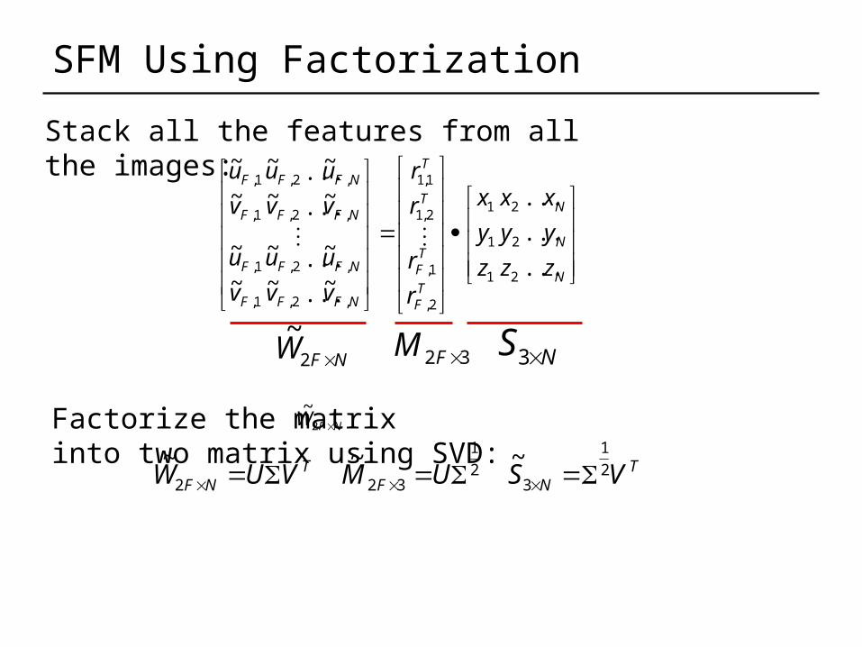
Stack all the features from all the images:

NS 3

Factorize the matrix into two matrix using SVD:

NFW 2

~

TNF

TNF VSUMVUW 2

1

32

1

322

~~~

NNFF SQSQMM

31

333333232

~~

SFM Using Factorization

N

N

N

TF

TF

T

T

NF

NF

F

F

F

F

NF

NF

F

F

F

F

z

y

x

z

y

x

z

y

x

r

r

r

r

v

u

v

u

v

u

v

u

v

u

v

u

...

...

...

~

~

...

...~

~

~

~

~

~

...

...~

~

~

~

2

2

2

1

1

1

2,

1,

2,1

1,1

,

,

2,

2,

1,

1,

,

,

2,

2,

1,

1,

NFW 2

~32 FM

Stack all the features from all the images:

W

NS 3

Factorize the matrix into two matrix using SVD:

NFW 2

~

TNF

TNF VSUMVUW 2

1

32

1

322

~~~

NNFF SQSQMM

31

333333232

~~

How to compute the matrix ? 33Q

SFM Using Factorization

2,2,2,11,1

2,

1,

2,1

1,1

3232 FF

TF

TF

T

T

TFF rrrr

r

r

r

r

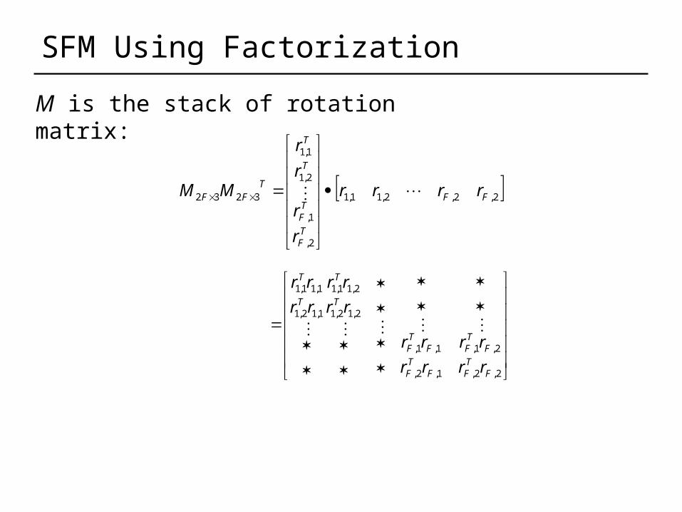
MM

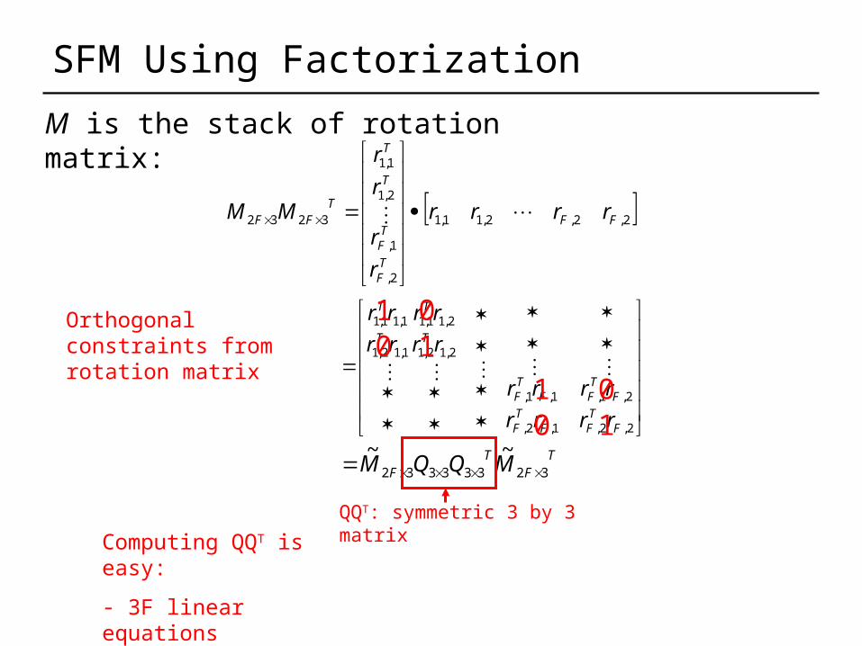
M is the stack of rotation matrix:

2,2,

2,1,

1,2,

1,1,

2,12,1

2,11,1

1,12,1

1,11,1

FTF

FTF

FTF

FTF

T

T

T

T

rr

rr

rr

rr

rr

rr

rr

rr

SFM Using Factorization

2,2,2,11,1

2,

1,

2,1

1,1

3232 FF

TF

TF

T

T

TFF rrrr

r

r

r

r

MM

M is the stack of rotation matrix:

2,2,

2,1,

1,2,

1,1,

2,12,1

2,11,1

1,12,1

1,11,1

FTF

FTF

FTF

FTF

T

T

T

T

rr

rr

rr

rr

rr

rr

rr

rr

1 010

1 010

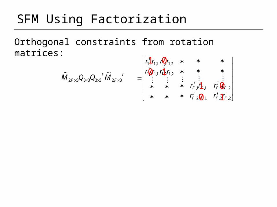
Orthogonal constraints from rotation matrix

SFM Using Factorization

2,2,2,11,1

2,

1,

2,1

1,1

3232 FF

TF

TF

T

T

TFF rrrr

r

r

r

r

MM

2,2,

2,1,

1,2,

1,1,

2,12,1

2,11,1

1,12,1

1,11,1

FTF

FTF

FTF

FTF

T

T

T

T

rr

rr

rr

rr

rr

rr

rr

rr

M is the stack of rotation matrix:

1 010

1 010

Orthogonal constraints from rotation matrix

TF

TF MQQM 32333332

~~

SFM Using Factorization

TF

TF MQQM 32333332

~~

2,2,

2,1,

1,2,

1,1,

2,12,1

2,11,1

1,12,1

1,11,1

FTF

FTF

FTF

FTF

T

T

T

T

rr

rr

rr

rr

rr

rr

rr

rr

1 010

1 010

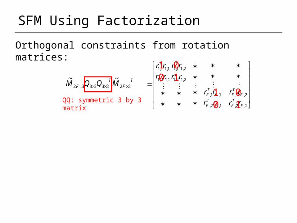
Orthogonal constraints from rotation matrices:

SFM Using Factorization

TF

TF MQQM 32333332

~~

2,2,

2,1,

1,2,

1,1,

2,12,1

2,11,1

1,12,1

1,11,1

FTF

FTF

FTF

FTF

T

T

T

T

rr

rr

rr

rr

rr

rr

rr

rr

1 010

1 010

Orthogonal constraints from rotation matrices:

QQ: symmetric 3 by 3 matrix

SFM Using Factorization

TF

TF MQQM 32333332

~~

2,2,

2,1,

1,2,

1,1,

2,12,1

2,11,1

1,12,1

1,11,1

FTF

FTF

FTF

FTF

T

T

T

T

rr

rr

rr

rr

rr

rr

rr

rr

1 010

1 010

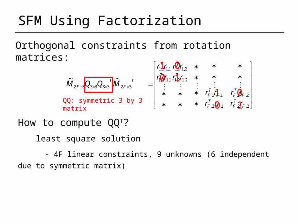
Orthogonal constraints from rotation matrices:

How to compute QQT?

least square solution

- 4F linear constraints, 9 unknowns (6 independent due to symmetric matrix)

QQ: symmetric 3 by 3 matrix

SFM Using Factorization

TF

TF MQQM 32333332

~~

2,2,

2,1,

1,2,

1,1,

2,12,1

2,11,1

1,12,1

1,11,1

FTF

FTF

FTF

FTF

T

T

T

T

rr

rr

rr

rr

rr

rr

rr

rr

1 010

1 010

Orthogonal constraints from rotation matrices:

How to compute QQT?

least square solution

- 4F linear constraints, 9 unknowns (6 independent due to symmetric matrix) How to compute Q from QQT:

SVD again: 2

1

UQVUQQ T

QQ: symmetric 3 by 3 matrix

SFM Using Factorization

2,2,2,11,1

2,

1,

2,1

1,1

3232 FF

TF

TF

T

T

TFF rrrr

r

r

r

r

MM

2,2,

2,1,

1,2,

1,1,

2,12,1

2,11,1

1,12,1

1,11,1

FTF

FTF

FTF

FTF

T

T

T

T

rr

rr

rr

rr

rr

rr

rr

rr

M is the stack of rotation matrix:

1 010

1 010

Orthogonal constraints from rotation matrix

TF

TF MQQM 32333332

~~

QQT: symmetric 3 by 3 matrix

Computing QQT is easy:

- 3F linear equations

- 6 independent unknowns

SFM Using Factorization

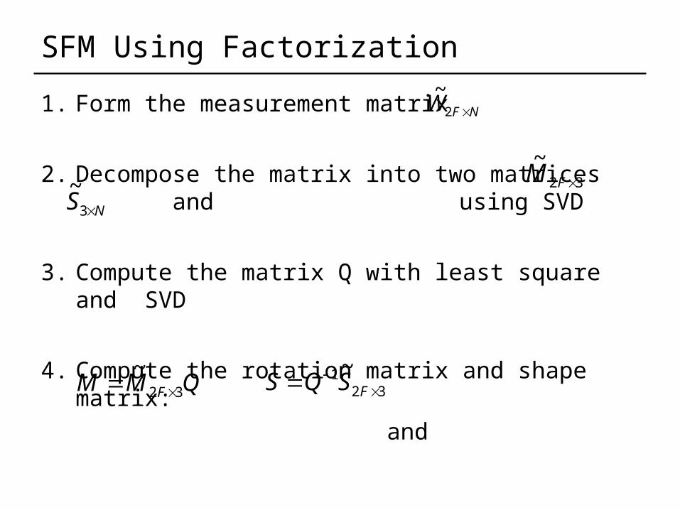
1. Form the measurement matrix

2. Decompose the matrix into two matrices and using SVD

3. Compute the matrix Q with least square and SVD

4. Compute the rotation matrix and shape matrix:

and

NFW 2

~

NS 3

~ 32

~FM

QMM F 32

~ 32

1 ~

FSQS

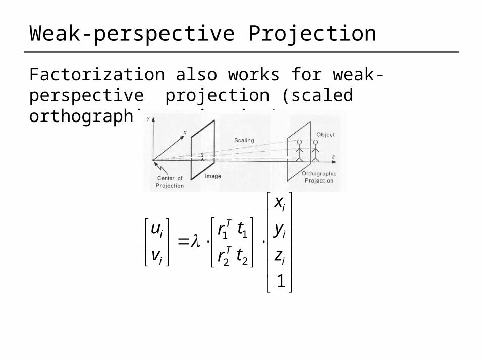
Weak-perspective Projection

Factorization also works for weak-perspective projection (scaled orthographic projection):

d z0

12

1

2

1

i

i

i

T

T

i

i

z

y

x

t

t

r

r

v

u

Factorization for Full-perspective Cameras

[Han and Kanade]

SFM for Deformable Objects

For detail, click here

SFM for Articulated Objects

For video, click here

SFM Using Factorization

Bundle adjustment (nonlinear optimization) - work with perspective camera model - work with incomplete data - prone to local minima

Factorization: - closed-form solution for weak perspective camera - simple and efficient - usually need complete data - becomes complicated for full-perspective camera model

Phil Torr’s structure from motion toolkit in matlab (click here)

Voodoo camera tracker (click here)

All Together Video

Click here

- feature detection

- feature matching (epipolar geometry)

- structure from motion

- stereo reconstruction

- triangulation

- texture mapping