Computational methods for hidden Markov tree models-An application to wavelet trees

IEEE TRANSACTIONS ON SIGNAL PROCESSING, VOL. 52, NO. 9, SEPTEMBER 2004 2551

Computational Methods for Hidden Markov TreeModels—An Application to Wavelet Trees

Jean-Baptiste Durand, Paulo Gonçalvès, and Yann Guédon

Abstract—The hidden Markov tree models were introduced byCrouse et al. in 1998 for modeling nonindependent, non-Gaussianwavelet transform coefficients. In their paper, they developed theequivalent of the forward–backward algorithm for hidden Markovtree models and called it the “upward-downward algorithm.” Thisalgorithm is subject to the same numerical limitations as the for-ward–backward algorithm for hidden Markov chains (HMCs). Inthis paper, adapting the ideas of Devijver from 1985, we proposea new “upward–downward” algorithm, which is a true smoothingalgorithm and is immune to numerical underflow. Furthermore,we propose a Viterbi-like algorithm for global restoration of thehidden state tree. The contribution of those algorithms as diagnosistools is illustrated through the modeling of statistical dependenciesbetween wavelet coefficients with a special emphasis on local reg-ularity changes.

Index Terms—Change detection, EM algorithm, hiddenMarkov tree model, hidden state tree restoration, scaling laws,upward–downward algorithm, wavelet decomposition.

I. INTRODUCTION

H IDDEN Markov tree (HMT) models were introduced byCrouse et al. in 1998 [5]. The context of their work was

the modeling of statistical dependencies between wavelet coeffi-cients in signal processing, for which observations are organizedin a tree structure. Applications of such models are image seg-mentation, signal classification, denoising, and image documentcategorization; see Hyeokho and Baraniuk [11] and Diligenti etal. [8]. Dasgputa et al. [6] used a mixture of HMTs with a Mar-kovian regime for target classification using measured acousticscattering data.

These models share similarities with hidden Markov chains(HMCs); both are models with hidden states, parameterized by atransition probability matrix and emission (or observation) dis-tributions. Both models can be identified through the EM algo-rithm, involving two recursions acting in opposite directions. Inboth cases, these recursions involve probabilities that tend to-ward zero exponentially fast, causing underflow problems oncomputers.

The use of hidden Markov models (HMMs) relies on twomain algorithms, namely, the smoothing algorithm and the

Manuscript received February 21, 2002; revised August 17, 2003. The as-sociate editor coordinating the review of this manuscript and approving it forpublication was Dr. Hamid Krim.

J.-B. Durand is with the INRIA Rhône-Alpes, Montbonnot, France (e-mail:[email protected]).

P. Gonçalvès is with the System and Robotic Group (ISR), Institute Supe-rior of Technology (IST), Lisbon, Portugal, on leave from INRIA Rhône-Alpes,Montbonnot, France (e-mail: [email protected]).

Y. Guédon is with the CIRAD, Montpellier, France (e-mail:[email protected]).

Digital Object Identifier 10.1109/TSP.2004.832006

global restoration algorithm. The former computes the prob-abilities of being in state at node , given all the observeddata. These probabilities, as a function of the index parameter

, constitute a relevant diagnosis tool; see Churchill [4] in thecontext of DNA sequence analysis. The smoothing algorithmalso enables an efficient implementation of the E step of the ex-pectation–maximization (EM) algorithm. In most applications,the knowledge of the hidden states provides an interpretationof the data, based on the model. This motivates the need for thelatter algorithm. The aim of this paper is to provide a smoothingalgorithm, which is immune to underflow, and a solution forthe global hidden state tree restoration.

Thus, we derive a smoothing algorithm for the HMT model,adapted from the forward-backward algorithm of Devijver [7]for HMCs. This algorithm is based on a direct decompositionof the smoothed probabilities. However, the adaptation to HMTmodels is not straightforward, and the resulting algorithmrequires an additional recursion consisting in computing thehidden state marginal distributions. Then, we present the Viterbialgorithm for HMT models. We show that the well-knownViterbi algorithm for HMCs cannot be adaptated to the HMTmodel. Thus, we propose a Viterbi algorithm for HMCs basedon a backward recursion, which appears as a building block ofthe hybrid restoration algorithm of Brushe et al. [3]. This thebasis for our HMT Viterbi algorithm.

Thereafter, for illustrative purposes, we apply our proposedalgorithms to a segmentation problem, which is a standardand yet difficult signal processing task. This canonical studyechoes a host of real-world situations (image processing,network traffic analysis, biomedical engineering, etc.) wherethe classifying parameter is the local regularity of the measure.Wavelets have proved particularly efficient at estimating thisparameter, and we show how our upward–downward algorithmcircumvents the underflow problem that generally precludesclassical approaches from applying to large data sets. In asecond step, we elaborate on a specific use of the smoothingalgorithm we propose, and principally, we motivate the use-fulness of probabilistic maps when the local regularity is nolonger a deterministic parameter but the realization of a randomvariable with unknown density (e.g., multifractals).

This paper is organized as follows. The HMT models areintroduced in Section II. The upward–downward algorithm ofCrouse et al. [5] is summarized in Section III. A parallel isdrawn between the forward–backward algorithm for HMCsand their algorithm, which is shown to be subject to underflow.Then, we give an upward–downward algorithm using smoothedprobabilities for HMT models. A solution for the global restora-tion problem is proposed in Section IV. An application based

1053-587X/04$20.00 © 2004 IEEE

2552 IEEE TRANSACTIONS ON SIGNAL PROCESSING, VOL. 52, NO. 9, SEPTEMBER 2004

on simulations is provided in Section V. This illustrates theimportance of the HMT model and that of our algorithms insignal processing. Section VI consists of concluding remarks.

II. HMT MODEL

We use the general notation to denote either a proba-bility mass function or a probability density function, the truenature of being obvious from the context. This notation ob-viates any assumption on the discrete or continuous nature ofthe output process.

Let be the output process, which is as-sumed to be indexable as a tree rooted in . An HMT modelis composed of the observed random tree and ahidden random tree , which has the same indexingstructure as the observed tree. The variables are discrete with

states, which are denoted . These variables can beindexed as a tree rooted in . This model can be considered tobe an unobservable state process called a Markov tree and isrelated to the “output” tree by a probabilistic mapping pa-rameterized by observation or emission distributions.

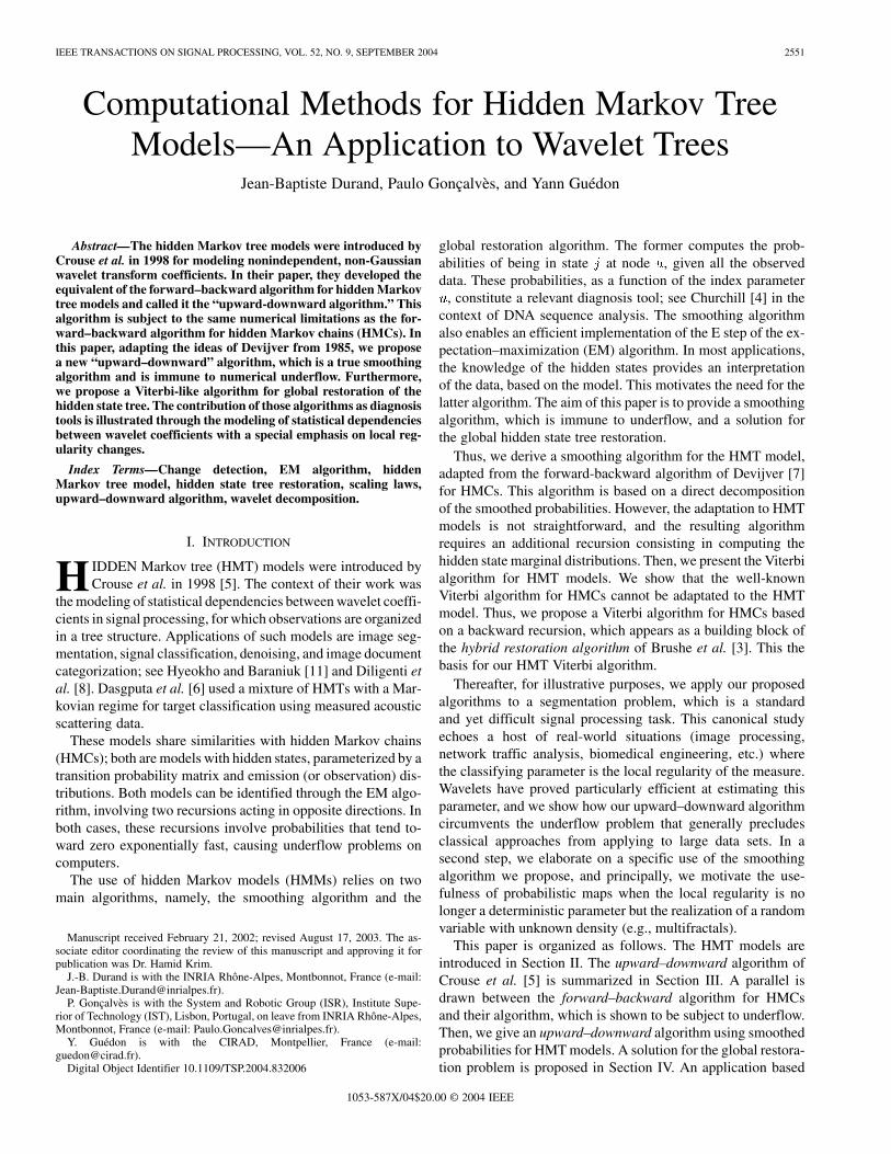
Let denote the set of children of node , and letdenote the parent of node for . We also introduce thefollowing notations.

• is the observed subtree rooted at node . Thus,is the entire observed tree.

• denotes the collection of observed subtreesrooted at children of node (that is the subtree exceptits root ).

• If is a proper subtree of , then is thesubtree rooted at node , except for the subtree rooted atnode .

• denotes the entire tree, except for thesubtrees rooted at children of node .

These notations, which are illustrated in Fig. 1, transpose to thehidden state tree, with, for instance, , which is the statesubtree rooted at node .

A distribution is said to satisfy the HMT property if andonly if it fulfills the following two assumptions.

• , arise from a mixture of distributionswith probability

• Factorization property:

(1)

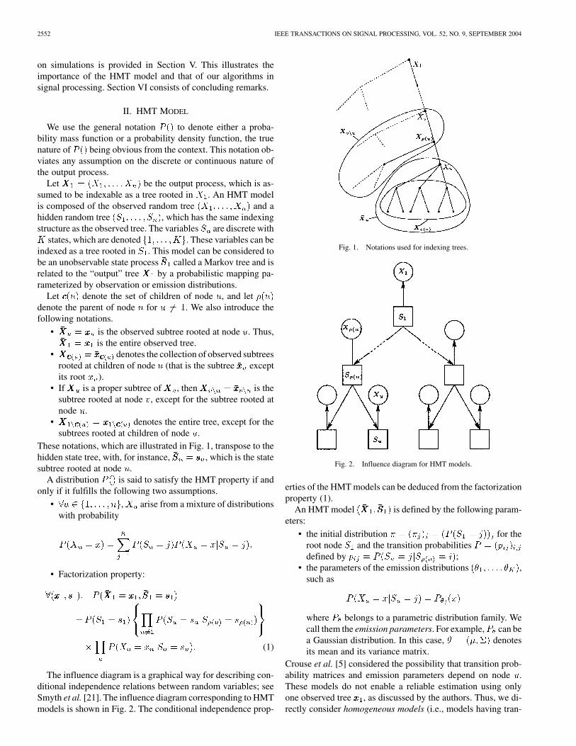
The influence diagram is a graphical way for describing con-ditional independence relations between random variables; seeSmyth et al. [21]. The influence diagram corresponding to HMTmodels is shown in Fig. 2. The conditional independence prop-

Fig. 1. Notations used for indexing trees.

Fig. 2. Influence diagram for HMT models.

erties of the HMT models can be deduced from the factorizationproperty (1).

An HMT model is defined by the following param-eters:

• the initial distribution for theroot node and the transition probabilitiesdefined by ;

• the parameters of the emission distributions ,such as

where belongs to a parametric distribution family. Wecall them the emission parameters. For example, can bea Gaussian distribution. In this case, denotesits mean and its variance matrix.

Crouse et al. [5] considered the possibility that transition prob-ability matrices and emission parameters depend on node .These models do not enable a reliable estimation using onlyone observed tree , as discussed by the authors. Thus, we di-rectly consider homogeneous models (i.e., models having tran-

DURAND et al.: COMPUTATIONAL METHODS FOR HIDDEN MARKOV TREE MODELS 2553

sition probabilities and emission parameters independent of ),which is usual in the literature of HMMs. Our results can beeasily extended to nonhomogeneous models at the cost of te-dious notation.

III. UPWARD–DOWNWARD ALGORITHM

Since the state tree is not observable, the EM algorithmis a natural way to obtain maximum likelihood estimates of anHMT. The E step requires the computation of the conditionaldistributions (smoothed prob-abilities) and . Crouse etal. [5] proposed the so-called upward–downward algorithm tocalculate these quantities, which basically computes

for each node and each state . This is a di-rect transposition to the HMT context of the forward–backwardalgorithm for HMCs proposed by Baum et al. [2]. Both the up-ward–downward and the forward–backward algorithms sufferfrom underflow problems; see Ephraim and Merhav [9] for thecase of HMCs. This difficulty has been initially overcome byLevinson et al. [14], who proposed the use of scaling factors onrather heuristic grounds. On the basis of this work, Devijver [7]derived a true smoothing algorithm for HMCs, which can be in-terpreted in the setting of state-space models. This motivates theneed for a true smoothing algorithm for HMT models with thefollowing properties.

• The smoothed probabilities arecomputed instead of . These quan-tities are also useful diagnosis tools for HMT models, aswill be shown in the application (Section V).

• The probabilities can bedirectly extracted from this smoothing algorithm. Conse-quently, it implements the E step of the EM algorithm forparameter estimation.

• This algorithm is immune to underflow.

A. Upward–Downward Algorithm of Crouse et al.

Its objective is to compute the probabilityfor each node and each state . The authors define the

following quantities:

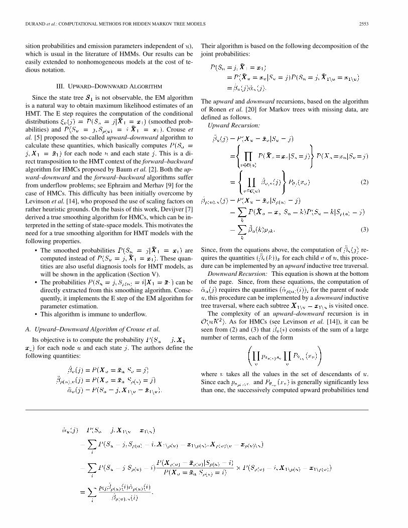
Their algorithm is based on the following decomposition of thejoint probabilities:

The upward and downward recursions, based on the algorithmof Ronen et al. [20] for Markov trees with missing data, aredefined as follows.

Upward Recursion:

(2)

(3)

Since, from the equations above, the computation of re-quires the quantities for each child of , this proce-dure can be implemented by an upward inductive tree traversal.

Downward Recursion: This equation is shown at the bottomof the page. Since, from these equations, the computation of

requires the quantities for the parent of node, this procedure can be implemented by a downward inductive

tree traversal, where each subtree is visited once.The complexity of an upward–downward recursion is in

. As for HMCs (see Levinson et al. [14]), it can beseen from (2) and (3) that consists of the sum of a largenumber of terms, each of the form

where takes all the values in the set of descendants of .Since each and is generally significantly lessthan one, the successively computed upward probabilities tend


to zero exponentially fast when progressing toward the rootnode, whereas the successively computed downward probabil-ities tend to zero exponentially fast when progressing towardthe leaf nodes. In the next section, we present an algorithm thatovercomes this difficulty.

B. Upward–Downward Algorithm for Smoothed Probabilities

We present an alternative upward–downward algorithm,which is a true smoothing algorithm that is immune to under-flow problems and whose complexity remains in .

In order to avoid underflow problems with HMCs, Devijver[7] suggests the replacement of the decomposition of the jointprobabilities

with the decomposition

where for HMCs, we denote the observed sequenceby . A natural adaptation of

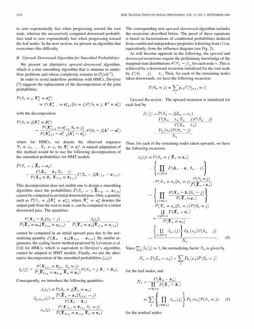
this method would be to use the following decomposition ofthe smoothed probabilities for HMT models

This decomposition does not enable one to design a smoothingalgorithm since the probabilitiescannot be computed in an initial downward pass. Only a quantitysuch as , where denotes theoutput path from the root to node , can be computed in a initialdownward pass. The quantities

cannot be computed in an initial upward pass due to the nor-malizing quantity . By similar ar-guments, the scaling factor method proposed by Levinson et al.[14] for HMCs, which is equivalent to Devijver’s algorithm,cannot be adapted to HMT models. Finally, we use the alter-native decomposition of the smoothed probabilities

Consequently, we introduce the following quantities:

The corresponding new upward–downward algorithm includesthe recursions described below. The proof of these equationsis based on factorizations of conditional probabilities deducedfrom conditional independence properties following from (1) or,equivalently, from the influence diagram (see Fig. 2).

As will become apparent in the following, the upward anddownward recursions require the preliminary knowledge of themarginal state distributions for each node . This isachieved by a downward recursion initialized for the root nodeby . Then, for each of the remaining nodestaken downwards, we have the following recursion:

Upward Recursion: The upward recursion is initialized foreach leaf by

Then, for each of the remaining nodes taken upwards, we havethe following recursion:

(4)

Since , the normalizing factor is given by

for the leaf nodes, and

(5)

for the nonleaf nodes.


The upward recursion also involves the computation of thequantities , which are extracted from thequantities since

(6)

In a first step, the quantities

are computed with . By convention,for the leaf nodes. In a second step, the

quantities are extracted as . Finally, the quan-tities are extracted from , and the algorithmprocesses the nodes at a lower depth.

It can be seen that

(recall that for each leaf , ). Hence, thelog-likelihood is

It follows from (5) that the log-likelihood can be computed asa byproduct of the upward recursion. The log-likelihood com-putation allows, among other potential applications, the mon-itoring of the EM algorithm convergence; see McLachlan andKrishnan [16].

It is possible to build a downward recursion on the basis ofthe quantities or on the basis of the smoothed probabilities

. This is a direct transposition ofthe argument of Devijver [7] to the case of HMT models.

Downward Recursion Based on : The downward recur-sion is initialized for the root node by

Then, for each of the remaining nodes taken downwards, wehave the following recursion:

(7)

Since for each , , the downward recursionbased on is directly deduced from (7). This is initializedby , and for each of the remaining nodes taken down-wards, we have the following recursion:

The conditional probabilitiesrequired for the re-estimation of the parameters by the EM

algorithm are directly extracted during the downward recursion

Table I points out the differences between the upward–down-ward algorithm of Crouse et al. [5], using the decomposition ofjoint probabilities, and our algorithm, using the decompositionof the smoothed probabilities.

As for Devijver’s algorithm, the execution of the above pro-cedure does not cause underflow problems. The term that domi-nates the recursion complexity for the computation of the hiddenstate distributions is . The complexities of our upward anddownward recursions also have dominant term for binarytrees (or for any tree such as the degree of each node remainsbounded). Thus, the complexity of the upward–downward algo-rithm using smoothed probabilities remains in , as thealgorithm of Crouse et al. , but with the complexity increasingby 50%.

IV. VITERBI ALGORITHM

Given an observed tree , our aim is to find the hidden statetree maximizing or,equivalently, (see Rabiner [18]) andthe value of the maximum. We call any algorithm solvingthis problem a Viterbi algorithm in reference to the HMC termi-nology.

The initial global restoration algorithm for nonindependentmixture models is due to Viterbi. The Viterbi algorithm isoriginally intended for the analysis of Markov processesobserved in memoryless noise. In the case of an HMC

, let denote the state sequenceof length , and let denote the output sequenceof length . The Viterbi algorithm for HMCs is basically aforward recursion computing the quantities

(8)

starting at the initial state .A natural adaptation of the Viterbi algorithm to HMT models

would involve a downward recursion starting at the root state


TABLE IDIFFERENCES BETWEEN THE

UPWARD–DOWNWARD ALGORITHM OF CROUSE et al. AND OUR SMOOTHING

UPWARD–DOWNWARD ALGORITHM

. We claim that this is not possible, for the same reason asfor our smoothing algorithm, namely, that the downward recur-sion would require the results of the upward recursion (see Sec-tion III). Thus, we need to design a new Viterbi algorithm forHMCs based on a backward recursion, which will be the basisof our adaptation to HMT models.

Because the state process is a Markov chain, we have for allthe decomposition in (9), adaptated from Jelinek [13], and

shown at the bottom of the page. Let us define

Decomposition (9) can then be rewritten as

Using the quantities , we can build a Viterbi algorithm forHMCs based on a backward recursion, which is equivalent tothat of Brushe et al. [3]. This is initialized for by

The backward recursion is given, for , by thesecond equation shown at the bottom of the page. We obtain,

for , .

Hence, the probability of the optimal state sequence associatedwith the observed sequence is

Transposing decomposition (9) to HMT models yields, for all, (10), shown at the bottom of the page. Let us define

(11)

(12)

Hence, (10) can be rewritten as

The main change with respect to HMCs is that it is not possibleto design a downward recursion on the basis of this type of de-composition but solely an upward recursion.

The Viterbi algorithm for an HMT is initialized for each leafby

Then, for each of the remaining nodes taken upwards, we havethe recursion shown in the equation at the bottom of the nextpage. The probability of the optimal state tree associated withthe observed tree is

The Viterbi algorithm is similar to the upward recursion ofCrouse et al. [5], where the summations on the states arereplaced by maximizations. Its complexity is in , andno normalization quantities are required. To retrieve the optimalstate tree, it is necessary to store, for each node and each state

(9)

(10)


, the optimal states corresponding to each of the children. Thebacktracking procedure consists of tracing downward alongthe backpointers from the optimal root state to the optimal leafstates.

V. APPLICATION TO SIGNAL PROCESSING

In this section, we develop one example of applica-tion, illustrating the importance of the HMT model. Let

be a realization of a sampled piecewiseconstant (Hölder) regularity process, for example, a piecewisehomogeneous fractional Brownian motion (H-FBM). The localregularity of a function (or of the trajectory of a stochasticprocess) is defined by Mallat [15] as follows: The functionhas local regularity , at time , if there existstwo constants and as well as a polynomial

of order , such that for all and for all

(13)

In our simulation, we consider the slightly modified model ofa compound. This model assumes that and that from

to with , the local regularity ofthe process is , and from to , itslocal regularity is . Our aim is not to estimate or

but rather to determine the transition time . To motivateour work, we recall, for instance, the work of Abry and Veitch[1], where they show the major importance of detecting localregularity changes in the context of network traffic analysis.

Our method is based on a multiresolution analysis of. As a first step, we compute an orthonormal dis-

crete wavelet transform of through the followinginner product: , with

and corresponding to thefinest scale.

As in Crouse et al., we combine a statistical approach withwavelet-based signal processing. This means that we process thesignal by operating on its wavelet coefficients andthat we consider these coefficients to be realizations of random

variables . The authors justify a hidden Markov bi-nary tree model for the wavelet coefficients by two observations.

• Residual dependencies remain between wavelet coeffi-cients.

• Wavelet coefficients are generally non-Gaussian.We recall that the path of an H-FBM has local Hölder regu-

larity almost surely almost everywhere. Hence, from Jaffard[12], Flandrin [10], and Wornell et al. [22], the random variables

of its wavelet decomposition are normally, identically dis-tributed within scale and centered with variance

var

In our simple test signal, where the local regularity is forand for , we consider a two-state

model with the following conditional distributions:

Thus, we model the distribution of by the followingHMT model:

• arises from a mixture of distributions with density

where is a discrete variable with two states, which aredenoted {0, 1}, and is the Gaussian distributiondensity with mean 0 and variance .

• is a Markov binary tree (i.e., each nonterminalnode has exactly two children) with parameters and

.• The wavelet coefficients are independent, conditionally to

the hidden states.As in Section II, we denote the observed tree by

and the hidden tree by .In the case of an abrupt regularity jump at time , the hidden

tree model satisfies the following two properties.

• For each subtree of , there exists in {0, 1} suchthat the left subtree of is entirely in state , or its rightsubtree is entirely in state .


• If and are two leaves with such as, then for all between and , .

To detect the local regularity jump, we compute the discretewavelet transform of the signal using a compact supportDaubechies wavelet. An important proviso is that the chosenwavelet has regularity larger than the regularity of the processitself. In our case, we are dealing with ; therefore, wechoose the simplest possible wavelet: the Haar with regularityone. Since our model assumes two states per tree, here, we needa single tree decomposition. This imposes only one wavelet co-efficient at the coarsest scale (root node), and thus, fora full -level tree.1 Then, we estimate the model parametersby the EM algorithm, using our upward–downward algorithmwith smoothed probabilities to implement the E step. We couldnot use the upward–downward algorithm of Crouse et al. [5]directly (i.e., without an ad hoc scaling procedure) since under-flow errors occur for values of typically greater than 128.

The and parameters are estimated at the M step witha procedure adaptated from the maximum likelihood estimationderived by Wornell and Oppenheim [22]. Thus, we obtain ,

, , , , and . The jump detection is performed by ahidden state restoration under the two constraints above, usingthe Viterbi algorithm. We obtain a value for the hidden treesuch that exactly one subtree of is in state , and isin state . Thus, there is only one leave such as

. The jump time is estimated by

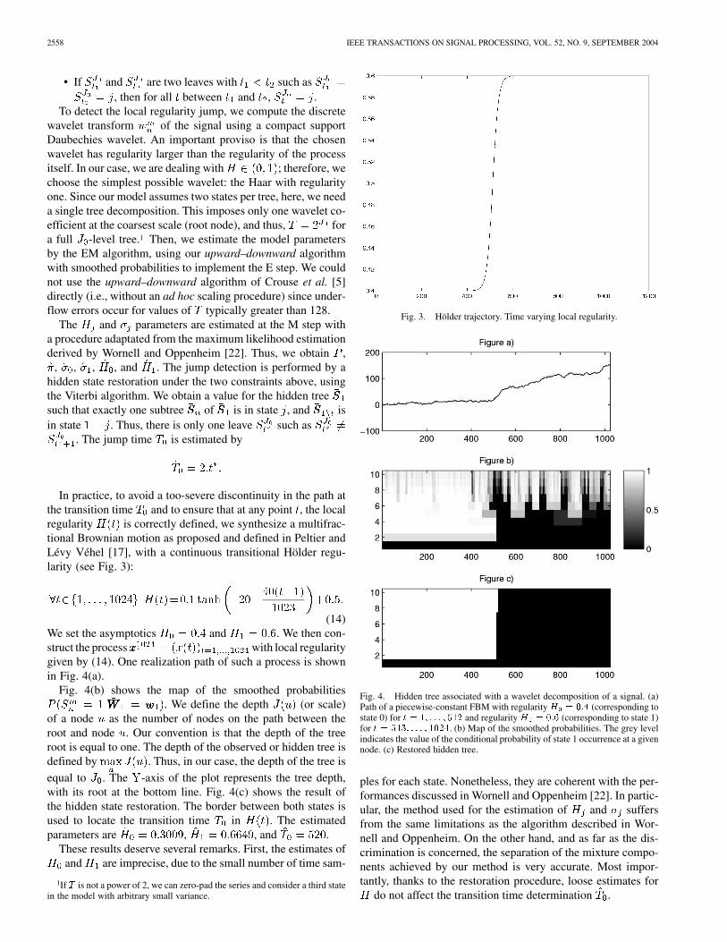
In practice, to avoid a too-severe discontinuity in the path atthe transition time and to ensure that at any point , the localregularity is correctly defined, we synthesize a multifrac-tional Brownian motion as proposed and defined in Peltier andLévy Véhel [17], with a continuous transitional Hölder regu-larity (see Fig. 3):

(14)We set the asymptotics and . We then con-struct the process with local regularitygiven by (14). One realization path of such a process is shownin Fig. 4(a).

Fig. 4(b) shows the map of the smoothed probabilities. We define the depth (or scale)

of a node as the number of nodes on the path between theroot and node . Our convention is that the depth of the treeroot is equal to one. The depth of the observed or hidden tree isdefined by . Thus, in our case, the depth of the tree is

equal to . The -axis of the plot represents the tree depth,with its root at the bottom line. Fig. 4(c) shows the result ofthe hidden state restoration. The border between both states isused to locate the transition time in . The estimatedparameters are , , and .

These results deserve several remarks. First, the estimates ofand are imprecise, due to the small number of time sam-

1If T is not a power of 2, we can zero-pad the series and consider a third statein the model with arbitrary small variance.

Fig. 3. Hölder trajectory. Time varying local regularity.

Fig. 4. Hidden tree associated with a wavelet decomposition of a signal. (a)Path of a piecewise-constant FBM with regularity H = 0:4 (corresponding tostate 0) for t = 1; . . . ; 512 and regularity H = 0:6 (corresponding to state 1)for t = 513; . . . ; 1024. (b) Map of the smoothed probabilities. The grey levelindicates the value of the conditional probability of state 1 occurrence at a givennode. (c) Restored hidden tree.

ples for each state. Nonetheless, they are coherent with the per-formances discussed in Wornell and Oppenheim [22]. In partic-ular, the method used for the estimation of and suffersfrom the same limitations as the algorithm described in Wor-nell and Oppenheim. On the other hand, and as far as the dis-crimination is concerned, the separation of the mixture compo-nents achieved by our method is very accurate. Most impor-tantly, thanks to the restoration procedure, loose estimates for

do not affect the transition time determination .


In a perspective viewpoint, to improve the estimates, wecould substitute likelihood maximization with alternativemethods. For instance, to derive estimates of the parameters

and , it is possible to use a (weighted) linear regressionof the within-scale empirical variance, which is restricted to amore relevant scale subrange.

In our elementary example, the smoothed probability map[see Fig. 4(b)] is merely a complementary stage to restoration.Yet, let us comment on the apparent uncertainty of the statesobserved after transition time . Recalling the definition of thelocal Hölder regularity of a given path, is the supremum overall satisfying the inequality in (13). This means that point-wise, smaller estimated regularities are likely to occur. Now,when analyzing the more regular part of the trace, the retainedtwo-state model actually allows for the estimation of local regu-larities smaller than the effective one, hence, these changeovers.Again, in accordance with (13), this clearly does not happenwith the left-hand side of the path (less regular part).

More interestingly, now, a probabilistic map becomes fullyinteresting on its own, when exploring more complex situations.To support our claim, let us elaborate on two examples.

• We return to our previous two-state example, and assumea smooth transition from to . This means that thelocal Hölder regularity takes on infinitely many valueswithin interval , turning the frontier betweenthe two stable states very fuzzy. A binary segmentationobtained with the restoration algorithm may not be sosensible and necessarily implies some arbitrariness inselecting the transition time . Instead, the probabilisticmap, which is output of the smoothing algorithm, pro-vides us with a fuzzy segmentation that conveys morevaluable information concerning the dynamics of thetransition.

• The second example concerns situations referred to asmultifractals; see, e.g., Riedi [19]. In short, for suchprocesses, local Hölder regularity is itself a randomvariable, leading to utterly erratic Hölder pathswhose pointwise estimation becomes totally unrealistic.Instead, we resort to the notion of singularity spectrumthat allows for the quantification of how frequently agiven singularity strength is assumed. Then,probabilistic maps, like the one displayed in Fig. 4(b),can easily be thought as a measure of occurrence ofthe quantized regularity associatedwith the given state . Conceptually, it would sufficeto marginalize these distributions and to represent theobtained a priori probabilities versus to get adiscrete singularity density .

Another very interesting extension of HMT models is to con-sider, as for HMCs, continuous-valued hidden states. It is knownthat the estimation problem in such models is difficult. However,from an application viewpoint and when the model is entirelyspecified, it would allow us to model signals with continuouslytime-varying local regularity. In this context, it would be pos-sible to compute the local regularity distribution conditionallyto the observed wavelet coefficients.

VI. CONCLUDING REMARKS

In this paper, we developed a smoothing algorithm that imple-ments the E step of the EM algorithm for parameter estimation.The important improvement carried out to the existing algorithmof Crouse et al. [5] is that ours is not subject to underflow. Thisallows us to apply HMTs to large data sets.

Another important innovation of our methodology is the useof the smoothed probability map. In particular, we showed it tobe relevant in a wavelet-tree application and, in possible exten-sions, to models with continuous-valued hidden states.

As this application demonstrates the need for a global restora-tion algorithm, a solution based on the adaptation of a backwardViterbi algorithm for HMCs has been proposed.

ACKNOWLEDGMENT

The authors acknowledge helpful advice and discussion aboutinference algorithms in mixture models with G. Celeux. Theyare thankful to the anonymous reviewers for their useful com-ments.

REFERENCES

[1] P. Abry and D. Veitch, “Wavelet analysis of long range dependanttraffic,” IEEE Trans. Inform. Theory, vol. 44, pp. 2–15, Jan. 1998.

[2] L. E. Baum, T. Petrie, G. Soules, and N. Weiss, “A maximization tech-nique occurring in the statistical analysis of probabilistic functions ofMarkov chains,” Ann. Math. Statist., vol. 41, no. 1, pp. 164–171, 1970.

[3] G. D. Brushe, R. E. Mahony, and J. B. Moore, “A soft output hybridalgorithm for ML/MAP sequence estimation,” IEEE Trans. Inform.Theory, vol. 44, pp. 3129–3134, Nov. 1998.

[4] G. A. Churchill, “Stochastic models for heterogeneous DNA se-quences,” Bull. Math. Biol., vol. 51, pp. 79–94, 1989.

[5] M. S. Crouse, R. D. Nowak, and R. G. Baraniuk, “Wavelet-based sta-tistical signal processing using hidden Markov models,” IEEE Trans.Signal Processing, vol. 46, pp. 886–902, Apr. 1998.

[6] N. Dasgputa, P. Runkle, L. Couchman, and L. Carin, “Dual hiddenMarkov model for characterizing wavelet coefficients from multi-aspectscattering data,” Signal Process., vol. 81, no. 6, pp. 1303–1316, 2001.

[7] P. A. Devijver, “Baum’s forward-backward algorithm revisited,” PatternRecogn. Lett., vol. 3, pp. 369–373, 1985.

[8] M. Diligenti, P. Frasconi, and M. Gori, “Image document categoriza-tion using hidden tree Markov models and structured representations,” inProc. Second Int. Conf. Adv. Pattern Recogn., Lecture Notes in Comput.Sci., S. Singh, N. Murshed, and W. Kropatsch, Eds., 2001.

[9] Y. Ephraim and N. Merhav, “Hidden Markov processes,” IEEE Trans.Inform. Theory, vol. 48, pp. 1518–1569, June 2002.

[10] P. Flandrin, “Wavelet analysis and synthesis of fractional Brownian mo-tion,” IEEE Trans. Inform. Theory, vol. 38, pp. 910–917, Mar. 1992.

[11] H. Choi and R. G. Baraniuk, “Multiscale image segmentation usingwavelet-domain hidden Markov models,” IEEE Trans. Image Pro-cessing, vol. 10, pp. 1309–1321, Sept. 2001.

[12] S. Jaffard, “Pointwise smoothness, two-microlocalization and waveletcoefficients,” Publ. Mathé., vol. 35, pp. 155–168, 1991.

[13] F. Jelinek, Statistical Methods for Speech Recognition. Cambridge,MA: MIT Press, 1997.

[14] S. E. Levinson, L. R. Rabiner, and M. M. Sondhi, “An introductionto the application of the theory of probabilistic functions of a Markovprocess in automatic speech recognition,” Bell Syst. Tech. J., vol. 62, pp.1035–1074, 1983.

[15] S. Mallat, A Wavelet Tour of Signal Processing. San Diego, CA: Aca-demic, 1998, vol. XXIV.

[16] G. McLachlan and T. Krishnan, The EM Algorithm and Exten-sions. New York: Wiley, 1997.

[17] R. Peltier and J. Levy-Vehel, “Multifractional Brownian motion : Defi-nition and preliminary results,” INRIA, Tech. Rep. RR-2645, StochasticProcesses and their Applications, 1995, submitted for publication.

[18] L. R. Rabiner, “A tutorial on hidden Markov models and selected appli-cations in speech recognition,” Proc. IEEE, vol. 77, pp. 257–286, Feb.1989.


[19] R. Riedi, “Multifractal processes,” in Long Range Dependence: Theoryand Applications. Boston, MA: Birkhauser, 2000.

[20] O. Ronen, J. R. Rohlicek, and M. Ostendorf, “Parameter estimation ofdependance tree models using the EM algorithm,” IEEE Signal Pro-cessing Lett., vol. 2, pp. 157–159, Aug. 1995.

[21] P. Smyth, D. Heckerman, and M. I. Jordan, “Probabilistic independencenetworks for hidden Markov probability models,” Neural Comput., vol.9, no. 2, pp. 227–270, 1997.

[22] G. W. Wornell and A. V. Oppenheim, “Estimation of fractal signals fromnoisy measurements using wavelets,” IEEE Trans. Signal Processing,vol. 40, pp. 611–623, Mar. 1992.

Jean-Baptiste Durand received the engineeringdegree in applied mathematics and computer sciencefrom the Technological University of Grenoble(INPG), Grenoble, France, in 1999 and the Ph.D.degree in applied mathematics in 2003 from theUniversity of Grenoble I.

From 1999 to 2003, he worked on statistical mod-eling at the French National Institute for Researchin Computer Science and Control (INRIA), Mont-bonnot, France. Presently, he is a Postdoctoral Re-search Fellow at the Plant Modeling Mixed Research

Unit, Montpellier, France. His research interests include hidden Markov modelsand statistical analysis of tree-structured processes.

Paulo Gonçalvès graduated from the Electrical andComputer Engineering Department, ICPI, Lyon,France, in 1990. He received the PhD. degree in1993 from INPG, Grenoble, France, while workingwith P. Flandrin (his advisor) at École NormaleSupérieure de Lyon.

From 1994 to 1996, he was with the faculty of theElectrical and Computer Engineering Department,Rice University, Houston, TX, with R. G. Baraniuk.Since 1996, he has been an associate researcher atINRIA, first with the FRACTALES group (until

1999) and now with the IS2 group, Montbonnot, France. He is currently onleave for one year with the System and Robotic Group (ISR), Institute Superiorof Technology (IST), Lisbon, Portugal. His current research interests are instatistical inference on wavelets for signals and image processing.

Yann Guédon received the engineer degree inbiomedical engineering and the Ph.D. degree insystem control from Université de Technologie,Compiègne, France, in 1986 and 1990, respectively.

In 1987, he was a Research Engineer at Alcatel Al-sthom Recherche, Marcoussis, France. In 1991, hejoined CIRAD, Montpellier, France. His research in-terests include hidden Markov models and related ap-plications to biology.

Computational methods for hidden Markov tree models-An application to wavelet trees

Documents