Computational Logic Query Processing and Optimization 2014 (Most slides adapted from Werner Nutt Thomas Eiter and Leonid Libkin) Computational Logic 1 Query Processing and Optimization • Query optimization: finding a good way to evaluate a query • Queries are declarative, and can be translated into procedural languages in more than one way • Hence one has to choose the best (or at least good) procedural query • This happens in the context of query processing • A query processor turns queries and updates into sequences of operations on the database Query Processing and Optimization

Welcome message from author
This document is posted to help you gain knowledge. Please leave a comment to let me know what you think about it! Share it to your friends and learn new things together.
Transcript
Computational Logic
Query Processing and Optimization
2014
(Most slides adapted from Werner Nutt Thomas Eiter and Leonid Libkin)
Computational Logic 1
Query Processing and Optimization
• Query optimization: finding a good way to evaluate a query
• Queries are declarative, and can be translated into procedural languages in
more than one way
• Hence one has to choose the best (or at least good) procedural query
• This happens in the context of query processing
• A query processor turns queries and updates into sequences of operations on
the database
Query Processing and Optimization
Computational Logic 2
Query Processing and Optimization Stages
• Queries are translated into an extended relational algebra (operator + execution
method): Which algebra expressions will allow for an efficient execution?
• Algebraic operators can be implemented by different methods (Examples?):
Which algorithm should be used for each operator?
• How do operators pass data (write into main memory, write on disk, pipeline into
other operators)?
Issues:
• Translate the query into extended relational algebra (“query plans”)
• Estimate the execution of the plans: We need to know how data is stored, how it
accessed, how large are intermediate results, etc.
Decisions are based on general guidelines and statistical information
Query Processing and Optimization
Computational Logic 3
Overview of Query Processing
• Start with a declarative query:
SELECT R.A, S.B, T.E
FROM R,S,T
WHERE R.C=S.C AND S.D=T.D AND R.A>5 AND S.B<3 AND T.D=T.E
• Translate into an algebra expression:
πR.A,S.B,T.E(σR.A>5∧S.B<3∧T.D=T.E(R 1 S 1 T ))
• Optimization step: rewrite to an equivalent but more efficient expression:
πR.A,S.B,T.E(σA>5(R) 1 σB<3(S) 1 σD=E(T )))
Why may this be more efficient? Is there a still more efficient plan?
Query Processing and Optimization
Computational Logic 4
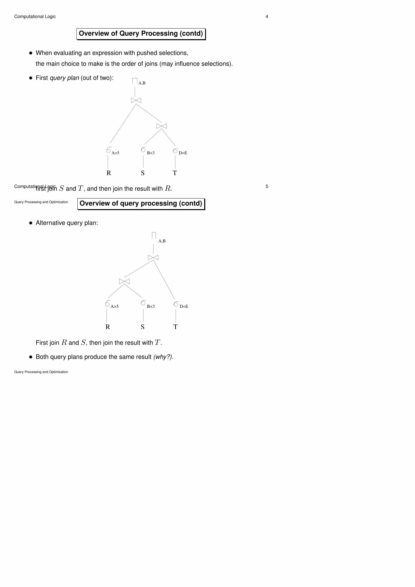
Overview of Query Processing (contd)
• When evaluating an expression with pushed selections,
the main choice to make is the order of joins (may influence selections).
• First query plan (out of two):
R S T
A>5 B<3 D=E
A,B
first join S and T , and then join the result with R.
Query Processing and Optimization
Computational Logic 5
Overview of query processing (contd)
• Alternative query plan:
R S T
A>5 B<3 D=E
A,B
First join R and S, then join the result with T .
• Both query plans produce the same result (why?).
Query Processing and Optimization
Computational Logic 6
Why choose one and not the other?
Query Processing and Optimization
Computational Logic 7
Optimization by Algebraic Equivalences
• Given a relational algebra expression E, find another expression E′ equivalent
to E that is easier (faster) to evaluate.
• Basic question: Given two relational algebra expressions E1, E2, are they
equivalent?
• If there were a method to decide equivalence, we could turn it into one to decide
whether an expression E is empty, i.e., whether E(I) = ∅ for every instance I.
How does one show this?
• Problem: Testing whether E ≡ ∅ is undecidable for expressions of full relational
algebra i.e., including union and difference. (Any idea why?)
• Good news:
We can still list some useful equalities.
Equivalence is decidable for important classes of queries (SPJR, SPC)
Query Processing and Optimization
Computational Logic 8
Optimization by Algebraic Equivalences (cntd)
Systematic way of query optimization: Apply equivalences
• 1 and× are commutative and associative, hence applicable in any order
• Cascaded projections can be simplified: If the attributes A1, . . . , An are among
B1, . . . , Bm, then
πA1,...,An(πB1,...,Bm(E)) = πA1,...,An(E)
• Cascaded selections might be merged:
σC1(σC2
(E)) = σC1∧C2(E)
• Commuting selection with join. If c only involves attributes from E1, then
σC(E1 1 E2) = σC(E1) 1 E2
• etc
We will not treat this here.
Query Processing and Optimization
Computational Logic 9
Optimization by Algebraic Equivalences (contd)
• Rules combining σ, π with ∪ and \
• Commuting selection and union:
σC(E1 ∪ E2) = σC(E1) ∪ σC(E2)
• Commuting selection and difference:
σC(E1 \ E2) = σC(E1) \ σC(E2)
• Commuting projection and union:
πA1,...,An(E1 ∪ E2) = πA1,...,An(E1) ∪ πA1,...,An(E2)
• Question: what about projection and difference?
Is πA(E1 \ E2) equal to πA(E1) \ πA(E2)?
Query Processing and Optimization
Computational Logic 10
Optimization of Conjunctive Queries
• Reminder:
Conjunctive queries
= SPJR queries
= simple SELECT-FROM-WHERE SQL queries
(only AND and (in)equality in the WHERE clause)
• Extremely common, and thus special optimization techniques have been
developed
• Reminder: for two relational algebra expressions E1, E2,
“E1 = E2” is undecidable.
• But for conjunctive queries, even E1 ⊆ E2 is decidable.
• Main goal of optimizing conjunctive queries: reduce the number of joins.
Query Processing and Optimization
Computational Logic 11
Optimization of Conjunctive Queries: An Example
• Given a relation R with two attributes A,B
• Two SQL queries:Q1 Q2
SELECT DISTINCT R1.B, R1.A SELECT DISTINCT R3.A, R1.A
FROM R R1, R R2 FROM R R1, R R2, R R3
WHERE R2.A=R1.B WHERE R1.B=R2.B AND R2.B=R3.A
• Are they equivalent?
• If they are, we can save one join operation.
• In relational algebra:
Q1 = π2,1(σ2=3(R×R))
Q2 = π5,1(σ2=4∧4=5(R×R×R))
Query Processing and Optimization
Computational Logic 12
Optimization of Conjunctive Queries (contd)
• We will show that Q1 and Q2 are equivalent!
• We cannot do this by using our equivalences for relational algebra expression.
(Why?)
• Alternative idea: CQs are like patterns that have to be matched by a database.
If a CQ returns an answer over a db, a part of the db must “look like” the query.
• Use rule based notation to find a representation of part of the db:
Q1(x, y) :– R(y, x), R(x, z)
Q2(x, y) :– R(y, x), R(w, x), R(x, u)
Query Processing and Optimization
Computational Logic 13
Containment is a Key Property
Definition. (Query containment) A query Q is contained in a query Q′
(written Q ⊆ Q′) if
Q(I) ⊆ Q′(I)
for every database instance I.
Translations:
• If we can decide containment for a class of queries, then we can also decide
equivalence.
• IfQ is a class of queries that is closed under intersection, then the containment
problem forQ can be reduced to the equivalence problem forQ.
Query Processing and Optimization
Computational Logic 14
Checking Containment of Conjunctive Queries: Ideas
• We want to check containment of two CQs Q, Q′
• We consider CQs without equalities and inequalities
(How serious is this restriction?)
• We also assume that Q and Q′ have the same arity and identical vectors of
head variables, that is, they are defined as Q(~x) :– B, Q′(~x) :– B′
• Intuition: a conjunctive query Q(~x) :– B returns an answer over instance I
if I “matches the pattern B”
• Instead of checking containment over all instances, we consider only finitely
many test instances (or better, one!)
Query Processing and Optimization
Computational Logic 15
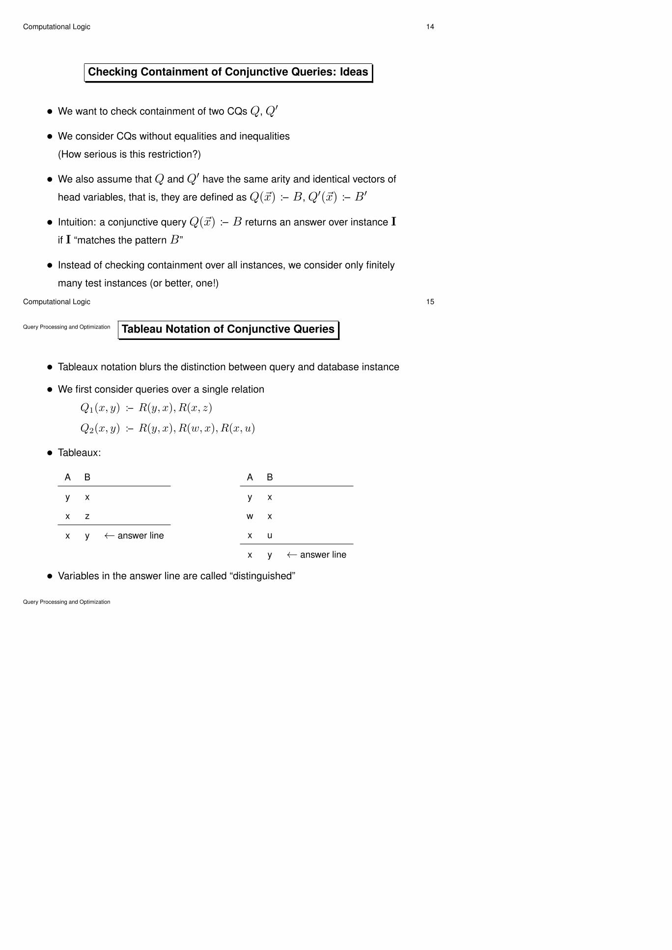
Tableau Notation of Conjunctive Queries
• Tableaux notation blurs the distinction between query and database instance
• We first consider queries over a single relation
Q1(x, y) :– R(y, x), R(x, z)
Q2(x, y) :– R(y, x), R(w, x), R(x, u)
• Tableaux:
A B
y x
x z
x y ← answer line
A B
y x
w x
x u
x y ← answer line
• Variables in the answer line are called “distinguished”
Query Processing and Optimization
Computational Logic 16
Tableau Homomorphisms
• Tableaux (as well as database instances or first order structures) are compared
by homomorphisms
• Idea: T ′ is more general than T if there is a homomorphism from T ′ to T
• Reminder: Terms are variables or constants
• A homomorphism δ from Tableau T1 to tableau T2 is a mapping
δ : {terms of T1} → {terms of T2}
such that
– δ(a) = a for every constant
– δ(x) = x for every distinguished x
– if (t1, ..., tk) is a row in T1, then (δ(t1), ..., δ(tk)) is a row in T2
Query Processing and Optimization
Computational Logic 17
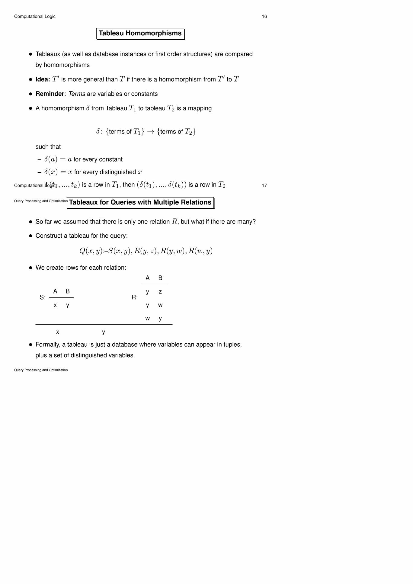
Tableaux for Queries with Multiple Relations
• So far we assumed that there is only one relation R, but what if there are many?
• Construct a tableau for the query:
Q(x, y):–S(x, y), R(y, z), R(y, w), R(w, y)
• We create rows for each relation:
S:A B
x yR:
A B
y z
y w
w y
x y
• Formally, a tableau is just a database where variables can appear in tuples,
plus a set of distinguished variables.
Query Processing and Optimization
Computational Logic 18
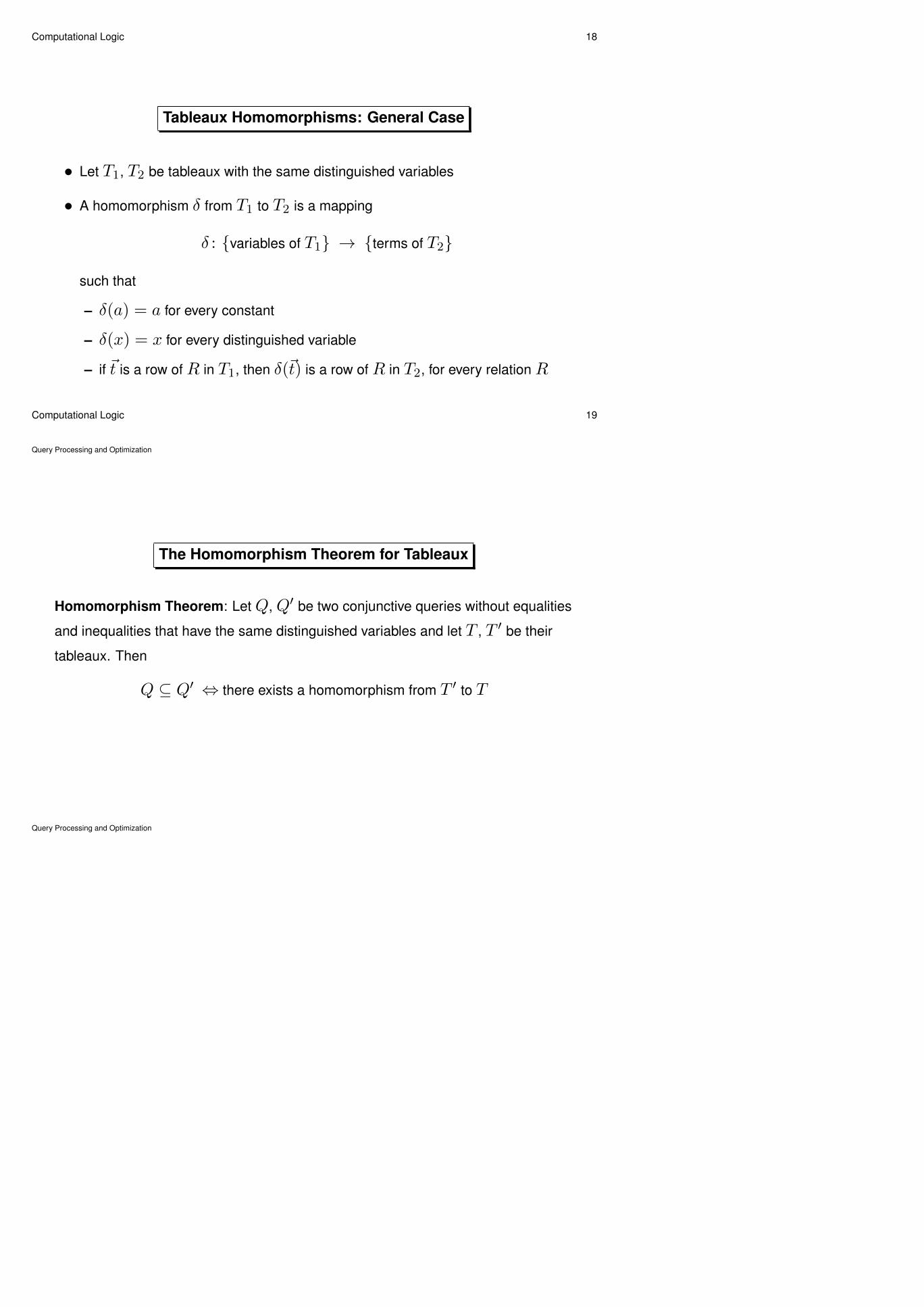
Tableaux Homomorphisms: General Case
• Let T1, T2 be tableaux with the same distinguished variables
• A homomorphism δ from T1 to T2 is a mapping
δ : {variables of T1} → {terms of T2}
such that
– δ(a) = a for every constant
– δ(x) = x for every distinguished variable
– if ~t is a row of R in T1, then δ(~t) is a row of R in T2, for every relation R
Query Processing and Optimization
Computational Logic 19
The Homomorphism Theorem for Tableaux
Homomorphism Theorem: Let Q, Q′ be two conjunctive queries without equalities
and inequalities that have the same distinguished variables and let T , T ′ be their
tableaux. Then
Q ⊆ Q′ ⇔ there exists a homomorphism from T ′ to T
Query Processing and Optimization
Computational Logic 20
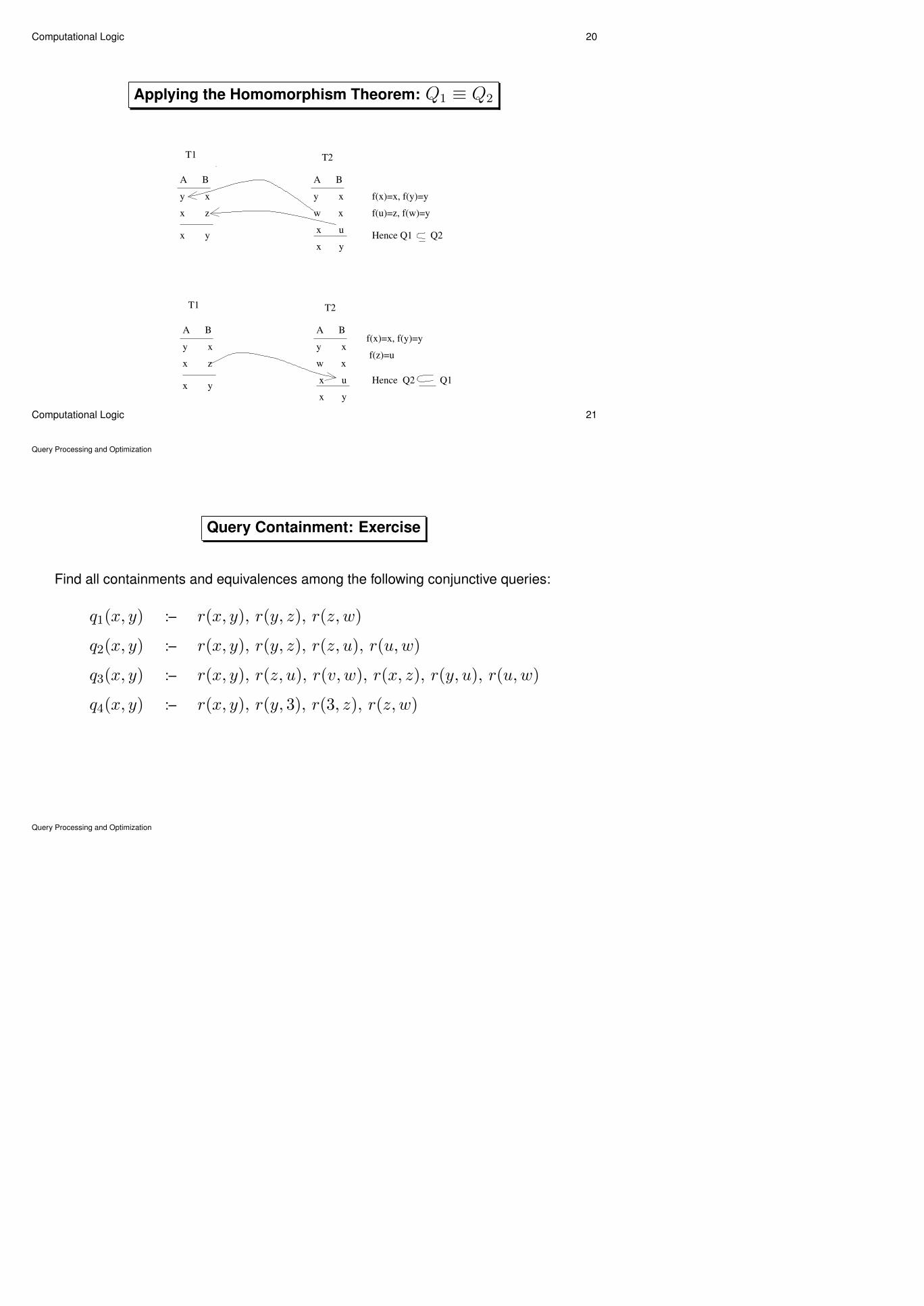
Applying the Homomorphism Theorem: Q1 ≡ Q2
A B
y x
x z
x y
A B
y x
w x
x u
T1 T2
x y
A B
y x
x z
x y
A B
y x
w x
x u
T1 T2
x y
f(x)=x, f(y)=y
f(u)=z, f(w)=y
Hence Q1 Q2
f(x)=x, f(y)=y
f(z)=u
Hence Q2 Q1
Query Processing and Optimization
Computational Logic 21
Query Containment: Exercise
Find all containments and equivalences among the following conjunctive queries:
q1(x, y) :– r(x, y), r(y, z), r(z, w)
q2(x, y) :– r(x, y), r(y, z), r(z, u), r(u,w)
q3(x, y) :– r(x, y), r(z, u), r(v, w), r(x, z), r(y, u), r(u,w)
q4(x, y) :– r(x, y), r(y, 3), r(3, z), r(z, w)
Query Processing and Optimization
Computational Logic 22
Query Containment: Complexity
Given two conjunctive queries, how hard is it to test whether Q ⊆ Q′?
• It is easy to transform them into tableaux, from either SPJ relational algebra
queries, or SQL queries, or rule-based queries. However, . . .
Theorem. The following problem is NP-hard.
Given: tableaux T , T ′
Question: is there a homomorphism from T ′ to T ?
Proof Ideas: Reductions of graph problems like Hamiltonian Path or Clique.
Also, reduction of 3SAT. (This one is interesting, because it can be modified to
prove that containment is harder for generalisations of conjunctive queries, such
as CQs with comparisons or CQs over databases with nulls.)
• In practice, query expressions are small, and thus conjunctive query optimization
is nonetheless feasible in polynomial time
Query Processing and Optimization
Computational Logic 23
Minimizing Conjunctive Queries
Goal: Given a conjunctive query Q, find an equivalent conjunctive query Q′ with the
minimum number of joins.
Questions: How many such queries can exist? How different are they?
Assumption: We consider only CQs without equalities and inequalities.
We call these queries simple conjunctive queries (SCQs) .
If nothing else is said in this chapter, CQs are simple CQs
Terminology: If
Q(~x) :– R1(~u1), . . . , Rk(~uk)
is a CQ, then Q′ is a subquery of Q if Q′ is of the form
Q′(~x) :– Ri1(~ui1), . . . , Ril(~uil)
where 1 ≤ i1 < i2 < . . . < il ≤ k.
Query Processing and Optimization
Computational Logic 24
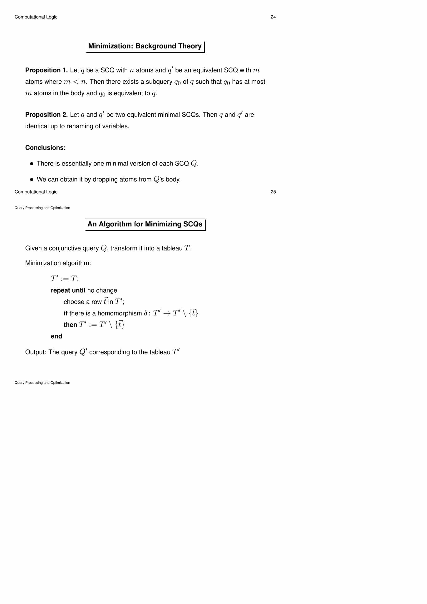
Minimization: Background Theory
Proposition 1. Let q be a SCQ with n atoms and q′ be an equivalent SCQ with m
atoms where m < n. Then there exists a subquery q0 of q such that q0 has at most
m atoms in the body and q0 is equivalent to q.
Proposition 2. Let q and q′ be two equivalent minimal SCQs. Then q and q′ are
identical up to renaming of variables.
Conclusions:
• There is essentially one minimal version of each SCQ Q.
• We can obtain it by dropping atoms from Q’s body.
Query Processing and Optimization
Computational Logic 25
An Algorithm for Minimizing SCQs
Given a conjunctive query Q, transform it into a tableau T .
Minimization algorithm:
T ′ := T ;
repeat until no change
choose a row ~t in T ′;
if there is a homomorphism δ : T ′ → T ′ \ {~t}then T ′ := T ′ \ {~t}
end
Output: The query Q′ corresponding to the tableau T ′
Query Processing and Optimization
Computational Logic 26
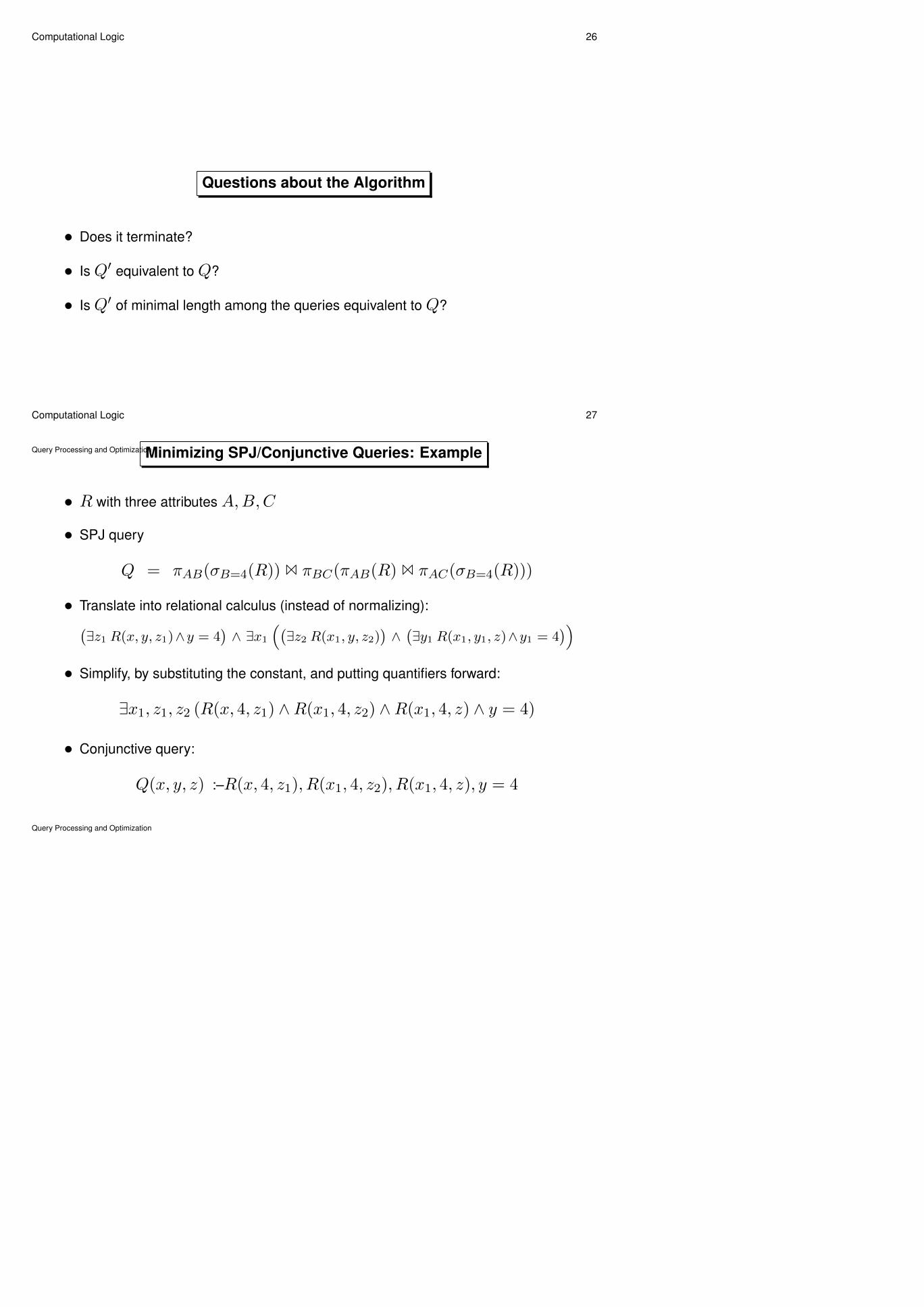
Questions about the Algorithm
• Does it terminate?
• Is Q′ equivalent to Q?
• Is Q′ of minimal length among the queries equivalent to Q?
Query Processing and Optimization
Computational Logic 27
Minimizing SPJ/Conjunctive Queries: Example
• R with three attributes A,B,C
• SPJ query
Q = πAB(σB=4(R)) 1 πBC(πAB(R) 1 πAC(σB=4(R)))
• Translate into relational calculus (instead of normalizing):(∃z1 R(x, y, z1)∧y = 4
)∧ ∃x1
((∃z2 R(x1, y, z2)
)∧
(∃y1 R(x1, y1, z)∧y1 = 4
))• Simplify, by substituting the constant, and putting quantifiers forward:
∃x1, z1, z2 (R(x, 4, z1) ∧R(x1, 4, z2) ∧R(x1, 4, z) ∧ y = 4)
• Conjunctive query:
Q(x, y, z) :–R(x, 4, z1), R(x1, 4, z2), R(x1, 4, z), y = 4
Query Processing and Optimization
Computational Logic 28
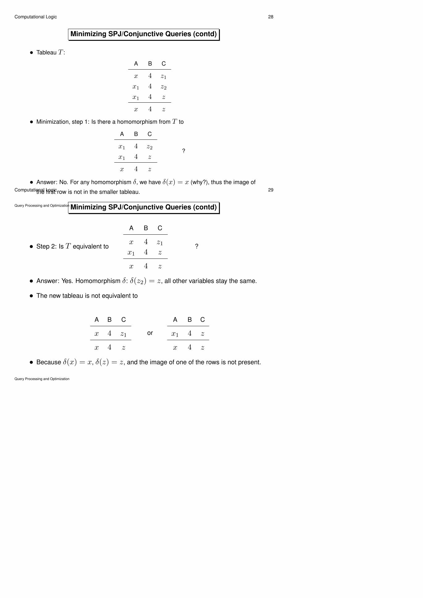
Minimizing SPJ/Conjunctive Queries (contd)
• Tableau T :
A B C
x 4 z1
x1 4 z2
x1 4 z
x 4 z
• Minimization, step 1: Is there a homomorphism from T to
A B C
x1 4 z2
x1 4 z
x 4 z
?
• Answer: No. For any homomorphism δ, we have δ(x) = x (why?), thus the image of
the first row is not in the smaller tableau.
Query Processing and Optimization
Computational Logic 29
Minimizing SPJ/Conjunctive Queries (contd)
• Step 2: Is T equivalent to
A B C
x 4 z1x1 4 z
x 4 z
?
• Answer: Yes. Homomorphism δ: δ(z2) = z, all other variables stay the same.
• The new tableau is not equivalent to
A B C
x 4 z1
x 4 z
or
A B C
x1 4 z
x 4 z
• Because δ(x) = x, δ(z) = z, and the image of one of the rows is not present.
Query Processing and Optimization
Computational Logic 30
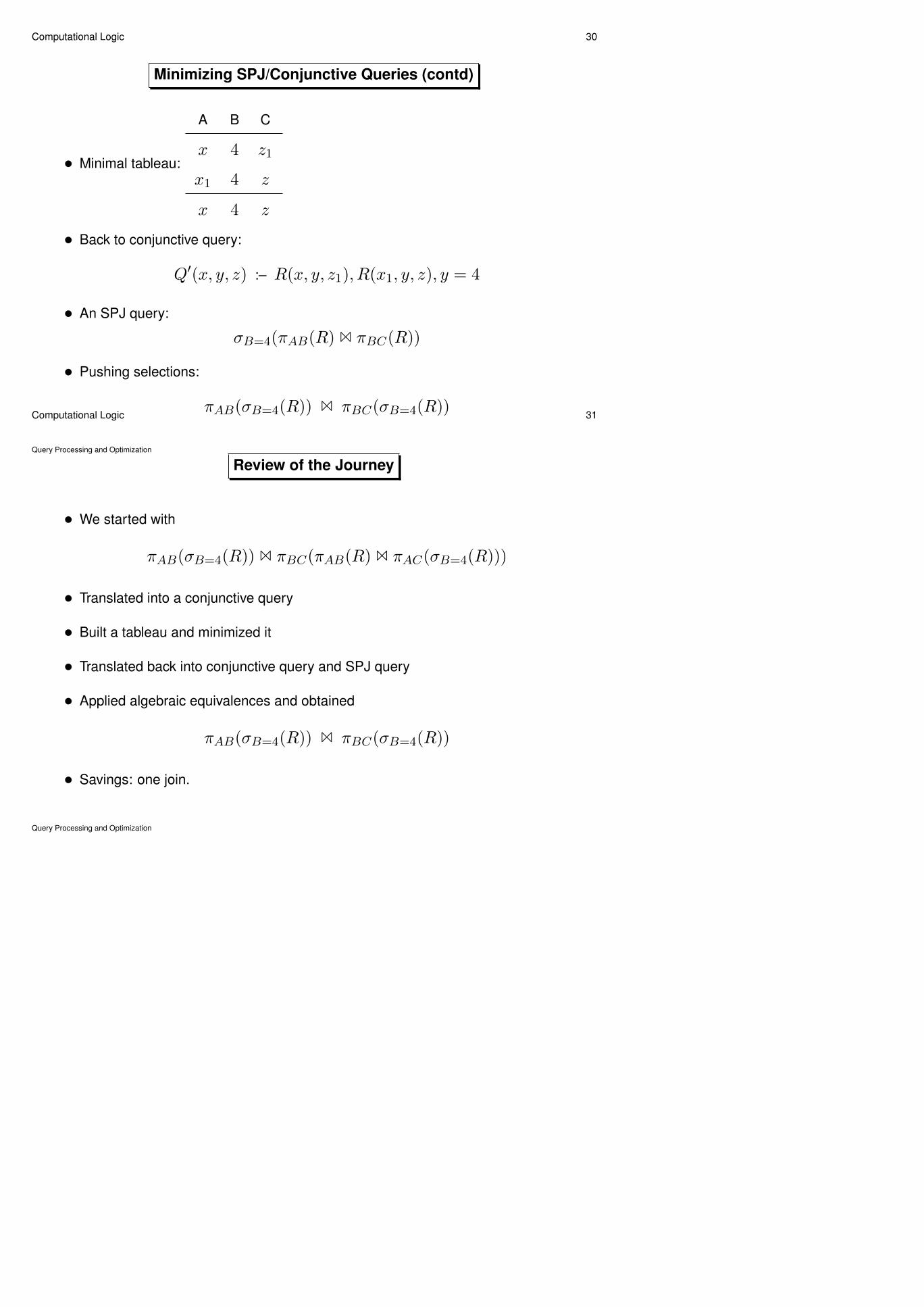
Minimizing SPJ/Conjunctive Queries (contd)
• Minimal tableau:
A B C
x 4 z1
x1 4 z
x 4 z
• Back to conjunctive query:
Q′(x, y, z) :– R(x, y, z1), R(x1, y, z), y = 4
• An SPJ query:
σB=4(πAB(R) 1 πBC(R))
• Pushing selections:
πAB(σB=4(R)) 1 πBC(σB=4(R))
Query Processing and Optimization
Computational Logic 31
Review of the Journey
• We started with
πAB(σB=4(R)) 1 πBC(πAB(R) 1 πAC(σB=4(R)))
• Translated into a conjunctive query
• Built a tableau and minimized it
• Translated back into conjunctive query and SPJ query
• Applied algebraic equivalences and obtained
πAB(σB=4(R)) 1 πBC(σB=4(R))
• Savings: one join.
Query Processing and Optimization
Computational Logic 32
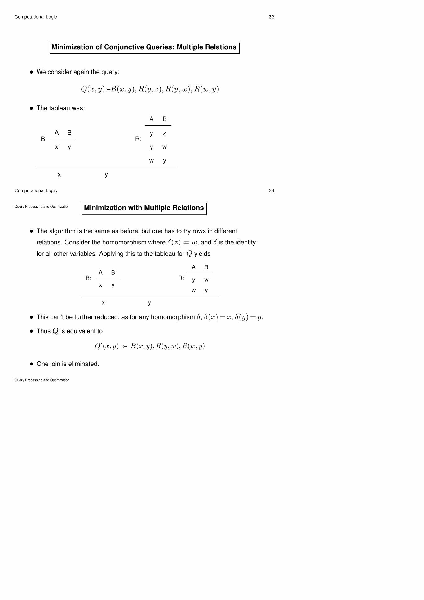
Minimization of Conjunctive Queries: Multiple Relations
• We consider again the query:
Q(x, y):–B(x, y), R(y, z), R(y, w), R(w, y)
• The tableau was:
B:A B
x yR:
A B
y z
y w
w y
x y
Query Processing and Optimization
Computational Logic 33
Minimization with Multiple Relations
• The algorithm is the same as before, but one has to try rows in different
relations. Consider the homomorphism where δ(z) = w, and δ is the identity
for all other variables. Applying this to the tableau for Q yields
B:A B
x yR:
A B
y w
w y
x y
• This can’t be further reduced, as for any homomorphism δ, δ(x)=x, δ(y)= y.
• Thus Q is equivalent to
Q′(x, y) :– B(x, y), R(y, w), R(w, y)
• One join is eliminated.
Query Processing and Optimization
Computational Logic 34
Conjunctive Queries with Equalities and Disequalities
• Equality/Disequality atoms x = y, x = a, x 6= z, etc
• Let T , T ′ be the tableaux of the parts of conjunctive queries Q and Q′ with
ordinary relations
• Sufficiency: Q ⊆ Q′ if there exists a homomorphism δ : T ′ → T such that for
each (dis)equality atom t1θt2 in Q′, we have that δ(t1)θδ(t2) is logically
implied by the equality and disequality atoms in Q
• However, existence of a homomorphims is no more a necessary condition for
containment.
• It holds under certain conditions, though.
Note: Deciding whether a set of equality/disequality atoms logically implies an
equality/disequality atom is (relatively) easy.
Query Processing and Optimization
Computational Logic 35
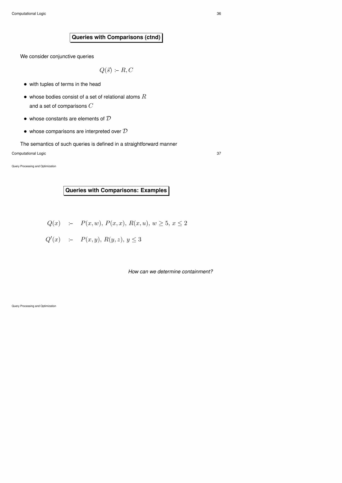
Queries with Comparisons
For queries with comparison atoms s ≤ t we have to refine our semantics
• An ordered domain is a nonempty setD with a linear order (written “≤D”)
• LetD be fixed. Wlog, dom = D. That is, from now on, database instances
have constants fromD.
• Real database languages support many domains, ordered and not ordered, by
typing relation symbols and admitting only queries that are well-typed.
Query Processing and Optimization
Computational Logic 36
Queries with Comparisons (ctnd)
We consider conjunctive queries
Q(~s) :– R,C
• with tuples of terms in the head
• whose bodies consist of a set of relational atoms R
and a set of comparisons C
• whose constants are elements ofD
• whose comparisons are interpreted overD
The semantics of such queries is defined in a straightforward manner
Query Processing and Optimization
Computational Logic 37
Queries with Comparisons: Examples
Q(x) :– P (x,w), P (x, x), R(x, u), w ≥ 5, x ≤ 2
Q′(x) :– P (x, y), R(y, z), y ≤ 3
How can we determine containment?
Query Processing and Optimization
Computational Logic 38
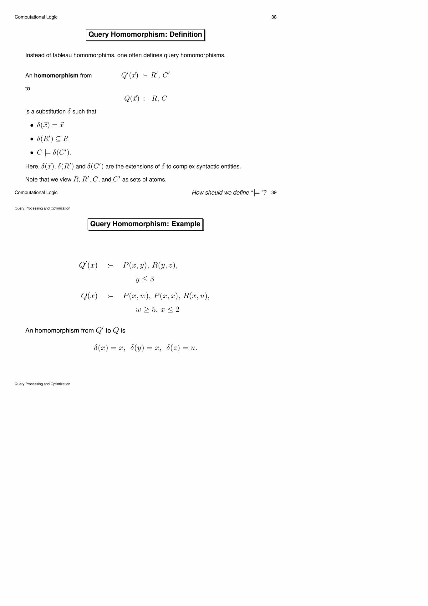
Query Homomorphism: Definition
Instead of tableau homomorphims, one often defines query homomorphisms.
An homomorphism from Q′(~x) :– R′, C ′
to
Q(~x) :– R, C
is a substitution δ such that
• δ(~x) = ~x
• δ(R′) ⊆ R
• C |= δ(C ′).
Here, δ(~x), δ(R′) and δ(C ′) are the extensions of δ to complex syntactic entities.
Note that we view R, R′, C , and C ′ as sets of atoms.
How should we define “ |= ”?
Query Processing and Optimization
Computational Logic 39
Query Homomorphism: Example
Q′(x) :– P (x, y), R(y, z),
y ≤ 3
Q(x) :– P (x,w), P (x, x), R(x, u),
w ≥ 5, x ≤ 2
An homomorphism from Q′ to Q is
δ(x) = x, δ(y) = x, δ(z) = u.
Query Processing and Optimization
Computational Logic 40
Homomorphisms: The General Case
Existence of a homomorphism is not a necessary, but a sufficient condition for
containment.
Theorem: Let Q, Q′ be two conjunctive queries, possibly with comparisons and
inequalities, such that Q and Q′ have the same distinguished variables. Then
Q ⊆ Q′ if there exists a homomorphism from Q′ to Q.
Query Processing and Optimization
Computational Logic 41
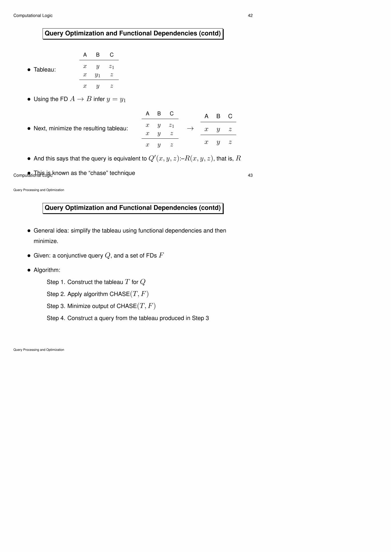
Query Optimization and Functional Dependencies
• Additional equivalences hold if db instances satisfy integrity constraints
• We consider here functional dependencies
• Example: Let R have attributes A,B,C . Assume that I(R) satisfies A→ B.
• Then it holds that
(πAB(R) 1 πAC(R))(I) = R(I)
(We have considered the expressions πAB(R) 1 πAC(R) and R as queries.)
• Tableaux can help with these optimizations!
• πAB(R) 1 πAC(R) as a conjunctive query:
Q(x, y, z) :– R(x, y, z1), R(x, y1, z)
Query Processing and Optimization
Computational Logic 42
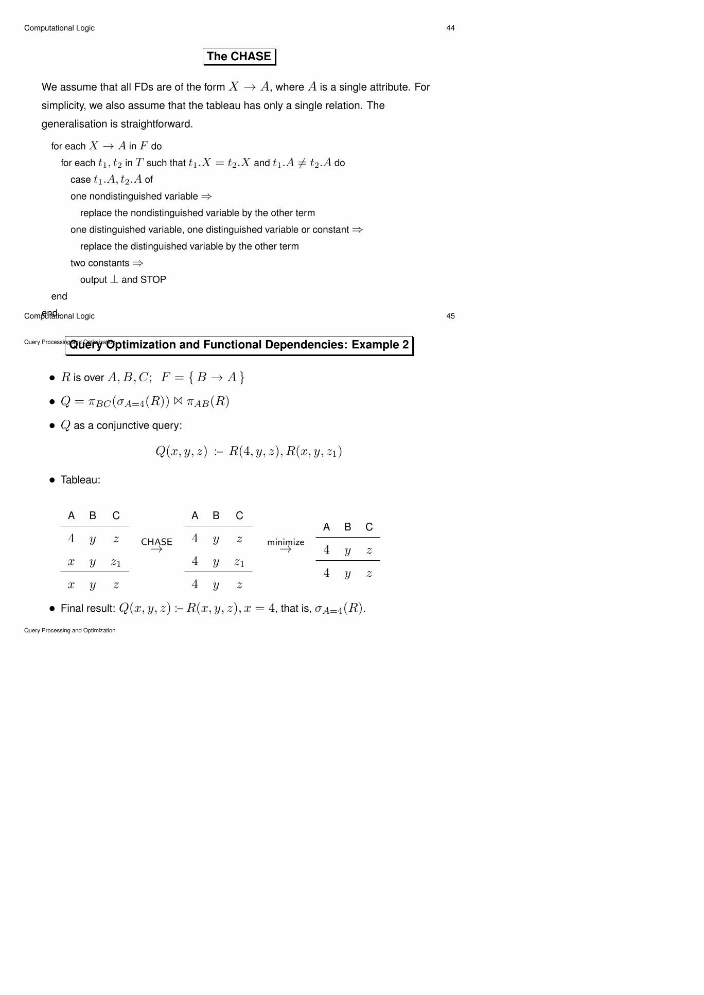
Query Optimization and Functional Dependencies (contd)
• Tableau:
A B C
x y z1x y1 z
x y z
• Using the FD A→ B infer y = y1
• Next, minimize the resulting tableau:
A B C
x y z1x y z
x y z
→A B C
x y z
x y z
• And this says that the query is equivalent to Q′(x, y, z):–R(x, y, z), that is, R
• This is known as the “chase” technique
Query Processing and Optimization
Computational Logic 43
Query Optimization and Functional Dependencies (contd)
• General idea: simplify the tableau using functional dependencies and then
minimize.
• Given: a conjunctive query Q, and a set of FDs F
• Algorithm:
Step 1. Construct the tableau T for Q
Step 2. Apply algorithm CHASE(T, F )
Step 3. Minimize output of CHASE(T, F )
Step 4. Construct a query from the tableau produced in Step 3
Query Processing and Optimization
Computational Logic 44
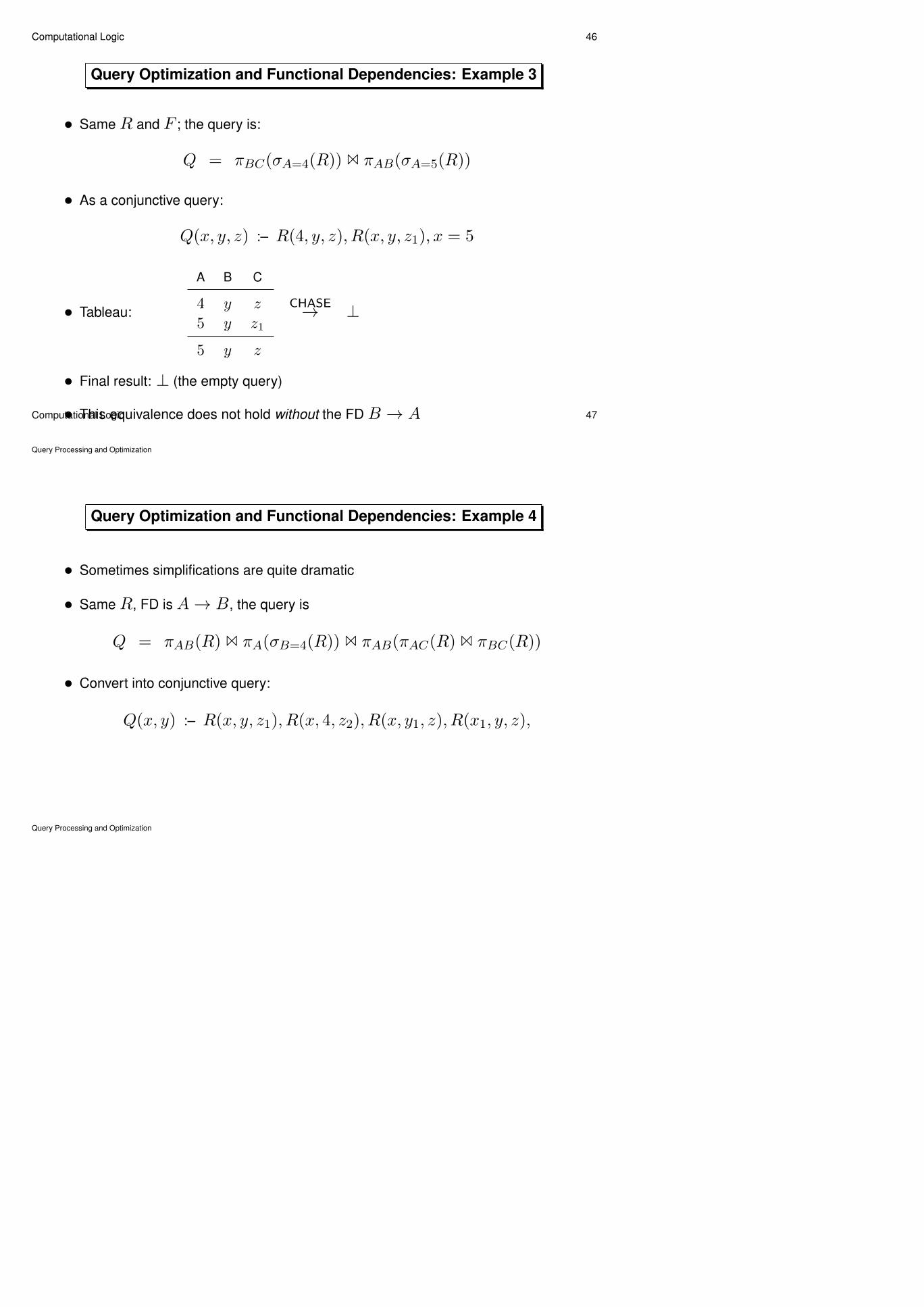
The CHASE
We assume that all FDs are of the form X → A, where A is a single attribute. For
simplicity, we also assume that the tableau has only a single relation. The
generalisation is straightforward.
for each X → A in F do
for each t1, t2 in T such that t1.X = t2.X and t1.A 6= t2.A do
case t1.A, t2.A of
one nondistinguished variable⇒replace the nondistinguished variable by the other term
one distinguished variable, one distinguished variable or constant⇒replace the distinguished variable by the other term
two constants⇒output⊥ and STOP
end
end.
Query Processing and Optimization
Computational Logic 45
Query Optimization and Functional Dependencies: Example 2
• R is over A,B,C ; F = {B → A }
• Q = πBC(σA=4(R)) 1 πAB(R)
• Q as a conjunctive query:
Q(x, y, z) :– R(4, y, z), R(x, y, z1)
• Tableau:
A B C
4 y z
x y z1
x y z
CHASE→
A B C
4 y z
4 y z1
4 y z
minimize→A B C
4 y z
4 y z
• Final result: Q(x, y, z) :– R(x, y, z), x = 4, that is, σA=4(R).
Query Processing and Optimization
Computational Logic 46
Query Optimization and Functional Dependencies: Example 3
• Same R and F ; the query is:
Q = πBC(σA=4(R)) 1 πAB(σA=5(R))
• As a conjunctive query:
Q(x, y, z) :– R(4, y, z), R(x, y, z1), x = 5
• Tableau:
A B C
4 y z
5 y z1
5 y z
CHASE→ ⊥
• Final result: ⊥ (the empty query)
• This equivalence does not hold without the FD B → A
Query Processing and Optimization
Computational Logic 47
Query Optimization and Functional Dependencies: Example 4
• Sometimes simplifications are quite dramatic
• Same R, FD is A→ B, the query is
Q = πAB(R) 1 πA(σB=4(R)) 1 πAB(πAC(R) 1 πBC(R))
• Convert into conjunctive query:
Q(x, y) :– R(x, y, z1), R(x, 4, z2), R(x, y1, z), R(x1, y, z),
Query Processing and Optimization
Computational Logic 48
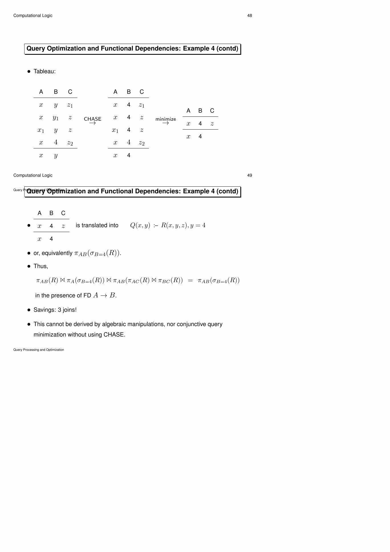
Query Optimization and Functional Dependencies: Example 4 (contd)
• Tableau:
A B C
x y z1
x y1 z
x1 y z
x 4 z2
x y
CHASE→
A B C
x 4 z1
x 4 z
x1 4 z
x 4 z2
x 4
minimize→A B C
x 4 z
x 4
Query Processing and Optimization
Computational Logic 49
Query Optimization and Functional Dependencies: Example 4 (contd)
•A B C
x 4 z
x 4
is translated into Q(x, y) :– R(x, y, z), y = 4
• or, equivalently πAB(σB=4(R)).
• Thus,
πAB(R) 1 πA(σB=4(R)) 1 πAB(πAC(R) 1 πBC(R)) = πAB(σB=4(R))
in the presence of FD A→ B.
• Savings: 3 joins!
• This cannot be derived by algebraic manipulations, nor conjunctive query
minimization without using CHASE.
Query Processing and Optimization

Computational Logic 50
Questions about the CHASE
• Does the CHASE algorithm terminate? What is the run time?
• What is the relation between a tableau and its CHASE’d version?
• Query containment wrt a set of FD’s:
– How can we define this problem?
– Can we decide this problem?
• Query minimsation wrt to a set of FDs
• Consider SCQs: we know from previous exercises that all such queries are
satisfiable. Is the same true if we assume only database instances that satisfy a
given set of FDs F?
Query Processing and Optimization
Related Documents