1 Computational Industrial Economics – A Generative Approach to Dynamic Analysis in Industrial Organization Myong-Hun Chang Department of Economics, Cleveland State University, Cleveland, OH 44115 [email protected] ABSTRACT The field of modern industrial economics focuses on the structure and performance of the industry in equilibrium when firms make decisions in an optimizing way, typically with perfect foresight. The patterns that arise in the process of adjustment, induced by persistent external shocks, are often ignored for lack of a proper tool for analysis. This chapter offers a basic agent-based computational model of industry dynamics which allows us to study the evolving industry structure through entry and exit of heterogeneous firms. This approach induces turbulence in market structure through unpredictable shocks to the firms’ technological environment. The base model pre- sented here enables the analysis of interactive dynamics between firms as they compete in a changing environment with limited rationality and foresight. A possible extension of the base model, allowing for R&D by firms, is also discussed. 1.1 Introduction I propose a computational modeling framework which can form the basis for carrying out dynamic analysis in industrial organization (IO). The main idea is to create an artificial industry within a computational setting, which can then be populated with firms who enter, compete, and exit over the course of the industry’s growth and de- velopment. These actions of the firms are driven by pre-specified decision rules, the interactions of which then generate a rich historical record of the industry’s evolution. With this framework, one can study the complex interactive dynamics of heterogeneous firms as well as the evolving structure and performance of the industry.

Welcome message from author
This document is posted to help you gain knowledge. Please leave a comment to let me know what you think about it! Share it to your friends and learn new things together.
Transcript
1
Computational Industrial Economics– A Generative Approach toDynamic Analysis in IndustrialOrganization
Myong-Hun ChangDepartment of Economics, Cleveland State University, Cleveland, OH 44115
ABSTRACT
The field of modern industrial economics focuses on the structure and performance ofthe industry in equilibrium when firms make decisions in an optimizing way, typicallywith perfect foresight. The patterns that arise in the process of adjustment, inducedby persistent external shocks, are often ignored for lack of a proper tool for analysis.This chapter offers a basic agent-based computational model of industry dynamicswhich allows us to study the evolving industry structure through entry and exit ofheterogeneous firms. This approach induces turbulence in market structure throughunpredictable shocks to the firms’ technological environment. The base model pre-sented here enables the analysis of interactive dynamics between firms as they competein a changing environment with limited rationality and foresight. A possible extensionof the base model, allowing for R&D by firms, is also discussed.
1.1 Introduction
I propose a computational modeling framework which can form the basis for carryingout dynamic analysis in industrial organization (IO). The main idea is to create anartificial industry within a computational setting, which can then be populated withfirms who enter, compete, and exit over the course of the industry’s growth and de-velopment. These actions of the firms are driven by pre-specified decision rules, theinteractions of which then generate a rich historical record of the industry’s evolution.With this framework, one can study the complex interactive dynamics of heterogeneousfirms as well as the evolving structure and performance of the industry.
2 Computational Industrial Economics
The base model of industry dynamics presented here can be extended and refinedto address a variety of standard issues in IO, but it is particularly well-suited foranalyzing the dynamic process of adjustment in industries that are subject to per-sistent external shocks. The empirical significance of such processes is well-reflectedin the literature that explores patterns in the turnover dynamics of firms in variousindustries. The seminal work in this literature is Dunne et al. (1988). They found thatthe turnovers are significant and persistent over time in a wide variety of industries,though they also noticed substantial cross-industry differences in their rates: “[W]e findsubstantial and persistent differences in entry and exit rates across industries. Entryand exit rates at a point in time are also highly correlated across industries so thatindustries with higher than average entry rates tend to also have higher than averageexit rates.” To the extent that firm turnovers are the manifestation of the aforemen-tioned adjustment process, this literature brings to light the empirical significance ofthe out-of-equilibrium industrial dynamics. Furthermore, it identifies patterns to thisadjustment process that the standard equilibrium models (static or dynamic) are notwell-equipped to address. For instance, Caves (2007) states: “Turnover in particularaffects entrants, who face high hazard rates in their infancy that drop over time. It islargely because of high infant mortality that rates of entry and exit from industriesare positively correlated (compare the obvious theoretical model that implies eitherentry or exit should occur but not both). The positive entry-exit correlation appearsin cross-sections of industries, and even in time series for individual industries, if theirlife-cycle stages are controlled.” The approach proposed here addresses this uneasyco-existence of equilibrium-theorizing and the non-equilibrium empirical realities inindustrial organization.
The model entails a population of firms; each of whom endowed with a uniquetechnology that remains fixed over the course of its life. The firms go through a re-peated sequence of entry-output-exit decisions. The market competition takes placeamid a technological environment that is subject to external shocks, inducing changesin the relative production efficiencies of the firms. Because the firms’ technologies areheld fixed, there is no firm-level adaptation to the environmental shifts. However, anindustry-level adaptation takes place through the process of firm entry and exit, whichis driven by the selective force of the market competition.
The implementation of the adjustment process in the proposed model rests on twoassumptions. First, the firms in the model are myopic. They do not have the foresightthat is frequently assumed in the orthodox industrial organization literature. Instead,their decisions are made on the basis of fixed rules motivated by myopic but maximiz-ing tendencies. Second, the technological environment within which the firms operateis stochastic. How efficient a firm was in one environment does not indicate how ef-ficient it will be in another environment. As such, there is always a possibility thatthe firms may be re-shuffled when the environment changes. These two assumptions -myopia (or, more broadly, bounded rationality) of firms and stochastic technologicalenvironment - lead to persistent firm heterogeneity. It is this heterogeneity that pro-vides the raw materials over which the selective force of market competition can act.Firm myopia drives the entry process; the selective force of market process, acting onthe heterogeneous firms, drives the exit process; all the while the stochastic techno-
Industry dynamics: An overview of the theoretical literature 3
logical environment guarantees the resulting process never settles down, giving us anopportunity to study patterns that may emerge along the process.
I offer two sets of results in this chapter. The first set of results is obtained underthe assumption of stable market demand; hence the only source of turbulence is theshocks to the technological environment. The results show that the entry and exitdynamics inherent in the process generate patterns that are consistent with empiricalobservations, including the phenomenon of infant mortality and the positive corre-lation between entry and exit. Furthermore, the base model enables the analysis ofthe relationships between the industry-specific demand and technological conditionsand the endogenous structure and performance of the industry along the steady-state,thereby generating cross-sectional implications in a fully dynamic setting. The secondset of results is generated under the assumption of fluctuating demand; hence, the de-mand shocks are now superimposed on the technological shocks. The basic relationshipbetween the rate of entry and the rate of exit continues to hold with this extension.In addition, the extension enables a characterization of the way fluctuating demandaffects the turnover as well as the structure and performance of the industry. Finally,I discuss a potential extension of the base model, in which the R&D activities of firmscan be incorporated.
1.2 Industry dynamics: An overview of the theoretical literature
IO theorists have used analytical approaches to explore the entry and exit dynamicsof firms and their impact on the growth of the industry. Most of these works involvedynamic models of firm behavior, in which heterogeneous firms with perfect foresight(but with incomplete information) make entry, production, and exit decisions to max-imize the expected discounted value of future net cash flow. Jovanovic (1982) was thefirst significant attempt in this line of research. He presented an equilibrium modelin which firms learn about their efficiency through productivity shocks as they op-erate in the industry. The shocks were specified to follow a non-stationary processand represented noisy signals which provided evidence to firms about their true costs.The “perfect foresight” equilibrium leads to selection through entry and exit in thismodel. However, there is no firm turnover in the long run, once learning is completed;hence, the patterns in the persistent series of entry and exit, identified in the empiricalliterature, cannot be explored with this model.
Hopenhayn (1992) offers a tractable framework, in which perpetual and simulta-neous entry and exit are endogenously generated in the long run. His approach entailsa dynamic stochastic model of a competitive industry with a continuum of firms. Themovements of firms in the long run are part of the stationary equilibrium he developsin order to analyze the behavior of firms along the steady state as they are hit withindividual productivity shocks. This model assumes perfect competition and, hence,the stationary equilibria in the model maximize net discounted surplus. In this sense,it is similar to Lucas and Prescott (1971) which looks at a competitive industry withaggregate shocks but with no entry and exit. Hopenhayn (1992) finds that changesin aggregate demand do not affect the rate of turnover, though they raise the totalnumber of firms. As Asplund and Nocke (2006) point out, this result hinges on theassumption of perfect competition in which there is no price competition effect in-
4 Computational Industrial Economics
duced by the increase in the mass of active firms. As such, the price-cost margins areindependent of market size in this model.
Asplund and Nocke (2006) adopt the basic framework of Hopenhayn (1992) andextend it to the case of imperfect competition. [Melitz (2003) is another extension ofHopenhayn’s approach to monopolistic competition, though his focus is on interna-tional trade.] It is an equilibrium model of entry and exit which utilizes the steadystate analysis developed in Hopenhayn (1992). The model uses the reduced-form profitfunction and, hence, avoids specifying the details of the demand system as well as thenature of the oligopoly competition (e.g., output competition, price competition, pricecompetition with differentiated products, etc.). The key difference between Hopenhayn(1992) and their model is that they assume the existence of the price competition effect
which implies a negative relationship between the number of entrants and the profitsof active incumbents. The assumptions made about the reduced-form profit functionlead to two countervailing forces in the model: 1) the rise in market size increases theprofits of all firms proportionally through an increase in output levels, holding pricesfixed; 2) the distribution of firms also increases with the market size, hence reducingthe price and the price-cost margin through the price competition effect. The mainresult is that an increase in market size leads to a rise in the turnover rate and a de-cline in the age distribution of firms in the industry. They provide empirical supportfor these results using the data on hair salons in Sweden.
Asplund and Nocke (2006) is a significant contribution in that they were able togenerate persistent entry and exit along the steady state of the industry and performcomparative statics analysis with respect to market-specific factors such as marketsize and the fixed cost. However, their equilibrium approach, while appropriate for thestudy of the steady state behavior, is inadequate when the focus is on the behaviorof firms along the non-equilibrium transitory path. In contrast to Asplund and Nocke(2006), the model presented in this chapter specifies a linear demand function andCournot output competition. The price competition effect, instead of being assumed,is generated as an endogenous outcome of the entry-competition process. While thefunctional forms specified in this model are more restrictive than the reduced-formprofits approach used by Asplund and Nocke (2006), they are necessary for the task inhand: Given that the research objective is to examine the effects of the market-specificfactors on the evolving structure and performance of the industry, it is imperative thatthe model fully specify the demand and cost structure so that the relevant variablessuch as price, outputs, and market shares can be endogenously derived. This allowsfor a detailed analysis of the firms’ behavior along the transitory phase, identifyingand interpreting the patterns that exist in the non-equilibrium state of the industry,further enhancing our understanding of the comparative dynamics properties.
Another important development is the concept of Markov Perfect Equilibrium(MPE) that incorporates strategic decision making by firms with perfect foresight infully dynamic models of oligopolistic interactions with firm entry and exit - see Pakesand McGuire (1994) and Ericson and Pakes (1995). The MPE framework is directly im-ported from the game-theoretic approach to dynamic oligopoly, which models strategicinteractions among players (firms) who take into account each other’s strategies andactions. Firms in these models are endowed with perfect foresight: they maximize the
Industry dynamics: An overview of the theoretical literature 5
expected net present value of future cash flows, taking into calculation all likely futurestates of its rivals conditional on all possible realizations of industry-wide shocks. Theassumption of perfect foresight implies that the firms’ decision making process usesrecursive methodology; hence, solving for the equilibrium entails Bellman equations.Given the degree of complexity in the model specification and the solution conceptinvolving recursive methods, this approach requires extensive use of computationalmethodologies. Although this approach is conceptually well positioned to address thecentral issues of industry dynamics, its success thus far has been limited due to thewell-known “curse of dimensionality” as described by Doraszelski and Pakes (2007):
“The computational burden of computing equilibria is large enough to oftenlimit the type of applied problems that can be analyzed. There are two aspectsof the computation that can limit the complexity of the models we analyze; thecomputer memory required to store the value and policies, and the CPU timerequired to compute the equilibrium .... [I]f we compute transition probabilitiesas we usually do using unordered states then the number of states that we needto sum over to compute continuation values grows exponentially in both thenumber of firms and the number of firm-specific state variables.” [Doraszelskiand Pakes (2007), pp. 1915-1916]
As they point out, the computational burden is mainly due to the size of the statespace that needs to be explored in the process of evaluating the value functions andthe policy functions. The exponential growth of the state space that results fromincreasing the number of firms or the set of decision variables imposes a significantcomputational constraint on the scale and scope of the research questions one can ask.1 Furthermore, if the objective is to generate analytical results that can match data,the MPE approach often falls short of meeting it.
The agent-based computational economics (ACE) approach taken in this chapteroffers a viable alternative to the MPE approach. Tesfatsion and Judd (2006) providea succinct description:
“ACE is the computational study of economic processes modeled as dynamicsystems of interacting agents who do not necessarily possess perfect rationalityand information. Whereas standard economic models tend to stress equilibria,ACE models stress economic processes, local interactions among traders andother economic agents, and out-of-equilibrium dynamics that may or may notlead to equilibria in the long run. Whereas standard economic models requirea careful consideration of equilibrium properties, ACE models require detailedspecifications of structural conditions, institutional arrangements, and behav-ioral dispositions.”[Tesfatsion and Judd (2006), p. xi]
In the same vein, my model does away with the standard assumption of perfect fore-sight on the part of the firms. By assuming myopia and limited rationality in theirdecision making, I eliminate the need to evaluate the values and policies for all pos-sible future states for all firms, thus effectively avoiding the curse of dimensionalitythat is inherent in the MPE approach. The computational resource thus saved is then
1See Weintraub, Benkard, and Van Roy (2008, 2010) for attempts to circumvent this problemwhile remaining within the general conceptual framework of the MPE approach.
6 Computational Industrial Economics
utilized in studying the complex interactions among firms and tracking the movementsof relevant endogenous variables over time for a large number of firms. The trade-offis then the reduction in the degree of firms’ rationality and foresight in return for theability to analyze in detail the non-equilibrium dynamics of the industry. In view ofthe increased scale and scope of the research questions that can be addressed, the useof the agent-based computational model is deemed well-justified.
Given the current state of the literature as outlined above, the present study makestwo contributions. First, it offers a computational model that can be used as a testbed for large-scale experiments that involve generating and growing artificial indus-tries. By systematically varying the characteristics of the environment within whichthe industry evolves, I am able to identify the patterns inherent in the growth processof a given industry as well as any difference in those patterns that may exist acrossindustries. Such computational experiments allow re-evaluation of the comparativedynamics results obtained in the past analytical works; but they also offer additionalresults and insights, including the cyclical industry dynamics that may result fromfluctuations in market demand. The in-depth investigation of the non-equilibrium ad-justment dynamics offered here is not feasible with the standard equilibrium models.
The second contribution is in generating predictions that can match data betterthan the existing models. The agent-based computational approach taken here greatlyreduces the demand for computational resources at the level of individual firm’s de-cision making. Instead, the saved resources are allocated to tracking and analyzingthe complex interactions among firms over time. Compared to the numerical mod-els formulated in the MPE framework, the model described in this chapter offers aflexible platform for generating predictions that can better match empirical data byincorporating a larger number of firms and their decision variables.
1.3 Methodology
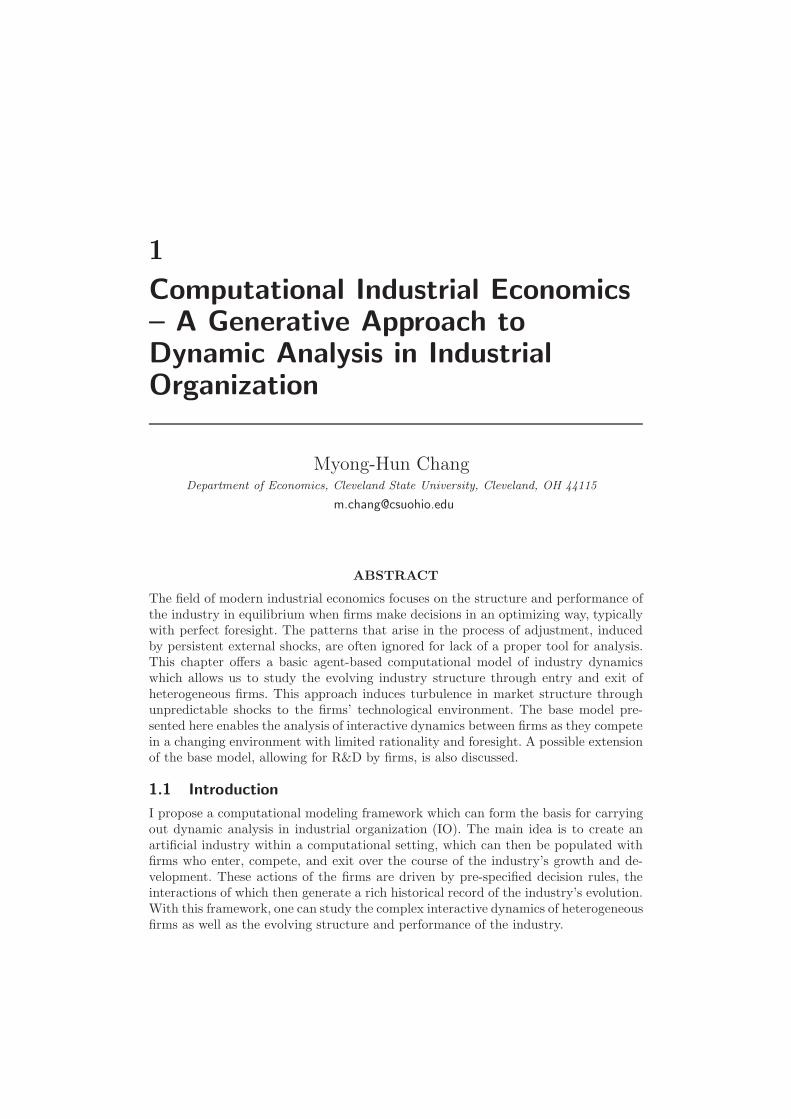
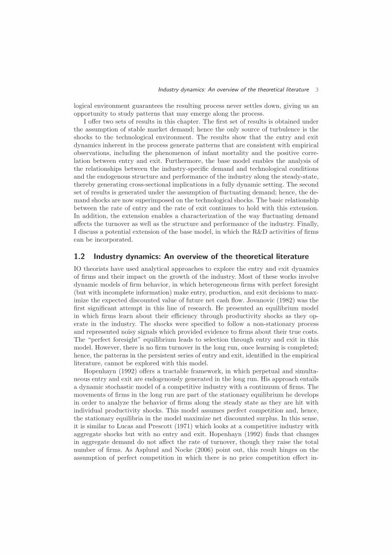
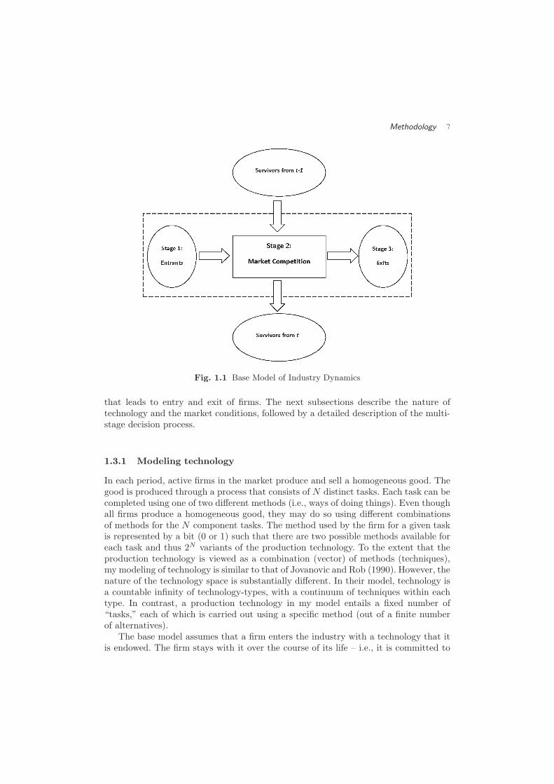
The base model entails an evolving population of firms which interact with one anotherthrough repeated market competition.2 Figure 1.1 captures the overall structure of themodel.
Each period t starts out with a group of surviving incumbents from the previousperiod, and consists of three decision stages. In stage 1, each potential entrant makesa decision to enter. A new entrant is assumed to enter with a random (but unique)technology and a start-up fund that is common for all entrants. In stage 2, the newentrants and the incumbents, given their endowed technologies, compete in the market.The outcome of the competition in stage 2 generates profits (and losses) for the firms.In stage 3, all firms update their net wealth based on the profits earned (and lossesincurred) from the stage-2 competition and decide whether or not to exit the industry.Once the exit decisions are made, the surviving incumbents with their technologiesand the updated net wealth move on to period t+ 1 where the process is repeated.
Central to this process are the heterogeneous production technologies held by thefirms (which imply cost asymmetry) and the selective force of market competition
2It should be noted that while the surviving incumbents may be engaged in “repeated interaction”with one another, the assumption of myopia precludes the possibility of collusion in this model.
Methodology 7
Fig. 1.1 Base Model of Industry Dynamics
that leads to entry and exit of firms. The next subsections describe the nature oftechnology and the market conditions, followed by a detailed description of the multi-stage decision process.
1.3.1 Modeling technology
In each period, active firms in the market produce and sell a homogeneous good. Thegood is produced through a process that consists of N distinct tasks. Each task can becompleted using one of two different methods (i.e., ways of doing things). Even thoughall firms produce a homogeneous good, they may do so using different combinationsof methods for the N component tasks. The method used by the firm for a given taskis represented by a bit (0 or 1) such that there are two possible methods available foreach task and thus 2N variants of the production technology. To the extent that theproduction technology is viewed as a combination (vector) of methods (techniques),my modeling of technology is similar to that of Jovanovic and Rob (1990). However, thenature of the technology space is substantially different. In their model, technology isa countable infinity of technology-types, with a continuum of techniques within eachtype. In contrast, a production technology in my model entails a fixed number of“tasks,” each of which is carried out using a specific method (out of a finite numberof alternatives).
The base model assumes that a firm enters the industry with a technology that itis endowed. The firm stays with it over the course of its life – i.e., it is committed to
8 Computational Industrial Economics
using a particular method for a given task at all times.3 A firm’s technology is thenfully characterized by a binary vector of N dimensions which captures the completeset of methods it uses to produce the good. Denote it by zi ∈ {0, 1}N , where zi ≡(zi(1), zi(2)..., zi(N)) and zi(h) ∈ {0, 1} is firm i′s method in task h.
In measuring the degree of heterogeneity between any two technologies (i.e., methodvectors), zi and zj , we use “Hamming Distance,” which is the number of positions forwhich the corresponding bits differ:
D(zi, zj) ≡∑N
h=1|zi(h)− zj(h)|. (1.1)
How efficient a given technology is depends on the environment it operates in. Inorder to represent the technological environment that prevails in period t, I specify aunique methods vector, zt ∈ {0, 1}N , which is defined as the optimal technology forthe industry in t. How well a firm’s technology performs in the current environmentthen depends on how close it is to the prevailing optimal technology in the technologyspace. More specifically, the marginal cost of firm i in period t is specified to be a directfunction of D(zi, z
t) the Hamming distance between the firm’s endowed technology,zi, and the current optimal technology, zt. The optimal technology in t is common forall firms - i.e., all firms in a given industry face the same technological environment ata given point in time. As such, once it is defined for a given industry, its technologicalenvironment is completely specified for all firms since the efficiency of any technologyis well-defined as a function of its distance to this optimal technology.4
1.3.2 Modeling market competition
In each period, there exist a finite number of firms that operate in the market. In thissubsection, I define the static market equilibrium among such operating firms. Thetechnological environment and the endowed technologies for all firms jointly deter-mine the marginal costs of the firms and, hence, the resulting equilibrium. The staticmarket equilibrium defined here is then used to approximate the outcome of marketcompetition in each period. In this sub-section, I temporarily abstract away from thetime superscript for ease of exposition.
Let m be the number of firms operating in the market. The firms are Cournotoligopolists, who choose production quantities of a homogeneous good. In definingthe Cournot equilibrium in this setting, I assume that all m firms produce positivequantities in equilibrium. The inverse market demand function is specified as:
P (Q) = a−Q
s(1.2)
where Q =∑m
j=1qj and s denotes the size of the market.
3There is, hence, no adaptation at the firm-level in this model, although adaptation at theindustry-level is possible through the selection of firms via market competition.
4Given that an entering firm is endowed with a fixed technology that cannot be modified, it doesnot matter whether the optimal technology is known to the firms or not. In a more general settingwhere the technology can be modified, any knowledge of the optimal technology, however imperfect,will affect the direction of the firm’s adaptive modification through its R&D decisions.
Methodology 9
Each operating firm has its production technology, zi, and faces the following totalcost:
C (qi; zi, z) = fi + ci (zi, z) · qi (1.3)
For simplicity, the firms are assumed to have identical fixed cost:f1 = f2 = · · · = fm =f. The firm’s marginal cost, ci(zi, z), depends on how different its technology, zi, isfrom the optimal technology, z:
ci ≡ ci (zi, z) = 100 ·D(zi, z)
N(1.4)
Hence, ci increases in the Hamming distance between the firm’s technology and theoptimal technology for the industry. It is at its minimum of zero when zi = z and atits maximum of 100 when all N bits in the two technologies are different from oneanother.5 The total cost can then be re-written as:
C (qi; zi, z) = f + 100 ·D(zi, z)
N· qi (1.5)
Given the demand and cost functions, firm i′s profit is:
πi (qi, Q− qi) =
a−1
s
m∑
j=1
qj
· qi − f − ci · qi. (1.6)
Taking the first-order condition for each i and summing over m firms, we derive theequilibrium industry output rate, which gives us the equilibrium market price, P ,through equation (2):
P =
(
1
m+ 1
)
(
a+∑m
j=1cj
)
(1.7)
Given the vector of marginal costs defined by the firms’ technologies and the optimaltechnology, P is uniquely determined and is independent of the market size, s. Fur-thermore, the equilibrium market price depends only on the sum of the marginal costsand not on the distribution of cis.
In deriving the equilibrium output rate, qi, I assume that allm firms are active and,hence, qi > 0 for all i ∈ {1, 2, ...,m} . This assumption is relaxed in the simulationsreported later in the chapter, given that the cost asymmetry inherent in this modelmay force some of the firms to shut down and become inactive - the algorithm usedto identify inactive firms is discussed in Section 1.3.3.2. The equilibrium firm outputrate is then:
qi = s ·
[(
1
m+ 1
)
(
a+∑m
j=1cj
)
− ci
]
(1.8)
A firm’s equilibrium output rate depends on its own marginal cost and the equilibriummarket price such that qi = s · (P − ci). Finally, the Cournot equilibrium firm profit is
5For concreteness, suppose N = 10 and the current technological environment is captured bythe optimal vector of z = (1100101100). If a firm i entered the industry with a technology, z
i=
(0010011100), then D(zi, z) = 5 and the firm’s marginal cost is 50.
10 Computational Industrial Economics
π(qi) = P · qi − f − ci · qi =1
s(qi)
2 − f. (1.9)
Note that qi is a function of ci and∑m
j=1cj , where cj is a function of zj and z for
all j. It is then straightforward that the equilibrium firm profit is fully determined,once the vectors of methods are known for all firms. Further note that ci ≤ ck impliesqi ≥ qk and, hence, π(qi) ≥ π(qk)∀i, k ∈ {1, ...,m} .
1.3.3 The base model of industry dynamics
In the beginning of any typical period t, the industry opens with two groups of decisionmakers: 1) a group of incumbent firms surviving from t − 1, each of whom enters t
with its endowed technology, zi, and its net wealth, wt−1
i , carried over from t − 1; 2)a group of potential entrants ready to consider entering the industry in t, each withan endowed technology of zj and its start-up wealth. All firms face a common techno-logical environment within which his/her technology will be used; this environment isfully represented by the prevailing optimal technology, zt.
Central to the model is the assumption that the production environment is in-herently stochastic - that is, the technology which was optimal in one period is notnecessarily optimal in the next period. This is captured by allowing the optimal tech-nology, zt , to vary from one period to the next in a systematic manner. The mechanismthat guides this shift dynamic is described next.
1.3.3.1 Random shifts in technological environment.
Consider a binary vector, x ∈ {0, 1}N . Define δ(x, l) ⊂ {0, 1}N as the set of points thatare exactly Hamming distance l from x. The set of points that are within Hammingdistance l of x is then defined as
△(x, l) ≡ U li=0
δ(x, i) (1.10)
The following rule drives the shift dynamic of the optimal technology:
zt =
{
z′
zt−1
with probability γ
with probability 1− γ(1.11)
where z′
∈ △(zt−1, g) and γ and g are constant over all t. Hence, with probabilityγ the optimal technology shifts to a new one within g Hamming distance from thecurrent technology, while with probability 1 − γ it remains unchanged at zt−1. Thevolatility of the technological environment is then captured by γ and g, where γ is thefrequency and g is the maximum magnitude of changes in technological environment.
An example of the type of changes in the technological environment envisioned inthis model is the series of innovations in computers and digital technologies that haveoccurred over the last 30 years. Although many of these innovations originated fromthe military or the academia (e.g., Arpanet or internet from the Department of Defenseand the email from MIT’s Compatible Time-Sharing System), the gradual adoption ofthese technologies by the suppliers and customers in the complex network of marketrelationships fundamentally and asymmetrically affected the way firms operate and
Methodology 11
compete. As a timely example, consider the challenges the on-line business models posefor the retail establishments entrenched in the traditional brick-and-mortar modes ofoperation: those firms using a set of practices deemed acceptable in the old environmentcan no longer compete effectively in the new environment. It is these innovationscreated from outside of the given industry that are treated as exogenous shocks in mymodel. In a framework closer to the neoclassical production theory, one could also viewan externally generated innovation as a shock that affects the relative input prices forthe firms. If firms, at any given point in time, are using heterogeneous productionprocesses with varying mix of inputs, such a change in input prices will have diverseimpact on the relative efficiencies of firms’ production processes - some may benefitfrom the shock; some may not.
The change in technological environment is assumed to take place in the beginning
of each period before firms make any decisions. While the firms do not know whatthe optimal technology is for the new environment, they are assumed to get accuratesignals of their own marginal costs based on the new environment when making theirdecisions to enter. They, however, do not have this information about the existing
incumbents. Nevertheless, because they observe Pt−1
and qt−1
j for each j in t − 1,
they can infer ct−1
j for all firms. As such, in calculating the attractiveness of entry, a
potential entrant i relies on cti and ct−1
j for all j in the set of surviving incumbentsfrom t− 1.
1.3.3.2 Three-stage decision making.
Denote by St−1 the set of surviving firms from t−1, where S0 = ∅. The set of survivingfirms includes those firms which were active in t− 1 in that their outputs were strictlypositive as well as those firms which were inactive with their plants shut down duringthe previous period. The inactive firms in t − 1 survive to t if and only if they havesufficient net wealth to cover their fixed costs in t− 1. Each firm i ∈ St−1 possesses aproduction technology, zi, it entered the industry with, which gives rise to its marginalcost in t of cti as defined in equation (1.4). It also has a current net wealth of wt−1
i itcarries over from t− 1.
Let Rt denote the finite set of potential entrants who contemplate entering theindustry in the beginning of t. I assume that the size of the pool of potential entrantsis fixed and constant at r throughout the entire horizon. I also assume that this poolof r potential entrants is renewed fresh each period. Each potential entrant j in Rt isendowed with a technology, zj , randomly chosen from {0, 1}N according to uniformdistribution. In addition, each potential entrant has a fixed start-up wealth it entersthe market with.
Stage 1: Entry Decisions In stage 1 of each period, the potential entrants in Rt
first make their decisions to enter. Just as each firm in St−1 has its current net wealthof wt−1
i , we will let wt−1
j = b for all j ∈ Rt where b is the fixed “start-up” fund commonto all potential entrants. The start-up wealth, b, may be viewed as a firm’s availablefund that remains after paying for the one-time set-up cost of entry. For example, ifone wishes to consider a case where a firm has zero fund available, but must incur apositive entry cost, it would be natural to consider b as having a negative value.
12 Computational Industrial Economics
The entry rule takes the simple form that an outsider will be attracted to enter theindustry if and only if it perceives its post-entry net wealth in period t to be strictlyabove a threshold level representing the opportunity cost to operating in this industry.The entry decision then depends on the profits that it expects to earn in the periodsfollowing entry. Realistically, this would be the present discounted value of the profitsto be earned over some foreseeable future starting from t. In the base model presentedhere, I assume the firms to be completely myopic such that the expected profit is simplythe static one-period Cournot equilibrium profit based on three things: 1) the marginalcost of the potential entrant accurately reflecting the new technological environmentin t; 2) the marginal costs of the active firms from t− 1; and 3) the potential entrant’sbelief that it is the only new entrant in the market6 In terms of rationality, the extentof myopia assumed here is obviously extreme. The other end of the spectrum is thestrategic firm with perfect foresight as typically assumed in the MPE models 7. Therealistic representation of firm decision making would lie somewhere in between thesetwo extremes. The assumption of myopia is made here to focus on computing the finerdetails of the interactive dynamics that evolve over the growth and development of anindustry. Relaxing this assumption in ways that are consistent with the observationsand theories built up in the behavioral literature will be an important agenda for thefuture.
The decision rule of a potential entrant k ∈ Rt is then:
{
Enter, if and only if πek(zk) + b > W
Do not enter, otherwise(1.12)
where πek is the static Cournot equilibrium profit the entrant expects to make in the
period of its entry and W is the threshold level of wealth for a firm’s survival (commonto all firms). Once every potential entrant in Rt makes its entry decision on the basis ofthe above criterion, the resulting set of actual entrants, Et ⊆ Rt, contains only thosefirms with sufficiently efficient technologies which will guarantee some threshold level ofprofits given its belief about the market structure and the technological environment.
Denote by M t the set of firms ready to compete in the industry: M t ≡ St−1∪Et. Iwill denote by mt the number of competing firms in period t such that mt = |M t|. Atthe end of stage 1 of period t, we then have a well-defined set of competing firms, M t,with their current net wealth,
{
wt−1
i
}
∀i∈Mt, and their technologies, zi for all i ∈ St−1
and zj for all j ∈ Et.
Stage 2: Output Decisions and Market Competition The firms in M t, with theirtechnologies and current net wealth, engage in Cournot competition in the market,where we “approximate” the outcome with the standard Cournot-Nash equilibrium
6This requires: 1) a potential entrant (correctly) perceives its own marginal cost from its endowedtechnology and the prevailing optimal technology; and 2) the market price and the active firms’production quantities in t− 1 are common knowledge. Each active incumbent’s marginal cost can bedirectly inferred from the market price and the production quantities as q
i= s(P − ci).
7Weintraub et al. (2008), Weintraub et al. (2010) represent attempts to relax the assumption ofperfect foresight while remaining within the MPE framework.
Methodology 13
defined in Section 1.3.28 The use of Cournot-Nash equilibrium in this context is admit-tedly inconsistent with the “limited rationality” assumption employed in this model.A more consistent approach would be to explicitly model the process of market ex-perimentation. Instead of modeling this process, which would further complicate themodel, I implicitly assume that it is done instantly and without cost. Cournot-Nashequilibrium is then assumed to be a reasonable approximation of the outcome fromthat process. A support for this assumption is provided in the small body of litera-ture in which experimental studies are conducted to determine whether firm behaviorindeed converges to the Cournot-Nash equilibrium: Fouraker and Siegel (1963), Coxand Walker (1998), Theocharis (1960), and Huck et al. (1999) all show that the exper-imental subjects who play according to the best-reply dynamic do indeed converge onthe Nash equilibrium. [See Armstrong and Huck (2010) for a survey of this literature.]In contrast, Vega-Redondo (1997), using an evolutionary model of oligopoly, showedhow introducing imitation of successful behavior into the Cournot games leads to theWalrasian outcome in the long run where the price converges to the marginal cost:Imitative dynamic, hence, intensifies the oligopolistic competition, driving the marketprice below the Nash equilibrium level. It should also be noted, however, Apesteguiaet al. (2010) found that the theoretical result of Vega-Redondo (1997) is quite fragilein that a minor degree of cost asymmetry – an inherent part of my model – can leadto outcomes other than the Walrasian outcome9 .
Note that the equilibrium in Section 1.3.2 was defined for m firms under the as-sumption that all m firms produce positive quantities. In actuality, given asymmetriccosts, there is no reason to think that all mt firms will produce positive quantitiesin equilibrium. Some relatively inefficient firms may shut down their plants and stayinactive. What we need is a mechanism for identifying the set of active firms out ofM t such that the Cournot equilibrium among these firms will indeed entail positivequantities only. This is done in the following sequence of steps. Starting from the ini-tial set of active firms, compute the equilibrium outputs for each firm. If the outputsfor one or more firms are negative, then de-activate the least efficient firm from theset of currently active firms - i.e., set qti = 0 where i is the least efficient firm. Re-define the set of active firms (as the previous set of active firms minus the de-activatedfirms) and recompute the equilibrium outputs. Repeat the procedure until all activefirms are producing non-negative outputs. Each inactive firm produces zero outputand incurs the economic loss equivalent to its fixed cost. Each active firm produces
8As an alternative mode of oligopoly competition, Bertrand price competition may be considered.The computational implementation of this alternative mode is straightforward if firms are assumedto produce homogeneous product, though its ultimate impact on industry dynamics will require awhole new set of simulations and analyses. On the other hand, price competition with “differentiatedproducts” will require an innovative approach to modeling the demand system since new entrants arenow expected to enter with products that are differentiated from those offered by the incumbents.The linear city model of Hotelling (1929) or the circular city model of Salop (1979) may be consideredfor this purpose, but how the modeling of demand affects the industry dynamics will have to be leftfor future research.
9Interestingly, their experiments allowing subjects access to information about their rivals gener-ated outcomes that are much more competitive than the prediction of the Cournot-Nash equilibrium;hence, demonstrating the need for further refined theory on firm behavior.
14 Computational Industrial Economics
its equilibrium output and earns the corresponding profit. We then have πti for i ∈ M t.
Stage 3: Exit Decisions Given the single-period profits or losses made in stage 2 ofthe game, the firms in M t consider exiting the industry in the final stage. Each firm’snet wealth is first updated on the basis of the profit (or loss) made in stage 2:
wti = wt−1
i + πti (1.13)
The exit decision rule for each firm is then:{
Stay in, if and only if wti ≥ W
Exit, otherwise(1.14)
where W is the threshold level of net wealth (as previously defined). Denote by Lt theset of firms that leave the market in t. Once the exit decisions are made by all firmsin M t, the set of surviving firms from period t is then defined as:
St ≡{
all i ∈ M t∣
∣wti ≥ W
}
. (1.15)
The set of surviving firms, St, their technologies, {zi}∀i∈St , and their current netwealth, {wt
i}∀i∈St , are then passed on to t+ 1 as state variables.
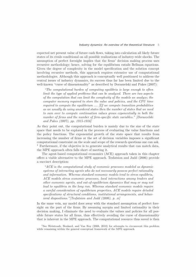
1.4 Design of computational experiments
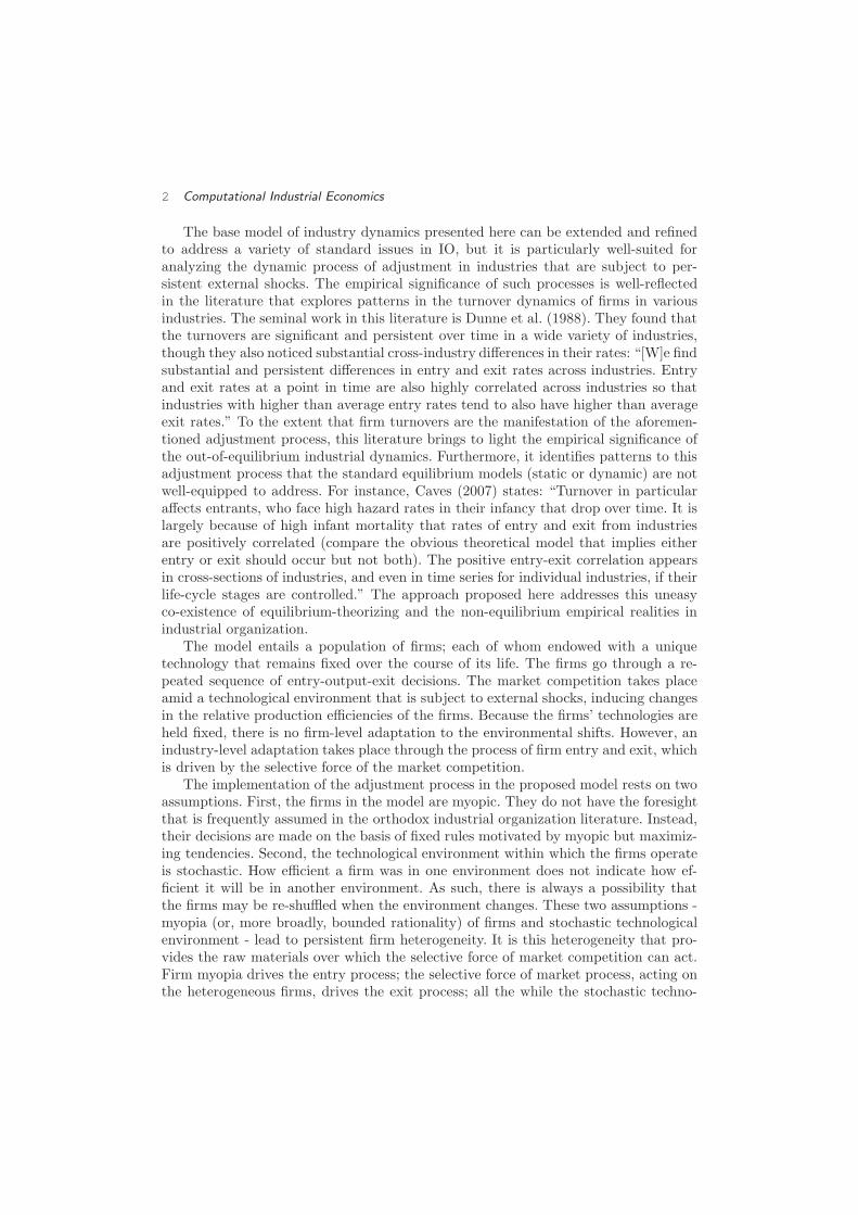
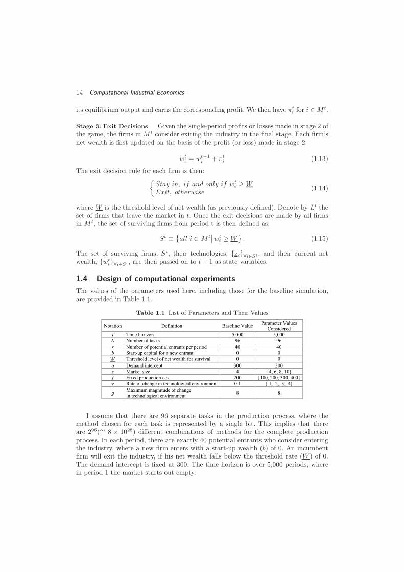
The values of the parameters used here, including those for the baseline simulation,are provided in Table 1.1.
Table 1.1 List of Parameters and Their Values
�
�
�
�
�
�
�
�
�
��������� ��������� ��� ����� ������������ ���
���������
�� ������������ ������ ������
�� �������������� ��� ���
�� ��������������� ������������������ �� ��
�� !����"���#����� �������$�������� �� ��
�� ������ �� % ������$� ���������%�%� � �� ��
�� ����������#��� &��� &���
�� '��������� � ( �����)��*�+�
�� ,�-�������#�����#���� .��� (*����.����&���� ��+�
�� /�����#���0�����#��� �0�#� ��%�������� �1*� (1*��1.��1&��1 +�
��'�-�������0��������#���0�
����#��� �0�#� ��%��������)� )�
�
�
�
� �
I assume that there are 96 separate tasks in the production process, where themethod chosen for each task is represented by a single bit. This implies that thereare 296(∼= 8 × 1028) different combinations of methods for the complete productionprocess. In each period, there are exactly 40 potential entrants who consider enteringthe industry, where a new firm enters with a start-up wealth (b) of 0. An incumbentfirm will exit the industry, if his net wealth falls below the threshold rate (W ) of 0.The demand intercept is fixed at 300. The time horizon is over 5,000 periods, wherein period 1 the market starts out empty.
Design of computational experiments 15
The focus of my analysis is on the impacts of the market size (s) and the fixed cost(f), as well as of the turbulence parameter, γ. I consider four different values for eachof these parameters: s ∈ {4, 6, 8, 10}, f ∈ {100, 200, 300, 400} and γ ∈ {.1, .2, .3, .4}.The maximum magnitude of change, g, is held fixed at 8. Note that a higher value ofγ reflects more frequent changes in the technological environment.
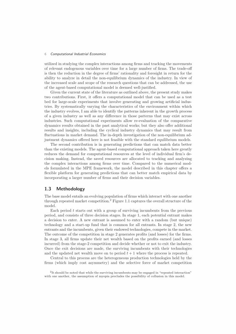
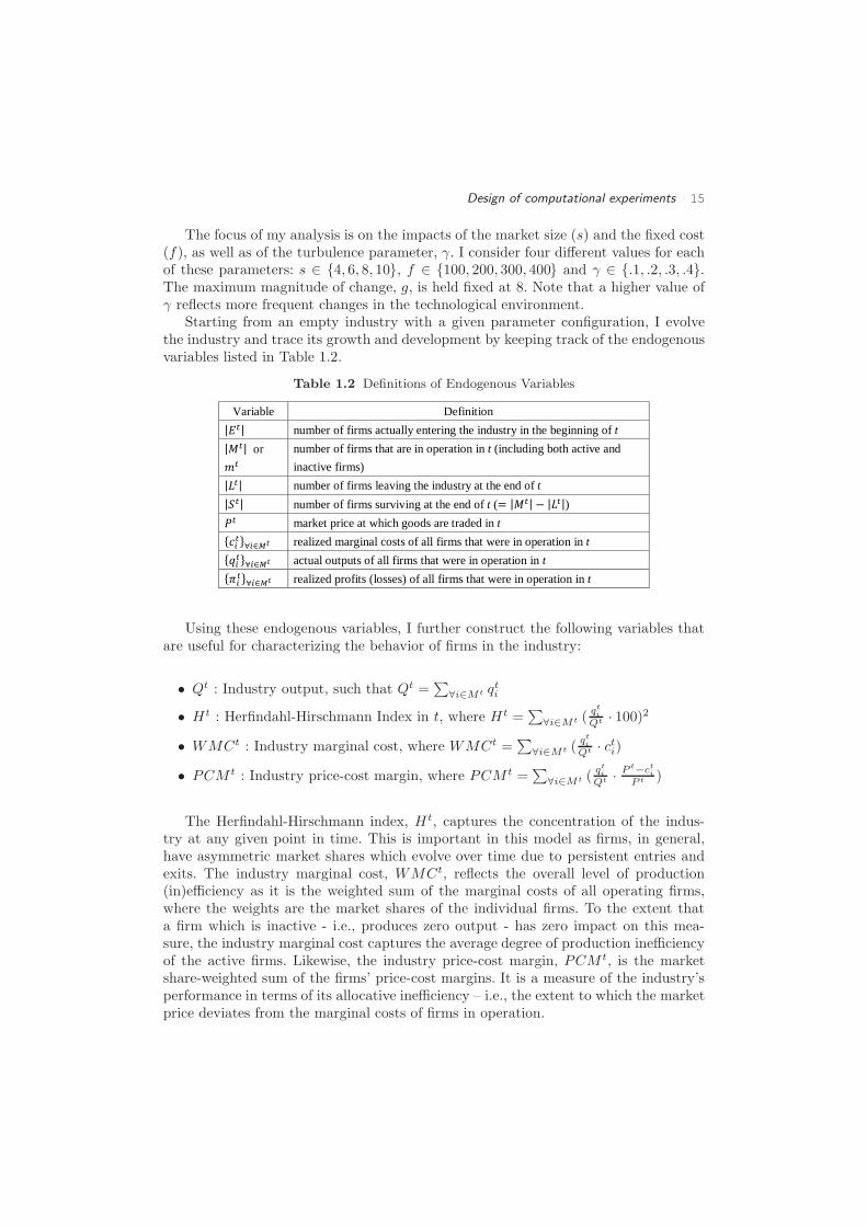
Starting from an empty industry with a given parameter configuration, I evolvethe industry and trace its growth and development by keeping track of the endogenousvariables listed in Table 1.2.
Table 1.2 Definitions of Endogenous Variables
Variable Definition
|��| number of firms actually entering the industry in the beginning of t
|��| or
��
number of firms that are in operation in t (including both active and
inactive firms)
|��| number of firms leaving the industry at the end of t
|��| number of firms surviving at the end of t (� |��| |��|)
� market price at which goods are traded in t
�� ��� ��� realized marginal costs of all firms that were in operation in t
�� ��� ��� actual outputs of all firms that were in operation in t
�� ��� ��� realized profits (losses) of all firms that were in operation in t
Using these endogenous variables, I further construct the following variables thatare useful for characterizing the behavior of firms in the industry:
• Qt : Industry output, such that Qt =∑
∀i∈Mt qti
• Ht : Herfindahl-Hirschmann Index in t, where Ht =∑
∀i∈Mt (qti
Qt · 100)2
• WMCt : Industry marginal cost, where WMCt =∑
∀i∈Mt (qti
Qt · cti)
• PCM t : Industry price-cost margin, where PCM t =∑
∀i∈Mt (qti
Qt ·P t−ct
i
P t )
The Herfindahl-Hirschmann index, Ht, captures the concentration of the indus-try at any given point in time. This is important in this model as firms, in general,have asymmetric market shares which evolve over time due to persistent entries andexits. The industry marginal cost, WMCt, reflects the overall level of production(in)efficiency as it is the weighted sum of the marginal costs of all operating firms,where the weights are the market shares of the individual firms. To the extent thata firm which is inactive - i.e., produces zero output - has zero impact on this mea-sure, the industry marginal cost captures the average degree of production inefficiencyof the active firms. Likewise, the industry price-cost margin, PCM t, is the marketshare-weighted sum of the firms’ price-cost margins. It is a measure of the industry’sperformance in terms of its allocative inefficiency – i.e., the extent to which the marketprice deviates from the marginal costs of firms in operation.
16 Computational Industrial Economics
1.5 Results I: The base model with stable market demand
1.5.1 Firm behavior over time: Technological change and recurrent
shakeouts
I start by examining the outcomes from a single run of the industry, given the baselineset of parameter values as indicated in Table 1.1. To see the underlying source ofthe industry dynamics, I first assume an industry which is perfectly protected fromexternal technological shocks – hence an industry with γ = 0 such that its technologicalenvironment never changes.
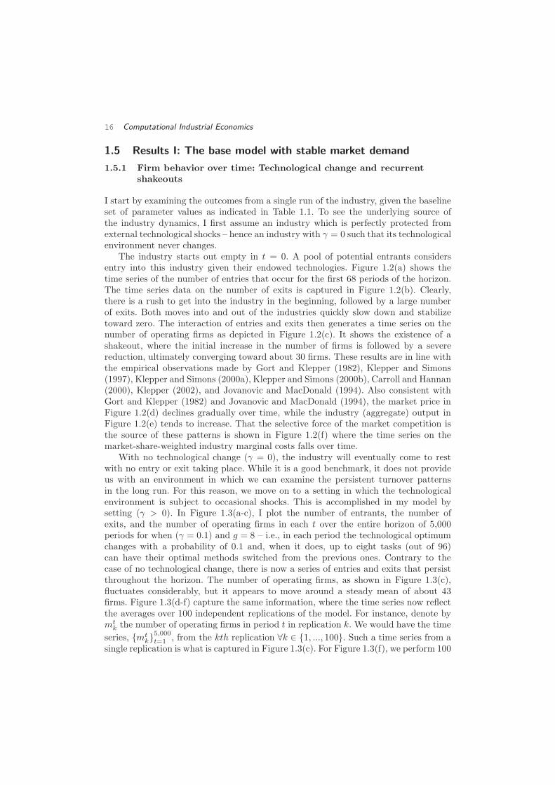
The industry starts out empty in t = 0. A pool of potential entrants considersentry into this industry given their endowed technologies. Figure 1.2(a) shows thetime series of the number of entries that occur for the first 68 periods of the horizon.The time series data on the number of exits is captured in Figure 1.2(b). Clearly,there is a rush to get into the industry in the beginning, followed by a large numberof exits. Both moves into and out of the industries quickly slow down and stabilizetoward zero. The interaction of entries and exits then generates a time series on thenumber of operating firms as depicted in Figure 1.2(c). It shows the existence of ashakeout, where the initial increase in the number of firms is followed by a severereduction, ultimately converging toward about 30 firms. These results are in line withthe empirical observations made by Gort and Klepper (1982), Klepper and Simons(1997), Klepper and Simons (2000a), Klepper and Simons (2000b), Carroll and Hannan(2000), Klepper (2002), and Jovanovic and MacDonald (1994). Also consistent withGort and Klepper (1982) and Jovanovic and MacDonald (1994), the market price inFigure 1.2(d) declines gradually over time, while the industry (aggregate) output inFigure 1.2(e) tends to increase. That the selective force of the market competition isthe source of these patterns is shown in Figure 1.2(f) where the time series on themarket-share-weighted industry marginal costs falls over time.
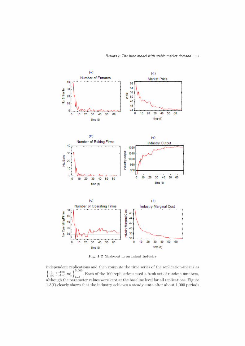
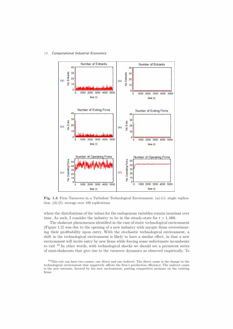
With no technological change (γ = 0), the industry will eventually come to restwith no entry or exit taking place. While it is a good benchmark, it does not provideus with an environment in which we can examine the persistent turnover patternsin the long run. For this reason, we move on to a setting in which the technologicalenvironment is subject to occasional shocks. This is accomplished in my model bysetting (γ > 0). In Figure 1.3(a-c), I plot the number of entrants, the number ofexits, and the number of operating firms in each t over the entire horizon of 5,000periods for when (γ = 0.1) and g = 8 – i.e., in each period the technological optimumchanges with a probability of 0.1 and, when it does, up to eight tasks (out of 96)can have their optimal methods switched from the previous ones. Contrary to thecase of no technological change, there is now a series of entries and exits that persistthroughout the horizon. The number of operating firms, as shown in Figure 1.3(c),fluctuates considerably, but it appears to move around a steady mean of about 43firms. Figure 1.3(d-f) capture the same information, where the time series now reflectthe averages over 100 independent replications of the model. For instance, denote bymt
k the number of operating firms in period t in replication k. We would have the time
series, {mtk}
5,000
t=1, from the kth replication ∀k ∈ {1, ..., 100}. Such a time series from a
single replication is what is captured in Figure 1.3(c). For Figure 1.3(f), we perform 100
Results I: The base model with stable market demand 17
Fig. 1.2 Shakeout in an Infant Industry
independent replications and then compute the time series of the replication-means as{
1
100
∑100
k=1mt
k
}5,000
t=1
. Each of the 100 replications used a fresh set of random numbers,
although the parameter values were kept at the baseline level for all replications. Figure1.3(f) clearly shows that the industry achieves a steady state after about 1,000 periods
18 Computational Industrial Economics
Fig. 1.3 Firm Turnovers in a Turbulent Technological Environment. (a)-(c): single replica-
tion. (d)-(f): average over 100 replications
where the distributions of the values for the endogenous variables remain invariant overtime. As such, I consider the industry to be in the steady-state for t > 1, 000.
The shakeout phenomenon identified in the case of static technological environment(Figure 1.2) was due to the opening of a new industry with myopic firms overestimat-ing their profitability upon entry. With the stochastic technological environment, ashift in the technological environment is likely to have a similar effect, in that a newenvironment will invite entry by new firms while forcing some unfortunate incumbentsto exit 10.In other words, with technological shocks we should see a persistent seriesof mini-shakeouts that give rise to the turnover dynamics as observed empirically. To
10This exit can have two causes, one direct and one indirect. The direct cause is the change in thetechnological environment that negatively affects the firm’s production efficiency. The indirect causeis the new entrants, favored by the new environment, putting competitive pressure on the existingfirms.
Results I: The base model with stable market demand 19
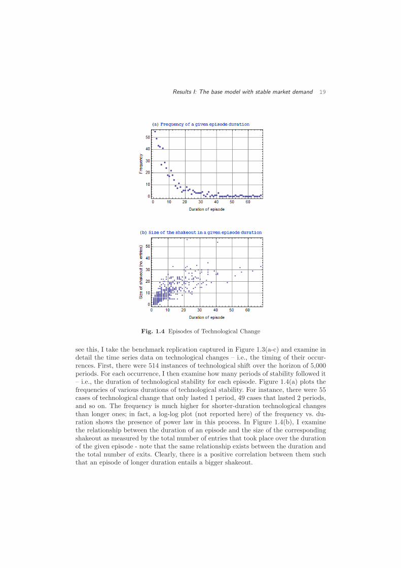
Fig. 1.4 Episodes of Technological Change
see this, I take the benchmark replication captured in Figure 1.3(a-c) and examine indetail the time series data on technological changes – i.e., the timing of their occur-rences. First, there were 514 instances of technological shift over the horizon of 5,000periods. For each occurrence, I then examine how many periods of stability followed it– i.e., the duration of technological stability for each episode. Figure 1.4(a) plots thefrequencies of various durations of technological stability. For instance, there were 55cases of technological change that only lasted 1 period, 49 cases that lasted 2 periods,and so on. The frequency is much higher for shorter-duration technological changesthan longer ones; in fact, a log-log plot (not reported here) of the frequency vs. du-ration shows the presence of power law in this process. In Figure 1.4(b), I examinethe relationship between the duration of an episode and the size of the correspondingshakeout as measured by the total number of entries that took place over the durationof the given episode - note that the same relationship exists between the duration andthe total number of exits. Clearly, there is a positive correlation between them suchthat an episode of longer duration entails a bigger shakeout.

20 Computational Industrial Economics
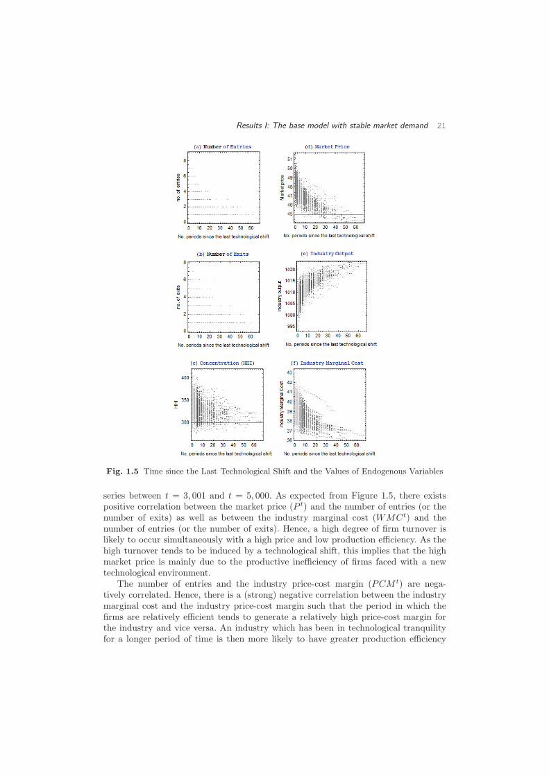
For each period t on the horizon, I also ask how long it has been since the lasttechnological shift. This will tell us whereabouts the firms are in a given (mini-) shake-out. In Figure 1.5(a, b), I plot for each period the numbers of entries and exits againstthe number of periods the industry has been in the current technological environment.Interestingly, in those time periods for which the technological environment has beenstable for a longer duration, the number of entries as well as the number of exitstends to be lower on average. These results suggest that those periods immediatelyfollowing a technological change should have high occurrences of entries and exits;such turnovers should diminish over time as industry stabilizes around the new tech-nological environment until the next technological shift. The co-movement of entryand exit then implies a positive correlation between entry and exit over time for anygiven industry.
Property 1: In any given industry, a period with a larger (smaller) number of entriesis also likely to have a larger (smaller) number of exits.
Figure 1.5(c) shows that the industry tends to be more concentrated immediatelyfollowing the technological change; as the industry gradually adjusts to the new en-vironment, concentration tends to fall. Figure 1.5(d) shows that the market pricegenerally is higher in the early periods following the technological shift and it tends todecline as the industry stabilizes. The industry output, of course, moves in the oppo-site direction from the price. Both of these observations are consistent with what wasobserved in a single shakeout case of the benchmark industry having no technologicalchange – Figure 1.2(d, e). It is also worthwhile to point out that the decline in themarket price shown in Figure 1.5(d) is largely due to the selection effect of the marketcompetition which tends to put a downward pressure on the industry marginal cost.This is shown in Figure 1.5(f). As a given technological environment persists, ineffi-cient firms are gradually driven out by the new entrants having technologies that arebetter suited for the environment.
Table 1.3 Correlations (The Case of Stable Demand)
|��| |��| �� �� ���� ���
|��| 1 .377893 .229091 -.146535 -.253699 .313877
|��| 1 .178438 -.123290 -.207645 .249140
�� 1 .324510 -.094246 .872944
�� 1 .909583 -.174888
���� 1 -.565350
��� 1
The observations made in Figure 1.5 imply that we are likely to observe certainrelationships between these endogenous variables. Table 1.3 reports these correlationsas the average over 100 replications - the correlations are for the steady-state time
Results I: The base model with stable market demand 21
Fig. 1.5 Time since the Last Technological Shift and the Values of Endogenous Variables
series between t = 3, 001 and t = 5, 000. As expected from Figure 1.5, there existspositive correlation between the market price (P t) and the number of entries (or thenumber of exits) as well as between the industry marginal cost (WMCt) and thenumber of entries (or the number of exits). Hence, a high degree of firm turnover islikely to occur simultaneously with a high price and low production efficiency. As thehigh turnover tends to be induced by a technological shift, this implies that the highmarket price is mainly due to the productive inefficiency of firms faced with a newtechnological environment.
The number of entries and the industry price-cost margin (PCM t) are nega-tively correlated. Hence, there is a (strong) negative correlation between the industrymarginal cost and the industry price-cost margin such that the period in which thefirms are relatively efficient tends to generate a relatively high price-cost margin forthe industry and vice versa. An industry which has been in technological tranquilityfor a longer period of time is then more likely to have greater production efficiency
22 Computational Industrial Economics
and a higher price-cost margin.While the industry concentration (Ht) is negatively correlated with the number
of entries, it is positively correlated with the market price and the industry price-costmargin: The period of high concentration is likely to show high market price andhigh price-cost margins. These correlations were for the baseline parameter values,but when they are computed for all s ∈ {4, 6, 8, 10} and f ∈ {100, 200, 300, 400}, theresults (not reported here) confirm that these relationships are robust to varying thevalues of the two parameters.
1.5.2 Comparative dynamics analysis: Implications for cross-sectional
studies
There are two parameters, s and f , that affect the demand and cost conditions of thefirms in the industry and two parameters, γ and g, that affect the volatility of thetechnological environment surrounding the firms. The main objective in this section isto examine how these parameters - mainly s and f – affect the long-run development ofan industry. The approach is to run 500 independent replications for each parameterconfiguration that represents a particular industry. For each replication, I computethe steady-state values (average values over the periods from 3, 001 to 5, 000) of theendogenous variables and then average them over the 500 replications.11 The resultingmean steady-state values for the relevant endogenous variables are denoted as follows:H , P , WMC and PCM . For instance, H is computed as:
H =
(
1
500
)
∑500
k=1
(
1
2, 000
)
∑5,000
t=3,001Ht
k (1.16)
where Htk is the HHI in period t from replication k.
Note that the steady-state number of operating firms is likely to vary as a functionof the two parameters, s and f . While the absolute numbers of entries and exitsare sufficient for capturing the degree of firm turnovers for a given industry, it isnot adequate when we carry out comparative dynamics analysis with implications forcross-industry differences in firm behavior. In this section, I then use the rates of entryand exit to represent the degree of turnovers:
• ERt : Rate of entry in t, where ERt =|Et||Mt|
• XRt : Rate of exit in t, where XRt =|Lt||Mt|
These time series are again averaged over the 500 independent replications and theresulting mean steady-state values are denoted as ER and XR.
We start the analysis by first looking at the above endogenous variables for variouscombinations of the demand and cost parameters, s and f , given γ = 0.1 and g = 8. Iplot in Figure 1.6 the steady-state values of (a) the rate of entry, (b) the rate of exit, and(c) the number of operating firms for all s ∈ {4, 6, 8, 10} and f ∈ {100, 200, 300, 400}.
11The number of replications is raised from 100 to 500 for the analysis of steady states in thissection. This is to reduce the variance in the distribution of the steady state values (of endogenousvariables) as much as possible.

Results I: The base model with stable market demand 23
Fig. 1.6 Firm Turnovers in Steady State
They show that both ER and XR decline with the size of the market, s, but increasewith the fixed cost, f . Since the two rates move in the same direction in response tothe changes in the two parameters, I will say that the rate of firm turnover increasesor decreases as either of these rates goes up or down, respectively.
Closely related to the rates of entry and exit is the age distribution of the dyingfirms. In order to investigate the relationship between the rate of turnovers and theseverity of infant mortality, I collected the age (at the time of exit) of every firm thatexited the industry between t = 3, 001 and t = 5, 000. The proportion of those firmsthat exited at a given age or younger (out of all exiting firms) was then computed and
24 Computational Industrial Economics
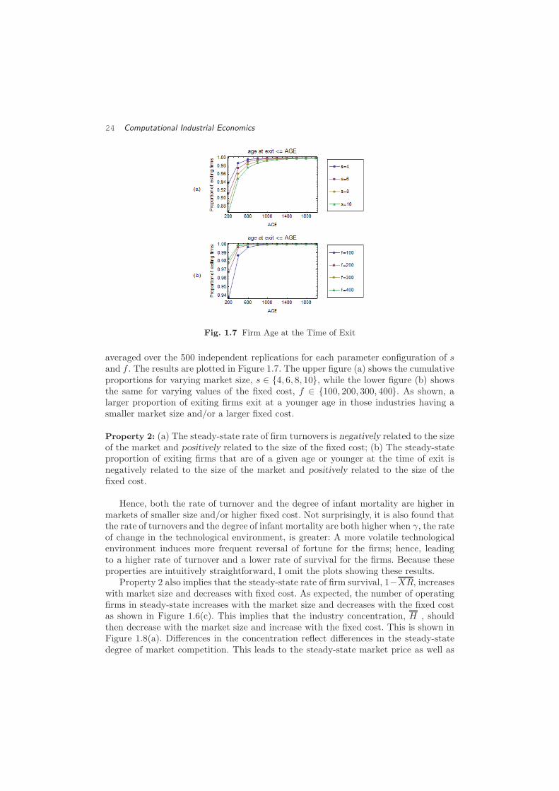
Fig. 1.7 Firm Age at the Time of Exit
averaged over the 500 independent replications for each parameter configuration of sand f . The results are plotted in Figure 1.7. The upper figure (a) shows the cumulativeproportions for varying market size, s ∈ {4, 6, 8, 10}, while the lower figure (b) showsthe same for varying values of the fixed cost, f ∈ {100, 200, 300, 400}. As shown, alarger proportion of exiting firms exit at a younger age in those industries having asmaller market size and/or a larger fixed cost.
Property 2: (a) The steady-state rate of firm turnovers is negatively related to the sizeof the market and positively related to the size of the fixed cost; (b) The steady-stateproportion of exiting firms that are of a given age or younger at the time of exit isnegatively related to the size of the market and positively related to the size of thefixed cost.
Hence, both the rate of turnover and the degree of infant mortality are higher inmarkets of smaller size and/or higher fixed cost. Not surprisingly, it is also found thatthe rate of turnovers and the degree of infant mortality are both higher when γ, the rateof change in the technological environment, is greater: A more volatile technologicalenvironment induces more frequent reversal of fortune for the firms; hence, leadingto a higher rate of turnover and a lower rate of survival for the firms. Because theseproperties are intuitively straightforward, I omit the plots showing these results.
Property 2 also implies that the steady-state rate of firm survival, 1−XR, increaseswith market size and decreases with fixed cost. As expected, the number of operatingfirms in steady-state increases with the market size and decreases with the fixed costas shown in Figure 1.6(c). This implies that the industry concentration, H , shouldthen decrease with the market size and increase with the fixed cost. This is shown inFigure 1.8(a). Differences in the concentration reflect differences in the steady-statedegree of market competition. This leads to the steady-state market price as well as
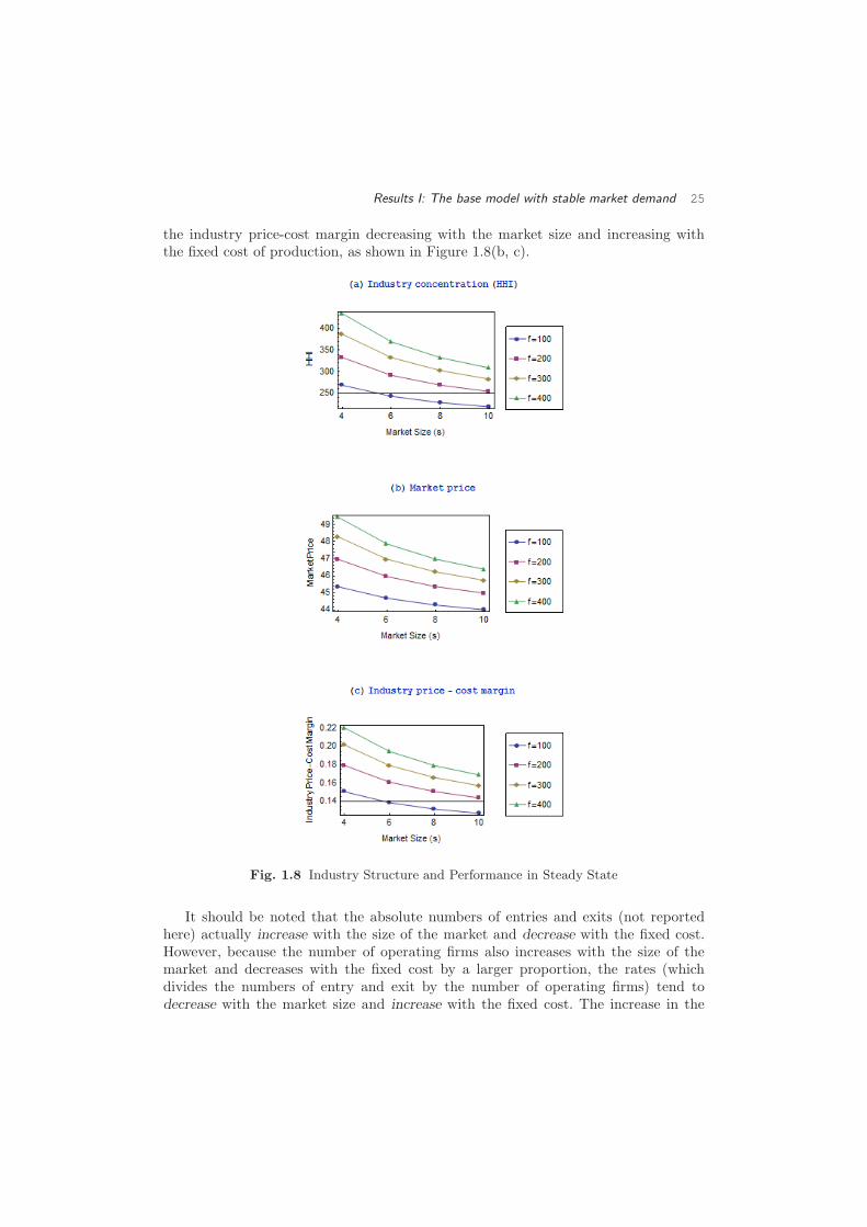
Results I: The base model with stable market demand 25
the industry price-cost margin decreasing with the market size and increasing withthe fixed cost of production, as shown in Figure 1.8(b, c).
Fig. 1.8 Industry Structure and Performance in Steady State
It should be noted that the absolute numbers of entries and exits (not reportedhere) actually increase with the size of the market and decrease with the fixed cost.However, because the number of operating firms also increases with the size of themarket and decreases with the fixed cost by a larger proportion, the rates (whichdivides the numbers of entry and exit by the number of operating firms) tend todecrease with the market size and increase with the fixed cost. The increase in the
26 Computational Industrial Economics
number of operating firms that comes with larger market size and lower fixed cost thenintensifies market competition, putting a downward pressure on the market price aswell as the price-cost margin: Hence, the price competition effect assumed in Asplundand Nocke (2006) is endogenously generated in my model.
Note that the effect the market size has on the market price or the price-cost marginis due to the relative strength of the two countervailing forces: 1) the direct positiveimpact on the profits through larger demand; 2) the indirect negative impact throughthe price competition effect. The negative relationship between the market size andthe price (or the price-cost margin) then implies the price competition effect dominatesthe demand effect; a feature absent in the competitive market model of Hopenhayn(1992) but assumed as part of the imperfect competition model in Asplund and Nocke(2006).
While the impact of fixed cost on the turnover rate is the same in both Asplund andNocke (2006) model and this model, the impact of the market size on the turnover rateis not: Asplund and Nocke (2006) predict the impact to be positive while my modelpredicts it to be negative. It is difficult to pinpoint the exact source of the discrepancy,since the two models are substantially different – in terms of both how demand andtechnology are specified and how the degree of firms’ foresight is modeled (i.e., perfectforesight vs. myopia). What is clear, however, is the chain of endogenous relationshipsthat are affected by the way the demand function is specified. To be specific, notethat the entry decisions (and consequently the rate of turnovers) are based on thepost-entry expected profits that are computed as a present value of discounted profitsunder perfect foresight and as a single-period profit under myopia. In both cases, amain determinant of the post-entry profit is the price and price-cost margin, the levelsof which depend on the magnitude of the price competition effect identified above.As the magnitude of the price competition effect is likely to be influenced by theshape of the demand curve (price elasticity of demand, to be specific), the relationshipbetween the market size and the rate of turnovers may be conditional on the precisespecification of the demand function. While this is an important issue that deservesa thorough investigation, it is beyond the scope of the present study and is left forfuture research.
An important property that emerges from this comparative dynamics analysis isthe relationship between the endogenous variables such as the rate of firm turnover,industry concentration, market price, and the industry price-cost margins. As can beinferred from Figure 1.6 and Figure 1.8, all these variables tend to decrease with themarket size and increase with the fixed cost. The following property emerges fromthese relationships.
Property 3: An industry with a high turnover rate is likely to be concentrated, havehigh market price and high price-cost margins.
Hence, if one carries out a cross-sectional study of these endogenous variablesacross industries having different market sizes and fixed costs, such a study is likely toidentify positive relationships between these variables – i.e., the market price, as wellas the industry price-cost margin, is likely to be higher in more concentrated industries

Results II: The base model with fluctuating market demand 27
(those industries with a smaller market size or a larger fixed cost). Finally, I find thatthe properties identified in Figure 1.6 through 1.8 are robust to all γ ∈ {.1, .2, .3, .4}.
1.6 Results II: The base model with fluctuating market demand
How do cyclical variations in market demand affect the evolving structure and per-formance of an industry? Is the market selection of firms more effective (and, hence,firms are more efficient on average) when there are fluctuations in demand? What arethe relationships between the movement of demand and those of endogenous variablessuch as industry concentration, price, aggregate efficiency, and price-cost margins? Arethey pro-cyclical or counter-cyclical? The proposed model of industry dynamics canaddress these issues by computationally generating the time series of these variablesin the presence of demand fluctuation.
These issues have been explored in the past by researchers from two distinct fieldsof economics – macroeconomics and industrial organization. A number of stylizedfacts has been established by the two strands of empirical research. For instance, manypapers find procyclical variations in the number of competitors. Chatterjee et al. (1993)find that both net business formation and new business incorporations are stronglyprocyclical. Devereux et al. (1996) confirms this finding and further reports that theaggregate number of business failure is countercyclical. Many papers find that markupsare countercyclical and negatively correlated with the number of competitors [Bils(1987), Cooley and Ohanian (1991), Rotemberg and Woodford (1990), Rotembergand Woodford (1999), Chevalier and Scharfstein (1995), Warner and Barsky (1995),MacDonald (2000), Chevalier et al. (2003), Wilson and Reynolds (2005)].12 Martinset al. (1996) covers different industries in 14 OECD countries and find markups to becountercyclical in 53 of the 56 cases they consider, with statistically significant resultsin most of these. In addition, these authors conclude that entry rates have a negativeand statistically significant correlation with markups. Bresnahan and Reiss (1991)find that an increase in the number of producers increases the competitiveness in themarkets they analyze. Campbell and Hopenhayn (2005) provide empirical evidenceto support the argument that firms’ pricing decisions are affected by the numberof competitors they face; they show that markups react negatively to increases inthe number of firms. Rotemberg and Saloner (1986) provide empirical evidence ofcountercyclical price movements and offer a model of collusive pricing when demandis subject to i.i.d. shocks. Their model generates countercyclical collusion and predictscountercyclical pricing13.
The model presented here has the capacity to replicate many of the empiricalregularities mentioned above and explain them in terms of the selective forces of marketcompetition in the presence of firm entry and exit. In particular, it can incorporatedemand fluctuation by allowing the market size, s, to shift from one period to the next
12A deviation from this set of papers is Domowitz et al. (1986) who suggested that markupsare procyclical. Rotemberg and Woodford (1999) highlight some biases in these results, as they usemeasures of average variable costs and not marginal costs.
13See Haltiwanger and Harrington Jr. (1991) and Kandori (1991) for further support. In contrast,Green and Porter (1984) develops a model of trigger pricing which predicts positive co-movements ofprices and demand.
28 Computational Industrial Economics
in a systematic fashion. As a starting point, the market size parameter can be shiftedaccording to a deterministic cycle such as a sine wave. Section 1.6.1 investigates themovement of the endogenous variables with this demand dynamic. In Section 1.6.2, Iallow the market size to be randomly drawn from a fixed range according to uniformdistribution. By examining the correlations between the time series of the market sizeand that of various endogenous variables I study the impact that demand fluctuationhas on the evolving structure and performance of the industry.
1.6.1 Cyclical demand
I run 100 independent replications of the base model with the baseline parameterconfiguration. The only change is in the specification of the market size, s. It is assumedto stay fixed at the baseline value of 4 for the first 2,000 periods and then follow adeterministic cycle as specified by the following rule:
st = s+ sa · sin[π
τ· t]
(1.17)
for all t≥ 2, 001, where s is the mean market size (set at 4), sa is the amplitudeof the wave (set at 2), and τ (set at 500) is the period for half-turn (hence, one fullperiod is 2τ).
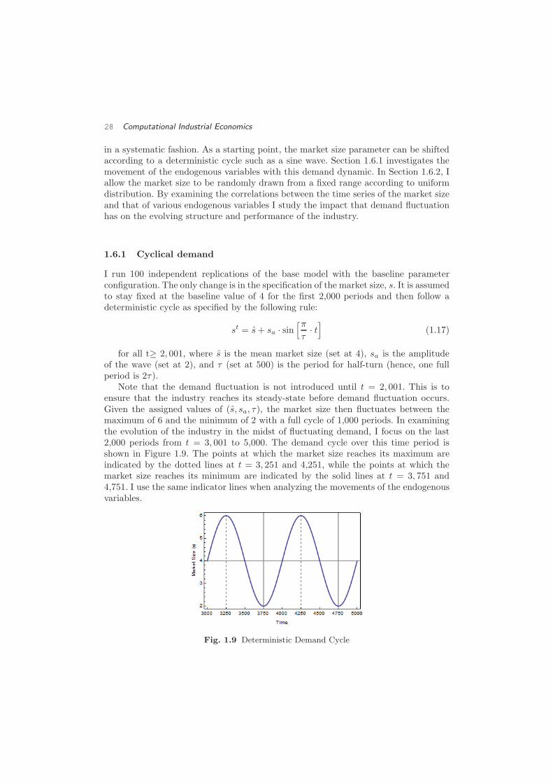
Note that the demand fluctuation is not introduced until t = 2, 001. This is toensure that the industry reaches its steady-state before demand fluctuation occurs.Given the assigned values of (s, sa, τ), the market size then fluctuates between themaximum of 6 and the minimum of 2 with a full cycle of 1,000 periods. In examiningthe evolution of the industry in the midst of fluctuating demand, I focus on the last2,000 periods from t = 3, 001 to 5,000. The demand cycle over this time period isshown in Figure 1.9. The points at which the market size reaches its maximum areindicated by the dotted lines at t = 3, 251 and 4,251, while the points at which themarket size reaches its minimum are indicated by the solid lines at t = 3, 751 and4,751. I use the same indicator lines when analyzing the movements of the endogenousvariables.
Fig. 1.9 Deterministic Demand Cycle
Results II: The base model with fluctuating market demand 29
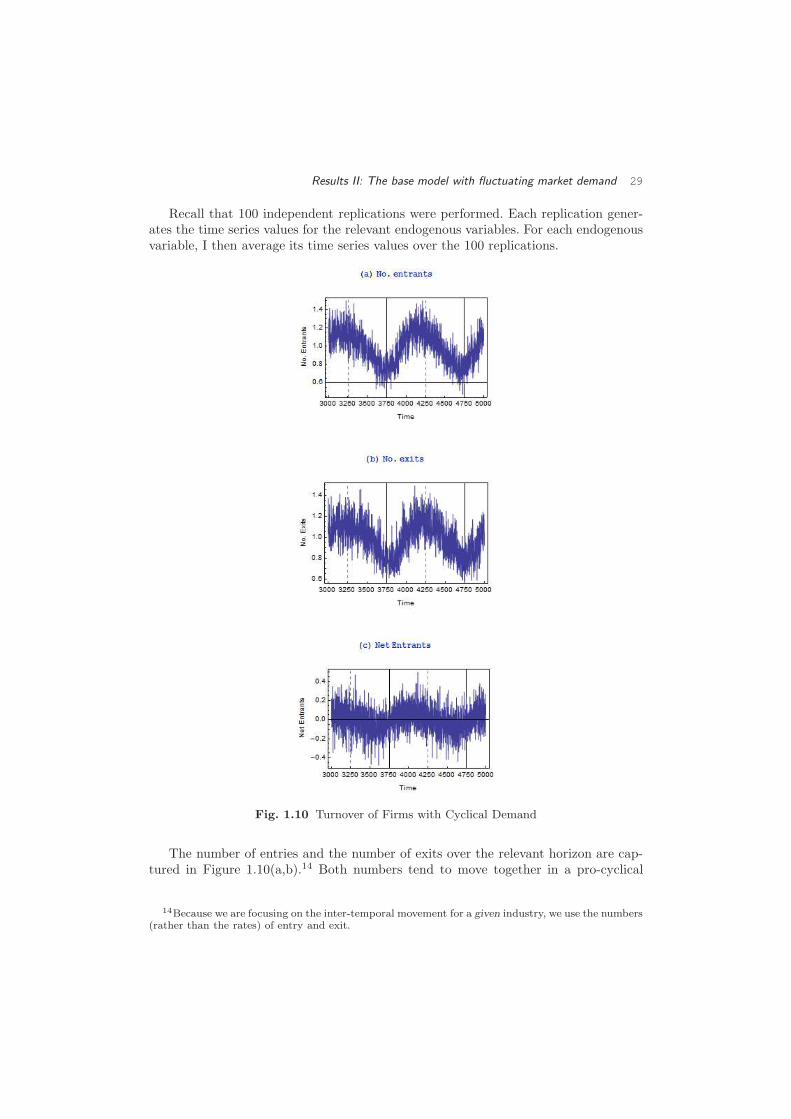
Recall that 100 independent replications were performed. Each replication gener-ates the time series values for the relevant endogenous variables. For each endogenousvariable, I then average its time series values over the 100 replications.
Fig. 1.10 Turnover of Firms with Cyclical Demand
The number of entries and the number of exits over the relevant horizon are cap-tured in Figure 1.10(a,b).14 Both numbers tend to move together in a pro-cyclical
14Because we are focusing on the inter-temporal movement for a given industry, we use the numbers(rather than the rates) of entry and exit.
30 Computational Industrial Economics
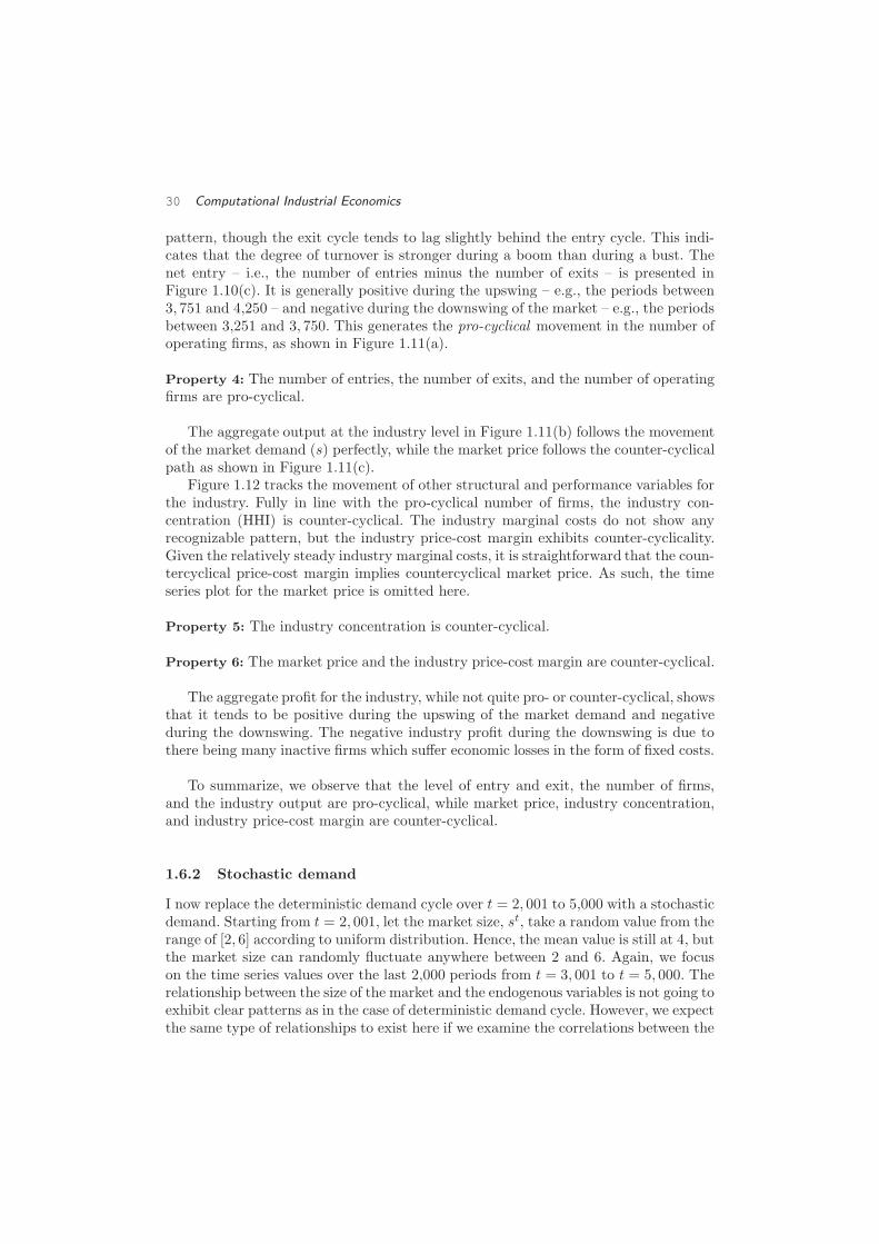
pattern, though the exit cycle tends to lag slightly behind the entry cycle. This indi-cates that the degree of turnover is stronger during a boom than during a bust. Thenet entry – i.e., the number of entries minus the number of exits – is presented inFigure 1.10(c). It is generally positive during the upswing – e.g., the periods between3, 751 and 4,250 – and negative during the downswing of the market – e.g., the periodsbetween 3,251 and 3, 750. This generates the pro-cyclical movement in the number ofoperating firms, as shown in Figure 1.11(a).
Property 4: The number of entries, the number of exits, and the number of operatingfirms are pro-cyclical.
The aggregate output at the industry level in Figure 1.11(b) follows the movementof the market demand (s) perfectly, while the market price follows the counter-cyclicalpath as shown in Figure 1.11(c).
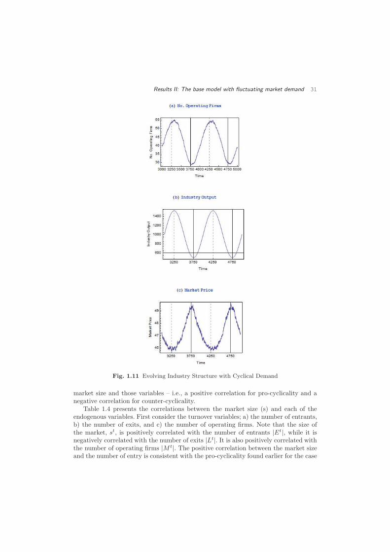
Figure 1.12 tracks the movement of other structural and performance variables forthe industry. Fully in line with the pro-cyclical number of firms, the industry con-centration (HHI) is counter-cyclical. The industry marginal costs do not show anyrecognizable pattern, but the industry price-cost margin exhibits counter-cyclicality.Given the relatively steady industry marginal costs, it is straightforward that the coun-tercyclical price-cost margin implies countercyclical market price. As such, the timeseries plot for the market price is omitted here.
Property 5: The industry concentration is counter-cyclical.
Property 6: The market price and the industry price-cost margin are counter-cyclical.
The aggregate profit for the industry, while not quite pro- or counter-cyclical, showsthat it tends to be positive during the upswing of the market demand and negativeduring the downswing. The negative industry profit during the downswing is due tothere being many inactive firms which suffer economic losses in the form of fixed costs.
To summarize, we observe that the level of entry and exit, the number of firms,and the industry output are pro-cyclical, while market price, industry concentration,and industry price-cost margin are counter-cyclical.
1.6.2 Stochastic demand
I now replace the deterministic demand cycle over t = 2, 001 to 5,000 with a stochasticdemand. Starting from t = 2, 001, let the market size, st, take a random value from therange of [2, 6] according to uniform distribution. Hence, the mean value is still at 4, butthe market size can randomly fluctuate anywhere between 2 and 6. Again, we focuson the time series values over the last 2,000 periods from t = 3, 001 to t = 5, 000. Therelationship between the size of the market and the endogenous variables is not going toexhibit clear patterns as in the case of deterministic demand cycle. However, we expectthe same type of relationships to exist here if we examine the correlations between the
Results II: The base model with fluctuating market demand 31
Fig. 1.11 Evolving Industry Structure with Cyclical Demand
market size and those variables – i.e., a positive correlation for pro-cyclicality and anegative correlation for counter-cyclicality.
Table 1.4 presents the correlations between the market size (s) and each of theendogenous variables. First consider the turnover variables; a) the number of entrants,b) the number of exits, and c) the number of operating firms. Note that the size ofthe market, st, is positively correlated with the number of entrants |Et|, while it isnegatively correlated with the number of exits |Lt|. It is also positively correlated withthe number of operating firms |M t|. The positive correlation between the market sizeand the number of entry is consistent with the pro-cyclicality found earlier for the case
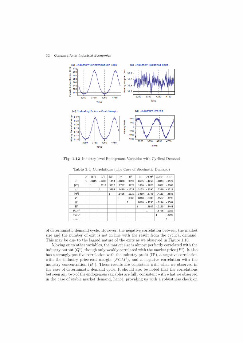
32 Computational Industrial Economics
Fig. 1.12 Industry-level Endogenous Variables with Cyclical Demand
Table 1.4 Correlations (The Case of Stochastic Demand)
�� |��| |��| |��| �� �� � ��� ��� �� �
�� 1 .3815 -.1706 .1153 -.0838 .9999 .8695 -.1250 -.0043 -.1522
|��| 1 .2513 .3372 .1757 .3779 .1866 -.2825 .2892 -.2003
|��| 1 .3398 .1410 -.1727 -.3173 -.2390 .2380 -.1718
|��| 1 .1426 .1129 -.3469 -.5743 .4113 -.4886
�� 1 -.0988 -.0848 -.0788 .8587 .3190
�� 1 .8696 -.1235 -.0174 -.1567
Π� 1 .2927 -.2193 .2441
��� 1 -.5766 .9185
��� 1 -.2093
�� � 1
of deterministic demand cycle. However, the negative correlation between the marketsize and the number of exit is not in line with the result from the cyclical demand.This may be due to the lagged nature of the exits as we observed in Figure 1.10.
Moving on to other variables, the market size is almost perfectly correlated with theindustry output (Qt), though only weakly correlated with the market price (P t). It alsohas a strongly positive correlation with the industry profit (Πt), a negative correlationwith the industry price-cost margin (PCM t), and a negative correlation with theindustry concentration (Ht). These results are consistent with what we observed inthe case of deterministic demand cycle. It should also be noted that the correlationsbetween any two of the endogenous variables are fully consistent with what we observedin the case of stable market demand, hence, providing us with a robustness check on
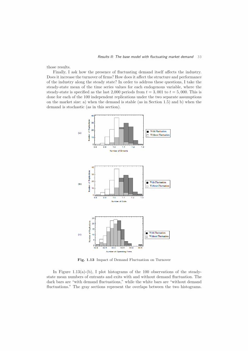
Results II: The base model with fluctuating market demand 33
those results.Finally, I ask how the presence of fluctuating demand itself affects the industry.
Does it increase the turnover of firms? How does it affect the structure and performanceof the industry along the steady state? In order to address these questions, I take thesteady-state mean of the time series values for each endogenous variable, where thesteady-state is specified as the last 2,000 periods from t = 3, 001 to t = 5, 000. This isdone for each of the 100 independent replications under the two separate assumptionson the market size: a) when the demand is stable (as in Section 1.5) and b) when thedemand is stochastic (as in this section).
Fig. 1.13 Impact of Demand Fluctuation on Turnover
In Figure 1.13(a)-(b), I plot histograms of the 100 observations of the steady-state mean numbers of entrants and exits with and without demand fluctuation. Thedark bars are “with demand fluctuations,” while the white bars are “without demandfluctuations.” The gray sections represent the overlaps between the two histograms.

34 Computational Industrial Economics
The plots show that the numbers of entrants and exits both tend to be higher withfluctuation than without. Hence, the fluctuation in market demand tends to raise the
degree of firm turnovers. Figure 1.13(c) shows that the number of operating firmsis generally higher with fluctuation; this is likely to be due to the higher number ofinactive firms that results from the greater turbulence in the market.
Fig. 1.14 Impact of Demand Fluctuation on Industry Structure and Performance
In Figure 1.14, I plot similar information on other structural and performancevariables. Both market price and industry price-cost margin tend to be higher withdemand fluctuation. The industry marginal cost is also likely to be higher with fluctu-ation, thereby implying a loss of efficiency that results from the fluctuation in marketdemand. Finally, the industry is more concentrated with demand fluctuation. It is in-teresting that the presence of demand fluctuation raises both the number of operatingfirms and the industry concentration. This seeming contradiction is due to the factthat the set of operating firms includes both active and inactive firms. The presenceof fluctuating demand, while increasing the number of inactive firms (and the numberof operating firms), actually reduces the number of active firms. Since the industryconcentration takes into consideration the market shares of the active firms only, it islikely to increase as demand fluctuation is introduced into the market.

Potential extension: Endogenizing R&D 35
1.7 Potential extension: Endogenizing R&D
Variants of the base model, as described here, have been used in two earlier publica-tions, Chang (2009, 2011). In both papers, an extra stage of decision making on R&Dwas added into the base model. Specifically, the R&D stage was inserted in betweenstage 1 (entry) and stage 2 (competition). Figure 1.15 shows the overall structure.
Fig. 1.15 Base Model of Industry Dynamics with R&D
In both Chang (2009) and Chang (2011), the R&D activity was assumed to beexogenous and costless. 15 More specifically, R&D was viewed as serendipitous discov-ery, in which the methods used in one or more of the tasks were randomly altered forexperimentation. Chang (2009) assumed a stable technological environment in whichthe optimal technology did not change from one period to next – i.e., γ = 0. Instead,the technology itself was assumed to be complex in nature such that there were mul-tiple optima that a firm could converge on. The main focus was on the determinants
15It should be noted that many of the results obtained in the base model with the stable demandalso hold with these extensions. That they hold in the base model without the R&D activities impliesthat it is the market selection mechanism, and not the firm-level adaptation, that is central to theemergent patterns in the non-equilibrium industry dynamics.
36 Computational Industrial Economics
of the shakeout phase of an industry’s life cycle. Chang (2011) allowed turbulence intechnological environment as in this paper – i.e., γ > 0. The focus was on the steadystate in which continual series of entries and exits were observed.
A more satisfying approach is to endogenize the process of R&D into the base modelof industry dynamics. Let me sketch here one possible way to pursue this extension.[A preliminary attempt in this direction is currently in progress.] Suppose we assumethat the R&D-related decisions of a firm are driven by a pair of choice probabilities,αti and βt
i , that evolve over time on the basis of reinforcement learning mechanism.Specifically, a firm i chooses to pursue R&D in period t with probability αt
i. If itchooses not to pursue R&D (which happens with probability 1 − αt
i), its technologystays the same as the previous period’s. If a firm decides to pursue R&D, it can do sothrough either innovation or imitation. Between these two modes of R&D, the firmchooses innovation mode with probability βt
i and imitation mode with 1−βti . The firm
incurs the R&D expenditure, the size of which depends on which of the two modes itchooses. The R&D intensity and the innovation-to-imitation intensity at the firm-levelcan be inferred from the time paths of these two probabilities. Similar intensities atthe industry-level can be inferred from the aggregate expenditure for the overall R&Das well as that for innovation or imitation.
Modeling R&D as endogenous search within the finite technology space allows forprecise representation of the knowledge acquisition process that the firms go through;it also captures the possibility of two different firms pursuing two distinct paths oftechnological development that may prove equally adaptive over time. Jovanovic andRob (1990) also viewed innovation as search within a well-defined technology space.In their model, a firm could engage in two types of search: an intensive search and anextensive search. An intensive search focuses on searching within a given type, while anextensive search encompasses searching across different technology types. Given thatthe number of tasks in my model is known and held fixed, R&D in this setting onlyinvolves intensive search – i.e., searching among multiple methods for each well-definedtask.
Incorporating R&D into the base model opens up a large number of issues. First,it allows us to examine the two Schumpeterian hypotheses: 1) innovation activity ismore intense in larger rather than small firms and, hence,firm size matters ;2)inno-vation activity is more intense in concentrated rather than unconcentrated industriesand, hence, industry structure matters. Given the process of creative destruction asenvisioned by Schumpeter, both firm size and industry structure coevolve with R&Dactivities of the firms over the course of the industrial development. The model pre-sented here can explore such evolving relationships in sufficient detail so that the twohypotheses can be tested in a fully dynamic framework.
Another issue of interest is to relate the empirical regularities on firm turnovers tothe endogenous R&D intensities. The point is that the persistence of entry and exit byfirms, as noted in this chapter with the base model, indicates the underlying instabilityin the cost-positions of the firms. Such instability may be due to the R&D activitiesof the firms as well as their changing fortunes in the competitive and turbulent envi-ronment. What are the theoretical connections between the degree of turnovers, theintensities of R&D activities, and the degree of technological turbulence (as captured
Concluding remarks 37
by γ or g) in industries that are differentiated in terms their structural characteristics(e.g., s and f)? For instance, Geroski (1995) states: “High rates of entry are oftenassociated with high rates of innovation and increases in efficiency. ... Numerous casestudies have suggested that entry is often used as a vehicle for introducing new innova-tions (frequently because incumbents are more interested in protecting existing rentsthan in seeking out new profit opportunities), and many show that entry often en-courages incumbents to drastically cut slack from their operations.” Lying underneathsuch a relationship is the unpredictable external shocks to the technological environ-ment surrounding the firm. The base model with endogenous R&D should enable us toperform a detailed analysis of how γ and g affect the endogenous relationship betweenthe turnover rate and the level of aggregate R&D.
1.8 Concluding remarks
I proposed a computational model of industry dynamics, in which a population offirms could interact with one another through the process of market competition. Theentry and exit of firms are generated endogenously in this model, thereby giving us anopportunity to study the historical patterns in the turnover dynamics for industrieshaving different demand and technological conditions. The generative approach takenhere allows a detailed study of the historical path an industry may take from birth tomaturity. The results from the model could be compared to those from the voluminousempirical literature on time series and cross-sectional studies of industrial organization,providing substantive understanding of the evolutionary dynamics of industries. Whilethere have been other attempts to explain some of the stylized facts using standardanalytical approaches, the agent-based computational approach taken here makes aunique contribution by generating the out-of-equilibrium industry dynamics with arealistically large number of firms, hence potentially providing a better fit to empiricaldata.
References
Apesteguia, J., S. Huck, J. Oechssler, and S. Weidenholzer (2010). Imitation andthe evolution of walrasian behavior: Theoretically fragile but behaviorally robust.Journal of Economic Theory 145, 1603–1617.
Armstrong, M. and S. Huck (2010). Behavioral economics as applied to firms: Aprimer. Competition Policy International 6, 3–45.
Asplund, M. and V. Nocke (2006). Firm turnover in imperfectly competitive markets.Review of Economic Studies 73, 295–327.
Bils, M. (1987). The cyclical behavior of marginal cost and price. American EconomicReview 77, 838–855.
Bresnahan, T. F. and P. C. Reiss (1991). Entry and competition in concentratedmarkets. Journal of Political Economy 99, 977–1009.
Campbell, J. R. and H. A. Hopenhayn (2005). Market size matters. Journal ofIndustrial Economics LIII, 1–25.
Carroll, G. R. and M. T. Hannan (2000). The Demography of Corporations and In-dustries. Princeton: Princeton University Press.
Caves, R. E. (2007). In praise of the old i.o. International Journal of IndustrialOrganization 25, 1–12.
Chang, M.-H. (2009). Industry dynamics with knowledge-based competition: A com-putational study of entry and exit patterns. Journal of Economic Interaction andCoordination 4, 73–114.
Chang, M.-H. (2011). Entry, exit, and the endogenous market structure in technolog-ically turbulent industries. Eastern Economic Journal 37, 51–84.
Chatterjee, S., R. Cooper, and B. Ravikumar (1993). Strategic complementarity inbusiness formation: Aggregate fluctuations and sunspot equilibria. Review of Eco-nomic Studies 60, 795–811.
Chevalier, J. A., A. K. Kashyap, and P. E. Rossi (2003). Why don’t prices rise dur-ing periods of peak demand? Evidence from scanner data. American EconomicReview 93, 15–37.
Chevalier, J. A. and D. S. Scharfstein (1995). Capital structure and product-marketbehavior. American Economic Review: Papers and Proceedings 82, 390–396.
Cooley, T. F. and L. E. Ohanian (1991). The cyclical behavior of prices. Journal ofMonetary Economics 28, 25–60.
Cox, J. C. and M.Walker (1998). Learning to play Cournot duopoly strategies. Journalof Economic Behavior & Organization 36, 141–161.
Devereux, M. B., A. C. Head, and B. J. Lapham (1996). Aggregate fluctuations withincreasing returns to specialization and scale. Journal of Economic Dynamics andControl 20, 627–656.
REFERENCES 39
Domowitz, I., R. G. Hubbard, and B. C. Petersen (1986). Business cycles and therelationship between concentration and price-cost margins. RAND Journal of Eco-nomics 17, 1–17.
Doraszelski, U. and A. Pakes (2007). A framework for applied dynamic analysis inio. In M. Armstrong and R. Porter (Eds.), Handbook of Industrial Organization,Volume 3. Amsterdam, The Netherlands: Elsevier B. V.
Dunne, T., M. J. Roberts, and L. Samuelson (1988). Dynamic patterns of firm entry,exit, and growth. RAND Journal of Economics 19, 495–515.
Ericson, R. and A. Pakes (1995). Markov-perfect industry dynamics: A framework forempirical work. Review of Economic Studies 62, 53–82.
Fouraker, L. E. and S. Siegel (1963). Bargaining Behavior. McGraw-Hill Book Com-pany, Inc.
Geroski, P. A. (1995). What do we know about entry. International Journal of Indus-trial Organization 13, 421–440.
Gort, M. and S. Klepper (1982). Time paths in the diffusion of product innovations.Economic Journal 92, 630–653.
Green, E. J. and R. H. Porter (1984). Non-cooperative collusion under imperfect priceinformation. Econometrica 52, 87–100.
Haltiwanger, J. C. and J. E. Harrington Jr. (1991). The impact of cyclical demandmovements on collusive behavior. RAND Journal of Economics 22, 89–106.
Hopenhayn, H. A. (1992). Entry, exit, and firm dynamics in long run equilibrium.Econometrica 60, 1127–1150.
Hotelling, H. (1929). Stability in competition. Economic Journal 39, 41–57.
Huck, S., H.-T. Normann, and J. Oechssler (1999). Learning in Cournot oligopoly- anexperiment. Economic Journal 109, C80–C95.
Jovanovic, B. (1982). Selection and the evolution of industry. Econometrica 50, 649–670.
Jovanovic, B. and G. M. MacDonald (1994). The life cycle of a competitive industry.Journal of Political Economy 102, 322–347.
Jovanovic, B. and R. Rob (1990). Long waves and short waves: Growth throughintensive and extensive search. Econometrica 58, 1391–1409.
Kandori, M. (1991). Correlated demand shocks and price wars during booms. Reviewof Economic Studies 58, 171–180.
Klepper, S. (2002). Firm survival and the evolution of oligopoly. RAND Journal ofEconomics 33, 37–61.
Klepper, S. and K. L. Simons (1997). Technological extinctions of industrial firms: Aninquiry into their nature and causes. Industrial and Corporate Change 6, 379–460.
Klepper, S. and K. L. Simons (2000a). Dominance by birthright: Entry of prior ra-dio producers and competitive ramifications in the US television receiver industry.Strategic Management Journal 21, 997–1016.
Klepper, S. and K. L. Simons (2000b). The making of an oligopoly: Firm survival andtechnological change in the evolution of the US tire industry. Journal of PoliticalEconomy 108, 728–760.
40 REFERENCES
Lucas, R. E. and E. C. Prescott (1971). Investment under uncertainty. Economet-rica 39, 659–681.
MacDonald, J. M. (2000). Demand, information, and competition: Why do food pricesfall at seasonal demand peaks? Journal of Industrial Economics XLVIII, 27–45.
Martins, J. O., S. Scarpetta, and D. Pilat (1996). Mark-up ratios in manufacturing in-dustries: Estimates for 14 OECD countries. OECD Economics Department WorkingPapers No. 162.
Melitz, M. J. (2003). The impact of trade on intra-industry reallocations and aggregateindustry productivity. Econometrica 71, 1695–1725.
Pakes, A. and P. McGuire (1994). Computing Markov-perfect Nash equilibria: Nu-merical implications of a dynamic differentiated product model. RAND Journal ofEconomics 25, 555–589.
Rotemberg, J. J. and G. Saloner (1986). A supergame-theoretic model of price warsduring booms. American Economic Review 76, 390–407.
Rotemberg, J. J. and M. Woodford (1990). Cyclical markups: Theories and evidence.NBER Working Paper No. 3534 .
Rotemberg, J. J. and M. Woodford (1999). The cyclical behavior of prices and costs.Working Paper .
Salop, S. C. (1979). Monopolistic competition with outside goods. The Bell Journalof Economics 10, 141–156.
Tesfatsion, L. and K. L. Judd (2006). Handbook of Compuational Economics, Volume2: Agent-based Computational Economics. Amsterdam: Elsevier B. V.
Theocharis, R. D. (1960). On the stability of the Cournot solution on the oligopolyproblem. Review of Economic Studies 27, 133–134.
Vega-Redondo, F. F. (1997). The evolution of Walrasian behavior. Econometrica 65,375–384.
Warner, E. J. and R. B. Barsky (1995). The timing and magnitude of retail store mark-downs: Evidence from weekends and holidays. Quarterly Journal of Economics 110,321–352.
Weintraub, G. Y., L. Benkard, and B. Van Roy (2008). Markov perfect industrydynamics with many firms. Econometrica 76, 1375–1411.
Weintraub, G. Y., L. Benkard, and B. Van Roy (2010). Computational methods foroblivious equilibrium. Operations Research 58, 1247–1265.
Wilson, B. J. and S. S. Reynolds (2005). Market power and price movements over thebusiness cycle. Journal of Industrial Economics LIII, 145–174.
Related Documents


![The computational generative patterns in Indonesian batikcogprints.org/6077/1/2008-5.pdf · The computational generative patterns in Indonesian batik Hokky Situngkir [hs@compsoc.bandungfe.net]](https://static.cupdf.com/doc/110x72/5cea9d1e88c9935c028ca024/the-computational-generative-patterns-in-indonesian-the-computational-generative.jpg)