Computational Complexity, Physical Mapping III + Perl CIS 667 March 4, 2004.

Computational Complexity, Physical

Mapping III + Perl

CIS 667 March 4, 2004

Computational Complexity - An Overview

• We are primarily interested in efficient algorithms Efficient means that the running time of

the algorithm is bounded by some polynomial function p(n)

The size of the problem is measured by n We use big-oh notation, e.g. O(n2), in which

lower order terms are ignored Thus for small problem sizes, an O(n2)

algorithm may run slower than an O(n) one

Computational Complexity - An Overview

• This means that we are talking about asymptotic behavior

• An inefficient algorithm is one whose asymptotic efficiency is exponential - e.g. O(2n)

• Problems for which efficient algorithms exist belong to a class P

• Problems for which no efficient algorithms are known to exist belong to class NP

NP-complete Problems

• An important subset of these problems is called NP-complete The solutions to problems in NP, once found,

can be checked in polynomial time NP includes the class P as a subset Any NP-complete problem can be transformed

in polynomial time to an instance of any other NP-complete problem

So all NP-complete problems are equivalent under polynomial transformation

NP-complete Problems

• So, if a polynomial time algorithm is found for one NP-complete problem, there are polynomial time algorithms for all NP-complete problems If so, then P=NP Most researchers believe that PNP The model of computation that is used

in defining NP-complete problems is the Nondeterministic Turing Machine

NP-hard Problems

• Classes P and NP include only decision problems - the answer is yes or no

• An NP-hard problem is one which is at least as hard as NP-complete problems If an NP-hard problem can be solved in

polynomial time, then so can all NP-complete problems

NP-hard problem is not necessarily a decision problem

NP-hard Problems

• NP-completeNP-hard• Example: does there exist a solution

to the Traveling Salesman problem is NP-hard and NP-complete. Find a solution to the Traveling

Salesman is NP-hard, but not NP-complete (not decision form)

But if we have a polynomial solution for the 2nd, we can use it to solve the 1st (and hence all NP-complete problems)

NP-completeness

• Initially, several hard problems were shown to solvable in polynomial time on a nondeterministic TM Polynomial time reductions between the

problems were also shown Nowadays, to show a problem is NP-complete

Verify the problem is in NP (solution can be verified in polynomial time)

Show a polynomial time reduction of any NP-complete to your problem

NP-completeness

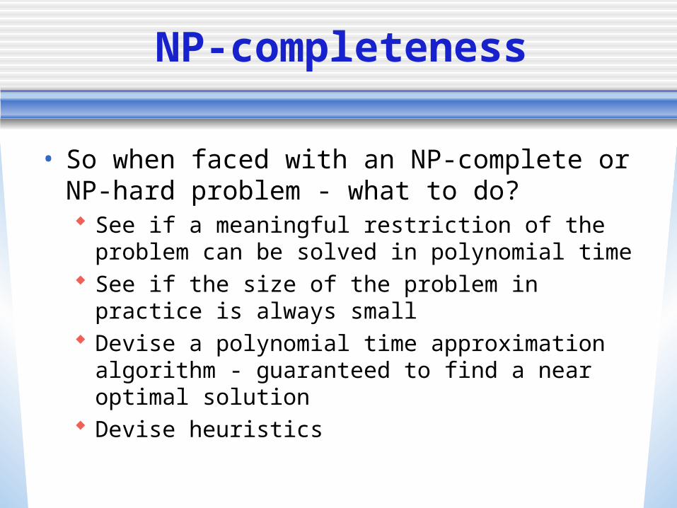
• So when faced with an NP-complete or NP-hard problem - what to do? See if a meaningful restriction of the problem

can be solved in polynomial time See if the size of the problem in practice is

always small Devise a polynomial time approximation

algorithm - guaranteed to find a near optimal solution

Devise heuristics

Algorithmic Implications

• We are trying to solve a real-life problem The models we use may give us many

solutions, but we want to find the one solution which corresponds to the real ordering of the clones in the target DNA

Use the algorithmic results in an iterative fashion with the experimental biologist

Algorithmic Implications

• A mapping algorithm should Work better with more data, assuming a

constant error rate Give a solution which makes it clear how

it was obtained and tell which parts of the solution are good and which bad

Give all candidate solutions

An algorithm for C1P

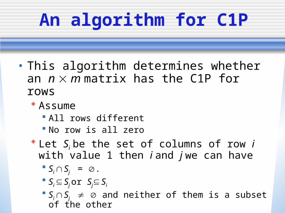
• This algorithm determines whether an n m matrix has the C1P for rows Assume

All rows different No row is all zero

Let Si be the set of columns of row i with value 1 then i and j we can have Si Sj = . Si Sj or Sj Si

Si Sj and neither of them is a subset of the other

An algorithm for C1P

• In the first case, we don’t need to consider the two rows together, so we separate them into two components Deal with them separately

• For non-empty intersection Suppose there is a row that is either a

subset or has empty intersection with every row in the component - move it out of the component

An algorithm for C1P

• To see if two rows belong to the same component Build a graph Gc using M

Each vertex of Gc will be a row from M• There will be an undirected edge from i to j if Si Sj

and neither of them is a subset of the other So the components we want are the

connected components of Gc

Basic Algorithm

• The algorithm will have the following phases Separate rows into components

according to above rules Permute the columns of each

component to achieve C1P for component

Join components together

Example Matrix

c1 c2 c3 c4 c5 c6 c7 c8 c9

l1 1 1 0 1 1 0 1 0 1

l2 0 1 1 1 1 1 1 1 1

l3 0 1 0 1 1 0 1 0 1

l4 0 0 1 0 0 0 0 1 0

l5 0 0 1 0 0 1 0 0 0

l6 0 0 0 1 0 0 1 0 0

l7 0 1 0 0 0 0 1 0 0

l8 0 0 0 1 1 0 0 0 1

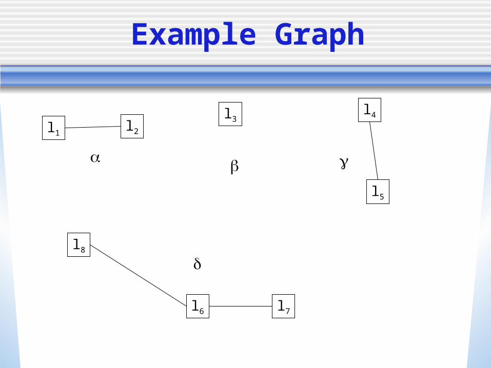
Example Graph

l1l2

l3

l5

l4

l7l6

l8

Placing Rows in a Component

c1 c2 c3 c4 c5 c6 c7 c8

l1 0 1 0 0 0 0 1 1

l2 0 1 0 0 1 0 1 0

l3 1 0 0 1 0 0 1 1

How can the first row (by itself) be arranged? (Keep track of all possibilities)

l1 … 0 1 1 1 0 … {2, 7, 8} {2, 7, 8} {2, 7, 8}

Now add the second row - it can go to right or left of first

l1 … 0 0 1 1 1 0 …

l2 … 0 1 1 1 0 0…

{5} {2, 7} {2, 7} {8}

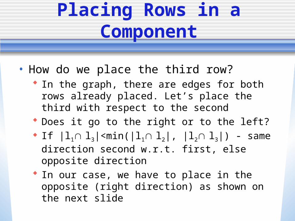
Placing Rows in a Component

• How do we place the third row? In the graph, there are edges for both rows

already placed. Let’s place the third with respect to the second

Does it go to the right or to the left? If |l1 l3|<min(|l1 l2|, |l2 l3|) - same direction

second w.r.t. first, else opposite direction In our case, we have to place in the opposite

(right direction) as shown on the next slide

Placing Rows in a Component

l1 … 0 0 1 1 1 0 0 0…

l2 … 0 1 1 1 0 0 0 0…

{5} {2} {7} {8} {1, 4} {1, 4}

l3 … 0 0 0 1 1 1 1 0…

Placing Rows in a Component

• All of the other rows in the component are placed in the same way, using two previously place rows: One which has an edge to the row to be

placed in the graph Second has an edge to the previous row

in the graph

Joining Components Together

• For the next part of the solution, we use a graph GM which tells us how the components fit together Each component of the original matrix

will be a vertex in GM A directed edge is added between and

if the sets Si for all i in are contained in at least one set Sj of component

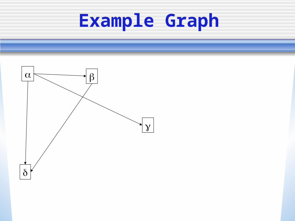
Example Graph

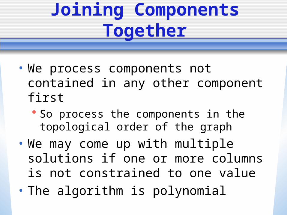
Joining Components Together

• We process components not contained in any other component first So process the components in the

topological order of the graph

• We may come up with multiple solutions if one or more columns is not constrained to one value

• The algorithm is polynomial