Computational challenges in high angle of attack flow prediction

Progress in Aerospace Sciences 39 (2003) 369–384

Computational challenges in high angle ofattack flow prediction

Russell M. Cummingsa,*, James R. Forsytheb, Scott A. Mortonb, Kyle D. Squiresc

aAerospace Engineering Department, California Polytechnic State University, San Luis Obispo, CA 93407, USAbDepartment of Aeronautics, United States Air Force Academy, USAF Academy, CO 80840, USA

cDepartment of Mechanical and Aerospace Engineering, Arizona State University, Tempe, AZ 85287, USA

Abstract

Aircraft aerodynamics have been predicted using computational fluid dynamics for a number of years. While viscous

flow computations for cruise conditions have become commonplace, the non-linear effects that take place at high angles

of attack are much more difficult to predict. A variety of difficulties arise when performing these computations,

including challenges in properly modeling turbulence and transition for vortical and massively separated flows, the need

to use appropriate numerical algorithms if flow asymmetry is possible, and the difficulties in creating grids that allow

for accurate simulation of the flowfield. These issues are addressed and recommendations are made for further

improvements in high angle of attack flow prediction. Current predictive capabilities for high angle of attack flows are

reviewed, and solutions based on hybrid turbulence models are presented.

r 2003 Elsevier Science Ltd. All rights reserved.

Contents

1. Introduction . . . . . . . . . . . . . . . . . . . . . . . . . . . . . . . . . . . . . . . . . . 370

2. Computational challenges . . . . . . . . . . . . . . . . . . . . . . . . . . . . . . . . . . . 372

2.1. Governing equation complexity . . . . . . . . . . . . . . . . . . . . . . . . . . . . . 372

2.2. Turbulence modeling . . . . . . . . . . . . . . . . . . . . . . . . . . . . . . . . . . . 374

2.3. Transition modeling . . . . . . . . . . . . . . . . . . . . . . . . . . . . . . . . . . . 376

2.4. Flowfield asymmetry and algorithm symmetry . . . . . . . . . . . . . . . . . . . . . . 377

2.5. Grid generation and density . . . . . . . . . . . . . . . . . . . . . . . . . . . . . . . 379

2.6. Numerical dissipation . . . . . . . . . . . . . . . . . . . . . . . . . . . . . . . . . . 380

3. Computational results and future directions . . . . . . . . . . . . . . . . . . . . . . . . . . 381

4. Conclusions . . . . . . . . . . . . . . . . . . . . . . . . . . . . . . . . . . . . . . . . . . . 382

References . . . . . . . . . . . . . . . . . . . . . . . . . . . . . . . . . . . . . . . . . . . . . . 383

*Corresponding author. Tel.: +1-805-756-1359; fax: +1-805-756-2376.

E-mail address: [email protected] (R.M. Cummings).

0376-0421/03/$ - see front matter r 2003 Elsevier Science Ltd. All rights reserved.

doi:10.1016/S0376-0421(03)00041-1

1. Introduction

Aircraft fly at a variety of incidence angles, depending

on their purpose and flight requirements. For instance,

commercial transports rarely fly at an angle of attack

larger than a ¼ 10�; but tactical aircraft and missiles fly

regularly at angles of attack above a ¼ 20�: During

unsteady maneuvers, such as the Cobra maneuver

performed by the Su-27, aircraft may even fly at angles

of attack over a ¼ 90�: Key geometric components of

aircraft while flying at high angles of attack are

forebodies, wings, and strakes (or leading-edge exten-

sions); each of these creates special difficulties when

attempting to model the flowfield.

While it is somewhat difficult to precisely describe the

various angle of attack regions, a good categorization

system has been developed [1–4]:

* low angle of attack 0�pap15� (attached, symmetric,

steady flow, linear lift variation);

* medium angle of attack 15�pap30� (separated,

symmetric rolled-up vortices, steady flow, non-linear

lift variation);* high angle of attack 30�pap65� (separated, asym-

metric rolled-up vortices, steady/unsteady flow, non-

linear lift variation);* very high angle of attack a > 65� (separated, un-

steady turbulent wake, post stall).

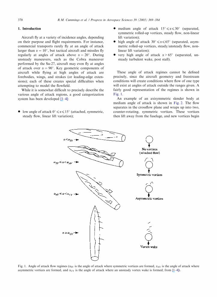
These angle of attack regimes cannot be defined

precisely, since the aircraft geometry and freestream

conditions will create conditions where flow of one type

will exist at angles of attack outside the ranges given. A

fairly good representation of the regimes is shown in

Fig. 1.

An example of an axisymmetric slender body at

medium angle of attack is shown in Fig. 2. The flow

separates in the crossflow plane and wraps up into two,

counter-rotating, symmetric vortices. These vortices

then lift away from the fuselage, and new vortices begin

Fig. 1. Angle of attack flow regimes (aSV is the angle of attack where symmetric vortices are formed, aAV is the angle of attack where

asymmetric vortices are formed, and aUV is the angle of attack where an unsteady vortex wake is formed; from [1–4]).

R.M. Cummings et al. / Progress in Aerospace Sciences 39 (2003) 369–384370

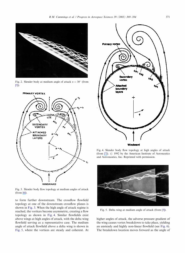
to form further downstream. The crossflow flowfield

topology at one of the downstream crossflow planes is

shown in Fig. 3. When the high angle of attack regime is

reached, the vortices become asymmetric, creating a flow

topology as shown in Fig. 4. Similar flowfields exist

above wings at high angles of attack, with the delta wing

flowfield serving as a representative case. The medium

angle of attack flowfield above a delta wing is shown in

Fig. 5, where the vortices are steady and coherent. At

higher angles of attack, the adverse pressure gradient of

the wing causes vortex breakdown to take place, yielding

an unsteady and highly non-linear flowfield (see Fig. 6).

The breakdown location moves forward as the angle of

Fig. 2. Slender body at medium angle of attack a ¼ 30� (from

[5]).

Fig. 3. Slender body flow topology at medium angles of attack

(from [6]).

Fig. 4. Slender body flow topology at high angles of attack

(from [7]). r 1992 by the American Institute of Aeronautics

and Astronautics, Inc. Reprinted with permission.

Fig. 5. Delta wing at medium angle of attack (from [5]).

R.M. Cummings et al. / Progress in Aerospace Sciences 39 (2003) 369–384 371

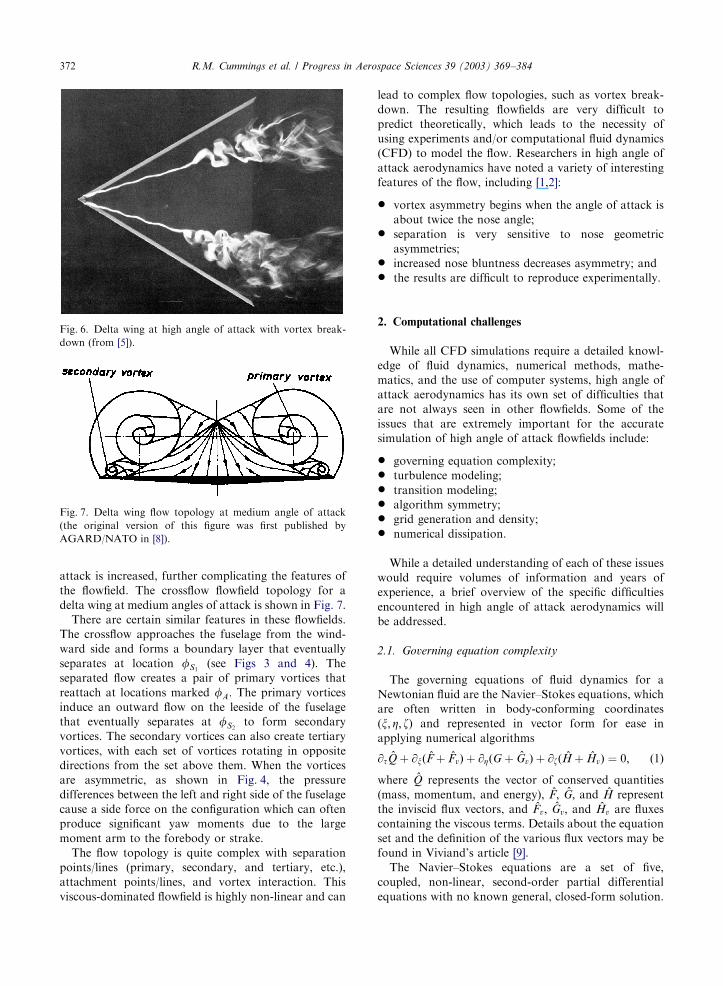
attack is increased, further complicating the features of

the flowfield. The crossflow flowfield topology for a

delta wing at medium angles of attack is shown in Fig. 7.

There are certain similar features in these flowfields.

The crossflow approaches the fuselage from the wind-

ward side and forms a boundary layer that eventually

separates at location fS1(see Figs 3 and 4). The

separated flow creates a pair of primary vortices that

reattach at locations marked fA: The primary vortices

induce an outward flow on the leeside of the fuselage

that eventually separates at fS2to form secondary

vortices. The secondary vortices can also create tertiary

vortices, with each set of vortices rotating in opposite

directions from the set above them. When the vortices

are asymmetric, as shown in Fig. 4, the pressure

differences between the left and right side of the fuselage

cause a side force on the configuration which can often

produce significant yaw moments due to the large

moment arm to the forebody or strake.

The flow topology is quite complex with separation

points/lines (primary, secondary, and tertiary, etc.),

attachment points/lines, and vortex interaction. This

viscous-dominated flowfield is highly non-linear and can

lead to complex flow topologies, such as vortex break-

down. The resulting flowfields are very difficult to

predict theoretically, which leads to the necessity of

using experiments and/or computational fluid dynamics

(CFD) to model the flow. Researchers in high angle of

attack aerodynamics have noted a variety of interesting

features of the flow, including [1,2]:

* vortex asymmetry begins when the angle of attack is

about twice the nose angle;* separation is very sensitive to nose geometric

asymmetries;* increased nose bluntness decreases asymmetry; and* the results are difficult to reproduce experimentally.

2. Computational challenges

While all CFD simulations require a detailed knowl-

edge of fluid dynamics, numerical methods, mathe-

matics, and the use of computer systems, high angle of

attack aerodynamics has its own set of difficulties that

are not always seen in other flowfields. Some of the

issues that are extremely important for the accurate

simulation of high angle of attack flowfields include:

* governing equation complexity;* turbulence modeling;* transition modeling;* algorithm symmetry;* grid generation and density;* numerical dissipation.

While a detailed understanding of each of these issues

would require volumes of information and years of

experience, a brief overview of the specific difficulties

encountered in high angle of attack aerodynamics will

be addressed.

2.1. Governing equation complexity

The governing equations of fluid dynamics for a

Newtonian fluid are the Navier–Stokes equations, which

are often written in body-conforming coordinates

(x; Z; z) and represented in vector form for ease in

applying numerical algorithms

@t #Q þ @xð #F þ #FvÞ þ @ZðG þ #GvÞ þ @zð #H þ #HvÞ ¼ 0; ð1Þ

where #Q represents the vector of conserved quantities

(mass, momentum, and energy), #F; #G; and #H represent

the inviscid flux vectors, and #Fv; #Gv; and #Hv are fluxes

containing the viscous terms. Details about the equation

set and the definition of the various flux vectors may be

found in Viviand’s article [9].

The Navier–Stokes equations are a set of five,

coupled, non-linear, second-order partial differential

equations with no known general, closed-form solution.

Fig. 6. Delta wing at high angle of attack with vortex break-

down (from [5]).

Fig. 7. Delta wing flow topology at medium angle of attack

(the original version of this figure was first published by

AGARD/NATO in [8]).

R.M. Cummings et al. / Progress in Aerospace Sciences 39 (2003) 369–384372

There are various techniques for the numerical predic-

tion of turbulent flows, ranging from Reynolds-averaged

Navier–Stokes (RANS), to large eddy simulation (LES),

to direct numerical simulation (DNS). DNS attempts to

resolve all scales of turbulence, from the largest to the

smallest, by solving Eq. (1) directly. Because of this, the

grid resolution requirements are very high, and increase

drastically with Reynolds number—this is only currently

possible for low Reynolds number flowfields, such as flat

plates, shear layers, and simple three-dimensional

geometries [10]. LES attempts to model the smaller,

more homogeneous scales, while resolving the larger,

energy-containing scales, which makes the grid require-

ments for LES significantly less than for DNS. To

accurately resolve the boundary layer, however, LES

must accurately resolve the energy-containing eddies in

the boundary layer, which requires very small stream-

wise and spanwise grid spacing. Finally, the RANS

approach attempts to solve the time-averaged flow,

which means that all scales of turbulence must be

modeled. The RANS equations appear to be identical to

the full Navier–Stokes equations (Eq. (1)), although all

flow variables have been replaced with time-averaged

values. RANS models often fail to provide accurate

results for high angle of attack flows since the large

turbulence scales for separated flows are very dependent

on the geometry. RANS models, however, can provide

accurate results for attached boundary layer flows, thin

shear layers, and steady coherent vortical flowfields, but

at the cost of increasing empiricism due to the closure

problem. Spalart provides a good discussion and

comparison of these various approaches [11].

These various techniques have very different compu-

tational requirements. In 1997, Spalart et al. estimated

that LES computations over an entire aircraft would not

be possible for over 45 years [12]. Of course, that makes

DNS computations for full aircraft unthinkable for the

foreseeable future. Spalart’s estimate led to the formula-

tion of detached-eddy simulation (DES), which is a

hybrid approach combining the advantages of LES and

RANS into one model. For the DES approach, RANS

is used in the boundary layer, where it performs well

(and with much lower grid requirements than LES), and

LES is then used in the separated regions where its

ability to predict turbulence length scales is important.

Shur et al. [13] calibrated the model for isotropic

turbulence, and applied it to an NACA 0012 airfoil

section; the model agreed well with lift and drag

predictions to 90� angle of attack.

Historically, solutions of the Navier–Stokes equations

required a great deal of computer resources, and until

recently solutions were only obtainable on supercom-

puters. Because of the limitations of computers, even the

RANS equations were often simplified for the high angle

of attack case. One way to simplify the RANS equation

set is to assume that the flow is steady and that the

longitudinal viscous terms may be neglected (Eq. (2)).

This creates a parabolic-hyperbolic equation set that

allows for solution by marching longitudinally in space.

These assumptions restrict solutions to supersonic flow

cases at high Reynolds numbers (thin boundary layers)

with no upstream recirculation in the flowfield. The

advantage of the parabolized form of the equations is

that solutions may be obtained very quickly when

compared with the full RANS equations (Eq. (1)) [10]:

@x #F þ @Z #G þ @z #H ¼1

Reð@Z #S þ @z #SÞ: ð2Þ

Another simplification of the RANS equations that has

been used is the ‘‘thin layer’’ equations. These equations

are derived from Eq. (1) by assuming that only the

viscous terms in the surface-normal direction are

essential for resolving the flowfield, yielding

@t #Q þ @x #F þ @Z #G þ @z #H ¼1

Re@z #S: ð3Þ

Various alternative forms of the thin-layer equations

exist, all based on the assumption that various viscous

derivatives may be neglected (such as cross derivatives).

Eq. (3) is only valid for thin boundary layers, and thus is

used for flows at high Reynolds numbers. The equations

require considerably more time to compute than Eq. (2),

however, because they must be solved by marching in

time. Upstream propagation and recirculation, however,

are allowed, and thus these equations can be used in

subsonic flow with separated regions. Degani and

Marcus showed that these equations could adequately

resolve steady vortical flow structures in the medium

angle of attack range where the vortices were symmetric

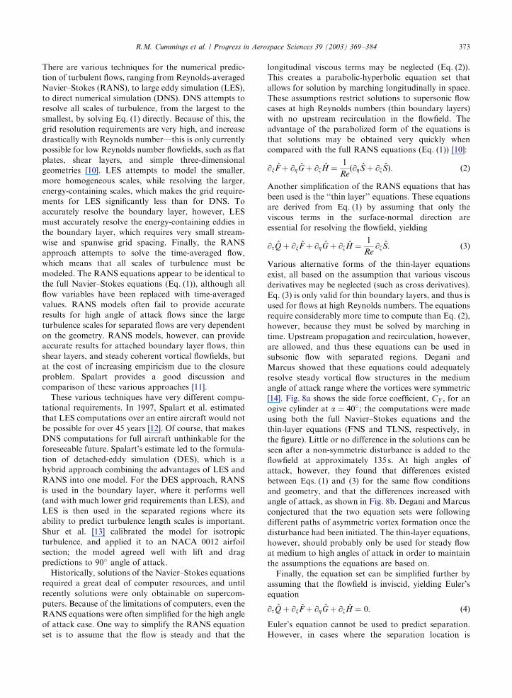
[14]. Fig. 8a shows the side force coefficient, CY ; for anogive cylinder at a ¼ 40�; the computations were madeusing both the full Navier–Stokes equations and the

thin-layer equations (FNS and TLNS, respectively, in

the figure). Little or no difference in the solutions can be

seen after a non-symmetric disturbance is added to the

flowfield at approximately 135 s. At high angles of

attack, however, they found that differences existed

between Eqs. (1) and (3) for the same flow conditions

and geometry, and that the differences increased with

angle of attack, as shown in Fig. 8b. Degani and Marcus

conjectured that the two equation sets were following

different paths of asymmetric vortex formation once the

disturbance had been initiated. The thin-layer equations,

however, should probably only be used for steady flow

at medium to high angles of attack in order to maintain

the assumptions the equations are based on.

Finally, the equation set can be simplified further by

assuming that the flowfield is inviscid, yielding Euler’s

equation

@t #Q þ @x #F þ @Z #G þ @z #H ¼ 0: ð4Þ

Euler’s equation cannot be used to predict separation.

However, in cases where the separation location is

R.M. Cummings et al. / Progress in Aerospace Sciences 39 (2003) 369–384 373

known a priori, the equations can be used to compute

the vortical flowfield. The most common application of

Euler’s equation to high angle of attack aerodynamics is

for delta wing configurations. Delta wings with sharp

leading edges have a fixed primary vortex separation

location, and the equations do a reasonable job in

simulating the linear characteristics of the flowfield, but

cannot model the non-linear interaction of secondary or

tertiary vortices on the location and strength of the

primary vortices. Configurations without fixed separa-

tion locations cannot be handled well using Euler’s

equation; most practical aircraft configurations would

make it difficult to obtain good high angle of attack flow

simulations using the Euler equations.

2.2. Turbulence modeling

The RANS form of the Navier–Stokes equations is

used in many practical high angle of attack applications

to reduce the computational time and memory required

for performing non-averaged computations. While DNS

Navier–Stokes calculations are being performed on

increasingly complex geometries, these geometries are

still relatively basic and can be solved only at very low

Reynolds numbers. Because of these restrictions, the

Navier–Stokes equations have been Reynolds (time or

ensemble) averaged [15]. For compressible flows the

equations are Favre (mass-weighted) averaged [16]. The

averaging process introduces correlations between fluc-

tuating flow variables (the Reynolds stresses, Eq. 5) that

require the use of a turbulence model in order to affect

closure of the equation set

tij ¼ �ru0iu0j : ð5Þ

Turbulence models are semi-empirical formulations that

are used to close the RANS equations by providing the

Reynolds stresses. They are generally calibrated on

building block flows such as boundary layers, shear

layers, and wakes [17]. The Reynolds stresses are

modeled in one of two ways: either through an eddy-

viscosity model or a stress-transport model. Stress

transport models make no general assumptions about

the form of the six components of the Reynolds stress.

Unless additional assumptions are made, these models

are therefore solving for six unknowns. The more

common eddy-viscosity models are based on the

Boussinesq approximation—that the Reynolds stresses

are proportional to the strain rate of the mean flow. The

turbulent eddy viscosity (mt) is the constant of propor-tionality, i.e.

�ru0iu0j ¼ mt

@ui

@xj

þ@uj

@xi

� �: ð6Þ

This assumption reduces the number of unknowns from

the six components of the Reynolds stresses to a single

unknown, the turbulent eddy viscosity. Because Eq. (6)

takes the same form as the laminar stresses, the

turbulent eddy viscosity can simply be added to the

laminar viscosity in the Navier–Stokes equation, i.e. m ¼ml þ mt (ml is the laminar viscosity and mt is the turbulenteddy viscosity). This is the reason Eq. (1) appears similar

for both the DNS and RANS form of the Navier–Stokes

equations. In addition, all flow variables are replaced by

their time-averaged values (e.g. ui is replaced by %ui). The

turbulent viscosity is then provided by the turbulence

model, which is often classified by the number of partial

differential equations it adds. Most common are zero-,

one-, and two-equation turbulence models. The zero-

equation models use algebraic relationships rather than

a partial differential equation. Since the modeled

equations are semi-empirical, they require experimen-

tally determined coefficients that are usually found for

flow over simple geometries like a flat plate or various

types of shear layers.

For compressible flows additional terms similar to

Reynolds stresses appear in the energy equation invol-

ving correlations of fluctuating velocities and tem-

perature—the turbulent heat flux vector. These terms

Fig. 8. Time history of side-force coefficient (from [14]);

B-W=body-wing, FNS=full Navier–Stokes (RANS),

TLNS=thin-layer Navier–Stokes.

R.M. Cummings et al. / Progress in Aerospace Sciences 39 (2003) 369–384374

account for enhanced heat transfer due to the turbulent

motions, and are commonly modeled by appealing to

the Reynolds analogy which relates the heat transfer to

the momentum transfer by the Prandtl number. By

assuming a turbulent Prandtl number (generally as-

sumed constant), the turbulent heat transfer can there-

fore be obtained without any additional equations. See

Ref. [18] for a more complete discussion.

But what happens at high angles of attack? Do the

turbulence models adequately resolve the flow features

found in separated, vortical flowfields? An illustration of

the difficulties can be seen by using the zero-equation

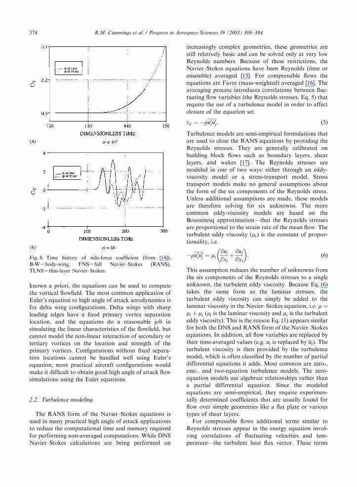
(algebraic) turbulence model of Baldwin and Lomax [19]

as an example. The Baldwin–Lomax model contains a

function, F ðyÞ, which is used as part of the outer-layer

model

F ðyÞ ¼ yO½1� e�ðyþ=AþÞ; ð7Þ

where y is the normal distance to a flat plate and O is the

vorticity magnitude. In an attached boundary layer (see

Fig. 3, f ¼ f1 radial line), F ðyÞ increases to a maximum

value and then decreases near the edge of the boundary

layer. However, in a separated vortical flow layer (see

Fig. 3, f ¼ f2 radial line), F ðyÞ attains a local maxima

in the attached boundary layer and then reaches a global

maxima in the separated layer (see Fig. 9). The

turbulence model chooses the highest F ðyÞ and its

corresponding distance from the wall, which greatly

overpredicts the turbulent viscosity in this region. The

overpredicted turbulent viscosity creates non-physical

results when added to the laminar viscosity, altering

separation locations and the proper formation of

secondary and tertiary vortices.

A variety of researchers have proposed methods for

altering algebraic turbulence models for high angle of

attack flow [6,20,21]. Degani and Schiff proposed a

modification to the model (and hence to all eddy-

viscosity turbulence models) that obtains the correct

value of F ðyÞ and gives better prediction of the flow

topology in a separated flow region [6]. This modifica-

tion has led to the ability to accurately simulate steady

vortical flows with RANS computations. An example of

the improvements to both zero-equation and one-

equation turbulence models for predicting vortical

flowfields was done by Gee et al. [22]. Vortical flow

modifications for the k � e turbulence model have alsobeen suggested [23] and have been applied to flow over

slender bodies at high incidence angles [24]. However, in

spite of these improvements the RANS-based equations

still lead to questionable predictions at high to very high

angles of attack, where the flow is unsteady and the

time-averaged equations are no longer capable of

properly modeling the flowfield. This has led to further

developments in equation and turbulence modeling,

including vortex filtering [25] and the DES method.

DES was proposed by Spalart et al. [11,12] as a

method to combine the best features of LES with the

best features of the RANS approach. RANS tends to be

able to predict attached flows very well with a relatively

low computation cost. LES, on the other hand, has a

high computation cost, but can predict unsteady

separated flows more accurately. The model was

originally based on the Spalart–Allmaras one-equation

RANS turbulence model [26]. The wall destruction term

is proportional to *u=d2; where d is the distance to the

closest wall. When this term is balanced with the

production term, the eddy viscosity becomes *upSd2;where S is the local strain rate. The Smagorinski LES

model [27] varies the sub-grid-scale (SGS) turbulent

viscosity with the local strain rate and the grid spacing,

D (i.e. uSGSpSD2 ). If, therefore, d is replaced by D in

the wall destruction term, the Spalart–Allmaras model

will act as a Smagorinski LES model.

To exhibit both RANS and LES behavior, d in

the Spalart–Allmaras model is replaced by *d ¼minðd ;CDESDÞ; where CDES is the DES model constant.

When d ¼ D; the model acts as a RANS model, and

when d{D; the model acts as a Smagorinski LES

model. Therefore, the model can be ‘‘switched’’ to LES

mode by locally refining the grid. In an attached

boundary layer, a RANS simulation will have highly

stretched grids in the streamwise direction. To retain

RANS behavior in this case, D is taken as the largest

spacing in any direction (D ¼ maxðDx;Dy;DzÞ). This

type of extension can be applied to other turbulence

models as well, as has been shown by Strelets [28] and

Forsythe et al. [29]. The DES approach provides a way

to model unsteady, asymmetric flowfields at high to very

high angles of attack without resorting to new and

untrustworthy ‘‘fixes’’ to flat-plate turbulence models.

DES has the advantage of computing the unsteady

three-dimensional flow features necessary to accurately

predict flow quantities in massively separated flows. The

additional computational cost of DES can be attributedFig. 9. Variation of Baldwin–Lomax outer layer function, F ðyÞ(from [6]).

R.M. Cummings et al. / Progress in Aerospace Sciences 39 (2003) 369–384 375

to the need to compute a time-accurate flowfield (i.e., it

may require more solutions or time steps), as well as a

need to accurately resolve small three-dimensional flow

structures spatially (i.e., it may require more grid

points).

2.3. Transition modeling

Most high angle of attack computations are per-

formed under either fully laminar or fully turbulent

conditions, with no attempt to model transition. Note

that in the present context, ‘‘fully laminar’’ implies a

solution of the Navier–Stokes equations in which no

explicit turbulence model is included in the calculation.

‘‘Fully turbulent’’ solutions imply that the turbulence

model is everywhere active within the boundary layers

formed over solid surfaces. Such solutions are estab-

lished in Reynolds-averaged methods that employ the

Boussinesq approximation, for example, by specifying at

the inflow boundary a small level of eddy viscosity,

sufficient to ignite the model as the fluid enters the

boundary layer. Fully laminar or fully turbulent

computations are limiting cases but represent the norm

in practice since the numerical prediction of laminar-to-

turbulent transition and application of transition models

within large-scale CFD computations remains difficult.

Such approaches introduce uncertainty since researchers

often compute both fully laminar and fully turbulent

solutions and then compare with experimental data. One

complication introduced by such an approach is that the

amount of transitional flow present in the experiment is

often unknown, in turn complicating interpretation of

CFD results against measurements.

Further, in many applications of practical impor-

tance, laminar-to-turbulent transition can have a crucial

effect on the overall behavior of the flow, substantially

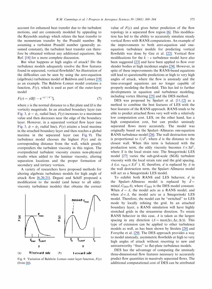
altering forces and moments. One example is provided

by a notional forebody in a crossflow, shown in Fig. 10.

The forebody cross section is a rounded-corner square,

similar to the cross sections of the X-29 and T-38. The

flow around the cross section was measured by

Polhamus et al. [30] for a range of Reynolds numbers

and angles of attack. The motivation was to understand

spin characteristics of aircraft forebodies, the angle of

attack being idealized to represent an actual aircraft in a

flat spin.

The effect of laminar-to-turbulent transition is cru-

cially important for the forebody shown in Fig. 10, as it

alters the locations at which boundary layer separation

occurs, which in turn affects the streamwise and lateral

(side) forces acting on the body. Polhamus et al. found

that the side force reverses from positive (along the

positive y-axis in Fig. 10) to negative at a critical

Reynolds number, analogous to the drag crisis which

occurs over cylinders and spheres. A reversal of the side

force is important since at sub-critical Reynolds

numbers the negative side force is spin-propelling, while

the positive side force at higher Reynolds numbers is

spin-damping. Reversal of the side force is influenced by

the location of boundary layer separation along the

upper surface of the forebody, which in turn is sensitive

to the location of laminar-to-turbulent transition.

Super-critical regimes can be accurately modeled via

prediction of the fully turbulent flow. Squires et al. [31]

applied DES to prediction of the three-dimensional flow

around the forebody shown in Fig. 10, obtaining

accurate predictions of the pressure distribution and

averaged streamwise and side forces at a Reynolds

number of 800,000, above the critical value. Prediction

of the sub-critical flows requires an approach for

handling the effect of laminar-to-turbulent transition.

One approach is the ‘‘tripless’’ method employed by

Travin et al. [32] used for prediction of the sub-critical

flow over a circular cylinder. These investigators applied

DES, with the baseline closure being based on the

Spalart–Allmaras model. Effects of laminar-to-turbulent

transition were modeled by seeding the initial condition

with a small level of eddy viscosity, and with the level of

eddy viscosity at the inlet boundary equal to zero. Once

the flow attains equilibrium in the attached regions of

the flow (prior to boundary layer separation), the eddy

viscosity is zero and the boundary layers are effectively

laminar. Recirculation of the flow in the wake of the

cylinder provided a mechanism for sweeping non-zero

values of the eddy viscosity from downstream to

upstream. In this case the turbulence model is sustained

by the recirculating motion of the wake, the turbulent

region of the flow beginning downstream of separation.

While the tripless approach does not attempt to mimic

the very complex details governing transition, the

method possesses the substantial advantage that the

location of transition (identified by the region over

which the eddy viscosity sharply increases from zero) is

dictated by the turbulence model and flow conditions,

rather than the initial and/or boundary conditions.Fig. 10. Cross section of notional rounded-corner forebody.

R.M. Cummings et al. / Progress in Aerospace Sciences 39 (2003) 369–384376

An additional example illustrating some of the com-

plexities introduced by details of the process of transition

on the interpretation of flowfield predictions is provided

by a forebody at angle of attack, for which a crossflow is

established as shown in Fig. 2. For the configuration

shown, transition can take place along streamlines that

convect along the windward plane of symmetry before

flowing around the fuselage—what is the laminar run for

such a flowfield? Very different results are obtained if the

flow attaches within a crossflow plane and then flows

around the vehicle than if the flow travels down the

length of the forebody (or some partial length of the

forebody) and then flows around the vehicle.

A good review of transition models has been

performed [33], and various researchers have attempted

to apply transition models to CFD computations

[34,35]. The difficulty with transition modeling is similar

to the difficulties with turbulence modeling: most models

are either theoretical or semi-empirical and are for-

mulated for flat plates or curved surfaces, but do not

possess the breadth of development to support high

angle of attack flow predictions. These methods often

require the solution of stability equations, which also

increases the total computation time for a solution

(again, similar to turbulence models). It is doubtful that

transition models will be accurate enough to be used in

high-angle flow simulations for the foreseeable future;

useful modeling of transition should be targeted as a

pacing item for full aircraft simulations.

2.4. Flowfield asymmetry and algorithm symmetry

As more researchers have simulated medium, high,

and very high angle of attack flowfields, a controversy

has developed regarding vortex flow asymmetries. As

anyone who works in aircraft or missile aerodynamics

knows, side forces and yaw moments develop at high

angles of attack due to vortex asymmetries on ‘‘real-life’’

configurations. The cause of the asymmetries, however,

is not well understood.

Two possible explanations have surfaced for the

vortex asymmetry: (1) the asymmetry is due to an

absolute hydrodynamic instability—small perturbations

yield a bifurcated asymmetry, even after the perturba-

tion is removed (example: the Karman vortex street

behind the flow over a cylinder), or (2) the asymmetry is

due to a convective instability—small, permanent

perturbations are required for asymmetry to exist, and

the flowfield is not limited to the two bifurcated states. A

good overview of the two views, including references for

supporting simulations and theoretical concepts was

reported by Thomas [36].

In either case, however, a perturbation is required! In

experiments the perturbation is always present, but

rarely the same, due to flowfield angularity, freestream

turbulence, or surface imperfections on the model. But,

what causes the perturbation in numerical calculations?

Certainly, a variety of usual suspects can be rounded up,

including truncation error, round-off error, the numer-

ical algorithm, boundary conditions, or initial condi-

tions. Everyone agrees that the flow asymmetry in a very

high angle of attack flowfield is caused by an absolute

instability, but the asymmetries in the high angle of

attack region are more difficult to understand, and

therefore, to accurately predict.

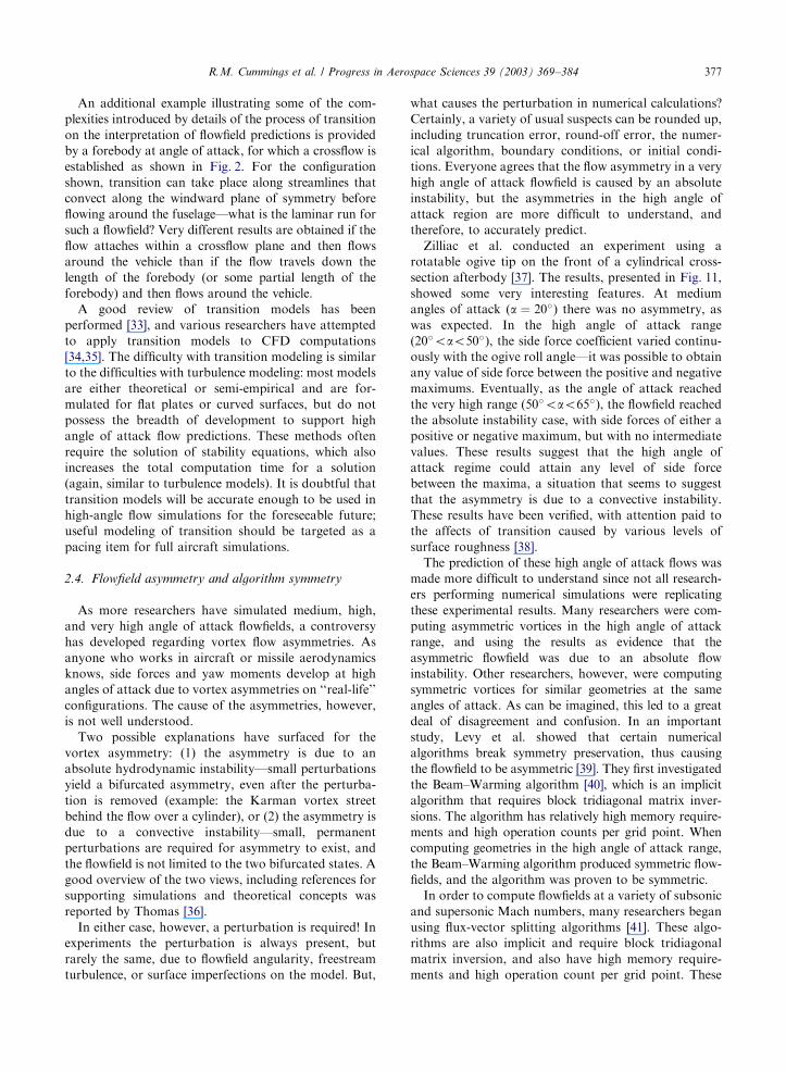
Zilliac et al. conducted an experiment using a

rotatable ogive tip on the front of a cylindrical cross-

section afterbody [37]. The results, presented in Fig. 11,

showed some very interesting features. At medium

angles of attack (a ¼ 20�) there was no asymmetry, as

was expected. In the high angle of attack range

(20�oao50�), the side force coefficient varied continu-

ously with the ogive roll angle—it was possible to obtain

any value of side force between the positive and negative

maximums. Eventually, as the angle of attack reached

the very high range (50�oao65�), the flowfield reached

the absolute instability case, with side forces of either a

positive or negative maximum, but with no intermediate

values. These results suggest that the high angle of

attack regime could attain any level of side force

between the maxima, a situation that seems to suggest

that the asymmetry is due to a convective instability.

These results have been verified, with attention paid to

the affects of transition caused by various levels of

surface roughness [38].

The prediction of these high angle of attack flows was

made more difficult to understand since not all research-

ers performing numerical simulations were replicating

these experimental results. Many researchers were com-

puting asymmetric vortices in the high angle of attack

range, and using the results as evidence that the

asymmetric flowfield was due to an absolute flow

instability. Other researchers, however, were computing

symmetric vortices for similar geometries at the same

angles of attack. As can be imagined, this led to a great

deal of disagreement and confusion. In an important

study, Levy et al. showed that certain numerical

algorithms break symmetry preservation, thus causing

the flowfield to be asymmetric [39]. They first investigated

the Beam–Warming algorithm [40], which is an implicit

algorithm that requires block tridiagonal matrix inver-

sions. The algorithm has relatively high memory require-

ments and high operation counts per grid point. When

computing geometries in the high angle of attack range,

the Beam–Warming algorithm produced symmetric flow-

fields, and the algorithm was proven to be symmetric.

In order to compute flowfields at a variety of subsonic

and supersonic Mach numbers, many researchers began

using flux-vector splitting algorithms [41]. These algo-

rithms are also implicit and require block tridiagonal

matrix inversion, and also have high memory require-

ments and high operation count per grid point. These

R.M. Cummings et al. / Progress in Aerospace Sciences 39 (2003) 369–384 377

algorithms were also found to yield symmetric flowfields

at high angles of attack, and were shown to be

symmetric algorithms.

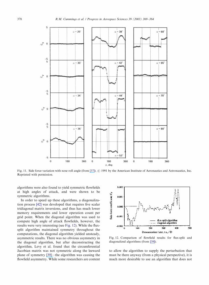
In order to speed up these algorithms, a diagonaliza-

tion process [42] was developed that requires five scalar

tridiagonal matrix inversions, and thus has much lower

memory requirements and lower operation count per

grid point. When the diagonal algorithm was used to

compute high angle of attack flowfields, however, the

results were very interesting (see Fig. 12). While the flux-

split algorithm maintained symmetry throughout the

computations, the diagonal algorithm yielded unsteady,

asymmetric results. There was no obvious asymmetry in

the diagonal algorithm, but after deconstructing the

algorithm, Levy et al. found that the circumferential

Jacobian matrix was not symmetric along the leeward

plane of symmetry [39]—the algorithm was causing the

flowfield asymmetry. While some researchers are content

to allow the algorithm to supply the perturbation that

must be there anyway (from a physical perspective), it is

much more desirable to use an algorithm that does not

Fig. 11. Side force variation with nose roll angle (from [37]). r 1991 by the American Institute of Aeronautics and Astronautics, Inc.

Reprinted with permission.

Fig. 12. Comparison of flowfield results for flux-split and

diagonalized algorithms (from [39]).

R.M. Cummings et al. / Progress in Aerospace Sciences 39 (2003) 369–384378

add an unknown level of perturbation. It would be

superior to have the perturbation be added explicitly as

a geometric disturbance or flowfield disturbance.

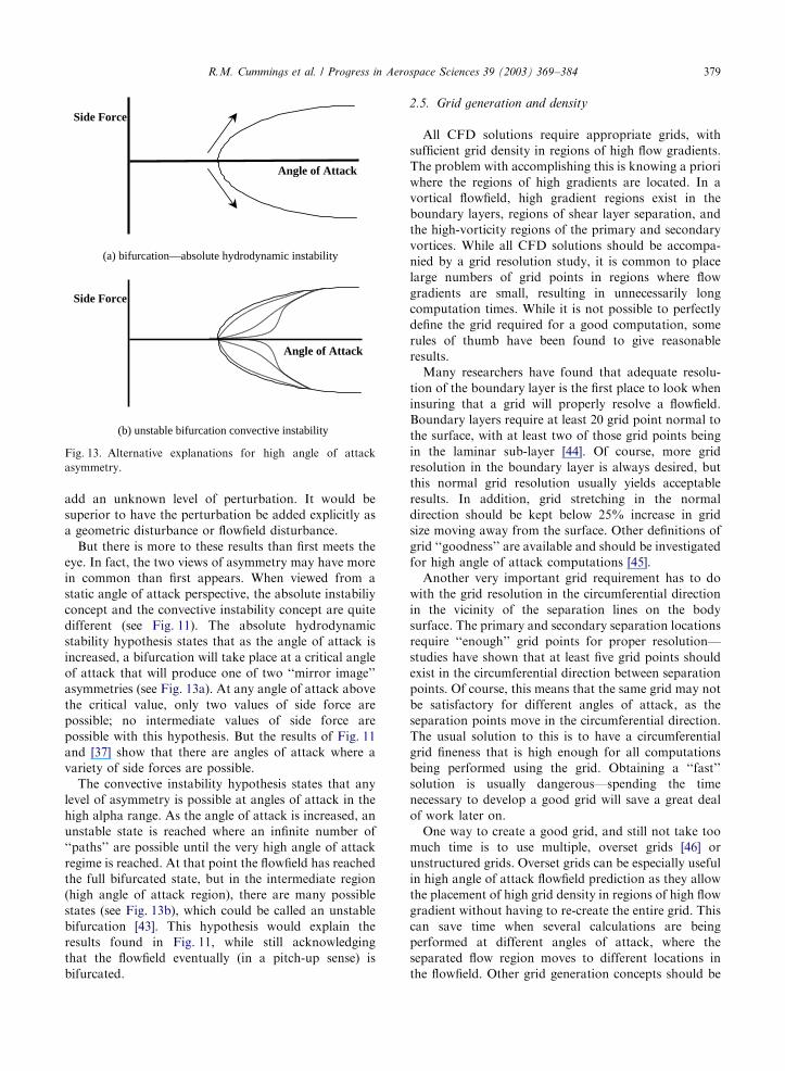
But there is more to these results than first meets the

eye. In fact, the two views of asymmetry may have more

in common than first appears. When viewed from a

static angle of attack perspective, the absolute instabiliy

concept and the convective instability concept are quite

different (see Fig. 11). The absolute hydrodynamic

stability hypothesis states that as the angle of attack is

increased, a bifurcation will take place at a critical angle

of attack that will produce one of two ‘‘mirror image’’

asymmetries (see Fig. 13a). At any angle of attack above

the critical value, only two values of side force are

possible; no intermediate values of side force are

possible with this hypothesis. But the results of Fig. 11

and [37] show that there are angles of attack where a

variety of side forces are possible.

The convective instability hypothesis states that any

level of asymmetry is possible at angles of attack in the

high alpha range. As the angle of attack is increased, an

unstable state is reached where an infinite number of

‘‘paths’’ are possible until the very high angle of attack

regime is reached. At that point the flowfield has reached

the full bifurcated state, but in the intermediate region

(high angle of attack region), there are many possible

states (see Fig. 13b), which could be called an unstable

bifurcation [43]. This hypothesis would explain the

results found in Fig. 11, while still acknowledging

that the flowfield eventually (in a pitch-up sense) is

bifurcated.

2.5. Grid generation and density

All CFD solutions require appropriate grids, with

sufficient grid density in regions of high flow gradients.

The problem with accomplishing this is knowing a priori

where the regions of high gradients are located. In a

vortical flowfield, high gradient regions exist in the

boundary layers, regions of shear layer separation, and

the high-vorticity regions of the primary and secondary

vortices. While all CFD solutions should be accompa-

nied by a grid resolution study, it is common to place

large numbers of grid points in regions where flow

gradients are small, resulting in unnecessarily long

computation times. While it is not possible to perfectly

define the grid required for a good computation, some

rules of thumb have been found to give reasonable

results.

Many researchers have found that adequate resolu-

tion of the boundary layer is the first place to look when

insuring that a grid will properly resolve a flowfield.

Boundary layers require at least 20 grid point normal to

the surface, with at least two of those grid points being

in the laminar sub-layer [44]. Of course, more grid

resolution in the boundary layer is always desired, but

this normal grid resolution usually yields acceptable

results. In addition, grid stretching in the normal

direction should be kept below 25% increase in grid

size moving away from the surface. Other definitions of

grid ‘‘goodness’’ are available and should be investigated

for high angle of attack computations [45].

Another very important grid requirement has to do

with the grid resolution in the circumferential direction

in the vicinity of the separation lines on the body

surface. The primary and secondary separation locations

require ‘‘enough’’ grid points for proper resolution—

studies have shown that at least five grid points should

exist in the circumferential direction between separation

points. Of course, this means that the same grid may not

be satisfactory for different angles of attack, as the

separation points move in the circumferential direction.

The usual solution to this is to have a circumferential

grid fineness that is high enough for all computations

being performed using the grid. Obtaining a ‘‘fast’’

solution is usually dangerous—spending the time

necessary to develop a good grid will save a great deal

of work later on.

One way to create a good grid, and still not take too

much time is to use multiple, overset grids [46] or

unstructured grids. Overset grids can be especially useful

in high angle of attack flowfield prediction as they allow

the placement of high grid density in regions of high flow

gradient without having to re-create the entire grid. This

can save time when several calculations are being

performed at different angles of attack, where the

separated flow region moves to different locations in

the flowfield. Other grid generation concepts should be

(a) bifurcation—absolute hydrodynamic instability

(b) unstable bifurcation convective instability

Angle of Attack

Side Force

Side Force

Angle of Attack

Fig. 13. Alternative explanations for high angle of attack

asymmetry.

R.M. Cummings et al. / Progress in Aerospace Sciences 39 (2003) 369–384 379

developed to aid in reducing the considerable time that

grid generation requires. An example of such a valuable

grid generation tool is adaptive mesh refinement [47,48].

2.6. Numerical dissipation

Numerical solutions always have some type of artificial

viscosity or numerical dissipation, either explicitly or

implicitly added. While implicit dissipation is the

preferred method in many modern algorithms, the

downside of implicit dissipation is the inability to control

the level of dissipation added, even though the levels are

usually quite low. The ease of use of implicit dissipation

should not allow the user to be deceived into thinking

that the dissipation levels will not impact the solutions.

High angle of attack flows are especially sensitive to

artificially dissipation, perhaps more than many other

flowfields. When the prediction of separation lines,

including secondary or even tertiary separation lines, is

an essential aspect of the flowfield prediction, it may be

more satisfying to use explicitly added, fourth-order,

dissipation. Solutions usually require fairly high levels of

dissipation at the early iteration stages, but once the

flowfield has settled down, the artificial dissipation should

be reduced to the smallest possible levels. While it may be

tempting to turn the artificial dissipation to extremely low

levels, care should be taken to insure that pressure

oscillations do not occur near the body surface—these

oscillations can have a negative impact on the solution. A

numerical experiment of dissipation levels can be found in

[44]—investigations such as this should be conducted in

all high angle of attack calculations. Another possible

approach would be to use explicitly added viscosity and

accounts for its effects [49].

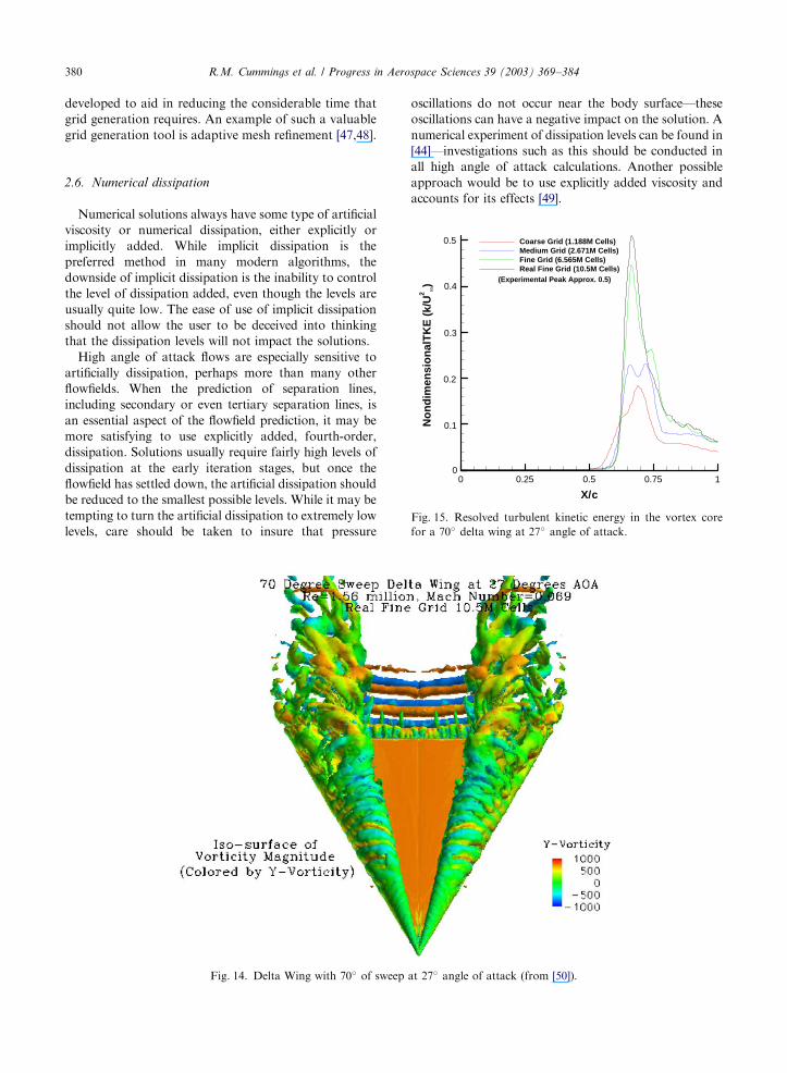
Fig. 14. Delta Wing with 70� of sweep at 27� angle of attack (from [50]).

X/c

No

nd

imen

sio

nal

TK

E (

k/U

2 ∞)

0 0.25 0.5 0.75 10

0.5

0.4

0.3

0.2

0.1

Coarse Grid (1.188M Cells)Medium Grid (2.671M Cells)Fine Grid (6.565M Cells)Real Fine Grid (10.5M Cells)

(Experimental Peak Approx. 0.5)

Fig. 15. Resolved turbulent kinetic energy in the vortex core

for a 70� delta wing at 27� angle of attack.

R.M. Cummings et al. / Progress in Aerospace Sciences 39 (2003) 369–384380

3. Computational results and future directions

Recent computations using DES have shown great

promise for predicting massively separated flowfields. A

detailed numerical evaluation of the flow over a delta

wing at high angles of attack shows incredible detail in

the flow [50]. Fig. 14 shows the delta wing flowfield

where the shear layer instability along the leading edge is

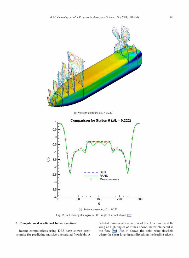
Fig. 16. 6:1 rectangular ogive at 90� angle of attack (from [52]).

R.M. Cummings et al. / Progress in Aerospace Sciences 39 (2003) 369–384 381

clearly evident, as well as vortex breakdown, and shear

layer roll-up from the delta wing blunt base. Computa-

tions of this complexity are not possible with RANS

calculations, since the unsteady flow features would not

be able to be resolved using time-averaged turbulence

models.

Fig. 15 displays the resolved turbulent kinetic energy

along the vortex core compared with experimental data

[51]. As the grid is resolved the experimental peak is

reached, although the computation required 10.5 million

unstructured cells to attain the experimental level of

resolved turbulent kinetic energy.

Another recent application of DES for a massively

separated flowfield is a 6:1 rectangular ogive at 90� angle

of attack (see Fig. 16a; the forebody cross-section is

shown in Fig. 10) [52]. This flowfield challenges RANS

models because they are unable to properly resolve the

pressure variations on the leeward side of the body.

Even with modifications such as Degani–Schiff, the

results for RANS models are still ‘‘averaged’’, and the

averaging process does not allow for true unsteadiness

to develop in the separated flow region. When DES is

applied to the flowfield, the unsteady movement of the

vortical structures ‘‘washes out’’ the pressures on the

leeward surface, giving a flat pressure profile that

matches experimental data, as shown in Fig. 16b.

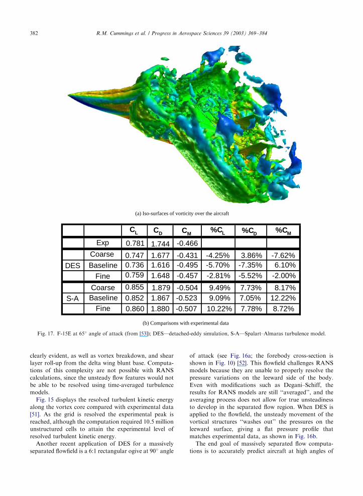
The end goal of massively separated flow computa-

tions is to accurately predict aircraft at high angles of

(a) Iso-surfaces of vorticity over the aircraft

CL CD CM%CL %CD %CM

Exp 0.781 1.744 -0.466

Coarse 0.747 1.677 -0.431 -4.25% 3.86% -7.62%DES Baseline 0.736 1.616 -0.495 -5.70% -7.35% 6.10%

Fine 0.759 1.648 -0.457 -2.81% -5.52% -2.00%

Coarse 0.855 1.879 -0.504 9.49% 7.73% 8.17%S-A Baseline 0.852 1.867 -0.523 9.09% 7.05% 12.22%

Fine 0.860 1.880 -0.507 10.22% 7.78% 8.72%

(b) Comparisons with experimental data

Fig. 17. F-15E at 65� angle of attack (from [53]); DES—detached-eddy simulation, S-A—Spalart–Almaras turbulence model.

R.M. Cummings et al. / Progress in Aerospace Sciences 39 (2003) 369–384382

attack, including post-stall flowfields. Shown in Fig. 17

is the F-15E at 65� angle of attack modeled as a half

body with nearly 6 million cells [53]. Iso-surfaces of

vorticity are shown, and comparisons with available

experimental data reveal that the results are within 6%

for lift, drag, and pitch moment coefficients. Of course,

the aircraft would have to be resolved with both left and

right sides in order to obtain the asymmetric flowfields

that are certainly occurring, but the ability of DES to

capture the complexities of this massively separated

flowfield are impressive.

While these DES results are impressive, they do not

represent a final stage of high angle of attack flow

prediction. Researchers will need to continue to

investigate these types of hybrid RANS-LES models

and insure that they work well for a wide variety of

separated, vortical flowfields. In spite of this, however,

the current state of CFD prediction for high angle of

attack flowfields has progressed significantly, with the

accurate prediction of full-scale maneuvering aircraft

at hand.

4. Conclusions

High angle of attack flow computations have a variety

of unusual aspects that make accurate predictions

challenging. A variety of influences on high angle of

attack flow predictions have been discussed, including:

governing equation complexity, turbulence modeling,

transition modeling, algorithm symmetry, grid genera-

tion and density, and numerical dissipation. While some

of these issues are important in many flowfield calcula-

tions, successful simulation of high angle of attack

flowfields must consider all of these factors. It is very

easy to get a poor solution for these highly separated,

vortical flowfields! A little careful forethought, planning,

and evaluation can lead to amazingly useful simulations.

Researchers should realize that when it comes to high

angle of attack flow predictions, faster is rarely better—

spend extra time in the beginning of the simulation work

and very good results are obtainable.

References

[1] Keener ER, Chapman GT. Similarity in vortex asymme-

tries over slender bodies and wings. AIAA J 1977;15:

1370–2.

[2] Rom J. High angle of attack aerodynamics. New York:

Springer, 1992.

[3] Ericsson LE, Reding JP. Asymmetric vortex shedding

from bodies of revolution. In: Hemsch MJ, Nielsen JN,

editors. Tactical missile aerodynamics. New York: Amer-

ican Institute of Aeronautics and Astronautics, 1986.

[4] Bertin JJ. Aerodynamics for engineers. Upper Saddle

River, NJ: Prentice-Hall, 2002.

[5] Van Dyke M. An album of fluid motion. Stanford: The

Parabolic Press, 1982.

[6] Degani D, Schiff LB. Computation of turbulent flows

around pointed bodies having crossflow separation.

J Comput Phys 1986;66(1):173–96.

[7] Degani D, Levy Y. Asymmetric turbulent vortical flows

over slender bodies. AIAA J 1992;30(9):2267–73.

[8] Hummel D. On the vortex formation over a slender wing at

large angles of incidence. In: High Angle of Attack Aero-

dynamics, AGARD Conference Proceedings CP-247, 1979.

[9] Viviand H. Conservation forms of gas dynamics equations.

La Recherche Arospatiale 1974;1:65–6.

[10] Moin P. Advances in large eddy simulation methodology

for complex flows. Int J Heat Fluid Flow 2002;23:

710–20.

[11] Spalart PR. Strategies for turbulence modeling and simula-

tions. Proceedings of the Fourth International Symposium

on Engineering Turbulence Modeling and Measurements.

Amsterdam: Elsevier Science, 1999. p. 3–17.

[12] Spalart PR, Jou W-H, Strelets M, Allmaras SR. Com-

ments on the feasibility of LES for wings, and on a hybrid

RANS/LES approach. Advances in DNS/LES, First

AFOSR International Conference on DNS/LES, Rusliton,

CA, Greyden Press, Columbus, 1997.

[13] Shur M, Spalart PR, Strelets, M, Travin A. Detached-eddy

simulation of an airfoil at high angle of attack. Proceedings

of the Fourth International Symposium on Engineering

Turbulence Modeling and Measurements. Amsterdam:

Elsevier Science, 1999. p. 669–78.

[14] Degani D, Marcus SW. Thin vs. full Navier–Stokes

computation for high-angle-of-attack aerodynamics.

AIAA J 1997;35(3):565–7.

[15] Reynolds O. On the dynamical theory of incompressible

viscous fluids and the determination of the criterion. Philos

Trans. R Soc London Ser A 1895;186:123–64.

[16] Favre A. Equations des gaz turbulents compressibles. J Mc

1965;4:361–90.

[17] Reynolds WC. Computation of turbulent flows. Annu Rev

Fluid Mech 1976;8:183–208.

[18] Wilcox DC. Turbulence modeling for CFD, 2nd ed..

LaCanada, CA: DCW Industries, 2002.

[19] Baldwin B, Lomax H. Thin-layer approximation and

algebraic model for separated turbulent flows. AIAA

Paper 78-257, January 1978.

[20] Hartwich PM, Hall RM. Navier–Stokes solutions for

vortical flows over a tangent-ogive cylinder. AIAA J 1990;

28(7):1171–9.

[21] Vatsa VN. Viscous flow solutions for slender bodies of

revolution at incidence. Comput Fluids 1991;23(3):313–20.

[22] Gee K, Cummings RM, Schiff LB. Turbulence model

effects on separated flow about a prolate spheroid. AIAA J

1992;30(3):655–64.

[23] Dacles-Mariani J, Zilliac GG, Chow JS, Bradshaw P.

Numerical/experimental study of a wingtip vortex in the

near field. AIAA J 1995;33(9):1561–8.

[24] Josyula E. Computational simulation improvements of

supersonic high-angle-of-attack missile flows. J Spacecr

Rockets 1999;36(1):59–66.

[25] Murman, SR. Vortex filtering for turbulence models

applied to crossflow separation. AIAA Paper 2001-0114,

January 2001.

R.M. Cummings et al. / Progress in Aerospace Sciences 39 (2003) 369–384 383

[26] Spalart PR, Allmaras SR. A one-equation turbulence

model for aerodynamic flows. AIAA Paper 92-0439,

January 1992.

[27] Smagorinski J. General circulation experiments with the

primitive equations. Mon Weather Rev 1963;91:261–341.

[28] Strelets M. Detached eddy simulation of massively

separated flows. AIAA Paper 2001-0879, January 2001.

[29] Forsythe JR, Hoffmann KA, Cummings RM, Squires KD.

Detached-eddy simulation with compressibility corrections

applied to a supersonic axisymmetric base flow. J Fluids

Eng 2002;124(4):911–23.

[30] Polhamus EC, Geller EW, Grunwald KJ. Pressure and

force characteristics of noncircular cylinders as affected by

Reynolds number with a method included for determining

the potential flow about arbitrary shapes. NASA Technical

Report R-46, 1959.

[31] Squires KD, Forsythe JR, Spalart PR. Detached-eddy

simulation of the separated flow around a forebody cross-

section. In: Geurts BJ, Friedrich R, M!etais O, editors.

Direct and large-eddy simulation IV. Dordrecht: Kluwer

Academic Publishers, 2001. p. 481–500.

[32] Travin A, Shur M, Strelets M, Spalart P. Detached-eddy

simulations past a circular cylinder. Flow Turbulence

Combust 2000;63(1):293–313.

[33] Arnal D, Casalis G. Laminar-turbulent transition predic-

tion in three-dimensional flows. Progr Aerospace Sci

2000;36(2):173–91.

[34] Stock HW, Haase W. Feasbility Study of eN transition

prediction in Navier–Stokes methods for airfoils. AIAA J

1999;37(10):1187–96.

[35] Crouch JD, Crouch IWM, Ng LL. Transition prediction

for three-dimensional boundary layers in computational

fluid dynamics applications. AIAA J 2002;40(8):1536–41.

[36] Thomas JL. Reynolds number effects on supersonic

asymmetrical flows over a cone. J Aircr 1993;30(4):488–95.

[37] Zilliac GG, Degani D, Tobak M. Asymmetric vortices on

a slender body of revolution. AIAA J 1991;29(5):667–75.

[38] Luo SC, Lua KB, Goh EKR. Side force on an ogive

cylinder: effects of surface roughness. J Aircr 2002;39(4):

716–8.

[39] Levy Y, Hesselink L, Degani D. Anomalous asymmetries

in flows generated by algorithms that fail to conserve

symmetry. AIAA J 1995;33(6):999–1007.

[40] Beam RM, Warming RF. An implicit finite-difference

algorithm for hyperbolic systems in conservation law form.

J Comput Phys 1976;22(9):87–110.

[41] Steger JL, Warming RF. Flux vector splitting of the

inviscid gasdynamic equations with applications to

finite-difference methods. J Comput Phys 1981;40(2):

263–93.

[42] Pulliam TH, Chausee DS. A diagonal form of an implicit

approximate-factorization algorithm. J Comput Phys

1981;39(2):347–63.

[43] Huerre P. private communication.

[44] Schiff LB, Degani D, Cummings RM. Computation of

three dimensional turbulent vortical flows on bodies at

high incidence. J Aircr 1991;28(10):689–99.

[45] Thompson J, Matlin C, Gatlin B. Analysis and control of

grid quality in computational simulation. Wright Labora-

tory TR-91-83, June 1992.

[46] Cummings RM, Rizk YM, Schiff LB, Chaderjian NM.

Simulation of high-incidence flow about the F-18 fuselage

forebody. J Aircr 1992;29(11):565–74.

[47] Pirzadeh SZ. Vortical flow prediction using an adaptive

unstructured grid method. NATO Research & Technology

Organization, Applied Vehicle Technology Panel Meeting,

Norway, 7–11 May 2001.

[48] Mitchell A, Morton S, Forsythe J. Analysis of delta wing

vortical substructures using detached-eddy simulation.

AIAA Paper 2002-2968, June 2002.

[49] Varma RR, Caughey DA. Evaluation of Navier–Stokes

solutions using the integrated effect of numerical dissipa-

tion. AIAA J 1994;32(2):294–300.

[50] Morton SA, Forsythe JR, Mitchell AM, Hajek D.

Detached-eddy simulations and Reynolds-averaged

Navier–Stokes simulations of delta wing vortical flow-

fields. J Fluids Eng 2002;124(4):924–32.

[51] Mitchell AM, Molten P. Vortical substructures in the shear

layers forming leading-edge vortices. AIAA J 2002;40(8):

1689–92.

[52] Viswanathan A, Klismith K, Forsythe JR, Squires KD.

Detached-eddy simulation around a rotating forebody,

AIAA Paper 2003-0263, January 2003.

[53] Forsythe JR, Squires KD, Wurtzler KE, Spalart PR.

Detached-eddy simulation of fighter aircraft at high alpha,

AIAA Paper 2002-0591, January 2002.

R.M. Cummings et al. / Progress in Aerospace Sciences 39 (2003) 369–384384