From the Institute for Cardiogenetics of the University of Lübeck Director: Prof. Dr. rer. nat. Jeanette Erdmann – Genomatics – Computational Approaches to Unravel the Genetics Underlying Cardiological Traits Dissertation for Fulfillment of Requirements for the Doctoral Degree of the University of Lübeck from the Department of Natural Sciences Submitted by Dipl.-Biol. Benedikt Reiz born in Koblenz Lübeck, 2017

Welcome message from author
This document is posted to help you gain knowledge. Please leave a comment to let me know what you think about it! Share it to your friends and learn new things together.
Transcript

From the Institute for Cardiogeneticsof the University of Lübeck
Director: Prof. Dr. rer. nat. Jeanette Erdmann
– Genomatics –Computational Approaches to Unravel theGenetics Underlying Cardiological Traits
Dissertationfor Fulfillment ofRequirements
for the Doctoral Degreeof the University of Lübeck
from the Department of Natural Sciences
Submitted by
Dipl.-Biol. Benedikt Reizborn in Koblenz
Lübeck, 2017

Board of examiners
First referee: Prof. Dr. rer. nat. Jeanette Erdmann
Second referee: PD Dr. rer. nat. Amir Madany Mamlouk
Chairman: Prof. Dr. rer. nat. Walther Traut
Date of oral examination: 07.05.2018
Approved for printing: Lübeck, 15.05.2018
Abstract
There is a broad spectrum of genetic diseases, ranging from very rare Mendelian diseaseswith a clearly monogenic inheritance to more common complex diseases which are causedby joint effects of common variants with more subtle effect sizes. One example of such acommon and complex disease is coronary artery disease (CAD), which is the leading causeof mortality worldwide and accounts for around 46% of all deaths in Europe. Hence, a bigchallenge in human genetics is to unravel the genetic cause, to get a better understanding of thedisease etiology. A profound understanding of the disturbed mechanisms is crucial for the earlydiagnosis, prevention, and ultimately the treatment of these diseases.
The first step to unravel the genetics underlying a disease is often to access the geneticinformation by sequencing or similar approaches. Technical advances in sequencing sincethe Human Genome Project (HGP) allow us to transfer the genetic information into a human-readable sequence at a relatively low cost and in a high-throughput manner. However, to map agenetic locus to a disease, we have to identify the causal variants and/or genes from the list ofcandidates, which can be often very long. Depending on the studied disease and the cohort(families, siblings, few or thousands of unrelated individuals) different approaches are neededto pin down the genetic cause.
The central theme of my PhD was to unravel the genetic factors underlying cardiological traitsby utilizing different sequencing techniques and computational approaches in three projects.The first one was about the functional characterization of CAD loci, which have been identifiedby genome-wide association studies (GWAS). The main aim was to assign the most likelyaffected genes to the identified loci/SNPs and to rank these genes based on their CAD relevance.State of the art gene assignment was mainly based on proximity rather than functional data. Weidentified 97 novel genes, which were not linked to CAD previously. Moreover, our functionalannotations led to a changed gene assignment for several loci, giving new insight into theunderlying molecular mechanisms.
Characteristically for a complex disease, the common variants identified by GWAS only explainparts of the expected CAD heritability. Hence, the second project, which is still ongoing, aimedto assess the impact of rare variants with intermediate or large effects in selected CAD genes,to unravel the extent they contribute to the so-called “missing heritability”. For this reason, apanel sequencing approach of 106 known CAD genes in 10 000 CAD cases and 10 000 controlswas established, which made use of molecular inversion probes (MIPs). To get a first ideaof which results can be expected, we performed a pilot study with 655 CAD cases and 400controls. Although none of the results from this study were significant, because of the relatively
low sample size, these findings suggest that the final panel with roughly 20 000 samples willallow us to gain new insights into the mechanisms underlying CAD etiology.
In the last project, we studied a family severely affected by congenital heart defects (CHDs)with an apparent monogenic type of inheritance. Although CHDs are mainly explained throughcomplex inheritance patterns, there are some examples of a monogenic inheritance in families.To our surprise, the genetic cause of CHD in this family showed to be more complex than thepattern of inheritance suggested. Hence, we were not able to identify a single causal variant.We found one nonsynonymous variant in the BMPR1A gene by sequencing, which stronglycosegregated with the disease and was predicted to be deleterious. In addition, a region onchromosome 1, overlapping 17 genes, also cosegregated with CHD. One of the genes in thislocus, GIPC2, has been linked to CHDs before and is involved in the TGF-β/BMP pathway,in which the BMPR1A gene is a key player. This pathway is known to be involved in heartdevelopment, although it is also involved in multiple other functions. Eventually, we werenot able to completely unravel the underlying genetics in this family, but our results suggesta complex mode of inheritance with the BMPR1A gene and the TGF-β/BMP pathway as keyplayers. Based on the results of the family study, we also performed a panel sequencingapproach of TGF-β/BMP pathway genes in a cohort of unrelated individuals affected by CHDs,which gained no further insight into CHD genetics.

Zusammenfassung
Es existiert ein breites Spektrum genetischer Erkrankungen, von sehr seltenen MendelschenErkrankungen mit eindeutig monogener Vererbung, bis hin zu häufigeren, komplexen Er-krankungen. Letztere werden durch das Zusammenwirken mehrerer häufiger Varianten mitgeringeren Effekten verursacht. Ein Beispiel einer solchen komplexen Erkrankung ist dieKoronare Herzkrankheit (KHK), welche eine der häufigsten Todesursachen weltweit darstelltund für 46% aller Todesfälle in Europa verantwortlich ist. Aus diesem Grund ist es eine großeHerausforderung der Humangenetik, die genetischen Ursachen aufzuklären um ein besseresVerständnis der Krankheitsursachen zu erlangen. Ein tiefgreifendes Verständnis der gestörtengenetischen Mechanismen ist entscheidend für eine frühzeitige Diagnose, die Prävention undschlussendlich auch die Behandlung dieser Erkrankungen.
Der erste Schritt um die einer Krankheit zugrundeliegende Genetik aufzuklären, ist fürgewöhnlich die genetische Information durch Sequenzierung oder ähnliche Herangehensweisenzugänglich zu machen. Die technischen Fortschritte im Bereich des Sequenzierens seit demHuman Genome Project (HGP) erlauben es uns, die genetische Information zu relativ geringenKosten in eine für uns lesbare Sequenz zu übertragen. Um jedoch einen genetischen Locuseiner Krankheit zuzuordnen, müssen die kausalen Varianten/Gene aus einer oft sehr langenListe an Kandidaten ermitteln werden. In Abhängigkeit von der untersuchten Erkrankung undder Kohorte (Familien, Geschwister, einige oder tausende unverwandte Individuen) werdenverschiedene Herangehensweisen benötigt, um die genetische Ursache zu identifizieren.
Das zentrale Thema meiner Promotion war die Aufklärung der genetischen Faktoren, welchekardiologischen Erkrankungen zugrunde liegen. Dabei kamen in drei Projekten verschiedeneSequenzierungstechniken und computerbasierte Verfahren zum Einsatz. Das erste Projektbeschäftigte sich mit der funktionellen Charakterisierung von KHK-Loci, welche durchgenomweite Assoziationsstudien (GWAS) identifiziert wurden. Das Hauptziel war es, jedemidentifizierten Locus/SNP das amwahrscheinlichsten betroffeneGen zuzuordnen und dieseGenebasierend auf ihrer KHK-Relevanz zu klassifizieren. Die meisten bisherigen Genzuordnungenbasierten auf der Distanz zum identifizierten Locus und nicht auf funktionellen Daten. Wirkonnten 97 neue Gene identifizieren, welche bisher nicht mit KHK assoziiert waren. Darüberhinaus wurde durch funktionelle Daten an vielen Loci eine veränderte Genzuordnung gefunden,wodurch neue Erkenntnisse über die zugrundeliegendenMechanismen erlangt werden können.
Wie für eine komplexe Erkrankung üblich, erklären die häufigen durch GWAS identifiziertenVarianten nur einen Teil der angenommenen Erblichkeit der KHK. Daher zielte das zweite,noch laufende Projekt darauf ab, den Einfluss seltener Varianten mit intermediären oder starken
Effekten auf ausgewählte KHK-Gene abzuschätzen, um zu bestimmen, welcher Anteil dersogenannten „fehlenden Erblichkeit“ (engl.“missing heritability”) durch diese Varianten erklärtwerden kann. Aus diesem Grund wurde eine Panelsequenzierung von 106 bekannten KHK-Genen in 10 000 KHK-Fällen und 10 000 Kontrollen etabliert, welche auf dem Prinzip dermolecular inversion probes (MIPs) beruht. Um eine erste Vorstellung von den zu erwartendenErgebnissen zu bekommen, wurde eine Vorstudie mit 655 KHK-Fällen und 400 Kontrollendurchgeführt. Obwohl die Ergebnisse dieser Studie wegen der geringen Individuenzahl nichtsignifikant waren, deuten sie darauf hin, dass die finale Panelsequenzierung von ungefähr 20 000Individuen uns neue Einblicke in die der KHK zugrundeliegenden Mechanismen gewährenwerden.
Im letzten Projekt untersuchtenwir eine sehr stark von angeborenenHerzfehlern (engl. congenitalheart defects (CHDs)) betroffene Familie, in der scheinbar eine monogene Vererbung zugrundelag. Obwohl CHDs im Allgemeinen durch komplexe Vererbungsmuster erklärt werden gibtes auch einige Fälle monogener Vererbung in betroffenen Familien. Zu unserer Überraschungstellte sich die genetische Ursache der angeborenen Herzfehler in dieser Familie als weitauskomplexer heraus, als aufgrund des Vererbungsmusters erwartet. Daher konnte keine ein-zelne krankheitsursächliche Variante bestimmt werden. Mittels Sequenzierung wurde einenicht-synonyme Variante im BMPR1A-Gen identifiziert, welche deutlich mit der Erkrankungkosegregierte und deren Funktion als schädlich prognostiziert wurde. Darüber hinaus zeigte eine17 Gene überspannende Region auf Chromosom 1 eine starke Kosegregation mit der Krankheit.Eines der Gene in dieser Region, GIPC2, wurde schon vorher mit angeborenen Herzfehlern inVerbindung gebracht und ist in den TGF-β/BMP Signalweg involviert, in welchem BMPR1Aeine Schlüsselrolle spielt. Dieser Signalweg ist an der Herzentwicklung beteiligt, wenngleicher auch in vielen anderen molekularen Prozessen eine Rolle spielt. Obwohl die genetischenUrsachen der Herzfehler in dieser Familie nicht komplett aufgeklärt werden konnten, weisenunsere Ergebnisse klar auf eine komplexe Vererbung hin, bei der BMPR1A und der TGF-β/BMPSignalweg eine zentrale Rolle spielen. Basierend auf den Ergebnissen der Familienanalysewurde zudem noch eine Panelsequenzierung von zentralen Genen des TGF-β/BMP Signalwegesin unverwandten Patienten mit angeborenen Herzfehlern durchgeführt, welche keine weiterenEinblicke in die zugrundeliegende Genetik gewährte.

There is a theory which states that if ever anyone discoversexactly what the Universe is for and why it is here, it willinstantly disappear and be replaced by something even morebizarre and inexplicable.
– There is another theory which statesthat this has already happened.
– Douglas Adams, The Restaurant at the End of the Universe
Table of Contents
Abstract IV
Zusammenfassung VI
1. General Introduction 11.1. A Matter of Heart . . . . . . . . . . . . . . . . . . . . . . . . . . . . . . . . . 11.2. Inheritance and the Discovery of DNA . . . . . . . . . . . . . . . . . . . . . . . 11.3. Accessing the Genetic Information . . . . . . . . . . . . . . . . . . . . . . . . . 3
1.3.1. Study Design – Choosing the Right Tool for the Job . . . . . . . . . . . . . 51.4. Identifying the Right Variants/Genes . . . . . . . . . . . . . . . . . . . . . . . . 71.5. The Goal of the Thesis . . . . . . . . . . . . . . . . . . . . . . . . . . . . . . . 8
2. General Methods 112.1. High-Throughput Sequencing . . . . . . . . . . . . . . . . . . . . . . . . . . . 11
2.1.1. Gene Panel Sequencing . . . . . . . . . . . . . . . . . . . . . . . . . . 132.1.1.1. Ion AmpliSeq Targeted Sequencing Technology . . . . . . . . . . 152.1.1.2. Molecular Inversion Probes . . . . . . . . . . . . . . . . . . . . 27
2.1.2. HTS Data Processing . . . . . . . . . . . . . . . . . . . . . . . . . . . . 412.1.2.1. Alignment . . . . . . . . . . . . . . . . . . . . . . . . . . . . 432.1.2.2. Variant Calling . . . . . . . . . . . . . . . . . . . . . . . . . . 432.1.2.3. Joint Genotyping . . . . . . . . . . . . . . . . . . . . . . . . . 442.1.2.4. Variant Quality Score Recalibration . . . . . . . . . . . . . . . . 45
2.2. Variant Annotation . . . . . . . . . . . . . . . . . . . . . . . . . . . . . . . . . 492.2.1. Annovar . . . . . . . . . . . . . . . . . . . . . . . . . . . . . . . . . . 49
2.2.1.1. Annotation Tables . . . . . . . . . . . . . . . . . . . . . . . . 50
3. Functional Characterization of Coronary Artery Disease Loci Identified by GWAS 593.1. Introduction . . . . . . . . . . . . . . . . . . . . . . . . . . . . . . . . . . . . 593.2. Methods . . . . . . . . . . . . . . . . . . . . . . . . . . . . . . . . . . . . . . 63
3.2.1. Identification of Protein-Altering Effects . . . . . . . . . . . . . . . . . . 633.2.2. Assignment of Genes Based on Gene Expression Changes . . . . . . . . . . 643.2.3. Identification of SNPs which Alter microRNA Binding . . . . . . . . . . . 653.2.4. Ranking of the Identified Genes . . . . . . . . . . . . . . . . . . . . . . 653.2.5. Key Driver Analysis for CAD Gene Regulatory Networks . . . . . . . . . . 66
3.3. Results . . . . . . . . . . . . . . . . . . . . . . . . . . . . . . . . . . . . . . 673.3.1. CAD Loci with Predicted Nonsynonymous or Deleterious Mutations . . . . . 673.3.2. CAD Loci with Regulatory Effects on Gene Expression . . . . . . . . . . . 683.3.3. Multiple eQTL Genes in CAD Loci . . . . . . . . . . . . . . . . . . . . . 693.3.4. Expression SNPs Located in Promoter Regions . . . . . . . . . . . . . . . 693.3.5. Tissue-Specific eQTL Effects . . . . . . . . . . . . . . . . . . . . . . . . 693.3.6. Amino Acid Changes and eQTLs . . . . . . . . . . . . . . . . . . . . . . 723.3.7. CAD SNPs Affecting miRNA-Binding . . . . . . . . . . . . . . . . . . . 723.3.8. CAD SNPs Affecting miRNA-Binding and Promoter Regions . . . . . . . . 73
IX
Table of Contents
3.3.9. Prediction of Novel CAD Genes and Candidate Gene Prioritization . . . . . 743.4. Discussion . . . . . . . . . . . . . . . . . . . . . . . . . . . . . . . . . . . . . 81
3.4.1. Function-Based Gene Assignment Instead of Proximity . . . . . . . . . . . 813.4.2. Most GWAS Loci Affect Expression Changes in Multiple Genes and Tissues . 843.4.3. Expectation Bias Leads to False Gene Assignment . . . . . . . . . . . . . 863.4.4. Ranking of Identified CAD Genes . . . . . . . . . . . . . . . . . . . . . 863.4.5. Conclusion and Future Perspective . . . . . . . . . . . . . . . . . . . . . 87
4. The Impact of Rare Genetic Variants in Selected Coronary Artery Disease Genes 914.1. Introduction . . . . . . . . . . . . . . . . . . . . . . . . . . . . . . . . . . . . 914.2. Methods . . . . . . . . . . . . . . . . . . . . . . . . . . . . . . . . . . . . . . 95
4.2.1. Generation of the MIP Panel . . . . . . . . . . . . . . . . . . . . . . . . 954.2.2. A Pilot Study on Rare Variant Enrichment in Selected CAD Genes . . . . . . 96
4.3. Results and Discussion . . . . . . . . . . . . . . . . . . . . . . . . . . . . . . . 994.3.1. A Pilot Study on Rare Variant Enrichment in Selected CAD Genes . . . . . . 99
5. Congenital Heart Defects – A Family Study 1035.1. Introduction . . . . . . . . . . . . . . . . . . . . . . . . . . . . . . . . . . . . 103
5.1.1. Syndromic Congenital Heart Defects . . . . . . . . . . . . . . . . . . . . 1045.1.2. Nonsyndromic Congenital Heart Defects . . . . . . . . . . . . . . . . . . 1045.1.3. A Family with High Recurrence of Nonsyndromic Congenital Heart Defects . 105
5.2. Material and Methods . . . . . . . . . . . . . . . . . . . . . . . . . . . . . . . 1095.2.1. Family Description . . . . . . . . . . . . . . . . . . . . . . . . . . . . . 1095.2.2. Linkage Analysis . . . . . . . . . . . . . . . . . . . . . . . . . . . . . . 111
5.2.2.1. Short Tandem Repeat Markers . . . . . . . . . . . . . . . . . . 1165.2.2.2. Single Nucleotide Polymorphism Markers . . . . . . . . . . . . 1175.2.2.3. Linkage Analysis Pipeline . . . . . . . . . . . . . . . . . . . . 118
5.2.3. Copy Number Variation Analysis . . . . . . . . . . . . . . . . . . . . . . 1215.2.4. Whole Exome/Genome Sequencing . . . . . . . . . . . . . . . . . . . . . 1225.2.5. Panel Sequencing of TGF beta and BMP Signaling Pathway Genes . . . . . 124
5.2.5.1. Panel Sequencing Cohort . . . . . . . . . . . . . . . . . . . . . 1245.2.5.2. Variant Annotation and Filtering . . . . . . . . . . . . . . . . . 125
5.3. Results . . . . . . . . . . . . . . . . . . . . . . . . . . . . . . . . . . . . . . 1275.3.1. Linkage Analysis of the CHD Family . . . . . . . . . . . . . . . . . . . . 127
5.3.1.1. Linkage Based on Single Nucleotide Polymorphisms . . . . . . . 1275.3.1.2. Linkage Based on Short Tandem Repeats . . . . . . . . . . . . . 1275.3.1.3. Linkage Based on Single Nucleotide Polymorphisms and Short Tan-
dem Repeats . . . . . . . . . . . . . . . . . . . . . . . . . . . 1295.3.2. Copy Number Variation Analysis of the CHD Family . . . . . . . . . . . . 1335.3.3. Whole Exome/Genome Sequencing of the CHD Family . . . . . . . . . . . 133
5.3.3.1. Exonic Data . . . . . . . . . . . . . . . . . . . . . . . . . . . 1335.3.3.2. Whole Genome Data . . . . . . . . . . . . . . . . . . . . . . . 135
5.3.4. Genomic Variants that Overlap Identified Linkage Regions . . . . . . . . . 1365.3.5. Panel Sequencing of an AVSD Cohort . . . . . . . . . . . . . . . . . . . 137
5.4. Discussion . . . . . . . . . . . . . . . . . . . . . . . . . . . . . . . . . . . . . 1395.4.1. Possible NS-CHD Locus on Chromosome 1 Identified by Linkage Analysis . 1395.4.2. Potential NS-CHD Causing Variant in the BMPR1A Gene . . . . . . . . . . 1405.4.3. Familial Clustering of NS-CHDs – A Multifactorial Disease Mechanism? . . 142
5.4.3.1. The TGF beta and BMP Signaling Pathway . . . . . . . . . . . . 144
X
Table of Contents
5.4.4. Panel Sequencing of TGF beta and BMP Signaling Pathway Genes in an AVSDCohort . . . . . . . . . . . . . . . . . . . . . . . . . . . . . . . . . . . 146
5.4.5. Conclusion and Future Perspective of the Family Study . . . . . . . . . . . 147
6. General Conclusion and Perspective 149
A. Appendix 155A.1. Functional Characterization of Coronary Artery Disease Loci Identified by GWAS . . 155A.2. The Impact of Rare Genetic Variants in Selected Coronary Artery Disease Genes . . 173A.3. Congenital Heart Defects – A Family Study . . . . . . . . . . . . . . . . . . . . . 178
List of Figures 183
List of Tables 185
List of Code Listings 187
List of Abbreviations 189
Bibliography 193
Curriculum Vitae 207List of Own Publications . . . . . . . . . . . . . . . . . . . . . . . . . . . . . . . . 208
XI


1. General Introduction
“Begin at the beginning,” the King said, gravely, “and go on till you come to an end; then stop.”– Lewis Carroll, Alice in Wonderland
1.1. A Matter of Heart
The risk to develop a disease is not only a matter of genetics or a matter of environment but,as it seems, also a matter of luck. We all carry a large number of variants, common and rare,inherited and de-novo. Some of these variants increase our risk of a disease, cause a disease,or save us from the same. Single variants or a combination of variants make us more or lesssusceptible to a disease and more or less susceptible to environmental factors. Looking atit from the outside, it is almost like a lottery; it is about getting the right variants, the rightcombination. However, we have not identified all the variants reducing or increasing the risk.We do not know the winning combination. We also do not know the disturbed mechanisms orthe cause of all disease. In other words, to enable risk prediction, enhance diagnosis or improvetreatment, we need to identify the disease-causing variants. It is all a matter of understanding.
1.2. Inheritance and the Discovery of DNA
We all know that we inherit traits from our parents and that traits can be common within afamily. Who cannot remember the times we were told how much we look like our parents,especially when our parents were our age. Unfortunately, big ears, a long nose, or a verydistinctive chin are not the only things our parents pass on, this is also true for some diseases.The heritability of a specific trait can be quantified, for example, by comparing the recurrenceof a trait between monozygotic and dizygotic twins where at least one twin carries the trait[1, 2]. The heritability for complex diseases, like coronary artery disease (CAD), is estimatedto be 20 – 50% [3, 4]. Before going into the details on genetic diseases, let us take a short lookat the history of genetics/heritability and the discovery of the DNA as the carrier of geneticinformation.
The general idea of the inheritance of traits is anything but new. A Babylonian tablet createdmore than 6 000 years ago shows pedigrees of horses and inherited characteristics, proving thatthe basic knowledge of inheritance has been around for a long time and was used for breeding
1
1. General Introduction
animals.∗ The first more concrete hypotheses were expressed around 400 BC in ancient Greece.Hippocrates developed his pangenesis theory and believed that acquired characteristics wereinherited somehow with the contribution of the whole parental organism. Aristotle thought thatour blood carried the information about inherited characteristics.
However, it was not until 2 000 years later, in 1866, when Gregor Mendel postulated a setof rules about inheritance identified through crossbreeding of pea plants and observing theresulting phenotypes [5]. These experiments laid the basis for modern genetics. Only threeyears later, Friedrich Miescher was the first to extract phosphate-rich compounds from thenuclei of human white blood cells [6]. He called it “nuclein” and in the following years he foundthat it mainly consisted of nucleic acid and proteins [7]. Over the next decades, it became clearthat the heredity units (genes) were located on chromosomes which are found in the nucleus[8–11]. In 1911 Edmund B. Wilson was the first who could link a disease (color blindness)to a chromosome [12]. He observed how the disease segregated in families and found that itwas linked to the X chromosome, because of the way affected fathers and mothers passed iton in a different way, e.g., affected fathers never passed it on to their sons. In 1951, Jan Mohrdetected an autosomal linkage between the Lutheran blood group and the Secretor locus [13].However, the chromosomal location was yet unclear. The first assignment of a gene (encodingthe Duffy blood group) to a specific autosome was reported in 1968 by Donahue et al. [14].The gene could be linked to a microscopically visible partially unraveled chromosomal location(“uncoiler element” on chromosome 1). Moreover, Archibald Garrod proposed that geneticdefects result in the loss of enzymes and lead to hereditary metabolic diseases. More amazingdiscoveries were made during the first half of the 20th century, until it was finally shownthat DNA, not proteins, was the carrier of the genetic information by the famous experimentsby Griffith (1928), Avery, MacLeod, and McCarty (1944), and Hershey and Chase (1952)[15–17].
Despite the many breakthroughs in modern genetics, the structure of the DNA, how it wasorganized, and how it transferred information from one generation to the next was still amystery. And of course, there was no way to access the information stored in every cell ofour body (with the exception of red blood cells). In 1953, the picture became clearer whenJames Watson and Francis Crick published the molecular structure of the DNA, using crucialevidence from an X-ray crystallography photos by Rosalind Franklin: a double helix formedby specific base pairs attached to a sugar-phosphate backbone [18]. One sentence near theend of their publication became very famous: “It has not escaped our notice that the specificpairing we have postulated immediately suggests a possible copying mechanism for the geneticmaterial.” The identification of the “possible copying mechanism” did not only explain how
∗https://www.britannica.com/science/genetics Retrieved October 10, 2017.
2

1.3. Accessing the Genetic Information
genetic information is duplicated during cell division and what happens during gametogenesisbut was also crucial to develop techniques to access the genetic information.
1.3. Accessing the Genetic Information
The discovery of Watson and Crick revolutionized the genetic field. Soon after unraveling thestructure, the first attempts to “read” the DNA followed in the 1970s. A few years later, in 1977,two reliable techniques were presented, one by Allen Maxam and Walter Gilbert [19] and oneby Frederick Sanger [20]. The latter one, which became more famous, made direct use of theDNA copying mechanism and is explained in more detail in Section 2.1 on Page 11. For thefirst time, fragments of DNA could be transferred into human-readable sequences, with theletters A, C, G, and T representing the four different bases. However, only small parts of thehuman genome could be sequenced at once and even this was very laborious. Nevertheless, in1990 the Human Genome Project (HGP) started with the ambitious goal to sequence the entirehuman genome. The first draft was presented in 2001 [21, 22] and the project was claimed tobe “finished” in 2003 with most of the euchromatin covered at a 99.99% accuracy [23].
This project also catalyzed the development of faster, cheaper, and more efficient sequencingtechniques [24]. Most of these techniques were still based on the Sanger principle, butautomated, parallelized, and miniaturized which reduced the workload significantly. In addition,the radioactive labeling was replaced by fluorescence labeling, which made sequencing saferand easier to handle. At the same time, new techniques were developed and became knownas high-throughput sequencing (HTS) or next generation sequencing (NGS) [24]. This led toa massive decrease in the sequencing cost: While the first human genome sequencing in theHGP cost an estimated $2.7 billion,† genomes could be sequenced for around $100 millionalready in 2001. Over the next decade, sequencing costs decreased rapidly, hand in hand withnew HTS methods (see Figure 1.1). As of today, the “magic” threshold of $1000 per genome isalmost reached.
All these technical improvements did not only promote individual sequencing projects inresearch and clinical applications, but also led to some large-scale sequencing projects thatmade their results available to the public and boosted our understanding of the human genome.The first of these projects was the 1 000 Genomes Project (see Page 55) which as of todayprovides publicly available whole genome data for roughly 2 500 individuals from all overthe world [25]. More recently, the Exome Aggregation Consortium (ExAC) and GenomeAggregation Database (gnomAD) published more than 123 000 exomes and over 15 000 whole
†https://www.genome.gov/11006943/ Retrieved October 27, 2017.
3

1. General Introduction
2002 2003 2004 2005 2006 2007 2008 2009 2010 2011 2012 2013 2014 20152001
$100M
$10M
$1M
$100K
$10K
$1K
Moores‘s Law
Cost per Genome
genome.gov/sequencingcosts
National Human GenomeResearch InstituteNIH
Figure 1.1.: Cost per sequencing of an entire human genome from 2001-2015.This figure illustrates the reduction of sequencing costs for a human genome from 2001 to 2015.In 2008, sequencing centers mainly transitioned from Sanger-based techniques to HTS/NGStechniques and the decline of sequencing costs clearly outpaced Moore’s Law since that time.Today, sequencing a human genome costs slightly more than $1000. Adapted from https://www.genome.gov/sequencingcosts/. Retrieved October 27, 2017
genome sequences of unrelated individuals [26]. This data is valuable not only as a reference forannotational purpose but provides novel insights into the variation of human genomes/exomes(see Section 2.2 on Page 49).
However, sequencing is not the only way to access genetic variability. Another commontechnique is by means of DNA microarrays. These arrays are based on DNA hybridization,again making use of the specific pairing of nucleotides. DNA fragments hybridize to allele-specific oligonucleotides (ASOs) which are bound to a solid surface [27]. The binding isgenerally detected by fluorescence and allows to analyze which DNA fragments are present inthe tested DNA. One application is the single nucleotide polymorphism (SNP) genotyping.Moreover, it is possible to quantify the DNA fragments for copy number variation (CNV)detection or to measure gene expression with messenger RNA (mRNA)-specific probes.
Common SNP arrays to date contain 200 000 – 2 000 000 SNPs [28] and the data generatedby these arrays can be used to identify loci linked to a trait by genome-wide associationstudies (GWAS) (see Chapter 3 on Page 59) or linkage analyses (see Chapter 5 on Page 103).GWAS use statistical methods to find loci associated with a disease or trait by comparing allelefrequencies between large numbers of affected and unaffected individuals. Linkage analysesare similar but are the method of choice when searching for the variant/locus which underlies a
4
1.3. Accessing the Genetic Information
familial trait [29]. The aim is to identify the genomic locus which harbors the causative variantby pinpointing genomic breakpoints. Before DNA microarrays were available, linkage analyseswere performed based on genetic markers like microsattellites that were accessed by classicalmethods of molecular biology.
1.3.1. Study Design – Choosing the Right Tool for the Job
To dissect the mechanisms underlying a disease, the first step is to identify the variants thatalter the disease risk. Although whole genome sequencing comes at a relatively low cost today,it is still too expensive for large scale studies and in some cases of no earthly use. Moreover,a huge amount of data is generated and slows down the downstream analysis. The coverageis normally low for whole genome sequencing and hence, not always sufficient. For instance,tumor sequencing or mosaicisms require a much deeper sequencing. Therefore, it is crucial tochoose the right technique to access the genetic information for each task.
A major factor that has to be taken into account when deciding which approach to choose isthe kind of inheritance and what type of causal variants can be expected. One way to classifygenetic diseases is in monogenic and complex diseases. Monogenic disease are mainly causedby single mutations that affect one gene. These mutations are usually very rare (minor allelefrequency (MAF) much lower than 1%) but have severe effects (Figure 1.2). The inheritancemode is referred to as Mendelian, as they follow Mendel’s rules of segregation. Well-knownexamples are familial hypercholesterolemia, cystic fibrosis, Huntington’s disease, or sickle-cellanemia. On the other hand, complex (or multifactorial) disease are usually polygenic, i.e.,multiple variants in multiple genes contribute to the disease risk in an additive manner and, inaddition, environmental factors do often play a central role as well (see Chapter 3 on Page 59).The underlying variants are usually more common (MAF > 1%) but the effect size is low(Figure 1.2). The resulting disorders are also more common in general and include, e.g.,coronary artery disease (CAD), type 2 diabetes, or schizophrenia. As the genetic mechanismsunderlying complex and monogenic diseases are very different they require different ways toaccess the underlying genetics.
To access the variants underlying monogenic diseases, sequencing studies are a good tool, butit is not always necessary to perform whole genome sequencing. Another common optionis the whole exome sequencing which only covers the transcribed genomic regions encodingprotein-coding genes. If candidate genes are already known, it can be sufficient to only sequencea subset of selected genes (panel sequencing) or simply just one gene (see Chapter 5 onPage 103).
5
1. General Introduction
Allele Frequency
Effe
ct s
ize
Low
High
Very Rare≤ 0.001
Rare Common≥ 0.1
Rare variantscausing
Mendelian disease
Common variantsimplicated in
common disease
Low-frequencyvariants with
intermediate effects
Rare variants withsmall effects
- hard to identify -
Common variantswith large effects- very unusual -
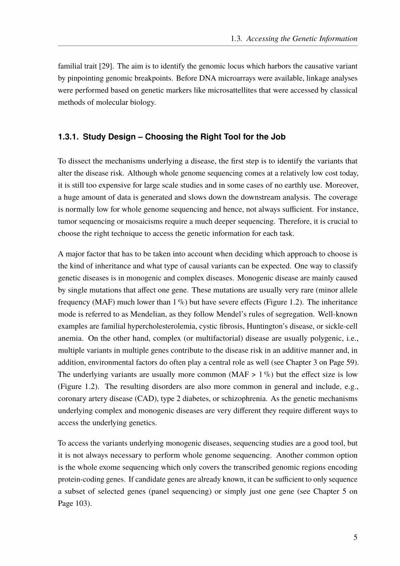
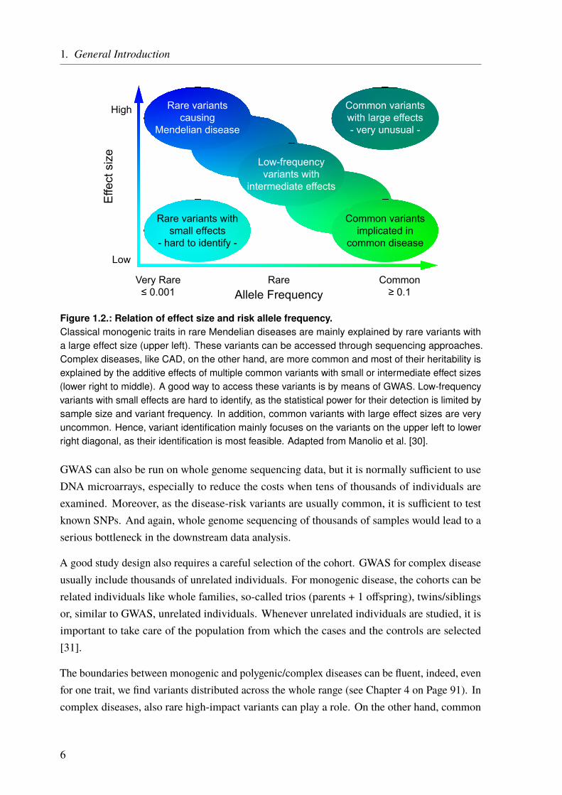
Figure 1.2.: Relation of effect size and risk allele frequency.Classical monogenic traits in rare Mendelian diseases are mainly explained by rare variants witha large effect size (upper left). These variants can be accessed through sequencing approaches.Complex diseases, like CAD, on the other hand, are more common and most of their heritability isexplained by the additive effects of multiple common variants with small or intermediate effect sizes(lower right to middle). A good way to access these variants is by means of GWAS. Low-frequencyvariants with small effects are hard to identify, as the statistical power for their detection is limited bysample size and variant frequency. In addition, common variants with large effect sizes are veryuncommon. Hence, variant identification mainly focuses on the variants on the upper left to lowerright diagonal, as their identification is most feasible. Adapted from Manolio et al. [30].
GWAS can also be run on whole genome sequencing data, but it is normally sufficient to useDNA microarrays, especially to reduce the costs when tens of thousands of individuals areexamined. Moreover, as the disease-risk variants are usually common, it is sufficient to testknown SNPs. And again, whole genome sequencing of thousands of samples would lead to aserious bottleneck in the downstream data analysis.
A good study design also requires a careful selection of the cohort. GWAS for complex diseaseusually include thousands of unrelated individuals. For monogenic disease, the cohorts can berelated individuals like whole families, so-called trios (parents + 1 offspring), twins/siblingsor, similar to GWAS, unrelated individuals. Whenever unrelated individuals are studied, it isimportant to take care of the population from which the cases and the controls are selected[31].
The boundaries between monogenic and polygenic/complex diseases can be fluent, indeed, evenfor one trait, we find variants distributed across the whole range (see Chapter 4 on Page 91). Incomplex diseases, also rare high-impact variants can play a role. On the other hand, common
6
1.4. Identifying the Right Variants/Genes
variants can modify the phenotype in an apparently monogenic disease. Hence, the right toolfor each task has to be selected carefully and it might be helpful in some situations to thinkoutside the box.
1.4. Identifying the Right Variants/Genes
Modern sequencing or microarray techniques make it relatively easy to access genetic infor-mation and to find single variants or potential disease-associated loci in a large number ofindividuals. To map a locus to a disease, the challenge is to identify the disease-causing variantsand/or genes from the list of candidates [32].
On average, we find 4.1 to 5.0 million positions that differ from the reference genome [25].The majority of these variants is common and shared by more than 0.5% of the population.Conversely, 40 000 – 200 000 rare variants of a genome are found in less than 0.5% of thepopulation. The germline de-novo mutation rate for single nucleotide variations (SNVs) wascalculated to be 1.0 – 1.8 · 10−8 per nucleotide per generation, resulting in 44 – 82 de-novoSNVs in the genome of every individual [33–38].
From this wealth of genomic data, we have to identify the right variant(s) that underlies theinvestigated disease. For rare Mendelian diseases, it is usually a good idea to focus on rarevariants first. Moreover, tools exist to predict the functional implications of SNVs based on,e.g., their conservation, localization in protein-coding regions, or regulatory elements (seePage 55). Some of them use machine learning methods and incorporate multiple scores andinformation into a single metric. However, these tools are of course limited by our incompleteknowledge about genetic mechanisms. And even if we identify variants that clearly impair agene’s function, it does not mean that these variants also have an effect on the phenotype. Infact, a recent study reported that even complete knockouts (KOs) of genes that were thought tobe essential, sometimes show no phenotypic effects [39]. This is also reflected by the high rateof reported damaging variants, which could not be replicated in later studies or were shown tobe false-positives. Analyses of databases like the human gene mutation database (HGMD®) orClinVar (see Page 57) showed that a lot of variants, one study reported 27%, marked to bedamaging and disease-associated, are in fact also present in healthy controls [40, 41]. Moreover,we do not only deal with damaging mutations but also protective ones. These protective allelescan also influence polygenic traits making it even harder to unravel the disease mechanisms[42].
Variant annotation is always the first step to get an overview and to start searching for the causalvariant by filtering the data (see Chapter 2.2 on Page 49). The exact approach depends on factors
7
1. General Introduction
such as the disease, cohort, and the analyzed data. Family studies, for example, are a great toolto find variants underlying rare Mendelian disease. If multiple family members are affected itis most likely that they share the same genetic variant. On the other hand, non-affected familymembers do not carry the variant. An example of a family study can be found in Chapter 5 onPage 103.
For complex diseases, studied by GWAS, the challenges are different. Given a sufficient samplesize and allele frequency, the problem is not so much to find loci that are associated withthe studied phenotype but rather to find the causal SNP at each locus and to understand itsfunctional implications. As explained before, GWAS test preselected variants for some ofwhich an association might be found. However, this does not mean that an identified variant iscausal itself, as association must not be confused with causality. The actual causal variant canbe one of the variants in linkage disequilibrium (LD) with the identified lead SNP (Chapter 3on Page 59). The second challenge is to unravel the underlying mechanisms of such a GWASlocus and to identify the involved or affected gene(s). This is not always straightforward and abioinformatics approach to functionally characterize GWAS loci is presented in Chapter 3 onPage 59.
No matter how good our annotations and predictions are, in the end, we might end up with a listof candidates. A perfect analogy is the search for the “needle in the stack of needles”, whichwas the title of a review on the identification of disease-causal variants [43]. Hence, functionalstudies are always the last step to validate the generated hypotheses.
1.5. The Goal of the Thesis
The central theme of my PhD was to unravel the genetics underlying cardiological traits.In the chapters 3 – 5, I describe three studies that required different sequencing techniques,computational toolsets, and study designs. The thesis moves along the diagonal shown inFigure 1.2 on Page 6 from the lower right to the upper left; from common variants with loweffect size to rare variants with strong effects.
The first approach, described in Chapter 3, is about the functional characterization of CADloci, which have been identified by GWAS. The main aim was to assign genes to the identifiedloci/SNPs and to rank these genes based on CAD relevance. As for all complex diseases, theSNPs are common and have rather low effect sizes (lower right corner in Figure 1.2).
In Chapter 4, a sequencing approach and the preliminary data of an ongoing project aredescribed. In this project, we aimed to assess the impact of rare variants with intermediate or
8

1.5. The Goal of the Thesis
large effects in selected CAD genes (middle to upper left corner in Figure 1.2). Although theheritability of CAD is largely attributed to common variants there is still a large fraction ofheritability that we cannot explain. Here we tried to unravel whether rare variants resolve partsof this “missing heritability” for CAD.
The next chapter (Chapter 5) describes a family study on congenital heart defects (CHDs) withan apparent monogenic type of inheritance. Although CHDs are mainly explained throughcomplex inheritance patterns, there are some examples of a monogenic inheritance in families.The goal of this study was to identify the presumably rare variant(s) with a large effect size(upper left corner in Figure 1.2) that we expected to underlie the observed phenotype. Based onthe results of the family study, we also performed a panel sequencing approach in a cohort ofunrelated individuals affected by CHDs.
9


2. General Methods
My methodology is not knowing what I’m doing and making that work for me.– Stone Gossard
2.1. High-Throughput Sequencing
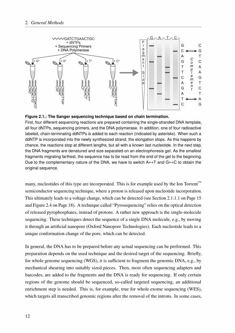
One of the first reliable DNA sequencing techniques was the one developed by Frederick Sangerin 1977 [20] (Figure 2.1) and it is based on the DNA replication mechanism described before.Most of the time, genomic DNA forms a double helix, consisting of two DNA strands. Thisdouble helix is split for DNA replication. During this process a new strand is synthesizedmatching the now single-stranded templates, forming a new double-stranded helix. This processis used for the Sanger sequencing technique. First, the template DNA is denatured by heat.The single-stranded DNA is then divided into four separate sequencing reactions, containingall four of the standard deoxynucleoside triphosphates (dNTPs) (dATP, dGTP, dCTP, anddTTP), sequencing primers, and a DNA polymerase. In addition, one of four chain-terminatingdideoxynucleotides triphosphates (ddNTPs) is added to each reaction. When such a nucleotideis incorporated into the elongating DNA strand, the elongation is terminated because of amissing 3’-hydroxyl group. As this happens by chance, different-sized fragments are produced,all with a known nucleotide at the end. Moreover, the ddNTPs are radioactive labeled. Usinggel electrophoresis the fragments can be separated by length and made visible under UV light.From the visible bands, the original DNA sequence can be reconstructed. The whole process isshown in Figure 2.1. Modern implementations of Sanger sequencing replaced the radioactivelabel by fluorophores. This is not only safer but in addition, different fluorophores can be usedper nucleotide. Hence, only one reaction is needed instead of four. Moreover, the whole processwas miniaturized and parallelized, using automated capillary sequencing machines. Instead ofusing an electrophoresis gel, the fragments are separated in a thin acrylic-fiber capillary and thefluorophores are detected by a laser and a camera while passing through the capillary.
Modern sequencing techniques are also often based on theDNAreplication principle (sequencingby synthesis). But the elongation is not terminated permanently. Often the incorporatednucleotides are detected more or less in real time. Illumina, e.g., uses dNTPs with an attachedfluorescence marker and a reversible terminator. After a nucleotide is incorporated, thecorresponding fluorophore is detected by a camera, the terminator is released, and the nextround starts. Other techniques only add one type of dNTPs at a time and detect if, and how
2. General Methods
GATCTGAACTGC+ dNTPs
+ G* + A* + T*
CTAG*CTAG
ACTTG*CTAG
ACTTGACG*
CTA*CTAG
A*CTAG
ACTTGA*
CT*CTAG
ACT*CTAG
ACTT*
C* CTAGAC*
CTAGACTTG
AC*
+ C*
+ DNA Polymerase+ Sequencing Primers
G A T CFragment Size
GCA
TG
GA
A
T
T
C
C
G
G
G
C
C
C
AA
A
T
T
T
Complement
Figure 2.1.: The Sanger sequencing technique based on chain termination.First, four different sequencing reactions are prepared containing the single-stranded DNA template,all four dNTPs, sequencing primers, and the DNA polymerase. In addition, one of four radioactivelabeled, chain-terminating ddNTPs is added to each reaction (indicated by asterisks). When such addNTP is incorporated into the newly synthesized strand, the elongation stops. As this happens bychance, the reactions stop at different lengths, but all with a known last nucleotide. In the next step,the DNA fragments are denatured and size separated on an electrophoresis gel. As the smallestfragments migrating farthest, the sequence has to be read from the end of the gel to the beginning.Due to the complementary nature of the DNA, we have to switch A↔T and G↔C to obtain theoriginal sequence.
many, nucleotides of this type are incorporated. This is for example used by the Ion Torrent™
semiconductor sequencing technique, where a proton is released upon nucleotide incorporation.This ultimately leads to a voltage change, which can be detected (see Section 2.1.1.1 on Page 15and Figure 2.4 on Page 18). A technique called “Pyrosequencing” relies on the optical detectionof released pyrophosphates, instead of protons. A rather new approach is the single-moleculesequencing. These techniques detect the sequence of a single DNA molecule, e.g., by movingit through an artificial nanopore (Oxford Nanopore Technologies). Each nucleotide leads to aunique conformation change of the pore, which can be detected.
In general, the DNA has to be prepared before any actual sequencing can be performed. Thispreparation depends on the used technique and the desired target of the sequencing. Briefly,for whole genome sequencing (WGS), it is sufficient to fragment the genomic DNA, e.g., bymechanical shearing into suitably sized pieces. Then, most often sequencing adapters andbarcodes, are added to the fragments and the DNA is ready for sequencing. If only certainregions of the genome should be sequenced, so-called targeted sequencing, an additionalenrichment step is needed. This is, for example, true for whole exome sequencing (WES),which targets all transcribed genomic regions after the removal of the introns. In some cases,
12
2.1. High-Throughput Sequencing
even smaller portions of the genome are targeted, e.g., a set of a few to hundreds of genes, onlycertain exons, or other selected regions. This is called “panel sequencing”. The enrichment isperformed to get a higher amount of the target DNA in a mixture with genomic DNA or isolatethe target DNA from the rest. A wide variety of enrichment techniques exist, all with theirspecific advantages and disadvantages.
In this thesis, WGS, WES, and panel sequencing were used. However, I will focus on themethodological description of two panel sequencing approaches, as these techniques are not ascommon as other techniques. In addition, WGS and WES were performed by service providersor cooperation partners, whereas the described techniques were established and utilized byme.
2.1.1. Gene Panel Sequencing
For the projects described in this thesis, two gene panel sequencing approaches were used. Acommercial one by Thermo Fisher Scientific, which uses the Ion AmpliSeq™ technology forlibrary construction together with Ion Torrent™ semiconductor sequencing (see Section 2.1.1.1on Page 15). This technique was used for the sequencing of an atrioventricular septaldefect (AVSD) cohort (see Chapter 5 on Page 103).
The other panel uses an enrichment technique based on molecular inversion probes (MIPs) andallows sequencing on almost every sequencer (see Section 2.1.1.2 on Page 27). In our case,the sequencing is done on the Illumina HiSeq system. We used this technique for the projectdescribed in Chapter 4 on Page 91.
13

2.1. High-Throughput Sequencing
2.1.1.1. Ion AmpliSeq Targeted Sequencing Technology
One approach that we used for a targeted sequencing is the Ion AmpliSeq™ technology byThermo Fisher Scientific (former Life Technologies) for library construction together withthe Ion Torrent™ semiconductor sequencing technology. We used the Ion Personal GenomeMachine™ (Ion PGM™) for sequencing. Benefits of this technology are the little DNA inputamounts (only 10 ng) and a very simple workflow because of polymerase chain reaction (PCR)-based target enrichment. In addition, it is very fast. Depending on the library and sample size ittakes only one day from DNA preparation to sequencing results. It is also very scalable, asup to 24 000 primers can be used per pool, which allows sequencing of one up to thousandsof genes and there are 96 barcodes available for multiplexing multiple samples. ThermoFisher Scientific offers several ready-to-use panels, e.g., for cancer research, inherited diseases,infectious diseases, human identification or whole exomes. In addition, custom panels can begenerated using the Ion AmpliSeq™ Designer online software.
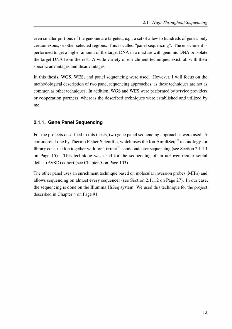
The general workflow of the Ion AmpliSeq™ technology is shown in Figure 2.2. After the panelis chosen or designed the library is constructed. It starts with a target enrichment by adding thepanel primers to each DNA sample and running a PCR. The primers are then partially digestedand sample-specific barcodes are added to the amplified targets. Next, the library is purifiedto remove all remains like salts or proteins. All samples are then equilibrated to the sameconcentration, a very crucial step to achieve similar sequencing coverage. Next, depending onthe panel size and the desired coverage, multiple equalized samples are pooled together.
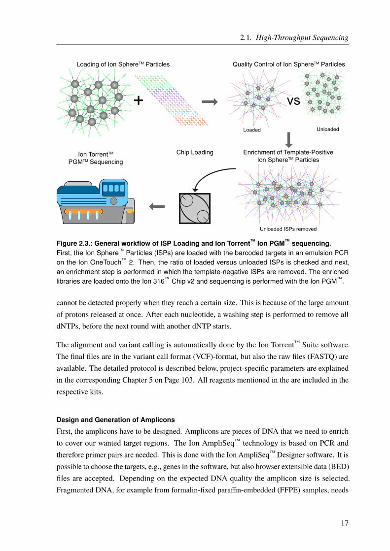
After the library preparation is done, the sequencing (preparation) is performed according toFigure 2.3 on Page 17. First, the sequencing templates are prepared using the Ion OneTouch™ 2machine. In an emulsion PCR, the barcoded targets are ligated to Ion Sphere™ Particles (ISPs)such that only one molecule binds to one ISP. This is a stochastic process, as a lot more ISPsthan DNA templates are added to an oily emulsion. The aim is to have one ISP together withone DNA molecule in a single oil droplet. In the PCR step, these molecules are amplified andall copies are still bound to the ISPs. The quality, i.e., the percentage of template-positive ISPsversus unloaded ISPs, is measured and next, the template-positive ISPs are enriched. Then,the finished sequencing templates are loaded onto the sequencing chip and in the last step, theactual semiconductor sequencing takes place on the Ion PGM™.
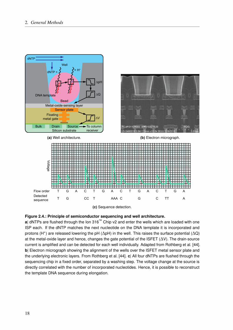
The basic principle of semiconductor sequencing was first described by Rothberg et al. [44]and is shown in Figure 2.4 on Page 18. The actual sequencing chip consists of millions ofsmall wells (3.5 µm), etched into a dielectric layer. On the bottom, there is a proton-sensitivemetal-oxide-sensing layer (tantalum oxide), which is connected to a sensor plate which actsas the gate of an ion-sensitive field-effect transistor (ISFET). The source terminal of the
15
2. General Methods
Probe Design
BMPR1A
Pool 1
Pool 2
Probe Ordering
Pool 2
Pool 1Target Amplification
Partial Primer Digestion
Amplificationand Equilibration
100 pM
Pooling of the Equalized Libraries
Adapter Ligation & Barcoding
P1 SequenceBarcoded Adapter A
Library Purification
SaltsProteins
Figure 2.2.: General workflow of the Ion AmpliSeq™ library preparation.The first step is the design of the probes in the Ion AmpliSeq™ Designer software. As some targetsare larger than the maximal amplicon size multiple amplicons are needed to cover these regions.These amplicons are designed in a way that they partially overlap to ensure complete coverage ofthe target regions. Hence, at least 2 primer pools are needed to avoid unspecific PCR productsfrom overlapping primers. With the primer pools, the DNA targets are amplified by PCR. Then,the primers are partially digested and sample-specific barcodes and adapters for sequencing andISP-binding are attached. Next, the library is purified and all samples are equilibrated to the sameDNA concentration. After this step, the barcoded samples can be pooled. FWD primer (orange),REV primer (dark blue), target DNA (black), amplified target (violet), P1 Sequence (green), barcode(light blue), Adapter A (red).
ISFET is connected to the sensing electronics. In each well, there is one ISP loaded with thesingle-stranded DNA templates. Now, one type of dNTPs at a time is washed over the chipsurface, entering the wells. If the respective dNTP matches the next nucleotide on the template,it is incorporated into the growing strand. This leads to the release of a proton (hydrogen ionH+), which lowers the pH of the well (∆pH). The lower pH raises the surface potential (∆Q) atthe metal-oxide layer and hence changes the gate potential leading to a current flow betweendrain and source (basic principle of a field-effect transistor (FET)). The current is then detectedfor each well individually. It has to be mentioned, that, of course, each bead is loaded with a lotof identical DNA templates, and therefore not only one proton is released. One disadvantageof this technique is the fact that long homopolymers, i.e., stretches of the same nucleotides,
16
2.1. High-Throughput Sequencing
Loading of Ion SphereTM Particles
+
Quality Control of Ion SphereTM Particles
vs
UnloadedLoaded
Enrichment of Template-PositiveIon SphereTM Particles
Unloaded ISPs removed
Chip LoadingIon TorrentTM
PGMTM Sequencing
Figure 2.3.: General workflow of ISP Loading and Ion Torrent™ Ion PGM™ sequencing.First, the Ion Sphere™ Particles (ISPs) are loaded with the barcoded targets in an emulsion PCRon the Ion OneTouch™ 2. Then, the ratio of loaded versus unloaded ISPs is checked and next,an enrichment step is performed in which the template-negative ISPs are removed. The enrichedlibraries are loaded onto the Ion 316™ Chip v2 and sequencing is performed with the Ion PGM™.
cannot be detected properly when they reach a certain size. This is because of the large amountof protons released at once. After each nucleotide, a washing step is performed to remove alldNTPs, before the next round with another dNTP starts.
The alignment and variant calling is automatically done by the Ion Torrent™ Suite software.The final files are in the variant call format (VCF)-format, but also the raw files (FASTQ) areavailable. The detailed protocol is described below, project-specific parameters are explainedin the corresponding Chapter 5 on Page 103. All reagents mentioned in the are included in therespective kits.
Design and Generation of Amplicons
First, the amplicons have to be designed. Amplicons are pieces of DNA that we need to enrichto cover our wanted target regions. The Ion AmpliSeq™ technology is based on PCR andtherefore primer pairs are needed. This is done with the Ion AmpliSeq™ Designer software. It ispossible to choose the targets, e.g., genes in the software, but also browser extensible data (BED)files are accepted. Depending on the expected DNA quality the amplicon size is selected.Fragmented DNA, for example from formalin-fixed paraffin-embedded (FFPE) samples, needs
17
2. General Methods
Well
dNTP
dNTP + + H+
DNA template
Metal-oxide-sensing layerSensor plate
Floatingmetal gate
Silicon substrateTo columnreceiver
Bulk Drain Source
Bead
(a) Well architecture. (b) Electron micrograph.
Voltage
Flow order T G A C T G A C T G A C T G ADetectedsequence T G CC T AAA C G C TT A
(c) Sequence detection.
Figure 2.4.: Principle of semiconductor sequencing and well architecture.a| dNTPs are flushed through the Ion 316™ Chip v2 and enter the wells which are loaded with oneISP each. If the dNTP matches the next nucleotide on the DNA template it is incorporated andprotons (H+) are released lowering the pH (∆pH) in the well. This raises the surface potential (∆Q)at the metal-oxide layer and hence, changes the gate potential of the ISFET (∆V). The drain-sourcecurrent is amplified and can be detected for each well individually. Adapted from Rothberg et al. [44].b| Electron micrograph showing the alignment of the wells over the ISFET metal sensor plate andthe underlying electronic layers. From Rothberg et al. [44]. c| All four dNTPs are flushed through thesequencing chip in a fixed order, separated by a washing step. The voltage change at the source isdirectly correlated with the number of incorporated nucleotides. Hence, it is possible to reconstructthe template DNA sequence during elongation.
18
2.1. High-Throughput Sequencing
shorter amplicons (125 – 175 bp). The amplicon size for normal DNA is 125 – 275 bp. If atarget, e.g., an exon, exceeds the maximal amplicon size, multiple amplicons are generated forthis area (see Figure 2.2 on Page 16). As they overlap, at least two separate primer pools haveto be generated to prevent a PCR reaction between the wrong primers. Finally, the softwareprovides statistics and information about the percentage of covered target regions, the totalsize of the panel, the amount of input DNA needed and the required library kits needed for theenrichment. The panel can then be ordered online.
Target Amplification
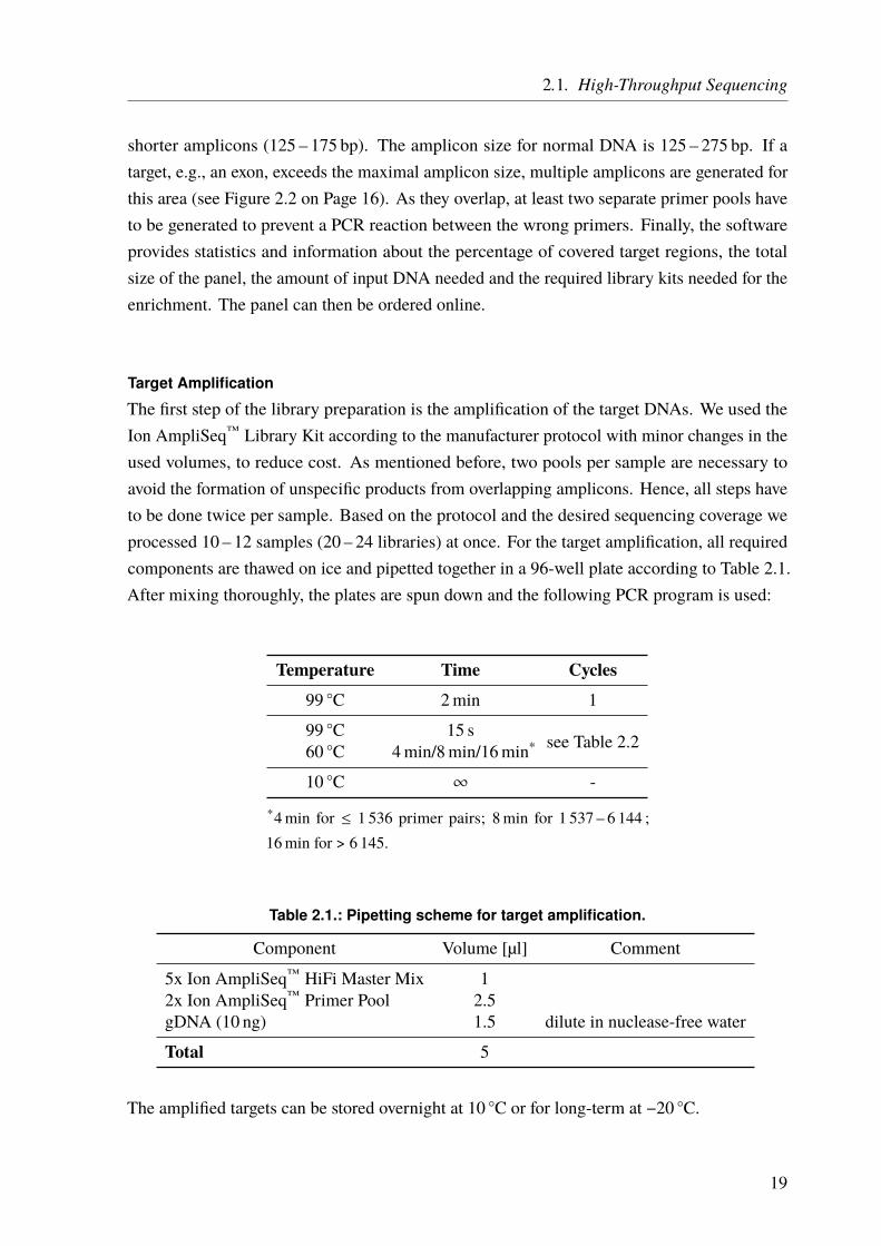
The first step of the library preparation is the amplification of the target DNAs. We used theIon AmpliSeq™ Library Kit according to the manufacturer protocol with minor changes in theused volumes, to reduce cost. As mentioned before, two pools per sample are necessary toavoid the formation of unspecific products from overlapping amplicons. Hence, all steps haveto be done twice per sample. Based on the protocol and the desired sequencing coverage weprocessed 10 – 12 samples (20 – 24 libraries) at once. For the target amplification, all requiredcomponents are thawed on ice and pipetted together in a 96-well plate according to Table 2.1.After mixing thoroughly, the plates are spun down and the following PCR program is used:
Temperature Time Cycles99 ◦C 2min 1
99 ◦C 15 s see Table 2.260 ◦C 4min/8min/16min*
10 ◦C ∞ -
*4min for ≤ 1 536 primer pairs; 8min for 1 537 – 6 144 ;16min for > 6 145.
Table 2.1.: Pipetting scheme for target amplification.
Component Volume [µl] Comment
5x Ion AmpliSeq™ HiFi Master Mix 12x Ion AmpliSeq™ Primer Pool 2.5gDNA (10 ng) 1.5 dilute in nuclease-free water
Total 5
The amplified targets can be stored overnight at 10 ◦C or for long-term at −20 ◦C.
19

2. General Methods
Table 2.2.: Number of cycles for target amplification.
Primer pairs per pool
Recommended number of amplification cycles(10 ng DNA, 3 000 copies)
High quality DNA Low quality DNA(FFPE DNA)
12 – 24 21 2425 – 48 20 2349 – 96 19 2297 – 192 18 21
193 – 384 17 20385 – 768 16 19769 – 1 536 15 18
1 537 – 3 072 14 173 073 – 6 144 13 166 145 – 12 288 12 15
12 289 – 24 576 11 14
Partial Primer Digestion
After the targets are amplified the primer sequences are partially digested by the “FuPa” reagent.This creates so-called “sticky ends”, i.e., overhangs of one of the two DNA strands. This isneeded for the ligation of the adapter sequences in the next step (Figure 2.5a).
The FuPa has to be handled on ice all the time. 1 µl is added to each library (total volume 6 µl).The reagents are mixed, spun down and the following program is used in a thermal cycler:
Temperature Time Cycles50 ◦C 10min 155 ◦C 10min 160 ◦C 20min 110 ◦C ∞ (up to 1 h) -
Adapter Ligation and Barcoding
In this step, the P1 adapters and the sample-specific barcodes are ligated to the amplified targets(Figure 2.5b). The P1 adapters are later needed for the ligation to the ISPs and the sample-specific barcodes allow pooling of multiple samples. The sequences can be demultiplexedlater, based on the barcodes. At this point, there are still two separate pools for each sample,meaning that both of this pools get the same barcode now. The barcode-adapter mix is preparedaccording to Table 2.3 with a unique barcode per sample.
20

2.1. High-Throughput Sequencing
+DNA Template
FuPa Reagent
Digested Template(a) Partial Primer Digestion.
P1 AdapterBarcoded Adapter A
Digested Template+
(b) Adapter Ligation & Barcoding.
Figure 2.5.: Partial primer digestion, adapter ligation, and barcoding.a| The amplified DNA targets are treated with the FuPa Reagent to partially digest the primers andcreate sticky ends for the next step. b| The partially digested primer sequences allow ligation ofthe P1 Adapter and the Adapter A with the attached sample-specific barcode. Both adapters areneeded for ISP loading and sequencing. FWD primer (orange), REV primer (dark blue), amplifiedtarget (violet), P1 Sequence (green), barcode (light blue), Adapter A (red).
Table 2.3.: Barcode-Adapter mix for 2 reactions.
Component Volume [µl] Comment
Ion P1 Adapter 1Ion Xpress™ Barcode X 1 X = choose one of 96 barcodesNuclease-free Water 2
Total 4
The reaction for the barcode/adapter ligation is prepared according to Table 2.4. In addition,1 µl DNA Ligase is added right before the samples are placed into the thermal cycler with thefollowing program:
Temperature Time Cycles22 ◦C 30min 172 ◦C 10min 110 ◦C ∞ -
Table 2.4.: Pipetting scheme for barcode/adapter ligation.
Component Volume [µl] Comment
Switch Solution 2Diluted Barcode-Adapter Mix 1 See Table 2.3Digested Amplicons 6
Total 9
21
2. General Methods
Purification of the Unamplified Library
To remove all remaining contaminants like proteins or salts, the samples are purified usingthe Agentcourt™ AMPure™ XPReagentThe Agentcourt™ AMPure™ XPReagent is warmedto room temperature and 70% Ethanol is prepared freshly (in Nuclease-free water). 22.5 µlAgentcourt™ AMPure™ XPReagent are added to each sample and mixed thoroughly followedby 5min incubation at room temperature. Next, the samples are placed in a magnetic rackand incubated for another 2min. The supernatant is carefully removed and discarded. Theremaining pellet is washed with 150 µl 70% Ethanol and the tube is placed in the magneticrack for 2min again. The supernatant is discarded and the washing repeated. After additional2min in the magnetic rack, the Ethanol is removed completely (including all droplets) and thepellet is dried for ≈ 5min. Attention has to be paid to not overdry the pellet. The next stepfollows immediately.
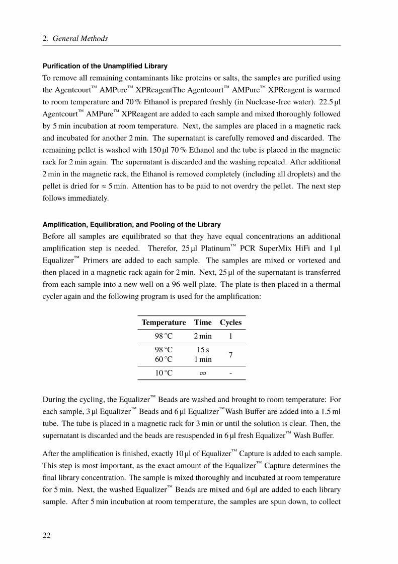
Amplification, Equilibration, and Pooling of the Library
Before all samples are equilibrated so that they have equal concentrations an additionalamplification step is needed. Therefor, 25 µl Platinum™ PCR SuperMix HiFi and 1 µlEqualizer™ Primers are added to each sample. The samples are mixed or vortexed andthen placed in a magnetic rack again for 2min. Next, 25 µl of the supernatant is transferredfrom each sample into a new well on a 96-well plate. The plate is then placed in a thermalcycler again and the following program is used for the amplification:
Temperature Time Cycles98 ◦C 2min 1
98 ◦C 15 s 760 ◦C 1min
10 ◦C ∞ -
During the cycling, the Equalizer™ Beads are washed and brought to room temperature: Foreach sample, 3 µl Equalizer™ Beads and 6 µl Equalizer™Wash Buffer are added into a 1.5mltube. The tube is placed in a magnetic rack for 3min or until the solution is clear. Then, thesupernatant is discarded and the beads are resuspended in 6 µl fresh Equalizer™ Wash Buffer.
After the amplification is finished, exactly 10 µl of Equalizer™ Capture is added to each sample.This step is most important, as the exact amount of the Equalizer™ Capture determines thefinal library concentration. The sample is mixed thoroughly and incubated at room temperaturefor 5min. Next, the washed Equalizer™ Beads are mixed and 6 µl are added to each librarysample. After 5min incubation at room temperature, the samples are spun down, to collect
22
2.1. High-Throughput Sequencing
all liquid/droplets, and are placed in a magnetic rack for 2min or until the solution is clear.The supernatant is removed carefully and kept, in case any problems occur. Now, the pelletis washed twice by adding 150 µl Equalizer™ Wash Buffer to the pellets, moving it inside themagnetic rack to rinse the beads and finally incubate it for 2min in the magnetic rack or untilthe solution is clear. The Equalizer™ Wash Buffer is completely removed carefully withoutdisturbing the pellet.
Next, the equalized library is eluted. The samples are removed from the magnetic rack and100 µl Equalizer™ Elution Buffer is added to each pellet. The samples are vortexed and spundown to collect all droplets and then placed in a thermal cycler at 32 ◦C for 5min. Now, thesamples are placed in the magnetic rack again for 5min or until the solution is clear. Thesupernatant now contains the equalized library at a 100 pM and can be stored for up to onemonth at 4 – 8 ◦C. Long-term storage is possible at −20 ◦C. In the last step, the libraries of thedifferentially barcoded samples can be combined with equal volumes, e.g., 10 µl of each sampleis pooled in a 1.5ml tube.
Loading of Ion Sphere™ Particles
For the generation of template-positive ISPs, we used the Ion PGM™ Template OT2 200 Kitand the Ion OneTouch™ 2 System. In this step, the barcoded amplicons bind the ISPs with theiradapter sequence. It is most important to have the correct ratio between DNA and ISPs, so that,based on stochastics, only one DNA molecule binds to one ISP within one oil droplet. In anemulsion PCR, the DNA molecules are amplified and the result is as many ISPs as possiblecompletely loaded with the copies of only one template molecule (monoclonal ISPs). First,the Ion OneTouch™ 2 has to be cleaned and prepared according to the user manual. Thepooled libraries, equilibrated to 100 pM, are diluted again. For DNA sequencing on the IonPGM™, 2 µl of the sample pool are added to 23 µl nuclease-free water. Next, the amplificationsolution is prepared by warming the provided Reagent Mix, the Reagent B, and the ISPs toroom temperature and vortexing them. The Ion OneTouch™ 2 Enzyme Mix is vortexed for 2 sand put on ice, as well as the pooled and diluted library. The reaction is prepared accordingto Table 2.5; reagents are added in the order listed. Next, the solution is vortexed and spundown.
The next step is the preparation of the ISPs. First, they need to be vortexed for 1min atmaximum speed to make sure they are resuspended very well. Then, they are spun down (2 s)and immediately after this 100 µl of the ISPs are added to the 900 µl amplification solution.After vortexing for 5 s, the solution is transferred into the Ion OneTouch™ 2 machine, accordingto the instructions. Next, the Ion OneTouch™ 2 is started and the run takes roughly 5 h.
23
2. General Methods
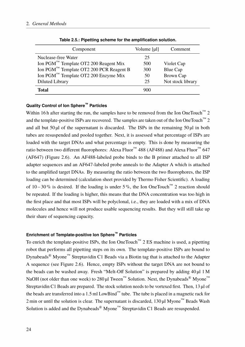
Table 2.5.: Pipetting scheme for the amplification solution.
Component Volume [µl] Comment
Nuclease-free Water 25Ion PGM™ Template OT2 200 Reagent Mix 500 Violet CapIon PGM™ Template OT2 200 PCR Reagent B 300 Blue CapIon PGM™ Template OT2 200 Enzyme Mix 50 Brown CapDiluted Library 25 Not stock library
Total 900
Quality Control of Ion Sphere™ Particles
Within 16 h after starting the run, the samples have to be removed from the Ion OneTouch™ 2and the template-positive ISPs are recovered. The samples are taken out of the Ion OneTouch™ 2and all but 50 µl of the supernatant is discarded. The ISPs in the remaining 50 µl in bothtubes are resuspended and pooled together. Next, it is assessed what percentage of ISPs areloaded with the target DNAs and what percentage is empty. This is done by measuring theratio between two different fluorophores: Alexa Fluor™ 488 (AF488) and Alexa Fluor™ 647(AF647) (Figure 2.6). An AF488-labeled probe binds to the B primer attached to all ISPadapter sequences and an AF647-labeled probe anneals to the Adapter A which is attachedto the amplified target DNAs. By measuring the ratio between the two fluorophores, the ISPloading can be determined (calculation sheet provided by Thermo Fisher Scientific). A loadingof 10 – 30% is desired. If the loading is under 5%, the Ion OneTouch™ 2 reaction shouldbe repeated. If the loading is higher, this means that the DNA concentration was too high inthe first place and that most ISPs will be polyclonal, i.e., they are loaded with a mix of DNAmolecules and hence will not produce usable sequencing results. But they will still take uptheir share of sequencing capacity.
Enrichment of Template-positive Ion Sphere™ Particles
To enrich the template-positive ISPs, the Ion OneTouch™ 2 ES machine is used, a pipettingrobot that performs all pipetting steps on its own. The template-positive ISPs are bound toDynabeads® Myone™ Streptavidin C1 Beads via a Biotin tag that is attached to the AdapterA sequence (see Figure 2.6). Hence, empty ISPs without the target DNA are not bound tothe beads can be washed away. Fresh “Melt-Off Solution” is prepared by adding 40 µl 1MNaOH (not older than one week) to 280 µl Tween™ Solution. Next, the Dynabeads® Myone™
Streptavidin C1 Beads are prepared. The stock solution needs to be vortexed first. Then, 13 µl ofthe beads are transferred into a 1.5ml LowBind™ tube. The tube is placed in a magnetic rack for2min or until the solution is clear. The supernatant is discarded, 130 µl Myone™ Beads WashSolution is added and the Dynabeads® Myone™ Streptavidin C1 Beads are resuspended.
24

2.1. High-Throughput Sequencing
AF 488
AF 488
AF 488
AF 488
AF 488
AF 488
AF 488
AF 488
B Primer
P1 Seq
uenc
e
Targe
t DNA
Digeste
d FWD Prim
er
Digeste
d Rev
Primer
Barcod
e
Adapte
r A
ISP AF 647
Biotin
Figure 2.6.: Quality control of Ion Sphere™ Particles after emulsion PCR.After the emulsion PCR, some of the ISPs are loaded with the DNA samples (only one strandshown here) or are empty. The percentage of loaded versus unloaded ISPs can be detected bya fluorometer. This is done by measuring the ratio between the two different fluorophores AlexaFluor™ 488 (AF488) and Alexa Fluor™ 647 (AF647). An AF488-labeled probe binds to the B primerattached to all ISP adapter sequences and an AF647-labeled probe anneals to the Adapter A whichis attached only to the amplified target DNAs. In addition, the Adapter A is Biotin-labeled, whichallows binding of the template-positive ISPs to Dynabeads® Myone™ Streptavidin C1 Beads duringthe enrichment step.
An 8-well strip is loaded according to Table 2.6 and placed in the Ion OneTouch™ 2 ES.In addition, a 0.2ml PCR tube filled with 10 µl Neutralization Solution is placed in the IonOneTouch™ 2 ES.
Table 2.6.: Loading of an 8-well strip to enrich template-positive Ion Sphere™ Particles.
Well Component Volume [µl] Comment
1 Template-positive ISPs 100
2 Dynabeads® Myone™
Streptavidin C1 Beads 130 washed in Myone™ Beads WashSolution and resuspended
3 Ion OneTouch™ 2 Wash Solution 3004 Ion OneTouch™ 2 Wash Solution 3005 Ion OneTouch™ 2 Wash Solution 3006 empty -7 Melt-Off Solution 300 freshly prepared8 empty -
The Ion OneTouch™ 2 ES is started and after around 35min of running time the enriched ISPs(≈ 200 µl) can be found in the collection PCR tube. The tube is closed an inverted 5 timesbefore proceeding. The enriched ISPs can be stored for up to three days at 2 – 8 ◦C before thesequencing run is started.
25
2. General Methods
Ion Torrent™ Ion PGM™ Sequencing
As the semiconductor sequencing is based on the release and detection of hydrogen ions (orprotons H+), the Ion PGM™ needs a lot of washing and cleaning with chloride solutions andultrapure water (Resistivity > 18MW cm at 25 ◦C) to achieve the right pH. The cleaning stepsand the initialization are performed according to the Ion PGM™ user guide. For differentsized panels/coverages, there are different sequencing chips available. We used the Ion 316™
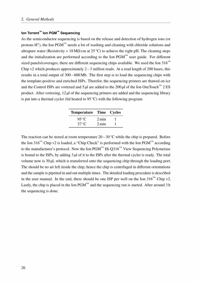
Chip v2 which produces approximately 2 – 3 million reads. At a read length of 200 bases, thisresults in a total output of 300 – 600Mb. The first step is to load the sequencing chips withthe template-positive and enriched ISPs. Therefor, the sequencing primers are thawed on iceand the Control ISPs are vortexed and 5 µl are added to the 200 µl of the Ion OneTouch™ 2 ESproduct. After vortexing, 12 µl of the sequencing primers are added and the sequencing libraryis put into a thermal cycler (lid heated to 95 ◦C) with the following program:
Temperature Time Cycles95 ◦C 2min 137 ◦C 2min 1
The reaction can be stored at room temperature 20 – 30 ◦C while the chip is prepared. Beforethe Ion 316™ Chip v2 is loaded, a “Chip Check” is performed with the Ion PGM™ accordingto the manufacturer’s protocol. Now the Ion PGM™ Hi-Q316™ View Sequencing Polymeraseis bound to the ISPs, by adding 3 µl of it to the ISPs after the thermal cycler is ready. The totalvolume now is 30 µl, which is transferred onto the sequencing chip through the loading port.The should be no air left inside the chip; hence the chip is centrifuged in different orientationsand the sample is pipetted in and out multiple times. The detailed loading procedure is describedin the user manual. In the end, there should be one ISP per well on the Ion 316™ Chip v2.Lastly, the chip is placed in the Ion PGM™ and the sequencing run is started. After around 3 hthe sequencing is done.
26
2.1. High-Throughput Sequencing
2.1.1.2. Molecular Inversion Probes
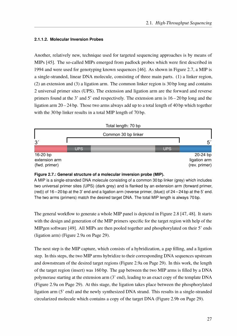
Another, relatively new, technique used for targeted sequencing approaches is by means ofMIPs [45]. The so-called MIPs emerged from padlock probes which were first described in1994 and were used for genotyping known sequences [46]. As shown in Figure 2.7, a MIP isa single-stranded, linear DNA molecule, consisting of three main parts. (1) a linker region,(2) an extension and (3) a ligation arm. The common linker region is 30 bp long and contains2 universal primer sites (UPS). The extension and ligation arm are the forward and reverseprimers found at the 3’ and 5’ end respectively. The extension arm is 16 – 20 bp long and theligation arm 20 – 24 bp. Those two arms always add up to a total length of 40 bp which togetherwith the 30 bp linker results in a total MIP length of 70 bp.
UPS
Common 30 bp linker
3´ 5´
16-20 bpextension arm(fwd. primer)
20-24 bpligation arm(rev. primer)
Total length: 70 bp
UPS
Figure 2.7.: General structure of a molecular inversion probe (MIP).A MIP is a single-stranded DNA molecule consisting of a common 30 bp linker (grey) which includestwo universal primer sites (UPS) (dark grey) and is flanked by an extension arm (forward primer,(red)) of 16 – 20 bp at the 3’ end and a ligation arm (reverse primer, (blue)) of 24 – 24 bp at the 5’ end.The two arms (primers) match the desired target DNA. The total MIP length is always 70 bp.
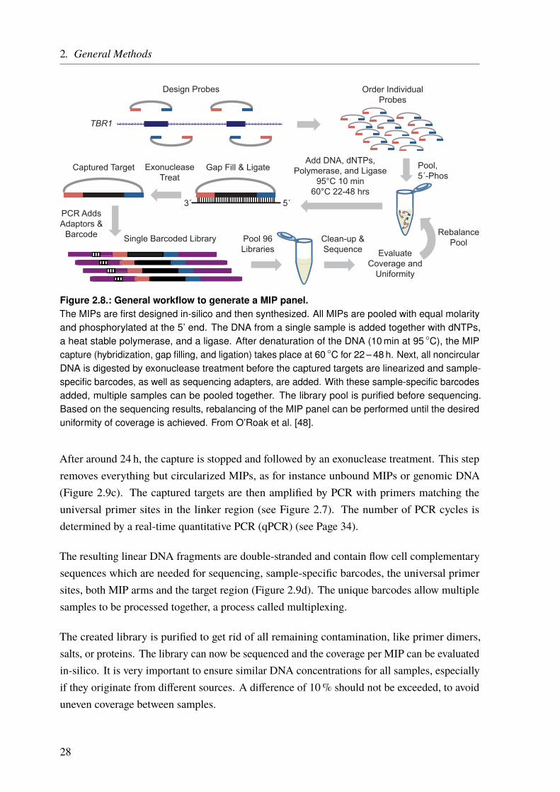
The general workflow to generate a whole MIP panel is depicted in Figure 2.8 [47, 48]. It startswith the design and generation of the MIP primers specific for the target region with help of theMIPgen software [49]. All MIPs are then pooled together and phosphorylated on their 5’ ends(ligation arm) (Figure 2.9a on Page 29).
The next step is the MIP capture, which consists of a hybridization, a gap filling, and a ligationstep. In this steps, the two MIP arms hybridize to their corresponding DNA sequences upstreamand downstream of the desired target regions (Figure 2.9a on Page 29). In this work, the lengthof the target region (insert) was 160 bp. The gap between the two MIP arms is filled by a DNApolymerase starting at the extension arm (3’ end), leading to an exact copy of the template DNA(Figure 2.9a on Page 29). At this stage, the ligation takes place between the phosphorylatedligation arm (5’ end) and the newly synthesized DNA strand. This results in a single-strandedcircularized molecule which contains a copy of the target DNA (Figure 2.9b on Page 29).
27
2. General Methods
PCR AddsAdaptors &
Barcode Single Barcoded Library Pool 96Libraries
Clean-up &Sequence Evaluate
Coverage andUniformity
RebalancePool
5´3´
Gap Fill & LigateExonucleaseTreat
Captured TargetAdd DNA, dNTPs,
Polymerase, and Ligase95°C 10 min
60°C 22-48 hrs
Pool,5´-Phos
Order IndividualProbes
Design Probes
TBR1
Figure 2.8.: General workflow to generate a MIP panel.The MIPs are first designed in-silico and then synthesized. All MIPs are pooled with equal molarityand phosphorylated at the 5’ end. The DNA from a single sample is added together with dNTPs,a heat stable polymerase, and a ligase. After denaturation of the DNA (10 min at 95 ◦C), the MIPcapture (hybridization, gap filling, and ligation) takes place at 60 ◦C for 22 – 48 h. Next, all noncircularDNA is digested by exonuclease treatment before the captured targets are linearized and sample-specific barcodes, as well as sequencing adapters, are added. With these sample-specific barcodesadded, multiple samples can be pooled together. The library pool is purified before sequencing.Based on the sequencing results, rebalancing of the MIP panel can be performed until the desireduniformity of coverage is achieved. From O’Roak et al. [48].
After around 24 h, the capture is stopped and followed by an exonuclease treatment. This stepremoves everything but circularized MIPs, as for instance unbound MIPs or genomic DNA(Figure 2.9c). The captured targets are then amplified by PCR with primers matching theuniversal primer sites in the linker region (see Figure 2.7). The number of PCR cycles isdetermined by a real-time quantitative PCR (qPCR) (see Page 34).
The resulting linear DNA fragments are double-stranded and contain flow cell complementarysequences which are needed for sequencing, sample-specific barcodes, the universal primersites, both MIP arms and the target region (Figure 2.9d). The unique barcodes allow multiplesamples to be processed together, a process called multiplexing.
The created library is purified to get rid of all remaining contamination, like primer dimers,salts, or proteins. The library can now be sequenced and the coverage per MIP can be evaluatedin-silico. It is very important to ensure similar DNA concentrations for all samples, especiallyif they originate from different sources. A difference of 10% should not be exceeded, to avoiduneven coverage between samples.
28
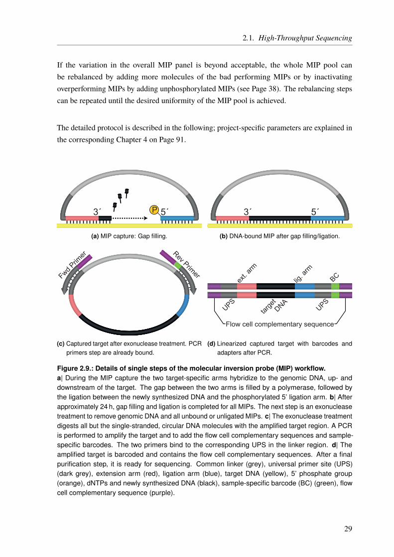
2.1. High-Throughput Sequencing
If the variation in the overall MIP panel is beyond acceptable, the whole MIP pool canbe rebalanced by adding more molecules of the bad performing MIPs or by inactivatingoverperforming MIPs by adding unphosphorylated MIPs (see Page 38). The rebalancing stepscan be repeated until the desired uniformity of the MIP pool is achieved.
The detailed protocol is described in the following; project-specific parameters are explained inthe corresponding Chapter 4 on Page 91.
P3´ 5´
(a) MIP capture: Gap filling.
3´ 5´
(b) DNA-bound MIP after gap filling/ligation.
Fwd Prim
er Rev Primer
(c) Captured target after exonuclease treatment. PCRprimers step are already bound.
Flow cell complementary sequence
BC
UPSUPS
ext. a
rm
lig. a
rm
targe
t
DNA
(d) Linearized captured target with barcodes andadapters after PCR.
Figure 2.9.: Details of single steps of the molecular inversion probe (MIP) workflow.a| During the MIP capture the two target-specific arms hybridize to the genomic DNA, up- anddownstream of the target. The gap between the two arms is filled by a polymerase, followed bythe ligation between the newly synthesized DNA and the phosphorylated 5’ ligation arm. b| Afterapproximately 24 h, gap filling and ligation is completed for all MIPs. The next step is an exonucleasetreatment to remove genomic DNA and all unbound or unligated MIPs. c| The exonuclease treatmentdigests all but the single-stranded, circular DNA molecules with the amplified target region. A PCRis performed to amplify the target and to add the flow cell complementary sequences and sample-specific barcodes. The two primers bind to the corresponding UPS in the linker region. d| Theamplified target is barcoded and contains the flow cell complementary sequences. After a finalpurification step, it is ready for sequencing. Common linker (grey), universal primer site (UPS)(dark grey), extension arm (red), ligation arm (blue), target DNA (yellow), 5’ phosphate group(orange), dNTPs and newly synthesized DNA (black), sample-specific barcode (BC) (green), flowcell complementary sequence (purple).
29
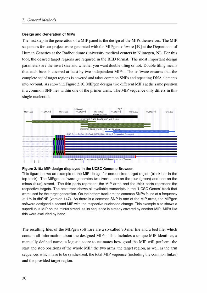
2. General Methods
Design and Generation of MIPs
The first step in the generation of a MIP panel is the design of the MIPs themselves. The MIPsequences for our project were generated with the MIPgen software [49] at the Department ofHuman Genetics at the Radboudumc (university medical center) in Nijmegen, NL. For thistool, the desired target regions are required in the BED format. The most important designparameters are the insert size and whether you want double tiling or not. Double tiling meansthat each base is covered at least by two independent MIPs. The software ensures that thecomplete set of target regions is covered and takes common SNPs and repeating DNA elementsinto account. As shown in Figure 2.10, MIPgen designs two different MIPs at the same positionif a common SNP lies within one of the primer arms. The MIP sequence only differs in thissingle nucleotide.
100 bases hg19
11,241,900 11,241,950 11,242,000 11,242,050 11,242,100 11,242,150 11,242,200 11,242,250 11,242,300Wanted_regions
520822316_FINAL_PANEL_CAD_AH_f0_plus
520822316_FINAL_PANEL_CAD_AH_f0_minus
UCSC Genes (RefSeq, GenBank, CCDS, Rfam, tRNAs & Comparative Genomics)
Simple Nucleotide Polymorphisms (dbSNP 147) Found in >= 1% of Samples
Figure 2.10.: MIP design displayed in the UCSC Genome Browser.This figure shows an example of the MIP design for one desired target region (black bar in thetop track). The MIPgen software generates two tracks, one on the plus (green) and one on theminus (blue) strand. The thin parts represent the MIP arms and the thick parts represent therespective targets. The next track shows all available transcripts in the “UCSC Genes” track thatwere used for the target generation. On the bottom track are the common SNPs found at a frequency≥ 1 % in dbSNP (version 147). As there is a common SNP in one of the MIP arms, the MIPgensoftware designed a second MIP with the respective nucleotide change. This example also shows asuperfluous MIP on the minus strand, as its sequence is already covered by another MIP. MIPs likethis were excluded by hand.
The resulting files of the MIPgen software are a so-called 70-mer file and a bed file, whichcontain all information about the designed MIPs. This includes a unique MIP identifier, amanually defined name, a logistic score to estimates how good the MIP will perform, thestart and stop positions of the whole MIP, the two arms, the target region, as well as the armsequences which have to be synthesized, the total MIP sequence (including the common linker)and the provided target region.
30
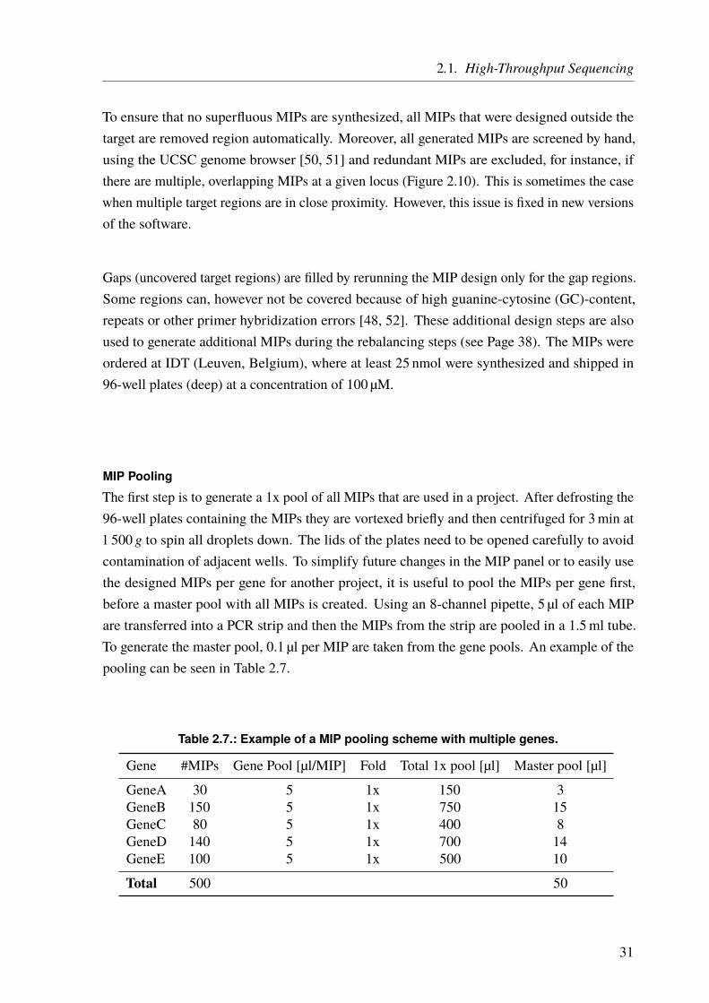
2.1. High-Throughput Sequencing
To ensure that no superfluous MIPs are synthesized, all MIPs that were designed outside thetarget are removed region automatically. Moreover, all generated MIPs are screened by hand,using the UCSC genome browser [50, 51] and redundant MIPs are excluded, for instance, ifthere are multiple, overlapping MIPs at a given locus (Figure 2.10). This is sometimes the casewhen multiple target regions are in close proximity. However, this issue is fixed in new versionsof the software.
Gaps (uncovered target regions) are filled by rerunning the MIP design only for the gap regions.Some regions can, however not be covered because of high guanine-cytosine (GC)-content,repeats or other primer hybridization errors [48, 52]. These additional design steps are alsoused to generate additional MIPs during the rebalancing steps (see Page 38). The MIPs wereordered at IDT (Leuven, Belgium), where at least 25 nmol were synthesized and shipped in96-well plates (deep) at a concentration of 100 µM.
MIP Pooling
The first step is to generate a 1x pool of all MIPs that are used in a project. After defrosting the96-well plates containing the MIPs they are vortexed briefly and then centrifuged for 3min at1 500 g to spin all droplets down. The lids of the plates need to be opened carefully to avoidcontamination of adjacent wells. To simplify future changes in the MIP panel or to easily usethe designed MIPs per gene for another project, it is useful to pool the MIPs per gene first,before a master pool with all MIPs is created. Using an 8-channel pipette, 5 µl of each MIPare transferred into a PCR strip and then the MIPs from the strip are pooled in a 1.5ml tube.To generate the master pool, 0.1 µl per MIP are taken from the gene pools. An example of thepooling can be seen in Table 2.7.
Table 2.7.: Example of a MIP pooling scheme with multiple genes.
Gene #MIPs Gene Pool [µl/MIP] Fold Total 1x pool [µl] Master pool [µl]
GeneA 30 5 1x 150 3GeneB 150 5 1x 750 15GeneC 80 5 1x 400 8GeneD 140 5 1x 700 14GeneE 100 5 1x 500 10
Total 500 50
31

2. General Methods
MIP Phosphorylation
For the ligation step the, MIPs are phosphorylated at their 5’ end (ligation arm). The componentvolumes for the phosphorylation are calculated according to the example in Table 2.8 and arepooled together in 200 µl PCR tubes. To ensure optimal thermal conditions it is important tomake sure not to exceed 100 µl per tube. The phosphorylation takes place in a thermal cyclerand the following program is used:
Temperature Time Cycles37 ◦C 45min 165 ◦C 20min 14 ◦C ∞ –
If multiple tubes are used, they are pooled after this step.
Table 2.8.: Pipetting scheme for MIP phosphorylation.
Component Volume [µl] Comment
MIPs (0.1 µl pool) 50T4 PNK 2 1 µl per 25 µl of 100 µMMIPswater (H2O) 2 Add for a total volume10x T4 DNA ligase buffer with 10mM ATP 6 10% of total volume
Total 60
MIP Capture
The final MIP pool concentration (C f = 0.16 µM) is calculated according to the equation:
C f =Ci ∗ Vi
Vf
where Ci is the initial MIP concentration (100 µM), Vi the initial volume per MIP (0.1 µl) andVf the final volume of the MIP pool (60 µl). This concentration is used to calculate how manyMIP molecules are needed per sample. The ratio of MIPs to a haploid genome is 800 : 1.As there are 330 haploid genome copies per ng genomic DNA, 26.4 · 106 MIP molecules areadded per 100 ng genomic DNA:
Needed MIPs = 330haploid genomes
1 ng genomic DNA∗ 100 ng DNA ∗ 800
MIPs1 haploid genome
32

2.1. High-Throughput Sequencing
This equals to 4.38 · 10−5 pmol or 2.63 · 10−4 µl of the final MIP pool per sample:
26.4 · 106 MIPsNA
≈ 4.38 · 10−5 pmol4.38 · 10−5 pmol
C f≈ 2.63 · 10−4 µl
where NA is the Avogadro constant (6.022 140 857 · 1023mol−1) [53] and C f the final MIPconcentration (0.16 µM). To get a volume which can be handled better, the MIP pool is diluted.In this example, we diluted twice 1:30 (total 1:900). The volume of this diluted pool, to beadded per sample with 100 ng DNA, is:
2.63 · 10−4 µl900
≈ 0.24 µl
The master mix for the MIP capture is prepared according to Table 2.9. As the amount ofAmpligase is most critical, it is very important not to pipette less than 0.30 µl. Therefore, thecapture is always prepared for at least 30 reactions. 15 µl of this mix are then added to 100 ngDNA in 10 µl, making it a total volume of 25 µl per reaction. In addition, a blank control (10 µlwater) is prepared. The following PCR program is used for the capture, which is stopped bycooling the samples down on ice immediately followed by the exonuclease treatment:
Temperature Time Cycles95 ◦C 10min 160 ◦C 22 – 24 h 1
Table 2.9.: Pipetting scheme for MIP capture.At least 30 reactions are prepared due to the low Ampligase volume.
Component Volume [µl] Comment
10x Ampligase DNA Ligase Buffer 2.50MIP pool dilution 0.24 Calculated beforedNTPs (0.25 µM) 0.032Hemo Klentaq (10U µl−1) 0.32Ampligase DNA Ligase (100U µl−1) 0.01 Most critical. Pipette at least 0.30 µlH2O 11.90 Add for total volume
Total master mix 15
Sample DNA (100 ng) 10 Dilute 100 ng in 10 µl
Total 25
33

2. General Methods
Exonuclease Treatment
A master mix for the exonuclease treatment of the captured MIP pool is prepared according toTable 2.10. After cooling down, 2 µl of the master mix are added to each captured sample andthe water control. The following PCR program is used for the exonuclease treatment:
Temperature Time Cycles37 ◦C 45min 195 ◦C 2min 14 ◦C ∞ –
Table 2.10.: Pipetting scheme for MIP exonuclease treatment.
Component Volume [µl]
EXO I 0.5EXO III 0.510x Ampligase DNA Ligase Buffer 0.2H2O 0.8
Total master mix 2
Captured samples 25
Total 27
Real-Time Quantitative PCR (qPCR)
The qPCR is performed using a real-time PCR machine. We used a Rotor-Gene (Qiagen, Venlo,Netherlands). A master mix is prepared according to Table 2.11. It contains a common forwardprimer for all samples. 18.75 µl of the master mix are then added to 1.25 µl of a sample-specificreverse primer and 5 µl of the exonuclease treated samples/controls. After brief vortexing andspinning down the samples, the following qPCR program is used:
Temperature Time Cycles98 ◦C 30 s 1
98 ◦C 10 s60 ◦C 30 s 3572 ◦C 30 s
72 ◦C 2min 125 ◦C ∞ -
34
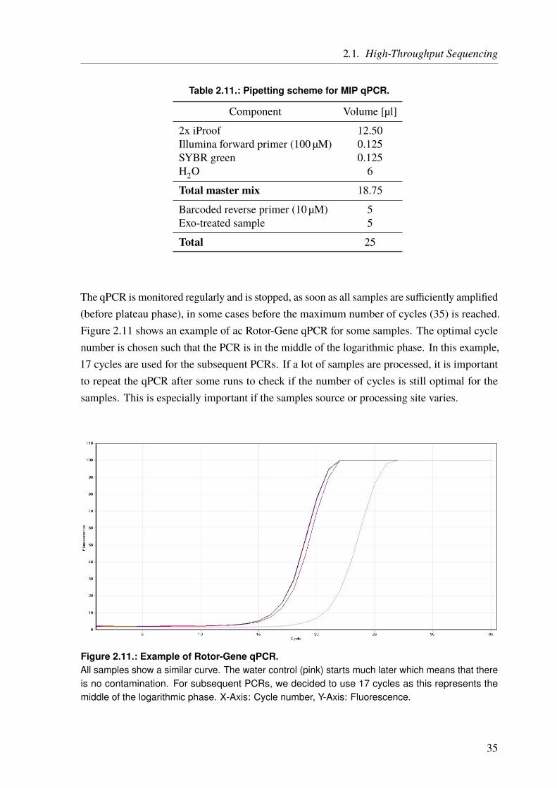
2.1. High-Throughput Sequencing
Table 2.11.: Pipetting scheme for MIP qPCR.
Component Volume [µl]
2x iProof 12.50Illumina forward primer (100 µM) 0.125SYBR green 0.125H2O 6
Total master mix 18.75
Barcoded reverse primer (10 µM) 5Exo-treated sample 5
Total 25
The qPCR is monitored regularly and is stopped, as soon as all samples are sufficiently amplified(before plateau phase), in some cases before the maximum number of cycles (35) is reached.Figure 2.11 shows an example of ac Rotor-Gene qPCR for some samples. The optimal cyclenumber is chosen such that the PCR is in the middle of the logarithmic phase. In this example,17 cycles are used for the subsequent PCRs. If a lot of samples are processed, it is importantto repeat the qPCR after some runs to check if the number of cycles is still optimal for thesamples. This is especially important if the samples source or processing site varies.
Figure 2.11.: Example of Rotor-Gene qPCR.All samples show a similar curve. The water control (pink) starts much later which means that thereis no contamination. For subsequent PCRs, we decided to use 17 cycles as this represents themiddle of the logarithmic phase. X-Axis: Cycle number, Y-Axis: Fluorescence.
35
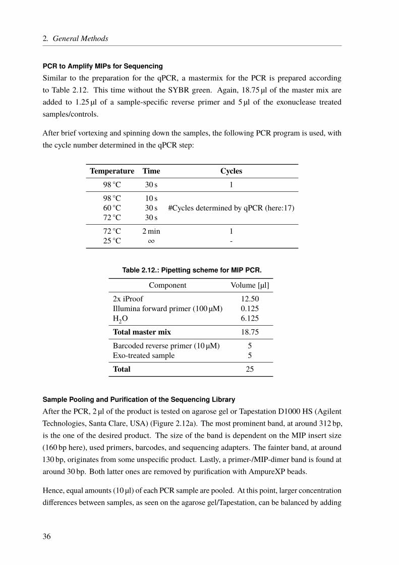
2. General Methods
PCR to Amplify MIPs for Sequencing
Similar to the preparation for the qPCR, a mastermix for the PCR is prepared accordingto Table 2.12. This time without the SYBR green. Again, 18.75 µl of the master mix areadded to 1.25 µl of a sample-specific reverse primer and 5 µl of the exonuclease treatedsamples/controls.
After brief vortexing and spinning down the samples, the following PCR program is used, withthe cycle number determined in the qPCR step:
Temperature Time Cycles98 ◦C 30 s 1
98 ◦C 10 s60 ◦C 30 s #Cycles determined by qPCR (here:17)72 ◦C 30 s
72 ◦C 2min 125 ◦C ∞ -
Table 2.12.: Pipetting scheme for MIP PCR.
Component Volume [µl]
2x iProof 12.50Illumina forward primer (100 µM) 0.125H2O 6.125
Total master mix 18.75
Barcoded reverse primer (10 µM) 5Exo-treated sample 5
Total 25
Sample Pooling and Purification of the Sequencing Library
After the PCR, 2 µl of the product is tested on agarose gel or Tapestation D1000 HS (AgilentTechnologies, Santa Clare, USA) (Figure 2.12a). The most prominent band, at around 312 bp,is the one of the desired product. The size of the band is dependent on the MIP insert size(160 bp here), used primers, barcodes, and sequencing adapters. The fainter band, at around130 bp, originates from some unspecific product. Lastly, a primer-/MIP-dimer band is found ataround 30 bp. Both latter ones are removed by purification with AmpureXP beads.
Hence, equal amounts (10 µl) of each PCR sample are pooled. At this point, larger concentrationdifferences between samples, as seen on the agarose gel/Tapestation, can be balanced by adding
36
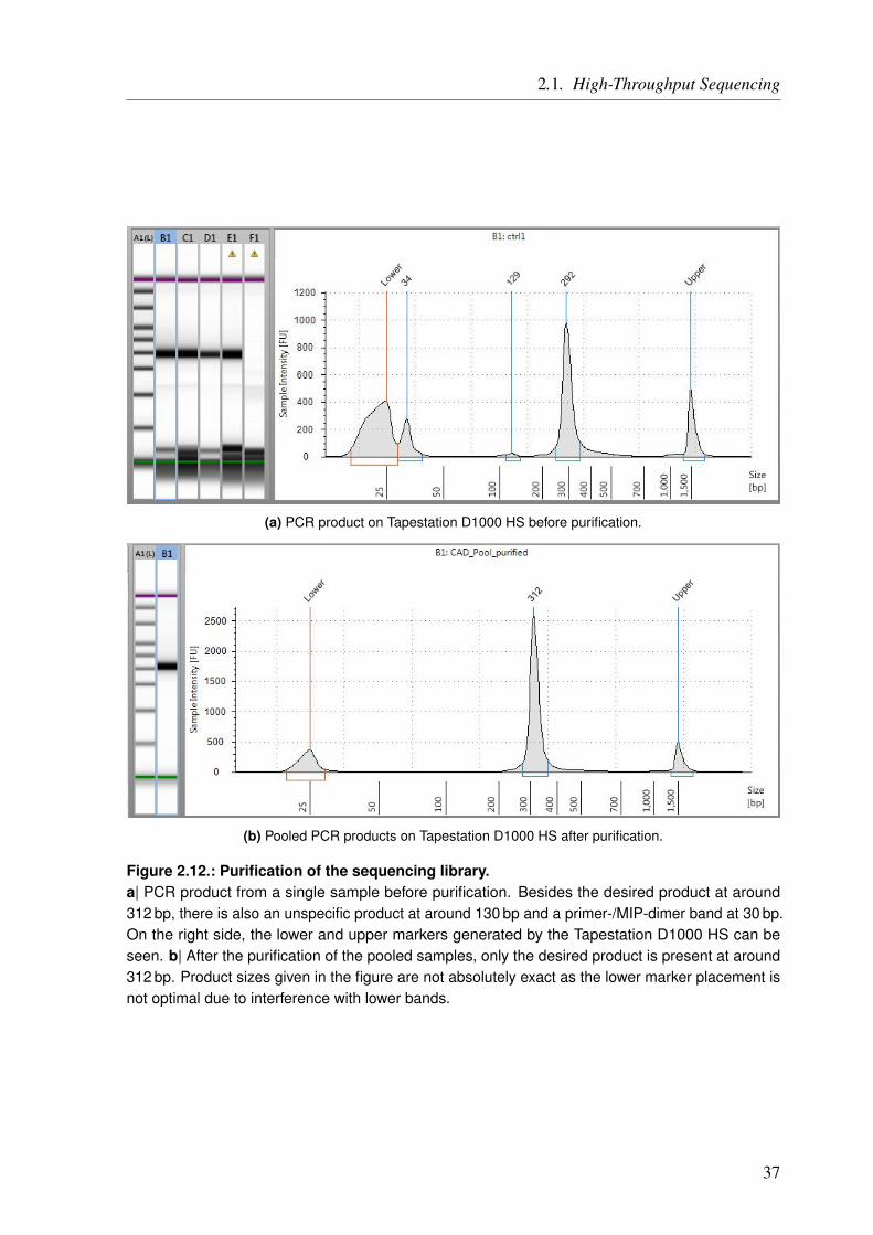
2.1. High-Throughput Sequencing
(a) PCR product on Tapestation D1000 HS before purification.
(b) Pooled PCR products on Tapestation D1000 HS after purification.
Figure 2.12.: Purification of the sequencing library.a| PCR product from a single sample before purification. Besides the desired product at around312 bp, there is also an unspecific product at around 130 bp and a primer-/MIP-dimer band at 30 bp.On the right side, the lower and upper markers generated by the Tapestation D1000 HS can beseen. b| After the purification of the pooled samples, only the desired product is present at around312 bp. Product sizes given in the figure are not absolutely exact as the lower marker placement isnot optimal due to interference with lower bands.
37
2. General Methods
different sample volumes to the pool. AmpureXP beads at room temperature are vortexed and avolume of 0.7x–1.0x of the pooled samples is added. The stronger the second band, the fewerbeads need to be added, as lower concentrations are biased towards bigger fragments. Themixture is vortexed, spun down and incubated for 10minute at room temperature. Next, thetube is placed in a magnetic rack for 5min. Although the DNA is bound to the beads at thisstage, the supernatant is transferred to a new tube and kept until the final results are verified.
Beads are washed with 70% freshly made ethanol, by slightly inverting the tube in the rack, for30 s. The ethanol is discarded carefully to not lose the beads. Having repeated the washingstep, all ethanol is carefully removed. The tube is left open for around 5min to dry the beads,while making sure not to overdry. 30 µl low TE buffer is added for elution. The tube is vortexedand spun down before placing it in the magnetic rack again for 1min. The supernatant, nowcontaining the purified library, is transferred to a clean tube.
The purification can be evaluated on Tapestation D1000 HS (Figure 2.12b). On success,only the band of the desired product remains. The purified pool can be stored at 4 ◦C untilsequencing. Long-term storage is possible at −20 ◦C. If multiple libraries are sequencedtogether, their concentrations should be measured right before sequencing and adjusted bydiluting, if needed.
Sequencing Evaluation and Rebalancing of the MIP Pool
There are two ways to look at the coverage data. One is to count the reads per MIP position aftermapping them to the reference genome. This has the advantage of also merging the SNP-MIPs,which gives a good idea of how good each desired MIP sequence is covered. An example of thecoverage per mapped MIP is shown Figure 2.13 on Page 40. The second way is to only countthe specific adapter sequences of each MIP, before aligning them to the reference genome. Thisis useful to find MIPs that bound off-target, as they will not be seen in the mapped data. Inaddition, off-target MIPs are often very unspecific and tend to bind to repetitive regions all overthe genome which leads to an overrepresentation, wasting even more sequencing capacity. Assequencing, in general, is performed as paired-end sequencing, each read contains only a part(e.g., half) of the whole MIP target. Therefore, two reads correspond to only one completecovered target sequence.
The aim of the rebalancing is to get a more even coverage over all MIPs, by adding theunderperforming and repressing the overperforming MIPs. For the underperformers the worst1% are added at a 20-fold concentration and the worst 10% at a 10-fold concentration. For someMIPs which are not present in any sample additional MIPs need to be designed, as described onPage 30. To get more MIPs to choose from the MIPgen software can be provided with different
38
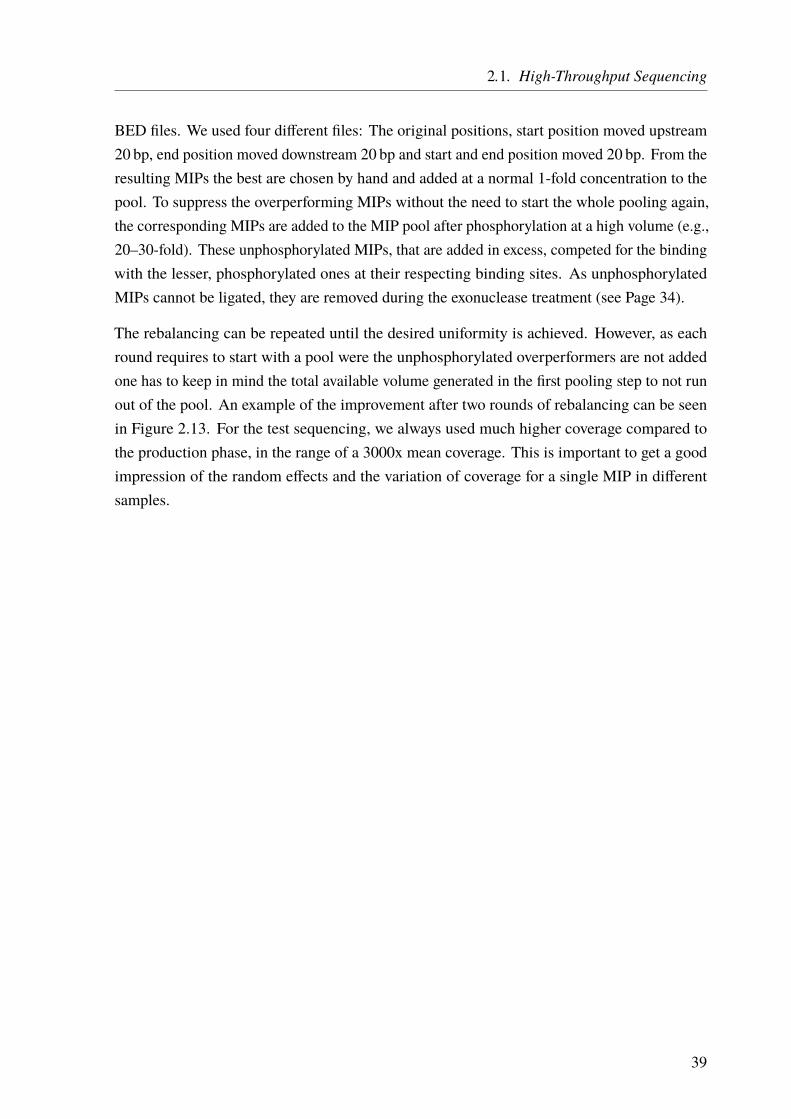
2.1. High-Throughput Sequencing
BED files. We used four different files: The original positions, start position moved upstream20 bp, end position moved downstream 20 bp and start and end position moved 20 bp. From theresulting MIPs the best are chosen by hand and added at a normal 1-fold concentration to thepool. To suppress the overperforming MIPs without the need to start the whole pooling again,the corresponding MIPs are added to the MIP pool after phosphorylation at a high volume (e.g.,20–30-fold). These unphosphorylated MIPs, that are added in excess, competed for the bindingwith the lesser, phosphorylated ones at their respecting binding sites. As unphosphorylatedMIPs cannot be ligated, they are removed during the exonuclease treatment (see Page 34).
The rebalancing can be repeated until the desired uniformity is achieved. However, as eachround requires to start with a pool were the unphosphorylated overperformers are not addedone has to keep in mind the total available volume generated in the first pooling step to not runout of the pool. An example of the improvement after two rounds of rebalancing can be seenin Figure 2.13. For the test sequencing, we always used much higher coverage compared tothe production phase, in the range of a 3000x mean coverage. This is important to get a goodimpression of the random effects and the variation of coverage for a single MIP in differentsamples.
39
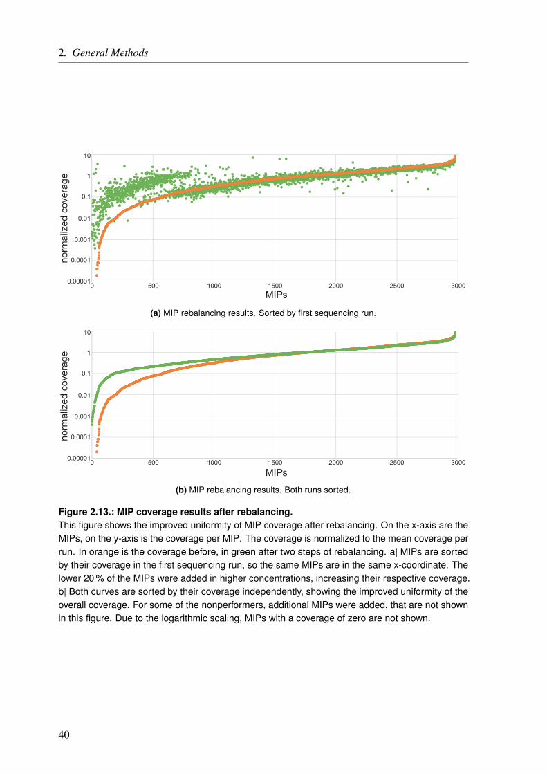
2. General Methods
0.00001
0.0001
0.001
0.01
0.1
1
10
0 500 1500 2500 300020001000MIPs
norm
aliz
ed c
over
age
(a) MIP rebalancing results. Sorted by first sequencing run.
0.00001
0.0001
0.001
0.01
0.1
1
10
0 500 1500 2500 300020001000
MIPs
norm
aliz
ed c
over
age
(b) MIP rebalancing results. Both runs sorted.
Figure 2.13.: MIP coverage results after rebalancing.This figure shows the improved uniformity of MIP coverage after rebalancing. On the x-axis are theMIPs, on the y-axis is the coverage per MIP. The coverage is normalized to the mean coverage perrun. In orange is the coverage before, in green after two steps of rebalancing. a| MIPs are sortedby their coverage in the first sequencing run, so the same MIPs are in the same x-coordinate. Thelower 20 % of the MIPs were added in higher concentrations, increasing their respective coverage.b| Both curves are sorted by their coverage independently, showing the improved uniformity of theoverall coverage. For some of the nonperformers, additional MIPs were added, that are not shownin this figure. Due to the logarithmic scaling, MIPs with a coverage of zero are not shown.
40
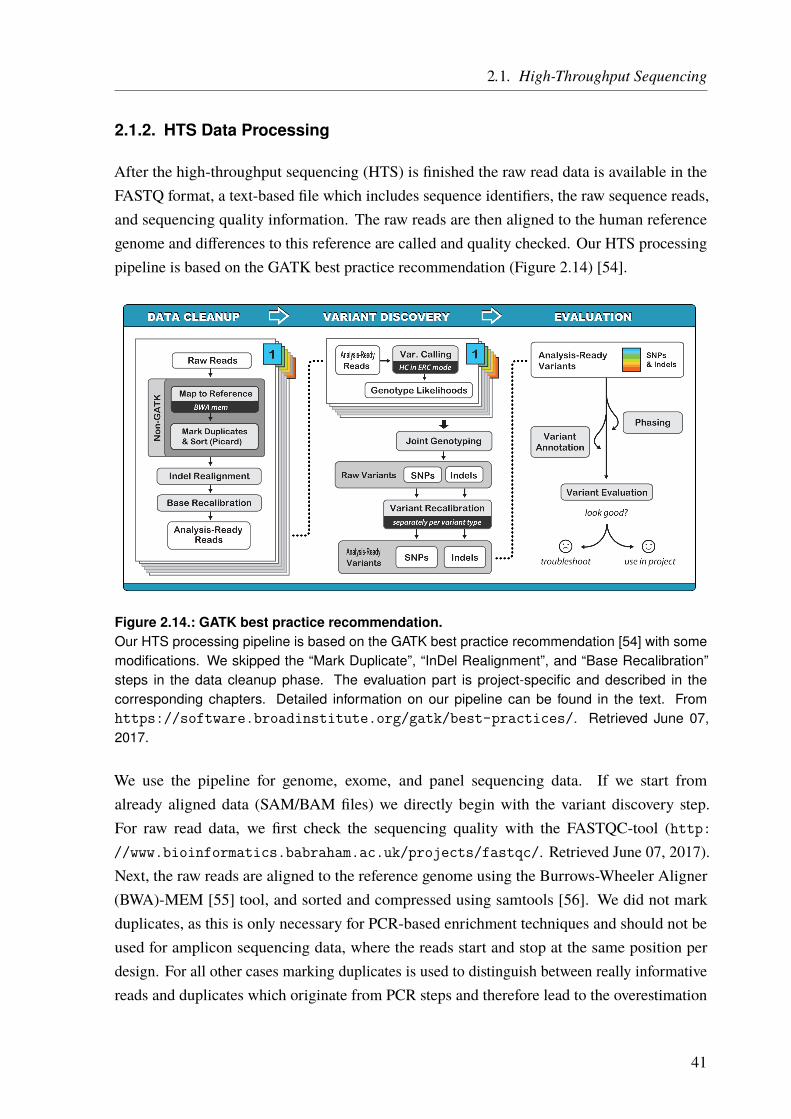
2.1. High-Throughput Sequencing
2.1.2. HTS Data Processing
After the high-throughput sequencing (HTS) is finished the raw read data is available in theFASTQ format, a text-based file which includes sequence identifiers, the raw sequence reads,and sequencing quality information. The raw reads are then aligned to the human referencegenome and differences to this reference are called and quality checked. Our HTS processingpipeline is based on the GATK best practice recommendation (Figure 2.14) [54].
Figure 2.14.: GATK best practice recommendation.Our HTS processing pipeline is based on the GATK best practice recommendation [54] with somemodifications. We skipped the “Mark Duplicate”, “InDel Realignment”, and “Base Recalibration”steps in the data cleanup phase. The evaluation part is project-specific and described in thecorresponding chapters. Detailed information on our pipeline can be found in the text. Fromhttps://software.broadinstitute.org/gatk/best-practices/. Retrieved June 07,2017.
We use the pipeline for genome, exome, and panel sequencing data. If we start fromalready aligned data (SAM/BAM files) we directly begin with the variant discovery step.For raw read data, we first check the sequencing quality with the FASTQC-tool (http://www.bioinformatics.babraham.ac.uk/projects/fastqc/. Retrieved June 07, 2017).Next, the raw reads are aligned to the reference genome using the Burrows-Wheeler Aligner(BWA)-MEM [55] tool, and sorted and compressed using samtools [56]. We did not markduplicates, as this is only necessary for PCR-based enrichment techniques and should not beused for amplicon sequencing data, where the reads start and stop at the same position perdesign. For all other cases marking duplicates is used to distinguish between really informativereads and duplicates which originate from PCR steps and therefore lead to the overestimation
41
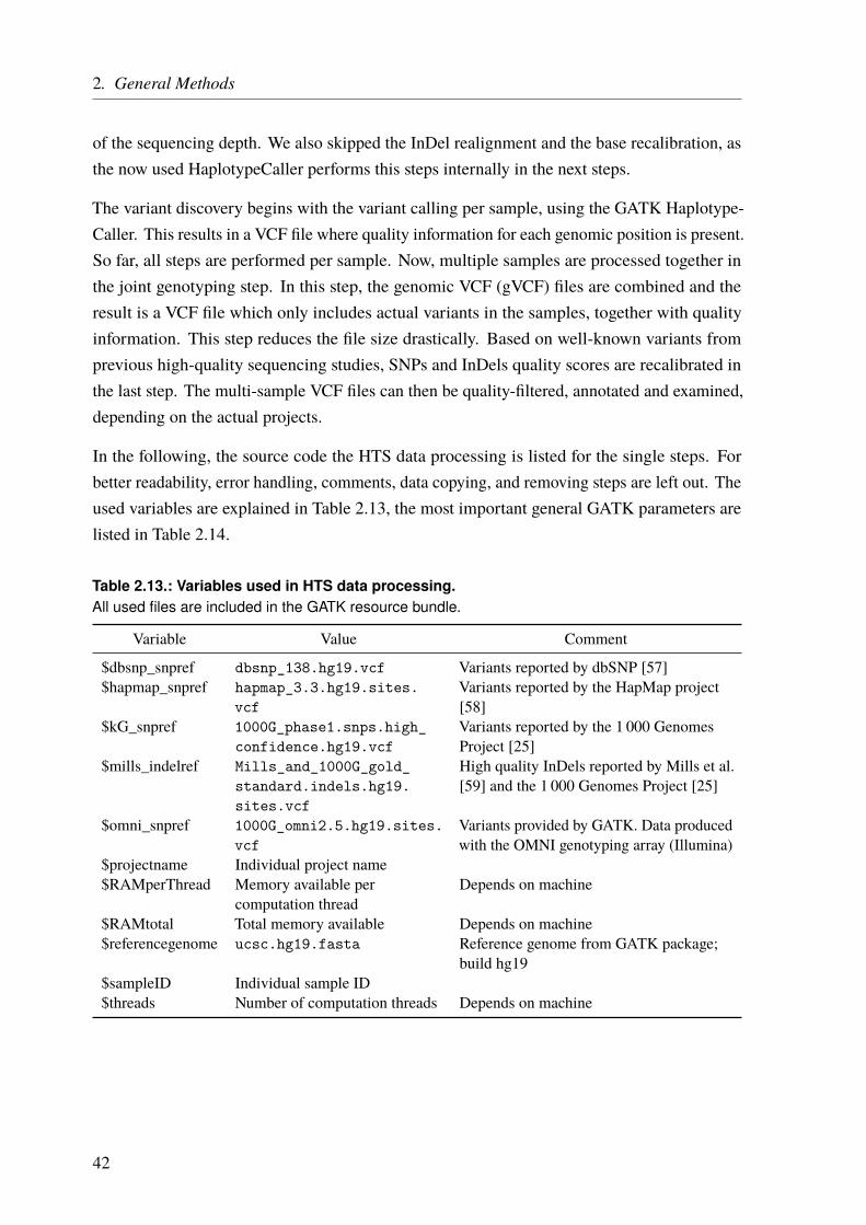
2. General Methods
of the sequencing depth. We also skipped the InDel realignment and the base recalibration, asthe now used HaplotypeCaller performs this steps internally in the next steps.
The variant discovery begins with the variant calling per sample, using the GATK Haplotype-Caller. This results in a VCF file where quality information for each genomic position is present.So far, all steps are performed per sample. Now, multiple samples are processed together inthe joint genotyping step. In this step, the genomic VCF (gVCF) files are combined and theresult is a VCF file which only includes actual variants in the samples, together with qualityinformation. This step reduces the file size drastically. Based on well-known variants fromprevious high-quality sequencing studies, SNPs and InDels quality scores are recalibrated inthe last step. The multi-sample VCF files can then be quality-filtered, annotated and examined,depending on the actual projects.
In the following, the source code the HTS data processing is listed for the single steps. Forbetter readability, error handling, comments, data copying, and removing steps are left out. Theused variables are explained in Table 2.13, the most important general GATK parameters arelisted in Table 2.14.
Table 2.13.: Variables used in HTS data processing.All used files are included in the GATK resource bundle.
Variable Value Comment
$dbsnp_snpref dbsnp_138.hg19.vcf Variants reported by dbSNP [57]$hapmap_snpref hapmap_3.3.hg19.sites.
vcfVariants reported by the HapMap project[58]
$kG_snpref 1000G_phase1.snps.high_confidence.hg19.vcf
Variants reported by the 1 000 GenomesProject [25]
$mills_indelref Mills_and_1000G_gold_standard.indels.hg19.sites.vcf
High quality InDels reported by Mills et al.[59] and the 1 000 Genomes Project [25]
$omni_snpref 1000G_omni2.5.hg19.sites.vcf
Variants provided by GATK. Data producedwith the OMNI genotyping array (Illumina)
$projectname Individual project name$RAMperThread Memory available per
computation threadDepends on machine
$RAMtotal Total memory available Depends on machine$referencegenome ucsc.hg19.fasta Reference genome from GATK package;
build hg19$sampleID Individual sample ID$threads Number of computation threads Depends on machine
42

2.1. High-Throughput Sequencing
Table 2.14.: General GATK parameters.Special parameters for single tools are explained in the corresponding section.
Parameter Explanation
-I Input file containing sequencing data-L Interval file with genomic regions over which to operate-nt Number of data threads to allocate to this analysis (for parallelization)-R Reference sequence file (e.g., hg19.fasts)-T Name of the GATK tool to run
2.1.2.1. Alignment
First, the raw reads are aligned to the reference sequence (genome) (Code Listing 2.1) withBWA-MEM. If applicable, all forward (R1 here) and all reverse (R2 here) reads from paired-endsequencing are joined forward and reverse reads are loaded separately. The resulting SAMfile is then sorted, compressed and indexed with samtools (Code Listing 2.2). The pipelinepresented here used BWA Version 0.7.15.
Code Listing 2.1: BWA alignment.BWA Version 0.7.15 was used here. -M defines split read handling, -R read group (@RG) name, -tthreads for parallelization. Forward reads and reverse reads are loaded separately.
1 bwa mem -M -R "@RG\tID:run_${ sampleID }\ tSM:${ sampleID }" \2 -t ${ threads } ${ referencegenome } \3 <(zcat $(ls -1 *_R1_*fastq.gz | sort)) \4 <(zcat $(ls -1 *_R2_*fastq.gz | sort)) > ${ sampleID }. sam
Code Listing 2.2: Sorting and compressing SAM file.-m memory per thread, -@ threads for parallelization, -O output format, -o output file name.
1 samtools sort -m ${ RAMperThread } \2 -@ ${ threads } \3 -O bam \4 -o ${ sampleID }_sort.bam \5 ${ sampleID }. sam6
7 samtools index ${ sampleID }_sort.bam
2.1.2.2. Variant Calling
We used the GATK nightly build 2016-07-15-ge5173a7 for the pipeline shown here. Thefirst step is the variant calling with the HaplotypeCaller (Code Listing 2.3). It is parallelizedmanually and each part is numbered (i). To split the parts we used the -L option with BED files,which define similar sized genome chunks. The gVCF file is compressed and indexed.
43
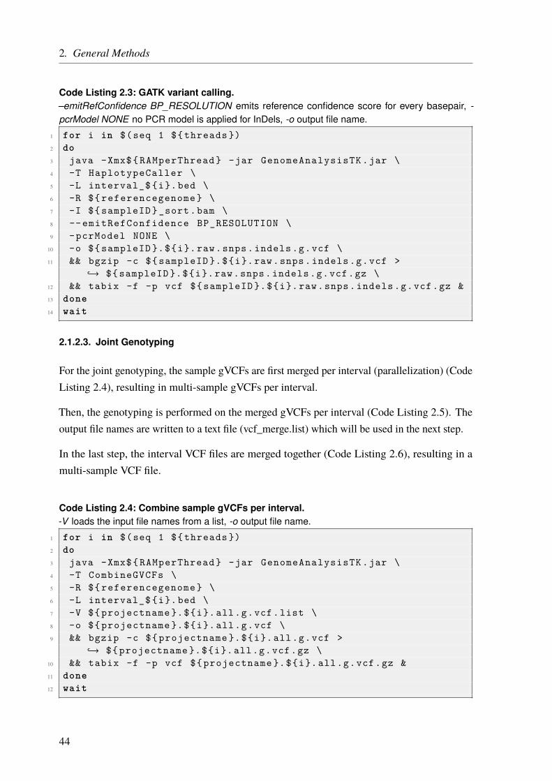
2. General Methods
Code Listing 2.3: GATK variant calling.–emitRefConfidence BP_RESOLUTION emits reference confidence score for every basepair, -pcrModel NONE no PCR model is applied for InDels, -o output file name.
1 for i in $(seq 1 ${ threads })2 do3 java -Xmx${ RAMperThread } -jar GenomeAnalysisTK .jar \4 -T HaplotypeCaller \5 -L interval_$ {i}. bed \6 -R ${ referencegenome } \7 -I ${ sampleID }_sort.bam \8 -- emitRefConfidence BP_RESOLUTION \9 -pcrModel NONE \
10 -o ${ sampleID }.${i}. raw.snps. indels .g.vcf \11 && bgzip -c ${ sampleID }.${i}. raw.snps. indels .g.vcf >
↪→ ${ sampleID }.${i}. raw.snps. indels .g.vcf.gz \12 && tabix -f -p vcf ${ sampleID }.${i}. raw.snps. indels .g.vcf.gz &13 done14 wait
2.1.2.3. Joint Genotyping
For the joint genotyping, the sample gVCFs are first merged per interval (parallelization) (CodeListing 2.4), resulting in multi-sample gVCFs per interval.
Then, the genotyping is performed on the merged gVCFs per interval (Code Listing 2.5). Theoutput file names are written to a text file (vcf_merge.list) which will be used in the next step.
In the last step, the interval VCF files are merged together (Code Listing 2.6), resulting in amulti-sample VCF file.
Code Listing 2.4: Combine sample gVCFs per interval.-V loads the input file names from a list, -o output file name.
1 for i in $(seq 1 ${ threads })2 do3 java -Xmx${ RAMperThread } -jar GenomeAnalysisTK .jar \4 -T CombineGVCFs \5 -R ${ referencegenome } \6 -L interval_$ {i}. bed \7 -V ${ projectname }.${i}. all.g.vcf.list \8 -o ${ projectname }.${i}. all.g.vcf \9 && bgzip -c ${ projectname }.${i}. all.g.vcf >
↪→ ${ projectname }.${i}. all.g.vcf.gz \10 && tabix -f -p vcf ${ projectname }.${i}. all.g.vcf.gz &11 done12 wait
44
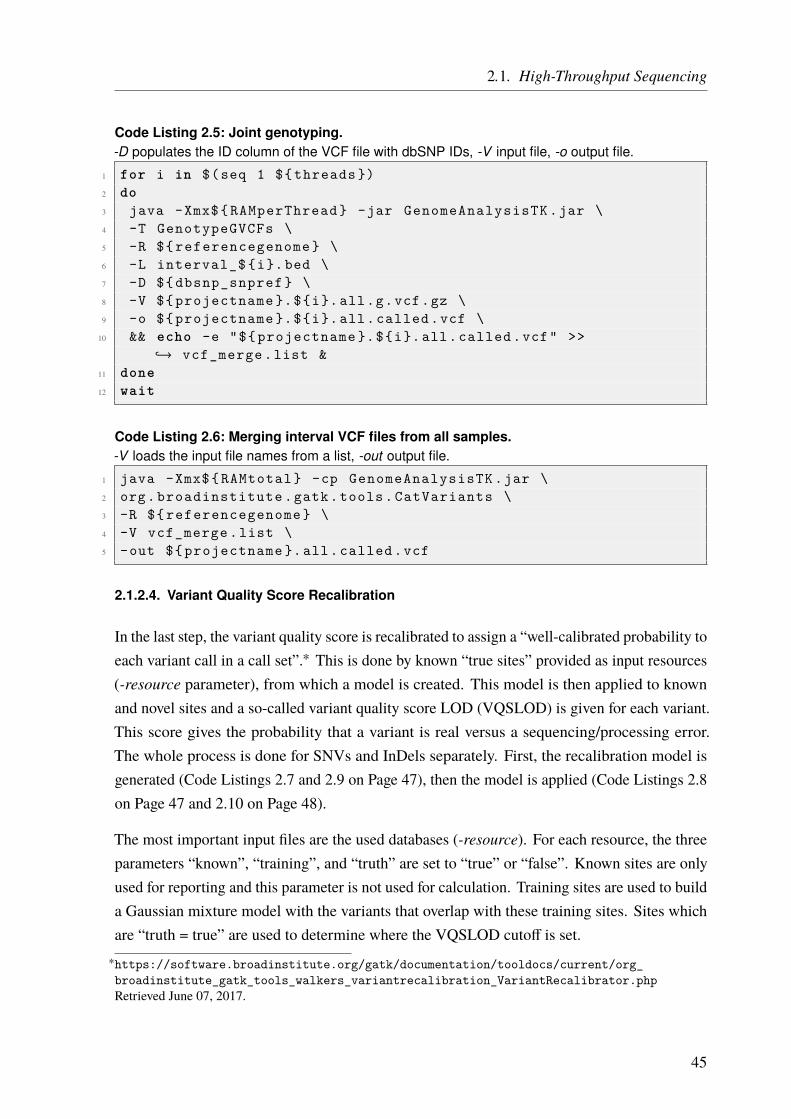
2.1. High-Throughput Sequencing
Code Listing 2.5: Joint genotyping.-D populates the ID column of the VCF file with dbSNP IDs, -V input file, -o output file.
1 for i in $(seq 1 ${ threads })2 do3 java -Xmx${ RAMperThread } -jar GenomeAnalysisTK .jar \4 -T GenotypeGVCFs \5 -R ${ referencegenome } \6 -L interval_$ {i}. bed \7 -D ${ dbsnp_snpref } \8 -V ${ projectname }.${i}. all.g.vcf.gz \9 -o ${ projectname }.${i}. all. called .vcf \
10 && echo -e "${ projectname }.${i}. all. called .vcf" >>↪→ vcf_merge .list &
11 done12 wait
Code Listing 2.6: Merging interval VCF files from all samples.-V loads the input file names from a list, -out output file.
1 java -Xmx${ RAMtotal } -cp GenomeAnalysisTK .jar \2 org. broadinstitute .gatk.tools. CatVariants \3 -R ${ referencegenome } \4 -V vcf_merge .list \5 -out ${ projectname }. all. called .vcf
2.1.2.4. Variant Quality Score Recalibration
In the last step, the variant quality score is recalibrated to assign a “well-calibrated probability toeach variant call in a call set”.∗ This is done by known “true sites” provided as input resources(-resource parameter), from which a model is created. This model is then applied to knownand novel sites and a so-called variant quality score LOD (VQSLOD) is given for each variant.This score gives the probability that a variant is real versus a sequencing/processing error.The whole process is done for SNVs and InDels separately. First, the recalibration model isgenerated (Code Listings 2.7 and 2.9 on Page 47), then the model is applied (Code Listings 2.8on Page 47 and 2.10 on Page 48).
The most important input files are the used databases (-resource). For each resource, the threeparameters “known”, “training”, and “truth” are set to “true” or “false”. Known sites are onlyused for reporting and this parameter is not used for calculation. Training sites are used to builda Gaussian mixture model with the variants that overlap with these training sites. Sites whichare “truth = true” are used to determine where the VQSLOD cutoff is set.
∗https://software.broadinstitute.org/gatk/documentation/tooldocs/current/org_broadinstitute_gatk_tools_walkers_variantrecalibration_VariantRecalibrator.phpRetrieved June 07, 2017.
45
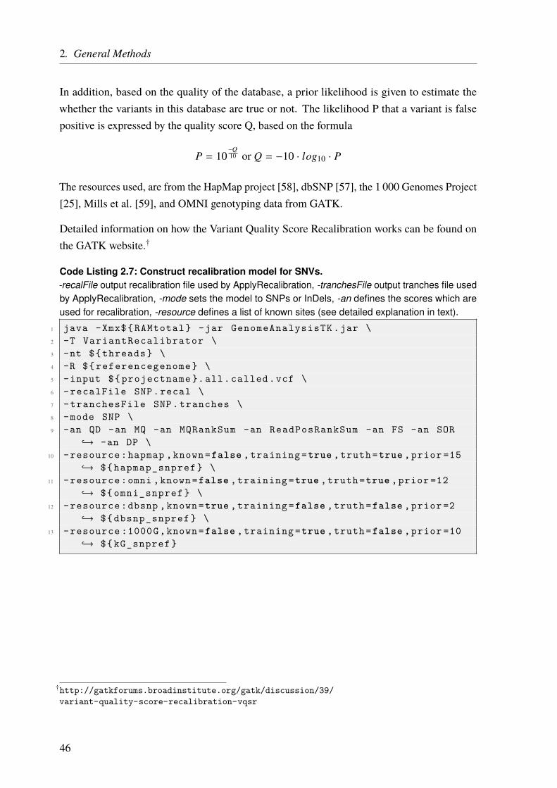
2. General Methods
In addition, based on the quality of the database, a prior likelihood is given to estimate thewhether the variants in this database are true or not. The likelihood P that a variant is falsepositive is expressed by the quality score Q, based on the formula
P = 10−Q10 or Q = −10 · log10 · P
The resources used, are from the HapMap project [58], dbSNP [57], the 1 000 Genomes Project[25], Mills et al. [59], and OMNI genotyping data from GATK.
Detailed information on how the Variant Quality Score Recalibration works can be found onthe GATK website.†
Code Listing 2.7: Construct recalibration model for SNVs.-recalFile output recalibration file used by ApplyRecalibration, -tranchesFile output tranches file usedby ApplyRecalibration, -mode sets the model to SNPs or InDels, -an defines the scores which areused for recalibration, -resource defines a list of known sites (see detailed explanation in text).
1 java -Xmx${ RAMtotal } -jar GenomeAnalysisTK .jar \2 -T VariantRecalibrator \3 -nt ${ threads } \4 -R ${ referencegenome } \5 -input ${ projectname }. all. called .vcf \6 -recalFile SNP.recal \7 -tranchesFile SNP. tranches \8 -mode SNP \9 -an QD -an MQ -an MQRankSum -an ReadPosRankSum -an FS -an SOR
↪→ -an DP \10 -resource :hapmap ,known=false , training =true ,truth=true ,prior =15
↪→ ${ hapmap_snpref } \11 -resource :omni ,known=false , training =true ,truth=true ,prior =12
↪→ ${ omni_snpref } \12 -resource :dbsnp ,known=true , training =false ,truth=false ,prior =2
↪→ ${ dbsnp_snpref } \13 -resource :1000G,known=false , training =true ,truth=false ,prior =10
↪→ ${ kG_snpref }
†http://gatkforums.broadinstitute.org/gatk/discussion/39/variant-quality-score-recalibration-vqsr
46

2.1. High-Throughput Sequencing
Code Listing 2.8: Apply recalibration model for SNVs.-recalFile input recalibration file created by VariantRecalibrator, -tranchesFile input tranches filedescribing where to cut the data (created by VariantRecalibrator), –ts_filter_level truth sensitivitylevel at which to start filtering.
1 java -Xmx${ RAMtotal } -jar GenomeAnalysisTK .jar \2 -T ApplyRecalibration \3 -nt ${ threads } \4 -R ${ referencegenome } \5 -input ${ projectname }. all. called .vcf \6 -recalFile SNP.recal \7 -tranchesFile SNP. tranches \8 -mode SNP \9 --ts_filter_level 99.5 \
10 -o ${ projectname }. all. called . snprecall .vcf
Code Listing 2.9: Construct recalibration model for InDels.-recalFile output recalibration file used by ApplyRecalibration, -tranchesFile output tranches file usedby ApplyRecalibration, -mode sets the model to SNPs or InDels, -an defines the scores which areused for recalibration, -resource defines a list of known sites (see detailed explanation in text).
1 java -Xmx${ RAMtotal } -jar GenomeAnalysisTK .jar \2 -T VariantRecalibrator \3 -nt ${ threads } \4 -R ${ referencegenome } \5 -input ${ projectname }. all. called . snprecall .vcf \6 -recalFile InDel.recal \7 -tranchesFile InDel. tranches \8 -mode INDEL \9 -an QD -an DP -an FS -an SOR -an ReadPosRankSum -an MQRankSum \
10 --maxGaussians 4 \11 -resource :mills ,known=false , training =true ,truth=true ,prior =12
↪→ ${ mills_indelref } \12 -resource :dbsnp ,known=true , training =false ,truth=false ,prior =2
↪→ ${ dbsnp_snpref }
47
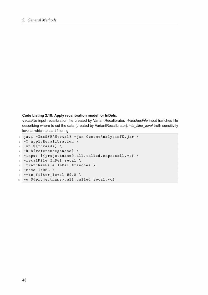
2. General Methods
Code Listing 2.10: Apply recalibration model for InDels.-recalFile input recalibration file created by VariantRecalibrator, -tranchesFile input tranches filedescribing where to cut the data (created by VariantRecalibrator), –ts_filter_level truth sensitivitylevel at which to start filtering.
1 java -Xmx${ RAMtotal } -jar GenomeAnalysisTK .jar \2 -T ApplyRecalibration \3 -nt ${ threads } \4 -R ${ referencegenome } \5 -input ${ projectname }. all. called . snprecall .vcf \6 -recalFile InDel.recal \7 -tranchesFile InDel. tranches \8 -mode INDEL \9 --ts_filter_level 99.0 \
10 -o ${ projectname }. all. called .recal.vcf
48
2.2. Variant Annotation
To filter, rank or assess variants that were identified by high-throughput sequencing (HTS) orother sequencing methods it is necessary to annotate these variants with different information,for example, where a variant is located. This includes the chromosome, gene, whether it isintronic or exonic, and which exact transcripts are affected and of course if it leads to proteinchanges. Moreover, it is important to know the frequency of a variant in different populationsand different studies. Moreover, if it is no de-novo variant there might already be a variantID assigned, for example from the Single Nucleotide Polymorphism Database (dbSNP). Forpotential disease-causing variants, we also use functional prediction scores which help to assesswhether a variant is likely pathogenic or not. In addition, all other kinds of data can be assigned,depending on the on the particular research question.
2.2.1. Annovar
As we mainly deal with large numbers of variants at once on the one hand, and a lot ofinformation that should be assigned to them on the other hand, it is crucial to have an automatedannotation process that is fast, flexible and capable of handling our input data. Therefore,we used the ANNOVAR software [60], which is freely available for non-commercial use andcan handle single nucleotide polymorphisms (SNPs) and copy number variations (CNVs). Ingeneral, ANNOVAR offers three types of annotations:
Gene-based annotation Assigns variants to genes/transcripts and identifies if they are locatedin the intron, exon, at a splice site, untranslated regions (UTRs) or in intergenic regions.For exonic variants, it identifies whether they lead to protein-changes and which aminoacids (AAs) are affected. ANNOVAR can utilize the data from RefSeq genes [61, 62],UCSC genes [63], ENSEMBL genes [64], GENCODE genes [65], or user-defined tables.
Region-based annotation Annotates data to variants located in specific genomic regions, forexample, conserved regions, duplicated regions, transcription factor binding sites (TFBS),ENCODE genome segmentation tracks [66, 67], or other user-defined data. A variantgets annotated if it overlaps the defined region.
Filter-based annotation This annotation is variant specific, meaning that not only the positionbut also the nucleotide exchange (or the exact insertion, deletion) has to match theused database. This is, for example, used for allele frequencies, dbSNP-ID annotation,functional prediction scores, or information about the known pathogenicity of the variant.

2. General Methods
Annovar offers several accessory tools for data conversion and annotation. We mainly usedthe table_annovar.pl program which allowed us to choose which annotation tables wewant to use, and for some of them to select optional arguments. It also allows to define theoutput string for an annotation, if no hit is found. We used “NA” for this case. To run thetable_annovar.pl program, a compatible input file is needed. This file can be generatedby the accessory convert2annovar.pl program. The input for this program can be either aVCF file or a list of variant identifiers (dbSNP-IDs). We configured convert2annovar.pland table_annovar.pl such that the original data is appended at the end of the annotated file.The resulting text file is tab-separated and can easily be used in all kinds of downstream analysis,like filtering or comparison tasks. Plenty of tables for the annotation can be downloaded fromthe ANNOVAR website directly or through the UCSC table browser. In addition, it is easy toprovide user-generated tables. The most important tables that we used are listed and explainedbelow. However, not all of them were used for the projects described in this thesis.
2.2.1.1. Annotation Tables
This section describes the databases or tables that we used most frequently for our projects,separately for gene-based, region-based, and filter-based annotation.
Gene-based annotation tables
This annotation is used to identify which genes (transcripts) are affected by the variant or wherethe variant is located in general (variant function). For the “variant function” ANNOVARdefines different classes, according to the sequence ontology [68]. The possible values andtheir explanations are listed in Table 2.15. If a variant fits multiple functional categories, theone with the highest precedence is printed, in the following order:
exonic = splicing > ncRNA > 5’ UTR = 3’ UTR
> intron > upstream = downstream > intergenic
In addition, the name of the affected or upstream/downstream gene(s) is listed. The thresholdfrom a splice junction at which a variant is annotated as “splicing” and the distance forupstream/downstream genes can be altered.
For variants, that affect exonic regions of a gene, ANNOVAR provides the field “exonic variantfunction”. It lists the most severe effect for each transcript, according to the precedence inTable 2.16 on Page 52. In addition, each affected gene, transcript, nucleotide and, if applicable,amino acid is listed. For example, a change from Thymidine (T) to Guanosin (G) at the genomicposition hg19 chr10:g.91007360T>G, will lead to a nonsynonymous mutation in the second
50

2.2. Variant Annotation
Table 2.15.: Available “variant function” annotations from ANNOVAR.There are 9 “variant” function classes available, with different precedences. If a variant matches mul-tiple classes, the one with the highest precedence is printed. Sequence Ontology data is taken fromEilbeck et al. [68]. Adapted from the ANNOVAR user guide (http://annovar.openbioinformatics.org/en/latest/user-guide/gene/ Retrieved April 27, 2017).
Annotation Precedence Explanation Sequence Ontology
exonic 1 variant overlaps a coding region exon_variant(SO:0001791)
splicing 1 variant is within 2 bp of a splicing junction(-splicing_threshold changes this)
splicing_variant(SO:0001568)
ncRNA 2 variant overlaps a transcript without codingannotation in the gene definition
non_coding_transcript-_variant(SO:0001619)
UTR5 3 variant overlaps a 5’ UTR 5_prime_UTR_variant(SO:0001623)
UTR3 3 variant overlaps a 3’ UTR 3_prime_UTR_variant(SO:0001624)
intronic 4 variant overlaps an intron intron_variant(SO:0001627)
upstream 5 variant overlaps 1 kb region upstream oftranscription start site
upstream_gene_variant(SO:0001631)
downstream 5 variant overlaps 1 kb region downstream oftranscription end site (-neargene changes this)
down-stream_gene_variant(SO:0001632)
intergenic 6 variant is in intergenic region intergenic_variant(SO:0001628)
exon of the LIPA gene (RefSeq transcript: NM_000235) at the complementary DNA (cDNA)position 46. As this gene is oriented antisense, the nucleotide change is written as Adenosine(A) to Cytidine (C). This also leads to an AA-change at position 16 from Threonine (T) toProline (P). Annovar will list this change as: LIPA:NM_000235:exon2:c.A46C:p.T16P. Ifmultiple genes and/or transcripts are affected all of them are listed independently.
RefSeq Genes [61, 62] This is the gene annotation system we used mainly as most databasesand tools we used downstream can easily handle the RefSeq accession numbers. To coverthe important splice site changes, we changed the “-splicing_threshold” to 3, to annotateall variants ±3 bp from a splice site as splicing mutation.
UCSC Genes [63] This gene annotation from UCSC is, in fact, a set of gene predictionsmerged from several sources. It includes RefSeq [61, 62], GenBank [69], CCDS [70, 71],Rfam [72], UniProt [73], and the tRNA Genes track [74]. For some projects, it is usefulto make sure that as many genes as possible are taken into account when annotating.As opposed to RefSeq the genes here are not manually curated and therefore includefalse-positives. We also set the “-splicing_threshold” to 3 (see above).
51

2. General Methods
Table 2.16.: Available “exonic variant function” annotations from ANNOVAR.There are 11 “exonic variant function” classes available, with different precedences. If a variantmatches multiple classes, the one with the highest precedence is printed. Sequence Ontologydata is taken from Eilbeck et al. [68]. Adapted from the ANNOVAR user guide (http://annovar.openbioinformatics.org/en/latest/user-guide/gene/ Retrieved April 27, 2017).
Annotation Precedence Explanation Sequence Ontology
frameshiftinsertion
1 an insertion of one or more nucleotides thatcause frameshift changes in protein-codingsequence
frameshift_elongation(SO:0001909)
frameshiftdeletion
2 a deletion of one or more nucleotides that causeframeshift changes in protein-coding sequence
frameshift_truncation(SO:0001910)
frameshift blocksubstitution
3 a block substitution of one or more nucleotidesthat cause frameshift changes in protein-codingsequence
frameshift_variant(SO:0001589)
stopgain 4 a nonsynonymous SNV, frameshiftinsertion/deletion, nonframeshiftinsertion/deletion or block substitution that leadto the immediate creation of stop codon at thevariant site. For frameshift mutations, thecreation of stop codon downstream of thevariant will not be counted as "stopgain"!
stop_gained(SO:0001587)
stoploss 5 a nonsynonymous SNV, frameshiftinsertion/deletion, nonframeshiftinsertion/deletion or block substitution that leadto the immediate elimination of stop codon atthe variant site
stop_lost(SO:0001578)
nonframeshiftinsertion
6 an insertion of (multiples of) 3 nucleotides thatdo not cause frameshift changes inprotein-coding sequence
inframe_insertion(SO:0001821)
nonframeshiftdeletion
7 a deletion of (mutliples of) 3 nucleotides thatdo not cause frameshift changes inprotein-coding sequence
inframe_deletion(SO:0001822)
nonframeshiftblocksubstitution
8 a block substitution of one or more nucleotidesthat do not cause frameshift changes inprotein-coding sequence
inframe_variant(SO:0001650)
nonsynonymousSNV
9 a single nucleotide change that cause an aminoacid change
missense_variant(SO:0001583)
continued on next page
52
2.2. Variant Annotation
Annotation Precedence Explanation Sequence Ontology
synonymousSNV
10 a single nucleotide change that does not causean amino acid change
synonymous_variant(SO:0001819)
unknown 11 unknown function (due to various errors in thegene structure definition)
sequence_variant(SO:0001060)
Region-based annotation tables
Conservation (phastConsElemts46way) [75] For the evaluation of variants it is interestingto know, whether their positions are conserved among different species or not. ThephastConsElemts46way is provided throughANNOVAR gives an estimate of conservationfrom 46 vertebrates. The scores reaches from 0 to 1000, with higher scores indicatingstronger conservation. Nonconserved positions are less likely to be functionally important.
Segmental duplication (genomicSuperDups) [76] Segmental duplications are genomic re-gions that have been duplicated. This makes it very difficult to map these regions tothe reference genome and variants identified to be located in this regions are often falsepositive. Especially if they are located within coding regions, pseudogenes are often thereal source for a variant, as they do not undergo selective pressure. In general, we ignorevariants in this regions or at least treat them with special caution.
Transcription Factor ChIP-seq (161 factors) from ENCODE with Factorbook Motifs[77–79] This TFBS track is based on chromatin immunoprecipitation (ChIP)-Seq datafrom the ENCODE project in 91 cell types. The DNA motifs for the 161 transcriptionfactors (TFs) are taken from Factorbook. We used version 3 from the Encyclopedia ofDNA Elements (ENCODE) data freeze in March 2012. Variants within these regionsmight alter transcription factor binding and therefore alter gene expression.
Conserved TFBS (tfbsConsSites) This track is used to identify TFBS conserved in thehuman/mouse/rat alignment. It was created for the UCSC genome browser. As opposedto the ENCODE TFBS track, this data is purely computational. Hence, not all listedbinding sites might be functional.
microRNA (miRNA) bindings sites (targetScanS) [80] This track shows mammalian con-served miRNA binding sites in 3’ UTR regions of RefSeq genes, predicted by TargetScan-Human 5.1. miRNAs are small noncoding RNA molecules that affect RNA silencingand post-transcriptional gene expression, mostly by binding specifically to the 3’ UTR ofthe target mRNAs [81, 82].
53

2. General Methods
GWAS Catalog [83] The GWAS catalog lists SNPs, that were identified by published GWASfor different phenotypes. If a variant is reported in this catalog the correspondingphenotype is annotated. The reason why this is a region-based annotation, rather than afilter-based one, is that a lot of studies only report the SNP but not the risk allele. Hence,each variant at a GWAS SNP position is reported.
Pfam Domains (ucscGenePfam) [84] As most proteins are composed of distinct functionalregions, called domains, it is often important in which of these domains a variant islocated. This information can be retrieved from the manually curated Pfam database.The ucscGenePfam table, available at the UCSC website identifies these domains intranscripts from the UCSC Genes track.
Chromosome bands (cytoBand) [85] This track only supplies additional positional infor-mation about a variant. Chromosome bands are defined by Giemsa-staining and thenomenclature distinguishes short (p) and long (q) chromosome arms. The different bandsare numbered from the centromere outwards.
Chromatin State Segmentation by HMM from ENCODE/Broad [66, 67] This track pre-dicts chromatin states based on ChIP-Seq data from nine factors (histone marks) plusinput. Computationally learning using a Hidden Markov Model (HMM) was utilizedto define 15 different states like promoters (active/inactive), enhancers (strong/weak),transcribed regions or repressed regions. We annotated this data for nine different celltypes (GM12878, H1-hESC, K562, HepG2, HUVEC, HMEC, HSMM, NHEK, NHLF).
Filter-based annotation tables
Single Nucleotide Polymorphism Database (dbSNP) [57] The Single Nucleotide Polymor-phism Database (dbSNP) is a public archive of sequence variants, with unique identifiers.Most variants are SNPs but also InDels, repeats or short tandem repeats (STRs) forexample are listed. The goal of dbSNP is to provide scientists with a unique identifier foralready known variants to facilitate referencing. Large projects like the 1 000 GenomesProject or the Exome Aggregation Consortium (ExAC) usually submit their data. Hence,most variants that are identified and do not have a dbSNP ID assigned by now are verylikely to be rare.
Allele Frequencies
As we are often interested in rare variants, we need to know the allele frequencies from thegeneral population. With the decrease in sequencing cost more and more data is availablewhich improves the accuracy of allele frequencies and also allows to filter variants based onselected (sub-)populations.
54
2.2. Variant Annotation
The 1 000 Genomes Project [25] The 1 000 Genomes Project sequenced the whole genomesof 2 504 healthy individuals from 26 populations and detected 84.4 million variants(phase3, version 5). The goal of the project was to detect most genetic variants with afrequency of at least 1% in the studied populations. The data is freely available.
NHLBI Exome Sequencing Project The goal of the NHLBI GO Exome Sequencing Project(ESP) is to discover novel genes and mechanisms contributing to heart, lung and blooddisorders.∗ Exome sequencing data is available from 6 500 individuals; 2 203 African-Americans and 4 300 European-Americans. The data comes from different projectsand contains healthy controls as well as affected individuals with heart, lung and blooddisorders.
Exome Aggregation Consortium (ExAC) [26] The Exome Aggregation Consortium (ExAC)collected exome sequencing data from 60 706 unrelated individuals. The data comesfrom various disease-specific and population genetic studies. Individuals with severepediatric disease where removed. The individuals were assigned to one of 6 populations(and “others”). Because of the huge sample size rare variants were detected as well andthe frequencies are also more accurate than in others projects.
Functional Prediction Scores
To assess the functional effects of identified variants functional prediction scores exist. Theyare based on different datasets and some of them, like CADD, also integrate multiple scoresinto one.
SIFT [86] The Sorting Intolerant From Tolerant (SIFT) algorithm predicts whether AA-changes have an effect on protein function or not. The prediction is based on theAA-conservation. The SIFT score ranges from 0 – 1 , with scores ≤ 0.05 predicted to bedamaging and > 0.05 tolerated.
PolyPhen-2 [87] Polymorphism Phenotyping v2 (PolyPhen-2) is a tool which predicts possibleimpact of an amino acid substitution on the structure and function of a human proteinusing straightforward physical and comparative considerations.† A machine learningapproach is used to rank the mutations, which takes several parameters into account. Thisincludes sequence-specific features, like localization in at a disulfide bond position, orfunctional domains. In addition, structural features, of the 3D protein folding, are alsoincluded. There are two datasets available based on different training sets: HumDiv andHumVar. HumVar should be used for Mendelian disease with a drastic effect, whereas
∗http://evs.gs.washington.edu/EVS/ Retrieved May 2, 2017.†http://genetics.bwh.harvard.edu/pph2/ Retrieved May 2, 2017.
55
2. General Methods
HumDiv is better suited for complex diseases, or loci identified by GWAS. Detailedexplanation of the datasets can be found in the documentation.‡ The algorithm assignsone of 3 categories to a variant: benign, possibly damaging, or probably damaging.
MutationTaster2 [88] As opposed to the functional prediction scores described beforeMutationTaster2 can also assess noncoding and synonymous variants. The softwareperforms multiple tests based for example on conservation (amino acids and nucleotides),functional domains, effects on splicing, alteration of binding sites and also integratesknown information from sources like Ensemble, ClinVar, ExAC, the 1 000 GenomesProject or ExAC. The results from all the single tests are then assessed by a machinelearning algorithm (Naive Bayes classifier) to decide if the variant might be deleterious.Four types of prediction are possible: “Disease-causing”, meaning the variant is probablydeleterious; “disease-causing automatic” - this variant is already known to be deleterious(based on dbSNP, ClinVar or HGMD® for example); “polymorphism” - the variant isprobably harmless and “polymorphism automatic” - this variant is known to be harmless(see above).
SPIDEX™ [89] SPIDEX™ predicts the influence of genetic variants on splicing. It is free touse for non-commercial purposes and provides prediction for 328 million SNVs. TheSPIDEX™ prediction is based on a deep learning algorithm, a “Bayesian ensemble ofdeep neural networks trained with RNA sequencing data from a diverse set of healthyhuman tissues and thousands of carefully engineered RNA features. It captures 65%of the variance of splicing levels across exon triplets observed to undergo alternativecassette splicing”.§ For each tested variant SPIDEX™ gives a probability in percent ofhow likely this variant leads to alternative splicing.
CADD [90] Combined Annotation Dependent Depletion (CADD) is a tool for scoring thedeleteriousness of single nucleotide variants as well as insertion/deletions variantsin the human genome.¶ CADD integrates multiple available scores (like the onesmentioned before) into one metric to assess the deleteriousness of a variant. A supportvector machine (SVM) is trained with all the features derived from this annotations, for29.4 million variants (half observed, half simulated). After this training, the model wasapplied to all 8.6 billion possible substitutions in the human genome, resulted in a rawC-score. As this score has no absolute meaning, it was transferred into a scaled C-scoreranging from 1 to 99, based on the rank of each variant relative to all possible 8.6 billion
‡http://genetics.bwh.harvard.edu/pph2/dokuwiki/overview§https://www.deepgenomics.com/spidex/ Retrieved May 4, 2017.¶http://cadd.gs.washington.edu/
56
2.2. Variant Annotation
substitutions in the human reference genome.‖ These values were “PHRED-scaled”according to the formula
C-scorescaled = −10 · log10 · ranktotal
Hence, a scaled C-score of 10 represents a variant in the top 10% of all variants, a scoreof 20 in the top 1%, a score of 30 in the top 0.1% and so on. The CADDwebsite suggestsa cutoff between 10 – 20 for the identification of pathogenic variants. A score of 15 isalso the median value for all possible canonical splice site changes and nonsynonymousvariants. However, there is no hard cutoff. As the underlying database is quite huge,we removed all variants with a score ≤ 10 as they are most likely non-pathogenic. Thisreduced the file size from ≈ 300GB to ≈ 30GB and also drastically improved annotationtime. This reduced data set is now also available through the ANNOVAR website. Forall our studies we used CADD version 1.3.
DANN [91] The Deleterious Annotation of Genetic Variants using Neural Networks (DANN)score, like CADD, integrates multiple scores into one metric. It also uses the sametraining and annotation as CADD. The main difference is that CADD uses a machinelearning algorithm (SVM), whereas DANN uses a deep neural network (DNN), with a“nonlinear model”. The score ranges from 0 – 1, with the best threshold at 0.96 (maximumdifference between the number of true positives).∗∗
Reported Pathogenicity Information
As we are mainly searching for disease-causing variants, it is important to know if a certainvariant has been reported as deleterious or perhaps benign before. Instead of manually searchingthe literature, some databases hold (curated) information about variants, which was extractedfrom the literature or submitted by researchers before.
HGMD® [92] The human gene mutation database (HGMD®) is a manually curated databasewith information about potential disease-causing variants, extracted from the literature.There is a free online version for nonprofit organizations which currently (May 2017)holds 141 615 variants. In addition, there is a professional version, which can also bedownloaded. This version currently (version 2017.1) lists 203 885 variants. Althoughmanually curated, it seems like there are still a lot of false-positive variants present in thedatabase which also occur in healthy individuals [41]. One reason for this is that often
‖http://cadd.gs.washington.edu/info Retrieved May 4, 2017.∗∗http://www.enlis.com/blog/2015/03/17/
the-best-variant-prediction-method-that-no-one-is-using/ Retrieved, June 6, 2017.
57
2. General Methods
reported variants from old (association) studies are still present in the database, althoughnewer sequencing studies have shown that the variants are in fact not pathogenic.
ClinVar [93] Similar to HGMD®, ClinVar is an archive with relationships among humanvariations and phenotypes, with supporting evidence.†† It is not based on data extractionfrom the literature but on submissions of variants and their pathogenicity. Not onlydamaging variants are reported but also variants which were tested and shown to bebenign. If multiple submissions are made for the same variant, ClinVar calculates a levelof confidence and offers an estimate whether a variant is pathogenic or not. Anotheradvantage of ClinVar is, that it is freely available. Currently, ClinVar has information on482 941 variants reported by 703 submitters (Status from May 1, 2017).
Known Influence on Gene Expression
Another class of genetic variants that can influence the phenotype are variants that alter theexpression of genes. Loci that are involved in changes in the mRNA level are called expressionquantitative trait loci (eQTLs). Some studies measure the expression levels of genes in theabsence and presence of a certain variant to assess whether these variants influence expressionlevels. Although we used multiple eQTL data for some projects (see Chapter 3), we onlydescribe our most used data set here.
HaploReg [94] HaploReg is, in fact, an annotation tool itself. However, we used parts ofthe underlying data in our annotation with ANNOVAR, mainly the eQTL data whichoriginates from 12 different studies with a lot of different tissues. The biggest data setused, is the one by the GTEx Consortium [95]. The GTEx database alone has eQTL dataon 44 tissues from 7 051 samples (Status from May 4, 2017). If a variant is found in thisdatabase, the corresponding studies, tissues, and p-values are given.
††https://www.ncbi.nlm.nih.gov/clinvar/intro/ Retrieved May 1, 2017.
58
3. Functional Characterization of Coronary
Artery Disease Loci Identified by GWAS
Explanations exist; they have existed for all time; there is always a well-known solution to everyhuman problem – neat, plausible, and wrong.
– Henry L. Mencken
3.1. Introduction
Coronary artery disease (CAD) is the leading cause of mortality worldwide and accounts foraround 46% of all deaths in Europe [3, 96, 97]. It is the manifestation of atherosclerosisin the coronary arteries which supply the myocardium with oxygen and other nutrients [98].Atherosclerosis is an inflammatory process during which the coronary artery wall thickens,forming a plaque which eventually leads to reduced blood flow and ultimately to ischemia of themyocardial cells. The major sequelae include angina, myocardial infarction (MI), arrhythmia,heart failure, and sudden cardiac death (SCD) [98, 99].
CAD is a complex disease, since different environmental factors, aswell as genetic predisposition,play a role in the disease etiology [100]. A large number of environmental factors influence therisk of CAD. These factors include age, cigarette smoking, diabetes, hypercholesterolemia,hypertension, male gender, obesity, sedentary lifestyle, and an unhealthy diet [3, 101]. Likewise,the genetic predisposition is polygenic, with a broad range of variants affecting multiplegenes [3].
The influence of heritability on CAD is known for a long time [102] and inheritance is estimatedto account for 40 – 50% of CAD cases [103–105]. The inherited risk of CAD is particularlyevident in families with multiple affected family members [106–108]. However, the vast numberof genetic variants altering disease risk was not discovered before the era of GWAS ten yearsago, marking the beginning of the so-called gold rush of CAD genetics [3, 98, 109–113].
GWAS are used to associate selected genetic variants with an increased risk of a disease or traitby comparing allele frequencies between affected and unaffected individuals. It is importantto note, that an association does not imply causality, i.e., the genotyped SNP (lead SNP) onlyrepresents a genetic locus, similar to a linkage analysis (see Page 111). Hence, associationmust not be confused with causality. The causal variant, however, is likely to cosegregate
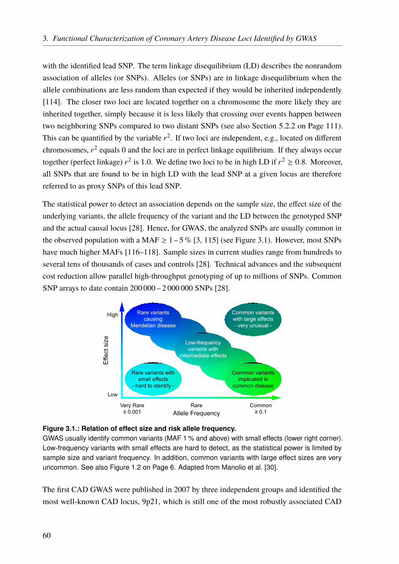
3. Functional Characterization of Coronary Artery Disease Loci Identified by GWAS
with the identified lead SNP. The term linkage disequilibrium (LD) describes the nonrandomassociation of alleles (or SNPs). Alleles (or SNPs) are in linkage disequilibrium when theallele combinations are less random than expected if they would be inherited independently[114]. The closer two loci are located together on a chromosome the more likely they areinherited together, simply because it is less likely that crossing over events happen betweentwo neighboring SNPs compared to two distant SNPs (see also Section 5.2.2 on Page 111).This can be quantified by the variable r2. If two loci are independent, e.g., located on differentchromosomes, r2 equals 0 and the loci are in perfect linkage equilibrium. If they always occurtogether (perfect linkage) r2 is 1.0. We define two loci to be in high LD if r2 ≥ 0.8. Moreover,all SNPs that are found to be in high LD with the lead SNP at a given locus are thereforereferred to as proxy SNPs of this lead SNP.
The statistical power to detect an association depends on the sample size, the effect size of theunderlying variants, the allele frequency of the variant and the LD between the genotyped SNPand the actual causal locus [28]. Hence, for GWAS, the analyzed SNPs are usually common inthe observed population with a MAF ≥ 1 – 5% [3, 115] (see Figure 3.1). However, most SNPshave much higher MAFs [116–118]. Sample sizes in current studies range from hundreds toseveral tens of thousands of cases and controls [28]. Technical advances and the subsequentcost reduction allow parallel high-throughput genotyping of up to millions of SNPs. CommonSNP arrays to date contain 200 000 – 2 000 000 SNPs [28].
Allele Frequency
Effe
ct s
ize
Low
High
Very Rare≤ 0.001
Rare Common≥ 0.1
Rare variantscausing
Mendelian disease
Common variantsimplicated in
common disease
Low-frequencyvariants with
intermediate effects
Rare variants withsmall effects
- hard to identify -
Common variantswith large effects- very unusual -
Figure 3.1.: Relation of effect size and risk allele frequency.GWAS usually identify common variants (MAF 1 % and above) with small effects (lower right corner).Low-frequency variants with small effects are hard to detect, as the statistical power is limited bysample size and variant frequency. In addition, common variants with large effect sizes are veryuncommon. See also Figure 1.2 on Page 6. Adapted from Manolio et al. [30].
The first CAD GWAS were published in 2007 by three independent groups and identified themost well-known CAD locus, 9p21, which is still one of the most robustly associated CAD
60
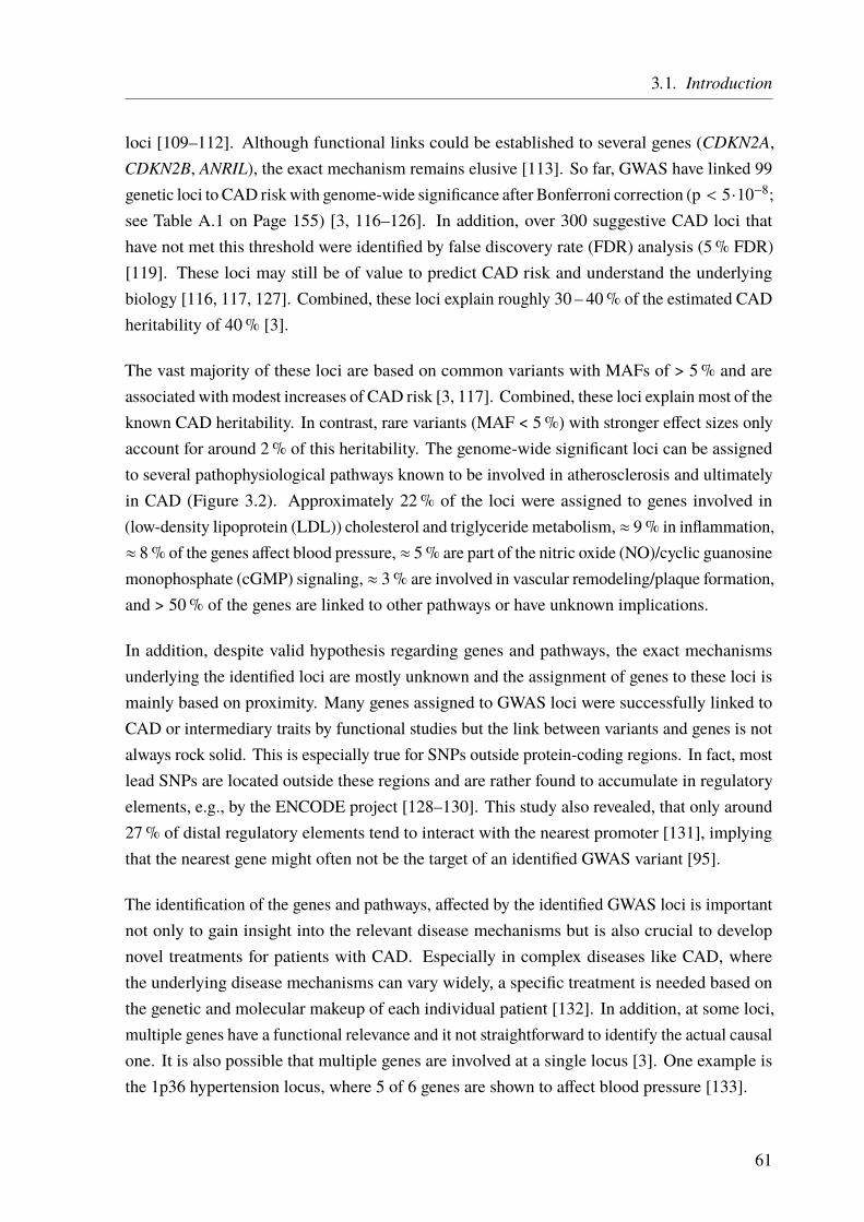
3.1. Introduction
loci [109–112]. Although functional links could be established to several genes (CDKN2A,CDKN2B, ANRIL), the exact mechanism remains elusive [113]. So far, GWAS have linked 99genetic loci to CAD riskwith genome-wide significance after Bonferroni correction (p < 5·10−8;see Table A.1 on Page 155) [3, 116–126]. In addition, over 300 suggestive CAD loci thathave not met this threshold were identified by false discovery rate (FDR) analysis (5% FDR)[119]. These loci may still be of value to predict CAD risk and understand the underlyingbiology [116, 117, 127]. Combined, these loci explain roughly 30 – 40% of the estimated CADheritability of 40% [3].
The vast majority of these loci are based on common variants with MAFs of > 5% and areassociated with modest increases of CAD risk [3, 117]. Combined, these loci explain most of theknown CAD heritability. In contrast, rare variants (MAF < 5%) with stronger effect sizes onlyaccount for around 2% of this heritability. The genome-wide significant loci can be assignedto several pathophysiological pathways known to be involved in atherosclerosis and ultimatelyin CAD (Figure 3.2). Approximately 22% of the loci were assigned to genes involved in(low-density lipoprotein (LDL)) cholesterol and triglyceride metabolism, ≈ 9% in inflammation,≈ 8% of the genes affect blood pressure, ≈ 5% are part of the nitric oxide (NO)/cyclic guanosinemonophosphate (cGMP) signaling, ≈ 3% are involved in vascular remodeling/plaque formation,and > 50% of the genes are linked to other pathways or have unknown implications.
In addition, despite valid hypothesis regarding genes and pathways, the exact mechanismsunderlying the identified loci are mostly unknown and the assignment of genes to these loci ismainly based on proximity. Many genes assigned to GWAS loci were successfully linked toCAD or intermediary traits by functional studies but the link between variants and genes is notalways rock solid. This is especially true for SNPs outside protein-coding regions. In fact, mostlead SNPs are located outside these regions and are rather found to accumulate in regulatoryelements, e.g., by the ENCODE project [128–130]. This study also revealed, that only around27% of distal regulatory elements tend to interact with the nearest promoter [131], implyingthat the nearest gene might often not be the target of an identified GWAS variant [95].
The identification of the genes and pathways, affected by the identified GWAS loci is importantnot only to gain insight into the relevant disease mechanisms but is also crucial to developnovel treatments for patients with CAD. Especially in complex diseases like CAD, wherethe underlying disease mechanisms can vary widely, a specific treatment is needed based onthe genetic and molecular makeup of each individual patient [132]. In addition, at some loci,multiple genes have a functional relevance and it not straightforward to identify the actual causalone. It is also possible that multiple genes are involved at a single locus [3]. One example isthe 1p36 hypertension locus, where 5 of 6 genes are shown to affect blood pressure [133].
61
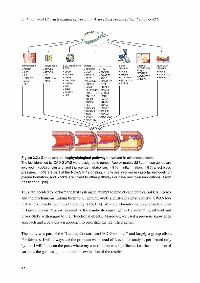
3. Functional Characterization of Coronary Artery Disease Loci Identified by GWAS
Others• PPAP2B• MIA3• WDR12• ZEB2• VAMP5/8• EDNRA• NOA1• SLC22A4/5• PHACTR1• ANKS1A• TCF21• KCNK5• PLG• BCAP29• ZC3HC1• 9p21• SVEP1• KIAA1462
• LIPA• PDGFD• SWAP70• KSR2• COL4A1/2• FLT1• HHIPL1• SMAD3• MFGE8• SMG6• RASD1• UBE2Z• BCAS3• PMAIP1• ZNF507• KCNE2• ADORA2A
Triglycerides• APOA5• APOC3• LPL• ANGPTL4• APOE
LDL-cholesterol/Lp(a)• LDLR• PCSK9• APOB• ABCG5/8• HNF1A• AB0• TRIB1• SORT1• LPA
Inflammation• SH2B3• IL6R• IL5• CXCL12• MRAS• PLG
NO/cGMPsignaling• NOS3• GUCY1A3
Vascularremodelling/Plaqueformation• ADAMTS7• HDAC9
Bloodpressure• NOS3• SH2B3• CYP17A1• GUCY1A3• FURIN
Loci associated with CAD
• PDE5A
Figure 3.2.: Genes and pathophysiological pathways involved in atherosclerosis.The loci identified by CAD GWAS were assigned to genes. Approximately 22 % of these genes areinvolved in (LDL) cholesterol and triglyceride metabolism, ≈ 9 % in inflammation, ≈ 8 % affect bloodpressure, ≈ 5 % are part of the NO/cGMP signaling, ≈ 3 % are involved in vascular remodeling/-plaque formation, and > 50 % are linked to other pathways or have unknown implications. FromKessler et al. [98].
Thus, we decided to perform the first systematic attempt to predict candidate causal CAD genesand the mechanisms linking them to all genome-wide significant and suggestive GWAS locithat were known by the time of the study [116, 134]. We used a bioinformatics approach, shownin Figure 3.3 on Page 64, to identify the candidate causal genes by annotating all lead andproxy SNPs with regard to their functional effects. Moreover, we used a previous knowledgeapproach and a data-driven approach to prioritize the identified genes.
The study was part of the “Leducq Consortium CAD Genomics” and largely a group effort.For fairness, I will always use the pronoun we instead of I, even for analysis performed onlyby me. I will focus on the parts where my contribution was significant, i.e., the annotation ofvariants, the gene assignment, and the evaluation of the results.
62

3.2. Methods
Detailed information on all methods that are not described here (in detail), is available in theonline supplementary material to the corresponding publication [134].
We identified 159 independent CAD-associated lead SNPs, of which 153 were reported bythe CARDIoGRAMplusC4D 1 000 Genomes-based genome-wide meta-analysis [116]. Sixadditional SNPs were reported in Reilly et al. [135] (rs1994016, rs3825807, rs4380028), Wanget al. [136] (rs6903956), and Schunkert et al. [137] (rs964184, rs10953541). We used the SNAPbioinformatics tool [138] to retrieve all SNPs that were in high linkage disequilibrium (LD)(r2 ≥ 0.8) with these lead SNPs, based on the 1 000 Genomes project data (pilot 1, CEUpopulation) [25], within 500 kb distance of the lead SNP. We found a total of 3432 proxy(and lead) SNPs. Nine SNPs were single SNP loci without SNPs in high LD. (See Table I inthe online supplement of Brænne et al. [134]). The SNPs span 135 nonoverlapping genomicregions with an average size of 76.5 kb (ranging from 488 bp to 566 kb).
A detailed description of the methods follows below, in brief: We developed an in-silico pipeline(Figure 3.3) to estimate the functional effects of the loci. For this, we assigned all CAD leadand proxy SNPs of a locus to genes by functionally linking the SNP with gene expression or aprotein-altering effect (part A) In addition we annotated SNPs located in regulatory regions. Inpart B of the pipeline, we identified the most likely causal SNP per locus and prioritized thegenes using a prior-knowledge and a data-driven approach. This left us with scored candidategenes from both approaches.
3.2.1. Identification of Protein-Altering Effects
The pipeline links a SNP with a gene by regulatory or protein-altering effects. Protein-alteringeffects were annotated using the ANNOVAR software [60]. The RefSeq genes [61, 62]and UCSC genes [63] tables provided through the UCSC table browser were used for geneannotation. To estimate if a nonsynonymous SNP is tolerated or deleterious, we utilizedwell-established SNP scores such as SIFT [86], PolyPhen [87], andMutation Taster [88] derivedfrom the LJB2 database [139] provided through the ANNOVAR software. In addition, we alsoused the CADD score [90], which integrates multiple annotations into one metric by takingadvantage of modern machine learning algorithms.
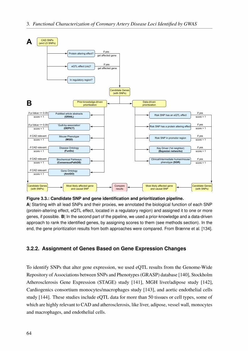
3. Functional Characterization of Coronary Artery Disease Loci Identified by GWAS
CAD SNPs(and LD SNPs)
Protein altering effect?
eQTL effect (cis)?
In regulatory region?
Candidate Genes(with SNPs)
if yesget affected gene
if yesget affected gene
Prior-knowledge-drivenprioritization
PubMed article abstracts(GRAIL)
‘Guilt-by-association‘(DEPICT)
Mouse Phenotype(MGD)
Disease Ontology(FunDo)
Biochemical Pahtways(ConsensusPathDB)
Gene Ontology(AmiGO)
if p-Value <= 0.05score + 1
if p-Value <= 0.05score + 1
if CAD relevantscore + 1
if CAD relevantscore + 1
if CAD relevantscore + 1
if CAD relevantscore + 1
Data-drivenprioritization
Risk SNP has an eQTL effect
Risk SNP has a protein altering effect
Risk SNP in promotor region
Key Driver (1st neighbor)(Bayesian networks)
Clinical/intermediate human/mousephenotype (SGR)
if yesscore + 1
if yesscore + 1
if yesscore + 1
if yesscore + 1
if yesscore + 1
Candidate Genes(with SNPs)
Candidate Genes(with SNPs)
Compareresults
Most likely affected geneand causal SNP
Most likely affected geneand causal SNP
A
B
Figure 3.3.: Candidate SNP and gene identification and prioritization pipeline.A| Starting with all lead SNPs and their proxies, we annotated the biological function of each SNP(protein-altering effect, eQTL effect, located in a regulatory region) and assigned it to one or moregenes, if possible. B| In the second part of the pipeline, we used a prior-knowledge and a data-drivenapproach to rank the identified genes, by assigning scores to them (see methods section). In theend, the gene prioritization results from both approaches were compared. From Brænne et al. [134].
3.2.2. Assignment of Genes Based on Gene Expression Changes
To identify SNPs that alter gene expression, we used eQTL results from the Genome-WideRepository of Associations between SNPs and Phenotypes (GRASP) database [140], StockholmAtherosclerosis Gene Expression (STAGE) study [141], MGH liver/adipose study [142],Cardiogenics consortium monocytes/macrophages study [143], and aortic endothelial cellsstudy [144]. These studies include eQTL data for more than 50 tissues or cell types, some ofwhich are highly relevant to CAD and atherosclerosis, like liver, adipose, vessel wall, monocytesand macrophages, and endothelial cells.
64
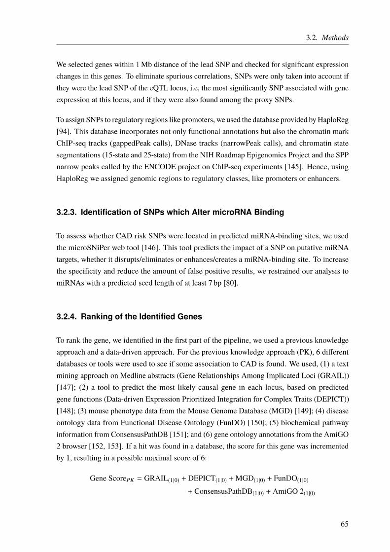
3.2. Methods
We selected genes within 1Mb distance of the lead SNP and checked for significant expressionchanges in this genes. To eliminate spurious correlations, SNPs were only taken into account ifthey were the lead SNP of the eQTL locus, i.e, the most significantly SNP associated with geneexpression at this locus, and if they were also found among the proxy SNPs.
To assign SNPs to regulatory regions like promoters, we used the database provided byHaploReg[94]. This database incorporates not only functional annotations but also the chromatin markChIP-seq tracks (gappedPeak calls), DNase tracks (narrowPeak calls), and chromatin statesegmentations (15-state and 25-state) from the NIH Roadmap Epigenomics Project and the SPPnarrow peaks called by the ENCODE project on ChIP-seq experiments [145]. Hence, usingHaploReg we assigned genomic regions to regulatory classes, like promoters or enhancers.
3.2.3. Identification of SNPs which Alter microRNA Binding
To assess whether CAD risk SNPs were located in predicted miRNA-binding sites, we usedthe microSNiPer web tool [146]. This tool predicts the impact of a SNP on putative miRNAtargets, whether it disrupts/eliminates or enhances/creates a miRNA-binding site. To increasethe specificity and reduce the amount of false positive results, we restrained our analysis tomiRNAs with a predicted seed length of at least 7 bp [80].
3.2.4. Ranking of the Identified Genes
To rank the gene, we identified in the first part of the pipeline, we used a previous knowledgeapproach and a data-driven approach. For the previous knowledge approach (PK), 6 differentdatabases or tools were used to see if some association to CAD is found. We used, (1) a textmining approach on Medline abstracts (Gene Relationships Among Implicated Loci (GRAIL))[147]; (2) a tool to predict the most likely causal gene in each locus, based on predictedgene functions (Data-driven Expression Prioritized Integration for Complex Traits (DEPICT))[148]; (3) mouse phenotype data from the Mouse Genome Database (MGD) [149]; (4) diseaseontology data from Functional Disease Ontology (FunDO) [150]; (5) biochemical pathwayinformation from ConsensusPathDB [151]; and (6) gene ontology annotations from the AmiGO2 browser [152, 153]. If a hit was found in a database, the score for this gene was incrementedby 1, resulting in a possible maximal score of 6:
Gene ScorePK = GRAIL(1|0) + DEPICT(1|0) +MGD(1|0) + FunDO(1|0)+ ConsensusPathDB(1|0) + AmiGO 2(1|0)
65

3. Functional Characterization of Coronary Artery Disease Loci Identified by GWAS
For the data-driven approach (DD) we scored the genes based on 5 categories. The first threecategories were based on the identified effect of the SNP on the gene: (1) nonsynonymousSNPs (AA-changes); (2) eQTL SNPs; (3) CAD SNPs within promoter regions. The remainingtwo categories were based on gene attributes: (4) key drivers of a CAD-relevant BayesianNetwork constructed from CAD-relevant tissue gene expression studies; and (5) correlationwith aortic root lesion size in a systems genetics study of atherosclerosis in mice [154]. Thescore was calculated analog to the previous knowledge-based score (maximal score 5):
Gene ScoreDD = AA-change(1|0) + eQTL SNP(1|0) + Promoter SNP(1|0)+ Key driver(1|0) + Systems genetics mice(1|0)
3.2.5. Key Driver Analysis for CAD Gene Regulatory Networks
To identify the gene regulatory networks of CAD genes, human tissue-specific Bayesian networkmodels, constructed from transcriptomic and genetic datasets, were retrieved from multiplehuman and mouse studies, including adipose tissue, liver, blood, brain, kidney, islet, andmuscle [155–163]. The network topology of these tissue-specific Bayesian networks defines apartitioned joint probability distribution over all genes, capturing detailed gene-gene regulatoryrelationships of CAD genes. A key driver analysis algorithm of gene-gene interaction networks,previously developed by consortium members [164–166], was applied to CAD datasets toidentify the key regulatory genes.
66
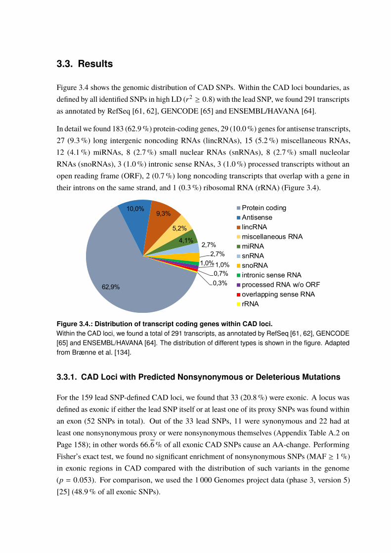
3.3. Results
Figure 3.4 shows the genomic distribution of CAD SNPs. Within the CAD loci boundaries, asdefined by all identified SNPs in high LD (r2 ≥ 0.8) with the lead SNP, we found 291 transcriptsas annotated by RefSeq [61, 62], GENCODE [65] and ENSEMBL/HAVANA [64].
In detail we found 183 (62.9%) protein-coding genes, 29 (10.0%) genes for antisense transcripts,27 (9.3%) long intergenic noncoding RNAs (lincRNAs), 15 (5.2%) miscellaneous RNAs,12 (4.1%) miRNAs, 8 (2.7%) small nuclear RNAs (snRNAs), 8 (2.7%) small nucleolarRNAs (snoRNAs), 3 (1.0%) intronic sense RNAs, 3 (1.0%) processed transcripts without anopen reading frame (ORF), 2 (0.7%) long noncoding transcripts that overlap with a gene intheir introns on the same strand, and 1 (0.3%) ribosomal RNA (rRNA) (Figure 3.4).
62,9%
10,0%9,3%
5,2%
4,1% 2,7%2,7%
1,0%1,0%0,7%0,3%
Protein codingAntisenselincRNAmiscellaneous RNAmiRNAsnRNAsnoRNAintronic sense RNAprocessed RNA w/o ORFoverlapping sense RNArRNA
Figure 3.4.: Distribution of transcript coding genes within CAD loci.Within the CAD loci, we found a total of 291 transcripts, as annotated by RefSeq [61, 62], GENCODE[65] and ENSEMBL/HAVANA [64]. The distribution of different types is shown in the figure. Adaptedfrom Brænne et al. [134].
3.3.1. CAD Loci with Predicted Nonsynonymous or Deleterious Mutations
For the 159 lead SNP-defined CAD loci, we found that 33 (20.8%) were exonic. A locus wasdefined as exonic if either the lead SNP itself or at least one of its proxy SNPs was found withinan exon (52 SNPs in total). Out of the 33 lead SNPs, 11 were synonymous and 22 had atleast one nonsynonymous proxy or were nonsynonymous themselves (Appendix Table A.2 onPage 158); in other words 66.6% of all exonic CAD SNPs cause an AA-change. PerformingFisher’s exact test, we found no significant enrichment of nonsynonymous SNPs (MAF ≥ 1%)in exonic regions in CAD compared with the distribution of such variants in the genome(p = 0.053). For comparison, we used the 1 000 Genomes project data (phase 3, version 5)[25] (48.9% of all exonic SNPs).

3. Functional Characterization of Coronary Artery Disease Loci Identified by GWAS
In the downstream analysis, we focused on the deleterious SNPs as these are more likely tobe causal. A SNP was defined as deleterious using state of the art scoring algorithms (seePage 63). Out of five lead SNPs that cause an AA-change, three were predicted to be deleterious(rs867186, rs2571445, and rs11556924). For two of these, we also identified a proxy SNPcausing a deleterious AA-change. For 7 other lead SNPs, we identified nonsynonymous proxySNPs that were predicted to be deleterious. In summary, we found 12 deleterious AA-changingSNPs, mapping to 10 independent lead SNPs (6.3% of all lead SNPs) (Table 3.1).
Table 3.1.: Predicted deleterious CAD SNPs.We found 12 SNPs in 10 independent loci (lead SNPs) predicted to be deleterious by at least one ofthe used prediction scores. Transcript IDs are taken from RefSeq.
Proxy SNP Lead SNP CHR Position (hg19) Gene Transcript ID AA-change
rs35107735 rs12125501 1 169 390 957 CCDC181 NM_021179 p.F238Irs2820312 rs2820315 1 201 869 257 LMOD1 NM_012134 p.T295Mrs35212307 rs2351524 2 203 765 756 WDR12 NM_018256 p.I75Vrs2571445 rs2571445 2 218 683 154 TNS1 NM_022648 p.W1197Rrs1137524 rs7642590 3 47 956 424 MAP4 NM_001134364 p.V628Lrs1060407 rs7642590 3 47 958 037 MAP4 NM_001134364 p.S427Yrs11556924 rs11556924 7 129 663 496 ZC3HC1 NM_016478 p.R363Hrs11528010 rs7074064 10 88 635 779 BMPR1A NM_004329 p.P2Trs1169288 rs2244608 12 121 416 650 HNF1A NM_000545 p.I27Lrs4584886 rs4299203 17 17 896 205 LRRC48 NM_001130092 p.R191Wrs11906160 rs867186 20 33 565 755 MYH7B NM_020884 p.A25Trs867186 rs867186 20 33 764 554 PROCR NM_006404 p.S219G
Some loci also harbor multiple deleterious SNPs. For instance, chromosome 3p21.31 locusharbors two deleterious SNPs (rs1137524 and rs1060407) that both affect theMAP4 gene. Asecond example is the lead SNP, rs867186, in the 20q11.22 locus, which is predicted to cause adeleterious AA-change in the PROCR gene. The same SNP is also in high LD with rs11906160(r2 = 0.92) which causes a deleterious AA-change in the MYH7B gene.
3.3.2. CAD Loci with Regulatory Effects on Gene Expression
Beside protein-altering effects, SNPs can also be assigned to genes based on their regulatoryfunction, e.g., influence on gene expression. These SNPs are often located in regulatory regionssuch as promoters. We found 66 CAD loci that were significantly associated with nearby geneexpression, either by the lead SNP or by one of the proxy SNPs. Hence, if we compare thenumber of loci altering the protein structure (20.8%) with the number of loci altering geneexpression (41.5%), it becomes evident that most CAD loci act through gene regulation.
68
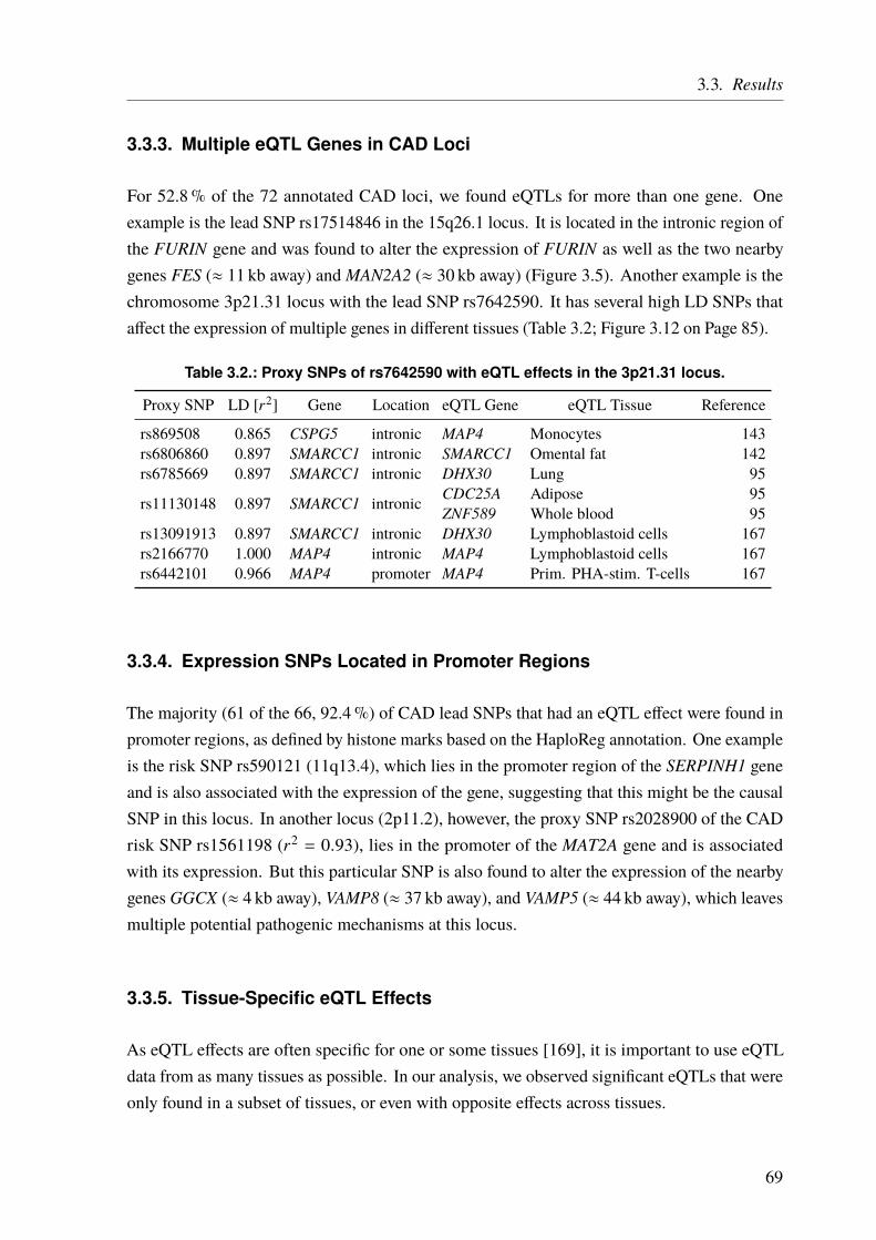
3.3. Results
3.3.3. Multiple eQTL Genes in CAD Loci
For 52.8% of the 72 annotated CAD loci, we found eQTLs for more than one gene. Oneexample is the lead SNP rs17514846 in the 15q26.1 locus. It is located in the intronic region ofthe FURIN gene and was found to alter the expression of FURIN as well as the two nearbygenes FES (≈ 11 kb away) andMAN2A2 (≈ 30 kb away) (Figure 3.5). Another example is thechromosome 3p21.31 locus with the lead SNP rs7642590. It has several high LD SNPs thataffect the expression of multiple genes in different tissues (Table 3.2; Figure 3.12 on Page 85).
Table 3.2.: Proxy SNPs of rs7642590 with eQTL effects in the 3p21.31 locus.
Proxy SNP LD [r2] Gene Location eQTL Gene eQTL Tissue Reference
rs869508 0.865 CSPG5 intronic MAP4 Monocytes 143rs6806860 0.897 SMARCC1 intronic SMARCC1 Omental fat 142rs6785669 0.897 SMARCC1 intronic DHX30 Lung 95
rs11130148 0.897 SMARCC1 intronic CDC25A Adipose 95ZNF589 Whole blood 95
rs13091913 0.897 SMARCC1 intronic DHX30 Lymphoblastoid cells 167rs2166770 1.000 MAP4 intronic MAP4 Lymphoblastoid cells 167rs6442101 0.966 MAP4 promoter MAP4 Prim. PHA-stim. T-cells 167
3.3.4. Expression SNPs Located in Promoter Regions
The majority (61 of the 66, 92.4%) of CAD lead SNPs that had an eQTL effect were found inpromoter regions, as defined by histone marks based on the HaploReg annotation. One exampleis the risk SNP rs590121 (11q13.4), which lies in the promoter region of the SERPINH1 geneand is also associated with the expression of the gene, suggesting that this might be the causalSNP in this locus. In another locus (2p11.2), however, the proxy SNP rs2028900 of the CADrisk SNP rs1561198 (r2 = 0.93), lies in the promoter of the MAT2A gene and is associatedwith its expression. But this particular SNP is also found to alter the expression of the nearbygenes GGCX (≈ 4 kb away), VAMP8 (≈ 37 kb away), and VAMP5 (≈ 44 kb away), which leavesmultiple potential pathogenic mechanisms at this locus.
3.3.5. Tissue-Specific eQTL Effects
As eQTL effects are often specific for one or some tissues [169], it is important to use eQTLdata from as many tissues as possible. In our analysis, we observed significant eQTLs that wereonly found in a subset of tissues, or even with opposite effects across tissues.
69
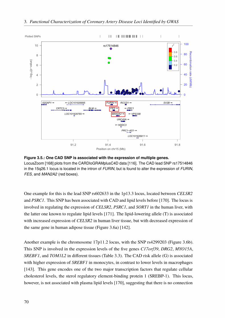
3. Functional Characterization of Coronary Artery Disease Loci Identified by GWAS
Figure 3.5.: One CAD SNP is associated with the expression of multiple genes.LocusZoom [168] plots from the CARDIoGRAMplusC4D data [116]. The CAD lead SNP rs17514846in the 15q26.1 locus is located in the intron of FURIN, but is found to alter the expression of FURIN,FES, and MAN2A2 (red boxes).
One example for this is the lead SNP rs602633 in the 1p13.3 locus, located between CELSR2and PSRC1. This SNP has been associated with CAD and lipid levels before [170]. The locus isinvolved in regulating the expression of CELSR2, PSRC1, and SORT1 in the human liver, withthe latter one known to regulate lipid levels [171]. The lipid-lowering allele (T) is associatedwith increased expression of CELSR2 in human liver tissue, but with decreased expression ofthe same gene in human adipose tissue (Figure 3.6a) [142].
Another example is the chromosome 17p11.2 locus, with the SNP rs4299203 (Figure 3.6b).This SNP is involved in the expression levels of the five genes C17orf39, DRG2, MYO15A,SREBF1, and TOM1L2 in different tissues (Table 3.3). The CAD risk allele (G) is associatedwith higher expression of SREBF1 in monocytes, in contrast to lower levels in macrophages[143]. This gene encodes one of the two major transcription factors that regulate cellularcholesterol levels, the sterol regulatory element-binding protein 1 (SREBP-1). This locus,however, is not associated with plasma lipid levels [170], suggesting that there is no connection
70
3.3. Results
CELSR2 eQTL
0
1
2
-1
-2
0
1
2
-1
-2
3
-3
GG GT TT GG GT TT
liver adipose
rs602633 genotype rs602633 genotype
(a) rs602633 affects CELSR2 expression in liver andadipose tissue inversely.
SREBF1 eQTL
7.2
7.4
7.6
7.0
6.8
8.0
7.5
8.5
TT GT GG TT GT GG
monocytes macrophages
6.6
rs4299203 genotype rs4299203 genotype
(b) rs4299203 affects SREBF1 expression in mono-cytes and macrophages inversely.
Figure 3.6.: Tissue-specific eQTL effects in CAD loci.LocusZoom [168] plots from the CARDIoGRAMplusC4D data [116] and eQTL data for two CADloci with tissue-specific eQTL effects. a| The CAD SNP rs602633 at the chromosome 1p13.3 areassociated with the expression of CELSR2, PSRC1, and SORT1. The risk allele (G) of rs602633 isassociated with the lower expression of CELSR2 in liver tissue but with higher expression levels inadipose tissue [142]. b| The CAD SNP rs4299203 at the chromosome 17p11.2 are associated withthe expression of DRG2, C17orf39, MYO15A, TOM1L2, and SREBF1. The CAD risk allele (G) isassociated with higher expression of SREBF1 in monocytes, but lower expression in macrophages[143]. Adapted from Brænne et al. [134].
between the SNP effect on SREBPF1 levels and the possible effects of this locus on lipidlevels.
Table 3.3.: eQTL effects in the 17p11.2 locus with CAD lead SNP rs4299203.
Proxy SNP LD [r2] Gene Location eQTL Gene eQTL Tissue Reference
rs7219320 1.000 LRRC48 intronic TOM1L2 Ileum 95rs4459604 0.833 LRRC48 intronic SREBF1 Monocytes 143rs9913277 0.833 LRRC48 intronic DRG2 Prefrontal cortex 95rs2955359 0.833 GID4 intronic C17orf39 Subcutaneous fat 158
rs2955355 0.833 GID4 intronic C17orf39 Omental fat 142MYO15A Blood 157
rs2955372 0.833 LRRC48 3’ UTR C17orf39 Lung 95
71
3. Functional Characterization of Coronary Artery Disease Loci Identified by GWAS
3.3.6. Amino Acid Changes and eQTLs
A subset of the CAD loci both harbor nonsynonymous SNPs and SNPs influencing geneexpression, hence adding another level of complexity. One example is the lead SNP rs2246833at the 10q23.31 locus. The risk allele (T) for instance, is directly associated with increasedexpression levels of LIPA in the cardiogenics monocyte eQTL data (p = 3.4 · 10−130; n = 785),matching earlier results [172]. This association is also found in the MGH data for liver(p = 2 · 10−44; n = 741), subcutaneous fat (p = 1 · 10−3; n = 612), and omental adipose tissue(p = 2 · 10−15; n = 567). The SNP is also in high LD (r2 = 0.89) with rs1051338, which leadsto an AA-change in the same gene.
3.3.7. CAD SNPs Affecting miRNA-Binding
Another component involved in gene regulation are microRNAs (miRNAs). miRNAs are smallnoncoding RNA molecules that affect RNA silencing and post-transcriptional gene expression,mostly by binding specifically to the 3’ UTR of the target genes mRNA [81, 82]. Hence, CADrisk SNPs located within miRNA-binding sites could contribute to the disease mechanism. TheCAD SNP rs12190287 in the 6q23.2 locus lies in the 3’ UTR of the TCF21 gene and was shownto affect binding of miR-224 [173]. Therefore, we reviewed CAD risk SNPs mapping to 3’ UTRregions and checked if they lie in predicted miRNA-binding sites, using the microSNIPERdatabase [146]. We found 55 3’ UTR CAD SNPs in 33 distinct genes that were predicted to liewithin a miRNA-binding site, with a total of 254 different miRNAs affected (Table IV in theonline data supplement [134]). The 3’ UTR regions were annotated to harbor between 1 (forBCAP29, MAP4, RND3, and WDR12) and 29 (for MRAS) different miRNAs. Twenty-threeof the miRNAs were predicted to bind more than one candidate gene. Two examples arehsa-miR-130a-5p which was predicted to bind UBE2Z (with the 3’ UTR SNP rs15563) andSLC22A3 (with the 3’ UTR SNP rs3088442), and hsa-miR-4722-5p which was predicted tobind APOA5 (with the 3’ UTR SNP rs2266788) and ICA1L (with the 3’ UTR SNP rs72932707).Matching the expected effect on APOA5, rs2266788 was significantly associated with plasmatriglyceride levels [170].
Thirteen of the 55 CADSNPs that affect miRNA-binding were also found to have an eQTL effecton the respective genes. For instance, rs360137 (11p15.4) affects the binding of hsa-miR-3198to the 3’ UTR of SWAP70 and also the expression of the same gene. Similarly, rs1058588 at the2p11.2 locus is predicted to affect the binding of hsa-miR-5197-3p to the 3’ UTR of VAMP8 andis also involved in regulating its expression. In the 1q32.1 locus, rs12733378 affects the bindingof 5 miRNAs at the 3’ UTR of CAMSAP2 (hsa-miR-3121-3p, hsa-miR-1257, hsa-miR-4765,
72

3.3. Results
hsa-miR-200c-3p, hsa-miR-7-2-3p, hsa-miR-4765, hsa-miR-7-1-3p) and is also associated withthe same gene’s expression. In this examples, it is likely that the observed eQTL effects arebased on the altered miRNA-binding to the target genes, due to the SNPs in the 3’ UTR.
However, we did not use miRNA to assign genes to GWAS loci, for two reasons. First, theinfluence on miRNA binding is only predicted and not validated experimentally. Second, evenif the binding is altered, it is not clear how or if the gene’s expression is influenced. Therefore,we used the predicted miRNA binding change only to rank the genes which were identifiedthrough effects on structural protein changes and altered gene expression.
3.3.8. CAD SNPs Affecting miRNA-Binding and Promoter Regions
As opposed to the previous examples, where the eQTL effect might be caused by the SNPspredicted to alter miRNA-binding site, we also found more complex patterns. For example,rs7642590 in the chromosome 3p21.31 locus has two proxy SNPs, rs6442101 (r2 = 0.97) andrs1061003 (r2 = 1.00). The proxy SNP rs6442101 is predicted to lie in the promoter region ofMAP4 in various cell types and tissues examined in the ENCODE [66, 67] and NIH RoadMapEpigenome project. This SNP, however, is also in high LD with rs1061003 (r2 = 0.97), whichis predicted to affect binding of miR-378a-5p in the 3’ UTR ofMAP4 (Figure 3.7). Hence, fromthe in-silico annotation, it is not clear which mechanism underlies the altered gene expression.
GM12878 ChromHMMH1-hESC ChromHMM
K562 ChromHMMHepG2 ChromHMM
HUVEC ChromHMMHMEC ChromHMMHSMM ChromHMMNHEK ChromHMMNHLF ChromHMM
UCSC Genes (RefSeq, GenBank, CCDS, Rfam, tRNAs & Comparative Genomics)
Chromatin State Segmentation by HMM from ENCODE/Broad
MAP4MAP4MAP4MAP4MAP4MAP4MAP4
MAP4MAP4
MAP4 MAP4
MAP4
rs1061003 rs6442101rs7642590
Figure 3.7.: miRNA-binding and promoter regions.CAD lead SNP rs7642590 in the chromosome 3p21.31 locus has two proxy SNPs, rs6442101(r2 = 0.97) and rs1061003 (r2 = 1.00). rs6442101 is predicted to be located in the promoter regionof MAP4 in nine cell types based on ENCODE genome segmentation data (red parts in the lowertrack). However, rs1061003 is predicted to affect binding of miR-378a-5p in the 3’ UTR of MAP4.Figure from the UCSC genome browser with the UCSC genes track [63] and the Chromatin StateSegmentation by HMM track from ENCODE/Broad [66, 67].
73
3. Functional Characterization of Coronary Artery Disease Loci Identified by GWAS
Another example is rs999474 which is located in the promoter region of UBE2Z. It is a proxySNP of rs15563 (r2 = 0.85) and is predicted to affect the binding of eight different miRNAs(hsa-miR-4743-3p, hsa-miR-4724-3p, hsa-miR-130a-5p, hsa-miR-4704-3p, hsa-miR-4704-3p,hsa-miR-1248, hsa-miR-3182, hsa-miR-4665-5p) in the 3’ UTR of the same gene. Hence, itis possible that the respective locus influence the expression ofMAP4 and UBE2Z by eitheraltering TF-binding sites in the promoter region and thus modulating the transcription processitself, or by altering the affinity of miRNA-binding in the 3’ UTR regions and thereby changingthe post-transcriptional gene expression. However, the expression profile of the correspondingtranscription factors and miRNAs in different tissues might allow us to predict the tissues inwhich these genes are functional in the context of CAD.
3.3.9. Prediction of Novel CAD Genes and Candidate Gene Prioritization
Traditionally, GWAS loci were assigned to genes mainly by proximity and GWAS on CAD areno exception. This proximity-based annotation of loci assigned 164 genes to the 159 CAD loci(Appendix Table A.3 on Page 160). However, recent literature evidence [95, 131, 174], as wellas our eQTL results, suggest that the nearest gene is often not the causal one. Our annotation,based on eQTLs and nonsynonymous AA-changes resulted in 150 CAD candidate risk genesfor 159 CAD risk SNPs. Off note, not all loci could be mapped to a gene by our approach, usingthe data we had available as we only assigned genes based on functional links. If we compareour annotation with the previous one [116], we found 97 genes, that were not linked with CADso far (Figure 3.8 and Table A.4 on Page 166). 111 genes were not found with our annotationefforts. These genes might not be affected by CAD SNPs or were missed by our annotationefforts because of incomplete data or because they are acting through other mechanisms.
To prioritize the genes annotated by our pipeline, we used a previous knowledge and a data-driven approach (Figure 3.3 on Page 64). The previous knowledge-driven approach was basedon text mining, scoring the genes based on literature and databases. The data-driven approachused the results from our pipeline and other data from within the consortium. Ranking scoresfor all genes can be found in Appendix Table A.5 on Page 169. More detailed results of theprioritization are available in Table VI of the online supplement [134].
For the previous knowledge approach, 4 genes (CDKN2B, LPL, FURIN, and PROCR) reachedthe maximum score of 6 (see Table 3.4 on Page 76 and Table A.5 on Page 169 for all scores).All of them are also found in the Coronary Artery Disease Gene Database (CADgene) V2.0[176]. This database is specific for CAD genes and is manually curated based on scientificpublications.
74

3.3. Results
1
2
3
45
6
789
10
11
1213
1415
1617
18 19 20 21 22
MAPKAPK5-AS1
RP11-
541N
10.2
hsa-miR
-185
CALCOCO2
AL591069.5
MAPKAPK5
HS.539450
WBSCR16
ZNF589
ANKRD25
POM
121C
AF075
116
TRPC4AP
CCDC
181
C2or
f44
ALS2CR8
FLJ4
2875
FLJ38264
FLJ25841
SMARCC1
YN62D03
FLJ21127
ITGB4BP
C12orf30
C17orf39
C17orf53
CD
KN2A
MYO15A
MAN2A2
UBXN
2A
CDC25A
GALNT4
CEL
SR2
SEC24D
SREBF1
TBXAS1
UBA
P2L
NBEAL1
PMS2L3
ATP8
B2AT
P1B1
KIAA1143
RO
MO
1
C1or
f58
WDR61
SHIS
A4
TRIM73
CH
TOPM
YH7B
CSPG5
OVOL1
VAMP5
POLG2UB
XD4
SFTPC
ALDH2
GG
TL3G
TF2B
MAT
1A
KANK2
SPG21
MT1P3
LTF
CEP70
ASB16
SF3A1
C4orf3
CO
MT
TRIP4
SIPA1
SRPR
ICA1LCARFDRG2
BRAP
KIF1
4
REST
MSL2
RELA
SNX1
EML1
GJC1
AIDAIP
O9
IRS2
EIF6
YY1
DHX30
CAM
SAP1
L1
SERPINH1
HSD17B12
SMARCA4
ADAMTS7
KIAA
1462
PPP2R3A
SLC22A3
TOM
M40
MYB
PHL
CD
KN2B
LIPASWAP70
RBPMS2
PECAM1
SCARB1
ZC3H
C1
TOM1L2
PCNXL3
LRRC48
BMPR
1A
WDR12
PROCR
CNNM2
APOC4
APOC2 LM
OD1
ANXA
11
PSR
C1
SOR
T1
VAMP8
LRRC2
HNF1A
DDX5
9
ATXN2
UBE2Z
NT5C2
SH2B3
FURIN
GGCX
LPAL2
MRAS
APOE N
ME7
MAP4
UBTF
TNS1
MIA
3IL6R
OBFC1 PLG
FES
LPL
ZEB2-AC07
4093
.1
C21orf82
AK09
7927
ARHGAP26
BNC
2
TMEM161B
ALS2CR16
DQ592230
DQ582071
APOB
DYNC2L
I1
AX746739
AX74
7950
BC031936BC038576
BC041459
BC044614BC042673
BC036442
GUCY1A3
PHACTR1PLEKHG1
SLCO1B1
TSC22D2
CYP17
A1
CYP46A1
SLC22A4SLC22A5
PDGFRAGNPDA2
C6orf105
DKFZp564A247
ANKS1A
MAP3K4
CTAGE1
TRAFD1
VAMP10
COL4A4
COL4A1COL4A2
FKSG52AKAP13
BCAP29
PPAP
2B
MST109
CXCL
12
PARP12
ATP2B1
ATPAF2
ATP5SL
ZNF259
ZNF652
C3orf38
C4orf14
C8orf80
C21orf7
ABCG5
ABCG8EDNRA
APOA1
HHIPL1
APOC1
MRG15M
ARK4
ARVC
F
APO5A
PDGFD
HDAC9
POD
XL
ACSS2
KCNK5
RPH3A
RASD1KC
NE2 PC
SK9
PDE3A
SNX10
SPC24
USP53
TCF21JAZF1
LOC3
8893
1
COG
5
TRIB
1RAI1
DCPS
PEMT
SAR
S
RND3
MAP9
BMP1M
TAP
MC
L1
CD
KN2B
AS
CUX2
PKN
2
TERT
RPEL
LDLR
CA10
FLT1
OSM
LY86
HIP1
SMG6
CKM
ABO
NG
F
LPA
SKI
Figure 3.8.: Comparison of the new with the previous annotations of CAD loci.Circos plot [175] shows CAD genes that were only annotated in previous studies (111, black), newlyannotated genes by our pipeline (97, blue) that show no overlap with previous annotations andconcordant annotated genes (53, green). Chromosomes 1 – 22 are shown in different colors and thecorresponding cytoBands (Giemsa staining). See also Table A.4 on Page 166.
75

3. Functional Characterization of Coronary Artery Disease Loci Identified by GWAS
Table 3.4.: Gene ranking based on previous knowledge.The previous knowledge gene score (Gene ScorePK) was calculated based on findings from (1)a text mining approach on Medline abstracts (GRAIL) [147]; (2) a tool to predict the most likelycausal gene in each locus, based on predicted gene functions (DEPICT)[148]; (3) mouse phenotypedata from the MGD [149]; (4) disease ontology data from FunDO [150]; (5) biochemical pathwayinformation from ConsensusPathDB [151]; and (6) gene ontology annotations from the AmiGO 2browser [152, 153].
Gene GRAIL DEPICT MGD FunDO ConsensusPathDB AmiGO 2 Gene ScorePKCDKN2B 4 4 4 4 4 4 6FURIN 4 4 4 4 4 4 6LPL 4 4 4 4 4 4 6PROCR 4 4 4 4 4 4 6
The previous knowledge approach might be biased because there is more information availableon well-studied genes and also more research has been done based on the CAD GWAS. Hence,we also designed an alternative data-driven approach to rank the genes. Four genes, GIP, REST,TMEM116, and LIPA reached a score of 4 in our data-driven approach (see Table 3.5 andTable A.5 on Page 169 for all scores). Only LIPA was linked with CAD previously [172]. Theother three genes represent potential new important CAD genes. We will discuss these genes inmore detail below. Of note, no gene was found in all 5 categories and therefore the top score of5 was not reached.
Table 3.5.: Gene ranking based on our data-driven approach.The data-driven gene score (Gene ScoreDD) was calculated based on findings from (1) Genesthat harbored nonsynonymous SNPs (AA-changes); (2) genes with an assigned eQTL signal; (3)genes that harbor CAD SNPs within their promoter regions; (4) genes that were key drivers of aCAD-relevant Bayesian Network constructed from CAD-relevant tissue gene expression studies;and (5) genes that were significantly correlated with aortic root lesion size in a systems geneticsstudy of atherosclerosis in mice [154].
Gene AA-change eQTL Promoter Key driver Systems genetics mice Gene ScoreDDGIP 4 4 4 - 4 4LIPA 4 4 4 - 4 4REST 4 4 4 - 4 4TMEM116 4 4 4 - 4 4
Gastric Inhibitory Polypeptide (GIP) The CAD lead SNP, rs15563, in the chromosome17q21.32 locus is located in the 3’ UTR of the UBE2Z gene but has a proxy SNP that leads to anonsynonymous AA-change in the GIP gene. The locus is also associated with the expressionof this gene and also with the expression of CALCOCO2, DLX4, SPAG9, ATP5G1, D6RB11,and UBE2Z. Based on our ranking GIP is the highest ranked gene in this locus. The Gastric
76

3.3. Results
Inhibitory Polypeptide (GIP) is an incretin hormone from the glucagon superfamily and wasreported to be involved in insulin secretion [177]. Mouse knockouts of Gip led to reducedobesity and insulin resistance [178, 179]. We also found a positive correlation between Gipexpression and aortic lesion size in the mouse data sets (r = 0.23; p = 0.05) [154].
RE1 Silencing Transcription Factor (REST ) At the chromosome 4q12 locus, the lead SNPrs17087335 is located in the intron of the NOA1 gene. The SNP also has a proxy SNP(rs3796529; r2 = 0.95) that leads to a nonsynonymous AA-change in the REST gene. Moreover,the lead SNP is associated with the expression of REST in lung tissue and another proxySNP (rs6853156; r2 = 0.81) is located in the promoter region of REST (Figure 3.9). In totalrs17087335 has 18 proxy SNPs within a 75.5 kb range. Furthermore, there is a significantcorrelation between aortic Rest expression and the lesion size in mice [154]. REST (RE1Silencing Transcription Factor) encodes for a transcriptional repressor that was reported toplay a role in the phenotypic modulation of vascular smooth muscle cells [180]. It binds tothe promoter of KCNN4, a gene coding for the KCa3.1 potassium channel, and represses itsexpression during intimal hyperplasia. There seems to be an inverse correlation between theexpression of REST and vascular smooth muscle cell proliferation in humans [180]. This isconsistent with the mouse data [154], where we find a negative correlation between aorticexpression of REST and the lesion size (r = −0.24; p = 0.03).
rs170
8733
5
NOA1REST
PromoterIntronicExonic
No annotationeQTLAA-change
rs379
6529
LT
rs685
3156
Figure 3.9.: CAD locus 4q12 (lead SNP rs17087335) with proxy SNPs and their effects.The lead SNP (red) is located in the intron of NOA1 and influences the expression of REST inlung tissue (LT) [95]. It is in high LD (r2 = 0.95) with rs3796529, that leads to a nonsynonymousAA-change in the REST gene. This change is not predicted to be deleterious. Moreover, anotherproxy SNP (rs6853156; r2 = 0.81) is located in the promoter region of REST but has no predictedeffect. In addition, there is a significant correlation between aortic REST expression and the lesionsize in mice [154]. 16 more proxy SNPs without a specific effect or position are not shown. Figurenot to scale.
77
3. Functional Characterization of Coronary Artery Disease Loci Identified by GWAS
Transmembrane Protein 116 (TMEM116) The 12q24.13 locus, lead SNP rs3809274, wastraditionally assigned to the ATXN2 gene [116]. Interestingly, we found multiple eQTL effectsin this locus, TMEM116, C12orf30, SH2B3, BRAP, ALDH2, MAPKAPK5-AS1, HECTD4, andMAPKAPK5, but none for ATXN2. One of the proxy SNPs, rs632650 (r2 = 0.81), is associatedwith increased expression of the transmembrane protein 116 (TMEM116), which is one of thefour genes with the highest score in our data-driven approach. However, not much is knownabout the function of this gene. Nevertheless, TMEM116, got the highest score for this locusas it also harbors a CAD SNP (rs57646770) in its promoter region and its expression wassignificantly associated with aortic lesion size in mice [154].
By comparing both approaches we found that all genes that were prioritized by the previousknowledge approach were also prioritized using the data-driven approach. 69% of all prioritizedgenes were found by both the previous knowledge and data-driven approach. However, for 31%of the genes prioritized by the data-driven approach, we did not find any support for CAD inthe literature (see Table A.5 on Page 169).
To evaluate our annotation efforts per locus, we compared the results of our data-driven approachto the genes previously assigned to the CAD GWAS loci [116] (Figure 3.10 and AppendixTable A.3 on Page 160). For the 159 CAD GWAS loci, 15 loci (9.4%) showed identicalannotation. 25 loci (15.7%) showed no overlap between the old and new annotation, i.e., wefound no evidence for the traditionally annotated genes but found at least one other gene instead.For 3 loci (1.9%), with more than one gene per locus, we could not find evidence for all of thegenes using our pipeline, resulting in fewer genes reported at this loci. For 22 loci (13.8%)we assigned additional genes in addition to the traditional assigned one, which we also foundwith our approach. For 7 loci (4.4%), which have been linked to more than one gene we foundevidence for some of the previously reported genes but not for all, and also found additionalgenes. For 87 loci, we did not find any functional link to any gene.
78

3.3. Results
9,4%
15,7%
1,9%
13,8%
4,4%
54,7%
Identical annotationDifferent annotationLess genesAdditional genesInconsitent annotationNo annotation
Figure 3.10.: Comparison of previous CAD loci annotation and with our new annotation.Previous gene annotations of CAD loci were mainly based on proximity. We used multiple data setsto assign genes to the 159 known loci. 15 loci (9.4 %) showed identical annotation. 25 loci (15.7 %)had a different annotation (only other genes then before). For 3 loci (1.9 %) we found fewer genesthan assigned to a locus previously. For 22 loci (13.8 %) we found genes in addition to the previousones. 7 loci (4.4 %) were inconsistent. We found no evidence for all of the previously assignedgenes, but additional ones instead. For the majority of loci (87, 54.7 %) we were not able to assign agene based on our functional data.
79


3.4. Discussion
Genome-wide association studies (GWAS) for coronary artery disease (CAD) have led to theidentification of numerous genotype-phenotype associations during the last years, resulting inmultiple DNA variants found to be associated with the disease. The main challenge, however,remains the identification of genes and pathways affected by these variants and to understandhow they influence the disease. To date, we have only been able to unravel the mechanisms,which underlie the increased disease risk, for a few loci. Notable examples are the CAD riskalleles at the 1p13, 6q23, and 4q32 loci, which displayed functional links to gene expressionand related disease mechanisms involving SORT1, TCF21, and GUCY1A3 [106, 173, 180, 181].A prominent example of how difficult it is to go from associations to disease mechanism is themost robustly and well-known CAD locus 9p21. This locus was first described in the course ofthe first large-scale GWAS [109–113] in 2007 and has been studied ever since. Despite severalhypotheses, the mechanisms underlying this association are still to be unraveled.
3.4.1. Function-Based Gene Assignment Instead of Proximity
For the majority of GWAS so far, the genes assigned to a given locus were the ones in closestproximity to the identified lead SNP. Recent studies on genetic interaction illustrate, thatbecause of the three-dimensional chromosomal conformation of the DNA, distant genomicregions can interact. Hence, a variant might have an influence on genes several kbp up- ordownstream [182]. For instance, the 16q12.2 locus for obesity, located at the FTO gene, wasshown to interact with the enhancer of IRX3, a transcription factor 1Mb downstream of theidentified SNP [183]. Most genomic variants identified by GWAS are located in noncodingregions of the genome. Hence, common risk SNPs often act through regulatory elementslike transcriptional enhancers and silencers. These elements influence transcription throughlong-range interactions and are typically located > 1 kb away from their target genes [174].For instance, analysis by the ENCODE consortium demonstrated that only around 27% ofdistal regulatory elements tend to interact with the nearest promoter [131], implying that thenearest gene might often not be the target of an identified GWAS variant [95]. To assign genesirrespective of proximity but rather based on functional interaction, we utilized cis-eQTL datafrom different resources, which is based on actual measurements, as well as information aboutprotein-altering SNPs, and SNPs in regulatory elements. This allowed us to identify 97 novelcandidate genes (Figure 3.8 on Page 75 and Table A.4 on Page 166), that had not been linked tothe CAD loci before. Moreover, we also linked some known CAD genes to new loci.
3. Functional Characterization of Coronary Artery Disease Loci Identified by GWAS
Gene assignment without functional evidence illustrates the misleading potential of GWAS.While it is natural to assign genes to loci based on proximity, we have to keep in mind,that GWAS are statistical approaches only linking genetic regions to a trait. This providesinformation about association but not about causality. Although a powerful approach to generatehypotheses, it does not reveal the underlying genetic mechanisms. To interpret and put theGWAS results in a genetic context, we need to systematically map these loci with functionallinks to genes. This work demonstrates how already publicly available data can be used toinform GWAS results and can be used as a blueprint for GWAS to come. Although eQTLsprovide a functional link between loci and genes it does however not link the gene to the disease.This requires functional validation of the findings in the lab. Nevertheless, one of our keyfindings is that some of the CAD SNPs were not associated with the expression of the mostproximal gene but to more distal ones. In the following, I will review some examples of howour annotation effort give new insights into the genetic mechanisms underlying CAD.
The SNP rs12936587 in the chromosome 17p11.2 locus is located between the genes PEMT(≈ 49 kb away) and RAI1 (≈ 41 kb away) but is linked to the expression of TOM1L2 (≈ 200 kbaway). Similarly, the SNP rs9608859 (22q12.2) was found to alter the expression of SF3A1roughly 65 kb away, rather opposed to influencing the expression of the previously assignedand closest genes OSM (≈ 4.5 kb away) and GATSL3 (≈ 14 kb away) [116].
In fact, some CAD risk SNPs were even found within intronic regions of one gene, alsoinfluencing the expression of other (nearby) genes. One example is the 12q21.33 locus withthe SNP rs2681472, which is located in an intron of the ATP2B1 gene. The eQTL effect is,however, on GALNT4 which is approximately 1 kb away. Likewise, rs2895811 (14q32.2) is anintronic CAD SNP within the HHIPL1 gene, but is associated with the expression of the YY1gene in CD19+ B cells that lies roughly 500 kb away [184]. Although there are over a dozengenes in this region, the only potential mechanism we found at this locus was the altered YY1expression.
Another example with misleading potential is the 12q24.12 locus, which harbors two CAD leadSNPs rs3809274 and rs3184504 that are not in LD (r2 = 0.09). rs3809274 is located betweenATXN2 (≈ 7 kb upstream) and BRAP (≈ 36 kb downstream) and was traditionally assigned tothe closest gene ATXN2 [116]. However, with our annotation effort, we found no link betweenthe SNP and ATXN2, but instead with six other genes. One of these genes is SH2B3, whichwas assigned to the SNP rs3184504 previously. This nonsynonymous SNP is located in the3rd exon of SH2B3 (NM_005475.2) and leads to the AA-change from Tryptophan to Arginine(NM_005475.2:c.784T>C(NP_005466.1:p.(W262R))). It seems to be very intuitive to linkthis SNP to SH2B3. However, this SNP is very common in European (non-finish) populations
82
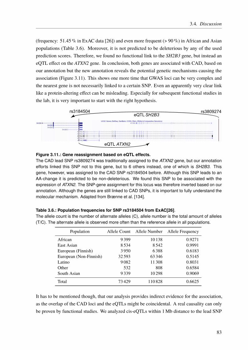
3.4. Discussion
(frequency: 51.45% in ExAC data [26]) and even more frequent (> 90%) in African and Asianpopulations (Table 3.6). Moreover, it is not predicted to be deleterious by any of the usedprediction scores. Therefore, we found no functional link to the SH2B3 gene, but instead aneQTL effect on the ATXN2 gene. In conclusion, both genes are associated with CAD, based onour annotation but the new annotation reveals the potential genetic mechanisms causing theassociation (Figure 3.11). This shows one more time that GWAS loci can be very complex andthe nearest gene is not necessarily linked to a certain SNP. Even an apparently very clear linklike a protein-altering effect can be misleading. Especially for subsequent functional studies inthe lab, it is very important to start with the right hypothesis.
UCSC Genes (RefSeq, GenBank, CCDS, Rfam, tRNAs & Comparative Genomics)SH2B3
SH2B3SH2B3
SH2B3ATXN2ATXN2ATXN2ATXN2ATXN2
ATXN2
rs3184504 rs3809274eQTL SH2B3
eQTL ATXN2
Figure 3.11.: Gene reassignment based on eQTL effects.The CAD lead SNP rs3809274 was traditionally assigned to the ATXN2 gene, but our annotationefforts linked this SNP not to this gene, but to 6 others instead, one of which is SH2B3. Thisgene, however, was assigned to the CAD SNP rs3184504 before. Although this SNP leads to anAA-change it is predicted to be non-deleterious. We found this SNP to be associated with theexpression of ATXN2. The SNP-gene assignment for this locus was therefore inverted based on ourannotation. Although the genes are still linked to CAD SNPs, it is important to fully understand themolecular mechanism. Adapted from Brænne et al. [134].
Table 3.6.: Population frequencies for SNP rs3184504 from ExAC[26].The allele count is the number of alternate alleles (C), allele number is the total amount of alleles(T/C). The alternate allele is observed more often than the reference allele in all populations.
Population Allele Count Allele Number Allele Frequency
African 9 399 10 138 0.9271East Asian 8 534 8 542 0.9991European (Finnish) 3 950 6 388 0.6183European (Non-Finnish) 32 593 63 346 0.5145Latino 9 082 11 308 0.8031Other 532 808 0.6584South Asian 9 339 10 298 0.9069
Total 73 429 110 828 0.6625
It has to be mentioned though, that our analysis provides indirect evidence for the association,as the overlap of the CAD loci and the eQTLs might be coincidental. A real causality can onlybe proven by functional studies. We analyzed cis-eQTLs within 1Mb distance to the lead SNP
83

3. Functional Characterization of Coronary Artery Disease Loci Identified by GWAS
and ignored trans effects which limits our study. Moreover, to reduce spurious findings, we onlymapped the most significant eQTL SNP (eSNP) to the GWAS loci. Although this is a goodstrategy to avoid false positive results, it also leads to false negative ones. To include long-rangeinteractions without losing specificity, results from chromatin conformation capture methodscould be included [185–187]. This would allow to identify genomic regions that interact orare isolated, making interactions likely or unlikely. In addition, chromosome conformationcapture data is generated for specific tissues, allowing to investigate tissue-specific effects moreaccurate.
3.4.2. Most GWAS Loci Affect Expression Changes in Multiple Genes and
Tissues
In concordance with previous studies, which predicted 70 – 80% of GWAS SNPs to beregulatory [128, 182], we found the majority of the 159 GWAS loci to affect gene expression(41.5%) opposed to protein function (6.3%). Interestingly, among the loci that were linkedto gene expression, we revealed that several are in fact associated with expression changes inmultiple genes in multiple tissues. It has been shown before and became also clear by ouranalysis, that it is crucial to consider data from disease relevant tissues, as eQTLs are to alarge percentage tissue-specific [159, 173] and trait-associated variants tend to exert moretissue-specific effects [188, 189]. In addition, some loci overlap regulatory elements andinfluence gene expression but at the same time also alter the protein. The fact that one locus canbe associated with the expression of multiple genes, makes it even more difficult to untanglethe underlying mechanisms at the GWAS loci. This becomes particularly evident when we findmultiple functional links between a locus and its surrounding genes. It is not easy to work outwhether only a single gene at a given locus influences the disease or if multiple genes contributeto the phenotype. And if multiple genes play a role, what is the contribution of each gene andhow are they functionally related? A recent publication by Boyle et al. [190] led to an intensediscussion about the relevance of GWAS findings, which are based on ever-increasing samplesizes [191]. Although large sample sizes and meta-analyses are able to link more and morevariants to a disease does not mean that they have a real-life relevance, as they often have oddsratios (ORs) close to 1 and very low MAFs. These loci might even be misleading, as they mightaffect disease risk through very complex pathways and move the focus away from the real keyplayers.
One example is the highly complex chromosome 3p21.31 locus, represented by the lead SNPrs7642590 in the MAP4 gene (Figure 3.12). This SNP is in high LD (r2 ≥ 0.8) with 12 SNPswith functional implications. Three of them lead to AA-changes in MAP4 and CSPG5, two of
84
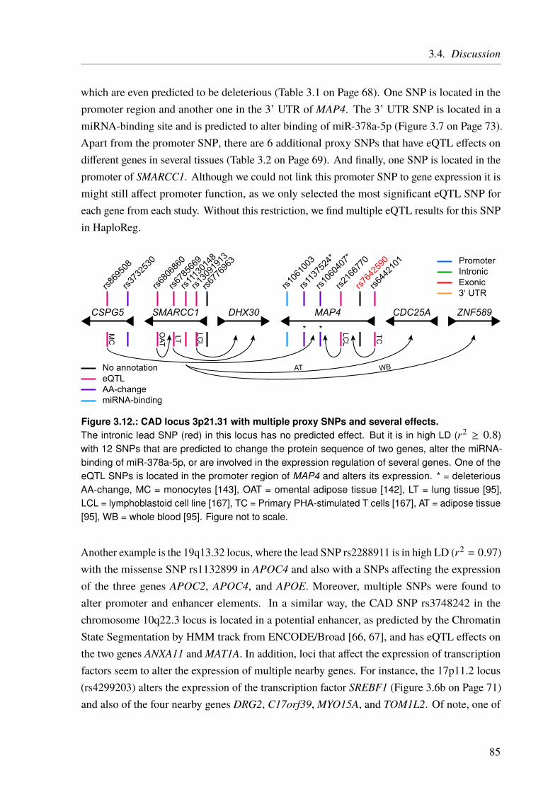
3.4. Discussion
which are even predicted to be deleterious (Table 3.1 on Page 68). One SNP is located in thepromoter region and another one in the 3’ UTR of MAP4. The 3’ UTR SNP is located in amiRNA-binding site and is predicted to alter binding of miR-378a-5p (Figure 3.7 on Page 73).Apart from the promoter SNP, there are 6 additional proxy SNPs that have eQTL effects ondifferent genes in several tissues (Table 3.2 on Page 69). And finally, one SNP is located in thepromoter of SMARCC1. Although we could not link this promoter SNP to gene expression it ismight still affect promoter function, as we only selected the most significant eQTL SNP foreach gene from each study. Without this restriction, we find multiple eQTL results for this SNPin HaploReg.
rs869
508
rs106
1003
rs373
2530
rs680
6860
rs678
5669
rs111
3014
8
rs130
9191
3
rs113
7524
*
rs106
0407
*
rs216
6770
rs764
2590
rs644
2101
rs677
6963
MAP4DHX30SMARCC1CSPG5 CDC25A ZNF589
PromoterIntronic
3‘ UTRExonic
No annotationeQTL
miRNA-bindingAA-change
OAT
AT WBLC
L
LCL
LT
MC
TC
* *
Figure 3.12.: CAD locus 3p21.31 with multiple proxy SNPs and several effects.The intronic lead SNP (red) in this locus has no predicted effect. But it is in high LD (r2 ≥ 0.8)with 12 SNPs that are predicted to change the protein sequence of two genes, alter the miRNA-binding of miR-378a-5p, or are involved in the expression regulation of several genes. One of theeQTL SNPs is located in the promoter region of MAP4 and alters its expression. * = deleteriousAA-change, MC = monocytes [143], OAT = omental adipose tissue [142], LT = lung tissue [95],LCL = lymphoblastoid cell line [167], TC = Primary PHA-stimulated T cells [167], AT = adipose tissue[95], WB = whole blood [95]. Figure not to scale.
Another example is the 19q13.32 locus, where the lead SNP rs2288911 is in high LD (r2 = 0.97)with the missense SNP rs1132899 in APOC4 and also with a SNPs affecting the expressionof the three genes APOC2, APOC4, and APOE. Moreover, multiple SNPs were found toalter promoter and enhancer elements. In a similar way, the CAD SNP rs3748242 in thechromosome 10q22.3 locus is located in a potential enhancer, as predicted by the ChromatinState Segmentation by HMM track from ENCODE/Broad [66, 67], and has eQTL effects onthe two genes ANXA11 and MAT1A. In addition, loci that affect the expression of transcriptionfactors seem to alter the expression of multiple nearby genes. For instance, the 17p11.2 locus(rs4299203) alters the expression of the transcription factor SREBF1 (Figure 3.6b on Page 71)and also of the four nearby genes DRG2, C17orf39,MYO15A, and TOM1L2. Of note, one of
85

3. Functional Characterization of Coronary Artery Disease Loci Identified by GWAS
the proxy SNPs (rs4584886) is also predicted to cause a deleterious AA-change (Table 3.1 onPage 68).
In summary, the majority (38 out of 72; 52.8%) of loci with an annotation were linked tomultiple genes based on our data (Table A.3 on Page 160). This is also in concordance with otherstudies, for example by the ENCODE consortium [131], where it was shown that the averagenumber of target genes for a distal regulatory element is 2.5. This leads to the conclusion,that multiple genes affected by one locus are not rare, indeed, it is rather the rule than theexception.
3.4.3. Expectation Bias Leads to False Gene Assignment
Another challenge is to avoid bias by assigning loci to genes based on the “most likely”hypothesis. This bias is caused by known reported phenotypic effects and the biologicalrelevance of neighboring genes. In other words, if a well-known gene maps to a locus, genesthat are not so well studied are often ignored. One example from our analysis is the chromosome19p13.2 locus with the lead SNP rs1122608. This SNP is located in an intron of SMARCA4.It has been assigned to not only SMARCA4 but also to the neighboring LDLR gene (≈ 36 kbaway) [116, 117]. LDLR is very well studied and established to play an important role inregulating plasma low-density lipoprotein (LDL) levels. In this work, we only found an eQTLassociation to the SMARCA4 gene and not to the LDLR gene. Of note, with limited eQTL data(especially for specific tissues), we could not identify all functional links. However, in thiscase, it is rather unlikely that we missed a clear association as LDLR is primarily expressed inthe liver and our databases included liver eQTLs from multiple studies. Hence, the 19p13.2locus is a good example of the misleading potential of GWAS studies. With the LDLR beinga well-known familial hypercholesterolemia (FH) gene, its natural to assume the locus to beacting through the LDLR increasing the risk for CAD. However, the molecular mechanismleading to an association with CAD in this locus might be the altered expression of SMARCA4,rather than the involvement of LDLR. Nevertheless, the LDLR gene is clearly a causal CADgene, but perhaps not the causal gene at this particular locus.
3.4.4. Ranking of Identified CAD Genes
Linking loci to genes is only the first hurdle we have to take towards understanding the diseasemechanisms. As many loci influence multiple genes in different tissues there are too manygenes to investigate in detail. Hence, it is necessary to rank these genes and find the ones that
86
3.4. Discussion
are most likely involved in pathogenesis and presumably have the strongest effects. These genescan be investigated first, using functional “wet-lab” techniques.
To rank the genes that were identified in the first part of our analysis (Figure 3.3 on Page 64)we used two approaches. One was based on previous knowledge from literature and manuallycurated databases, and the other one was data-driven, based on functional data. Ranking usingprevious biological knowledge about candidate genes leads to a strong bias for well-studiedgenes. For some genes, we found a lot of different functional annotations, based on severalstudies. For other genes, especially those that were not linked to CAD or some other well-studiedphenotype before, only a few data sets were available. This makes it very difficult to link GWASloci to novel genes. Hence, our approach is limited by incomplete information about genefunctions. Most functional annotations were found when searching for biochemical pathwaysin the ConsensusPathDB database and for gene ontology annotations. We could annotate 75 of150 genes (49.6%) with at least one annotation term. However, this also indicates that for halfof the candidate genes no functional annotation was available and that these genes could not beconsidered for prioritization. This previous knowledge-driven approach would again lead tothe high ranking of already well-described genes (the rich get richer principle), whereas thebiological function of underinvestigated and underannotated genes could not be resolved. Forthis reason, it is important to also use an unbiased approach that also allows identification ofnew genes which have not been linked to any phenotype before.
3.4.5. Conclusion and Future Perspective
Our annotation efforts illustrate that the downstream effects of a locus may be highly complexand do not fit into one pathway and that some loci might even affect multiple causal genes.Indeed, this might even be the case for the most cited CAD locus, 9p21. A SNP identified byGWAS might affect several genes, either by altering the expression, the protein sequence or bymore complex mechanisms and therefore increase the disease risk in an additive fashion. It isalso possible that only one, or a few, affected genes actually contribute to the disease mechanismmaking it anything but straightforward to reveal which genes are involved in pathogenesis at agiven locus. In-silico predictions, however, are a good starting point as they establish linksbetween the identified genomic locus, the molecular function, and the disease. It has to be notedthat our annotations only represents the tip of the iceberg, as we limited ourselves regarding thefunctional data and the distance of interactions, to keep the work focused. We relied mainly oneQTL data from multiple sources, to identify likely causal genes, as a large fraction of geneticvariants affecting common diseases, seem to be regulatory [128, 129, 182]. Therefore, most ofthe 72 annotated loci show at least one eQTL effect (66 loci; 91.2%). The sample size of the
87

3. Functional Characterization of Coronary Artery Disease Loci Identified by GWAS
eQTL studies used in this work varies greatly. Hence, there might be insufficient power to detectall eQTLs at the investigated CAD loci. Moreover, only a few studies provided tissues relevantfor CAD or atherosclerosis, such as endothelial cells [144] or the vascular wall [142], as thesetissues are difficult to obtain. One recent example is the 6p24 locus, which was traditionallyassigned to the PHACTR1 gene. We could not replicate this gene in our analysis, although thereare functional studies supporting the role of PHACTR1 in CAD etiology [192–195]. However,the causal gene at this locus remained uncertain. A recent study identified the putative causalvariant at this locus in the third intron of the PHACTR1 gene. Epigenomic data from humantissue revealed that this variant is located in an enhancer, that is exclusive to aortic tissue [196].Functional studies in stem cell-derived endothelial cells demonstrated that this SNP regulatesthe expression of the EDN1 gene, which is located 600 kb upstream of PHACTR1. The knowneffects of EDN1 on the vasculature fit the observed vascular phenotypes, associated with the6p24 locus. This illustrates the importance of tissue-specific analysis.
Further efforts are needed to analyze and understand how pathways and gene networks areaffected by individual loci. In the future, new resources and tools will greatly assist in-silicoannotation efforts. Examples are noncoding RNA annotation, RNA-binding maps, and detailedmaps of regulatory elements like enhancers, silencers, promoters or transcription factors froma variety of CAD-relevant cell types and tissues. Moreover, a better understanding of, forexample, splice site altering mutations, (non)synonymous, and rare variants will help us toestimate the molecular impact of these variants. Nevertheless, functional characterization usingmolecular biology and genetic approaches are required to understand the mechanisms in moredetail. Projects, like the Genotype-Tissue Expression (GTEx) project [95], for example, willcontribute to the identification of eQTLs in disease-relevant tissues. In the end, each CADlocus needs to be investigated individually by in-vitro and in-vivo techniques. This includesexperimental organisms and induced pluripotent stem cells (iPSCs), for example.
We found no gene assignment for 87 CAD loci, partly because of the already discussedlimitations of our used datasets. In addition, there are a lot more (regulatory) mechanisms,that could shed light on CAD pathogenesis, that we have not taken into account. For example,amongst the 291 genes, which were located within the CAD regions, as defined by the high-LDor proxy SNPs, around 40% were noncoding. Recent functional and RNA sequencing studiessuggest, that noncoding RNAs make up a large amount of all transcribed RNAs and play animportant role in the regulation of transcription and translation [197, 198]. Another class ofvariants that might be relevant but are mainly ignored until today are synonymous mutations,which are located in coding regions but do not change the AA sequence. There are multiplestudies that link these variants to disease. Regarding GWAS, in a comprehensive analysisof 21 429 disease-SNP associations, it was concluded that synonymous and nonsynonymous
88
3.4. Discussion
variants share similar likelihood and effect size for disease association [199, 200]. However,the functional relevance of these variants is still hard to assess which is why we did not takethem into account in this first study.
As mentioned before, we only considered SNPs that were in high LD (r2 ≥ 0.8) with the peakSNP and within 500 kb distance to either side. It is possible that the LD between the functionalSNP at a locus and the identified lead SNP is slightly lower than r2 = 0.8. Focusing on SNPswith r2 ≥ 0.8 might, therefore, lead to improper or incomplete conclusions about the functionalvariant and the causal gene. Also, long-range interactions could play a role and the use ofchromatin conformation capture data [185], to define interacting regions, would be of use.However, we used a stringent cutoff, to prevent spurious associations, as high sensitivity alwaysgoes along with reduced specificity. Additional approaches that could be used in the futureinclude the application of novel algorithms for causal SNP analysis [201], network analysisand identification of rare variants. For the identification of rare CAD variants, we alreadyestablished a panel sequencing approach, that is ongoing (see Chapter 4 on Page 91).
89

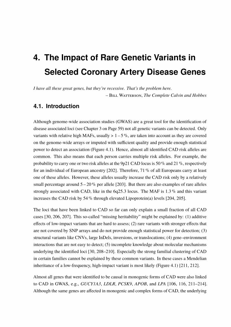
4. The Impact of Rare Genetic Variants in
Selected Coronary Artery Disease Genes
I have all these great genes, but they’re recessive. That’s the problem here.– Bill Watterson, The Complete Calvin and Hobbes
4.1. Introduction
Although genome-wide association studies (GWAS) are a great tool for the identification ofdisease associated loci (see Chapter 3 on Page 59) not all genetic variants can be detected. Onlyvariants with relative high MAFs, usually > 1 – 5%, are taken into account as they are coveredon the genome-wide arrays or imputed with sufficient quality and provide enough statisticalpower to detect an association (Figure 4.1). Hence, almost all identified CAD risk alleles arecommon. This also means that each person carries multiple risk alleles. For example, theprobability to carry one or two risk alleles at the 9p21 CAD locus is 50% and 21%, respectivelyfor an individual of European ancestry [202]. Therefore, 71% of all Europeans carry at leastone of these alleles. However, these alleles usually increase the CAD risk only by a relativelysmall percentage around 5 – 20% per allele [203]. But there are also examples of rare allelesstrongly associated with CAD, like in the 6q25.3 locus. The MAF is 1.3% and this variantincreases the CAD risk by 54% through elevated Lipoprotein(a) levels [204, 205].
The loci that have been linked to CAD so far can only explain a small fraction of all CADcases [30, 206, 207]. This so-called “missing heritability” might be explained by: (1) additiveeffects of low-impact variants that are hard to assess; (2) rare variants with stronger effects thatare not covered by SNP arrays and do not provide enough statistical power for detection; (3)structural variants like CNVs, large InDels, inversions, or translocations; (4) gene–environmentinteractions that are not easy to detect; (5) incomplete knowledge about molecular mechanismsunderlying the identified loci [30, 208–210]. Especially the strong familial clustering of CADin certain families cannot be explained by these common variants. In these cases a Mendelianinheritance of a low-frequency, high-impact variant is most likely (Figure 4.1) [211, 212].
Almost all genes that were identified to be causal in monogenic forms of CAD were also linkedto CAD in GWAS, e.g., GUCY1A3, LDLR, PCSK9, APOB, and LPA [106, 116, 211–214].Although the same genes are affected in monogenic and complex forms of CAD, the underlying
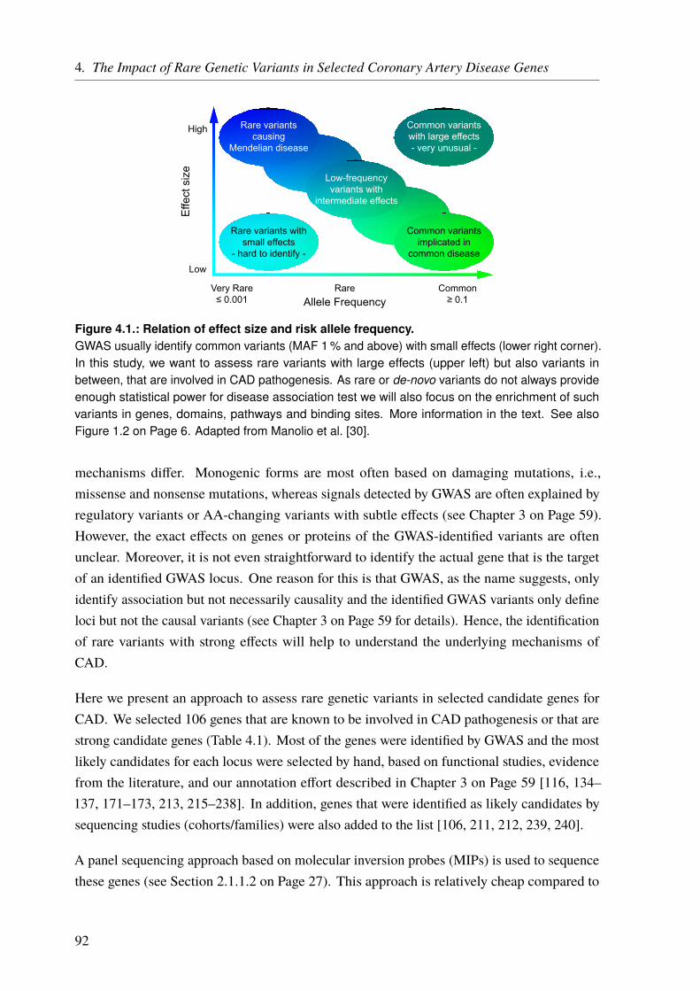
4. The Impact of Rare Genetic Variants in Selected Coronary Artery Disease Genes
Allele Frequency
Effe
ct s
ize
Low
High
Very Rare≤ 0.001
Rare Common≥ 0.1
Rare variantscausing
Mendelian disease
Common variantsimplicated in
common disease
Low-frequencyvariants with
intermediate effects
Rare variants withsmall effects
- hard to identify -
Common variantswith large effects- very unusual -
Figure 4.1.: Relation of effect size and risk allele frequency.GWAS usually identify common variants (MAF 1 % and above) with small effects (lower right corner).In this study, we want to assess rare variants with large effects (upper left) but also variants inbetween, that are involved in CAD pathogenesis. As rare or de-novo variants do not always provideenough statistical power for disease association test we will also focus on the enrichment of suchvariants in genes, domains, pathways and binding sites. More information in the text. See alsoFigure 1.2 on Page 6. Adapted from Manolio et al. [30].
mechanisms differ. Monogenic forms are most often based on damaging mutations, i.e.,missense and nonsense mutations, whereas signals detected by GWAS are often explained byregulatory variants or AA-changing variants with subtle effects (see Chapter 3 on Page 59).However, the exact effects on genes or proteins of the GWAS-identified variants are oftenunclear. Moreover, it is not even straightforward to identify the actual gene that is the targetof an identified GWAS locus. One reason for this is that GWAS, as the name suggests, onlyidentify association but not necessarily causality and the identified GWAS variants only defineloci but not the causal variants (see Chapter 3 on Page 59 for details). Hence, the identificationof rare variants with strong effects will help to understand the underlying mechanisms ofCAD.
Here we present an approach to assess rare genetic variants in selected candidate genes forCAD. We selected 106 genes that are known to be involved in CAD pathogenesis or that arestrong candidate genes (Table 4.1). Most of the genes were identified by GWAS and the mostlikely candidates for each locus were selected by hand, based on functional studies, evidencefrom the literature, and our annotation effort described in Chapter 3 on Page 59 [116, 134–137, 171–173, 213, 215–238]. In addition, genes that were identified as likely candidates bysequencing studies (cohorts/families) were also added to the list [106, 211, 212, 239, 240].
A panel sequencing approach based on molecular inversion probes (MIPs) is used to sequencethese genes (see Section 2.1.1.2 on Page 27). This approach is relatively cheap compared to
92
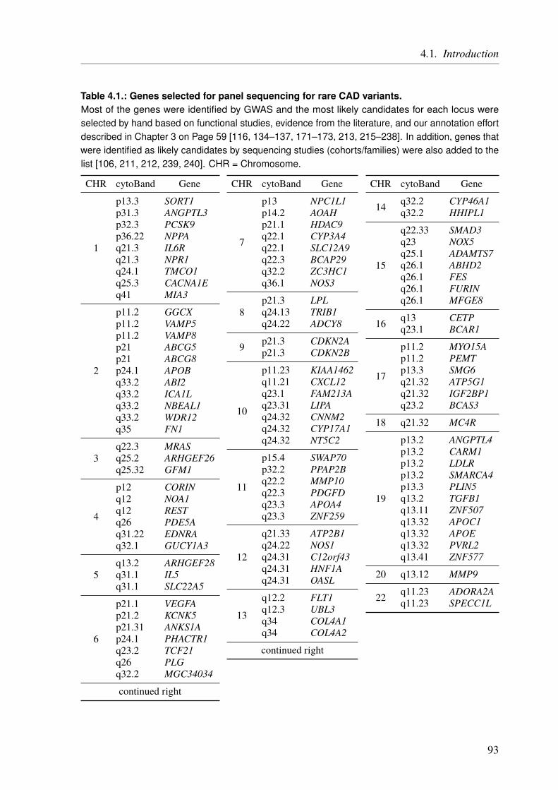
4.1. Introduction
Table 4.1.: Genes selected for panel sequencing for rare CAD variants.Most of the genes were identified by GWAS and the most likely candidates for each locus wereselected by hand based on functional studies, evidence from the literature, and our annotation effortdescribed in Chapter 3 on Page 59 [116, 134–137, 171–173, 213, 215–238]. In addition, genes thatwere identified as likely candidates by sequencing studies (cohorts/families) were also added to thelist [106, 211, 212, 239, 240]. CHR = Chromosome.
CHR cytoBand Gene
1
p13.3 SORT1p31.3 ANGPTL3p32.3 PCSK9p36.22 NPPAq21.3 IL6Rq21.3 NPR1q24.1 TMCO1q25.3 CACNA1Eq41 MIA3
2
p11.2 GGCXp11.2 VAMP5p11.2 VAMP8p21 ABCG5p21 ABCG8p24.1 APOBq33.2 ABI2q33.2 ICA1Lq33.2 NBEAL1q33.2 WDR12q35 FN1
3q22.3 MRASq25.2 ARHGEF26q25.32 GFM1
4
p12 CORINq12 NOA1q12 RESTq26 PDE5Aq31.22 EDNRAq32.1 GUCY1A3
5q13.2 ARHGEF28q31.1 IL5q31.1 SLC22A5
6
p21.1 VEGFAp21.2 KCNK5p21.31 ANKS1Ap24.1 PHACTR1q23.2 TCF21q26 PLGq32.2 MGC34034
continued right
CHR cytoBand Gene
7
p13 NPC1L1p14.2 AOAHp21.1 HDAC9q22.1 CYP3A4q22.1 SLC12A9q22.3 BCAP29q32.2 ZC3HC1q36.1 NOS3
8p21.3 LPLq24.13 TRIB1q24.22 ADCY8
9 p21.3 CDKN2Ap21.3 CDKN2B
10
p11.23 KIAA1462q11.21 CXCL12q23.1 FAM213Aq23.31 LIPAq24.32 CNNM2q24.32 CYP17A1q24.32 NT5C2
11
p15.4 SWAP70p32.2 PPAP2Bq22.2 MMP10q22.3 PDGFDq23.3 APOA4q23.3 ZNF259
12
q21.33 ATP2B1q24.22 NOS1q24.31 C12orf43q24.31 HNF1Aq24.31 OASL
13
q12.2 FLT1q12.3 UBL3q34 COL4A1q34 COL4A2
continued right
CHR cytoBand Gene
14 q32.2 CYP46A1q32.2 HHIPL1
15
q22.33 SMAD3q23 NOX5q25.1 ADAMTS7q26.1 ABHD2q26.1 FESq26.1 FURINq26.1 MFGE8
16 q13 CETPq23.1 BCAR1
17
p11.2 MYO15Ap11.2 PEMTp13.3 SMG6q21.32 ATP5G1q21.32 IGF2BP1q23.2 BCAS3
18 q21.32 MC4R
19
p13.2 ANGPTL4p13.2 CARM1p13.2 LDLRp13.2 SMARCA4p13.3 PLIN5q13.2 TGFB1q13.11 ZNF507q13.32 APOC1q13.32 APOEq13.32 PVRL2q13.41 ZNF577
20 q13.12 MMP9
22 q11.23 ADORA2Aq11.23 SPECC1L
93
4. The Impact of Rare Genetic Variants in Selected Coronary Artery Disease Genes
WES orWGS and allows screening of a large number of probands to achieve sufficient statisticalpower. As MIPs are not available as commercial kits, the panel has to be designed, set-up, andoptimized by oneself, which is one reason for the low cost. The details of the MIP workflowand the general steps to establish the panel for our assay are explained in Section 2.1.1.2 onPage 27. We are going to analyze around 10 000 cases with premature CAD/MI and 10 000healthy controls. In addition, we make use of other available data sets like in-house exomes orpublicly available data like from the database of Genotypes and Phenotypes (dbGaP) [241].
Targeted sequencing approaches for selected genes, MIPs particularly, are not only cheaperthan WES and WGS, they also have some technical advantages [48]. As only a small subset ofthe genome is sequenced the coverage per gene is much higher, which improves the sensitivityto detect variants. It is easy to modify a MIP panel by adding genes or by increasing thecoverage for single regions which might be hard to analyze otherwise. The coverage for eachMIP is very similar in all samples, which allows the easy detection of CNVs and InDels byanalyzing the read count. In addition, it is easy to transfer the already existent MIP pool toa different sequencing system if needed. For example, if new techniques have technical orfinancial advantages. Recent studies in other clinical settings already displayed the advantagesof MIP-based targeted sequencings [242, 243].
Although this approach will allow us to detect recurrent mutations, our focus lies on very rare,or even de-novo mutations. These mutations are not very likely to be observed multiple timesin our data set. Hence, our analysis will focus on the enrichment of variants in selected genes,gene domains, pathways, or binding sites for specific TFs or miRNAs.
To get a first idea of what to expect from this large-scale sequencing project, a pilot study wasperformed. The genomic regions that are covered by our MIP panel were selected from 655cases with early CAD and 400 healthy controls. Then we performed a simple enrichment testper gene.
We expect to identify variants, genes, and pathways that have profound effects on CAD risk.This might give new insights into the mechanisms underlying CAD etiology and may explain afraction of the “missing heritability”. Such findings can also lead to improved risk predictionin families and the overall population. It is important to start treatment early even beforeclinical symptoms occur. Moreover, new druggable targets might be identified and may allow amore personalized treatment for affected individuals (personalized medicine) which not onlyimproves the therapy but also reduces unwanted side effects.
94
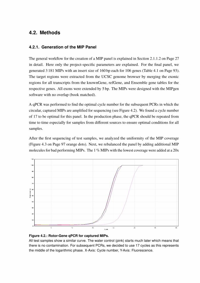
4.2. Methods
4.2.1. Generation of the MIP Panel
The general workflow for the creation of a MIP panel is explained in Section 2.1.1.2 on Page 27in detail. Here only the project-specific parameters are explained. For the final panel, wegenerated 3 181 MIPs with an insert size of 160 bp each for 106 genes (Table 4.1 on Page 93).The target regions were extracted from the UCSC genome browser by merging the exonicregions for all transcripts from the knownGene, refGene, and Ensemble gene tables for therespective genes. All exons were extended by 5 bp. The MIPs were designed with the MIPgensoftware with no overlap (book matched).
A qPCR was performed to find the optimal cycle number for the subsequent PCRs in which thecircular, captured MIPs are amplified for sequencing (see Figure 4.2). We found a cycle numberof 17 to be optimal for this panel. In the production phase, the qPCR should be repeated fromtime to time especially for samples from different sources to ensure optimal conditions for allsamples.
After the first sequencing of test samples, we analyzed the uniformity of the MIP coverage(Figure 4.3 on Page 97 orange dots). Next, we rebalanced the panel by adding additional MIPmolecules for bad performingMIPs. The 1%MIPs with the lowest coverage were added at a 20x
Figure 4.2.: Rotor-Gene qPCR for captured MIPs.All test samples show a similar curve. The water control (pink) starts much later which means thatthere is no contamination. For subsequent PCRs, we decided to use 17 cycles as this representsthe middle of the logarithmic phase. X-Axis: Cycle number, Y-Axis: Fluorescence.
4. The Impact of Rare Genetic Variants in Selected Coronary Artery Disease Genes
concentration, the lowest 10% at a 10x concentration. In addition, we added unphosphorylatedMIPs for the top 5 unspecific over performers to suppress these MIPs (see Section 2.1.1.2 onPage 27 for details). Moreover, we designed and added 23 new MIPs for regions where theMIPs did not seem to work at all. The results of this rebalancing are shown in Figure 4.3(yellow dots). The resulting panel was rebalanced a second time. MIPs with a coverage of≤ 10% of the mean panel coverage at a 10x concentration and MIPs with a coverage of ≤ 1%at a 20x concentration. The final results are shown in Figure 4.3 (green dots).
The samples for the production phase come from different in-house case/control studies andfrom collaboration partners. The concentrations of the sample DNAs were adjusted by LGCGenomics GmbH (Berlin) to 25 ng µl−1 as this step is crucial for the panel performance (seealso Section 2.1.1.2 on Page 27).
4.2.2. A Pilot Study on Rare Variant Enrichment in Selected CAD Genes
A pilot study was performed to get a first idea of what can be expected of the panel sequencingapproach, especially how many variants might be found per gene. The genomic regions thatare also covered by the MIPs were extracted from 655 exome-sequenced cases with prematureCAD and 400 exome-sequenced healthy controls. The variants in this regions were called (seeSection 2.1.2 on Page 41) and annotated with the ANNOVAR software. Only variants with aMAF ≤ 1% in the 1 000 Genomes Project data (All and European samples) and the ExAC data(All and non-finish Europeans) were used further. Then, two data sets were created. For thefirst one, only variants at splice sites and AA-changing variants were taken into account. Thesecond data set only consists of variants in exonic and splice site regions which are predictedto be deleterious by the DANN score (DANN > 0.96). Next, in both data sets the number ofvariants in each gene was counted for cases and controls individually. Based on this numbers,a Fisher’s exact test was performed to see if there is a significant difference between casesand controls (OR > 1 or OR < 1). Results are considered to be significant when the errorprobability is below 5%. Hence, the corresponding p-value would be p ≤ 4.72 · 10−4 afterBonferroni correction for 106 genes (0.05
106 = 4.72 · 10−4).
96

4.2. Methods
0.00001
0.0001
0.001
0.01
0.1
1
10
Sequencing2 Sequencing3Sequencing1MIPs
norm
aliz
ed c
over
age
(a) MIP rebalancing results. Sorted by first sequencing run coverage.
0.00001
0.0001
0.001
0.01
0.1
1
10
Sequencing2 Sequencing3Sequencing1MIPs
norm
aliz
ed c
over
age
(b) MIP rebalancing results. All sequencing runs sorted individually by coverage.
Figure 4.3.: Results of the MIP panel rebalancing.To achieve a more uniform coverage of all MIPs we rebalanced the panel two times. After thefirst sequencing (orange), bad performing MIPs were added to boost the coverage and new MIPsfor nonperformers were designed and added. The panel was sequenced again and rebalanceda second time (green). The coverage is normalized to the average of each sequencing run. Dueto the logarithmic scale, non-performing MIPs (coverage 0) are not shown. Detailed informationcan be found in the text and method Section 2.1.1.2 on Page 27. a| The MIPs are sorted by thecoverage of the first sequencing (orange). The yellow and green dots show the enhanced coverageof the individual bad performing MIPs after the first and second rebalancing. b| All sequencing runsare sorted individually and the yellow and green dots show the overall improved coverage of thesequencing after rebalancing.
97

4.3. Results and Discussion
Although the design and rebalancing of the MIP panel was successful, technical issues occuredduring the first sequencing test runs. In addition, the preparation of the DNA samples waslaborious and time-consuming. Hence, only preliminary results from the pilot study can bepresented so far (Section 4.3.1).
4.3.1. A Pilot Study on Rare Variant Enrichment in Selected CAD Genes
The results for all 106 tested genes are listed in the Appendix Tables A.6 on Page 173 and A.7on Page 175. No significant differences could be found when applying the Bonferroni correctedp-value threshold of p ≤ 4.72 · 10−4, most likely due to the small sample size of 655 casesand 400 controls. However, some genes reached a p-value of ≤ 0.05 and are shown with theirrespective ORs in Figure 4.4. If the ratio of variants in cases and controls stays the same inthe final panel, with 10 000 cases and 10 000 controls, the p-values will most likely becomesignificant for these genes.
Although there was no gene with a significant difference in the amount of variants afterBonferroni correction, there is still some valuable conclusion to draw from this pilot study.Some interesting examples of the genes with a nominally significant p-value ≤ 0.05 will bediscussed in the following.
In the CYP46A1 gene, for example, rare AA-changing and splice site variants as well as variantspredicted to be deleterious were only present in the CAD cases and not the controls (Figure 4.4)This gene encodes a member of the cytochrome P450 superfamily and is involved in thesynthesis of cholesterol, steroids and other lipids.∗ However, it is unclear how many variantswill be found in the healthy controls in the large data set.
Likewise, variants predicted to be deleterious were only found in CAD cases and not controls inthe TGFB1 gene (Figure 4.4b). This gene is part of the transforming growth factor-β (TGF-β)pathway (see also Chapter 5 on Page 103), which is involved in a plethora of molecularfunctions like proliferation and differentiation and plays a role in the pathophysiology ofendothelial and vascular smooth muscle cells [244]. TGFB1 has clearly been linked to CAD andrelated phenotypes like atherosclerosis, hypertension, inflammation, and aneurysms [244–248].However, the effect sizes of identified variants were often rather small and even the effectdirections were not always consistent [249]. Nevertheless, most studies report increased CADrisk for the GWAS-identified minor alleles and recent studies report eQTLs that increase the
∗https://www.ncbi.nlm.nih.gov/gene/10858 Retrieved September 4, 2017.

4. The Impact of Rare Genetic Variants in Selected Coronary Artery Disease Genes
Gene ORp-value
ABCG5 50 15 1.18 · 10-2 2.12APOE 22 5 4.32 · 10-2 2.74COL4A2 47 16 4.38 · 10-2 1.85CYP46A1 12 0 4.81 · 10-3 InfFES 34 8 9.28 · 10-3 2.68ZNF507 9 15 1.76 · 10-2 0.36
# of VariantsCases(n=655)
Controls(n=400)
0.1 1 10OR (95% CI)
(a) AA-changing and splice site variants.
Gene ORp-value
CYP46A1 11 0 8.83 · 10-3 InfFES 23 5 2.92 · 10-2 2.87KCNK5 25 6 3.74 · 10-2 2.60LDLR 26 7 4.61 · 10-2 2.32TGFB1 16 0 9.22 · 10-4 Inf
# of VariantsCases(n=655)
Controls(n=400)
0.1 1 10OR (95% CI)
(b) Exonic/splice site variants with a DANN score ≥ 0.96.
Figure 4.4.: Forest plots of genes with a Fisher’s p-value ≤ 0.05.a| AA-changing and splice site variants with a MAF ≤ 1 % were counted. b| Exonic and splice sitevariants with a MAF ≤ 1 % and a DANN score ≥ 0.96, indicating functional relevance, were counted.The Fisher’s p-value was calculated for the null hypothesis OR = 1. To allow for an error probabilityof 5 % a Bonferroni correction was applied (0.05
106 = 4.72 · 10−4). However, none of the 106 genesreached this threshold (p ≤ 4.72 · 10−4). Hence, genes with a p-value ≤ 0.05 are shown here, toillustrate the basic principle. OR = odds ratio; CI = confidence interval. Arrows indicate that the endvalue lies outside the displayed range. See text for details. All genes can be found in Tables A.6 onPage 173 and A.7 on Page 175.
TGFB1 expression and the CAD risk [244, 249]. This also matches the findings that TGFB1serum levels are higher in CAD patients [250]. Hence, one would expect increased TGFB1expression or gain of function mutations to be associated with higher CAD risk. However, thisis not reflected in our pilot study, as we find deleterious variants only in CAD cases. It will beinteresting to see if these results are confirmed in the final panel. A possible explanation couldbe the variety of molecular pathways in which TGFB1 is involved. The CAD risk could beinfluenced differently through multiple pathways, especially given the multifactorial backgroundCAD. Anyhow, this gene illustrates the complexity underlying CAD loci and studying thefunctional effects of the variants identified by the final panel might help us to combine theapparently conflicting findings to get a better understanding of what is going on at this locus.
100
4.3. Results and Discussion
The gene with the highest OR, ignoring the genes with no variants in the controls, based onAA-changing and splice site variants is APOE (OR = 2.74, p-value = 4.32 · 10−2). This geneis well-known for its role in lipid metabolism where it is essential for the normal catabolism oftriglyceride-rich lipoprotein constituents [251]. Hence, mutations in APOE are known to causeelevated triglyceride and cholesterol levels, which is a major risk factor for CAD. APOE isalso within a CAD GWAS locus, although the associated SNPs lie outside the coding region[116, 117]. Our annotation efforts of GWAS loci (Chapter 3 on Page 59) also found this geneto be affected by eQTLs. The results from this pilot study provide direct evidence that rarevariants in APOE contribute to the CAD risk. Although this is already known for this specificgene, it is a proof of principle for our assay. If we just extrapolate the number of variants incases and controls to the final sample size, the result would be significant with a p-value ofp = 2.2 · 10−16 (336 variants in 10 000 cases/125 in 10 000 controls).
A second example is the FES gene, which has the highest OR (OR = 2.87, p-value = 2.92 ·10−2)of the genes with a p-value ≤ 0.05 based on variants predicted to be deleterious and the secondhighest OR (OR = 2.68, p-value = 9.28 · 10−3) among the genes identified by AA-changingand splice site variants. FES was identified as a potential CAD risk gene through GWAS[116, 117] and we also found eQTLs for this gene (Chapter 3 on Page 59). However, this geneis an oncogene, involved in cellular transformation and hematopoiesis.† The mechanisms forits involvement in CAD are not known although it has been linked to elevated blood pressure[252] before and plays a role in growth and differentiation of hematopoietic, neuronal, vascularendothelial and epithelial cell types [253]. If the panel sequencing confirms a major role ofrare variants in FES, it might worth to functionally investigate this gene in more detail.
Another interesting example is the gene ZNF507 with an OR of 0.36 in the rare splice site andAA-changing variants (p-value = 1.76 · 10−2). These variants seem to have a protective effecton CAD. This is also reflected by the results of GWAS, where the OR for the minor allele isreported to be 0.69 [117]. However, it is not known how this allele affects the gene’s expressionor function. The GWAS lead SNP rs12976411 lies in a uncharacterized non-coding RNA(LOC400684) 3.4 kb downstream of ZNF507 and several high LD SNPs overlap functionalelements in the introns of this gene, as predicted by ENCODE. However, our preliminaryresults suggest direct evidence for a protective effect of AA-changing mutations in ZNF507.
Although none of the results from our pilot study were significant, which is not surprising giventhe relatively low sample size, these findings suggest that the final panel with roughly 20 000samples will allow us to gain new insights into the mechanisms underlying CAD etiology.Especially for genes that were only linked to CAD through indirect evidence from GWAS so
†https://www.ncbi.nlm.nih.gov/gene/2242 Retrieved September 4, 2017.
101

4. The Impact of Rare Genetic Variants in Selected Coronary Artery Disease Genes
far, rare variants may allow us to establish more direct, functional links (see Chapter 3 onPage 59). Because of the low sample size, the enrichment of rare variants in pathways or inspecific regions/domains of genes has not been tested in the pilot study. Moreover, binding sitesfor miRNAs or TFs might be of interest, although they are mostly located outside the codingregions covered by our assay. We decided not to cover these regions, like UTRs, because theyare hard to access by MIPs as they are not as conserved as coding regions, making it difficultto design primers for this region. Although it is possible, a lot more MIPs would need to bedesigned making the whole panel less cost efficient and reducing the overall coverage.
102
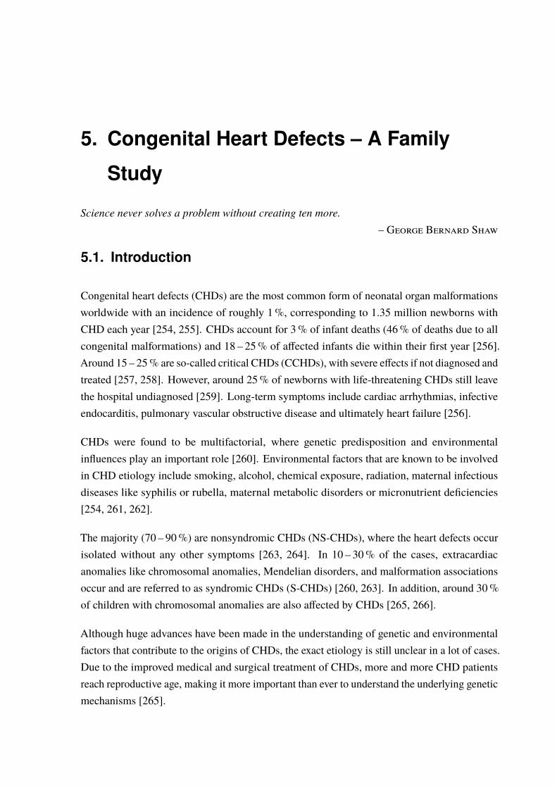
5. Congenital Heart Defects – A Family
Study
Science never solves a problem without creating ten more.– George Bernard Shaw
5.1. Introduction
Congenital heart defects (CHDs) are the most common form of neonatal organ malformationsworldwide with an incidence of roughly 1%, corresponding to 1.35 million newborns withCHD each year [254, 255]. CHDs account for 3% of infant deaths (46% of deaths due to allcongenital malformations) and 18 – 25% of affected infants die within their first year [256].Around 15 – 25% are so-called critical CHDs (CCHDs), with severe effects if not diagnosed andtreated [257, 258]. However, around 25% of newborns with life-threatening CHDs still leavethe hospital undiagnosed [259]. Long-term symptoms include cardiac arrhythmias, infectiveendocarditis, pulmonary vascular obstructive disease and ultimately heart failure [256].
CHDs were found to be multifactorial, where genetic predisposition and environmentalinfluences play an important role [260]. Environmental factors that are known to be involvedin CHD etiology include smoking, alcohol, chemical exposure, radiation, maternal infectiousdiseases like syphilis or rubella, maternal metabolic disorders or micronutrient deficiencies[254, 261, 262].
The majority (70 – 90%) are nonsyndromic CHDs (NS-CHDs), where the heart defects occurisolated without any other symptoms [263, 264]. In 10 – 30% of the cases, extracardiacanomalies like chromosomal anomalies, Mendelian disorders, and malformation associationsoccur and are referred to as syndromic CHDs (S-CHDs) [260, 263]. In addition, around 30%of children with chromosomal anomalies are also affected by CHDs [265, 266].
Although huge advances have been made in the understanding of genetic and environmentalfactors that contribute to the origins of CHDs, the exact etiology is still unclear in a lot of cases.Due to the improved medical and surgical treatment of CHDs, more and more CHD patientsreach reproductive age, making it more important than ever to understand the underlying geneticmechanisms [265].

5. Congenital Heart Defects – A Family Study
5.1.1. Syndromic Congenital Heart Defects
It has been shown that some CHDs are more often associated with (specific) genetic syndromesand genotype-phenotype studies suggested that certain morphogenetic mechanisms affected byspecific genes can result in distinct cardiac phenotypes [267].
Well-studied classical chromosomal anomalies associated to CHDs include trisomy 21 (Downsyndrome (DS); 40 – 50% CHDs), trisomy 13 (Patau syndrome; 80% CHDs), trisomy 18(Edwards syndrome; 90 – 100% CHDs), monosomy X (Turner syndrome; 25 – 35% CHDs),47, XXY (Klinefelter Syndrome; 50% CHDs), 22q11.2 deletion (DiGeorge Syndrome;50% CHDs), and 7q11.23 deletion (Williams-Beuren Syndrome; 50 – 85% CHDs). Allchromosomal anomalies show associations with distinct types of CHDs, e.g., trisomy 21 isassociated with atrial septal defect (ASD), ventricular septal defect (VSD), and atrioventricularseptal defect (AVSD) (see Appendix Table A.8 on Page 178) [263, 265, 267–269].
In addition, CNVs play an important role in the more frequent chromosomal syndromes andCNV analysis led to the discovery of several genomic conditions, associated with differenttypes of CHDs [263, 270, 271]. They include distal 22q11.2 deletion syndrome which maps atend of the common DiGeorge/22q11.2 deleted region [272, 273], microdeletion (del 1q21.1)and microduplication (dup 1q21.1) at the 1q21.1 locus [269, 274], or one of the most commongenomic disorders, the deletion 1p36 syndrome [268, 275].
There are also monogenic syndromes, that are characteristically associated with CHD like theNoonan syndrome and other RASopathies, Costello syndrome, LEOPARD Syndrome, AlagilleSyndrome, Marfan Syndrome, Holt-Oram Syndrome, Heterotaxy Syndrome, Char Syndrome,CHARGE Syndrome, and Cornelia de Lange syndromes (see Appendix Table A.9 on Page 179)[265, 276–278].
5.1.2. Nonsyndromic Congenital Heart Defects
The etiology of most NS-CHDs is thought to be explained by a multifactorial inheritancehypothesis, where environmental triggers interact with genetic predispositions [279, 280]. Inaddition, the genetic component is presumed to be polygenic with (small) additive effects ofmultiple variants (Figure 5.1). This is not only true for sporadic cases, but also a general lowsibling recurrence risk is often described, suggesting an important contribution of de novomutations (DNMs) and/or reduced penetrance [264, 281–283]. If a disease-causing varianthas a reduced penetrance, not all individuals who carry this variant show the correspondingphenotype, e.g., symptoms of a disease.
104
5.1. Introduction
Allele Frequency
Effe
ct s
ize
Low
High
Very Rare≤ 0.001
Rare Common≥ 0.1
Rare variantscausing
Mendelian disease
Common variantsimplicated in
common disease
Low-frequencyvariants with
intermediate effects
Rare variants withsmall effects
- hard to identify -
Common variantswith large effects- very unusual -
Figure 5.1.: Relation of effect size and risk allele frequency.Most NS-CHDs are thought to be explained by additive effects of multiple (mainly) common variantswith low effect sizes and additional environmental contribution. However, there are also reports ofcases with a monogenic inheritance pattern, especially in families with a high recurrence of CHDs.The underlying variants are very rare and have large effect sizes (classical Mendelian disease).More information in the text. See also Figure 1.2 on Page 6. Adapted from Manolio et al. [30].
On the other hand, some studies reported that specific CHDs show a highly variable but strongfamilial clustering [263, 284]. Monogenic inheritance can therefore mainly be presumed inpedigrees with a clear recurrence of the same CHD (Figure 5.1). And although these examplesexist, the number of identified genes for NS-CHDs is still limited as it is not easy to find theunderlying genetic mechanisms of NS-CHDs [285–291]. One reason is the great clinical andgenetic heterogeneity of these cardiac malformations and another the fact that the identifiedgenes only play a role in a small proportion of CHDs [263].
Although the majority of monogenic NS-CHDs are caused by single high-penetrance autosomaldominant mutations [291], CNVs seem to also play an important role in sporadic NS-CHDsand are reported to account for 5 – 10% of cases [292–295]. However, they are often located inalready known genes or regions.
5.1.3. A Family with High Recurrence of Nonsyndromic Congenital Heart
Defects
As described before, monogenic inheritance was mainly observed in families with a highrecurrence of CHDs. Such families may allow identifying genes or regions which also contributeto the etiology in sporadic NS-CHD cases or pedigrees with low penetrance.
Here, we analyzed a family with unusual clustering of CHDs, first described as “A LargePedigree With Valvuloseptal Defects” by Schunkert et al. [296] (Figure 5.3 on Page 110).
105

5. Congenital Heart Defects – A Family Study
Clinical examination of the extended family implied a recurrence risk of 50%. Although theobserved phenotypes are still heterogeneous, it seems reasonable that they emerge from thesame genetic cause, as mainly the atrioventricular (AV) valves and cardiac septa are affected.
Hence, the morphogenetic origins of the CHDs in this family are most likely associated withthe development of the endocardial cushions. The endocardial cushions are the precursors ofcardiac septa, valves and the outflow tract [297, 298]. Impaired embryonic development ofthese endocardial cushions is known to cause CHDs like ASD, VSD, and AVSD [299, 300].
The most frequently observed CHD phenotypes in the present family are explained briefly inthe following:
Atrial Septal Defect (ASD) This malformation is characterized by an open connection betweenthe right and left atrium of the heart. Normally, the two atria are separated by the interatrialseptum. As the oxygen-rich blood from the left heart side passes to the right side (left-rightshunt) it is acyanotic. However, over time it can lead to the Eisenmenger’s syndromein which this shunt changes to a right-left shunt, causing cyanosis [301]. If the ASD islarge, the opening can lead to an overload of the right heart side, resulting in enlargementof the right side and eventually heart failure [301].
Atrioventricular Septal Defect (AVSD) AVSD is a combination of malformations of the atria,ventricles, the atrial and ventricular septum, and the mitral and tricuspid valves [302]. Itis differentiated between partial and complete AVSD, and in addition, there are differentclassifications based on the severity of the defect. Without surgical treatment, manypatients will die in infancy or will develop a pulmonary vascular disease and eventuallydie with Eisenmenger’s syndrome [303].
Ebstein’s Anomaly This CHD was first described in 1866 [304]. It is characterized by adownward displacement of the tricuspid valve towards the apex of the right ventricle,which leads to an enlarged atrium and reduced ventricle on the right side. With anincidence of 5.2 · 10−3 – 7.2 · 10−3% in live births, it only accounts for 1% of all cardiaclesions [305, 306]. It is often accompanied by structural lesions like pulmonary valvestenosis or atresia, tricuspid insufficiency, Wolff-Parkinson-White syndrome (WPW),and ASDs [307, 308].
Right Bundle Branch Block (RBBB) An RBBB is a heart block in the electrical conductivesystem of the right ventricle. Hence, the right ventricle is not directly activated. As it isstill activated through excitation from the left ventricle it mainly remains asymptomatic[309] itself. However, it is often found as a secondary phenotype in other heart diseases,particularly ASDs [310].
106
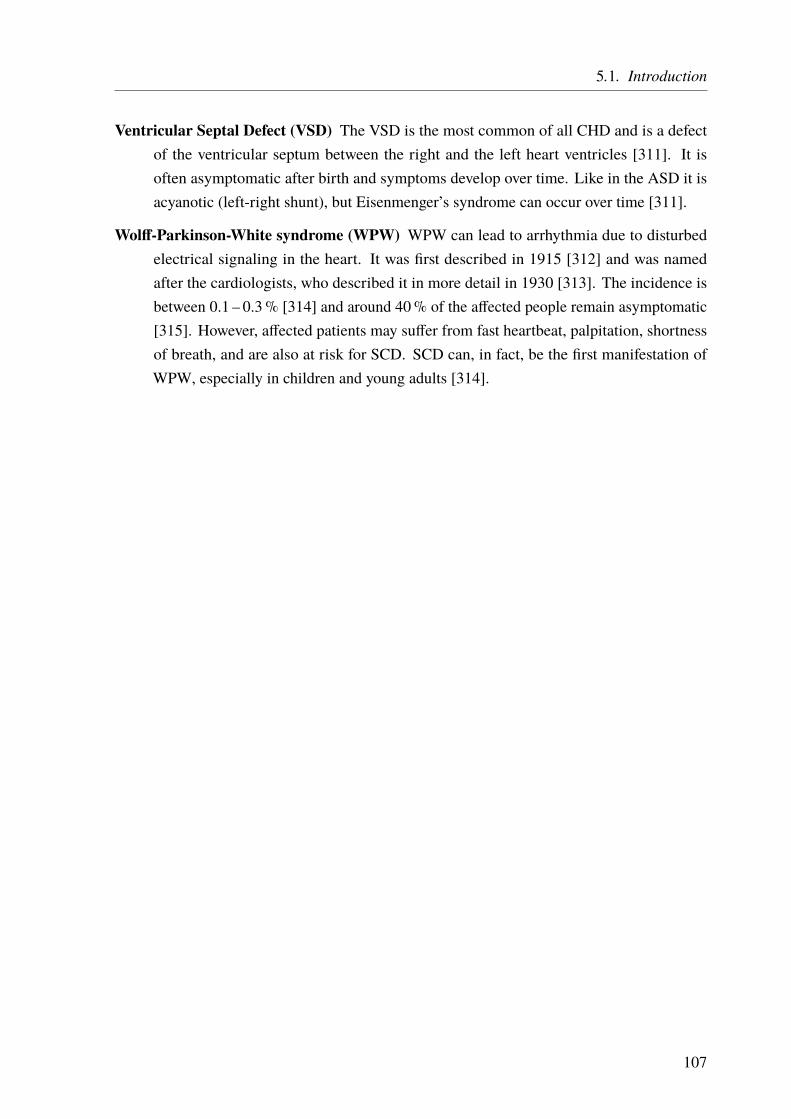
5.1. Introduction
Ventricular Septal Defect (VSD) The VSD is the most common of all CHD and is a defectof the ventricular septum between the right and the left heart ventricles [311]. It isoften asymptomatic after birth and symptoms develop over time. Like in the ASD it isacyanotic (left-right shunt), but Eisenmenger’s syndrome can occur over time [311].
Wolff-Parkinson-White syndrome (WPW) WPW can lead to arrhythmia due to disturbedelectrical signaling in the heart. It was first described in 1915 [312] and was namedafter the cardiologists, who described it in more detail in 1930 [313]. The incidence isbetween 0.1 – 0.3% [314] and around 40% of the affected people remain asymptomatic[315]. However, affected patients may suffer from fast heartbeat, palpitation, shortnessof breath, and are also at risk for SCD. SCD can, in fact, be the first manifestation ofWPW, especially in children and young adults [314].
107


5.2. Material and Methods
The family that we studied here (Figure 5.3), was first described by Schunkert et al. [296]and the clinical features are explained in the next section. To identify the causal variants(s)in this family we performed linkage analyses, a CNV analysis, as well as exome and genomesequencing. In addition, we performed a panel sequencing in unrelated CHD patients based onthe findings in this family. The general workflow is shown in Figure 5.2 and an overview ofavailable data for the family members can be found in the Appendix Table A.10 on Page 180.
Clinical Examination
Compare Results
CNV AnalysisLinkage AnalysisSTRs SNPs
SequencingExome Genome
Panel Sequencing
Case/Ctrl Selection
Figure 5.2.: Workflow used for the family analysis.After the clinical examination of the family, affected cases and healthy control members were selectedfor linkage analyses (STR- and SNP-based), a CNV analysis, and exome and genome sequencings.The results of the different approaches were compared and based on our findings selected geneswere analyzed in unrelated individuals in a panel sequencing approach.
5.2.1. Family Description
Since the first description of the family [296], two more affected family members (22 and 25)were identified. In this family, several CHDs are present, with 13 out of 19 affected familymembers (68%) (Figure 5.3). No extracardiac anomalies were reported (NS-CHDs).
It has to be mentioned though, that not all presumably affected family members underwentclinical examination, for several reasons. The clinical features are described in the followingand are also summed up in Table 5.1 on Page 112. All features are based on the publication bySchunkert et al. [296] or reports by family members.
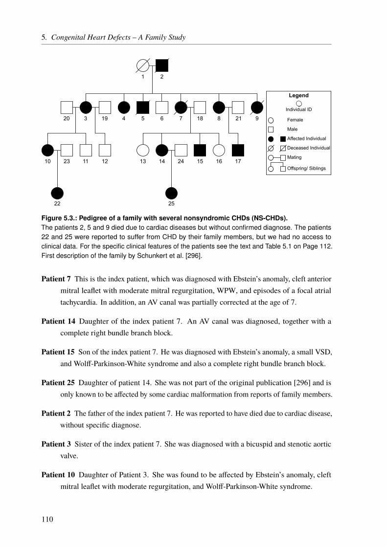
5. Congenital Heart Defects – A Family Study
1 2
20 3 19 4 5 6 187 218 9
10 11 12 13 14 15 16 17
22
23 24
25
Female
Male
Affected Individual
Deceased Individual
Mating
Offspring/ Siblings
Individual ID
Legend
Figure 5.3.: Pedigree of a family with several nonsyndromic CHDs (NS-CHDs).The patients 2, 5 and 9 died due to cardiac diseases but without confirmed diagnose. The patients22 and 25 were reported to suffer from CHD by their family members, but we had no access toclinical data. For the specific clinical features of the patients see the text and Table 5.1 on Page 112.First description of the family by Schunkert et al. [296].
Patient 7 This is the index patient, which was diagnosed with Ebstein’s anomaly, cleft anteriormitral leaflet with moderate mitral regurgitation, WPW, and episodes of a focal atrialtachycardia. In addition, an AV canal was partially corrected at the age of 7.
Patient 14 Daughter of the index patient 7. An AV canal was diagnosed, together with acomplete right bundle branch block.
Patient 15 Son of the index patient 7. He was diagnosed with Ebstein’s anomaly, a small VSD,and Wolff-Parkinson-White syndrome and also a complete right bundle branch block.
Patient 25 Daughter of patient 14. She was not part of the original publication [296] and isonly known to be affected by some cardiac malformation from reports of family members.
Patient 2 The father of the index patient 7. He was reported to have died due to cardiac disease,without specific diagnose.
Patient 3 Sister of the index patient 7. She was diagnosed with a bicuspid and stenotic aorticvalve.
Patient 10 Daughter of Patient 3. She was found to be affected by Ebstein’s anomaly, cleftmitral leaflet with moderate regurgitation, and Wolff-Parkinson-White syndrome.
110
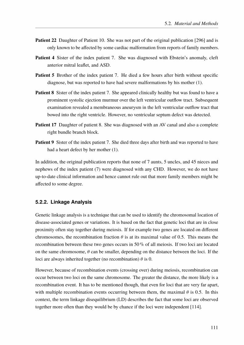
5.2. Material and Methods
Patient 22 Daughter of Patient 10. She was not part of the original publication [296] and isonly known to be affected by some cardiac malformation from reports of family members.
Patient 4 Sister of the index patient 7. She was diagnosed with Ebstein’s anomaly, cleftanterior mitral leaflet, and ASD.
Patient 5 Brother of the index patient 7. He died a few hours after birth without specificdiagnose, but was reported to have had severe malformations by his mother (1).
Patient 8 Sister of the index patient 7. She appeared clinically healthy but was found to have aprominent systolic ejection murmur over the left ventricular outflow tract. Subsequentexamination revealed a membraneous aneurysm in the left ventricular outflow tract thatbowed into the right ventricle. However, no ventricular septum defect was detected.
Patient 17 Daughter of patient 8. She was diagnosed with an AV canal and also a completeright bundle branch block.
Patient 9 Sister of the index patient 7. She died three days after birth and was reported to havehad a heart defect by her mother (1).
In addition, the original publication reports that none of 7 aunts, 5 uncles, and 45 nieces andnephews of the index patient (7) were diagnosed with any CHD. However, we do not haveup-to-date clinical information and hence cannot rule out that more family members might beaffected to some degree.
5.2.2. Linkage Analysis
Genetic linkage analysis is a technique that can be used to identify the chromosomal location ofdisease-associated genes or variations. It is based on the fact that genetic loci that are in closeproximity often stay together during meiosis. If for example two genes are located on differentchromosomes, the recombination fraction θ is at its maximal value of 0.5. This means therecombination between these two genes occurs in 50% of all meiosis. If two loci are locatedon the same chromosome, θ can be smaller, depending on the distance between the loci. If theloci are always inherited together (no recombination) θ is 0.
However, because of recombination events (crossing over) during meiosis, recombination canoccur between two loci on the same chromosome. The greater the distance, the more likely is arecombination event. It has to be mentioned though, that even for loci that are very far apart,with multiple recombination events occurring between them, the maximal θ is 0.5. In thiscontext, the term linkage disequilibrium (LD) describes the fact that some loci are observedtogether more often than they would be by chance if the loci were independent [114].
111

5. Congenital Heart Defects – A Family Study
Table 5.1.: Phenotypes of affected family members.This table lists the main phenotypes found in the described family. Septal defects include AVSD, ASD,and VSD. For some individuals, no specific diagnose is available (“Unknown”). Rare phenotypesare listed under “Other”. Detailed information on each patient can be found in the text and in theoriginal publication [296].
Individu
alID Ebstein’s
Anomaly
Wolff-Parkinson-White Syndrome
(WPW)
SeptalDefects
CleftMitralValve
Right BundleBranch Block
(RBBB)
Other/Unknown
2 - - - - - 43 - - - - - 44 4 - 4 4 - -5 - - - - - 47 4 4 4 4 - -8 - - - - - 49 - - - - - 410 4 4 - 4 - -14 - - 4 - 4 -15 4 4 4 - 4 -17 - - 4 - 4 -22 - - - - - 425 - - - - - 4
This knowledge can be used to identify genetic markers that are in high LD with the unknowndisease-associated locus, by linking these markers with the phenotype. To be informative, thegenetic markers have to be heterozygous in at least one of the parents.
As an example, we want to know if the genetic marker A1 in Figure 5.4a is associated to theobserved phenotype. The first step is to calculate the likelihood (L) for the observed data at agiven recombination fraction θ (L(θ)). Assuming that the locus is linked to the disease, wecount in how many of all meiosis (n) a recombination (r) occurs.
In the example pedigree in Figure 5.4a, there are five offspring in generation III, hence, n = 5meiosis took place. Four of the offspring show no recombination, as the affected individualscarry the marker A1, or unaffected individuals do not carry the marker A1. However, individualIII.5 is affected and does not carry this marker. Hence, r = 1 recombination is observed. Thelikelihood for observation at a given recombination fraction θ can now be calculated accordingto the following equation:
L(θ) = θr · (1 − θ)n−r
112
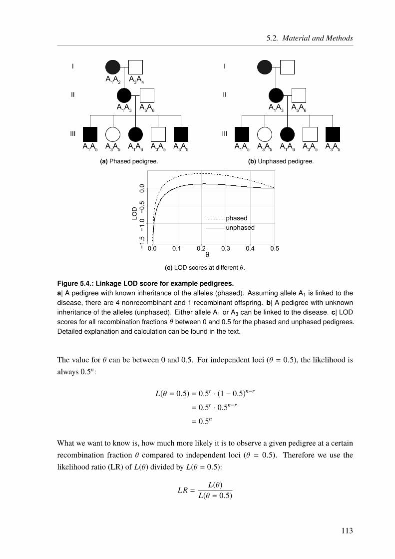
5.2. Material and Methods
I
II
III
A1A2 A3A4
A1A3 A5A6
A1A5 A3A5 A1A6 A3A5 A3A5
(a) Phased pedigree.
I
II
III
A1A3 A5A6
A1A5 A3A5 A1A6 A3A5 A3A5
(b) Unphased pedigree.
0.0 0.1 0.2 0.3 0.4 0.5−1.5
−1.0
−0.5
0.0
θ
LOD
phasedunphased
(c) LOD scores at different θ.
Figure 5.4.: Linkage LOD score for example pedigrees.a| A pedigree with known inheritance of the alleles (phased). Assuming allele A1 is linked to thedisease, there are 4 nonrecombinant and 1 recombinant offspring. b| A pedigree with unknowninheritance of the alleles (unphased). Either allele A1 or A3 can be linked to the disease. c| LODscores for all recombination fractions θ between 0 and 0.5 for the phased and unphased pedigrees.Detailed explanation and calculation can be found in the text.
The value for θ can be between 0 and 0.5. For independent loci (θ = 0.5), the likelihood isalways 0.5n:
L(θ = 0.5) = 0.5r · (1 − 0.5)n−r
= 0.5r · 0.5n−r
= 0.5n
What we want to know is, how much more likely it is to observe a given pedigree at a certainrecombination fraction θ compared to independent loci (θ = 0.5). Therefore we use thelikelihood ratio (LR) of L(θ) divided by L(θ = 0.5):
LR =L(θ)
L(θ = 0.5)
113
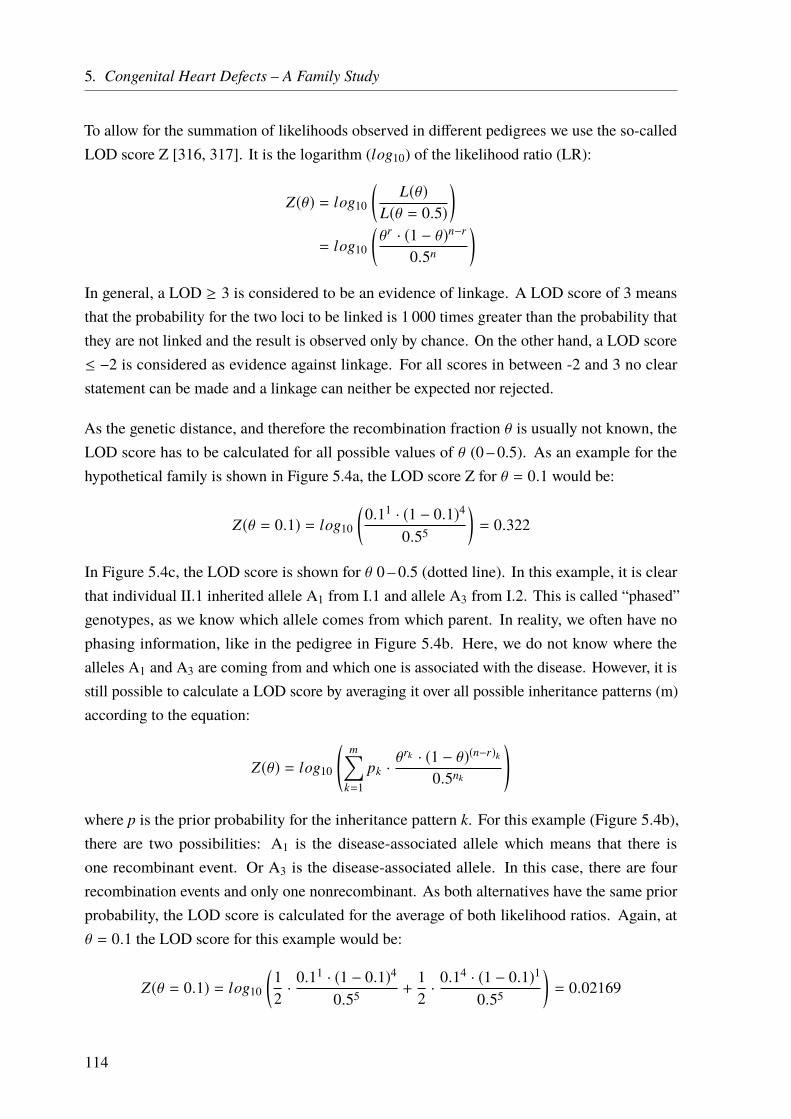
5. Congenital Heart Defects – A Family Study
To allow for the summation of likelihoods observed in different pedigrees we use the so-calledLOD score Z [316, 317]. It is the logarithm (log10) of the likelihood ratio (LR):
Z(θ) = log10
(L(θ)
L(θ = 0.5)
)= log10
(θr · (1 − θ)n−r
0.5n
)In general, a LOD ≥ 3 is considered to be an evidence of linkage. A LOD score of 3 meansthat the probability for the two loci to be linked is 1 000 times greater than the probability thatthey are not linked and the result is observed only by chance. On the other hand, a LOD score≤ −2 is considered as evidence against linkage. For all scores in between -2 and 3 no clearstatement can be made and a linkage can neither be expected nor rejected.
As the genetic distance, and therefore the recombination fraction θ is usually not known, theLOD score has to be calculated for all possible values of θ (0 – 0.5). As an example for thehypothetical family is shown in Figure 5.4a, the LOD score Z for θ = 0.1 would be:
Z(θ = 0.1) = log10
(0.11 · (1 − 0.1)4
0.55
)= 0.322
In Figure 5.4c, the LOD score is shown for θ 0 – 0.5 (dotted line). In this example, it is clearthat individual II.1 inherited allele A1 from I.1 and allele A3 from I.2. This is called “phased”genotypes, as we know which allele comes from which parent. In reality, we often have nophasing information, like in the pedigree in Figure 5.4b. Here, we do not know where thealleles A1 and A3 are coming from and which one is associated with the disease. However, it isstill possible to calculate a LOD score by averaging it over all possible inheritance patterns (m)according to the equation:
Z(θ) = log10
(m∑
k=1pk · θ
rk · (1 − θ)(n−r)k
0.5nk
)where p is the prior probability for the inheritance pattern k. For this example (Figure 5.4b),there are two possibilities: A1 is the disease-associated allele which means that there isone recombinant event. Or A3 is the disease-associated allele. In this case, there are fourrecombination events and only one nonrecombinant. As both alternatives have the same priorprobability, the LOD score is calculated for the average of both likelihood ratios. Again, atθ = 0.1 the LOD score for this example would be:
Z(θ = 0.1) = log10
(12· 0.1
1 · (1 − 0.1)40.55 +
12· 0.1
4 · (1 − 0.1)10.55
)= 0.02169
114

5.2. Material and Methods
This score is lower than before, which is shown for all θ from 0 – 0.5 in Figure 5.4c on Page 113(solid line).
The same calculation can be performed if there are multiple possible inheritance patterns. Thismight be the case in larger pedigrees, especially with missing information. Sometimes it isnot clear if a variant is identical by descent (IBD) or identical by state (IBS). It is IBS if thevariant is the same in two individuals, but IBD if the variant is inherited from a commonancestor without recombination. I such cases the population frequency of the variant in questionhas to be taken into account. The certainty, that a shared variant is IBS, is expressed by theinformation content, which can also act as a measure of genetic marker quality in a pedigree.Moreover, the expected penetrance of a variant has to be considered. That is the proportionof individuals that carry a genetic variant and also show the corresponding phenotype. Fordominant variants, a penetrance of 1 is usually expected. As these calculations become verycomplex for larger pedigrees, they are usually performed in-silico.
All the calculations explained so far need a lot of previous knowledge about the inheritancepattern, variant frequencies, penetrance and more. As some (or all) of this parameters areset before the calculation, this kind of linkage analysis is called parametric linkage analysis.Another kind of linkage analysis makes no assumptions on the disease models and is thereforecalled nonparametric linkage (NPL) analysis. This analysis is generally based on allele sharingbetween siblings.
In the pedigree shown below (Figure 5.5a) the probability of the unaffected siblings II.1 and II.2sharing 0,1, or 2 alleles is 0.25:0.5.0.25. In the case of a dominantly inherited phenotype, theallele sharing probabilities change if the two siblings are affected to 0:0.5:0.5 (see Figure 5.5b).Now, all observed markers can be compared to this distribution and a statistic test like Pearson’sχ2 test [318] can be applied to evaluate the goodness of fit.
I
II
A1A2 A3A4
(a) Unaffected sibling pair.
I
II
A1A2 A3A4
(b) Affected sibling pair.
Figure 5.5.: Allele sharing example.a| The probability that the unaffected siblings share 0,1, or 2 alleles is 0.25:0.5:0.25. b| If bothsiblings are affected by a dominantly inherited phenotype, they will share 1 or 2 alleles with aprobability of 0.5 each.
115

5. Congenital Heart Defects – A Family Study
Because of missing data, it is often not possible to determine how many alleles are shared IBDby a sibling pair, resulting in a lot of different possible allele sharing patterns. For this reasons,different methods have been developed to solve these problems computationally. One methodthat is used in this thesis was developed by Kong and Cox [319] and performs testing not onlyfor single markers (single-point analysis) but also takes nearby markers into consideration(multi-point analysis). Off note, single-point analysis are sometimes referred to as two-pointanalysis, as one marker and the potential disease locus are taken into account.
5.2.2.1. Short Tandem Repeat Markers
One type of genetic markers that can be used for linkage analysis are short tandem repeats (STRs),also called microsatellites. They make up around 0.5% of the genome and are the shortesttypes of variable number tandem repeats (VNTRs). STRs are short (usually 1 – 5 bp) repetitiveDNA sequences with 5 – 50 repeats [320]. The number of repeats varies within the population,which makes these markers suitable for linkage analysis. In average, mutation (length change)of STRs occurs around once in 1 000 generations, but with high variation between STRs [321].This means that STRs that are inherited usually remain unchanged and therefore it is easy todistinguish between IBS and IBD. The main cause of STR mutations is slippage of the DNApolymerase, which occurs at repetitive regions [320, 322]. STRs are also associated with arange of disease [323]. However, the ones used for genotyping/linkage analysis are usually notaffecting the phenotype.
For the family described in this project, a STR-based linkage analysis was performed in 1998,shortly after the first description of the family [324]. STR linkage data was available forthe individuals 1, 3, 4, 6 – 8, 10, 11, 13 – 17, 19, and 21 (see Figure 5.10 on Page 131 andTable A.10 on Page 180). A scan of the whole genome was performed using 321 STR markerswith an average spacing of 11 cM. After an initial two-point and multi-point linkage analysis, allsuggestive regions with a LOD score > 1 were investigated in more detail by adding additionalmarkers in these regions.
We had only access to the STR data (repeat numbers) from a region on chromosome 1. (hg19position: 48 281 221 – 106 281 721; deCode genetic map position: 71.29 – 126.35 cM [325]).All available markers and their positions can be found in Table A.11 on Page 181. We used thisdata to reanalyze the linkage in this region with the STRs alone and in combination with theSNP linkage data described below (see Figure 5.6).
116
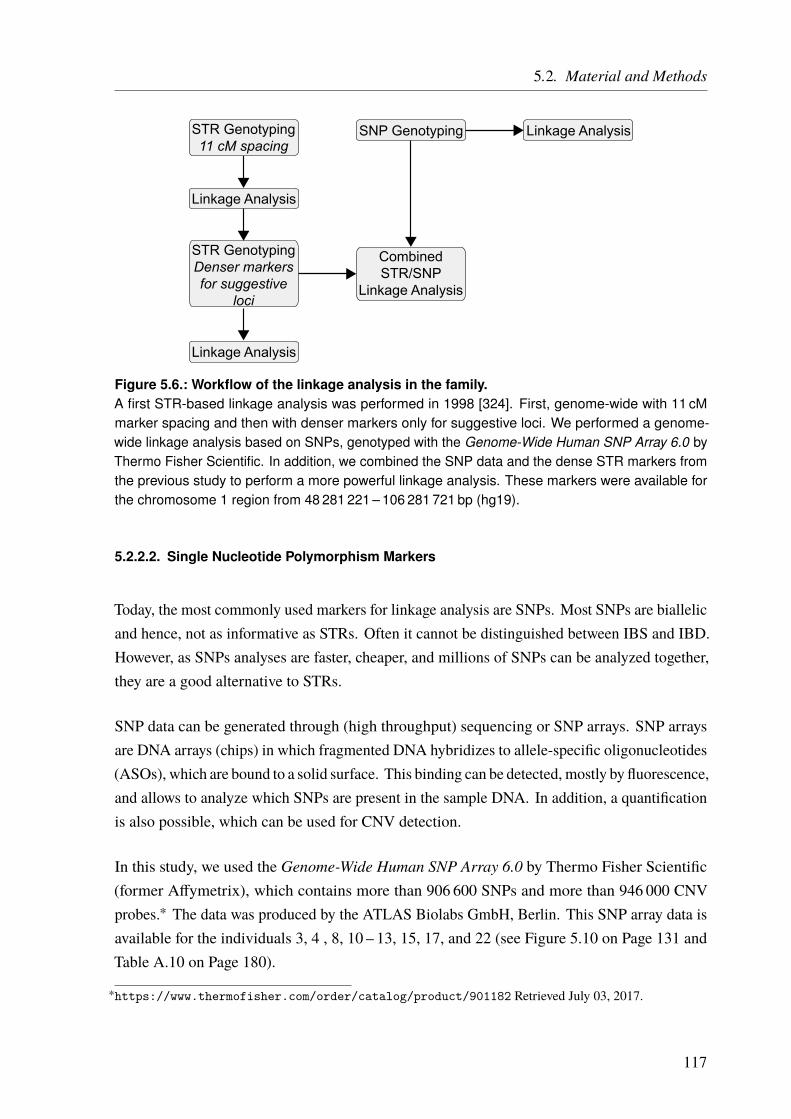
5.2. Material and Methods
STR Genotyping11 cM spacing
SNP Genotyping
Linkage Analysis
STR GenotypingDenser markersfor suggestive
loci
CombinedSTR/SNP
Linkage Analysis
Linkage Analysis
Linkage Analysis
Figure 5.6.: Workflow of the linkage analysis in the family.A first STR-based linkage analysis was performed in 1998 [324]. First, genome-wide with 11 cMmarker spacing and then with denser markers only for suggestive loci. We performed a genome-wide linkage analysis based on SNPs, genotyped with the Genome-Wide Human SNP Array 6.0 byThermo Fisher Scientific. In addition, we combined the SNP data and the dense STR markers fromthe previous study to perform a more powerful linkage analysis. These markers were available forthe chromosome 1 region from 48 281 221 – 106 281 721 bp (hg19).
5.2.2.2. Single Nucleotide Polymorphism Markers
Today, the most commonly used markers for linkage analysis are SNPs. Most SNPs are biallelicand hence, not as informative as STRs. Often it cannot be distinguished between IBS and IBD.However, as SNPs analyses are faster, cheaper, and millions of SNPs can be analyzed together,they are a good alternative to STRs.
SNP data can be generated through (high throughput) sequencing or SNP arrays. SNP arraysare DNA arrays (chips) in which fragmented DNA hybridizes to allele-specific oligonucleotides(ASOs), which are bound to a solid surface. This binding can be detected, mostly by fluorescence,and allows to analyze which SNPs are present in the sample DNA. In addition, a quantificationis also possible, which can be used for CNV detection.
In this study, we used the Genome-Wide Human SNP Array 6.0 by Thermo Fisher Scientific(former Affymetrix), which contains more than 906 600 SNPs and more than 946 000 CNVprobes.∗ The data was produced by the ATLAS Biolabs GmbH, Berlin. This SNP array data isavailable for the individuals 3, 4 , 8, 10 – 13, 15, 17, and 22 (see Figure 5.10 on Page 131 andTable A.10 on Page 180).
∗https://www.thermofisher.com/order/catalog/product/901182 Retrieved July 03, 2017.
117
5. Congenital Heart Defects – A Family Study
5.2.2.3. Linkage Analysis Pipeline
A short overview of the whole linkage analysis pipeline is shown in Figure 5.6. To analyze theSNP array data we used the Affymetrix Power Tools (APT)† to call the genotypes from the rawread data. Next, LINKDATAGE [326] was used to convert the genotype data to input data forthe actual linkage analysis program MERLIN (version 1.1.2) [327].
In addition, we converted the STR linkage data to the MERLIN input data by hand. Thecentimorgan (cM) positions are taken from deCode Genetics [325] as these positions are alsoused by Affymetrix. We calculated linkage from the SNP data alone, the STR data (onlyavailable for chromosome 1) alone, and for the combined data in the chromosome 1 region. Wealso used MERLIN for haplotyping, which produced the most likely pattern of gene flow. Wevisualized this data in a pedigree using the HaploPainter software [328].
As MERLIN is used for multiple steps, the main parameters are explained in Table 5.2.
Table 5.2.: General MERLIN parameters.Special parameters for single tools are explained in the corresponding section.
Parameter Explanation
-m MAP file with chromosome and cM positions for all markers-p MERLIN PED file, generated by LINKDATAGEN. Includes the pedigree information,
individual information, and genotypes for all markers-d Datafile, describing the contents of the corresponding PED file–bits sets the maximal complexity of the pedigrees to be analyzed. Default is 24 and
pedigrees with more individual will be skipped
Genotype Calling
The first step was the genotype calling from the Genome-Wide Human SNP Array 6.0 chip rawdata (CEL files). We used the apt-probeset-genotype command from the Affymetrix PowerTools software (version 1.18.2). The parameters are shown in Code Listing 5.1. We applied theBirdseed (v2) genotype calling algorithm, as recommended by the MERLIN software.
Input Dataset Generation
In this step, the input data for MERLIN was created by the LINKDATAGEN software fromthe birdseed v2 call files. The code is shown in Code Listing 5.2. The software does not onlyconvert the data to the right input format but also selects the most informative markers, based
†https://www.thermofisher.com/de/de/home/life-science/microarray-analysis/microarray-analysis-partners-programs/affymetrix-developers-network/affymetrix-power-tools.html
118

5.2. Material and Methods
Code Listing 5.1: Genotype calling from SNP array data.apt-probeset-genotype was used to call the genotypes from the raw data (CEL files). -c filedefining the probe set. –set-gender-method sets the gender calling method, we used the ratio ofprobes on the X and Y chromosomes. –special-snps defines probe IDs of SNPs with unusual copynumber (mitochondria, X/Y-chromosome). –chrX-probes defines probe IDs on the X chromosome.–chrY-probes defines probe IDs on the Y chromosome. -o output directory name. -a sets the analysismethod (here birdseed (v2) calling algorithm). –read-models-birdseed file to read the precomputedbirdseed SNP specific models from.
1 apt -probeset - genotype -c GenomeWideSNP_6 .cdf \2 --set -gender - method cn -probe -chrXY -ratio \3 --special -snps GenomeWideSNP_6 . specialSNPs \4 --chrX - probes GenomeWideSNP_6 . chrXprobes \5 --chrY - probes GenomeWideSNP_6 . chrYprobes \6 -o results -a birdseed -v2 \7 --read -models - birdseed GenomeWideSNP_6 .birdseed -v2. models *. CEL
on information from HapMap [58] and depending on the desired marker density (set in cM).In addition, error checking/removal can be performed. Besides the birdseed v2 call files, twoother files are needed. A pedigree (PED) file which describes the family pedigree, includingsex, affection status and relationship status and a “Which Sample File” (WSF), that assigns theSNP chip data to the corresponding individuals. These text files were created manually.
Code Listing 5.2: Input file generation for MERLIN with LINKDATAGEN.-data defines the data source (a = Affymetrix). -pedfile pedigree file, describing the family. -whichSamplesFile file assigning the chip data to the corresponding individuals. -callfile callfilecreated in the previous step. -chip sets the used chip (6 = Genome-Wide Human SNP Array 6.0).-annotDir directory with files used for the annotation (provided by Affymetrix). -prog program forwhich the input data is generated (me = MERLIN). -binsize marker spacing in cM. -MendelErrorsdefines how to treat Mendelian errors (removeSNPs = removes all SNPs that show Mendelianerrors). -outputDir output directory.
1 perl linkdatagen .pl \2 -data a -pedfile CHD.ped -whichSamplesFile CHD.wsf \3 -callfile birdseed -v2.calls.txt -chip 6 \4 -annotDir mappingfiles_affy_build37 / -prog me -binsize 0.3 \5 -MendelErrors removeSNPs -outputDir CHD_Linkage_015 \
MERLIN Input Data Checking
In this step, the PEDSTATS tool [329] from the MERLIN package is used to check the dataintegrity, quality, and formatting (Code Listing 5.3). In addition, statistics are provided on thefamily/families.
119
5. Congenital Heart Defects – A Family Study
Code Listing 5.3: MERLIN Input data checking with PEDSTATS.PEDSTATS checks the data integrity/quality of the MERLIN input files. –pdf Family statistics aresupplied in PDF format.
1 pedstats \2 -d merlin_autosome_CHD .dat \3 -p merlin_genome_CHD .ped \4 --pdf
Genotyping Error Removal
Although LINKDATAGEN already removed Mendelian errors, MERLIN was used again toremove any errors in the input data. This was especially useful for the STR data, which wasnot processed through LINKDATAGEN but generated by hand. This is a two-step process:First, the errors are detected and the corresponding marker names are saved (Code Listing 5.4).Then, the pedwipe command is used to remove the respective markers from the DAT and PEDfiles (Code Listing 5.5).
Code Listing 5.4: MERLIN error detection.–error sets MERLIN to error detection mode. Markers that show Mendelian errors are saved in anintermediate file for the next step.
1 merlin \2 -d merlin_autosome_CHD .dat \3 -p merlin_genome_CHD .ped \4 -m merlin_genome_CHD .map \5 --bits 26 \6 --error
Code Listing 5.5: Error removal with Pedwipe.Removes Mendelian errors detected in the previous step from DAT and PED files.
1 pedwipe \2 -d merlin_autosome_CHD .dat \3 -p merlin_genome_CHD .ped
Nonparametric Linkage Analysis
Now, the actual LOD scores are calculated using the nonparametric linkage (–npl) option fromMERLIN (Code Listing 5.6). The calculation is performed using the linear model by Kongand Cox [319]. In addition, we used the –exp option to also calculate the exponential model[319], as it is better suited for “a large increase in allele sharing among affected individuals”, asstated by the MERLIN user guide.‡ However, it is more computationally intensive and can only
‡http://csg.sph.umich.edu/abecasis/merlin/tour/linkage.html Retrieved July 4, 2017.
120
5.2. Material and Methods
be used in addition to the linear model. We performed this calculation for the SNP array dataalone, the STR data alone, and combined for the chromosome 1 regions, where both markertypes were available.
Code Listing 5.6: Nonparametric linkage analysis with MERLIN.The linear (–npl) and exponential (–exp) models by Kong and Cox [319] were calculated. –informationcalculates information content (based on entropy) for each analysis position. –tabulate outputsresults in a tabular text file. –pdf outputs results in a graphical form in a PDF file. –MarkerNamesmarker names are used instead of cM positions. –prefix the prefix for the output files.
1 merlin \2 -d wiped.dat -p wiped.ped -m merlin_genome_CHD .map \3 --bits 26 --npl --exp \4 --information --tabulate --pdf \5 --MarkerNames --prefix CHD_Linkage
Haplotyping
A graphical representation of the identified linkage region was generated using the HaploPaintertool [328]. This software generates pedigrees and allows to add haplotype information to it.The input data was generated by MERLIN’s haplotyping function, which generates a map of themost likely gene flow in a pedigree (Code Listing 5.7). We used the SNP array data with 0.5 cMmarker spacing (–binsize option in Code Listing 5.2 on Page 119), to not overload the graphic.In addition, we added the STR data after removing genotyping errors (see above). To furtherremove superfluous information from the pedigree some markers, with no recombination eventbetween them, were removed by hand.
Code Listing 5.7: Haplotyping with MERLIN.Using the –best option MERLIN calculates a map of the most likely gene flow in a pedigree.
1 merlin \2 -d wiped.dat -p wiped.ped -m merlin_genome_CHD .map \3 --bits 26 --best
5.2.3. Copy Number Variation Analysis
Sometimes DNA sections or whole genes are duplicated or depleted, for example by nonallelichomologous recombination duringmeiosis or unequal crossing over [330]. This leads to changesin the so-called copy number of these regions, hence the name copy number variation (CNV).This CNVs can be detected, on microarrays in the same way as described earlier. DNAmolecules of the respective regions hybridize to probes that are bound to a solid surface. The
121

5. Congenital Heart Defects – A Family Study
quantity of bound probes can be measured through fluorescence and the intensity correlateswith the copy number of this regions. However, the intensity is not always a multiple of “1-fold”intensity. Hence, calling algorithms are needed to assign a distinct copy number value to aDNA fragment.
We used the apt-copynumber-workflow command from the Affymetrix Power Tools to callthe CNVs from the raw intensity data (see Code Listing 5.8). Next, we used the CNViewer tool[331], to visualize the results and to create a tab separated text file with CNV information forall individuals. We then compared the CNV states of affected and unaffected individuals toeach other.
Code Listing 5.8: CNV calling.–cdf-file file defining the probeset. –special-snps defines probe IDs of SNPs with unusual copynumber (mitochondria, X/Y-chromosome). –chrX-probes defines probe IDs on the X chromosome.–chrY-probes defines probe IDs on the Y chromosome. –annotation-file file used for annotation(provided by Affymetrix). –reference-input CNV reference file (provided by Affymetrix). –o outputdirectory name.
1 apt -copynumber - workflow --cdf -file GenomeWideSNP_6 .cdf \2 --special -snps GenomeWideSNP_6 . specialSNPs \3 --chrX - probes GenomeWideSNP_6 . chrXprobes \4 --chrY - probes GenomeWideSNP_6 . chrYprobes \5 --annotation -file GenomeWideSNP_6 .na34.annot.db \6 --reference -input GenomeWideSNP_6 . hapmap270 .na34.r1.a5.ref \7 --o CHD_CNVs *. CEL
5.2.4. Whole Exome/Genome Sequencing
Since the first description of the family in 1997, three different sequencing approaches wereused in this family. This includes two whole genome sequencing and one exome sequencingapproach. The affected individuals 4, 8, and 15 were exome sequenced in 2012 at the Institute ofHuman Genetics (Helmholtz Zentrum München) on a Genome Analyzer IIx system (Illumina,USA) after in-solution enrichment of exonic sequences with the SureSelect Human All Exon50 Mb kit (Agilent, USA). We received raw files and VCF files. The family members 13,15, and 17 were whole genome sequenced by Complete Genomics (Mountain View, USA) in2012, using their proprietary platform. The affected family members 4 and 22 were wholegenome sequenced by Centogene (Rostock, Germany) in 2016 at 30x coverage on an IlluminaHiSeq platform. Raw data alignment and processing was performed by us (see Section 2.1.2 onPage 41). Because of the limited DNA availability, not all family members were sequenced.
122

5.2. Material and Methods
For the individuals 4 and 15 we used the whole genome data for further processing, aftercomparing it to the exome data. The Complete Genomics variant files were lifted over to thehg19 genome build and converted to VCF files. Then, all sample VCF files were merged into asingle file. All variants on the Y chromosome were removed. As we were only interested invariants that are shared by all affected but not the unaffected family members, we removed allvariants that did not match this criteria.
We annotated all variants with ANNOVAR (see Section 2.2 on Page 49). The used tables arementioned in the corresponding results section. As for patient 8 only exonic data was availablewe did all the processing one time with and one time without this data, to also access variantsin noncoding regions. Hence, we ignored the exonic data in this step. The sequencing andfiltering workflow is shown in Figure 5.7.
Combine and Annotate Variants
Genome SequencingComplete GenomicsIDs 13, 15, and 17
Centogene (HiSeq)IDs 4 and 22
Exome SequencingGenome Analyzer II
ID 8
Search for Exonic/Splice Variants
Present in all casesNot present in control
Located in exon or at splice siteMAF ≤ 1%
Search for All Genomic Variants
Present in all genome sequenced casesNot present in control
Heterozygous in all casesMAF ≤ 1%
No overlap with segmental duplication
Figure 5.7.: Workflow of exome and genome sequencing and data analysis.The unaffected individual 13 and the affected individuals 15 and 17 were whole genome sequencedby Complete Genomics. The patients 4 and 22 were whole genome sequenced by Centogene onan Illumina HiSeq platform. Patient 8 was exome sequenced at the Helmholtz Zentrum München ona Genome Analyzer IIx system. After the variant calling, all sample data was pooled and annotatedusing ANNOVAR. Exonic and splice-site variants that were present in all cases but not the controlwere filtered for a MAF of ≤ 1 %. To also analyze noncoding variants, a second round of filtering wasperformed without the data of patient 8. The variants had to be present in all genome sequencedcases but not the control, had to be heterozygous, with a MAF of ≤ 1 %, and must not overlapsegmental duplications.
123

5. Congenital Heart Defects – A Family Study
5.2.5. Panel Sequencing of TGF beta and BMP Signaling Pathway Genes
We used a panel sequencing approach (see Section 2.1.1 on Page 13) to sequence eightTGF-β and bone morphogenetic protein (BMP) signaling pathway genes: ACVR1, ACVR1,BMP2, BMPR1A, BMPR1B, BMPR2, TGFBR1, and TGFBR3. The detailed Ion AmpliSeq™
library preparation and Ion Torrent™ semiconductor sequencing workflow is described inSection 2.1.1.1 on Page 15.
The Ion AmpliSeq™ Designer software was used to generate the amplicons. For some genesonly the coding sequence (CDS) was used, for others the UTR regions were added as well(Table 5.3). The amplicon size was 125 – 275 bp (for standard DNA), the total panel size30.39 kb, and 92.22% of the desired target regions were covered. The coverage per gene canbe found in Table 5.3.
Table 5.3.: Ion AmpliSeq™ Designer results for TGF beta and BMP signaling pathway genes.The amplicons were designed for the coding sequences (CDS) or the CDS plus the untrans-lated regions (UTRs). Alternative, but commonly used, gene names are given in parentheses.CHR = Chromosome.
Type Name CHR Target [bp] Missed [bp] Covered [%]
CDS + UTR ACVR1 (ALK2) 2 3 244 107 96.70CDS ACVRL1 (ALK1) 12 1 611 2 99.88CDS BMP2 20 1 213 2 99.84CDS BMPR1A (ALK3) 10 1 720 0 100.00CDS + UTR BMPR1B (ALK6) 4 5 703 390 93.16CDS + UTR BMPR2 2 12 213 1 723 85.89CDS TGFBR1 (ALK5) 9 1 611 124 92.30CDS TGFBR3 1 3 078 17 99.45
Total 30 393 2 365 92.22
The variant calling parameters in the Ion Torrent™ Suite software were set to “Germ LineHigh-Stringency”, to ensure a good detection rate while minimizing false positive results.
5.2.5.1. Panel Sequencing Cohort
We received DNA samples from unrelated individuals with complete AVSDs from the group ofProf. Dr. Schunkert at the “Deutsches Herzzentrum München” in Munich. In addition, someof the patients also suffered from Down syndrome (DS)/trisomy 21. We sequenced 62 AVSDpatients without and 32 AVSD patients with trisomy 21. As control group, we sequenced 32population matched in-house DNA samples from healthy individuals.
124

5.2. Material and Methods
5.2.5.2. Variant Annotation and Filtering
The variants were annotated with ANNOVAR (see Section 2.2 on Page 49) and filtered for aMAF of < 1% in the 1 000 Genomes Project data and the ExAC data. For both, we filteredbased on the total MAF and the MAF only based on (non-Finish) European samples. Wealso removed all variants that were neither exonic nor at splice site regions (±3 bp from exonboundary), as defined by the RefSeq data. For the exonic regions, we removed all synonymousvariants. The remaining variants were validated by Sanger sequencing to identify false positivesequencing results.
125

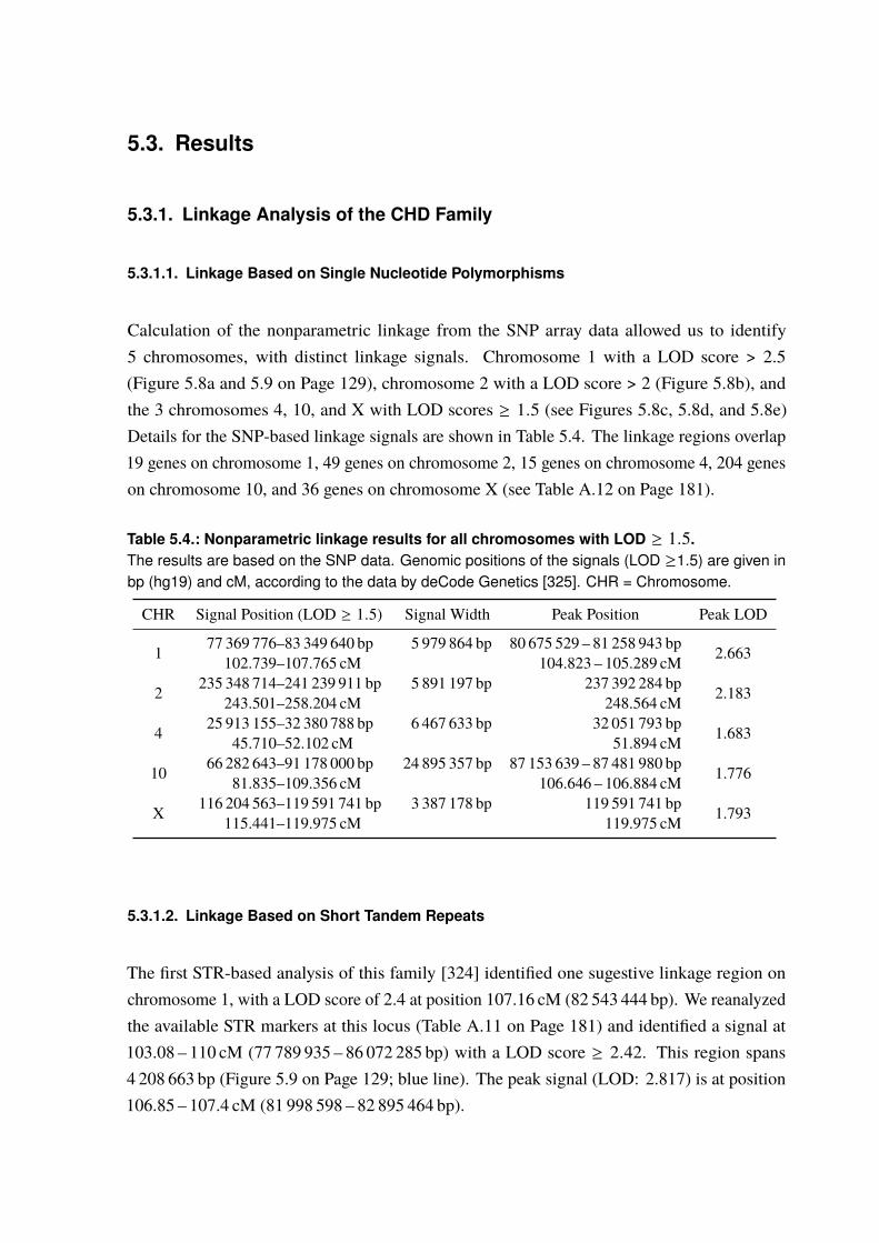
5.3. Results
5.3.1. Linkage Analysis of the CHD Family
5.3.1.1. Linkage Based on Single Nucleotide Polymorphisms
Calculation of the nonparametric linkage from the SNP array data allowed us to identify5 chromosomes, with distinct linkage signals. Chromosome 1 with a LOD score > 2.5(Figure 5.8a and 5.9 on Page 129), chromosome 2 with a LOD score > 2 (Figure 5.8b), andthe 3 chromosomes 4, 10, and X with LOD scores ≥ 1.5 (see Figures 5.8c, 5.8d, and 5.8e)Details for the SNP-based linkage signals are shown in Table 5.4. The linkage regions overlap19 genes on chromosome 1, 49 genes on chromosome 2, 15 genes on chromosome 4, 204 geneson chromosome 10, and 36 genes on chromosome X (see Table A.12 on Page 181).
Table 5.4.: Nonparametric linkage results for all chromosomes with LOD ≥ 1.5.The results are based on the SNP data. Genomic positions of the signals (LOD ≥1.5) are given inbp (hg19) and cM, according to the data by deCode Genetics [325]. CHR = Chromosome.
CHR Signal Position (LOD ≥ 1.5) Signal Width Peak Position Peak LOD
1 77 369 776–83 349 640 bp 5 979 864 bp 80 675 529 – 81 258 943 bp 2.663102.739–107.765 cM 104.823 – 105.289 cM
2 235 348 714–241 239 911 bp 5 891 197 bp 237 392 284 bp 2.183243.501–258.204 cM 248.564 cM
4 25 913 155–32 380 788 bp 6 467 633 bp 32 051 793 bp 1.68345.710–52.102 cM 51.894 cM
10 66 282 643–91 178 000 bp 24 895 357 bp 87 153 639 – 87 481 980 bp 1.77681.835–109.356 cM 106.646 – 106.884 cM
X 116 204 563–119 591 741 bp 3 387 178 bp 119 591 741 bp 1.793115.441–119.975 cM 119.975 cM
5.3.1.2. Linkage Based on Short Tandem Repeats
The first STR-based analysis of this family [324] identified one sugestive linkage region onchromosome 1, with a LOD score of 2.4 at position 107.16 cM (82 543 444 bp). We reanalyzedthe available STR markers at this locus (Table A.11 on Page 181) and identified a signal at103.08 – 110 cM (77 789 935 – 86 072 285 bp) with a LOD score ≥ 2.42. This region spans4 208 663 bp (Figure 5.9 on Page 129; blue line). The peak signal (LOD: 2.817) is at position106.85 – 107.4 cM (81 998 598 – 82 895 464 bp).
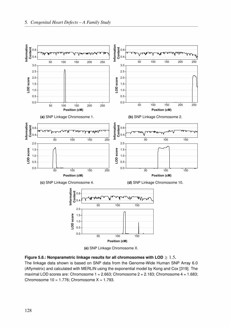
5. Congenital Heart Defects – A Family Study
50 100 150 200 250
50 100 150 200 250Position (cM)
0.4
0.6
Info
rmat
ion
Con
tent
0.0
0.5
1.0
1.5
2.0
2.5
3.0
LOD
sco
re
(a) SNP Linkage Chromosome 1.
Position (cM)
0.4
0.6
Info
rmat
ion
Con
tent
0.0
0.5
1.0
1.5
2.0
2.5
3.0
LOD
sco
re
50 100 150 200 250
50 100 150 200 250
(b) SNP Linkage Chromosome 2.
50 100 150
0.4
0.6
Info
rmat
ion
Con
tent
200
Position (cM)
0.0
0.5
1.0
1.5
2.0
LOD
sco
re
50 100 150 200
(c) SNP Linkage Chromosome 4.
50 100 150
0.4
0.6
Info
rmat
ion
Con
tent
Position (cM)
0.0
0.5
1.0
1.5
2.0
LOD
sco
re
50 100 150
(d) SNP Linkage Chromosome 10.
50 100 150
0.4
0.6
Info
rmat
ion
Con
tent
50 100 150
Position (cM)
0.0
0.5
1.0
1.5
2.0
LOD
sco
re
(e) SNP Linkage Chromosome X.
Figure 5.8.: Nonparametric linkage results for all chromosomes with LOD ≥ 1.5.The linkage data shown is based on SNP data from the Genome-Wide Human SNP Array 6.0(Affymetrix) and calculated with MERLIN using the exponential model by Kong and Cox [319]. Themaximal LOD scores are: Chromosome 1 = 2.663; Chromosome 2 = 2.183; Chromosome 4 = 1.683;Chromosome 10 = 1.776; Chromosome X = 1.793.
128
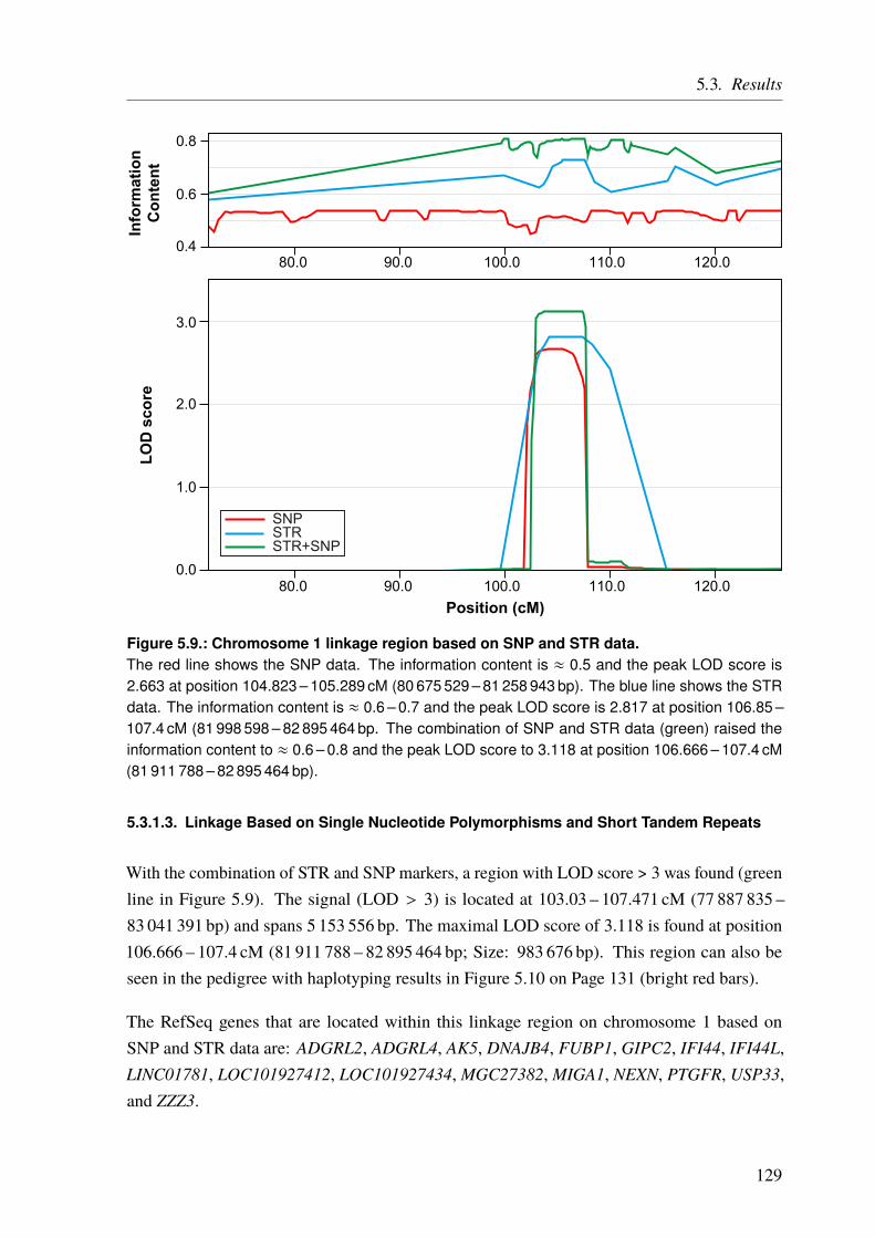
5.3. Results
80.0 90.0 100.0 110.0 120.00.4
0.6
0.8In
form
atio
nC
onte
nt
Position (cM)
0.0
1.0
2.0
3.0
LOD
sco
re
80.0 90.0 100.0 110.0 120.0
STRSNP
STR+SNP
Figure 5.9.: Chromosome 1 linkage region based on SNP and STR data.The red line shows the SNP data. The information content is ≈ 0.5 and the peak LOD score is2.663 at position 104.823 – 105.289 cM (80 675 529 – 81 258 943 bp). The blue line shows the STRdata. The information content is ≈ 0.6 – 0.7 and the peak LOD score is 2.817 at position 106.85 –107.4 cM (81 998 598 – 82 895 464 bp. The combination of SNP and STR data (green) raised theinformation content to ≈ 0.6 – 0.8 and the peak LOD score to 3.118 at position 106.666 – 107.4 cM(81 911 788 – 82 895 464 bp).
5.3.1.3. Linkage Based on Single Nucleotide Polymorphisms and Short Tandem Repeats
With the combination of STR and SNP markers, a region with LOD score > 3 was found (greenline in Figure 5.9). The signal (LOD > 3) is located at 103.03 – 107.471 cM (77 887 835 –83 041 391 bp) and spans 5 153 556 bp. The maximal LOD score of 3.118 is found at position106.666 – 107.4 cM (81 911 788 – 82 895 464 bp; Size: 983 676 bp). This region can also beseen in the pedigree with haplotyping results in Figure 5.10 on Page 131 (bright red bars).
The RefSeq genes that are located within this linkage region on chromosome 1 based onSNP and STR data are: ADGRL2, ADGRL4, AK5, DNAJB4, FUBP1, GIPC2, IFI44, IFI44L,LINC01781, LOC101927412, LOC101927434, MGC27382, MIGA1, NEXN, PTGFR, USP33,and ZZZ3.
129
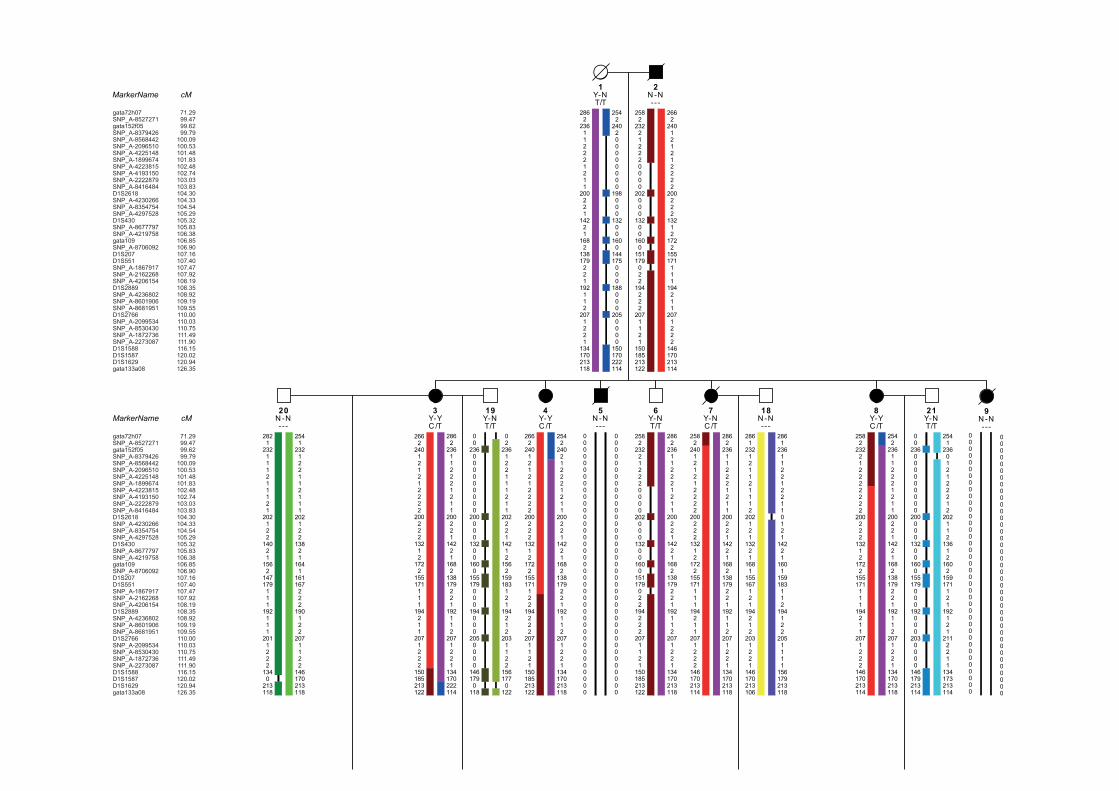
2862
236112221211
200221
14221
1682
138179221
192112
2071221
134170213118
2542
240200000000
198000
13200
1600
144175000
188000
2050000
150170222114
2582
232212220000
202000
13200
1600
151179022
194222
2071121
150185213122
2662
240121212222
200222
13212
1722
155171111
194211
2071222
146170213114
2821
232111211121
202122
14021
1562
147179111
192111
2011222
1340
213118
2541
232122112111
202122
13821
1641
161167222
190122
2071122
146170213118
2662
240121212222
200222
13212
1722
155171111
194211
2071222
150185213122
2862
236112221211
200221
14221
1682
138179221
192112
2071221
134170222114
00
236000000000
200000
13200
1600
155179000
194000
2050000
1461790
118
02
236122111211
202221
14212
1562
159183121
194212
2031122
1561770
122
2662
240121212222
200222
13212
1722
155171122
194222
2071121
150185213122
2542
240212221211
200221
14221
1682
138179221
192112
2071221
134170213118
2582
232212220000
202000
13200
1600
151179022
194222
2071121
150185213122
2862
236112221211
200221
14221
1682
138179221
192112
2071221
134170213118
2582
240121212222
200222
13212
1722
155171111
194211
2071222
146170213114
2862
236112221211
200221
14221
1682
138179221
192112
2071221
134170213118
2861
232121121112
202121
13221
1681
155167121
194212
2031221
146170213106
2861
2361122122110121
14221
1601
159183112
194122
2051111
156179213118
2582
232212222222
200222
13212
1722
155171111
194211
2071222
146170213114
2542
236112221211
200221
14221
1682
138179221
192112
2071221
134170213118
00
236000000000
200000
13200
1600
155179000
192000
2030000
146179213114
2541
236012122212
202112
13612
1602
159171121
192121
2112211
134173213114
2N -N---
1Y-NT/T
9N -N---
19Y-NT/T
4Y-YC /T
7Y-NC /T
20N -N---
5N -N---
8Y-YC /T
18N -N---
6Y-NT/T
3Y-YC /T
21Y-NT/T
000000000000000000000000000000000000000
000000000000000000000000000000000000000
000000000000000000000000000000000000000
000000000000000000000000000000000000000
MarkerName cM
MarkerName cM
gata72h07SNP_A-8527271gata152f05SNP_A-8379426SNP_A-8568442SNP_A-2096510SNP_A-4225148SNP_A-1899674SNP_A-4223815SNP_A-4193150SNP_A-2222879SNP_A-8416484D1S2618SNP_A-4230266SNP_A-8354754SNP_A-4297528D1S430SNP_A-8677797SNP_A-4219758gata109SNP_A-8706092D1S207D1S551SNP_A-1867917SNP_A-2162268SNP_A-4206154D1S2889SNP_A-4236802SNP_A-8601906SNP_A-8681951D1S2766SNP_A-2099534SNP_A-8530430SNP_A-1872736SNP_A-2273087D1S1588D1S1587D1S1629gata133a08
71.2999.4799.6299.79
100.09100.53101.48101.83102.48102.74103.03103.83104.30104.33104.54105.29105.32105.83106.38106.85106.90107.16107.40107.47107.92108.19108.35108.92109.19109.55110.00110.03110.75111.49111.90116.15120.02120.94126.35
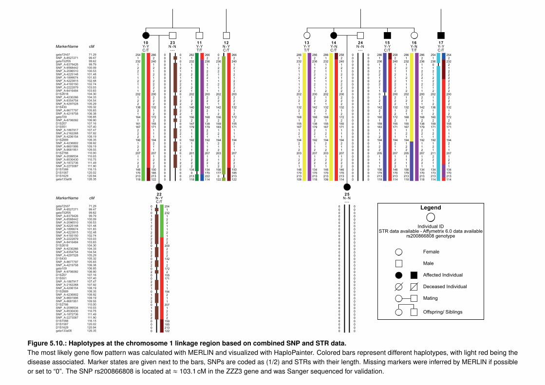
010121212222012202202002210122011220000
2541
232122112122
200222
13212
1722
155171111
194211
2071222
150185213122
000000000000000000000000000000000000000
2541
232122112111
202122
13821
1641
161167222
190122
2071122
146170213118
2662
240121212222
200222
13212
1722
155171111
194211
2071222
150185213122
000000000000000000000000000000000000000
010121212222012202202002210122011220000
2821
232111211121
202122
14021
1562
147179111
192111
2011222
1340
213118
2662
236112221211
200221
14221
1682
138179221
192112
2071221
134170222114
02
236122111211
202221
14212
1562
159183121
194212
2031122
1561770
122
2662
240121212222
200222
13212
1722
155171111
194211
2071222
150185213122
2861
232121121112
202121
13221
1681
155167121
194212
2031221
146170213106
2862
236112221211
200221
14221
1682
138179221
192112
2071221
134170213118
2861
232121121112
202121
13221
1681
155167121
194212
2031221
146170213106
2582
240121212222
200222
13212
1722
155171111
194211
2071222
146170213114
000000000000000000000000000000000000000
000000000000000000000000000000000000000
2861
2361122122110121
14221
1601
159183112
194122
2051111
156179213118
2582
240121212222
200222
13212
1722
155171111
194211
2071222
146170213114
2861
232121121112
202121
13221
1681
155167121
194122
2051111
156179213118
2862
236112221211
200221
14221
1682
138179221
192112
2071221
134170213118
2541
236012122212
202112
13612
1602
159171121
192121
2112211
134173213114
2542
232212222222
200222
13212
1722
155171111
194211
2071221
134170213114
22N -YC /T
25N -N---
16Y-NT/T
12N -Y
24N -N---
23N -N---
11Y-YT/T
13Y-YT/T
17Y-YC /T
10Y-YC /T
14 15Y-YC /T
000000000000000000000000000000000000000
MarkerName cM
MarkerName cM
Female
Male
Affected Individual
Deceased Individual
Mating
Offspring/ Siblings
STR data available - Affymetrix 6.0 data availablers200866808 genotype
Individual ID
Legend
Y-NC /TC /T
gata72h07SNP_A-8527271gata152f05SNP_A-8379426SNP_A-8568442SNP_A-2096510SNP_A-4225148SNP_A-1899674SNP_A-4223815SNP_A-4193150SNP_A-2222879SNP_A-8416484D1S2618SNP_A-4230266SNP_A-8354754SNP_A-4297528D1S430SNP_A-8677797SNP_A-4219758gata109SNP_A-8706092D1S207D1S551SNP_A-1867917SNP_A-2162268SNP_A-4206154D1S2889SNP_A-4236802SNP_A-8601906SNP_A-8681951D1S2766SNP_A-2099534SNP_A-8530430SNP_A-1872736SNP_A-2273087D1S1588D1S1587D1S1629gata133a08
71.2999.4799.6299.79
100.09100.53101.48101.83102.48102.74103.03103.83104.30104.33104.54105.29105.32105.83106.38106.85106.90107.16107.40107.47107.92108.19108.35108.92109.19109.55110.00110.03110.75111.49111.90116.15120.02120.94126.35
Figure 5.10.: Haplotypes at the chromosome 1 linkage region based on combined SNP and STR data.The most likely gene flow pattern was calculated with MERLIN and visualized with HaploPainter. Colored bars represent different haplotypes, with light red being thedisease associated. Marker states are given next to the bars, SNPs are coded as (1/2) and STRs with their length. Missing markers were inferred by MERLIN if possibleor set to “0”. The SNP rs200866808 is located at ≈ 103.1 cM in the ZZZ3 gene and was Sanger sequenced for validation.
5. Congenital Heart Defects – A Family Study
No relevant information could be found for the nine genes ADGRL2, ADGRL4, IFI44, IFI44L,LINC01781, LOC101927412, LOC101927434,MGC27382, and ZZZ3. The other genes aredescribed below.
Adenylate Kinase 5 (AK5) This protein-coding gene is part of the adenylate kinase family. Itis involved in the conversion of adenine nucleotides and although not much is knownabout the gene, it has mainly been reported to play a role in diseases affecting the brain.This includes limbic encephalitis, prosopagnosia (face blindness), anterograde amnesia,and temporal lobe epilepsy [332, 333]. One study also links it to celiac disease [334],and another study links AK5, among other adenylate kinase genes, to stem cell cardiacdifferentiation [335].
DnaJ Heat Shock Protein Family (Hsp40) Member B4 (DNAJB4) This gene, encodes amember of the heat shock protein-40 family [336]. It is a chaperone for E-cadherin andhence might influence cell-cell adhesion [337]. In addition, it is known to act as a tumorsuppressor and is used as a biomarker [338–340].
Far Upstream Element Binding Protein 1 (FUBP1) FUBP1 encodes a DNA binding proteinwhich is mainly reported to be involved in tumor proliferation of oligodendroglioma andalso seems to be involved in apoptosis [341–343].
GIPC PDZ Domain Containing Family Member 2 (GIPC2) The GIPC2 gene is a paralogof GIPC1. The whole GIPC-family is known to interact with the “Transforming GrowthFactor Beta Receptor 3” (TGFBR3) (Betaglycan), which is part of the TGF-β/BMPpathway (Figure 5.14 on Page 145) [344, 345]. TGFBR3 is a key player during endothelial-mesenchymal transition (EndoMT), and interactions with GIPC-genes have been shownto be essential [346–348].
Mitoguardin 1 (MIGA1) Not much is known about this gene, apart from the fact that it playsa role in mitochondria fusion, neuronal homeostasis, and oocyte maturation in mice[349, 350].
Nexilin (NEXN) The gene encodes a Z-disc protein and knockouts in animal models, as well asmutations in humans, lead to the disruption of the Z-discs/sarcomeres [351–353]. Nexilinplays a well-known role in cardiomyopathies, especially dilated cardiomyopathy (DCM),but it is also described to be involved in hypertrophic cardiomyopathy (HCM) [353–355].Both cardiomyopathies are usually late onset disease. However, recent studies alsosuggest a role of the NEXN in CHDs, like ASD and left ventricular noncompactioncardiomyopathy (LVNC) [356, 357].
132

5.3. Results
Prostaglandin F Receptor (PTGFR) This gene encodes a member of the G-protein coupledreceptor family. The protein is a key player during luteolysis but is also involved inangiogenesis and embryo-maternal interactions during implantation [358, 359]. It is alsoreported to be associated with glaucomas, ocular hypertension, and other eye diseases[360, 361]. In addition, some results suggest an involvement in the signaling in smoothmuscle cells, regulation of endothelial cell functions, and a possible role in hypertension[362–364].
Ubiquitin Specific Peptidase 33 (USP33) The protein encoded by the USP33 gene, is adeubiquitinases, that is also involved in proteolysis [365, 366]. It also plays a role inmultiple types of cancer and influences cell migration [367–369].
In total, the carrier status for this linkage region is available or can be surely inferred for 16individuals (unrelated parents excluded). Ten of this individuals are affected and all of themcarry the linkage region. Hence, six individuals are unaffected, with one of them (Individual12) carrying the linkage region (Figure 5.10 on Page 131). This results in an OR significantlygreater than 1 in a Fisher’s exact test (p = 1.374 · 10−3).
5.3.2. Copy Number Variation Analysis of the CHD Family
Based on the > 906 600 SNPs and > 946 000 CNV probes from the Genome-Wide Human SNPArray 6.0, we could not identify any CNVs that differed between the seven affected and threeunaffected individuals. All identified CNVs were specific for a single individual or a mixedgroup of affected and unaffected individuals.
5.3.3. Whole Exome/Genome Sequencing of the CHD Family
In total, we identified 10 491 999 variants in the sequenced individuals. The mean number ofvariants in the HiSeq genome data was 5 062 310, in the Complete Genomics data 3 925 865,and 49 107 in the exome data (Figure 5.11). We analyzed the exonic regions based on allsamples and the whole genome only based on individuals with whole genome data available.
5.3.3.1. Exonic Data
First, we filtered for variants that were shared by all examined affected individuals but not bythe unaffected individual 13, which left us with 1 344 variants (Figure 5.11a). 512 of thesevariants were located in exonic regions or at splice sites (±3 bp from exon borders) based on
133
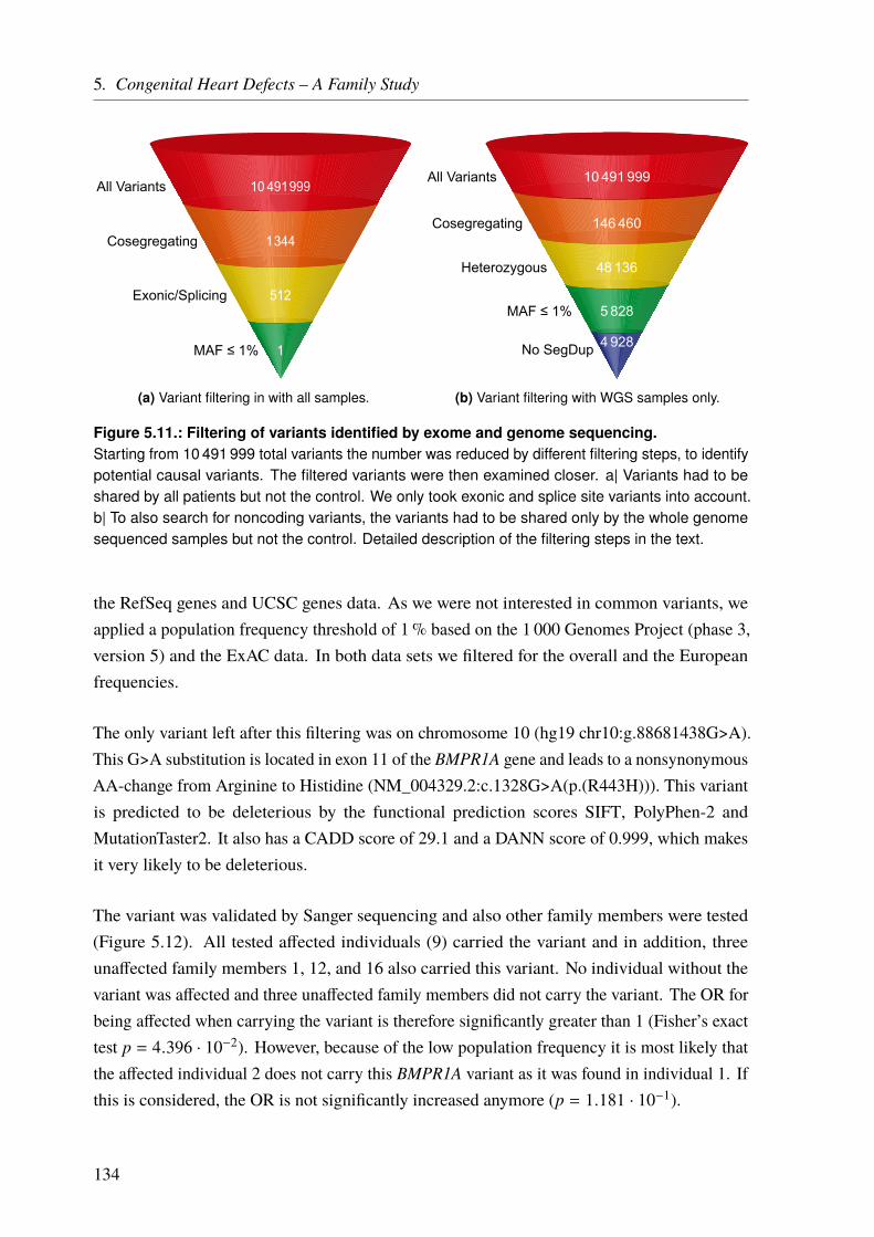
5. Congenital Heart Defects – A Family Study
1
512
1 344
10 491 999All Variants
Cosegregating
Exonic/Splicing
MAF ≤ 1%
(a) Variant filtering in with all samples.
4 928
5 828
48 136
146 460
10 491 999All Variants
Cosegregating
Heterozygous
MAF ≤ 1%
No SegDup
(b) Variant filtering with WGS samples only.
Figure 5.11.: Filtering of variants identified by exome and genome sequencing.Starting from 10 491 999 total variants the number was reduced by different filtering steps, to identifypotential causal variants. The filtered variants were then examined closer. a| Variants had to beshared by all patients but not the control. We only took exonic and splice site variants into account.b| To also search for noncoding variants, the variants had to be shared only by the whole genomesequenced samples but not the control. Detailed description of the filtering steps in the text.
the RefSeq genes and UCSC genes data. As we were not interested in common variants, weapplied a population frequency threshold of 1% based on the 1 000 Genomes Project (phase 3,version 5) and the ExAC data. In both data sets we filtered for the overall and the Europeanfrequencies.
The only variant left after this filtering was on chromosome 10 (hg19 chr10:g.88681438G>A).This G>A substitution is located in exon 11 of the BMPR1A gene and leads to a nonsynonymousAA-change from Arginine to Histidine (NM_004329.2:c.1328G>A(p.(R443H))). This variantis predicted to be deleterious by the functional prediction scores SIFT, PolyPhen-2 andMutationTaster2. It also has a CADD score of 29.1 and a DANN score of 0.999, which makesit very likely to be deleterious.
The variant was validated by Sanger sequencing and also other family members were tested(Figure 5.12). All tested affected individuals (9) carried the variant and in addition, threeunaffected family members 1, 12, and 16 also carried this variant. No individual without thevariant was affected and three unaffected family members did not carry the variant. The OR forbeing affected when carrying the variant is therefore significantly greater than 1 (Fisher’s exacttest p = 4.396 · 10−2). However, because of the low population frequency it is most likely thatthe affected individual 2 does not carry this BMPR1A variant as it was found in individual 1. Ifthis is considered, the OR is not significantly increased anymore (p = 1.181 · 10−1).
134

5.3. Results
1G/A
2-
20 3G/A
19 4G/A
5-
6G/G
187G/A
218G/A
9-
10G/A
11G/G
12G/A
13G/G
14G/A
15G/A
16G/A
17G/A
22G/A
23 24
25-
Female
Male
Affected Individual
Deceased Individual
Mating
Offspring/ Siblings
Individual IDBMPR1A c.1328 genotype
Legend
Figure 5.12.: Genotype status of the BMPR1A variant NM_004329.2:c.1328G>A in the CHDfamily.Besides all affected individuals, three unaffected family members carried the identified BMPR1Avariant (1, 12, and 15). All other tested unaffected individuals did not carry the variant. For theaffected individuals 2, 5, 9, and 25 no DNA was available. The OR is significantly increased (Fisher’sp = 4.396 · 10−2). However, if it is assumed that individual 2 does not carry the variant, the increaseis not significant anymore (Fisher’s p = 1.181 · 10−1)
5.3.3.2. Whole Genome Data
Additionally, to test variants outside exonic regions, we filtered also for variants that were onlyshared by all affected individuals with genome data available (4, 15, 17, 22) and not present inthe control genome data (individual 13) (Figure 5.11b). We ignored the genotype of individual 8(exome only data). 146 460 shared variants were identified, 48 136 of which were heterozygous.Then, we removed the variants with a population frequency > 1% in the 1 000 Genomes Project(phase 3, version 5) and the ExAC data. This left us with 5 828 variants. In the last step, weremoved all variants located in segmental duplications, leaving 4 928 variants.
The vast majority of variants are located in intergenic (3 393; 68.91%) and intronic (1 512;30.68%) regions. Of the intergenic variants, 63 are locatedwithin 1 kb distance of a transcriptionstart site (TSS). 16 variants (0.32%) are located within UTR regions (14 in 3’ UTRs; 2 in5’ UTRs). 5 variants (0.1%) are located in the exons of noncoding RNAs (ncRNAs) and 2variants (0.04 ) in the exons of protein-coding genes.
135
5. Congenital Heart Defects – A Family Study
Apart from the already described BMPR1A variant, the other exonic variant is a substitutionlocated on chromosome 4 (hg19 chr4:g.8443084C>T). Although it leads to an AA-change(NM_152544.2:c.535C>T(:p.(L179F))), all prediction scores classify this variant as benign.
179 variants have a CADD score > 10, 33 variants a CADD score > 15, and 6 variants have aCADD score > 20. Of these six variants, only two also have DANN scores that suggest clearpathogenicity: The already described variant in BMPR1A (NM_004329.2:c.1328G>A) and anintergenic A>G substitution on chromosome X, between the DIAPH2 gene and the pseudogeneXRCC6P5 (hg19 chrX:g.98098215A>G).
There are also 68 variants with eQTL effects, based on the HaploReg database. We could notidentify any potential splicing changes based on the SPIDEX™database.
5.3.4. Genomic Variants that Overlap Identified Linkage Regions
Linkage data is available for more individuals than sequencing data, and hence reduces thenumber of potential disease associated variants. Therefore, we took a close look at the variantsthat overlap the linkage regions with a LOD score > 1.5 in the SNP data (see Table 5.4 onPage 127). This also covers the whole region identified by STR markers.
We used the “genome-only” data for this comparison and found 3 685 variants in all linkageregions. 1 759 were heterozygous and 217 had a frequency ≤ 1%. 99 variants overlapped thechromosome 1 region, six the chromosome 2 region, twelve the chromosome 4 region, 90 thechromosome 10 region, and ten variants were found in the identified linkage region on the Xchromosome.
The only exonic variant among these, that overlapped a linkage region was the already describednonsynonymous substitution in the BMPR1A gene (NM_004329.2:c.1328G>A).
As most variants were located in noncoding regions, we used CADD and DANN to evaluatethe functional implications. We found 9 variants with a CADD score > 10 (5 on chromosome 1and 4 on chromosome 10). Two of these variants also have a DANN score over 0.96 (Table 5.5).The BMPR1A variant and an intergenic variant on chromosome 10, between theWAPAL andOPN4 genes (hg19 chr10:g.88329240T>C; CADD: 18.27; DANN:0.96).
136
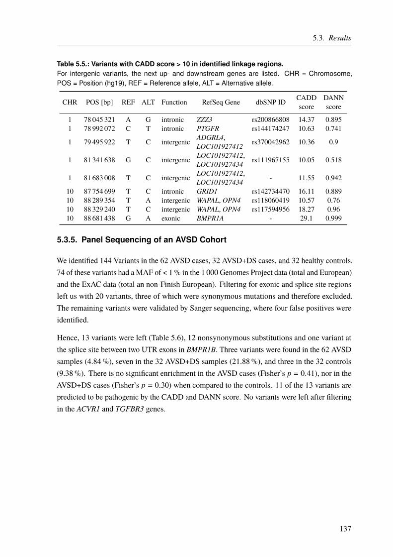
5.3. Results
Table 5.5.: Variants with CADD score > 10 in identified linkage regions.For intergenic variants, the next up- and downstream genes are listed. CHR = Chromosome,POS = Position (hg19), REF = Reference allele, ALT = Alternative allele.
CHR POS [bp] REF ALT Function RefSeq Gene dbSNP ID CADDscore
DANNscore
1 78 045 321 A G intronic ZZZ3 rs200866808 14.37 0.8951 78 992 072 C T intronic PTGFR rs144174247 10.63 0.741
1 79 495 922 T C intergenic ADGRL4,LOC101927412 rs370042962 10.36 0.9
1 81 341 638 G C intergenic LOC101927412,LOC101927434 rs111967155 10.05 0.518
1 81 683 008 T C intergenic LOC101927412,LOC101927434 - 11.55 0.942
10 87 754 699 T C intronic GRID1 rs142734470 16.11 0.88910 88 289 354 T A intergenic WAPAL, OPN4 rs118060419 10.57 0.7610 88 329 240 T C intergenic WAPAL, OPN4 rs117594956 18.27 0.9610 88 681 438 G A exonic BMPR1A - 29.1 0.999
5.3.5. Panel Sequencing of an AVSD Cohort
We identified 144 Variants in the 62 AVSD cases, 32 AVSD+DS cases, and 32 healthy controls.74 of these variants had a MAF of < 1% in the 1 000 Genomes Project data (total and European)and the ExAC data (total an non-Finish European). Filtering for exonic and splice site regionsleft us with 20 variants, three of which were synonymous mutations and therefore excluded.The remaining variants were validated by Sanger sequencing, where four false positives wereidentified.
Hence, 13 variants were left (Table 5.6), 12 nonsynonymous substitutions and one variant atthe splice site between two UTR exons in BMPR1B. Three variants were found in the 62 AVSDsamples (4.84%), seven in the 32 AVSD+DS samples (21.88%), and three in the 32 controls(9.38%). There is no significant enrichment in the AVSD cases (Fisher’s p = 0.41), nor in theAVSD+DS cases (Fisher’s p = 0.30) when compared to the controls. 11 of the 13 variants arepredicted to be pathogenic by the CADD and DANN score. No variants were left after filteringin the ACVR1 and TGFBR3 genes.
137
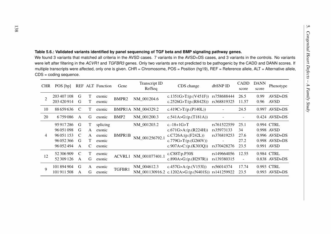
5.CongenitalH
eartDefects–
AFam
ilyStudy
Table 5.6.: Validated variants identified by panel sequencing of TGF beta and BMP signaling pathway genes.We found 3 variants that matched all criteria in the AVSD cases. 7 variants in the AVSD+DS cases, and 3 variants in the controls. No variantswere left after filtering in the ACVR1 and TGFBR3 genes. Only two variants are not predicted to be pathogenic by the CADD and DANN scores. Ifmultiple transcripts were affected, only one is given. CHR = Chromosome, POS = Position (hg19), REF = Reference allele, ALT = Alternative allele,CDS = coding sequence.
CHR POS [bp] REF ALT Function Gene Transcript IDRefSeq CDS change dbSNP ID CADD
scoreDANNscore Phenotype
2 203 407 108 G T exonic BMPR2 NM_001204.6 c.1351G>T:(p.(V451F)) rs758688444 26.5 0.99 AVSD+DS203 420 914 G T exonic c.2526G>T:(p.(R842S)) rs368819325 11.57 0.96 AVSD
10 88 659 636 C T exonic BMPR1A NM_004329.2 c.419C>T:(p.(P140L)) - 24.5 0.997 AVSD+DS
20 6 759 086 A G exonic BMP2 NM_001200.3 c.541A>G:(p.(T181A)) - - 0.424 AVSD+DS
4
95 917 286 G T splicing
BMPR1B
NM_001203.2 c.-18+1G>T rs761522559 25.1 0.994 CTRL96 051 098 G A exonic
NM_001256792.1
c.671G>A:(p.(R224H)) rs35973133 34 0.998 AVSD96 051 153 C A exonic c.C726A:(p.(F242L)) rs376819253 27.6 0.996 AVSD+DS96 052 366 G T exonic c.779G>T:(p.(G260V)) - 27.2 0.998 AVSD+DS96 052 494 A C exonic c.907A>C:(p.(K303Q)) rs370428276 23.5 0.991 AVSD
12 52 306 909 C T exonic ACVRL1 NM_001077401.1 c.C88T:p.P30S rs149664056 12.55 0.984 CTRL52 309 126 A G exonic c.890A>G:(p.(H297R)) rs139380315 - 0.838 AVSD+DS
9 101 894 904 G A exonic TGFBR1 NM_004612.3 c.457G>A:(p.(V153I)) rs56014374 17.74 0.993 CTRL101 911 508 A G exonic NM_001130916.2 c.1202A>G:(p.(N401S)) rs141259922 23.5 0.993 AVSD+DS
138
5.4. Discussion
This family was first analyzed in 1998 by STR-based linkage analysis [296, 324]. Althougha region on chromosome 1 was identified, the signal did not yield genome-wide significancebased on the established LOD threshold of 3. Given the large region and the back then limitedsequencing techniques, no further analysis was performed. Almost two decades later we startedto reanalyze the family by state of the art linkage analysis techniques and genome and exomesequencing.
5.4.1. Possible NS-CHD Locus on Chromosome 1 Identified by Linkage
Analysis
To identify a disease associated location in this family we performed another genome widelinkage analysis based on dense SNPs markers. Unfortunately, we did not have SNP data forall family members (Table A.10 on Page 180) which is reflected in the rather low informationcontent (Figures 5.8 on Page 128 and 5.9 on Page 129). This problem is described in theliterature and especially missing founder data reduces the information content [370–372].
Although we observed distinct linkage signals on the chromosomes 1, 2, 4, 10, and X none ofthe signals reached a LOD score ≥ 3 (Figure 5.8 on Page 128). The strongest signal with aLOD score of 2.66 was found again at the same chromosome 1 locus as before.
To boost the power of the linkage analysis, we combined the STR and SNP data. It has tobe mentioned that we only had access to the STR data from the identified linkage regionon chromosome 1 (Table A.11 on Page 181). With the combined data, we could narrowdown the linkage region and increase the LOD score to 3.12 which is considered to besignificant. Haplotyping of this region allowed to identify the respective allele and itsbreakpoints (Figure 5.10 on Page 131). The identified region spans 5Mb at and overlaps 17genes. The LOD score is > 3 for all markers in this region.
All of the 11 CHD affected family members that could be examined carry this linkage region(Figure 5.10 on Page 131 and blue mark in Figure 5.13 on Page 143). In addition, one unaffectedfamily member (individual 12) also carries the linkage region, suggesting a reduced penetrance,a multifactorial inheritance, and/or the contribution of environmental factors in this family, as itis often described for NS-CHDs [254, 260–262, 264, 279–283]. This will be discussed in moredetail in Section 5.4.3 on Page 142. A Fisher’s exact test showed that the OR is significantlygreater than 1 (OR ≥ 1) (p = 1.37 · 10−3).
5. Congenital Heart Defects – A Family Study
Out of the 17 identified genes in the linkage region, no relevant information could be found for thenine genes ADGRL2, ADGRL4, IFI44, IFI44L, LINC01781, LOC101927412, LOC101927434,MGC27382, and ZZZ3. The other genes (AK5, DNAJB4, FUBP1, GIPC2, MIGA1, NEXN,PTGFR, and USP33) are described on Page 132.
Two of the genes located within the linkage region are good candidates for further functionalanalysis: GIPC2 and NEXN. The others genes have not been linked to cardiac malformationsso far. Still, they should not be ignored as they might represent new genes involved in CHD.This might be especially true for the nine genes without any known relevant information ontheir function.
GIPC2 can easily be linked to CHD through its essential interaction with TGFBR3, which isa receptor in the TGF-β pathway (Figure 5.14 on Page 145). It is known as a key regulatorof EndoMT during embryonic morphogenesis of the heart [344–348, 373, 374]. EndoMT iscrucial for heart development, especially for the endocardial cushions. Disturbed endocardialcushion formation is a major reason for specific types of CHD [299, 300].
For NEXN on the other hand, the link to CHDs is not as clear. Although it is already known tobe involved in heart defects, most studies associate it to cardiomyopathies, especially DCM andin addition, HCM [351–355]. Few studies link NEXN to CHDs, through a possible interactionwithGATA4, a major transcription factor essential for cardiac development [356, 357, 375, 376].Mutations in GATA4 are also described to cause CHD [288, 291, 377–380]. Interestingly theunderlying mechanism involves the TGF-β/BMP signaling and hence, the same pathway asGIPC2 (Figure 5.14 on Page 145).
To identify the possible disease-causing variant(s) in GIPC2, NEXN, other genes in thelinkage region, or in other genomic regions, we sequenced the family using WGS and WES(Section 5.4.2).
5.4.2. Potential NS-CHD Causing Variant in the BMPR1A Gene
After the identification of potential disease associated loci by linkage analysis, we went on toscreen the regions in more detail. Thus, we decided to perform sequencing studies (WGS andWES) with the aim to identify the disease-causing variant(s) or at least very likely candidates.
The pedigree and the observed phenotypes suggested an autosomal dominant inheritance of arare causal variant with a strong effect. Hence, we filtered for rare variants that were sharedamong all sequenced affected individuals but not found in the healthy control. No variants thatmatched these criteria were found in the linkage region on chromosome 1.
140
5.4. Discussion
In fact, the only variant that was identified was an AA-changing substitution in the BoneMorphogenetic Protein Receptor Type 1A (BMPR1A) gene on chromosome 10 (hg19 genomicposition: chr10:g.88681438G>A; CDS change: NM_004329.2:c.1328G>A(p.(R443H))). Thisgene lies within the identified linkage peak (Figure 5.8 on Page 128), which had a maximalLOD score of 1.778. The variant was not found in any large-scale sequencing projects (1 000Genomes Project, ExAC, gnomAD) and might represent a de-novo mutation in this family.However, the variant has been reported to ClinVar before and might be associated with cancerpredisposition (flagged as “uncertain significance”).§ The assigned dbSNP ID is rs876659155.The variant is located within the active kinase domain of the gene and in addition, it is predictedto be deleterious by the functional prediction scores SIFT, PolyPhen-2 and MutationTaster2. Italso has a CADD score of 29.1 and a DANN score of 0.999, which makes it very likely to bedeleterious.
However, validation of this variant by Sanger sequencing in additional family members revealedthat the cosegregation with the disease is not perfect (Figure 5.12 on Page 135 and green markin Figure 5.13 on Page 143). Although all tested affected family members carried the variant, itwas also found in three unaffected family members (1, 12, and 16). Still, the variant frequencyis significantly increased in cases compared to controls (Fisher’s p = 4.396 · 10−2). The variantis presumably a de-novo mutation inherited through individual 1. Given the low populationfrequency and only heterozygous carriers, it is very unlikely that also individual 2 carriesthe variant. Consanguinity can also be excluded to our knowledge. If a Fisher’s exact test isperformed under the assumption that individual 2 does not carry the variant the result is notsignificant anymore (p = 1.181 · 10−1). In summary, our results suggest reduced penetrance, amultifactorial inheritance, and/or the contribution of environmental factors in this family, if thisvariant contributes to the disease etiology. This will be discussed in the next section ( 5.4.3).
BMPR1A is a central receptor in the BMP pathway and in general it is often associated with thejuvenile polyposis syndrome (JPS), a predisposition to the occurrence of hamartomatous polypsin the gastrointestinal tract [381, 382]. However, several case reports also linked BMPR1A toCHDs [383–387]. Cardiac defects were often found in conjunction with extracardiac anomalies(S-CHDs), namely JPS, macrocephaly, developmental delay, and dysmorphic features. Thesefindings are often linked to the 10q22q23 deletion syndrome. In addition, BMPR1A mutationshave also been reported to cause isolated CHDs [388]. Functional studies in mice support therole of BMPR1A in the morphogenesis of the heart [389, 390].
Moreover, the BMP pathway is very closely linked to the TGF-β pathway (see Section 5.4.1on Page 139 and Figure 5.14 on Page 145), and is likewise well-known for its role in heart
§https://www.ncbi.nlm.nih.gov/clinvar/RCV000216122/ Retrieved July 28, 2017.
141
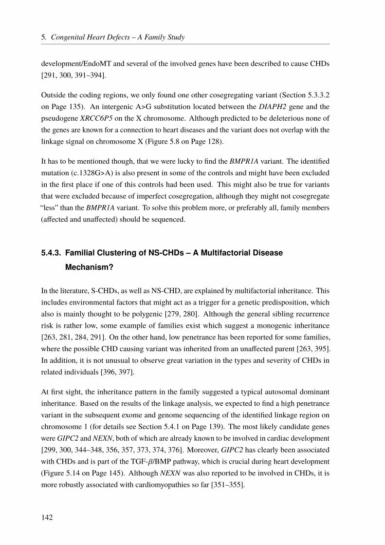
5. Congenital Heart Defects – A Family Study
development/EndoMT and several of the involved genes have been described to cause CHDs[291, 300, 391–394].
Outside the coding regions, we only found one other cosegregating variant (Section 5.3.3.2on Page 135). An intergenic A>G substitution located between the DIAPH2 gene and thepseudogene XRCC6P5 on the X chromosome. Although predicted to be deleterious none ofthe genes are known for a connection to heart diseases and the variant does not overlap with thelinkage signal on chromosome X (Figure 5.8 on Page 128).
It has to be mentioned though, that we were lucky to find the BMPR1A variant. The identifiedmutation (c.1328G>A) is also present in some of the controls and might have been excludedin the first place if one of this controls had been used. This might also be true for variantsthat were excluded because of imperfect cosegregation, although they might not cosegregate“less” than the BMPR1A variant. To solve this problem more, or preferably all, family members(affected and unaffected) should be sequenced.
5.4.3. Familial Clustering of NS-CHDs – A Multifactorial Disease
Mechanism?
In the literature, S-CHDs, as well as NS-CHD, are explained by multifactorial inheritance. Thisincludes environmental factors that might act as a trigger for a genetic predisposition, whichalso is mainly thought to be polygenic [279, 280]. Although the general sibling recurrencerisk is rather low, some example of families exist which suggest a monogenic inheritance[263, 281, 284, 291]. On the other hand, low penetrance has been reported for some families,where the possible CHD causing variant was inherited from an unaffected parent [263, 395].In addition, it is not unusual to observe great variation in the types and severity of CHDs inrelated individuals [396, 397].
At first sight, the inheritance pattern in the family suggested a typical autosomal dominantinheritance. Based on the results of the linkage analysis, we expected to find a high penetrancevariant in the subsequent exome and genome sequencing of the identified linkage region onchromosome 1 (for details see Section 5.4.1 on Page 139). The most likely candidate geneswere GIPC2 and NEXN, both of which are already known to be involved in cardiac development[299, 300, 344–348, 356, 357, 373, 374, 376]. Moreover, GIPC2 has clearly been associatedwith CHDs and is part of the TGF-β/BMP pathway, which is crucial during heart development(Figure 5.14 on Page 145). Although NEXN was also reported to be involved in CHDs, it ismore robustly associated with cardiomyopathies so far [351–355].
142
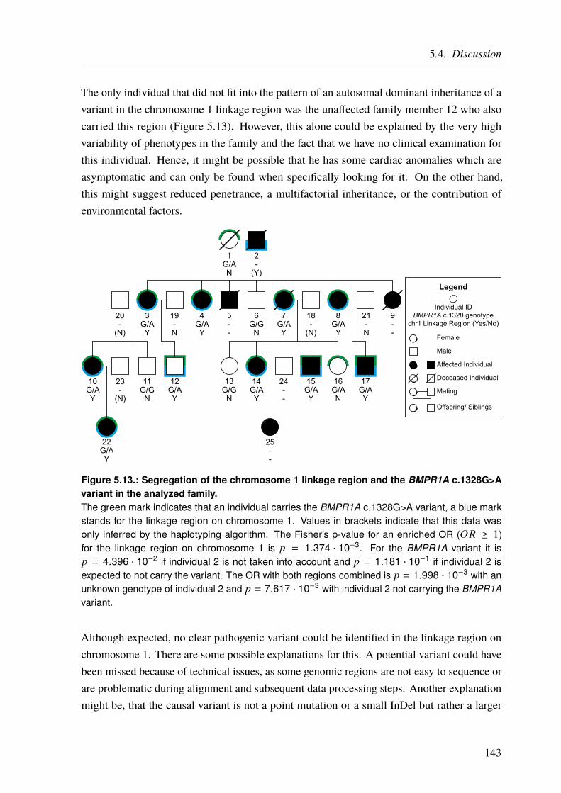
5.4. Discussion
The only individual that did not fit into the pattern of an autosomal dominant inheritance of avariant in the chromosome 1 linkage region was the unaffected family member 12 who alsocarried this region (Figure 5.13). However, this alone could be explained by the very highvariability of phenotypes in the family and the fact that we have no clinical examination forthis individual. Hence, it might be possible that he has some cardiac anomalies which areasymptomatic and can only be found when specifically looking for it. On the other hand,this might suggest reduced penetrance, a multifactorial inheritance, or the contribution ofenvironmental factors.
1G/AN
2-
(Y)
20-
(N)
3G/AY
19-N
4G/AY
5--
6G/G
N
18-
(N)
7G/AY
21-N
8G/AY
9--
10G/AY
11G/G
N
12G/AY
13G/G
N
14G/AY
15G/AY
16G/AN
17G/AY
22G/AY
23-
(N)
24--
25--
Female
Male
Affected Individual
Deceased Individual
Mating
Offspring/ Siblings
Individual IDBMPR1A c.1328 genotype
chr1 Linkage Region (Yes/No)
Legend
Figure 5.13.: Segregation of the chromosome 1 linkage region and the BMPR1A c.1328G>Avariant in the analyzed family.The green mark indicates that an individual carries the BMPR1A c.1328G>A variant, a blue markstands for the linkage region on chromosome 1. Values in brackets indicate that this data wasonly inferred by the haplotyping algorithm. The Fisher’s p-value for an enriched OR (OR ≥ 1)for the linkage region on chromosome 1 is p = 1.374 · 10−3. For the BMPR1A variant it isp = 4.396 · 10−2 if individual 2 is not taken into account and p = 1.181 · 10−1 if individual 2 isexpected to not carry the variant. The OR with both regions combined is p = 1.998 · 10−3 with anunknown genotype of individual 2 and p = 7.617 · 10−3 with individual 2 not carrying the BMPR1Avariant.
Although expected, no clear pathogenic variant could be identified in the linkage region onchromosome 1. There are some possible explanations for this. A potential variant could havebeen missed because of technical issues, as some genomic regions are not easy to sequence orare problematic during alignment and subsequent data processing steps. Another explanationmight be, that the causal variant is not a point mutation or a small InDel but rather a larger
143
5. Congenital Heart Defects – A Family Study
structural change in the DNA. Although we performed a CNV analysis and found no results thisis still possible as only specific markers were tested. To identify such structural changes, it wouldbe necessary to perform either cytogenetic scans or to use up-to-date genome sequencing data.The available sequencing data for this family comes from different sequencing approaches atdifferent time points and the coverage and uniformity does not allow to perform this analysis.
However, a variant with a strong cosegregation was found in the BMPR1A gene on chromosome10 (hg19 genomic position: chr10:g.88681438G>A). This variant leads to an AA-change(NM_004329.2:c.1328G>A(p.(R443H))) and is predicted to be deleterious by all used functionalprediction scores (see Section 5.4.2 on Page 140 for details). Although subsequent validationsin other family members revealed that the cosegregation of the BMPR1A variant with the diseaseis not perfect (Section 5.4.2 on Page 140), BMPR1A is a very likely candidate gene in this family.It plays an important role in the TGF-β/BMP pathway (Figure 5.14) [291, 300, 391–394].The same pathway in which also GIPC2 and NEXN in the chromosome 1 linkage region areinvolved, and through which its role in CHDs is explained. Moreover, BMPR1A has been linkedto CHDs directly, although most often in conjunction with other diseases (see Section 5.4.2 onPage 140) [383–390].
Although neither the chromosome 1 locus nor the variant in the BMPR1A gene show perfectcosegregation, both loci could contribute to the disease in a multifactorial manner. They areeven connected through the TGF-β/BMP pathway which is known to be involved in cardiacdevelopment, amongst a plethora of other functions. Multiple variants that influence thispathway also provide a possible explanation for the reduced penetrance in this family. TheBMPR1A variant and the linkage region are most likely inherited independently through theindividuals 1 and 2. Hence, the TGF-β/BMP pathway might be affected slightly different inevery individual. In addition, other loci like the ones with weaker linkage signals (Figure 5.8 onPage 128) or environmental factors could play a role in the family. However, the chromosome 1locus, the BMPR1A variant, and the TGF-β/BMP pathway are most likely key players in thedisease etiology of this family. The TGF-β/BMP pathway is briefly explained below and inFigure 5.14.
5.4.3.1. The TGF beta and BMP Signaling Pathway
Besides many other cellular mechanisms, the TGF-β/BMP pathway has been reported to beinvolved in cardiac development before and might also play a central role in the etiology ofCHDs in the described family (see above). A simplified version of this signaling pathway isshown in Figure 5.14 and will be briefly explained in the following.
144

5.4. Discussion
BMP2BMP2
TGFBR2
TGFBR1
TGFβ
TGFBR3 P P
BMPR2
ACVRL1
P ACVR1/BMPR1A/BMPR1B
SMAD phosphorylation
Nucleus
Transcriptionregulation GATA 4
NEXN
TGFβ
GIPC
Figure 5.14.: Simplified TGF-beta/BMP signaling pathwayTGF-β or BMP superfamily ligands bind to type II receptors (TGFBR2 or BMPR2), which recruitand phosphorylate type I receptors (TGFBR1, ACVRL1, ACVR1, BMPR1A, or BMPR1B). Thesereceptors then phosphorylate intracellular TFs (SMADs) which migrate to the nucleus and influencegene expression. The SMADs can also activate the TF GATA4 first, which can be inhibited by theNexilin protein (NEXN). The type III receptor TGFBR3 is not directly involved in the signaling butbinds TGF-βs and presents them to the type II receptor. The expression of TGFBR3 is regulatedby proteins of the GIPC family. Arrows indicate activation, blunt ends inhibition. Dotted lines standfor more complex steps, and not necessarily a direct interaction. Detailed information can be foundin the text. Based on Kruithof et al. [300], Blobe et al. [348], Monzen et al. [375], Gaussin et al.[391], Hill et al. [398], Hyun and Lavulo [399], Guo and Wang [400].
The first step is the binding of extracellular ligands, from the TGF-β or the BMP superfamilyto membrane-bound homodimers of type II receptors (TGFBR2 or BMPR2) [300, 348, 399].These homodimers recruit another homodimer which consists of type I receptors (TGFBR1,ACVRL1, ACVR1, BMPR1A, or BMPR1B) [401]. Together they form a heterotetramer. Inaddition, the type I receptor dimer is phosphorylated by the type II receptor. This leads to thephosphorylation of several intracellular SMAD proteins, which migrate into the nucleus andact as transcription factors (TFs). Alternatively, the SMAD can activate another nuclear TF,GATA4 [375]. One protein that has been shown to inhibit GATA4 is Nexilin, encoded by theNEXN gene [356]. Besides type I and type II receptors, a type III receptor (TGFBR3) exists.
145
5. Congenital Heart Defects – A Family Study
Although it seems not be involved directly in the TGF-β signaling, it binds TGF-βs and presentsthem to the type II receptors [348]. In addition, proteins of the GIPC-family were found tobind the cytoplasmatic domain of the type III receptor, regulating its expression [398, 399].Increased expression of the TGF-β receptor 3 subsequently enhances cellular responsiveness toTGF-β [344, 345, 348].
Based on the findings in this family, we wanted to take a closer look at this pathway inunrelated CHD patients. Therefore we performed a panel sequencing of selected genes fromthe TGF-β/BMP pathway, which is described in the next chapter (5.4.4).
5.4.4. Panel Sequencing of TGF beta and BMP Signaling Pathway Genes in
an AVSD Cohort
Based on our results from the linkage analysis and the sequencing studies in the family, as wellas reports in the literature, the TGF-β/BMP pathway is most likely to play a central role inthe disease etiology in this family. Hence, we decided to perform a panel sequencing studyof selected genes involved in this pathway in unrelated patients with a clear CHD phenotype.There were two main aims of this study. On the one hand, we wanted to see if there is anyenrichment of potential pathogenic variants in the sequenced pathway genes. On the otherhand, we wanted to identify additional patients which carry variants in these pathway genes(especially BMPR1A) and also have a familial background of CHDs.
We sequenced 62 AVSD patients with no reported extracardiac anomalies, 32 AVSD patientswhich also suffered from Trisomy 21 (Down syndrome (DS); S-CHD), and 32 healthy controls.We selected eight genes, which play a central role in the TGF-β/BMP pathway (see Table 5.3on Page 124). Five genes encode type I receptors (ACVR1, ACVRL1, BMPR1A, BMPR1B,TGFBR1), one gene a type II receptor (BMPR2), one gene a type III receptor (TGFBR3), andone gene the main ligand of the BMP pathway BMP2. All of these genes/proteins are shown inFigure 5.14.
Although DNA samples were available for some more samples we stopped the panel at thispoint as it became clear that there was most likely no clear enrichment of variants or that atleast our sample size would not be sufficient to detect it. Three variants were found in the 62AVSD samples (4.84%), seven in the 32 AVSD+DS samples (21.88%), and three in the 32controls (9.38%) (Table 5.6 on Page 138). There is no significant enrichment in the AVSDcases (Fisher’s p = 0.41), nor in the AVSD+DS cases (Fisher’s p = 0.30) when compared tothe controls.
146
5.4. Discussion
These results are not unexpected, as we only sequenced some of the genes involved in theTGF-β/BMP pathway and it is most likely that this pathway only plays a role in a small subsetof all CHDs cases. In addition, structural DNA changes are known to play a huge role in CHD,but they are not covered in our analysis. Moreover, most of the cases, especially the sporadicones, might be explained by a multifactorial inheritance with low penetrance variants, whichmight also be more common. On top, environmental factors will play a role in some of thepatients.
However, the families of the patients with identified variants will be examined in collaborationwith the group of Prof. Dr. Schunkert at the “Deutsches Herzzentrum München” in Munich,which also supplied us with the DNA samples.
5.4.5. Conclusion and Future Perspective of the Family Study
Despite lack of evidence, it might be possible that an undetected (structural) variant in thechromosome 1 linkage region is the causal one in the described family. Apart from individual12, this could fit an autosomal dominant inheritance pattern. On the other hand, a multifactorialinheritance with a major contribution of the chromosome 1 region and the BMPR1A variantcould explain the phenotypic variability in the family, perhaps in conjunction with environmentalfactors. Especially given the fact that both loci can be robustly linked to CHD through theTGF-β/BMP pathway. In this case, the pedigree would resemble a multifactorial inheritancelike it is most often described for CHD. In addition, we cannot exclude the possibility that evenmore genomic loci contribute to the observed phenotypes in the family. Candidate regionsare the nonsignificant linkage signals on chromosome 2, 4, and X, as the LOD score for theBMPR1A locus on chromosome 10 in the same range.
We were not able to identify a genetic variant underlying the disease in this family, but ourresults suggest potential mechanisms that play a role in the disease development. With the vastmajority of our results pointing towards a multifactorial cause it might be impossible to identifyone, or few, causal variants in this family. It might still be possible to shed some more light onthe underlying mechanisms if more patients and controls in this family would be examined,both clinically as well as genetically. More WGS data would allow to reduce the number ofvariants solely based on cosegregation without the need of possible too stringent subsequentfiltering steps. In addition, variants with reduced penetrance could be identified by allowingvariants to be present also in a subset of the controls, or to be absent in some cases.
Based on our findings, it is a sound strategy to take a closer look at the TGF-β/BMP pathway,the genes in the linkage region, and the BMPR1A first. We already started this a the panel
147

5. Congenital Heart Defects – A Family Study
sequencing of unrelated AVSD patients and the subsequent analysis of the patient’s families(ongoing). In addition, our group performed functional studies in Zebrafish (Danio rerio)[402], to investigate the functional consequences of the BMPR1A c.1328G>A mutation and thepossible connection to the chromosome 1 region. This work, however, only represents a firstapproach and further functional studies would be needed to link this two regions.
148

6. General Conclusion and Perspective
Es hängt alles irgendwo zusammen. Wenn man sich am Hintern ein Haar ausreißt, dann träntdas Auge.∗
– Dettmar Cramer
The results of the different projects presented in this thesis demonstrate how complex thegenetic mechanisms underlying traits really are and what challenges have to be overcome tounravel the molecular functions underlying the full spectrum from monogenic to complexgenetic diseases.
Although modern sequencing techniques make it easy to access the genetic variability, it isnot always straightforward to identify the causal variant(s), even in a family with an apparentmonogenic inheritance pattern. An example of such a family with severe clustering of CHDscan be found in Chapter 5 on Page 103. Although different techniques were used to examinethe family, we could not identify the causal variant. Indeed, the inheritance pattern showed tobe more complex with presumably at least two genomic loci contributing to the disease risk.Both loci were linked to the TGF-β/BMP pathway, suggesting the potential pathomechanism.However, failing to identify the expected one causal variant in a seemingly monogenic disorderis not uncommon. In fact, other studies reported that less than 50% of Mendelian disordersare resolved by sequencing the affected families [403]. One potential explanation for thesurprisingly low success is that not all “monogenic” diseases are monogenic but rather causedby the interaction of several genetic factors.
Not only monogenic diseases surprise us with unexpected complexity. Even for complexdiseases, the term “complex” appears to be a euphemism from time to time. Although we wereable to link lots of CAD loci identified by GWAS to genes based on functional data and evenassign 97 genes not known to be involved in CAD before, we are still lacking gene assignmentfor 87 out of the 159 examined CAD loci (see Chapter 3 on Page 59). As our study was mainlyfocused on AA-changing SNPs and eQTLs we may have missed some functional links.
On the other hand, several loci could be functionally linked to multiple genes, implying verycomplex underlying mechanisms. Hence, the idea of the one causal gene per locus might beincorrect for most loci. A recently published study proposed the so-called “omnigenic” modeladdressing this phenomenon [190]. According to this model, “gene regulatory networks are
∗Everything is connected somewhere. If you pull a hair out on the butt, then the eye waters.
149
6. General Conclusion and Perspective
sufficiently interconnected such that all genes expressed in disease-relevant cells are liable toaffect the functions of core disease-related genes” [190]. This hypothesis might also explainparts of the missing heritability, as a huge amount of variants has very subtle effects on genes byindirectly altering the core-disease genes. And by having low effect size, GWAS lack the powerto identify the associations. So far, only around 30 – 40% of the estimated CAD heritabilitycan be explained by the identified GWAS loci. However, one might argue how reasonableit is to perform GWAS with the immense sample sizes required to reach sufficient statisticalpower to detect these low-risk variants. Although they may explain an unknown fraction ofthe missing heritability, they will most likely not contribute to our understanding of the majordisease mechanisms and likewise provide no real targets for drug development, as the individualeffect sizes are too low and do not affect core-disease genes. However, they are necessary tounderstand the whole picture and may be crucial to predict the individual disease risk.
Parts of the missing heritability might also be explained by the sum of rare variants believed tohave substantial effect sizes. These variants cannot be detected by GWAS because of their lowfrequency and hence, other approaches, like the one described in Chapter 4 on Page 91, areneeded [404].
Whether we try to identify the causal variants and their underlying effects in monogenic orcomplex diseases, we need to collect evidence for the functional implications. However, thereare multiple molecular functions that are disturbed by genetic variation but not all of them canbe annotated with the current knowledge or available data. In addition, it is most likely thatthere are factors that we do not even know off today.
One example is reduced penetrance or variable expressivity. If a variant has a reduced penetrance,not all individuals who carry this variant show the corresponding phenotype, e.g., symptomsof a disease. Likewise, variable expressivity leads to variable phenotypes, e.g., symptomsdiffer among affected individuals. Possible reasons for these effects are environmental factors,gene-environment interactions, genetic modifiers, or just undetected additional variants thatnot always cosegregate with the identified variant [405]. These variants are hard to detect,especially when using statistical approaches like GWAS or linkage analysis.
Genetic mosaicism is another example. Here, different cells of the body have different genotypes,mainly due to mutations during embryogenesis. Hence, genetic variants cannot be detected ifthe DNA is isolated from the “wrong” cells, and even if the “right” ones are selected, a highsequencing depth is often required [406].
Similarly, there are variants that have tissue-specific effects. Some genes, for example, arenot ubiquitously expressed and some variants in regulatory regions, for instance, only alter
150
6. General Conclusion and Perspective
expression in one tissue. Here it is important to make sure that the tissue of action is alsodisease-relevant (see Chapter 3). Tissue specificity is not only limited to regulatory variants.Splice isoforms can be tissue-specific as well and hence, a candidate variant might not be locatedin the final transcript. Moreover, variants can have different effects in different transcripts ofthe same gene, or can even be located in multiple overlapping genes.
Another challenge when annotating or assessing variants is incomplete data. Although ourunderstanding of genetic mechanisms has improved over the last decades and scientists havegathered lots of associated data, it is still far from complete. Hence, we might miss somefunctional links or candidate variants. One example are eQTL studies which test tissue-specificexpression changes. Although eQTL analyses have been performed for multiple tissues, the datafor some disease-relevant tissues is often not available, especially for tissues that are difficult toaccess (see Chapter 3). Likewise, projects like ENCODE provided invaluable insights into thefunctional implications of noncoding, often regulatory variants. However, we still need moredata on binding sites, TFs, or cell types to use them for annotation.
Large-scale sequencing studies, like ExAC/gnomAD, revealed that some previously disease-causing labeled variants are more frequent than expected and hence, their effect size is mostlikely lower than predicted (see Figure 1.2 on Page 6). To make matters worse, variantfrequencies differ amongst populations. Hence, population-specific data is needed, not onlybecause of different variant frequencies but also because phenotypic effects of variants candiffer, depending on the genetic background [407].
We are not only limited by incomplete data, but also by an incomplete understanding ofthe genetic mechanisms. This is, for example, true for synonymous variants that alter thecoding sequence in a protein-coding gene without changing the AA sequence. These variantswere shown to have similar effects as AA-changing variants and are mediated by two mainmechanisms [199, 200]. The first is the dual function of the DNA, as exonic regions might notonly code for proteins but can also have regulatory functions such as forming binding sites forTFs [408]. The second involves codon usage bias and the degeneration of the genetic code.There are more codon combinations (nucleotide triplets; 43 = 64) than canonical proteinogenicAAs and hence, some triplets encode the same AA. But not all codons are used at equalfrequencies across species (codon usage bias), suggesting an effect on transcription or othermechanisms. Synonymous variants can have an effect on AA-synthesis leading to a differentfolding of the protein, as they might slow down transcription/translation [199]. Although someprediction tools take synonymous variants into account, the functional relevance is mainlybased on the conservation or localization in known regulatory sites. To really assess their
151
6. General Conclusion and Perspective
implications in human disease we need a more profound understanding of how these variantsaffect molecular mechanisms.
The same is true for the field of epigenetics which deals with altered genetic informationwithout changes in the DNA sequence. This includes, for example, histone modificationsby methylation, phosphorylation, or acetylation, which influences the DNA accessibility at alocus. Hence, epigenetic defects usually alter the gene expression [409]. Off note, epigeneticmodifications are known to be heavily influenced by environmental factors. Although a lot ofdiseases have already been linked to epigenetic defects, we are only scratching the surface.
Despite all these pitfalls, over the last decades NGS sequencing studies and GWAS haveidentified many disease-causing variants and the underlying mechanisms, both for monogenicand complex diseases [3, 28, 196, 264, 410–412]. These variants enable personalized riskpredictions and treatments, and some have led to the development of new drugs [106, 413].One example are PCSK9 inhibitors, which mimic inactivating mutations in the correspondinggene. Mutations in PCSK9 were associated with decreased LDL cholesterol levels and thereforereduced risk of CAD [3, 414, 415]. However, these findings only represent the tip of the icebergand it is most likely that variants and mechanisms that could not be unraveled so far, are evenmore complex and need new techniques and additional knowledge to be assessed.
To maximize the success rate in future genetic studies, we need to: (1) perform more basicresearch to get a better general understanding of the molecular mechanisms in genetic diseases;(2) generate more (population-specific) sequencing data to get insight into general geneticvariability, especially on the population-level; (3) better integrate other “OMICS” data sets,like expression data, into our often heavily sequencing-based workflows; (4) further utilizecomputational approaches to unravel the contribution of gene networks and pathways instead ofsingle genes; (5) optimize the study design by selecting the right individuals in families andlarge cohorts, paying attention to environmental factors, and choosing the optimal tools to studythe selected individual(s) (see Section 1.3.1 on Page 5).
These tasks will again be facilitated by further improved sequencing techniques. Not only willreduced cost allow to sequence more individuals, but, in addition, new tools like single-moleculesequencing will make sequencing faster, easier, and more powerful. For example, the very longreads that are generated need less computational power for alignment. At the same time, longreads make it possible to detect structural variants that are hard or impossible to detect withshort reads. Moreover, these techniques can detect epigenetic modifications directly duringsequencing [416].
152
6. General Conclusion and Perspective
Even with the robust prediction of high-impact genetic defects, we can be wrong. A recentstudy reported that complete KOs of genes that were thought to be essential, sometimes show nophenotypic effects [39]. This illustrates that predictions are never sufficient without functionalvalidation.
Ultimately, we need to validate all hypotheses in the lab by functional assays. As we cannot testall potential variants in the lab, it is crucial to start with solid hypotheses about which variantsare most likely causal, what their function may be, and which tissue/cell type should be studied.Starting with the wrong assumptions does not only waste time and money, but might also leadto a dead end and eventually the causal variant might be identified as false positive because thewrong functional studies were performed. Hence, computational approaches and functionalanalyses go hand in hand and can be based on each other, the one way or the other.
153


A. Appendix
A.1. Functional Characterization of Coronary Artery Disease Loci Identified
by GWAS
Table A.1.: Known genome-wide significant CAD risk loci as of September 2017.Currently (September 2017), 99 genome-wide significant CAD loci have been identified by GWAS.CHR = CHR, EAF = effect allele frequency (and effect allele), OR = odds ratio.
CHR Position (hg19) SNP EAF OR Gene(s) at locus Reference
1
55 496 039 rs11206510 T (0.82) 1.08 PCSK9 123, 414, 415, 41756 962 821 rs17114036 A (0.91) 1.17 PPAP2B 137, 417109 822 166 rs599839 A (0.78) 1.11 SORT1, PSCR1, CELSR2 111, 137, 417151 762 308 rs11810571 G (0.79) 1.07 TDRKH, RP11-98D18.9 119, 122
154 422 067 rs4845625 T (0.47) 1.06 IL6R, AQP10, ATP8B2, CHTOP,UBAP2L 116
169 094 459 rs1892094 C (0.50) 1.04 ATP1B1, BLZF1, CCDC181, F5,NME7, SELP, SLC19A2 120
200 646 073 rs6700559 C (0.53) 1.04 DDX59, CAMSAP2, KIF14 120
201 872 264 rs2820315 T (0.30) 1.05 LMOD1, IPO9, NAV1, SHISA4,TIMM17A 120
222 823 529 rs17465637 C (0.74) 1.14 MIA3, AIDA, C1orf58 111, 137
2
21 286 057 rs515135 G (0.83) 1.07 APOB 116, 41744 073 881 rs6544713 T (0.30) 1.06 ABCG5, ABCG8 126, 137, 41785 809 989 rs1561198 A (0.45) 1.06 VAMP5, VAMP8, GGCX 116145 801 461 rs2252641 G (0.46) 1.06 ZEB2, TEX41 116
203 745 885 rs6725887 C (0.15) 1.14 WDR12, CARF, FAM117B,ICA1L, NBEAL1 123, 137
216 304 384 rs1250229 T (0.26) 1.07 FN1, ATIC, LOC102724849,ABCA12, LINC00607 119, 121
218 683 154 rs2571445 A (0.39) 1.04 TNS1, CXCR2, RUFY4 120227 100 698 rs2972146 T (0.65) 1.07 LOC646736, IRS1, MIR5702 121233 633 460 rs1801251 A (0.35) 1.05 KCNJ13, GIGYF2 418
3
14 928 077 rs748431 G (0.36) 1.04 FGD5 121
49 448 566 rs7623687 A (0.86) 1.07 RHOA, AMT, TCTA, CDHRA,KLHDC8B 119–122
124 475 201 rs142695226 G (0.14) 1.08 UMPS, ITGB5 119, 121, 122138 119 952 rs2306374 C (0.18) 1.12 MRAS, CEP70 124, 137153 839 866 rs12493885 C (0.85) 1.07 ARHGEF26 119, 121, 122
continued on next page
155
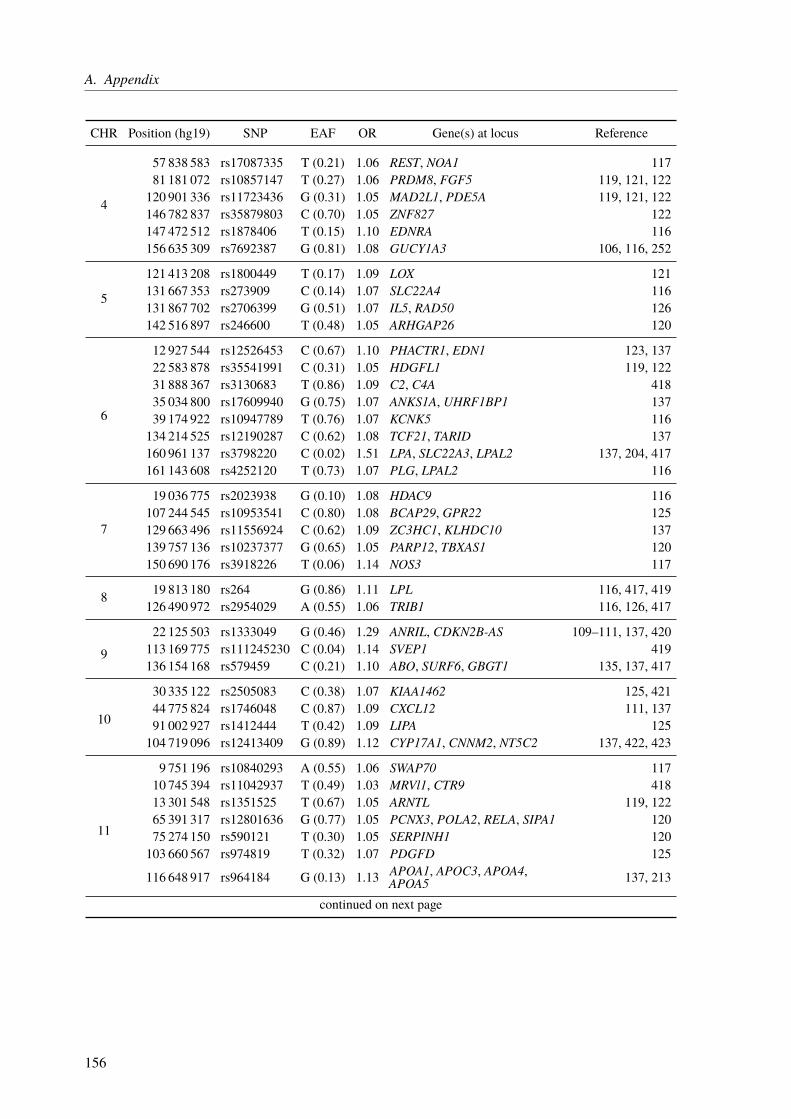
A. Appendix
CHR Position (hg19) SNP EAF OR Gene(s) at locus Reference
4
57 838 583 rs17087335 T (0.21) 1.06 REST, NOA1 11781 181 072 rs10857147 T (0.27) 1.06 PRDM8, FGF5 119, 121, 122120 901 336 rs11723436 G (0.31) 1.05 MAD2L1, PDE5A 119, 121, 122146 782 837 rs35879803 C (0.70) 1.05 ZNF827 122147 472 512 rs1878406 T (0.15) 1.10 EDNRA 116156 635 309 rs7692387 G (0.81) 1.08 GUCY1A3 106, 116, 252
5
121 413 208 rs1800449 T (0.17) 1.09 LOX 121131 667 353 rs273909 C (0.14) 1.07 SLC22A4 116131 867 702 rs2706399 G (0.51) 1.07 IL5, RAD50 126142 516 897 rs246600 T (0.48) 1.05 ARHGAP26 120
6
12 927 544 rs12526453 C (0.67) 1.10 PHACTR1, EDN1 123, 13722 583 878 rs35541991 C (0.31) 1.05 HDGFL1 119, 12231 888 367 rs3130683 T (0.86) 1.09 C2, C4A 41835 034 800 rs17609940 G (0.75) 1.07 ANKS1A, UHRF1BP1 13739 174 922 rs10947789 T (0.76) 1.07 KCNK5 116134 214 525 rs12190287 C (0.62) 1.08 TCF21, TARID 137160 961 137 rs3798220 C (0.02) 1.51 LPA, SLC22A3, LPAL2 137, 204, 417161 143 608 rs4252120 T (0.73) 1.07 PLG, LPAL2 116
7
19 036 775 rs2023938 G (0.10) 1.08 HDAC9 116107 244 545 rs10953541 C (0.80) 1.08 BCAP29, GPR22 125129 663 496 rs11556924 C (0.62) 1.09 ZC3HC1, KLHDC10 137139 757 136 rs10237377 G (0.65) 1.05 PARP12, TBXAS1 120150 690 176 rs3918226 T (0.06) 1.14 NOS3 117
8 19 813 180 rs264 G (0.86) 1.11 LPL 116, 417, 419126 490 972 rs2954029 A (0.55) 1.06 TRIB1 116, 126, 417
9
22 125 503 rs1333049 G (0.46) 1.29 ANRIL, CDKN2B-AS 109–111, 137, 420113 169 775 rs111245230 C (0.04) 1.14 SVEP1 419136 154 168 rs579459 C (0.21) 1.10 ABO, SURF6, GBGT1 135, 137, 417
10
30 335 122 rs2505083 C (0.38) 1.07 KIAA1462 125, 42144 775 824 rs1746048 C (0.87) 1.09 CXCL12 111, 13791 002 927 rs1412444 T (0.42) 1.09 LIPA 125104 719 096 rs12413409 G (0.89) 1.12 CYP17A1, CNNM2, NT5C2 137, 422, 423
11
9 751 196 rs10840293 A (0.55) 1.06 SWAP70 11710 745 394 rs11042937 T (0.49) 1.03 MRVl1, CTR9 41813 301 548 rs1351525 T (0.67) 1.05 ARNTL 119, 12265 391 317 rs12801636 G (0.77) 1.05 PCNX3, POLA2, RELA, SIPA1 12075 274 150 rs590121 T (0.30) 1.05 SERPINH1 120103 660 567 rs974819 T (0.32) 1.07 PDGFD 125
116 648 917 rs964184 G (0.13) 1.13 APOA1, APOC3, APOA4,APOA5 137, 213
continued on next page
156
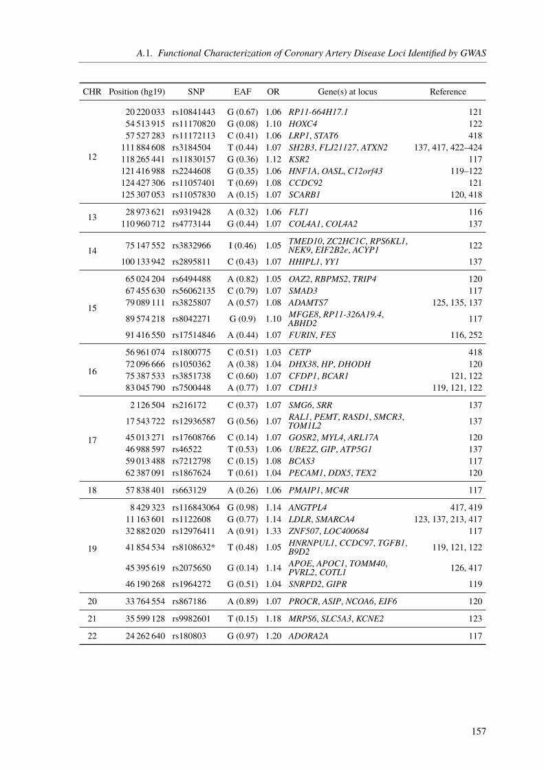
A.1. Functional Characterization of Coronary Artery Disease Loci Identified by GWAS
CHR Position (hg19) SNP EAF OR Gene(s) at locus Reference
12
20 220 033 rs10841443 G (0.67) 1.06 RP11-664H17.1 12154 513 915 rs11170820 G (0.08) 1.10 HOXC4 12257 527 283 rs11172113 C (0.41) 1.06 LRP1, STAT6 418111 884 608 rs3184504 T (0.44) 1.07 SH2B3, FLJ21127, ATXN2 137, 417, 422–424118 265 441 rs11830157 G (0.36) 1.12 KSR2 117121 416 988 rs2244608 G (0.35) 1.06 HNF1A, OASL, C12orf43 119–122124 427 306 rs11057401 T (0.69) 1.08 CCDC92 121125 307 053 rs11057830 A (0.15) 1.07 SCARB1 120, 418
13 28 973 621 rs9319428 A (0.32) 1.06 FLT1 116110 960 712 rs4773144 G (0.44) 1.07 COL4A1, COL4A2 137
14 75 147 552 rs3832966 I (0.46) 1.05 TMED10, ZC2HC1C, RPS6KL1,NEK9, EIF2B2e, ACYP1 122
100 133 942 rs2895811 C (0.43) 1.07 HHIPL1, YY1 137
15
65 024 204 rs6494488 A (0.82) 1.05 OAZ2, RBPMS2, TRIP4 12067 455 630 rs56062135 C (0.79) 1.07 SMAD3 11779 089 111 rs3825807 A (0.57) 1.08 ADAMTS7 125, 135, 137
89 574 218 rs8042271 G (0.9) 1.10 MFGE8, RP11-326A19.4,ABHD2 117
91 416 550 rs17514846 A (0.44) 1.07 FURIN, FES 116, 252
16
56 961 074 rs1800775 C (0.51) 1.03 CETP 41872 096 666 rs1050362 A (0.38) 1.04 DHX38, HP, DHODH 12075 387 533 rs3851738 C (0.60) 1.07 CFDP1, BCAR1 121, 12283 045 790 rs7500448 A (0.77) 1.07 CDH13 119, 121, 122
17
2 126 504 rs216172 C (0.37) 1.07 SMG6, SRR 137
17 543 722 rs12936587 G (0.56) 1.07 RAL1, PEMT, RASD1, SMCR3,TOM1L2 137
45 013 271 rs17608766 C (0.14) 1.07 GOSR2, MYL4, ARL17A 12046 988 597 rs46522 T (0.53) 1.06 UBE2Z, GIP, ATP5G1 13759 013 488 rs7212798 C (0.15) 1.08 BCAS3 11762 387 091 rs1867624 T (0.61) 1.04 PECAM1, DDX5, TEX2 120
18 57 838 401 rs663129 A (0.26) 1.06 PMAIP1, MC4R 117
19
8 429 323 rs116843064 G (0.98) 1.14 ANGTPL4 417, 41911 163 601 rs1122608 G (0.77) 1.14 LDLR, SMARCA4 123, 137, 213, 41732 882 020 rs12976411 A (0.91) 1.33 ZNF507, LOC400684 117
41 854 534 rs8108632* T (0.48) 1.05 HNRNPUL1, CCDC97, TGFB1,B9D2 119, 121, 122
45 395 619 rs2075650 G (0.14) 1.14 APOE, APOC1, TOMM40,PVRL2, COTL1 126, 417
46 190 268 rs1964272 G (0.51) 1.04 SNRPD2, GIPR 119
20 33 764 554 rs867186 A (0.89) 1.07 PROCR, ASIP, NCOA6, EIF6 120
21 35 599 128 rs9982601 T (0.15) 1.18 MRPS6, SLC5A3, KCNE2 123
22 24 262 640 rs180803 G (0.97) 1.20 ADORA2A 117
157
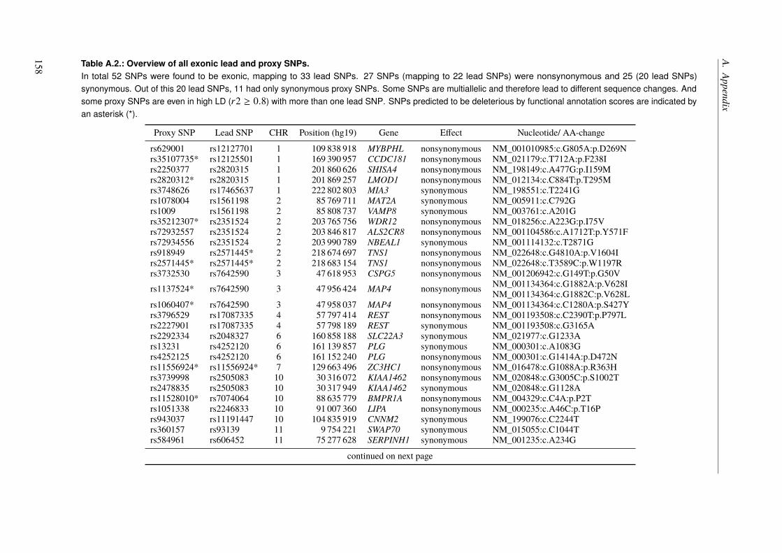
A.Appendix
Table A.2.: Overview of all exonic lead and proxy SNPs.In total 52 SNPs were found to be exonic, mapping to 33 lead SNPs. 27 SNPs (mapping to 22 lead SNPs) were nonsynonymous and 25 (20 lead SNPs)synonymous. Out of this 20 lead SNPs, 11 had only synonymous proxy SNPs. Some SNPs are multiallelic and therefore lead to different sequence changes. Andsome proxy SNPs are even in high LD (r2 ≥ 0.8) with more than one lead SNP. SNPs predicted to be deleterious by functional annotation scores are indicated byan asterisk (*).
Proxy SNP Lead SNP CHR Position (hg19) Gene Effect Nucleotide/ AA-change
rs629001 rs12127701 1 109 838 918 MYBPHL nonsynonymous NM_001010985:c.G805A:p.D269Nrs35107735* rs12125501 1 169 390 957 CCDC181 nonsynonymous NM_021179:c.T712A:p.F238Irs2250377 rs2820315 1 201 860 626 SHISA4 nonsynonymous NM_198149:c.A477G:p.I159Mrs2820312* rs2820315 1 201 869 257 LMOD1 nonsynonymous NM_012134:c.C884T:p.T295Mrs3748626 rs17465637 1 222 802 803 MIA3 synonymous NM_198551:c.T2241Grs1078004 rs1561198 2 85 769 711 MAT2A synonymous NM_005911:c.C792Grs1009 rs1561198 2 85 808 737 VAMP8 synonymous NM_003761:c.A201Grs35212307* rs2351524 2 203 765 756 WDR12 nonsynonymous NM_018256:c.A223G:p.I75Vrs72932557 rs2351524 2 203 846 817 ALS2CR8 nonsynonymous NM_001104586:c.A1712T:p.Y571Frs72934556 rs2351524 2 203 990 789 NBEAL1 synonymous NM_001114132:c.T2871Grs918949 rs2571445* 2 218 674 697 TNS1 nonsynonymous NM_022648:c.G4810A:p.V1604Irs2571445* rs2571445* 2 218 683 154 TNS1 nonsynonymous NM_022648:c.T3589C:p.W1197Rrs3732530 rs7642590 3 47 618 953 CSPG5 nonsynonymous NM_001206942:c.G149T:p.G50Vrs1137524* rs7642590 3 47 956 424 MAP4 nonsynonymous NM_001134364:c.G1882A:p.V628I
NM_001134364:c.G1882C:p.V628Lrs1060407* rs7642590 3 47 958 037 MAP4 nonsynonymous NM_001134364:c.C1280A:p.S427Yrs3796529 rs17087335 4 57 797 414 REST nonsynonymous NM_001193508:c.C2390T:p.P797Lrs2227901 rs17087335 4 57 798 189 REST synonymous NM_001193508:c.G3165Ars2292334 rs2048327 6 160 858 188 SLC22A3 synonymous NM_021977:c.G1233Ars13231 rs4252120 6 161 139 857 PLG synonymous NM_000301:c.A1083Grs4252125 rs4252120 6 161 152 240 PLG nonsynonymous NM_000301:c.G1414A:p.D472Nrs11556924* rs11556924* 7 129 663 496 ZC3HC1 nonsynonymous NM_016478:c.G1088A:p.R363Hrs3739998 rs2505083 10 30 316 072 KIAA1462 nonsynonymous NM_020848:c.G3005C:p.S1002Trs2478835 rs2505083 10 30 317 949 KIAA1462 synonymous NM_020848:c.G1128Ars11528010* rs7074064 10 88 635 779 BMPR1A nonsynonymous NM_004329:c.C4A:p.P2Trs1051338 rs2246833 10 91 007 360 LIPA nonsynonymous NM_000235:c.A46C:p.T16Prs943037 rs11191447 10 104 835 919 CNNM2 synonymous NM_199076:c.C2244Trs360157 rs93139 11 9 754 221 SWAP70 synonymous NM_015055:c.C1044Trs584961 rs606452 11 75 277 628 SERPINH1 synonymous NM_001235:c.A234G
continued on next page
158

A.1.FunctionalC
haracterizationofC
oronaryArtery
Disease
LociIdentifiedby
GWAS
Proxy SNP Lead SNP CHR Position (hg19) Gene Effect Nucleotide/ AA-change
rs650241 rs590121 11 75 277 757 SERPINH1 synonymous NM_001235:c.C363Grs649257 rs590121 11 75 279 846 SERPINH1 synonymous NM_001235:c.C693Trs585821 rs590121 11 75 282 882 SERPINH1 synonymous NM_001235:c.G1011Ars3184504 rs3184504 12 111 884 608 SH2B3 nonsynonymous NM_005475:c.T784C:p.W262Rrs3752630 rs3809274 12 112 375 990 TMEM116 nonsynonymous NM_001193453:c.T235G:p.C79Grs1169288* rs2244608 12 121 416 650 HNF1A nonsynonymous NM_000545:c.A79C:p.I27Lrs7495616 rs11072794 15 79 054 900 ADAMTS7 nonsynonymous NM_014272:c.G4748C:p.G1583Ars3825807 rs1994016 15 79 089 111 ADAMTS7 nonsynonymous NM_014272:c.T640C:p.S214Prs3825807rs7173267 rs1994016 15 79 092 750 ADAMTS7 synonymous NM_014272:c.C240Grs3825807rs11539637 rs17514846 15 91 428 290 FES synonymous NM_001143783:c.C15G
NM_001143783:c.C15Trs749240 rs2281727 17 2 186 100 SMG6 synonymous NM_017575:c.G2502Ars216193 rs2281727 17 2 203 453 SMG6 synonymous NM_017575:c.T594Crs4368210 rs4299203 17 17 896 090 LRRC48 synonymous NM_001130092:c.C456Trs4584886* rs4299203 17 17 896 205 LRRC48 nonsynonymous NM_001130092:c.C571T:p.R191Wrs2955355 rs4299203 17 17 948 475 GID4 synonymous NM_024052:c.G453Ars2071167 rs2071167 17 42 287 519 UBTF synonymous NM_001076683:c.G1488Ars1058018 rs15563 17 47 000 251 UBE2Z synonymous NM_023079:c.C846Trs2291725 rs15563 17 47 039 132 GIP nonsynonymous NM_004123:c.A307G:p.S103Grs11556505 rs2075650 19 45 396 144 TOMM40 synonymous NM_001128917:c.C393Trs1132899 rs2288911 19 45 448 036 APOC4 nonsynonymous NM_001646:c.T107C:p.L36Prs11906160* rs867186* 20 33 565 755 MYH7B nonsynonymous NM_020884:c.G73A:p.A25Trs55734215 rs867186* 20 33 585 437 MYH7B synonymous NM_020884:c.C3867Trs80109502 rs867186* 20 33 587 596 MYH7B synonymous NM_020884:c.G4794Ars867186* rs867186* 20 33 764 554 PROCR nonsynonymous NM_006404:c.A655G:p.S219G
159

A. Appendix
Table A.3.: Comparison of gene assignment per CAD GWAS locus.Traditional assignment of genes to GWAS loci was based on proximity. Our functional data-driven pipelinechanges the gene assignment for multiple loci. Lead SNPs and previously annotated genes are based onDeloukas et al. [116] if not stated otherwise. Additional sources were Reilly et al. [135], Wang et al. [136],and Schunkert et al. [137]. A 4indicates if and how the annotation at a given locus has changed. Moreinformation can be found in Section 3.3.9 on Page 74.
Chrom
osom
e
Lead
SNP
cytoBand
Old
annotatio
n
New
annotatio
n
Identicalannotatio
n
Differentannotation
Less
genes
Additionalgenes
Inconsistentannotation
Noannotatio
n
1
rs11806316 p13.2 NGF - - - - - 4
rs12127701 p13.3 MYBPHL MYBPHL 4 - - - - -rs4268379 p13.3 SARS - - - - - 4
rs602633 p13.3 PSRC1, SORT1 CELSR2, PSRC1,SORT1 - - - 4 - -
rs7515901 p13.3 MYBPHL - - - - - 4
rs1490738 p22.2 PKN2 GTF2B - 4 - - - -rs17114036 p32.2 PPAP2B - - - - - 4
rs11206510 p32.3 PCSK9 - - - - - 4
rs10797416 p36.33 SKI FLJ42875 - 4 - - - -rs11204666 q21.3 MCL1 - - - - - 4
rs4845625 q21.3 IL6R ATP8B2, CHTOP, IL6R,UBAP2L - - - 4 - -
rs12125501 q24.2 NME7 ATP1B1, CCDC181,NME7 - - - 4 - -
rs2292096 q32.1 CAMSAP1L1 CAMSAP1L1 4 - - - - -
rs2820315 q32.1 LMOD1 IPO9, LMOD1,SHISA4 - - - 4 - -
rs6700559 q32.1 DDX59 CAMSAP1L1, DDX59,KIF14 - - - 4 - -
rs17465637 q41 MIA3 AIDA, C1orf58, MIA3 - - - 4 - -continued on next page
160
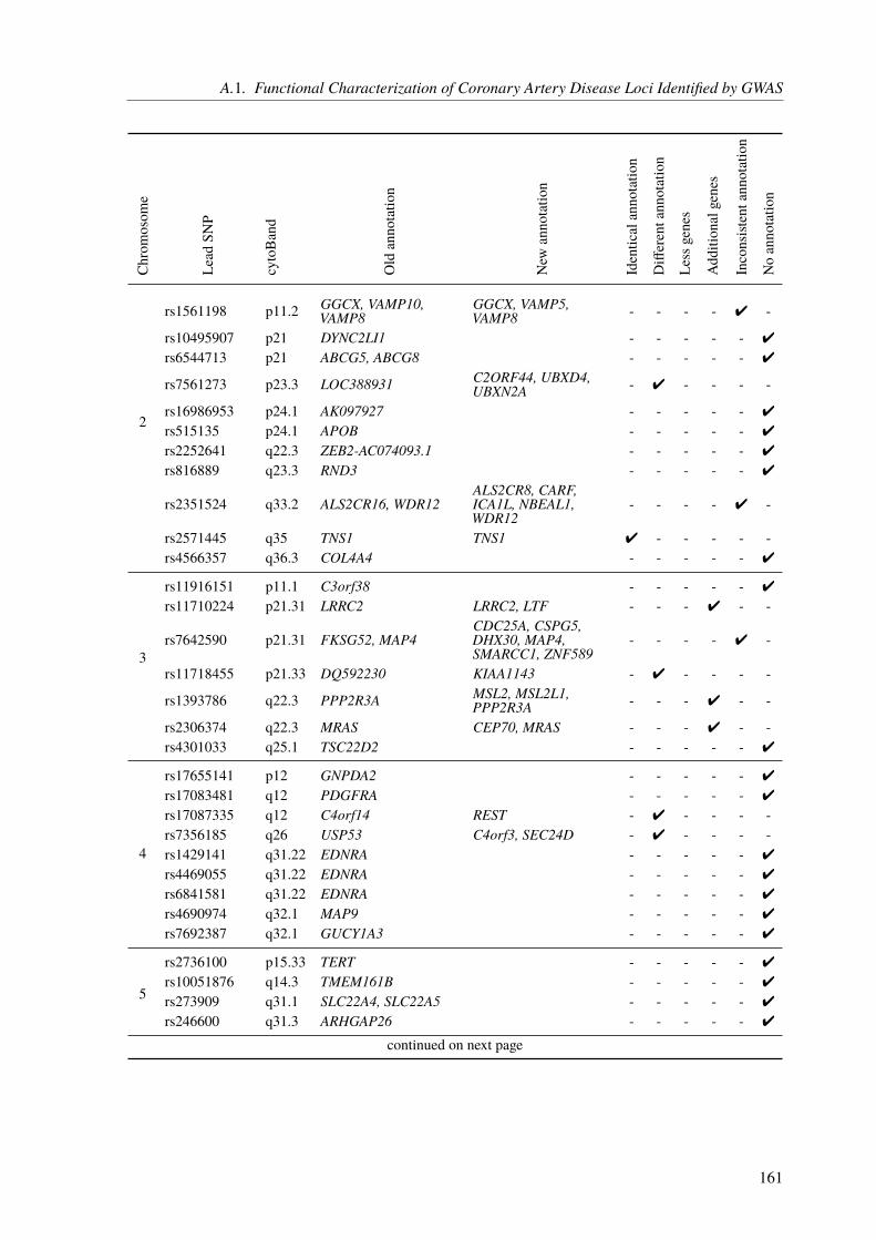
A.1. Functional Characterization of Coronary Artery Disease Loci Identified by GWAS
Chrom
osom
e
Lead
SNP
cytoBand
Old
annotatio
n
New
annotatio
n
Identicalannotatio
n
Differentannotation
Less
genes
Additionalgenes
Inconsistentannotation
Noannotatio
n
2
rs1561198 p11.2 GGCX, VAMP10,VAMP8
GGCX, VAMP5,VAMP8 - - - - 4 -
rs10495907 p21 DYNC2LI1 - - - - - 4
rs6544713 p21 ABCG5, ABCG8 - - - - - 4
rs7561273 p23.3 LOC388931 C2ORF44, UBXD4,UBXN2A - 4 - - - -
rs16986953 p24.1 AK097927 - - - - - 4
rs515135 p24.1 APOB - - - - - 4
rs2252641 q22.3 ZEB2-AC074093.1 - - - - - 4
rs816889 q23.3 RND3 - - - - - 4
rs2351524 q33.2 ALS2CR16, WDR12ALS2CR8, CARF,ICA1L, NBEAL1,WDR12
- - - - 4 -
rs2571445 q35 TNS1 TNS1 4 - - - - -rs4566357 q36.3 COL4A4 - - - - - 4
3
rs11916151 p11.1 C3orf38 - - - - - 4
rs11710224 p21.31 LRRC2 LRRC2, LTF - - - 4 - -
rs7642590 p21.31 FKSG52, MAP4CDC25A, CSPG5,DHX30, MAP4,SMARCC1, ZNF589
- - - - 4 -
rs11718455 p21.33 DQ592230 KIAA1143 - 4 - - - -
rs1393786 q22.3 PPP2R3A MSL2, MSL2L1,PPP2R3A - - - 4 - -
rs2306374 q22.3 MRAS CEP70, MRAS - - - 4 - -rs4301033 q25.1 TSC22D2 - - - - - 4
4
rs17655141 p12 GNPDA2 - - - - - 4
rs17083481 q12 PDGFRA - - - - - 4
rs17087335 q12 C4orf14 REST - 4 - - - -rs7356185 q26 USP53 C4orf3, SEC24D - 4 - - - -rs1429141 q31.22 EDNRA - - - - - 4
rs4469055 q31.22 EDNRA - - - - - 4
rs6841581 q31.22 EDNRA - - - - - 4
rs4690974 q32.1 MAP9 - - - - - 4
rs7692387 q32.1 GUCY1A3 - - - - - 4
5
rs2736100 p15.33 TERT - - - - - 4
rs10051876 q14.3 TMEM161B - - - - - 4
rs273909 q31.1 SLC22A4, SLC22A5 - - - - - 4
rs246600 q31.3 ARHGAP26 - - - - - 4
continued on next page
161
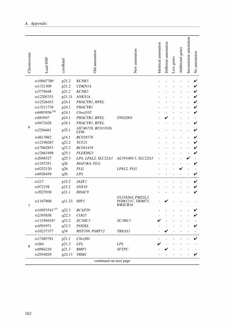
A. AppendixChrom
osom
e
Lead
SNP
cytoBand
Old
annotatio
n
New
annotatio
n
Identicalannotatio
n
Differentannotation
Less
genes
Additionalgenes
Inconsistentannotation
Noannotatio
n
6
rs10947789 p21.2 KCNK5 - - - - - 4
rs1321309 p21.2 CDKN1A - - - - - 4
rs3778448 p21.2 KCNK5 - - - - - 4
rs12205331 p21.31 ANKS1A - - - - - 4
rs12526453 p24.1 PHACTR1, RPEL - - - - - 4
rs13211739 p24.1 PHACTR1 - - - - - 4
rs6903956136 p24.1 C6orf105 - - - - - 4
rs883947 p24.1 PHACTR1, RPEL YN62D03 - 4 - - - -rs9472428 p24.1 PHACTR1, RPEL - - - - - 4
rs2294461 p25.1 AX746739, BC031936,LY86 - - - - - 4
rs4613862 q14.1 BC038576 - - - - - 4
rs12190287 q23.2 TCF21 - - - - - 4
rs17062853 q23.2 BC041459 - - - - - 4
rs12663498 q25.1 PLEKHG1 - - - - - 4
rs2048327 q25.3 LPA, LPAL2, SLC22A3 AL591069.5, SLC22A3 - - - - 4 -rs1247351 q26 MAP3K4, PLG - - - - - 4
rs4252120 q26 PLG LPAL2, PLG - - - 4 - -rs6926458 q26 LPA - - - - - 4
7
rs217 p15.2 JAZF1 - - - - - 4
rs972158 p15.2 SNX10 - - - - - 4
rs2023938 p21.1 HDAC9 - - - - - 4
rs1167800 q11.23 HIP1FLJ38264, PMS2L3,POM121C, TRIM73,WBSCR16
- 4 - - - -
rs10953541137 q22.3 BCAP29 - - - - - 4
rs2395858 q22.3 COG5 - - - - - 4
rs11556924* q32.2 ZC3HC1 ZC3HC1 4 - - - - -rs4591971 q32.3 PODXL - - - - - 4
rs10237377 q34 MST109, PARP12 TBXAS1 - 4 - - - -
8
rs17485781 p21.1 C8orf80 - - - - - 4
rs264 p21.3 LPL LPL 4 - - - - -rs6984210 p21.3 BMP1 SFTPC - 4 - - - -rs2954029 q24.13 TRIB1 - - - - - 4
continued on next page
162

A.1. Functional Characterization of Coronary Artery Disease Loci Identified by GWAS
Chrom
osom
e
Lead
SNP
cytoBand
Old
annotatio
n
New
annotatio
n
Identicalannotatio
n
Differentannotation
Less
genes
Additionalgenes
Inconsistentannotation
Noannotatio
n
9
rs10965228 p21.3 CDKN2BAS - - - - - 4
rs1333049 p21.3 CDKN2BAS CDKN2B - 4 - - - -rs16905599 p21.3 CDKN2BAS - - - - - 4
rs3217992 p21.3 CDKN2B, CDKN2BAS,MTAP CDKN2A, CDKN2B - - - - 4 -
rs10962774 p22.2 BNC2 - - - - - 4
rs495828 q34.2 ABO - - - - - 4
10
rs2505083 p11.23 KIAA1462 KIAA1462 4 - - - - -rs11238956 q11.21 CXCL12 - - - - - 4
rs17155842 q11.21 CXCL12 - - - - - 4
rs2047009 q11.21 AX747950, CXCL12 - - - - - 4
rs501120 q11.21 CXCL12 - - - - - 4
rs3748242 q22.3 ANXA11 ANXA11, MAT1A - - - 4 - -rs7074064 q23.2 BMPR1A BMPR1A 4 - - - - -rs11203042 q23.31 LIPA - - - - - 4
rs2246833 q23.31 LIPA LIPA 4 - - - - -
rs11191447 q24.32 CNNM2, CYP17A1,NT5C2 CNNM2, NT5C2 - - 4 - - -
rs12765878 q24.33 OBFC1 OBFC1,RP11-541N10.2 - - - 4 - -
11
rs7116641 p11.2 HSD17B12 HSD17B12 4 - - - - -rs93139 p15.4 SWAP70 AF075116, SWAP70 - - - 4 - -
rs12801636 q13.1 PCNXL3 OVOL1, PCNXL3,RELA, SIPA1 - - - 4 - -
rs590121 q13.5 SERPINH1 SERPINH1 4 - - - - -rs606452 q13.5 SERPINH1 - - - - - 4
rs974819 q22.3 PDGFD - - - - - 4
rs9326246 q23.3 APO5A, APOA1,ZNF259 - - - - - 4
rs964184137 q23.3 ZNF259 - - - - - 4
rs683800 q24.2 DCPS SRPR - 4 - - - -continued on next page
163

A. AppendixChrom
osom
e
Lead
SNP
cytoBand
Old
annotatio
n
New
annotatio
n
Identicalannotatio
n
Differentannotation
Less
genes
Additionalgenes
Inconsistentannotation
Noannotatio
n
12
rs4149033 p12.1 SLCO1B1 - - - - - 4
rs4762911 p12.2 PDE3A HS.539450 - 4 - - - -rs2681472 q21.33 ATP2B1 GALNT4 - 4 - - - -rs6490029 q24.11 CUX2 - - - - - 4
rs3184504 q24.12 SH2B3 ATXN2, FLJ21127,SH2B3 - - - 4 - -
rs3809274 q24.12 ATXN2
ALDH2, BRAP,C12orf30, HECTD4,MAPKAPK5,MAPKAPK5-AS1,SH2B3, TMEM116
- 4 - - - -
rs17630235 q24.13 SH2B3, TRAFD1 C12orf30 - 4 - - - -rs2891403 q24.13 RPH3A, SH2B3 - - - - - 4
rs11057841 q24.31 SCARB1 SCARB1 4 - - - - -rs2244608 q24.31 HNF1A HNF1A 4 - - - - -
13
rs9319428 q12.3 FLT1 - - - - - 4
rs9316753 q21.1 BC044614 - - - - - 4
rs10507753 q21.33 BC042673 - - - - - 4
rs11617955 q34 COL4A1, COL4A2 - - - - - 4
rs11619057 q34 COL4A2 - - - - - 4
rs12873154 q34 COL4A1, COL4A2 - - - - - 4
rs4773144 q34 COL4A1, COL4A2 - - - - - 4
rs7139492 q34 COL4A1, COL4A2 - - - - - 4
rs9515201 q34 COL4A1, COL4A2 IRS2 - 4 - - - -rs9515203 q34 COL4A1, COL4A2 - - - - - 4
14 rs2146238 q32.2 CYP46A1 EML1 - 4 - - - -rs2895811 q32.2 HHIPL1 YY1 - 4 - - - -
15
rs6494488 q22.31 RBPMS2 RBPMS2, SNX1,SPG21, TRIP4 - - - 4 - -
rs11072794 q25.1 ADAMTS7, DQ582071 ADAMTS7, WDR61 - - - - 4 -rs1994016135 q25.1 ADAMTS7 ADAMTS7 4 - - - - -rs3825807135 q25.1 ADAMTS7 ADAMTS7 4 - - - - -rs4380028135 q25.1 ADAMTS7 - - - - - 4
rs7173743 q25.1 ADAMTS7, MRG15 - - - - - 4
rs7181240 q25.1 MRG15 - - - - - 4
rs2880765 q25.3 AKAP13 - - - - - 4
rs17514846 q26.1 FES, FURIN FES, FURIN, MAN2A2 - - - 4 - -rs2521501 q26.1 FES FES 4 - - - - -rs7496815 q26.1 BC036442 - - - - - 4
continued on next page
164
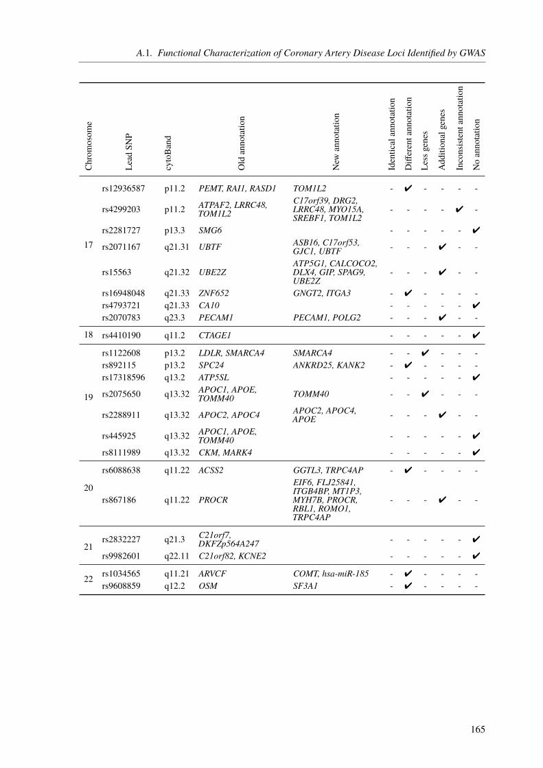
A.1. Functional Characterization of Coronary Artery Disease Loci Identified by GWAS
Chrom
osom
e
Lead
SNP
cytoBand
Old
annotatio
n
New
annotatio
n
Identicalannotatio
n
Differentannotation
Less
genes
Additionalgenes
Inconsistentannotation
Noannotatio
n
17
rs12936587 p11.2 PEMT, RAI1, RASD1 TOM1L2 - 4 - - - -
rs4299203 p11.2 ATPAF2, LRRC48,TOM1L2
C17orf39, DRG2,LRRC48, MYO15A,SREBF1, TOM1L2
- - - - 4 -
rs2281727 p13.3 SMG6 - - - - - 4
rs2071167 q21.31 UBTF ASB16, C17orf53,GJC1, UBTF - - - 4 - -
rs15563 q21.32 UBE2ZATP5G1, CALCOCO2,DLX4, GIP, SPAG9,UBE2Z
- - - 4 - -
rs16948048 q21.33 ZNF652 GNGT2, ITGA3 - 4 - - - -rs4793721 q21.33 CA10 - - - - - 4
rs2070783 q23.3 PECAM1 PECAM1, POLG2 - - - 4 - -
18 rs4410190 q11.2 CTAGE1 - - - - - 4
19
rs1122608 p13.2 LDLR, SMARCA4 SMARCA4 - - 4 - - -rs892115 p13.2 SPC24 ANKRD25, KANK2 - 4 - - - -rs17318596 q13.2 ATP5SL - - - - - 4
rs2075650 q13.32 APOC1, APOE,TOMM40 TOMM40 - - 4 - - -
rs2288911 q13.32 APOC2, APOC4 APOC2, APOC4,APOE - - - 4 - -
rs445925 q13.32 APOC1, APOE,TOMM40 - - - - - 4
rs8111989 q13.32 CKM, MARK4 - - - - - 4
20
rs6088638 q11.22 ACSS2 GGTL3, TRPC4AP - 4 - - - -
rs867186 q11.22 PROCR
EIF6, FLJ25841,ITGB4BP, MT1P3,MYH7B, PROCR,RBL1, ROMO1,TRPC4AP
- - - 4 - -
21rs2832227 q21.3 C21orf7,
DKFZp564A247 - - - - - 4
rs9982601 q22.11 C21orf82, KCNE2 - - - - - 4
22 rs1034565 q11.21 ARVCF COMT, hsa-miR-185 - 4 - - - -rs9608859 q12.2 OSM SF3A1 - 4 - - - -
165
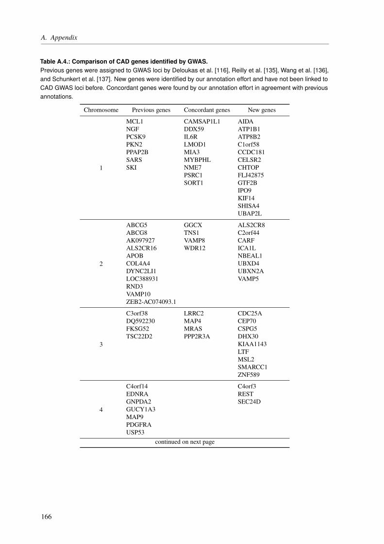
A. Appendix
Table A.4.: Comparison of CAD genes identified by GWAS.Previous genes were assigned to GWAS loci by Deloukas et al. [116], Reilly et al. [135], Wang et al. [136],and Schunkert et al. [137]. New genes were identified by our annotation effort and have not been linked toCAD GWAS loci before. Concordant genes were found by our annotation effort in agreement with previousannotations.
Chromosome Previous genes Concordant genes New genes
1
MCL1 CAMSAP1L1 AIDANGF DDX59 ATP1B1PCSK9 IL6R ATP8B2PKN2 LMOD1 C1orf58PPAP2B MIA3 CCDC181SARS MYBPHL CELSR2SKI NME7 CHTOP
PSRC1 FLJ42875SORT1 GTF2B
IPO9KIF14SHISA4UBAP2L
2
ABCG5 GGCX ALS2CR8ABCG8 TNS1 C2orf44AK097927 VAMP8 CARFALS2CR16 WDR12 ICA1LAPOB NBEAL1COL4A4 UBXD4DYNC2LI1 UBXN2ALOC388931 VAMP5RND3VAMP10ZEB2-AC074093.1
3
C3orf38 LRRC2 CDC25ADQ592230 MAP4 CEP70FKSG52 MRAS CSPG5TSC22D2 PPP2R3A DHX30
KIAA1143LTFMSL2SMARCC1ZNF589
4
C4orf14 C4orf3EDNRA RESTGNPDA2 SEC24DGUCY1A3MAP9PDGFRAUSP53
continued on next page
166

A.1. Functional Characterization of Coronary Artery Disease Loci Identified by GWAS
Chromosome Previous genes Concordant genes New genes
5
ARHGAP26SLC22A4SLC22A5TERTTMEM161B
6
ANKS1A LPAL2 AL591069.5AX746739 PLG YN62D03BC031936 SLC22A3BC038576BC041459C6orf105CDKN1AKCNK5LPALY86MAP3K4PHACTR1PLEKHG1RPELTCF21
7
BCAP29 ZC3HC1 FLJ38264COG5 PMS2L3HDAC9 POM121CHIP1 TBXAS1JAZF1 TRIM73MST109 WBSCR16PARP12PODXLSNX10
8BMP1 LPL SFTPCC8orf80TRIB1
9
ABO CDKN2B CDKN2ABNC2CDKN2BASMTAP
10
AX747950 ANXA11 MAT1ACXCL12 BMPR1A RP11-541N10.2CYP17A1 CNNM2
KIAA1462LIPANT5C2OBFC1
11
APO5A HSD17B12 AF075116APOA1 PCNXL3 OVOL1DCPS SERPINH1 RELAPDGFD SWAP70 SIPA1ZNF259 SRPR
continued on next page
167
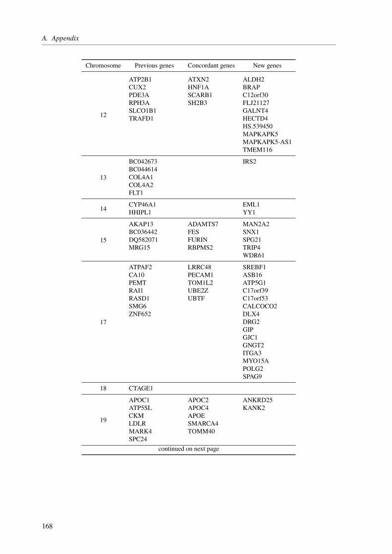
A. Appendix
Chromosome Previous genes Concordant genes New genes
12
ATP2B1 ATXN2 ALDH2CUX2 HNF1A BRAPPDE3A SCARB1 C12orf30RPH3A SH2B3 FLJ21127SLCO1B1 GALNT4TRAFD1 HECTD4
HS.539450MAPKAPK5MAPKAPK5-AS1TMEM116
13
BC042673 IRS2BC044614COL4A1COL4A2FLT1
14 CYP46A1 EML1HHIPL1 YY1
15
AKAP13 ADAMTS7 MAN2A2BC036442 FES SNX1DQ582071 FURIN SPG21MRG15 RBPMS2 TRIP4
WDR61
17
ATPAF2 LRRC48 SREBF1CA10 PECAM1 ASB16PEMT TOM1L2 ATP5G1RAI1 UBE2Z C17orf39RASD1 UBTF C17orf53SMG6 CALCOCO2ZNF652 DLX4
DRG2GIPGJC1GNGT2ITGA3MYO15APOLG2SPAG9
18 CTAGE1
19
APOC1 APOC2 ANKRD25ATP5SL APOC4 KANK2CKM APOELDLR SMARCA4MARK4 TOMM40SPC24
continued on next page
168

A.1. Functional Characterization of Coronary Artery Disease Loci Identified by GWAS
Chromosome Previous genes Concordant genes New genes
20
ACSS2 PROCR EIF6FLJ25841GGTL3ITGB4BPMT1P3MYH7BRBL1ROMO1TRPC4AP
21
C21orf7C21orf82DKFZp564A247KCNE2
22ARVCF COMTOSM hsa-miR-185
SF3A1
Table A.5.: Ranking scores for all CAD genes identified by our annotation.Hits in a database or score are indicated by 4. A previous knowledge score (Gene ScorePK), a data-drivenscore (Gene ScoreDD), and a total score (Gene ScoreTOTAL) is calculated. Detailed information on the scoresis available in Section 3.3.9 on Page 74.
Previous knowledge ranking Data-driven ranking
Gene GRAIL
DEP
ICT
MGD
FunD
O
ConsensusPathDB
AmiGO2
GeneScore P
K
AA-change
eQTL
Prom
oter
Key
driver
Sys.geneticsm
ice
GeneScore D
D
GeneScore T
otal
ADAMTS7 4 4 - - 4 4 4 4 4 4 - - 3 7AF075116 - - - - - - 0 - 4 - - - 1 1AIDA - - - - - - 0 - 4 - - - 1 1AL591069.5 - - - - - - 0 - 4 - - - 1 1ALDH2 - 4 4 4 4 4 5 - 4 - - - 1 6ALS2CR8 - - - - - - 0 4 - - - 4 2 2ANKRD25 - - - - - - 0 - 4 - - 4 2 2ANXA11 - 4 - - - 4 2 - 4 - - - 1 3APOC2 - - - 4 4 4 3 - 4 4 - 4 3 6APOC4 - 4 - - 4 4 3 4 4 4 - - 3 6APOE 4 - 4 4 4 4 5 - 4 - - - 1 6ASB16 - - - - 4 - 1 - 4 - - 4 2 3ATP1B1 - - 4 - 4 4 3 - 4 - - - 1 4ATP5G1 - - - - 4 4 2 - 4 4 - - 2 4ATP8B2 - - 4 - - - 1 - 4 - - - 1 2ATXN2 - - 4 - - 4 2 - 4 - - 4 2 4BMPR1A - 4 4 - 4 4 4 4 - - - 4 2 6BRAP - - 4 - 4 - 2 - 4 - - 4 2 4
continued on next page
169
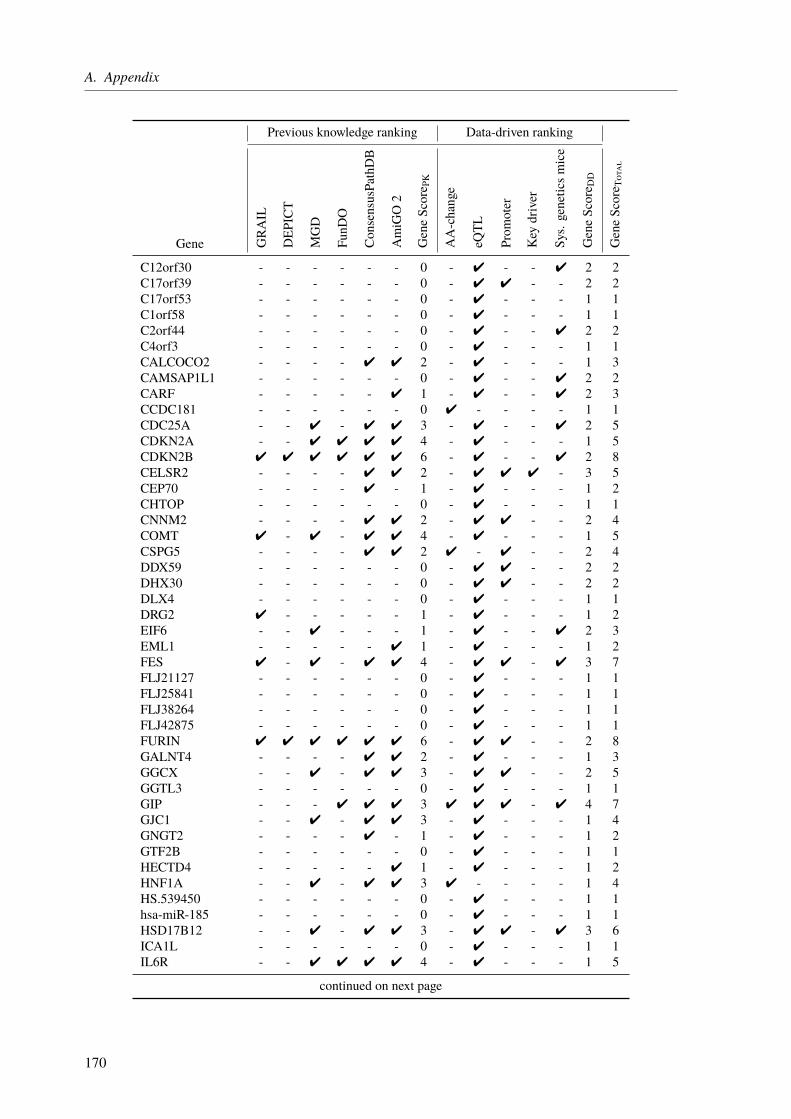
A. Appendix
Previous knowledge ranking Data-driven ranking
Gene GRAIL
DEP
ICT
MGD
FunD
O
ConsensusPathDB
AmiGO2
GeneScore P
K
AA-change
eQTL
Prom
oter
Key
driver
Sys.geneticsm
ice
GeneScore D
D
GeneScore T
otal
C12orf30 - - - - - - 0 - 4 - - 4 2 2C17orf39 - - - - - - 0 - 4 4 - - 2 2C17orf53 - - - - - - 0 - 4 - - - 1 1C1orf58 - - - - - - 0 - 4 - - - 1 1C2orf44 - - - - - - 0 - 4 - - 4 2 2C4orf3 - - - - - - 0 - 4 - - - 1 1CALCOCO2 - - - - 4 4 2 - 4 - - - 1 3CAMSAP1L1 - - - - - - 0 - 4 - - 4 2 2CARF - - - - - 4 1 - 4 - - 4 2 3CCDC181 - - - - - - 0 4 - - - - 1 1CDC25A - - 4 - 4 4 3 - 4 - - 4 2 5CDKN2A - - 4 4 4 4 4 - 4 - - - 1 5CDKN2B 4 4 4 4 4 4 6 - 4 - - 4 2 8CELSR2 - - - - 4 4 2 - 4 4 4 - 3 5CEP70 - - - - 4 - 1 - 4 - - - 1 2CHTOP - - - - - - 0 - 4 - - - 1 1CNNM2 - - - - 4 4 2 - 4 4 - - 2 4COMT 4 - 4 - 4 4 4 - 4 - - - 1 5CSPG5 - - - - 4 4 2 4 - 4 - - 2 4DDX59 - - - - - - 0 - 4 4 - - 2 2DHX30 - - - - - - 0 - 4 4 - - 2 2DLX4 - - - - - - 0 - 4 - - - 1 1DRG2 4 - - - - - 1 - 4 - - - 1 2EIF6 - - 4 - - - 1 - 4 - - 4 2 3EML1 - - - - - 4 1 - 4 - - - 1 2FES 4 - 4 - 4 4 4 - 4 4 - 4 3 7FLJ21127 - - - - - - 0 - 4 - - - 1 1FLJ25841 - - - - - - 0 - 4 - - - 1 1FLJ38264 - - - - - - 0 - 4 - - - 1 1FLJ42875 - - - - - - 0 - 4 - - - 1 1FURIN 4 4 4 4 4 4 6 - 4 4 - - 2 8GALNT4 - - - - 4 4 2 - 4 - - - 1 3GGCX - - 4 - 4 4 3 - 4 4 - - 2 5GGTL3 - - - - - - 0 - 4 - - - 1 1GIP - - - 4 4 4 3 4 4 4 - 4 4 7GJC1 - - 4 - 4 4 3 - 4 - - - 1 4GNGT2 - - - - 4 - 1 - 4 - - - 1 2GTF2B - - - - - - 0 - 4 - - - 1 1HECTD4 - - - - - 4 1 - 4 - - - 1 2HNF1A - - 4 - 4 4 3 4 - - - - 1 4HS.539450 - - - - - - 0 - 4 - - - 1 1hsa-miR-185 - - - - - - 0 - 4 - - - 1 1HSD17B12 - - 4 - 4 4 3 - 4 4 - 4 3 6ICA1L - - - - - - 0 - 4 - - - 1 1IL6R - - 4 4 4 4 4 - 4 - - - 1 5
continued on next page
170
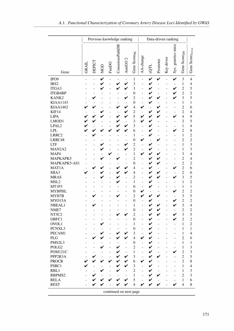
A.1. Functional Characterization of Coronary Artery Disease Loci Identified by GWAS
Previous knowledge ranking Data-driven ranking
Gene GRAIL
DEP
ICT
MGD
FunD
O
ConsensusPathDB
AmiGO2
GeneScore P
K
AA-change
eQTL
Prom
oter
Key
driver
Sys.geneticsm
ice
GeneScore D
D
GeneScore T
otal
IPO9 - - 4 - - - 1 - 4 4 - 4 3 4IRS2 - - 4 - 4 4 3 - 4 - - - 1 4ITGA3 - - 4 - 4 4 3 - 4 - - 4 2 5ITGB4BP - - - - - - 0 - 4 - - 4 2 2KANK2 - 4 - - - 4 2 - 4 4 - 4 3 5KIAA1143 - - - - - - 0 - 4 - - - 1 1KIAA1462 4 4 - - 4 4 4 4 - 4 - - 2 6KIF14 - - 4 - - 4 2 - 4 4 - - 2 4LIPA 4 4 4 - 4 4 5 4 4 4 - 4 4 9LMOD1 4 4 - - 4 - 3 4 4 - - - 2 5LPAL2 4 - - - 4 4 3 - 4 - - - 1 4LPL 4 4 4 4 4 4 6 - 4 - - 4 2 8LRRC2 - 4 - - - - 1 - 4 - - - 1 2LRRC48 - - - - - - 0 4 - 4 - - 2 2LTF - - 4 - - 4 2 - 4 - - - 1 3MAN2A2 - - 4 - - 4 2 - 4 - - - 1 3MAP4 - - - 4 - - 1 4 4 4 - - 3 4MAPKAPK5 - - 4 - 4 - 2 - 4 4 - - 2 4MAPKAPK5-AS1 - - - - - - 0 - 4 4 - - 2 2MAT1A - 4 4 - 4 4 4 - 4 - - 4 2 6MIA3 4 - 4 - 4 4 4 - 4 4 - - 2 6MRAS - - 4 - 4 - 2 - 4 4 - 4 3 5MSL2 - - - - 4 - 1 - 4 - - - 1 2MT1P3 - - - - - - 0 - 4 - - - 1 1MYBPHL - - - - - - 0 4 - - - 4 2 2MYH7B - 4 - - 4 - 2 4 4 4 - - 3 5MYO15A - - - - - - 0 - 4 - - 4 2 2NBEAL1 - 4 - - - - 1 - 4 4 - 4 3 4NME7 - - - - - - 0 - 4 4 - - 2 2NT5C2 - - - - 4 4 2 - 4 4 - 4 3 5OBFC1 - - - - - - 0 - 4 - - 4 2 2OVOL1 - - 4 - - - 1 - 4 - - - 1 2PCNXL3 - - - - - - 0 - 4 - - - 1 1PECAM1 - - 4 - 4 4 3 - 4 - - - 1 4PLG - 4 4 - 4 4 4 4 4 - - - 2 6PMS2L3 - - - - - - 0 - 4 - - - 1 1POLG2 - - 4 - 4 - 2 - 4 - - - 1 3POM121C - - - - 4 - 1 - 4 - - 4 2 3PPP2R3A - 4 - - 4 4 3 - 4 4 - - 2 5PROCR 4 4 4 4 4 4 6 4 4 - - - 2 8PSRC1 4 - - - 4 4 3 - 4 - - - 1 4RBL1 - - 4 - 4 - 2 - 4 - - - 1 3RBPMS2 - 4 - - - - 1 - 4 4 - - 2 3RELA - 4 4 4 4 4 5 - 4 - - - 1 6REST - 4 4 - 4 4 4 4 4 4 - 4 4 8
continued on next page
171
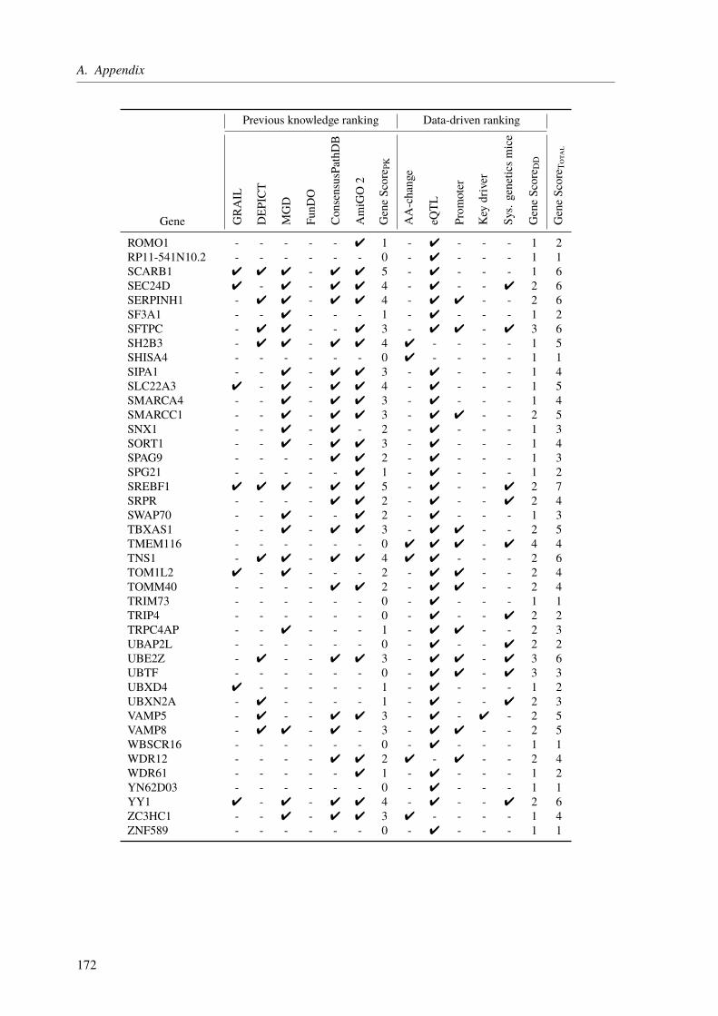
A. Appendix
Previous knowledge ranking Data-driven ranking
Gene GRAIL
DEP
ICT
MGD
FunD
O
ConsensusPathDB
AmiGO2
GeneScore P
K
AA-change
eQTL
Prom
oter
Key
driver
Sys.geneticsm
ice
GeneScore D
D
GeneScore T
otal
ROMO1 - - - - - 4 1 - 4 - - - 1 2RP11-541N10.2 - - - - - - 0 - 4 - - - 1 1SCARB1 4 4 4 - 4 4 5 - 4 - - - 1 6SEC24D 4 - 4 - 4 4 4 - 4 - - 4 2 6SERPINH1 - 4 4 - 4 4 4 - 4 4 - - 2 6SF3A1 - - 4 - - - 1 - 4 - - - 1 2SFTPC - 4 4 - - 4 3 - 4 4 - 4 3 6SH2B3 - 4 4 - 4 4 4 4 - - - - 1 5SHISA4 - - - - - - 0 4 - - - - 1 1SIPA1 - - 4 - 4 4 3 - 4 - - - 1 4SLC22A3 4 - 4 - 4 4 4 - 4 - - - 1 5SMARCA4 - - 4 - 4 4 3 - 4 - - - 1 4SMARCC1 - - 4 - 4 4 3 - 4 4 - - 2 5SNX1 - - 4 - 4 - 2 - 4 - - - 1 3SORT1 - - 4 - 4 4 3 - 4 - - - 1 4SPAG9 - - - - 4 4 2 - 4 - - - 1 3SPG21 - - - - - 4 1 - 4 - - - 1 2SREBF1 4 4 4 - 4 4 5 - 4 - - 4 2 7SRPR - - - - 4 4 2 - 4 - - 4 2 4SWAP70 - - 4 - - 4 2 - 4 - - - 1 3TBXAS1 - - 4 - 4 4 3 - 4 4 - - 2 5TMEM116 - - - - - - 0 4 4 4 - 4 4 4TNS1 - 4 4 - 4 4 4 4 4 - - - 2 6TOM1L2 4 - 4 - - - 2 - 4 4 - - 2 4TOMM40 - - - - 4 4 2 - 4 4 - - 2 4TRIM73 - - - - - - 0 - 4 - - - 1 1TRIP4 - - - - - - 0 - 4 - - 4 2 2TRPC4AP - - 4 - - - 1 - 4 4 - - 2 3UBAP2L - - - - - - 0 - 4 - - 4 2 2UBE2Z - 4 - - 4 4 3 - 4 4 - 4 3 6UBTF - - - - - - 0 - 4 4 - 4 3 3UBXD4 4 - - - - - 1 - 4 - - - 1 2UBXN2A - 4 - - - - 1 - 4 - - 4 2 3VAMP5 - 4 - - 4 4 3 - 4 - 4 - 2 5VAMP8 - 4 4 - 4 - 3 - 4 4 - - 2 5WBSCR16 - - - - - - 0 - 4 - - - 1 1WDR12 - - - - 4 4 2 4 - 4 - - 2 4WDR61 - - - - - 4 1 - 4 - - - 1 2YN62D03 - - - - - - 0 - 4 - - - 1 1YY1 4 - 4 - 4 4 4 - 4 - - 4 2 6ZC3HC1 - - 4 - 4 4 3 4 - - - - 1 4ZNF589 - - - - - - 0 - 4 - - - 1 1
172
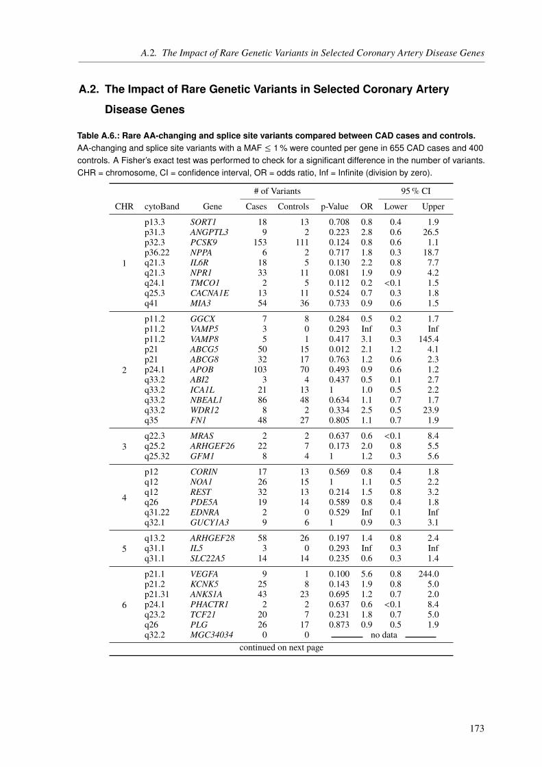
A.2. The Impact of Rare Genetic Variants in Selected Coronary Artery Disease Genes
A.2. The Impact of Rare Genetic Variants in Selected Coronary Artery
Disease Genes
Table A.6.: Rare AA-changing and splice site variants compared between CAD cases and controls.AA-changing and splice site variants with a MAF ≤ 1 % were counted per gene in 655 CAD cases and 400controls. A Fisher’s exact test was performed to check for a significant difference in the number of variants.CHR = chromosome, CI = confidence interval, OR = odds ratio, Inf = Infinite (division by zero).
# of Variants 95% CI
CHR cytoBand Gene Cases Controls p-Value OR Lower Upper
1
p13.3 SORT1 18 13 0.708 0.8 0.4 1.9p31.3 ANGPTL3 9 2 0.223 2.8 0.6 26.5p32.3 PCSK9 153 111 0.124 0.8 0.6 1.1p36.22 NPPA 6 2 0.717 1.8 0.3 18.7q21.3 IL6R 18 5 0.130 2.2 0.8 7.7q21.3 NPR1 33 11 0.081 1.9 0.9 4.2q24.1 TMCO1 2 5 0.112 0.2 <0.1 1.5q25.3 CACNA1E 13 11 0.524 0.7 0.3 1.8q41 MIA3 54 36 0.733 0.9 0.6 1.5
2
p11.2 GGCX 7 8 0.284 0.5 0.2 1.7p11.2 VAMP5 3 0 0.293 Inf 0.3 Infp11.2 VAMP8 5 1 0.417 3.1 0.3 145.4p21 ABCG5 50 15 0.012 2.1 1.2 4.1p21 ABCG8 32 17 0.763 1.2 0.6 2.3p24.1 APOB 103 70 0.493 0.9 0.6 1.2q33.2 ABI2 3 4 0.437 0.5 0.1 2.7q33.2 ICA1L 21 13 1 1.0 0.5 2.2q33.2 NBEAL1 86 48 0.634 1.1 0.7 1.7q33.2 WDR12 8 2 0.334 2.5 0.5 23.9q35 FN1 48 27 0.805 1.1 0.7 1.9
3q22.3 MRAS 2 2 0.637 0.6 <0.1 8.4q25.2 ARHGEF26 22 7 0.173 2.0 0.8 5.5q25.32 GFM1 8 4 1 1.2 0.3 5.6
4
p12 CORIN 17 13 0.569 0.8 0.4 1.8q12 NOA1 26 15 1 1.1 0.5 2.2q12 REST 32 13 0.214 1.5 0.8 3.2q26 PDE5A 19 14 0.589 0.8 0.4 1.8q31.22 EDNRA 2 0 0.529 Inf 0.1 Infq32.1 GUCY1A3 9 6 1 0.9 0.3 3.1
5q13.2 ARHGEF28 58 26 0.197 1.4 0.8 2.4q31.1 IL5 3 0 0.293 Inf 0.3 Infq31.1 SLC22A5 14 14 0.235 0.6 0.3 1.4
6
p21.1 VEGFA 9 1 0.100 5.6 0.8 244.0p21.2 KCNK5 25 8 0.143 1.9 0.8 5.0p21.31 ANKS1A 43 23 0.695 1.2 0.7 2.0p24.1 PHACTR1 2 2 0.637 0.6 <0.1 8.4q23.2 TCF21 20 7 0.231 1.8 0.7 5.0q26 PLG 26 17 0.873 0.9 0.5 1.9q32.2 MGC34034 0 0 no data
continued on next page
173

A. Appendix
# of Variants 95% CI
CHR cytoBand Gene Cases Controls p-Value OR Lower Upper
7
p13 NPC1L1 55 36 0.736 0.9 0.6 1.5p14.2 AOAH 12 13 0.149 0.6 0.2 1.3p21.1 HDAC9 13 10 0.665 0.8 0.3 2.0q22.1 CYP3A4 20 11 0.853 1.1 0.5 2.6q22.1 SLC12A9 39 20 0.582 1.2 0.7 2.2q22.3 BCAP29 9 4 0.776 1.4 0.4 6.2q32.2 ZC3HC1 5 5 0.517 0.6 0.1 2.7q36.1 NOS3 40 19 0.408 1.3 0.7 2.4
8p21.3 LPL 11 6 1 1.1 0.4 3.7q24.13 TRIB1 7 4 1 1.1 0.3 5.0q24.22 ADCY8 20 10 0.704 1.2 0.5 3.0
9 p21.3 CDKN2A 22 21 0.149 0.6 0.3 1.2p21.3 CDKN2B 3 4 0.437 0.5 0.1 2.7
10
p11.23 KIAA1462 20 10 0.704 1.2 0.5 3.0q11.21 CXCL12 4 5 0.312 0.5 0.1 2.3q23.1 FAM213A 3 4 0.437 0.5 0.1 2.7q23.31 LIPA 7 2 0.496 2.1 0.4 21.3q24.32 CNNM2 2 2 0.637 0.6 <0.1 8.4q24.32 CYP17A1 6 4 1 0.9 0.2 4.4q24.32 NT5C2 19 10 0.847 1.2 0.5 2.8
11
p15.4 SWAP70 5 1 0.417 3.1 0.3 145.4p32.2 PPAP2B 6 4 1 0.9 0.2 4.4q22.2 MMP10 18 17 0.215 0.6 0.3 1.3q22.3 PDGFD 5 2 0.716 1.5 0.2 16.1q23.3 APOA4 11 8 0.812 0.8 0.3 2.4q23.3 ZNF259 23 17 0.619 0.8 0.4 1.7
12
q21.33 ATP2B1 10 4 0.586 1.5 0.4 6.7q24.22 NOS1 55 30 0.642 1.1 0.7 1.9q24.31 C12orf43 10 6 1 1.0 0.3 3.4q24.31 HNF1A 5 3 1 1.0 0.2 6.6q24.31 OASL 10 12 0.121 0.5 0.2 1.3
13
q12.2 FLT1 22 9 0.351 1.5 0.7 3.8q12.3 UBL3 1 0 1 Inf <0.1 Infq34 COL4A1 22 18 0.406 0.7 0.4 1.5q34 COL4A2 47 16 0.044 1.9 1.0 3.6
14 q32.2 CYP46A1 12 0 0.005 Inf 1.7 Infq32.2 HHIPL1 33 13 0.214 1.6 0.8 3.3
15
q22.33 SMAD3 3 2 1 0.9 0.1 11.0q23 NOX5 11 8 0.812 0.8 0.3 2.4q25.1 ADAMTS7 99 58 0.859 1.0 0.7 1.5q26.1 ABHD2 0 0 no dataq26.1 FES 34 8 0.009 2.7 1.2 6.8q26.1 FURIN 16 9 1 1.1 0.4 2.8q26.1 MFGE8 12 12 0.287 0.6 0.2 1.5
16 q13 CETP 14 6 0.643 1.4 0.5 4.6q23.1 BCAR1 39 25 0.894 0.9 0.6 1.7
continued on next page
174
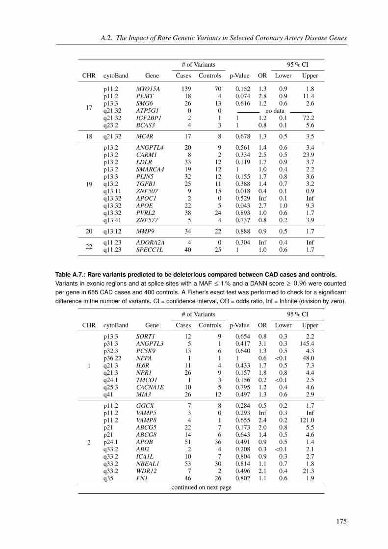
A.2. The Impact of Rare Genetic Variants in Selected Coronary Artery Disease Genes
# of Variants 95% CI
CHR cytoBand Gene Cases Controls p-Value OR Lower Upper
17
p11.2 MYO15A 139 70 0.152 1.3 0.9 1.8p11.2 PEMT 18 4 0.074 2.8 0.9 11.4p13.3 SMG6 26 13 0.616 1.2 0.6 2.6q21.32 ATP5G1 0 0 no dataq21.32 IGF2BP1 2 1 1 1.2 0.1 72.2q23.2 BCAS3 4 3 1 0.8 0.1 5.6
18 q21.32 MC4R 17 8 0.678 1.3 0.5 3.5
19
p13.2 ANGPTL4 20 9 0.561 1.4 0.6 3.4p13.2 CARM1 8 2 0.334 2.5 0.5 23.9p13.2 LDLR 33 12 0.119 1.7 0.9 3.7p13.2 SMARCA4 19 12 1 1.0 0.4 2.2p13.3 PLIN5 32 12 0.155 1.7 0.8 3.6q13.2 TGFB1 25 11 0.388 1.4 0.7 3.2q13.11 ZNF507 9 15 0.018 0.4 0.1 0.9q13.32 APOC1 2 0 0.529 Inf 0.1 Infq13.32 APOE 22 5 0.043 2.7 1.0 9.3q13.32 PVRL2 38 24 0.893 1.0 0.6 1.7q13.41 ZNF577 5 4 0.737 0.8 0.2 3.9
20 q13.12 MMP9 34 22 0.888 0.9 0.5 1.7
22 q11.23 ADORA2A 4 0 0.304 Inf 0.4 Infq11.23 SPECC1L 40 25 1 1.0 0.6 1.7
Table A.7.: Rare variants predicted to be deleterious compared between CAD cases and controls.Variants in exonic regions and at splice sites with a MAF ≤ 1 % and a DANN score ≥ 0.96 were countedper gene in 655 CAD cases and 400 controls. A Fisher’s exact test was performed to check for a significantdifference in the number of variants. CI = confidence interval, OR = odds ratio, Inf = Infinite (division by zero).
# of Variants 95% CI
CHR cytoBand Gene Cases Controls p-Value OR Lower Upper
1
p13.3 SORT1 12 9 0.654 0.8 0.3 2.2p31.3 ANGPTL3 5 1 0.417 3.1 0.3 145.4p32.3 PCSK9 13 6 0.640 1.3 0.5 4.3p36.22 NPPA 1 1 1 0.6 <0.1 48.0q21.3 IL6R 11 4 0.433 1.7 0.5 7.3q21.3 NPR1 26 9 0.157 1.8 0.8 4.4q24.1 TMCO1 1 3 0.156 0.2 <0.1 2.5q25.3 CACNA1E 10 5 0.795 1.2 0.4 4.6q41 MIA3 26 12 0.497 1.3 0.6 2.9
2
p11.2 GGCX 7 8 0.284 0.5 0.2 1.7p11.2 VAMP5 3 0 0.293 Inf 0.3 Infp11.2 VAMP8 4 1 0.655 2.4 0.2 121.0p21 ABCG5 22 7 0.173 2.0 0.8 5.5p21 ABCG8 14 6 0.643 1.4 0.5 4.6p24.1 APOB 51 36 0.491 0.9 0.5 1.4q33.2 ABI2 2 4 0.208 0.3 <0.1 2.1q33.2 ICA1L 10 7 0.804 0.9 0.3 2.7q33.2 NBEAL1 53 30 0.814 1.1 0.7 1.8q33.2 WDR12 7 2 0.496 2.1 0.4 21.3q35 FN1 46 26 0.802 1.1 0.6 1.9
continued on next page
175
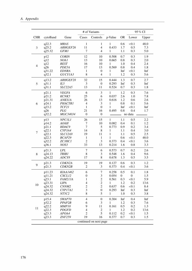
A. Appendix
# of Variants 95% CI
CHR cytoBand Gene Cases Controls p-Value OR Lower Upper
3q22.3 MRAS 1 1 1 0.6 <0.1 48.0q25.2 ARHGEF26 11 4 0.433 1.7 0.5 7.3q25.32 GFM1 7 4 1 1.1 0.3 5.0
4
p12 CORIN 12 10 0.508 0.7 0.3 1.9q12 NOA1 13 10 0.665 0.8 0.3 2.0q12 REST 16 10 1 1.0 0.4 2.4q26 PDE5A 17 13 0.569 0.8 0.4 1.8q31.22 EDNRA 1 0 1 Inf <0.1 Infq32.1 GUCY1A3 8 4 1 1.2 0.3 5.6
5q13.2 ARHGEF28 32 15 0.444 1.3 0.7 2.7q31.1 IL5 3 0 0.293 Inf 0.3 Infq31.1 SLC22A5 13 11 0.524 0.7 0.3 1.8
6
p21.1 VEGFA 6 3 1 1.2 0.3 7.6p21.2 KCNK5 25 6 0.037 2.6 1.0 7.8p21.31 ANKS1A 26 13 0.616 1.2 0.6 2.6p24.1 PHACTR1 4 3 1 0.8 0.1 5.6q23.2 TCF21 1 0 1 Inf <0.1 Infq26 PLG 21 16 0.495 0.8 0.4 1.7q32.2 MGC34034 0 0 no data
7
p13 NPC1L1 26 15 1 1.1 0.5 2.2p14.2 AOAH 7 10 0.082 0.4 0.1 1.2p21.1 HDAC9 7 5 0.773 0.9 0.2 3.4q22.1 CYP3A4 14 8 1 1.1 0.4 3.0q22.1 SLC12A9 19 11 1 1.1 0.5 2.5q22.3 BCAP29 1 1 1 0.6 <0.1 48.0q32.2 ZC3HC1 2 3 0.373 0.4 <0.1 3.6q36.1 NOS3 33 13 0.214 1.6 0.8 3.3
8p21.3 LPL 7 6 0.573 0.7 0.2 2.6q24.13 TRIB1 8 3 0.548 1.6 0.4 9.6q24.22 ADCY8 17 8 0.678 1.3 0.5 3.5
9 p21.3 CDKN2A 19 19 0.127 0.6 0.3 1.2p21.3 CDKN2B 2 3 0.373 0.4 <0.1 3.6
10
p11.23 KIAA1462 6 7 0.258 0.5 0.1 1.8q11.21 CXCL12 0 3 0.054 0 0 1.5q23.1 FAM213A 1 2 0.561 0.3 <0.1 5.9q23.31 LIPA 4 2 1 1.2 0.2 13.6q24.32 CNNM2 2 2 0.637 0.6 <0.1 8.4q24.32 CYP17A1 3 0 0.293 Inf 0.3 Infq24.32 NT5C2 8 5 1 1.0 0.3 3.8
11
p15.4 SWAP70 4 0 0.304 Inf 0.4 Infp32.2 PPAP2B 6 3 1 1.2 0.3 7.6q22.2 MMP10 9 11 0.161 0.5 0.2 1.3q22.3 PDGFD 4 2 1 1.2 0.2 13.6q23.3 APOA4 2 5 0.112 0.2 <0.1 1.5q23.3 ZNF259 19 16 0.377 0.7 0.3 1.5
continued on next page
176

A.2. The Impact of Rare Genetic Variants in Selected Coronary Artery Disease Genes
# of Variants 95% CI
CHR cytoBand Gene Cases Controls p-Value OR Lower Upper
12
q21.33 ATP2B1 10 3 0.391 2.1 0.5 11.7q24.22 NOS1 49 29 1 1.0 0.6 1.7q24.31 C12orf43 2 2 0.637 0.6 <0.1 8.4q24.31 HNF1A 5 3 1 1.0 0.2 6.6q24.31 OASL 6 6 0.387 0.6 0.2 2.3
13
q12.2 FLT1 9 3 0.551 1.8 0.5 10.6q12.3 UBL3 0 0 no dataq34 COL4A1 16 13 0.443 0.7 0.3 1.7q34 COL4A2 31 14 0.433 1.4 0.7 2.8
14 q32.2 CYP46A1 11 0 0.009 Inf 1.5 Infq32.2 HHIPL1 26 9 0.157 1.8 0.8 4.4
15
q22.33 SMAD3 2 1 1 1.2 0.1 72.2q23 NOX5 4 4 0.487 0.6 0.1 3.3q25.1 ADAMTS7 47 22 0.307 1.3 0.8 2.4q26.1 ABHD2 0 0 no dataq26.1 FES 23 5 0.029 2.9 1.1 9.8q26.1 FURIN 13 8 1 1.0 0.4 2.8q26.1 MFGE8 5 7 0.229 0.4 0.1 1.6
16 q13 CETP 4 2 1 1.2 0.2 13.6q23.1 BCAR1 23 14 1 1.0 0.5 2.1
17
p11.2 MYO15A 98 58 0.859 1.0 0.7 1.5p11.2 PEMT 10 2 0.147 3.1 0.7 29.1p13.3 SMG6 21 9 0.447 1.4 0.6 3.6q21.32 ATP5G1 0 0 no dataq21.32 IGF2BP1 2 1 1 1.2 0.1 72.2q23.2 BCAS3 3 3 0.679 0.6 0.1 4.6
18 q21.32 MC4R 2 4 0.208 0.3 <0.1 2.1
19
p13.2 ANGPTL4 10 5 0.795 1.2 0.4 4.6p13.2 CARM1 6 2 0.717 1.8 0.3 18.7p13.2 LDLR 26 7 0.046 2.3 1.0 6.4p13.2 SMARCA4 16 9 1 1.1 0.4 2.8p13.3 PLIN5 25 10 0.290 1.5 0.7 3.7q13.2 TGFB1 16 0 0.001 Inf 2.4 Infq13.11 ZNF507 5 9 0.052 0.3 0.1 1.1q13.32 APOC1 0 0 no dataq13.32 APOE 13 3 0.127 2.7 0.7 14.7q13.32 PVRL2 20 9 0.561 1.4 0.6 3.4q13.41 ZNF577 1 2 0.561 0.3 <0.1 5.9
20 q13.12 MMP9 30 20 0.767 0.9 0.5 1.7
22 q11.23 ADORA2A 3 0 0.293 Inf 0.3 Infq11.23 SPECC1L 40 25 1 1.0 0.6 1.7
177
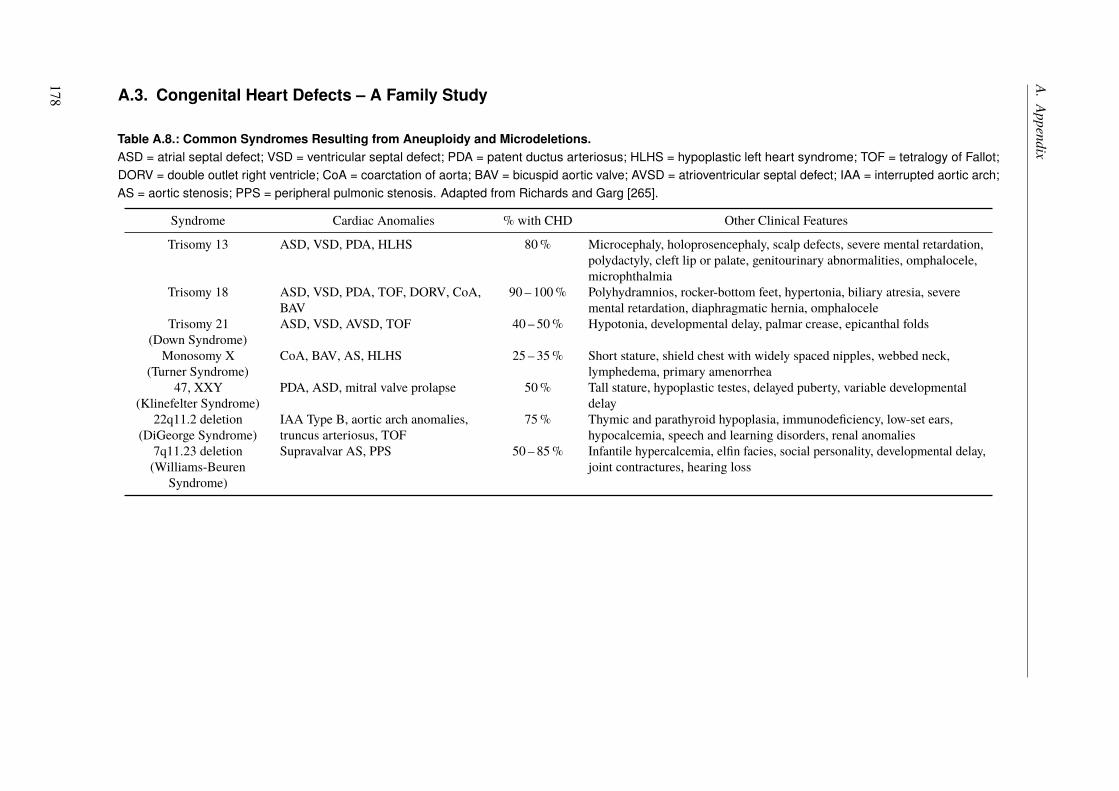
A.Appendix
A.3. Congenital Heart Defects – A Family Study
Table A.8.: Common Syndromes Resulting from Aneuploidy and Microdeletions.ASD = atrial septal defect; VSD = ventricular septal defect; PDA = patent ductus arteriosus; HLHS = hypoplastic left heart syndrome; TOF = tetralogy of Fallot;DORV = double outlet right ventricle; CoA = coarctation of aorta; BAV = bicuspid aortic valve; AVSD = atrioventricular septal defect; IAA = interrupted aortic arch;AS = aortic stenosis; PPS = peripheral pulmonic stenosis. Adapted from Richards and Garg [265].
Syndrome Cardiac Anomalies % with CHD Other Clinical Features
Trisomy 13 ASD, VSD, PDA, HLHS 80% Microcephaly, holoprosencephaly, scalp defects, severe mental retardation,polydactyly, cleft lip or palate, genitourinary abnormalities, omphalocele,microphthalmia
Trisomy 18 ASD, VSD, PDA, TOF, DORV, CoA,BAV
90 – 100% Polyhydramnios, rocker-bottom feet, hypertonia, biliary atresia, severemental retardation, diaphragmatic hernia, omphalocele
Trisomy 21(Down Syndrome)
ASD, VSD, AVSD, TOF 40 – 50% Hypotonia, developmental delay, palmar crease, epicanthal folds
Monosomy X(Turner Syndrome)
CoA, BAV, AS, HLHS 25 – 35% Short stature, shield chest with widely spaced nipples, webbed neck,lymphedema, primary amenorrhea
47, XXY(Klinefelter Syndrome)
PDA, ASD, mitral valve prolapse 50% Tall stature, hypoplastic testes, delayed puberty, variable developmentaldelay
22q11.2 deletion(DiGeorge Syndrome)
IAA Type B, aortic arch anomalies,truncus arteriosus, TOF
75% Thymic and parathyroid hypoplasia, immunodeficiency, low-set ears,hypocalcemia, speech and learning disorders, renal anomalies
7q11.23 deletion(Williams-Beuren
Syndrome)
Supravalvar AS, PPS 50 – 85% Infantile hypercalcemia, elfin facies, social personality, developmental delay,joint contractures, hearing loss
178
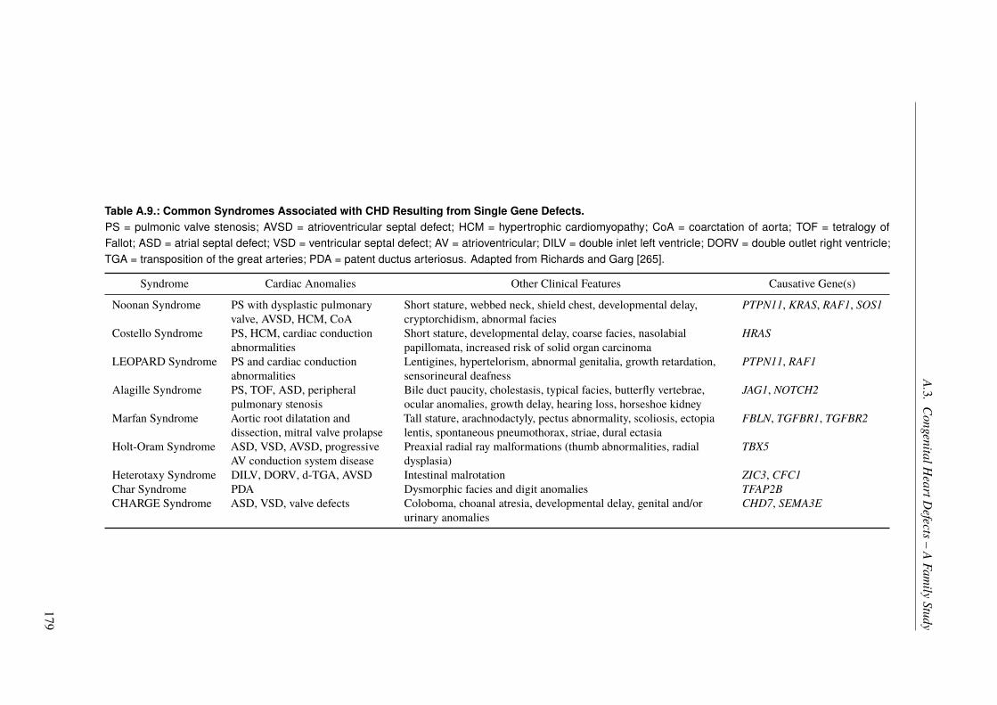
A.3.CongenitalH
eartDefects–
AFam
ilyStudy
Table A.9.: Common Syndromes Associated with CHD Resulting from Single Gene Defects.PS = pulmonic valve stenosis; AVSD = atrioventricular septal defect; HCM = hypertrophic cardiomyopathy; CoA = coarctation of aorta; TOF = tetralogy ofFallot; ASD = atrial septal defect; VSD = ventricular septal defect; AV = atrioventricular; DILV = double inlet left ventricle; DORV = double outlet right ventricle;TGA = transposition of the great arteries; PDA = patent ductus arteriosus. Adapted from Richards and Garg [265].
Syndrome Cardiac Anomalies Other Clinical Features Causative Gene(s)
Noonan Syndrome PS with dysplastic pulmonaryvalve, AVSD, HCM, CoA
Short stature, webbed neck, shield chest, developmental delay,cryptorchidism, abnormal facies
PTPN11, KRAS, RAF1, SOS1
Costello Syndrome PS, HCM, cardiac conductionabnormalities
Short stature, developmental delay, coarse facies, nasolabialpapillomata, increased risk of solid organ carcinoma
HRAS
LEOPARD Syndrome PS and cardiac conductionabnormalities
Lentigines, hypertelorism, abnormal genitalia, growth retardation,sensorineural deafness
PTPN11, RAF1
Alagille Syndrome PS, TOF, ASD, peripheralpulmonary stenosis
Bile duct paucity, cholestasis, typical facies, butterfly vertebrae,ocular anomalies, growth delay, hearing loss, horseshoe kidney
JAG1, NOTCH2
Marfan Syndrome Aortic root dilatation anddissection, mitral valve prolapse
Tall stature, arachnodactyly, pectus abnormality, scoliosis, ectopialentis, spontaneous pneumothorax, striae, dural ectasia
FBLN, TGFBR1, TGFBR2
Holt-Oram Syndrome ASD, VSD, AVSD, progressiveAV conduction system disease
Preaxial radial ray malformations (thumb abnormalities, radialdysplasia)
TBX5
Heterotaxy Syndrome DILV, DORV, d-TGA, AVSD Intestinal malrotation ZIC3, CFC1Char Syndrome PDA Dysmorphic facies and digit anomalies TFAP2BCHARGE Syndrome ASD, VSD, valve defects Coloboma, choanal atresia, developmental delay, genital and/or
urinary anomaliesCHD7, SEMA3E
179
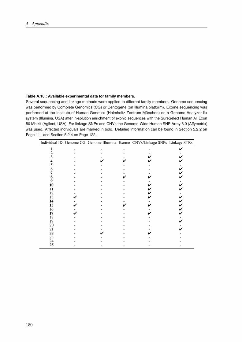
A. Appendix
Table A.10.: Available experimental data for family members.Several sequencing and linkage methods were applied to different family members. Genome sequencingwas performed by Complete Genomics (CG) or Centogene (on Illumina platform). Exome sequencing wasperformed at the Institute of Human Genetics (Helmholtz Zentrum München) on a Genome Analyzer IIxsystem (Illumina, USA) after in-solution enrichment of exonic sequences with the SureSelect Human All Exon50 Mb kit (Agilent, USA). For linkage SNPs and CNVs the Genome-Wide Human SNP Array 6.0 (Affymetrix)was used. Affected individuals are marked in bold. Detailed information can be found in Section 5.2.2 onPage 111 and Section 5.2.4 on Page 122.
Individual ID Genome CG Genome Illumina Exome CNVs/Linkage SNPs Linkage STRs1 - - - - 42 - - - - -3 - - - 4 44 - 4 4 4 45 - - - - -6 - - - - 47 - - - - 48 - - 4 4 49 - - - - -10 - - - 4 411 - - - 4 412 - - - 4 -13 4 - - 4 414 - - - - 415 4 - 4 4 416 - - - - 417 4 - - 4 418 - - - - -19 - - - - 420 - - - - -21 - - - - 422 - 4 - 4 -23 - - - - -24 - - - - -25 - - - - -
180
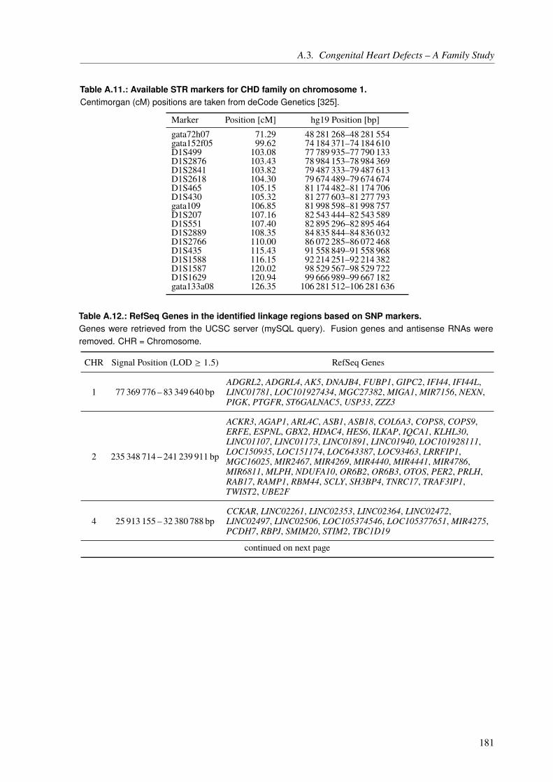
A.3. Congenital Heart Defects – A Family Study
Table A.11.: Available STR markers for CHD family on chromosome 1.Centimorgan (cM) positions are taken from deCode Genetics [325].
Marker Position [cM] hg19 Position [bp]gata72h07 71.29 48 281 268–48 281 554gata152f05 99.62 74 184 371–74 184 610D1S499 103.08 77 789 935–77 790 133D1S2876 103.43 78 984 153–78 984 369D1S2841 103.82 79 487 333–79 487 613D1S2618 104.30 79 674 489–79 674 674D1S465 105.15 81 174 482–81 174 706D1S430 105.32 81 277 603–81 277 793gata109 106.85 81 998 598–81 998 757D1S207 107.16 82 543 444–82 543 589D1S551 107.40 82 895 296–82 895 464D1S2889 108.35 84 835 844–84 836 032D1S2766 110.00 86 072 285–86 072 468D1S435 115.43 91 558 849–91 558 968D1S1588 116.15 92 214 251–92 214 382D1S1587 120.02 98 529 567–98 529 722D1S1629 120.94 99 666 989–99 667 182gata133a08 126.35 106 281 512–106 281 636
Table A.12.: RefSeq Genes in the identified linkage regions based on SNP markers.Genes were retrieved from the UCSC server (mySQL query). Fusion genes and antisense RNAs wereremoved. CHR = Chromosome.
CHR Signal Position (LOD ≥ 1.5) RefSeq Genes
1 77 369 776 – 83 349 640 bpADGRL2, ADGRL4, AK5, DNAJB4, FUBP1, GIPC2, IFI44, IFI44L,LINC01781, LOC101927434, MGC27382, MIGA1, MIR7156, NEXN,PIGK, PTGFR, ST6GALNAC5, USP33, ZZZ3
2 235 348 714 – 241 239 911 bp
ACKR3, AGAP1, ARL4C, ASB1, ASB18, COL6A3, COPS8, COPS9,ERFE, ESPNL, GBX2, HDAC4, HES6, ILKAP, IQCA1, KLHL30,LINC01107, LINC01173, LINC01891, LINC01940, LOC101928111,LOC150935, LOC151174, LOC643387, LOC93463, LRRFIP1,MGC16025, MIR2467, MIR4269, MIR4440, MIR4441, MIR4786,MIR6811, MLPH, NDUFA10, OR6B2, OR6B3, OTOS, PER2, PRLH,RAB17, RAMP1, RBM44, SCLY, SH3BP4, TNRC17, TRAF3IP1,TWIST2, UBE2F
4 25 913 155 – 32 380 788 bpCCKAR, LINC02261, LINC02353, LINC02364, LINC02472,LINC02497, LINC02506, LOC105374546, LOC105377651, MIR4275,PCDH7, RBPJ, SMIM20, STIM2, TBC1D19
continued on next page
181
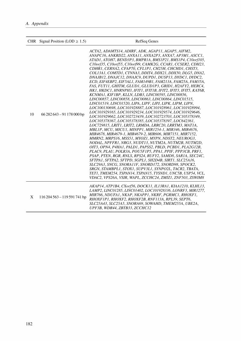
A. Appendix
CHR Signal Position (LOD ≥ 1.5) RefSeq Genes
10 66 282 643 – 91 178 000 bp
ACTA2, ADAMTS14, ADIRF, ADK, AGAP11, AGAP5, AIFM2,ANAPC16, ANKRD22, ANXA11, ANXA2P3, ANXA7, AP3M1, ASCC1,ATAD1, ATOH7, BEND3P3, BMPR1A, BMS1P21, BMS1P4, C10orf105,C10orf35, C10orf55, C10orf99, CAMK2G, CCAR1, CCSER2, CDH23,CDHR1, CERNA2, CFAP70, CFL1P1, CH25H, CHCHD1, CHST3,COL13A1, COMTD1, CTNNA3, DDIT4, DDX21, DDX50, DLG5, DNA2,DNAJB12, DNAJC12, DNAJC9, DUPD1, DUSP13, DYDC1, DYDC2,ECD, EIF4EBP2, EIF5AL1, FAM149B1, FAM213A, FAM25A, FAM35A,FAS, FUT11, GHITM, GLUD1, GLUD1P3, GRID1, H2AFY2, HERC4,HK1, HKDC1, HNRNPH3, IFIT1, IFIT1B, IFIT2, IFIT3, IFIT5, KAT6B,KCNMA1, KIF1BP, KLLN, LDB3, LINC00595, LINC00856,LINC00857, LINC00858, LINC00863, LINC00864, LINC01515,LINC01519, LINC01520, LIPA, LIPF, LIPJ, LIPK, LIPM, LIPN,LOC100130698, LOC101928887, LOC101928961, LOC101928994,LOC101929165, LOC101929234, LOC101929574, LOC101929646,LOC101929662, LOC102723439, LOC102723703, LOC105378349,LOC105378367, LOC105378385, LOC105378397, LOC642361,LOC729815, LRIT1, LRIT2, LRMDA, LRRC20, LRRTM3, MAT1A,MBL1P, MCU, MICU1, MINPP1, MIR1254-1, MIR346, MIR4676,MIR4678, MIR4679-1, MIR4679-2, MIR606, MIR7151, MIR7152,MMRN2, MRPS16, MSS51, MYOZ1, MYPN, NDST2, NEUROG3,NODAL, NPFFR1, NRG3, NUDT13, NUTM2A, NUTM2B, NUTM2D,OIT3, OPN4, P4HA1, PALD1, PAPSS2, PBLD, PCBD1, PLA2G12B,PLAC9, PLAU, POLR3A, POU5F1P5, PPA1, PPIF, PPP3CB, PRF1,PSAP, PTEN, RGR, RNLS, RPS24, RUFY2, SAMD8, SAR1A, SEC24C,SFTPA1, SFTPA2, SFTPD, SGPL1, SH2D4B, SIRT1, SLC25A16,SLC29A3, SNCG, SNORA11F, SNORD172, SNORD98, SPOCK2,SRGN, STAMBPL1, STOX1, SUPV3L1, SYNPO2L, TACR2, TBATA,TET1, TMEM254, TSPAN14, TSPAN15, TYSND1, UNC5B, USP54, VCL,VDAC2, VPS26A, VSIR, WAPL, ZCCHC24, ZMIZ1, ZNF503, ZSWIM8
X 116 204 563 – 119 591 741 bp
AKAP14, ATP1B4, CXorf56, DOCK11, IL13RA1, KIAA1210, KLHL13,LAMP2, LINC01285, LINC01402, LOC101928336, LONRF3,MIR1277,MIR766, NDUFA1, NKAP, NKAPP1, NKRF, PGRMC1, RHOXF1,RHOXF1P1, RHOXF2, RHOXF2B, RNF113A, RPL39, SEPT6,SLC25A43, SLC25A5, SNORA69, SOWAHD, TMEM255A, UBE2A,UPF3B, WDR44, ZBTB33, ZCCHC12
182
List of Figures
1.1. Cost per sequencing of an entire human genome from 2001-2015. . . . . . . 41.2. Relation of effect size and risk allele frequency. . . . . . . . . . . . . . . . . 6
2.1. The Sanger sequencing technique based on chain termination. . . . . . . . . 122.2. General workflow of the Ion AmpliSeq™ library preparation. . . . . . . . . . 162.3. General workflow of ISP Loading and Ion Torrent™ Ion PGM™ sequencing. . 172.4. Principle of semiconductor sequencing and well architecture. . . . . . . . . . 182.5. Partial primer digestion, adapter ligation, and barcoding. . . . . . . . . . . . 212.6. Quality control of Ion Sphere™ Particles after emulsion PCR. . . . . . . . . . 252.7. General structure of a molecular inversion probe (MIP). . . . . . . . . . . . . 272.8. General workflow to generate a MIP panel. . . . . . . . . . . . . . . . . . . 282.9. Details of single steps of the molecular inversion probe (MIP) workflow. . . . 292.10. MIP design displayed in the UCSC Genome Browser. . . . . . . . . . . . . . 302.11. Example of Rotor-Gene qPCR. . . . . . . . . . . . . . . . . . . . . . . . . . 352.12. Purification of the sequencing library. . . . . . . . . . . . . . . . . . . . . . 372.13. MIP coverage results after rebalancing. . . . . . . . . . . . . . . . . . . . . . 402.14. GATK best practice recommendation. . . . . . . . . . . . . . . . . . . . . . 41
3.1. Relation of effect size and risk allele frequency. . . . . . . . . . . . . . . . . 603.2. Genes and pathophysiological pathways involved in atherosclerosis. . . . . . 623.3. Candidate SNP and gene identification and prioritization pipeline. . . . . . . 643.4. Distribution of transcript coding genes within CAD loci. . . . . . . . . . . . 673.5. One CAD SNP is associated with the expression of multiple genes. . . . . . . 703.6. Tissue-specific eQTL effects in CAD loci. . . . . . . . . . . . . . . . . . . . 713.7. miRNA-binding and promoter regions. . . . . . . . . . . . . . . . . . . . . . 733.8. Comparison of the new with the previous annotations of CAD loci. . . . . . . 753.9. CAD locus 4q12 (lead SNP rs17087335) with proxy SNPs and their effects. . 773.10. Comparison of previous CAD loci annotation and with our new annotation. . 793.11. Gene reassignment based on eQTL effects. . . . . . . . . . . . . . . . . . . . 833.12. CAD locus 3p21.31 with multiple proxy SNPs and several effects. . . . . . . 85
4.1. Relation of effect size and risk allele frequency. . . . . . . . . . . . . . . . . 924.2. Rotor-Gene qPCR for captured MIPs. . . . . . . . . . . . . . . . . . . . . . 954.3. Results of the MIP panel rebalancing. . . . . . . . . . . . . . . . . . . . . . 974.4. Forest plots of genes with a Fisher’s p-value ≤ 0.05. . . . . . . . . . . . . . . 100
5.1. Relation of effect size and risk allele frequency. . . . . . . . . . . . . . . . . 1055.2. Workflow used for the family analysis. . . . . . . . . . . . . . . . . . . . . . 1095.3. Pedigree of a family with several nonsyndromic CHDs (NS-CHDs). . . . . . 1105.4. Linkage LOD score for example pedigrees. . . . . . . . . . . . . . . . . . . 1135.5. Allele sharing example. . . . . . . . . . . . . . . . . . . . . . . . . . . . . . 115
183
List of Figures
5.6. Workflow of the linkage analysis in the family. . . . . . . . . . . . . . . . . . 1175.7. Workflow of exome and genome sequencing and data analysis. . . . . . . . . 1235.8. Nonparametric linkage results for all chromosomes with LOD ≥ 1.5. . . . . . 1285.9. Chromosome 1 linkage region based on SNP and STR data. . . . . . . . . . . 1295.10. Haplotypes at the chromosome 1 linkage region based on combined SNP and
STR data. . . . . . . . . . . . . . . . . . . . . . . . . . . . . . . . . . . . . 1315.11. Filtering of variants identified by exome and genome sequencing. . . . . . . . 1345.12. Genotype status of the BMPR1A variant NM_004329.2:c.1328G>A in the
CHD family. . . . . . . . . . . . . . . . . . . . . . . . . . . . . . . . . . . . 1355.13. Segregation of the chromosome 1 linkage region and the BMPR1A c.1328G>A
variant in the analyzed family. . . . . . . . . . . . . . . . . . . . . . . . . . 1435.14. Simplified TGF-beta/BMP signaling pathway . . . . . . . . . . . . . . . . . 145
184

List of Tables
2.1. Pipetting scheme for target amplification. . . . . . . . . . . . . . . . . . . . 192.2. Number of cycles for target amplification. . . . . . . . . . . . . . . . . . . . 202.3. Barcode-Adapter mix for 2 reactions. . . . . . . . . . . . . . . . . . . . . . . 212.4. Pipetting scheme for barcode/adapter ligation. . . . . . . . . . . . . . . . . . 212.5. Pipetting scheme for the amplification solution. . . . . . . . . . . . . . . . . 242.6. Loading of an 8-well strip to enrich template-positive Ion Sphere™ Particles. . 252.7. Example of a MIP pooling scheme with multiple genes. . . . . . . . . . . . . 312.8. Pipetting scheme for MIP phosphorylation. . . . . . . . . . . . . . . . . . . 322.9. Pipetting scheme for MIP capture. . . . . . . . . . . . . . . . . . . . . . . . 332.10. Pipetting scheme for MIP exonuclease treatment. . . . . . . . . . . . . . . . 342.11. Pipetting scheme for MIP qPCR. . . . . . . . . . . . . . . . . . . . . . . . . 352.12. Pipetting scheme for MIP PCR. . . . . . . . . . . . . . . . . . . . . . . . . . 362.13. Variables used in HTS data processing. . . . . . . . . . . . . . . . . . . . . 422.14. General GATK parameters. . . . . . . . . . . . . . . . . . . . . . . . . . . . 432.15. Available “variant function” annotations from ANNOVAR. . . . . . . . . . . 512.16. Available “exonic variant function” annotations from ANNOVAR. . . . . . . 52
3.1. Predicted deleterious CAD SNPs. . . . . . . . . . . . . . . . . . . . . . . . 683.2. Proxy SNPs of rs7642590 with eQTL effects in the 3p21.31 locus. . . . . . . 693.3. eQTL effects in the 17p11.2 locus with CAD lead SNP rs4299203. . . . . . . 713.4. Gene ranking based on previous knowledge. . . . . . . . . . . . . . . . . . . 763.5. Gene ranking based on our data-driven approach. . . . . . . . . . . . . . . . 763.6. Population frequencies for SNP rs3184504 from ExAC. . . . . . . . . . . . . 83
4.1. Genes selected for panel sequencing for rare CAD variants. . . . . . . . . . . 93
5.1. Phenotypes of affected family members. . . . . . . . . . . . . . . . . . . . . 1125.2. General MERLIN parameters. . . . . . . . . . . . . . . . . . . . . . . . . . 1185.3. Ion AmpliSeq™ Designer results for TGF beta and BMP signaling pathway genes.1245.4. Nonparametric linkage results for all chromosomes with LOD ≥ 1.5. . . . . . 1275.5. Variants with CADD score > 10 in identified linkage regions. . . . . . . . . . 1375.6. Validated variants identified by panel sequencing of TGF beta and BMP
signaling pathway genes. . . . . . . . . . . . . . . . . . . . . . . . . . . . . 138
A.1. Known genome-wide significant CAD risk loci as of september 2017. . . . . 155A.2. Overview of all exonic lead and proxy SNPs. . . . . . . . . . . . . . . . . . . 158A.3. Comparison of gene assignment per CAD GWAS locus. . . . . . . . . . . . . 160A.4. Comparison of CAD genes identified by GWAS. . . . . . . . . . . . . . . . . 166A.5. Ranking scores for all CAD genes identified by our annotation. . . . . . . . . 169A.6. Rare AA-changing and splice site variants compared between CAD cases and
controls. . . . . . . . . . . . . . . . . . . . . . . . . . . . . . . . . . . . . . 173
185

List of Tables
A.7. Rare variants predicted to be deleterious compared between CAD cases andcontrols. . . . . . . . . . . . . . . . . . . . . . . . . . . . . . . . . . . . . . 175
A.8. Common Syndromes Resulting from Aneuploidy and Microdeletions. . . . . 178A.9. Common Syndromes Associated with CHD Resulting from Single Gene Defects.179A.10.Available experimental data for family members. . . . . . . . . . . . . . . . 180A.11.Available STR markers for CHD family on chromosome 1. . . . . . . . . . . 181A.12.RefSeq Genes in the identified linkage regions based on SNP markers. . . . . 181
186
List of Code Listings
2.1. BWA alignment. . . . . . . . . . . . . . . . . . . . . . . . . . . . . . . . . . 432.2. Sorting and compressing SAM file. . . . . . . . . . . . . . . . . . . . . . . . 432.3. GATK variant calling. . . . . . . . . . . . . . . . . . . . . . . . . . . . . . . 442.4. Combine sample gVCFs per interval. . . . . . . . . . . . . . . . . . . . . . . 442.5. Joint genotyping. . . . . . . . . . . . . . . . . . . . . . . . . . . . . . . . . 452.6. Merging interval VCF files from all samples. . . . . . . . . . . . . . . . . . . 452.7. Construct recalibration model for SNVs. . . . . . . . . . . . . . . . . . . . . 462.8. Apply recalibration model for SNVs. . . . . . . . . . . . . . . . . . . . . . . 472.9. Construct recalibration model for InDels. . . . . . . . . . . . . . . . . . . . 472.10. Apply recalibration model for InDels. . . . . . . . . . . . . . . . . . . . . . 48
5.1. Genotype calling from SNP array data. . . . . . . . . . . . . . . . . . . . . . 1195.2. Input file generation for MERLIN with LINKDATAGEN. . . . . . . . . . . . 1195.3. MERLIN Input data checking with PEDSTATS. . . . . . . . . . . . . . . . . 1205.4. MERLIN error detection. . . . . . . . . . . . . . . . . . . . . . . . . . . . . 1205.5. Error removal with Pedwipe. . . . . . . . . . . . . . . . . . . . . . . . . . . 1205.6. Nonparametric linkage analysis with MERLIN. . . . . . . . . . . . . . . . . 1215.7. Haplotyping with MERLIN. . . . . . . . . . . . . . . . . . . . . . . . . . . 1215.8. CNV calling. . . . . . . . . . . . . . . . . . . . . . . . . . . . . . . . . . . 122
187


List of Abbreviations
AA amino acidAS aortic stenosisASD atrial septal defectASO allele-specific oligonucleotideATP adenosine triphosphateAV atrioventricularAVSD atrioventricular septal defectBAV bicuspid aortic valveBC barcodeBED browser extensible dataBMP bone morphogenetic proteinbp base pairBWA Burrows-Wheeler Aligner◦C degree CelsiusCAD coronary artery diseaseCADD Combined Annotation Dependent DepletionCCDS Consensus CDScDNA complementary DNACDS coding sequenceCCHD critical CHDcGMP cyclic guanosine monophosphatecM centimorganCoA coarctation of aortaCHD congenital heart defectCHD coronary heart diseaseChIP chromatin immunoprecipitationCI confidence intervalCNV copy number variationDANN Deleterious Annotation of Genetic Variants using Neural NetworksdATP deoxyadenosine triphosphatedbGaP database of Genotypes and PhenotypesdbSNP Single Nucleotide Polymorphism DatabaseDCM dilated cardiomyopathydCTP deoxycytidine triphosphateddNTP dideoxynucleotides triphosphate
189

List of Abbreviations
DEPICT Data-driven Expression Prioritized Integration for Complex TraitsdGTP deoxyguanosine triphosphateDILV double inlet left ventricleDNA deoxyribonucleic acidDNM de novo mutationDNN deep neural networkdNTP deoxynucleoside triphosphateDORV double outlet right ventricleDS Down syndromedTTP deoxythymidine triphosphateEAF effect allele frequencyEDTA ethylenediaminetetraacetic acidENCODE Encyclopedia of DNA ElementsEndoMT endothelial-mesenchymal transitioneQTL expression quantitative trait locusExAC Exome Aggregation ConsortiumFDR false discovery rateFET field-effect transistorFFPE formalin-fixed paraffin-embeddedFH familial hypercholesterolemiaFunDO Functional Disease Ontologyg Acceleration due to Gravity [9.81m s−2]GB gigabyteGC guanine-cytosinegDNA genomic DNAgnomAD Genome Aggregation DatabaseGRAIL Gene Relationships Among Implicated LociGRASP Genome-Wide Repository of Associations between SNPs and PhenotypesgVCF genomic VCFGWAS genome-wide association studyGWAS genomweite Assoziationsstudieh hourH2O waterHCM hypertrophic cardiomyopathyHGMD® human gene mutation databaseHGP Human Genome ProjectHLHS hypoplastic left heart syndromeHMM Hidden Markov ModelHTS high-throughput sequencingIAA interrupted aortic arch
190

List of Abbreviations
IBD identical by descentIBS identical by stateInDel insertion or deletioniPSC induced pluripotent stem cellISFET ion-sensitive field-effect transistorISP Ion Sphere™ ParticleJPS juvenile polyposis syndromeKHK Koronare HerzkrankheitKO knockoutLD linkage disequilibriumLDL low-density lipoproteinlincRNA long intergenic noncoding RNALOD logarithm of the oddsLVNC left ventricular noncompaction cardiomyopathyM molar [mol dm−3]MAF minor allele frequencyMb megabaseMGD Mouse Genome DatabaseMI myocardial infarctionmin minuteMIP molecular inversion probemiRNA microRNAµl microliterµM micromolarmRNA messenger RNAncRNA noncoding RNAng nanogramNGS next generation sequencingNIH National Institutes of Health, USAnmol nanomoleNO nitric oxideNS-CHD nonsyndromic CHDOR odds ratioORF open reading framePCR polymerase chain reactionPDA patent ductus arteriosusPHA phytohaemagglutininPh.D. permanent head damagePolyPhen-2 Polymorphism Phenotyping v2PPS peripheral pulmonic stenosis
191

List of Abbreviations
PS pulmonic valve stenosisqPCR real-time quantitative PCRRBBB right bundle branch blockRNA ribonucleic acidrRNA ribosomal RNAs secondSCD sudden cardiac deathS-CHD syndromic CHDSIFT Sorting Intolerant From TolerantSMAD small mothers against decapentaplegicsnoRNA small nucleolar RNASNP single nucleotide polymorphismsnRNA small nuclear RNASNV single nucleotide variationSTAGE Stockholm Atherosclerosis Gene ExpressionSTR short tandem repeatSVM support vector machineT4 PNK T4 polynucleotide kinaseTE TRIS EDTATF transcription factorTFBS transcription factor binding siteTGA transposition of the great arteriesTGF-β transforming growth factor-βTOF tetralogy of FallotTRIS tris(hydroxymethyl)-aminomethantRNA transfer RNATSS transcription start siteU UnitsUCSC University of California, Santa CruzUPS universal primer siteUTR untranslated regionUV ultravioletVCF variant call formatVNTR variable number tandem repeatVQSLOD variant quality score LODVQSR variant quality score recalibrationVSD ventricular septal defectWES whole exome sequencingWGS whole genome sequencingWPW Wolff-Parkinson-White syndrome
192
Bibliography[1] Evans A., et al. The genetics of coronary heart disease: The contribution of twin studies. Twin Res.,
6(5):432–441 (2003).[2] Boomsma D., Busjahn A., and Peltonen L. Classical twin studies and beyond. Nat. Rev. Genet.,
3(11):872–882 (2002).[3] Khera A.V. and Kathiresan S. Genetics of coronary artery disease: Discovery, biology and clinical
translation. Nat. Rev. Genet., 18(6):331–344 (2017).[4] Hirschhorn J.N. and Gajdos Z.K.Z. Genome-wide association studies: Results from the first few years and
potential implications for clinical medicine. Annu. Rev. Med., 62(1):11–24 (2011).[5] Mendel G. Versuche über pflanzen-hybriden. Verhandlungen des naturforschenden Vereines in Brünn,
42:3–47 (1866).[6] Miescher F. Letter I; to Wilhelm His; Tübingen, February 26th, 1869. In W. His, et al., editor, Die
Histochemischen und Physiologischen Arbeiten von Friedrich Miescher – Aus dem WissenschaftlichenBriefwechsel von F. Miescher, volume 1, pages 33–38. Vogel (Leipzig) (1869).
[7] Miescher F. Ueber die chemische zusammensetzung der eiterzellen. Hoppe-Seyler’s medizinisch-chemischeUntersuchungen, 4:441–460 (1871).
[8] Dahm R. Friedrich miescher and the discovery of DNA. Dev. Biol., 278(2):274–288 (2005).[9] Flemming W. Zellsubstanz, Kern und Zelltheilung. Vogel (Leipzig) (1882).[10] Sutton W.S. The chromosomes in heredity. Biol. Bull., 4(5):231–250 (1903).[11] Boveri T. Ergebnisse über die Konstitution der chromatischen Substanz des Zellkerns. Von Theodor Boveri.
G. Fischer, (1904).[12] Wilson E.B. The sex chromosomes. Archiv für Mikroskopische Anatomie, 77:249–271 (1911).[13] Mohr J. A search for linkage between the lutheran blood group and other hereditary characters. Acta Pathol.
Microbiol. Scand., 28:207–210 (1951).[14] Donahue R.P., Bias W.B., Renwick J.H., and McKusick V.A. Probable assignment of the Duffy blood
group locus to chromosome 1 in man. Proc. Natl. Acad. Sci. U.S.A., 61:949–955 (1968).[15] Avery O.T., MacLeod C.M., and McCarty M. Studies on the chemical nature of the substance inducing
transformation of pneumococcal types: Induction of transformation by a desoxyribonucleic acid fractionisolated from pneumococcus type III. J. Exp. Med., 79(2):137–158 (1944).
[16] Griffith F. The significance of pneumococcal types. J. Hyg., 27:113–159 (1928).[17] Hershey A.D. and Chase M. Independent functions of viral protein and nucleic acid in growth of
bacteriophage. J. Gen. Physiol., 36:39–56 (1952).[18] Watson J.D. and Crick F.H. Molecular structure of nucleic acids; a structure for deoxyribose nucleic acid.
Nature, 171:737–738 (1953).[19] Maxam A.M. and Gilbert W. A newmethod for sequencing DNA. Proc. Natl. Acad. Sci. U.S.A., 74:560–564
(1977).[20] Sanger F., Nicklen S., and Coulson A.R. DNA sequencing with chain-terminating inhibitors. Proc. Natl.
Acad. Sci. U.S.A., 74:5463–5467 (1977).[21] Lander E.S., et al. Initial sequencing and analysis of the human genome. Nature, 409(6822):860–921
(2001).[22] Venter J.C. The sequence of the human genome. Science, 291(5507):1304–1351 (2001).[23] Consortium I.H.G.S. Finishing the euchromatic sequence of the human genome. Nature, 431(7011):931–945
(2004).[24] Heather J.M. and Chain B. The sequence of sequencers: The history of sequencing DNA. Genomics,
107(1):1–8 (2016).[25] The 1000 Genomes Project Consortium. A global reference for human genetic variation. Nature,
526(7571):68–74 (2015).[26] Lek M., et al. Analysis of protein-coding genetic variation in 60,706 humans. Nature, 536(7616):285–291
(2016).[27] Wang D.G. Large-scale identification, mapping, and genotyping of single-nucleotide polymorphisms in the
human genome. Science, 280(5366):1077–1082 (1998).[28] Visscher P.M., et al. 10 years of GWAS discovery: Biology, function, and translation. Am. J. Hum. Genet.,
101(1):5–22 (2017).[29] Ott J., Kamatani Y., and Lathrop M. Family-based designs for genome-wide association studies. Nat. Rev.
Genet., 12(7):465–474 (2011).[30] Manolio T.A., et al. Finding the missing heritability of complex diseases. Nature, 461(7265):747–753
(2009).
193

Bibliography
[31] Zondervan K.T. and Cardon L.R. Designing candidate gene and genome-wide case-control associationstudies. Nat. Protoc., 2(10):2492–2501 (2007).
[32] Altshuler D., Daly M.J., and Lander E.S. Genetic mapping in human disease. Science, 322(5903):881–888(2008).
[33] Acuna-Hidalgo R., Veltman J.A., and Hoischen A. New insights into the generation and role of de novomutations in health and disease. Genome Biol., 17(1) (2016).
[34] Roach J.C., et al. Analysis of genetic inheritance in a family quartet by whole-genome sequencing. Science,328(5978):636–639 (2010).
[35] Michaelson J.J., et al. Whole-genome sequencing in autism identifies hot spots for de novo germlinemutation. Cell, 151(7):1431–1442 (2012).
[36] Rahbari R., et al. Timing, rates and spectra of human germline mutation. Nat. Genet., 48(2):126–133(2015).
[37] Francioli L.C., et al. Genome-wide patterns and properties of de novo mutations in humans. Nat. Genet.,47(7):822–826 (2015).
[38] Goldmann J.M., et al. Parent-of-origin-specific signatures of de novo mutations. Nat. Genet., 48(8):935–939(2016).
[39] Narasimhan V.M., et al. Health and population effects of rare gene knockouts in adult humans with relatedparents. Science, 352(6284):474–477 (2016).
[40] Bell C.J., et al. Carrier testing for severe childhood recessive diseases by next-generation sequencing. Sci.Transl. Med., 3(65):65ra4–65ra4 (2011).
[41] Xue Y., et al. Deleterious- and disease-allele prevalence in healthy individuals: Insights from currentpredictions, mutation databases, and population-scale resequencing. Am. J. Hum. Genet., 91(6):1022–1032(2012).
[42] Harper A.R., Nayee S., and Topol E.J. Protective alleles and modifier variants in human health and disease.Nat. Rev. Genet., 16(12):689–701 (2015).
[43] Cooper G.M. and Shendure J. Needles in stacks of needles: Finding disease-causal variants in a wealth ofgenomic data. Nat. Rev. Genet., 12(9):628–640 (2011).
[44] Rothberg J.M., et al. An integrated semiconductor device enabling non-optical genome sequencing. Nature,475(7356):348–352 (2011).
[45] Porreca G.J., et al. Multiplex amplification of large sets of human exons. Nat. Methods, 4(11):931–936(2007).
[46] Nilsson M., Malmgren H., Samiotaki M., Kwiatkowski M., Chowdhary B.P., and Landegren U. Padlockprobes: Circularizing oligonucleotides for localized DNA detection. Science, 265(5181):2085–2088(1994).
[47] Turner E.H., Lee C., Ng S.B., Nickerson D.A., and Shendure J. Massively parallel exon capture andlibrary-free resequencing across 16 genomes. Nat. Methods, 6(5):315–316 (2009).
[48] O’Roak B.J., et al. Multiplex targeted sequencing identifies recurrently mutated genes in autism spectrumdisorders. Science, 338(6114):1619–1622 (2012).
[49] Boyle E.A., O’Roak B.J., Martin B.K., Kumar A., and Shendure J. MIPgen: Optimized modeling anddesign of molecular inversion probes for targeted resequencing. Bioinformatics, 30(18):2670–2672 (2014).
[50] Kent W.J., et al. The human genome browser at UCSC. Genome Res., 12(6):996–1006 (2002).[51] Speir M.L., et al. The UCSC genome browser database: 2016 update. Nucleic Acids Res., 44(D1):D717–
D725 (2016).[52] Yoon J.K., et al. microDuMIP: Target-enrichment technique for microarray-based duplex molecular
inversion probes. Nucleic Acids Res., 43(5):e28 (2015).[53] Mohr P.J., Newell D.B., and Taylor B.N. CODATA recommended values of the fundamental physical
constants: 2014 (2015).[54] DePristo M.A., et al. A framework for variation discovery and genotyping using next-generation DNA
sequencing data. Nat. Genet., 43:491–498 (2011).[55] Li H. Aligning sequence reads, clone sequences and assembly contigs with BWA-MEM (2013).
ArXiv:1303.3997v1 [q-bio.GN].[56] Li H., et al. The sequence alignment/map format and SAMtools. Bioinformatics, 25:2078–2079 (2009).[57] Sherry S.T. dbSNP: The NCBI database of genetic variation. Nucleic Acids Res., 29(1):308–311 (2001).[58] International HapMap Consortium. The international HapMap project. Nature, 426:789–796 (2003).[59] Mills R.E., et al. An initial map of insertion and deletion (INDEL) variation in the human genome. Genome
Res., 16:1182–1190 (2006).[60] Wang K., Li M., and Hakonarson H. ANNOVAR: Functional annotation of genetic variants from
high-throughput sequencing data. Nucleic Acids Res., 38(16):e164 (2010).[61] Pruitt K.D., et al. RefSeq: An update on mammalian reference sequences. Nucleic Acids Res., 42(D1):D756–
D763 (2014).[62] Pruitt K.D., Katz K.S., Sicotte H., and Maglott D.R. Introducing RefSeq and LocusLink: Curated human
genome resources at the NCBI. Trends Genet., 16(1):44–47 (2000).
194
Bibliography
[63] Hsu F., Kent W.J., Clawson H., Kuhn R.M., Diekhans M., and Haussler D. The UCSC known genes.Bioinformatics, 22(9):1036–1046 (2006).
[64] Flicek P., et al. Ensembl 2014. Nucleic Acids Res., 42(D1):D749–D755 (2014).[65] Harrow J., et al. GENCODE: The reference human genome annotation for the ENCODE project. Genome
Res., 22(9):1760–1774 (2012).[66] Ernst J. and Kellis M. Discovery and characterization of chromatin states for systematic annotation of the
human genome. Nat. Biotechnol., 28(8):817–825 (2010).[67] Ernst J., et al. Mapping and analysis of chromatin state dynamics in nine human cell types. Nature,
473(7345):43–49 (2011).[68] Eilbeck K., et al. The sequence ontology: A tool for the unification of genome annotations. Genome Biol.,
6(5):R44 (2005).[69] Benson D.A. GenBank. Nucleic Acids Res., 33(Database issue):D34–D38 (2004).[70] Pruitt K.D., et al. The consensus coding sequence (CCDS) project: Identifying a common protein-coding
gene set for the human and mouse genomes. Genome Res., 19(7):1316–1323 (2009).[71] Hubbard T., et al. The ensembl genome database project. Nucleic Acids Res., 30:38–41 (2002).[72] Gardner P.P., et al. Rfam: Updates to the RNA families database. Nucleic Acids Res., 37(Database):D136–
D140 (2009).[73] The UniProt Consortium. UniProt: The universal protein knowledgebase. Nucleic Acids Res., 45(D1):D158–
D169 (2016).[74] Chan P.P. and Lowe T.M. GtRNAdb: A database of transfer RNA genes detected in genomic sequence.
Nucleic Acids Res., 37(Database):D93–D97 (2009).[75] Hubisz M.J., Pollard K.S., and Siepel A. PHAST and RPHAST: Phylogenetic analysis with space/time
models. Briefings Bioinf., 12(1):41–51 (2010).[76] Bailey J.A., et al. Recent segmental duplications in the human genome. Science, 297(5583):1003–1007
(2002).[77] Gerstein M.B., et al. Architecture of the human regulatory network derived from ENCODE data. Nature,
489(7414):91–100 (2012).[78] Wang J., et al. Factorbook.org: A wiki-based database for transcription factor-binding data generated by
the ENCODE consortium. Nucleic Acids Res., 41(D1):D171–D176 (2012).[79] Wang J., et al. Sequence features and chromatin structure around the genomic regions bound by 119 human
transcription factors. Genome Res., 22(9):1798–1812 (2012).[80] Lewis B.P., Burge C.B., and Bartel D.P. Conserved seed pairing, often flanked by adenosines, indicates
that thousands of human genes are MicroRNA targets. Cell, 120(1):15–20 (2005).[81] Ambros V. The functions of animal microRNAs. Nature, 431(7006):350–355 (2004).[82] Guo H., Ingolia N.T., Weissman J.S., and Bartel D.P. Mammalian microRNAs predominantly act to
decrease target mRNA levels. Nature, 466(7308):835–840 (2010).[83] MacArthur J., et al. The new NHGRI-EBI catalog of published genome-wide association studies (GWAS
catalog). Nucleic Acids Res., 45(D1):D896–D901 (2016).[84] Finn R.D., et al. The Pfam protein families database. Nucleic Acids Res., 38(suppl_1):D211–D222 (2009).[85] Furey T.S. and Haussler D. Integration of the cytogenetic map with the draft human genome sequence.
Hum. Mol. Genet., 12:1037–1044 (2003).[86] Kumar P., Henikoff S., and Ng P.C. Predicting the effects of coding non-synonymous variants on protein
function using the SIFT algorithm. Nat. Protoc., 4(8):1073–1081 (2009).[87] Ramensky V., Bork P., and Sunyaev S. Human non-synonymous SNPs: Server and survey. Nucleic Acids
Res., 30(17):3894–3900 (2002).[88] Schwarz J.M., Cooper D.N., Schuelke M., and Seelow D. MutationTaster2: Mutation prediction for the
deep-sequencing age. Nat. Methods, 11(4):361–362 (2014).[89] Xiong H.Y., et al. The human splicing code reveals new insights into the genetic determinants of disease.
Science, 347(6218):1254806–1254806 (2014).[90] Kircher M., Witten D.M., Jain P., O’Roak B.J., Cooper G.M., and Shendure J. A general framework for
estimating the relative pathogenicity of human genetic variants. Nat. Genet., 46(3):310–315 (2014).[91] Quang D., Chen Y., and Xie X. DANN: A deep learning approach for annotating the pathogenicity of
genetic variants. Bioinformatics, 31:761–763 (2015).[92] Stenson P.D., et al. Human gene mutation database (HGMD®): 2003 update. Hum. Mutat., 21(6):577–581
(2003).[93] Landrum M.J., et al. ClinVar: Public archive of interpretations of clinically relevant variants. Nucleic
Acids Res., 44:D862–D868 (2016).[94] Ward L.D. and Kellis M. HaploReg: A resource for exploring chromatin states, conservation, and regulatory
motif alterations within sets of genetically linked variants. Nucleic Acids Res., 40(D1):D930–D934 (2011).[95] The GTEx Consortium. The genotype-tissue expression (GTEx) pilot analysis: Multitissue gene regulation
in humans. Science, 348(6235):648–660 (2015).
195

Bibliography
[96] Lozano R., et al. Global and regional mortality from 235 causes of death for 20 age groups in 1990 and2010: A systematic analysis for the global burden of disease study 2010. Lancet, 380(9859):2095–2128(2012).
[97] Nichols M., Townsend N., Scarborough P., and Rayner M. Cardiovascular disease in europe 2014:Epidemiological update. Eur. Heart J., 35(42):2950–2959 (2014).
[98] Kessler T., VilneB., and SchunkertH. The impact of genome-wide association studies on the pathophysiologyand therapy of cardiovascular disease. EMBO Mol. Med., 8(7):688–701 (2016).
[99] Wong N.D. Epidemiological studies of CHD and the evolution of preventive cardiology. Nat. Rev. Cardiol.,11(5):276–289 (2014).
[100] Khera A.V., et al. Genetic risk, adherence to a healthy lifestyle, and coronary disease. N. Engl. J. Med.,375(24):2349–2358 (2016).
[101] Mehta P.K., Wei J., and Wenger N.K. Ischemic heart disease in women: A focus on risk factors. TrendsCardiovasc. Med., 25(2):140–151 (2015).
[102] Gertler M.M. Young candidates for coronary heart disease. JAMA, 147(7):621 (1951).[103] Marenberg M.E., Risch N., Berkman L.F., Floderus B., and de Faire U. Genetic susceptibility to death
from coronary heart disease in a study of twins. N. Engl. J. Med., 330(15):1041–1046 (1994).[104] Zdravkovic S., Wienke A., Pedersen N.L., Marenberg M.E., Yashin A.I., and Faire U.D. Heritability
of death from coronary heart disease: A 36-year follow-up of 20 966 swedish twins. J. Intern. Med.,252(3):247–254 (2002).
[105] Won H.H., et al. Disproportionate contributions of select genomic compartments and cell types to geneticrisk for coronary artery disease. PLOS Genet., 11(10):e1005622 (2015).
[106] Erdmann J., et al. Dysfunctional nitric oxide signalling increases risk of myocardial infarction. Nature,504(7480):432–436 (2013).
[107] Lloyd-Jones D.M., et al. Parental cardiovascular disease as a risk factor for cardiovascular disease inmiddle-aged adults. JAMA, 291(18):2204 (2004).
[108] Murabito J.M. Sibling cardiovascular disease as a risk factor for cardiovascular disease in middle-agedadults. JAMA, 294(24):3117 (2005).
[109] Helgadottir A., et al. A common variant on chromosome 9p21 affects the risk of myocardial infarction.Science, 316(5830):1491–1493 (2007).
[110] McPherson R., et al. A common allele on chromosome 9 associated with coronary heart disease. Science,316(5830):1488–1491 (2007).
[111] Samani N.J., et al. Genomewide association analysis of coronary artery disease. N. Engl. J. Med.,357(5):443–453 (2007).
[112] Wellcome Trust Case Control Consortium. Genome-wide association study of 14,000 cases of sevencommon diseases and 3,000 shared controls. Nature, 447(7145):661–678 (2007).
[113] Holdt L.M. and Teupser D. Recent studies of the human chromosome 9p21 locus, which is associated withatherosclerosis in human populations. Arterioscler. Thromb. Vasc. Biol., 32(2):196–206 (2012).
[114] Slatkin M. Linkage disequilibrium–understanding the evolutionary past and mapping the medical future.Nat. Rev. Genet., 9:477–485 (2008).
[115] Zuk O., et al. Searching for missing heritability: Designing rare variant association studies. Proc. Natl.Acad. Sci. U.S.A., 111(4):E455–E464 (2014).
[116] Deloukas P., et al. Large-scale association analysis identifies new risk loci for coronary artery disease. Nat.Genet., 45(1):25–33 (2013).
[117] Nikpay M., et al. A comprehensive 1000 genomes–based genome-wide association meta-analysis ofcoronary artery disease. Nat. Genet., 47(10):1121–1130 (2015).
[118] Dehghan A., et al. Genome-wide association study for incident myocardial infarction and coronary heartdisease in prospective cohort studies: The CHARGE consortium. PLOS ONE, 11(3):e0144997 (2016).
[119] Nelson C.P., et al. Association analyses based on false discovery rate implicate new loci for coronary arterydisease. Nat. Genet., 49(9):1385–1391 (2017).
[120] Howson J.M.M., et al. Fifteen new risk loci for coronary artery disease highlight arterial-wall-specificmechanisms. Nat. Genet., 49(7):1113–1119 (2017).
[121] Klarin D., et al. Genetic analysis in UK biobank links insulin resistance and transendothelial migrationpathways to coronary artery disease. Nat. Genet., 49(9):1392–1397 (2017).
[122] Verweij N., Eppinga R.N., Hagemeijer Y., and van der Harst P. Identification of 15 novel risk loci forcoronary artery disease and genetic risk of recurrent events, atrial fibrillation and heart failure. Sci. Rep.,7(1) (2017).
[123] Kathiresan S., et al. Genome-wide association of early-onset myocardial infarction with single nucleotidepolymorphisms and copy number variants. Nat. Genet., 41(3):334–341 (2009).
[124] Erdmann J., et al. New susceptibility locus for coronary artery disease on chromosome 3q22.3. Nat. Genet.,41(3):280–282 (2009).
[125] Peden J.F., et al. A genome-wide association study in europeans and south asians identifies five new locifor coronary artery disease. Nat. Genet., 43(4):339–344 (2011).
196
Bibliography
[126] The IBC 50K CAD Consortium. Large-scale gene-centric analysis identifies novel variants for coronaryartery disease. PLOS Genet., 7(9):e1002260 (2011).
[127] Storey J.D. and Tibshirani R. Statistical methods for identifying differentially expressed genes in DNAmicroarrays. In Functional Genomics, pages 149–158. Humana Press (2003).
[128] Maurano M.T., et al. Systematic localization of common disease-associated variation in regulatory DNA.Science, 337(6099):1190–1195 (2012).
[129] Nicolae D.L., Gamazon E., Zhang W., Duan S., Dolan M.E., and Cox N.J. Trait-associated SNPs are morelikely to be eQTLs: Annotation to enhance discovery from GWAS. PLOS Genet., 6(4):e1000888 (2010).
[130] Schaub M.A., Boyle A.P., Kundaje A., Batzoglou S., and Snyder M. Linking disease associations withregulatory information in the human genome. Genome Res., 22(9):1748–1759 (2012).
[131] Sanyal A., Lajoie B.R., Jain G., and Dekker J. The long-range interaction landscape of gene promoters.Nature, 489(7414):109–113 (2012).
[132] Björkegren J.L.M., Kovacic J.C., Dudley J.T., and Schadt E.E. Genome-wide significant loci: Howimportant are they? J. Am. Coll. Cardiol., 65(8):830–845 (2015).
[133] Flister M.J., et al. Identifying multiple causative genes at a single GWAS locus. Genome Res., 23(12):1996–2002 (2013).
[134] Brænne I., et al. Prediction of causal candidate genes in coronary artery disease loci. Arterioscler. Thromb.Vasc. Biol., 35(10):2207–2217 (2015).
[135] Reilly M.P., et al. Identification of ADAMTS7 as a novel locus for coronary atherosclerosis and associationof ABO with myocardial infarction in the presence of coronary atherosclerosis: Two genome-wideassociation studies. Lancet, 377(9763):383–392 (2011).
[136] Wang F., et al. Genome-wide association identifies a susceptibility locus for coronary artery disease in thechinese han population. Nat. Genet., 43(4):345–349 (2011).
[137] Schunkert H., et al. Large-scale association analysis identifies 13 new susceptibility loci for coronary arterydisease. Nat. Genet., 43(4):333–338 (2011).
[138] Johnson A.D., Handsaker R.E., Pulit S.L., Nizzari M.M., O’Donnell C.J., and de Bakker P.I.W. SNAP:A web-based tool for identification and annotation of proxy SNPs using HapMap. Bioinformatics,24(24):2938–2939 (2008).
[139] Liu X., Wu C., Li C., and Boerwinkle E. dbNSFP v3.0: A one-stop database of functional predictions andannotations for human nonsynonymous and splice-site SNVs. Hum. Mutat., 37(3):235–241 (2016).
[140] Eicher J.D., et al. GRASP v2.0: An update on the genome-wide repository of associations between SNPsand phenotypes. Nucleic Acids Res., 43(D1):D799–D804 (2015).
[141] Foroughi Asl H., et al. Expression quantitative trait loci acting across multiple tissues are enriched ininherited risk for coronary artery disease. Circ. Cardiovasc. Genet., 8(2):305–315 (2015).
[142] Zhong H., et al. Liver and adipose expression associated SNPs are enriched for association to type 2diabetes. PLOS Genet., 6(5):e1000932 (2010).
[143] Rotival M., et al. Integrating genome-wide genetic variations and monocyte expression data revealstrans-regulated gene modules in humans. PLOS Genet., 7(12):e1002367 (2011).
[144] Erbilgin A., et al. Identification of CAD candidate genes in GWAS loci and their expression in vascularcells. J. Lipid Res., 54(7):1894–1905 (2013).
[145] ENCODE Project Consortium. An integrated encyclopedia of DNA elements in the human genome. Nature,489(7414):57–74 (2012).
[146] Barenboim M., Zoltick B.J., Guo Y., and Weinberger D.R. MicroSNiPer: A web tool for prediction of SNPeffects on putative microRNA targets. Hum. Mutat., 31(11):1223–1232 (2010).
[147] Raychaudhuri S., et al. Identifying relationships among genomic disease regions: Predicting genes atpathogenic SNP associations and rare deletions. PLOS Genet., 5(6):e1000534 (2009).
[148] Pers T.H., et al. Biological interpretation of genome-wide association studies using predicted gene functions.Nat. Commun., 6:5890 (2015).
[149] Eppig J.T., Blake J.A., Bult C.J., Kadin J.A., Richardson J.E., and Mouse Genome Database Group. Themouse genome database (MGD): Comprehensive resource for genetics and genomics of the laboratorymouse. Nucleic Acids Res., 40(D1):D881–D886 (2012).
[150] Osborne J.D., et al. Annotating the human genome with disease ontology. BMC Genom., 10(Suppl 1):S6(2009).
[151] Kamburov A., Stelzl U., Lehrach H., and Herwig R. The ConsensusPathDB interaction database: 2013update. Nucleic Acids Res., 41(D1):D793–D800 (2013).
[152] Ashburner M., et al. Gene Ontology: Tool for the unification of biology. Nat. Genet., 25(1):25–29 (2000).[153] GeneOntology Consortium. Gene ontology consortium: Going forward. Nucleic Acids Res., 43(D1):D1049–
D1056 (2015).[154] Ghazalpour A., et al. Hybrid mouse diversity panel: A panel of inbred mouse strains suitable for analysis
of complex genetic traits. Mamm. Genome, 23(9-10):680–692 (2012).[155] Derry J.M.J., et al. Identification of genes and networks driving cardiovascular and metabolic phenotypes
in a mouse F2 intercross. PLOS ONE, 5(12):e14319 (2010).
197
Bibliography
[156] Emilsson V., et al. Genetics of gene expression and its effect on disease. Nature, 452(7186):423–428(2008).
[157] Fehrmann R.S.N., et al. Trans-eQTLs reveal that independent genetic variants associated with a complexphenotype converge on intermediate genes, with a major role for the HLA. PLOS Genet., 7(8):e1002197(2011).
[158] Greenawalt D.M., et al. A survey of the genetics of stomach, liver, and adipose gene expression from amorbidly obese cohort. Genome Res., 21(7):1008–1016 (2011).
[159] Nica A.C., et al. The architecture of gene regulatory variation across multiple human tissues: The MuTHERstudy. PLOS Genet., 7(2):e1002003 (2011).
[160] Schadt E.E., et al. Mapping the genetic architecture of gene expression in human liver. PLOS Biol.,6(5):e107 (2008).
[161] Tu Z., et al. Integrative analysis of a cross-loci regulation network identifies App as a gene regulatinginsulin secretion from pancreatic islets. PLOS Genet., 8(12):e1003107 (2012).
[162] Wang S.S., et al. Identification of pathways for atherosclerosis in mice: Integration of quantitative traitlocus analysis and global gene expression data. Circ. Res., 101(3):e11–e30 (2007).
[163] Yang X., et al. Tissue-specific expression and regulation of sexually dimorphic genes in mice. GenomeRes., 16(8):995–1004 (2006).
[164] Wang I.M., et al. Systems analysis of eleven rodent disease models reveals an inflammatome signature andkey drivers. Mol. Syst. Biol., 8(1):594 (2012).
[165] Yang X., et al. Systematic genetic and genomic analysis of cytochrome p450 enzyme activities in humanliver. Genome Res., 20(8):1020–1036 (2010).
[166] Zhu J., et al. Integrating large-scale functional genomic data to dissect the complexity of yeast regulatorynetworks. Nat. Genet., 40(7):854–861 (2008).
[167] Dimas A.S., et al. Common regulatory variation impacts gene expression in a cell type-dependent manner.Science, 325(5945):1246–1250 (2009).
[168] Pruim R.J., et al. LocusZoom: Regional visualization of genome-wide association scan results. Bioinfor-matics, 26(18):2336–2337 (2010).
[169] Gutierrez-Arcelus M., et al. Tissue-specific effects of genetic and epigenetic variation on gene regulationand splicing. PLOS Genet., 11(1):e1004958 (2015).
[170] Global Lipids Genetics Consortium. Discovery and refinement of loci associated with lipid levels. Nat.Genet., 45(11):1274–1283 (2013).
[171] Musunuru K., et al. From noncoding variant to phenotype via SORT1 at the 1p13 cholesterol locus. Nature,466(7307):714–719 (2010).
[172] Wild P.S., et al. A genome-wide association study identifies LIPA as a susceptibility gene for coronaryartery disease. Circ. Cardiovasc. Genet., 4(4):403–412 (2011).
[173] Miller C.L., et al. Coronary heart disease-associated variation in TCF21 disrupts a miR-224 binding siteand miRNA-mediated regulation. PLOS Genet., 10(3):e1004263 (2014).
[174] Sexton T., Bantignies F., and Cavalli G. Genomic interactions: Chromatin loops and gene meeting pointsin transcriptional regulation. Semin. Cell Dev. Biol., 20(7):849–855 (2009).
[175] Krzywinski M., et al. Circos: An information aesthetic for comparative genomics. Genome Res.,19(9):1639–1645 (2009).
[176] Liu H., et al. CADgene: A comprehensive database for coronary artery disease genes. Nucleic Acids Res.,39(Database):D991–D996 (2010).
[177] Thorens B. Glucagon-like peptide-1 and control of insulin secretion. Diabete. Metab., 21(5):311–318(1995).
[178] Miyawaki K., et al. Inhibition of gastric inhibitory polypeptide signaling prevents obesity. Nat. Med.,8(7):738–742 (2002).
[179] Nasteska D., et al. Chronic reduction of GIP secretion alleviates obesity and insulin resistance underhigh-fat diet conditions. Diabetes, 63(7):2332–2343 (2014).
[180] Cheong A., et al. Downregulated REST transcription factor is a switch enabling critical potassium channelexpression and cell proliferation. Mol. Cell, 20(1):45–52 (2005).
[181] Miller C.L., et al. Disease-related growth factor and embryonic signaling pathways modulate an enhancerof TCF21 expression at the 6q23.2 coronary heart disease locus. PLOS Genet., 9(7):e1003652 (2013).
[182] Albert F.W. and Kruglyak L. The role of regulatory variation in complex traits and disease. Nat. Rev.Genet., 16(4):197–212 (2015).
[183] Smemo S., et al. Obesity-associated variants within FTO form long-range functional connections withIRX3. Nature, 507(7492):371–375 (2014).
[184] Fairfax B.P., et al. Genetics of gene expression in primary immune cells identifies cell type–specific masterregulators and roles of HLA alleles. Nat. Genet., 44(5):502–510 (2012).
[185] Dostie J. and Dekker J. Mapping networks of physical interactions between genomic elements using 5Ctechnology. Nat. Protoc., 2(4):988–1002 (2007).
198
Bibliography
[186] Dixon J.R., Gorkin D.U., and Ren B. Chromatin domains: The unit of chromosome organization. Mol.Cell, 62(5):668–680 (2016).
[187] Spielmann M. and Mundlos S. Looking beyond the genes: The role of non-coding variants in humandisease. Hum. Mol. Genet., 25(R2):R157–R165 (2016).
[188] Brown C.D., Mangravite L.M., and Engelhardt B.E. Integrative modeling of eQTLs and cis-regulatoryelements suggests mechanisms underlying cell type specificity of eQTLs. PLOS Genet., 9(8):e1003649(2013).
[189] Fu J., et al. Unraveling the regulatory mechanisms underlying tissue-dependent genetic variation of geneexpression. PLOS Genet., 8(1):e1002431 (2012).
[190] Boyle E.A., Li Y.I., and Pritchard J.K. An expanded view of complex traits: From polygenic to omnigenic.Cell, 169(7):1177–1186 (2017).
[191] Callaway E. New concerns raised over value of genome-wide disease studies. Nature, 546(7659):463–463(2017).
[192] Jarray R., et al. Depletion of the novel protein PHACTR-1 from human endothelial cells abolishes tubeformation and induces cell death receptor apoptosis. Biochimie, 93(10):1668–1675 (2011).
[193] Jarray R., et al. Disruption of phactr-1 pathway triggers pro-inflammatory and pro-atherogenic factors:New insights in atherosclerosis development. Biochimie, 118:151–161 (2015).
[194] Reschen M.E., Lin D., Chalisey A., Soilleux E.J., and O’Callaghan C.A. Genetic and environmentalrisk factors for atherosclerosis regulate transcription of phosphatase and actin regulating gene PHACTR1.Atherosclerosis, 250:95–105 (2016).
[195] Aherrahrou R., Aherrahrou Z., Schunkert H., and Erdmann J. Coronary artery disease associatedgene Phactr1 modulates severity of vascular calcification in vitro. Biochem. Biophys. Res. Commun.,491(2):396–402 (2017).
[196] Gupta R.M., et al. A genetic variant associated with five vascular diseases is a distal regulator of endothelin-1gene expression. Cell, 170(3):522–533.e15 (2017).
[197] Jonas S. and Izaurralde E. Towards a molecular understanding of microRNA-mediated gene silencing. Nat.Rev. Genet., 16(7):421–433 (2015).
[198] Morris K.V. and Mattick J.S. The rise of regulatory RNA. Nat. Rev. Genet., 15(6):423–437 (2014).[199] Sauna Z.E. and Kimchi-Sarfaty C. Synonymous mutations as a cause of human genetic disease. In eLS.
John Wiley & Sons, Ltd (2001).[200] Chen R., Davydov E.V., Sirota M., and Butte A.J. Non-synonymous and synonymous coding SNPs show
similar likelihood and effect size of human disease association. PLOS ONE, 5(10):e13574 (2010).[201] Lee D., et al. A method to predict the impact of regulatory variants from DNA sequence. Nat. Genet.,
47(8):955–961 (2015).[202] Schunkert H., et al. Repeated replication and a prospective meta-analysis of the association between
chromosome 9p21.3 and coronary artery disease. Circulation, 117(13):1675–1684 (2008).[203] Kessler T., Erdmann J., and Schunkert H. Bedeutung moderner genomstudien für das herzinfarktrisiko.
Der Internist, 55(2):141–147 (2014).[204] Trégouët D.A., et al. Genome-wide haplotype association study identifies the SLC22A3-LPAL2-LPA gene
cluster as a risk locus for coronary artery disease. Nat. Genet., 41(3):283–285 (2009).[205] Clarke R., et al. Genetic variants associated with Lp(a) lipoprotein level and coronary disease. N. Engl. J.
Med., 361(26):2518–2528 (2009).[206] Hindorff L.A., et al. Potential etiologic and functional implications of genome-wide association loci for
human diseases and traits. Proc. Natl. Acad. Sci. U.S.A., 106(23):9362–9367 (2009).[207] Kessler T., Kaess B., Bourier F., Erdmann J., and Schunkert H. Genetische analysen als basis einer
individualisierten medizin bei koronarer herzkrankheit. Herz, 39(2):186–193 (2014).[208] Dai X. Genetics of coronary artery disease and myocardial infarction. World J. Cardiol., 8(1):1 (2016).[209] Gibson G. Hints of hidden heritability in GWAS. Nat. Genet., 42(7):558–560 (2010).[210] Eichler E.E., et al. Missing heritability and strategies for finding the underlying causes of complex disease.
Nat. Rev. Genet., 11(6):446–450 (2010).[211] Brænne I., et al. Whole-exome sequencing in an extended family with myocardial infarction unmasks
familial hypercholesterolemia. BMC Cardiovascular Disorders, 14(1) (2014).[212] Brænne I., et al. Systematic analysis of variants related to familial hypercholesterolemia in families with
premature myocardial infarction. Eur. J. Hum. Genet., 24(2):191–197 (2015).[213] Do R., et al. Exome sequencing identifies rare LDLR and APOA5 alleles conferring risk for myocardial
infarction. Nature, 518(7537):102–106 (2014).[214] Stitziel N.O., et al. Exome sequencing in suspected monogenic dyslipidemias. Circ. Cardiovasc. Genet.,
8(2):343–350 (2015).[215] Kathiresan S. A PCSK9 missense variant associated with a reduced risk of early-onset myocardial infarction.
N. Engl. J. Med., 358(21):2299–2300 (2008).[216] Wu C., et al. Mechanosensitive PPAP2B regulates endothelial responses to atherorelevant hemodynamic
forces. Circ. Res., 117(4):e41–e53 (2015).
199
Bibliography
[217] Reschen M.E., et al. Lipid-induced epigenomic changes in human macrophages identify a coronary arterydisease-associated variant that regulates PPAP2B expression through altered C/EBP-beta binding. PLOSGenet., 11(4):e1005061 (2015).
[218] Anderson D.R., et al. IL-6 and its receptors in coronary artery disease and acute myocardial infarction.Cytokine, 62(3):395–400 (2013).
[219] IL6R Genetics Consortium Emerging Risk Factors Collaboration. Interleukin-6 receptor pathways incoronary heart disease: A collaborative meta-analysis of 82 studies. Lancet, 379(9822):1205–1213 (2012).
[220] Stein E.A., et al. Effect of a monoclonal antibody to PCSK9, REGN727/SAR236553, to reduce low-densitylipoprotein cholesterol in patients with heterozygous familial hypercholesterolaemia on stable statin dosewith or without ezetimibe therapy: A phase 2 randomised controlled trial. Lancet, 380(9836):29–36 (2012).
[221] Oram J.F. and Vaughan A.M. ATP-binding cassette cholesterol transporters and cardiovascular disease.Circ. Res., 99(10):1031–1043 (2006).
[222] Yu Q., Zhang Y., and Xu C.B. Apolipoprotein B, the villain in the drama? Eur. J. Pharmacol., 748:166–169(2015).
[223] O'Donnell C.J., et al. Genome-wide association study for coronary artery calcification with follow-up inmyocardial infarction. Circulation, 124(25):2855–2864 (2011).
[224] Dichgans M., et al. Shared genetic susceptibility to ischemic stroke and coronary artery disease: Agenome-wide analysis of common variants. Stroke, 45(1):24–36 (2013).
[225] Schaefer A.S., et al. Genetic evidence for PLASMINOGEN as a shared genetic risk factor of coronaryartery disease and periodontitis. Circ. Cardiovasc. Genet., 8(1):159–167 (2014).
[226] Turner A.W. and McPherson R. PHACTR1: Functional clues linking a genome-wide association studylocus to coronary artery disease. Arterioscler. Thromb. Vasc. Biol., 35(6):1293–1295 (2015).
[227] Azghandi S., et al. Deficiency of the stroke relevant HDAC9 gene attenuates atherosclerosis in accord withallele-specific effects at 7p21.1. Stroke, 46(1):197–202 (2014).
[228] Douvris A., et al. Functional analysis of the TRIB1 associated locus linked to plasma triglycerides andcoronary artery disease. J. Am. Heart Assoc., 3(3):e000884–e000884 (2014).
[229] Li Y., et al. Lipoprotein lipase: From gene to atherosclerosis. Atherosclerosis, 237(2):597–608 (2014).[230] Döring Y., Pawig L., Weber C., and Noels H. The CXCL12/CXCR4 chemokine ligand/receptor axis in
cardiovascular disease. Front. Physiol., 5 (2014).[231] HuangY., et al. An abundant dysfunctional apolipoprotein A1 in human atheroma. Nat.Med., 20(2):193–203
(2014).[232] Hsu J. and Smith J.D. Genome-wide studies of gene expression relevant to coronary artery disease. Curr.
Opin. Cardiol., 27(3):210–213 (2012).[233] Kessler T., et al. ADAMTS-7 inhibits re-endothelialization of injured arteries and promotes vascular
remodeling through cleavage of thrombospondin-1. Circulation, 131(13):1191–1201 (2015).[234] Bauer R.C., et al. Knockout of Adamts7, a novel coronary artery disease locus in humans, reduces
atherosclerosis in mice. Circulation, 131(13):1202–1213 (2015).[235] Brautbar A., Leary E., Rasmussen K., Wilson D.P., Steiner R.D., and Virani S. Genetics of familial
hypercholesterolemia. Curr. Atheroscler. Rep., 17(4) (2015).[236] Piedrahita J.A., Zhang S.H., Hagaman J.R., Oliver P.M., and Maeda N. Generation of mice carrying a
mutant apolipoprotein E gene inactivated by gene targeting in embryonic stem cells. Proc. Natl. Acad. Sci.U.S.A., 89(10):4471–4475 (1992).
[237] Westerterp M., et al. Apolipoprotein C-I is crucially involved in lipopolysaccharide-induced atherosclerosisdevelopment in apolipoprotein E knockout mice. Circulation, 116(19):2173–2181 (2007).
[238] Plump A.S., et al. Severe hypercholesterolemia and atherosclerosis in apolipoprotein E-deficient micecreated by homologous recombination in ES cells. Cell, 71(2):343–353 (1992).
[239] Wobst J., Kessler T., Dang T.A., Erdmann J., and Schunkert H. Role of sGC-dependent NO signalling andmyocardial infarction risk. J. Mol. Med., 93(4):383–394 (2015).
[240] Wobst J., Rumpf P.M., Dang T.A., Segura-Puimedon M., Erdmann J., and Schunkert H. Molecular variantsof soluble guanylyl cyclase affecting cardiovascular risk. Circ. J., 79(3):463–469 (2015).
[241] Mailman M.D., et al. The NCBI dbGaP database of genotypes and phenotypes. Nat. Genet., 39(10) (2007).[242] Stessman H.A.F., et al. Targeted sequencing identifies 91 neurodevelopmental-disorder risk genes with
autism and developmental-disability biases. Nat. Genet., 49(4):515–526 (2017).[243] Zhang J., et al. A molecular inversion probe-based next-generation sequencing panel to detect germline
mutations in chinese early-onset colorectal cancer patients. Oncotarget (2017).[244] Brænne I., et al. Genomic correlates of glatiramer acetate adverse cardiovascular effects lead to a novel
locus mediating coronary risk. PLOS ONE, 12(8):e0182999 (2017).[245] Grainger D. TGF-β and atherosclerosis in man. Cardiovasc. Res., 74(2):213–222 (2007).[246] Mallat Z. and Tedgui A. The role of transforming growth factor beta in atherosclerosis: Novel insights and
future perspectives. Curr. Opin. Lipidol., 13(5):523–529 (2002).[247] Grainger D.J. Transforming growth factor and atherosclerosis: So far, so good for the protective cytokine
hypothesis. Arterioscler. Thromb. Vasc. Biol., 24(3):399–404 (2003).
200
Bibliography
[248] Bobik A. Transforming growth factor-βs and vascular disorders. Arterioscler. Thromb. Vasc. Biol.,26(8):1712–1720 (2006).
[249] Lu Y., et al. TGFB1 genetic polymorphisms and coronary heart disease risk: A meta-analysis. BMCMedical Genetics, 13(1) (2012).
[250] Wang X.L., Liu S.X., and Wilcken D.E. Circulating transforming growth factor β1 and coronary arterydisease. Cardiovasc. Res., 34(2):404–410 (1997).
[251] duo Zhang M., Gu W., bin Qiao S., jun Zhu E., ming Zhao Q., and zheng Lv S. Apolipoprotein E genepolymorphism and risk for coronary heart disease in the chinese population: A meta-analysis of 61 studiesincluding 6634 cases and 6393 controls. PLOS ONE, 9(4):e95463 (2014).
[252] Ehret G.B., et al. Genetic variants in novel pathways influence blood pressure and cardiovascular diseaserisk. Nature, 478(7367):103–109 (2011).
[253] Kanda. Downregulation of the c-Fes protein-tyrosine kinase inhibits the proliferation of human renalcarcinoma cells. Int. J. Oncol. (1992).
[254] Hoffman J.I.E. and Kaplan S. The incidence of congenital heart disease. J. Am. Coll. Cardiol., 39:1890–1900(2002).
[255] van der Linde D., et al. Birth prevalence of congenital heart disease worldwide. J. Am. Coll. Cardiol.,58(21):2241–2247 (2011).
[256] Knowles R., Griebsch I., Dezateux C., Brown J., Bull C., and Wren C. Newborn screening for congenitalheart defects: A systematic review and cost-effectiveness analysis. Health Technol. Assess., 9:1–152, iii–iv(2005).
[257] Oster M.E., Lee K.A., Honein M.A., Riehle-Colarusso T., Shin M., and Correa A. Temporal trends insurvival among infants with critical congenital heart defects. Pediatrics, 131(5):e1502–e1508 (2013).
[258] Bonnet D., et al. Detection of transposition of the great arteries in fetuses reduces neonatal morbidity andmortality. Circulation, 99(7):916–918 (1999).
[259] Wren C., Reinhardt Z., and Khawaja K. Twenty-year trends in diagnosis of life-threatening neonatalcardiovascular malformations. Arch. Dis. Child. Fetal Neonatal Ed., 93(1):F33–F35 (2008).
[260] Ferencz C., Loffredo C., Correa-Villasenor A., and Wilson D. Genetic and Environmental Risk Factorsof Major Cardiovascular Malformations: The baltimore-washington Infant Study: 1981-1989. Wiley-Blackwell (1997).
[261] Bruneau B.G. The developmental genetics of congenital heart disease. Nature, 451(7181):943–948 (2008).[262] World Health Organization. Global Atlas on Cardiovascular Disease Prevention and Control. World
Health Organization (2012).[263] Digilio M.C. and Marino B. What is new in genetics of congenital heart defects? Front. Pediatr., 4 (2016).[264] Sifrim A., et al. Distinct genetic architectures for syndromic and nonsyndromic congenital heart defects
identified by exome sequencing. Nat. Genet., 48(9):1060–1065 (2016).[265] Richards A.A. and Garg V. Genetics of congenital heart disease. Curr. Cardiol. Rev., 6(2):91–97 (2010).[266] Pierpont M.E., et al. Genetic basis for congenital heart defects: Current knowledge: A scientific statement
from the american heart association congenital cardiac defects committee, council on cardiovascular diseasein the young: Endorsed by the american academy of pediatrics. Circulation, 115(23):3015–3038 (2007).
[267] Marino B. and Digilio M.C. Congenital heart disease and genetic syndromes: Specific correlation betweencardiac phenotype and genotype. Cardiovasc. Pathol., 9:303–315 (2000).
[268] Cremer K., Lüdecke H.J., Ruhr F., and Wieczorek D. Left-ventricular non-compaction (LVNC): A clinicalfeature more often observed in terminal deletion 1p36 than previously expected. Eur. J. Med. Genet.,51:685–688 (2008).
[269] Digilio M.C., et al. Congenital heart defects in recurrent reciprocal 1q21.1 deletion and duplicationsyndromes: Rare association with pulmonary valve stenosis. Eur. J. Med. Genet., 56(3):144–149 (2013).
[270] de La Rochebrochard C., et al. The intrafamilial variability of the 22q11.2 microduplication encompasses aspectrum from minor cognitive deficits to severe congenital anomalies. Am. J. Med. Genet. A., 140:1608–1613 (2006).
[271] Fagerberg C.R., et al. Heart defects and other features of the 22q11 distal deletion syndrome. Eur. J. Med.Genet., 56:98–107 (2013).
[272] Ben-Shachar S., et al. 22q11.2 distal deletion: A recurrent genomic disorder distinct from digeorgesyndrome and velocardiofacial syndrome. Am. J. Hum. Genet., 82:214–221 (2008).
[273] Portnoï M.F. Microduplication 22q11.2: A new chromosomal syndrome. Eur. J. Med. Genet., 52:88–93(2009).
[274] Mefford H.C., et al. Recurrent rearrangements of chromosome 1q21.1 and variable pediatric phenotypes.N. Engl. J. Med., 359:1685–1699 (2008).
[275] Battaglia A., et al. Further delineation of deletion 1p36 syndrome in 60 patients: a recognizable phenotypeand common cause of developmental delay and mental retardation. Pediatrics, 121:404–410 (2008).
[276] Digilio M., Marino B., Sarkozy A., Versacci P., and Dallapiccola B. The heart in Ras-MAPK pathwaydisorders. In M. Zenker, editor, Noonan Syndrome and Related Disorders - A Matter of Deregulated RasSignaling, volume 17 of Monographs in Human Genetics, pages 109–118. S. Karger (2009).
201
Bibliography
[277] Digilio M.C., et al. Atrioventricular canal defect in patients with RASopathies. Eur. J. Hum. Genet.,21(2):200–204 (2012).
[278] Roberts A.E., Allanson J.E., Tartaglia M., and Gelb B.D. Noonan syndrome. Lancet, 381:333–342 (2013).[279] Nora J.J. Multifactorial inheritance hypothesis for the etiology of congenital heart diseases. the genetic-
environmental interaction. Circulation, 38(3):604–617 (1968).[280] Syamasundar P. Congenital heart defects – a review. In Congenital Heart Disease - Selected Aspects.
InTech (2012).[281] Gill H.K., Splitt M., Sharland G.K., and Simpson J.M. Patterns of recurrence of congenital heart disease. J.
Am. Coll. Cardiol., 42(5):923–929 (2003).[282] Schulkey C.E., et al. The maternal-age-associated risk of congenital heart disease is modifiable. Nature,
520(7546):230–233 (2015).[283] Li Y., et al. Global genetic analysis in mice unveils central role for cilia in congenital heart disease. Nature,
521(7553):520–524 (2015).[284] Oyen N., Poulsen G., Boyd H.A., Wohlfahrt J., Jensen P.K.A., and Melbye M. Recurrence of congenital
heart defects in families. Circulation, 120(4):295–301 (2009).[285] Payne A.R., Chang S.W., Koenig S.N., Zinn A.R., and Garg V. Submicroscopic chromosomal copy number
variations identified in children with hypoplastic left heart syndrome. Pediatr. Cardiol., 33(5):757–763(2012).
[286] Goldmuntz E., Geiger E., and Benson D.W. NKX2.5 mutations in patients with tetralogy of fallot.Circulation, 104(21):2565–2568 (2001).
[287] Elliott D.A., et al. Cardiac homeobox gene NKX2-5mutations and congenital heart disease. J. Am. Coll.Cardiol., 41(11):2072–2076 (2003).
[288] Garg V., et al. GATA4 mutations cause human congenital heart defects and reveal an interaction withTBX5. Nature, 424(6947):443–447 (2003).
[289] Iascone M., et al. Identification of de novo mutations and rare variants in hypoplastic left heart syndrome.Clin. Genet., 81(6):542–554 (2011).
[290] Rauch R., et al. Comprehensive genotype-phenotype analysis in 230 patients with tetralogy of fallot. J.Med. Genet., 47(5):321–331 (2009).
[291] Wessels M. and Willems P. Genetic factors in non-syndromic congenital heart malformations. Clin. Genet.,78(2):103–123 (2010).
[292] Silversides C.K., et al. Rare copy number variations in adults with tetralogy of fallot implicate novel riskgene pathways. PLOS Genet., 8(8):e1002843 (2012).
[293] Soemedi R., et al. Contribution of global rare copy-number variants to the risk of sporadic congenital heartdisease. Am. J. Hum. Genet., 91(3):489–501 (2012).
[294] Hitz M.P., et al. Rare copy number variants contribute to congenital left-sided heart disease. PLOS Genet.,8(9):e1002903 (2012).
[295] Priest J.R., Girirajan S., Vu T.H., Olson A., Eichler E.E., and Portman M.A. Rare copy number variants inisolated sporadic and syndromic atrioventricular septal defects. Am. J. Med. Genet. A., 158A(6):1279–1284(2012).
[296] Schunkert H., Bröckel U., Kromer E.P., Elsner D., Jacob H.J., and Riegger G.A. A large pedigree withvalvuloseptal defects. Am. J. Cardiol., 80(7):968–970 (1997).
[297] Eisenberg L.M. and Markwald R.R. Molecular regulation of atrioventricular valvuloseptal morphogenesis.Circ. Res., 77(1):1–6 (1995).
[298] Calkoen E.E., et al. Atrioventricular septal defect: From embryonic development to long-term follow-up.Int. J. Cardiol., 202:784–795 (2016).
[299] Briggs L.E., Kakarla J., and Wessels A. The pathogenesis of atrial and atrioventricular septal defects withspecial emphasis on the role of the dorsal mesenchymal protrusion. Differentiation, 84(1):117–130 (2012).
[300] Kruithof B.P., Duim S.N., Moerkamp A.T., and Goumans M.J. TGFβ and BMP signaling in cardiaccushion formation: Lessons from mice and chicken. Differentiation, 84(1):89–102 (2012).
[301] John J., Abrol S., Sadiq A., and Shani J. Mixed atrial septal defect coexisting ostium secundum and sinusvenosus atrial septal defect. J. Am. Coll. Cardiol., 58:e9 (2011).
[302] Craig B. Atrioventricular septal defect: From fetus to adult. Heart, 92:1879–1885 (2006).[303] Berger T.J., Blackstone E.H., Kirklin J.W., Bargeron L.M., Hazelrig J.B., and Turner M.E. Survival and
probability of cure without and with operation in complete atrioventricular canal. Ann. Thorac. Surg.,27:104–111 (1979).
[304] Ebstein W. Über einen sehr seltenen Fall von Insufficienz der Valvula tricuspidalis, bedingt durch eineangeborene hochgradige Missbildung derselben. Veit (1866).
[305] Lupo P.J., Langlois P.H., and Mitchell L.E. Epidemiology of ebstein anomaly: Prevalence and patterns intexas, 1999-2005. Am. J. Med. Genet. A., 155(5):1007–1014 (2011).
[306] Correa-Villaseñor A., Ferencz C., Neill C.A., Wilson P.D., and and J.A.B. Ebstein’s malformation of thetricuspid valve: Genetic and environmental factors. Teratology, 50(2):137–147 (1994).
202
Bibliography
[307] Celermajer D.S., et al. Ebstein’s anomaly: Presentation and outcome from fetus to adult. J. Am. Coll.Cardiol., 23(1):170–176 (1994).
[308] Mathew S.T., Matthew S.T., Federico G.F., and Singh B.K. Ebstein’s anomaly presenting as wolff-parkinsonwhite syndrome in a postpartum patient. Cardiol. Rev., 11(4):208–210 (2003).
[309] Da Costa D., Brady W.J., and Edhouse J. Bradycardias and atrioventricular conduction block. BMJ,324(7336):535–538 (2002).
[310] Sung R.J., Tamer D.M., Agha A.S., Castellanos A., Myerburg R.J., and Gelband H. Etiology ofthe electrocardiographic pattern of "incomplete right bundle branch block" in atrial septal defect: anelectrophysiologic study. J. Pediatr., 87:1182–1186 (1975).
[311] Minette M.S. and Sahn D.J. Ventricular septal defects. Circulation, 114(20):2190–2197 (2006).[312] Wilson F.N. A case in which the vagus influenced the form of the ventricular complex of the electrocardio-
gram. Arch. Intern. Med., XVI(6):1008 (1915).[313] Wolff L., Parkinson J., and White P.D. Bundle-branch block with short P-R interval in healthy young
people prone to paroxysmal tachycardia. Am. Heart J., 5(6):685–704 (1930).[314] Torner Montoya P., et al. Ventricular fibrillation in the wolff-parkinson-white syndrome. Eur. Heart J.,
12:144–150 (1991).[315] Kim S.S. and Knight B.P. Long term risk of wolff-parkinson-white pattern and syndrome. Trends
Cardiovasc. Med., 27:260–268 (2017).[316] MORTON N.E. Sequential tests for the detection of linkage. Am. J. Hum. Genet., 7:277–318 (1955).[317] Pulst S.M. Genetic linkage analysis. Arch. Neurol., 56:667–672 (1999).[318] Pearson K. On the criterion that a given system of deviations from the probable in the case of a correlated
system of variables is such that it can be reasonably supposed to have arisen from random sampling. Philos.Mag., 50(302):157–175 (1900).
[319] Kong A. and Cox N.J. Allele-sharing models: LOD scores and accurate linkage tests. Am. J. Hum. Genet.,61:1179–1188 (1997).
[320] Tautz D. and Schlötterer. Simple sequences. Curr. Opin. Genet. Dev., 4:832–837 (1994).[321] Weber J.L. and Wong C. Mutation of human short tandem repeats. Hum. Mol. Genet., 2:1123–1128 (1993).[322] Klintschar M., et al. Haplotype studies support slippage as the mechanism of germline mutations in short
tandem repeats. Electrophoresis, 25:3344–3348 (2004).[323] Brouwer J.R., Willemsen R., and Oostra B.A. Microsatellite repeat instability and neurological disease.
Bioessays, 31:71–83 (2009).[324] Broeckel U., Simon J., Kwitek-Black A., Jacob H., Rieggert G., and Schunkert H. Suggestive linkage of
ebstein’s anomaly and concomitant valvuloseptal defects to chromosome 1. Eur. Heart J., 19(AbstractSupplement):485 (1998). Conference Abstract.
[325] Kong A., et al. Fine-scale recombination rate differences between sexes, populations and individuals.Nature, 467:1099–1103 (2010).
[326] Bahlo M. and Bromhead C.J. Generating linkage mapping files from affymetrix SNP chip data. Bioinfor-matics, 25(15):1961–1962 (2009).
[327] Abecasis G.R., Cherny S.S., Cookson W.O., and Cardon L.R. Merlin–rapid analysis of dense genetic mapsusing sparse gene flow trees. Nat. Genet., 30:97–101 (2002).
[328] Thiele H. and Nürnberg P. HaploPainter: A tool for drawing pedigrees with complex haplotypes.Bioinformatics, 21:1730–1732 (2005).
[329] Wigginton J.E. and Abecasis G.R. PEDSTATS: Descriptive statistics, graphics and quality assessment forgene mapping data. Bioinformatics, 21:3445–3447 (2005).
[330] Pâques F. and Haber J.E. Multiple pathways of recombination induced by double-strand breaks insaccharomyces cerevisiae. Microbiol. Mol. Biol. Rev., 63:349–404 (1999).
[331] Carr I.M., et al. Rapid visualisation of microarray copy number data for the detection of structural variationslinked to a disease phenotype. PLOS ONE, 7:e43466 (2012).
[332] Do L.D., et al. Characteristics in limbic encephalitis with anti–adenylate kinase 5 autoantibodies. Neurology,88(6):514–524 (2017).
[333] Lai Y., Hu X., Chen G., Wang X., and Zhu B. Down-regulation of adenylate kinase 5 in temporal lobeepilepsy patients and rat model. J. Neurol. Sci., 366:20–26 (2016).
[334] Al-Aama J.Y., et al. Whole exome sequencing of a consanguineous family identifies the possible modifyingeffect of a globally rare AK5 allelic variant in celiac disease development among saudi patients. PLOSONE, 12(5):e0176664 (2017).
[335] Dzeja P.P., Chung S., Faustino R.S., Behfar A., and Terzic A. Developmental enhancement of adenylatekinase-AMPK metabolic signaling axis supports stem cell cardiac differentiation. PLOS ONE, 6(4):e19300(2011).
[336] Hoe K.L., et al. Isolation of a new member of DnaJ-like heat shock protein 40 (hsp40) from human liver.Biochim. Biophys. Acta, 1383(1):4–8 (1998).
[337] Simões-Correia J., et al. DNAJB4 molecular chaperone distinguishes WT from mutant e-cadherin,determining their fate in vitro and in vivo. Hum. Mol. Genet., 23(8):2094–2105 (2013).
203
Bibliography
[338] Albini A. and Pfeffer U. A new tumor suppressor gene: Invasion, metastasis, and angiogenesis as potentialkey targets. J. Natl. Cancer Inst., 98(12):800–801 (2006).
[339] Acun T., et al. HLJ1 (DNAJB4) gene is a novel biomarker candidate in breast cancer. OMICS, 21(5):257–265(2017).
[340] Liu Y., et al. HLJ1 is a novel biomarker for colorectal carcinoma progression and overall patient survival.Int. J. Clin. Exp. Path., 7(3):969–977 (2014).
[341] Komotar R.J., Starke R.M., Sisti M.B., and Connolly E. CIC and FUBP1 mutations in oligodendroglioma.Neurosurgery, 70(6):N22–N23 (2012).
[342] Jang M., et al. Far upstream element-binding protein-1, a novel caspase substrate, acts as a cross-talkerbetween apoptosis and the c-myc oncogene. Oncogene, 28(12):1529–1536 (2009).
[343] Duan J., et al. Upregulation of far upstream element-binding protein 1 (FUBP1) promotes tumor proliferationand tumorigenesis of clear cell renal cell carcinoma. PLOS ONE, 12(1):e0169852 (2017).
[344] Katoh M. GIPC gene family (review). Int. J. Mol. Med. (2002).[345] Sánchez N.S., et al. The cytoplasmic domain of TGFβR3 through its interaction with the scaffolding
protein, GIPC, directs epicardial cell behavior. Dev. Biol., 358(2):331–343 (2011).[346] von Gise A. and Pu W.T. Endocardial and epicardial epithelial to mesenchymal transitions in heart
development and disease. Circ. Res., 110(12):1628–1645 (2012).[347] Townsend T.A., Robinson J.Y., How T., DeLaughter D.M., Blobe G.C., and Barnett J.V. Endocardial
cell epithelial-mesenchymal transformation requires type III TGFβ receptor interaction with GIPC. Cell.Signalling, 24(1):247–256 (2012).
[348] Blobe G.C., Liu X., Fang S.J., How T., and Lodish H.F. A novel mechanism for regulating transforminggrowth factor β (TGF-β) signaling. J. Biol. Chem., 276(43):39608–39617 (2001).
[349] Zhang Y., et al. Mitoguardin regulates mitochondrial fusion through MitoPLD and is required for neuronalhomeostasis. Mol. Cell, 61(1):111–124 (2016).
[350] Liu X.M., et al. Mitoguardin-1 and -2 promote maturation and the developmental potential of mouseoocytes by maintaining mitochondrial dynamics and functions. Oncotarget, 7(2):1155–1167 (2015).
[351] Aherrahrou Z., et al. Knock-out of nexilin in mice leads to dilated cardiomyopathy and endomyocardialfibroelastosis. Basic Res. Cardiol., 111(1) (2015).
[352] Soni S., et al. A proteomics approach to identify new putative cardiac intercalated disk proteins. PLOSONE, 11(5):e0152231 (2016).
[353] Hassel D., et al. Nexilin mutations destabilize cardiac Z-disks and lead to dilated cardiomyopathy. Nat.Med., 15(11):1281–1288 (2009).
[354] Waldmüller S., et al. Targeted 46-gene and clinical exome sequencing for mutations causing cardiomy-opathies. Mol. Cell. Probes, 29(5):308–314 (2015).
[355] Wang H., et al. Mutations in NEXN, a Z-disc gene, are associated with hypertrophic cardiomyopathy. Am.J. Hum. Genet., 87(5):687–693 (2010).
[356] Yang F., et al. NEXN inhibits GATA4 and leads to atrial septal defects in mice and humans. Cardiovasc.Res., 103(2):228–237 (2014).
[357] Pardun E., Wenzel K., Kramer H.H., Berger F., Gerull B., and Klaassen S. Nexilin mutations are associatedwith left ventricular noncompaction cardiomyopathy. Mol. Cell. Pediatr., 2(Suppl 1):A7 (2015).
[358] Kim S.O., Markosyan N., Pepe G.J., and Duffy D.M. Estrogen promotes luteolysis by redistributingprostaglandin F2 receptors within primate luteal cells. Reproduction, 149(5):453–464 (2015).
[359] Kaczynski P., Kowalewski M., and Waclawik A. Prostaglandin F2α promotes angiogenesis and em-bryo–maternal interactions during implantation. Reproduction, 151(5):539–552 (2016).
[360] Sakurai M., Higashide T., Ohkubo S., Takeda H., and Sugiyama K. Association between geneticpolymorphisms of the prostaglandin F2α receptor gene, and response to latanoprost in patients withglaucoma and ocular hypertension. Br. J. Ophthalmol., 98(4):469–473 (2014).
[361] Cui X.J., Zhao A.G., and Wang X.L. Correlations of AFAP1, GMDS and PTGFR gene polymorphismswith intra-ocular pressure response to latanoprost in patients with primary open-angle glaucoma. J. Clin.Pharm. Ther., 42(1):87–92 (2016).
[362] Goupil E., et al. Angiotensin II type I and prostaglandin F2α receptors cooperatively modulate signaling invascular smooth muscle cells. J. Biol. Chem., 290(5):3137–3148 (2014).
[363] Keightley M.C., Brown P., Jabbour H.N., and Sales K.J. F-Prostaglandin receptor regulates endothelial cellfunction via fibroblast growth factor-2. BMC Cell Biol., 11(1):8 (2010).
[364] Xiao B., et al. Rare SNP rs12731181 in the miR-590-3p target site of the prostaglandin F2α receptor geneconfers risk for essential hypertension in the han chinese population. Arterioscler. Thromb. Vasc. Biol.,35(7):1687–1695 (2015).
[365] Shenoy S.K. Deubiquitinases and their emerging roles in β-arrestin-mediated signaling. In Methods inEnzymology, pages 351–370. Elsevier (2014).
[366] Cheng Q., et al. Deubiquitinase USP33 is negatively regulated by β-TrCP through ubiquitin-dependentproteolysis. Exp. Cell. Res. (2017).
204
Bibliography
[367] Wen P., et al. USP33, a new player in lung cancer, mediates slit-robo signaling. Protein & Cell, 5(9):704–713(2014).
[368] Huang Z., et al. USP33 mediates slit-robo signaling in inhibiting colorectal cancer cell migration. Int. J.Cancer, 136(8):1792–1802 (2014).
[369] Yuasa-Kawada J., Kinoshita-Kawada M., Rao Y., and Wu J.Y. Deubiquitinating enzyme USP33/VDU1is required for slit signaling in inhibiting breast cancer cell migration. Proc. Natl. Acad. Sci. U.S.A.,106(34):14530–14535 (2009).
[370] Evans D.M. and Cardon L.R. Guidelines for genotyping in genomewide linkage studies: Single-nucleotide–polymorphism maps versus microsatellite maps. Am. J. Hum. Genet., 75(4):687–692 (2004).
[371] Guo X. and Elston R. Linkage information content of polymorphic genetic markers. Hum. Hered.,49(2):112–118 (1999).
[372] Guo X., Olson J.M., Elston R.C., and Niu T. The linkage information content value of polymorphismgenetic markers in model-free linkage analysis. Hum. Hered., 53(1):45–48 (2002).
[373] Azhar M., et al. Transforming growth factor beta in cardiovascular development and function. CytokineGrowth Factor Rev., 14(5):391–407 (2003).
[374] Arthur H.M. and Bamforth S.D. TGFβ signaling and congenital heart disease: Insights from mouse studies.Birt. Defects Res. A. Clin. Mol. Teratol., 91(6):423–434 (2011).
[375] Monzen K., et al. Bone morphogenetic proteins induce cardiomyocyte differentiation through the mitogen-activated protein kinase kinase kinase TAK1 and cardiac transcription factors Csx/Nkx-2.5 and GATA-4.Mol. Cell. Biol., 19(10):7096–7105 (1999).
[376] Rivera-Feliciano J. Development of heart valves requires Gata4 expression in endothelial-derived cells.Development, 133(18):3607–3618 (2006).
[377] Moskowitz I.P., et al. Transcription factor genes Smad4 and Gata4 cooperatively regulate cardiac valvedevelopment. Proc. Natl. Acad. Sci. U.S.A., 108(10):4006–4011 (2011).
[378] Tomita-Mitchell A., Maslen C.L., Morris C.D., Garg V., and Goldmuntz E. GATA4 sequence variants inpatients with congenital heart disease. J. Med. Genet., 44(12):779–783 (2007).
[379] Sarkozy A. Spectrum of atrial septal defects associated with mutations of NKX2.5 and GATA4 transcriptionfactors. J. Med. Genet., 42(2):e16–e16 (2005).
[380] Nemer G., et al. A novel mutation in the GATA4 gene in patients with tetralogy of fallot. Hum. Mutat.,27(3):293–294 (2006).
[381] Handra-Luca A., et al. Vessels' morphology in SMAD4 and BMPR1A-related juvenile polyposis. Am. J.Med. Genet. A., 138A(2):113–117 (2005).
[382] Cichy W., Klincewicz B., and Plawski A. State of the art paper juvenile polyposis syndrome. Arch. Med.Sci., 3:570–577 (2014).
[383] Zhou X.P., et al. Germline mutations in BMPR1A/ALK3 cause a subset of cases of juvenile polyposissyndrome and of cowden and bannayan-riley-ruvalcaba syndromes. Am. J. Hum. Genet., 69(4):704–711(2001).
[384] Menko F., et al. Variable phenotypes associated with 10q23 microdeletions involving the PTEN andBMPR1A genes. Clin. Genet., 74(2):145–154 (2008).
[385] Breckpot J., et al. BMPR1A is a candidate gene for congenital heart defects associated with the recurrent10q22q23 deletion syndrome. Eur. J. Med. Genet., 55(1):12–16 (2012).
[386] Osoegawa K., et al. Identification of novel candidate gene loci and increased sex chromosome aneuploidyamong infants with conotruncal heart defects. Am. J. Med. Genet. A., 164(2):397–406 (2013).
[387] Septer S. Aggressive juvenile polyposis in children with chromosome 10q23 deletion. World J. Gastroen-terol., 19(14):2286 (2013).
[388] D’Alessandro L.C.A., et al. Exome sequencing identifies rare variants in multiple genes in atrioventricularseptal defect. Genet. Med., 18(2):189–198 (2015).
[389] Gaussin V. Alk3/Bmpr1a receptor is required for development of the atrioventricular canal into valves andannulus fibrosus. Circ. Res., 97(3):219–226 (2005).
[390] Song L., Fässler R., Mishina Y., Jiao K., and Baldwin H.S. Essential functions of Alk3 during AV cushionmorphogenesis in mouse embryonic hearts. Dev. Biol., 301(1):276–286 (2007).
[391] Gaussin V., et al. Endocardial cushion and myocardial defects after cardiac myocyte-specific conditionaldeletion of the bone morphogenetic protein receptor ALK3. Proc. Natl. Acad. Sci. U.S.A., 99(5):2878–2883(2002).
[392] Garside V.C., Chang A.C., Karsan A., and Hoodless P.A. Co-ordinating notch, BMP, and TGF-β signalingduring heart valve development. Cell. Mol. Life Sci., 70(16):2899–2917 (2012).
[393] Ma L. Bmp2 is essential for cardiac cushion epithelial-mesenchymal transition and myocardial patterning.Development, 132(24):5601–5611 (2005).
[394] Wang J., Greene S.B., and Martin J.F. BMP signaling in congenital heart disease: New developments andfuture directions. Birt. Defects Res. A. Clin. Mol. Teratol., 91(6):441–448 (2011).
[395] Luca A.D., et al. New mutations in ZFPM2/FOG2 gene in tetralogy of fallot and double outlet rightventricle. Clin. Genet., 80(2):184–190 (2010).
205

Bibliography
[396] Prendiville T., Jay P.Y., and PuW.T. Insights into the genetic structure of congenital heart disease from humanand murine studies on monogenic disorders. Cold Spring Harb. Perspect. Med., 4(10):a013946–a013946(2014).
[397] Whittemore R., Wells J.A., and Castellsague X. A second-generation study of 427 probands with congenitalheart defects and their 837 children. J. Am. Coll. Cardiol., 23(6):1459–1467 (1994).
[398] Hill C.R., et al. BMP2 signals loss of epithelial character in epicardial cells but requires the type III TGFβreceptor to promote invasion. Cell. Signalling, 24(5):1012–1022 (2012).
[399] Hyun C. and Lavulo L. Congenital heart diseases in small animals: Part I. Genetic pathways and potentialcandidate genes. Vet. J., 171(2):245–255 (2006).
[400] Guo X. and Wang X.F. Signaling cross-talk between TGF-β/BMP and other pathways. Cell Res.,19(1):71–88 (2009).
[401] Wrana J.L., et al. TGFβ signals through a heteromeric protein kinase receptor complex. Cell, 71(6):1003–1014 (1992).
[402] Demal T.J., et al. Elucidating the potential role of a familial BMPR1A mutation in the multigenic origin ofa congenital cardiac valve defect (2017). In preparation.
[403] Chong J.X., et al. The genetic basis of mendelian phenotypes: Discoveries, challenges, and opportunities.Am. J. Hum. Genet., 97(2):199–215 (2015).
[404] McCarthy M.I. and Hirschhorn J.N. Genome-wide association studies: Potential next steps on a geneticjourney. Hum. Mol. Genet., 17(R2):R156–R165 (2008).
[405] Castel S.E., et al. Modified penetrance of coding variants by cis-regulatory variation shapes human traits.bioRxiv (2017).
[406] Braunholz D., et al. Hidden mutations in cornelia de lange syndrome limitations of sanger sequencing inmolecular diagnostics. Hum. Mutat., 36(1):26–29 (2014).
[407] Maher M.C., Uricchio L.H., Torgerson D.G., and Hernandez R.D. Population genetics of rare variants andcomplex diseases. Hum. Hered., 74(3-4):118–128 (2012).
[408] Hirsch N. and Birnbaum R.Y. Dual function of DNA sequences: Protein-coding sequences function astranscriptional enhancers. Perspect. Biol. Med., 58(2):182–195 (2015).
[409] Zoghbi H.Y. and Beaudet A.L. Epigenetics and human disease. Cold Spring Harbor Perspect. Biol.,8(2):a019497 (2016).
[410] Bonnefond A. and Froguel P. Next-generation sequencing for identifying new genes in rare genetic diseases:Many challenges and a pinch of luck. Genome Biol., 14(7):309 (2013).
[411] LohmannK. andKlein C. Next generation sequencing and the future of genetic diagnosis. Neurotherapeutics,11(4):699–707 (2014).
[412] Kalayinia S., Goodarzynejad H., Maleki M., and Mahdieh N. Next generation sequencing applications forcardiovascular disease. Ann. Med., pages 1–19 (2017).
[413] Sun D., et al. Recent development of risk-prediction models for incident hypertension: An updatedsystematic review. PLOS ONE, 12(10):e0187240 (2017).
[414] Abifadel M., et al. Mutations in PCSK9 cause autosomal dominant hypercholesterolemia. Nat. Genet.,34(2):154–156 (2003).
[415] Cohen J.C., Boerwinkle E., Mosley T.H., and Hobbs H.H. Sequence variations in PCSK9, low LDL, andprotection against coronary heart disease. N. Engl. J. Med., 354(12):1264–1272 (2006).
[416] Simpson J.T., Workman R., Zuzarte P.C., David M., Dursi L.J., and Timp W. Detecting DNA methylationusing the oxford nanopore technologies MinION sequencer. bioRxiv (2016).
[417] Teslovich T.M., et al. Biological, clinical and population relevance of 95 loci for blood lipids. Nature,466(7307):707–713 (2010).
[418] Webb T.R., et al. Systematic evaluation of pleiotropy identifies 6 further loci associated with coronaryartery disease. J. Am. Coll. Cardiol., 69(7):823–836 (2017).
[419] Morrison A.C., Fu Y.P., O’Donnell C.J., the Cohorts for Heart, in Genomic Epidemiology (CHARGE)Consortium Subclinical Atherosclerosis A.R., and Group C.W. Variants in ANGPTL4 and the risk ofcoronary artery disease. N. Engl. J. Med., 375(23):2303–2306 (2016).
[420] Holdt L.M., et al. ANRIL expression is associated with atherosclerosis risk at chromosome 9p21.Arterioscler. Thromb. Vasc. Biol., 30(3):620–627 (2010).
[421] Erdmann J., et al. Genome-wide association study identifies a new locus for coronary artery disease onchromosome 10p11.23. Eur. Heart J., 32(2):158–168 (2010).
[422] Levy D., et al. Genome-wide association study of blood pressure and hypertension. Nat. Genet.,41(6):677–687 (2009).
[423] Newton-Cheh C., et al. Genome-wide association study identifies eight loci associated with blood pressure.Nat. Genet., 41(6):666–676 (2009).
[424] Gudbjartsson D.F., et al. Sequence variants affecting eosinophil numbers associate with asthma andmyocardial infarction. Nat. Genet., 41(3):342–347 (2009).
206

Benedikt ReizCurriculum Vitae born 30.08.1986 in Koblenz
Academic EducationUniversity
since 2013 PhD student, University of Lübeck, Lübeck, Germany.{ Bioinformatic identification of disease-causing variants in families and case/control
settings of coronary artery disease and congenital heart defects
2008–2013 Diploma Biology, Johannes Gutenberg-University Mainz, Mainz, Germany.{ Examination subjects: Molecular Genetics, Anthropology, Zoology{ Additional focuses: Biochemical Psychiatry, Physiological Chemistry
2007–2008 Bachelor (unfinished), Philipps-Universität Marburg, Marburg, Germany.{ Subjects: Biology, Mathematics, and Educational Studies
School1997–2006 Abitur (university-entrance diploma), Martin von Cochem Gymnasium,
Cochem, Germany.
1993–1997 Primary school, Grundschule Hambuch-Gamlen, Hambuch and Gamlen,Germany.
PhD thesisTitle Genomatics – Computational Approaches to Unravel the Genetics Underlying
Cardiological Traits
Institute Institute for Cardiogenetics, University of Lübeck
Supervisor Prof. Dr. Jeanette Erdmann
Diploma thesisTitle Untersuchungen zur Proteinhomöostase in Modellen der Amyotrophen Lateral-
sklerose
Institute Institute for Pathobiochemistry, University Medical Center of the Johannes Guten-berg University Mainz
Supervisors Prof. Dr. Christian Behl; Dr. Albrecht Clement
207
List of Own PublicationsDemal T.J.*, Heise M.*, REIZ B., Brænne I., Schunkert H., Reichenspurner H., Aherrahrou Z.,
Erdmann J.†, and Abdelilah-Seyfried S.†. Elucidating the potential role of a familial BMPR1Amutation in the multigenic origin of a congenital cardiac valve defect (2018). In Review.
Brænne I., Willenborg C., Tragante V., Kessler T., Zeng L., REIZ B., Kleinecke M., von Ameln S.,Willer C.J., Laakso M., Wild P.S., Zeller T., Wallentin L., Franks P.W., Salomaa V., DehghanA., Meitinger T., Samani N.J., Asselbergs F.W., Erdmann J., and Schunkert H. A genomicexploration identifies mechanisms that may explain adverse cardiovascular effects of COX-2inhibitors. Scientific Reports, 7(1) (2017). doi: 10.1038/s41598-017-10928-4.
Hollstein R.*, REIZ B.*, Kötter L.*, Richter A., Schaake S., Lohmann K., and Kaiser F.J.Dystonia-causing mutations in the transcription factor THAP1 disrupt HCFC1 cofactor recruit-ment and alter gene expression. Human Molecular Genetics, 26(15):2975–2983 (2017). doi:10.1093/hmg/ddx187.
Parenti I., Teresa-Rodrigo M.E., Pozojevic J., Ruiz Gil S., Bader I., Braunholz D., Bramswig N.C.,Gervasini C., Larizza L., Pfeiffer L., Ozkinay F., Ramos F., REIZ B., Rittinger O., Strom T.M.,Watrin E., Wendt K., Wieczorek D., Wollnik B., Baquero-Montoya C., Pié J., Deardorff M.A.,Gillessen-Kaesbach G., and Kaiser F.J. Mutations in chromatin regulators functionally link corneliade lange syndrome and clinically overlapping phenotypes. Human Genetics, 136(3):307–320(2017). doi: 10.1007/s00439-017-1758-y.
Werner R., Mönig I., Lünstedt R., Wünsch L., Thorns C., REIZ B., Krause A., Schwab K.O., BinderG., Holterhus P.M., and Hiort O. New NR5A1 mutations and phenotypic variations of gonadaldysgenesis. PLOS ONE, 12(5):e0176720 (2017). doi: 10.1371/journal.pone.0176720.
REIZ B., Erdmann J., and Rehmann-Sutter C. Making genomes visible. In J. Erdmann, C. Rehmann-Sutter, and M. Dreyer, editors, Genetic Transparency? Ethical and Social Implications ofNext Generation Human Genomics and Genetic Medicine, pages 51–79. Brill (2016). doi:10.1163/9789004311893_004.
Brænne I.*, Civelek M.*, Vilne B.*, Narzo A.D., Johnson A.D., Zhao Y., REIZ B., Codoni V., WebbT.R., Asl H.F., Hamby S.E., Zeng L., Trégouët D.A., Hao K., Topol E.J., Schadt E.E., Yang X.,Samani N.J., Björkegren J.L., Erdmann J., Schunkert H.†, and Lusis A.J.†. Prediction of causalcandidate genes in coronary artery disease loci. Arteriosclerosis, Thrombosis, and VascularBiology, 35(10):2207–2217 (2015a). doi: 10.1161/atvbaha.115.306108.
Brænne I.*, Kleinecke M.*, REIZ B., Graf E., Strom T., Wieland T., Fischer M., Kessler T., Hengsten-berg C., Meitinger T., Erdmann J.†, and Schunkert H.†. Systematic analysis of variants related tofamilial hypercholesterolemia in families with premature myocardial infarction. European Journalof Human Genetics, 24(2):191–197 (2015b). doi: 10.1038/ejhg.2015.100.
Thiele S., Werner R., Grötzinger J., Brix B., Staedt P., Struve D., REIZ B., Farida J., and HiortO. A positive genotype–phenotype correlation in a large cohort of patients with pseudohy-poparathyroidism type Ia and pseudo-pseudohypoparathyroidism and 33 newly identified muta-tions in the GNAS gene. Molecular Genetics & Genomic Medicine, 3(2):111–120 (2015). doi:10.1002/mgg3.117.
Curriculum Vitae
208
Werner R., Merz H., Birnbaum W., Marshall L., Schröder T., REIZ B., Kavran J.M., Bäumer T.,Capetian P., and Hiort O. 46,XY gonadal dysgenesis due to a homozygous mutation in deserthedgehog (DHH) identified by exome sequencing. The Journal of Clinical Endocrinology &Metabolism, 100(7):E1022–E1029 (2015a). doi: 10.1210/jc.2015-1314.
Werner R., Mönig I., August J., Freiberg C., Lünstedt R., REIZ B., Wünsch L., Holterhus P.M., KulleA., Döhnert U., Wudy S.A., Richter-Unruh A., Thorns C., and Hiort O. Novel insights into 46,XYdisorders of sex development due to NR5A1 gene mutation. Sexual Development, 9(5):260–268(2015b). doi: 10.1159/000442309.
Brænne I., REIZ B., Medack A., Kleinecke M., Fischer M., Tuna S., Hengstenberg C., Deloukas P.,Erdmann J†, and Schunkert H†. Whole-exome sequencing in an extended family with myocardialinfarction unmasks familial hypercholesterolemia. BMC Cardiovascular Disorders, 14(1):108(2014). doi: 10.1186/1471-2261-14-108.
Braunholz D., Obieglo C., Parenti I., Pozojevic J., Eckhold J., REIZ B., Braenne I., Wendt K.S.,Watrin E., Vodopiutz J., Rieder H., Gillessen-Kaesbach G., and Kaiser F.J. Hidden mutations incornelia de lange syndrome limitations of sanger sequencing in molecular diagnostics. HumanMutation, 36(1):26–29 (2014). doi: 10.1002/humu.22685.
Brænne I., REIZ B., and Erdmann J. Tippfehler im Genom: Erbliche Ursachen von Herzerkrankun-gen. BIOspektrum, 19(6):642–644 (2013). doi: 10.1007/s12268-013-0368-z.
*,†Authors contributed equally to this work
List of Own Publications
209

Of all the things I’ve lost, I miss my mind the most.
– Ozzy Osbourne
Related Documents