TECHNISCHE UNIVERSITÄT MÜNCHEN Lehrstuhl für Numerische Mechanik Computational and Experimental Modeling of Lung Parenchyma Sophie M.K. Rausch Vollständiger Abdruck der von der Fakultät für Maschinenwesen der Technischen Univer- sität München zur Erlangung des akademischen Grades eines Doktor-Ingenieurs (Dr.-Ing.) genehmigten Dissertation. Vorsitzender: Univ.-Prof. Dr. mont. habil., Dr. h. c. Ewald Werner Prüfer der Dissertation: 1. Univ.-Prof. Dr.-Ing. Wolfgang A. Wall 2. Univ.-Prof. Dr.-Ing. Markus Böl, Technische Universität Braunschweig Die Dissertation wurde am 21.05.2012 bei der Technischen Universität München einge- reicht und durch die Fakultät für Maschinenwesen am 17.07.2012 angenommen.

Welcome message from author
This document is posted to help you gain knowledge. Please leave a comment to let me know what you think about it! Share it to your friends and learn new things together.
Transcript
TECHNISCHE UNIVERSITÄTMÜNCHEN
Lehrstuhl für Numerische Mechanik
Computational and ExperimentalModeling of Lung Parenchyma
Sophie M.K. Rausch
Vollständiger Abdruck der von der Fakultät für Maschinenwesen der Technischen Univer-sität München zur Erlangung des akademischen Grades eines
Doktor-Ingenieurs (Dr.-Ing.)
genehmigten Dissertation.
Vorsitzender: Univ.-Prof. Dr. mont. habil., Dr. h. c. Ewald Werner
Prüfer der Dissertation:
1. Univ.-Prof. Dr.-Ing. Wolfgang A. Wall
2. Univ.-Prof. Dr.-Ing. Markus Böl,
Technische Universität Braunschweig
Die Dissertation wurde am 21.05.2012 bei der Technischen Universität München einge-reicht und durch die Fakultät für Maschinenwesen am 17.07.2012 angenommen.

Abstract
Acute Lung Injury (ALI) and its more severe form Acute Respiratory Distress Syndrome(ARDS) are serious diseases of the lung, with mortality rates of up to 33%. Typically,patients suffering from ALI/ARDS need mechanical ventilation. However, the mechani-cal ventilation may lead to regional, inhomogeneous overstraining of the lung tissue, es-pecially in the alveolar region. The damage caused by this overstraining is a so-calledventilator-associated lung injury (VALI), which contributes significantly to the high mor-tality rates of ALI/ARDS patients.
The goal of this study is to develop mathematical models that enable the quantificationof strains and stresses of the lung tissue during ventilation. These models can be used tooptimize mechanical ventilation strategies in the future.
Therefore, in a first step, the material behavior of lung parenchyma is experimentally char-acterized. By treating the tissue with specific enzymes, the contribution of the individualload-bearing components and their interaction is quantified for the first time. In a secondstep, suitable non-linear, compressible and elastic mathematical models are formulated,which reproduce the experimentally determined behavior in an adequate way. The modelparameters are determined using an inverse analysis approach. Thereby, the experimentsare simulated using the finite element (FE) method and the parameters of the models areoptimized until the computational and the experimental results match. Different materialmodels are compared, regarding their suitability to model the complex elastic behavior oflung tissue. Based on this comparison two optimal material models for lung parenchymaare defined. While the first model is purely phenomenological, the second model considersthe individual contributions of the tissue components, i.e. ground substance, collagen andelastin fibers, as well as the fiber-fiber interaction. With this constituent-based materialmodel, diseased states involving pathologic changes of the composition of the tissue, e.g.fibrosis, can be modeled in a straight forward manner. Using one of the proposed modelsthe global strains and stresses within lung parenchyma can be determined.
In the next step, the correlation between global strains within the lung parenchyma andlocal stains within individual alveolar walls is investigated, by performing FE simulationsof three-dimensional image-based alveolar geometries. With these simulations, the three-dimensional strain-state within alveolar walls is determined for the first time. It turns outthat the local strains are a multiple of the global tissue expansion and areas of slim wallplaces have a higher risk of overstretch. Consequently, resolving the realistic alveolarmorphology is crucial when investigating phenomena like VALI.
i
Zusammenfassung
Die akute Lungenschädigung (Acute Lung Injury, ALI) und das daraus resultierende akuteLungenversagen (Acute Respiratory Distress Syndrome, ARDS) sind schwere Erkrankun-gen der Lunge, mit Sterblichkeitsraten von bis zu 33%. ALI/ARDS-Patienten müssen inder Regel künstlich beatmet werden. Dabei kann es jedoch zu regionalen, inhomogenenÜberdehnungen des Lungengewebes, besonders im Alveolarbereich, kommen. Die, durchdiese Überbeanspruchung hervorgerufenen, Verletzungen werden als beatmungsinduzier-te Lungenschäden bezeichnet. Sie tragen wesentlich zu der hohen Sterblichkeitsrate vonALI/ARDS-Patienten bei.
In dieser Studie sollen mathematische Modelle entwickelt werden, um die Spannungenund Dehnungen im Lungengewebe während der Beatmung zu quantifizieren. Mit Hilfedieser Modelle kann die künstliche Beatmung in Zukunft optimiert werden.
Zu diesem Zweck wird zunächst das Materialverhalten des Lungengewebes experimentelluntersucht. Durch die Behandlung des Lungengewebes mit Enzymen können die Beiträ-ge der einzelnen Gewebebestandteile zur Lastabtragung erstmalig quantifiziert werden.Anschließend werden geeignete nichtlineare, kompressible und elastische mathematischeModelle formuliert, die das beobachtete Verhalten abbilden können. Durch lösen eines in-versen Problems werden die zugehörigen Modellparameter bestimmt. Dabei werden dieExperimente mit der Methode der Finiten Elemente (FE) simuliert und die Modellpa-rameter optimiert, bis die Ergebnisse der Modelle mit den experimentellen Ergebnissenübereinstimmen. Anschließend werden verschiedene Materialmodelle bezüglich ihrer Eig-nung, das Verhalten des komplexen Lungengewebes optimal abzubilden, verglichen. Die-ser Vergleich lieferte zwei optimale Materialmodelle für das Lungengewebe. Während daserste Model rein phänomenologisch ist, berücksichtigt das zweite Modell die individuel-len Beiträge der einzelnen Gewebebestandteile, wie die Grundsubstanz, die Kollagen- undElastinfasern und deren Interaktion. Mit diesem Materialmodell der Gewebebestandteilekönnen Krankheiten, bei denen sich die Gewebezusammensetzung pathologisch verän-dert, direkt modelliert werden. Mit Hilfe eines der beiden Modelle können die globalenSpannungen und Dehnungen im Lungengewebe bei der künstlichen Beatmung berechnetwerden.
In einem weiteren Schritt wird der Zusammenhang zwischen globalen Dehnungen desLungengewebes und die lokalen Dehnungen in den Alveolarwänden bestimmt. Mit einerauf gescannten dreidimensionalen Alveolargeometrien basierenden FE-Simulation könnendie dreidimensionalen Verzerrungen des Alveolargewebes erstmalig quantifiziert werden.Dabei zeigt sich, dass die lokalen Verzerrungen in den Aveloarwänden ein Vielfaches der
ii

globalen Verzerrungen erreichen und dass besonders für schlanke Strukturen ein erhöhtesÜberdehnungsrisiko besteht. Folglich ist die Berücksichtigung der realen alveolaren Mor-phologie entscheidend für die Unteruchung von beatmungsinduzierten Lungenschäden.
iii

iv
Danksagung
An dieser Stelle möchte ich mich bei allen, die mich während der letzten fünf Jahrenbegleitet und unterstützt haben, herzlich bedanken.
Bei meinem Doktorvater Prof. Dr. Wolfgang A. Wall bedanke ich mich für sein Vertrauenund seine Geduld.
Weiterhin bedanke ich mich bei Prof. Dr. Markus Böl vom Institut für Festkörpermechanikan der Technische Universität Braunschweig für die Übernahme des Mitberichts und beidem Vorsitzenden meiner Prüfungskommission Prof. Dr. Dr. Ewald Werner vom Lehrstuhlfür Werkstoffkunde und Werkstoffmechanik der Technischen Universität München.
Bei meinen derzeitigen und ehemaligen Kollegen möchte ich mich herzlich für die an-genehme Arbeitsatmosphäre bedanken. Besonders die Zusammenarbeit und Freundschaftmit Dr. Lena Yoshihara im “Team Lung” war für mich in den letzten Jahren sehr wichtig.Außerdem möchte ich mich bei Dr. Burkhard Bornemann, Dr. Ulrich Küttler, Dr. ThomasKlöppel und Caroline Danowski für ihre umfassende Unterstützung bedanken.
Für die Förderung durch die Deutsche Forschungsgemeinschaft (DFG) im Rahmen desForschungsschwerpunktes “Protektive Beatmung” bin ich sehr dankbar. Die Zusammen-arbeit mit renommierten Wissenschaftlern aus verschiedenen Disziplinen habe ich als gro-ßes Privileg empfunden. Vor allem danke ich Prof. Dr. Stefan Uhlig, Dr. Christian Martin,Oliver Pack, Prof. Dr. Johannes Schittny, Dr. David Haberthür, Prof. Dr. Josef Guttmann,Prof. Dr. Knut Möller, Prof. Dr. Edmund Koch und Dr. Constanze Dassow. Die vielen hilf-reichen Erklärungen und ergiebigen Diskussionen haben meine Arbeit sehr vorangebracht.
Besonderer Dank gebührt auch meiner Familie und meinen Freunden für ihre Geduld,Anteilnahme und Unterstützung in allen Phasen meiner Promotion.
Sophie Rausch
v

vi
Contents
1 Introduction and Motivation 1
2 Anatomy, Physiology and Pathology of the Lung 3
2.1 Anatomy of the Lung . . . . . . . . . . . . . . . . . . . . . . . . . . . . 3
2.1.1 Upper Airways . . . . . . . . . . . . . . . . . . . . . . . . . . . 3
2.1.2 Airways - Conducting Zone . . . . . . . . . . . . . . . . . . . . 4
2.1.3 Transitional and Respiratory Zone . . . . . . . . . . . . . . . . . 4
2.2 Physiology and Pathology of the Lung . . . . . . . . . . . . . . . . . . . 11
2.2.1 Respiration . . . . . . . . . . . . . . . . . . . . . . . . . . . . . 11
2.2.2 Acute Lung Injury and Acute Respiratory Distress Syndrome . . 12
2.2.3 Ventilator Associated Lung Injuries . . . . . . . . . . . . . . . . 14
3 Theoretical Framework 17
3.1 Solid Continuum Mechanics . . . . . . . . . . . . . . . . . . . . . . . . 17
3.1.1 Kinematics . . . . . . . . . . . . . . . . . . . . . . . . . . . . . 17
3.1.2 Strain and Stress Measures . . . . . . . . . . . . . . . . . . . . . 20
3.1.3 Balance Principles . . . . . . . . . . . . . . . . . . . . . . . . . 23
3.2 Constitutive Equations for Hyperelastic Materials . . . . . . . . . . . . . 26
3.2.1 Coupled Strain Energy Density Functions . . . . . . . . . . . . . 28
3.2.2 Decoupled Strain Energy Density Functions . . . . . . . . . . . . 30
3.2.3 Requirements for Strain Energy Density Functions . . . . . . . . 32
4 State of the Art 35
4.1 Experimental Characterization of the Lung Tissue . . . . . . . . . . . . . 35
4.1.1 Pressure-Volume Curves . . . . . . . . . . . . . . . . . . . . . . 35
4.1.2 Tensile Tests on Lung Parenchyma Specimens . . . . . . . . . . 37
4.1.3 Determining Deformations of the Alveolar Wall . . . . . . . . . . 53
4.1.4 Cell Experiments (Mechanotransduction) . . . . . . . . . . . . . 54
4.2 Lung modeling . . . . . . . . . . . . . . . . . . . . . . . . . . . . . . . 55
vii
Contents
4.2.1 Network Models of Lung Parenchyma . . . . . . . . . . . . . . . 55
4.2.2 Continuum Mechanical Models . . . . . . . . . . . . . . . . . . 56
5 Goals 61
5.1 Long Term Goal . . . . . . . . . . . . . . . . . . . . . . . . . . . . . . . 61
5.2 Specific Goal . . . . . . . . . . . . . . . . . . . . . . . . . . . . . . . . 62
5.3 Specific Aims . . . . . . . . . . . . . . . . . . . . . . . . . . . . . . . . 63
6 Experiments 65
6.1 Methodology . . . . . . . . . . . . . . . . . . . . . . . . . . . . . . . . 66
6.1.1 Specimen Preparation . . . . . . . . . . . . . . . . . . . . . . . 66
6.1.2 Testing Apparatus . . . . . . . . . . . . . . . . . . . . . . . . . 67
6.1.3 Testing Protocol . . . . . . . . . . . . . . . . . . . . . . . . . . 70
6.2 Results . . . . . . . . . . . . . . . . . . . . . . . . . . . . . . . . . . . . 74
6.2.1 Homogenized Lung Parenchyma . . . . . . . . . . . . . . . . . . 74
6.2.2 Constituent-based Lung Parenchyma . . . . . . . . . . . . . . . 76
6.3 Discussion . . . . . . . . . . . . . . . . . . . . . . . . . . . . . . . . . . 78
6.3.1 Homogenized Lung Parenchyma . . . . . . . . . . . . . . . . . . 78
6.3.2 Constituent-based Lung Parenchyma . . . . . . . . . . . . . . . 80
6.4 Conclusion . . . . . . . . . . . . . . . . . . . . . . . . . . . . . . . . . 83
7 Material Identification 85
7.1 Methodology . . . . . . . . . . . . . . . . . . . . . . . . . . . . . . . . 85
7.1.1 Material Toolbox . . . . . . . . . . . . . . . . . . . . . . . . . . 85
7.1.2 Finite Element Model . . . . . . . . . . . . . . . . . . . . . . . 88
7.1.3 Inverse Analysis . . . . . . . . . . . . . . . . . . . . . . . . . . 89
7.1.4 Strain Energy Density Function Comparison . . . . . . . . . . . 94
7.2 Results . . . . . . . . . . . . . . . . . . . . . . . . . . . . . . . . . . . . 94
7.2.1 Homogenized Lung Parenchyma Model . . . . . . . . . . . . . . 94
7.2.2 Constituent-Based Lung Parenchyma Model . . . . . . . . . . . 98
7.3 Conclusion . . . . . . . . . . . . . . . . . . . . . . . . . . . . . . . . . 102
8 Local Strain Distribution in Real Three-Dimensional Alveolar Geometries 105
8.1 Methodology . . . . . . . . . . . . . . . . . . . . . . . . . . . . . . . . 105
8.1.1 Rat Lung Sample Preparation . . . . . . . . . . . . . . . . . . . 106
8.1.2 Beamline and Tomographic Imaging . . . . . . . . . . . . . . . . 106
8.1.3 Segmentation . . . . . . . . . . . . . . . . . . . . . . . . . . . . 107
viii
Contents
8.1.4 Meshing and Boundary Conditions . . . . . . . . . . . . . . . . 1078.1.5 Simulation . . . . . . . . . . . . . . . . . . . . . . . . . . . . . 109
8.2 Results . . . . . . . . . . . . . . . . . . . . . . . . . . . . . . . . . . . . 1108.3 Discussion . . . . . . . . . . . . . . . . . . . . . . . . . . . . . . . . . . 1138.4 Conclusion . . . . . . . . . . . . . . . . . . . . . . . . . . . . . . . . . 114
9 Summary and Outlook 117
A Appendix 123
A.1 Important Theorems . . . . . . . . . . . . . . . . . . . . . . . . . . . . . 123A.1.1 Reynolds Transport Theorem . . . . . . . . . . . . . . . . . . . . 123A.1.2 Gauss’ Divergence Theorem . . . . . . . . . . . . . . . . . . . . 123
A.2 Common Constants in Material Science . . . . . . . . . . . . . . . . . . 123A.2.1 Young’s Modulus . . . . . . . . . . . . . . . . . . . . . . . . . . 123A.2.2 Bulk Modulus . . . . . . . . . . . . . . . . . . . . . . . . . . . 124A.2.3 Shear Modulus . . . . . . . . . . . . . . . . . . . . . . . . . . . 124A.2.4 Poisson’s Ratio . . . . . . . . . . . . . . . . . . . . . . . . . . . 124A.2.5 Lamé’s first parameter . . . . . . . . . . . . . . . . . . . . . . . 124A.2.6 Transformation of Stiffness Measures . . . . . . . . . . . . . . . 125
A.3 Common Constants in Physiology . . . . . . . . . . . . . . . . . . . . . 125A.3.1 Compliance . . . . . . . . . . . . . . . . . . . . . . . . . . . . . 125A.3.2 Elastance . . . . . . . . . . . . . . . . . . . . . . . . . . . . . . 125A.3.3 Resistance . . . . . . . . . . . . . . . . . . . . . . . . . . . . . 126
A.4 Common Statistical Measures . . . . . . . . . . . . . . . . . . . . . . . 126A.4.1 Mean . . . . . . . . . . . . . . . . . . . . . . . . . . . . . . . . 126A.4.2 Standard Deviation . . . . . . . . . . . . . . . . . . . . . . . . . 126A.4.3 Coefficient of Variation . . . . . . . . . . . . . . . . . . . . . . . 126
ix

Contents
x
Nomenclature
Representation of Scalars and Tensors
Q, q Material and current scalar value
G, g Material and current second-order tensorC Higher-order tensor
Operators and Symbols
(•) Variable
(•)t Variable at time t
(•)0 Variable at the material configuration
(•)T Transpose of a tensor
(•)−1 Inverse of a tensor or mapping
(•)−T Transpose of the inverse of a tensor
˙(•) Time derivative
det Determinant
tr Trace operator
∇X Material gradient operator
∇x current gradient operator
∇ · Material divergence operator
⊗ Dyadic product
� Specific tensor product
1 Identity tensor
exp Exponential function
xi
Contents
Subscripts and Superscripts
(•)M Variable based on material mass
(•)V Variable based on material volume
(•)ext External
(•)int Internal
Domains and Boundaries
B Body
B0, Bt Body in the material and current domain
∂B0, ∂Bt Boundary in material and current configuration
∂uB0 Dirichlet partition of boundary in material configuration
∂SB0 Neumann partition of boundary in material configuration
Kinematics
X, x Position in material and current configuration
t0, t Stating and current time
f Force
ϕ Particle motion mapping
U, u Displacement vector in material and current configuration
V, v Velocity vector in material and current configuration
A, a Acceleration vector in material and current configuration
V, v Material and current volume
A, a Material and current surface area
L, l Material and current length
N, n Normal vector in material and current configuration
N, n Unit normal vector in material and current configuration
xii
Contents
ψ Ridged body movement
R Rotation tensor
c Translation tensor
F Deformation gradient
J Determinant of F
F Isochoric part of F
Strain Measures
C Right Cauchy-Green strain tensor
C Modified right Cauchy-Green strain tensor
I1, I2, I3 First, second and third invariant of C
I1, I2 Modified first and second invariant of C
E Green-Lagrange strain tensor
e Euler-Almansi strain tensor
E Strain rate tensor
U, v Right and left strain tensor
Stress Measures
T, t Material and current traction
P First Piola-Kirchhoff stress tensor
S Second Piola-Kirchhoff stress tensor
σ Cauchy stress tensor
τ Kirchhoff stress tensor
Governing Equations
M,m Mass in material and current configuration
xiii
Contents
ρ0,ρ Density in material and current configuration
L Linear Momentum
Y Arbitrary point in material configuration
R Torsion arm in material configuration
JY Angular momentum
Dint Internal dissipation
Pext External mechanical power
Qext Non-mechanical Power
S Entropy
SM Specific entropy
ε Energy
εint Internal energy
εint, M Internal energy referred to material mass
εkin Kinetic energy
T Absolute temperature
fext0 External force
mext0 External momentum
fbodyV Initial body force
Boundary Conditions
u0, u Displacement boundary condition in the material and current configu-ration
v0, v Velocity boundary condition in the material and current configuration
T Traction boundary condition in the material configuration
Constitutive Models
Ψv,Ψ Strain energy density function
xiv
Contents
ΨM Helmholtz free-energy
Ψtotal Sum of strain energy density functions
Ψiso Isochoric strain energy density functions
Ψvol Volumetric strain energy density functions
Ψsummand Potential strain energy density function summand
Ψpar Strain energy density function for lung parenchyma
Ψblako Coupled strain energy density function suggested by Blatz and Ko
Ψneo Coupled neo Hookean strain energy density function
Ψneo, Holzapfel Coupled neo Hookean strain energy density function suggested byHolzapfel
Ψiso, neo Isochoric neo Hookean strain energy density function summand
Ψiso, yeoh Isochoric strain energy density function summand suggested by Yeoh
Ψiso, lin Isochoric, linear strain energy density function summand
Ψiso, quad Isochoric, quadratic strain energy density function summand
Ψiso, cub Isochoric, cubic strain energy density function summand
Ψiso, pow(•) Isochoric, power function strain energy density function summand
Ψiso, exp Isochoric, exponential strain energy density function summand
Ψiso, mori Isochoric, mooney rivlin function strain energy density function sum-mand
Ψvol, ogd Volumetric strain energy density function summand suggested by Og-den
Ψvol, pen Penalty volumetric strain energy density function summand
Ψvol, suba Volumetric strain energy density function summand suggested by Suss-mann and Bathe
Ψex Example strain energy density function
ΨGS Ground substance strain energy density function
ΨCF Collagen fibers strain energy density function
ΨEF Elastin fibers strain energy density function
ΨFF Fiber-fibers interaction strain energy density function
xv
Contents
C Elasticity tensor
γ1−γ3 Derivation coefficients gamma for S
δ1−δ8 Derivation coefficients delta for C
γiso, 1, γiso, 2 Isochoric derivation coefficients gamma for S
γvol, 1 Volumetric derivation coefficient gamma for S
δiso, 1−δiso, 4 Isochoric derivation coefficients delta for C
δvol, 1, δvol, 2 Volumetric derivation coefficients delta for C
Material Constants
β Material parameter
c Material parameter
cyeoh, 1,cyeoh, 2,cyeoh, 3 Yeoh material parameter
cexp, 1,cexp, 1 Exponential material parameters
cmori, 1,cmori, 2 Mooney-Rivlin material parameters
clin Linear summand material parameter
cquad Quadratic summand material parameter
ccub Cubic summand material parameter
cpow(•) Power law material parameter
G Shear Modulus
λ Lame’s constant
ν Poisson’s ratio
E Young’s modulus
ε Material parameter
γ Material parameter
κ Bulk modulus
xvi
Contents
Experiments
ρpar Parenchyma density
L0, L Initial length before and after preconditioning
p Pressure
Inverse Analysis
ρpar Parenchyma density
n Number of time steps
k Number of material parameters
j Current run of the inverse analysis
jmax Maximal number of runs of the inverse analysis
T, Told Current and old target function
Tn Normalized target function
λ, λold Current and old damping factor
p0, p Initial and current parameter vector
∆p Delta parameter vector
r Residual vector
u Displacement vector
ui Subdisplacement vector
ux x-displacement
uy y-displacement
Jr Jacobian-matrix of r
g Gradient vector
H Hessian matrix
xvii
Contents
Abbreviations
ALI Acute Lung Injury
ARDS Acute Respiratory Distress Syndrome
BACI Bavarian Advanced Computational Initiative
BIC Bayesian information criterion
CF Collagen fiber(s)
CT Computer tomographic
CV Coefficient of variation
DFG German Research Foundation
dof Degree of freedom
EF Elastin fiber(s)
FE Finite element
FEM Finite element method
FF Fiber-fiber interaction
FRC Functional residual capacity
FSI Fluid-structure interaction
GAG Glycosaminoglycan
GS Ground substance
MEM Minimal essential medium
MRI Magnetic resonance imaging
ICU Intensive care unit
PCLS Precision-cut lung slice(s)
PEEP Positive end-expiratory pressure
sd Standard derivation
SEF Strain energy density function
SLS Swiss Light Source
SRXTM Synchrotron-based X-ray tomographic microscopy
STL Surface Tesselation Language
xviii
Contents
TLC Total lung capacity
TOMCAT Tomographic microscopy and coherent radiology experiments
VALI Ventilator-associated lung injury
VILI Ventilator-induced lung injury
xix

Contents
xx
List of Figures
2.1 Trachea and bronchi . . . . . . . . . . . . . . . . . . . . . . . . . . . . . 4
2.2 Schematic diagram of the airway tree . . . . . . . . . . . . . . . . . . . 5
2.3 The makeup of parenchymal and alveolar tissue . . . . . . . . . . . . . . 7
2.4 Collagen fiber network . . . . . . . . . . . . . . . . . . . . . . . . . . . 8
2.5 Elastin fiber network . . . . . . . . . . . . . . . . . . . . . . . . . . . . 9
2.6 Lung volumes and capacities . . . . . . . . . . . . . . . . . . . . . . . . 12
2.7 Normal and injured alveolus . . . . . . . . . . . . . . . . . . . . . . . . 16
3.1 Material and current configuration . . . . . . . . . . . . . . . . . . . . . 19
4.1 Comparison of specimens utilized in uniaxial tensile tests . . . . . . . . . 38
4.2 Fukaya’s tensile tests . . . . . . . . . . . . . . . . . . . . . . . . . . . . 39
4.3 Photograph of lung strip . . . . . . . . . . . . . . . . . . . . . . . . . . 40
4.4 Mijailovich’s tensile test . . . . . . . . . . . . . . . . . . . . . . . . . . 42
4.5 Navaja’s tensile test . . . . . . . . . . . . . . . . . . . . . . . . . . . . . 43
4.6 Maksym’s tensile test . . . . . . . . . . . . . . . . . . . . . . . . . . . . 44
4.7 Yuan’s tensile test . . . . . . . . . . . . . . . . . . . . . . . . . . . . . . 45
4.8 Jamal’s tensile test . . . . . . . . . . . . . . . . . . . . . . . . . . . . . 45
4.9 Schematic drawing of the biaxial tensile tests performed by Vawter . . . . 47
4.10 Comparison of stress-strain curves . . . . . . . . . . . . . . . . . . . . . 47
4.11 Zeng’s tensile test . . . . . . . . . . . . . . . . . . . . . . . . . . . . . . 49
4.12 Experimental set up of the biaxial testing of Gao . . . . . . . . . . . . . . 50
4.13 Photograph of a specimen under triaxial loading . . . . . . . . . . . . . . 51
4.14 Measurements of microstrain and change in angle of individual alveolar wall 53
4.15 Elastic network model . . . . . . . . . . . . . . . . . . . . . . . . . . . 57
5.1 Schematic of the ”virtual lung” model . . . . . . . . . . . . . . . . . . . 62
6.1 Preparation of living precision-cut lung slices . . . . . . . . . . . . . . . 66
6.2 Dimensions of precision-cut lung slices . . . . . . . . . . . . . . . . . . 67
xxi
List of Figures
6.3 Uniaxial tensile tester . . . . . . . . . . . . . . . . . . . . . . . . . . . . 696.4 Definition of x- and y-direction in the experiment and the simulations . . 696.5 Influence of different strain rates and surface tension . . . . . . . . . . . 716.6 Preconditioning of the parenchymal tissue strips . . . . . . . . . . . . . . 716.7 Schematic drawing of the experiment protocol . . . . . . . . . . . . . . . 736.8 Calculation of the individual tissue components . . . . . . . . . . . . . . 736.9 Comparison of stress-strain curves of each of the five rats . . . . . . . . . 756.10 Comparison of the coefficient of variation . . . . . . . . . . . . . . . . . 766.11 Comparison of mean stress-strain curves . . . . . . . . . . . . . . . . . . 766.12 Comparison between the two analysed precision-cut lung slices groups . . 776.13 Two calculation methods to determine the collagen fiber contribution . . . 776.14 Two calculation methods to determine the elastin fiber contribution . . . . 796.15 Averaged experimentally determined stress-strain curves . . . . . . . . . 806.16 Literature comparisson of stress-strain curves . . . . . . . . . . . . . . . 816.17 Comparison of the stiffness for the calculated contributions . . . . . . . . 816.18 Averaged stress-strain curves for each of the four load-bearing constituents 83
7.1 Simulation of uniaxial tensile test of a precision-cut lung slice . . . . . . 897.2 Flow chart of the inverse analysis . . . . . . . . . . . . . . . . . . . . . . 917.3 Comparison of coupled strain energy density functions . . . . . . . . . . 957.5 Comparison of recombined strain energy density functions . . . . . . . . 957.4 Comparison of decoupled strain energy density functions . . . . . . . . . 967.6 Comparison of selected isochoric strain energy density functions . . . . . 977.7 Comparison of volumetric strain energy density functions . . . . . . . . . 987.8 Stress-Strain curves of the four individual constituent . . . . . . . . . . . 1007.9 Comparison of combinations of strain energy density function terms . . . 101
8.1 Synchrotron-based X-ray tomographic microscopy image . . . . . . . . . 1078.2 Cut through the mesh . . . . . . . . . . . . . . . . . . . . . . . . . . . . 1088.3 Refinement study to test the mesh quality . . . . . . . . . . . . . . . . . 1088.4 Strain hotspot areas . . . . . . . . . . . . . . . . . . . . . . . . . . . . . 1098.5 The tested deformation states . . . . . . . . . . . . . . . . . . . . . . . . 1108.6 Strain eigenvalues of a hotspot . . . . . . . . . . . . . . . . . . . . . . . 1118.7 Comparison between uniaxial tension and shear deformation . . . . . . . 1118.8 Comparison of the 1st principal strain distributions for four different cases 113
9.1 Combining a multi-scale approach with the inverse analysis . . . . . . . . 121
xxii
List of Tables
3.1 Selection of different strain measures. . . . . . . . . . . . . . . . . . . . 213.2 Selection of different stress measures. . . . . . . . . . . . . . . . . . . . 223.3 Calculating the different stress measures from a strain energy density function 27
6.1 Weights of the rats and number of tested specimens per rat. . . . . . . . . 72
7.1 Comparison of the normalized target function . . . . . . . . . . . . . . . 997.3 Comparison of strain energy density functions for the isochoric part. . . . 100
8.1 Alveolar meshing statistics . . . . . . . . . . . . . . . . . . . . . . . . . 109
A.1 Transformation of the different stiffness moduli into each other. . . . . . . 125
xxiii

List of Tables
xxiv
1 Introduction and Motivation
“The acute respiratory distress syndrome continues as a contributor to
the morbidity and mortality of patients in intensive care units throughout
the world, imparting tremendous human and financial costs.”(Bernard et al.,
1994)
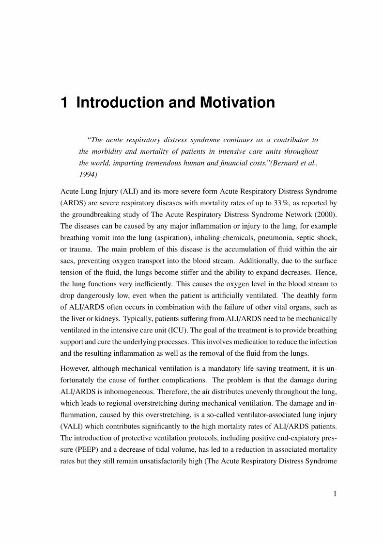
Acute Lung Injury (ALI) and its more severe form Acute Respiratory Distress Syndrome(ARDS) are severe respiratory diseases with mortality rates of up to 33%, as reported bythe groundbreaking study of The Acute Respiratory Distress Syndrome Network (2000).The diseases can be caused by any major inflammation or injury to the lung, for examplebreathing vomit into the lung (aspiration), inhaling chemicals, pneumonia, septic shock,or trauma. The main problem of this disease is the accumulation of fluid within the airsacs, preventing oxygen transport into the blood stream. Additionally, due to the surfacetension of the fluid, the lungs become stiffer and the ability to expand decreases. Hence,the lung functions very inefficiently. This causes the oxygen level in the blood stream todrop dangerously low, even when the patient is artificially ventilated. The deathly formof ALI/ARDS often occurs in combination with the failure of other vital organs, such asthe liver or kidneys. Typically, patients suffering from ALI/ARDS need to be mechanicallyventilated in the intensive care unit (ICU). The goal of the treatment is to provide breathingsupport and cure the underlying processes. This involves medication to reduce the infectionand the resulting inflammation as well as the removal of the fluid from the lungs.
However, although mechanical ventilation is a mandatory life saving treatment, it is un-fortunately the cause of further complications. The problem is that the damage duringALI/ARDS is inhomogeneous. Therefore, the air distributes unevenly throughout the lung,which leads to regional overstretching during mechanical ventilation. The damage and in-flammation, caused by this overstretching, is a so-called ventilator-associated lung injury(VALI) which contributes significantly to the high mortality rates of ALI/ARDS patients.The introduction of protective ventilation protocols, including positive end-expiatory pres-sure (PEEP) and a decrease of tidal volume, has led to a reduction in associated mortalityrates but they still remain unsatisfactorily high (The Acute Respiratory Distress Syndrome
1
1 Introduction and Motivation
Network, 2000). The usage of PEEP should prevent the lungs from partly collapsing (at-electrauma), by not letting the pressure drop to zero at the end of expiration. The reductionof tidal volume should prevent the tissue from being overstretched during ventilation (vo-lutrauma). Due to the unevenly distributed air within the lung, the optimal level of PEEP,tidal volume etc. are extremely difficult to determine for individual ALI/ARDS patients.
VALI includes both mechanical damage of the tissue and activation of an inflammatorysignaling cascade (biotrauma). How the ventilation exactly induces its deleterious effectsstill remains unclear. Studies both in vitro and in vivo have found that both the pattern andthe degree of stretching are important (Dos Santos and Slutsky, 2000, 2006; Dassow et al.,2010).
The work presented in this thesis is part of the German Research Foundation (DFG) pri-ority program “Protective Artificial Respiration”. The main goal of this interdisciplinary
initiative is to further improve mechanical ventilation in order to reduce the high mortality
rate due to VALI. For this purpose, a detailed “virtual lung model” is developed jointly atthe Institute for Computational Mechanics (TUM). One important part involves the mod-elling of the lung tissue behavior.
In this thesis, sophisticated material models for the lung parenchyma are be deducedfrom experimental studies of lung parenchyma. Based on these models global strainsand stresses within the lung parenchyma can be determined. As a next step, the rela-tion between the global strains of the lung parenchyma and the local deformation in in-dividual alveolar walls is investigated by performing finite element (FE) simulations onthree-dimensional image-based alveolar geometries. Using these simulations, a three-dimensional strain state within the alveolar walls is determined for the first time. Thisapproach will improve the understanding of the underlying processes causing the inflam-mation during VALI.
2
2 Anatomy, Physiology and Pathology
of the Lung
In this chapter, all the necessary background concerning anatomy, physiology and pathol-ogy of the lung will be provided as well as the pathology of Acute Lung Injury (ALI)and Acute Respiratory Distress Syndrome (ARDS) and ventilator-associated lung injury(VALI). This is in order to put the wider goals (see chapter 5) of this research into context.
2.1 Anatomy of the Lung
The primary function of the lung is gas exchange, i.e. introducing oxygen into and remov-ing carbon dioxide from the blood stream. In addition, the lung has other functions, e.g.filtering of unwanted materials. It is essential to understand the complex features of thelung structure, in order to understand how the lung reacts to injury and diseases.
Therefore, a brief introduction of the anatomy of the lung, from the upper airways, overthe conducting airways, down to the respiratory zone, is provided below.
2.1.1 Upper Airways
The upper airways are all conducting structures above the trachea (windpipe). They in-clude the nasal cavity, the pharynx (throat), and the larynx. The pharynx belongs to boththe respiratory and the digestive system. It splits into the larynx and the esophagus leadingto the digestive track. The nasopharynx humidifies the inhaled gas, clears out inhaled par-ticles and reactive substances, as well as contributes to senses like smell and taste (Crapo,2000).
3
2 Anatomy, Physiology and Pathology of the Lung
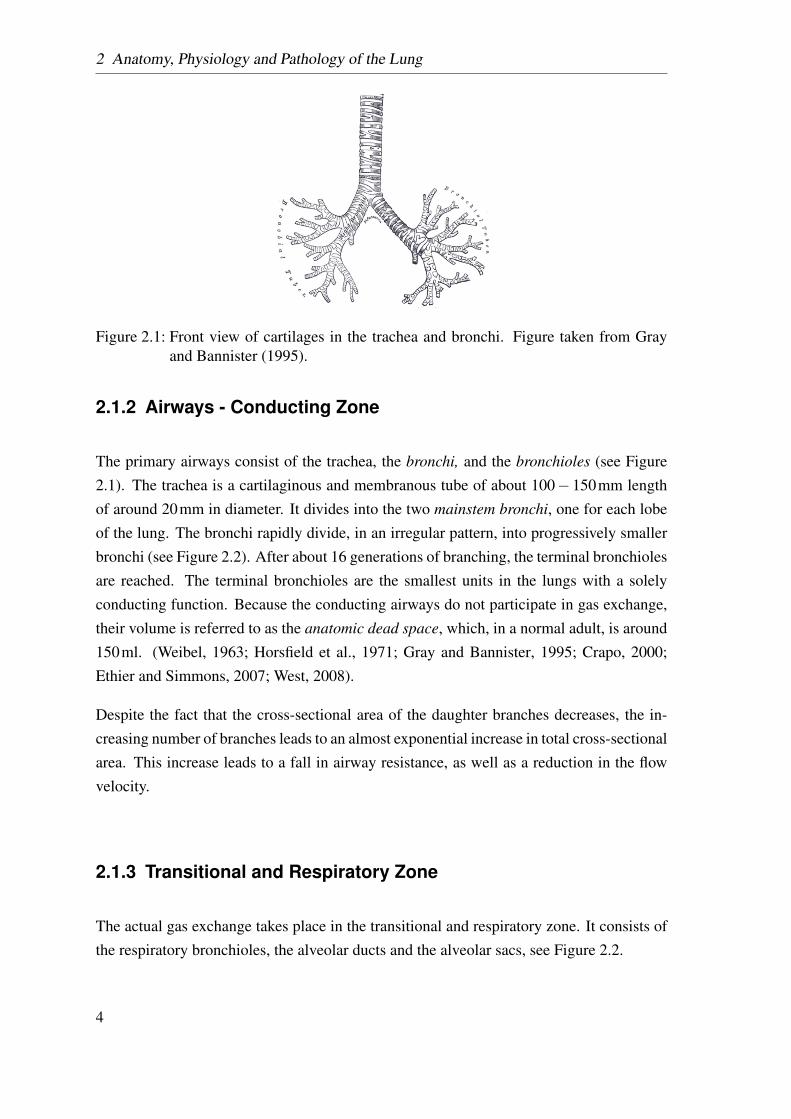
Figure 2.1: Front view of cartilages in the trachea and bronchi. Figure taken from Grayand Bannister (1995).
2.1.2 Airways - Conducting Zone
The primary airways consist of the trachea, the bronchi, and the bronchioles (see Figure2.1). The trachea is a cartilaginous and membranous tube of about 100− 150mm lengthof around 20mm in diameter. It divides into the two mainstem bronchi, one for each lobeof the lung. The bronchi rapidly divide, in an irregular pattern, into progressively smallerbronchi (see Figure 2.2). After about 16 generations of branching, the terminal bronchiolesare reached. The terminal bronchioles are the smallest units in the lungs with a solelyconducting function. Because the conducting airways do not participate in gas exchange,their volume is referred to as the anatomic dead space, which, in a normal adult, is around150ml. (Weibel, 1963; Horsfield et al., 1971; Gray and Bannister, 1995; Crapo, 2000;Ethier and Simmons, 2007; West, 2008).
Despite the fact that the cross-sectional area of the daughter branches decreases, the in-creasing number of branches leads to an almost exponential increase in total cross-sectionalarea. This increase leads to a fall in airway resistance, as well as a reduction in the flowvelocity.
2.1.3 Transitional and Respiratory Zone
The actual gas exchange takes place in the transitional and respiratory zone. It consists ofthe respiratory bronchioles, the alveolar ducts and the alveolar sacs, see Figure 2.2.
4
2.1 Anatomy of the Lung
2.1.3.1 Alveolar Acinus
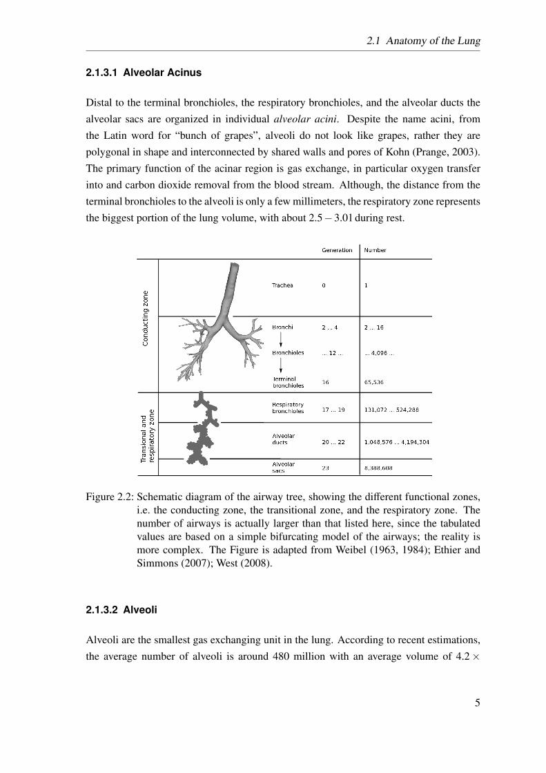
Distal to the terminal bronchioles, the respiratory bronchioles, and the alveolar ducts thealveolar sacs are organized in individual alveolar acini. Despite the name acini, fromthe Latin word for “bunch of grapes”, alveoli do not look like grapes, rather they arepolygonal in shape and interconnected by shared walls and pores of Kohn (Prange, 2003).The primary function of the acinar region is gas exchange, in particular oxygen transferinto and carbon dioxide removal from the blood stream. Although, the distance from theterminal bronchioles to the alveoli is only a few millimeters, the respiratory zone representsthe biggest portion of the lung volume, with about 2.5−3.0l during rest.
Figure 2.2: Schematic diagram of the airway tree, showing the different functional zones,i.e. the conducting zone, the transitional zone, and the respiratory zone. Thenumber of airways is actually larger than that listed here, since the tabulatedvalues are based on a simple bifurcating model of the airways; the reality ismore complex. The Figure is adapted from Weibel (1963, 1984); Ethier andSimmons (2007); West (2008).
2.1.3.2 Alveoli
Alveoli are the smallest gas exchanging unit in the lung. According to recent estimations,the average number of alveoli is around 480 million with an average volume of 4.2×
5
2 Anatomy, Physiology and Pathology of the Lung
106µm3 and a diameter of 100µm (Ochs et al., 2004). The total surface has been quoted tobe between 100−140m2 (Weibel, 1984; Crapo, 2000; West, 2008), which is of uppermostimportance for the gas exchange.
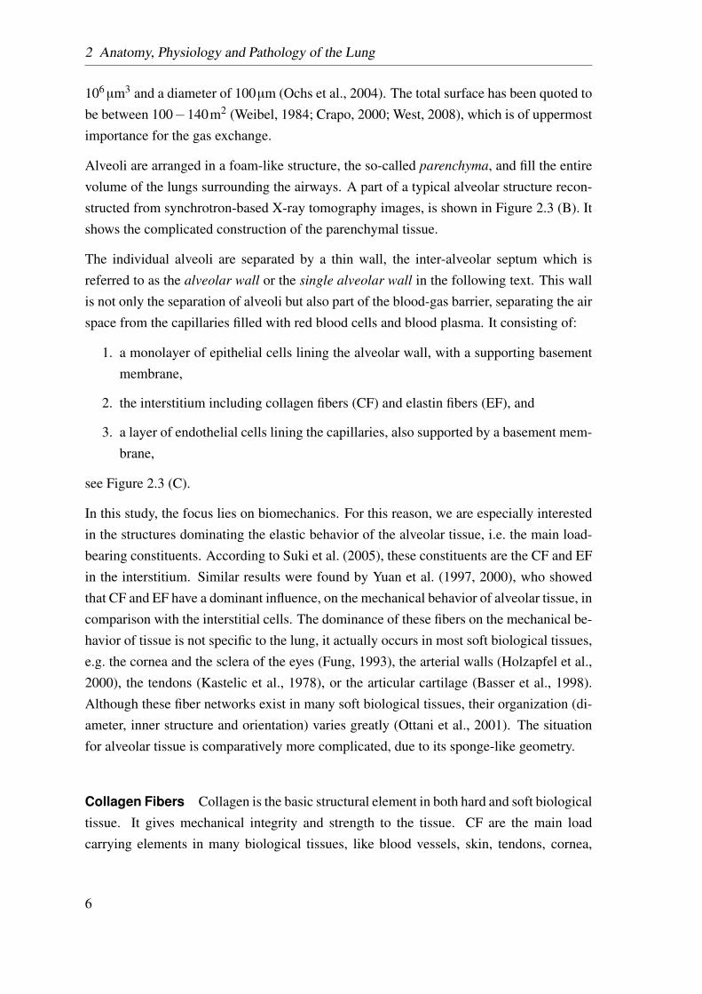
Alveoli are arranged in a foam-like structure, the so-called parenchyma, and fill the entirevolume of the lungs surrounding the airways. A part of a typical alveolar structure recon-structed from synchrotron-based X-ray tomography images, is shown in Figure 2.3 (B). Itshows the complicated construction of the parenchymal tissue.
The individual alveoli are separated by a thin wall, the inter-alveolar septum which isreferred to as the alveolar wall or the single alveolar wall in the following text. This wallis not only the separation of alveoli but also part of the blood-gas barrier, separating the airspace from the capillaries filled with red blood cells and blood plasma. It consisting of:
1. a monolayer of epithelial cells lining the alveolar wall, with a supporting basementmembrane,
2. the interstitium including collagen fibers (CF) and elastin fibers (EF), and
3. a layer of endothelial cells lining the capillaries, also supported by a basement mem-brane,
see Figure 2.3 (C).
In this study, the focus lies on biomechanics. For this reason, we are especially interestedin the structures dominating the elastic behavior of the alveolar tissue, i.e. the main load-bearing constituents. According to Suki et al. (2005), these constituents are the CF and EFin the interstitium. Similar results were found by Yuan et al. (1997, 2000), who showedthat CF and EF have a dominant influence, on the mechanical behavior of alveolar tissue, incomparison with the interstitial cells. The dominance of these fibers on the mechanical be-havior of tissue is not specific to the lung, it actually occurs in most soft biological tissues,e.g. the cornea and the sclera of the eyes (Fung, 1993), the arterial walls (Holzapfel et al.,2000), the tendons (Kastelic et al., 1978), or the articular cartilage (Basser et al., 1998).Although these fiber networks exist in many soft biological tissues, their organization (di-ameter, inner structure and orientation) varies greatly (Ottani et al., 2001). The situationfor alveolar tissue is comparatively more complicated, due to its sponge-like geometry.
Collagen Fibers Collagen is the basic structural element in both hard and soft biologicaltissue. It gives mechanical integrity and strength to the tissue. CF are the main loadcarrying elements in many biological tissues, like blood vessels, skin, tendons, cornea,
6
2.1 Anatomy of the Lung
Figure 2.3: The makeup of parenchymal and alveolar tissue - On the macro-scale (A), thelung parenchyma appears as a continuous tissue but zooming further downto, the meso-scale (B) or the tissue has a sponge-like structure, consisting ofonly 20% tissue and 80% air (Tschanz et al., 2003). At a micro-scale (C), theactual tissue components are visible. The collagen and elastin fibers, indicatedin yellow, are within the interstitium (dark blue). The endothelial cells areindicated in light blue with a green nucleus. The blood plasma is indicated witha light red and the red blood cells with a darker red. The basement membrane(light gray), and the surfactant layer, which is the liquid lining on the tissue-airinterfaces (see section 2.1.3.4), is indicated by shades of gray. The endothelialcells are not shown.
7
2 Anatomy, Physiology and Pathology of the Lung
sclera, bone. The CF make up 10% to 20% of the dry weight of an adult lung (Crystalet al., 1975).
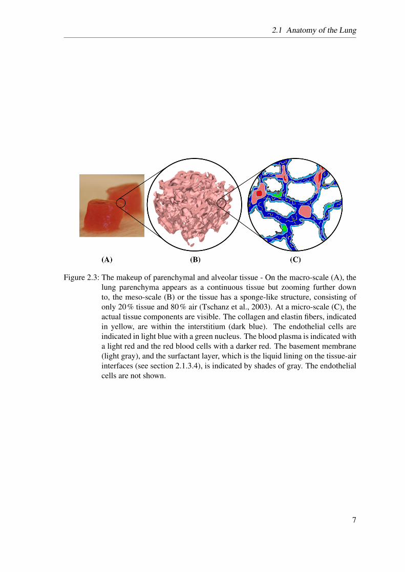
Figure 2.4: Electron microscopy pictures of collagen fiber (CF) networks in rat lungs. Fig-ures taken from Toshima et al. (2004). (A) CF network at the alveolar entrances(AE) in the collapsed lung. (B) CF network at the AE in the inflated rat lung.Both scale bars correspond to 100µm.
CF exhibit a strongly non-linear mechanical behavior. At low levels of strain (in the so-called “toe” region of the stress-strain curve), the CF take a wavelike configuration, seeFigure 2.4, and are easily extended, see Ethier and Simmons (2007); Toshima et al. (2004);Mercer and Crapo (1990). At higher levels of strain (in the “heel” and “linear” region),however, CF become straight and resist further stretch by increasing the stiffness of thefiber significantly. Compared to EF, the Young’s modulus (E) (see Appendix A.2.1) ofcollagen is about 10,000 to 100,000 times higher (Ethier and Simmons, 2007). Thus,collagen is assumed to provide a mechanical framework to limit excess distension.
Orientation of the Collagen Fibers
Toshima et al. (2004) investigated the fiber structure in rat and human lungs. They foundthe CF form a continuum, see Figure 2.4, extending throughout the lung and pleura. Theyare condensed into the alveolar mouths and subdivided into smaller fibers in the alveolarsepta, where they form basket-like networks. The fibers are wavy in the collapsed state,whereas they become straight in the inflated state, see Figure 2.4(A) and (B). Furthermore,Mercer and Crapo (1990) investigated the spatial distribution of the fibers in rat and human
8
2.1 Anatomy of the Lung
lungs. They found a high fiber concentration in the alveolar duct walls. Despite the fact thatthe fibers may have a predominant direction in the individual septum, there is no preferredfiber direction, if a large number of alveoli is considered. Hence, it seems reasonable toassume an isotropic fiber distribution within the lung parenchyma (Sobin et al., 1988).
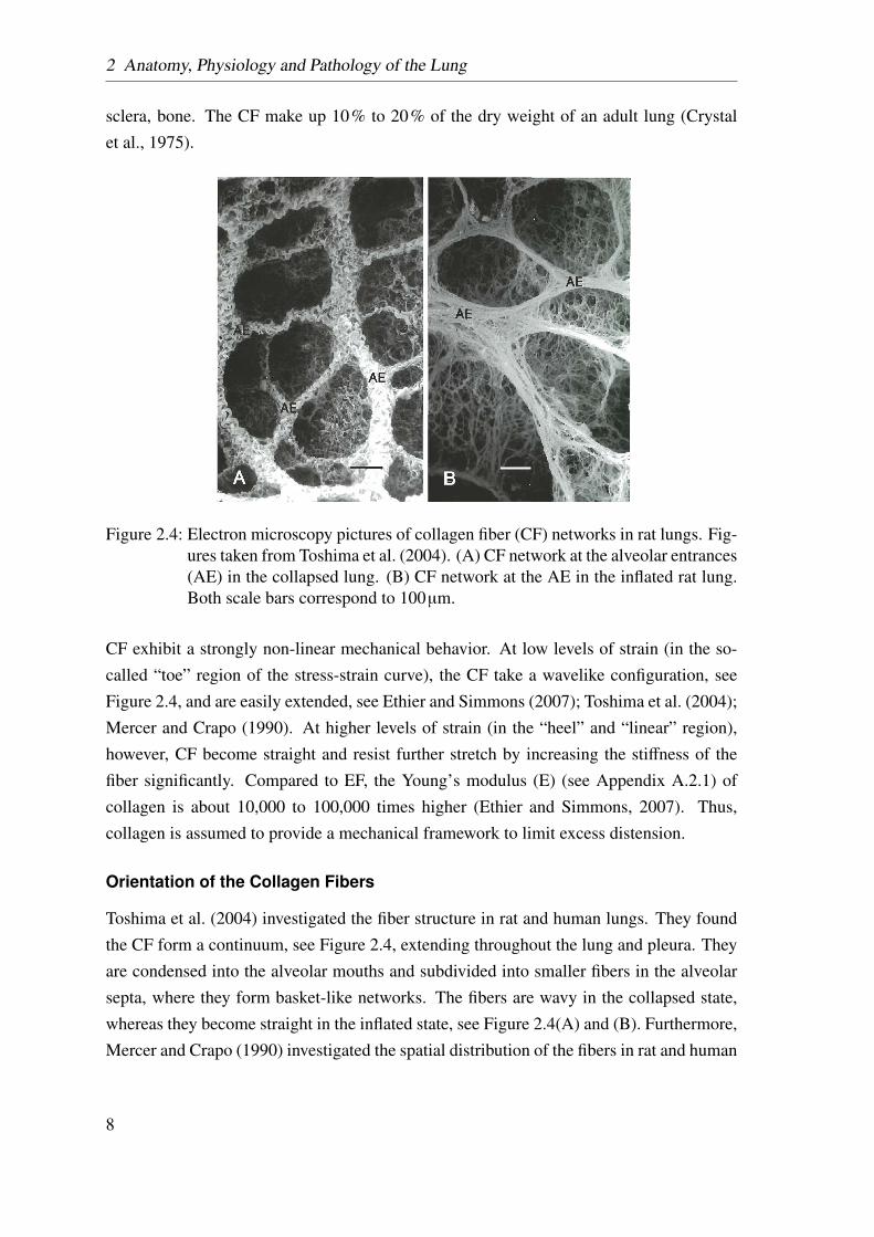
Elastin Fibers Elastin has a linear stress-strain curve, even for strains larger than 1.5,thus, making it the most “linearly” elastic biosolid material known (Fung and Sobin, 1981).The E of EF is between 30kPa (Ethier and Simmons, 2007) and 600kPa (Fung and Sobin,1981). EF are much softer than CF and can be extended up to 2.3 times their unloadedlength (Carton et al., 1962; Weibel, 1986). Elastin provides elasticity to the lung tissue(Fung and Sobin, 1981), allowing the lungs to effectively recoil in the normal breathingrange (Ethier and Simmons, 2007). A similar role of EF can be found in arteries, veins,and skin (Fung and Sobin, 1981).
Figure 2.5: Electron micrograph scans of the elastin fiber (EF) network in the human lung.Figures taken from Toshima et al. (2004). The EF form bands at the entrancesof the alveoli (*). Blood vessels (V) can also been seen in the scan. Both scalebars correspond to 100µm.
Orientation of the Elastin Fibers
The orientation of the EF is similar to the CF orientation, except for a band of EF aroundthe alveolar mouth, which forms an entrance ring into the single alveolus (Mercer andCrapo, 1990). Similar to CF, EF do not show a preferred fiber direction, see Figure 2.5,meaning they can be assumed to be distributed isotropically. The EF also form a contin-
9
2 Anatomy, Physiology and Pathology of the Lung
uum, with a higher density in the alveolar mouths than in the alveolar septa, however, theywere always found to be rather straight than wavy.
Connection Between Collagen and Elastin Fibers Detailed material descriptionsbased on micro-structural considerations are scarce in the literature.
In ligaments, Brown et al. (1994) found the CF and the EF to be mechanically connected.
Mercer and Crapo (1990) reported very close spatial proximity between EF and CF. Theyalso quantified the percentage of interwoven elastin in rats to be 51%, leading to the as-sumption that they are most likely mechanically connected as well.
The close proximity between CF and EF found by Toshima et al. (2004), suggests thatboth fiber families are mechanically connected. Furthermore, their findings suggest thatthe two fiber families act as parallel mechanical elements. Similar to Mercer and Crapo(1990), they believe the extension of the connective matrix to be in two stages. At lowstrain levels, the wavy CF are easily extended and the main stress is carried by the EF. Athigh strain levels, the CF become straight and act as a limit to further deformations of thetissue.
The review of Faffe and Zin (2009) discusses the influence of the two fiber families on themechanical behavior of the parenchymal tissue as well as the importance of modeling thefiber-fiber interaction (FF). However, to our best knowledge, none of these contributionshave yet been precisely quantified for the parenchymal tissue.
Ground Substance and Other Constituents In the inter cellular space, the twofiber families are embedded in a hydrophilic gel, the ground substance (GS) (Fung andSobin, 1981). Beside CF and EF, the GS contains proteoglycans and glycosaminoglycans(GAGs). Proteoglycans are macromolecules, consisting of protein cores, to which GAGside chains are covalently attached. The side chains can attract water molecules into thematrix, which can change the material properties of the tissue (Jamal et al., 2001).
2.1.3.3 Capillaries and Gas Exchange
The gas exchange occurs across the alveolar wall. Within the alveolar walls, the capillariesform a dense network, which is almost a continuous sheet of blood. In normal humans,200 ml of blood are distributed in the total surface area of the alveolar region, which isabout 100− 140m2, i.e. approximately the size of a tennis court (Weibel, 1984; Crapo,2000; West, 2008).
10
2.2 Physiology and Pathology of the Lung
2.1.3.4 Surface Tension and Surfactant
The alveoli are lined with a thin liquid film, which creates a surface tension acting againstan increase of alveolar surface area. When an interface is expanded, the minimum amountof work required to create the additional surface area is the product of the inter-facial ten-sion and the increase in area of the interface. This surface tension leads, amongst otherphenomena, to a hysteresis between pressure-volume (p-V) curves for inflation and defla-tion.
In the alveolar wall there are two types of alveolar epithelial cells (type I and II). TypeII cells are responsible for the production of surfactant, a surface active agent. Surfactantreduces the surface tension of the liquid lining at the tissue-gas interface (see Figure 2.3)and thereby, significantly changes the amount of work required to expand those surfaces(Rosen, 2004; West, 2008). Its absence drastically reduces the compliance of the lung(West, 2008).
2.2 Physiology and Pathology of the Lung
In this section a short overview over healthy respiration is given, before introduction thediseases ALI and ARDS and therefrom resulting VALI.
2.2.1 Respiration
During inspiration, the volume of the thoracic cavity is increased by lifting the rib cageand contracting the diaphragm. This causes the pressure in the pleural space to drop tomore negative values causing air to flow into the lungs. The air flows down to the terminalbronchioles. At this point, the overall cross-sectional area is so big, due to the large numberof branches, that the convective velocity of the gas becomes very small and diffusion takesover in the respiratory zone (West, 2008). During expiration, the diaphragm relaxes, whichincreases the pressure in the pleural space, resulting in airflow out of the lungs.
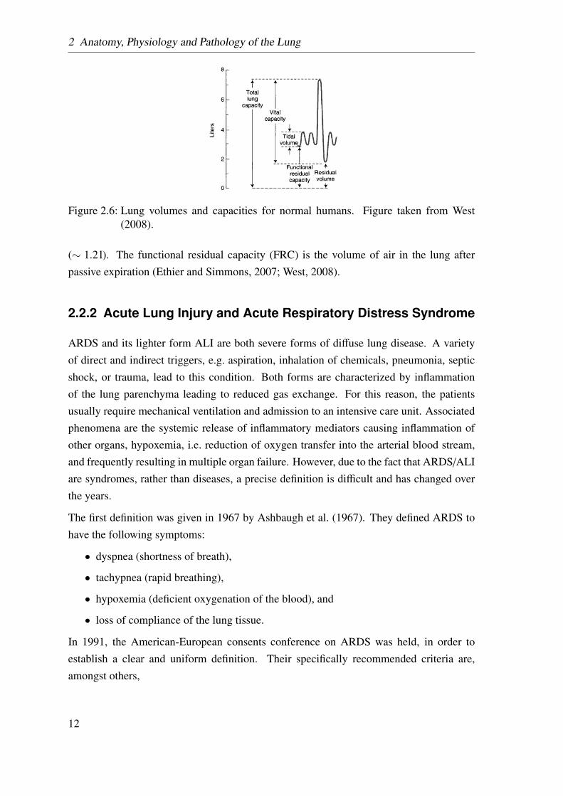
A number of clinically measured volumes are defined in Figure 2.6. The total lung capacity(TLC), which is the maximum air volume in the lung, is between 6 and 8l in a healthyadult. However, during normal breathing only 0.5l (tidal volume) are exchanged. Takinga deep breath, the whole vital capacity can be exchanged. The residual volume, includingthe anatomical dead space, is the volume remaining in the lung after maximal expiration
11
2 Anatomy, Physiology and Pathology of the Lung
Figure 2.6: Lung volumes and capacities for normal humans. Figure taken from West(2008).
(∼ 1.2l). The functional residual capacity (FRC) is the volume of air in the lung afterpassive expiration (Ethier and Simmons, 2007; West, 2008).
2.2.2 Acute Lung Injury and Acute Respiratory Distress Syndrome
ARDS and its lighter form ALI are both severe forms of diffuse lung disease. A varietyof direct and indirect triggers, e.g. aspiration, inhalation of chemicals, pneumonia, septicshock, or trauma, lead to this condition. Both forms are characterized by inflammationof the lung parenchyma leading to reduced gas exchange. For this reason, the patientsusually require mechanical ventilation and admission to an intensive care unit. Associatedphenomena are the systemic release of inflammatory mediators causing inflammation ofother organs, hypoxemia, i.e. reduction of oxygen transfer into the arterial blood stream,and frequently resulting in multiple organ failure. However, due to the fact that ARDS/ALIare syndromes, rather than diseases, a precise definition is difficult and has changed overthe years.
The first definition was given in 1967 by Ashbaugh et al. (1967). They defined ARDS tohave the following symptoms:
• dyspnea (shortness of breath),
• tachypnea (rapid breathing),
• hypoxemia (deficient oxygenation of the blood), and
• loss of compliance of the lung tissue.
In 1991, the American-European consents conference on ARDS was held, in order toestablish a clear and uniform definition. Their specifically recommended criteria are,amongst others,
12
2.2 Physiology and Pathology of the Lung
• the acute onset,
• bilateral infiltration, seen on the front chest radiograph,
• a threshold value for the oxygenation (different values for ALI and ARDS), and
• a threshold value for the hypertension (different values for ALI and ARDS).
The details can be found in the consents report, see Bernard et al. (1994).
Due to the wide range of definitions, the reported mortality rates vary between 10 and90%.
2.2.2.1 Pathogenesis
There is a great diversity of initiating causes of ALI and ARDS, like sepsis, trauma, aspi-ration, multiple blood transfusion, acute pancreatitis, inhalation injury, and drug toxicity.Although the initiating injury might be different, the resulting inflammation causes theinjury to propagate, especially when it is paired with additional trauma, like high-tidalvolume of the mechanical ventilation or hypoxemia, see section 2.2.3.
The pathogenesis of ARDS can be split into two phases:
• the earlier exudate phase, also called the acute inflammation; and
• the later fibrosing-alveolitis phase,
see Figure 2.7.
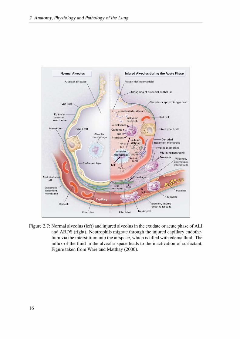
In the first phase, the alveolar wall barrier becomes more permeable, leading to an inflowof fluid and neutrophils into the alveolar air space. As mentioned above, the alveolar wallconsists, amongst others, of capillary endothelial and alveolar epithelial cells, the damageof which, could have a variety of reasons, results in ARDS. Injury of the endothelium (e.g.in case of sepsis) increases the capillary permeability, leading to an influx of protein-richfluid into the alveolar space (see Figure 2.7). Injury of the alveolar epithelium also leads tothe formation of pulmonary edema. As mentioned above, there are two types of alveolarepithelial cells. The alveolar type I cells are at high risk of damage. Their damage leads toan increased inflow of fluid into the alveoli and a decreased clearance of this fluid from thealveolar space. The alveolar type II cells are more resistant to damage; however, they have,amongst others, the task of producing surfactant, transporting ions, and the proliferationand differentiation into type I cells to replace them after injury. Injury of type II cells canlead to a reduced production of surfactant molecules, which increases the surface tension(see section 2.1.3.4), resulting in a decrease of compliance and alveolar collapse.
13
2 Anatomy, Physiology and Pathology of the Lung
In the second phase, the alveolar wall gets transparent, with varying degrees of interstitialfibrosis, leading to the resolution of the individual walls (Tsushima et al., 2009; Harman,2011).
2.2.2.2 Treatment
The standard treatment of ALI and ARDS is towards identification and management ofpulmonary and non-pulmonary dysfunction. In some cases, the underlying cause can betreated directly, e.g. in the case of pneumonia. However, the majority of cases, e.g. aspira-tion, cannot be treated except to provide essential supportive care.
Most ALI and ARDS patients develop a life-threatening hypoxemia. Furthermore, the highbreathing effort caused by the reduced lung compliance may lead to ventilatory failure. Forthese reasons, mechanical ventilation is the mainstay of the supportive care. The stabiliza-tion of the respiration allows time for the evolution of the natural healing process and, ifpossible, the treatment of the underlying cause (Brower et al., 2001).
2.2.3 Ventilator Associated Lung Injuries
Although mechanical ventilation is a lifesaving treatment, it can cause further lung dam-age itself. These injuries are called ventilator-induced lung injury (VILI) or ventilatorassociated lung injury (VALI).
VILI is defined as an acute lung injury directly caused by mechanical ventilation, whereasin VALI, the injury is not necessarily caused by mechanical ventilation but is associatedwith it. This means VALI is a lung injury that comes along with diseases like ARDS, wheremechanical ventilation is a mandatory treatment (American Thoracic Society, EuropeanSociety of Intensive Care Medicine, Societé de Réanimation Langue Française, 1999).
2.2.3.1 Pathogenesis
VALI damage the lung in an inhomogeneous manner. Supposedly healthy alveoli, whichare more compliant than affected alveoli, are at risk of becoming over distended duringmechanical ventilation. Furthermore, affected alveoli may experience further injury dueto shear forces arising from a cycle of collapse and re-expansion during the breathingcycle. In addition to mechanical damage, mechanical stimulation causes the cells to secreteproinflammatory cytokines, leading to an increase of inflammation and pulmonary edema.
14
2.2 Physiology and Pathology of the Lung
The clinical course of VALI is different; while some patients recover within a couple ofweeks, others need a long therapy, including mechanical ventilation. These patients facethe risk of superimposed infections or multi-organ failure, leading to the high mortalityrates (American Thoracic Society, European Society of Intensive Care Medicine, Societéde Réanimation Langue Française, 1999). The majority of patients suffering from VALIdo not die of primary respiratory causes rather of sepsis or multi-organ dysfunction (Wareand Matthay, 2000).
2.2.3.2 Prophylaxis and Treatment
The use of protective ventilation protocols, including positive end-expiatory pressure(PEEP) to prevent alveolar collapse, the use of low tidal volumes, and limited levels ofinspiratory filling pressures appear to be beneficial in diminishing the observed VALI. Thechange of “normal” mechanical ventilation to these protocols reduced the mortality ratesfrom 55− 65%, as reported in the 1980s and early 1990s, to 31% (Abel et al., 1998;Tsushima et al., 2009). This indicates that some cases were related to lung injury dueto VALI. A more effective treatment of sepsis and improvement in the supportive care ofcritically ill patients also influenced this reduction.
Dreyfuss et al. (1988) studied the effects of different ventilation strategies on pulmonaryedema, i.e. the respective effects of high airway pressure and high inflation with and with-out PEEP on the water content, micro-vascular permeability, and ultra-structure of thelungs on mechanically ventilated rats. They found, that the edema was only related tochanges in the lung volume and not the airway pressure.
Additionally, they found PEEP to:
• have a positive effect on the alveolar epithelial layer,
• prevent the animals from edema or reduce the amount of edema, and
• improve the arterial oxygenation during pulmonary edema.
The protein concentration within the edema fluid remained the same and the lung waterwas not decreased by PEEP, sometimes it even increased.
2.2.3.3 Conclusion
Despite these improvements, the mortality rates remain unacceptably high. A better under-standing of the connection between mechanical ventilation and implications of overstrain-ing the alveolar tissue is essential.
15
2 Anatomy, Physiology and Pathology of the Lung
Figure 2.7: Normal alveolus (left) and injured alveolus in the exudate or acute phase of ALIand ARDS (right). Neutrophils migrate through the injured capillary endothe-lium via the interstitium into the airspace, which is filled with edema fluid. Theinflux of the fluid in the alveolar space leads to the inactivation of surfactant.Figure taken from Ware and Matthay (2000).
16
3 Theoretical Framework
This chapter provides the necessary theoretical background knowledge to understand thiswork. In the first section a brief introduction into solid continuum mechanics is presented.In the second section the theoretical framework for hyperelastic material models is intro-duced.
3.1 Solid Continuum Mechanics
In continuum mechanics, a body B is considered as a continuous object. The fact thatit is actually built of discrete constituents, like atoms and molecules, is neglected. Thisassumption is valid if there is a large scale difference between the macro-scale, i.e. thecontinuous body, and the micro-scale, i.e. the molecules or atoms.
The theory of continuum mechanics is applicable for both solid and fluid mechanics andnot limited to Cartesian coordinates. However, here, the focus is restricted to solid me-chanics in Cartesian coordinates.
The aim of this section is to give a brief overview of the continuum mechanical backgroundof this work and to introduce the used notation. For a detailed background, the reader isreferred to Wall et al. (2010a) and Holzapfel (2004).
3.1.1 Kinematics
In the undeformed or material configuration, the body B0 ⊂ R3 is parametrized with X. Inthe deformed, current, or spatial configuration, the body Bt ⊂ R3 at t ∈ R+ is parametrizedwith x. The boundary of B is denoted with ∂B. The motion of the body B is described bythe particle motion mapping ϕ(X, t) : B0→ Bt, which relates the points X ∈ B0 with thepoints x ∈Bt at a fixed time t ∈ R+, i.e.
x = ϕ(X, t). (3.1.1)
17
3 Theoretical Framework
The transformation is invertible with
X = ϕ−1(x, t). (3.1.2)
The partial derivative of ϕ with respect to X is one of the most important kinematic quan-tities. The resulting tensor
∇Xϕ :=∂x∂X
=
∂x1
∂X1∂x1
∂X2∂x1
∂X3
∂x2
∂X1∂x2
∂X2∂x2
∂X3
∂x3
∂X1∂x3
∂X2∂x3
∂X3
:= F(X, t) (3.1.3)
is called deformation gradient F. In order to be invertible the deformation gradient F, itneeds to be non-singular, i.e.
J = detF , 0 (3.1.4)
with J being the determinant of the deformation gradient or the Jacobian determinant. Inthat case the inverse motion ϕ−1 with respect to the current position x of a material pointexists, the inverse deformation gradient F−1 reads
F−1 = F−1(x, t) :=∇xϕ−1 =
∂X∂x
=
∂X1
∂x1∂X1
∂x2∂X1
∂x3
∂X2
∂x1∂X2
∂x2∂X2
∂x3
∂X3
∂x1∂X3
∂x2∂X3
∂x3
. (3.1.5)
Based on the deformation gradient, there are three fundamental geometric mappings. Thedeformation gradient F itself defines a linear transformation of an infinitesimal line ele-ment dX ∈ B0 in the material configuration to an infinitesimal line element dx ∈ Bt in thecurrent configuration, i.e.
dx = FdX. (3.1.6)
Due to the fact that the deformation gradient F transforms points between two configura-tions, it is also called two-point tensor.
The change of volume of an infinitesimal volume element in the material configurationdV ⊂ B0 and the current configuration dv⊂ Bt at time t is defined as
dv = JdV = det(F)dV. (3.1.7)
18
3.1 Solid Continuum Mechanics
For this reason, the Jacobian determinant J is also called the volume ratio. Since F isinvertible and the volume elements cannot have negative volumes, the determinant J needsto be positive. An isochoric or volume preserving deformation is characterized by J = 1.In order to transform vector elements of infinitesimal area nda⊂ Bt and NdA⊂ B0 in thecurrent and the material configuration, respectively, with n and N being the material andspatial unit normal vector of the area element, respectively, the Nanson’s formula is used,i.e.
nda = JF−T NdA. (3.1.8)
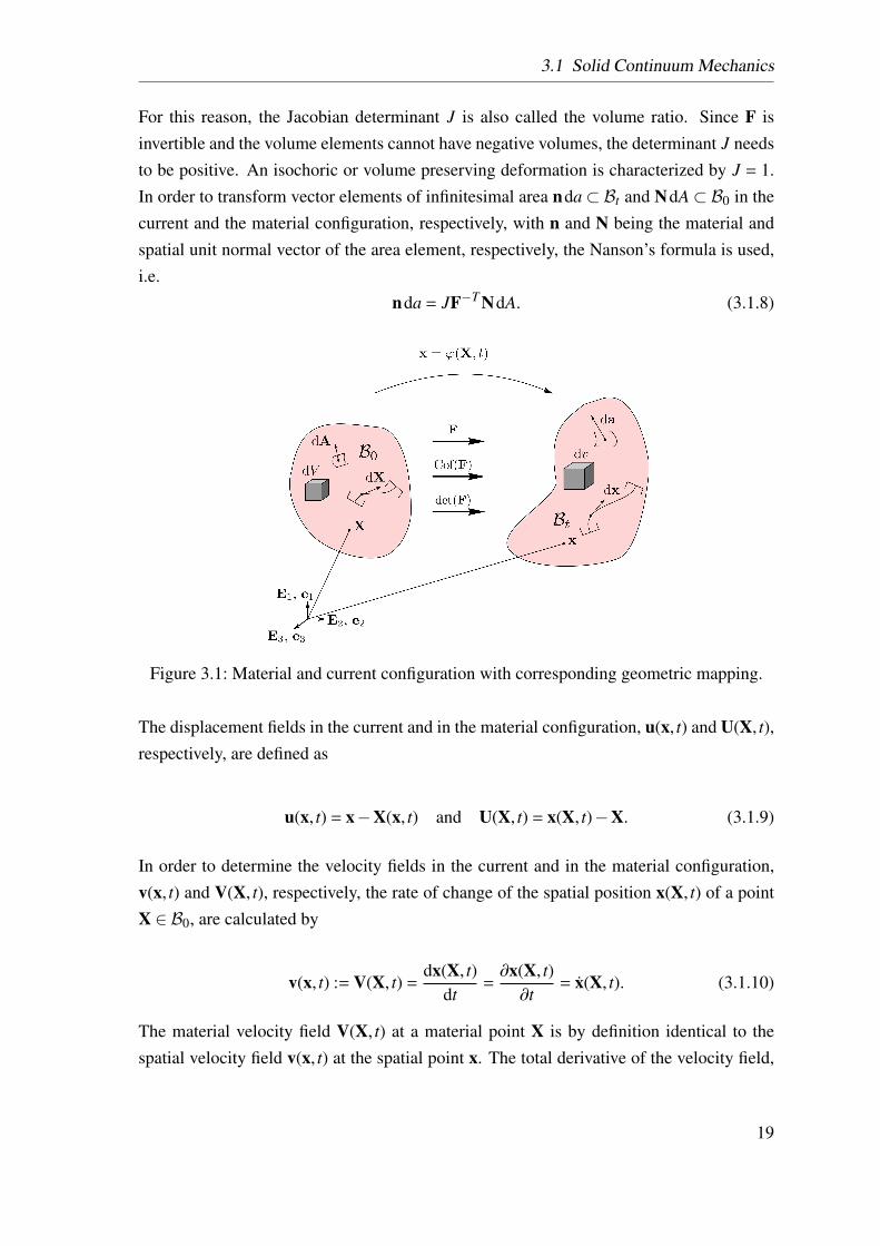
Figure 3.1: Material and current configuration with corresponding geometric mapping.
The displacement fields in the current and in the material configuration, u(x, t) and U(X, t),respectively, are defined as
u(x, t) = x−X(x, t) and U(X, t) = x(X, t)−X. (3.1.9)
In order to determine the velocity fields in the current and in the material configuration,v(x, t) and V(X, t), respectively, the rate of change of the spatial position x(X, t) of a pointX ∈ B0, are calculated by
v(x, t) := V(X, t) =dx(X, t)
dt=∂x(X, t)∂t
= x(X, t). (3.1.10)
The material velocity field V(X, t) at a material point X is by definition identical to thespatial velocity field v(x, t) at the spatial point x. The total derivative of the velocity field,
19
3 Theoretical Framework
with respect to the time t, defines the acceleration field. The acceleration field in the currentand the material configuration a(x, t) and A(X, t), respectively, are calculated by
A(X, t) = a(x, t) =dV(X, t)
dt=
d2x(X, t)d2t
(3.1.11)
or, equivalently,
a(x, t) = v(x, t) =dv(x, t)
dt=
∂v(x, t)∂t︸ ︷︷ ︸
partial derivative
+ (∇xv) ·v︸ ︷︷ ︸convective derivative
. (3.1.12)
The partial and the convective derivative are also called the local and convective accelera-tion, respectively.
3.1.2 Strain and Stress Measures
In order to determine the volume and shape change of a body, displacements are not suffi-cient. For this reason, strain measures based on the deformation gradient F are introducedin the following. The polar decomposition of the deformation gradient reads
F = RU = vR, (3.1.13)
with R being a rotation tensor, i.e. an orthogonal tensor (R−1 = RT ) and U and v are thesymmetric right and left stretch tensors, respectively. For this reason, the deformationgradient F is not invariant with respect to rigid body rotations, in contrast to the rightCauchy-Green strain tensor
C := FT F = UT RT R︸︷︷︸1
U = UT U, (3.1.14)
with 1 being the second-order identity tensor. The strain tensor C exclusivly depends onthe right stretch tensor U and, is therefore, well suited for describing the internal state of abody. Similar to the right Cauchy-Green strain tensor, the left Cauchy-Green strain tensorb is given as
b = FFT = vT v. (3.1.15)
20
3.1 Solid Continuum Mechanics
In many cases, it is usefully to have a strain measure, that is zero for the undeformedconfiguration (F = 1). For this reason the Green-Lagrange strain tensor E and the Euler-Almansi strain tensor e are given as
E :=12
(C−1) =12
(FT F−1
)(3.1.16)
and
e :=12
(1−b−1
). (3.1.17)
The Green-Lagrange strain tensor E and the right Cauchy-Green strain tensor C are definedin the material configuration and are material objective, whereas the Euler-Almansi straintensors e and the left Cauchy-Green b are defined in the current configuration and arespatial objective.
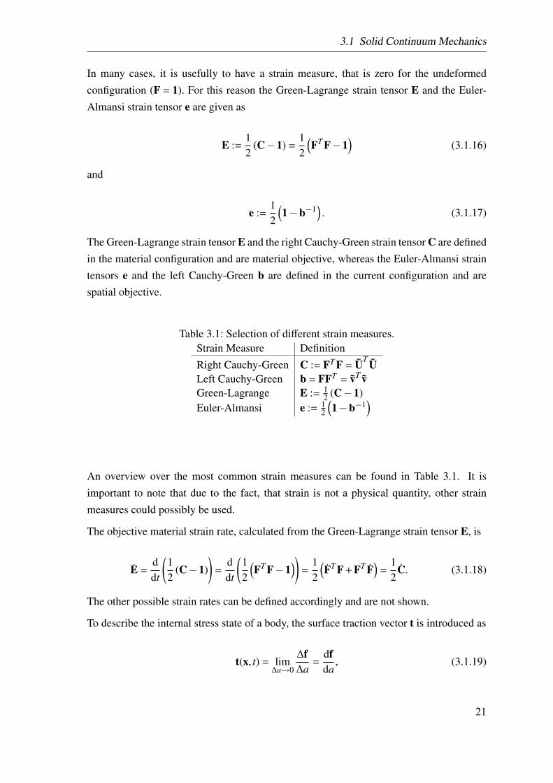
Table 3.1: Selection of different strain measures.Strain Measure DefinitionRight Cauchy-Green C := FT F = UT ULeft Cauchy-Green b = FFT = vT vGreen-Lagrange E := 1
2 (C−1)Euler-Almansi e := 1
2
(1−b−1
)
An overview over the most common strain measures can be found in Table 3.1. It isimportant to note that due to the fact, that strain is not a physical quantity, other strainmeasures could possibly be used.
The objective material strain rate, calculated from the Green-Lagrange strain tensor E, is
E =ddt
(12
(C−1))
=ddt
(12
(FT F−1
))=
12
(FT F + FT F
)=
12
C. (3.1.18)
The other possible strain rates can be defined accordingly and are not shown.
To describe the internal stress state of a body, the surface traction vector t is introduced as
t(x, t) = lim∆a→0
∆f∆a
=dfda, (3.1.19)
21
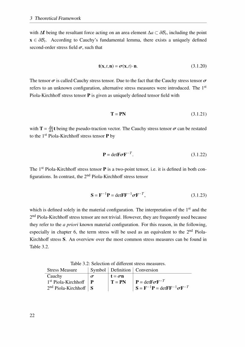
3 Theoretical Framework
with ∆f being the resultant force acting on an area element ∆a ⊂ ∂Bt, including the pointx ∈ ∂Bt. According to Cauchy’s fundamental lemma, there exists a uniquely definedsecond-order stress field σ, such that
t(x, t,n) = σ(x, t) ·n. (3.1.20)
The tensor σ is called Cauchy stress tensor. Due to the fact that the Cauchy stress tensor σrefers to an unknown configuration, alternative stress measures were introduced. The 1st
Piola-Kirchhoff stress tensor P is given as uniquely defined tensor field with
T = PN (3.1.21)
with T = dadA t being the pseudo-traction vector. The Cauchy stress tensor σ can be restated
to the 1st Piola-Kirchhoff stress tensor P by
P = detFσF−T . (3.1.22)
The 1st Piola-Kirchhoff stress tensor P is a two-point tensor, i.e. it is defined in both con-figurations. In contrast, the 2nd Piola-Kirchhoff stress tensor
S = F−1P = detFF−1σF−T , (3.1.23)
which is defined solely in the material configuration. The interpretation of the 1st and the2nd Piola-Kirchhoff stress tensor are not trivial. However, they are frequently used becausethey refer to the a priori known material configuration. For this reason, in the following,especially in chapter 6, the term stress will be used as an equivalent to the 2nd Piola-Kirchhoff stress S. An overview over the most common stress measures can be found inTable 3.2.
Table 3.2: Selection of different stress measures.Stress Measure Symbol Definition ConversionCauchy σ t = σn1st Piola-Kirchhoff P T = PN P = detFσF−T
2nd Piola-Kirchhoff S S = F−1P = detFF−1σF−T
22
3.1 Solid Continuum Mechanics
3.1.3 Balance Principles
Conservation laws and balance principles are the physical basis of continuum mechanics.They are material independent, i.e. valid for every continuum. In detail, there are fourbalance equations and one inequality. The balance equations are the conservation of mass,the balance of linear momentum, the balance of angular momentum, and the balance ofenergy. The entropy inequality will be further discussed in more detail in the followingsection 3.2.
3.1.3.1 Conservation of Mass
The law of conservation of mass states that, in a closed system, the mass M of the body Bremains constant during a deformation process. The first global form is given as
M :=∫B0
ρ0(X)dV︸ ︷︷ ︸dM
=
∫Bt
ρ(x, t)dv︸ ︷︷ ︸dm
= m = const., (3.1.24)
where ρ0 and ρ are the material and current density, respectively. Using equation (3.1.7),the first local form is derived to be
ρ0 = Jρ. (3.1.25)
Since the mass does not change over time (m = 0), the first global form can be equallywritten as
m = 0 =ddt
∫Bt
ρdv =
∫Bt
(ρ+ρ∇ ·v) dv, (3.1.26)
where the Reynolds transport theorem has been applied, see Appendix A.1.1.
The corresponding local forms reads
ρ+ρ∇ ·v = 0. (3.1.27)
3.1.3.2 Balance of Momentum
The balance of momentum state that the change over time of the linear momentum L andthe angular momentum JY equal the external forces fext
0 and the external momentum mext0 ,
respectively.
23
3 Theoretical Framework
Balance of Linear Momentum The linear momentum L is defined as
L :=∫B0
ρ0VdV. (3.1.28)
The change of linear momentum L in time leads to
L = fext0 :=
∫B0
fbodyV dV +
∫∂B0
TdA (3.1.29)
where fbodyV is the material volume type body load. With some lengthy transformations,
including Gauss’ divergence theorem, see Appendix A.1.2, it is derived as
∫B0
ρ0VdV =
∫B0
(fbody
V +∇ · (F ·S))
dV. (3.1.30)
The local material form of this equation reads
∇ · (F ·S) + fbodyV −ρ0V = 0. (3.1.31)
This equation is called the linear momentum equation or Cauchy’s first equation of motionand is the starting point of the numerical method.
Balance of Angular Momentum The angular momentum relative to a fixed point(characterized by the position vector Y) is defined as
JY :=∫B0
R×ρ0VdV (3.1.32)
with the identity of the velocity fields (equation (3.1.10)) and the position vector R = X−Y.The change of angular momentum JY with respect to time leads to
JY = mext0 :=
∫∂B0
R×TdA +
∫B0
R× fbodyV dV. (3.1.33)
With a lengthy transformation, Cauchy’s second equation of motion results in
S = ST (3.1.34)
or
24
3.1 Solid Continuum Mechanics
σ = σT . (3.1.35)
Thus, the balance of angular momentum is satisfied if the Cauchy stress tensor σ and the2nd Piola-Kirchhoff stress tensor S are symmetric.
3.1.3.3 Balance of Energy (First Principle of Thermodynamics)
The change over time of the sum of the internal energy εint and kinetic energy εkin equalsthe sum of the external mechanical power Pext and the non-mechanical power Qext
ddt
(εint + εkin) = Pext−Qext. (3.1.36)
Since only mechanical effect are considered within this work, Qext is set to zero. Forsimplicity, in the following the summands are given in the material configuration. In detail,equation (3.1.36) can be reformed as
ddt
∫B0
εint, Mρ0 dV︸ ︷︷ ︸εint
+
∫Bt
12ρ0
(V ·VT
)dV︸ ︷︷ ︸
εkin
=
∫∂B0
T ·VT dA +
∫B0
fbodyV ·VT dV︸ ︷︷ ︸
Pext
(3.1.37)
with εint, M being the specific internal energy, i.e. internal energy per unit mass. With sometransformations, the local form reads
S : E +ρ0(V ·VT
)=∇ ·
((S : E
)·VT
)+ fbody
V ·VT . (3.1.38)
3.1.3.4 Initial and Boundary Conditions
In order to solve the differential equation (3.1.31) initial and boundary conditions are re-quired. The boundary conditions account for the external stresses and displacements on Band the initial conditions define the stresses and displacements for the material state.
The initial conditions are given as
u(x, t0) = u0(x) (3.1.39)
25
3 Theoretical Framework
and
v(x, t0) = v0(x) (3.1.40)
on the Dirichlet boundary B0. Prescribed displacements u0 and an initial velocity v0 areneeded, since equation (3.1.31) is a second-order differential equation of the time.
The boundary conditions are given as
S ·N = T, (3.1.41)
on the Neumann boundary ∂SB0,
and
u = u (3.1.42)
on the Dirichlet boundary ∂uB0. It is important to note that every point of ∂B0 needs to beassigned to either a stress or displacement boundary condition, i.e. ∂SB0∪∂uB0 = ∂B0 and∂SB0∩∂uB0 = ∅.
3.2 Constitutive Equations for Hyperelastic Materials
The second law of thermodynamics states that heat always flows from the warmer to thecolder region of a body; friction converts mechanical energy into heat, which cannot beconverted back into mechanical energy. Based on this principle, the Clausius-Planck In-equality is
Dint = S : E−ρ0ΨM + Tρ0SM ≥ 0 (3.2.1)
with the internal dissipation Dint, the specific Helmholtz free energy ΨM which is a mea-sure for the work per unit mass obtainable from a closed thermodynamic system at constanttemperature and volume, the absolute temperature T and the specific entropy SM. Thecontraction S : E is the rate of internal mechanical work or stress-power per unit referencevolume. The absolute temperature multiplied by the rate of entropy ρ0SMT is zero for thisadiabatic process. This leads to the reversible process of
26
3.2 Constitutive Equations for Hyperelastic Materials
Dint = S : E−ρ0ΨM = 0. (3.2.2)
In the following, this study is restricted to Green-elastic or hyperelastic materials. In thiscase, the Helmholtz free energy ΨM solely depends on the current state of deformationrelative to an arbitrary material configuration. Besides this, the work needed to get to aparticular state of deformation is path independent. Consequently, the stress is derivablefrom a scalar potential function, the strain energy density function (SEF) Ψv, defined as
Ψv = ρ0ΨM. (3.2.3)
For homogeneous materials, the SEFs solely depend on the Green-Lagrange stress tensorE, i.e. Ψv = Ψv(E). With the material time derivation of Ψv being
Ψv(E(X, t)) =dΨv
dt=∂Ψv
∂t+∂Ψv
∂E:
dEdt
=∂Ψv
∂E: E, (3.2.4)
equation (3.2.2) can be reformulated into
S =∂Ψv
∂E. (3.2.5)
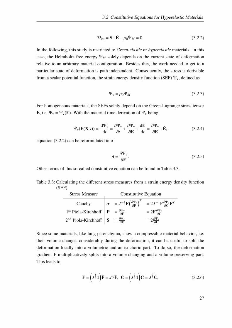
Other forms of this so-called constitutive equation can be found in Table 3.3.
Table 3.3: Calculating the different stress measures from a strain energy density function(SEF).
Stress Measure Constitutive Equation
Cauchy σ = J−1F(∂Ψv∂F
)T= 2J−1F∂Ψv
∂C FT
1st Piola-Kirchhoff P = ∂Ψv∂F = 2F∂Ψv
∂C
2nd Piola-Kirchhoff S = ∂Ψv∂E = 2∂Ψv
∂C
Since some materials, like lung parenchyma, show a compressible material behavior, i.e.their volume changes considerably during the deformation, it can be useful to split thedeformation locally into a volumetric and an isochoric part. To do so, the deformationgradient F multiplicatively splits into a volume-changing and a volume-preserving part.This leads to
F =
(J
13 1
)F = J
13 F, C =
(J
23 1
)C = J
23 C, (3.2.6)
27
3 Theoretical Framework
with J13 1 and J
23 1 being associated with the volume-changing deformation. The isochoric
deformation gradient F and the isochoric right Cauchy-Green strain tensor C, are associ-ated with the volume-preserving deformation.
In order to solve the initial boundary value problem with the FEM, the linearized consti-tutive equation is needed. For this reason, the forth-order elasticity tensor is introducedas
C :=∂S∂E
=∂2Ψv
∂E∂E= 4
∂2Ψv
∂C∂C. (3.2.7)
For more details the reader is referred to textbooks (Holzapfel, 2004; Schröder and Neff,2003; Ogden, 1997).
There are two fiber families in the alveolar tissue, the CF and EF. However, as discussedabove, see section 2.1.3.2, the fiber orientation within the alveolar tissue can be assumedto be isotropic. For this reason, the focus of this work is put on isotropic SEFs. In thiscase, the SEF is by definition invariant with respect to rotation, i.e.
Ψv (C) = Ψv (RCR) , (3.2.8)
for any rotation tensor R.
This invariance towards rotation allows Ψv to be expressed in terms of the principle in-variants of its argument C. In the following section, coupled and decoupled SEFs will bepresented, where the decoupled forms are split into an isochoric and a volumetric contri-bution.
3.2.1 Coupled Strain Energy Density Functions
The coupled SEFs considered in this work, are formulated as
Ψv(C) = Ψv (I1, I2, I3) (3.2.9)
where I1, I2, and I3 are the invariants of the right Cauchy–Green strain tensor C, definedas
I1 := trC, I2 := 12
[(trC)2− tr(C2)
], I3 := detC. (3.2.10)
This leads to the calculation of the 2nd Piola-Kirchhoff stress tensor
28
3.2 Constitutive Equations for Hyperelastic Materials
S = 2∂Ψv (C)∂C
= 2(∂Ψv
∂I1+ I1
∂Ψv
∂I2
)︸ ︷︷ ︸
γ1
1 + (−2)∂Ψv
∂I2︸ ︷︷ ︸γ2
C + 2I3∂Ψv
∂I3︸ ︷︷ ︸γ3
C−1 (3.2.11)
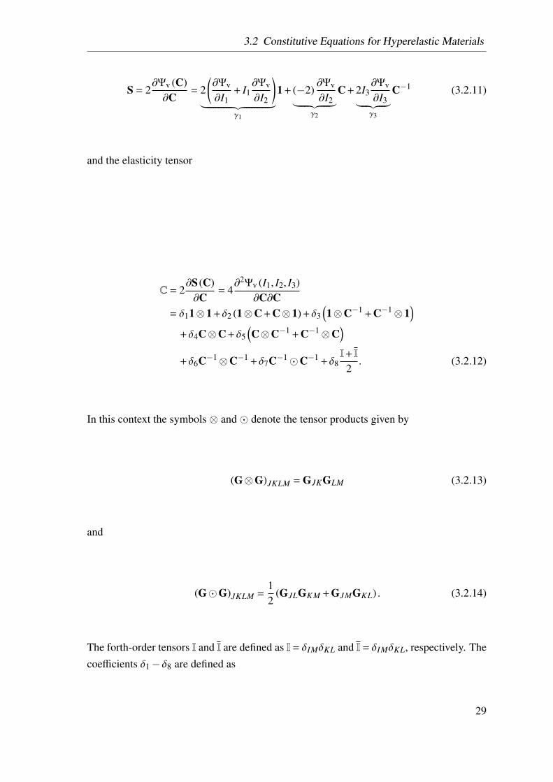
and the elasticity tensor
C = 2∂S (C)∂C
= 4∂2Ψv (I1, I2, I3)
∂C∂C= δ11⊗1 +δ2 (1⊗C + C⊗1) +δ3
(1⊗C−1 + C−1⊗1
)+δ4C⊗C +δ5
(C⊗C−1 + C−1⊗C
)+δ6C−1⊗C−1 +δ7C−1�C−1 +δ8
I+ I
2. (3.2.12)
In this context the symbols ⊗ and � denote the tensor products given by
(G⊗G)JKLM = GJKGLM (3.2.13)
and
(G�G)JKLM =12
(GJLGKM + GJMGKL) . (3.2.14)
The forth-order tensors I and I are defined as I = δIMδKL and I = δIMδKL, respectively. Thecoefficients δ1−δ8 are defined as
29

3 Theoretical Framework
δ1 = 4(∂2Ψv
∂I1∂I1+ 2I1
∂2Ψv
∂I1∂I2+∂Ψv
∂I2+ I2
1∂2Ψv
∂I2∂I2
), (3.2.15)
δ2 =−4(∂2Ψv
∂I1∂I2+ I1
∂2Ψv
∂I2∂I2
), (3.2.16)
δ3 = 4(I3∂2Ψv
∂I1∂I3+ I1I3
∂2Ψv
∂I2∂I3
), (3.2.17)
δ4 = 4∂2Ψv
∂I2∂I2, (3.2.18)
δ5 =−4I3∂2Ψv
∂I2∂I3, (3.2.19)
δ6 = 4(I3∂Ψv
∂I3+ I2
3∂2Ψv
∂I3∂I3
), (3.2.20)
δ7 =−4I3∂Ψv
∂I3, and (3.2.21)
δ8 =−4∂Ψv
∂I2. (3.2.22)
3.2.2 Decoupled Strain Energy Density Functions
The decoupled SEFs, which are split up into a volumetric part Ψvol and an isochoric partΨiso, are formulated as
Ψv(I1, I2, J) = Ψiso(I1, I2) +Ψvol(J), (3.2.23)
withI1 = I1J−
23 and I2 = I2J−
43 , (3.2.24)
being the first and the second modified invariant of C. The modified third invariant I3 iszero by definition since an isochoric deformation is volume preserving. The volumetricpart of the SEF Ψvol depends solely on J, i.e. the change of volume. The decoupled stresstensor is defined as
S = Siso + Svol. (3.2.25)
The isochoric stress contribution Siso is given by
30
3.2 Constitutive Equations for Hyperelastic Materials
Siso = 2∂Ψiso
(C)
∂C= J−2/3S-
13
[S : C
]C−1 (3.2.26)
with the fictitious second Piola-Kirchhoff stress tensor S being defined by
S = 2∂Ψiso
(C)
∂C= 2
(∂Ψiso
∂I1+ I1
∂Ψiso
∂I2
)︸ ︷︷ ︸
γiso, 1
1−2∂Ψiso
∂I2︸ ︷︷ ︸γiso, 2
C. (3.2.27)
The volumetric stress stress contribution Svol is given by
Svol = J∂Ψvol
∂I3︸︷︷︸γvol, 1
C−1. (3.2.28)
Based on equation (3.2.25), the elasticity tensor for a decoupled hyperelastic SEF is
C = Ciso +Cvol. (3.2.29)
The isochoric part Ciso depends on the isochoric stress contribution Siso and thus is definedas
Ciso = 2∂Siso
∂C= P : C : PT +
23
((I− 1
33 S
): C
)P− 2
3
(C−1⊗Siso + Siso ⊗C−1
)(3.2.30)
with P =I− 13C−1⊗C and P = C−1�C−1− 1
3C−1⊗C−1 being a forth-order projectionand a forth-order modified projection tensor, respectively, and C denoting the fourth-orderfictitious elasticity tensor
C = 2J−43∂S∂C
= 4J−43∂2Ψiso
(I1, I2
)∂C∂C
= J−43
δiso, 11⊗1 +δiso, 2(1⊗ C + C⊗1
)+δiso, 3C⊗ C +δiso, 4
I+ I
2
. (3.2.31)
The coefficients δiso, 1−δiso, 4 are defined as
31
3 Theoretical Framework
δiso, 1 = 4(∂2Ψiso
∂I1∂I1+ 2I1
∂2Ψiso
∂I1∂I2+∂Ψiso
∂I2+ I2
1∂2Ψiso
∂I2∂I2
), (3.2.32)
δiso, 2 =−4(∂2Ψiso
∂I1∂I2+ I1
∂2Ψiso
∂I2∂I2
), (3.2.33)
δiso, 3 = 4∂2Ψiso
∂I2∂I2, and (3.2.34)
δiso, 4 =−4∂Ψiso
∂I2. (3.2.35)
The volumetric part of the elasticity tensor can be expressed as follows
Cvol = 2∂Svol
∂C= J
(∂Ψvol
∂J+ J
∂2Ψvol
∂J∂J
)︸ ︷︷ ︸
δvol, 1
C−1⊗C−1−2J∂Ψvol
∂J︸︷︷︸δvol, 2
C−1�C−1. (3.2.36)
The coefficients δvol, 1 and δvol, 2 are defined as
δvol, 1 =∂Ψvol
∂J+ J
∂2Ψvol
∂J∂Jand (3.2.37)
δvol, 2 =∂Ψvol
∂J. (3.2.38)
More detailed derivations can be found in Holzapfel (2004).
3.2.3 Requirements for Strain Energy Density Functions
The SEFs have to fulfill different requirements in order to produce thermodynamicallystable and physically reasonable results. The following contains a brief overview over themost important aspects.
Strain Energy Density Functions Must be Positive For any state of deformation,the stored energy,
Ψv(C , 1) > 0, (3.2.39)
32
3.2 Constitutive Equations for Hyperelastic Materials
must be positive (Doll and Schweizerhof, 2000).
Stress Free Reference Configuration The requirement of a stress free reference con-figuration is physically reasonable, since in hyperelastic materials only deformations in-duce stresses. This condition can be written as
S(C = 1) = 0. (3.2.40)
Limit Cases In the limit of a completely degenerated continuum to a single point, thestrain energy needs to tend towards positive infinity and the volumetric stress to negativeinfinity. Accordingly, in the limit of an infinite stretch the continuum the strain energy aswell as the volumetric stress have to tend towards positive infinity.
Principle of Material Frame Indifference - Objectivity The description of a physicalquantity associated with the motion of a body is generally dependent on the observer. Incontrast, the constitutive equation has to be independent of the particular observer, i.e.indifferent to a change of the reference system.
Hence, rigid body movements should not change the internal quantities. An arbitrarymovement ϕ(•) should lead to the same internal state as the same movement superimposedwith a rigid body movement ψ(•), leading to ϕ+(•) = ψ(ϕ(•)). Due to the superposition,the spatial point X gets mapped to x+ = ϕ+(X). In case of
x+ = c(t) + R(t)x, (3.2.41)
where c(t) can be interpreted as a translation and R(t) as a rotation, the deformation gradi-ent F+ can be obtained as
F+ =∂x+
∂x∂x∂X
= RF. (3.2.42)
The principle of material frame indifference requires both observers to register the sameamount of energy and the same state of stress of the deformed body, i.e.
Ψv (RF) = Ψv (F) , S (RF) = RS (F) . (3.2.43)
33
3 Theoretical Framework
With the right Cauchy-Green tensor being a priori frame objective, i.e. C+ = F+T F+ =
RT FT RF = C, the SEF introduced above fulfills the below requirement as well
Ψv (C) = Ψv(C+
). (3.2.44)
Existence of a Minimizer It has to be assured that the boundary value problem hasat least one solution. It has been been shown that, polyconvexity is the most suitablerestriction for the construction of physically reasonable SEFs, guaranteeing the existenceof at least one minimum.
The polyconvexity requires
Ψv(F) = f (F, JFT , J), (3.2.45)
i.e. a function of the 19-dimensional space, to be convex. In a more descriptive way, thismeans that the transformations of line, area and volume elements, see equations (3.1.6),(3.1.8) and (3.1.7), need to be unique. An additional advantage is that polyconvex functionscan be constructed by summing up polyconvex summands. More details on polyconvexitycan be found in Ball (1977); Schröder (2004); Balzani (2006).
For more details on hyperelastic materials, the reader is referred to Ogden (1997);Holzapfel (2004).
34
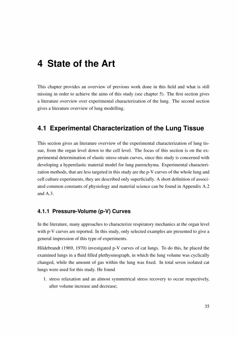
4 State of the Art
This chapter provides an overview of previous work done in this field and what is stillmissing in order to achieve the aims of this study (see chapter 5). The first section givesa literature overview over experimental characterization of the lung. The second sectiongives a literature overview of lung modelling.
4.1 Experimental Characterization of the Lung Tissue
This section gives an literature overview of the experimental characterization of lung tis-sue, from the organ level down to the cell level. The focus of this section is on the ex-perimental determination of elastic stress-strain curves, since this study is concerned withdeveloping a hyperelastic material model for lung parenchyma. Experimental characteri-zation methods, that are less targeted in this study are the p-V curves of the whole lung andcell culture experiments, they are described only superficially. A short definition of associ-ated common constants of physiology and material science can be found in Appendix A.2and A.3.
4.1.1 Pressure-Volume (p-V) Curves
In the literature, many approaches to characterize respiratory mechanics at the organ levelwith p-V curves are reported. In this study, only selected examples are presented to give ageneral impression of this type of experiments.
Hildebrandt (1969, 1970) investigated p-V curves of cat lungs. To do this, he placed theexamined lungs in a fluid filled plethysmograph, in which the lung volume was cyclicallychanged, while the amount of gas within the lung was fixed. In total seven isolated catlungs were used for this study. He found
1. stress relaxation and an almost symmetrical stress recovery to occur respectively,after volume increase and decrease;
35
4 State of the Art
2. dynamic elastance (Appendix A.3.2), to increase linearly with the logarithm of cyclicfrequency (0.1 increase in elastance a 10-fold increase in frequency); and
3. hysteresis loop area, i.e. the area between the loading and unloading p-V curve, tovary with the square of the tidal volume but to be independent of the cyclic frequency.
Stamenovic and Yager (1988) studied the mechanical properties of the parenchymal tis-sue with and without surface tension, in air and saline filled rabbit lungs, respectively. Inthe first step, the lungs were inflated to transpulmonary pressure of 30mmH2O. The as-sociated volume was defined as the volume at TLC. The pressure was then successivelyreduced down to zero. At every step, small p-V loops were performed to determine thelocal bulk moduli. They found little difference in the shape of the curves describing theelastic behavior of air and saline filled lungs, suggesting that the mechanism of resistingdeformation in both cases is similar. However, the air-filled lungs showed stiffer behavior,which they explained with the surface tension at the air-liquid interface.
Bates et al. (1989) determined the resistance (Appendix A.3.3) and elastance of the res-piratory system using data obtained from healthy anesthetized dogs during mechanicalventilation at different frequencies and tidal volumes. They found resistance and elastanceto decrease with increasing frequency. The variations of resistance and elastance with fre-quency are similar to the variations determined from regular ventilation data. There were,however, some systematic differences between the actual values of resistance and elastanceobtained by the two methods, which may reflect certain non-linear characteristics. Theyalso found a slight decrease for both resistance and elastance with increasing tidal volumeat all frequencies.
Suki et al. (1989) measured the lung impedance in six healthy humans for frequenciesbetween 0.01−0.1Hz. They superimposed small amplitude signals in order to force oscil-lations on spontaneous breathing. They did not find a difference between applying a forceor a pressure. They found the compliance to decrease from 0.97kPa/l via 0.27kPa/l to0.23kPa/l at 0.01Hz, 0.03Hz, and 0.1Hz, respectively. It is remarkable that at very smallfrequencies, the change in compliance is much larger than at higher frequencies, which arecloser to actual breathing frequencies.
Summing up, the p-V curves are an adequate way to understand global lung mechanics,which is especially important for adjusting the ventilator towards the needs of a venti-lated patient. However, the focus of this work is on a more local behavior of the lungparenchyma and even further down to the individual alveolar walls. For this reason p-Vcurves of the whole lung, including airways etc., are too coarse for this purpose.
36
4.1 Experimental Characterization of the Lung Tissue
4.1.2 Tensile Tests on Lung Parenchyma Specimens
To investigate the local material behavior of lung parenchyma, tests on isolated samplesare required. In the literature, a wide range of experiments have been presented such asuni-, bi-, or triaxial tensile tests in a saline bath or in air. Consequently, this section givesan overview of the most important tensile tests on parenchymal tissue specimens.
4.1.2.1 Uniaxial Tensile Tests
Fukaya et al. (1968) performed uniaxial tensile tests on cat lung specimens with the di-mensions 30×30×200µm, see Figure 4.1. Contrary to the title ”Mechanical properties ofalveolar walls”, they investigated the material behavior of the parenchymal tissue and notof the individual alveolar wall. The tests were performed in a saline bath, in order to obtainthe osmolarity of the cells, at room temperature. Their findings are briefly summarized inthe following.
• The length-tension relationship did not change within the first 36h after dissectionof the lungs.
• A strong hysteresis occurred in the length-tension relationship.
– The hysteresis depends on final force and length-tension history, see Figure4.2(A) (Remark: The hysteresis measured is not due to the air-liquid interface,because the tests were performed in a saline bath).
– However, the hysteresis is not dependent on cyclic frequencies between6cycles/min and 0.2cycles/min. The independence of the cyclic frequency hasbeen previously reported by Hildebrandt (1966).
• The length increase of the specimens is limited to an extension of 100−130% overthe initial length; stretch beyond this length resulted in tissue damage.
• Stress relaxation and recovery, with the fast component of stress relaxation, is com-plete within 60s after the initial deformation.
• The hysteresis, in a quasi-static experiment, is reduced but does not disappear, seeFigure 4.2(B). This shows that the hysteresis is not solely dependent on the fastcomponent of stress relaxation.
• A 5min resting period is necessary to reset the tissue back to its initial state prior totesting.
37
4 State of the Art
Figure 4.1: Comparison of specimens utilized in uniaxial tensile tests. First row from leftto right: Rausch et al. (2011b), Fukaya et al. (1968), Sugihara et al. (1971),Navajas et al. (1995), Karlinsky et al. (1985), and Jamal et al. (2001). Secondrow from left to right: Bates et al. (1994), Yuan et al. (1997), Mijailovichet al. (1994), Cavalcante et al. (2005), and Faffe et al. (2001). The dashedlines indicate that the specimen dimensions were not clearly defined in thecorresponding paper. The units are given in mm.
38
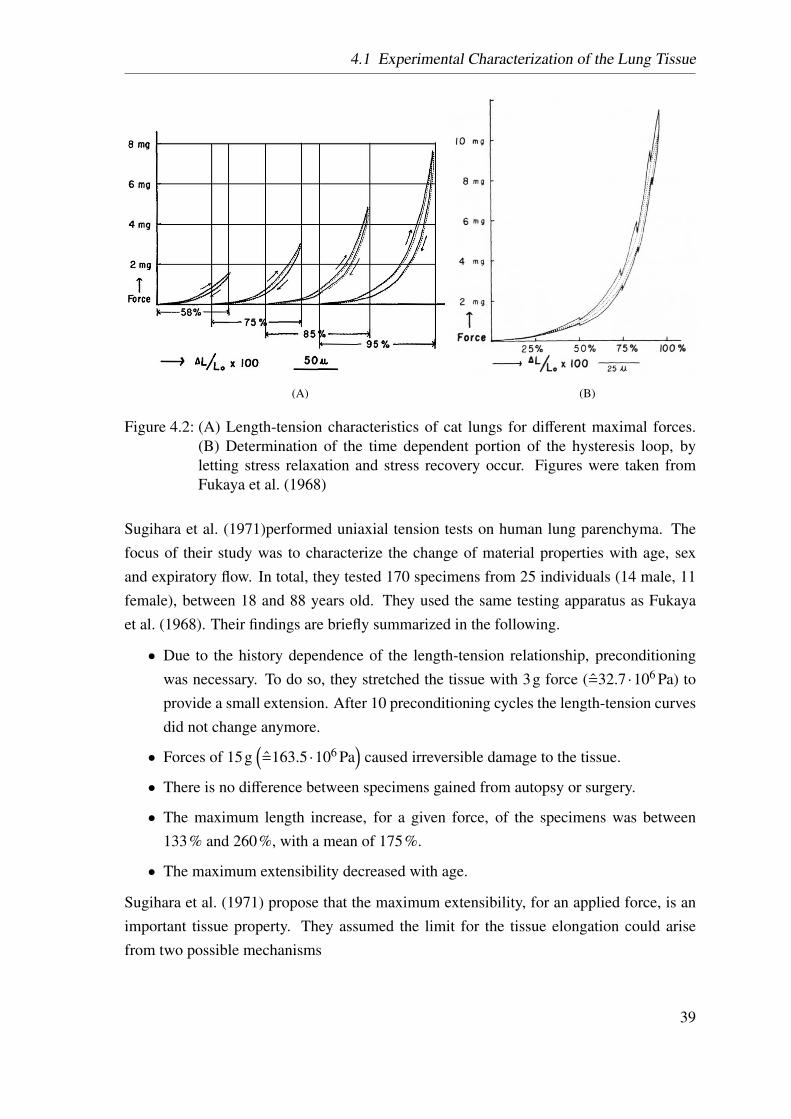
4.1 Experimental Characterization of the Lung Tissue
(A) (B)
Figure 4.2: (A) Length-tension characteristics of cat lungs for different maximal forces.(B) Determination of the time dependent portion of the hysteresis loop, byletting stress relaxation and stress recovery occur. Figures were taken fromFukaya et al. (1968)
Sugihara et al. (1971)performed uniaxial tension tests on human lung parenchyma. Thefocus of their study was to characterize the change of material properties with age, sexand expiratory flow. In total, they tested 170 specimens from 25 individuals (14 male, 11female), between 18 and 88 years old. They used the same testing apparatus as Fukayaet al. (1968). Their findings are briefly summarized in the following.
• Due to the history dependence of the length-tension relationship, preconditioningwas necessary. To do so, they stretched the tissue with 3g force (=32.7·106 Pa) toprovide a small extension. After 10 preconditioning cycles the length-tension curvesdid not change anymore.
• Forces of 15g(=163.5·106 Pa
)caused irreversible damage to the tissue.
• There is no difference between specimens gained from autopsy or surgery.
• The maximum length increase, for a given force, of the specimens was between133% and 260%, with a mean of 175%.
• The maximum extensibility decreased with age.
Sugihara et al. (1971) propose that the maximum extensibility, for an applied force, is animportant tissue property. They assumed the limit for the tissue elongation could arisefrom two possible mechanisms
39
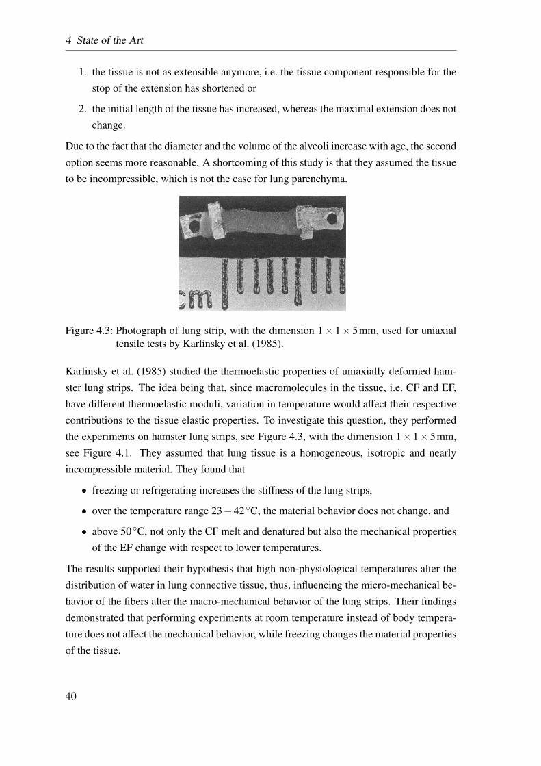
4 State of the Art
1. the tissue is not as extensible anymore, i.e. the tissue component responsible for thestop of the extension has shortened or
2. the initial length of the tissue has increased, whereas the maximal extension does notchange.
Due to the fact that the diameter and the volume of the alveoli increase with age, the secondoption seems more reasonable. A shortcoming of this study is that they assumed the tissueto be incompressible, which is not the case for lung parenchyma.
Figure 4.3: Photograph of lung strip, with the dimension 1× 1× 5mm, used for uniaxialtensile tests by Karlinsky et al. (1985).
Karlinsky et al. (1985) studied the thermoelastic properties of uniaxially deformed ham-ster lung strips. The idea being that, since macromolecules in the tissue, i.e. CF and EF,have different thermoelastic moduli, variation in temperature would affect their respectivecontributions to the tissue elastic properties. To investigate this question, they performedthe experiments on hamster lung strips, see Figure 4.3, with the dimension 1×1×5mm,see Figure 4.1. They assumed that lung tissue is a homogeneous, isotropic and nearlyincompressible material. They found that
• freezing or refrigerating increases the stiffness of the lung strips,
• over the temperature range 23−42◦C, the material behavior does not change, and
• above 50◦C, not only the CF melt and denatured but also the mechanical propertiesof the EF change with respect to lower temperatures.
The results supported their hypothesis that high non-physiological temperatures alter thedistribution of water in lung connective tissue, thus, influencing the micro-mechanical be-havior of the fibers alter the macro-mechanical behavior of the lung strips. Their findingsdemonstrated that performing experiments at room temperature instead of body tempera-ture does not affect the mechanical behavior, while freezing changes the material propertiesof the tissue.
40
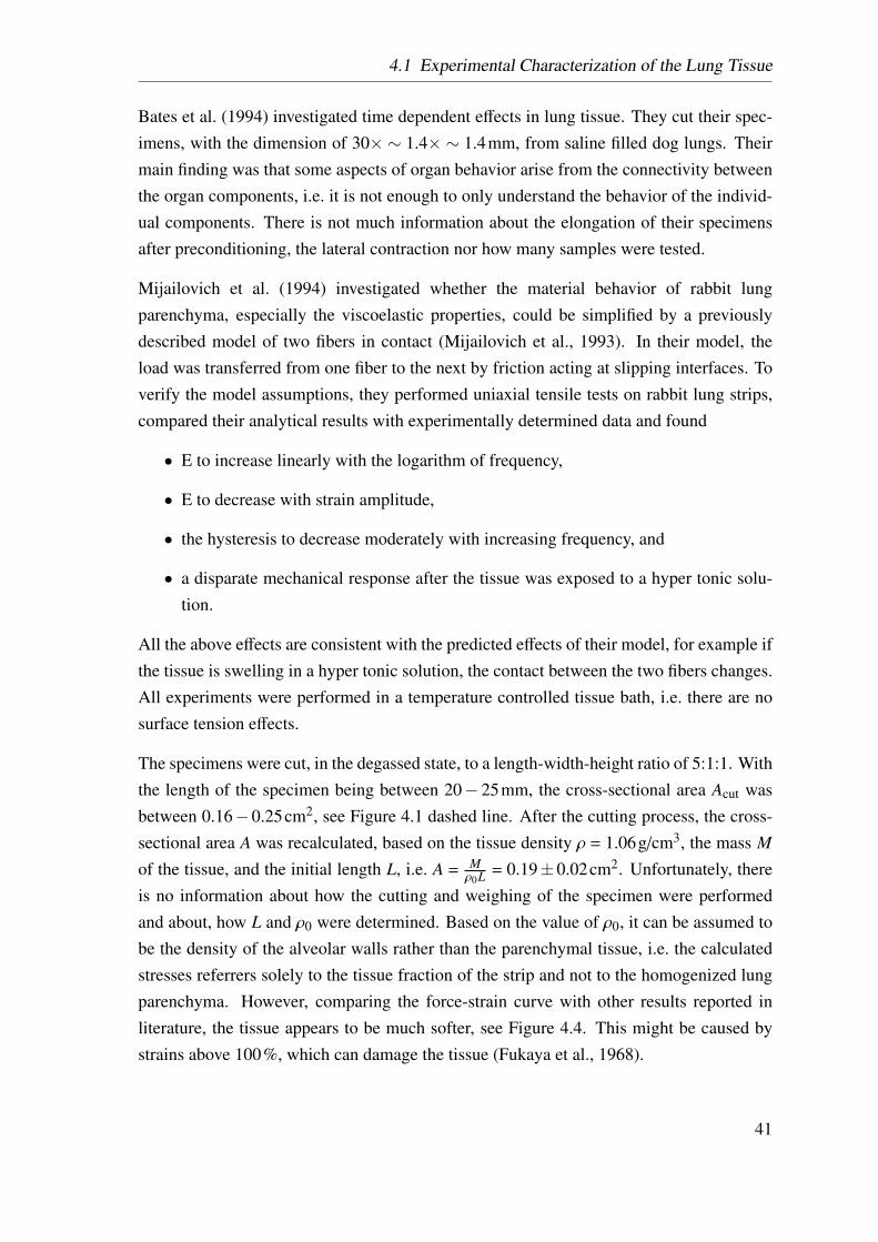
4.1 Experimental Characterization of the Lung Tissue
Bates et al. (1994) investigated time dependent effects in lung tissue. They cut their spec-imens, with the dimension of 30× ∼ 1.4× ∼ 1.4mm, from saline filled dog lungs. Theirmain finding was that some aspects of organ behavior arise from the connectivity betweenthe organ components, i.e. it is not enough to only understand the behavior of the individ-ual components. There is not much information about the elongation of their specimensafter preconditioning, the lateral contraction nor how many samples were tested.
Mijailovich et al. (1994) investigated whether the material behavior of rabbit lungparenchyma, especially the viscoelastic properties, could be simplified by a previouslydescribed model of two fibers in contact (Mijailovich et al., 1993). In their model, theload was transferred from one fiber to the next by friction acting at slipping interfaces. Toverify the model assumptions, they performed uniaxial tensile tests on rabbit lung strips,compared their analytical results with experimentally determined data and found
• E to increase linearly with the logarithm of frequency,
• E to decrease with strain amplitude,
• the hysteresis to decrease moderately with increasing frequency, and
• a disparate mechanical response after the tissue was exposed to a hyper tonic solu-tion.
All the above effects are consistent with the predicted effects of their model, for example ifthe tissue is swelling in a hyper tonic solution, the contact between the two fibers changes.All experiments were performed in a temperature controlled tissue bath, i.e. there are nosurface tension effects.
The specimens were cut, in the degassed state, to a length-width-height ratio of 5:1:1. Withthe length of the specimen being between 20− 25mm, the cross-sectional area Acut wasbetween 0.16−0.25cm2, see Figure 4.1 dashed line. After the cutting process, the cross-sectional area A was recalculated, based on the tissue density ρ = 1.06g/cm3, the mass M
of the tissue, and the initial length L, i.e. A = Mρ0L = 0.19±0.02cm2. Unfortunately, there
is no information about how the cutting and weighing of the specimen were performedand about, how L and ρ0 were determined. Based on the value of ρ0, it can be assumed tobe the density of the alveolar walls rather than the parenchymal tissue, i.e. the calculatedstresses referrers solely to the tissue fraction of the strip and not to the homogenized lungparenchyma. However, comparing the force-strain curve with other results reported inliterature, the tissue appears to be much softer, see Figure 4.4. This might be caused bystrains above 100%, which can damage the tissue (Fukaya et al., 1968).
41
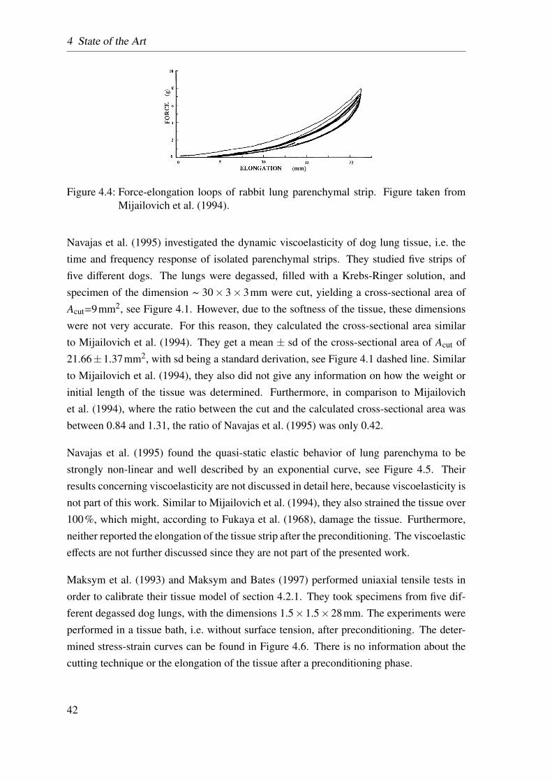
4 State of the Art
Figure 4.4: Force-elongation loops of rabbit lung parenchymal strip. Figure taken fromMijailovich et al. (1994).
Navajas et al. (1995) investigated the dynamic viscoelasticity of dog lung tissue, i.e. thetime and frequency response of isolated parenchymal strips. They studied five strips offive different dogs. The lungs were degassed, filled with a Krebs-Ringer solution, andspecimen of the dimension ∼ 30× 3× 3mm were cut, yielding a cross-sectional area ofAcut=9mm2, see Figure 4.1. However, due to the softness of the tissue, these dimensionswere not very accurate. For this reason, they calculated the cross-sectional area similarto Mijailovich et al. (1994). They get a mean ± sd of the cross-sectional area of Acut of21.66±1.37mm2, with sd being a standard derivation, see Figure 4.1 dashed line. Similarto Mijailovich et al. (1994), they also did not give any information on how the weight orinitial length of the tissue was determined. Furthermore, in comparison to Mijailovichet al. (1994), where the ratio between the cut and the calculated cross-sectional area wasbetween 0.84 and 1.31, the ratio of Navajas et al. (1995) was only 0.42.
Navajas et al. (1995) found the quasi-static elastic behavior of lung parenchyma to bestrongly non-linear and well described by an exponential curve, see Figure 4.5. Theirresults concerning viscoelasticity are not discussed in detail here, because viscoelasticity isnot part of this work. Similar to Mijailovich et al. (1994), they also strained the tissue over100%, which might, according to Fukaya et al. (1968), damage the tissue. Furthermore,neither reported the elongation of the tissue strip after the preconditioning. The viscoelasticeffects are not further discussed since they are not part of the presented work.
Maksym et al. (1993) and Maksym and Bates (1997) performed uniaxial tensile tests inorder to calibrate their tissue model of section 4.2.1. They took specimens from five dif-ferent degassed dog lungs, with the dimensions 1.5×1.5×28mm. The experiments wereperformed in a tissue bath, i.e. without surface tension, after preconditioning. The deter-mined stress-strain curves can be found in Figure 4.6. There is no information about thecutting technique or the elongation of the tissue after a preconditioning phase.
42
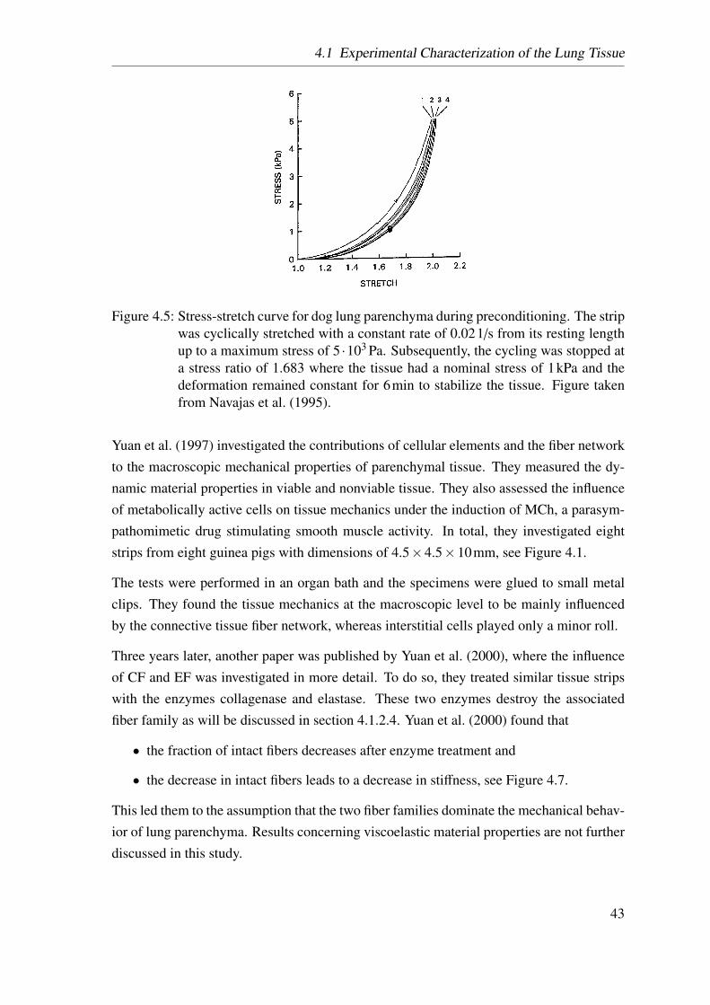
4.1 Experimental Characterization of the Lung Tissue
Figure 4.5: Stress-stretch curve for dog lung parenchyma during preconditioning. The stripwas cyclically stretched with a constant rate of 0.021/s from its resting lengthup to a maximum stress of 5 ·103 Pa. Subsequently, the cycling was stopped ata stress ratio of 1.683 where the tissue had a nominal stress of 1kPa and thedeformation remained constant for 6min to stabilize the tissue. Figure takenfrom Navajas et al. (1995).
Yuan et al. (1997) investigated the contributions of cellular elements and the fiber networkto the macroscopic mechanical properties of parenchymal tissue. They measured the dy-namic material properties in viable and nonviable tissue. They also assessed the influenceof metabolically active cells on tissue mechanics under the induction of MCh, a parasym-pathomimetic drug stimulating smooth muscle activity. In total, they investigated eightstrips from eight guinea pigs with dimensions of 4.5×4.5×10mm, see Figure 4.1.
The tests were performed in an organ bath and the specimens were glued to small metalclips. They found the tissue mechanics at the macroscopic level to be mainly influencedby the connective tissue fiber network, whereas interstitial cells played only a minor roll.
Three years later, another paper was published by Yuan et al. (2000), where the influenceof CF and EF was investigated in more detail. To do so, they treated similar tissue stripswith the enzymes collagenase and elastase. These two enzymes destroy the associatedfiber family as will be discussed in section 4.1.2.4. Yuan et al. (2000) found that
• the fraction of intact fibers decreases after enzyme treatment and
• the decrease in intact fibers leads to a decrease in stiffness, see Figure 4.7.
This led them to the assumption that the two fiber families dominate the mechanical behav-ior of lung parenchyma. Results concerning viscoelastic material properties are not furtherdiscussed in this study.
43
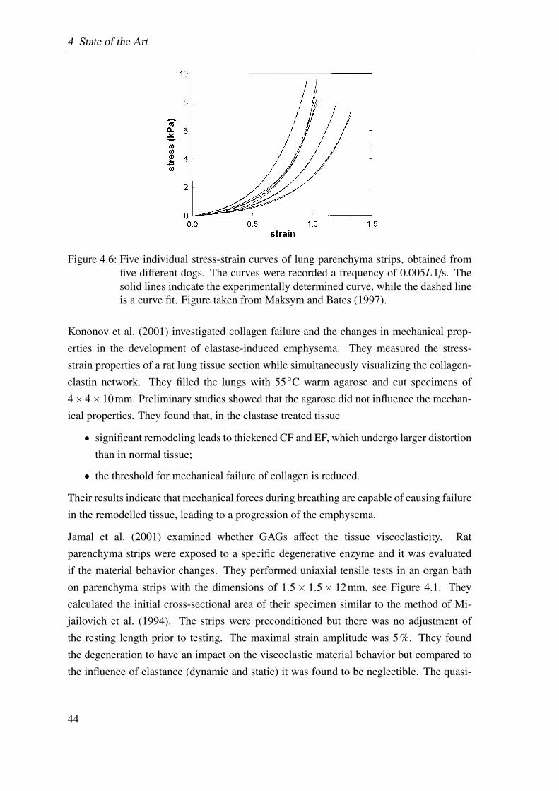
4 State of the Art
Figure 4.6: Five individual stress-strain curves of lung parenchyma strips, obtained fromfive different dogs. The curves were recorded a frequency of 0.005L1/s. Thesolid lines indicate the experimentally determined curve, while the dashed lineis a curve fit. Figure taken from Maksym and Bates (1997).
Kononov et al. (2001) investigated collagen failure and the changes in mechanical prop-erties in the development of elastase-induced emphysema. They measured the stress-strain properties of a rat lung tissue section while simultaneously visualizing the collagen-elastin network. They filled the lungs with 55◦C warm agarose and cut specimens of4×4×10mm. Preliminary studies showed that the agarose did not influence the mechan-ical properties. They found that, in the elastase treated tissue
• significant remodeling leads to thickened CF and EF, which undergo larger distortionthan in normal tissue;
• the threshold for mechanical failure of collagen is reduced.
Their results indicate that mechanical forces during breathing are capable of causing failurein the remodelled tissue, leading to a progression of the emphysema.
Jamal et al. (2001) examined whether GAGs affect the tissue viscoelasticity. Ratparenchyma strips were exposed to a specific degenerative enzyme and it was evaluatedif the material behavior changes. They performed uniaxial tensile tests in an organ bathon parenchyma strips with the dimensions of 1.5× 1.5× 12mm, see Figure 4.1. Theycalculated the initial cross-sectional area of their specimen similar to the method of Mi-jailovich et al. (1994). The strips were preconditioned but there was no adjustment ofthe resting length prior to testing. The maximal strain amplitude was 5%. They foundthe degeneration to have an impact on the viscoelastic material behavior but compared tothe influence of elastance (dynamic and static) it was found to be neglectible. The quasi-
44
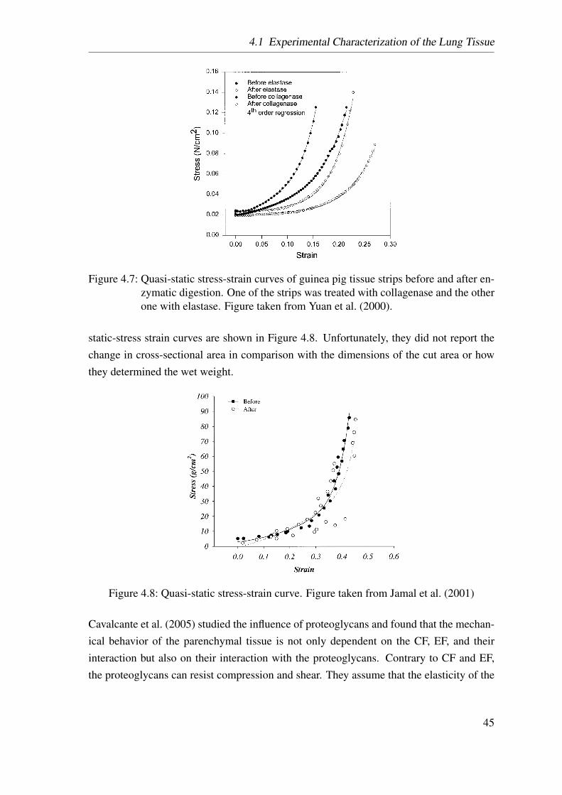
4.1 Experimental Characterization of the Lung Tissue
Figure 4.7: Quasi-static stress-strain curves of guinea pig tissue strips before and after en-zymatic digestion. One of the strips was treated with collagenase and the otherone with elastase. Figure taken from Yuan et al. (2000).
static-stress strain curves are shown in Figure 4.8. Unfortunately, they did not report thechange in cross-sectional area in comparison with the dimensions of the cut area or howthey determined the wet weight.
Figure 4.8: Quasi-static stress-strain curve. Figure taken from Jamal et al. (2001)
Cavalcante et al. (2005) studied the influence of proteoglycans and found that the mechan-ical behavior of the parenchymal tissue is not only dependent on the CF, EF, and theirinteraction but also on their interaction with the proteoglycans. Contrary to CF and EF,the proteoglycans can resist compression and shear. They assume that the elasticity of the
45
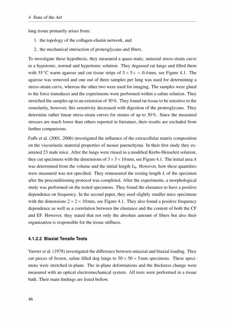
4 State of the Art
lung tissue primarily arises from:
1. the topology of the collagen-elastin network, and
2. the mechanical interaction of proteoglycans and fibers.
To investigate these hypothesis, they measured a quasi-static, uniaxial stress-strain curvein a hypotonic, normal and hypertonic solution. They degassed rat lungs and filled themwith 55◦C warm agarose and cut tissue strips of 5× 5× ∼ 0.4mm, see Figure 4.1. Theagarose was removed and one out of three samples per lung was used for determining astress-strain curve, whereas the other two were used for imaging. The samples were gluedto the force transducer and the experiments were performed within a saline solution. Theystretched the samples up to an extension of 30%. They found rat tissue to be sensitive to theosmolarity, however, this sensitivity decreased with digestion of the proteoglycans. Theydetermine rather linear stress-strain curves for strains of up to 30%. Since the measuredstresses are much lower than others reported in literature, their results are excluded fromfurther comparisons.
Faffe et al. (2001, 2006) investigated the influence of the extracellular matrix compositionon the viscoelastic material properties of mouse parenchyma. In their first study they ex-amined 23 male mice. After the lungs were rinsed in a modified Krebs-Henseleit solution,they cut specimens with the dimensions of 3×3×10mm, see Figure 4.1. The initial area A
was determined from the volume and the initial length L0. However, how these quantitieswere measured was not specified. They remeasured the resting length L of the specimenafter the preconditioning protocol was completed. After the experiments, a morphologicalstudy was performed on the tested specimens. They found the elastance to have a positivedependence on frequency. In the second paper, they used slightly smaller mice specimenswith the dimensions 2×2×10mm, see Figure 4.1. They also found a positive frequencydependence as well as a correlation between the elastance and the content of both the CFand EF. However, they stated that not only the absolute amount of fibers but also theirorganization is responsible for the tissue stiffness.
4.1.2.2 Biaxial Tensile Tests
Vawter et al. (1978) investigated the difference between uniaxial and biaxial loading. Theycut pieces of frozen, saline filled dog lungs to 50× 50× 5mm specimens. These speci-mens were stretched in-plane. The in-plane deformations and the thickness change weremeasured with an optical electromechanical system. All tests were performed in a tissuebath. Their main findings are listed bellow.
46
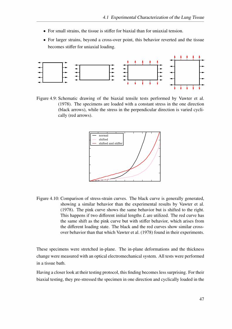
4.1 Experimental Characterization of the Lung Tissue
• For small strains, the tissue is stiffer for biaxial than for uniaxial tension.
• For larger strains, beyond a cross-over point, this behavior reverted and the tissuebecomes stiffer for uniaxial loading.
Figure 4.9: Schematic drawing of the biaxial tensile tests performed by Vawter et al.(1978). The specimens are loaded with a constant stress in the one direction(black arrows), while the stress in the perpendicular direction is varied cycli-cally (red arrows).
normalshiftedshifted and stiffer
Figure 4.10: Comparison of stress-strain curves. The black curve is generally generated,showing a similar behavior than the experimental results by Vawter et al.(1978). The pink curve shows the same behavior but is shifted to the right.This happens if two different initial lengths L are utilized. The red curve hasthe same shift as the pink curve but with stiffer behavior, which arises fromthe different loading state. The black and the red curves show similar cross-over behavior than that which Vawter et al. (1978) found in their experiments.
These specimens were stretched in-plane. The in-plane deformations and the thicknesschange were measured with an optical electromechanical system. All tests were performedin a tissue bath.
Having a closer look at their testing protocol, this finding becomes less surprising. For theirbiaxial testing, they pre-stressed the specimen in one direction and cyclically loaded in the
47
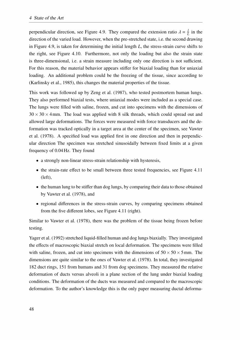
4 State of the Art
perpendicular direction, see Figure 4.9. They compared the extension ratio λ = lL in the
direction of the varied load. However, when the pre-stretched state, i.e. the second drawingin Figure 4.9, is taken for determining the initial length L, the stress-strain curve shifts tothe right, see Figure 4.10. Furthermore, not only the loading but also the strain stateis three-dimensional, i.e. a strain measure including only one direction is not sufficient.For this reason, the material behavior appears stiffer for biaxial loading than for uniaxialloading. An additional problem could be the freezing of the tissue, since according to(Karlinsky et al., 1985), this changes the material properties of the tissue.
This work was followed up by Zeng et al. (1987), who tested postmortem human lungs.They also performed biaxial tests, where uniaxial modes were included as a special case.The lungs were filled with saline, frozen, and cut into specimens with the dimensions of30× 30× 4mm. The load was applied with 8 silk threads, which could spread out andallowed large deformations. The forces were measured with force transducers and the de-formation was tracked optically in a target area at the center of the specimen, see Vawteret al. (1978). A specified load was applied first in one direction and then in perpendic-ular direction The specimen was stretched sinusoidally between fixed limits at a givenfrequency of 0.04Hz. They found
• a strongly non-linear stress-strain relationship with hysteresis,
• the strain-rate effect to be small between three tested frequencies, see Figure 4.11(left),
• the human lung to be stiffer than dog lungs, by comparing their data to those obtainedby Vawter et al. (1978), and
• regional differences in the stress-strain curves, by comparing specimens obtainedfrom the five different lobes, see Figure 4.11 (right).
Similar to Vawter et al. (1978), there was the problem of the tissue being frozen beforetesting.
Yager et al. (1992) stretched liquid-filled human and dog lungs biaxially. They investigatedthe effects of macroscopic biaxial stretch on local deformation. The specimens were filledwith saline, frozen, and cut into specimens with the dimensions of 50× 50× 5mm. Thedimensions are quite similar to the ones of Vawter et al. (1978). In total, they investigated182 duct rings, 151 from humans and 31 from dog specimens. They measured the relativedeformation of ducts versus alveoli in a plane section of the lung under biaxial loadingconditions. The deformation of the ducts was measured and compared to the macroscopicdeformation. To the author’s knowledge this is the only paper measuring ductal deforma-
48
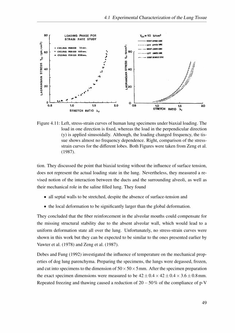
4.1 Experimental Characterization of the Lung Tissue
Figure 4.11: Left, stress-strain curves of human lung specimens under biaxial loading. Theload in one direction is fixed, whereas the load in the perpendicular direction(y) is applied sinusoidally. Although, the loading changed frequency, the tis-sue shows almost no frequency dependence. Right, comparison of the stress-strain curves for the different lobes. Both Figures were taken from Zeng et al.(1987).
tion. They discussed the point that biaxial testing without the influence of surface tension,does not represent the actual loading state in the lung. Nevertheless, they measured a re-vised notion of the interaction between the ducts and the surrounding alveoli, as well astheir mechanical role in the saline filled lung. They found
• all septal walls to be stretched, despite the absence of surface-tension and
• the local deformation to be significantly larger than the global deformation.
They concluded that the fiber reinforcement in the alveolar mouths could compensate forthe missing structural stability due to the absent alveolar wall, which would lead to auniform deformation state all over the lung. Unfortunately, no stress-strain curves wereshown in this work but they can be expected to be similar to the ones presented earlier byVawter et al. (1978) and Zeng et al. (1987).
Debes and Fung (1992) investigated the influence of temperature on the mechanical prop-erties of dog lung parenchyma. Preparing the specimens, the lungs were degassed, frozen,and cut into specimens to the dimension of 50×50×5mm. After the specimen preparationthe exact specimen dimensions were measured to be 42± 0.4× 42± 0.4× 3.6± 0.8mm.Repeated freezing and thawing caused a reduction of 20−50% of the compliance of p-V
49
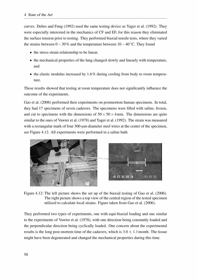
4 State of the Art
curves. Debes and Fung (1992) used the same testing device as Yager et al. (1992). Theywere especially interested in the mechanics of CF and EF, for this reason they eliminatedthe surface tension prior to testing. They performed biaxial tensile tests, where they variedthe strains between 0−30% and the temperature between 10−40◦C. They found
• the stress-strain relationship to be linear,
• the mechanical properties of the lung changed slowly and linearly with temperature,and
• the elastic modulus increased by 1.6% during cooling from body to room tempera-ture.
These results showed that testing at room temperature does not significantly influence theoutcome of the experiments.
Gao et al. (2006) performed their experiments on postmortem human specimens. In total,they had 17 specimens of seven cadavers. The specimens were filled with saline, frozen,and cut to specimens with the dimensions of 50× 50× 4mm. The dimensions are quitesimilar to the ones of Vawter et al. (1978) and Yager et al. (1992). The strain was measuredwith a rectangular mark of four 300-µm-diameter steel wires at the center of the specimen,see Figure 4.12. All experiments were performed in a saline bath.
Figure 4.12: The left picture shows the set up of the biaxial testing of Gao et al. (2006).The right picture shows a top view of the central region of the tested specimenutilized to calculate local strains. Figure taken from Gao et al. (2006).
They performed two types of experiments, one with equi-biaxial loading and one similarto the experiments of Vawter et al. (1978), with one direction being constantly loaded andthe perpendicular direction being cyclically loaded. One concern about the experimentalresults is the long post-mortem time of the cadavers, which is 3.0 ± 1.1month. The tissuemight have been degenerated and changed the mechanical properties during this time.
50
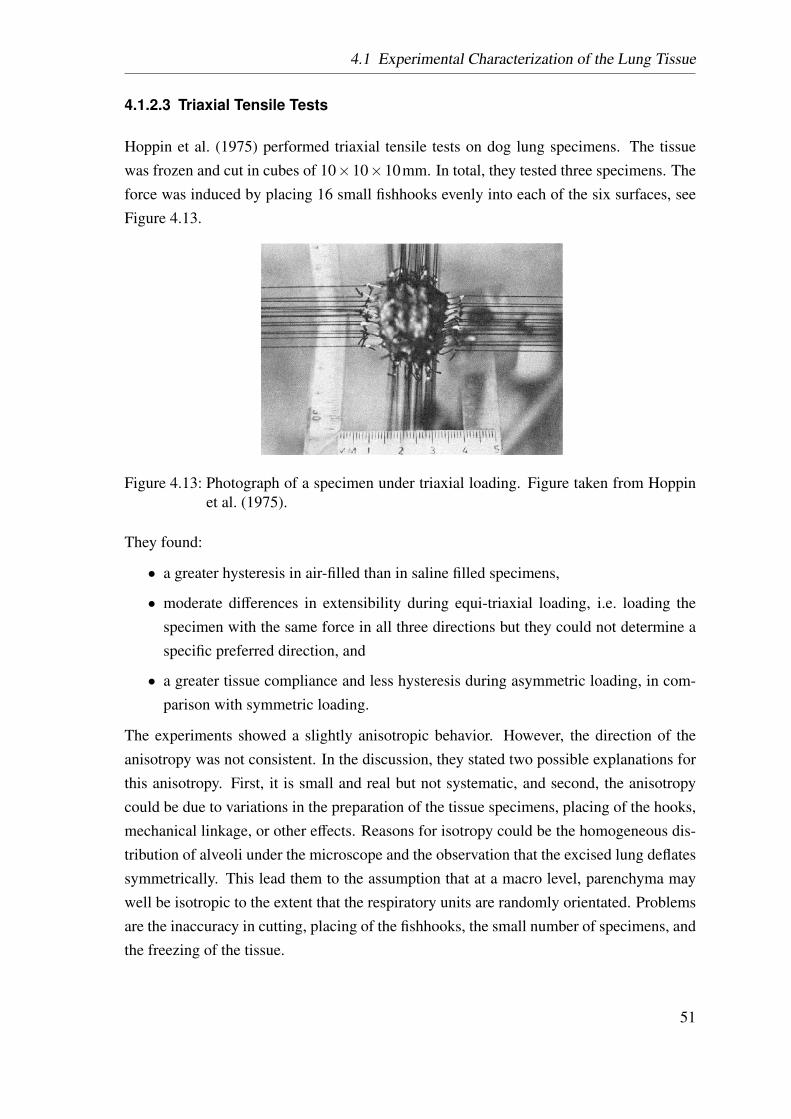
4.1 Experimental Characterization of the Lung Tissue
4.1.2.3 Triaxial Tensile Tests
Hoppin et al. (1975) performed triaxial tensile tests on dog lung specimens. The tissuewas frozen and cut in cubes of 10×10×10mm. In total, they tested three specimens. Theforce was induced by placing 16 small fishhooks evenly into each of the six surfaces, seeFigure 4.13.
Figure 4.13: Photograph of a specimen under triaxial loading. Figure taken from Hoppinet al. (1975).
They found:
• a greater hysteresis in air-filled than in saline filled specimens,
• moderate differences in extensibility during equi-triaxial loading, i.e. loading thespecimen with the same force in all three directions but they could not determine aspecific preferred direction, and
• a greater tissue compliance and less hysteresis during asymmetric loading, in com-parison with symmetric loading.
The experiments showed a slightly anisotropic behavior. However, the direction of theanisotropy was not consistent. In the discussion, they stated two possible explanations forthis anisotropy. First, it is small and real but not systematic, and second, the anisotropycould be due to variations in the preparation of the tissue specimens, placing of the hooks,mechanical linkage, or other effects. Reasons for isotropy could be the homogeneous dis-tribution of alveoli under the microscope and the observation that the excised lung deflatessymmetrically. This lead them to the assumption that at a macro level, parenchyma maywell be isotropic to the extent that the respiratory units are randomly orientated. Problemsare the inaccuracy in cutting, placing of the fishhooks, the small number of specimens, andthe freezing of the tissue.
51
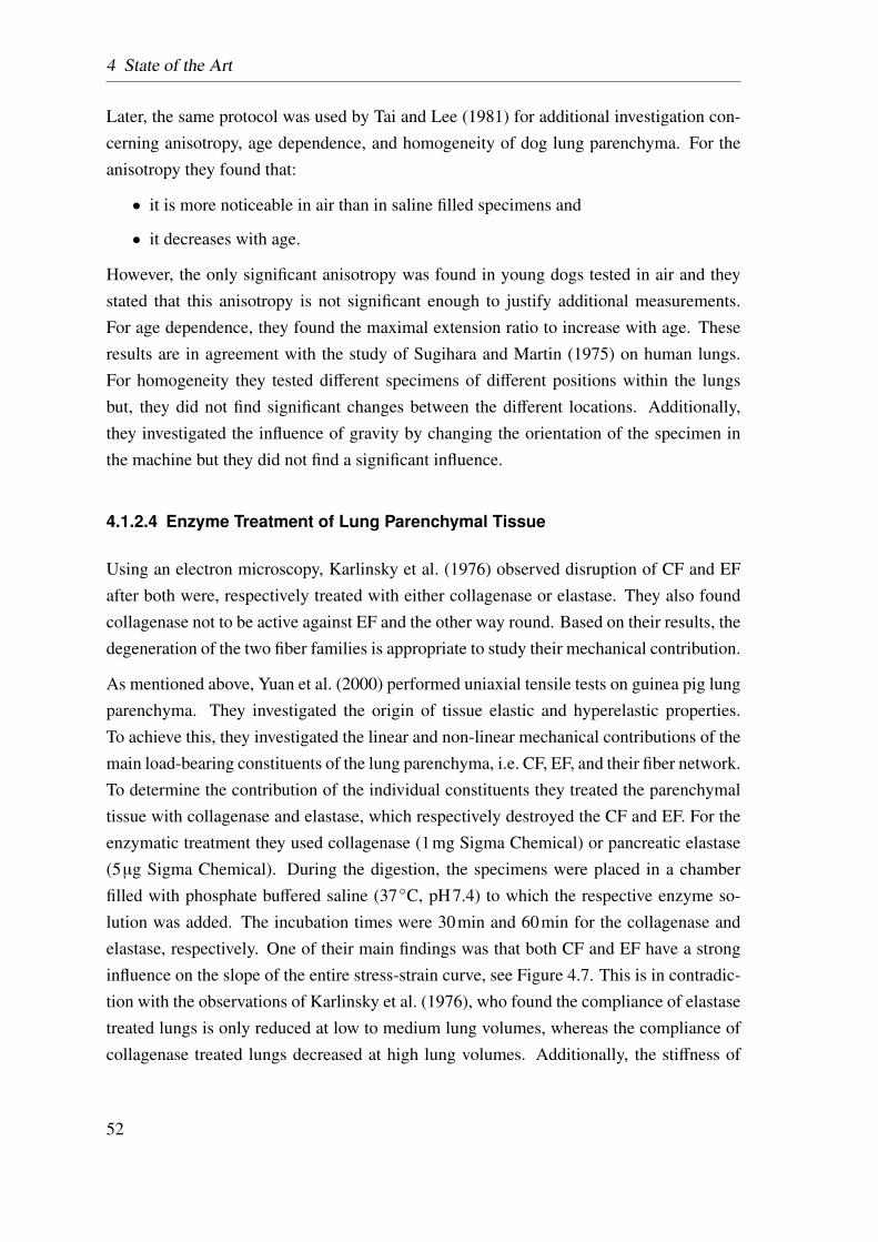
4 State of the Art
Later, the same protocol was used by Tai and Lee (1981) for additional investigation con-cerning anisotropy, age dependence, and homogeneity of dog lung parenchyma. For theanisotropy they found that:
• it is more noticeable in air than in saline filled specimens and
• it decreases with age.
However, the only significant anisotropy was found in young dogs tested in air and theystated that this anisotropy is not significant enough to justify additional measurements.For age dependence, they found the maximal extension ratio to increase with age. Theseresults are in agreement with the study of Sugihara and Martin (1975) on human lungs.For homogeneity they tested different specimens of different positions within the lungsbut, they did not find significant changes between the different locations. Additionally,they investigated the influence of gravity by changing the orientation of the specimen inthe machine but they did not find a significant influence.
4.1.2.4 Enzyme Treatment of Lung Parenchymal Tissue
Using an electron microscopy, Karlinsky et al. (1976) observed disruption of CF and EFafter both were, respectively treated with either collagenase or elastase. They also foundcollagenase not to be active against EF and the other way round. Based on their results, thedegeneration of the two fiber families is appropriate to study their mechanical contribution.
As mentioned above, Yuan et al. (2000) performed uniaxial tensile tests on guinea pig lungparenchyma. They investigated the origin of tissue elastic and hyperelastic properties.To achieve this, they investigated the linear and non-linear mechanical contributions of themain load-bearing constituents of the lung parenchyma, i.e. CF, EF, and their fiber network.To determine the contribution of the individual constituents they treated the parenchymaltissue with collagenase and elastase, which respectively destroyed the CF and EF. For theenzymatic treatment they used collagenase (1mg Sigma Chemical) or pancreatic elastase(5µg Sigma Chemical). During the digestion, the specimens were placed in a chamberfilled with phosphate buffered saline (37◦C, pH7.4) to which the respective enzyme so-lution was added. The incubation times were 30min and 60min for the collagenase andelastase, respectively. One of their main findings was that both CF and EF have a stronginfluence on the slope of the entire stress-strain curve, see Figure 4.7. This is in contradic-tion with the observations of Karlinsky et al. (1976), who found the compliance of elastasetreated lungs is only reduced at low to medium lung volumes, whereas the compliance ofcollagenase treated lungs decreased at high lung volumes. Additionally, the stiffness of
52
4.1 Experimental Characterization of the Lung Tissue
the intact tissue strip is lower than of the individual fiber families, which is most likely anetwork effect.
Furthermore, the above discussed studies by Kononov et al. (2001); Jamal et al. (2001);Cavalcante et al. (2005); Faffe et al. (2001, 2006) also investigate enzyme treated speci-mens, see section 4.1.2.1.
4.1.3 Determining Deformations of the Alveolar Wall
Brewer et al. (2003) investigated the influence of in vivo elastance treatment on micro-scopic and macroscopic deformation. They performed uniaxial tensile tests on immunoflu-orescently labeled tissue strips. Utilizing a fluorescent microscope, they were able to fol-low the microscopic length change and angular orientation, see Figure 4.14. Additionally,the macroscopic strain was measured and a network simulation, based on the networkmodel introduced by Mishima et al. (1999) (section 4.2.1), was performed.
Figure 4.14: An example of the measurements of microstrain and change in angle of indi-vidual alveolar wall segments. At 0% strain (A), the alveolar wall segmentsare traced and their lengths L and angles with respect to the direction of strainα0 are measured. At 30% strain (B), the new lengths l and angles α aremeasured. Microstrain is defined for each segment as the change in lengthdivided by the length at 0% strain, and change in angle is the current angleminus the angle at 0% strain. Bar equals 100µm. Figure taken from Breweret al. (2003).
They found considerable heterogeneity within the micro strains and the change in angle ofthe alveolar walls, see Figure 4.14, which they interpreted based on their network model.However, due to the imaging technique, the authors were only able to investigate two-dimensional images of a three-dimensional deformation state.
53
4 State of the Art
A similar method was used by Cavalcante et al. (2005). They investigated the influenceof the tissue constituents in the alveolar wall. Among others, they compared the localextension of the alveolar wall with the global deformation of the strip.
DiRocco et al. (2006) investigated the dynamics of rat alveoli in vivo. They utilizedvideomicroscopy to image the alveoli located directly beneath the pleura. The changein area between inspiration and expiration of manually outlined alveoli was calculated forhealthy and diseased lungs. The imaging technique is again two-dimensional and addi-tional only subpleural alveoli can be investigated, which are pathologically not as impor-tant during ARDS.
Perlman and Bhattacharya (2007) utilized real time confocal microscopy to determine themicro mechanics of alveolar perimeter distension in perfused rat lungs. They were ableto image a 2-µm-thick optical section 20µm under the pleura. They identified the alve-oli to be polygons with five to eight corners, which is in contrast to the abovementionedauthors who claimed that the alveoli are hexagons. The average length of these segmentswas compared for normal and hyper inflation. They found the segment distension to beheterogeneous within the single alveolus. Two shortcomings of this technique are that thealveolar extension is measured only in two dimensions and due to the imaging technique,only alveoli located close to the pleura can be included.
4.1.4 Cell Experiments (Mechanotransduction)
As mentioned above, mechanical stimulation of cells, for example during mechanical ven-tilation, can cause biochemical and biomolecular alterations. This mechanism is calledmechanotransduction. The lung is a dynamic organ being exposed to varying mechanicalforces throughout life. However, the magnitude of mechanical deformation observed dur-ing injurious mechanical ventilation are unlikely to occur during natural breathing. Forthis reason, the inflammation is probably not due to evolutionarily developed processes,rather is an unwanted reaction. For more details see Dos Santos and Slutsky (2006).
To get a better understanding of the kind of stretching causing inflammation, in vitro ex-periments on cells were performed. In this section, selected studies are briefly reviewed topresent the variety of outcomes.
Vlahakis et al. (1999) found cyclic cell stretch to cause an inflammatory response in hu-man alveolar epithelium in the absence of structural cell damage stimulation. In their ex-periments, they cultured alveolar epithelial cells on a deformable silicoelastic membrane.When stretched by 30% for up to 48h, the cells released 49 ± 34% (P < 0.001) more
54
4.2 Lung modeling
IL-8, a major mediator of the inflammatory response, than static controls. This led to theconclusion that deformation itself can trigger inflammatory signaling.
Ning and Wang (2007) investigated the influence of the pathological state of human alve-olar epithelium on cell response to different mechanical stretches. In contrast to Vlahakiset al. (1999), they found IL-8 release already after 5% strain.
Copland and Post (2007) performed cyclic continuous radial elongations, of 5, 10, and17% on fetal lung epithelial cells. These stretches were applied with a frequency of30cycles/min. Control cells were grown on Bioflex collagen I plates, treated in the samemanner as stretched cells but were not subjected to stretch. They compared the appearanceof diverse signaling mechanisms of the stretched and the control group.
Summing up, there is a disagreement in the literature: the strain magnitudes, which causean inflammatory reaction, vary between 5 and 30% during cyclic loading.
4.2 Lung modeling
A major problem is that there is no possibility to measure local deformations in vivo. Forthis reason, a connection between the global deformation of a tissue strip or the whole or-gan and the strains occurring in individual cells lining the alveolar walls is needed. How-ever, due to the complex alveolar geometry, the determination of this relationship is notstraightforward.
There are several different approaches for modeling the individual alveolar wall and lungparenchymal tissue. Due to the large number of modeling approaches, only some selectedexamples will be introduced in this section. In the following, two different approaches willbe distinguished: first, network models and second, continuum mechanical models.
4.2.1 Network Models of Lung Parenchyma
Network models assume that the resistance to deformation is provided solely by the sup-porting fiber network (CF and EF). Corresponding models approximate alveolar tissue byan arrangement of discrete elements representing the connective tissue fibers without con-sidering the effect of the surrounding GS. In this section, three exemplarily network modelsare introduced.
Wilson and Bachofen (1982) developed a two-dimensional model for the mechanical struc-ture of alveolar ducts. Their model consists of two networks: the first one is solely depen-
55
4 State of the Art
dent on changes of the lung volume; the second one is composed of line-elements, formingthe rims of the alveolar openings, which are extended by the outward force of surface ten-sion. The alveolar walls themselves are neglected as mechanical components, althoughthey are the place, where for surface-tension on the air-liquid interface occures. Theirmodel mimics the relations between surface area, recoil pressure, lung volume, and sur-face tension. It shows consistent results with published data of lung volumes below 80%TLC. Furthermore, the model shows qualitative agreement with the p-V curves presentedby Budiansky and Kimmel (1987).
Maksym and Bates (1997) presented an one-dimensional material model for lung tissue in-cluding the load-bearing constituents, CF and EF. The fiber pair is modeled as a spring forthe EF and a non-linear string element, extending to a limited length for the CF. Multiplefiber pairs can be used in series to create analytical and numerical models. The calibrationof the model was performed on stress-strain curves of dog lungs and can also be applied top-V curves of human lungs.
Mishima et al. (1999) developed a two-dimensional elastic spring network model repre-senting a slice of lung tissue. The model consisted of a 500× 500 grid of nodes connectedin a square grid with prestressed springs, capable of stress relaxation or adaption. Theborder nodes of the grid were fixed and the internal nodes were free to move. Areas oflow tissue density in a Computed tomography (CT) image, were mimicked by randomlyremoved nodes from the grid.
Cavalcante et al. (2005) developed a two-dimensional network model of non-linear springsconnected with pin joints, see Figure 4.15. This model is not only able to reproduce ex-perimentally determined stress-strain curves but also to predict microscopic distortion ofalveolar constituents, CF and EF. Based on microscopic images, the springs are arrangedas hexagons. Each spring represents the combined material behavior of the CF and EFwith a second-order force-length relationship. The nodes at the top and bottom of thenetwork are fixed. Due to the hexagonal shape, the network itself is unstable. For thisreason, the springs were constrained against rotation. This model shows good agreementwith experimentally determined stress-strain curves from the same paper.
4.2.2 Continuum Mechanical Models
The continuum mechanical approach models a body as a continuum mass, rather than re-solving its micro-structure. For the alveolar tissue, there are several possibilities: first, theindividual alveolar wall is modeled as a continuum, which is numerically very expensive
56
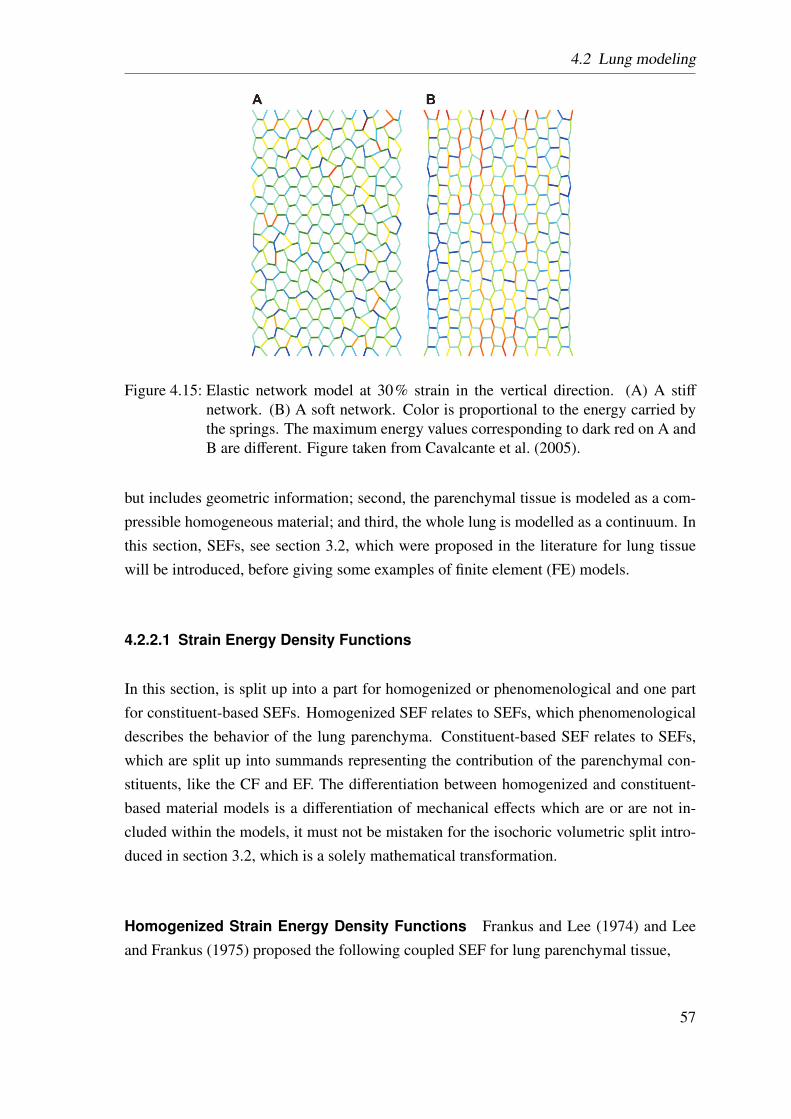
4.2 Lung modeling
Figure 4.15: Elastic network model at 30% strain in the vertical direction. (A) A stiffnetwork. (B) A soft network. Color is proportional to the energy carried bythe springs. The maximum energy values corresponding to dark red on A andB are different. Figure taken from Cavalcante et al. (2005).
but includes geometric information; second, the parenchymal tissue is modeled as a com-pressible homogeneous material; and third, the whole lung is modelled as a continuum. Inthis section, SEFs, see section 3.2, which were proposed in the literature for lung tissuewill be introduced, before giving some examples of finite element (FE) models.
4.2.2.1 Strain Energy Density Functions
In this section, is split up into a part for homogenized or phenomenological and one partfor constituent-based SEFs. Homogenized SEF relates to SEFs, which phenomenologicaldescribes the behavior of the lung parenchyma. Constituent-based SEF relates to SEFs,which are split up into summands representing the contribution of the parenchymal con-stituents, like the CF and EF. The differentiation between homogenized and constituent-based material models is a differentiation of mechanical effects which are or are not in-cluded within the models, it must not be mistaken for the isochoric volumetric split intro-duced in section 3.2, which is a solely mathematical transformation.
Homogenized Strain Energy Density Functions Frankus and Lee (1974) and Leeand Frankus (1975) proposed the following coupled SEF for lung parenchymal tissue,
57
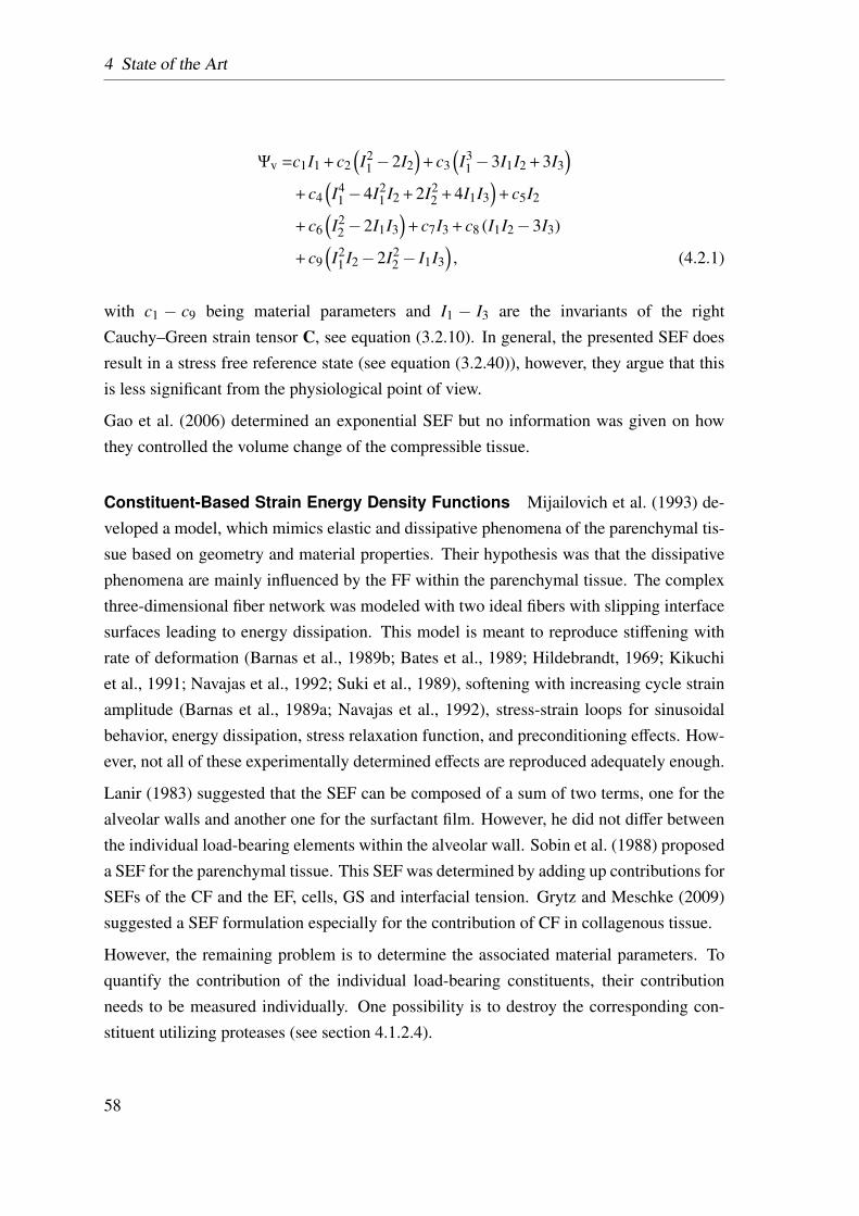
4 State of the Art
Ψv =c1I1 + c2(I21−2I2
)+ c3
(I31−3I1I2 + 3I3
)+ c4
(I41−4I2
1 I2 + 2I22 + 4I1I3
)+ c5I2
+ c6(I22−2I1I3
)+ c7I3 + c8 (I1I2−3I3)
+ c9(I21 I2−2I2
2− I1I3), (4.2.1)
with c1 − c9 being material parameters and I1 − I3 are the invariants of the rightCauchy–Green strain tensor C, see equation (3.2.10). In general, the presented SEF doesresult in a stress free reference state (see equation (3.2.40)), however, they argue that thisis less significant from the physiological point of view.
Gao et al. (2006) determined an exponential SEF but no information was given on howthey controlled the volume change of the compressible tissue.
Constituent-Based Strain Energy Density Functions Mijailovich et al. (1993) de-veloped a model, which mimics elastic and dissipative phenomena of the parenchymal tis-sue based on geometry and material properties. Their hypothesis was that the dissipativephenomena are mainly influenced by the FF within the parenchymal tissue. The complexthree-dimensional fiber network was modeled with two ideal fibers with slipping interfacesurfaces leading to energy dissipation. This model is meant to reproduce stiffening withrate of deformation (Barnas et al., 1989b; Bates et al., 1989; Hildebrandt, 1969; Kikuchiet al., 1991; Navajas et al., 1992; Suki et al., 1989), softening with increasing cycle strainamplitude (Barnas et al., 1989a; Navajas et al., 1992), stress-strain loops for sinusoidalbehavior, energy dissipation, stress relaxation function, and preconditioning effects. How-ever, not all of these experimentally determined effects are reproduced adequately enough.
Lanir (1983) suggested that the SEF can be composed of a sum of two terms, one for thealveolar walls and another one for the surfactant film. However, he did not differ betweenthe individual load-bearing elements within the alveolar wall. Sobin et al. (1988) proposeda SEF for the parenchymal tissue. This SEF was determined by adding up contributions forSEFs of the CF and the EF, cells, GS and interfacial tension. Grytz and Meschke (2009)suggested a SEF formulation especially for the contribution of CF in collagenous tissue.
However, the remaining problem is to determine the associated material parameters. Toquantify the contribution of the individual load-bearing constituents, their contributionneeds to be measured individually. One possibility is to destroy the corresponding con-stituent utilizing proteases (see section 4.1.2.4).
58
4.2 Lung modeling
4.2.2.2 Finite Element Models
The finite element method (FEM) provides the possibility to simulate the deformation ofthe whole lung, the parenchymal tissue and the individual alveolar wall.
There are several studies investing the deformation of the whole lung. However, this workis focused on the local deformations, for this reason, only one example is mentioned,namely the work of West and Matthews (1972). They investigated the deformation oflungs caused by gravity. Additionally, they showed that due to the large deformation of thelung during ventilation, a non-linear analysis is needed.
The number of studies concerned with the local deformation of the lung parenchyma isvery limited and mainly uses artificially generated geometries. A short overview is givenin the following.
Denny and Schroter (1997, 2000) investigated the oscillatory behavior of an isolated alve-olar duct. Their model includes discrete fibers as well as the surface tension acting overthe air-liquid interface. The tissue is simulated using a visco-elastic model involving non-linear quasi-static stress-strain behavior combined with a reduced relaxation function. Thesurface tension force is simulated with a time and area dependent model of surfactant be-havior. They used artificially generated geometries composed of truncated octahedra.
There are also several other groups investigating the mechanical behavior of artificiallygenerated three-dimensional geometries (Karakaplan et al., 1980; Kowe et al., 1986).
Because of missing realistic images of alveolar geometries, all these methods used sym-metric, generated octahedra and miss the complexity of the real geometry. In summary,none of the abovementioned studies were able to determine the local three-dimensionaldeformation state of the alveolar wall.
To the author’s knowledge, the only simulation performed on image-based two-dimensional alveolar geometries was performed by Gefen et al. (1999). The major ad-vantage of this method is that it allows for the investigation of the strain distribution withinthe alveolar wall, whereas the abovementioned experimental methods only investigatedoverall wall extension. Despite these advantages they used a very simplified linear elasticconstitutive model and a two-dimensional simulation. However, since the lung undergoesa three-dimensional deformation state, three-dimensional simulations are essential.
59

4 State of the Art
60
5 Goals
5.1 Long Term Goal
This work is part of the priority program ”Protective Artificial Respiration” funded bythe German Research Foundation (DFG). The priority project consists of several groupswith medical, biological, imaging and engineering backgrounds. Its main goal is to further
improve mechanical ventilation in order to reduce the high mortality rates due to VALI. Forthis purpose, the Institute for Computational Mechanics (TUM) is developing a detailed“virtual lung model”, see Figure (5.1).
Our virtual lung model starts with the tracheo-bronchial region. Here, the airflow interact-ing with the deformation of the airway walls and the surrounding parenchymal tissue, thefluid-structure interaction (FSI), is simulated. The FSI is important to reproduce in vivo
fluid mechanics in the tracheo-bronchial region, as well as stresses and strains in the airwaywall, which are potentially associated with the onset of inflammation and remodeling of theepithelium (Wall and Rabczuk, 2008). Due to limitations on the number of visible airwaysin CT scans, only a part of the airway tree can be resolved in three-dimensions. Therefore,realistic boundary conditions at the outlets of the three-dimensional domain are developed.To take the peripheral region into account simplified reduced-dimensional airway trees arecoupled to every outlet of the three-dimensional region (Comerford et al., 2010; Ismailet al., 2012). The flow in individual acini can be linked to the structural deformation of theparenchyma, utilizing a newly developed volume-coupling method (Yoshihara and Wall,2012). From these deformations, strains and stresses in the individual alveolar walls can bedetermined by using a multi-scale approach (Wiechert and Wall, 2010). The deformationwithin the alveolar walls is our main interest, since this is the area where the inflamma-tion during VALI initiates. For more details of our virtual lung model, e.g. see Wall et al.(2010b).
61
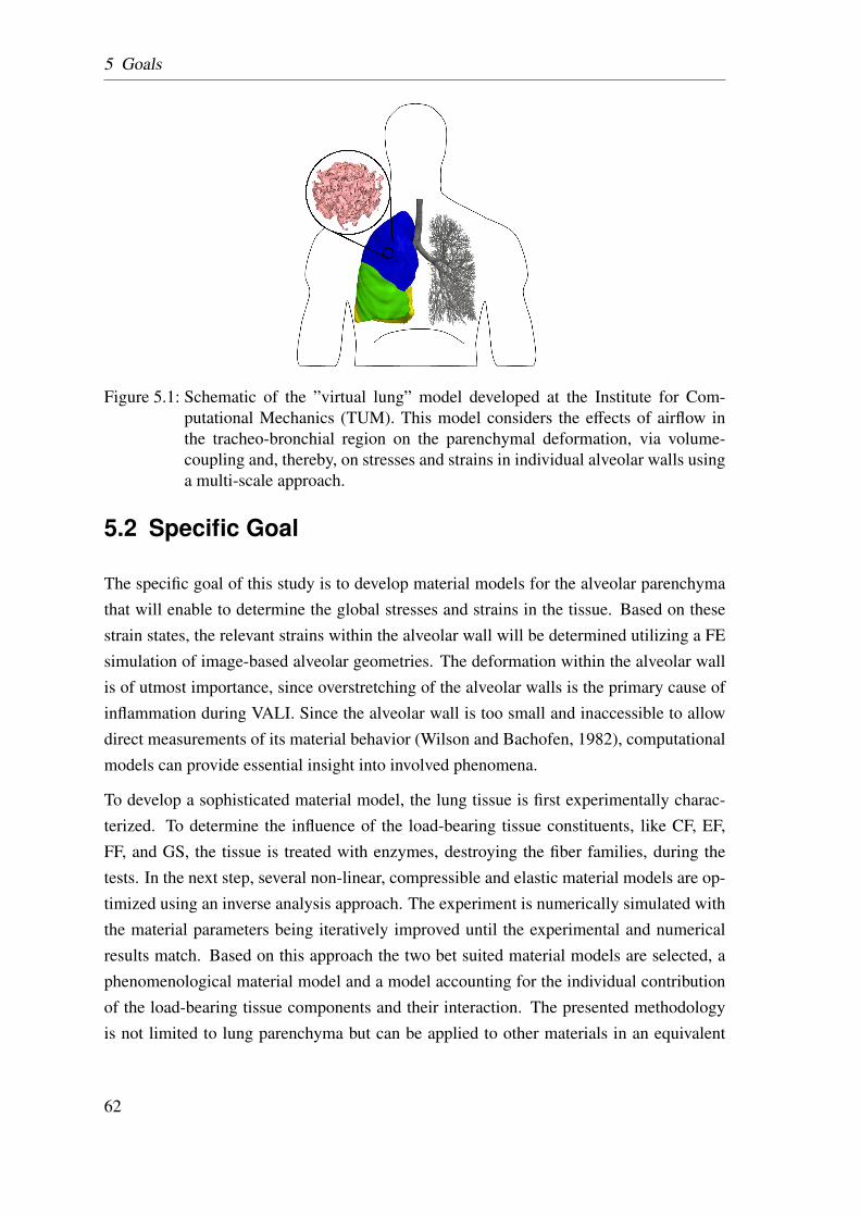
5 Goals
Figure 5.1: Schematic of the ”virtual lung” model developed at the Institute for Com-putational Mechanics (TUM). This model considers the effects of airflow inthe tracheo-bronchial region on the parenchymal deformation, via volume-coupling and, thereby, on stresses and strains in individual alveolar walls usinga multi-scale approach.
5.2 Specific Goal
The specific goal of this study is to develop material models for the alveolar parenchymathat will enable to determine the global stresses and strains in the tissue. Based on thesestrain states, the relevant strains within the alveolar wall will be determined utilizing a FEsimulation of image-based alveolar geometries. The deformation within the alveolar wallis of utmost importance, since overstretching of the alveolar walls is the primary cause ofinflammation during VALI. Since the alveolar wall is too small and inaccessible to allowdirect measurements of its material behavior (Wilson and Bachofen, 1982), computationalmodels can provide essential insight into involved phenomena.
To develop a sophisticated material model, the lung tissue is first experimentally charac-terized. To determine the influence of the load-bearing tissue constituents, like CF, EF,FF, and GS, the tissue is treated with enzymes, destroying the fiber families, during thetests. In the next step, several non-linear, compressible and elastic material models are op-timized using an inverse analysis approach. The experiment is numerically simulated withthe material parameters being iteratively improved until the experimental and numericalresults match. Based on this approach the two bet suited material models are selected, aphenomenological material model and a model accounting for the individual contributionof the load-bearing tissue components and their interaction. The presented methodologyis not limited to lung parenchyma but can be applied to other materials in an equivalent
62
5.3 Specific Aims
manner.
The actual damage during VALI occurs due to overstraining of the alveolar wall. For thisreason, the strain state within the individual alveolar wall needs to be quantified. Becauseof the foam-like structure of the lung parenchyma, the local deformation of the alveolarwall cannot be directly deduced of the global deformation of the lung parenchyma. Fur-thermore, the currently available classical imaging techniques, i.e. CT, magnetic resonanceimaging (MRI) etc., do not have a sufficient resolution to image the deformation state invivo. However, using the novel imaging techniques presented by Schittny (2008) the in-dividual alveolar walls of fixated rat lungs are visible with adequate resolution. Based onthese images and a prescribed global strains a three-dimensional deformation state can bedetermined by FE simulations.
In this work, all simulations are based on the FEM. For more details on this method theinterested reader is referred to textbooks from Belytschko et al. (2005); Hughes (2000),and lecture notes from Wall et al. (2010a, 2012).
All material models of this work were implemented in the in-house FE software platformBavarian Advanced Computational Initiative (BACI, Wall and Gee (2010)). This multi-purpose parallel research-code is written in C++ and integrates open-source libraries ofthe Trilinos Project (Heroux et al., 2005). BACI has been and is developed jointly at theInstitute for Computational Mechanics (Technische Universität München).
It has to be noted, though, that the introduced material models are based on general solidcontinuum mechanics, i.e. they are not limited to the FEM.
5.3 Specific Aims
The above introduced goals can be narrowed down to the following five specific aims:
AIM 1
To develop an experimental testing protocol in order to determine the elastic material be-havior of lung parenchyma.
63
5 Goals
AIM 2
To extend the experimental methodology to investigate the influence of the individual tis-sue constituents (CF and EF).
AIM 3
To develop an inverse analysis methodology in order to deduce a hyperelastic materialmodel for soft biological tissue from experiments.
AIM 4
To determine a phenomenological and a constituent-based material model for lungparenchyma.
AIM 5
To perform a FE simulation on image-based alveolar geometries, in order to determine thedeformation within the alveolar walls for a given global deformation state.
64
6 Experiments
Although experiments on lung parenchymal tissue have been carried out since the late1960s, they mainly focused on the qualitative mechanical behavior. Thus, from theseresults it is difficult to determine a quantitative stress-strain relationship for computationalsimulations. The major drawbacks of previous experimental approaches are:
• Global p-V measurements are too coarse to determine a sophisticated material modelfor lung parenchyma. The problem is that a distinction between the individual con-tribution of the airways and the parenchymal tissue is not possible.
• Only a few studies use viable tissue. However, it has not been satisfactorily shownthat cell death does not change the material behavior of parenchymal tissue.
• The production of the tested specimens was performed by hand rather than fullyautomated, which can cause large variations in the dimensions of the specimens.
• In many studies the tissue was frozen in order to cut the specimen, which has beenshown before to change the material properties of the tissue.
• Many studies perform their experiments only on one single specimen, i.e. there is noinformation about the repeatability of the experiment or the statistical spread of themeasured values.
• The lateral contraction or other measurements determining the volume change ofthe compressible lung parenchyma have only been determined in multi-axial tensiletests.
• In some studies critical information, i.e. cross-sectional area or length, were notprovided at all or their determination was not further specified.
• In most cases, it was poorly documented, which initial length (before or after precon-ditioning) or initial cross-sectional area (including the air-space or not) was taken, orhow these quantities were determined. This is very important, since these quantitieshave an essential influence on the scaling and position of the determined stress-straincurves.
65
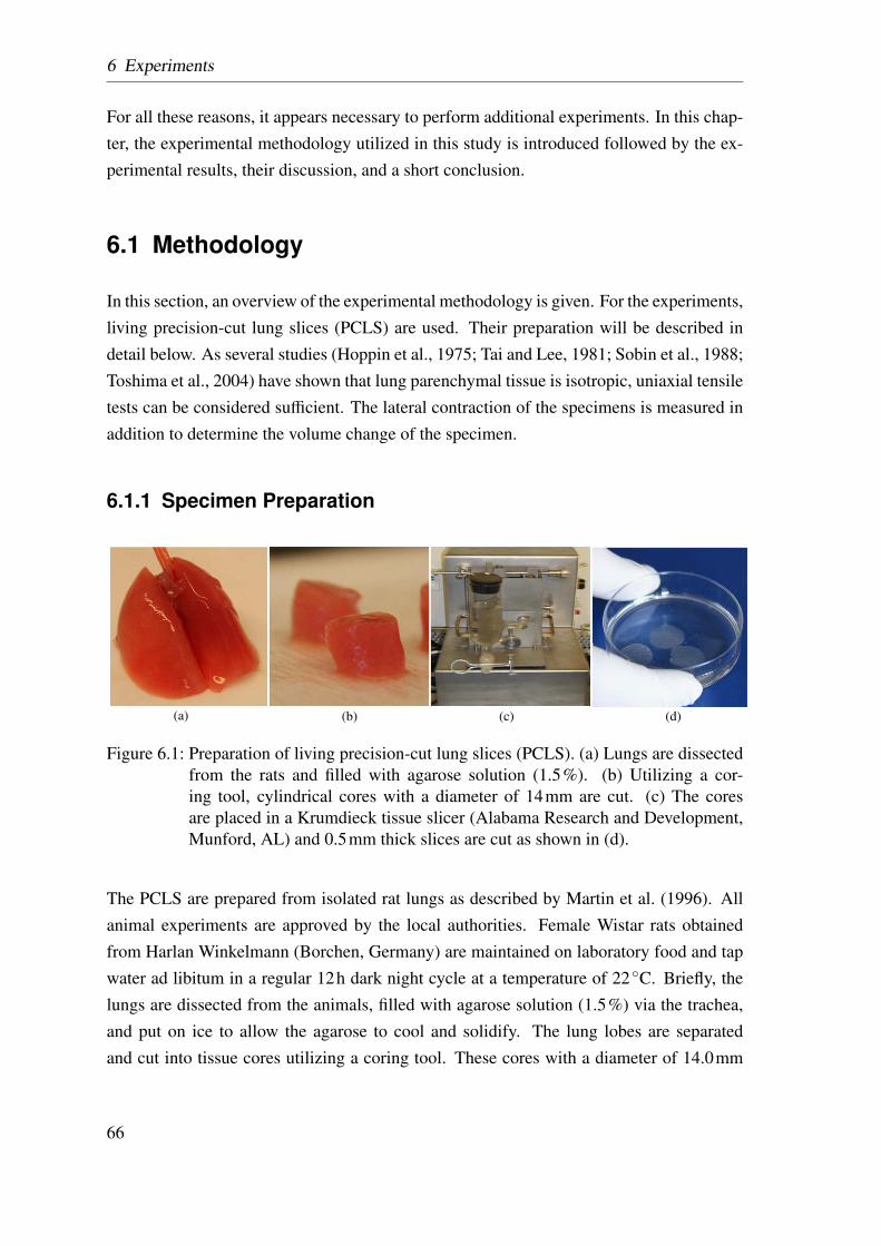
6 Experiments
For all these reasons, it appears necessary to perform additional experiments. In this chap-ter, the experimental methodology utilized in this study is introduced followed by the ex-perimental results, their discussion, and a short conclusion.
6.1 Methodology
In this section, an overview of the experimental methodology is given. For the experiments,living precision-cut lung slices (PCLS) are used. Their preparation will be described indetail below. As several studies (Hoppin et al., 1975; Tai and Lee, 1981; Sobin et al., 1988;Toshima et al., 2004) have shown that lung parenchymal tissue is isotropic, uniaxial tensiletests can be considered sufficient. The lateral contraction of the specimens is measured inaddition to determine the volume change of the specimen.
6.1.1 Specimen Preparation
(a) (b) (c) (d)
Figure 6.1: Preparation of living precision-cut lung slices (PCLS). (a) Lungs are dissectedfrom the rats and filled with agarose solution (1.5%). (b) Utilizing a cor-ing tool, cylindrical cores with a diameter of 14mm are cut. (c) The coresare placed in a Krumdieck tissue slicer (Alabama Research and Development,Munford, AL) and 0.5mm thick slices are cut as shown in (d).
The PCLS are prepared from isolated rat lungs as described by Martin et al. (1996). Allanimal experiments are approved by the local authorities. Female Wistar rats obtainedfrom Harlan Winkelmann (Borchen, Germany) are maintained on laboratory food and tapwater ad libitum in a regular 12h dark night cycle at a temperature of 22◦C. Briefly, thelungs are dissected from the animals, filled with agarose solution (1.5%) via the trachea,and put on ice to allow the agarose to cool and solidify. The lung lobes are separatedand cut into tissue cores utilizing a coring tool. These cores with a diameter of 14.0mm
66
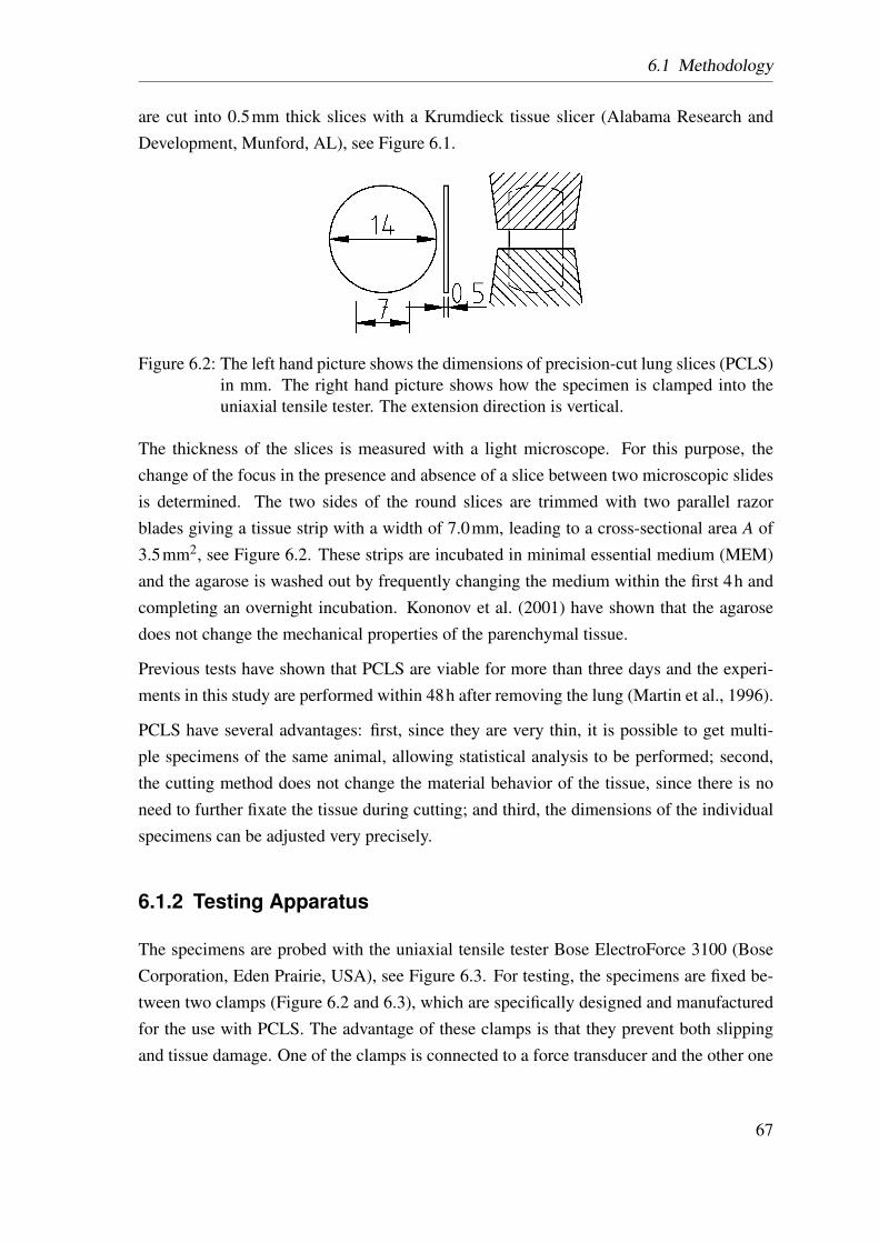
6.1 Methodology
are cut into 0.5mm thick slices with a Krumdieck tissue slicer (Alabama Research andDevelopment, Munford, AL), see Figure 6.1.
Figure 6.2: The left hand picture shows the dimensions of precision-cut lung slices (PCLS)in mm. The right hand picture shows how the specimen is clamped into theuniaxial tensile tester. The extension direction is vertical.
The thickness of the slices is measured with a light microscope. For this purpose, thechange of the focus in the presence and absence of a slice between two microscopic slidesis determined. The two sides of the round slices are trimmed with two parallel razorblades giving a tissue strip with a width of 7.0mm, leading to a cross-sectional area A of3.5mm2, see Figure 6.2. These strips are incubated in minimal essential medium (MEM)and the agarose is washed out by frequently changing the medium within the first 4h andcompleting an overnight incubation. Kononov et al. (2001) have shown that the agarosedoes not change the mechanical properties of the parenchymal tissue.
Previous tests have shown that PCLS are viable for more than three days and the experi-ments in this study are performed within 48h after removing the lung (Martin et al., 1996).
PCLS have several advantages: first, since they are very thin, it is possible to get multi-ple specimens of the same animal, allowing statistical analysis to be performed; second,the cutting method does not change the material behavior of the tissue, since there is noneed to further fixate the tissue during cutting; and third, the dimensions of the individualspecimens can be adjusted very precisely.
6.1.2 Testing Apparatus
The specimens are probed with the uniaxial tensile tester Bose ElectroForce 3100 (BoseCorporation, Eden Prairie, USA), see Figure 6.3. For testing, the specimens are fixed be-tween two clamps (Figure 6.2 and 6.3), which are specifically designed and manufacturedfor the use with PCLS. The advantage of these clamps is that they prevent both slippingand tissue damage. One of the clamps is connected to a force transducer and the other one
67
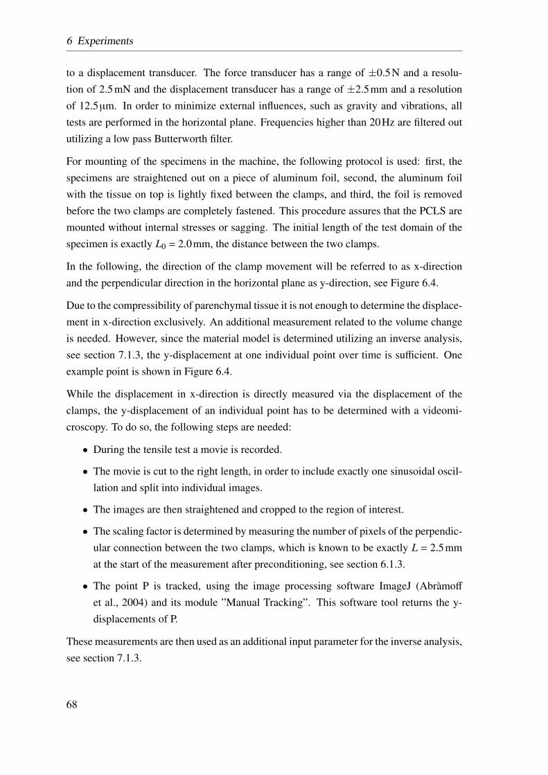
6 Experiments
to a displacement transducer. The force transducer has a range of ±0.5N and a resolu-tion of 2.5mN and the displacement transducer has a range of ±2.5mm and a resolutionof 12.5µm. In order to minimize external influences, such as gravity and vibrations, alltests are performed in the horizontal plane. Frequencies higher than 20Hz are filtered oututilizing a low pass Butterworth filter.
For mounting of the specimens in the machine, the following protocol is used: first, thespecimens are straightened out on a piece of aluminum foil, second, the aluminum foilwith the tissue on top is lightly fixed between the clamps, and third, the foil is removedbefore the two clamps are completely fastened. This procedure assures that the PCLS aremounted without internal stresses or sagging. The initial length of the test domain of thespecimen is exactly L0 = 2.0mm, the distance between the two clamps.
In the following, the direction of the clamp movement will be referred to as x-directionand the perpendicular direction in the horizontal plane as y-direction, see Figure 6.4.
Due to the compressibility of parenchymal tissue it is not enough to determine the displace-ment in x-direction exclusively. An additional measurement related to the volume changeis needed. However, since the material model is determined utilizing an inverse analysis,see section 7.1.3, the y-displacement at one individual point over time is sufficient. Oneexample point is shown in Figure 6.4.
While the displacement in x-direction is directly measured via the displacement of theclamps, the y-displacement of an individual point has to be determined with a videomi-croscopy. To do so, the following steps are needed:
• During the tensile test a movie is recorded.
• The movie is cut to the right length, in order to include exactly one sinusoidal oscil-lation and split into individual images.
• The images are then straightened and cropped to the region of interest.
• The scaling factor is determined by measuring the number of pixels of the perpendic-ular connection between the two clamps, which is known to be exactly L = 2.5mmat the start of the measurement after preconditioning, see section 6.1.3.
• The point P is tracked, using the image processing software ImageJ (Abràmoff
et al., 2004) and its module ”Manual Tracking”. This software tool returns the y-displacements of P.
These measurements are then used as an additional input parameter for the inverse analysis,see section 7.1.3.
68
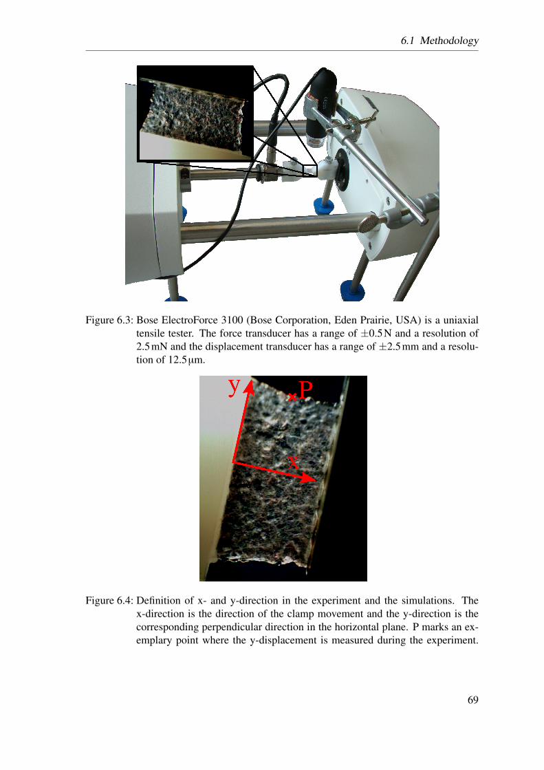
6.1 Methodology
Figure 6.3: Bose ElectroForce 3100 (Bose Corporation, Eden Prairie, USA) is a uniaxialtensile tester. The force transducer has a range of ±0.5N and a resolution of2.5mN and the displacement transducer has a range of ±2.5mm and a resolu-tion of 12.5µm.
Figure 6.4: Definition of x- and y-direction in the experiment and the simulations. Thex-direction is the direction of the clamp movement and the y-direction is thecorresponding perpendicular direction in the horizontal plane. P marks an ex-emplary point where the y-displacement is measured during the experiment.
69
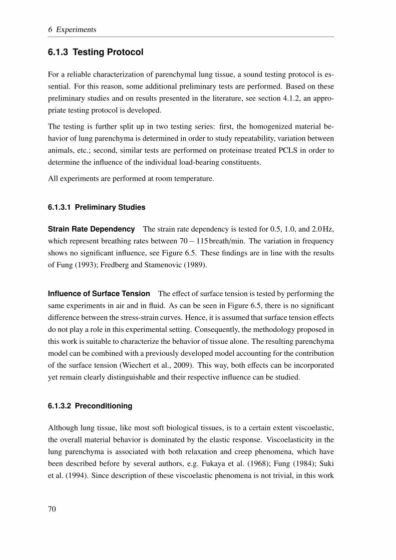
6 Experiments
6.1.3 Testing Protocol
For a reliable characterization of parenchymal lung tissue, a sound testing protocol is es-sential. For this reason, some additional preliminary tests are performed. Based on thesepreliminary studies and on results presented in the literature, see section 4.1.2, an appro-priate testing protocol is developed.
The testing is further split up in two testing series: first, the homogenized material be-havior of lung parenchyma is determined in order to study repeatability, variation betweenanimals, etc.; second, similar tests are performed on proteinase treated PCLS in order todetermine the influence of the individual load-bearing constituents.
All experiments are performed at room temperature.
6.1.3.1 Preliminary Studies
Strain Rate Dependency The strain rate dependency is tested for 0.5, 1.0, and 2.0Hz,which represent breathing rates between 70− 115breath/min. The variation in frequencyshows no significant influence, see Figure 6.5. These findings are in line with the resultsof Fung (1993); Fredberg and Stamenovic (1989).
Influence of Surface Tension The effect of surface tension is tested by performing thesame experiments in air and in fluid. As can be seen in Figure 6.5, there is no significantdifference between the stress-strain curves. Hence, it is assumed that surface tension effectsdo not play a role in this experimental setting. Consequently, the methodology proposed inthis work is suitable to characterize the behavior of tissue alone. The resulting parenchymamodel can be combined with a previously developed model accounting for the contributionof the surface tension (Wiechert et al., 2009). This way, both effects can be incorporatedyet remain clearly distinguishable and their respective influence can be studied.
6.1.3.2 Preconditioning
Although lung tissue, like most soft biological tissues, is to a certain extent viscoelastic,the overall material behavior is dominated by the elastic response. Viscoelasticity in thelung parenchyma is associated with both relaxation and creep phenomena, which havebeen described before by several authors, e.g. Fukaya et al. (1968); Fung (1984); Sukiet al. (1994). Since description of these viscoelastic phenomena is not trivial, in this work
70
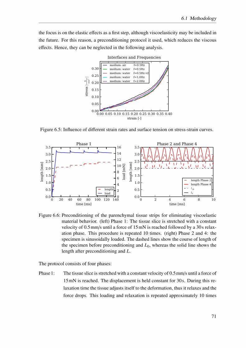
6.1 Methodology
the focus is on the elastic effects as a first step, although viscoelasticity may be included inthe future. For this reason, a preconditioning protocol it used, which reduces the viscouseffects. Hence, they can be neglected in the following analysis.
0.00 0.05 0.10 0.15 0.20 0.25 0.30 0.35 0.40strain [-]
0.00
0.05
0.10
0.15
0.20
0.25
0.30
stre
ss [
N
mm
2]
Interfaces and Frequenciesmedium: air f=0.5Hzmedium: water f=0.5Hzmedium: water f=0.5Hz v2medium: water f=1.0Hzmedium: water f=2.0Hz
Figure 6.5: Influence of different strain rates and surface tension on stress-strain curves.
0 20 40 60 80 100 120 140time [ms]
0.0
0.5
1.0
1.5
2.0
2.5
3.0
3.5
length [mm]
Phase 1
0
2
4
6
8
10
12
14
16
load [mN]
length
load
0 2 4 6 8 10time [ms]
0.0
0.5
1.0
1.5
2.0
2.5
3.0
3.5
leng
th [m
m]
Phase 2 and Phase 4
length Phase 2length Phase 4lA0
l0
Figure 6.6: Preconditioning of the parenchymal tissue strips for eliminating viscoelasticmaterial behavior. (left) Phase 1: The tissue slice is stretched with a constantvelocity of 0.5mm/s until a force of 15mN is reached followed by a 30s relax-ation phase. This procedure is repeated 10 times. (right) Phase 2 and 4: thespecimen is sinusoidally loaded. The dashed lines show the course of length ofthe specimen before preconditioning and L0, whereas the solid line shows thelength after preconditioning and L.
The protocol consists of four phases:
Phase1: The tissue slice is stretched with a constant velocity of 0.5mm/s until a force of15mN is reached. The displacement is held constant for 30s. During this re-laxation time the tissue adjusts itself to the deformation, thus it relaxes and theforce drops. This loading and relaxation is repeated approximately 10 times
71
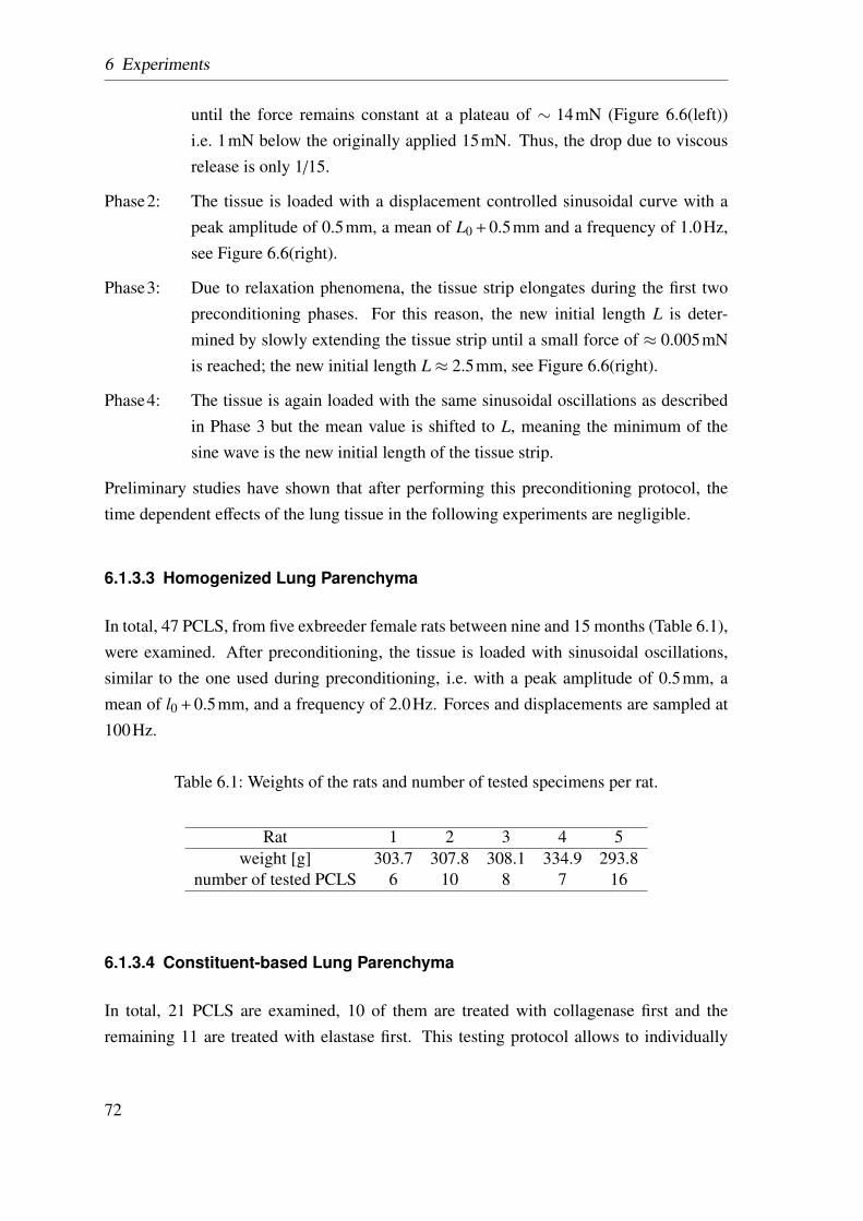
6 Experiments
until the force remains constant at a plateau of ∼ 14mN (Figure 6.6(left))i.e. 1mN below the originally applied 15mN. Thus, the drop due to viscousrelease is only 1/15.
Phase2: The tissue is loaded with a displacement controlled sinusoidal curve with apeak amplitude of 0.5mm, a mean of L0 + 0.5mm and a frequency of 1.0Hz,see Figure 6.6(right).
Phase3: Due to relaxation phenomena, the tissue strip elongates during the first twopreconditioning phases. For this reason, the new initial length L is deter-mined by slowly extending the tissue strip until a small force of ≈ 0.005mNis reached; the new initial length L≈ 2.5mm, see Figure 6.6(right).
Phase4: The tissue is again loaded with the same sinusoidal oscillations as describedin Phase 3 but the mean value is shifted to L, meaning the minimum of thesine wave is the new initial length of the tissue strip.
Preliminary studies have shown that after performing this preconditioning protocol, thetime dependent effects of the lung tissue in the following experiments are negligible.
6.1.3.3 Homogenized Lung Parenchyma
In total, 47 PCLS, from five exbreeder female rats between nine and 15 months (Table 6.1),were examined. After preconditioning, the tissue is loaded with sinusoidal oscillations,similar to the one used during preconditioning, i.e. with a peak amplitude of 0.5mm, amean of l0 + 0.5mm, and a frequency of 2.0Hz. Forces and displacements are sampled at100Hz.
Table 6.1: Weights of the rats and number of tested specimens per rat.
Rat 1 2 3 4 5weight [g] 303.7 307.8 308.1 334.9 293.8
number of tested PCLS 6 10 8 7 16
6.1.3.4 Constituent-based Lung Parenchyma
In total, 21 PCLS are examined, 10 of them are treated with collagenase first and theremaining 11 are treated with elastase first. This testing protocol allows to individually
72
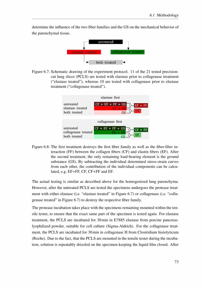
6.1 Methodology
determine the influence of the two fiber families and the GS on the mechanical behavior ofthe parenchymal tissue.
Figure 6.7: Schematic drawing of the experiment protocol. 11 of the 21 tested precision-cut lung slices (PCLS) are tested with elastase prior to collagenase treatment(“elastase treated”), whereas 10 are tested with collagenase prior to elastasetreatment (“collagenase treated”).
collagenase first
CF + EF + FF + GS
EF + GS
GS
CF + FF
EF
untreatedcollagenase treated
both treated
untreatedelastase treated
both treated
elastase first
CF + EF + FF + GS
CF + GS
GS
EF + FF
CF
Figure 6.8: The first treatment destroys the first fiber family as well as the fiber-fiber in-teraction (FF) between the collagen fibers (CF) and elastin fibers (EF). Afterthe second treatment, the only remaining load-bearing element is the groundsubstance (GS). By subtracting the individual determined stress-strain curvesfrom each other, the contribution of the individual components can be calcu-lated, e.g. EF+FF, CF, CF+FF and EF.
The actual testing is similar as described above for the homogenized lung parenchyma.However, after the untreated PCLS are tested the specimens undergoes the protease treat-ment with either elastase (i.e. “elastase treated” in Figure 6.7) or collagenase (i.e. “colla-genase treated” in Figure 6.7) to destroy the respective fiber family.
The protease incubation takes place with the specimens remaining mounted within the ten-sile tester, to ensure that the exact same part of the specimen is tested again. For elastasetreatment, the PCLS are incubated for 30min in E7885 elastase from porcine pancreas-lyophilized powder, suitable for cell culture (Sigma-Aldrich). For the collagenase treat-ment, the PCLS are incubated for 30min in collagenase H from Clostridium histolyticum(Roche). Due to the fact, that the PCLS are mounted in the tensile tester during the incuba-tion, solution is repeatably drizzled on the specimen keeping the liquid film closed. After
73
6 Experiments
the first protease treatment, the specimens are tested again, including the preconditioningprotocol, before they are treated with the corresponding other protease (indicated as “bothtreated” in Figure 6.8) and tested for the third time.
6.2 Results
In the following section the experimental results will be presented, which are used as atarget for the material fitting. First, the results of the homogenized lung parenchyma areprovided, in order to get a better understanding and a solid establishment and verifica-tion of the experimental protocol. Second, the results of the proteinase treated PCLS arepresented.
In the following section strain and stress refers to lL and T
A .
6.2.1 Homogenized Lung Parenchyma
First, the experimentally determined stress-strain curves of each of the five tested animalsare compared. Figure 6.9 shows the mean curve, averaged over all tested PCLS of oneindividual animal, and the area between the mean ± one standard deviation (sd) (mean ±sd) and the mean ± 1.96sd, i.e. 95% of all values, highlighted as lighter and darker color,respectively. For a short explanation of the statistical measures, see Appendix A.4.1 andA.4.2. All shown curves are similar in shape and order of magnitude. However, a variationof curves for each animal exists. This variation does not correlate with the number of testedPCLS per animal.
74
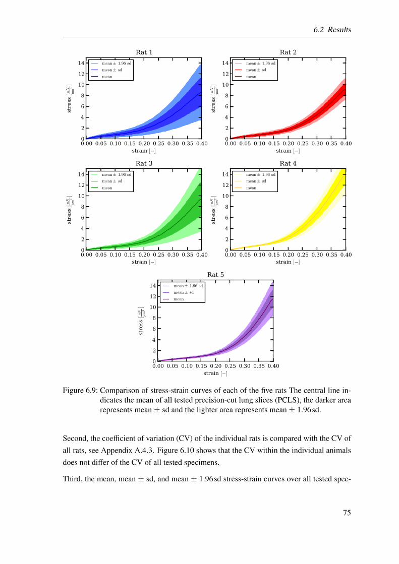
6.2 Results
0.00 0.05 0.10 0.15 0.20 0.25 0.30 0.35 0.40strain [−]
0
2
4
6
8
10
12
14stress [nN
µm
2]
Rat 1
mean± 1.96 sd
mean± sd
mean
0.00 0.05 0.10 0.15 0.20 0.25 0.30 0.35 0.40strain [−]
0
2
4
6
8
10
12
14
stress [nN
µm
2]
Rat 2
mean± 1.96 sd
mean± sd
mean
0.00 0.05 0.10 0.15 0.20 0.25 0.30 0.35 0.40strain [−]
0
2
4
6
8
10
12
14
stress [nN
µm
2]
Rat 3
mean± 1.96 sd
mean± sd
mean
0.00 0.05 0.10 0.15 0.20 0.25 0.30 0.35 0.40strain [−]
0
2
4
6
8
10
12
14
stress [nN
µm
2]
Rat 4
mean± 1.96 sd
mean± sd
mean
0.00 0.05 0.10 0.15 0.20 0.25 0.30 0.35 0.40strain [−]
0
2
4
6
8
10
12
14
stress [nN
µm
2]
Rat 5
mean± 1.96 sd
mean± sd
mean
Figure 6.9: Comparison of stress-strain curves of each of the five rats The central line in-dicates the mean of all tested precision-cut lung slices (PCLS), the darker arearepresents mean ± sd and the lighter area represents mean ± 1.96sd.
Second, the coefficient of variation (CV) of the individual rats is compared with the CV ofall rats, see Appendix A.4.3. Figure 6.10 shows that the CV within the individual animalsdoes not differ of the CV of all tested specimens.
Third, the mean, mean ± sd, and mean ± 1.96sd stress-strain curves over all tested spec-
75
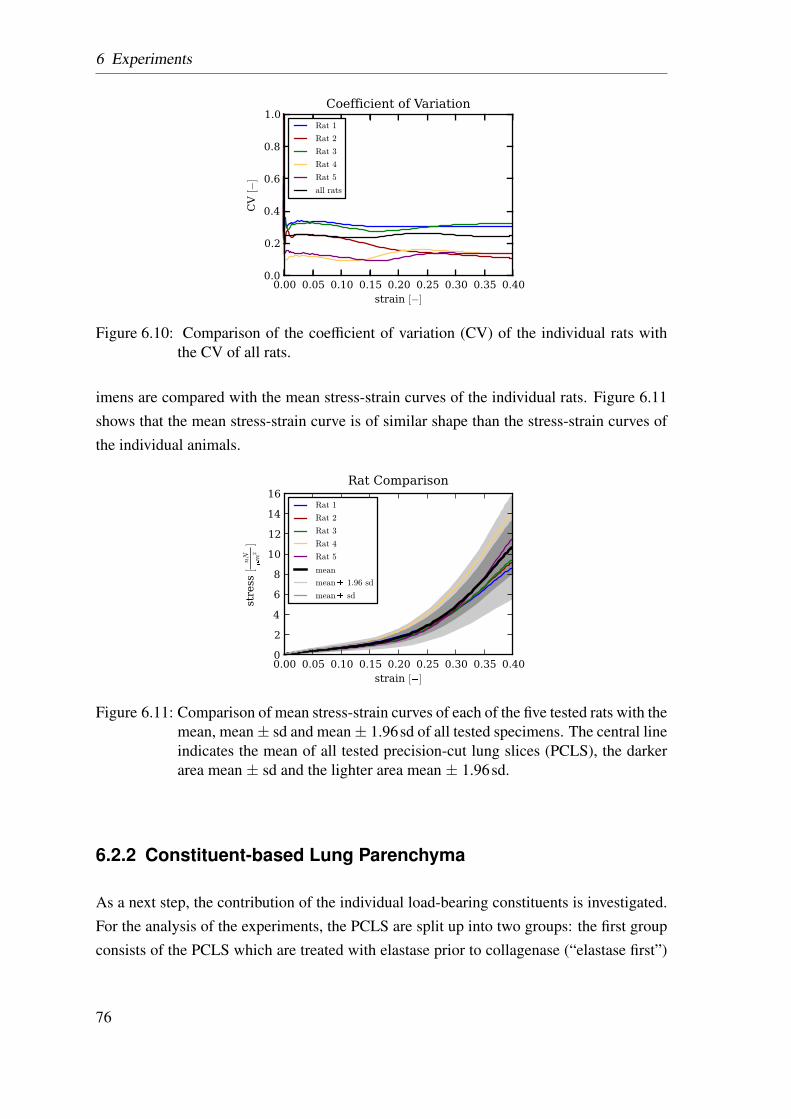
6 Experiments
0.00 0.05 0.10 0.15 0.20 0.25 0.30 0.35 0.40strain [−]
0.0
0.2
0.4
0.6
0.8
1.0
CV [−]
Coefficient of Variation
Rat 1
Rat 2
Rat 3
Rat 4
Rat 5
all rats
Figure 6.10: Comparison of the coefficient of variation (CV) of the individual rats withthe CV of all rats.
imens are compared with the mean stress-strain curves of the individual rats. Figure 6.11shows that the mean stress-strain curve is of similar shape than the stress-strain curves ofthe individual animals.
0.00 0.05 0.10 0.15 0.20 0.25 0.30 0.35 0.40strain [�]
02468
10121416
stre
ss [
nN
�
m2]
Rat ComparisonRat 1
Rat 2
Rat 3
Rat 4
Rat 5
mean
mean� 1.96 sd
mean� sd
Figure 6.11: Comparison of mean stress-strain curves of each of the five tested rats with themean, mean± sd and mean± 1.96sd of all tested specimens. The central lineindicates the mean of all tested precision-cut lung slices (PCLS), the darkerarea mean ± sd and the lighter area mean ± 1.96sd.
6.2.2 Constituent-based Lung Parenchyma
As a next step, the contribution of the individual load-bearing constituents is investigated.For the analysis of the experiments, the PCLS are split up into two groups: the first groupconsists of the PCLS which are treated with elastase prior to collagenase (“elastase first”)
76
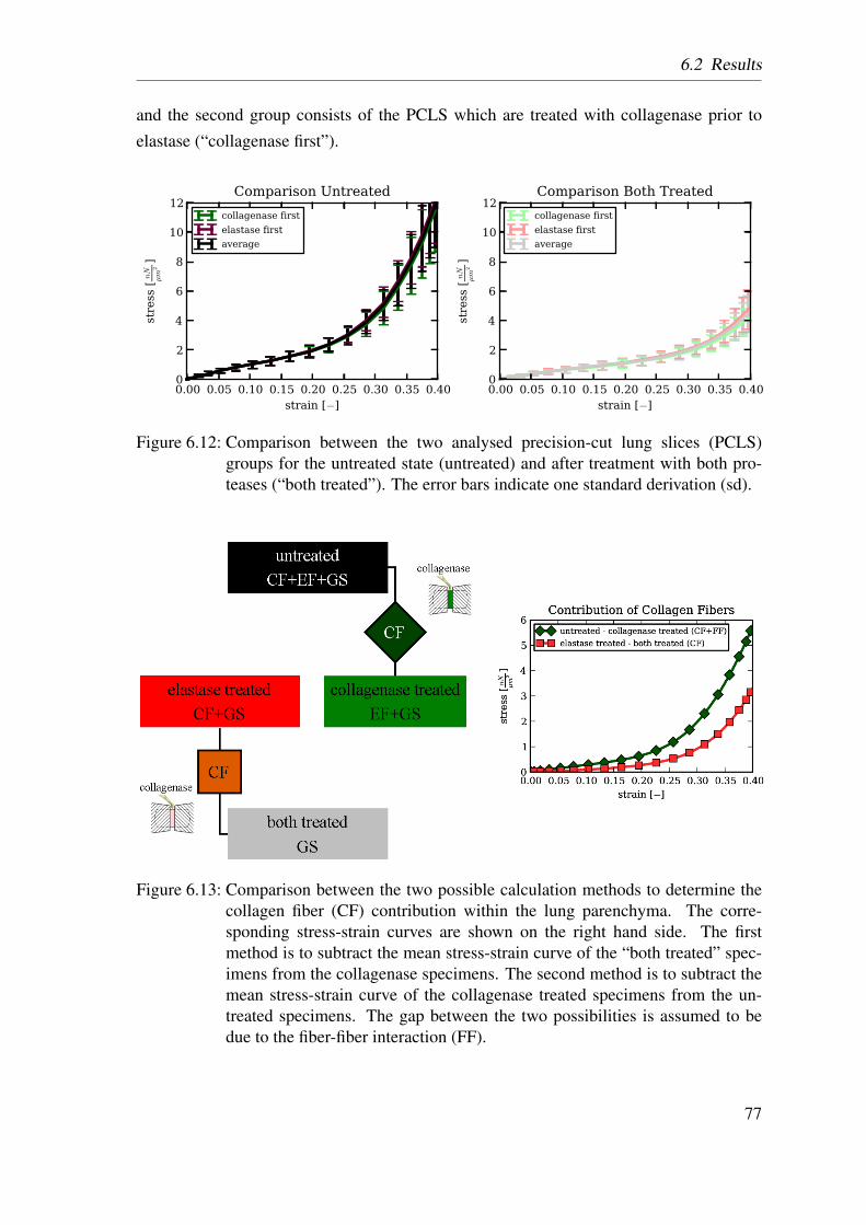
6.2 Results
and the second group consists of the PCLS which are treated with collagenase prior toelastase (“collagenase first”).
0.00 0.05 0.10 0.15 0.20 0.25 0.30 0.35 0.40strain [−]
0
2
4
6
8
10
12
stress [nN
µm
2]
Comparison Untreated
collagenase first
elastase first
average
0.00 0.05 0.10 0.15 0.20 0.25 0.30 0.35 0.40strain [−]
0
2
4
6
8
10
12
stress [nN
µm
2]
Comparison Both Treated
collagenase first
elastase first
average
Figure 6.12: Comparison between the two analysed precision-cut lung slices (PCLS)groups for the untreated state (untreated) and after treatment with both pro-teases (“both treated”). The error bars indicate one standard derivation (sd).
Figure 6.13: Comparison between the two possible calculation methods to determine thecollagen fiber (CF) contribution within the lung parenchyma. The corre-sponding stress-strain curves are shown on the right hand side. The firstmethod is to subtract the mean stress-strain curve of the “both treated” spec-imens from the collagenase specimens. The second method is to subtract themean stress-strain curve of the collagenase treated specimens from the un-treated specimens. The gap between the two possibilities is assumed to bedue to the fiber-fiber interaction (FF).
77
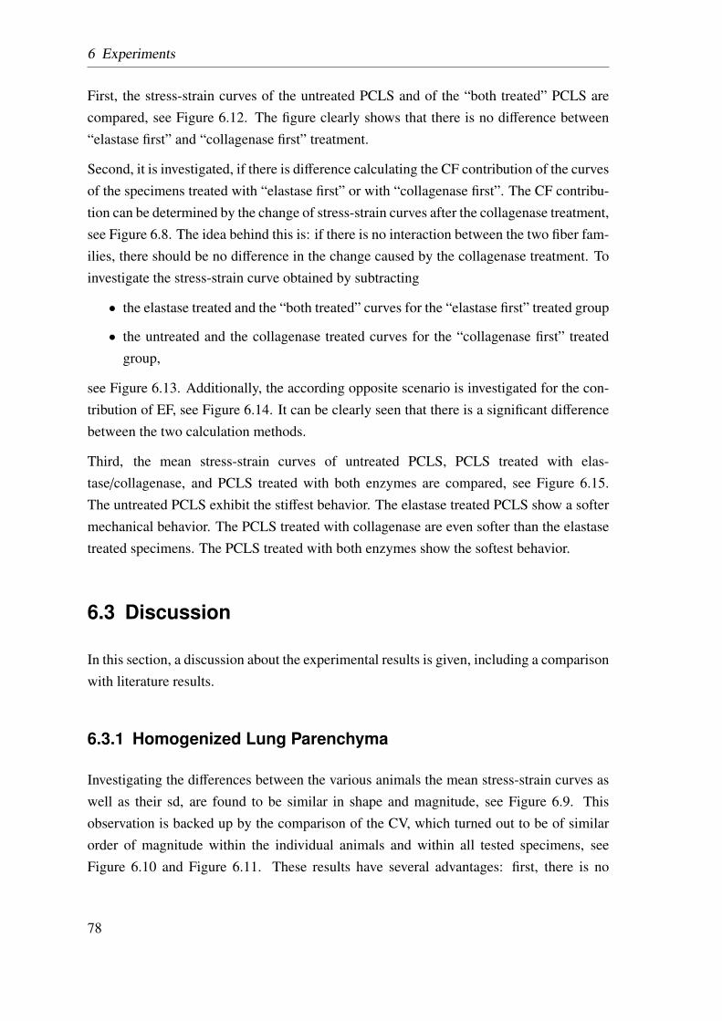
6 Experiments
First, the stress-strain curves of the untreated PCLS and of the “both treated” PCLS arecompared, see Figure 6.12. The figure clearly shows that there is no difference between“elastase first” and “collagenase first” treatment.
Second, it is investigated, if there is difference calculating the CF contribution of the curvesof the specimens treated with “elastase first” or with “collagenase first”. The CF contribu-tion can be determined by the change of stress-strain curves after the collagenase treatment,see Figure 6.8. The idea behind this is: if there is no interaction between the two fiber fam-ilies, there should be no difference in the change caused by the collagenase treatment. Toinvestigate the stress-strain curve obtained by subtracting
• the elastase treated and the “both treated” curves for the “elastase first” treated group
• the untreated and the collagenase treated curves for the “collagenase first” treatedgroup,
see Figure 6.13. Additionally, the according opposite scenario is investigated for the con-tribution of EF, see Figure 6.14. It can be clearly seen that there is a significant differencebetween the two calculation methods.
Third, the mean stress-strain curves of untreated PCLS, PCLS treated with elas-tase/collagenase, and PCLS treated with both enzymes are compared, see Figure 6.15.The untreated PCLS exhibit the stiffest behavior. The elastase treated PCLS show a softermechanical behavior. The PCLS treated with collagenase are even softer than the elastasetreated specimens. The PCLS treated with both enzymes show the softest behavior.
6.3 Discussion
In this section, a discussion about the experimental results is given, including a comparisonwith literature results.
6.3.1 Homogenized Lung Parenchyma
Investigating the differences between the various animals the mean stress-strain curves aswell as their sd, are found to be similar in shape and magnitude, see Figure 6.9. Thisobservation is backed up by the comparison of the CV, which turned out to be of similarorder of magnitude within the individual animals and within all tested specimens, seeFigure 6.10 and Figure 6.11. These results have several advantages: first, there is no
78
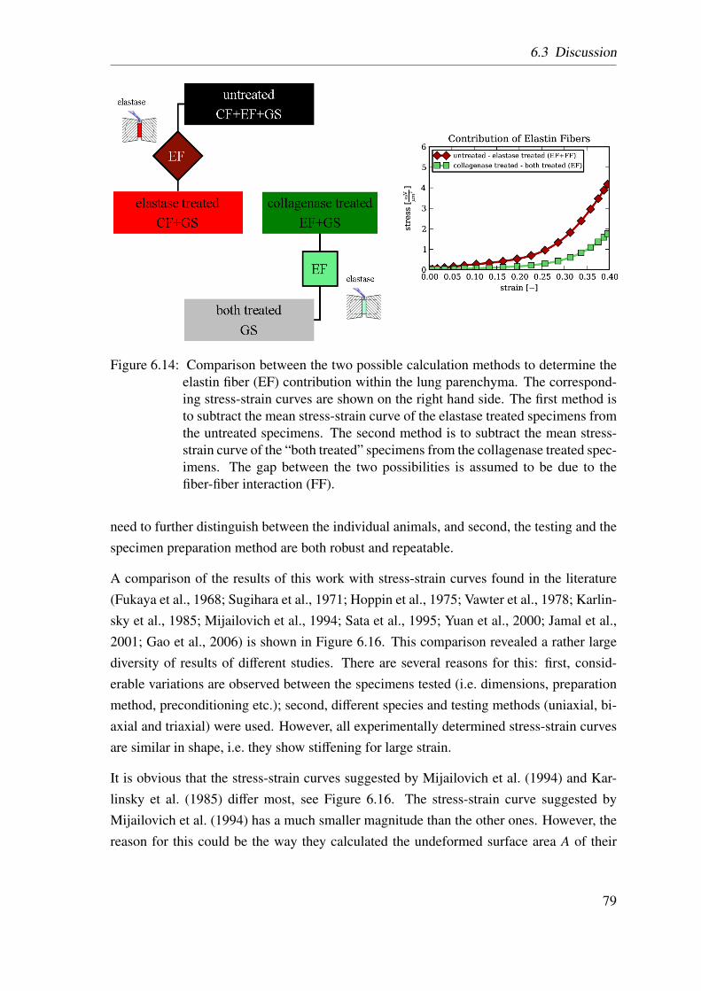
6.3 Discussion
Figure 6.14: Comparison between the two possible calculation methods to determine theelastin fiber (EF) contribution within the lung parenchyma. The correspond-ing stress-strain curves are shown on the right hand side. The first method isto subtract the mean stress-strain curve of the elastase treated specimens fromthe untreated specimens. The second method is to subtract the mean stress-strain curve of the “both treated” specimens from the collagenase treated spec-imens. The gap between the two possibilities is assumed to be due to thefiber-fiber interaction (FF).
need to further distinguish between the individual animals, and second, the testing and thespecimen preparation method are both robust and repeatable.
A comparison of the results of this work with stress-strain curves found in the literature(Fukaya et al., 1968; Sugihara et al., 1971; Hoppin et al., 1975; Vawter et al., 1978; Karlin-sky et al., 1985; Mijailovich et al., 1994; Sata et al., 1995; Yuan et al., 2000; Jamal et al.,2001; Gao et al., 2006) is shown in Figure 6.16. This comparison revealed a rather largediversity of results of different studies. There are several reasons for this: first, consid-erable variations are observed between the specimens tested (i.e. dimensions, preparationmethod, preconditioning etc.); second, different species and testing methods (uniaxial, bi-axial and triaxial) were used. However, all experimentally determined stress-strain curvesare similar in shape, i.e. they show stiffening for large strain.
It is obvious that the stress-strain curves suggested by Mijailovich et al. (1994) and Kar-linsky et al. (1985) differ most, see Figure 6.16. The stress-strain curve suggested byMijailovich et al. (1994) has a much smaller magnitude than the other ones. However, thereason for this could be the way they calculated the undeformed surface area A of their
79
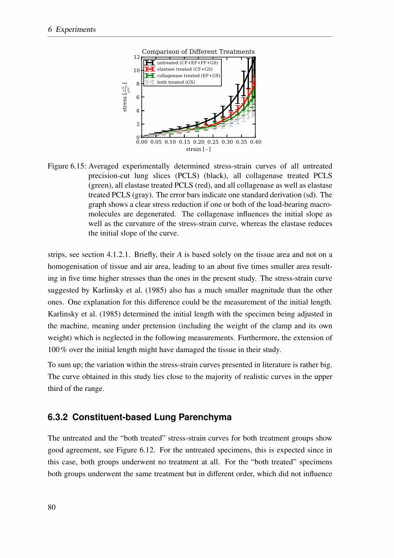
6 Experiments
0.00 0.05 0.10 0.15 0.20 0.25 0.30 0.35 0.40strain [−]
0
2
4
6
8
10
12
stress [nN
µm
2]
Comparison of Different Treatments
untreated (CF+EF+FF+GS)
elastase treated (CF+GS)
collagenase treated (EF+GS)
both treated (GS)
Figure 6.15: Averaged experimentally determined stress-strain curves of all untreatedprecision-cut lung slices (PCLS) (black), all collagenase treated PCLS(green), all elastase treated PCLS (red), and all collagenase as well as elastasetreated PCLS (gray). The error bars indicate one standard derivation (sd). Thegraph shows a clear stress reduction if one or both of the load-bearing macro-molecules are degenerated. The collagenase influences the initial slope aswell as the curvature of the stress-strain curve, whereas the elastase reducesthe initial slope of the curve.
strips, see section 4.1.2.1. Briefly, their A is based solely on the tissue area and not on ahomogenisation of tissue and air area, leading to an about five times smaller area result-ing in five time higher stresses than the ones in the present study. The stress-strain curvesuggested by Karlinsky et al. (1985) also has a much smaller magnitude than the otherones. One explanation for this difference could be the measurement of the initial length.Karlinsky et al. (1985) determined the initial length with the specimen being adjusted inthe machine, meaning under pretension (including the weight of the clamp and its ownweight) which is neglected in the following measurements. Furthermore, the extension of100% over the initial length might have damaged the tissue in their study.
To sum up; the variation within the stress-strain curves presented in literature is rather big.The curve obtained in this study lies close to the majority of realistic curves in the upperthird of the range.
6.3.2 Constituent-based Lung Parenchyma
The untreated and the “both treated” stress-strain curves for both treatment groups showgood agreement, see Figure 6.12. For the untreated specimens, this is expected since inthis case, both groups underwent no treatment at all. For the “both treated” specimensboth groups underwent the same treatment but in different order, which did not influence
80
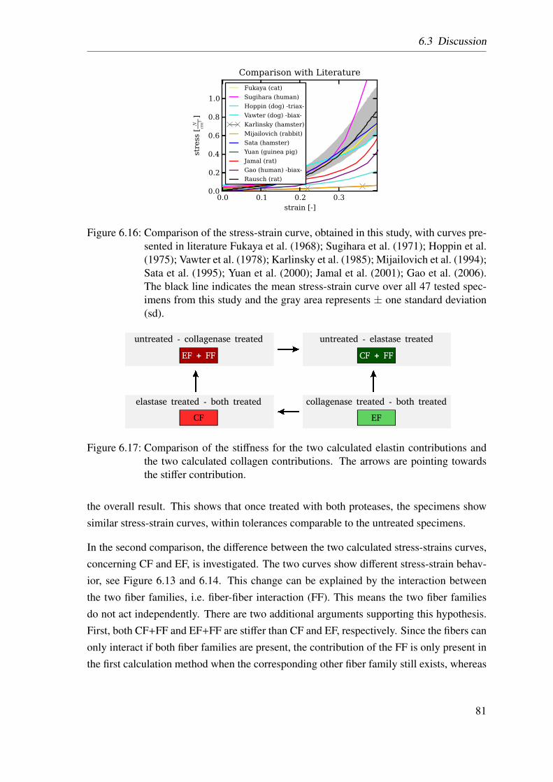
6.3 Discussion
0.0 0.1 0.2 0.3strain [-]
0.0
0.2
0.4
0.6
0.8
1.0
stress [
N
cm2]
Comparison with Literature
Fukaya (cat)
Sugihara (human)
Hoppin (dog) -triax-
Vawter (dog) -biax-
Karlinsky (hamster)
Mijailovich (rabbit)
Sata (hamster)
Yuan (guinea pig)
Jamal (rat)
Gao (human) -biax-
Rausch (rat)
Figure 6.16: Comparison of the stress-strain curve, obtained in this study, with curves pre-sented in literature Fukaya et al. (1968); Sugihara et al. (1971); Hoppin et al.(1975); Vawter et al. (1978); Karlinsky et al. (1985); Mijailovich et al. (1994);Sata et al. (1995); Yuan et al. (2000); Jamal et al. (2001); Gao et al. (2006).The black line indicates the mean stress-strain curve over all 47 tested spec-imens from this study and the gray area represents ± one standard deviation(sd).
EF + FF
untreated - collagenase treated
CF
elastase treated - both treated
EF
collagenase treated - both treated
CF + FF
untreated - elastase treated
Figure 6.17: Comparison of the stiffness for the two calculated elastin contributions andthe two calculated collagen contributions. The arrows are pointing towardsthe stiffer contribution.
the overall result. This shows that once treated with both proteases, the specimens showsimilar stress-strain curves, within tolerances comparable to the untreated specimens.
In the second comparison, the difference between the two calculated stress-strains curves,concerning CF and EF, is investigated. The two curves show different stress-strain behav-ior, see Figure 6.13 and 6.14. This change can be explained by the interaction betweenthe two fiber families, i.e. fiber-fiber interaction (FF). This means the two fiber familiesdo not act independently. There are two additional arguments supporting this hypothesis.First, both CF+FF and EF+FF are stiffer than CF and EF, respectively. Since the fibers canonly interact if both fiber families are present, the contribution of the FF is only present inthe first calculation method when the corresponding other fiber family still exists, whereas
81
6 Experiments
in the second calculation method the corresponding other fiber family has been destroyedin advance. Second, upon closer investigation of the stiffness of the individual measuredPCLS (data not shown), it turned out that for the “elastase first” treated specimens, whereEF+FF and CF are calculated, EF+FF is always stiffer than CF. However, for the “colla-genase first” treated specimens, where CF+FF and EF are calculated, CF+FF is alwaysstiffer than EF. This means the first determined fiber contribution is stiffer than the seconddetermined fiber contribution independent of which fiber family this is. By comparing themean stress-strain curve of the CF and EF with the same calculation method, i.e. EF+FFwith CF+FF and EF with CF, the CF turned out to be stiffer, see Figure 6.17. This seamsreasonable, since the CF are known to be stiffer than the EF. This again backs up the as-sumption that with the first treatment not only one of the fiber family was destroyed butalso the FF.
In the third comparison, the differences between the different treated PCLS are investi-gated, see Figure 6.15. The untreated PCLS still include all major load-bearing elements(CF+EF+GS) and FF, and hence, exhibit the stiffest behavior. The elastase treated PCLSwhich lack the structural support of the EF and the FF show a softer mechanical behavior.The PCLS treated with collagenase are even softer than the elastase treated specimens.The PCLS treated with both enzymes show the softest behavior. Another interesting factis that the stress-strain curves of the PCLS treated with collagenase have a reduced curva-ture. This agrees with the study of Haut and Little (1972), who showed that the CF exhibitstrongly non-linear material behavior.
A comparison with the results found in the literature is essentially impossible, since theonly paper presenting relevant results (Yuan et al., 2000) provided only two static stress-strain curves; these curves additionally showed a variation of over 100% between eachother. However, the general trend, meaning the shape of the curve, the order of magnitudeand the behavior after collagenase/elastase treatment is similar.
Other interesting aspects are: the contribution of the FF is always more dominant than thecontribution of the EF; for small strains. the FF is stiffer than the CF as well as the EF. Thiscan be explained with the CF not being fully extended, i.e. their waviness can potentiallyinhibit their own extension as well as the extension of the EF.
Due to these findings, the material law presented in the following section will not only ac-count for the three major load-bearing constituents but also include an additional summandrepresenting the FF. In order not to get too much influence of intersubject variability, thematerial model is fitted to the averaged curves rather than to the individually determinedcurves, see Figure 6.18.
82
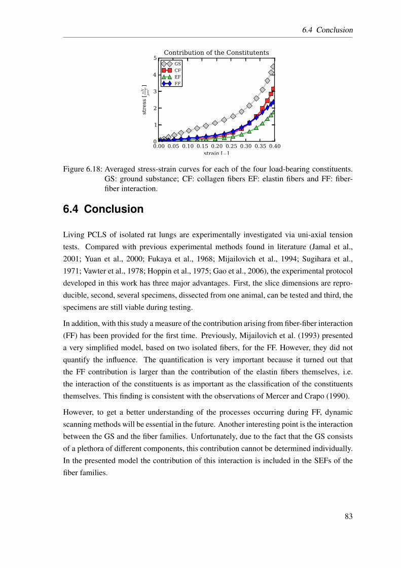
6.4 Conclusion
0.00 0.05 0.10 0.15 0.20 0.25 0.30 0.35 0.40strain [−]
0
1
2
3
4
5
stress [nN
µm
2]
Contribution of the Constitutents
GS
CF
EF
FF
Figure 6.18: Averaged stress-strain curves for each of the four load-bearing constituents.GS: ground substance; CF: collagen fibers EF: elastin fibers and FF: fiber-fiber interaction.
6.4 Conclusion
Living PCLS of isolated rat lungs are experimentally investigated via uni-axial tensiontests. Compared with previous experimental methods found in literature (Jamal et al.,2001; Yuan et al., 2000; Fukaya et al., 1968; Mijailovich et al., 1994; Sugihara et al.,1971; Vawter et al., 1978; Hoppin et al., 1975; Gao et al., 2006), the experimental protocoldeveloped in this work has three major advantages. First, the slice dimensions are repro-ducible, second, several specimens, dissected from one animal, can be tested and third, thespecimens are still viable during testing.
In addition, with this study a measure of the contribution arising from fiber-fiber interaction(FF) has been provided for the first time. Previously, Mijailovich et al. (1993) presenteda very simplified model, based on two isolated fibers, for the FF. However, they did notquantify the influence. The quantification is very important because it turned out thatthe FF contribution is larger than the contribution of the elastin fibers themselves, i.e.the interaction of the constituents is as important as the classification of the constituentsthemselves. This finding is consistent with the observations of Mercer and Crapo (1990).
However, to get a better understanding of the processes occurring during FF, dynamicscanning methods will be essential in the future. Another interesting point is the interactionbetween the GS and the fiber families. Unfortunately, due to the fact that the GS consistsof a plethora of different components, this contribution cannot be determined individually.In the presented model the contribution of this interaction is included in the SEFs of thefiber families.
83
6 Experiments
84
7 Material Identification
In this chapter, a sophisticated material model adequately reproducing the experimental re-sults presented in chapter 6 is derived. Since the optimal constitutive model is not knowna priori, this study is not limited to the optimization of one predetermined SEF, but rathercompares several possible SEFs, which will be referred to as “potential SEF” in the latter.For this reason, a material toolbox is implemented in the research-code BACI. This mate-rial toolbox allows implemented SEFs to be arbitrarily combined. For each of these “po-tential SEFs”, the individual material parameters are optimized to fit the experimentally de-termined behavior. For the parameter optimization, an inverse analysis is performed. Thecorresponding algorithm is also included in BACI. In the last step, the “potential SEFs” arecompared with each other, in order to obtain the optimal description of the experimentalmaterial behavior.
7.1 Methodology
This section is divided in four subsections. The first one introduces the material toolboxand the included SEFs. The second one describes the utilized FE model. The third onedescribes the inverse analysis algorithm, i.e. the parameter optimization for the “potentialSEFs”. The fourth one describes the comparison between the different “potential SEFs”for the homogenized as well as for the constituent-based material model.
7.1.1 Material Toolbox
Due to the fact that a SEF can be composed of additive summands (Balzani, 2006), amaterial toolbox has been implemented in the research-code BACI. In the following, Ψ
will replace Ψv, for simplicity. Each SEF can be defined as the sum of its individualsummands implemented in the toolbox, i.e.
Ψtotal =∑
Ψsummand. (7.1.1)
85
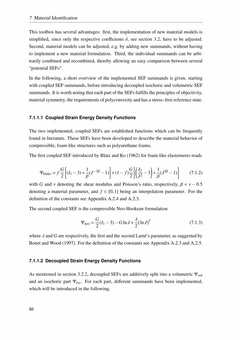
7 Material Identification
This toolbox has several advantages: first, the implementation of new material models issimplified, since only the respective coefficients δ, see section 3.2, have to be adjusted.Second, material models can be adjusted, e.g. by adding new summands, without havingto implement a new material formulation. Third, the individual summands can be arbi-trarily combined and recombined, thereby allowing an easy comparison between several“potential SEFs”.
In the following, a short overview of the implemented SEF summands is given, startingwith coupled SEF summands, before introducing decoupled isochoric and volumetric SEFsummands. It is worth noting that each part of the SEFs fulfills the principles of objectivity,material symmetry, the requirements of polyconvexity and has a stress–free reference state.
7.1.1.1 Coupled Strain Energy Density Functions
The two implemented, coupled SEFs are established functions which can be frequentlyfound in literature. These SEFs have been developed to describe the material behavior ofcompressible, foam-like structures such as polyurethane foams.
The first coupled SEF introduced by Blatz and Ko (1962) for foam-like elastomeres reads
Ψblako = fG2
[(I1−3) +
1β
(J−2β−1)]+ (1− f )
G2
[(I2
J2 −3)+
1β
(J2β−1)]
(7.1.2)
with G and ν denoting the shear modulus and Poisson’s ratio, respectively, β = ν− 0.5denoting a material parameter, and f ∈ [0,1] being an interpolation parameter. For thedefinition of the constants see Appendix A.2.4 and A.2.3.
The second coupled SEF is the compressible Neo-Hookean formulation
Ψneo =G2
(I1−3)−G ln J +λ
2(ln J
)2 (7.1.3)
where λ and G are respectively, the first and the second Lamé’s parameter, as suggested byBonet and Wood (1997). For the definition of the constants see Appendix A.2.3 and A.2.5.
7.1.1.2 Decoupled Strain Energy Density Functions
As mentioned in section 3.2.2, decoupled SEFs are additively split into a volumetric Ψvol
and an isochoric part Ψiso. For each part, different summands have been implemented,which will be introduced in the following.
86
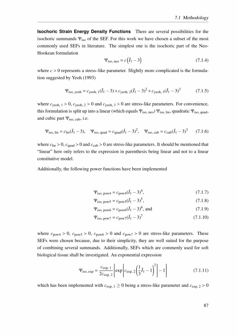
7.1 Methodology
Isochoric Strain Energy Density Functions There are several possibilities for theisochoric summands Ψiso of the SEF. For this work we have chosen a subset of the mostcommonly used SEFs in literature. The simplest one is the isochoric part of the Neo-Hookean formulation
Ψiso, neo = c(I1−3
)(7.1.4)
where c > 0 represents a stress–like parameter. Slightly more complicated is the formula-tion suggested by Yeoh (1993)
Ψiso, yeoh = cyeoh, 1(I1−3) + cyeoh, 2(I1−3)2 + cyeoh, 3(I1−3)3 (7.1.5)
where cyeoh, 1 > 0, cyeoh, 2 > 0 and cyeoh, 3 > 0 are stress-like parameters. For convenience,this formulation is split up into a linear (which equals Ψiso, neo) Ψiso, lin, quadratic Ψiso, quad,and cubic part Ψiso, cub, i.e.
Ψiso, lin = clin(I1−3), Ψiso, quad = cquad(I1−3)2, Ψiso, cub = ccub(I1−3)3 (7.1.6)
where clin > 0, cquad > 0 and ccub > 0 are stress-like parameters. It should be mentioned that“linear” here only refers to the expression in parenthesis being linear and not to a linearconstitutive model.
Additionally, the following power functions have been implemented
Ψiso, pow4 = cpow4(I1−3)4, (7.1.7)
Ψiso, pow5 = cpow5(I1−3)5, (7.1.8)
Ψiso, pow6 = cpow6(I1−3)6, and (7.1.9)
Ψiso, pow7 = cpow7(I1−3)7 (7.1.10)
where cpow4 > 0, cpow5 > 0, cpow6 > 0 and cpow7 > 0 are stress-like parameters. TheseSEFs were chosen because, due to their simplicity, they are well suited for the purposeof combining several summands. Additionally, SEFs which are commenly used for softbiological tissue shall be investigated. An exponential expression
Ψiso, exp =cexp, 1
2cexp, 2
exp
cexp, 2
(13
I1−1)2−1
(7.1.11)
which has been implemented with cexp, 1 ≥ 0 being a stress-like parameter and cexp, 2 > 0
87
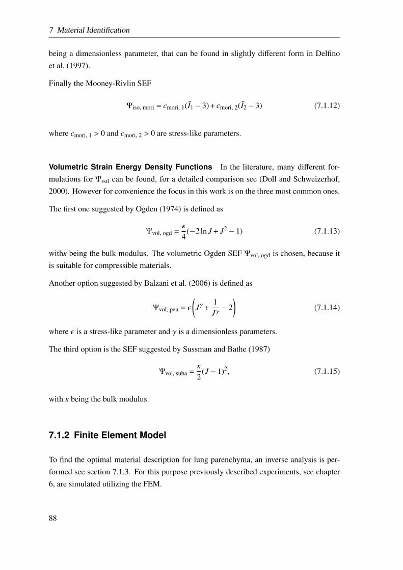
7 Material Identification
being a dimensionless parameter, that can be found in slightly different form in Delfinoet al. (1997).
Finally the Mooney-Rivlin SEF
Ψiso, mori = cmori, 1(I1−3) + cmori, 2(I2−3) (7.1.12)
where cmori, 1 > 0 and cmori, 2 > 0 are stress-like parameters.
Volumetric Strain Energy Density Functions In the literature, many different for-mulations for Ψvol can be found, for a detailed comparison see (Doll and Schweizerhof,2000). However for convenience the focus in this work is on the three most common ones.
The first one suggested by Ogden (1974) is defined as
Ψvol, ogd =κ
4(−2ln J + J2−1) (7.1.13)
withκ being the bulk modulus. The volumetric Ogden SEF Ψvol, ogd is chosen, because itis suitable for compressible materials.
Another option suggested by Balzani et al. (2006) is defined as
Ψvol, pen = ε
(Jγ +
1Jγ−2
)(7.1.14)
where ε is a stress-like parameter and γ is a dimensionless parameters.
The third option is the SEF suggested by Sussman and Bathe (1987)
Ψvol, suba =κ
2(J−1)2, (7.1.15)
with κ being the bulk modulus.
7.1.2 Finite Element Model
To find the optimal material description for lung parenchyma, an inverse analysis is per-formed see section 7.1.3. For this purpose previously described experiments, see chapter6, are simulated utilizing the FEM.
88
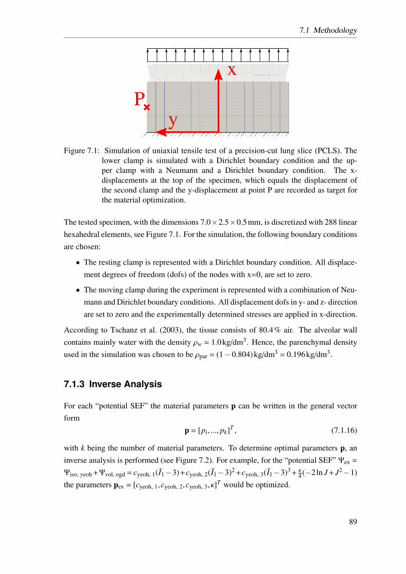
7.1 Methodology
Figure 7.1: Simulation of uniaxial tensile test of a precision-cut lung slice (PCLS). Thelower clamp is simulated with a Dirichlet boundary condition and the up-per clamp with a Neumann and a Dirichlet boundary condition. The x-displacements at the top of the specimen, which equals the displacement ofthe second clamp and the y-displacement at point P are recorded as target forthe material optimization.
The tested specimen, with the dimensions 7.0×2.5×0.5mm, is discretized with 288 linearhexahedral elements, see Figure 7.1. For the simulation, the following boundary conditionsare chosen:
• The resting clamp is represented with a Dirichlet boundary condition. All displace-ment degrees of freedom (dofs) of the nodes with x=0, are set to zero.
• The moving clamp during the experiment is represented with a combination of Neu-mann and Dirichlet boundary conditions. All displacement dofs in y- and z- directionare set to zero and the experimentally determined stresses are applied in x-direction.
According to Tschanz et al. (2003), the tissue consists of 80.4% air. The alveolar wallcontains mainly water with the density ρw = 1.0kg/dm3. Hence, the parenchymal densityused in the simulation was chosen to be ρpar = (1−0.804)kg/dm3 = 0.196kg/dm3.
7.1.3 Inverse Analysis
For each “potential SEF” the material parameters p can be written in the general vectorform
p = [pi, ..., pk]T , (7.1.16)
with k being the number of material parameters. To determine optimal parameters p, aninverse analysis is performed (see Figure 7.2). For example, for the “potential SEF” Ψex =
Ψiso, yeoh +Ψvol, ogd = cyeoh, 1(I1−3)+cyeoh, 2(I1−3)2 +cyeoh, 3(I1−3)3 + κ4 (−2ln J + J2−1)
the parameters pex = [cyeoh, 1,cyeoh, 2,cyeoh, 3, κ]T would be optimized.
89
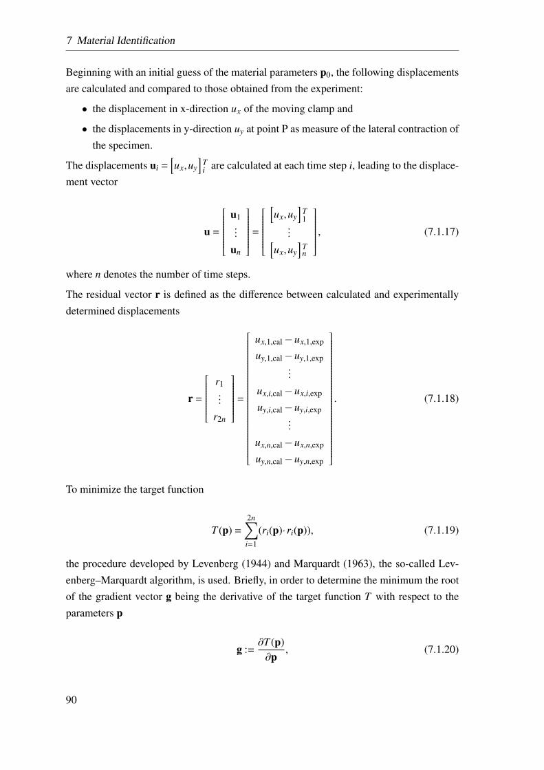
7 Material Identification
Beginning with an initial guess of the material parameters p0, the following displacementsare calculated and compared to those obtained from the experiment:
• the displacement in x-direction ux of the moving clamp and
• the displacements in y-direction uy at point P as measure of the lateral contraction ofthe specimen.
The displacements ui =[ux,uy
]Ti are calculated at each time step i, leading to the displace-
ment vector
u =
u1...
un
=
[ux,uy
]T1
...[ux,uy
]Tn
, (7.1.17)
where n denotes the number of time steps.
The residual vector r is defined as the difference between calculated and experimentallydetermined displacements
r =
r1...
r2n
=
ux,1,cal−ux,1,exp
uy,1,cal−uy,1,exp...
ux,i,cal−ux,i,exp
uy,i,cal−uy,i,exp...
ux,n,cal−ux,n,exp
uy,n,cal−uy,n,exp
. (7.1.18)
To minimize the target function
T (p) =
2n∑i=1
(ri(p)·ri(p)), (7.1.19)
the procedure developed by Levenberg (1944) and Marquardt (1963), the so-called Lev-enberg–Marquardt algorithm, is used. Briefly, in order to determine the minimum the rootof the gradient vector g being the derivative of the target function T with respect to theparameters p
g :=∂T (p)∂p
, (7.1.20)
90
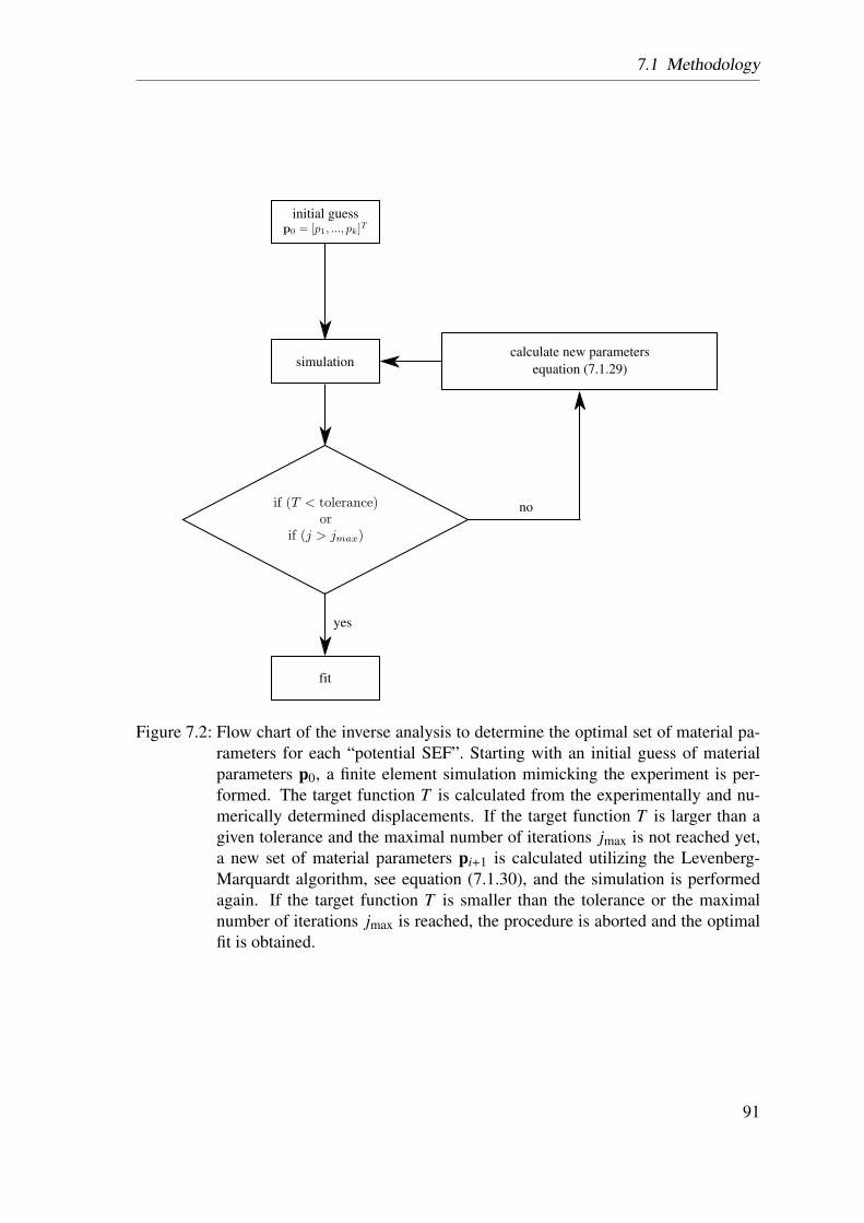
7.1 Methodology
initial guess
no
simulation
yes
fit
calculate new parameters
equation (7.1.29)
Figure 7.2: Flow chart of the inverse analysis to determine the optimal set of material pa-rameters for each “potential SEF”. Starting with an initial guess of materialparameters p0, a finite element simulation mimicking the experiment is per-formed. The target function T is calculated from the experimentally and nu-merically determined displacements. If the target function T is larger than agiven tolerance and the maximal number of iterations jmax is not reached yet,a new set of material parameters pi+1 is calculated utilizing the Levenberg-Marquardt algorithm, see equation (7.1.30), and the simulation is performedagain. If the target function T is smaller than the tolerance or the maximalnumber of iterations jmax is reached, the procedure is aborted and the optimalfit is obtained.
91
7 Material Identification
need to be determined. The individual components of the gradient vector g are calculatedas
gl = 22n∑i=1
ri∂ri
∂pl. (7.1.21)
The Hessian matrix H is the second derivation of the target function T with respect to theparameters p
H :=∂2T (p)
(∂p)2 . (7.1.22)
The individual components of the Hessian matrix H are calculated as
Hkl = 22n∑i=1
(∂ri
∂pk
∂ri
∂pl+ ri
∂2ri
∂pk∂pl
). (7.1.23)
In order to solve the non-linear problem
g (p) != 0 (7.1.24)
the problems is linearized and iteratively solved using the well-known Newton’s method(also called Newton-Raphson method). The approximation p j+1 is calculated from p j as
p j+1 = p j−H−1g. (7.1.25)
For the Gauss-Newton method the second-order derivative terms are ignored, leading tothe approximation of the Hessian matrix of
Hkl ≈ Hkl = 22n∑i=1
(∂ri
∂pk
∂ri
∂pl
). (7.1.26)
Introducing the Jacobian-matrix as
Jr =
[∂ri∂p j
]=
∂r1∂p1
... ∂r1∂pk
......
∂r2n∂p1
... ∂r2n∂pk
, (7.1.27)
92
7.1 Methodology
the gradient vector g and the approximate Hessian matrix H can be written as
g = 2JrT r, H = 2Jr
T Jr. (7.1.28)
Substituting this in the recurrence equation (7.1.25) yields
p j+1 = p j−(Jr
T Jr)−1
JrT r (7.1.29)
which is known as the Gauss-Newton procedure. This methodology can be further im-proved by introducing a damped version, the Levenberg–Marquardt algorithm
p j+1 = p j−(Jr
T Jr +λdiag(Jr
T Jr))−1
JrT r, (7.1.30)
with λ being a damping factor that is adjusted at each iteration j. For a fast reduction of thetarget function T a small damping factor λ brings the algorithm closer to the Gauss-Newtonmethod, whereas a larger damping factor λ brings the algorithm closer to the gradientdescent direction. The damping factor λ factor is initially set to 1.0 and adapted withthe help of the relative error, such that λ = λold
TTold
, with λold and Told being the dampingfactor and the target function of the last iteration, respectivly. The loop of simulationand the calculation of a new set of material parameters terminates once maximal numberof iterations jmax is reached. For the optimization, presented in this study, the maximalnumber of iterations jmax is chosen to be 25, since preliminary studies have shown thatby then the target function T has converged to a constant value. Furthermore the stopcriteria of a predefined tolerance turned out to be contra productive for the comparison ofthe quality of fit for the “potential SEFs”.
For a better comparison of the error, a normalized form of the target function is used, i.e.
Tn =1L
√T2n
=1L
√∑2ni=1(ri(p)·ri(p))
2n. (7.1.31)
This algorithm has already shown good results for soft biological tissue (Kauer et al., 2002;Mahnken and Stein, 1996; Moulton et al., 1995; Seshaiyer and Humphrey, 2003). How-ever, one common drawback of most optimization algorithms is that it might only convergeto a local minimum instead of a global minimum. Therefore, in a preliminary study, theparameter optimization was performed with several randomly picked initial guesses of p.For example, for the coupled SEF Ψblako, the initial values were chosen in the range of
93
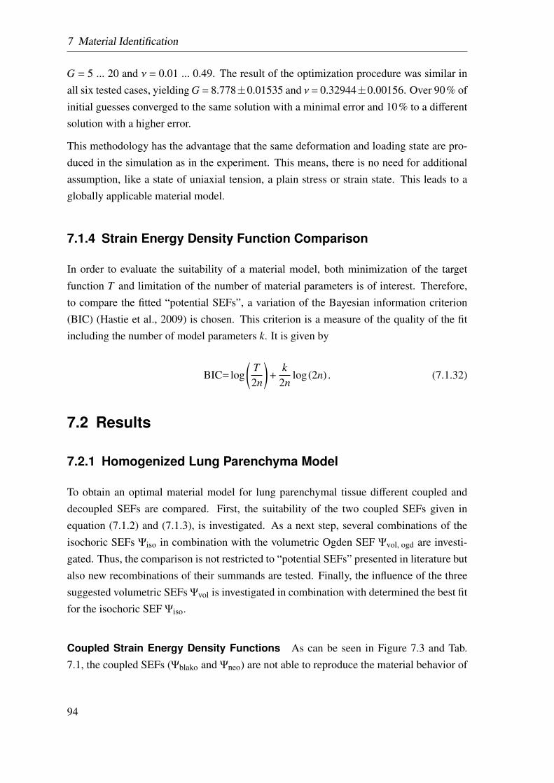
7 Material Identification
G = 5 ... 20 and ν = 0.01 ... 0.49. The result of the optimization procedure was similar inall six tested cases, yielding G = 8.778±0.01535 and ν= 0.32944±0.00156. Over 90% ofinitial guesses converged to the same solution with a minimal error and 10% to a differentsolution with a higher error.
This methodology has the advantage that the same deformation and loading state are pro-duced in the simulation as in the experiment. This means, there is no need for additionalassumption, like a state of uniaxial tension, a plain stress or strain state. This leads to aglobally applicable material model.
7.1.4 Strain Energy Density Function Comparison
In order to evaluate the suitability of a material model, both minimization of the targetfunction T and limitation of the number of material parameters is of interest. Therefore,to compare the fitted “potential SEFs”, a variation of the Bayesian information criterion(BIC) (Hastie et al., 2009) is chosen. This criterion is a measure of the quality of the fitincluding the number of model parameters k. It is given by
BIC= log(
T2n
)+
k2n
log(2n) . (7.1.32)
7.2 Results
7.2.1 Homogenized Lung Parenchyma Model
To obtain an optimal material model for lung parenchymal tissue different coupled anddecoupled SEFs are compared. First, the suitability of the two coupled SEFs given inequation (7.1.2) and (7.1.3), is investigated. As a next step, several combinations of theisochoric SEFs Ψiso in combination with the volumetric Ogden SEF Ψvol, ogd are investi-gated. Thus, the comparison is not restricted to “potential SEFs” presented in literature butalso new recombinations of their summands are tested. Finally, the influence of the threesuggested volumetric SEFs Ψvol is investigated in combination with determined the best fitfor the isochoric SEF Ψiso.
Coupled Strain Energy Density Functions As can be seen in Figure 7.3 and Tab.7.1, the coupled SEFs (Ψblako and Ψneo) are not able to reproduce the material behavior of
94
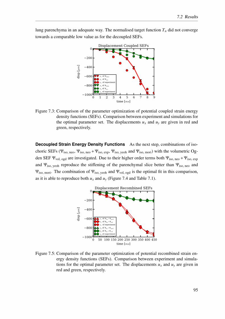
7.2 Results
lung parenchyma in an adequate way. The normalised target function Tn did not convergetowards a comparable low value as for the decoupled SEFs.
0 1 2 3 4 5 6 7 8 9time [ms]
−1000
−800
−600
−400
−200
0
dis
p [µm
]
Displacement Coupled SEFs
ux of Ψblako
ux of Ψneo
ux of experiment
uy of Ψblako
uy of Ψneo
uy of experiment
Figure 7.3: Comparison of the parameter optimization of potential coupled strain energydensity functions (SEFs). Comparison between experiment and simulations forthe optimal parameter set. The displacements ux and uy are given in red andgreen, respectively.
Decoupled Strain Energy Density Functions As the next step, combinations of iso-choric SEFs (Ψiso, neo, Ψiso, neo + Ψiso, exp, Ψiso, yeoh and Ψiso, mori) with the volumetric Og-den SEF Ψvol, ogd are investigated. Due to their higher order terms both Ψiso, neo + Ψiso, exp
and Ψiso, yeoh reproduce the stiffening of the parenchymal slice better than Ψiso, neo andΨiso, mori. The combination of Ψiso, yeoh and Ψvol, ogd is the optimal fit in this comparison,as it is able to reproduce both ux and uy (Figure 7.4 and Table 7.1).
0 50 100 150 200 250 300 350 400 450time [ms]
−1000
−800
−600
−400
−200
0
dis
p [µm
]
Displacement Recombined SEFs
ux of Ψlin+Ψquad
ux of Ψlin+Ψcub
ux of experiment
uy of Ψlin+Ψquad
uy of Ψlin+Ψcub
uy of experiment
Figure 7.5: Comparison of the parameter optimization of potential recombined strain en-ergy density functions (SEFs). Comparison between experiment and simula-tions for the optimal parameter set. The displacements ux and uy are given inred and green, respectively.
95
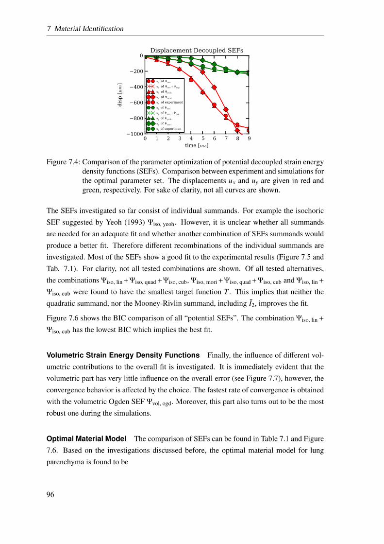
7 Material Identification
0 1 2 3 4 5 6 7 8 9time [ms]
−1000
−800
−600
−400
−200
0
dis
p [µm
]
Displacement Decoupled SEFs
ux of Ψneo
ux of Ψneo+Ψexp
ux of Ψyeoh
ux of Ψmori
ux of experiment
uy of Ψneo
uy of Ψneo+Ψexp
uy of Ψyeoh
uy of Ψmori
uy of experimen
Figure 7.4: Comparison of the parameter optimization of potential decoupled strain energydensity functions (SEFs). Comparison between experiment and simulations forthe optimal parameter set. The displacements ux and uy are given in red andgreen, respectively. For sake of clarity, not all curves are shown.
The SEFs investigated so far consist of individual summands. For example the isochoricSEF suggested by Yeoh (1993) Ψiso, yeoh. However, it is unclear whether all summandsare needed for an adequate fit and whether another combination of SEFs summands wouldproduce a better fit. Therefore different recombinations of the individual summands areinvestigated. Most of the SEFs show a good fit to the experimental results (Figure 7.5 andTab. 7.1). For clarity, not all tested combinations are shown. Of all tested alternatives,the combinations Ψiso, lin +Ψiso, quad +Ψiso, cub, Ψiso, mori +Ψiso, quad +Ψiso, cub and Ψiso, lin +
Ψiso, cub were found to have the smallest target function T . This implies that neither thequadratic summand, nor the Mooney-Rivlin summand, including I2, improves the fit.
Figure 7.6 shows the BIC comparison of all “potential SEFs”. The combination Ψiso, lin +
Ψiso, cub has the lowest BIC which implies the best fit.
Volumetric Strain Energy Density Functions Finally, the influence of different vol-umetric contributions to the overall fit is investigated. It is immediately evident that thevolumetric part has very little influence on the overall error (see Figure 7.7), however, theconvergence behavior is affected by the choice. The fastest rate of convergence is obtainedwith the volumetric Ogden SEF Ψvol, ogd. Moreover, this part also turns out to be the mostrobust one during the simulations.
Optimal Material Model The comparison of SEFs can be found in Table 7.1 and Figure7.6. Based on the investigations discussed before, the optimal material model for lungparenchyma is found to be
96
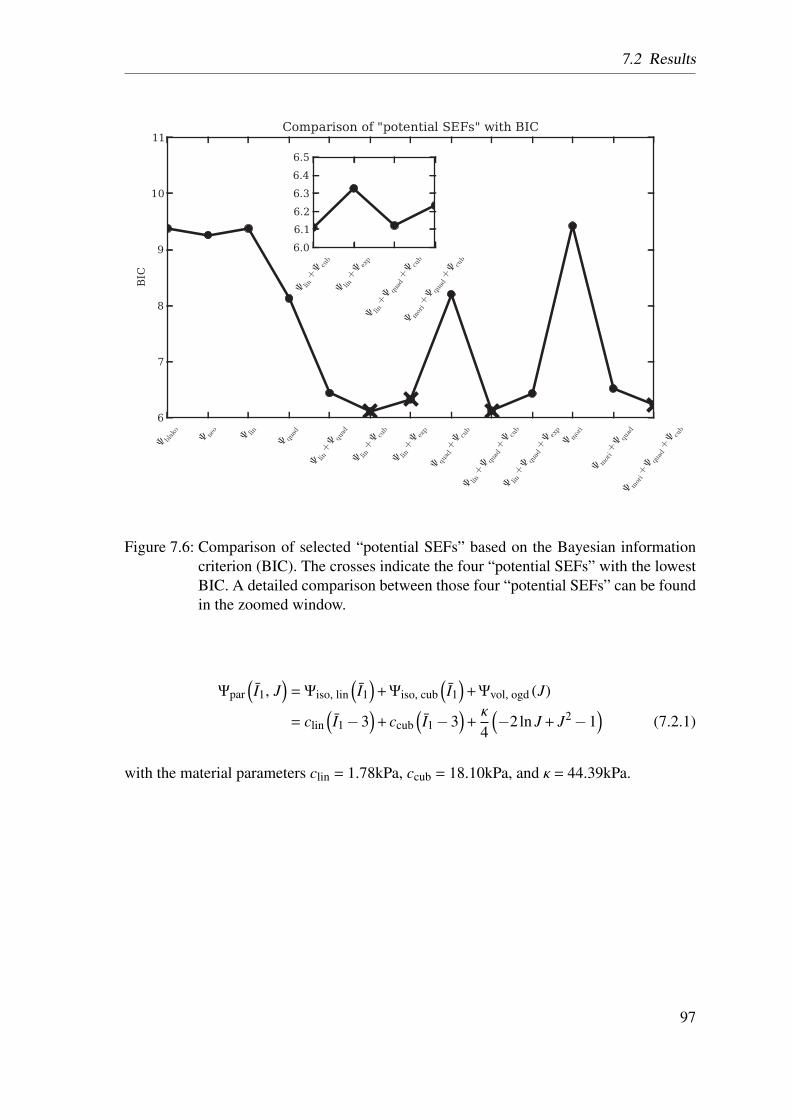
7.2 Results
Figure 7.6: Comparison of selected “potential SEFs” based on the Bayesian informationcriterion (BIC). The crosses indicate the four “potential SEFs” with the lowestBIC. A detailed comparison between those four “potential SEFs” can be foundin the zoomed window.
Ψpar(I1, J
)= Ψiso, lin
(I1)+Ψiso, cub
(I1)+Ψvol, ogd (J)
= clin(I1−3
)+ ccub
(I1−3
)+κ
4
(−2ln J + J2−1
)(7.2.1)
with the material parameters clin = 1.78kPa, ccub = 18.10kPa, and κ = 44.39kPa.
97
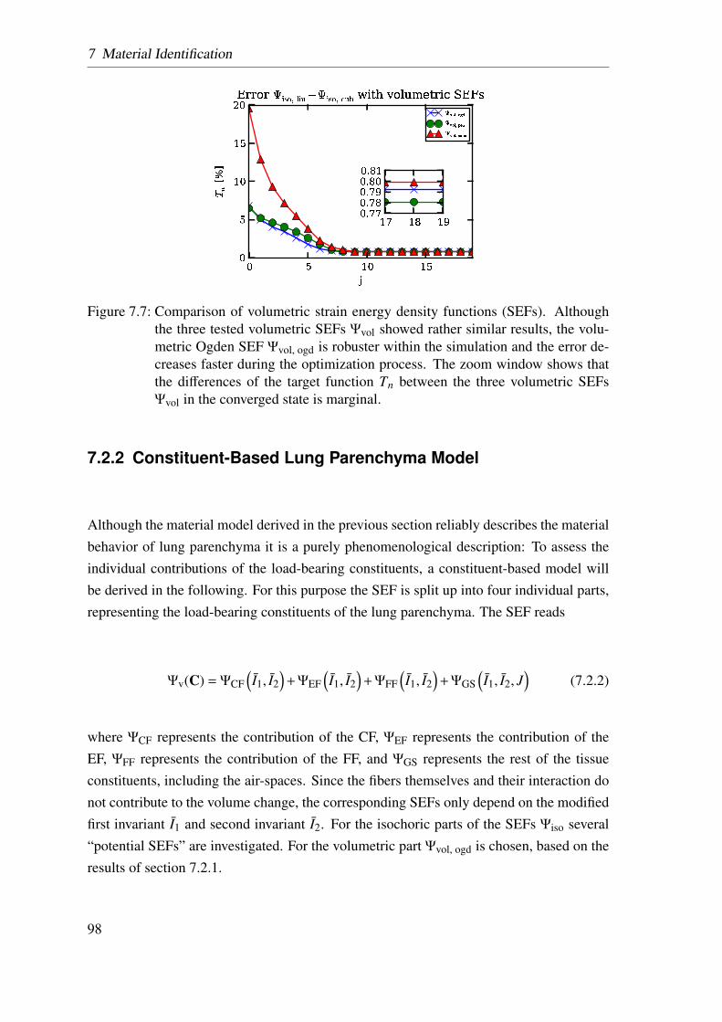
7 Material Identification
Figure 7.7: Comparison of volumetric strain energy density functions (SEFs). Althoughthe three tested volumetric SEFs Ψvol showed rather similar results, the volu-metric Ogden SEF Ψvol, ogd is robuster within the simulation and the error de-creases faster during the optimization process. The zoom window shows thatthe differences of the target function Tn between the three volumetric SEFsΨvol in the converged state is marginal.
7.2.2 Constituent-Based Lung Parenchyma Model
Although the material model derived in the previous section reliably describes the materialbehavior of lung parenchyma it is a purely phenomenological description: To assess theindividual contributions of the load-bearing constituents, a constituent-based model willbe derived in the following. For this purpose the SEF is split up into four individual parts,representing the load-bearing constituents of the lung parenchyma. The SEF reads
Ψv(C) = ΨCF(I1, I2
)+ΨEF
(I1, I2
)+ΨFF
(I1, I2
)+ΨGS
(I1, I2, J
)(7.2.2)
where ΨCF represents the contribution of the CF, ΨEF represents the contribution of theEF, ΨFF represents the contribution of the FF, and ΨGS represents the rest of the tissueconstituents, including the air-spaces. Since the fibers themselves and their interaction donot contribute to the volume change, the corresponding SEFs only depend on the modifiedfirst invariant I1 and second invariant I2. For the isochoric parts of the SEFs Ψiso several“potential SEFs” are investigated. For the volumetric part Ψvol, ogd is chosen, based on theresults of section 7.2.1.
98
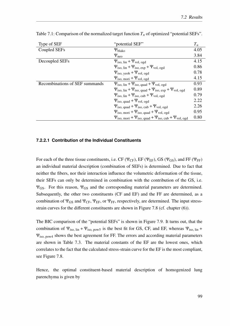
7.2 Results
Table 7.1: Comparison of the normalized target function Tn of optimized “potential SEFs”.
Type of SEF “potential SEF” TnCoupled SEFs Ψblako 4.05
Ψneo 3.84Decoupled SEFs Ψiso, lin +Ψvol, ogd 4.15
Ψiso, lin +Ψiso, exp +Ψvol, ogd 0.86Ψiso, yeoh +Ψvol, ogd 0.78Ψiso, mori +Ψvol, ogd 4.15
Recombinations of SEF summands Ψiso, lin +Ψiso, quad +Ψvol, ogd 0.93Ψiso, lin +Ψiso, quad +Ψiso, exp +Ψvol, ogd 0.89Ψiso, lin +Ψiso, cub +Ψvol, ogd 0.79Ψiso, quad +Ψvol, ogd 2.22Ψiso, quad +Ψiso, cub +Ψvol, ogd 2.26Ψiso, mori +Ψiso, quad +Ψvol, ogd 0.95Ψiso, mori +Ψiso, quad +Ψiso, cub +Ψvol, ogd 0.80
7.2.2.1 Contribution of the Individual Constituents
For each of the three tissue constituents, i.e. CF (ΨCF), EF (ΨEF), GS (ΨGS), and FF (ΨFF)an individual material description (combination of SEFs) is determined. Due to fact thatneither the fibers, nor their interaction influence the volumetric deformation of the tissue,their SEFs can only be determined in combination with the contribution of the GS, i.e.ΨGS. For this reason, ΨGS and the corresponding material parameters are determined.Subsequently, the other two constituents (CF and EF) and the FF are determined, as acombination of ΨGS and ΨCF, ΨEF, or ΨFF, respectively, are determined. The input stress-strain curves for the different constituents are shown in Figure 7.8 (cf. chapter (6)).
The BIC comparison of the “potential SEFs” is shown in Figure 7.9. It turns out, that thecombination of Ψiso, lin + Ψiso, pow5 is the best fit for GS, CF, and EF, whereas Ψiso, lin +
Ψiso, pow4 shows the best agreement for FF. The errors and according material parametersare shown in Table 7.3. The material constants of the EF are the lowest ones, whichcorrelates to the fact that the calculated stress-strain curve for the EF is the most compliant,see Figure 7.8.
Hence, the optimal constituent-based material description of homogenized lungparenchyma is given by
99
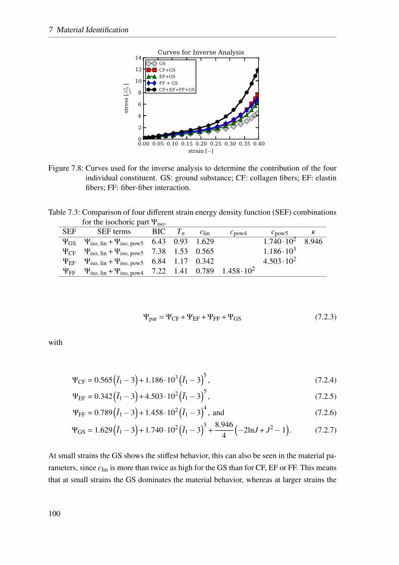
7 Material Identification
0.00 0.05 0.10 0.15 0.20 0.25 0.30 0.35 0.40strain [−]
0
2
4
6
8
10
12
14
stress [nN
µm
2]
Curves for Inverse Analysis
GS
CF+GS
EF+GS
FF + GS
CF+EF+FF+GS
Figure 7.8: Curves used for the inverse analysis to determine the contribution of the fourindividual constituent. GS: ground substance; CF: collagen fibers; EF: elastinfibers; FF: fiber-fiber interaction.
Table 7.3: Comparison of four different strain energy density function (SEF) combinationsfor the isochoric part Ψiso.
SEF SEF terms BIC Tn clin cpow4 cpow5 κ
ΨGS Ψiso, lin +Ψiso, pow5 6.43 0.93 1.629 1.740·102 8.946ΨCF Ψiso, lin +Ψiso, pow5 7.38 1.53 0.565 1.186·103
ΨEF Ψiso, lin +Ψiso, pow5 6.84 1.17 0.342 4.503·102
ΨFF Ψiso, lin +Ψiso, pow4 7.22 1.41 0.789 1.458·102
Ψpar = ΨCF +ΨEF +ΨFF +ΨGS (7.2.3)
with
ΨCF = 0.565(I1−3
)+ 1.186·103
(I1−3
)5, (7.2.4)
ΨEF = 0.342(I1−3
)+ 4.503·102
(I1−3
)5, (7.2.5)
ΨFF = 0.789(I1−3
)+ 1.458·102
(I1−3
)4, and (7.2.6)
ΨGS = 1.629(I1−3
)+ 1.740·102
(I1−3
)5+
8.9464
(−2lnJ + J2−1
). (7.2.7)
At small strains the GS shows the stiffest behavior, this can also be seen in the material pa-rameters, since clin is more than twice as high for the GS than for CF, EF or FF. This meansthat at small strains the GS dominates the material behavior, whereas at larger strains the
100
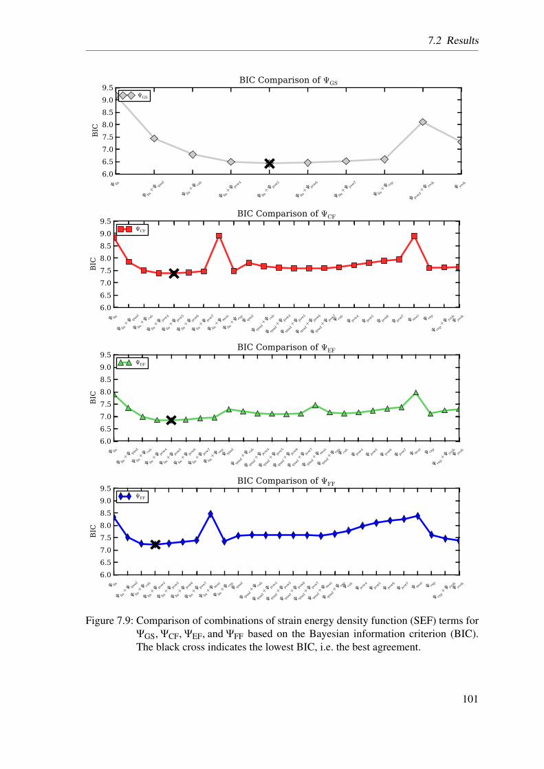
7.2 Results
Ψ lin
Ψ lin+Ψ qu
ad
Ψ lin+Ψ cu
b
Ψ lin+Ψ po
w4
Ψ lin+Ψ po
w5
Ψ lin+Ψ po
w6
Ψ lin+Ψ po
w7
Ψ lin+Ψ ex
p
Ψ pow4+Ψ ye
oh
Ψ yeoh
6.0
6.5
7.0
7.5
8.0
8.5
9.0
9.5BIC
BIC Comparison of ΨGS
ΨGS
Ψ lin
Ψ lin+Ψ qu
ad
Ψ lin+Ψ cu
b
Ψ lin+Ψ po
w4
Ψ lin+Ψ po
w5
Ψ lin+Ψ po
w6
Ψ lin+Ψ po
w7
Ψ lin+Ψ m
ori
Ψ lin+Ψ ex
p Ψ qu
ad
Ψ quad+Ψ cu
b
Ψ quad+Ψ po
w4
Ψ quad+Ψ po
w5
Ψ quad+Ψ po
w6
Ψ quad+Ψ po
w7 Ψ cu
b
Ψ pow4
Ψ pow5
Ψ pow6
Ψ pow7
Ψ mori
Ψ exp
Ψ exp+Ψ ye
oh Ψ ye
oh
6.0
6.5
7.0
7.5
8.0
8.5
9.0
9.5
BIC
BIC Comparison of ΨCF
ΨCF
Ψ lin
Ψ lin+Ψ qu
ad
Ψ lin+Ψ cu
b
Ψ lin+Ψ po
w4
Ψ lin+Ψ po
w5
Ψ lin+Ψ po
w6
Ψ lin+Ψ po
w7
Ψ lin+Ψ ex
p Ψ qu
ad
Ψ quad+Ψ cu
b
Ψ quad+Ψ po
w4
Ψ quad+Ψ po
w5
Ψ quad+Ψ po
w6
Ψ quad+Ψ po
w7
Ψ quad+Ψ m
ori
Ψ quad+Ψ ex
p Ψ cu
b
Ψ pow4
Ψ pow5
Ψ pow6
Ψ pow7
Ψ mori
Ψ exp
Ψ exp+Ψ ye
oh Ψ ye
oh
6.0
6.5
7.0
7.5
8.0
8.5
9.0
9.5
BIC
BIC Comparison of ΨEF
ΨEF
Ψ lin
Ψ lin+Ψ qu
ad
Ψ lin+Ψ cu
b
Ψ lin+Ψ po
w4
Ψ lin+Ψ po
w5
Ψ lin+Ψ po
w6
Ψ lin+Ψ po
w7
Ψ lin+Ψ m
ori
Ψ lin+Ψ ex
p Ψ qu
ad
Ψ quad+Ψ cu
b
Ψ quad+Ψ po
w4
Ψ quad+Ψ po
w5
Ψ quad+Ψ po
w6
Ψ quad+Ψ po
w7
Ψ quad+Ψ m
ori
Ψ quad+Ψ ex
p Ψ cu
b
Ψ pow4
Ψ pow5
Ψ pow6
Ψ pow7 Ψ m
ori Ψ ex
p
Ψ exp+Ψ ye
oh Ψ ye
oh
6.0
6.5
7.0
7.5
8.0
8.5
9.0
9.5
BIC
BIC Comparison of ΨFF
ΨFF
Figure 7.9: Comparison of combinations of strain energy density function (SEF) terms forΨGS, ΨCF, ΨEF, and ΨFF based on the Bayesian information criterion (BIC).The black cross indicates the lowest BIC, i.e. the best agreement.
101
7 Material Identification
contribution of the fibers rises significantly. Comparing the stress-strain curves of the CFwith the FF, a cross-over point exists, meaning the CF are more compliant at the start butbecome stiffer for large strains; this effect is reflected in the material parameters since clin
is smaller for the CF, whereas the higher order term is the smallest for the FF.
7.3 Conclusion
In this chapter, a method to determine a homogenized and a constituent-based materialmodel for lung parenchyma has been presented. The proposed methodology allows usto compare the suitability of different existing and new models with each other. In theliterature no SEF can be found that is capable of sufficiently reproducing the complexcompressible, stiffening behavior observed in the experiments presented in chapter 6. Tothe author’s knowledge, previously only Gao et al. (2006) determined material parametersfor a SEF describing the homogenized lung parenchyma. However, as mentioned in theintroduction, this approach has some major limitations and an exponential SEF (as theyproposed) is found to be incapable to reproduce the experimental results adequately.
A mayor advantage of this study is that not only the material parameters of one preselectedSEF are optimized but rather many “potential SEF” are compared with each other, in orderto find the optimal material model. Another advantage is the usage of the FEM, becauseit reproduces the same loading states for the fitting as the specimen experienced duringthe experiment. This means, there is no need for additional assumption, like a state ofuniaxial tension, a plain stress or strain state. This leads to a globally applicable materialmodel. In order to validate our determined material model a simulation of the biaxialtensile test performed by Vawter et al. (1978) is performed (data not shown). Qualitatively,our material model showed good agreement.
Therefore, the constitutive models proposed in this work are the first material models forlung parenchymal tissue that adequately reflects the complex behavior of lung parenchymaltissue.
Additionally, the constituent-based material model is the first material model for lungparenchyma including quantified contributions for the three major load-bearing con-stituents, i.e. the EF, the CF and the GS, as well as their interaction, i.e. FF.
It is important to note that the methodology presented here can also be used for the de-velopment of any material model, homogenized as well as constituent-based and henceshould have a large range of applications in the future.
102
7.3 Conclusion
The presented material models are used within our virtual lung model (Wall et al., 2010b),in order to realistically determine the loading of the lung tissue during mechanical ventila-tion. The homogenized material model can be used to model the influence of the healthylung parenchyma, whereas the constituent-based material model can be applied to simulatehealthy as well as diseased parenchymal tissue, e.g. for simulations of fibrosis, where thefiber density changes dramatically. To do so, the corresponding constituent contribution,can be increased or completely removed.
To conclude, the development of novel sophisticated constitutive models for homogenizedlung parenchyma and for the individual load-bearing constituents was presented. Thisapproach will help to model the behavior of the lung tissue and quantify its strains andstresses during mechanical ventilation.
103

7 Material Identification
104
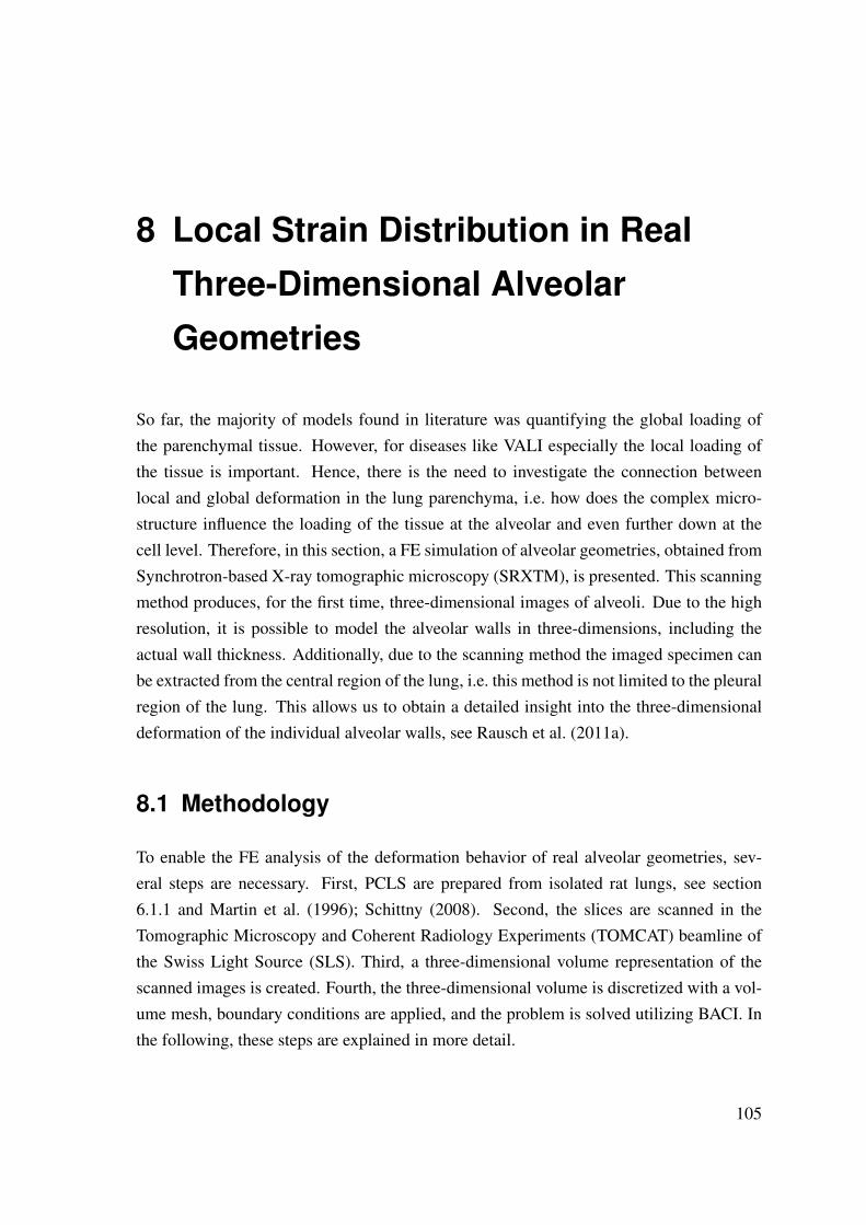
8 Local Strain Distribution in Real
Three-Dimensional Alveolar
Geometries
So far, the majority of models found in literature was quantifying the global loading ofthe parenchymal tissue. However, for diseases like VALI especially the local loading ofthe tissue is important. Hence, there is the need to investigate the connection betweenlocal and global deformation in the lung parenchyma, i.e. how does the complex micro-structure influence the loading of the tissue at the alveolar and even further down at thecell level. Therefore, in this section, a FE simulation of alveolar geometries, obtained fromSynchrotron-based X-ray tomographic microscopy (SRXTM), is presented. This scanningmethod produces, for the first time, three-dimensional images of alveoli. Due to the highresolution, it is possible to model the alveolar walls in three-dimensions, including theactual wall thickness. Additionally, due to the scanning method the imaged specimen canbe extracted from the central region of the lung, i.e. this method is not limited to the pleuralregion of the lung. This allows us to obtain a detailed insight into the three-dimensionaldeformation of the individual alveolar walls, see Rausch et al. (2011a).
8.1 Methodology
To enable the FE analysis of the deformation behavior of real alveolar geometries, sev-eral steps are necessary. First, PCLS are prepared from isolated rat lungs, see section6.1.1 and Martin et al. (1996); Schittny (2008). Second, the slices are scanned in theTomographic Microscopy and Coherent Radiology Experiments (TOMCAT) beamline ofthe Swiss Light Source (SLS). Third, a three-dimensional volume representation of thescanned images is created. Fourth, the three-dimensional volume is discretized with a vol-ume mesh, boundary conditions are applied, and the problem is solved utilizing BACI. Inthe following, these steps are explained in more detail.
105
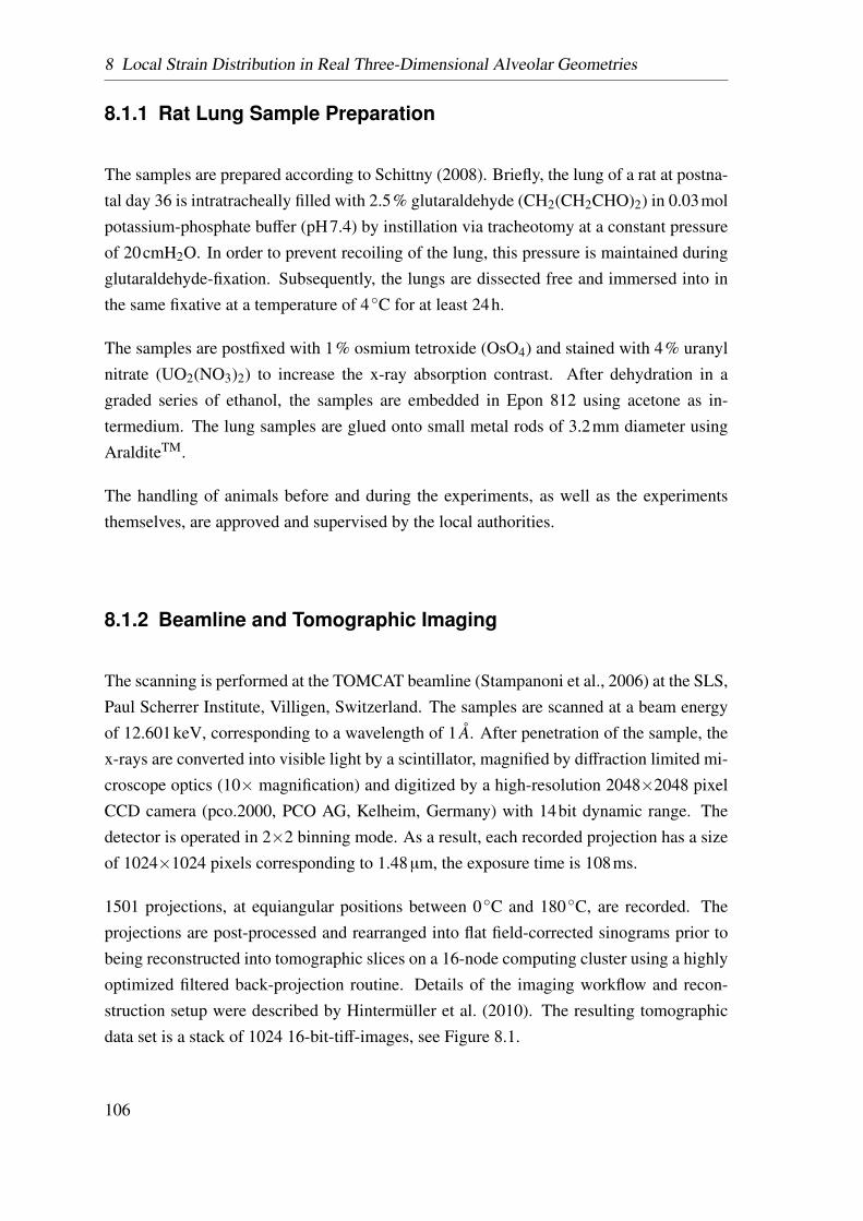
8 Local Strain Distribution in Real Three-Dimensional Alveolar Geometries
8.1.1 Rat Lung Sample Preparation
The samples are prepared according to Schittny (2008). Briefly, the lung of a rat at postna-tal day 36 is intratracheally filled with 2.5% glutaraldehyde (CH2(CH2CHO)2) in 0.03molpotassium-phosphate buffer (pH7.4) by instillation via tracheotomy at a constant pressureof 20cmH2O. In order to prevent recoiling of the lung, this pressure is maintained duringglutaraldehyde-fixation. Subsequently, the lungs are dissected free and immersed into inthe same fixative at a temperature of 4◦C for at least 24h.
The samples are postfixed with 1% osmium tetroxide (OsO4) and stained with 4% uranylnitrate (UO2(NO3)2) to increase the x-ray absorption contrast. After dehydration in agraded series of ethanol, the samples are embedded in Epon 812 using acetone as in-termedium. The lung samples are glued onto small metal rods of 3.2mm diameter usingAralditeTM.
The handling of animals before and during the experiments, as well as the experimentsthemselves, are approved and supervised by the local authorities.
8.1.2 Beamline and Tomographic Imaging
The scanning is performed at the TOMCAT beamline (Stampanoni et al., 2006) at the SLS,Paul Scherrer Institute, Villigen, Switzerland. The samples are scanned at a beam energyof 12.601keV, corresponding to a wavelength of 1 A. After penetration of the sample, thex-rays are converted into visible light by a scintillator, magnified by diffraction limited mi-croscope optics (10× magnification) and digitized by a high-resolution 2048×2048 pixelCCD camera (pco.2000, PCO AG, Kelheim, Germany) with 14bit dynamic range. Thedetector is operated in 2×2 binning mode. As a result, each recorded projection has a sizeof 1024×1024 pixels corresponding to 1.48µm, the exposure time is 108ms.
1501 projections, at equiangular positions between 0◦C and 180◦C, are recorded. Theprojections are post-processed and rearranged into flat field-corrected sinograms prior tobeing reconstructed into tomographic slices on a 16-node computing cluster using a highlyoptimized filtered back-projection routine. Details of the imaging workflow and recon-struction setup were described by Hintermüller et al. (2010). The resulting tomographicdata set is a stack of 1024 16-bit-tiff-images, see Figure 8.1.
106
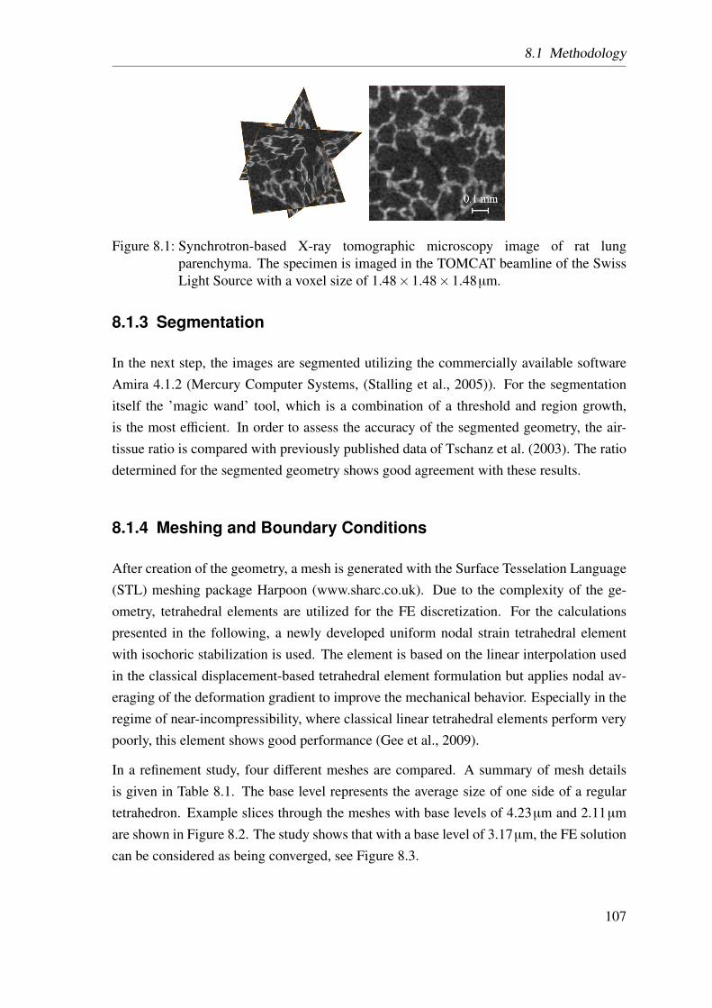
8.1 Methodology
Figure 8.1: Synchrotron-based X-ray tomographic microscopy image of rat lungparenchyma. The specimen is imaged in the TOMCAT beamline of the SwissLight Source with a voxel size of 1.48×1.48×1.48µm.
8.1.3 Segmentation
In the next step, the images are segmented utilizing the commercially available softwareAmira 4.1.2 (Mercury Computer Systems, (Stalling et al., 2005)). For the segmentationitself the ’magic wand’ tool, which is a combination of a threshold and region growth,is the most efficient. In order to assess the accuracy of the segmented geometry, the air-tissue ratio is compared with previously published data of Tschanz et al. (2003). The ratiodetermined for the segmented geometry shows good agreement with these results.
8.1.4 Meshing and Boundary Conditions
After creation of the geometry, a mesh is generated with the Surface Tesselation Language(STL) meshing package Harpoon (www.sharc.co.uk). Due to the complexity of the ge-ometry, tetrahedral elements are utilized for the FE discretization. For the calculationspresented in the following, a newly developed uniform nodal strain tetrahedral elementwith isochoric stabilization is used. The element is based on the linear interpolation usedin the classical displacement-based tetrahedral element formulation but applies nodal av-eraging of the deformation gradient to improve the mechanical behavior. Especially in theregime of near-incompressibility, where classical linear tetrahedral elements perform verypoorly, this element shows good performance (Gee et al., 2009).
In a refinement study, four different meshes are compared. A summary of mesh detailsis given in Table 8.1. The base level represents the average size of one side of a regulartetrahedron. Example slices through the meshes with base levels of 4.23µm and 2.11µmare shown in Figure 8.2. The study shows that with a base level of 3.17µm, the FE solutioncan be considered as being converged, see Figure 8.3.
107
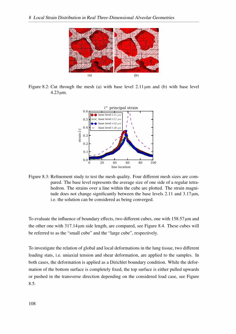
8 Local Strain Distribution in Real Three-Dimensional Alveolar Geometries
Figure 8.2: Cut through the mesh (a) with base level 2.11µm and (b) with base level4.23µm.
0 20 40 60 80 100line location
0.0
0.1
0.2
0.3
0.4
0.5
0.6
stra
in [-]
1st principal strain
base level 2.11 µm
base level 3.17 µm
base level 4.23 µm
base level 5.29 µm
Figure 8.3: Refinement study to test the mesh quality. Four different mesh sizes are com-pared. The base level represents the average size of one side of a regular tetra-hedron. The strains over a line within the cube are plotted. The strain magni-tude does not change significantly between the base levels 2.11 and 3.17µm,i.e. the solution can be considered as being converged.
To evaluate the influence of boundary effects, two different cubes, one with 158.57µm andthe other one with 317.14µm side length, are compared, see Figure 8.4. These cubes willbe referred to as the “small cube” and the “large cube”, respectively.
To investigate the relation of global and local deformations in the lung tissue, two differentloading stats, i.e. uniaxial tension and shear deformation, are applied to the samples. Inboth cases, the deformation is applied as a Dirichlet boundary condition. While the defor-mation of the bottom surface is completely fixed, the top surface is either pulled upwardsor pushed in the transverse direction depending on the considered load case, see Figure8.5.
108
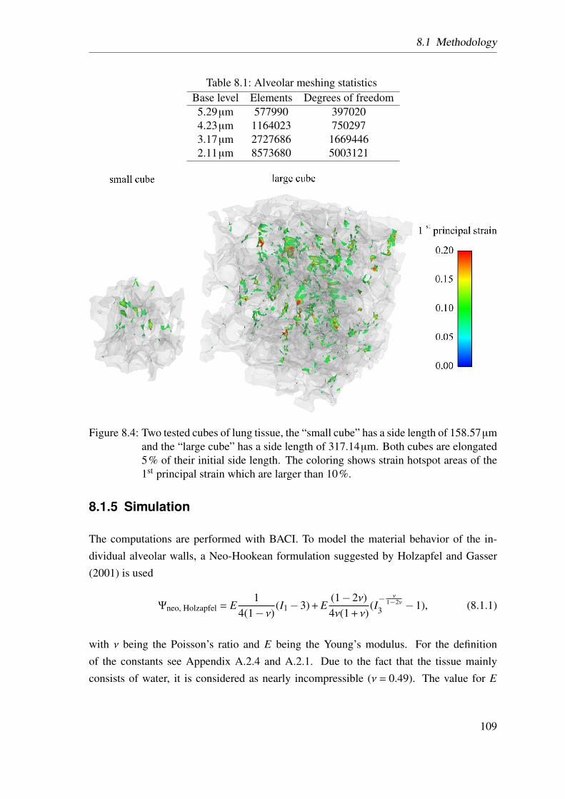
8.1 Methodology
Table 8.1: Alveolar meshing statisticsBase level Elements Degrees of freedom5.29µm 577990 3970204.23µm 1164023 7502973.17µm 2727686 16694462.11µm 8573680 5003121
Figure 8.4: Two tested cubes of lung tissue, the “small cube” has a side length of 158.57µmand the “large cube” has a side length of 317.14µm. Both cubes are elongated5% of their initial side length. The coloring shows strain hotspot areas of the1st principal strain which are larger than 10%.
8.1.5 Simulation
The computations are performed with BACI. To model the material behavior of the in-dividual alveolar walls, a Neo-Hookean formulation suggested by Holzapfel and Gasser(2001) is used
Ψneo, Holzapfel = E1
4(1− ν)(I1−3) + E
(1−2ν)4ν(1 + ν)
(I− ν
1−2ν3 −1), (8.1.1)
with ν being the Poisson’s ratio and E being the Young’s modulus. For the definitionof the constants see Appendix A.2.4 and A.2.1. Due to the fact that the tissue mainlyconsists of water, it is considered as nearly incompressible (ν = 0.49). The value for E
109
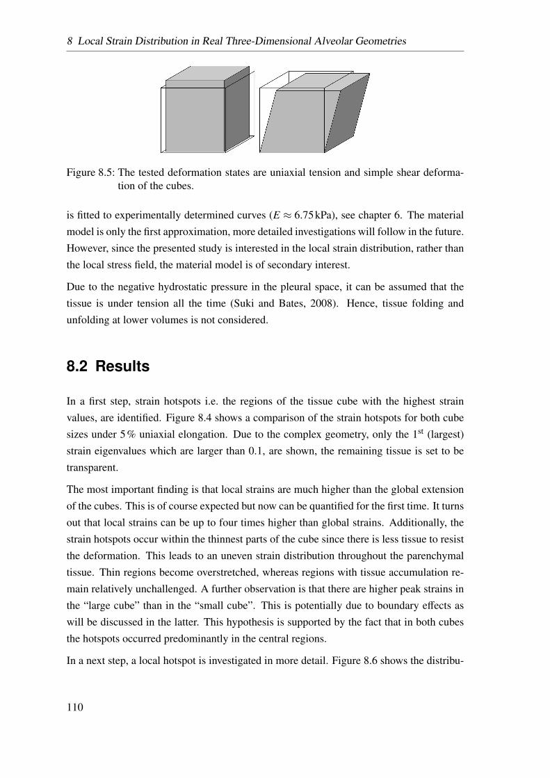
8 Local Strain Distribution in Real Three-Dimensional Alveolar Geometries
Figure 8.5: The tested deformation states are uniaxial tension and simple shear deforma-tion of the cubes.
is fitted to experimentally determined curves (E ≈ 6.75kPa), see chapter 6. The materialmodel is only the first approximation, more detailed investigations will follow in the future.However, since the presented study is interested in the local strain distribution, rather thanthe local stress field, the material model is of secondary interest.
Due to the negative hydrostatic pressure in the pleural space, it can be assumed that thetissue is under tension all the time (Suki and Bates, 2008). Hence, tissue folding andunfolding at lower volumes is not considered.
8.2 Results
In a first step, strain hotspots i.e. the regions of the tissue cube with the highest strainvalues, are identified. Figure 8.4 shows a comparison of the strain hotspots for both cubesizes under 5% uniaxial elongation. Due to the complex geometry, only the 1st (largest)strain eigenvalues which are larger than 0.1, are shown, the remaining tissue is set to betransparent.
The most important finding is that local strains are much higher than the global extensionof the cubes. This is of course expected but now can be quantified for the first time. It turnsout that local strains can be up to four times higher than global strains. Additionally, thestrain hotspots occur within the thinnest parts of the cube since there is less tissue to resistthe deformation. This leads to an uneven strain distribution throughout the parenchymaltissue. Thin regions become overstretched, whereas regions with tissue accumulation re-main relatively unchallenged. A further observation is that there are higher peak strains inthe “large cube” than in the “small cube”. This is potentially due to boundary effects aswill be discussed in the latter. This hypothesis is supported by the fact that in both cubesthe hotspots occurred predominantly in the central regions.
In a next step, a local hotspot is investigated in more detail. Figure 8.6 shows the distribu-
110
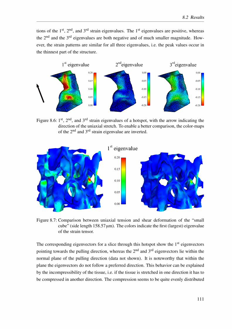
8.2 Results
tions of the 1st, 2nd, and 3rd strain eigenvalues. The 1st eigenvalues are positive, whereasthe 2nd and the 3rd eigenvalues are both negative and of much smaller magnitude. How-ever, the strain patterns are similar for all three eigenvalues, i.e. the peak values occur inthe thinnest part of the structure.
Figure 8.6: 1st, 2nd, and 3rd strain eigenvalues of a hotspot, with the arrow indicating thedirection of the uniaxial stretch. To enable a better comparison, the color-mapsof the 2nd and 3rd strain eigenvalue are inverted.
Figure 8.7: Comparison between uniaxial tension and shear deformation of the “smallcube” (side length 158.57µm). The colors indicate the first (largest) eigenvalueof the strain tensor.
The corresponding eigenvectors for a slice through this hotspot show the 1st eigenvectorspointing towards the pulling direction, whereas the 2nd and 3rd eigenvectors lie within thenormal plane of the pulling direction (data not shown). It is noteworthy that within theplane the eigenvectors do not follow a preferred direction. This behavior can be explainedby the incompressibility of the tissue, i.e. if the tissue is stretched in one direction it has tobe compressed in another direction. The compression seems to be quite evenly distributed
111
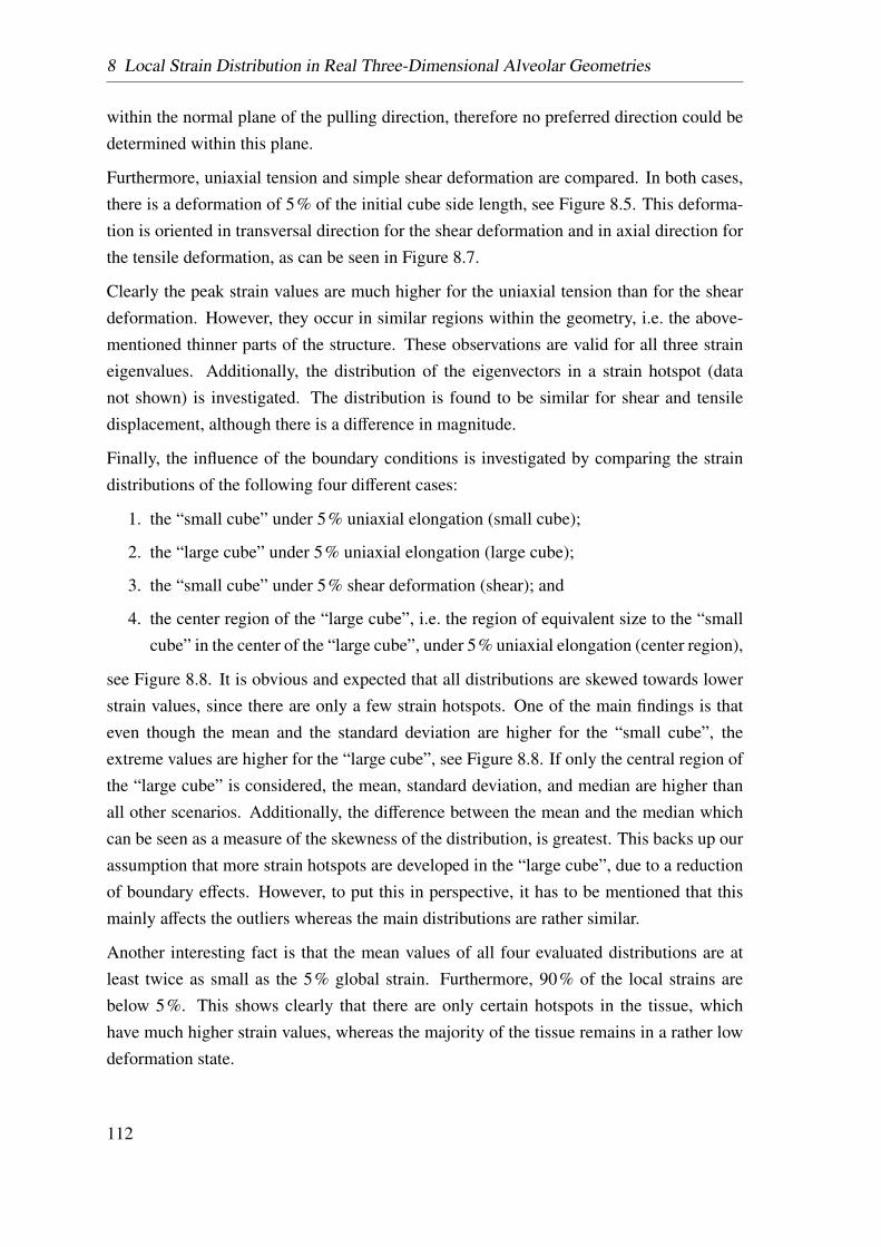
8 Local Strain Distribution in Real Three-Dimensional Alveolar Geometries
within the normal plane of the pulling direction, therefore no preferred direction could bedetermined within this plane.
Furthermore, uniaxial tension and simple shear deformation are compared. In both cases,there is a deformation of 5% of the initial cube side length, see Figure 8.5. This deforma-tion is oriented in transversal direction for the shear deformation and in axial direction forthe tensile deformation, as can be seen in Figure 8.7.
Clearly the peak strain values are much higher for the uniaxial tension than for the sheardeformation. However, they occur in similar regions within the geometry, i.e. the above-mentioned thinner parts of the structure. These observations are valid for all three straineigenvalues. Additionally, the distribution of the eigenvectors in a strain hotspot (datanot shown) is investigated. The distribution is found to be similar for shear and tensiledisplacement, although there is a difference in magnitude.
Finally, the influence of the boundary conditions is investigated by comparing the straindistributions of the following four different cases:
1. the “small cube” under 5% uniaxial elongation (small cube);
2. the “large cube” under 5% uniaxial elongation (large cube);
3. the “small cube” under 5% shear deformation (shear); and
4. the center region of the “large cube”, i.e. the region of equivalent size to the “smallcube” in the center of the “large cube”, under 5% uniaxial elongation (center region),
see Figure 8.8. It is obvious and expected that all distributions are skewed towards lowerstrain values, since there are only a few strain hotspots. One of the main findings is thateven though the mean and the standard deviation are higher for the “small cube”, theextreme values are higher for the “large cube”, see Figure 8.8. If only the central region ofthe “large cube” is considered, the mean, standard deviation, and median are higher thanall other scenarios. Additionally, the difference between the mean and the median whichcan be seen as a measure of the skewness of the distribution, is greatest. This backs up ourassumption that more strain hotspots are developed in the “large cube”, due to a reductionof boundary effects. However, to put this in perspective, it has to be mentioned that thismainly affects the outliers whereas the main distributions are rather similar.
Another interesting fact is that the mean values of all four evaluated distributions are atleast twice as small as the 5% global strain. Furthermore, 90% of the local strains arebelow 5%. This shows clearly that there are only certain hotspots in the tissue, whichhave much higher strain values, whereas the majority of the tissue remains in a rather lowdeformation state.
112
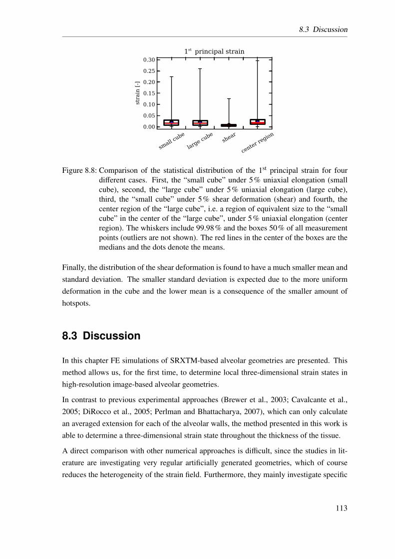
8.3 Discussion
small cu
be
large cu
beshe
ar
center
regio
n
0.00
0.05
0.10
0.15
0.20
0.25
0.30
strain [-]
1st principal strain
Figure 8.8: Comparison of the statistical distribution of the 1st principal strain for fourdifferent cases. First, the “small cube” under 5% uniaxial elongation (smallcube), second, the “large cube” under 5% uniaxial elongation (large cube),third, the “small cube” under 5% shear deformation (shear) and fourth, thecenter region of the “large cube”, i.e. a region of equivalent size to the “smallcube” in the center of the “large cube”, under 5% uniaxial elongation (centerregion). The whiskers include 99.98% and the boxes 50% of all measurementpoints (outliers are not shown). The red lines in the center of the boxes are themedians and the dots denote the means.
Finally, the distribution of the shear deformation is found to have a much smaller mean andstandard deviation. The smaller standard deviation is expected due to the more uniformdeformation in the cube and the lower mean is a consequence of the smaller amount ofhotspots.
8.3 Discussion
In this chapter FE simulations of SRXTM-based alveolar geometries are presented. Thismethod allows us, for the first time, to determine local three-dimensional strain states inhigh-resolution image-based alveolar geometries.
In contrast to previous experimental approaches (Brewer et al., 2003; Cavalcante et al.,2005; DiRocco et al., 2005; Perlman and Bhattacharya, 2007), which can only calculatean averaged extension for each of the alveolar walls, the method presented in this work isable to determine a three-dimensional strain state throughout the thickness of the tissue.
A direct comparison with other numerical approaches is difficult, since the studies in lit-erature are investigating very regular artificially generated geometries, which of coursereduces the heterogeneity of the strain field. Furthermore, they mainly investigate specific
113
8 Local Strain Distribution in Real Three-Dimensional Alveolar Geometries
effects, rather than developing a general model, see Cavalcante et al. (2005); Denny andSchroter (2006). The only other FE study on real alveolar geometries was performed byGefen et al. (1999). However their model was limited to two-dimensional geometries.
A further advantage of the presented method is the quality of the newly developed sta-bilized node-based uniform strain tetrahedron. The problem with normal tetrahedral ele-ments is that they produce parasitic stresses for nearly incompressible materials, leading totoo stiff behavior. With the nodal strain tetrahedron, however, these so-called volumetriclocking effects can be neglected.
8.4 Conclusion
From the FE analysis, two main conclusions can be drawn. First, there are certain hotspotsin the alveolar geometry which are especially at risk for overstretching. These obviouslytend to be in the thinnest regions. Second, a small global strain can lead to significantlylarger local strains. These conclusions are found to be independent of the loading type.
Looking at in vitro experiments on alveolar type II cells (Ning and Wang, 2007; Vlahakiset al., 1999; Chandel and Sznajder, 2000; Copland and Post, 2007), there is disagreementon how much stretch causes inflammatory reactions. The numbers range from strainsof 0.05 up to strains of 0.3, see section 4.1.4. Comparing these values with the localpeak strains found in the presented simulations, a global strain of 0.05 turns out to besufficient to cause inflammation in any cases, since it causes local strains of up to 0.4 whichis higher than every threshold value reported in literature. This presents an interestingobservation as it suggests that the amount of stretching done in these experiments may notbe representative of the in vivo environment or at the very least maybe an underestimation.This large increase in strain from the global to the local level shows that inflammatoryreactions potentially initiate much earlier than previously thought.
For this reason, the presented simulations will be included within a multi-scale approachfor alveolar ensemble (Wiechert and Wall, 2010). This allows us to project the globalparenchymal deformation down to the level of a single alveolar ensemble, in order toprovide realistic boundary conditions. This method has the advantage that local alveolarstrain fields in large geometries, for example PCLS, can be determined.
Dassow et al. (2010) recently measured calcium fluxes, which are known to be induced bylung stretch, within the alveolar walls of these PCLS in a bioreactor. With this experimentalapproach and our computational models, the local strain fields in PCLS could be directly
114
8.4 Conclusion
compared with the locations of increased calcium fluxes, hence providing a mechanical-biological pathway for the initiation of ventilator-induced lung inflammation.
The presented model does not include any surface tension effects. Hence in reality, anoverall stiffer behavior can be expected. To investigate these effects further, a surfacetension model developed previously by Wiechert et al. (2009) will be included in the future.
115
8 Local Strain Distribution in Real Three-Dimensional Alveolar Geometries
116
9 Summary and Outlook
In this thesis, sophisticated material models for alveolar parenchyma were developed. Withthese material models stresses and strains in the parenchymal tissue can be determined.Furthermore, the relation between these global stresses and strains and the deformationwithin individual alveolar walls was determined by performing FE simulations of image-based three-dimensional alveolar geometries.
In the following, a short overview of the achievement of the specific aims, defined insection 5, is given.
AIM 1 To develop an experimental testing protocol in order to determine the
elastic material behavior of lung parenchyma.
This aim was achieved. An experimental protocol in order to determine the material be-haviour of lung parenchyma is developed. This testing procedure includes a precondi-tioning protocol, needed to eliminate viscous effects. The three major advantages of theproposed testing protocol are:
1. The slice dimensions are reproducible.
2. Several specimens per animal can be tested.
3. The specimens are still viable during testing.
A drawback of the testing protocol is the lateral contraction is very coarse. This is due tothe low time and space resolution of the utilized camera. For the future, image trackingwith a high-resolution camera is suggested. This could further improve the experimentalresults, for the reasons described below:
1. The higher spatial resolution increases the accuracy of the measured values.
2. The higher time resolution increases the number of measured values.
3. Automatic image tracking, in comparison to the manual tracking used in this work,can reduce the post-processing time of the experiment.
117
9 Summary and Outlook
4. Image tracking allows to determine a strain field, rather than individual points, whichwould increase the accuracy of the fit.
AIM 2 To extend the experimental methodology to investigate the influence of
the individual tissue constituents (CF and EF).
This aim was achieved. An experimental protocol, which allows the determination ofthe influence of the individual tissue components and their interaction was developed Itdetermines the influence of the ground substance (GS), the collagen fibers (CF), the elastinfibers (EF) and their interaction (FF). The presented protocol allows for the first time toquantify the contribution of these components. Despite the fact that it was tested that theindividual fiber networks were destroyed, it remains unclear if leftover fibers remain inthe tissue. These remnants could cause artificial changes in the determined stress-straincurves. A possibility to investigate the influence of the remaining fiber parts would be toperform the tensile tests under a 2-photon microscope. This has the advantage that fibersare visible and the amount of remaining fibers could be documented and included in thestudies.
Furthermore, since the lung tissue is viscoelastic the experimental protocol will need to beextended, in order to enable the characterization of time-dependent effects.
AIM 3 To develop an inverse analysis methodology in order to deduce a
hyperelastic material model for soft biological tissue from experiments.
This aim was achieved. An inverse analysis methodology to determine hyperelastic ma-terial models for soft biological tissues from experimental results was developed. Suit-able non-linear, compressible and elastic mathematical models were formulated (“poten-tial SEF”), which reproduce the experimentally determined behavior in an adequate way.To optimize the material parameters of a “potential SEF”, the experiment is simulated withvarying material parameters, according to an optimization algorithm, until the optimal fitfor a predefined target function is achieved. Using this methodology several “potentialSEFs” were compared with each other in order to determine the material model that issuited best to describe the complex behavior of lung parenchyma. The advantages of thismethodology are described below:
1. Due to the fact that a three-dimensional deformation state of the specimen duringthe experiment can be accurately mapped with the FE simulation, the approach is
118
not limited to a specific strain or stress state, like for example uni-axial tension. Asa consequence, the determined SEF can predict other strain-states as well.
2. The optimization is implemented directly in the FE code. Hence, no additional pro-grams are necessary.
3. The methodology is not limited to lung tissue. It can be applied to any material andis suitable for arbitrary behavior including viscoelastic and anisotropic materials.
AIM 4 To determine a phenomenological and a constituent-based material
model for lung parenchyma.
This aim was achieved. Two material models for lung parenchyma, a phenomenologicaland a constituent-based approach, were determined. The constituent-based material modelis the first material model quantitatively accounting for the contribution of individual fiberfamilies and their interaction. The material models will be used within our virtual lungmodel for the following applications:
• Simulation of diseases, like fibrosis, in order to get a better understanding of theunderlying processes.
• Comparison of the influence of different ventilation protocols on stresses and stainsin the parenchymal tissue, in order to compare the outcome of different ventilationstrategies.
In the future, further experiments are needed in order to validate the predictive behaviorof the material models. Furthermore, the material models need to be extended, in order toinclude viscoelastic effects. Additionally, due to the fact that a constituent-based materialmodel includes individual summands for both fiber families, the fiber density distributioncan be included in our virtual lung model. This means that the contribution of the individ-ual constituents can be correlated with the fiber density distribution gained from imaging.This would allow us to consider spatial differences and improve the localization of riskareas within the alveolar tissue.
AIM 5 To perform a FE simulation on image-based alveolar geometries, in
order to determine the deformation within the alveolar walls for a given global
deformation state.
This aim was achieved. The deformation within the alveolar wall was determined, usingFE simulations with image-based alveolar geometries. The two main conclusions of the
119
9 Summary and Outlook
FE analysis are that:
1. There are certain hotspots in the alveolar geometry, which are especially at risk ofoverstretching.
2. A small global strain can cause up to a fourfold as high local strains within thintissue regions.
One major problem with this type of simulations is the large size of the discretization,making the simulation numerically very expensive. For this reason, it should be investi-gated whether the image-based alveolar geometries could be replaced by artificially gen-erated alveolar geometries, see Wall et al. (2010b). The advantage of artificially generatedgeometries is that, due to their regular shape, they can be meshed with less hexahedralelements, which reduces the computational effort.
Furthermore, the influence of the surface tension on the strain-peaks will need furtherattention. Since the surface tension always works against the deformation it needs to beinvestigated whether including the surface tension effects will even out the deformationsand reduce the peak strains. This could be further investigated by including a previouslydeveloped surfactant model in the simulations (Wiechert et al., 2009).
In the next step, a material model for the individual alveolar wall will be determined. Forthis reason, the material model fitting procedure will be combined with a previously de-veloped multi-scale approach (Wiechert and Wall, 2010). With this method, the behavioron the parenchymal level and on the alveolar level can be simulated simultaneously. Themacro-scale (parenchymal level) gives its deformation state (F) to the micro-scale (alve-olar level), thereby defining a boundary condition for alveolar simulations similar to thescenario investigated in chapter 8. After having performed the alveolar simulation, the ho-mogenized parenchymal stresses are determined by averaging over the cube volume. Theresulting stresses (S) are returned to the macro-scale. Hence, the micro-scale acts like amaterial model for the macro-scale. In order to determine the material parameters for themicro-scale, a similar simulation as introduced in chapter 7 is performed. However, inthis case the material parameters of the micro-scale are fitted. A preliminary study, witha simplified micro-structure has already shown that the methodology is suitable to deducemicro-scale parameters from macroscopic experiments, see Figure 9.1.
120
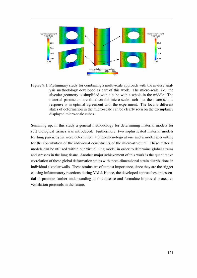
Figure 9.1: Preliminary study for combining a multi-scale approach with the inverse anal-ysis methodology developed as part of this work. The micro-scale, i.e. thealveolar geometry is simplified with a cube with a whole in the middle. Thematerial parameters are fitted on the micro-scale such that the macroscopicresponse is in optimal agreement with the experiment. The locally differentstates of deformation in the micro-scale can be clearly seen on the exemplarilydisplayed micro-scale cubes.
Summing up, in this study a general methodology for determining material models forsoft biological tissues was introduced. Furthermore, two sophisticated material modelsfor lung parenchyma were determined, a phenomenological one and a model accountingfor the contribution of the individual constituents of the micro-structure. These materialmodels can be utilized within our virtual lung model in order to determine global strainsand stresses in the lung tissue. Another major achievement of this work is the quantitativecorrelation of these global deformation states with three-dimensional strain distributions inindividual alveolar walls. These strains are of utmost importance, since they are the triggercausing inflammatory reactions during VALI. Hence, the developed approaches are essen-tial to promote further understanding of this disease and formulate improved protectiveventilation protocols in the future.
121

9 Summary and Outlook
122
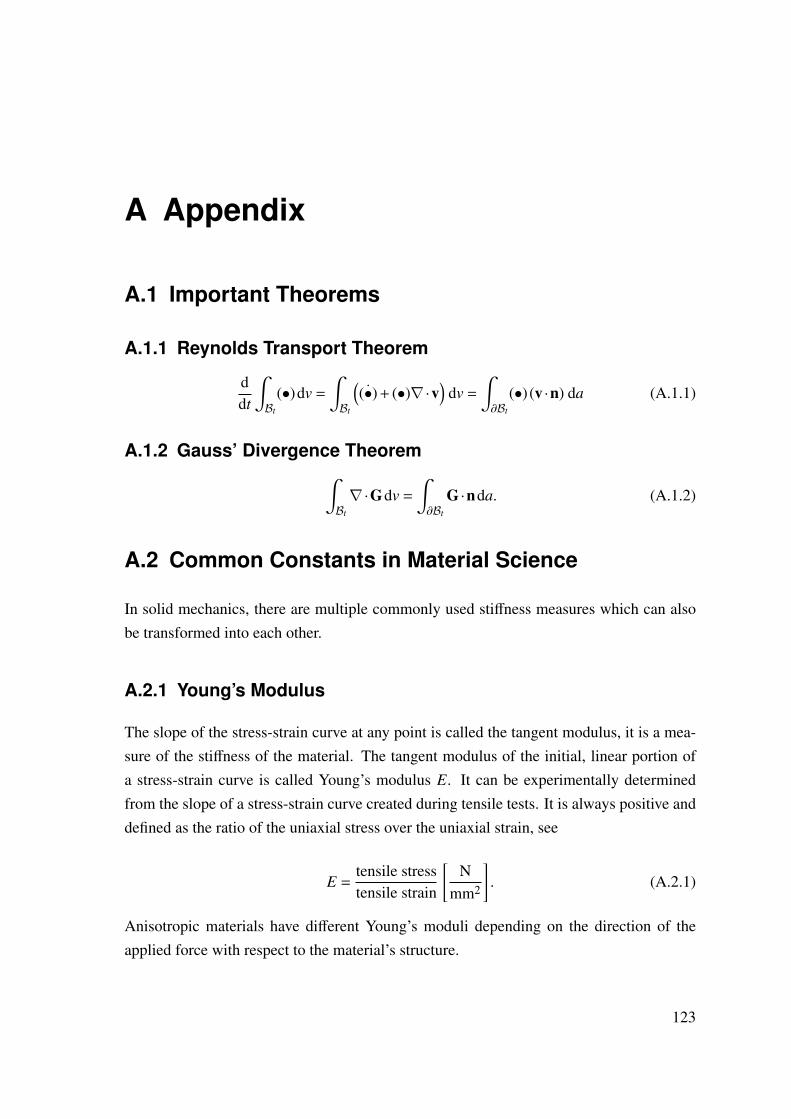
A Appendix
A.1 Important Theorems
A.1.1 Reynolds Transport Theorem
ddt
∫Bt
(•)dv =
∫Bt
(˙(•) + (•)∇ ·v
)dv =
∫∂Bt
(•) (v ·n) da (A.1.1)
A.1.2 Gauss’ Divergence Theorem∫Bt
∇ ·Gdv =
∫∂Bt
G ·nda. (A.1.2)
A.2 Common Constants in Material Science
In solid mechanics, there are multiple commonly used stiffness measures which can alsobe transformed into each other.
A.2.1 Young’s Modulus
The slope of the stress-strain curve at any point is called the tangent modulus, it is a mea-sure of the stiffness of the material. The tangent modulus of the initial, linear portion ofa stress-strain curve is called Young’s modulus E. It can be experimentally determinedfrom the slope of a stress-strain curve created during tensile tests. It is always positive anddefined as the ratio of the uniaxial stress over the uniaxial strain, see
E =tensile stresstensile strain
[N
mm2
]. (A.2.1)
Anisotropic materials have different Young’s moduli depending on the direction of theapplied force with respect to the material’s structure.
123
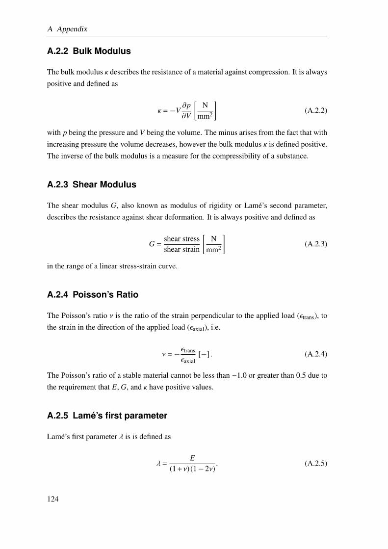
A Appendix
A.2.2 Bulk Modulus
The bulk modulus κ describes the resistance of a material against compression. It is alwayspositive and defined as
κ =−V∂p∂V
[N
mm2
](A.2.2)
with p being the pressure and V being the volume. The minus arises from the fact that withincreasing pressure the volume decreases, however the bulk modulus κ is defined positive.The inverse of the bulk modulus is a measure for the compressibility of a substance.
A.2.3 Shear Modulus
The shear modulus G, also known as modulus of rigidity or Lamé’s second parameter,describes the resistance against shear deformation. It is always positive and defined as
G =shear stressshear strain
[N
mm2
](A.2.3)
in the range of a linear stress-strain curve.
A.2.4 Poisson’s Ratio
The Poisson’s ratio ν is the ratio of the strain perpendicular to the applied load (εtrans), tothe strain in the direction of the applied load (εaxial), i.e.
ν =−εtrans
εaxial[−] . (A.2.4)
The Poisson’s ratio of a stable material cannot be less than −1.0 or greater than 0.5 due tothe requirement that E, G, and κ have positive values.
A.2.5 Lamé’s first parameter
Lamé’s first parameter λ is is defined as
λ =E
(1 + ν) (1−2ν). (A.2.5)
124
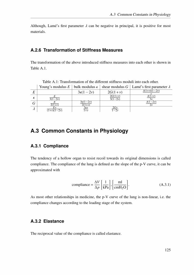
A.3 Common Constants in Physiology
Although, Lamé’s first parameter λ can be negative in principal, it is positive for mostmaterials.
A.2.6 Transformation of Stiffness Measures
The transformation of the above introduced stiffness measures into each other is shown inTable A.1.
Table A.1: Transformation of the different stiffness moduli into each other.Young’s modulus E bulk modulus κ shear modulus G Lamé’s first parameter λ
E 3κ(1−2ν) 2G(1 + ν) λ(1+ν)(1−2ν)ν
κ E3(1−2ν)
2G(1+ν)3(1−2ν)
λ(1+ν)3ν
G E2(1+ν)
3κ(1−2ν)2(1+ν)
λ(1−2ν)2ν
λ Eν(1+ν)(1−2ν)
3κν1+ν
2Gν1−2ν
A.3 Common Constants in Physiology
A.3.1 Compliance
The tendency of a hollow organ to resist recoil towards its original dimensions is calledcompliance. The compliance of the lung is defined as the slope of the p-V curve, it can beapproximated with
compliance =∆V∆p
[l
kPa
],
[ml
cmH2O
]. (A.3.1)
As most other relationships in medicine, the p-V curve of the lung is non-linear, i.e. thecompliance changes according to the loading stage of the system.
A.3.2 Elastance
The reciprocal value of the compliance is called elastance.
125
A Appendix
A.3.3 Resistance
To keep gas flowing through a pipe (V > 0), a pressure change (∆p) is needed. The ratiobetween pressure change and resulting flow is defined as resistance. The resistance equalsthe slope of the pressure-flow curve and can be calculated as
resistance=∆pV. (A.3.2)
A.4 Common Statistical Measures
A.4.1 Mean
In this work, the term mean refers to the arithmetic mean, which is calculated as
mean =1n
·n∑
i=1
xi, (A.4.1)
with n being the number of measurements and xi being the individual measurement values.
A.4.2 Standard Deviation
The standard deviation (sd) of a sample calculates as
sd =
√√1n
n∑i=1
(xi−mean)2 (A.4.2)
with the mean given in equation (A.4.1), n being the number of measurements, and xi
being the individual measurement values.
A.4.3 Coefficient of Variation
The coefficient of variation (CV) is defined as
CV =sd
mean(A.4.3)
the mean and sd given in equation (A.4.1) and (A.4.2), respectively.
126
Bibliography
Abel, S., Finney, S., Brett, S., Keogh, B., Morgan, C., and Evans, T. (1998). Reducedmortality in association with the acute respiratory distress syndrome (ARDS). British
Medical Journal, 53(4):292–294.
Abràmoff, M., Magalhaes, P., and Ram, S. (2004). Image processing with imagej. Bio-
photonics International, 11(7):36–42.
American Thoracic Society, European Society of Intensive Care Medicine, Societé deRéanimation Langue Française (1999). International consensus conferences in inten-sive care medicine. Ventilator-associated lung injury in ARDS. Intensive Care Medcine,25(12):1444–1452.
Ashbaugh, D., Bigelow, D. B., Petty, T., and Levine, B. (1967). Acute respiratory distressin adults. The Lancet, 290(7511):319–323.
Ball, J. (1977). Convexity conditions and existence theorems in nonlinear elasticity.Archive for Rational Mechanics and Analysis, 63(4):337–403.
Balzani, D. (2006). Polyconvex Anisotropic Energies and Modeling of Damage Applied
to Arterial Walls. PhD thesis, Institut für Mechanik, Abteilung Bauwissenschaften,Fakultät für Ingenieurwissenschaften.
Balzani, D., Neff, P., Schröder, J., and Holzapfel, G. (2006). A polyconvex framework forsoft biological tissues. adjustment to experimental data. International Journal of Solids
and Structures, 43:6052–6070.
Barnas, G., Yoshino, K., Stamenovic, D., Kikuchi, Y., Loring, S., and Mead, J. (1989a).Chest wall impedance partitioned into rib cage and diaphragm-abdominal pathways.Journal of Applied Physiology, 66(1):350–359.
Barnas, G. M., Mackenzie, C. F., Skacel, M., Hempleman, S. C., Wicke, K. M., Ska-cel, C. M., and Loring, S. H. (1989b). Amplitude dependency of regional chest wallresistance and elastance at normal breathing frequencies. The American Review of Res-
piratory Disease, 140(1):25–30.
127
Bibliography
Basser, P., Schneiderman, R., Bank, R., Wachtel, E., and Maroudas, A. (1998). Mechanicalproperties of the collagen network in human articular cartilage as measured by osmoticstress technique. Archives of Biochemistry and Biophysics, 351(2):207–219.
Bates, J., Maksym, G., and Suki, B. (1994). Lung tissue rheology and 1/f noise. Annals of
Biomedical Engineering, 22(6):674–681.
Bates, J. H., Shardonofsky, F., and Stewart, D. E. (1989). The low-frequency dependenceof respiratory system resistance and elastance in normal dogs. Respiration Physiology,78(3):369–382.
Belytschko, T., Liu, K., and Moran, B. (2005). Nonlinear Finite Elements for Continua
and Structures. John Wiley & Sons, LTD.
Bernard, G. R., Artigas, A., Brigham, K. L., Carlet, J., Falke, K., Hudson, L., Lamy, M.,LeGall, J. R., Morris, A., and Spragg, R. (1994). Report of the american-europeanconsensus conference on acute respiratory distress syndrome: definitions, mechanisms,relevant outcomes, and clinical trial coordination. consensus committee. Journal of
Critical Care, 9(1):72–81.
Blatz, P. J. and Ko, W. L. (1962). Application of finite elastic theory to the deformation ofrubbery materials. Journal of Rheology, 6(1):223–252.
Bonet, J. and Wood, R. D. (1997). Nonlinear contiuum mechanics for finite element anal-
ysis. Cambridge University Press, Cambridge.
Brewer, K. K., Sakai, H., Alencar, A. M., Majumdar, A., Arold, S. P., Lutchen, K. R.,Ingenito, E. P., and Suki, B. (2003). Lung and alveolar wall elastic and hysteretic be-havior in rats: effects of in vivo elastase treatment. Journal of Applied Physiology,95(5):1926–1936.
Brower, R., Ware, L., Berthiaume, Y., and Matthay, M. (2001). Treatment of ards. Chest,120(4):1347–1367.
Brown, R., Butler, J., Rogers, R., and Leith, D. (1994). Mechanical connections betweenelastin and collagen. Connective Tissue Research, 30(4):295–308.
Budiansky, B. and Kimmel, E. (1987). Elastic moduli of lungs. Journal of Applied Me-
chanics, 54(2):351–358.
Carton, R. W., Dainauskas, J., and Clark, J. W. (1962). Elastic properties of single elasticfibers. Journal of Applied Physiology, 17:547–551.
Cavalcante, F. S., Ito, S., Sakai, H., Alencar, A. M., Almeida, M. P., Andrade, I. S., A,M., Ingenito, E. P., and Suki, B. (2005). Mechanical interactions between collagen
128
Bibliography
and proteoglycans: implications for the stability of lung tissue. Journal of Applied
Physiology, 98(2):672–679.
Chandel, N. S. and Sznajder, J. I. (2000). Stretching the lung and programmed celldeath. American Journal of Physiology- Lung Cellular and Molecular Physiology,279(6):1003–1004.
Comerford, A., Förster, C., and Wall, W. A. (2010). Structured tree impedance outflowboundary conditions for 3d lung simulations. Journal of Biomechanical Engineering,132(8):081002–1–10.
Copland, I. B. and Post, M. (2007). Stretch-activated signaling pathways responsible forearly response gene expression in fetal lung epithelial cells. Journal of Cellular Physi-
ology, 210(1):133–143.
Crapo, J. (2000). Respiratory structure and function. Cecil Textbook of Medicine.Philadelphia. WB Saunders Company.
Crystal, R. G., Bradley, K. H., McConnell-Breu, S. D., Collins, J. F., Hanca, A. J., andCowan, M. J. (1975). Collagen in the lung: development of a technology applicable tohuman lung disease. Chest, 67(2 Suppl):30–31.
Dassow, C., Wiechert, L., Martin, C., Schumann, S., Müller-Newen, G., Pack, O.,Guttmann, J., Wall, W. A., and Uhlig, S. (2010). Biaxial distension of precision-cutlung slices. Journal of Applied Physiology, 108(3):713–721.
Debes, J. C. and Fung, Y. C. (1992). Effect of temperature on the biaxial mechanics ofexcised lung parenchyma of the dog. Journal of Applied Physiology, 73(3):1171–1180.
Delfino, A., Stergiopulos, N., Moore, J. E., and Meister, J. J. (1997). Residual strain effectson the stress field in a thick wall finite element model of the human carotid bifurcation.Journal of Biomechanics, 30(8):777–786.
Denny, E. and Schroter, R. C. (1997). Relationships between alveolar size and fibre distri-bution in a mammalian lung alveolar duct model. Journal of Biomechanical Engineer-
ing, 119(3):289–297.
Denny, E. and Schroter, R. C. (2000). Viscoelastic behavior of a lung alveolar duct model.Journal of Biomechanical Engineering, 122(2):143–151.
Denny, E. and Schroter, R. C. (2006). A model of non-uniform lung parenchyma distortion.Journal of Biomechanics, 39(4):652–663.
DiRocco, J. D., Carney, D. E., and Nieman, G. F. (2005). The Mechanism of Ventilator-
induced Lung Injury: Role of Dynamic Alveolar Mechanics. Springer Berlin Heidelberg.
129
Bibliography
DiRocco, J. D., Pavone, L. A., Carney, D. E., Lutz, C. J., Gatto, L. A., Landas, S. K.,and Nieman, G. F. (2006). Dynamic alveolar mechanics in four models of lung injury.Intensive Care Medicine, 32(1):140–148.
Doll, S. and Schweizerhof, K. (2000). On the development of volumetric strain energyfunctions. Journal of Applied Mechanics, 67:17–21.
Dos Santos, C. C. and Slutsky, A. S. (2000). Invited review: mechanisms of ventilator-induced lung injury: a perspective. Journal of Applied Physiology, 89(4):1645–1655.
Dos Santos, C. C. and Slutsky, A. S. (2006). The contribution of biophysical lung injuryto the development of biotrauma. Annual Review of Physiology, 68:585–618.
Dreyfuss, D., Soler, P., Basset, G., and Saumon, G. (1988). High inflation pres-sure pulmonary edema. respective effects of high airway pressure, high tidal volume,and positive end-expiratory pressure. The American Review of Respiratory Disease,137(5):1159–1164.
Ethier, C. R. and Simmons, C. A. (2007). Introductory biomechanics: from cells to organ-
isms. Cambridge University Press.
Faffe, D. and Zin, W. (2009). Lung parenchymal mechanics in health and disease. Physi-
ological Reviews, 89(3):759–775.
Faffe, D. S., D’Alessandro, E. S., Xisto, D. G., Antunes, M. A., Romero, P. V., Negri,E. M., Rodrigues, N. R. D., Capelozzi, V. L., Zin, W. A., and Rocco, P. R. M. (2006).Mouse strain dependence of lung tissue mechanics: role of specific extracellular matrixcomposition. Respiratory Physiology and Neurobiology, 152(2):186–196.
Faffe, D. S., Silva, G. H., Kurtz, P. M. P., Negri, E. M., Capelozzi, V. L., Rocco, P. R. M.,and Zin, W. A. (2001). Lung tissue mechanics and extracellular matrix composition ina murine model of silicosis. Journal of Applied Physiology, 90(4):1400–1406.
Frankus, A. and Lee, G. C. (1974). A theory for distortion studies of lung parenchymabased on alveolar membrane properties. Journal of Biomechanics, 7(1):101–107.
Fredberg, J. J. and Stamenovic, D. (1989). On the imperfect elasticity of lung tissue.Journal of Applied Physiology, 67(6):2408–2419.
Fukaya, H., Martin, C. J., Young, A. C., and Katsura, S. (1968). Mechanial properties ofalveolar walls. Journal of Applied Physiology, 25(6):689–695.
Fung, Y. (1984). Structure and stress-strain relationship of soft tissues. American Zoolo-
gist, 24(1):13–22.
130
Bibliography
Fung, Y. (1993). Biomechanics Mechanical Properties of living Tissue Seccond Edition.Springer-Verlag.
Fung, Y. C. and Sobin, S. S. (1981). The retained elasticity of elastin under fixation agents.Journal of Biomechanical Engineering, 103(2):121–122.
Gao, J., Huang, W., and Yen, R. T. (2006). Mechanical properties of human lungparenchyma. Biomedical Sciences Instrumentation, 42:172–180.
Gee, M. W., Dohrmann, C. R., Key, S. W., and Wall, W. A. (2009). A uniform nodal straintetrahedron with isochoric stabilization. International Journal for Numerical Methods
in Engineering, 78(4):429–443.
Gefen, A., Elad, D., and Shiner, R. J. (1999). Analysis of stress distribution in the alve-olar septa of normal and simulated emphysematic lungs. Journal of Biomechanics,32(9):891–897.
Gray, H. and Bannister, L. H. (1995). Gray’s anatomy: The Anatomical Basis of Medicine
and Surgery. Churchill Livingstone London.
Grytz, R. and Meschke, G. (2009). Constitutive modeling of crimped collagen fibrils insoft tissues. Journal of the Mechanical Behavior of Biomedical Materials, 2(5):522–533.
Harman, E. (2011). Acute respiratory distress syndrome. eMedcine.
Hastie, T., Tibshirani, R., and Friedman, J. (2009). The Elements of Statistical Learning:
Data Mining, Inference, and Prediction. Springer.
Haut, R. and Little, R. (1972). A constitutive equation for collagen fibers. Journal of
Biomechanics, 5(5):423–430.
Heroux, M., Bartlett, R., Howle, V., Hoekstra, R., Hu, J., Kolda, T., Lehoucq, R., Long,K., Pawlowski, R., and Phipps, E. (2005). An overview of the trilinos project. ACM
Transactions on Mathematical Software (TOMS), 31(3):397–423.
Hildebrandt, J. (1966). Mechanical Properties of Mammalian Lung. PhD thesis, Universityof Washington.
Hildebrandt, J. (1969). Dynamic properties of air-filled excised cat lung determined byliquid plethysmograph. Journal of Applied Physiology, 27(2):246–250.
Hildebrandt, J. (1970). Pressure-volume data of cat lung interpreted by a plastoelastic,linear viscoelastic model. Journal of Applied Physiology, 28(3):365–372.
131
Bibliography
Hintermüller, C., Marone, F., Isenegger, A., and Stampanoni, M. (2010). Image pro-cessing pipeline for synchrotron-radiation-based tomographic microscopy. Journal of
Synchrotron Radiation, 17(4):550–559.
Holzapfel, G. A. (2004). Nonlinear Solid Mechanics. John Wiley & Sons, LTD.
Holzapfel, G. A. and Gasser, T. C. (2001). A viscoelastic model for fiber-reinforced com-posites at finite strains: Continuum basis, computational aspects and applications. Com-
puter Methods in Applied Mechanics and Engineering, 190(34):4379–4403.
Holzapfel, G. A., Gasser, T. C., and Ogden, R. W. (2000). A new constitutive frameworkfor arterial wall mechanics and a comparative study of material models. Journal of
Elasticity, 61(1 - 3):1 – 48.
Hoppin, F. G., Lee, G. C., and Dawson, S. V. (1975). Properties of lung parenchyma indistortion. Journal of Applied Physiology, 39(5):742–751.
Horsfield, K., Dart, G., Olson, D. E., Filley, G. F., and Cumming, G. (1971). Models ofthe human bronchial tree. Journal of Applied Physiology, 31(2):207–217.
Hughes, T. (2000). The finite element method: linear static and dynamic finite element
analysis. Dover Civil and Mechanical Engineering Series. Dover Publications.
Ismail, M., Comerford, A., and Wall, W. (2012). Coupled and reduced dimensional mod-elling of respiratory mechanics during spotaneous breathing. Preprint.
Jamal, R. A., Roughley, P., and Ludwig, M. (2001). Effect of glycosaminoglycan degrada-tion on lung tissue viscoelasticity. American Journal of Physiology- Lung Cellular and
Molecular Physiology, 280(2):306–315.
Karakaplan, A. D., Bieniek, M. P., and Skalak, R. (1980). A mathematical model of lungparenchyma. Journal of Biomechanical Engineering, 102(2):124–136.
Karlinsky, J. B., Bowers, J. T., Fredette, J. V., and Evans, J. (1985). Thermoelastic proper-ties of uniaxially deformed lung strips. Journal of Applied Physiology, 58(2):459–467.
Karlinsky, J. B., Snider, G. L., Franzblau, C., Stone, P. J., and Hoppin, F. G. (1976). Invitro effects of elastase and collagenase on mechanical properties of hamster lungs. The
American Review of Respiratory Disease, 113(6):769–777.
Kastelic, J., Galeski, A., and Baer, E. (1978). The multicomposite structure of tendon.Connective Tissue Research, 6(1):11–23.
Kauer, M., Vuskovic, V., Dual, J., Szekely, G., and Bajka, M. (2002). Inverse finite elementcharacterization of soft tissues. Medical Image Analysis, 6(3):275–287.
132
Bibliography
Kikuchi, Y., Stamenovic, D., and Loring, S. H. (1991). Dynamic behavior of excised dogrib cage: dependence on muscle. Journal of Applied Physiology, 70(3):1059–1067.
Kononov, S., Brewer, K., Sakai, H., Cavalcante, F. S., Sabayanagam, C. R., Ingenito, E. P.,and Suki, B. (2001). Roles of mechanical forces and collagen failure in the developmentof elastase-induced emphysema. American Journal of Respiratory and Critical Care
Medicine, 164(10):1920–1926.
Kowe, R., Schroter, R. C., Matthews, F. L., and Hitchings, D. (1986). Analysis of elasticand surface tension effects in the lung alveolus using finite element methods. Journal of
Biomechanics, 19(7):541–549.
Lanir, Y. (1983). Constitutive equations for the lung tissue. Journal of Biomechanical
Engineering, 105(4):374–380.
Lee, G. and Frankus, A. (1975). Elasticity properties of lung parenchyma derived fromexperimental distortion data. Biophysical Journal, 15:481–493.
Levenberg, K. (1944). A method for the solution of certain nonlinear problems in leastsquares. Quarterly of Applied Mathematics, 11:164–168.
Mahnken, R. and Stein, E. (1996). Parameter identification for viscoplastic models basedon analytical derivatives of a least-squares functional and stability investigations. Inter-
national Journal of Plasticity, 12(4):451–480.
Maksym, G., Bates, J., and Navajas, D. (1993). Lung parenchyma stress response to stepstrain. Proceedings 15th Annual IEEE International ASIC/SOC Conference, 93:1116–1117.
Maksym, G. N. and Bates, J. H. (1997). A distributed nonlinear model of lung tissueelasticity. Journal of Applied Physiology, 82(1):32–41.
Marquardt, D. (1963). An algorithm for least-squares estimation of nonlinear parameters.Journal of the Society for Industrial and Applied Mathematics, 11:431–441.
Martin, C., Uhlig, S., and Ullrich, V. (1996). Videomicroscopy of methacholine-inducedcontraction of individual airways in precision-cut lung slices. European Respiratory
Journal, 9(12):2479–2487.
Mercer, R. and Crapo, J. (1990). Spatial distribution of collagen and elastin fibers in thelungs. Journal of Applied Physiology, 69(2):756–765.
Mijailovich, S., Stamenovic., D., and Fredberg, J. (1993). Toward a kinetic theory ofconnective tissue micromechanics. Journal of Applied Physiology, 74(2):665–681.
133
Bibliography
Mijailovich, S. M., D. Stamenovic, D., Brown, R., Leith, D. E., and Fredberg, J. J. (1994).Dynamic moduli of rabbit lung tissue and pigeon ligamentum propatagiale undergoinguniaxial cyclic loading. Journal of Applied Physiology, 76(2):773–782.
Mishima, M., Hirai, T., Itoh, H., Nakano, Y., Sakai, H., Muro, S., Nishimura, K., Oku,Y., Chin, K., and Ohi, M. (1999). Complexity of terminal airspace geometry assessedby lung computed tomography in normal subjects and patients with chronic obstructivepulmonary disease. Proceedings of the National Academy of Sciences, 96(16):8829–8834.
Moulton, M., Creswell, L., Actis, R., Myers, K., Vannier, M., Szabo, B., and Pasque, M.(1995). An inverse approach to determining myocardial material properties. Journal of
Biomechanics, 28(8):935–948.
Navajas, D., Maksym, G. N., and Bates, J. H. (1995). Dynamic viscoelastic nonlinearityof lung parenchymal tissue. Journal of Applied Physiology, 79(1):348–356.
Navajas, D., Mijailovich, S., Glass, G. M., Stamenovic, D., and Fredberg, J. J. (1992).Dynamic response of the isolated passive rat diaphragm strip. Journal of Applied Phys-
iology, 73(6):2681–2692.
Ning, Q. and Wang, X. (2007). Response of alveolar type ii epithelial cells to mechanicalstretch and lipopolysaccharide. Respiration, 74(5):579–585.
Ochs, M., Nyengaard, J., Jung, A., Knudsen, L., Voigt, M., Wahlers, T., Richter, J., andGundersen, H. (2004). The number of alveoli in the human lung. American Journal of
Respiratory and Critical Care Medicine, 169(1):120–124.
Ogden, R. (1974). On the overall moduli of non-linear elastic composite materials. Journal
of the Mechanics and Physics of Solids, 22:541–553.
Ogden, R. (1997). Non-linear elastic deformations. Dover Pubns.
Ottani, V., Raspanti, M., and Ruggeri, A. (2001). Collagen structure and functional impli-cations. Micron, 32(3):251–260.
Perlman, C. E. and Bhattacharya, J. (2007). Alveolar expansion imaged by optical sec-tioning microscopy. Journal of Applied Physiology, 103(3):1037–1044.
Prange, H. D. (2003). Laplace’s law and the alveolus: a misconception of anatomy and amisapplication of physics. Advances in Physiology Education, 27(1-4):34–40.
Rausch, S. M. K., Haberthür, D., Stampanoni, M., Schittny, J. C., and Wall, W. A.(2011a). Local strain distribution in real three-dimensional alveolar geometries. An-
nals of Biomedical Engineering, 39(11):2835–2843.
134
Bibliography
Rausch, S. M. K., Martin, C., Bornemann, P. B., Uhlig, S., and Wall, W. A. (2011b).Material model of lung parenchyma based on living precision-cut lung slice testing.Journal of the Mechanical Behavior of Biomedical Materials, 4:583 – 592.
Rosen, M. (2004). Surfactants and internfacial phenomena. Wiley, 3 edition.
Sata, M., Takahashi, K., Sato, S., and Tomoike, H. (1995). Structural and functionalcharacteristics of peripheral pulmonary parenchyma in golden hamsters. Journal of
Applied Physiology, 78(1):239–246.
Schittny, J. (2008). High resolution 3d visualization of lung parenchyma. do new imagesforce us to rewrite lung development? In CMGM (internal seminar).
Schröder, J. (2004). Fluch der dimensionen? Essen Unikate, 23:37–49.
Schröder, J. and Neff, P. (2003). Invariant formulation of hyperelastic transverse isotropybased on polyconvex free energy functions. International Journal of Solids and Struc-
tures, 40(2):401–445.
Seshaiyer, P. and Humphrey, J. (2003). A sub-domain inverse finite element character-ization of hyperelastic membranes including soft tissues. Journal of Biomechanical
Engineering, 125(3):363–371.
Sobin, S., Fung, Y., and Tremer, H. (1988). Collagen and elastin fibers in human pul-monary alveolar walls. Journal of Applied Physiology, 64(4):1659–1675.
Stalling, D., Westerhoff, M., and Hege, H. (2005). Amira: A highly interactive system forvisual data analysis. The visualization handbook, 38:749–767.
Stamenovic, D. and Yager, D. (1988). Elastic properties of air- and liquid-filled lungparenchyma. Journal of Applied Physiology, 65(6):2565–2570.
Stampanoni, M., Groso, A., Isenegger, A., Mikuljan, G., Chen, Q., Bertrand, A., Henein,S., Betemps, R., Frommherz, U., Böhler, P., Meister, D., Lange, M., and Abela, R.(2006). Trends in synchrotron-based tomographic imaging: the sls experience. In Soci-
ety of Photo-Optical Instrumentation Engineers (SPIE) Conference Series.
Sugihara, T., Martin, C., and Hildebrandt, J. (1971). Length-tension properties of alveolarwall in man. Journal of Applied Physiology, 30(6):874–8.
Sugihara, T. and Martin, C. J. (1975). Simulation of lung tissue properties in age andirreversible obstructive syndromes using an aldehyde. Journal of Clinical Investigation,56(1):23–29.
Suki, B., Barabasi, A., and Lutchen, K. (1994). Lung tissue viscoelasticity: a mathematicalframework and its molecular basis. Journal of Applied Physiology, 76(6):2749–2759.
135
Bibliography
Suki, B. and Bates, J. H. T. (2008). Extracellular matrix mechanics in lung parenchymaldiseases. Respiratory Physiology and Neurobiology, 163(1-3):33–43.
Suki, B., Ito, S., Stamenovic, D., Lutchen, K. R., and Ingenito, E. P. (2005). Biomechanicsof the lung parenchyma: critical roles of collagen and mechanical forces. Journal of
Applied Physiology, 98(5):1892–1899.
Suki, B., Peslin, R., Duvivier, C., and Farre, R. (1989). Lung impedance in healthy humansmeasured by forced oscillations from 0.01 to 0.1 Hz. Journal of Applied Physiology,67(4):1623–1629.
Sussman, T. and Bathe, K.-J. (1987). A finite element formulation for nonlinear incom-pressible elastic and inelastic analysis. Computers & Structures, 26(1-2):357 – 409.
Tai, R. C. and Lee, G. C. (1981). Isotropy and homogeneity of lung tissue deformation.Journal of Biomechanics, 14(4):243–252.
The Acute Respiratory Distress Syndrome Network (2000). Ventilation with lower tidalvolumes as compared with traditional tidal volumes for acute lung injury and the acuterespiratory distress syndrome. New England Journal of Medicine, 342(18):1301–1308.
Toshima, M., Ohtani, Y., and Ohtani, O. (2004). Three-dimensional architecture of elastinand collagen fiber networks in the human and rat lung. Archives of Histology&Cytology,67(1):31–40.
Tschanz, S. A., Makanya, A. N., Haenni, B., and Burri, P. H. (2003). Effects of neonatalhigh-dose short-term glucocorticoid treatment on the lung: a morphologic and morpho-metric study in the rat. Pediatric Research, 53(1):72–80.
Tsushima, K., King, L. S., Aggarwal, N. R., Gorordo, A. D., D’Alessio, F. R., and Kubo,K. (2009). Acute lung injury review. Internal Medicine, 48(9):621–630.
Vawter, D. L., Fung, Y. C., and West, J. B. (1978). Elasticity of excised dog lungparenchyma. Journal of Applied Physiology, 45(2):261–269.
Vlahakis, N. E., Schröder, M. A., Limper, A. H., and Hubmayr, R. D. (1999). Stretchinduces cytokine release by alveolar epithelial cells in vitro. American Journal of Phys-
iology, 277(1):167–173.
Wall, W. A., Bornemann, P. B., and Cyron, C. (2010a). Nichtlineare Kontinuumsmechanik.Institute for Computational Mechanics, Technische Universität München.
Wall, W. A. and Gee, M. W. (2010). BACI: A parallel multiphysics simulation environ-ment. Technical report, Institute for Computational Mechanics, Technische UniversitätMünchen.
136
Bibliography
Wall, W. A. and Rabczuk, T. (2008). Fluid structure interaction in lower airways of ct-based lung geometries. International Journal for Numerical Methods in Fluids, 57:653–675.
Wall, W. A., Wiechert, L., Comerford, A., and Rausch, S. (2010b). Towards a comprehen-sive computational model for the respiratory system. International Journal for Numeri-
cal Methods in Biomedical Engineering, 26(7):807–827.
Wall, W. A., Yoshihara, L., Bornemann, P. B., and Tinkl, S. (2012). Nichtlineare Finite-
Element-Methoden. Institute for Computational Mechanics, Technische UniversitätMünchen.
Ware, L. B. and Matthay, M. A. (2000). The acute respiratory distress syndrome. New
England Journal of Medicine, 233(2):309–319.
Weibel, E. R. (1963). Morphometry of the human lung. Springer-Verlag.
Weibel, E. R. (1984). The pathway for oxygen. Harvard University Press Cambridge, MA.
Weibel, E. R. (1986). Functional morphology of lung parenchyma. Wiley Online Library.
West, J. B. (2008). Respiratory Physiology The Essentials. Wolters Kluwer-LippincottWilliams & Wilkins, 8 edition.
West, J. B. and Matthews, F. L. (1972). Stresses, strains, and surface pressures in the lungcaused by its weight. Journal of Applied Physiology, 32(3):332–345.
Wiechert, L., Metzke, R., and Wall, W. A. (2009). Modeling the mechanical behavior oflung tissue at the microlevel. Journal of Engineering Mechanics, 135(5):434–438.
Wiechert, L. and Wall, W. A. (2010). A nested dynamic multi-scale approach for 3dproblems accounting for micro-scale multi-physics. Computer Methods in Applied Me-
chanics and Engineering, 199(21-22):1342–1351.
Wilson, T. A. and Bachofen, H. (1982). A model for mechanical structure of the alveolarduct. Journal of Applied Physiology, 52(4):1064–1070.
Yager, D., Feldman, H., and Fung, Y. C. (1992). Microscopic vs. macroscopic deformationof the pulmonary alveolar duct. Journal of Applied Physiology, 72(4):1348–1354.
Yeoh, O. (1993). Some forms of the strain energy function for rubber. Rubber Chemistry
and Technology, 66(5):754–771.
Yoshihara, L. and Wall, W. A. (2012). Fluid-structure interaction including volume cou-pling of homogenized subdomains for treating artificial boundaries. Preprint.
137
Bibliography
Yuan, H., Ingenito, E., and Suki, B. (1997). Dynamic properties of lung parenchyma: me-chanical contributions of fiber network and interstitial cells. Journal of Applied Physi-
ology, 83(5):1420–1431.
Yuan, H., Kononov, S., Cavalcante, F., Lutchen, K., Ingenito, E., and Suki, B. (2000).Effects of collagenase and elastase on the mechanical properties of lung tissue strips.Journal of Applied Physiology, 89(1):3–14.
Zeng, Y., Yager, D., and Fung, Y. (1987). Measurement of the mechanical properties ofthe human lung tissue. Journal of Biomechanical Engineering, 109(2):169–174.
138
Related Documents


![Clinical Implications of SARS-Cov2 Interaction with Renin ... · ACE2 is a type I integral membrane glycoprotein [15] expressed predominantly in the bronchus, lung parenchyma, heart,](https://static.cupdf.com/doc/110x72/5f3a8423c3f35b6ce73caa34/clinical-implications-of-sars-cov2-interaction-with-renin-ace2-is-a-type-i-integral.jpg)


