Computational Algebraic Geometry Thomas Markwig Fachbereich Mathematik Technische Universit¨ at Kaiserslautern A short course taught at the EMALCA 2010 in Villahermosa, Mexico August 2010

Welcome message from author
This document is posted to help you gain knowledge. Please leave a comment to let me know what you think about it! Share it to your friends and learn new things together.
Transcript

Computational Algebraic
Geometry
Thomas Markwig
Fachbereich Mathematik
Technische Universitat Kaiserslautern
A short course taught at the
EMALCA 2010 in Villahermosa, Mexico
August 2010

Contents
1 Introduction 1
A) Robotics 2
B) Elliptic curve cryptography 3
C) Coding theory 3
D) Chip design 4
E) Sudoku 4
F) Exercises 5
2 Affine algebraic varieties 7
A) Basic definitions 7
B) Grobner bases 9
C) Finite solution sets and Grobner bases 13
D) Hilbert’s Nullstellensatz 16
E) Decomposition into irreducible components 18
F) The coordinate ring and the dimension of a variety 21
G) Exercises 23
3 Regular functions and morphisms 26
A) The Zariski topology 26
B) Regular functions 27
C) Morphisms 29
D) Computing the image of a morphism 30
E) Exercises 33
4 Local properties of algebraic varieties 36
A) The local ring of X at p 36
B) Standard bases in local rings 38
C) The tangent space of X at p 39
D) Regular and singular points 41
E) Intersection multiplicity of two plane curves at a point 44
F) Local parametrisations 46
G) Exercises 50

II
5 Projective plane curves 52
A) The projective plane 52
B) Projective plane curves 53
C) Visualising the projective plane P2R
57
D) The Theorem of Bezout for projective plane curves 58
E) Parametrisations via the Theorem of Bezout 61
F) Exercises 62
6 Projective varieties 64
A) The projective n-space 64
B) Projective algebraic varieties 65
C) The projective Nullstellensatz 66
D) Regular functions and morphisms on projective algebraic varieties 67
E) The Hilbert polynomial of a projective algebraic variety 68
F) The Theorem of Bezout 70
Appendix A Short introduction to Singular 73
1) First steps 73
2) Types of data in Singular and rings 79
3) Some elements of the programming language Singular 81
4) Some selected functions in Singular 83
5) ESingular - or the editor Emacs 83
6) Exercises 84
7) Solutions 84
Appendix B First steps with surfex 89
References 91
Some comments on the origin of the images
Most of the images were created by myself with the programme surfex [HL08] or
the LATEX-package texdraw. The singular plane curve in Figure 3 was produced by
Rudiger Stobbe at the University of Kaiserslautern many years ago, and the space
curve in Figure 4 was produced with the aid of Maple. The images in Figure 34 and
35 are snapshots of the programme surfex produced by xv.

III
The image in Figure 5 can be found on the web page:
http://de.wikipedia.org/wiki/Stewart Platform
as well as the first image in Figure 6. The second image in Figure 6 can be found
on the web page:
http://www.physikinstrumente.de/de/produkte/primages.php?sortnr=700800
The image in Figure 9 was obtained from the web page:
http://static.howstuffworks.com/gif/microprocessor-athlon-64.jpg
Finally the image in Figure 10 was taken from the web page:
http://en.wikipedia.org/wiki/Sudoku

1
1 Introduction
We want to study the solution set V(f1, . . . , fk) of a system of equations
f1(x1, . . . , xn) = 0
...
fk(x1, . . . , xn) = 0
where the fi are polynomials.
Figure 1. The Cayley Cubic
x1x2 + x1x3 + x2x3 + x1x2x3 = 0.
Figure 2. The Heart
(
2x21 + x22 + x
23 − 1
)3− 1
10x21x
33 − x
22x
33 = 0
Figure 3. A plane curve
32x21 − 2097152x112 + 1441792x92
− 360448x72 + 39424x52
− 1760x32 + 22x2 − 1 = 0
Figure 4. A Space Curve
x1 − x23 = 0
x22 − x33 = 0
The first case to consider would be n = k = 1, that is, we have a single polynomial
f = am · xm + am−1 · xm−1 + . . .+ a1 · x+ a0and we are looking for the roots of that polynomial. In theory, this is not too hard
to deal with. There are at most n roots, and if the base field is algebraically closed

2
like C, then there are exactly n roots counted with the appropriate multiplicity.
However, it is very hard in practise to find any of the roots.
The second case to consider would have n and k arbitrary, but the polynomials are
all linear, i.e. they are of the form
fi = ai1 · x1 + . . .+ ain · xn + bi.
Then the solution set is an affine vector space, and it is even easy to compute using
the Gauß algorithm.
In general, life is much more difficult and much more interesting as already the above
examples show. Before introducing the theory we want to mention some applications
where such polynomial systems of equations come up naturally.
A) Robotics
A frequently used robotic system is the hexapod (see Figure 5). A platform is
Figure 5. Schematic image of a hexapod robot
connected to six legs via rotational joints. The length of the legs can be varied
in order to adjust the position of the platform in space. Note that one has three
translational and three rotational directions of movement, that is one has six degrees
of freedom, and fixing the length of the six legs one thus expects to fix the position
of the platform. Robots using this basic scheme are used in many applications, e.g.
Figure 6. Applications: Flight simulator and micro surgery

3
for flight simulators or in micro surgery (see Figure 6). To deduce the length of the
legs needed in order to achieve a given position one has to solve a system of eight
polynomial equations, one of which is shown in Figure 7.
2x40 + 4x20x21 + 2x
41 + 4x
20x22 + 4x
21x22 + 2x
42 + 4x
20x23 + 4x
21x23
+ 4x22x23 + 2x
43 − 2x
20x2y0 − 2x
21x2y0 − 2x
32y0 − 2x
20x3y0
− 2x21x3y0 − 2x22x3y0 − 2x2x
23y0 − 2x
33y0 + x
20y20 + x
21y20
+ x22y20 + x
23y20 + 2x
20x2y1 + 2x
21x2y1 + 2x
32y1 − 2x
20x3y1
− 2x21x3y1 − 2x22x3y1 + 2x2x
23y1 − 2x
33y1 + x
20y21 + x
21y21
+ x22y21 + x
23y21 + 2x
30y2 − 2x
20x1y2 + 2x0x
21y2 − 2x
31y2
+ 2x0x22y2 − 2x1x
22y2 + 2x0x
23y2 − 2x1x
23y2 + x
20y22 + x
21y22
+ x22y22 + x
23y22 + 2x
30y3 + 2x
20x1y3 + 2x0x
21y3 + 2x
31y3
+ 2x0x22y3 + 2x1x
22y3 + 2x0x
23y3 + 2x1x
23y3 + x
20y23 + x
21y23
+ x22y23 + x
23y23 + 4x0x2 + 4x1x2 − 4x0x3 + 4x1x3
− 2x1y0 + 2x0y1 − 2x3y2 + 2x2y3 −72= 0
Figure 7. One equation for the leg-length of a hexapod
B) Elliptic curve cryptography
Equations like
y2z− x ·(
x− 12· z)
· (x− z) = 0define elliptic curves in the projective plane (see Figure 8). They carry in a natural
way the structure of an abelian group, that is, one can add and subtract points on
the curve from each other. If the base filed K over which one considers the solutions
is finite, then these groups are very well suited as alphabets for cryptographical
methods, and they are widely used nowadays. Note that, while it is easy to add a
point P several times to itself, e.g. P + P + P = 3 · P, it is very hard to find P if
you are given the result 3 · P. One says, that it is very hard to compute the discrete
logarithm.
C) Coding theory
Also for coding theory one can use projective curves over a finite field K. However,
this time one considers the global sections of a divisor on the curve and its image
under the map evaluating the sections at n fixed points. This gives a subspace of
Kn which serves as the code and has pretty good properties. These ideas go back to
Goppa.

4
Figure 8. A visualisation of y2z− x ·(
x− 12· z)
· (x− z) = 0
D) Chip design
A modern micro processor chip contains several layers of electrical circuits with
millions of transistors, resistors and capacitors. The functionality of certain units of
such an electrical circuit within itself and with other units leads eventually to systems
of partial differential equations. These can be treated symbolically as polynomial
equations which one uses in a preprocessing step before applying numerical methods.
Certain properties of the circuits can thus be predicted by pure simulation and
computations without actually building the chip (see Figure 9).
Figure 9. A micro processor chip
E) Sudoku
A Sudoku is a scheme of digits as in Figure 10. One should fill the table by digits
Figure 10. Sudoku

5
in such a way that in each row, in each column and in each block each of the nine
digits 1, . . . , 9 occurs precisely once.
Let us now associate coordinates x1, . . . , x81 to each of the 81 squares and consider
the set of pairs
B = {(i, j) | 1 ≤ i < j ≤ 81, xi and xj are in the same row, column or block}.
For i = 1, . . . , 81 we define
Fi =
9∏
k=1
xi − k,
and for (i, j) ∈ B we set
Gij =Fi − Fj
xi − xj.
Then the Fi and the Gij are polynomials. Moreover, a1, . . . , a81 is a feasible solution
for a sudoku if and only if it is a solution of the system of equations
Gij = 0, Fk = 0 where (i, j) ∈ B, k = 1, . . . , 9.
F) Exercises
Exercise 1.1
How do the solution sets in R2 of the following equations look like?
a. y− x2 = 0.
b. y− x4 + 1 = 0.
c. y2 − x2 = 0.
d. x2 − y3 = 0.
e. y2 − x2 − x3 = 0.
f. (x2 + y2)3 − 4x2y2 = 0.
Which image belongs to which equation?

6
Exercise 1.2
How do the solution sets in R3 of the following systems of equations look like?
a. x2 − y3 = 0.
b. z− x2 − y2 = 0.
c. z2 − x2 − y2 = 0.
d. z2 − x2 − y2 = 0 and z2 − 1 = 0.
e. xz = 0 and yz = 0.
f. x2 + y2 + z2 − 1 = 0.
Which image belongs to which system of equations?

7
2 Affine algebraic varieties
Studying solution sets of systems of polynomial equations does not in general mean
that we want to write down all solutions. That is in general impossible even if the
number is finite which in general is not the case. Instead we want to study the
structure of these sets, properties such as its dimension or if it decomposes into
several components or how it looks locally at some point. The latter is important if
one wants to control parameters which allow to travel along the solution set without
fearing any sudden and instable behaviour. In this section we will introduce the
basic notions needed to deal with the theory of the solution sets of finite systems of
polynomial equations, called affine algebraic varieties.
Throughout these lecture notes K will always denote a field.
For computations it is best to choose K = Q or K = Z/pZ for some prime number
p; for visualisations it is best to choose K = R; for applications one usually needs
K = R or some finite field of size pn for some large prime number p and some large
integer n; finally, the theory works best when K is algebraically closed like K = C.
We will always choose whatever field is best for the purpose at hand!
A) Basic definitions
Definition 2.1 (The polynomial ring)
We define the polynomial ring in n indeterminates x1, . . . , xn over K as
K[x] = K[x1, . . . , xn] =
d∑
|α|=0
aα · xα∣
∣
∣
∣
∣
d ∈ N, aα ∈ K
,
where we use the notation
• x = (x1, . . . , xn),
• α = (α1, . . . , αn) ∈ Nn,
• xα = xα1
1 · · · xαnn ,
• |α| = α1 + . . .+ αn.
This set is a commutative ring with one via the addition∑
α
aα · xα +∑
α
bαxα =∑
α
(aα + bα) · xα
and the multiplication∑
α
aα · xα ·∑
β
bβxβ =∑
γ
∑
α+β=γ
aα · bβ · xγ.

8
The number
deg
(
∑
α
aα · xα)
= sup{|α|∣
∣ aα 6= 0}∈ N ∪ {−∞}
is the degree of the polynomial∑
α aα · xα.
Remark 2.2 (Properties of the polynomial ring)
Let us gather some easy and well known facts about the polynomial ring K[x].
a. For f, g ∈ K[x] we have:
• deg(f · g) = deg(f) + deg(g),
• f is a unit ⇐⇒ f ∈ K \ {0} ⇐⇒ deg(f) = 0.
b. A non-constant polynomial f is said to be irreducible if it does not factor
properly, i.e. f = g ·h implies that either g or h is a unit. Otherwise it is said
to be reducible.
c. An ideal in K[x] is a non-empty subset I of K[x] which is closed under addition
and scalar multiplication, i.e.
f+ g, r · f ∈ I ∀ f, g ∈ I, r ∈ K[x].
We denote this by I✂ K[x].
d. If M ⊆ K[x] is any subset, then
〈M〉 :=⋂
M⊆I✂K[x]
I =
{k∑
i=1
ri · fi∣
∣
∣ ri ∈ K[x], fi ∈M,k ∈ N
}
is the ideal generated by M. It is the smallest ideal containing M, and its
elements are precisely the finite linear combinations of elements in M.
Definition 2.3 (Affine algebraic varieties)
a. We call AnK = Kn = {(a1, . . . , an) | ai ∈ K} the affine n-space.
b. For any subset M ⊆ K[x] we define the vanishing set of M as
V(M) = {p ∈ AnK | f(p) = 0 ∀ f ∈M}.
c. A subset X ⊆ AnK is an affine algebraic variety if it is the vanishing set X =
V(M) of some (not necessarily finite) set M of polynomials in K[x].
Remark 2.4 (First properties of affine algebraic varieties)
a. AnK = V(0) and ∅ = V(1) are affine algebraic varieties.
b. If M ⊆ N ⊆ K[x], then V(M) ⊇ V(N).
c. Since the polynomials in 〈M〉 are the linear combinations of polynomials in
M we have
V(M) = V(
〈M〉)
.
That is, every affine algebraic variety is the vanishing set of an ideal.

9
We started by considering finite systems of polynomial equations and their solution
sets, that is by considering vanishing sets of finite sets of polynomials. The last
remark encourages us to replace any given set of polynomials by the ideal which it
generates and which in general will contain infinitely many polynomials. The ideals
are more suitable for theoretical purposes and Hilbert’s Basis Theorem states that
we have not enlarged the universe of geometric objects we are interested in.
Theorem 2.5 (Hilbert’s Basis Theorem)
Every ideal in K[x] is finitely generated, and hence every affine algebraic variety is
the solution set of a finite system of polynomial equations!
Idea of the proof: One proves the statement by induction on the number n of
variables. We set R = K[x1, . . . , xn−1] and consider the polynomials in K[x] = R[xn]
as polynomials in the variable xn with coefficients in R. Given an ideal I in K[x]
the ideal J in R generated by the leading coefficients of the elements in I is finitely
generated by induction. That is, there are finitely many polynomials f1, . . . , fk ∈ Isuch that there leading coefficients generate J. If d is an upper bound for the degree
of these polynomials, then one can show by some kind of division with remainder
that I is generated by f1, . . . , fk together with the finite generating set of the ideal
〈1, xn, x2n, . . . , xd−1n 〉R ∩ J in R. �
Example 2.6
It is easy to see that the set
I = {f ∈ K[x, y] | f(1, 1) = 0} ⊂ K[x, y]
is an ideal. By Hilbert’s Basis Theorem it must be finitely generated, and it is
actually just
I = 〈x− 1, y− 1〉.
B) Grobner bases
Remark 2.7
Suppose we are given a system of polynomials f1, . . . , fk and we are interested in
their vanishing set X = V(f1, . . . , fk). Remark 2.4 then says that we may replace the
given set of generators of I = 〈f1, . . . , fk〉 by any other set of generators of I without
changing the vanishing set X. The idea is now to change to a set of generators which
reveals more information on the vanishing set.
Definition 2.8 (Monomial orderings)
A total ordering > on the set
Mon(x) ={xα∣
∣ α ∈ Nn}
of monomials in the indeterminates x1, . . . , xn is a monomial ordering if and only if
xα > x
β =⇒ xα · xγ > x
β · xγ ∀ γ ∈ Nn.

10
That is, the ordering is compatible with the obvious semi group structure on Mon(x).
A monomial ordering is called global if 1 < xα for all α 6= 0, and it is called local if
1 > xα for all α 6= 0.
Example 2.9 (Monomial orderings on Mon(x))
On Mon(x) = {xn | n ∈ N} there are exactly two monomial orderings defined by
either
xn > xm ⇐⇒ n > m
or
xn > xm ⇐⇒ n < m.
The first one is global, the second one is local.
Example 2.10 (Global monomial orderings)a. Define the global lexicographical ordering >lp on Mon(x) by x
α >lp xβ if
∃ i ∈ {1, . . . , n} : α1 = β1, . . . , αi−1 = βi−1, and αi > βi.
b. Define the global degree reverse lexicographical ordering >dp on Mon(x) by
xα >dp x
β if
deg(
xα)
> deg(
xβ)
,
or deg(
xα)
= deg(
xβ)
, but then
∃ i ∈ {1, . . . , n} : αn = βn, . . . , αi+1 = βi+1, and αi < βi.
c. E.g., x21 >lp x1x32, but x1x
32 >dp x
21.
Definition 2.11 (Leading monomial)
Let > be a monomial ordering on Mon(x) and 0 6= f =∑d|α|=0 aα · xα ∈ K[x].
a. lm>(f) = max{xα | aα 6= 0
}is the leading monomial of f w.r.t. >.
b. lc>(f) = aα, if lm>(f) = xα, is the leading coefficient of f w.r.t. >.
c. lt>(f) = lc>(f) · lm>(f) is the leading term of f w.r.t. >.
For the sake of completeness we define
lm>(0) := 0, lt>(0) := 0, lc>(0) := 0.
Example 2.12
We consider Mon(x, y) with the lexicographical respectively the degree reverse lex-
icographical ordering and the polynomial f = 2x2 + 5xy3 − y, then
lm>lp(f) = x2, lc>lp
(f) = 2, lt>lp(f) = 2x2,
while
lm>dp(f) = xy3, lc>dp
(f) = 5, lt>dp(f) = 5xy3.
Remark 2.13 (Singular)
Below you find the Singular commands for the last example. It is important to
note that in Singular one always has to specify the polynomial ring one is working
with. The command

11
ring r=0,(x,y),dp;
does so. It attributes the name r to the ring, specifies the base field to be the
rational numbers by stating the characteristic to be 0, introduces the indeterminates
x and y, and finally specifies the ordering to be dp, i.e. the global degree reverse
lexicographical ordering. The remaining parts should be more or less self explaining.
SINGULAR /
A Computer Algebra System for Polynomial Computations / version 3-1-1
0<
by: G.-M. Greuel, G. Pfister, H. Schoenemann \ Feb 2010
FB Mathematik der Universitaet, D-67653 Kaiserslautern \
> ring r=0,(x,y),dp;
> poly f=3*x^2+5*x*y^3-y;
> leadmonom(f);
xy3
> leadcoef(f);
5
> lead(f);
5xy3
Remark 2.14 (Standard representations for global monomial orderings)
If the leading monomial xα of a polynomial f is divisible by the leading monomial
xβ of a polynomial g (i.e. βi ≤ αi for all i), then we can cancel out the leading term
of f by the leading term of g, i.e.
h = f−lt>(f)
lt>(g)· g
has a leading monomial which is strictly smaller than that of f. That is, we can
write f as a monomial multiple of g plus some polynomial with a strictly smaller
leading term:
f =lt>(f)
lt>(g)· g+ h.
Replacing f by h and continuing like this we can finally write f as a polynomial mul-
tiple of g plus some remainder r whose leading term is no longer divisible by lm>(g)
(the termination of this process is guarantueed for global orderings by Exercise 2.44):
f = q · g+ r.
The same works if we replace g by several polynomials g1, . . . , gk, i.e. successively
canceling out leading terms by the leading term of some gi we get a representation
f = q1 · g1 + . . . qk · gk + r (1)
12
where the leading monomial of r is no longer divisible by the leading monomial of
any gi and where by construction the leading monomial of qi ·gi is never larger thanlm>(f). Such a representation of f is called a standard representation or a division
with remainder of f with respect to G and >.
Definition 2.15 (Leading ideal)
Let > be a monomial ordering on Mon(x).
a. For a subset M ⊆ K[x] we call the ideal
L>(M) = 〈lm>(f) | f ∈M〉✂ K[x]
generated by the leading monomials of the elements in M its leading ideal.
b. A finite subset G = {f1, . . . , fk} of an ideal I ✂ K[x] is a Grobner basis or
standard basis of I w.r.t. >, if the leading monomials of the fi generate the
leading ideal L>(I) of I.
Example 2.16
If I = 〈x − 1, y − 1〉 and > is any global monomial ordering on Mon(x, y), then
G = {x− 1, y− 1} is a Grobner basis of I since L>(I) = 〈x, y〉.
> ring r=0,(x,y),dp;
> ideal I=x-1,y-1;
> groebner(I);
_[1]=y-1
_[2]=x-1
> leadmonom(groebner(I));
_[1]=y
_[2]=x
Grobner bases are good generating systems, as the following proposition shows.
Proposition 2.17 (Ideal membership test)
Let I be an ideal in K[x], G = {g1, . . . , gk} ∈ K[x] and > a monomial ordering.
a. If G is a Grobner basis of I, then G generates I, i.e. I = 〈G〉.b. If G is a Grobner basis of I and f =
∑ki=1 qi ·gi+r is a standard representation,
then
f ∈ I ⇐⇒ r = 0.
Idea of the proof: If f ∈ I and f = ∑ki=1 qi · gi + r is a standard representation,
then r = f −∑k
i=1 qi · gi is in I and thus its leading monomial is divisible by the
leading monomial of some gi if G is a Grobner basis. Thus r must be zero and the
gi generate I. �

13
Example 2.18
Let I = 〈x−y2, x+y2〉 and consider the lexicographical ordering >lp on Mon(x, y).
Then
y2 = 0 · (x− y2) + 0 · (x+ y2) + y2
is a standard representation with r = y2 6= 0, however
y2 =1
2· (x+ y2) − 1
2· (x− y2) ∈ I.
This shows that G = {x− y2, x+ y2} is not a Grobner basis of I.
Example 2.19 (Ideal membership and syzygies)
Suppose we want to find a standard representation of the polynomial f = x4 + y4
with respect to G = {x− 1, y− 1} and to >dp on Mon(x, y). The command
reduce(f,I);
gives us the remainder r. And in the Singular code below we see, how the command
syz can be used to find q1 and q2.
> ring r=0,(x,y),dp;
> ideal I=x-1,y-1;
> poly f=x4+y4;
> reduce(f,I);
2
> ideal J=I,f-reduce(f,I);
> print(syz(J));
-y+1,x3+x2+x+1,
x-1, y3+y2+y+1,
0, -1
The last column of the matrix that we get, has a −1 as its last entry. Thus the
entries above are q1 = x3 + x2 + x + 1 in the first row and q2 = y
3 + y2 + y + 1 in
the second row. This comes from the fact that each column (a1, a2, a3) represents
polynomials such that
a1 · (x− 1) + a2 · (y− 1) + a3 · (f− r) = 0.One calls such a vector (a1, a2, a3) a syzygy of the polynomials x− 1, y− 1, f− r.
C) Finite solution sets and Grobner bases
Proposition 2.20 (Finite affine algebraic varieties)
Let I be an ideal in K[x]. Then V(I) is finite if and only if for each i = 1, . . . , n
I ∩ K[xi] = 〈fi〉 6= {0}.
Moreover, then V(I) ⊆ {(p1, . . . , pn) | fi(pi) = 0, i = 1, . . . , n}.

14
Idea of the proof: If V(I) is finite and fi is the polynomial that has all the i-th
coordinates of points in V(I) as zero, then one expects some power of fi in I. �
Remark 2.21
We now want to explain how one can easily compute I∩K[xi] using Grobner bases.
Reorder the variables x1, . . . , xn in such a way, that xi is the last one and call the
new variables y1, . . . , yn. Then compute a Grobner basis G of I with respect to the
lexicographical ordering on Mon(y1, . . . , yn). There will be at least one polynomial
in G which only depends on the variable yn = xi, and among those only depending
on that variable the one of lowest degree will be a generator of I ∩ K[xi].There is actually a simple Singular command, eliminate, which allows to com-
pute the generators directly. We will come back to this command further down.
Example 2.22 (Elimination of variables)
Let us consider the ideal I = 〈x2 + y2 − 1, xy〉 in K[x, y]. Then the following
Singular commands can be used to find generators for I ∩ K[x] and I ∩ K[y]:
> ring r=0,(x,y),lp;
> ideal i=x2+y2-1,xy;
> groebner(i);
_[1]=y3-y
_[2]=xy
_[3]=x2+y2-1
> ring r=0,(y,x),lp;
> ideal i=x2+y2-1,xy;
> groebner(i);
_[1]=x3-x
_[2]=yx
_[3]=y2+x2-1
We thus see that
I ∩ K[x] = 〈x3 − x〉and
I ∩ K[y] = 〈y3 − y〉.This implies that
V(I) ⊆ V(x3 − x)× V(y3 − y) ={(a, b)
∣
∣ a, b ∈ {−1, 0, 1}},
but since V(I) is the intersection of the unit circle with the coordinate axes we know
that indeed
V(I) = {(0, 1), (0,−1), (1, 0), (−1, 0)}.
It would of course be an easy task to verify which of the above (a, b) is actually in
V(I) by just evaluating the generators of I at each (a, b).

15
We could have computed the generator of I∩K[x] by eliminating the variable y with
the aid of the command eliminate:
> ring r=0,(x,y),lp;
> ideal i=x2+y2-1,xy;
> eliminate(i,y);
_[1]=x3-x
Remark 2.23 (The commands factorize and solve)
The idea that one can find the solutions of V(I) as above if there are only finitely
many, depends of course on whether we can find the roots of the univariate polyno-
mials fi, which in general is impossible.
However, if the solutions happen to be all rational numbers, then one can factorise
the polynomial.
> ring r=0,x,dp;
> poly f=(x-1)*(x-4)*(x-5)^2*(x+3)^3*(x^2+1);
> f;
x9-6x8-28x7+162x6+314x5-1254x4-1412x3+1278x2-1755x+2700
> factorize(f);
[1]:
_[1]=1
_[2]=x+3
_[3]=x-5
_[4]=x-1
_[5]=x2+1
_[6]=x-4
[2]:
1,3,2,1,1,1
The command factorize applied to a univariate polynomial factorises this poly-
nomial into its irreducible factors. The output is a list containing a constant coef-
ficient and the irreducible factors together with a vector of integers containing the
corresponding multiplicities of the factors. E.g. the second list entry x + 3 has as
multiplicity the second entry 3 in the vector.
The command works also if the base field is a field of type Z/pZ, e.g. in Z/2Z[x]
we have x8 + 1 = (x+ 1)8.

16
> ring s=2,x,lp;
> poly f=x8+1;
> factorize(f);
[1]:
_[1]=1
_[2]=x+1
[2]:
1,8
One can also try to approximate the solutions if they are not rational using the
command solve from the library solve.lib. A library is loaded using the command
LIB as in the following example.
> LIB "solve.lib";
> ring r=0,x,dp;
> poly g=(x^2+1)*(x^2-2)*(x+5);
> g;
x5+5x4-x3-5x2-2x-10
> solve(g);
[1]:
-5
[2]:
-1.41421356
[3]:
1.41421356
[4]:
-i
[5]:
i
D) Hilbert’s Nullstellensatz
Definition 2.24 (Radicals, prime ideals and vanishing ideals)a. A strict ideal P ✁ K[x] is a prime ideal if and only if K[x]/P is an integral
domain, i.e. a · b ∈ P implies a ∈ P or b ∈ P.We denote by Spec(K[x]) the set of all prime ideals of K[x] and call this the
spectrum of K[x].
b. A strict ideal m✁ K[x] is a maximal ideal if and only if K[x]/m is a field, i.e.
there is no further ideal between m and K[x].
We denote by Max(K[x]) the set of all maximal ideals of K[x] and call this the
maximal spectrum of K[x].

17
c. If I✂ K[x] is an ideal, we denote the radical of I by√I =
⋂
I⊆P∈Spec(K[x])
P = {f ∈ K[x] | ∃ n ∈ N : fn ∈ I}.
d. For any subset X ⊆ AnK we call the radical ideal
I(X) = {f ∈ K[x] | f(p) = 0 ∀ p ∈ X}✂ K[x]
the vanishing ideal of X.
Remark 2.25
Since fn(p) = 0 if and only if f(p) = 0, for any ideal I✂ K[x] we have
V(I) = V(√I)
.
Thus, every affine algebraic variety is the vanishing set of a radical ideal.
Moreover, it is obvious that √I ⊆ I
(
V(I))
.
Exercise 2.26
Find a maximal ideal I✂R[x] such that√I 6= I
(
V(I))
and such that I is not of the
form 〈x− a〉.
Something like this cannot happen for K = C. There life is much better as the
following theorem states.
Theorem 2.27 (Hilbert’s Nullstellensatz)
Let K be an algebraically closed field.
a. For any ideal I✂ K[x]
I(
V(I))
=√I.
Hence there is a one-to-one correspondence between the affine algebraic vari-
eties and the radical ideals
{X ⊆ AnK | X aff. alg. var.}
V//
{I✂ K[x] | I =√I}
I
1:1oo
b. The maximal ideals in K[x] are precisely the ideals of the form
mp = 〈x1 − p1, . . . , xn − pn〉
for p = (p1, . . . , pn) ∈ AnK. Thus there is a one-to-one correspondence
AnK
1:1−→ Max(K[x]) : p = (p1, . . . , pn) 7→ mp = 〈x1 − p1, . . . , xn − pn〉.
Proof: One first shows that if K[x]/m is a field then dimK(K[x]/m) is finite using
results from commutative algebra on finite ring extensions and localisation. In
particular K[x]/m is an algebraic extension of K, but if K is algebraically closed then
K[x]/m must coincide with K, i.e. the map
K −→ K[x]/m : a 7→ a

18
is an isomorphism. Thus, there is some ai ∈ K such that xi ≡ ai(mod m), and hence
m = 〈x1 − a1, . . . , xn − an〉. For part a. one then shows that
I(V(I)) =⋂
p∈V(I)
I(V(p)) =⋂
p∈V(I)
mp =√I,
i.e. the radical of I is already the intersection of all maximal ideals containing I. �
Example 2.28 (Radical)
We can compute the radical of an ideal with Singular with the aid of the command
radical from the library primdec.lib. This may help to see what the vanishing
set is. E.g. in the following example the ideal I describes just the line x = y = z.
> ring r=0,(x,y,z),dp;
> ideal I=x2-2xy+2y2-2yz+z2,x2-2xy+2yz-z2;
> LIB "primdec.lib";
> radical(I);
_[1]=y-z
_[2]=x-z
E) Decomposition into irreducible components
Definition 2.29 (Irreducible varieties)
An affine algebraic variety X is irreducible if it cannot be decomposed as X = Y ∪Zfor two strictly smaller affine algebraic varieties Y and Z.
Remark 2.30
It is straight forward to see that for ideals I, J✂ K[x] we have
V(I) ∪ V(J) = V(I ∩ J) = V(I · J).
One can compute the intersection of two ideals in Singular using the command
intersect. In the following example we compute an ideal defining the union of a
double cone and a line (see Figure 11).
> ring r=0,(x,y,z),dp;
> ideal I=x2+y2-z2;
> ideal J=x-1,z-2;
> intersect(I,J);
_[1]=x2z+y2z-z3-2x2-2y2+2z2
_[2]=x3+xy2-xz2-x2-y2+z2

19
Figure 11. A double cone and a line.
Proposition 2.31 (Irreducible = prime)
A non-empty affine algebraic variety X is irreducible if and only if I(X) is prime.
Idea of the proof: X = X1 ∪ X2 ⇐⇒ I(X) = I(X1) ∩ I(X2) ⊇ I(X1) · I(X2). �
Proposition 2.32 (Lemma of Gauß + primary decomposition)
a. The polynomial ring K[x] is factorial, i.e. every non-constant polynomial fac-
torises uniquely as a product of irreducible polynomials.
b. Every radical ideal I =√I in K[x] factorises uniquely as an intersection of
finitely many prime ideals
I = P1 ∩ . . . ∩ Pk (2)
such that none of the Pi is superfluous. We call the decomposition (2) the
minimal primary decomposition of I and we call the prime ideals in
Ass(I) = {P1, . . . , Pk}
the associated prime ideals of I.
Corollary 2.33 (Irreducible decomposition)
Every affine algebraic variety X decomposes uniquely as a union
X = X1 ∪ . . . ∪ Xkof irreducible affine algebraic varieties, non of which is superfluous. We call these
the irreducible components of X.
Idea of the proof: Let I(X) = P1∩ . . .∩Pk be the minimal primary decomposition
of I(X), then
X = V(I(X)) = V(P1 ∩ . . . ∩ Pk) = V(P1) ∪ . . . ∪ V(Pk),and none of these irreducible varieties is superfluous since none of the Pi is so. �
Example 2.34 (Decomposition of a hypersurface)
If an affine algebraic variety X is defined by the vanishing of a single polynomial f,
we call it a hypersurface in AnK, moreover, if n = 2 we simply call X a plane curve,
and if n = 3 we call X a surface. In that case the primary decomposition I(X) can be
computed by decomposing f into its irreducible factors, and the irreducible factors

20
thus define the irreducible components of X.
E.g. in the following example the curve V(f) decomposes as a union of the three
lines (see Figure 12).
> ring s=0,(x,y),dp;
> poly f=x^3-x*y^2;
> factorize(f);
[1]:
_[1]=-1
_[2]=-x+y
_[3]=x+y
_[4]=x
[2]:
1,1,1,1
Figure 12. V(x3 − xy2) = V(x) ∪ V(x− y) ∪ V(x+ y).
Example 2.35 (Associated primes and irreducible decomposition)
We can compute the associated primes of an ideal via minAssGTZ and we can thus
compute the irreducible components of an affine algebraic variety.
> ring r=0,(x,y,z),dp;
> LIB "primdec.lib";
> ideal I=xz,yz;
> minAssGTZ(I);
[1]:
_[1]=z
[2]:
_[1]=y
_[2]=x
This shows that the affine algebraic variety defined by xz = yz = 0 decomposes as
the union of the xy-plane V(z) and the z-axis V(x, y) (see Figure 13).

21
Figure 13. The affine algebraic variety V(xz, yz) = V(z) ∪ V(x, y).
F) The coordinate ring and the dimension of a variety
Remark 2.36
It is easy to see that affine algebraic varieties X, Y ⊆ AnK satisfy
X $ Y ⇐⇒ I(X) % I(Y).
We then call X a subvariety of Y.
This motivates the following definition of the dimension of an affine algebraic variety.
Definition 2.37 (Dimension)
Let X ⊆ AnK be an affine algebraic variety and I✂ K[x] an ideal.
a. The dimension of X is one less than the maximal length of a strictly descending
chain of irreducible subvarieties of X, i.e.
dim(X) = max{d | X ⊇ X0 % X1 % . . . % Xd, Xi irred. aff. alg. var.}.b. The Krull dimension dim(R) of a ring R is one less than the maximal length
of a strictly ascending chain of prime ideals in R. Thus the Krull dimension
of K[x]/I is
dim(K[x]/I) = max{d | I ⊆ P0 $ P1 $ . . . $ Pd, Pi ∈ Spec(K[x])}.
c. We call the ring K[X] = K[x]/ I(X) the coordinate ring of X.
Proposition 2.38 (Dimension)
If X ⊆ AnK is an affine algebraic variety and K is algebraically closed, then
dim(X) = dim(
K[X])
= max{dim(K[x]/P) | P ∈ Ass(I)}.
The dimension of X is the maximum of the dimensions of its irreducible components.
Idea of the proof: Y is an irreducible subvariety of X if and only if I(Y) is a prime
ideal containing I(X). Moreover, by Hilbert’s Nullstellensatz two different prime
ideals define different varieties. �
Theorem 2.39 (Krull’s Principle Ideal Theorem)
Let K be an algebraically closed field.
a. dimAnK = dimK[x] = n.

22
b. If f ∈ K[x] \ K, then dimV(f) = dimK[x]/〈f〉 = n− 1.
c. If I = 〈f1, . . . , fk〉 with fi ∈ K[x] \ K, then dimV(I) ≥ n− k.
If the equality in c. holds, we call V(I) a complete intersection and we say that V(I)
has the expected dimension.
Idea of the proof: One shows by induction on k that a prime ideal which is min-
imal such that it contains polynomials f1, . . . , fk contains no chain with more than
k+ 1 prime ideals. The hard part is the case k = 1. But then Hilbert’s Nullstellen-
satz shows that the dimension of K[x] is at most n since the maximal ideals are all
generated by n polynomials, and there is also a chain with n+ 1 prime ideals
〈0〉 $ 〈x1〉 $ 〈x1, x2〉 $ . . . $ 〈x1, x2, . . . , xn〉.�
Example 2.40
The dimension of X = V(xz, yz) = V(z) ∪ V(x, y) isdim(X) =max{dimV(z), dimV(x, y)}
=max{dimK[x, y, z]/〈z〉, dimK[x, y, z]/〈x, y〉 = max{2, 1} = 2.
Remark 2.41 (How to compute the dimension.)
The dimension of K[x]/I can easily be computed as “dim(I)” with Singular using
the command dim. The reason for that is that for any global monomial ordering >
dim(
K[x]/I)
= dim(
K[x]/L>(I))
,
and since the latter is a monomial ideal one only has to check how many variables at
most are algebraically independent modulo the monomial generators. That is rather
simple. Note, that Singular simply computes the leading terms of the generators
and proceeds with these. Thus the ideal I should already be given by a Grobner
basis.
E.g. in the following example the ideal I defines a curve in space, for which three
equations are needed. It is an example of an irreducible affine algebraic variety
which is not a complete intersection.
> ring r=0,(x,y,z),dp;
> ideal I=y2-xz,x2y-z2,x3-yz;
> dim(groebner(I));
1
> ideal J=lead(groebner(I));
> J;
J[1]=y2
J[2]=x2y
J[3]=x3

23
> dim(groebner(J));
1
> LIB "primdec.lib";
> size(minAssGTZ(I));
1
By the last command we show that I has only one associated prime ideal, which
shows that V(I) is irreducible. One can indeed easily compute that I is prime. (See
Figure 14.)
Figure 14. A space curve drawn on a shadow of the surface V(y2 − xz).
G) Exercises
Exercise 2.42
Let M,N ⊆ K[x].
a. Show, if M ⊆ N, then V(M) ⊇ V(N).
b. Show that V(M) = V(〈M〉) for M ⊆ K[x].
Exercise 2.43
Show that the monomial orderings in Example 2.9 are global monomial orderings.
Exercise 2.44 (Global monomial orderings)
Show that for a total ordering > on Mon(x) which is compatible with the semigroup
structure on Mon(x) the following are equivalent:
a. > is a monomial ordering.
b. 1 < xi for i = 1, . . . , xn.
c. If αi ≤ βi for i = 1, . . . , n, then xα ≤ x
β.
d. > is a well-ordering (i.e. every non-empty set of monomials contains a minimal
element).

24
Exercise 2.45
Show that the monomial orderings in Example 4.9 are local monomial orderings.
Exercise 2.46
Find an example of a monomial ordering which is neither local nor global.
Exercise 2.47
Compute the leading monomial and the leading coefficient of the polynomial f =
x31x2 − 4x1x52 + x
21 − x
22 with respect to >lp, >dp, >ls, and >ds by hand and using
Singular. (For the definition of >ls and >ds see Example 4.9).
Exercise 2.48
Compute a standard representation of the polynomial f = x2yz2 + 3z3 with respect
to g1 = x2y+ y, g2 = z
2 − x and the ordering >dp using Singular.
Exercise 2.49
Compute the leading ideal of I = 〈x3y+ 2x, x2yz+ 3xy, z3−x2〉 with respect to >dpwith Singular.
Exercise 2.50
Check with Singular if the polynomial x3y4 − 3yz2 − x2z is contained in the ideal
I = 〈x3y+ 2x, x2yz+ 3xy, z3 − x2〉.Exercise 2.51
Show that the set of solutions of
x2 + y2 − 8 = x2 − y2 = 0
is finite and compute the solutions with the aid of minAssGTZ as well as with the aid
of solve. Moreover, find a non-zero polynomial in I∩K[x] for I = 〈x2+y2−8, x2−y2〉.Exercise 2.52
Consider the three plane curves Ci in A2Cgiven by the equations fi = 0, i = 1, 2, 3,
where
f1 = y2 − 5x2 − x3, f2 = x
4 + y4 − 2, respectively f3 = y2 + 5x2 + x3.
How many intersection points do C1 and C2 respectively C1 and C3 have? How many
of these points are real? You may use Singular for the computations. Verify the
real points by drawing the curves using surf.
Exercise 2.53
Factorize the polynomial f = −x2y4z−xy5z−xy4z2+x4yz+x3y2z+x3yz2+2x2y3+
2xy4 + 2xy3z− 2x4 − 2x3y− 2x3z using Singular.
Exercise 2.54
Show that V(I) is finite if and only if dimK K[x]/I is finite.
Exercise 2.55
Find a maximal ideal I✂R[x] such that√I 6= I
(
V(I))
and such that I is not of the
form 〈x− a〉.

25
Exercise 2.56
Compute the vanishing ideal of intersection of V(x2 − y3) and V(x − y2) in C[x, y]
using Singular.
Exercise 2.57
Prove that V(I · J) = V(I ∩ J) = V(I) ∪ V(J) for ideals I, J✂ K[x].
Exercise 2.58
Show that I(X) =√
I(X) for any X ⊆ AnK.
Exercise 2.59
Let X be the union of the three coordinate axes in A3C. Compute the vanishing ideal
of X in K[x, y, z]. Is X a complete intersection?
Exercise 2.60
Consider the surface V(f) ⊂ A3Cdefined by the polynomials f = x2 + y2 + xyz and
consider the planes Hc = V(x − c) ⊂ A3Cfor c ∈ C arbitrary. Determine I(Xc) for
Xc = Hc ∩ V(f).
Exercise 2.61
Compute the irreducible components of V(x3 + x2y + x2z − xyz − y2z − yz2) and
visualise them with surfex.
Exercise 2.62
Compute first the vanishing ideal of X = V(x2−z, xy−z2)∩V(x+y+z) and compute
then its irreducible components. Visualise the irreducible components with surfex
and compute their dimension. What is the dimension of X?
Exercise 2.63
Consider the ideal I generated by the 2× 2-minors of the matrix
A =
(
x0 x1 x2 x3 x4
x5 x6 x7 x8 x9
)
in C[x0, . . . , x9] and the variety X = V(I). Compute the dimension of X. You may
use the Singular command minor.
Exercise 2.64
Let X = V(
yz2 − yz, xz2 − xz, xyz + xz − y2z − yz, y3z − yz)
⊆ A3C. Compute the
irreducible components of the variety X as well as the dimension of X and of each
of its irreducible components.

26
3 Regular functions and morphisms
Affine algebraic varieties carry more structure than mere sets. They are topologi-
cal spaces with additional structure. In this section we first introduce the Zariski
topology on affine algebraic varieties, and then we want to study morphisms between
affine algebraic varieties, i.e. maps which respect their structure. For that we intro-
duce first the notion of regular functions, i.e. admissible maps on open subsets of
affine algebraic varieties which take values in the base field K. They will locally be
given as rational functions. The regular functions are the additional structure, and
they are gathered in the so called structure sheaf. A morphism then should respect
these regular functions via composition. One of the main results will be that only
polynomial maps do so.
A) The Zariski topology
Definition 3.1 (Topology)
Let X be a set.
a. A topology on X is a set T of subsets of X which is closed with respect to
finite unions and arbitrary intersections and which contains X and ∅. We call
the elements of T the closed subsets of X, and we call X together with T a
topological space.
b. A subset of a topological space is open if its complement is closed.
c. A map between topological spaces is continuous if the preimage of closed
subsets is closed or, equivalently, if the preimage of open subsets is open.
Proposition 3.2 (Zariski topology on AnK)
The collection of all affine algebraic varieties in AnK is the Zariski topology on An
K.
Idea of the proof:
• AnK = V(0) and ∅ = V(1) are closed.
• A finite union of closed subsets⋃ki=1 V(Ii) = V
(
⋂ki=1 Ii
)
is closed.
• An arbitrary intersection of closed subsets⋂
λ∈Λ V(Iλ) = V(⋃
λ∈Λ Iλ)
is closed.
�
Example 3.3 (Zariski topology on A1K)
In A1K only finite sets and A1
K are closed. The Zariski topology is a rather coarse
topology.
Remark 3.4 (Zariski topology on X)
Every subvariety X ⊆ AnK of the affine n-space is a topological space with respect to
the subspace topology. That is, a subset of X is closed if and only if it is an affine
algebraic variety which is contained in X.

27
Exercise 3.5
If f ∈ K[x] we call Xf = X \ V(f) a basic open subset of X. Show that every open
subset of X is a union of finitely many basic open subsets. One says that the basic
open subsets form a basis of the Zariski topology.
Exercise 3.6
Let X be an irreducible affine algebraic variety and U ⊆ X a non-empty open subset
of X. Then U is dense in X, i.e. its topological closure is all of X.
We will consider all algebraic varieties as topological spaces w.r.t. the Zariski
topology. We write K = K to indicate that K is algebraically closed.
B) Regular functions
Definition 3.7 (Regular functions)
Let X be an affine algebraic variety inAnK andU ⊆ X be open. A function f : U −→ K
is called regular if it locally is a quotient of two polynomials, i.e.
∀ p ∈ U ∃ p ∈ V ⊆ U open and g, h ∈ K[x] s.t. ∀ q ∈ V : f(q) =g(q)
h(q).
By OX(U) we denote all regular functions on U, and we call the functions in OX(X)
global regular functions. Note that with the usual operations OX(U) is a K-algebra.
Exercise 3.8
If X = V(x1x2 − x3x4) ⊂ A4Cand U = X \ V(x1, x3) then the function
f : U −→ C : (x1, x2, x3, x4) 7→{
x2x3, if x3 6= 0,
x4x1, if x1 6= 0
is well-defined and regular. However, it is impossible to write f as a quotient of two
polynomials on the whole of U!
Example 3.9 (Elements in the coordinate ring as regular functions)
Every polynomial f ∈ K[x] defines a regular function
f : X 7→ K : p 7→ f(p)
on an affine algebraic variety X, and two polynomials f and g define the same
function on X if their difference is in I(X). One may thus in a natural way identify
the elements of the coordinate ring of X with regular functions on X.
It turns out that indeed there are no other regular functions on all of X.
Theorem 3.10 (Global regular functions)
Let X be an affine algebraic variety and K = K, then OX(X) ∼= K[X] as K-algebras.
In particular, every global regular function is globally defined by a polynomial.

28
Idea of the proof: Considering the elements in K[X] as regular functions gives an
injective K-algebra homomorphism from K[X] to OX(X). It remains to show that
every regular function on X is globally given by a polynomial. For that we note that
for any given regular function f : X −→ K there is a finite covering of X by basic
open subsets Xh1, . . . , Xhk such that f coincides on Xhi with a quotient gihi. But then
〈h1, . . . , hk〉+ I(X) = K[x] and thus
1 ≡k∑
i=1
fi · hi (mod I(X)),
and since gi · hj ≡ gj · hi we get
gj ≡k∑
i=1
fi · hi · gj ≡k∑
i=1
fi · hj · gi ≡ hj · g
for g =∑k
i=1 fi ·gi ∈ K[x]. This shows that the regular function f ≡gjhj
≡ g coincides
with g on each Xhi and hence on X. �
This result generalises to basic open sets.
Remark 3.11 (Localisation at f)
Let X ⊆ AnK be an affine algebraic variety and 0 6= f ∈ K[X]. We call the K-algebra
K[X]f ={ gfm
∣
∣
∣g ∈ K[X],m ∈ N
}
the localisation of K[X] at f.
Theorem 3.12 (Regular functions on basic open sets)
Let X be an affine algebraic variety, K = K and f ∈ K[x]\I(X), then OX(Xf) ∼= K[X]f.
In particular, every regular function on a basic open set is globally a quotient of two
polynomials.
Proof: This is proved as Theorem 3.10 with X replaced by Xf. �
Remark 3.13 (The structure sheaf OX)
For every open subset U of an affine algebraic variety X we have the K-algebra
OX(U) of regular functions on U, and for two open subsets V ⊆ U ⊆ X of X the
restriction map
resU,V : OX(U) −→ OX(V) : f 7→ f|V
which restricts a regular function on U to the subset V is a K-algebra homomor-
phism. Moreover, the restriction maps behave nicely, i.e. resU,U = idOX(U) and
resV,W ◦ resU,V = resU,W. This all amounts to the fact that the collection of K-algebras
OX(U) and restriction maps resU,V , where U and V run over all open subsets of X
such that V ⊆ U, forms a sheaf of K-algebras. We call it the structure sheaf of X
and denote it by OX.
In modern algebraic geometry the language of sheaves is vital. In this minicourse,
however, we will avoid it since it is rather technical and not that important for
computational questions.

29
C) Morphisms
Definition 3.14 (Morphisms)
Let X ⊆ AnK and Y ⊆ Am
K be two affine algebraic varieties. A morphism from X
to Y is a continuous map ϕ : X −→ Y such that regular functions pull back to
regular functions, i.e. for any open subset U ⊆ Y and f ∈ OY(U) the function
ϕ∗(f) = f ◦ϕ ∈ OX
(
ϕ−1(U))
:
ϕ−1(U)ϕ
//
ϕ∗(f)=f◦ϕ##❋
❋❋❋❋
❋❋❋❋
U
f����������
K
We denote by Mor(X, Y) the set of morphisms from X to Y. A morphism is an
isomorphism if it is bijective and its inverse in a morphism as well.
Example 3.15 (Polynomial maps are morphisms.)
If f1, . . . , fm ∈ K[X] then we get a morphism
X −→ AmK : p 7→
(
f1(p), . . . , fm(p))
by just taking the fi as component functions. This works since composing a rational
function with a polynomial gives a rational function.
The following theorem states that actually this is the only way to get a morphism.
Theorem 3.16 (Morphisms are polynomial maps.)
If X ⊆ AnK and Y ⊆ Am
K are affine algebraic varieties and K = K, then the pull-back
Mor(X, Y) −→ HomK−alg(K[Y], K[X]) : ϕ 7→ ϕ∗
is a bijection.
In particular, if ϕ : X→ Y is a morphism, then the components of ϕ are polynomials.
Idea of the proof: The inverse map is given by assigning to a K-algebra homo-
morphism ψ : K[Y] −→ K[X] the morphism X −→ Y with component functions
ψ(y1), . . . , ψ(ym) ∈ K[X]. �
Corollary 3.17 (Isomorphisms)
Let ϕ : X −→ Y be a morphism of affine algebraic varieties over K = K and let
ϕ∗ : K[Y] −→ K[X] be its pull back. Then ϕ is an isomorphism of varieties if and
only if ϕ∗ is an isomorphism of K-algebras.
Exercise 3.18 (Bijective morphisms need not be isomorphisms.)
Show that the morphism ϕ : A1C−→ A2
C: t 7→ (t2, t3) is bijective onto its image
Y = V(x3 − y2), but it is not an isomorphism, since the pull back
ϕ∗ : C[Y] = C[x, y]/〈x3 − y2〉 −→ C[t] : x 7→ t2, y 7→ t3
is not surjective — t is not in its image.

30
Remark 3.19 (Morphisms on open subsets of X)
If one replaces in Theorem 3.16 K[X] and K[Y] by OX(X) and OY(Y) respectively,
then the assumption K = K can be dropped.
One can of course define morphisms on open subsets of X in the same way, and if one
then replaces in Theorem 3.16 X by some open subset U of X and K[X] by OX(U)
the statement holds still true. However, this is not the case for Corollary 3.17. For
X = A2Cand U = X \ {(0, 0)} one can show that OX(U) = K[x, y] and the inclusion
i : U → X induces the isomorphism
i∗ = id : K[Y] = K[x, y] −→ K[x, y] = OX(U)
without being an isomorphism itself.
Remark 3.20 (Morphisms in Singular)
One can define a ring homomorphism between two polynomial rings in Singular
and then map polynomials or ideals with this homomorphism from the previous ring
to the new ring. E.g. R = K[x, y, z] and S = K[s, t] with
ϕ : R −→ S : x 7→ s2, y 7→ st, z 7→ t2
and we would like to compute the image of x2+y2−z2. We have to define a variable
of type map by specifying the domain of definition and the polynomials to which the
coordinates in the domain of definition should be mapped.
> ring R=0,(x,y,z),dp;
> poly f=x^2+y^2-z^2;
> ring S=0,(s,t),dp;
> map phi=R,s2,st,t2;
> phi(f);
s4+s2t2-t4
There are also predefined maps which can be accessed by the commands imap and
fetch. imap works like the identity and does not change anything, fetch simply
maps the i-th variable of the domain of definition to the i-th variable of the new
ring. For more details on how to use these one should consult the manual.
D) Computing the image of a morphism
Example 3.21 (Projections)
The simplest type of a morphism is a projection which simply forgets some compo-
nents. If n ≥ m then we get the projection
prn,m : AnK −→ Am
K : (p1, . . . , pn) 7→ (p1, . . . , pm).
Unfortunately, the image of an affine algebraic variety under a projection need no
longer be an affine algebraic variety. E.g. the image of V(xy − 1) ⊂ A2K under the

31
projection to the x-axis is A1K \ {0}. However, it is never far from being a variety and
it is safe to compute its topological closure, i.e. the smallest affine algebraic variety
in which it is contained. This can be done as follows.
If X = V(I) ⊆ AnK is an affine algebraic variety then the closure of πn,m(X) in Am
K is
πn,m(X) = V(
I ∩ K[x1, . . . , xm])
.
That is, we can compute the closure of the image of an affine algebraic variety under
a projection by intersecting a defining ideal with a subalgebra. This can be done
by computing a Grobner basis similar to Remark 2.21 using the concept of block
orderings. In Singular one can instead use the built-in command eliminate which
computes the intersection of an ideal with a subalgebra by eliminating the variables
one wants to get rid of.
> ring r=0,(x,y,z),dp;
> ideal I=y2-xz,x2y-z2,x3-yz;
> eliminate(I,x);
_[1]=y5-z4
The example shows that if we project the space curve V(I) to the yz-plane we get
a curve with the equation y5 − z4 = 0 (see Figure 15).
//
Figure 15. A projection of a space curve
Remark 3.22 (Computing the image of a morphism by projecting its graph.)
If ϕ : X −→ AmK with X ⊆ An
K is any morphism, then its graph is the set
Graph(ϕ) ={(p,ϕ(p)
)
∈ An+mK
∣
∣ p ∈ X}.
It actually is an affine algebraic variety, namely the one defined by the ideal
〈f1, . . . , fk, y1 − g1, . . . , ym − gm〉✂ K[x1, . . . , xn, y1, . . . , ym]if X = V(f1, . . . , fk) and ϕ = (g1, . . . , gm).

32
Moreover, it is clear that
ϕ(X) = πn,m(
Graph(ϕ))
,
and we can thus compute the closure of the image of ϕ as the projection of the
graph of ϕ.
E.g. consider the morphism
ϕ : A1R−→ A2
R: t 7→
(
1− t2
1+ t2,2t
1+ t2
)
and its graph
Graph(ϕ) ={(t,ϕ(t)
) ∣
∣ t ∈ R}=
{(t,1− t2
1+ t2,2t
1+ t2
)
∣
∣
∣ t ∈ R
}.
The graph of ϕ is a curve in space which lies on the surface of a cylinder. The
coordinates in space are given by t, x and y, and the axis of the cylinder is the
t-axis. If we project the curve into the xy-plane we get a circle. This is the image
of the morphism. The morphism, its graph and the projection are displayed in
Figure 16.
Graph(ϕ)
π3,1
t
ϕ
x
y
t
Figure 16. The black curve on the cylinder is the graph of ϕ
Example 3.23
If we consider the plane curve X = V(y2 − x2 − x3), the so called Newton node, and
the map ϕ : A2K −→ A2
K : (x, y) 7→ (x− 1, x+ y), then we can compute ϕ(X):
> ring r=0,(x,y,X,Y),dp;
> ideal I=y2-x2-x3,X-x+1,Y-x-y;
> eliminate(I,xy);
_[1]=X3+3X2+2XY-Y2+3X+2Y+1

33
//
Figure 17. The image of the Newton node
Remark 3.24 (Parametrisations)
A particularly interesting case is the image of morphism
ϕ : AnK −→ Am
K
on the whole of AnK when the morphism is nearly everywhere injective and its image
is closed. We then say that ϕ parametrises its image.
E.g. the morphism
ϕ : A1K −→ A3
K : t 7→(
t3, t4, t5)
is a parametrisation of the space curve considered in Remark 2.41 as the following
computation basically shows:
> ring R=0,(x,y,z,t),dp;
> ideal I=x-t3,y-t4,z-t5;
> eliminate(I,t);
_[1]=y2-xz
_[2]=x2y-z2
_[3]=x3-yz
E) Exercises
Exercise 3.25
If f ∈ K[x] we call Xf = X \ V(f) a basic open subset of X. Show that every open
subset of X is a union of finitely many basic open subsets. One says that the basic
open subsets form a basis of the Zariski topology.
Exercise 3.26
Let X be an irreducible affine algebraic variety and U ⊆ X a non-empty open subset
of X. Then U is dense in X, i.e. its topological closure is all of X.
Exercise 3.27
Show that any two non-empty open subsets of AnK have a non-empty intersection.

34
Exercise 3.28
If X = V(x1x2 − x3x4) ⊂ A4Cand U = X \ V(x1, x3) then the function
f : U −→ C : (x1, x2, x3, x4) 7→{
x2x3, if x3 6= 0,
x4x1, if x1 6= 0
is well-defined and regular. However, it is impossible to write f as a quotient of two
polynomials on the whole of U!
Exercise 3.29
Let U = A2C\ V(y3 − y2, y2 + y− 2). Are all regular functions on U globally given
by rational functions? If so, explain why, if not, give a counter example.
Exercise 3.30
Show that a regular function is continuous w.r.t. the Zariski topology.
Exercise 3.31
Let X ⊆ AnK be an affine algebraic variety with irreducible decomposition X =
X1 ∪ . . . ∪ Xk and let f ∈ K[x]. Show that the residue class of f is a zero-divisor in
K[X] if and only if f vanishes identically on some Xi.
Exercise 3.32
Let K be algebraically closed and U = A2K \ {0}. Show that OX(U) = K[x, y], i.e.
each regular function on U extends to a regular function on all of A2K.
Exercise 3.33 (Bijective morphisms need not be isomorphisms.)
Show that the morphism ϕ : A1C−→ A2
C: t 7→ (t2, t3) is bijective onto its image
Y = V(x3 − y2), but it is not an isomorphism, since the pull back
ϕ∗ : C[Y] = C[x, y]/〈x3 − y2〉 −→ C[t] : x 7→ t2, y 7→ t3
is not surjective — t is not in its image.
Exercise 3.34
Let K be algebraically closed. Show that V(y− x2) ⊆ A2K is isomorphic to A1
K.
Exercise 3.35
Which of the following algebraic sets are isomorphic?
A1C
V(xy) ⊆ A2C
V(x2 + y2) ⊆ A2C
V(x2 − y3) ⊆ A2C
V(y− x2, z− x3) ⊆ A3C.
Exercise 3.36
Define in Singular a the map
ϕ : Q[x, y] −→ Q[a, b, c] : x 7→ a2 − bc, y 7→ abc− 2
and compute the image of f = x2 − y2.
Exercise 3.37
Compute the image of the morphism A2K −→ A3
K : (s, t) 7→ (s, t, s2+t2) and visualise
it with surfex.

35
Exercise 3.38
Compute the image of the morphism A2K −→ A3
K : (s, t) 7→ (t2 − st, s2 − st, t2 − s2)
and visualise it with surfex.
Exercise 3.39
Consider the variety X from exercise 2.63 and compute the vanishing ideal of its
projection under π10,7.
Exercise 3.40
Let g1, . . . , gm ∈ K[x]. Show that the topological closure of the image of
ϕ : AnK −→ Am
K : p 7→ (g1(p), . . . , gk(p))
is the vanishing set of
〈y1 − g1, . . . , ym − gm〉 ∩ K[y1, . . . , ym].
Exercise 3.41
Find a parametrisation of the Newton node V(y2 − x2 − x3).
Exercise 3.42
Compute the vanishing ideal of the image of the map
ϕ : A1R−→ A2
R: t 7→
(
t3 + 1
t4 + 1,t4 + t
t4 + 1
)
.
How can we deal with the denominator t4 + 1? Visualise the resulting plane curve
with surfex.

36
4 Local properties of algebraic varieties
In this section we want to consider the behaviour of an algebraic variety locally at
some point. This leads naturally to the notion of the tangent space at a point.
A) The local ring of X at p
Remark 4.1 (Germs of regular functions)
Let X be an affine algebraic variety and p ∈ X. We call two regular functions
f : U −→ K and g : V −→ K which are defined in two open neighbourhoods of p
equivalent if they coincide on some possibly smaller open neighbourhood of p. This
defines an equivalence relation on the set of all regular functions which are defined
on some open neighbourhood of p.
The equivalence classes are called germs of regular functions at p, and they are
represented by some regular function which is defined on an arbitrarily small neigh-
bourhood of p.
The set of germs of regular functions at p is denoted by OX,p. If we define operations
on OX,p via representatives then it is straight forward to see that OX,p is a local K-
algebra and its unique maximal ideal consists of those germs whose representatives
vanish at the point p. We call OX,p the local ring of X at p.
Remark 4.2 (Localisation at p)
Let X ⊆ AnK be an affine algebraic variety and p ∈ X. We call the local K-algebra
K[X]mp ={gh
∣
∣
∣g, h ∈ K[X], h(p) 6= 0
}
the localisation of K[X] at mp = 〈x1−p1, . . . , xn−pn〉 or at p. By abuse of notation
we call the unique maximal ideal in K[X]mp again mp. It is generated by the xi−pi.
The next theorem shows that the elements in K[X]mp are precisely the germs of
regular functions at p.
Theorem 4.3 (The local ring of X at p)
Let X be an affine algebraic variety over K = K and p ∈ X, then OX,p∼= K[X]mp.
Idea of the proof: We consider the K-algebra homomorphism
K[X]mp −→ OX,p :f
g7→ f
g
which assigns to a rational function its germ at the point p. If fgis the zero germ, then
f vanishes in some open neighbourhood of p, but since f is continuous and any open
neighbourhood of p intersects all irreducible components of X, which contain p, in a
dense set it follows that f vanishes identically on each irreducible component which
passes through p. Thus fgis zero in K[X]mp and the homomorphism is injective.
Moreover, it is obviously surjective since every regular function locally in p is a
rational function. �

37
Example 4.4
The local ring of affine n-space at the origin is
OAnK,0∼= K[x]〈x1,...,xn〉 =
{f
g
∣
∣
∣f, g ∈ K[x], g(0) 6= 0
}.
Definition 4.5
Let X be an affine algebraic variety with irreducible components X1, . . . , Xk and let
p ∈ X. We define the dimension of X locally at p as
dim(X, p) = max{dim(Xi) | p ∈ Xi}
the maximal dimension of an irreducible component of X containing p.
Proposition 4.6 (The dimension locally at a point)
If X is an affine algebraic variety over K = K and p ∈ X, then
dim(X, p) = dimOX,p = dimK[X]mp,
the dimension of X locally at p is the Krull dimension of the local ring of X at p.
Idea of the proof: When localising at p all components which do not pass through
p are lost. �
Example 4.7
Consider X = V(xz, yz) = V(z)∪V(x, y) and p = (0, 0, 1) ∈ V(x, y). Since only the
component V(x, y) contains p the dimension of X locally at p is 1. Moreover,
K[X]mp∼= K[x, y, z]〈x,y,z−1〉/〈xz, yz〉 = K[x, y, z]〈x,y,z−1〉/〈x, y〉 ∼= K[z]〈z−1〉
since after localising at 〈x, y, z− 1〉 the element z becomes a unit. The ring on the
right hand side has also dimension one. (See Figure 18.)
Figure 18. Dimension locally at p.

38
B) Standard bases in local rings
Remark 4.8 (Computing in local rings)
We can compute in the ring K[x]〈x1,...,xn〉 as we did in K[x] provided that we work
with a local monomial ordering instead of a global one. The algorithms behind the
scenes are somewhat more involved and some notions have to be slightly adjusted,
but we will not do so here. The philosophy is that everything works basically in
the same way as for global orderings. In local rings one rather uses the notion of
standard basis than Grobner basis.
Example 4.9 (Local monomial orderings)
a. Define the local lexicographical ordering >ls on Mon(x) by xα >ls x
β if
∃ i ∈ {1, . . . , n} : α1 = β1, . . . , αi−1 = βi−1, and αi < βi.
b. Define the local degree reverse lexicographical ordering >ds on Mon(x) by
xα >ds x
β if
deg(
xα)
< deg(
xβ)
,
or deg(
xα)
= deg(
xβ)
, but then
∃ i ∈ {1, . . . , n} : αn = βn, . . . , αi+1 = βi+1, and αi < βi.
c. E.g., x21 >ds x1x32, but x1x
32 >ls x
21.
Example 4.10 (Computing dimensions locally at a point)
If one wants to compute the dimension of an affine algebraic variety locally at a
point p, then one should first move the point p to the origin by substituting xi+ pifor xi in the defining polynomials and then one can compute the dimension of the
ideal in the local ring K[x]〈x1,...,xn〉.
E.g. X = V(xz, yz) and p = (0, 0, 1) then the following Singular commands com-
pute the dimension of X locally at p, where in the definition of the ring we use the
local ordering ls. Note also that we have to replace the command groebner by the
command std to compute a standard basis:
> ring r=0,(x,y,z),ds;
> ideal I=xz,yz;
> I=subst(I,z,z+1);
> I;
I[1]=x+xz
I[2]=y+yz
> dim(std(I));
1

39
C) The tangent space of X at p
Remark 4.11
If X is an affine algebraic variety, p ∈ X and mp is the maximal ideal of the local
ring K[X]mp of X at p, then mp/m2p is a finite dimensional K-vector space generated
by x1 − p1, . . . , xn − pn, so that
dimKmp/m2p ≤ n.
We call mp/m2p the Zariski cotangent space of X at p.
Remark 4.12 (Tangent space to a hypersurface)
It is known from basic courses in calculus that the tangent hyperplane at a point
p to the level space f−1(c) of a function f : Rn −→ R has the gradient of f at p as
its normal vector. In our terminology this mean that the tangent hyperplane to the
hypersurface X = V(f− c) at a point p is given by
H = V
(
∂f
x1(p) · (x1 − p1) + . . .+
∂f
xn(p) · (xn − pn)
)
.
Note that this is indeed a hyperplane unless the gradient of f at p vanishes identically.
It is custom to move the tangent hyperplane H to the origin by subtracting p in
order to end up with a K-vector space. We thus call the K-vector space
Tp(X) = V
(
∂f
x1(p) · x1 + . . .+
∂f
xn(p) · xn
)
= Ker
(
∂f
x1(p), . . . ,
∂f
xn(p)
)
the tangent space of X.
This leads us to the following generalisation of the notion of tangent space.
Theorem 4.13 (The tangent space of X at p)
Let X ⊆ AnK be an affine algebraic variety with I(X) = 〈f1, . . . , fk〉 and let p ∈ X.
Then
mp/m2p∼= Ker
(
Df(p))
as K-vector spaces, where
Df(p) =
∂f1∂x1
(p) . . . ∂f1∂xn
(p)...
...∂fk∂x1
(p) . . . ∂fk∂xn
(p)
is the Jacobian matrix of f = (f1, . . . , fk) at p.
In particular, the vector space
Tp(X) = Ker(
Df(p))
is independent of the chosen generators of I(X). We call it the tangent space of X
at p.

40
Example 4.14
Consider the affine algebraic variety X = V(x2 + y2 − z) and p = (1, 0, 1).
> ring r=0,(x,y,z),dp;
> ideal I=x2+y2-z;
> matrix J[1][3]=jacob(I);
> print(J);
2x,2y,-1
> LIB "poly.lib";
> J=substitute(J,x,1,y,0,z,1);
> print(J);
2,0,-1
> print(syz(J));
0,1,
1,0,
0,2
We have thus computed the tangent space of X at p to be
Tp(X) = Ker(2 0 − 1) =
⟨
0
1
0
,
1
0
2
⟩
K
= V(2x− z).
In the Singular code above we have loaded the library poly.lib to have the
command substitute at hand which allows to substitute values for the variables
x, y and z all at once. Moreover, we have used the command jacob in order to
compute the Jacobian matrix of the generators of I and we have used the command
syz in order to compute generators of the kernel of the Jacobian matrix. In Figure
19 we have translated the tangent space by the point p, and we have marked p by
a small green sphere.
Figure 19. A tangent space.

41
D) Regular and singular points
Proposition 4.15 (Local version of Krull’s Principle Ideal Theorem)
If X is an affine algebraic variety over K = K and p ∈ X, then
dim(X, p) = dimK[X]mp ≤ dimKmp/m2p = dimK Tp(X).
Idea of the proof: The dimension of mp/m2p is by Nakayama’s Lemma the minimal
number of generators of mp and by Krull’s Principle Ideal Theorem this is an upper
bound for the length of a chain of prime ideals ending at mp, which is the dimension
of K[X]mp . �
One expects of course that the tangent space to a geometric object has the same
dimension as the object itself. That is the regular behaviour, everything else is
irregular or singular.
Definition 4.16 (Regular and singular points)
Let X be an affine algebraic variety and p ∈ X. We call p regular if dim(X, p) =
dimK Tp(X), i.e. the dimension of X locally at p coincides with the dimension of the
tangent space to X at p. Otherwise we call p singular or a singularity, and that
means that dim(X, p) < dimK Tp(X). We denote by Reg(X) all regular points of X
and by Sing(X) all singular points of X.
Remark 4.17
If f1, . . . , fk generate I(X) and f = (f1, . . . , fk), then p is regular if and only if
dim(X, p) = dimK Tp(X) = n− rank(
Df(p))
.
This can be generalised even if we do not know that the fi generate the vanishing
ideal of X.
Theorem 4.18 (Jacobian Criterion)
Let X = V(f1, . . . , fk) ⊆ AnK with K = K and f = (f1, . . . , fk).
Then p ∈ X is regular if and only if
dim(X, p) ≥ n− rank(
Df(p))
.
Idea of the proof: Choose polynomials g1, . . . , gl such that the vanishing ideal is
I(X) = 〈f1, . . . , fk, g1, . . . , gl〉. Setting F = (f1, . . . , gl) we have by definition
dimK Tp(X) = n− rank(
DF(p))
≤ n− rank(
Df(p))
.
�
Corollary 4.19 (Jacobian Criterion for hypersurfaces)
If X = V(f) ⊆ AnK with K = K is a hypersurface and f ∈ K[x] is squarefree, then p
is a singular point of X if and only if
f(p) =∂f
∂x1(p) = . . . =
∂f
∂xn(p) = 0.

42
Idea of the proof: The hypersurface X has dimension n− 1 locally at each point,
so that a point on X is singular if and only if the Jacobian matrix of f at p has rank
zero, i.e. all partial derivatives vanish at p. That p ∈ X requires f(p) = 0. �
Corollary 4.20 (The regular locus is open and dense in X.)
If X is an affine algebraic variety, then Reg(X) is open and dense in X.
In particular, Sing(X) is an affine algebraic variety.
Idea of the proof: Let I(X) = 〈f1, . . . , fk〉 and f = (f1, . . . , fk). That the rank of
the Jacobian matrix Df(p) is smaller than a certain value can be expressed by the
vanishing of certain minors of the matrix. Thus Sing(X) has these minors and the
fi as equations. �
Example 4.21
Newton’s node X = V(y2 − x2 − x3) ⊆ A2K is an irreducible curve and has thus
dimension one locally at each point. The singular points are thus those points on
the curve where the rank of the Jacobian is zero, i.e. where the Jacobian vanishes.
> ring r=0,(x,y),dp;
> ideal I=y2-x2-x3;
> ideal J=I,jacob(I);
> LIB "primdec.lib";
> minAssGTZ(J);
[1]:
_[1]=y
_[2]=x
Thus the origin p = (0, 0) is the only singular point of X, i.e. it is the only point
where we have difficulties to say what the tangent line should be (see Figure 20).
Figure 20. Newton node V(y2 − x2 − x3)
Example 4.22
Consider the affine algebraic variety X = V(x2 − y3 + z2, z− y2) ⊆ A2K. We want to
compute the dimension of X as well as its singular locus.

43
> ring r=0,(x,y,z),dp;
> ideal I=x2-y3+z2,z-y2;
> size(minAssGTZ(I));
1
> dim(groebner(I));
1
> matrix J[2][3]=jacob(I);
> ideal JJ=I,minor(J,2);
> LIB "primdec.lib";
> minAssGTZ(JJ);
[1]:
_[1]=-y2+z
_[2]=y
_[3]=x
We have first checked that X is indeed an irreducible space curve. Then we defined
the Jacobian matrix of the given two equations, which is a 2 × 3-matrix. The
Jacobian Criterion says that a point p is singular if and only if the rank of the
Jacobian matrix is strictly smaller than n−dim(X, p) = 3− 1 = 2. That is the case
if and only if the 2×2-minors of the Jacobian vanish. Thus the singular locus of X is
an algebraic variety which has the two equations in I together with the 2×2-minors
of the Jacobian as entries. We computed this ideal as JJ above. Then we computed
the associated primes of JJ, and it turns out, that the irreducible space curve X has
only the origin as singular point (see Figure 22).
Singular offers a short cut for the computation of JJ via the command slocus
from the library sing.lib.
> ring r=0,(x,y,z),dp;
> ideal I=x2-y3+z2,z-y2;
> LIB "sing.lib";
> ideal JJ=slocus(I);
> LIB "primdec.lib";
> minAssGTZ(JJ);
[1]:
_[1]=-y2+z
_[2]=y
_[3]=x

44
Figure 21. The singular space curve V(x2 − y3 + z2, z− y2).
E) Intersection multiplicity of two plane curves at a point
Definition 4.23 (Intersection multiplicity)
Let X = V(f) and Y = V(g) be two plane curves given by squarefree polynomials
f, g ∈ K[x, y] \ K, and let p ∈ X ∩ Y.
a. We define the intersection multiplicity of X and Y at p as
multp(X ∩ Y) = dimK K[x, y]mp/〈f, g〉.
Unless the two curves share a common component at p this is a positive
integer.
b. We say that X and Y meet non-transversally at p if one of the tangent spaces
Tp(X) respectively Tp(Y) is contained in the other, i.e. either p is a singular
point of one of the two curves or they have the same tangent line at p.
Proposition 4.24 (Intersection multiplicity)
Let f, g ∈ K[x, y] \ K be squarefree, X = V(f) and Y = V(g) and p ∈ X ∩ Y.Then X and Y meet non-transversally at p if and only if multp(X ∩ Y) ≥ 2.
Idea of the proof: If the curves X and Y meet transversally at p then f and g
generate the maximal ideal in K[x, y]mp . �
Example 4.25
We can again compute the intersection multiplicity. For that we should move the
point p in question to the origin, since we want to compute in K[x, y]〈x,y〉.
E.g. we can compute the intersection multiplicity of the circle X = V(x2 + y2 − 1)
and the line Y = V(x − 1) at the intersection point p = (1, 0) as follows, where the
command vdim computes the vector space dimension of the K[x, y]〈x,y〉 modulo the
given ideal:
> ring r=0,(x,y),ds;
> poly f=x2+y2-1;

45
> poly g=x-1;
> ideal I=f,g;
> I=subst(I,x,x+1);
> vdim(std(I));
2
Thus the intersection multiplicity is
multp(X ∩ Y) = 2,
and the line meets the circle non-transversally, which is not surprising since it is the
tangent line to the circle at this point.
Figure 22. The intersection of the two curves is non-transversal.
Definition 4.26 (The multiplicity of a curve at a point)
For a squarefree f =∑
i,j aij · xi · yj ∈ K[x, y] and X = V(f) we call
multp(X) = ord(f) = inf{i+ j | aij 6= 0}
the multiplicity of X at the origin. The multiplicity at an arbitrary point p is defined
by first moving the point to the origin and then computing the multiplicity there.
Example 4.27
The multiplicity of V(f) at the origin is easy to compute with Singular via the
command mult, but one has to use a local ordering, since one should rather think
of f as a power series (see also Remark 4.29).
> ring r=0,(x,y),ds;
> poly f=x3y-5x2y2+7x4y5;
> mult(std(f));
4

46
Proposition 4.28 (Multiplicity versus intersection multiplicity)
If X and Y are two plane curves with p ∈ X ∩ Y, thenmultp(X ∩ Y) ≥ multp(X) ·multp(Y).
Idea of the proof: We consider just the case that Y = V(y) and p = (0, 0). From
the definition it is clear that
multp(f) ·multp(y) = multp(f) ≤ multp(
f(x, 0))
.
Moreover, for m = multp(
f(x, 0))
we have
f(x, 0) = xm · ufor some unit u ∈ K[x]〈x〉, so that
multp(X ∩ Y) = dimK K[x, y]〈x,y〉/〈f, y〉= dimK K[x, y]〈x,y〉/〈f(x, 0), y〉= dimK K[x]〈x〉/〈f(x, 0)〉= dimK K[x]〈x〉/〈xm〉 = m.
It thus follows
multp(f) ·multp(y) ≤ m = multp(X ∩ Y).�
F) Local parametrisations
Remark 4.29 (The power series ring)
If g ∈ K[x, y] is a polynomial with a non-zero constant term c = g(0, 0) 6= 0, then1
g=1
c· 1
1− c−gc
=1
c·
∞∑
k=0
(
c− g
c
)k
∈ K[[x, y]]
can be written as a formal power series, i.e. it is an element of the ring of formal
power series
K[[x, y]] =
{∞∑
i+j=0
aij · xi · yj∣
∣ aij ∈ K}.
This shows that the local ring
K[x, y]〈x,y〉 ⊂ K[[x, y]]is a subring of the ring of formal power series. Moreover, if f, g ∈ K[x, y] then
dimK K[x, y]〈x,y〉/〈f, g〉 = dimK K[[x, y]]/〈f, g〉,that is, it does not make any difference if we compute intersection multiplicities in
the local ring K[x, y]〈x,y〉 or in the power series ring.
Moreover, one can even define local monomial orderings and standard bases for the
formal power series ring in the same way as for K[x, y]〈x,y〉, and a finite set of poly-
nomials will be a standard basis in K[x, y]〈x,y〉 if and only if it is one in the power

47
series ring. Thus, as long as we start with polynomial generators we can compute
in the power series ring K[[x, y]].
There is, however, one remarkable difference between the rings K[x, y]〈x,y〉 and
K[[x, y]]. A polynomial f which is irreducible in K[x, y]〈x,y〉 may very well decompose
into several irreducible factors in K[[x, y]]. These are then called the branches of the
plane curve locally at the origin. E.g. the polynomial f = y2 − x2 − x3 is irreducible
in R[x, y]〈x,y〉, but it decomposes in R[[x, y]] as
f =(
y− x ·√1+ x
)
·(
y+ x ·√1+ x
)
since√1+ x can be expanded into a power series using the Taylor formula. This
reflects the fact that in a small Euclidean neighbourhood of the origin the curve
V(y2 − x2 − x3) has two components, its branches (see Figure 23).
Figure 23. A plane curve with two branches locally at the origin
Remark 4.30 (Parametrisations of plane curve singularities)
A global parametrisation of a plane curve ⊆ A2K is a surjective polynomial map
ϕ : A1K −→ X,
but only so called rational curves admit such parametrisations and rational curves
are rare.
For many questions it suffices to have local parametrisations, i.e. parametrisations
of the branches of a curve locally in a point. Suppose that X = V(f) ⊆ A2K is an
algebraic plane curve through the origin and that X(t), Y(t) ∈ K[[t]] are two power
series such that f(
X(t), Y(t))
= 0, then we call the assignment
t 7→(
X(t), Y(t))
a local parametrisation of a branch of X, and we call a local parametrisation primitive
if it is not derived from another local parametrisation by replacing t by some power
of t. E.g.
t 7→(
t, t ·√1+ t
)
is a primitive local parametrisation of the branch y− x ·√1+ x of the plane curve
V(y2 − x2 − x3).

48
Such local parametrisation can be computed via Puiseux expansion in characteris-
tic zero or Hamburger-Noether expansion in arbitrary characteristic. We will not
explain the theory of those here, but rather show how to compute primitive local
parametrisations in Singular instead. The command hnexpansion is used to com-
pute a Hamburger-Noether expansion of each branch, and the command param can
then be used to compute the parametrisation for each branch up to some finite order
— we can of course not compute all infinitely many terms of a power series. Both
commands belong to the library hnoether.lib.
> LIB "hnoether.lib";
> ring r=0,(x,y),ds;
> poly f=y2-x2-x3;
> list HNE=hnexpansion(f);
> size(HNE);
2
> param(HNE[1]);
// ** Warning: result is exact up to order 2 in y !
_[1]=x
_[2]=x+1/2x2
> param(HNE[2]);
// ** Warning: result is exact up to order 2 in y !
_[1]=x
_[2]=-x-1/2x2
For the example of the curve given by f = y2 − x2 − x3 compute two branches and
their local parametrisations up to order 2. If we want to have a parametrisation up
a higher order we can extend the Hamburger-Noether expansion by the command
extdevelop.
> list L=extdevelop(HNE[1],5);
> param(L);
// ** Warning: result is exact up to order 5 in y !
_[1]=x
_[2]=x+1/2x2-1/8x3+1/16x4-5/128x5
Local parametrisations can now be used to compute intersection multiplicities. For
this we recall that the order of a power series h =∑
∞
k=0 ak · tk ∈ K[[t]] is
ordt(h) = inf{k | ak 6= 0}.

49
Proposition 4.31 (Intersection multiplicities via local parametrisations)
Let f, g ∈ K[x, y]\K and suppose that(
X1(t), Y1(t))
, . . . ,(
Xk(t), Yk(t))
are primitive
local parametrisations of the k branches of V(g) at the origin p = (0, 0), then
multp(
V(f) ∩ V(g))
=
k∑
i=1
ordt f(
Xi(t), Yi(t))
.
In particular, the intersection multiplicity behaves additive w.r.t. the branches.
Idea of the proof: Let us prove the statement in the case where V(g) is a line.
We may assume that g = y− ax so that
〈f, g〉 = 〈f(x, ax), y− ax〉✁ K[[x, y]].
If we now apply the coordinate transformation
ϕ : K[[x, y]]∼=−→ K[[x, y]] : x 7→ x, y 7→ y− ax
we see that
K[[x, y]]/〈f, g〉 =K[[x, y]]/〈f(x, ax), y− ax〉∼=K[[x, y]]/〈f(x, ax), y〉 ∼= K[[x]]/〈f(x, ax)〉.
Note that t 7→ (t, at) is a primitive parametrisation of V(g) and ifm = ordt(f(t, at))
is the order of f(t, at), then
f(x, ax) = xordx(f(x,ax)) · u = xm · u
for some unit u ∈ K[[x]], so that
K[[x]]/〈f(x, ax)〉 = K[[x]]/〈xm〉.
But then
multp(
V(f) ∩ V(g))
= dimK K[[x, y]]/〈f, g〉= dimK K[[x]]/〈xm〉 = m = ordt
(
f(t, at))
as required. �
Example 4.32 (Intersection multiplicities and local parametrisations)
Let f = x2 − 2xy+ y2 − x− y, g = y2 − x2 − x3 and p = (0, 0).
> LIB "hnoether.lib";
> ring r=0,(x,y),ds;
> poly f=x2-2xy+y2-x-y;
> poly g=y2-x2-x3;
> list HNE=hnexpansion(g);
> ideal XY=param(HNE[1]);
> ord(substitute(f,x,XY[1],y,XY[2]));
1

50
> XY=param(HNE[2]);
> ord(substitute(f,x,XY[1],y,XY[2]));
2
> vdim(std(ideal(f,g)));
3
The computation shows that the first branch of g gives order 1 and the second
branch of g gives order 2 so that the intersection multiplicity of f and g in the origin
is 1+ 2. This was verified by computing the intersection multiplicity directly.
Figure 24. An intersection of multiplicity 3
G) Exercises
Exercise 4.33
Let X = V(I) ⊆ A3Cwhere
I =〈x2y+ xy2 + xyz− xz2 − yz2 − z3,
x3 + 2x2y+ xy2 + x2z+ xyz− xz2 − yz2 − z3 − xz− yz− z2,
x2z2 + xyz2 + xz3 − xyz− y2z− yz2〉.Show that the points p = (0, 0, 0) and q = (0, 1, 0) are contained in X and compute
the dimension of X locally at these points.
Exercise 4.34
Consider the space curve X given by the parametrisation
A1C−→ A3
C: t 7→ (t3, t4, t5).
Compute the tangent space of X at the point (1, 1, 1). Visualise the space curve and
the tangent line at (1, 1, 1) with surfex.
Exercise 4.35
Check if the origin is a singular point of the variety X in Exercise 4.33.
Exercise 4.36
Compute the singular locus Sing(X) for X = V(x2 − y3, x− y2 − z2 + 1).

51
Exercise 4.37
Compute for the following polynomials f and g the intersection multiplicity of X =
V(f) and Y = V(g) at p = (0, 0):
a. f = x3 + 4xy4 and g = x+ y.
b. f =(
x2 + y2)2
+ 3x2y− y3 and g = x+ 2y.
c. f =(
x2 + y2)2
+ 3x2y− y3 and g = y.
d. f =(
x2 + y2)2
+ 3x2y− y3 and g = y− x2.
e. f =(
x2 + y2)2
+ 3x2y− y3 and g = y2 − x.
f. f =(
x2 + y2)2
+ 3x2y− y3 and g = y2 − x2.
In which of the cases do we have
multp(X ∩ Y) = multp(X) ·multp(Y)?
Visualise X and Y locally at p = (0, 0) with surfex.
Exercise 4.38
Compute local parametrisations at the origin of the plane curves in Exercise 4.37 and
compute the intersection multiplicities there with the aid of these local parametri-
sations.

52
5 Projective plane curves
The following section is a first introduction into aspects of projective geometry.
A) The projective plane
Remark 5.1 (Defects of the affine plane)
If we consider the lines
L1 = V(x− y− 1)
and
L2 = V(x+ y− 1)
in the affine plane A2R, we find that they intersect in a point
L1 ∩ L2 = {(1, 0)},
while the line L1 and the line
L3 = V(x− y+ 1)
do not intersect at all, they are parallel. This distinction is rather unsatisfactory,
L1
L2
L1
L3
Figure 25. Intersection types of lines in the affine plane A2R
and projective geometry is a way to get around this problem by adding points, as
we say, at infinity.
Definition 5.2 (The projective plane)
We define the projective plane P2K to be the set of lines through the origin in affine
3-space A3K. We denote the line through the origin determined by a non-zero point
0 6= p = (p0, p1, p2) ∈ A3K by
P = (p0 : p1 : p2) = {λ · p | λ ∈ K} ∈ P2K
and call the pi the homogeneous coordinates of P.
Remark 5.3 (A2K as a subset of P2K)
Let us consider the plane E in affine 3-space parallel to the xy-plane through the
point (0, 0, 1), which can be viewed as a copy of A2K (see Figure 26).

53
Figure 26. The plane E=A2K in affine 3-space
Each point P = (p0 : p1 : p2) ∈ P2Ris a line through the origin in affine 3-space. The
line intersects E if and only if it is not contained in the xy-plane. Let us denote the
set of lines in the xy-plane by
P1K = {(p0 : p1 : 0) | (p0, p1) 6= (0, 0)}
and call it the line at infinity, then with Uz = P2K \ P1K=E we have
P2R= Uz ·∪P1K = E ·∪P1K = A2
K ·∪P1K.
Thus P2K is the affine plane together with some additional points — we will explain
in Example 5.9, why we call P1K a line.
B) Projective plane curves
Remark 5.4 (Evaluating a polynomial at a point in P2K)
Note that the homogeneous coordinates of a point in P2K are only determined up
to a common scalar 0 6= λ ∈ K. That makes it difficult to evaluate a polynomial
f ∈ K[x, y, z] at P by inserting the coordinates. E.g. let P = (1 : 2 : 1) = (2 : 4 : 2)
and f = 2xz− y then
f(1, 2, 1) = 0 6= 4 = f(2, 4, 2).We see that it is in general not even possible to say whether a point in P2K is a
zero of a polynomial. However, the latter is possible, if we restrict to homogeneous
polynomials, where a polynomial F ∈ K[x, y, z] of degree d is called homogeneous if
for 0 6= λ ∈ KF(λ · x, λ · y, λ · z) = λd · F(x, y, z), (3)
or equivalently if all monomials of F have degree d. E.g. F = x2 − 3xy + z2 is
homogeneous while f = x2 − 3xy+ 1 is not.
Note that (3) implies that
F(p) = 0 ⇐⇒ F(λ · p) = 0 ∀ 0 6= λ ∈ K,
and we may define F(P) = 0 for P ∈ P2K if F(p) = 0 for some non-zero point p on P.
We will in the sequel use capital letters (e.g. F) for homogeneous polynomials in
K[x, y, z] and lower case letters (e.g. f) for not necessarily homogeneous polynomials
in K[x, y] or K[x, y, z].
54
The Singular command homog can be used to check if a polynomial is homoge-
neous. The return value 1 means TRUE and the return value 0 means FALSE.
> ring r=0,(x,y,z),dp;
> homog(x2-xy+z2);
1
> homog(x2-xyz);
0
Definition 5.5
A projective plane curve is the zero locus
V(F) = {P ∈ P2K | F(P) = 0} ⊂ P2K
of a non-constant homogeneous polynomial F ∈ K[x, y, z] \ K. If F is squarefree we
call deg(F) the degree of the projective plane curve and denote it by deg(V(F)).
Note that by abuse of notation we have used the same notation for the surface
V(F) = {p ∈ A3K | F(p) = 0} ⊂ A3
K
which we call the cone over the corresponding projective curve. It should always be
clear from the context what V(F) actually means.
Remark 5.6 (The irreducible components of a curve)
A squarefree homogeneous polynomial F ∈ K[x, y, z] factorises into a product F =
F1 · · · Fk of irreducible homogeneous polynomials and
V(F) = V(F1) ∪ . . . ∪ V(Fk).
We call the V(Fi) the irreducible components of V(F).
> ring r=0,(x,y,z),dp;
> poly F=-x2y3+y5+x4z-x2y2z;
> homog(F);
1
> factorize(F);
[1]:
_[1]=1
_[2]=x-y
_[3]=x+y
_[4]=-y3+x2z
[2]:
1,1,1,1
55
Remark 5.7 (The Zariski topology on P2K)
It is easy to see that
{X ⊂ P2K | X finite} ∪ {V(F) | F homogeneous} ∪ {P2K}
are the closed sets of a topology on P2K, the Zariski topology.
Remark 5.8 (Homogenisation and projective closure)
If f =∑
i,j ai,j · xi · yj ∈ K[x, y] is a non-constant polynomial of degree d, then we
define its homogenisation as
F =∑
i,j
ai,j · xi · yj · zd−i−j ∈ K[x, y, z].
It is a homogeneous polynomial and thus defines a projective plane curve V(F). If
we consider the homeomorphism
ϕ : A2K
∼=−→ Uz ⊂ P2K : (p0, p1) 7→ (p0 : p1 : 1),
then it turns out that
ϕ(
V(f))
= V(F) ∩Uzand V(F) is the topological closure of V(f) which we get by just adding points at
infinity. We call it also the projective closure of V(f).
The Singular command homog can also be used to homogenise a polynomial.
> ring r=0,(x,y,z),dp;
> poly f=y2-x2-x3;
> homog(f,z);
-x3-x2z+y2z
Example 5.9 (Lines in P2K)
A projective line in the projective plane P2K is the projective plane curve defined by
a homogeneous linear polynomial F = ax+by+ cz. Note that the line V(F) is thus
the projective closure of the line V(xy + by + c) in the affine plane, and note also
that the line at infinity
P1K = V(z)
is indeed a projective line in the projective plane. It is the only line which is not
the projective closure of a line in the affine plane.
If we consider the affine cone of V(xy + by + cz), then this is a plane EL in affine
3-space through the origin. Its intersection with the plane E representing A2K is the
line L = ϕ(
V(ax+ by+ c))
(see Figure 27).
Note that any two distinct lines P and Q through the origin in 3-space span a
unique plane EL through the origin in 3-space. Translating this to the projective
plane means that through any two distinct points P and Q there is a unique line L
as was the case in the affine plane. (See Figure 27.)

56
Figure 27. The line L through the points P and Q
Moreover, any two planes EL and EL ′ in affine 3-space through the origin intersect
in a line Q through the origin. Translating this to the projective plane means that
any two lines L and L ′ in the projective plane intersect in a point Q. There are no
parallel lines as in the affine plane! The defect of the affine plane is resolved. (See
Figure 28.)
Figure 28. Two projective lines intersecting in a point
Remark 5.10 (Affine charts)
We have seen that the set Uz = P2K \ V(z) is an open and dense set of P2K which is
homeomorphic to A2K. Similarly, the sets Ux = P2K \ V(x) and Uy = P2K \ V(y) are
open and dense in P2K and homeomorphic to A2K, and moreover
P2K = Ux ∪Uy ∪Uz,
that is they form an open cover of the projective plane. We call Ux, Uy and Uz the
affine charts of P2K, and whenever we want to study a local property of the projective
plane or of projective curves at a point P, we can restrict to an affine chart which
contains the point P. But then we are in the affine setting and the affine theory
as explained in Section 4 applies. In particular, we can talk of tangent spaces, of
singularities and of intersection multiplicities multP(X ∩ Y) for two projective plane
curves X and Y at a point P ∈ X ∩ Y.

57
C) Visualising the projective plane P2R
Remark 5.11 (Visualising the affine cone of a projective plane curve)
A first method of visualising a projective plane curve in P2Rwould be by visualising
its affine cone. E.g. in Figure 29 we show the affine cone of the projective plane
curve V(xyz+ x2y− y3).
Figure 29. The affine cone of V(xyz+ x2y− y3).
This is, however, somewhat unsatisfactory since one expects to see a curve, i.e. a
one dimensional object, rather than a surface. One can now intersect this surface
with the plane E in order to see a curve (see Figure 30.), but that would only be
the affine part of the curve, which again is somewhat unsatisfactory.
Figure 30. The affine cone and part of the curve V(xyz+ x2y− y3)
In the following remark we explain how we can actually visualise the global picture.
Remark 5.12 (The sphere as a model for visualising P2R)
Any line through the origin meets the unit sphere in exactly two antipodal points.
We may thus identify the projective plane P2Rwith sets of antipodal pairs of points
on the unit-sphere. Moreover, the points on the upper hemisphere (omitting the
equator) are in one-to-one correspondence with the points in E=Uz, i.e. with the
points in the affine part of the projective plane, and the equator is the line at infinity,
where we have to identify antipodal points (see Figure 31).
This allows us to visualise a projective curve like V(xyz + x2y − y3) ⊆ P2R
(see
Figure 32). The affine plane curve in Figure 30 consists of a line and two branches
of a hyperbola. If we compare this to the curve in the upper hemisphere in Figure 32,

58
Figure 31. The unit sphere with the equator and a pair of antipodal points
Figure 32. A model of P2Rwith the curve V(xyz+ x2y− y3)
we find there as well the line an the two branches of the hyperbola. However, the
line intersects the equator in two antipodal points which have to be identified, that
is, the open ends of the line are closed up by a point. Similarly, the two branches
of the hyperbola intersect the equator in two sets of antipodal points which means
that one end of one of the branches is connected to one end of the other branch.
Topologically the hyperbola thus becomes an ellipse. Altogether this reflects the fact
that projective curves or more generally projective algebraic varieties are compact.
D) The Theorem of Bezout for projective plane curves
The following theorem counts the number of intersection points of two projective
plane curves with multiplicity and claims that the result does only depend on the
degree of the two curves.
Theorem 5.13 (Bezout)
Let X and Y be two projective plane curves without a common component and K = K,
then ∑
P∈X∩Y
multP(X ∩ Y) = deg(X) · deg(Y).
In particular, X and Y must intersect.
Idea of the proof: Let us prove the statement in the special case where Y = V(y)
is the x-axis and X∩Y has no point on the line at infinity. We thus have deg(Y) = 1
and if X = V(F) for some squarefree homogeneous polynomial F, then
deg(X) = deg(F) = deg(f) = deg(
f(x, 0))

59
where f = F(x, y, 1) ∈ K[x, y].Moreover, we can compute the intersection multiplic-
ities in the affine chart Uz ∼= A2K. Note that
〈f, y〉 = 〈f(x, 0), y〉✁ K[x, y]
and that the polynomial f(x, 0) ∈ K[x] factorises into linear factors
f(x, 0) = c · (x− c1)m1 · · · (x− xk)mk
since K is algebraically closed. But the intersection of X and Y is then
X ∩ Y = {(c1 : 0 : 1), . . . , (ck : 0 : 1)}.
If we want to compute the intersection multiplicity of V(f) and V(y) in pi = (ci, 0)
we first of all apply the coordinate change
ϕ : x 7→ x+ ci, y 7→ y
so that
f(x, 0) 7→ f(x+ ci, 0) = c · xmi ·∏
j6=i
(x+ ci − cj)mj .
Setting Pi = (ci : 0 : 1) and pi = (ci, 0) we compute the intersection multiplicity
multPi(X ∩ Y) = multpi(
V(f) ∩ V(y))
= dimK K[x, y]〈x−c1,y〉/〈f, y〉= dimK K[x, y]〈x,y〉/〈f(x+ ci, 0), y〉
= dimK K[x]〈x〉/⟨
c · xmi ·∏
j6=i
(x+ ci − cj)mj⟩
= dimK K[x]〈x〉/〈xmi〉 = mi.
But then we have
deg(X) · deg(Y) = deg(X) = deg(
f(x, 0))
= m1 + . . .+mk =∑
P∈X∩Y
multP(X ∩ Y).
�
Example 5.14
Let us consider the two plane quadrics
Ct = V(
x2 + t · y2 − z2)
⊂ P2R
and
C ′ = V(
4xy− z2)
⊂ P2R,
where the parameter t varies in the interval [1, 4]. In order to compute the points
of intersection of Ct and C′ we insert z2 = 4xy into the equation x2+ t ·y2− z2 = 0.
This leads to
x2 + t · y2 − 4xy = 0,

60
or alternatively
(x− 2y)2 = (4− t) · y2.
Taking square roots on both sides we get two solutions
x =(
2±√4− t
)
· y.
Plugging these into the equation 4xy− z2 = 0 we get
z2 =(
8± 4 ·√4− t
)
· y2,
and taking square roots on both sides gives the four solutions
z = ±√
8± 4√4− t · y.
In order to compute the projective coordinates of the points of intersection we choose
y = 1 and get
P1 =
(
2−√4− t : 1 :
√
8− 4 ·√4− t
)
,
P2 =
(
2+√4− t : 1 :
√
8+ 4 ·√4− t
)
,
P3 =
(
2−√4− t : 1 : −
√
8− 4 ·√4− t
)
,
P4 =
(
2+√4− t : 1 : −
√
8+ 4 ·√4− t
)
.
Note that only for t < 4 the points are pairwise different. If t = 4 then the points
P1 and P2 coincide as do the points P3 and P4. That means we only get two points
of intersection. Note also that in the latter case the tangents to C4 and C ′ in P1coincide and the same holds in P3. The common tangent of C4 and C ′ in P1 is
V(4x+8y−16z). The intersection multiplicity of C4 and C′ in P1 as well as in P3 is
two, so that the statement of the Theorem of Bezout works out in this case as well
even though the base field R is not algebraically closed. (See Figure 33.)
Figure 33. C1 ∩ C ′ und C4 ∩ C ′

61
E) Parametrisations via the Theorem of Bezout
Proposition 5.15 (Parametrisations via the Theorem of Bezout)
Let X be a projective algebraic curve of degree d and suppose that P ∈ X with
multP(X) = d− 1, then there exists a parametrisation ϕ : P1K −→ X. The analogous
result for affine algebraic curves holds as well.
Idea of the proof: The lines through the point p are actually a P1K. By the The-
orem of Bezout each of these lines L intersects X in exactly one further point, since
d = deg(X) · deg(L) = multP(X ∩ L) +∑
P 6=Q∈X∩L
multQ(X ∩ L)
and multP(X∩L) ≥ multP(X) = d−1. Thus we can associate to the line L (considered
as a point in P1K) this additional intersection point. That gives the parametrisation.
�
Remark 5.16
We can actually compute a parametrisation as above using the following Singular
procedure if P = (0 : 0 : 1).
proc parametrise (poly F)
"USAGE: parametrise(F); F a homogeneous polynomial in three variables
ASSUME: the multiplicity of f at (0:0:1) is one less than the degree of F;
x=0 is not a tangent direction at (0:0:1)
RETURN: a list containing a parametrisation of F"
{
def BASERING=basering;
ring S=(0,s,t),(x,y,z),dp;
poly F=fetch(BASERING,F);
poly f=subst(F,z,1);
poly h=substitute(f,y,tx);
h=h/x^(deg(f)-1);
poly xnumerator=-leadcoef(h-lead(h));
poly denominator=leadcoef(h);
poly ynumerator=t*xnumerator;
ring R=0,(s,t),dp;
poly xnumerator=homog(imap(S,xnumerator),s);
poly ynumerator=homog(imap(S,ynumerator),s);
poly denominator=homog(imap(S,denominator),s);
int d=deg(xnumerator);
if (d<deg(ynumerator)){d=deg(ynumerator);}
if (d<deg(denominator)){d=deg(denominator);}
xnumerator=xnumerator*s^(d-deg(xnumerator));

62
ynumerator=ynumerator*s^(d-deg(ynumerator));
denominator=denominator*s^(d-deg(denominator));
return(list(string(xnumerator),string(ynumerator),string(denominator)));
}
example
{ "EXAMPLE:";echo = 2;
ring RING=0,(x,y,z),lp;
poly F=x3+y3-3xyz;
parametrisiere(F);
}
If we apply the procedure to the Newton node V(y2z−x2z−x3) we get the following
parametrisation.
> ring r=0,(x,y,z),dp;
> poly F=y2z-x2z-x3;
> parametrise(F);
[1]:
s3-st2
[2]:
s2t-t3
[3]:
-s3
F) Exercises
Exercise 5.17
Check the Theorem of Bezout for the projective plane curves V(F) and V(G) with
F = y2z− x · (x− z) · (x− 2z)
and
G = y2 + 2x2 − 2xz.
Visualise both curves and their intersection in the sphere model of the projective
plane.
Exercise 5.18
Compute a parametrisation of the projective plane curve
V(
x3z− 3x2yz+ 3xy2z− y3z+ 4x2y2)
and visualise the curve in P2Rwith surfex.

63
Exercise 5.19
Find more examples of plane curves of degree d with one singular point of multi-
plicity d− 1 and compute parametrisations for these.
Exercise 5.20
Let V(F) be a projective plane curve and let P be a regular point on V(F). Show
that the projective closure of the tangent line of V(F) at P is
V
(
∂F
∂x(P) · x+ ∂F
∂y(P) · y+
∂F
∂z(P) · z
)
.

64
6 Projective varieties
In this section we want to generalise the results from Section 5 to arbitrary projective
varieties. We will not be able to treat this Section in the lectures of this summer
school, however. Consider it as an additional reading which may complete the
picture on basic facts about algebraic geometry introduced throughout this course.
In this section we set x = (x0, . . . , xn) and K[x] = K[x0, . . . , xn].
A) The projective n-space
Definition 6.1 (Projective n-space)
We define on the set Kn+1 \ {0} an equivalence relation by setting
p ∼ q ⇐⇒ ∃ 0 6= λ ∈ K : q = λ · p.
The equivalence class of a point p = (p0, . . . , pn) is denoted by
P = (p0 : . . . : pn),
and we call the pi the homogeneous coordinates of P. Moreover, the set of equivalence
classes
PnK ={(p0 : . . . : pn)
∣
∣ (p0, . . . , pn) ∈ Kn+1 \ {0}}
is the projective n-space.
Remark 6.2 (The points of projective n-space)
The points in projective n-space are by definition lines in Kn+1 through the origin
omitting the origin. We will, however, for simplicity call them lines through the
origin.
Definition 6.3 (Affine charts)
For i = 0, . . . , n we call the injective map
φi : AnK −→ PnK : (p1, . . . , pn) 7→ (p1 : . . . : pi−1 : 1 : pi : . . . : pn)
the i-th affine chart of PnK. The image of φi is denoted by
Ui = Im(φi) = {(p0 : . . . : pn) | pi 6= 0}.
Remark 6.4 (Affine charts and the decomposition of PnK)
The affine charts can be used to identify affine n-space with certain subsets of
projective n-space. At the same time it follows from
PnK = U0 ∪ . . . ∪Unthat projective n-space can be covered by n+ 1 copies of affine n-space. Finally, if
we identify U0 with AnK and note
PnK \U0 = {(0 : p1 : . . . : pn) | (p1 : . . . : pn) ∈ Pn−1K }=Pn−1K

65
we see that
PnK=AnK ·∪Pn−1K
is a disjoint union of a copy of affine n-space and of projective n− 1-space.
B) Projective algebraic varieties
Remark 6.5 (Homogeneous polynomials)
A polynomial F ∈ K[x] of degree d is called homogeneous if for 0 6= λ ∈ K
F(λ · x0, . . . , λ · xn) = λd · F(x0, . . . , xn), (4)
or equivalently if all monomials of F have degree d. Note that (4) implies that
F(p) = 0 ⇐⇒ F(λ · p) = 0 ∀ 0 6= λ ∈ K,
and we may define F(P) = 0 for P ∈ PnK if F(p) = 0 for some representative p of P.
Definition 6.6 (Homogeneous ideals)
If f ∈ K[x] is any polynomial of degree d then we can write
f = f0 + f1 + . . .+ fd
where fi is homogeneous of degree i, by just collecting in fi all terms of f of degree
d. We call the fi the homogeneous parts of f.
An ideal I ✂ K[x] is called homogeneous if it contains for any polynomial f also its
homogeneous parts.
Remark 6.7 (Homogeneous ideals)
It is easy to see that an ideal is homogeneous if and only if it is generated by homo-
geneous polynomials. Moreover, if the homogeneous generators of a homogeneous
ideal vanish at a point P ∈ PnK then actually all (not necessarily homogeneous)
polynomials in the ideal do so as well, independently of the chosen homogeneous
coordinates. This justifies the following definition.
Definition 6.8 (Projective algebraic varieties)
For a homogeneous ideal I✂ K[x] we call
V(I) = {P ∈ PnK | f(P) = 0 ∀ f ∈ I}
the projective vanishing set of I. And we call a subset X ⊆ PnK a projective algebraic
variety if it is the projective vanishing set of some homogeneous ideal.
Remark 6.9 (Cones over projective algebraic varieties)
One should note that for a homogeneous ideal I ✂ K[x] the notion V(I) is used for
both, the projective algebraic variety
V(I) = {P ∈ PnK | f(P) = 0 ∀ f ∈ I}
as well as the affine algebraic variety
V(I) = {p ∈ An+1K | f(p) = 0 ∀ f ∈ I}.

66
The latter is often called the affine cone over the corresponding projective algebraic
variety, and one has to understand from the context which one is meant.
Since the intersection and the sum of homogeneous ideals is again homogeneous the
Zariski topology generalises to projective n-space.
Proposition 6.10 (Zariski topology on PnK)
The collection of all projective algebraic varieties in PnK is a topology.
Remark 6.11
Given a polynomial f ∈ K[x0, . . . , xi−1, xi+1, . . . , xn] of degree d we define its ho-
mogenisation with respect to xi as
fhi = xdi · f
(
x0xi, . . . , xi−1
xi, xi+1
xi, . . . , xn
xi
)
∈ K[x0, . . . , xn]
which is homogeneous of degree d.
For a homogeneous polynomial F ∈ K[x0, . . . , xn] we define its dehomogenisation
with respect to xi as
Fdi = F(x0, . . . , xi−1, 1, xi+1, . . . , xn) ∈ K[x0, . . . , xi−1, xi+1, . . . , xn],
which is a not necessarily homogeneous polynomial of degree at most d.
For an ideal I in K[x0, . . . , xi−1, xi+1, . . . , xn] we define its homogenisation Ihi w.r.t.
xi to be the ideal generated by the homogenisations of all elements in I, and for a
homogeneous ideal I in K[x0, . . . , xn] we define its dehomogenisation Idi w.r.t. xi to
be the set of dehomogenisations of elements in I.
Proposition 6.12
a. If I is an ideal in K[x0, . . . , xi−1, xi+1, . . . , xn] and X = V(I) ⊆ AnK, then the
topological closure of φi(X) in PnK is the vanishing set of Ihi .
b. If I is a homogeneous ideal in K[x0, . . . , xn] and X = V(I) ⊆ PnK, then φ−1i (X) =
V(Idi ) ⊆ AnK.
Corollary 6.13
The affine charts φi : AnK → PnK are continuous.
C) The projective Nullstellensatz
Remark 6.14
The ideals 〈x0, . . . , xn〉 and K[x] are both homogeneous radical ideals and their pro-
jective vanishing set is empty. But this is the only ambiguity of this sort when
considering a projective version of Hilbert’s Nullstellensatz. Note that any homoge-
neous ideal which is not the whole ring is contained in the ideal 〈x0, . . . , xn〉.Analogously to the affine case we can define a homogeneous vanishing ideal
I(X) = 〈F ∈ K[x] | F is homogeneous, F(P) = 0 ∀ P ∈ X〉

67
for a subset X ⊆ PnK, and I(X) will be a radical ideal. Moreover, we call the graded
K-algebra
K[x]/I(X)
the coordinate ring of the projective algebraic variety X, if X is a projective algebraic
variety.
Theorem 6.15 (Projective Nullstellensatz)
Let I✁ K[x] be a strict homogeneous ideal and K = K then
I(V(I)) =√I.
In particular, there is a one-to-one correspondence between the projective algebraic
varieties in PnK and the strict homogeneous radical ideals in K[x].
Remark 6.16
One defines the notion of irreducibility for projective algebraic varieties analogous
to the same notion for affine algebraic varieties, and it turns out that a projective
algebraic variety is irreducible if and only if its vanishing ideal is prime. Also, the
associated prime ideals of I(X) give the irreducible components of X as in the affine
case. The dimension of a projective algebraic variety can be defined analogously to
that of an affine algebraic variety, and if K = K then dim(X) = dimK[X]− 1, i.e. the
dimension of the variety coincides with that of its coordinate ring minus one. The
minus one reflects the fact that a point in projective space is line in affine space.
D) Regular functions and morphisms on projective algebraic varieties
Definition 6.17 (Regular functions and morphisms)
Let X ⊆ PnK and Y ⊆ PmK be two projective algebraic varieties and U ⊆ X be open.
a. A function f : U −→ K is regular if and only if f is locally at each point of U
the quotient of two homogeneous polynomials of the same degree. We again
denote by OU(X) the K-algebra of regular functions on U.
b. A morphism from X to Y is a continuous map such that the pull back of a
regular function is a regular function.
Remark 6.18 (Regular functions on projective algebraic varieties)
For a projective algebraic variety the elements of K[X] are in general not regular
functions, since we cannot evaluate polynomials on projective space as we have
seen above. Actually, there are not many global regular functions on a projective
algebraic variety, as the following theorem shows – the constant functions are the
only global regular functions! But open subsets, such as the affine charts Ui ∼= A2K,
may have plenty of regular functions – e.g. OPnK(Ui) ∼= K[x0, . . . , xi−1, xi+1, . . . , xn].
Theorem 6.19 (Global regular functions on projective algebraic varieties)
If X ⊆ PnK is an irreducible projective algebraic variety and K = K, then OX(X) = K.

68
Remark 6.20 (Morphisms of projective algebraic varieties)
While even homogeneous polynomials are no regular functions on projective alge-
braic varieties, they can be used to define morphisms. If F0, . . . , Fm ∈ K[x0, . . . , xn]are homogeneous polynomials of the same degree and if X ⊆ PnK is a projective
algebraic variety such V(F0, . . . , Fm) ∩ X = ∅, then
ϕ : PnK −→ PmK : P 7→(
F0(P) : . . . : Fm(P))
is a morphism. This is the most common way to write down a morphism on a
projective algebraic variety, but we should like to point out that not every morphism
of projective algebraic varieties has such a global description.
Theorem 6.21 (Projective morphisms are closed.)
If ϕ : X −→ Y is a morphism of projective algebraic varieties, then the image of
every closed subset of X is closed in Y.
Example 6.22
The analogous statements for affine algebraic varieties is wrong, as the image of
V(xy− 1) ⊆ A2K under the projection to the x-axis is not closed in A1
K.
Example 6.23 (Computing the image of a projective morphism)
Since the image of a projective morphism is closed, the method in Remark 3.22
applied to the projective situation actually computes the image of the projective
morphism and no topological closure is needed. E.g. we can compute the image of
the 2-uple Veronese embedding of P2K
P2K −→ P6K : (x : y : z) 7→ (x2, y2, z2, xy, xz, yz)
which uses the monomials of degree two as component functions.
> ring r=0,(x,y,z,a(0..5)),dp;
> ideal I=a(0)-x2,a(1)-y2,a(2)-z2,a(3)-xy,a(4)-xz,a(5)-yz;
> eliminate(I,xyz);
_[1]=a(3)*a(4)-a(0)*a(5)
_[2]=a(1)*a(4)-a(3)*a(5)
_[3]=a(2)*a(3)-a(4)*a(5)
_[4]=a(1)*a(2)-a(5)^2
_[5]=a(0)*a(2)-a(4)^2
_[6]=a(0)*a(1)-a(3)^2
E) The Hilbert polynomial of a projective algebraic variety
Remark 6.24 (The Hilbert function)
The coordinate ring K[X] = K[x]/I(X) of a projective algebraic variety X is a K-
vector space, and we denote by K[X]d the subspace generated by the residue classes

69
of all monomials of degree d. The function
HX : Z −→ Z : d 7→ dimK K[X]d
is the Hilbert function of X. E.g. for X = PnK we have
HPnK(d) =
(
d+ n
n
)
.
Theorem 6.25 (Hilbert polynomial)
If X is a projective variety, then there is a polynomial HPX ∈ Q[t] of degree dim(X)
such that
HPX(d) = HX(d)
for d sufficiently large. We call HPX the Hilbert polynomial of X.
Remark 6.26 (The degree of a projective algebraic variety)
The Hilbert polynomial HPX of a projective algebraic variety X of dimension d is of
the form
HPX(t) = ad · td + ad−1 · td−1 + . . .+ a0 ∈ Q[t]. (5)
We call the number
deg(X) = d! · ad ∈ Z
the degree of the variety X, and it turns out that this number is always a positive
integer. In the case that X = V(F) for some squarefree homogeneous polynomial F,
then
deg(X) = deg(F).
Example 6.27 (Computing the Hilbert polynomial)
The Hilbert polynomial of a projective algebraic variety can be computed with the
Singular command hilbPoly. It returns an integer vector containing the entries
d! · a0, d! · a1, . . . , d! · adwhere we use the notation in (5). E.g. the so called twisted cubic is the image of the
parametrisation
P1K −→ P3K : (s : t) 7→ (s3 : s2t : st2 : t3).
We want to show that the result is actually a space curve of degree 3 as the name
suggests.
> ring R=0,(w,x,y,z,s,t),dp;
> ideal J=w-s3,x-s2t,y-st2,z-t3;
> ideal I=eliminate(J,st);
> ring r=0,(w,x,y,z),dp;
> ideal I=imap(R,I);
> I;
I[1]=y2-xz
I[2]=xy-wz

70
I[3]=x2-wy
> hilbPoly(I);
1,3
> dim(groebner(I));
2
We first compute the ideal of the image of the parametrisation in the ring
K[w, x, y, z, s, t] and we then map with the command fetch to the ring K[w, x, y, z].
There we compute the Hilbert polynomial and get
HPX =3
1!· t+ 1
1!= 3t+ 1.
This shows in particular that X = V(I) is a curve in projective 3-space of degree
3. We finally verified that the dimension is 1 by computing the dimension of the
coordinate ring which should be one more than the dimension of the projective
algebraic variety.
F) The Theorem of Bezout
Definition 6.28 (Pure-dimensional)
We call a projective algebraic variety pure-dimensional if all its irreducible compo-
nents have the same dimension.
Remark 6.29 (Intersection multiplicity)
One can generalise the notion of intersection multiplicity of two curves to higher
dimensions. If a point p is an irreducible component of the intersection X∩Y of two
affine algebraic varieties in AnK then we define
multp(X ∩ Y) = dimK K[x1, . . . , xn]/I(X) + I(Y).
In the projective case one passes to some affine chart which contains the point.
Theorem 6.30 (Bezout)
Let X, Y ⊆ PnK be two pure-dimensional projective varieties over K = K such that no
component of X is contained in Y and vice versa.
a. If dim(X) + dim(Y) = n, then X ∩ Y is a finite set and∑
P∈X∩Y
multP(X ∩ Y) = deg(X) · deg(Y).
b. If dim(X) + dim(Y) = n+ 1, then X ∩ Y is a curve of degree
deg(X ∩ Y) = deg(X) · deg(Y).
Corollary 6.31 (The degree of a projective algebraic variety)
The degree of a projective algebraic variety X over K = K is the number of intersec-
tion points with a generic linear space of dimension n− dim(X).

71
Example 6.32
Intersecting V(wz − xy) with V(w3 + x3 + y3 + z3) in P3Cwe get a space curve of
degree 6.
> ring r=0,(w,x,y,z),dp;
> poly F=wz-xy;
> poly G=w3+x3+y3+z3;
> LIB "poly.lib";
> hilbPoly(ideal(F,G));
-3,6
Intersecting V(w3 + x3 + y3 + z3) with a generic line in P3Cwe should find three
intersection points. A generic line is given by two random linear polynomials, but
in order to use the command solve in Singular we have to concentrate on one of
the affine charts, e.g. we can add the polynomial z − 1 to the ideal — if the linear
polynomials were chosen randomly then no intersection point should occur on one
of the coordinate hyperplanes.
> ring r=0,(w,x,y,z),dp;
> poly F=w3+x3+y3+z3;
> ideal H=3w+x+2y-12z,13w-x-y+21z;
> ideal I=F,H,z-1;
> LIB "solve.lib";
> solve(I);
[1]:
[1]:
-1.61509409
[2]:
-16.8377286
[3]:
16.84150544
[4]:
1
[2]:
[1]:
(-0.88699321+i*0.12160413)
[2]:
(4.27719681+i*3.52651968)
[3]:
(5.19189141-i*1.945666)

72
[4]:
1
[3]:
[1]:
(-0.88699321-i*0.12160413)
[2]:
(4.27719681-i*3.52651968)
[3]:
(5.19189141+i*1.945666)
[4]:
1

73
Appendix A Short introduction to Singular
This short introduction to the computer algebra system Singular does not claim
to be complete. It introduces step by step basic structures and commands in Singu-
lar. The introduction is not written in a strictly systematic manner. Therefore, for
a systematical and complete documentation of Singular, we refer to the manual
[DGPS10]. Anyone wishing to install Singular on their personal computer can
find the sources and the installation instructions on the Singular home page:
http://www.singular.uni-kl.de
1) First steps
1.1 Notations. The following notations will be used in this introduction:
• Singular input and output as well as set words will be written in typewriter
face, e.g. exit; oder help.
• The symbol 7→ starts Singular output, e.g.:int i=5;
i;
7→ 5• Square brackets mark the parts of the syntax which are optional, that is, can
be left out. E.g.
pmat(M[,n]);
The above command, a procedure of the library matrix.lib is used to show
a matrix M as a formatted matrix. The optional parameter n defines the width
of the columns. If this is missing, a standard value will be used.
• Keys are also shown in typewriter face, such as:n (press the key n),
RETURN (press the enter key),
CTRL-P (press the control key and P simultaneously).
1.2 Starting and terminating Singular. Obviously, the first question is, how does
one start the programme and how can it be terminated? Singular is started by
using the command
Singular
in the command line of the system.
After the start, Singular shows an input prompt, >, and is available to the user
for interactive use. As soon as the user no longer wants to use this possibility, it
is recommended to terminate the programme. There are three commands available
for this: exit;, quit; or, for very lazy users, $.
Please note that the semicolons in the preceding paragraph are part of the Singular
commands.
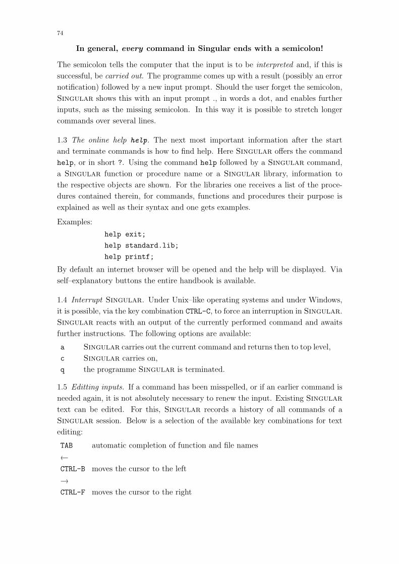
74
In general, every command in Singular ends with a semicolon!
The semicolon tells the computer that the input is to be interpreted and, if this is
successful, be carried out. The programme comes up with a result (possibly an error
notification) followed by a new input prompt. Should the user forget the semicolon,
Singular shows this with an input prompt ., in words a dot, and enables further
inputs, such as the missing semicolon. In this way it is possible to stretch longer
commands over several lines.
1.3 The online help help. The next most important information after the start
and terminate commands is how to find help. Here Singular offers the command
help, or in short ?. Using the command help followed by a Singular command,
a Singular function or procedure name or a Singular library, information to
the respective objects are shown. For the libraries one receives a list of the proce-
dures contained therein, for commands, functions and procedures their purpose is
explained as well as their syntax and one gets examples.
Examples:
help exit;
help standard.lib;
help printf;
By default an internet browser will be opened and the help will be displayed. Via
self–explanatory buttons the entire handbook is available.
1.4 Interrupt Singular. Under Unix–like operating systems and under Windows,
it is possible, via the key combination CTRL-C, to force an interruption in Singular.
Singular reacts with an output of the currently performed command and awaits
further instructions. The following options are available:
a Singular carries out the current command and returns then to top level,
c Singular carries on,
q the programme Singular is terminated.
1.5 Editting inputs. If a command has been misspelled, or if an earlier command is
needed again, it is not absolutely necessary to renew the input. Existing Singular
text can be edited. For this, Singular records a history of all commands of a
Singular session. Below is a selection of the available key combinations for text
editing:
TAB automatic completion of function and file names
←CTRL-B moves the cursor to the left
→CTRL-F moves the cursor to the right

75
CTRL-A moves the cursor to the beginning of the line
CTRL-E moves the cursor to the end of the line
CTRL-D deletes the letter under the cursor — never use in an empty line!
BACKSPACE
DEL
CTRL-H deletes the letter in front of the cursor
CTRL-K deletes all from the cursor to the end of the line
CTRL-U deletes all from the cursor to the beginning of the line
↓CTRL-N supplies the next line from the history
↑CTRL-P supplies the preceding line from the history
RETURN sends the current line to the Singular parser
1.6 Procedures. The user can create new commands in Singular. These are called
procedures. The syntax of a procedure is fairly simple:
proc PROCEDURENAME [PARAMETERLIST]
{PROCEDUREBODY
}For PROCEDURENAME, any not otherwise resevered sequence of letters can be used.
The types and names of the arguments which are passed on to the procedure are
laid down in the PARAMETERLIST. The PARAMETERLIST should be encased in round
brackets. The PROCEDUREBODY contains a sequence of Singular code. If the proce-
dure is to return a result, the result should be stored in a variable result and the
procedure should terminate with the command return(result);.
An example is more useful than thousands of words:
proc permcol (matrix A, int c1, int c2)
{matrix B=A;
B[1..nrows(B),c1]=A[1..nrows(A),c2];
B[1..nrows(B),c2]=A[1..nrows(A),c1];
return(B);
}The procedure permcol should exchange two columns of a matrix. For this three
arguments are necessary. The first argument of name A is of type matrix, the two
following arguments c1 and c2 are of type int. Singular instructions follow and
the result is stored in the variable B of type matrix, which is then returned with
return(B);. This means, in particular, that the result of the procedure is of type
matrix.

76
A procedure can be invoked by entering the procedure name, followed by the argu-
ments in round brackets. E.g.
LIB "matrix.lib"; LIB "inout.lib";
ring r=0,(x),lp;
matrix A[3][3]=1,2,3,4,5,6,7,8,9;
pmat(A,2);
7→ 1 2 3
4 5 6
7 8 9
matrix B=permcol(A,2,3);
pmat(B,2);
7→ 1 3 2
4 6 5
7 9 8
Variables, which are defined within a procedure, are only known there and may,
therefore, have the same name as objects which are defined outside the procedure.
1.7 Libraries. To make procedures available for more than one Singular session,
it makes sense to store them in files, which can be loaded as Singular libraries.
The library names always have the ending .lib. Libraries are read into Singular
through the command LIB followed by library name enclosed in ", such as
LIB "123456.lib";
(Library names should, if possible, only consist of eight letters, to guarantee com-
patibility with systems such as Dos!) If they are not builtin Singular libraries,
then they should be in the subdirectory from which Singular is started.
Of course, a library must conform to certain syntax rules, and procedures, which
are stored in libraries, should be extended by two explanatory additions. We show
this in an example:
////////////////////////////////////////////////////////////////////
version="1.0";
info="LIBRARY: linalgeb.lib FIRST STEPS IN LINEAR ALGEBRA
AUTHOR: Thomas Markwig, email: [email protected]
PROCEDURES:
permcol(matrix,int,int) permutes columns of the matrix
permrow(matrix,int,int) permutes rows of the matrix";
////////////////////////////////////////////////////////////////////
LIB "inout.lib";

77
////////////////////////////////////////////////////////////////////
proc permcol (matrix A, int c1, int c2)
"USAGE: permcol(A,c1,c2); A matrix, c1,c2 positive integers
RETURN: matrix, A being modified by permuting column c1 and c2
NOTE: space for important remark
can be stretched over several lines
EXAMPLE: example permcol; shows an example"
{matrix B=A;
B[1..nrows(B),c1]=A[1..nrows(A),c2];
B[1..nrows(B),c2]=A[1..nrows(A),c1];
return(B);
}example
{"EXAMPLE:";
echo = 2;
ring r=0,(x),lp;
matrix A[3][3]=1,2,3,4,5,6,7,8,9;
pmat(A);
pmat(permcol(A,2,3));
}...
If a double slash // in a line appears, the rest of the line is interpreted as a comment
and ignored.
The first section is the head of the library. The first line contains the reserved
name version, through which the version number of the library is fixed. General
information to the library follows the reserved name info.
It should be noted that under the item PROCEDURES: all procedure names are listed
with a one-line description.
Singular shows this part when the help command is called on the library, that is
help linalgeb.lib;
It should also be noted that strings are allocated to version and info by means of
the sign of equality, =, so that the " are just as necessary as the semicolon at the
end of the line!
Section two serves the loading of further libraries, whose procedures one wants to
use. As an example, the library inout.lib is loaded, whose procedure pmat is used
in the example part of the procedure permcol.

78
In the third section the procedures follow one by one. (It should be noted that the
command proc always has to be at the start of a new line!)
It is recommended that the Syntax in section 1.6 is extended by two sections for
procedures. A commentary block can be inserted between the procedure head and
body, enclosed in ", which contains certain key words followed by the relative infor-
mation. Under USAGE: should be shown how the command is invoked and of which
type the arguments are. RETURN: should contain information on the type of the
return value and, if necessary, further information. NOTE: is used to show important
comments to the procedure, its use, etc. EXAMPLE: shows how an example of the use
of the procedure can be displayed in Singular. The commentary block contains
the information which is shown when the help command is called for the procedure,
e.g. through
help permcol;
The second additional section at the end of the procedure is initiated through the
reserved name example, followed by a section in curly brackets which contains the
Singular code. The aim is to show an example for the operation of the procedure
which explains its use to the user. The user obtains the example by entering example
PROCEDURENAME;.
1.8 Write to files / read from files. The command write offers the possibility to
store the values of variables or any string in a file. For this, the variable values are
converted to strings. The following lines store variable values, resp. a string, in the
file hello.txt:
int a=5;
int b=4;
write("hello.txt",a,b);
write("hello.txt","This is Singular.");
Several variables or strings can be stored at a time, separated by commas. The
value of each variable is written in a separate line.
Data contained in a file can be read in by the command read. They are, however,
interpreted as strings, e.g.
read("hello.txt");
7→ 5
4
This is Singular.
Should Singular code, which is read in from a file, be recognised as such, then the
read command must be passed on to the command execute. If the file hello.txt
contains the following lines,
4*5-3;
6/3;

79
then the command
execute(read("hello.txt"));
leads to the following Singular output:
7→ 17
2
A short form for execute(read(...)) is <, e.g.
< "hello.txt";
Anyone wanting to document a Singular session for security in a file, e.g.
hello.txt, can do this with the command monitor, e.g.
monitor("hello.txt","io");
The option "io" causes input as well as output to be stored. The omission of one
of the letters leads to only the input or only the output being stored. The option
monitor is very helpful when working on an operating system on which Singular
is instable.
Please note that monitor opens a file, but does not terminate it. This can be done
by the following input:
monitor("");
2) Types of data in Singular and rings
In Singular different data types are available, and when introducing a variable
first one has to specify the data type of the variable. Most data types in Singular
depend on a meta structure, the base ring, over which they exist. Exceptions are
string, int, intvec und intmat. To perform a computation in Singular it is
first absolutely necessary to define the ring over which one is working.
ring r=0,x(0..2),lp; The ring of polynomials in the variables
x(0), x(1), x(2) with coefficients in the rational
numbers Q and global lexicographical ordering.
ring r=(0,a,b),(x,y,z),dp; The ring of polynomials in the variables x, y, z,
where the coefficients are rational functions in
the variables a and b. The global degree reverse
lexicographical ordering is used.
ring r=(real,15),x,ls; The localised ring of polynomials in the variables
x with coefficients in real numbers R — for com-
putations with 15 places after the decimal point.
The local lexicographical ordering is used.
ring r=5,x,ds; The localised ring of polynomials in the variables
x with coefficients in Z/5Z and local degree re-
verse lexicographical ordering.

80
A list of the available data types in Singular is given below.
int i=1; The data type int represents the machine
integers (between −231 und 231 − 1). In
addition, boolean values are represented as
integers, 0 = FALSE, 1 = TRUE.
string s="Hallo"; strings are chains of letters enclosed by ”.
intvec iv=1,2,3,4; A vector of integers.
intmat im[2][3]=1,2,3,4,5,6; A matrix with two lines and three columns
with integer entries.
ring R=(0,a),(x,y),lp; Q(a)[x, y] with lexicographical order.
number n=4/6; numbers are the elements of the base field
of the ring. By ring r=0,x,lp; the ratio-
nal numbers, by ring r=(0,a),x,lp; also
fractions of polynomials in a, e.g. a2+1a−1
.
list l=n,iv,s; A list can contain objects of different types.
l[2] refers to the second entry of l.
matrix m[2][3]=1,2,3,4,5,6; A matrix with two lines and three columns,
the entries being of type poly,
vector v=[1,2,3]; A vector in the module R3.
proc The data type procedure is discussed at
length in 1.6.
poly f=x2+2x+1; A polynomial in the indeterminates of the
ring with numbers as coefficients, here f =
x2 + 2x + 1. Note that numbers in front of
the monomials are interpreted as coefficients,
whereas Singular interprets integers after
single variables as exponents.
ideal i=f,x3; The ideal generated by f and x3.
qring Q=i; The quotient ring R/i.
map g=R,x; A map from the ring R to the current ring
sending the first variable of R to x.
module mo=v,[x,x2,x+1]; The module generated v and (x, x2, x+ 1).
def j; In case one does not want to specify the data
type yet, one can use the type def. The first
time a value is assigned to j this value deter-
mines the data type of j.
link For the data type link, we refer to the man-
ual [DGPS10].
resolution For the data type resolution, we refer to
the manual [DGPS10].
81
At the first glance it might seem as though the matrices im and m are identical. For
Singular that is not the case as they are of different types!
3) Some elements of the programming language Singular
3.1 Allocations. In Singular the operator = is used to assign a value to a variable.
It is possible to assign a value at the time of the definition of the variable,
int i=1;
or later,
int i;...
i=2;
3.2 Loops. There are two types of loops, the for and the while loop.
The for loop is used typically, if a command sequence is to be performed several
times and the number of times is known beforehand. E.g.
int s=0;
int i;
for (i=1; i<=10; i=i+1)
{s=s+i;
}The command sequence in curly brackets are the commands executed when passing
the loop. The commands in round brackets determine how often the loop is to be
passed. The first entry fixes the control variable and is here of type int; the second
entry shows the termination condition, i.e. the loop is passed through as long as this
condition is fulfilled; the third entry fixes how the control variable should change in
each passage. The example computes the sum of the first ten natural numbers.
while loops are used, when the number of passages is not a priori clear. E.g.
int s=10000;
int i=1;
while (s > 50)
{i=i*i;
s=s-i;
}Again the command sequence is shown in curly brackets, whilst the termination
conditions are shown in round brackets. As long as these show the value TRUE, the
loop is performed.
The termination condition is checked before the first entry into the loop.

82
3.3 Branchings. Singular offers as a branching the if-else command, where,
however, the else part could be missing. E.g.
int i=10;
int s=7;
if (i<5 or s<10)
{s=5;
}else
{s=0;
}Again the command sequences are shown as a block in curly brackets, whereas the
branching conditions are in round brackets.
3.4 Comparison operators. In Singular we have the comparison operators == and
!=, with which objects of the same type (e.g. int, string, matrix, etc.) can be
compared to one another. == tests for equality and supplies the value 1 if the objects
are the same and otherwise 0. != checks for inequality. <> has the same effect.
For the data types int, number, poly and vector, the operators <, >, <= and >=
are available. Its significance for integers and monomials is clear. We refer to the
manual for further data types [DGPS10].
3.5 Some further operators in Singular. As we have already seen, the operators
may depend on the data types.
boolean: For boolean variables, the connecting operators and and or as well as
the negating operator not are defined.not ((1==0) or (1!=0));
7→ 0int: For integers the operations +, - and * are entirely clear. ^ means raising
to some powerint i=4;
i^3;
7→ 64The commands div and mod are more difficult, whereby the first is synonymous
to /. If, for two integers, a division with remainder is performed, then mod
supplies the remainder, and div the result without remainder. E.g. 7 = 2∗3+1,also
7 div 3;
7→ 2
7 mod 3;
7→ 1

83
list: The following operators are given for the data type list.+ Combines the elements of two lists.
delete Deletes an element from a list, delete(L,3) deletes the third
element of the list L.
insert Inserts an element into a list. insert(L,4) inserts the ele-
ment 4 at the start of the list L, insert(L,4,2) inserts four
into into the second position.matrix: The operators +, - and * are available with their obvious meaning. We
show, by examples, how single entries of a matrix, resp. whole lines or columns
of a matrix, can by accessed:
matrix m[2][3]=1,2,3,4,5,6;
print(m);
7→ 1,2,3,
4,5,6
m[1,2];
7→ 2;
m[1,1..3];
7→ 1 2 3
m[1..2,3];
7→ 3 6
4) Some selected functions in Singular
Singular has a quite notable arsenal of functions available, which are, in part,
integrated in the Singular core, in part made available via libraries. We only wish
to show a small selection of function names, which are useful for computations in
linear algebra. Information on their syntax can be found via help or in the manual.
4.1 Functions which are connected to the data type matrix. ncols, nrows,
print, size, transpose, det, as functions in the core of Singular. Fur-
thermore there are the functions of the library matrix.lib, in particular
permrow, permcol, multrow, multcol, addrow, addcol, concat, unitmat,
gauss row, gauss col, rowred, colred. Also the function pmat from the library
inout.lib is interesting.
4.2 Functions which are connected to the data type int. random, gcd, prime as
functions in the core of Singular.
5) ESingular - or the editor Emacs
There are many editors in which Singular procedures and libraries can be written.
On Unix or similar systems the editor emacs (oder Xemacs) should be considered, as
it simplifies the entered code through using coloured highlighting of the key words,
and they offer many options which simplify editing and error correction.

84
There is another reason for the recommendation to use Emacs. Singular can be
started in a special Emacs mode, as ESingular. This means that first the editor
Emacs is started and then inside Emacs the programme Singular. The advantage
is that apart from the full functionality of the editor Emacs for editing files, a bunch
of further options can be made available, which simplify the use — in particular for
the inexperienced user, for whom pulldown menu buttons are available. By calling
ESingular --emacs=xemacs
it is possible to fix the version of Emacs which is to be used, in this case Xemacs.
6) Exercises
Exercise A.1
Write a procedure binomi, which reads in two natural numbers n and k and returns
the binomial coefficient(
nk
)
. (Convention, if k < 0 or k > n, then(
nk
)
= 0.)
Exercise A.2
Write a procedure squaresum, which reads in the natural number n and returns the
sum of the square numbers 12, 22, 32, . . . , n2.
Exercise A.3
Write a procedure minimum, which reads in a vector of natural numbers and returns
the minimum of the numbers.
Exercise A.4
Write a procedure rowsumnorm, maximumnorm and q eukl norm, which read in a
(m× n) matrix A of real numbers and calculate
a. the row summmation norm of A (i.e. maxi=1,...,m(
Σnj=1|Aij|)
),
b. the maximum norm of A (i.e. max(
|Aij|∣
∣ i = 1, . . . ,m, j = 1, . . . , n)
), respec-
tively
c. the square of the euclidian norm of A (i.e. Σi,j|Aij|2).
Use the function abs from the library linalg.lib for the absolute value.
7) Solutions
Solution to Exercise A.1
proc binomi (int n, int k)
"USAGE: binomi(n,k); int n, int k
RETURN: int, binomial coefficient n over k
EXAMPLE: example binomi; shows an example"
{if ((k < 0) or (k > n))
{return(0);

85
}else
{int i;
int denominator,nominator1,nominator2 = 1,1,1;
for (i=1;i<=n;i++)
{denominator = denominator * i;
}for (i=1;i<=k;i++)
{nominator1 = nominator1 * i;
}for (i=1;i<=n-k;i++)
{nominator2 = nominator2 *i;
}return (denominator / (nominator1 * nominator2));
}}example
{"Example:";
echo = 2;
binomi(5,2);
binomi(7,5);
}
Solution to Exercise A.2
proc squaresum (int n)
"USAGE: squaresum(n); int n
RETURN: int, the sum of the first n square numbers
EXAMPLE: example squaresum; shows an example"
{if (n < 0)
{return (0);
}else
{int i;
int result = 0;

86
for (i=1;i<=n;i++)
{result = result + i*i;
}return (result);
}}example
{"Example:";
echo = 2;
squaresum(3);
squaresum(5);
}
Solution to Exercise A.3
proc minimum (intvec iv)
"USAGE: minimum(iv); iv intvector
RETURN: int, the minimum of the entries in iv
EXAMPLE: example minium; shows an example"
{int i;
int k=size(iv);
int result=iv[1];
for (i=2;i<=k;i++)
{if (iv[i] < result)
{result=iv[i];
}}
return(result);
}example
{"EXAMPLE:";
echo=2;
intvec iv=3,2,5,2,1;
print(iv);
minimum(iv);
iv =-3,4,5,3,-6,7;
print(iv);
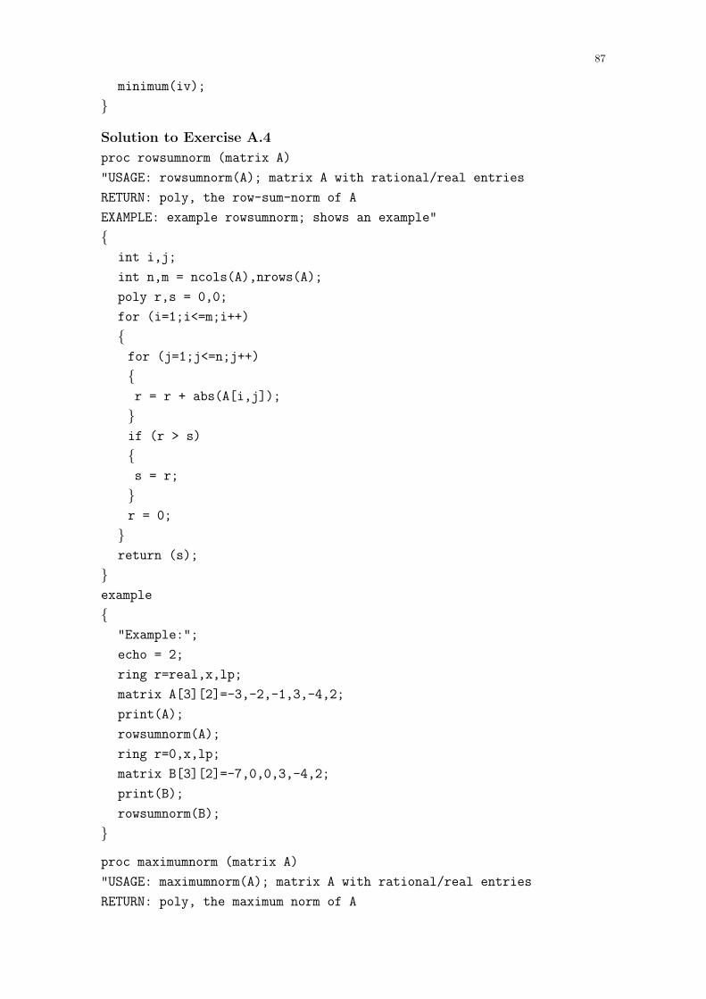
87
minimum(iv);
}
Solution to Exercise A.4
proc rowsumnorm (matrix A)
"USAGE: rowsumnorm(A); matrix A with rational/real entries
RETURN: poly, the row-sum-norm of A
EXAMPLE: example rowsumnorm; shows an example"
{int i,j;
int n,m = ncols(A),nrows(A);
poly r,s = 0,0;
for (i=1;i<=m;i++)
{for (j=1;j<=n;j++)
{r = r + abs(A[i,j]);
}if (r > s)
{s = r;
}r = 0;
}return (s);
}example
{"Example:";
echo = 2;
ring r=real,x,lp;
matrix A[3][2]=-3,-2,-1,3,-4,2;
print(A);
rowsumnorm(A);
ring r=0,x,lp;
matrix B[3][2]=-7,0,0,3,-4,2;
print(B);
rowsumnorm(B);
}
proc maximumnorm (matrix A)
"USAGE: maximumnorm(A); matrix A with rational/real entries
RETURN: poly, the maximum norm of A

88
EXAMPLE: example maximumnorm; shows an example"
{int i,j;
int n,m = ncols(A),nrows(A);
poly r = 0;
for (i=1;i<=m;i++)
{for (j=1;j<=n;j++)
{if (abs(A[i,j]) > r)
{r = abs(A[i,j]);
}}
}return(r);
}example
{"Example:";
echo = 2;
ring r=real,x,lp;
matrix A[3][2]=-3,-2,-1,3,-4,2;
print(A);
maximumnorm(A);
ring r=0,x,lp;
matrix B[3][2]=-7,0,0,3,-4,2;
print(B);
maximumnorm(B);
}
proc q eukl norm (matrix A)
"USAGE: q eukl norm(A); matrix A with rational/real entries
RETURN: poly, the square of the euclidean norm of A
EXAMPLE: example q eukl norm; shows an example"
{int i,j;
int n,m = ncols(A),nrows(A);
poly r = 0;
for (i=1;i<=m;i++)
{for (j=1;j<=n;j++)

89
{r = r + abs(A[i,j]) * abs(A[i,j]);
}}return (r);
}example
{"Example:";
echo = 2;
ring r=real,x,lp;
matrix A[3][2]=-3,-2,-1,3,-4,2;
print(A);
q eukl norm(A);
ring r=0,x,lp;
matrix B[3][2]=-7,0,0,3,-4,2;
print(B);
q eukl norm(B);
}
Appendix B First steps with surfex
The programme surfex (see [HL08]) offers a graphical interface to visualise algebraic
surfaces in 3-space and curves on such surfaces. One can either start surfex directly
or one can invoke it from within a Singular session. If you should want to invoke
surfex from within Singular then you have to load the library surfex.lib first.
The Singular command to plot a surface would then be plotRot. We demonstrate
this with for the polynomial f = x2 − y2 · (t2 − y).
SINGULAR /
A Computer Algebra System for Polynomial Computations / version 3-1-2
0<
by: W. Decker, G.-M. Greuel, G. Pfister, H. Schoenemann \ Oct 2010
FB Mathematik der Universitaet, D-67653 Kaiserslautern \
> ring r=0,(t,x,y),dp;
> poly f=x^2-y^2*(t^2-y);
> LIB "surfex.lib";
> plotRot(f);
The command plotRot starts the programme surfex and opens three new windows
(see Figure 34). The leftmost window contains the equation of the surface as well
as most of the control buttons to direct the programme; the upper right window

90
Figure 34. Surfex
allows to rotate the surface and to zoom in and out; the third window displays the
surface.
If you start surfex from within Singular your Singular session is interrupted
as long as surfex is running. In order to continue in Singular you have to shut
down surfex. Moreover, you should be aware that your Singular variables will
be renamed, so that the first variable becomes x, the second y and the third z. In
the above example the variable t becomes x, x becomes y and y becomes z. The
polynomial x2 − y2 · (t2 − y) is thus transformed into y2 − z2 · (y2 − z).As mentioned above one can use surfex in order to cut two surfaces and to draw
the intersection curve on one of the two surfaces. We show this for the surface
V(y2 − z2 · (y2 − z)) and the plane V(x − 1). In Figure 35 we added besides the
polynomial y2− z2 · (y2− z), that could already be seen in Figure 34 the polynomial
x− 1 by using the button add eqn. Both polynomials can be seen in the third part
of the control window, and both surfaces are displayed in the left part of Figure 36.
There you can also see the intersection curve in black. In order to produce this we
have used the button add curve. By this we got the option to choose some numbers
in the fourth part of the control window. We chose the numbers 1 and 2. This means
that on the surface given by the polynomial f1 the intersection curve that we get
by intersecting this surface with the surface given by the polynomial f2 should be
drawn. In the right part of Figure 36 only the surface V(
y2 − z2 · (y2 − z))
and the
intersection curve can be seen. This is achieved by removing the hook in front of
the polynomial x − 1 in the control window of surfex (see Figure 35). For further
details on the use of surfex we refer to the manual [HL08] and to the surfex web
page:
http://www.surfex.algebraicsurface.net
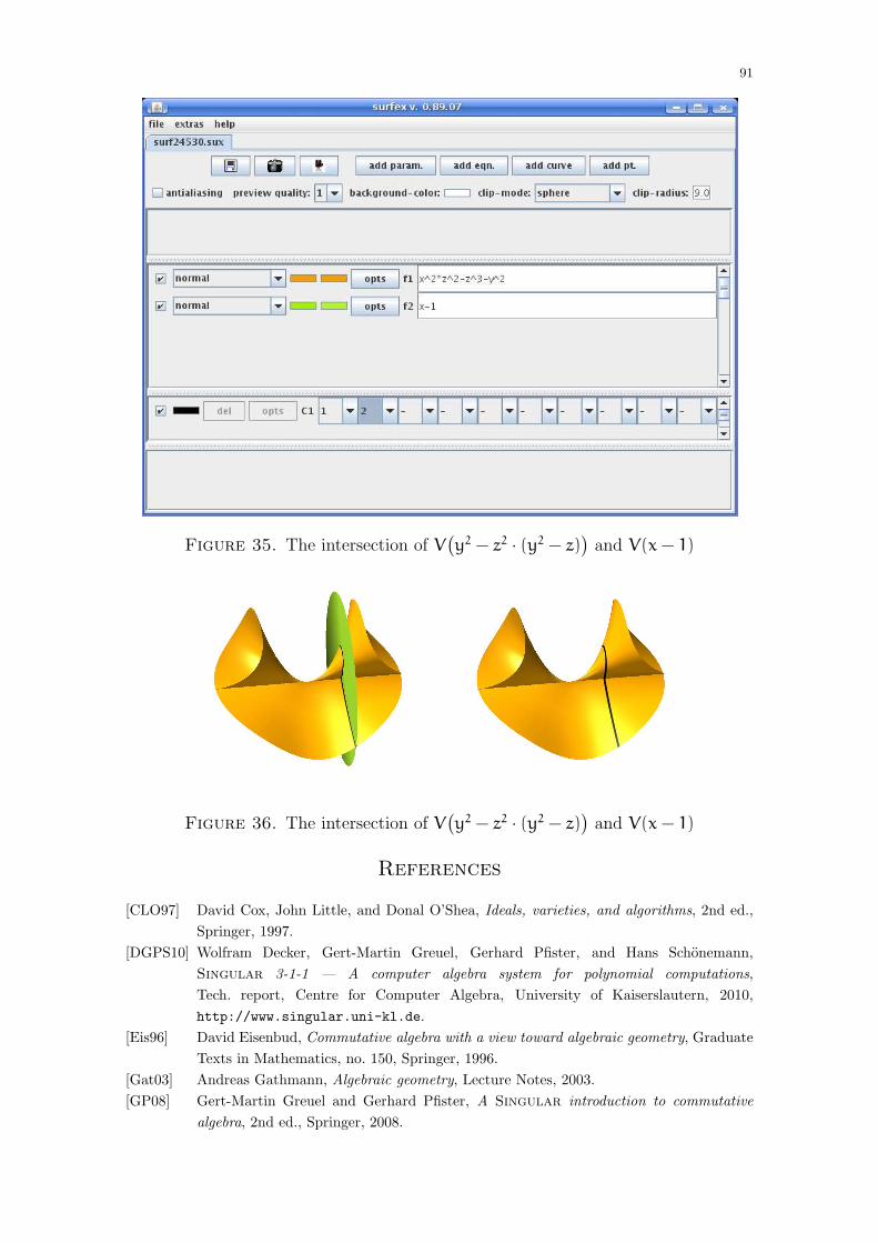
91
Figure 35. The intersection of V(
y2 − z2 · (y2 − z))
and V(x− 1)
Figure 36. The intersection of V(
y2 − z2 · (y2 − z))
and V(x− 1)
References
[CLO97] David Cox, John Little, and Donal O’Shea, Ideals, varieties, and algorithms, 2nd ed.,
Springer, 1997.
[DGPS10] Wolfram Decker, Gert-Martin Greuel, Gerhard Pfister, and Hans Schonemann,
Singular 3-1-1 — A computer algebra system for polynomial computations,
Tech. report, Centre for Computer Algebra, University of Kaiserslautern, 2010,
http://www.singular.uni-kl.de.
[Eis96] David Eisenbud, Commutative algebra with a view toward algebraic geometry, Graduate
Texts in Mathematics, no. 150, Springer, 1996.
[Gat03] Andreas Gathmann, Algebraic geometry, Lecture Notes, 2003.
[GP08] Gert-Martin Greuel and Gerhard Pfister, A Singular introduction to commutative
algebra, 2nd ed., Springer, 2008.

92
[Har77] Robin Hartshorne, Algebraic geometry, Springer, 1977.
[Har92] Joe Harris, Algebraic geometry, a first course, Graduate Texts in Mathematics, no. 133,
Springer, 1992.
[HL08] Stephan Holzer and Oliver Labs, surfex 0.90, Tech. report, University of Mainz,
University of Saarbrucken, 2008, www.surfex.AlgebraicSurface.net.
Related Documents