Computation Theory Introduction to Turing Machine.

Computation Theory

Introduction to Turing Machine

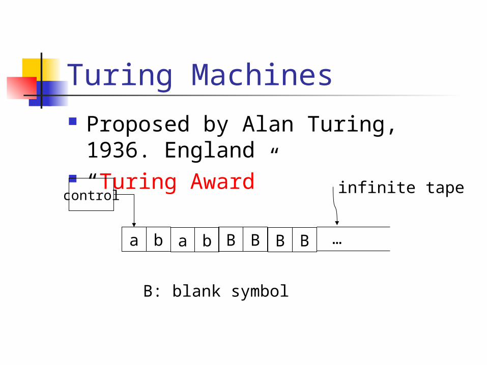
Turing Machines Proposed by Alan Turing, 1936.

England “Turing Award”control

a b a b B B B B …

infinite tape

B: blank symbol

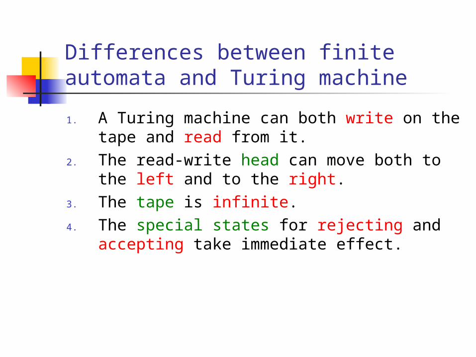
Differences between finite automata and Turing machine

1. A Turing machine can both write on the tape and read from it.

2. The read-write head can move both to the left and to the right.

3. The tape is infinite.4. The special states for rejecting and accepting

take immediate effect.

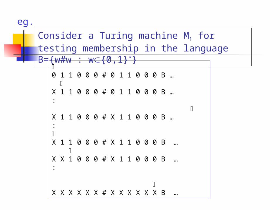
Consider a Turing machine M1 for testing membership in the language B={w#w : w{0,1}*}

eg.

0 1 1 0 0 0 # 0 1 1 0 0 0 B … X 1 1 0 0 0 # 0 1 1 0 0 0 B …: X 1 1 0 0 0 # X 1 1 0 0 0 B …:X 1 1 0 0 0 # X 1 1 0 0 0 B … X X 1 0 0 0 # X 1 1 0 0 0 B …: X X X X X X # X X X X X X B …

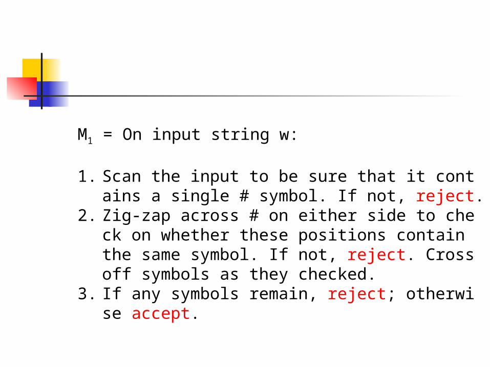
M1 = On input string w:

1. Scan the input to be sure that it contains a single # symbol. If not, reject.

2. Zig-zap across # on either side to check on whether these positions contain the same symbol. If not, reject. Cross off symbols as they checked.

3. If any symbols remain, reject; otherwise accept.

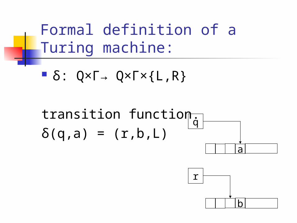
Formal definition of a Turing machine:

δ: Q×Γ→ Q×Γ×{L,R}

transition function. δ(q,a) = (r,b,L)

q

a

r

b

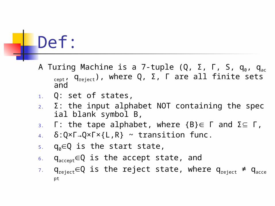
Def:A Turing Machine is a 7-tuple (Q, Σ, Γ, S, q0, qaccept, qrejec

t), where Q, Σ, Γ are all finite sets and1. Q: set of states,2. Σ: the input alphabet NOT containing the special

blank symbol B,3. Γ: the tape alphabet, where {B} Γ and Σ Γ,4. δ:Q×Γ→Q×Γ×{L,R} ~ transition func.5. q0Q is the start state,6. qacceptQ is the accept state, and7. qrejectQ is the reject state, where qreject ≠ qaccept

As a Turing machine computes, it may halt with ‘accept’ or ‘reject’, or it may never halt!

During computation, changes occur in1. the current state, 2. the current tape contents, and3. the current head location.

The above three items form a “configuration” of the Turing machine.

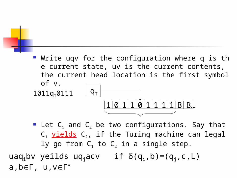
Write uqv for the configuration where q is the current state, uv is the current contents, the current head location is the first symbol of v.

1011qT0111

Let C1 and C2 be two configurations. Say that C1 yields C2, if the Turing machine can legally go from C1 to C2 in a single step.

1 0 1 1 0 1 1 1 1 B B…

qT

uaqibv yeilds uqjacv if δ(qi,b)=(qj,c,L)a,bΓ, u,vΓ*

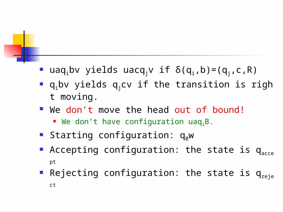
uaqibv yields uacqjv if δ(qi,b)=(qj,c,R) qibv yields qjcv if the transition is right moving. We don’t move the head out of bound!

We don’t have configuration uaqiB. Starting configuration: q0w Accepting configuration: the state is qaccept

Rejecting configuration: the state is qreject

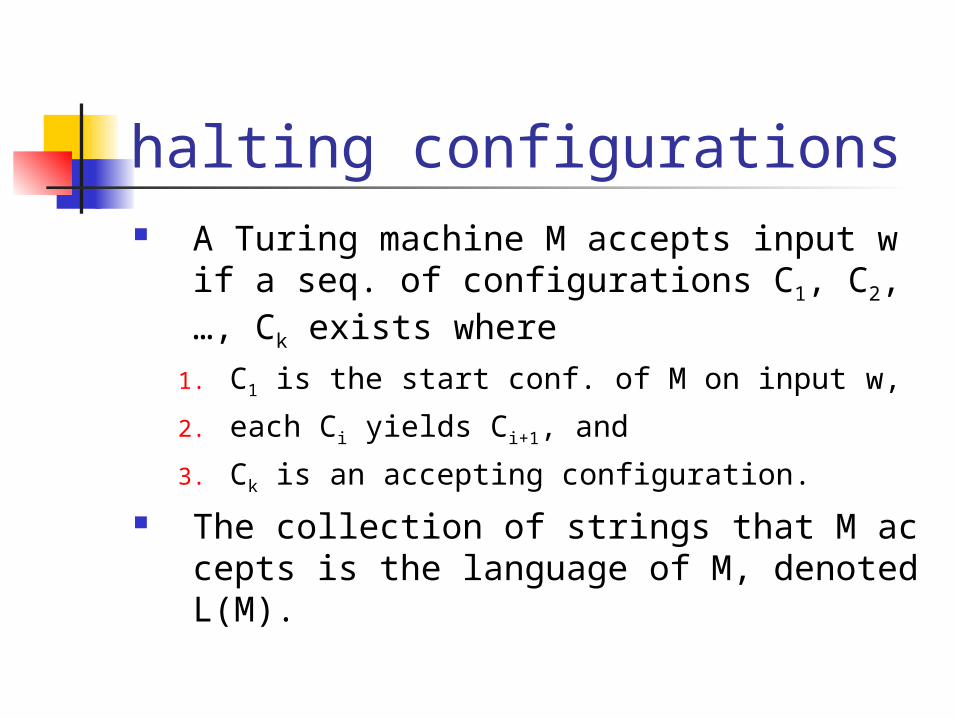
halting configurations A Turing machine M accepts input w if a se

q. of configurations C1, C2, …, Ck exists where

1. C1 is the start conf. of M on input w,2. each Ci yields Ci+1, and3. Ck is an accepting configuration.

The collection of strings that M accepts is the language of M, denoted L(M).

Def: A language is Turing-recognizable if some Turing machine recognizes it. (or recursively enumerable)

r.e.Def: A language is Turing-decidable or

decidable if some Turing machine decides it.(or recursive)

r.

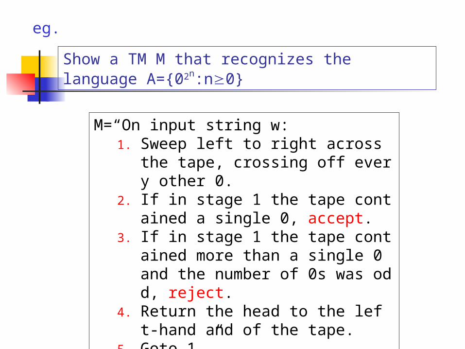
eg.

Show a TM M that recognizes the language A={02n:n0}

M=“On input string w:1. Sweep left to right across the tape,

crossing off every other 0.2. If in stage 1 the tape contained a si

ngle 0, accept.3. If in stage 1 the tape contained mo

re than a single 0 and the number of 0s was odd, reject.

4. Return the head to the left-hand and of the tape.

5. Goto 1.”

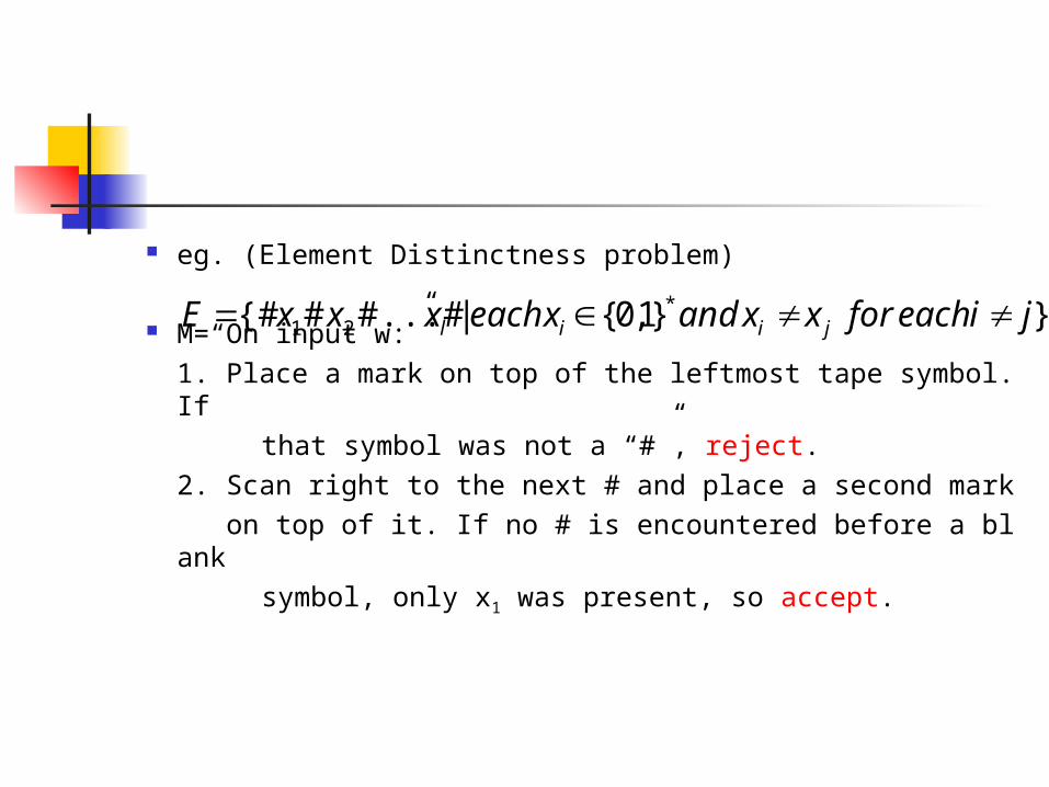
eg. (Element Distinctness problem)

M=“On input w:”1. Place a mark on top of the leftmost tape symbol. If

that symbol was not a “#”, reject.2. Scan right to the next # and place a second mark on top of it. If no # is encountered before a blank

symbol, only x1 was present, so accept.

} }1,0{ |#...##{# *21 jieachforxxandxeachxxxE jiil

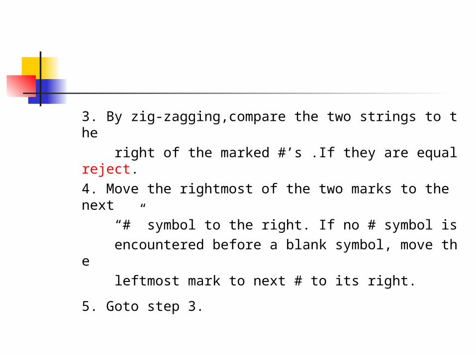
3. By zig-zagging,compare the two strings to the right of the marked #’s .If they are equal reject.4. Move the rightmost of the two marks to the next “#” symbol to the right. If no # symbol is encountered before a blank symbol, move the leftmost mark to next # to its right.

5. Goto step 3.

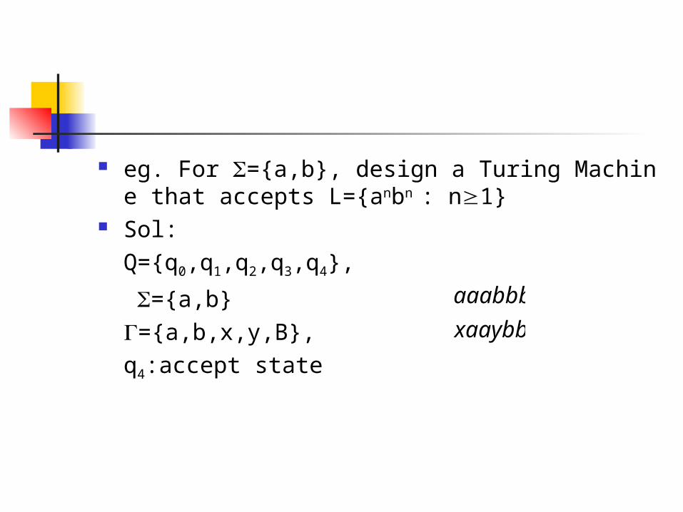
eg. For ={a,b}, design a Turing Machine that accepts L={anbn : n1}

Sol:Q={q0,q1,q2,q3,q4}, ={a,b}={a,b,x,y,B},q4:accept state

xaaybb

aaabbb

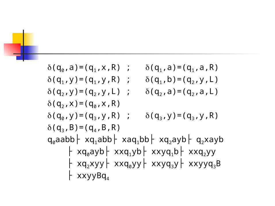
(q0,a)=(q1,x,R) ; (q1,a)=(q1,a,R)(q1,y)=(q1,y,R) ; (q1,b)=(q2,y,L)(q2,y)=(q2,y,L) ; (q2,a)=(q2,a,L)(q2,x)=(q0,x,R)(q0,y)=(q3,y,R) ; (q3,y)=(q3,y,R)(q3,B)=(q4,B,R)q0aabb├ xq1abb├ xaq1bb├ xq2ayb├ q2xayb ├ xq0ayb├ xxq1yb├ xxyq1b├ xxq2yy ├ xq2xyy├ xxq0yy├ xxyq3y├ xxyyq3B ├ xxyyBq4

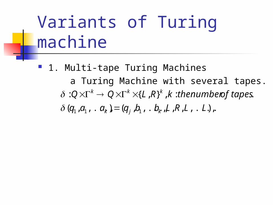
Variants of Turing machine 1. Multi-tape Turing Machines

a Turing Machine with several tapes.

).,...,,,,,...,,(),...,,(

. : ,},{:

111 LLRLbbqaaq

tapesofnumberthekRLQQ

kjk

kkk

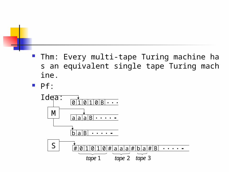
Thm: Every multi-tape Turing machine has an equivalent single tape Turing machine.

Pf:Idea:

M

0 1 0 1 0 B

a a a B

b a B

......

............

............

S # 0 1 0 1 0 # a a a # b a # B ............

1tape 2tape 3tape

q

q0

0

0

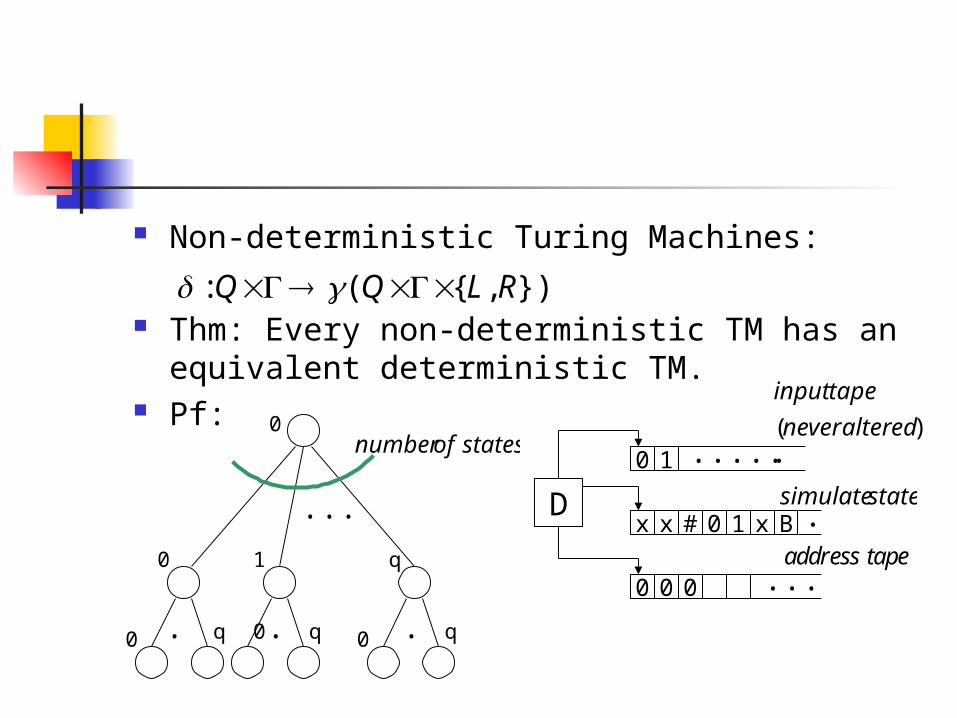
Non-deterministic Turing Machines:

Thm: Every non-deterministic TM has an equivalent deterministic TM.

Pf:

) },{ (: RLQQ

q0

1

q0 .........

......

statesofnumber

D

0 1

x x # 0

0 0

1 x B

............

0 ......

...

) (

alterednever

tapeinput

statesimulate

address tape

1. Initially tape 1 contains the input w, and tapes 2 and 3 are empty.

2. Copy tape 1 to tape 2.3. Use tape 2 to simulate N with input w on one bran

ch of its non-det. computation. Before each step of N consult the next symbol on tape 3 to decide which branch to move. If no symbol remains or this choice is invalid goto step 4. If reject also goto 4.

4. Increase the count on tape 3. go to step 2.

Corollary:A language is Turing-recognizable if and only if some non-deterministic TM recognizes it.

Corollary: A language is decidable if and only if some non-deterministic TM decides it

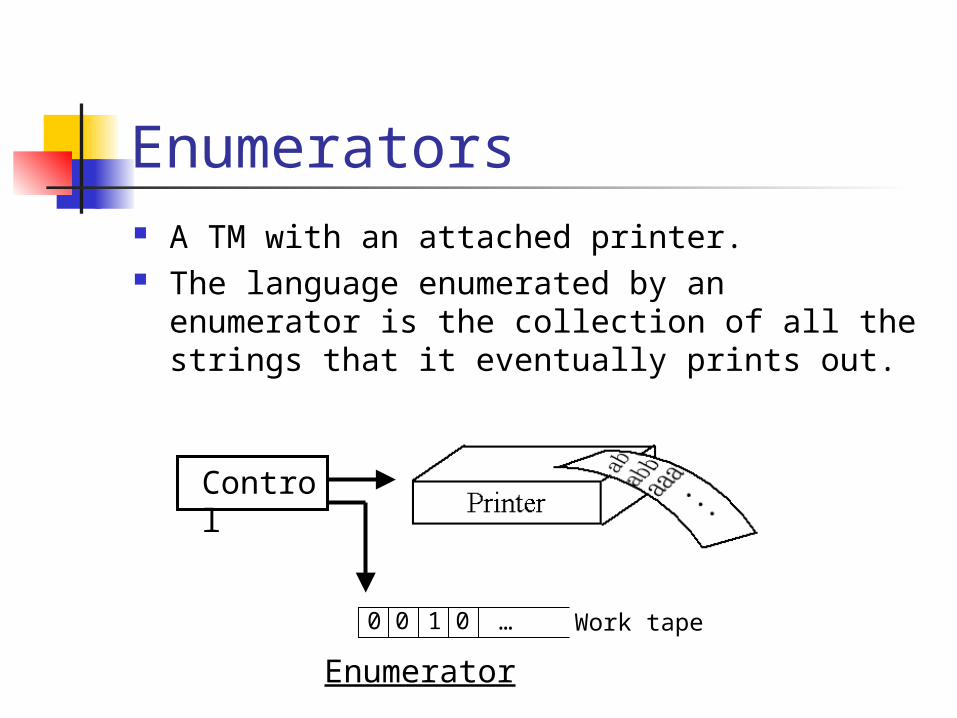
Enumerators A TM with an attached printer. The language enumerated by an enumerator is

the collection of all the strings that it eventually prints out.

Control

0 0 1 0 … Work tape

Enumerator

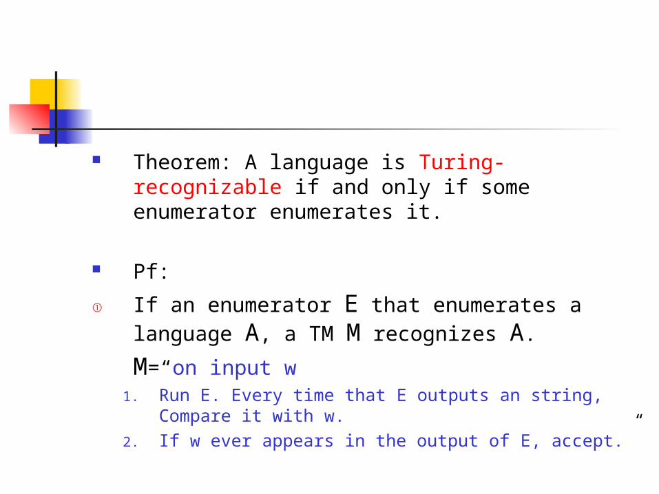
Theorem: A language is Turing-recognizable if and only if some enumerator enumerates it.

Pf:

① If an enumerator E that enumerates a language A, a TM M recognizes A.

M=“on input w1. Run E. Every time that E outputs an string,

Compare it with w.2. If w ever appears in the output of E, accept.”

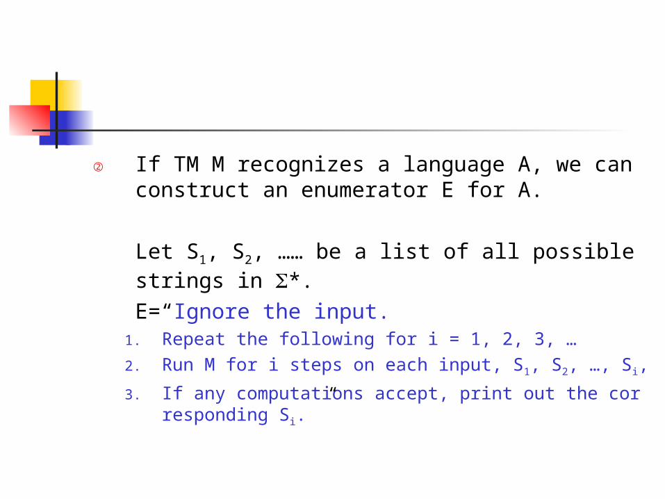
② If TM M recognizes a language A, we can construct an enumerator E for A.

Let S1, S2, …… be a list of all possible strings in *.E=“Ignore the input.

1. Repeat the following for i = 1, 2, 3, …2. Run M for i steps on each input, S1, S2, …, Si,3. If any computations accept, print out the correspondin

g Si. ”

Definition of algorithm Hilbert’s problems:

In 1900, mathematician David Hilbert delivered a famous address at the “International congress of Mathematicians in Paris.”He proposed 23 mathematical problems.

Hilbert’s tenth problem:Design an algorithm that tests whether a multi-variable polynomial has an integral root.

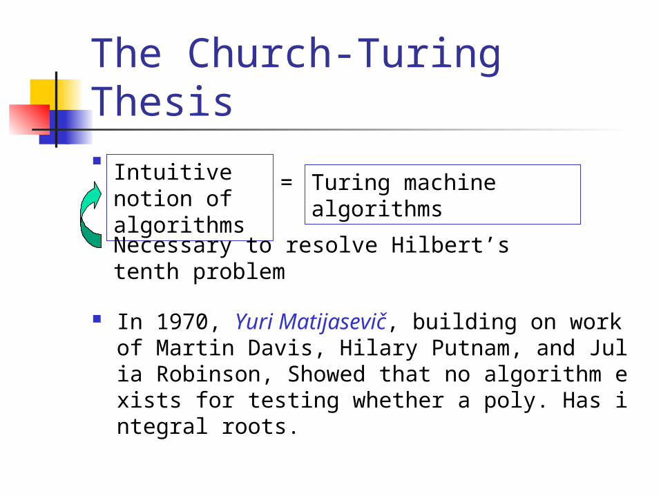
The Church-Turing Thesis

In 1970, Yuri MatijasevicQ, building on work of Martin Davis, Hilary Putnam, and Julia Robinson, Showed that no algorithm exists for testing whether a poly. Has integral roots.

Intuitive notion of algorithms

Turing machine algorithms

=

Necessary to resolve Hilbert’s tenth problem

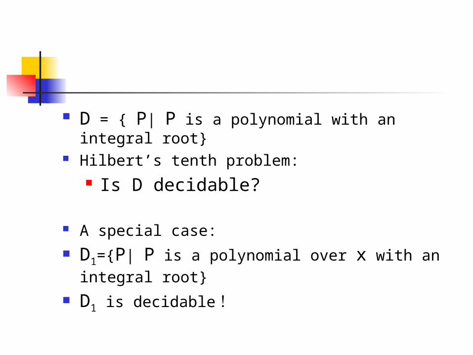
D = { P| P is a polynomial with an integral root}

Hilbert’s tenth problem: Is D decidable?

A special case: D1={P| P is a polynomial over x with an

integral root} D1 is decidable！

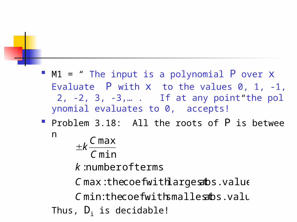
M1 = “ The input is a polynomial P over x Evaluate P with x to the values 0, 1, -1, 2, -2, 3, -3,… .

If at any point the polynomial evaluates to 0, accepts! ”

Problem 3.18: All the roots of P is between

Thus, Di is decidable! valueabs.smallest with coef. the

valueabs.largest with coef. the

terms ofnumber

:min

:max

:min

max

C

C

kC

Ck