Computation of three-dimensional periodic orbits in the sun-earth … · 2019-10-02 · Eapen & Sharma32 discussed the planar photogravitational CRTBP including solar radiation pressure

Submit Manuscript | http://medcraveonline.com

IntroductionFrom the last few decades, the space science community has shown

considerable interest in missions which take place in the vicinity of the Lagrangian points in the restricted three-body problem (RTBP) of the Sun-Earth and the Earth-Moon systems.1 Designing trajectories for these missions is a challenging task due to inadequacy of the conic approximations. The RTBP deals the situation where one of the three bodies has a negligible mass, and moves under the gravitational influence of two other bodies.2–9 In the RTBP, the circular restricted three-body problem (CRTBP) is a special case where two massive bodies move in the circular motion around their common centre of mass.10–14 The collinear Lagrangian point orbits have paid a lot of attentions for the mission design and transfer of trajectories.15–22 When the frequencies of two oscillations are commensurable, the motion becomes periodic and such an orbit in the three-dimensional space is called halo.23 Lyapunov orbits are the two-dimensional planar periodic orbits. These planar periodic orbits are not suitable for space applications since they do not allow the out-of-plane motion, e.g., a spacecraft placed in the Sun-Earth 2L point must have an out-of-plane amplitude in order to avoid the solar exclusion zone (dangerous for the downlink); a space telescope around the Sun-Earth 2L point must avoid the eclipses and hence requires a three-dimensional periodic orbit. Since the RTBP does not have any analytic solution, the periodic orbits are difficult to obtain because the problem is highly nonlinear and small changes in the initial conditions break the periodicity.24 Farquhar23 was the first person who introduced analytic computation of the halo orbit in his PhD thesis. In 1980,25 introduced a third-order analytic approximation of the halo orbits near the collinear libration points in the classical CRTBP for the Sun-Earth system. Thurman & Worfolk1 and Koon et al.,26 found the halo orbits for the CRTBP with the Sun-Earth system in the absence of any perturbative force using Richardson method25 up to third-order. Breakwell & Brown27 and Howell28 numerically obtained the halo orbits in the classical CRTBP Earth-Moon system using the single step differential correction scheme. Numerous applications of the halo orbits in the scientific

mission design can be seen such as investigations concerning solar exploration and helio-spheric effects on planetary environments using the spacecraft placed in these orbits at different phases. ISEE-3 was the first mission in a halo orbit of the Sun-Earth system around 1Lto study the interaction between the Earth’s magnetic field and solar wind.29 Solar and Heliospheric Observatory (SOHO) mission was second libration point mission launched jointly by ESA and NASA in a halo orbit around the Sun-Earth 1L point, still operational till date, which was a virtual carbon copy of ISEE-3’s orbit.30

The classical model of the RTBP does not account perturbing forces such as oblateness, radiation pressure and variations of masses of the primaries. The photogravitational RTBP arises from the classical RTBP if at least one of the bodies is an intense emitter of radiation. Radzievskii31 derived the photogravitational RTBP and discussed it for three specific bodies: the Sun, a planet and a dust particle. Recently, Eapen & Sharma32 discussed the planar photogravitational CRTBP including solar radiation pressure in the Sun-Mars system around 1L point using the initial guess of the classical CRTBP.

Numerical computation of the periodic orbits requires an initial approximation to the orbit as an approximate analytic solution. However, the analytic solutions that are available do not generally include solar radiation pressure and other perturbing forces. Including these perturbed forces in the analytic approximation increases accuracy of the approximation and therefore, simplifies the numerical computations.33 In this paper, we discuss analytic as well as numerical computations of the halo orbits around the libration points 1L and

2L in the CRTBP including solar radiation pressure of the Sun. The paper is organized as follows: Section 2 deals with the governing equations of motion considering the Sun as a radiating source. Section 3 describes the construction of a third-order analytic approximate solution for the periodic orbit using the Lindstedt-Poincare method. Section 4 illustrates numerical computation of the halo orbit using Newton’s method of differential correction. Results and discussion are given in Section 5 while Section 6 concludes our study.

Phys Astron Int J. 2018;2(1):81‒90. 81©2018 Tiwary et al. This is an open access article distributed under the terms of the Creative Commons Attribution License, which permits unrestricted use, distribution, and build upon your work non-commercially.

Computation of three-dimensional periodic orbits in the sun-earth system

Volume 2 Issue 1 - 2018

Tiwary RD,1 Srivastava VK,1,2 Kushvah BS1

1Department of Applied Mathematics, Indian Institute of Technology (Indian School of Mines) Dhanbad, India2Flight Dynamics Group, ISRO Telemetry Tracking and Command Network, India

Correspondence: Vineet K Srivastava, Department of Applied Mathematics, Indian Institute of Technology (Indian School of Mines) Dhanbad, Dhanbad-826004, India, Tel 8050682145, Email

Received: November 20, 2017 | Published: February 08, 2018

Abstract

In this paper, a third-order analytic approximation is described for computing the three-dimensional periodic halo orbits near the collinear 1L and 2L Lagrangian points for the photo gravitational circular restricted three-body problem in the Sun-Earth system. The constructed third-order approximation is chosen as a starting initial guess for the numerical computation using the differential correction method. The effect of the solar radiation pressure on the location of two collinear Lagrangian points and on the shape of the halo orbits is discussed. It is found that the time period of the halo orbit increases whereas the Jacobi constant decreases around both the collinear points taking into account the solar radiation pressure of the Sun for the fixed out-of-plane amplitude.

Keywords: photogravitational CRTBP, halo orbits, lindstedt-poincare method, Newton’s method, radiation pressure

Physics & Astronomy International Journal

Research Article Open Access

Computation of three-dimensional periodic orbits in the sun-earth system 82Copyright:

©2018 Tiwary et al.

Citation: Tiwary RD, Srivastava VK, Kushvah BS. Computation of three-dimensional periodic orbits in the sun-earth system. Phys Astron Int J. 2018;2(1):81‒90. DOI: 10.15406/paij.2018.02.00052

Mathematical modelWe suppose that the CRTBP consists of the Sun, the Earth and the

Moon, and an infinitesimal body such as a spacecraft having masses1m , 2m and m , respectively. Here the Earth and the Moon are clubbed

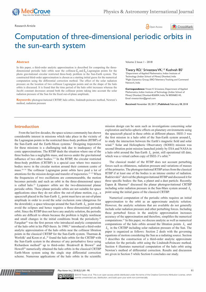
as a single entity and we say this as the Earth. The spacecraft moves under the gravitational influence of the Sun and the Earth (Figure 1). The Sun is assumed as the radiating body contributing solar radiation pressure.

Figure 1 Geometry of the problem in the Sun-Earth system.

Let ( ), ,x y z , ( ), 0, 0µ− , and ( )1 , 0, 0µ− denote the coordinates of the spacecraft, the Sun, and the Earth, respectively, where µ is the mass ratio parameter of the Sun and the Earth. The equations of motion of the spacecraft in the rotating reference frame accounting solar radiation pressure of the Sun can be expressed as,32

2 ,

∂− =

∂

Ux y

x

(1)

2 ,∂

+ =∂

Uy x

y

(2)

,

∂=

∂

Uz

z

(3)

WhereU is the pseudo-potential of the system and it is expressed as

( ) ( )2 2

1 2

1.

2

µ µ+ −= + +

x y qU

r r

(4)

Where q is known as the mass reduction factor, 2r and 2r are the position vectors of the spacecraft from the Sun and the Earth, respectively, and these quantities are defined as,34

( )

( )

2 2 21

2 2 22

ü

: ,

ü

µ

µ

= −

= + + +

= + − + +

p

q

Fq

F

r x y z

r x y z

(5)

In Equation (5), qF and qF are solar radiation pressure and gravitational attraction forces, respectively. Note that when 1=q , the governing equations of motion (1)-(3) reduce to the classical CRTBP.

The Jacobi constant of the motion also exists and is given by

( ) ( )2 2 22 , , .= − + + C U x y z x y z (6)

When the kinetic energy is zero, Equation (6) reduces to

( )2 , , ,=C U x y z (7)

And defines the zero velocity surfaces in the configuration space. These surfaces projected in the rotating −xy plane generate some lines called zero velocity curves.

Analytic computation

We construct a third-order analytic approximation using the method of successive approximation (Lindstedt-Poincare method) to compute the halo orbit around the collinear Lagrangian points 2L and 2L in the photogravitational Sun-Earth system. The origin is translated at the libration points 1L and 2L , and the distance is normalized by taking distance between the Earth to the Lagrangian point as a unit,26 using the new coordinates

( )1

, , ,µ γ

γ γ γ

− −= = =

x y zX Y Z

(8)

Where Y , Y and Z are the new coordinates when origins are shifted at the Lagrangian points, and γ is the distance from the Lagrangian point to the Earth. In Equation (8), the upper (lower) sign corresponds to 2L ( 2L ).

Now using the transformation (8), the equations of motion (1)-(3) are expressed as

( )2 ,γ∂Ψ

− =∂

X YX

(9)

( )2 ,γ∂Ψ

+ =∂

Y XY

(10)

(11)Where

( ) ( )2 2

2

1 2

1.

2

µ µγ

+ −Ψ = + +

X Y q

R R

(12)

In Equation (12), 1R and 2R are given by

( ) ( ) ( )

( ) ( ) ( )

2 2 2

1

2 2 2

2

1 ,

.

γ γ γ γ

γ γ γ γ

= + ± + +

= ± + +

R X Y Z

R X Y Z

(13)

The location of the Lagrangian points 2L and 2L from the Earth are computed from the root of the fifth degree polynomial:

( ) ( ) ( )( )5 4 3 23 3 2 1 1 2 0.γ µ γ µ γ µ µ γ µγ µ± − + − − − ± ± − = q (14)

In Equation (14) upper and lower signs correspond to 2L and 2L points, respectively. We expand the nonlinear terms,

( )1 2

1 µ µ−+

q

R R , in

Equation (12) using the formula,26

(15)

,γ∂Ψ

=∂

ZZ

( ) ( ) ( )2 2 2 0

1 1,

ρ

ρ

∞

=

+ +∑=

− + − + −

m

mm

Ax By CzP

D D Dx A y B z C

Computation of three-dimensional periodic orbits in the sun-earth system 83Copyright:

©2018 Tiwary et al.

Citation: Tiwary RD, Srivastava VK, Kushvah BS. Computation of three-dimensional periodic orbits in the sun-earth system. Phys Astron Int J. 2018;2(1):81‒90. DOI: 10.15406/paij.2018.02.00052

Where 2 2 2 2= + +D A B C and 2 2 2 2ρ = + +x y z , and ρ

m

xP

is the thm degree Legendre polynomial of first kind with argument. After some algebraic manipulation, the equations of motion (9)-(11) can be written as:35,36

( )2

32 1 2 ,ρ

ρ

∞

≥

∂∑− − + =

∂

mm m

m

XX Y c X c P

X

(16)

( )23

2 1 ,ρρ

∞

≥

∂∑+ + − =

∂

mm m

m

XY X c Y c P

Y

(17)

23

,ρρ

∞

≥

∂∑+ =

∂

mm

mm

XZ c Z c P

Z

(18)

Where the left hand side contains the linear terms and the right hand side contains the nonlinear terms. The coefficient ( )µmc is expressed as

( ) ( ) ( ) ( )( )

1

13

111 1 , 0,1, 2, ...

1

µ γµ µ

γ γ

+

+

−= ± + − =

mm m

m m

qc m

(19)

Where the upper sign is for 2L and the lower one for 2L .

A third-order approximation of Equations (16)-(18) is given by,25

( ) ( ) ( )2 2 2 2 2 22 3

32 1 2 2 2 2 3 3 ,42

− − + = − − + − − X Y c X c X Y Z c X X Y Z

(20)

( ) ( )2 2 22 3 4

32 1 3 4 ,

2+ + − = − − − − Y X c Y c XY c Y X Y Z

(21)

( )2 2 22 3 4

33 4 .

2+ = − − − −Z c Z c XZ c Z X Y Z

(22)

A correction term 22λ∆ = − c

is required for computing the halo orbit which is introduced on the left-hand-side of Equation (22) to make the out-of-plane frequency equals to the in-plane frequency. The new third-order z -equation then becomes:

( )2 2 2 23 4

33 4 .

2λ+ = − − − − + ∆Z Z c XZ c Z X Y Z Z

(23)

While using the successive approximation procedure, some secular terms arise. To avoid the secular terms, one uses a new independent variable τ and introduces a frequency connection ω through τ ω= t. The equations of motion (20), (21) & (23) can be then rewritten in terms of new independent variableτ :

( ) ( ) ( )2 2 2 2 2 2 22 3 4

32 1 2 2 2 2 3 3 ,

2ω ω′′ ′− − + = − − + − −X Y c X c X Y Z c X X Y Z (24)

( ) ( )2 2 2 22 3 4

32 1 3 4 ,

2ω ω′′ ′+ + − = − − − −Y X c Y c XY c Y X Y Z

(25)

( )2 2 2 2 23 4

33 4 ,

2ω λ′′ + = − − − − + ∆Z Z c XZ c Z X Y Z Z

(26)

Where 2

2

",

τ τ′ ′′= =

dX d XX X

d d etc.

We assume the solutions of Equations (24)-(26), using the perturbation technique, of the form:

( ) ( ) ( ) ( )( ) ( ) ( ) ( )( ) ( ) ( ) ( )

2 31 2 3

2 31 2 3

2 31 2 3

...,

...,

...,

τ ε τ ε τ ε τ

τ ε τ ε τ ε τ

τ ε τ ε τ ε τ

= + + +

= + + +

= + + +

X X X X

Y Y Y Y

Z Z Z Z

(27)

And

(28)

In Equation (28) ∈ is the perturbation parameter. Using Equations (27) & (28) into Equations (24)-(26) and equating the coefficient of the same order of∈ , 2∈ , and 3∈ from both sides we get the first, second, and third-order equations, respectively.1

a. First order equations

The first order linearized equations are given by

( )22 1 0,+ + − = Y X c Y (29)

( )22 1 0,+ + − = Y X c Y (30)

2 0,λ+ =Z Z (31)

Whose periodic solutions are given by:

( ) ( )( ) ( )( ) ( )

cos ,

sin ,

sin .

λ φ

κ λ φ

λ ψ

= − +

= +

= +

X

X

Z

X t A t

Y t A t

Z t A t

(32)

b. Second order equations

Collecting the coefficients of 2∈ , we get( ) ( ) ( )2 2 2

2 2 2 2 1 1 1 3 1 1 1

32 1 2 2 2 ,

2ω′′ ′ ′′ ′− − + = − − + − −X Y c X X Y c X Y Z (33)

( ) ( )2 2 2 2 1 1 1 3 1 12 1 2 3 ,ω′′ ′ ′′ ′+ + − = − + −Y X c Y Y X c X Y (34)

22 2 1 1 1 132 3 .λ ω′′ ′′+ = − −Z Z Z c X Z (35)

Now using Equation (32) into (33)-(35), the following equations are obtained

( ) ( )2 2 2 2 1 1 1 1 1 2 22 1 2 2 cos cos 2 cos 2 ,ω λ κ λ τ α γ τ γ τ′′ ′− − + = − + + +XX nY c X A (36)

( ) ( )2 2 2 2 1 1 1 12 1 2 1 sin sin 2 ,ω λ κλ τ β τ′′ ′+ + − = − +XY X c Y A (37)

( ) ( )2 22 2 1 2 1 1 2 2 2 12 sin sin sin ,λ ω λ τ δ τ τ δ τ τ′′ + = + + + −ZZ Z A (38)

Where 1 2,τ λτ φ τ λτ ψ= + = + . Equations (36)-(38) are a set of non-homogenous linear differential equations whose bounded homogenous solution is incorporated from the first-order equations. We need to find only particular solutions of (36)-(38). The secular terms 1sinτ , 2sinτ and 2sinτ are eliminated by setting 1 0ω = . Hence, the solutions of the second-order equations are given by

( ) ( ) ( )( ) ( ) ( )( ) ( ) ( )

2 21 1 22 2

2 21 1 22 2

2 21 1 2 22 2 1

20 cos 2 cos 2 ,

sin 2 sin 2 ,

sin sin .

τ ρ ρ τ ρ τ

τ σ τ σ τ

τ κ τ τ κ τ τ

= + +

= +

= + + −

X

Y

Z

(39)

c. Third order equations

Now collecting the coefficients of 3∈ and setting 1 0ω = , we get

(40)

(41)

(42)

Using Equations (32) and (39) into Equations (40)-(42), we get

(43)

( ) ( ) ( ) ( )2 31 2 31 ... ..., 1.ω εω τ ε ω τ ε ω τ ε ω τ ω= + + + + + + <i

i iwhere

( ) ( ) ( ) ( )2 2 23 3 2 3 2 1 1 3 1 2 1 2 1 2 4 1 1 12 1 2 2 3 2 2 2 3 3 ,ω′′ ′ ′′ ′− − + = − − + − − + − −X Y c X X Y c X X Y Y Z Z c X X Y Z

( ) ( ) ( ) ( )2 2 23 3 2 3 1 1 3 1 2 2 1 4 1 1 1 12

32 1 2 3 4 ,

2ω′′ ′ ′′ ′+ + − = − + − + − − −Y X c Y Y X c X Y X Y c Y X Y Z

( ) ( )2 2 2 23 3 2 1 1 3 2 1 1 2 4 1 1 1 12

32 3 4 .

2λ ω

∆′′ ′′+ = − + − + − − −

∈Z Z Z Z c X Z X Z c Z X Y Z

( ) ( ) ( ) ( )3 3 2 3 1 2 1 3 1 4 2 1 5 2 12 1 2 2 cos cos cos 2 cos 2 ,υ ω λ κ λ τ γ τ γ τ τ γ τ τ′′ ′− − + = + − + + + + − XX Y c X A n

Computation of three-dimensional periodic orbits in the sun-earth system 84Copyright:

©2018 Tiwary et al.

Citation: Tiwary RD, Srivastava VK, Kushvah BS. Computation of three-dimensional periodic orbits in the sun-earth system. Phys Astron Int J. 2018;2(1):81‒90. DOI: 10.15406/paij.2018.02.00052

(44)

(45)

The secular terms in the 3 3−X Y equations (43)-(44) and in the 2ω equation (45) cannot be removed by setting a value of 2ω .

1 These terms from Equations. (43)-(45) are removed by adjusting phases of

2τ and 2τ so that ( )1 2 2sin 2 ~ sinτ τ τ− which can be achieved by setting the phase constraint relationship

, 0,1, 2, 3.

2

πφ ψ= + =p where p (46)

After removing the secular terms from Equation (46), the 3Z solution is bounded when

(47)

The phase constraint (47) reflects the 3 3−X Y equations, each now contains one secular term. The secular terms from both equations are removed by using a single condition from their particular solutions:

( )( ) ( )( )1 2 5 2 2 52 2 0.ν ω λ κ λ ζγ κ ν ω λ κ λ ζβ+ − + − + − + =X XA A n (48)

Condition (48) is satisfied if

(49)

Where similar type of expressions for 1s and 2s can be referred in.1 Substituting the value of 2ω from Equation (49) into Equation (48), we get

(50)

Where similar type of expressions for 1l and 2l can be followed from.1 Equation (50) gives a relationship between the in-plane and the out-of-plane amplitudes. Assuming these constraints, the third-order equations become

( ) ( )3 3 2 3 6 1 3 4 12 1 2 cos cos3 ,X Y c X κβ τ γ ζγ τ′′ ′− − + = + + (51)

( ) ( )3 3 2 3 6 1 3 4 12 1 sin sin 3 ,Y X c Y β τ β ζβ τ′′ ′+ + − = + + (52)

(53)

Where ( )6 2 2 52 1XAβ ν ω λ λκ ζβ= + − + . Thus, the solutions of Equations (51)-(53) are given as

(54)

The expressions for all the coefficients can be referred to.29

d. Final approximation

Halo orbits of third-order approximations are obtained on removing ∈ from all solutions of equations by using the transformation

∈X XA A and ∈Z ZA A . Then one can use ZA or ZA as a small parameter. Combining the above computed solutions, the third-order approximate solution is thus given by

(55)

Time period (in non-dimensional form) of the halo orbit is expressed as

1 2 1

2, 1 ; 0.

πω ω ω ω

λω= = + + =haloT where (56)

Numerical computation

In this section, Newton’s method of differential correction is briefly described for the numerical computation of halo orbit. Assume X denote a column vector containing all of the six state variables of

the governing equations of motion, i.e.,

[ ] ,=

TX x y z x y z (57)

Where superscript “ T ” denotes the transpose.

The state transition matrix (STM), 6 6× , is a 6 6× matrix composed of the partial derivatives of the state:

(58)

With initial conditions ( )0 0,Φ =t t I . Note that the state transition matrix is called monodromy matrix for the full periodic orbit. The eigenvalues of the monodromy matrix tells about the stability of the halo orbit.

The STM is propagated using the relationship:

( ) ( ) ( )0

0

,, ,

Φ= Φ

d t tA t t t

dt

(59)

Where the matrix ( )A t is known as variational matrix and is made of the partial derivatives of the state derivative with respect to the state variables, i.e.,

( ) ( )

( ).

∂=∂

X tA t

X t (60)

The variation matrix 3 3× can be partitioned into four 3 3× sub-matrices:

( ) ,2

=ϒ Ω

O IA t

(61)

( ) ( ) ( ) ( )3 3 2 3 2 2 1 3 1 4 1 2 5 2 12 1 2 1 sin sin 3 sin 2 sin 2 ,ν ω λ λκ τ β τ β τ τ β τ τ′′ ′+ + − = + − + + + + − XY X c Y A

( ) ( )2 23 3 3 2 2 3 2 4 1 2 5 1 222 sin sin 3 sin 2 sin 2 .λ ν ω λ τ δ τ δ τ τ δ τ τ

∆′′ + = + + + + + + −

∈

ZZ Z A

( )23 2 522 0, -1 .ν ω λ ζδ ζ

∆+ + + = =

∈

p

ZA

( )( )

2 21 2 5 52 1 22

,2 1 2

ν κν ζ γ κβω

λ λ κ κ

− + −= = +

+ − X Z

X

s A s AA

2 21 2 2 0,

∆+ + =

∈X Zl A l A

( ) ( )

( ) ( )

23 4 12

3 3 12

4 3 1

1 sin 3 , 0,2,

1 cos3 , 1,3,

p

p

pZ Z

p

δ δ τλ

δ δ τ−

− + =′′+ = − − =

( )( )

( ) ( )

( )

3 31 1

3 31 1 32 1

231 1

3 12

132

cos 3 ,

sin 3 sin ,

1 sin 3 , 0, 2,

1 cos 3 , 1, 3.

τ ρ τ

τ σ τ σ τ

κ ττ

κ τ−

=

= +

− ==

− =

p

p

X

Y

pZ

p

( ) ( )( ) ( ) ( )

( ) ( ) [ ]

( ) [ ]

20 1 21 22 1 31 1

32 1 21 22 1 31 1

21 21 1 31 1

12

1 21 1 22 32 1

cos cos 2 cos 3 ,

sin sin 2 sin 3 ,

1 sin sin 2 sin 3 , 0, 2

1 cos cos 2 cos 3 , 1, 3.

τ ρ τ ρ ζρ τ ρ τ

τ κ σ τ σ ζσ τ σ τ

τ κ τ κ ττ

τ κ τ κ κ τ−

= − + + +

= + + + +

− + + ==

− + + + =

X

X

p

Z

p

Z

X A

Y A

A pZ

A p

( ) ( )( )0

0

, ,∂

Φ =∂

X tt t

X t

Computation of three-dimensional periodic orbits in the sun-earth system 85Copyright:

©2018 Tiwary et al.

Citation: Tiwary RD, Srivastava VK, Kushvah BS. Computation of three-dimensional periodic orbits in the sun-earth system. Phys Astron Int J. 2018;2(1):81‒90. DOI: 10.15406/paij.2018.02.00052

Where

(62)

Note that the matrix U is a symmetric matrix of second order partial derivatives of U with respect to x , y , and z evaluated along the orbit. Thus, Equation (59) represents a system of 36 first-order differential equations. These equations, coupled with the equations of motion (1)-(3), are the basic equations that define the dynamical model in the photo-gravitational CRTBP accounting solar radiation pressure. Trajectories are computed by simultaneous numerical integration of the 42 first-order differential equations. It can be easily seen that the governing equations of motion (1)-(3) are symmetric about the −xzplane by using the transformation → −y y and → −t t .

Let ( )0X t be the state of a periodic symmetric orbit at the −xzplane crossing and let ( )

2TX t denotes the state of the orbit half of

its orbital period later at the −xz plane. If the orbit is periodic and symmetric about the −xz plane, then

( ) [ ] ( )0 0 02 2 2 2

0 0 0 0 0 0 .= ⇒ =

TT

T T T TX t x z y X t x z y (63)

Assume that ( )0X t be an initial state of a desirable state. Integrating this state forward in time until the next −xz plane crossing, we obtain the state ( )ˆ

2

ˆTX t :

( )ˆ ˆ ˆ ˆ ˆ2 2 2 2 2

ˆ 0 .=

T

T T T T TX t x z x y z (64)

We adjust the initial state of the trajectory in such a way so that the values of ˆ

2

Tx and ˆ2

Tz become zero. Note that by adjusting the initial state, not only the values of x and z change, but the propagation time, ˆ

2T , needed to penetrate the −xz plane also changes. In order

to target a proper state ( )2

TX t , one may vary the initial values of z , z and/or y . The linearized system of equations relating the final state to the initial state can be written as:

( ) ( ) ( ) ( )0 02 2

, ,2

δ δ δ∂

≈ Φ +∂

T T

X TX t t t X tt

(65)

Where ( )2

δ TX t denotes the deviation in the final state due to a deviation in the initial state, ( )0δ X t , and a corresponding deviation in the orbit’s period, ( )2

δ T .

Results and discussionThe variation in the locations of 1L and 2L with the mass reduction

factor, q are given in Table 1 from the Barycenter. It can be observed that as the value of 1L decreases, the distance between 1L ( 2L ) and the Barycenter decreases (increases). Thus, as solar radiation pressure dominates, the location of 1L moves towards the Sun while that of 2Lmoves away from the Sun.

Halo orbits are computed using the constructed third-order analytic approximate solution as the starting initial guess. Figures 2–5 are generated using the following characteristic properties of ISEE-3

mission:37 mass of the spacecraft 435= kg; solar reflectivity constant,1.2561=k ; spacecraft effective cross sectional area, 3.55=A m2;

speed of light, 82.998 10= ×c m/sec; solar light flux, 0 1352.098 =S kg/sec2 at one astronomical unit from the Sun. We have chosen the out-of-plane amplitude, =ZA 1,10000km of ISEE-3, for the sake of simplicity, the corresponding value of the in-plane amplitude, XA is 2,06000km.

Table 1 Variation of 1L and 2L locations vs q with-63.0402988 10µ = ×

qBarycentric Distance of 1L

Barycentric Distance of 2L

1.000000 0.98998611876418 1.01007439102449

0.999934 0.98997872566874 1.01008168361141

0.999668 0.98994870654538 1.01011129019736

0.999336 0.98991073085203 1.01014873382821

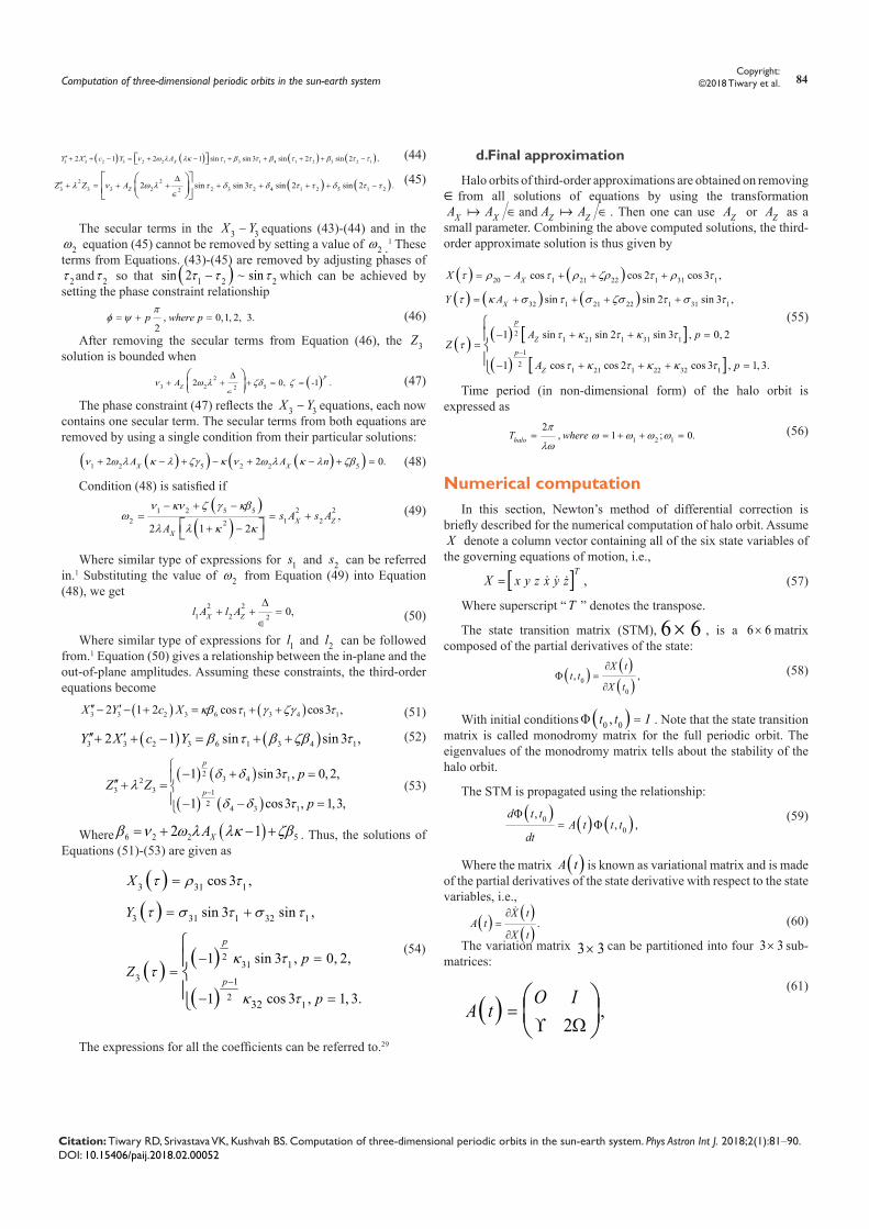
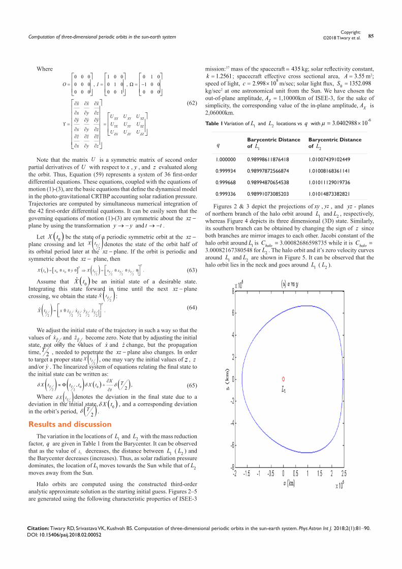
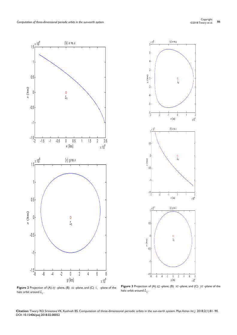
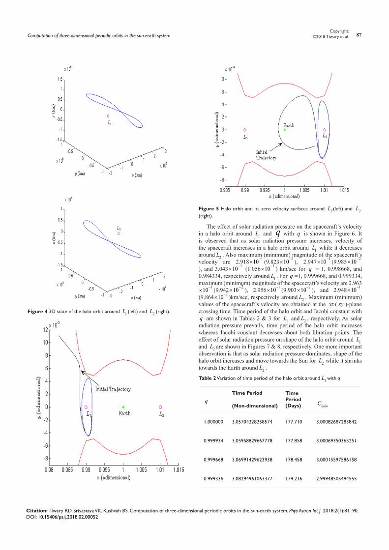
Figures 2 & 3 depict the projections of xy , yz , and yz - planes of northern branch of the halo orbit around 1L and 2L , respectively, whereas Figure 4 depicts its three dimensional (3D) state. Similarly, its southern branch can be obtained by changing the sign of z since both branches are mirror images to each other. Jacobi constant of the halo orbit around 1L is =haloC 3.00082686598735 while it is =haloC3.00082167380548 for 2L . The halo orbit and it’s zero velocity curves around 1L and 2L are shown in Figure 5. It can be observed that the halo orbit lies in the neck and goes around 1L ( 2L ).

0 0 0 1 0 0 0 1 00 0 0 , 0 1 0 , 1 0 00 0 0 0 0 1 0 0 0

= = Ω = −

∂ ∂ ∂

∂ ∂ ∂∂ ∂ ∂

ϒ = =∂ ∂ ∂∂ ∂ ∂

∂ ∂ ∂

XX XY XZ

YX YY YZ

ZX ZY ZZ

O I

x x x

x y zU U U

y y yU U U

x y z U U Uz z z

x y z

Computation of three-dimensional periodic orbits in the sun-earth system 86Copyright:

©2018 Tiwary et al.

Citation: Tiwary RD, Srivastava VK, Kushvah BS. Computation of three-dimensional periodic orbits in the sun-earth system. Phys Astron Int J. 2018;2(1):81‒90. DOI: 10.15406/paij.2018.02.00052

Figure 2 Projection of (A) xy -plane, (B) xz -plane, and (C) 1L -plane of the halo orbit around 1L .

Figure 3 Projection of (A) xz -plane, (B) xz -plane, and (C) yz -plane of the halo orbit around 2L .

Computation of three-dimensional periodic orbits in the sun-earth system 87Copyright:

©2018 Tiwary et al.

Citation: Tiwary RD, Srivastava VK, Kushvah BS. Computation of three-dimensional periodic orbits in the sun-earth system. Phys Astron Int J. 2018;2(1):81‒90. DOI: 10.15406/paij.2018.02.00052

Figure 4 3D state of the halo orbit around 1L (left) and 2L (right).

Figure 5 Halo orbit and its zero velocity surfaces around 2L (left) and 2L(right).

The effect of solar radiation pressure on the spacecraft’s velocity in a halo orbit around 1L and q with q is shown in Figure 6. It is observed that as solar radiation pressure increases, velocity of the spacecraft increases in a halo orbit around 1L while it decreases around 2L . Also maximum (minimum) magnitude of the spacecraft’s velocity are 2.918 110−× (9.823 210−× ), 2.947 110−× (9.985 210−×), and 3.043 110−× (1.056 110−× ) km/sec for q = 1, 0.998668, and 0.984334, respectively around 1L . For q =1, 0.999668, and 0.999334, maximum (minimum) magnitude of the spacecraft’s velocity are 2.963

110−× (9.942 210−× ), 2.956 110−× (9.903 210−× ), and 2.948 110−×(9.864 210−× )km/sec, respectively around 2L . Maximum (minimum) values of the spacecraft’s velocity are obtained at the xz ( xy )-plane crossing time. Time period of the halo orbit and Jacobi constant with q are shown in Tables 2 & 3 for 1L and 2L , respectively. As solar radiation pressure prevails, time period of the halo orbit increases whereas Jacobi constant decreases about both libration points. The effect of solar radiation pressure on shape of the halo orbit around 1L and 2L are shown in Figures 7 & 8, respectively. One more important observation is that as solar radiation pressure dominates, shape of the halo orbit increases and move towards the Sun for 2L while it shrinks towards the Earth around 2L .

Table 2 Variation of time period of the halo orbit around 1L with q

qTime Period

(Non-dimensional)

Time Period (Days) haloC

1.000000 3.05704228258574 177.710 3.00082687283842

0.999934 3.05958829667778 177.858 3.00069350365251

0.999668 3.06991429623938 178.458 3.00015597586158

0.999336 3.08294961063377 179.216 2.99948505494555

Computation of three-dimensional periodic orbits in the sun-earth system 88Copyright:

©2018 Tiwary et al.

Citation: Tiwary RD, Srivastava VK, Kushvah BS. Computation of three-dimensional periodic orbits in the sun-earth system. Phys Astron Int J. 2018;2(1):81‒90. DOI: 10.15406/paij.2018.02.00052

Table 3 Variation of time period of the halo orbit around q with q

qTime Period

(Non-dimensional)

Time Period (Days) haloC

1.000000 3.09884183709780 180.140 3.00082168051684

0.999934 3.10140754272003 180.289 3.00069103137700

0.999668 3.11181365407607 180.894 3.00016446672677

0.999336 3.12495070966240 181.658 2.99950723047497

Figure 6 Velocity variation of the spacecraft in the halo orbit with q around

1L (left) and 2L (right).Figure 7 Variation in shape of (A) xz -plane, (B) xz -plane, and (C) yz -plane of the halo orbit with q around 1L

Computation of three-dimensional periodic orbits in the sun-earth system 89Copyright:

©2018 Tiwary et al.

Citation: Tiwary RD, Srivastava VK, Kushvah BS. Computation of three-dimensional periodic orbits in the sun-earth system. Phys Astron Int J. 2018;2(1):81‒90. DOI: 10.15406/paij.2018.02.00052

Figure 8 Variation in shape of (A) xy -plane, (B) yz -plane, and (C) yz -plane of the halo orbit with q around 2L .

According to Floquet theory,26,38,39 stability of the halo orbits is described by the eigenvalues of its monodromy matrix. The monodromy matrix corresponding to the halo orbit around 1L and 2Lhas six eigenvalues ( )1 2 3 4 5 6, , , , ,λ λ λ λ λ λ which are given by

(71)

And

(72)

for 1L and 2L , respectively.

The periodic orbit is stable only if the modulus of all eigenvalues of its monodromy matrix is less than one.28 It can be noted that for these orbits two eigenvalues are non-unity ( 1λ and 2λ ) near both 1L and 2L, and the complex eigenvalues lie on the unit circle. Thus, there exists both stable and unstable halo orbits, and orbits near the halo which remain near the halo for all time around 2L and 2L . The eigenvectors corresponding to stable and unstable eigenvalues direct stable and unstable manifolds of the orbit whereas complex eigenvalues correspond to the center directions of the orbit. The eigenvalues show that halo orbits have ×saddle center and × ×saddle center centertypecharacteristics behavior around 1L and 2L points, respectively.

ConclusionIn this study, a third-order analytic approximate solution using

the Lindstedt-Poincare method and Newton’s single step differential correction scheme are used to compute the halo orbit analytically and numerically around the collinear points 1L and 2L in the photogravitational circular restricted three-body problem accounting radiation pressure of the Sun. The effects of solar radiation pressure are studied around both collinear libration points. For q = 1, 0.999934, 0.999668, and 0.999336, the Barycentric distance of 2L ( 2L ) are 1.481019 810× (1.511071 810× ), 1.481008 810× (1.511082 810×), 1.480963 810× (1.511126 810× ), and 1.480906 810× (1.511183

810× ) kilometers, respectively for 1L ( 2L ) which shows that as solar radiation pressure dominates, the distance between 1L ( 2L ) and the Barycenter decreases (increases). The achieved maximum (minimum) velocity (in terms of magnitude) of the spacecraft are 2.918 210−×(9.823 210−× ), 2.947 110−× (9.985 210−× ), and 3.043 110−× (1.056

110−× )km/sec around 1L whereas around 2L are 2.963 110−× (9.942210−× ), 2.956 110−× (9.903 210−× ), and 2.948 110−× (9.864 210−× )

km/sec, respectively for 1L =1, 0.999668, and 0.999334, respectively. In other words, as solar radiation pressure increases, velocity of the spacecraft increases around 1L point while it decreases around 2Lpoint. It is found that time period of the halo orbit increases around both 1L and 2L points. Further, as solar radiation pressure dominates, shape of the halo orbit around 1L increases and moves towards the Sun while it shrinks around 2L and moves towards the Earth. The eigenvalues of the monodromy matrix depict that the halo orbits have ×saddle center ( 1L ) and × ×saddle center center ( 2L ) type of behavior in the photogravitational circular restricted three-body problem for the Sun-Earth system.

AcknowledgementsNone.

Conflicts of interestAuthors declare there is no conflict of interest.

( )1732.916, 0. 0005770619,1.0000018,1.0000018, 0. 9999982, 0.9968152 0.0797459 ,± i

( )1664.2099, 0.00060088575, 0.9970228 0.0771079 ,1.000000 0.0000024 ,± ±i i

Computation of three-dimensional periodic orbits in the sun-earth system 90Copyright:

©2018 Tiwary et al.

Citation: Tiwary RD, Srivastava VK, Kushvah BS. Computation of three-dimensional periodic orbits in the sun-earth system. Phys Astron Int J. 2018;2(1):81‒90. DOI: 10.15406/paij.2018.02.00052

References1. Thurman R, Worfolk PA. The geometry of halo orbits in the circular

restricted three-body problem. Technical report. CiteSeerX, USA; 1996.

2. Schuerman DW. The restricted three-body problem including radiation pressure. The Astrophysical Journal. 1980;238:337–342.

3. Simmons JFL, McDonald AJC, Brown JC. The restricted 3-body problem with radiation pressure. Celestial mechanics. 1985;35(2):145–187.

4. Ragos O, Zafiropoulos FA. A numerical study of the influence of the Poynting-Robertson effect on the equilibrium points of the photogravitational restricted three-body problem. I. Coplanar case. Astronomy and Astrophysics. 1995;300:579–590.

5. McInnes CR. Solar Sailing: Technology, Dynamics and Mission Applications. Springer-Verlag, Berlin, Germany. 1990.

6. Waters TJ, McInnes CR. Periodic orbits above the ecliptic in the solar-sail restricted three-body problem. Journal of Guidance Control and Dynamics. 2007;30(3):687–693.

7. Kishor R, Kushvah BS. Periodic orbits in the generalized photogravitational Chermnykh-like problem with power-law profile. Astrophysics and Space Science. 2013;344(2):333–346.

8. Verrier P, Waters W, Sieber J. Evolution of the L1 halo family in the radial solar sail circular restricted three-body problem. Celestial Mechanics and Dynamical Astronomy. 2014;120(4):373–400.

9. Srivastava VK, Kumar J, Kushvah BS. The effects of oblateness and solar radiation pressure on halo orbits in the photogravitational Sun-Earth system. Acta Astronautica. 2014;129:389–399.

10. Moulton FR. An Introduction to Celestial Mechanics. Kessinger Publishing, USA. 1914.

11. McCuskey SW. Introduction to Celestial Mechanics. Dover Publications, USA. 1963.

12. Szebehely V. Theory of Orbits, The Restricted Problem of Three Bodies. Academic Press, USA. 1967.

13. Baoyin H, McInnes C. Solar sail halo orbits at the Sun-Earth artificial L1 point. Celestial Mechanics and Dynamical Astronomy. 2006;94(2):155–171.

14. Heiligers J, McInnes C. Novel Solar Sail Mission Concepts for Space Weather Forecasting. 24th AAS/AIAA Space Flight Mechanics Meeting. Santa Fe, New Mexico, USA, 2014. p. 1–20.

15. Farquhar RW, Kamel AA. Quasi-periodic orbits about the translunar libration point. Celestial mechanics. 1973;7(4):458–473.

16. D’Amario LA, Bright LE, Wolf AA. Galileo trajectory design. Space Science Reviews. 1992;60(1–4):23–78.

17. Martin WL. Libration point trajectory design. Numerical Algorithms. 1997;14(1–3):153–164.

18. Gomez G, Koon WS, Martin WL, et al. Connecting orbits and invariant manifolds in the spatial restricted three-body problem. Nonlinearity. 2004;17(5):1571–1606.

19. Xu R, Cui P, Qiao D, et al. Design and optimization of trajectory to Near-Earth asteroid for sample return mission using gravity assists. Advances in Space Research. 2007;40(20):220–225.

20. Pergola P, Geurts K, Casaregola C, et al. Earth–Mars halo to halo low thrust manifold transfers. Celestial Mechanics and Dynamical Astronomy. 2009;105.

21. Landgraf M, Renk F, Vogeleer BD. Mission design and analysis of European astrophysics missions orbiting libration points. Acta Astronautica. 2013;84:49–55.

22. Vaquero M, Howell KC. Design of transfer trajectories between resonant orbits in the Earth–Moon restricted problem. Acta Astronautica. 2014;94(1):302–317.

23. Farquhar RW. The control and Use of Libration-Point Satellites. Department of Aeronautics and Astronautics, Stanford University, USA; 1968. p. 1–138.

24. Zazzera FB, Topputo F, Massari M. Assessment of Mission Design Including Utilization of Libration Points and Weak Stability Boundaries. ESA, ACT, France; 2005. p. 1–173.

25. Richardson DL. Analytic construction of periodic orbits about the collinear points. Celestial Mechanics. 1980;22(2):241–253.

26. Koon WS, Lo MW, Marsden JE. Dynamical Systems: The Three-Body Problem and Space Mission Design. Interdisciplinary Applied Mathematics, Springer, Berlin, Germany; 2011. p. 1–331.

27. Breakwell JV, Brown JV. The ‘Halo’ family of 3-dimensional periodic orbits in the Earth-Moon restricted 3-body problem. Celestial mechanics. 1979;20(4):389–404.

28. Howell KC. Three-dimensional, periodic, ‘halo’ orbits. Celestial mechanics. 1984;32(1):53–71.

29. Tiwary RD, Kushvah BS. Computation of halo orbits in the photogravitational Sun-Earth system with oblateness. Astrophysics and Space Science. 2015;73:357.

30. Dunham DW, Farquhar RW. Libration point missions, 1978–2002. In: Gómez G, et al. editors. Proceedings of the Conference on Libration Point Orbits and Applications, World Scientific, Singapore; 2003.

31. Radzievskii VV. Astronomical Journal USSR. 1950;27(5):250.

32. Eapen RT, Sharma RK. A study of halo orbits at the Sun–Mars L1 Lagrangian point in the photogravitational restricted three-body problem. Astrophysics and Space Science. 2014;352(2):437–441.

33. Bell JL. The impact of solar radiation pressure on Sun-Earth L1 Libration point orbits. MS thesis, Department of Aeronautics and Astronautics, Purdue University, USA. 1991.

34. Srivastava VK, Kumar J, Kushvah BS. Regularization of circular restricted three-body problem accounting radiation pressure and oblateness. Astrophysics and Space Science. 2017;362.

35. Jorba A, Masdemont J. Dynamics in the center manifold of the collinear points of the restricted three body problem. Physica D. 1999;132(1–2):189–213.

36. Bucciarelli S, Ceccaroni M, Celletti A. Annali di matematica pura e applicata 01, Springer, Germany. 2015.

37. Pernicka HJ. The numerical determination of nominal Libration point trajectories and development of a stationkeeping strategy. Department of Aeronautics and Astronautics, Purdue University, USA. 1990.

38. Baig S, McInnes MC. Artificial halo orbits for low-thrust propulsion spacecraft. Celestial Mechanics and Dynamical Astronomy. 2009;104(4):321–335.

39. Gomez G, Mondelo, JM. The dynamics around the collinear equilibrium

points of the RTBP. Physica D. 2001;157(4):283–321.