Computation of Riemann solutions using the Dafermos regularization and continuation

DISCRETE AND CONTINUOUS Website: http://AIMsciences.orgDYNAMICAL SYSTEMSVolume 10, Number 4, June 2004 pp. 965–986

COMPUTATION OF RIEMANN SOLUTIONS USING

THE DAFERMOS REGULARIZATION AND CONTINUATION

Stephen Schecter

Department of MathematicsNorth Carolina State University, Raleigh, NC 27695-8205

Bradley J. Plohr

Departments of Mathematics and of Applied Mathematics and StatisticsUniversity at Stony Brook, Stony Brook, NY 11794-3651

Dan Marchesin

Instituto de Matematica Pura e AplicadaEstrada Dona Castorina 110, 22460 Rio de Janeiro, RJ, Brazil

Abstract. We present a numerical method, based on the Dafermos regularization,for computing a one-parameter family of Riemann solutions of a system of conser-vation laws. The family is obtained by varying either the left or right state of theRiemann problem. The Riemann solutions are required to have shock waves thatsatisfy the viscous profile criterion prescribed by the physical model. The system isnot required to satisfy strict hyperbolicity or genuine nonlinearity; the left and rightstates need not be close; and the Riemann solutions may contain an arbitrary num-ber of waves, including composite waves and nonclassical shock waves. The methoduses standard continuation software to solve a boundary-value problem in which theleft and right states of the Riemann problem appear as parameters. Because thecontinuation method can proceed around limit point bifurcations, it can sucessfullycompute multiple solutions of a particular Riemann problem, including ones thatcorrespond to unstable asymptotic states of the viscous conservation laws.

1. Introduction.

1.1. Conservation laws. A system of conservation laws

ut + f(u)x = 0, (1.1)

where u(x, t) ∈ Rn and f : R

n → Rn, admits solutions with jump discontinuities

called shock waves. The simplest take the form

u(x, t) =

{

u− for x < st,

u+ for x > st.(1.2)

For the shock wave (1.2) to be a weak solution of system (1.1), the triple (u−, s, u+)must satisfy the Rankine-Hugoniot condition

f(u+)− f(u−)− s(u+ − u−) = 0. (1.3)

2000 Mathematics Subject Classification. 35L65, 35L67, 35K50.Key words and phrases. conservation law, viscous conservation law, Riemann problem, viscous

profile, Dafermos regularization, continuation, numerical method.This work was supported in part by: the NSF under Grant DMS-9973105; the NSF under

Grant DMS-9732876; the DOE under Grant DE-FG02-90ER25084; the ARO under Grant 38338-MA; CNPq under Grant 300204/83-3; CTPETRO/FINEP under Grant 21.01.0248.00; and ANPunder Grant PRH-32.

965

966 SCHECTER, PLOHR, AND MARCHESIN

However, too many discontinuities of the form (1.2) satisfy condition (1.3). Themeaningful discontinuities must be selected based on physical modeling.

A viscous regularization of system (1.1) is a partial differential equation of theform

ut + f(u)x = ε(B(u)ux)x, (1.4)

where ε > 0 and B(u) is an n × n matrix for which all eigenvalues have positivereal part. A system of conservation laws (1.1) is an approximation of a viscoussystem (1.4) obtained by setting ε = 0 in a situation where ε is small. Courantand Friedrichs [4] and Gelfand [8] therefore proposed that, if system (1.1) arises inthis way, then a shock wave (1.2) should be admitted as a solution of system (1.1)provided that Eq. (1.4) has a traveling wave solution

uε(x, t) = u

(

x− st

ε

)

(1.5)

that satisfies the boundary conditions

u(−∞) = u−, u(+∞) = u+. (1.6)

Such a solution uε converges to the shock wave (1.2) as ε → 0+. If a travelingwave solution of Eq. (1.4) exists, then the shock wave (1.2) is said to satisfy theviscous profile criterion for B(u). A traveling wave solution of Eq. (1.4) satisfyingthe boundary conditions (1.6) exists if and only if the traveling wave ODE

u = B(u)−1 [f(u)− f(u−)− s(u− u−)] (1.7)

has an equilibrium at u+ (it automatically has one at u−) and a connecting orbitfrom u− to u+.

Suppose that Df(u−) is strictly hyperbolic (i.e., its eigenvalues are real anddistinct) and the genuine nonlinearity condition [21] is satisfied at u−. Then foreach eigenvalue λ of Df(u−), there exists a curve u+(s), defined for s near λ, withu+(λ) = u−, and tangent at u− to the corresponding eigendirection of Df(u−),such that each triple (u−, s, u+(s)) satisfies the Rankine-Hugoniot condition (1.3)(see, e.g., Ref. [21]). If, in addition, B(u−) is strictly stable with respect to Df(u−),then for s sufficiently close to λ, there is a connecting orbit of the traveling waveODE (1.7) joining u− to u+(s) if and only if s < λ [16]. Thus, for u+ close to u−,existence of the connecting orbit is rather insensitive to the viscosity matrix that isused. However, for a solution (u−, s, u+) of the Rankine-Hugoniot condition (1.3)with u+ farther from u−, existence of a connecting orbit depends strongly on B(u).

1.2. Riemann problems. The most basic initial-value problem for the system ofconservation laws (1.1) is the Riemann problem:

u(x, 0) =

{

uL for x < 0,

uR for x > 0.(1.8)

In conformance with the scale-invariance of system (1.1) and the initial condi-tions (1.8), a solution is expected to have the form u(x, t) = u(ξ), where ξ = x/t,consisting of constant parts, continuously changing parts (rarefaction waves), andjump discontinuities (shock waves). Shock waves occur when

limξ→s−

u(ξ) = u− 6= u+ = limξ→s+

u(ξ). (1.9)

One requires each such triple (u−, s, u+) to satisfy the viscous profile criterion forB(u).

COMPUTATION OF RIEMANN SOLUTIONS 967

It is known that, even when shock waves are required to satisfy the viscous profilecriterion, certain Riemann problems can have multiple solutions. At first sight, thisfact is disconcerting, because the Riemann problem is formally an initial-value prob-lem. In fact, the Riemann initial data for the invicid conservation laws should beregarded as an idealization of smooth initial data for the viscous conservation laws.In this light, there are two competing length scales in the initial-value problem—theviscous length scale and length scale of smoothing of initial data—and the limitingsolution obtained as these length scales vanish can depend on the manner in whichthe limit is taken.

However, solutions of Riemann problems can also be regarded as asymptoticsolutions of system (1.4), and the occurrence of multiple asymptotic solutions is notsurprising. More precisely, let u be a solution of the initial/boundary-value problemfor system (1.4) with initial and boundary conditions

u(x, 0) = u0(x), (1.10)

limx→−∞

u(x, t) = uL, limx→∞

u(x, t) = uR, (1.11)

where the initial data u0 is required to satisfy

limx→−∞

u0(x) = uL, limx→∞

u0(x) = uR. (1.12)

Define u(ξ, t) = u(ξt, t). Then it is believed that, for each fixed ξ, u(ξ, t) typicallyapproaches a limit u(ξ) as t →∞, where u solves the Riemann problem (1.1), (1.8)with shock waves that satisfy the viscous profile criterion for B(u). This has beenproved in some cases (see, e.g., Refs. [18, 12, 9, 14, 15, 23, 13, 25]) and is seen tooccur in numerical simulations.

From this perspective, multiple solutions of a Riemann problem represent multi-ple asymptotic solutions of the initial/boundary-value problem (1.4), (1.10), (1.11),which are approached for different initial conditions u0. For an example with threeRiemann solutions, Azevedo, Marchesin, Plohr, and Zumbrun [1] have performedanalysis and numerical calculations that confirm this picture. Two of the Riemannsolutions appear to be stable, in that they attract all nearby solutions; the thirdappears to be the limit of a codimension-one set of initial conditions, which formsthe boundary between the domains of attraction of the first two solutions.

1.3. Numerical Riemann solvers. There are many numerical Riemann solversspecialized for particular systems of conservation laws. However, for general sys-tems, there are only a few numerical methods for finding Riemann solutions withshock waves that satisfy a given viscous profile criterion:

(1) Solve the viscous regularization (1.4) for some choice of initial condition sat-isfying conditions (1.11) and observe the time-asymptotic limit. This methodis limited to finding asymptotic solutions that are stable. A variant of thismethod, which we mention below, is used in Ref. [1].

(2) Piece together wave curves. For n = 2, this can be done using the interactiveRiemann Problem Package of Isaacson, Marchesin, Plohr et al. This methodyields, in addition to Riemann solutions, a good understanding of the wavesthat they comprise, but it is labor-intensive.

In this paper, we propose another numerical method for finding Riemann solutions.This method finds one-parameter families of Riemann solutions, including unstableones, and is therefore especially useful for studying the bifurcations of Riemannsolutions.


Remark . One could solve the inviscid conservation laws (1.1) with Riemann initialdata (1.8), but such an approach ignores the viscosity matrix B(u); in problemswhere the shock waves depend sensitively on the viscosity, the computed solutionsare wrong.

An analogy to autonomous ordinary differential equations y = g(y), where y(t) ∈R

m, is perhaps helpful here. A solution of such an ODE often approaches anequilibrium as t →∞. Therefore one way to find an equilibrium is to solve an initial-value problem and observe the time-asymptotic limit. An equilibrium found thisway is usually asymptotically stable. This method of finding equilibria is analogousto the method (1) above for finding Riemann solutions.

A second numerical approach to finding equilibria of autonomous ODEs appliesto one-parameter families y = g(y, λ), where y(t) ∈ R

m and λ ∈ R. The equilibriasatisfy g(y, λ) = 0 and typically form a curve in (y, λ)-space. Suppose that, for someλ0, an equilibrium y0 of y = g(y, λ0) is known, so that g(y0, λ0) = 0. (The solution(y0, λ0) might be available because the equation g(y, λ0) = 0 is simple enough to besolved analytically, or because it has been solved numerically by Newton’s method,or because a stable equilibrium has been found by solving an initial-value problemand observing the time-asymptotic limit.) Then the branch of the curve g(y, λ) = 0through (y0, λ0) can be computed by a continuation method. Continuation methodswork by approximating the tangent vector to the curve, moving a little distancealong the tangent vector, and then using Newton’s method to return to the curve.They can be designed to accurately compute solutions even near limit points of thecurve g(y, λ) = 0. Thus, if the starting point (y0, λ0) is a stable equilibrium, theycan follow the curve g(y, λ) = 0 around a limit point to a portion of the curve thatconsists of unstable equilibria.

Continuation methods can also be used to solve ODE boundary-value problemsthat depend on a parameter. The reason is that a BVP can be regarded as anequation of the form G(y, λ) = 0, where y lies in a function space. The functionspace can be approximated by a finite-dimensional one (for example, by discretizingthe ODE), and a known solution (y0, λ0) can be continued as before.

The numerical method described in this paper is analogous to the continuationmethod for computing equilibria of a one-parameter family of ODEs. Indeed, anapproximate Riemann solution can be regarded as a solution of a boundary-valueproblem for an ODE, and a standard continuation software package for continuingsolutions of BVPs can then used.

1.4. Dafermos regularization. The ODE that we solve comes from Dafermos

regularization. Given a viscous regularization (1.4) of a system of conservationlaws (1.1), the associated Dafermos regularization is

ut + f(u)x = εt(B(u)ux)x. (1.13)

Like the Riemann problem, but unlike the viscous regularization (1.4), system (1.13)is scale-invariant and therefore has many solutions of the form u(x, t) = u(ξ) withξ = x/t. Such a solution satisfies the Dafermos ODE

[Df(u)− ξI ] u′ = ε [B(u)u′]′

, (1.14)

where the prime denotes differentiation with respect to ξ. Corresponding to theRiemann data (1.8), we impose the boundary conditions

u(−∞) = uL, u(+∞) = uR. (1.15)


For the case B(u) ≡ I , Dafermos conjectured that solutions of the boundary-value problem (1.14)–(1.15) converge to the corresponding Riemann solution asε → 0+. This conjecture has been proved for uR close to uL by Tzavaras [24], whotakes a sequence of solutions as ε → 0+, shows that a subsequence converges, anddemonstrates that the limit is a Riemann solution.

Recently, Szmolyan [22] studied the boundary-value problem (1.14)–(1.15) for thecase B(u) ≡ I using geometric singular perturbation theory. His idea is to regarda Riemann solution as a singular solution (ε = 0) and then show that, for smallε > 0, there is a nearby solution. Szmolyan proved that for small ε > 0, a classicalRiemann solution consisting of n waves, each being a rarefaction or compressiveshock wave, has a solution of (1.14)–(1.15) nearby. There is no requirement thatuL and uR be close.

In our view, a key advantage of the Dafermos regularization is that it appliesto general B(u). Schecter [20] makes this point explicit and shows that any struc-turally stable Riemann solution [19] consisting entirely of shock waves that satisfythe viscous profile criterion for a given B(u) has, for small ε > 0, a solution ofEqs. (1.14)–(1.15) nearby. Transitional, or undercompressive, shock waves, whichare sensitively dependent on B(u), are explicitly allowed. It is likely that, by ana-lyzing rarefaction and composite waves, one can prove that any structurally stableRiemann solution whose shock waves satisfy the viscous profile criterion has solu-tions of the corresponding Dafermos regularization nearby.

1.5. Continuation method. The preceding discussion motivates trying to ap-proximate Riemann solutions by numerically solving Eqs. (1.14)–(1.15) for smallε > 0. We have implemented this idea using AUTO [6], which has been successfullyused for many years to conduct continuation and bifurcation studies of ODEs.

We first convert the second-order ODE (1.14) to a first-order ODE by definingv = εB(u)u′:

εu′ = B(u)−1v, (1.16)

εv′ = [Df(u)− ξI ] B(u)−1v. (1.17)

To use AUTO, we make the ξ-interval finite, namely −T ≤ ξ ≤ T , and adopt theboundary conditions

u(−T ) = uL, u(T ) = uR. (1.18)

The interval −T ≤ ξ ≤ T must be large enough so that the true solutions forξ ∈ R are close enough to being constant for |ξ| ≥ T . Since AUTO requires thatboundary-value problems be defined on the interval [0, 1], we let ζ = (ξ + T )/(2T ).Then the system (1.16)–(1.17) becomes

du

dζ=

2T

εB(u)−1v, (1.19)

dv

dζ=

2T

ε[Df(u)− ξI ] B(u)−1v, (1.20)

where ξ = −T + 2Tζ, and the boundary conditions (1.18) become

u(0) = uL, u(1) = uR. (1.21)

We take (ε, T, uL, uR) to be the vector of parameters, so that AUTO can performcontinuation in ε, T , or any component of uL or uR. We initialize the parametersby choosing ε, T , and uL and setting uR = uL. One corresponding solution of the


boundary-value problem (1.19)–(1.21) is u(ζ) ≡ uL, v(ζ) ≡ 0. The continuationproceeds from this exact solution.

AUTO discretizes ODE boundary-value problems by the method of orthogonalcollocation using piecewise polynomials with 2 to 7 collocation points per meshinterval. The mesh automatically adapts to equidistribute the local discretizationerror. In the context of the Dafermos ODE, this means that mesh points automat-ically concentrate near shock waves.

An important feature of AUTO is that continuation proceeds around limit pointbifurcations without difficulty. This sometimes allows AUTO to locate multiplesolutions of a single Riemann problem, including solutions that are unstable for thecorresponding viscous regularization.

2. Computations. In this section we describe some numerical experiments onthe system studied in [1]. This system was chosen because (1) it has Riemanndata with multiple solutions; (2) for such data there are published numericallycomputed multiple Riemann solutions, as well as published numerical experimentsindicating that they are of different stability; and (3) the system’s Riemann solutionsinclude, in addition to classical shock waves and rarefactions, both homoclinic andheteroclinic transitional shock waves, composite waves, and shock waves with anend state in an elliptic region.

Let u = (u1, u2), v = (v1, v2), uL = (u1L, u2L), and uR = (u1R, u2R). As in [1],let

f(u) = f(u1, u2) =

(

− 12u2

1 + 12u2

2 − 0.12u1 + 0.23u2

u1u2 − 0.23u1 − 0.12u2

)

(2.1)

and

B(u) = B(u1, u2) =

(

1 0.70.7 1

)

−1

. (2.2)

We are interested in Riemann solutions of (1.1) for which the shock waves satisfythe viscous profile criterion for the viscous regularization (1.4). We approximatethese Riemann solutions by solving the truncated Dafermos BVP (1.19)–(1.21) withε = .0002 and T = 1.5. In all of our numerical experiments, we fix

uL = (u1L, u2L) = (0.366078, 0.308156). (2.3)

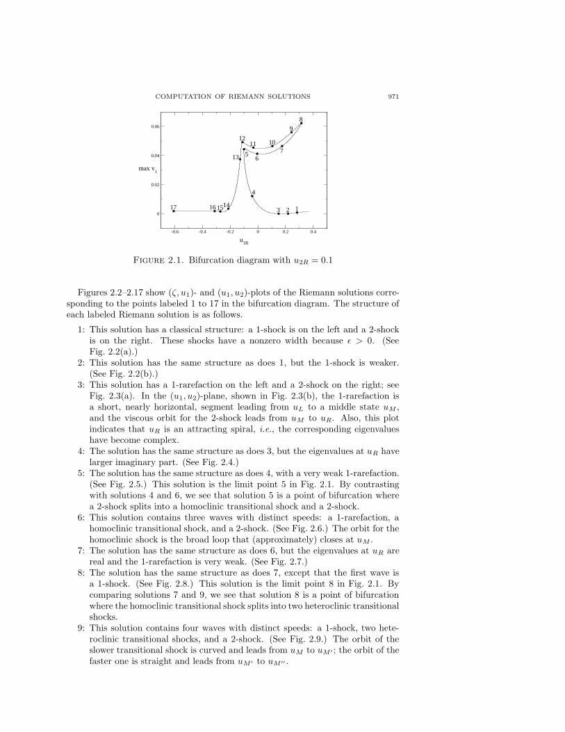
2.1. Experiment 1. We begin by setting uR equal to uL, so that the Riemannproblem, and our truncated boundary value problem, have a constant solution. Nextwe use AUTO to continue the solution as u2R is decreased to u2R = 0.1. Then wecontinue the solution by decreasing u1R down to −0.6. Fig. 2.1 shows the resultingbifurcation diagram. A single number is chosen to represent the computed Riemannsolution; specifically, we choose the maximum value of v1 over the solution (recallthat v = εB(u)u′). In the bifurcation diagram, this number is plotted vs. u1R.

The bifurcation diagram has several interesting features. Evidently, it has twolimit points, labeled 5 and 8 (with u1R approximately −0.1 and 0.32, respectively).As a result, for each u1R in the interval defined by the abscissae of points 5 and 8,there are three Riemann solutions. As we discuss in more detail below, this three-fold nonuniqueness of solutions of a Riemann problem is the same as investigatedin [1]: a Riemann solution on the lower branch has the classical structure consistingof two waves; one on the middle branch involves three waves, the third wave beinga shock wave with a homoclinic connection; and one on the upper branch containsfour waves, two being transitional shock waves. Also notice the rather angularbends near point 12 and between points 14 and 15.


123

4

56

7

8

9

101112

13

14151617

-0.6 -0.4 -0.2 0 0.2 0.4

u1R

0

0.02

0.04

0.06

max v1

Figure 2.1. Bifurcation diagram with u2R = 0.1

Figures 2.2–2.17 show (ζ, u1)- and (u1, u2)-plots of the Riemann solutions corre-sponding to the points labeled 1 to 17 in the bifurcation diagram. The structure ofeach labeled Riemann solution is as follows.

1: This solution has a classical structure: a 1-shock is on the left and a 2-shockis on the right. These shocks have a nonzero width because ε > 0. (SeeFig. 2.2(a).)

2: This solution has the same structure as does 1, but the 1-shock is weaker.(See Fig. 2.2(b).)

3: This solution has a 1-rarefaction on the left and a 2-shock on the right; seeFig. 2.3(a). In the (u1, u2)-plane, shown in Fig. 2.3(b), the 1-rarefaction isa short, nearly horizontal, segment leading from uL to a middle state uM ,and the viscous orbit for the 2-shock leads from uM to uR. Also, this plotindicates that uR is an attracting spiral, i.e., the corresponding eigenvalueshave become complex.

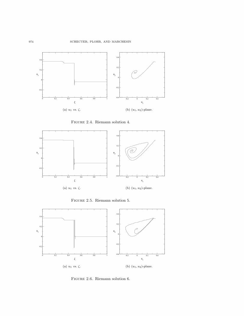
4: The solution has the same structure as does 3, but the eigenvalues at uR havelarger imaginary part. (See Fig. 2.4.)

5: The solution has the same structure as does 4, with a very weak 1-rarefaction.(See Fig. 2.5.) This solution is the limit point 5 in Fig. 2.1. By contrastingwith solutions 4 and 6, we see that solution 5 is a point of bifurcation wherea 2-shock splits into a homoclinic transitional shock and a 2-shock.

6: This solution contains three waves with distinct speeds: a 1-rarefaction, ahomoclinic transitional shock, and a 2-shock. (See Fig. 2.6.) The orbit for thehomoclinic shock is the broad loop that (approximately) closes at uM .

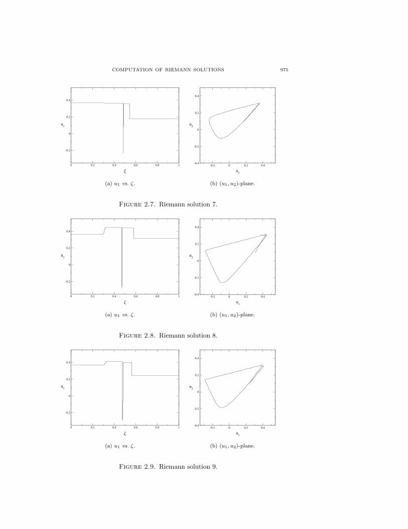
7: The solution has the same structure as does 6, but the eigenvalues at uR arereal and the 1-rarefaction is very weak. (See Fig. 2.7.)

8: The solution has the same structure as does 7, except that the first wave isa 1-shock. (See Fig. 2.8.) This solution is the limit point 8 in Fig. 2.1. Bycomparing solutions 7 and 9, we see that solution 8 is a point of bifurcationwhere the homoclinic transitional shock splits into two heteroclinic transitionalshocks.

9: This solution contains four waves with distinct speeds: a 1-shock, two hete-roclinic transitional shocks, and a 2-shock. (See Fig. 2.9.) The orbit of theslower transitional shock is curved and leads from uM to uM ′ ; the orbit of thefaster one is straight and leads from uM ′ to uM ′′ .


10: The solution has the same structure as does 9, except that the first wave isa 1-rarefaction. Also, the eigenvalues at uR have just become complex. (SeeFig. 2.10.)

11: The solution has the same structure as does 10, but the eigenvalues at uR

have larger imaginary part. (See Fig. 2.11.)12: This solution consists of a very weak 1-shock, a transitional shock with a

a curved orbit, and a 2-shock wave for which uR has complex eigenvalues.(See Fig. 2.12.) This 2-shock is the result of the coalescence of two wavesin solution 11, namely, the transitional shock with a straight orbit and the2-shock. The intermediate state uM ′′ has disappeared.

13: Just as solution 12, this solution has three waves with distinct speeds: a1-shock, a transitional shock, and a 2-shock. (See Fig. 2.13.)

14: This solution again has a three-wave structure, with the eigenvalues at uR

being real. o(See Fig. 2.14.)15: This solution again has a four-wave structure: the heteroclinic transitional

shock in solution 14 has split into two heteroclinic transitional shocks withalmost identical speeds. Also, the 2-shock is very weak. (See Fig. 2.15.)

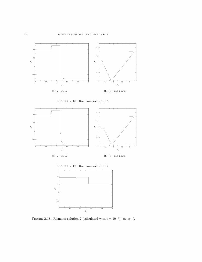
16: The solution has the same structure as does 15, except that the 2-shock hasbeen replaced by a 2-rarefaction. (See Fig. 2.16.)

17: The solution has three waves: the second transitional shock and the 2-rarefactionhave coalesced into a composite 2-wave (in this case, a 2-shock adjacent to a2-rarefaction). (See Fig. 2.17.) The nearly coincident pairs of shock waves insolutions 15 and 16 have clearly distinct speeds.

Let us make several remarks on these figures.

A. In Riemann solution 2 (see Fig. 2.2(b)), and in several others, shocks arenot very sharp. Shocks becomes sharper when ε is decreased. For example,starting from Riemann solution 2, we can use AUTO to reduce ε from 2×10−4

to 10−6. The result is Fig. 2.18, in which the shocks are much sharper.B. The rather sharp bends in the bifurcation diagram of Fig. 2.1 near points 5, 8,

12 and 15 correspond to the following transitions in the structure of the Rie-mann solution: (i) splitting of a 2-shock into a homoclinic transitional shockfollowed by a 2-shock; (ii) splitting of a homoclinic transitional shock into twoheteroclinic transitional shocks; (iii) coalescence of a heteroclinic transitionalshock and a 2-shock into a 2-shock; (iv) splitting of a heteroclinic transitionalshock into two heteroclinic transitional shocks. These transitions can producecorners in the underlying Riemann solution bifurcation diagram [17].

C. In the numerical experiments of Ref. [1], Riemann solutions with homoclinicshock waves are unstable. Moreover, in the authors’ experience with numericalsimulations, shock waves with complex eigenvalues at one end are sometimesunstable. Nonetheless it is useful to consider Riemann solutions that are un-stable. For example, in the bifurcation diagram of Fig. 2.1, there are threeRiemann solutions for u1R between approximately −0.09 and 0.32. For Rie-mann solutions 1–3 and 7–9 (u1R between approximately 0.17 and 0.32), the2-shock has real eigenvalues at both ends, and only solution 7 (on the “mid-dle” solution branch) contains a homoclinic shock. However, our use of acontinuation method to find the solutions that are likely to be stable (solu-tions 1–3, 8, and 9) involved passing through Riemann solutions with complex


0 0.2 0.4 0.6 0.8 1

ζ

-0.2

0

0.2

0.4

u1

(a) Riemann solution 1

0 0.2 0.4 0.6 0.8 1

ζ

-0.2

0

0.2

0.4

u1

(b) Riemann solution 2

Figure 2.2. Riemann solutions 1 and 2: u1 vs. ζ.

0 0.2 0.4 0.6 0.8 1

ζ

-0.2

0

0.2

0.4

u1

(a) u1 vs. ζ.

-0.2 0 0.2 0.4

u1

-0.4

-0.2

0

0.2

0.4

u2

(b) (u1, u2)-plane.

Figure 2.3. Riemann solution 3.


0 0.2 0.4 0.6 0.8 1

ζ

-0.2

0

0.2

0.4

u1

(a) u1 vs. ζ.

-0.2 0 0.2 0.4

u1

-0.4

-0.2

0

0.2

0.4

u2

(b) (u1, u2)-plane.


0 0.2 0.4 0.6 0.8 1

ζ

-0.2

0

0.2

0.4

u1

(a) u1 vs. ζ.

-0.2 0 0.2 0.4

u1

-0.4

-0.2

0

0.2

0.4

u2

(b) (u1, u2)-plane.


0 0.2 0.4 0.6 0.8 1

ζ

-0.2

0

0.2

0.4

u1

(a) u1 vs. ζ.

-0.2 0 0.2 0.4

u1

-0.4

-0.2

0

0.2

0.4

u2

(b) (u1, u2)-plane.



0 0.2 0.4 0.6 0.8 1

ζ

-0.2

0

0.2

0.4

u1

(a) u1 vs. ζ.

-0.2 0 0.2 0.4

u1

-0.4

-0.2

0

0.2

0.4

u2

(b) (u1, u2)-plane.


0 0.2 0.4 0.6 0.8 1

ζ

-0.2

0

0.2

0.4

u1

(a) u1 vs. ζ.

-0.2 0 0.2 0.4

u1

-0.4

-0.2

0

0.2

0.4

u2

(b) (u1, u2)-plane.


0 0.2 0.4 0.6 0.8 1

ζ

-0.2

0

0.2

0.4

u1

(a) u1 vs. ζ.

-0.2 0 0.2 0.4

u1

-0.4

-0.2

0

0.2

0.4

u2

(b) (u1, u2)-plane.



0 0.2 0.4 0.6 0.8 1

ζ

-0.2

0

0.2

0.4

u1

(a) u1 vs. ζ.

-0.2 0 0.2 0.4

u1

-0.4

-0.2

0

0.2

0.4

u2

(b) (u1, u2)-plane.


0 0.2 0.4 0.6 0.8 1

ζ

-0.2

0

0.2

0.4

u1

(a) u1 vs. ζ.

-0.2 0 0.2 0.4

u1

-0.4

-0.2

0

0.2

0.4

u2

(b) (u1, u2)-plane.


0 0.2 0.4 0.6 0.8 1

ζ

-0.2

0

0.2

0.4

u1

(a) u1 vs. ζ.

-0.2 0 0.2 0.4

u1

-0.4

-0.2

0

0.2

0.4

u2

(b) (u1, u2)-plane.



0 0.2 0.4 0.6 0.8 1

ζ

-0.2

0

0.2

0.4

u1

(a) u1 vs. ζ.

-0.2 0 0.2 0.4

u1

-0.4

-0.2

0

0.2

0.4

u2

(b) (u1, u2)-plane.


0 0.2 0.4 0.6 0.8 1

ζ

-0.2

0

0.2

0.4

u1

(a) u1 vs. ζ.

-0.2 0 0.2 0.4

u1

-0.4

-0.2

0

0.2

0.4

u2

(b) (u1, u2)-plane.


0 0.2 0.4 0.6 0.8 1

ζ

-0.2

0

0.2

0.4

u1

(a) u1 vs. ζ.

-0.2 0 0.2 0.4

u1

-0.4

-0.2

0

0.2

0.4

u2

(b) (u1, u2)-plane.



0 0.2 0.4 0.6 0.8 1

ζ

-0.2

0

0.2

0.4

u1

(a) u1 vs. ζ.

-0.2 0 0.2 0.4

u1

-0.4

-0.2

0

0.2

0.4

u2

(b) (u1, u2)-plane.


0 0.2 0.4 0.6 0.8 1

ζ

-0.2

0

0.2

0.4

u1

(a) u1 vs. ζ.

-0.2 0 0.2 0.4

u1

-0.4

-0.2

0

0.2

0.4

u2

(b) (u1, u2)-plane.


0 0.2 0.4 0.6 0.8 1

ζ

-0.2

0

0.2

0.4

u1

Figure 2.18. Riemann solution 2 (calculated with ε = 10−6): u1 vs. ζ.


2-shocks (solutions 4–6 and 10–13) and homoclinic transitional shocks (solu-tions 6 and 7). Thus it is useful to allow such possibly unstable solutions toarise during continuation even if one is only interested in stable solutions.

D. One can ask how closely the computed bifurcation diagram of Fig. 2.1 cor-responds to the underlying Riemann solution bifurcation diagram near tran-sition points from one structurally stable Riemann solution to another (forexample, the two fold points). At present there is no theory about this ques-tion.

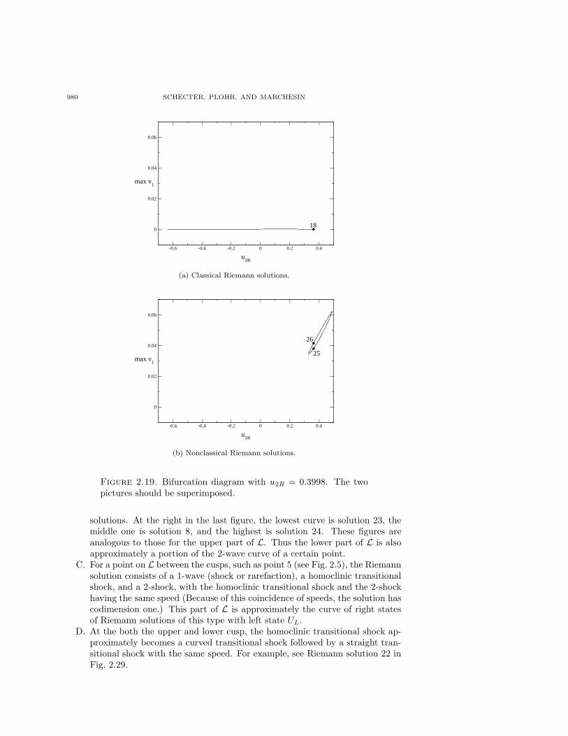
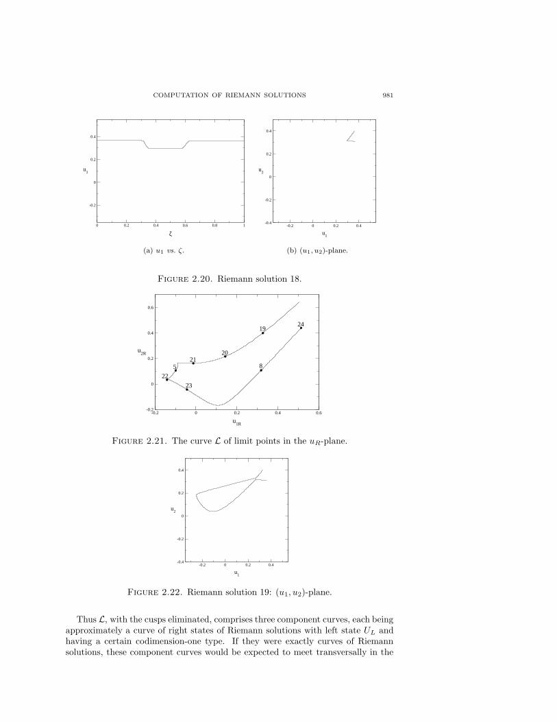
2.2. Experiment 2. Next, starting from uR = uL, we increase u2R to 0.3998 andthen vary u1R. The bifurcation diagram is shown in Fig. 19(a). The point in thisbifurcation diagram with u1R = 0.362832 is labeled 18; Figs. 20(a) and 20(b) showthe (ζ, u1)- and (u1, u2)-plots of this Riemann solution. In fact, no limit points occurduring this continuation; the Riemann solution remains classical, throughout, justlike solution 18. Note, however, that in [1], three different Riemann solutions occurfor uR = (0.362832, 0.3998). The additional two solutions, which are labeled 25and 26 in Fig. 19(b), are found via Experiments 3 and 4.

2.3. Experiment 3. To see better how the multiple solutions occur, we start atthe limit point 8 in Fig. 2.1 and use AUTO to plot a curve of limit points in theuR-plane. The resulting curve L is shown in Fig. 2.21. Note that the line u2R = 0.1meets L in two points. These points correspond to points 5 and 8 in Fig. 2.1; theyare also labeled 5 and 8 here. Also note the occurrence of two cusps. Cusps occurgenerically along curves of limit points; this is the well-known “cusp catastrophe.”

The points of L correspond approximately to certain Riemann solutions thatare not structurally stable, having codimension two at the cusps and otherwisecodimension one. The type of codimension-one Riemann solution changes at eachcusp:

A. Points on the upper and lower parts of L correspond approximately to Rie-mann solutions consisting of a 1-wave (shock or rarefaction), two heteroclinictransitional shocks (one curved, one straight), and a 2-wave (shock or rarefac-tion). The two heteroclinic transitional shocks have the same speed; this iswhat makes the Riemann solution fail to be structurally stable.

Figures 2.22–2.24 show phase portraits for points 19, 20, and 21 on theupper part of L. The corresponding Riemann solutions differ only in thatthe last wave is a 2-rarefaction for point 19, a 2-shock with real eigenvaluesfor point 20, and a 2-shock with complex eigenvalues for point 21. All threeRiemann solutions (indeed, all Riemann solutions on the top part of L) beginwith the same three waves. The top part of L is, in fact, approximately aportion of the 2-wave curve of the right-most state of the third of these waves.

Figure 2.25 shows superimposed (ζ, u1)-plots for these three solutions. Atthe right in this figure, the highest curve is solution 19, the middle one issolution 20, and the lowest is solution 21. One sees clearly that the threesolutions have the same first three waves. One also sees that as one movesto the left along L, the speed of the last wave approaches the common speedof the two heteroclinic shocks. The cusp point is close to a codimension-twoRiemann solution in which the two heteroclinic shocks and the 2-shock allhave the same speed.

B. Figures 2.26, 2.8, and 2.27 show phase portraits for points 23, 8, and 24 onthe lower part of L, and Fig. 2.28 shows superimposed (ζ, u1)-plots for these


18

-0.6 -0.4 -0.2 0 0.2 0.4

u1R

0

0.02

0.04

0.06

max v1

(a) Classical Riemann solutions.

25

26

-0.6 -0.4 -0.2 0 0.2 0.4

u1R

0

0.02

0.04

0.06

max v1

(b) Nonclassical Riemann solutions.

Figure 2.19. Bifurcation diagram with u2R = 0.3998. The twopictures should be superimposed.

solutions. At the right in the last figure, the lowest curve is solution 23, themiddle one is solution 8, and the highest is solution 24. These figures areanalogous to those for the upper part of L. Thus the lower part of L is alsoapproximately a portion of the 2-wave curve of a certain point.

C. For a point on L between the cusps, such as point 5 (see Fig. 2.5), the Riemannsolution consists of a 1-wave (shock or rarefaction), a homoclinic transitionalshock, and a 2-shock, with the homoclinic transitional shock and the 2-shockhaving the same speed (Because of this coincidence of speeds, the solution hascodimension one.) This part of L is approximately the curve of right statesof Riemann solutions of this type with left state UL.

D. At the both the upper and lower cusp, the homoclinic transitional shock ap-proximately becomes a curved transitional shock followed by a straight tran-sitional shock with the same speed. For example, see Riemann solution 22 inFig. 2.29.


0 0.2 0.4 0.6 0.8 1

ζ

-0.2

0

0.2

0.4

u1

(a) u1 vs. ζ.

-0.2 0 0.2 0.4

u1

-0.4

-0.2

0

0.2

0.4

u2

(b) (u1, u2)-plane.


521

20

22

23

8

2419

-0.2 0 0.2 0.4 0.6

u1R

-0.2

0

0.2

0.4

0.6

u2R

Figure 2.21. The curve L of limit points in the uR-plane.

-0.2 0 0.2 0.4

u1

-0.4

-0.2

0

0.2

0.4

u2

Figure 2.22. Riemann solution 19: (u1, u2)-plane.

Thus L, with the cusps eliminated, comprises three component curves, each beingapproximately a curve of right states of Riemann solutions with left state UL andhaving a certain codimension-one type. If they were exactly curves of Riemannsolutions, these component curves would be expected to meet transversally in the


-0.2 0 0.2 0.4

u1

-0.4

-0.2

0

0.2

0.4

u2


-0.2 0 0.2 0.4

u1

-0.4

-0.2

0

0.2

0.4

u2


0 0.2 0.4 0.6 0.8 1

ζ

-0.2

0

0.2

0.4

u1

192021

Figure 2.25. Riemann solutions 19, 20, and 21: ζ vs. u1.

space of Riemann solutions [17]. Instead, because they are curves in the space ofDafermos-regularized solutions, they intersect in cusps, as is appropriate for genericfold curves. This difference is illustrated in Fig. 2.30. Thus near the cusps ofFig. 2.1, the solutions computed via Dafermos regularization are quite differentfrom the underlying Riemann solution. At present there is no theory about thisissue.

2.4. Experiment 4. Finally, we set uR to correspond to point 19 in Fig. 2.21,which has second component being 0.3998, and vary u1R. The resulting bifurcation


-0.2 0 0.2 0.4

u1

-0.4

-0.2

0

0.2

0.4

u2


-0.2 0 0.2 0.4

u1

-0.4

-0.2

0

0.2

0.4

u2


0 0.2 0.4 0.6 0.8 1

ζ

-0.2

0

0.2

0.4

u1

23824

Figure 2.28. Riemann solutions 8, 23, and 24: ζ vs. u1.

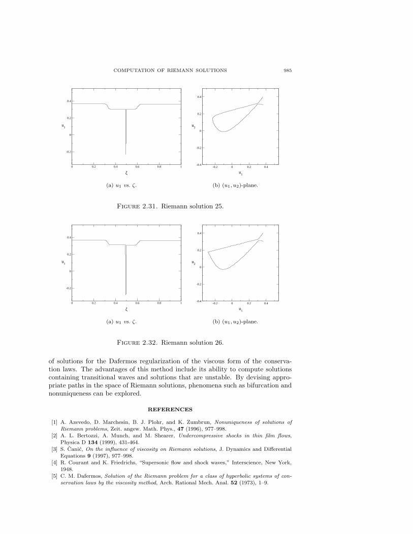
diagram is shown in Fig. 19(b). The points with u1R = 0.362832 (which is the u1R

component for point 18 in Fig. 19(a)) are labeled 25 and 26.Figures 2.20, 2.31, and 2.32 show (ζ, u1)- and (u1, u2)-plots of the Riemann

solutions corresponding to points 18, 25, and 26. They should be compared toFigs. 2.1–2.3 of [1]. As in Ref. [1], these Riemann solutions can be understood asfollows:

18: Classical Riemann solution: 1-rarefaction followed by 2-rarefaction.


0 0.2 0.4 0.6 0.8 1

ζ

-0.2

0

0.2

0.4

u1

(a) u1 vs. ζ.

-0.2 0 0.2 0.4

u1

-0.4

-0.2

0

0.2

0.4

u2

(b) (u1, u2)-plane.


Figure 2.30. The space of Riemann solutions and the space ofDafermos-regularized solutions near a cusp point of the latter. Foldcurves, as projected onto UR-space, are shown below the spaces ofsolutions.

25: Three waves with distinct speeds: 1-rarefaction, homoclinic transitional shock,2-rarefaction.

26: Four waves with distinct speeds: 1-rarefaction, two heteroclinic transitionalshocks, 2-rarefaction.

The superposition of Figs. 19(a) and 19(b) is to be contrasted with Fig. 2.1.The superposition corresponds to a slice of Fig. 2.21 with u2R = 0.3998, whereasFig. 2.1 corresponds to a slice with u2R = 0.1. Therefore, as u2R is increasedfrom 0.1 to 0.3998, the bifurcation diagram for fixed u2R evolves from Fig. 2.1 tothe superposition of Figs. 19(a) and 19(b). A natural expectation is that points 5and 12 pinch together when the slice approaches the upper cusp point of Fig. 2.21from below, at which stage a bifurcation occurs to two disconnected branches, abranch of “classical” solutions and a loop of “nonclassical” solutions.

3. Conclusion. In this paper we have demonstrated a practical numerical methodfor constructing Riemann solutions such that all shock waves obey the viscous profileadmissibility criterion for a specified viscosity. This method is based continuation


0 0.2 0.4 0.6 0.8 1

ζ

-0.2

0

0.2

0.4

u1

(a) u1 vs. ζ.

-0.2 0 0.2 0.4

u1

-0.4

-0.2

0

0.2

0.4

u2

(b) (u1, u2)-plane.


0 0.2 0.4 0.6 0.8 1

ζ

-0.2

0

0.2

0.4

u1

(a) u1 vs. ζ.

-0.2 0 0.2 0.4

u1

-0.4

-0.2

0

0.2

0.4

u2

(b) (u1, u2)-plane.


of solutions for the Dafermos regularization of the viscous form of the conserva-tion laws. The advantages of this method include its ability to compute solutionscontaining transitional waves and solutions that are unstable. By devising appro-priate paths in the space of Riemann solutions, phenomena such as bifurcation andnonuniqueness can be explored.

REFERENCES

[1] A. Azevedo, D. Marchesin, B. J. Plohr, and K. Zumbrun, Nonuniqueness of solutions ofRiemann problems, Zeit. angew. Math. Phys., 47 (1996), 977–998.

[2] A. L. Bertozzi, A. Munch, and M. Shearer, Undercompressive shocks in thin film flows,Physica D 134 (1999), 431-464.

[3] S. Canic, On the influence of viscosity on Riemann solutions, J. Dynamics and DifferentialEquations 9 (1997), 977–998.

[4] R. Courant and K. Friedrichs, “Supersonic flow and shock waves,” Interscience, New York,1948.

[5] C. M. Dafermos, Solution of the Riemann problem for a class of hyperbolic systems of con-servation laws by the viscosity method, Arch. Rational Mech. Anal. 52 (1973), 1–9.


[6] E. Doedel and J. Kernevez, AUTO: Software for continuation problems in ordinary differen-tial equations with applications, Technical Report, California Institute of Technology, 1986.(Available at http://indy.cs.concordia.ca/auto/doc/index.html.)

[7] N. Fenichel, Geometric singular perturbation theory for ordinary differential equations, J.Differential Eqs. 31 (1979), 53–98.

[8] I. Gelfand, Some problems in the theory of quasi-linear equations, Uspehi Mat. Nauk. 14

(1959), 87–158; Amer. Math. Soc. Transl. (2) 29 (1963), 295–381.[9] J. Goodman, Nonlinear asymptotic stability of viscous shock profiles for conservation laws,

Arch. Rational Mech. Anal. 95 (1986), 325–344.[10] C.K.R.T. Jones, Geometric singular perturbation theory. In Dynamical systems (Montecatini

Terme, 1994), 44–118, Lecture Notes in Math. 1609, Springer, Berlin, 1995.[11] C.K.R.T. Jones and T. Kapper, A primer on the exchange lemma for fast-slow systems, in

“Multiple Time-Scale Dynamical Systems,” C.K.R.T. Jones and A. Khibnik, editors, IMAVolumes in Mathematics and its Applications 122 (2000), 85–132.

[12] T.-P. Liu, Nonlinear stability of shock waves for viscous conservation laws, Mem. Amer.Math. Soc. 56 (1985) no. 328, 1–108.

[13] T.-P. Liu, Pointwise convergence to shock waves for viscous conservation laws, Comm. PureAppl. Math. 50 (1997), 1113–1182.

[14] T.-P. Liu and K. Zumbrun, Nonlinear stability of an undercompressive shock for complexBurgers equation, Commun. Math. Phys. 168 (1995), 163–186.

[15] T.-P. Liu and K. Zumbrun, On nonlinear stability of general undercompressive viscous shockwaves, Commun. Math. Phys. 174 (1995), 319–345.

[16] A. Majda and R. Pego, Stable viscosity matrices for systems of conservation laws, J. Differ-ential Equations 56 (1985), 229–262.

[17] D. Marchesin, B. J. Plohr, S. Schecter, Codimension-One Riemann Problems, J. Dynamicsand Differential Equations, 13 (2001), 523–588.

[18] A. Matsumura and K. Nishihara, On the stability of travelling wave solutions of a one-dimensional model system for compressible viscous gas, Japan J. Appl. Math. 2 (1985), 17–25.

[19] S. Schecter, D. Marchesin, and B. J. Plohr, Structurally stable Riemann solutions, J. Differ-ential Equations 126 (1996), 303–354.

[20] S. Schecter, Undercompressive shock waves and the Dafermos regularization, Nonlinearity 15

(2002), 1361–1377.[21] J. Smoller, “Shock Waves and Reaction-Diffusion Equations,” Springer-Verlag, New York,

1983.[22] P. Szmolyan, in preparation.[23] A. Szepessy and K. Zumbrun, Stability of rarefaction waves in viscous media, Arch. Rational

Mech. Anal. 133 (1996), 249–298.[24] A. E. Tzavaras, Wave interactions and variation estimates for self-similar zero-viscosity

limits in systems of conservation laws, Arch. Rational Mech. Anal. 135 (1996), 1–60.[25] K. Zumbrun and P. Howard, Pointwise semigroup methods and stability of viscous shock

waves, Indiana Univ. Math. J. 47 (1998), 741–871.

Received September 2002; revised June 2003; final version December 2003.

E-mail address: [email protected]



Computation of Riemann solutions using the Dafermos regularization and continuation

Documents