Computation Methods

7/23/2019 Computation Methods

http://slidepdf.com/reader/full/computation-methods 1/30

Computational Methods

In this appendix we summarize many of the fundamental computa-

tional procedures required in reactor analysis and design. We illustrate

these procedures using the numerical computing language Octave [4, 5]

or, equivalently, MATLAB. The MATLAB

package is commercially available

from The MathWorks, Inc., and is becoming a commonly available

tool of industrial engineering practice. One is naturally free to use any

numerical solution procedure that is convenient, but we have found

that these two environments pro-vide reliable and high-quality

numerical solutions, and convenient user interfaces.

Many

of

the

figures

and

tables

in

this

text

required

numerical

solu-tions of various types of chemical reactor problems. All computations

required to produce every figure and table in this text were performed

with Octave.

A.1 Linear Algebra and Least Squares

In this section we briefly introduce Octave and MATLAB, and show how to

enter reaction networks quickly and perform linear algebra operations

of interest.

After starting an Octave session, type doc and select menu item

Introduction at the Octave prompt or demo at the MATLAB prompt

for information on how to enter matrices and perform matrix multi-

plication. Consider again the water gas shift reaction chemistry, for

634



A.1 Linear Algebra and Least Squares 635

example,

0 1 0 −1 −1 1

−1 1 1 −1 0 01 0 −1 0 −1 1

H

H2

OH

H2O

CO

CO2

=

0

00

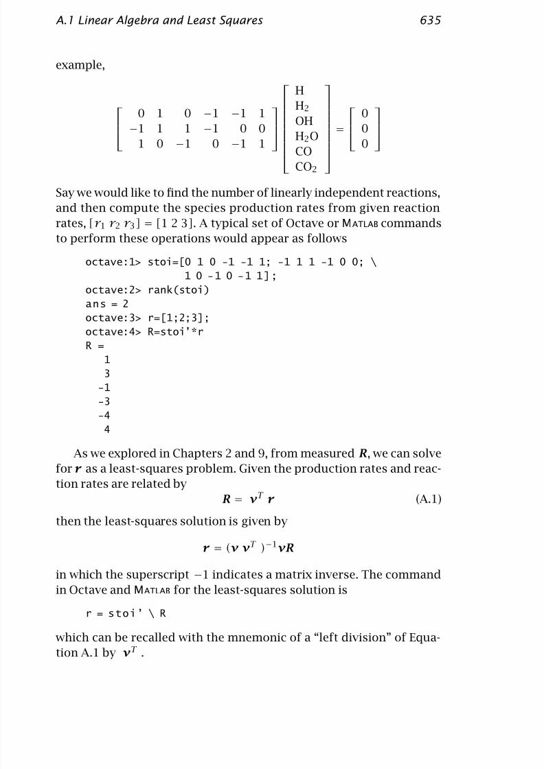
Say we would like to find the number of linearly independent reactions,

and then compute the species production rates from given reaction

rates, [r 1 r 2 r 3] = [1 2 3]. A typical set of Octave or MATLAB commands

to perform these operations would appear as follows

octave:1> stoi=[0 1 0 -1 -1 1; -1 1 1 -1 0 0; \

1 0 - 1 0 - 1 1 ] ;

octave:2> rank(stoi)

ans = 2

octave:3> r=[1;2;3];

octave:4> R=stoi’*r

R =

1

3

-1-3

-4

4

As we explored in Chapters 2 and 9, from measured R, we can solve

for r as a least-squares problem. Given the production rates and reac-

tion rates are related by

R = νT r (A.1)

then the least-squares solution is given by

r = (ν νT )−1νR

in which the superscript −1 indicates a matrix inverse. The command

in Octave and MATLAB for the least-squares solution is

r = stoi’ \ R

which can be recalled with the mnemonic of a “left division” of Equa-tion A.1 by νT .



636 Computational Methods

1.9

1.95

2

2.05

2.1

0.9 0.95 1 1.05 1.1

r 1

r 2

Figure A.1: Estimated reaction rates from 2000 production-rate mea-

surements subject to measurement noise.

Example A.1: Estimating reaction rates

Consider the first and second water gas shift reaction as an indepen-

dent set and let [r 1 r 2] = [1 2]. Create 2000 production rate measure-

ments by adding noise to R = νT r and estimate the reaction rates

from these data. Plot the distribution of estimated reaction rates.

SolutionThe Octave commands to generate these results are

s t o i = [ 0 1 0 - 1 - 1 1 ; - 1 1 1 - 1 0 0 ] ;

[nr, nspec] = size(stoi);

r = [1;2];

R = stoi’*r;

nmeas = 2000;

for i = 1:nmeas

R_meas(:,i) = 0.05*randn(nspec, 1) + R;end

r_est = stoi’ \ R_meas;



A.2 Nonlinear Algebraic Equations and Optimization 637

plot(r_est(1,:), r_est(2,:), ’o’)

Figure A.1 shows the estimates. We know from Chapter 9 that the

distribution of estimates is a multivariate normal. We also know how

to calculate the α-level confidence intervals.

A.2 Nonlinear Algebraic Equations and Optimization

Determining equilibria for reacting systems with multiple phases and

reactions can require significant computational effort. As we saw in

Chapter 3, the phase and reaction equilibrium conditions generally lead

to mathematical problems of two types: solving nonlinear algebraic

equations and minimizing a nonlinear function subject to constraints.We explore computing solutions to these types of problems in Octave or

MATLAB. In this section it is assumed that the required thermochemical

data are available, but finding or measuring these data is often another

significant challenge in computing equilibria for systems of industrial

interest. See also Section 3.2.1 for a brief discussion of thermochemical

databases.

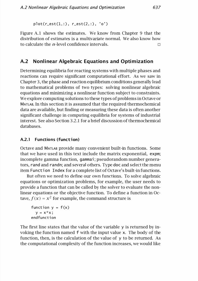
A.2.1 Functions (function)

Octave and MATLAB provide many convenient built-in functions. Some

that we have used in this text include the matrix exponential, expm;

incomplete gamma function, gammai; pseudorandom number genera-

tors, rand and randn; and several others. Type doc and select the menu

item Function Index for a complete list of Octave’s built-in functions.

But often we need to define our own functions. To solve algebraic

equations or optimization problems, for example, the user needs to

provide a function that can be called by the solver to evaluate the non-linear equations or the objective function. To define a function in Oc-

tave, f (x) = x2 for example, the command structure is

function y = f(x)

y = x*x;

endfunction

The first line states that the value of the variable y is returned by in-

voking the function named f with the input value x. The body of the

function, then, is the calculation of the value of y to be returned. As

the computational complexity of the function increases, we would like




to store our work so that it does not need to be reentered at the be-

ginning of each subsequent Octave session. Storing, documenting and

maintaining the calculations performed in solving complex industrial

problems is one of the significant challenges facing practicing chemical

engineers. Even for our purposes, we should be able to store and editour computational problems. Octave commands and function defini-

tions can be stored in text files, called m-files; the naming convention

is filename.m. Editing these files with a text editor during an inter-

active Octave session provides a convenient means for debugging new

calculations.

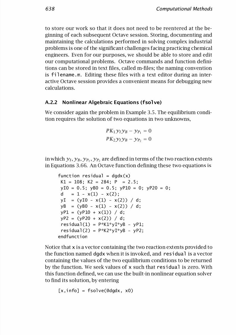
A.2.2 Nonlinear Algebraic Equations (fsolve)

We consider again the problem in Example 3.5. The equilibrium condi-tion requires the solution of two equations in two unknowns,

P K 1y I y B − y P 1 = 0

P K 2y I y B − y P 2 = 0

in which y I , y B, y P 1 , y P 2 are defined in terms of the two reaction extents

in Equations 3.66. An Octave function defining these two equations is

function residual = dgdx(x)

K1 = 108; K2 = 284; P = 2.5;

yI0 = 0.5; yB0 = 0.5; yP10 = 0; yP20 = 0;

d = 1 - x(1) - x(2);

yI = (yI0 - x(1) - x(2)) / d;

yB = (yB0 - x(1) - x(2)) / d;

yP1 = (yP10 + x(1)) / d;

yP2 = (yP20 + x(2)) / d;

residual(1) = P*K1*yI*yB - yP1;residual(2) = P*K2*yI*yB - yP2;

endfunction

Notice that x is a vector containing the two reaction extents provided to

the function named dgdx when it is invoked, and residual is a vector

containing the values of the two equilibrium conditions to be returned

by the function. We seek values of x such that residual is zero. With

this function defined, we can use the built-in nonlinear equation solver

to find its solution, by entering

[x,info] = fsolve(@dgdx, x0)



A.2 Nonlinear Algebraic Equations and Optimization 639

The fsolve function requires the name of the function, following the @

sign, and an initial guess for the unknown extents, provided in the vari-

able x0, and returns the solution in x and a flag info indicating if the

calculation was successful. It is highly recommended to examine these

information flags after all calculations. Reactor equilibrium problemscan be numerically challenging, and even the best software can run into

problems. After the function dgdx is defined, the following is a typical

session to compute the solution given in Example 3.5

octave:1> x0=[0.2;0.2];

octave:2> [x,info] = fsolve(@dgdx,x0)

x =

0.13317

0.35087

info = 1

The value of info = 1 indicates that the solution has converged.

A.2.3 Nonlinear Optimization (fmincon)

The other main approach to finding the reaction equilibrium is to min-

imize the appropriate energy function, in this case the Gibbs energy.

This optimization-based formulation of the problem, as shown in Ex-

ample 3.3, can be more informative than the algebraic approach dis-

cussed above. In Chapter 3, we derived the following Gibbs energy

function for an ideal-gas mixture

G = −

i

ε

i ln K i +

1 +

i

νiε

i

ln P

+

j

y j0 +

i

νij ε

i

ln

y j0 +

i νij ε

i

1 +

i νiε

i

(A.2)

The minimization of this function of εi then determines the two equi-librium extents. Figure A.2 shows the lines of constant Gibbs energy

determined by Equation A.2 as a function of the two reaction extents.

We see immediately that the minimum is unique. Notice that G is not

defined for all reaction extents, and the following constraints are re-

quired to ensure nonnegative concentrations

0 ≤ ε

1 0 ≤ ε

2 ε

1 + ε

2 ≤ 0.5

We proceed to translate this version of the equilibrium condition

into a computational procedure. First we define a function that evalu-

ates G given the two reaction extents.




0

0.1

0.2

0.3

0.4

0.5

0 0.1 0.2 0.3 0.4 0.5

ε

1

ε

2

-2.559-2.55-2.53

-2.5

-2-10

Figure A.2: Gibbs energy contours for the pentane reactions as a

function of the two reaction extents.

function retval=gibbs(x)

dg1= -3.72e3; dg2= -4.49e3; T=400; R=1.987; P=2.5;

K1 = exp(-deltag1/(R*T)); K2 = exp(-deltag2/(R*T));

yI0 = 0.5; yB0 = 0.5; yP10 = 0; yP20 = 0;

d = 1 - x(1) - x(2);

yI = (yI0 - x(1) - x(2)) / d;

yB = (yB0 - x(1) - x(2)) / d;

yP1 = (yP10 + x(1)) / d;

yP2 = (yP20 + x(2)) / d;

retval = - (x(1)*log(K1)+x(2)*log(K2)) + ...

(1-x(1)-x(2))*log(P) + yI*d*log(yI) + ...

yB*d*log(yB) + yP1*d*log(yP1) + yP2*d*log(yP2);

endfunction

To solve the optimization we use the Octave or MATLAB function fmincon

[x,obj,info]=fmincon(@gibbs,x0, A, b, Aeq, beq, lb,ub)

in which x0 is the initial guess as before and the new variables are

used to define the constraints (if any). The variable lb provides lower



A.3 Differential Equations 641

bounds for the extents and ub provides upper bounds for the extents.

These are required to prevent the optimizer from “guessing” reaction

extent values for which the Gibbs energy function is not defined. For

example, consider what the gibbs function returns given negative re-

action extents. Finally, we specify the sum of extents is less than 0.5with the A and b arguments, which define linear inequality constraints

of the form

Ax ≤ b

For our problem, ε

1 + ε

2 ≤ 0.5, so A = [ 1 1 ] and b = 0.5. In

problems requiring equality constraints, we use the arguments Aeq and

beq, which define linear equality constraints of the form

Aeqx =

beq

Since we do not have equality constraints in this problem, we use [] to

indicate that these arguments are empty . Therefore, a typical session

to solve for equilibrium composition by minimizing Gibbs energy is

octave:1> A=[1 1]; b=0.4999

octave:2> lb=[0;0]; ub=[0.5;0.5];

octave:3> x0=[0.2;0.2];

octave:4> [x,obj,info]=fmincon(@gibbs,x0,A,b,[],[],lb,ub)

x =

0.13317

0.35087

obj = -2.5593

info = 2

In this case, the value of info = 2 indicates that the solution has con-

verged, and the results are in good agreement with those computedusing the algebraic approach, and the Gibbs energy contours depicted

in Figure A.2.

Optimization is a powerful tool for solving many types of engineer-

ing modeling and design problems. We also rely heavily on optimiza-

tion tools in Chapter 9 on parameter estimation.

A.3 Differential Equations

The real workhorse for simulating chemical reactors is the differential

equation solver. A high-quality solver is an indispensable tool of the




reactor designer because chemical reactions can take place at widely

different rates and time scales, presenting difficult numerical chal-

lenges. In the following we discuss several types of differential equa-

tions, including ordinary differential equations (ODEs), implicit differ-

ential equations, and differential-algebraic equations (DAEs), and thesolvers that have been developed for each type.

A.3.1 Ordinary Differential Equations (lsode)

We start with ordinary differential equations (ODEs). The ODEs re-

quired to describe transient batch reactors and CSTRs, and steady-state

PFR reactors are of the form

dxdt

= f(x)

x(0) = x0

in which x(t) is a vector of species concentrations to be found, t is time

in the batch reactor and CSTR, but volume or length in the steady-state

PFR, and f is the function defining the material balances for the species.

If the differential equations are nonlinear (f is not a linear function of

x) and one must keep track of several species simultaneously, then an-alytical solution is not possible and a numerical procedure is required.

Type

doc

and select the menu item

Differential Equations

for an overview of Octave’s ODE solver, lsode [6]. Type

help ode15s

for an overview of MATLAB’s ODE solvers. We recommend always using

the so-called “stiff” solvers for chemical reactor modeling. The time

scales for different reactions may be widely separated, leading to stiff

ODEs.

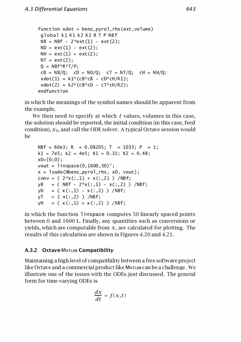
The first task is to formulate a function which defines f . If we ex-

amine the benzene pyrolysis example, Example 4.5, a suitable function

is




function xdot = benz_pyrol_rhs(ext,volume)

global k1 K1 k2 K2 R T P NBf

NB = NBf - 2*ext(1) - ext(2);

ND = ext(1) - ext(2);

NH = ext(1) + ext(2);

NT = ext(2);

Q = NBf*R*T/P;

cB = NB/Q; cD = ND/Q; cT = NT/Q; cH = NH/Q;

xdot(1) = k1*(cB*cB - cD*cH/K1);

xdot(2) = k2*(cB*cD - cT*cH/K2);

endfunction

in which the meanings of the symbol names should be apparent from

the example.

We then need to specify at which t values, volumes in this case,the solution should be reported, the initial condition (in this case, feed

condition), x0, and call the ODE solver. A typical Octave session would

be

NBf = 60e3; R = 0.08205; T = 1033; P = 1;

k1 = 7e5; k2 = 4e5; K1 = 0.31; K2 = 0.48;

x0=[0;0];

vout = linspace(0,1600,50)’;

x = lsode(@benz_pyrol_rhs, x0, vout);conv = ( 2*x(:,1) + x(:,2) ) /NBf;

yB = ( NBf - 2*x(:,1) - x(:,2) ) /NBf;

yD = ( x(:,1) - x(:,2) ) /NBf;

yT = ( x(:,2) ) /NBf;

yH = ( x(:,1) + x(:,2) ) /NBf;

in which the function linspace computes 50 linearly spaced points

between 0 and 1600 L. Finally, any quantities such as conversions or

yields, which are computable from x, are calculated for plotting. Theresults of this calculation are shown in Figures 4.20 and 4.21.

A.3.2 Octave-MATLAB Compatibility

Maintaining a high level of compatibility between a free software project

like Octave and a commercial product like MATLAB can be a challenge. We

illustrate one of the issues with the ODEs just discussed. The general

form for time-varying ODEs is

dx

dt = f(x,t)




in which f may depend on time t as well as state x . Octave’s interface

to lsode defines this function as follows

function xdot = benz pyrol rhs(ext, volume)

In most problems in science and engineering, however, the function f is time invariant. For these time-invariant ODEs, we can simply drop

the second argument and write more compactly

function xdot = benz pyrol rhs(ext)

In MATLAB on the other hand, the function defining the right-hand side

for ode15s has to be of the form

function xdot = benz pyrol mat(volume, ext)

Notice that the order of the time argument, volume, and state argu-

ment, ext, have been reversed compared to the Octave convention.

Even though the function seldom requires the argument volume, it

must be present in the argument list in MATLAB.

We can enhance compatibility by defining an interface (or wrapper)

in Octave with the name ode15s. The octave interface ode15s allows

the user to follow the MATLAB convention for the right-hand side func-

tion, and calls lsode to solve the differential equations. The advan-

tage is that the same user’s code works correctly inside Octave andMATLAB. But the user should be aware that the solver lsode, which is a

variable order predictor/corrector method, is being invoked when call-

ing ode15s in Octave while the solver ode15s in MATLAB is a different

method [8]. The choice of solution method should be transparent to the

user as long as both methods are solving the problem accurately. But

when the user encounters numerical difficulties on challenging prob-

lems, which is expected no matter what numerical tools one is using,

knowing what is actually underneath the hood becomes important indiagnosing and fixing the problem. If we wish to solve the ODEs by

calling the wrapper instead of lsode directly, then we change the line

x = lsode(@benz pyrol rhs, x0, vout);

to

[vsolver, x] = ode15s(@benz pyrol mat, vout, x0, opts);

Notice that ode15s returns the times (volumes) at which the solution

was found vsolver in the first argument and the solution x as the

second argument in the output. Comparing lsode and ode15s input




Problem type Wrapper name Octave solver

Optimization fmincon sqp

ODEs ode15s lsode

Implicit DEs ode15i daspk

Implict DEs ode15i dasrt

with root finding

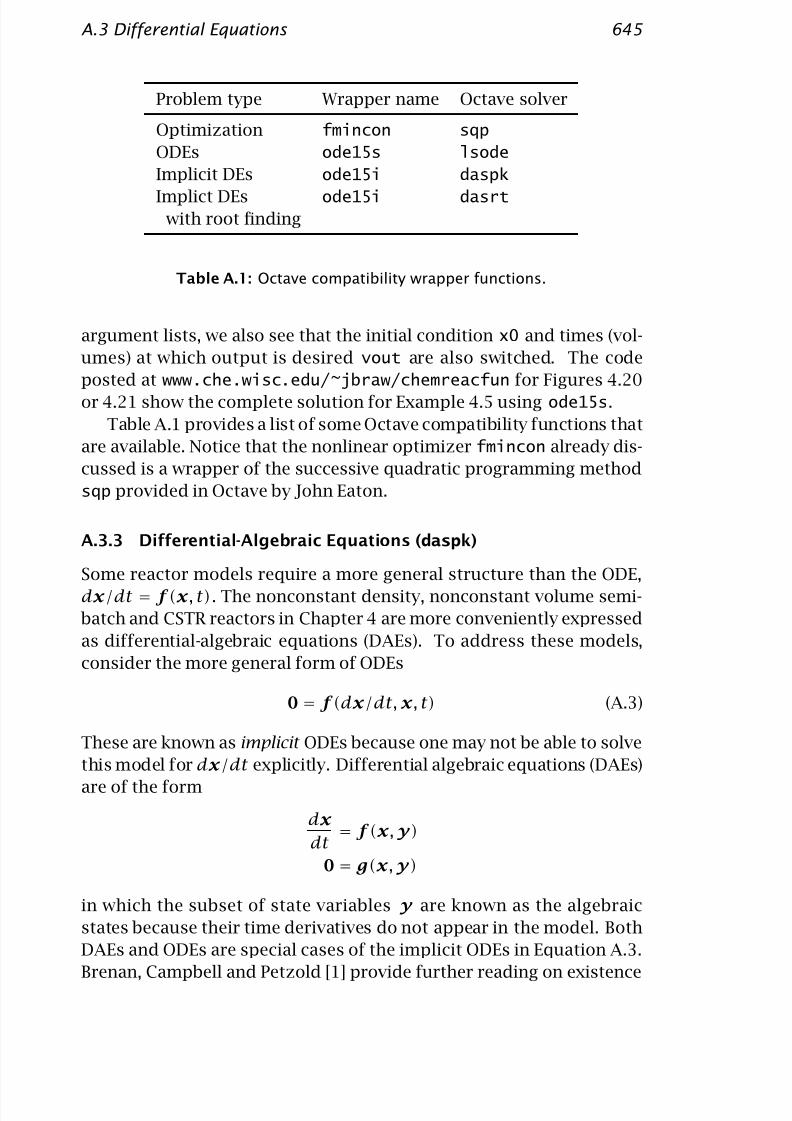
Table A.1: Octave compatibility wrapper functions.

argument lists, we also see that the initial condition x0 and times (vol-

umes) at which output is desired vout are also switched. The code

posted at www.che.wisc.edu/~jbraw/chemreacfun for Figures 4.20or 4.21 show the complete solution for Example 4.5 using ode15s.

Table A.1 provides a list of some Octave compatibility functions that

are available. Notice that the nonlinear optimizer fmincon already dis-

cussed is a wrapper of the successive quadratic programming method

sqp provided in Octave by John Eaton.

A.3.3 Differential-Algebraic Equations (daspk)

Some reactor models require a more general structure than the ODE,

dx /dt = f (x , t). The nonconstant density, nonconstant volume semi-

batch and CSTR reactors in Chapter 4 are more conveniently expressed

as differential-algebraic equations (DAEs). To address these models,

consider the more general form of ODEs

0 = f (dx /dt, x , t) (A.3)

These are known as implicit ODEs because one may not be able to solvethis model for dx /dt explicitly. Differential algebraic equations (DAEs)

are of the form

dx

dt = f (x , y)

0 = g(x , y)

in which the subset of state variables y are known as the algebraic

states because their time derivatives do not appear in the model. Both

DAEs and ODEs are special cases of the implicit ODEs in Equation A.3.

Brenan, Campbell and Petzold [1] provide further reading on existence




and uniqueness of solutions to these models, which are considerably

more complex issues than in the case of simple ODEs. Initial conditions

are required for dx /dt as well as x in this model,

dx

dt (t ) = x

0 x (t) = x

0, at t = 0

Brown, Hindmarsh and Petzold [2, 3] have provided a numerical pack-

age, daspk, to compute solutions to implicit differential, and differential-

algebraic equations. The main difference between using daspk and

lsode is the form of the user-supplied function defining the model. A

second difference is that the user must supply x 0 as well as x 0.

As an example, we can solve the previous ODEs using daspk. First

we modify the right-hand side function benz pyrol rhs of the ODEs

to return the residual given in Equation A.3. We call the new functionbenz pyrol

function res = benz_pyrol(ext, extdot, volume)

global k1 K1 k2 K2 R T P NBf

NB = NBf - 2*ext(1) - ext(2);

ND = ext(1) - ext(2);

NH = ext(1) + ext(2);

NT = ext(2);

Q = NBf*R*T/P;

cB = NB/Q; cD = ND/Q; cT = NT/Q; cH = NH/Q;res(1) = extdot(1) - k1*(cB*cB - cD*cH/K1);

res(2) = extdot(2) - k2*(cB*cD - cT*cH/K2);

endfunction

Notice that when this function returns zero for res, the variables extdot

and ext satisfy the differential equation. With this function defined,

we then solve the model by calling daspk

x0=[0;0]; xdot0 = [0;0];

vout = linspace(0,1600,50)’;[x, xdot] = daspk(@benz_pyrol, x0, xdot0, vout);

Notice that both the state x and state time (volume) derivative xdot are

returned at the specified times (volumes) vout.

For compatibility with MATLAB’s implicit ODE solver, ode15i, Octave

provides a wrapper function with this name. The differences are that

arguments are in a different order in the function defining the residual

function resid = benz pyrol mat(volume, x, xdot)

and in the call to ode15i

[vstop,x] = ode15i (@benz pyrol mat, vout, x0, xdot0);




A.3.4 Automatic Stopping Times (dasrt)

We often need to stop ODE solvers when certain conditions are met.

Two examples are when we have reached a certain conversion, and

when we have created a new phase of matter and need to change the

ODEs governing the system. The program dasrt enables us to stop

when specified conditions are met exactly. The following code illus-

trates how to find the PFR volume at which 50% conversion of benzene

is achieved. The user provides one new function, stop, which the ODE

solver checks while marching forward until the function reaches the

value zero. The PFR volume is found to be V R = 403.25 L, in good

agreement with Figure 4.20.

function val = stop(ext, volume)

global NBf xBstop

NB = NBf - 2*ext(1) - ext(2);

xB = 1 - NB/NBf;

val = xBstop - xB;

endfunction

octave:1> x0 = [0;0]; xdot0 = [0;0];

octave:2> vout = linspace(0,1600,50)’; xBstop = 0.5;

octave:3> [x, xdot, vstop] = dasrt(@benz_pyrol, ...

@stop, x0, xdot0, vout);octave:4> vstop(end)

ans = 403.25

For compatibility with MATLAB, Octave provides an option flag to

ode15i that signals that a stopping condition has been specified in the

model. To use ode15i to solve the benzene pyrolysis problem, replace

the call to dasrt

[x,xdot,vstop] = dasrt(@benz pyrol,@stop,x0,xdot0,vout);

with

opts = odeset (’Events’, @stop_mat);

[vstop,x] = ode15i(@benz_pyrol_mat,vout,x0,xdot0,opts);

The opts flag ’Events’ tells ode15i to look for stopping conditions as

zeros of function stop mat. Note that the function stop mat requires

the arguments in the following order

function val = stop(volume, ext)

which is the reverse required by dasrt in function stop defined above.




A.4 Parametric Sensitivities of Differential Equations

(cvode sens)

As discussed in Chapter 9, it is often valuable to know not just the so-

lution to a set of ODEs, but how the solution changes with the model

parameters. Consider the following vector of ODEs with model param-

eters θ.

dx

dt = f (x ; θ)

x (0) = g(x 0; θ)

The sensitivities, S , are defined as the change in the solution with re-

spect to the model parameters

S ij =∂xi

∂θj

θk≠j

S =∂x

∂θT

We can differentiate the S ij to obtain

dS ij

dt =

d

dt

∂xi

∂θj

=

∂

∂θj

dxi

dt =

∂

∂θjf i(x ; θ)

Using the chain rule to perform the final differentiation gives∂f i

∂θj

θk≠j

=

k

∂f i

∂xk

xl≠k,θj

∂xk

∂θj

θk≠j

+

∂f i

∂θj

xl,θk≠j

(A.4)

Substituting this back into Equation A.4 and writing the sum as a matrix

multiply yieldsdS

dt = f x S + f θ

in which the subscript denotes differentiation with respect to that vari-

able. Notice the sensitivity differential equation is linear in the un-

known S . The initial conditions for this matrix differential equation is

easily derived from the definition of S

S ij (0) =∂xi(0)

∂θj=

∂gi

∂θj

dS

dt =

f x S +

f θ

S (0) = gθ



A.4 Sensitivities of Differential Equations ( cvode sens) 649

Notice that if none of the initial conditions are parameters for which

one is computing sensitivities, then S (0) = 0.

Example A.2: Two simple sensitivity calculations

Consider the differential equation describing a first-order, isothermal,irreversible reaction in a constant-volume batch reactor

dcA

dt = −kcA

cA(0) = cA0 (A.5)

1. First write out the solution to the differential equation.

2. Next consider the rate constant to be the parameter in the prob-lem, θ = k. Take the partial derivative of the solution directly to

produce the sensitivity to this parameter, S = ∂cA/∂k.

3. Next write the differential equation describing dS/dt. What is

S(0)? Solve this differential equation and compare to your previ-

ous result. Plot cA(t),S(t) versus t .

4. Repeat steps 2 and 3 using the initial concentration as the param-

eter in the problem, θ = cA0.

Solution

1. Equation A.5 is our standard, first-order linear equation, whose

solution is

cA = cA0e−kt

2. Taking the partial derivative of cA(t) with respect to θ = k pro-

duces directlyS 1 = −tcA0e−kt (A.6)

Evaluating the various partial derivatives gives

f x = −k f θ = −cA gθ = 0

so the sensitivity differential equation is

dS 1

dt = −

kS 1−

cA

S 1(0) = 0




-1

-0.5

0

0.5

1

1.5

2

0 1 2 3 4 5

t

cA

S 2

S 1

Figure A.3: Solution to first-order differential equation dcA/dt =

−kcA, and sensitivities S 1 = ∂cA/∂k and S 2 = ∂cA/∂cA0.

This equation is linear and can be solved with the method used in

the series reactions in Chapter 4, or with Laplace transforms as

in Exercise 4.6. The result is

S 1(t) = −tcA0e−kt

which agrees with Equation A.6. The functions cA(t),S 1(t) are

shown in Figure A.3.

3. Taking the partial derivative of cA(t) with respect to θ = cA0 pro-

duces directly

S 2(t) = e−kt (A.7)

Evaluating the various partial derivatives for this parameter choice

gives

f x = −k f θ = 0 gθ = 1



A.4 Sensitivities of Differential Equations ( cvode sens) 651

so the sensitivity differential equation is

dS 2

dt = −kS 2

S 2(0) = 1

This equation is our standard, first-order linear equation whose

solution is

S 2(t) = e−kt

which agrees with Equation A.7. This sensitivity also is plotted

in Figure A.3. Notice that only when the initial condition is the

parameter is the sensitivity initially nonzero.

SUNDIALS (SUite of Nonlinear and DIfferential/ALgebraic equation

Solvers), developed at Lawrence Livermore National Laboratory, solves

ODEs and DAEs and computes sensitivities [7]. In addition, SUNDIALS

provides an Octave and MATLAB interface to the solvers, sundialsTB. The

software can be downloaded from www.llnl.gov/CASC/sundials

The following Octave commands show how to use cvode sens to

solve Example A.2.

function [xdot, flag, new_data] = firstorder(t, x, data)

global ca0 k

ca = x(1);

k = data.theta(1);

xdot = -k*ca;

flag = 0;

new_data = [];

endfunction

x0 = ca0;data.theta = [k, ca0];

sx0 = [0, 1];

%% sensitivities for which parameters

sensflag = [1;2];

[x, sx, status] = cvode_sens(@firstorder, [], x0, ...

sensflag, data, sx0, tout);

ca = x;

dcadk = sx(1,1,:);

dcadca0 = sx(1,2,:);plot(tout, [ca(:), dcadk(:), dcadca0(:)])




c

r

r 1 r 2 r 3 r 4 r 5

dcdr r i

= j

Aij cj

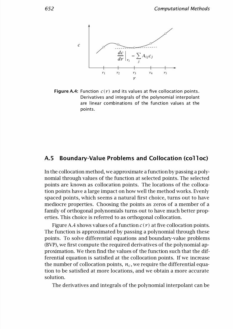
Figure A.4: Function c(r) and its values at five collocation points.

Derivatives and integrals of the polynomial interpolant

are linear combinations of the function values at the

points.

A.5 Boundary-Value Problems and Collocation (colloc)

In the collocation method, we approximate a function by passing a poly-

nomial through values of the function at selected points. The selected

points are known as collocation points. The locations of the colloca-

tion points have a large impact on how well the method works. Evenly

spaced points, which seems a natural first choice, turns out to have

mediocre properties. Choosing the points as zeros of a member of a

family of orthogonal polynomials turns out to have much better prop-

erties. This choice is referred to as orthogonal collocation.

Figure A.4 shows values of a function c(r) at five collocation points.

The function is approximated by passing a polynomial through these

points. To solve differential equations and boundary-value problems

(BVP), we first compute the required derivatives of the polynomial ap-

proximation. We then find the values of the function such that the dif-

ferential equation is satisfied at the collocation points. If we increase

the number of collocation points, nc , we require the differential equa-

tion to be satisfied at more locations, and we obtain a more accurate

solution.

The derivatives and integrals of the polynomial interpolant can be



A.5 Boundary-Value Problems and Collocation ( colloc ) 653

computed as linear combinations of the values at the collocation points

dc

dr

r i

=

ncj=1

Aij cj

d2cdr 2

r i

=nc

j=1

Bij cj

10

f(r)dr =

ncj=1

Qj f (r j )

To obtain the locations of the collocation points and derivatives and

integral weighting matrices and vectors, we use the function colloc,

based on the methods described by Villadsen and Michelsen [9].

[R A B Q] = colloc(npts-2, ’left’, ’right’);

The strings ’left’ and ’right’ specify that we would like to have col-

location points at the endpoints of the interval in addition to the zeros

of the orthogonal polynomial. We solve for the concentration profile

for the reaction-diffusion problem in a catalyst pellet to illustrate the

collocation method.

Example A.3: Single-pellet profile

Consider the isothermal, first-order reaction-diffusion problem in a

spherical pellet1

r 2d

dr

r 2

dc

dr

− Φ

2c = 0 (A.8)

c = 1, r = 3

dc

dr = 0, r = 0

The effectiveness factor is given by

η =1

Φ2

dc

dr

r =3

1. Compute the concentration profile for a first-order reaction in a

spherical pellet. Solve the problem for φ = 10.

2. Plot the concentration profile for nc = 5, 10, 30 and 50. How many

collocation points are required to reach accuracy in the concen-

tration profile for this value of Φ.




-0.4

-0.2

0

0.2

0.4

0.6

0.8

1

0 0.5 1 1.5 2 2.5 3

r

c

nc = 50nc = 30nc = 10nc = 5

Figure A.5: Dimensionless concentration versus dimensionless ra-

dial position for different numbers of collocation points.

3. How many collocation points are required to achieve a relative

error in the effectiveness factor of less than 10−5?

Solution

First we perform the differentiation in Equation A.8 to obtain

d2cdr 2

+2r

dcdr

− Φ2c = 0

We define the following Octave function to evaluate this equation at the

interior collocation points. At the two collocation endpoints, we satisfy

the boundary conditions dc/dr = 0 at r = 0 and c = 1 at r = 3. The

function is therefore

function retval = pellet(c)

global Phi A B R% differential equation at all points

retval = B*c + 2*A*c./R - Phi^2*c;



A.5 Boundary-Value Problems and Collocation ( colloc ) 655

10−12

10−10

10−8

10−6

10−4

10−2

1

5 10 15 20 25 30

η e r r o r

nc

Figure A.6: Relative error in the effectiveness factor versus number

of collocation points.

% write over first and last points with BCs

retval(1) = A(1,:)*c;

retval(end) = 1 - c(end);

endfunction

Figure A.5 shows the concentration profiles for different numbers of

collocation points. We require about nc = 30 to obtain a converged

concentration profile. Figure A.6 shows the relative error in the ef-fectiveness factor versus number of collocation points. If one is only

interested in the pellet reaction rate, about 16 collocation points are

required to achieve a relative error of less than 10−6.

Example A.4: A simple fixed-bed reactor problem

Here we set up the collocation approach of this section for the single,

second-order reaction

A → B r = kc2A




2

3

4

5

6

7

8

9

10

0 50 100 150 200 250 300 350 400

V R (L)

N A

( m o l / s )

η =1

Φ

η =1

Φ

1

tanh3Φ −

1

3Φ

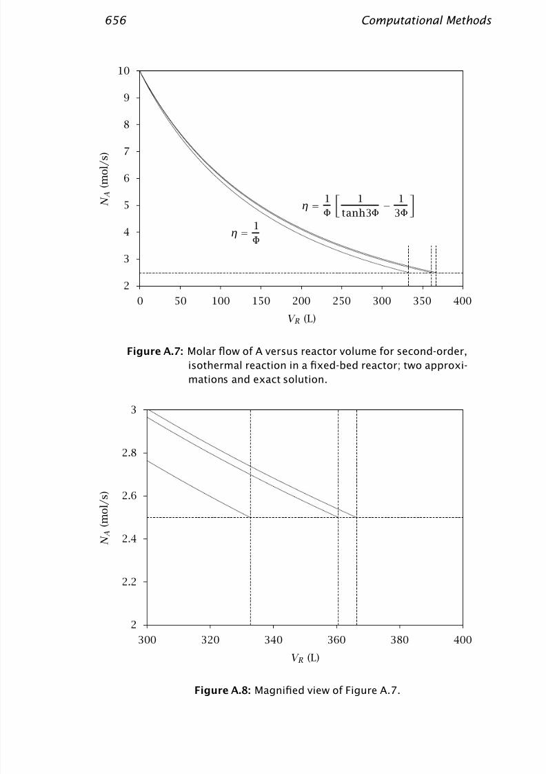
Figure A.7: Molar flow of A versus reactor volume for second-order,

isothermal reaction in a fixed-bed reactor; two approxi-

mations and exact solution.

2

2.2

2.4

2.6

2.8

3

300 320 340 360 380 400

V R (L)

N A

( m

o l / s )

Figure A.8: Magnified view of Figure A.7.



A.6 Parameter Estimation with ODE Models ( parest ) 657

Solve the model exactly and compare the numerical solution to the so-

lution obtained with the approximate Thiele modulus and effectiveness

factor approaches shown in Figure 7.26.

Solution

The model for the fluid and particle phases can be written from Equa-

tions 7.67–7.77

dN A

dV = RA = −(1 − B)

S p

V pDA

dcA

dr

r =R

d2

cA

dr 2 +

2

r

d

cA

dr +

RA

DA

= 0

cA = cA r = R

dcA

dr = 0 r = 0

The collocation method produces algebraic equations for the pellet pro-

file as for the previous example. We use a DAE solver to integrate the

differential equation for N A and these coupled algebraic equations.The results for N A versus reactor length using 25 collocation points

for the pellet are shown in Figure A.7. Also shown are the simplified

effectiveness factor calculations for this problem from Example 7.5. A

magnified view is shown in Figure A.8. Notice the effectiveness factor

approach gives a good approximation for the bed performance. It is

not exact because the reaction is second order.

A.6 Parameter Estimation with ODE Models (parest)

We have developed the function parest.m to estimate parameters in

differential equation models. It is based on SUNDIALS for the solution

of the ODEs and sensitivities, and sqp (wrapper fmincon) for the non-

linear optimization of the parameters subject to the constraints. Type

help parest at the command line to get an idea of the many options

available. We present a simple example to illustrate some of the fea-

tures.




0

0.2

0.4

0.6

0.8

1

0 1 2 3 4 5

cj

t

cA

cB

cC

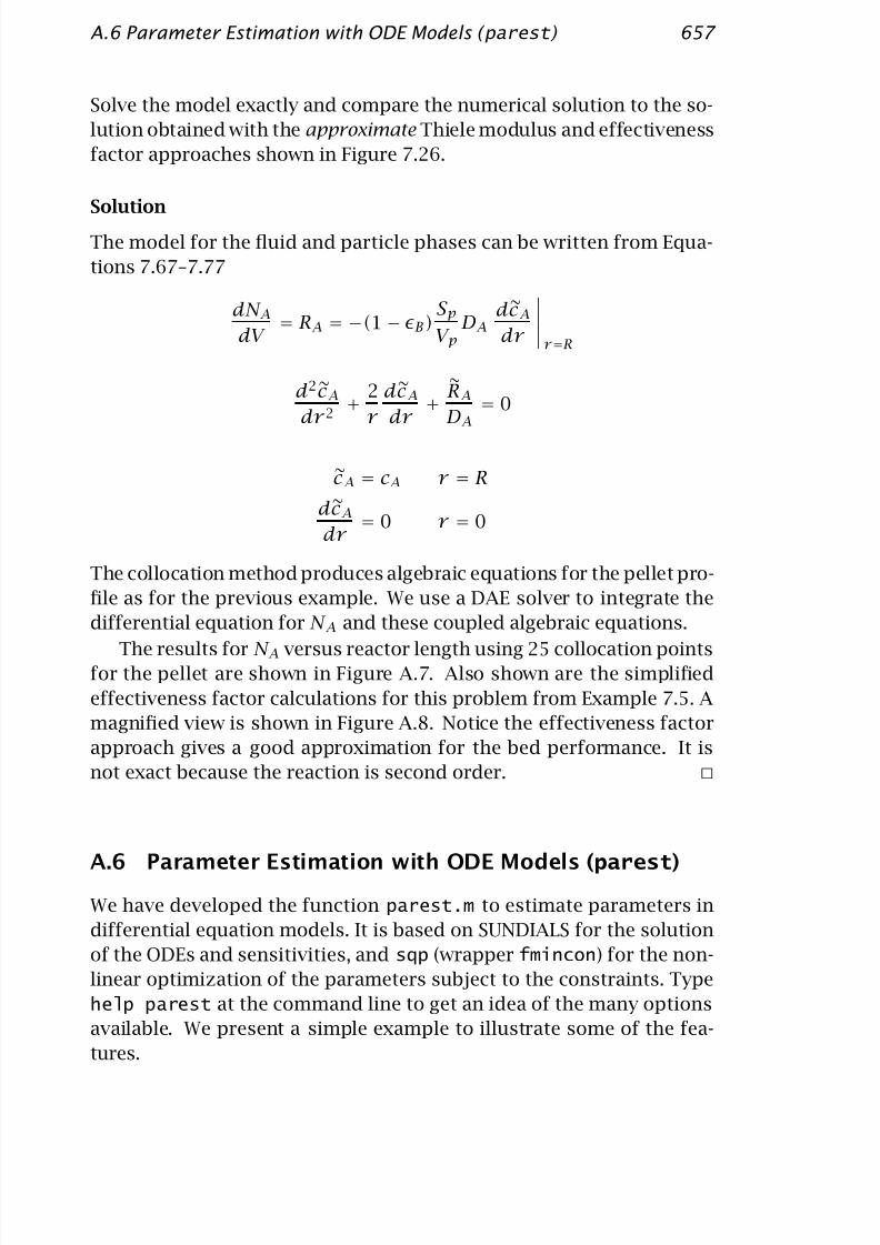
Figure A.9: Measurements of species concentrations in Reac-

tions A.9 versus time.

0

0.2

0.4

0.6

0.8

1

0 1 2 3 4 5

cj

t

cA

cB

cC

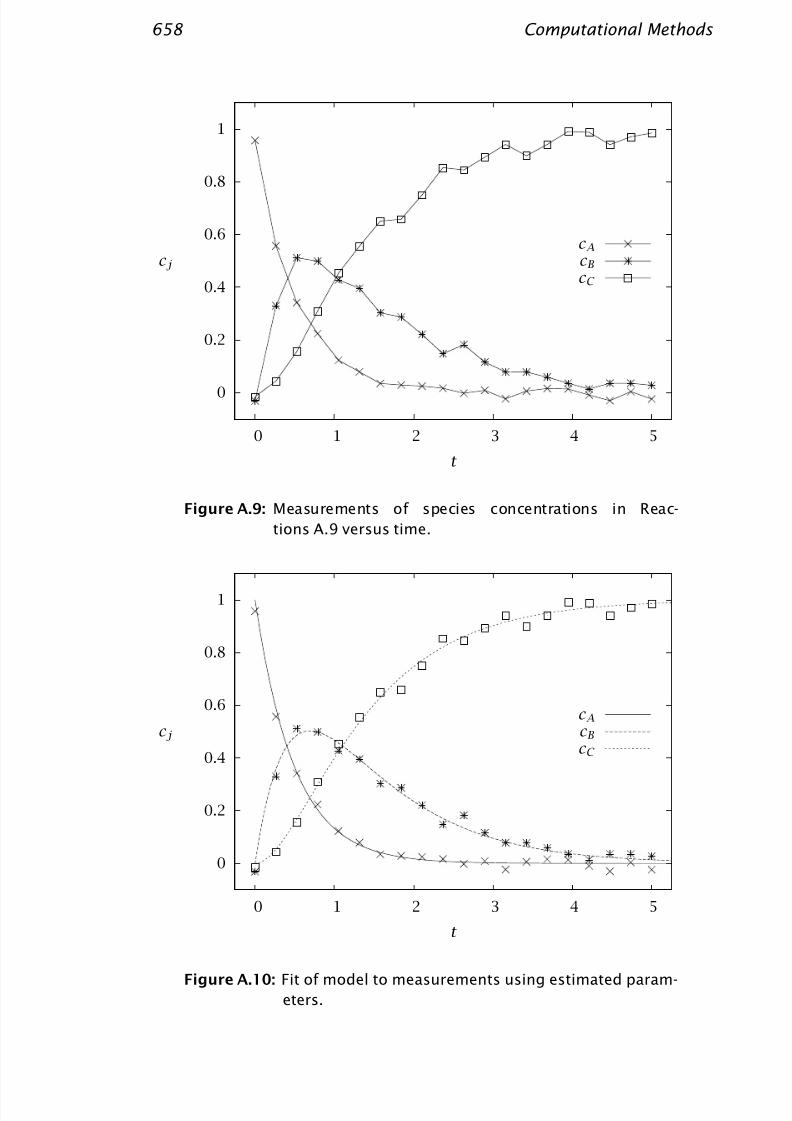
Figure A.10: Fit of model to measurements using estimated param-

eters.



A.6 Parameter Estimation with ODE Models ( parest ) 659

Example A.5: Estimating two rate constants in reaction A→ B→ C

Consider the irreversible series reactions

A k1 → B

k2 → C (A.9)

Estimate the two rate constants k1 and k2 from the measurements

shown in Figure A.9. We would also like to know how much confidence

to place in these parameter estimates.

Solution

For this problem we require only the following simple parest options.

%% ABC.m

%% Estimate parameters for the A->B->C model

%% jbr, 11/2008

% make sure ensure sundials/cvode is in the path

startup_STB

k 1 = 2 ; k 2 = 1 ;

ca0 = 1; cb0 = 0; cc0 = 0;

thetaac = [k1; k2];

tfinal = 6; nplot = 100;

model.odefcn = @massbal_ode;

model.tplot = linspace(0, tfinal, nplot)’;

model.param = thetaac;

model.ic = [ca0; cb0; cc0];

objective.estflag = [1, 2];

objective.paric = [0.5; 3];

objective.parlb = [1e-4; 1e-4;];objective.parub = [10; 10];

measure.states = [1,2,3];

%% load measurements from a file

table = load (’ABC_data.dat’);

measure.time = table(:,1);

measure.data = table(:,2:end);

%% estimate the parametersestimates = parest(model, measure, objective);




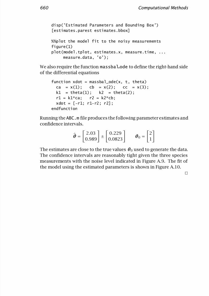
disp(’Estimated Parameters and Bounding Box’)

[estimates.parest estimates.bbox]

%%plot the model fit to the noisy measurements

figure(1)

plot(model.tplot, estimates.x, measure.time, ...

measure.data, ’o’);

We also require the function massbal ode to define the right-hand side

of the differential equations

function xdot = massbal_ode(x, t, theta)

ca = x(1); cb = x(2); cc = x(3);

k1 = theta(1); k2 = theta(2);

r1 = k1*ca; r2 = k2*cb;xdot = [-r1; r1-r2; r2];

endfunction

Running the ABC.m file produces the following parameter estimates and

confidence intervals.

θ =

2.03

0.989

±

0.229

0.0823

θ0 =

2

1

The estimates are close to the true values θ0 used to generate the data.The confidence intervals are reasonably tight given the three species

measurements with the noise level indicated in Figure A.9. The fit of

the model using the estimated parameters is shown in Figure A.10.



A.7 Exercises 661

A.7 Exercises

Exercise A.1: Water gas shift reaction and production rates

Consider the water gas shift reactions

H2O + CO CO2 + H2

H2O + H H2 + OH

OH + CO CO2 + H

Take the second and third reactions as an independent set and estimate the reaction

rates from the same 2000 production-rate measurements used in Example A.1.

(a) What value of [r 2 r 3] produces the error-free production rate corresponding to

[r 1 r 2] = [1 2]

(b) Create 2000 production-rate data points with measurement noise as in Exam-

ple A.1. Estimate [r 2 r 3] from these data and plot the result. Compare to Fig-

ure A.1. Explain the differences and similarities in the two figures.

Exercise A.2: Semi-batch polymerization reactor

Consider again Example 4.3, in which monomer is converted to polymer in a semi-batch

reactor.

(a) Solve the problem with dasrt and compute the time t1 at which the reactor fills.

Compare your answer with the result t1 = 11.2 min given in Chapter 4.

(b) Calculate the solution for both addition policies and compare your numerical

result to the analytical result in Figures 4.15-4.18.

Exercise A.3: Sensitivity for second-order kinetics

Repeat the analysis in Example A.2 for the differential equation describing a second-

order , isothermal, irreversible reaction in a constant-volume batch reactor

dcA

dt = −kc2A

cA(0) = cA0

Note: instead of solving the sensitivity differential equation, show only that the sen-

sitivity computed by taking the partial derivative of the solution to the differential

equation, cA(t), satisfies the sensitivity differential equation and initial condition.

Exercise A.4: Multiple solutions to the Weisz-Hicks problem

Using orthogonal collocation, compute the solution c(r) to the Weisz-Hicks problem,

Equations 7.65–7.66, for the following parameter values: β = 0.6, γ = 30, Φ = 0.001.

Compare your result to the calculation presented in Figure A.11.




-0.2

0

0.2

0.4

0.6

0.8

1

1.2

0 0.5 1 1.5 2 2.5 3

r

c

C

B

A

γ = 30

β = 0.6

Φ = 0.001

Figure A.11: Dimensionless concentration versus radius for the non-

isothermal spherical pellet: lower (A), unstable middle

(B), and upper (C) steady states.

Exercise A.5: Weisz-Hicks problem, increasing β

Using orthogonal collocation, resolve the Weisz-Hicks problem for the following pa-

rameter values: β = 0.85, γ = 30, Φ = 0.001. Use initial guesses for the c(r) profile

based on the results in Figure A.11.

(a) How many solutions are you able to find? Given the results in Figure 7.19, how

many solutions do you expect. Explain and justify your answer.

(b) Compare and contrast your c(r) solutions to those in Figure A.11.

Exercise A.6: Comparing shooting and collocationSolve the isothermal, first-order reaction-diffusion problem with an ODE solver, an

algebraic equation solver, and the shooting method.

1

r qd

dr

r q

dc

dr

−

2

n + 1Φ

2cn= 0

c = 1, r = q + 1

dc

dr = 0, r = 0

(a) Solve the problem with the shooting method for the first-order reaction in aspherical geometry, n = 1, q = 2, using Φ = 0.1, 1, 10, 50. Compare c(r) from

the shooting method with the analytical solution.



A.7 Exercises 663

(b) Solve the problem using the collocation method. Which method do you prefer

and why?

(c) Consider the variable transformation

w = ln(c)

Write the model and boundary conditions in the new variable, w. Solve the trans-

formed model with the collocation method. Compare the collocation solution

of the transformed model to the solution of the original model.

Exercise A.7: Transient solution of the dispersed PFR

Revisit the transient PFR example of Chapter 8, Example 8.1. Solve the problem for a

range of dispersion numbers. Can you get a CSTR-like solution for large values of the

dispersion number? Can you get a PFR-like solution for small values of the dispersion

number? Do you have numerical accuracy problems at either of these limits?

Computation Methods

Documents