Computation accuracy and efficiency of a power series analytic method for two- and three- space-dependent transient problems

lable at ScienceDirect

Progress in Nuclear Energy 51 (2009) 451–464

Contents lists avai

Progress in Nuclear Energy

journal homepage: www.elsevier .com/locate/pnucene

Computation accuracy and efficiency of a power series analytic method fortwo- and three- space-dependent transient problems

Ahmed E. Aboanber*, Yasser M. HamadaDepartment of Mathematics, Faculty of Science, Tanta University, Tanta 31527, Egypt

Keywords:Neutron diffusion equationAnalytic solutionPower seriesControl rod withdrawalPower densityDoppler feedback

* Corresponding author. Tel.: þ20 040 3450408; faE-mail addresses: [email protected]

(A.E. Aboanber), [email protected] (Y.M. Ham

0149-1970/$ – see front matter � 2008 Elsevier Ltd.doi:10.1016/j.pnucene.2008.10.003

a b s t r a c t

The establishment of solutions to large-scale three-dimensional (3-D) reactor benchmark problems isneeded to serve as standards for the verification of design codes and for the detailed error analysis ofcalculational methods. A number of partially and fully inserted control rods, represented by absorberadded to certain subassemblies, cause a strong nonseparable power distribution. In addition, the exis-tence of a very large thermal flux peak in the reflector makes this a very difficult and challengingproblem to solve.PWS code has been developed to include a numerical solution for the time-dependent neutron diffusionequations for the nuclear reactor analysis. The new technique employs a new parameter (a) which canreduce the rapid increase in magnitude of the power series coefficients. These coefficients, in turn, aredetermined by back substitutions in the non-linear canonical diffusion equations and treating terms ofthe same degree to obtain a modified recurrence relation which is valid for any type of the stiff non-linear kinetic diffusion equations.The validity of the algorithm was tested with three kinds of well-known two-group benchmark prob-lems. The first one is the two-dimensional TWIGL seed-blanket reactor kinetics problem. The second isthe two- and three-dimensional LAR BWR benchmark problem simulating a rod drop accident of a BWRcore. The third is the three-dimensional LMW LRA transient problem which simulates an operationaltransient involving rod movements. The obtained results with the proposed PWS code are comparedwith those provided by other reference codes, indicating an overall agreement and excellentperformance.

� 2008 Elsevier Ltd. All rights reserved.

1. Introduction

Nuclear safety requires precise knowledge of the behavior ofreactor cores in accidental situations, such as, for instance, anejection of control rods from the core and the resultant chainreaction runaway. In order to define the core refueling patterns, it isnecessary to solve analytically and/or numerically the neutron-kinetics equations which describe and predict the temporalevolution of the neutron population throughout the reactor.Reactor kinetics has developed along two paths based on the pointand the space–time models. The governing equations and solutionmethods for the models have been analyzed and reviewed exten-sively by many workers (e. g. Weinberg and Wigner, 1958; Clarkand Hansen, 1964; Ash, 1979; Stacey, 1969; Bell and Glasstone,

x: þ20 040 3350804., [email protected]).

All rights reserved.

1970; Hetrick, 1971; Henry, 1975; Lewins, 1978; Gehin, 1992; Stacey,2001).

The accurate prediction of reactor behavior and power is diffi-cult because it is necessary to calculate the three-dimensionalpower distribution in large and geometrically complicated cores.Furthermore, rapid transients of reactor power caused by a reac-tivity insertion due to a postulated drop or abnormal withdrawal ofthe control rod from the core have strong space-dependent feed-back associated with them. Therefore, a fast time-dependent three-dimensional transient analysis code is needed for simulating suchphenomena. This paper gives a description of the main features,capabilities and development of the power series (PWS) kineticscode (Aboanber and Hamada, 2002, 2003) system for the analyticsolution of the two- and three-dimensional kinetics diffusionequations with reactivity feedback due to a postulated drop orabnormal withdrawal of control rods from the core and an adiabaticfuel heatup thermal model. The code is used for reload safetyanalysis and all kinds of transients in which the power distributionis significantly affected.

A.E. Aboanber, Y.M. Hamada / Progress in Nuclear Energy 51 (2009) 451–464452

A literature search indicates a noticeable paucity of analyticsolution to the space–time kinetics equations. Garabedian andLeffert (1959) employed modal expansion methods to determineflux shape changes due to a local reactivity insertion in an inho-mogeneous reactor. Expanding the spatial dependence of theneutron flux and precursor concentrations in terms of the Helm-holtz eigensolutions, an infinite system of second-order differentialequations with constant coefficients results. The method appearedpractical only for simple geometries in which neutron slowingdown was uniform and non-linear feedback was omitted. Nationalmode expansions, of the initial reference reactor system, wereinvestigated by Foulke and Gyftopoulos (1967) through expandingthe neutron flux in a finite product series of unknown time-dependent coefficients and known mode space-dependentexpansion vectors. Garelis (1967) derived the analytic solution tothe space–time reactor kinetics equations for an infinite reflectedslab reactor with one group of prompt and delayed neutrons. Heassumed a d-function (in time and space) external source term andzero initial conditions for the density and precursor concentrations,but presented no benchmark evaluated solutions. Lee et al. (1983)derived and evaluated the analytic space–time solution for onegroup of prompt and delayed neutrons in a single-region slab. Aconstant external source and a constant initial condition forneutron flux and precursor concentrations were assumed. Analyticsolutions to the space–time reactor kinetics equations are evalu-ated numerically using one/two groups of prompt neutrons and sixgroups of delayed-neutron precursors in one-region sphericalreactors by Rottler and Lee (1986).

To analyze such advanced cores accurately, spatial kineticscodes based on nodal methods have been developed. In general,nodal methods are classified into three types. The first type, isthe polynomial nodal method introduced by Finnemann et al.(1977), as used in CUBBOX developed by Langenbuch et al. (1977)and in SPANDEX introduced by Aviles (1993), which employsa non-linear algorithm and a fifth-order expansion of the trans-verse-integrated fluxes. It can be easily applied to multi-energygroups by expanding the flux, source and leakage with poly-nomials. But it needs higher-order expansion to obtain accurateintra-node thermal flux shape. The second one is the analyticnodal method, which is characterized by the use of an analyticsolution in some portion of the procedures used to solve thetransverse-integrated equations. The quadratic transfer leakageapproximation form is employed in the QUANDRY (Greenmanet al., 1979). The refinement of the analytic nodal method (whichemploys analytic solutions of the one-dimensional diffusionequations to determine spatial coupling) has been investigated bySmith (1979). The PANTHER code, based on the analytic nodalmethod and used the quadratic transverse leakage approximationis recently developed by Hutt and Knight (1990, 1993). It isthought to be the most accurate but difficult to extend to morethan two energy groups, because it has the complexity inherentin the evaluation of coupling expressions. The third type is theanalytic polynomial nodal method developed by Iwamoto andYamamoto (1999). It is a hybrid of analytic and polynomialexpansions, so it gives high accuracy as well as extensibility. Withthe analytic polynomial nodal method, the flux is solvedanalytically by expanding the source term with polynomials, sothe method can be easily applied for multi-groups and a highaccuracy is obtained for cores having large spectral mismatcheffects between fuel assemblies. In order to obtain better accu-racy with three energy groups, Tamitani et al. (2003) adopted theanalytic polynomial nodal method for a BWR core simulatorAETNA (EM and FTM).

In our previous work, Aboanber and Hamada (2008), thegeneralized Runge–Kutta method, GRK-4A code, has beendeveloped for the numerical integration of the stiff space–time

diffusion equations. The method is fourth-order accurate, usingan embedded third-order solution to arrive at an estimate of thetruncation error for automatic time step control. In addition, theA(a)-stability properties of the method are investigated. Our aimin this work is to develop an efficient analytic power series(PWS) technique for two- and three-dimensional core system ofstiff coupled differential equations. Using the power series (PWS)model, the power density is obtained by expanding the flux andsource term with polynomial matrix. The reactor core is dividedinto a number of geometrically identical sub regions or ‘‘nodes’’.The size of node is most conveniently chosen in accordance withthe physical cell structure given by the fuel assembly array andan additional requirement that the node should be of approxi-mately cubical shape. In this situation a mesh grid is thenconstructed with mesh points located at the node center.Numerical solutions for several two- and three-dimensionalbenchmark problems including adiabatic Doppler feedback andcontrol rod movement have been obtained using the adoptedmethod.

This paper proposes an efficient methodology to apply, developand improve the accuracy of the neutron flux in a modal analysis fora power of the system with reactivity feedback due to a postulateddrop or abnormal withdrawal of control rods from the core, and anadiabatic fuel heatup thermal model. Section 2 describes the powerseries model for kinetics system including feedback and an adia-batic fuel model. The stability of the proposed method was dis-cussed in the same section. Numerical results of differentbenchmark problems are presented and discussed in Section 3.Section 4 summarizes the general conclusion.

2. Multigroup reactor kinetics equations with adiabaticheatup and doppler feedback

2.1. Basic mathematical model

The behavior of neutrons in a nuclear reactor is adequatelydescribed by the time-dependent Boltzmann transport equation forthe angular flux. Numerical solutions of the coupled time-depen-dent transport and precursor equations for reactor kinetics prob-lems of practical interest are prohibitively difficult, so approximatemethods are employed. The concern here is focused on the mostcommon approximation to the time-dependent transport equa-tiondthe time-dependent multigroup diffusion equation. Thederivation of the diffusion equation from the continuous energytransport equation is described in detail in a number of referencesand can be written in terms of the Doppler feedback model asfollows:

v�1g

v

vtFgðr;tÞ ¼V$Dgðr;tÞVFgðr;tÞ�Stgðr;tÞFgðr;tÞ

þXG

g0 ¼1

�Sgg0 ðr;tÞþð1�bÞcgp

g�1VSfg0 ðr;tÞ�

Fg0 ðr;tÞ

þXD

[¼1

cg[l[C[ðr;tÞþQfg

ðr;tÞ; 1�g�G ð1Þ

The rate of change of the precursor concentrations satisfy theequation:

v

vtC[ðr; tÞ ¼

XG

g¼1

ng�1b[gSfgðr; tÞFgðr; tÞ � l[C[ðr; tÞ; 1 � [ � D

(2)

The feedback model (an adiabatic fuel heatup thermal modeland feedback Doppler effects) is given by:

A.E. Aboanber, Y.M. Hamada / Progress in Nuclear Energy 51 (2009) 451–464 453

v

vtTðr; tÞ ¼ a˛

XG

g¼1

SfgFgðr; tÞ (3)

Sa1ðr; tÞ ¼ Sa1ðr;0Þn

1þ g� ffiffiffiffiffiffiffiffiffiffiffiffiffi

Tðr; tÞp

�ffiffiffiffiffiT0

p �oa ¼ 1:1954 K cm3 J�1 ðconversion factor from power to fuel temperatureÞg ¼ 0:003034 K�1=2 ðFeedback constantÞ˛ ¼ 0:3204� 10�10 J ðEnergy release per fissionÞ

)(4)

Where, vg is the neutron velocity for group g (cm s�1), Fg(r,t) isthe scalar neutron flux at position r and time t for group g(cm�2 s�1), Dg(r,t) is the diffusion coefficient (cm), D is the totalnumber of delayed-neutron precursor families, cgp

is the fractionof neutrons that appear in group g as a result of the fissionprocess (i.e. prompt fission neutron spectrum to group g), G is thetotal number of neutron energy groups, C[ is the density ofdelayed-neutron precursors in family [ (cm�3), Stg is the macro-scopic total cross section for group g (cm�1), Sgg0 is the macro-scopic transfer cross section from group g to group g0 (cm�1), n isthe mean number of neutrons emitted per fission, g is theeigenvalues which make all of the time derivatives identicallyzero, Sfg is the macroscopic fission cross section for group g(cm�1), cg[

is the delayed-neutron spectrum for family [ in groupg, b[g is the delayed-neutron fraction for precursor group [ andneutron group g, T(r,t) is the temperature of the reactor at positionr and time t and Qfg

ðr; tÞ is the external neutron source density atposition r and time t (cm�3 s�1).

Equations (1) and (2) must be completed by the appropriateinitial and boundary conditions. Regarding the boundary condi-tions, these equations are solved subject to the boundary condi-tions at the inner and outer surfaces of the reactor. The innerboundary condition is:

�DgVFgðr; tÞ ¼ J0gðtÞ at r ¼ 0; 1 � g � G (5)

Where J0gðtÞ is the return current for group g (cm�2 s�1) at positionr¼ 0. The inner boundary condition is:

pgVFgðr; tÞ þ qgFgðr; tÞ ¼ 0 at r ¼ R; 1 � g � G (6)

The zero-flux boundary is obtained with pg¼ 0 and qg¼ 1. Thezero-current boundary condition is obtained with pg¼ 0 and qg¼ 1.These conditions taking into considerations the constraintsFg(0,t)¼Fg(H,t)¼ 0 and Ci(0,t)¼ Ci(H,t)¼ 0, where r¼ 0 and r¼Hdenote the extrapolated abscissa of the boundaries of the reactorincluding the top and the bottom.

The initial conditions are

Fgðr;0Þ ¼ FgðrÞ and Ciðr;0Þ ¼ CiðrÞ

Where Fg(r) and Ci(r) are known functions. In practice, all tran-sient analysis start from an initial state in which reactor is exactlycritical, so that Fg(r) coincides with the fundamental eigenvectorof the multigroup diffusion operator at criticality and theprecursor concentrations are assumed to be in equilibrium withthe flux. Therefore, neutron-kinetics codes always includea steady state (criticality) subroutine. As however, the powerseries technique used for the point kinetics equations can beadopted to solve the diffusion equations (1) and (2) including the

feedback model, equations (1) and (2) can be rewritten in matrixform as:

v

vtFgðr; tÞ ¼ vgV$Dgðr; tÞVFgðr; tÞ þ

XG

g0 ¼1

Tgg0 ðr; tÞFg0 ðr; tÞ

þXD

i¼1

FgiCiðr; tÞ; 1 � g � G (7)

v

vtCiðr; tÞ ¼

XG

g¼1

PigFgðr; tÞ � liCiðr; tÞ; 1 � i � D (8)

where,

Tg;g ¼ vg

�cgngSfgð1� bÞ � Sag �

Xg0>g

Ssgg0

�;

Fgi ¼ vgfgili;

Pig ¼ biVgSfg and

Tg;g0 ¼ vg

�cgng0Sfg0 ð1� bÞ þ Ssg0g

�; Ssg0g ¼ 0 for g0 > g

The matrices are defined as: Fg, Ci are column matrices;Tg;g0 ; Pig and li are diagonal matrices.

The feedback model equations are solved at each mesh point ofthe nodes. The reactivity r(t) is represented in the generalizednotation:

rðtÞ ¼ IðtÞ þ FðtÞ

Where F(t) is a function representing the reactivity feedback. Forexample, I(t) may have the form sin(ut), exp(ut), or a polynomial int; while F(t) may be a function of temperature, power level, densityor other variables.

The estimated finite-difference approximation of the tempera-ture feedback for the three-dimensional geometry at time tj þ 1

starting from time tj takes the following form:

T�r; tjþ1

�zT

�r; tj�þ ðDtÞ

0@a3

XG

g¼1

SfgFg�r; tj�1A (9)

The leakage term V$DgVFgfor the three-dimensional geometryis approximated using the seven-point central by finite-differenceapproximation according to Varga (1962).

A.E. Aboanber, Y.M. Hamada / Progress in Nuclear Energy 51 (2009) 451–464454

V$DgVFgy1

ðDxÞ2hDg;j�1

2;k;lFg;j�1;k;l�

�Dg;j�1

2;k;lþDg;jþ1

2;k;l

�Fg;j;k;l

þDg;jþ12;k;l

Fg;jþ1;k;l

iþ 1

ðDyÞ2hDg;j;k�1

2;lFg;j;k�1;l

��

Dg;j;k�12;lþDg;j;kþ1

2;l

�Fg;j;k;lþDg;j;kþ1

2;lFg;j;kþ1;l

iþ 1

ðDzÞ2hDg;j;k;l�1

2Fg;j;k;l�1�

�Dg;j;k;l�1

2þDg;j;k;lþ1

2

�Fg;j;k;l

þDg;j;k;lþ12Fg;j;k;lþ1

ið10Þ

Accordingly, equations (7) and (8) can be rewritten in the matrixform as:

ddt

J ¼ MðtÞJ (11)

The matrix M(t) contains the coefficients of the flux at eachmesh point from (1 / m), and is given by:

MðtÞ ¼

26666666666664

W11 W12 W13 W14 W15 W16 W17 W18 0W21 W22 0 0 0 0 0 0 0W31 W32 W33 0 0 0 0 0 0W41 W42 0 W44 0 0 0 0 0W51 W52 0 0 W55 0 0 0 0W61 W62 0 0 0 W66 0 0 0W71 W72 0 0 0 0 W77 0 0W81 W82 0 0 0 0 0 W88 0W91 W92 0 0 0 0 0 0 0

37777777777775

where, Wij, i¼ 1, ., n, j¼ 1, ., n signifies G�G square matrices; n isthe number of energy groups for neutron flux plus six precursorgroups of delayed neutrons in addition to the adiabatic tempera-ture feedback. The fast group parameters are included in W11,which represents a seven and/or nine (2-D and/or 3-D) stripesmatrix, including the fast group terms v1[V$D1(r,t) V], v1[S1R(r,t)]and v1[v1(1�b)Sf1(r,t)], respectively. The matrix W12 corresponds toa diagonal matrix including the term v1ðv2ð1� bÞSf 2ðr; tÞÞ. Thediagonal matrices W13, W14, .,W18 correspond to a diagonal matrixincluding the terms v1ln, n¼ 1, 2, ., [. The matrix W21, representsa diagonal matrix including the term v2S1/2

s , while W22 representsa seven and/or nine (2-D and/or 3-D) stripes matrix including thethermal group terms v2[V$D2(r,t) V] and v2½S2Rðr; tÞ�. The remainderof the first column W31, ., W81 are diagonal matrices which includethe terms b1V1Sf 1ðr; tÞ;.;b6v1Sf 1ðr; tÞ, respectively. The remnantterms in the second column of the matrix W32, ., W82 are diagonalmatrices which include the terms b1v2Sf 2ðr; tÞ;.; b6v2Sf 2ðr; tÞ,respectively. The remnants of the diagonal W33, ., W88 corre-sponding to the diagonal matrices contains the terms �l1, ., �l6,respectively. Finally, W91, W92 are diagonal matrices which containthe terms aeSf 1 and aeSf 2, respectively.

The column matrix J is defined as:

J ¼ colhFft Fth C1 C2 . C[ T

iwhere, Fft¼ col[F11 F12 . F1G] describes a column vector for fastgroup fluxes defined at each mesh point, Fth¼ [F21 F22 . F2G]characterizes a column vector for thermal group fluxes defined ateach mesh point. Similarly, the precursor concentrations and theadiabatic temperature given by C1, C2, ., C6 and T should be welldefined at every mesh point.

Formally, the solution of the initial value problem in equation(11) can be written (for constant matrix M) as:

JðtÞ ¼ expðtMÞJð0Þ (12)

where, J(0) is the steady-state constant matrix determined from

the initial conditions. The aim of this work now is to investigatea method for computing an analytic solution of equation (11) that isbased on the power series expansion. Actually, the problem rep-resented by equation (11) is difficult to solve because the charac-teristic times of the system vary from the asymptotic period (orderof seconds) to the prompt-neutron lifetime (fractions of micro-seconds for some systems). Stated another way, the eigenvalues ofM vary from order þ1 inverse second to order �109 inverse second(Wight et al., 1971). Also, because M is not Hermitian it is difficult toanalyze mathematically.

By assuming power series solution of the form:

YðtÞ ¼�

A0 þ A1t þ A2t2 þ/þ Antn þ/�

eat ¼XNn¼0

ðAntnÞeat

(13)

This solution satisfies the governing differential equation andappropriates initial condition. The arbitrary constant a is chosen asan acceleration parameter which expected to reduce the rapidincrease in coefficient values of the power series and A0, A1,., An

are in general constants having a column matrix vector formdefined as:

A0 ¼ ½F11 F12 / F1m F21 F22 / F2m/ C11 C12 / C1m�T

A1 ¼F011 F012 / F01m F021 F022 / F02m / C011 C012 / C01m

TA3 ¼

F0011 F0012 / F001m F0021 F0022 / F002m / C0011 C0012 / C001m

T«

An ¼hFðnÞ11 FðnÞ12 /FðnÞ1m FðnÞ21 FðnÞ22 / FðnÞ2m / CðnÞ11 CðnÞ12 / CðnÞ1m

iT

(14)

where, Fig h Fig(0) and, Cim h Cim(0).Applying the initial condition to equation (13), the following set

of equations will be obtained:

Yð0Þ ¼ A0; Y0ð0Þ ¼ aA0 þ A1;Y00ð0Þ ¼ a2A0 þ 2aA1 þ 2A2;Y000ð0Þ ¼ a3A0 þ 3a2A1 þ 6aA2 þ 6A3;

Yð4Þð0Þ ¼ a4A0 þ 4a3A1 þ 12a2A2 þ 24aA3 þ 24A4;«

9>>>>=>>>>;

(15)

Equation (11) for higher derivatives gives:

YðiÞ ¼Xn

i¼0

�n� 1

r

�MðiÞYðn�iÞ k ¼ 0;1;2;.

¼Xn

i¼0

ðn� 1Þ!r!ðn� r � 1Þ!M

ðiÞYðn�iÞ (16)

Comparing the coefficients of equations (15) and (16) at t¼ 0,the following system of equations will be obtained:

An ¼1n

"Xn

i¼1

1ði� 1Þ!An�iM

ði�1Þð0Þ � aAi�1

#; n ¼ 0;1;2;.

An equation of this kind is usually called a recurrence relation ina general form for any order of power series. The algorithm wascoded in Visual FORTRAN for a personal computer. The resultingmodified-PWS code is applied to calculate the coefficients ofa series and so the fluxes at different mesh points and times.

By using the parameter a in the modified-PWS methodpreserves the rate of convergence of the power series and makes anadvantage that the number of coefficients taken from the powerseries can be increased without worried of divergence conse-quently, enhancing the results. Similarly, the step time interval canbe maximized without affecting the results. The estimated value of

A.E. Aboanber, Y.M. Hamada / Progress in Nuclear Energy 51 (2009) 451–464 455

the parameter a takes the entire range of interval which is(�0.005 3 a 3 0.005). The results indicated that using theparameter a improved the accuracy of flux density. The maximumerrors for 2-D TWIGLE benchmark problem as a test case was 1.9%.

To be usable, a numerical method cannot allow errors in thesolution vector to grow faster than the correct solution; that is, themethod must be stable. To ensure stability, the solution shouldremain bounded for both finite times and finite time steps. Moreprecisely, we used the definition of stability introduced byD’Alembert (Kreyszig, 1993); that is the power series is stable if(An þ 1/An)� R 3 1 for all sufficiently large n, and R is independentof n, then SnAn is convergent. If (An þ 1/An)� 1 for all sufficientlylarge n, then SnAn is divergent. However, we must impose anadditional requirement on the definition above keeping in mindthat the matrix M contains quantities of the form hvgDg/(Dx)2

arising from the approximation to the diffusion operator, whichbecomes very large when (Dx)2 becomes very small. If we fix Dx andmerely shrink Dt, then the method will be stable, as indeed almostall methods would be. Yet, the real problem exists when both Dtand Dx approach zero together. To examine this case we shouldrequire that Dt and Dx are related so that they approach zerotogether with the ratio hvgDg/(Dx)2 held fixed. For any value of theratio hvgDg/(Dx)2 is being used, the method is said to be uncondi-tionally stable. The stability analysis places no limit on the numberof neutron or precursor groups.

2.2. Power distribution

Fuel depletion and the compensating control actions affect thereactor power distribution over the lifetime of the fuel in the core.Any strong tendency of the power distribution to peak as a result offuel depletion (change in neutron flux) must be compensated bycontrol rod movement. However, the control rod movement tooffset fuel depletion reactivity effects itself produce power peaking;the presence of the rods shields the nearby fuel from depletion andwhen the rods are withdrawn, the higher local reactivity, causespower peaking.

The flux distribution in a reactor may have any amplitudebetween zero and infinity. In practice, the flux amplitude is limited byheat removal considerations and by temperature feedback effects, asthe temperature changes vary changes in the reactor occur. Forexample, the size of the reactor changes owing to thermal expansion.In addition, the neutron spectrum changes too. But at any rate, thereactor will operate at critical, within a certain rate of the power level.

To determine the amplitude of the neutron flux, the power levelof the reactor must be specified. Since each fission liberatesapproximately 200 MeV of useful energy (90% of the energy in theform of kinetic energy of fission products and electrons and 10% ofthe energy in the form of energetic neutrons and gamma rays,Stacey, 2001) the heat deposition distribution is approximately thesame as the fission rate distribution and so:

Power ¼ Total Fission Rate� 200 MeV

Introducing an expression for the fission rate,

P ¼ 3

Zreactor

Sf FðrÞd3r; in Watt

where, 3¼ 0.3204 � 10�10 J (is the energy released per fission).In more general case the power formula can be expressed in

terms of fast and thermal fluxes as:

P ¼ 3�

F1Sf 1 þ F2Sf 2

�; in Watt

where,

F1 ¼Z

reactord3rF1ðrÞ; and F2 ¼

Zreactor

d3rF2ðrÞ

The neutron flux distribution affects the temperature in the fueland coolant/moderator; the temperature of the fuel affects the fuelresonance cross section; and the temperature of the coolant/moderator affects the moderating power, both of them, in turn,affect the neutron flux distribution. In order to assess the accuracyof the cases involved in the transient calculations carefully, nodalsolutions with finer meshes are taken as a reference, namelya solution with 16 nodes per assembly. For purposes of summa-rizing results of comparisons, all figures and tables presented in thenext section gives the error in flux density or power distribution,where all the errors were calculated by taking the following form:

Relative power error ¼ reference value-tested valuereference value

� 100ð%Þ

3. Numerical results and discussion

The accurate prediction of reactor behavior is difficult because itis necessary to calculate the three-dimensional power distributionin large and geometrically complicated cores. The design aspect ofrunning spatial kinetics calculations should be mentioned, whereall of the transients considered in this section are initiated byperturbing a steady-state situation, and it is assumed that whenperturbation occurs, the flux and precursor concentrations are attheir steady-state values. These initial conditions are generallyobtained from a static calculations. It is quite unlikely, however,that the eigenvalue of the static solution will be precisely unity.Thus, to obtain a truly steady-state unperturbed problem, thefission cross section values in the diffusion and precursor equationsare redefined through divided by the static eigenvalue.

A comparison of eigenvalues and powers (or power density) forthree kinds of well-known two group benchmark problems, TWI-GLE seed-blanket reactor kinetics problem, LRA BWR benchmarkproblem and LMW LWR transient problem are described. Theresults are compared with some effective references, several testshave been carried out to validate the developed method and to testits performance in terms of numerical accuracy and computationaleffort. The method proved to perform well in all cases, includingboth step and ramp perturbations from critical configurations.

3.1. Test case I: two-dimensional TWIGLE seed-blanket reactor

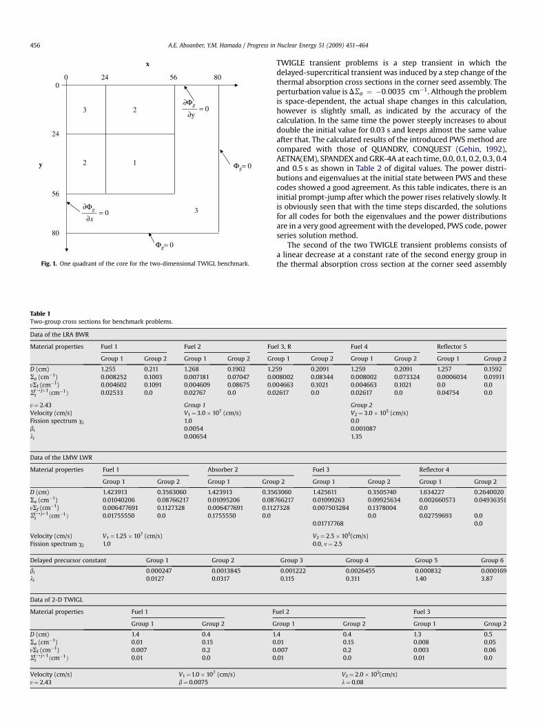
This test case is one with spatial dependence of the solutions thatwas first proposed by Hageman and Yasinsky, 1969. Analytic solu-tions are not available, and approximate results are obtained fromthe finite-difference TWIGL code. This benchmark problem is a two-dimensional core consisting of two kinds of fuel regions with noreflector region and the initial condition was a critical distribution asshown in Fig. 1. A complete data description corresponding to thisproblem is given in Table 1. As shown from the specified data, region1 is the same fuel as region 2 but it is simulated with control rodinsertion. This benchmark is a two-dimensional model of a 160 cmsquare, unreflected seed-blanket reactor using two neutron energygroups and one delayed precursor family, with a quarter-coresymmetry. The spatial meshes of PWS are taken at 8 cm interval ofsquare nodes in each direction. The small size of this transientproblem allows a study of different calculation procedures.

Two different transients are initiated to the region 1, the first isa step reactivity insertion and the second is a ramp reactivityperturbation of the corner seed assembly. The first of the two

x

00

24 56 80

24

56

80

y

3 2

2 1

3

0=∂y

∂Φg

Φg= 0

Φg= 0

= 0∂

∂Φg

x

Fig. 1. One quadrant of the core for the two-dimensional TWIGL benchmark.

Table 1Two-group cross sections for benchmark problems.

Data of the LRA BWR

Material properties Fuel 1 Fuel 2 Fu

Group 1 Group 2 Group 1 Group 2 Gr

D (cm) 1.255 0.211 1.268 0.1902 1.2Sa (cm�1) 0.008252 0.1003 0.007181 0.07047 0.0ySf (cm�1) 0.004602 0.1091 0.004609 0.08675 0.0Sj/jþ1

s ðcm�1Þ 0.02533 0.0 0.02767 0.0 0.0

y¼ 2.43 Group 1Velocity (cm/s) V1¼3.0� 107 (cm/s)Fission spectrum ci 1.0bi 0.0054li 0.00654

Data of the LMW LWR

Material properties Fuel 1 Absorber 2

Group 1 Group 2 Group 1 Grou

D (cm) 1.423913 0.3563060 1.423913 0.35Sa (cm�1) 0.01040206 0.08766217 0.01095206 0.08ySf (cm�1) 0.006477691 0.1127328 0.006477691 0.112Sj/jþ1

s ðcm�1Þ 0.01755550 0.0 0.1755550 0.0

Velocity (cm/s) V1¼1.25� 107 (cm/s)Fission spectrum ci 1.0

Delayed precursor constant Group 1 Group 2

bi 0.000247 0.0013845li 0.0127 0.0317

Data of 2-D TWIGL

Material properties Fuel 1 F

Group 1 Group 2 G

D (cm) 1.4 0.4 1Sa (cm�1) 0.01 0.15 0ySf (cm�1) 0.007 0.2 0Sj/jþ1

s ðcm�1Þ 0.01 0.0 0

Velocity (cm/s) V1¼1.0� 107 (cm/s)y¼ 2.43 b¼ 0.0075

A.E. Aboanber, Y.M. Hamada / Progress in Nuclear Energy 51 (2009) 451–464456

TWIGLE transient problems is a step transient in which thedelayed-supercritical transient was induced by a step change of thethermal absorption cross sections in the corner seed assembly. Theperturbation value is DSa ¼ �0:0035 cm�1. Although the problemis space-dependent, the actual shape changes in this calculation,however is slightly small, as indicated by the accuracy of thecalculation. In the same time the power steeply increases to aboutdouble the initial value for 0.03 s and keeps almost the same valueafter that. The calculated results of the introduced PWS method arecompared with those of QUANDRY, CONQUEST (Gehin, 1992),AETNA(EM), SPANDEX and GRK-4A at each time, 0.0, 0.1, 0.2, 0.3, 0.4and 0.5 s as shown in Table 2 of digital values. The power distri-butions and eigenvalues at the initial state between PWS and thesecodes showed a good agreement. As this table indicates, there is aninitial prompt-jump after which the power rises relatively slowly. Itis obviously seen that with the time steps discarded, the solutionsfor all codes for both the eigenvalues and the power distributionsare in a very good agreement with the developed, PWS code, powerseries solution method.

The second of the two TWIGLE transient problems consists ofa linear decrease at a constant rate of the second energy group inthe thermal absorption cross section at the corner seed assembly

el 3, R Fuel 4 Reflector 5

oup 1 Group 2 Group 1 Group 2 Group 1 Group 2

59 0.2091 1.259 0.2091 1.257 0.159208002 0.08344 0.008002 0.073324 0.0006034 0.0191104663 0.1021 0.004663 0.1021 0.0 0.02617 0.0 0.02617 0.0 0.04754 0.0

Group 2V2¼ 3.0� 105 (cm/s)0.00.0010871.35

Fuel 3 Reflector 4

p 2 Group 1 Group 2 Group 1 Group 2

63060 1.425611 0.3505740 1.634227 0.2640020766217 0.01099263 0.09925634 0.002660573 0.049363517328 0.007503284 0.1378004 0.0

0.0 0.02759693 0.00.01717768 0.0

V2¼ 2.5� 105(cm/s)0.0, y¼ 2.5

Group 3 Group 4 Group 5 Group 6

0.001222 0.0026455 0.000832 0.0001690.115 0.311 1.40 3.87

uel 2 Fuel 3

roup 1 Group 2 Group 1 Group 2

.4 0.4 1.3 0.5.01 0.15 0.008 0.05.007 0.2 0.003 0.06.01 0.0 0.01 0.0

V2¼ 2.0� 105(cm/s)l¼ 0.08

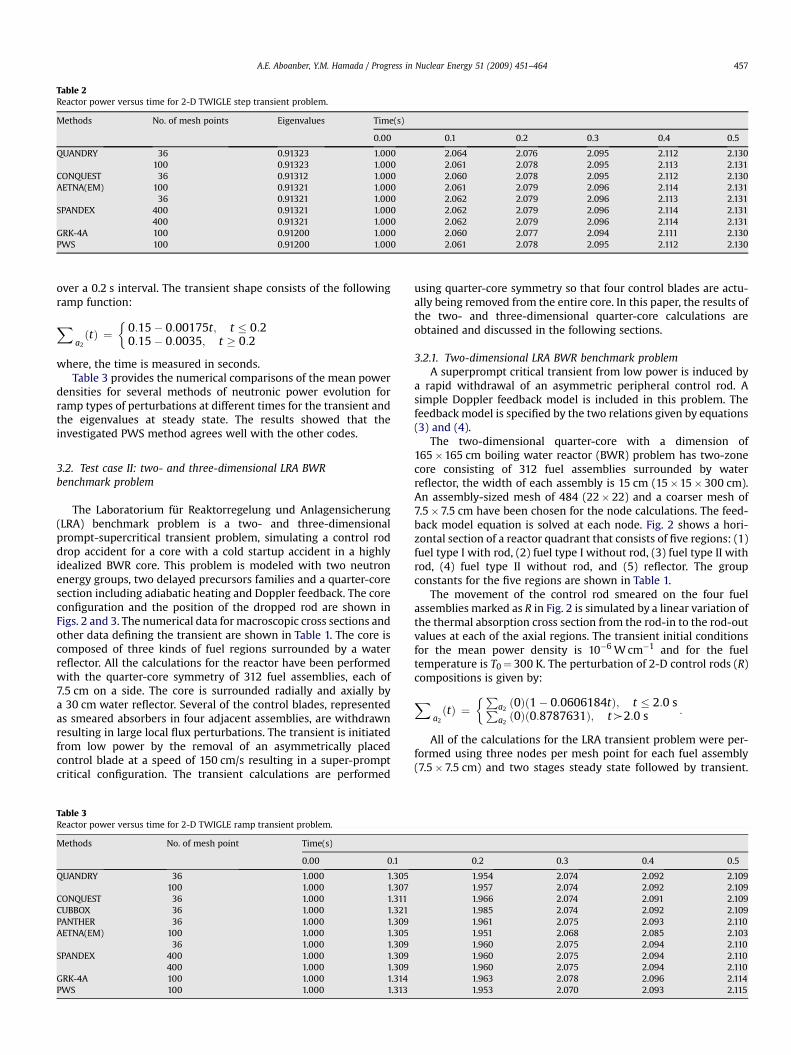
Table 2Reactor power versus time for 2-D TWIGLE step transient problem.

Methods No. of mesh points Eigenvalues Time(s)

0.00 0.1 0.2 0.3 0.4 0.5

QUANDRY 36 0.91323 1.000 2.064 2.076 2.095 2.112 2.130100 0.91323 1.000 2.061 2.078 2.095 2.113 2.131

CONQUEST 36 0.91312 1.000 2.060 2.078 2.095 2.112 2.130AETNA(EM) 100 0.91321 1.000 2.061 2.079 2.096 2.114 2.131

36 0.91321 1.000 2.062 2.079 2.096 2.113 2.131SPANDEX 400 0.91321 1.000 2.062 2.079 2.096 2.114 2.131

400 0.91321 1.000 2.062 2.079 2.096 2.114 2.131GRK-4A 100 0.91200 1.000 2.060 2.077 2.094 2.111 2.130PWS 100 0.91200 1.000 2.061 2.078 2.095 2.112 2.130

A.E. Aboanber, Y.M. Hamada / Progress in Nuclear Energy 51 (2009) 451–464 457

over a 0.2 s interval. The transient shape consists of the followingramp function:

Xa2

ðtÞ ¼�

0:15� 0:00175t; t � 0:20:15� 0:0035; t � 0:2

where, the time is measured in seconds.Table 3 provides the numerical comparisons of the mean power

densities for several methods of neutronic power evolution forramp types of perturbations at different times for the transient andthe eigenvalues at steady state. The results showed that theinvestigated PWS method agrees well with the other codes.

3.2. Test case II: two- and three-dimensional LRA BWRbenchmark problem

The Laboratorium fur Reaktorregelung und Anlagensicherung(LRA) benchmark problem is a two- and three-dimensionalprompt-supercritical transient problem, simulating a control roddrop accident for a core with a cold startup accident in a highlyidealized BWR core. This problem is modeled with two neutronenergy groups, two delayed precursors families and a quarter-coresection including adiabatic heating and Doppler feedback. The coreconfiguration and the position of the dropped rod are shown inFigs. 2 and 3. The numerical data for macroscopic cross sections andother data defining the transient are shown in Table 1. The core iscomposed of three kinds of fuel regions surrounded by a waterreflector. All the calculations for the reactor have been performedwith the quarter-core symmetry of 312 fuel assemblies, each of7.5 cm on a side. The core is surrounded radially and axially bya 30 cm water reflector. Several of the control blades, representedas smeared absorbers in four adjacent assemblies, are withdrawnresulting in large local flux perturbations. The transient is initiatedfrom low power by the removal of an asymmetrically placedcontrol blade at a speed of 150 cm/s resulting in a super-promptcritical configuration. The transient calculations are performed

Table 3Reactor power versus time for 2-D TWIGLE ramp transient problem.

Methods No. of mesh point Time(s)

0.00 0.1

QUANDRY 36 1.000 1.305100 1.000 1.307

CONQUEST 36 1.000 1.311CUBBOX 36 1.000 1.321PANTHER 36 1.000 1.309AETNA(EM) 100 1.000 1.305

36 1.000 1.309SPANDEX 400 1.000 1.309

400 1.000 1.309GRK-4A 100 1.000 1.314PWS 100 1.000 1.313

using quarter-core symmetry so that four control blades are actu-ally being removed from the entire core. In this paper, the results ofthe two- and three-dimensional quarter-core calculations areobtained and discussed in the following sections.

3.2.1. Two-dimensional LRA BWR benchmark problemA superprompt critical transient from low power is induced by

a rapid withdrawal of an asymmetric peripheral control rod. Asimple Doppler feedback model is included in this problem. Thefeedback model is specified by the two relations given by equations(3) and (4).

The two-dimensional quarter-core with a dimension of165�165 cm boiling water reactor (BWR) problem has two-zonecore consisting of 312 fuel assemblies surrounded by waterreflector, the width of each assembly is 15 cm (15�15� 300 cm).An assembly-sized mesh of 484 (22� 22) and a coarser mesh of7.5�7.5 cm have been chosen for the node calculations. The feed-back model equation is solved at each node. Fig. 2 shows a hori-zontal section of a reactor quadrant that consists of five regions: (1)fuel type I with rod, (2) fuel type I without rod, (3) fuel type II withrod, (4) fuel type II without rod, and (5) reflector. The groupconstants for the five regions are shown in Table 1.

The movement of the control rod smeared on the four fuelassemblies marked as R in Fig. 2 is simulated by a linear variation ofthe thermal absorption cross section from the rod-in to the rod-outvalues at each of the axial regions. The transient initial conditionsfor the mean power density is 10�6 W cm�1 and for the fueltemperature is T0¼ 300 K. The perturbation of 2-D control rods (R)compositions is given by:

Xa2

ðtÞ ¼�P

a2ð0Þð1� 0:0606184tÞ; t � 2:0 sP

a2ð0Þð0:8787631Þ; t_2:0 s :

All of the calculations for the LRA transient problem were per-formed using three nodes per mesh point for each fuel assembly(7.5�7.5 cm) and two stages steady state followed by transient.

0.2 0.3 0.4 0.5

1.954 2.074 2.092 2.1091.957 2.074 2.092 2.1091.966 2.074 2.091 2.1091.985 2.074 2.092 2.1091.961 2.075 2.093 2.1101.951 2.068 2.085 2.1031.960 2.075 2.094 2.1101.960 2.075 2.094 2.1101.960 2.075 2.094 2.1101.963 2.078 2.096 2.1141.953 2.070 2.093 2.115

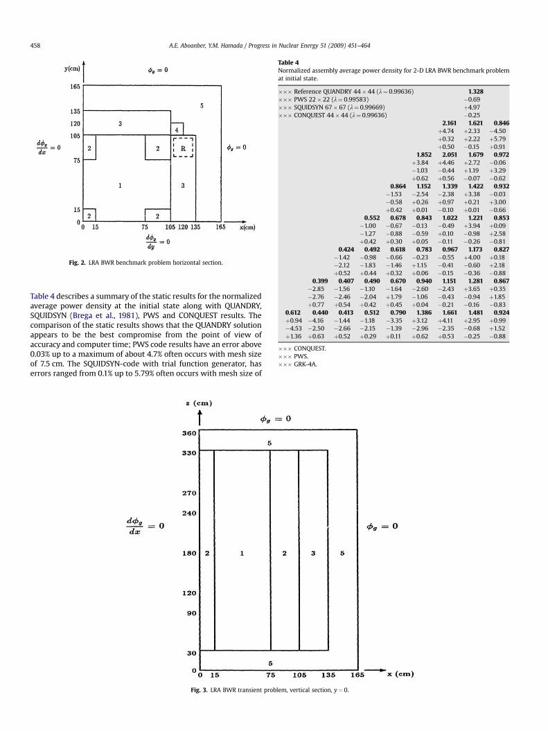
Fig. 2. LRA BWR benchmark problem horizontal section.

Table 4Normalized assembly average power density for 2-D LRA BWR benchmark problemat initial state.

��� Reference QUANDRY 44� 44 (l¼ 0.99636) 1.328��� PWS 22� 22 (l¼ 0.99583) �0.69��� SQUIDSYN 67� 67 (l¼ 0.99669) þ4.97��� CONQUEST 44� 44 (l¼ 0.99636) �0.25

2.161 1.621 0.846þ4.74 þ2.33 �4.50þ0.32 þ2.22 þ5.79þ0.50 �0.15 þ0.91

1.852 2.051 1.679 0.972þ3.84 þ4.46 þ2.72 �0.06�1.03 �0.44 þ1.19 þ3.29þ0.62 þ0.56 �0.07 �0.62

0.864 1.152 1.339 1.422 0.932�1.53 �2.54 �2.38 þ3.38 �0.03�0.58 þ0.26 þ0.97 þ0.21 þ3.00þ0.42 þ0.01 �0.10 þ0.01 �0.66

0.552 0.678 0.843 1.022 1.221 0.853�1.00 �0.67 �0.13 �0.49 þ3.94 þ0.09�1.27 �0.88 �0.59 þ0.10 �0.98 þ2.58þ0.42 þ0.30 þ0.05 �0.11 �0.26 �0.81

0.424 0.492 0.618 0.783 0.967 1.173 0.827�1.42 �0.98 �0.66 �0.23 �0.55 þ4.00 þ0.18�2.12 �1.83 �1.46 þ1.15 �0.41 �0.60 þ2.18þ0.52 þ0.44 þ0.32 þ0.06 �0.15 �0.36 �0.88

0.399 0.407 0.490 0.670 0.940 1.151 1.281 0.867�2.85 �1.56 �1.10 �1.64 �2.60 �2.43 þ3.65 þ0.35�2.76 �2.46 �2.04 þ1.79 �1.06 �0.43 �0.94 þ1.85þ0.77 þ0.54 þ0.42 þ0.45 þ0.04 �0.21 �0.16 �0.83

0.612 0.440 0.413 0.512 0.790 1.386 1.661 1.481 0.924þ0.94 �4.16 �1.44 �1.18 �3.35 þ3.12 þ4.11 þ2.95 þ0.99�4.53 �2.50 �2.66 �2.15 �1.39 �2.96 �2.35 �0.68 þ1.52þ1.36 þ0.63 þ0.52 þ0.29 þ0.11 þ0.62 þ0.53 �0.25 �0.88

��� CONQUEST.��� PWS.��� GRK-4A.

A.E. Aboanber, Y.M. Hamada / Progress in Nuclear Energy 51 (2009) 451–464458

Table 4 describes a summary of the static results for the normalizedaverage power density at the initial state along with QUANDRY,SQUIDSYN (Brega et al., 1981), PWS and CONQUEST results. Thecomparison of the static results shows that the QUANDRY solutionappears to be the best compromise from the point of view ofaccuracy and computer time; PWS code results have an error above0.03% up to a maximum of about 4.7% often occurs with mesh sizeof 7.5 cm. The SQUIDSYN-code with trial function generator, haserrors ranged from 0.1% up to 5.79% often occurs with mesh size of

Fig. 3. LRA BWR transient problem, vertical section, y¼ 0.

Table 5Normalized power distributions for 2-D LRA transient problems at t¼ 3.0 s.

Y¼ 9 0.5004 0.5043 0.5520 0.6768 0.8723 1.0511 1.05480.4982 0.5002 0.5485 0.6706 0.8594 1.0335 0.99100.5052 0.5078 0.5584 0.6857 0.8835 1.0651 1.0167

Y¼ 8 0.7991 0.7427 0.7861 0.9839 1.3694 1.8946 2.1939 2.24210.8025 0.7534 0.8040 1.0050 1.3827 1.8978 2.1870 2.18540.8134 0.7651 0.8196 1.0298 1.4274 1.9546 2.2023 2.1843

Y¼ 7 0.8993 0.6630 0.6531 0.8420 1.3341 2.4244 3.1672 3.5009 2.25180.9017 0.6320 0.6384 0.8245 1.2770 2.4654 3.2243 3.6234 2.19510.9131 0.6416 0.6509 0.8465 1.3135 2.5077 3.1510 3.5428 2.1850

Y¼ 6 0.7557 0.5464 0.5356 0.7058 1.1645 2.2115 3.0238 3.5799 2.44180.7421 0.5174 0.5266 0.6951 1.1165 2.2419 3.0697 3.7050 2.47600.7507 0.5242 0.5362 0.7121 1.1386 2.2453 2.9256 3.5631 2.4361

Y¼ 5 0.4368 0.3995 0.4267 0.5612 0.8468 1.3041 1.7794 2.2192 1.58900.4144 0.3908 0.4206 0.5516 0.8208 1.2490 1.6959 2.2367 1.56250.4183 0.3949 0.4274 0.5635 0.8356 1.2378 1.6010 2.1079 1.5250

Y¼ 4 0.2902 0.2969 0.3364 0.4353 0.6073 0.8416 1.1250 1.4444 1.05300.2861 0.2937 0.3333 0.4300 0.5978 0.8303 1.1048 1.4869 1.05530.2883 0.2963 0.3376 0.4379 0.6100 0.8392 1.0972 1.4809 1.0646

Y¼ 3 0.2366 0.2453 0.2801 0.3583 0.4867 0.6544 0.8529 1.0780 0.77940.2347 0.2436 0.2786 0.3561 0.4831 0.6515 0.8461 1.1220 0.78890.2360 0.2544 0.2814 0.3610 0.4916 0.6634 0.8587 1.1395 0.8044

Y¼ 2 0.2498 0.2362 0.2571 0.3303 0.4699 0.6708 0.8421 0.9682 0.66840.2429 0.2331 0.2563 0.3292 0.4640 0.6576 0.8275 1.0103 0.68090.2436 0.2342 0.2582 0.3323 0.4701 0.6667 0.8388 1.0250 0.6917

Y¼ 1 0.3461 0.2551 0.2538 0.3298 0.5209 0.9274 1.1254 1.0164 0.64370.3533 0.2486 0.2535 0.3299 0.5079 0.9578 1.1732 1.0560 0.66130.3538 0.2494 0.2549 0.3321 0.5125 0.9673 1.1815 1.0671 0.6692X¼ 1 X¼ 2 X¼ 3 X¼ 4 X¼ 5 X¼ 6 X¼ 7 X¼ 8 X¼ 9

��� CONQUEST.��� PWS.��� GRK-4A.

A.E. Aboanber, Y.M. Hamada / Progress in Nuclear Energy 51 (2009) 451–464 459

2.5 cm. Finally, the CONQUEST code is more accurate for thisproblem since the error does not exceed 1.36%. Thus, however, theerrors in the assembly power densities obtained by PWS codesignificantly agree with those of CONQUEST and SQUIDSYN.

The prompt-supercritical transient is initiated by linearlydecreasing the thermal absorption cross section in a portion of thecore for 2 s, and then maintaining the cross section at the new value

Table 6Fuel temperatures for 2-D LRA transient problems at t¼ 3.0 s.

Y¼ 9 716.21 719.55 759.48 863.08689.92 691.52 744.10 859.67711.09 713.21 754.03 856.06

Y¼ 8 965.74 918.89 955.29 1119.8996.98 939.54 999.21 1086.2963.89 923.87 967.24 1135.2

Y¼ 7 1048.4 851.97 844.00 1000.81024.0 828.17 833.86 1010.41044.2 822.44 828.86 984.39

Y¼ 6 926.58 753.04 744.28 885.24920.23 701.90 716.21 877.30909.56 725.11 733.69 874.26

Y¼ 5 659.76 628.90 651.64 762.86610.63 588.81 617.43 745.39637.30 618.06 643.43 752.35

Y¼ 4 536.11 541.86 574.88 656.88512.00 512.00 534.90 623.66529.47 536.11 569.13 649.48

Y¼ 3 489.02 497.52 526.98 592.32480.47 487.84 512.00 551.28485.30 493.16 522.70 587.11

Y¼ 2 498.02 488.32 507.07 568.97484.28 478.25 496.91 527.25489.06 482.70 503.21 564.23

Y¼ 1 572.72 502.28 503.78 568.52538.21 488.56 494.15 527.58573.04 493.67 500.21 564.37X¼ 1 X¼ 2 X¼ 3 X¼ 4

��� CONQUEST.��� PWS.��� GRK-4A.

for the remainder of the calculations. In order to examine theeffects of the temperature shapes on the transient solutions, a verysimple model for the temperature distribution within each node isemployed. The fluxes in each quarter node are approximated by themean of the node-averaged fluxes in the four nodes. Once theaverage fluxes in the four quarter nodes are determined, they arerenormalized such that the average flux in each node is preserved.

1023.0 1163.6 1154.01024.0 1113.1 1024.01011.5 1150.2 1103.91436.1 1855.1 2064.1 2051.41461.6 1898.3 2048.3 2023.51448.1 1862.7 2065.7 2014.51404.6 2282.4 2823.7 2952.9 1960.41355.3 2311.7 2996.8 3128.7 1924.71358.0 2322.5 2884.5 3046.4 1914.41260.6 2103.3 2704.2 3013.4 2110.01204.1 2048.0 2851.7 3182.7 2048.01221.1 2132.6 2753.8 3109.4 2131.1996.60 1363.2 1725.2 2039.5 1527.3999.89 1313.1 1706.0 2048.0 1565.0973.88 1318.9 1663.1 2062.3 1510.7798.13 987.53 1210.9 1458.2 1137.2784.73 1001.1 1174.0 1541.1 1087.8787.87 976.91 1193.8 1491.4 1136.8698.88 836.84 997.76 1177.8 931.43665.94 833.76 1011.3 1189.4 964.66692.36 831.18 988.78 1208.9 935.38685.80 853.23 995.15 1097.5 848.50650.93 842.84 1005.3 1065.1 859.16676.33 836.89 976.90 1124.5 853.34728.55 1067.2 1233.0 1141.9 831.71688.58 1024.0 1249.3 1138.3 846.29712.31 1082.8 1261.8 1165.4 840.13X¼ 5 X¼ 6 X¼ 7 X¼ 8 X¼ 9

A.E. Aboanber, Y.M. Hamada / Progress in Nuclear Energy 51 (2009) 451–464460

Average fuel temperatures in each quarter node at a given time stepare then advanced to the next time step by using the quarter node-averaged fluxes. Tables 5 and 6 presented the normalized powerdistributions and the fuel temperature for 2-D problem at timet¼ 3 s. The accuracy of the PWS is estimated against GRK-4A andCONQUEST codes. These tables show that the average error for the2-D transient problem is more closely to those at the end of ramp attime t¼ 3.0 s. In this case, the choice of the time steps is dictated bystability problems. As a matter of fact, smaller time steps aresometimes needed for the PWS method. There are two spatialeffects which are responsible for most of the errors. First, there isthe inaccuracy in the neutronic model due to large mesh spacing.This effect is quite small and cannot account for the large errors.The fact that the temperature feedback is computed with the samespatial mesh as the neutronics is, however, the second quiteimportant effect.

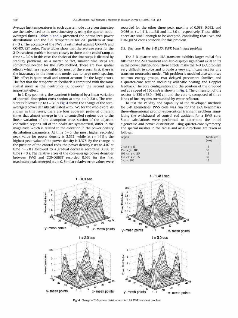
In 2-D xy geometry, the transient is induced by a linear variationof thermal absorption cross section at time t¼ 0–2.0 s. The tran-sient is followed up to t¼ 3.0 s. Fig. 4 shows the change of the core-averaged power density calculated with PWS for the whole core. Asshown in this figure, there are four apparent peaks at differenttimes that almost emerge in the uncontrolled regions due to thelinear variation of the absorption cross section of the adjacentcontrolled regions. All of the peaks are symmetrical, differ in themagnitude which is related to the elevation in the power densitydistribution parameters. At time t¼ 0, the most higher recordedpeak value for power density is 2.312; while at t¼ 1.411 s thehighest peak value of the power density is 3.378. By the change inthe position of the control rods, the power density rises to 4.07 attime t¼ 2.0 s followed by a gradual decrease recording 3.886 attime t¼ 3 s. The relative error of the core-average power densitiesbetween PWS and CONQUEST recorded 0.062 for the firstmaximum peak emerged at t¼ 0. Similar relative error values were

Fig. 4. Change of 2-D power distributio

recorded for the other three peak maxima of 0.088, 0.092, and0.056 at t¼ 1.411, t¼ 2.0 and t¼ 3.0 s, respectively. These differ-ences are small enough to be accepted, concluding that PWS andCONQUEST codes coincide for this problem.

3.3. Test case II: the 3-D LRA BWR benchmark problem

The 3-D quarter-core LRA transient exhibits larger radial fluxtilts than the 2-D transient and also displays significant axial shiftsin the power distribution. These effects make the 3-D LRA problemvery difficult to solve and provide a very significant test for anytransient neutronics model. This problem is modeled also with twoneutron energy groups, two delayed precursors families anda quarter-core section including adiabatic heating and Dopplerfeedback. The core configuration and the position of the droppedrod at a speed of 150 cm/s is shown in Fig. 3. The dimension of thereactor is 330� 330� 360 cm and the core is composed of threekinds of fuel regions surrounded by water reflector.

To test the validity and capability of the developed methodsfor 3-D geometries, PWS code was run for the LRA benchmarkthree-dimensional prompt-supercritical transient problem simu-lating the withdrawal of control rod accident for a BWR core.Static calculations were performed to determine the initialeigenvalue and power distribution using quarter-core symmetry.The special meshes in the radial and axial directions are taken asfollows:Region Mesh size

ns for LRA BWR transient problem.

(cm)

0< x, y< 15

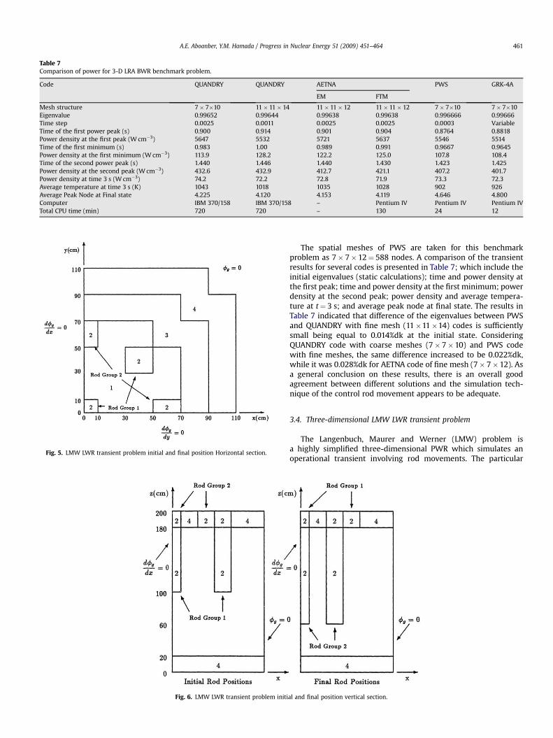
Table 7Comparison of power for 3-D LRA BWR benchmark problem.

Code QUANDRY QUANDRY AETNA PWS GRK-4A

EM FTM

Mesh structure 7� 7�10 11� 11� 14 11� 11� 12 11� 11� 12 7� 7�10 7� 7�10Eigenvalue 0.99652 0.99644 0.99638 0.99638 0.996666 0.99666Time step 0.0025 0.0011 0.0025 0.0025 0.0003 VariableTime of the first power peak (s) 0.900 0.914 0.901 0.904 0.8764 0.8818Power density at the first peak (W cm�3) 5647 5532 5721 5637 5546 5514Time of the first minimum (s) 0.983 1.00 0.989 0.991 0.9667 0.9645Power density at the first minimum (W cm�3) 113.9 128.2 122.2 125.0 107.8 108.4Time of the second power peak (s) 1.440 1.446 1.440 1.430 1.423 1.425Power density at the second peak (W cm�3) 432.6 432.9 412.7 421.1 407.2 401.7Power density at time 3 s (W cm�3) 74.2 72.2 72.8 71.9 73.3 72.3Average temperature at time 3 s (K) 1043 1018 1035 1028 902 926Average Peak Node at Final state 4.225 4.120 4.153 4.119 4.646 4.800Computer IBM 370/158 IBM 370/158 – Pentium IV Pentium IV Pentium IVTotal CPU time (min) 720 720 – 130 24 12

Fig. 5. LMW LWR transient problem initial and final position Horizontal section.

Fig. 6. LMW LWR transient problem initi

A.E. Aboanber, Y.M. Hamada / Progress in Nuclear Energy 51 (2009) 451–464 461

The spatial meshes of PWS are taken for this benchmarkproblem as 7� 7�12¼ 588 nodes. A comparison of the transientresults for several codes is presented in Table 7; which include theinitial eigenvalues (static calculations); time and power density atthe first peak; time and power density at the first minimum; powerdensity at the second peak; power density and average tempera-ture at t¼ 3 s; and average peak node at final state. The results inTable 7 indicated that difference of the eigenvalues between PWSand QUANDRY with fine mesh (11�11�14) codes is sufficientlysmall being equal to 0.014%dk at the initial state. ConsideringQUANDRY code with coarse meshes (7� 7�10) and PWS codewith fine meshes, the same difference increased to be 0.022%dk,while it was 0.028%dk for AETNA code of fine mesh (7� 7�12). Asa general conclusion on these results, there is an overall goodagreement between different solutions and the simulation tech-nique of the control rod movement appears to be adequate.

3.4. Three-dimensional LMW LWR transient problem

The Langenbuch, Maurer and Werner (LMW) problem isa highly simplified three-dimensional PWR which simulates anoperational transient involving rod movements. The particular

al and final position vertical section.

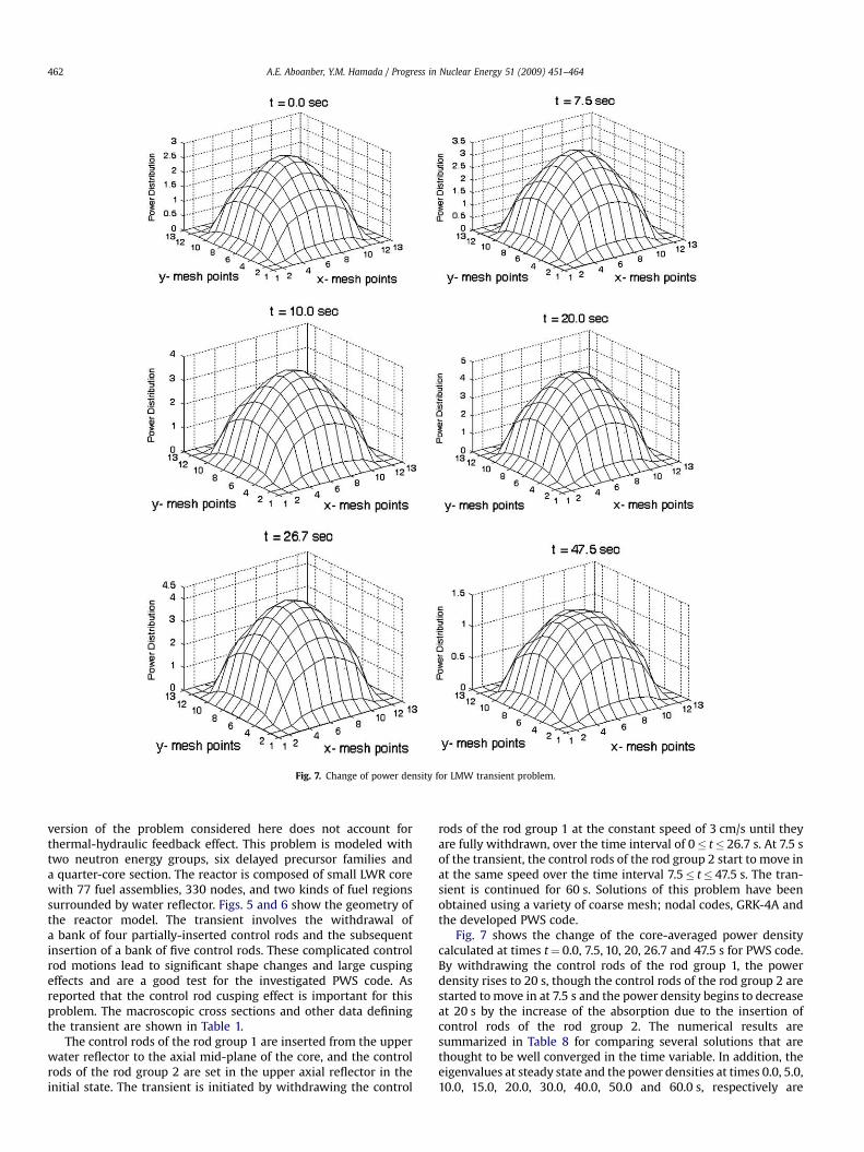
Fig. 7. Change of power density for LMW transient problem.

A.E. Aboanber, Y.M. Hamada / Progress in Nuclear Energy 51 (2009) 451–464462

version of the problem considered here does not account forthermal-hydraulic feedback effect. This problem is modeled withtwo neutron energy groups, six delayed precursor families anda quarter-core section. The reactor is composed of small LWR corewith 77 fuel assemblies, 330 nodes, and two kinds of fuel regionssurrounded by water reflector. Figs. 5 and 6 show the geometry ofthe reactor model. The transient involves the withdrawal ofa bank of four partially-inserted control rods and the subsequentinsertion of a bank of five control rods. These complicated controlrod motions lead to significant shape changes and large cuspingeffects and are a good test for the investigated PWS code. Asreported that the control rod cusping effect is important for thisproblem. The macroscopic cross sections and other data definingthe transient are shown in Table 1.

The control rods of the rod group 1 are inserted from the upperwater reflector to the axial mid-plane of the core, and the controlrods of the rod group 2 are set in the upper axial reflector in theinitial state. The transient is initiated by withdrawing the control

rods of the rod group 1 at the constant speed of 3 cm/s until theyare fully withdrawn, over the time interval of 0� t� 26.7 s. At 7.5 sof the transient, the control rods of the rod group 2 start to move inat the same speed over the time interval 7.5� t� 47.5 s. The tran-sient is continued for 60 s. Solutions of this problem have beenobtained using a variety of coarse mesh; nodal codes, GRK-4A andthe developed PWS code.

Fig. 7 shows the change of the core-averaged power densitycalculated at times t¼ 0.0, 7.5, 10, 20, 26.7 and 47.5 s for PWS code.By withdrawing the control rods of the rod group 1, the powerdensity rises to 20 s, though the control rods of the rod group 2 arestarted to move in at 7.5 s and the power density begins to decreaseat 20 s by the increase of the absorption due to the insertion ofcontrol rods of the rod group 2. The numerical results aresummarized in Table 8 for comparing several solutions that arethought to be well converged in the time variable. In addition, theeigenvalues at steady state and the power densities at times 0.0, 5.0,10.0, 15.0, 20.0, 30.0, 40.0, 50.0 and 60.0 s, respectively are

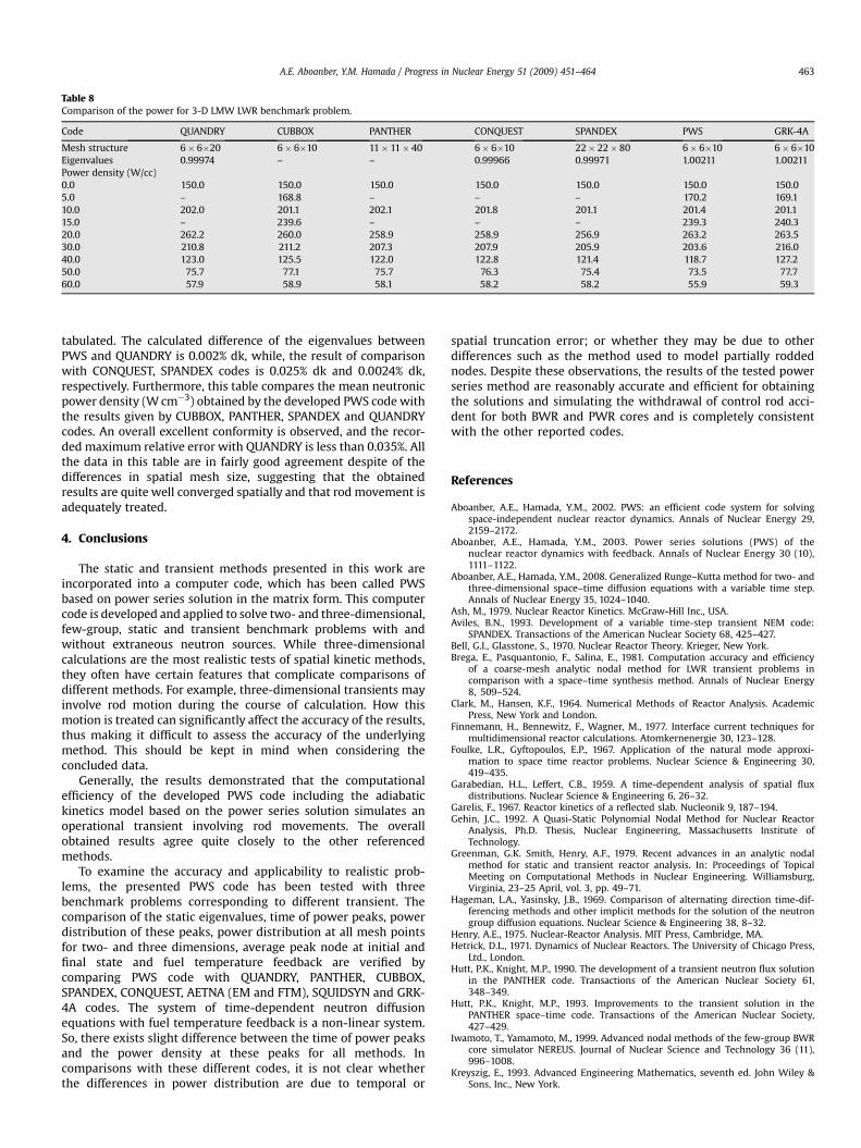
Table 8Comparison of the power for 3-D LMW LWR benchmark problem.

Code QUANDRY CUBBOX PANTHER CONQUEST SPANDEX PWS GRK-4A

Mesh structure 6� 6�20 6� 6�10 11� 11� 40 6� 6�10 22� 22� 80 6� 6�10 6� 6�10Eigenvalues 0.99974 – – 0.99966 0.99971 1.00211 1.00211Power density (W/cc)0.0 150.0 150.0 150.0 150.0 150.0 150.0 150.05.0 – 168.8 – – – 170.2 169.110.0 202.0 201.1 202.1 201.8 201.1 201.4 201.115.0 – 239.6 – – – 239.3 240.320.0 262.2 260.0 258.9 258.9 256.9 263.2 263.530.0 210.8 211.2 207.3 207.9 205.9 203.6 216.040.0 123.0 125.5 122.0 122.8 121.4 118.7 127.250.0 75.7 77.1 75.7 76.3 75.4 73.5 77.760.0 57.9 58.9 58.1 58.2 58.2 55.9 59.3

A.E. Aboanber, Y.M. Hamada / Progress in Nuclear Energy 51 (2009) 451–464 463

tabulated. The calculated difference of the eigenvalues betweenPWS and QUANDRY is 0.002% dk, while, the result of comparisonwith CONQUEST, SPANDEX codes is 0.025% dk and 0.0024% dk,respectively. Furthermore, this table compares the mean neutronicpower density (W cm�3) obtained by the developed PWS code withthe results given by CUBBOX, PANTHER, SPANDEX and QUANDRYcodes. An overall excellent conformity is observed, and the recor-ded maximum relative error with QUANDRY is less than 0.035%. Allthe data in this table are in fairly good agreement despite of thedifferences in spatial mesh size, suggesting that the obtainedresults are quite well converged spatially and that rod movement isadequately treated.

4. Conclusions

The static and transient methods presented in this work areincorporated into a computer code, which has been called PWSbased on power series solution in the matrix form. This computercode is developed and applied to solve two- and three-dimensional,few-group, static and transient benchmark problems with andwithout extraneous neutron sources. While three-dimensionalcalculations are the most realistic tests of spatial kinetic methods,they often have certain features that complicate comparisons ofdifferent methods. For example, three-dimensional transients mayinvolve rod motion during the course of calculation. How thismotion is treated can significantly affect the accuracy of the results,thus making it difficult to assess the accuracy of the underlyingmethod. This should be kept in mind when considering theconcluded data.

Generally, the results demonstrated that the computationalefficiency of the developed PWS code including the adiabatickinetics model based on the power series solution simulates anoperational transient involving rod movements. The overallobtained results agree quite closely to the other referencedmethods.

To examine the accuracy and applicability to realistic prob-lems, the presented PWS code has been tested with threebenchmark problems corresponding to different transient. Thecomparison of the static eigenvalues, time of power peaks, powerdistribution of these peaks, power distribution at all mesh pointsfor two- and three dimensions, average peak node at initial andfinal state and fuel temperature feedback are verified bycomparing PWS code with QUANDRY, PANTHER, CUBBOX,SPANDEX, CONQUEST, AETNA (EM and FTM), SQUIDSYN and GRK-4A codes. The system of time-dependent neutron diffusionequations with fuel temperature feedback is a non-linear system.So, there exists slight difference between the time of power peaksand the power density at these peaks for all methods. Incomparisons with these different codes, it is not clear whetherthe differences in power distribution are due to temporal or

spatial truncation error; or whether they may be due to otherdifferences such as the method used to model partially roddednodes. Despite these observations, the results of the tested powerseries method are reasonably accurate and efficient for obtainingthe solutions and simulating the withdrawal of control rod acci-dent for both BWR and PWR cores and is completely consistentwith the other reported codes.

References

Aboanber, A.E., Hamada, Y.M., 2002. PWS: an efficient code system for solvingspace-independent nuclear reactor dynamics. Annals of Nuclear Energy 29,2159–2172.

Aboanber, A.E., Hamada, Y.M., 2003. Power series solutions (PWS) of thenuclear reactor dynamics with feedback. Annals of Nuclear Energy 30 (10),1111–1122.

Aboanber, A.E., Hamada, Y.M., 2008. Generalized Runge–Kutta method for two- andthree-dimensional space–time diffusion equations with a variable time step.Annals of Nuclear Energy 35, 1024–1040.

Ash, M., 1979. Nuclear Reactor Kinetics. McGraw-Hill Inc., USA.Aviles, B.N., 1993. Development of a variable time-step transient NEM code:

SPANDEX. Transactions of the American Nuclear Society 68, 425–427.Bell, G.I., Glasstone, S., 1970. Nuclear Reactor Theory. Krieger, New York.Brega, E., Pasquantonio, F., Salina, E., 1981. Computation accuracy and efficiency

of a coarse-mesh analytic nodal method for LWR transient problems incomparison with a space–time synthesis method. Annals of Nuclear Energy8, 509–524.

Clark, M., Hansen, K.F., 1964. Numerical Methods of Reactor Analysis. AcademicPress, New York and London.

Finnemann, H., Bennewitz, F., Wagner, M., 1977. Interface current techniques formultidimensional reactor calculations. Atomkernenergie 30, 123–128.

Foulke, L.R., Gyftopoulos, E.P., 1967. Application of the natural mode approxi-mation to space time reactor problems. Nuclear Science & Engineering 30,419–435.

Garabedian, H.L., Leffert, C.B., 1959. A time-dependent analysis of spatial fluxdistributions. Nuclear Science & Engineering 6, 26–32.

Garelis, F., 1967. Reactor kinetics of a reflected slab. Nucleonik 9, 187–194.Gehin, J.C., 1992. A Quasi-Static Polynomial Nodal Method for Nuclear Reactor

Analysis, Ph.D. Thesis, Nuclear Engineering, Massachusetts Institute ofTechnology.

Greenman, G.K. Smith, Henry, A.F., 1979. Recent advances in an analytic nodalmethod for static and transient reactor analysis. In: Proceedings of TopicalMeeting on Computational Methods in Nuclear Engineering. Williamsburg,Virginia, 23–25 April, vol. 3, pp. 49–71.

Hageman, L.A., Yasinsky, J.B., 1969. Comparison of alternating direction time-dif-ferencing methods and other implicit methods for the solution of the neutrongroup diffusion equations. Nuclear Science & Engineering 38, 8–32.

Henry, A.E., 1975. Nuclear-Reactor Analysis. MIT Press, Cambridge, MA.Hetrick, D.L., 1971. Dynamics of Nuclear Reactors. The University of Chicago Press,

Ltd., London.Hutt, P.K., Knight, M.P., 1990. The development of a transient neutron flux solution

in the PANTHER code. Transactions of the American Nuclear Society 61,348–349.

Hutt, P.K., Knight, M.P., 1993. Improvements to the transient solution in thePANTHER space–time code. Transactions of the American Nuclear Society,427–429.

Iwamoto, T., Yamamoto, M., 1999. Advanced nodal methods of the few-group BWRcore simulator NEREUS. Journal of Nuclear Science and Technology 36 (11),996–1008.

Kreyszig, E., 1993. Advanced Engineering Mathematics, seventh ed. John Wiley &Sons, Inc., New York.

A.E. Aboanber, Y.M. Hamada / Progress in Nuclear Energy 51 (2009) 451–464464

Langenbuch, S., Maurer, W., Werner, W., 1977. Coarse-mesh flux-expansion methodfor the analysis of space–time effects in large light water reactor cores. NuclearScience & Engineering 63, 437–456.

Lee, C.E., Fan, W.C.P., Rottler, J.S., 1983. Diffusion and kinetics analytic benchmarkcalculations. Transactions of the American Nuclear Society 44, 280–281.

Lewins, J.I., 1978. Nuclear Reactor Kinetics and Control. Pergamon Press, New York.Rottler, S., Lee, C.E., 1986. Analytic solution of the multigroup space–time reactor

kinetics equation-II. Annals of Nuclear Energy 13 (5), 269–285.Smith, K.S., 1979. An Analytic Nodal Method for Solving the Two-Group, Multidi-

mensional, Static and Transient Neutron Diffusion Equations, Engineers Thesis,Dept. Nucl. Eng. MIT, Cambridge, MA.

Stacey, W.M., 1969. Space–Time Nuclear Reactor Kinetics. Academic Press,New York.

Stacey, W.M., 2001. Nuclear Reactor Physics. John Wiley & Sons, Inc., New York.Tamitani, M., Iwamoto, T., Moore, B.R., 2003. Development of kinetics model for BWR

core simulator AETNA. Journal of Nuclear Science and Technology 40 (4), 201–212.Varga, R.S.,1962. Matrix Iterative Analysis. Prentice Hall, Englewood Cliffs, New Jersey.Wight, A.L., Hansen, K.F., Ferguson, D.R., 1971. Application of alternating-direction

implicit methods to the space-dependent kinetics equations. Nuclear Science &Engineering 44, 239–251.

Weinberg, A.M., Wigner, E.P., 1958. The Physical Theory of Neutron Chain Reactors.University of Chicago Press, Chicago.