Computability of Brolin-Lyubich Measure

arX

iv:1

009.

3464

v2 [

mat

h.D

S] 9

Nov

201

0

COMPUTABILITY OF BROLIN-LYUBICH MEASURE

ILIA BINDER, MARK BRAVERMAN, CRISTOBAL ROJAS, MICHAEL YAMPOLSKY

Abstract. Brolin-Lyubich measure λR of a rational endomorphism R : C →

C with degR ≥ 2 is the unique invariant measure of maximal entropy hλR=

htop(R) = log d. Its support is the Julia set J(R). We demonstrate that λR isalways computable by an algorithm which has access to coefficients of R, evenwhen J(R) is not computable. In the case when R is a polynomial, Brolin-Lyubich measure coincides with the harmonic measure of the basin of infinity.We find a sufficient condition for computability of the harmonic measure of adomain, which holds for the basin of infinity of a polynomial mapping, andshow that computability may fail for a general domain.

1. Foreword

This paper continues the line of works [5, 4, 3, 6, 7] of several of the authors onalgorithmic computability of Julia sets. In this brief introduction we outline ourresults and attempt to give a brief motivation for them.

Numerical simulation of a chaotic dynamical system: the modern para-digm. A dynamical system can be simple, and thus easy to implement numerically.Yet its orbits may exhibit a very complex behaviour. The famous paper of Lorenz[15], for example, described a rather simple nonlinear system of ordinary differen-tial equations x′(t) = F (x) in three dimension which exhibits chaotic dynamics. Inparticular, while the flow of the system Φt(x0) is easy to calculate with an arbitraryprecision for any initial value x0 and any time t. However, any error in estimatingthe initial value x0 grows exponentially with t. This renders impractical attemptingto numerically simulate the behaviour of a trajectory of the system for an extendedperiod of time: small computational errors are magnified very rapidly. If we recallthat the Lorenz system was introduced as a simple model of weather forecasting, oneunderstands why predicting weather conditions several days in advance is difficultto do with any accuracy.

On the other hand, there is a great regularity in the global structure of a typicaltrajectory of Lorenz system. As was ultimately shown by Tucker [26], there existsa set A ⊂ R3 such that for almost every initial point x0, the limit set of the orbit,

ω(x0) = A.This set is the attractor of the system [25, 19]. Moreover, for any continuous testfunction ψ, the time average of ψ along a typical orbit

1

T

∫ T

t=0

ψ(Φx0(t)dt

Date: September 9, 2010.I.B. and M.Y. were partially supported by NSERC Discovery Grants. Part of this work was

done while M.B. was a Postdoctoral Fellow at Microsoft Research, New England.

1

http://arxiv.org/abs/1009.3464v2

2 ILIA BINDER, MARK BRAVERMAN, CRISTOBAL ROJAS, MICHAEL YAMPOLSKY

converges to the integral∫

ψdµ with respect to a measure µ supported on A.Thus, both the spatial layout and the statistical properties of a large segment of

a typical trajectory can be understood, and, indeed, simulated on a computer: evenmathematicians unfamiliar with dynamics have seen the butterfly-shaped picture ofLorenz attractor A. This example summarizes the modern paradigm of numericalstudy of chaos: while the simulation of an individual orbit for an extended periodof time does not make a practical sense, one should study the limit set of a typicalorbit (both as a spatial object and as a statistical distribution). A modern summaryof this paradigm is found, for example, in the article of J. Palis [21].

Julia sets as counterexamples, and the topic of this paper. Julia sets arerepellers of discrete dynamical systems generated by rational maps R of the Rie-mann sphere C of degree d ≥ 2. For all but finitely many points z ∈ C the limitof the n-th preimages R−n(z) coincides with the Julia set J(R). The dynamics ofR on the set J is chaotic, again rendering numerical simulation of individual orbitsimpractical. Yet Julia sets are among the most drawn mathematical objects, andcountless programs have been written for visualizing them.

In spite of this, two of the authors showed in [6] that there exist quadraticpolynomials fc(z) = z2 + c with the following paradoxical properties:

• an iterate fc(z) can be effectively computed with an arbitrary precision;• there does not exist an algorithm to visualize J(fc) with an arbitrary finiteprecision.

This phenomenon of non-computability is rather subtle and rare. For a detailedexposition, the reader is referred to the monograph [7]. In practical terms it shouldbe seen as a tale of caution in applying the above paradigm.

We cannot accurately simulate the set of limit points of the preimages (fc)−n(z),

but what about their statistical distribution? The question makes sense, as for allz 6= ∞ and every continuous test function ψ, the averages

1

2n

∑

w∈(fc)−n(z)

ψ(w) −→n→∞

∫

ψdλ,

where λ is the Brolin-Lyubich probability measure [8, 16] supported on the Julia setJ(fc). We can thus ask whether the value of the integral on the right-hand sidecan be algorithmically computed with an arbitrary precision.

Even if J(fc) = Supp(λ) is not a computable set, the answer does not a priorihave to be negative. Informally speaking, a positive answer would imply a dramaticdifference between the rates of convergence in the following two limits:

lim(fc)−n(z) −→

HausdorffJ(fc) and lim

1

2n

∑

w∈(fc)−n(z)

δw −→weak

λ.

The main results of the present paper are the following:

Theorem A. The Brolin-Lyubich measure is always computable.

The result of Theorem A is uniform, in the sense that there is a single algorithm thattakes the rational map R as a parameter and computes the corresponding Brolin-Lyubich measure. Surprisingly, the proof of Theorem A does not involve muchanalytic machinery. The result follows from the general computable properties ofthe relevant space of measures.

COMPUTABILITY OF BROLIN-LYUBICH MEASURE 3

Using the analytic tools given by the work of Drasin and Okuyama [10], or Dinhand Sibony [9], we get the following:

Theorem B. For each rational map R, there is an algorithm A(R) that computesthe Brolin-Lyubich measure in exponential time.

The running time of A(R) will be of the form exp(c(R) ·n), where n is the precisionparameter, and c(R) is a constant that depends only on the map R (but not on n).Theorems A and B are not comparable, since Theorem B bounds the growth of thecomputation’s running time in terms of the precision parameter, while Theorem Agives a single algorithm that works for all rational functions R.

Lastly, the Brolin-Lyubich measure for a polynomial coincides with the harmonicmeasure of the complement of the filled Julia set. As shown in [6] by two of theauthors, the filled Julia set of a polynomial is always computable. In view ofTheorem A, it is natural to ask what property of a computable compact set in theplane ensures computability of the harmonic measure of the complement. We show:

Theorem C. If a closed set K ⊂ C is computable and uniformly perfect, and hasa connected complement, then the harmonic measure of the complement is com-putable.

It is well-known [17] that filled Julia sets are uniformly perfect. Theorem C thusimplies Theorem A in the polynomial case. Computability of the set K is notenough to ensure computability of the harmonic measure: we present a counter-example of a computable closed set with a non-computable harmonic measure ofthe complement.

2. Julia sets of rational mappings

2.1. Dynamics on the Riemann sphere. We attempt to summarize here forconvenience of a reader, unfamiliar with Complex Dynamics, the basic facts aboutJulia sets of rational mappings. An excellent book of Milnor [20] presents a detailedand self-contained introduction to the subject; proofs of most of the facts we statecan be found there.

We first recall that the Riemann sphere C is the Riemann surface with thetopological type of the 2-sphere, S2. Such a complex-analytic manifold can beconstructed by gluing together two copies of the complex plane C1 = C, C2 = C

by identifying z ∈ C1 \ 0 with w = 1/z ∈ C2. This procedure can be looselydescribed as adjoining a point at infinity to the complex plane C1 – we will denote∞ the origin in C2 (so that “∞ = 1/0”). It is convenient sometimes to visualize C

as the unit sphereS2 = x2 + y2 + z2 = 1 ⊂ R3.

To this end, consider the stereographic projection from the “north pole” (0, 0, 1) ⊂S2, which sends S2 \ (0, 0, 1) to the plane z = 0 which we naturally identify withC1 = C by z = x+ iy. In this model, the north pole becomes the point at infinity.

The Euclidean metric on R3 restricted to S2 is transferred by the stereographicprojection to the spherical metric on C. This metric is given by

ds2 =

(

2

1 + |z|2)

|dz|2.

We will refer to the spherical distance as dC, as opposed to the usual Euclidean

distance d.


A rational function R(z) = P (z)/Q(z) induces an analytic covering C → C

branched at the finitely many critical points ζ ∈ C with R′(ζ) = 0. The degree dof this covering is finite, and coincides with the algebraic degree of R:

d = max(deg(P ), deg(Q)),

assuming P and Q have no common factors. Every analytic branched covering ofC of a finite degree is given by a rational function.

We will consider a rational mapping R of degree degR = d ≥ 2 (that is, non-linear) as a dynamical system on the Riemann sphere; and denote Rn the n-thiterate of R. The R-orbit of a point ζ is the sequence Rn(ζ)∞n=0. The Julia set isdefined as the complement of the set where the dynamics is Lyapunov-stable:

Definition 2.1. Denote F (R) the set of points z ∈ C having an open neighborhoodU(z) on which the family of iterates Rn|U(z) is equicontinuous; that is for everyǫ > 0 there exists δ > 0 such that if d

C(z, w) < δ then for every n ∈ N one has

dC(Rn(z), Rn(w)) < ǫ. The set F (R) is called the Fatou set of R and its complement

J(R) = C \ F (R) is the Julia set.

In the case when the rational mapping is a polynomial

P (z) = a0 + a1z + · · ·+ adzd : C → C

an equivalent way of defining the Julia set is as follows. Obviously, there exists

a neighborhood of ∞ on C on which the iterates of P uniformly converge to ∞.DenotingA(∞) the maximal such domain of attraction of∞we haveA(∞) ⊂ F (R).We then have

J(P ) = ∂A(∞).

The bounded set C\A(∞) is called the filled Julia set, and denotedK(P ); it consistsof points whose orbits under P remain bounded:

K(P ) = z ∈ C| supn

|Pn(z)| <∞.

For future reference, let us summarize in a proposition below the main propertiesof Julia sets:

Proposition 2.1. Let R : C → C be a rational function. Then the followingproperties hold:

(a) J(R) is a non-empty compact subset of C which is completely invariant:R−1(J(R)) = J(R);

(b) J(R) = J(Rn) for all n ∈ N;(c) J(R) has no isolated points;

(d) if J(R) has non-empty interior, then it is the whole of C;

(e) let U ⊂ C be any open set with U ∩J(R) 6= ∅. Then there exists n ∈ N suchthat Rn(U) ⊃ J(R);

(f) periodic orbits of R are dense in J(R).

Let us further comment on the last property. For a periodic point z0 = Rp(z0) ofperiod p its multiplier is the quantity λ = λ(z0) = DRp(z0). We may speak of themultiplier of a periodic cycle, as it is the same for all points in the cycle by the ChainRule. In the case when |λ| 6= 1, the dynamics in a sufficiently small neighborhoodof the cycle is governed by the Mean Value Theorem: when |λ| < 1, the cycle is


attracting (super-attracting if λ = 0), if |λ| > 1 it is repelling. All repelling periodicpoints are in the Julia set, and all attracting ones are in the Fatou set.

The situation is much more complicated when |λ| = 1; understanding of the localdynamics in this case is not yet complete.

One of the founders of the subject, P. Fatou, has shown that that for a rationalmapping R with degR = d ≥ 2 at most finitely many periodic orbits are non-repelling. A sharp bound on their number depending on d has been established byShishikura; it is equal to the number of critical points ofR counted with multiplicity:

Fatou-Shishikura Bound. For a rational mapping of degree d the number of thenon-repelling periodic cycles taken together with the number of cycles of Hermanrings is at most 2d − 2. For a polynomial of degree d the number of non-repellingperiodic cycles in C is at most d− 1.

Therefore, we may refine the last statement of Proposition 2.1:

(f’) J(R) = repelling periodic orbits of R.We also note a useful corollary of Proposition 2.1 (e):

Corollary 2.2. Let w ∈ J(R). Then

J(R) =⋃

k≥0

f−k(w).

To conclude the discussion of the basic properties of Julia sets, let us considerthe simplest examples of non-linear rational endomorphisms of the Riemann sphere,the quadratic polynomials. Every affine conjugacy class of quadratic polynomialshas a unique representative of the form fc(z) = z2 + c, the family

fc(z) = z2 + c, c ∈ C

is often referred to as the quadratic family. For a quadratic map the structure ofthe Julia set is governed by the behavior of the orbit of the only finite critical point0. In particular, the following dichotomy holds:

Proposition 2.3. Let K = K(fc) denote the filled Julia set of fc, and J = J(fc) =∂K. Then:

• 0 ∈ K implies that K is a connected, compact subset of the plane withconnected complement;

• 0 /∈ K implies that K = J is a planar Cantor set.

The Mandelbrot set M ⊂ C is defined as the set of parameter values c for whichJ(fc) is connected.

2.2. Brolin-Lyubich measure on the Julia set.

Definition 2.2. Consider a rational map R : C → C of degree d ≥ 2. We say thata probability measure µ on C is balanced (with respect to R) if for every set X ⊂ C

on which R is injective we have

µ(R(X)) = d · µ(X),

that is, the Jacobian of µ is equal to d.


We see that a balanced measure µ is necessarily invariant: as most points in C

have d preimages under R,

µ(R−1(X)) = µ(X).

However, a rational map has many invariant probability measures (as a simplisticexample, for a periodic orbit z0 7→ z1 7→ · · · zp−1 7→ z0 define µ = 1

p

∑

δzi). On

the other hand there is exactly one balanced measure for R: the Brolin-Lyubichmeasure λ. Constructed by Brolin [8] for polynomials, and later by Lyubich [16] fora general rational function, it is supported on the Julia set J(R). Lyubich showed

that for all but finitely many points z ∈ C the weak limit

limn→∞

1

dn

∑

w∈R−n(z)

δw = λ. (2.1)

In general, given a transformation T of a compact space X , denote by htop(T )and hµ(T ) the topological and measure-theoretic entropies, respectively. The wellknown Variational Principle, tell us that:

htop(T ) = supµ∈MT

hµ(T ),

whereMT denotes the set of T -invariant measures. A measure µ is called a measureof maximal entropy if hµ(T ) = htop(T ).

Lyubich showed that λ is the unique measure of maximal entropy of R:

Theorem 2.4 ([16]). The measure λ is the unique measure on C for which themetric entropy hλ(R) coincides with the topological entropy of R:

hλ(R) = htop(R) = log d.

Note that for any invariant measure µ we have∫

Jacµfdµ ≤ d,

therefore a measure of maximal entropy is necessarily balanced.

2.3. Harmonic measure in polynomial dynamics. A detailed discussion ofharmonic measure can be found in [12]. Here we briefly recall some of the relevantfacts.

Let G be a simply-connected domain in C whose complement K contains at leasttwo points, and g ∈ G. The harmonic measure ωG,g is defined on the boundary ∂G.For a set E ⊂ ∂G it is equal to the probability that a Brownian path originatingat g will first hit ∂G within the set E.

To define the harmonic measure for a non simply-connected domain G ≡ C \Kwe have to require that a Brownian path originating in G will hit ∂G almost surely,a condition which is satisfied automatically for a simply-connected domain. Aquantitative measure of a likelyhood that such a set will be hit by a Brownian pathis defined as follows. Consider K ⋐ C, and let Bt be a Brownian path which isstarted uniformly at a circle |z| = R which surrounds K. Denote τ the firstmoment when Bτ ∈ K. The logarithmic capacity of K is

Cap(K) = exp(E(log |Bτ |)).


By way of an example, consider a connected and locally-connected compact setK ⊂ C. In this case, ∂G is a continuous image of the unit circle. In fact, considerthe unique conformal Riemann mapping

ψ : G ≡ C \K → C \DR(0) ≡ (DR(0))c, with ψ(∞) = ∞ and ψ′(∞) = 1.

The quantity r(G,∞) ≡ 1/R is the conformal radius of G about ∞.By a classical theorem of Caratheodory, ψ−1 extends continuously to map G→

C \DR(0). By symmetry considerations, the harmonic measure ω(DR(0))c,∞ coin-cides with the Lebesgue measure µ on the circle ∂DR(0) = |z| = R. Conformalinvariance of Brownian motion implies that ωG,∞ is obtained by pushing forwardµ by ψ−1|∂DR(0), and that

Cap(G) = 1/r(G,∞).

Consider a polynomial P : C → C with degP ≥ 2. The capacity of the filledJulia set K(P ) is equal to one. This follows from a classical result of Bottcher whenK(P ) is connected (see [8] for the general case). Brolin [8] was the first to show thatthe balanced measure λ of P coincides with the harmonic measure ω

C\K(P ),∞.

3. Computability

3.1. Algorithms and computable functions on integers. The notion of analgorithm was formalized in the 30’s, independently by Post, Markov, Church, and,most famously, Turing. Each of them proposed a model of computation which de-termines a set of integer functions that can be computed by some mechanical oralgorithmic procedure. Later on, all these models were shown to be equivalent,so that they define the same class of integer functions, which are now called com-putable (or recursive) functions. It is standard in Computer Science to formalizean algorithm as a Turing Machine [27]. We will not define it here, and instead willrefer an interested reader to any standard introductory textbook in the subject. Itis more intuitively familiar, and provably equivalent, to think of an algorithm as aprogram written in any standard programming language.

In any programming language there is only a countable number of possible algo-rithms. Fixing the language, we can enumerate them all (for instance, lexicograph-ically). Given such an ordered list (An)

∞n=1 of all algorithms, the index n is usually

called the Godel number of the algorithm An.We will call a function f : N → N computable (or recursive), if there exists an

algorithm A which, upon input n, outputs f(n). Computable functions of severalinteger variables are defined in the same way.

A function f : W → N, which is defined on a subset W ⊂ N, is called partialrecursive if there exists an algorithm A which outputs f(n) on input n ∈ W , andruns forever if the input n /∈W .

3.2. Time complexity of a problem. For an algorithm A with input w therunning time is the number of steps A makes before terminating with an output.The size of an input w is the number of dyadic bits required to specify w. Thusfor w ∈ N, the size of w is the integer part of log2 w. The running time of A is thefunction

TA : N → N

such that

TA(n) = maxthe running time of A(w) for inputs w of size n.


In other words, TA(n) is the worst case running time for inputs of size n. For acomputable function f : N → 0, 1 the time complexity of f is said to have anupper bound T (n) if there exists an algorithm A with running time bounded byT (n) that computes f .

3.3. Computable and semi-computable sets of naturals numbers. A setE ⊆ N is said to be computable if its characteristic function χE : N → 0, 1 iscomputable. That is, if there is an algorithm A : N → 0, 1 that, upon input n,halts and outputs 1 if n ∈ E or 0 if n /∈ E. Such an algorithm allows to decidewhether or not a number n is an element of E. Computable sets are also calledrecursive or decidable.

Since there are only countably many algorithms, there exist only countably manycomputable subsets of N. A well known “explicit” example of a non computableset is given by the Halting set

H := i such that Ai halts.Turing [27] has shown that there is no algorithmic procedure to decide, for anyi ∈ N, whether or not the algorithm with Godel number i, Ai, will eventually halt.

On the other hand, it is easy to describe an algorithmic procedure which, oninput i, will halt if i ∈ H , and will run forever if i /∈ H . Such a procedure caninformally be described as follows: on input i emulate the algorithm Ai; if Ai halts

then halt.

In general, we will say that a set E ⊂ N is lower-computable (or semi-decidable,or recursively enumerable) if there exists an algorithm AE which on an input nhalts if n ∈ E, and never halts otherwise. Thus, the algorithm AE can verify theinclusion n ∈ E, but not the inclusion n ∈ Ec. We say that AE semi-decidesn ∈ E (or semi-decides E). The complement of a lower-computable set is calledupper-computable.

The following is an easy excercise:

Proposition 3.1. A set is computable if and only if it is simultaneously upper-and lower-computable.

3.4. Computability over the reals. Strictly speaking, algorithms only work onnatural numbers, but this can be easily extended to the objects of any countableset once a bijection with integers has been established. The operative power ofan algorithm on the objects of such a numbered set obviously depends on whatcan be algorithmically recovered from their numbers. For example, the set Q ofrational numbers can be injectively numbered Q = q0, q1, . . . in an effective way:the number i of a rational a/b can be computed from a and b, and vice versa.The abilities of algorithms on integers are then transferred to the rationals. Forinstance, algorithms can perform algebraic operations and decide whether or notqi > qj (in the sense that the set (i, j) : qi > qj is decidable).

Extending algorithmic notions to functions of real numbers was pioneered byBanach and Mazur [1, 18], and is now known under the name of Computable Anal-ysis. Let us begin by giving the definition of a computable real number, going backto the seminal paper of Turing [27].

Definition 3.1. A real number x is called

• computable if there is a computable function f : N → Q such that

|f(n)− x| < 2−n;


• lower-computable if there is a computable function f : N → Q such that

f(n) ր x;

• upper-computable if there is a computable function f : N → Q such that

f(n) ց x.

Algebraic numbers or the familiar constants such as π, e, or the Feigembaumconstant are all computable. However, the set of all computable numbers RC isnecessarily countable, as there are only countably many computable functions.

We also remark that if x is lower-computable then there is an algorithm to semi-decide the set qi < x: just compute f(n) for each n and halt if qi < f(n). Inother words, the set q ∈ Q : q < x is lower-computable. The converse is alsoobviously true:

Proposition 3.2. If E ⊂ Q is lower-computable and x = supE < ∞, then x islower-computable.

In the same way as there exist lower-computable sets which are not computable,there exists lower-computable numbers which are not computable. The usual con-struction is as follows: let (ai)i be an algorithmic enumeration (without repetitions)of a lower-computable set A which is not computable. For instance, we can take

A = i ∈ N such that Ai halts.Define

qn =

n∑

i=0

2−ai−1.

Clearly, (qn)n is a computable non-decreasing sequence of rational numbers. Be-ing bounded by 1, it converges. The limit, say x, is then a lower-computable num-ber. It x were computable, it would be possible to compute the binary expansionof x which, in turn, would allow to decide the set A.

We also note:

Proposition 3.3. A real number x is computable if and only if it is simultaneouslylower- and upper-computable.

Proof. Let us assume that x is both lower- and upper-computable. Thus there existalgorithms A1 and A2 which compute sequences of rationals aj and bj respectivelywith

aj ր x and bj ց x.

Consider the algorithm A which on the input n emulates A1, A2 to find the firstk(n) such that |ak(n) − bk(n)| < 2−n, and then outputs ak(n). Then f(n) = ak(n) is

a computable function such that |f(n)− x| < 2−n and hence x ∈ RC .The other direction is trivial.

3.5. Uniform computability. In this paper we will use algorithms to define com-putability notions on more general objects. Depending on the context, these objectswill take particulars names (computable, lower-computable, etc...) but the defini-tion will always follow the scheme:

an object x is computable if there exists an algorithm A satisfying the propertyP(A, x).


For example, a real number x is computable if there exists an algorithm A whichcomputes a function f : N → Q satisfying |f(n) − x| < 2−n for all n. Each timesuch definition is made, a uniform version will be implicitly defined:

the objects xγγ∈Γ are computable uniformly on a countable set Γ if there existsan algorithm A with an input γ ∈ Γ, such that for all γ ∈ Γ, Aγ := A(γ, ·) satisfiesthe property P(Aγ , xγ).

In our example, a sequence of reals (xi)i is computable uniformly in i if there existsA with two natural inputs i and n which computes a function f(i, n) : N× N → Q

such that for all i ∈ N, the values of the function fi(·) := f(i, ·) satisfy

|fi(n)− xi| < 2−n for all n ∈ N.

3.6. Computable metric spaces. The above definitions equip the real numberswith a computability structure. This can be extended to virtually any separablemetric space, making them computable metric spaces. We now give a short intro-duction. For more details, see [28].

Definition 3.2. A computable metric space is a triple (X, d,S) where:(1) (X, d) is a separable metric space,(2) S = si : i ∈ N is a dense sequence of points in X ,(3) d(si, sj) are computable real numbers, uniformly in (i, j).

The points in S are called ideal.

Example 3.1. A basic example is to take the space X = Rn with the usual notionof Euclidean distance d(·, ·), and to let the set S consist of points x = (x1, . . . , xn)with rational coordinates. In what follows, we will implicitly make these choices ofS and d(·, ·) when discussing computability in Rn.

Definition 3.3. A point x is computable if there is a computable function f : N →N such that

|sf(n) − x| < 2−n for all n.

If x ∈ X and r > 0, the metric ball B(x, r) is defined as

B(x, r) = y ∈ X : d(x, y) < r.Since the set B := B(s, q) : s ∈ S, q ∈ Q, q > 0 of ideal balls is countable, we canfix an enumeration B = Bi : i ∈ N.Proposition 3.4. A point x is computable if and only if the relation x ∈ Bi issemi-decidable, uniformly in i.

Proof. Assume first that x is computable. We have to show that there is an algo-rithm A which inputs a natural number i and halts if and only if x ∈ Bi. Since x iscomputable, for any n we can produce an ideal point sn satisfying |sn − x| < 2−n.The algorithm A work as follows: upon input i, it computes the center and radiusof Bi, say s and r. It then searches for n ∈ N such that

d(sn, s) + 2−n < r.

Evidently, the above inequality will hold for some n if and only if x ∈ Bi.Conversely, assume that the relation x ∈ Bi, s semi-decidable uniformly in i. To

produce an ideal point sn satisfying |sn − x| < 2−n, we only need to enumerate all


ideal balls of radius 2−n+1 until one containing x is found. We can take sn to bethe center of this ball.

Definition 3.4. An open set U is called lower-computable if there is a computablefunction f : N → N such that

U =⋃

n∈N

Bf(n).

Example 3.2. Let ǫ > 0 be a lower-computable real. Then the ball B(0, ǫ) isa lower-computable open set. Indeed: B(s0, ǫ) =

⋃

nB(0, qn), where (qn)n is thecomputable sequence converging to ǫ from below.

It is not difficult to see that finite intersections or infinite unions of (uniformly)lower-computable open sets are again lower computable. As in Proposition (3.4),one can show that the relation x ∈ U is semi-decidable for a computable point xand an open lower-computable set.

We will now introduce computable functions. Let X ′ be another computablemetric space with idea balls B′ = B′

i.Definition 3.5. A function f : X → X ′ is computable if the sets f−1(B′

i) arelower-computable open, uniformly in i.

An immediate corollary of the definition is:

Proposition 3.5. Every computable function is continuous.

The above definition of a computable function is concise, yet not very transpar-ent. To give its ǫ − δ version, we need another concept. We say that a functionφ : N → N is an oracle for x ∈ X if

d(sφ(m), x) < 2−m.

An algorithm may query an oracle by reading the values of the function φ for anarbitrary n ∈ N. We have the following:

Proposition 3.6. A function f : X → X ′ is computable if and only if there existsan algorithm A with an oracle for x ∈ X and an input n ∈ N which outputs s′n ∈ S ′

such that d(s′n, f(x)) < 2−n.

In other words, given an arbitrarily good approximation of the input of f it ispossible to constructively approximate the value of f with any desired precision.

3.6.1. Computability of closed sets. Having dfined lower-computable open sets, wenaturally proceed to the following definition.

Definition 3.6. A closed set K is upper-computable if its complement is lower-computable.

Let us look at two examples. Firstly,

Example 3.3. A closed ideal ball cl(B(s, q)) is clearly upper-computable. To seethis, observe that a point sn belongs to X \ cl(B(s, q)) if and only if d(sn, s) >q. Since this last relation is semi-decidable, we can enumerate such ideal points.Moreover, for each of them we can also find qn satisfying 0 < qn < d(sn, s)− q, sothat B(sn, qn) ⊂ X \ cl(B(s, q)).

Our second example is more interesting:


Example 3.4. Let P : C → C be a computable polynomial of degree degP ≥ 2.Then the filled Julia set K(P ) is upper-computable.

Proof. Indeed, let M ∈ Q be such that K(P ) ⊂ B(0,M). Enumerate the points inR2 with rational coordinates S = sn = (an, bn), and set ζn = an + ibn. For everypoint ζn ∈ C \K(P ) we can identify an iterate P l(ζn) /∈ B(0,M). Moreover, forsuch a point we can find ǫn ∈ Q such that

P l(B(ζn, ǫn)) ∩B(0,M) = ∅.We can thus algorithmically enumerate a sequence of open ideal balls which ex-hausts R2 \K(P ).

Definition 3.7. A closed set K is lower-computable if the relation K ∩ Bi 6= ∅ issemi-decidable, uniformly in i.

In other words, a closed set K is lower-computable if there exists an algorithm Awhich enumerates all ideal balls which have non-empty intersection with K.

To see that this definition is a natural extension of lower computability of opensets, we note:

Example 3.5.

(1) The closure of an ideal ball cl(B(s, q)) is lower-computable. Indeed, B(si, qi)∩cl(B(s, q)) 6= ∅ if and only if d(s, sn) < q + qn.

(2) More generally, the closure cl(U) of any open lower-computable set U islower-computable since Bi∩cl(U) 6= ∅ if and only if there exists s ∈ Bi∩U .

The following is a useful characterization of lower-computable sets:

Proposition 3.7. A closed set K is lower-computable if and only if there exists asequence of uniformly computable points xi ∈ K which is dense in K.

Proof. Observe that, given some ideal ball B = B(s, q) intersecting K, the relationscl(Bi) ⊂ B, qi ≤ 2−k and Bi ∩K 6= ∅ are all semi-decidable and then we can findan exponentially decreasing sequence of ideal balls (Bk) intersecting K. Hencex = ∩kBk is a computable point lying in B ∩K.

The other direction is obvious.

Example 3.6. Let R be a computable rational map of degree degR ≥ 2. Thenthe Julia set J(R) is lower-computable.

Sketch of proof. We will use Corollary 2.2. Periodic points of R are computable (byany standard root-finding algorithm) and so are their multipliers. We can semi-decide whether a periodic point is repelling (if the multiplier is greater than 1 we willbe able to establish this with a certainty by computing the point and its multiplierprecisely enough). Therefore, the repelling periodic points of R are computable.Let w be any such point. The points in ∪k≥0f

−k(w) are uniformly computable,and dense in J(R). By Proposition 3.7, J(R) is a closed lower-computable set.

Definition 3.8. A closed set is computable if it is lower and upper computable.

Putting together Examples 3.4 and 3.6, we obtain the following theorem of [4]:

Example 3.7. Let P be a computable polynomial with degP ≥ 2, and supposethat K(P ) has empty interior, that is, K(P ) = J(P ). Then K(P ) is a computableset.


(a) (b)

(c)

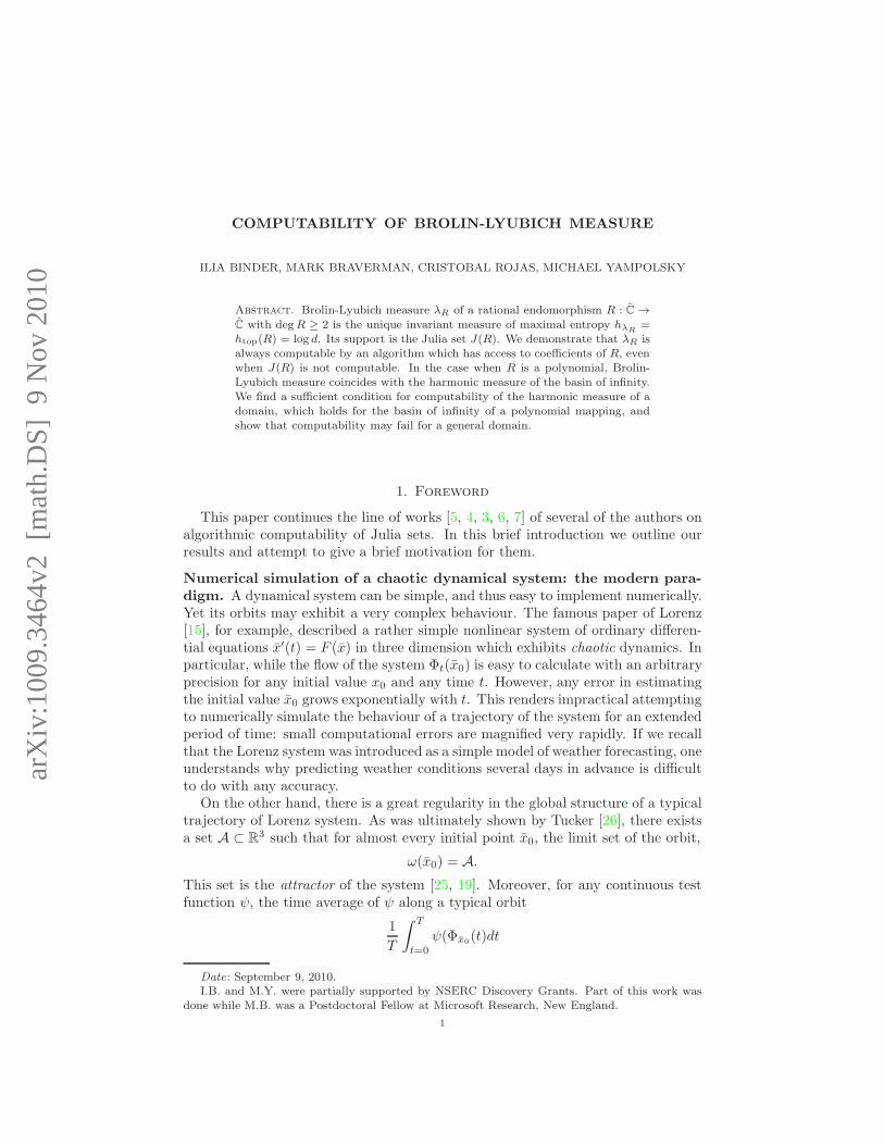
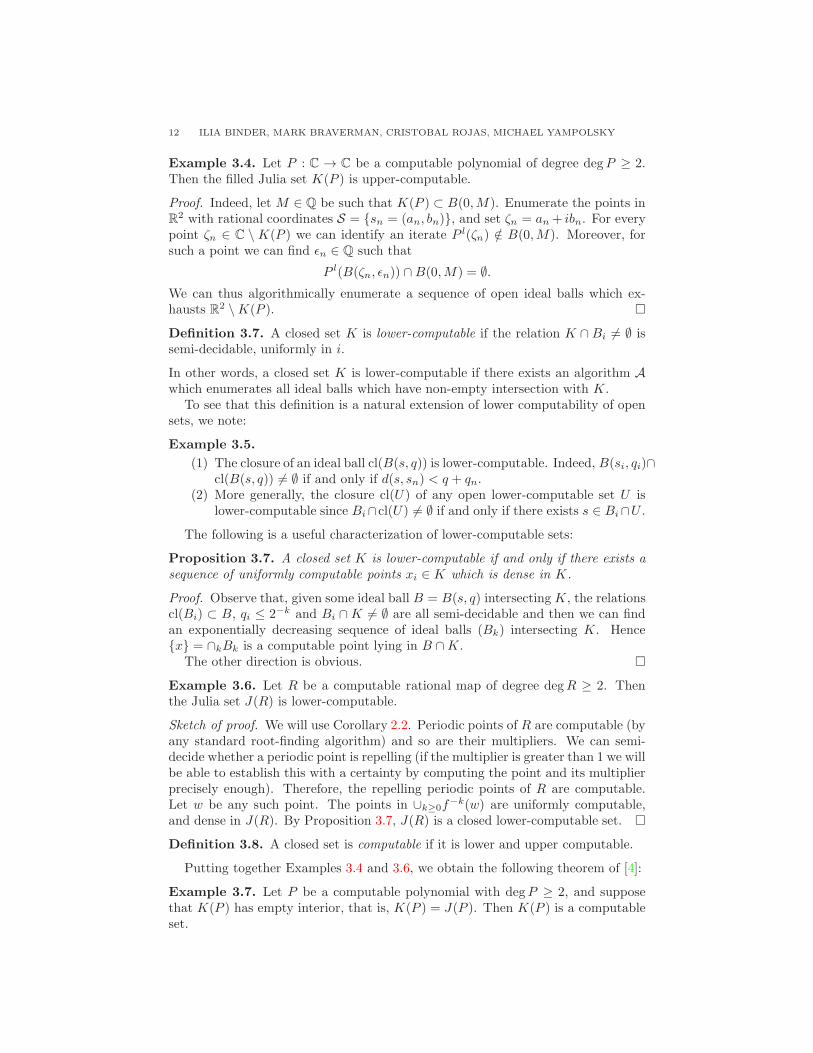
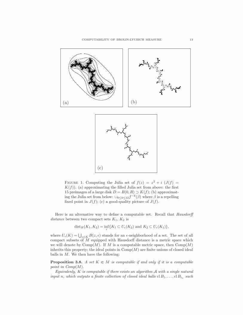
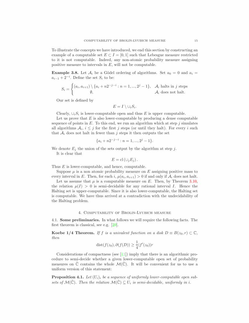
Figure 1. Computing the Julia set of f(z) = z2 + i (J(f) =K(f)). (a) approximating the filled Julia set from above: the first15 preimages of a large disk D = B(0, R) ⊃ K(f); (b) approximat-ing the Julia set from below: ∪0≤k≤12f

−k(β) where β is a repellingfixed point in J(f); (c) a good-quality picture of J(f).

Here is an alternative way to define a computable set. Recall that Hausdorffdistance between two compact sets K1, K2 is

distH(K1,K2) = infǫK1 ⊂ Uǫ(K2) and K2 ⊂ Uǫ(K1),

where Uǫ(K) =⋃

z∈K B(z, ǫ) stands for an ǫ-neighborhood of a set. The set of allcompact subsets of M equipped with Hausdorff distance is a metric space whichwe will denote by Comp(M). If M is a computable metric space, then Comp(M)inherits this property; the ideal points in Comp(M) are finite unions of closed idealballs in M . We then have the following:

Proposition 3.8. A set K ⋐ M is computable if and only if it is a computablepoint in Comp(M).

Equivalenly, K is computable if there exists an algorithm A with a single naturalinput n, which outputs a finite collection of closed ideal balls clB1, . . . , clBin such


that

distH(⋃

clBin ,K) < 2−n.

3.7. Computable probability measures. Let M(X) denote the set of Borelprobability measures over a metric space X . We recall the notion of weak conver-gence of measures:

Definition 3.9. A sequence of measures µn ∈M(X) is said to be weakly convergentto µ ∈M(X) if

∫

fdµn →∫

fdµ for each f ∈ C0(X).

Any smaller family of functions characterizing the weak convergence is calledsufficient. It is well-known, that when X is a compact separable and completemetric space, then so is M(X).Weak convergence onM(X) is compatible with the notion ofWasserstein-Kantorovichdistance, defined by:

W1(µ, ν) = supf∈1-Lip(X)

∣

∣

∣

∣

∫

fdµ−∫

fdν

∣

∣

∣

∣

where 1-Lip(X) is the space of Lipschitz functions on X , having Lipschitz constantless than one.

The following result (see [13]) says that, when X is a computable metric space,M(X) inherits its computability structure.

Proposition 3.9. Let D be the set of finite convex rational combinations of Diracmeasures supported on ideal points of X. Then the triple (M(X),W1,D) is acomputable metric space.

Definition 3.1. A computable measure is a computable point in (M(X),W1,D).That is, it is a measure which can be algorithmically approximated in the weaksense by discrete measures with any given precision.

As examples of computable measures, consider the Lebesgue measure in Rn, or anysmooth measure in Rn with a computable density function.

The following proposition (see [13]) gives a useful characterization of the com-putability of the measure.

Proposition 3.10. Let µ be a Borel probability measure. The following statementsare equivalent:

(1) µ is computable,(2) µ(Bi1 ∪ . . . ∪Bin) are lower-computable, uniformly in i1, . . . , in,(3) for any uniformly computable sequence of functions (fi)i, the integral

∫

fidµis computable uniformly in i.

We will also need the following fact (see [24]), :

Proposition 3.11. If (fi)i is a uniformly computable sequence of functions, thenthe integral operators

Li : M(X) → R defined by Li(µ) :=

∫

fidµ,

are uniformly computable.


To illustrate the concepts we have introduced, we end this section by constructing anexample of a computable set E ⊂ I = [0, 1] such that Lebesgue measure restrictedto it is not computable. Indeed, any non-atomic probability measure assigningpositive measure to intervals in E, will not be computable.

Example 3.8. Let Ai be a Godel ordering of algorithms. Set a0 = 0 and ai =ai−1 + 2−i. Define the set Si to be:

Si =

(ai, ai+1) \ ai + n2−j−i : n = 1, ..., 2j − 1, Ai halts in j steps

∅, Ai does not halt.

Our set is defined by

E = I \ ∪iSi.

Clearly, ∪iSi is lower-computable open and thus E is upper computable.Let us prove that E is also lower-computable by producing a dense computable

sequence of points in E. To this end, we run an algorithm which at step j simulatesall algorithms Ai, i ≤ j for the first j steps (or until they halt). For every i suchthat Ai does not halt in fewer than j steps it then outputs the set

ai + n2−j−i : n = 1, ..., 2j − 1.We denote Ej the union of the sets output by the algorithm at step j.

It is clear that

E = cl (∪jEj) .

Thus E is lower-computable, and hence, computable.Suppose µ is a non atomic probability measure on E assigning positive mass to

every interval in E. Then, for each i, µ(ai, ai+1) > 0 if and only if Ai does not halt.Let us assume that µ is a computable measure on E. Then, by Theorem 3.10,

the relation µ(I) > 0 is semi-decidable for any rational interval I. Hence theHalting set is upper-computable. Since it is also lower-computable, the Halting setis computable. We have thus arrived at a contradiction with the undecidability ofthe Halting problem.

4. Computability of Brolin-Lyubich measure

4.1. Some preliminaries. In what follows we will require the following facts. Thefirst theorem is classical, see e.g. [20].

Koebe 1/4 Theorem. If f is a univalent function on a disk D ≡ B(z0, r) ⊂ C,then

dist(f(z0), ∂(f(D)) ≥ 1

4|f ′(z0)|r

Considerations of compactness (see [11]) imply that there is an algorithmic pro-cedure to semi-decide whether a given lower-computable open set of probability

measures on C contains the whole M(C). It will be convenient for us to use auniform version of this statement:

Proposition 4.1. Let (Ui)i be a sequence of uniformly lower-computable open sub-

sets of M(C). Then the relation M(C) ⊆ Ui is semi-decidable, uniformly in i.


Sketch of proof. It is enough that for any given finite list of ideal balls Bkimi=1,

we can semi-decide the relation

M(C) ⊆⋃

i≤m

Bki.

If this last relation holds, then the union on the right must contain the elements of

any 2−n-net of M(C), provided that 2−n is less than (half of) the Lebesgue number

of the covering Bkimi=1. Such a net can be computed from a net of C and a net

of [0, 1].

4.2. Proof of Theorem A. Consider a rational map R(z) = P (z)/Q(z) of degreed. The coefficients of P and Q form two (d + 1)-tuples of complex numbers, andwe can thus specify R by a (2d+ 2)-tuple of coefficients, or a point in C2d+2. It isclear that

Proposition 4.2. R : C → C is a computable function if and only if there exists acomputable point in C2d+2 which specifies R.

Let us now formulate a precise version of the Theorem A:

Theorem 4.3. For a rational map R denote by λR its Brolin-Lyubich measure.Then the functional

F : C2d+2 → M(C)

R 7→ λR

is computable.

Remark 4.4. In other words, there exists an algorithm A with an oracle for v ∈C2d+2 and a single natural input n which outputs a measure µ ∈ D which has thefollowing property. If R is the rational map with coefficients v then

W1(µ, λR) < 2−n.

Of course, if R is computable, then the oracle can be replaced with an algorithmcomputing the coefficients of R.

Proof of the Theorem A. Let R be a rational map of degree d and φ be an oraclefor the coefficients of R. Given n ∈ N, we will show how to compute an ideal ball

Bn ⊂ M(C) with radius 2−n containing λR.

Let U ⊂ M(C) be the set of probability measures which are not invariant with

respect to R, and let V ⊂ M(C) be the set of probability measures which are notbalanced. In the following, we show that, using the oracle φ, both U and V arelower-computable open sets.

Let us introduce a certain fixed, enumerated sequence of Lipschitz computablefunctions which we will use as test functions. Let H0 be the set of functions of theform:

ϕs,r,ǫ = |1− |d(x, s)− r|+/ǫ|+ (4.1)

where s is a rational point in C, r, ǫ ∈ Q and |a|+ = maxa, 0. These are uniformlycomputable Lipschitz functions equal to 1 in the ball B(s, r), to 0 outside B(s, r+ǫ)and with intermediate values in between.


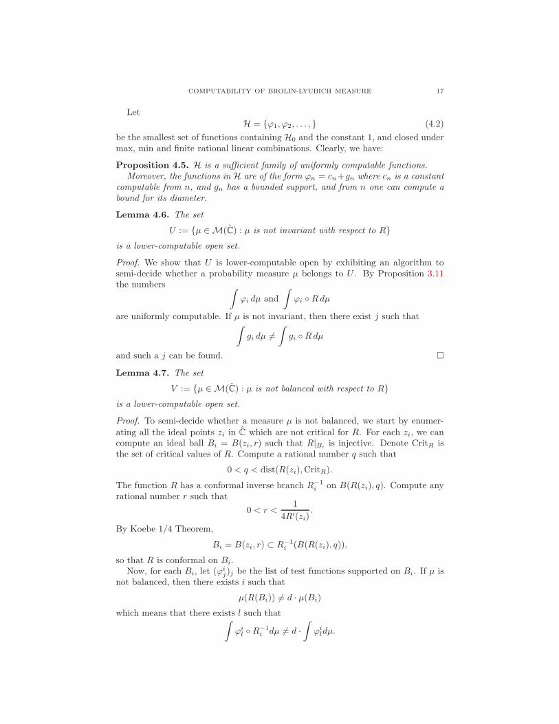
Let

H = ϕ1, ϕ2, . . . , (4.2)

be the smallest set of functions containing H0 and the constant 1, and closed undermax, min and finite rational linear combinations. Clearly, we have:

Proposition 4.5. H is a sufficient family of uniformly computable functions.Moreover, the functions in H are of the form ϕn = cn+gn where cn is a constant

computable from n, and gn has a bounded support, and from n one can compute abound for its diameter.

Lemma 4.6. The set

U := µ ∈ M(C) : µ is not invariant with respect to Ris a lower-computable open set.

Proof. We show that U is lower-computable open by exhibiting an algorithm tosemi-decide whether a probability measure µ belongs to U . By Proposition 3.11the numbers

∫

ϕi dµ and

∫

ϕi Rdµ

are uniformly computable. If µ is not invariant, then there exist j such that∫

gi dµ 6=∫

gi Rdµ

and such a j can be found.

Lemma 4.7. The set

V := µ ∈ M(C) : µ is not balanced with respect to Ris a lower-computable open set.

Proof. To semi-decide whether a measure µ is not balanced, we start by enumer-

ating all the ideal points zi in C which are not critical for R. For each zi, we cancompute an ideal ball Bi = B(zi, r) such that R|Bi

is injective. Denote CritR isthe set of critical values of R. Compute a rational number q such that

0 < q < dist(R(zi),CritR).

The function R has a conformal inverse branch R−1i on B(R(zi), q). Compute any

rational number r such that

0 < r <1

4R′(zi).

By Koebe 1/4 Theorem,

Bi = B(zi, r) ⊂ R−1i (B(R(zi), q)),

so that R is conformal on Bi.Now, for each Bi, let (ϕ

ij)j be the list of test functions supported on Bi. If µ is

not balanced, then there exists i such that

µ(R(Bi)) 6= d · µ(Bi)

which means that there exists l such that∫

ϕil R−1

i dµ 6= d ·∫

ϕildµ.


By Proposition 3.11, the numbers∫

ϕij R−1

i dµ and d∫

ϕijdµ are uniformly com-

putable, and thus l can be found.

It follows that the open set U = U ∪ V of measures which are either not in-variant or not balanced is lower-computable with an oracle φ. Its complement isthe singleton λR. To compute λR with precision 2−n, enumerate all the ideal

balls Bn ⊂ M(C) of radius 2−n and semi-decide the relation λR ⊂ Bn. This ispossible because

λR ⊂ Bn ⇐⇒ M(C) ⊂ U ∪Bn,

and the last relation is semi-decidable by Proposition 4.1.

4.3. A comparison of rates of convergence. In [6] two of the authors haveshown:

Theorem 4.8. There exists a computable quadratic polynomial fc(z) = z2 + cwhose Julia set Jc is not computable.

Together with Theorem A this statement has the following amusing consequence:

Theorem 4.9 (Incommensurability of rates of convergence). For a polyno-mial fc and z ∈ C denote

φ1(n) = distH((fc)−n(z), Jc) and φ2(n) =W1

1

2n

∑

w∈(fc)−n(z)

δw , λc

,

where λc is the Brolin-Lyubich measure of fc. Even though both φ1 and φ2 convergeto 0 as n → ∞, there exists a parameter c such that there does not exist anycomputable function F : R → R such that F (0) = 0 and

φ1(n) ≤ F φ2(n).

Proof. If c is computable, Theorem A implies the computability of λc. Hence, φ2(n)is a computable function. On the other hand, if there exists a computable boundφ1(n) −→

n→∞0, then Jc is a computable set. Therefore, such a bound cannot exist

for a parameter c as in Theorem 4.8.

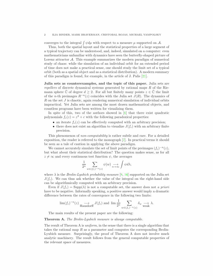
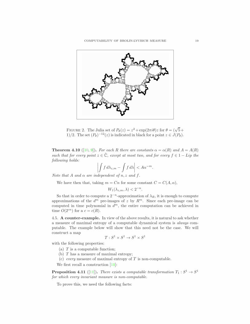
As an illustration, consider Figure 2. The Julia set of a quadratic polynomial isrendered in gray. This particular polynomial can be written in the form Pθ(z) =

z2 + exp(2πiθ)z for θ = (√5 + 1)/2. The preimage (Pθ)

−12(z) (highlighted inblack) for a point z ∈ J(Pθ) gives an excellent approximation of λ, but a very poorapproximation of the whole Julia set.

4.4. Proof of Theorem B. For a given point z ∈ C, set

λz,m =1

dm

∑

w∈R−m(a)

δw.

The following result is due to Drasin and Okuyama [10], and, in more generality,to Dinh and Sibony [9].


Figure 2. The Julia set of Pθ(z) = z2+exp(2πiθ)z for θ = (√5+

1)/2. The set (Pθ)−12(z) is indicated in black for a point z ∈ J(Pθ).

Theorem 4.10 ([10, 9]). For each R there are constants α = α(R) and A = A(R)

such that for every point z ∈ C, except at most two, and for every f ∈ 1− Lip thefollowing holds:

∣

∣

∣

∣

∫

f dλz,m −∫

f dλ

∣

∣

∣

∣

< Aα−m.

Note that A and α are independent of n, z and f .

We have then that, taking m = Cn for some constant C = C(A,α),

W1(λz,m, λ) < 2−n.

So that in order to compute a 2−n-approximation of λR, it is enough to computeapproximations of the dm pre-images of z by Rm. Since each pre-image can becomputed in time polynomial in dm, the entire computation can be achieved intime O(2cn) for a c = c(R).

4.5. A counter-example. In view of the above results, it is natural to ask whethera measure of maximal entropy of a computable dynamical system is always com-putable. The example below will show that this need not be the case. We willconstruct a map

T : S1 × S1 → S1 × S1

with the following properties:

(a) T is a computable function;(b) T has a measure of maximal entropy;(c) every measure of maximal entropy of T is non-computable.

We first recall a construction [11]:

Proposition 4.11 ([11]). There exists a computable transformation T1 : S1 → S1

for which every invariant measure is non-computable.

To prove this, we need the following facts:


Proposition 4.12. Let µ be a computable Borel measure on a computable metricspace X. Then the support of µ contains a computable point x ∈ X.

Sketch of proof. We outline the proof here and leave the details to the reader. First,for each ideal ball B = B(x, r) set

ψB ≡ φx,r/2,r/2

as in (4.1). An exhaustive search can be used to find a sequence of ideal ballsBi = B(xi, ri) with the following properties:

• ri ≤ 2−i;• B(xi, ri) ⊂ B(xi−1, 2ri−1);•∫

ψBidµ > 0.

The algorithm can then be used to compute x = limxi ∈ supp(µ).

Proposition 4.13. There exists a lower-computable open set V ⊂ (0, 1) such that(0, 1) \ V 6= ∅ and V contains all computable numbers in (0, 1).

Sketch of proof. Consider an algorithm A which at step m emulates the first malgorithms Ai(i), i ≤ m with respect to the Godel ordering for m steps. That is,the i-th algorithm in the ordering is given the number i as the input parameter.From time to time, an emulated algorithm Ai(i) may output a rational number xiin (0, 1). Our algorithm A will output an interval

Li = (xi − 3−i/2, xi + 3−i/2) ∩ (0, 1)

for each term in this sequence. The union V = ∪Li is a lower-computable set. It iseasy to see from the definition of a computable real that V ⊃ RC ∩ (0, 1). If x ∈ RC

then there is a machine An(j) that on input j outputs a 3−j/4-approximation of x.Thus the execution of An(n) will halt with an output q such that |x− q| < 3−n/4,and x will be included in V . On the other hand, the Lebesgue measure of V isbounded by 1/2, and thus does not cover all of [0, 1].

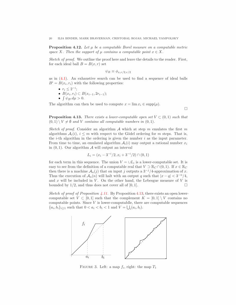
Sketch of proof of Proposition 4.11. By Proposition 4.13, there exists an open lower-computable set V ⊂ [0, 1] such that the complement K = [0, 1] \ V contains nocomputable points. Since V is lower-computablle, there are computable sequencesai, bii≥1 such that 0 < ai < bi < 1 and V =

⋃

i(ai, bi).

ai bi

fi

Figure 3. Left: a map fi, right: the map T1


Let us define non-decreasing, uniformly computable functions fi : [0, 1] → [0, 1]such that

fi(x) > x if x ∈ (ai, bi) and fi(x) = x otherwise.

For instance, we can set

fi(x) = 2x− ai on

[

ai,ai + bi

2

]

, and

fi(x) = bi on

[

ai + bi2

, bi

]

.

As neither 0 nor 1 belongs to K, there is a rational number ǫ > 0 such thatK ⊆ [ǫ, 1− ǫ]. Let us define f : [0, 1] → R by

f(x) =

x on [ǫ, 1− ǫ],2x− (1− ǫ) on [1− ǫ, 1]ǫ on [0, ǫ]

We then define t(x) : [0, 1] → R by

t(x) =f

2+∑

i≥2

2−ifi.

By construction, the function t(x) is computable and non-decreasing, and t(x) > xif and only if x ∈ [0, 1] \K. As

t(1) = f(1) = 1 + ǫ = 1 + t(0),

we can take the quotient

T1(x) ≡ t(x)modZ.

It is easy to see that T1 moves all points towards the set K. More precisely,every point x ∈ K is fixed under T1, and the orbit of every point x /∈ K convergesto infy ∈ K ∩ [x, 1]. Further, for any interval J ⋐ U , all but finitely many T1-translates of J are disjoint from J . Hence, no finite invariant measure of T1 canbe supported on J . Thus the support of every T1-invariant measure is contained inK. By Proposition 4.12, no such measure can be computable.

We are now equipped to present the counter-example T . We define T2 : S1 → S1

by T2(x) = 2xmodZ, and set

T = T1 × T2.

Firstly, by the same reasoning as above, every invariant measure µ of T is supportedon K × S1 and hence is not computable by Proposition 4.12. On the other hand,T possesses invariant measures of maximal entropy. Indeed, let ν be any invariantmeasure of T1 and λ the Lebegue measure on S1. Setting µ = ν × λ, we have

hµ(T ) = htop(T ) = log 2.


5. Harmonic Measure

5.1. Proof of Theorem C. Let us start with several definitions.

Definition 5.1. We recall that a compact set K ⊂ C which contains at leasttwo points is uniformly perfect if the moduli of the ring domains separating K arebounded from above. Equivalently, there exists some C > 0 such that for anyx ∈ K and r > 0, we have

(B(x,Cr) \B(x, r)) ∩K = ∅ =⇒ K ⊂ B(x, r).

In particular, every connected set is uniformly perfect.

It is known that:

Theorem 5.1 (see [17]). The Julia set of a polynomial P of degree d ≥ 2 is auniformly perfect compact set.

Recall that the logarithmic capacity Cap(·) has been defined in Section 2.3. Wenext define:

Definition 5.2. Let Ω ⊂ C be an open and connected domain and set J = ∂Ω. Wesay that Ω satisfies the capacity density condition if there exists a constant C > 0such that

Cap(B(x, r) ∩ ∂Ω) ≥ Cr for all x ∈ ∂Ω and r ≤ r0. (5.1)

We note:

Theorem 5.2 (see Theorem 1 in [22]). Condition (5.1) is equivalent to uniformperfectness of ∂Ω.

The celebrated result of Kakutani [14], gives a connection between Brownian motionand the Harmonic measure.

Theorem 5.3. [14] Let K ⊂ C be a compact set with a connected complement Ω.Fix a point x ∈ Ω and let Bt denote a Brownian path started at x. Let the randomvariable T be the first moment when Bt hits ∂Ω, and let ωx = ωΩ,x denote theharmonic measure corresponding to x. Then for any measurable function f on ∂Ω,

∫

fdωx = E[f(BT )].

In [2] the following computable version of the Dirichlet problem has been proved:

Theorem 5.4. Let K ⊂ C be a compact computable set with a connected comple-ment Ω. Let x ∈ Ω be any point in Ω and let Bt denote a Brownian path started atx. There is an algorithm A that, given access to K, x, and a precision parameterε, outputs an ε/4-approximate sample βε from a random variable BTε

where Tε isa stopping rule on Bt that always satisfies

ε/2 < dist(BTε,K) < ε.

In other words, we are able to stop the Brownian motion at distance ≈ ε from theboundary. We now formulate the following proposition that is a reformulation ofTheorem C:

Proposition 5.5. Let Ω ⊂ C be the complement of a computable compact set Kand x0 be a point in Ω. Suppose Ω is connected and satisfies the capacity densitycondition. Then the harmonic measure ωΩ,x0

is computable with an oracle for x0.


Proof. Fix x0 ∈ Ω. As before, we denote by (Bt) the Brownian Motion started atx0 and set

T = mint : Bt ∈ ∂Ω.We will use Theorem 5.4 together with the capacity density condition to proveProposition 5.5.

The capacity density condition implies the following (see [12], page 343):

Proposition 5.6. There exists a constant ν = ν(C) (with C as in the capacitydensity condition) such that for any η > 0 the following holds. Let y ∈ Ω be a pointsuch that dist(y, ω) ≤ η, and let Bω be a Brownian Motion started at y. Let

T y := mint : Byt ∈ ∂Ω

be the first time By hits the boundary of Ω. Then

P[|ByTy

− y| ≥ 2η] < ν. (5.2)

In other words, there is at least a constant probability that the first point whereBy hits the boundary is close to the starting point y.

Now let f be any function on K satisfying the 1-Lip condition. Our goal is tocompute

∫

f dω = E[f(BT )].

within any prescribed precision parameter δ. Note that

E[f(BT )] = EBTε[E[f(BT )|BTε

|]].We first claim that we can compute an ε such that

|f2ε(BTε)− E[f(BT )|BTε

|]| < δ/2. (5.3)

Here Tε is given by the any stopping rule as in Proposition 5.4, and f2ε(BTε) is any

evaluation of f in a 2ε-neighborhood of BTε(note that f itself is not defined on

BTε/∈ K).

LetM be a universal bound on the absolute value of f . By (5.2) we can computean ε < δ/20 such that if y is ε-close to K, the probability that |By

Ty− y| > δ/10 is

smaller than δ/10M . We split the probabilities into two cases: one where BT staysδ/10-close to BTε

, and the complementary case. By (5.3) we have


|]| =|f2ε(BTε

)− E[f(BT )|BTε|, |BT −BTε

| < δ/10]| · P[|BT −BTε| < δ/10]+


|, |BT −BTε| ≥ δ/10]| · P[|BT − BTε

| ≥ δ/10] ≤(δ/6) · 1 +M · (δ/10M) < δ/2.

To complete the proof of the proposition it remains to note that given a βε thatε/4-approximates BTε

as in Theorem 5.4, we can evaluate f2ε(BTε) by evaluating

f3ε/2(βε) (by evaluating f at any point in a 3ε/2-neighborhood of βε). In this way,we obtain

Eβε|f3ε/2(βε)− E[f(BT )]| < δ/2. (5.4)

Thus, being able to evaluate f3ε/2(βε) with precision δ/2 suffices.


5.2. A counter-example. As demonstrated by the following example, even for acomputable regular domain, the harmonic measure is not necessarily computable.Thus the capacity density condition in Theorem C is cruicial.

For a, b ∈ R, we denote by [a, b] the shortest arc of the unit circle between e2πia

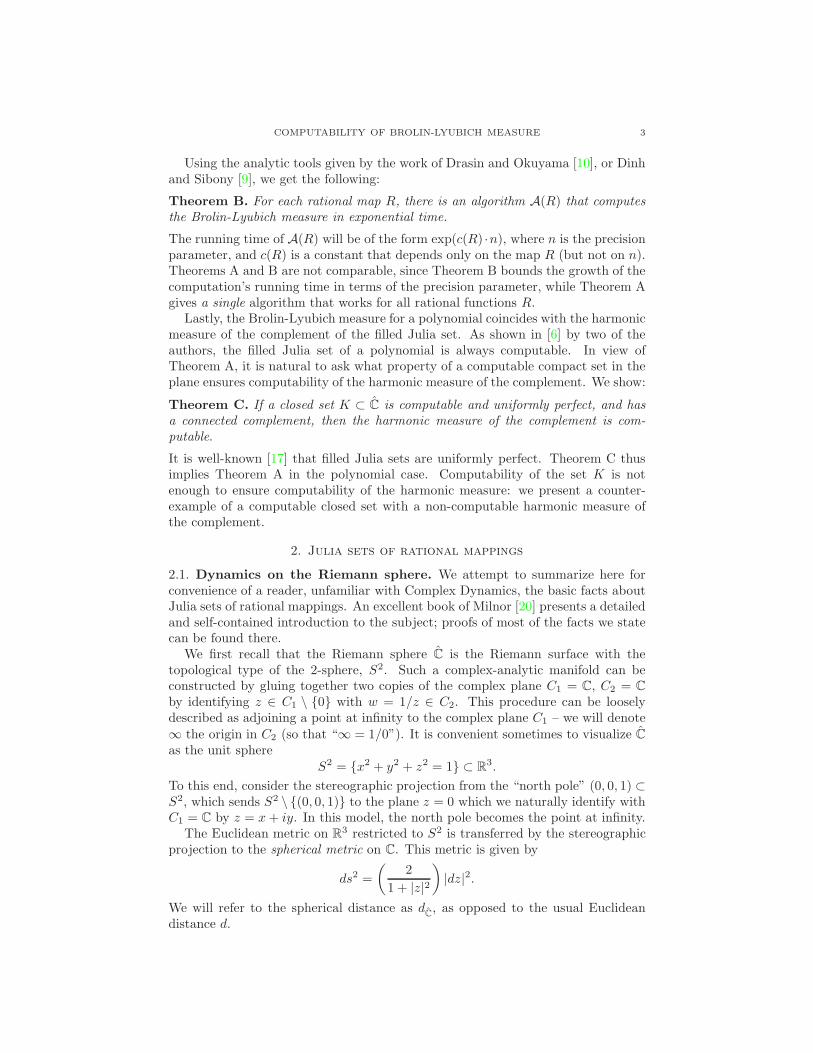
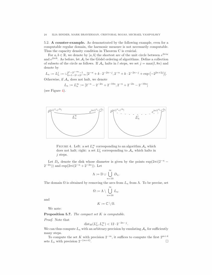
and e2πib. As before, let Ai be the Godel ordering of algorithms. Define a collectionof subsets of the circle as follows. If An halts in l steps, we set j = max(l, 8n) anddenote by

Ln := Ljn := ∪2j−2j−8n−1

k=1−2j+2j−8n [2−n + k · 2−2n−j, 2−n + k · 2−2n−j + exp

(

−22n+2j)

].

Otherwise, if An does not halt, we denote

Ln := L∞n := [2−n − 2−2n + 2−10n, 2−n + 2−2n − 2−10n]

(see Figure 4).

e 2-n -2niπ2 ( )2-e 2

-n -2niπ2 ( )2+e 2-n -2niπ2 ( )2- e 2

-n -2niπ2 ( )2+

Ln

8 jLn

Figure 4. Left: a set L∞n corresponding to an algorithmAn which

does not halt; right: a set Ljn corresponding to An which halts in

j steps.

Let Dn denote the disk whose diameter is given by the points exp(2πi(2−n −2−2n)) and exp(2πi(2−n + 2−2n)). Let

Λ := D ∪∞⋃

n=10

Dn.

The domain Ω is obtained by removing the arcs from Ln from Λ. To be precise, set

Ω := Λ \∞⋃

n=10

Ln.

andK := C \ Ω.

We note:

Proposition 5.7. The compact set K is computable.

Proof. Note thatdistH(Lj

n, L∞n ) < 12 · 2−2n−j.

We can thus compute Ln with an arbitrary precision by emulatingAn for sufficientlymany steps.

To compute the set K with precision 2−m, it suffices to compute the first 2m+4

sets Ln with precision 2−(m+4).


Now let us show that:

Proposition 5.8. The harmonic measure

ω := ωΩ,0

is not computable.

For a set K0 ⊂ z : 0 < δ < |z| < r < 1 set

γ(K0) := − logCap(K0).

We need an auxilliary lemma:

Lemma 5.9 (Theorem 5.1.4 in [23]). If K1, . . . ,Kn are compact subsets of the unitdisk, then

1

γ(K1 ∪ · · · ∪Kn)≤ 1

γ(K1)+ · · ·+ 1

γ(Kn).

Let Sn be the part of the boundary of the disk Dn lying outside of D, Sn :=∂Dn \ D. Harmonic measure is always non-atomic, so if ω is computable, thenω(Sn) is also computable. We show:

Proposition 5.10. If An does not halt, then ω(Sn) < 2−9n+2. If An halts,ω(Sn) > 2−2n−3.

Proof. As before, let Bt be the Brownian motion started at 0 and let T denote thehitting time of ∂Ω,

T := inft : Bt ∈ ∂Ω.Let us recall that for E ⊂ ∂Ω we have

ω(E) = P[BT ∈ E].

Assume now that An does not halt. Let us introduce a new domain Ω′ :=C \ [2−n − 2−2n, 2−n + 2−2n] and T ′ be the corresponding hitting time. Observethat if BT ∈ Sn then

BT ′ ∈ Kn := [2−n − 2−2n, 2−n − 2−2n +2−10n]∪ [2−n +2−2n − 2−10n, 2−n + 2−2n].

ThusωΩ,0(Sn) = P[BT ∈ Sn] ≤ P[BT ′ ∈ Kn] = ωΩ′,0(Kn).

The desired estimate is now obtained by mapping (Ω′, 0) conformally to (D, 0).Assume that An halts in j steps. To bound ω(Sn) in this case, we will use the

following estimate on harmonic measure ([12], Equation (III.9.2)):Let K0 ⊂ z : 0 < δ < |z| < r < 1. Then

ωD\K0,0(K0) ≤log

(

1δ

)

γ(K0) + log(1− r2)(5.5)

Let T ′′ denote the hitting time of ∂D by Bt, and let

Mn :=

z ∈ L∞n : dist(z, ∂Ω) > 2−2n−j−4

be the part of the arc L∞n lying relatively far away from the boundary.

Conformally mapping Dn to the unit disk centered at z ∈ Mn and using theestimate (5.5) and Lemma 5.9, we obtain that for z ∈Mn we have

ωDn\Ln,z(Ln) ≤ 2−j+3 < 1/8 (5.6)

We will also need T1 ≥ T ′′ – the first hitting time of ∂Dn after hitting ∂D, andT2 ≤ T1 – the first hitting time of ∂Dn ∪ Ln after hitting ∂D.


Note now that

P[BT ′′ ∈Mn] = length(Mn)/2π ≥ 2−2n−1 (5.7)

Let us note that by symmetry and estimate (5.6), we have

P[BT ∈ Sn | BT ′′ ∈Mn] ≥ P[BT1∈ Sn | BT ′′ ∈Mn]−P[BT2

∈ Ln | BT ′′ ∈Mn] =

1

2− P[BT2

∈ Ln | BT ′′ ∈Mn] ≥1

2− max

z∈Mn

ωDn\Ln,z(Ln) > 1/4. (5.8)

The desired lower estimate on ω is now obtained by combining (5.7) and (5.8).

We now conclude the proof of Proposition 5.8:

Proof of Proposition 5.8. Assume the contrary, that is, suppose that ω is com-putable. For every n ∈ N let Un

j (z)∞j=1 be a sequence of functions given by:

Unj (z) =

1 if dist(z, Sn) < 2−j ;0 if dist(z, Sn) > 2 · 2−j;1− 2j(d− 2−j) if d = dist(z, Sn) ∈ [2−j, 2 · 2−j ]

We have:

(a) the functions Unj (z) are computable uniformly in n and j.

Since ω is non-atomic,

(b) for a fixed n we have∫

Unj (z)dω > ω(Sn) and

∫

Unj (z)dω −→

j→∞ω(Sn).

Similarly, we can costruct a sequence of functions Lnj (z) such that

(c) the functions Lnj (z) are computable uniformly in n and j;

(d) for a fixed n we have∫

Lnj (z)dω < ω(Sn) and

∫

Lnj (z)dω −→

j→∞ω(Sn).

We leave the details of the second construction to the reader.By part (3) of Proposition 3.10, properties (a) and (c) imply that the integrals

∫

Unj (z)dω and

∫

Lnj (z)dω

are uniformly computable. Consider and algorithm Ahalt which upon inputting anatural number n does the following:

(1) j := 1;(2) evaluate uj, lj such that

|uj −∫

Unj (z)dω| < 2−20n and |lj −

∫

Lnj (z)dω| < 2−20n;

(3) if uj < 2−9n+2 + 2−19n then output 0 and halt;(4) if lj > 2−2n−3 − 2−19n then output 1 and halt;(5) j := j + 1 and go to (2).

By Proposition 5.10 and properties (b) and (d), we have the following:

• if An halts then Ahalt outputs 1 and halts, and• if An does not halt then Ahalt outputs 0 and halts.


Thus Ahalt is an algorithm solving the Halting Problem, which contradicts thealgorithmic unsolvability of the Halting Problem.

References

[1] S. Banach and S. Mazur. Sur les fonctions caluclables. Ann. Polon. Math., 16, 1937.[2] I. Binder and M. Braverman. Derandomization of euclidean random walks. In APPROX-

RANDOM, pages 353–365, 2007.[3] I. Binder, M. Braverman, and M. Yampolsky. On computational complexity of Siegel Julia

sets. Commun. Math. Phys., 264(2):317–334, 2006.[4] I. Binder, M. Braverman, and M. Yampolsky. Filled Julia sets with empty interior are com-

putable. Journ. of FoCM, 7:405–416, 2007.[5] M. Braverman and M. Yampolsky. Non-computable Julia sets. Journ. Amer. Math. Soc.,

19(3):551–578, 2006.[6] M Braverman and M. Yampolsky. Computability of Julia sets. Moscow Math. Journ., 8:185–

231, 2008.[7] M Braverman and M. Yampolsky. Computability of Julia sets, volume 23 of Algorithms and

Computation in Mathematics. Springer, 2008.[8] H. Brolin. Invariant sets under iteration of rational functions. Ark. Mat., 6:103–144, 1965.[9] T. Dinh and N. Sibony. Equidistribution speed for endomorphisms of projective spaces. Math.

Ann., 347:613–626, 2009.[10] D. Drasin and Y. Okuyama. Equidistribution and Nevanlinna theory. Bull. Lond. Math. Soc.,

39:603–613, 2007.[11] S. Galatolo, M. Hoyrup, and C. Rojas. Dynamics and abstract computability: computing

invariant measures. Discr. Cont. Dyn. Sys. Ser A, 2010.[12] J.B. Garnett and D.E. Marshall. Harmonic measure. Cambridge University Press, 2005.[13] M. Hoyrup and C. Rojas. Computability of probability measures and Martin-Lof randomness

over metric spaces. Information and Computation, 207(7):830–847, 2009.[14] S. Kakutani. Two-dimensional Brownian motion and harmonic functions. In Proc. Imp. Acad.

Tokyo, volume 20, 1944.[15] E. N. Lorenz. Deterministic nonperiodic flow. J. Atmos. Sci., 20:130–141, 1963.

[16] M. Lyubich. The measure of maximal entropy of a rational endomorphism of a Riemannsphere. Funktsional. Anal. i Prilozhen., 16:78–79, 1982.

[17] R. Mane and L.F. da Rocha. Julia sets are uniformly perfect. Proc. Amer. Math. Soc.,116:251–257, 1992.

[18] S. Mazur. Computable Analysis, volume 33. Rosprawy Matematyczne, Warsaw, 1963.[19] J. Milnor. On the concept of attractor. Commun. Math. Phys, 99:177–195, 1985.[20] J. Milnor. Dynamics in one complex variable. Introductory lectures. Princeton University

Press, 3rd edition, 2006.[21] J. Palis. A global view of dynamics and a conjecture on the denseness of finitude of attractors.

Asterisque, 261:339 – 351, 2000.[22] Ch. Pommerenke. Uniformly perfect sets and the Poincare metric. Arch. Math., 32:192–199,

1979.[23] Thomas Ransford. Potential theory in the complex plane, volume 28 of London Mathematical

Society Student Texts. Cambridge University Press, Cambridge, 1995.[24] C. Rojas. Randomness and ergodic theory: an algorithmic point of view. PhD thesis, Ecole

Polytechnique, 2008.[25] S. Smale. Differential dynamical systems. Bull. Am. Math. Soc., 73:747–817, 1967.[26] W. Tucker. A rigorous ODE solver and Smale’s 14th problem. Found. Comp. Math., 2:53–117,

2002.[27] A. M. Turing. On computable numbers, with an application to the Entscheidungsproblem.

Proceedings, London Mathematical Society, pages 230–265, 1936.[28] K. Weihrauch. Computable Analysis. Springer-Verlag, Berlin, 2000.

Computability of Brolin-Lyubich Measure

Documents