Compressive Sampling and Lossy Compression

© DIGITAL VISION

IEEE SIGNAL PROCESSING MAGAZINE [48] MARCH 2008 1053-5888/08/$25.00©2008IEEE

Recent results in compressive sampling have shown that sparse signals can berecovered from a small number of random measurements. This propertyraises the question of whether random measurements can provide an effi-cient representation of sparse signals in an information-theoretic sense.Through both theoretical and experimental results, we show that encoding a

sparse signal through simple scalar quantization of random measurements incurs a sig-nificant penalty relative to direct or adaptive encoding of the sparse signal. Informationtheory provides alternative quantization strategies, but they come at the cost of muchgreater estimation complexity.

[Vivek K Goyal,

Alyson K. Fletcher, and

Sundeep Rangan]

Compressive Samplingand Lossy Compression

[Do random measurements provide an efficient method of representing sparse signals?]

Digital Object Identifier 10.1109/MSP.2007.915001

IEEE SIGNAL PROCESSING MAGAZINE [49] MARCH 2008

BACKGROUND

SPARSE SIGNALSSince the 1990s, modeling signals through sparsity has emergedas an important and widely applicable technique in signal pro-cessing. Its most well-known success is in image processing,where great advances in compression and estimation have comefrom modeling images as sparse in a wavelet domain [1].

In this article we use a simple, abstract model for sparsesignals. Consider an N-dimensional vector x that can be repre-sented as x = Vu, where V is some orthogonal N-by-N matrixand u ∈ RN has only K nonzero entries. In this case, we saythat u is K-sparse and that x is K-sparse with respect to V. Theset of positions of nonzeros coefficients in u is called the spar-sity pattern, and we call α = K/N the sparsity ratio.

Knowing that x is K-sparse with respect to a given basis Vcan be extremely valuable for signal processing. For example, incompression, x can be represented by the K positions and valuesof the nonzero elements in u, as opposed to the N elements of x.When the sparsity ratio α is small, the compression gain can besignificant. Similarly, in estimating x in the presence of noise,one only has to estimate K as opposed to N real parameters.

Another important property of sparse signals has recently beenuncovered: they can be recovered in a computationally tractablemanner from a relatively small number of random samples. Themethod, known as compressive sampling (sometimes called com-pressed sensing or compressive sensing), was developed in [2], [3]and [4] and is detailed in other articles in this issue.

A basic model for compressive sampling is shown in Figure 1.The N-dimensional signal x is assumed to be K-sparse withrespect to some orthogonal matrix V. The “sampling” of x is rep-resented as a linear transformation by a matrix � yielding a sam-ple vector y = �x. Let the size of � be M-by-N, so y has Melements; we call each element of y a measurement of x. Adecoder must recover the signal x from y knowing V and �, butnot necessarily the sparsity pattern of the unknown signal u.

Since u is K-sparse, x must belong to one of (N

K

)subspaces in

RN . Similarly, y must belong to one of (N

K

)subspaces in RM .

For almost all �s with M ≥ K + 1, an exhaustive searchthrough the subspaces can determine which subspace x belongsto and thereby recover the signal’s sparsity pattern and values.Therefore, in principle, a K sparse signal can be recovered fromas few as M = K + 1 random samples.

Unfortunately, the exhaustive search described above is nottractable for interesting sizes of problems since the number ofsubspaces to search,

(NK

), can be enormous; if α is held constant

as N is increased, the number of subspaces grows exponentiallywith N. The remarkable main result of compressive sampling isto exhibit recovery methods that are computationally feasible,numerically stable, and robust against noise while requiring anumber of measurements not much larger than K.

SIGNAL RECOVERY WITH COMPRESSIVE SAMPLINGCompressive sampling is based on recovering x via convex opti-mization. When we observe y = �x and x is sparse with respect

to V, we are seeking x consistent with y and such that V −1 x hasfew nonzero entries. To try to minimize the number of nonzeroentries directly yields an intractable problem [5]. Instead, solv-ing the optimization problem

(LP reconstruction) xLP = argminx : y=�x

‖V −1 x‖1

often gives exactly the desired signal recovery, and there aresimple conditions that guarantee exact recovery. Following pio-neering work by Logan in the 1960s, Donoho and Stark [6]obtained results that apply, for example, when V is the N-by-Nidentity matrix and the rows of � are taken from the matrix rep-resentation of the length-N discrete Fourier transform (DFT).Subsequent works considered randomly selected rows from theDFT matrix [2] and then certain other random matrix ensem-bles [3], [4]. In this article, we will concentrate on the case when� has independent Gaussian entries.

A central question is: How many measurements M are need-ed for linear program (LP) reconstruction to be successful?Since � is random, there is always a chance that reconstructionwill fail. We are interested in how M should scale with signaldimension N and sparsity K so that the probability of successapproaches one. A result of Donoho and Tanner [7] indicatesthat M ∼ 2K log(N/K ) is a sharp threshold for successfulrecovery. Compared to the intractable exhaustive searchthrough all possible subspaces, LP recovery requires only a fac-tor 2 log(N/K ) more measurements.

If measurements are subject to additive Gaussian noise sothat y = �x + η is observed, with η ∼ N (0, σ 2), then the LPreconstruction should be adjusted to allow slack in the con-straint y = �x. A typical method for reconstruction is the fol-lowing convex optimization:

(Lasso reconstruction)

x Lasso = argminx

(‖ y − �x‖2

2 + λ‖V −1 x‖1

),

where the parameter λ > 0 trades off data fidelity and reconstruc-tion sparsity. The best choice for λ depends on the variance of the

[FIG1] Block diagram representation of compressive sampling.The signal x is sparse with respect to V, meaning that u = V−1xhas only a few nonzero entries. y = �x is “compressed” in that itis shorter than x. (White boxes represent zero elements.)

u x yV Φ Estimation

x

noise and problem size parameters.Wainwright [8] has shown that the scalingM ∼ 2K log (N − K ) + K is a sharpthreshold for V −1 x Lasso to have the correctsparsity pattern with high probability. Whilethis M may be much smaller than N, it is sig-nificantly more measurements than requiredin the noiseless case.

COMPRESSIVE SAMPLINGAS SOURCE CODINGIn the remainder of this article, we will beconcerned with the tradeoff between qualityof approximation and the number of bits ofstorage for a signal x that is K-sparse withrespect to orthonormal basis V. An immediate distinction fromthe “Background” section is that the currency in which wedenominate the cost of a representation is bits rather than realcoefficients.

In any compression involving scalar quantization, the choiceof coordinates is key. Traditionally, signals to be compressed are

modeled as jointly Gaussian vectors. These vectors can be visu-alized as lying in an ellipsoid, since this is the shape of the levelcurves of their probability density [see Figure 2(a)]. Source cod-ing theory for jointly Gaussian vectors suggests to chooseorthogonal coordinates aligned with the principal axes of theellipsoid (the Karhunen–Loeve basis) and then allocate bits tothe dimensions based on their variances. This gives a codinggain relative to arbitrary coordinates [9]. For high-quality (lowdistortion) coding, the coding gain is a constant number of bitsper dimension that depends on the eccentricity of the ellipse.

Sparse signal models are geometrically quite different thanjointly Gaussian vector models. Instead of being visualized asellipses, they yield unions of subspaces [see Figure 2(b)]. A nat-ural encoding method for a signal x that is K-sparse withrespect to V is to identify the subspace containing x and thenquantize within the subspace, spending a number of bits pro-portional to K. Note that doing this requires the encoder toknow V and that there is a cost to communicating the subspaceindex, denoted J, that will be detailed later. With all the properaccounting, when K � N, the savings is more dramatic thanjust a constant number of bits.

Following the compressive sampling framework one obtainsa rather different way to compress x:quantize the measurements y = �x,with � and V known to the decoder.Since � spreads the energy of thesignal uniformly across the measure-ments, each measurement should beallocated the same number of bits.The decoder should estimate x as wellas it can; we will not limit the com-putational capability of the decoder.

How well will compressive sam-pling work? It depends both on howmuch it matters to use the best basis(V) rather than a set of random vec-tors (�) and how much the quantiza-tion of y affects the ability of thedecoder to infer the correct subspace.We separate these issues, and our

[FIG2] (a) Depiction of Gaussian random vectors as an ellipsoid.Classical rate-distortion theory and transform coding results arefor this sort of source, which serves as a good model for discretecosine transform (DCT) coefficients of an image or MDCTcoefficients of audio. (b) Depiction of two sparse signals in R3,which form a union of three subspaces. This serves as a goodconceptual model for wavelet coefficients of images.

(a) (b)

[FIG3] Block diagram representation of the compressive sampling scenario analyzedinformation theoretically. V is a random orthogonal matrix, u is a K-sparse vector withN (0, 1) nonzero entries, and � is a Gaussian measurement matrix. More specifically, thesparsity pattern of u is represented by J and the nonzero entries are denoted uK. In the initialanalysis, the encoding of y = �x is by scalar quantization and scalar entropy coding.

Source ofRandomness

V

J

uK

Φ

uV

xΦ

yEncoder

BitsDecoder

x

yQ(·)

EntropyCoding

Bits

ˆ

IEEE SIGNAL PROCESSING MAGAZINE [50] MARCH 2008

ENCODER

(SPARSIFYING (RANDOM BASIS) USES V MEASUREMENTS) USES �

KNOWS J c2−2R c2−2(R−R ∗)

A PRIORIDECODER IS TOLD J c2−2(R−H(α)/α) c2−2(R−H(α)/α−R ∗)

INFERS J cδ(log N)2−2δR

[TABLE 1] PERFORMANCE SUMMARY: DISTORTIONS FOR SEVERAL SCENARIOSWHEN N IS LARGE WITH α = K/N HELD CONSTANT. RATE R ANDDISTORTION D ARE BOTH NORMALIZED BY K. J REPRESENTS THESPARSITY PATTERN OF u. THE BOXED RED ENTRY IS A HEURISTICANALYSIS OF THE COMPRESSIVE SAMPLING CASE. H(·) REPRESENTSTHE BINARY ENTROPY FUNCTION AND THE ROTATIONAL LOSS R ∗SATISFIES R ∗ = O(log R).

results are previewed and summa-rized in Table 1. We will derive theresults in blue and then the result inred, which requires much moreexplanation. But first we establish thesetting more concretely.

MODELING ASSUMPTIONSTo reflect the concept that the orthonormal basis V is not used inthe sensor/encoder, we model V as random and available only atthe estimator/decoder. It is chosen uniformly at random from theset of orthogonal matrices. The source vector x is also random;to model it as K-sparse with respect to V, we let x = Vu whereu ∈ RN has K nonzero entries in positions chosen uniformly atrandom. As depicted in Figure 3, we denote the nonzero entriesof u by uK ∈ RK and let the discrete random variable J representthe sparsity pattern. Note that both V and � can be consideredside information available at the decoder but not at the encoder.

Let the components of uK be independent and GaussianN (0, 1). Observe that E[‖u‖2] = K, and since V is orthogonal wealso have E[‖x‖2] = K. For the measurement matrix �, let theentries be independent N (0, 1/K ) and independent of V and u.This normalization makes the entries of y each have unit variance.

Let us now establish some notation to describe scalarquantization. When scalar yi is quantized to yield yi, it is con-venient to define the relative quantization errorβ = E[|yi − yi|2]/E[|yi|2] and then further define ρ = 1 − β

and vi = yi − ρyi . These definitions yield a gain-plus-noisenotation yi = ρyi + vi , where

σ 2v = E[|vi|2] = β(1 − β)E[|yi|2], (1)

to describe the effect of quantization. Quantizers with optimal(centroid) decoders result in v being uncorrelated with y [10,Lemma 5.1]; other precise justifications are also possible [11].

In subsequent analyses, we will want to relate β to the rate(number of bits) of the quantizer. The exact value of β dependsnot only on the rate R but also on the distribution of yi and theparticular quantization method. However, the scaling of β withR is as 2−2R under many different scenarios (see “QuantizerPerformance and Quantization Error”). We will write

β = c 2−2R (2)

without repeatedly specifying the constant c ≥ 1.With the established notation, the overall quantizer output

vector can be written as

y = ρ�Vu + v = Au + v, (3)

where A = ρ�V. The overall source coding and decodingprocess, with the gain-plus-noise representation for quantiza-tion, is depicted in Figure 4. Our use of (3) is to enable easyanalysis of linear estimation of x from y.

QUANTIZER PERFORMANCE AND QUANTIZATION ERROR

A quantity that takes on uncountably many values—like a realnumber—cannot have an exact digital representation. Thus digi-tal processing always involves quantized values. The relation-ships between the number of bits in a representation (rate R),the accuracy of a representation (distortion D), and properties ofquantization error are central to this article and are developedin this sidebar.

The simplest form of quantization—uniform scalar quan-tization—is to round x ∈ R to the nearest multiple of somefixed resolution parameter � to obtain quantized versionx. For this type of quantizer, rate and distortion can be eas-ily related through the step size �. Suppose x has a smoothdistribution over an interval of length C. Then the quantiz-er produces about C/� intervals, which can be indexedwith R ≈ log2(C/�) b. The error x − x is approximately uni-formly distributed over [−�/2,�/2], so the mean-squarederror is D = E[(x − x)2] ≈ (1/12)�2 . Eliminating � , weobtain D ≈ (1/12)C22−2R .

The 2−2R dependence on rate is fundamental for compressionwith respect to MSE distortion. For any distribution of x, the bestpossible distortion as a function of rate (obtained with high-dimensional vector quantization [25]) satisfies

(2πe)−122h2−2R ≤ D(R) ≤ σ 22−2R,

where h and σ 2 are the differential entropy and variance of x.Also, under high resolution assumptions and with entropy cod-ing, D(R) ≈ (1/12)22h2−2R performance is obtained with uni-form scalar quantization, which for a Gaussian random variableis D(R) ≈ (1/6)πeσ 22−2R . Covering all of these variationstogether, we write the performance as D(R) = cσ 22−2R withoutspecifying the constant c.

More subtle is to understand the quantization error e = x − x.With uniform scalar quantization, e is in the interval[−�/2,�/2], and it is convenient to think of it as a uniform ran-dom variable over this interval, independent of x. This is merelya convenient fiction, since x is a deterministic function of x. Infact, as long as quantizers are regular and estimation proceduresuse linear combinations of many quantized values, second-orderstatistics (which are well understood [11]) are sufficient forunderstanding estimation performance. When x is Gaussian, arather counterintuitive model where e is Gaussian and inde-pendent of x can be justified precisely: optimal quantization of alarge block of samples is described by the optimal test channel,which is additive Gaussian [28].

IEEE SIGNAL PROCESSING MAGAZINE [51] MARCH 2008

[FIG4] Source coding of x with additive noise representation for quantization.

u V x=Vu MeasurementΦ

y=ΦxQuantization

y=ρy+vDecoding x

ˆ

ANALYSESSince the sparsity level K is the inherent number of degrees offreedom in the signal, we will let there be K R bits available forthe encoding of x and also normalize the distortion byK : D = (1/K)E[‖x − x‖2]. Where applicable, the number ofmeasurements M is a design parameter that can optimized togive the best distortion-rate tradeoff. In particular, increasing Mgives better conditioning of certain matrices, but it reduces thenumber of quantization bits per measurement.

Before analyzing the compressive sampling scenario(Figure 3), we consider some simpler alternatives, yielding theblue entries in Table 1.

SIGNAL IN A KNOWN SUBSPACEIf the sparsifying basis V and subspace J are fixed and known toboth encoder and decoder, the communication of x can beaccomplished by sending quantized versions of the nonzeroentries of V −1 x. Each of the K nonzero entries has unitvariance and is allotted R b, so D(R ) = c2−2R performance isobtained, as given by the first entry in Table 1.

ADAPTIVE ENCODING WITH COMMUNICATION OF JNow suppose that V is known to both encoder and decoder, butthe subspace index J is random, uniformly selected from the

(NK

)possibilities. A natural adaptive approach is to spend log2

(NK

)bits

to communicate J and the remaining available bits to quantizethe nonzero entries of V −1 x. Defining R0 = (1/K) log2

(NK

), the

encoder has K R − K R0 b for the K nonzero entries of V −1 x andthus attains performance

Dadaptive = c2−2(R−R0), R ≥ R0. (4)

When K and N are large with the ratio α = K/N held constant,log 2

(NK

) ≈ NH (α) where H(p) = −p log 2 p− (1 − p) log 2(1 − p) is the binary entropy function [12, p. 530]. ThusR0 ≈ H(α)/α, giving a second entry in Table 1.

If R does not exceed R0, then the derivation above doesnot make sense, and even if R exceeds R0 by a small amount,it may not pay to communicate J. A direct approach is tosimply quantize each component of x with K R/N b. Sincethe components of x have variance K/N , performance ofE[(xi − xi)

2] ≤ c(K/N)2−2K R/N can be obtained, yieldingoverall performance

Ddirect(R ) = c2−2K R/N. (5)

By choosing the better between (4) and (5) for a given rate, oneobtains a simple baseline for the performance using V at theencoder. A convexification by time sharing could also be applied,and more sophisticated techniques are presented in [13].

LOSS FROM RANDOM MEASUREMENTSNow let us try to understand in isolation the effect of observingx only through �x. The encoder sends a quantized version ofy = �x, and the decoder knows V and the sparsity pattern J.

From (3), the decoder has y = ρ�Vu + v and knows whichK elements of u are nonzero. The performance of a linear esti-mate of the form x = F (J )y will depend on the singular valuesof the M-by-K matrix formed by the K relevant columns of �V.(One should expect a small improvement—roughly a multiplica-tion of the distortion by K/M—from the use of a nonlinear esti-mate that exploits boundedness of quantization noise [14], [15].The dependence on �V is roughly unchanged [16].) Using ele-mentary results from random matrix theory, one can find howthe distortion varies with M and R. (The distortion does notdepend on N because the zero components of u are known.) Theanalysis given in [17] shows that for moderate to high R, the dis-tortion is minimized when K/M ≈ 1 − ((2 ln 2)R )−1. Choosingthe number of measurements accordingly gives performance

DJ(R ) ≈ 2(ln 2)eR · c2−2R = c2−2(R−R∗) (6)

where R∗ = (1/2) log2(2(ln 2)eR ), giving the final blue entry inTable 1. Comparing to c2−2R, we see that having access only torandom measurements induces a significant performance loss.

One interpretation of this analysis is that the coding rate haseffectively been reduced by R∗ b per degree of freedom. Since R∗grows sublinearly with R, the situation is not too bad—at least theperformance does not degrade with increasing K or N. The analy-sis when J is not known at the decoder—i.e., it must be inferredfrom y—reveals a much worse situation.

LOSS FROM SPARSITY RECOVERYAs we have mentioned before, compressive sampling is motivatedby the idea that the sparsity pattern J can be detected, through acomputationally tractable convex optimization, with a “small”number of measurements M. However, the number of measure-ments required depends on the noise level. We sawM ∼ 2K log(N − K) + K scaling is required by lasso reconstruc-tion; if the noise is from quantization and we are trying to codewith K R total bits, this scaling leads to a vanishing number of bitsper measurement.

Unfortunately, the problem is more fundamental than subopti-mality of lasso decoding. We will show that trying to code withK R total bits makes reliable recovery of the sparsity patternimpossible as the signal dimension N increases. In this analysis,we assume the sparsity ratio α = K/N is held constant as theproblems scale, and we see that no number of measurements Mcan give good performance.

To see why the sparsity pattern cannot be recovered, consider theproblem of estimating the sparsity pattern of u from the noisy meas-urement y in (3). Let Esignal = E[‖Au‖2] and Enoise = E[‖v‖2] bethe signal and noise energies, respectively, and define the signal-to-noise ratio (SNR) as SNR = Esignal / Enoise. The number of meas-urements M required to recover the sparsity pattern of u from y canbe bounded below with the following theorem.

THEOREM 1Consider any estimator for recovering the sparsity pattern of aK-sparse vector u from measurements y of the form (3), where v

IEEE SIGNAL PROCESSING MAGAZINE [52] MARCH 2008

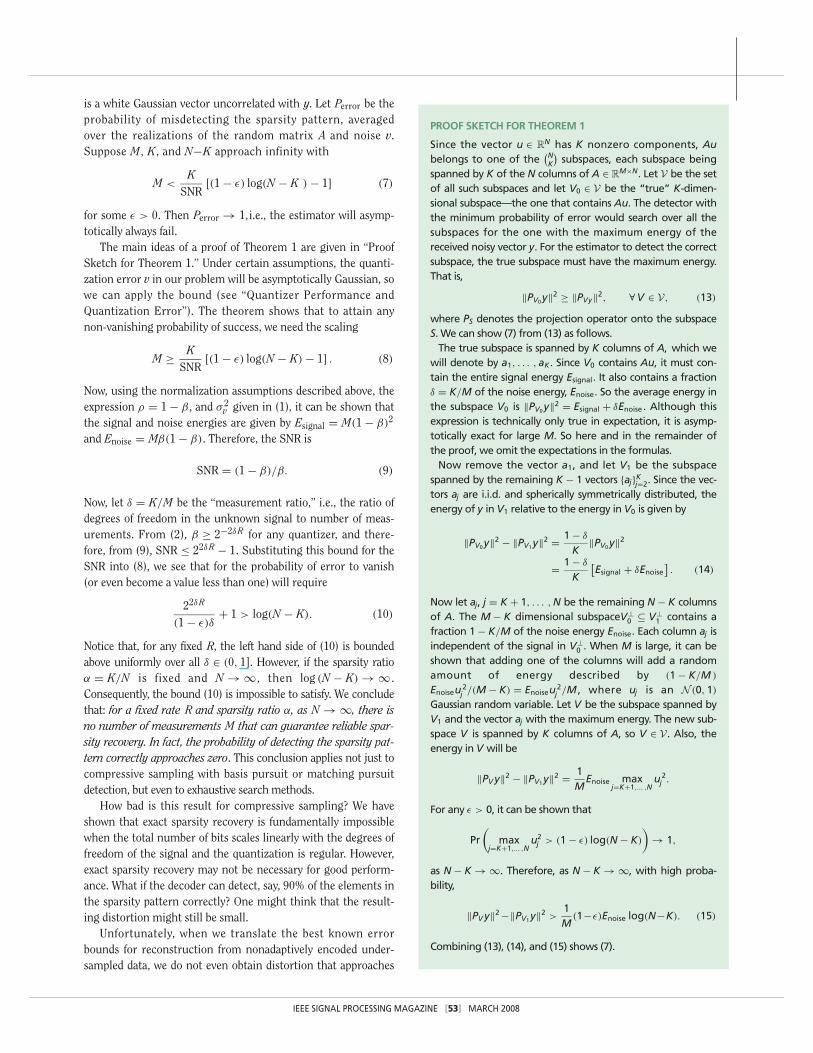
is a white Gaussian vector uncorrelated with y. Let Perror be theprobability of misdetecting the sparsity pattern, averagedover the realizations of the random matrix A and noise v.Suppose M, K, and N−K approach infinity with

M <K

SNR[(1 − ε) log(N − K ) − 1] (7)

for some ε > 0. Then Perror → 1,i.e., the estimator will asymp-totically always fail.

The main ideas of a proof of Theorem 1 are given in “ProofSketch for Theorem 1.” Under certain assumptions, the quanti-zation error v in our problem will be asymptotically Gaussian, sowe can apply the bound (see “Quantizer Performance andQuantization Error”). The theorem shows that to attain anynon-vanishing probability of success, we need the scaling

M ≥ KSNR

[(1 − ε) log(N − K) − 1] . (8)

Now, using the normalization assumptions described above, theexpression ρ = 1 − β , and σ 2

v given in (1), it can be shown thatthe signal and noise energies are given by Esignal = M(1 − β)2

and Enoise = Mβ(1 − β). Therefore, the SNR is

SNR = (1 − β)/β. (9)

Now, let δ = K/M be the “measurement ratio,” i.e., the ratio ofdegrees of freedom in the unknown signal to number of meas-urements. From (2), β ≥ 2−2δR for any quantizer, and there-fore, from (9), SNR ≤ 22δR − 1. Substituting this bound for theSNR into (8), we see that for the probability of error to vanish(or even become a value less than one) will require

22δR

(1 − ε)δ+ 1 > log(N − K). (10)

Notice that, for any fixed R, the left hand side of (10) is boundedabove uniformly over all δ ∈ (0, 1]. However, if the sparsity ratioα = K/N is fixed and N → ∞, then log (N − K) → ∞ .Consequently, the bound (10) is impossible to satisfy. We concludethat: for a fixed rate R and sparsity ratio α, as N → ∞, there isno number of measurements M that can guarantee reliable spar-sity recovery. In fact, the probability of detecting the sparsity pat-tern correctly approaches zero. This conclusion applies not just tocompressive sampling with basis pursuit or matching pursuitdetection, but even to exhaustive search methods.

How bad is this result for compressive sampling? We haveshown that exact sparsity recovery is fundamentally impossiblewhen the total number of bits scales linearly with the degrees offreedom of the signal and the quantization is regular. However,exact sparsity recovery may not be necessary for good perform-ance. What if the decoder can detect, say, 90% of the elements inthe sparsity pattern correctly? One might think that the result-ing distortion might still be small.

Unfortunately, when we translate the best known errorbounds for reconstruction from nonadaptively encoded under-sampled data, we do not even obtain distortion that approaches

PROOF SKETCH FOR THEOREM 1

Since the vector u ∈ RN has K nonzero components, Au

belongs to one of the (N

K

)subspaces, each subspace being

spanned by K of the N columns of A ∈ RM×N. Let V be the set

of all such subspaces and let V0 ∈ V be the “true” K-dimen-sional subspace—the one that contains Au. The detector withthe minimum probability of error would search over all thesubspaces for the one with the maximum energy of thereceived noisy vector y. For the estimator to detect the correctsubspace, the true subspace must have the maximum energy.That is,

‖PV0y‖2 ≥ ‖PVy‖2, ∀ V ∈ V, (13)

where PS denotes the projection operator onto the subspaceS. We can show (7) from (13) as follows.

The true subspace is spanned by K columns of A, which wewill denote by a1, . . . , aK. Since V0 contains Au, it must con-tain the entire signal energy Esignal. It also contains a fractionδ = K/M of the noise energy, Enoise. So the average energy inthe subspace V0 is ‖PV0y‖2 = Esignal + δEnoise . Although thisexpression is technically only true in expectation, it is asymp-totically exact for large M. So here and in the remainder ofthe proof, we omit the expectations in the formulas.

Now remove the vector a1, and let V1 be the subspacespanned by the remaining K − 1 vectors {aj}K

j=2. Since the vec-tors aj are i.i.d. and spherically symmetrically distributed, theenergy of y in V1 relative to the energy in V0 is given by

‖PV0y‖2 − ‖PV1y‖2 = 1 − δ

K‖PV0y‖2

= 1 − δ

K

[Esignal + δEnoise

]. (14)

Now let aj, j = K + 1, . . . , N be the remaining N − K columnsof A. The M − K dimensional subspaceV⊥

0 ⊆ V⊥1 contains a

fraction 1 − K/M of the noise energy Enoise. Each column aj isindependent of the signal in V⊥

0 . When M is large, it can beshown that adding one of the columns will add a randomamount of energy described by (1 − K/M )

Enoiseu2j /(M − K) = Enoiseu2

j /M , where uj is an N (0, 1)

Gaussian random variable. Let V be the subspace spanned byV1 and the vector aj with the maximum energy. The new sub-space V is spanned by K columns of A, so V ∈ V. Also, theenergy in V will be

‖PV y‖2 − ‖PV1y‖2 = 1M

Enoise maxj=K+1,... ,N

u2j .

For any ε > 0, it can be shown that

Pr(

maxj=K+1,... ,N

u2j > (1 − ε) log(N − K)

)→ 1,

as N − K → ∞. Therefore, as N − K → ∞, with high proba-bility,

‖PV y‖2 −‖PV1y‖2 >1M

(1−ε)Enoise log(N−K). (15)

Combining (13), (14), and (15) shows (7).

IEEE SIGNAL PROCESSING MAGAZINE [53] MARCH 2008

zero as the rate is increased with K, M, and N fixed. [Rememberthat without undersampling, one can at least obtain the per-formance (5).] For example, Candès and Tao [18] prove that anestimator similar to the lasso estimator attains a distortion

1K

‖x − x‖2 ≤ c1KM

(log N)σ 2, (11)

with large probability, from M measurements with noise vari-ance σ 2, provided that the number of measurements is ade-quate. There is a constant δ ∈ (0, 1) such that M = K/δ issufficient for (11) to hold with probability approaching one as Nis increased with K/N held constant; but for any finite N, thereis a nonzero probability of failure. Spreading RK bits amongstthe measurements and relating the number of bits to the quan-tization noise variance gives

D = 1K

E[‖x − x‖2] ≤ c2δ(log N )2−2δR + Derr, (12)

where D err is the distortion due to the failure event. (Haupt andNowak [19] consider optimal estimators and obtain a bound simi-lar to (12) in that it has a term that is constant with respect to thenoise variance. See also [20] for related results.) Thus if Derr isnegligible, the distortion will decrease exponentially in the rate,but with an exponent reduced by a factor δ. However, as N increas-es to infinity, the distortion bound increases and is not useful.

NUMERICAL SIMULATIONTo get some idea of the possible performance, we performedthe following numerical experiment. We fixed the signaldimensions to N = 100 and K = 10, so the signal has a sparsi-ty of α = K/N = 0.1. We varied the quantization rate R from4 to 12 b per degree of freedom, which spans low to high ratesince (1/K) log2

(NK

) ≈ 4.4. The resulting simulated perform-ance of compressive sampling is shown in Figure 5. The per-formance of direct quantization [D direct (R ) from (5)] and

baseline quantization with time sharing [see (4) and (5)] areshown for comparison.

The distortion of compressive sampling was simulated as fol-lows: For both lasso and orthogonal matching pursuit (OMP)reconstruction and for integer rates R, the number of measure-ments M was varied from K to N in steps of ten. At each value ofM, the distortion was estimated by averaging 500 Monte Carlo tri-als with random encoder matrices � and quantization noise vec-tors v. To give the best-case performance of compressive sampling,the distortion was taken to be the minimum distortion over thetested values of M and, for lasso, over several values of the regular-ization parameter λ. The optimal M is not necessarily the mini-mum M to guarantee sparsity recovery. Instead, optimizing Mtrades off errors in the sparsity pattern against errors in the esti-mated values for the components. The optimal value does notresult in small probability of subspace misdetection. More exten-sive sets of simulations consistent with these are presented in [21].

From (4), the distortion with adaptive quantization decreasesexponentially with the rate R through the multiplicative factor2−2R. This appears in Figure 5 as a decrease in distortion of approx-imately 6 dB/b. In contrast, simple direct quantization achieves adistortion given by (5), which in this case is only 0.6 dB/b. Thus,there is potentially a large gap between direct quantization thatdoes not exploit the sparsity and adaptive quantization that does.

Both compressive sampling methods, lasso and OMP, are ableto perform slightly better than simple direct quantization,achieving approximately 1.4–1.6 dB/b. (A finer analysis thatallows computation of the largest possible δ in (12) might predictthis slope.) Thus, compressive sampling is able to exploit thesparsity to some degree and narrow the gap between linear andadaptive quantization. However, neither algorithm is able tocome close to the performance of the baseline encoder that canuse adaptive quantization. Indeed, comparing to the baselinequantization, there a multiplicative rate penalty in this simula-tion of approximately a factor of four. This is large by source cod-ing standards, and we can conclude that compressive samplingdoes not achieve performance similar to adaptive quantization.

INFORMATION THEORY TO THE RESCUE?We have thus far used information theory to provide context andanalysis tools. It has shown us that compressing sparse signalsby scalar quantization of random measurements incurs a signifi-cant penalty. Can information theory also suggest alternatives tocompressive sampling? In fact, it does provide techniques thatwould give much better performance for source coding, but thecomplexity of decoding algorithms becomes even higher.

Let us return to Figure 3 and interpret it as a communica-tion problem where x is to be reproduced approximately and thenumber of bits that can be used is limited. We would like toextract source coding with side information and distributedsource coding problems from this setup. This will lead to resultsmuch more positive than those developed above.

In developing the baseline quantization method, we discussedhow an encoder that knows V can recover J and uK from x andthus send J exactly and uK approximately. Compressive sampling

[FIG5] Rate-distortion performance of compressive samplingusing reconstruction via OMP and lasso. At each rate, thenumber of measurements M is optimized to minimize thedistortion. Also plotted are the theoretical distortion curves fordirect and baseline quantization. In all simulations(K, N) = (10, 100).

4 5 6 7 8 9 10 11 12−45

−40

−35

−30

−25

−20

−15

−10

−5

0

Rate

MS

E (

dB)

DirectOMPLassoBaseline

IEEE SIGNAL PROCESSING MAGAZINE [54] MARCH 2008

is to apply when the encoder does not know (or want to use) thesparsifying basis V. In this case, an information theorist would saythat we have a problem of lossy source coding of x with side infor-mation V available at the decoder—an instance of the Wyner-Zivproblem [22]. In contrast to the analogous lossless coding prob-lem (see “Slepian-Wolf Coding”), the unavailability of the sideinformation at the encoder does in general hurt the best possibleperformance. Specifically, let L(D ) denote the rate loss (increasedrate because V is unavailable) to achieve distortion D. Then thereare upper bounds to L(D ) that depend only on the source alpha-bet, the way distortion is measured, and the value of the distor-tion—not on the distribution of the source or side information[23]. For the scenario of interest to us [(continuous-valued sourceand mean-squared error (MSE) distortion)], L(D) ≤ 0.5 b for allD. The techniques to achieve this are complicated, but note theconstant additive rate penalty is in dramatic contrast to Figure 5.

Compressive sampling not only allows side information V tobe available only at the decoder, it also allows the components ofthe measurement vector y to be encoded separately. The way tointerpret this information theoretically is to considery1, y2, . . . , yM as distributed sources whose joint distributiondepends on side information (V,�) available at the decoder.Imposing a constraint of distributed encoding of y (while allow-ing joint decoding) generally creates a degradation of the bestpossible performance. (Again, there is no performance penalty inthe lossless case; see “Slepian-Wolf Coding.”) Let us sketch a par-ticular strategy that is not necessarily optimal but exhibits only asmall additive rate penalty. This is inspired by [23] and [24].

Suppose that each of M distributed encoders performs scalarquantization of its own yi to yield q(yi). Before this seemed toimmediately get us in trouble (recall our interpretation ofTheorem 1), but now we will do further encoding. The quantizedvalues give us a lossless distributed compression problem with sideinformation (V,�) available at the decoder. Using Slepian-Wolfcoding, a total rate arbitrarily close to H(q(y)) can be achieved.The remaining question is how the rate and distortion relate.

For the sake of analysis, let us assume that the encoder anddecoder share some randomness Z so that the scalar quantizationabove can be subtractively dithered (see, e.g., [25]). Then follow-ing the analysis in [24] and [26], encoding the quantized samplesq(y) at rate H(q(y) | V, Z) is within 0.755 b of the conditionalrate-distortion bound for source x given V. Thus the combinationof universal dithered quantization with Slepian-Wolf coding givesa method of distributed coding with only a constant additive ratepenalty. These methods inspired by information theory depend oncoding across independent signal acquisition instances, and theygenerally incur large decoding complexity.

Let us finally interpret the “quantization plus Slepian-Wolf”approach described above when limited to a single instance.Suppose the yi s are separately quantized as described above. Themain negative result of this article indicates that ideal separateentropy coding of each q (yi ) is not nearly enough to get to goodperformance. The rate must be reduced by replacing an ordinaryentropy code with one that collapses some distinct quantized val-ues to the same index. The hope has to be that in the joint decod-

ing of q (y), the dependence between components will save theday. This is equivalent to saying that the quantizers in use arenot regular [25], much like multiple description quantizers [27].This approach is developed and simulated in [21].

CONCLUSIONS—WHITHER COMPRESSIVE SAMPLING?To an information theorist, “compression” is the efficient repre-sentation of data with bits. In this article, we have looked atcompressive sampling from this perspective, to see if randommeasurements of sparse signals provide an efficient method ofrepresenting sparse signals.

The source coding performance depends sharply on how therandom measurements are encoded into bits. Using familiarforms of quantization (regular quantizers; see [25]) even veryweak forms of universality are precluded. One would want to

SLEPIAN-WOLF CODING

When two related quantities are to be compressed, there isgenerally an advantage to doing the compression jointly.What does “jointly” mean? On its face, “jointly” would seemto mean that the quantities are inseparably mapped to a bitstring. However, Slepian and Wolf [29] remarkably showedthat it can be good enough for the decoding to be “joint”—the encoding can be separate.

To understand the result precisely, suppose a sequence ofindependent replicas (X(1)

1 , X (1)

2 ), (X (2)

1 , X (2)

2 ), . . . , of the pairof jointly distributed discrete random variables (X1, X2) is tobe compressed. The minimum possible rate is H(X1, X2), thejoint entropy of X1 and X2. The normal way to approach thisminimum rate is to treat (X1, X2) as a single discrete randomvariable (over an alphabet that is the Cartesian product of thealphabets of X1 and X2) and apply an entropy code to thisrandom variable. This requires an encoder that operates onX1 and X2 together. The main result of [29] indicates that thistotal rate can be approached with encoders that see X1 andX2 separately as long as the decoding is joint. The recovery ofthe Xk s is perfect (or has vanishing error probability) withoutrequiring any excess total rate (or arbitrarily small excess rate):R1 + R2 = H(X1, X2). The individual rates need only satisfyR1 ≥ H(X1 | X2) and R2 ≥ H(X2 | X1).

As a very simple example, suppose X1 has any distributionon the integers; and X2 − X1 equals zero or one with equalprobability, independent of X1. Then (X1, X2) has preciselyone more bit of information than X1 alone. The optimal totalrate R1 + R2 = H(X1) + 1 can be achieved by having Encoder1 compress X1 as if communicating X1 were the only goal andhaving Encoder 2 send only the parity of X2.

Slepian-Wolf coding can be extended to any number of cor-related sources with no “penalty” in the rate [30, Thm.14.4.2]. Also, simpler than Slepian-Wolf coding is for one ofthe sources (say, X2) to be available to the decoder but not tothe encoder. Then a rate of R1 = H(X1 | X2) is sufficient toallow the decoder to recover X1, even though the encodingof X1 is done without knowledge of X2. The main text usesthese results to give information-theoretic bounds for encod-ing of random measurements.

IEEE SIGNAL PROCESSING MAGAZINE [55] MARCH 2008

spend a number of bits proportional to the number of degrees offreedom of the sparse signal, but this does not lead to good per-formance. In this case, we can conclude analytically that recoveryof the sparsity pattern is asymptotically impossible. Furthermore,simulations show that the MSE performance is far from optimal.

Information theory provides alternatives based on universalversions of distributed lossless coding (Slepian-Wolf coding)and entropy-coded dithered quantization. These information-theoretic constructions indicate that it is reasonable to ask forgood performance with merely linear scaling of the number ofbits with the sparsity of the signal. However, practical imple-mentation of such schemes remains an open problem.

It is important to keep our mainly negative results in propercontext. We have shown that compressive sampling combinedwith ordinary quantization is a bad compression technique, butour results say nothing about whether compressive sampling is aneffective initial step in data acquisition. A good analogy within therealm of signal acquisition is oversampling in analog-to-digitalconversion (ADC). Since MSE distortion in oversampled ADCdrops only polynomially (not exponentially) with the oversamplingfactor, high oversampling alone—without other processing—leadsto poor rate-distortion performance. Nevertheless, oversampling isubiquitous. Similarly, compressive sampling is useful in contextswhere sampling itself is very expensive, but the subsequent storageand communication of quantized samples is less constricted.

ACKNOWLEDGMENTSThe authors thank Sourav Dey, Lav Varshney, ClaudioWeidmann, Joseph Yeh, and an anonymous reviewer forthoughtful comments that helped us improve the article.

AUTHORSVivek K Goyal ([email protected]) received the B.S. degree in mathe-matics and the B.S.E. degree in electrical engineering from theUniversity of Iowa and the M.S. and Ph.D. degrees in electrical engi-neering from the University of California, Berkeley. He is currentlyEsther and Harold E. Edgerton Assistant Professor of ElectricalEngineering at the Massachusetts Institute of Technology. He hasreceived the UC-Berkeley Eliahu Jury Award for outstandingachievement in systems, communications, control, or signal pro-cessing, the IEEE SPS Magazine Award and an NSF CAREERAward. He is on the IEEE SPS Image and Multiple DimensionalSignal Processing Technical Committee and cochair of the SPIEWavelets conference series. He is a Senior Member of the IEEE.

Alyson K. Fletcher received the B.S. degree in mathematicsfrom the University of Iowa and the M.A. degree in mathematicsand the M.S. and Ph.D. degrees in electrical engineering from theUniversity of California, Berkeley. She is currently a President’sPostdoctoral Fellow at the University of California, Berkeley. Sheis a member of SWE, SIAM, and Sigma Xi. She has been awardedthe University of California Eugene L. Lawler Award, the HenryLuce Foundation’s Clare Boothe Luce Fellowship, and theSoroptimist Dissertation Fellowship. Her research interestsinclude estimation, image processing, statistical signal process-ing, sparse approximation, wavelets, and control theory.

Sundeep Rangan received the B.A.Sc. degree in electrical engi-neering from the University of Waterloo, Canada, and the M.S. andPh.D. degrees in electrical engineering from the University ofCalifornia, Berkeley. He was a postdoctoral research fellow at theUniversity of Michigan. He then joined the Wireless ResearchCenter at Bell Laboratories, and in 2000, he co-founded FlarionTechnologies with four others. He is currently a director of engi-neering at Qualcomm Technologies, where he is involved in thedevelopment of next generation cellular wireless systems.

REFERENCES[1] D.L. Donoho, M. Vetterli, R.A. DeVore, and I. Daubechies, “Data compressionand harmonic analysis,” IEEE Trans. Inform. Theory, vol. 44, no. 6, pp.2435–2476, Oct. 1998.[2] E.J. Candes, J. Romberg, and T. Tao, “Robust uncertainty principles: Exact sig-nal reconstruction from highly incomplete frequency information,” IEEE Trans.Inform. Theory, vol. 52, no. 2, pp. 489–509, Feb. 2006.[3] E.J. Candes and T. Tao, “Near-optimal signal recovery from random projections:Universal encoding strategies?” IEEE Trans. Inform. Theory, vol. 52, no. 12, pp.5406–5425, Dec. 2006.[4] D.L. Donoho, “Compressed sensing,” IEEE Trans. Inform. Theory, vol. 52, no.4, pp. 1289–1306, Apr. 2006.[5] B.K. Natarajan, “Sparse approximate solutions to linear systems,” SIAM J.Comput., vol. 24, no. 2, pp. 227–234, Apr. 1995.[6] D.L. Donoho and P.B. Stark, “Uncertainty principles and signal recovery,” SIAMJ. Appl. Math., vol. 49, no. 3, pp. 906–931, June 1989.[7] D.L. Donoho and J. Tanner, “Counting faces of randomly-projected polytopeswhen the projection radically lowers dimension,” submitted for publication. [8] M.J. Wainwright, “Sharp thresholds for high-dimensional and noisy recovery ofsparsity,” Univ. California, Berkeley, Dept. of Statistics, Tech. Report#arXiv:math.ST/0605740 v1 30, May 2006.[9] V.K. Goyal, “Theoretical foundations of transform coding,” IEEE SignalProcessing Mag., vol. 18, no. 5, pp. 9–21, Sept. 2001.[10] A.K. Fletcher, “A jump linear framework for estimation and robust communi-cation with Markovian source and channel dynamics.” Ph.D. dissertation, Dept. ofElectrical Eng. Comp. Sci., Univ. California, Berkeley, Nov. 2005. [11] H. Viswanathan and R. Zamir, “On the whiteness of high-resolution quantiza-tion errors,” IEEE Trans. Inform. Theory, vol. 47, no. 5, pp. 2029–2038, July 2001.[12] R.G. Gallager, Information Theory and Reliable Communication. New York:Wiley, 1968.[13] C. Weidmann and M. Vetterli, “Rate-distortion analysis of spike processes,” inProc. IEEE Data Compression Conf., Snowbird, Utah, Mar. 1999, pp. 82–91.[14] V.K. Goyal, M. Vetterli, and N.T. Thao, “Quantized overcomplete expansionsin RN : Analysis, synthesis, and algorithms,” IEEE Trans. Inform. Theory, vol. 44,no. 1, pp. 16–31, Jan. 1998.[15] S. Rangan and V.K. Goyal, “Recursive consistent estimation with boundednoise,” IEEE Trans. Inform. Theory, vol. 47, no. 1, pp. 457–464, Jan. 2001.[16] V.K. Goyal, J. Kovacevic, and J.A. Kelner, “Quantized frame expansions witherasures,” Appl. Comput. Harmon. Anal., vol. 10, no. 3, pp. 203–233, May 2001.[17] A.K. Fletcher, S. Rangan, and V.K. Goyal, “On the rate-distortion performanceof compressed sensing,” in Proc. IEEE Int. Conf. Acoustics, Speech, SignalProcessing, Honolulu, HI, vol. 3, Apr. 2007, pp. 885–888.[18] E.J. Candes and T. Tao, “The Dantzig selector: Statistical estimation when p ismuch larger than n,” submitted for publication. [19] J. Haupt and R. Nowak, “Signal reconstruction from noisy random projec-tions,” IEEE Trans. Inform. Theory, vol. 52, no. 9, pp. 4036–4048, Sept. 2006.[20] N. Meinshausen and B. Yu, “Lasso-type recovery of sparse representations forhigh-dimensional data,” Univ. of California, Berkeley, Dept. of Statistics, Sept. 2007. [21] R.J. Pai, “Nonadaptive lossy encoding of sparse signals,” M.S thesis, Dept. ofElectrical Eng. Comp. Sci., MIT, Cambridge, MA, Aug. 2006. [22] A.D. Wyner and J. Ziv, “The rate-distortion function for source coding withside information at the decoder,” IEEE Trans. Inform. Theory, vol. IT-22, no. 1,pp. 1–10, Jan. 1976.[23] R. Zamir, “The rate loss in the Wyner–Ziv problem,” IEEE Trans. Inform.Theory, vol. 42, no. 6, pp. 2073–2084, Nov. 1996.[24] J. Ziv, “On universal quantization,” IEEE Trans. Inform. Theory, vol. IT-31,no. 3, pp. 344–347, May 1985.[25] R.M. Gray and D.L. Neuhoff, “Quantization,” IEEE Trans. Inform. Theory, vol.44, no. 6, pp. 2325–2383, Oct. 1998.[26] R. Zamir and M. Feder, “On universal quantization by randomizeduniform/lattice quantization,” IEEE Trans. Inform. Theory, vol. 38, no. 2, pp. 428–436, Mar. 1992.[27] V.K. Goyal, “Multiple description coding: Compression meets the network,”IEEE Signal Processing Mag., vol. 18, no. 5, pp. 74–93, Sept. 2001.[28] T. Berger, Rate Distortion Theory. Englewood Cliffs, NJ: Prentice-Hall, 1971.[29] D. Slepian and J.K. Wolf, “Noiseless coding of correlated information sources,”IEEE Trans. Inform. Theory, vol. IT-19, no. 4, pp. 471–480, July 1973.[30] T.M. Cover and J.A. Thomas, Elements of Information Theory. New York:Wiley, 1991.

IEEE SIGNAL PROCESSING MAGAZINE [56] MARCH 2008

[SP]