Compressed network monitoring for IP and all-optical …networks.ece.mcgill.ca/sites/default/files/coates_IMC07.pdf · Compressed network monitoring for IP and all-optical networks

Compressed network monitoringfor IP and all-optical networks ∗

Mark Coates, Yvan Pointurier and Michael RabbatDepartment of Electrical and Computer Engineering

McGill UniversityMontreal, Quebec H3A-2A7, Canada

mark.coates, yvan.pointurier, [email protected]

ABSTRACTWe address the problem of efficient end-to-end network mon-itoring of path metrics in communication networks. Our goalis to minimize the number of measurements or monitors re-quired to maintain an acceptable estimation accuracy. Wepresent a framework based on diffusion wavelets and non-linear estimation. Our procedure involves the developmentof a diffusion wavelet basis that is adapted to the monitor-ing problem. This basis exploits spatial and temporal corre-lations in the measured phenomena to provide a compress-ible representation of the path metrics. The framework em-ploys nonlinear estimation techniques usingℓ1 minimiza-tion to generate estimates for the unmeasured paths. We de-scribe heuristic approaches for the selection of the paths thatshould be monitored, or equivalently, where hardware mon-itors should be located. We demonstrate how our estimationframework can improve the efficiency of end-to-end delayestimation in IP networks and reduce the number of hard-ware monitors required to track bit-error rates in all-opticalnetworks (networks with no electrical regenerators).

Categories and Subject DescriptorsC.2.3 [Network Operations]: Network Operations—Network monitoring; E.4 [Coding and InformationTheory]: Data compaction and compression

∗This work was supported by the Natural Sciences and En-gineering Research Council (NSERC) of Canada and in-dustrial and government partners, through the Agile All-Photonic Networks (AAPN) Research Network and theMathematics of Information Technology and Complex Sys-tems (MITACS) Network of Centres of Excellence (NCE).

Permission to make digital or hard copies of all or part of this work forpersonal or classroom use is granted without fee provided that copies arenot made or distributed for profit or commercial advantage and that copiesbear this notice and the full citation on the first page. To copy otherwise, torepublish, to post on servers or to redistribute to lists, requires prior specificpermission and/or a fee.IMC’07, October 24-26, 2007, San Diego, California, USA.Copyright 2007 ACM 978-1-59593-908-1/07/0010 ...$5.00.

General TermsAlgorithms, Measurement, Performance

Keywordsnetwork monitoring, diffusion wavelets, compressed sens-ing

1. INTRODUCTIONDirect monitoring of a network – either at the path

level or the link level – does not scale in any prac-tical setting. For the past decade, researchers havebeen actively investigating techniques for inferring net-work characteristics from incomplete or indirect mea-surements [6,20]. This paper describes a scheme for es-timating performance metrics such as delay or loss rateson many end-to-end paths in a network using measure-ments taken on only a few of these paths. Similar torelated previous work [3, 5], we exploit the notion thatthe performance on two overlapping paths should becorrelated. For example, delay statistics of two pathswith at least one link in common are correlated becausepackets from both flows are being delayed in a commonqueue. Similarly, in all-optical networks, two lightpathswith at least one link in common are correlated due tocrosstalk across wavelengths. For either of these exam-ples, it is possible to predict the performance on un-measured paths using measurements of a few paths andknowledge of routing and the network topology. In thispaper we also address the topic of exploiting temporalcorrelation for path-level performance monitoring.

Our methodology begins with the identification of abasis, which we design using diffusion wavelets, that en-ables us to accurately approximate the vector of pathmetrics using only a small number of non-zero coeffi-cients. The coefficients efficiently summarize end-to-end performance on all paths. Diffusion wavelets gen-eralize the concept of wavelets by providing a multi-scale decomposition of functions defined on a graph [7].The diffusion wavelet framework is applicable to a widerange of monitoring scenarios and allows us to simulta-neously take advantage of spatial and temporal corre-

1

lation among the monitored paths. Posing the networkmonitoring problem as a wavelet coefficient estimationexercise allows us to make use of recently-developed,powerful tools from the theory of compressed sensingfor estimating a sparse vector using a relatively smallnumber of measurements.

The rest of the paper is organized as follows. Sec-tion 2 formally defines the monitoring problem andframework introduced in this paper, and provides anoverview of diffusion wavelets and nonlinear estima-tors from the theory of compressed sensing. Section 3describes how we use diffusion wavelets to constructcompressible representations of the path metric func-tions. Section 4 discusses heuristics for selecting thepaths to monitor and deciding where to place monitor-ing devices. Section 5 and Section 6 provide case stud-ies of the application of our monitoring and estimationframework. The estimation of mean end-to-end Inter-net queuing delays is explored in Section 5, and Sec-tion 6 focuses on monitoring bit-error rate in all-opticalnetworks. Section 7 provides concluding remarks andindicates avenues of future research.

2. COMPRESSED NETWORKMONITORING FRAMEWORK

2.1 Problem Formulation and NotationOur goal in this paper is to accurately monitor perfor-

mance metrics (e.g., end-to-end delays in an IP networkor bit-error rates in an all-optical network) on a collec-tion of np end-to-end paths using measurements on asubset of these paths. The size of the subset, ns < np,is (ideally) much smaller than the total number of paths.Let y(k) ∈ R

np denote the vector of performance valuesat time instant k on paths indexed from 1 to np; i.e.,

the ith component, y(k)i , is the performance value on

the ith path at time k. Let y(k)s ∈ R

ns denote the per-formance values we observe on the subset of measuredpaths. Given y

(k)s , our task is to estimate y(k).

The measured and complete set of performance valuesare related via an ns×np binary-valued selection matrix,

A(k), defined such that A(k)i,j = 1 if the ith measured

path corresponds to the jth entry of y(k); i.e., (y(k)s )i =

(y(k))j . Using this notation, we have y(k)s = A(k)y(k),

where each row of A(k) contains exactly one non-zeroentry (identifying which paths we measure), and eachcolumn of A(k) contains at most one non-zero entry (wemeasure each path at most once in each time-step).

In practice, we would like to monitor path-levelperformance over a sequence of time-steps, k =1, . . . , τ . Stacking the path-level performance vectorsfrom multiple time-steps into one vector, we write

y = [y(1)T, . . . , y(τ)T ]T , and similarly, for the mea-

sured performance at each time-step we write ys =

[y(1)s

T, . . . , y

(τ)s

T]T . It is convenient to combine the

selection matrices from each time-step into a block-diagonal matrix, A, with the selection matrices at eachtime-step, A(1), . . . , A(τ), along the diagonal, so that wehave ys = Ay relating the observations and path-levelperformance values over multiple time-steps.

A special case of the monitoring framework occurswhen there is a known linear relationship between thelink and path metrics. Suppose we are monitoring a net-work with nl links, and assume we are given a np × nl

binary-valued routing matrix, G, where Gi,j = 1 if linkj appears in the ith path and Gi,j = 0 otherwise. Manyrelevant performance metrics, including mean delay anddelay variance, satisfy the property that the end-to-endmetric on a path is equal to the sum of the performancemetric of individual links in the path, so we can writey(k) = Gx(k), where x(k) ∈ R

nl are the link-level met-rics. This relationship not only provides valuable infor-mation about the correlation structure, but typicallynl ≪ np, so we can achieve an immediate reduction inthe dimensionality of the estimation task by formulat-ing the problem in “link-space”, i.e., writing ys = AGx.

2.2 Diffusion WaveletsWavelet transforms are a staple of modern compres-

sion and signal processing methods due to their abilityto efficiently represent piece-wise smooth signals (sig-nals which are smooth everywhere, except for a few dis-continuities). Traditionally, discrete wavelet transformsprovide a multi-scale decomposition of functions definedon a regularly sampled interval or grid. A “motherwavelet” is dilated by powers of two and translated toobtain orthonormal wavelet bases. However, in the con-text of network monitoring, we seek to efficiently repre-sent a function (performance metrics) defined on a net-work topology which does not, in general, have a regularstructure, so standard wavelets cannot be directly ap-plied. Crovella and Kolaczyk [8] describe one method ofconstructing wavelets on a graph for decomposing trafficon an arbitrary topology based on dilating and scalinga mother wavelet, similar to the traditional approach.The primary shortcoming of this approach is that itdoes not lead to an orthogonal basis, limiting its use asa mechanism for generating a compressible representa-tion of a network function. More recently, Coifman andMaggioni [7] have introduced diffusion wavelets, gener-alizing the concept of wavelets to functions supportedon a graph through the use of diffusion operators.

The construction of a diffusion wavelet basis is basedon a diffusion operator, D, defined on the support of theunderlying graph. For a graph with n nodes, D is ann×n matrix where Di,j > 0 if and only if there is a linkbetween nodes i and j. The magnitude of Di,j modelsthe strength of the correlation or similarity between thefunction values at nodes i and j. Much like traditional

2

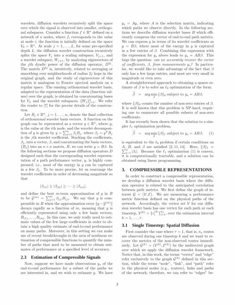
wavelets, diffusion wavelets recursively split the spaceover which the signal is observed into smaller, orthogo-nal subspaces. Consider a function f ∈ R

n defined on anetwork of n nodes, where fi corresponds to the valueat node i; the function is initially defined on the spaceV0 = R

n. At scale j = 1, . . . , L, for some pre-specifieddepth L, the diffusion wavelet construction recursivelysplits the space Vj into a scaling subspace, Vj+1, anda wavelet subspace, Wj+1, by analyzing eigenvectors ofthe jth dyadic power of the diffusion operator, D2j .The matrix D2j is, intuitively, related to averaging orsmoothing over neighborhoods of radius 2j hops in theoriginal graph, and the study of eigenvectors of thismatrix is analogous to Fourier spectral analysis on aregular space. The ensuing orthonormal wavelet basis,adapted to the representation of the data (function val-ues) over the graph, is obtained by concatenating basesfor VL and the wavelet subspaces, WjL

j=1. We referthe reader to [7] for the precise details of the construc-tion.

Let Bj ∈ Rn, j = 1, . . . , n, denote the final collection

of orthonormal wavelet basis vectors. A function on thegraph can be represented as a vector y ∈ R

n, where yi

is the value at the ith node, and the wavelet decomposi-tion of y is given by y =

∑nj=1 βjBj , where βj = yT Bj

is the jth wavelet coefficient. Stacking the coefficients,βj , into a vector, β, and concatenating the basis vectors,Bj into an n×n matrix, B, we can write y = Bβ. Inthe following sections we propose diffusion operators Ddesigned such that the corresponding wavelet represen-tation of a path performance vector, y, is highly com-pressed; i.e., most of the energy in y can be capturedin a few βj . To be more precise, let us rearrange thewavelet coefficients in order of decreasing magnitude sothat

|β(1)| ≥ |β(2)| ≥ · · · ≥ |β(n)|,

and define the best m-term approximation of y in Bto be y(m) =

∑mj=1 β(j)B(j). We say that y is com-

pressible in B when the approximation error ‖y− y(m)‖decays rapidly as a function of m, meaning that y isefficiently represented using only a few basis vectors,B(1), . . . , B(m). In this case, we only really need to esti-mate values of the few large coefficients in order to ob-tain a high quality estimate of end-to-end performanceon many paths. Moreover, in this setting we can makeuse of recent breakthroughs in the area of nonlinear es-timation of compressible functions to quantify the num-ber of paths that need to be measured to obtain esti-mates of performance at a specified level of accuracy.

2.3 Estimation of Compressible SignalsNow, suppose we have made observations ys of the

end-to-end performance for a subset of the paths weare interested in, and we wish to estimate y. We have

ys = Ay, where A is the selection matrix, indicatingwhich paths we observe directly. In the following sec-tions we describe diffusion wavelet bases B which effi-ciently compress the vector of end-to-end path metrics.We can express y in terms of its wavelet coefficients asy = Bβ, where most of the energy in y is capturedin a few entries of β. Combining this expression withthe expression for ys above leads to ys = ABβ. Thisbegs the question: can we accurately recover the vector

of coefficients, β, from measurements ys? In particu-lar, we would like to take advantage of the fact that βonly has a few large entries, and most are very small inmagnitude or even zero.

A straightforward approach to obtaining a sparse es-timate of β is to solve an ℓ0 optimization of the form:

β = argminβ

‖β‖0 subject to ys = ABβ,

where ‖β‖0 counts the number of non-zero entries of β.It is well known that this problem is NP-hard, requir-ing one to enumerate all possible subsets of non-zerocoefficients.

It has recently been shown that the solution to a sim-pler ℓ1 optimization problem,

β = argminβ

‖β‖1 subject to ys = ABβ, (1)

is equivalent to the ℓ0 problem if certain conditions onA, B, and β are satisfied [2, 11, 14]. Here, ‖β‖1 =∑n

i=1 |βi|. Because the ℓ1 optimization (1) is convex,it is computationally tractable, and a solution can beobtained using linear programming.

3. COMPRESSIBLE REPRESENTATIONSIn order to construct a compressible representation,

we develop a diffusion wavelet basis where the diffu-sion operator is related to the anticipated correlationbetween path metrics. We first define the graph of in-terest G = (V , E). We are measuring a performancemetric function defined on the physical paths of thenetwork. Accordingly, the vertex set V for our diffu-sion wavelet basis has one vertex for each path at each

timestep, V(k) = v(k)i np

i=1, over the estimation intervalk = 1, . . . , τ .

3.1 Single Timestep: Spatial DiffusionFirst consider the case where τ = 1, that is, ns routes

are observed during one timestep k and we want to re-cover the metrics of the non-observed routes immedi-ately. Let G(k) = (V(k), E(k)) be the undirected graphover which we apply the diffusion wavelet framework.Notice that, in this work, the terms “vertex” and “edge”refer exclusively to the graph G(k) defined in this sec-tion, while the terms “node”, “link”, and “path” referto the physical nodes (e.g., routers), links and pathsof the network; therefore, we can refer to “edges” be-

3

tween “paths”. The graph G(k) is defined as follows.The vertices V(k) of G(k) correspond to the paths of thenetwork of interest, and there is an edge between thevertices vi and vj if and only if paths i and j shareat least one link. Therefore, vertices of the graph areneighbors when their corresponding paths share a link.The function to be studied over G is the set of metricsassociated with the vertices (paths).

We assign a weight wi,j to the edge between the ver-tices vi and vj to model the correlation between pathmetrics on routes that share the same links. The choiceof these weights is problem-dependent and is deter-mined by the anticipated relationship between link andpath metrics. It effectively forms an a priori model forthe correlation structure in the estimation problem.

For concreteness, we outline a methodology for choos-ing weights that is appropriate when there is an approx-imately linear relationship between path and link met-rics. In this setting, it is reasonable to choose a weightthat is proportional to the fraction of shared links inthe two paths. Consider two paths i and j, and denoteby Ri the set of links used by path i. We define theweight wi,j associated with the edge between vi and vj

as:

wi,j =|Ri ∩Rj ||Ri ∪Rj |

. (2)

More weight is given to edges between paths that sharemany links, thereby emphasizing the spatial correlationintrinsic to end-to-end performance metrics — theseedges are thus “spatial correlation edges”, as opposedto the “time correlation edges”, defined next.

The diffusion wavelet procedure in [7] requires a diffu-sion operator D(k) to generate a wavelet representationover G(k). To obtain a diffusion operator from the con-struction described above, we apply Sinkhorn balanc-ing [18] to the matrix of weights, [w], to form a doublystochastic matrix, D.

3.2 Multiple Timesteps: Incorporating TimeDiffusion

When metrics change slowly with time, relative tothe sampling rate, as is the case with mean end-to-enddelays or BERs on lightpaths, time-correlation betweenthe samples can be exploited to improve estimation ac-curacy. We account for time correlation in the diffusionoperator as follows. Let G = (V , E) be the graph withvertex set,

V =

τ⋃

k=1

V(k) , (3)

which is the union of the paths of the network at eachtimestep, and with edge set E such that:

E =

(τ⋃

k=1

E(k)

)∪(

v(k)i , v

(k+1)i

)

i∈1,...,np,k∈1,...,τ−1.

In the edge set, the first term,⋃

k E(k), is the union ofthe edge sets for each individual timestep, as introducedin the previous subsection. The second term containstime-correlation edges, which connect the subsets V(k)

of the vertex set V together: an edge is present betweena path at timestep k and the same path at timestepk + 1. We keep the weights already defined in the pre-vious section for the edges between paths at the sametimestep (spatial correlation edges) and we only needto define the weights for the inter-timestep edges.

With the a priori assumption that time correlationhas the same strength across the network, we assign aweight of wt to each of these new edges (time correlationedges), except for the edges between vertices of V(1)

and V(2), and V(τ−1) and V(τ), which are assigned aweight of 2wt (for balancing purposes). The specificvalue of wt depends on the anticipated relative strengthsof spatial and temporal correlation. We use a value of0.5 in the examples described later in the paper, whichreflects expectation of reasonably strong correlation; itis equivalent to the anticipated spatial correlation forpaths that share half of their combined links.

The weight matrix w ∈ Rnpτ×npτ is then defined

as the block matrix whose elements are equal to theweights defined above (Inp

is the np × np identity ma-trix):

w =

D(1) 2wtInp0 · · · 0

wtInpD(2) wtInp

. . ....

0. . .

. . .. . . 0

.... . . wtInp

D(τ−1) wtInp

0 · · · 0 2wtInpD(τ)

.

(4)Again, we perform Sinkhorn balancing on [w] in orderto obtain a doubly stochastic matrix D, which we usewhen constructing a diffusion wavelet basis.

3.3 Link-level RepresentationsA special case of our framework arises when there

is a strictly linear relationship between path and linkmetrics. A good example is mean delay; the delay onlinks that share many routes is often strongly correlatedbecause the same traffic sources are generating backlogin queues. In this case, it becomes valuable to formulatethe problem in “link-space”. In this formulation wehave ys = AGBβ, where G is the np ×nl binary-valuedrouting matrix, B is an nl × nl diffusion wavelet basis,and β is now a vector of nl coefficients. The task isstill the estimation of y, and it should be emphasizedthat although the by-product of this formulation is anestimate of x, this is not the goal.

In general, nl ≪ np so the link-space formulationsignificantly reduces the dimensionality of the prob-lem. This formulation also means that any solution

4

automatically satisfies the known relationships betweenpath and link metrics. In the path formulation outlinedabove, these relationships would have to be incorpo-rated as constraints in the ℓ1-minimization (1), makingthe optimization problem significantly more challeng-ing. The derivation of a suitable diffusion operator pro-ceeds exactly as described for the path case, but nowthe nodes in the graph are links in the physical networkand the edges are weighted according to the fraction ofshared paths.

4. PATH SELECTIONSo far, we have discussed why and how it is pos-

sible to accurately estimate end-to-end metrics froma limited number of observations. However, we havenot discussed how to select which routes should be ob-served. This problem is challenging and the appropri-ate approach depends on the measurement constraintsor costs. We will examine two scenarios and proposeheuristics. In the first scenario, we consider that thecost (or constraint) is the average number of measure-ments made per timestep. In this scenario, we do notconstrain which paths are measured at each timestep.Rather, the set of paths measured can change fromtimestep to timestep. In the second scenario, we con-sider the case where the constraint is the number ofmonitoring devices and we must decide where to placethem in the network. Each monitoring device can mea-sure any incoming path on its interface.

4.1 Constraint on Number of MeasurementsFirst we consider the case where the only constraint is

on the total number of paths to be selected over a fixednumber of timesteps. For this scenario, we adapt thepath selection technique presented by Chua et al. in [5]to include our correlation model. The path selectionprocedure in [5] strives to minimize the mean square ofthe prediction error of a linear end-to-end delay estima-tor. The exact minimization procedure is NP-complete(it amounts to the problem of subset selection) andhence heuristics are needed.

Chua et al. propose a heuristic that consists of findingthe rows of the routing matrix G that approximate thespan of the first ns left singular vectors of GCl, where Cl

is a non-singular matrix that satisfies Σl = ClCTl . For

example, Cl = Σ1/2l , and Σl is the covariance of x. Note

that the estimation methodology in [5] is restricted tothe case where path metrics are a linear combination oflink-level performance values. In this case we can writey = Gx, which leads to the incorporation of a link-level covariance matrix in this path selection procedure.In the case where this covariance matrix is not known,reasonable results can be obtained by setting Σl = I.An algorithm (see Alg. 1) that implements this heuristiccan be found in [13].

Algorithm 1 Path selectionInput: Matrix Cp

Number of paths to select ns

Output: Selection matrix A

1: Perform singular value decomposition (SVD) on Cp:Cp = USV T where S contains the singular valuesin descending order.

2: Perform QR decomposition with column pivotingon the first ns columns of U : QR = UT

(1,...,ns)PT .

3: return A = P(1,...,ns), the matrix formed from thefirst ns columns of P .

The intuition behind this heuristic is that most of theenergy of the path metric signal should reside in thespace spanned by the ns left singular vectors of GC.Identifying a set of paths that approximately span thisspace is thus a desirable goal. Here, we do not haveaccess to the link covariance matrix, but the diffusionoperator provides a model of the path-level covariance,Σp. We therefore set Σp = Dτ (recall D is the diffusionoperator and τ the number of timesteps used to accountfor time-correlation). We then strive to identify a subsetof rows of G that approximately spans the same space as

the first ns left singular vectors of the matrix Cp = Σ1/2p .

In the case of a link-level representation, we set Σl = Dτ

and use Cp = GCl, with Cl defined as above. Pathselection is performed using Algorithm 1.

4.2 Constraint on Number of MonitorsIn this scenario, there is a more restrictive constraint.

We have a limited number of monitoring devices, M ,and we must choose where to place them. Our intuitivegoal is the same as for the previous scenario: to ap-proximately span the space where most signal energy isexpected to lie. The same algorithm is applicable, butthere is not a direct mapping from ns to M , becausethe number of monitors required to measure ns pathsvaries according to how many of the paths terminate atthe same interface. We therefore iterate, running Al-gorithm 1 repeatedly for increasing values of ns untilM monitors are used. The resultant procedure is de-scribed by Algorithm 2. The output of the algorithm isa selection matrix A and a set of monitoring locationsEs.

5. MEAN END-TO-END DELAYSTo illustrate the estimation technique presented in

this paper, we use experimental delay data collected onthe Abilene network depicted in Fig. 1. The networkconsists of 11 nodes and 30 unidirectional links. Meanend-to-end delay measurements are collected betweenevery pair of nodes over 400 five-minute intervals. Thereare thus 121 path metrics to be estimated at each timestep. Owing to the large scale of the Abilene network,

5

Algorithm 2 Monitor location selectionInput: routing matrix G, covariance matrix Cp

number of monitors to select MOutput: selection matrix A, monitor set Es.

1: M ′ = M .2: Perform SVD on Cp: Cp = USV T where S contains

the singular values in descending order.3: repeat4: Perform QR decomposition with column piv-

oting on the first M ′ columns of U : QR =UT

(1,...,M ′)PT .

5: Let P ′ = P(1,...,M ′) be the matrix formed of thefirst M ′ columns of P .

6: Es = ∅.7: for i=1 . . . M’ do8: Interpret P ′ as a routing matrix and determine

the last link ℓ on the path described by the ith

row of P ′.9: Es = Es ∪ ℓ.

10: end for11: M ′ = M ′ + 1.12: until |Es| = M .13: return A = P(1,...,M), the matrix formed of the first

M columns of P .

the experimental Abilene end-to-end delays are domi-nated by the propagation delays; those delays can bedetermined accurately using fiber maps. Therefore, weapply our estimation framework to (end-to-end) queu-ing delays, which are more variable. To obtain the end-to-end queuing delays from the end-to-end delays, weassume that the propagation delay for any path is theminimum end-to-end delay over the duration of the ex-periment for this path and subtract off the minimumfor each path. In the remainder of this section, we des-ignate by “end-to-end delay” the end-to-end queuingdelays.

Fig. 2(a) provides a visualization of one of the waveletbasis vectors, which allows us to assess how the energyof wavelets is spatially distributed. In this figure, thesize of each vertex of G is scaled according to the magni-tude of corresponding wavelet coefficient. Visualization(vertex layout) of the graph is achieved through the ap-plication of Isomap [19], where the distances betweenvertices is set to the inverse of the weight matrix. Thefigure provides a clear depiction of the clustering in-duced by the routing matrix. There are two primaryclusters of vertices (on the left and the right) corre-sponding approximately to links appearing primarily ineast-west and west-east paths respectively. Addition-ally, nodes 14 and 17 (corresponding to links 14 and 17in Figure 1) are separate from the clusters. These aretwo of the more “vertical” links in the network whichare used in both east-to-west and west-to-east paths

3

1

24 5

67

8

10

11

9

12

13

1415

16

17

1820

21

22

19

23

2425

26

27

28

2930

Figure 1: Abilene backbone: 11 nodes, 30 (uni-directional) links. The numbers are link identi-fiers.

across the network.Such graphical representation of wavelet basis vec-

tors can be extended to the multi-timestep case. In themulti-timestep case, the time dimension is representedusing a third dimension, as is shown in Fig. 2(b) for8 timesteps. Vertical slices of the plot represent per-timestep network state while the sequence in time isrepresented over the labeled axis. Again, such visual-ization allows one to study where wavelet energy lies inspace and time. In this case for example, the waveletenergy is concentrated on four links in the network mostof the time.

We now verify the compressibility of the data. Fig. 3shows the delays for all links and the absolute valuesof the diffusion wavelet coefficients, over τ = 1 (toppanel) and τ = 8 (bottom panel) timesteps, sorted indescending order. The decay of the delays expressedin the original basis is very slow and exhibits a heavytail. In the diffusion wavelet basis however, the link de-lays exhibit a power law-like decay, as can be seen bycomparison to the reference functions k 7→ αk−p. More-over, the coefficients decay at a much faster rate in the8-timestep case than in the 1-timestep case, indicatingthe value of incorporating time-correlation.

We have seen how, in the diffusion wavelet construc-tion step (Section 2), deeper scales correspond to finergranularity. In the Fourier domain, deeper scales cor-respond to higher frequencies. Queuing delays are rel-atively low frequency signals, especially in the time di-mension. During the nonlinear estimation step (1),estimated coefficients corresponding to high frequen-cies should be encouraged to be small; indeed, in caseof estimation errors (unavoidable when the number ofobservations is low compared to the total number ofcoefficients to estimate), assigning high values to high-frequency coefficients leads to poor signal reconstruc-tion. We make use of the knowledge that the signal tobe estimated has a mainly low frequency spectrum as

6

123

45

6

7

8

910

11

12

13

14

15

16

17

18

19

20

21

22

23 24

25

26

27

28

29

30

(a) Single timestep graph.

(b) Multiple timesteps graph (The labeled axis is the timeaxis.)

Figure 2: Representation of an example waveletbasis vector on G. Each vertex depicted herecorresponds to a link of the network, and thethickness of the edge between vertices i and jincreases relative to the weight wij . Each ver-tex is scaled according to the magnitude of thewavelet basis vector at the vertex. Vertex layoutis determined by application of Isomap [19].

follows: we penalize in (1) the coefficients associatedto deeper scales of the diffusion wavelet basis by themassigning weights ωi, such that (1) becomes:

β = argminβ

‖β‖1 subject to ys = ABΩβ, (5)

where Ω is the diagonal matrix such that Ωi,i = ωi. Re-call each βi is a coefficient in the diffusion wavelet basis.Following the discussion above, the weights should in-crease with the depth of the scale associated to βi. Here,we chose a geometric increase in the weights: denotingby k the scale associated to a diffusion wavelet coeffi-cient βi, then ωi = αk where α is a parameter that isfixed to 2 in the remainder of this section.

We show how our estimation techniques performs inFigure 4, which plots performance as the number of

1 1010

−1

100

101

Raw delay valuesDiffusion wavelet coefficientsReference power law decay (power: −0.7)

1 10 10010

−2

10−1

100

101

102

Coefficient index (k)

Que

uing

del

ay/C

oeffi

cien

ts m

agni

tude

Raw delay valuesDiffusion wavelet coefficientsReference power law decay (power: −1.1)

Figure 3: Link delays for the complete net-work over 1 (top panel) and 8 timesteps (bot-tom panel), sorted by magnitude, in the orig-inal basis (raw delay values) and in the diffu-sion wavelet basis (wavelet coefficients magni-tudes). For comparative purposes, we also showthe power-law decay functions k 7→ αk−p (for con-stant α, for p = 0.7 in the 1-timestep case, andp = 1.1 in the 8-timestep case).

paths-per-timestep varies from 1 to 30, with the block-size set to τ = 1 and τ = 8 timesteps. For the τ = 8case, end-to-end delays are estimated by blocks. Ourdataset includes measurements for all paths in the net-work, so we can verify the accuracy of our estima-tion procedure against ground truth. We assess per-formance in terms of the relative end-to-end mean de-lay error, |〈y − yest〉|/〈y〉, and the relative ℓ2 error,||y − yest||2/||y||2, where ||y||2 =

√∑i y2

i . Perfor-mance is averaged over 400 timesteps.

First consider the single timestep case, τ = 1 inFig. 4. We verify that the rank of G is equal to thenumber of links nl and thus the observation of nl pathsensures exact recovery of all end-to-end link delays withany estimation technique we are presenting. Our tech-nique outperforms linear estimation (network kriging),with the performance improvement being most substan-tial when there are few measurements per timestep.

However, to fully harness the power of the nonlinearestimator, we need to consider data (and its diffusion,via the diffusion operator) over several timesteps. Nowconsider the block estimation case, τ = 8, in Fig. 4;when less than 10 samples per timestep are collected,nonlinear estimation in a wavelet basis exhibits muchlower estimation error than the linear estimator in termsof average end-to-end delay; ℓ2 error is also loweredwhen nonlinear estimation in a wavelet basis is used.

7

0

0.2

0.4

0.6

0.8

1R

ela

tiv

eℓ 2

error

Linear estimationNonlinear estimation in diffusion wavelet basis, τ=1Nonlinear estimation in diffusion wavelet basis, τ=8

5 10 15 20 25 300

0.2

0.4

0.6

0.8

1

Rela

tiv

em

ean

error

Number of samples per timestep

Figure 4: Relative ℓ2 end-to-end delay error(top) and relative mean error (bottom) as func-tions of the average number of measurementsper timestep (for τ = 1 and τ = 8), for our non-linear estimation framework and the linear esti-mator [5].

In terms of mean end-to-end delay (Fig. 4, bottompanel), our results suggest that by making only 3 mea-surements per timestep we can hope to recover the meannetwork end-to-end delay with an error of less than 10%.The error stabilizes for larger number of samples pertimestep and decreases to 0 as the number of samplesper timestep approaches 21.

In the last figure (see Fig. 5), we provide a more de-tailed insight into the nature of our end-to-end delayrecovery techniques. We show the recovered end-to-enddelay (original data, estimation via nonlinear estima-tion in the wavelet basis and path selection accountingfor time-correlation, and linear estimation) over timefor 2 different paths. We used τ = 8 and 10 sam-ples per timestep in the estimation procedure. In Fig 5(bottom panel), for example, we see that linear estima-tion severely underestimates the end-to-end delay forthe chosen path. In general, the linear estimation ex-hibits substantial bias. In contrast, the nonlinear esti-mator exhibits much less bias but more variability. Itis possible to estimate the bias if we are provided mea-surements of all link-level queueing delays (or can makesufficient estimates to form unbiased estimates.) How-ever, such observations are not always available and wefocus here on the case where estimating the bias is notpossible. In the following section, we study an appli-cation to our technique where physical constraints onthe observations prohibit the utilization of full-rankedobservations to precompute the bias

The presented nonlinear estimation technique is out-

0

2

4

6

Original dataLinear estimationNonlinear estimation

0 50 100 150 200 250 300 350 4000

2

4

6

8

Time (timestep)

Que

uein

g de

lay

(ms)

Figure 5: Comparison between nonlinear esti-mation and linear estimation of path delays fortwo example paths.

performs the standard linear estimation technique. Interms of computation time, on standard hardware, mostof the time is spent computing the basis B (seconds tominutes depending on τ for the Abilene topology). Thisis a one-time cost since B only depends on the networktopology. The nonlinear estimation part is typically anorder of magnitude slower than linear estimation, how-ever it only takes tens to hundreds of milliseconds, de-pending on τ , to estimate a block of end-to-end delaysfor all paths (110τ end-to-end delays), making the tech-nique deployable for real-time monitoring in networkswith tens of nodes.

6. ALL-OPTICAL NETWORKMONITORING

In this section, we apply the compressive networkmonitoring framework derived in this paper to the par-ticular case of bit-error rate (BER) monitoring in all-optical networks. We address the problem of monitor-ing circuit-switched all-optical networks with no wave-length conversion subject to a variety of physical im-pairments. More specifically, we tackle the specific casewhere signal statistics (which are used to determine sig-nals’ bit-error rates) can only be measured at certainlocations. This is a key issue in all-optical networkssince the equipment needed to take measurements atone location is extremely costly. The problem is thentwo-fold: given fixed BER monitors and hence the BERof observed lightpaths, what is the best estimate of theBERs of unobserved lightpaths? Then, how shouldBER monitors be placed to facilitate the estimationproblem?

8

All-optical networks are high-speed, optical net-works where OEO (optical-electrical-optical) conver-sion, which takes place at the nodes in traditional op-tical networks (e.g., SONET networks), is removed [21].In all-optical networks, signal are transmitted in the op-tical domain with no electrical regeneration from endto end. In the nodes, which are called optical cross-connects (OXCs), signals are switched spatially in theoptical domain [10]. The absence of OEO conversion al-lows (among other benefits) all-optical networks to by-pass the capacity bottleneck incurred by the relativelylow speed of electronic components, as data process-ing at 40 Gbit/s and above requires expensive devices.However, removing OEO conversion results in two mainpractical issues for all-optical network operation andmanagement.

First, signals are propagated over very long dis-tances without electrical regeneration and physical im-pairments accumulate as signals propagate in opticalfiber and OXCs. Recently, network-layer techniques,namely, Routing and Wavelength Assignment (RWA)techniques, have been harnessed to counter these phys-ical impairments. Assuming circuit-switched networkswith no wavelength conversion1, a RWA algorithmchooses a route and a wavelength (the combination ofwhich is called “lightpath” [4]) to accommodate eachincoming call at call admission time. It is possible toincrease the quality of transmission in optical networksby using appropriate RWA techniques [15, 16]. In thispaper, we make no assumption regarding the particularRWA used in the network.

The second major issue in all-optical networks is theabsence of OEO converters, which makes monitoringdifficult. Indeed, in traditional, non all-optical net-works, signals are detected at each node, allowing errordetection and correction. For example, SONET framescarry parity bits to detect errors [17]. Monitoring in all-optical networks is therefore restricted, both in terms ofwhat can be measured and where it can be measured.Since electrical signals are not available at intermediatenodes of a lightpath, only a few optical quantities suchas the optical power of the signal are measurable, andobtaining such intermediate measurements requires ex-pensive optical spectrometers. Error detection can onlybe performed at the edge of the network, since that isthe only place where electrical conversion is performed.

6.1 All-Optical Network ModelWe consider circuit-switched all-optical networks

where data is carried over lightpaths, that is, the com-bination of a route (assumed to be fixed for the dura-tion of the call) and a wavelength, fixed from start to

1All-optical packet switched networks and wavelength con-version devices are currently at the experimental stage andare not ready for industrialization.

end of the route. Opaque networks, which allow wave-length conversion within a route, are beyond the scopeof this paper. Links are assumed to be unidirectionaland each link can carry C channels (wavelengths) simul-taneously. A model for a lightpath is depicted in Fig. 6.The figure represents the lightpath and the sources ofphysical impairments considered in this paper. Otherphysical devices such as dispersion compensators andmultiplexers/demultiplexers, which are assumed not tofurther degrade the signal’s SNR, are not representedhere. At the source of a call, a transmitter, located atan OXC, modulates data and sends it over optical fiberas an on-off keyed signal over a given wavelength. Asit is transmitted over the optical fiber, the signal sus-tains chromatic dispersion and self-phase modulationwhich combine and contribute to intersymbol interfer-ence (ISI).

The transmitted signal is also subject to nonlinearcrosstalk, that is, the nonlinear interaction with othersignals that are transmitted simultaneously over thesame fiber spans: cross-phase modulation and four-wavemixing. Optical amplifiers inject amplifier spontaneousemission (ASE) noise, and the signal is also subject tonode crosstalk, which refers to signal leakages caused,for instance, by imperfect filtering at the nodes [12]. Werefer the reader to [23], [22], [9], [15] for more details re-garding the models of ASE noise, nonlinear crosstalk,node crosstalk, and their combined effects, respectively.Note that we ignore here a number of physical impair-ments such as receiver noise and polarization mode dis-persion, but these effects can be incorporated easily inour model as additional noise variances, as will be seenshortly. Fig. 6 also illustrates the physical degradationof the transmitted signal in terms of an eye diagram;at the receiver, the eye diagram gets closed, therebyindicating a degraded SNR.

We denote by µ0 and µ1 the means of the distribu-tions of the “0” and “1” samples, respectively, and byσ0 and σ1 their standard deviations. Let

Q =µ1 − µ0

σ0 + σ1(6)

be the Q-factor associated with the considered light-path. The Q-factor can be interpreted as a signal-to-noise ratio, from which we can derive the bit-error rare,using a Gaussian assumption [1]:

BER =1

2erfc(Q/

√2). (7)

We model each of the physical impairments describedabove by a noise variance in the SNR of the signal. As-suming these effects are statistically independent, thesevariances due to these effects are additive. Let σ2

isi bethe noise variance caused by ISI, σ2

ase the noise variancecaused by ASE noise, σ2

nl the noise variance caused bynonlinear crosstalk, and σ2

oxc the noise variance caused

9

sourcecall

OXC OXC

ASE noisenode crosstalk

OXC and amplifiersfiber spans

amplifiers, OXCsfiber spans,

node crosstalk

photodetectorpower

the ‘‘0’’s ‘‘1’’s distributions of

node crosstalk

powerinterchannel crosstalk

diagrameye

probability densitytime

| · |2σ1

σ0

µ1

µ0

Figure 6: Model for a lightpath in an all-optical network, and sources of physical impairment. Thesignal traverses nodes (OXCs), spans of optical fiber and optical amplifiers before reaching destination,where it is detected by a photodetector — represented here by a square law device. Each devicedegrades the SNR of the signal: nodes inject node crosstalk, fiber spans injects nonlinear crosstalk,and amplifiers inject amplifier (ASE) noise. The BER associated to the signal can be computed fromthe distributions of the received “0” and “1” samples, and is related to the appearance of the eyediagram of the signal.

by node crosstalk, then we have σ21 = σ2

isi +σ2ase +σ2

nl +σ2

oxc. Therefore, determining the BER of a lightpathboils down to determining four quantities, which canbe measured at receivers using adapted equipment: µ0,µ1, σ0, σ1. In the remainder of this section, the BERestimation for a lightpath designates the simultaneousestimation of these four quantities.

In this work, we consider that the BER of a lightpathdepends only on the network state, that is, on the net-work topology and on the lightpaths that are alreadyestablished in the network. Indeed, in our model a Qfactor depends on the topology via µ0, µ1, σ0, σisi, σase,and the crosstalk injected by other lightpaths via σoxc

and σnl. In particular, we consider that the network isan event-driven system where events are lightpath es-tablishment and tear-down. A timestep here thus con-sists in the arrival or the termination of new call. Caseswhere BERs vary between calls arrivals and departure,e.g., because of link failures, can be easily dealt withby sampling the BER measurements on a regular basis.Therefore, in this section, we denote by k a timestep

(equivalently, a network state) and call y(k)µ0 , y

(k)µ1 , y

(k)σ0 ,

and y(k)σ0 the vectors of the quantities we want to esti-

mate, respectively, µ0, µ1, σ0 and σ1 for all lightpaths

established at time k. We denote by G(k) ∈ Rn(k)

p ×nl

the routing matrix at time k, where n(k)p is the num-

ber of established lightpaths at time k and nl is thenumber of (unidirectional) links in the network. Eachrow of G(k) corresponds to an established lightpath and

G(k)i,j = 1 when lightpath i uses link j. Contrary to the

network delay case, here G(k) varies with k — in par-ticular, the routing matrices at two different timestepsmay not even have the same number of rows.

Our goal here is to estimate the BER of all lightpaths,at all timesteps, given a reduced number of lightpathshave actually been observed. To do so, we are using the

spatial and time correlation between lightpaths. Thespatial correlation is induced by the physical behav-ior of the network: physical impairments are causedat the link level and thus the BERs of two differentlightpaths (on different wavelengths) sharing links arecorrelated. The time correlation is induced by the sta-tionarity of the BERs with time; between two timesteps,only one lightpath can be established or torn down,thus the BER of a given lightpath between times k andk + 1 varies little. Before we turn to the estimationproblem, which will again be expressed in the diffu-sion wavelet framework, we first address the problemof sample (lightpath) selection, which we recast as theproblem of physically placing BER monitor devices inan all-optical network.

6.2 BER Monitor PlacementIn the context of all-optical networks, it is not pos-

sible to observe samples (that is, to measure the BERof lightpaths) independently from one time step to thenext. Monitors are physical devices that cannot bemoved from one site to another. Each monitor is lo-cated at a node, at the end of a link, and all light-paths that terminate at this link can be observed —each monitor can thus observe up to C lightpaths si-multaneously. However, lightpaths traversing but notending at a monitored link cannot be observed by theBER monitor since those lightpaths’ signals remain inthe optical domain. If we could equip all links with aBER monitor, then the BER of all lightpaths in the net-work would be known at all times. However, this bruteforce monitoring scheme is very expensive and does notscale. In this section, we consider the scenario where weare given a fixed budget, or, equivalently, a number Mof BER monitors. The problem is thus to select linkswhere the monitors should be placed so as to facilitatethe estimation of BERs of the lightpaths that are not

10

directly observed. This corresponds to the second pathselection scenario described in Section 4.

Note that the physical constraint that BER monitorsare fixed is actually very restrictive. BER monitors arefixed before the network starts operating. The num-ber of observed lightpaths varies with time and it ispossible that no lightpath is observed at all if no es-tablished lightpath ends at a link where a monitor isplaced. The freedom to observe different (light)paths atdifferent timesteps is lost. The situation is made sub-stantially more complex if alternate or adaptive routingis used. In alternate routing, K > 1 shortest paths arepre-computed between any two nodes, such that if nowavelength is available on the shortest path betweentwo nodes to accommodate some call, another routecan be chosen to accommodate the call; adaptive rout-ing can be viewed as the case K = ∞. Indeed, withfixed non-alternate routing (K = 1), we can exploitforeknowledge of the routes used by lightpaths to placemonitors. This is not possible with alternate or adap-tive routing. For the purpose of path selection (butnot estimation), we assume that routing is fixed (non-alternate, non-adaptive) and K = 1. We then computethe shortest path routing matrix and use this in Algo-rithm 2, together with Cp derived from the diffusionwavelet basis, to determine the locations of the moni-tors.

6.3 Numerical ResultsWe apply the estimation framework described in Sec-

tion 2 to the bit-error case, estimating in turn µ1, µ0,σ1 and σ0 for all lightpaths, at all times. We simu-late the operation of an all-optical network where BERsare computed according to the model described in Sec-tion 6.1. Physical-layer parameters for the network aredescribed in [15]. We simulated the arrival and depar-ture of 350 calls in a downscaled version2 of the NSFnetwork, depicted in Fig. 7. This topology contains 14nodes and 42 unidirectional links. We used C = 8 wave-lengths in the simulations and adaptive routing. Whena network starts operating, there is no lightpath yet es-tablished in the network, and when a sufficient numberof calls have arrived, the number of lightpaths in thenetwork ceases to increase and the network operates insteady state. Our simulation results only account forthe steady-state operation of the network, not for theinitial period where calls keep arriving without depart-ing.

We illustrate the compressibility of each of the fourmetrics µ0, µ1, σ0 and σ1 for τ = 8 timesteps in Fig. 8.All metrics are highly compressible in the diffusion waveletbasis, allowing for the utilization of the nonlinear esti-

2It is currently not possible to build a continental-sized all-optical network; we modeled a regional-sized network, basedon the NSF topology.

1

22

2

4

4

1

1 2

1

2

1

1 121

1

4

2

2 1

Figure 7: Down-scaled version of the NSF topol-ogy (scaling factor: 1/10) used to perform thesimulations. On the figure, the weights repre-sent the number of 70-km spans for the links.Each link is bidirectional.

100

101

102

10−8

10−7

10−6

10−5

10−4

10−3

10−2

Coefficient index (k)

σ 1 (W

2 )

Raw dataDiff. wavelet coefficients

Figure 8: Compressibility of σ1 for τ = 8timesteps and L = 10 diffusion wavelet scales.All three other metrics µ0, µ1 and σ0 exhibit asimilarly fast decay in the diffusion wavelet ba-sis.

mation framework.We compare the performance of the nonlinear estima-

tor in a diffusion wavelet basis with the linear estima-tion framework presented in [5]. Contrary to the non-linear estimation framework where correlation betweenend-to-end metrics is accounted for via the diffusion op-erator, the linear estimation framework requires thatthere exist a linear relation between the link-level andthe end-to-end delay metrics. Although such a linear re-lation follows directly from the physics of the problemin the end-to-end delay case, such is not the case here.However, we can show that, after appropriate transfor-mations, each end-to-end metric can be approximated

11

by a linear combination of link-level metrics.Recall that G(k) is the routing matrix of the net-

work at timestep k. In Section 2.1, the linear relationy(k) = G(k)x(k) where y(k) is a per-path metric and x(k)

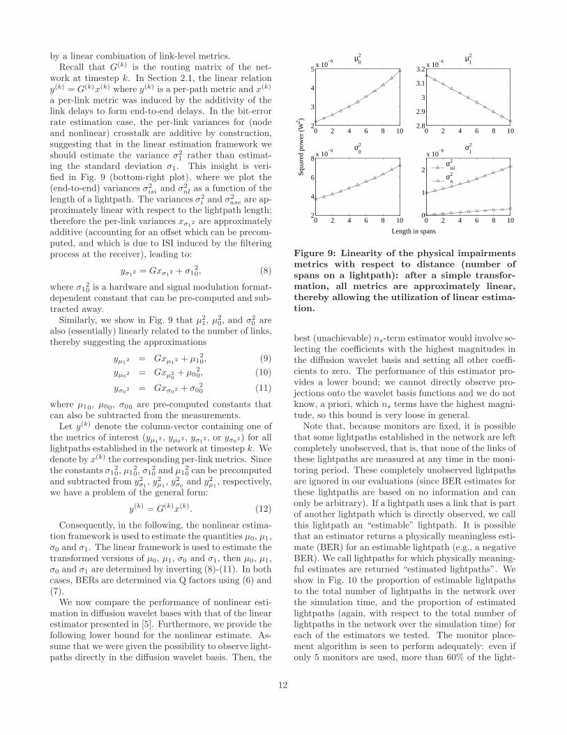
a per-link metric was induced by the additivity of thelink delays to form end-to-end delays. In the bit-errorrate estimation case, the per-link variances for (nodeand nonlinear) crosstalk are additive by construction,suggesting that in the linear estimation framework weshould estimate the variance σ2

1 rather than estimat-ing the standard deviation σ1. This insight is veri-fied in Fig. 9 (bottom-right plot), where we plot the(end-to-end) variances σ2

isi and σ2nl as a function of the

length of a lightpath. The variances σ2i and σ2

ase are ap-proximately linear with respect to the lightpath length;therefore the per-link variances xσ1

2 are approximatelyadditive (accounting for an offset which can be precom-puted, and which is due to ISI induced by the filteringprocess at the receiver), leading to:

yσ12 = Gxσ1

2 + σ120, (8)

where σ120 is a hardware and signal modulation format-

dependent constant that can be pre-computed and sub-tracted away.

Similarly, we show in Fig. 9 that µ21, µ2

0, and σ20 are

also (essentially) linearly related to the number of links,thereby suggesting the approximations

yµ12 = Gxµ1

2 + µ120, (9)

yµ02 = Gxµ2

0+ µ0

20, (10)

yσ02 = Gxσ0

2 + σ020 (11)

where µ10, µ00, σ00 are pre-computed constants thatcan also be subtracted from the measurements.

Let y(k) denote the column-vector containing one ofthe metrics of interest (yµ1

2 , yµ02 , yσ1

2 , or yσ02) for all

lightpaths established in the network at timestep k. Wedenote by x(k) the corresponding per-link metrics. Sincethe constants σ1

20, µ1

20, σ1

20 and µ1

20 can be precomputed

and subtracted from y2σ1

, y2µ1

, y2σ0

and y2µ1

, respectively,we have a problem of the general form:

y(k) = G(k)x(k). (12)

Consequently, in the following, the nonlinear estima-tion framework is used to estimate the quantities µ0, µ1,σ0 and σ1. The linear framework is used to estimate thetransformed versions of µ0, µ1, σ0 and σ1, then µ0, µ1,σ0 and σ1 are determined by inverting (8)-(11). In bothcases, BERs are determined via Q factors using (6) and(7).

We now compare the performance of nonlinear esti-mation in diffusion wavelet bases with that of the linearestimator presented in [5]. Furthermore, we provide thefollowing lower bound for the nonlinear estimate. As-sume that we were given the possibility to observe light-paths directly in the diffusion wavelet basis. Then, the

0 2 4 6 8 102

3

4

5x 10

−9 µ02

0 2 4 6 8 102.8

2.9

3

3.1

3.2x 10

−6 µ12

0 2 4 6 8 102

4

6

8x 10

−9 σ02

0 2 4 6 8 100

1

2

x 10−8 σ

12

Length in spans

Squ

ared

pow

er (

W2 )

σisi2

σn2

Figure 9: Linearity of the physical impairmentsmetrics with respect to distance (number ofspans on a lightpath): after a simple transfor-mation, all metrics are approximately linear,thereby allowing the utilization of linear estima-tion.

best (unachievable) ns-term estimator would involve se-lecting the coefficients with the highest magnitudes inthe diffusion wavelet basis and setting all other coeffi-cients to zero. The performance of this estimator pro-vides a lower bound; we cannot directly observe pro-jections onto the wavelet basis functions and we do notknow, a priori, which ns terms have the highest magni-tude, so this bound is very loose in general.

Note that, because monitors are fixed, it is possiblethat some lightpaths established in the network are leftcompletely unobserved, that is, that none of the links ofthese lightpaths are measured at any time in the moni-toring period. These completely unobserved lightpathsare ignored in our evaluations (since BER estimates forthese lightpaths are based on no information and canonly be arbitrary). If a lightpath uses a link that is partof another lightpath which is directly observed, we callthis lightpath an “estimable” lightpath. It is possiblethat an estimator returns a physically meaningless esti-mate (BER) for an estimable lightpath (e.g., a negativeBER). We call lightpaths for which physically meaning-ful estimates are returned “estimated lightpaths”. Weshow in Fig. 10 the proportion of estimable lightpathsto the total number of lightpaths in the network overthe simulation time, and the proportion of estimatedlightpaths (again, with respect to the total number oflightpaths in the network over the simulation time) foreach of the estimators we tested. The monitor place-ment algorithm is seen to perform adequately: even ifonly 5 monitors are used, more than 60% of the light-

12

5 10 15 20 25 30 35 400.5

0.6

0.7

0.8

0.9

1

Number of monitors

Fra

ctio

n of

est

imat

ed o

r ob

serv

ed li

ghtp

aths

Estimated lightpaths (Nonlinear estimator)Estimated lightpaths (Linear estimator)Estimable lightpaths

Figure 10: Fraction of estimable and estimatedlightpaths. The BERs of some lightpaths are notestimable because none of their links is observedthrough any other lightpath; among estimablelightpaths, some are not estimated at all becausethe estimates returned by the estimator werephysically meaningless (e.g., negative BER).

paths are estimable. This proportion rises to 90% if 15monitors are used. The nonlinear estimator estimatesthe BER of all of the estimable lightpaths, whereas thelinear estimator consistently leaves the BER of a smallproportion (5–10%) of estimable lightpaths unestimatedunless a very high number (35 and more) monitors areinstalled in the network.

In optical networks, only the order of magnitude ofthe BER is relevant and hence we work solely withlog(BER) to evaluate the performance of the estima-tors. We compare in Fig. 11 the performance of the lin-ear and the nonlinear estimators in the diffusion waveletframework for the relative ℓ2 error ||(y − yest)||2/||y||2(top panel) and the relative mean error |〈y − yest〉|/〈y〉(bottom panel), where y is the vector containing thelog of the BER for each lightpath, at each time instant.We also give 5% confidence intervals. The performanceimprovement achieved by the nonlinear estimation tech-nique is largest when few monitors are available. In par-ticular, when 15 monitors or less are placed in the net-work (out of a maximum of 42 monitors), correspondingto a maximum of 90% of estimated lightpaths, the non-linear estimation technique exhibits a significant advan-tage over the linear estimator in terms of ℓ2 norm. Interms of mean BER, the nonlinear estimator is able topredict the true mean BER over the network even witha very small number of monitors (less than 1% errorin mean on log(BER) with 5 monitors), while the lin-ear estimator requires 25 monitors to achieve the same

5 10 15 20 25 30 35 400

0.1

0.2

0.3

Number of monitors

Rela

tiv

eℓ 2

error

Nonlinear estimationLinear estimationNonlinear estimation bound

5 10 15 20 25 30 35 400

0.1

0.2

Number of monitors

Rela

tiv

em

ean

error

Figure 11: Relative ℓ2 (top panel) and mean er-ror (bottom panel) for the two estimators, forlog(BER). Also depicted is the lower bound onthe nonlinear estimation described in the text.

performance. As was the case for end-to-end delays,the nonlinear estimator has a very low bias. When thenumber of estimators increase the gap between the non-linear and linear estimation techniques closes and linearestimation actually performs slightly better than thenonlinear estimation. We emphasize that practical sit-uations are really those where the number of monitorsis small, which is when our nonlinear framework appliesbest and performs best.

Moreover, the nonlinear estimation technique appliesto more general situations than the linear estimationframework. Indeed, for the linear estimation frameworkto apply, we need to identify a linear relationship be-tween link-level (x) and lightpath-level metrics (y). Forthe case of lightpath BER estimation, we were able todefine an approximately linear relationship for trans-formed metrics. This artificial construct is unnecessaryin our nonlinear estimation framework, since correla-tion between lightpaths is naturally modeled throughthe diffusion operator. Finally, we give in Fig. 11 lowerbounds on the performance of the nonlinear estima-tor. These lower bounds are substantially lower thanwhat is achieved by our nonlinear estimator, which isexpected given we picked coefficients directly in the dif-fusion wavelet basis to construct the bound.

7. CONCLUSIONWe have presented a framework for monitoring path

metrics based on incomplete end-to-end measurements.The core of the framework is the development of a basis

13

in which the path metric signal is compressible, whichallows us to use powerful nonlinear estimators from thetheory of compressed sensing. Diffusion wavelets pro-vide an appealing mechanism for developing the basis,because the specification of a diffusion operator allowsus to create very general models for the correlations be-tween metrics on different paths. Case studies involvingthe estimation of mean end-to-end delays and the moni-toring of lightpath BERs in all-optical networks indicatethe promise of our framework. Currently we are inves-tigating the development of alternate bases which canbetter capture spatial localization of signal changes. Weare also developing theoretical bounds on the numberof paths that need to be measured to achieve a specifiedaccuracy.

8. REFERENCES[1] G. Agrawal. Fiber-Optic Communications

Systems. John Wiley & Sons, Inc., third edition,2002.

[2] E. Candes, J. Romberg, and T. Tao. Robustuncertainty principles: Exact signalreconstruction from highly incomplete frequencyinformation. IEEE Trans. Inform. Theory,52(2):489–509, Feb. 2006.

[3] Y. Chen, D. Bindel, H. Song, and R. Katz. Analgebraic approach to practical and scalableoverlay network monitoring. In Proc. ACM

SIGCOMM, Portland, USA, Aug. 2004.[4] I. Chlamtac, A. Ganz, and G. Karmi. Lightpath

communications: a novel approach to highbandwidth optical WANs. IEEE Trans.

Commun., 40(7):1171–1182, July 1992.[5] D. Chua, E. Kolaczyk, and M. Crovella. Efficient

monitoring of end-to-end network properties. InProc. Infocom, Miami, USA, Mar. 2005.

[6] M. Coates, A. Hero, R. Nowak, and B. Yu.Internet tomography. IEEE Signal Processing

Mag., May 2002.[7] R. Coifman and M. Maggioni. Diffusion wavelets.

Applied and Computational Harmonic Analysis,21(1):53–94, July 2006.

[8] M. Crovella and E. Kolaczyk. Graph wavelets forspatial traffic analysis. In Proc. IEEE Infocom,San Francisco, USA, Mar. 2003.

[9] T. Deng, S. Subramaniam, and J. Xu.Crosstalk-aware wavelength assignment indynamic wavelength-routed optical networks. InProc. Broadnets, Oct. 2004.

[10] P. D. Dobbelaere, K. Falta, L. Fan, S. Gloekner,

and S. Patra. Digital MEMS for optical switching.IEEE Commun. Mag., pages 88–95, Mar. 2002.

[11] D. Donoho. Compressed sensing. IEEE Trans.

Inform. Theory, 52(4):1289–1306, Apr. 2006.[12] E. Goldstein and L. Eskildsen. Scaling limitations

in transparent optical networks due to low-levelcrosstalk. IEEE Photon. Technol. Lett.,7(1):93–94, Jan. 1995.

[13] G. Golub and C. V. Loan. Matrix Computations.The Johns Hopkins University Press, Baltimore,1996.

[14] J. Haupt and R. Nowak. Signal reconstructionfrom noisy random projections. IEEE Trans.

Inform. Theory, 52(9):4036–4048, Sept. 2006.[15] Y. Pointurier, M. Brandt-Pearce, T. Deng, and

S. Subramaniam. Fair QoS-aware adaptiveRouting and Wavelength Assignment in all-opticalnetworks. In Proc. IEEE ICC, June 2006.

[16] B. Ramamurthy, D. Datta, H. Feng, J. Heritage,and B. Mukherjee. Impact of transmissionimpairments on the teletraffic performance ofwavelength-routed optical networks. J. Lightwave

Technol., 17(10):1713–1723, Oct. 1999.[17] R. Ramaswami and K. Sivarajan. Optical

Networks: A Practical Perspective. MorganKaufmann Publishers, second edition, 2002.

[18] R. Sinkhorn. A relationship between arbitrarypositive matrices and double stochastic matrices.Ann. Mathematical Statistics, 35(2):876–879, June1964.

[19] J. Tenenbaum, V. de Silva, and J. Langford. Aglobal geometric framework for nonlineardimensionality reduction. Science,5500(290):2319–2323, Dec. 2000.

[20] Y. Vardi. Network tomography: Estimatingsource-destination traffic intensities from linkdata. J. American Statistical Assosciation,91(433):365–377, Mar. 1996.

[21] A. Willner, M. Cardakli, O. Adamczyk, Y.-W.Song, and D. Gurkan. Key building blocks forall-optical networks. IEICE Trans. Commun.,E83-B:2166–2177, Oct. 2000.

[22] B. Xu and M. Brandt-Pearce. Comparison ofFWM- and XPM-induced crosstalk using theVolterra Series Transfer Function method. J.

Lightwave Technol., 21(1):40–53, Jan. 2003.[23] B. Xu and M. Brandt-Pearce. Analysis of noise

amplification by a CW pump signal due to fibernonlinearity. IEEE Photon. Technol. Lett.,16(4):1062–1064, Apr. 2004.

14