Comprehensive comparison of gap-filling techniques for eddy covariance net carbon fluxes Antje M. Moffat a, * , Dario Papale b , Markus Reichstein a , David Y. Hollinger c , Andrew D. Richardson d , Alan G. Barr e , Clemens Beckstein f , Bobby H. Braswell g , Galina Churkina a , Ankur R. Desai h , Eva Falge i , Jeffrey H. Gove c , Martin Heimann a , Dafeng Hui j , Andrew J. Jarvis k , Jens Kattge a , Asko Noormets l , Vanessa J. Stauch m a Max-Planck-Institute for Biogeochemistry, Hans-Kno ¨ll-Str. 10, 07745 Jena, Germany b DISAFRI, University of Tuscia, via C. de Lellis, 01100 Viterbo, Italy c USDA Forest Service, Northern Research Station, 271 Mast Rd., Durham, NH 03824, USA d Complex Systems Research Center, University of New Hampshire, Durham, NH 03824, USA e Climate Research Division Atmospheric Sciences and Technology Directorate Environment Canada, 11 Innovation Boulevard, Saskatoon, Sask., Canada f Friedrich-Schiller-Universita ¨t Jena, Institut fu ¨r Informatik, Ernst-Abbe-Platz 1-4, 07743 Jena, Germany g Institute for the Study of Earth, Ocean, and Space, University of New Hampshire Durham, NH 03824, USA h Department of Atmospheric and Oceanic Sciences, University Wisconsin-Madison, 1225 W Dayton St., Madison, WI 53706, USA i Max-Planck-Institute for Chemistry, Biogeochemistry Department, J.J.v. Becherweg 27, 55128 Mainz, Germany j School of Forestry and Wildlife Sciences, Auburn University, Auburn, AL 36849-5418, USA k Environmental Science Department, Lancaster University, UK l North Carolina State University/USDA Forest Service, 920 Main Campus Drive, Venture Center II, Suite 300, Raleigh, NC 27606, USA m Federal Office for Meteorology and Climatology (MeteoSwiss), Zurich, Switzerland Received 11 March 2007; received in revised form 4 August 2007; accepted 14 August 2007 Abstract We review 15 techniques for estimating missing values of net ecosystem CO 2 exchange (NEE) in eddy covariance time series and evaluate their performance for different artificial gap scenarios based on a set of 10 benchmark datasets from six forested sites in Europe. The goal of gap filling is the reproduction of the NEE time series and hence this present work focuses on estimating missing NEE values, not on editing or the removal of suspect values in these time series due to systematic errors in the measurements (e.g., nighttime flux, advection). The gap filling was examined by generating 50 secondary datasets with artificial gaps (ranging in length from single half-hours to 12 consecutive days) for each benchmark dataset and evaluating the performance with a variety of statistical metrics. The performance of the gap filling varied among sites and depended on the level of aggregation (native half- hourly time step versus daily), long gaps were more difficult to fill than short gaps, and differences among the techniques were more pronounced during the day than at night. The non-linear regression techniques (NLRs), the look-up table (LUT), marginal distribution sampling (MDS), and the semi- parametric model (SPM) generally showed good overall performance. The artificial neural network based techniques (ANNs) were generally, if only slightly, superior to the other techniques. The simple interpolation technique of mean diurnal variation (MDV) www.elsevier.com/locate/agrformet Agricultural and Forest Meteorology 147 (2007) 209–232 * Corresponding author. Tel.: +49 3641 576314; fax: +49 3641 577300. E-mail address: [email protected] (A.M. Moffat). 0168-1923/$ – see front matter # 2007 Elsevier B.V. All rights reserved. doi:10.1016/j.agrformet.2007.08.011

Welcome message from author
This document is posted to help you gain knowledge. Please leave a comment to let me know what you think about it! Share it to your friends and learn new things together.
Transcript
www.elsevier.com/locate/agrformet
Agricultural and Forest Meteorology 147 (2007) 209–232
Comprehensive comparison of gap-filling techniques for
eddy covariance net carbon fluxes
Antje M. Moffat a,*, Dario Papale b, Markus Reichstein a, David Y. Hollinger c,Andrew D. Richardson d, Alan G. Barr e, Clemens Beckstein f,
Bobby H. Braswell g, Galina Churkina a, Ankur R. Desai h, Eva Falge i,Jeffrey H. Gove c, Martin Heimann a, Dafeng Hui j, Andrew J. Jarvis k,
Jens Kattge a, Asko Noormets l, Vanessa J. Stauch m
a Max-Planck-Institute for Biogeochemistry, Hans-Knoll-Str. 10, 07745 Jena, Germanyb DISAFRI, University of Tuscia, via C. de Lellis, 01100 Viterbo, Italy
c USDA Forest Service, Northern Research Station, 271 Mast Rd., Durham, NH 03824, USAd Complex Systems Research Center, University of New Hampshire, Durham, NH 03824, USA
e Climate Research Division Atmospheric Sciences and Technology Directorate Environment Canada,
11 Innovation Boulevard, Saskatoon, Sask., Canadaf Friedrich-Schiller-Universitat Jena, Institut fur Informatik, Ernst-Abbe-Platz 1-4, 07743 Jena, Germany
g Institute for the Study of Earth, Ocean, and Space, University of New Hampshire Durham, NH 03824, USAh Department of Atmospheric and Oceanic Sciences, University Wisconsin-Madison, 1225 W Dayton St., Madison, WI 53706, USA
i Max-Planck-Institute for Chemistry, Biogeochemistry Department, J.J.v. Becherweg 27, 55128 Mainz, Germanyj School of Forestry and Wildlife Sciences, Auburn University, Auburn, AL 36849-5418, USA
k Environmental Science Department, Lancaster University, UKl North Carolina State University/USDA Forest Service, 920 Main Campus Drive, Venture Center II, Suite 300,
Raleigh, NC 27606, USAm Federal Office for Meteorology and Climatology (MeteoSwiss), Zurich, Switzerland
Received 11 March 2007; received in revised form 4 August 2007; accepted 14 August 2007
Abstract
We review 15 techniques for estimating missing values of net ecosystem CO2 exchange (NEE) in eddy covariance time series
and evaluate their performance for different artificial gap scenarios based on a set of 10 benchmark datasets from six forested sites in
Europe.
The goal of gap filling is the reproduction of the NEE time series and hence this present work focuses on estimating missing NEE
values, not on editing or the removal of suspect values in these time series due to systematic errors in the measurements (e.g.,
nighttime flux, advection). The gap filling was examined by generating 50 secondary datasets with artificial gaps (ranging in length
from single half-hours to 12 consecutive days) for each benchmark dataset and evaluating the performance with a variety of
statistical metrics. The performance of the gap filling varied among sites and depended on the level of aggregation (native half-
hourly time step versus daily), long gaps were more difficult to fill than short gaps, and differences among the techniques were more
pronounced during the day than at night.
The non-linear regression techniques (NLRs), the look-up table (LUT), marginal distribution sampling (MDS), and the semi-
parametric model (SPM) generally showed good overall performance. The artificial neural network based techniques (ANNs) were
generally, if only slightly, superior to the other techniques. The simple interpolation technique of mean diurnal variation (MDV)
* Corresponding author. Tel.: +49 3641 576314; fax: +49 3641 577300.
E-mail address: [email protected] (A.M. Moffat).
0168-1923/$ – see front matter # 2007 Elsevier B.V. All rights reserved.
doi:10.1016/j.agrformet.2007.08.011
A.M. Moffat et al. / Agricultural and Forest Meteorology 147 (2007) 209–232210
showed a moderate but consistent performance. Several sophisticated techniques, the dual unscented Kalman filter (UKF), the
multiple imputation method (MIM), the terrestrial biosphere model (BETHY), but also one of the ANNs and one of the NLRs
showed high biases which resulted in a low reliability of the annual sums, indicating that additional development might be needed.
An uncertainty analysis comparing the estimated random error in the 10 benchmark datasets with the artificial gap residuals
suggested that the techniques are already at or very close to the noise limit of the measurements. Based on the techniques and site
data examined here, the effect of gap filling on the annual sums of NEE is modest, with most techniques falling within a range of
�25 g C m�2 year�1.
# 2007 Elsevier B.V. All rights reserved.
Keywords: Eddy covariance; Carbon flux; Net ecosystem exchange (NEE); FLUXNET; Review of gap-filling techniques; Gap-filling comparison
1. Introduction
1.1. Motivation
Several hundred flux tower sites have been estab-
lished around the world (Baldocchi et al., 2001a),
recording CO2 flux, energy and momentum flux, storage
change of CO2 in the canopy air layer, and meteor-
ological variables including global radiation (Rg),
photosynthetic photon flux density (PPFD), air and
soil temperature (Ta, Ts), relative humidity (Rh),
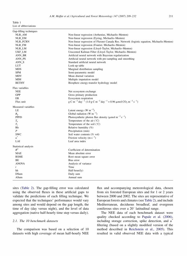
precipitation (P) and soil water content (SWC). A list
of abbreviations can be found in Table 1.
The eddy covariance method is the main monitoring
tool for measuring the net ecosystem exchange (NEE),
which is defined as the net flux of CO2 and equals the
balance of ecosystem respiration (release) minus photo-
synthesis (uptake). The measurements are reported on a
half-hourly or hourly basis. Calibrations or equipment
failures result in occasional gaps in these data time series.
Data quality checks including stationarity tests and the
detection of system ‘‘spikes’’ lead to the rejection of
‘‘bad’’data, generating additional gaps in the data record.
A major limitation of the eddy covariance technique is
the requirement for turbulent atmospheric conditions.
Rejecting data acquired during low turbulence conditions
based on a friction velocity threshold (u*) (Goulden et al.,
1997; Aubinet et al., 2000; Papale et al., 2006), or other
criteria (Foken et al., 2004; Ruppert et al., 2006) results in
further gaps such that typically 20–60% of an annual
dataset is missing, with the majority of the gaps occurring
during nighttime.
These fragmented data sets contain sufficient
information for half-hourly model fitting but complete-
ness is needed for daily and annual sums. These sums
are of widespread interest, e.g., to estimate ecosystem
carbon budgets, to evaluate process model predictions,
and for comparison with biometric measurements.
Availability of the associated meteorological data
permits a reconstruction of the NEE during the gaps,
and has led to the development of a variety of gap-filling
techniques to provide complete NEE datasets.
1.2. Goals of the comparison
Since the pioneering work of Falge et al. (2001), the
number of gap-filling techniques in use has increased.
Many investigators have independently developed and
implemented their own site-specific gap-filling techni-
ques. Current gap-filling techniques (Barr et al., 2004;
Braswell et al., 2005; Desai et al., 2005; Falge et al.,
2001; Gove and Hollinger, 2006; Hollinger et al., 2004;
Hui et al., 2004; Knorr and Kattge, 2005; Noormets
et al., 2007; Ooba et al., 2006; Papale and Valentini,
2003; Reichstein et al., 2005; Richardson et al., 2006b;
Schwalm et al., 2007; Stauch and Jarvis, 2006) are
based on a wide range of approaches, including
interpolation, probabilistic filling, look-up tables,
non-linear regression, artificial neural networks, and
process-based models in a data-assimilation mode. This
diversity hinders synthesis activities because the biases
and uncertainties associated with each technique are
unknown (Morgenstern et al., 2004).
This study reviews a variety of gap-filling techniques
and applies the techniques to a set of standardized
benchmark datasets from six forested sites in Europe.
Artificial gaps were added to observed NEE time series,
and the ability of different gap-filling techniques to
replicate the missing data was evaluated using tradi-
tional statistical analysis. Our analysis does not attempt
to address matters related to the quality of the measured
fluxes themselves, such as systematic biases or
representativeness.
2. Comparison materials and method
For this comparison, we created a series of 50
artificial gap scenarios (Appendix A.1), which were
superimposed on observed NEE time series of 10
benchmark datasets from six different European forest
A.M. Moffat et al. / Agricultural and Forest Meteorology 147 (2007) 209–232 211
Table 1
List of abbreviations
Gap-filling techniques
NLR_AM Non-linear regression (Arrhenius, Michaelis–Menten)
NLR_EM Non-linear regression (Eyring, Michaelis–Menten)
NLR_FCRN Non-linear regression of Fluxnet Canada Res. Network (logistic equation, Michaelis-Menten)
NLR_FM Non-linear regression (Fourier, Michaelis–Menten)
NLR_LM Non-linear regression (Lloyd–Taylor, Michaelis–Menten)
UKF_LM Unscented Kalman Filter (Lloyd–Taylor, Michaelis–Menten)
ANN_BR Artificial neural network with Bayesian regularization
ANN_PS Artificial neural network with pre-sampling and smoothing
ANN_S Standard artificial neural network
LUT Look-up table
MDS Marginal distribution sampling
SPM Semi-parametric model
MDV Mean diurnal variation
MIM Multiple imputation model
BETHY Biosphere energy-transfer hydrology model
Flux variables
NEE Net ecosystem exchange
GPP Gross primary production
ER Ecosystem respiration
Flux unit g C m�2 day�1 (1.0 g C m�2 day�1 = 0.96 mmol CO2 m�2 s�1)
Measured variables
LE Latent energy (W m�2)
Rg Global radiation (W m�2)
PPFD Photosynthetic photon flux density (mmol m�2 s�1)
Ta Temperature of the air (8C)
Ts Temperature of the soil (8C)
Rh Relative humidity (%)
P Precipitation (mm)
SWC Soil water contents (% vol)
u* Friction velocity (m s�1)
LAI Leaf area index
Statistical analysis
R2 Coefficient of determination
MAE Mean absolute error
RSME Root mean square error
BE Bias error
ANOVA Analysis of variance
t Time
hh Half-hour(ly)
DSum Daily sum
ASum Annual sum
sites (Table 2). The gap-filling error was calculated
using the observed fluxes in these artificial gaps to
validate the predictions of each filling technique. We
expected that the techniques’ performance would vary
among sites and would depend on the gap length, the
time of day (day versus night), and the level of data
aggregation (native half-hourly time step versus daily).
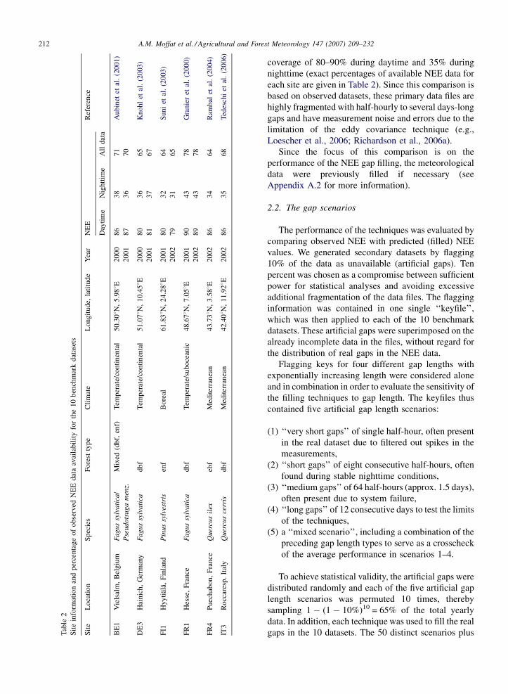
2.1. The 10 benchmark datasets
The comparison was based on a selection of 10
datasets with high coverage of mean half-hourly NEE
flux and accompanying meteorological data, chosen
from six forested European sites and for 1 or 2 years
between 2000 and 2002. The sites are representative of
European forests and climates (see Table 2), and include
Mediterranean, deciduous broadleaf, and evergreen
coniferous sites over a 208 latitudinal range.
The NEE data of each benchmark dataset were
quality checked according to Papale et al. (2006),
including storage correction, spike detection, and u*
filtering (based on a slightly modified version of the
method described in Reichstein et al., 2005). This
resulted in valid observed NEE data with a typical
A.M. Moffat et al. / Agricultural and Forest Meteorology 147 (2007) 209–232212
Tab
le2
Sit
ein
form
atio
nan
dp
erce
nta
ge
of
ob
serv
edN
EE
dat
aav
aila
bil
ity
for
the
10
ben
chm
ark
dat
aset
s
Sit
eL
oca
tio
nS
pec
ies
Fo
rest
typ
eC
lim
ate
Lo
ngit
ud
e,la
titu
de
Yea
rN
EE
Ref
eren
ce
Day
tim
eN
ightt
ime
All
dat
a
BE
1V
iels
alm
,B
elg
ium
Fagus
sylv
ati
ca/
Pse
udo
tsu
ga
men
z.
Mix
ed(d
bf,
enf)
Tem
per
ate/
conti
nen
tal
50.3
08N
,5
.988E
20
00
86
38
71
Au
bin
etet
al.
(20
01)
20
01
87
36
70
DE
3H
ain
ich
,G
erm
any
Fagus
sylv
ati
cadbf
Tem
per
ate/
conti
nen
tal
51.0
78N
,1
0.4
58E
20
00
80
36
65
Kn
oh
let
al.
(20
03)
20
01
81
37
67
FI1
Hy
yti
ala,
Fin
land
Pin
us
sylv
estr
isen
fB
ore
al6
1.8
38N
,2
4.2
88E
20
01
80
32
64
Su
ni
etal
.(2
00
3)
20
02
79
31
65
FR
1H
esse
,F
ran
ceF
agus
sylv
ati
cadbf
Tem
per
ate/
suboce
anic
48.6
78N
,7
.058E
20
01
90
43
78
Gra
nie
ret
al.
(20
00)
20
02
89
43
78
FR
4P
uec
hab
on
,F
ran
ceQ
uer
cus
ilex
ebf
Med
iter
ranea
n43.7
38N
,3
.588E
20
02
86
34
64
Ram
bal
etal
.(2
00
4)
IT3
Rocc
ares
p.
Ital
yQ
uer
cus
cerr
isdbf
Med
iter
ranea
n42.4
08N
,1
1.9
28E
20
02
86
35
68
Ted
esch
iet
al.
(20
06)
coverage of 80–90% during daytime and 35% during
nighttime (exact percentages of available NEE data for
each site are given in Table 2). Since this comparison is
based on observed datasets, these primary data files are
highly fragmented with half-hourly to several days-long
gaps and have measurement noise and errors due to the
limitation of the eddy covariance technique (e.g.,
Loescher et al., 2006; Richardson et al., 2006a).
Since the focus of this comparison is on the
performance of the NEE gap filling, the meteorological
data were previously filled if necessary (see
Appendix A.2 for more information).
2.2. The gap scenarios
The performance of the techniques was evaluated by
comparing observed NEE with predicted (filled) NEE
values. We generated secondary datasets by flagging
10% of the data as unavailable (artificial gaps). Ten
percent was chosen as a compromise between sufficient
power for statistical analyses and avoiding excessive
additional fragmentation of the data files. The flagging
information was contained in one single ‘‘keyfile’’,
which was then applied to each of the 10 benchmark
datasets. These artificial gaps were superimposed on the
already incomplete data in the files, without regard for
the distribution of real gaps in the NEE data.
Flagging keys for four different gap lengths with
exponentially increasing length were considered alone
and in combination in order to evaluate the sensitivity of
the filling techniques to gap length. The keyfiles thus
contained five artificial gap length scenarios:
(1) ‘‘
very short gaps’’ of single half-hour, often presentin the real dataset due to filtered out spikes in the
measurements,
(2) ‘‘
short gaps’’ of eight consecutive half-hours, oftenfound during stable nighttime conditions,
(3) ‘‘
medium gaps’’ of 64 half-hours (approx. 1.5 days),often present due to system failure,
(4) ‘‘
long gaps’’ of 12 consecutive days to test the limitsof the techniques,
(5) a
‘‘mixed scenario’’, including a combination of thepreceding gap length types to serve as a crosscheck
of the average performance in scenarios 1–4.
To achieve statistical validity, the artificial gaps were
distributed randomly and each of the five artificial gap
length scenarios was permuted 10 times, thereby
sampling 1 � (1 � 10%)10 = 65% of the total yearly
data. In addition, each technique was used to fill the real
gaps in the 10 datasets. The 50 distinct scenarios plus

A.M. Moffat et al. / Agricultural and Forest Meteorology 147 (2007) 209–232 213
the real gap scenario were processed separately for each
of the 10 benchmark data files. This added up to a total
of 510 submitted run results per gap-filling technique.
A detailed description of the keyfile with the gap
scenarios is given in Appendix A.1. The 10 benchmark
data files and the keyfile are archived on a server at
http://gaia.agraria.unitus.it/database/gfc so that as new
gap-filling techniques are developed in the future, the
results of the present study can serve as a benchmark
against which other techniques can be evaluated.
2.3. Statistical performance measures
The performance of the techniques was evaluated by
comparing observed NEE with predicted (filled) NEE
values. The performance measures (Janssen and
Heuberger, 1995) included the coefficient of determi-
nation (R2) to measure the phase correlation, the
absolute and relative root mean square error (RMSE)
and mean absolute error (MAE) to indicate the
magnitude and distribution of the individual errors,
and the bias error (BE) to indicate the bias induced on
the annual sums.
The statistical sums were calculated using the
individual observed NEE data oi and the predicted
values pi, with o and p denoting their means:
R2 ¼
�Pð pi � pÞðoi � oÞ
�2
Pð pi � pÞ2
Pðoi � oÞ2
Absolute RMSE ¼ffiffiffiffiffiffiffiffiffiffiffiffiffiffiffiffiffiffiffiffiffiffiffiffiffiffiffiffiffiffiffiffi1
N
Xð pi � oiÞ2
r
Relative RMSE ¼
ffiffiffiffiffiffiffiffiffiffiffiffiffiffiffiffiffiffiffiffiffiffiffiffiffiffiPð pi � oiÞ2PðoiÞ2
s
MAE ¼ 1
N
Xj pi � oij
BE ¼ 1
N
Xð pi � oiÞ
The statistical metrics were computed for each of the 50
gap scenarios, and then grouped and averaged to aid in
distilling relevant comparison information.
2.4. Daytime and nighttime differentiation
Each of the statistical metrics was computed
separately for the qualitatively different daytime and
nighttime data. Daytime was defined as a positive
photosynthetic photon flux density (PPFD) and night-
time refers to periods of the day with no light (zero
PPFD, with non-zero nocturnal PPFD values set to
zero). During the daytime, positive sensible heat fluxes
create buoyancy that helps to mix the atmosphere. At
nighttime, however, radiative cooling leads to stable
conditions that suppress turbulent mixing. In addition to
the changed meteorological conditions, the absence of
photosynthesis changes the underlying biological
processes. This leads to dramatically different perfor-
mance and behavior of the gap-filling techniques.
For the comparison of gap-filling techniques, the
weighting of the daytime and nighttime contributions to
the statistical metrics is incorrect when day and night
are taken together. More precisely, the ratio of the
number of daytime to nighttime gaps for the real gaps is
at odds with the day–night ratio of the artificial gaps.
The percentage of available observed NEE data in the
10 benchmark datasets is on average 85% for daytime
and 35% for nighttime data (detailed percentages can be
found in Table 2). Thus, the distribution of real gaps of
15% daytime to 65% nighttime results in a day–night
ratio of approximately 1:4. By contrast, the secondary
datasets have 10 percent artificial gaps resulting in 8.5%
daytime and 3.5% nighttime gaps, a ratio of approxi-
mately 2:1. Therefore, in this paper the analysis was
performed separately for daytime and nighttime
periods.
2.5. Analysis of daily and annual sums
An important level of data aggregation is the daily
NEE since it is used in many vegetation and ecosystem
models for parameterization and validation (e.g.,
Hanson et al., 2004). The daily sum of NEE is defined
as the sum of daily half-hourly flux rates NEEhh times
the measurement time interval Dthh:
DSum ¼X
NEEhh � Dthh:
This comparison used real datasets with fragmented
observed daily data (see Section 2.4). An estimate of the
daily sums was obtained by separating the daytime sum
DSumd and the nighttime sum DSumn and by weighting
these sums with the amount of half-hours of daylight
hhd and the amount of half-hours during nighttime hhn,
respectively:
Weighted DSum ¼ DSumd �hhd
48þ DSumn �
hhn
48:
The observed DSums were then compared with the
predicted DSums for all artificial gaps spanning over a
whole day from the medium and long gap length
A.M. Moffat et al. / Agricultural and Forest Meteorology 147 (2007) 209–232214
scenario. About 65% of the days in each year are
sampled by the gap scenarios (see Section 2.3) but only
days with a minimum of four observed data points for
daytime and for nighttime in the benchmark dataset
were considered, which reduced the number of DSums
used to calculate the statistical performance measures to
approximately 150 DSums per benchmark dataset and
gap length scenario.
The annual sum ASum is the sum over all half-hourly
NEE values in a given year, i.e.,
ASum ¼X
measured
oi þX
gapfilled
p j
Persistent biases in the gap filling will lead to an over- or
underestimate of the annual sum.
The annual sum offset DASum resulting from gap-
filling can be estimated from the biases BE of the half-
hourly NEE values or the daily sums as:
DASum ¼ BEðNEEhhÞ � Nhh � Dthh ¼ BEðDSumÞ � Np
with Nhh denoting the number of predicted (gap filled)
0.5-h and Np is the number of predicted days.
3. The gap-filling techniques
3.1. Overview
Fifteen different gap-filling techniques for estimat-
ing net carbon fluxes were evaluated; five non-linear
regression (NLR) methods, a dual unscented Kalman
filter (UKF) approach, three artificial neural networks
(ANN), three types of look-up tables (fixed look-up
table (LUT), marginal distribution sampling (MDS)
method, and semi-parametric model (SPM)), a mean
diurnal variation (MDV) approach, a multiple imputa-
tion method (MIM), and a terrestrial biosphere model
(BETHY). Minor variants of two of the NLR methods
and the BETHY model were also assessed.
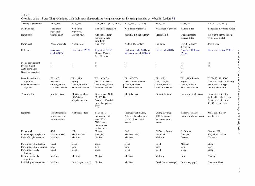
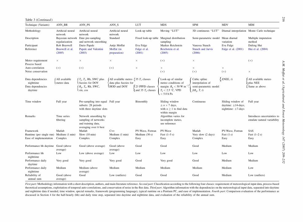
A comprehensive overview of the individual
techniques and their performance is given in Table 3.
The following sections complement this table by
describing the basic principles of the different
methodologies.
3.2. Basic principles
3.2.1. Non-linear regressions (NLRs)
The non-linear regressions are based on parameter-
ized non-linear equations which express (semi-)empiri-
cal relationships between the NEE flux and
environmental variables such as temperature and light.
Each technique (Falge et al., 2001; Hollinger et al.,
2004; Barr et al., 2004; Desai et al., 2005; Richardson
et al., 2006b; Noormets et al., 2007) uses one equation
for the ecosystem respiration (ER) and one equation for
the light response of the ecosystem, which is the gross
primary production (GPP). NEE is estimated as
NEE = GPP � ER with GPP = 0 at night. The para-
meterized equations are fit to the observed data and then
used to fill missing NEE values.
The modeled relationships of ER vary from
technique to technique and are specified in Table 3.
Most common are semi-empirical equations with an
exponential or logistic dependence on temperature. The
NLR_FM technique implemented the seasonal depen-
dence of ER via a second-order Fourier function.
Details of the formulas used for filling ER data are given
in Appendix A.3.
The response of GPP to the photosynthetic photon
flux density PPFD is modeled using the rectangular
hyperbola:
GPP ¼ f ðPPFDÞ ¼ b1PPFD
PPFDþ b2
;
where b1 and b2 are the regression parameters (Michae-
lis and Menten, 1913; Falge et al., 2001) which are
related to the maximum ecosystem photosynthetic
capacity and the half-saturation point of PPFD at which
GPP = 0.5b1.
The regression parameters are only kept constant for
a certain period of time to accommodate the variation
over the year. This time window varied from technique
to technique (see Table 3).
In a companion paper (Desai et al., submitted for
publication), the NEE partitioning into GPP and ER of
the NLR techniques but also of UKF, ANN_PS, LUT,
MDV, SPM, and BETHY has been further investigated.
3.2.2. Dual unscented Kalman filter (UKF)
The UKF was developed for time series where the
data are auto-correlated (Gove and Hollinger, 2006). It
is a two-step recursive predictor–corrector method that
uses the noisy observed data to continuously adjust the
parameters of the non-linear regression equations (see
Section 3.2.1). In a prediction step the filter uses the
regression equations to predict the next NEE data point
(state). It then combines this predicted value with the
observed value to optimally adjust the previous
parameters and NEE states. This recursion is then
applied at each successive time period and leads to time-
varying parameter estimates for NEE over the whole
year. The UKF was run with the same values for process
A.M
.M
offa
tet
al./A
gricu
ltura
la
nd
Fo
restM
eteoro
log
y1
47
(20
07
)2
09
–2
32
21
5
{{ {{
{{
{
{{
{{
{
{
Table 3
Overview of the 15 gap-filling techniques with their main characteristics, complementary to the basic principles described in Section 3.2
Technique (Variants) NLR_AM NLR_EM NLR_FCRN (STD, MOD) NLR_FM (AD, OLS) NLR_LM UKF_LM BETHY (12, ALL)
Methodology Non-linear
regression
Non-linear
regression
Non-linear regression Non-linear regression Non-linear regression Kalman filter Terrestrial biosphere model
Description Classic NLR Classic NLR Additional linear
regression with
time LR(t)
Seasonal ER dependency Classic NLR Dual unscented
Kalman filter
Biosphere energy-transfer
hydrology model
Participant Asko Noormets Ankur Desai Alan Barr Andrew Richardson Eva Falge David Hollinger,
Jeff Gove
Jens Kattge
Reference Noormets
et al. (2007)
Desai et al. (2005) Barr et al. (2004),
Fluxnet Canada
Res. Network
Hollinger et al. (2004) and
Richardson et al. (2006b)
Falge et al. (2001) Gove and Hollinger
(2006)
Knorr and Kattge (2005)
Meteo requirement � � � � � � �Process based � � � � � � �Auto-correlation �Noise conservation �
Data dependencies
nighttime
ER = f(Ta);
Arrhenius
ER = f(Ts);
Eyring
ER = a(t)f(Ts);
logistic equation
ER = f(DOY);
second-order Fourier
ER = f(Ts);
Lloyd–Taylor
ER = f(Ts); Lloyd–
Taylor
PPFD, Ta, Rh, SWC,
LAI, LE, height of canopy
and tower, soil type,
texture, and depth
Data dependencies
daytime
GPP = f(PPFD);
Michaelis-Menten
GPP = f(PPFD);
Michaelis-Menten
GPP = b(t)f(PPFD);
Michaelis-Menten
GPP = f(PPFD);
Michaelis-Menten
GPP = f(PPFD);
Michaelis-Menten
GPP = f(PPFD);
Michaelis-Menten
Time window Monthly fixed Moving window
(30–60 day
adaptive length)
First: annual NLR
(Ts, PPFD)
Monthly fixed Bimonthly fixed Recursive single steps Parameterization for
ALL: all available data
Second: 100-valid
mov. data points
LR(t)
Parameterization for
12: 12 days of data
Remarks Simultaneous fit
of daytime and
nighttime data
Additional t-test STD: linear
interpolation of
gaps �4 hhs.
MOD: zero
intercept and
no interpolat
Parameter estimation,
AD: absolute deviation,
OLS: ordinary least
squares
During daytime:
48 C-Ta-classes
air temperature
classes
Winter dormancy:
random walk plus noise
Modeled NEE for
whole year
Framework SAS IDL Matlab SAS PV-Wave, Fortran R, Fortran Fortran, IDL
Runtime (per single run) Medium (30 s) Medium (30 s) Fast (5 s) Medium (30 s) Fast (5 s) Fast (5 s) Very slow (2–6 h)
Ease of implementation Medium Medium Medium Medium Medium Complex Complex
Performance hh daytime Good Good Good Good Good Medium Good
Performance hh nighttime Low Low Low Low Low Low Low
Performance daily
daytime
Good Good Good Good Good Good Good
Performance daily
nighttime
Medium Medium Medium Medium Medium Low Medium
Reliability of annual sum Medium Low (negative bias) Medium Medium Good (above average) Low (long gaps) Low (site bias)
A.M
.M
offa
tet
al./A
gricu
ltura
la
nd
Fo
restM
eteoro
log
y1
47
(20
07
)2
09
–2
32
21
6
{{ {
{ { {{
{
{{{
Technique (Variants) ANN_BR ANN_PS ANN_S LUT MDS SPM MDV MIM
Methodology Artificial neural
network
Artificial neural
network
Artificial neural
network
Look-up table Moving ‘‘LUT’’ 3D continuous ‘‘LUT’’ Diurnal interpolation Monte Carlo technique
Description Bayesian network
regularization
Date pre-sampling
and network smoothing
Standard Fixed look-up table Marginal distribution
sampling
Semi-parametric model Mean diurnal
variation
Multiple imputation
method
Participant Rob Braswell Dario Papale Antje Moffat Eva Falge Markus Reichstein Vanessa Stauch Eva Falge Dafeng Hui
Reference Braswell et al.
(2005)
Papale and Valentini
(2003)
Moffat (in
preparation)
Falge et al.
(2001)
Reichstein et al.
(2005)
Stauch and Jarvis
(2006)
Falge et al. (2001) Hui et al. (2004)
Meteo requirement � � � � (�) � (�)
Process based
Auto-correlation (�) (�) (�) � � � �Noise conservation (�) (�) (�) �
Data dependencies
nighttime
All available
meteo data
Ta, Ts, Rh, SWC plus
fuzzies for DOY
All available meteo
data plus fuzzies for
HOD and DOY
35 Ts classes Look-up of similar
meteo conditions of
margin: Rg < 50 W m�2,
Ta < 2.5 8C, VPD
< 5.0 h Pa
Cubic spline
interpolation of
semi-parametric model
f(Rg, T, t)
f(NEE, t) All available meteo
plus NEE
Data dependencies
daytime
Rg, Ta, Rh, SWC,
sin, cos
23 PPFD classes
and 35 Ta classes
Same as above
Time window Full year Pre-sampling into equal
subsets: 28 periods
with three daytime slots
Full year Bimonthly Sliding window
� n � 7 days,
with n � 1 to find data
within margin
Continuous Sliding window of
daytime: �14-days,
nighttime: �7-days
Full year
Remarks Time series
filtering
Network smoothing by
sampling of networks
and training data,
averaging over 6 best
Algorithm varies for
incomplete meteo,
see reference
Introduces uncertainties to
emulate natural variability
Framework Matlab Matlab C++ PV-Wave, Fortran PV-Wave Matlab PV-Wave, Fortran SAS
Runtime (per single run) Medium (1 min) Slow (10 min) Medium (1 min) Medium (30 s) Fast (1–5 s) Very slow (2 days) Fast (1 s) Fast (1–2 s)
Ease of implementation Complex Complex Complex Easy Easy Complex Easy Easy
Performance hh daytime Good (above
average)
Good (above average) Good (above
average)
Good Good Good Medium Medium
Performance hh
nighttime
Low Low (above average) Low Low Low Low Low Low
Performance daily
daytime
Very good Very good Very good Good Very good Good Medium Medium
Performance daily
nighttime
Medium Medium (above
average)
Medium Medium Medium Medium Medium Low
Reliability of
annual sum
Good (above
average)
Good Low (outliers) Good Good Good Medium Low (outliers)
First part: Methodology information with a short description, authors, and main literature reference. Second part: Classification according to the following four classes: requirement of meteorological input data, process-based
theoretical assumptions, exploitation of temporal auto-correlations, and conservation of noise in the flux data. Third part: Algorithm information with the dependencies on the meteorological input data, separated into daytime
and nighttime data if needed, time window, special remarks, framework (programming language), typical runtime on a Pentium PC, and ease of implementation. Fourth part: Comparison evaluation of the performance as
discussed in Section 4 for the half-hourly (hh) and daily time step, separated into daytime and nighttime data, and evaluation of the reliability of the annual sum.
Table 3 (Continued )
A.M. Moffat et al. / Agricultural and Forest Meteorology 147 (2007) 209–232 217
and measurement noise variances as given in Gove and
Hollinger (2006) and not specifically ‘‘tuned’’ to the
sites evaluated here. Kalman filtering takes a probabil-
istic interpretation to the estimation of the unknown
system states (here NEE). As a consequence, any
Kalman-based filter will not try to ‘‘match’’ the
measurements unless the ratio of system to process
noise variances is reduced towards zero (thus weighting
the measurements in preference to the model predic-
tions in the update step); in essence, the assumption is
that of perfect observational data. In the presence of
gaps, the filter is still estimating the probability density
of the states, not the missing measurements.
3.2.3. Artificial neural networks (ANNs)
The ANNs are purely empirical non-linear regres-
sion models. An ANN consists of nodes connected by
weights that are the regression parameters (Bishop,
1995; Hagan et al., 1996; Rojas, 1996). The network is
trained by presenting it with sets of input data (here, the
meteorological variables) and associated output data
(here, NEE). All techniques evaluated use the classical
back-propagation algorithm where the training of the
ANN is performed by propagating the input data
through the nodes via the weighted connections and
then back-propagating the error and adjusting the
weights so that the network output optimally approx-
imates NEE. After training, the underlying dependen-
cies of NEE on the meteorological input variables are
mapped onto the weights and the ANN is then used to
predict the missing NEE values.
The performance of an ANN is influenced by the
following criteria:
� Q
uality of the training dataset: The ANN can only mapand extract information present in the NEE and
accompanying meteorological dataset. Therefore,
factors such as completeness and accuracy are essential
to the ANN performance. Additional information such
as time can be added as a fuzzy variable.
� N
etwork architecture: The more degrees of freedom(nodes, weights), the better the mapping of the
training dataset but this is achieved at the cost of the
ability to generalize.
� N
etwork training: The training process requires anappropriate learning rate (weight adjustment steps)
and a stopping criterion to avoid overtraining.
Different algorithms have been developed to address
these criteria and we tested several different approaches
to training. ANN_S (Moffat, in preparation) used the
complete training dataset for the training of one network
with two hidden layers. The ANN_PS (Papale and
Valentini, 2003) pre-sampled the training datasets and
averaged the results over multiple trained networks of
different architectures. The ANN_BR (Braswell et al.,
2005) used a stochastic Bayesian algorithm for the
regularization of the network training.
3.2.4. Look-up tables and further developments
In a look-up table, the NEE data are binned by
variables such as light and temperature presenting
similar meteorological conditions, so that a missing
NEE value with similar meteorological conditions can
be ‘‘looked up’’. The standard look-up table (LUT)
consists of fixed periods over a year with corresponding
fixed intervals for the variables (Falge et al., 2001).
An enhancement to the standard LUT is marginal
distribution sampling (MDS). Here similar meteorolo-
gical conditions (of a fixed margin) are sampled in the
temporal vicinity of the gap to be filled (Reichstein et al.,
2005). Hence, this moving look-up table technique is able
to exploit the temporal auto-correlation structure of NEE.
The semi-parametric model technique (SPM) can be
seen as a three-dimensional, non-linear look-up table
sorted with environmental variables of interest (global
radiation, soil temperature) and time and is therefore a
continuous representation of the response of NEE to
these variables. The underlying semi-parametric rela-
tionships are defined by three-dimensional cubic splines
estimated within a weighted non-linear least squares
optimization framework (Stauch and Jarvis, 2006).
3.2.5. Mean diurnal variation (MDV)
MDV is an interpolation technique where the missing
NEE value for a certain 0.5-h is replaced with the
averaged value of the adjacent days at exactly that time
of day (Falge et al., 2001).
3.2.6. Multiple imputation method (MIM)
MIM uses multivariate correlation to replace the
missing NEE data with several simulated (imputed)
values (Hui et al., 2004). The Markov Chain Monte
Carlo algorithm is used to generate the imputed data
sets. Then these sets of plausible values are analyzed
using normal statistical metrics. Finally, the results are
pooled by averaging to provide the missing NEE data.
3.2.7. Biosphere energy-transfer hydrology model
(BETHY)
BETHY (Knorr and Kattge, 2005) is a process-based
model developed to calculate NEE, water and energy
fluxes of the terrestrial biosphere and is not strictly a
gap-filling technique. In addition to the meteorological

A.M. Moffat et al. / Agricultural and Forest Meteorology 147 (2007) 209–232218
data provided in the 10 benchmark datasets, it uses the
daily leaf area index (LAI) derived from remote sensing
data, soil type, texture, and depth, canopy height, and
tower height as model inputs. Model parameters are
optimized against observed fluxes of NEE and latent
energy (LE), considering prior information about
parameter values to constrain these within reasonable
ranges. The optimized parameter sets are then used to
model NEE for the whole year.
The BETHY model was evaluated to test the
feasibility of using a more complete biophysical model
for gap filling. Two scenarios were evaluated; first
BETHY model parameters were estimated from all of the
observed data, and secondly, the parameters were
estimated using only 12 days of observed data, chosen
to represent seasonality. The NEE results for the two
optimizations were simply replicated 50 times to provide
data for the different gap length scenarios and hence,
BETHY results are not strictly comparable to the others.
4. Results
4.1. Site dependency of the techniques’
performance
The differences in the RMSE performance of the
gap-filling techniques for the 10 benchmark sets
Fig. 1. Site dependency of the techniques’ performance for half-hourly data
the 10 benchmark datasets. The symbols denote the RMSE performance o
(calculated over all 50 permutations of the gap length
scenarios) in Fig. 1 shows that most of the techniques
worked nearly equally well. This finding expands on the
results of Falge et al. (2001) who investigated the
artificial gap-filling performance of MDV, LUTs, and
NLR techniques for four sites (conifers, deciduous
forest, crop, and grassland) and found that the
performance of these techniques was also similar at
these four contrasting sites.
Results from an analysis of variance (ANOVA) of
the individual RMSE, with ‘‘site’’ and ‘‘technique’’ as the
main effect, are given in Table 4. A Bonferroni multiple
comparison test, which conservatively controls the
overall Type I error rate, was used to assess differences
in performance among techniques and across sites. This
analysis indicated that nine of the techniques (the
methods followed by the letter ‘‘G’’ in the ‘‘Daytime’’
panel of Table 4) consistently out-performed any of the
other techniques during the day and although the three
ANNs consistently performed best for all 10 datasets
(Fig. 1), they are not significantly better than the other six
techniques with the letter ‘‘G’’. At nighttime however, by
the same test, almost all the techniques performed more
or less equally (the 14 methods followed by the letter ‘‘E’’
in the ‘‘Nighttime’’ panel of Table 4).
The site dependency of additional metrics (R2, the
absolute and relative RMSE and the bias error, BE) is
, separated into daytime (left) and nighttime (right) data and sorted by
f the individual techniques as given in the legend.
A.M. Moffat et al. / Agricultural and Forest Meteorology 147 (2007) 209–232 219
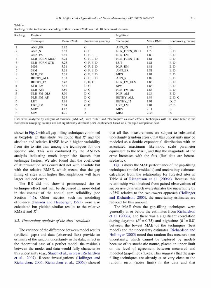
Table 4
Ranking of the techniques according to their mean RMSE over all 10 benchmark datasets
Ranking Daytime Nighttime
Technique Mean RMSE Bonferroni grouping Technique Mean RMSE Bonferroni grouping
1 ANN_BR 2.82 G ANN_PS 1.75 E
2 ANN_S 2.93 G, F NLR_FCRN_MOD 1.79 E, D
3 ANN_PS 2.98 G, F, E NLR_LM 1.80 E, D
4 NLR_FCRN_MOD 3.24 G, F, E, D NLR_FCRN_STD 1.81 E, D
5 NLR_FCRN_STD 3.25 G, F, E, D LUT 1.81 E, D
6 MDS 3.31 G, F, E, D NLR_EM 1.81 E, D
7 SPM 3.31 G, F, E, D ANN_BR 1.81 E, D
8 NLR_EM 3.31 G, F, E, D MDS 1.81 E, D
9 BETHY_ALL 3.33 G, F, E, D ANN_S 1.82 E, D
10 BETHY_12 3.42 E, D, C NLR_FM_OLS 1.83 E, D
11 NLR_LM 3.47 D, C SPM 1.83 E, D
12 NLR_AM 3.50 D, C NLR_FM_AD 1.83 E, D
13 NLR_FM_OLS 3.50 D, C NLR_AM 1.86 E, D
14 NLR_FM_AD 3.54 D, C BETHY_ALL 1.89 E, D, C
15 LUT 3.61 D, C BETHY_12 1.91 D, C
16 UKF_LM 3.74 C, B UKF_LM 2.01 C, B
17 MDV 4.12 B MDV 2.11 B
18 MIM 4.76 A MIM 2.36 A
Data were analyzed by analysis of variance (ANOVA) with ‘‘site’’ and ‘‘technique’’ as main effects. Techniques with the same letter in the
Bonferroni Grouping column are not significantly different (95% confidence) based on a multiple comparison test.
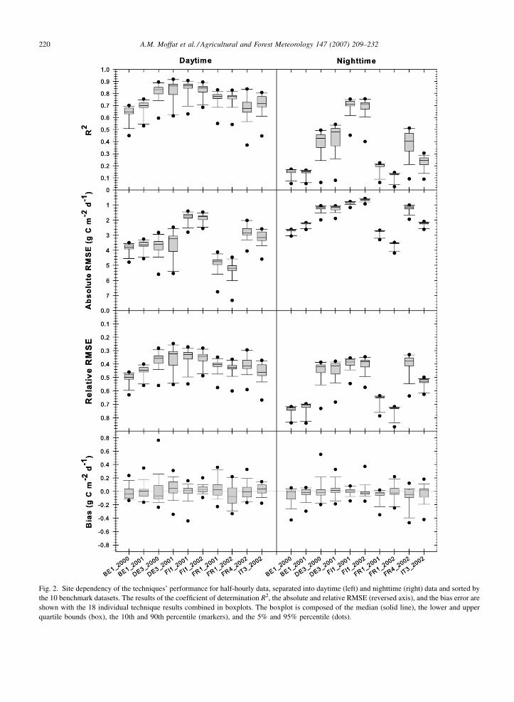
shown in Fig. 2 with all gap-filling techniques combined
as boxplots. In this study, we found that R2 and the
absolute and relative RMSE have a higher variability
from site to site than among the techniques for one
specific site. This was confirmed by the ANOVA
analysis indicating much larger site factors than
technique factors. We also found that the coefficient
of determination was correlated not with absolute but
with the relative RMSE, which means that the gap
filling of sites with higher flux amplitudes will have
larger induced errors.
The BE did not show a pronounced site or
technique effect and will be discussed in more detail
in the context of the annual sum reliability (see
Section 4.6). Other metrics such as modeling
efficiency (Janssen and Heuberger, 1995) were also
calculated but yielded similar results to the relative
RMSE and R2.
4.2. Uncertainty analysis of the sites’ residuals
The variance of the difference between model results
(artificial gaps) and data (observed flux) provide an
estimate of the random uncertainty in the data; in fact in
the theoretical case of a perfect model, the residuals
between the model and data would fully characterize
this uncertainty (e.g., Stauch et al., in press; Richardson
et al., 2007). Recent investigations (Hollinger and
Richardson, 2005; Richardson et al., 2006a) showed
that all flux measurements are subject to substantial
uncertainty (random error), that this uncertainty may be
modeled as a double exponential distribution with an
associated maximum likelihood scale parameter
equivalent to the MAE, and that the magnitude of the
error increases with the flux (flux data are hetero-
scedastic).
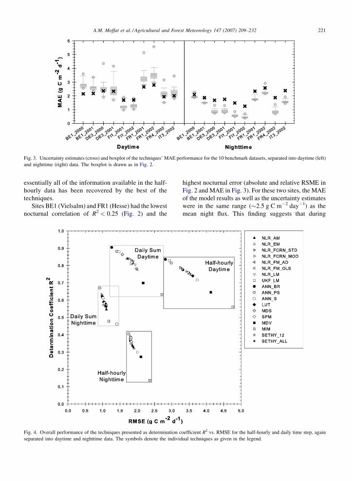
Fig. 3 shows the MAE performance of the gap-filling
techniques (model residuals) and uncertainty estimates
calculated from the relationship for forested sites in
Table 4 of Richardson et al. (2006a). Because this
relationship was obtained from paired observations of
successive days which overestimates the uncertainty by
25% relative to the two-towers approach (Hollinger
and Richardson, 2005), the uncertainty estimates are
reduced by this amount.
The MAE from the gap-filling techniques were
generally at or below the estimates from Richardson
et al. (2006a) and there was a significant correlation
during daytime (R2 = 0.75) and nighttime (R2 = 0.8)
between the lowest MAE of the techniques (best
model) and the uncertainty estimates. Richardson and
Hollinger (2005) noted that random flux measurement
uncertainty, which cannot be captured by models
because of its stochastic nature, placed an upper limit
on the level of agreement between measured and
modeled (gap-filled) fluxes. This suggests that the gap-
filling techniques are already at or very close to the
random error (noise limit) in the data and that
A.M. Moffat et al. / Agricultural and Forest Meteorology 147 (2007) 209–232220
Fig. 2. Site dependency of the techniques’ performance for half-hourly data, separated into daytime (left) and nighttime (right) data and sorted by
the 10 benchmark datasets. The results of the coefficient of determination R2, the absolute and relative RMSE (reversed axis), and the bias error are
shown with the 18 individual technique results combined in boxplots. The boxplot is composed of the median (solid line), the lower and upper
quartile bounds (box), the 10th and 90th percentile (markers), and the 5% and 95% percentile (dots).
A.M. Moffat et al. / Agricultural and Forest Meteorology 147 (2007) 209–232 221
Fig. 3. Uncertainty estimates (cross) and boxplot of the techniques’ MAE performance for the 10 benchmark datasets, separated into daytime (left)
and nighttime (right) data. The boxplot is drawn as in Fig. 2.
essentially all of the information available in the half-
hourly data has been recovered by the best of the
techniques.
Sites BE1 (Vielsalm) and FR1 (Hesse) had the lowest
nocturnal correlation of R2 < 0.25 (Fig. 2) and the
Fig. 4. Overall performance of the techniques presented as determination c
separated into daytime and nighttime data. The symbols denote the individ
highest nocturnal error (absolute and relative RSME in
Fig. 2 and MAE in Fig. 3). For these two sites, the MAE
of the model results as well as the uncertainty estimates
were in the same range (2.5 g C m�2 day�1) as the
mean night flux. This finding suggests that during
oefficient R2 vs. RMSE for the half-hourly and daily time step, again
ual techniques as given in the legend.

A.M. Moffat et al. / Agricultural and Forest Meteorology 147 (2007) 209–232222
nighttime at these two sites the real flux signal is buried
under the measurement noise.
Interestingly, the mean nocturnal errors generated by
the gap-filling techniques at the six European sites were
lower than the uncertainty estimates; this may be
attributed to site-specific differences in the way in
which uncertainty scales with flux magnitude or
Fig. 5. Case study of the long gap scenario for benchmark dataset IT3_2002
course of observed (gray) and predicted (black) half-hourly NEE flux for the fi
due to real gaps in the observed data. (B) Scatter plot of half-hourly NEE value
(black) dots. (C) Annual course of observed daily NEE sums (gray dots) and p
sums (predicted vs. observed).
differences in the way that the Carboeurope IP data
were screened and filtered (for example, the stationarity
tests of Foken et al., 2004, were not used in the data
analyzed by Richardson et al., 2006a,b). This dis-
crepancy and the statistical properties of the uncertainty
are discussed more fully in a companion paper
(Richardson et al., 2007).
and four techniques, NLR_LM, ANN_PS, MDS, and MDV: (A) Daily
rst 5 days of a 12-day-long gap (scenario L0). Missing nighttime data is
s (predicted vs. observed), separated into daytime (gray) and nighttime
redicted daily NEE sums (black dots). (D) Scatter plot of the daily NEE

A.M. Moffat et al. / Agricultural and Forest Meteorology 147 (2007) 209–232 223
4.3. Overall performance of the gap-filling
techniques
To evaluate the overall performance of the techni-
ques, the gap-filling results were averaged over the 10
benchmark datasets and all 50 artificial gap scenarios
for the half-hourly time step (500 data points) and over
the 10 benchmark datasets and the medium and long
gap length results for the daily sums (20 data points).
The results are shown as R2 versus RMSE in Fig. 4.
Since the coefficient of determination R2 and the RMSE
showed an almost linear dependence, the overall
performance given in Table 3 was judged based only
on R2 which was labeled according to the following four
clusters: ‘‘Very good’’ (R2 > 0.85), ‘‘Good’’ (0.75 < R2
� 0.85), ‘‘Medium’’ (0.5 < R2 � 0.75) and ‘‘Low’’
(R2 � 0.5).
For the half-hourly time step, the three ANNs
(ANN_BR, ANN_S, and ANN_PS) yielded highest R2
and lowest RMSE during daytime, while the MDV,
UKF, and MIM techniques behaved in an opposite
manner. The other techniques were distributed between
these two extremes. During nighttime, both R2 and
RMSE decreased relative to the daytime performance
for all techniques and showed only low correlations
(R2 < 0.5).
Fig. 6. Sensitivity of technique performance to gap length, separated for day
individual techniques for the four different gap lengths: one single 0.5-h (ve
(long). For BETHY, the white bar corresponds to BETHY_12 and the dark
The daily performance (DSum) was better for all
techniques during daytime and nighttime due to
averaging out some of the random noise and resulted
in a medium to good confidence in the daily sum
prediction.
4.4. Visualization of the gap-filling results
Despite the similar performance of the techniques,
the individual ‘‘look’’ of the filled gaps on the half-
hourly and daily sum basis is quite different. Fig. 5
shows a case study for the long gap scenario of
dataset IT3_2002 with four representative techniques
(NLR_LM, ANN_PS, MDS, and MDV) and illustrates
some typical characteristics of the methodologies.
The daily course of half-hourly predicted and
observed NEE flux for a 12-day long gap is shown in
Fig. 5A. The NLR technique showed little day-to-day
variation and constant values at night (driven only by
slowly changing temperatures). The ANN, however,
seemed more sensitive to small changes in the provided
meteorological variables or auto-correlations in the
data. The small peak at night–day transition is generally
reproduced by the ANNs and is attributed to a morning
‘‘flush’’ of CO2 from the canopy; because this signal
was present in the training datasets, it appeared in the
time (left) and nighttime (right) data. The bars denote the RMSE of the
ry short), four full hours (short), 1.5 days (medium), and 12 full days
bar to BETHY_ALL (for more information see Section 4.5).
A.M. Moffat et al. / Agricultural and Forest Meteorology 147 (2007) 209–232224
gap-filled values, too. MDS worked better in responding
to the meteorological changes than the basic LUT due to
its marginal sampling. But MDV, since it relied only on
the interpolation of adjacent days for this 12-day gap
and did not make use of ancillary meteorological
drivers, was not able to predict any intermediate
changes in the flux.
Due to the significantly reduced variation during
nighttime resulting from the difference between the
relatively constant estimated values and noisy nighttime
data, the nighttime scatter plots of NLR_LM, ANN_PS,
and MDS shown in Fig. 5B have a horizontal shape. In
contrast, MDV reproduced the night fluctuations of the
observed flux and shows an even distribution of the
scatter. The same is true for MIM (not shown).
The predicted and observed daily sums of the long
gap scenarios are shown in Fig. 5C with the
corresponding scatter plots in Fig. 5D. There were
significant differences between the techniques with
major discrepancies for individual days. ANN_PS and
MDS were best at predicting the daily sums due to the
ability to react to sudden meteorological changes even
in the middle of 12 day long gaps. The differences
between the techniques were much less pronounced for
the medium size gaps (not shown).
4.5. Sensitivity of technique performance to gap
length
Another important aspect is the differences in
performance of the techniques as a function of gap
length. The same subset of artificial gaps for each gap
length was chosen to avoid effects caused by different
positions of the gaps. The results were averaged over the
10 benchmark datasets and 10 permutations (20 data
points).
The RMSE increased and hence the performance of
the gap filling decreased with gap length (Fig. 6). This
result must be expected from potential (and unknown)
changes in the ecosystem properties, particularly as
related to canopy development and senescence (Stauch
and Jarvis, 2006; Richardson and Hollinger, 2007).
Some techniques (the two NLR_FCRN variants, MDS,
SPM, and MDV) had a larger increase in RMSE moving
towards the long gap type during daytime than the other
techniques. During nighttime, the decrease in perfor-
mance with increasing gap length was less marked than
during daytime for all techniques.
For the very short gap scenarios, NLR_FCRN_STD
showed very good performance during daytime due to
its linear interpolation of the short gaps. During
nighttime, this interpolation seemed to have a negative
effect, but looking at the individual site results (not
shown), this linear interpolation led to a slightly better
(reduced) RMSE for most sites but much greater error at
site BE1, leading to an overall increase in RMSE.
The process-based model BETHY generated mod-
eled NEE results independent of the gap length
scenarios but using two schemes for parameter
optimization: once with all available observed data
(BETHY_ALL, white bar, Fig. 6), and once with only
12 (representative) days of observed data (BETHY_12,
dark bar, Fig. 6). There was only a slight decrease
in performance moving from BETHY_ALL to
BETHY_12; BETHY_12 had a remarkably good
performance considering only 12 days out of the whole
year were used.
4.6. Annual sum bias of the gap-filling techniques
Bias in the annual sum prediction is an important
criterion for the characterization of the gap-filling
techniques. The annual sum offset DASum can be
estimated from the bias error on a half-hourly or daily
time step (see Section 2.5).
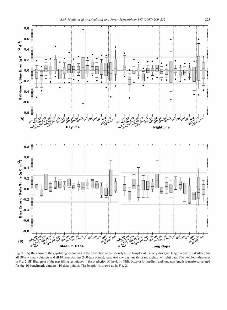
Fig. 7A shows the half-hourly bias error as a function
of technique for the very short gap length scenario
calculated for all 10 benchmark datasets and all 10
permutations (100 data points), separated for daytime
and nighttime data. The span between the lower and
upper quartiles (boxes in Fig. 7) for most techniques
was less than 0.25 g C m�2 day�1. Results were more
variable for some of the techniques including ANN_S
due to outliers (high bias of a single permutation) and
for MIM and BETHY due to a site bias that was
enhanced for BETHY_12 by using only 12 days for
parameter optimization.
Fig. 7B shows the bias error of the daily sums for the
medium and long gap length scenario, calculated for
the 10 benchmark datasets (10 data points). Here the
quartiles of the bias error were predominantly less than
0.25 g C m�2 for the medium gaps and less than
0.30 g C m�2 for the long gaps. Most techniques show a
positive bias for the medium and long gaps resulting in a
positive annual sum offset. Only NLR_EM had a
consistent and persistent negative bias on half-hourly
and daily basis. NLR_FCRN_MOD, UKF_LM, MIM,
and BETHY_12 produced more variable results than the
other techniques for the long gap length scenarios.
To summarize our evaluation of bias, the annual sum
reliability of the techniques stated in Table 3 was
classified ‘‘good’’ if the quartiles of the bias estimates
were less than 0.25 g C m�2 day�1 on a half-hourly and
A.M. Moffat et al. / Agricultural and Forest Meteorology 147 (2007) 209–232 225
Fig. 7. (A) Bias error of the gap-filling techniques in the prediction of half-hourly NEE: boxplot of the very short gap length scenario calculated for
all 10 benchmark datasets and all 10 permutations (100 data points), separated into daytime (left) and nighttime (right) data. The boxplot is drawn as
in Fig. 2. (B) Bias error of the gap-filling techniques in the prediction of the daily NEE: boxplot for medium and long gap length scenario calculated
for the 10 benchmark datasets (10 data points). The boxplot is drawn as in Fig. 2.
A.M
.M
offa
tet
al./A
gricu
ltura
la
nd
Fo
restM
eteoro
log
y1
47
(20
07
)2
09
–2
32
22
6
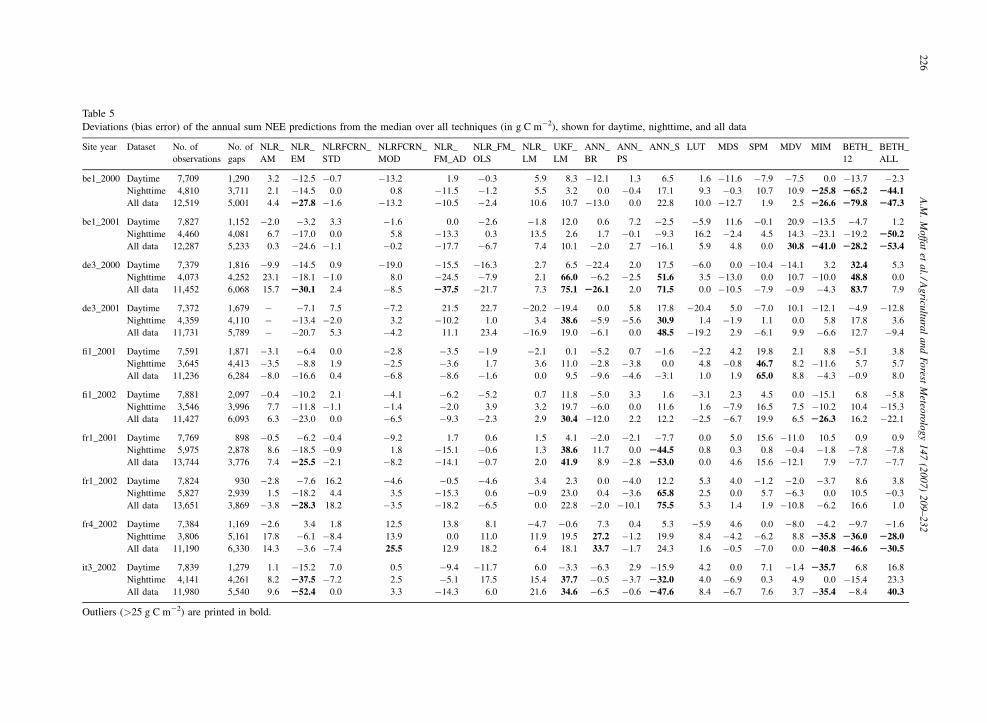
Table 5
Deviations (bias error) of the annual sum NEE predictions from the median over all techniques (in g C m�2), shown for daytime, nighttime, and all data
Site year Dataset No. of
observations
No. of
gaps
NLR_
AM
NLR_
EM
NLRFCRN_
STD
NLRFCRN_
MOD
NLR_
FM_AD
NLR_FM_
OLS
NLR_
LM
UKF_
LM
ANN_
BR
ANN_
PS
ANN_S LUT MDS SPM MDV MIM BETH_
12
BETH_
ALL
be1_2000 Daytime 7,709 1,290 3.2 �12.5 �0.7 �13.2 1.9 �0.3 5.9 8.3 �12.1 1.3 6.5 1.6 �11.6 �7.9 �7.5 0.0 �13.7 �2.3
Nighttime 4,810 3,711 2.1 �14.5 0.0 0.8 �11.5 �1.2 5.5 3.2 0.0 �0.4 17.1 9.3 �0.3 10.7 10.9 S25.8 S65.2 S44.1
All data 12,519 5,001 4.4 S27.8 �1.6 �13.2 �10.5 �2.4 10.6 10.7 �13.0 0.0 22.8 10.0 �12.7 1.9 2.5 S26.6 S79.8 S47.3
be1_2001 Daytime 7,827 1,152 �2.0 �3.2 3.3 �1.6 0.0 �2.6 �1.8 12.0 0.6 7.2 �2.5 �5.9 11.6 �0.1 20.9 �13.5 �4.7 1.2
Nighttime 4,460 4,081 6.7 �17.0 0.0 5.8 �13.3 0.3 13.5 2.6 1.7 �0.1 �9.3 16.2 �2.4 4.5 14.3 �23.1 �19.2 S50.2
All data 12,287 5,233 0.3 �24.6 �1.1 �0.2 �17.7 �6.7 7.4 10.1 �2.0 2.7 �16.1 5.9 4.8 0.0 30.8 S41.0 S28.2 S53.4
de3_2000 Daytime 7,379 1,816 �9.9 �14.5 0.9 �19.0 �15.5 �16.3 2.7 6.5 �22.4 2.0 17.5 �6.0 0.0 �10.4 �14.1 3.2 32.4 5.3
Nighttime 4,073 4,252 23.1 �18.1 �1.0 8.0 �24.5 �7.9 2.1 66.0 �6.2 �2.5 51.6 3.5 �13.0 0.0 10.7 �10.0 48.8 0.0
All data 11,452 6,068 15.7 S30.1 2.4 �8.5 S37.5 �21.7 7.3 75.1 S26.1 2.0 71.5 0.0 �10.5 �7.9 �0.9 �4.3 83.7 7.9
de3_2001 Daytime 7,372 1,679 � �7.1 7.5 �7.2 21.5 22.7 �20.2 �19.4 0.0 5.8 17.8 �20.4 5.0 �7.0 10.1 �12.1 �4.9 �12.8
Nighttime 4,359 4,110 � �13.4 �2.0 3.2 �10.2 1.0 3.4 38.6 �5.9 �5.6 30.9 1.4 �1.9 1.1 0.0 5.8 17.8 3.6
All data 11,731 5,789 � �20.7 5.3 �4.2 11.1 23.4 �16.9 19.0 �6.1 0.0 48.5 �19.2 2.9 �6.1 9.9 �6.6 12.7 �9.4
fi1_2001 Daytime 7,591 1,871 �3.1 �6.4 0.0 �2.8 �3.5 �1.9 �2.1 0.1 �5.2 0.7 �1.6 �2.2 4.2 19.8 2.1 8.8 �5.1 3.8
Nighttime 3,645 4,413 �3.5 �8.8 1.9 �2.5 �3.6 1.7 3.6 11.0 �2.8 �3.8 0.0 4.8 �0.8 46.7 8.2 �11.6 5.7 5.7
All data 11,236 6,284 �8.0 �16.6 0.4 �6.8 �8.6 �1.6 0.0 9.5 �9.6 �4.6 �3.1 1.0 1.9 65.0 8.8 �4.3 �0.9 8.0
fi1_2002 Daytime 7,881 2,097 �0.4 �10.2 2.1 �4.1 �6.2 �5.2 0.7 11.8 �5.0 3.3 1.6 �3.1 2.3 4.5 0.0 �15.1 6.8 �5.8
Nighttime 3,546 3,996 7.7 �11.8 �1.1 �1.4 �2.0 3.9 3.2 19.7 �6.0 0.0 11.6 1.6 �7.9 16.5 7.5 �10.2 10.4 �15.3
All data 11,427 6,093 6.3 �23.0 0.0 �6.5 �9.3 �2.3 2.9 30.4 �12.0 2.2 12.2 �2.5 �6.7 19.9 6.5 S26.3 16.2 �22.1
fr1_2001 Daytime 7,769 898 �0.5 �6.2 �0.4 �9.2 1.7 0.6 1.5 4.1 �2.0 �2.1 �7.7 0.0 5.0 15.6 �11.0 10.5 0.9 0.9
Nighttime 5,975 2,878 8.6 �18.5 �0.9 1.8 �15.1 �0.6 1.3 38.6 11.7 0.0 S44.5 0.8 0.3 0.8 �0.4 �1.8 �7.8 �7.8
All data 13,744 3,776 7.4 S25.5 �2.1 �8.2 �14.1 �0.7 2.0 41.9 8.9 �2.8 S53.0 0.0 4.6 15.6 �12.1 7.9 �7.7 �7.7
fr1_2002 Daytime 7,824 930 �2.8 �7.6 16.2 �4.6 �0.5 �4.6 3.4 2.3 0.0 �4.0 12.2 5.3 4.0 �1.2 �2.0 �3.7 8.6 3.8
Nighttime 5,827 2,939 1.5 �18.2 4.4 3.5 �15.3 0.6 �0.9 23.0 0.4 �3.6 65.8 2.5 0.0 5.7 �6.3 0.0 10.5 �0.3
All data 13,651 3,869 �3.8 S28.3 18.2 �3.5 �18.2 �6.5 0.0 22.8 �2.0 �10.1 75.5 5.3 1.4 1.9 �10.8 �6.2 16.6 1.0
fr4_2002 Daytime 7,384 1,169 �2.6 3.4 1.8 12.5 13.8 8.1 �4.7 �0.6 7.3 0.4 5.3 �5.9 4.6 0.0 �8.0 �4.2 �9.7 �1.6
Nighttime 3,806 5,161 17.8 �6.1 �8.4 13.9 0.0 11.0 11.9 19.5 27.2 �1.2 19.9 8.4 �4.2 �6.2 8.8 S35.8 S36.0 S28.0
All data 11,190 6,330 14.3 �3.6 �7.4 25.5 12.9 18.2 6.4 18.1 33.7 �1.7 24.3 1.6 �0.5 �7.0 0.0 S40.8 S46.6 S30.5
it3_2002 Daytime 7,839 1,279 1.1 �15.2 7.0 0.5 �9.4 �11.7 6.0 �3.3 �6.3 2.9 �15.9 4.2 0.0 7.1 �1.4 S35.7 6.8 16.8
Nighttime 4,141 4,261 8.2 S37.5 �7.2 2.5 �5.1 17.5 15.4 37.7 �0.5 �3.7 S32.0 4.0 �6.9 0.3 4.9 0.0 �15.4 23.3
All data 11,980 5,540 9.6 S52.4 0.0 3.3 �14.3 6.0 21.6 34.6 �6.5 �0.6 S47.6 8.4 �6.7 7.6 3.7 �35.4 �8.4 40.3
Outliers (>25 g C m�2) are printed in bold.

A.M. Moffat et al. / Agricultural and Forest Meteorology 147 (2007) 209–232 227
daily basis. Reasons for low reliability are noted in
parentheses.
For techniques with ‘‘good’’ reliability, the offset
in the annual sum prediction is generally <25 g C m�2 year�1 for the 10 benchmark datasets
which had on average 30% real gaps (equivalent to
approximately 100 days of gap-filled data). This
estimate was examined on the real run results: in
addition to the 50 artificial gap scenarios, each
technique was also used to fill the actual gaps in the
10 benchmark datasets. Considering the differences in
the approaches of the various filling techniques, the
median of all techniques was assumed to be close to the
true annual sum, although this cannot be verified
without independent estimates of C exchange (from,
e.g., direct measures of biomass change). Many
techniques (NLR_LM, ANN_BR, ANN_PS, LUT,
MDS, and SPM) generated annual values that were
almost always within 25 g C m�2 year�1 of the median
with other techniques (Table 5), whereas others
(NLR_EM, UKF_LM, ANN_S, MIM, BETHY_12,
and BETHY_ALL) generated more extreme deviations
of up to 75 g C m�2 year�1.
Based on the techniques and site data examined here,
the effect of gap filling on the annual sums of NEE is
modest, with the techniques with ‘‘good’’ reliability
falling within a range of �25 g C m�2 year�1. This
estimate is comparable in magnitude to the uncertainty
(due to random measurement error) in gap filled annual
sums of NEE reported by Richardson et al. (2006a) and
Stauch et al. (in press), the sampling uncertainty reported
by Goulden et al. (1996), and the estimated uncertainty in
annual sums of GEE reported by Hagen et al. (2006).
5. Discussion
The five non-linear regression techniques
(NLR_AM, NLR_EM, NLR_FCRN, NLR_FM, and
NLR_LM) all showed a good overall RSME and R2
performance (Table 3, bottom). NLR_LM had very low
biases resulting in an above average annual sum
reliability and the three techniques NLR_AM,
NLR_FCRN, and NLR_FM had medium annual sum
reliability. NLR_EM showed persistent negative biases
due to the linear formulation of the Eyring function that
puts less regression weight on high respiration (night-
time NEE) values, leading to an underestimate of high
NEE values. Improvements to the fitting routine should
be implemented to ensure better reliability in predicting
the annual sum.
The UKF_LM showed an average performance with
large deviations of the bias for the long gap length
scenario and for the prediction of the actual gaps. The
filter as implemented here moved sequentially through
the data and thus did not utilize post-gap information in
the time series. A Kalman smoother moves through the
data set in both directions and would presumably yield
improved results.
The neural networks ANN_BR and ANN_PS
produced the best results with the lowest RMSE and
highest R2 values and low bias. Though ANN_S also
generated low RMSE and high R2 values, it lacked
annual sum reliability due to a few outliers which
contributed to a higher bias in the predicted fluxes. This
problem of bias outliers in the simple ANN_S indicates
that ANNs are complex to implement and require
regularization (as in ANN_BR) or smoothing (as in
ANN_PS) to ensure good reliability in the annual sums.
One solution for the problem of bias outliers in ANN_S
is averaging (smoothing) over 10 trained networks.
The basic look-up table (LUT) and the enhance-
ments, MDS and SPM, all showed a good performance
and good annual sum reliability.
The MDV technique had a medium but consistent
performance and reliability. For MDV, the method does
not make use of the ancillary meteorological data and
can be expected to have additional problems filling gaps
of more than 3–7 days in length, as synoptic changes
in weather are strongly linked to changes in diurnal
cycles of photosynthesis and respiration (Baldocchi
et al., 2001b).
MIM showed a low to medium performance and
reliability, and further development of this technique is
needed before it can be recommended as a gap-filling
tool.
BETHY showed a good RMSE and R2 performance
even for the model run with only 12 days out of the
whole year, which hints at potential future adoption of
process-based models for the filling of very long gaps.
But at this stage BETHY cannot be recommended as a
standard gap-filling tool due to the somewhat larger
biases resulting in a low annual sum reliability.
Though most techniques (NLR_AM, NLR_FCRN,
NLR_FM, NLR_LM, ANN_BR, ANN_PS, LUT, MDS,
and SPM) performed well, these results show that there
were systematic differences between techniques and
that some techniques had significant shortcomings. This
highlights the importance of a standardized evaluation
method. The example of the very good results of
ANN_S with low RMSE and high R2 but low annual
sum reliability because of a broad range of bias
estimates, shows that RMSE and R2 are not sufficient
for the evaluation of a gap-filling tool and that an
assessment of the bias error is also required. We
A.M. Moffat et al. / Agricultural and Forest Meteorology 147 (2007) 209–232228
strongly recommend that researchers wishing to utilize
gap-filling techniques not considered here test them
against our standardized benchmark datasets and gap
scenarios. The 10 benchmark dataset and the keyfile are
available at http://gaia.agraria.unitus.it/database/gfc/.
The choice of a technique should be based on the
application, e.g., a simple non-linear regression method
will serve well for an annual sum estimate but an
artificial neural network will best reproduce the half-
hourly profile of the flux. Another important considera-
tion is the availability of the ancillary meteorological
data since only MDV, MDS and ANN_BR are able to
deal with missing meteorological data. When available,
however, these data will always help to improve the
accuracy of gap filled values. While long gaps continue
to present some challenges even in forested sites
(Richardson and Hollinger, 2007), alternative data
sources that may capture changes in the ecosystem
state, such as remotely sensed products from the
MODIS platform, may prove valuable.
The adoption of a standardized gap-filling protocol
across sites reduces the uncertainty in comparing annual
sums since the gap-filling techniques have different
mean biases. A standardized method will greatly
facilitate large-scale, multi-site syntheses such as those
now being pursued by Carboeurope IP and FLUXNET.
6. Conclusions
Fifteen current gap-filling techniques (and variants)
for estimating net carbon fluxes (NEE) were reviewed
and their gap-filling performance was evaluated based
on a set of 10 benchmark datasets from six forested sites
in Europe. The performance of the filling techniques
depended on the site, gap length, and time of day (day
versus night). Based on this analysis with artificial gaps
superimposed on real datasets, the relative differences
between techniques were smaller than anticipated, with
most techniques performing nearly equally well. The
finding that the residual error is at (or below)
independent estimates of uncertainty suggests that
there is little room for improvement on the best of the
gap-filling techniques evaluated here. While not perfect,
the best gap-filling techniques perform well enough that
model-data mismatch at the sites evaluated here can be
attributed almost exclusively to measurement uncer-
tainties rather than model uncertainties. The effect of
the gap filling on the annual sum was estimated to be
�25 g C m�2 year�1 for the benchmark datasets.
These results both confirm and extend the previous
gap-filling comparison of Falge et al. (2001), who
showed that different techniques performed almost
equally well and demonstrated the general utility of
non-linear regression techniques. However, we tested a
wider range of gap-filling techniques and, unlike Falge
et al. (2001) were able to distinguish differences
between techniques in RMSE and R2 performance and
annual sum bias among techniques.
Based on the results of this comparison, the
Carboeurope IP project and FLUXNET have adopted
the ANN_PS and MDS as standardized gap-filling
techniques (Papale et al., 2006). In this study, both
techniques showed a consistently good gap-filling
performance and low annual sum bias, and we
recommend their use in flux data syntheses and
comparison activities. The tools are available online
at http://gaia.agraria.unitus.it/database/.
Further work on the comparison of techniques
should be based not only on European forest sites but
also other vegetation types, such as wetlands, grassland,
crops, urban environment, and other climate zones, such
as arid or tropical. These may make an excellent
companion paper to the present analysis. Since the two
artificial neural networks (ANN_BR and ANN_PS)
were best in performance and annual sum reliability and
since the ANNs replicate underlying patterns in the
data, especially as related to key environmental driving
variables (and, unlike the NLR methods, without
making assumptions about the functional form of these
relationships), we anticipate that ANN performance
would also be good even in ecosystems different from
those studied here.
Acknowledgements
The authors thank the Carboeurope IP research
program funded by the European Commission, and the
Max-Planck-Institute for Biogeochemistry for provid-
ing funding for the Gap Filling Comparison Workshop.
Dario Papale was also supported by the Carboeurope IP
project. We thank David Schimel, Bill Sacks and
Stephen Hagen for their role in this implementation of
the Bayesian neural network regression; and David
MacKay and Christopher Bishop for developing the
underlying algorithm. Asko Noormets was supported by
the University of Toledo and the Southern Global
Change Program of the United States Department of
Agriculture (USDA) Forest Service. David Y. Hollinger
and Andrew D. Richardson gratefully acknowledge
support from the Office of Science (BER), U.S.
Department of Energy, Interagency Agreement No.
DE-AI02-00ER63028. Site PIs Marc Aubinet (Viel-
salm), Werner Kutsch (Hainich), Andre Granier
(Hesse), Serge Rambal (Puechabon), Riccardo Valen-

A.M. Moffat et al. / Agricultural and Forest Meteorology 147 (2007) 209–232 229
tini (Roccarespampani) and Timo Vesala (Hyytiala) are
thanked for making their data available. We also thank
the editor Brian Amiro and two anonymous reviewers
for their comments and constructive criticism, which
have greatly helped to improve this paper.
Appendix A
A.1. Artificial gap scenarios
The 50 distinct artificial gap scenarios used in this
comparison are presented in Table A.1. These 50
scenarios were provided in a keyfile and superimposed
on the NEE data of each of the 10 benchmark datasets to
produce secondary datasets with artificial gaps. The
white space delimited ASCII keyfile had a one-line
header of the gap scenario names and 17,520 rows for
each half-hours of the year. The first column was the
half-hours of the year (‘hh’) and the next 50 columns
were the 50 different artificial gap scenarios (‘v0’ to
‘x9) with data flagged as artificial gap (‘1’) or no
restrictions (‘0’). The detailed superimposition scheme
is given in Table A.2. One additional scenario (‘r0’) had
no artificial gaps (only ‘0’s) to fill the real gaps in the
observed NEE data.
The starting point of each artificial gap was chosen
randomly, except that we blocked off periods before
and after each gap so that no two artificial gaps could
overlap one another. For the mixed gap scenarios, we
did not prevent gaps from overlapping, and the long
gaps (one per permutation) were distributed evenly
across the year over the 10 different permutations. The
Table A.1
Description of the five artificial gap length scenarios (‘v’, ‘s’, ‘m’, ‘l’, ‘x’)
Header Gap length Amount of half-ho
v0, . . ., v9 Very short 1 (0.5 h)
s0, . . ., s9 Short 8 (4 h)
m0, . . ., m9 Medium 64 (1.5 days)
l0, . . ., l9 Long 576 (12 full days)
x0, . . ., x9 Mix of the above 400 v, 50 s, 6 m an
Table A.2
Superimposition scheme of the artificial gap filling for each 0.5-h of the 1
Half-hourly data availability Key Status
Observed NEE value 0 Observ
Observed NEE value 1 Artific
Missing NEE (�9999) 0 Real g
Missing NEE (�9999) 1 Real a
The four logical combinations of observed NEE data (presence or absence
keyfile and the 10 benchmark datasets can be
downloaded from http://gaia.agraria.unitus.it/data-
base/gfc.
A.2. Prefilling gaps in the meteorological data
Since most techniques required complete (gap free)
ancillary meteorological data and the emphasis of this
comparison was on the filling of NEE, complete sets
of gap-filled meteorological data were provided to the
participants. The datasets of the meteorological
measurements were filled only if more than 70% of
data was available; wind speed (WS), wind direction
(WD) and u* were not gap filled. Short gaps for global
radiation (Rg) and photosynthetic photon flux density
(PPFD) were filled by linear interpolation; longer gaps
were filled using an artificial neural network (ANN)
with all other meteorological data, as well as fuzzy
variables to characterize diurnal and seasonal pat-
terns, used as input drivers. For air temperature (Ta),
gaps up to 8 half-hours in length were linearly
interpolated; longer gaps were filled using mean
diurnal variation and a sliding window depending on
gap size. For soil temperature (Ts) and soil water
content (SWC), all gaps were linearly interpolated.
For precipitation, missing values were set to zero if
the data density was higher than 95% but if the data
density was lower than 95%, the entire column was set
to missing. The availability of the meteorological
variables for the 10 benchmark datasets is given in
Table A.3.
with 10 random permutations each (‘0’ to ‘9’)
urs Count of gaps Count of total hhs
1752 1752
219 1752
27 1728
3 1728
d 1 l gap 457 1760
0 benchmark datasets in the year
Procedure
ed NEE value Available for gap-filling procedure
ial gap Not available! to be filled
ap Ignore or fill
nd artificial gap Ignore or fill
) and keyfile flag (available data or artificial gap).
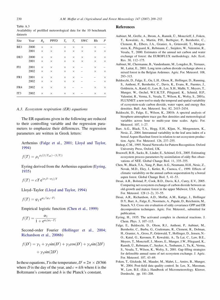
A.M. Moffat et al. / Agricultural and Forest Meteorology 147 (2007) 209–232230
Table A.3
Availability of prefilled meteorological data for the 10 benchmark
datasets
Site Year Rg PPFD Ta Ts SWC Rh P
BE1 2000 � � � � � � –
2001 � � � � � � �
DE3 2000 � � � � � � �2001 � � � � � � �
FI1 2001 � � � � – � –
2002 � � � � – � �
FR1 2001 � � � � – – �2002 � � � � – – �
FR4 2002 � � � – – � �
IT3 2002 � � � � – � �
A.3. Ecosystem respiration (ER) equations
The ER equations given in the following are reduced
to their controlling variable and the regression para-
meters to emphasize their differences. The regression
parameters are written in Greek letters:
Arrhenius (Falge et al., 2001; Lloyd and Taylor,
1994)
f ðTÞ ¼ r1r2ðð1=T ref Þ�ð1=TÞÞ
Eyring derived from the Arrhenius equation (Eyring,
1935)
f ðTÞ ¼ cT eðs1T�s2Þ=T
Lloyd–Taylor (Lloyd and Taylor, 1994)
f ðTÞ ¼ ’1 e’2=ð’3�TÞ
Empirical logistic function (Chen et al., 1999)
f ðTÞ ¼ a1
1þ ea2ða3�TÞ
Second-order Fourier (Hollinger et al., 2004;
Richardson et al., 2006b)
f ðD0Þ ¼ g1 þ g2sinðD0Þ þ g3cosðD0Þ þ g4sinð2D0Þ
þ g5sinð2D0Þ
In these equations, T is the temperature, D0 = 2p � D/366
where D is the day of the year, and c = k/h where k is the
Boltzmann’s constant and h is the Planck’s constant.
References
Aubinet, M., Grelle, A., Ibrom, A., Rannik, U., Moncrieff, J., Foken,
T., Kowalski, A., Martin, P.H., Berbigier, P., Bernhofer, C.,
Clement, R., Elbers, J.A., Granier, A., Grunwald, T., Morgen-
stern, K., Pilegaard, K., Rebmann, C., Snijders, W., Valentini, R.,
Vesala, T., 2000. Estimates of the annual net carbon and water
exchange of forest: the EUROFLUX methodology. Adv. Ecol.
Res. 30, 112–175.
Aubinet, M., Chermanne, B., Vandenhaute, M., Longdoz, B., Yernaux,
M., Laitat, E., 2001. Long term carbon dioxide exchange above a
mixed forest in the Belgian Ardennes. Agric. For. Meteorol. 108,
293–315.
Baldocchi, D., Falge, E., Gu, L.H., Olson, R., Hollinger, D., Running,
S., Anthoni, P., Bernhofer, C., Davis, K., Evans, R., Fuentes, J.,
Goldstein, A., Katul, G., Law, B., Lee, X.H., Malhi, Y., Meyers, T.,
Munger, W., Oechel, W.U.K.T.P., Pilegaard, K., Schmid, H.P.,
Valentini, R., Verma, S., Vesala, T., Wilson, K., Wofsy, S., 2001a.
FLUXNET: a new tool to study the temporal and spatial variability
of ecosystem-scale carbon dioxide, water vapor, and energy flux
densities. Bull. Am. Meteorol. Soc. 82, 2415–2434.
Baldocchi, D., Falge, E., Wilson, K., 2001b. A spectral analysis of
biosphere-atmosphere trace gas flux densities and meteorological
variables across hour to multi-year time scales. Agric. For.
Meteorol. 107, 1–27.
Barr, A.G., Black, T.A., Hogg, E.H., Kljun, N., Morgenstern, K.,
Nesic, Z., 2004. Interannual variability in the leaf area index of a
boreal Aspen-Hazelnut forest in relation to net ecosystem produc-
tion. Agric. For. Meteorol. 126, 237–255.
Bishop, C.M., 1995. Neural Networks for Pattern Recognition. Oxford
University Press, Oxford, UK.
Braswell, B.H., Sacks, B., Linder, E., Schimel, D.S., 2005. Estimating
ecosystem process parameters by assimilation of eddy flux obser-
vations of NEE. Global Change Biol. 11, 335–355.
Chen, W., Black, T.A., Yang, P., Barr, A.G., Neumann, H.H., Nesic, Z.,
Novak, M.D., Eley, J., Ketler, R., Cuenca, C., 1999. Effects of
climatic variability on the annual carbon sequestration by a boreal
aspen forest. Global Change Biol. 5, 41–53.
Desai, A.R., Bolstad, P., Cook, B.D., Davis, K.J., Carey, E.V., 2005.
Comparing net ecosystem exchange of carbon dioxide between an
old-growth and mature forest in the upper Midwest, USA. Agric.
For. Meteorol. 128 (1–2), 33–55.
Desai, A.R., Richardson, A.D., Moffat, A.M., Kattge, J., Hollinger
D.Y., Barr, A., Falge, E., Noormets, A., Papale, D., Reichstein, M.,
Stauch, V.J. Cross site evaluation of eddy covariance GPP and ER
decomposition techniques. Agric. For. Meteorol., submitted for
publication.
Eyring, H., 1935. The activated complex in chemical reactions. J.
Chem. Phys. 3, 107–115.
Falge, E., Baldocchi, D., Olson, R.J., Anthoni, P., Aubinet, M.,
Bernhofer, C., Burba, G., Ceulemans, R., Clement, R., Dolman,
H., Granier, A., Gross, P., Grunwald, T., Hollinger, D., Jensen, N.-
O., Katul, G., Keronen, P., Kowalski, A., Ta Lai, C., Law, B.E.,
Meyers, T., Moncrieff, J., Moors, E., Munger, J.W., Pilegaard, K.,
Rannik, U., Rebmann, C., Suyker, A., Tenhunen, J., Tu, K., Verma,
S., Vesala, T., Wilson, K., Wofsy, S., 2001. Gap filling strategies
for defensible annual sums of net ecosystem exchange. J. Agric.
For. Meteorol. 107, 43–69.
Foken, T., Gockede, M., Mauder, M., Mahrt, L., Amiro, B., Munger,
W., 2004. Post-field data quality control. In: Lee, X., Massman,
W., Law, B.E. (Eds.), Handbook of Micrometeorology. Kluwer,
Dordrecht, pp. 181–208.
A.M. Moffat et al. / Agricultural and Forest Meteorology 147 (2007) 209–232 231
Goulden, M.L., Munger, J.W., Fan, S.-M., Daube, B.C., Wofsy, S.C.,
1996. Measurements of carbon sequestration by long-term eddy
covariance: methods and a critical evaluation of accuracy. Global
Change Biol. 2, 169–182.
Goulden, M.L., Daube, B.C., Fan, S.-M., Sutton, D.J., Bazzaz, A.,
Munger, J.W., Wofsy, S.C., 1997. Physiological responses of
black spruce forest to weather. J. Geophys. Res. 102, 28987–
28996.
Gove, J.H., Hollinger, D.Y., 2006. Application of a dual unscented
Kalman filter for simultaneous state and parameter estimation in
problems of surface-atmosphere exchange. J. Geophys. Res. 111,
D08S07, doi:10.1029/2005JD006021.
Granier, A., Ceschia, E., Damesin, C., Dufrene, E., Epron, D., Gross,
P., Lebaube, S., Le Dantec, V., Le Goff, N., Lemoine, D., Lucot, E.,
Ottorini, J.M., Pontailler, J.Y., Saugier, B., 2000. The carbon
balance of a young Beech forest. Funct. Ecol. 14, 312–325.
Hagan, M.T., Demuth, H.B., Beale, M.H., 1996. Neural Network
Design. PWS Publishing, Boston.
Hagen, S.C., Braswell, B.H., Linder, E., Frolking, S., Richardson,
A.D., Hollinger, D.Y., 2006. Statistical uncertainty of eddy-flux
based estimates of gross ecosystem carbon exchange at Howland
Forest, Maine. J. Geophys. Res.—Atmos. 111 (Art. No.
D08S03).
Hanson, P.J., Amthor, J.S., Wullschleger, S.D., Wilson, K.B., Grant,
R.F., Hartley, A., Hui, D., Hunt JR., E.R., Johnson, D.W.,
Kimball, J.S., King, A.W., Luo, Y., McNulty, S.G., Sun, G.,
Thornton, P.E., Wang, S.S., Williams, M., Cushman, R.M., 2004.
Oak forest carbon and water simulations: model intercompar-
isons and evaluations against independent data. Ecol. Monogr.
74 (3), 443–489.
Hollinger, D.Y., Aber, J., Dail, B., Davidson, E.A., Goltz, S.M.,
Hughes, H., Leclerc, M., Lee, J.T., Richardson, A.D., Rodrigues,
C., Scott, N.A., Varier, D., Walsh, J., 2004. Spatial and temporal
variability in forest-atmosphere CO2 exchange. Global Change
Biol. 10, 1689–1706.
Hollinger, D.Y., Richardson, A.D., 2005. Uncertainty in eddy covar-
iance measurements and its application to physiological models.
Tree Physiol. 25, 873–885.
Hui, D., Wan, S., Su, B., Katul, G., Monson, R., Luo, Y., 2004. Gap-
filling missing data in eddy covariance measurements using multi-
ple imputation (MI) for annual estimations. Agric. For. Meteorol.
121, 93–111.
Janssen, P.H.M., Heuberger, P.S.C., 1995. Calibration of process-
oriented models. Ecol. Modell. 83, 55–66.
Knohl, A., Schulze, E.-D., Kolle, O., Buchmann, N., 2003. Large
carbon uptake by an unmanaged 250-year-old deciduous forest in
Central Germany. Agric. For. Meteorol. 118, 151–167.
Knorr, W., Kattge, J., 2005. Inversion of terrestrial ecosystem model
parameter values against eddy covariance measurements by Monte
Carlo sampling. Global Change Biol. 11, 1333–1351.
Lloyd, J., Taylor, J.A., 1994. On the temperature dependence of soil
respiration. Funct. Ecol. 8, 315–323.
Loescher, H.W., Law, B.E., Mahrt, L., Hollinger, D.Y., Campbell, J.,
Wofsy, S.C., 2006. Uncertainties in, and interpretation of, carbon
flux estimates using the eddy covariance technique. J. Geophys.
Res. 111, D21S90.
Moffat, A. M., Ph. D. Thesis, in preparation.
Morgenstern, K., Black, T.A., Humphreys, E.R., Griffis, T.J., Drewitt,
G.B., Cai, T.B., Nesic, Z., Spittlehouse, D.L., Livingston, N.J.,
2004. Sensitivity and uncertainty of the carbon balance of a Pacific
Northwest Douglas-fir forest during an El Nino-La Nina cycle.
Agric. For. Meteorol. 123, 201–219.
Michaelis, L., Menten, M.L., 1913. Die Kinetik der Invertinwirkung.
Biochemische Zeitschrift 49, 333.
Noormets, A., Chen, J., Crow, T.R., 2007. Age-dependent changes in
ecosystem carbon fluxes in managed forests in northern Wiscon-
sin, USA. Ecosystems 10, 187–203.
Ooba, M., Hirano, T., Mogami, J.-I., Hirata, R., Fujinumba, Y., 2006.
Comparisons of gap-filling methods for carbon flux dataset: a
combination of a genetic algorithm and an artificial neural net-
work. Ecol. Modell. 198, 473–486.
Papale, D., Valentini, R., 2003. A new assessment of European forests
carbon exchanges by eddy fluxes and artificial neural network
spatialization. Global Change Biol. 9, 525–535.
Papale, D., Reichstein, M., Aubinet, M., Canfora, E., Bernhofer, C.,
Longdoz, B., Kutsch, W., Rambal, S., Valentini, R., Vesala, T.,
Yakir, D., 2006. Towards a standardized processing of Net Eco-
system Exchange measured with eddy covariance technique:
algorithms and uncertainty estimation. Biogeosciences 3, 571–
583.
Rambal, S., Joffre, R., Ourcival, J.M., Cavender-Bares, J., Rocheteau,
A., 2004. The growth respiration component in eddy CO2 flux
from a Quercus ilex mediterranean forest. Global Change Biol. 10,
1460–1469.
Reichstein, M., Falge, E., Baldocchi, D., Papale, D., Aubinet, M.,
Berbigier, P., Bernhofer, C., Buchmann, N., Gilmanov, T., Granier,
A., Grunwald, T., Havrankova, K., Ilvesniemi, H., Janous, D.,
Knohl, A., Laurila, T., Lohila, A., Loustau, D., Matteucci, G.,
Meyers, T., Miglietta, F., Ourcival, J.M., Pumpanen, J., Rambal,
S., Rotenberg, E., Sanz, M., Tenhunen, J., Seufert, G., Vaccari, F.,
Vesala, T., Yakir, D., Valentini, R., 2005. On the separation of net
ecosystem exchange into assimilation and ecosystem respiration:
review and improved algorithm. Global Change Biol. 11, 1424–
1439.
Richardson, A.D., Hollinger, D.Y., 2005. Statistical modeling of
ecosystem respiration using eddy covariance data: maximum
likelihood parameter estimation, and Monte Carlo simulation of
model and parameter uncertainty, applied to three simple models.
Agric. For. Meteorol. 131, 191–208.
Richardson, A.D., Hollinger, D.Y., Davis, K.J., Flanagan, L.B., Katul,
G.G., Stoy, P.C., Verma, S.B., Wofsy, S.C., 2006a. A multi-site
analysis of random error in tower-based measurements of carbon
and energy fluxes. Agric. For. Meteorol. 136, 1–18.
Richardson, A.D., Braswell, B.H., Hollinger, D.Y., Burman, P.,
Davidson, E.A., Evans, R.S., Flanagan, L.B., Munger, J.W.,
Savage, K., Urbanski, S.P., Wofsy, S.C., 2006b. Comparing simple
respiration models for eddy flux and dynamic chamber data.
Agric. For. Meteorol. 141, 219–234.
Richardson, A.D., Hollinger, D.Y., 2007. A method to estimate the
additional uncertainty in gap-filled NEE resulting from long
gaps in the CO2 flux record. Agric. For. Meteorol. 147, 199–
208.
Richardson, A.D., Mahecha, M., Falge, E., Kattge, J., Moffat, A.M.,
Papale, D., Reichstein, M., Stauch, V.J., Braswell, B.H., Churkina,
G., Kruijt, B., Hollinger, D.Y., 2007. Statistical properties of
random CO2 flux measurement uncertainty inferred from model
residuals. Agric. For. Meteorol. 147, 209–232.
Rojas, R., 1996. Neural Networks. Springer, Berlin.
Ruppert, J., Mauder, M., Thomas, C., Luers, J., 2006. Innovative gap-
filling strategy for annual sums of CO2 net ecosystem exchange.
Agric. For. Meteorol. 138, 5–18.
Schwalm, C.R., Black, T.A., Morgenstern, K., Humphreys, E.R.,
2007. A method for deriving net primary productivity and com-
ponent respiratory fluxes from tower-based eddy covariance data:

A.M. Moffat et al. / Agricultural and Forest Meteorology 147 (2007) 209–232232
a case study using a 17-year data record from a Douglas-fir
chronosequence. Global Change Biol. 13, 370–385.
Stauch, V.J., Jarvis, A.J., 2006. A semi-parametric model for eddy
covariance CO2 flux time series data. Global Change Biol. 12 (9),
1707–1716.
Stauch, V.J., Jarvis, A.J., Schulz, K. Estimation of net carbon
exchange using eddy covariance CO2 flux observations and a
stochastic model. J. Geophys. Res., in press.
Suni, T., Rinne, J., Reissell, A., Altimir, N., Keronen, P., Rannik, U.,
Dal Maso, M., Kulmala, M., Vesala, T., 2003. Long-term mea-
surements of surface fluxes above a Scots pine forest in Hyytiala,
southern Finland, 1996–2001. Boreal Environ. Res. 8, 287–301.
Tedeschi, V., Rey, A.N.A., Manca, G., Valentini, R., Jarvis, P.G.,
Borghetti, M., 2006. Soil respiration in a Mediterranean oak forest
at different developmental stages after coppicing. Global Change
Biol. 12, 110–121.
Related Documents