CONFERENCE PROCEEDINGS EIGHTH ANNUAL CONFERENCE ON CARBON CAPTURE AND SEQUESTRATION - DOE/NETL May 4 - 7, 2009 Comprehensive Analysis of Enhanced CBM Production via CO 2 Injection Using a Surrogate Reservoir Model Jalal Jalali and Shahab D. Mohaghegh, West Virginia University

Welcome message from author
This document is posted to help you gain knowledge. Please leave a comment to let me know what you think about it! Share it to your friends and learn new things together.
Transcript
CONFERENCE PROCEEDINGS
EIGHTH ANNUAL CONFERENCE ON CARBON CAPTURE AND SEQUESTRATION - DOE/NETL May 4 - 7, 2009
Comprehensive Analysis of Enhanced CBM Production via CO2 Injection Using a Surrogate
Reservoir Model
Jalal Jalali and Shahab D. Mohaghegh, West Virginia University

EIGHTH ANNUAL CONFERENCE ON CARBON CAPTURE AND SEQUESTRATION - DOE/NETL May 4 – 7, 2009
Abstract
Reservoir simulation is the industry standard for reservoir management. Complex reservoir
models usually contain hundreds of thousands or millions of grid cells.
Complexity of reservoir models can result in long simulation time. Companies usually use a
cluster of computers to decrease the simulation time for complex reservoir models. There is also the
issue of uncertainty associated with the geologic model. Static data (net thickness, porosity,
permeability, etc.) are generated by geo-statistical techniques using a small number of samples (core
samples, logs, etc.). Uncertainty analysis techniques such as Monte Carlo Simulation (MCS) can be
used to quantify the uncertainties associated with these parameters. MCS technique requires thousands
of realizations of the reservoir in order to provide meaningful results. The large number of realizations
required by MCS means that a large amount of time is required to run the simulation models, which
could become impractical for complex reservoir models. Efforts have been made to develop new
techniques to perform uncertainty analysis with less number of reservoir simulation models.
This paper presents the utilization of a newly developed technique to perform uncertainty
analysis on a Coalbed Methane (CBM) reservoir. This technique uses Artificial Neural Networks
(ANN) in order to build a Surrogate Reservoir Model (SRM). An SRM is a replica of the full-field
reservoir model that mimics the behavior of the reservoir. A small number of realizations of the
reservoir are required to develop the SRM. This is a key difference between SRM technique and other
techniques in the literature, such as developing a Response Surface Model using Experimental Design
technique or using Reduced Models. Once trained, SRMs can make thousands of simulation runs in a
matter of seconds. The high speed of SRM enables the engineer to exhaustively explore the solution
space and perform uncertainty analysis. During the development process of SRM, Key Performance
Indicators (KPIs) are identified. KPIs are the reservoir parameters that have the most influence on the
desired objective of the simulation study.
Introduction
Reservoir simulation provides information on the behavior of the modeled reservoir under
various production and/or injection conditions. Reservoir engineers and managers use reservoir
simulators to better understand the reservoir, perform future performance predictions and uncertainty
analysis. Because of non-uniqueness of simulation models and uncertainty in reservoir parameters,
uncertainty analysis is an important task that is required in order to quantify the uncertainties associated
with reservoir parameters.
Different techniques are used to quantify the uncertainties associated with reservoir parameters.
MCS is a technique that is widely used in the oil and gas industry for the purpose of uncertainty analysis.
MCS requires thousands of reservoir realizations in order to provide a meaningful conclusion on the
reservoir’s future performance uncertainties. Generating thousands of simulation models especially in
the case of large and complex models, which could take a long time to make a single simulation run,
could be impractical. Attempts have been made to perform uncertainty analysis with as small number of
realizations as possible. Common techniques that have gained popularity in the oil and gas industry are
the Experimental Design technique and Reduced Models. Response Surfaces Models are generated in
order to analyze the results obtained from Experimental Design.
Experimental Design has been used in reservoir simulation since 1990s. It is used to get
maximum information at the lowest experimental cost, by changing all the uncertain parameters
simultaneously. The aim of experimental design is to provide maximum information about the reservoir
from the least number of experiments. It is essentially an equation derived from all the multiple
regressions of all the main parameters that affect the reservoir response (1)
.

EIGHTH ANNUAL CONFERENCE ON CARBON CAPTURE AND SEQUESTRATION - DOE/NETL May 4 – 7, 2009
Reduced Models are approximations of full three dimensional numerical simulation models that
approach an analytical model for tractability (2)
.
Methodology
In this section, Surrogate Reservoir Modeling is introduced and the procedure for developing an
SRM is explained. Interested readers are encouraged to review other published papers by the authors to
learn more about SRMs (3) (4) (5) (6) (7)
.
Surrogate Reservoir Modeling
Surrogate Reservoir Models are essentially Artificial Neural Networks that behave like a
reservoir simulation model. Once trained, the SRM can run thousands of simulation runs in a matter of
seconds. Also, the number of reservoir realizations required to develop the SRM is significantly small
when compared to other traditional techniques. The reason SRMs can be developed with a small
number of realizations is due to the way a single reservoir model is presented to the SRM.
Let us assume that the reservoir we are going to model contains 10 operating wells. Wells can
be looked at as a communication path between the operator (reservoir engineers) and the reservoir.
Each well is telling a story about a specific area of the reservoir by providing production rate and
pressure data. We can look at each well area, the estimated ultimate drainage area (EUDA), as a
representation of the reservoir. Therefore, a reservoir can be divided into several sub-reservoirs (the
number of EUDAs) that are different in their production and reservoir characteristics. With this
observation, we can see that one simulation model can be seen as several models (in this example, one
simulation model can be seen as 10 potential models). So, if we generate 10 simulation models, we will
end up having 100 models (10 models × the number of EUDAs). In addition, SRM technique fits more
appropriately within the system theory (8)
rather than the approach that is commonly used in our industry,
which is based on geostatistics (4)
. When using SRMs, changes in input data directly influence the
output of the system since the SRM is acting as the reservoir simulator.
The objective of the project should be defined as the very first step in developing an SRM. The
reader is reminded that it is not possible to develop a global SRM that can predict all the possible
outputs of a reservoir model. This is not necessarily a limitation of SRMs since, in most cases, reservoir
models are built to study a very limited number of phenomena (such as the effect of water flooding on
hydrocarbon recovery, or the effect of in-fill drilling location on the total field production, etc.). It is
possible to develop several SRMs for the same reservoir, where each SRM can be used to study a certain
reservoir behavior. It is possible however that the reservoir runs designed and generated for an SRM
with the objective of predicting production from wells will be different from runs made for an SRM that
its objective is to track the pressure and saturation changes at the grid block level.
In this study, a Coalbed Methane (CBM) reservoir is being modeled. The CBM reservoir
includes 13 pinnate pattern wells (wells with branching laterals a.k.a. fishbone) on an area of
approximately 600 acres. All the wells start producing at the same time and will continue production for
15 years. Well constraint for all the wells was constant Bottom-Hole Pressure (BHP). The developed
SRM was responsible to predict the cumulative methane production (CH4-CUM) due to changes in well
BHP constraint. Fig. 1 shows the structure of the CBM reservoir and the locations of the thirteen wells.
EIGHTH ANNUAL CONFERENCE ON CARBON CAPTURE AND SEQUESTRATION - DOE/NETL May 4 – 7, 2009
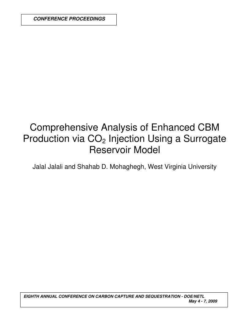
Figure 1 shows the CBM reservoir structure. The black cones are the well-heads. (Source: CMG-Builder)
As Fig.1 shows, the reservoir is an irregular structure with heterogeneous porosity and
permeability characteristics. All 13 pinnate pattern wells have a main lateral and three branches on each
side. The lengths of the main lateral and branches are different from one well to another.
In the design phase, realizations were generated such that the effect of changing BHP was shown
to the network. It was assumed that all the wells in a model were producing at the same constant BHP
value. For different simulation runs, BHP values of 50, 100, 150, and 200 psia were selected, for all
wells. Also, three different geologic realizations were used for the models. This would provide more
information on the effect of porosity and permeability heterogeneity on the reservoir’s performance.
Once all the models are run, geologic information, well configuration, and wells’ production are
extracted and prepared for SRM development. Twelve realizations (four different BHP cases for three
different geologic realizations) were generated and results were exported. To develop the SRM, IDEA
(9), a commercial software, was used. The software provided multiple Neural Network algorithms from
which, Back-Propagation algorithm (10)
(BP) with one hidden layer was used.
Back-Propagation algorithm is one of the most popular algorithms in Artificial Neural Networks.
It is an easy to understand algorithm with applications in pattern-recognition and with some minor
modifications can be implemented to model time-series problems. The BP algorithm looks for the
minimum of the error function in weight space using the method of gradient descent. The combination
of weights that minimizes the error function is considered to be a solution of the learning problem.
Sigmoid activation function is used for BP networks. Sigmoid activation function is a popular function
since it is continuous and differentiable. Sigmoid is defined as:
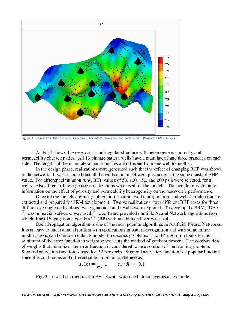
Fig. 2 shows the structure of a BP network with one hidden layer as an example.
EIGHTH ANNUAL CONFERENCE ON CARBON CAPTURE AND SEQUESTRATION - DOE/NETL May 4 – 7, 2009
Figure 2 shows the structure of a Back-Propagation Neural Network with one hidden layer.
Once the outputs are generated by the network and an error is generated by comparing the
network’s output with the actual outputs, the weights are adjusted based on the generated error starting
from the weights connecting the hidden neurons to the output neurons in a back-propagating fashion.
Results
For the purpose of this study where the objective was to develop an SRM capable of predicting
cumulative methane production by changing the production wells’ BHP value, 12 realizations were
generated using the commercial reservoir simulator CMG-GEM (11)
. These models were different in
their porosity and permeability maps and BHP values at the production wells. Table 1 shows the
summary of these models.
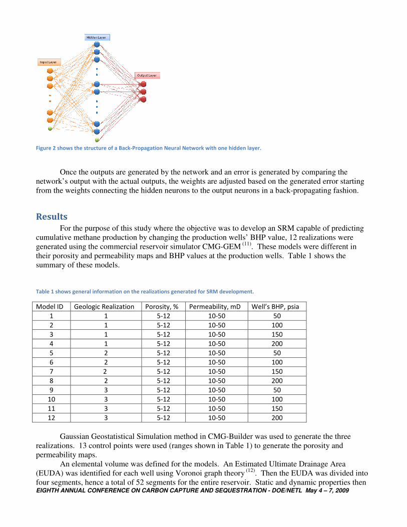
Table 1 shows general information on the realizations generated for SRM development.
Model ID Geologic Realization Porosity, % Permeability, mD Well’s BHP, psia
1 1 5-12 10-50 50
2 1 5-12 10-50 100
3 1 5-12 10-50 150
4 1 5-12 10-50 200
5 2 5-12 10-50 50
6 2 5-12 10-50 100
7 2 5-12 10-50 150
8 2 5-12 10-50 200
9 3 5-12 10-50 50
10 3 5-12 10-50 100
11 3 5-12 10-50 150
12 3 5-12 10-50 200
Gaussian Geostatistical Simulation method in CMG-Builder was used to generate the three
realizations. 13 control points were used (ranges shown in Table 1) to generate the porosity and
permeability maps.
An elemental volume was defined for the models. An Estimated Ultimate Drainage Area
(EUDA) was identified for each well using Voronoi graph theory (12)
. Then the EUDA was divided into
four segments, hence a total of 52 segments for the entire reservoir. Static and dynamic properties then
EIGHTH ANNUAL CONFERENCE ON CARBON CAPTURE AND SEQUESTRATION - DOE/NETL May 4 – 7, 2009
were averaged for these segments. SRM dataset can be divided into two major categories; cell-based
and well-based data. Cell-based data are the reservoir properties, such as depth, thickness, porosity,
permeability, etc. Well-based data include well location, well configuration information, and well
production data. Tables 2 and 3 show the list of cell-based and well-based data used in this study,
respectively.
Table 2 shows cell-based data used for SRM development.
Cell-Based Data Used for the SRM Development
Depth to top Thickness
Gross Block Volume Fracture Gas Saturation @ Reference Point
Fracture Water Saturation @ Reference Point Fracture Pressure @ Reference Point
Matrix Adsorbed Gas @ Reference Point
Table 3 shows well-based data used for SRM development.
Well-Based Data Used for the SRM Development
Location – X Location – Y
Main Leg Length First Branch Length
Distance of First Branch from Wellbore Second Branch Length
Distance of Second Branch from Wellbore Third Branch Length
Distance of Third Branch from Wellbore Total Well Length
Well Initial Bottom-Hole Pressure
Three reference points were selected in this study and some of the reservoir properties were
evaluated at these reference points (times during simulation). The three reference points were, 1/1/2000
(start date of simulation), 1/1/2002, and 1/1/2005. The values of matrix adsorbed gas, fracture gas
saturation, fracture water saturation, and fracture pressure were recorded for each grid cell in these times
and were introduced to the SRM. The reason for this is to show the network the way the reservoir
produces each fluid. It was assumed that the reservoir simulation model generated in CMG was history
matched using the first five years of the production data.
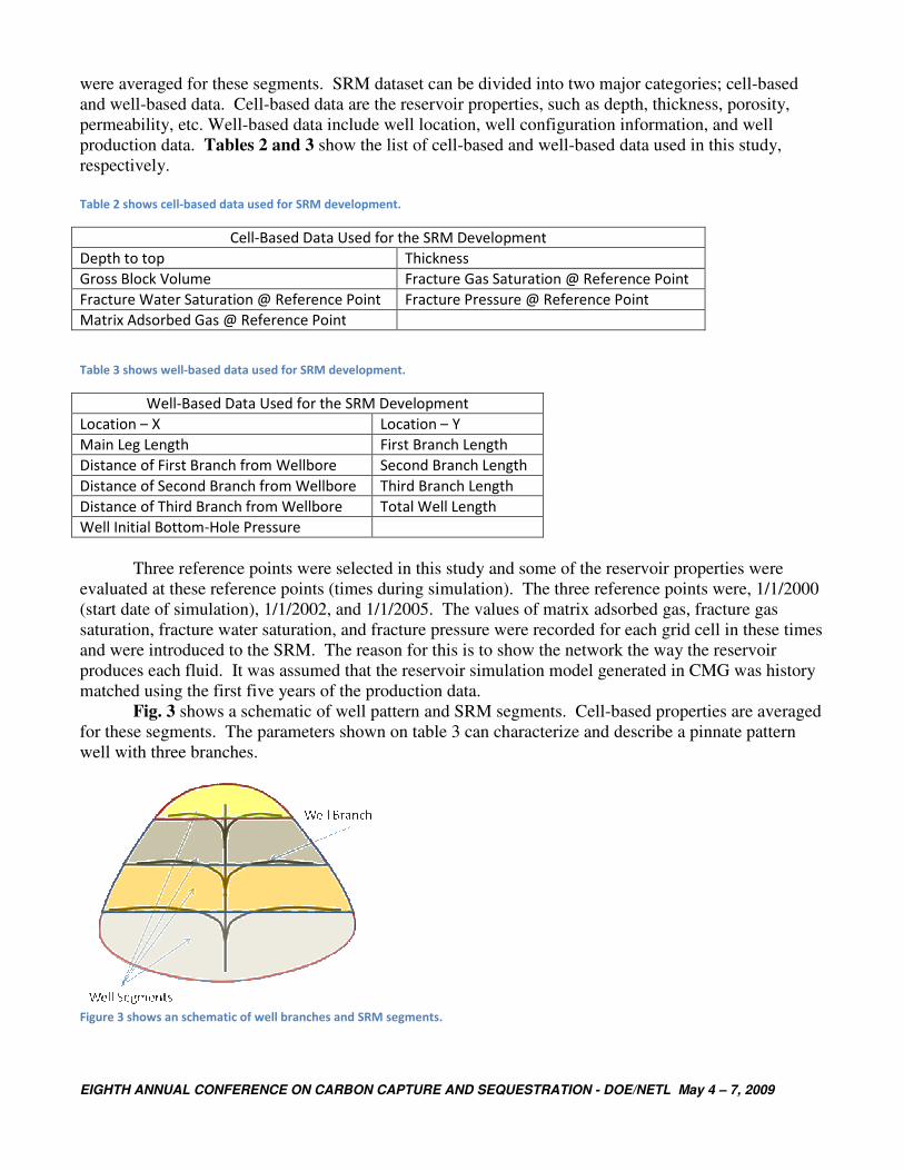
Fig. 3 shows a schematic of well pattern and SRM segments. Cell-based properties are averaged
for these segments. The parameters shown on table 3 can characterize and describe a pinnate pattern
well with three branches.
Figure 3 shows an schematic of well branches and SRM segments.
EIGHTH ANNUAL CONFERENCE ON CARBON CAPTURE AND SEQUESTRATION - DOE/NETL May 4 – 7, 2009
The generated dataset was divided into three sub-sets; training set, calibration set, and
verification set. Only training set is directly used for training, calculating errors, and adjusting weights.
Calibration set is used for cross-validation in order to see the accuracy of the network in predicting
outputs of some input data that the network has not seen before, also to identify a good time to stop the
training process. Once training is completed, the network is applied to the verification set and the
network’s outputs are compared with the actual results in the verification set.
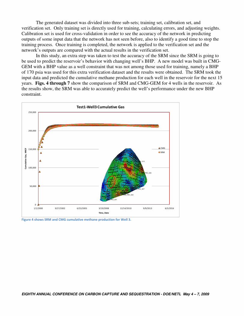
In this study, an extra step was taken to test the accuracy of the SRM since the SRM is going to
be used to predict the reservoir’s behavior with changing well’s BHP. A new model was built in CMG-
GEM with a BHP value as a well constraint that was not among those used for training, namely a BHP
of 170 psia was used for this extra verification dataset and the results were obtained. The SRM took the
input data and predicted the cumulative methane production for each well in the reservoir for the next 15
years. Figs. 4 through 7 show the comparison of SRM and CMG-GEM for 4 wells in the reservoir. As
the results show, the SRM was able to accurately predict the well’s performance under the new BHP
constraint.
0
50,000
100,000
150,000
200,000
250,000
1/1/2000 9/27/2002 6/23/2005 3/19/2008 12/14/2010 9/9/2013 6/5/2016
Cu
mu
lati
ve
Ga
s, M
SC
F
Time, Date
Test1-Well3 Cumulative Gas
CMG
SRM
PINN_PRO_001
PINN_PRO_002
PINN_PRO_003
PINN_PRO_004
PINN_PRO_005
PINN_PRO_006
PINN_PRO_007
PINN_PRO_008
PINN_PRO_009
PINN_PRO_010
PINN_PRO_011
PINN_PRO_012PINN_PRO_013
Figure 4 shows SRM and CMG cumulative methane production for Well 3.
EIGHTH ANNUAL CONFERENCE ON CARBON CAPTURE AND SEQUESTRATION - DOE/NETL May 4 – 7, 2009
0
20,000
40,000
60,000
80,000
100,000
120,000
140,000
160,000
180,000
200,000
1/1/2000 9/27/2002 6/23/2005 3/19/2008 12/14/2010 9/9/2013 6/5/2016
Cu
mu
lati
ve
Ga
s, M
SC
F
Time, Date
Test1-Well6 Cumulative Gas
CMG
SRM
PINN_PRO_001
PINN_PRO_002
PINN_PRO_003
PINN_PRO_004
PINN_PRO_005
PINN_PRO_006
PINN_PRO_007
PINN_PRO_008
PINN_PRO_009
PINN_PRO_010
PINN_PRO_011
PINN_PRO_012PINN_PRO_013
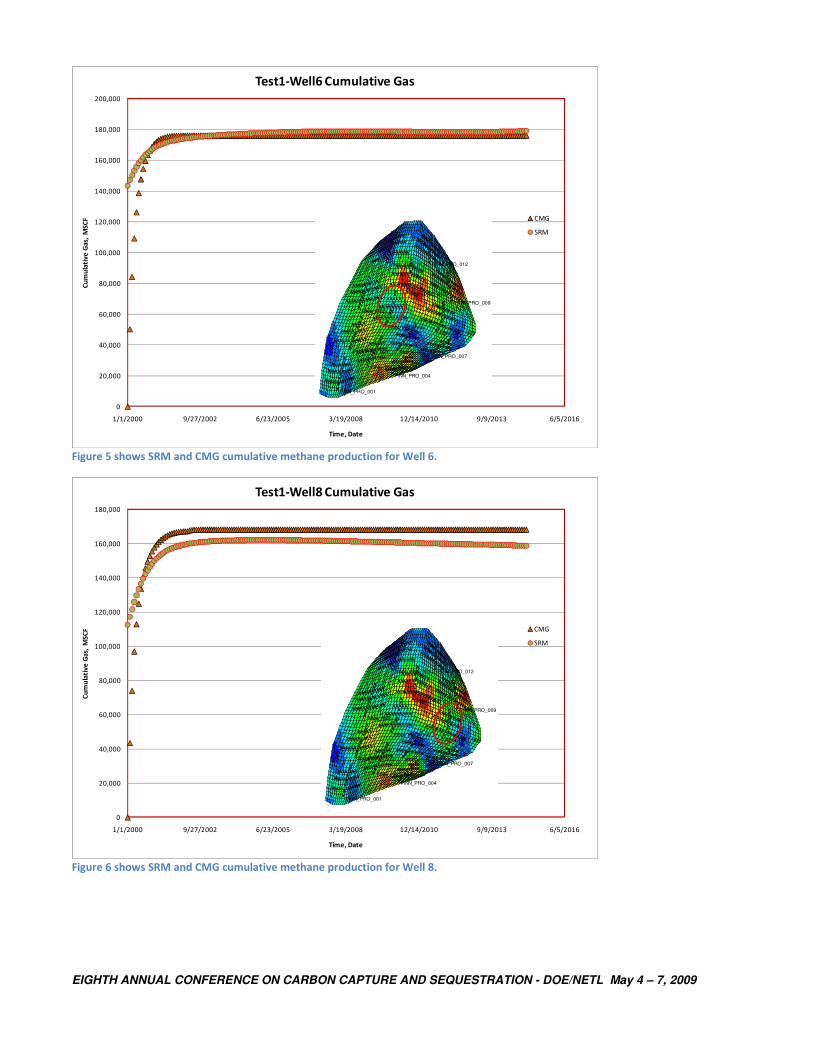
Figure 5 shows SRM and CMG cumulative methane production for Well 6.
0
20,000
40,000
60,000
80,000
100,000
120,000
140,000
160,000
180,000
1/1/2000 9/27/2002 6/23/2005 3/19/2008 12/14/2010 9/9/2013 6/5/2016
Cu
mu
lati
ve
Ga
s, M
SC
F
Time, Date
Test1-Well8 Cumulative Gas
CMG
SRM
PINN_PRO_001
PINN_PRO_002
PINN_PRO_003
PINN_PRO_004
PINN_PRO_005
PINN_PRO_006
PINN_PRO_007
PINN_PRO_008
PINN_PRO_009
PINN_PRO_010
PINN_PRO_011
PINN_PRO_012PINN_PRO_013
Figure 6 shows SRM and CMG cumulative methane production for Well 8.
EIGHTH ANNUAL CONFERENCE ON CARBON CAPTURE AND SEQUESTRATION - DOE/NETL May 4 – 7, 2009
0
50,000
100,000
150,000
200,000
250,000
1/1/2000 9/27/2002 6/23/2005 3/19/2008 12/14/2010 9/9/2013 6/5/2016
Cu
mu
lati
ve
Ga
s, M
SC
F
Time, Date
Test1-Well11 Cumulative Gas
CMG
SRM
PINN_PRO_001
PINN_PRO_002
PINN_PRO_003
PINN_PRO_004
PINN_PRO_005
PINN_PRO_006
PINN_PRO_007
PINN_PRO_008
PINN_PRO_009
PINN_PRO_010
PINN_PRO_011
PINN_PRO_012PINN_PRO_013
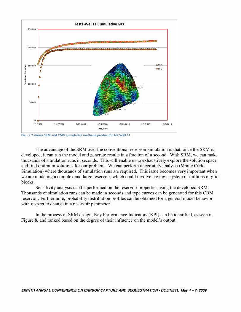
Figure 7 shows SRM and CMG cumulative methane production for Well 11.
The advantage of the SRM over the conventional reservoir simulation is that, once the SRM is
developed, it can run the model and generate results in a fraction of a second. With SRM, we can make
thousands of simulation runs in seconds. This will enable us to exhaustively explore the solution space
and find optimum solutions for our problem. We can perform uncertainty analysis (Monte Carlo
Simulation) where thousands of simulation runs are required. This issue becomes very important when
we are modeling a complex and large reservoir, which could involve having a system of millions of grid
blocks.
Sensitivity analysis can be performed on the reservoir properties using the developed SRM.
Thousands of simulation runs can be made in seconds and type curves can be generated for this CBM
reservoir. Furthermore, probability distribution profiles can be obtained for a general model behavior
with respect to change in a reservoir parameter.
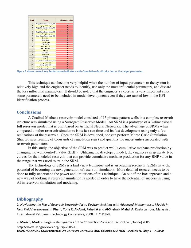
In the process of SRM design, Key Performance Indicators (KPI) can be identified, as seen in
Figure 8, and ranked based on the degree of their influence on the model’s output.
EIGHTH ANNUAL CONFERENCE ON CARBON CAPTURE AND SEQUESTRATION - DOE/NETL May 4 – 7, 2009
Figure 8 shows ranked Key Performance Indicators with Cumulative Gas Production as the target parameter.
This technique can become very helpful when the number of input parameters to the system is
relatively high and the engineer needs to identify, use only the most influential parameters, and discard
the less influential parameters. It should be noted that the engineer’s expertise is very important since
some parameters need to be included in model development even if they are ranked low in the KPI
identification process.
Conclusions
A Coalbed Methane reservoir model consisted of 13 pinnate pattern wells in a complex reservoir
structure was simulated using a Surrogate Reservoir Model. An SRM is a prototype of a 3-dimensional
full reservoir model that is built based on Artificial Neural Networks. The advantage of SRMs when
compared to other reservoir simulators is its fast run time and its fast development using only a few
realizations of the reservoir. Once the SRM is developed, one can perform Monte Carlo Simulation
(that requires running of thousands of simulation runs) and quantify the uncertainties associated with
reservoir parameters.
In this study, the objective of the SRM was to predict well’s cumulative methane production by
changing the well control’s value (BHP). Utilizing the developed model, the engineer can generate type
curves for the modeled reservoir that can provide cumulative methane production for any BHP value in
the range that was used to train the SRM.
The technology of SRMs is a fairly new technique and is an ongoing research. SRMs have the
potential of becoming the next generation of reservoir simulators. More detailed research needs to be
done to fully understand the power and limitations of this technique. An out of the box approach and a
new way of looking at reservoir simulation is needed in order to have the potential of success in using
AI in reservoir simulation and modeling.
Bibliography 1. Navigating the Fog of Reservoir Uncertainties to Decision Makings with Advanced Mathematical Models in
New Field Developement. Pham, Tony R, Al-Ajmi, Fahad A and Al-Shehab, Mahdi A. Kuala Lumpur, Malaysia :
International Petroleum Technology Conference, 2008. IPTC 11978.
2. Miesch, Mark S. Large-Scale Dynamics of the Convection Zone and Tachocline. [Online] 2005.
http://www.livingreviews.org/lrsp-2005-1.

EIGHTH ANNUAL CONFERENCE ON CARBON CAPTURE AND SEQUESTRATION - DOE/NETL May 4 – 7, 2009
3. Intelligent Systems Can Design Optimum Fracturing Jobs. Mohaghegh, S., Popa, A.S., and Ameri, S.
Charleston, WV : SPE 57433, 1999.
4. Uncertainty Analysis of a Giant Oil Field in the Middle East Using Surrogate Reservoir Model. Mohaghegh,
S.D., Hafez, H., Gaskari, R., Haajizadeh, M., and Kenawy, M. Abu Dhabi, U.A.E. : SPE 101474, 2006.
5. Identifying Best Practices in Hydraulic Fracturing Using Virtual Intelligence Techniques. Mohaghegh, Shahab
D, et al. Canton, Ohio : SPE 72385, 2001.
6. Quantifying Uncertainties Associated with Reservoir Simulation Studies using Surrogate Reservoir Models.
Mohaghegh, Shahab. San Antonio, Texas : 2006 SPE Annual Technical Conference and Exhibition, 2006. SPE
102492.
7. Development of Surrogate Reservoir Models (SRM) for Fast Track Analysis of Complex Reservoirs. Mohaghegh,
et. al. Amsterdam, The Netherlands : SPE 99667, 2006.
8. What is System Theory? [Online] http://pespmc1.vub.ac.be/SYSTHEOR.html.
9. Intelligent Data Evaluation and Analysis (IDEA). Intelligent Solutions Inc. [Online]
http://www.intelligentsolutionsinc.com/IDEA.htm.
10. Rojas, Raul. The Backpropagation Algorithm. Neural Networks: A Systematic Introduction. Berlin : Springer-
Verlag, 1996.
11. Computer Modelling Group LTD. [Online] http://www.cmgroup.com/software/gem.htm.
12. What is Voronoi Diagram in Rd. [Online] http://www.ifor.math.ethz.ch/~fukuda/polyfaq/node29.html.
Related Documents


