Compound-specific isotope analysis to delineate the sources and fate of organic contaminants in complex aquifer systems Dissertation zur Erlangung des Grades eines Doktors der Naturwissenschaften der Geowissenschaftlichen Fakultät der Eberhard Karls Universität Tübingen vorgelegt von Michaela Blessing aus Schwäbisch Gmünd 2008

Welcome message from author
This document is posted to help you gain knowledge. Please leave a comment to let me know what you think about it! Share it to your friends and learn new things together.
Transcript
Compound-specific isotope analysis to delineate the sources and fate of organic contaminants
in complex aquifer systems
Dissertation
zur Erlangung des Grades eines Doktors der Naturwissenschaften
der Geowissenschaftlichen Fakultät der Eberhard Karls Universität Tübingen
vorgelegt von Michaela Blessing
aus Schwäbisch Gmünd
2008

ii
Tag der mündlichen Prüfung: 08. August 2008 Dekan: Prof. Dr. Peter Grathwohl 1. Berichterstatter: Prof. Dr. Stefan Haderlein 2. Berichterstatter: Prof. Dr. Torsten Schmidt
Eidesstattliche Erklärung iii
Hiermit versichere ich, dass ich die
vorliegende Arbeit selbständig verfasst, keine
anderen als die angegebenen Quellen und
Hilfsmittel benutzt und wörtlich oder inhaltlich
übernommene Stellen als solche
gekennzeichnet habe.
iv Danksagung
Danksagung
Mein besonderer Dank gilt meinen Betreuern Torsten Schmidt und Stefan Haderlein für
hilfreiche Diskussionen und konstruktive Kritik in allen Phasen meiner Arbeit. Danke für Rat und
Tat, Motivation, organisatorische sowie finanzielle Unterstützung.
Bei den Mitarbeitern im ZAG, vor allem im Labor möchte ich mich für die angenehme
Arbeitsatmosphäre und Hilfestellung bedanken. Ganz besonders möchte ich Maik hervorheben,
der entscheidenden Anteil daran hatte, dass ich die Arbeit im Labor nicht gleich aufgegeben habe
und der es geschafft hat, doch tatsächlich noch einen Mechaniker aus mir zu machen. Für
besonders viel Spaß während der gemeinsamen Arbeit in Labor und Büro möchte ich Anke
lobenswert erwähnen, Thomas für unzählige He-Flaschenwechsel, Bernd und Heiner für die
EA/IRMS-Messungen, Erping und Satoshi für ihre Hilfe und Expertise bei den
Sorptionsexperimenten, meinem Hiwi Lunliang für die Aufreinigung der Bodenextrakte, meinen
beiden AEG-Studentinnen Oxana und Kathryn für ihre engagierte Arbeit zum einen an
Sorptionsversuchen und zum anderen bei der reaktiven Transportmodellierung, deren
Masterarbeiten einen wertvollen Beitrag geleistet haben.
Ferner möchte ich mich bei allen Projektpartnern für die gute Zusammenarbeit bei der
Bearbeitung der kontaminierten Standorte bedanken, insbesondere bei Rainer Dinkel und
Christian Kiffer von der UW Umweltwirtschaft GmbH, Anita Peter und Eugen Martac vom
Tübinger Grundwasserforschungsinstitut, sowie den Herren Ufrecht, Wolff und Carle vom Amt
für Umweltschutz der Stadt Stuttgart.
Nicht zuletzt bedanke ich mich bei der Deutschen Bundesstiftung Umwelt für die finanzielle
Unterstützung sowie für die Organisation von abwechslungsreichen Stipendiatenseminaren und -
veranstaltungen an ausgesprochen schönen Orten.
Guido, danke dafür, dass Du mich mit deiner stoischen Ruhe immer wieder schnell aus dem
Wahnsinn zurückgeholt hast – auch mit der Anschaffung der zwei kleinen, gemütlichen Kater
gleich zu Beginn meiner Promotionsphase hast Du einen wertvollen Beitrag geleistet.
Bei allen ehemaligen und aktuellen Leidensgenossen, insbesondere Anke, Florian, Iris, Katja,
Katharina, Kerstin, Lihua, Maik, Michael, Nicole, Safi und Satoshi für die nötige Abwechslung
zwischendurch. Die Abende mit den Ehemaligen vermisse ich bereits seit geraumer Zeit, alle
anderen erholsamen und lustigen Freizeitaktivitäten mit Euch Aktuellen werde ich in Zukunft
bestimmt schwer vermissen...
Abstract v
Compound-specific isotope analysis to delineate the sources and
fate of organic contaminants in complex aquifer systems
Abstract
The extensive use of organic compounds has frequently caused soil and groundwater
contamination. Volatile organic compounds, such as chlorinated and aromatic hydrocarbons and
the semi-volatile polycyclic aromatic hydrocarbons are among the most widespread organic
pollutants. The fate and behavior of such compounds in the subsurface depend on a number of
physicochemical and biological processes, which may lead to ‘natural attenuation’. For the
consideration of these in-situ contaminant-reducing processes as a valid remedial approach, it is
necessary to attain an appropriate understanding of the key processes occurring in natural
aquifers. Compound-specific isotope analysis (CSIA) with on-line gas chromatography-isotope
ratio mass spectrometry (GC/IRMS) offers a versatile tool for the characterization of origin and
fate of organic contaminants in environmental analytical chemistry.
The aim of the present work was to evaluate and demonstrate the potential and limitations of
CSIA for studying sources and fate of organic contaminants at heterogeneous and complex
aquifer systems. One major drawback in the application of CSIA to field studies, is that current
GC/IRMS systems are limited in their sensitivity. To overcome this limitation and to enhance
method detection limits, various sample extraction and injection techniques were optimized and
validated for their use in CSIA field studies. For volatile compounds, a commercially available
purge-and-trap sample extractor has been technically improved to meet the specific requirements
at real sites. The results obtained demonstrate the good performance of the sample
preconcentration and extraction techniques applied for the compound-specific carbon isotope
analysis of volatile compounds at trace concentrations. Applied to different field sites, the
techniques helped to assess the potential for biodegradation according to the Rayleigh-equation.
A new analytical approach, based on the injection of large sample volumes (large-volume
injection, LVI) of organic extracts into a programmable temperature vaporizer (PTV) injector,
has been developed and validated for the determination of compound-specific carbon isotope
ratios. The PTV-LVI method was thoroughly optimized in terms of its accuracy, precision,
linearity, reproducibility and limits of detection. It was shown that the technique allows to
determine accurately and precisely δ13C values of semi-volatile organic contaminants at low
vi Abstract
concentrations (1-3 µg/L for aqueous or 10-20 µg/kg for soil samples) and thus expands the
applicability of CSIA considerably in environmental applications. The applicability of the
method was verified for δ13C determination of individual PAHs and exemplified by a source
apportionment study at a creosote-contaminated site.
So far, most field applications of CSIA have been limited to fairly homogeneous aquifers. To
evaluate the applicability of the CSIA concept for studying the source and fate of organic
contaminants and to quantify the rate of in-situ degradation in contaminant plumes even at highly
complex conditions, extensive site investigations were performed at an urban, heterogeneous
bedrock aquifer system. The study highlights the potential of using δ13C values of chlorinated
hydrocarbons (tetrachloroethene and its transformation products) as a tracer for discriminating
different contaminant sources even in the presence of biodegradation. It was shown that careful
statistical evaluation and interpretation of highly precise compound specific isotope signatures,
geochemical data and site-specific additional information may allow for a comprehensive site
assessment under complex boundary conditions. In addition, for a plume in the southern part of
this site, a reactive transport model-based analysis of concentration and isotope data was carried
out to assess natural attenuation of the chlorinated ethenes in this part of the aquifer. The results
provided strong evidence for the occurrence of aerobic TCE and DCE degradation. As PCE is
recalcitrant at aerobic conditions, it could be used as a conservative tracer to estimate the extent
of dilution. The dilution-corrected concentrations together with stable carbon isotope data
allowed for the reliable assessment of the extent of in-situ biodegradation at the site. Finally,
limitations of CSIA under natural field conditions and potential analytical pitfalls of the method
are critically discussed and strategies to avoid possible sources of error are provided. The results
of this work exemplify how CSIA can contribute for a reliable assessment of contaminated sites,
even at complex contamination scenarios. Moreover, future work will significantly benefit from
the method developments attained in this study.
Kurzfassung vii
Komponentenspezifische Isotopenanalyse zur Aufklärung der
Herkunft und des Verbleibs von organischen Schadstoffen in
komplexen Grundwasserleitern
Kurzfassung
Auf intensiv genutzten Industriestandorten kommt es oft zu einer hohen organischen
Schadstoffbelastung in Grundwasser und Böden. Die flüchtigen chlorierten und aromatischen
Kohlenwasserstoffverbindungen, sowie polyzyklische aromatische Kohlenwasserstoffe (PAK),
gehören dabei zu den am häufigsten nachgewiesenen organischen Schadstoffen an
kontaminierten Standorten. Physikalisch-chemische und biologische Abbau- und
Rückhalteprozesse in der gesättigten und ungesättigten Bodenzone können dabei die Ausbreitung
der Schadstoffe verlangsamen und unter günstigen Bedingungen zu einer Begrenzung der
Schadstofffahne führen („Natural Attenuation“). In-situ Prozesse, die zu einer tatsächlichen
Minimierung der Schadstofffrachten führen, stellen dabei eine alternative Sanierungsstrategie
dar, deren Anwendung allerdings ein gutes Prozessverständnis des Transport- und
Abbauverhaltens der Schadstoffe im Untergrund voraussetzen. Die substanzspezifische
Isotopenanalyse (CSIA) mittels gekoppelter Gaschromatographie-Isotopenverhältnis-
Massenspektrometrie (GC/IRMS) stellt in der Umweltanalytik eine wertvolle Methode dar, um
solche Aussagen über die Herkunft und den Verbleib von organischen Schadstoffen zu
ermöglichen.
Ziel der vorliegenden Arbeit war das Aufzeigen des Potentials und Grenzen der CSIA bei der
Untersuchung der Herkunft und des Verbleibs von Schadstoffen an heterogenen und komplexen
Feldstandorten. Die begrenzte Empfindlichkeit derzeitiger GC/IRMS-Systeme ist häufig der
limitierende Faktor beim Einsatz der CSIA in Feldstudien. Um die Empfindlichkeit zu steigern
im Sinne verbesserter Nachweisgrenzen, wurden verschiedene Probenextraktions- und
Probenaufgabetechniken optimiert und für den Einsatz in der CSIA evaluiert. Für eine
effizientere Extraktion flüchtiger Verbindungen konnte ein kommerziell erhältliches
Purge&Trap-System im Rahmen dieser Arbeit für die speziellen Anforderungen optimiert
werden. Die erhaltenen Ergebnisse zeigen, dass die hier eingesetzten Probenanreicherungs- und
Extraktionstechniken effizient und zuverlässig in der substanzspezifischen Isotopenanalytik
angewendet werden können. In den durchgeführten Studien konnte damit an unterschiedlichen
Feldstandorten das biologische Abbaupotential anhand der Rayleigh-Gleichung abgeschätzt
viii Kurzfassung
werden. Für weniger flüchtige Verbindungen (z.B. PAK) wurde eine neue Methode evaluiert:
PTV-LVI. Diese Technik basiert auf der Injektion größerer Probenmengen (large-volume
injection; LVI) in einen speziellen, temperatursteuerbaren Injektor (PTV-Injektor). Für ihre
Anwendung in der Isotopenanalytik wurde diese neue Technik auf Genauigkeit, Linearität,
Präzision und Reproduzierbarkeit untersucht, sowie die methodenspezifische Nachweisgrenze
ermittelt. Diese Injektionstechnik (PTV-LVI) ermöglicht jetzt auch für die bisher
problematischen mittelflüchtigen organischen Verbindungen verlässliche δ13C-Bestimmungen im
Spurenkonzentrationsbereich (1-3 µg/L für wässrige Proben, bzw. 10-20 µg/kg-Bereich für
Bodenproben) und erweitert damit das mögliche Anwendungsspektrum der CSIA-Methode in der
Umweltanalytik erheblich, wie am Beispiel eines Kreosot-kontaminierten Standorts gezeigt wird.
Da bislang die Feldanwendung der CSIA auf relativ homogene Aquifer-Systeme beschränkt war,
lag der Anwendungschwerpunkt der Methoden auf Feldstandorten mit komplexen Bedingungen
und Kontaminationsgeschichte. Dabei konnte gezeigt werden, dass die über CSIA ermittelten
δ13C Werte von chlorierten Kohlenwasserstoffen, in diesem Fall Tetrachlorethen und seinen
Abbauprodukten, zur Identifizierung von potentiellen Verursachern (Kontaminationsquellen)
herangezogen werden können, auch wenn Bioabbau eine Rolle spielt. In einem komplexen
Realfall können, wie in der Arbeit am Beispiel eines geklüfteten Festgesteinsaquifer dargelegt,
δ13C Werte zusammen mit geochemischen und anderen standortspezifischen Informationen
zuverlässig und mit hoher statistischer Aussagekraft interpretiert werden. In einer
Schadstofffahne im südlichen Bereich des Standorts wurde zudem, durch die Integration der
gemessenen Konzentrations- und Isotopendaten in ein reaktives Transportmodell, das NA-
Potential in diesem Teil des Aquifers quantitativ erfasst. Die Resultate zeigen den biologischen
Abbau von Tri- und cis-1,2-Dichlorethen unter aeroben Bedingung am Standort an.
Tetrachlorethen wird unter aeroben Bedingungen nicht abgebaut, und kann daher als
konservativer Tracer zur Abschätzung des Verdünnungsgrades dienen. Die um den so erhaltenen
Verdünnungsfaktor korrigierten Konzentrationen ließen in Zusammenhang mit den Isotopendaten
dann eine zuverlässige Abschätzung des Bioabbaus vor Ort zu. Ausgehend von den Ergebnissen
der im Rahmen dieser Arbeit bearbeiteten Standorte werden die Beschränkungen und potentielle
Fallgruben der CSIA unter Realbedingungen kritisch diskutiert und Strategien vorgeschlagen,
mögliche Fehlerquellen zu vermeiden. Insgesamt verdeutlichen die hier erzielten Ergebnisse, wie
CSIA-Methoden zu einer erfolgreichen Standortuntersuchung, auch für komplexe Schadensfälle,
beitragen können. Zudem werden künftige Untersuchungen einen hohen Nutzen aus den hier
verbesserten Methoden ziehen können.
Content ix
Content
Eidesstattliche Erklärung ............................................................................................................... iii
Danksagung ....................................................................................................................................iv
Abstract ...........................................................................................................................................v
Kurzfassung .................................................................................................................................. vii
Content ...........................................................................................................................................ix
1. General Introduction ................................................................................................................1
1.1. Contaminated Site Evaluation and Management .............................................................1
1.2. Compound-Specific Isotope Ratio Analyses and Terminology.......................................2
1.3. CSIA Applications in Environmental Analytical Chemistry ...........................................3
1.4. Physical Processes Controlling the Extent of Isotope Fractionation................................5
1.5. Scope of the Present Study...............................................................................................8
1.6. References ........................................................................................................................9
2. Compound-Specific Isotope Analysis of Volatile Organic Compounds (VOCs) at Trace
Levels ....................................................................................................................................12
2.1. Introduction ....................................................................................................................12
2.2. Materials and Methods ...................................................................................................14
2.3. Description of Field Sites...............................................................................................16
2.4. Results ............................................................................................................................18
2.4.1. P&T-analysis with enhanced purge volume and PEEK sample loop ....................18
2.4.2. Comparison of accuracy and reproducibility .........................................................21
2.4.3. Application to environmental field studies ............................................................22
2.5. References ......................................................................................................................29
2.6. Appendix ........................................................................................................................31
3. Semi-Volatile Contaminants at Trace Concentrations: Evaluation of a Large Volume
Injection – GC/IRMS-Method ..............................................................................................34
3.1. Introduction ....................................................................................................................34
3.2. Experimental Section .....................................................................................................36
3.3. Results and Discussion...................................................................................................38
3.4. Conclusions ....................................................................................................................49
3.5. References ......................................................................................................................50
3.6. Appendix ........................................................................................................................53
x Content
4. Analytical Problems and Limitations in Compound-Specific Isotope Analysis of
Environmental Samples.........................................................................................................54
4.1. Introduction ....................................................................................................................54
4.2. Groundwater Sampling ..................................................................................................55
4.3. Sensitivity and Linearity of CSIA..................................................................................58
4.4. Problems Related to Chromatographic Resolution ........................................................64
4.5. CSIA of Non-Volatile Compounds ................................................................................67
4.6. Uncertainties of Data Interpretation...............................................................................68
4.7. References ......................................................................................................................69
5. Delineation of Multiple Chlorinated Ethene Sources in an Industrialized Area....................73
5.1. Introduction ....................................................................................................................73
5.2. Material and Methods.....................................................................................................74
5.3. Results and Discussion...................................................................................................77
5.4. References ......................................................................................................................87
5.5. Appendix ........................................................................................................................89
6. Quantitative Assessment of Aerobic Biodegradation of Chlorinated Ethenes in a Fractured
Bedrock Aquifer ....................................................................................................................95
6.1. Introduction ....................................................................................................................95
6.2. Material and Methods.....................................................................................................97
6.3. Results and Discussion.................................................................................................100
6.4. References ....................................................................................................................109
6.5. Appendix ......................................................................................................................111
7. General Conclusions and Outlook........................................................................................117
List of Figures and Tables ...........................................................................................................120
List of Abbreviations ...................................................................................................................125
Curriculum Vitae .........................................................................................................................127
Chapter 1 General Introduction 1
1. General Introduction
1.1. Contaminated Site Evaluation and Management
Organic contaminants deriving from industry, oil spills, improper disposal and/or leaking storage
tanks, landfill leachates, household use, motor vehicle emissions as well as agricultural fertilizers
and pesticides may pose a severe threat to soil and groundwater. Chlorinated solvents, polycyclic-
and mono-aromatic hydrocarbons are among the most widespread environmental pollutants. Due
to their toxic and carcinogenic potential they are of common concern (1). A variety of naturally
occurring biological, chemical, and physical processes are capable to reduce the contaminant
concentration in soil and groundwater over time. These self-induced in-situ processes are termed
‘natural attenuation’ (NA) and can be classified due to their either destructive or nondestructive
nature. While biotic and abiotic degradation processes destroy or transform the compounds in
general to minimize associated environmental risks, physical attenuation mechanisms including
dispersion, diffusion, sorption, and volatilization only influence the transport of contaminants in
groundwater. The consideration of these NA-processes in contaminated site management is
defined by the US-EPA directive on monitored natural attenuation (MNA) as the ‘reliance on
natural attenuation processes – within the context of a carefully controlled and monitored site
cleanup approach – to achieve site-specific remediation objectives within a time frame that is
reasonable compared to that offered by other, more active methods’ (2). For the concept of MNA
to become a generally accepted remediation approach it is necessary to develop a mechanistic
understanding of the key subsurface processes occurring in natural aquifers.
Approaches of determining the extent of in-situ degradation include indicators for microbial
activity such as contaminant and electron acceptor concentrations supported by other
geochemical parameters, concentrations of specific metabolites, and microbiological methods.
However, conclusive evidence of in-situ degradation by traditional mass balance approaches are
intricate, as other, nondestructive, processes can also reduce the contaminant concentration in the
field and the detection of metabolites is often difficult. Hence, especially under complex site
conditions, such measurements provide only limited or ambiguous data for the estimation of
degradation rates (3,4). Microbiological techniques such as microcosm studies or molecular
microbiology provide a direct evidence of microbial diversity in the field and are powerful
qualitative tools for demonstrating degradation processes. However, the methods are
straightforward to apply and interpret on homogeneous systems; in fact, physical and
2 Chapter 1 General Introduction
geochemical heterogeneities within the aquifer may hamper the interpretation and extrapolation
of laboratory-based biodegradation rates to the field scale situation (5). In some cases,
microbiological assays might be misleading because only a subset of microbes are grown on the
typical laboratory media and the real site conditions may not be reflected by laboratory-based
parameters. Moreover, not the mere existence of microorganisms but rather the proof of their
degradative activities is important, which requires molecular techniques that allow the
determination of specific degradative enzymes (6). In the field of contaminant hydrology the
analysis of stable isotope signatures of individual contaminants has gained raising attention as an
approach to assess in-situ degradation of organic pollutants in aquifer systems. Within the past
decade compound-specific isotope analysis (CSIA) with on-line gas chromatography-isotope
ratio mass spectrometry (GC/IRMS) evolved as valuable tool for the characterization of origin
and fate of organic contaminants in environmental analytical chemistry (7,8).
1.2. Compound-Specific Isotope Ratio Analyses and Terminology
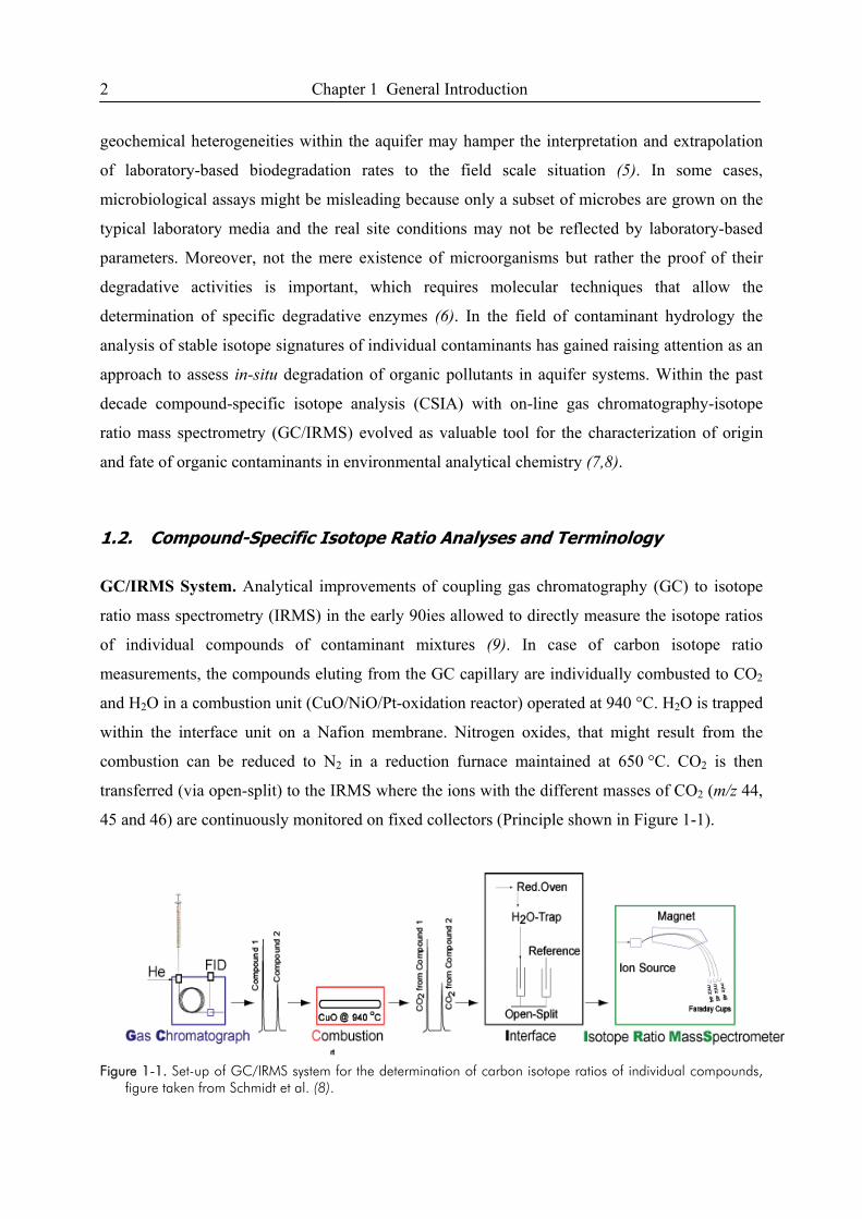
GC/IRMS System. Analytical improvements of coupling gas chromatography (GC) to isotope
ratio mass spectrometry (IRMS) in the early 90ies allowed to directly measure the isotope ratios
of individual compounds of contaminant mixtures (9). In case of carbon isotope ratio
measurements, the compounds eluting from the GC capillary are individually combusted to CO2
and H2O in a combustion unit (CuO/NiO/Pt-oxidation reactor) operated at 940 °C. H2O is trapped
within the interface unit on a Nafion membrane. Nitrogen oxides, that might result from the
combustion can be reduced to N2 in a reduction furnace maintained at 650 °C. CO2 is then
transferred (via open-split) to the IRMS where the ions with the different masses of CO2 (m/z 44,
45 and 46) are continuously monitored on fixed collectors (Principle shown in Figure 1-1).
Figure 1-1. Set-up of GC/IRMS system for the determination of carbon isotope ratios of individual compounds,
figure taken from Schmidt et al. (8).
Chapter 1 General Introduction 3
Terminology. Stable carbon isotope analysis involves measurement of the two stable isotopes of
carbon, 12C and 13C. Isotopic compositions are reported in per mill deviation (‰) relative to an
international standard using the conventional δ-notation (δ13C):
δ13C = (Rsample / Rstandard -1) x 1000
where Rsample and Rstandard are the ratios of the heavy isotope to the light isotope (13C/12C) of a
compound and of the international standard. The standard reference material for carbon isotope
analyses is VPDB (10). The relative changes in isotope signatures are expressed with the
fractionation factor α, defined as:
α = Rproduct/Rreactant
For carbon isotope ratios R represents the ratio of the heavy to the light isotope (13C/12C). Values
of α are derived from experimental results by using the simple form of the Rayleigh equation
after Mariotti et al. (11):
Rt/R0 = (Ct/C0) (α-1) = f (α-1)
where α is the isotope fractionation factor, Rt and R0 are the isotope ratios (13C/12C) of the
residual contaminant and the initial, unreacted compound, respectively and Ct/C0 is the fraction
(f) of compound remaining at time t. In the literature isotope changes are commonly expressed as
the enrichment factor ε, which can be easily rearranged using the equation ε = (α-1) x 1000.
By substituting the Rayleigh equation, where Rt and R0 are the isotope ratios (13C/12C) of the
residual contaminant and the initial isotopic composition of the source, respectively, the
percentage of biodegradation (B) can be calculated:
Rt/R0 = Ct/C0 (α-1) or Rt/R0 = f (α-1)
ln Rt/R0 = ln f (α-1)
f = exp (ln (δ13Ct/1000+1)/(δ13C0/1000+1) / (α-1))
B = (1-f) x 100 (in %)
1.3. CSIA Applications in Environmental Analytical Chemistry
The application of stable isotope analysis to evaluate and quantify intrinsic degradation relies on
the fact that chemical and microbial transformation reactions are frequently associated with a
shift in the isotopic composition of the compound being degraded (12-16). This kinetic isotope
fractionation effect occurs since bonds formed by the lighter isotopes of an element (e.g. 12C-12C)
react faster than bonds formed by the heavy isotopes (e.g. 12C-13C bonds). As a consequence, the
4 Chapter 1 General Introduction
lighter isotopologues are preferentially degraded, leading to a change in the isotopic composition
of the parent compound and the product (17). The preferential degradation of molecules
containing light isotopes, leads to a progressive enrichment of the heavy isotopologues in the
remaining contaminant fraction (exemplarilly shown in Figure 1-2), while the product becomes
depleted in heavy isotopologues.
Isotope fractionation effects have been investigated mainly for aromatic hydrocarbons (e.g.
benzene, toluene) (15,18-24), fuel oxygenates (methyl tert-butyl ether) (25-27) and chlorinated
solvents (such as trichloroethene) (14,16,28-31) during aerobic and anaerobic biodegradation.
Studies demonstrated that fractionation factors may change for various microbial cultures. For
example, the aerobic degradation of toluene by an enrichment culture was not associated with
carbon isotope fractionation (16), while pure strains showed significant isotope fractionation
effects (22). Observed fractionation factors may be specific not only for the bacterial strains, but
may also be characteristic for reaction mechanisms or degradation pathways (32). As microcosm
experiments have been performed under different aquifer conditions, fractionation factors are
available for a wide range of redox conditions (e.g. oxic, nitrate-reducing, sulphate-reducing,
methanogenic). Fractionation of organic compounds was not only studied in laboratory batch
systems but also tested under simulated aquifer conditions in flow-through column experiments
(15,33,34). In addition, isotope fractionation factors of abiotic transformation reactions are
available for some chlorinated hydrocarbons (33-36). More detailed information on
environmental applications of CSIA, and various biochemical mechanisms and pathways
involved in biodegradation reactions, are reviewed by Schmidt et al. (8) and Meckenstock et al.
(7), where also an extensive compilation of various enrichment factors for aerobic and anaerobic
degradation of important groundwater contaminants can be found.
Chapter 1 General Introduction 5
-27,0
-25,0
-23,0
-21,0
-19,0
-17,0
0 50 100 150 200 250 300
Concentration [µg/L]
δ13C
[‰]
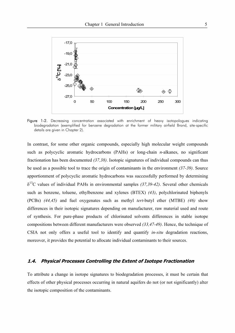
Figure 1-2. Decreasing concentration associated with enrichment of heavy isotopologues indicating
biodegradation (exemplified for benzene degradation at the former military airfield Brand, site-specific details are given in Chapter 2).
In contrast, for some other organic compounds, especially high molecular weight compounds
such as polycyclic aromatic hydrocarbons (PAHs) or long-chain n-alkanes, no significant
fractionation has been documented (37,38). Isotopic signatures of individual compounds can thus
be used as a possible tool to trace the origin of contaminants in the environment (37-39). Source
apportionment of polycyclic aromatic hydrocarbons was successfully performed by determining
δ13C values of individual PAHs in environmental samples (37,39-42). Several other chemicals
such as benzene, toluene, ethylbenzene and xylenes (BTEX) (43), polychlorinated biphenyls
(PCBs) (44,45) and fuel oxygenates such as methyl tert-butyl ether (MTBE) (46) show
differences in their isotopic signatures depending on manufacturer, raw material used and route
of synthesis. For pure-phase products of chlorinated solvents differences in stable isotope
compositions between different manufacturers were observed (33,47-49). Hence, the technique of
CSIA not only offers a useful tool to identify and quantify in-situ degradation reactions,
moreover, it provides the potential to allocate individual contaminants to their sources.
1.4. Physical Processes Controlling the Extent of Isotope Fractionation
To attribute a change in isotope signatures to biodegradation processes, it must be certain that
effects of other physical processes occurring in natural aquifers do not (or not significantly) alter
the isotopic composition of the contaminants.
6 Chapter 1 General Introduction
Advective-Dispersive Transport (Including Diffusion). Laboratory and field results evidence
that δ13C values of dissolved solvents are not significantly different from those of the DNAPL
causing the plume, source-near δ13C values may therefore be representative for the initial isotopic
composition of the source (14,50,51). In plumes not affected by biodegradation, isotope values of
dissolved chlorinated solvents remained unchanged along the groundwater flow path, indicating
that the effect of dispersion, including diffusion, has no influence on the isotopic composition of
organic compounds (48,50). Preferential diffusion of 12C molecules over 13C molecules could
only be observed to a minor extent and only in the plume fringes where vertical concentration
gradients were large (50). Hence, isotope fractionation effects associated with groundwater flow
can be neglected.
Volatilization. Evaporation of organic compounds from aqueous solution was demonstrated to
be a non-fractionating process (51), while small enrichments of 13C in the vapor phase were
observed in experiments with vaporization of pure phase compounds (51-54). A significant
isotope fractionation due to vaporization will only occur if a very high percentage of contaminant
mass is lost through evaporation, and is less relevant in natural aquifer systems, where the loss
due to vaporization is likely to be small (55). However, the observed isotope fractionation effects
may be relevant for soil vapor extraction and air sparging techniques used in remediation
processes (52).
Sorption/Desorption. The isotope effects of sorption have been characterized in several
laboratory experiments. In single-step batch experiments, no significant isotope fractionation
(±0.5‰) could be observed during equilibrium sorption on different carbonaceous sorbents
(including activated carbon, graphite, lignite and lignite coke) even if very high amounts (>95%)
of the compound has been sorbed (56,57).
In contrast, stable carbon isotope fractionation was observed to a certain extent for benzene and
toluene in multi-step batch experiments with sorption on suspended humic acid under equilibrium
conditions (58). The isotopic composition of both analytes evidenced that the lighter
isotopologues are prone to sorption, resulting in a 13C-enrichment measured in the residual
fractions. Similar observations were made for trichloroethene and toluene on peat and charcoal as
sorption materials in multi-step batch experiments (59). Kopinke et al. proposed that, depending
on aquifer properties together with plume source, length and variance with time, sorption based
isotope fractionation might play a role and may be expressed in the isotopic composition of a
migrating plume front (58). In HPLC column experiments with humic acid-coated silica
performed under simulated non-equilibrium conditions, the observed shift in δ13C values between
Chapter 1 General Introduction 7
the front and the tail of the peaks was up to 4‰ (benzene), 8‰ (2,4-dimethylphenol) and 13‰
(ο-xylene), representing enrichment factors of 0.17, 0.35, and 0.92‰, respectively (58). These
results suggest that in an expanding contaminant plume (under non-stationary aquifer conditions)
the heavier isotopologues tend to move faster and fractionation factors tend to increase with
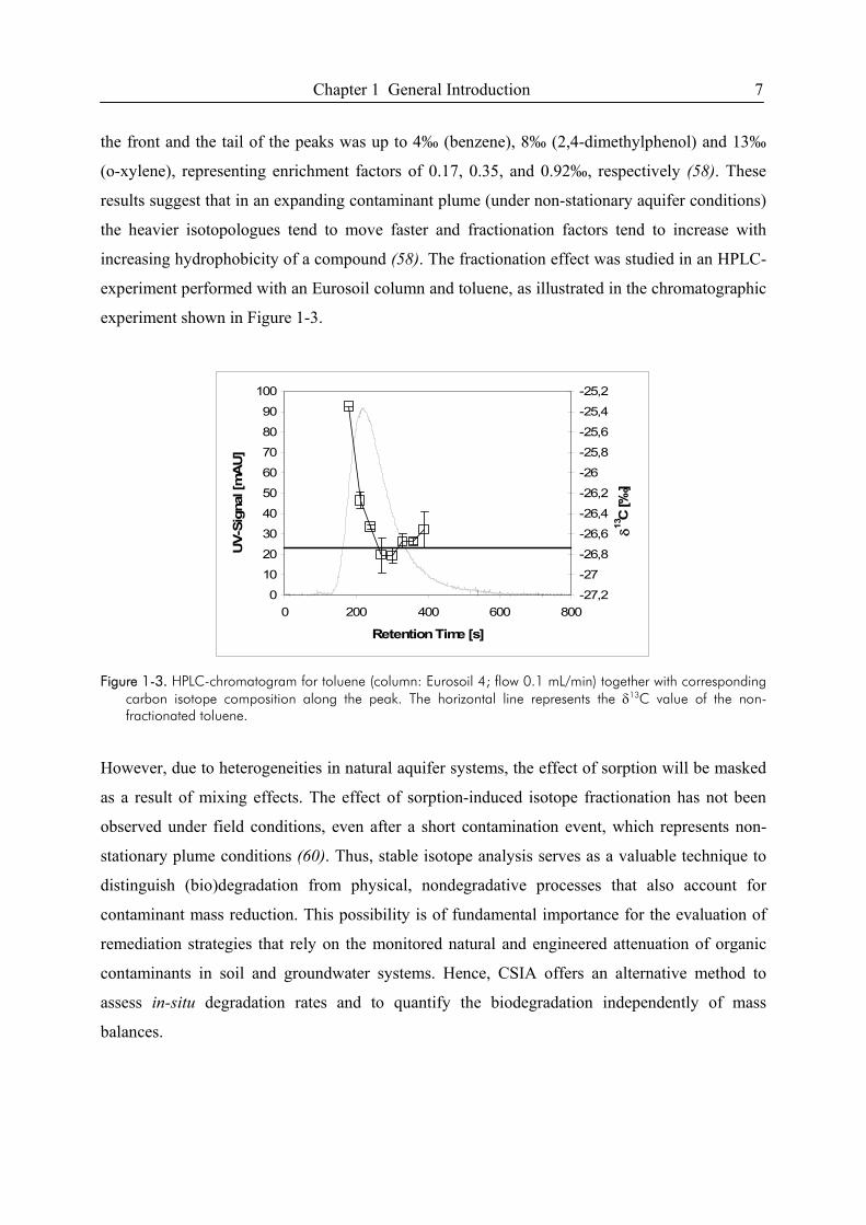
increasing hydrophobicity of a compound (58). The fractionation effect was studied in an HPLC-
experiment performed with an Eurosoil column and toluene, as illustrated in the chromatographic
experiment shown in Figure 1-3.
0
10
20
30
40
50
60
70
80
90
100
0 200 400 600 800
Retention Time [s]
UV-
Sign
al [m
AU
]
-27,2
-27
-26,8
-26,6
-26,4
-26,2
-26
-25,8
-25,6
-25,4
-25,2
δ13C
[‰]
Figure 1-3. HPLC-chromatogram for toluene (column: Eurosoil 4; flow 0.1 mL/min) together with corresponding
carbon isotope composition along the peak. The horizontal line represents the δ13C value of the non-fractionated toluene.
However, due to heterogeneities in natural aquifer systems, the effect of sorption will be masked
as a result of mixing effects. The effect of sorption-induced isotope fractionation has not been
observed under field conditions, even after a short contamination event, which represents non-
stationary plume conditions (60). Thus, stable isotope analysis serves as a valuable technique to
distinguish (bio)degradation from physical, nondegradative processes that also account for
contaminant mass reduction. This possibility is of fundamental importance for the evaluation of
remediation strategies that rely on the monitored natural and engineered attenuation of organic
contaminants in soil and groundwater systems. Hence, CSIA offers an alternative method to
assess in-situ degradation rates and to quantify the biodegradation independently of mass
balances.
8 Chapter 1 General Introduction
1.5. Scope of the Present Study
The main aim of the present work is to evaluate and demostrate the potential and limitations of
CSIA for studying sources and fate of organic contaminants at heterogeneous and complex
aquifer systems. The first chapters of this work deal with compound-specific isotope analysis
(CSIA) with on-line gas chromatography-isotope ratio mass spectrometry (GC-C-IRMS) as an
emerging technique with significant potential for tracing the origin of contaminants and
elucidating the processes controlling their fate and transport in hydrogeologic environments. As
the isotope changes are relatively independent of physical processes, CSIA has the potential for
identification and quantification of key processes occurring in natural aquifers. However, in
particular for field applications, a major drawback of CSIA is its rather poor sensitivity in terms
of amount of compound required on column. This currently limits or even prevents the use of
CSIA in some application areas such as fate studies of semi-volatile compounds, for example. To
overcome this problem, various sample extraction and injection techniques, some of which are
already well established in quantitative water analysis at trace levels will be optimized and
validated within this work for their application in CSIA studies.
To date, most field studies are limited to homogeneous aquifer systems. As CSIA is gaining more
and more popularity in the assessment of in-situ biodegradation of organic contaminants, an
increasing number of authorities and environmental consulting offices are interested in the
application of the method for contaminated site remediation. Therefore, the present work aims to
demonstrate the potential of the method at site conditions, usually confronted with in practical
contaminated site management. To this end, site investigations will focus on heterogeneous
aquifer systems to validate the applicability of the methods under complex conditions. The
performance of newly developed sample extraction and injection techniques will be tested at
different sampling locations to cover the broad variety of contaminants, concentrations and
hydrologic and geochemical conditions that are typically found at NA field investigation sites.
Limitations associated with compound-specific isotope measurements of environmental samples
will be studied and discussed. To validate the applicability of the CSIA concept for studying the
fate and transport of organic contaminants and to reliably quantify the rate of in-situ degradation
in contaminant plumes even at highly complex conditions, site investigations will be performed
at an urban, heterogeneous bedrock aquifer system. To this end groundwater samples will be
taken and isotope ratios of individual chlorinated hydrocarbons measured. Data interpretation
will be performed in order to distinguish various potential sources of the contaminants within the
Chapter 1 General Introduction 9
plume and to estimate the potential for natural attenuation in the investigated aquifer. One goal of
this study will be to quantify natural degradation processes based on compound-specific carbon
isotope data. A possible approach might be to incorporate information on isotope fractionation in
a reactive transport model in order to maximize information from isotope data gained at this
complex field site, in particular for the potential degradation intermediates. Further steps will be
to apply and evaluate prospects and limitations of CSIA under field conditions and develop a
guideline to make CSIA methods better accessible for stakeholders such as authorities and
consultants.
1.6. References
(1) U.S. Environmental Protection Agency. National primary drinking water regulations, list of drinking water contaminants & their MCLs, EPA 816-F-03-016. http://www.epa.gov/safewater/consumer/pdf/mcl.pdf 2003.
(2) U.S. Environmental Protection Agency. Use of Monitoring Natural Attenuation at Superfund, RCRA Corrective Action, and Underground Storage Tank Sites. Office of Solid Waste and Emergency Response Directive 9200.4-17. 1997.
(3) Madsen, E. L. Determining in-situ biodegradation - facts and challenges. Environ. Sci. Technol. 1991, 25, 1662-1673.
(4) Aggarwal, P. K.; Fuller, M. E.; Gurgas, M. M.; Manning, J. F.; Dillon, M. A. Use of Stable Oxygen and Carbon Isotope Analyses for Monitoring the Pathways and Rates of Intrinsic and Enhanced in Situ Biodegradation. Environ. Sci. Technol. 1997, 31, 590-596.
(5) Wiedemeier, T. H.; Swanson, M. A.; Moutoux, D. E.; Gordon, E. K.; Wilson, J. T.; Wilson, B. H.; Kampbell, D. H.; Haas, P. E.; Miller, R. N.; Hansen, J. E.; Chapelle, F. H. Technical Protocol for Evaluating Natural Attenuation of Chlorinated Solvents in Ground Water. EPA/600/R-98/128 National Risk Management Research Laboratory, Office of Research and Development, U. S. ENVIRONMENTAL PROTECTION AGENCY; Cincinnati, Ohio 1998.
(6) Stapleton, R. D.; Sayler, G. S.; Boggs, J. M.; Libelo, E. L.; Stauffer, T.; MacIntyre, W. G. Changes in Subsurface Catabolic Gene Frequencies during Natural Attenuation of Petroleum Hydrocarbons. Environ. Sci. Technol. 2000, 34, 1991-1999.
(7) Meckenstock, R. U.; Morasch, B.; Griebler, C.; Richnow, H. H. Stable isotope fractionation analysis as a tool to monitor biodegradation in contaminated acquifers. J. Contam. Hydrol. 2004, 75, 215-255.
(8) Schmidt, T. C.; Zwank, L.; Elsner, M.; Berg, M.; Meckenstock, R. U.; Haderlein, S. B. Compound-specific stable isotope analysis of organic contaminants in natural environments: a critical review of the state of the art, prospects, and future challenges. Anal. Bioanal. Chem. 2004, 378, 283-300.
(9) Hayes, J. M.; Freeman, K. H.; Popp, B. N.; Hoham, C. H. Compound-specific isotopic analyses: A novel tool for reconstruction of ancient biogeochemical processes. Org. Geochem. 1990, 16, 1115-1128.
(10) Coplen, T. B. New IUPAC guidelines for the reporting of stable hydrogen, carbon, and oxygen isotope-ratio data. J. Res. Natl. Inst. Stand. Technol. 1995, 100, 285.
(11) Mariotti, A.; Germon, J. C.; Hubert, P.; Kaiser, P.; Letolle, R.; Tardieux, A.; Tardieux, P. Experimental determination of nitrogen kinetic isotope fractionation: some principles; illustration for the denitrification and nitrification processes. Plant Soil 1981, 62, 413-430.
(12) Sturchio, N. C.; Clausen, J. L.; Heraty, L. J.; Huang, L.; Holt, B. D.; Abrajano, T. A. Chlorine isotope investigation of natural attenuation of trichloroethene in an aerobic aquifer. Environ. Sci. Technol. 1998, 32, 3037-3042.
(13) Heraty, L. J.; Fuller, M. E.; Huang, L.; Abrajano, T.; Sturchio, N. C. Isotopic fractionation of carbon and chlorine by microbial degradation of dichloromethane. Org. Geochem. 1999, 30, 793-799.
(14) Hunkeler, D.; Aravena, R.; Butler, B. J. Monitoring microbial dechlorination of tetrachloroethene (PCE) in groundwater using compound-specific stable carbon isotope ratios: Microcosm and field studies. Environ. Sci. Technol. 1999, 33, 2733-2738.
10 Chapter 1 General Introduction
(15) Meckenstock, R. U.; Morasch, B.; Warthmann, R.; Schink, B.; Annweiler, E.; Michaelis, W.; Richnow, H. H. C-13/C-12 isotope fractionation of aromatic hydrocarbons during microbial degradation. Environ. Microbiol. 1999, 1, 409-414.
(16) Sherwood Lollar, B.; Slater, G. F.; Ahad, J.; Sleep, B.; Spivack, J.; Brennan, M.; MacKenzie, P. Contrasting carbon isotope fractionation during biodegradation of trichloroethylene and toluene: Implications for intrinsic bioremediation. Org. Geochem. 1999, 30, 813-820.
(17) Hoefs, J. Stable isotope geochemistry; 4th. completely rev., upd, and enl. edition ed.; Springer Verlag: Berlin, Heidelberg, 1997.
(18) Ahad, J. M. E.; Sherwood Lollar, B.; Edwards, E. A.; Slater, G. F.; Sleep, B. E. Carbon isotope fractionation during anaerobic biodegradation of toluene: Implications for intrinsic bioremediation. Environ. Sci. Technol. 2000, 34, 892-896.
(19) Wilkes, H.; Boreham, C.; Harms, G.; Zengler, K.; Rabus, R. Anaerobic degradation and carbon isotopic fractionation of alkylbenzenes in crude oil by sulphate-reducing bacteria. Org. Geochem. 2000, 31, 101-115.
(20) Hunkeler, D.; Andersen, N.; Aravena, R.; Bernasconi, S. M.; Butler, B. J. Hydrogen and carbon isotope fractionation during aerobic biodegradation of benzene. Environ. Sci. Technol. 2001, 35, 3462-3467.
(21) Morasch, B.; Richnow, H. H.; Schink, B.; Meckenstock, R. U. Stable hydrogen and carbon isotope fractionation during microbial toluene degradation: Mechanistic and environmental aspects. Appl. Environ. Microbiol. 2001, 67, 4842-4849.
(22) Morasch, B.; Richnow, H. H.; Schink, B.; Vieth, A.; Meckenstock, R. U. Carbon and hydrogen stable isotope fractionation during aerobic bacterial degradation of aromatic hydrocarbons. Appl. Environ. Microbiol. 2002, 68, 5191-5194.
(23) Mancini, S. A.; Ulrich, A. C.; Lacrampe-Couloume, G.; Sleep, B.; Edwards, E. A.; Sherwood Lollar, B. Carbon and hydrogen isotopic fractionation during anaerobic biodegradation of benzene. Appl. Environ. Microbiol. 2003, 69, 191-198.
(24) Morasch, B.; Richnow, H. H.; Vieth, A.; Schink, B.; Meckenstock, R. U. Stable isotope fractionation caused by glycyl radical enzymes during bacterial degradation of aromatic compounds. Appl. Environ. Microbiol. 2004, 70, 2935-2940.
(25) Hunkeler, D.; Butler, B. J.; Aravena, R.; Barker, J. F. Monitoring biodegradation of methyl tert-butyl ether (MTBE) using compound-specific carbon isotope analysis. Environ. Sci. Technol. 2001, 35, 676-681.
(26) Gray, J. R.; Lacrampe-Couloume, G.; Gandhi, D.; Scow, K. M.; Wilson, R. D.; Mackay, D. M.; Sherwood Lollar, B. Carbon and hydrogen isotopic fractionation during biodegradation of methyl tert-butyl ether. Environ. Sci. Technol. 2002, 36, 1931-1938.
(27) Kolhatkar, R.; Kuder, T.; Philp, P.; Allen, J.; Wilson, J. T. Use of compound-specific stable carbon isotope analyses to demonstrate anaerobic biodegradation of MTBE in groundwater at a gasoline release site. Environ. Sci. Technol. 2002, 36, 5139-5146.
(28) Bloom, Y.; Aravena, R.; Hunkeler, D.; Edwards, E.; Frape, S. K. Carbon isotope fractionation during microbial dechlorination of trichloroethene, cis-1,2-dichloroethene, and vinyl chloride: Implications for assessment of natural attenuation. Environ. Sci. Technol. 2000, 34, 2768-2772.
(29) Slater, G. F.; Sherwood Lollar, B.; Sleep, B. E.; Edwards, E. A. Variability in carbon isotopic fractionation during biodegradation of chlorinated ethenes: Implications for field applications. Environ. Sci. Technol. 2001, 35, 901-907.
(30) Barth, J. A. C.; Slater, G.; Schüth, C.; Bill, M.; Downey, A.; Larkin, M.; Kalin, R. M. Carbon isotope fractionation during aerobic biodegradation of trichloroethene by Burkholderia cepacia G4: a tool to map degradation mechanisms. Appl. Environ. Microbiol. 2002, 68, 1728-1734.
(31) Chu, K. H.; Mahendra, S.; Song, D. L.; Conrad, M. E.; Alvarez-Cohen, L. Stable carbon isotope fractionation during aerobic biodegradation of chlorinated ethenes. Environ. Sci. Technol. 2004, 38, 3126-3130.
(32) Hirschorn, S. K.; Dinglasan, M. J.; Elsner, M.; Mancini, S. A.; Lacrampe-Couloume, G.; Edwards, E. A.; Sherwood Lollar, B. Pathway dependent isotopic fractionation during aerobic biodegradation of 1,2-dichloroethane. Environ. Sci. Technol. 2004, 38, 4775-4781.
(33) Shouakar-Stash, O.; Frape, S. K.; Drimmie, R. J. Stable hydrogen, carbon and chlorine isotope measurements of selected chlorinated organic solvents. J. Contam. Hydrol. 2003, 60, 211-228.
(34) VanStone, N. A.; Focht, R. M.; Mabury, S. A.; Sherwood Lollar, B. Effect of iron type on kinetics and carbon isotopic enrichment of chlorinated ethylenes during abiotic reduction on Fe(0). Ground Water 2004, 42, 268-276.
(35) Dayan, H.; Abrajano, T.; Sturchio, N. C.; Winsor, L. Carbon isotopic fractionation during reductive dehalogenation of chlorinated ethenes by metallic iron. Org. Geochem. 1999, 30, 755-763.
(36) Bill, M.; Schüth, C.; Barth, J. A. C.; Kalin, R. M. Carbon isotope fractionation during abiotic reductive dehalogenation of trichloroethene (TCE). Chemosphere 2001, 44, 1281-1286.
Chapter 1 General Introduction 11
(37) O'Malley, V. P.; Abrajano, T. A.; Hellou, J. Determination of the 13C/12C ratios of individual PAH from environmental samples: can PAH sources be apportioned? Org. Geochem. 1994, 21, 809-822.
(38) Mansuy, L.; Philp, R. P.; Allen, J. Source identification of oil spills based on the isotopic composition of individual components in weathered oil samples. Environ. Sci. Technol. 1997, 31, 3417-3425.
(39) Hammer, B. T.; Kelley, C. A.; Coffin, R. B.; Cifuentes, L. A.; Mueller, J. G. Delta C-13 values of polycyclic aromatic hydrocarbons collected from two creosote-contaminated sites. Chem. Geol. 1998, 152, 43-58.
(40) Mazeas, L.; Budzinski, H. Quantification of petrogenic PAH in marine sediment using molecular stable carbon isotopic ratio measurement. Analusis 1999, 27, 200-203.
(41) Okuda, T.; Kumata, H.; Naraoka, H.; Takada, H. Origin of atmospheric polycyclic aromatic hydrocarbons (PAHs) in Chinese cities solved by compound-specific stable carbon isotopic analyses. Org. Geochem. 2002, 33, 1737-1745.
(42) Stark, A.; Abrajano, T.; Hellou, J.; Metcalf-Smith, J. L. Molecular and isotopic characterization of polycyclic aromatic hydrocarbon distribution and sources at the international segment of the St. Lawrence River. Org. Geochem. 2003, 34, 225-237.
(43) Dempster, H. S.; Sherwood Lollar, B.; Feenstra, S. Tracing organic contaminants in groundwater: A new methodology using compound-specific isotopic analysis. Environ. Sci. Technol. 1997, 31, 3193-3197.
(44) Jarman, W. M.; Hilkert, A.; Bacon, C. E.; Collister, J. W.; Ballschmiter, K.; Risebrough, R. W. Compound-specific carbon isotopic analysis of Aroclors, Clophens, Kaneclors, and Phenoclors. Environ. Sci. Technol. 1998, 32, 833-836.
(45) Drenzek, N. J.; Tarr, C. H.; Eglinton, T. I.; Heraty, L. J.; Sturchio, N. C.; Shiner, V. J.; Reddy, C. M. Stable chlorine and carbon isotopic compositions of selected semi-volatile organochlorine compounds. Org. Geochem. 2002, 33, 437-444.
(46) Smallwood, B. J.; Philp, R. P.; Burgoyne, T. W.; Allen, J. D. The use of stable isotopes to differentiate specific source markers for MTBE. Environ. Forensics 2001, 2, 215-221.
(47) van Warmerdam, E. M.; Frape, S. K.; Aravena, R.; Drimmie, R. J.; Flatt, H.; Cherry, J. A. Stable chlorine and carbon isotope measurements of selected chlorinated organic solvents. Appl. Geochem. 1995, 10, 547-552.
(48) Beneteau, K. M.; Aravena, R.; Frape, S. K. Isotopic characterization of chlorinated solvents-laboratory and field results. Org. Geochem. 1999, 30, 739-753.
(49) Jendrzejewski, N.; Eggenkamp, H. G. M.; Coleman, M. L. Characterisation of chlorinated hydrocarbons from chlorine and carbon isotopic compositions: scope of application to environmental problems. Appl. Geochem. 2001, 16, 1021-1031.
(50) Hunkeler, D.; Chollet, N.; Pittet, X.; Aravena, R.; Cherry, J. A.; Parker, B. L. Effect of source variability and transport processes on carbon isotope ratios of TCE and PCE in two sandy aquifers. J. Contam. Hydrol. 2004, 74, 265-282.
(51) Slater, G. F.; Dempster, H. S.; Sherwood Lollar, B.; Ahad, J. Headspace analysis: A new application for isotopic characterization of dissolved organic contaminants. Environ. Sci. Technol. 1999, 33, 190-194.
(52) Harrington, R. R.; Poulson, S. R.; Drever, J. I.; Colberg, P. J. S.; Kelly, E. F. Carbon isotope systematics of monoaromatic hydrocarbons: vaporization and adsorption experiments. Org. Geochem. 1999, 30, 765-775.
(53) Huang, L.; Sturchio, N. C.; Abrajano, T.; Heraty, L. J.; Holt, B. D. Carbon and chlorine isotope fractionation of chlorinated aliphatic hydrocarbons by evaporation. Org. Geochem. 1999, 30, 777-785.
(54) Poulson, S. R.; Drever, J. I. Stable isotope (C, Cl, and H) fractionation during vaporization of trichloroethylene. Environ. Sci. Technol. 1999, 33, 3689-3694.
(55) Wang, Y.; Huang, Y. Hydrogen isotopic fractionation of petroleum hydrocarbons during vaporization: implications for assessing artificial and natural remediation of petroleum contamination. Appl. Geochem. 2003, 18, 1641-1651.
(56) Slater, G. F.; Ahad, J. M. E.; Sherwood Lollar, B.; Allen-King, R.; Sleep, B. Carbon isotope effects resulting from equilibrium sorption of dissolved VOCs. Anal. Chem. 2000, 72, 5669-5672.
(57) Schüth, C.; Taubald, H.; Bolaño, N.; Maciejczyk, K. Carbon and hydrogen isotope effects during sorption of organic contaminants on carbonaceous materials. J. Contam. Hydrol. 2003, 64, 269-281.
(58) Kopinke, F. D.; Georgi, A.; Voskamp, M.; Richnow, H. H. Carbon isotope fractionation of organic contaminants due to retardation on humic substances: Implications for natural attenuation studies in aquifers. Environ. Sci. Technol. 2005, 39, 6052-6062.
(59) Botalova, O. Sorption-based isotope fractionation. Master thesis, Center for Applied Geoscience, Eberhard-Karls-University. Tübingen, 2006: 49 pp.
(60) Fischer, A.; Bauer, J.; Meckenstock, R. U.; Stichler, W.; Griebler, C.; Maloszewski, P.; Kästner, M.; Richnow, H. H. A multitracer test proving the reliability of Rayleigh equation-based approach for assessing biodegradation in a BTEX contaminated aquifer. Environ. Sci. Technol. 2006, 40, 4245-4252.
12 Chapter 2 CSIA of volatile organic compounds at trace levels
2. Compound-Specific Isotope Analysis of Volatile Organic
Compounds (VOCs) at Trace Levels
2.1. Introduction
Due to their widespread use, chlorinated hydrocarbons (CHCs) and soluble fuel compounds such
as tetra- and trichloroethene, benzene, toluene, ethylbenzene, and xylene-isomers (BTEX) are
among the most prevalent volatile organic groundwater contaminants. In environmental sciences,
compound-specific isotope analysis (CSIA) is an emerging technique for the allocation of
contaminant sources, and for the identification and quantification of (bio)transformation reactions
on scales ranging from batch experiments to field sites (1-3). A limitation of CSIA, especially in
field applications, is the fact that an accurate carbon isotope ratio measurement requires at least 1
nmol carbon of a given compound on column (optimal chromatographic resolution and peak
sharpness presumed). Turner et al. emphasized the need for developing reliable techniques for
isotope measurements on compounds at field concentrations in the low μg/L-range to assess
microbial degradation processes and reactive transport at catchment scales and to address
pertinent research and application areas such as fate studies of pesticides, and differentiation
between diffuse and point sources of contaminants based on their isotope signature (3). These
limitations and requirements motivate the development of efficient enrichment techniques to
lower method detection limits in GC/IRMS applications.
To overcome this limitation, preconcentration techniques for on-line CSIA have been developed
to meet the instrumental sensitivity of the GC/IRMS. For volatile organic compounds solid-phase
microextraction (SPME) and purge-and-trap (P&T) have been shown to be the most effective
techniques to preconcentrate the analytes prior to CSIA without compromising accurate and
precise isotope ratio determinations (4,5). For compound-specific isotope analysis SPME has
been applied directly in the water phase (direct immersion) as well as in the headspace of the
sample (4,6,7). SPME is a solvent-free, highly sensitive and rapid extraction method for the
determination of analytes (8). The SPME device consists of a re-usable, polymer-coated fiber in a
syringe-like holder. The fiber is exposed to the sample matrix, where analytes partition between
coating and the sample (8,9). According to their sorption affinity, compounds are extracted into
the stationary phase of the fiber and then thermally desorbed in the gas chromatographic injector.
P&T is commonly referred to as a dynamic headspace technique where the compounds are
Chapter 2 CSIA of volatile organic compounds at trace levels 13
purged/stripped from the sample (e.g. water) with a stream of inert gas, subsequently trapped
directly on a sorbent or cold trap and thermally desorbed prior to analysis. P&T is implemented
in several US Environmental Protection Agency protocols for the quantification of volatiles in
drinking, waste and hazardous waste water (e.g. US EPA method 524.4 (10)) and has also been
used successfully for determining isotope ratios of a wide range of VOCs in aqueous samples at
low concentrations (5,11,12). SPME and P&T method validation included comparisons of δ13C
values determined by GC/IRMS with EA/IRMS measurements as well as comparisons of values
obtained with different injection modes (4,5,11,12). Isotopic fractionation effects of the various
processes involved in SPME and/or P&T (i.e., evaporation, sorption, desorption, and
condensation of the analytes) were within the range of analytical uncertainty (< 0.5‰) for most
of the compounds studied (4,11,12); greater deviations were found to be compound-specific
(5,11,12). Zwank et al. (5) reported that SPME lowered the method detection limits by 3-4 orders
of magnitude compared with liquid injection, while P&T extraction was the most efficient
preconcentration technique reaching method detection limits (MDLs) below 5 µg/L. In
combination with cryofocusing of analytes, P&T gave the best resolution of adjacent peaks (5).
Slight but highly reproducible deviations of the δ13C signatures compared to EA/IRMS
measurements of pure phase compounds occurred in all of the evaluated injection and
preconcentration techniques (5). Hence, the choice of the optimal technique used within the
following work depended mainly on the concentrations observed at the individual field sites and
the required method detection limits.
As P&T is the most sensitive preconcentration technique for on-line CSIA of volatile organic
compounds, a commercially available P&T system was modified to further enhance the
sensitivity to allow for GC/IRMS measurements of volatile compounds at trace concentrations.
An improvement of the sample concentration for P&T was achieved by increasing the amount of
water purged (12). The improved P&T method showed good reproducibility and high linearity
with significant deviations (> 0.5‰) from pure phase values only observable for chloroform.
MDLs for monoaromatic compounds between 0.07 and 0.35 µg/L are the lowest values reported
so far for continuous-flow isotope ratio measurements using an automated system. MDLs for
halogenated hydrocarbons were between 0.76 and 27 µg/L (12). More recently, the development
of a custom made continuous-flow purge and trap system was described which allowed for an
adaptation of the sample size and by using an ultrasonic nebuliser extremely low MDLs were
achieved (11). Although highly efficient, the instrumentation is not automated and not
commercially available.
14 Chapter 2 CSIA of volatile organic compounds at trace levels
Previous work showed that synthetic polymers in devices used for sampling groundwater, such as
flexible tubings made of polytetrafluoroethylene (PTFE), polyvinyl chloride (PVC), or
polypropylene (PP) significantly absorb organic compounds from aqueous solution (13,14). As
the commercially available P&T-GC/IRMS device was equipped with a PTFE sample transfer
loop, the present study aimed to evaluate an alternative material for sample transfer and thus, to
further increase the detection limits of a commercially available P&T system. The present work
aims to demonstrate the performance of SPME and P&T extraction techniques for determining
δ13C values of VOCs in environmental samples. To this end, site investigations are performed at
different sampling locations to cover the broad variety of contaminants, concentrations and
hydrologic and geochemical conditions that are typically found at NA field investigation sites.
Innovative sampling techniques were applied in order to extend the information attained by CSIA
measurements at contaminated sites, especially when the number of sampling wells is limited.
Major goals were to evaluate if NA processes are active and to quantify the rate of in-situ
degradation in the contaminant plumes.
2.2. Materials and Methods
Chemicals and Reagents. As a solvent for the preparation of standard solutions for CSIA,
Millipore water from a Milli-Q Plus water purification system (Millipore, Bedford, MA, USA)
was used. Aromatic hydrocarbon standards contained benzene (99.5%, Fluka, Buchs,
Switzerland), toluene (99.9%, Merck, Darmstadt, Germany), ethylbenzene (99.8%, Acros
Organics, Geel, Belgium), para-xylene (99%, Aldrich, Steinheim, Germany), n-propylbenzene
(98%, Aldrich), isopropylbenzene (99%, Aldrich), 1,3,5-trimethylbenzene (99%, Fluka), 1,2,4-
trimethylbenzene (98%, Aldrich) and 1,2,3-trimethylbenzene (90-95%, Fluka). Chlorinated
hydrocarbon standards included trans-1,2-dichloroethene (trans-DCE, 98%, Aldrich), cis-1,2-
dichloroethene (cis-DCE, 97%, Aldrich), trichloroethene (TCE, 99.5%, Merck) and
tetrachloroethene (PCE, 99.9%, Aldrich). Tests for vinyl chloride measurements were performed
with vinyl chloride solution in methanol purchased from Sigma-Aldrich. Concentration analyses
of field samples were carried out in external laboratories.
GC/IRMS Instrumentation. The compound-specific isotope ratios in the present work were
determined using a Trace gas chromatograph (Thermo Finnigan, Milan, Italy) coupled to an
isotope ratio mass spectrometer (DeltaPLUS XP; Thermo Finnigan MAT, Bremen, Germany) via
a combustion interface (GC Combustion III; Thermo Finnigan MAT) maintained at 940 °C. The
Chapter 2 CSIA of volatile organic compounds at trace levels 15
gas chromatograph was equipped with a programmable temperature vaporizer (PTV) injector
(Optic 3; ATAS GL International B.V., Veldhoven, The Netherlands). Sample introduction was
performed with a CombiPAL autosampler system. According to the recommendation given by
Zwank et al. (5) reoxidation of the CuO/NiO/Pt combustion reactor was carried out regularly
after approximately 40 measurements.
Solid-Phase Microextraction (SPME). Two different fibers, a polydimethylsiloxane (PDMS,
film thickness 100 µm) and a 75 µm Carboxen/PDMS for autosampler use, were obtained from
Supelco (Supelco, Bellefonte, PA, USA). Before use, the fibers were conditioned in the needle
heater of the CombiPAL system for 0.5-2 h and at 250-300 °C, according to the instructions
provided by the manufacturer. Aqueous samples containing only PCE and in concentration
higher than 300 µg/L were extracted using the PDMS fiber. The Carboxen/PDMS fiber was most
appropriate for samples that contained chlorinated hydrocarbons in concentrations between 15 to
40 µg/L. 18 mL of sample were placed in 20-mL headspace vials with magnetic screw caps
sealed with PTFE-coated septa. Extraction of the analytes was carried out by immersing the fiber
in the aqueous phase (direct immersion, with an agitational speed of 500 rpm) at 35 °C for
20 min. Since the samples did not contain unresolved cosolvents, direct immersion SPME could
be applied to increase extraction efficiencies (4). After extraction, the analytes were thermally
desorbed from the fiber in the splitless liner of the GC injector port for 1 min at 250 °C (100 µm
PDMS fiber) or 270 °C (75 µm Carboxen/PDMS fiber). Following each injection the fiber was
conditioned in the needle heater (maintained at 250 °C and 300 °C, respectively) for 2-3 min.
Blanks were run periodically to check for carryover.
Purge-and-Trap Sample Extraction. A purge and trap sample concentrator (Velocity XPT™)
equipped with a liquid autosampler AquaTek 70™ (both Tekmar-Dohrmann, Mason, OH, USA)
was coupled online to the PTV injector unit of the GC/IRMS. To increase sample volumes, the
autosampler tray holder was modified to carry twenty 100-mL glass bottles. Aqueous samples
were either filled into 40-mL VOC vials or into 100-mL amber glass bottles sealed with PTFE-
coated silicone septa screw caps (free of headspace). For 40-mL vials, a 25-mL aliquot of the
sample was transferred by the autosampler into a fritted sparging glassware and purged for 11
min with He (40 mL/min). For 100-mL bottles 76 mL of sample were transferred to the sparger,
purged for 16 min at a He flow of 50 mL/min; technical constraints of the autosampler did not
allow to transfer an aliquot greater than 76 mL of the sample from the bottle to the system. To
allow for purging higher sample volumes, the 25-mL fritted sparger was modified to keep 100
mL of an aqueous sample and the original sample loop was replaced by a 50 m long 1/8”-
16 Chapter 2 CSIA of volatile organic compounds at trace levels
polytetrafluoroethylene (PTFE) tubing (1.6 mm i.d.). The replacement parts (tray holder, frit
sparger and sample loop) were provided by PAS Analytik (Magdala, Germany). To further
improve the sensitivity by reducing sorptive losses, the PTFE sample loop was replaced by a
27 m long 1/8”-polyetheretherketone (PEEK) tubing (2.0 mm i.d.) purchased from MedChrom
GmbH (Eppelheim, Germany).
The purged analytes were trapped on a VOCARB 3000 (Supelco) trap at room temperature. By
heating the trap to 250 °C for 1 min, the analytes were thermodesorbed and transferred to the GC
injection port. The GC temperature program was started with the end of desorption. The injector
and transfer line temperatures of the P&T instrument were held at 250 °C. The GC was equipped
with a deactivated precolumn (0.4 m x 0.53 mm) leading through a cryofocusing unit, where the
analytes were trapped at -100 °C during transfer from the P&T instrument. The cryofocusing unit
is cooled by gas flowing through a heat exchanger immersed in a Dewar with liquid nitrogen
(LN2). The use of nitrogen gas instead of compressed air is recommended as water vapour
present in the air freezes and might block the gas flow through the heat exchanger. For the
thermal desorption process, the cryotrap was heated with a rate of 30 °C/s to 240 °C. Cooling and
heating of the trap are controlled by the OPTIC 3 control unit.
Method parameters optimized by Zwank et al. (5) were applied to the non-modified P&T-system
in order to obtain sufficient extraction efficiencies. The P&T parameters for the modified 100-mL
system were thoroughly evaluated in our recent study Jochmann et al. (12). The optimized
parameters have also been applied to the PEEK system. All P&T parameters for the three
different methods applied within the present work are summarized in the Appendix of this
chapter. The performance of the P&T-system equipped with the PEEK sample transfer loop was
tested for the most commonly detected chlorinated solvents trans-1,2-dichloroethene, cis-1,2-
dichloroethene, trichloroethene and tetrachlorethene (trans-DCE, cis-DCE, TCE and PCE).
Method parameters used for measurement of samples from the different contaminated sites, the
techniques involved and GC parameters for separation of the analytes are listed in the Appendix
of this chapter.
2.3. Description of Field Sites
KORA-Site Rosengarten-Ehestorf. VOC containing aqueous samples for analyte extraction by
SPME were obtained from a former dry-cleaning site located near Hamburg (15). A substantial
chlorinated hydrocarbon spillage into a deep unsaturated zone led to the development of a PCE
Chapter 2 CSIA of volatile organic compounds at trace levels 17
plume in the saturated zone. The location is a demonstration site for field-scale quantification of
the potential of NA in a deep large-scale aquifer as the groundwater contamination plume lies at a
depth of > 40 m. A special concern is the proximity of the local drinking water supply
downgradient of the site. Major goals were to evaluate if NA processes are active and to what
extent the contamination might effect the downstream groundwater quality by CSIA
measurements. Due to the difficulties associated with investigations in deep aquifers the number
of groundwater wells is limited. Therefore, innovative techniques were combined with CSIA to
extend the validity of only few measuring points available at the site. A dense monitoring
network would be required for point-scale isotope values as they need to be representative for the
entire aquifer system (16). Therefore, a combined approach of immission pumping tests together
with CSIA was applied to provide isotope information comprising differences owing to
heterogeneities of the aquifer system. A multilevel sampling technique was applied to provide
depth-discrete groundwater samples and a more vertically resolved profile of microbial activity
within the contaminant plume.
KORA-Site OLES-Epple. VOC containing aqueous samples for the conventional P&T
technique (40-mL vials) were obtained from a former mineral oil facility located in Stuttgart (17).
The site provides an illustrative example of an urban industrial area with multiple potential
releases of chlorinated hydrocarbons that is underlain by a complex bedrock aquifer with
preferential flow and various layers partly connected through vertical faults. East of the site,
important urban mineral springs are located, which explains the major interest in contaminant
fate by local authorities. Aim of this work was to use isotope data in combination with existing
geochemical data and hydrogeological modeling to distinguish various sources of the
contaminants within the plume and to estimate the potential of natural attenuation in the aquifers
investigated. Further details and results are given in chapters 5 and 6 of this thesis.
KORA-Sites Brand and Niedergörsdorf TL1. BTEX containing groundwater samples for the
validation of the enhanced volume P&T-GC/IRMS method were obtained at disused military
airfields located south of Berlin (18), in the state of Brandenburg. During the use of the areas,
especially beneath the fuel handling and storage facilities, massive subsurface contamination with
kerosene jet fuel occurred. Low-flow sampling of groundwater at wells that have direct contact to
the surrounding sediment allow for a relatively undisturbed point-sampling to resolve vertical
concentration gradients e.g. of contaminants and geochemical parameters. Wells are placed using
direct-push techniques; the wells are screened over the desired depth of the aquifer at which
concentration gradients were supposed to occur. Due to time-intensive, depth-discrete
18 Chapter 2 CSIA of volatile organic compounds at trace levels
groundwater sampling strategies using inflatable double packer systems and pneumatic driven
mini pumps, only 120 mL of a sample could be provided for isotopic analyses. During the whole
sampling procedure, the groundwater stayed within a closed system to minimize losses of volatile
compounds. 13C/12C-isotope ratio measurements have been performed for important volatile
groundwater contaminants such as the monoaromatics benzene, toluene, ethylbenzene and xylene
isomers (BTEX) and various isomers of trimethylbenzene.
Stuttgart – Bad Cannstatt. For VOC containing aqueous samples contaminated at trace
concentrations water was sampled at some of the mineral springs located in Stuttgart-Bad
Cannstatt. Stuttgart is ranked right after Budapest as having the second largest source of mineral
water in Europe; the total discharge rate of the system is around 500 L/s (19,20). Chlorinated
solvents, which were detected at low concentrations since 1984 in the overlying Keuper aquifer,
pose a significant risk to the resource (21). The complex hydrogeological setting of the area with
confined aquifers and artesian outflow, highly mineralised water rich in carbon dioxide, as well
as vertical interaction with under- and overlying groundwater bodies, demand special procedures
and methods to gain better information on sources and fate of the contaminants. To prevent or
minimize losses of volatile compounds during sampling, the sampling campaignes at the CO2-
rich mineral-water fountains were performed during two days in March 2008, when ambient
temperatures where below 7 °C, sampling bottles contained some drops of NaOH (to adjust the
pH to ~8), and the sampling was performed as free of disturbance as possible. Samples were
transported on ice, measured at the day of sampling and the bottles used for sampling were the
same as used for P&T-analyses to avoid losses due to storage or sample preparation.
2.4. Results
2.4.1. P&T-analysis with enhanced purge volume and PEEK sample loop
Extraction Efficiency. The extraction efficiency of the improved sample transfer was tested with
an aqueous standard solution containing trans- and cis-DCE, TCE and PCE at a concentration of
2.5, 2.6, 3.0 and 3.3 µg/L, respectively. Figure 2-1 shows a comparison of the extraction
efficiencies for the two different types of sample transfer tubing used. Extraction efficiencies for
cis-DCE (log Kow 1.86) (22), showed comparable peak heights for the PTFE- and PEEK- type
loop. For trans-DCE (log Kow of 2.08) (22), the extraction efficiency was slightly better (~10%)
for the PEEK-system. The extraction efficiencies for TCE and especially for PCE were
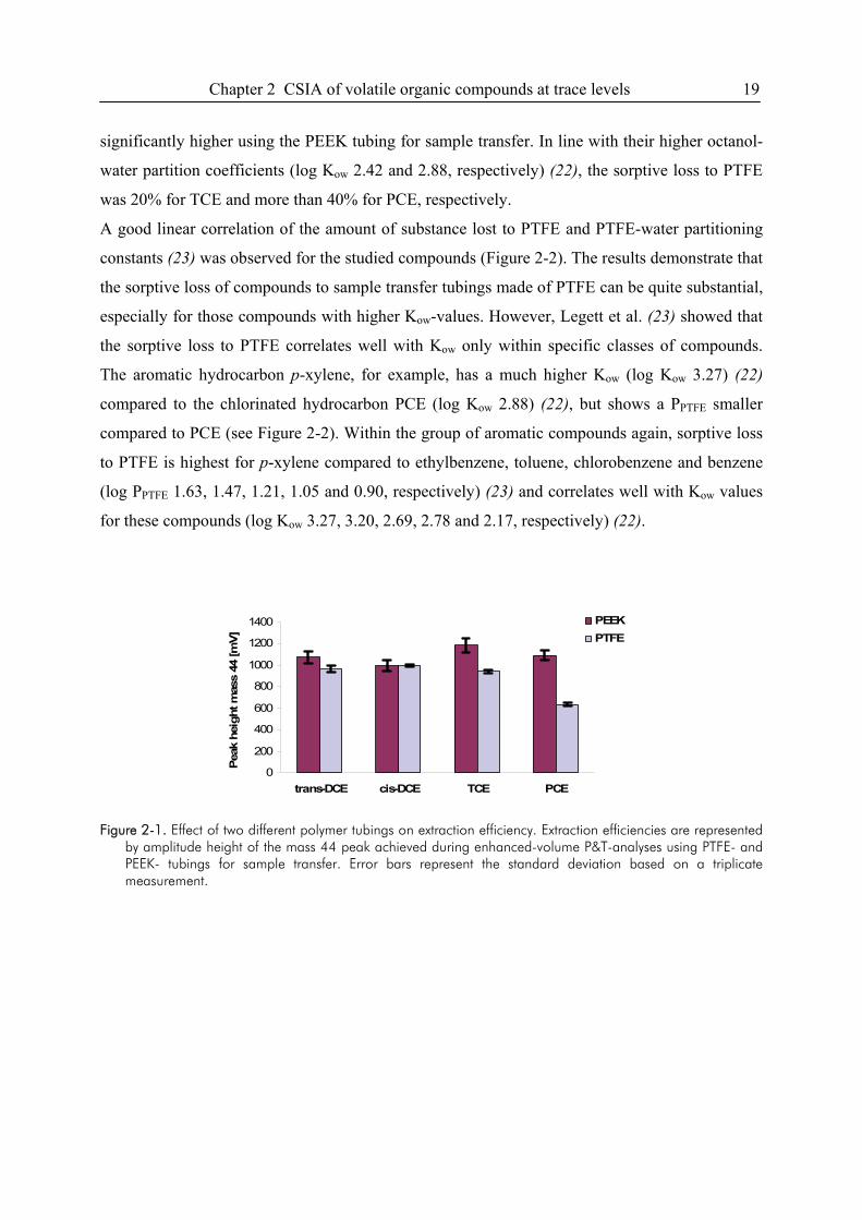
Chapter 2 CSIA of volatile organic compounds at trace levels 19
significantly higher using the PEEK tubing for sample transfer. In line with their higher octanol-
water partition coefficients (log Kow 2.42 and 2.88, respectively) (22), the sorptive loss to PTFE
was 20% for TCE and more than 40% for PCE, respectively.
A good linear correlation of the amount of substance lost to PTFE and PTFE-water partitioning
constants (23) was observed for the studied compounds (Figure 2-2). The results demonstrate that
the sorptive loss of compounds to sample transfer tubings made of PTFE can be quite substantial,
especially for those compounds with higher Kow-values. However, Legett et al. (23) showed that
the sorptive loss to PTFE correlates well with Kow only within specific classes of compounds.
The aromatic hydrocarbon p-xylene, for example, has a much higher Kow (log Kow 3.27) (22)
compared to the chlorinated hydrocarbon PCE (log Kow 2.88) (22), but shows a PPTFE smaller
compared to PCE (see Figure 2-2). Within the group of aromatic compounds again, sorptive loss
to PTFE is highest for p-xylene compared to ethylbenzene, toluene, chlorobenzene and benzene
(log PPTFE 1.63, 1.47, 1.21, 1.05 and 0.90, respectively) (23) and correlates well with Kow values
for these compounds (log Kow 3.27, 3.20, 2.69, 2.78 and 2.17, respectively) (22).
0
200
400
600
800
1000
1200
1400
trans-DCE cis-DCE TCE PCE
Peak
hei
ght m
ass
44 [m
V]
PEEKPTFE
Figure 2-1. Effect of two different polymer tubings on extraction efficiency. Extraction efficiencies are represented by amplitude height of the mass 44 peak achieved during enhanced-volume P&T-analyses using PTFE- and PEEK- tubings for sample transfer. Error bars represent the standard deviation based on a triplicate measurement.
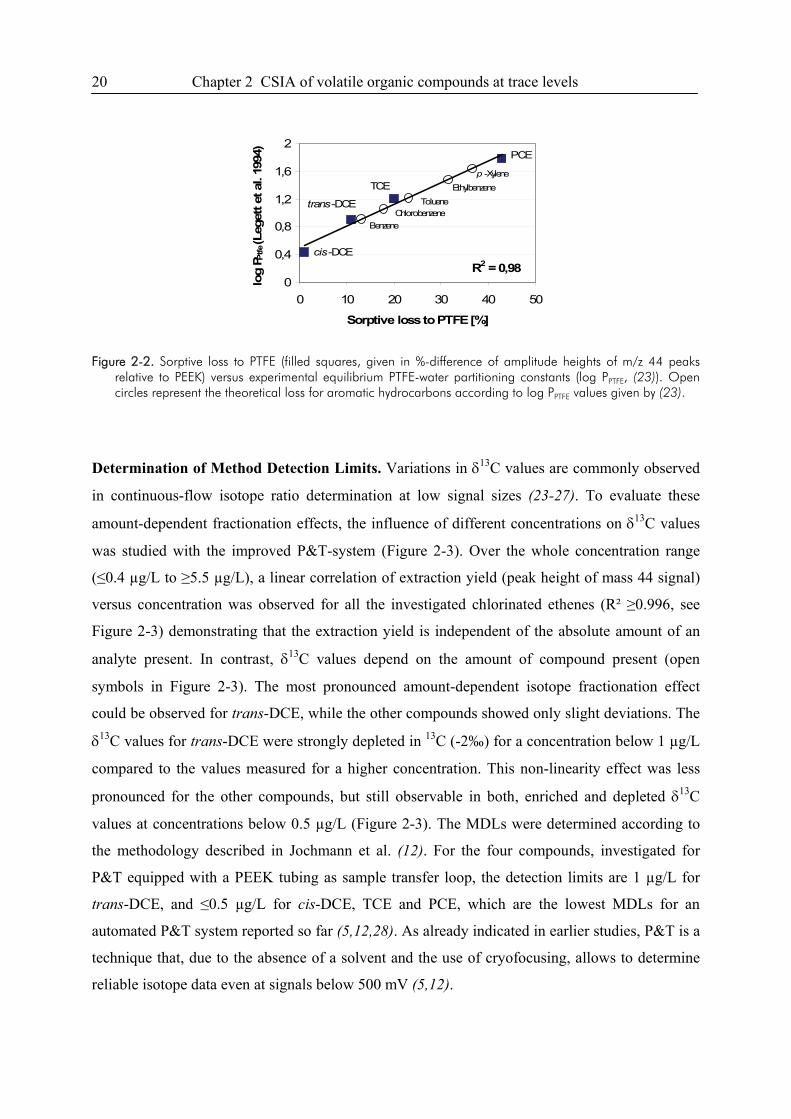
20 Chapter 2 CSIA of volatile organic compounds at trace levels
cis-DCE
trans-DCE
TCE
PCE
p -XyleneEthylbenzene
Toluene
BenzeneChlorobenzene
R2 = 0,980
0,4
0,8
1,2
1,6
2
0 10 20 30 40 50
Sorptive loss to PTFE [%]
log
P Ptfe (L
eget
t et a
l. 19
94)
Figure 2-2. Sorptive loss to PTFE (filled squares, given in %-difference of amplitude heights of m/z 44 peaks
relative to PEEK) versus experimental equilibrium PTFE-water partitioning constants (log PPTFE, (23)). Open circles represent the theoretical loss for aromatic hydrocarbons according to log PPTFE values given by (23).
Determination of Method Detection Limits. Variations in δ13C values are commonly observed
in continuous-flow isotope ratio determination at low signal sizes (23-27). To evaluate these
amount-dependent fractionation effects, the influence of different concentrations on δ13C values
was studied with the improved P&T-system (Figure 2-3). Over the whole concentration range
(≤0.4 µg/L to ≥5.5 µg/L), a linear correlation of extraction yield (peak height of mass 44 signal)
versus concentration was observed for all the investigated chlorinated ethenes (R² ≥0.996, see
Figure 2-3) demonstrating that the extraction yield is independent of the absolute amount of an
analyte present. In contrast, δ13C values depend on the amount of compound present (open
symbols in Figure 2-3). The most pronounced amount-dependent isotope fractionation effect
could be observed for trans-DCE, while the other compounds showed only slight deviations. The
δ13C values for trans-DCE were strongly depleted in 13C (-2‰) for a concentration below 1 µg/L
compared to the values measured for a higher concentration. This non-linearity effect was less
pronounced for the other compounds, but still observable in both, enriched and depleted δ13C
values at concentrations below 0.5 µg/L (Figure 2-3). The MDLs were determined according to
the methodology described in Jochmann et al. (12). For the four compounds, investigated for
P&T equipped with a PEEK tubing as sample transfer loop, the detection limits are 1 µg/L for
trans-DCE, and ≤0.5 µg/L for cis-DCE, TCE and PCE, which are the lowest MDLs for an
automated P&T system reported so far (5,12,28). As already indicated in earlier studies, P&T is a
technique that, due to the absence of a solvent and the use of cryofocusing, allows to determine
reliable isotope data even at signals below 500 mV (5,12).
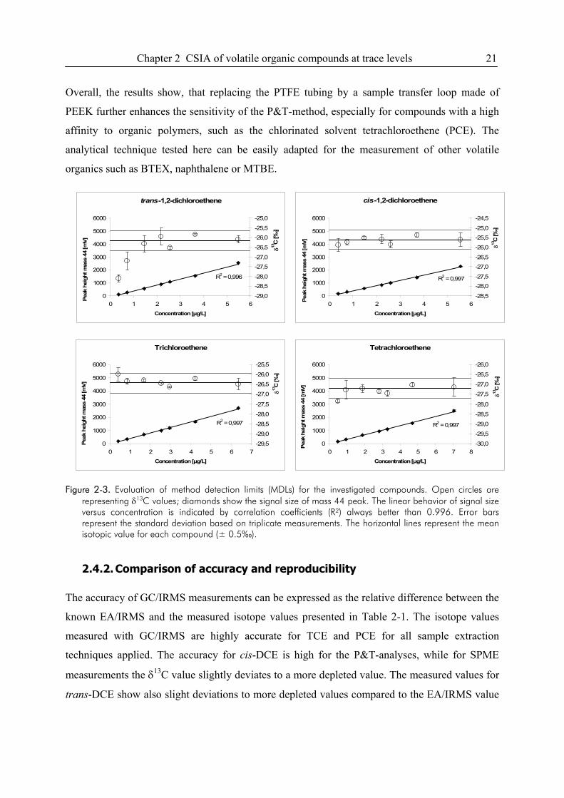
Chapter 2 CSIA of volatile organic compounds at trace levels 21
Overall, the results show, that replacing the PTFE tubing by a sample transfer loop made of
PEEK further enhances the sensitivity of the P&T-method, especially for compounds with a high
affinity to organic polymers, such as the chlorinated solvent tetrachloroethene (PCE). The
analytical technique tested here can be easily adapted for the measurement of other volatile
organics such as BTEX, naphthalene or MTBE.
Figure 2-3. Evaluation of method detection limits (MDLs) for the investigated compounds. Open circles are
representing δ13C values; diamonds show the signal size of mass 44 peak. The linear behavior of signal size versus concentration is indicated by correlation coefficients (R²) always better than 0.996. Error bars represent the standard deviation based on triplicate measurements. The horizontal lines represent the mean isotopic value for each compound (± 0.5‰).
2.4.2. Comparison of accuracy and reproducibility
The accuracy of GC/IRMS measurements can be expressed as the relative difference between the
known EA/IRMS and the measured isotope values presented in Table 2-1. The isotope values
measured with GC/IRMS are highly accurate for TCE and PCE for all sample extraction
techniques applied. The accuracy for cis-DCE is high for the P&T-analyses, while for SPME
measurements the δ13C value slightly deviates to a more depleted value. The measured values for
trans-DCE show also slight deviations to more depleted values compared to the EA/IRMS value
cis-1,2-dichloroethene
R2 = 0,997
0
1000
2000
3000
4000
5000
6000
0 1 2 3 4 5 6
Concentration [µg/L]
Peak
hei
ght m
ass
44 [m
V]
-28,5
-28,0
-27,5
-27,0
-26,5
-26,0
-25,5
-25,0
-24,5
δ13C
[‰]
trans-1,2-dichloroethene
R2 = 0,996
0
1000
2000
3000
4000
5000
6000
0 1 2 3 4 5 6
Concentration [µg/L]
Peak
hei
ght m
ass
44 [m
V]
-29,0
-28,5
-28,0
-27,5
-27,0
-26,5
-26,0
-25,5
-25,0
δ13C
[‰]
Trichloroethene
R2 = 0,997
0
1000
2000
3000
4000
5000
6000
0 1 2 3 4 5 6 7Concentration [µg/L]
Peak
hei
ght m
ass
44 [m
V]
-29,5
-29,0
-28,5
-28,0
-27,5
-27,0
-26,5
-26,0
-25,5
δ13C
[‰]
Tetrachloroethene
R2 = 0,997
0
1000
2000
3000
4000
5000
6000
0 1 2 3 4 5 6 7 8Concentration [µg/L]
Peak
hei
ght m
ass
44 [m
V]
-30,0
-29,5
-29,0
-28,5
-28,0
-27,5
-27,0
-26,5
-26,0
δ13C
[‰]
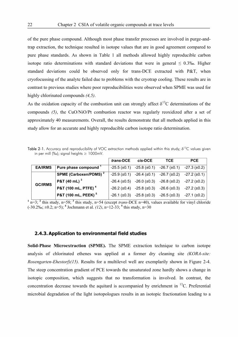
22 Chapter 2 CSIA of volatile organic compounds at trace levels
of the pure phase compound. Although most phase transfer processes are involved in purge-and-
trap extraction, the technique resulted in isotope values that are in good agreement compared to
pure phase standards. As shown in Table 1 all methods allowed highly reproducible carbon
isotope ratio determinations with standard deviations that were in general ≤ 0.3‰. Higher
standard deviations could be observed only for trans-DCE extracted with P&T, when
cryofocussing of the analyte failed due to problems with the cryotrap cooling. These results are in
contrast to previous studies where poor reproducibilities were observed when SPME was used for
highly chlorinated compounds (4,5).
As the oxidation capacity of the combustion unit can strongly affect δ13C determinations of the
compounds (5), the CuO/NiO/Pt combustion reactor was regularly reoxidized after a set of
approximately 40 measurements. Overall, the results demonstrate that all methods applied in this
study allow for an accurate and highly reproducible carbon isotope ratio determination.
Table 2-1. Accuracy and reproducibility of VOC extraction methods applied within this study; δ13C values given in per mill (‰); signal heights ≥ 1000mV.
trans-DCE cis-DCE TCE PCE
EA/IRMS Pure phase compound 1 -25.5 (±0.1) -25.8 (±0.1) -26.7 (±0.1) -27.3 (±0.2)
SPME (Carboxen/PDMS) 2 -25.9 (±0.1) -26.4 (±0.1) -26.7 (±0.2) -27.2 (±0.1)
P&T (40 mL) 3 -26.4 (±0.5) -26.0 (±0.3) -26.8 (±0.2) -27.2 (±0.2)
P&T (100 mL, PTFE) 4 -26.2 (±0.4) -25.8 (±0.3) -26.6 (±0.3) -27.2 (±0.3)GC/IRMS
P&T (100 mL, PEEK) 5 -26.1 (±0.3) -25.8 (±0.3) -26.5 (±0.3) -27.1 (±0.2)1 n=3; 2 this study, n=58; 3 this study, n=54 (except trans-DCE n=40), values available for vinyl chloride (-30.2‰; ±0.2; n=5); 4 Jochmann et al. (12), n=12-33; 5 this study, n=30
2.4.3. Application to environmental field studies
Solid-Phase Microextraction (SPME). The SPME extraction technique to carbon isotope
analysis of chlorinated ethenes was applied at a former dry cleaning site (KORA-site:
Rosengarten-Ehestorf)(15). Results for a multilevel well are exemplarily shown in Figure 2-4.
The steep concentration gradient of PCE towards the unsaturated zone hardly shows a change in
isotopic composition, which suggests that no transformation is involved. In contrast, the
concentration decrease towards the aquitard is accompanied by enrichment in 13C. Preferential
microbial degradation of the light isotopologues results in an isotopic fractionation leading to a
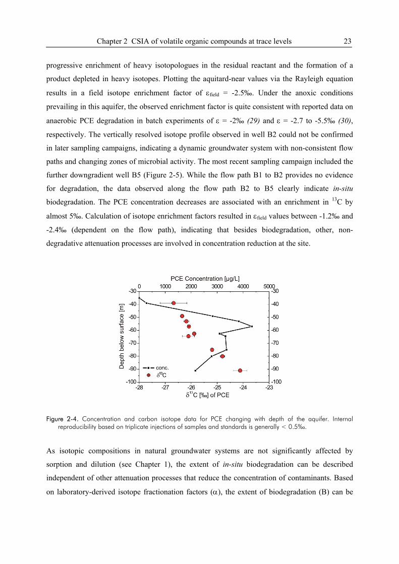
Chapter 2 CSIA of volatile organic compounds at trace levels 23
progressive enrichment of heavy isotopologues in the residual reactant and the formation of a
product depleted in heavy isotopes. Plotting the aquitard-near values via the Rayleigh equation
results in a field isotope enrichment factor of εfield = -2.5‰. Under the anoxic conditions
prevailing in this aquifer, the observed enrichment factor is quite consistent with reported data on
anaerobic PCE degradation in batch experiments of ε = -2‰ (29) and ε = -2.7 to -5.5‰ (30),
respectively. The vertically resolved isotope profile observed in well B2 could not be confirmed
in later sampling campaigns, indicating a dynamic groundwater system with non-consistent flow
paths and changing zones of microbial activity. The most recent sampling campaign included the
further downgradient well B5 (Figure 2-5). While the flow path B1 to B2 provides no evidence
for degradation, the data observed along the flow path B2 to B5 clearly indicate in-situ
biodegradation. The PCE concentration decreases are associated with an enrichment in 13C by
almost 5‰. Calculation of isotope enrichment factors resulted in εfield values between -1.2‰ and
-2.4‰ (dependent on the flow path), indicating that besides biodegradation, other, non-
degradative attenuation processes are involved in concentration reduction at the site.
Figure 2-4. Concentration and carbon isotope data for PCE changing with depth of the aquifer. Internal
reproducibility based on triplicate injections of samples and standards is generally < 0.5‰.
As isotopic compositions in natural groundwater systems are not significantly affected by
sorption and dilution (see Chapter 1), the extent of in-situ biodegradation can be described
independent of other attenuation processes that reduce the concentration of contaminants. Based
on laboratory-derived isotope fractionation factors (α), the extent of biodegradation (B) can be
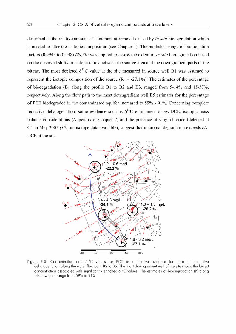
24 Chapter 2 CSIA of volatile organic compounds at trace levels
described as the relative amount of contaminant removal caused by in-situ biodegradation which
is needed to alter the isotopic composition (see Chapter 1). The published range of fractionation
factors (0.9945 to 0.998) (29,30) was applied to assess the extent of in-situ biodegradation based
on the observed shifts in isotope ratios between the source area and the downgradient parts of the
plume. The most depleted δ13C value at the site measured in source well B1 was assumed to
represent the isotopic composition of the source (R0 = -27.1‰). The estimates of the percentage
of biodegradation (B) along the profile B1 to B2 and B3, ranged from 5-14% and 15-37%,
respectively. Along the flow path to the most downgradient well B5 estimates for the percentage
of PCE biodegraded in the contaminated aquifer increased to 59% - 91%. Concerning complete
reductive dehalogenation, some evidence such as δ13C enrichment of cis-DCE, isotopic mass
balance considerations (Appendix of Chapter 2) and the presence of vinyl chloride (detected at
G1 in May 2005 (15), no isotope data available), suggest that microbial degradation exceeds cis-
DCE at the site.
Figure 2-5. Concentration and δ13C values for PCE as qualitative evidence for microbial reductive
dehalogenation along the water flow path B2 to B5. The most downgradient well of the site shows the lowest concentration associated with significantly enriched δ13C values. The estimates of biodegradation (B) along this flow path range from 59% to 91%.
1.8 - 3.2 mg/L -27.1 ‰
1.0 – 1.3 mg/L -26.2 ‰
3.4 - 4.3 mg/L -26.8 ‰
0.2 – 0.6 mg/L -22.3 ‰
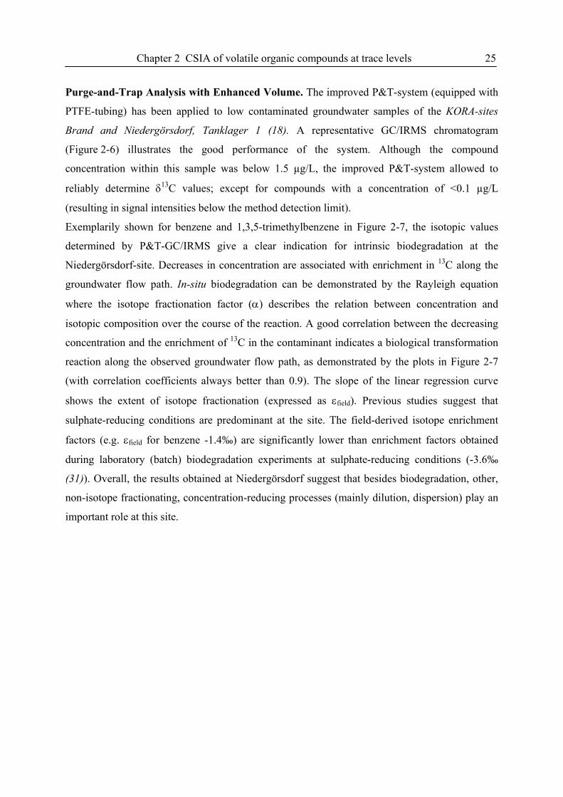
Chapter 2 CSIA of volatile organic compounds at trace levels 25
Purge-and-Trap Analysis with Enhanced Volume. The improved P&T-system (equipped with
PTFE-tubing) has been applied to low contaminated groundwater samples of the KORA-sites
Brand and Niedergörsdorf, Tanklager 1 (18). A representative GC/IRMS chromatogram
(Figure 2-6) illustrates the good performance of the system. Although the compound
concentration within this sample was below 1.5 µg/L, the improved P&T-system allowed to
reliably determine δ13C values; except for compounds with a concentration of <0.1 µg/L
(resulting in signal intensities below the method detection limit).
Exemplarily shown for benzene and 1,3,5-trimethylbenzene in Figure 2-7, the isotopic values
determined by P&T-GC/IRMS give a clear indication for intrinsic biodegradation at the
Niedergörsdorf-site. Decreases in concentration are associated with enrichment in 13C along the
groundwater flow path. In-situ biodegradation can be demonstrated by the Rayleigh equation
where the isotope fractionation factor (α) describes the relation between concentration and
isotopic composition over the course of the reaction. A good correlation between the decreasing
concentration and the enrichment of 13C in the contaminant indicates a biological transformation
reaction along the observed groundwater flow path, as demonstrated by the plots in Figure 2-7
(with correlation coefficients always better than 0.9). The slope of the linear regression curve
shows the extent of isotope fractionation (expressed as εfield). Previous studies suggest that
sulphate-reducing conditions are predominant at the site. The field-derived isotope enrichment
factors (e.g. εfield for benzene -1.4‰) are significantly lower than enrichment factors obtained
during laboratory (batch) biodegradation experiments at sulphate-reducing conditions (-3.6‰
(31)). Overall, the results obtained at Niedergörsdorf suggest that besides biodegradation, other,
non-isotope fractionating, concentration-reducing processes (mainly dilution, dispersion) play an
important role at this site.
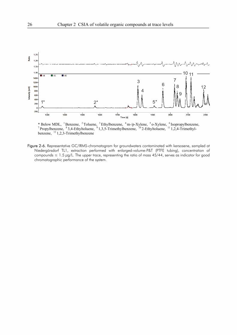
26 Chapter 2 CSIA of volatile organic compounds at trace levels
* Below MDL, 1 Benzene, 2 Toluene, 3 Ethylbenzene, 4 m-/p-Xylene, 5 o-Xylene, 6 Isopropylbenzene, 7 Propylbenzene, 8 3,4-Ethyltoluene, 9 1,3,5-Trimethylbenzene, 10 2-Ethyltoluene, 11 1,2,4-Trimethyl-benzene, 12 1,2,3-Trimethylbenzene
Figure 2-6. Representative GC/IRMS-chromatogram for groundwaters contaminated with kersosene, sampled at
Niedergörsdorf TL1, extraction performed with enlarged-volume-P&T (PTFE tubing), concentration of compounds ≤ 1.5 μg/L. The upper trace, representing the ratio of mass 45/44, serves as indicator for good chromatographic performance of the system.
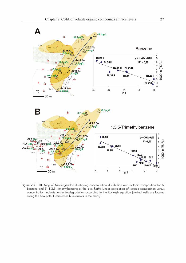
Chapter 2 CSIA of volatile organic compounds at trace levels 27
Figure 2-7. Left: Map of Niedergörsdorf illustrating concentration distribution and isotopic composition for A)
benzene and B) 1,3,5-trimethylbenzene at the site. Right: Linear correlation of isotope composition versus concentration indicate in-situ biodegradation according to the Rayleigh equation (plotted wells are located along the flow path illustrated as blue arrows in the maps).
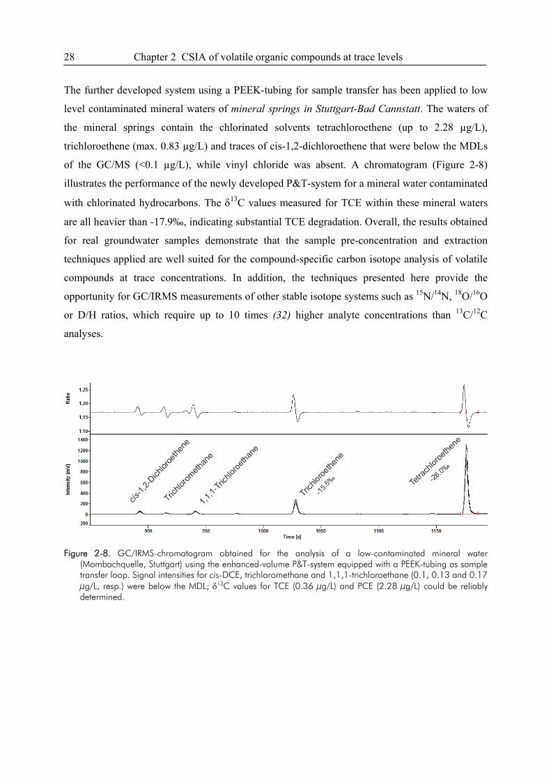
28 Chapter 2 CSIA of volatile organic compounds at trace levels
The further developed system using a PEEK-tubing for sample transfer has been applied to low
level contaminated mineral waters of mineral springs in Stuttgart-Bad Cannstatt. The waters of
the mineral springs contain the chlorinated solvents tetrachloroethene (up to 2.28 µg/L),
trichloroethene (max. 0.83 µg/L) and traces of cis-1,2-dichloroethene that were below the MDLs
of the GC/MS (<0.1 µg/L), while vinyl chloride was absent. A chromatogram (Figure 2-8)
illustrates the performance of the newly developed P&T-system for a mineral water contaminated
with chlorinated hydrocarbons. The δ13C values measured for TCE within these mineral waters
are all heavier than -17.9‰, indicating substantial TCE degradation. Overall, the results obtained
for real groundwater samples demonstrate that the sample pre-concentration and extraction
techniques applied are well suited for the compound-specific carbon isotope analysis of volatile
compounds at trace concentrations. In addition, the techniques presented here provide the
opportunity for GC/IRMS measurements of other stable isotope systems such as 15N/14N, 18O/16O
or D/H ratios, which require up to 10 times (32) higher analyte concentrations than 13C/12C
analyses.
Figure 2-8. GC/IRMS-chromatogram obtained for the analysis of a low-contaminated mineral water
(Mombachquelle, Stuttgart) using the enhanced-volume P&T-system equipped with a PEEK-tubing as sample transfer loop. Signal intensities for cis-DCE, trichloromethane and 1,1,1-trichloroethane (0.1, 0.13 and 0.17 μg/L, resp.) were below the MDL; δ13C values for TCE (0.36 μg/L) and PCE (2.28 μg/L) could be reliably determined.
Chapter 2 CSIA of volatile organic compounds at trace levels 29
2.5. References
(1) Slater, G. F. Stable isotope forensics - When isotopes work. Environ. Forensics 2003, 4, 13-23. (2) Meckenstock, R. U.; Morasch, B.; Griebler, C.; Richnow, H. H. Stable isotope fractionation analysis as a tool
to monitor biodegradation in contaminated acquifers. J. Contam. Hydrol. 2004, 75, 215-255. (3) Turner, J.; Albrechtsen, H. J.; Bonell, M.; Duguet, J. P.; Harris, B.; Meckenstock, R.; McGuire, K.; Moussa,
R.; Peters, N.; Richnow, H. H.; Sherwood Lollar, B.; Uhlenbrook, S.; van Lanen, H. Future trends in transport and fate of diffuse contaminants in catchments, with special emphasis on stable isotope applications. Hydrol. Process. 2006, 20, 205-213.
(4) Hunkeler, D.; Aravena, R. Determination of compound-specific carbon isotope ratios of chlorinated methanes, ethanes, and ethenes in aqueous samples. Environ. Sci. Technol. 2000, 34, 2839-2844.
(5) Zwank, L.; Berg, M.; Schmidt, T. C.; Haderlein, S. B. Compound-specific carbon isotope analysis of volatile organic compounds in the low-microgram per liter range. Anal. Chem. 2003, 75, 5575-5583.
(6) Dayan, H.; Abrajano, T.; Sturchio, N. C.; Winsor, L. Carbon isotopic fractionation during reductive dehalogenation of chlorinated ethenes by metallic iron. Org. Geochem. 1999, 30, 755-763.
(7) Dias, R. F.; Freeman, K. H. Carbon isotope analyses of semivolatile organic compounds in aqueous media using solid-phase microextraction and isotope ratio monitoring GC/MS. Anal. Chem. 1997, 69, 944-950.
(8) Arthur, C. L.; Pawliszyn, J. Solid phase microextraction with thermal desorption using fused silica optical fibers. Anal. Chem. 1990, 62, 2145-2148.
(9) Koziel, J.; Jia, M.; Khaled, A.; Noah, J.; Pawliszyn, J. Field air analysis with SPME device. Anal. Chim. Acta 1999, 400, 153-162.
(10) Measurement of Purgeable Organic Compounds in Water by Capillary Column Gas Chromatography/Mass Spectrometry; Method 524.4, Revision 4.1, US Environmental Protection Agency. Cincinnati, OH, 1995: 48 pp.
(11) Auer, N. R.; Manzke, B. U.; Schulz-Bull, D. E. Development of a purge and trap continuous flow system for the stable carbon isotope analysis of volatile halogenated organic compounds in water. J. Chromatogr. A 2006, 1131, 24-36.
(12) Jochmann, M. A.; Blessing, M.; Haderlein, S. B.; Schmidt, T. C. A new approach to determine method detection limits for compound-specific isotope analysis of volatile organic compounds. Rapid Commun. Mass Spectrom. 2006, 20, 3639-3648.
(13) Barcelona, M. J.; Helfrich, J. A.; Garske, E. E. Sampling Tubing Effects on Groundwater Samples. Anal. Chem. 1985, 57, 460-464.
(14) Reynolds, G. W.; Hoff, J. T.; Gillham, R. W. Sampling Bias Caused by Materials Used To Monitor Halocarbons in Groundwater. Environ. Sci. Technol. 1990, 24, 135-142.
(15) Martac, E.; Zamfirescu, D.; Teutsch, G.; KORA – TV3.5: Gemeinsamer Schlussbericht, Förderkennzeichen 02WN0437; Feldmaßstäbliche Quantifizierung des NA-Potentials in mächtigen Grundwasserleitern mit hohem Flurabstand; Beispiel: CKW-Schaden, Chemische Reinigung in Rosengarten-Ehestorf; Tübingen, 2006.
(16) Peter, A.; Steinbach, A.; Liedl, R.; Ptak, T.; Michaelis, W.; Teutsch, G. Assessing microbial degradation of o-xylene at field-scale from the reduction in mass flow rate combined with compound-specific isotope analyses. J. Contam. Hydrol. 2004, 71, 127-154.
(17) Amt für Umweltschutz Stuttgart, KORA - TV1: Forschungsbericht, Förderkennzeichen 02WN0353; Projekt 1.3: Natürlicher Abbau und Rückhalt eines komplexen Schadstoffcocktails in einem Grundwasserleiter am Beispiel des ehemaligen Mineralölwerks Epple; Stuttgart, 2007.
(18) Peter, A.; Miles, B.; Teutsch, G.; KORA – TV1: Abschlussbericht zum Forschungsvorhaben, Förderkenn-zeichen 02WN0352; Natural Attenuation (NA) und Enhanced Natural Attenuation (ENA) an typischen Mineralölstandorten am Beispiel Brand und Niedergörsdorf; Tübingen, 2007.
(19) Armbruster, H.; Dornstädter, J.; Kappelmeyer, O.; Ufrecht, W. Thermische Untersuchungen im Neckar zwischen Bad-Cannstatt und Münster zum Nachweis von Mineralwasseraustritten. Deutsche Gewässerkundliche Mitteilungen 1998, 42, 9-14.
(20) Ufrecht, W. Vulnerabilität und Schutzmaßnahmen im Quellgebiet der Stuttgarter Mineral- und Heilwässer. Zeitschrift für Angewandte Geologie 2001, 47, 47-54.
(21) Goldscheider, N.; Hötzl, H.; Käss, W.; Ufrecht, W. Combined tracer tests in the karst aquifer of the artesian mineral springs of Stuttgart, Germany. Environmental Geology 2003, 43, 922-929.
(22) Schwarzenbach, R. P.; Gschwend, P. M.; Imboden, D. M. Environmental Organic Chemistry; 2nd edition ed.; John Wiley & Sons: New York, 2003.
(23) Leggett, D. C.; Parker, L. V. Modeling the Equilibrium Partitioning of Organic Contaminants between PTFE, PVC, and Groundwater. Environ. Sci. Technol. 1994, 28, 1229-1233.
30 Chapter 2 CSIA of volatile organic compounds at trace levels
(24) Glaser, B.; Amelung, W. Determination of C-13 natural abundance of amino acid enantiomers in soil: methodological considerations and first results. Rapid Commun. Mass Spectrom. 2002, 16, 891-898.
(25) Schmitt, J.; Glaser, B.; Zech, W. Amount-dependent isotopic fractionation during compound-specific isotope analysis. Rapid Commun. Mass Spectrom. 2003, 17, 970-977.
(26) Sherwood Lollar, B.; Hirschorn, S. K.; Chartrand, M. M. G.; Lacrampe-Couloume, G. An approach for assessing total instrumental uncertainty in compound-specific carbon isotope analysis: Implications for environmental remediation studies. Anal. Chem. 2007, 79, 3469-3475.
(27) Wilcke, W.; Krauss, M.; Amelung, W. Carbon isotope signature of polycyclic aromatic hydrocarbons (PAHs): Evidence for different sources in tropical and temperate environments? Environ. Sci. Technol. 2002, 36, 3530-3535.
(28) Song, D. L.; Conrad, M. E.; Sorenson, K. S.; Alvarez-Cohen, L. Stable carbon isotope fractionation during enhanced in situ bioremediation of trichloroethene. Environ. Sci. Technol. 2002, 36, 2262-2268.
(29) Hunkeler, D.; Aravena, R.; Butler, B. J. Monitoring microbial dechlorination of tetrachloroethene (PCE) in groundwater using compound-specific stable carbon isotope ratios: Microcosm and field studies. Environ. Sci. Technol. 1999, 33, 2733-2738.
(30) Slater, G. F.; Sherwood Lollar, B.; Sleep, B. E.; Edwards, E. A. Variability in carbon isotopic fractionation during biodegradation of chlorinated ethenes: Implications for field applications. Environ. Sci. Technol. 2001, 35, 901-907.
(31) Mancini, S. A.; Ulrich, A. C.; Lacrampe-Couloume, G.; Sleep, B.; Edwards, E. A.; Sherwood Lollar, B. Carbon and hydrogen isotopic fractionation during anaerobic biodegradation of benzene. Appl. Environ. Microbiol. 2003, 69, 191-198.
(32) Schmidt, T. C.; Zwank, L.; Elsner, M.; Berg, M.; Meckenstock, R. U.; Haderlein, S. B. Compound-specific stable isotope analysis of organic contaminants in natural environments: a critical review of the state of the art, prospects, and future challenges. Anal. Bioanal. Chem. 2004, 378, 283-300.
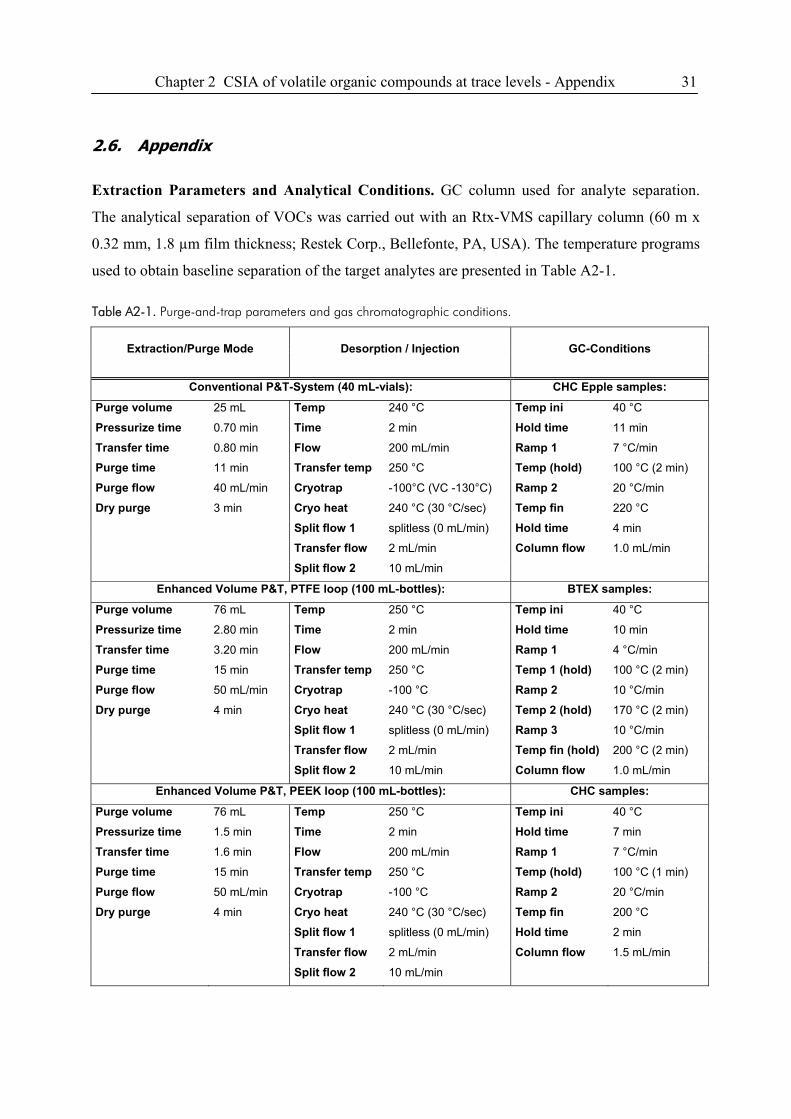
Chapter 2 CSIA of volatile organic compounds at trace levels - Appendix 31
2.6. Appendix
Extraction Parameters and Analytical Conditions. GC column used for analyte separation.
The analytical separation of VOCs was carried out with an Rtx-VMS capillary column (60 m x
0.32 mm, 1.8 µm film thickness; Restek Corp., Bellefonte, PA, USA). The temperature programs
used to obtain baseline separation of the target analytes are presented in Table A2-1.
Table A2-1. Purge-and-trap parameters and gas chromatographic conditions.
Extraction/Purge Mode Desorption / Injection GC-Conditions
Conventional P&T-System (40 mL-vials): CHC Epple samples:
Purge volume 25 mL Temp 240 °C Temp ini 40 °C
Pressurize time 0.70 min Time 2 min Hold time 11 min
Transfer time 0.80 min Flow 200 mL/min Ramp 1 7 °C/min
Purge time 11 min Transfer temp 250 °C Temp (hold) 100 °C (2 min)
Purge flow 40 mL/min Cryotrap -100°C (VC -130°C) Ramp 2 20 °C/min
Dry purge 3 min Cryo heat 240 °C (30 °C/sec) Temp fin 220 °C
Split flow 1 splitless (0 mL/min) Hold time 4 min
Transfer flow 2 mL/min Column flow 1.0 mL/min
Split flow 2 10 mL/min
Enhanced Volume P&T, PTFE loop (100 mL-bottles): BTEX samples:
Purge volume 76 mL Temp 250 °C Temp ini 40 °C
Pressurize time 2.80 min Time 2 min Hold time 10 min
Transfer time 3.20 min Flow 200 mL/min Ramp 1 4 °C/min
Purge time 15 min Transfer temp 250 °C Temp 1 (hold) 100 °C (2 min)
Purge flow 50 mL/min Cryotrap -100 °C Ramp 2 10 °C/min
Dry purge 4 min Cryo heat 240 °C (30 °C/sec) Temp 2 (hold) 170 °C (2 min)
Split flow 1 splitless (0 mL/min) Ramp 3 10 °C/min
Transfer flow 2 mL/min Temp fin (hold) 200 °C (2 min)
Split flow 2 10 mL/min Column flow 1.0 mL/min
Enhanced Volume P&T, PEEK loop (100 mL-bottles): CHC samples:
Purge volume 76 mL Temp 250 °C Temp ini 40 °C
Pressurize time 1.5 min Time 2 min Hold time 7 min
Transfer time 1.6 min Flow 200 mL/min Ramp 1 7 °C/min
Purge time 15 min Transfer temp 250 °C Temp (hold) 100 °C (1 min)
Purge flow 50 mL/min Cryotrap -100 °C Ramp 2 20 °C/min
Dry purge 4 min Cryo heat 240 °C (30 °C/sec) Temp fin 200 °C
Split flow 1 splitless (0 mL/min) Hold time 2 min
Transfer flow 2 mL/min Column flow 1.5 mL/min
Split flow 2 10 mL/min
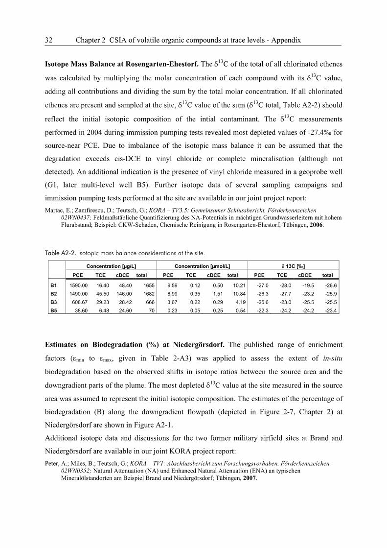
32 Chapter 2 CSIA of volatile organic compounds at trace levels - Appendix
Isotope Mass Balance at Rosengarten-Ehestorf. The δ13C of the total of all chlorinated ethenes
was calculated by multiplying the molar concentration of each compound with its δ13C value,
adding all contributions and dividing the sum by the total molar concentration. If all chlorinated
ethenes are present and sampled at the site, δ13C value of the sum (δ13C total, Table A2-2) should
reflect the initial isotopic composition of the intial contaminant. The δ13C measurements
performed in 2004 during immission pumping tests revealed most depleted values of -27.4‰ for
source-near PCE. Due to imbalance of the isotopic mass balance it can be assumed that the
degradation exceeds cis-DCE to vinyl chloride or complete mineralisation (although not
detected). An additional indication is the presence of vinyl chloride measured in a geoprobe well
(G1, later multi-level well B5). Further isotope data of several sampling campaigns and
immission pumping tests performed at the site are available in our joint project report: Martac, E.; Zamfirescu, D.; Teutsch, G.; KORA – TV3.5: Gemeinsamer Schlussbericht, Förderkennzeichen
02WN0437; Feldmaßstäbliche Quantifizierung des NA-Potentials in mächtigen Grundwasserleitern mit hohem Flurabstand; Beispiel: CKW-Schaden, Chemische Reinigung in Rosengarten-Ehestorf; Tübingen, 2006.
Table A2-2. Isotopic mass balance considerations at the site.
Concentration [µg/L] Concentration [µmol/L] δ 13C [‰]
PCE TCE cDCE total PCE TCE cDCE total PCE TCE cDCE total
B1 1590.00 16.40 48.40 1655 9.59 0.12 0.50 10.21 -27.0 -28.0 -19.5 -26.6B2 1490.00 45.50 146.00 1682 8.99 0.35 1.51 10.84 -26.3 -27.7 -23.2 -25.9B3 608.67 29.23 28.42 666 3.67 0.22 0.29 4.19 -25.6 -23.0 -25.5 -25.5B5 38.60 6.48 24.60 70 0.23 0.05 0.25 0.54 -22.3 -24.2 -24.2 -23.4
Estimates on Biodegradation (%) at Niedergörsdorf. The published range of enrichment
factors (εmin to εmax, given in Table 2-A3) was applied to assess the extent of in-situ
biodegradation based on the observed shifts in isotope ratios between the source area and the
downgradient parts of the plume. The most depleted δ13C value at the site measured in the source
area was assumed to represent the initial isotopic composition. The estimates of the percentage of
biodegradation (B) along the downgradient flowpath (depicted in Figure 2-7, Chapter 2) at
Niedergörsdorf are shown in Figure A2-1.
Additional isotope data and discussions for the two former military airfield sites at Brand and
Niedergörsdorf are available in our joint KORA project report: Peter, A.; Miles, B.; Teutsch, G.; KORA – TV1: Abschlussbericht zum Forschungsvorhaben, Förderkennzeichen
02WN0352; Natural Attenuation (NA) und Enhanced Natural Attenuation (ENA) an typischen Mineralölstandorten am Beispiel Brand und Niedergörsdorf; Tübingen, 2007.
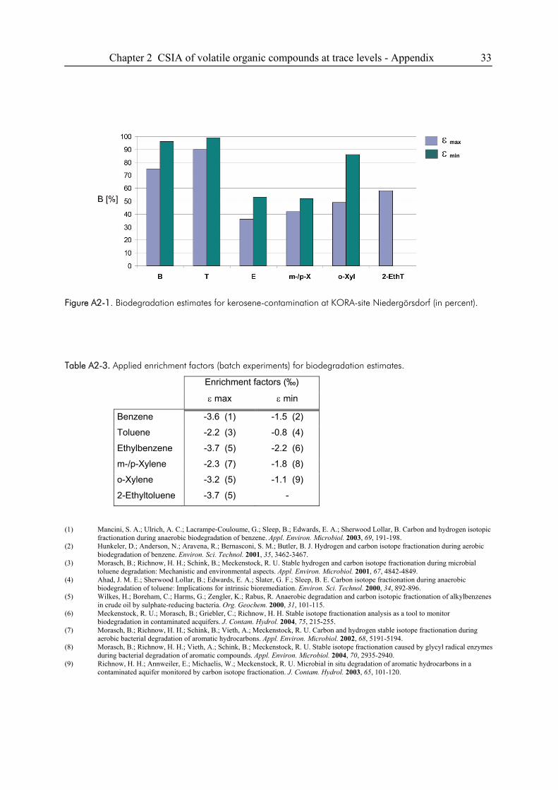
Chapter 2 CSIA of volatile organic compounds at trace levels - Appendix 33
Figure A2-1. Biodegradation estimates for kerosene-contamination at KORA-site Niedergörsdorf (in percent).
Table A2-3. Applied enrichment factors (batch experiments) for biodegradation estimates.
Enrichment factors (‰)
ε max ε min
Benzene -3.6 (1) -1.5 (2)
Toluene -2.2 (3) -0.8 (4)
Ethylbenzene -3.7 (5) -2.2 (6)
m-/p-Xylene -2.3 (7) -1.8 (8)
o-Xylene -3.2 (5) -1.1 (9)
2-Ethyltoluene -3.7 (5) -
(1) Mancini, S. A.; Ulrich, A. C.; Lacrampe-Couloume, G.; Sleep, B.; Edwards, E. A.; Sherwood Lollar, B. Carbon and hydrogen isotopic
fractionation during anaerobic biodegradation of benzene. Appl. Environ. Microbiol. 2003, 69, 191-198. (2) Hunkeler, D.; Anderson, N.; Aravena, R.; Bernasconi, S. M.; Butler, B. J. Hydrogen and carbon isotope fractionation during aerobic
biodegradation of benzene. Environ. Sci. Technol. 2001, 35, 3462-3467. (3) Morasch, B.; Richnow, H. H.; Schink, B.; Meckenstock, R. U. Stable hydrogen and carbon isotope fractionation during microbial
toluene degradation: Mechanistic and environmental aspects. Appl. Environ. Microbiol. 2001, 67, 4842-4849. (4) Ahad, J. M. E.; Sherwood Lollar, B.; Edwards, E. A.; Slater, G. F.; Sleep, B. E. Carbon isotope fractionation during anaerobic
biodegradation of toluene: Implications for intrinsic bioremediation. Environ. Sci. Technol. 2000, 34, 892-896. (5) Wilkes, H.; Boreham, C.; Harms, G.; Zengler, K.; Rabus, R. Anaerobic degradation and carbon isotopic fractionation of alkylbenzenes
in crude oil by sulphate-reducing bacteria. Org. Geochem. 2000, 31, 101-115. (6) Meckenstock, R. U.; Morasch, B.; Griebler, C.; Richnow, H. H. Stable isotope fractionation analysis as a tool to monitor
biodegradation in contaminated acquifers. J. Contam. Hydrol. 2004, 75, 215-255. (7) Morasch, B.; Richnow, H. H.; Schink, B.; Vieth, A.; Meckenstock, R. U. Carbon and hydrogen stable isotope fractionation during
aerobic bacterial degradation of aromatic hydrocarbons. Appl. Environ. Microbiol. 2002, 68, 5191-5194. (8) Morasch, B.; Richnow, H. H.; Vieth, A.; Schink, B.; Meckenstock, R. U. Stable isotope fractionation caused by glycyl radical enzymes
during bacterial degradation of aromatic compounds. Appl. Environ. Microbiol. 2004, 70, 2935-2940. (9) Richnow, H. H.; Annweiler, E.; Michaelis, W.; Meckenstock, R. U. Microbial in situ degradation of aromatic hydrocarbons in a
contaminated aquifer monitored by carbon isotope fractionation. J. Contam. Hydrol. 2003, 65, 101-120.
34 Chapter 3 CSIA of semi-volatile organic compounds at trace levels
3. Semi-Volatile Contaminants at Trace Concentrations:
Evaluation of a Large Volume Injection – GC/IRMS-Method
3.1. Introduction
Compound-specific isotope analysis (CSIA) allows to determine the isotopic composition of
individual contaminants by hyphenated gas chromatography and isotope ratio mass spectrometry
(GC/IRMS) with applications ranging from pharmacology, doping analysis, food adulteration to
the broad field of forensic and environmental studies (1). Especially in the past decade, CSIA has
emerged as a mature technique to investigate both the fate and the source of organic contaminants
in environmental forensics (2). Polycyclic aromatic hydrocarbons (PAHs) are ubiquitous
environmental contaminants, naturally occurring in coal, crude oil and gasoline and their
byproducts, e.g. coal tar or creosote. PAHs are primarily derived through combustion processes
of organic materials, such as wood or fossil fuels (3). For example, PAHs are often found at coal
gasification sites, persistently impairing the quality of soil, water and air. Several studies have
demonstrated the usefulness of compound-specific isotope analysis as a tool for the
apportionment of multiple sources of PAH contaminants in the environment (4-8).
IRMS detectors are designed for measuring isotope ratios with a very high precision at or near
their natural abundance; four orders of magnitude greater than with a conventional mass
spectrometer (9). Typically, 1 nmol carbon of each analyte is necessary for an adequate and
reliable determination of δ13C with GC/IRMS instruments (9,10). That means, in case of a 1µL-
splitless injection a concentration of 83 mg/L for tetrachloroethene, and 13 mg/L for naphthalene
is demanded in the solvent extract. A requirement that would premise aqueous concentrations
that are often much higher than actually found at a contaminated field site, especially at the
fringes of a plume. With increasing demand of lowering detection limits in GC/IRMS
applications, efficient methods for preconcentration of the analytes and improved injection
techniques have been developed. Methods that were evaluated for this purpose include, in order
of increasing sensitivity, split/splitless injection (11,12), on-column injection (12), headspace
methods (13-15), solid-phase microextraction (SPME) (12,16-19), and the purge and trap (P&T)
extraction technique (12,20,21) as method with the lowest detection limits. In quantitative
analysis of semi-volatile compounds such as PAHs, large volume injection (LVI) techniques for
gas chromatography have been developed that can easily improve sensitivity by injecting larger
Chapter 3 CSIA of semi-volatile organic compounds at trace levels 35
volumes instead of injecting the conventional 1 to 2 µL of a solvent extract into the capillary GC
system. While SPME and P&T are well established methods for the compound-specific isotope
analysis of individual organic compounds at trace concentrations, the application of large volume
injection techniques has been restricted to quantitative analysis. LVI techniques have been
applied to environmental measurements since the early 1990s (22); most of the methods are
based on programmed temperature vaporizer (PTV) injectors where the sample is injected at a
temperature below the boiling point of the solvent. The solvent is subsequentially evaporated
from the liner while simultaneously the less volatile compounds are trapped in the cold liner (23).
During the last decade a number of papers applying large volume injection techniques to the
quantitative analysis of semi-volatile compounds such as polychlorinated biphenyls, pesticides
and polycyclic aromatic hydrocarbons have been published (22-25).
It has been shown that isotope fractionation during sample injection may lead to systematic errors
due to mass discrimination effects (26-28). Large volume sample introduction using a PTV-
split/splitless-injector might be sensitive to isotope fractionation, e.g. due to the process of
solvent evaporation or adsorption of analytes to the liner packing. Therefore, particular attention
should be paid to the possibility of isotope fractionation associated with the application of this
new method in GC/IRMS. This work presents a method validation for a PTV-based large volume
injection technique linked with a GC/IRMS device. A PTV-based solvent-split injection
technique where the sample is injected at temperatures below the boiling point of the solvent was
applied. The solvent is subsequentially vented via the split outlet, while the analytes of interest
are retained on the liner packing. The PTV is then heated with a defined speed to a temperature,
necessary for the complete evaporation of the sample and the analytes are transferred to the
analytical column in splitless mode. The analytical methodology was thoroughly evaluated in
terms of its accuracy, precision, linearity, reproducibility and limits of detection. A sensitive and
precise sample introduction strategy for measuring isotope compositions of individual
compounds (LVI-GC/IRMS) was developed, especially important for the environmental analysis
of semi-volatile organic contaminants at trace levels. Finally, the method was validated in a case
study to distinguish the origin of polycyclic aromatic hydrocarbons in soil samples taken from a
former mineral oil facility with long and in parts unknown operational history.
36 Chapter 3 CSIA of semi-volatile organic compounds at trace levels
3.2. Experimental Section
Reagents and Solvents. Napthalene (N, 99%), acenaphthylene (Ay, 97%), acenaphthene (Ace,
99%), dibenzofuran (Dbf, 99%), fluorene (Fl, 98%), phenanthrene (Phe, 98-99%), fluoranthene
(Fla, 98-99%), pyrene (Pyr, 99%), benzo(a)anthracene (BaA, 99%) were all obtained from
Aldrich. Perylene (Per, 99.9%) and 1-methylnaphthalene (MeN, 99.8%) were purchased from Dr.
Ehrenstorfer and RiedelDeHaen, respectively. Cyclohexane (CH, SupraSolv® from Merck) was
used to prepare the stock solution. CH (SupraSolv®) and n-pentane (UniSolv®) both from Merck
were used to dilute for standard solutions. Acetone (SupraSolv® from Merck) was used for soil
sample extractions; silica gel 60 (0.063-0.2 mm, from Carl Roth), CH and Trichloromethane
(HPLC grade from Aldrich) were used for cleanup of the extracts.
Compound-Specific Isotope Analysis (CSIA). Carbon isotope compositions (δ13C) of
individual PAHs were determined using a gas chromatograph (Trace GC ultra, Thermo Finnigan,
Milan, Italy) that was connected to a DeltaPLUS XP (Thermo Finnigan, Bremen, Germany) isotope
ratio mass spectrometer. The device was coupled on-line via a combustion interface (GC
Combustion III) operated at 940 °C (with CuO, NiO and Pt wires as the oxidant and catalyst,
respectively). The gas chromatograph was equipped with a DB-5ms capillary column, 30m
length, 0.25 mm i.d., and 0.25 µm film thickness from J&W Scientific (Agilent Technologies).
For separation of PAH compounds, the GC oven temperature program started from 45 °C (4 min
isothermal), was heated at a rate of 10 °C/min to 310 °C and held isothermally at this temperature
for 5 min until the end of the GC run. Helium5.0 was used as carrier gas at a column flow rate of 2
mL/min. Isotope signatures of the compounds are reported in the δ-notation relative to Vienna
Pee Dee Belemnite (VPDB) and were obtained using CO2 that was calibrated against referenced
CO2. Before each measurement three pulses of CO2 reference gas were injected via the interface
unit to the IRMS. The combustion reactor was reoxidized before each set of samples
(approximately every 30-35 measurements). Each data point was recorded in triplicate.
PTV Solvent Vent Mode Injections. The injection system consisted of a programmable
temperature vaporizer (PTV) injector (Optic 3, ATAS GL, Veldhoven, The Netherlands). Large-
volume injections were performed using the CombiPAL autosampler with a 250 µL syringe set to
an injection speed of 25 µL/s. Injection volumes were 50, 100, and 150 µL, respectively. The
PTV injector was equipped with an ATAS GL 8270 LVI packed liner (3.4 mm liner i.d.)
developed to meet all US EPA Method 8270 performance requirements for the analysis of semi-
volatiles by GC and GC-MS. (The material of the liner packing is unknown.) The volume of the
Chapter 3 CSIA of semi-volatile organic compounds at trace levels 37
inserted liner allows sample amounts to be injected of up to 150 µL (23). During large-volume
injection the inlet temperature was held at 20 °C for pentane, and 60°C for cyclohexane, while
the flow rate through the split vent was set to 100 mL/min. Adequate solvent elimination was
performed automatically, as the end time of venting was controlled by a solvent level sensor (set
to 1, 5 and 10% of solvent remaining, resp.). After the split valve was closed, subsequent heating
with a rate of 15 °C/sec until 300 °C transferred the analytes to the analytical column with a flow
of 3 mL for 1 min. For comparison of the results 1µL injections were performed in splitless
mode. The injector was then equipped with a splitless liner and operated at 300 °C.
Concentrations and volumes injected were chosen to deliver a sample amount of approximately
between 2 to 2.5 and 200 to 300 ng C per compound on the column (between 10-15 and 150-220
ng for 1 µL injections).
Preparation of Soil Samples. Soil samples taken from a former mineral oil facility were
extracted with pressurized solvent extraction working with acetone at 100 °C and 100 bar using
an accelerated solvent extractor (ASE 200 from Dionex, Sunnyvale, CA, USA). The collected
solvent extracts were exchanged to 15 mL cyclohexane by liquid-liquid extraction (with addition
of millipore water). After concentrating the cyclohexane extracts to 5 mL (rotary evaporator at 40
°C and 230 mbar), the extracts were purified on a 18 cm silica gel column with flash
chromatography using non-polar solvents. Details on the clean-up procedure are provided in the
Appendix at the end of this chapter.
Validation of the Method. Different injection parameters have been tested for a representative
set of individual PAH compounds ranging from 2- to 5-ring molecular structures (naphthalene to
perylene). In addition, a medium sized heterocyclic aromatic compound was included
(dibenzofuran). Volumes of 50, 100 and 150 µL of the same standard solution were injected,
different solvents and injection temperatures and various solvent levels (set to 1, 5 and 10% of
solvent remaining, resp.) were compared. Comparisons included also the results of a
conventional 1 µL injection versus large volume injection (LVI). The concentrations used to test
for amount-dependent non-linearity effects in this work range from 0.05 to 1.9-2.9 mg/L
(according to compound) for PTV-large volume injections and from 10-15 to 150-220 mg/L
(according to compound) for the conventional 1µL-splitless injections. Signal intensities are
reported using the area or peak height of the 12CO2 peak (m/z 44), δ13C values are given in ‰
relative to VPDB, standard deviations (Stdev, S) are based on triplicate measurements. Method
detection limits are determined according to a previously described approach that assesses the
total instrumental uncertainty in GC/IRMS analysis (29).
38 Chapter 3 CSIA of semi-volatile organic compounds at trace levels
3.3. Results and Discussion
Discrimination Effects and Signal Intensity. To study the effect of different solvents on the
instrumental response, PAH standards were diluted in cyclohexane and n-pentane and injected
with varying initial PTV inlet temperatures. Injection of cyclohexane extracts was performed at
60 °C and 20 °C, respectively, and n-pentane extracts were injected at 20 °C and 10 °C,
respectively. Working with these solvents at the different PTV initial temperatures resulted in
significant differences in sensitivities, especially for low-molecular weight PAH compounds
(illustrated in Figure 3-1). Substantial loss of volatile compounds of the PAH mixture diluted in
cyclohexane occurred at 60 °C and at 20 °C, due to co-evaporation with the solvent. Similar
observations were reported for quantitative analysis where PTV initial inlet temperatures were a
critical factor in determining the sensitivity of PAHs with 2 to 3 rings (22,23). However, the
discrimination effects observed show that the limiting factor is not merely the PTV initial
temperature, but also the fact that the difference in boiling points between the solvent and the
compound of interest needs to be high enough (>200 °C). Responses for compounds with
molecular structures larger than fluorene increased with higher PTV initial inlet temperatures
(60 °C for cyclohexane and 20 °C for n-pentane, respectively.) The slight increase in recoveries
with increasing initial temperatures for high-molecular weight PAHs was also reported by
Norlock et al. (22). Appropriate analysis of the 2- to 3-ring PAH compounds requires the use of
n-pentane (at 10 or 20 °C) as a solvent. Both, 20 °C for cyclohexane and 10 °C for n-pentane
required impractically long evaporation times and hence, are not considered in the following. The
general enhancement in sensitivities with LVI-GC/IRMS is illustrated in examplary
chromatograms of PAH standards comparing a 100 µL PTV large volume injection with a
conventional 1 µL splitless injection (see Figure 3-5 in the chromatographical resolution section).
A linear correlation of instrumental response (peak area) and amount of compound injected was
observed. Coefficients of determination (R2) were better than 0.99 for all compounds under the
various parameters that were tested, with the exception of low-molecular weight PAHs diluted in
cyclohexane. Correlation coefficients for cyclohexane are increasing with dibenzofuran (R2 0.58)
and fluorene (R2 >0.95) and are better than 0.99 for all compounds with a molecular weight of
phenanthrene and higher. Figure 3-2 shows the linear behavior exemplarily for a 2-ring and a 5-
ring PAH molecule. The effect of different rates of solvent elimination on peak area was tested
with the PTV solvent level sensor set to 1, 5 and 10%, respectively, during injection of 100 µL of
PAH standards diluted in n-pentane. A linear relationship of injection volume versus peak area
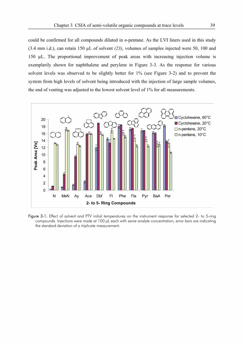
Chapter 3 CSIA of semi-volatile organic compounds at trace levels 39
could be confirmed for all compounds diluted in n-pentane. As the LVI liners used in this study
(3.4 mm i.d.), can retain 150 µL of solvent (23), volumes of samples injected were 50, 100 and
150 µL. The proportional improvement of peak areas with increasing injection volume is
exemplarily shown for naphthalene and perylene in Figure 3-3. As the response for various
solvent levels was observed to be slightly better for 1% (see Figure 3-2) and to prevent the
system from high levels of solvent being introduced with the injection of large sample volumes,
the end of venting was adjusted to the lowest solvent level of 1% for all measurements.
Figure 3-1. Effect of solvent and PTV initial temperatures on the instrument response for selected 2- to 5-ring
compounds. Injections were made at 100 μL each with same analyte concentration, error bars are indicating the standard deviation of a triplicate measurement.
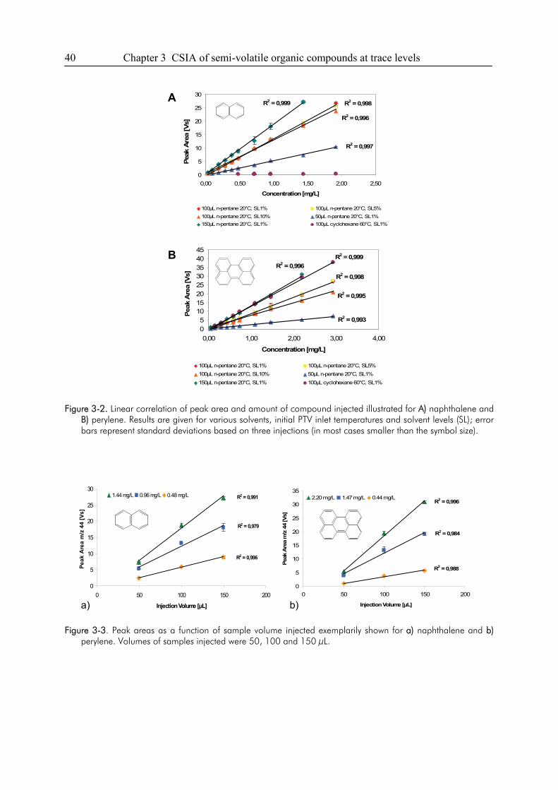
40 Chapter 3 CSIA of semi-volatile organic compounds at trace levels
Figure 3-2. Linear correlation of peak area and amount of compound injected illustrated for A) naphthalene and
B) perylene. Results are given for various solvents, initial PTV inlet temperatures and solvent levels (SL); error bars represent standard deviations based on three injections (in most cases smaller than the symbol size).
Figure 3-3. Peak areas as a function of sample volume injected exemplarily shown for a) naphthalene and b)
perylene. Volumes of samples injected were 50, 100 and 150 μL.
R2 = 0,999 R2 = 0,998
R2 = 0,997
R2 = 0,996
0
5
10
15
20
25
30
0,00 0,50 1,00 1,50 2,00 2,50
Concentration [mg/L]Pe
ak A
rea
[Vs]
100µL n-pentane 20°C, SL1% 100µL n-pentane 20°C, SL5%100µL n-pentane 20°C, SL10% 50µL n-pentane 20°C, SL1%150µL n-pentane 20°C, SL1% 100µL cyclohexane 60°C, SL1%
R2 = 0,996R2 = 0,999
R2 = 0,998
R2 = 0,993
R2 = 0,995
05
1015202530354045
0,00 1,00 2,00 3,00 4,00
Concentration [mg/L]
Peak
Are
a [V
s]
100µL n-pentane 20°C, SL1% 100µL n-pentane 20°C, SL5%100µL n-pentane 20°C, SL10% 50µL n-pentane 20°C, SL1%150µL n-pentane 20°C, SL1% 100µL cyclohexane 60°C, SL1%
A
B
R2 = 0,991
R2 = 0,979
R2 = 0,996
0
5
10
15
20
25
30
0 50 100 150 200
Injection Volume [µL]
Peak
Are
a m
/z 4
4 [V
s]
1.44 mg/L 0.96 mg/L 0.48 mg/LR2 = 0,996
R2 = 0,984
R2 = 0,988
0
5
10
15
20
25
30
35
0 50 100 150 200
Injection Volume [µL]
Peak
Are
a m
/z 4
4 [V
s]
2.20 mg/L 1.47 mg/L 0.44 mg/L
a) b)
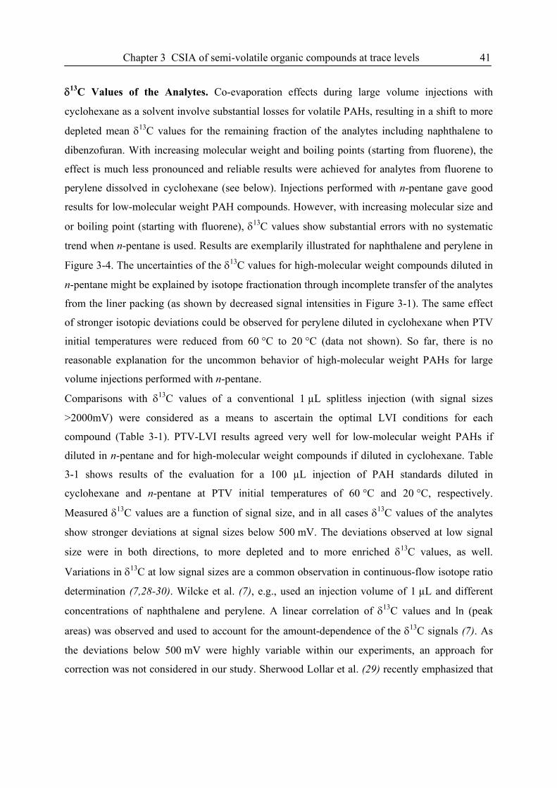
Chapter 3 CSIA of semi-volatile organic compounds at trace levels 41
δ13C Values of the Analytes. Co-evaporation effects during large volume injections with
cyclohexane as a solvent involve substantial losses for volatile PAHs, resulting in a shift to more
depleted mean δ13C values for the remaining fraction of the analytes including naphthalene to
dibenzofuran. With increasing molecular weight and boiling points (starting from fluorene), the
effect is much less pronounced and reliable results were achieved for analytes from fluorene to
perylene dissolved in cyclohexane (see below). Injections performed with n-pentane gave good
results for low-molecular weight PAH compounds. However, with increasing molecular size and
or boiling point (starting with fluorene), δ13C values show substantial errors with no systematic
trend when n-pentane is used. Results are exemplarily illustrated for naphthalene and perylene in
Figure 3-4. The uncertainties of the δ13C values for high-molecular weight compounds diluted in
n-pentane might be explained by isotope fractionation through incomplete transfer of the analytes
from the liner packing (as shown by decreased signal intensities in Figure 3-1). The same effect
of stronger isotopic deviations could be observed for perylene diluted in cyclohexane when PTV
initial temperatures were reduced from 60 °C to 20 °C (data not shown). So far, there is no
reasonable explanation for the uncommon behavior of high-molecular weight PAHs for large
volume injections performed with n-pentane.
Comparisons with δ13C values of a conventional 1 µL splitless injection (with signal sizes
>2000mV) were considered as a means to ascertain the optimal LVI conditions for each
compound (Table 3-1). PTV-LVI results agreed very well for low-molecular weight PAHs if
diluted in n-pentane and for high-molecular weight compounds if diluted in cyclohexane. Table
3-1 shows results of the evaluation for a 100 µL injection of PAH standards diluted in
cyclohexane and n-pentane at PTV initial temperatures of 60 °C and 20 °C, respectively.
Measured δ13C values are a function of signal size, and in all cases δ13C values of the analytes
show stronger deviations at signal sizes below 500 mV. The deviations observed at low signal
size were in both directions, to more depleted and to more enriched δ13C values, as well.
Variations in δ13C at low signal sizes are a common observation in continuous-flow isotope ratio
determination (7,28-30). Wilcke et al. (7), e.g., used an injection volume of 1 µL and different
concentrations of naphthalene and perylene. A linear correlation of δ13C values and ln (peak
areas) was observed and used to account for the amount-dependence of the δ13C signals (7). As
the deviations below 500 mV were highly variable within our experiments, an approach for
correction was not considered in our study. Sherwood Lollar et al. (29) recently emphasized that
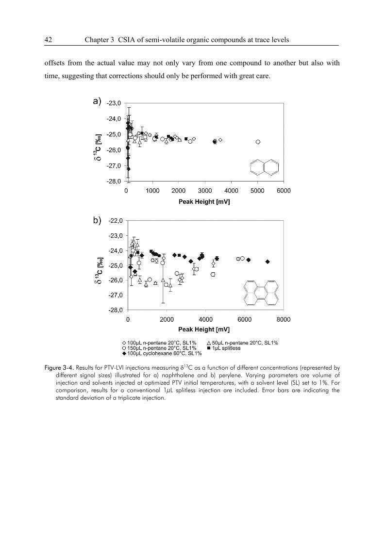
42 Chapter 3 CSIA of semi-volatile organic compounds at trace levels
offsets from the actual value may not only vary from one compound to another but also with
time, suggesting that corrections should only be performed with great care.
Figure 3-4. Results for PTV-LVI injections measuring δ13C as a function of different concentrations (represented by
different signal sizes) illustrated for a) naphthalene and b) perylene. Varying parameters are volume of injection and solvents injected at optimized PTV initial temperatures, with a solvent level (SL) set to 1%. For comparison, results for a conventional 1μL splitless injection are included. Error bars are indicating the standard deviation of a triplicate injection.
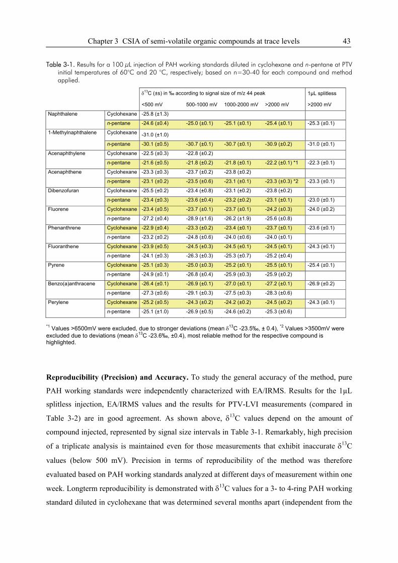
Chapter 3 CSIA of semi-volatile organic compounds at trace levels 43
Table 3-1. Results for a 100 μL injection of PAH working standards diluted in cyclohexane and n-pentane at PTV initial temperatures of 60°C and 20 °C, respectively; based on n=30-40 for each compound and method applied.
δ13C (±s) in ‰ according to signal size of m/z 44 peak 1µL splitless
<500 mV 500-1000 mV 1000-2000 mV >2000 mV >2000 mV
Naphthalene Cyclohexane -25.8 (±1.3)
n-pentane -24.6 (±0.4) -25.0 (±0.1) -25.1 (±0.1) -25.4 (±0.1) -25.3 (±0.1)
1-Methylnaphthalene Cyclohexane -31.0 (±1.0) n-pentane -30.1 (±0.5) -30.7 (±0.1) -30.7 (±0.1) -30.9 (±0.2) -31.0 (±0.1)
Acenaphthylene Cyclohexane -22.5 (±0.3) -22.8 (±0.2)
n-pentane -21.6 (±0.5) -21.8 (±0.2) -21.8 (±0.1) -22.2 (±0.1) *1 -22.3 (±0.1)
Acenaphthene Cyclohexane -23.3 (±0.3) -23.7 (±0.2) -23.8 (±0.2)
n-pentane -23.1 (±0.2) -23.5 (±0.6) -23.1 (±0.1) -23.3 (±0.3) *2 -23.3 (±0.1)
Dibenzofuran Cyclohexane -25.5 (±0.2) -23.4 (±0.8) -23.1 (±0.2) -23.8 (±0.2)
n-pentane -23.4 (±0.3) -23.6 (±0.4) -23.2 (±0.2) -23.1 (±0.1) -23.0 (±0.1)
Fluorene Cyclohexane -23.4 (±0.5) -23.7 (±0.1) -23.7 (±0.1) -24.2 (±0.3) -24.0 (±0.2)
n-pentane -27.2 (±0.4) -28.9 (±1.6) -26.2 (±1.9) -25.6 (±0.8)
Phenanthrene Cyclohexane -22.9 (±0.4) -23.3 (±0.2) -23.4 (±0.1) -23.7 (±0.1) -23.6 (±0.1)
n-pentane -23.2 (±0.2) -24.8 (±0.6) -24.0 (±0.6) -24.0 (±0.1)
Fluoranthene Cyclohexane -23.9 (±0.5) -24.5 (±0.3) -24.5 (±0.1) -24.5 (±0.1) -24.3 (±0.1)
n-pentane -24.1 (±0.3) -26.3 (±0.3) -25.3 (±0.7) -25.2 (±0.4)
Pyrene Cyclohexane -25.1 (±0.3) -25.0 (±0.3) -25.2 (±0.1) -25.5 (±0.1) -25.4 (±0.1)
n-pentane -24.9 (±0.1) -26.8 (±0.4) -25.9 (±0.3) -25.9 (±0.2)
Benzo(a)anthracene Cyclohexane -26.4 (±0.1) -26.9 (±0.1) -27.0 (±0.1) -27.2 (±0.1) -26.9 (±0.2)
n-pentane -27.3 (±0.6) -29.1 (±0.3) -27.5 (±0.3) -28.3 (±0.6)
Perylene Cyclohexane -25.2 (±0.5) -24.3 (±0.2) -24.2 (±0.2) -24.5 (±0.2) -24.3 (±0.1)
n-pentane -25.1 (±1.0) -26.9 (±0.5) -24.6 (±0.2) -25.3 (±0.6)
*1 Values >6500mV were excluded, due to stronger deviations (mean δ13C -23.5‰, ± 0.4), *2 Values >3500mV were excluded due to deviations (mean δ13C -23.6‰, ±0.4), most reliable method for the respective compound is highlighted.
Reproducibility (Precision) and Accuracy. To study the general accuracy of the method, pure
PAH working standards were independently characterized with EA/IRMS. Results for the 1µL
splitless injection, EA/IRMS values and the results for PTV-LVI measurements (compared in
Table 3-2) are in good agreement. As shown above, δ13C values depend on the amount of
compound injected, represented by signal size intervals in Table 3-1. Remarkably, high precision
of a triplicate analysis is maintained even for those measurements that exhibit inaccurate δ13C
values (below 500 mV). Precision in terms of reproducibility of the method was therefore
evaluated based on PAH working standards analyzed at different days of measurement within one
week. Longterm reproducibility is demonstrated with δ13C values for a 3- to 4-ring PAH working
standard diluted in cyclohexane that was determined several months apart (independent from the
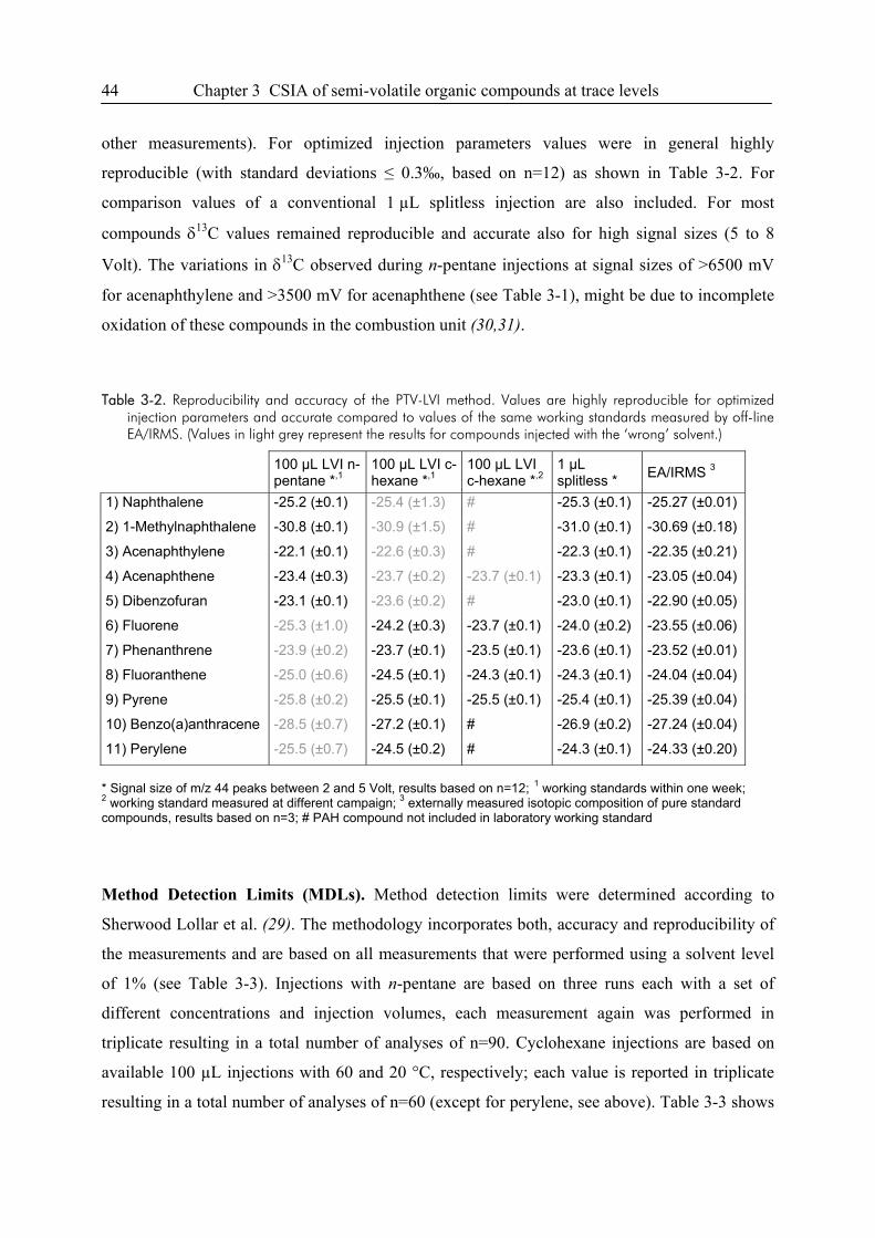
44 Chapter 3 CSIA of semi-volatile organic compounds at trace levels
other measurements). For optimized injection parameters values were in general highly
reproducible (with standard deviations ≤ 0.3‰, based on n=12) as shown in Table 3-2. For
comparison values of a conventional 1 µL splitless injection are also included. For most
compounds δ13C values remained reproducible and accurate also for high signal sizes (5 to 8
Volt). The variations in δ13C observed during n-pentane injections at signal sizes of >6500 mV
for acenaphthylene and >3500 mV for acenaphthene (see Table 3-1), might be due to incomplete
oxidation of these compounds in the combustion unit (30,31).
Table 3-2. Reproducibility and accuracy of the PTV-LVI method. Values are highly reproducible for optimized injection parameters and accurate compared to values of the same working standards measured by off-line EA/IRMS. (Values in light grey represent the results for compounds injected with the ‘wrong’ solvent.)
100 µL LVI n-pentane *,1
100 µL LVI c-hexane *,1
100 µL LVI c-hexane *,2
1 µL splitless * EA/IRMS 3
1) Naphthalene -25.2 (±0.1) -25.4 (±1.3) # -25.3 (±0.1) -25.27 (±0.01)
2) 1-Methylnaphthalene -30.8 (±0.1) -30.9 (±1.5) # -31.0 (±0.1) -30.69 (±0.18)
3) Acenaphthylene -22.1 (±0.1) -22.6 (±0.3) # -22.3 (±0.1) -22.35 (±0.21)
4) Acenaphthene -23.4 (±0.3) -23.7 (±0.2) -23.7 (±0.1) -23.3 (±0.1) -23.05 (±0.04)
5) Dibenzofuran -23.1 (±0.1) -23.6 (±0.2) # -23.0 (±0.1) -22.90 (±0.05)
6) Fluorene -25.3 (±1.0) -24.2 (±0.3) -23.7 (±0.1) -24.0 (±0.2) -23.55 (±0.06)
7) Phenanthrene -23.9 (±0.2) -23.7 (±0.1) -23.5 (±0.1) -23.6 (±0.1) -23.52 (±0.01)
8) Fluoranthene -25.0 (±0.6) -24.5 (±0.1) -24.3 (±0.1) -24.3 (±0.1) -24.04 (±0.04)
9) Pyrene -25.8 (±0.2) -25.5 (±0.1) -25.5 (±0.1) -25.4 (±0.1) -25.39 (±0.04)
10) Benzo(a)anthracene -28.5 (±0.7) -27.2 (±0.1) # -26.9 (±0.2) -27.24 (±0.04)
11) Perylene -25.5 (±0.7) -24.5 (±0.2) # -24.3 (±0.1) -24.33 (±0.20)
* Signal size of m/z 44 peaks between 2 and 5 Volt, results based on n=12; 1 working standards within one week; 2 working standard measured at different campaign; 3 externally measured isotopic composition of pure standard compounds, results based on n=3; # PAH compound not included in laboratory working standard
Method Detection Limits (MDLs). Method detection limits were determined according to
Sherwood Lollar et al. (29). The methodology incorporates both, accuracy and reproducibility of
the measurements and are based on all measurements that were performed using a solvent level
of 1% (see Table 3-3). Injections with n-pentane are based on three runs each with a set of
different concentrations and injection volumes, each measurement again was performed in
triplicate resulting in a total number of analyses of n=90. Cyclohexane injections are based on
available 100 µL injections with 60 and 20 °C, respectively; each value is reported in triplicate
resulting in a total number of analyses of n=60 (except for perylene, see above). Table 3-3 shows
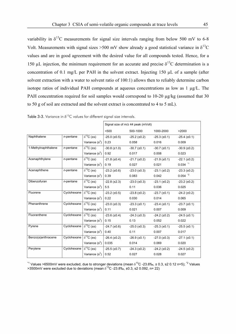
Chapter 3 CSIA of semi-volatile organic compounds at trace levels 45
variability in δ13C measurements for signal size intervals ranging from below 500 mV to 6-8
Volt. Measurements with signal sizes >500 mV show already a good statistical variance in δ13C
values and are in good agreement with the desired value for all compounds tested. Hence, for a
150 µL injection, the minimum requirement for an accurate and precise δ13C determination is a
concentration of 0.1 mg/L per PAH in the solvent extract. Injecting 150 µL of a sample (after
solvent extraction with a water to solvent ratio of 100:1) allows then to reliably determine carbon
isotope ratios of individual PAH compounds at aqueous concentrations as low as 1 µg/L. The
PAH concentration required for soil samples would correspond to 10-20 µg/kg (assumed that 30
to 50 g of soil are extracted and the solvent extract is concentrated to 4 to 5 mL).
Table 3-3. Variance in δ13C values for different signal size intervals.
Signal size of m/z 44 peak (mVolt)
<500 500-1000 1000-2000 >2000
Naphthalene n-pentane δ13C (±s) -25.0 (±0.5) -25.2 (±0.2) -25.3 (±0.1) -25.4 (±0.1)
Variance (s2) 0.23 0.058 0.016 0.009
1-Methylnaphthalene n-pentane δ13C (±s) -30.8 (±1.0) -30.7 (±0.1) -30.7 (±0.1) -30.9 (±0.2)
Variance (s2) 0.92 0.017 0.008 0.023
Acenaphthylene n-pentane δ13C (±s) -21.8 (±0.4) -21.7 (±0.2) -21.9 (±0.1) -22.1 (±0.2)
Variance (s2) 0.19 0.027 0.021 0.034 *1
Acenaphthene n-pentane δ13C (±s) -23.2 (±0.6) -23.0 (±0.3) -23.1 (±0.2) -23.3 (±0.2)
Variance (s2) 0.39 0.083 0.042 0.054 *2
Dibenzofuran n-pentane δ13C (±s) -22.8 (±2.3) -23.0 (±0.3) -23.1 (±0.2) -23.2 (±0.2)
Variance (s2) 5.5 0.11 0.036 0.025
Fluorene Cyclohexane δ13C (±s) -23.2 (±0.5) -23.8 (±0.2) -23.7 (±0.1) -24.2 (±0.2)
Variance (s2) 0.22 0.030 0.014 0.065
Phenanthrene Cyclohexane δ13C (±s) -23.0 (±0.3) -23.3 (±0.1) -23.4 (±0.1) -23.7 (±0.1)
Variance (s2) 0.11 0.021 0.007 0.009
Fluoranthene Cyclohexane δ13C (±s) -23.6 (±0.4) -24.3 (±0.3) -24.2 (±0.2) -24.5 (±0.1)
Variance (s2) 0.15 0.13 0.052 0.022
Pyrene Cyclohexane δ13C (±s) -24.7 (±0.6) -25.0 (±0.3) -25.3 (±0.1) -25.5 (±0.1)
Variance (s2) 0.40 0.11 0.007 0.017
Benzo(a)anthracene Cyclohexane δ13C (±s) -26.4 (±0.2) -26.9 (±0.1) -27.0 (±0.3) -27.1 (±0.1)
Variance (s2) 0.035 0.014 0.069 0.020
Perylene Cyclohexane δ13C (±s) -25.5 (±0.7) -24.3 (±0.2) -24.2 (±0.2) -24.5 (±0.2)
Variance (s2) 0.52 0.027 0.028 0.027
*1 Values >6500mV were excluded, due to stronger deviations (mean δ13C -23.6‰, ± 0.3, s2 0.12 n=5); *2 Values >3500mV were excluded due to deviations (mean δ13C -23.8‰, ±0.3, s2 0.092, n= 22)
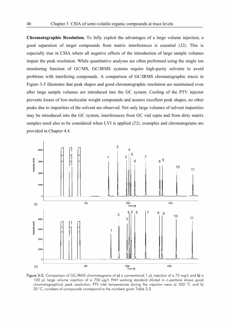
46 Chapter 3 CSIA of semi-volatile organic compounds at trace levels
Chromatographic Resolution. To fully exploit the advantages of a large volume injection, a
good separation of target compounds from matrix interferences is essential (32). This is
especially true in CSIA where all negative effects of the introduction of large sample volumes
impair the peak resolution. While quantitative analyses are often performed using the single ion
monitoring function of GC/MS, GC/IRMS systems require high-purity solvents to avoid
problems with interfering compounds. A comparison of GC/IRMS chromatographic traces in
Figure 3-5 illustrates that peak shapes and good chromatographic resolution are maintained even
after large sample volumes are introduced into the GC system. Cooling of the PTV injector
prevents losses of low-molecular weight compounds and assures excellent peak shapes, no other
peaks due to impurities of the solvent are observed. Not only large volumes of solvent impurities
may be introduced into the GC system, interferences from GC vial septa and from dirty matrix
samples need also to be considered when LVI is applied (22), examples and chromatograms are
provided in Chapter 4.4.
Figure 3-5. Comparison of GC/IRMS chromatograms of a) a conventional 1 μL injection of a 75 mg/L and b) a
100 μL large volume injection of a 750 μg/L PAH working standard diluted in n-pentane shows good chromatographical peak resolution, PTV inlet temperatures during the injection were a) 300 °C and b) 20 °C, numbers of compounds correspond to the numbers given Table 3-2.
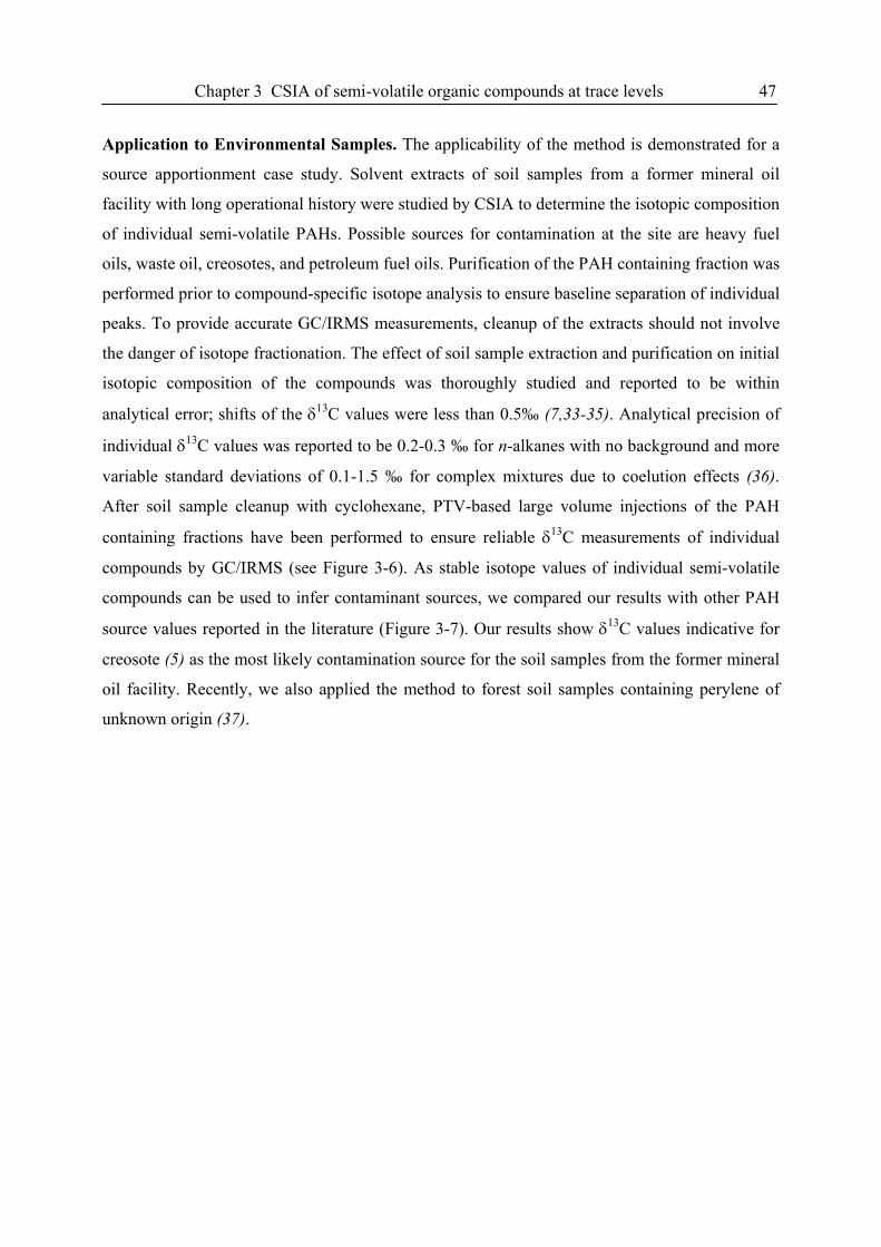
Chapter 3 CSIA of semi-volatile organic compounds at trace levels 47
Application to Environmental Samples. The applicability of the method is demonstrated for a
source apportionment case study. Solvent extracts of soil samples from a former mineral oil
facility with long operational history were studied by CSIA to determine the isotopic composition
of individual semi-volatile PAHs. Possible sources for contamination at the site are heavy fuel
oils, waste oil, creosotes, and petroleum fuel oils. Purification of the PAH containing fraction was
performed prior to compound-specific isotope analysis to ensure baseline separation of individual
peaks. To provide accurate GC/IRMS measurements, cleanup of the extracts should not involve
the danger of isotope fractionation. The effect of soil sample extraction and purification on initial
isotopic composition of the compounds was thoroughly studied and reported to be within
analytical error; shifts of the δ13C values were less than 0.5‰ (7,33-35). Analytical precision of
individual δ13C values was reported to be 0.2-0.3 ‰ for n-alkanes with no background and more
variable standard deviations of 0.1-1.5 ‰ for complex mixtures due to coelution effects (36).
After soil sample cleanup with cyclohexane, PTV-based large volume injections of the PAH
containing fractions have been performed to ensure reliable δ13C measurements of individual
compounds by GC/IRMS (see Figure 3-6). As stable isotope values of individual semi-volatile
compounds can be used to infer contaminant sources, we compared our results with other PAH
source values reported in the literature (Figure 3-7). Our results show δ13C values indicative for
creosote (5) as the most likely contamination source for the soil samples from the former mineral
oil facility. Recently, we also applied the method to forest soil samples containing perylene of
unknown origin (37).
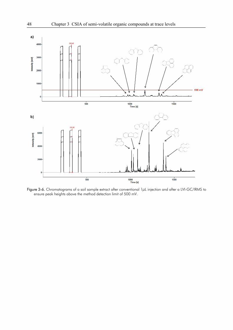
48 Chapter 3 CSIA of semi-volatile organic compounds at trace levels
Figure 3-6. Chromatograms of a soil sample extract after conventional 1μL injection and after a LVI-GC/IRMS to
ensure peak heights above the method detection limit of 500 mV.
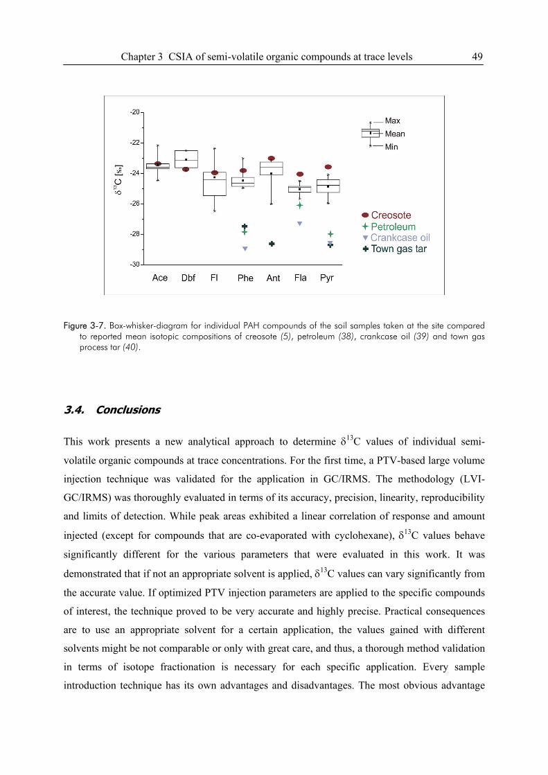
Chapter 3 CSIA of semi-volatile organic compounds at trace levels 49
Figure 3-7. Box-whisker-diagram for individual PAH compounds of the soil samples taken at the site compared to reported mean isotopic compositions of creosote (5), petroleum (38), crankcase oil (39) and town gas process tar (40).
3.4. Conclusions
This work presents a new analytical approach to determine δ13C values of individual semi-
volatile organic compounds at trace concentrations. For the first time, a PTV-based large volume
injection technique was validated for the application in GC/IRMS. The methodology (LVI-
GC/IRMS) was thoroughly evaluated in terms of its accuracy, precision, linearity, reproducibility
and limits of detection. While peak areas exhibited a linear correlation of response and amount
injected (except for compounds that are co-evaporated with cyclohexane), δ13C values behave
significantly different for the various parameters that were evaluated in this work. It was
demonstrated that if not an appropriate solvent is applied, δ13C values can vary significantly from
the accurate value. If optimized PTV injection parameters are applied to the specific compounds
of interest, the technique proved to be very accurate and highly precise. Practical consequences
are to use an appropriate solvent for a certain application, the values gained with different
solvents might be not comparable or only with great care, and thus, a thorough method validation
in terms of isotope fractionation is necessary for each specific application. Every sample
introduction technique has its own advantages and disadvantages. The most obvious advantage
50 Chapter 3 CSIA of semi-volatile organic compounds at trace levels
by LVI-GC/IRMS is that the instrumental limit of detection can be easily and significantly
improved just by introducing larger volumes of a sample. It is a user-friendly, automated
technique that can be applied in a broad range of applications. Off-line sample pretreatment can
be avoided or simplified, e.g. in combination with preperative HPLC it offers an effective, fast,
time and labour efficient method for the determination of isotopic compositions of semi-volatiles
even in difficult matrices. Dirty extracts, and thus, matrix interferences place special demands on
large volume injection and often require improved clean-up strategies. However, matrix
components, which might be present even after sample clean-up, can be retained in the liner
packing material. Problems with volatile compounds that are co-evaporated with the solvent can
be avoided if the volatility of the solvent used is significantly lower than that of the compounds
that are trapped in the cooled packed liner. The choice of the LVI injection technique depends
largely on the composition of the sample and the type of analytes to be determined.
3.5. References
(1) Benson, S.; Lennard, C.; Maynard, P.; Roux, C. Forensic applications of isotope ratio mass spectrometry - A review. Forensic Sci.Int. 2006, 157, 1-22.
(2) Philp, R. P. The emergence of stable isotopes in environmental and forensic geochemistry studies: a review. Environ. Chem. Lett. 2007, 5, 57-66.
(3) Poster, D. L.; Schantz, M. M.; Sander, L. C.; Wise, S. A. Analysis of polycyclic aromatic hydrocarbons (PAHs) in environmental samples: A critical review of gas chromatographic (GC) methods. Anal. Bioanal. Chem. 2006, 386, 859-881.
(4) O'Malley, V. P.; Abrajano, T. A.; Hellou, J. Determination of the 13C/12C ratios of individual PAH from environmental samples: can PAH sources be apportioned? Org. Geochem. 1994, 21, 809-822.
(5) Hammer, B. T.; Kelley, C. A.; Coffin, R. B.; Cifuentes, L. A.; Mueller, J. G. Delta C-13 values of polycyclic aromatic hydrocarbons collected from two creosote-contaminated sites. Chem. Geol. 1998, 152, 43-58.
(6) McRae, C.; Sun, C. G.; McMillan, C. F.; Snape, C. E.; Fallick, A. E. Sourcing of fossil fuel-derived PAH in the environment. Polycycl. Aromat. Compd. 2000, 20, 97-109.
(7) Wilcke, W.; Krauss, M.; Amelung, W. Carbon isotope signature of polycyclic aromatic hydrocarbons (PAHs): Evidence for different sources in tropical and temperate environments? Environ. Sci. Technol. 2002, 36, 3530-3535.
(8) Sun, C. G.; Cooper, M.; Snape, C. E. Use of compound-specific delta C-13 and delta D stable isotope measurements as an aid in the source apportionment of polyaromatic hydrocarbons. Rapid Commun. Mass Spectrom. 2003, 17, 2611-2613.
(9) Sessions, A. L. Isotope-ratio detection for gas chromatography. J. Sep. Sci. 2006, 29, 1946-1961. (10) Meier-Augenstein, W. On-line Recording of 13C/12C Ratios and Mass Spectra in one Gas Chromatographic
Analysis. J. High Resol. Chromatogr. 1995, 18, 28-32. (11) Dempster, H. S.; Sherwood Lollar, B.; Feenstra, S. Tracing organic contaminants in groundwater: A new
methodology using compound-specific isotopic analysis. Environ. Sci. Technol. 1997, 31, 3193-3197. (12) Zwank, L.; Berg, M.; Schmidt, T. C.; Haderlein, S. B. Compound-specific carbon isotope analysis of volatile
organic compounds in the low-microgram per liter range. Anal. Chem. 2003, 75, 5575-5583. (13) Slater, G. F.; Dempster, H. S.; Sherwood Lollar, B.; Ahad, J. Headspace analysis: A new application for
isotopic characterization of dissolved organic contaminants. Environ. Sci. Technol. 1999, 33, 190-194.
Chapter 3 CSIA of semi-volatile organic compounds at trace levels 51
(14) Kalin, R. M.; Hamilton, J. T. G.; Harper, D. B.; Miller, L. G.; Lamb, C.; Kennedy, J. T.; Downey, A.; McCauley, S.; Goldstein, A. H. Continuous flow stable isotope methods for study of d13C fractionation during halomethane production and degradation. Rapid Commun. Mass Spectrom. 2001, 15, 357-363.
(15) Morrill, P. L.; Lacrampe-Couloume, G.; Sherwood Lollar, B. Dynamic headspace: a single-step extraction for isotopic analysis of mu g/L concentrations of dissolved chlorinated ethenes. Rapid Commun. Mass Spectrom. 2004, 18, 595-600.
(16) Dias, R. F.; Freeman, K. H. Carbon isotope analyses of semivolatile organic compounds in aqueous media using solid-phase microextraction and isotope ratio monitoring GC/MS. Anal. Chem. 1997, 69, 944-950.
(17) Hunkeler, D.; Aravena, R. Determination of compound-specific carbon isotope ratios of chlorinated methanes, ethanes, and ethenes in aqueous samples. Environ. Sci. Technol. 2000, 34, 2839-2844.
(18) Ferchaud-Roucher, V.; Albert, C.; Champ, M.; Krempf, M. Solid-phase microextraction method for carbon isotopic analysis of volatile carboxylic acids in human plasma by gas chromatography/combustion/isotope ratio mass spectrometry. Rapid Commun. Mass Spectrom. 2006, 20, 3573-3578.
(19) Yamada, K.; Yoshida, N.; Calderone, G.; Guillou, C. Determination of hydrogen, carbon and oxygen isotope ratios of ethanol in aqueous solution at millimole levels. Rapid Commun. Mass Spectrom. 2007, 21, 1431-1437.
(20) Auer, N. R.; Manzke, B. U.; Schulz-Bull, D. E. Development of a purge and trap continuous flow system for the stable carbon isotope analysis of volatile halogenated organic compounds in water. J. Chromatogr. A 2006, 1131, 24-36.
(21) Jochmann, M. A.; Blessing, M.; Haderlein, S. B.; Schmidt, T. C. A new approach to determine method detection limits for compound-specific isotope analysis of volatile organic compounds. Rapid Commun. Mass Spectrom. 2006, 20, 3639-3648.
(22) Norlock, F. M.; Jang, J. K.; Zou, Q.; Schoonover, T. M.; Li, A. Large-volume injection PTV-GC-MS analysis of polycyclic aromatic hydrocarbons in air and sediment samples. J. Air & Waste Manage. Assoc. 2002, 52, 19-26.
(23) Mol, H. G. J.; Althuizen, M.; Janssen, H. G.; Cramers, C. A.; Brinkman, U. A. T. Environmental applications of large volume injection in capillary GC using PTV injectors. J. High Resol. Chromatogr. 1996, 19, 69-79.
(24) Vecera, Z.; Bartosikova, A.; Sklenska, J.; Mikuska, P. A large volume injection procedure for GC-MS determination of PAHs and PCBs. Chromatographia 2005, 61, 197-200.
(25) Yusà, V.; Pardo, O.; Pastor, A.; de la Guardia, M. Optimization of a microwave-assisted extraction large-volume injection and gas chromatography-ion trap mass spectrometry procedure for the determination of polybrominated diphenyl ethers, polybrominated biphenyls and polychlorinated naphthalenes in sediments. Anal. Chim. Acta 2006, 557, 304-313.
(26) Baylis, S. A.; Hall, K.; Jumeau, E. J. The analysis of the C1-C5 components of natural gas samples using gas chromatography-combustion-isotope ratio mass spectrometry. Org. Geochem. 1994, 21, 777-785.
(27) Meier-Augenstein, W. Applied gas chromatography coupled to isotope ratio mass spectrometry. J. Chromatogr. A 1999, 842, 351-371.
(28) Schmitt, J.; Glaser, B.; Zech, W. Amount-dependent isotopic fractionation during compound-specific isotope analysis. Rapid Commun. Mass Spectrom. 2003, 17, 970-977.
(29) Sherwood Lollar, B.; Hirschorn, S. K.; Chartrand, M. M. G.; Lacrampe-Couloume, G. An approach for assessing total instrumental uncertainty in compound-specific carbon isotope analysis: Implications for environmental remediation studies. Anal. Chem. 2007, 79, 3469-3475.
(30) Glaser, B.; Amelung, W. Determination of C-13 natural abundance of amino acid enantiomers in soil: methodological considerations and first results. Rapid Commun. Mass Spectrom. 2002, 16, 891-898.
(31) Merritt, D. A.; Freeman, K. H.; Ricci, M. P.; Studley, S. A.; Hayes, J. M. Performance and Optimization of a Combustion Interface for Isotope Ratio Monitoring Gas Chromatography/Mass Spectrometry. Anal. Chem. 1995, 67, 2461-2473.
(32) Cavagnino, D.; Magni, P.; Zilioli, G.; Trestianu, S. Comprehensive two-dimensional gas chromatography using large sample volume injection for the determination of polynuclear aromatic hydrocarbons in complex matrices. J. Chromatogr. A 2003, 1019, 211-220.
(33) Bakel, A. J.; Ostrom, P. H.; Ostrom, N. E. Carbon isotopic analysis of individual n-aikanes: evaluation of accuracy and application to marine particulate organic material. Org. Geochem. 1994, 21, 595-602.
(34) Kim, M. K.; Kennicutt, M. C.; Qian, Y. R. Polycyclic aromatic hydrocarbon purification procedures for compound specific isotope analysis. Environ. Sci. Technol. 2005, 39, 6770-6776.
(35) Mazeas, L.; Budzinski, H. Molecular and stable carbon isotopic source identification of oil residues and oiled bird feathers sampled along the Atlantic coast of France after the Erika oil spill. Environ. Sci. Technol. 2002, 36, 130-137.

52 Chapter 3 CSIA of semi-volatile organic compounds at trace levels
(36) Schoell, M.; McCaffrey, M. A.; Fago, F. J.; Moldowan, J. M. Carbon isotopic compositions of 28,30-bisnorhopanes and other biological markers in a Monterey crude oil. Geochim. Cosmochim. Acta 1992, 56, 1391-1399.
(37) Gocht, T.; Barth, J. A. C.; Epp, M.; Jochmann, M.; Blessing, M.; Schmidt, T. C.; Grathwohl, P. Indications for pedogenic formation of perylene in a terrestrial soil profile: Depth distribution and first results from stable carbon isotope ratios. Appl. Geochem. 2007, 22, 2652-2663.
(38) Mazeas, L.; Budzinski, H. Polycyclic aromatic hydrocarbon C-13/C-12 ratio measurement in petroleum and marine sediments - Application to standard reference materials and a sediment suspected of contamination from the Erika oil spill. J. Chromatogr. A 2001, 923, 165-176.
(39) O'Malley, V. P.; Burke, R. A.; Schlotzhauer, W. S. Using GC-MS/Combustion/IRMS to determine the C-13/C-12 ratios of individual hydrocarbons produced from the combustion of biomass materials - application to biomass burning. Org. Geochem. 1997, 27, 567-581.
(40) McRae, C.; Sun, C. G.; Snape, C. E.; Fallick, A. E.; Taylor, D. Delta C-13 values of coal-derived PAHs from different processes and their application to source apportionment. Org. Geochem. 1999, 30, 881-889.
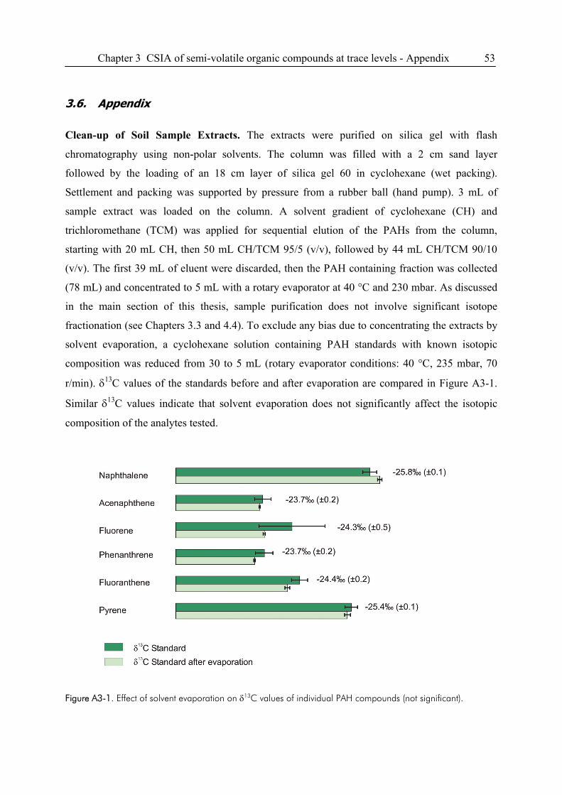
Chapter 3 CSIA of semi-volatile organic compounds at trace levels - Appendix 53
3.6. Appendix
Clean-up of Soil Sample Extracts. The extracts were purified on silica gel with flash
chromatography using non-polar solvents. The column was filled with a 2 cm sand layer
followed by the loading of an 18 cm layer of silica gel 60 in cyclohexane (wet packing).
Settlement and packing was supported by pressure from a rubber ball (hand pump). 3 mL of
sample extract was loaded on the column. A solvent gradient of cyclohexane (CH) and
trichloromethane (TCM) was applied for sequential elution of the PAHs from the column,
starting with 20 mL CH, then 50 mL CH/TCM 95/5 (v/v), followed by 44 mL CH/TCM 90/10
(v/v). The first 39 mL of eluent were discarded, then the PAH containing fraction was collected
(78 mL) and concentrated to 5 mL with a rotary evaporator at 40 °C and 230 mbar. As discussed
in the main section of this thesis, sample purification does not involve significant isotope
fractionation (see Chapters 3.3 and 4.4). To exclude any bias due to concentrating the extracts by
solvent evaporation, a cyclohexane solution containing PAH standards with known isotopic
composition was reduced from 30 to 5 mL (rotary evaporator conditions: 40 °C, 235 mbar, 70
r/min). δ13C values of the standards before and after evaporation are compared in Figure A3-1.
Similar δ13C values indicate that solvent evaporation does not significantly affect the isotopic
composition of the analytes tested.
Figure A3-1. Effect of solvent evaporation on δ13C values of individual PAH compounds (not significant).
54 Chapter 4 Analytical problems and limitations in CSIA of environmental samples
4. Analytical Problems and Limitations in Compound-Specific
Isotope Analysis of Environmental Samples
4.1. Introduction
Since 1976, when it was introduced, the technique of measuring stable isotope ratios of
individual GC peaks was further developed (1-4). Since the early 90ies, when GC/IRMS systems
became commercially available, the technique has become known as compound-specific isotope
analysis (CSIA) (5-7). Especially over the past decade, CSIA has evolved as a indispensable tool
in many areas where an allocation of sources is required, such as in food authenticity studies,
pharmaceutical research, doping analysis, and environmental chemistry (8-11).
Numerous studies have demonstrated CSIA as a useful tool in contaminated site assessment.
Instrumental effects and other technical issues in the determination of compound-specific isotope
ratios have been thouroughly discussed in the early stages of GC/IRMS (12-14). Accuracy,
precision and quality assurance were always carefully considered in isotope data processing.
Sherwood Lollar et al. (15) defined explicit criteria which have to be met for applications of
CSIA to biodegradation field studies. Recent reviews of Slater (16), Schmidt et al. (10),
Meckenstock et al. (17) and Elsner et al. (18) have focussed on the potentials of CSIA techniques
and cover important aspects for assessing biodegradation and source identification with CSIA.
They all, and most recently, a consensus guide (19) focus on possible areas of applications of
CSIA and interpretation of data rather than isotope measurements in CSIA. The more
fundamental technical aspects have been addressed in previous reviews (9,20) without focussing
on environmental sample analysis and the more practical aspects regarding field applications.
Since CSIA is gaining more and more popularity and an increasing numbers of environmental
authorities and environmental consultancies are interested in the application of the method in
contaminated site remediation, it is important to demonstrate the problems and limitations
associated with environmental samples. Recent GC and separation papers that were not as
extensively focused on in past reviews, will be discussed, aspects that have to be considered
when applying GC/IRMS in contaminated site management will be highlighted and additional
material with respect to environmental samples will be provided.
Chapter 4 Analytical problems and limitations in CSIA of environmental samples 55
4.2. Groundwater Sampling
Well Locations. Most field applications have relied on sampling plans collecting data from
different parts of the contaminant plumes, but at only one point in time (21). Chartrand et al. (21)
emphasized the need to study fluctuating hydraulic systems time-resolved to more reliably assess
the temporal variability and the effectiveness of biodegradation. Due to heterogeneities of the
aquifer system and thus preferential flowpaths, point-scale measurements of the groundwater
might lead to unacceptable levels of uncertainty with respect to the flow and contamination
situation. As discussed by Peter et al. (22), point-scale isotope values need to be representative
for the entire aquifer system, and hence would require a dense monitoring network covering both
the fringes and the center of a contaminant plume, which is hardly possible at sites with complex
hydrogeology. Their study, therefore, used a combined approach of CSIA and integral pumping
tests that allows for a more reliable determination of the degree of biodegradation in
heterogeneous aquifer systems (22). An important point that should be considered in terms of
well locations is that some modeling approaches require sampling wells to be positioned on the
center line of the contaminant plume to reliably estimate first order degradation rate constants,
especially if combined with compound-specific stable isotope data (23).
Depth-discrete sampling, where an aquifer system can be vertically resolved should be favoured
over whole screen sampling. Otherwise, due to heterogeneities within aquifer systems, one might
miss important information on active degradation processes in parts of the plume. If mixing of
different flow paths with different extents of degradation occurs during sampling, the measured
isotopic composition of this mixed sample will reflect the isotope ratio of the fraction with the
highest contaminant concentration (commonly the less degraded fraction). Hence, the true extent
of biodegradation will be underestimated (24,25), a problem common to all hydrogeological
sampling and analytical approaches. This is especially true for wells located near the contaminant
source as isotope fractionation due to degradation can be masked due to continual dissolution of
fresh, undegraded material (26). The major advantage of depth-discrete groundwater sampling is
illustrated in Figure 4-1. A multi-level well system allows to investigate the vertical profile of a
structured contaminant plume and to elucidate the different zones of microbial activity within the
aquifer system (KORA site Rosengarten-Ehestorf, discussed in Chapter 2.4.3). In this well,
conventional sampling would have resulted in a mean concentration of 2900 µg/L for PCE and a
mixed overall δ13C value of -25.7 ‰ (weighted average) and would have missed important in-situ
information on effective degradation processes.
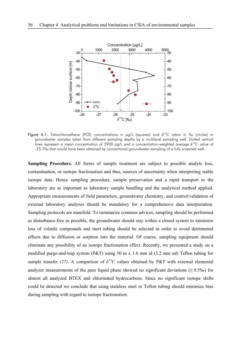
56 Chapter 4 Analytical problems and limitations in CSIA of environmental samples
Figure 4-1. Tetrachloroethene (PCE) concentrations in μg/L (squares) and δ13C ratios in ‰ (circles) in
groundwater samples taken from different sampling depths by a multilevel sampling well. Dotted vertical lines represent a mean concentration of 2900 μg/L and a concentration-weighted average δ13C value of -25.7‰ that would have been obtained by conventional groundwater sampling of a fully screened well.
Sampling Procedure. All forms of sample treatment are subject to possible analyte loss,
contamination, or isotope fractionation and thus, sources of uncertainty when interpreting stable
isotope data. Hence sampling procedure, sample preservation and a rapid transport to the
laboratory are as important as laboratory sample handling and the analytical method applied.
Appropriate measurements of field parameters, groundwater chemistry, and control/validation of
external laboratory analyses should be mandatory for a comprehensive data interpretation.
Sampling protocols are manifold. To summarize common advices, sampling should be performed
as disturbance-free as possible, the groundwater should stay within a closed system to minimize
loss of volatile compounds and inert tubing should be selected in order to avoid detrimental
effects due to diffusion or sorption into the material. Of course, sampling equipment should
eliminate any possibility of an isotope fractionation effect. Recently, we presented a study on a
modified purge-and-trap system (P&T) using 50 m x 1.6 mm id (3.2 mm od) Teflon tubing for
sample transfer (27). A comparison of δ13C values obtained by P&T with external elemental
analyzer measurements of the pure liquid phase showed no significant deviations (≤ 0.5‰) for
almost all analyzed BTEX and chlorinated hydrocarbons. Since no significant isotope shifts
could be detected we conclude that using stainless steel or Teflon tubing should minimize bias
during sampling with regard to isotope fractionation.
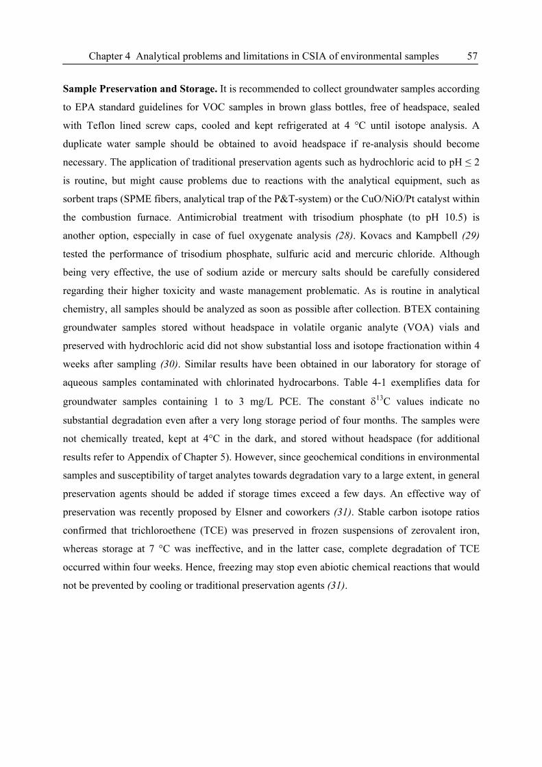
Chapter 4 Analytical problems and limitations in CSIA of environmental samples 57
Sample Preservation and Storage. It is recommended to collect groundwater samples according
to EPA standard guidelines for VOC samples in brown glass bottles, free of headspace, sealed
with Teflon lined screw caps, cooled and kept refrigerated at 4 °C until isotope analysis. A
duplicate water sample should be obtained to avoid headspace if re-analysis should become
necessary. The application of traditional preservation agents such as hydrochloric acid to pH ≤ 2
is routine, but might cause problems due to reactions with the analytical equipment, such as
sorbent traps (SPME fibers, analytical trap of the P&T-system) or the CuO/NiO/Pt catalyst within
the combustion furnace. Antimicrobial treatment with trisodium phosphate (to pH 10.5) is
another option, especially in case of fuel oxygenate analysis (28). Kovacs and Kampbell (29)
tested the performance of trisodium phosphate, sulfuric acid and mercuric chloride. Although
being very effective, the use of sodium azide or mercury salts should be carefully considered
regarding their higher toxicity and waste management problematic. As is routine in analytical
chemistry, all samples should be analyzed as soon as possible after collection. BTEX containing
groundwater samples stored without headspace in volatile organic analyte (VOA) vials and
preserved with hydrochloric acid did not show substantial loss and isotope fractionation within 4
weeks after sampling (30). Similar results have been obtained in our laboratory for storage of
aqueous samples contaminated with chlorinated hydrocarbons. Table 4-1 exemplifies data for
groundwater samples containing 1 to 3 mg/L PCE. The constant δ13C values indicate no
substantial degradation even after a very long storage period of four months. The samples were
not chemically treated, kept at 4°C in the dark, and stored without headspace (for additional
results refer to Appendix of Chapter 5). However, since geochemical conditions in environmental
samples and susceptibility of target analytes towards degradation vary to a large extent, in general
preservation agents should be added if storage times exceed a few days. An effective way of
preservation was recently proposed by Elsner and coworkers (31). Stable carbon isotope ratios
confirmed that trichloroethene (TCE) was preserved in frozen suspensions of zerovalent iron,
whereas storage at 7 °C was ineffective, and in the latter case, complete degradation of TCE
occurred within four weeks. Hence, freezing may stop even abiotic chemical reactions that would
not be prevented by cooling or traditional preservation agents (31).
58 Chapter 4 Analytical problems and limitations in CSIA of environmental samples
Table 4-1: Effect of δ13C on storage time for groundwater samples containing perchloroethene (PCE) with concentrations between 1 and 3 mg/L, stored at 4 °C in the dark, without headspace. Each sample was measured in triplicates (n = 3). Sampling was performed at KORA-site Rosengarten-Ehestorf (described in Chapter 2).
Sample δ13C in ‰ Standard deviation δ13C in ‰ Standard deviation
after 2 weeks (n = 3) after 4 months (n = 3)
sample no.1 -27,2 ± 0.3 -27,2 ± 0.1
sample no.2 -27,1 ± 0.3 -27,0 ± 0.1
sample no.3 -27,1 ± 0.1 -26,9 ± 0.1
sample no.4 -27,1 ± 0.2 -26,7 ± 0.1
4.3. Sensitivity and Linearity of CSIA
IRMS systems provide specialised and highly sensitive detectors achieving a precision four
orders of magnitude better than conventional (mass-scanning) mass spectrometers. However, to
achieve this level of precision in continuous-flow techniques coupled with gas-chromatography,
ca. 1 nmol of carbon or 8 nmol of hydrogen need to be injected on-column. Sensitivity and
precision of continuous-flow IRMS measurements have been discussed in detail recently by
Sessions (20). Deciphering the source and fate of contaminants with the help of CSIA is
nowadays possible even at low contaminant concentrations that are frequently found in the fringe
zones of contaminant plumes. Effective extraction and pre-concentration techniques for the
analysis of isotope ratios for analytes in the low µg/L range are available. Another benefit of
these techniques is that there is no, or at least a reduced consumption of organic solvents.
Although pre-concentration techniques such as LVI (large volume injection), SPME (solid-phase
microextraction) or purge-and-trap (P&T) have been well established in several analytical
working laboratories, the use of these techniques in combination with GC/IRMS is much less
routine. Hence, some potential pitfalls of these techniques are discussed in the following.
Higher sensitivities for apolar and non-volatile contaminants in soil samples can be attained by
liquid extraction techniques such as accelerated solvent extraction (ASE) or Soxhlet extraction.
As already mentioned, methods for sample preparation might introduce an isotope fractionation
and, thus, need a careful evaluation by means of internal standards of known isotopic
composition. Soxhlet extraction, for example, did not significantly change the isotopic
composition of PAH compounds (32). Graham et al. (33) reported that ASE followed by cleanup,
resulted in more consistent and reproducible stable carbon isotope data compared with other
extraction techniques applied.
Chapter 4 Analytical problems and limitations in CSIA of environmental samples 59
It has been reported that split/splitless injectors are sensitive to isotope fractionation effects
(34,35). The flow conditions in the injector can cause an amount-dependent isotope fractionation
during split injections. Thus, early work strongly favored on-column injection or splitless
injection with long enough splitless times. An optimization of injection parameters is highly
recommended to prevent or at least minimize fractionation effects. Smallwood et al. (36) studied
four different injection techniques for analysing MTBE samples with GC/IRMS in comparison
with a conventional dual-inlet isotope measurement. They concluded that both direct and
headspace injection of neat MTBE into a split/splitless-injector (with a split ratio 100:1) provided
a precise method for determining δ13C values. Headspace analysis of water samples containing
MTBE was neither precise nor accurate, whereas a purge-and-trap sample concentrator interfaced
to the GC/IRMS provided the most accurate and precise method for determination of δ13C values
of MTBE in groundwater samples (36). While Smallwood and coworkers questioned the use of
headspace analysis for MTBE, other authors demonstrated the headspace or headspace-SPME
technique could indeed be used precisely (37-39). For CSIA of volatile groundwater constituents,
analyte pre-concentration techniques such as SPME and P&T can be employed to improve
sensitivity (27,40). An isotope fractionation effect of SPME- and P&T-techniques has been
evaluated thoroughly (27,40,41), see also results obtained in this study (Chapter 2). To maximize
partitioning into the headspace, NaCl is often added to the sample. The procedure, which
increases the ionic strength of the solution, does not induce isotope fractionation (40,42).
Since low contaminant concentrations in groundwater samples may require the extraction of large
water volumes with very small amounts of solvent, microseparator systems can be used to
guarantee complete recovery of the solvent phase (43). As discussed in Chapter 3, PTV
(programmable temperature vaporizer) injectors allow for the injection of large volumes of
extracts (LVI) enhancing the detection limit of the IRMS 100 to 200 times compared to a
standard 1 to 2 µL injection (for a comparison in signal size, see Figures 4-2b and 4-2c). When
working with LVI systems, there is a need to assure that the extractant is of sufficiently high
purity to permit its use without compromising the accuracy of the determination. Dempster et al.
(44) used liquid liquid extraction (LLE) with n-pentane as solvent for the extraction of dissolved
BTEX in water. Their study confirmed that LLE is isotopically non-fractionating regardless of
extraction efficiency. The same observation was made for δ13C and δ2H of selected
monoaromatic and polyaromatic hydrocarbons after pentane extraction (43).
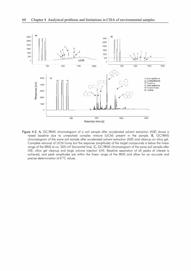
60 Chapter 4 Analytical problems and limitations in CSIA of environmental samples
Figure 4-2. A, GC/IRMS chromatogram of a soil sample after accelerated solvent extraction (ASE) shows a
raised baseline due to unresolved complex mixture (UCM) present in the sample. B, GC/IRMS chromatogram of the same soil sample after accelerated solvent extraction (ASE) and cleanup on silica gel. Complete removal of UCM hump but the response (amplitude) of the target compounds is below the linear range of the IRMS at ca. 500 mV (horizontal line). C, GC/IRMS chromatogram of the same soil sample after ASE, silica gel cleanup and large volume injection (LVI). Baseline separation of all peaks of interest is achieved, and peak amplitudes are within the linear range of the IRMS and allow for an accurate and precise determination of δ13C values.
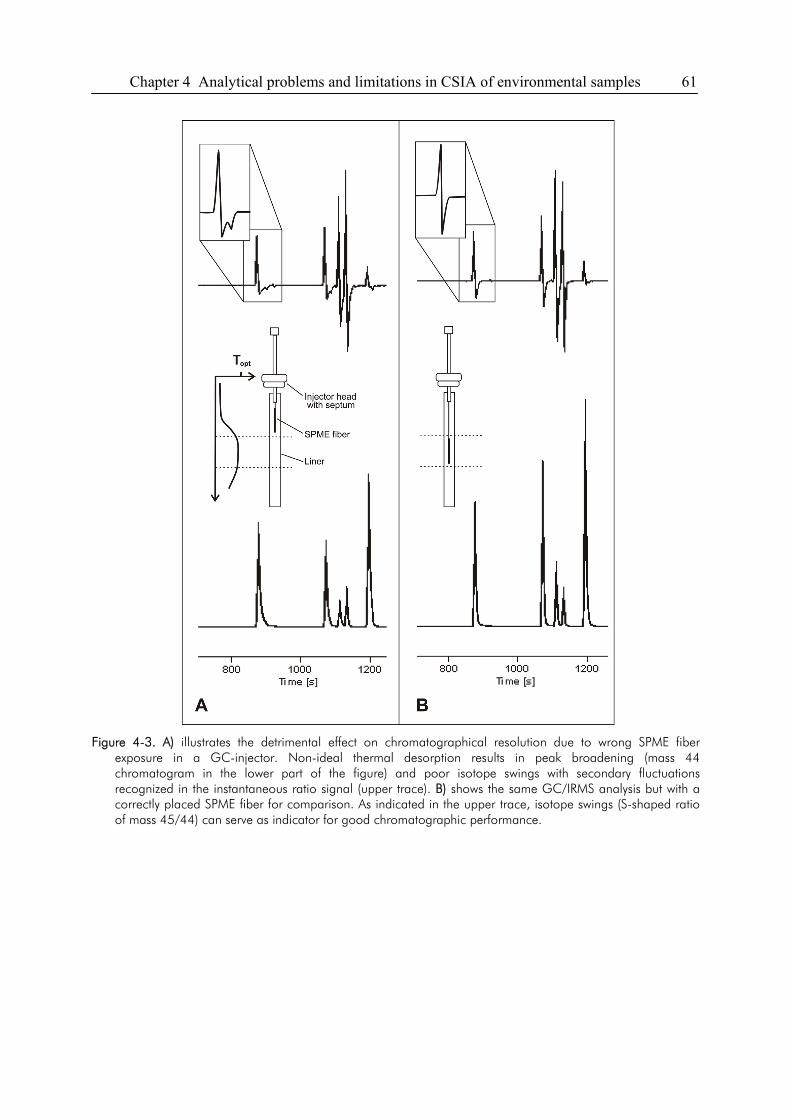
Chapter 4 Analytical problems and limitations in CSIA of environmental samples 61
Figure 4-3. A) illustrates the detrimental effect on chromatographical resolution due to wrong SPME fiber
exposure in a GC-injector. Non-ideal thermal desorption results in peak broadening (mass 44 chromatogram in the lower part of the figure) and poor isotope swings with secondary fluctuations recognized in the instantaneous ratio signal (upper trace). B) shows the same GC/IRMS analysis but with a correctly placed SPME fiber for comparison. As indicated in the upper trace, isotope swings (S-shaped ratio of mass 45/44) can serve as indicator for good chromatographic performance.
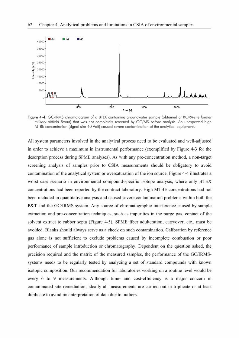
62 Chapter 4 Analytical problems and limitations in CSIA of environmental samples
Figure 4-4. GC/IRMS chromatogram of a BTEX containing groundwater sample (obtained at KORA-site former
military airfield Brand) that was not completely screened by GC/MS before analysis. An unexpected high MTBE concentration (signal size 40 Volt) caused severe contamination of the analytical equipment.
All system parameters involved in the analytical process need to be evaluated and well-adjusted
in order to achieve a maximum in instrumental performance (exemplified by Figure 4-3 for the
desorption process during SPME analyses). As with any pre-concentration method, a non-target
screening analysis of samples prior to CSIA measurements should be obligatory to avoid
contamination of the analytical system or oversaturation of the ion source. Figure 4-4 illustrates a
worst case scenario in environmental compound-specific isotope analysis, where only BTEX
concentrations had been reported by the contract laboratory. High MTBE concentrations had not
been included in quantitative analysis and caused severe contamination problems within both the
P&T and the GC/IRMS system. Any source of chromatographic interference caused by sample
extraction and pre-concentration techniques, such as impurities in the purge gas, contact of the
solvent extract to rubber septa (Figure 4-5), SPME fiber adulteration, carryover, etc., must be
avoided. Blanks should always serve as a check on such contamination. Calibration by reference
gas alone is not sufficient to exclude problems caused by incomplete combustion or poor
performance of sample introduction or chromatography. Dependent on the question asked, the
precision required and the matrix of the measured samples, the performance of the GC/IRMS-
systems needs to be regularly tested by analyzing a set of standard compounds with known
isotopic composition. Our recommendation for laboratories working on a routine level would be
every 6 to 9 measurements. Although time- and cost-efficiency is a major concern in
contaminated site remediation, ideally all measurements are carried out in triplicate or at least
duplicate to avoid misinterpretation of data due to outliers.
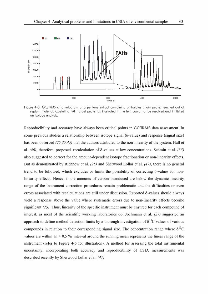
Chapter 4 Analytical problems and limitations in CSIA of environmental samples 63
Figure 4-5. GC/IRMS chromatogram of a pentane extract containing phthalates (main peaks) leached out of
septum material. Coeluting PAH target peaks (as illustrated in the left) could not be resolved and inhibited an isotope analysis.
Reproducibility and accuracy have always been critical points in GC/IRMS data assessment. In
some previous studies a relationship between isotope signal (δ-value) and response (signal size)
has been observed (25,35,45) that the authors attributed to the non-linearity of the system. Hall et
al. (46), therefore, proposed recalculation of δ-values at low concentrations. Schmitt et al. (35)
also suggested to correct for the amount-dependent isotope fractionation or non-linearity effects.
But as demonstrated by Richnow et al. (25) and Sherwood Lollar et al. (47), there is no general
trend to be followed, which excludes or limits the possibility of correcting δ-values for non-
linearity effects. Hence, if the amounts of carbon introduced are below the dynamic linearity
range of the instrument correction procedures remain problematic and the difficulties or even
errors associated with recalculations are still under discussion. Reported δ-values should always
yield a response above the value where systematic errors due to non-linearity effects become
significant (25). Thus, linearity of the specific instrument must be ensured for each compound of
interest, as most of the scientific working laboratories do. Jochmann et al. (27) suggested an
approach to define method detection limits by a thorough investigation of δ13C values of various
compounds in relation to their corresponding signal size. The concentration range where δ13C
values are within an ± 0.5 ‰ interval around the running mean represents the linear range of the
instrument (refer to Figure 4-6 for illustration). A method for assessing the total instrumental
uncertainty, incorporating both accuracy and reproducibility of CSIA measurements was
described recently by Sherwood Lollar et al. (47).
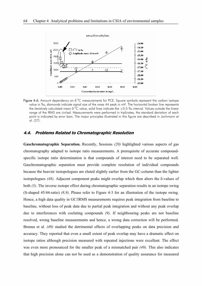
64 Chapter 4 Analytical problems and limitations in CSIA of environmental samples
Figure 4-6. Amount dependency on δ13C measurements for PCE. Square symbols represent the carbon isotope
value in ‰, diamonds indicate signal size of the mass 44 peak in mV. The horizontal broken line represents the iteratively calculated mean δ13C value, solid lines indicate the ±0.5 ‰ interval. Values outside the linear range of the IRMS are circled. Measurements were performed in triplicates, the standard deviation of each point is indicated by error bars. The major principles illustrated in this figure are described in Jochmann et al. (27).
4.4. Problems Related to Chromatographic Resolution
Gaschromatographic Separation. Recently, Sessions (20) highlighted various aspects of gas
chromatography adapted to isotope ratio measurements. A prerequisite of accurate compound-
specific isotope ratio determination is that compounds of interest need to be separated well.
Gaschromatographic separation must provide complete resolution of individual compounds
because the heavier isotopologues are eluted slightly earlier from the GC-column than the lighter
isotopologues (48). Adjacent component peaks might overlap which then alters the δ-values of
both (5). The inverse isotope effect during chromatographic separation results in an isotope swing
(S-shaped 45/44-ratio) (8,9). Please refer to Figure 4-3 for an illustration of the isotope swing.
Hence, a high data quality in GC/IRMS measurements requires peak integration from baseline to
baseline, without loss of peak data due to partial peak integration and without any peak overlap
due to interferences with coeluting compounds (9). If neighbouring peaks are not baseline
resolved, wrong baseline measurements and hence, a wrong data correction will be performed.
Brenna et al. (49) studied the detrimental effects of overlapping peaks on data precision and
accuracy. They reported that even a small extent of peak overlap may have a dramatic effect on
isotope ratios although precision measured with repeated injections were excellent. The effect
was even more pronounced for the smaller peak of a mismatched pair (49). This also indicates
that high precision alone can not be used as a demonstration of quality assurance for measured
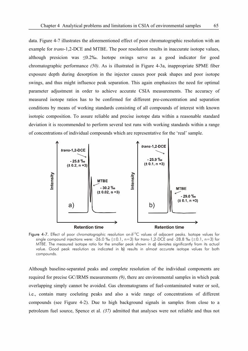
Chapter 4 Analytical problems and limitations in CSIA of environmental samples 65
data. Figure 4-7 illustrates the aforementioned effect of poor chromatographic resolution with an
example for trans-1,2-DCE and MTBE. The poor resolution results in inaccurate isotope values,
although presicion was ≤0.2‰. Isotope swings serve as a good indicator for good
chromatographic performance (50). As is illustrated in Figure 4-3a, inappropriate SPME fiber
exposure depth during desorption in the injector causes poor peak shapes and poor isotope
swings, and thus might influence peak separation. This again emphasizes the need for optimal
parameter adjustment in order to achieve accurate CSIA measurements. The accuracy of
measured isotope ratios has to be confirmed for different pre-concentration and separation
conditions by means of working standards consisting of all compounds of interest with known
isotopic composition. To assure reliable and precise isotope data within a reasonable standard
deviation it is recommended to perform several test runs with working standards within a range
of concentrations of individual compounds which are representative for the ‘real’ sample.
Figure 4-7. Effect of poor chromatographic resolution on δ13C values of adjacent peaks. Isotope values for
single compound injections were: -26.0 ‰ (±0.1, n=3) for trans-1,2-DCE and -28.8 ‰ (±0.1, n=3) for MTBE. The measured isotope ratio for the smaller peak shown in a) deviates significantly from its actual value. Good peak resolution as indicated in b) results in almost accurate isotope values for both compounds.
Although baseline-separated peaks and complete resolution of the individual components are
required for precise GC/IRMS measurements (9), there are environmental samples in which peak
overlapping simply cannot be avoided. Gas chromatograms of fuel-contaminated water or soil,
i.e., contain many coeluting peaks and also a wide range of concentrations of different
compounds (see Figure 4-2). Due to high background signals in samples from close to a
petroleum fuel source, Spence et al. (37) admitted that analyses were not reliable and thus not
66 Chapter 4 Analytical problems and limitations in CSIA of environmental samples
reported. Optimal peak separation was only achieved for samples containing relatively few
analytes (37). Note that the compounds or constituents of environmental samples often show
large differences in their individual concentrations within one sample, which often prevents an
adjustment for optimal precision of the isotope measurement in a single analysis and thus results
in larger standard deviations at small analyte concentrations (25). Yanik et al. (51) concluded in
their study that variations in the isotope ratio might not represent different sources but may in fact
represent contributions of minor compounds influencing the isotopic composition of even well-
resolved compounds. The GC/IRMS-system allows not only for backflushing of solvent peaks at
the beginning of a chromatogram, but also at different times within a single run. Hence, one way
to circumvent the problem would be to adjust for peaks with low concentrations and backflush
components with higher concentrations to avoid oversaturation of the ion source. Backflushing of
single compounds is often restricted by the time necessary for transferring the compound from
the GC to the IRMS system. If given time windows are too short, one might miss either the 13C-
enriched part at the beginning of a peak or the 13C-depleted part at the end of a peak of interest.
Thus, backflushing of single compounds needs a thorough, system-specific pre-investigation with
standards of known isotopic composition. Furthermore, in case that isotope analysis of major
components is also required, samples need to be split and analyzed twice, once with appropriate
dilution, once without dilution and the described backflushing.
Strategies to Avoid Matrix Interference. A limiting factor in CSIA of environmental samples is
the fact that an organic contamination often contains hundreds of different compounds resulting
in interferences in the chromatography. In particular, the unresolved complex mixture (UCM) of
hydrocarbons in petroleum-contaminated soils and sediments often hamper reliable isotope ratio
measurements. The term UCM is referring to the hump-shaped baseline raise that is often found
in gas chromatograms of petroleum products (see Figure 4-2a). Due to the complex chemical
composition of predominantly high-molecular weight, complex hydrocarbons, such as branched
alkanes, cycloalkanes and PAHs (52), also peaks of interest remain unresolved in the UCM
hump. Corrections required for coeluting and unresolved baseline components might be achieved
using background subtraction software (53), if only low levels of background matrix or UCM are
present. As compounds of interest need to be well resolved from neighbouring peaks in CSIA,
and due to the detrimental influence of co-extracted compounds on almost every GC analysis step
(54), there is a strong demand of improved cleanup strategies. Figure 4-2 exemplarily shows a
GC/IRMS chromatogram of PAHs before and after cleanup with silica column chromatography
that allowed to completely remove the UCM hump.
Chapter 4 Analytical problems and limitations in CSIA of environmental samples 67
As mentioned before, all sample treatment procedures hold the potential of isotope fractionation.
Hence, every step of the sample preparation protocol must be thoroughly evaluated by means of
standards with known isotopic composition that are treated identical to the samples. ASE
extraction of soil samples and purification using alumina/silica column chromatography resulted
in a maximum δ13C shift of -0.5 ‰ for individual PAHs (45), which is within standard precision
of GC/IRMS instruments. Cleanup using a alumina column eluted with hexane/toluene and
cleanup on a silica column using dichloromethane as the eluting solvent resulted in almost the
same hydrocarbon δ13C values (33). Kim et al. (55) reported that, although extensive cleanup
incorporating alumina/silica gel column, gel permeation, and thin layer chromatography was
performed, the original carbon isotopic composition of individual PAHs could be preserved.
Mazeas and Budzinski (56) tested three different purification procedures and concluded that it did
not introduce any significant isotope fractionation to the initial standard solution. O’Malley et al.
(32) did not achieve complete elimination of the UCM. Paying close attention to background
corrections in samples with prominent UCM, they introduced internal standards with known
isotopic composition to aid a careful selection of background points and thus, a reliable
determination of δ13C values of individual PAHs even if significant UCM was present.
Another way to achieve an increased sensitivity due to reduction in background and elimination
of coeluting compounds is to use two-dimensional gas chromatography prior to combustion
although this combination so far has hardly been reported in literature (57). In 2D-GC/IRMS, the
GC-system needs to be equipped with a column switching device such as moving capillary
stream switching (MCSS). By column switching parts of the effluent from the first column are
cut and transferred to a second column, where separation of compounds of interest can be
enhanced. Horii et al. (57) demonstrated δ13C measurements of individual congeners of
polychlorinated biphenyls and chloronaphthalenes by application of the MCSS technique. As
reported by Sessions (20) comprehensive GCxGC methods and fast GC, respectively, require
very fast detector response times and thus, seem not to be appropriate analyte separation
techniques for continuous-flow IRMS.
4.5. CSIA of Non-Volatile Compounds
GC-based applications are limited to volatile and thermally stable analytes. To improve
chromatographic separation of non-volatile compounds and organic functional groups,
68 Chapter 4 Analytical problems and limitations in CSIA of environmental samples
derivatization is commonly performed. Some requirements need to be fulfilled to guarantee
accurate isotope analysis. Derivatizing reagents have to react quantitatively with the analytes,
isotope dilution effects by addition of the element being analyzed should be excluded or limited,
the reagents should not cause any adverse chromatographic effects and should have no
detrimental effects on the reaction interface or result in an incomplete combustion (9,20). Due to
the several potential problems of derivatization in CSIA there have been many attempts to
hyphenate liquid chromatography with IRMS. Earlier approaches include a thermospray/particle
beam interface (58) and a moving-wire interface (59,60). Although the latter has seen recent
advances for the very sensitive carbon isotope analysis of discrete liquid samples (61), these
interfaces have never been commercialized and thus their use remains restricted to the developing
laboratories. In 2004, though, another interface design based on an on-line TOC equipment has
been commercialized that is much more promising for future work (62). So far, on-line LC/IRMS
based on this interface has been applied successfully for the isotope analysis of various analyte
classes including proteins (63), carbohydrates (64), underivatized amino acids (65), and volatile
fatty acids (66). However, there are still major challenges in this area. First, the commercial
interface only allows for carbon isotope analysis. Second, separation is limited to pure aqueous
eluents which requires the development of fully new separation approaches. Besides pH and ionic
strength of the eluent that can be optimized for the separation of ionic compounds, temperature is
one of the parameters that might be used to influence retention. Thus, LC/IRMS will certainly
benefit from further developments in the area of high-temperature HPLC. Third, with regard to
trace contaminants in environmental chemistry, the sensitivity of LC/IRMS may not be sufficient,
thus requiring validated preconcentration steps. For example, Penning and Elsner estimated
sensitivity to be 8 times lower for the carbon isotope analysis of isoproturon using LC/IRMS
instead of GC/IRMS (67). The lower sensitivity currently achieved in LC/IRMS is partly due to
the non-negligible background of carbon stemming in particular from column bleed.
4.6. Uncertainties of Data Interpretation
As both isotope analysis and further data processing can include sources of uncertainty (47), a
strong collaboration of the isotope analyst and the customers is necessary to assure a high quality
in data interpretation. Furthermore, it has to be emphasized that a prerequisite of environmental
field work is a thorough characterization of field sites, for example, detailed knowledge on
groundwater flow regimes and site-specific geochemical parameters. Slater (16) discussed
Chapter 4 Analytical problems and limitations in CSIA of environmental samples 69
important points to be considered when interpreting data from field applications in a realistic and
defensible way. He pointed out the challenge of determining the isotopic composition of the
source zone, the problems connected with temporal variability of δ-values in field applications, as
well as the importance to obtain transects of samples at a high density. The study also mentioned
quantification problems related to the application of the Rayleigh model at field sites.
Overestimation of degradation rates is a major concern in assessing the natural attenuation
potential at a contaminated site. Laboratory studies have shown that different bacterial strains
may cause different magnitudes of isotope fractionation (from large to non-detectable) dependent
on the substrate and the different mechanisms in the rate-limiting step of the enzymatic reaction
(17). Studies by Meckenstock et al. (17) and Abé and Hunkeler (68) demonstrated the difficulties
when calculating the extent of in-situ biodegradation at field sites, an in-depth discussion of this
issue is provided by Morrill et al. (69). Fischer et al. (70) reported on the relevance of non-
fractionating processes in estimating in-situ degradation rates from field data. Those difficulties
are especially important as systems become more and more complex. One should always keep in
mind that most of the field studies reported in literature have focussed on homogeneous and
unconsolidated aquifer systems. Until now, only a few were considering hydrogeological
complex and heterogeneous systems, e.g., fractured bedrock (37,21).
4.7. References
(1) Sano, M.; Yotsui, Y.; Abe, H.; Sasaki, S. A new technique for the detection of metabolites labelled by the isotope 13C using mass fragmentography. Biomed. Mass Spectrom. 1976, 3, 1-3.
(2) Matthews, D. E.; Hayes, J. M. Isotope-ratio-monitoring gas chromatography-mass spectrometry. Anal. Chem. 1978, 50, 1465-1473.
(3) Barrie, A.; Bricout, J.; Koziet, J. Gas chromatography - stable isotope ratio analysis at natural abundance levels. Biomed. Mass Spectrom. 1984, 11, 583-588.
(4) Freedman, P. A.; Gillyon, E. C. P.; Jumeau, E. J. Design and application of a new instrument for GC-isotope ratio MS Am. Lab. 1988, 20, 114-119.
(5) Hayes, J. M.; Freeman, K. H.; Popp, B. N.; Hoham, C. H. Compound-specific isotopic analyses: A novel tool for reconstruction of ancient biogeochemical processes. Org. Geochem. 1990, 16, 1115-1128.
(6) Schoell, M.; McCaffrey, M. A.; Fago, F. J.; Moldowan, J. M. Carbon isotopic compositions of 28,30-bisnorhopanes and other biological markers in a Monterey crude oil. Geochim. Cosmochim. Acta 1992, 56, 1391-1399.
(7) Ruble, T. E.; Bakel, A. J.; Philp, R. P. Compound specific isotopic variability in Uinta Basin native bitumens: paleoenvironmental implications. Org. Geochem. 1994, 21, 661-671.
(8) Brand, W. A. High precision isotope ratio monitoring techniques in mass spectrometry. J. Mass Spectrom. 1996, 31, 225-235.
(9) Meier-Augenstein, W. Applied gas chromatography coupled to isotope ratio mass spectrometry. J. Chromatogr. A 1999, 842, 351-371.
(10) Schmidt, T. C.; Zwank, L.; Elsner, M.; Berg, M.; Meckenstock, R. U.; Haderlein, S. B. Compound-specific stable isotope analysis of organic contaminants in natural environments: a critical review of the state of the art, prospects, and future challenges. Anal. Bioanal. Chem. 2004, 378, 283-300.
70 Chapter 4 Analytical problems and limitations in CSIA of environmental samples
(11) Benson, S.; Lennard, C.; Maynard, P.; Roux, C. Forensic applications of isotope ratio mass spectrometry - A review. Forensic Sci. Int. 2006, 157, 1-22.
(12) Eakin, P. A.; Fallick, A. E.; Gerk, J. Some instrumental effects in the determination of stable carbon isotope ratios by gas chromatography-isotope ratio mass spectrometry. Chem. Geol. 1992, 101, 71-79.
(13) Ricci, M. P.; Merritt, D. A.; Freeman, K. H.; Hayes, J. M. Acquisition and processing of data for isotope-ratio-monitoring mass spectrometry. Org. Geochem. 1994, 21, 561-571.
(14) Merritt, D. A.; Freeman, K. H.; Ricci, M. P.; Studley, S. A.; Hayes, J. M. Performance and Optimization of a Combustion Interface for Isotope Ratio Monitoring Gas Chromatography/Mass Spectrometry. Anal. Chem. 1995, 67, 2461-2473.
(15) Sherwood Lollar, B.; Slater, G. F.; Ahad, J.; Sleep, B.; Spivack, J.; Brennan, M.; MacKenzie, P. Contrasting carbon isotope fractionation during biodegradation of trichloroethylene and toluene: Implications for intrinsic bioremediation. Org. Geochem. 1999, 30, 813-820.
(16) Slater, G. F. Stable isotope forensics - When isotopes work. Environ. Forensics 2003, 4, 13-23. (17) Meckenstock, R. U.; Morasch, B.; Griebler, C.; Richnow, H. H. Stable isotope fractionation analysis as a tool
to monitor biodegradation in contaminated acquifers. J. Contam. Hydrol. 2004, 75, 215-255. (18) Elsner, M.; Zwank, L.; Hunkeler, D.; Schwarzenbach, R. P. A new concept linking observable stable isotope
fractionation to transformation pathways of organic pollutants. Environ. Sci. Technol. 2005, 39, 6896-6916. (19) Hunkeler, D.; Meckenstock, R. U.; Sherwood Lollar, B.; Schmidt, T. C.; Wilson, J. T. A. A consensus guide
for assessing biodegradation and source identification with compound-specific isotope analysis (CSIA). 2007, submitted.
(20) Sessions, A. L. Isotope-ratio detection for gas chromatography Review. J. Sep. Sci. 2006, 29, 1946-1961. (21) Chartrand, M. M. G.; Morrill, P. L.; Lacrampe-Couloume, G.; Sherwood Lollar, B. Stable isotope evidence for
biodegradation of chlorinated ethenes at a fractured bedrock site. Environ. Sci. Technol. 2005, 39, 4848-4856. (22) Peter, A.; Steinbach, A.; Liedl, R.; Ptak, T.; Michaelis, W.; Teutsch, G. Assessing microbial degradation of o-
xylene at field-scale from the reduction in mass flow rate combined with compound-specific isotope analyses. J. Contam. Hydrol. 2004, 71, 127-154.
(23) Blum, P.; Kamkar, P.; Melzer, R. Sensitivitätsanalyse von Natural Attenuation anhand analytischer Transportmodelle. Altlasten Spektrum 2007, 2, 74-81.
(24) Kopinke, F. D.; Georgi, A.; Voskamp, M.; Richnow, H. H. Carbon isotope fractionation of organic contaminants due to retardation on humic substances: Implications for natural attenuation studies in aquifers. Environ. Sci. Technol. 2005, 39, 6052-6062.
(25) Richnow, H. H.; Annweiler, E.; Michaelis, W.; Meckenstock, R. U. Microbial in situ degradation of aromatic hydrocarbons in a contaminated aquifer monitored by carbon isotope fractionation. J. Contam. Hydrol. 2003, 65, 101-120.
(26) Song, D. L.; Conrad, M. E.; Sorenson, K. S.; Alvarez-Cohen, L. Stable carbon isotope fractionation during enhanced in situ bioremediation of trichloroethene. Environ. Sci. Technol. 2002, 36, 2262-2268.
(27) Jochmann, M. A.; Blessing, M.; Haderlein, S. B.; Schmidt, T. C. A new approach to determine method detection limits for compound-specific isotope analysis of volatile organic compounds. Rapid Commun. Mass Spectrom. 2006, 20, 3639-3648.
(28) McLoughlin, P. W.; Pirkle, R. J.; Fine, D.; Wilson, J. T. TBA production by acid hydrolysis of MTBE during heated headspace analysis and evaluation of a base as a preservative. Ground Water Monit. Remediat. 2004, 24, 57-66.
(29) Kovacs, D. A.; Kampbell, D. H. Improved method for the storage of groundwater samples containing volatile organic analytes. Arch. Environ. Contamin. Toxicol. 1999, 36, 242-247.
(30) Kelley, C. A.; Hammer, B. T.; Coffin, R. B. Concentrations and stable isotope values of BTEX in gasoline- contaminated groundwater. Environ. Sci. Technol. 1997, 31, 2469-2472.
(31) Elsner, M.; Lacrampe-Couloume, G.; Sherwood Lollar, B. Freezing to preserve groundwater samples and improve headspace quantification limits of water-soluble organic contaminants for carbon isotope analysis. Anal. Chem. 2006, 78, 7528-7534.
(32) O'Malley, V. P.; Abrajano, T. A.; Hellou, J. Determination of the 13C/12C ratios of individual PAH from environmental samples: can PAH sources be apportioned? Org. Geochem. 1994, 21, 809-822.
(33) Graham, M. C.; Allan, R.; Fallick, A. E.; Farmer, J. G. Investigation of extraction and clean-up procedures used in the quantification and stable isotopic characterisation of PAHs in contaminated urban soils. Sci. Total Environ. 2006, 360, 81-89.
(34) Baylis, S. A.; Hall, K.; Jumeau, E. J. The analysis of the C1-C5 components of natural gas samples using gas chromatography-combustion-isotope ratio mass spectrometry. Org. Geochem. 1994, 21, 777-785.
(35) Schmitt, J.; Glaser, B.; Zech, W. Amount-dependent isotopic fractionation during compound-specific isotope analysis. Rapid Commun. Mass Spectrom. 2003, 17, 970-977.
Chapter 4 Analytical problems and limitations in CSIA of environmental samples 71
(36) Smallwood, B. J.; Philp, R. P.; Burgoyne, T. W.; Allen, J. D. The use of stable isotopes to differentiate specific source markers for MTBE. Environ.l Forensics 2001, 2, 215-221.
(37) Spence, M. J.; Bottrell, S. H.; Thornton, S. F.; Richnow, H. H.; Spence, K. H. Hydrochemical and isotopic effects associated with petroleum fuel biodegradation pathways in a chalk aquifer. J. Contam. Hydrol. 2005, 79, 67-88.
(38) Hunkeler, D.; Butler, B. J.; Aravena, R.; Barker, J. F. Monitoring biodegradation of methyl tert-butyl ether (MTBE) using compound-specific carbon isotope analysis. Environ. Sci. Technol. 2001, 35, 676-681.
(39) Gray, J. R.; Lacrampe-Couloume, G.; Gandhi, D.; Scow, K. M.; Wilson, R. D.; Mackay, D. M.; Sherwood Lollar, B. Carbon and hydrogen isotopic fractionation during biodegradation of methyl tert-butyl ether. Environ. Sci. Technol. 2002, 36, 1931-1938.
(40) Zwank, L.; Berg, M.; Schmidt, T. C.; Haderlein, S. B. Compound-specific carbon isotope analysis of volatile organic compounds in the low-microgram per liter range. Anal. Chem. 2003, 75, 5575-5583.
(41) Hunkeler, D.; Aravena, R. Determination of compound-specific carbon isotope ratios of chlorinated methanes, ethanes, and ethenes in aqueous samples. Environ. Sci. Technol. 2000, 34, 2839-2844.
(42) Slater, G. F.; Dempster, H. S.; Sherwood Lollar, B.; Ahad, J. Headspace analysis: A new application for isotopic characterization of dissolved organic contaminants. Environ. Sci. Technol. 1999, 33, 190-194.
(43) Steinbach, A.; Seifert, R.; Annweiler, E.; Michaelis, W. Hydrogen and carbon isotope fractionation during anaerobic biodegradation of aromatic hydrocarbons - A field study. Environ. Sci. Technol. 2004, 38, 609-616.
(44) Dempster, H. S.; Sherwood Lollar, B.; Feenstra, S. Tracing organic contaminants in groundwater: A new methodology using compound-specific isotopic analysis. Environ. Sci. Technol. 1997, 31, 3193-3197.
(45) Wilcke, W.; Krauss, M.; Amelung, W. Carbon isotope signature of polycyclic aromatic hydrocarbons (PAHs): Evidence for different sources in tropical and temperate environments? Environ. Sci. Technol. 2002, 36, 3530-3535.
(46) Hall, J. A.; Barth, J. A. C.; Kalin, R. M. Routine analysis by high precision gas chromatography mass selective detector isotope ratio mass spectrometry to 0.1 parts per mil. Rapid Commun. Mass Spectrom. 1999, 13, 1231-1236.
(47) Sherwood Lollar, B.; Hirschorn, S. K.; Chartrand, M. M. G.; Lacrampe-Couloume, G. An approach for assessing total instrumental uncertainty in compound-specific carbon isotope analysis: Implications for environmental remediation studies. Anal. Chem. 2007, 79, 3469-3475.
(48) van Hook, W. A.; Emmet, P. H. The Gas Chromatographic Determination of Hydrogen, Deuterium and HD. J. Physical Chem. 1960, 673-675.
(49) Brenna, J. T.; Corso, T. N.; Tobias, H. J.; Caimi, R. J. High-precision continuous-flow isotope ratio mass spectrometry. Mass Spectrom. Reviews 1997, 16, 227-258.
(50) Hilkert, A. W.; Douthitt, C. B.; Schlüter, H. J.; Brand, W. A. Isotope ratio monitoring gas chromatography mass spectrometry of D H by high temperature conversion isotope ratio mass spectrometry. Rapid Commun. Mass Spectrom. 1999, 13, 1226-1230.
(51) Yanik, P. J.; O'Donnell, T. H.; Macko, S. A.; Qian, Y.; Kennicutt, M. C. Source apportionment of polychlorinated biphenyls using compound specific isotope analysis. Org. Geochem. 2003, 34, 239-251.
(52) Frysinger, G. S.; Gaines, R. B.; Xu, L.; Reddy, C. M. Resolving the unresolved complex mixture in petroleum-contaminated sediments. Environ. Sci. Technol. 2003, 37, 1653-1662.
(53) Sun, Y. G.; Sheng, G. Y.; Peng, P.; Fu, J. M. Compound-specific stable carbon isotope analysis as a tool for correlating coal-sourced oils and interbedded shale-sourced oils in coal measures: an example from Turpan basin, north-western China. Org. Geochem. 2000, 31, 1349-1362.
(54) Dabrowski, L.; Giergielewicz-Mozajska, H.; Gorski, L.; Biziuk, M.; Namiesnik, J.; Janicki, B. Determination of environmental pollutants in soil and sediments - Some aspects of sample clean-up and GC analysis. J. Sep. Sci. 2002, 25, 290-296.
(55) Kim, M.; Kennicutt Il, M. C.; Qian, Y. Polycyclic aromatic hydrocarbon purification procedures for compound specific isotope analysis. Environ. Sci. Technol. 2005, 39, 6770-6776.
(56) Mazeas, L.; Budzinski, H. Polycyclic aromatic hydrocarbon C-13/C-12 ratio measurement in petroleum and marine sediments - Application to standard reference materials and a sediment suspected of contamination from the Erika oil spill. J. Chromatogr. A 2001, 923, 165-176.
(57) Horii, Y.; Kannan, K.; Petrick, G.; Gamo, T.; Falandysz, J.; Yamashita, N. Congener-specific carbon isotopic analysis of technical PCB and PCN mixtures using two-dimensional gas chromatography - Isotope ratio mass spectrometry. Environ. Sci. Technol. 2005, 39, 4206-4212.
(58) Teffera, Y.; Kusmierz, J. J.; Abramson, F. P. Continuous-Flow Isotope Ratio Mass Spectrometry Using the Chemical Reaction Interface with Either Gas or Liquid Chromatographic Introduction. Anal. Chem. 1996, 68, 1888-1894.
(59) Caimi, R. J.; Brenna, J. T. High-precision liquid chromatography-combustion isotope ratio mass spectrometry. Anal. Chem. 1993, 65, 3497-3500.
72 Chapter 4 Analytical problems and limitations in CSIA of environmental samples
(60) Brand, W. A.; Dobberstein, P. Isotope-ratio-monitoring liquid chromatography mass spectrometry (IRM-LCMS): First results from a moving wire interface system. Isot. Environ. Health Stud. 1996, 32, 275-283.
(61) Sessions, A. L.; Sylva, S. P.; Hayes, J. M. Moving-Wire Device for Carbon Isotopic Analyses of Nanogram Quantities of Nonvolatile Organic Carbon. Anal. Chem. 2005, 77, 6519-6527.
(62) Krummen, M.; Hilkert, A. W.; Juchelka, D.; Duhr, A.; Schlüter, H. J.; Pesch, R. A new concept for isotope ratio monitoring liquid chromatography/mass spectrometry. Rapid Commun. Mass Spectrom. 2004, 18, 2260-2266.
(63) Godin, J. P.; Hau, J.; Fay, L. B.; Hopfgartner, G. Isotope ratio monitoring of small molecules and macromolecules by liquid chromatography coupled to isotope ratio mass spectrometry. Rapid Commun. Mass Spectrom. 2005, 19, 2689-2698.
(64) Cabanero, A. I.; Recio, J. L.; Ruperez, M. Liquid chromatography coupled to isotope ratio mass spectrometry: A new perspective on honey adulteration detection. J. Agricul. Food Chem. 2006, 54, 9719-9727.
(65) McCullagh, J. S. O.; Juchelka, D.; Hedges, R. E. M. Analysis of amino acid C-13 abundance from human and faunal bone collagen using liquid chromatography/isotope ratio mass spectrometry. Rapid Commun. Mass Spectrom. 2006, 20, 2761-2768.
(66) Heuer, V.; Elvert, M.; Tille, S.; Krummen, M.; Mollar, X. P.; Hmelo, L. R.; Hinrichs, K. U. Online delta C-13 analysis of volatile fatty acids in sediment/porewater systems by liquid chromatography-isotope ratio mass spectrometry. Limnol. Oceanogr. Meth. 2006, 4, 346-357.
(67) Penning, H.; Elsner, M. 2007. GSF Neuherberg, Germany, personal communication. (68) Abe, Y.; Hunkeler, D. Does the Rayleigh Equation Apply to Evaluate Field Isotope Data in Contaminant
Hydrogeology? Environ. Sci. Technol. 2006, 40, 1588-1596. (69) Morrill, P. L.; Lacrampe-Couloume, G.; Slater, G. F.; Sleep, B. E.; Edwards, E. A.; McMaster, M. L.; Major,
D. W.; Sherwood Lollar, B. Quantifying chlorinated ethene degradation during reductive dechlorination at Kelly AFB using stable carbon isotopes. J. Contam. Hydrol. 2005, 76, 279-293.
(70) Fischer, A.; Theuerkorn, K.; Stelzer, N.; Gehre, M.; Thullner, M.; Richnow, H. H. Applicability of Stable Isotope Fractionation Analysis for the Characterization of Benzene Biodegradation in a BTEX-contaminated Aquifer. Environ. Sci. Technol. 2007, 41, 3689-3696.
Chapter 5 Delineation of multiple chlorinated ethene sources 73
5. Delineation of Multiple Chlorinated Ethene Sources in an
Industrialized Area
5.1. Introduction
Extensive groundwater contamination has been caused by the almost ubiquitous use of the
chlorinated solvents tetrachloroethene (PCE), trichloroethene (TCE), carbon tetrachloride (CT),
and 1,1,1-trichloroethane (1,1,1-TCA), as cleaning and degreasing solvents (1,2). These
compounds are toxic and/or carcinogenic and are regulated in drinking water at low levels (3).
Especially in fractured bedrock aquifers these dense non-aqueous phase liquids (DNAPL) lead to
a very complex contamination pattern and due to their slow dissolution rates provide a persistent
source of contamination for decades (4).
Liabilities for expensive field investigations and remediation effort may be assessed by different
means of environmental forensic litigation, including historical records, mathematical methods,
chemical fingerprinting, and isotope analyses. However, all of these methods have severe
drawbacks and thus rarely provide the required information on their own. Historical records
documenting the usage of chemicals, although often not available or incomplete, typically serve
as starting point. Evaluation of concentration data with mathematical methods such as
probabilistic and geostatistical simulation, inverse modeling and regression approaches usually
require homogeneous aquifer parameters with simple geometries and flow conditions (5-7).
Environmental fingerprinting can be powerful for complex mixtures of contaminants such as oil,
fuel or gasoline (8) but may be ambiguous if heavy weathering has occurred (9). Because of these
limitations, stable isotope analysis has emerged as an important additional tool in forensic
investigations (10,11). Studies where compound-specific isotope analysis (CSIA) have been
successfully applied, include source allocation of polycyclic aromatic compounds (9,12,13).
Several priority groundwater contaminants such as benzene, toluene, ethylbenzene, xylenes
(BTEX), methyl tert-butyl ether, and chlorinated solvents exhibit different stable isotope
signatures in products of different manufacturers (14). Hunkeler et al. (15) delineated different
zones, each representing a different episode and location of DNAPL release using CSIA data at a
site contaminated with PCE. Studies, so far, suggested that if no biodegradation occurs and
sufficient field data are available, source differentiation can be successful when isotope
signatures of PCE from various sources differ by more than 1‰ in δ13C (14,15). Surprisingly,
74 Chapter 5 Delineation of multiple chlorinated ethene sources
CSIA has not yet been applied in a forensic study to allocate different sources of chlorinated
solvents at a contaminated site although these compounds may differ in carbon or chlorine
isotope signatures depending on their manufacturing process (1,16-18).
Most of the reported CSIA field studies on chlorinated hydrocarbons focus on identification and
quantification of in-situ biodegradation in unconsolidated porous aquifers (19-24). Stable carbon
isotope analysis was applied to confirm degradation pathways at a field site contaminated with a
complex mixture of chlorinated compounds (24). Measurements of isotope ratios not only
allowed for estimating enrichment factors and quantifying transformation processes; they also
provided insight into the origin of degradation products (24). Thus, CSIA data help to
demonstrate if a substance was already present as a primary contaminant or if it is a degradation
byproduct and to specify the precursor it originates from. CSIA has also been used to assess
biodegradation of chlorinated ethenes at a hydrogeologically complex site (25). When CSIA is
used as a sole technique, source apportionment may be problematic when more than two possible
sources are involved in the contamination (26). A multiple-line-of-evidence approach including
evaluation of historical, hydrological, geochemical and isotopic data as well as statistical analysis
was applied to unravel the contamination scenario at the site. A major purpose of this study was
to determine under which conditions stable isotope ratios can be used for environmental forensic
purposes in the presence of adverse conditions such as biodegradation and complex
hydrogeological conditions. A key factor turned out to be the determination of highly precise
δ13C values of chlorinated ethenes in groundwater even at concentrations in the low µg/L-range
which allowed to cover a wide range of the contaminant plumes. The results presented here
provide the first successful example of a forensic isotope field study on chlorinated ethenes in a
fractured bedrock aquifer.
5.2. Material and Methods
Field Site. The site is located in an early industrialized urban area in southwestern Germany with
a long operational history. At the end of the 19th century parts of the region were used
extensively by industry and trade. Heavy industry in the region included metal working industries
and reprocessing of used mineral oil. A substantial contamination with chemicals used by these
industries occurred in the soil and the groundwater in the region, particularly through damage
during World War II. During the reconstruction period, industry in the valley expanded further
uphill. Most notably the widespread use of chlorinated solvents by various industrial production
Chapter 5 Delineation of multiple chlorinated ethene sources 75
facilities induced severe contamination of the soil and the associated bedrock groundwater
system. Consequently, multiple suspected contaminant sources were created over the past
decades resulting in several overlapping plumes. Main organic contaminants are chlorinated
ethenes; mineral oil hydrocarbons, BTEX and polycyclic aromatic hydrocarbons (PAHs) have
also been detected in some of the wells. Site-specific historical information is available within the
city’s register of contaminated sites.
Geology and Hydrogeology. The site is located in fractured Keuper rocks which are overlain by
a few meters of artificial fill and Quaternary deposits. The subsurface at the site is part of the
‘Gipskeuper’, a geological unit that is characterized by its high gypsum content consisting of
alternating sequences of marl, a lime-rich mudstone, claystone and dolomites. The geology leads
to several hydrostratigraphical units including the two aquifers (Dunkelroter Mergel, DRM and
Bochinger Horizont, BH) where the contamination was detected. A hydraulic connection between
the DRM and the BH aquifer attributed to fissures and fractures within the formation has been
observed (27). The majority of the contaminant mass remained in the upper aquifer (DRM), a
reddish-brown claystone containing thin layers of lime-rich mudstone with a dense network of
fine, connected fissures. The general groundwater flow conditions and the distribution of
contaminants at the site are given in Figure 5-1a. Likewise, additional data are accessible from
earlier groundwater sampling campaigns. An east-west fault zone with low hydraulic
conductivity may constrain the contaminant mass transport from north to south (27). The distance
between the contamination under investigation and the region’s main groundwater wells is
between 500 m and 1700 m. Due to their length and extension the chlorinated solvent plumes are
therefore of major concern to local authorities.
Groundwater Sampling. Within the framework of a groundwater sampling campaign
throughout the industrial zone in April 2005 samples were collected from 68 monitoring wells for
hydrogeochemical characterization and contaminant concentration analyses. Concentration data
were provided for the upper (DRM) and the subjacent aquifer (BH). A total of 27 of these
groundwater wells have been sampled for isotope analysis of the specific chlorinated ethene
compounds PCE, TCE, cis-1,2-dichloroethene (cis-DCE) and vinyl chloride (VC). Samples for
isotope analysis were filled in 1-L amber glass bottles without headspace, sealed with Teflon-
lined caps and kept at 4 °C until analysis; a preservation agent was not added. Carbon isotope
measurements were performed within 1 to 10 weeks after sampling; an effect of holding times on
isotope values can be excluded (data shown in the Appendix of this chapter). Figure 5-1b shows
the location of all observation wells that were sampled for isotope measurements. As the main
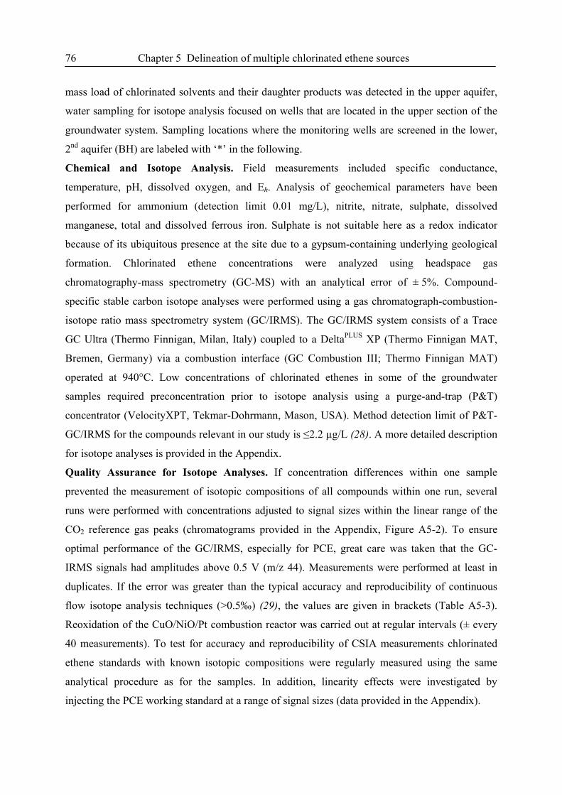
76 Chapter 5 Delineation of multiple chlorinated ethene sources
mass load of chlorinated solvents and their daughter products was detected in the upper aquifer,
water sampling for isotope analysis focused on wells that are located in the upper section of the
groundwater system. Sampling locations where the monitoring wells are screened in the lower,
2nd aquifer (BH) are labeled with ‘*’ in the following.
Chemical and Isotope Analysis. Field measurements included specific conductance,
temperature, pH, dissolved oxygen, and Eh. Analysis of geochemical parameters have been
performed for ammonium (detection limit 0.01 mg/L), nitrite, nitrate, sulphate, dissolved
manganese, total and dissolved ferrous iron. Sulphate is not suitable here as a redox indicator
because of its ubiquitous presence at the site due to a gypsum-containing underlying geological
formation. Chlorinated ethene concentrations were analyzed using headspace gas
chromatography-mass spectrometry (GC-MS) with an analytical error of ± 5%. Compound-
specific stable carbon isotope analyses were performed using a gas chromatograph-combustion-
isotope ratio mass spectrometry system (GC/IRMS). The GC/IRMS system consists of a Trace
GC Ultra (Thermo Finnigan, Milan, Italy) coupled to a DeltaPLUS XP (Thermo Finnigan MAT,
Bremen, Germany) via a combustion interface (GC Combustion III; Thermo Finnigan MAT)
operated at 940°C. Low concentrations of chlorinated ethenes in some of the groundwater
samples required preconcentration prior to isotope analysis using a purge-and-trap (P&T)
concentrator (VelocityXPT, Tekmar-Dohrmann, Mason, USA). Method detection limit of P&T-
GC/IRMS for the compounds relevant in our study is ≤2.2 µg/L (28). A more detailed description
for isotope analyses is provided in the Appendix.
Quality Assurance for Isotope Analyses. If concentration differences within one sample
prevented the measurement of isotopic compositions of all compounds within one run, several
runs were performed with concentrations adjusted to signal sizes within the linear range of the
CO2 reference gas peaks (chromatograms provided in the Appendix, Figure A5-2). To ensure
optimal performance of the GC/IRMS, especially for PCE, great care was taken that the GC-
IRMS signals had amplitudes above 0.5 V (m/z 44). Measurements were performed at least in
duplicates. If the error was greater than the typical accuracy and reproducibility of continuous
flow isotope analysis techniques (>0.5‰) (29), the values are given in brackets (Table A5-3).
Reoxidation of the CuO/NiO/Pt combustion reactor was carried out at regular intervals (± every
40 measurements). To test for accuracy and reproducibility of CSIA measurements chlorinated
ethene standards with known isotopic compositions were regularly measured using the same
analytical procedure as for the samples. In addition, linearity effects were investigated by
injecting the PCE working standard at a range of signal sizes (data provided in the Appendix).
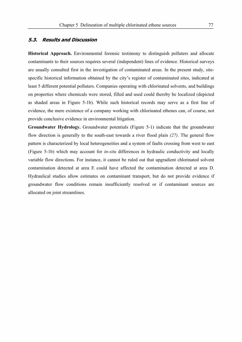
Chapter 5 Delineation of multiple chlorinated ethene sources 77
5.3. Results and Discussion
Historical Approach. Environmental forensic testimony to distinguish polluters and allocate
contaminants to their sources requires several (independent) lines of evidence. Historical surveys
are usually consulted first in the investigation of contaminated areas. In the present study, site-
specific historical information obtained by the city’s register of contaminated sites, indicated at
least 5 different potential polluters. Companies operating with chlorinated solvents, and buildings
on properties where chemicals were stored, filled and used could thereby be localized (depicted
as shaded areas in Figure 5-1b). While such historical records may serve as a first line of
evidence, the mere existence of a company working with chlorinated ethenes can, of course, not
provide conclusive evidence in environmental litigation.
Groundwater Hydrology. Groundwater potentials (Figure 5-1) indicate that the groundwater
flow direction is generally to the south-east towards a river flood plain (27). The general flow
pattern is characterized by local heterogeneities and a system of faults crossing from west to east
(Figure 5-1b) which may account for in-situ differences in hydraulic conductivity and locally
variable flow directions. For instance, it cannot be ruled out that upgradient chlorinated solvent
contamination detected at area E could have affected the contamination detected at area D.
Hydraulical studies allow estimates on contaminant transport, but do not provide evidence if
groundwater flow conditions remain insufficiently resolved or if contaminant sources are
allocated on joint streamlines.
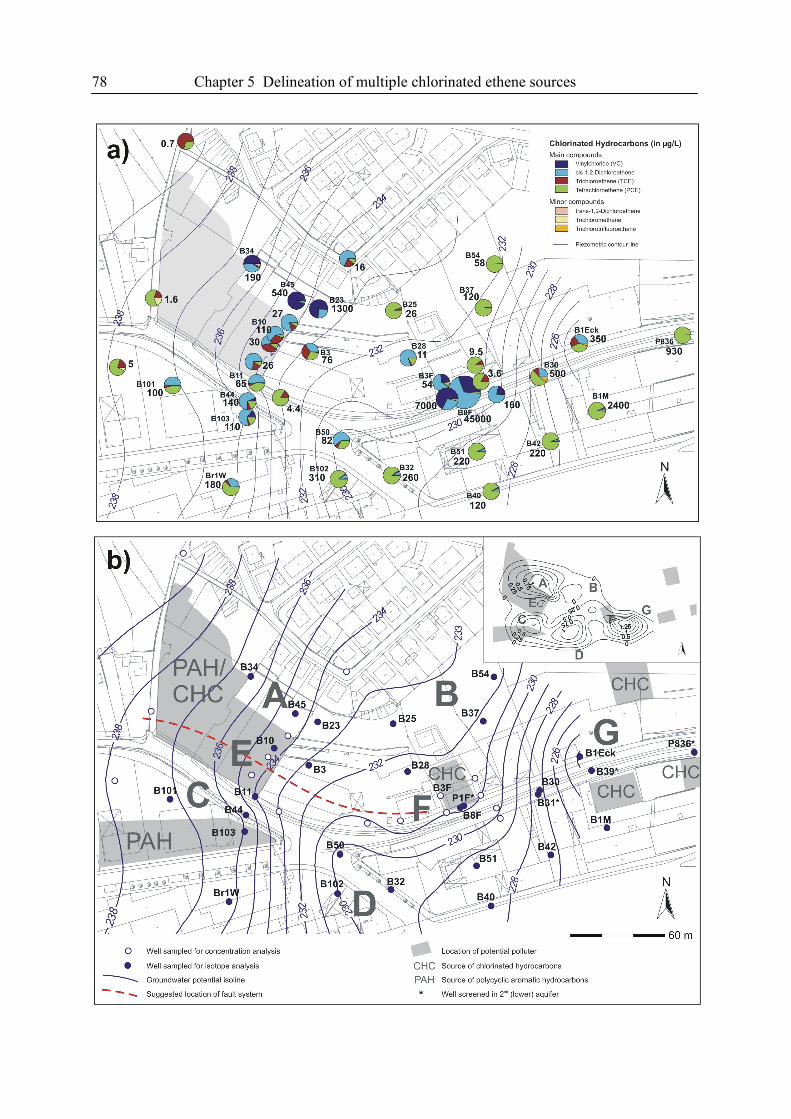
78 Chapter 5 Delineation of multiple chlorinated ethene sources
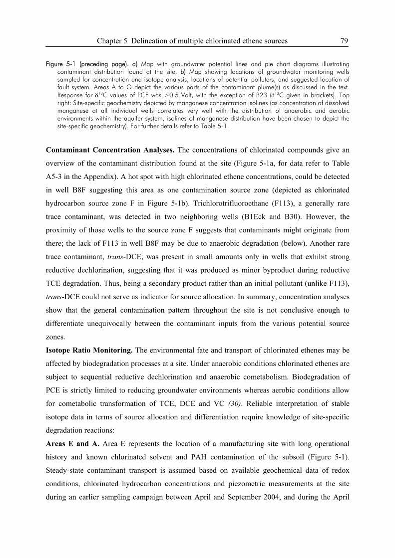
Chapter 5 Delineation of multiple chlorinated ethene sources 79
Figure 5-1 (preceding page). a) Map with groundwater potential lines and pie chart diagrams illustrating contaminant distribution found at the site. b) Map showing locations of groundwater monitoring wells sampled for concentration and isotope analysis, locations of potential polluters, and suggested location of fault system. Areas A to G depict the various parts of the contaminant plume(s) as discussed in the text. Response for δ13C values of PCE was >0.5 Volt, with the exception of B23 (δ13C given in brackets). Top right: Site-specific geochemistry depicted by manganese concentration isolines (as concentration of dissolved manganese at all individual wells correlates very well with the distribution of anaerobic and aerobic environments within the aquifer system, isolines of manganese distribution have been chosen to depict the site-specific geochemistry). For further details refer to Table 5-1.
Contaminant Concentration Analyses. The concentrations of chlorinated compounds give an
overview of the contaminant distribution found at the site (Figure 5-1a, for data refer to Table
A5-3 in the Appendix). A hot spot with high chlorinated ethene concentrations, could be detected
in well B8F suggesting this area as one contamination source zone (depicted as chlorinated
hydrocarbon source zone F in Figure 5-1b). Trichlorotrifluoroethane (F113), a generally rare
trace contaminant, was detected in two neighboring wells (B1Eck and B30). However, the
proximity of those wells to the source zone F suggests that contaminants might originate from
there; the lack of F113 in well B8F may be due to anaerobic degradation (below). Another rare
trace contaminant, trans-DCE, was present in small amounts only in wells that exhibit strong
reductive dechlorination, suggesting that it was produced as minor byproduct during reductive
TCE degradation. Thus, being a secondary product rather than an initial pollutant (unlike F113),
trans-DCE could not serve as indicator for source allocation. In summary, concentration analyses
show that the general contamination pattern throughout the site is not conclusive enough to
differentiate unequivocally between the contaminant inputs from the various potential source
zones.
Isotope Ratio Monitoring. The environmental fate and transport of chlorinated ethenes may be
affected by biodegradation processes at a site. Under anaerobic conditions chlorinated ethenes are
subject to sequential reductive dechlorination and anaerobic cometabolism. Biodegradation of
PCE is strictly limited to reducing groundwater environments whereas aerobic conditions allow
for cometabolic transformation of TCE, DCE and VC (30). Reliable interpretation of stable
isotope data in terms of source allocation and differentiation require knowledge of site-specific
degradation reactions:
Areas E and A. Area E represents the location of a manufacturing site with long operational
history and known chlorinated solvent and PAH contamination of the subsoil (Figure 5-1).
Steady-state contaminant transport is assumed based on available geochemical data of redox
conditions, chlorinated hydrocarbon concentrations and piezometric measurements at the site
during an earlier sampling campaign between April and September 2004, and during the April
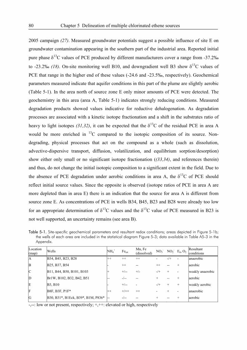
80 Chapter 5 Delineation of multiple chlorinated ethene sources
2005 campaign (27). Measured groundwater potentials suggest a possible influence of site E on
groundwater contamination appearing in the southern part of the industrial area. Reported initial
pure phase δ13C values of PCE produced by different manufacturers cover a range from -37.2‰
to -23.2‰ (18). On-site monitoring well B10, and downgradient well B3 show δ13C values of
PCE that range in the higher end of these values (-24.6 and -23.5‰, respectively). Geochemical
parameters measured indicate that aquifer conditions in this part of the plume are slightly aerobic
(Table 5-1). In the area north of source zone E only minor amounts of PCE were detected. The
geochemistry in this area (area A, Table 5-1) indicates strongly reducing conditions. Measured
degradation products showed values indicative for reductive dehalogenation. As degradation
processes are associated with a kinetic isotope fractionation and a shift in the substrates ratio of
heavy to light isotopes (31,32), it can be expected that the δ13C of the residual PCE in area A
would be more enriched in 13C compared to the isotopic composition of its source. Non-
degrading, physical processes that act on the compound as a whole (such as dissolution,
advective-dispersive transport, diffusion, volatilization, and equilibrium sorption/desorption)
show either only small or no significant isotope fractionation ((33,34), and references therein)
and thus, do not change the initial isotopic composition to a significant extent in the field. Due to
the absence of PCE degradation under aerobic conditions in area A, the δ13C of PCE should
reflect initial source values. Since the opposite is observed (isotope ratios of PCE in area A are
more depleted than in area E) there is an indication that the source for area A is different from
source zone E. As concentrations of PCE in wells B34, B45, B23 and B28 were already too low
for an appropriate determination of δ13C values and the δ13C value of PCE measured in B23 is
not well supported, an uncertainty remains (see area B).
Table 5-1. Site-specific geochemical parameters and resultant redox conditions; areas depicted in Figure 5-1b; the wells of each area are included in the statistical diagram Figure 5-3; data available in Table A5-3 in the Appendix.
Location (map) Wells NH4
+ Fetot Mn, Fe (dissolved) NO3
- NO2- Eh, O2
Resultant conditions
A B34, B45, B23, B28 ++ ++ ++ - -/+ - anaerobic
B B25, B37, B54 - ++ -- ++ -- + aerobic
C B11, B44, B50, B101, B103 + +/-- +/- -/+ + - weakly anaerobic
D Br1W, B102, B32, B42, B51 -- -/-- -- + -- + aerobic
E B3, B10 - +/-- - -/+ + + weakly aerobic
F B8F, B3F, P1F* ++ +/++ ++ - + - anaerobic
G B30, B31*, B1Eck, B39*, B1M, P836* -- -/-- -- + -- + aerobic
-,--: low or not present, respectively; +,++: elevated or high, respectively
Chapter 5 Delineation of multiple chlorinated ethene sources 81
Area B. Field measurements of redox potential and dissolved oxygen content indicate aerobic
conditions in wells B25, B37 and B54. Accordingly, groundwater chemistry of these samples is
characterized by elevated nitrate concentrations, low concentrations of dissolved iron and
manganese, and no detectable concentrations of ammonium (Table 5-1). Constant isotope
signatures of PCE (-24.5 to -24.3‰) in the presence of oxic conditions suggest that they have
derived from the same contaminant pool, possibly indicating the presence of a new source.
However, as historical files contain no suspected contamination source, PCE might be deriving
from solvent barrels bunkered in the 1940s. Groundwater flow conditions may provide a
hydraulic connection in this northern part of the aquifer system, therefore it can also not be
excluded that the manufacturing site responsible for areas A and E may be also responsible in
that case. As the values measured in area A are not well supported and the δ13C values of PCE
measured in wells B3 and B10 (area E) and those measured in area B are within error of each
other, the assumption is reasonable (compare with the statistical evaluation of the complete data
set given in Figure 5-3).
Area C. Southern wells B11, B44, B101, B103 and B50 exhibit δ13C values of PCE between
-27.5 and -26.7‰ and are within error of each other (for statistical significance refer to Figure
5-3). Geochemistry of these waters reveal weakly anaerobic aquifer conditions (Table 5-1),
which is also supported by field measurements of dissolved oxygen and redox potential (Eh).
High amounts of the degradation product cis-DCE and the presence of VC in some of these wells
are indicating reductive dechlorination processes active in this part of the aquifer. To summarize:
we observe aerobic conditions and PCE enriched in 13C in source zone E (-24.6 to -23.5‰)
whereas in the wells located in area C we observe reductive dechlorination processes occurring
under anaerobic conditions but PCE much more depleted in 13C (ranging from -27.5 to-26.7‰).
Consequently, those samples represent a contamination derived from an other, isotopically
distinct chlorinated solvent source. These findings are corroborated by hydrological pumping
tests where an influence of source zone E on downgradient wells B50, B102 and B32 located in
the southern part of the aquifer was excluded (27) and do support the assumption of two
separated flow streams attributed to the east-western fault disturbance within this area.
Area D. Well Br1W and its downgradient wells until B42 in the southern part of the
contaminated aquifer show δ13C values of PCE between -27.5 and -26.9‰ (within error of each
other, Figure 5-3). Under aerobic conditions (Table 5-1) the isotope signatures of PCE remain
constant in this aquifer section (area D). Thus, the source location for this contamination is
apparently located in the western, upgradient part of the aquifer. Indicated by almost identical
82 Chapter 5 Delineation of multiple chlorinated ethene sources
isotope ratios, the contaminations in this area derive most likely from the same source that is
responsible for the contamination detected in area C. Under strongly aerobic aquifer conditions
biodegradation of PCE is absent (supported by constant isotope signatures of PCE). In contrast,
pronounced isotope shifts for TCE (from -12.8‰ subsequentially enriched to +14.6‰) and cis-
DCE (enrichment from -22 to -3.9‰) suggest aerobic biodegradation processes successively
occurring with flow direction.
Area F. Massive contaminant concentrations alone provide already evidence from yet another
source in this area. At the same time, parent to daughter relationships (high cis-DCE/TCE
concentration ratios, presence of VC), product isotope ratios and redox conditions indicate
significant anaerobic reductive dehalogenation. The geochemistry within this area indicates
strongly reducing conditions: Samples are characterized by low nitrate concentrations, a high
Fediss/Fetot ratio and elevated concentrations of dissolved iron and manganese. Additionally,
ammonium was present in this zone. Furthermore, although less reliable, field measurements of
dissolved oxygen and redox potential (Eh) indicate reducing conditions. Anaerobic degradation of
chlorinated compounds requires hydrogen as an electron donor, which has to be provided by
other sources of carbon (30). Indeed, a significant co-contamination with petroleum-derived
hydrocarbons (mineral oil hydrocarbons and PAHs downgradient of source zone E) detected in
well B3F provides a source of organic carbon in this part of the plume that in course of
degradation reactions consumes oxygen and other electron acceptors available. Carbon isotope
composition of PCE observed in source area F (B8F/P1F) are consistent with anaerobic reductive
dechlorination and shows an enrichment in 13C with δ13C values of -23.4 and -22.9‰,
respectively. Unfortunately, no free-phase DNAPL was available to determine the initial δ13C
values. Taken isotope fractionation associated with reductive dehalogenation into account, the
initial δ13C of the original PCE source in area F must have been more depleted than -23‰. All
information together, confirm the assumption of the presence of a new source in area F compared
to areas A,C and E.
Area G. In contrast to anaerobic conditions in area F, groundwater samples further downgradient
are characterized by geochemical parameters that indicate aerobic conditions (Table 5-1), with
B30/B31* being located in the anaerobic/aerobic transition zone. An anaerobic source area that is
followed further downgradient by a plume that exhibits aerobic behavior is a quite common
observation at contaminated sites (30,35). Since PCE degradation does not take place under
aerobic conditions, prevalent attenuation mechanisms of PCE will be dilution and dispersion in
this part of the plume and hence, downgradient carbon isotope compositions of PCE should
Chapter 5 Delineation of multiple chlorinated ethene sources 83
remain constant. However, δ13C values of PCE measured in wells B30, B31*, B39* and B1Eck
show carbon isotope compositions depleted in 13C (-25.5‰) in comparison with source zone F. A
first supposition would be that another source might be involved, as it was discussed in areas E
and C, for example. Considering the geological situation and historical files, an alternative
explanation seems to be more realistic: Figure 5-2 shows a conceptual model to illustrate our
view of the contaminant distribution in this part of the fractured bedrock aquifer system.
DNAPLs in bedrock penetrate the subsurface and spread along fractures and fissures. Vertical
PCE isotope profiles from well pairs B8F/P1F* (-23.4/-22.9‰), B30/B31* (-25.4/-25.0‰) and
B1Eck/B39* (-25.7/-26.1‰), respectively, with similar δ13C of PCE (±0.5‰ variance within
each well pair) support that the two aquifers are connected via vertical fractures. In the aerobic
zone G, dissolution of PCE from DNAPL trapped in fractures might create an input of
undegraded, isotopically depleted, original material deriving from source area F. Considering the
concentration distribution of PCE, TCE and cis-DCE in well B8F compared to downgradient well
B30 and their corresponding δ13C values entail only a minor influence of already degraded
material and hence a higher amount of “fresh”, isotopically light source material. A strong
influence of undegraded source material is also well reflected by the depleted isotope signature of
-27.6‰ for cis-DCE measured in well B30. Assuming a linear mixing model (δ13Cmixture = fdegraded
δ13Cdegraded + finitial δ13Cinitial) the isotope signature of PCE observed in well B30 (-25.4‰) would
represent a mixture of already degraded (-23‰ measured in upgradient wells) and freshly
dissolved (undegraded) material. Based on a linear mixing model of > 60% undegraded and
< 40% degraded contaminants would then reflect an initial isotope value for PCE of
approximately -27‰.
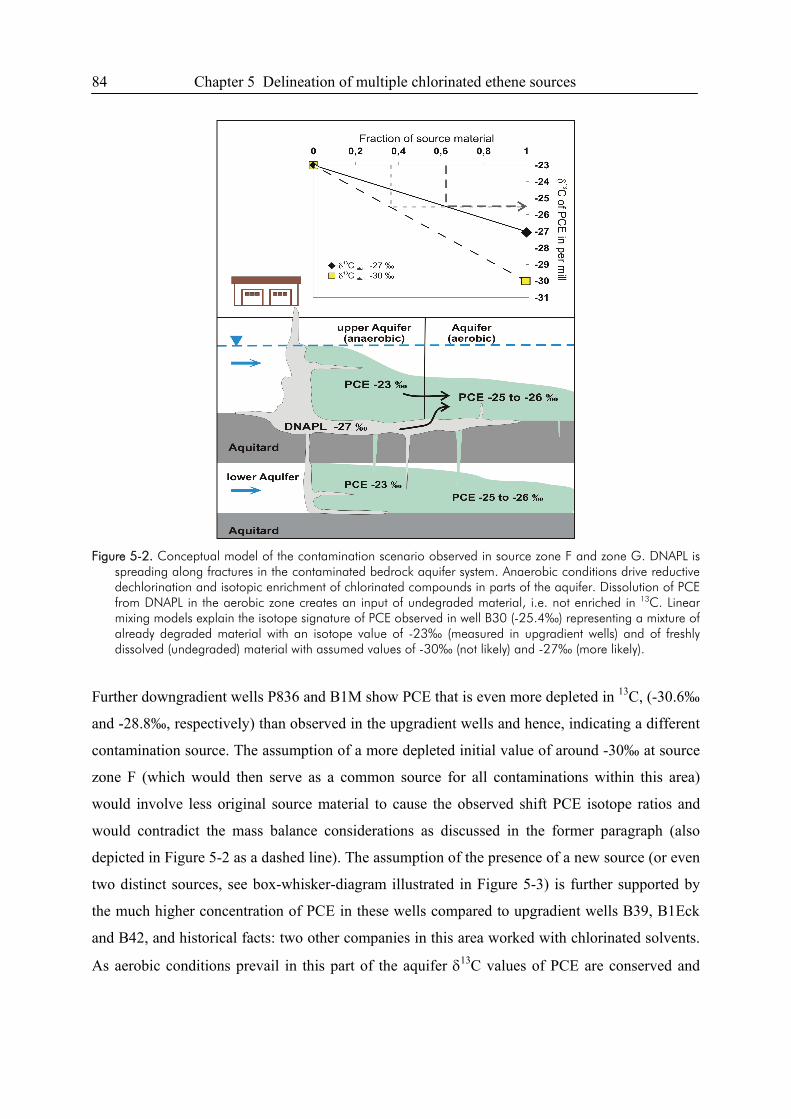
84 Chapter 5 Delineation of multiple chlorinated ethene sources
Figure 5-2. Conceptual model of the contamination scenario observed in source zone F and zone G. DNAPL is
spreading along fractures in the contaminated bedrock aquifer system. Anaerobic conditions drive reductive dechlorination and isotopic enrichment of chlorinated compounds in parts of the aquifer. Dissolution of PCE from DNAPL in the aerobic zone creates an input of undegraded material, i.e. not enriched in 13C. Linear mixing models explain the isotope signature of PCE observed in well B30 (-25.4‰) representing a mixture of already degraded material with an isotope value of -23‰ (measured in upgradient wells) and of freshly dissolved (undegraded) material with assumed values of -30‰ (not likely) and -27‰ (more likely).
Further downgradient wells P836 and B1M show PCE that is even more depleted in 13C, (-30.6‰
and -28.8‰, respectively) than observed in the upgradient wells and hence, indicating a different
contamination source. The assumption of a more depleted initial value of around -30‰ at source
zone F (which would then serve as a common source for all contaminations within this area)
would involve less original source material to cause the observed shift PCE isotope ratios and
would contradict the mass balance considerations as discussed in the former paragraph (also
depicted in Figure 5-2 as a dashed line). The assumption of the presence of a new source (or even
two distinct sources, see box-whisker-diagram illustrated in Figure 5-3) is further supported by
the much higher concentration of PCE in these wells compared to upgradient wells B39, B1Eck
and B42, and historical facts: two other companies in this area worked with chlorinated solvents.
As aerobic conditions prevail in this part of the aquifer δ13C values of PCE are conserved and
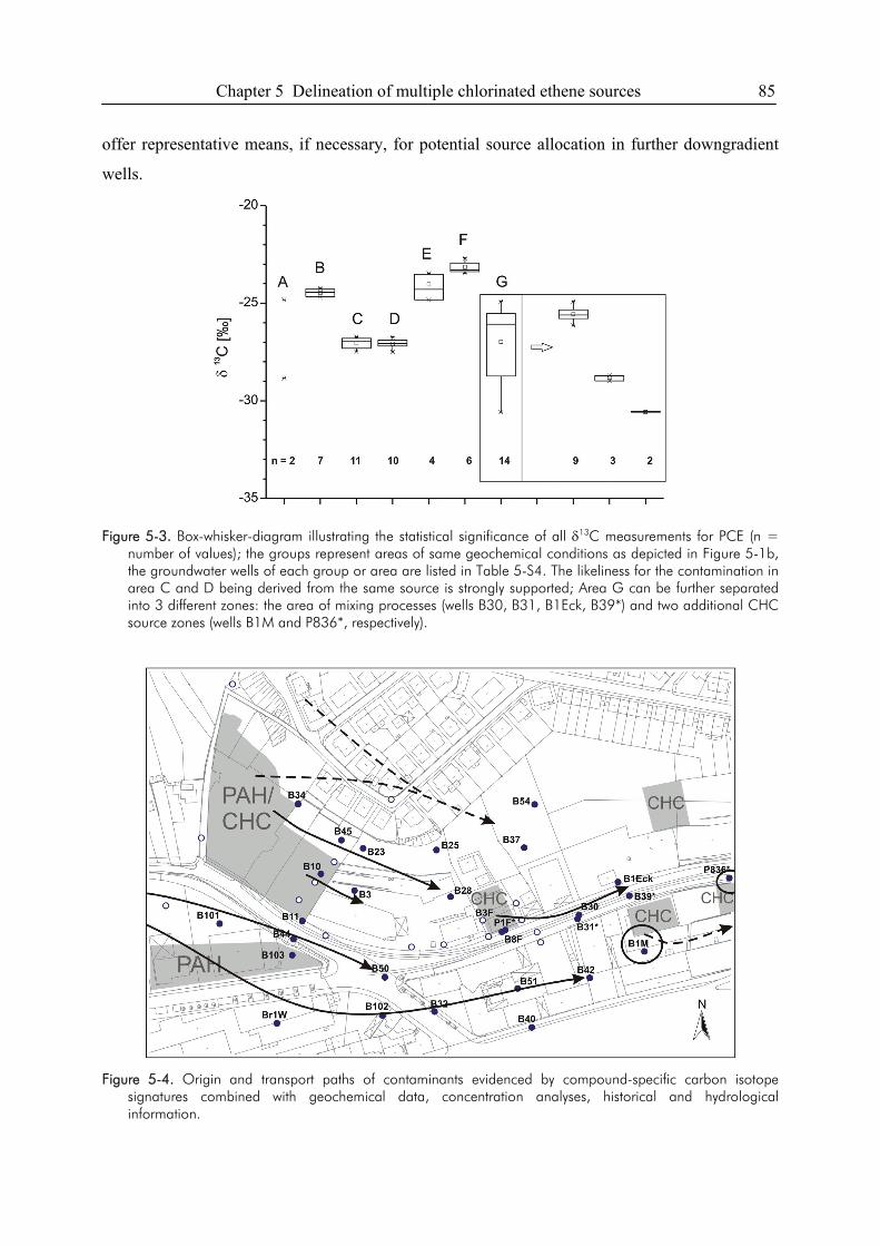
Chapter 5 Delineation of multiple chlorinated ethene sources 85
offer representative means, if necessary, for potential source allocation in further downgradient
wells.
Figure 5-3. Box-whisker-diagram illustrating the statistical significance of all δ13C measurements for PCE (n =
number of values); the groups represent areas of same geochemical conditions as depicted in Figure 5-1b, the groundwater wells of each group or area are listed in Table 5-S4. The likeliness for the contamination in area C and D being derived from the same source is strongly supported; Area G can be further separated into 3 different zones: the area of mixing processes (wells B30, B31, B1Eck, B39*) and two additional CHC source zones (wells B1M and P836*, respectively).
Figure 5-4. Origin and transport paths of contaminants evidenced by compound-specific carbon isotope
signatures combined with geochemical data, concentration analyses, historical and hydrological information.
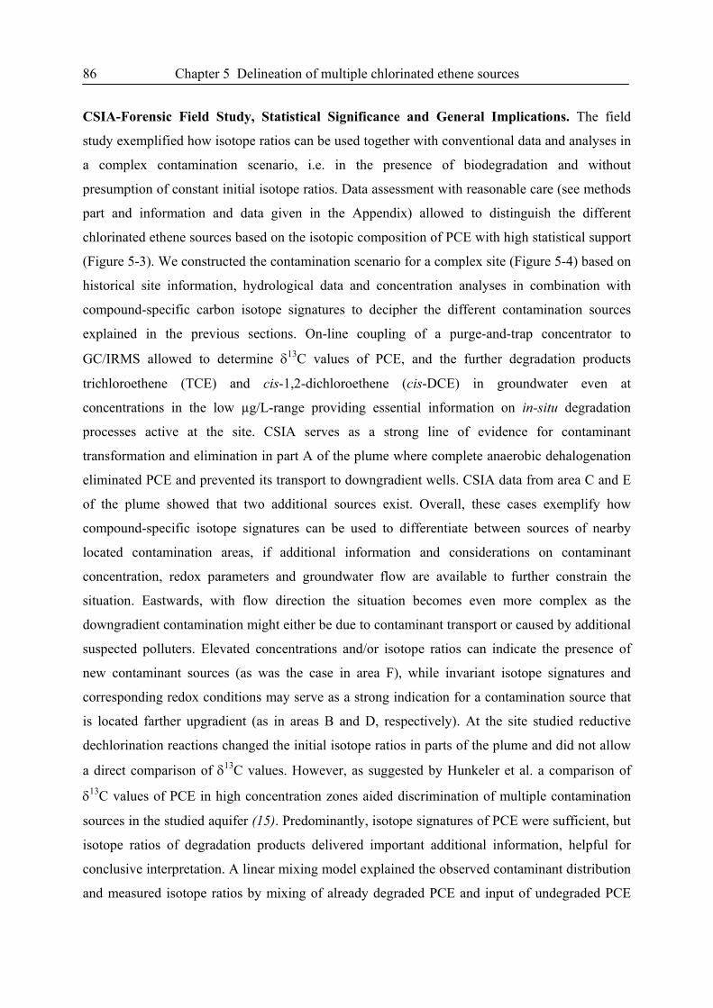
86 Chapter 5 Delineation of multiple chlorinated ethene sources
CSIA-Forensic Field Study, Statistical Significance and General Implications. The field
study exemplified how isotope ratios can be used together with conventional data and analyses in
a complex contamination scenario, i.e. in the presence of biodegradation and without
presumption of constant initial isotope ratios. Data assessment with reasonable care (see methods
part and information and data given in the Appendix) allowed to distinguish the different
chlorinated ethene sources based on the isotopic composition of PCE with high statistical support
(Figure 5-3). We constructed the contamination scenario for a complex site (Figure 5-4) based on
historical site information, hydrological data and concentration analyses in combination with
compound-specific carbon isotope signatures to decipher the different contamination sources
explained in the previous sections. On-line coupling of a purge-and-trap concentrator to
GC/IRMS allowed to determine δ13C values of PCE, and the further degradation products
trichloroethene (TCE) and cis-1,2-dichloroethene (cis-DCE) in groundwater even at
concentrations in the low µg/L-range providing essential information on in-situ degradation
processes active at the site. CSIA serves as a strong line of evidence for contaminant
transformation and elimination in part A of the plume where complete anaerobic dehalogenation
eliminated PCE and prevented its transport to downgradient wells. CSIA data from area C and E
of the plume showed that two additional sources exist. Overall, these cases exemplify how
compound-specific isotope signatures can be used to differentiate between sources of nearby
located contamination areas, if additional information and considerations on contaminant
concentration, redox parameters and groundwater flow are available to further constrain the
situation. Eastwards, with flow direction the situation becomes even more complex as the
downgradient contamination might either be due to contaminant transport or caused by additional
suspected polluters. Elevated concentrations and/or isotope ratios can indicate the presence of
new contaminant sources (as was the case in area F), while invariant isotope signatures and
corresponding redox conditions may serve as a strong indication for a contamination source that
is located farther upgradient (as in areas B and D, respectively). At the site studied reductive
dechlorination reactions changed the initial isotope ratios in parts of the plume and did not allow
a direct comparison of δ13C values. However, as suggested by Hunkeler et al. a comparison of
δ13C values of PCE in high concentration zones aided discrimination of multiple contamination
sources in the studied aquifer (15). Predominantly, isotope signatures of PCE were sufficient, but
isotope ratios of degradation products delivered important additional information, helpful for
conclusive interpretation. A linear mixing model explained the observed contaminant distribution
and measured isotope ratios by mixing of already degraded PCE and input of undegraded PCE
Chapter 5 Delineation of multiple chlorinated ethene sources 87
due to DNAPL dissolution in area G. Our study showed that careful interpretation of isotope
ratios, geochemical data and site-specific additional information are essential for a
comprehensive site assessment. It could be demonstrated that a comprehensive CSIA approach
can provide the extra information for a conclusive source allocation despite hydrologically
complex transport of chlorinated ethenes in fractured bedrock aquifer systems if detection limits
are sufficiently low to cover a wide range of the plume and additional constraining geochemical
and historical data is available. Small differences in isotope signatures between sources may,
however, hamper a reliable discrimination, especially if additional lines of evidence are missing
or controversial data have to be discussed. In such cases two dimensional CSIA (multiple isotope
analysis, e.g. δ37Cl or δ2H) may further improve the conclusive power for constraining
contaminant sources.
5.4. References
(1) Beneteau, K. M.; Aravena, R.; Frape, S. K. Isotopic characterization of chlorinated solvents-laboratory and field results. Org. Geochem. 1999, 30, 739-753.
(2) Doherty, R. E. A History of the Production and Use of Carbon Tetrachloride, Tetrachloroethylene, Trichloroethylene and 1,1,1-Trichloroethane in the United States: Part 1--Historical Background; Carbon Tetrachloride and Tetrachloroethylene. Environ. Forensics 2000, 1, 69 - 81.
(3) U.S. Environmental Protection Agency. National primary drinking water regulations, list of drinking water contaminants & their MCLs, EPA 816-F-03-016. http://www.epa.gov/safewater/consumer/pdf/mcl.pdf. 2003.
(4) Johnson, R. L.; Pankow, J. F. Dissolution of dense chlorinated solvents into groundwater. 2. Source functions for pools of solvent. Environ. Sci. Technol. 1992, 26, 896-901.
(5) Woodbury, A.; Sudicky, E.; Ulrych, T. J.; Ludwig, R. Three-dimensional plume source reconstruction using minimum relative entropy inversion. J. Contam. Hydrol. 1998, 32, 131-158.
(6) Alapati, S.; Kabala, Z. J. Recovering the release history of a groundwater contaminant using a non-linear least-squares method. Hydrological Processes 2000, 14, 1003-1016.
(7) Atmadja, J.; Bagtzoglou, A. C. State of the art report on mathematical methods for groundwater pollution source identification. Environ. Forensics 2001, 2, 205-214.
(8) Alimi, H.; Ertel, T.; Schug, B. Fingerprinting of hydrocarbon fuel contaminants: Literature review. Environ. Forensics 2003, 4, 25-38.
(9) Mansuy, L.; Philp, R. P.; Allen, J. Source identification of oil spills based on the isotopic composition of individual components in weathered oil samples. Environ. Sci. Technol. 1997, 31, 3417-3425.
(10) Smallwood, B. J.; Philp, R. P.; Allen, J. D. Stable carbon isotopic composition of gasolines determined by isotope ratio monitoring gas chromatography mass spectrometry. Org. Geochem. 2002, 33, 149-159.
(11) Benson, S.; Lennard, C.; Maynard, P.; Roux, C. Forensic applications of isotope ratio mass spectrometry - A review. Forensic Sci.Int. 2006, 157, 1-22.
(12) Walker, S. E.; Dickhut, R. M.; Chisholm-Brause, C.; Sylva, S.; Reddy, C. M. Molecular and isotopic identification of PAH sources in a highly industrialized urban estuary. Org. Geochem. 2005, 36, 619-632.
(13) Okuda, T.; Kumata, H.; Naraoka, H.; Takada, H. Origin of atmospheric polycyclic aromatic hydrocarbons (PAHs) in Chinese cities solved by compound-specific stable carbon isotopic analyses. Org. Geochem. 2002, 33, 1737-1745.
(14) Slater, G. F. Stable isotope forensics - When isotopes work. Environ. Forensics 2003, 4, 13-23. (15) Hunkeler, D.; Chollet, N.; Pittet, X.; Aravena, R.; Cherry, J. A.; Parker, B. L. Effect of source variability and
transport processes on carbon isotope ratios of TCE and PCE in two sandy aquifers. J. Contam. Hydrol. 2004, 74, 265-282.
88 Chapter 5 Delineation of multiple chlorinated ethene sources
(16) Holt, B. D.; Sturchio, N. C.; Abrajano, T. A.; Heraty, L. J. Conversion of Chlorinated Volatile Organic Compounds to Carbon Dioxide and Methyl Chloride for Isotopic Analysis of Carbon and Chlorine. Anal. Chem. 1997, 69, 2727-2733.
(17) Jendrzejewski, N.; Eggenkamp, H. G. M.; Coleman, M. L. Characterisation of chlorinated hydrocarbons from chlorine and carbon isotopic compositions: scope of application to environmental problems. Appl. Geochem. 2001, 16, 1021-1031.
(18) vanWarmerdam, E. M.; Frape, S. K.; Aravena, R.; Drimmie, R. J.; Flatt, H.; Cherry, J. A. Stable chlorine and carbon isotope measurements of selected chlorinated organic solvents. Appl. Geochem. 1995, 10, 547-552.
(19) Chartrand, M. M. G.; Hirschorn, S. K.; Lacrampe-Couloume, G.; Sherwood Lollar, B. Compound specific hydrogen isotope analysis of 1,2-dichloroethane: potential for delineating source and fate of chlorinated hydrocarbon contaminants in groundwater. Rapid Commun. Mass Spectrom. 2007, 21, 1841-1847.
(20) Hunkeler, D.; Aravena, R.; Butler, B. J. Monitoring microbial dechlorination of tetrachloroethene (PCE) in groundwater using compound-specific stable carbon isotope ratios: Microcosm and field studies. Environ. Sci. Technol. 1999, 33, 2733-2738.
(21) Morrill, P. L.; Lacrampe-Couloume, G.; Slater, G. F.; Sleep, B. E.; Edwards, E. A.; McMaster, M. L.; Major, D. W.; Sherwood Lollar, B. Quantifying chlorinated ethene degradation during reductive dechlorination at Kelly AFB using stable carbon isotopes. J. Contam. Hydrol. 2005, 76, 279-293.
(22) Sherwood Lollar, B.; Slater, G. F.; Sleep, B.; Witt, M.; Klecka, G. M.; Harkness, M.; Spivack, J. Stable carbon isotope evidence for intrinsic bioremediation of tetrachloroethene and trichloroethene at area 6, Dover Air Force Base. Environ. Sci. Technol. 2001, 35, 261-269.
(23) Song, D. L.; Conrad, M. E.; Sorenson, K. S.; Alvarez-Cohen, L. Stable carbon isotope fractionation during enhanced in situ bioremediation of trichloroethene. Environ. Sci. Technol. 2002, 36, 2262-2268.
(24) Hunkeler, D.; Aravena, R.; Berry-Spark, K.; Cox, E. Assessment of degradation pathways in an aquifer with mixed chlorinated hydrocarbon contamination using stable isotope analysis. Environ. Sci. Technol. 2005, 39, 5975-5981.
(25) Chartrand, M. M. G.; Morrill, P. L.; Lacrampe-Couloume, G.; Sherwood Lollar, B. Stable isotope evidence for biodegradation of chlorinated ethenes at a fractured bedrock site. Environ. Sci. Technol. 2005, 39, 4848-4856.
(26) Glaser, B.; Dreyer, A.; Bock, M.; Fiedler, S.; Mehring, M.; Heitmann, T. Source apportionment of organic pollutants of a highway-traffic-influenced urban area in Bayreuth (Germany) using biomarker and stable carbon isotope signatures. Environ. Sci. Technol. 2005, 39, 3911-3917.
(27) Amt für Umweltschutz Stuttgart, KORA - TV1: Forschungsbericht, Förderkennzeichen 02WN0353; Projekt 1.3: Natürlicher Abbau und Rückhalt eines komplexen Schadstoffcocktails in einem Grundwasserleiter am Beispiel des ehemaligen Mineralölwerks Epple; Stuttgart, 2007.
(28) Zwank, L.; Berg, M.; Schmidt, T. C.; Haderlein, S. B. Compound-specific carbon isotope analysis of volatile organic compounds in the low-microgram per liter range. Anal. Chem. 2003, 75, 5575-5583.
(29) Slater, G. F.; Dempster, H. S.; Lollar, B. S.; Ahad, J. Headspace analysis: A new application for isotopic characterization of dissolved organic contaminants. Environ. Sci. Technol. 1999, 33, 190-194.
(30) Wiedemeier, T. H.; Rifai, H. S.; Newell, C. J.; Wilson, J. T. Natural attenuation of fuels and chlorinated solvents in the subsurface; John Wiley & Sons Inc.: New York, 1999.
(31) Schmidt, T. C.; Zwank, L.; Elsner, M.; Berg, M.; Meckenstock, R. U.; Haderlein, S. B. Compound-specific stable isotope analysis of organic contaminants in natural environments: a critical review of the state of the art, prospects, and future challenges. Anal. Bioanal. Chem. 2004, 378, 283-300.
(32) Meckenstock, R. U.; Morasch, B.; Griebler, C.; Richnow, H. H. Stable isotope fractionation analysis as a tool to monitor biodegradation in contaminated acquifers. J. Contam. Hydrol. 2004, 75, 215-255.
(33) Elsner, M.; McKelvie, J.; Lacrampe-Couloume, G.; Sherwood Lollar, B. Insight into methyl tert-butyl ether (MTBE) stable isotope fractionation from abiotic reference experiments. Environ. Sci. Technol. 2007, 41, 5693-5700.
(34) Elsner, M.; Zwank, L.; Hunkeler, D.; Schwarzenbach, R. P. A new concept linking observable stable isotope fractionation to transformation pathways of organic pollutants. Environ. Sci. Technol. 2005, 39, 6896-6916.
(35) Lee, M. D.; Odom, J. M.; Buchanan Jr., R. J. New perspectives on microbial dehalogenation of chlorinated solvents: Insights from the field. Annu. Rev. Microbiol. 1998, 52, 423-452.
(36) Jochmann, M. A.; Blessing, M.; Haderlein, S. B.; Schmidt, T. C. A new approach to determine method detection limits for compound-specific isotope analysis of volatile organic compounds. Rapid Commun. Mass Spectrom. 2006, 20, 3639-3648.
Chapter 5 Delineation of multiple chlorinated ethene sources - Appendix 89
5.5. Appendix
Detailed Information on GC/IRMS Measurements. Compound-specific stable carbon isotope
analyses were performed using the gas chromatograph-combustion-isotope ratio mass
spectrometry system (GC/IRMS) described in Chapter 2.2. Low concentrations of chlorinated
ethenes in some of the groundwater samples required preconcentration prior to isotope analysis.
To this end a purge-and-trap (P&T) concentrator (VelocityXPT, Tekmar-Dohrmann, Mason,
USA) equipped with an AQUATek 70 autosampler (Tekmar-Dohrmann) was coupled online to
the PTV injector of the GC/IRMS system. Volatile compounds were extracted from the samples
by purging 25 mL of the groundwater in a fritted sparger with helium at 40 mL/min for 11 min
and trapped on a VOCARB 3000 (Supelco, Bellefonte, USA) at room temperature. After heating
the trap to 240 °C for 2 min to desorb the compounds, they were then transferred to the
GC/IRMS. The transfer line between the P&T instrument and the PTV injector was held at
250 °C. Analytes were preconcentrated in a deactivated precolumn with cooled nitrogen gas in an
on-column cryofocusing unit (ATAS GL International), which was held at -100 °C during analyte
transfer from the P&T instrument. Samples containing vinyl chloride (VC) were preconcentrated
at -130 °C. For the thermal desorption process, the cryofocusing unit was heated with a rate of
30°C/s to 240°C. A 60 m x 0.32 mm Rtx-VMS capillary column with a film thickness of 1.8 µm
(Restek, Bellefonte, USA) was used for the analytical separation of the chlorinated compounds.
The GC temperature program used to obtain separation of compounds of interest started at 40 °C
held for 11 min, increased at a rate of 7 °C/min to 100 °C held for 2 min, then to to 220 °C at
20 °C/min for additional 4 min (Helium5.0 was used as carrier gas; column flow:1 mL/min).
Accuracy and Reproducibility of CSIA Measurements. Chlorinated ethene standards with
known isotopic compositions were regularly measured using the same analytical procedure as for
the samples. Precision and reproducibility of δ13C values determined by purge-and-trap
GC/IRMS are given in Table A5-1. Measurements of those standards was performed regularly
every 5th to 6th measurement, at least in duplicates. The δ13C values obtained were compared to
externally measured isotope values (EA/IRMS, n=3, see Table A5-1). The results demonstrate
that the P&T-GC/IRMS provides both accurate and reproducible δ13C values. Only trans-DCE
shows higher deviations, which is a common observation in P&T-GC/IRMS for this compound
(1,2). Figure A5-1 shows the results of investigating the effect of signal size on δ13C
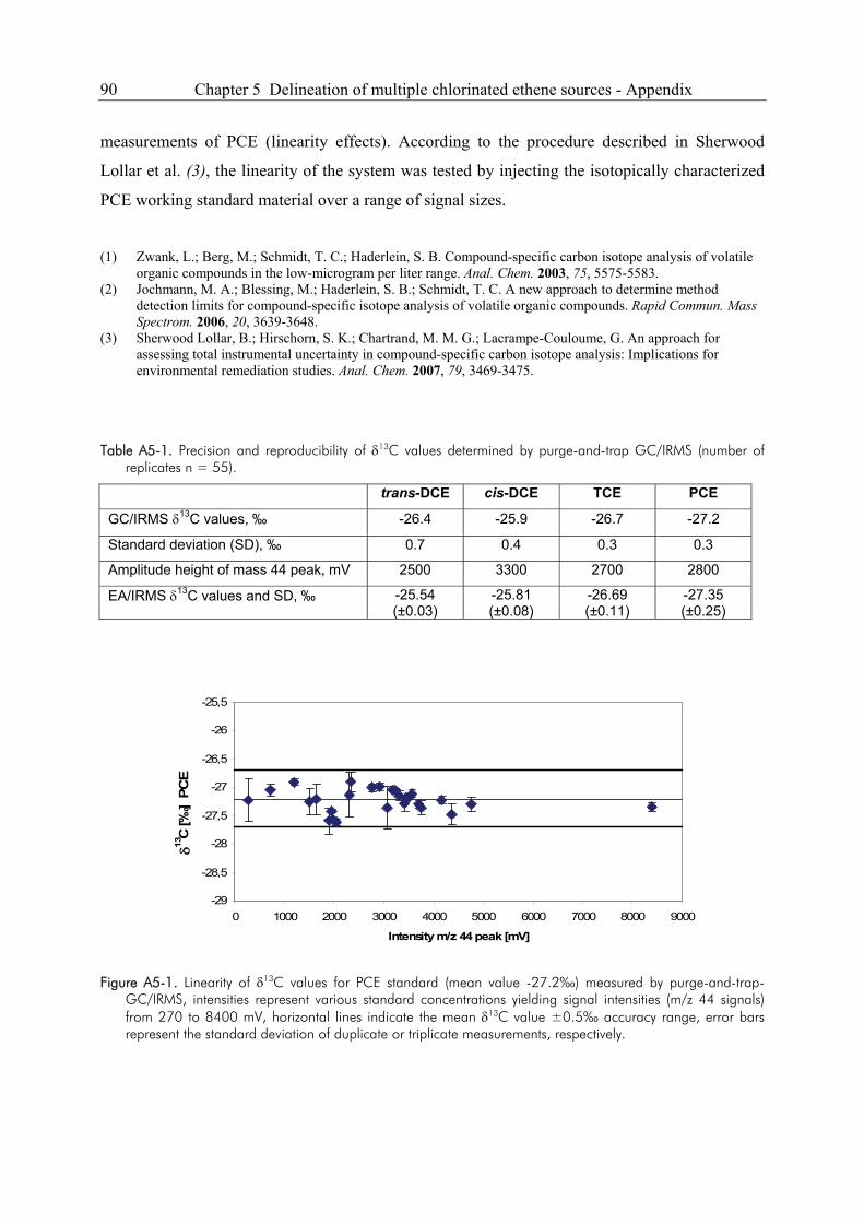
90 Chapter 5 Delineation of multiple chlorinated ethene sources - Appendix
measurements of PCE (linearity effects). According to the procedure described in Sherwood
Lollar et al. (3), the linearity of the system was tested by injecting the isotopically characterized
PCE working standard material over a range of signal sizes.
(1) Zwank, L.; Berg, M.; Schmidt, T. C.; Haderlein, S. B. Compound-specific carbon isotope analysis of volatile
organic compounds in the low-microgram per liter range. Anal. Chem. 2003, 75, 5575-5583. (2) Jochmann, M. A.; Blessing, M.; Haderlein, S. B.; Schmidt, T. C. A new approach to determine method
detection limits for compound-specific isotope analysis of volatile organic compounds. Rapid Commun. Mass Spectrom. 2006, 20, 3639-3648.
(3) Sherwood Lollar, B.; Hirschorn, S. K.; Chartrand, M. M. G.; Lacrampe-Couloume, G. An approach for assessing total instrumental uncertainty in compound-specific carbon isotope analysis: Implications for environmental remediation studies. Anal. Chem. 2007, 79, 3469-3475.
Table A5-1. Precision and reproducibility of δ13C values determined by purge-and-trap GC/IRMS (number of replicates n = 55).
trans-DCE cis-DCE TCE PCE
GC/IRMS δ13C values, ‰ -26.4 -25.9 -26.7 -27.2
Standard deviation (SD), ‰ 0.7 0.4 0.3 0.3
Amplitude height of mass 44 peak, mV 2500 3300 2700 2800
EA/IRMS δ13C values and SD, ‰ -25.54 (±0.03)
-25.81 (±0.08)
-26.69 (±0.11)
-27.35 (±0.25)
-29
-28,5
-28
-27,5
-27
-26,5
-26
-25,5
0 1000 2000 3000 4000 5000 6000 7000 8000 9000
Intensity m/z 44 peak [mV]
δ13C
[‰]
PCE
Figure A5-1. Linearity of δ13C values for PCE standard (mean value -27.2‰) measured by purge-and-trap-
GC/IRMS, intensities represent various standard concentrations yielding signal intensities (m/z 44 signals) from 270 to 8400 mV, horizontal lines indicate the mean δ13C value ±0.5‰ accuracy range, error bars represent the standard deviation of duplicate or triplicate measurements, respectively.
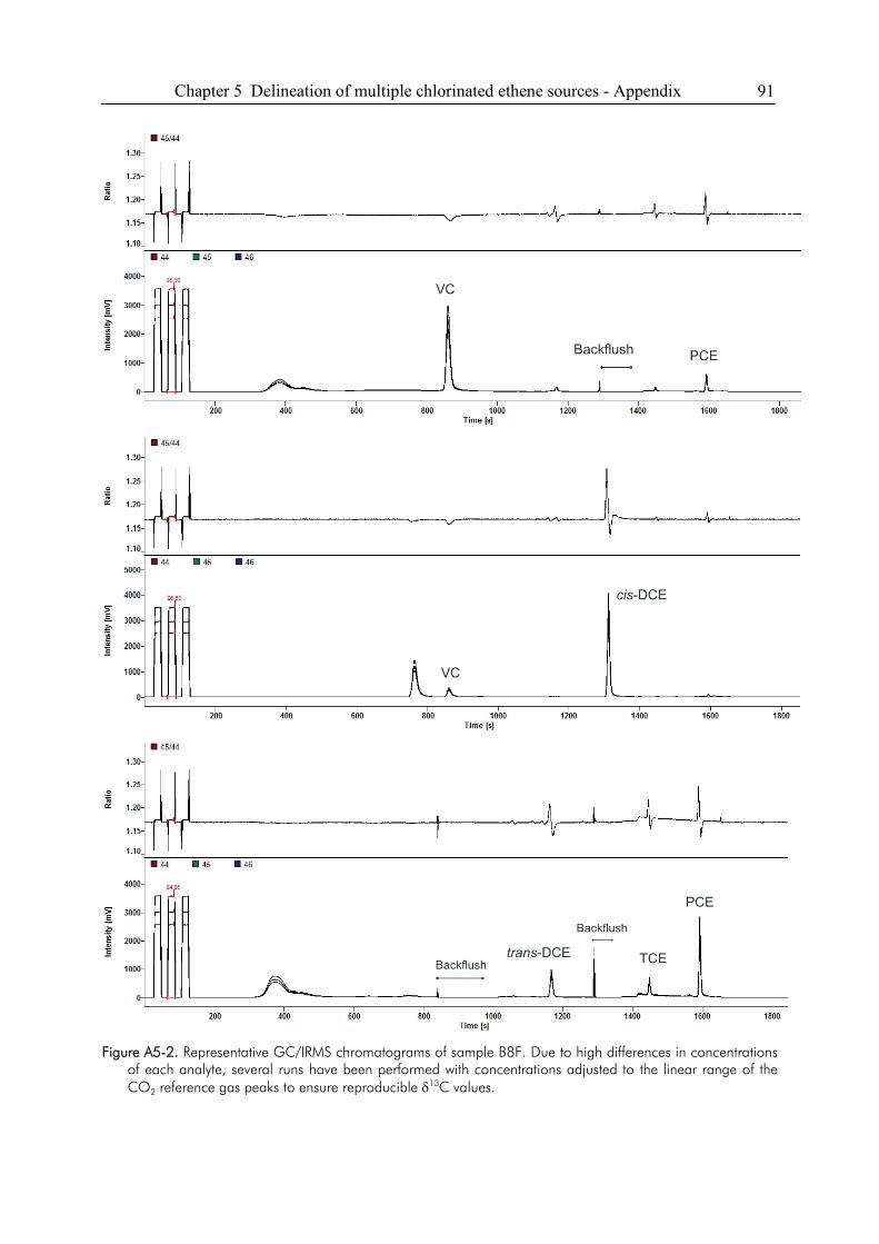
Chapter 5 Delineation of multiple chlorinated ethene sources - Appendix 91
Figure A5-2. Representative GC/IRMS chromatograms of sample B8F. Due to high differences in concentrations
of each analyte, several runs have been performed with concentrations adjusted to the linear range of the CO2 reference gas peaks to ensure reproducible δ13C values.
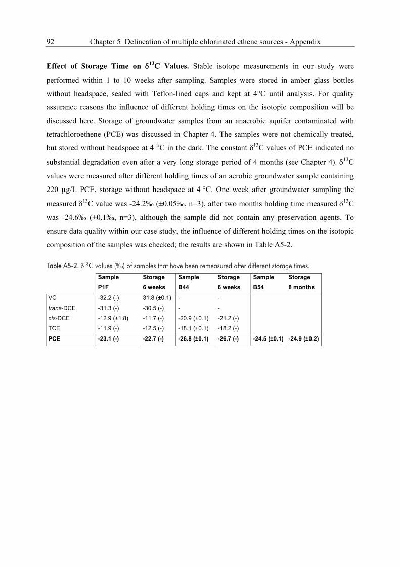
92 Chapter 5 Delineation of multiple chlorinated ethene sources - Appendix
Effect of Storage Time on δ13C Values. Stable isotope measurements in our study were
performed within 1 to 10 weeks after sampling. Samples were stored in amber glass bottles
without headspace, sealed with Teflon-lined caps and kept at 4°C until analysis. For quality
assurance reasons the influence of different holding times on the isotopic composition will be
discussed here. Storage of groundwater samples from an anaerobic aquifer contaminated with
tetrachloroethene (PCE) was discussed in Chapter 4. The samples were not chemically treated,
but stored without headspace at 4 °C in the dark. The constant δ13C values of PCE indicated no
substantial degradation even after a very long storage period of 4 months (see Chapter 4). δ13C
values were measured after different holding times of an aerobic groundwater sample containing
220 µg/L PCE, storage without headspace at 4 °C. One week after groundwater sampling the
measured δ13C value was -24.2‰ (±0.05‰, n=3), after two months holding time measured δ13C
was -24.6‰ (±0.1‰, n=3), although the sample did not contain any preservation agents. To
ensure data quality within our case study, the influence of different holding times on the isotopic
composition of the samples was checked; the results are shown in Table A5-2.
Table A5-2. δ13C values (‰) of samples that have been remeasured after different storage times.
Sample Storage Sample Storage Sample Storage P1F 6 weeks B44 6 weeks B54 8 months
VC -32.2 (-) 31.8 (±0.1) - -
trans-DCE -31.3 (-) -30.5 (-) - -
cis-DCE -12.9 (±1.8) -11.7 (-) -20.9 (±0.1) -21.2 (-)
TCE -11.9 (-) -12.5 (-) -18.1 (±0.1) -18.2 (-)
PCE -23.1 (-) -22.7 (-) -26.8 (±0.1) -26.7 (-) -24.5 (±0.1) -24.9 (±0.2)
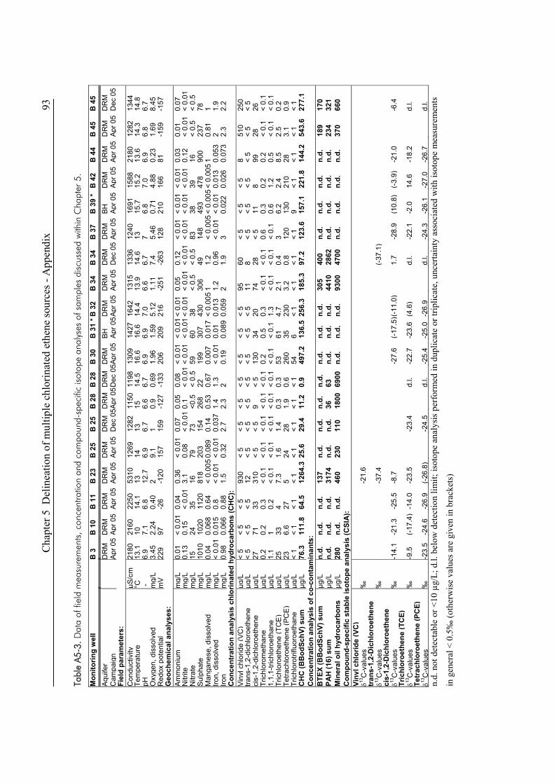
C
hapt
er 5
Del
inea
tion
of m
ultip
le c
hlor
inat
ed e
then
e so
urce
s - A
ppen
dix
93
Tabl
e A5
-3. D
ata
of fi
eld
mea
sure
men
ts, c
once
ntra
tion
and
com
poun
d-sp
ecifi
c is
otop
e an
alys
es o
f sam
ples
dis
cuss
ed w
ithin
Cha
pter
5.
Mon
itorin
g w
ell
B
3
B 1
0 B
11
B 2
3 B
25
B 2
5 B
28
B 2
8 B
30
B
31
*B 3
2 B
34
B 3
4 B
37
B 3
9 *
B 4
2 B
44
B 4
5 B
45
Aq
uife
r
DR
M
DR
M
DR
M
DR
M
DR
M
DR
M
DR
M
DR
M
DR
M
BH
DR
M
DR
M
DR
M
DR
M
BH
DR
M
DR
M
DR
M
DR
M
Cam
paig
n
Apr 0
5Ap
r 05
Apr 0
5Ap
r 05
Apr 0
5D
ec 0
5Apr
05D
ec 0
5Apr
05
Apr 0
5Apr
05
Apr 0
5D
ec 0
5Ap
r 05
Apr 0
5Ap
r 05
Apr 0
5Ap
r 05
Dec
05
Fiel
d pa
ram
eter
s:C
ondu
ctiv
ityµS
/cm
21
8021
6022
5053
1012
6912
8211
5011
9813
09
1427
1642
1315
1336
1240
1691
1588
2180
1282
1344
Te
mpe
ratu
re°C
13
.110
14.1
1314
1315
14.5
16.6
16
.614
.413
.914
.613
15.7
15.2
13.6
14.3
14.8
pH
- 6.
97.
16.
812
.76.
96.
76.
66.
76.
9 6.
9 7.
06.
66.
77
6.8
7.0
6.9
6.8
6.7
Oxy
gen,
dis
solv
edm
g/L
3.45
2.24
0.40
29.
11
0.9
0.69
1.96
1.
595.
121.
117.
45.
460.
714.
880.
231.
698.
45R
edox
pot
entia
lm
V 22
997
-26
-120
157
159
-127
-133
206
209
216
-251
-263
128
210
166
81-1
59-1
57
Geo
chem
ical
ana
lyse
s:
Amm
oniu
mm
g/L
0.01
< 0.
010.
040.
36<
0.01
0.07
0.05
0.08
< 0.
01
< 0.
01<
0.01
0.05
0.12
< 0.
01<
0.01
< 0.
010.
030.
010.
07N
itrite
mg/
L 0.
130.
15<
0.01
3.1
0.08
< 0.
010.
1<
0.01
< 0.
01
< 0.
01<
0.01
< 0.
01<
0.01
< 0.
01<
0.01
< 0.
010.
12<
0.01
< 0.
01
Nitr
ate
mg/
L 15
2435
1679
73<0
.5<
0.5
5960
38
< 0.
5<
0.5
8338
3916
< 0.
5<
0.5
Sulp
hate
mg/
L 10
1010
2011
2081
820
315
426
822
199
307
430
306
4914
849
347
890
023
778
Man
gane
se, d
isso
lved
m
g/L
0.04
0.06
80.
64<
0.00
50.
089
0.14
0.53
0.67
0.00
7 0.
017
< 0.
005
11.
2<
0.00
5<
0.00
5<
0.00
51
0.81
1Iro
n, d
isso
lved
mg/
L <
0.01
0.01
50.
8<
0.01
< 0.
010.
037
1.4
1.3
< 0.
01
0.01
0.01
31.
20.
96<
0.01
< 0.
010.
013
0.05
32
1.9
Iron
m
g/L
0.98
0.06
60.
881.
50.
322.
72.
32
0.19
0.
089
0.05
92
1.9
30.
022
0.02
60.
073
2.3
2.2
Con
cent
ratio
n an
alys
is c
hlor
inat
ed h
ydro
carb
ons
(CH
C):
Viny
l chl
orid
e(V
C)
µg/L
<
5<
5<
593
0<
5<
5<
5<
5<
5 <
5 <
595
60<
5<
5<
58
510
250
trans
-1,2
-dic
hlor
oeth
ene
µg/L
<
5<
5<
512
< 5
< 5
< 5
< 5
< 5
< 5
< 5
118
< 5
< 5
< 5
< 5
< 5
< 5
cis-
1,2-
dich
loro
ethe
ne
µg/L
27
7133
310
< 5
< 5
9<
513
0 34
20
7428
< 5
118
9928
26Tr
ichl
orom
etha
neµg
/L
0.2
0.2
0.3
< 0.
1<
0.1
< 0.
1<
0.1
< 0.
10.
2 0.
5 0.
3<
0.1
< 0.
10.
60.
30.
20.
2<
0.1
< 0.
1 1,
1,1-
trich
loro
etha
ne
µg/L
1.
11
0.2
< 0.
1<
0.1
< 0.
1<
0.1
< 0.
1<
0.1
< 0.
11.
3<
0.1
< 0.
1<
0.1
0.6
1.2
0.5
< 0.
1<
0.1
Tric
hlor
oeth
ene
(TC
E)
µg/L
25
334
7.3
1.6
1.4
0.3
0.3
5361
4.
72.
10.
43
6.2
2.4
8.5
2.5
0.2
Tetra
chlo
roet
hene
(PC
E)
µg/L
23
6.6
275
2428
1.9
0.6
260
35
230
3.2
0.8
120
130
210
283.
10.
9Tr
ichl
orot
riflu
oroe
than
e µg
/L
< 1
< 1
< 1
< 1
< 1
< 1
< 1
< 1
546
< 1
< 1
< 1
< 1
9<
1<
1<
1<
1C
HC
(BB
odSc
hV) s
um
µg/L
76
.311
1.8
64.5
1264
.325
.629
.411
.20.
949
7.2
136.
525
6.3
185.
397
.212
3.6
157.
122
1.8
144.
254
3.6
277.
1 C
once
ntra
tion
anal
ysis
of c
o-co
ntam
inan
ts:
BTE
X (B
Bod
SchV
) sum
µg
/L
n.d.
n.d.
n.d.
137
n.d.
n.d.
n.d.
n.d.
n.d.
n.
d.n.
d.30
540
0n.
d.n.
d.n.
d.n.
d.18
917
0PA
H (1
6) s
umµg
/L
n.d.
n.d.
n.d.
3174
n.d.
n.d.
3663
n.d.
n.
d.n.
d.44
1028
62n.
d.n.
d.n.
d.n.
d.23
432
1M
iner
al o
il hy
droc
arbo
ns
µg/L
28
0n.
d.n.
d.46
023
011
018
0069
00n.
d.
n.d.
n.d.
9300
4700
n.d.
n.d.
n.d.
n.d.
370
660
Com
poun
d-sp
ecifi
c st
able
isot
ope
anal
ysis
(CSI
A):
Viny
l chl
orid
e(V
C)
δ13
C-v
alue
s ‰
-21.
6
tran
s-1,
2-D
ichl
oroe
then
e
δ13C
-val
ues
‰
-3
7.4
(-3
7.1)
cis-
1,2-
Dic
hlor
oeth
ene
δ13
C-v
alue
s ‰
-1
4.1
-21.
3-2
5.5
-8.7
-27.
6 (-1
7.5)
(-11.
0)1.
7-2
8.9
(10.
8)(-3
.9)
-21.
0-6
.4Tr
ichl
oroe
then
e (T
CE)
δ13C
-val
ues
‰
-9.5
(-17
.4)
-14.
0-2
3.5
-23.
4d.
l.-2
2.7
-23.
6(4
.6)
d.l.
-22.
1-2
.014
.6-1
8.2
d.l.
Tetr
achl
oroe
then
e (P
CE)
δ13C
-val
ues
‰
-23.
5-2
4.6
-26.
9(-
26.8
)-2
4.5
d.l.
-25.
4 -2
5.0
-26.
9d.
l.-2
4.3
-26.
1-2
7.0
-26.
7d.
l.n.
d. n
ot d
etec
tabl
e or
<10
µg/
L; d
.l. b
elow
det
ectio
n lim
it; is
otop
e an
alys
is p
erfo
rmed
in d
uplic
ate
or tr
iplic
ate,
unc
erta
inty
ass
ocia
ted
with
isot
ope
mea
sure
men
ts
in g
ener
al <
0.5
‰ (o
ther
wis
e va
lues
are
giv
en in
bra
cket
s)
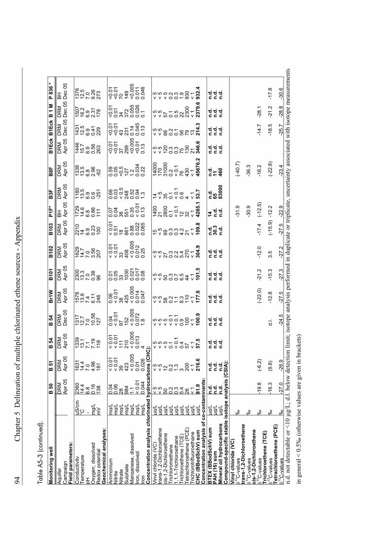
94
Cha
pter
5 D
elin
eatio
n of
mul
tiple
chl
orin
ated
eth
ene
sour
ces -
App
endi
x
Tabl
e A5
-3 (c
ontin
ued)
.
Mon
itorin
g w
ell
B
50
B 5
1 B
54
B 5
4 B
r1W
B10
1B
102
B10
3P1
F*B
3F
B8F
B1E
ck B
1Eck
B 1
MP
836
*Aq
uife
r
DR
M
DR
M
DR
M
DR
M
DR
M
DR
M
DR
M
DR
M
BH
DR
M
DR
M
DR
M
DR
M
DR
M
BH
Cam
paig
n
Apr 0
5Ap
r 05
Apr 0
5D
ec 0
5Ap
r 05
Apr 0
5Ap
r 05
Apr 0
5Ap
r 05
Apr 0
5Ap
r 05
Apr 0
5D
ec 0
5D
ec 0
5D
ec 0
5Fi
eld
para
met
ers:
Con
duct
ivity
µS/c
m
2360
1631
1339
1317
1578
2300
1629
22
1017
2911
8013
3814
4614
3115
0713
76Te
mpe
ratu
re°C
14
.414
.413
.112
.713
.613
.314
.7
1414
.613
.513
.515
.712
.516
.212
.5pH
-
6.8
7.0
7.1
7.0
7.4
7.0
7.0
6.9
6.8
6.9
6.8
6.9
6.9
6.9
7.0
Oxy
gen,
dis
solv
edm
g/L
0.16
4.96
7.19
10.5
86.
110.
383.
56
0.23
0.86
0.6
2.96
0.56
0.41
2.31
9.26
Red
ox p
oten
tial
mV
138
181
118
127
246
9620
7 10
011
1-2
51-6
226
322
917
827
3G
eoch
emic
al a
naly
ses:
Am
mon
ium
mg/
L 0.
04<
0.01
< 0.
010.
040.
060.
01<
0.01
<
0.01
0.07
0.66
0.59
<0.0
1<0
.01
<0.0
1<0
.01
Nitr
item
g/L
0.06
< 0.
01<
0.01
< 0.
01<
0.01
0.05
< 0.
01
0.51
0.04
0.03
0.05
<0.0
1<0
.01
0.01
<0.0
1N
itrat
em
g/L
2839
111
9738
3333
1838
< 0.
5<0
.537
4334
70Su
lpha
tem
g/L
984
423
210
152
425
1030
408
861
551
248
127
299
231
372
149
Man
gane
se, d
isso
lved
m
g/L
1.1
< 0.
005
<0.
005
< 0.
005
< 0.
005
0.02
1<
0.00
5 0.
880.
350.
521.
2<0
.005
0.14
0.05
5<0
.005
Iron,
dis
solv
edm
g/L
< 0.
010.
010.
013
0.07
20.
014
0.01
70.
012
0.02
2<
0.01
0.94
0.03
4<0
.01
0.04
50.
026
0.01
1Iro
n
mg/
L 0.
044
0.02
64
1.8
0.04
70.
080.
25
0.06
50.
131.
30.
220.
130.
130.
10.
046
Con
cent
ratio
n an
alys
is c
hlor
inat
ed h
ydro
carb
ons
(CH
C):
Viny
l chl
orid
e(V
C)
µg/L
<
5<
5<
5<
5<
5<
5<
515
1400
1414
000
< 5
< 5
< 5
< 5
trans
-1,2
-Dic
hlor
oeth
ene
µg/L
<
5<
5<
5<
5<
5<
5<
5<
521
< 5
170
< 5
< 5
< 5
< 5
cis-
1,2-
Dic
hlor
oeth
ene
µg/L
50
12<
5<
558
5027
6928
0035
3100
012
066
57<
5Tr
ichl
orom
etha
neµg
/L
0.2
0.2
0.1
< 0.
10.
20.
30.
30.
30.
10.
10.
20.
30.
20.
10.
21,
1,1-
Tric
hlor
oeth
ane
µg/L
0.
31.
3<
0.1
< 0.
11.
10.
72.
20.
3<
0.1
< 0.
1<
0.1
0.3
0.1
0.5
0.3
Tric
hlor
oeth
ene
(TC
E)
µg/L
5.
43
0.4
0.9
8.3
6.5
5.4
4.2
120.
676
7556
221.
9Te
trach
loro
ethe
ne (P
CE)
µg
/L
2620
057
100
110
4427
0 21
324
430
130
7923
0093
0Tr
ichl
orot
riflu
oroe
than
e µg
/L
< 1
< 1
< 1
< 1
< 1
< 1
< 1
< 1
< 1
< 1
< 1
2113
< 1
< 1
CH
C (B
Bod
SchV
) sum
µg
/L
81.9
216.
657
.510
0.9
177.
610
1.5
304.
9 10
9.8
4265
.153
.745
676.
234
6.6
214.
323
79.6
932.
4C
once
ntra
tion
anal
ysis
of c
o-co
ntam
inan
ts:
BTE
X (B
Bod
SchV
) sum
µg
/L
n.d.
n.d.
n.d.
n.d.
n.d.
n.d.
n.d.
n.
d.14
n.d.
n.d.
n.d.
n.d.
n.d.
n.d.
PAH
(16)
sum
µg/L
n.
d.n.
d.n.
d.n.
d.n.
d.n.
d.n.
d.
30.3
n.d.
6511
n.d.
n.d.
n.d.
n.d.
Min
eral
oil
hydr
ocar
bons
µg
/L
n.d.
n.d.
n.d.
n.d.
n.d.
n.d.
n.d.
n.
d.n.
d.83
000
460
n.d.
n.d.
n.d.
n.d.
Com
poun
d-sp
ecifi
c st
able
isot
ope
anal
ysis
(CSI
A):
Viny
l chl
orid
e(V
C)
δ13
C-v
alue
s ‰
-3
1.9
(-40
.7)
tran
s-1,
2-D
ichl
oroe
then
e
δ13C
-val
ues
‰
-30.
9-3
6.3
cis-
1,2-
Dic
hlor
oeth
ene
δ13
C-v
alue
s ‰
-1
9.8
(-6.2
)(-2
2.0)
-21.
2-1
2.0
-17.
4(-
12.5
)-1
6.2
-14.
7-2
8.1
Tric
hlor
oeth
ene
(TC
E)
δ13
C-v
alue
s ‰
-1
6.3
(9.8
)d.
l.-1
2.8
-15.
33.
5(-
15.9
)-1
2.2
(-22
.8)
-18.
5-2
1.2
-17.
8Te
trac
hlor
oeth
ene
(PC
E)
δ13
C-v
alue
s ‰
-2
7.0
-26.
9-2
4.5
-27.
5-2
7.3
-27.
2 -2
7.5
-22.
9-2
3.4
-25.
7-2
8.8
-30.
6n.
d. n
ot d
etec
tabl
e or
<10
µg/
L; d
.l. b
elow
det
ectio
n lim
it; is
otop
e an
alys
is p
erfo
rmed
in d
uplic
ate
or tr
iplic
ate,
unc
erta
inty
ass
ocia
ted
with
isot
ope
mea
sure
men
ts
in g
ener
al <
0.5
‰ (o
ther
wis
e va
lues
are
giv
en in
bra
cket
s)

Chapter 6 Quantitative assessment of biodegradation in a fractured aquifer 95
6. Quantitative Assessment of Aerobic Biodegradation of
Chlorinated Ethenes in a Fractured Bedrock Aquifer (*)
6.1. Introduction
Releases of dense chlorinated hydrocarbons (CHC) often cause substantial and persistent sources
of groundwater contamination, potentially hazardous to the aquatic environment and human
health. In-situ processes such as biodegradation, chemical transformation, dispersion, sorption, or
volatilization, determine the fate of chlorinated ethenes in groundwater (1,2) and need to be
quantified when monitored natural attenuation is considered as a remedial approach.
CHCs, especially the highly chlorinated solvents perchloroethene (PCE) and trichloroethene
(TCE), are biodegradable under highly anaerobic conditions via sequential reductive
dehalogenation (1,2). The less chlorinated CHCs, dichloroethene (DCE) and vinyl chloride (VC),
can be oxidized in the presence of molecular oxygen by various aerobic bacteria (3,4). A wide
range of chlorinated solvents (including TCE) can also be biodegraded under aerobic conditions
by cometabolic transformations (5,6). While reductive dehalogenation has frequently been
detected under field conditions (7-9), aerobic degradation of TCE is sparsely documented
(10,11). PCE, however, is generally not expected to degrade aerobically (1,2).
Methods to assess natural attenuation at field scales may include monitoring of contaminant mass
and/or contaminant and electron acceptor/donor concentrations over time, appearance of specific
co-metabolites and metabolic by-products and/or enzymes, degradation intermediates and
products, or specific analyses to identify the microbial populations present. However, evidence of
reduction of contaminant mass often is not precise enough, and clearly demonstrating CHC
degradation in aquifers remains difficult. Therefore compound-specific isotope analysis (CSIA)
has gained significant attention as a technique to assess both the occurrence and extent of in-situ
transformation of organic pollutants in contaminated aquifers (12-18). The method relies on the
kinetic isotope fractionation effect during transformation reactions which produces an enrichment
of heavy isotopes in the parent compound and a concomitant formation of isotopically lighter
products. In contrast, nondegradative attenuation processes that act on the compound as a whole
* performed in collaboration with K.E. Pooley, K.T.B. MacQuarrie and H. Prommer
96 Chapter 6 Quantitative assessment of biodegradation in a fractured aquifer
such as advective-dispersive transport, volatilization or sorption/desorption are assumed not to
significantly alter isotopic compositions (e.g. (18) and references therein). Carbon isotope
fractionation during biological and chemical transformations of CHCs is a well-documented
process, observed in laboratory experiments as well as in the field (16-18).
The extent of carbon isotope fractionation between substrate and product and the amount of
contaminant degraded can be quantitatively described using the Rayleigh equation (7,12-15)
Rs = Rs,0 f (α-1)
where Rs is the carbon isotope ratio (13C/12C) at a fraction of substrate or contaminant remaining
(f or concentration of the residual contaminant = ct/c0) at time t, Rs,0 is the initial isotopic
composition of the contaminant and α is the fractionation factor. The fractionation factor α is
often expressed as the enrichment factor ε, where ε = 1000(α-1).
The isotope enrichment factor for each compound being degraded may vary with, and thus can be
indicative of, degradation pathways (18-20). A compilation of isotope enrichment factors for
various specific biochemical conditions is provided in Meckenstock et al. (16). Significant
differences in isotope fractionation of chlorinated ethenes was also observed for abiotic processes
with zerovalent iron from different iron sources (21). Dissimilar enrichment factors for different
bacterial strain isolates, compared to an enrichment culture, reveals the inherent difficulties in
predicting isotope fractionation for undefined bacterial communities (22). While a qualitative
assessment of degradation based on fractionation is always possible, the actual extent of in-situ
transformation may only be quantified from isotope ratios measured in the field, if an appropriate
laboratory-derived ε, valid for the specific-site conditions, is known.
The Rayleigh model of fractionation, however, becomes invalid when the degradation process
involves competing parallel degradation pathways and where fractionation factors are pathway
dependent (18). Furthermore, it is applicable only to well mixed systems and thus unsuited for
those field site where differential flow/transport is significant (18,23). To overcome these
limitations numerical modeling approaches have been developed. They can account for
heterogeneous flow and transport, aid in the identification of relevant degradation pathways
(18,24,25), and provide information on the relative rates of intermediate degradation steps (26-
28). For example, one-dimensional (1D) simulations of PCE degradation were used to
demonstrate how the incorporation of isotope data may improve the efficiency and accuracy of
determining reaction rates and concentration profiles (24). Using a two-dimensional (2D)
Lagrangian approach, Abé and Hunkeler (23) demonstrated systematic errors of the Rayleigh
model for the quantification of biodegradation and estimation of first-order rate constants for
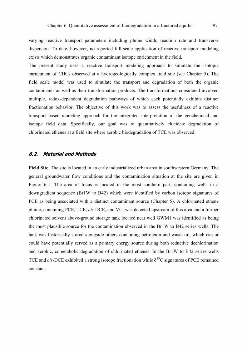
Chapter 6 Quantitative assessment of biodegradation in a fractured aquifer 97
varying reactive transport parameters including plume width, reaction rate and transverse
dispersion. To date, however, no reported full-scale application of reactive transport modeling
exists which demonstrates organic contaminant isotope enrichment in the field.
The present study uses a reactive transport modeling approach to simulate the isotopic
enrichment of CHCs observed at a hydrogeologically complex field site (see Chapter 5). The
field scale model was used to simulate the transport and degradation of both the organic
contaminants as well as their transformation products. The transformations considered involved
multiple, redox-dependent degradation pathways of which each potentially exhibits distinct
fractionation behavior. The objective of this work was to assess the usefulness of a reactive
transport based modeling approach for the integrated interpretation of the geochemical and
isotope field data. Specifically, our goal was to quantitatively elucidate degradation of
chlorinated ethenes at a field site where aerobic biodegradation of TCE was observed.
6.2. Material and Methods
Field Site. The site is located in an early industrialized urban area in southwestern Germany. The
general groundwater flow conditions and the contamination situation at the site are given in
Figure 6-1. The area of focus is located in the most southern part, containing wells in a
downgradient sequence (Br1W to B42) which were identified by carbon isotope signatures of
PCE as being associated with a distinct contaminant source (Chapter 5). A chlorinated ethene
plume, containing PCE, TCE, cis-DCE, and VC, was detected upstream of this area and a former
chlorinated solvent above-ground storage tank located near well GWM1 was identified as being
the most plausible source for the contamination observed in the Br1W to B42 series wells. The
tank was historically stored alongside others containing petroleum and waste oil, which can or
could have potentially served as a primary energy source during both reductive dechlorination
and aerobic, cometabolic degradation of chlorinated ethenes. In the Br1W to B42 series wells
TCE and cis-DCE exhibited a strong isotope fractionation while δ13C signatures of PCE remained
constant.
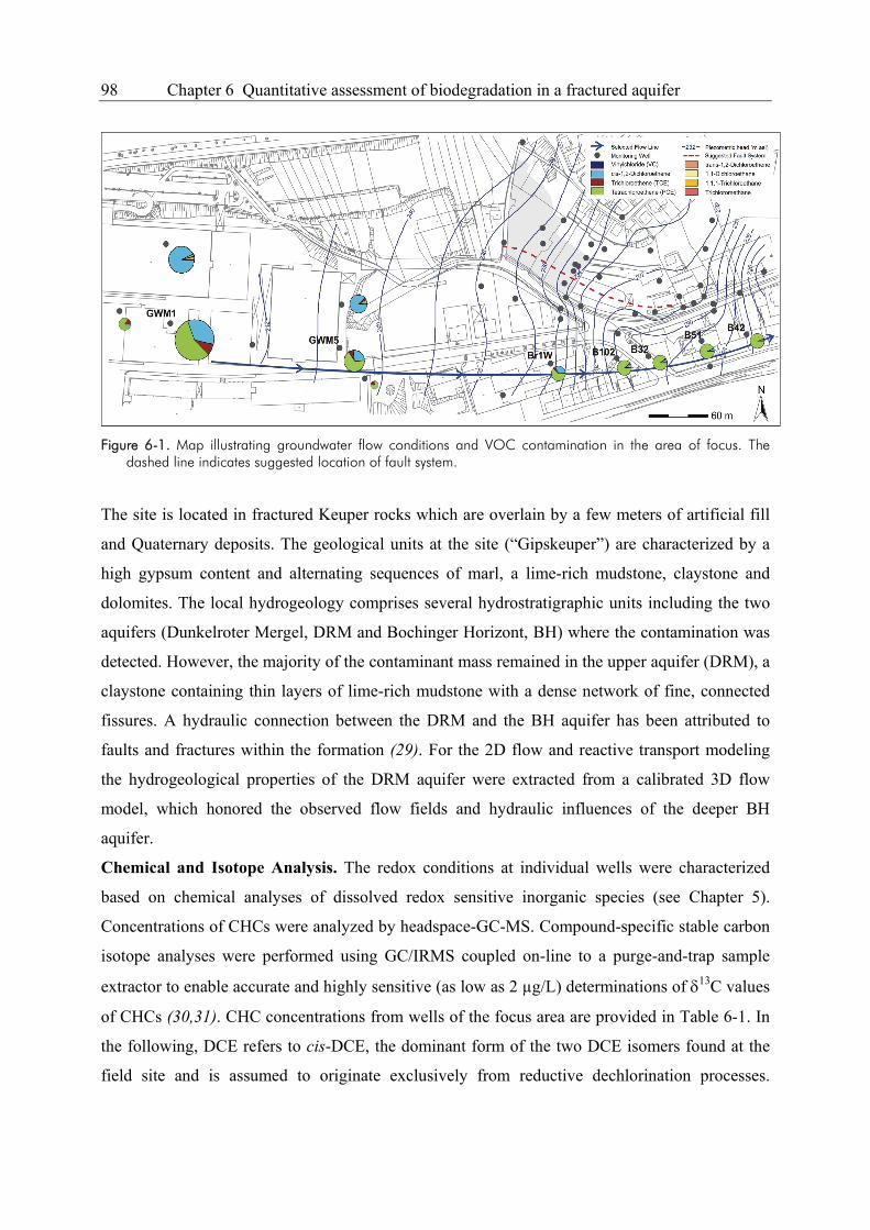
98 Chapter 6 Quantitative assessment of biodegradation in a fractured aquifer
Figure 6-1. Map illustrating groundwater flow conditions and VOC contamination in the area of focus. The
dashed line indicates suggested location of fault system.
The site is located in fractured Keuper rocks which are overlain by a few meters of artificial fill
and Quaternary deposits. The geological units at the site (“Gipskeuper”) are characterized by a
high gypsum content and alternating sequences of marl, a lime-rich mudstone, claystone and
dolomites. The local hydrogeology comprises several hydrostratigraphic units including the two
aquifers (Dunkelroter Mergel, DRM and Bochinger Horizont, BH) where the contamination was
detected. However, the majority of the contaminant mass remained in the upper aquifer (DRM), a
claystone containing thin layers of lime-rich mudstone with a dense network of fine, connected
fissures. A hydraulic connection between the DRM and the BH aquifer has been attributed to
faults and fractures within the formation (29). For the 2D flow and reactive transport modeling
the hydrogeological properties of the DRM aquifer were extracted from a calibrated 3D flow
model, which honored the observed flow fields and hydraulic influences of the deeper BH
aquifer.
Chemical and Isotope Analysis. The redox conditions at individual wells were characterized
based on chemical analyses of dissolved redox sensitive inorganic species (see Chapter 5).
Concentrations of CHCs were analyzed by headspace-GC-MS. Compound-specific stable carbon
isotope analyses were performed using GC/IRMS coupled on-line to a purge-and-trap sample
extractor to enable accurate and highly sensitive (as low as 2 µg/L) determinations of δ13C values
of CHCs (30,31). CHC concentrations from wells of the focus area are provided in Table 6-1. In
the following, DCE refers to cis-DCE, the dominant form of the two DCE isomers found at the
field site and is assumed to originate exclusively from reductive dechlorination processes.
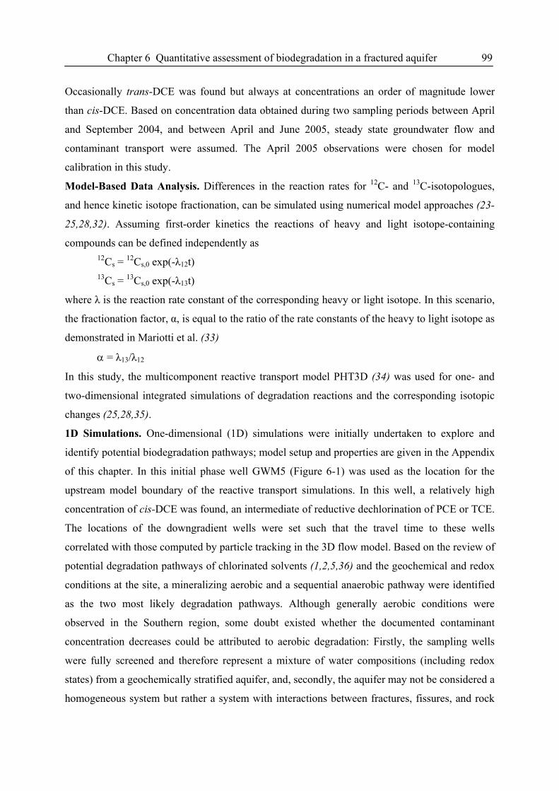
Chapter 6 Quantitative assessment of biodegradation in a fractured aquifer 99
Occasionally trans-DCE was found but always at concentrations an order of magnitude lower
than cis-DCE. Based on concentration data obtained during two sampling periods between April
and September 2004, and between April and June 2005, steady state groundwater flow and
contaminant transport were assumed. The April 2005 observations were chosen for model
calibration in this study.
Model-Based Data Analysis. Differences in the reaction rates for 12C- and 13C-isotopologues,
and hence kinetic isotope fractionation, can be simulated using numerical model approaches (23-
25,28,32). Assuming first-order kinetics the reactions of heavy and light isotope-containing
compounds can be defined independently as
12Cs = 12Cs,0 exp(-λ12t)
13Cs = 13Cs,0 exp(-λ13t)
where λ is the reaction rate constant of the corresponding heavy or light isotope. In this scenario,
the fractionation factor, α, is equal to the ratio of the rate constants of the heavy to light isotope as
demonstrated in Mariotti et al. (33)
α = λ13/λ12
In this study, the multicomponent reactive transport model PHT3D (34) was used for one- and
two-dimensional integrated simulations of degradation reactions and the corresponding isotopic
changes (25,28,35).
1D Simulations. One-dimensional (1D) simulations were initially undertaken to explore and
identify potential biodegradation pathways; model setup and properties are given in the Appendix
of this chapter. In this initial phase well GWM5 (Figure 6-1) was used as the location for the
upstream model boundary of the reactive transport simulations. In this well, a relatively high
concentration of cis-DCE was found, an intermediate of reductive dechlorination of PCE or TCE.
The locations of the downgradient wells were set such that the travel time to these wells
correlated with those computed by particle tracking in the 3D flow model. Based on the review of
potential degradation pathways of chlorinated solvents (1,2,5,36) and the geochemical and redox
conditions at the site, a mineralizing aerobic and a sequential anaerobic pathway were identified
as the two most likely degradation pathways. Although generally aerobic conditions were
observed in the Southern region, some doubt existed whether the documented contaminant
concentration decreases could be attributed to aerobic degradation: Firstly, the sampling wells
were fully screened and therefore represent a mixture of water compositions (including redox
states) from a geochemically stratified aquifer, and, secondly, the aquifer may not be considered a
homogeneous system but rather a system with interactions between fractures, fissures, and rock
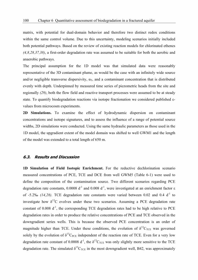
100 Chapter 6 Quantitative assessment of biodegradation in a fractured aquifer
matrix, with potential for dual-domain behavior and therefore two distinct redox conditions
within the same control volume. Due to this uncertainty, modeling scenarios initially included
both potential pathways. Based on the review of existing reaction models for chlorinated ethenes
(4,8,28,37,38), a first-order degradation rate was assumed to be suitable for both the aerobic and
anaerobic pathways.
The principal assumption for the 1D model was that simulated data were reasonably
representative of the 3D contaminant plume, as would be the case with an infinitely wide source
and/or negligible transverse dispersivity, αT, and a contaminant concentration that is distributed
evenly with depth. Underpinned by measured time series of piezometric heads from the site and
regionally (29), both the flow field and reactive transport processes were assumed to be at steady
state. To quantify biodegradation reactions via isotope fractionation we considered published ε-
values from microcosm experiments.
2D Simulations. To examine the effect of hydrodynamic dispersion on contaminant
concentrations and isotope signatures, and to assess the influence of a range of potential source
widths, 2D simulations were conducted. Using the same hydraulic parameters as those used in the
1D model, the upgradient extent of the model domain was shifted to well GWM1 and the length
of the model was extended to a total length of 650 m.
6.3. Results and Discussion
1D Simulation of Field Isotopic Enrichment. For the reductive dechlorination scenario
measured concentrations of PCE, TCE and DCE from well GWM5 (Table 6-1) were used to
define the composition of the contamination source. Two different scenarios regarding PCE
degradation rate constants, 0.0008 d-1 and 0.008 d-1, were investigated at an enrichment factor ε
of -5.2‰ (14,28). TCE degradation rate constants were varied between 0.02 and 0.4 d-1 to
investigate how δ13C evolves under these two scenarios. Assuming a PCE degradation rate
constant of 0.008 d-1, the corresponding TCE degradation rates had to be high relative to PCE
degradation rates in order to produce the relative concentrations of PCE and TCE observed in the
downgradient series wells. This is because the observed PCE concentration is an order of
magnitude higher than TCE. Under these conditions, the evolution of δ13CTCE was governed
solely by the evolution of δ13CPCE independent of the reaction rate of TCE. Even for a very low
degradation rate constant of 0.0008 d-1, the δ13CTCE was only slightly more sensitive to the TCE
degradation rate. The simulated δ13CTCE in the most downgradient well, B42, was approximately
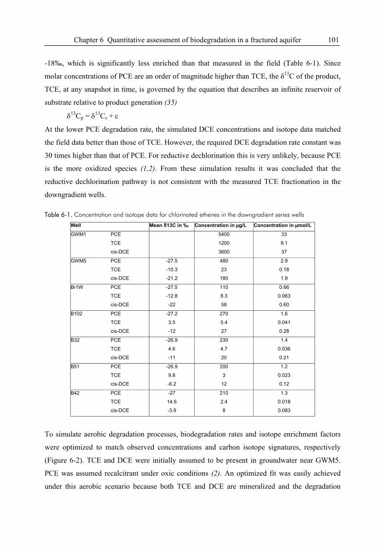
Chapter 6 Quantitative assessment of biodegradation in a fractured aquifer 101
-18‰, which is significantly less enriched than that measured in the field (Table 6-1). Since
molar concentrations of PCE are an order of magnitude higher than TCE, the δ13C of the product,
TCE, at any snapshot in time, is governed by the equation that describes an infinite reservoir of
substrate relative to product generation (35)
δ13Cp = δ13Cs + ε
At the lower PCE degradation rate, the simulated DCE concentrations and isotope data matched
the field data better than those of TCE. However, the required DCE degradation rate constant was
30 times higher than that of PCE. For reductive dechlorination this is very unlikely, because PCE
is the more oxidized species (1,2). From these simulation results it was concluded that the
reductive dechlorination pathway is not consistent with the measured TCE fractionation in the
downgradient wells.
Table 6-1. Concentration and isotope data for chlorinated ethenes in the downgradient series wells
Well Mean δ13C in ‰ Concentration in µg/L Concentration in µmol/L
GWM1 PCE 5400 33
TCE 1200 9.1
cis-DCE 3600 37
GWM5 PCE -27.5 480 2.9
TCE -10.3 23 0.18
cis-DCE -21.2 180 1.9
Br1W PCE -27.5 110 0.66
TCE -12.8 8.3 0.063
cis-DCE -22 58 0.60
B102 PCE -27.2 270 1.6
TCE 3.5 5.4 0.041
cis-DCE -12 27 0.28
B32 PCE -26.9 230 1.4
TCE 4.6 4.7 0.036
cis-DCE -11 20 0.21
B51 PCE -26.9 200 1.2
TCE 9.8 3 0.023
cis-DCE -6.2 12 0.12
B42 PCE -27 210 1.3
TCE 14.6 2.4 0.018
cis-DCE -3.9 8 0.083
To simulate aerobic degradation processes, biodegradation rates and isotope enrichment factors
were optimized to match observed concentrations and carbon isotope signatures, respectively
(Figure 6-2). TCE and DCE were initially assumed to be present in groundwater near GWM5.
PCE was assumed recalcitrant under oxic conditions (2). An optimized fit was easily achieved
under this aerobic scenario because both TCE and DCE are mineralized and the degradation
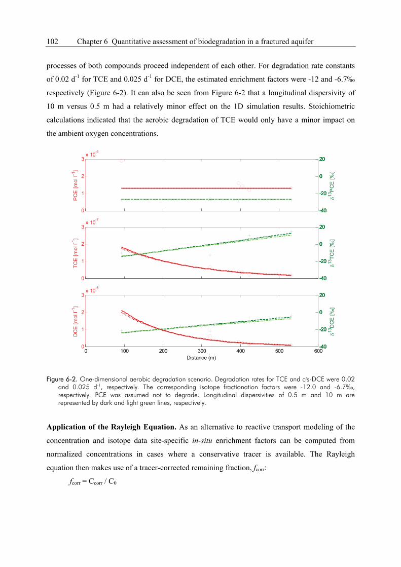
102 Chapter 6 Quantitative assessment of biodegradation in a fractured aquifer
processes of both compounds proceed independent of each other. For degradation rate constants
of 0.02 d-1 for TCE and 0.025 d-1 for DCE, the estimated enrichment factors were -12 and -6.7‰
respectively (Figure 6-2). It can also be seen from Figure 6-2 that a longitudinal dispersivity of
10 m versus 0.5 m had a relatively minor effect on the 1D simulation results. Stoichiometric
calculations indicated that the aerobic degradation of TCE would only have a minor impact on
the ambient oxygen concentrations.
0
1
2
3x 10⁻⁶
PC
E [m
ol l-1
]
-40
-20
0
20
-40
-20
0
20
-40
-20
0
20
δ13P
CE
[‰]
-40
-20
0
20
0
1
2
3x 10⁻⁷
TCE
[mol
l-1]
-40
-20
0
20
-40
-20
0
20
-40
-20
0
20
δ13TC
E [‰
]
-40
-20
0
20
0
1
2
3x 10⁻⁶
DC
E [m
ol l-1
]
-40
-20
0
20
-40
-20
0
20
-40
-20
0
20
δ13D
CE
[‰]
0 100 200 300 400 500 600-40
-20
0
20
Distance (m)
Figure 6-2. One-dimensional aerobic degradation scenario. Degradation rates for TCE and cis-DCE were 0.02 and 0.025 d-1, respectively. The corresponding isotope fractionation factors were -12.0 and -6.7‰, respectively. PCE was assumed not to degrade. Longitudinal dispersivities of 0.5 m and 10 m are represented by dark and light green lines, respectively.
Application of the Rayleigh Equation. As an alternative to reactive transport modeling of the
concentration and isotope data site-specific in-situ enrichment factors can be computed from
normalized concentrations in cases where a conservative tracer is available. The Rayleigh
equation then makes use of a tracer-corrected remaining fraction, fcorr:
fcorr = Ccorr / C0
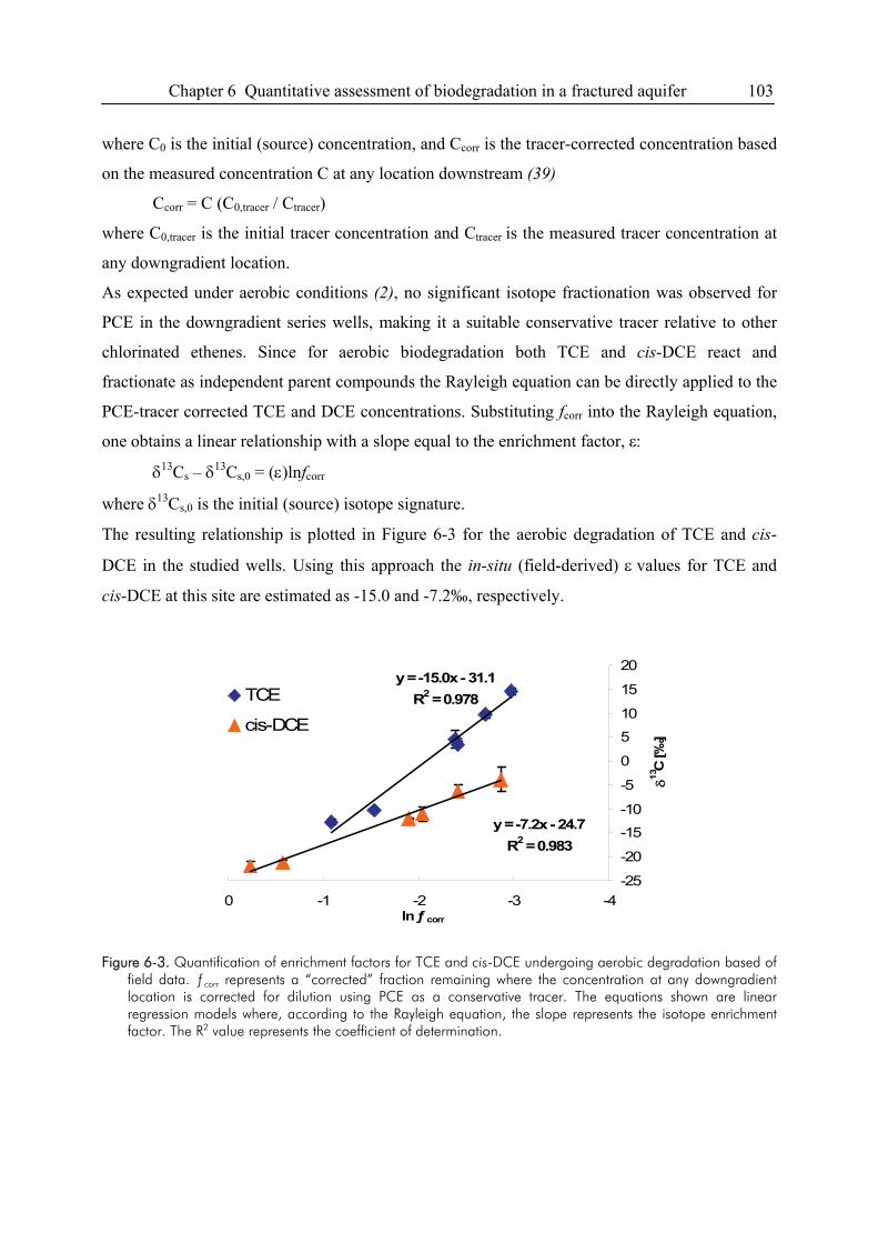
Chapter 6 Quantitative assessment of biodegradation in a fractured aquifer 103
where C0 is the initial (source) concentration, and Ccorr is the tracer-corrected concentration based
on the measured concentration C at any location downstream (39)
Ccorr = C (C0,tracer / Ctracer)
where C0,tracer is the initial tracer concentration and Ctracer is the measured tracer concentration at
any downgradient location.
As expected under aerobic conditions (2), no significant isotope fractionation was observed for
PCE in the downgradient series wells, making it a suitable conservative tracer relative to other
chlorinated ethenes. Since for aerobic biodegradation both TCE and cis-DCE react and
fractionate as independent parent compounds the Rayleigh equation can be directly applied to the
PCE-tracer corrected TCE and DCE concentrations. Substituting fcorr into the Rayleigh equation,
one obtains a linear relationship with a slope equal to the enrichment factor, ε:
δ13Cs – δ13Cs,0 = (ε)lnfcorr
where δ13Cs,0 is the initial (source) isotope signature.
The resulting relationship is plotted in Figure 6-3 for the aerobic degradation of TCE and cis-
DCE in the studied wells. Using this approach the in-situ (field-derived) ε values for TCE and
cis-DCE at this site are estimated as -15.0 and -7.2‰, respectively.
y = -7.2x - 24.7R2 = 0.983
y = -15.0x - 31.1R2 = 0.978
-25
-20
-15
-10
-5
0
5
10
15
20
-4-3-2-10ln ƒ corr
δ13C
[‰]
TCE
cis-DCE
Figure 6-3. Quantification of enrichment factors for TCE and cis-DCE undergoing aerobic degradation based of field data. ƒcorr represents a “corrected” fraction remaining where the concentration at any downgradient location is corrected for dilution using PCE as a conservative tracer. The equations shown are linear regression models where, according to the Rayleigh equation, the slope represents the isotope enrichment factor. The R2 value represents the coefficient of determination.
104 Chapter 6 Quantitative assessment of biodegradation in a fractured aquifer
2D Simulations. To study the influence of dispersive processes on the interpretation of field data,
the 1D model was modified and extended to 2D. In the absence of detailed information on the
geometry of the source zone located near GWM1, scenarios with a range of source widths were
investigated in combination with varying horizontal transverse dispersivities (αT), using the
observed PCE concentrations as constraints. The sampled wells were assumed to be located at or
near the plume centerline. Results of plume simulations, demonstrated that the range of possible
plume widths extends to around 6 m at the most, for a reasonable range of transverse dispersivity
values. A source width of 4m most closely matched the measured PCE concentrations for αT of 1
m, which was adopted for the 2D simulations (see Appendix of this chapter).
The simulated 2D concentration and isotope values for TCE obtained by fitting degradation rates
relative to isotope data are presented in Figure 6-4. The degradation rates required to obtain the
best linear fit of the isotope data in the 2D model differed slightly from those estimated by the
PCE-tracer corrected Rayleigh equation, because of the effect of longitudinal dispersion
demonstrated in Figure 6-2. For the scenario presented, λTCE was 0.015 d-1 and λDCE was
0.023 d-1. This can be seen by plotting the plume centerline data for this scenario, shown in
Figure 6-5a. In this figure, the concentration and isotope data along the centerline of the plume
were plotted together with the 0D batch (zero dispersion) simulation having the same degradation
rates. The simulated 2D plume exhibits the same isotopic changes as the corresponding 1D case
with the same longitudinal dispersion, suggesting that for first-order degradation the transverse
dispersion has no effect on isotope data at the centerline of the plume. Off the center line, the
modeled isotope signature of the degrading parent compounds TCE and cis-DCE are slightly
affected by transverse dispersion in that δ13C gradually increases the more offset a measurement
point is from the centerline of the plume (Figure 6-4).
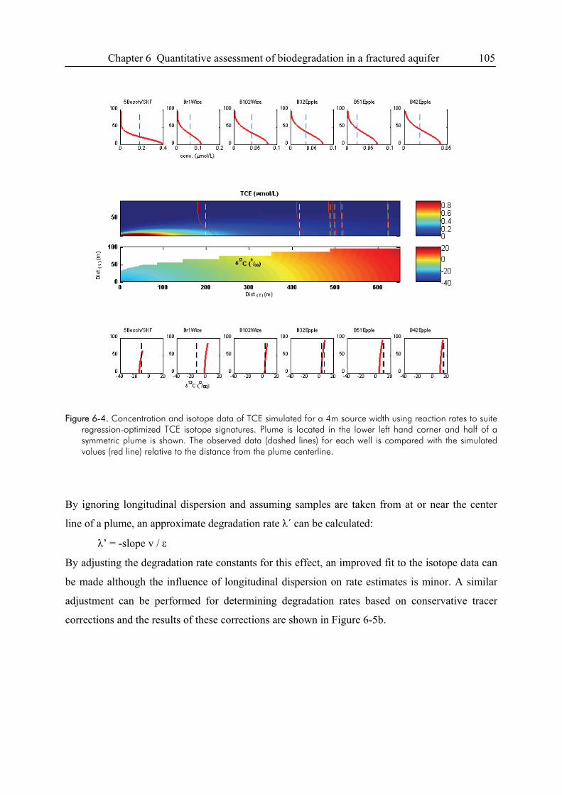
Chapter 6 Quantitative assessment of biodegradation in a fractured aquifer 105
Figure 6-4. Concentration and isotope data of TCE simulated for a 4m source width using reaction rates to suite regression-optimized TCE isotope signatures. Plume is located in the lower left hand corner and half of a symmetric plume is shown. The observed data (dashed lines) for each well is compared with the simulated values (red line) relative to the distance from the plume centerline.
By ignoring longitudinal dispersion and assuming samples are taken from at or near the center
line of a plume, an approximate degradation rate λ΄ can be calculated:
λ’ = -slope v / ε
By adjusting the degradation rate constants for this effect, an improved fit to the isotope data can
be made although the influence of longitudinal dispersion on rate estimates is minor. A similar
adjustment can be performed for determining degradation rates based on conservative tracer
corrections and the results of these corrections are shown in Figure 6-5b.
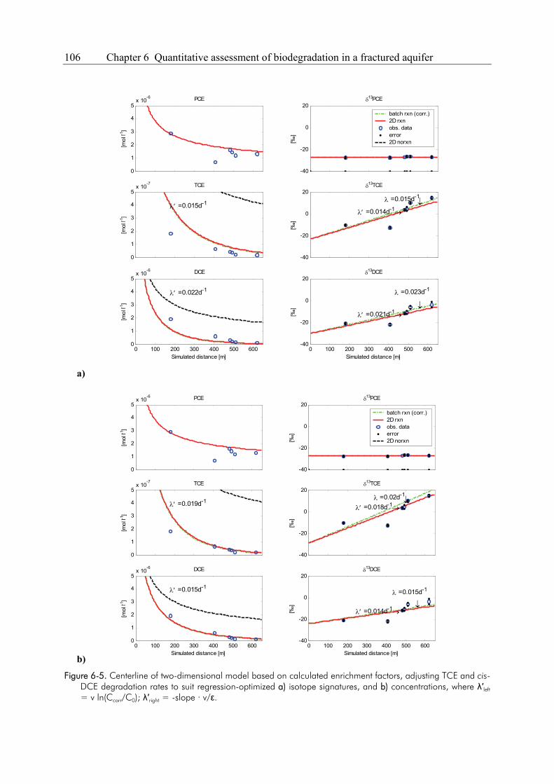
106 Chapter 6 Quantitative assessment of biodegradation in a fractured aquifer
a)
0
1
2
3
4
5x 10
-6 PCE
[mol
l-1]
-40
-20
0
20δ13PCE
[‰]
batch rxn (corr.)2D rxnobs. dataerror2D norxn
0
1
2
3
4
5x 10
-7
λ′ =0.015d-1
TCE
[mol
l-1]
-40
-20
0
20
λ′ =0.014d-1→ ↓ λ =0.015d-1
δ13TCE
[‰]
0 100 200 300 400 500 6000
1
2
3
4
5x 10
-6
λ′ =0.022d-1
DCE
Simulated distance [m]
[mol
l-1]
0 100 200 300 400 500 600-40
-20
0
20
λ′ =0.021d-1→ ↓
λ =0.023d-1
δ13DCE
Simulated distance [m]
[‰]
b)
0
1
2
3
4
5x 10
-6 PCE
[mol
l-1]
-40
-20
0
20δ13PCE
[‰]
batch rxn (corr.)2D rxnobs. dataerror2D norxn
0
1
2
3
4
5x 10
-7
λ′ =0.019d-1
TCE
[mol
l-1]
-40
-20
0
20
λ′ =0.018d-1→ ↓ λ =0.02d-1
δ13TCE
[‰]
0 100 200 300 400 500 6000
1
2
3
4
5x 10
-6
λ′ =0.015d-1
DCE
Simulated distance [m]
[mol
l-1]
0 100 200 300 400 500 600-40
-20
0
20
λ′ =0.014d-1→ ↓
λ =0.015d-1
δ13DCE
Simulated distance [m]
[‰]
Figure 6-5. Centerline of two-dimensional model based on calculated enrichment factors, adjusting TCE and cis-DCE degradation rates to suit regression-optimized a) isotope signatures, and b) concentrations, where λ′left = v ln(Ccorr/C0); λ′right = -slope · v/ε.
Chapter 6 Quantitative assessment of biodegradation in a fractured aquifer 107
Plotting the Rayleigh function for the 2D plume demonstrates the difference between isotope
reactive transport modeling and analytical modeling using a simple Rayleigh equation (36). The
plot compares different representations of remaining fractions: the first based on measured
concentrations, where ƒ = C/C0; the second based on concentration corrections by advective-
dispersive nonreactive transport modeling, where ƒ = C/Cdisp; and the third based on corrections
using a conservative tracer, where ƒ = Ccorr/C0. It was shown that correction by advective-
dispersive nonreactive transport modeling and correction using a conservative tracer produce the
same results (see Appendix of this chapter). The interpreted enrichment factors based on these
correction methods do not equate precisely to the “true” (i.e., model) enrichment factors, a result
of longitudinal dispersion effects.
Systematic Effects on Enrichment Factors. The calculated enrichment factor for TCE (Figure
6-3) is within the range of those reported for aerobic degradation (-1.1 to -20.7‰). This large
range, however, is based on only two studies, each using an isolated bacterial strain under
controlled laboratory conditions. A strong enrichment of TCE during aerobic degradation was
reported by Barth et al. for aerobic cometabolism of TCE by the toluene-degrading strain,
Burkholderia cepacia G4 (40). In contrast, Methylosinus trichosporium OB3b growing on
methane as primary substrate caused insignificant fractionation for aerobic co-metabolic
biodegradation of both cis-DCE and TCE (41).
Possible errors related to the estimated enrichment factors, besides sampling and analytical errors
in the concentration and isotope measurements, may result from longitudinal dispersion (minor
but not accounted for in the conservative tracer method; Figure 6-2), vertically heterogeneous
flow, and the assumption of first-order reaction rates. Effects of longitudinal dispersion and
heterogeneous flow will underestimate enrichment factors by dilution-corrected methods which
may result in slight overestimation of degradation rates. This effect is demonstrated by
comparing the variations in ε with increasing αL for each compound in the Rayleigh plots, where
a maximum deviation of 0.9‰ in the true εTCE was calculated for the highest longitudinal
dispersion of 20 m (see Appendix of this chapter), which is a considerably larger dispersivity
than reported for most aquifers (42). The degree of underestimation, however, is much lower than
when estimating an enrichment factor from field data using a direct application of the Rayleigh
equation.
Implications for Field Sites. This study demonstrates the potential for aerobic degradation of
chlorinated ethenes, TCE and cis-DCE, under natural field conditions. Aerobic TCE degradation
has been described earlier in lab experiments as a cometabolic process (37). At a site with an
108 Chapter 6 Quantitative assessment of biodegradation in a fractured aquifer
extensive history of industrial activity such as this one, sufficient organic primary substrate
should be present. Prior to this study, fractionation due to aerobic TCE degradation has only been
studied for two particular strains of bacteria and never for a mixed culture. Fractionation due to
aerobic DCE degradation is even less well documented. This study may present the first field
based mixed aerobic microbial enrichment factor for these compounds, as well as being the first
reactive transport-based in-situ enrichment factor reported.
Using reactive transport modeling with carbon isotope fractionation, the relationship between a
source and an observed plume can be better understood. A comparison of isotope analysis only at
the field scale to isotope analysis with reactive transport modeling has demonstrated the need,
when quantifying natural attenuation processes, for an integrated approach, particularly when
similar degradation processes can result in a range of enrichment factors. In addition, modeling
changing isotope ratios of contaminants degrading through different reactive pathways and the
production/consumption of sequential daughter products may allow for the verification of the
relevant processes occurring in the contaminant plume. Because (intrinsic) reaction kinetics
rather than supply of oxygen was rate limiting in this field study, simulation of dissolved oxygen
dispersion/diffusion was not necessary. In cases where oxygen supply is limited by physical
mixing processes (diffusion/dispersion), the isotopic changes will vary greatly depending on the
location of an observation well relative to the plume fringe (35). This aspect will need to be
considered in the quantification of biodegradation rates and overall mass removal at a field site.
As seen from the Rayleigh plots of the 2D simulation results, the direct application of isotope
data to quantify enrichment factors will result in underestimated enrichment factors and therefore
overestimated biodegradation. This is due to the fact that when plotting a Rayleigh equation of ƒ
= C/C0, the assumption is that all decreases in concentration are due to biodegradation and all
calculated mass removals using this enrichment value will maintain this assumption. Microcosm
quantification of a mixed microbial community sampled from a field site of interest should be
representative of fractionation processes in-situ and has been, until now, the only direct method
of quantifying biodegradation of contaminants in-situ, in the absence of a conservative tracer
(16). In this study, corrections for dispersive processes were made with the conservative tracer
method prior to the calculation of enrichment factors. There is potential to achieve similarly
robust estimates of degradation rates by multi-parameter optimization of transport and
degradation processes integrating both concentration and isotope field data into reactive transport
modeling.
Chapter 6 Quantitative assessment of biodegradation in a fractured aquifer 109
6.4. References
(1) Lee, M. D.; Odom, J. M.; Buchanan Jr., R. J. New perspectives on microbial dehalogenation of chlorinated solvents: Insights from the field. Annu. Rev. Microbiol. 1998, 52, 423-452.
(2) Wiedemeier, T. H.; Swanson, M. A.; Moutoux, D. E.; Gordon, E. K.; Wilson, J. T.; Wilson, B. H.; Kampbell, D. H.; Haas, P. E.; Miller, R. N.; Hansen, J. E.; Chapelle, F. H. Technical Protocol for Evaluating Natural Attenuation of Chlorinated Solvents in Ground Water. EPA/600/R-98/128 National Risk Management Research Laboratory, Office of Research and Development, U. S. Environmental Protection Agency; Cincinnati, Ohio 1998.
(3) Davis, J. W.; Carpenter, C. L. Aerobic biodegradation of vinyl chloride in groundwater samples. Appl. Environ. Microbiol. 1990, 56, 3878-3880.
(4) Bradley, P. M.; Chapelle, F. H. Effect of contaminant concentration on aerobic microbial mineralization of DCE and VC in stream-bed sediments. Environ. Sci. Technol. 1998, 32, 553-557.
(5) Ensley, B. D. Biochemical diversity of trichloroethylene metabolism. Annu. Rev. Microbiol. 1991, 45, 283-299.
(6) Fliermans, C. B.; Phelps, T. J.; Ringelberg, D.; Mikell, A. T.; White, D. C. Mineralization of trichloroethylene by heterotrophic enrichment cultures. Appl. Environ. Microbiol. 1998, 54, 1709-1714.
(7) Sherwood Lollar, B.; Slater, G. F.; Sleep, B.; Witt, M.; Klecka, G. M.; Harkness, M.; Spivack, J. Stable carbon isotope evidence for intrinsic bioremediation of tetrachloroethene and trichloroethene at area 6, Dover Air Force Base. Environ. Sci. Technol. 2001, 35, 261-269.
(8) Clement, T. P.; Johnson, C. D.; Sun, Y. G.; Klecka, G. M.; Bartlett, C. Natural attenuation of chlorinated ethene compounds: model development and field-scale application at the Dover site. J. Contam. Hydrol. 2000, 42, 113-140.
(9) Song, D. L.; Conrad, M. E.; Sorenson, K. S.; Alvarez-Cohen, L. Stable carbon isotope fractionation during enhanced in situ bioremediation of trichloroethene. Environ. Sci. Technol. 2002, 36, 2262-2268.
(10) Sturchio, N. C.; Clausen, J. L.; Heraty, L. J.; Huang, L.; Holt, B. D.; Abrajano, T. A. Chlorine isotope investigation of natural attenuation of trichloroethene in an aerobic aquifer. Environ. Sci. Technol. 1998, 32, 3037-3042.
(11) Sorenson, K. S. J.; Peterson, L. N.; Hinchee, R. E.; Ely, R. L. An evaluation of aerobic trichloroethene attenuation using first-order rate estimation. Bioremediation 2000, 4, 337-357.
(12) Hunkeler, D.; Aravena, R.; Butler, B. J. Monitoring microbial dechlorination of tetrachloroethene (PCE) in groundwater using compound-specific stable carbon isotope ratios: Microcosm and field studies. Environ. Sci. Technol. 1999, 33, 2733-2738.
(13) Sherwood Lollar, B.; Slater, G. F.; Ahad, J.; Sleep, B.; Spivack, J.; Brennan, M.; MacKenzie, P. Contrasting carbon isotope fractionation during biodegradation of trichloroethylene and toluene: Implications for intrinsic bioremediation. Org. Geochem. 1999, 30, 813-820.
(14) Slater, G. F.; Sherwood Lollar, B.; Sleep, B. E.; Edwards, E. A. Variability in carbon isotopic fractionation during biodegradation of chlorinated ethenes: Implications for field applications. Environ. Sci. Technol. 2001, 35, 901-907.
(15) Mancini, S. A.; Lacrampe-Couloume, G.; Jonker, H.; Breukelen, B. M. V.; Groen, J.; Folkering, F.; Sherwood Lollar, B. Hydrogen isotope enrichment: An indicator of biodegradation at a petroleum hydrocarbon field site. Environ. Sci. Technol. 2002, 36, 2464-2470.
(16) Meckenstock, R. U.; Morasch, B.; Griebler, C.; Richnow, H. H. Stable isotope fractionation analysis as a tool to monitor biodegradation in contaminated acquifers. J. Contam. Hydrol. 2004, 75, 215-255.
(17) Schmidt, T. C.; Zwank, L.; Elsner, M.; Berg, M.; Meckenstock, R. U.; Haderlein, S. B. Compound-specific stable isotope analysis of organic contaminants in natural environments: a critical review of the state of the art, prospects, and future challenges. Anal. Bioanal. Chem. 2004, 378, 283-300.
(18) Elsner, M.; Zwank, L.; Hunkeler, D.; Schwarzenbach, R. P. A new concept linking observable stable isotope fractionation to transformation pathways of organic pollutants. Environ. Sci. Technol. 2005, 39, 6896-6916.
(19) Morasch, B.; Richnow, H. H.; Schink, B.; Meckenstock, R. U. Stable hydrogen and carbon isotope fractionation during microbial toluene degradation: Mechanistic and environmental aspects. Appl. Environ. Microbiol. 2001, 67, 4842-4849.
(20) Nijenhuis, I.; Andert, J.; Beck, K.; Kästner, M.; Diekert, G.; Richnow, H. H. Stable isotope fractionation of tetrachloroethene during reductive dechlorination by Sulfurospirillum multivorans and Desulfitobacterium sp strain PCE-S and abiotic reactions with cyanocobalamin. Appl. Environ. Microbiol. 2005, 71, 3413-3419.
(21) VanStone, N. A.; Focht, R. M.; Mabury, S. A.; Sherwood Lollar, B. Effect of iron type on kinetics and carbon isotopic enrichment of chlorinated ethylenes during abiotic reduction on Fe(0). Ground Water 2004, 42, 268-276.
110 Chapter 6 Quantitative assessment of biodegradation in a fractured aquifer
(22) Lee, P. K. H.; Conrad, M. E.; Alvarez-Cohen, L. Stable carbon isotope fractionation of chloroethenes by dehalorespiring isolates. Environ. Sci. Technol. 2007, 41, 4277-4285.
(23) Abé, Y.; Hunkeler, D. Does the Rayleigh equation apply to evaluate field isotope data in contaminant hydrogeology? Environ. Sci. Technol. 2006, 1588-1596.
(24) Béranger, S. C.; Sleep, B. E.; Sherwood Lollar, B.; Monteagudo, F. P. Transport, biodegradation and isotopic fractionation of chlorinated ethenes: Modeling and parameter estimation methods. Advances in Water Resources 2005, 28, 87-98.
(25) Prommer, H.; Aziz, L. H.; Bolaño, N.; Taubald, H.; Schüth, C. Modelling of geochemical and isotopic changes in a column experiment for degradation of TCE by zero-valent iron. J. Contam. Hydrol. 2008, 97, 13-26.
(26) Hunkeler, D.; Aravena, R.; Cox, E. Carbon isotopes as a tool to evaluate the origin and fate of vinyl chloride: Laboratory experiments and modeling of isotope evolution. Environ. Sci. Technol. 2002, 36, 3378-3384.
(27) Morrill, P. L.; Sleep, B. E.; Slater, G. F.; Edwards, E. A.; Sherwood Lollar, B. Evaluation of isotopic enrichment factors for the biodegradation of chlorinated ethenes using a parameter estimation model: toward an improved quantification of biodegradation. Environ. Sci. Technol. 2006, 40, 3886-3892.
(28) van Breukelen, B. M.; Hunkeler, D.; Volkering, F. Quantification of sequential chlorinated ethene degradation by use of a reactive transport model incorporating isotope fractionation. Environ. Sci. Technol. 2005, 39, 4189-4197.
(29) Amt für Umweltschutz Stuttgart, KORA - TV1: Forschungsbericht, Förderkennzeichen 02WN0353; Projekt 1.3: Natürlicher Abbau und Rückhalt eines komplexen Schadstoffcocktails in einem Grundwasserleiter am Beispiel des ehemaligen Mineralölwerks Epple; Stuttgart, 2007.
(30) Zwank, L.; Berg, M.; Schmidt, T. C.; Haderlein, S. B. Compound-specific carbon isotope analysis of volatile organic compounds in the low-microgram per liter range. Anal. Chem. 2003, 75, 5575-5583.
(31) Jochmann, M. A.; Blessing, M.; Haderlein, S. B.; Schmidt, T. C. A new approach to determine method detection limits for compound-specific isotope analysis of volatile organic compounds. Rapid Commun. Mass Spectrom. 2006, 20, 3639-3648.
(32) Chen, D. J. Z.; MacQuarrie, K. T. B. Numerical simulation of organic carbon, nitrate, and nitrogen isotope behavior during denitrification in a riparian zone. J. Hydrol. 2004, 293, 235-254.
(33) Mariotti, A.; Germon, J. C.; Hubert, P.; Kaiser, P.; Letolle, R.; Tardieux, A.; Tardieux, P. Experimental determination of nitrogen kinetic isotope fractionation: some principles; illustration for the denitrification and nitrification processes. Plant and Soil 1981, 62, 413-430.
(34) Prommer, H.; Barry, D. A.; Zheng, C. MODFLOW/MT3DMS-based reactive multicomponent transport modeling. Ground Water 2003, 41, 247-257.
(35) Van Breukelen, B. M.; Prommer, H. Beyond the Rayleigh Equation: isotope fractionation reactive transport modeling improves quantification of biodegradation. Environ. Sci. Technol. 2008, 42, 2457-2463.
(36) Vogel, T. M.; Criddle, C. S.; McCarty, P. L. Transformations of halogenated aliphatic compounds. Environ. Sci. Technol. 1987, 21, 722-736.
(37) Alvarez-Cohen, L.; Gerald E. Speitel, J. Kinetics of aerobic cometabolism of chlorinated solvents. Biodegradation 2001, 12, 105-126.
(38) Haston, Z. C.; McCarty, P. L. Chlorinated ethene half-velocity coefficients (Ks) for reductive dehalogenation. Environ. Sci. Technol. 1999, 33, 223-226.
(39) Wiedemeier, T. H.; Swanson, M. A.; Wilson, J. T.; Kampbell, D. H.; Miller, R. N.; Hansen, J. E. Approximation of biodegradation rate constants for monoaromatic hydrocarbons (BTEX) in groundwater. Ground Water Monit. Remediat. 1996, 16, 186-194.
(40) Barth, J. A. C.; Slater, G.; Schüth, C.; Bill, M.; Downey, A.; Larkin, M.; Kalin, R. M. Carbon isotope fractionation during aerobic biodegradation of trichloroethene by Burkholderia cepacia G4: a tool to map degradation mechanisms. Appl. Environ. Microbiol. 2002, 68, 1728-1734.
(41) Chu, K. H.; Mahendra, S.; Song, D. L.; Conrad, M. E.; Alvarez-Cohen, L. Stable carbon isotope fractionation during aerobic biodegradation of chlorinated ethenes. Environ. Sci. Technol. 2004, 38, 3126-3130.
(42) Gelhar, L. W.; Welty, C.; Rehfeldt, K. R. Critical Review of Data on Field-Scale Dispersion in Aquifers. Water Resources Research 1992, 28, 1955-1974.
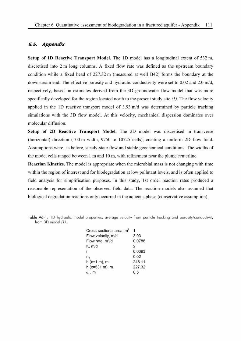
Chapter 6 Quantitative assessment of biodegradation in a fractured aquifer - Appendix 111
6.5. Appendix
Setup of 1D Reactive Transport Model. The 1D model has a longitudinal extent of 532 m,
discretised into 2 m long columns. A fixed flow rate was defined as the upstream boundary
condition while a fixed head of 227.32 m (measured at well B42) forms the boundary at the
downstream end. The effective porosity and hydraulic conductivity were set to 0.02 and 2.0 m/d,
respectively, based on estimates derived from the 3D groundwater flow model that was more
specifically developed for the region located north to the present study site (1). The flow velocity
applied in the 1D reactive transport model of 3.93 m/d was determined by particle tracking
simulations with the 3D flow model. At this velocity, mechanical dispersion dominates over
molecular diffusion.
Setup of 2D Reactive Transport Model. The 2D model was discretised in transverse
(horizontal) direction (100 m width, 9750 to 10725 cells), creating a uniform 2D flow field.
Assumptions were, as before, steady-state flow and stable geochemical conditions. The widths of
the model cells ranged between 1 m and 10 m, with refinement near the plume centerline.
Reaction Kinetics. The model is appropriate when the microbial mass is not changing with time
within the region of interest and for biodegradation at low pollutant levels, and is often applied to
field analysis for simplification purposes. In this study, 1st order reaction rates produced a
reasonable representation of the observed field data. The reaction models also assumed that
biological degradation reactions only occurred in the aqueous phase (conservative assumption).
Table A6-1. 1D hydraulic model properties; average velocity from particle tracking and porosity/conductivity from 3D model (1).
Cross-sectional area, m2 1 Flow velocity, m/d 3.93 Flow rate, m3/d 0.0786 K, m/d 2 i 0.0393 ne 0.02 h (x=1 m), m 248.11 h (x=531 m), m 227.32 αL, m 0.5
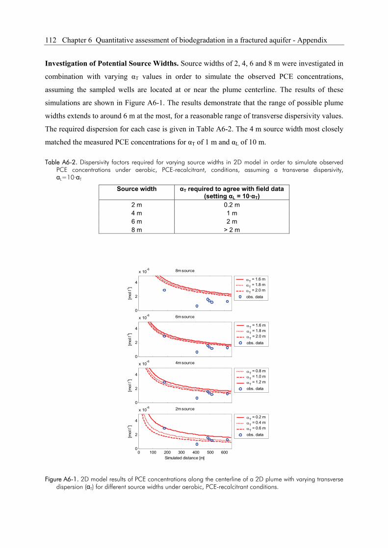
112 Chapter 6 Quantitative assessment of biodegradation in a fractured aquifer - Appendix
Investigation of Potential Source Widths. Source widths of 2, 4, 6 and 8 m were investigated in
combination with varying αT values in order to simulate the observed PCE concentrations,
assuming the sampled wells are located at or near the plume centerline. The results of these
simulations are shown in Figure A6-1. The results demonstrate that the range of possible plume
widths extends to around 6 m at the most, for a reasonable range of transverse dispersivity values.
The required dispersion for each case is given in Table A6-2. The 4 m source width most closely
matched the measured PCE concentrations for αT of 1 m and αL of 10 m.
Table A6-2. Dispersivity factors required for varying source widths in 2D model in order to simulate observed PCE concentrations under aerobic, PCE-recalcitrant, conditions, assuming a transverse dispersivity, αL=10·αT
Source width αT required to agree with field data (setting αL = 10·αT)
2 m 0.2 m 4 m 1 m 6 m 2 m 8 m > 2 m
0
2
4
x 10-6
[mol
l-1]
8m source
αT = 1.6 mαT = 1.8 mαT = 2.0 mobs. data
0
2
4
x 10-6
[mol
l-1]
6m source
αT = 1.6 mαT = 1.8 mαT = 2.0 mobs. data
0
2
4
x 10-6
[mol
l-1]
4m source
αT = 0.8 mαT = 1.0 mαT = 1.2 mobs. data
0 100 200 300 400 500 6000
2
4
x 10-6
Simulated distance [m]
[mol
l-1]
2m source
αT = 0.2 mαT = 0.4 mαT = 0.6 mobs. data
Figure A6-1. 2D model results of PCE concentrations along the centerline of a 2D plume with varying transverse dispersion (αT) for different source widths under aerobic, PCE-recalcitrant conditions.
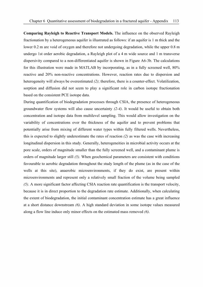
Chapter 6 Quantitative assessment of biodegradation in a fractured aquifer - Appendix 113
Comparing Rayleigh to Reactive Transport Models. The influence on the observed Rayleigh
fractionation by a heterogeneous aquifer is illustrated as follows: if an aquifer is 1 m thick and the
lower 0.2 m are void of oxygen and therefore not undergoing degradation, while the upper 0.8 m
undergo 1st order aerobic degradation, a Rayleigh plot of a 4 m wide source and 1 m transverse
dispersivity compared to a non-differentiated aquifer is shown in Figure A6-3b. The calculations
for this illustration were made in MATLAB by incorporating, as in a fully screened well, 80%
reactive and 20% non-reactive concentrations. However, reaction rates due to dispersion and
heterogeneity will always be overestimated (2); therefore, there is a counter-effect. Volatilization,
sorption and diffusion did not seem to play a significant role in carbon isotope fractionation
based on the consistent PCE isotope data.
During quantification of biodegradation processes through CSIA, the presence of heterogeneous
groundwater flow systems will also cause uncertainty (2-4). It would be useful to obtain both
concentration and isotope data from multilevel sampling. This would allow investigation on the
variability of concentrations over the thickness of the aquifer and to prevent problems that
potentially arise from mixing of different water types within fully filtered wells. Nevertheless,
this is expected to slightly underestimate the rates of reaction (2) as was the case with increasing
longitudinal dispersion in this study. Generally, heterogeneities in microbial activity occurs at the
pore scale, orders of magnitude smaller than the fully screened well, and a contaminant plume is
orders of magnitude larger still (5). When geochemical parameters are consistent with conditions
favourable to aerobic degradation throughout the study length of the plume (as in the case of the
wells at this site), anaerobic microenvironments, if they do exist, are present within
microenvironments and represent only a relatively small fraction of the volume being sampled
(5). A more significant factor affecting CSIA reaction rate quantification is the transport velocity,
because it is in direct proportion to the degradation rate estimate. Additionally, when calculating
the extent of biodegradation, the initial contaminant concentration estimate has a great influence
at a short distance downstream (6). A high standard deviation in some isotope values measured
along a flow line induce only minor effects on the estimated mass removed (6).
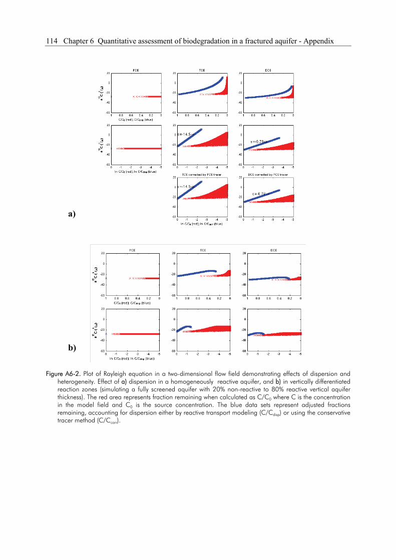
114 Chapter 6 Quantitative assessment of biodegradation in a fractured aquifer - Appendix
Figure A6-2. Plot of Rayleigh equation in a two-dimensional flow field demonstrating effects of dispersion and heterogeneity. Effect of a) dispersion in a homogeneously reactive aquifer, and b) in vertically differentiated reaction zones (simulating a fully screened aquifer with 20% non-reactive to 80% reactive vertical aquifer thickness). The red area represents fraction remaining when calculated as C/C0 where C is the concentration in the model field and C0 is the source concentration. The blue data sets represent adjusted fractions remaining, accounting for dispersion either by reactive transport modeling (C/Cdisp) or using the conservative tracer method (C/Ccorr).
b)
a)
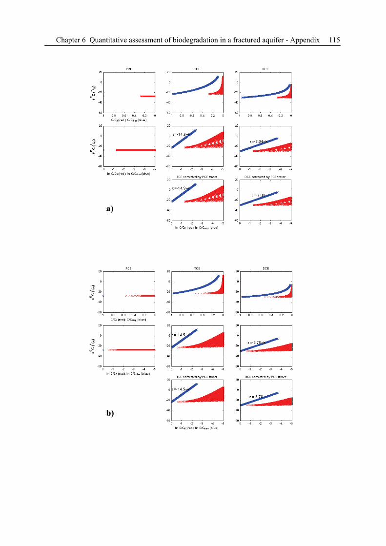
Chapter 6 Quantitative assessment of biodegradation in a fractured aquifer - Appendix 115
a)
b)
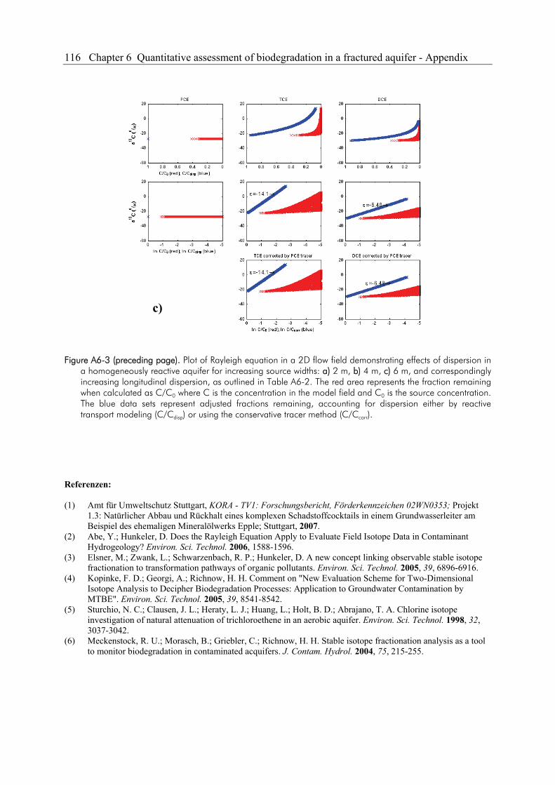
116 Chapter 6 Quantitative assessment of biodegradation in a fractured aquifer - Appendix
Figure A6-3 (preceding page). Plot of Rayleigh equation in a 2D flow field demonstrating effects of dispersion in
a homogeneously reactive aquifer for increasing source widths: a) 2 m, b) 4 m, c) 6 m, and correspondingly increasing longitudinal dispersion, as outlined in Table A6-2. The red area represents the fraction remaining when calculated as C/C0 where C is the concentration in the model field and C0 is the source concentration. The blue data sets represent adjusted fractions remaining, accounting for dispersion either by reactive transport modeling (C/Cdisp) or using the conservative tracer method (C/Ccorr).
Referenzen: (1) Amt für Umweltschutz Stuttgart, KORA - TV1: Forschungsbericht, Förderkennzeichen 02WN0353; Projekt
1.3: Natürlicher Abbau und Rückhalt eines komplexen Schadstoffcocktails in einem Grundwasserleiter am Beispiel des ehemaligen Mineralölwerks Epple; Stuttgart, 2007.
(2) Abe, Y.; Hunkeler, D. Does the Rayleigh Equation Apply to Evaluate Field Isotope Data in Contaminant Hydrogeology? Environ. Sci. Technol. 2006, 1588-1596.
(3) Elsner, M.; Zwank, L.; Schwarzenbach, R. P.; Hunkeler, D. A new concept linking observable stable isotope fractionation to transformation pathways of organic pollutants. Environ. Sci. Technol. 2005, 39, 6896-6916.
(4) Kopinke, F. D.; Georgi, A.; Richnow, H. H. Comment on "New Evaluation Scheme for Two-Dimensional Isotope Analysis to Decipher Biodegradation Processes: Application to Groundwater Contamination by MTBE". Environ. Sci. Technol. 2005, 39, 8541-8542.
(5) Sturchio, N. C.; Clausen, J. L.; Heraty, L. J.; Huang, L.; Holt, B. D.; Abrajano, T. A. Chlorine isotope investigation of natural attenuation of trichloroethene in an aerobic aquifer. Environ. Sci. Technol. 1998, 32, 3037-3042.
(6) Meckenstock, R. U.; Morasch, B.; Griebler, C.; Richnow, H. H. Stable isotope fractionation analysis as a tool to monitor biodegradation in contaminated acquifers. J. Contam. Hydrol. 2004, 75, 215-255.
c)
Chapter 7 General conclusions and outlook 117
7. General Conclusions and Outlook
The main aim of the present work was to demonstrate the potential of compound-specific isotope
analysis (CSIA) for studying the source and fate of organic contaminants at heterogeneous and
complex aquifer systems. One major drawback in the application of CSIA to field studies, is that
current GC/IRMS systems are limited in their sensitivity. To overcome this limitation, various
sample extraction and injection techniques were optimized and validated for their use in CSIA
field studies. For volatile compounds, a commercially available purge-and-trap sample extractor
has been technically improved within this work. Good performance of the system was
demonstrated for low-contaminated sites and by a comparison with extraction techniques that are
already well-established in CSIA for volatile organics. Overall, the results obtained and discussed
within Chapter 2 demonstrate that the sample preconcentration and extraction techniques applied
are well suited for the compound-specific carbon isotope analysis of volatile compounds at trace
concentrations. For semi-volatile organic compounds, a sample introduction technique, that (until
now) has been restricted to quantitative analysis, was applied in the present study to continuous-
flow isotope ratio determinations for the first time. The technique, based on the injection of large
sample volumes of organic extracts into a programmable temperature vaporizer (PTV) injector
with subsequent solvent-venting and trapping of the analytes on a cooled packed liner, was
thoroughly validated for the application in GC/IRMS in terms of its accuracy, precision, linearity,
reproducibility and limits of detection (Chapter 3). The optimized PTV-LVI method allows to
determine accurately and precisely δ13C values of semi-volatile organic contaminants at low µg/L
or µg/kg concentrations and thus expands the applicability of CSIA considerably in
environmental studies. The applicability of the method was validated for δ13C determination of
individual PAHs and exemplified by a source apportionment study at a contaminated site. As one
of the most important requirements in GC/IRMS is the baseline-separation of peaks (see Chapter
4) sample cleanup before analysis was mandatory.
The combination of the PTV-LVI method with preparative HPLC would offer a time and labour
efficient method for the determination of isotopic compositions of semi-volatile organic
compounds even in difficult matrices. Due to the method developments attained in the present
study, future work could be extended to assess contaminant sources and degradation reactions at
larger scales, e.g. in catchment hydrology. The use of CSIA is open to a range of new application
areas, e.g. future studies should include other important soil and groundwater contaminants such
118 Chapter 7 General conclusions and outlook
as pesticides, herbicides, or polychlorinated biphenyls. Latest developments in hyphenation of
liquid chromatography to IRMS systems (LC/IRMS) would allow for compound-specific stable
isotope analysis of non-volatile and thermally unstable compounds in the future.
The present work aimed not only to demonstrate the potential of CSIA in NA field site
investigation, but also to test the performance at site conditions, typically confronted with in
practical contaminated site management. Potential pitfalls of the analytical procedure were
critically discussed and strategies to avoid possible sources of error were provided in Chapter 4.
In addition, the need for a thorough investigation of compound-specific isotope fractionation
effects possibly involved in any step of the overall analytical method by standards with known
isotopic composition was emphasized.
To validate the applicability of the CSIA concept for studying the source and fate of organic
contaminants and to reliably quantify the rate of in-situ degradation in contaminant plumes even
at highly complex conditions, extensive site investigations were performed at an urban,
heterogeneous bedrock aquifer system. Chapter 5 demonstrates how compound-specific carbon
isotope analysis can be used to allocate contaminant sources at a site with multiple and
overlapping plumes. A multiple-line-of-evidence approach including evaluation of historical,
hydrological, geochemical and isotopic data and statistical analysis unravelled the contamination
scenario at the site. In the present work it was shown that careful statistical evaluation and
interpretation of highly precise compound specific isotope signatures, geochemical data and site-
specific additional information are essential for a comprehensive site assessment under complex
boundary conditions. However, in cases where uncertainties remain, two dimensional CSIA
(multiple isotope analysis, e.g. δ37Cl or δ2H) may further improve the conclusive power for
constraining contaminant sources.
A model-based analysis of concentration and isotope data was carried out to assess natural
attenuation of chlorinated ethenes in an aerobic fractured bedrock aquifer. The results (Chapter 6)
provided strong evidence for the occurrence of aerobic TCE and DCE degradation. As PCE is
recalcitrant in aerobic conditions, it could be used as a conservative tracer to estimate the extent
of dilution. The dilution-corrected concentrations together with stable carbon isotope data
allowed for the reliable assessment of the extent of biodegradation at the site and plume
simulations quantitatively linked aerobic biodegradation with isotope signatures in the field. A
comparison of isotope analysis only at the field scale to isotope analysis with reactive transport
Chapter 7 General conclusions and outlook 119
modeling has demonstrated the need, when quantifying natural attenuation processes, for an
integrated approach, particularly when similar degradation processes can result in a range of
enrichment factors. Prior to this study, fractionation due to aerobic TCE degradation has only
been studied for two particular strains of bacteria and never for a mixed culture. Fractionation
due to aerobic DCE degradation is even less well documented. In general, there is a range of
compounds with no reported fractionation factors available or the laboratory parameters are not
representing the prevailing site-specific conditions. Therefore, further work should be adressed to
the investigation of enrichment factors for less-studied compounds. Future laboratory
experiments should be performed for a set of various redox conditions and microbial cultures to
provide enrichment factors for a wide range of environmental conditions. In addition, further
research is required to assess the processes that control these enrichment factors.
120 List of figures and tables
List of Figures and Tables
Figure 1-1. Set-up of GC/IRMS system for the determination of carbon isotope ratios of individual compounds,
figure taken from Schmidt et al. (8)...................................................................................................................... 2
Figure 1-2. Decreasing concentration associated with enrichment of heavy isotopologues indicating biodegradation
(exemplified for benzene degradation at the former military airfield Brand, site-specific details are given in
Chapter 2). ............................................................................................................................................................ 5
Figure 1-3. HPLC-chromatogram for toluene (column: Eurosoil 4; flow 0.1 mL/min) together with corresponding
carbon isotope composition along the peak. The horizontal line represents the δ13C value of the non-
fractionated toluene. ............................................................................................................................................. 7
Figure 2-1. Effect of two different polymer tubings on extraction efficiency. Extraction efficiencies are represented
by amplitude height of the mass 44 peak achieved during enhanced-volume P&T-analyses using PTFE- and
PEEK- tubings for sample transfer. Error bars represent the standard deviation based on a triplicate
measurement....................................................................................................................................................... 19
Figure 2-2. Sorptive loss to PTFE (filled squares, given in %-difference of amplitude heights of m/z 44 peaks
relative to PEEK) versus experimental equilibrium PTFE-water partitioning constants (log PPTFE, (23)). Open
circles represent the theoretical loss for aromatic hydrocarbons according to log PPTFE values given by (23)... 20
Figure 2-3. Evaluation of method detection limits (MDLs) for the investigated compounds. Open circles are
representing δ13C values; diamonds show the signal size of mass 44 peak. The linear behavior of signal size
versus concentration is indicated by correlation coefficients (R²) always better than 0.996. Error bars represent
the standard deviation based on triplicate measurements. The horizontal lines represent the mean isotopic value
for each compound (± 0.5‰). ............................................................................................................................ 21
Figure 2-4. Concentration and carbon isotope data for PCE changing with depth of the aquifer. Internal
reproducibility based on triplicate injections of samples and standards is generally < 0.5‰. ........................... 23
Figure 2-5. Concentration and δ13C values for PCE as qualitative evidence for microbial reductive dehalogenation
along the water flow path B2 to B5. The most downgradient well of the site shows the lowest concentration
associated with significantly enriched δ13C values. The estimates of biodegradation (B) along this flow path
range from 59% to 91%...................................................................................................................................... 24
Figure 2-6. Representative GC/IRMS-chromatogram for groundwaters contaminated with kersosene, sampled at
Niedergörsdorf TL1, extraction performed with enlarged-volume-P&T (PTFE tubing), concentration of
compounds ≤ 1.5 µg/L. The upper trace, representing the ratio of mass 45/44, serves as indicator for good
chromatographic performance of the system...................................................................................................... 26
Figure 2-7. Left: Map of Niedergörsdorf illustrating concentration distribution and isotopic composition for A)
benzene and B) 1,3,5-trimethylbenzene at the site. Right: Linear correlation of isotope composition versus
concentration indicate in-situ biodegradation according to the Rayleigh equation (plotted wells are located
along the flow path illustrated as blue arrows in the maps)................................................................................ 27
Figure 2-8. GC/IRMS-chromatogram obtained for the analysis of a low-contaminated mineral water
(Mombachquelle, Stuttgart) using the enhanced-volume P&T-system equipped with a PEEK-tubing as sample
transfer loop. Signal intensities for cis-DCE, trichloromethane and 1,1,1-trichloroethane (0.1, 0.13 and 0.17
List of figures and tables 121
µg/L, resp.) were below the MDL; δ13C values for TCE (0.36 µg/L) and PCE (2.28 µg/L) could be reliably
determined. ......................................................................................................................................................... 28
Figure A2-1. Biodegradation estimates for kerosene-contamination at KORA-site Niedergörsdorf (in percent). ..... 33
Figure 3-1. Effect of solvent and PTV initial temperatures on the instrument response for selected 2- to 5-ring
compounds. Injections were made at 100 µL each with same analyte concentration, error bars are indicating the
standard deviation of a triplicate measurement. ................................................................................................. 39
Figure 3-2. Linear correlation of peak area and amount of compound injected illustrated for A) naphthalene and B)
perylene. Results are given for various solvents, initial PTV inlet temperatures and solvent levels (SL); error
bars represent standard deviations based on three injections (in most cases smaller than the symbol size)....... 40
Figure 3-3. Peak areas as a function of sample volume injected exemplarily shown for a) naphthalene and b)
perylene. Volumes of samples injected were 50, 100 and 150 µL. .................................................................... 40
Figure 3-4. Results for PTV-LVI injections measuring δ13C as a function of different concentrations (represented by
different signal sizes) illustrated for a) naphthalene and b) perylene. Varying parameters are volume of
injection and solvents injected at optimized PTV initial temperatures, with a solvent level (SL) set to 1%. For
comparison, results for a conventional 1µL splitless injection are included. Error bars are indicating the
standard deviation of a triplicate injection.......................................................................................................... 42
Figure 3-5. Comparison of GC/IRMS chromatograms of a) a conventional 1 µL injection of a 75 mg/L and b) a 100
µL large volume injection of a 750 µg/L PAH working standard diluted in n-pentane shows good
chromatographical peak resolution, PTV inlet temperatures during the injection were a) 300 °C and b) 20 °C,
numbers of compounds correspond to the numbers given Table 3-2. ................................................................ 46
Figure 3-6. Chromatograms of a soil sample extract after conventional 1µL injection and after a LVI-GC/IRMS to
ensure peak heights above the method detection limit of 500 mV. .................................................................... 48
Figure 3-7. Box-whisker-diagram for individual PAH compounds of the soil samples taken at the site compared to
reported mean isotopic compositions of creosote (5), petroleum (38), crankcase oil (39) and town gas process
tar (40). ............................................................................................................................................................... 49
Figure A3-1. Effect of solvent evaporation on δ13C values of individual PAH compounds (not significant). ........... 53
Figure 4-1. Tetrachloroethene (PCE) concentrations in µg/L (squares) and δ13C ratios in ‰ (circles) in groundwater
samples taken from different sampling depths by a multilevel sampling well. Dotted vertical lines represent a
mean concentration of 2900 µg/L and a concentration-weighted average δ13C value of -25.7‰ that would
have been obtained by conventional groundwater sampling of a fully screened well. ....................................... 56
Figure 4-2. A, GC/IRMS chromatogram of a soil sample after accelerated solvent extraction (ASE) shows a raised
baseline due to unresolved complex mixture (UCM) present in the sample. B, GC/IRMS chromatogram of the
same soil sample after accelerated solvent extraction (ASE) and cleanup on silica gel. Complete removal of
UCM hump but the response (amplitude) of the target compounds is below the linear range of the IRMS at ca.
500 mV (horizontal line). C, GC/IRMS chromatogram of the same soil sample after ASE, silica gel cleanup
and large volume injection (LVI). Baseline separation of all peaks of interest is achieved, and peak amplitudes
are within the linear range of the IRMS and allow for an accurate and precise determination of δ13C values... 60
Figure 4-3. A) illustrates the detrimental effect on chromatographical resolution due to wrong SPME fiber exposure
in a GC-injector. Non-ideal thermal desorption results in peak broadening (mass 44 chromatogram in the lower
122 List of figures and tables
part of the figure) and poor isotope swings with secondary fluctuations recognized in the instantaneous ratio
signal (upper trace). B) shows the same GC/IRMS analysis but with a correctly placed SPME fiber for
comparison. As indicated in the upper trace, isotope swings (S-shaped ratio of mass 45/44) can serve as
indicator for good chromatographic performance. ............................................................................................. 61
Figure 4-4. GC/IRMS chromatogram of a BTEX containing groundwater sample (obtained at KORA-site former
military airfield Brand) that was not completely screened by GC/MS before analysis. An unexpected high
MTBE concentration (signal size 40 Volt) caused severe contamination of the analytical equipment. ............. 62
Figure 4-5. GC/IRMS chromatogram of a pentane extract containing phthalates (main peaks) leached out of septum
material. Coeluting PAH target peaks (as illustrated in the left) could not be resolved and inhibited an isotope
analysis. .............................................................................................................................................................. 63
Figure 4-6. Amount dependency on δ13C measurements for PCE. Square symbols represent the carbon isotope value
in ‰, diamonds indicate signal size of the mass 44 peak in mV. The horizontal broken line represents the
iteratively calculated mean δ13C value, solid lines indicate the ±0.5 ‰ interval. Values outside the linear range
of the IRMS are circled. Measurements were performed in triplicates, the standard deviation of each point is
indicated by error bars. The major principles illustrated in this figure are described in Jochmann et al. (27). .. 64
Figure 4-7. Effect of poor chromatographic resolution on δ13C values of adjacent peaks. Isotope values for single
compound injections were: -26.0 ‰ (±0.1, n=3) for trans-1,2-DCE and -28.8 ‰ (±0.1, n=3) for MTBE. The
measured isotope ratio for the smaller peak shown in a) deviates significantly from its actual value. Good peak
resolution as indicated in b) results in almost accurate isotope values for both compounds.............................. 65
Figure 5-1 (preceding page). a) Map with groundwater potential lines and pie chart diagrams illustrating
contaminant distribution found at the site. b) Map showing locations of groundwater monitoring wells sampled
for concentration and isotope analysis, locations of potential polluters, and suggested location of fault system.
Areas A to G depict the various parts of the contaminant plume(s) as discussed in the text. Response for δ13C
values of PCE was >0.5 Volt, with the exception of B23 (δ13C given in brackets). Top right: Site-specific
geochemistry depicted by manganese concentration isolines (as concentration of dissolved manganese at all
individual wells correlates very well with the distribution of anaerobic and aerobic environments within the
aquifer system, isolines of manganese distribution have been chosen to depict the site-specific geochemistry).
For further details refer to Table 5-1. ................................................................................................................. 79
Figure 5-2. Conceptual model of the contamination scenario observed in source zone F and zone G. DNAPL is
spreading along fractures in the contaminated bedrock aquifer system. Anaerobic conditions drive reductive
dechlorination and isotopic enrichment of chlorinated compounds in parts of the aquifer. Dissolution of PCE
from DNAPL in the aerobic zone creates an input of undegraded material, i.e. not enriched in 13C. Linear
mixing models explain the isotope signature of PCE observed in well B30 (-25.4‰) representing a mixture of
already degraded material with an isotope value of -23‰ (measured in upgradient wells) and of freshly
dissolved (undegraded) material with assumed values of -30‰ (not likely) and -27‰ (more likely)............... 84
Figure 5-3. Box-whisker-diagram illustrating the statistical significance of all δ13C measurements for PCE (n =
number of values); the groups represent areas of same geochemical conditions as depicted in Figure 5-1b, the
groundwater wells of each group or area are listed in Table 5-S4. The likeliness for the contamination in area C
and D being derived from the same source is strongly supported; Area G can be further separated into 3
List of figures and tables 123
different zones: the area of mixing processes (wells B30, B31, B1Eck, B39*) and two additional CHC source
zones (wells B1M and P836*, respectively)....................................................................................................... 85
Figure 5-4. Origin and transport paths of contaminants evidenced by compound-specific carbon isotope signatures
combined with geochemical data, concentration analyses, historical and hydrological information. ................ 85
Figure A5-1. Linearity of δ13C values for PCE standard (mean value -27.2‰) measured by purge-and-trap-
GC/IRMS, intensities represent various standard concentrations yielding signal intensities (m/z 44 signals)
from 270 to 8400 mV, horizontal lines indicate the mean δ13C value ±0.5‰ accuracy range, error bars
represent the standard deviation of duplicate or triplicate measurements, respectively. .................................... 90
Figure A5-2. Representative GC/IRMS chromatograms of sample B8F. Due to high differences in concentrations of
each analyte, several runs have been performed with concentrations adjusted to the linear range of the CO2
reference gas peaks to ensure reproducible δ13C values. .................................................................................... 91
Figure 6-1. Map illustrating groundwater flow conditions and VOC contamination in the area of focus. The dashed
line indicates suggested location of fault system................................................................................................ 98
Figure 6-2. One-dimensional aerobic degradation scenario. Degradation rates for TCE and cis-DCE were 0.02 and
0.025 d-1, respectively. The corresponding isotope fractionation factors were -12.0 and -6.7‰, respectively.
PCE was assumed not to degrade. Longitudinal dispersivities of 0.5 m and 10 m are represented by dark and
light green lines, respectively. .......................................................................................................................... 102
Figure 6-3. Quantification of enrichment factors for TCE and cis-DCE undergoing aerobic degradation based of
field data. ƒcorr represents a “corrected” fraction remaining where the concentration at any downgradient
location is corrected for dilution using PCE as a conservative tracer. The equations shown are linear regression
models where, according to the Rayleigh equation, the slope represents the isotope enrichment factor. The R2
value represents the coefficient of determination. ............................................................................................ 103
Figure 6-4. Concentration and isotope data of TCE simulated for a 4m source width using reaction rates to suite
regression-optimized TCE isotope signatures. Plume is located in the lower left hand corner and half of a
symmetric plume is shown. The observed data (dashed lines) for each well is compared with the simulated
values (red line) relative to the distance from the plume centerline. ................................................................ 105
Figure 6-5. Centerline of two-dimensional model based on calculated enrichment factors, adjusting TCE and cis-
DCE degradation rates to suit regression-optimized a) isotope signatures, and b) concentrations, where λ′left = v
ln(Ccorr/C0); λ′right = -slope · v/ε. ........................................................................................................................ 106
Figure A6-1. 2D model results of PCE concentrations along the centerline of a 2D plume with varying transverse
dispersion (αT) for different source widths under aerobic, PCE-recalcitrant conditions. ................................. 112
Figure A6-2. Plot of Rayleigh equation in a two-dimensional flow field demonstrating effects of dispersion and
heterogeneity. Effect of a) dispersion in a homogeneously reactive aquifer, and b) in vertically differentiated
reaction zones (simulating a fully screened aquifer with 20% non-reactive to 80% reactive vertical aquifer
thickness). The red area represents fraction remaining when calculated as C/C0 where C is the concentration in
the model field and C0 is the source concentration. The blue data sets represent adjusted fractions remaining,
accounting for dispersion either by reactive transport modeling (C/Cdisp) or using the conservative tracer
method (C/Ccorr)................................................................................................................................................ 114
124 List of figures and tables
Figure A6-3 (preceding page). Plot of Rayleigh equation in a 2D flow field demonstrating effects of dispersion in a
homogeneously reactive aquifer for increasing source widths: a) 2 m, b) 4 m, c) 6 m, and correspondingly
increasing longitudinal dispersion, as outlined in Table A6-2. The red area represents the fraction remaining
when calculated as C/C0 where C is the concentration in the model field and C0 is the source concentration.
The blue data sets represent adjusted fractions remaining, accounting for dispersion either by reactive transport
modeling (C/Cdisp) or using the conservative tracer method (C/Ccorr)............................................................... 116
Table 2-1. Accuracy and reproducibility of VOC extraction methods applied within this study; δ13C values given in
per mill (‰); signal heights ≥ 1000mV.............................................................................................................. 22
Table A2-1. Purge-and-trap parameters and gas chromatographic conditions. ........................................................... 31
Table A2-2. Isotopic mass balance considerations at the site...................................................................................... 32
Table A2-3. Applied enrichment factors (batch experiments) for biodegradation estimates. ..................................... 33
Table 3-1. Results for a 100 µL injection of PAH working standards diluted in cyclohexane and n-pentane at PTV
initial temperatures of 60°C and 20 °C, respectively; based on n=30-40 for each compound and method
applied. ............................................................................................................................................................... 43
Table 3-2. Reproducibility and accuracy of the PTV-LVI method. Values are highly reproducible for optimized
injection parameters and accurate compared to values of the same working standards measured by off-line
EA/IRMS. (Values in light grey represent the results for compounds injected with the ‘wrong’ solvent.) ....... 44
Table 3-3. Variance in δ13C values for different signal size intervals. ........................................................................ 45
Table 4-1: Effect of δ13C on storage time for groundwater samples containing perchloroethene (PCE) with
concentrations between 1 and 3 mg/L, stored at 4 °C in the dark, without headspace. Each sample was
measured in triplicates (n = 3). Sampling was performed at KORA-site Rosengarten-Ehestorf (described in
Chapter 2). .......................................................................................................................................................... 58
Table 5-1. Site-specific geochemical parameters and resultant redox conditions; areas depicted in Figure 5-1b; the
wells of each area are included in the statistical diagram Figure 5-3; data available in Table A5-3 in the
Appendix. ........................................................................................................................................................... 80
Table A5-1. Precision and reproducibility of δ13C values determined by purge-and-trap GC/IRMS (number of
replicates n = 55). ............................................................................................................................................... 90
Table A5-2. δ13C values (‰) of samples that have been remeasured after different storage times. ........................... 92
Table A5-3. Data of field measurements, concentration and compound-specific isotope analyses of samples
discussed within Chapter 5. ................................................................................................................................ 93
Table A5-3 (continued). ............................................................................................................................................. 94
Table 6-1. Concentration and isotope data for chlorinated ethenes in the downgradient series wells....................... 101
Table A6-1. 1D hydraulic model properties; average velocity from particle tracking and porosity/conductivity from
3D model (1). ................................................................................................................................................... 111
Table A6-2. Dispersivity factors required for varying source widths in 2D model in order to simulate observed PCE
concentrations under aerobic, PCE-recalcitrant, conditions, assuming a transverse dispersivity, αL=10·αT.... 112
List of abbreviations 125
List of Abbreviations
‰ per mill (permil)
α Fractionation factor
ε Enrichment factor
Ace Acenaphthene
Ant Anthracene
ASE Accelerated solvent extraction
Ay Acenaphthylene
B Biodegradation (in %)
BaA Benzo(a)anthracene
BH Bochinger Horizont (geological/hydrostratigraphic unit)
BTEX Benzene, toluene, xylenes, ethylbenzene
c cis-1,2-
C Concentration
CH Cyclohexane
CHC Chlorinated hydrocarbon
CSIA Compound-specific isotope analysis
Dbf Dibenzofuran
DCE Dichloroethene
DNAPL Dense non-aqueous phase liquid
DRM Dunkelrote Mergel (geological/hydrostratigraphic unit)
EA Elemental analyzer
f Fraction of contaminant remaining
Fl Fluorene
Fla Fluoranthene
GC Gas chromatography
HPLC High-performance liquid chromatography
IRMS Isotope ratio mass spectrometry
Kow Octanol-water partitioning constant
KORA Kontrollierter natürlicher Rückhalt und Abbau (project name)
LC Liquid chromatography
LVI Large-volume injection
126 List of abbreviations
MDL Method detection limit
MeN 1-methylnaphthalene
MNA Monitored natural attenuation
MTBE Methyl tert-butyl ether
N Naphthalene
NA Natural attenuation
PPTFE Water-Teflon partitioning constant
P&T Purge-and-trap
PAH Polycyclic aromatic hydrocarbon
PCE Tetrachloroethene
PDMS Polydimethylsiloxane
PEEK Polyetheretherketone
Per Perylene
PTFE Polytetrafluoroethylene (Teflon)
PTV Programmable temperature vaporizer
Pyr Pyrene
SPME Solid-phase microextraction
TCE Trichloroethene
TCM Trichloromethane (Chloroform)
t trans-1,2-
UCM Unresolved complex mixture
US EPA United States Environmental Protection Agency
VC Vinyl chloride
VOC Volatile organic compound
VPDB Vienna Peedee Belemnite
Curriculum vitae 127
Lebenslauf
Name Michaela Blessing
Geburtsdatum 03. April 1977
Geburtsort Schwäbisch Gmünd
1983 – 1987 Grundschule in Reichenbach u.R.
1987 – 1993 Geschwister-Scholl-Realschule in Süssen
1993 – 1996 Wirtschaftsgymnasium der Kaufmännischen Schule in Göppingen
(Abitur 02. Juli 1996)
1997 – 2003 Studium der Geologie an der Eberhard-Karls-Universität Tübingen mit
den Hauptfächern Geochemie und Angewandte Geologie
SS 1999 Praktikantin am Geologischen Landesamt, München
2002 – 2003 Diplomarbeit: "Veränderungen von mineralischen
Deponieabdichtungen im Kontakt mit Modellsickerwässern unter
Auflast" (Diplom 03. März 2003)
Seit Juli 2004 Promotionsstudium an der Eberhard-Karls-Universität Tübingen,
Doktorandin am Zentrum für Angewandte Geowissenschaften
2004 – 2007 Stipendiatin der Deutschen Bundesstiftung Umwelt
Seit Juli 2007 Wissenschaftliche Mitarbeiterin am Zentrum für Angewandte
Geowissenschaften, Tübingen
Related Documents